Targeting E¢ ciency:

How well can we identify the poorest of the poor?

Abhijit Banerjee, Esther Du�o, Raghabendra Chattopadhyay

and Jeremy Shapiro �

This Draft: July 18, 2009

�We thank Bandhan, in particular Mr. Ghosh and Ramaprasad Mohanto, for their tirelesssupport and collaboration, Jyoti Prasad Mukhopadhyay and Sudha Kant for their researchassistance, Prasid Chakraborty for his work collecting data, CGAP and the Ford Foundationfor funding, and, especially, Annie Du�o and the Center for Micro�nance for their outstandingsupport of this project.

1

Abstract

In this study, we evaluate how well various systems for identifying and

targeting assistance to the poorest of the poor actually identify the poor-

est. Firstly, we consider the methods used to identify households eligible

for participation in assistance programs administered by the Indian gov-

ernment. Secondly, we evaluate Participatory Rural Appraisals (PRAs)

as a mechanism to identify exceptionally poor households. Finally, we in-

vestigate whether additional veri�cation of information gathered in PRAs

improves targeting. For each method of targeting, we examine whether

the households identi�ed by that process are more disadvantaged accord-

ing to several measures of economic well-being than households which

were not identi�ed. We conclude that PRAs and PRAs coupled with

additional veri�cation successfully identify a population which is measur-

ably poorer in various respects, especially those which are more readily

observed. The standard government procedures, however, do not appear

to target the very poorest for assistance. Based on this sample, house-

holds targeted for government assistance are observationally equivalent to

those that are not.

2

1 Introduction

Nearly all poverty alleviation programs target a particular sub-population. This

feature is most readily apparent in programs designed to aid those who have suf-

fered a particular tragedy, such as grants to widows of debt-ridden Maharashtra

farmers, but is also generally true of large, broad based development interven-

tions. Conditional and unconditional cash transfer programs, for example, are

also designed to reach speci�c households, such as the most impoverished or

households with school children. At �rst blush, this may seem unremarkable

and not to warrant particular consideration. But e¤ective identi�cation of the

target population is crucial to the success of aid programs which operate with

limited resources. If, for instance, households which are adequately nourished

are identi�ed as eligible for subsidized food, the program is unlikely to signi�-

cantly reduce malnutrition. Given that several countries have begun large scale

cash transfer programs, the issue of e¤ective targeting has become especially

important.

When the targeted population is not distinguished by a well-de�ned, observ-

able trait, however, identifying members of that population may be complicated.

Evidence suggests that the targeting e¢ ciency of aid programs is less than per-

fect. A report by the Indian National Sample Survey Organization, for example,

found that 18% of the wealthiest 20% of the rural population (ranked by monthly

per capita expenditure) held Below Poverty Line (BPL) rationing cards.1 The

1National Sample Survey Organisation (NSSO), Ministry of Statistics and Programme Im-plementation. Report No. 510 �Public Distribution System and Other Sources of HouseholdConsumption, 2004-05.�Summary at: http://mospi.nic.in/press_note_510-Final.htm

3

imperfect track record of such expansive development projects makes e¤ective

targeting not only important but controversial.

Part of the debate about targeting revolves around which methods should be

used, in particular whether these methods should rely on administrative data

or on information generated through participatory processes. In this study

we assess the relative performance of administrative and participatory methods

in identifying the poorest of the poor, who may be particularly marginalized

and di¢ cult to single out. Importantly, we conduct this analysis on the same

sample, allowing us to make a direct comparison between the two methods.

Firstly, we consider the targeting e¢ ciency of various assistance programs

operated by the government of India, which are targeted using an administrative

census. We �nd that the methods used to identify eligible households do not

particularly target the very poorest. Since our sample is drawn from the lower

economic spectrum, we can not evaluate the overall targeting e¢ ciency of these

programs, but we �nd that within this group of households, those who actually

receive government assistance do not appear worse o¤, according to our measures

of poverty, than households which do not.

We also evaluate the targeting e¢ ciency, in terms of identifying the very

poorest segment of the population, of Participatory Rural Appraisals (PRAs)

which are a popular alternative to census methodologies. PRAs are widely

practiced by NGOs, both within India and internationally, when conducting de-

velopment interventions. Increasingly, PRA methodologies are used to identify

bene�ciaries for assistance programs. Consequently, it is important that the

4

information collected from a PRA accurately re�ects the conditions within the

village where it was conducted.

Other studies provide evidence suggesting that certain types of information,

such as the presence of village infrastructure (e.g. water systems) or students�

needs for scholarships, can accurately be obtained using PRAs (Chattopadhyay

and Du�o, 2001; Du�o et al. (2008); Chambers, 1994). In this study we assess

whether PRAs reliably rank village residents according to economic status.

Using data generated in PRAs conducted by Bandhan, a Kolkata-based mi-

cro�nance institution, we evaluate how well measures of poverty collected in

a detailed household survey accord with the evaluation of poverty established

by the PRA. Since the information collected in the PRA is used to identify

households eligible for a program to enable the poorest of the poor to access

microcredit, targeting the most poor households is crucial in this context. Along

some dimensions of poverty, notably consumption and expenditure, the results

are imprecise; it does not appear that per capita consumption among those

identi�ed as poor in the PRA is less than among those not so classi�ed. The

analysis does reveal, however, that those ranked as most poor in the PRA are

in fact poorer than others in terms of observable characteristics such as land

and asset ownership. They also have less access to credit.

As Bandhan�s process incorporated additional veri�cation of the informa-

tion collected in the PRA, we also assess the extent to which this veri�cation

improves targeting. Our results indicate that further veri�cation successfully

narrows in on a group which appears poorer in various respects, particularly

5

land ownership.

A limitation of this analysis is that, although comprehensive and detailed,

our household survey is not an error-free measure of economic well-being. Con-

sumption and expenditure, for example, is not always reliably measured with

household interviews (see e.g. Deaton 1997). Moreover, poverty can be de�ned

in various ways; the indicators collected in this survey are only one way of doing

so and are not necessarily perfectly aligned with the de�nition of poverty es-

tablished in a PRA. Finally poverty is dynamic, low consumption today is not

always indicative of long term depravation. As community members have long-

term relationships, it is possible that participatory targeting methods capture

more of the dynamic element of poverty than our household survey. Notwith-

standing these concerns, we are able to assess how classi�cation as impover-

ished through various targeting techniques correlates with important indicators

of poverty captured in our survey, such as land holdings and credit access.

Moreover, this study is able to contrast census and participatory methods by

comparing them to an equivalent external benchmark of poverty.

This study is closely related to Alatas et al. (2009) who contrast the tar-

geting performance of census techniques and participatory community wealth

rankings in Indonesia. Their �ndings indicate that participatory methods do

not identify a poorer population in terms of consumption and suggest that com-

munity members may perceive poverty along other dimensions. The results

presented here coincide with those of Alatas et al.; we �nd that PRAs identify a

population which does not appear worse o¤ in terms of consumption but which

6

is poorer according to other important poverty metrics, suggesting that PRA

rankings accord with multiple dimensions of economic well-being and can serve

as the basis for targeting.

2 Data

In order to improve their targeting process, Bandhan requested that we do a

study to assess how e¤ectively they were identifying the poorest households in

each village, or the �Ultra Poor.�To accomplish this we conducted a detailed

survey among those not identi�ed as Ultra Poor as well as among those identi�ed

as Ultra Poor in a sample of villages where Bandhan operates.

Initially, the surveying team conducted a census of all households in the

village. Each household was classi�ed on a 1-5 scale along several characteris-

tics, such as land holdings, quality of house, ownership of assets, educational

achievement, employment status and access to credit. This census utilized sim-

ilar classi�cation criteria as the government administered BPL census, which is

intended to identify the population living below the poverty line and determine

who is eligible for certain government assistance programs.

In line with our objective to understand the feasibility of identifying the very

poorest of the poor, the sampling frame was restricted to the poorer population

within the village. To be considered for our survey, a household must meet one

of the following requirements: own less than 1 acre of irrigated land or less than

2 acres of non-irrigated land, not live in a pucca house (i.e. one made of brick,

7

stone or concrete), own less that 4 articles of clothing, and own none or only

one durable household good.2

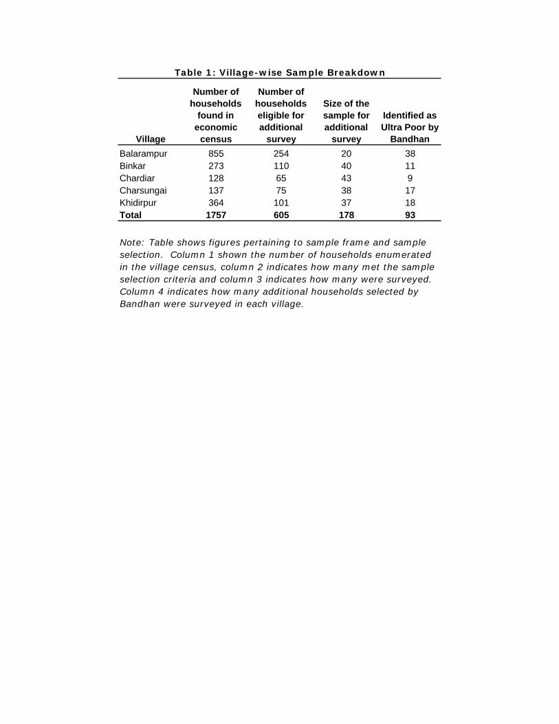
Of 1,757 households enumerated in the economic census, 605 satis�ed the

criteria above. From this restricted list, a random sample of households was

selected and administered a survey similar to that given to households identi�ed

as Ultra Poor by Bandhan. This survey was conducted among 178 households

in �ve villages. Table 1 shown a breakdown of this sampling by village.

Among these surveyed households, 48 were not enumerated in the PRA con-

ducted by Bandhan. That the PRA process fails to enumerate some households

which are relatively worse o¤ (as determined by the economic census) is indica-

tive that it may be especially di¢ cult to identify the poorest of the poor within

a village. For the purposes of this study, however, we restrict our analysis to

the households appearing in the PRA list since we are interested in making com-

parisons across targeting mechanisms, including the additional veri�cation done

by Bandhan, which was only done for those households appearing in the PRA.

Our �nal dataset contains 215 households, 93 were identi�ed as Ultra Poor by

Bandhan and 122 were identi�ed as impoverished by the economic census but

not classi�ed as Ultra Poor by Bandhan.3

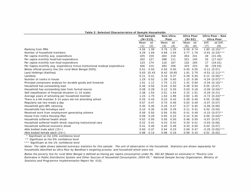
Table 2 provides summary statistics for our entire sample as well as sepa-

rately according to whether households were identi�ed as Ultra Poor by Band-

2The items considered were: computer, telephone, refrigerator, husking machine, colortelevision, electric cooking appliances, costly furniture, LPG (gas) connection, light motorvehicle or commercial vehicle, tractor, two or three wheeler, motor van, power driven tiller.

3Eight of the surveyed households from the economic census were under consideration byBandhan and were subsequently veri�ed as eligible to receive a grant. Thus the number ofnon Ultra Poor households in the sample is 122 (170-48) rather than 130 (178-48). Thesehouseholds are included in the �gure of 93 identi�ed as Ultra Poor.

8

han or not. As might be expected given the mandate of Bandhan�s identi�cation

process and the sampling design of the additional survey, this is a relatively poor

population. The mean per capita monthly average expenditure is Rs. 425 (Rs.

14 per day or $1.25 in PPP adjusted 2006 U.S. dollars). Average monthly per

capita expenditure on food and fuel is Rs. 302 (Rs. 10 per day or $0.89 in PPP

adjusted 2006 U.S. dollars). For both measures of consumption, approximately

half the sample population spends less than one dollar a day and nearly all the

population spends less than two dollars a day.

Other variables conform to what one would expect in this sample. Mean

land holdings are 5.6 katthas (approximately 0.11 acres). In addition 21% of

the sample is landless. While 46% of households have obtained loans, only 8%

obtained credit from a formal source.4 As well as being poor, this population

lacks education; average completed years of education per household member is

1.2 years and 25% of households have school aged children (5-14 years old) out

of school.

This is also a vulnerable population; only 67% report that everyone in the

household regularly eats two meals a day, approximately half of those surveyed

report having experienced a medical shock in the last year, 22% su¤ered a med-

ical shock requiring institutional care and 41% su¤ered an economic shock.5

4A formal source is de�ned as a commercial bank, government bank, self-help group or acooperative. Informal sources include family members, friends, neighbors, moneylenders andshopkeepers.

5A medical shock is de�ned as having spent more than Rs. 500 (44 PPP adjusted 2006$U.S.) on any one household member�s medical care. A medical shock requiring institutionalcare is de�ned as having spent more than Rs. 500 (44 PPP adjusted 2006 $U.S.) on insti-tutional medicine in the last year. An economic shock is de�ned as any of the followingoccurring in the past year: house was severely damaged, livestock became ill, livestock died,con�ict/dispute/legal case, or theft.

9

Moreover, to the extent that receipt of assistance is an indication of need, this

is a needy population. Two thirds report receiving assistance from one of

the government programs listed in the questionnaire (such as Below Poverty

Line rationing, subsidized housing or participation in employment generating

schemes). Figures for the most common assistance programs are reported sep-

arately in Table 2.

2.1 Empirical Strategy

In what follows, we are primarily concerned with the di¤erence in some nu-

merical measure of poverty or economic status, denoted y, between sub-groups.

These groups will be households receiving some form of government assistance

and those that do not, households identi�ed as poor in the PRA and those that

are not or households identi�ed as Ultra Poor by Bandhan and those that are

not so identi�ed. Letting Di be an indicator variable that household i receives

a certain form of government aid or that the household was identi�ed as poor

in the PRA or was identi�ed as Ultra Poor, we estimate the following equation

yiv = �Div + �v + "iv (1)

where the subscript v indicates villages. In some speci�cations we include

household covariates, Xiv, in addition to the village �xed e¤ects, �v. The

parameter of interest in �, which measures the mean di¤erence in y between

those who are somehow identi�ed as poor and those that are not after removing

10

the e¤ect of common village level determinates of y.

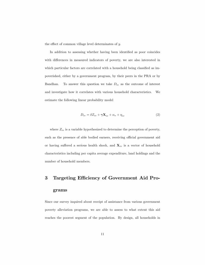
In addition to assessing whether having been identi�ed as poor coincides

with di¤erences in measured indicators of poverty, we are also interested in

which particular factors are correlated with a household being classi�ed as im-

poverished, either by a government program, by their peers in the PRA or by

Bandhan. To answer this question we take Div as the outcome of interest

and investigate how it correlates with various household characteristics. We

estimate the following linear probability model

Div = �Ziv + Xiv + �v + �iv (2)

where Ziv is a variable hypothesized to determine the perception of poverty,

such as the presence of able bodied earners, receiving o¢ cial government aid

or having su¤ered a serious health shock, and Xiv is a vector of household

characteristics including per capita average expenditure, land holdings and the

number of household members.

3 Targeting E¢ ciency of Government Aid Pro-

grams

Since our survey inquired about receipt of assistance from various government

poverty alleviation programs, we are able to assess to what extent this aid

reaches the poorest segment of the population. By design, all households in

11

our sample are drawn from the bottom of India�s economic spectrum. While

these government programs are not explicitly designed to target the very poor-

est of the poor, to the extent that they are intended to bene�t impoverished

households we should expect that either the poorest within our sample over-

whelmingly receive this aid or that all households in our sample do. As is

evident from Table 2 the latter case does not appear true; for instance only

30% receive BPL rationing and 10% have an Antodaya card (variables which

indicate participation in government food assistance programs).

Targeting for many government aid programs is based on the BPL cen-

sus, conducted by the government to identify those households living below the

poverty line. This census, however, has been criticized for systematic exclusion

of extremely poor households. Moreover, there are concerns that the �nal lists

of BPL households are directly manipulated to include non-poor households

(Mukherjee, 2005). Jalan and Murgai (2007) �nd that many households who

are below the poverty line according to consumption measures are incorrectly

classi�ed by the BPL census.

To assess the e¢ ciency of this targeting process in these villages, we contrast

the features of those who participate in government programs and those who do

not. Speci�cally, we estimate (1) where yiv is taken to be per capita expendi-

ture6 , land holdings, house size, whether members eat two meals a day, access to

credit, self-classi�cation of �nancial condition, an index of asset holdings based

on principal component analysis of durable goods and livestock holdings or an

6Replacing the level of expenditure with the logarithm of expenditure does not substan-tively change the results discussed below.

12

indicator for the presence of an able bodied male adult in the household.

In particular, we perform this comparison separately for four government aid

programs by letting Div be an indicator that the household receives BPL ra-

tioning, receives Antodaya rationing, participates in the Indira housing program

or participates in an employment generating scheme. The BPL and Antodaya

programs provide a card which entitles households to purchase subsidized food

and fuel at ration shops. BPL cards are intended for those living below the

poverty line while Antodaya cards are intended to go to exceptionally poor

households. The Indira housing program (Indira Awaas Yojana) evolved into

its present form by 1996, the goal of this program is to improve housing for the

disadvantaged rural population. To this end grants are distributed to build or

repair homes and, in some cases, loans are facilitated for these purposes. Prefer-

ence for the Indira housing program is supposed to be given to those identi�ed

as below the poverty line by the government BPL census (Jalan and Murgai,

2007). Preference may also be given to widows of servicemen.

The National Rural Employment Guarantee Act (NREGA) was launched

in 2005. The mission of NREGA is to provide �at least one hundred days of

guaranteed wage employment in every �nancial year to every household whose

adult members volunteer to do unskilled manual work and for matters connected

therewith or incidental thereto.�7 Participation in the program requires regis-

tration with the Gram Panchayat (local o¢ cial) to obtain a job card. Holders

7The National Rural Employment Guarantee Act of 2005. Retrieved from: The Gazetteof India, New Delhi , Wednesday, September 7 2005 pp:1. http://rural.nic.in/rajaswa.pdf[viewed October 2007]

13

of this card become eligible to apply for jobs allocated under the program.

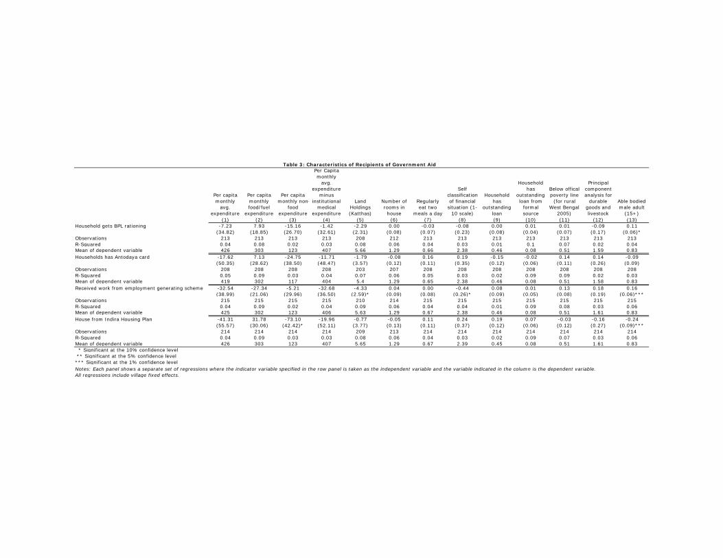
According to our results, the population which receives assistance from these

programs is not statistically di¤erent, with respect to our poverty indicators,

from the population which does not. Table 3 presents the results. For recipients

of BPL rationing we �nd that these households are slightly more likely to have an

able bodied adult male member, which is the opposite of what might be expected

if this program targeted particularly disadvantaged households. We are unable

to reject that the means between those that receive BPL rationing and those

that do not are equal for any other indicator of poverty. Moreover, some of

these coe¢ cients take the opposite sign than would be expected. Comparing

households which have Antodaya cards with those that do not we can not reject

that the means between the groups are equal for any outcome.

There is at least the suggestion that households which have received work

from an employment generating scheme are poorer than others. The coe¢ cient

on participation in this program enters with the predicted negative sign when

any of the expenditure measures are taken as the left hand side variable, al-

though no coe¢ cient is signi�cant at the 10% level. The results also suggest

that these households own an average of 4.3 katthas (0.09 acres) less land, a

di¤erence which is signi�cant at the 10% level. We also �nd that these house-

holds are more likely to include an able bodied male member. These results

may be driven by the fact that there is also a component of self-selection in

employment generating programs. Since bene�ts require work, only households

who are poor enough to lack more attractive work opportunities will take up

14

these programs. Mukherjee (2005) notes the potential of self-selecting programs

to overcome barriers, whether political or logistical, to e¤ective targeting.

In terms of consumption, only with respect to per capita non food expendi-

ture do bene�ciaries of the Indira housing program appear statistically di¤erent

(at the 10% con�dence level) from their peers. Also, bene�ciaries are less

likely to have an able bodied male in the household, indicating the targeting of

widows was likely e¤ective. No other measure is signi�cantly di¤erent between

recipients and non-recipients.

Perhaps owning to the failures of censuses to identify poor households, many

organizations have turned to other methods. A particularly popular method

used for ascertaining the economic status of households is the Participatory

Rural Appraisal (PRA). Indeed, Mukherjee (2005) draws on information gath-

ered in PRAs to evaluate the targeting e¢ ciency of the BPL census. The PRA

process was pioneered in the 1980�s and 90�s, largely by government and non-

government organizations in Kenya and India. By 1997, the practice had spread

globally; PRA activities had been conducted in over 30 countries, both develop-

ing and developed, by the end of 1996. In India, PRA methods have been used

by numerous NGOs as well as by several government agencies.8 International

organizations, such as USAID, Save the Children and Care International, also

employ PRA methods in conducting their operations.9 In light of the target-

8Chambers, 1997. p.114, 248.9Burde, Dana. Save the Children�s Afghan Refugee Education Program in Balochistan,

Pakistan, 1995- 2005 2 Report, 2005 http://www.savethechildren.org/publications/technical-resources/education/pakistan-afghan-refugees-education-project-report-9-26-05.pdf [viewedOctober 2007]; http://www.usaid.gov/regions/afr/success_stories/ghana.html[viewed Octo-ber 2007]; http://www.care.org/careswork/projects/ETH051.asp [viewed October 2007].

15

ing process used by Bandhan, we evaluate the accuracy with which PRAs can

identify especially poor households. Before proceeding, however, we provide an

overview of Bandhan�s assistance program and the speci�cs of the process used

to identify bene�ciaries.

4 Analysis of Bandhan�s Identi�cation Process

4.1 Overview of Bandan�s �Targeting the Ultra Poor�

In light of evidence that micro�nance does not reach the poorest of the poor

(Morduch 1999, Rabbani, et al. 2006) various initiatives have begun which aim

to "graduate" the poorest to micro�nance. The intervention operated by Band-

han is intended to ease credit constraints for exceptionally poor individuals by

helping them establish a reliable income stream which can be used to service

loan payments.10 To that end, Consultative Group to Assist the Poor (CGAP)

provided $30,000 as grants for the purchase of income generating assets to be

distributed to households identi�ed as �Ultra Poor.�Grants of $100 were dis-

tributed to 300 bene�ciaries residing in rural villages in Murshidabad, India (a

district north of Kolkata) by Bandhan. The design of this program was based

on the pioneering work of BRAC, a Bangladeshi development organization. For

several years, BRAC has been distributing grants through its �Challenging the

Frontiers of Poverty Reduction-Targeting the Ultra Poor" (CFPR-TUP) pro-

gram with the aim of helping the absolute poorest graduate to micro�nance.11

10The impact of this intervention is the subject of an ongoing study by the authors.11BRAC website http://www.brac.net/cfpr.htm [viewed October 2007].

16

Working in close consultation with BRAC, Bandhan developed the criteria to

identify the Ultra Poor.

The initial phase of the intervention consists of Bandhan identifying those

eligible for the grants; the poorest of the poor within each village. An average

of 17 households were identi�ed as Ultra Poor in each village. Following iden-

ti�cation, half of the potential bene�ciaries were randomly selected to receive

assets. Rather than transferring cash, Bandhan procures assets, such as live-

stock or inventory, and distributes them to bene�ciaries. The grants are also

used to �nance other inputs, such as fodder and sheds to house the animals.

Eighteen months after receipt of the asset, the bene�ciaries will be eligible for

micro-�nance provided by Bandhan.

4.2 Details of the Identi�cation Process

To make the concept of �Ultra Poor�operational and de�ne the targeted popu-

lation, Bandhan used a set of criteria adapted from those used by BRAC in their

CFPR-TUP program. Firstly, an eligible household must have an able-bodied

female member. The rationale for this requirement is that the program is in-

tended particularly to bene�t women12 and any bene�t accruing from the grant

requires that the bene�ciary be capable of undertaking some enterprise. The

second mandatory requirement is that the household not be associated with any

micro�nance institution (in keeping with the aim of targeting those who lack

12While the majority of bene�ciaries are female, some men were identi�ed as eligible underspecial circumstances such as physical disability.

17

credit access) or receive su¢ cient support through a government aid program.13

In addition to these two criteria, eligible households should meet three of the

following �ve criteria: the primary source of income should be informal labor or

begging, land holdings below 20 decimals (10 katthas, 0.2 acres), no ownership

of productive assets other than land, no able bodied male in the household and

having school-aged children working rather than attending school.

To identify those households satisfying this de�nition of Ultra Poor, Band-

han utilized a multi-phase process. The initial task is to identify the poorer

hamlets in the region. Since Bandhan has operations in Murshidabad, this is

accomplished by consulting with local branch managers who are familiar with

the economic conditions in these villages.

In the second phase, Bandhan conducts Participatory Rural Appraisals (PRAs)

in particular hamlets of selected villages to identify the subset of the popula-

tion most likely to be Ultra Poor. To ensure that the PRA includes a su¢ cient

number of participants, Bandhan employees enter the hamlet on the day prior

to the PRA; they meet with teachers and other local �gures to build rapport

with the residents, announce that the PRA will occur on the following day and

encourage participation. Bandhan aims for 12-15 PRA participants, but often

the �gure is as high as 20. Moreover, they encourage household members from

various religions, castes and social groups to attend.

In this particular context, the PRA consists of social mapping and wealth

13�Su¢ cient support�was determined on a case-by-case basis by Bandhan; while many ofthe households they identi�ed as Ultra Poor participate in some government aid program, theydetermined that this assistance was not su¢ cient to alleviate the poverty of the household.

18

ranking, following a sophisticated process to identify the poor. At the outset,

the main road and any prominent hamlet landmarks (temples, mosques, rivers,

etc.) are etched into the ground, usually in front of a central house in the

hamlet. Subsequently the participants enumerate each household residing in

the hamlet and mark the location of the households on the hamlet map. For

each household, the name of the household head is recorded on an index card.

In the wealth ranking stage, the index cards are sorted into piles correspond-

ing to socioeconomic status. To accomplish this, Bandhan�s employees select

one of the index cards and inquire about that household�s occupation, assets,

land holdings and general economic well-being. They then take another card

and ask how this household compares to the prior household. A third card is

selected, classi�ed as similar in wealth to one or the other of the prior house-

holds and then whether it is better o¤ or worse o¤ than that household. This

process is continued until all the cards have been sorted into piles, usually 5 of

them, corresponding to poverty status (the �fth pile representing the poorest

group). Often a large percentage of the cards end up in the �fth pile, in which

case these households are sorted in a similar manner into two or more piles.

PRA participants are involved in determining what criteria constitute a dis-

advantaged household, relative to their neighbors, within that particular area.

Additionally, the relative socioeconomic status of a given household, which de-

termines into which pile they will be sorted, is established through the discussion

of participants. Based on the belief that a lively discussion among many people

will generate the most precise de�nition of (relative) poverty and facilitate accu-

19

rate wealth ranking, Bandhan attempts to include the voices of many villagers

in the discussions. Anecdotally, however, it is sometimes the case that a few

prominent voices dominate the PRA process and largely determine the rank-

ing of households. A potential concern is that these persons may misrepresent

the socioeconomic status of certain households (for example friends, relatives or

households favored by that individual) in the expectation that the households

identi�ed as most disadvantaged will receive some assistance. Although Band-

han does not reveal the details of the intervention at the time of the PRA14

there may be an implicit association between PRAs and future development

programs.

Following the PRA, Bandhan selects the households assigned to the lowest

few ranks, progressively taking higher categories until they have approximately

30 households. In the second phase of their identi�cation process a Bandhan

employee visits these households to conduct a short questionnaire. The ques-

tionnaire pertains to the criteria for Ultra Poor classi�cation; inquiring about

the presence of an able-bodied woman, the presence and ability to work of a male

household head, land holdings, assets, NGO membership and so on. Based on

the information collected in this survey, Bandhan narrows its list of potentially

Ultra Poor households in that hamlet to 10-15.

In the �nal stage of the process, the project coordinator, who is primarily

responsible for administration of this program, visits the households. He veri�es

the questionnaire through visual inspection and conversations with the house-

14The stated intent of the PRA is simply to assess the economic situation of the villages forresearch purposes.

20

hold members. Final identi�cation as Ultra Poor is determined by the project

coordinator, according to the established criteria and his subjective evaluation

of the households�economic situation.

4.3 Analysis of the PRA Process

Using data collected from the PRAs carried out by Bandhan, we are able to

investigate the extent to which the use of a PRA can improve targeting by

identifying the sub-population of interest. For each household in our sample,

we observe the wealth rank (corresponding to the pile of index cards into which

that household name was sorted) determined by the PRA. These ranks range

from 1 to 6, representing categories classi�ed as �very rich�, �rich�, �average�,

�poor�, �very poor� and �exceptionally poor.� A lower rank corresponds to

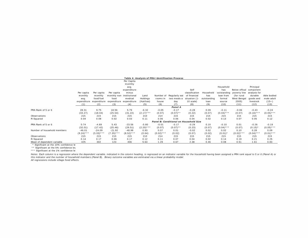
richer households. In Panel A of Table 4 we investigate how those identi�ed in

the PRA as �very poor�or �exceptionally poor�(PRA rank of 5 or 6) compare to

those with a PRA rank below 5. Speci�cally we regress the indicators of poverty

obtained in the household survey on a dummy indicating PRA rank of 5 or 6

and a set of village dummies. From the perspective of targeting, it may be less

of a concern if those ranked as "very" or "exceptionally" poor are not especially

di¤erent from those classi�ed as "average" or "poor" but more concerning if

they were not observably poorer than those ranked as rich. Comparing only the

highest ranked to the lowest ranked households, however, generates qualitatively

similar, but predictably ampli�ed, estimates to those discussed below.15

15 In particular, comparing those with a PRA rank of 5 or 6 only to those ranked 1,2 or3 or only those ranked 1 or 2 ampli�es the results pertaining to land holdings, assets, self-

21

Those assigned a high PRA rank appear poorer than others in several im-

portant respects. For one thing, these households tend to have substantially

less land than others. On average, very or exceptionally poor households own

6.3 katthas (0.13 acres) less land. The coe¢ cient is statistically signi�cant at

the 1% con�dence level and the magnitude of the point estimate is substantial;

this di¤erence represents 75% of mean land holdings among those not identi�ed

as Ultra Poor (8.4 katthas).

Figure 1, which plots the cumulative distribution functions (cdfs) of land

holdings separately for those ranked very or exceptionally poor in the PRA and

those given a lower rank, con�rms these results. A statistical test (Abadie,

2002) indicates that the distribution of households ranked 5 or 6 in the PRA

stochastically dominates the distribution of those given a lower rank (p-value <

0:01), meaning that for a given level of land holdings a higher percentage of

those ranked 5 or 6 own less than that quantity of land than the corresponding

percentage for those ranked 1-4. The advantage of this comparison relative

to the regression analysis is that it reveals di¤erences between the two groups

that are una¤ected by a few exceptionally large landowners; focusing on the

population with low values of land holdings, the �gure reveals that those ranked

5 or 6 tend to own even less than others.

We also �nd that these households are poorer in terms of asset holdings:

when our index of durable goods and livestock is taken as the left hand variable

the coe¢ cient on the PRA rank dummy is negative and signi�cant at the 1%

classi�cation of �nancial status and credit from a formal source. The results pertaining toother outcomes are generally unchanged.

22

con�dence level. While these households do not appear to be any less likely to

have taken loans, they are 11% less likely to have obtained loans from a formal

source, a di¤erence which is also signi�cant at the 1% con�dence level. The

table also indicates that these households are 17% less likely to report regularly

eating two meals a day. This coe¢ cient is signi�cant at a 5% con�dence level.

While not statistically di¤erent from zero, our point estimates suggest that this

group lives in smaller homes and self-classify their �nancial situation as worse

than their lower ranked neighbors. When we consider our various measures of

expenditure, the coe¢ cients take the unexpected, positive, sign; but none of

these coe¢ cients are statistically distinguishable from zero.

Di¤erences in per capita expenditure, however, are not entirely informa-

tive when the outcome of interest is not expenditure itself but the economic

well-being implied by an expenditure level (Olken 2003). One issue is with

equivalence scales; certain household members, such as the elderly, may require

only a fraction of the expenditure required by others to achieve the same level of

well-being (nutritional status for example). Furthermore, per capita variables

do not account for economies of scale (it may be cheaper per capita to feed or

clothe a large family) and public goods (a radio, for example, bene�ts all mem-

bers although the per capita cost is higher in a small household). In light of

these considerations, we re-run the regressions while controlling for household

size, and present these results in Panel B of Table 4.16 When considering food

and fuel expenditures and total expenditures less institutional medical expendi-

16The results are similar using the equivalence scales reported in Meenakshi and Ray (2002).

23

tures the coe¢ cient on the PRA rank dummy now takes the expected negative

sign, although the estimates are not signi�cant at the 10% con�dence level.

When total expenditures or non-food expenditures are taken as the left hand

side variable, the coe¢ cients remain positive but are drastically smaller. The

the statistically signi�cant and negative coe¢ cient on the number of household

members indicates that expenditure per capita falls as household size increases,

which is indicative of economies of scale in household consumption. These re-

sults suggest that when averaging across households of all sizes those ranked

very or exceptionally poor appear to spend more per capita. When comparing

two households with the same number of members, however, the households

ranked poorer appear to spend less per capita (with respect to food and fuel

expenditures and total expenditures less institutional medical expenditures).

As a robustness check, we also controlled for total household members when

considering other indicators of poverty which should not necessarily be impacted

by household size (land holdings, credit access, etc.). When considering these

other variables the estimated di¤erences between those ranked very or extremely

poor and those ranked richer do not change appreciably.

These expenditure patterns are illustrated visually in Figure 2 which shows

the cdfs for per capita total expenditure, food expenditure, non-food expendi-

ture and total less institutional medical expenditure for the two groups. The

divergence of the cdfs for higher levels of expenditure when considering non-

food expenditures suggests that higher expenditure and higher PRA rank could

both be driven by an omitted variable. For example, an economic shock to the

24

household could simultaneously increase expenditures and also cause villagers

to view the a­ icted household as less fortunate. If that were the case, per capita

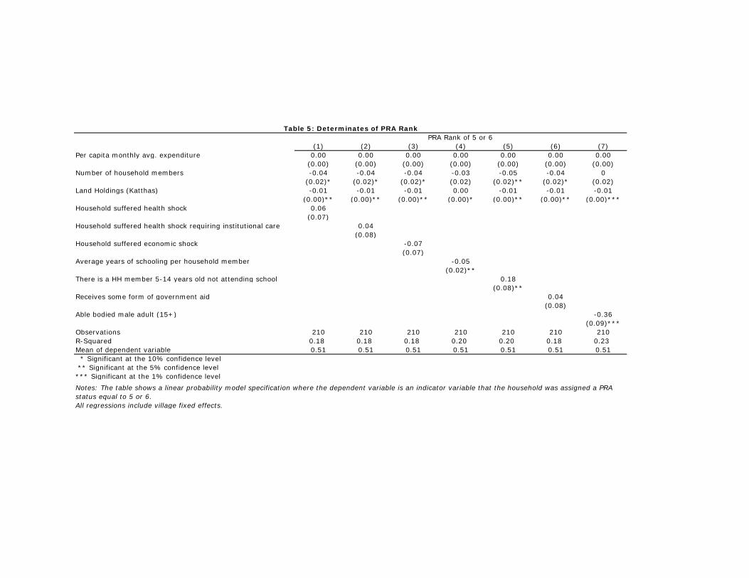
expenditure would be mis-measuring true household well-being. In Table 5 we

investigate this hypothesis.

Using the linear probability model speci�cation from (2), we regress a dummy

indicating PRA rank of 5 or 6 on land holdings, per capita consumption and a

set of variables which may cause villagers to perceive a household as especially

poor.17 Since PRA rank is relative to other households in the same geographic

area, these speci�cations contain a set of village dummies. Also, in light of

the importance of household size, we condition on the number of household

members. In all speci�cations the coe¢ cient on per capita total monthly ex-

penditure is statistically indistinguishable from zero. For land holdings the

coe¢ cient takes the predicted negative sign and is statistically signi�cant. The

table shows that having su¤ered a shock is not a signi�cant determinant of high

PRA status; the coe¢ cients on having experienced a medical shock in the last

year (i.e. having spent more than Rs. 500 on any member�s medical care), hav-

ing experienced a medical shock requiring institutional care (i.e. having spent

more than Rs. 500 on institutional medical care) and on having experienced

an economic shock (house was severely damaged, livestock became ill, livestock

died, con�ict/dispute/legal case or theft) are all indistinguishable from zero.

Nor are households which have been identi�ed by the government as in need of

aid, indicated by participation in some government aid program, more likely to

17We also estimated an OLS speci�cation where the outcome is PRA rank in levels (1-6)rather than a binary varible, the results are similar.

25

be seen as particularly poor by their neighbors. We do �nd that education is

correlated with PRA status; an additional year of schooling per capita makes

households 5% less likely to be ranked very or exceptionally poor and a house-

hold with a child out of school is 18% more likely to be so ranked. Both of these

coe¢ cients are signi�cant at the 5% con�dence level. Another result from this

exercise is that the presence of an able bodied adult (older than 14) male makes

households 36% less likely to be assigned the highest PRA ranks.18

4.4 Comparing PRA and Government Targeting

In addition to considering whether di¤erent targeting procedures successfully

identify the poorest of the poor, we are also interested in making comparisons

across methods. Tables 3 and 4 seem to suggest that the PRA identi�es individ-

uals who are relatively more disadvantaged according to various measures than

government procedures, but we also test these apparent di¤erences formally. In

particular we statistically test for equality of the coe¢ cients on the indicator

for receiving a particular form of government aid and the indicator on having

been identi�ed as poor in the PRA. These results (which are relegated to Ap-

pendix Table A1) demonstrate that there are statistically signi�cant di¤erences

between the coe¢ cients for the outcomes which generate statistically signi�cant

results in Table 4.

With the exception of participants in employment generating schemes, we

can reject equality of the coe¢ cients for land holdings above a 5% con�dence

18This coe¢ cient is similar in magnitude using over 18 years as the de�nition of adult.

26

level, indicating that the di¤erence in land holdings between those identi�ed

as poor in the PRA and others is larger than the di¤erence for individuals

participating in government assistance programs and those that are not. We

can also reject equality of the coe¢ cients above a 5% level for all government

programs when considering having taken a loan from a formal source. With

respect to the other outcomes for which we found a signi�cant di¤erence between

those identi�ed as poor in the PRA and those not identi�ed (food security,

asset ownership and the presence of an able bodied male) the coe¢ cients are

statistically di¤erent above a 10% con�dence level only when compared to 2 or

3 of the 4 government programs.

Another important concern is how potential di¤erences in the objectives of

the PRA and government identi�cation a¤ects targeting. The PRA studied here

was intended to identify a particularly poor population to participate in a local

anti-poverty program. Government programs, on the other hand, reach millions

of people and may target at a di¤erent poverty threshold. If the threshold for

government assistance is set above the level captured in our sample of fairly

impoverished households and targeting were perfect, we would expect to see all

households in our sample receiving aid, which is not the case empirically. Even

so, the threshold for identi�cation may be di¤erent for government programs.

While di¤erent thresholds for some poverty measure does not necessarily af-

fect the di¤erence in means between households above and below the threshold

(even though it a¤ects levels ), it may a¤ect how targeting is done. For exam-

ple if the aim of the program is to reduce the number of households in poverty,

27

targeting may focus speci�cally on households just below the threshold as it is

easier to move these households above the poverty line. To investigate this

possibility we plot the percentage of households participating in a given govern-

ment program against quintiles of poverty measures in Figure 3. In some cases,

the �gure shows that a higher percentage of individuals in the lower quintiles

are receiving aid or identi�ed as poor in the PRA, suggesting targeting along

this dimension of poverty, but the �gure does not suggest an obvious targeting

threshold at which the percent receiving aid drops and remains persistently low.

Moreover, there does not appear to be a systematically di¤erent threshold for

identi�cation in the PRA and receiving government assistance.

A related concern is that the concept of poverty used for classi�cation in

the PRA is locally de�ned, thus our analysis includes village level �xed e¤ects.

Government programs, however, may be less concerned with targeting those

who are relatively disadvantaged vis-à-vis their neighbors than with targeting

according to state or national benchmarks. In light of this, we conduct simi-

lar analysis without �xed e¤ects which compares targeting across rather than

within villages. The estimates from this exercise (shown in Appendix Tables

A2 and A3) are quite similar to those including village �xed e¤ects. Comparing

across villages, the estimated di¤erences between recipients of BPL, Antodaya

rationing or government housing support and non-recipients are striking simi-

lar to the within village comparisons; recipient are not notably worse o¤ than

non-recipients. For participants in employment generating schemes, the across

village comparison with non-participants suggests that participants may be dis-

28

advantaged in some respects (they have lower monthly food consumption) but

it no longer appears that they own less land.

Across villages, it remains the case that PRAs identify households which

own less land, have limited credit access and are less likely to have an able

bodied male member. The results with respect to food security and assets are

somewhat attenuated without village �xed e¤ects, but continue to indicate that

households identi�ed as poor in the PRA have greater food insecurity and fewer

assets.

4.5 Analysis of Bandhan�s Veri�cation Process

In addition to conducting PRAs, Bandhan visited and interviewed households

several times to identify those to be classi�ed as Ultra Poor. In this section, we

analyze how the additional veri�cation narrowed the targeted population and

how those identi�ed as Ultra Poor di¤er from those not so identi�ed.

The fourth column in Table 2 o¤ers some insight into this question. It is

apparent that households identi�ed as Ultra Poor have less land. On average

they have 6.5 katthas (0.13 acres) less and they are 12 percentage points more

likely to be landless, di¤erences which are both statistically di¤erent from zero

at or above a 5% con�dence level. In terms of assets, the Ultra Poor are in fact

poorer on average; they live in smaller homes and own fewer durable goods and

livestock, these di¤erences are also signi�cant at or above a 5% con�dence level.

Like those classi�ed as poor in the PRA, the Ultra Poor are less likely to have

obtained credit from a formal source, by 9 percentage points, but are no less

29

likely to have obtained loans. They classify themselves as poorer and are less

likely to report eating two meals a day, but the di¤erence in unconditional means

are not statistically di¤erent from zero. The Ultra Poor are also less educated,

the average member of an Ultra Poor household has completed 0.7 less years of

schooling, signi�cant at the 1% level. Although the di¤erences are not generally

statistically di¤erent from zero, the table indicates that Ultra Poor households

report higher expenditure than other households. Another noteworthy feature

of Ultra Poor households is that only 69% include an able bodied adult male

member whereas nearly 94% of not Ultra Poor households do, a di¤erence which

is statistically signi�cant at the 1% con�dence level.

To increase the precision of our comparison, we control for village speci�c

characteristics. The results, shown in Panel A of Table 6, con�rm what can

be gleaned from the summary statistics. When including village �xed e¤ects,

however, it appears that Ultra Poor households spend more per capita than

other households (although the di¤erence is not statistically distinguishable from

zero when conditioning on households size). We explore this result further in

Section 4.5. Other than for expenditure, our analysis of the PRA alone and of

Bandhan�s identi�cation process as a whole have similar implications. This is

not particularly surprising, since Bandhan selects households with a high PRA

rank to visit for subsequent veri�cation.

Given the similarity of the results, we assess whether additional veri�cation

of the information collected in the PRA, as Bandhan does to identify the Ultra

Poor, improves targeting of the poorest households beyond what is achieved by

30

the PRA. To accomplish this we restrict our sample only to those households

which were ranked as very or exceptionally poor in the PRA, leaving us with 111

observations. Of these 111 households Bandhan identi�ed 85 as Ultra Poor and

the remaining 26 as not Ultra Poor. Panel A of Table 7 compares the Ultra Poor

households to the others. The point estimates, while not statistically signi�cant,

suggest that the Ultra Poor have higher expenditure even when compared only

to others ranked very or exceptionally poor. In Panel B we control for household

size which results in smaller, but still positive coe¢ cients. In terms of assets,

credit access, food security and self-classi�cation of �nancial situation we can not

make a clear distinction between the Ultra Poor and others. The most salient

result is that Ultra Poor households own less land, 3.1 katthas less on average.

The economic magnitude of this coe¢ cient is quite large since it represents 125%

of mean land holdings within this very or exceptionally poor group. The Ultra

Poor also live in smaller homes on average.

We now turn to directly investigating what determines the likelihood that

a household is identi�ed as Ultra Poor via equation (2). When analyzing the

full sample, the results reveal that the variables which appear to determine

identi�cation as Ultra Poor are generally the same as those which determine

PRA rank. Therefore, we restrict to the sample of households ranked as very

or exceptionally poor in the PRA for this analysis. Table 8 shows that for these

households, the only signi�cant determinates of identi�cation as Ultra Poor are

the presence of an able bodied adult male, which makes identi�cation as Ultra

Poor 19% less likely, and land holdings.

31

4.6 Revisiting Consumption

A noteworthy di¤erence between the implications of Table 6 and the summary

statistics is that the regression framework suggests that the Ultra Poor spend

more than others and that these di¤erences are statistically di¤erent from zero.

In particular, our results suggest that the average Ultra Poor household spends

Rs. 68 more per household member per month than not identi�ed households

and Rs. 36 more per household member per month on food and fuel. The point

estimates are considerable in magnitude since Rs. 36 represent 12% of the mean

per capita monthly food and fuel expenditure.

Although consumption and expenditure are notoriously di¢ cult to measure

(see e.g. Deaton 1997), making these particular variables imprecise, we are

interested in ascertaining what drives these estimates given that per capita con-

sumption is a widely used and important indicator of poverty. One factor which

may cause us to observe Ultra Poor households spending more than non Ultra

poor households is if Ultra Poor households have experienced economic shocks

(e.g. need to repair house damage or pay medical bills). This will be partic-

ularly true if having experienced such a shock makes a household more likely

to be identi�ed as Ultra Poor. Closer inspection of the expenditures enumer-

ated by the households revealed that this phenomenon may occur; several of

the most costly single expenditures were for institutional medical care. More-

over, the largest of these expenditures were reported by those identi�ed as Ultra

Poor; the maximum such expenditure reported by a not identi�ed household is

Rs. 10,000 (� $255) whereas identi�ed households reported expenditures of Rs.

32

10,000, 12,000, 16,000, 35,000 and 60,000 (� $255� 1; 538).

This concern is what motivated us to look separately at per capita monthly

average expenditure less institutional medical expenditure in the preceding

analysis. But that we continue to observe a positive point estimate for this

outcome in Table 6 and do not �nd that su¤ering a medical or economic shock

makes a household particularly likely to be identi�ed as Ultra Poor in Table 8

does not provide robust evidence for this hypothesis.

Since they tend to own much less land, it may be that the Ultra Poor spend

more on food because they do not produce anything for home consumption and

the non Ultra Poor may underestimate the value of what they produce at home.

Since we lack complete information on home production we are unable to test

this conjecture directly. We do, however, investigate this concern by restricting

our sample only to those households with 15 or fewer katthas (0.3 acres) of land

(this causes us to drop 21 observations or 10% of our sample). We run the same

regressions for the expenditure variables as in Table 6, the results in Table 9

show that the di¤erences in total and non food expenditure between the Ultra

Poor and not Ultra Poor are ampli�ed when considering only these households.

In terms of food and fuel expenditure, the estimate of the di¤erence between

the two groups is essentially the same. This suggests that home production of

food in not the primary reason for these di¤erences.

Additionally, although our initial survey is designed to capture all consump-

tion, rather than just expenditure, we created a supplementary survey instru-

ment with more detailed questions pertaining to production for own consump-

33

tion and returned to the households in this study. Due to migration and absences

we were not able to resurvey 11% of the households in the initial dataset. Us-

ing the data collected in this secondary survey, we again compared levels of per

capita consumption between those households identi�ed as Ultra Poor and other

households. Table 10 presents the results from this analysis. Columns 1 and

2 repeat the analysis from Table 6, using the initial data but restricted to the

sample which was resurveyed. Columns 3 and 4 use the data from the secondary

survey. Again the point estimates suggest that households identi�ed as Ultra

Poor consume more per capita than other households, both in terms of food

and fuel consumption and total consumption. These di¤erences, however, do

not appear statistically signi�cant, as was the case when considering the initial

data. That the estimates using the data from this additional, more detailed,

survey are similar to those obtained using the initial data suggests that failure

to capture production for own consumption is not responsible for the perplexing

sign of the coe¢ cients.

Given the potential importance of household economies of scale, we con-

dition on household size in Panel B. When using the data from the detailed

consumption resurvey the coe¢ cients on the Ultra Poor indicator take the pre-

dicted negative sign in these regressions, but the estimates are not statistically

di¤erent from zero. That the point estimates, conditional on household size,

suggest that Ultra Poor households spend more than others in one survey and

less than others in a secondary survey of the same households limits the cred-

ibility of the initial results; our analysis can not distinguish clear di¤erences

34

between the two groups in terms of per capita consumption.

To further explore the hypothesis of household economies of scale, we also ran

the expenditure comparison regressions using the disaggregated components of

per capita monthly food and fuel expenditure. When considering each item sep-

arately the coe¢ cient on having been identi�ed as Ultra Poor generally remains

positive, as is shown in Table 11. These coe¢ cients, however, are imprecisely

estimated; the only variables for which we can detect a statistically signi�cant

di¤erence are �Other food�and �Fuel and Light.�The latter �nding in particu-

lar, coupled with the observation that Ultra Poor households tend to have fewer

members, suggests that there may be economies of scale driving our previous

results; if a home is to be lit or a meal cooked regardless of how many people

reside in that home, then per capita fuel and light expenditure will appear larger

in a smaller household.

5 Conclusions

Targeting a sub-population can be challenging, particularly when the target

group is designated by a broad, ill-de�ned characteristic such as �extreme poverty.�

Various mechanisms can be employed to learn who the poorest of the poor actu-

ally are. Censuses which record household characteristics are one such method.

This approach, however, captures only a limited set of poverty metrics and suf-

fers from the fact that many indicators of poverty are not easily observable.

Another commonly used targeting method is to conduct group discussions, such

35

as a PRA, which rely not only on the responses of a speci�c household but

also on the input of their neighbors to ascertain which households are most

disadvantaged.

In this paper, we consider the relative performance of each of these mecha-

nisms with respect to identifying the poorest of the poor. In particular, we eval-

uate how well classi�cation as impoverished according to a particular method

accords with statistical measures of poverty collected in a detailed household

survey.

We �rstly examine various government assistance programs which utilize a

census as part of their targeting process. Our results suggest that these programs

do not overwhelmingly reach the very poorest, which may be due to de�ciencies

in the identi�cation process. Subsequently, we evaluate whether PRAs reliably

identify the poorest households within a village. We compare characteristics of

households ranked as especially poor in the PRA by their neighbors to other

disadvantaged households within the village. The comparison indicates that the

ranking from the PRA accurately identi�es a poorer sub-population in terms of

land holdings, assets and credit access.

Finally, since the PRA was part of a more extensive process conducted by

Bandhan, a Kolkata-based micro�nance institution, to identify the poorest of

the poor, we consider what further gains can be made by verifying the infor-

mation from the PRA with household visits. We �nd that the additional steps

taken by Bandhan narrows the identi�ed population to those who are more

disadvantaged in crucial respects, particularly land holdings.

36

Although our results do not indicate that either the PRA or government

procedures particularly target the poorest of the poor in terms of consumption,

which is a crucial measure of poverty, we do �nd that participatory targeting

methods, such as a PRA, perform better than census techniques in identifying

households which are most disadvantaged according to various other important

measures of poverty.

37

References

Abadie, A. (2002). Bootstrap tests for distributional treatment e¤ects in in-

strumental variable models. Journal of the American Statistical Associa-

tion 79 (457), 284�292.

Alatas, V., A. Banerjee, R. Hanna, B. A. Olken, and J. Tobias (2009). How

to target the poor: Evidence from a �eld experiment in Indonesia. Un-

published manuscript, MIT .

Amin, S., A. S. Rai, and G. Topa (2003). Does microcredit reach the poor and

vulnerable? Evidence from northern Bangladesh. Journal of Development

Economics 70, 59�82.

Anderson, G. (1996). Nonparametric tests of stochastic dominance in income

distributions. Econometrica 64 (5), 1183�1193.

Chambers, R. (1994). Participatory rural appraisal (PRA): Analysis of expe-

rience. World Development 22 (9), 1253�1268.

Chambers, R. (1997). Whose Reality Counts? Putting the �rst last. London:

ITDG Publishing.

Chattopadhyay, R. and E. Du�o (2001). Women�s leadership and policy deci-

sions: Evidence from a nationwide randomized experiment in India.Work-

ing Paper . http://ideas.repec.org/p/bos/iedwpr/dp-114.html.

Conn, K., E. Du�o, P. Dupas, M. Kremer, and O. Ozier (2008). Bursary

targeting strategies: Which method(s) most e¤ectively identify the poor-

est primary school students for secondary school bursaries? Unpublished

38

Manuscript .

Deaton, A. (1997). The Analysis of Household Surveys. Baltimore: The Johns

Hopkins University Press.

Jalan, J. and R. Murgai (2007). An e¤ective "Targeting Shortcut"? An

assessment of the 2002 below-poverty line census method. http://

www.ihdindia.org/ourcontrol/rinku_murgai.doc. Viewed September

2007.

Meenakshi, J. and R. Ray (2002). Impact of household size and family com-

position on poverty in rural India. Journal of Policy Modeling 24 (6), 539�

559.

Morduch, J. (1999). The micro�nance promise. Journal of Economic Litera-

ture 37 (4), 1569�1614.

Olken, B. (2005). Revealed community equivalence scales. Journal of Public

Economics 89 (2-3), 545�566.

Rabbani, M., V. Prakash, and M. Sulaiman (2006). Impact assessment

of CFPR/TUP: A descriptive analysis based on 2002-2005 panel data.

CFPR/TUP Working Paper Series No. 12.

39

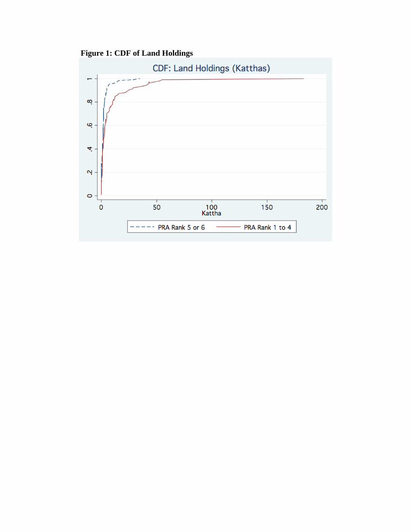
Figure 1: CDF of Land Holdings

                          

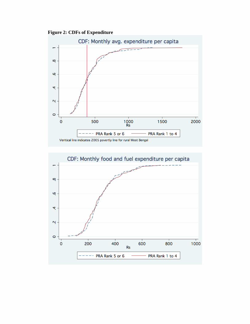
Figure 2: CDFs of Expenditure

  

      

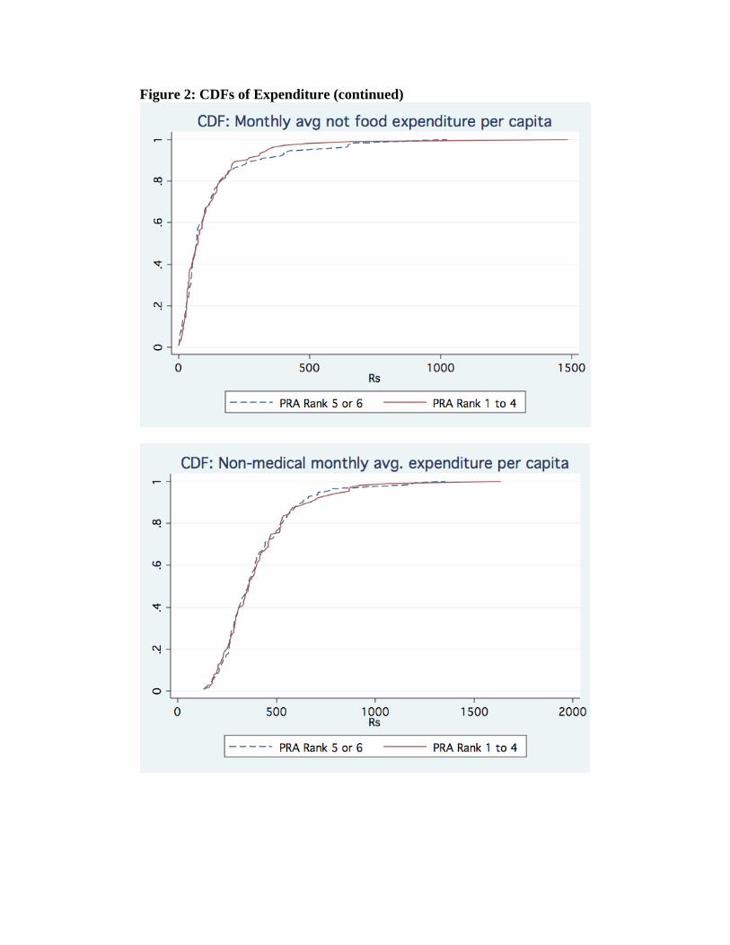
Figure 2: CDFs of Expenditure (continued) 

  

    

  

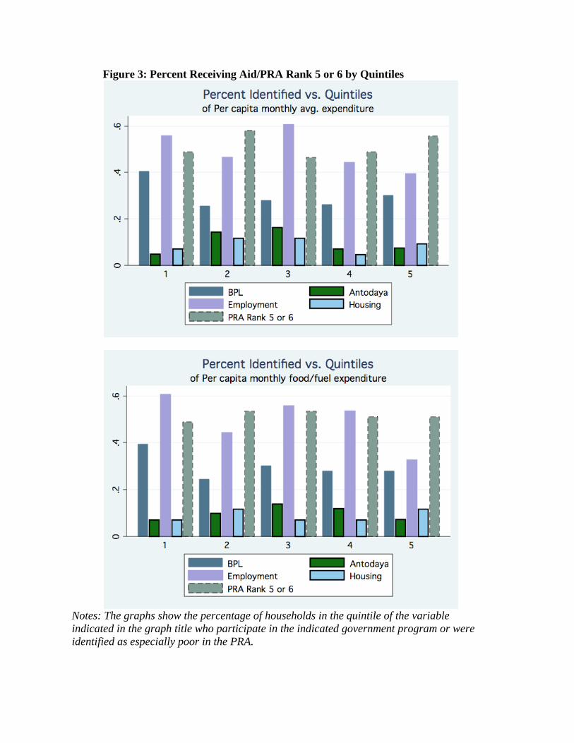
Figure 3: Percent Receiving Aid/PRA Rank 5 or 6 by Quintiles

  

 Notes: The graphs show the percentage of households in the quintile of the variable indicated in the graph title who participate in the indicated government program or were identified as especially poor in the PRA.

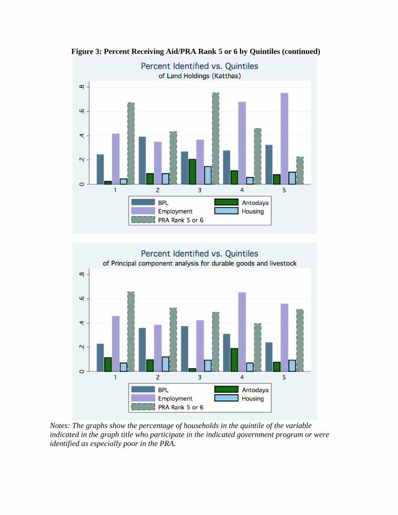
Figure 3: Percent Receiving Aid/PRA Rank 5 or 6 by Quintiles (continued)

 

 Notes: The graphs show the percentage of households in the quintile of the variable indicated in the graph title who participate in the indicated government program or were identified as especially poor in the PRA.

 

Village

Number of households

found in economic

census

Number of households eligible for additional

survey

Size of the sample for additional

survey

Identified as Ultra Poor by

BandhanBalarampur 855 254 20 38Binkar 273 110 40 11Chardiar 128 65 43 9Charsungai 137 75 38 17Khidirpur 364 101 37 18Total 1757 605 178 93

Table 1: Village-wise Sample Breakdown

Note: Table shows figures pertaining to sample frame and sample selection. Column 1 shown the number of households enumerated in the village census, column 2 indicates how many met the sample selection criteria and column 3 indicates how many were surveyed. Column 4 indicates how many additional households selected by Bandhan were surveyed in each village.

Mean sd Mean sd Mean sd Diff. sd Diff.(1) (2) (3) (4) (5) (6) (7) (8)

Ranking from PRA 4.55 1.39 3.76 1.25 5.59 0.74 1.83 (0.15)***Number of household members 4.29 1.69 4.69 1.54 3.77 1.76 -0.91 (0.23)***Per capita monthly avg. expenditure 425 229 404 218 453 241 49 (31.45)Per capita monthly food/fuel expenditure 302 127 288 111 321 145 32 (17.42)*Per capita monthly non-food expenditure 123 174 116 167 132 184 17 (24.01)Per Capita monthly avg. expenditure minus institutional medical expenditure 406 215 393 208 423 223 30 (29.53)Below official poverty line (for rural West Bengal 2005) 0.51 0.50 0.56 0.50 0.45 0.50 -0.11 (0.07)Land Holdings (Katthas) 5.63 15.43 8.42 19.85 1.91 2.79 -6.51 (2.11)***Landless 0.21 0.41 0.16 0.37 0.28 0.45 0.12 (0.06)**Number of rooms in house 1.29 0.52 1.39 0.60 1.15 0.36 -0.24 (0.07)***Principal component analysis for durable goods and livestock 1.61 1.12 1.75 1.22 1.41 0.94 -0.34 (0.15)**Household has outstanding loan 0.46 0.50 0.43 0.50 0.48 0.50 0.05 (0.07)Household has outstanding loan from formal source 0.08 0.28 0.12 0.33 0.03 0.18 -0.09 (0.04)**Self classification of financial situation (1-10 scale) 2.38 1.53 2.51 1.54 2.22 1.51 -0.29 (0.21)Average years of schooling per household member 1.23 1.75 1.54 1.89 0.82 1.45 -0.72 (0.24)***There is a HH member 5-14 years old not attending school 0.25 0.43 0.23 0.42 0.28 0.45 0.05 (0.06)Regularly eat two meals a day 0.67 0.47 0.70 0.46 0.62 0.49 -0.07 (0.07)Household gets BPL rationing 0.30 0.46 0.33 0.47 0.27 0.45 -0.06 (0.06)Households has Antodaya card 0.10 0.30 0.09 0.29 0.11 0.31 0.02 (0.04)Received work from employment generating scheme 0.49 0.50 0.56 0.50 0.41 0.49 -0.15 (0.07)**House from Indira Housing Plan 0.09 0.29 0.05 0.22 0.14 0.35 0.09 (0.04)**Household suffered health shock 0.52 0.50 0.55 0.50 0.48 0.50 -0.07 (0.07)Household suffered health shock requiring institutional care 0.22 0.41 0.23 0.42 0.20 0.41 -0.03 (0.06)Household suffered economic shock 0.41 0.49 0.40 0.49 0.43 0.50 0.03 (0.07)Able bodied male adult (15+) 0.83 0.37 0.94 0.23 0.69 0.47 -0.25 (0.05)***Able bodied female adult (15+) 0.98 0.14 0.98 0.16 0.99 0.10 0.01 (0.02) * Significant at the 10% confidence level ** Significant at the 5% confidence level*** Significant at the 1% confidence level

Table 2: Selected Characteristics of Sample Households

Below the poverty line for rural West Bengal is defined as having per capita consumption under Rs. 382.82 (Based on estimates in "Poverty Line Estimates in Public Distribution System and Other Sources of Household Consumption, 2004-05." National Sample Survey Organization, Ministry of Statistics and Programme Implementation Report No. 510).

Notes: The table shows selected summary statistics for this sample. The unit of observation in the household. Statistics are shown separately for households identified as Ultra Poor by Bandhan's targeting process and household which were not.

Full Sample (N=213)

Non Ultra Poor

Ultra Poor (N=92)

Ultra Poor - Non Ultra Poor

Per capita monthly

avg. expenditure

Per capita monthly food/fuel

expenditure

Per capita monthly non-

food expenditure

Per Capita monthly

avg. expenditure

minus institutional

medical expenditure

Land Holdings (Katthas)

Number of rooms in house

Regularly eat two

meals a day

Self classification of financial

situation (1-10 scale)

Household has

outstanding loan

Household has

outstanding loan from

formal source

Below offical poverty line

(for rural West Bengal

2005)

Principal component analysis for

durable goods and livestock

Able bodied male adult

(15+)(1) (2) (3) (4) (5) (6) (7) (8) (9) (10) (11) (12) (13)

Household gets BPL rationing -7.23 7.93 -15.16 -1.42 -2.29 0.00 -0.03 -0.08 0.00 0.01 0.01 -0.09 0.11 (34.82) (18.85) (26.70) (32.61) (2.31) (0.08) (0.07) (0.23) (0.08) (0.04) (0.07) (0.17) (0.06)*Observations 213 213 213 213 208 212 213 213 213 213 213 213 213R-Squared 0.04 0.08 0.02 0.03 0.08 0.06 0.04 0.03 0.01 0.1 0.07 0.02 0.04Mean of dependent variable 426 303 123 407 5.66 1.29 0.66 2.38 0.46 0.08 0.51 1.59 0.83Households has Antodaya card -17.62 7.13 -24.75 -11.71 -1.79 -0.08 0.16 0.19 -0.15 -0.02 0.14 0.14 -0.09 (50.35) (28.62) (38.50) (48.47) (3.57) (0.12) (0.11) (0.35) (0.12) (0.06) (0.11) (0.26) (0.09)Observations 208 208 208 208 203 207 208 208 208 208 208 208 208R-Squared 0.05 0.09 0.03 0.04 0.07 0.06 0.05 0.03 0.02 0.09 0.09 0.02 0.03Mean of dependent variable 419 302 117 404 5.4 1.29 0.65 2.38 0.46 0.08 0.51 1.58 0.83Received work from employment generating scheme -32.54 -27.34 -5.21 -32.68 -4.33 0.04 0.00 -0.44 0.08 0.01 0.13 0.18 0.16 (38.99) (21.06) (29.96) (36.50) (2.59)* (0.09) (0.08) (0.26)* (0.09) (0.05) (0.08) (0.19) (0.06)***Observations 215 215 215 215 210 214 215 215 215 215 215 215 215R-Squared 0.04 0.09 0.02 0.04 0.09 0.06 0.04 0.04 0.01 0.09 0.08 0.03 0.06Mean of dependent variable 425 302 123 406 5.63 1.29 0.67 2.38 0.46 0.08 0.51 1.61 0.83House from Indira Housing Plan -41.31 31.78 -73.10 -19.96 -0.77 -0.05 0.11 0.24 0.19 0.07 -0.03 -0.16 -0.24 (55.57) (30.06) (42.42)* (52.11) (3.77) (0.13) (0.11) (0.37) (0.12) (0.06) (0.12) (0.27) (0.09)***Observations 214 214 214 214 209 213 214 214 214 214 214 214 214R-Squared 0.04 0.09 0.03 0.03 0.08 0.06 0.04 0.03 0.02 0.09 0.07 0.03 0.06Mean of dependent variable 426 303 123 407 5.65 1.29 0.67 2.39 0.45 0.08 0.51 1.61 0.83 * Significant at the 10% confidence level ** Significant at the 5% confidence level *** Significant at the 1% confidence level

All regressions include village fixed effects.

Table 3: Characteristics of Recipients of Government Aid

Notes: Each panel shows a separate set of regressions where the indicator variable specified in the row panel is taken as the independent variable and the variable indicated in the column is the dependent variable.

Per capita monthly

avg. expenditure

Per capita monthly food/fuel

expenditure

Per capita monthly non-

food expenditure

Per Capita monthly

avg. expenditure

minus institutional

medical expenditure

Land Holdings (Katthas)

Number of rooms in house

Regularly eattwo meals a

day

Self classification of financial

situation (1-10 scale)

Household has

outstanding loan

Household has

outstanding loan from

formal source

Below offical poverty line (for rural

West Bengal 2005)

Principal component analysis for

durable goods and livestock

Able bodied male adult

(15+)(1) (2) (3) (4) (5) (6) (7) (8) (9) (10) (11) (12) (13)

PRA Rank of 5 or 6 28.31 9.75 18.56 5.79 -6.32 -0.05 -0.17 -0.28 0.09 -0.11 -0.06 -0.43 -0.24 (33.27) (18.04) (25.54) (31.22) (2.17)*** (0.07) (0.07)** (0.22) (0.07) (0.04)*** (0.07) (0.16)*** (0.05)***Observations 215 215 215 215 210 214 215 215 215 215 215 215 215R-Squared 0.04 0.08 0.02 0.03 0.11 0.06 0.06 0.04 0.02 0.13 0.07 0.05 0.12

PRA Rank of 5 or 6 0.74 -4.69 5.43 -23.56 -5.80 -0.01 -0.17 -0.29 0.10 -0.10 0.01 -0.26 -0.19 (32.01) (17.42) (25.46) (29.51) (2.20)*** (0.07) (0.07)** (0.23) (0.07) (0.04)*** (0.07) (0.15)* (0.05)***Number of household members -46.01 -24.09 -21.92 -48.98 0.93 0.07 0.01 -0.02 0.02 0.02 0.10 0.28 0.09 (9.24)*** (5.03)*** (7.35)*** (8.52)*** (0.64) (0.02)*** (0.02) (0.07) (0.02) (0.01)* (0.02)*** (0.04)*** (0.01)***Observations 215 215 215 215 210 214 215 215 215 215 215 215 215R-Squared 0.14 0.17 0.06 0.17 0.12 0.11 0.07 0.04 0.02 0.14 0.19 0.21 0.25Mean of dependent variable 425 302 123 406 5.63 1.29 0.67 2.38 0.46 0.08 0.51 1.61 0.83 * Significant at the 10% confidence le ** Significant at the 5% confidence lev *** Significant at the 1% confidence lev

All regressions include village fixed effects.

Panel A

Panel B: Conditional on Household Size

Table 4: Analysis of PRA Identification Process

Notes: Each column is a regression where the dependent variable, indicated in the column heading, is regressed on an indicator variable for the household having been assigned a PRA rank equal to 5 or 6 (Panel A) or this indicator and the number of household members (Panel B). Binary outcome variables are estimated via a linear probability model.

(1) (2) (3) (4) (5) (6) (7)

Per capita monthly avg. expenditure 0.00 0.00 0.00 0.00 0.00 0.00 0.00 (0.00) (0.00) (0.00) (0.00) (0.00) (0.00) (0.00) Number of household members -0.04 -0.04 -0.04 -0.03 -0.05 -0.04 0 (0.02)* (0.02)* (0.02)* (0.02) (0.02)** (0.02)* (0.02) Land Holdings (Katthas) -0.01 -0.01 -0.01 0.00 -0.01 -0.01 -0.01 (0.00)** (0.00)** (0.00)** (0.00)* (0.00)** (0.00)** (0.00)*** Household suffered health shock 0.06 (0.07) Household suffered health shock requiring institutional care 0.04 (0.08) Household suffered economic shock -0.07 (0.07) Average years of schooling per household member -0.05 (0.02)** There is a HH member 5-14 years old not attending school 0.18 (0.08)** Receives some form of government aid 0.04 (0.08) Able bodied male adult (15+) -0.36 (0.09)*** Observations 210 210 210 210 210 210 210 R-Squared 0.18 0.18 0.18 0.20 0.20 0.18 0.23 Mean of dependent variable 0.51 0.51 0.51 0.51 0.51 0.51 0.51 * Significant at the 10% confidence level ** Significant at the 5% confidence level *** Significant at the 1% confidence level

All regressions include village fixed effects.

PRA Rank of 5 or 6Table 5: Determinates of PRA Rank

Notes: The table shows a linear probability model specification where the dependent variable is an indicator variable that the household was assigned a PRA status equal to 5 or 6.

Per capita monthly avg. expenditure

Per capita monthly food/fuel

expenditure

Per capita monthly non-

food expenditure

Per Capita monthly avg. expenditure

minus institutional

medical expenditure

Land Holdings (Katthas)

Number of rooms in house

Regularly eat two meals a

day

Self classification of financial situation (1-

10 scale)

Household has

outstanding loan

Household has

outstanding loan from

formal source

Below offical poverty line (for rural

West Bengal 2005)

Principal component analysis for

durable goods and livestock

Able bodied male adult

(15+)(1) (2) (3) (4) (5) (6) (7) (8) (9) (10) (11) (12) (13)

Identified as Ultra Poor 68.50 35.78 32.72 45.09 -6.15 -0.21 -0.13 -0.26 0.09 -0.07 -0.13 -0.46 -0.26 (33.74)** (18.29)* (26.05) (31.76) (2.23)*** (0.08)*** (0.07)* (0.23) (0.08) (0.04)* (0.07)* (0.16)*** (0.05)***Observations 215 215 215 215 210 214 215 215 215 215 215 215 215R-Squared 0.05 0.1 0.02 0.04 0.11 0.09 0.05 0.04 0.01 0.1 0.08 0.06 0.13

Identified as Ultra Poor 36.28 19.1 17.18 10.48 -5.48 -0.16 -0.12 -0.27 0.1 -0.05 -0.05 -0.25 -0.2 (32.85) (17.89) (26.18) (30.41) (2.28)** (0.08)** (0.07)* (0.23) (0.08) (0.04) (0.07) (0.15) (0.05)***Number of household members -43.93 -22.74 -21.19 -47.19 0.86 0.06 0.01 -0.02 0.02 0.02 0.10 0.28 0.08 (9.27)*** (5.05)*** (7.39)*** (8.59)*** (0.65) (0.02)*** (0.02) (0.07) (0.02) (0.01)* (0.02)*** (0.04)*** (0.01)***Observations 215 215 215 215 210 214 215 215 215 215 215 215 215R-Squared 0.15 0.18 0.06 0.16 0.11 0.13 0.05 0.04 0.02 0.12 0.19 0.21 0.25Mean of dependent variable 425 302 123 406 5.63 1.29 0.67 2.38 0.46 0.08 0.51 1.61 0.83 * Significant at the 10% confidence leve ** Significant at the 5% confidence leve *** Significant at the 1% confidence leve

Table 6: Analysis of Bandhan's Identification Process

Panel A

Panel B: Conditional on Household Size

All regressions include village fixed effects.

Notes: Each column is a regression where the dependent variable, indicated in the column heading, is regressed on an indicator variable for the household having been identified as Ultra Poor by Bandhan (Panel A) or this indicator and the number of household members (Panel B). Binary outcome variables are estimated via a linear probability model.

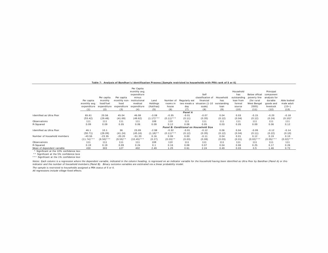
Per capita monthly avg. expenditure

Per capita monthly food/fuel

expenditure

Per capita monthly non-

food expenditure

Per Capita monthly avg. expenditure

minus institutional

medical expenditure

Land Holdings (Katthas)

Number of rooms in house

Regularly eat two meals a

day

Self classification of

financial situation (1-10

scale)

Household has

outstanding loan

Household has

outstanding loan from

formal source

Below offical poverty line (for rural

West Bengal 2005)

Principal component analysis for

durable goods and livestock

Able bodied male adult

(15+)(1) (2) (3) (4) (5) (6) (7) (8) (9) (10) (11) (12) (13)

Identified as Ultra Poor 65.61 20.56 45.04 46.08 -3.08 -0.35 -0.01 -0.07 0.04 0.03 -0.15 -0.20 -0.18 (53.42) (29.48) (41.69) (49.62) (1.17)*** (0.11)*** (0.11) (0.35) (0.12) (0.04) (0.12) (0.24) (0.10)*Observations 111 111 111 111 108 110 111 111 111 111 111 111 111R-Squared 0.09 0.09 0.05 0.06 0.09 0.12 0.08 0.05 0.03 0.05 0.09 0.06 0.12

Identified as Ultra Poor 46.1 10.1 36 23.09 -2.98 -0.32 -0.01 -0.12 0.06 0.04 -0.09 -0.12 -0.14 (50.71) (28.09) (41.24) (45.16) (1.18)** (0.11)*** (0.12) (0.35) (0.12) (0.04) (0.11) (0.22) (0.10)Number of household members -43.55 -23.35 -20.20 -51.33 0.16 0.06 0.00 -0.11 0.04 0.01 0.12 0.19 0.10 (11.74)*** (6.50)*** (9.55)** (10.45)*** (0.27) (0.03)** (0.03) (0.08) (0.03) (0.01) (0.02)*** (0.05)*** (0.02)***Observations 111 111 111 111 108 110 111 111 111 111 111 111 111R-Squared 0.19 0.19 0.09 0.24 0.1 0.16 0.08 0.07 0.04 0.06 0.25 0.17 0.26Mean of dependent variable 430 303 127 402 2.49 1.25 0.61 2.24 0.49 0.03 0.5 1.46 0.72 * Significant at the 10% confidence leve ** Significant at the 5% confidence leve *** Significant at the 1% confidence leve

Notes: Each column is a regression where the dependent variable, indicated in the column heading, is regressed on an indicator variable for the household having been identified as Ultra Poor by Bandhan (Panel A) or this indicator and the number of household members (Panel B). Binary outcome variables are estimated via a linear probability model.

The sample is restricted to households assigned a PRA status of 5 or 6.

Table 7: Analysis of Bandhan's Identification Process (Sample restricted to households with PRA rank of 5 or 6)

Panel A

Panel B: Conditional on Household Size

All regressions include village fixed effects.

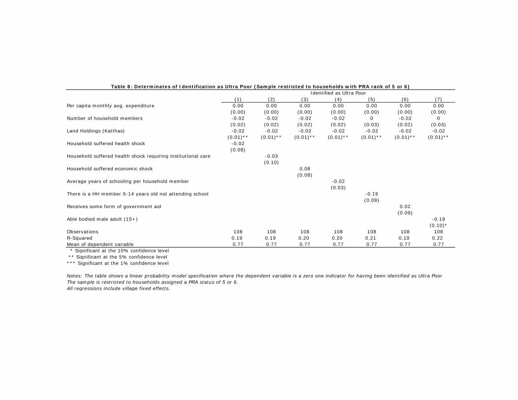
(1) (2) (3) (4) (5) (6) (7)

Per capita monthly avg. expenditure 0.00 0.00 0.00 0.00 0.00 0.00 0.00 (0.00) (0.00) (0.00) (0.00) (0.00) (0.00) (0.00)Number of household members -0.02 -0.02 -0.02 -0.02 0 -0.02 0 (0.02) (0.02) (0.02) (0.02) (0.03) (0.02) (0.03)Land Holdings (Katthas) -0.02 -0.02 -0.02 -0.02 -0.02 -0.02 -0.02 (0.01)** (0.01)** (0.01)** (0.01)** (0.01)** (0.01)** (0.01)**Household suffered health shock -0.02 (0.08) Household suffered health shock requiring institutional care -0.03 (0.10) Household suffered economic shock 0.08 (0.08) Average years of schooling per household member -0.02 (0.03) There is a HH member 5-14 years old not attending school -0.15 (0.09) Receives some form of government aid 0.02 (0.09) Able bodied male adult (15+) -0.19 (0.10)*Observations 108 108 108 108 108 108 108R-Squared 0.19 0.19 0.20 0.20 0.21 0.19 0.22Mean of dependent variable 0.77 0.77 0.77 0.77 0.77 0.77 0.77 * Significant at the 10% confidence level ** Significant at the 5% confidence level *** Significant at the 1% confidence level

All regressions include village fixed effects. The sample is restricted to households assigned a PRA status of 5 or 6.

Identified as Ultra PoorTable 8: Determinates of Identification as Ultra Poor (Sample restricted to households with PRA rank of 5 or 6)

Notes: The table shows a linear probability model specification where the dependent variable is a zero one indicator for having been identified as Ultra Poor

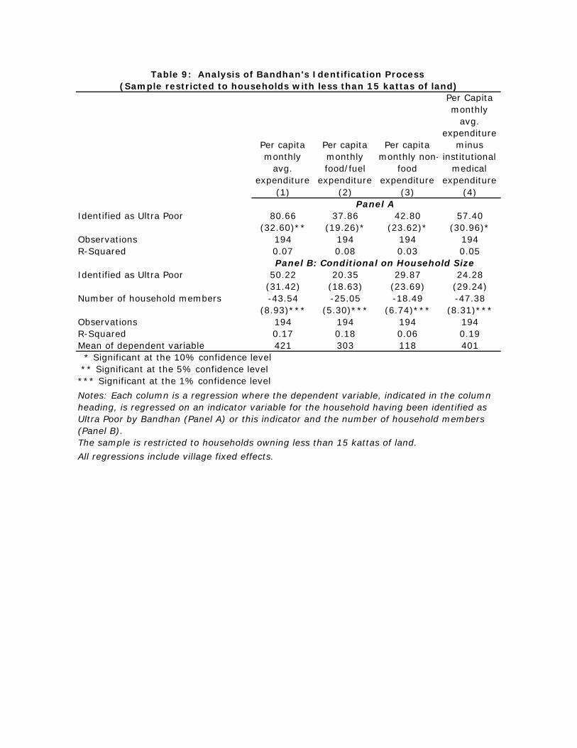
Per capita monthly

avg. expenditure

Per capita monthly food/fuel

expenditure

Per capita monthly non-

food expenditure

Per Capita monthly

avg. expenditure

minus institutional

medical expenditure

(1) (2) (3) (4)

Identified as Ultra Poor 80.66 37.86 42.80 57.40 (32.60)** (19.26)* (23.62)* (30.96)*Observations 194 194 194 194R-Squared 0.07 0.08 0.03 0.05

Identified as Ultra Poor 50.22 20.35 29.87 24.28 (31.42) (18.63) (23.69) (29.24)Number of household members -43.54 -25.05 -18.49 -47.38 (8.93)*** (5.30)*** (6.74)*** (8.31)***Observations 194 194 194 194R-Squared 0.17 0.18 0.06 0.19Mean of dependent variable 421 303 118 401

Table 9: Analysis of Bandhan's Identification Process

The sample is restricted to households owning less than 15 kattas of land.

All regressions include village fixed effects.

* Significant at the 10% confidence level ** Significant at the 5% confidence level*** Significant at the 1% confidence level

Panel A

Panel B: Conditional on Household Size

Notes: Each column is a regression where the dependent variable, indicated in the column heading, is regressed on an indicator variable for the household having been identified as Ultra Poor by Bandhan (Panel A) or this indicator and the number of household members (Panel B).

(Sample restricted to households with less than 15 kattas of land)

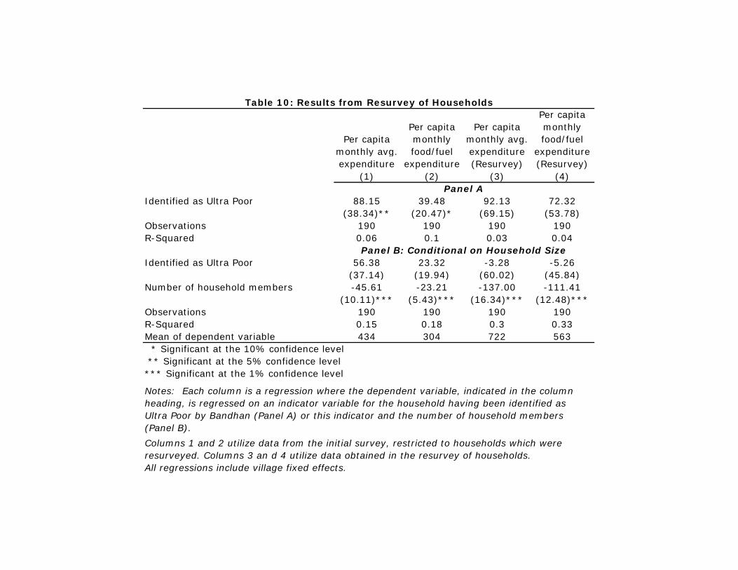
Per capita monthly avg. expenditure

Per capita monthly food/fuel

expenditure

Per capita monthly avg. expenditure (Resurvey)

Per capita monthly food/fuel

expenditure (Resurvey)

(1) (2) (3) (4)

Identified as Ultra Poor 88.15 39.48 92.13 72.32 (38.34)** (20.47)* (69.15) (53.78)Observations 190 190 190 190R-Squared 0.06 0.1 0.03 0.04

Identified as Ultra Poor 56.38 23.32 -3.28 -5.26 (37.14) (19.94) (60.02) (45.84)Number of household members -45.61 -23.21 -137.00 -111.41 (10.11)*** (5.43)*** (16.34)*** (12.48)***Observations 190 190 190 190R-Squared 0.15 0.18 0.3 0.33Mean of dependent variable 434 304 722 563

All regressions include village fixed effects.

* Significant at the 10% confidence level ** Significant at the 5% confidence level*** Significant at the 1% confidence level

Columns 1 and 2 utilize data from the initial survey, restricted to households which were resurveyed. Columns 3 an d 4 utilize data obtained in the resurvey of households.

Table 10: Results from Resurvey of Households

Panel A

Panel B: Conditional on Household Size

Notes: Each column is a regression where the dependent variable, indicated in the column heading, is regressed on an indicator variable for the household having been identified as Ultra Poor by Bandhan (Panel A) or this indicator and the number of household members (Panel B).

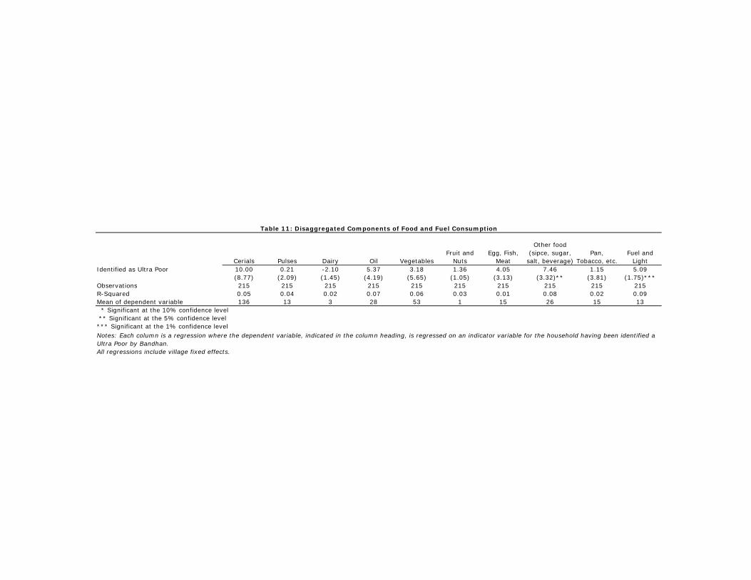
Cerials Pulses Dairy Oil VegetablesFruit and

NutsEgg, Fish,

Meat

Other food (sipce, sugar,

salt, beverage)Pan,

Tobacco, etc.Fuel and

LightIdentified as Ultra Poor 10.00 0.21 -2.10 5.37 3.18 1.36 4.05 7.46 1.15 5.09 (8.77) (2.09) (1.45) (4.19) (5.65) (1.05) (3.13) (3.32)** (3.81) (1.75)***Observations 215 215 215 215 215 215 215 215 215 215R-Squared 0.05 0.04 0.02 0.07 0.06 0.03 0.01 0.08 0.02 0.09Mean of dependent variable 136 13 3 28 53 1 15 26 15 13

Table 11: Disaggregated Components of Food and Fuel Consumption

Notes: Each column is a regression where the dependent variable, indicated in the column heading, is regressed on an indicator variable for the household having been identified asUltra Poor by Bandhan.All regressions include village fixed effects.

* Significant at the 10% confidence level ** Significant at the 5% confidence level*** Significant at the 1% confidence level

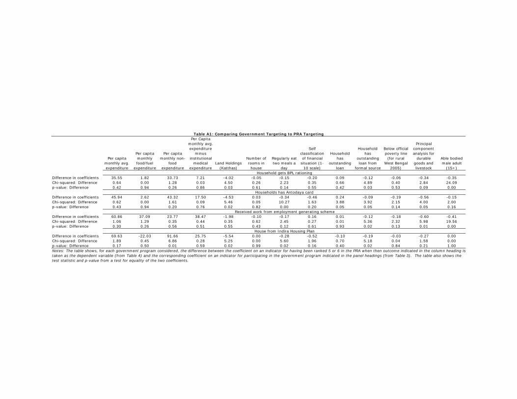
Per capita monthly avg. expenditure

Per capita monthly food/fuel

expenditure

Per capita monthly non-

food expenditure

Per Capita monthly avg. expenditure

minus institutional

medical expenditure

Land Holdings (Katthas)

Number of rooms in house

Regularly eat two meals a

day

Self classification of financial

situation (1-10 scale)

Household has

outstanding loan

Household has

outstanding loan from

formal source

Below official poverty line (for rural

West Bengal 2005)

Principal component analysis for

durable goods and livestock

Able bodied male adult

(15+)

Difference in coefficients 35.55 1.82 33.73 7.21 -4.02 -0.05 -0.15 -0.20 0.09 -0.12 -0.06 -0.34 -0.35Chi-squared: Difference 0.64 0.00 1.28 0.03 4.50 0.26 2.23 0.35 0.66 4.89 0.40 2.84 24.09p-value: Difference 0.42 0.94 0.26 0.86 0.03 0.61 0.14 0.55 0.42 0.03 0.53 0.09 0.00

Difference in coefficients 45.94 2.62 43.32 17.50 -4.53 0.03 -0.34 -0.46 0.24 -0.09 -0.19 -0.56 -0.15Chi-squared: Difference 0.62 0.00 1.61 0.09 5.46 0.05 10.27 1.63 3.88 3.92 2.15 4.00 2.00p-value: Difference 0.43 0.94 0.20 0.76 0.02 0.82 0.00 0.20 0.05 0.05 0.14 0.05 0.16

Difference in coefficients 60.86 37.09 23.77 38.47 -1.98 -0.10 -0.17 0.16 0.01 -0.12 -0.18 -0.60 -0.41Chi-squared: Difference 1.06 1.29 0.35 0.44 0.35 0.62 2.45 0.27 0.01 5.36 2.32 5.98 19.56p-value: Difference 0.30 0.26 0.56 0.51 0.55 0.43 0.12 0.61 0.93 0.02 0.13 0.01 0.00

Difference in coefficients 69.63 -22.03 91.66 25.75 -5.54 0.00 -0.28 -0.52 -0.10 -0.19 -0.03 -0.27 0.00Chi-squared: Difference 1.89 0.45 6.86 0.28 5.25 0.00 5.60 1.96 0.70 5.18 0.04 1.58 0.00p-value: Difference 0.17 0.50 0.01 0.59 0.02 0.99 0.02 0.16 0.40 0.02 0.84 0.21 1.00

Table A1: Comparing Government Targeting to PRA Targeting

Notes: The table shows, for each government program considered, the difference between the coefficient on an indicator for having been ranked 5 or 6 in the PRA when then outcome indicated in the column heading is taken as the dependent variable (from Table 4) and the corresponding coefficient on an indicator for participating in the government program indicated in the panel headings (from Table 3). The table also shows the test statistic and p-value from a test for equality of the two coefficients.

Household gets BPL rationing

Households has Antodaya card

Received work from employment generating scheme

House from Indira Housing Plan

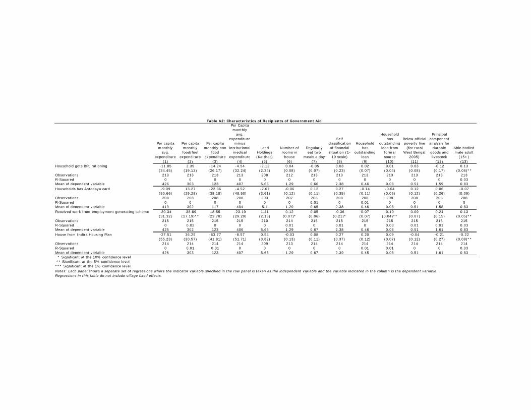
Per capita monthly

avg. expenditure

Per capita monthly food/fuel

expenditure

Per capita monthly non-

food expenditure

Per Capita monthly

avg. expenditure

minus institutional

medical expenditure

Land Holdings (Katthas)

Number of rooms in house

Regularly eat two

meals a day

Self classification of financial

situation (1-10 scale)

Household has

outstanding loan

Household has

outstanding loan from

formal source

Below official poverty line

(for rural West Bengal

2005)

Principal component analysis for

durable goods and livestock

Able bodied male adult

(15+)(1) (2) (3) (4) (5) (6) (7) (8) (9) (10) (11) (12) (13)

Household gets BPL rationing -11.85 2.39 -14.24 -4.54 -2.12 0.04 -0.05 0.03 0.02 0.01 0.03 -0.12 0.13 (34.45) (19.12) (26.17) (32.24) (2.34) (0.08) (0.07) (0.23) (0.07) (0.04) (0.08) (0.17) (0.06)**Observations 213 213 213 213 208 212 213 213 213 213 213 213 213R-Squared 0 0 0 0 0 0 0 0 0 0 0 0 0.03Mean of dependent variable 426 303 123 407 5.66 1.29 0.66 2.38 0.46 0.08 0.51 1.59 0.83Households has Antodaya card -9.09 13.27 -22.36 -4.52 -2.67 -0.06 0.12 0.27 -0.14 -0.04 0.12 0.06 -0.07 (50.66) (29.28) (38.18) (48.50) (3.61) (0.12) (0.11) (0.35) (0.11) (0.06) (0.12) (0.26) (0.09)Observations 208 208 208 208 203 207 208 208 208 208 208 208 208R-Squared 0 0 0 0 0 0 0.01 0 0.01 0 0 0 0Mean of dependent variable 419 302 117 404 5.4 1.29 0.65 2.38 0.46 0.08 0.51 1.58 0.83Received work from employment generating scheme -20.34 -38.89 18.55 -23.19 1.41 0.12 0.05 -0.36 0.07 0.10 0.09 0.24 0.13 (31.32) (17.19)** (23.78) (29.29) (2.13) (0.07)* (0.06) (0.21)* (0.07) (0.04)** (0.07) (0.15) (0.05)**Observations 215 215 215 215 210 214 215 215 215 215 215 215 215R-Squared 0 0.02 0 0 0 0.01 0 0.01 0 0.03 0.01 0.01 0.03Mean of dependent variable 425 302 123 406 5.63 1.29 0.67 2.38 0.46 0.08 0.51 1.61 0.83House from Indira Housing Plan -27.51 36.25 -63.77 -8.57 0.54 -0.03 0.08 0.27 0.20 0.09 -0.04 -0.21 -0.22 (55.23) (30.57) (41.81) (51.71) (3.82) (0.13) (0.11) (0.37) (0.12) (0.07) (0.12) (0.27) (0.09)**Observations 214 214 214 214 209 213 214 214 214 214 214 214 214R-Squared 0 0.01 0.01 0 0 0 0 0 0.01 0.01 0 0 0.03Mean of dependent variable 426 303 123 407 5.65 1.29 0.67 2.39 0.45 0.08 0.51 1.61 0.83 * Significant at the 10% confidence level ** Significant at the 5% confidence level *** Significant at the 1% confidence level

Table A2: Characteristics of Recipients of Government Aid

Notes: Each panel shows a separate set of regressions where the indicator variable specified in the row panel is taken as the independent variable and the variable indicated in the column is the dependent variable.Regressions in this table do not include village fixed effects.

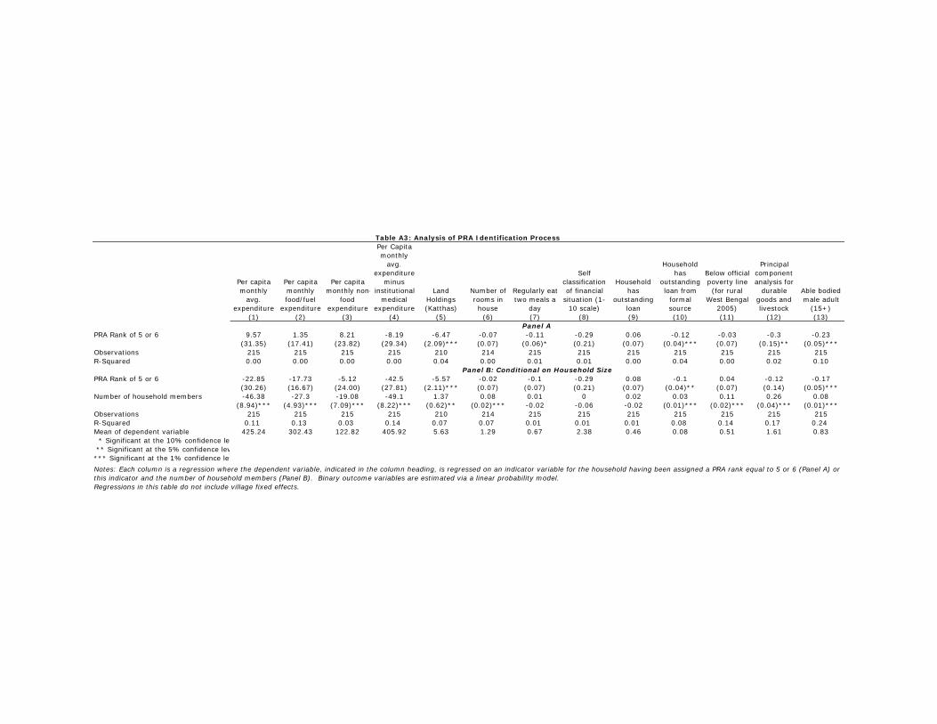
Per capita monthly

avg. expenditure

Per capita monthly food/fuel

expenditure

Per capita monthly non-

food expenditure

Per Capita monthly

avg. expenditure

minus institutional

medical expenditure

Land Holdings (Katthas)

Number of rooms in house

Regularly eattwo meals a

day

Self classification of financial

situation (1-10 scale)

Household has

outstanding loan

Household has

outstanding loan from

formal source

Below official poverty line (for rural

West Bengal 2005)

Principal component analysis for

durable goods and livestock

Able bodied male adult

(15+)(1) (2) (3) (4) (5) (6) (7) (8) (9) (10) (11) (12) (13)

PRA Rank of 5 or 6 9.57 1.35 8.21 -8.19 -6.47 -0.07 -0.11 -0.29 0.06 -0.12 -0.03 -0.3 -0.23 (31.35) (17.41) (23.82) (29.34) (2.09)*** (0.07) (0.06)* (0.21) (0.07) (0.04)*** (0.07) (0.15)** (0.05)***Observations 215 215 215 215 210 214 215 215 215 215 215 215 215R-Squared 0.00 0.00 0.00 0.00 0.04 0.00 0.01 0.01 0.00 0.04 0.00 0.02 0.10

PRA Rank of 5 or 6 -22.85 -17.73 -5.12 -42.5 -5.57 -0.02 -0.1 -0.29 0.08 -0.1 0.04 -0.12 -0.17 (30.26) (16.67) (24.00) (27.81) (2.11)*** (0.07) (0.07) (0.21) (0.07) (0.04)** (0.07) (0.14) (0.05)***Number of household members -46.38 -27.3 -19.08 -49.1 1.37 0.08 0.01 0 0.02 0.03 0.11 0.26 0.08 (8.94)*** (4.93)*** (7.09)*** (8.22)*** (0.62)** (0.02)*** -0.02 -0.06 -0.02 (0.01)*** (0.02)*** (0.04)*** (0.01)***Observations 215 215 215 215 210 214 215 215 215 215 215 215 215R-Squared 0.11 0.13 0.03 0.14 0.07 0.07 0.01 0.01 0.01 0.08 0.14 0.17 0.24Mean of dependent variable 425.24 302.43 122.82 405.92 5.63 1.29 0.67 2.38 0.46 0.08 0.51 1.61 0.83 * Significant at the 10% confidence le ** Significant at the 5% confidence lev *** Significant at the 1% confidence lev

Regressions in this table do not include village fixed effects.

Panel A

Panel B: Conditional on Household Size

Table A3: Analysis of PRA Identification Process

Notes: Each column is a regression where the dependent variable, indicated in the column heading, is regressed on an indicator variable for the household having been assigned a PRA rank equal to 5 or 6 (Panel A) or this indicator and the number of household members (Panel B). Binary outcome variables are estimated via a linear probability model.