An Algorithm for Incremental Unsupervised

Learning and Topology Representation

耐ノイズ性を有し教師なし追加的クラスタリング・位相学習が

可能な自己増殖型ニューラルネットワークに関する研究

By

Shen Furao

Under the supervision of

Dr. Osamu Hasegawa

Department of Computational Intelligence and Systems Science

The Interdisciplinary Graduate School of Science and Engineering

Tokyo Institute of Technology

Contents

1 Introduction 1

1.1 Clustering . . . . . . . . . . . . . . . . . . . . . . . . . . . . . 2

1.2 Topology representation . . . . . . . . . . . . . . . . . . . . . 4

1.3 Organization . . . . . . . . . . . . . . . . . . . . . . . . . . . 6

2 Vector quantization 8

2.1 Definition . . . . . . . . . . . . . . . . . . . . . . . . . . . . . 9

2.2 LBG algorithm . . . . . . . . . . . . . . . . . . . . . . . . . . 11

2.3 Considerations about LBG algorithm . . . . . . . . . . . . . . 13

3 Adaptive incremental LBG 16

3.1 Incrementally inserting codewords . . . . . . . . . . . . . . . . 17

3.2 Distance measuring function . . . . . . . . . . . . . . . . . . . 21

3.3 Removing and inserting codewords . . . . . . . . . . . . . . . 23

3.4 Adaptive incremental LBG . . . . . . . . . . . . . . . . . . . . 27

4 Experiment of adaptive incremental LBG 32

4.1 Predefining the number of codewords . . . . . . . . . . . . . . 32

4.2 Predefining the PSNR threshold . . . . . . . . . . . . . . . . . 38

i

4.3 Predefining the same PSNR threshold for different images . . 39

5 Self-organizing incremental neural network 43

5.1 Overview of SOINN . . . . . . . . . . . . . . . . . . . . . . . . 44

5.2 Complete algorithm . . . . . . . . . . . . . . . . . . . . . . . . 49

5.3 Parameter discussion . . . . . . . . . . . . . . . . . . . . . . . 55

5.3.1 Similarity threshold Ti of node i . . . . . . . . . . . . . 55

5.3.2 Adaptive learning rate . . . . . . . . . . . . . . . . . . 57

5.3.3 Decreasing rate of accumulated variables E (error) and

M (number of signals) . . . . . . . . . . . . . . . . . . 59

6 Experiment with artificial data 61

6.1 Stationary environment . . . . . . . . . . . . . . . . . . . . . . 62

6.2 Non-stationary environment . . . . . . . . . . . . . . . . . . . 64

7 Application for real-world image data 75

7.1 Face recognition . . . . . . . . . . . . . . . . . . . . . . . . . . 75

7.2 Vector quantization . . . . . . . . . . . . . . . . . . . . . . . . 80

7.3 Handwritten digits recognition . . . . . . . . . . . . . . . . . . 88

8 Conclusion and discussion 93

ii

Chapter 1

Introduction

What a human brain does is not just computing - processing data - but more

importantly and more fundamentally, developing the computing engine itself,

from real-world, online sensory data streams [1]. Although a lot of studies

remain to be done and many open questions are waiting to be answered,

the incremental development of a “processor” plays a central role in brain

development. If we intend to bridge the gap between the learning abilities of

humans and machines, then we need to consider which circumstances allow

a sequential acquisition of knowledge.

Incremental learning addresses the ability of repeatedly training a network

with new data, without destroying the old prototype patterns. On account

of noise and other influences in learning an open data-set, possible discrete

overlaps of decision areas turn into continuous overlaps and non-separable

areas emerge. Furthermore, decision boundaries may change over time. In

contrast to only adapting to a changing environment, incremental learning

suggests preserving previously learned knowledge if it does not contradict

1

the current task. This demand immediately raises the Stability-Plasticity

Dilemma [2]. We have to face the problem that learning in artificial neural

networks inevitably implies forgetting. Later input patterns tend to wash out

prior knowledge. A purely stable network is unable to absorb new knowledge

from its interactions, whereas a purely plastic network cannot preserve its

knowledge. Is the network flexible enough to learn new patterns and can

the network preserve old prototype patterns? The proposed self-organizing

incremental neural network (SOINN) of this paper addresses both. We also

use the proposed network to do some clustering and topology learning task.

1.1 Clustering

One objective of unsupervised learning is construction of decision boundaries

based on unlabeled training data. Unsupervised classification is also known

as data clustering and is defined as the problem of finding homogeneous

groups of data points in a given multidimensional data set [3]. Each of these

groups is called a cluster and defined as a region in which the density of

objects is locally higher than in other regions.

Clustering algorithms are classifiable into hierarchical clustering, parti-

tional clustering, fuzzy clustering, nearest-neighbor clustering, artificial neu-

ral networks for clustering, etc. [4]. Hierarchical clustering algorithms such as

single-link [5], complete-link [6], and CURE [7] usually find satisfiable clus-

tering results but suffer from computational overload and the requirement

for much memory space [4]. Hierarchical clustering algorithms are there-

fore unsuitable for large data sets or on-line data. BIRCH is an extremely

2

efficient hierarchical clustering algorithm [8], but is properly applicable to

data sets consisting only of isotropic clusters: a two-dimensional (2-D) cir-

cle, or a three-dimensional (3-D) sphericity, etc. Specifically, chain-like and

concentric clusters are difficult to identify using BIRCH [7][9].

Most partitional clustering algorithms run in linear time and work on

large data sets [10]. The k-means algorithm, a conventionally used partitional

clustering algorithms, suffers from deficiencies such as dependence on initial

starting conditions [11] and a tendency to result in local minima. Likas,

Vlassis, and Verbeek (2003) [12] proposed a global k-means algorithm, an

incremental approach to clustering that dynamically adds one cluster center

at a time through a deterministic global search consisting of N (the data

set size) execution of the k-means algorithm from suitable initial positions.

Compared to traditional k-means, this algorithm can obtain equivalent or

better results, but it suffers from high computation load. The enhanced LBG

algorithm proposed by [13] defines one parameter — utility of a codeword — to

overcome the drawback of LBG algorithm: the dependence on initial starting

condition. The main difficulties of such methods are how to determine the

number of clusters k in advance and the limited applicability to data sets

consisting only of isotropic clusters.

Some clustering methods combine features of hierarchical and partitional

clustering algorithms, partitioning an input data set into sub-clusters and

then constructing a hierarchical structure based on these sub-clusters [14].

Representing a sub-cluster as only one point, however, renders the multilevel

algorithm inapplicable to some cases, especially when the dimension of a

sub-cluster is on the same order as the corresponding final cluster [10].

3

1.2 Topology representation

Another possible objective of unsupervised learning can be described as

topology learning: given a high-dimensional data distribution, find a topo-

logical structure that closely reflects the topology of the data distribution.

Self-organizing map (SOM) models [15][16] generate mapping from high-

dimensional signal space to lower-dimensional topological structure. The

predetermined structure and size of Kohonen’s model imply limitations on

resulting mapping [17]. Methods that identify and repair topological defects

are costly [18]. A posterior choice of class labels for prototypes of the (un-

supervised) SOM causes further problems: class borders are not taken into

account in SOM and several classes may share common prototypes [19]. As

an alternative, a combination of competitive Hebbian learning (CHL) [20]

and neural gas (NG) [21] is effective in constructing topological structure

[17]. For each input signal, CHL connects the two closest centers by an edge,

and NG adapts k nearest centers whereby k is decreasing from a large ini-

tial value to a small final value. Problems arise in practical application: it

requires an a priori decision about network size; it must rank all nodes in

each adaptation step; furthermore, once adaptation strength has decayed, the

use of adaptation parameters “freezes” the network, which thereby becomes

unable to react to subsequent changes in signal distribution. Two nearly

identical algorithms are proposed to solve such problems: growing neural gas

(GNG) [22] and dynamic cell structures [23]. Nodes in the network compete

for determining the node with the highest similarity to the input pattern.

Local error measures are gathered during the learning process to determine

where to insert new nodes, and new node is inserted near the node with the

4

highest accumulated error. The major drawbacks of these methods are their

permanent increase in the number of nodes and drift of the centers to capture

the input probability density [24]. Thresholds such as a maximum number of

nodes predetermined by the user, or an insertion criterion depending on over-

all error or on quantization error are not appropriate, because appropriate

figures for these criteria are unknown a priori.

For the much more difficult problems of non-stationary data distributions,

online learning or life-long learning tasks, the above-mentioned methods are

not suitable. The fundamental issue for such problems is how a learning

system can adapt to new information without corrupting or forgetting pre-

viously learned information — the Stability-Plasticity Dilemma [2]. Using a

utility-based removal criterion, GNG-U [25] deletes nodes that are located

in regions of low input probability density. GNG-U uses a network of lim-

ited size to track the distribution in each moment, and the target of GNG-U

is to represent the actual state. Life-long learning [24] emphasizes learn-

ing through the entire lifespan of a system. For life-long learning, the “dead

nodes” removed by GNG-U can be interpreted as a kind of memory that may

be useful again, for example, when the probability distribution takes on a

previously held shape. Therefore, those “dead nodes” preserve the knowledge

of previous situations for future decisions and play a major role in life-long

learning. The GNG-U serves to follow a non-stationary input distribution,

but the previously learned prototype patterns are destroyed. For that reason,

GNG-U is unsuitable for life-long learning tasks.

Lim and Harrison (1997) [26] propose a hybrid network that combines

advantages of Fuzzy ARTMAP and probabilistic neural networks for incre-

5

mental learning. Hamker (2001) [24] proposes a life-long learning cell struc-

ture (LLCS) that is able to learn the number of nodes needed to solve a task

and to dynamically adapt the learning rate of each node separately. Both

methods work for supervised online learning or life-long learning tasks, but

how to process unsupervised learning remains controversial.

1.3 Organization

The goal of the present study is to design an autonomous learning system for

unsupervised classification and topology representation tasks. The objective

is to develop a network that operates autonomously, online or life-long, and

in a non-stationary environment. The network grows incrementally, learns

the number of nodes needed to solve a current task, learns the number of

clusters, accommodates input patterns of online non-stationary data distri-

bution, and dynamically eliminates noise in input data. We call this network

self-organizing incremental neural network (SOINN).

Vector Quantization (VQ) is the basic technique to be used in the pro-

posed method to generate the Voronoi region of every node of the network.

The CHL technique used in the proposed method also requires the use of

some vector quantization method. Chapter 2 introduces the basic VQ con-

cepts and LBG algorithm; it presents an analysis of LBG; Chapter 3 describes

improvements to LBG in several aspects and presents experiments to sup-

port our improvements, finally proposing the adaptive incremental LBG [27]

method; and Chapter 4 explains numerous experiments to test the adaptive

incremental LBG method and compare it with LBG and ELBG.

6

We describe the proposed SOINN [28] in Chapter 5, and then use artificial

data sets to illustrate the learning process and observe details in Chapter 6. A

comparison with typical incremental networks, GNG and GNG-U, elucidates

the learning behavior. In Chapter 7, we realized some applications with

SOINN, and compared SOINN with some other methods using real-world

data set.

7

Chapter 2

Vector quantization

The purpose of vector quantization (VQ) [29] is to encode data vectors in

order to transmit them over a digital communications channel. Vector quan-

tization is appropriate for applications in which data must be transmitted

(or stored) with high bandwidth, but tolerating some loss in fidelity. Appli-

cations in this class are often found in speech and image processing such as

audio [30], video [31], data compression, pattern recognition [32], computer

vision [33], medical image recognition [34], and others.

To create a vector quantization system, we must design both an encoder

(quantizer) and a decoder. First, we partition the input space of the vectors

into a number of disjoint regions. Then, we must find a prototype vector (a

codeword) for each region. When given an input vector, the encoder produces

the index of the region where the input vector lies. This index is designated

as a channel symbol. The channel symbol is the result of an encoding pro-

cess and is transmitted over a binary channel. At the decoder, the channel

symbol is mapped to its corresponding prototype vector (codeword). The

8

transmission rate is dependent on the number of quantization regions. Given

the number of regions, the task of designing a vector quantizer system is to

determine the regions and codewords that minimize the distortion error.

Many vector quantization algorithms have been proposed; new algorithms

continue to appear. These methods are classifiable into two groups [13]: k-

means based algorithms and competitive-learning based algorithms. Typi-

cally, k-means based algorithms are designed to minimize distortion error by

selecting a suitable codebook. An exemplary method of this group is the

LBG algorithm [35]. Competitive learning based methods mean that code-

words are obtained as a consequence of a process of mutual competition.

Typical methods of this kind are self-organizing map (SOM) [16], neural gas

(NG) [20], and growing neural gas (GNG) [22].

In general, algorithms of vector quantization focus on solving this kind of

problem: given the number of codewords, determine the quantization regions

and the codewords that minimize the distortion error. In some applications,

for example, to set up an image database with the same distortion error for

every image in the database, the quantization problem becomes this kind of

problem: given the distortion error, minimize the number of codewords and

determine the quantization regions and codewords.

2.1 Definition

A vector quantizerQ is a mapping of a l-dimensional vector setX = x1, x2, . . . , xn

into a finite l-dimensional vector set C = c1, c2, . . . , cm , where l 2 and

9

m n. Thus

Q : X C (2.1)

C is called a codebook. Its elements c1, c2, . . . , cm are called codewords.

Associated with m codewords, there is a partition R1, R2, . . . , Rm for X ,

where

Rj = Q−1(cj) = x X : Q(x) = cj . (2.2)

From this definition, the regions defining the partition are non-overlapping

(disjoint) and their union is X . A quantizer is uniquely definable by jointly

specifying the output set C and the corresponding partition Rj. This def-

inition combines the encoding and decoding steps as one operation called

quantization.

Vector quantizer design consists of choosing a distance function d(x, c)

that measures the distance between two vectors x and c. A commonly used

distance function is the squared Euclidean distance.

d(x, c) =

lXi=1

(xi ci)2 (2.3)

A vector quantizer is optimal if, for a given value of m, it minimizes the

distortion error. Generally, mean quantization error (MQE) is used as the

measure of distortion error:

MQE1

n

mXi=1

Ei (2.4)

where

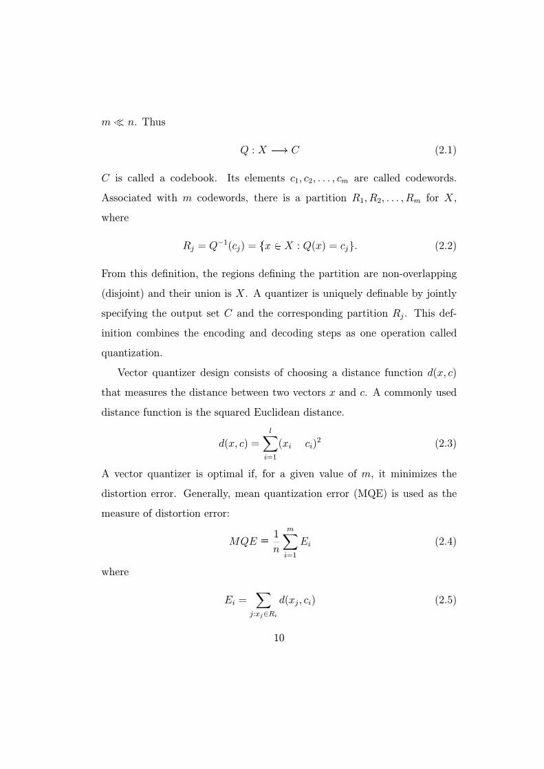
Ei =X

j:xj∈Rid(xj, ci) (2.5)

10

is the Local Quantization Error (LQE) of codeword ci.

Two necessary conditions exist for an optimal vector quantizer — the

Lloyd-Max conditions [36][37].

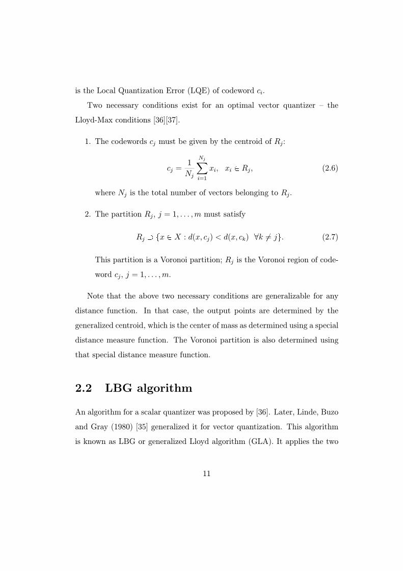
1. The codewords cj must be given by the centroid of Rj:

cj =1

Nj

NjXi=1

xi, xi Rj, (2.6)

where Nj is the total number of vectors belonging to Rj.

2. The partition Rj, j = 1, . . . ,m must satisfy

Rj x X : d(x, cj) < d(x, ck) k = j . (2.7)

This partition is a Voronoi partition; Rj is the Voronoi region of code-

word cj, j = 1, . . . ,m.

Note that the above two necessary conditions are generalizable for any

distance function. In that case, the output points are determined by the

generalized centroid, which is the center of mass as determined using a special

distance measure function. The Voronoi partition is also determined using

that special distance measure function.

2.2 LBG algorithm

An algorithm for a scalar quantizer was proposed by [36]. Later, Linde, Buzo

and Gray (1980) [35] generalized it for vector quantization. This algorithm

is known as LBG or generalized Lloyd algorithm (GLA). It applies the two

11

necessary conditions to inputting data in order to determine optimal vector

quantizers.

Given inputting vector data xi, i = 1, . . . , n, distance function d, and ini-

tial codewords cj(0), j = 1, . . . ,m, the LBG iteratively applies two conditions

to produce a codebook with the following algorithm:

Algorithm 2.1 : LBG algorithm

1. Partition the inputting vector data xi, i = 1, . . . , n into the channel

symbols using the minimum distance rule. This partitioning is stored

in an n m indicator matrix S whose elements are defined as the

following.

sij =

⎧⎨⎩ 1 if d(xi, cj(k)) = minp d(xi, cp(k))

0 otherwise(2.8)

2. Determine the centroids of the Voronoi regions by channel symbol.

Replace the old codewords with these centroids:

cj(k + 1) =

Pni=1 sijxiPni=1 sij

, j = 1, . . . ,m (2.9)

3. Repeat step1-step2 until no cj, j = 1, . . . ,m changes anymore.

Note that the two conditions (eqs. (2.6) and (2.7)) only give necessary con-

ditions for an optimal VQ system. Consequently, the LBG solution is only

locally optimal and might not be globally optimal. The quality of this solu-

tion depends on the choice of initial codebook.

12

2.3 Considerations about LBG algorithm

The LBG algorithm requires initial values for codewords cj, j = 1, . . . ,m.

The quality of the solution depends on this initialization. Obviously, if the

initial values are near an acceptable solution, a higher probability exists that

the algorithm will find an acceptable solution. However, poorly chosen initial

conditions for codewords lead to locally optimal solutions.

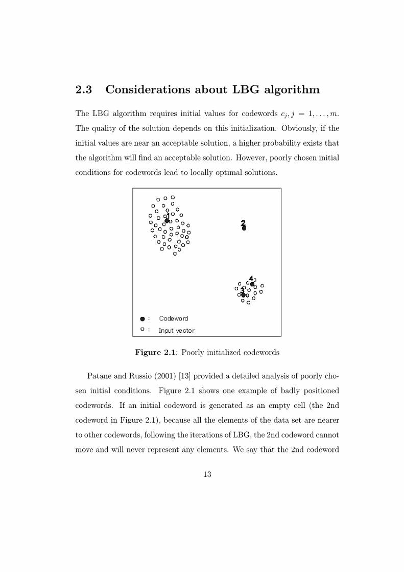
Figure 2.1: Poorly initialized codewords

Patane and Russio (2001) [13] provided a detailed analysis of poorly cho-

sen initial conditions. Figure 2.1 shows one example of badly positioned

codewords. If an initial codeword is generated as an empty cell (the 2nd

codeword in Figure 2.1), because all the elements of the data set are nearer

to other codewords, following the iterations of LBG, the 2nd codeword cannot

move and will never represent any elements. We say that the 2nd codeword

13

is useless because it has no contribution for the reduction of distortion error.

Another problem is that too many codewords are generated for small clus-

ters, but few codewords are generated for large clusters in the initial stage. In

Figure 2.1, the smaller cluster has two codewords (the 3rd codeword and the

4th codeword), in the larger cluster, only one codeword (the 1st codeword)

exists. Even the elements in the smaller cluster are well approximated by the

related codewords, but many elements in the larger one are badly approxi-

mated. The 3rd and 4th codewords are said to have a small contribution to

the reduction of distortion error; the 1st codeword has a large contribution to

the reduction of distortion error. From now on, we use the LQE (defined by

eq. (2.5)) to measure the contribution for the reduction of distortion error.

In signal processing, the dependence on initial conditions is usually cured

by applying the LBG algorithm repeatedly, starting with different initial con-

ditions, and then choosing the best solution. Both LBG-U [38] and Enhanced

LBG (ELBG) [13] define different utility parameters to realize a similar tar-

get, they try to identify codewords that do not contribute much to the reduc-

tion of distortion error and move them to somewhere near codewords that

contribute more to the reduction of distortion error.

Chapter 3 presents a new vector quantization algorithm called adaptive

incremental LBG (AILBG) [27]. It can accomplish both tasks: predefin-

ing the number of codewords to minimize distortion error; and predefining

the distortion error threshold to minimize the number of codewords. We

improved LBG in the following aspects: (1) By introducing some competi-

tive mechanism, the proposed method incrementally inserts a new codeword

near the codeword that contributes most to error minimization. This tech-

14

nique renders AILBG as suitable for the second task: the transmission rate

(or compression ratio) can be controlled using the distortion error. (2) By

adopting an adaptive distance function to measure the distance between vec-

tors, AILBG can obtain superior results to the use of Euclidean distance. (3)

By periodically removing codewords with no contribution or the lowest con-

tribution to error minimization, AILBG fine-tunes the codebook and makes

it independent of initial starting conditions.

Taking image compression as a real-world example, we conduct some

experiments to test AILBG in Chapter 4. Experimental results show that

AILBG is independent of initial conditions. It is able to find a better code-

book than previous algorithms such as ELBG. Furthermore, it is capable of

finding a suitable number of codewords with a predefined distortion error

threshold.

15

Chapter 3

Adaptive incremental LBG

As discussed in Chapter 2, the targets of the adaptive incremental LBG

method are:

To solve the problem caused by poorly chosen initial conditions, as

shown in Figure 2.1.

With a fixed number of codewords, find a suitable codebook to mini-

mize distortion error. It must work better than some recently published

efficient algorithms such as ELBG.

With fixed distortion error, minimize the number of codewords and find

a suitable codebook.

To realize such targets, we do some improvements for LBG. From now on,

we will do some experiments to test such improvements and compare such

improvements with LBG algorithm. We take the well-known Lena image

(512 512 8) (Figure 4.1) as the test image. The image is divided into

4 4 blocks and the resulting 16384 16-dimensional vectors are the input

16

vector data. In image compression applications, the peak signal to noise

ratio (PSNR) is used to evaluate the reconstructed images after encoding

and decoding. The PSNR is defined as:

PSNR = 10 log102552

1N

PNi=1(f(i) g(i))2

, (3.1)

where f and g respectively represent the original image and the reconstructed

one. All grey levels are represented with an integer value of [0, 255]. The total

number of pixels in image f is indicated by N . From our definition, higher

PSNR implies lower distortion error; therefore, the reconstructed image is

better.

3.1 Incrementally inserting codewords

To solve the k-clustering problem, Likas et al. [12] give the following assump-

tion: an optimal clustering solution with k clusters is obtainable by starting

from an initial state with

the k 1 centers placed at the optimal positions for the (k 1)-clustering

problem and

the remaining kth center placed at an appropriate position to be dis-

covered.

To find the appropriate position of the kth center, they fully search the

input data set by performing N executions of the k-means algorithm (here

N means the total number of vectors of the input vector set). In all experi-

ments (and for all values of k) they performed, the solution obtained by the

17

assumption was at least as good as that obtained using numerous random

restarts of the k-means algorithm. Nevertheless, the algorithm is a rather

computational heavy method and is very difficult to use for a large data set.

We hope that the k-codeword problem can be solved from the solution

of (k 1)-codeword problem once the additional codeword is placed at an

appropriate position within the data set. With this idea, we give Algorithm

3.1 to insert codewords incrementally.

Algorithm 3.1 : Incremental LBG: predefining number of codeword

1. Initialize the codebook C to contain one codeword c1, where c1 is chosen

randomly from the original data vector set. Predefine the total number

of codewords m. Adopt the squared Euclidean distance (defined by eq.

(2.3)) as the distance measure function.

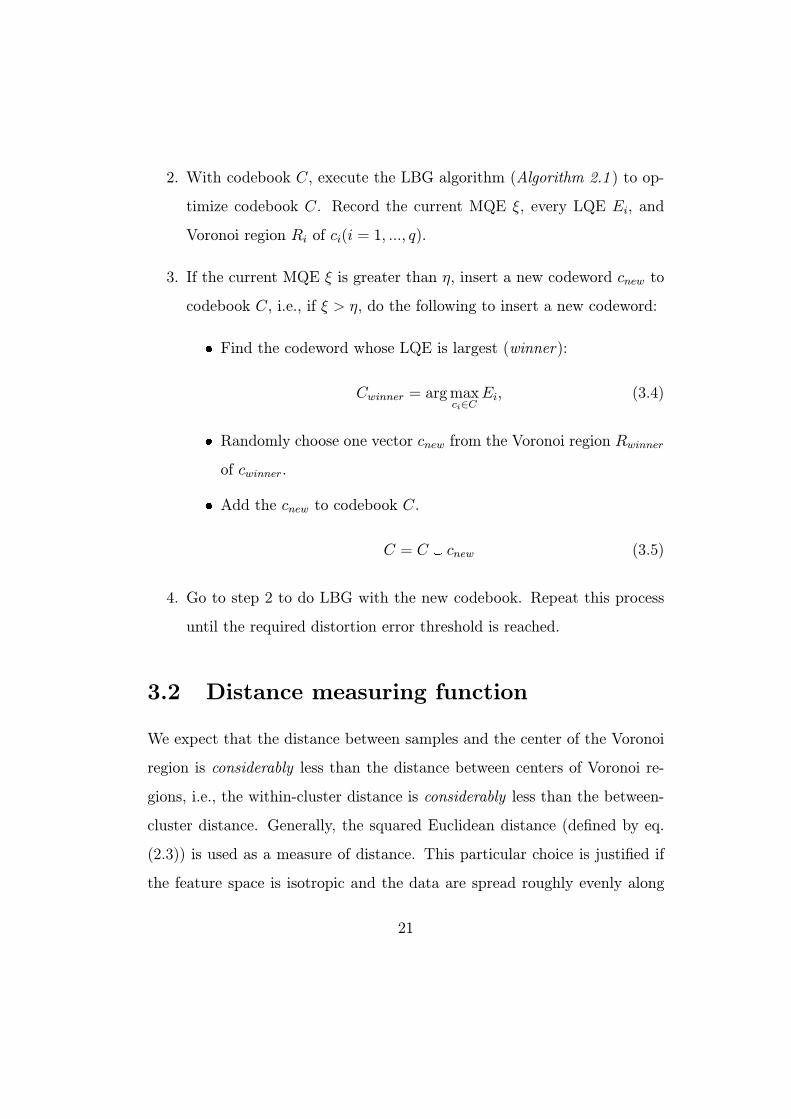
2. With codebook C, execute the LBG algorithm (Algorithm 2.1 ) to op-

timize codebook C. Record the current number of codewords q, every

LQE Ei, and Voronoi region Ri of ci(i = 1, ..., q).

3. If current codewords q are fewer than m, insert a new codeword cnew to

codebook C, i.e., if q < m, do the following to insert a new codeword:

Find the codeword whose LQE is largest (winner):

Cwinner = argmaxci∈C

Ei. (3.2)

Randomly choose one vector cnew from the Voronoi region Rwinner

of cwinner.

Add the cnew to codebook C.

C = C cnew (3.3)

18

4. Go to step 2 to execute LBG with the new codebook. Repeat this

process until the required number of codewords m is reached.

In Algorithm 3.1, we do not fully search the original data set to find an

appropriate new codeword, but randomly choose a vector from the Voronoi

region of winner. Even this choice cannot assure that the new codeword

position is optimal, but this choice has a higher probability of being optimal

than randomly choosing one vector from the original data set. This technique

obviates a great computation load and renders this method as amenable to

large data sets and real world tasks. We must note that such a choice leads

to the results depending on the initial position of new codeword. We will

solve this problem in section 3.3.

We tested Algorithm 3.1 with Lena (512 512 8) and compared the

results with LBG in Figure 3.1. We performed five runs for Algorithm 3.1

and LBG (Algorithm 2.1 ), then took the mean of the results as the last result.

These results show that, with the same number of codewords, Algorithm 3.1

obtains higher PSNR than LBG. We infer that, given the same compression

ratio, Algorithm 3.1 achieves better reconstruction quality than LBG.

An additional advantage of Improvement I (incrementally inserting code-

words) is that, in order to solve the m-codeword problem, all intermediate

k-codeword problems are also solved for k = 1, . . . ,m. This fact might prove

useful in many applications where the k-codeword problem is solved for sev-

eral values of k.

19

Figure 3.1: Comparison results: Improvement I and LBG (Improvement I

means incrementally inserting codewords)

One important performance advantage of the Improvement I is that we

can minimize the number of codewords with the given distortion error limi-

tation. This technique is very useful when we need to encode different data

sets with the same distortion error. We simply change Algorithm 3.1 to

Algorithm 3.2 to solve such a problem.

Algorithm 3.2 : Incremental LBG: predefining the distortion error thresh-

old

1. Initialize the codebook C to contain one codeword c1, where c1 is chosen

randomly from an original data vector set. Predefine the distortion

error threshold η. Adopt the squared Euclidean distance as the distance

measure function.

20

2. With codebook C, execute the LBG algorithm (Algorithm 2.1 ) to op-

timize codebook C. Record the current MQE ξ, every LQE Ei, and

Voronoi region Ri of ci(i = 1, ..., q).

3. If the current MQE ξ is greater than η, insert a new codeword cnew to

codebook C, i.e., if ξ > η, do the following to insert a new codeword:

Find the codeword whose LQE is largest (winner):

Cwinner = argmaxci∈C

Ei, (3.4)

Randomly choose one vector cnew from the Voronoi region Rwinner

of cwinner.

Add the cnew to codebook C.

C = C cnew (3.5)

4. Go to step 2 to do LBG with the new codebook. Repeat this process

until the required distortion error threshold is reached.

3.2 Distance measuring function

We expect that the distance between samples and the center of the Voronoi

region is considerably less than the distance between centers of Voronoi re-

gions, i.e., the within-cluster distance is considerably less than the between-

cluster distance. Generally, the squared Euclidean distance (defined by eq.

(2.3)) is used as a measure of distance. This particular choice is justified if

the feature space is isotropic and the data are spread roughly evenly along

21

all directions. For some particular applications (i.e. speech and image pro-

cessing), more specialized distance functions exist [39].

In Algorithm 3.1 and Algorithm 3.2, if we use the definite measure of

distance, such as the squared Euclidean distance, following the increasing of

number of codewords, the distance between codewords, i.e., the distance be-

tween the center of Voronoi regions (between-cluster distance) shrinks. Even

if the within-cluster distance (distance between samples and codeword) is

less than the between-cluster distance, it is difficult for the within-cluster

distance to be considerably less than the between-cluster distance. To solve

this problem, we adaptively measure the distance between vectors. Follow-

ing the increasing of codewords, the distance between vectors will also be

increased.

As an example, we define an adaptive distance function for image com-

pression tasks: assume that the current number of codewords is q, the dis-

tance function d(x, c) is defined as

p = log10 q + 1 (3.6)

d(x, c) = (lXi=1

(xi ci)2)p. (3.7)

In this definition, following the increase in the number of codewords q, p is

increased. Consequently, the measure of distance d(x, c) is also increased.

This technique ensures that the within-cluster distance is considerably less

than the between-cluster distance.

In Algorithm 3.1, we use the adaptive distance function to take the place

of the squared Euclidean distance, compare the adaptive distance method

with the squared Euclidean distance method and LBG. Lena (512 512 8)

22

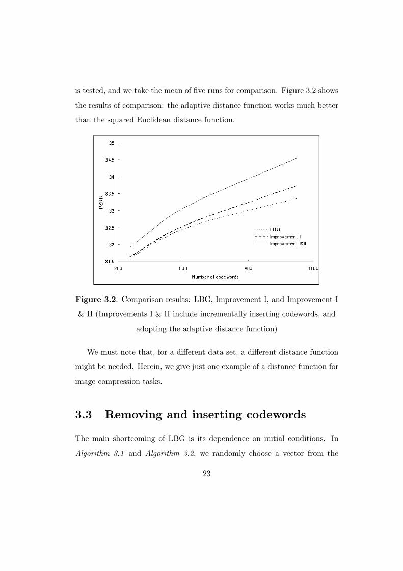
is tested, and we take the mean of five runs for comparison. Figure 3.2 shows

the results of comparison: the adaptive distance function works much better

than the squared Euclidean distance function.

Figure 3.2: Comparison results: LBG, Improvement I, and Improvement I

& II (Improvements I & II include incrementally inserting codewords, and

adopting the adaptive distance function)

We must note that, for a different data set, a different distance function

might be needed. Herein, we give just one example of a distance function for

image compression tasks.

3.3 Removing and inserting codewords

The main shortcoming of LBG is its dependence on initial conditions. In

Algorithm 3.1 and Algorithm 3.2, we randomly choose a vector from the

23

Voronoi region of the winner as the new codeword. This choice cannot as-

sure that it is the optimal choice. The results depend on the initial position

of the new codeword. Here, we use a removal-insertion process to fine-tune

the codebook generated by Algorithm 3.1 or Algorithm 3.2 (with adaptive

distance function) to render the algorithms as independent of initial condi-

tions.

Gersho [40] provided some theorems to show that with high resolution,

each cell contributes equally to the total distortion error in optimal vector

quantization. Here, high resolution means that the number of codewords

tends to be infinite. Chinrungrueng and Sequin [41] proved experimentally

that this conclusion maintains certain validity even when the number of code-

words is finite. Based on this conclusion, ELBG [13] defines the “utility in-

dex” for every element to help fine-tune the codebook and achieve better

results than some previous works.

Here we do not define any utility parameter; we only use the LQE as the

benchmark of removal and insertion. This removal-insertion is based on this

assumption: the LQEs of every codeword will be mutually equal. According

to this assumption, we delete the codewords with 0 LQE (we say it has

no contribution for the decreasing of distortion error) or the codeword with

lowest LQE (loser). Otherwise, we insert a vector in the winner ’s Voronoi

region as the new codeword and repeat this process until the termination

condition is satisfied.

We must determine how to remove and insert codewords, and what the

termination condition is.

Removing criteria. If the LQE of a codeword is 0, this codeword will be

24

removed directly. If the LQE of a codeword is the lowest, the codeword

is denoted as a loser: the loser will be removed. The codeword adjacent

to the loser (we call it neighbor of loser) accepts the Voronoi region

of a loser. For example, in Figure 2.1, the LQE of the 2nd codeword

is 0; it will be removed. Then, the LQE of the 3rd codeword becomes

the lowest; it will also be removed. If we remove the 3rd codeword, all

vectors in the Voronoi region R3 are assigned to Voronoi region R4 and

the 4th codeword is moved to the centroid of the new region.

Insertion criteria. To insert a new codeword, we must avoid the bad

situation shown by the 3rd codeword and the 4th codeword in Figure

2.1. Therefore, a new codeword is inserted near the codeword with the

highest LQE (winner). In Figure 2.1, the 1st codeword is the winner;

we randomly choose a vector that lies in the Voronoi region of the 1st

codeword as a new codeword.

Termination condition. We hope the removal-insertion of codewords is

able to fine-tune the codebook. For a fixed number of codeword tasks,

removal and subsequent insertion of codewords will engender a decrease

in distortion error; for fixed distortion error tasks, removal and subse-

quent insertion of codewords will decrease the number of codewords

without increasing the distortion error. Consequently, the termination

condition will be:

1. For predefined number of codewords (Algorithm 3.1 ), if the removal-

insertion process cannot engender a decrease in quantization error,

stop.

25

2. For a predefined distortion error threshold (Algorithm 3.2 ), if the

removal-insertion process cannot lead to a decrease in the number

of codewords, stop.

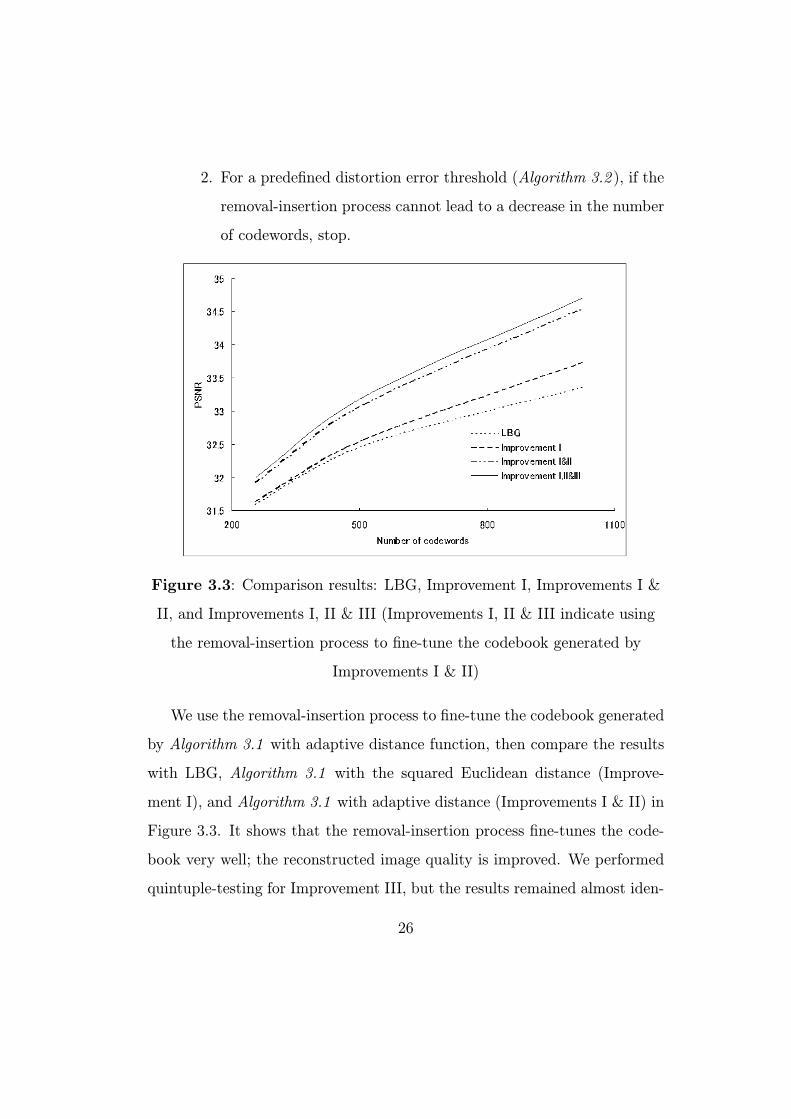
Figure 3.3: Comparison results: LBG, Improvement I, Improvements I &

II, and Improvements I, II & III (Improvements I, II & III indicate using

the removal-insertion process to fine-tune the codebook generated by

Improvements I & II)

We use the removal-insertion process to fine-tune the codebook generated

by Algorithm 3.1 with adaptive distance function, then compare the results

with LBG, Algorithm 3.1 with the squared Euclidean distance (Improve-

ment I), and Algorithm 3.1 with adaptive distance (Improvements I & II) in

Figure 3.3. It shows that the removal-insertion process fine-tunes the code-

book very well; the reconstructed image quality is improved. We performed

quintuple-testing for Improvement III, but the results remained almost iden-

26

tical, implying that the results obtained using the removal-insertion process

become stable and independent of initial conditions.

3.4 Adaptive incremental LBG

In the above sections and this section, some notations are used. Here we

specify those acronyms and notations.

Notations

C: codebook.

ci: ith codeword of codebook C.

Ei: Local Quantization Error (LQE) of codeword ci.

Ri: Voronoi region of codeword ci.

m: predefined number of codewords.

η: predefined distortion error limitation.

q: current number of codewords.

ξ: current Mean Quantization Error (MQE).

iq: inherited number of codewords. It stores the number of codewords

of the last iteration.

iξ: inherited MQE. It stores the MQE of last iteration.

iC: inherited codebook. It stores the codebook of last iteration.

27

winner: the codeword with largest LQE.

loser: the codeword whose LQE is the lowest.

With the above analysis, we give the proposed method in this section.

Algorithm 3.3 gives the outline of proposed method.

Algorithm 3.3 : Outline of adaptive incremental LBG

1. Initialize codebook C to contain one codeword; define the adaptive

distance function d.

2. Execute the LBG algorithm (Algorithm 2.1 ) for codebook C.

3. If the insertion condition is satisfied, insert a new codeword to codebook

C, then go to step 2. Else, if the termination condition is satisfied, out-

put the codebook and stop the algorithm; if the termination condition

is not satisfied, execute step 4.

4. Remove codewords with no contribution or the lowest contribution to

reduction of distortion error, go to step 2.

In step 3 of Algorithm 3.3, for the predefined number of codewords task,

the insertion condition pertains if the current codewords are fewer than a

predefined number of codewords; for the predefined distortion error task, the

insertion condition pertains if the current distortion error is larger than the

predefined distortion error.

In Algorithm 3.3, if we execute LBG for the whole codebook after every

codeword removal or insertion, the computation load will be very heavy. To

avoid heavy computation load, we propose the following technique: after in-

serting a new codeword, we only execute LBG within the Voronoi region of

28

winner for only two codewords (winner and the new codeword) and it will

need very small computation load; for removal of codewords, we just combine

the Voronoi region of removed codewords with the Voronoi region of adjacent

codeword and do not need to execute LBG, no increase of computational load

is incurred. In fact, the Voronoi regions of adjacent codewords will be influ-

enced after inserting a new codeword or removing a codeword. The proposed

technique limits the influence inside the Voronoi region of the winner or the

loser. Even though this technique does not assure an optimal distribution of

codewords, the experimental results in Chapter 4 demonstrate its validity.

With the above analysis, we give the detail of the proposed method in

Algorithm 3.4, which is a modification of Algorithm 3.3 for a small computa-

tion load. Algorithm 3.4 will not have great computation load; it is suitable

for large data sets or real world tasks.

Algorithm 3.4 : Adaptive incremental LBG

1. Initialize the codebook C to contain one codeword c1,

C = c1 , (3.8)

with codeword c1 chosen randomly from the original data vectors set.

Predefine the total number of codewords as m (or predefine the dis-

tortion error threshold as η), give the definition of adaptive distance

function d, initialize inherited numbers, inherited MQEs, and the in-

herited codebook as the following.

iq = + (3.9)

iξ = + (3.10)

iC = C (3.11)

29

2. With codebook C, execute the LBG algorithm (Algorithm 2.1 ) to opti-

mize codebook C. Record the current number of codewords q, current

MQE ξ, every LQE Ei, and Voronoi region Ri of ci (i = 1, . . . .q).

3. (a) If the current codewords q are fewer thanm (or if the current MQE

ξ is greater than η), insert a new codeword cnew to codebook C,

i.e., if q < m (or ξ > η), do the following to insert a new codeword:

Find the winner whose LQE is largest.

Cwinner = argmaxci∈C

Ei (3.12)

Randomly choose one vector cnew from the Voronoi region

Rwinner of cwinner.

Add the cnew to codebook C.

C = C cnew (3.13)

Execute LBG withinRwinner region with two codewords: winner

and cnew. Record the current q, MQE ξ, Ei, and Ri; then go

to step 3.

(b) If the current number of codewords q is equal to m (or if the

current MQE ξ is less than or equal to η), i.e. if q = m (or η ξ),

do the following:

If ξ < iξ (or q < iq),

iξ = ξ (3.14)

iq = q (3.15)

iC = C (3.16)

30

go to step 4.

If ξ iξ (or q iq), output iC (codebook), iq (number of

codewords), and iξ (MQE) are the final results, stop.

4. Execute the following steps to remove codewords with 0 or lowest LQE.

Find the codewords whose LQEs are 0, remove those codewords.

Find the loser, whose LQE is the lowest:

closer = arg minci∈C,Ei 6=0

Ei. (3.17)

Delete closer from codebook C.

C = C closer (3.18)

Find the codeword ca adjacent to closer, assign all vectors in Rloser

to Ra, substitute ca by the centroid of new Voronoi region.

R0a = Ra Rloser (3.19)

c0a =

1

Na

NaXi=1

xi, xi R0a (3.20)

Record current q, MQE ξ, Ei, and Ri; then go to step 3.

31

Chapter 4

Experiment of adaptive

incremental LBG

This chapter presents an examination of the adaptive incremental LBG algo-

rithm using several image compression tasks. We compare our results with

the recently published efficient algorithm ELBG [13]. In those experiments,

three images Lena (512 512 8) (Figure 4.1), Gray21 (512 512 8) (Figure

4.4), and Boat (512 512 8) (Figure 4.5) are tested.

Three experiments are performed to test the different properties of the

proposed method.

4.1 Predefining the number of codewords

In this experiment, we realize the traditional task of vector quantization,

i.e., with a fixed number of codewords, generate a suitable codebook and

maximize the PSNR (thereby minimizing the distortion error). The test

32

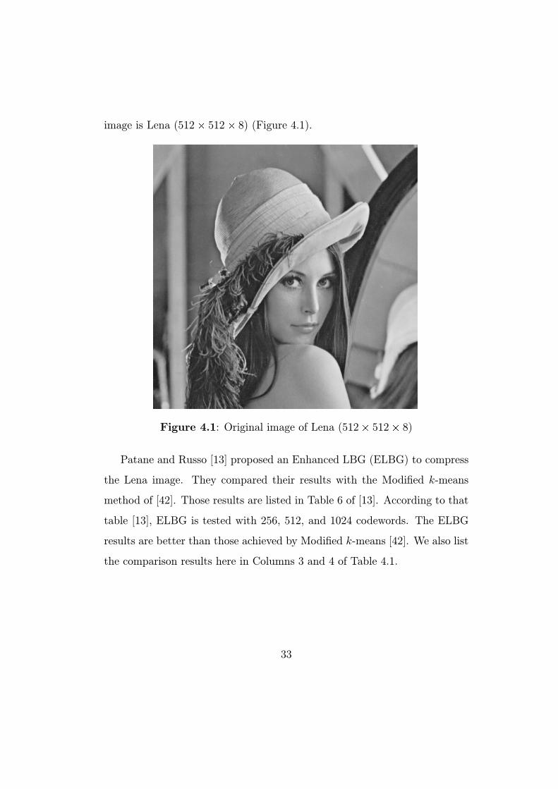
image is Lena (512 512 8) (Figure 4.1).

Figure 4.1: Original image of Lena (512 512 8)

Patane and Russo [13] proposed an Enhanced LBG (ELBG) to compress

the Lena image. They compared their results with the Modified k-means

method of [42]. Those results are listed in Table 6 of [13]. According to that

table [13], ELBG is tested with 256, 512, and 1024 codewords. The ELBG

results are better than those achieved by Modified k-means [42]. We also list

the comparison results here in Columns 3 and 4 of Table 4.1.

33

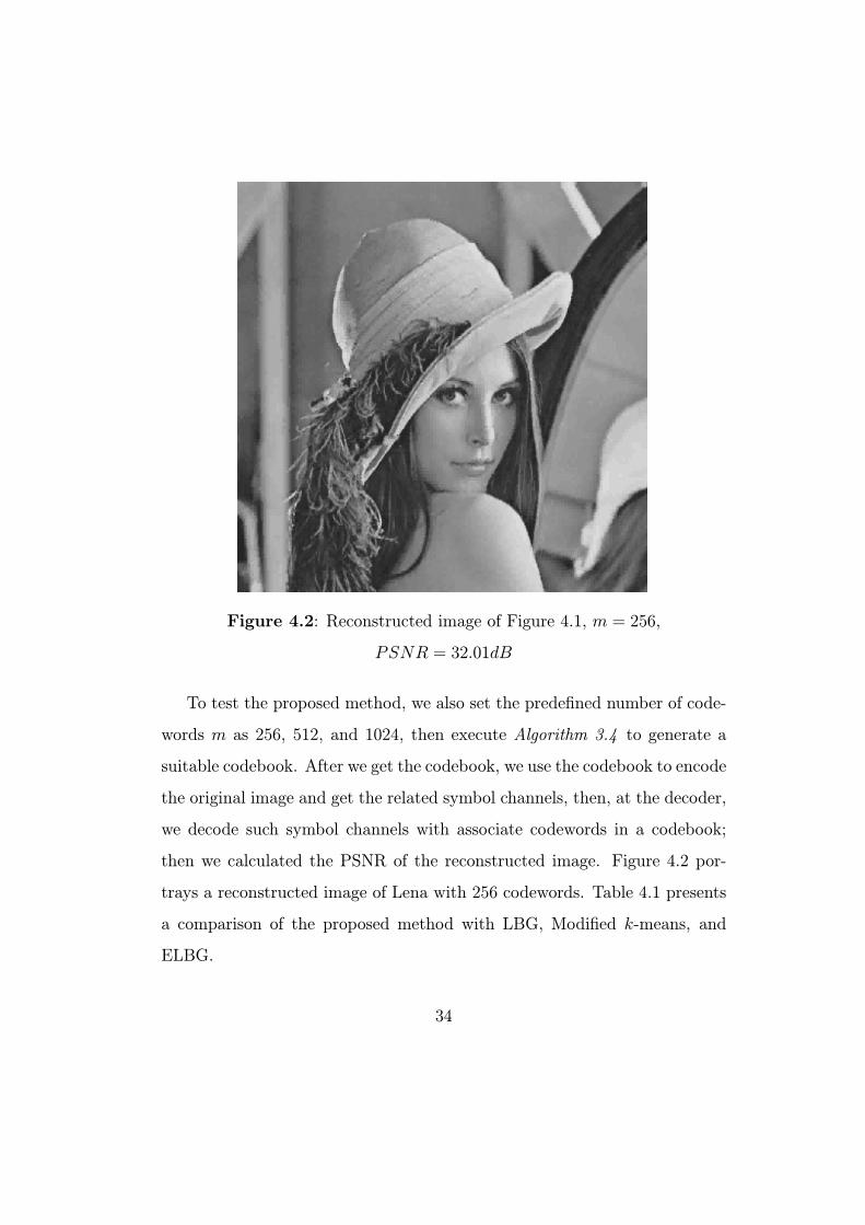
Figure 4.2: Reconstructed image of Figure 4.1, m = 256,

PSNR = 32.01dB

To test the proposed method, we also set the predefined number of code-

words m as 256, 512, and 1024, then execute Algorithm 3.4 to generate a

suitable codebook. After we get the codebook, we use the codebook to encode

the original image and get the related symbol channels, then, at the decoder,

we decode such symbol channels with associate codewords in a codebook;

then we calculated the PSNR of the reconstructed image. Figure 4.2 por-

trays a reconstructed image of Lena with 256 codewords. Table 4.1 presents

a comparison of the proposed method with LBG, Modified k-means, and

ELBG.

34

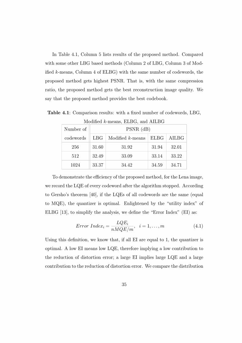
In Table 4.1, Column 5 lists results of the proposed method. Compared

with some other LBG based methods (Column 2 of LBG, Column 3 of Mod-

ified k-means, Column 4 of ELBG) with the same number of codewords, the

proposed method gets highest PSNR. That is, with the same compression

ratio, the proposed method gets the best reconstruction image quality. We

say that the proposed method provides the best codebook.

Table 4.1: Comparison results: with a fixed number of codewords, LBG,

Modified k-means, ELBG, and AILBG

Number of PSNR (dB)

codewords LBG Modified k-means ELBG AILBG

256 31.60 31.92 31.94 32.01

512 32.49 33.09 33.14 33.22

1024 33.37 34.42 34.59 34.71

To demonstrate the efficiency of the proposed method, for the Lena image,

we record the LQE of every codeword after the algorithm stopped. According

to Gersho’s theorem [40], if the LQEs of all codewords are the same (equal

to MQE), the quantizer is optimal. Enlightened by the “utility index” of

ELBG [13], to simplify the analysis, we define the “Error Index” (EI) as:

Error Indexi =LQEi

nMQE/m, i = 1, . . . ,m (4.1)

Using this definition, we know that, if all EI are equal to 1, the quantizer is

optimal. A low EI means low LQE, therefore implying a low contribution to

the reduction of distortion error; a large EI implies large LQE and a large

contribution to the reduction of distortion error. We compare the distribution

35

of EI of the proposed method with LBG and ELBG algorithms in Figure 4.3;

the number of codewords is 512 for all three algorithms.

Figure 4.3(a) shows the EI distribution of LBG results, the EI distributed

in [0, 6.5] shows that the codewords of LBGmake quite different contributions

to the reduction of distortion error. Too many codewords exist whose EI is

less than 1.0; some codewords have an EI that is greater than 6.0. The

distribution shows that these results are not optimal, many codewords are

assigned to small clusters and few codewords are assigned to large clusters.

Therefore, plenty of codewords must be moved from the low distortion error

region to the high distortion error region.

Figure 4.3(b) shows the EI distribution of ELBG results, the EI dis-

tributed in [0, 2.5], some codewords with low EI in Figure 4.3(a) are moved

to regions with high EI, and ELBG achieves a more balanced EI contribution

than LBG; it makes ELBG work better than LBG.

Figure 4.3(c) shows the EI distribution of the proposed method. The EI

are distributed in [0, 1.9] and the codewords with large LQE (EI is greater

than or equal to 1) are more than the codewords with small LQE. It shows

that the proposed method offers a more balanced contribution to the decreas-

ing of distortion error than LBG and ELBG. Many codewords are assigned to

large clusters; a few codewords are assigned to small clusters. It is impossible

for us to get exactly the same LQE for all codewords (because the number of

codewords is finite), the proposed method achieves a good distribution; more-

over, it enhances the proposed method better than some previously published

LBG-based methods.

36

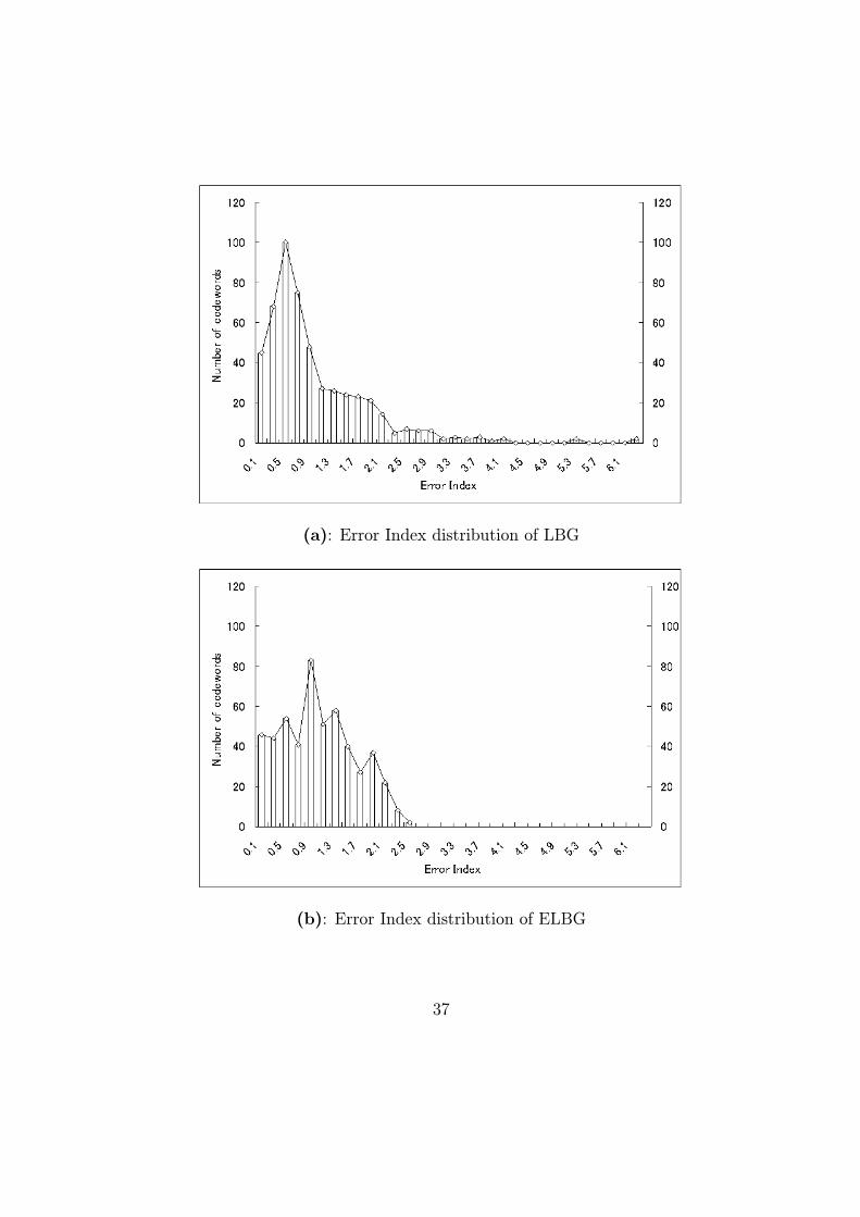
(a): Error Index distribution of LBG

(b): Error Index distribution of ELBG

37

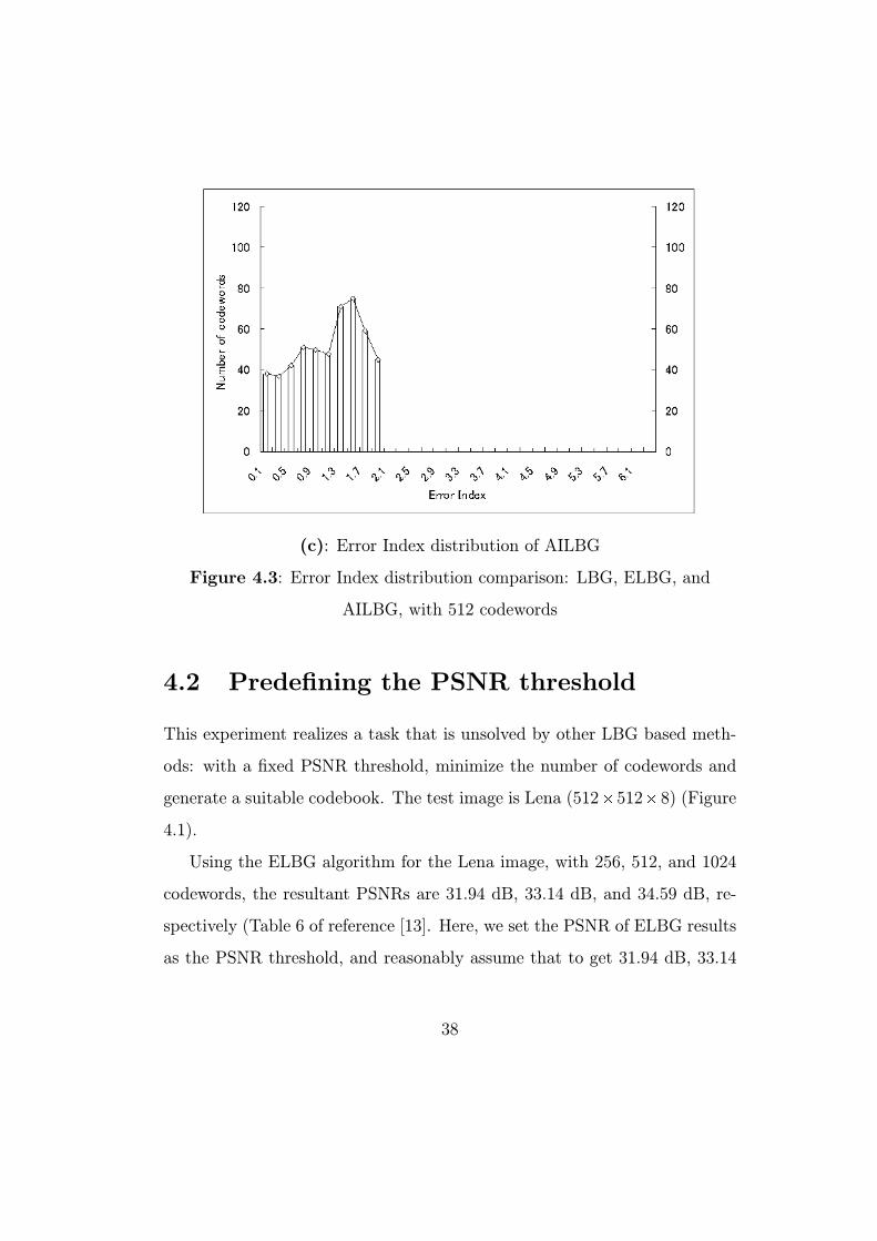
(c): Error Index distribution of AILBG

Figure 4.3: Error Index distribution comparison: LBG, ELBG, and

AILBG, with 512 codewords

4.2 Predefining the PSNR threshold

This experiment realizes a task that is unsolved by other LBG based meth-

ods: with a fixed PSNR threshold, minimize the number of codewords and

generate a suitable codebook. The test image is Lena (512 512 8) (Figure

4.1).

Using the ELBG algorithm for the Lena image, with 256, 512, and 1024

codewords, the resultant PSNRs are 31.94 dB, 33.14 dB, and 34.59 dB, re-

spectively (Table 6 of reference [13]. Here, we set the PSNR of ELBG results

as the PSNR threshold, and reasonably assume that to get 31.94 dB, 33.14

38

dB, or 34.59 dB PSNR, the ELBG algorithm needs 256, 512, or 1024 code-

words respectively, even ELBG cannot be used to solve this problem: given

a PSNR threshold, minimize the number of codewords.

Then, we set 31.94 dB, 33.14 dB, and 34.59 dB as the PSNR thresholds,

and use Algorithm 3.4 to minimize the required number of codewords to

thereby generate a codebook. Table 4.2 shows comparative results for ELBG

and the proposed method.

Table 4.2: Comparison results: with fixed PSNR, ELBG and AILBG

PSNR Number of codewords

(dB) ELBG AILBG

31.94 256 244

33.14 512 488

34.59 1024 988

The results obtained by the proposed method are listed in Column 3 of

Table 4.2. It shows that, with the same PSNR, the proposed method requires

fewer codewords than ELBG. With the same reconstruction quality (PSNR),

the proposed method obtains a higher compression ratio than ELBG.

4.3 Predefining the same PSNR threshold for

different images

In this experiment, we realize this task: using the same fixed PSNR threshold,

find suitable codebooks for different images with different detail. The test

images are Lena (512 512 8) (Figure 4.1), Gray21 (512 512 8) (Figure

4.4), and Boat (512 512 8) (Figure 4.5). The three images have different

39

details. For example, Gray21 is flat and little detail is visible. Lena has more

detail than Gray21, but less detail than Boat.

One target of this experiment is to test if the proposed method works

well for different images, not just works well for Lena image. Another target

is to check with the same PSNR threshold, if different images with different

details need different numbers of codewords. We set the PSNR thresholds as

28.0 dB, 30.0 dB, and 33.0 dB, then execute Algorithm 3.4 to minimize the

number of codewords and find suitable codebooks for the three images.

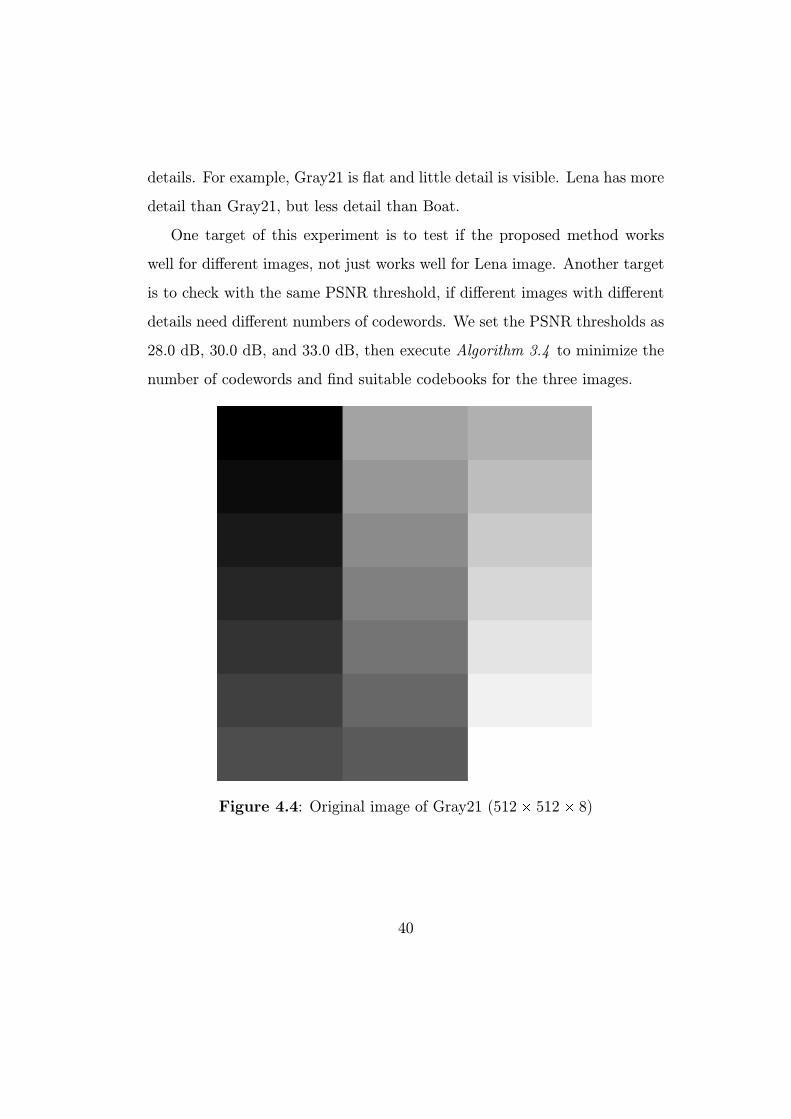
Figure 4.4: Original image of Gray21 (512 512 8)

40

Figure 4.5: Original image of Boat (512 512 8)

Table 4.3 lists the results. For different images, if there is less detail in

the image, fewer codewords are needed. Following the increase in detail, the

number of codewords will also be increased.

Table 4.3: With fixed PSNR, AILBG works for different images

PSNR Number of codewords

(dB) Gray21 Lena Boat

28 9 22 54

30 12 76 199

33 15 454 1018

This experiment proves that the proposed method is useful to minimize

41

the number of codewords. For different images, the number of codewords

might be different. This conclusion will be very useful in some applications

by which we need to encode different data set with the same distortion error.

For example, if we attempt to set up an image database (which is composed

of three images Lena, Gray21, and Boat) with the same PSNR (33.0 dB) for

every image, with the traditional LBG based methods (LBG, ELBG, etc.),

we must encode every image with at least 1018 codewords to ensure that

the reconstructed image quality can be satisfied for all images. In contrast,

using the proposed method, we need only 15 codewords for Gray21, 454

codewords for Lena, and 1018 codewords for Boat. Thereby, the proposed

method requires much less storage for this image database. If more images

exist in the image database, much storage space will be saved through the

use of the proposed method.

42

Chapter 5

Self-organizing incremental

neural network

For unsupervised online learning tasks, we separate unlabeled non-stationary

input data into different classes without prior knowledge such as how many

classes exist. We also intend to learn input data topologies. Briefly, the

targets of the proposed algorithm are:

To process online or life-long learning non-stationary data.

Using no prior conditions such as a suitable number of nodes or a

good initial codebook or knowing how many classes exist, to conduct

unsupervised learning, report a suitable number of classes and represent

the topological structure of input probability density.

To separate classes with low-density overlap and detect the main struc-

ture of clusters that are polluted by noise.

43

To realize these targets, we emphasize the key aspects of local represen-

tation, insertion of new nodes, similarity threshold, adaptive learning rate,

and deletion of low probability density nodes.

5.1 Overview of SOINN

In this study, we adopt a two-layer neural network structure to realize our

targets. The first layer is used to generate a topological structure of input

pattern. We obtain some nodes to represent the probability density of an

input pattern when we finish the first-layer learning. For the second layer,

we use nodes identified in the first layer as the input data set. We report the

number of clusters and give typical prototype nodes of every cluster when we

finish the second-layer learning. Figure 5.1 gives the flowchart of SOINN.

For unsupervised classification task, we must determine if an input sample

belongs to previously learned clusters or to a new cluster. Suppose we say

that two samples belong to the same cluster if the Euclidean distance between

them is less than threshold distance T . If T is too large, all samples will

be assigned to one cluster. If T is too small, each sample will form an

isolated, singleton cluster. To obtain “natural” clusters, T must be greater

than the typical within-cluster distance and less than the typical between-

cluster distance [43].

44

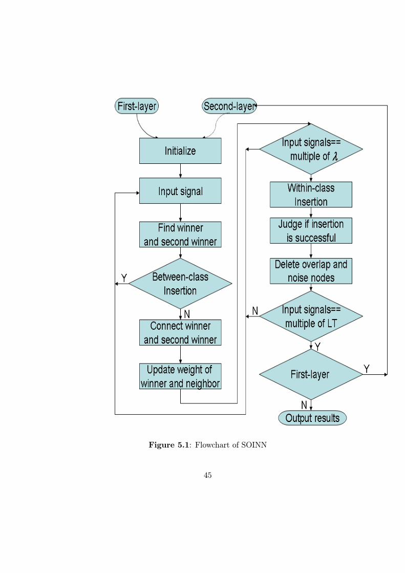
Figure 5.1: Flowchart of SOINN

45

For both layers, we must calculate the threshold distance T . In the first

layer, we set the input signal as a new node (the first node of a new cluster)

when the distance between the signal and the nearest node (or the second

nearest node) is greater than a threshold T that is permanently adapted to

the present situation. In the second layer, we calculate the typical within-

cluster distances and typical between-cluster distances based on those nodes

generated in the first layer, then give a constant threshold distance Tc ac-

cording to the within-cluster distances and between-cluster distances.

To represent the topological structure, in online or life-long learning tasks,

growth is an important feature for decreasing task error and adapting to

changing environments while preserving old prototype patterns. Therefore,

the insertion of new nodes is a very useful contribution to plasticity of the

Stability-Plasticity Dilemma without interfering with previous learning (sta-

bility). Insertion must be stopped to prohibit a permanent increase in the

number of nodes and to avoid overfitting. For that reason, we must decide

when and how to insert a new node within one cluster and when insertion is

to be stopped.

For within-cluster insertion, we adopt a scheme used by some incremental

networks (such as GNG [22], GCS [44]) to insert a node between node q with

maximum accumulated error and node f , which is among the neighbors of

q with maximum accumulated error. Current incremental networks (GNG,

GCS) have no ability to learn whether further insertion of a node is useful

or not. Node insertion leads to catastrophic allocation of new nodes. Here,

we suggest a strategy: when a new node is inserted, we evaluate insertion

by a utility parameter, the error-radius, to judge if insertion is successful.

46

This evaluation ensures that the insertion of a new node leads to decreasing

error and controls the increment of nodes, eventually stabilizing the number

of nodes.

We adopt the competitive Hebbian rule proposed by Martinetz in topol-

ogy representing networks (TRN) to build connections between neural nodes

[17]. The competitive Hebbian rule can be described as: for each input sig-

nal, connect the two closest nodes (measured by Euclidean distance) by an

edge. It is proved that each edge of the generated graph belongs to the

Delaunay triangulation corresponding to the given set of reference vectors,

and that the graph is optimally topology-preserving in a very general sense.

In online or life-long learning, the nodes change their locations slowly but

permanently. Therefore nodes that are neighboring at an early stage might

not be neighboring at a more advanced stage. It thereby becomes necessary

to remove connections that have not been recently refreshed.

In general, overlaps exist among clusters. To detect the number of clusters

precisely, we assume that input data are separable: the probability density

in the centric part of every cluster is higher than the density in intermediate

parts between clusters; and overlaps between clusters have low probability

density. We separate clusters by removing those nodes whose position is in a

region with very low probability density. To realize this, Fritzke [44] designed

an estimation to find the low probability-density region; if the density is

below threshold η, the node is removed. Here we propose a novel strategy:

if the number of input signals generated so far is an integer multiple of a

parameter, remove those nodes with only one or no topological neighbor.

We infer that, if the node has only one or no neighbor, during that period,

47

the accumulated error of this node has a very low probability of becoming

maximum and the insertion of new nodes near this node is difficult: the

probability density of the region containing the node is very low. However,

for one-dimensional input data, the nodes form a chain, the above criterion

will remove the boundary nodes repeatedly. In addition, if the input data

contain little noise, it is not good to delete those nodes having only one

neighbor. Thus, we use another parameter, the local accumulated number

of signals of the candidate-deleting node, to control the deletion behavior. If

this parameter is greater than an adaptive threshold, i.e., if the node is the

winner for numerous signals, the node will not be deleted because the node

does not lie in a low-density area. This strategy works well for removing

nodes in low-density regions without added computation load. In addition,

the use of this technique periodically removes nodes caused by noise because

the probability density of noise is very low.

If two nodes can be linked with a series of edges, a path exists between the

two nodes. Martinetz and Schulten [17] prove some theorems and reach the

conclusion that the competitive Hebbian rule is suitable for forming a path

preserving representations of a given manifold. If the number of nodes is

sufficient for obtaining a dense distribution, the connectivity structure of the

network corresponds to the induced Delaunay triangulation that defines both

a perfectly topology-preserving map and a path-preserving representation.

In TRN, neural gas (NG) is used to obtain weight vectors Wi M , i =

1, . . . , N ,M is the given manifold. The NG is an efficient vector quantization

procedure. It creates a homogeneous distribution of the weight vectors Wi

on M . After learning, the probability distribution of the weight vectors of

48

the NG is

ρ(Wi) P (Wi)α. (5.1)

With the magnification factor α =DeffDeff+2

, the intrinsic data dimension is

Deff [45]. Therefore, with the path-preserving representation, the competi-

tive Hebbian rule allows the determination of which parts of a given pattern

manifold are separated and form different clusters. In the proposed algo-

rithm, we adopt a scheme like neural gas with only nearest neighbor learning

for the weight vector adaptation; the competitive Hebbian rule is used to de-

termine topology neighbors. Therefore, we can use the conclusions of TRN

to identify clusters, i.e., if two nodes are linked with one path, we say the

two nodes belong to one cluster.

5.2 Complete algorithm

Using the analysis presented in Section 5.1, we give the complete algorithm

here. The same algorithm is used to train both the first layer and the second

layer. The difference between the two layers is that the input data set of

the second layer is the nodes generated by the first layer. A constant simi-

larity threshold is used in the second layer instead of the adaptive similarity

threshold used in the first layer.

Notations to be used in the algorithm

49

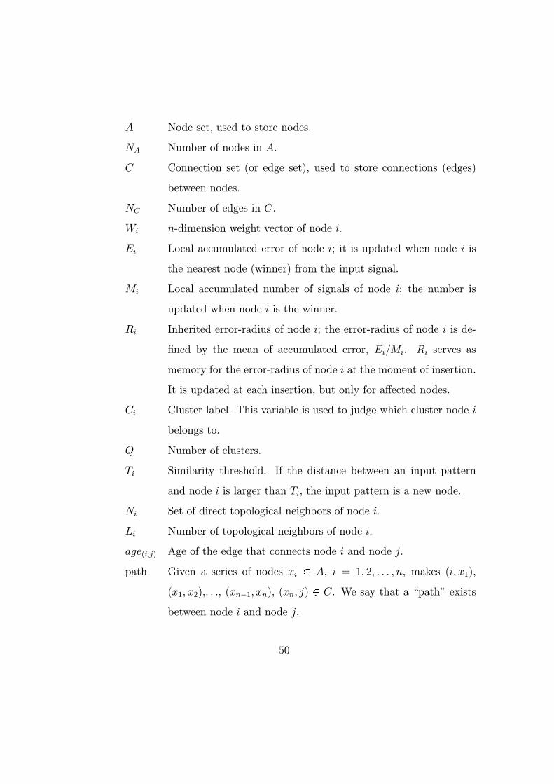
A Node set, used to store nodes.

NA Number of nodes in A.

C Connection set (or edge set), used to store connections (edges)

between nodes.

NC Number of edges in C.

Wi n-dimension weight vector of node i.

Ei Local accumulated error of node i; it is updated when node i is

the nearest node (winner) from the input signal.

Mi Local accumulated number of signals of node i; the number is

updated when node i is the winner.

Ri Inherited error-radius of node i; the error-radius of node i is de-

fined by the mean of accumulated error, Ei/Mi. Ri serves as

memory for the error-radius of node i at the moment of insertion.

It is updated at each insertion, but only for affected nodes.

Ci Cluster label. This variable is used to judge which cluster node i

belongs to.

Q Number of clusters.

Ti Similarity threshold. If the distance between an input pattern

and node i is larger than Ti, the input pattern is a new node.

Ni Set of direct topological neighbors of node i.

Li Number of topological neighbors of node i.

age(i,j) Age of the edge that connects node i and node j.

path Given a series of nodes xi A, i = 1, 2, . . . , n, makes (i, x1),

(x1, x2),. . ., (xn−1, xn), (xn, j) C. We say that a “path” exists

between node i and node j.

50

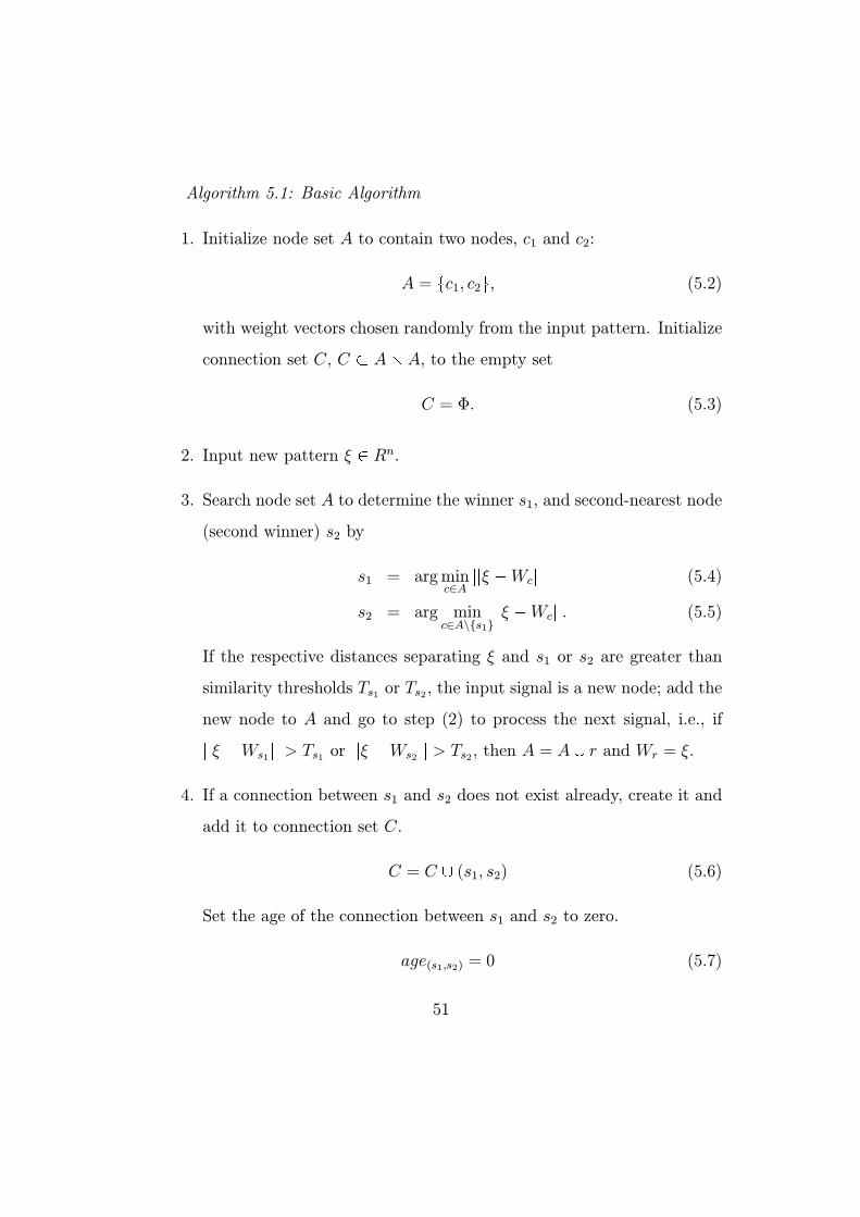
Algorithm 5.1: Basic Algorithm

1. Initialize node set A to contain two nodes, c1 and c2:

A = c1, c2 , (5.2)

with weight vectors chosen randomly from the input pattern. Initialize

connection set C, C A A, to the empty set

C = Φ. (5.3)

2. Input new pattern ξ Rn.

3. Search node set A to determine the winner s1, and second-nearest node

(second winner) s2 by

s1 = argminc∈A

ξ Wc (5.4)

s2 = arg minc∈A\{s1}

ξ Wc . (5.5)

If the respective distances separating ξ and s1 or s2 are greater than

similarity thresholds Ts1 or Ts2, the input signal is a new node; add the

new node to A and go to step (2) to process the next signal, i.e., if

ξ Ws1 > Ts1 or ξ Ws2 > Ts2, then A = A r and Wr = ξ.

4. If a connection between s1 and s2 does not exist already, create it and

add it to connection set C.

C = C (s1, s2) (5.6)

Set the age of the connection between s1 and s2 to zero.

age(s1,s2) = 0 (5.7)

51

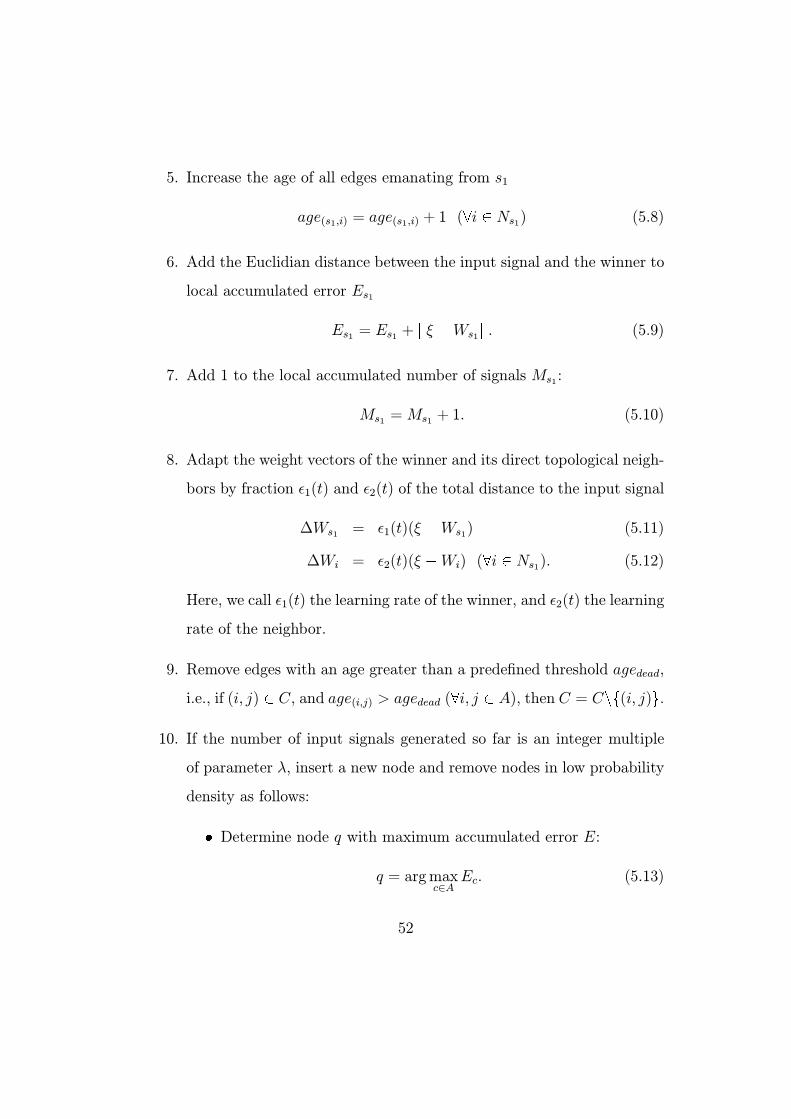
5. Increase the age of all edges emanating from s1

age(s1,i) = age(s1,i) + 1 ( i Ns1) (5.8)

6. Add the Euclidian distance between the input signal and the winner to

local accumulated error Es1

Es1 = Es1 + ξ Ws1 . (5.9)

7. Add 1 to the local accumulated number of signals Ms1:

Ms1 =Ms1 + 1. (5.10)

8. Adapt the weight vectors of the winner and its direct topological neigh-

bors by fraction ²1(t) and ²2(t) of the total distance to the input signal

∆Ws1 = ²1(t)(ξ Ws1) (5.11)

∆Wi = ²2(t)(ξ Wi) ( i Ns1). (5.12)

Here, we call ²1(t) the learning rate of the winner, and ²2(t) the learning

rate of the neighbor.

9. Remove edges with an age greater than a predefined threshold agedead,

i.e., if (i, j) C, and age(i,j) > agedead ( i, j A), then C = C (i, j) .

10. If the number of input signals generated so far is an integer multiple

of parameter λ, insert a new node and remove nodes in low probability

density as follows:

Determine node q with maximum accumulated error E:

q = argmaxc∈A

Ec. (5.13)

52

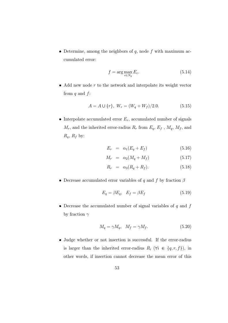
Determine, among the neighbors of q, node f with maximum ac-

cumulated error:

f = argmaxc∈Nq

Ec. (5.14)

Add new node r to the network and interpolate its weight vector

from q and f :

A = A r , Wr = (Wq +Wf )/2.0. (5.15)

Interpolate accumulated error Er, accumulated number of signals

Mr, and the inherited error-radius Rr from Eq, Ef , Mq, Mf , and

Rq, Rf by:

Er = α1(Eq + Ef ) (5.16)

Mr = α2(Mq +Mf ) (5.17)

Rr = α3(Rq + Rf). (5.18)

Decrease accumulated error variables of q and f by fraction β

Eq = βEq, Ef = βEf (5.19)

Decrease the accumulated number of signal variables of q and f

by fraction γ

Mq = γMq, Mf = γMf . (5.20)

Judge whether or not insertion is successful. If the error-radius

is larger than the inherited error-radius Ri ( i q, r, f ), in

other words, if insertion cannot decrease the mean error of this

53

local area, insertion is not successful; else, update the inherited

error-radius. I.e., if Ei/Mi > Ri ( i q, r, f ), insertion is not

successful, new node r is removed from set A, and all parameters

are restored; else, Rq = Eq/Mq, Rf = Ef/Mf , and Rr = Er/Mr.

If insertion is successful, insert edges connecting new node r with

nodes q and f , and remove the original edge between q and f .

C = C (r, q), (r, f) (5.21)

C = C (q, f) (5.22)

For all nodes in A, search for nodes having only one neighbor,

then compare the accumulated number of signals of these nodes

with the average accumulated number of all nodes. If a node has

only one neighbor and the accumulated number of signals is less

than an adaptive threshold, remove it from the node set, i.e., if

Li = 1 ( i A) and Mi < cPNA

j=1Mj/NA, then A = A i . Here,

c is determined by the user and 1 c > 0. If much noise exists in

the input data, c will be larger and vice versa.

For all nodes in A, search for isolated nodes, then delete them,

i.e., if Li = 0 ( i A), then A = A i .

11. After a long constant time period LT , report the number of clusters,

output all nodes belonging to different clusters. Use the following

method to classify nodes into different classes:

Initialize all nodes as unclassified.

54

Loop: Randomly choose one unclassified node i from node set A.

Mark node i as classified and label it as class Ci.

Search A to find all unclassified nodes connected to node i with

a “path.” Mark these nodes as classified and label them as the

same class as node i (Ci).

If unclassified nodes exist, go to Loop to continue the classification

process until all nodes are classified.

12. Go to step (2) to continue the online unsupervised learning process.

5.3 Parameter discussion

We determine parameters in Algorithm 5.1 as follows:

5.3.1 Similarity threshold T of node i

As discussed in Section 5.1, similarity threshold Ti is a very important vari-

able. In step3 of Algorithm 5.1, the threshold is used to judge if the input

signal belongs to previously learned clusters or not.

For the first layer, we have no prior knowledge of input data and therefore

adopt an adaptive threshold scheme. For every node i, the threshold Ti is

adopted independently. First, we assume that all data come from the same

cluster; thus, the initial threshold of every node will be + . After a period

of learning, the input pattern is separated into different small groups; each

group comprises one node and its direct topological neighbors. Some of

these groups can be linked to form a big group; the big groups are then

55

separated from each other. We designate such big groups as clusters. The

similarity threshold must be greater than within-cluster distances and less

than between-cluster distances. Based on this idea, we calculate similarity

threshold Ti of node i with the following algorithm.

Algorithm 5.2: Calculation of similarity threshold T for the first layer

1. Initialize the similarity threshold of node i to + when node i is gen-

erated as a new node.

2. When node i is a winner or second winner, update similarity threshold

Ti by

If the node has direct topological neighbors (Li > 0), Ti is updated

as the maximum distance between node i and all of its neighbors.

Ti = maxc∈Ni

Wi Wc (5.23)

If node i has no neighbors (Li = 0), Ti is updated as the minimum

distance of node i and all other nodes in A.

Ti = minc∈A\{i}

Wi Wc (5.24)

For the second layer, the input data set contains the results of the first

layer. After learning of the first layer, we obtain coarse clustering results and

a topological structure. Using this knowledge, we calculate the within-cluster

distance dw as

dw =1

NC

X(i,j)∈C

Wi Wj , (5.25)

56

and calculate the between-cluster distance db(Ci, Cj) of clusters Ci and Cj as

db(Ci, Cj) = mini∈Ci,j∈Cj

Wi Wj . (5.26)

That is, the within-cluster distance is the mean distance of all edges, and

the between-cluster distance is the minimum distance between two clusters.

With dw and db, we can give a constant threshold Tc for all nodes.

The threshold must be greater than the within-cluster distance and less

than the between-cluster distances. Influenced by overlap or noise, some

between-cluster distances are less than within-cluster distances, so we use

the following algorithm to calculate the threshold distance Tc for the second

layer.

Algorithm 5.3: Calculation of similarity threshold T for the second layer

1. Set Tc as the minimum between-cluster distance.

Tc = db(Ci1 , Cj1) = mink,l=1,...,Q,k 6=l

db(Ck, Cl) (5.27)

2. If Tc is less than within-cluster distance dw, set Tc as the next minimum

between-cluster distance.

Tc = db(Ci2 , Cj2) = mink,l=1,...,Q,k 6=l,k 6=i1,l 6=j1

db(Ck, Cl) (5.28)

3. Go to step (2) to update Tc until Tc is greater than dw.

5.3.2 Adaptive learning rate

In step (8) of Algorithm 5.1, the learning rate ²(t) determines the extent to

which the winner and the neighbors of the winner are adapted towards the

input signal.

57

A constant learning rate is adopted by GNG and GNG-U, i.e. ²(t) = c0,

1 c0 > 0. With this scheme, each reference vector Wi represents an

exponentially decaying average of those input signals for which the node i

has been a winner. However, the most recent input signal always determines

a fraction c0 of the current Wi. Even after numerous iterations, the current

input signal can cause a considerable change in the reference vector of the

winner.

Ritter et al. [46] proposed a decaying adaptation learning rate scheme.

This scheme was adopted in the neural gas (NG) network [20]. The expo-

nential decay scheme is

²(t) = ²i(²f/²i)t/tmax , (5.29)

wherein ²i and ²f are the initial and final values of the learning rate and tmax

is the total number of adaptation steps. This method is less susceptible to

poor initialization. For many data distributions, it gives a lower mean-square

error. However, we must choose parameter ²i and ²f by “trial and error” [20].

For online or life-long learning tasks, the total number of adaptation steps

tmax is not available.

In this study, we adopt a scheme like k-means to adapt the learning rate

over time by

²1(t) =1

t, ²2(t) =

1

100t. (5.30)

Here, time parameter t represents the number of input signals for which this

particular node has been a winner thus far, i.e., t = Mi. This algorithm is

known as k-means. The node is always the exact arithmetic mean of the

input signals it has been a winner for.

58

This scheme is adopted because we are hopeful of making the position

of the node more stable by decreasing the learning rate when the node be-

comes a winner for more and more input patterns. After the network size

becomes stable, the network is fine tuned by stochastic approximation [47].

This approximation denotes a number of adaptation steps with a strength ²(t)

decaying slowly, but not too slowly, i.e.,P∞

t=1 ²(t) = , andP∞

t=1 ²2(t) < .

The harmonic series, eq. (5.30), satisfies the conditions.

5.3.3 Decreasing rate of accumulated variables E (er-

ror) and M (number of signals)

When insertion between node q and f happens, how do we decrease accumu-

lated error Eq, Ef and the accumulated number of signals Mq, Mf? How do

we allocate the accumulated error Er and the accumulated number of signals

Mr to new node r?

In Figure 5.2, the Voronoi regions of node q and f before insertion are

shown at left, and Voronoi regions belonging to q, f , and new node r af-

ter insertion are shown at right. We assume that signals in these Voronoi

regions are distributed uniformly. Comparing left to right reveals that one-

fourth of the accumulated number of signals of q and f are reallocated to

new node r, and that three-fourths of the accumulated number of signals

remaining for q and f . For accumulated error, it is reasonable to assume

that error attributable to V 1 is double the error caused by V 2 for node q.

Consequently, after insertion, the accumulated error of q and f is two-thirds

of the accumulated error before insertion. We also assume that the error to r

caused by V 1 is equal to the error to q attributable to V 2. Consequently, the

59

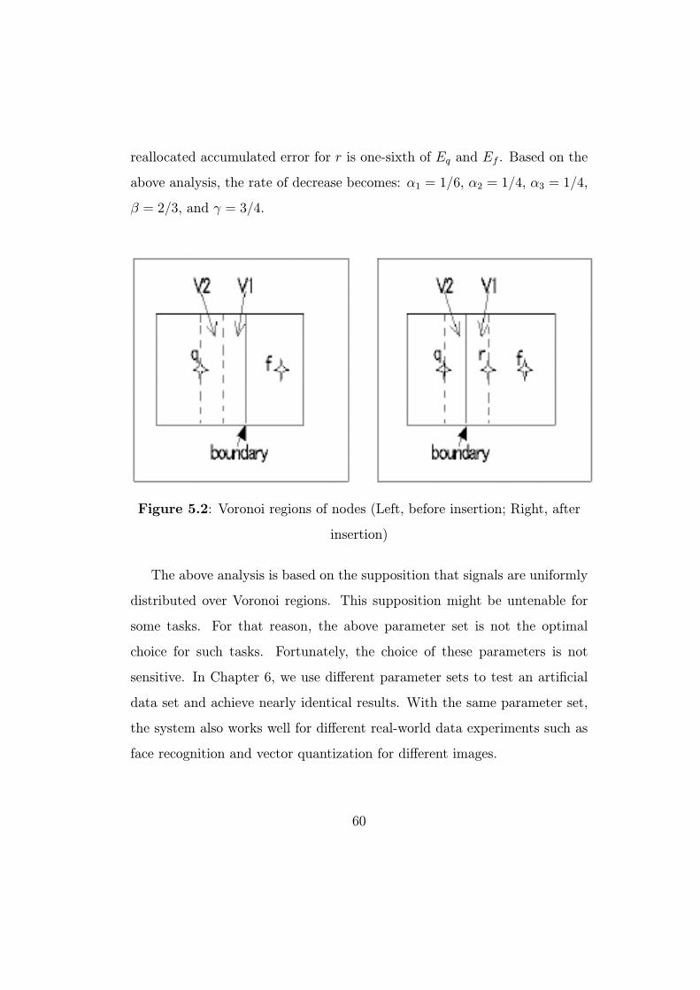
reallocated accumulated error for r is one-sixth of Eq and Ef . Based on the

above analysis, the rate of decrease becomes: α1 = 1/6, α2 = 1/4, α3 = 1/4,

β = 2/3, and γ = 3/4.

Figure 5.2: Voronoi regions of nodes (Left, before insertion; Right, after

insertion)

The above analysis is based on the supposition that signals are uniformly

distributed over Voronoi regions. This supposition might be untenable for

some tasks. For that reason, the above parameter set is not the optimal

choice for such tasks. Fortunately, the choice of these parameters is not

sensitive. In Chapter 6, we use different parameter sets to test an artificial

data set and achieve nearly identical results. With the same parameter set,

the system also works well for different real-world data experiments such as

face recognition and vector quantization for different images.

60

Chapter 6

Experiment with artificial data

We conducted our experiment on the data set shown in Figure 6.1. An

artificial 2-D data set is used to take advantage of its intuitive manipulation,

visualization, and resulting insight into system behavior. The data set is

separated into five parts: A, B, C, D, and E. Data sets A and B satisfy

2-D Gaussian distribution. The C and D data sets are a famous single-link

example. Finally, E is sinusoidal and separated into E1, E2, and E3 to clarify

incremental properties. We also add random noise (10% of useful data) to

the data set to simulate real-world data. As shown in Figure 6.1, overlaps

exist among clusters A and B; noise is distributed over the entire data set. As

stated in [7], neither BIRCH nor single-link clustering can correctly partition

such a data set. The CSM algorithm proposed by [10] partially solves this

problem, but it cannot eliminate noise, and noise forms new clusters.

61

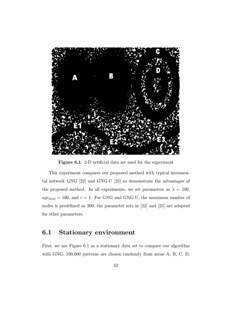
Figure 6.1: 2-D artificial data set used for the experiment

This experiment compares our proposed method with typical incremen-

tal network GNG [22] and GNG-U [25] to demonstrate the advantages of

the proposed method. In all experiments, we set parameters as λ = 100,

agedead = 100, and c = 1. For GNG and GNG-U, the maximum number of

nodes is predefined as 300; the parameter sets in [22] and [25] are adopted

for other parameters.

6.1 Stationary environment

First, we use Figure 6.1 as a stationary data set to compare our algorithm

with GNG; 100,000 patterns are chosen randomly from areas A, B, C, D,

62

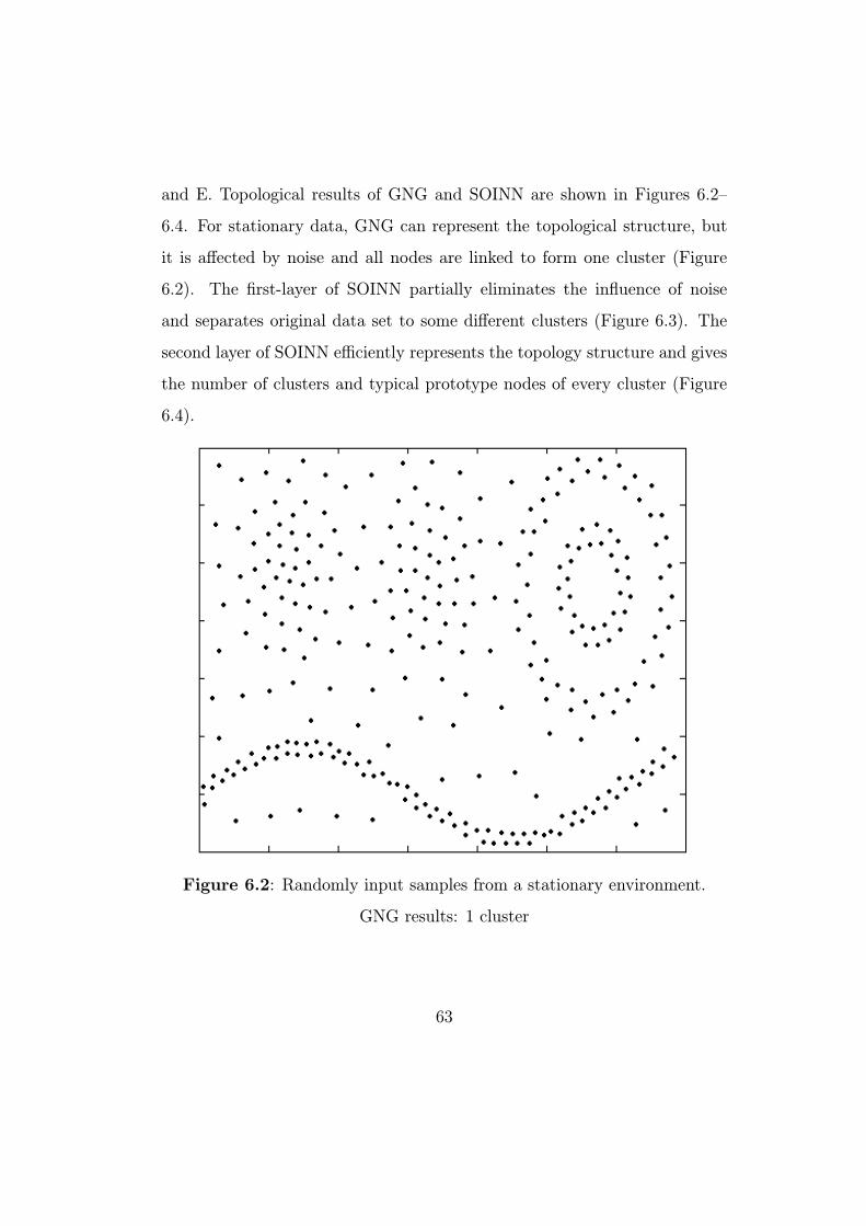
and E. Topological results of GNG and SOINN are shown in Figures 6.2—

6.4. For stationary data, GNG can represent the topological structure, but

it is affected by noise and all nodes are linked to form one cluster (Figure

6.2). The first-layer of SOINN partially eliminates the influence of noise

and separates original data set to some different clusters (Figure 6.3). The

second layer of SOINN efficiently represents the topology structure and gives

the number of clusters and typical prototype nodes of every cluster (Figure

6.4).

Figure 6.2: Randomly input samples from a stationary environment.

GNG results: 1 cluster

63

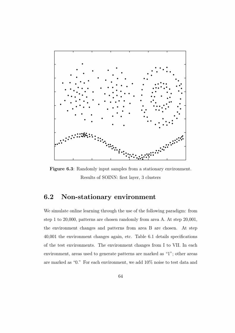
Figure 6.3: Randomly input samples from a stationary environment.

Results of SOINN: first layer, 3 clusters

6.2 Non-stationary environment

We simulate online learning through the use of the following paradigm: from

step 1 to 20,000, patterns are chosen randomly from area A. At step 20,001,

the environment changes and patterns from area B are chosen. At step

40,001 the environment changes again, etc. Table 6.1 details specifications

of the test environments. The environment changes from I to VII. In each

environment, areas used to generate patterns are marked as “1”; other areas

are marked as “0.” For each environment, we add 10% noise to test data and

64

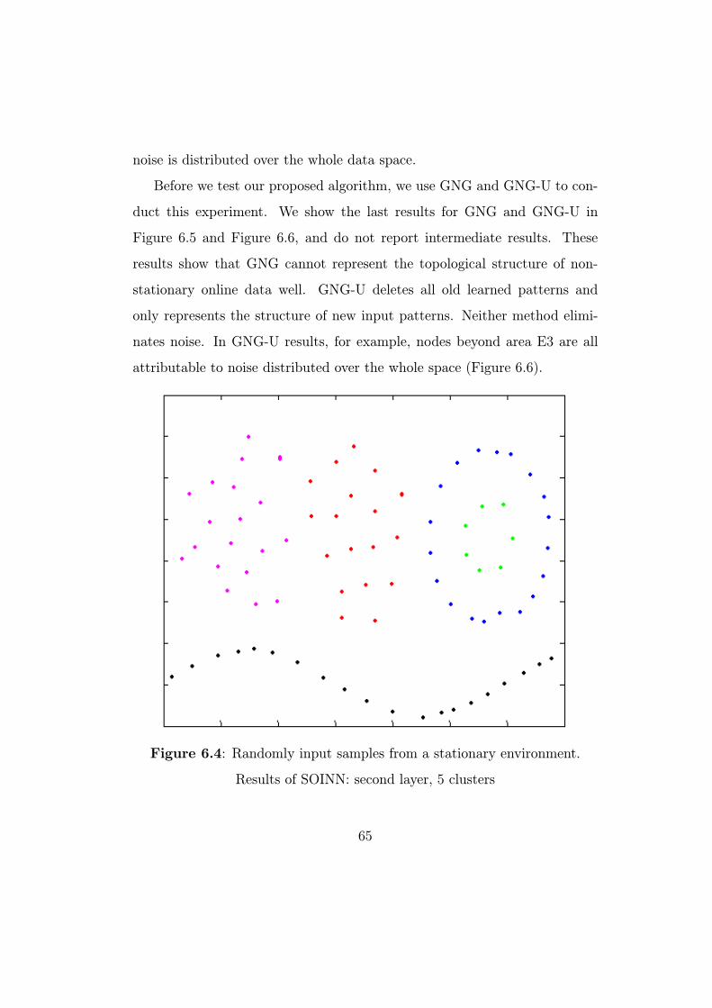
noise is distributed over the whole data space.

Before we test our proposed algorithm, we use GNG and GNG-U to con-

duct this experiment. We show the last results for GNG and GNG-U in

Figure 6.5 and Figure 6.6, and do not report intermediate results. These

results show that GNG cannot represent the topological structure of non-

stationary online data well. GNG-U deletes all old learned patterns and

only represents the structure of new input patterns. Neither method elimi-

nates noise. In GNG-U results, for example, nodes beyond area E3 are all

attributable to noise distributed over the whole space (Figure 6.6).

Figure 6.4: Randomly input samples from a stationary environment.

Results of SOINN: second layer, 5 clusters

65

Table 6.1: Experiment environments for online learning

Area Environment

I II III IV V VI VII

A 1 0 1 0 0 0 0

B 0 1 0 1 0 0 0

C 0 0 1 0 0 1 0

D 0 0 0 1 1 0 0

E1 0 0 0 0 1 0 0

E2 0 0 0 0 0 1 0

E3 0 0 0 0 0 0 1

Figure 6.5: Sequentially input samples from non-stationary environments.

GNG results

66

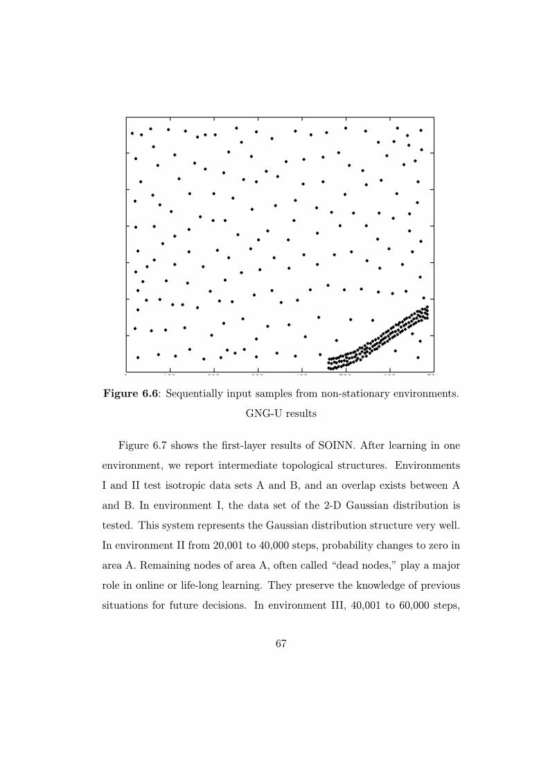
Figure 6.6: Sequentially input samples from non-stationary environments.

GNG-U results

Figure 6.7 shows the first-layer results of SOINN. After learning in one

environment, we report intermediate topological structures. Environments

I and II test isotropic data sets A and B, and an overlap exists between A

and B. In environment I, the data set of the 2-D Gaussian distribution is

tested. This system represents the Gaussian distribution structure very well.

In environment II from 20,001 to 40,000 steps, probability changes to zero in

area A. Remaining nodes of area A, often called “dead nodes,” play a major

role in online or life-long learning. They preserve the knowledge of previous

situations for future decisions. In environment III, 40,001 to 60,000 steps,

67

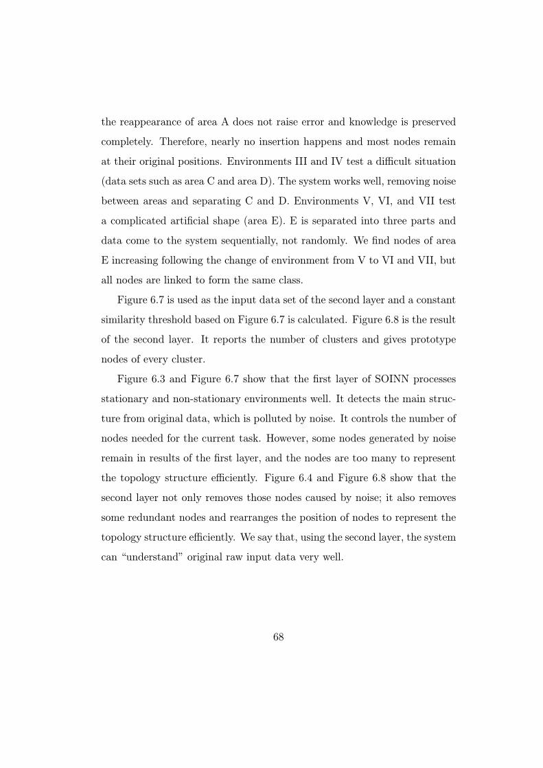
the reappearance of area A does not raise error and knowledge is preserved

completely. Therefore, nearly no insertion happens and most nodes remain

at their original positions. Environments III and IV test a difficult situation

(data sets such as area C and area D). The system works well, removing noise

between areas and separating C and D. Environments V, VI, and VII test

a complicated artificial shape (area E). E is separated into three parts and

data come to the system sequentially, not randomly. We find nodes of area

E increasing following the change of environment from V to VI and VII, but

all nodes are linked to form the same class.

Figure 6.7 is used as the input data set of the second layer and a constant

similarity threshold based on Figure 6.7 is calculated. Figure 6.8 is the result

of the second layer. It reports the number of clusters and gives prototype

nodes of every cluster.

Figure 6.3 and Figure 6.7 show that the first layer of SOINN processes

stationary and non-stationary environments well. It detects the main struc-

ture from original data, which is polluted by noise. It controls the number of

nodes needed for the current task. However, some nodes generated by noise

remain in results of the first layer, and the nodes are too many to represent

the topology structure efficiently. Figure 6.4 and Figure 6.8 show that the

second layer not only removes those nodes caused by noise; it also removes

some redundant nodes and rearranges the position of nodes to represent the

topology structure efficiently. We say that, using the second layer, the system

can “understand” original raw input data very well.

68

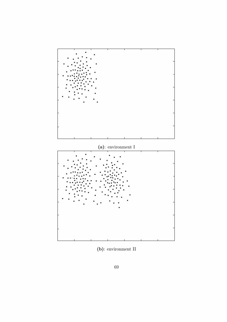
(a): environment I

(b): environment II

69

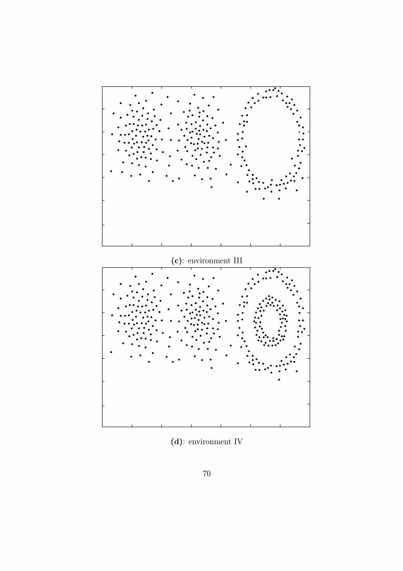
(c): environment III

(d): environment IV

70

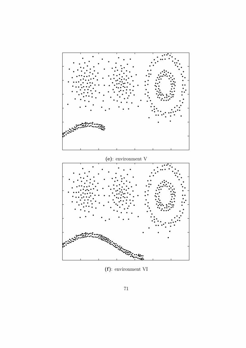
(e): environment V

(f): environment VI

71

(g): environment VII

Figure 6.7: Sequentially input samples from non-stationary environments.

Results of SOINN: first layer

Figure 6.9 shows how the number of nodes changes during online learning

(first-layer). The number of nodes increases when an input signal comes from

a new area (see Table 6.1, environment changes from I to VII). In the same

environment, after some learning steps, the increase in nodes stops and the

number of nodes converges to a constant because further insertion cannot

engender decreased error. Noise leads the system to frequently insert and

delete nodes. For that reason, a small fluctuation exists in the number of

nodes in Figure 6.9.

72

Figure 6.8: Sequentially input samples from non-stationary environments.

Results of SOINN: second layer, 5 clusters

Finally, we perform some experiments to test the sensitivity of parame-

ters. Four different parameter sets for α1, α2, α3, β, γ are used to test

the artificial data set (Figure 6.1): 14, 14, 14, 23, 34, 1

4, 14, 14, 23, 12, 1

6, 14,

14, 12, 12, and 1

6, 14, 14, 14, 34. The experiments are done in stationary and

non-stationary environments. In both environments, for all four parameter

sets, the system can detect the five clusters from the original data set and

give prototype nodes; the last results are nearly the same as those shown in

Figure 6.4 for a stationary environment and those shown in Figure 6.8 for a

non-stationary environment. Consequently, the experiment results indicate

that the choice of parameter set α1, α2, α3, β, γ is not influential. In the

following, we only use the original parameter set 16, 14, 14, 23, 34

to do differ-

73

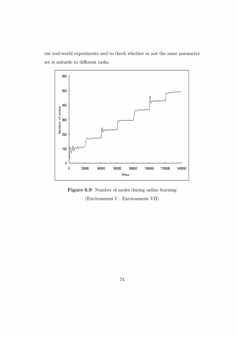
ent real-world experiments and to check whether or not the same parameter

set is suitable to different tasks.

Figure 6.9: Number of nodes during online learning

(Environment I — Environment VII)

74

Chapter 7

Application for real-world

image data

7.1 Face recognition

For application of clustering with the proposed method, we use some fa-

cial images as the input signal of the first layer. The input facial images

are taken from the ATT FACE database (http://www.uk.research.att.com/).

The database comprises 40 distinct subjects with 10 different images of every

subject. For some subjects, the images were taken at different times with

various lighting, facial expressions (open/closed eyes, smiling/not smiling)

and facial details (glasses/no glasses). The size of each image is 92 112

pixels, with 256 grey levels per pixel. We selected 10 subjects (Figure 7.1(a))

from the database to test SOINN. Figure 7.1(b) portrays the different im-

ages of the first subject in Figure 7.1(a). Feature vectors of such images are

taken as follows: first, the original image with size 92 112 is re-sampled to

75

23 28 image using the nearest neighbor interpolation method. Then Gaus-

sian smoothing is used to smooth the 23 28 image with Gaussian width =

4, σ = 2 to obtain the 23 28 dimensional input feature vectors (Figure 7.2).

The test consists of two processes: learning and evaluation. During learn-

ing, we choose vectors randomly (stationary) or sequentially (more difficult

task, non-stationary online) from an original image vector set for the first

layer, then input the results of the first layer to the second layer, and report

number of clusters and prototype vectors of every cluster as the results of

the second layer. In both layers, we set parameters λ = 25 and agedead = 25.

In the first layer, c is set to 1.0 because we want to delete nodes lying in

overlap area; for the second layer, c is set as 0.05 to focus on clustering and

to avoid deleting too many nodes. For both stationary and non-stationary

environments, we do 10,000 training iterations for the first layer and 2,000

training iterations for the second layer.

In the evaluation process, nearest neighbor is used to classify vectors in

the original image vector set to the clusters learned through the learning

process. The correct recognition ratio is reported as the performance index

of learning process.

For a stationary environment, i.e., vectors are randomly chosen from the

original data set, the learning process reports that 10 clusters exist in the

input patterns and gives prototype vectors of every cluster. The evaluation

process reports that the correct recognition ratio is 90%. In addition, GNG

is tested with parameter λ = 25 and amax = 25, maximum number of nodes

is predefined as 50, other parameters are the same as in (Fritzke, 1995), and

10,000 samples are used to train GNG. The GNG results show four clusters

76

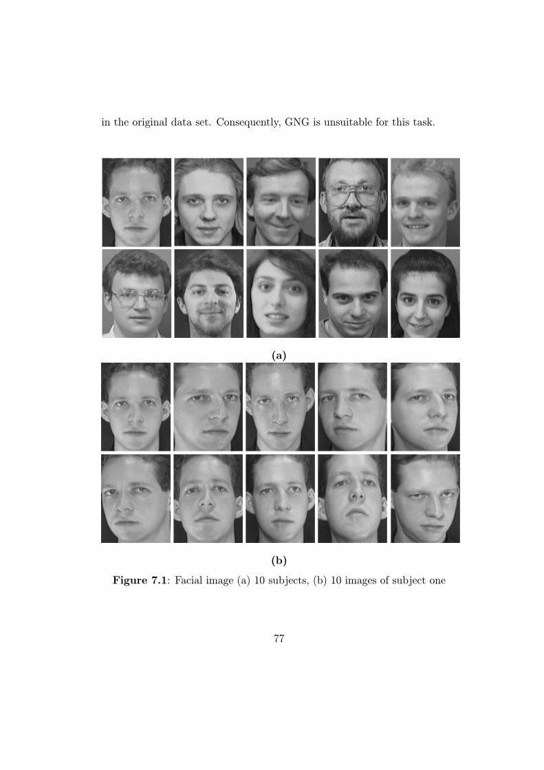
in the original data set. Consequently, GNG is unsuitable for this task.

(a)

(b)

Figure 7.1: Facial image (a) 10 subjects, (b) 10 images of subject one

77

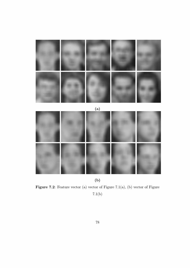
(a)

(b)

Figure 7.2: Feature vector (a) vector of Figure 7.1(a), (b) vector of Figure

7.1(b)

78

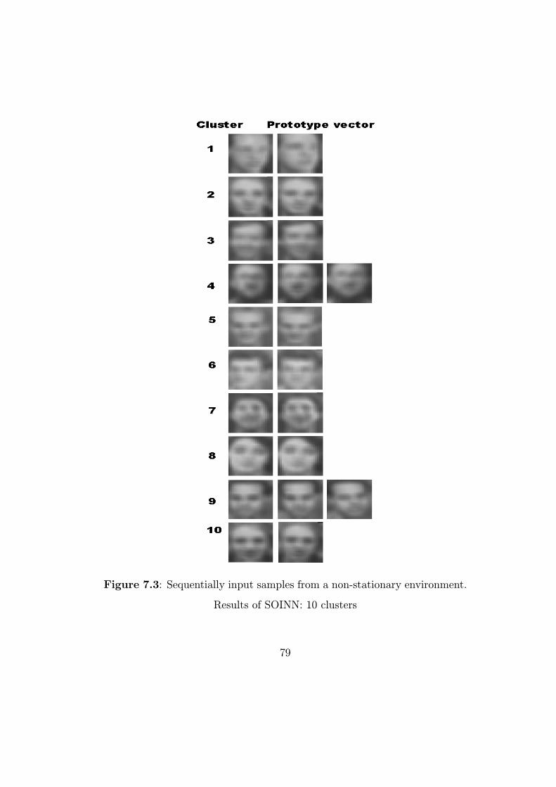
Figure 7.3: Sequentially input samples from a non-stationary environment.

Results of SOINN: 10 clusters

79

For a non-stationary online environment, i.e., 10,000 vectors are sequen-

tially taken from original data set (one class by one class, 1,000 samples for

each class), the learning process reports 10 clusters and gives prototype vec-

tors of every cluster (Figure 7.3). Comparison of Figure 7.3 with Figure 7.2

reveals that the proposed algorithm reports the number of clusters correctly.

It gives the prototype vectors of every cluster reasonably. The evaluation pro-

cess reports that the correct recognition ratio is 86%. Furthermore, GNG-U

is tested with parameter λ = 25 and amax = 25. The maximum number of

nodes is predefined as 25 and other parameters are the same as in (Fritzke,

1997); 10,000 samples are input sequentially to GNG-U (one class by one

class, 1,000 samples for each class). The GNG-U results show two clusters

in the original data set. That result indicates that GNG-U is unsuitable for

this task.

The experimental results show that SOINN works well for unsupervised

classification (learning the number of clusters and reporting prototype vectors

of every cluster). Some other typical incremental networks (such as GNG,

GNG-U) are unsuitable for this task.

7.2 Vector quantization

This experiment uses vector quantization to code a well-known image: Lena

(512 512 8)(Figure 4.1). SOINN is used to determine the codebook. Dif-

ferent from traditional methods, the codebook size is not predefined. Instead,

it is determined by the algorithm itself. Because GNG or GNG-U is unsuit-

able for sequential input vectors, this experiment only compares SOINN with

80

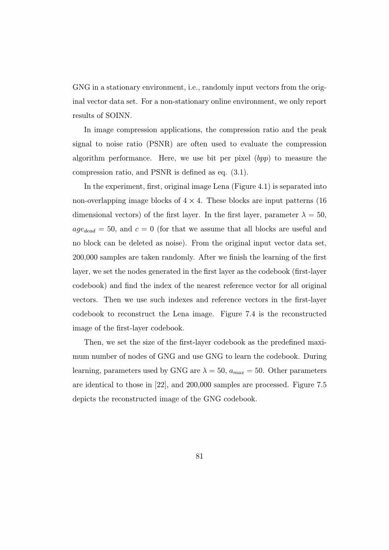
GNG in a stationary environment, i.e., randomly input vectors from the orig-

inal vector data set. For a non-stationary online environment, we only report

results of SOINN.

In image compression applications, the compression ratio and the peak

signal to noise ratio (PSNR) are often used to evaluate the compression

algorithm performance. Here, we use bit per pixel (bpp) to measure the

compression ratio, and PSNR is defined as eq. (3.1).

In the experiment, first, original image Lena (Figure 4.1) is separated into

non-overlapping image blocks of 4 4. These blocks are input patterns (16

dimensional vectors) of the first layer. In the first layer, parameter λ = 50,

agedead = 50, and c = 0 (for that we assume that all blocks are useful and

no block can be deleted as noise). From the original input vector data set,

200,000 samples are taken randomly. After we finish the learning of the first

layer, we set the nodes generated in the first layer as the codebook (first-layer

codebook) and find the index of the nearest reference vector for all original

vectors. Then we use such indexes and reference vectors in the first-layer

codebook to reconstruct the Lena image. Figure 7.4 is the reconstructed

image of the first-layer codebook.

Then, we set the size of the first-layer codebook as the predefined maxi-

mum number of nodes of GNG and use GNG to learn the codebook. During

learning, parameters used by GNG are λ = 50, amax = 50. Other parameters

are identical to those in [22], and 200,000 samples are processed. Figure 7.5

depicts the reconstructed image of the GNG codebook.

81

Figure 7.4: Randomly input samples from stationary environment.

Reconstructed image: the first-layer codebook with 130 nodes,

0.45 bpp, PSNR=30.79 dB

For the second layer, the first-layer codebook is set as the input data

set of the second layer. With the same parameter set as the first layer, i.e.,

λ = 50, agedead = 50, and c = 0, 10,000 samples are taken randomly from the

first-layer codebook to train the second layer. We obtain the second-layer

codebook and use this second-layer codebook to encode and reconstruct the

Lena image. With the size of second-layer codebook, GNG is also used to

obtain a codebook. We use this GNG codebook to encode and reconstruct

the Lena image, and calculate the PSNR. Table 7.1 summarizes a comparison

82

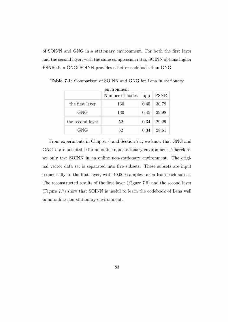
of SOINN and GNG in a stationary environment. For both the first layer

and the second layer, with the same compression ratio, SOINN obtains higher

PSNR than GNG: SOINN provides a better codebook than GNG.

Table 7.1: Comparison of SOINN and GNG for Lena in stationary

environment

Number of nodes bpp PSNR

the first layer 130 0.45 30.79

GNG 130 0.45 29.98

the second layer 52 0.34 29.29

GNG 52 0.34 28.61

From experiments in Chapter 6 and Section 7.1, we know that GNG and

GNG-U are unsuitable for an online non-stationary environment. Therefore,

we only test SOINN in an online non-stationary environment. The origi-

nal vector data set is separated into five subsets. These subsets are input

sequentially to the first layer, with 40,000 samples taken from each subset.

The reconstructed results of the first layer (Figure 7.6) and the second layer

(Figure 7.7) show that SOINN is useful to learn the codebook of Lena well

in an online non-stationary environment.

83

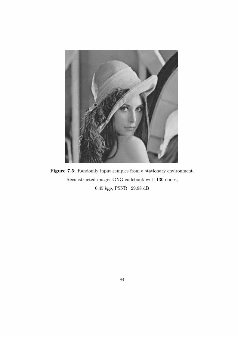
Figure 7.5: Randomly input samples from a stationary environment.

Reconstructed image: GNG codebook with 130 nodes,

0.45 bpp, PSNR=29.98 dB

84

Figure 7.6: Sequentially input samples from a non-stationary environment.

Reconstructed image: the first-layer codebook with 499 nodes,

0.56 bpp, PSNR=32.91 dB

85

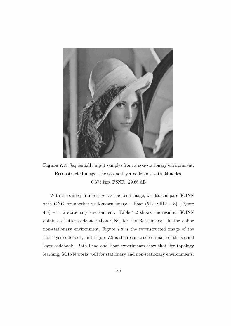
Figure 7.7: Sequentially input samples from a non-stationary environment.

Reconstructed image: the second-layer codebook with 64 nodes,

0.375 bpp, PSNR=29.66 dB

With the same parameter set as the Lena image, we also compare SOINN

with GNG for another well-known image — Boat (512 512 8) (Figure

4.5) — in a stationary environment. Table 7.2 shows the results: SOINN

obtains a better codebook than GNG for the Boat image. In the online

non-stationary environment, Figure 7.8 is the reconstructed image of the

first-layer codebook, and Figure 7.9 is the reconstructed image of the second

layer codebook. Both Lena and Boat experiments show that, for topology

learning, SOINN works well for stationary and non-stationary environments.

86

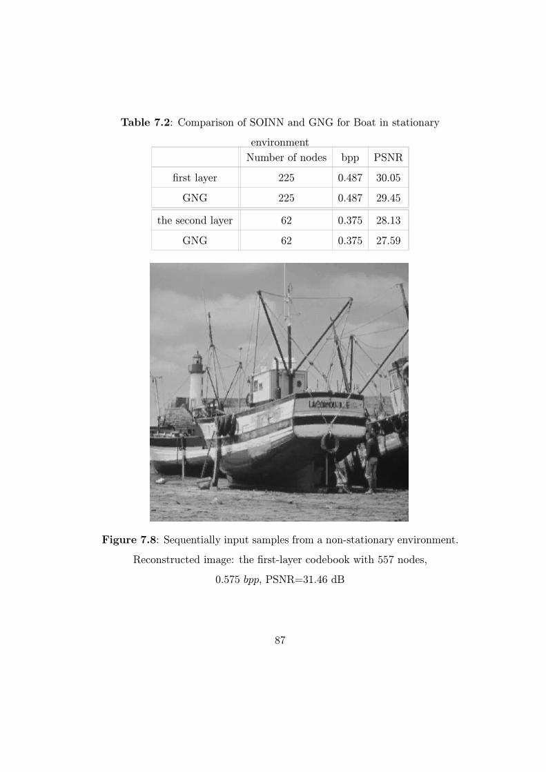
Table 7.2: Comparison of SOINN and GNG for Boat in stationary

environment

Number of nodes bpp PSNR

first layer 225 0.487 30.05

GNG 225 0.487 29.45

the second layer 62 0.375 28.13

GNG 62 0.375 27.59

Figure 7.8: Sequentially input samples from a non-stationary environment.

Reconstructed image: the first-layer codebook with 557 nodes,

0.575 bpp, PSNR=31.46 dB

87

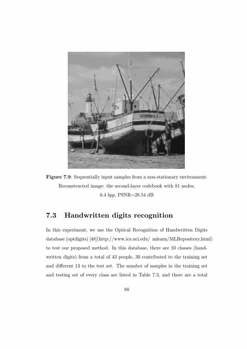
Figure 7.9: Sequentially input samples from a non-stationary environment.

Reconstructed image: the second-layer codebook with 81 nodes,

0.4 bpp, PSNR=28.54 dB

7.3 Handwritten digits recognition

In this experiment, we use the Optical Recognition of Handwritten Digits

database (optdigits) [48](http://www.ics.uci.edu/ mlearn/MLRepository.html)

to test our proposed method. In this database, there are 10 classes (hand-

written digits) from a total of 43 people, 30 contributed to the training set

and different 13 to the test set. The number of samples in the training set

and testing set of every class are listed in Table 7.3, and there are a total

88

of 3823 samples in the training set, and a total of 1797 samples in the test

set. The dimension of the samples is 64. With traditional Nearest Neighbor

method, using the 3823 training samples as the prototype vectors, we classify

the test samples to different classes using Euclidean distance as the metric.

The correct recognition ratio is 98%.

Table 7.3: Number of samples in optdigits database

Class No. of Training samples No. of Test samples

0 376 178

1 389 182

2 380 177

3 389 183

4 387 181

5 376 182

6 377 181

7 387 179

8 380 174

9 382 180

Total 3823 1797

We use the training set to train SOINN. We test SOINN under incre-

mental environment, i.e., at first stage, we randomly choose samples from

training set of class 0 to train the system, at this stage, no samples from

other classes are chosen; after 10,000 times training, at the second stage, the

samples inputting to the system are randomly chosen from training set of

class 1, and do 10,000 times training; and then for class 2, 3, ..., 9, we use

the same method as the first and second stage to incrementally train SOINN.

89

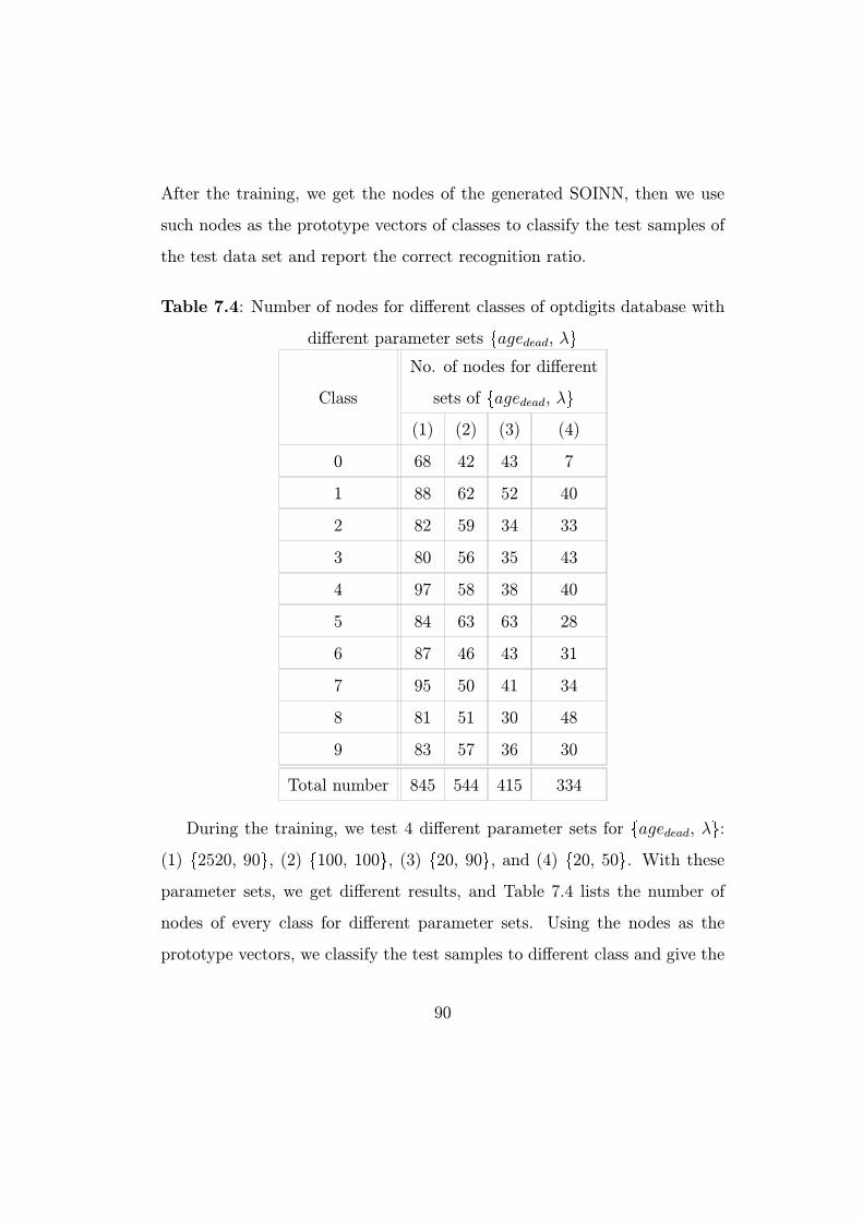
After the training, we get the nodes of the generated SOINN, then we use

such nodes as the prototype vectors of classes to classify the test samples of

the test data set and report the correct recognition ratio.

Table 7.4: Number of nodes for different classes of optdigits database with

different parameter sets agedead, λ

No. of nodes for different

Class sets of agedead, λ

(1) (2) (3) (4)

0 68 42 43 7

1 88 62 52 40

2 82 59 34 33

3 80 56 35 43

4 97 58 38 40

5 84 63 63 28

6 87 46 43 31

7 95 50 41 34

8 81 51 30 48

9 83 57 36 30

Total number 845 544 415 334

During the training, we test 4 different parameter sets for agedead, λ :

(1) 2520, 90 , (2) 100, 100 , (3) 20, 90 , and (4) 20, 50 . With these

parameter sets, we get different results, and Table 7.4 lists the number of

nodes of every class for different parameter sets. Using the nodes as the

prototype vectors, we classify the test samples to different class and give the

90

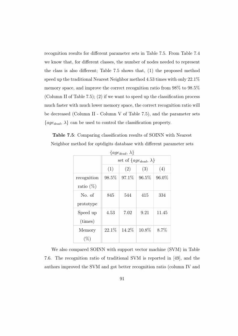
recognition results for different parameter sets in Table 7.5. From Table 7.4

we know that, for different classes, the number of nodes needed to represent

the class is also different; Table 7.5 shows that, (1) the proposed method

speed up the traditional Nearest Neighbor method 4.53 times with only 22.1%

memory space, and improve the correct recognition ratio from 98% to 98.5%

(Column II of Table 7.5); (2) if we want to speed up the classification process

much faster with much lower memory space, the correct recognition ratio will

be decreased (Column II - Column V of Table 7.5), and the parameter sets

agedead, λ can be used to control the classification property.

Table 7.5: Comparing classification results of SOINN with Nearest

Neighbor method for optdigits database with different parameter sets

agedead, λ

set of agedead, λ

(1) (2) (3) (4)

recognition 98.5% 97.1% 96.5% 96.0%

ratio (%)

No. of 845 544 415 334

prototype

Speed up 4.53 7.02 9.21 11.45

(times)

Memory 22.1% 14.2% 10.8% 8.7%

(%)

We also compared SOINN with support vector machine (SVM) in Table

7.6. The recognition ratio of traditional SVM is reported in [49], and the

authors improved the SVM and got better recognition ratio (column IV and

91

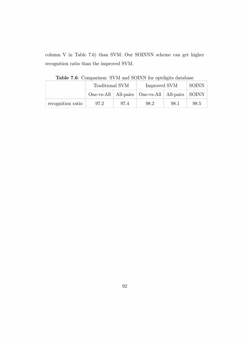
column V in Table 7.6) than SVM. Our SOINNN scheme can get higher

recognition ratio than the improved SVM.

Table 7.6: Comparison: SVM and SOINN for optdigits database

Traditional SVM Improved SVM SOINN

One-vs-All All-pairs One-vs-All All-pairs SOINN

recognition ratio 97.2 97.4 98.2 98.1 98.5

92

Chapter 8

Conclusion and discussion

In this study, we proposed a new online learning method for unsupervised

classification and topology representation. Using a similarity threshold-

based and a locally accumulated error-based insertion criterion, the sys-

tem can grow incrementally and accommodate input patterns of online non-

stationary data distribution. A novel online criterion for node removal in

low probability-density regions enables this system to separate clusters with

low-density overlap and to dynamically eliminate noise from input data. The

utility parameter “error-radius” is used to judge if the insertion is successful

and to control the increase of nodes. Adoption of a two-layer neural net-

work makes it possible for this system to “understand” the original data set

well. In summary, the algorithm can cope with difficulties in online or life-

long unsupervised learning such as overlap, never-seen inputs, temporarily

non-appearing patterns, and noise.

Other problems remain unsolved. For example, when a high-density over-

lap pertains between clusters, it is extremely difficult for the proposed al-

93

gorithm to separate clusters from each other. Three parameters must be

determined by the user: λ, agedead, and c. The difficulty of automatically

determining such parameters is based on the fact that, for different tasks, the

optimal choice of such parameters is different: it is difficult to give a stan-

dard of such parameters for every task. Although these parameters are not so

sensitive, we remain hopeful that some methods are useful to automatically

deduce optimal choice of such parameters for the task. Such problems will

be addressed in subsequent studies.

94

Bibliography

[1] J. Weng and I. Stockman. Proceedings of NSF/DARPA Workshop on

Development and Learning. East Lansing, Michigan, 2000.

[2] G.A. Carpenter and S. Grossberg. The art of adaptive pattern recog-

nition by a self-organizing neural network. IEEE Computer, 21:77—88,

1988.

[3] A. K. Jain and R.C. Dubes. Algorithms for clustering data. Prentice

Hall, Englewood Cliffs, 1988.

[4] M.N. Murty, A.K. Jain, and P.J. Flynn. Data clustering: a review. ACM

Comput. Surv., 31(3):264—323, 1999.

[5] H.A. Sneath and R.R. Sokal. Numerical taxonomy. Freeman, London,

UK, 1988.

[6] B. King. Step-wise clustering procedures. J. Am. Stat. Assoc., 69(3):86—

101, 1967.

[7] S. Guha, R. Rastogi, and K. Shim. Cure: An efficient clustering algo-

rithm for large databases. Proceeding of ACM SIGMOD Conference on

Management of Data, pages 73—84, 1998.

95

[8] T. Zhang, R. Ramakrishnan, and M. Livny. Birch: an efficient data

clustering method for a very large database. Proc. ACM SIGMOD Con-

ference on Management of Data, pages 103—114, 1996.

[9] Y.-J. Oyang, C.-Y., Chen, and T.-W. Yang. A study on the hierarchical

data clustering algorithm based on gravity theory. Proc. of 5th Euro-

pean Conference on Principles and Practice of Knowledge Discovery in

Databases, pages 350—361, 2001.

[10] C.R. Lin and M.S. Chen. A robust and efficient clustering algorithm

based on cohesion self-merging. Proceeding of ACM SIGKDD, Edmon-

ton, Alberta, Canada, 2002.

[11] J.A. Lozano, J.M. Pena, and Larranaga. An empirical comparison of four

initialization methods for the k-means algorithm. Pattern Recognition

Lett., 20:1027—1040, 1999.

[12] A. Likas, N. Vlassis, and J.J. Verbeek. The global k-means clustering

algorithm. Pattern Recognition, 36:451—461, 2003.

[13] G. Patane and M. Russo. The enhanced lbg algorithm. Neural Networks,

14:1219—1237, 2001.

[14] N.M. Murty and G. Krishna. A hybrid clustering procedure for con-

centric and chain-like clusters. International Journal of Computer and

Information Sciences, 10(6):397—412, 1981.

[15] D.J. Willshaw and C. von der Malsburg. How patterned neural connec-

tions can be set up by self-organization. Proc. Royal Society of London

B, pages 431—445, 1976.

96

[16] T. Kohonen. Self-organized formation of topologically correct feature

maps. Biological Cybernetics, 43:59—69, 1982.

[17] T. Martinetz and K. Schulten. Topology representing networks. Neural

Networks, 7(3):507—522, 1994.

[18] T. Villmann, R. Der, M. Herrmann, and T. Martinetz. Topology preser-

vation in self-organizing feature maps: exact definition and measure-

ment. IEEE Transactions on Neural Networks, 8(2):256—266, 1997.

[19] T. Villmann, F.-M. Schleif, and B. Hammer. Supervised neural gas and

relevance learning in learning vector quantization. Proc. Workshop on

Self-Organizing Maps (WSOM), Japan, 2003.

[20] T.M. Martinetz. Competitive hebbian learning rule forms perfectly

topology preserving maps. ICANN, pages 427—434, 1993.

[21] T.M. Martinetz, S.G. Berkovich, and K.J. Schulten. “neural-gas” net-

work for vector quantization and its application to time-series prediction.

IEEE Transactions on Neural Networks, 4(4):558—569, 1996.

[22] B. Fritzke. A growing neural gas network learns topologies. In Advances

in neural information processing systems (NIPS), pages 625—632, 1995.

[23] J. Bruske and G. Sommer. Dynamic cell structure learns perfectly topol-

ogy preserving map. Neural Computation, 7:845—865, 1995.

[24] F.H. Hamker. Life-long learning cell structures — continuously learning

without catastrophic interference. Neural Networks, 14:551—573, 2001.

97

[25] B. Fritzke. A self-organizing network that can follow non-stationary

distributions. Proceedings of ICANN-97, pages 613—618, 1997.

[26] C.P. Lim and R.F. Harrison. A incremental adaptive network for on-

line supervised learning and probability estimation. Neural Networks,

10:925—939, 1997.

[27] F. Shen and O. Hasegawa. An adaptive incremental lbg for vector quan-

tization. Neural Networks.

[28] F. Shen and O. Hasegawa. An incremental network for on-line unsuper-

vised classification and topology learning. Neural Networks.

[29] C. Vladimir and M. Filip. Learning from data — Concepts, Theory, and

Methods. John Wiley and Sons, Inc., 1997.

[30] K. Paliwal and B. Atal. Efficient vector quantization of lpc parameters

at 24 bits/fr ame. IEEE Transactions on Speech and Audio Processing,

1(1):3—14, 1993.

[31] P. Cosman, R. Gray, and M. Vetterli. Vector quantization of image

subbands: a survey. IEEE Transactions on Image Processing, 5(2):202—

225, 1996.

[32] L.A. Chan, N.M. Nasrabadi, and B. Mirelli. Multi-stage target recog-

nition using modular vector quantizers and multilayer perceptrons. In

Proc. CVPR’96, pages 114—119, 1996.

98

[33] J. Jolion, P. Meer, and S. Bataouche. Robust clustering with applica-

tions in computer vision. IEEE Transaction on Pattern Analysis and

Machine Intelligence, 13:791—802, 1991.

[34] K. Perlmutter, S. Perlmutter, R. Gray, R. Olshen, and K. Oehler. Bayes

risk weighted vector quantization with posterior estimation for image

compression and classification. IEEE Transactions on Image Processing,

5(2):347—360, 1996.

[35] A. Buzo Y. Linde and R.M. Gray. An algorithm for vector quantizer

design. IEEE Transactions on Communication, pages 84—95, 1980.

[36] S.P. Lloyd. Least squares quantization in pcm’s. Bell Telephone Labo-

ratories Paper, Murray Hill, NJ., 1957.

[37] J. Max. Quantizing for minimum distortion. IRE Trans. Info. Theory,

pages 7—12, 1960.

[38] B. Fritzke. The lbg-u method for vector quantization - an improvement

over lbg inspired from neural networks. Neural Processing Letters, 5(1),

1997.

[39] R.M. Gray. Vector quantization. IEEE ASSP Mag., 1:4—29, 1984.

[40] A. Gersho. Digital communications. North-Holland: Elsevier Science

Publisher, 1986.

[41] C. Chinrungrueng and C. Sequin. Optimal adaptive k -means algorithm

with dynamic adjustment of learning rate. IEEE Transactions on Neural

Networks, 8(5):729—743, 1995.

99

[42] D. Lee, S. Baek, and K. Sung. Modified k-means algorithm for vector

quantizer design. IEEE Signal Processing Letters, 4(1):2—4, 1997.

[43] R.O. Duda, P.E. Hart, and D.G. Stork. Pattern classification, 2nd ed.

Wiley-Interscience, 2001.

[44] B. Fritzke. Growing cell structures — a self-organizing network for unsu-

pervised and supervised learning. Neural Networks, 7:1441—1460, 1994.

[45] T. Villmann. Controlling strategies for the magnification factor in the

neural gas network. Neural Network World, 10:739—750, 2000.

[46] H.J. Ritter, T.M. Martinetz, and K.J. Schulten. Neuronale Netze.

Addison-Wesley, Munchen, 1991.

[47] M.T. Wasan. Stochastic approximation. Cambridge Univ. Press, 1969.

[48] C. Merz and M. Murphy. Uci repository of machine learning databases,

irvine, ca,. University of California Department of Information, 1996.

[49] A. Passerini, M. Pontil, and P. Frasconi. From margins to probabili-

ties in multiclass learning problems. Proceedings of the 15th European

Conference on Artificial Intelligence, 2002.

100

Acknowledgment

Without patient encouragement and support of many people, this thesis

could not have been realized.

This thesis is a collection of work conducted at the Hasegawa laboratory,

Department of Computational Intelligence and Systems Science, Interdis-

ciplinary Graduate School of Science and Engineering, Tokyo Institute of

Technology from 2003 to 2006.

First and foremost, the author would like to express his sincere gratitude

to his esteemed supervisor, Dr. Osamu Hasegawa, Associate Professor of

Imaging Science and Engineering Laboratory, Tokyo Institute of Technology,

for his constant supervision and fruitful discussions.

The author would also like to thank the members of my PhD commit-

tee who monitored my work and took effort in reading and providing me

with valuable comments on earlier version of this thesis: Professor Kaoru

Hirota, Professor Hiroshi Nagahashi, Professor Makoto Sato, Professor Kat-

sumi Nitta.

Finally, the author would like to express his deepest appreciation to his

parents for their heartful encouragement and support, and would like to

dedicate this thesis to them.

101

Publications

Journal papers

1. Shen Furao and Osamu Hasegawa, ”An adaptive incremental LBG for

vector quantization,” Neural Networks, in press.

2. Shen Furao and Osamu Hasegawa, ”An incremental network for on-line

unsupervised classification and topology learning,” Neural Networks,

Vol. 19, No.1, pp 90-106, 2006.

3. Shen Furao and Osamu Hasegawa, ”Fractal image coding with simu-

lated annealing search,” Journal of Advanced Computational Intelli-

gence and Intelligent Informatics, Vol.9, No.1, pp.80-88, 2005.

4. Shen Furao and Osamu Hasegawa, ”A fast no search fractal image cod-

ing method,” Signal Processing: Image Communication, vol.19, pp.393-

404, 2004.

5. Shen Furao and Osamu Hasegawa, ”A growing neural network for on-

line unsupervised learning,” Journal of Advanced Computational Intel-

ligence and Intelligent Informatics, Vol.8, No.2, pp.121-129, 2004.

102

Refereed international conference papers

1. Shen Furao, Youki Kamiya and Osamu Hasegawa, ”An incremental

neural network for online supervised learning and topology representa-

tion,” 12th International Conference on Neural Information Processing

(ICONIP 2005), Taipei, Taiwan, October 30 - November 2, 2005.

2. Shen Furao and Osamu Hasegawa, ”An incremental k-means clustering

algorithm with adaptive distance measure,” 12th International Confer-

ence on Neural Information Processing (ICONIP 2005), Taipei, Taiwan,

October 30 - November 2, 2005.

3. Shen Furao and Osamu Hasegawa, ”An on-line learning mechanism for

unsupervised classification and topology representation,” IEEE Com-

puter Society International Conference on Computer Vision and Pat-

tern Recognition (CVPR 2005), pp. 651-656, San Diego, CA, USA,

June 21-26, 2005.

4. Shen Furao and Osamu Hasegawa, ”An incremental neural network

for non-stationary unsupervised learning,” 11th International Confer-

ence on Neural Information Processing (ICONIP 2004), pp. 641-646,

Calcutta, India, November 22-25, 2004.

5. Shen Furao and Osamu Hasegawa, ”An effective fractal image coding

method without search,” IEEE International Conference on Image Pro-

cessing (ICIP 2004), pp. 3197-3200, Singapore, October 24-27, 2004.

103

6. Youki Kamiya, Shen Furao and Osamu Hasegawa, ”Non-stop learning:

a new scheme for continuous learning and recognition,” Joint 2nd SCIS

and 5th ISIS, CD-ROM TUP-3-5, Keio University, Yokohama, Japan,

September 21-24, 2004.

7. Osamu Hasegawa and Shen Furao, ”A self-structurizing neural network

for online incremental learning,” CD-ROM SICE Annual Conference,

FAII-5-2, Sapporo, Japan, August 4-6, 2004.

8. Shen Furao and Osamu Hasegawa, ”A self-organized growing network

for on-line unsupervised learning,” 2004 International Joint Confer-

ence on Neural Networks (IJCNN 2004), Budapest, Hungary, CD-ROM

ISBN 0-7803-8360-5, Vol.1, pp.11-16, 2004.

9. Shen Furao and Osamu Hasegawa, ”A fast and less loss fractal image

coding method using simulated annealing,” 7th Joint Conference on

Information Science (JCIS 2003), pp. 198-201, Cary, North Carolina,

USA, September 26-30, 2003.

Japanese conference papers

1. Shen Furao, Youki Kamiya and Osamu Hasegawa, ”An incremental

neural network for online supervised learning and topology learning,”

Meeting on Image Recognition and Understandings (MIRU 2005), Awaji

Yumebudai International Conference Center, July 18-20, 2005.

104

2. Shen Furao and Osamu Hasegawa, ”A self-controlled incremental method

for vector quantization,” PRMU 2004-65, CVIM2004-145, Kyoto, Septem-

ber 2004.

3. 神谷裕樹、申富饒、長谷川修, 追加的・連続的学習による自律的概念獲

得、計測自動制御学会、第９回　相互作用と賢さ　合同研究会、2004

4. 神谷裕樹、申富饒、長谷川修, ”実世界パターン情報の非停止型学習・認

識手法の提案”, 2004年人工知能学会全国大会、金沢, 2004年６月.

5. 神谷裕樹、申富饒、長谷川修, ”実世界パターン情報の非停止型学習認

識手法の提案”, 2004年　電子情報通信学会総合大会、東京, 2004年 3

月.

6. Shen Furao and Osamu Hasegawa, ”A growing network for on-line un-

supervised learning,” 2004 IEICE general conference, Tokyo, March

2004.

7. Shen Furao and Osamu Hasegawa, ”High quality and fast fractal image

coding by simulated annealing,” 9th Symposium on Sensing via Image

Information (SSII 2003), Yokohama, June 2003.

105