Transport under Emission Trading

A Computable General Equilibrium Assessment

Dissertation

Zur Erlangung des akademischen Grades

Doctor rerum politicarum (Dr. rer. pol.)

vorgelegt an der

Fakultät Wirtschaftswissenschaften

der Technischen Universität Dresden

im November 2009

von

Dipl.-Vw. Jan Abrell

(geboren am 8. Juli 1977 in Mannheim)

verteidigt am 12. Juli 2010

Betreuender Hochschullehrer (1 Gutachter): 2. Gutachter:

Prof. Dr. Christian von Hirschhausen Prof. Dr. Georg Hirte

Technische Universität Dresden Technische Universität Dresden

Lehrstuhl für Energiewirtschaft Professur Makroökonomik und Raum-

wirtschaftslehre/Regionalwissenschaften

Abstract

This thesis analysis the impact of private road transport under emission trading using two different

Computable General Equilibrium models. A static multi-region model with special emphasis on the

European Union, addresses the welfare impact of road transport under the European Emission Trading

System. Including terms-of-trade effects, this model does not account for congestion which is the main

externality of road transport. Furthermore, technological details of electricity generation which are an

important factor in evaluating climate policies are not included. Therefore, the second model is a static

Small Open Economy model of the German economy including congestion effects and detailed

technological characteristics of electricity generation. The results of both models highlight the

important role of already existing taxes on transport fuels for the evaluation of carbon mitigation

measures in road transportation.

JEL-code: D58, Q43, Q52

Keywords: Climate policy, emission trading, road transport, carbon dioxide emissions, European

Emission Trading System

Table of Content

Table of Content....................................................................................................................................... I

List of Tables......................................................................................................................................... IV

List of Figures ....................................................................................................................................... VI

List of Abbreviations............................................................................................................................VII

List of Mathematical Notation ............................................................................................................VIII

1 Introduction ..................................................................................................................................... 1

2 Regulation of Road Transport Carbon Emissions........................................................................... 3

2.1 Regulating externalities........................................................................................................... 3

2.1.1 Regulation in a first-best world ......................................................................................... 3

2.1.2 Regulation in a second-best world .................................................................................... 5

2.1.3 Environmental tax reforms................................................................................................ 6

2.2 Regulation of road transportation............................................................................................ 8

2.2.1 Externalities of road transportation ................................................................................... 8

2.2.2 Regulation in the road transport sector............................................................................ 10

2.2.2.1 Optimal regulation .................................................................................................. 11

2.2.2.2 Options to regulate carbon emissions in the transport sector.................................. 12

2.2.2.2.1 Fuel composition regulation and fuel switching................................................. 12

2.2.2.2.2 Fuel efficiency regulation................................................................................... 13

2.2.2.2.3 Pricing transport fuels ........................................................................................ 15

2.3 Summary ............................................................................................................................... 16

3 Methodological Background......................................................................................................... 17

3.1 Theoretical basics of applied general equilibrium models.................................................... 17

3.2 Computable general equilibrium modeling........................................................................... 18

3.2.1 Mathematical format ....................................................................................................... 19

3.2.2 Functional forms.............................................................................................................. 21

3.2.3 Empirical specification.................................................................................................... 22

3.2.4 Computational implementation ....................................................................................... 23

3.3 Technological details............................................................................................................. 24

3.3.1 The bottom-up/top-down discussion ............................................................................... 24

3.3.2 Integrating bottom-up and top-down............................................................................... 25

3.4 Relevant modeling literature ................................................................................................. 28

4 Transportation under the European Emission Trading System..................................................... 31

4.1 Introduction ........................................................................................................................... 31

4.2 Model description.................................................................................................................. 31

4.2.1 Overview ......................................................................................................................... 31

4.2.2 Algebraic description....................................................................................................... 32

4.2.2.1 Representative agent............................................................................................... 32

II

4.2.2.2 Production............................................................................................................... 32

4.2.2.3 International trade................................................................................................... 33

4.2.2.4 Government ............................................................................................................ 35

4.2.2.5 Market clearing conditions ..................................................................................... 35

4.2.2.6 Carbon restrictions.................................................................................................. 36

4.2.3 Specification.................................................................................................................... 37

4.2.3.1 Model dimensions................................................................................................... 37

4.2.3.2 Functional forms..................................................................................................... 38

4.2.4 Parameterization.............................................................................................................. 39

4.2.4.1 Baseline data........................................................................................................... 39

4.2.4.2 Substitution elasticities ........................................................................................... 42

4.2.4.3 Emissions................................................................................................................ 45

4.3 Simulations and results.......................................................................................................... 46

4.3.1 Policy scenarios............................................................................................................... 46

4.3.2 Group A: Introducing emission trading........................................................................... 48

4.3.2.1 Sectoral regulation .................................................................................................. 48

4.3.2.2 National uniform carbon prices .............................................................................. 50

4.3.2.3 Full European emission trading .............................................................................. 50

4.3.2.4 The European emission trading system ..................................................................50

4.3.2.5 Comparison............................................................................................................. 51

4.3.3 Group B: Regulation of transport emissions ................................................................... 52

4.3.3.1 Closed emission trading for transport sectors.........................................................52

4.3.3.2 Including transport into the European emission trading scheme ............................ 53

4.3.3.3 Exempting transport from carbon regulation.......................................................... 54

4.3.3.4 Comparison............................................................................................................. 54

4.3.4 Sensitivity analysis .......................................................................................................... 55

4.4 Conclusion............................................................................................................................. 55

5 Technology Rich CGE Model of Germany................................................................................... 57

5.1 Introduction ........................................................................................................................... 57

5.2 Model description.................................................................................................................. 57

5.2.1 Overview ......................................................................................................................... 57

5.2.2 Algebraic description....................................................................................................... 58

5.2.2.1 Representative agent............................................................................................... 58

5.2.2.2 Production............................................................................................................... 59

5.2.2.3 International trade and government ........................................................................ 62

5.2.3 Market clearing conditions.............................................................................................. 62

5.2.4 Extension of the basic model........................................................................................... 64

5.2.5 Specification.................................................................................................................... 65

III

5.2.5.1 Model dimensions................................................................................................... 65

5.2.5.2 Utility function and private transports .................................................................... 66

5.2.5.3 Production functions............................................................................................... 69

5.2.5.4 Congestion function................................................................................................ 72

5.2.6 Parameterization.............................................................................................................. 72

5.2.6.1 Underlying data ...................................................................................................... 72

5.2.6.2 Social accounting matrix ........................................................................................ 73

5.2.6.3 Private transport...................................................................................................... 75

5.2.6.4 Electricity generation.............................................................................................. 77

5.2.7 Model critics and extension............................................................................................. 81

5.3 Simulations and results.......................................................................................................... 82

5.3.1 Scenario description ........................................................................................................ 82

5.3.2 Introducing emission trading........................................................................................... 83

5.3.3 Including aviation into emission trading ......................................................................... 87

5.3.4 Fuel based regulation approaches.................................................................................... 88

5.3.5 Increasing subsidies on public transport.......................................................................... 90

5.4 Sensitivity analysis................................................................................................................ 91

5.4.1 Malleability of technology specific capital ..................................................................... 91

5.4.2 Private transport............................................................................................................... 92

5.5 Conclusion............................................................................................................................. 92

6 Conclusion..................................................................................................................................... 94

6.1 Summary and conclusion ...................................................................................................... 94

6.2 Future research ...................................................................................................................... 94

Literature...............................................................................................................................................96

Appendix A Additional results for Chapter 4 ..................................................................................... 110

Appendix B GAMS codes for the international model ....................................................................... 118

Appendix C Additional tables for Chapter 5....................................................................................... 134

Appendix D GAMS codes for the Small Open Economy model........................................................ 137

IV

List of Tables

Table 1: External cost of road transportation and trip characteristics................................................... 10

Table 2: External cost of road transport in 2005 [Million €1998] ........................................................... 10

Table 3: Model dimensions................................................................................................................... 37

Table 4: Parameters for household transport and emission calibration................................................. 40

Table 5: Cost shares in private transportation....................................................................................... 41

Table 6: Net export positions and fuel taxes in the benchmark ............................................................ 42

Table 7: Substitution and transformation elasticities ............................................................................ 43

Table 8: Emission coefficients in [t/TJ] ................................................................................................ 45

Table 9: Reduction requirements .......................................................................................................... 46

Table 10: Overview of scenario settings ............................................................................................... 48

Table 11: Welfare changes scenario group A [% HEV vs. BAU] ........................................................ 50

Table 12: Welfare changes scenario group B [% HEV vs. BAU]......................................................... 53

Table 13: Model dimensions................................................................................................................. 66

Table 14: Utility substitution elasticities............................................................................................... 67

Table 15: Production substitution elasticities........................................................................................ 71

Table 16: Armington elasticities ........................................................................................................... 72

Table 17: Selected benchmark tax rates [%] ......................................................................................... 74

Table 18: CO2 emissions by sector and energy input [million t] .......................................................... 75

Table 19: Basic data for car types ......................................................................................................... 76

Table 20: Cost shares of car types [%].................................................................................................. 76

Table 21: Data for calibration of the congestion function..................................................................... 77

Table 22: Data on electricity generation technologies .......................................................................... 79

Table 23: Generation technologies in the benchmark equilibrium ....................................................... 80

Table 24: Scenarios of the small open economy model........................................................................ 83

Table 25: Summery results of the small open economy model............................................................. 84

Table 26: CO2 reduction of selected sectors ......................................................................................... 84

Table 27: Electricity generation [TWh] ................................................................................................ 85

Table 28: Price and quantity effects [% vs. benchmark]....................................................................... 86

Table 29: Private transport .................................................................................................................... 87

Table 30: Change in new car purchases [% vs. benchmark]................................................................. 87

Table 31: Impacts on road speed [% vs. benchmark]............................................................................ 91

Table 32: Sensitivity to capacity malleability ....................................................................................... 92

Table 33: Sensitivity to substitution elasticities in household transport [‰ HEV]............................... 92

Table 34: Correspondence of GTAP6 and model commodities.......................................................... 110

Table 35: Correspondence of GTAP6 and model regions.................................................................. 111

Table 36: Selected carbon prices in the SECTORAL scenario [$/t CO2] ........................................... 112

Table 37: National carbon prices [$/t CO2]......................................................................................... 112

V

Table 38: European carbon prices [$/t CO2] ....................................................................................... 112

Table 39: Export of carbon permits [Mt CO2] .................................................................................... 113

Table 40: Compliance cost [billion $]................................................................................................. 114

Table 41: Emission reduction of selected sectors [%] ........................................................................ 115

Table 42: Sensitivity results substitution elasticity between own transport and consumption [% HEV

vs. BAU] ............................................................................................................................................. 116

Table 43: Sensitivity results fuel price demand elasticity [% HEV vs. BAU].................................... 116

Table 44: Sensitivity results substitution elasticity other transport cost [% HEV vs. BAU] .............. 116

Table 45: Sensitivity results substitution elasticity own and purchased transport [% HEV vs. BAU]117

Table 46: Private transport by trip purpose [billion pkm]................................................................... 134

Table 47: Private transport by trip distance [billion pkm] .................................................................. 134

Table 48: Private transport by travel period [billion pkm].................................................................. 135

Table 49: Effects on domestic production [% vs benchmark] ............................................................ 135

Table 50: Trade effects [% vs benchmark] ......................................................................................... 136

VI

List of Figures

Figure 1: Tax interaction effects ............................................................................................................. 8

Figure 2: Nesting tree............................................................................................................................ 22

Figure 3: Top-down versus bottom-up technology representation........................................................ 24

Figure 4: Utility function....................................................................................................................... 38

Figure 5: Production functions (a) non-extractive and (b) extractive industries................................... 39

Figure 6: Algebraic model formulation................................................................................................. 64

Figure 7: Utility structure...................................................................................................................... 68

Figure 8: Private transport structure...................................................................................................... 68

Figure 9: Non-electricity production..................................................................................................... 70

Figure 10: Electricity production .......................................................................................................... 70

Figure 11: Calibrated congestion functions for automobiles ................................................................ 77

Figure 12: Programming flow chart .................................................................................................... 123

VII

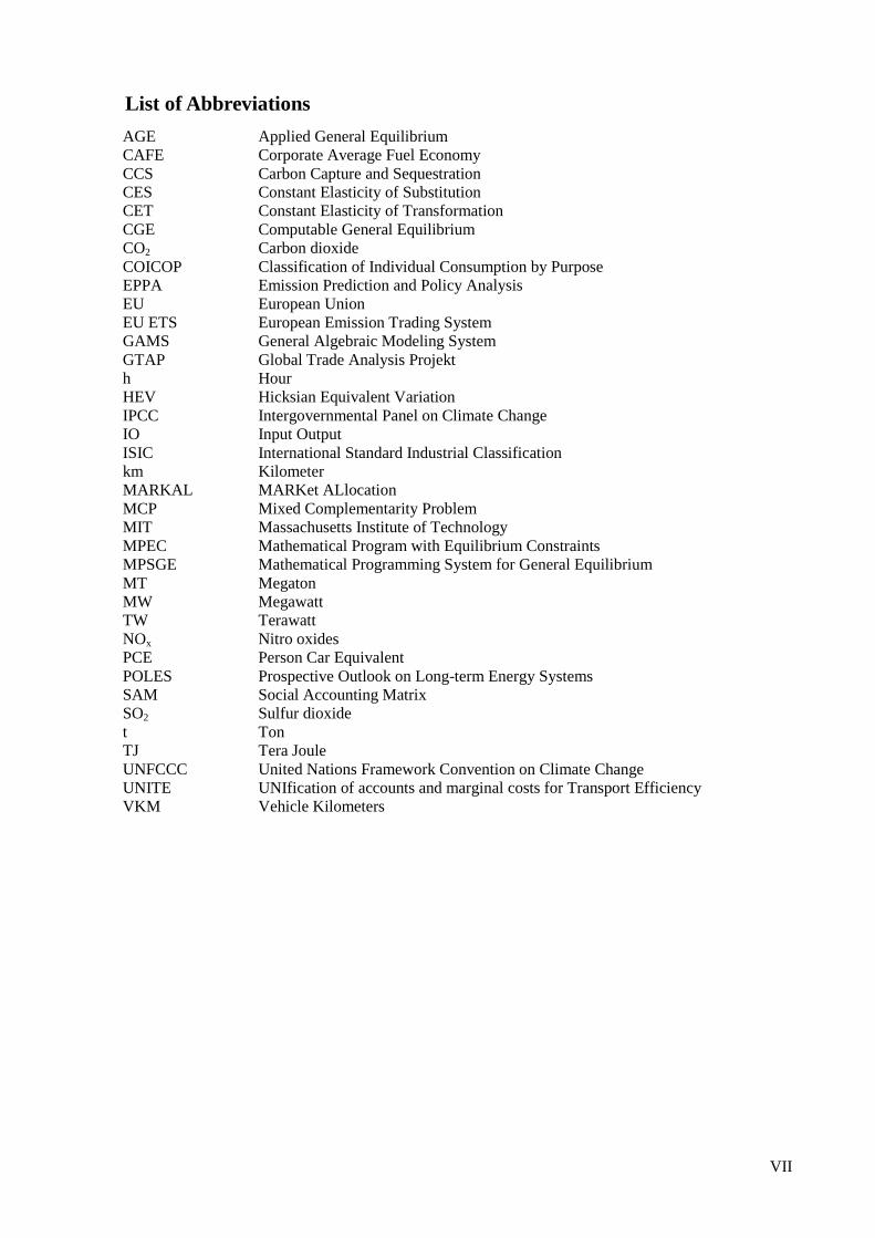
List of Abbreviations

AGE Applied General Equilibrium CAFE Corporate Average Fuel Economy CCS Carbon Capture and Sequestration CES Constant Elasticity of Substitution CET Constant Elasticity of Transformation CGE Computable General Equilibrium CO2 Carbon dioxide COICOP Classification of Individual Consumption by Purpose EPPA Emission Prediction and Policy Analysis EU European Union EU ETS European Emission Trading System GAMS General Algebraic Modeling System GTAP Global Trade Analysis Projekt h Hour HEV Hicksian Equivalent Variation IPCC Intergovernmental Panel on Climate Change IO Input Output ISIC International Standard Industrial Classification km Kilometer MARKAL MARKet ALlocation MCP Mixed Complementarity Problem MIT Massachusetts Institute of Technology MPEC Mathematical Program with Equilibrium Constraints MPSGE Mathematical Programming System for General Equilibrium MT Megaton MW Megawatt TW Terawatt NOx Nitro oxides PCE Person Car Equivalent POLES Prospective Outlook on Long-term Energy Systems SAM Social Accounting Matrix SO2 Sulfur dioxide t Ton TJ Tera Joule UNFCCC United Nations Framework Convention on Climate Change UNITE UNIfication of accounts and marginal costs for Transport Efficiency VKM Vehicle Kilometers

VIII

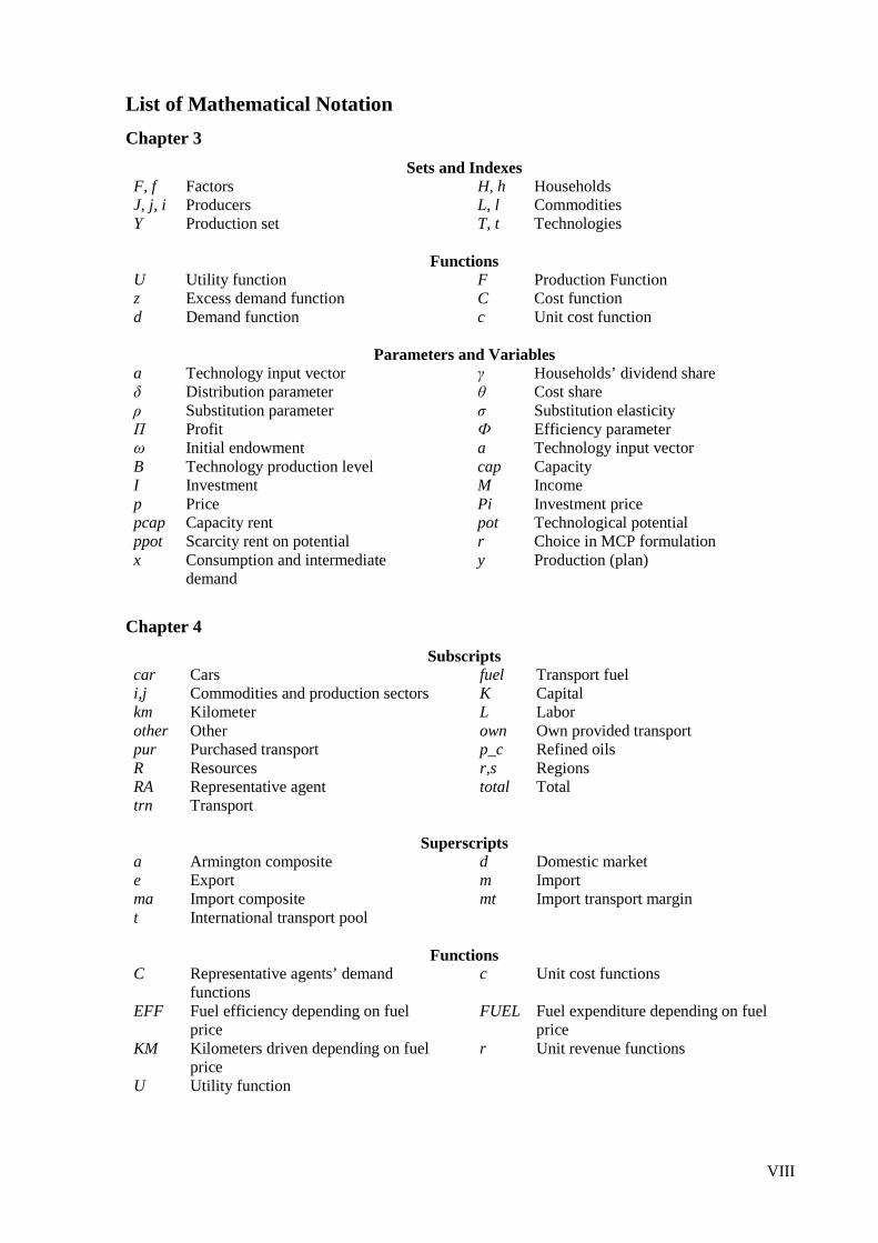
List of Mathematical Notation

Chapter 3

Sets and Indexes F, f Factors H, h Households J, j, i Producers L, l Commodities Y Production set T, t Technologies

Functions U Utility function F Production Function z Excess demand function C Cost function d Demand function c Unit cost function

Parameters and Variables a Technology input vector γ Households’ dividend share δ Distribution parameter θ Cost share ρ Substitution parameter σ Substitution elasticity Π Profit Ф Efficiency parameter ω Initial endowment a Technology input vector B Technology production level cap Capacity I Investment M Income p Price Pi Investment price pcap Capacity rent pot Technological potential ppot Scarcity rent on potential r Choice in MCP formulation x Consumption and intermediate

demand y Production (plan)

Chapter 4

Subscripts car Cars fuel Transport fuel i,j Commodities and production sectors K Capital km Kilometer L Labor other Other own Own provided transport pur Purchased transport p_c Refined oils R Resources r,s Regions RA Representative agent total Total trn Transport

Superscripts a Armington composite d Domestic market e Export m Import ma Import composite mt Import transport margin t International transport pool

Functions C Representative agents’ demand

functions c Unit cost functions

EFF Fuel efficiency depending on fuel price

FUEL Fuel expenditure depending on fuel price

KM Kilometers driven depending on fuel price

r Unit revenue functions

U Utility function

IX

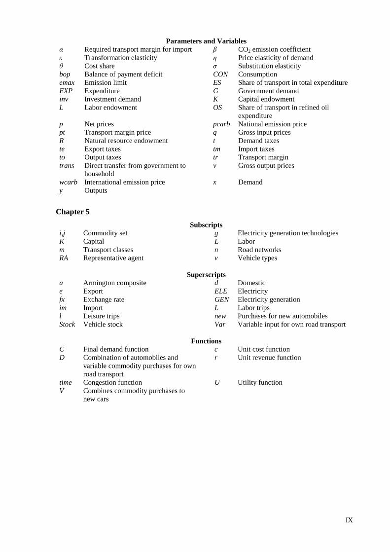
Parameters and Variables α Required transport margin for import β CO2 emission coefficient ε Transformation elasticity η Price elasticity of demand θ Cost share σ Substitution elasticity bop Balance of payment deficit CON Consumption emax Emission limit ES Share of transport in total expenditure EXP Expenditure G Government demand inv Investment demand K Capital endowment L Labor endowment OS Share of transport in refined oil

expenditure p Net prices pcarb National emission price pt Transport margin price q Gross input prices R Natural resource endowment t Demand taxes te Export taxes tm Import taxes to Output taxes tr Transport margin trans Direct transfer from government to

household v Gross output prices

wcarb International emission price x Demand y Outputs

Chapter 5

Subscripts i,j Commodity set g Electricity generation technologies K Capital L Labor m Transport classes n Road networks RA Representative agent v Vehicle types

Superscripts a Armington composite d Domestic e Export ELE Electricity fx Exchange rate GEN Electricity generation im Import L Labor trips l Leisure trips new Purchases for new automobiles Stock Vehicle stock Var Variable input for own road transport

Functions C Final demand function c Unit cost function D Combination of automobiles and

variable commodity purchases for own road transport

r Unit revenue function

time Congestion function U Utility function V Combines commodity purchases to

new cars

X

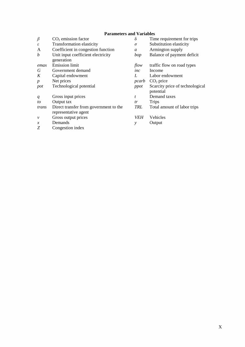
Parameters and Variables β CO2 emission factor δ Time requirement for trips ε Transformation elasticity σ Substitution elasticity A Coefficient in congestion function a Armington supply b Unit input coefficient electricity

generation bop Balance of payment deficit

emax Emission limit flow traffic flow on road types G Government demand inc Income K Capital endowment L Labor endowment p Net prices pcarb CO2 price pot Technological potential ppot Scarcity price of technological

potential q Gross input prices t Demand taxes to Output tax tr Trips trans Direct transfer from government to the

representative agent TRL Total amount of labor trips

v Gross output prices VEH Vehicles x Demands y Output Z Congestion index

1 Introduction

Global warming has become one of the most serious environmental problems for current and future

generations. In consequence, countries agreed to stabilize “…greenhouse gas concentrations in the

atmosphere at a level that would prevent dangerous anthropogenic interference with the climate

system” (UNFCCC, 1992, Art. 2) and signed the United Nations Framework Convention on Climate

Change (UNFCCC) in Rio de Janeiro in 1992. Following this agreement, industrial countries

implemented the Kyoto Protocol in 1997 and agreed to reduce greenhouse gas emissions by an

average of 5.2% as compared to 1990 within the period 2008-2012 (UNFCCC, 1998).

The main greenhouse gas is carbon dioxide (CO2) which is mainly produced by the combustion of

fossil fuels in the electricity and transport sectors. In 2007, energy industries were responsible for 32%

of the total emissions in the European Union (EU), followed by the transport sector emitting 19.5%

(Eurostat, 2009a). With more than 90% road transport is the main polluter in the transport sector

followed by aviation (ECMT, 2007).

In the line of the Kyoto Protocol, the EU started regulating CO2 emissions of electricity generation,

energy-intensive production, and refineries implementing the world largest emission trading system in

2005 (EC, 2003). The European Emission Trading System (EU ETS) is a classical cap and trade

system setting an upper bound on total emissions and allowing the trade of emission allowances. The

design of the EU ETS allows including further sectors and greenhouse gases in the future

development. Aviation will be included into the EU ETS from 2012 onwards (EC, 2008a). In contrast,

concerning private road transport the EU has released mandatory carbon efficiency standards for new

cars from 2012 onwards (EC, 2009c).

From an economic point of view, mandatory standards are suboptimal since they do not allow equal

marginal abatement cost of carbon across the economy, i.e. do not implement carbon reduction at

lowest cost. Thus, the central question of this thesis is whether the inclusion of road transport into the

EU ETS lowers the cost of carbon regulation in Europe. The question is numerically analyzed using

two different computable general equilibrium (CGE) models.

The remainder of this thesis is structured as follows: Chapter 2 provides the theoretical background of

carbon regulation in a first and second-best setting and under environmental tax reform concerns.

Furthermore, the complications of regulating road transport, namely multiple externalities of different

dimensions and the large number of polluters, are analyzed and possible strategies of carbon

regulations are derived. This chapter also provides the basic arguments in favor and against the

inclusion of road transport into the EU ETS. Chapter 3 provides the methodological background of

computable general equilibrium modeling. Special emphasis lies on the integration of technological

details into the CGE modeling framework. Furthermore, a review of the environmental-energy and

transport related CGE literature is given. Chapter 4 employs a multi-region CGE with a detailed

representation of the EU 27 countries analyzing the effects of transport under the EU ETS, a European

fuel tax increase, and the total exemption of transport from carbon regulation. The results indicate that

the most preferable strategy is exempting transport from regulation. The analysis in this chapter is

2

unique in the sense that the question is investigated on a detailed European member state level.

Chapter 5 presents a small open economy model with a detailed representation of electricity

generation technologies and private transport. Against the background that congestion is the most

important externality of transport, different time periods and road types are introduced to include the

impact of travel flow changes. Again, the results show that exempting transport from carbon

regulation is favorable to its inclusion into emission trading or increases in fuel taxes. Moreover, using

the income of carbon regulation to increase subsidies on public transport shows large positive effects

in two directions: the cost of carbon regulation decrease and the congestion externality is partly

decreased. The analysis in this chapter is unique in bringing together a detailed representation of

electricity generation and private transport. Moreover, the details of the private transport

representation including different road types based on empirical data have not been investigated for

Germany, yet. Chapter 6 summarizes the results, concludes, and suggests future research topics.

3

2 Regulation of Road Transport Carbon Emissions

This section analyzes approaches on how to regulate carbon emissions with a focus on the transport

sector. First, the theory of environmental regulation in a first and second-best setting and the effects of

environmental tax reforms are examined. Second, the special needs of regulation in road transport are

reviewed and different approaches to carbon emission regulation of road transport are analyzed.

2.1 Regulating externalities

2.1.1 Regulation in a first-best world

Internalization of external effects requires choosing an appropriate target level of the externality and

an adequate regulation instrument. Having implemented the instrument, it needs to be enforced and

monitored.

Theoretically, the optimal target level equates the marginal external cost to the marginally benefit (see

e.g. Baumol and Oates 1988). In the case of greenhouse gas regulation, the target level in terms of

emissions for a certain time period is predetermined by international climate agreements: The Kyoto

Protocol commits participating countries to reduce average yearly emissions for the period from 2008

to 2012 by a certain percentage as compared to the emission level of the year 1990. Accordingly, the

EU15 has to mitigate CO2 emissions by 8 %. In consequence, the EU has released the Burden Sharing

(EC, 2002) and more recently the Effort Sharing Agreement (EC, 2009a) which regulate the member

states’ mitigation requirements in a way to reach the overall European target. Therefore, the target

level of emissions is taken as given in the following analysis.1

A variety of policy instruments for the regulation of GHG exist. These can be classified into three

main categories: public spending, market-based instruments, and command and control policies.2 The

performance of instruments is compared in terms of costs and environmental effectiveness, dynamic

efficiency, implementation and monitoring costs, and political feasibility. Cost efficiency is given (i.e.

the environmental target is reached at lowest costs) if the marginal abatement costs equalize across

pollution sources (see e.g. Perman et al., 2003). Environmental effectiveness measures the distance

between the target pollution level and the level induced by the instruments. Dynamic efficiency

evaluates the incentives to invest in research, development, and adaptation of new technologies.3

1 In 2009 the EU committed to reduce emission by 20% below the 1990 level in the period 2012 to 2020 (EC, 2009b). While the burden sharing relates to t EU 15 countries, the new reduction commitment and the effort sharing agreement also includes new member states, i.e. relates to EU 27. In the case that the negotiations for a post-Kyoto climate agreement will be successful, the EU announced to reduce 30 % of its emission in this period. 2 Additionally, there exist informational policies like e.g. energy efficiency labelling or educational programs. Since the effectiveness of such measures can hardly be controlled, they should be seen as important additional policies to overcome transaction costs in the form of information costs on the final demand side. 3 A general statement about the dynamic efficiency of different instruments is not possible. Downing and White (1986) show that the innovation incentives are independent from governments’ reaction to adaptation of new technologies. However, adaptation depends on the reaction of other market participants, i.e. if they also adapt the technology. The study of Downing and White (1986) only examines the adaptation stage of technological progress. In subsequent analysis the problem is examined in terms of game theoretic analysis and considerations about research and development. Jaffe et al. (2002a, b) provide a survey.

4

Public spending policies could take place in the form of direct mitigation actions of the government or

in the form of subsidies. In the case of GHG, direct mitigation actions hardly exist. Subsidies can take

place in production or final demand sectors. A prominent example on the production side is the

support of electricity generation technologies from renewable energy sources (EC, 2008b); subsidies

for environmental friendly public transport are a demand side example. The fundamental problem of

public spending policies is the refinancing issue since the increase in the spending has to be rebalanced

by additional taxes.

Command and control policies are obligations which are introduced in the production process.

Possible measures are to constrain the upper emission level of every production site or firm, to dictate

technologies which may be used, or to put quotas on input commodities. These policies generally can

be shown to be highly ecologically efficient but lack cost effectiveness.

Economists favor the use of market-based instruments. Two classes exist: Pigouvian taxes (Pigou,

1920) and tradable permits (Dales, 1968). Pigouvian taxes implement taxes on polluting commodities

equal to the social marginal cost. The idea of tradable permits builds on the work of Coase (1960) who

noted that externalities are caused by lacking property rights. Consequently, property rights are

established by allocating pollution rights (i.e. the permits) to agents and allowing the trade of these

rights. Mitigation of pollution is achieved by either allocating only a limited number of permits, i.e.

setting an upper bound on pollution, or by open market policy, i.e. governments buy permits on the

market and hence avoid pollution. Both instruments are cost efficient in the sense of equating marginal

abatement costs across polluters (Montgomery, 1972). If the social marginal costs are correctly

estimated and the overall pollution target is optimally determined, the permit price will be equal to the

Pigouvian tax and both instruments achieve the same environmental target. However, under a given

target level of pollution, as is the case for GHG, the Pigouvian tax requires estimating the correct tax

rate in order to implement the imposed environmental target. Therefore, the aggregated marginal cost

curve needs to be determined. Thus, Cropper and Oates (1992) see the major advantage of an emission

trading system in gaining direct control over the emission quantity.

However, tradable rights systems raise the question of the initial allocation of permits. Two extreme

possibilities exist: The government can use grandfathering, i.e. allocate permits to installations for

free, or sell or auction permits. Montgomery (1972) proves that the initial distribution of permits does

not affect post-trading allocation and efficiency of the instrument. However, economists favor

auctioning of permits for at least two reasons. First, auctioning permits implements the polluter-pays

principle, i.e. polluting firms have to pay for emissions. Second, auctioning reveals a permit price at

the beginning of the trading scheme which improves liquidity of the permit market. Nevertheless,

grandfathering is an important option especially in the first establishment of trading schemes since this

improves the political acceptance of the system (Tietenberg, 2006).

5

2.1.2 Regulation in a second-best world

The basic theory of environmental regulation as described in the last section builds on a first-best

framework which is characterized by the absence of other distortions. Obviously, this assumption is

unrealistic since economies are full of distortions mainly due to governments’ needs to finance the

provision of public goods and non-convexities in the form of imperfect competition (Hahn, 1984;

Liski and Montero, 2008). The theory of second-best states that if one set of efficiency conditions is

violated, it is not necessarily optimal to achieve the remaining ones (Lipsey and Lancaster, 1956).

Thus, deviation from the basic assumptions may lead to optimal carbon taxes which are no longer

uniform across the economy, i.e. deviation from the Pigouvian tax.4

Generally, governments need to raise taxes in order to finance the provision of public goods. As long

as taxes do not correct for market failures, they are necessarily distortionary in the sense that raising

one dollar of public revenues causes a loss in welfare greater than one dollar. The cost of raising one

additional unit of government revenues is known as the marginal cost of public fund consisting of the

direct tax burden plus the associated welfare cost by distorting prices in the economy (Browning,

1976). The direct burden is the cost of raising one unit of revenue. The excess welfare costs are

referred to as excess burden of taxation. The theory of optimal taxation analyzes the optimal tax

structure under the need of raising public revenues by imposing taxes, i.e. in the absence of non-

distortionary lump-sum taxation (see Auerbach and Hines, 2002 for a survey). In a world without

externalities, optimal indirect taxes on commodity consumption rates are characterized by the Ramsey

or inverse elasticity rule: the more inelastic the commodity demand, the higher will be the tax rate

(Ramsey, 1927; Boiteaux, 1956). Furthermore, Diamond and Mirrlees (1971 a,b) show that taxes on

intermediate inputs are non-optimal as long as production exhibits constant returns to scale.

The presence of externalities alters these results. Sandamo (1975) shows that in the presence of

externalities optimal tax rates are the weighted average of the optimal tax and the Pigouvian tax rate.

The optimal tax schedule exhibits a property known as additivity property: in the presence of

externalities the optimal commodity tax rate in final consumption is the weighted average of the

optimal Ramsey tax and the Pigou tax equal to the marginal social cost caused by the consumption of

the commodity. Weights depend on the government’s budget need. In the case where corrective

taxation is able to fully finance the budget, the Ramsey component of the optimal tax becomes zero.

With increasing revenue raising requirement, the Ramsey tax component becomes more and more

important and the Pigou tax term vanishes. Bovenberg and van der Ploeg (1994) extend the result for

the more general case of interdependent demand functions and endogenous labor supply decisions.

Sandamo (1993) addresses distributional concerns considering consumers who differ in their

preferences and income and shows that weighted average property of optimal taxes still holds.

However, distributional considerations additionally influence the weighting factors: If the share of

high income consumers’ consumption for a commodity is high, the Ramsey tax component increases.

4 In the ongoing, Pigouvian taxes are discussed. Due to the inverse relation of environmental taxes and tradable rights schemes differentiated taxes offer arguments for exemptions of sectors from carbon regulation or rebate systems.

6

Similarly, if a high valuation of environmental quality is concentrated among high income consumers,

the Pigouvian tax component tends to be higher.

Bovenberg and Goulder (1996) show that in the presence of externalities it is also optimal to tax dirty

intermediate commodities at the Pigouvian tax rate corrected for the marginal cost of public fund, i.e.

with increasing excess burden of taxation the dirty intermediate input tax vanishes.

2.1.3 Environmental tax reforms

The optimal taxation approach faces two main criticisms: First, it assumes the existence of a welfare

function which generally does not exist (Arrow, 1950). Second, it assumes that policy makers newly

design tax systems. However, generally they do not create new tax systems but are confronted with

altering existing schemes, i.e. with tax reforms Feldstein (1976). In the light of environmental

regulation, governments impose environmental regulation on top of a pre-existing tax schedule. This

raises two questions: First, if environmental regulation raises revenues, how to spend the income

optimally? Second, what are the interactions of pre-existing taxes and the additional corrective tax

measures? Consequently, the occurring effects are known as revenue recycling and tax interaction or

intermediate effect (Parry, 1995; Goulder, 1995).

Generally, the revenue recycling effect is analyzed under the assumption that the provision of public

goods is constant in order to separate the question of environmental regulation from the topic of the

optimal size and composition of public spending.5 The double dividend hypothesis states that using the

additional government income to lower pre-existing distortionary taxation provides an additional

welfare gain beside the improvement of environmental quality (Pearce, 1991). Consequently, the gross

costs of environmental regulation, which are defined as the welfare loss of regulation without the

benefit of improved environmental quality, decrease. In order to maximize the double dividend the

lowered tax should be preferably broad based. Accordingly, the literature most often considers cutting

labor taxes. As a consequence, the double dividend hypothesis is often stated in terms of

unemployment: using the income of environmental regulation lowering existing labor taxes stipulates

labor demand and subsequently reduces involuntary unemployment (e.g. Bovenberg and de Mooij,

1994; Bovenberg, 1999). A survey of empirical evidences on the double dividend hypothesis is given

by Galeotti and Carraro (1996) and Bosquet (2000) which show that it holds in the short and medium

term but is uncertain in the long run.

Tax interaction has two direct aspects. First, raising the price of a commodity by environmental

taxation reduces commodity demand as long as the commodity is a normal good. This happens

naturally, since the aim of environmental regulation is to reduce the social cost associated with

commodity consumption. If the commodity is already taxed, a loss in the income of the pre-existing

tax results. This is known as tax base erosion effect. The tax base erosion effect counteracts the

5 Bovenberg and van der Ploeg (1994) investigate both issues in a single framework.

7

revenue recycling effect since it lowers tax income and, accordingly, the amount to be recycled in a

welfare enhancing way.

Environmental taxes also directly interact with the pre-existing tax schedule. For illustrative purpose,

assume that the regulator imposes an economy wide tax on carbon at the marginal rate of social cost

and abstract from the marginal cost of public fund. If the pre-existing tax scheme is optimal in the

sense that all commodities are taxed at their Ramsey tax rate in final consumption and intermediate

inputs are untaxed, the uniform carbon tax rate will be optimal since it implements an additional Pigou

tax term equal for all consumers and sectors. Now assume that the initial tax schedule is non-optimal,

for concreteness, taxes on final consumption are above the Ramsey tax. Imposing the uniform carbon

tax raises input prices of all sectors and consumers by the same amount. Consequently, taxes on final

consumption are also too high after the introduction of carbon regulation. By lowering the carbon tax

on final consumption the regulator can reduce the cost of carbon regulation since the after-regulation

tax schedule is closer to the optimal tax scheme, i.e. the distortionary effect of taxation is reduced. The

essential point is that a tax rate above the Ramsey tax already implies corrective taxation of the

externality. Consequently, the reduction of the carbon tax in final consumption leads to effective

carbon tax rates effectively closer to uniform across the economy.

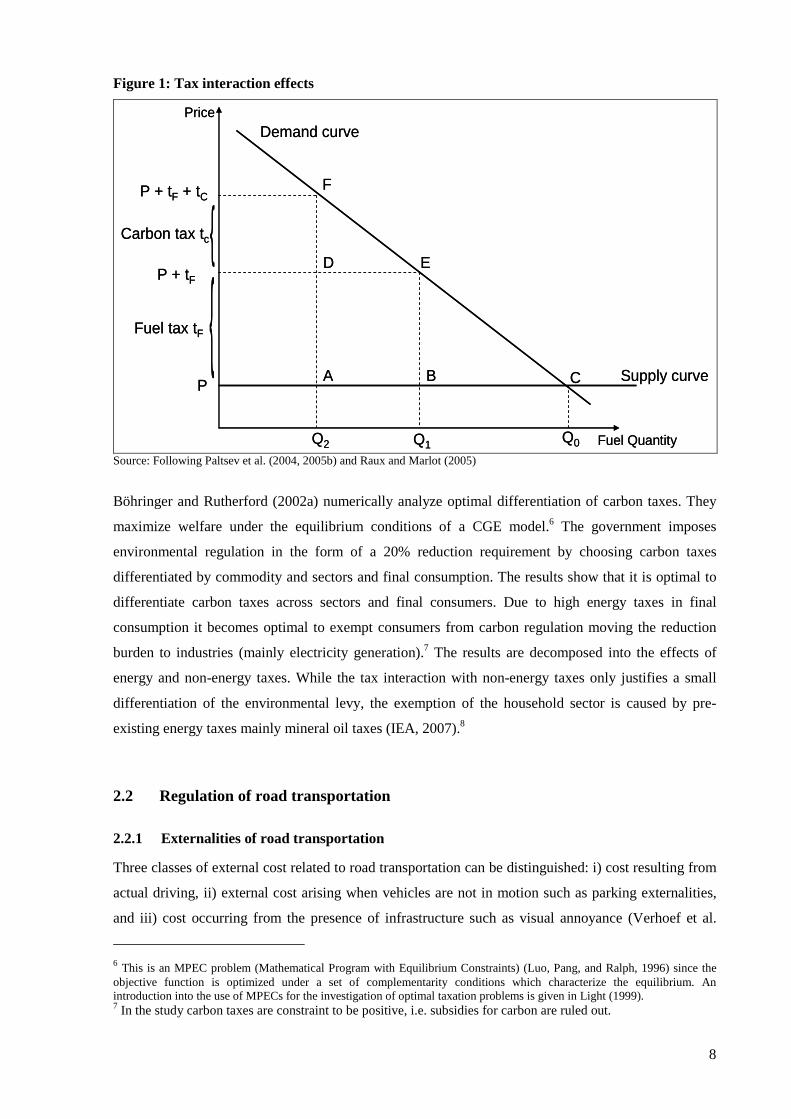
Figure 1 illustrates the tax interaction effect. The demand curve is given by the straight line FC.

Supply is assumed to be price inelastic and is given by the line AC. The welfare costs of tax

introduction are the area under the demand function net of production costs. Accordingly, the

introduction of a fuel tax tF is associated with welfare costs equal to the triangle BCE. Adding the

carbon tax tC results in an additional welfare loss equal to the triangle DEF and the rectangle ABDE.

The triangle DEF is equal to the area under the marginal abatement cost curve for carbon. On the one

hand, the rectangle ABDE represents the tax base erosion effect as the loss income of taxation. On the

other, it also represents the loss in consumer surplus due to the pre-existing fuel tax.

A lower carbon tax on some commodities translates into (partial) exemption in emission trading

schemes. In contrast to Pigou taxes, trading schemes set an upper bound on total quantity of emissions.

Accordingly, the question about which sector should carry the additional abatement burden resulting

from the exemption arises. Theoretical results on this issue do not exist.

8

Figure 1: Tax interaction effects

Fuel Quantity

P + tF

P

{Fuel tax tF

Price

P + tF + tC

Q2

BA C

D

{Carbon tax tc

E

F

Demand curve

Supply curve

Q1 Q0 Fuel Quantity

P + tF

P

{Fuel tax tF

Price

P + tF + tC

Q2

BA C

D

{Carbon tax tc

E

F

Demand curve

Supply curve

Q1 Q0

Source: Following Paltsev et al. (2004, 2005b) and Raux and Marlot (2005)

Böhringer and Rutherford (2002a) numerically analyze optimal differentiation of carbon taxes. They

maximize welfare under the equilibrium conditions of a CGE model.6 The government imposes

environmental regulation in the form of a 20% reduction requirement by choosing carbon taxes

differentiated by commodity and sectors and final consumption. The results show that it is optimal to

differentiate carbon taxes across sectors and final consumers. Due to high energy taxes in final

consumption it becomes optimal to exempt consumers from carbon regulation moving the reduction

burden to industries (mainly electricity generation).7 The results are decomposed into the effects of

energy and non-energy taxes. While the tax interaction with non-energy taxes only justifies a small

differentiation of the environmental levy, the exemption of the household sector is caused by pre-

existing energy taxes mainly mineral oil taxes (IEA, 2007).8

2.2 Regulation of road transportation

2.2.1 Externalities of road transportation

Three classes of external cost related to road transportation can be distinguished: i) cost resulting from

actual driving, ii) external cost arising when vehicles are not in motion such as parking externalities,

and iii) cost occurring from the presence of infrastructure such as visual annoyance (Verhoef et al.

6 This is an MPEC problem (Mathematical Program with Equilibrium Constraints) (Luo, Pang, and Ralph, 1996) since the objective function is optimized under a set of complementarity conditions which characterize the equilibrium. An introduction into the use of MPECs for the investigation of optimal taxation problems is given in Light (1999). 7 In the study carbon taxes are constraint to be positive, i.e. subsidies for carbon are ruled out.

9

1997). In the ongoing, I concentrate on the first category. External cost of actual driving are further

subdivided into intrasectional cost that road users impose on each other and social cost which are

imposed on the rest of the society (Mayeres et al., 1996).

Social cost come in two different forms: pollution damages and noise (Bickel et al., 2005).9,10

Pollution cost can occur either on a local or on a global level. On a local level pollutants like carbon

monoxide, nitro oxides (NOx), volatile organic compounds, particulate matter, sulfur dioxide (SO2),

polycyclic aromatic hydrocarbon, and heavy metals cause health damages in the form of mortality or

morbidity and environmental damages in the form of negative bio-system impacts (Bickel and

Friedrich, 2005).11 On a global level, pollutants add to global warming. Most important in this class

are carbon dioxide emissions. However, nitrogen dioxide and troposphere ozone also exhibit a positive

radiative forcing effect. Furthermore, SO2 and NOx lead to the creation of aerosols that have a negative

impact on the Earth’s energy balance (IPPC, 2007).12

Intrasectional external costs are congestion effects and increases in private resource cost. Congestion

occurs since average speed is negatively related to the traffic flow (measured in personal car

equivalent per hour; PCE/h). Consequently, each additional road vehicles increase the time cost of

traffic users since the travel flow raises (e.g. Walters, 1961; Vickery, 1963). Furthermore, monetary

vehicle operating costs per kilometer depend on the speed level (Mayeres, 1993). Since users only care

about their own cost and not about the effect on the speed-flow relationship, congestion implies

external cost.

Marginal accident costs relate to both classes, intersectional and social. Additional vehicles raise the

likelihood of medical and material cost (Button, 1990). Link (2005) subdivides external accident costs

into production loss due to accidents, the cost of medical treatment and rehabilitation if provided by

the public health system, cost of associated police and rescue services not covered by transport users,

and public material damage as not covered by insurances. Accordingly, the precise definition of the

external accident cost varies between countries depending on the insurance system, especially

regarding the payment of medical services.

Table 1 depicts the dependency of different externalities on trip characteristics. Even though it only

includes qualitative rankings it will prove useful in the discussion of regulation approaches.

8 The authors also analyzed other motive of carbon tax differentiation. Other arguments of differentiation come in form of carbon leakage (Hoel, 1996) and terms-of-trade effects (Krutilla, 1991) 9 Noise is sometime also regarded as intrasectional externality in the form of annoyance of other traffic participants. Additionally, in the case of heavy vehicles, social cost in the form of road damage occur which cause road repair and increased vehicle operating cost of other traffic participants (Newbery, 1988). 10 Parry et al. (2007) also mention the external cost of oil dependency in the form of military and geo-political cost imposed on the society and the vulnerability to oil price volatility and market power in the oil market. 11 For a detailed description of the impacts of the single pollutants see Bickel and Friedrich (2005, Table 1.1 p. 3). Most pollutants have a direct effect. However, NOx and VOC also have secondary effects in increasing troposphere ozone concentration. The oxidation products of SO2 lead to the acid rain problem. 12 While the level of scientific understanding of radiative of carbon dioxide is high, the role of ozone and aerosols is still at medium and low level respectively. For an assessment of the level of scientific understanding and radiative impacts see IPPC (2007, pp. 32 ff.).

10

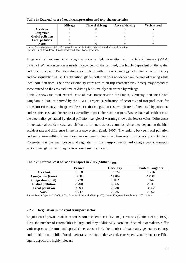
Table 1: External cost of road transportation and trip characteristics

Mileage Time of driving Area of driving Vehicle used Accidents + 0 0 -

Congestion + + + - Global pollution + - - + Local pollution + - 0 +

Noise + 0 + + Source: Verhoefen et al. (1995, 1997) extended by the distinction between global and local pollution. Legend: + high dependence, 0 moderate dependence, - low dependence.

In general, all external cost categories show a high correlation with vehicle kilometers (VKM)

travelled. While congestion is nearly independent of the car used, it is highly dependent on the spatial

and time dimension. Pollution strongly correlates with the car technology determining fuel efficiency

and consequently fuel use. By definition, global pollution does not depend on the area of driving while

local pollution does. The noise externality correlates to all trip characteristics. Safety may depend to

some extend on the area and time of driving but is mainly determined by mileage.

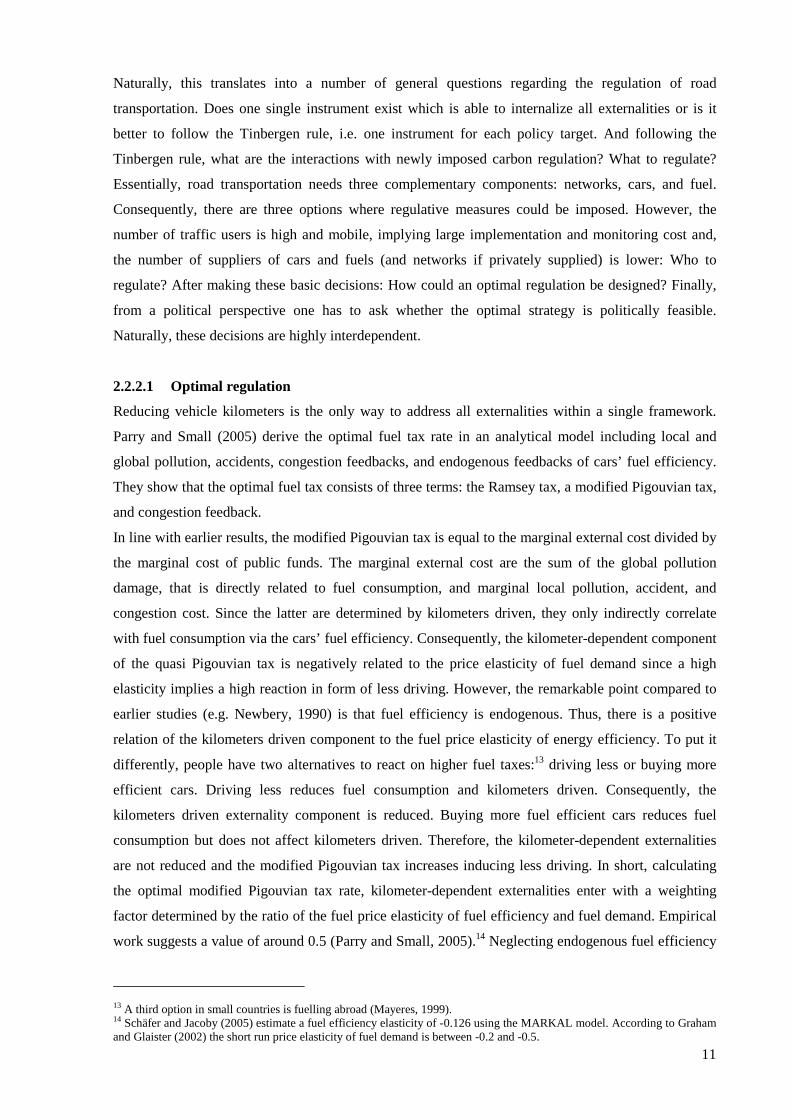
Table 2 shows the total external cost of road transportation for France, Germany, and the United

Kingdom in 2005 as derived by the UNITE Project (UNIfication of accounts and marginal costs for

Transport Efficiency). The general lesson is that congestion cost, which are differentiated by pure time

and resource cost, are the greatest externality imposed by road transport. Beside external accident cost,

the externality generated by global pollution, i.e. global warming shows the lowest value. Differences

in the external accident costs are difficult to compare across countries, since they depend on the high

accident rate and difference in the insurance system (Link, 2005). The ranking between local pollution

and noise externalities is non-homogenous among countries. However, the general point is clear:

Congestions is the main concern of regulation in the transport sector. Adopting a partial transport

sector view, global warming motives are of minor concern.

Table 2: External cost of road transport in 2005 [Million €1998]

France Germany United Kingdom Accident 1 818 17 324 1 716

Congestion (time) 18 803 20 484 23 981 Congestion (fuel) 1 778 1 102 264 Global pollution 2 700 4 555 2 741 Local pollution 9 394 7 030 3 952

Noise 4 747 7 825 7 592 Source: France: Jeger et al. (2001, p. 53); Germany: Link et al. (2001, p. 157); United Kingdom: Tweddel et al. (2001, p. 92)

2.2.2 Regulation in the road transport sector

Regulation of private road transport is complicated due to five major reasons (Verhoef et al., 1997):

First, the number of externalities is large and they additionally correlate. Second, externalities differ

with respect to the time and spatial dimensions. Third, the number of externality generators is large

and, in addition, mobile. Fourth, generally demand is derive and, consequently, quite inelastic Fifth,

equity aspects are highly relevant.

11

Naturally, this translates into a number of general questions regarding the regulation of road

transportation. Does one single instrument exist which is able to internalize all externalities or is it

better to follow the Tinbergen rule, i.e. one instrument for each policy target. And following the

Tinbergen rule, what are the interactions with newly imposed carbon regulation? What to regulate?

Essentially, road transportation needs three complementary components: networks, cars, and fuel.

Consequently, there are three options where regulative measures could be imposed. However, the

number of traffic users is high and mobile, implying large implementation and monitoring cost and,

the number of suppliers of cars and fuels (and networks if privately supplied) is lower: Who to

regulate? After making these basic decisions: How could an optimal regulation be designed? Finally,

from a political perspective one has to ask whether the optimal strategy is politically feasible.

Naturally, these decisions are highly interdependent.

2.2.2.1 Optimal regulation

Reducing vehicle kilometers is the only way to address all externalities within a single framework.

Parry and Small (2005) derive the optimal fuel tax rate in an analytical model including local and

global pollution, accidents, congestion feedbacks, and endogenous feedbacks of cars’ fuel efficiency.

They show that the optimal fuel tax consists of three terms: the Ramsey tax, a modified Pigouvian tax,

and congestion feedback.

In line with earlier results, the modified Pigouvian tax is equal to the marginal external cost divided by

the marginal cost of public funds. The marginal external cost are the sum of the global pollution

damage, that is directly related to fuel consumption, and marginal local pollution, accident, and

congestion cost. Since the latter are determined by kilometers driven, they only indirectly correlate

with fuel consumption via the cars’ fuel efficiency. Consequently, the kilometer-dependent component

of the quasi Pigouvian tax is negatively related to the price elasticity of fuel demand since a high

elasticity implies a high reaction in form of less driving. However, the remarkable point compared to

earlier studies (e.g. Newbery, 1990) is that fuel efficiency is endogenous. Thus, there is a positive

relation of the kilometers driven component to the fuel price elasticity of energy efficiency. To put it

differently, people have two alternatives to react on higher fuel taxes:13 driving less or buying more

efficient cars. Driving less reduces fuel consumption and kilometers driven. Consequently, the

kilometers driven externality component is reduced. Buying more fuel efficient cars reduces fuel

consumption but does not affect kilometers driven. Therefore, the kilometer-dependent externalities

are not reduced and the modified Pigouvian tax increases inducing less driving. In short, calculating

the optimal modified Pigouvian tax rate, kilometer-dependent externalities enter with a weighting

factor determined by the ratio of the fuel price elasticity of fuel efficiency and fuel demand. Empirical

work suggests a value of around 0.5 (Parry and Small, 2005).14 Neglecting endogenous fuel efficiency

13 A third option in small countries is fuelling abroad (Mayeres, 1999). 14 Schäfer and Jacoby (2005) estimate a fuel efficiency elasticity of -0.126 using the MARKAL model. According to Graham and Glaister (2002) the short run price elasticity of fuel demand is between -0.2 and -0.5.

12

implicitly assumes that both elasticities are equal resulting in a ratio of one. Consequently the

modified Pigouvian tax rate is overestimated.

The congestion feedback term in Parry and Small (2005) increases the optimal fuel tax since labor

supply is endogenous and taxed. Transport is modeled as a consumption commodity. Reduced

congestion lowers the price of transportation relative to leisure. Consequently, people substitute

transportation for leisure which is welfare improving since labor is taxed (also see Parry and Bento

2001).

Calibrating the model to the US and the UK, Parry and Small (2005) show that gasoline taxes in the

US should be increased while in the UK taxes are more than twice as high than the optimal tax. A

single fuel tax has the problem that kilometer-dependent externalities are only indirectly included via

fuel efficiency. Furthermore, fuel taxes do not change the pattern of driving time and location.

In contrast, imposing road pricing measures allows addressing the spatial and time dimension of

externalities but only indirectly addresses fuel efficiency of cars (Newberry, 2004). Thus, it is more

promising to regulate single externalities with different instruments and accounting for interactions.

For congestion the possibility of road pricing schemes, kilometer-dependent taxes, or infrastructure

policy exist. Such instruments also address other kilometer-dependent externalities. Emissions of cars

can be regulated by technology standards, fuel quality regulation, or fuel taxation. Newberry (2004)

calculates the optimal tax rates on fuels and equivalent road user charges for the United Kingdom.

Policy options to reduce carbon emissions including taxes of private transport are discussed in the next

section.

2.2.2.2 Options to regulate carbon emissions in the transport sector

Three main options to reduce carbon emissions of private cars are considered: regulating fuel

composition, fuel efficiency regulation of cars, and increasing fuel taxes. Further options that require

different regulation approaches are changing driving behavior and imposing speed limits.

Furthermore, subsidies on public transport can reduce private road transport by inducing transport

mode switches altering relative prices.

2.2.2.2.1 Fuel composition regulation and fuel switching

In general, a regulation of the transport fuel composition cannot change the direct emissions of private

transportation since the energy value of fuels is determined by the carbon content combusted.15 One

liter of gasoline (diesel) contains 0.640 kg C/l (0.734 kg C/l) with a net calorific value of 32.44 MJ/l

(35.87 MJ/l) (US Environmental Protection Agency, 2005). Assuming 99% of carbon oxidized and

multiplying with the ratio of molar weights of CO2 and carbon (~44/12) yields average CO2 emission

of 2.30 kg CO2/l (gasoline) and 2.66 kg CO2/l (diesel).

15 To be more precise: the energy content is determined by the carbon content and its oxidation state. However, changing the oxidation state would require a different composition of hydrocarbons which is not possible without altering combustion technologies (e.g. Archer, 2007).

13

The only way of to reduce total carbon emissions per liter combusted fuel is blending with biofuels

which are regarded as carbon neutral since the carbon content is absorbed from the atmosphere.

While biofuel blending regulation is able to reduce the net emissions of cars and, additionally, has the

advantage of reducing economies’ oil dependency, three major problems arise. First, blending is

restricted in the short run since changing the fuel composition requires adjustments in combustion

technologies, i.e. car technologies (Schallaböck et al., 2006). Second, the production of biofuels causes

interactions with food markets due to the changed use of agriculture areas and the use of food crops

for energy production. The second point may be overcome by using second generation biofuels based

on cellulose (UN, 2007). Third, increased biofuel production causes nitrogen dioxide emissions of

fertilization. Consequently including the whole lifecycle, biofuels are not carbon neutral (Crutzen et

al., 2008). Nevertheless, the EU aims to increase the biofuel share in transportation above ten percent

(EC, 2008b).

Another option on the fuel level is switching to alternative energy sources. The main opportunities are

natural gas, hydrogen, or electric cars. A problem arising for all new fuels is the dependency on a

service station network (Achtnicht et al., 2008). The problem can be addressed by using bivalent cars

and extending fuel station networks. Natural gas vehicles are already market mature while hydrogen

cars are not competitive today. Furthermore, hydrogen cars are only improving environmental quality

if the fuel is produced using renewable electricity generation, since hydrogen production is energy-

intensive (Sandoval, 2008). Electric cars are critical in terms of battery performance, limiting driving

range, and cost (Duvall, 2004). Karplus et al. (2009) show that even under very strict climate policies,

the adaptation of hybrid electric cars, that are additionally able to run on conventional fuels, requires

further research in battery design to lower costs. As in the case of hydrogen cars, carbon emission

reduction depends on electricity generation technologies.

2.2.2.2.2 Fuel efficiency regulation

Fuel efficiency improvements can be achieved by altering car design and improving combustion and

gearbox technologies. Altering car design takes place by either aerodynamic resistance improvements

for new designs or reducing the weight of automobiles. Weights can be reduced using light-weight

interiors or, more costly, using more aluminum in the autobody (Schäfer and Jacoby, 2006).

Combustion engines can be improved by various technological measures improving energy efficiency.

Schallaböck et al. (2006) estimate the technical potential to improve energy efficiency of gasoline

(diesel) cars from currently around 15% (18%) to 21% (24%) in the near term. In the long term,

further enhancements are possible to around 26% (30%). The main options are the introduction of

start-stop systems, hybrid cars, and downsizing. Start-stop systems, which stop the motor at zero speed

and start again without using the starter, are already observed on the market. Also, hybrid cars which

store dragging energy in batteries and use it for acceleration are on the market, yet. Downsizing is the

possibility to decrease fuel consumption by scaling down the cubic capacity of cars. For most cars the

most fuel efficient speed does not coincide with the average speed driven. Consequently, fuel

14

efficiency is improved by adjusting the cubic capacity such that the most fuel efficient speed coincides

with the average driving patterns. Although downsizing is regarded as one of the most promising

options to decrease fuel consumption, it conflicts with consumer preferences since the motor

performance is also scaled down.

Successfully improving fuel efficiency by regulatory measures depends on the right incentives for

technology adoption at the demand side and technology innovation at the supply side. Consequently,

the question is who and how to regulate. On the supply side, technological standards (possibility

tradable) concerning the carbon efficiency can be imposed. Besides increasing fuel prices, carbon-

dependent motor vehicle or sales taxes can be imposed on the demand side in order to alter relative

prices in favor of environmentally friendly technologies.

Recently, the EU has released mandatory carbon efficiency standards for new cars from 2012 onwards

(EC, 2009c).16 Manufactures average specific emission of newly sold cars may not exceed 130 CO2

g/km. This corresponds to an average fuel efficiency of around 5.7 l gasoline/100 km and 4.9 l

diesel/100 km. Emission targets for single cars are weight dependent, i.e. heavier cars are allowed to

emit more CO2. Elmer and Fischer (2009) show that the weight dependency of emission standards

leads to inefficiencies. Exceeding the specific emission target causes fines: 5, 15, and 25 € for the first

three excess grams, respectively, and 95 € for each additional gram.17 The directive implements

additional innovation incentives: given the use of environmental friendly innovations, manufacturers’

specific targets are reduced by up to 7 g CO2/km. The European approach allows pooling of

manufacturers, i.e. manufacturers are allowed to jointly fulfill their average specific emission targets.

Therefore, it imposes some flexibility of carbon mitigation but full flexibility using tradable permits is

not achieved.

A tradable permit approach would require specifying the unit of rights. This could be either specific

emission rights in g CO2/km or emissions over the whole lifetime cycle of the car (t CO2). The former,

has the disadvantage that trading is restricted to automobile manufacturers. The latter option, which

has been termed midstream trading, requires estimating lifetime emissions of a sold automobile. This

could be done bases on a representative driving cycle e.g. European Driving Cycle. Choosing the

lifetime emissions of cars has the advantage that it is consistent with the unit of carbon accounting in

the EU ETS. Accordingly, permit trading between automobile manufactures and EU ETS sectors can

be implemented. Albrecht (2000, 2001) proposes such an open midstream approach for the regulation

of private road transport emissions.

However, open midstream trading has some disadvantages. Generally, driving cycles are only an

approximate estimate of the real lifetime emissions which leads to uncertainties about reaching the

overall target. But such uncertainties are a general problem of fuel efficiency regulation since the ex

16 The most prominent example of fuel efficiency regulation is the US Corporate Average Fuel Economy (CAFE) program which was established in the wake of the 1973 oil crisis and imposes a 27.5 miles per gallon (~8.6 l/100 km) standard for passenger cars (e.g. Small and van Dender, 2007). 17 From 2019 onwards each excess gram will cost 95 €. The period 2008-2018 is regarded as the phase in of the regulation, which is characterized by only partly including newly sold cars (2012: 65%; 2013: 74%; 2014: 80%; 100% from 2015 onwards).

15

ante determination of carbon mitigation depends on the reactions of drivers. For example, fuel

efficiency improvements are considered to exhibit a rebound effect, i.e. an increase in kilometers

driven due to lower fuel cost, which partly offsets the carbon mitigation effect. Furthermore, increased

mileage increases other externalities like congestion and accidents (Fischer et al., 2007). A second

concern regarding open midstream trading arises from the design of the EU ETS: time inconsistency.

Currently, the EU ETS is divided into four year periods. Selling a car in one period it is unclear to

which period the required emission permits belong to due to the longer lifecycle of cars. The problem

is weakened by the extension of the EU ETS period to 8 years from 2013 onwards (EC, 2009b). A

general unsolved concern of fuel efficiency regulation at the supply side in the case that car prices

increase is the eventual delay of new car purchases due to decreased scrapping.

Additionally to the European directive, Germany has adopted CO2 dependent motor vehicle taxes

(Deutscher Bundestag, 2009). Every car initially registered after the July 1st, 2009 has to pay a yearly

tax of 2 € for every gram above 120 g CO2/km. The threshold level is decreased in 2012 (2014) to 110

(95) g CO2/km. Such an instrument additionally increases adoption incentives on the demand side.

2.2.2.2.3 Pricing transport fuels

Due to the one-to-one connection of fuel use and carbon emissions, fuel price regulation approaches

are the most direct measure to regulate carbon emissions of the private transportation sector. It is

possible to either use taxes or include emissions into the EU ETS.

Taxes can either uniformly increase or can be differentiated by fuels. The latter approach is more

sophisticated since differentiation can be oriented towards the carbon content of fuels. As a price

oriented measure, taxes hardly implement given reduction targets since future driving patterns are

uncertain (Raux, 2004). Furthermore even if the target could be reached for sure, due to the low own-

price elasticity of fuel demand, taxes have to be very high (Graham and Glaister, 2002; Sterner, 2007).

This contrasts the high consumers’ sensitivity to fuel price increases leaving political feasibility in

doubt (Raux and Marlot, 2005). Political feasibility is further restricted by equity aspects. Due to the

high share of fuel spending in low income groups, a tax on fuels is regressive (West, 2004). Fuel tax

rates across Europe are already at a high level. Sterner (2007) reports an average tax rate of 80% on

gasoline for West-Europe in 2007. The already high tax level restricts further tax increases due to the

high responsiveness of the public opinion to fuel taxes (Hammar et al., 2004).

Implementing emission trading has the advantage of reaching the carbon target for sure and allowing

equalization of marginal abatement cost, i.e. implementing cost efficiency. Beside the midstream

option, two further options exist to include road transportation into the EU ETS (e.g. Ellerman et al.,

2006; Stronzig et al., 2002): downstream and upstream trading.

In downstream trading the polluters, i.e. drivers, are obliged to hold emission allowances for every ton

of CO2 emitted. Due to the large number of polluters such a system is expected to incur high

transaction and information cost. Raux and Marlot (2005) argue that an electronic system for permit

sales and purchases can minimize transaction costs if the system is compatible with automatic teller

16

machines already existing at service stations. Information costs can be overcome by market

intermediaries like banks or service station operators. Even though the possibility of downstream

trading exists, it has never been regarded as a valid option for private transportation.

In upstream trading, the suppliers of fuels are required to hold emission allowances. For every sold

liter of fuel the resulting carbon emissions can be calculated and have to be deposited with permits.

Since the number of upstream fuel suppliers is far below the number of vehicle users, transaction costs

decrease. This argument is of particular importance for the EU ETS: Refineries are already part of the

EU ETS. Consequently, administrative costs are lowered since monitoring mechanisms already exist

and only need to be extended. Furthermore, refinery operators have experience in permit trading since

the beginning of the EU ETS in 2005. Therefore, information costs are lower, too.

Under prefect competition up- and downstream trading lead to equivalent results. Dobes (1999)

remarks that the equivalence breaks down if the fuel market is characterized by imperfect competition.

This is a serious point which has to be considered if upstream trading should be implemented.

2.3 Summary

This chapter laid out the theory of environmental regulation in a first and second-best setting and the

effects of environmental tax reforms. Both, environmental theory in a first and second-best setting,

state that it is optimal to impose Pigou taxes uniform across sectors and commodity since cost

efficiency is achieved by the equalization of marginal abatement costs. Consequently, they provide the

theoretical argument for the implementation of unrestricted emission allowances trade across the

economy. Following this argumentation, the emissions of road transport should be regulated by

integrating road transport into the EU ETS most favorably using an upstream approach. Since

refineries are already part of the EU ETS and since the number of refinery operators is far smaller than

the number of road transport users, such an approach incurs lower information, transaction, and

monitoring costs.

However, the theory of environmental tax reforms claims that the structure of the pre-existing tax

system is important. If initial taxes on some commodities are too high, lower carbon taxes or

exemption from emission trading decrease the cost of regulation since the after-regulation tax schedule

is closer to the optimal one. Observing high excise taxes on transport fuels across Europe, it can be

argued that the exemption of road transport from further carbon is optimal. On the other hand, the

existence of other externalities justifies high taxes on road transport. Congestion is the major concern

in the regulation of road transport followed by local pollution, accidents and noise. In the

consequence, the effect of an additional increase of fuel taxes crucially depends on the pre-existing

tax. If the tax is too high in the sense that it already includes a carbon tax component, a further

increase in the fuel tax will lower welfare.

17

3 Methodological Background

This chapter describes the methodological background of computable general equilibrium modeling. I

start by reviewing the basic theory of general equilibrium. Afterwards, the CGE format and its

representation as mixed complementarity problem are introduced; functional forms and empirical

specification are discussed. Finally, the inclusion of technological details is described.

3.1 Theoretical basics of applied general equilibrium models

Consider an economy with L commodities (indexed by l) which are traded at a single positive price pl.

J producers (indexed by j Є J:={1…J}) are characterized by technologies, represented by the set of

feasible production plans Yj which are part of the commodity space ℝL. The set of feasible production

plans is assumed to be strictly convex, compact and includes the possibility of inaction (0 Є Yj).18

Producers are assumed to behave profit maximizing. Furthermore, markets are assumed to be perfectly

competitive, i.e. every agent takes the price vector as given. Consequently, observing the price vector

p every producer chooses his production plan yj such that his profit is maximized and the production

plan is feasible:

( )jj j

y

j j

p max py

s.t. y Y

Π =

∈ (1)

The H households (indexed by h Є H:={1…H} ) are characterized by a utility function which

associates nonnegative consumption plans xh with utility levels Uh(xh). Utility functions are assumed to

be strictly quasiconvex, continuous, and nonsatiated.19 Each consumer receives income from two

sources: First, he is initially endowed with a positive commodity vector ωh being sold at the market

price and second, he owns nonnegative shares γhj of firm j for which he receives dividends γhjΠj.

Profits are fully distributed to households, i.e. the shares of firm j sum to one over all households.

Households are assumed to maximize utility under the constraint that consumption plans are feasible,

i.e. are within the budget set:

( )( )

hh h

x 0

h h hj jj

max U x

s.t. px p p

≥

≤ ω + γ Π∑ (2)

18 These assumptions imply a well-defined, nonempty, continuous point-valued supply function. The assumption of strict convexity can be relaxed to weak convexity. However, the supply function generally becomes set-valued, i.e. results in a supply correspondence (e.g. Starr, 1997). 19 These assumptions ensure that the associated demand functions are homogeneous of degree zero in prices and single valued. As in the production case, relaxing the strict quasiconvexity assumption leads to a demand correspondence (e.g. Mas-Colell, Whinston, and Green, 1995).

18

A general competitive equilibrium is then defined as production plans yj* and consumption plans xh

*

and a price vector p* such that given the equilibrium price vector the programs (1) and (2) are fulfilled.

Furthermore, markets are either cleared or in excess supply:

* *j h h

j h h

y x+ ω ≥∑ ∑ ∑ (3)

Equation (3) is commonly referred to as market clearing or material balance equation. It relates to the

concept of the excess demand function, which is defined as:

( ) h j hh j h

z p : x y= − − ω∑ ∑ ∑ (4)

Under the above formulated assumptions, the excess demand function is a continuous, single valued

function of prices. Furthermore, it is homogenous of degree zero in prices. Thus, the absolute value of

prices does not affect outcomes. Therefore, it is possible to normalize prices by choosing a numéraire

commodity for which the price is fixed to some arbitrary number (normally one). In addition, strict

Walras’ law holds, i.e. the value of excess demand is equal to zero:

( )p z p 0⋅ = (5)

As long as the assumption of satiated preferences is satisfied, the first fundamental theorem of welfare

economics holds which states that every equilibrium is Pareto efficient.

The existence of the equilibrium under the given assumption has been proven by Arrow and Debreu

(1954). Consequently, the described model format is often denoted as Arrow-Debreu format.

Alternative names are Walras’ or competitive general equilibrium model. An extensive discussion of

the underlying assumptions and the existence proof is given in Debreu (1959) and Arrow and Hahn

(1971).

3.2 Computable general equilibrium modeling

From a policy analysis point of view, the described economy is seen as a controlled system (Munk,

2009). Decision makers – generally governments – impose policies using instrument variables to

influence the value of goal variables in a desired way. For example, the goal of governments is to

reduce greenhouse gases in order to mitigate the consequences of global warming. As described in the

last chapter, various policy instruments exist, among them carbon taxes or emission trading schemes.

Possible choices of a goal variable are consumer welfare or total abatement cost. Applied general

equilibrium (AGE) models simulate the controlled system based on the Arrow-Debreu framework.

19

This involves setting up a parameterized model, i.e. choosing functional forms for production and

utility functions and determining the mathematical format. Parameters of these functions are

determined based on empirical data in order to obtain a fully specified model. The model is then used

to carry out comparative static exercises by quantifying the effect of a change of the instrument

variables on the goal variables. Since closed form solutions for higher dimensional models generally

do not exist, this involves solving the model using numerical methods.

3.2.1 Mathematical format

CGE models are AGE models adopting additional assumptions and a special mathematical format

(Ginsburgh and Keyzer, 1997)20. The commodity vector is divided into goods (index by i,j Є J) and

factors (index by f Є F). Factors are characterized by the fact that they are provided solely by

households. Furthermore, production functions are characterized by constant returns to scale.

Additionally, it is assumed that every firm produces one specific good, i.e. only firm j produces

commodity j.21 Let F(xij,xfj) be the production function of firm j with xij as intermediate input i Є J and

factor inputs xfj and C(p,yj) the associated cost function. Since the production is homogenous of degree

one, the cost function also exhibits constant returns (e.g. Mas-Colell et al., 1995). Consequently, the

profits optimization problem can be stated using the unit cost function c(p):

( )j

j j j jy

max p y c p y j JΠ = − ∀ ∈ (6)

The first order condition yields:22

( )j j jp c p y 0 j J ≤ ⊥ ≥ ∀ ∈ (7)

These conditions are known as zero profit conditions since the complementarity implies that the price

of commodity j is equal to the unit cost – the firm makes zero profits – and the corresponding

production level yj is positive or costs exceed the price and the production level drops to zero since the

firm otherwise would make losses.

Let Uh(xih,xfh) be the consumer h’s utility function with consumption xih of commodity i and xfh of

factor f. Additionally, let Mh be the income of the consumer defined as:

20 Another approach is to use the Negishi format which formulates AGE models as welfare optimization problems based on the Negishi theorem (1960). 21 This assumption is only for the ease of notation since it allows using the set J for firms and goods. The extension to multi-product firms is straightforward but requires introducing an additional set for goods. 22 The symbol ⊥ is used to express complementarity. In full notation the conditions reads as

( ) ( )( )j j j j jp c p c p - p y 0 j J ≤ = ∀ ∈

20

h k k hk J F

M p M 0 h H∈ ∪

= ω ⊥ ≥ ∀ ∈∑ (8)

The Walrasian demand functions are defined in means of the utility optimization problem:

( ) ( )kh

kh h kh h k khx 0 k J F

d p,M : arg max U x s.t. M p x k J F,h H≥ ∈ ∪

= = ∀ ∈ ∪ ∈

∑ (9)

where the assumption of non-satiated preferences is used to impose strict equality on budget

constraints.

Walras’ law implies complementarity between market clearing conditions and associated prices. Using

Shepard’s lemma the market clearing equations become:

ji i j ih i

j J h Hi

jf j fh f

j J h Hf

cy y d p 0 i J

p

cy d p 0 f F

p

∈ ∈

∈ ∈

∂+ ω ≥ + ⊥ ≥ ∀ ∈

∂∂

ω ≥ + ⊥ ≥ ∀ ∈∂

∑ ∑

∑ ∑ (10)

These complementarities express the fact that either the market clearing condition holds with strict

equality (i.e. the commodity is scarce) and the respective price is positive, or supply exceeds demand

and the corresponding price drops to zero.

The equilibrium conditions (7), (8), and (10) specify a square system of equations which can be solved

for the unknown prices, production, and income levels. Furthermore, the system imposes

complementarity between equilibrium conditions and variables. In mathematical programming such

programs are known as mixed complementarity problems (MCP) which are generally defined as (e.g.

Cottle et al.,1992; Rutherford, 1995):23

0)( 0)( 0 s.t.

find

:given

=≥≥ℜ∈

ℜ→ℜ

rfrrfr

r

f

T

n

nn

(11)

In the case of CGE models, r is defined as the vector of prices, incomes, and production levels and f(r)

are the equilibrium conditions. In contrast to welfare optimization formulations, which do not

represent dual variables (i.e. prices) explicitly in the formulation, the MCP format has the advantage of

the representation of these variables and, consequently, allows restrictions on dual variables. Put

23 For a survey of the use of MCP in economics and engineering applications see Ferris and Pang (1997).

21

differently, the MCP overcomes the integrability restriction of optimization formulations (Mathiesen,

1977, 1985).

3.2.2 Functional forms

The underlying assumptions restrict the choice of functional forms to the class of linear homogenous

ones. Most applied studies employ the Constant Elasticity of Substitution (CES) function (Arrow et

al., 1961):24

jj

1

j j kj kj kjk J F k J F

jj

y x ; 1

1

1

−ρ−ρ

∈ ∪ ∈ ∪

= φ δ δ =

σ =+ ρ

∑ ∑ (12)

with Фj > 0 being called the efficiency parameter, δkj Є ]0,1[ are distribution parameters, and ρj > -1 is

the substitution parameter which determines the constant substitution elasticity σj. The CES function

includes the Leontief (σj = 0) and Cobb-Douglas functions (σj = 1) as special cases (e.g. Chiang and

Wainwright, 2005). However, the CES function imposes equal substitution elasticities between all

inputs. In order to overcome the problem of equal substitutability of all inputs, nested CES functions

(Strotz, 1957) are used which can be depicted in the form of a nesting tree.25 Figure 2 shows an

arbitrary nesting tree for four inputs and a two level production function of firm j. Both nests

(aggregates, composites) at level 1 (i.e. N11 and N12) are single level CES functions as given in (12)

with the respective substitution elasticities combining the commodities. At level zero, these

composites are combined with the elasticity σ0. A discussion about nested CES functions, their

properties, and derivation of elasticities is given in Keller (1980, 1976).

24 More flexible functional forms within this class are the Translog (Christensen et al., 1971), Generalized Leontief (Diewert, 1971), or Normalized Quadratic (Diewert and Wales, 1987) function. Perroni and Rutherford (1998) compare the performance of flexible function forms in AGE modeling. They find that these function often fail to preserve desired global curvature properties which causes computational difficulties. 25 In the ongoing, I discuss separable nested CES functions. Even though non-separable CES function are more flexible (Perroni and Rutherford, 1995), they are rarely used in applied work since especially in large application with extensive nesting empirical specification becomes complicated.

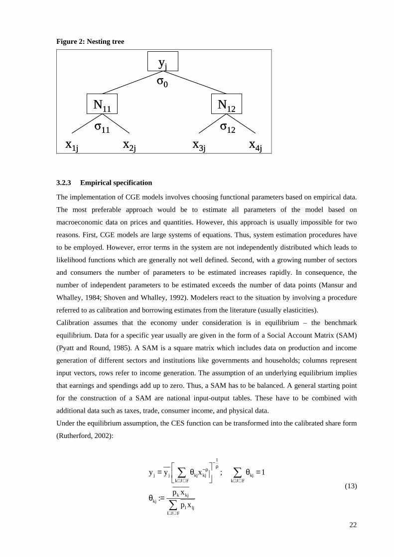
22

Figure 2: Nesting tree

yj

N11 N12

σ0

x1j x4jx3jx2j

σ11 σ12

yj

N11 N12

σ0

x1j x4jx3jx2j

σ11 σ12

3.2.3 Empirical specification

The implementation of CGE models involves choosing functional parameters based on empirical data.

The most preferable approach would be to estimate all parameters of the model based on

macroeconomic data on prices and quantities. However, this approach is usually impossible for two

reasons. First, CGE models are large systems of equations. Thus, system estimation procedures have

to be employed. However, error terms in the system are not independently distributed which leads to

likelihood functions which are generally not well defined. Second, with a growing number of sectors

and consumers the number of parameters to be estimated increases rapidly. In consequence, the

number of independent parameters to be estimated exceeds the number of data points (Mansur and

Whalley, 1984; Shoven and Whalley, 1992). Modelers react to the situation by involving a procedure

referred to as calibration and borrowing estimates from the literature (usually elasticities).

Calibration assumes that the economy under consideration is in equilibrium – the benchmark

equilibrium. Data for a specific year usually are given in the form of a Social Account Matrix (SAM)

(Pyatt and Round, 1985). A SAM is a square matrix which includes data on production and income

generation of different sectors and institutions like governments and households; columns represent

input vectors, rows refer to income generation. The assumption of an underlying equilibrium implies

that earnings and spendings add up to zero. Thus, a SAM has to be balanced. A general starting point

for the construction of a SAM are national input-output tables. These have to be combined with

additional data such as taxes, trade, consumer income, and physical data.

Under the equilibrium assumption, the CES function can be transformed into the calibrated share form

(Rutherford, 2002):

1

j j kj kj kjk J F k J F

k kjkj

l ljl J F

y y x ; 1

p x:

p x

−ρ

−ρ

∈ ∪ ∈ ∪

∈ ∪

= θ θ =

θ =

∑ ∑

∑

(13)

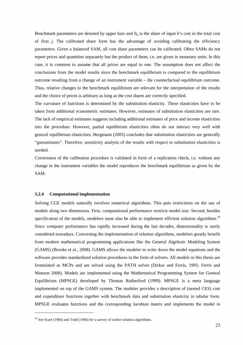
23

Benchmark parameters are denoted by upper bars and θkj is the share of input k’s cost in the total cost

of firm j. The calibrated share form has the advantage of avoiding calibrating the efficiency

parameters. Given a balanced SAM, all cost share parameters can be calibrated. Often SAMs do not

report prices and quantities separately but the product of them, i.e. are given in monetary units. In this

case, it is common to assume that all prices are equal to one. The assumption does not affect the

conclusions from the model results since the benchmark equilibrium is compared to the equilibrium

outcome resulting from a change of an instrument variable – the counterfactual equilibrium outcome.

Thus, relative changes to the benchmark equilibrium are relevant for the interpretation of the results

and the choice of prices is arbitrary as long as the cost shares are correctly specified.

The curvature of functions is determined by the substitution elasticity. These elasticities have to be

taken from additional econometric estimates. However, estimates of substitution elasticities are rare.

The lack of empirical estimates suggests including additional estimates of price and income elasticities

into the procedure. However, partial equilibrium elasticities often do not interact very well with

general equilibrium elasticities. Bergmann (2005) concludes that substitution elasticities are generally

“guesstimates”. Therefore, sensitivity analysis of the results with respect to substitution elasticities is

needed.

Correctness of the calibration procedure is validated in form of a replication check, i.e. without any

change in the instrument variables the model reproduces the benchmark equilibrium as given by the

SAM.

3.2.4 Computational implementation

Solving CGE models naturally involves numerical algorithms. This puts restrictions on the use of

models along two dimensions. First, computational performance restricts model size. Second, besides

specification of the models, modelers must also be able to implement efficient solution algorithms.26

Since computer performance has rapidly increased during the last decades, dimensionality is rarely

considered nowadays. Concerning the implementation of solution algorithms, modelers greatly benefit

from modern mathematical programming applications like the General Algebraic Modeling System

(GAMS) (Brooke et al., 2008). GAMS allows the modeler to write down the model equations and the

software provides standardized solution procedures in the form of solvers. All models in this thesis are

formulated as MCPs and are solved using the PATH solver (Dirkse and Ferris, 1995; Ferris and

Munson 2000). Models are implemented using the Mathematical Programming System for General

Equilibrium (MPSGE) developed by Thomas Rutherford (1999). MPSGE is a meta language

implemented on top of the GAMS system. The modeler provides a description of (nested CES) cost

and expenditure functions together with benchmark data and substitution elasticity in tabular form.

MPSGE evaluates functions and the corresponding Jacobian matrix and implements the model in

26 See Scarf (1984) and Todd (1984) for a survey of earlier solution algorithms.

24

MCP format. After generation of the model’s equations it is solved using the PATH solver.27 Beside

the advantage of avoiding the error prone explicit programming of nested CES function, MPSGE has

the benefit of automatically deriving demand functions as partial derivatives of provided functions

(Shepard’s lemma).

3.3 Technological details

3.3.1 The bottom-up/top-down discussion

Applied general equilibrium models have the advantage of capturing price interdependencies of

economic sectors by a comprehensive assessment of the circular flow of commodities and incomes.

However, especially in energy policy analysis, CGE models are often criticized for the lack of detailed

representation of technological details of the energy system. In this discussion, AGE models are often

termed top-down models since they adopt a view on the whole economy from the top and neglect

details of single sector representations. In contrast, bottom-up models adopted a technological rich

engineering view of single sectors but approximate macroeconomic changes in a rough manner, i.e. do

not capture macroeconomic feedbacks (Hourcade et al., 2006). Usually bottom-up models characterize

sectors in terms of different production technologies represented by Leontief technologies. A change

on relative input prices then leads to a switch from one technology to another. Such models are

implemented as linear programs. Prominent examples of bottom-up models of the energy system are

the MARKet ALlocation (MARKAL) (Loulou et al., 2004) or the Prospective Outlook on Long-term

Energy Systems (POLES) (Criqui et al., 1999) model.

Figure 3: Top-down versus bottom-up technology representation

K

L

T1

T2

T3

L

K K

L

T1

T2

T3

LL

KK

27 Alternatively the MILES Solver (Rutherford, 1993) can be used.

25

The discussion about technology representation is best explained in terms of Figure 3 which depicts

production function using capital K and labor L as inputs. From a bottom-up view, the sector is best

characterized in terms of three distinct technologies represented by dashed lines. The parameter

specification of the technologies’ cost functions is derived using engineering data. Under a given

demand for the output, the firm seeks to minimize production cost by choosing the output level of

different technologies, i.e. the technology mix. In contrast, the top-down approach describes the

sector’s cost by a smooth cost function depicted by the solid isoquant. The described calibration

procedure implies that the isoquant’s locus in the production space is determined by the sector’s

benchmark input of capital and labor. The substitution possibility among inputs is determined by the

curvature of the isoquant, i.e. by choosing the substitution elasticity. However, only by incident, a

substitution elasticity which correctly determines factor substitution as implied by detailed technology

analysis exists. Furthermore, even if the isoquant succeeds in replicating technology substitution, other

restrictions like pre-installed production capacities and technological potential which imply limited

technology substitution are not represented.

Generally, three different approaches exist to overcome the top-down/bottom-up problem. The softlink

approach links independently developed models using a convergence algorithm. Such approach used

for example in the MESSAGE-MACRO model (Messner and Schrattenholzer, 2000). This approach

often faces problems of different behavioral assumptions and accounting schemes (Böhringer and

Rutherford, 2008). In contrast the hardlink approach formulates a highly aggregated reduced form

macro model with a detailed deciption of the energy system in a single optimization problem. This

approach is followed for example in the REMIND model (Bauer et al., 2008; Leimbach et al., 2009).

Finally, using the MCP format, both model formats can be fully integrated. This thesis follows the

integrating approach which is described in detail in the next section.

3.3.2 Integrating bottom-up and top-down

Böhringer (1998) and Böhringer and Rutherford (2008) propose exploiting the MCP format in order to

overcome the problem of technology representation. The basic idea is to set up the bottom-up linear

programming model, deriving the first order complementarity conditions, and adding them to the CGE

model in MCP format.

Consider a specific sector s Є J being subject to the bottom-up representation. The sector uses T

different technologies (t Є T:={1,2,…,T}) to produce one homogenous output yj. Technologies are

characterized by unit inputs akt and installed capacities capt. Additionally, technologies’ production

levels are bounded from above by technological potentials pott.28 Imposing perfect competition, the

firm seeks to minimize production cost given commodity prices pk, prices for capacity investments pit

28 The term technological potential is a bit misleading since the potential also might be restricted by policy. For example, in the electricity sector the use of hydro power is naturally restricted by possible production sights. However, the potential of nuclear power might be restricted by the government’s intention for nuclear phase out.

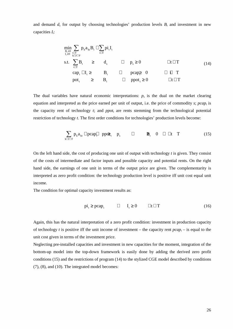
26

and demand ds for output by choosing technologies’ production levels Bt and investment in new

capacities I t:

t

t

k kt t t tB 0t T t TI 0k J F

t s st T

t t t t

t

min p a B pi I

s.t. B d p 0 t T

cap I B pcap 0 t T

pot

≥ ∈ ∈≥ ∈ ∪

∈

+

≥ ⊥ ≥ ∀ ∈

+ ≥ ⊥ ≥ ∀ ∈≥

∑ ∑

∑

t t B ppot 0 t T⊥ ≥ ∀ ∈

(14)

The dual variables have natural economic interpretations: ps is the dual on the market clearing

equation and interpreted as the price earned per unit of output, i.e. the price of commodity s; pcapt is

the capacity rent of technology t; and ppott are rents stemming from the technological potential

restriction of technology t. The first order conditions for technologies’ production levels become:

k kt t t s tk J F

p a pcap ppot p B 0 t T∈ ∪

+ + ≥ ⊥ ≥ ∀ ∈∑ (15)

On the left hand side, the cost of producing one unit of output with technology t is given. They consist

of the costs of intermediate and factor inputs and possible capacity and potential rents. On the right

hand side, the earnings of one unit in terms of the output price are given. The complementarity is

interpreted as zero profit condition: the technology production level is positive iff unit cost equal unit

income.

The condition for optimal capacity investment results as:

t t tpi pcap I 0 t T≥ ⊥ ≥ ∀ ∈ (16)

Again, this has the natural interpretation of a zero profit condition: investment in production capacity

of technology t is positive iff the unit income of investment – the capacity rent pcapt – is equal to the

unit cost given in terms of the investment price.

Neglecting pre-installed capacities and investment in new capacities for the moment, integration of the

bottom-up model into the top-down framework is easily done by adding the derived zero profit

conditions (15) and the restrictions of program (14) to the stylized CGE model described by conditions

(7), (8), and (10). The integrated model becomes:

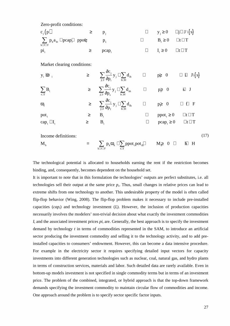
27

( ) { }j j j

k kt t t sk J F

Zero-profit conditions:

c p p y 0 j J \ s

p a pcap ppot p ∈ ∪

≥ ⊥ ≥ ∀ ∈

+ + ≥ ⊥∑ t

t t t

ji i j

j i

B 0 t T

pi pcap I 0 t T

Market clearing conditions:

cy y

p

≥ ∀ ∈

≥ ⊥ ≥ ∀ ∈

∂+ ω ≥

∂{ }ih i

J h H

jt j sh s

t T j J h Hs

f

d p 0 i J\ s

cB y d p 0 s J

p

c

∈ ∈

∈ ∈ ∈

+ ⊥ ≥ ∀ ∈

∂≥ + ⊥ ≥ ∈

∂∂

ω ≥

∑ ∑

∑ ∑ ∑

jj fh f

j J h Hf

t t t

t t

y d p 0 f Fp

pot B ppot 0 t T

cap I

∈ ∈+ ⊥ ≥ ∀ ∈

∂≥ ⊥ ≥ ∀ ∈

+ ≥

∑ ∑

t t

h k k t th hk J F t T

B pcap 0 t T

Income definitions:

M p ppot pot M 0 h H∈ ∪ ∈

⊥ ≥ ∀ ∈

= ω + ⊥ ≥ ∀ ∈∑ ∑

(17)

The technological potential is allocated to households earning the rent if the restriction becomes

binding, and, consequently, becomes dependent on the household set.

It is important to note that in this formulation the technologies’ outputs are perfect substitutes, i.e. all

technologies sell their output at the same price ps. Thus, small changes in relative prices can lead to

extreme shifts from one technology to another. This undesirable property of the model is often called

flip-flop behavior (Wing, 2008). The flip-flop problem makes it necessary to include pre-installed

capacities (capt) and technology investment (I t). However, the inclusion of production capacities

necessarily involves the modelers’ non-trivial decision about what exactly the investment commodities

I t and the associated investment prices pit are. Generally, the best approach is to specify the investment

demand by technology t in terms of commodities represented in the SAM, to introduce an artificial

sector producing the investment commodity and selling it to the technology activity, and to add pre-

installed capacities to consumers’ endowment. However, this can become a data intensive procedure.

For example in the electricity sector it requires specifying detailed input vectors for capacity

investments into different generation technologies such as nuclear, coal, natural gas, and hydro plants

in terms of construction services, materials and labor. Such detailed data are rarely available. Even in

bottom-up models investment is not specified in single commodity terms but in terms of an investment

price. The problem of the combined, integrated, or hybrid approach is that the top-down framework

demands specifying the investment commodity to maintain circular flow of commodities and income.

One approach around the problem is to specify sector specific factor inputs.

28

The stylized models of Böhringer (1998) and Böhringer and Rutherford (2008) specify fossil fuel

energy resources (coal, natural gas, and refined oil) as sector specific resources which are solely

supplied by consumers, i.e. energy resources are specified as factors which are only demanded by the

respective technologies. However, in empirical applications commodities’ supply is endogenously

determined and, thus, can not be specified as factor. Böhringer (1995) uses the framework for an

empirical evaluation of the influences of alternative coal subsidies on carbon taxes in Germany. In this

model, capital inputs are partially specified as sector specific leading to the same desired smooth

technology substitution. Wing (2008) is the first elaborating the problem explicitly; he proposes the

following modeling approach: If technologies are determined as Leontief production technologies, the

supply of sector specific capital naturally puts an upper bound on the output level. He introduces an

artificial activity taking malleable or intersectoral mobile capital as input and providing technology

specific capital stocks as output using a Constant Elasticity of Transformation (CET) function. This

corresponds to the view that capacities are partially reversible, i.e. can be retired and converted into

malleable capital, which can be used for investments into new technology specific capital.

Consequently, the malleability of capacity is governed by the transformation elasticity of the capital

activity. Additionally, he uses the share preserving character of the CES function that price changes do

not induce extreme deviation in technologies’ output shares: Each output unit is rewarded with a

technology specific output price. Outputs are aggregate to a homogenous commodity using a CES

function with a high substitution elasticity (σ = 10) which results in a nearly linear isoquant (perfect

substitutability).

3.4 Relevant modeling literature

In general, the global pollution externality of transport in AGE models is investigated from two

perspectives: On the on the hand, the energy/environmental approach focuses on the emission of

greenhouse gases especially from the combustion of fossil fuels. On the other hand, transport

economic modeling focuses mainly on the congestion externality and partly includes other

externalities such as pollution and accidents. While in the first class of models the main interest lies in

an efficient carbon pricing, cost-efficient abatement of emissions and the interaction across polluting

sectors, the second perspective is primarily interested in an efficient internalization of transport

externalities within the transport sector and the impacts of changed transport prices and infrastructure

investments on mode decisions and other sectors.

A detailed modeling of the transport sector in energy/environmental related studies is relatively rare

compared to the number of such studies.29 Paltsev et al. (2004, 2005b) develop a method to integrate

private transport into the MIT Emission Prediction and Policy Analysis (EPPA) model. The MIT

29 General surveys of the use of AGE models in energy/environment studies are given for example, in Conrad (1994), Bergman (2005), and Wing (2007). Springer (2003) summarizes the literature especially related to tradable greenhouse gas permits.

29

EPPA model is a large scale, recursive dynamic CGE model of the world economy.30 Carrying out

illustrative emission pricing scenarios, the authors show the critical importance of a disaggregated

representation of household transport to improve the representation of substitution possibilities for

fossil fuels. While the MIT EPPA model does include transport, it does not differentiate between the

durable stock of transport capital and the associated service flow. Such an approach is implemented in

the GEM-E3 model of the European Union (Capros et al., 1997). GEM-E3 offers a detailed

representation of the EU 15 region and six further aggregated world regions. It is also recursive

dynamic but includes cars as a stock variable which depreciates over time, is augmented by

investments, and necessary to obtain the service flow of transport.

Berg (2007) extends the EMEC model developed by Östblom and Berg (2006) by a detailed

representation of household transport demand. In this static model of the Swedish economy, different

transport modes, work and leisure trips are distinguished. Furthermore, households are differentiated

representing different income groups and locations of living. Berg analyzes the effect of carbon taxes

in the EMEC model with and without the augmented transport modeling. The model with the detailed

transport module always shows higher cost of carbon regulation. This result is based on the

endogenous labor/leisure choice: carbon taxes on fuels increase the price of work trips and thus, exert

a negative pressure on labor supply.

Another stream of the environmental/energy literature is concerned with the penetration of advanced

technologies in the automobile market. Schäfer and Jacoby (2005, 2006) implement a softlink

approach on the MIT EPPA model with an improved modeling of private transport. They use the

model together with a mode choice (Schäfer and Victor, 2000) and the MARKAL model (Louluo et

al., 2004). Transport demand is determined in the EPPA model and passed to the mode choice model.

The demand for different modes and prices of the EPPA model are processed in the MARKAL model

which is calibrated to an existing fleet of automobile technologies and other transport modes.

Consequently, MARKAL determines the penetration of advanced vehicle technologies. In order to

achieve consistency between the MARKAL energy and the EPPA transport demand, substitution

elasticities in the household transport module and the autonomous energy efficiency improvement

parameter are adjusted in an iterative procedure. Implementing different time paths for emission

reduction, the authors show that advanced technologies such as aluminum intensive vehicles or hybrid

drive trains do not play a significant role in emission abatement in the US for the next 30 years.

Sandoval et al. (2008) analyze the prospect of hydrogen cars by introducing a hydrogen production

sector in the EPPA model. They estimate that in the absence of any climate policy hydrogen cars

become competitive in the US at a purchase price which is 1.3 times the price of conventional

automobiles since they are more fuel efficient. In Europe, the technology will become competitive

even at a price twice the one of conventional cars since high fuel taxes stimulate the use of more fuel

efficient hydrogen cars. However, the penetration of hydrogen cars only slightly reduces carbon

30 Recently, a forward looking model version has also been developped (Babiker et al., 2008).

30

emissions since hydrogen production in mainly based on coal combustion. Imposing carbon

constraints favors the adoption of hydrogen vehicles.

Jokisch and Mennel (2009) calculate hydrogen penetration rates in the MARKAL model and impose

them exogenously on the PACE model (Böhringer and Vogt, 2003) to assess the macro-economic

impacts. PACE is a dynamic, forward looking of international energy use and global trade with a

special emphasis on Europe. Since hydrogen vehicles are assumed to have learning effects which drive

lifetime cost below the cost of conventional automobiles, the penetration yields positive welfare

effects. Karplus et al. (2009) analyze the potential role of plug-in hybrid electric vehicle for the US

and Japan by augmenting the EPPA model. They show that even in the presence of a strict climate

policy, additional research on battery design is necessary to lower purchase costs and increase driving

range.

The transport economic modeling literature is primarily interested in the congestion externality and the

welfare impacts of changed transport prices. Accordingly, often road pricing and/or infrastructure

investments are assessed. Such models often ignore externalities (e.g. Kalinowska et al., 2007;

Kremers and Kalinowska, 2009) or only focus congestion (e.g. Conrad, 1997; Conrad and Heng,

2002). Other studies use the same approach as the environmental/energy literature: they include the

generation of externalities, particularly greenhouse gas emissions, but do not model their impact on the

economic system (e.g. de Borger and Swysen, 1998; Steininger et al., 2007). Parry and Bento (1999)

note the importance of other externalities evaluating the welfare effects of congestion pricing.

Including accident and pollution externalities in a linear separable way into the utility function, they

show that reduced congestion offers additional positive welfare effects by reducing these externalities

and illustrate their results with a stylized CGE model. Non-separable transport externalities in the

utility function and the impacts on production sectors have been model by Meyeres and Proost (1997).

Mayeres (1999) extends this approach for different household types to assess the equity aspects of

transport policies.

31

4 Transportation under the European Emission Trading System

4.1 Introduction

This chapter employs a multi-region computable generally equilibrium model analyzing the impacts of

European-wide regulation measures addressing the carbon emissions of transport. The introduction of

a closed emission trading system for transport emissions, the inclusion of the transport sector into the

EU ETS, and the exemption of transport from carbon regulation are tested against the performance of

the current EU ETS. The results show that exempting transport from carbon regulation, i.e. shifting the

reduction burden to the EU ETS, is the most favorable strategy. Concerning fuel pricing strategies, the

inclusion of transport into the EU ETS incurs lower cost than a closed emission trading scheme.

Furthermore, a closed emission trading scheme performs only slightly better than transport under

national carbon taxes.

Multi-region models have the advantage that changes in terms-of-trade are endogenously determined.

Analyzing carbon restrictions, terms-of-trade changes occur in two dimensions. First, countries with a

lower carbon price gain comparative advantages in the production of energy intensive commodities.

Second, carbon restrictions affect the demand for fossil fuels. Consequently, prices change and create

substantial spillovers to other countries. The extensive literature on terms-of-trade reaction concludes

that fossil fuel price changes are the main determinant of terms-of-trade changes (e.g. Krutilla, 1991;

Böhringer and Rutherford, 2002b; Babiker et al., 2004). Analyzing the introduction of the EU ETS

compared to purely national regulation on a member state level, the model also shows this result.

Policies are analyzed at the EU 27 level, i.e. new member states with negative reduction burdens. The

results show, that these countries incur welfare gains by participating in the EU ETS since they are

able to sell excess emission allowances.

4.2 Model description

4.2.1 Overview

The multi-region model employed in this chapter is formulated as a mixed complementarity problem.

Three classes of equilibrium conditions exist. No activity makes positive profits (zero-profit

condition). Excess supply is weakly positive (market clearing condition). Each household fulfils his

budget restriction. Each class is associated to a class of variables. Activity levels are associated with

zero-profit conditions. Prices are connected to market clearing equations. Each budget restriction

determines the income level of the respective household.

The basic assumptions of the model are:

• The model is static.

• International commodity trade is unrestricted.

• All markets are perfectly competitive, i.e. all agents take prices as given.

32

• Households’ preferences are represented by a representative agent.

• The household is endowed with capital and labor which are intersectoral but not international

mobile. Furthermore, an endowment of immobile natural resources exists. All factors are

inelastically supplied.

• Investment demand and balance of payment deficits are exogenous and constant.

• The government imposes taxes to finance the provision of public goods which is assumed to

be constant.

• Production and utility functions are represented using nested CES functions.

4.2.2 Algebraic description

4.2.2.1 Representative agent

The representative agent (RA) in region r derives utility consuming commodities i (xi,RA,r) according to

the utility function Ur(.). The initial endowments of capital (Kr), labor (Lr), and natural resource used

in sector i (Ri,r) determine the income of representative agents. Factors are inelastically supplied.

While capital and labor are mobile across sectors but not international, natural resources are sector-

specific, i.e. immobile across sectors and regions. Given commodity prices pi,r, factor prices pK,r, pL,r,

and pR,i,r, the tax rate on final consumption ti,RA,r, and a direct transfer from the government to the

household transr, the representative agents maximize utility subject to the budget constraint:

( )

( )i ,RA,r

r i,RA,rx 0

K,r r L,r r R,i,r i,r r i,RA,r i,r i,RA,r i,ri i i

max U x

s.t. p K p L p R trans 1 t p x inv

≥

+ + + ≥ + +∑ ∑ ∑ (18)

invi,r is investment demand which is assumed to be constant. Solving the problem for each

representative consumer yields the demand function depending on prices (Ci,r).

4.2.2.2 Production

Each production sector i produces one commodity which can either be sold to the domestic market at

price pi,rd or be exported at price pi,r

e. The respective quantities are denoted yi,rd and yi,r

e and the activity

level by yi,r. xj,i,r is the intermediate input of commodity j to sector i in region r. Similar, xK,i,r, xL,i,r, and

xR,i,r are the respective factor inputs. Taxes are imposed on intermediate as well as factor inputs (tj,i,r,

tK,i,r, tL,i,r, tR,i,r) and on outputs (toi,r). Accordingly, tax inclusive input prices are defined as

qj,i,r:=(1+t j,i,r)pj,r, qK,i,r:=(1+t K,i,r)pK,r, qL,i,r:=(1+t L,i,r)pL,r, and qR,i,r:=(1+t R,i,r)pR,i,r. Furthermore, tax

inclusive output prices are given as vi,rd=(1-toi,r)pi,r

d and vi,re=(1-toi,r)pi,r

e. Assuming separability of

inputs and output and constant returns to scale in production, the unit revenue (r i,r) and cost functions

(ci,r) can be independently determined from a given production function. The profit optimization

problems become:

33

( ) ( )i ,r

d ei,r i,r i,r i,r j,i,r K,i,r L,i,r R ,i,r i,r

y 0max r v , v y c q ,q ,q ,q y i,r

≥+ ∀ (19)

The corresponding zero profit conditions become:

( ) ( )d ei,r j,i,r K,i,r L,i,r R,i,r i,r i,r i,rc q ,q ,q ,q r v , v y 0 i,r≥ ⊥ ≥ ∀ (20)

Shepard’s lemma and a similar relation on the output side (Ginsburgh and Keyzer, 1997) determine

the optimal input and output quantities:

i,r i,r i,r i,rj,i,r i,r K,i,r i,r L,i,r i,r R,i,r i,r

j,i,r K,i,r L,i,r R ,i,r

i,r i,rd ei,r i,r i,r i,rd e

i,r i,r

c c c cx y x y x y x y

q q q q

r ry y y y

v v

∂ ∂ ∂ ∂= = = =

∂ ∂ ∂ ∂

∂ ∂= =

∂ ∂

(21)

4.2.2.3 International trade

International trade is modeled using the Armington (1969) assumption, i.e. commodities are

distinguished by region of origin. First, commodities from different regions are combined to an import

composite, and second, domestic commodities and the import composite are aggregated.

Furthermore, international commodity trade is associated with a transport margin, i.e. trading

commodity i from region r to regions s requires the transport margin tr i,j,r,s of transport service j. The

importer of the commodity pays the margin. Transport services are produced by an international

transport pool which combines services from different regions.

Two different taxes apply on international trade. The export tax for commodity i shipped from region r

to region s, tei,r,s, applies on the value of the export. In contrast, the import tax tmi,r,s is levied on the

value of the import commodity including the transport margin.

Let pti be the price of transport margin i, cit(pi,r

e) the unit cost function of the international transport

pool depending on the export prices of commodities coming from different regions, and yit the activity

level of the international transport pool. Accordingly, the profit optimization problem becomes:

( )ti

t t e ti i i,r i

y 0max p c p y

≥ − (22)

The corresponding zero profit condition and the demand functions become:

( )t e t ti i,r i ic p p y 0 i≥ ≥ ∀ (23)

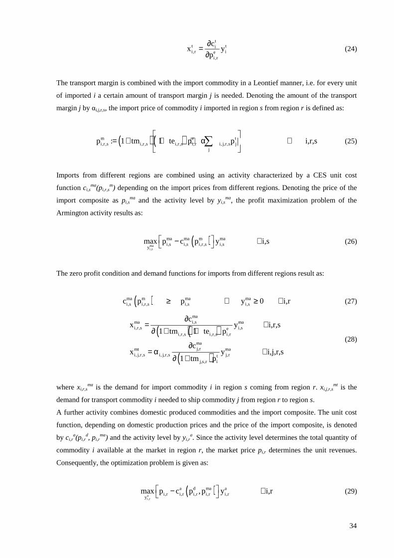
34

t

t tii,r ie

i,r

cx y

p

∂=∂

(24)

The transport margin is combined with the import commodity in a Leontief manner, i.e. for every unit

of imported i a certain amount of transport margin j is needed. Denoting the amount of the transport

margin j by αi,j,r,s, the import price of commodity i imported in region s from region r is defined as:

( ) ( )m e ti,r,s i,r ,s i,r ,s i,r i, j,r,s j

j

p : 1 tm 1 te p p i,r,s

= + + + α ∀

∑ (25)

Imports from different regions are combined using an activity characterized by a CES unit cost

function ci,sma(pi,r,s

m) depending on the import prices from different regions. Denoting the price of the

import composite as pi,sma and the activity level by yi,s

ma, the profit maximization problem of the

Armington activity results as:

( )mai ,s

ma ma m mai,s i,s i,r ,s i,s

ymax p c p y i,s − ∀ (26)

The zero profit condition and demand functions for imports from different regions result as:

( )ma m ma mai,s i,r,s i,s i,sc p p y 0 i,r≥ ⊥ ≥ ∀ (27)

( )( )

( )

mai,sma ma

i,r,s i,sei,r,s i,r,s i,r

maj,rmt ma

i, j,r ,s i, j,r,s j,rtj,s,r i

cx y i,r,s

1 tm 1 te p

cx y i,j,r,s

1 tm p

∂= ∀

∂ + +

∂= α ∀

∂ +

(28)

where xi,r,sma is the demand for import commodity i in region s coming from region r. xi,j,r,s

mt is the

demand for transport commodity i needed to ship commodity j from region r to region s.

A further activity combines domestic produced commodities and the import composite. The unit cost

function, depending on domestic production prices and the price of the import composite, is denoted

by ci,ra(pi,r

d, pi,rma) and the activity level by yi,r

a. Since the activity level determines the total quantity of

commodity i available at the market in region r, the market price pi,r determines the unit revenues.

Consequently, the optimization problem is given as:

( )ai ,r

a d ma ai,r i,r i,r i,r i,r

ymax p c p ,p y i,r − ∀ (29)

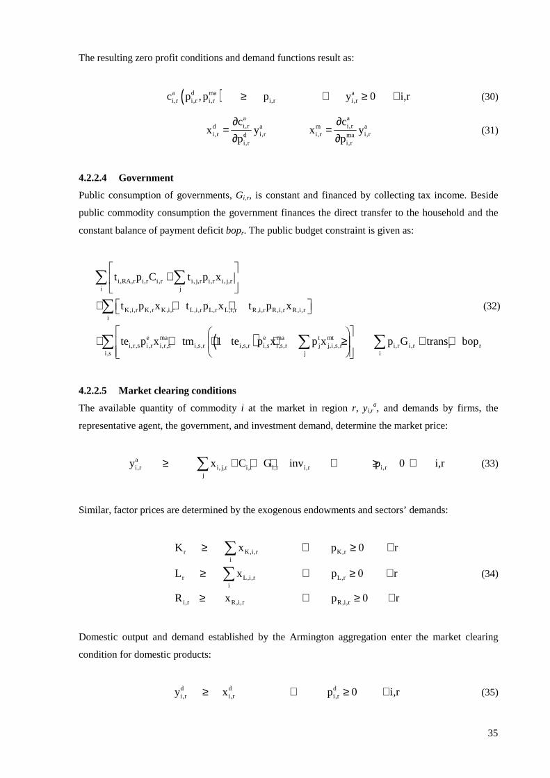
35

The resulting zero profit conditions and demand functions result as:

( )a d ma ai,r i,r i,r i,r i,rc p ,p p y 0 i,r≥ ⊥ ≥ ∀ (30)

a ai,r i,rd a m a

i,r i,r i,r i,rd mai,r i,r

c cx y x y

p p

∂ ∂= =

∂ ∂ (31)

4.2.2.4 Government

Public consumption of governments, Gi,r, is constant and financed by collecting tax income. Beside

public commodity consumption the government finances the direct transfer to the household and the

constant balance of payment deficit bopr. The public budget constraint is given as:

( )

i,RA,r i,r i,r i, j,r i,r i, j,ri j

K,i,r K,r K,i,r L,i,r L,r L,i,r R ,i,r R,i,r R,i,ri

e ma e ma t mti,r,s i,r i,r,s i,s,r i,s,r i,s i,s,r j j,i,s,r i,r i,r

i,s j i

t p C t p x

t p x t p x t p x

te p x tm 1 te p x p x p G

+

+ + +

+ + + + ≥

∑ ∑

∑

∑ ∑ ∑ r rtrans bop+ +

(32)

4.2.2.5 Market clearing conditions

The available quantity of commodity i at the market in region r, yi,ra, and demands by firms, the

representative agent, the government, and investment demand, determine the market price:

ai,r i, j,r i,r i,r i,r i,r

j

y x C G inv p 0 i,r ≥ + + + ⊥ ≥ ∀∑ (33)

Similar, factor prices are determined by the exogenous endowments and sectors’ demands:

r K,i,r K,ri

r L,i,r L,ri

i,r R,i,r R,i,r

K x p 0 r

L x p 0 r

R x p 0 r

≥ ⊥ ≥ ∀

≥ ⊥ ≥ ∀

≥ ⊥ ≥ ∀

∑

∑ (34)

Domestic output and demand established by the Armington aggregation enter the market clearing

condition for domestic products:

d d di,r i,r i,ry x p 0 i,r ≥ ⊥ ≥ ∀ (35)

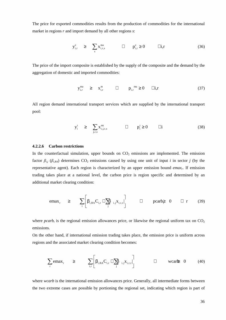
36

The price for exported commodities results from the production of commodities for the international

market in regions r and import demand by all other regions s:

e ma ei,r i,r,s i,r

s

y x p 0 i,r≥ ⊥ ≥ ∀∑ (36)

The price of the import composite is established by the supply of the composite and the demand by the

aggregation of domestic and imported commodities:

ma m mai,r i,r i,ry x p 0 i,r ≥ ⊥ ≥ ∀ (37)

All region demand international transport services which are supplied by the international transport

pool:

t mt ti i, j,r ,s i

j,r,s

y x p 0 i≥ ⊥ ≥ ∀∑ (38)

4.2.2.6 Carbon restrictions

In the counterfactual simulation, upper bounds on CO2 emissions are implemented. The emission

factor βi,j (βi,RA) determines CO2 emissions caused by using one unit of input i in sector j (by the

representative agent). Each region is characterized by an upper emission bound emaxr. If emission

trading takes place at a national level, the carbon price is region specific and determined by an

additional market clearing condition:

r i,RA i,r i, j i,r,r ri j

emax C x pcarb 0 r

≥ β + β ⊥ ≥ ∀

∑ ∑ (39)

where pcarbr is the regional emission allowances price, or likewise the regional uniform tax on CO2

emissions.

On the other hand, if international emission trading takes place, the emission price is uniform across

regions and the associated market clearing condition becomes:

r i,RA i,r i, j i,r,rr i,r j

emax C x wcarb 0

≥ β + β ⊥ ≥

∑ ∑ ∑ (40)

where wcarb is the international emission allowances price. Generally, all intermediate forms between

the two extreme cases are possible by portioning the regional set, indicating which region is part of

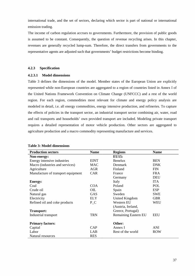
37

international trade, and the set of sectors, declaring which sector is part of national or international

emission trading.

The income of carbon regulation accrues to governments. Furthermore, the provision of public goods

is assumed to be constant. Consequently, the question of revenue recycling arises. In this chapter,

revenues are generally recycled lump-sum. Therefore, the direct transfers from governments to the

representative agents are adjusted such that governments’ budget restrictions become binding.

4.2.3 Specification

4.2.3.1 Model dimensions

Table 3 defines the dimensions of the model. Member states of the European Union are explicitly

represented while non-European countries are aggregated to a region of countries listed in Annex I of

the United Nations Framework Convention on Climate Change (UNFCCC) and a rest of the world

region. For each region, commodities most relevant for climate and energy policy analysis are

modeled in detail, i.e. all energy commodities, energy intensive production, and refineries. To capture

the effects of policies in the transport sector, an industrial transport sector combining air, water, road

and rail transports and households’ own provided transport are included. Modeling private transport

requires a detailed representation of motor vehicle production. Other sectors are aggregated to

agriculture production and a macro commodity representing manufacture and services.

Table 3: Model dimensions

Production sectors Name Regions Name Non-energy: EU15: Energy intensive industries EINT Benelux BEN Macro (industries and services) MAC Denmark DNK Agriculture AGR Finland FIN Manufacture of transport equipment CAR France FRA Germany DEU Energy: Italy ITA Coal COA Poland POL Crude oil OIL Spain ESP Natural gas GAS Sweden SWE Electricity ELY United Kingdom GBR Refined oil and coke products P_C WEU Transport:

Western EU (Austria, Ireland, Greece, Portugal)

Industrial transport TRN Remaining Eastern EU EEU Primary factors: Other: Capital CAP Annex I ANI Labor LAB Rest of the world ROW Natural resources RES

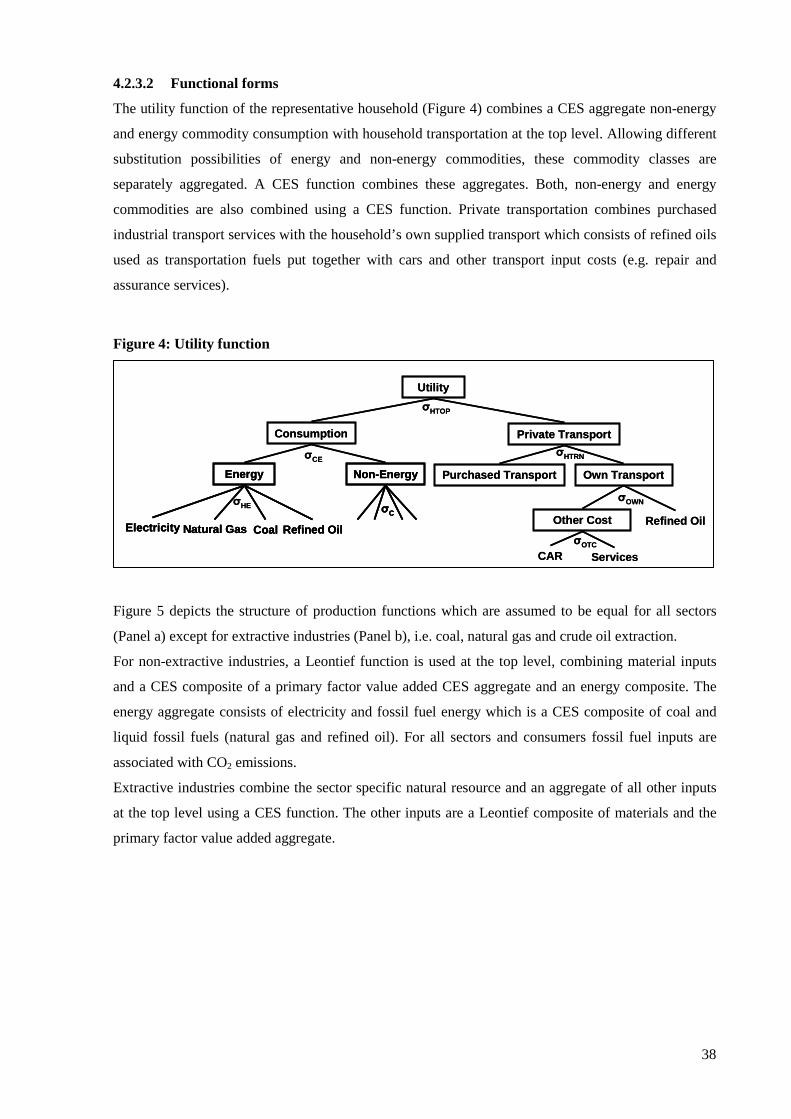
38

4.2.3.2 Functional forms

The utility function of the representative household (Figure 4) combines a CES aggregate non-energy

and energy commodity consumption with household transportation at the top level. Allowing different

substitution possibilities of energy and non-energy commodities, these commodity classes are

separately aggregated. A CES function combines these aggregates. Both, non-energy and energy

commodities are also combined using a CES function. Private transportation combines purchased

industrial transport services with the household’s own supplied transport which consists of refined oils

used as transportation fuels put together with cars and other transport input costs (e.g. repair and

assurance services).

Figure 4: Utility function

Figure 5 depicts the structure of production functions which are assumed to be equal for all sectors

(Panel a) except for extractive industries (Panel b), i.e. coal, natural gas and crude oil extraction.

For non-extractive industries, a Leontief function is used at the top level, combining material inputs

and a CES composite of a primary factor value added CES aggregate and an energy composite. The

energy aggregate consists of electricity and fossil fuel energy which is a CES composite of coal and

liquid fossil fuels (natural gas and refined oil). For all sectors and consumers fossil fuel inputs are

associated with CO2 emissions.

Extractive industries combine the sector specific natural resource and an aggregate of all other inputs

at the top level using a CES function. The other inputs are a Leontief composite of materials and the

primary factor value added aggregate.

Energy

Electricity Coal Refined OilNatural Gas

Utility

σHE

Non-Energy

σC

σCE

Consumption

σHTOP

Private Transport

Purchased Transport Own Transport

Refined OilOther Cost

CAR Services

σOWN

σOTC

σHTRN

Energy

Electricity Coal Refined OilNatural Gas

Energy

Electricity Coal Refined OilNatural Gas

Utility

σHE

Non-Energy

σC

Non-Energy

σC

σCE

Consumption

σHTOP

Private Transport

Purchased Transport Own Transport

Refined OilOther Cost

CAR Services

σOWN

σOTC

σHTRN

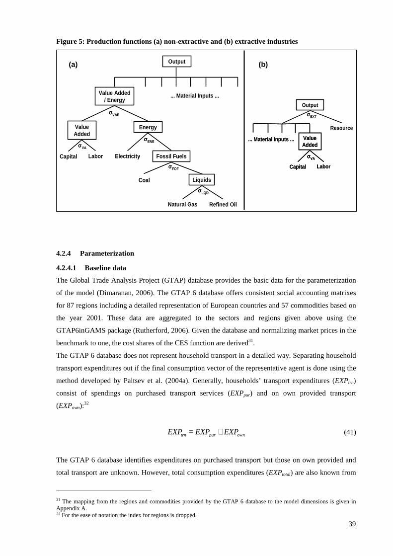
39

Figure 5: Production functions (a) non-extractive and (b) extractive industries

4.2.4 Parameterization

4.2.4.1 Baseline data

The Global Trade Analysis Project (GTAP) database provides the basic data for the parameterization

of the model (Dimaranan, 2006). The GTAP 6 database offers consistent social accounting matrixes

for 87 regions including a detailed representation of European countries and 57 commodities based on

the year 2001. These data are aggregated to the sectors and regions given above using the

GTAP6inGAMS package (Rutherford, 2006). Given the database and normalizing market prices in the

benchmark to one, the cost shares of the CES function are derived31.

The GTAP 6 database does not represent household transport in a detailed way. Separating household

transport expenditures out if the final consumption vector of the representative agent is done using the

method developed by Paltsev et al. (2004a). Generally, households’ transport expenditures (EXPtrn)

consist of spendings on purchased transport services (EXPpur) and on own provided transport

(EXPown):32

= +trn pur ownEXP EXP EXP (41)

The GTAP 6 database identifies expenditures on purchased transport but those on own provided and

total transport are unknown. However, total consumption expenditures (EXPtotal) are also known from

31 The mapping from the regions and commodities provided by the GTAP 6 database to the model dimensions is given in Appendix A. 32 For the ease of notation the index for regions is dropped.

Output

... Material Inputs ... Value Added

Capital Labor

σVA

... Material Inputs ... Value Added

Capital Labor

σVA

Resource

σEXT

Output

Value Added / Energy

... Material Inputs ...

Value Added

Energy

Capital Labor Electricity Fossil Fuels

σVAE

σVA

σENE

σFOF

Liquids

Natural Gas

Coal

Refined Oil

σLQD

(a) (b)

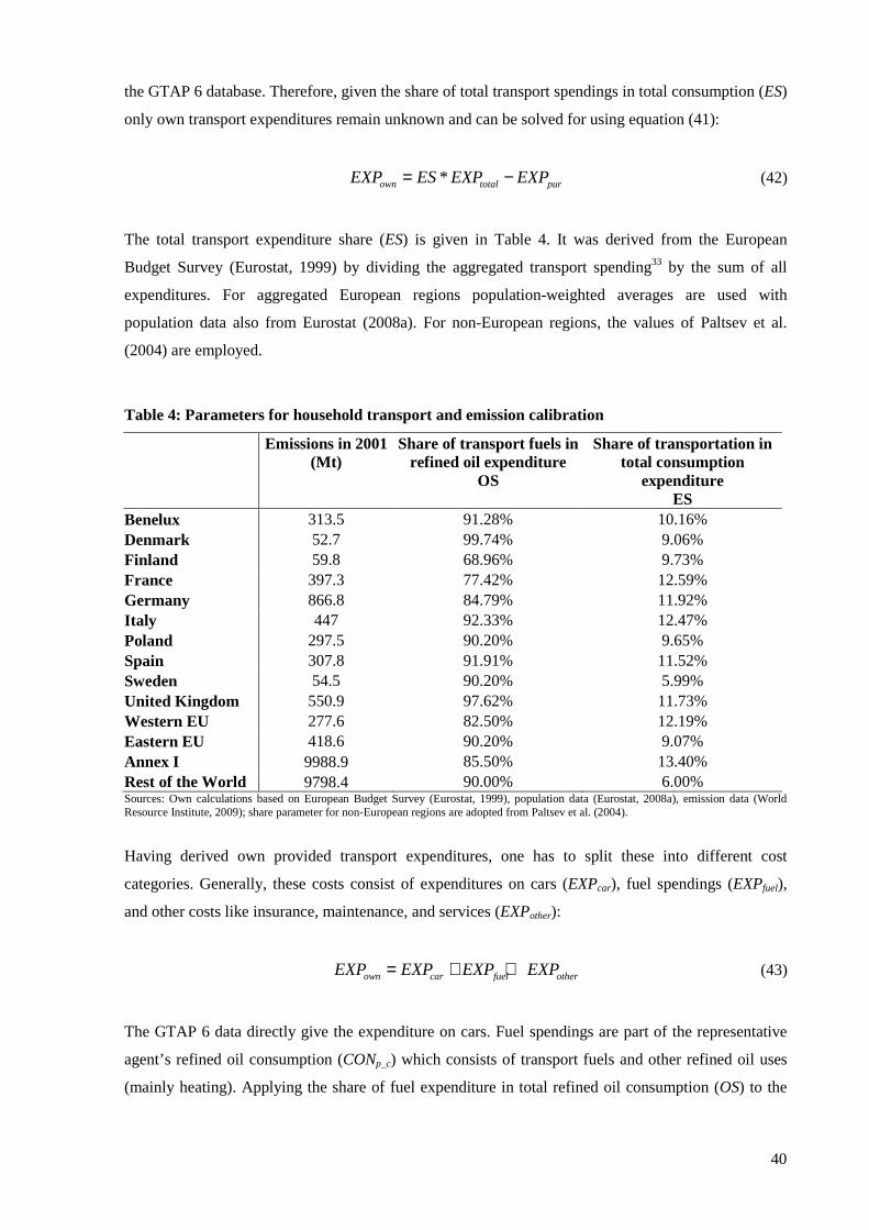
40

the GTAP 6 database. Therefore, given the share of total transport spendings in total consumption (ES)

only own transport expenditures remain unknown and can be solved for using equation (41):

*= −own total purEXP ES EXP EXP (42)

The total transport expenditure share (ES) is given in Table 4. It was derived from the European

Budget Survey (Eurostat, 1999) by dividing the aggregated transport spending33 by the sum of all

expenditures. For aggregated European regions population-weighted averages are used with

population data also from Eurostat (2008a). For non-European regions, the values of Paltsev et al.

(2004) are employed.

Table 4: Parameters for household transport and emission calibration

Emissions in 2001 (Mt)

Share of transport fuels in refined oil expenditure

OS

Share of transportation in total consumption

expenditure ES

Benelux 313.5 91.28% 10.16% Denmark 52.7 99.74% 9.06% Finland 59.8 68.96% 9.73% France 397.3 77.42% 12.59% Germany 866.8 84.79% 11.92% Italy 447 92.33% 12.47% Poland 297.5 90.20% 9.65% Spain 307.8 91.91% 11.52% Sweden 54.5 90.20% 5.99% United Kingdom 550.9 97.62% 11.73% Western EU 277.6 82.50% 12.19% Eastern EU 418.6 90.20% 9.07% Annex I 9988.9 85.50% 13.40% Rest of the World 9798.4 90.00% 6.00% Sources: Own calculations based on European Budget Survey (Eurostat, 1999), population data (Eurostat, 2008a), emission data (World Resource Institute, 2009); share parameter for non-European regions are adopted from Paltsev et al. (2004).

Having derived own provided transport expenditures, one has to split these into different cost

categories. Generally, these costs consist of expenditures on cars (EXPcar), fuel spendings (EXPfuel),

and other costs like insurance, maintenance, and services (EXPother):

= + +own car fuel otherEXP EXP EXP EXP (43)

The GTAP 6 data directly give the expenditure on cars. Fuel spendings are part of the representative

agent’s refined oil consumption (CONp_c) which consists of transport fuels and other refined oil uses

(mainly heating). Applying the share of fuel expenditure in total refined oil consumption (OS) to the

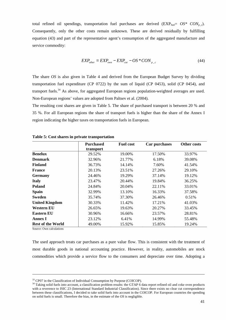
41

total refined oil spendings, transportation fuel purchases are derived (EXPfuel= OS* CONp_c).

Consequently, only the other costs remain unknown. These are derived residually by fulfilling

equation (43) and part of the representative agent’s consumption of the aggregated manufacture and

service commodity:

_*= − −other own car p cEXP EXP EXP OS CON (44)

The share OS is also given in Table 4 and derived from the European Budget Survey by dividing

transportation fuel expenditure (CP 0722) by the sum of liquid (CP 0453), solid (CP 0454), and

transport fuels.34 As above, for aggregated European regions population-weighted averages are used.

Non-European regions’ values are adopted from Paltsev et al. (2004).

The resulting cost shares are given in Table 5. The share of purchased transport is between 20 % and

35 %. For all European regions the share of transport fuels is higher than the share of the Annex I

region indicating the higher taxes on transportation fuels in European.

Table 5: Cost shares in private transportation

Purchased transport

Fuel cost Car purchases Other costs

Benelux 29.52% 19.00% 17.50% 33.97% Denmark 32.96% 21.77% 6.18% 39.08% Finland 36.73% 14.14% 7.60% 41.54% France 20.13% 23.51% 27.26% 29.10% Germany 24.46% 19.29% 37.14% 19.12% Italy 23.47% 20.44% 19.84% 36.25% Poland 24.84% 20.04% 22.11% 33.01% Spain 32.99% 13.10% 16.33% 37.58% Sweden 35.74% 37.30% 26.46% 0.51% United Kingdom 30.33% 11.42% 17.21% 41.03% Western EU 26.65% 19.63% 20.27% 33.45% Eastern EU 30.96% 16.66% 23.57% 28.81% Annex I 23.12% 6.41% 14.99% 55.48% Rest of the World 49.00% 15.92% 15.85% 19.24% Source: Own calculations

The used approach treats car purchases as a pure value flow. This is consistent with the treatment of

most durable goods in national accounting practice. However, in reality, automobiles are stock

commodities which provide a service flow to the consumers and depreciate over time. Adopting a

33 CP07 in the Classification of Individual Consumption by Purpose (COICOP). 34 Taking solid fuels into account, a classification problem results: the GTAP 6 data report refined oil and coke oven products with a reverence to ISIC 23 (International Standard Industrial Classification). Since there exists no clear cut correspondence between these classifications, I decided to take solid fuels into account in the COICOP. For European countries the spending on solid fuels is small. Therefore the bias, in the estimate of the OS is negligible.

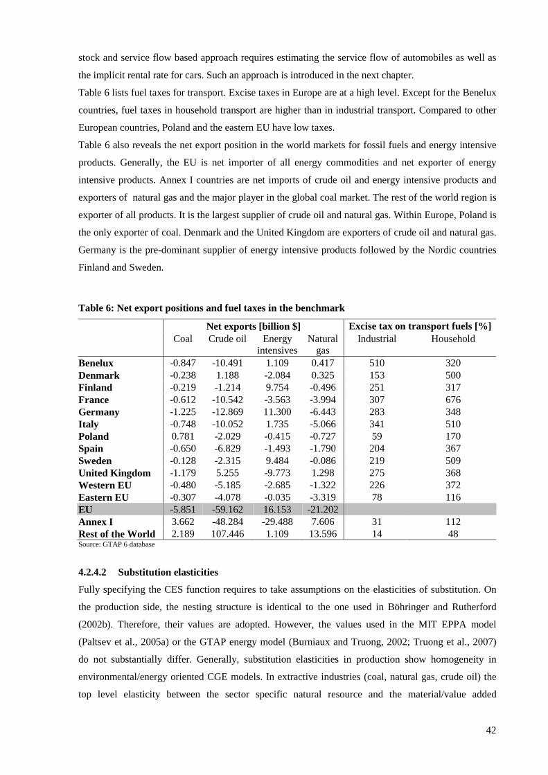
42

stock and service flow based approach requires estimating the service flow of automobiles as well as

the implicit rental rate for cars. Such an approach is introduced in the next chapter.

Table 6 lists fuel taxes for transport. Excise taxes in Europe are at a high level. Except for the Benelux

countries, fuel taxes in household transport are higher than in industrial transport. Compared to other

European countries, Poland and the eastern EU have low taxes.

Table 6 also reveals the net export position in the world markets for fossil fuels and energy intensive

products. Generally, the EU is net importer of all energy commodities and net exporter of energy

intensive products. Annex I countries are net imports of crude oil and energy intensive products and

exporters of natural gas and the major player in the global coal market. The rest of the world region is

exporter of all products. It is the largest supplier of crude oil and natural gas. Within Europe, Poland is

the only exporter of coal. Denmark and the United Kingdom are exporters of crude oil and natural gas.

Germany is the pre-dominant supplier of energy intensive products followed by the Nordic countries

Finland and Sweden.

Table 6: Net export positions and fuel taxes in the benchmark

Net exports [billion $] Excise tax on transport fuels [%]

Coal Crude oil Energy

intensives Natural

gas Industrial Household

Benelux -0.847 -10.491 1.109 0.417 510 320 Denmark -0.238 1.188 -2.084 0.325 153 500 Finland -0.219 -1.214 9.754 -0.496 251 317 France -0.612 -10.542 -3.563 -3.994 307 676 Germany -1.225 -12.869 11.300 -6.443 283 348 Italy -0.748 -10.052 1.735 -5.066 341 510 Poland 0.781 -2.029 -0.415 -0.727 59 170 Spain -0.650 -6.829 -1.493 -1.790 204 367 Sweden -0.128 -2.315 9.484 -0.086 219 509 United Kingdom -1.179 5.255 -9.773 1.298 275 368 Western EU -0.480 -5.185 -2.685 -1.322 226 372 Eastern EU -0.307 -4.078 -0.035 -3.319 78 116 EU -5.851 -59.162 16.153 -21.202 Annex I 3.662 -48.284 -29.488 7.606 31 112 Rest of the World 2.189 107.446 1.109 13.596 14 48 Source: GTAP 6 database

4.2.4.2 Substitution elasticities

Fully specifying the CES function requires to take assumptions on the elasticities of substitution. On

the production side, the nesting structure is identical to the one used in Böhringer and Rutherford

(2002b). Therefore, their values are adopted. However, the values used in the MIT EPPA model

(Paltsev et al., 2005a) or the GTAP energy model (Burniaux and Truong, 2002; Truong et al., 2007)

do not substantially differ. Generally, substitution elasticities in production show homogeneity in

environmental/energy oriented CGE models. In extractive industries (coal, natural gas, crude oil) the

top level elasticity between the sector specific natural resource and the material/value added

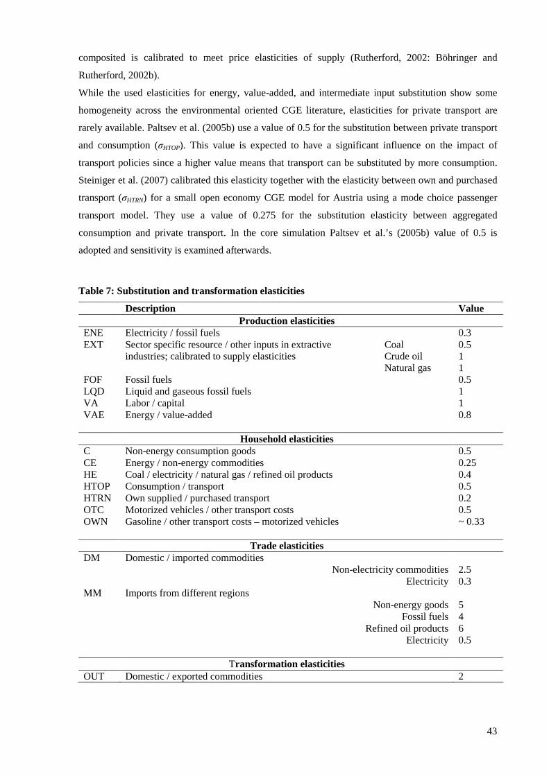
43

composited is calibrated to meet price elasticities of supply (Rutherford, 2002: Böhringer and

Rutherford, 2002b).

While the used elasticities for energy, value-added, and intermediate input substitution show some

homogeneity across the environmental oriented CGE literature, elasticities for private transport are

rarely available. Paltsev et al. (2005b) use a value of 0.5 for the substitution between private transport

and consumption (σHTOP). This value is expected to have a significant influence on the impact of

transport policies since a higher value means that transport can be substituted by more consumption.

Steiniger et al. (2007) calibrated this elasticity together with the elasticity between own and purchased

transport (σHTRN) for a small open economy CGE model for Austria using a mode choice passenger

transport model. They use a value of 0.275 for the substitution elasticity between aggregated

consumption and private transport. In the core simulation Paltsev et al.’s (2005b) value of 0.5 is

adopted and sensitivity is examined afterwards.

Table 7: Substitution and transformation elasticities

Description Value Production elasticities ENE Electricity / fossil fuels 0.3

Coal 0.5 Crude oil 1

EXT Sector specific resource / other inputs in extractive industries; calibrated to supply elasticities

Natural gas 1 FOF Fossil fuels 0.5 LQD Liquid and gaseous fossil fuels 1 VA Labor / capital 1 VAE Energy / value-added 0.8 Household elasticities C Non-energy consumption goods 0.5 CE Energy / non-energy commodities 0.25 HE Coal / electricity / natural gas / refined oil products 0.4 HTOP Consumption / transport 0.5 HTRN Own supplied / purchased transport 0.2 OTC Motorized vehicles / other transport costs 0.5 OWN Gasoline / other transport costs – motorized vehicles ~ 0.33 Trade elasticities DM Domestic / imported commodities Non-electricity commodities 2.5 Electricity 0.3 MM Imports from different regions Non-energy goods 5 Fossil fuels 4 Refined oil products 6 Electricity 0.5

Transformation elasticities OUT Domestic / exported commodities 2

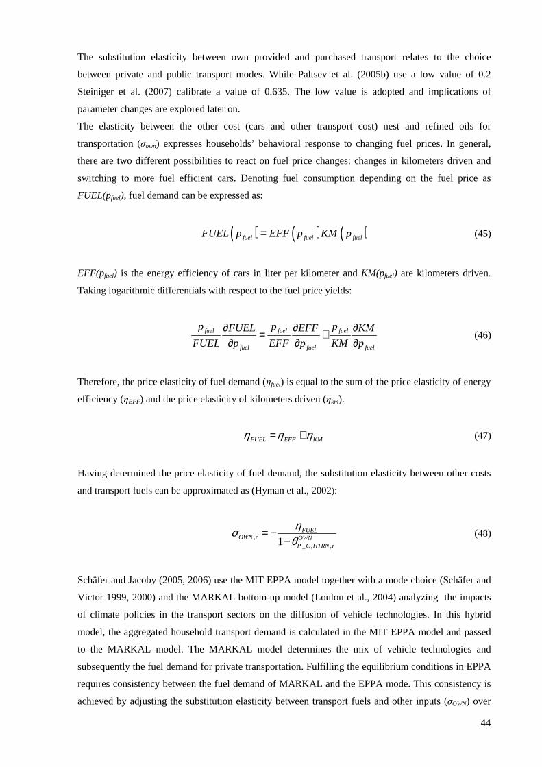
44

The substitution elasticity between own provided and purchased transport relates to the choice

between private and public transport modes. While Paltsev et al. (2005b) use a low value of 0.2

Steiniger et al. (2007) calibrate a value of 0.635. The low value is adopted and implications of

parameter changes are explored later on.

The elasticity between the other cost (cars and other transport cost) nest and refined oils for

transportation (σown) expresses households’ behavioral response to changing fuel prices. In general,

there are two different possibilities to react on fuel price changes: changes in kilometers driven and

switching to more fuel efficient cars. Denoting fuel consumption depending on the fuel price as

FUEL(pfuel), fuel demand can be expressed as:

( ) ( ) ( )=fuel fuel fuelFUEL p EFF p KM p (45)

EFF(pfuel) is the energy efficiency of cars in liter per kilometer and KM(pfuel) are kilometers driven.

Taking logarithmic differentials with respect to the fuel price yields:

∂ ∂ ∂= +∂ ∂ ∂

fuel fuel fuel

fuel fuel fuel

p p pFUEL EFF KM

FUEL p EFF p KM p (46)

Therefore, the price elasticity of fuel demand (ηfuel) is equal to the sum of the price elasticity of energy

efficiency (ηEFF) and the price elasticity of kilometers driven (ηkm).

FUEL EFF KMη η η= + (47)

Having determined the price elasticity of fuel demand, the substitution elasticity between other costs

and transport fuels can be approximated as (Hyman et al., 2002):

,_ , ,1FUEL

OWN r OWNP C HTRN r

ησθ

= −−

(48)

Schäfer and Jacoby (2005, 2006) use the MIT EPPA model together with a mode choice (Schäfer and

Victor 1999, 2000) and the MARKAL bottom-up model (Loulou et al., 2004) analyzing the impacts

of climate policies in the transport sectors on the diffusion of vehicle technologies. In this hybrid

model, the aggregated household transport demand is calculated in the MIT EPPA model and passed

to the MARKAL model. The MARKAL model determines the mix of vehicle technologies and

subsequently the fuel demand for private transportation. Fulfilling the equilibrium conditions in EPPA

requires consistency between the fuel demand of MARKAL and the EPPA mode. This consistency is

achieved by adjusting the substitution elasticity between transport fuels and other inputs (σOWN) over

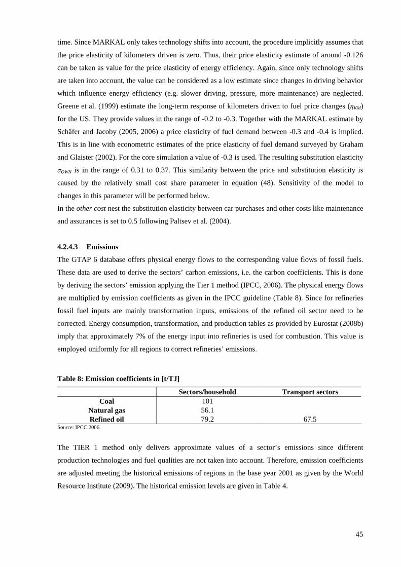
45

time. Since MARKAL only takes technology shifts into account, the procedure implicitly assumes that

the price elasticity of kilometers driven is zero. Thus, their price elasticity estimate of around -0.126

can be taken as value for the price elasticity of energy efficiency. Again, since only technology shifts

are taken into account, the value can be considered as a low estimate since changes in driving behavior

which influence energy efficiency (e.g. slower driving, pressure, more maintenance) are neglected.

Greene et al. (1999) estimate the long-term response of kilometers driven to fuel price changes (ηKM)

for the US. They provide values in the range of -0.2 to -0.3. Together with the MARKAL estimate by

Schäfer and Jacoby (2005, 2006) a price elasticity of fuel demand between -0.3 and -0.4 is implied.

This is in line with econometric estimates of the price elasticity of fuel demand surveyed by Graham

and Glaister (2002). For the core simulation a value of -0.3 is used. The resulting substitution elasticity

σOWN is in the range of 0.31 to 0.37. This similarity between the price and substitution elasticity is

caused by the relatively small cost share parameter in equation (48). Sensitivity of the model to

changes in this parameter will be performed below.

In the other cost nest the substitution elasticity between car purchases and other costs like maintenance

and assurances is set to 0.5 following Paltsev et al. (2004).

4.2.4.3 Emissions

The GTAP 6 database offers physical energy flows to the corresponding value flows of fossil fuels.

These data are used to derive the sectors’ carbon emissions, i.e. the carbon coefficients. This is done

by deriving the sectors’ emission applying the Tier 1 method (IPCC, 2006). The physical energy flows

are multiplied by emission coefficients as given in the IPCC guideline (Table 8). Since for refineries

fossil fuel inputs are mainly transformation inputs, emissions of the refined oil sector need to be

corrected. Energy consumption, transformation, and production tables as provided by Eurostat (2008b)

imply that approximately 7% of the energy input into refineries is used for combustion. This value is

employed uniformly for all regions to correct refineries’ emissions.

Table 8: Emission coefficients in [t/TJ]

Sectors/household Transport sectors Coal 101

Natural gas 56.1 Refined oil 79.2 67.5

Source: IPCC 2006

The TIER 1 method only delivers approximate values of a sector’s emissions since different

production technologies and fuel qualities are not taken into account. Therefore, emission coefficients

are adjusted meeting the historical emissions of regions in the base year 2001 as given by the World

Resource Institute (2009). The historical emission levels are given in Table 4.

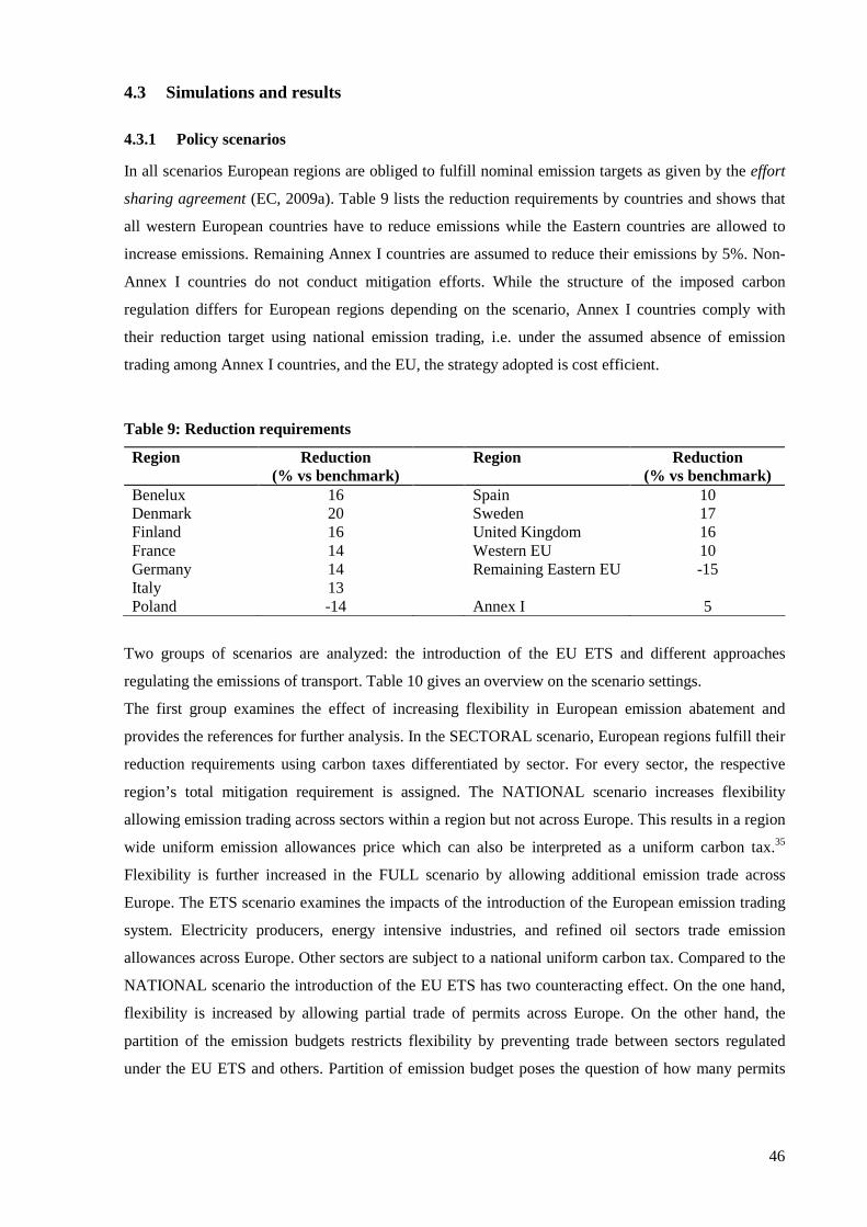
46

4.3 Simulations and results

4.3.1 Policy scenarios

In all scenarios European regions are obliged to fulfill nominal emission targets as given by the effort

sharing agreement (EC, 2009a). Table 9 lists the reduction requirements by countries and shows that

all western European countries have to reduce emissions while the Eastern countries are allowed to

increase emissions. Remaining Annex I countries are assumed to reduce their emissions by 5%. Non-

Annex I countries do not conduct mitigation efforts. While the structure of the imposed carbon

regulation differs for European regions depending on the scenario, Annex I countries comply with

their reduction target using national emission trading, i.e. under the assumed absence of emission

trading among Annex I countries, and the EU, the strategy adopted is cost efficient.

Table 9: Reduction requirements

Region Reduction (% vs benchmark)

Region Reduction (% vs benchmark)

Benelux 16 Spain 10 Denmark 20 Sweden 17 Finland 16 United Kingdom 16 France 14 Western EU 10 Germany 14 Remaining Eastern EU -15 Italy 13 Poland -14 Annex I 5

Two groups of scenarios are analyzed: the introduction of the EU ETS and different approaches

regulating the emissions of transport. Table 10 gives an overview on the scenario settings.

The first group examines the effect of increasing flexibility in European emission abatement and

provides the references for further analysis. In the SECTORAL scenario, European regions fulfill their

reduction requirements using carbon taxes differentiated by sector. For every sector, the respective

region’s total mitigation requirement is assigned. The NATIONAL scenario increases flexibility

allowing emission trading across sectors within a region but not across Europe. This results in a region

wide uniform emission allowances price which can also be interpreted as a uniform carbon tax.35

Flexibility is further increased in the FULL scenario by allowing additional emission trade across

Europe. The ETS scenario examines the impacts of the introduction of the European emission trading

system. Electricity producers, energy intensive industries, and refined oil sectors trade emission

allowances across Europe. Other sectors are subject to a national uniform carbon tax. Compared to the

NATIONAL scenario the introduction of the EU ETS has two counteracting effect. On the one hand,

flexibility is increased by allowing partial trade of permits across Europe. On the other hand, the

partition of the emission budgets restricts flexibility by preventing trade between sectors regulated

under the EU ETS and others. Partition of emission budget poses the question of how many permits

47

should be allocated to the emission trading sectors. It is assumed that countries with positive reduction

requirements split the emission budget according to the NATIONAL scenario.36 I.e. governments

provide emission allowances for the emission trading sectors equal to the emissions generated by

theses sectors in the NATIONAL scenario. Countries with negative reduction requirements do not face

a reduction burden. Consequently, their emission reductions in the NATIONAL scenario are less or

equal to zero. These countries allocate their total excess allowances budget to the EU ETS maximizing

the gain from being part of the emission trading system. Put differently: these countries cap the

emissions of the non-trading sectors at the benchmark level and allocate the remaining budget to the

EU ETS.

The second group of scenarios examines regulation approaches for emissions of the transport sectors.

All scenarios in this group build on the ETS scenario. The emission budget of transport is always

assigned according to the emissions caused by transport in the NATIONAL scenario. Three different

variants are considered.

ETS CLOSED TRN establishes a closed emission trading system for transport sectors. I.e. industrial

and household transport sectors are allowed to trade emissions across Europe but not with the

emission trading sectors or the national trading schemes. The scenario can be interpreted as a

European wide, uniform carbon tax in the transport sector which is set on top of pre-existing national

fuel taxes.

ETS TRN includes transport sectors into the EU ETS. Consequently, the emission budget of the EU

ETS is changed by adding transport emissions caused in the NATIONAL scenarios.

In ETS EXEMPT TRN transport sectors are exempted from carbon regulation. If transport is

exempted the reduction burden must increase elsewhere in the economy. Accordingly, the reduction

burden of the emission trading scheme is increased.

35 All carbon prices are derived using quantity restrictions ensuring equal ecological efficiency in all scenarios. The resulting emission prices can always be interpreted as a carbon tax applied to all agents included in the respective trading scheme. 36 Generally, the allocation of permits to the EU ETS depends on strategic consideration of the member states. Strategic partitioning of emission budgets under the EU ETS has been analyzed e.g. by Babiker et al. (2003) and Böhringer and Rosendahl (2009).

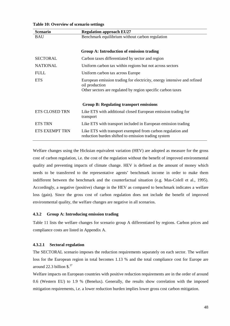
48

Table 10: Overview of scenario settings

Scenario Regulation approach EU27 BAU Benchmark equilibrium without carbon regulation

Group A: Introduction of emission trading

SECTORAL Carbon taxes differentiated by sector and region

NATIONAL Uniform carbon tax within regions but not across sectors

FULL Uniform carbon tax across Europe

ETS European emission trading for electricity, energy intensive and refined oil production Other sectors are regulated by region specific carbon taxes

Group B: Regulating transport emissions

ETS CLOSED TRN Like ETS with additional closed European emission trading for transport

ETS TRN Like ETS with transport included in European emission trading

ETS EXEMPT TRN Like ETS with transport exempted from carbon regulation and reduction burden shifted to emission trading system

Welfare changes using the Hicksian equivalent variation (HEV) are adopted as measure for the gross

cost of carbon regulation, i.e. the cost of the regulation without the benefit of improved environmental

quality and preventing impacts of climate change. HEV is defined as the amount of money which

needs to be transferred to the representative agents’ benchmark income in order to make them

indifferent between the benchmark and the counterfactual situation (e.g. Mas-Colell et al., 1995).

Accordingly, a negative (positive) change in the HEV as compared to benchmark indicates a welfare

loss (gain). Since the gross cost of carbon regulation does not include the benefit of improved

environmental quality, the welfare changes are negative in all scenarios.

4.3.2 Group A: Introducing emission trading

Table 11 lists the welfare changes for scenario group A differentiated by regions. Carbon prices and

compliance costs are listed in Appendix A.

4.3.2.1 Sectoral regulation

The SECTORAL scenario imposes the reduction requirements separately on each sector. The welfare

loss for the European region in total becomes 1.13 % and the total compliance cost for Europe are

around 22.3 billion $.37

Welfare impacts on European countries with positive reduction requirements are in the order of around

0.6 (Western EU) to 1.9 % (Benelux). Generally, the results show correlation with the imposed

mitigation requirements, i.e. a lower reduction burden implies lower gross cost carbon mitigation.

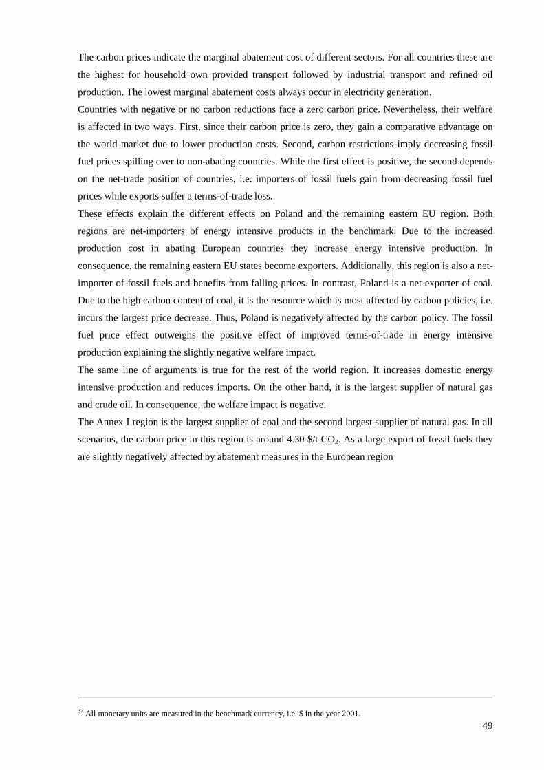
49

The carbon prices indicate the marginal abatement cost of different sectors. For all countries these are

the highest for household own provided transport followed by industrial transport and refined oil

production. The lowest marginal abatement costs always occur in electricity generation.

Countries with negative or no carbon reductions face a zero carbon price. Nevertheless, their welfare

is affected in two ways. First, since their carbon price is zero, they gain a comparative advantage on

the world market due to lower production costs. Second, carbon restrictions imply decreasing fossil

fuel prices spilling over to non-abating countries. While the first effect is positive, the second depends

on the net-trade position of countries, i.e. importers of fossil fuels gain from decreasing fossil fuel

prices while exports suffer a terms-of-trade loss.

These effects explain the different effects on Poland and the remaining eastern EU region. Both

regions are net-importers of energy intensive products in the benchmark. Due to the increased

production cost in abating European countries they increase energy intensive production. In

consequence, the remaining eastern EU states become exporters. Additionally, this region is also a net-

importer of fossil fuels and benefits from falling prices. In contrast, Poland is a net-exporter of coal.

Due to the high carbon content of coal, it is the resource which is most affected by carbon policies, i.e.

incurs the largest price decrease. Thus, Poland is negatively affected by the carbon policy. The fossil

fuel price effect outweighs the positive effect of improved terms-of-trade in energy intensive

production explaining the slightly negative welfare impact.

The same line of arguments is true for the rest of the world region. It increases domestic energy

intensive production and reduces imports. On the other hand, it is the largest supplier of natural gas

and crude oil. In consequence, the welfare impact is negative.

The Annex I region is the largest supplier of coal and the second largest supplier of natural gas. In all

scenarios, the carbon price in this region is around 4.30 $/t CO2. As a large export of fossil fuels they

are slightly negatively affected by abatement measures in the European region

37 All monetary units are measured in the benchmark currency, i.e. $ in the year 2001.

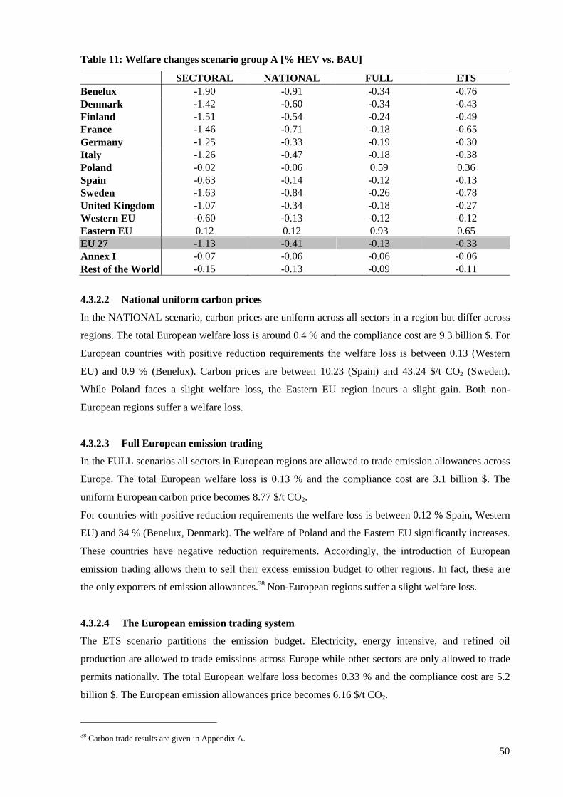
50

Table 11: Welfare changes scenario group A [% HEV vs. BAU]

SECTORAL NATIONAL FULL ETS Benelux -1.90 -0.91 -0.34 -0.76 Denmark -1.42 -0.60 -0.34 -0.43 Finland -1.51 -0.54 -0.24 -0.49 France -1.46 -0.71 -0.18 -0.65 Germany -1.25 -0.33 -0.19 -0.30 Italy -1.26 -0.47 -0.18 -0.38 Poland -0.02 -0.06 0.59 0.36 Spain -0.63 -0.14 -0.12 -0.13 Sweden -1.63 -0.84 -0.26 -0.78 United Kingdom -1.07 -0.34 -0.18 -0.27 Western EU -0.60 -0.13 -0.12 -0.12 Eastern EU 0.12 0.12 0.93 0.65 EU 27 -1.13 -0.41 -0.13 -0.33 Annex I -0.07 -0.06 -0.06 -0.06 Rest of the World -0.15 -0.13 -0.09 -0.11

4.3.2.2 National uniform carbon prices

In the NATIONAL scenario, carbon prices are uniform across all sectors in a region but differ across

regions. The total European welfare loss is around 0.4 % and the compliance cost are 9.3 billion $. For

European countries with positive reduction requirements the welfare loss is between 0.13 (Western

EU) and 0.9 % (Benelux). Carbon prices are between 10.23 (Spain) and 43.24 $/t CO2 (Sweden).

While Poland faces a slight welfare loss, the Eastern EU region incurs a slight gain. Both non-

European regions suffer a welfare loss.

4.3.2.3 Full European emission trading

In the FULL scenarios all sectors in European regions are allowed to trade emission allowances across

Europe. The total European welfare loss is 0.13 % and the compliance cost are 3.1 billion $. The

uniform European carbon price becomes 8.77 $/t CO2.

For countries with positive reduction requirements the welfare loss is between 0.12 % Spain, Western

EU) and 34 % (Benelux, Denmark). The welfare of Poland and the Eastern EU significantly increases.

These countries have negative reduction requirements. Accordingly, the introduction of European

emission trading allows them to sell their excess emission budget to other regions. In fact, these are

the only exporters of emission allowances.38 Non-European regions suffer a slight welfare loss.

4.3.2.4 The European emission trading system

The ETS scenario partitions the emission budget. Electricity, energy intensive, and refined oil

production are allowed to trade emissions across Europe while other sectors are only allowed to trade

permits nationally. The total European welfare loss becomes 0.33 % and the compliance cost are 5.2

billion $. The European emission allowances price becomes 6.16 $/t CO2.

38 Carbon trade results are given in Appendix A.

51

For countries with positive reduction burdens the welfare loss is between 0.12 (Western EU) and 0.78

% (Sweden). National carbon prices range between 10.81 (Western EU) and 46.73 $/t CO2 (Sweden).

Countries with negative reduction requirements allocate their excess budget to the emission trading

system. Consequently, they are able to export emission allowances and thus, incur a welfare gain.

Since emissions of non-trading sectors are capped at the benchmark level, they have slightly positive

domestic carbon prices. Again, non-European regions suffer a slight welfare loss.

4.3.2.5 Comparison

The ranking of the scenarios in terms of the European welfare loss is as expected. The SECTORAL

scenario shows the highest welfare loss followed by the NATIONAL approach since NATIONAL

emission trading increases the flexibility of carbon abatement. Put differently, domestic carbon trade

equalizes the marginal abatement costs within regions.

Compared the NATIONAL scenario, the introduction of the EU ETS has two counteracting effects.

On the one hand, flexibility is increased by allowing European trade of electricity, refined oil, and

energy intensive production. On the other, flexibility is decreasing since trade across sectors is

restricted by partitioning the emission budget. The results show that the positive effect of European

trade prevails and European welfare improves. Remarkably, the welfare of all European countries

improves, i.e. introducing the EU ETS under the effort sharing reduction requirements provides a

Pareto improvement.39

Since the FULL European emission trading system removes the partition of the emission budget and

allows fully flexible emission abatement across sectors and regions, it shows the lowest European

welfare loss. Again, the result also establishes at the member state level.

While the Annex I region is nearly unaffected by European regulation approaches, the welfare of the

rest of the world region improves with increasing flexibility of carbon abatement in Europe. Coal is

the resource with the highest emission factor. Accordingly, it is always favorable to substitute the

usage of coal by other energy resources. Increased flexibility in Europe also increases the substitution

possibilities of coal usage. Consequently, demand for other energy resources increases. The rest of

world region as the largest exporter of natural gas and crude oil benefits from this demand increase.

This result can also be seen in the welfare effects for Poland in the SECTORAL and NATIONAL

scenarios. Since Poland is an exporter of coal but importer of other resources, it is negatively affected

of the increased carbon abatement flexibility of European regions.

39 This result depends on the imposed reduction burdens. Using reduction requirements of the Burden Sharing Agreement (EC, 2002), Böhringer (2002) shows that the introduction of full emission trading across Europe does not provide a Pareto improvement. In his study, for some countries (Germany, Austria, France) the loss in comparative advantages in energy intensive production induced by equalization of carbon prices overbalances the positive effect of equalized marginal abatement cost.

52

4.3.3 Group B: Regulation of transport emissions

The second scenario group analyzes different regulation approaches to the emissions caused by

transport. The welfare results are listed in Table 12. As the results of this group are compared against

the current EU ETS system, the welfare results of the ETS scenario are repeated in this table.

4.3.3.1 Closed emission trading for transport sectors

The scenario ETS CLOSED TRN introduces a closed emission trading system for transport sectors

across Europe. Both, industrial and household transport, are allowed to trade allowances across

Europe. However, trade with EU ETS sectors is not possible. This scenario can also be interpreted as a

European wide carbon tax in the transport sector. Compared to the ETS scenario, the effects of this

scenario group are threefold: First, flexibility is positively influenced by allowing allowances trade of

transport sectors across Europe. Second, flexibility is negatively influenced by further restricting trade

across national sectors exempting transport sectors from the national strategy. Third, the emission

budget under the emission trading scheme alters. Countries with negative reduction requirements

allocate permits to the transport system according to the NATIONAL scenario. Since they do not face

a carbon restriction in this scenario, transport emissions are rising. Consequently, they allocate part of

there excess budget to the transport trading system. Furthermore, since emissions of national sectors in

these countries are capped at the benchmark level, the carbon budget of the EU ETS system

necessarily decreases compared to the ETS scenario.

The total European welfare loss becomes 0.31 % which is only a slight improvement compared to the

EU ETS system. Due to the lower emission budget under the EU ETS, the European allowances price

is increasing by 3.65 to 9.81 $/t CO2. The carbon price in the transport trading system becomes 17.71

$/t CO2 indicating the higher marginal abatement cost in transport sectors.

Although the gross cost of regulation are slightly decreasing, total compliance cost in Europe increase

by around 1.2 to 6.4 billion $. The increase of compliance cost is due to a restriction of the flexibility

of carbon mitigation which prevents equalization of marginal abatement cost across transport and

other sectors under the national emission trading schemes which overbalances the increased flexibility

by trade of transport sectors across Europe. However, refined oil in transport sectors is the commodity

which shows the highest tax rate across all inputs. Consequently, the decrease in the carbon price for

transport sectors reduces the tax interaction effect of carbon and transport taxes. This positive effect

outweighs the negative effect of increasing compliance cost.

The effect can be seen at the member state level. Countries with high national taxes in the ETS

scenario (Benelux, France, Italy, Sweden) gain, since for these countries the decline in the carbon

price of transport is the highest and, thus the positive effect of reduced tax interaction. Furthermore,

some of these countries also benefit from decreasing compliance cost. In contrast, countries with

carbon taxes in the ETS scenario below or the carbon price in the transport sector (Germany, Spain,

remaining west European countries) all incur a welfare loss, since tax interaction and compliance costs

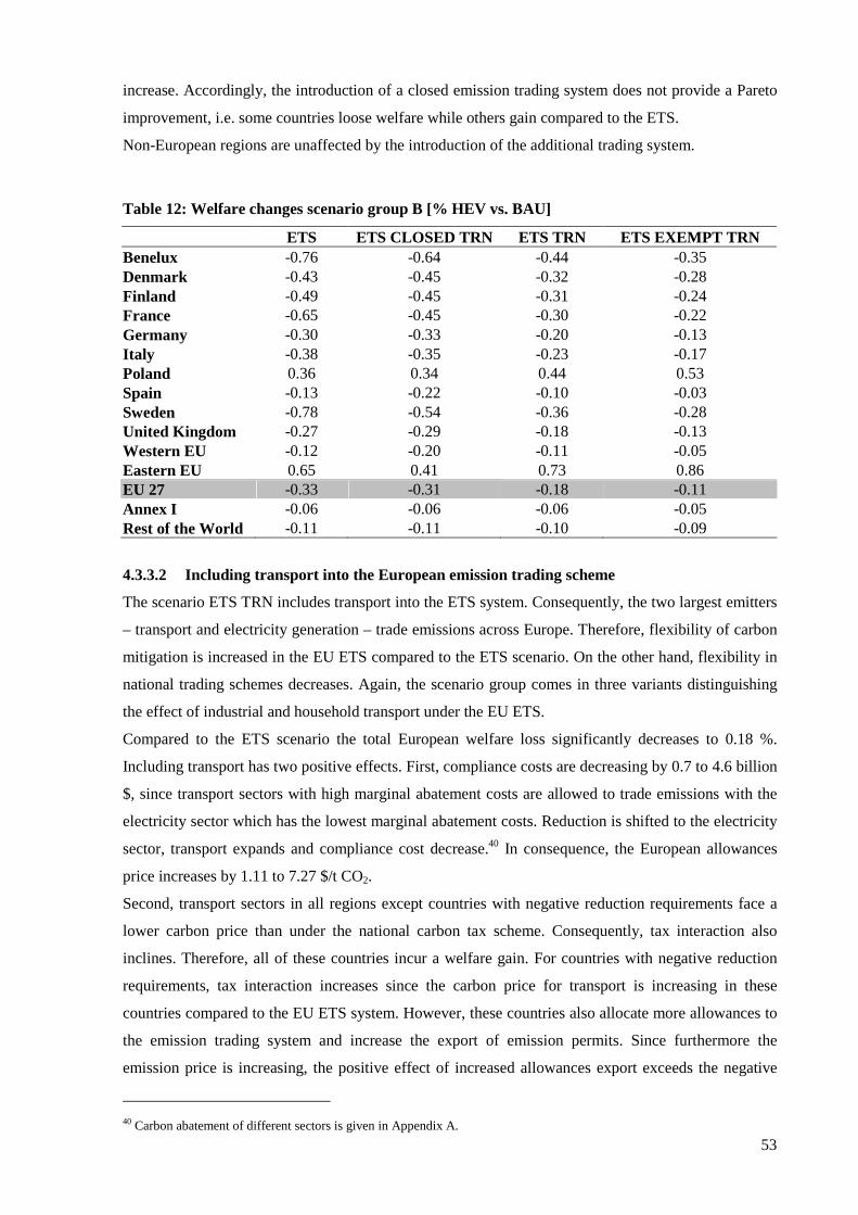
53

increase. Accordingly, the introduction of a closed emission trading system does not provide a Pareto

improvement, i.e. some countries loose welfare while others gain compared to the ETS.

Non-European regions are unaffected by the introduction of the additional trading system.

Table 12: Welfare changes scenario group B [% HEV vs. BAU]

ETS ETS CLOSED TRN ETS TRN ETS EXEMPT TRN Benelux -0.76 -0.64 -0.44 -0.35 Denmark -0.43 -0.45 -0.32 -0.28 Finland -0.49 -0.45 -0.31 -0.24 France -0.65 -0.45 -0.30 -0.22 Germany -0.30 -0.33 -0.20 -0.13 Italy -0.38 -0.35 -0.23 -0.17 Poland 0.36 0.34 0.44 0.53 Spain -0.13 -0.22 -0.10 -0.03 Sweden -0.78 -0.54 -0.36 -0.28 United Kingdom -0.27 -0.29 -0.18 -0.13 Western EU -0.12 -0.20 -0.11 -0.05 Eastern EU 0.65 0.41 0.73 0.86 EU 27 -0.33 -0.31 -0.18 -0.11 Annex I -0.06 -0.06 -0.06 -0.05 Rest of the World -0.11 -0.11 -0.10 -0.09

4.3.3.2 Including transport into the European emission trading scheme

The scenario ETS TRN includes transport into the ETS system. Consequently, the two largest emitters

– transport and electricity generation – trade emissions across Europe. Therefore, flexibility of carbon

mitigation is increased in the EU ETS compared to the ETS scenario. On the other hand, flexibility in

national trading schemes decreases. Again, the scenario group comes in three variants distinguishing

the effect of industrial and household transport under the EU ETS.

Compared to the ETS scenario the total European welfare loss significantly decreases to 0.18 %.

Including transport has two positive effects. First, compliance costs are decreasing by 0.7 to 4.6 billion

$, since transport sectors with high marginal abatement costs are allowed to trade emissions with the

electricity sector which has the lowest marginal abatement costs. Reduction is shifted to the electricity

sector, transport expands and compliance cost decrease.40 In consequence, the European allowances

price increases by 1.11 to 7.27 $/t CO2.

Second, transport sectors in all regions except countries with negative reduction requirements face a

lower carbon price than under the national carbon tax scheme. Consequently, tax interaction also

inclines. Therefore, all of these countries incur a welfare gain. For countries with negative reduction

requirements, tax interaction increases since the carbon price for transport is increasing in these

countries compared to the EU ETS system. However, these countries also allocate more allowances to

the emission trading system and increase the export of emission permits. Since furthermore the

emission price is increasing, the positive effect of increased allowances export exceeds the negative

40 Carbon abatement of different sectors is given in Appendix A.

54

one of increased tax interaction. Therefore welfare of these countries also improves. Consequently, the

introduction of transport provides a Pareto improvement for the European carbon policy.

Again, the effect on non-European countries is negligible.

4.3.3.3 Exempting transport from carbon regulation

The ETS EXEMPT TRN scenario analyzes the full exemption of transport from any carbon policy.

Transport sectors are unregulated and the resulting reduction burden is shifted to EU ETS. Other

sectors are still regulated under nationally uniform carbon taxes.

Compared to the ETS scenario, the loss in European welfare significantly decreases by 0.22 to 0.11 %.

Remarkably, welfare even improves compared to the FULL scenario, which implements full flexibility

of carbon mitigation by allowing trade across all sectors and European countries and showed a welfare

loss of 0.13 %.

Compared to the ETS scenario compliance costs are decreasing by 0.5 to 4.8 billion $. The decrease of

the compliance cost is explained by the increased reduction burden in the EU ETS. In the ETS case, all

countries with positive reduction requirements have higher national carbon prices. Since the increased

abatement effort in the EU ETS increases the allowances price by 1.94 to 8.10 $/t CO2, carbon prices

getting closer to uniform across sectors. Consequently, the marginal abatement cost are closer to

uniform and cost efficiency is improved. Countries with negative reduction burdens again gain by the

increase in the emission price since they are exporters of permits. Put differently, shifting the

reduction burden of the transport sector to the EU ETS system it is possible to reduce more emissions

in the electricity at lower cost. Therefore compliance costs decrease.

The exemption of transport completely removes the interaction effect between transport taxes and

carbon prices. Consequently, the positive effect of reducing the difference of effective carbon prices is

maximized.

The exemption is Pareto optimal in the sense that all member states benefit compared to the ETS

system.

The scenario also has an impact on the rest of the world region. The exemption of transport stipulates

the use of transport fuels compared to the ETS scenario. Accordingly, the crude oil price increases.

Since the rest of the world region is by far the largest exporter of crude oil, it incurs a welfare gain.

4.3.3.4 Comparison

Comparing the transport regulation approaches shows a clear-cut ranking in terms of welfare: The

total exemption of transport improves welfare compared to the inclusion into the EU ETS which

performs superior to the closed emission trading approach.

The improvement of emission trading under the EU ETS to the closed emission trading is caused by

two positive effects. Flexibility of carbon abatement increases and therefore the compliance cost

decrease. Furthermore since the carbon price for transport sectors is decreasing tax-interaction also

decreases.

55

Comparing emission trading under the EU ETS to the full exemption of transport, the effects are

counteracting. On the one hand, compliance costs in the ETS TRN case are lower, due to higher

flexibility of carbon abatement. On the other, tax interaction is completely reduced. The positive effect

of reduced interaction prevails explaining the welfare improvement.

4.3.4 Sensitivity analysis

Substitution elasticities used in production function show homogeneity across the environmental,

energy related modeling literature. However, elasticities in the household own provided transport

module and the elasticity between aggregated consumption and transport are uncertain. Therefore the

impact of these elasticities is examined by solving the model under different values.

The central value of the substitution elasticity between aggregated consumption and household

transport used in the core analysis was 0.5. The sensitivity of the model results to a change of this

elasticity is examined by varying its value between zero and one. The resulting welfare changes in the

mains scenarios (ETS, ETS TRN, ETS CLOSED TRN, ETS EXEMPT TRN) are listed in Appendix A

and shows that the model results are insensitive altering the elasticity. The same is true for the

elasticity between fuel purchases and other transport cost.

Changing the elasticity between household own provided and purchased transport also does not

influences the results in the core scenarios. While this might come as a surprise, it can be explained by

the fact that the main scenarios do not differentiate between carbon regulation in industrial and

household transport. Therefore, both face the same carbon price. Consequently, relative prices are

hardly affected and no substitution occurs.

The magnitude to welfare effects reacts sensitive to a change in the elasticity of fuel demand.

However, the qualitative implications are unaffected, i.e. the welfare ranking between imposed policy

measures remains stable.

4.4 Conclusion

This chapter employs a multi-region top-down computable general equilibrium model analyzing the

effect of different approaches to carbon mitigation in the transport sector. The GTAP 6 database

augmented by European data needed to model household transport provides the data necessary to

calibrate the model. Three different policy approaches for the transport sector are tested: i) a closed

emission trading system beside the EU; ii) the inclusion of transport into the EU ETS; and finally, iii)

the full exemption of transport from carbon regulation increasing the reduction burden in the EU ETS.

A closed emission trading system for transport only provides small welfare gains. Furthermore, the

political feasibility of introducing such a system is in doubt since it does not provide a Pareto

improvement on the member state level.

Both, transport under emission trading and the full exemption of transport, lead to the reduction of the

gross cost of carbon regulation. Independently on which approach is chosen, it is possible to shift

56

abatement to the electricity sector which has the lowest marginal abatement costs. Therefore,

European cost of compliance with the reduction requirements decrease. Moreover, both approaches

provide Pareto improvements on the member state level indicating good political feasibility.

The exemption of transport from carbon regulation shows lower welfare losses than the inclusion into

the EU ETS due to high taxes on transport fuels in the benchmark equilibrium. These taxes interact

with carbon prices in the transport sector leading to negative welfare impacts. Since the exemption of

transport leads to transport carbon taxes of zero, the negative tax interaction effect vanishes. In

consequence, the gross costs of carbon mitigation are even lower than in a situation where carbon

abatement is fully flexible across Europe and sectors.

However, the model employed in this chapter does not account for externalities in an explicit way. As

outlined, transport externalities other than global warming justify a higher tax on transport fuels to

internalize external effects auch as congestion, accidents, and noise. Therefore, neglecting these

externalities, the model overestimates the beneficial effect of excluding transport from carbon

regulation. Thus, congestion as the main externality of transport is explicitly included in the modeling

framework in the next chapter.

57

5 Technology Rich CGE Model of Germany

5.1 Introduction

This chapter employs a small open economy model calibrated to the German economy in the year

2004. Although small open economy models have the disadvantage of abstracting from changes in the

terms-of-trade assuming infinitely elastic world demand and supply, they have the advantage of

modeling technological details. The model presented is designed to analyze the interaction between

electricity generation and carbon measures in road transport, especially private transport. Accordingly,

electricity production is represented by different generation technologies and accounts for different

load segments. Private transport occurs by either using automobiles differentiated by fuel type or

public transport modes. Accounting endogenously for the main externality of transport, congestion is

included differentiated by travel period and road type.

The introduction of an emission trading between electricity generation, energy intensive industries,

and refineries is analyzed. It is compared to the inclusion of road transport into the trading scheme, a

separate fuel tax increase, and a full exemption of road transport from carbon regulation. Moreover,

including air transport in the trading system is examined. A further scenario relates to the recycling of

revenues raised by the introduction of emission trading increasing subsidies on private transport.

The results show that an increase in fuel taxation leads to large welfare losses. Also the inclusion of

transport into emission trading does not provide welfare gains. However, the full exemption of

transport and moving the reduction burden to the emission trading system decreases the gross cost of

carbon regulation. Including aviation into the trading scheme is a favorable option. Using the income

of carbon regulation to increase public transport subsidies shows the best performance of all scenarios.

5.2 Model description

5.2.1 Overview

The model is formulated as a mixed complementarity problem. Three classes of equilibrium

conditions exist. No activity makes positive profits (zero-profit condition). Excess supply is positive

(market clearing condition). Each household fulfils his budget restriction. Each class is associated to a

class of variables. Activity levels are associated with zero-profit conditions. Prices are connected to

market clearing equations. Each budget restriction determines the income level of the respective

household.

The basic assumptions of the model are:

• The model is static.

• The economy is small compared to the world market, i.e. world market prices are fix and

taken as given (small open economy assumption). Furthermore, the balance of payment deficit

is fix.

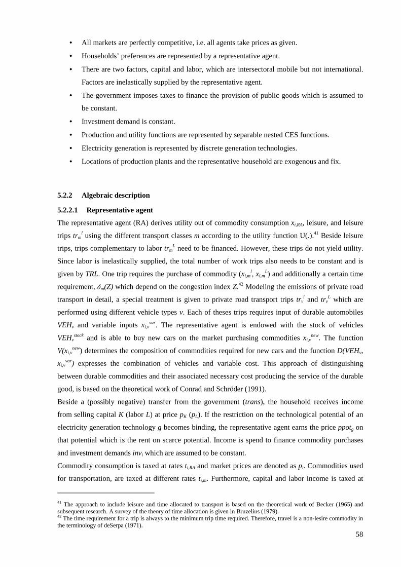
58

• All markets are perfectly competitive, i.e. all agents take prices as given.

• Households’ preferences are represented by a representative agent.

• There are two factors, capital and labor, which are intersectoral mobile but not international.

Factors are inelastically supplied by the representative agent.

• The government imposes taxes to finance the provision of public goods which is assumed to

be constant.

• Investment demand is constant.

• Production and utility functions are represented by separable nested CES functions.

• Electricity generation is represented by discrete generation technologies.

• Locations of production plants and the representative household are exogenous and fix.

5.2.2 Algebraic description

5.2.2.1 Representative agent

The representative agent (RA) derives utility out of commodity consumption xi,RA, leisure, and leisure

trips trml using the different transport classes m according to the utility function U(.).41 Beside leisure

trips, trips complementary to labor trmL need to be financed. However, these trips do not yield utility.

Since labor is inelastically supplied, the total number of work trips also needs to be constant and is

given by TRL. One trip requires the purchase of commodity (xi,ml, xi,m

L) and additionally a certain time

requirement, δm(Z) which depend on the congestion index Z.42 Modeling the emissions of private road

transport in detail, a special treatment is given to private road transport trips trvl and trv

L which are

performed using different vehicle types v. Each of theses trips requires input of durable automobiles

VEHv and variable inputs xi,vvar. The representative agent is endowed with the stock of vehicles

VEHvstock and is able to buy new cars on the market purchasing commodities xi,v

new. The function

V(xi,vnew) determines the composition of commodities required for new cars and the function D(VEHv,

xi,vvar) expresses the combination of vehicles and variable cost. This approach of distinguishing

between durable commodities and their associated necessary cost producing the service of the durable

good, is based on the theoretical work of Conrad and Schröder (1991).

Beside a (possibly negative) transfer from the government (trans), the household receives income

from selling capital K (labor L) at price pK (pL). If the restriction on the technological potential of an

electricity generation technology g becomes binding, the representative agent earns the price ppotg on

that potential which is the rent on scarce potential. Income is spend to finance commodity purchases

and investment demands invi which are assumed to be constant.

Commodity consumption is taxed at rates ti,RA and market prices are denoted as pi. Commodities used

for transportation, are taxed at different rates ti,m. Furthermore, capital and labor income is taxed at

41 The approach to include leisure and time allocated to transport is based on the theoretical work of Becker (1965) and subsequent research. A survey of the theory of time allocation is given in Bruzelius (1979). 42 The time requirement for a trip is always to the minimum trip time required. Therefore, travel is a non-lesire commodity in the terminology of deSerpa (1971).

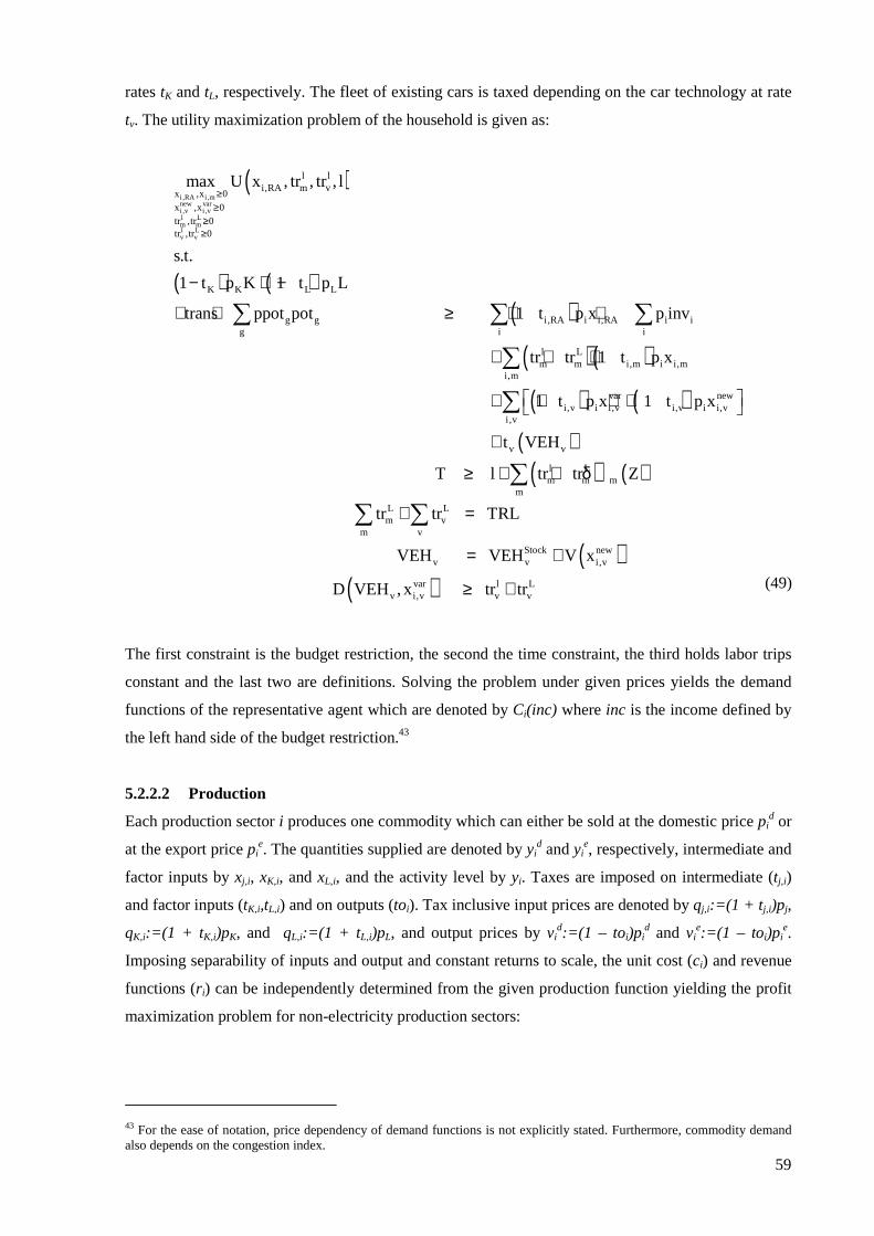
59

rates tK and tL, respectively. The fleet of existing cars is taxed depending on the car technology at rate

tv. The utility maximization problem of the household is given as:

( )

( ) ( )( )

i ,RA i ,mnew vari ,v i ,vl Lm ml Lv v

l li,RA m v

x ,x 0x ,x 0tr ,tr 0tr ,tr 0

K K L L

g g i,RA i i,RA i ig i i

max U x , tr , tr , l

s.t.

1 t p K 1 t p L

trans ppot pot 1 t p x p inv

≥≥

≥≥

− + −

+ + ≥ + +∑ ∑ ∑

( )( )

( ) ( )

l Lm m i,m i i,m

i,m

var newi,v i i,v i,v i i,v

i,v

tr tr 1 t p x

1 t p x 1 t p x

+ + +

+ + + +

∑

∑

( )( ) ( )

v v

l Lm m m

m

L Lm v

m

t VEH

T l tr tr Z

tr tr

+

≥ + + δ

+

∑

∑

( )( )

v

Stock newv v i,v

var l Lv i,v v v

TRL

VEH VEH V x

D VEH , x tr tr

=

= +

≥ +

∑

(49)

The first constraint is the budget restriction, the second the time constraint, the third holds labor trips

constant and the last two are definitions. Solving the problem under given prices yields the demand

functions of the representative agent which are denoted by Ci(inc) where inc is the income defined by

the left hand side of the budget restriction.43

5.2.2.2 Production

Each production sector i produces one commodity which can either be sold at the domestic price pid or

at the export price pie. The quantities supplied are denoted by yi

d and yie, respectively, intermediate and

factor inputs by xj,i, xK,i, and xL,i, and the activity level by yi. Taxes are imposed on intermediate (tj,i)

and factor inputs (tK,i,tL,i) and on outputs (toi). Tax inclusive input prices are denoted by qj,i:=(1 + t j,i)pj,

qK,i:=(1 + t K,i)pK, and qL,i:=(1 + t L,i)pL, and output prices by vid:=(1 – toi)pi

d and vie:=(1 – toi)pi

e.

Imposing separability of inputs and output and constant returns to scale, the unit cost (ci) and revenue

functions (r i) can be independently determined from the given production function yielding the profit

maximization problem for non-electricity production sectors:

43 For the ease of notation, price dependency of demand functions is not explicitly stated. Furthermore, commodity demand also depends on the congestion index.

60

( ) ( )i

d ei i i i i j,i K,i L,i i

y 0max r v , v y c q ,q ,q y i\{electricity}

≥− ∀ (50)

Solving the problem under given prices results in the firm’s zero-profit conditions which determine the

optimal activity levels:

( ) ( )d ei j,i K,i L,i i i i ic q ,q ,q r v , v y 0 i\{electricity}≥ ⊥ ≥ ∀ (51)

Given the optimal activity level, optimal input and output quantities can be derived using Shepard’s

lemma:

i i ij,i i K,i i L,i i

j,i K,i L,i

d ei ii i i id e

i i

c c cx y x y x y

q q q

r ry y y y

v v

∂ ∂ ∂= = =∂ ∂ ∂

∂ ∂= =∂ ∂

(52)

The electricity sector is involved in two activities: electricity generation and an activity which

represents overhead and transmission and distribution. Electricity generation is represented by

different technologies g. The technological potentials potg restrict the use of technologies. The

generation level of technology g is denoted as ygGEN and the associated price pg

GEN. One unit of

generation of technology requires bi,g (bK,g, bL,g) units of commodity i (capital, labor). Given the

demand for electricity (xELE), the optimal generation mix is determined by minimizing the generation

cost under the constraints that generation may not exceed the technological potential and that demand

has to be fulfilled.

ELEg

GENL L,g K K,g i i,g g

y 0 g i

GENg g g

GEN ELE ELEg

g

min p b p b p b y

s.t.

pot y ppot 0 g

y x p 0

≥

+ +

≥ ⊥ ≥ ∀

≥ ⊥ ≥

∑ ∑

∑

(53)

The Lagrangian multiplier ppotg, is the scarcity price of the technological potential. And pELE is the

price of one unit electricity under the optimal generation mix.44 Consequently, the constraints have the

interpretation of market clearing conditions. If potential exceeds generation, the price is zero; if the

44 The prices are given in monetary per energy units. For example, if generation is measured in megawatt hours and prices are given in euro, the objective function is measured in euro and the constraints in megawatt hours. Consequently, the multipliers are given in euro per megawatt hour. This implies that the technological potential and total electricity demand are also given in megawatt hours.

61

potential is scarce, the constraint is binding and the price becomes positive. A similar interpretation is

given for the demand constraint. However, the electricity price will never become zero as long as

demand is positive since excess generation results in excess cost which contrasts the objective of cost

minimization. The general equilibrium concept of circular value flows requires determining the supply

of the technological potential and electricity demand. Thus, the potential is added to the representative

agent’s endowment. Physical electricity demand is determined by the electricity sector (see below).

The first order condition of the optimization problem (53) is given as:

ELE GENL L,g K K,g i i,g g g

i

p b p b p b ppot p y 0 g+ + + ≥ ⊥ ≥ ∀∑ (54)

Equation (54) is the zero-profit condition for generation technologies. Producing one unit of electricity

yields revenues equal to the electricity price. Costs are determined by factor and commodity

requirements and rents on scarce technological potential. If costs exceed revenues the technology

makes losses and does not generate electricity. Otherwise the generation level becomes positive.

Given the optimal generation levels, the demand of technologies is given as:

GEN GEN GEN GEN GEN GENL L,g g L K,g g i i,g g

g g g

x b y x b y x b y= = =∑ ∑ ∑ (55)

The electricity sector combines factor and commodity demands for overhead and transmission and

distribution with electricity generation. Thus, physical electricity produced flows from generation

technologies to the electricity sector. Consequently, it produces the composite electricity commodity

including generation and overhead and transmission and distribution cost. The rest of the economy

demands this composite, i.e. pays a price sufficient to cover generation costs as well as the cost for

other activities. Therefore, the profit optimization problem of the electricity sector and the

corresponding zero-profit condition become:

( ) ( )i

d e ELEi i i i i j,i K,i L,i i

y 0max r v , v y c q ,q ,q ,p y i {electricity}

≥− = (56)

( ) ( )ELE d ei j,i K,i L,i i i i i ic q ,q ,q ,p r v , v y y 0 i {electricity}≥ ⊥ ≥ = (57)

The commodity and factor demand functions are equivalent to those stated in equation (52). Physical

electricity demand is given as:

( )ELE

i j,i K,i L,iELEELE

c q ,q ,q ,px

p

∂=

∂ (58)

62

5.2.2.3 International trade and government

Following Armington (1969), imported and domestic produced commodities are combined to the total

available quantity on the domestic market ai with a constant elasticity of substitution function.45 The

corresponding cost function is denoted cia(pi

d, piim) and depends on domestic producer prices pi

d and

import prices piim. The Armington sector sells the aggregate at the market price pi. Consequently, the

profit optimization problem becomes:

( )ai

a d im ai i i i i

y 0max p c p ,p y

≥ − (59)

The zero-profit condition, which determines the total availability of commodity i, is given as:

( )a d im ai i i i ic p ,p p y 0≥ ⊥ ≥ (60)

The demand for domestic and imported commodities is derived using Shephard’s Lemma:

( ) ( )a d im a d im

i i i i i id imi id im

i i

c p ,p c p ,px x

p p

∂ ∂= =

∂ ∂ (61)

The public demand of the government is constant and given by Gi. Furthermore, the government

finances the balance of payment deficit (bop), which is also assumed to be constant, and the transfer to

the household. Demand is financed by the imposed taxes. Consequently, if tax revenues are changing,

either the transfer or taxes need to be changed in order to balance the budget restriction of the

government. This approach allows analyzing refinancing and revenue-recycling effects but neglects

influences on the composition of public spending.

5.2.3 Market clearing conditions

The market price pi is determined by the supply of the Armington commodity and the demand of all

agents:

( )a GENi i, j i i i i

j

y x x C inc G p 0≥ + + + ⊥ ≥∑ (62)

45 A more sophisticated approach would be to specify an Armington aggregate for every agent in the economy. However, two problems arise. First, the models dimension increases. For example, if the number of commodities and production sectors is ten, it follows with one household and a government that twelve activities have to be modelled. Consequently, the number of Armington aggregates rises from ten to 120. Second and more important, reliable estimates of Armington elasticities differentiated by agent and commodity are not available.

63

Similar, the market clearing equations for factors are given as:

GENK,i K K

i

GENL,i L L

i

K x x p 0

L x x p 0

≥ + ⊥ ≥

≥ + ⊥ ≥

∑

∑ (63)

Under the small open economy assumption, world market prices are constant. Furthermore, the

balance of payments is assumed to be constant. Consequently, the sum of all exports evaluated at fix

world market prices equals the sum of all imports at world market prices and the balance of payment

deficit:

e e im im fxi i i i

i i

p y p x bop p 0≥ + ⊥ ≥∑ ∑ (64)

Upper bars denote constant world prices. The price pfx is the current exchange rate which adjusts in

order to fulfill the trade balance. The import and export prices faced by the economy’s agent are

connected to world market prices by the current exchange rate:

e e fx im im fxi i i ip p p p p p= + = + (65)

Figure 6 summarizes the full algebraic model formulation:

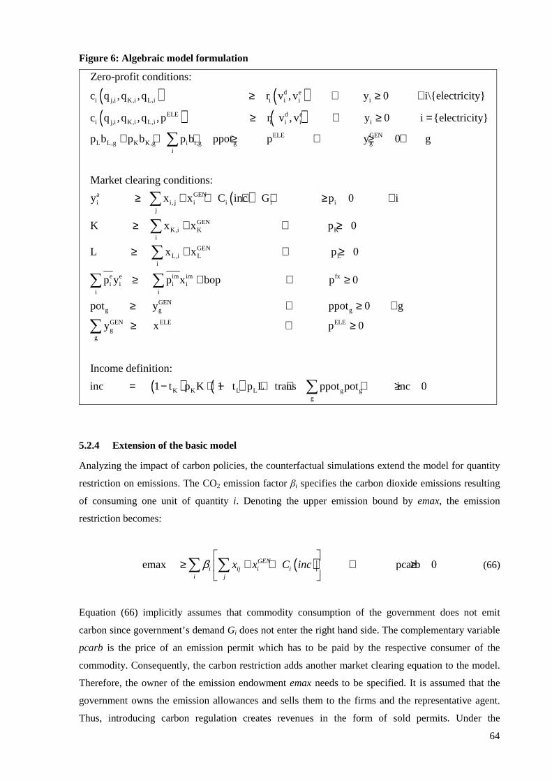
64

Figure 6: Algebraic model formulation

( ) ( )( ) ( )

d ei j,i K,i L,i i i i i

ELE d ei j,i K,i L,i i i i

Zero-profit conditions:

c q ,q ,q r v , v y 0 i\{electricity}

c q ,q ,q ,p r v , v

≥ ⊥ ≥ ∀

≥ ⊥

( )

i

ELE GENL L,g K K,g i i,g g g

i

a GENi i, j i i i i

j

y 0 i {electricity}

p b p b p b ppot p y 0 g

Market clearing conditions:

y x x C inc G p 0

≥ =

+ + + ≥ ⊥ ≥ ∀

≥ + + + ⊥ ≥

∑

∑GEN

K,i K Ki

GENL,i L L

i

e e im imi i i i

i i

i

K x x p 0

L x x p 0

p y p x bop

∀

≥ + ⊥ ≥

≥ + ⊥ ≥

≥ +

∑

∑

∑ ∑ fx

GENg g g

GEN ELE ELEg

g

p 0

pot y ppot 0 g

y x p 0

Income definitio

⊥ ≥

≥ ⊥ ≥ ∀

≥ ⊥ ≥∑

( ) ( )K K L L g gg

n:

inc 1 t p K 1 t p L trans ppot pot inc 0 = − + − + + ⊥ ≥∑

5.2.4 Extension of the basic model

Analyzing the impact of carbon policies, the counterfactual simulations extend the model for quantity

restriction on emissions. The CO2 emission factor βi specifies the carbon dioxide emissions resulting

of consuming one unit of quantity i. Denoting the upper emission bound by emax, the emission

restriction becomes:

( )emax pcarb 0

≥ + + ⊥ ≥

∑ ∑ GENi ij i i

i j

x x C incβ (66)

Equation (66) implicitly assumes that commodity consumption of the government does not emit

carbon since government’s demand Gi does not enter the right hand side. The complementary variable

pcarb is the price of an emission permit which has to be paid by the respective consumer of the

commodity. Consequently, the carbon restriction adds another market clearing equation to the model.

Therefore, the owner of the emission endowment emax needs to be specified. It is assumed that the

government owns the emission allowances and sells them to the firms and the representative agent.

Thus, introducing carbon regulation creates revenues in the form of sold permits. Under the

65

maintained assumption of constant public good provision, this gives rise to the question on how to

recycle this additional income which will be described in the scenario definitions.

5.2.5 Specification

5.2.5.1 Model dimensions

Table 13 summarizes the model dimensions of the model. The two columns on the upper left identify

the elements of the commodity and sector set i which are divided into three subclasses: non-energy,

energy and transport commodities. Since the model is designed to analyze the interactions of carbon

regulation approaches in the energy and transport market, non-energy commodities are chosen such

that the most important sectors are represented (electricity, energy intensive production, and motor

vehicle production). All fossil fuel energy sources, the refined oil, and transport sectors are explicitly

represented. The road and other transport sector also includes provision of metro and tram services.46

Other sectors are represented by industry classes which are aggregated along the NACE Rev. 2

(Eurostat, 2009) classification scheme. The two columns on the upper right of Table 13 define vehicle

and generation technologies. Two vehicle classes are considered: diesel and gasoline cars. The model

includes all electricity generation technologies used in Germany. The OTHER technology combines

mainly biomass and generation from municipal waste. In order to allow for important technology

switches resulting from carbon restriction, the most important future technologies which are not

already used are included: offshore wind generation and carbon capture and sequestration (CCS)

generation based on either natural gas or lignite.47 The lower part of Table 13 shows the differentiation

of transport trips. Five different transport modes are available for private transport: own private

transport and public transport in form of trains, busses, metros and trams, or airplanes. Furthermore, a

slow mode exists which only requires time input but no monetary cost. Since spatial characteristics are

important to account for the substitutability of the different trips, a further set distinguishes between

short and long distance trips. A trip above 500 km is classified to be long distance.48 Modeling

congestion, which is done for road trips – busses and own private road transport – the time dimension

as well as the area of transport are important. Thus, trips are further classified by the transport periods,

which are characterized by their congestion level, and the road network used. Road networks are

characterized by different freeflow time requirements and congestion levels. Generally, urban streets

have a lower freeflow speed than non-urban streets and are heavier congested.

46 It would by preferable to explicitly represent bus and metro and tram transport. However, the underlying SAM does not identify these production sectors and data allowing a disaggregation of the OTP are not available. Using the other road transport sector expresses the fact that choosing the model dimensions can not be done independently of the creation of the underlying empirical base. 47 The CCS technology based on hard coal is more expensive than based on lignite (Wissel et al., 2008). Consequently, a hard coal technology is not included since cost minimization of the generator implies, that it would never penetratze the market in the presented framework. 48 The distance classification is adopted from the underlying database.

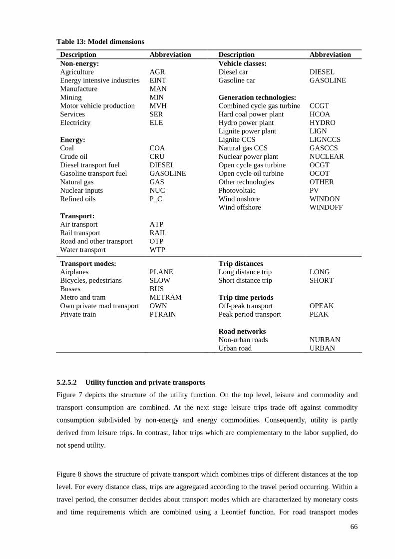
66

Table 13: Model dimensions

Description Abbreviation Description Abbreviation Non-energy: Vehicle classes: Agriculture AGR Diesel car DIESEL Energy intensive industries EINT Gasoline car GASOLINE Manufacture MAN Mining MIN Generation technologies: Motor vehicle production MVH Combined cycle gas turbine CCGT Services SER Hard coal power plant HCOA Electricity ELE Hydro power plant HYDRO Lignite power plant LIGN Energy: Lignite CCS LIGNCCS Coal COA Natural gas CCS GASCCS Crude oil CRU Nuclear power plant NUCLEAR Diesel transport fuel DIESEL Open cycle gas turbine OCGT Gasoline transport fuel GASOLINE Open cycle oil turbine OCOT Natural gas GAS Other technologies OTHER Nuclear inputs NUC Photovoltaic PV Refined oils P_C Wind onshore WINDON Wind offshore WINDOFF Transport: Air transport ATP Rail transport RAIL Road and other transport OTP Water transport WTP

Transport modes: Trip distances Airplanes PLANE Long distance trip LONG Bicycles, pedestrians SLOW Short distance trip SHORT Busses BUS Metro and tram METRAM Trip time periods Own private road transport OWN Off-peak transport OPEAK Private train PTRAIN Peak period transport PEAK Road networks Non-urban roads NURBAN Urban road URBAN

5.2.5.2 Utility function and private transports

Figure 7 depicts the structure of the utility function. On the top level, leisure and commodity and

transport consumption are combined. At the next stage leisure trips trade off against commodity

consumption subdivided by non-energy and energy commodities. Consequently, utility is partly

derived from leisure trips. In contrast, labor trips which are complementary to the labor supplied, do

not spend utility.

Figure 8 shows the structure of private transport which combines trips of different distances at the top

level. For every distance class, trips are aggregated according to the travel period occurring. Within a

travel period, the consumer decides about transport modes which are characterized by monetary costs

and time requirements which are combined using a Leontief function. For road transport modes

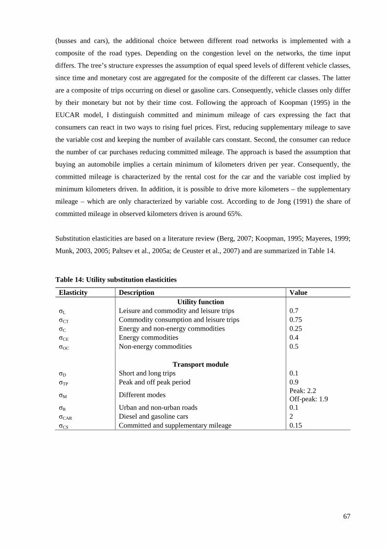
67

(busses and cars), the additional choice between different road networks is implemented with a

composite of the road types. Depending on the congestion level on the networks, the time input

differs. The tree’s structure expresses the assumption of equal speed levels of different vehicle classes,

since time and monetary cost are aggregated for the composite of the different car classes. The latter

are a composite of trips occurring on diesel or gasoline cars. Consequently, vehicle classes only differ

by their monetary but not by their time cost. Following the approach of Koopman (1995) in the

EUCAR model, I distinguish committed and minimum mileage of cars expressing the fact that

consumers can react in two ways to rising fuel prices. First, reducing supplementary mileage to save

the variable cost and keeping the number of available cars constant. Second, the consumer can reduce

the number of car purchases reducing committed mileage. The approach is based the assumption that

buying an automobile implies a certain minimum of kilometers driven per year. Consequently, the

committed mileage is characterized by the rental cost for the car and the variable cost implied by

minimum kilometers driven. In addition, it is possible to drive more kilometers – the supplementary

mileage – which are only characterized by variable cost. According to de Jong (1991) the share of

committed mileage in observed kilometers driven is around 65%.

Substitution elasticities are based on a literature review (Berg, 2007; Koopman, 1995; Mayeres, 1999;

Munk, 2003, 2005; Paltsev et al., 2005a; de Ceuster et al., 2007) and are summarized in Table 14.

Table 14: Utility substitution elasticities

Elasticity Description Value Utility function σL Leisure and commodity and leisure trips 0.7 σCT Commodity consumption and leisure trips 0.75 σC Energy and non-energy commodities 0.25 σCE Energy commodities 0.4 σOC Non-energy commodities 0.5 Transport module σD Short and long trips 0.1 σTP Peak and off peak period 0.9

σM Different modes Peak: 2.2 Off-peak: 1.9

σR Urban and non-urban roads 0.1 σCAR Diesel and gasoline cars 2 σCS Committed and supplementary mileage 0.15

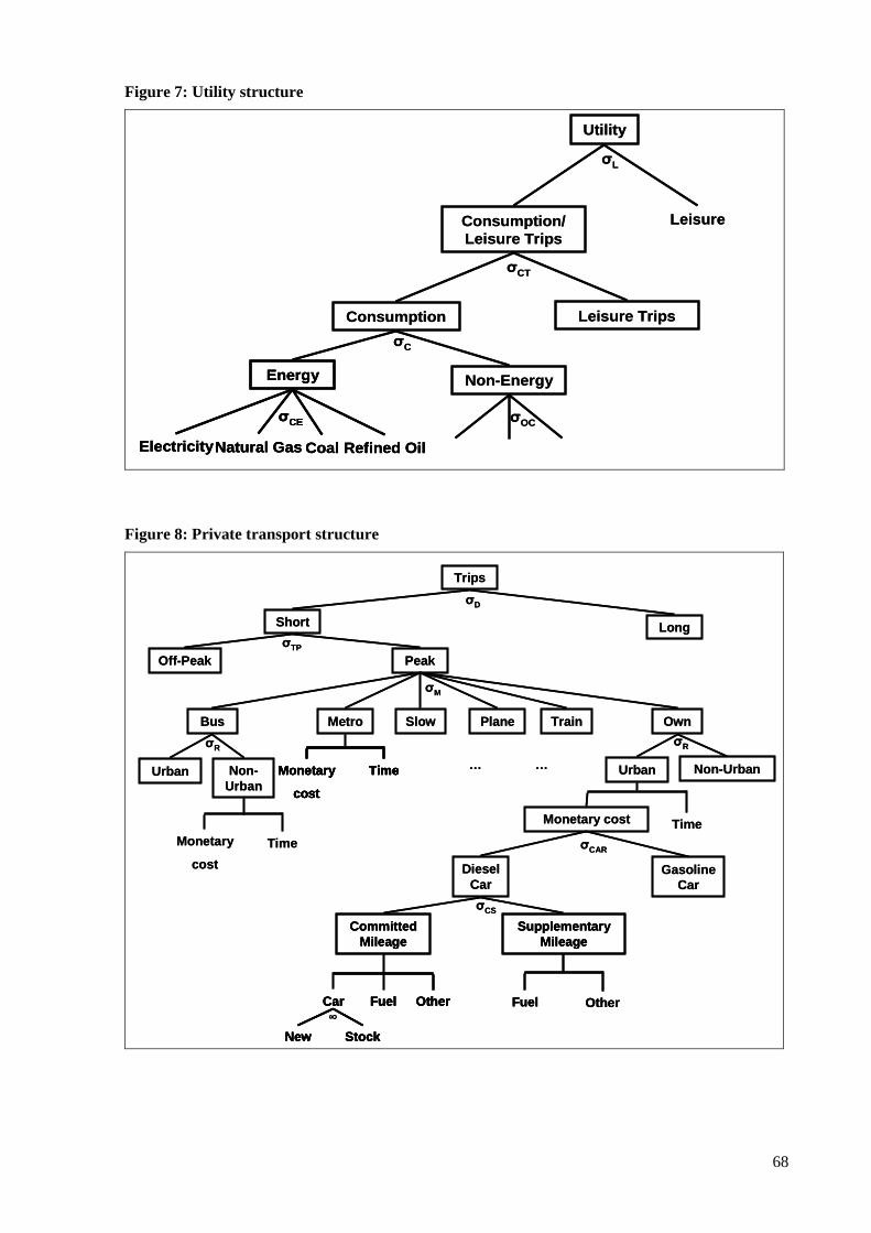
68

Figure 7: Utility structure

Consumption

Energy

Electricity Coal Refined OilNatural Gas

σCE

Non-Energy

σOC

σC

Consumption/ Leisure Trips

Leisure Trips

σCT

Leisure

σL

Utility

Consumption

Energy

Electricity Coal Refined OilNatural Gas

σCE

Energy

Electricity Coal Refined OilNatural Gas

σCE

Non-Energy

σOC

σC

Consumption/ Leisure Trips

Leisure Trips

σCT

Leisure

σL

Utility

Figure 8: Private transport structure

Trips

Short Long

σD

Off-Peak Peak

TrainPlaneBus Metro Slow Own

Monetary

cost

Time

σTP

σM

Time

Diesel Car

Gasoline Car

Committed Mileage

Car Fuel Other

New Stock

σCAR

σCS

Urban Non-Urban

Monetary

cost

Time

Monetary

cost

Time

Urban Non-Urban

Monetary cost

Supplementary Mileage

Fuel Other

… …

∞

σRσR

Trips

Short Long

σD

Off-Peak Peak

TrainPlaneBus Metro Slow Own

Monetary

cost

TimeMonetary

cost

Time

σTP

σM

Time

Diesel Car

Gasoline Car

Committed Mileage

Car Fuel Other

New Stock

Committed Mileage

Car Fuel Other

New Stock

Car Fuel Other

New Stock

σCAR

σCS

Urban Non-Urban

Monetary

cost

Time

Monetary

cost

Time

Urban Non-Urban

Monetary cost

Supplementary Mileage

Fuel Other

Supplementary Mileage

Fuel Other

… …

∞

σRσR

69

5.2.5.3 Production functions

Figure 9 shows the production function of non-electricity sectors. Outputs are modeled using a CET

function at the output side. At the top-level, material inputs, transport, and an aggregate of factor and

energy inputs are combined using a Leontief function. Transportation can either occur on roads or by

water or air transport. Road transport can either be own supplied or purchased from the road transport

sector. Own provided transport is distinguished by different transportation fuels. However, the

transport capital input is not modeled. On the factor and energy side, first a value added composite of

primary factors and an energy aggregate are combined. Another approach would be to combine labor

with a capital/energy aggregate (Burniaux and Truong, 2002). However, van der Werf (2008) tests

different nesting structures of primary factor and energy inputs for twelve OECD countries and shows

that the adopted nesting structure performs best in reproducing observed time series. The energy

aggregate trades off electricity input versus fossil fuel commodities which are further subdivided by

coal and liquid and gaseous commodities.

Figure 10 depicts the electricity production function. At the top level, electricity generation, transport,

material and a value added aggregate are combined using a Leontief function. The transport composite

is the same as for non-electricity sectors. Electricity generation is characterized by three different load

segments: base, middle, and peak load. Depending on their technological specification, generation

technologies produce in different load segments. The differentiation of load segments is important to

avoid unrealistic substitution patterns between technologies. From an economic point of view, base

load power plants are often characterized by high investment and low variable cost. Consequently,

these plants need to run for a large number of hours per year in order to cover fixed costs. From a

technical point of view, base load plants often exhibit a long-start up time, i.e. are limited in their

flexibility. On the other hand, peak load power plants are less expensive in terms of investment cost

but more flexible regarding the start-up time (e.g. Stoft, 2002). Within a load segment, technologies

are perfect substitutes. Technologies are either active or inactive in the benchmark equilibrium. For

active power plants, capital is technology specific expressing the effect of installed capacities. In order

to control the malleability of installed capacities, i.e. allowing deconstruction of existing power plants,

the approach of Wing (2006, 2008) is used: a CET function uses perfectly economy-wide malleable

capital endowment of the representative agent providing technology-specific capital stocks. The

capital stock of inactive technologies is not technology-specific.

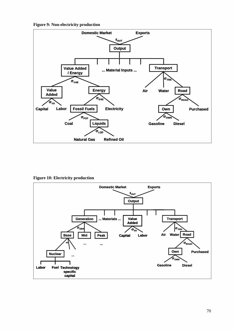
70

Figure 9: Non-electricity production

Output

Value Added / Energy

... Material Inputs ...

Value Added

Energy

Capital Labor Electricity

σVAE

σVA

σENE

Fossil Fuels

Coal

σFOF

Transport

Air Water Road

DieselGasoline

Own Purchased

Liquids

Natural Gas Refined Oil

Domestic Market Exports

σLQD

σTRN

σROAD

σOWN

εOUT

Output

Value Added / Energy

... Material Inputs ...

Value Added

Energy

Capital Labor Electricity

σVAE

σVA

σENE

Fossil Fuels

Coal

σFOF

Transport

Air Water Road

DieselGasoline

Own Purchased

Liquids

Natural Gas Refined Oil

Domestic Market Exports

σLQD

σTRN

σROAD

σOWN

εOUT

Figure 10: Electricity production

Output

Generation ... Materials ...

Base

σGEN

Value Added

Capital Labor

σVA

Mid Peak

Nuclear

∞ ... ...

Transport

Air Water Road

DieselGasoline

Own Purchased

σTRN

σROAD

σOWN

Domestic Market Exports

εOUT

Labor Technology specific capital

Fuel

...

Output

Generation ... Materials ...

Base

σGEN

Value Added

Capital Labor

σVA

Value Added

Capital Labor

σVA

Mid Peak

Nuclear

∞ ... ...

Transport

Air Water Road

DieselGasoline

Own Purchased

σTRN

σROAD

σOWN

Domestic Market Exports

εOUT

Labor Technology specific capital

FuelLabor Technology specific capital

Fuel

...

71

Essentially, the implementation of discrete generation technologies is a combination of the work of

Böhringer (1998) and Wing (2006, 2008). Böhringer (1998) treats technologies as perfect substitutes

with technology specific resources to limit unrealistic flip-flop behavior of technologies. However,

this approach does not allow for the deconstruction of installed capacities, i.e. capacities are not

malleable. Wing (2006, 2008) controls the malleability by introducing the CET transformation and

uses a nearly linear CES function to combine the output of power plants. However, using the CES

aggregator for power plants’ output does not work if new technologies are included: due to the zero-

value share in the benchmark equilibrium, the inactive technologies cannot be calibrated into the CES

aggregate. Consequently, the only possibility is to model them as perfect substitutes to the CES

aggregate of existing technologies. However, this approach favors the adoption of new technologies

since they do not use technology-specific capital. Additionally, the change in the generation of

existing technologies is restricted by the share preserving character of the CES aggregator leading to

unrealistic results. The approach used in this thesis has the advantage that it implements realistic

technology substitution by modeling them as perfect substitutes and allows controlling the malleability

of existing installed capacities using the CET transformation of technology specific capital.

Table 15 lists the substitution elasticities used in the production functions. The substitution elasticities

for the value added and value added/energy aggregated have been estimated by van der Werf (2008).

Elasticities for the transport module are obtained by a literature review but are generally subject to

uncertainty. Following Böhringer (1995), the substitution elasticity between load segments is set to a

value near zero. Other elasticities are adopted from Paltsev et al. (2005a) who employ the same

production structure. Empirical values for the transformation elasticity of technology specific capital

do not exist. Therefore, it is set to one and a sensitivity analysis is performed.

Table 15: Production substitution elasticities

Elasticity Description Value

Non-electricity production εOUT Exports vs. domestic production 2 σTRN Different transport modes 1 σVAE Value added and energy 0.33 σROAD Own and purchased road transport 1 σVA Labor and capital 0.43 σOWN Own transport with diesel and gasoline 0.9 σENE Electricity and fossil fuels 0.25 σFOF Coal and liquid fossil fuels 0.5 σLQD Natural gas and refined oils 1 Electricity production σGEN Load segments 0.1 εKE Transformation elasticity for technology-specific capital 1

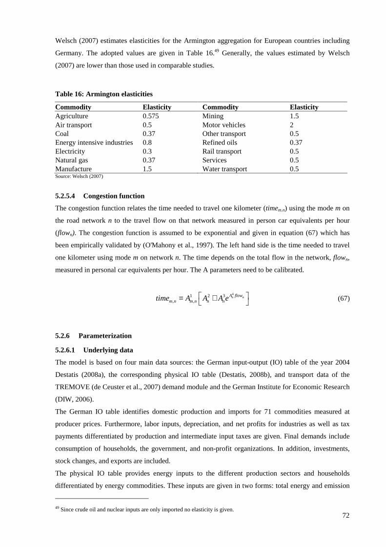
72

Welsch (2007) estimates elasticities for the Armington aggregation for European countries including

Germany. The adopted values are given in Table 16.49 Generally, the values estimated by Welsch

(2007) are lower than those used in comparable studies.

Table 16: Armington elasticities

Commodity Elasticity Commodity Elasticity Agriculture 0.575 Mining 1.5 Air transport 0.5 Motor vehicles 2 Coal 0.37 Other transport 0.5 Energy intensive industries 0.8 Refined oils 0.37 Electricity 0.3 Rail transport 0.5 Natural gas 0.37 Services 0.5 Manufacture 1.5 Water transport 0.5 Source: Welsch (2007)

5.2.5.4 Congestion function

The congestion function relates the time needed to travel one kilometer (timem.n) using the mode m on

the road network n to the travel flow on that network measured in person car equivalents per hour

(flown). The congestion function is assumed to be exponential and given in equation (67) which has

been empirically validated by (O'Mahony et al., 1997). The left hand side is the time needed to travel

one kilometer using mode m on network n. The time depends on the total flow in the network, flown,

measured in personal car equivalents per hour. The A parameters need to be calibrated.

41 2 3

, ,n nA flow

m n m n n ntime A A A e = +

(67)

5.2.6 Parameterization

5.2.6.1 Underlying data

The model is based on four main data sources: the German input-output (IO) table of the year 2004

Destatis (2008a), the corresponding physical IO table (Destatis, 2008b), and transport data of the

TREMOVE (de Ceuster et al., 2007) demand module and the German Institute for Economic Research

(DIW, 2006).

The German IO table identifies domestic production and imports for 71 commodities measured at

producer prices. Furthermore, labor inputs, depreciation, and net profits for industries as well as tax

payments differentiated by production and intermediate input taxes are given. Final demands include

consumption of households, the government, and non-profit organizations. In addition, investments,

stock changes, and exports are included.

The physical IO table provides energy inputs to the different production sectors and households

differentiated by energy commodities. These inputs are given in two forms: total energy and emission

49 Since crude oil and nuclear inputs are only imported no elasticity is given.

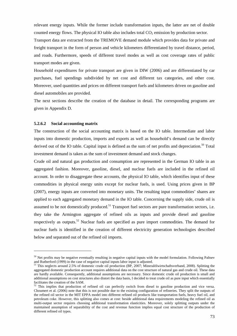
73

relevant energy inputs. While the former include transformation inputs, the latter are net of double

counted energy flows. The physical IO table also includes total CO2 emission by production sector.

Transport data are extracted from the TREMOVE demand module which provides data for private and

freight transport in the form of person and vehicle kilometers differentiated by travel distance, period,

and roads. Furthermore, speeds of different travel modes as well as cost coverage rates of public

transport modes are given.

Household expenditures for private transport are given in DIW (2006) and are differentiated by car

purchases, fuel spendings subdivided by net cost and different tax categories, and other cost.

Moreover, used quantities and prices on different transport fuels and kilometers driven on gasoline and

diesel automobiles are provided.

The next sections describe the creation of the database in detail. The corresponding programs are

given in Appendix D.

5.2.6.2 Social accounting matrix

The construction of the social accounting matrix is based on the IO table. Intermediate and labor

inputs into domestic production, imports and exports as well as household’s demand can be directly

derived out of the IO table. Capital input is defined as the sum of net profits and depreciation.50 Total

investment demand is taken as the sum of investment demand and stock changes.

Crude oil and natural gas production and consumption are represented in the German IO table in an

aggregated fashion. Moreover, gasoline, diesel, and nuclear fuels are included in the refined oil

account. In order to disaggregate these accounts, the physical IO table, which identifies input of these

commodities in physical energy units except for nuclear fuels, is used. Using prices given in BP

(2007), energy inputs are converted into monetary units. The resulting input commodities’ shares are

applied to each aggregated monetary demand in the IO table. Concerning the supply side, crude oil is

assumed to be not domestically produced.51 Transport fuel sectors are pure transformation sectors, i.e.

they take the Armington aggregate of refined oils as inputs and provide diesel and gasoline

respectively as outputs.52 Nuclear fuels are specified as pure import commodities. The demand for

nuclear fuels is identified in the creation of different electricity generation technologies described

below and separated out of the refined oil imports.

50 Net profits may be negative eventually resulting in negative capital inputs with the model formulation. Following Paltsev and Rutherford (1999) in the case of negative capital inputs labor input is adjusted. 51 This neglects around 2.5% of domestic crude oil production (BP, 2007; Mineralölwirtschaftsverband, 2008). Splitting the aggregated domestic production account requires additional data on the cost structure of natural gas and crude oil. These data are hardly available. Consequently, additional assumptions are necessary. Since domestic crude oil production is small and additional assumptions on cost structures also distort the data basis, I decided to treat crude oil as pure input which essentially facilitates the creation of the SAM. 52 This implies that production of refined oil can perfectly switch from diesel to gasoline production and vice versa. Choumert et al. (2006) note that this is not possible due to the existing configuration of refineries. They split the outputs of the refined oil sector in the MIT EPPA model into different refined oil products like transportation fuels, heavy fuel oil, and petroleum coke. However, this splitting also comes at cost: beside additional data requirements modeling the refined oil as multi-output sector requires choosing additional transformation elasticities. Moreover, solely splitting outputs under the maintained assumption of separability of the cost and revenue function implies equal cost structure of the production of different refined oil types.

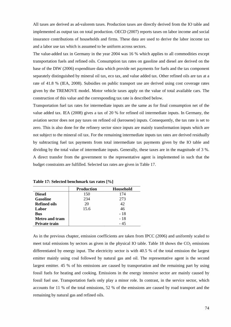
74

All taxes are derived as ad-valorem taxes. Production taxes are directly derived from the IO table and

implemented as output tax on total production. OECD (2007) reports taxes on labor income and social

insurance contributions of households and firms. These data are used to derive the labor income tax

and a labor use tax which is assumed to be uniform across sectors.

The value-added tax in Germany in the year 2004 was 16 % which applies to all commodities except

transportation fuels and refined oils. Consumption tax rates on gasoline and diesel are derived on the

base of the DIW (2006) expenditure data which provide net payments for fuels and the tax component

separately distinguished by mineral oil tax, eco tax, and value added tax. Other refined oils are tax at a

rate of 41.8 % (IEA, 2008). Subsidies on public transport use are derived using cost coverage rates

given by the TREMOVE model. Motor vehicle taxes apply on the value of total available cars. The

construction of this value and the corresponding tax rate is described below.

Transportation fuel tax rates for intermediate inputs are the same as for final consumption net of the

value added tax. IEA (2008) gives a tax of 20 % for refined oil intermediate inputs. In Germany, the

aviation sector does not pay taxes on refined oil (kerosene) inputs. Consequently, the tax rate is set to

zero. This is also done for the refinery sector since inputs are mainly transformation inputs which are

not subject to the mineral oil tax. For the remaining intermediate inputs tax rates are derived residually

by subtracting fuel tax payments from total intermediate tax payments given by the IO table and

dividing by the total value of intermediate inputs. Generally, these taxes are in the magnitude of 3 %.

A direct transfer from the government to the representative agent is implemented in such that the

budget constraints are fulfilled. Selected tax rates are given in Table 17.

Table 17: Selected benchmark tax rates [%]

Production Household Diesel 150 174 Gasoline 234 273 Refined oils 20 42 Labor 15.6 46 Bus - 18 Metro and tram - 18 Private train - 45

As in the previous chapter, emission coefficients are taken from IPCC (2006) and uniformly scaled to

meet total emissions by sectors as given in the physical IO table. Table 18 shows the CO2 emissions

differentiated by energy input. The electricity sector is with 40.5 % of the total emission the largest

emitter mainly using coal followed by natural gas and oil. The representative agent is the second

largest emitter. 45 % of his emissions are caused by transportation and the remaining part by using

fossil fuels for heating and cooking. Emissions in the energy intensive sector are mainly caused by

fossil fuel use. Transportation fuels only play a minor role. In contrast, in the service sector, which

accounts for 11 % of the total emissions, 52 % of the emissions are caused by road transport and the

remaining by natural gas and refined oils.

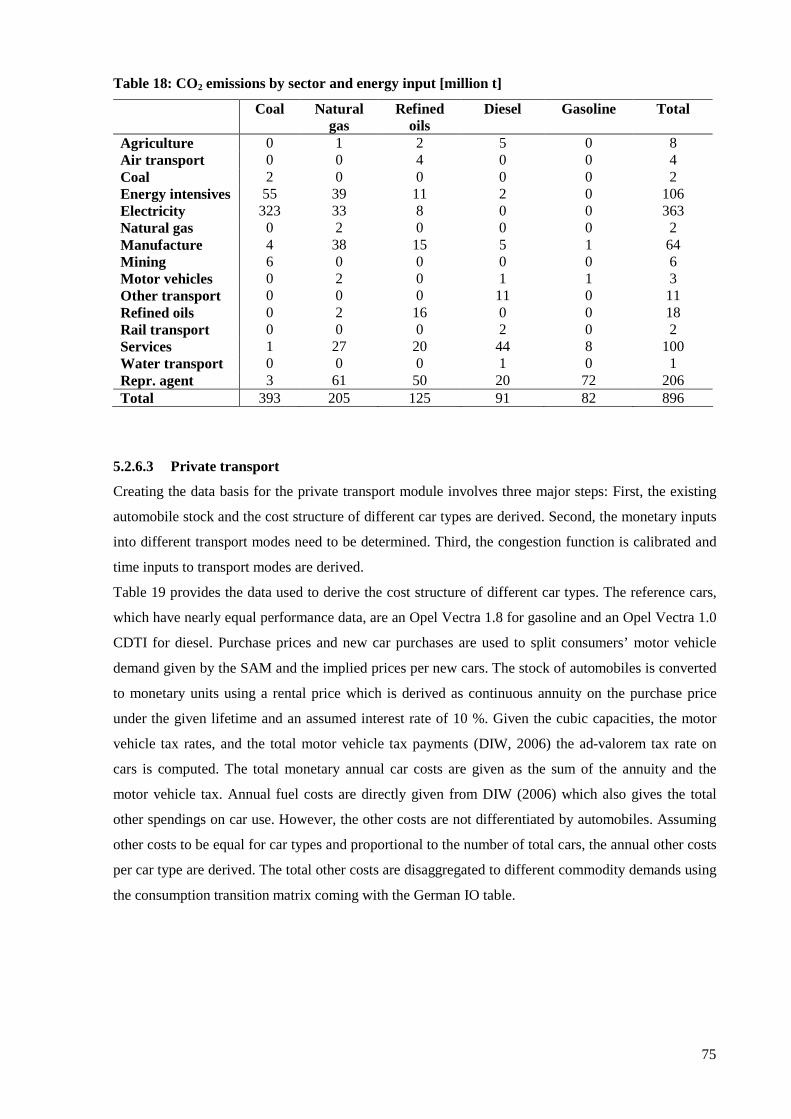
75

Table 18: CO2 emissions by sector and energy input [million t]

Coal Natural gas

Refined oils

Diesel Gasoline Total

Agriculture 0 1 2 5 0 8 Air transport 0 0 4 0 0 4 Coal 2 0 0 0 0 2 Energy intensives 55 39 11 2 0 106 Electricity 323 33 8 0 0 363 Natural gas 0 2 0 0 0 2 Manufacture 4 38 15 5 1 64 Mining 6 0 0 0 0 6 Motor vehicles 0 2 0 1 1 3 Other transport 0 0 0 11 0 11 Refined oils 0 2 16 0 0 18 Rail transport 0 0 0 2 0 2 Services 1 27 20 44 8 100 Water transport 0 0 0 1 0 1 Repr. agent 3 61 50 20 72 206 Total 393 205 125 91 82 896

5.2.6.3 Private transport

Creating the data basis for the private transport module involves three major steps: First, the existing

automobile stock and the cost structure of different car types are derived. Second, the monetary inputs

into different transport modes need to be determined. Third, the congestion function is calibrated and

time inputs to transport modes are derived.

Table 19 provides the data used to derive the cost structure of different car types. The reference cars,

which have nearly equal performance data, are an Opel Vectra 1.8 for gasoline and an Opel Vectra 1.0

CDTI for diesel. Purchase prices and new car purchases are used to split consumers’ motor vehicle

demand given by the SAM and the implied prices per new cars. The stock of automobiles is converted

to monetary units using a rental price which is derived as continuous annuity on the purchase price

under the given lifetime and an assumed interest rate of 10 %. Given the cubic capacities, the motor

vehicle tax rates, and the total motor vehicle tax payments (DIW, 2006) the ad-valorem tax rate on

cars is computed. The total monetary annual car costs are given as the sum of the annuity and the

motor vehicle tax. Annual fuel costs are directly given from DIW (2006) which also gives the total

other spendings on car use. However, the other costs are not differentiated by automobiles. Assuming

other costs to be equal for car types and proportional to the number of total cars, the annual other costs

per car type are derived. The total other costs are disaggregated to different commodity demands using

the consumption transition matrix coming with the German IO table.

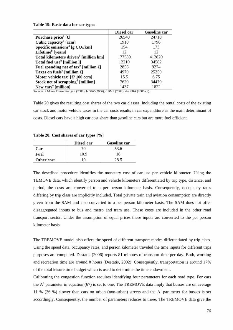
76

Table 19: Basic data for car types

Diesel car Gasoline car Purchase pricea [€] 26540 24710 Cubic capacitya [ccm] 1910 1796 Specific emissionsa [g CO2/km] 154 173 Lifetime b [years] 12 12 Total kilometers drivenb [million km] 177589 412820 Total fuel useb [million l] 12210 34582 Fuel spending net of taxb [million €] 2856 9274 Taxes on fuelsb [million €] 4970 25250 Motor vehicle taxc [€/ 100 ccm] 15.5 6.75 Stock net of scrappingd [million] 7620 34479 New carse [million] 1437 1822

Sources: a Motor Presse Stuttgart (2008); b DIW (2006); c BMF (2009); d,e KBA (2005a,b)

Table 20 gives the resulting cost shares of the two car classes. Including the rental costs of the existing

car stock and motor vehicle taxes in the car costs results in car expenditure as the main determinant of

costs. Diesel cars have a high car cost share than gasoline cars but are more fuel efficient.

Table 20: Cost shares of car types [%]

Diesel car Gasoline car Car 70 53.6 Fuel 10.9 18 Other cost 19 28.5

The described procedure identifies the monetary cost of car use per vehicle kilometer. Using the

TEMOVE data, which identify person and vehicle kilometers differentiated by trip type, distance, and

period, the costs are converted to a per person kilometer basis. Consequently, occupancy rates

differing by trip class are implicitly included. Total private train and aviation consumption are directly

given from the SAM and also converted to a per person kilometer basis. The SAM does not offer

disaggregated inputs to bus and metro and tram use. These costs are included in the other road

transport sector. Under the assumption of equal prices these inputs are converted to the per person

kilometer basis.

The TREMOVE model also offers the speed of different transport modes differentiated by trip class.

Using the speed data, occupancy rates, and person kilometer traveled the time inputs for different trips

purposes are computed. Destatis (2006) reports 81 minutes of transport time per day. Both, working

and recreation time are around 8 hours (Destatis, 2002). Consequently, transportation is around 17%

of the total leisure time budget which is used to determine the time endowment.

Calibrating the congestion function requires identifying four parameters for each road type. For cars

the A1 parameter in equation (67) is set to one. The TREMOVE data imply that busses are on average

11 % (26 %) slower than cars on urban (non-urban) streets and the A1 parameter for busses is set

accordingly. Consequently, the number of parameters reduces to three. The TREMOVE data give the

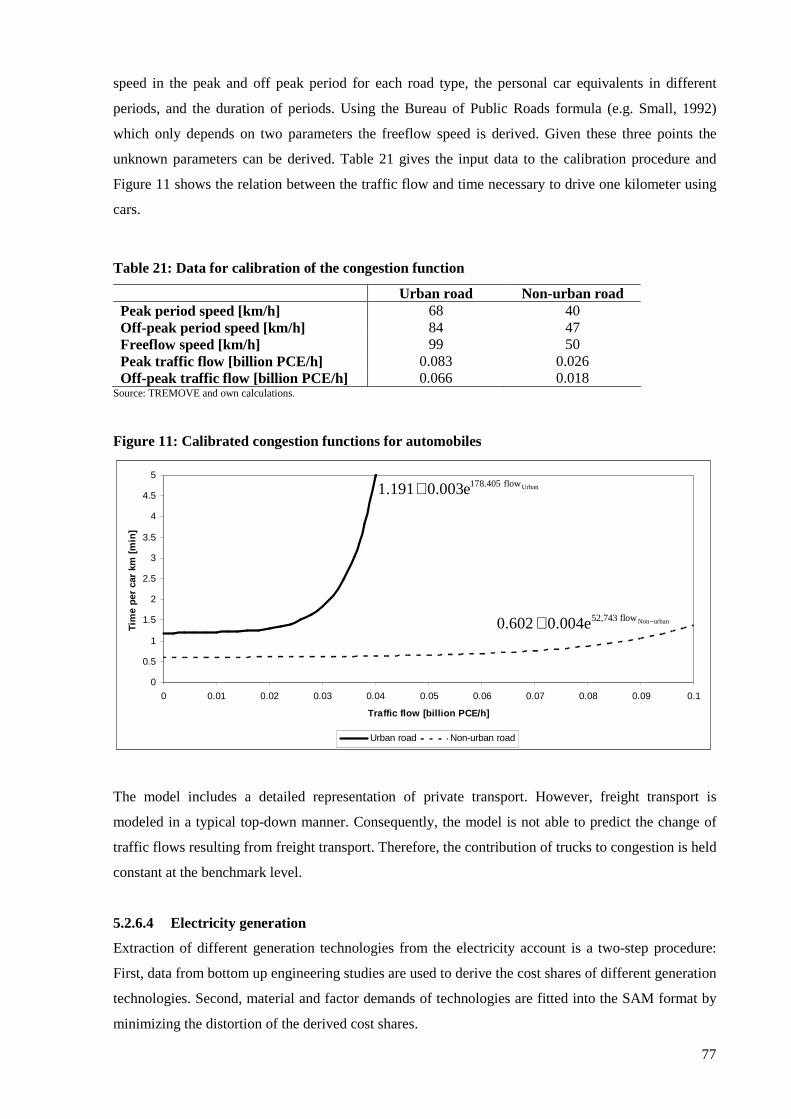
77

speed in the peak and off peak period for each road type, the personal car equivalents in different

periods, and the duration of periods. Using the Bureau of Public Roads formula (e.g. Small, 1992)

which only depends on two parameters the freeflow speed is derived. Given these three points the

unknown parameters can be derived. Table 21 gives the input data to the calibration procedure and

Figure 11 shows the relation between the traffic flow and time necessary to drive one kilometer using

cars.

Table 21: Data for calibration of the congestion function

Urban road Non-urban road Peak period speed [km/h] 68 40 Off-peak period speed [km/h] 84 47 Freeflow speed [km/h] 99 50 Peak traffic flow [billion PCE/h] 0.083 0.026 Off-peak traffic flow [billion PCE/h] 0.066 0.018

Source: TREMOVE and own calculations.

Figure 11: Calibrated congestion functions for automobiles

0

0.5

1

1.5

2

2.5

3

3.5

4

4.5

5

0 0.01 0.02 0.03 0.04 0.05 0.06 0.07 0.08 0.09 0.1

Traffic flow [billion PCE/h]

Tim

e pe

r ca

r km

[min

]

Urban road Non-urban road

Urban178.405 flow1.191 0.003e+

Non urban52,743 flow0.602 0.004e −+

0

0.5

1

1.5

2

2.5

3

3.5

4

4.5

5

0 0.01 0.02 0.03 0.04 0.05 0.06 0.07 0.08 0.09 0.1

Traffic flow [billion PCE/h]

Tim

e pe

r ca

r km

[min

]

Urban road Non-urban road

Urban178.405 flow1.191 0.003e+

Non urban52,743 flow0.602 0.004e −+

The model includes a detailed representation of private transport. However, freight transport is

modeled in a typical top-down manner. Consequently, the model is not able to predict the change of

traffic flows resulting from freight transport. Therefore, the contribution of trucks to congestion is held

constant at the benchmark level.

5.2.6.4 Electricity generation

Extraction of different generation technologies from the electricity account is a two-step procedure:

First, data from bottom up engineering studies are used to derive the cost shares of different generation

technologies. Second, material and factor demands of technologies are fitted into the SAM format by

minimizing the distortion of the derived cost shares.

78

Table 22 lists the technological characterization of the generation technologies and their physical

output levels in the benchmark equilibrium. According to David and Herzog (2000) the CO2 capture

rate of CCS technologies is set to 90 %.

Annualized capital costs are derived using the continuous annuity method on the product of plants’

size and investment costs under assumed interest rate of 7.5 %. Operation and maintenance costs are

regarded as annual labor cost. Using the plants’ availability and size, heat efficiencies, and fuel prices,

the annual fuel cost are obtained.

The method of integrating the generation technologies into the SAM framework is described in detail

in Wing (2008). The top-down framework requires that the material and factor inputs of all generation

technologies and the overhead activity sum to the total demands given by the SAM. Moreover, output

also has to equal the output of the electricity sector in the SAM. The sum of squared deviations of

predicted cost share and cost shares fitting into the top-down data is minimized. A further restriction is

added to minimize the deviation of the heat efficiency from its predicted value.53 The predicted and

used values consistent with the SAM are given in Table 23.

Table 23 also states the respective load segment for technologies. Conventional technologies active in

the benchmark equilibrium in the mid load segment, the CCGT and hard coal plant, are allowed to

produce in the base load segment, too. This allows substitution of lignite base load production by more

environmentally friendly but also more expensive mid load technologies. For inactive technologies,

the concept of cost markup over the benchmark price in the load segments is used (e.g. Böhringer,

1998; McFareland et al. 2004). The markup of technologies already active in the mid load but not in

the base load segment is equal to the average spread between the respective prices in 2004 (European

Energy Exchange, 2004). McFareland et al. 2004 estimate the markup of CCS technologies. The

values for offshore wind and photovoltaic are derived using the generation prices as implied by the

bottom-up data.

The technological potential given in Table 23 was estimated by BMU (2007) for wind and

photovoltaic technologies. For hydro power and other technologies no additional potential is given.

Consequently, the limit is set to the benchmark production. Since new installation of nuclear power

plants is prohibited in Germany (Deutscher Bundestag, 2002), generation of nuclear power is also

capped at the benchmark level.

53 See Appendix D for the employed GAMS code.

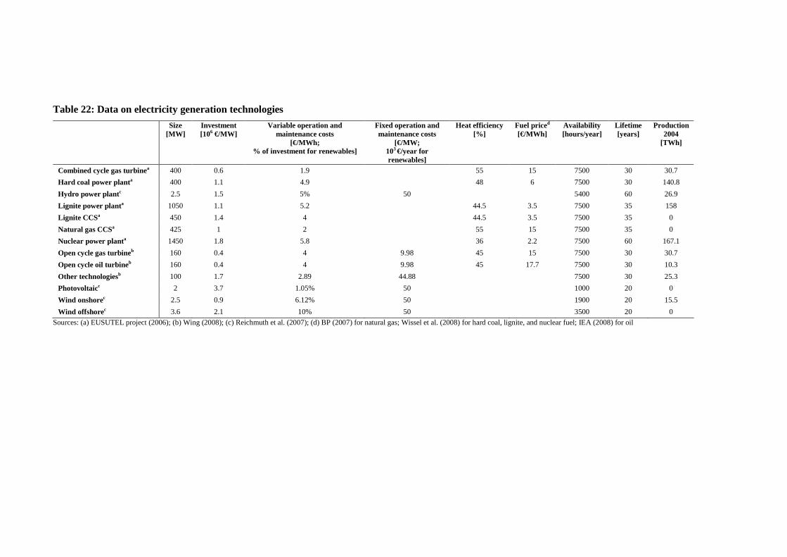
Table 22: Data on electricity generation technologies

Size [MW]

Investment [106 €/MW]

Variable operation and maintenance costs

[€/MWh; % of investment for renewables]

Fixed operation and maintenance costs

[€/MW; 103 €/year for renewables]

Heat efficiency [%]

Fuel priced

[€/MWh] Availability [hours/year]

Lifetime [years]

Production 2004

[TWh]

Combined cycle gas turbinea 400 0.6 1.9 55 15 7500 30 30.7

Hard coal power planta 400 1.1 4.9 48 6 7500 30 140.8

Hydro power plantc 2.5 1.5 5% 50 5400 60 26.9

Lignite power planta 1050 1.1 5.2 44.5 3.5 7500 35 158

Lignite CCSa 450 1.4 4 44.5 3.5 7500 35 0

Natural gas CCSa 425 1 2 55 15 7500 35 0

Nuclear power planta 1450 1.8 5.8 36 2.2 7500 60 167.1

Open cycle gas turbineb 160 0.4 4 9.98 45 15 7500 30 30.7

Open cycle oil turbineb 160 0.4 4 9.98 45 17.7 7500 30 10.3

Other technologiesb 100 1.7 2.89 44.88 7500 30 25.3

Photovoltaicc 2 3.7 1.05% 50 1000 20 0

Wind onshorec 2.5 0.9 6.12% 50 1900 20 15.5

Wind offshorec 3.6 2.1 10% 50 3500 20 0

Sources: (a) EUSUTEL project (2006); (b) Wing (2008); (c) Reichmuth et al. (2007); (d) BP (2007) for natural gas; Wissel et al. (2008) for hard coal, lignite, and nuclear fuel; IEA (2008) for oil

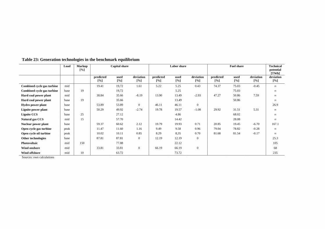
Table 23: Generation technologies in the benchmark equilibrium

Load Markup [%]

Capital share Labor share Fuel share Technical potential [TWh]

predicted [%]

used [%]

deviation [%]

predicted [%]

used [%]

deviation [%]

predicted [%]

used [%]

deviation [%]

deviation [%]

Combined cycle gas turbine mid 19.41 19,72 1.61 5.22 5.25 0.43 74.37 75.03 -0.45 ∞

Combined cycle gas turbine base 19 19,72 5.25 75.03 ∞

Hard coal power plant mid 38.84 35.66 -8.19 13.90 13.49 -2.93 47.27 50.86 7.59 ∞

Hard coal power plant base 19 35.66 13.49 50.86 ∞

Hydro power plant base 53.89 53.89 0 46.11 46.11 0 26.9

Lignite power plant base 50.29 49.92 -2.74 19.78 19.57 -1.08 29.92 31.51 5.31 ∞

Lignite CCS base 25 27.12 4.86 68.02 ∞

Natural gas CCS mid 15 57.70 14.42 28.08 ∞

Nuclear power plant base 59.37 60.62 2.12 19.79 19.93 0.71 20.85 19.45 -6.70 167.1

Open cycle gas turbine peak 11.47 11.60 1.16 9.49 9.58 0.96 79.04 78.82 -0.28 ∞

Open cycle oil turbine peak 10.02 10.11 0.85 8.29 8,35 0.70 81.68 81.54 -0.17 ∞

Other technologies base 87.81 87.81 0 12.19 12.19 0 25.3

Photovoltaic mid 150 77.88 22.12 105

Wind onshore mid 33.81 33.81 0 66.19 66.19 0 68

Wind offshore mid 10 63.72 73.72 235

Sources: own calculations

5.2.7 Model critics and extension

The presented framework overcomes the bottom-up/top-down discussion of technological details

including different electricity generation technologies. Furthermore, private transport is included in

detail and congestion is modeled. Although not done in this thesis, representing different road types

and congestion also allows analyzing the effect of infrastructure policies determining the effect of

infrastructure provision on the congestion function and road pricing policies.

Freight transport is addressed in an aggregated way considering intermediate inputs of transport

commodities and energy inputs differentiated by fuel type. Consequently, it is not possible to keep

track of the vehicle kilometers traveled by freight transport. Therefore, the contribution of freight

transport to the traffic flow in the congestion function is held constant at the benchmark level. Thus, a

fruitful extension of the model is the detailed representation of industrial transport. This requires

estimation of the transport capital by sector and of trips by travel period, distance and mode. The

TREMOVE demand module offers aggregated data on a vehicle and tone kilometer basis

distinguished by trip categories. Transport capital in form of the vehicle stock are given in KBA (2005

a,b). DIW (2006) includes data on transit transport in Germany. Given these data, there are two main

tasks to solve: First, the aggregated TREMOVE data on traffic use need to be disaggregated to a

sectoral basis, i.e. answering the question which sector uses how much of the transport volume.

Second, given the transport volume of single sectors it needs to be determined how much of the

sector’s transport is own provided and how much is purchased. Obviously, the main effort is in the

first task which is a matter of data. The second task might by solved by estimating own provided

transport using the data on transport capital and fuel expenditure.

The model treats labor supply as constant. This is done in order to concentrate on the interaction

between emission abatement in electricity generation and road transport and to facilitate the

interpretation by ruling out labor supply effects. Labor supply effects can be easily included specifying

labor as part of the time constraint. Including labor in the time constraint has an additional effect on

the private transport decisions since the value of time, which is endogenous in the model, is further

linked to the wage rate. Consequently, the decision on the travel mode is further influenced by the

model’s reactions on the labor market. Such an analysis has been carried out for example in the

empirical analysis of Berg (2007).

The modeling of households using a representative agent is costly in two directions: First, the model

does not allow for analyzing important equity aspects. Second, the location of living of households

which affects the substitution possibilities across transport modes and roads are not represented. A

more detailed representation of households requires splitting expenditure and income data as done for

Germany by Kalinowska et al. (2007) and Kremers and Kalinowska (2009).

New technologies for automobiles should be included in future versions of the model allowing for a

detailed analysis of fuel efficiency related policies. Modeling new technologies in the car market is

more complicated than in electricity generation since cars are not perfect substitutes like generation

82

technologies. Beside the important preferences of consumers, adoption of technologies also depends

on the availability of fueling networks (Achtnicht et al., 2008).

Athough the model accounts for the congestion externality, other externalities such as local pollution,

accidents, and noise are ignored. Therefore, a future extension of the model should include these

externalities, too, as done e.g. in Meyeres and Proost (1997) and Mayers (1999).

5.3 Simulations and results

5.3.1 Scenario description

In all scenarios the German economy reduces 20 % of its CO2 emissions in the benchmark which

amounts to 179.2 million tones. In the ETS scenario, the reduction requirement is achieved using

emission trading between the electricity sector, energy intensive industries, and refineries which are

referred to as ETS sectors. However, only emissions caused by coal, natural gas, or refined oil

combustion are included into the system. Emissions caused by using transport fuels are not covered.

Permits are owned by the government which sells them to the emission trading sectors. Consequently,

the introduction of carbon regulation increases the government’s revenues. The ETS AIR scenario

additionally includes the aviation sector. The ETS FUEL and FUEL TAX scenarios include reduction

efforts of road transportation. In ETS FUEL, all sectors and the representative agent have to hold

emission allowances for emissions caused by gasoline or diesel use. These allowances are tradable

with the ETS sectors. The FUEL TAX scenario implements a separated strategy for road transport

emissions. It requires road transport to reduce emissions by 5 %. Firms and the representative

household are allowed to trade allowances for transport fuels. However, they are not allowed to trade

permits with the ETS sectors which fulfill the remaining reduction requirement complying with the

overall 20 % reduction target. This closed emission trading system for road transport fuels is

equivalent to an increase of the existing fuel tax distinguishing carbon contents of transport fuels. In

all of these scenarios the revenues are recycled lump-sum to the representative agent holding the

provision of public goods constant. The ETS SUB scenario is the only exemption to this rule. In this

scenario, the income generated by the ETS system is used to uniformly increase the subsidies for bus,

metro and tram, and private train transport. Table 24 gives an overview over the scenario settings.

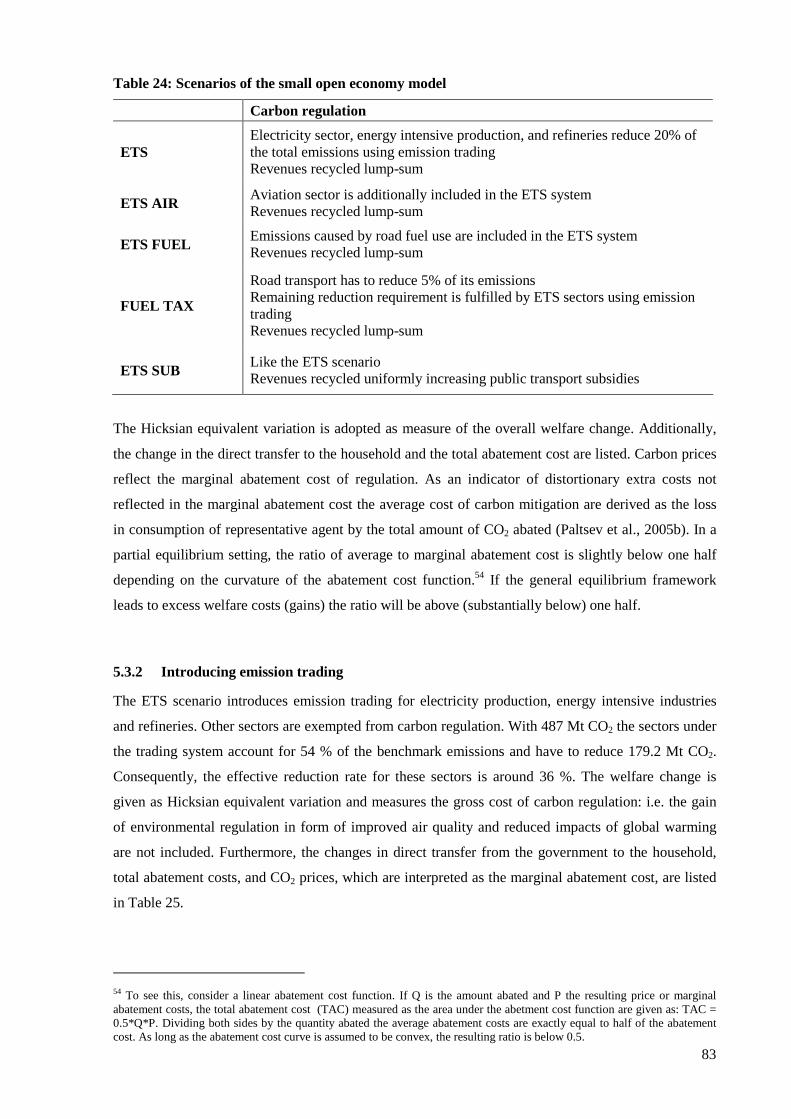
83

Table 24: Scenarios of the small open economy model

Carbon regulation

ETS Electricity sector, energy intensive production, and refineries reduce 20% of the total emissions using emission trading Revenues recycled lump-sum

ETS AIR Aviation sector is additionally included in the ETS system Revenues recycled lump-sum

ETS FUEL Emissions caused by road fuel use are included in the ETS system Revenues recycled lump-sum

FUEL TAX

Road transport has to reduce 5% of its emissions Remaining reduction requirement is fulfilled by ETS sectors using emission trading Revenues recycled lump-sum

ETS SUB Like the ETS scenario Revenues recycled uniformly increasing public transport subsidies

The Hicksian equivalent variation is adopted as measure of the overall welfare change. Additionally,

the change in the direct transfer to the household and the total abatement cost are listed. Carbon prices

reflect the marginal abatement cost of regulation. As an indicator of distortionary extra costs not

reflected in the marginal abatement cost the average cost of carbon mitigation are derived as the loss

in consumption of representative agent by the total amount of CO2 abated (Paltsev et al., 2005b). In a

partial equilibrium setting, the ratio of average to marginal abatement cost is slightly below one half

depending on the curvature of the abatement cost function.54 If the general equilibrium framework

leads to excess welfare costs (gains) the ratio will be above (substantially below) one half.

5.3.2 Introducing emission trading

The ETS scenario introduces emission trading for electricity production, energy intensive industries

and refineries. Other sectors are exempted from carbon regulation. With 487 Mt CO2 the sectors under

the trading system account for 54 % of the benchmark emissions and have to reduce 179.2 Mt CO2.

Consequently, the effective reduction rate for these sectors is around 36 %. The welfare change is

given as Hicksian equivalent variation and measures the gross cost of carbon regulation: i.e. the gain

of environmental regulation in form of improved air quality and reduced impacts of global warming

are not included. Furthermore, the changes in direct transfer from the government to the household,

total abatement costs, and CO2 prices, which are interpreted as the marginal abatement cost, are listed

in Table 25.

54 To see this, consider a linear abatement cost function. If Q is the amount abated and P the resulting price or marginal abatement costs, the total abatement cost (TAC) measured as the area under the abetment cost function are given as: TAC = 0.5*Q*P. Dividing both sides by the quantity abated the average abatement costs are exactly equal to half of the abatement cost. As long as the abatement cost curve is assumed to be convex, the resulting ratio is below 0.5.

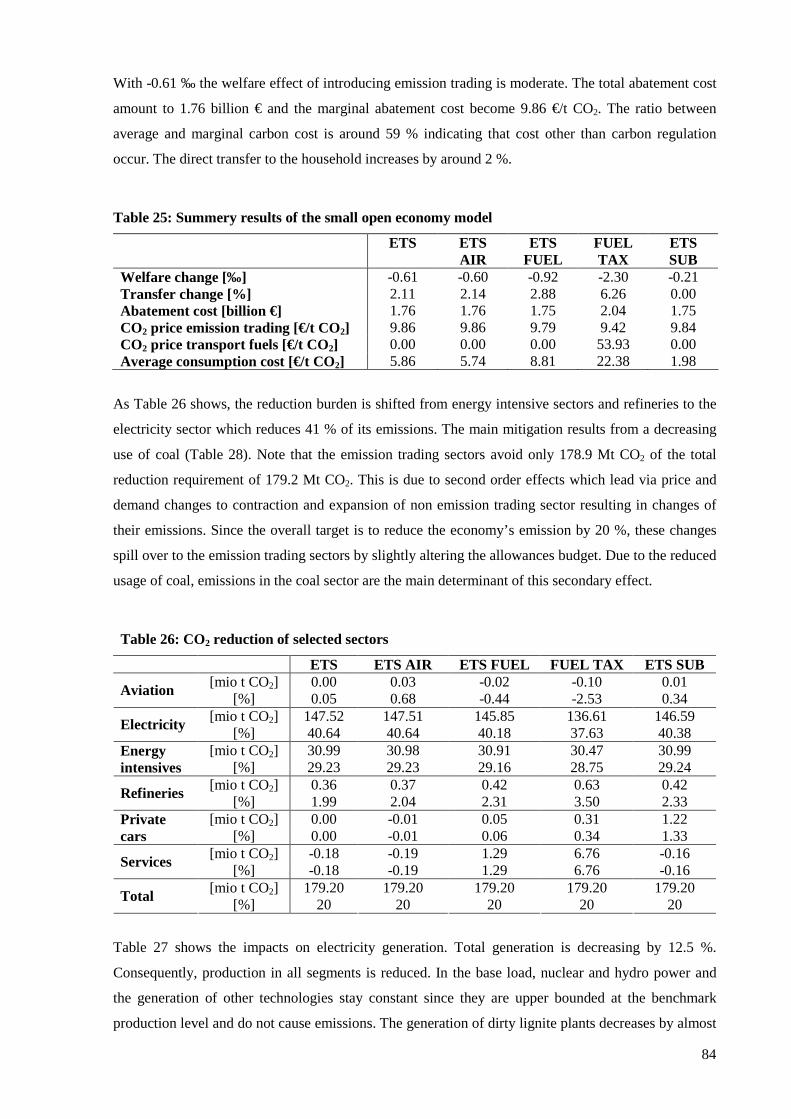
84

With -0.61 ‰ the welfare effect of introducing emission trading is moderate. The total abatement cost

amount to 1.76 billion € and the marginal abatement cost become 9.86 €/t CO2. The ratio between

average and marginal carbon cost is around 59 % indicating that cost other than carbon regulation

occur. The direct transfer to the household increases by around 2 %.

Table 25: Summery results of the small open economy model

ETS ETS AIR

ETS FUEL

FUEL TAX

ETS SUB

Welfare change [‰] -0.61 -0.60 -0.92 -2.30 -0.21 Transfer change [%] 2.11 2.14 2.88 6.26 0.00 Abatement cost [billion €] 1.76 1.76 1.75 2.04 1.75 CO2 price emission trading [€/t CO2] 9.86 9.86 9.79 9.42 9.84 CO2 price transport fuels [€/t CO2] 0.00 0.00 0.00 53.93 0.00 Average consumption cost [€/t CO2] 5.86 5.74 8.81 22.38 1.98

As Table 26 shows, the reduction burden is shifted from energy intensive sectors and refineries to the

electricity sector which reduces 41 % of its emissions. The main mitigation results from a decreasing

use of coal (Table 28). Note that the emission trading sectors avoid only 178.9 Mt CO2 of the total

reduction requirement of 179.2 Mt CO2. This is due to second order effects which lead via price and

demand changes to contraction and expansion of non emission trading sector resulting in changes of

their emissions. Since the overall target is to reduce the economy’s emission by 20 %, these changes

spill over to the emission trading sectors by slightly altering the allowances budget. Due to the reduced

usage of coal, emissions in the coal sector are the main determinant of this secondary effect.

Table 26: CO2 reduction of selected sectors

ETS ETS AIR ETS FUEL FUEL TAX ETS SUB [mio t CO2] 0.00 0.03 -0.02 -0.10 0.01 Aviation

[%] 0.05 0.68 -0.44 -2.53 0.34 [mio t CO2] 147.52 147.51 145.85 136.61 146.59 Electricity

[%] 40.64 40.64 40.18 37.63 40.38 [mio t CO2] 30.99 30.98 30.91 30.47 30.99 Energy

intensives [%] 29.23 29.23 29.16 28.75 29.24 [mio t CO2] 0.36 0.37 0.42 0.63 0.42 Refineries

[%] 1.99 2.04 2.31 3.50 2.33 [mio t CO2] 0.00 -0.01 0.05 0.31 1.22 Private

cars [%] 0.00 -0.01 0.06 0.34 1.33 [mio t CO2] -0.18 -0.19 1.29 6.76 -0.16 Services

[%] -0.18 -0.19 1.29 6.76 -0.16 [mio t CO2] 179.20 179.20 179.20 179.20 179.20 Total

[%] 20 20 20 20 20

Table 27 shows the impacts on electricity generation. Total generation is decreasing by 12.5 %.

Consequently, production in all segments is reduced. In the base load, nuclear and hydro power and

the generation of other technologies stay constant since they are upper bounded at the benchmark

production level and do not cause emissions. The generation of dirty lignite plants decreases by almost

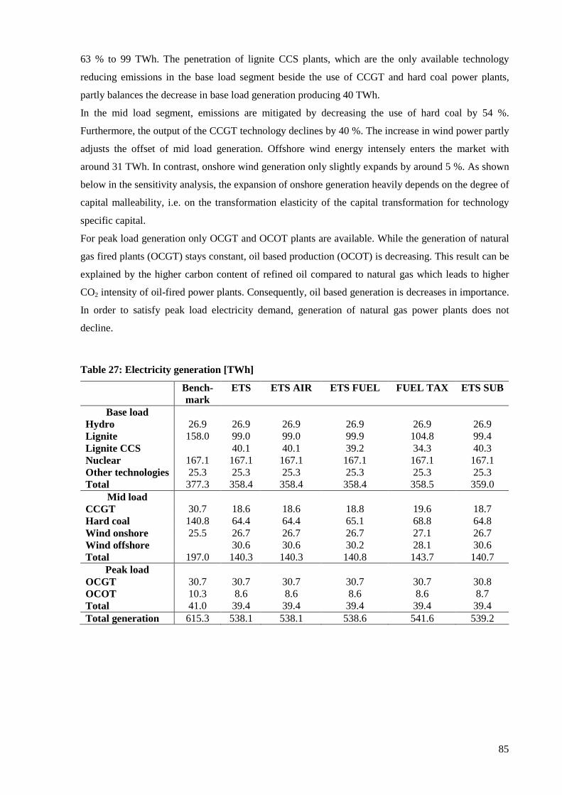
85

63 % to 99 TWh. The penetration of lignite CCS plants, which are the only available technology

reducing emissions in the base load segment beside the use of CCGT and hard coal power plants,

partly balances the decrease in base load generation producing 40 TWh.

In the mid load segment, emissions are mitigated by decreasing the use of hard coal by 54 %.

Furthermore, the output of the CCGT technology declines by 40 %. The increase in wind power partly

adjusts the offset of mid load generation. Offshore wind energy intensely enters the market with

around 31 TWh. In contrast, onshore wind generation only slightly expands by around 5 %. As shown

below in the sensitivity analysis, the expansion of onshore generation heavily depends on the degree of

capital malleability, i.e. on the transformation elasticity of the capital transformation for technology

specific capital.

For peak load generation only OCGT and OCOT plants are available. While the generation of natural

gas fired plants (OCGT) stays constant, oil based production (OCOT) is decreasing. This result can be

explained by the higher carbon content of refined oil compared to natural gas which leads to higher

CO2 intensity of oil-fired power plants. Consequently, oil based generation is decreases in importance.

In order to satisfy peak load electricity demand, generation of natural gas power plants does not

decline.

Table 27: Electricity generation [TWh]

Bench-mark

ETS ETS AIR ETS FUEL FUEL TAX ETS SUB

Base load Hydro 26.9 26.9 26.9 26.9 26.9 26.9 Lignite 158.0 99.0 99.0 99.9 104.8 99.4 Lignite CCS 40.1 40.1 39.2 34.3 40.3 Nuclear 167.1 167.1 167.1 167.1 167.1 167.1 Other technologies 25.3 25.3 25.3 25.3 25.3 25.3 Total 377.3 358.4 358.4 358.4 358.5 359.0

Mid load CCGT 30.7 18.6 18.6 18.8 19.6 18.7 Hard coal 140.8 64.4 64.4 65.1 68.8 64.8 Wind onshore 25.5 26.7 26.7 26.7 27.1 26.7 Wind offshore 30.6 30.6 30.2 28.1 30.6 Total 197.0 140.3 140.3 140.8 143.7 140.7

Peak load OCGT 30.7 30.7 30.7 30.7 30.7 30.8 OCOT 10.3 8.6 8.6 8.6 8.6 8.7 Total 41.0 39.4 39.4 39.4 39.4 39.4 Total generation 615.3 538.1 538.1 538.6 541.6 539.2

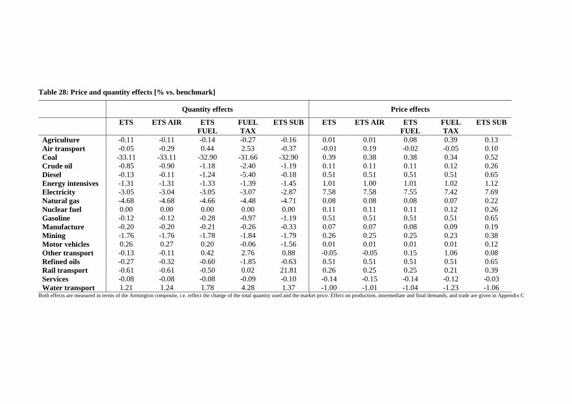
Table 28: Price and quantity effects [% vs. benchmark]

Quantity effects Price effects

ETS ETS AIR ETS FUEL

FUEL TAX

ETS SUB ETS ETS AIR ETS FUEL

FUEL TAX

ETS SUB

Agriculture -0.11 -0.11 -0.14 -0.27 -0.16 0.01 0.01 0.08 0.39 0.13 Air transport -0.05 -0.29 0.44 2.53 -0.37 -0.01 0.19 -0.02 -0.05 0.10 Coal -33.11 -33.11 -32.90 -31.66 -32.90 0.39 0.38 0.38 0.34 0.52 Crude oil -0.85 -0.90 -1.18 -2.40 -1.19 0.11 0.11 0.11 0.12 0.26 Diesel -0.13 -0.11 -1.24 -5.40 -0.18 0.51 0.51 0.51 0.51 0.65 Energy intensives -1.31 -1.31 -1.33 -1.39 -1.45 1.01 1.00 1.01 1.02 1.12 Electricity -3.05 -3.04 -3.05 -3.07 -2.87 7.58 7.58 7.55 7.42 7.69 Natural gas -4.68 -4.68 -4.66 -4.48 -4.71 0.08 0.08 0.08 0.07 0.22 Nuclear fuel 0.00 0.00 0.00 0.00 0.00 0.11 0.11 0.11 0.12 0.26 Gasoline -0.12 -0.12 -0.28 -0.97 -1.19 0.51 0.51 0.51 0.51 0.65 Manufacture -0.20 -0.20 -0.21 -0.26 -0.33 0.07 0.07 0.08 0.09 0.19 Mining -1.76 -1.76 -1.78 -1.84 -1.79 0.26 0.25 0.25 0.23 0.38 Motor vehicles 0.26 0.27 0.20 -0.06 -1.56 0.01 0.01 0.01 0.01 0.12 Other transport -0.13 -0.11 0.42 2.76 0.88 -0.05 -0.05 0.15 1.06 0.08 Refined oils -0.27 -0.32 -0.60 -1.85 -0.63 0.51 0.51 0.51 0.51 0.65 Rail transport -0.61 -0.61 -0.50 0.02 21.81 0.26 0.25 0.25 0.21 0.39 Services -0.08 -0.08 -0.08 -0.09 -0.10 -0.14 -0.15 -0.14 -0.12 -0.03 Water transport 1.21 1.24 1.78 4.28 1.37 -1.00 -1.01 -1.04 -1.23 -1.06

Both effects are measured in terms of the Armington composite, i.e. reflect the change of the total quantity used and the market price. Effect on production, intermediate and final demands, and trade are given in Appendix C

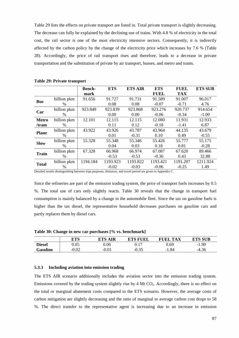
87

Table 29 lists the effects on private transport are listed in. Total private transport is slightly decreasing.

The decrease can fully be explained by the declining use of trains. With 4.8 % of electricity in the total

cost, the rail sector is one of the most electricity intensive sectors. Consequently, it is indirectly

affected by the carbon policy by the change of the electricity price which increases by 7.6 % (Table

28). Accordingly, the price of rail transport rises and therefore, leads to a decrease in private

transportation and the substitution of private by air transport, busses, and metro and trams.

Table 29: Private transport

Bench-

mark ETS ETS AIR ETS

FUEL FUEL TAX

ETS SUB

billion pkm 91.656 91.727 91.731 91.589 91.007 96.017 Bus

% 0.08 0.08 -0.07 -0.71 4.76 billion pkm 923.849 923.839 923.868 923.276 920.737 914.654

Car % 0.00 0.00 -0.06 -0.34 -1.00

billion pkm 12.101 12.115 12.115 12.080 11.931 12.933 Metro/tram % 0.11 0.12 -0.18 -1.41 6.87

billion pkm 43.922 43.926 43.787 43.964 44.135 43.679 Plane

% 0.01 -0.31 0.10 0.49 -0.55 billion pkm 55.328 55.348 55.346 55.426 55.777 55.175

Slow % 0.04 0.03 0.18 0.81 -0.28

billion pkm 67.328 66.968 66.974 67.087 67.620 89.466 Train

% -0.53 -0.53 -0.36 0.43 32.88 billion pkm 1194.184 1193.923 1193.822 1193.421 1191.207 1211.924

Total % -0.02 -0.03 -0.06 -0.25 1.49

Detailed results distinguishing between trips purposes, distances, and travel period are given in Appendix C.

Since the refineries are part of the emission trading system, the price of transport fuels increases by 0.5

%. The total use of cars only slightly reacts. Table 30 reveals that the change in transport fuel

consumption is mainly balanced by a change in the automobile fleet. Since the tax on gasoline fuels is

higher than the tax diesel, the representative household decreases purchases on gasoline cars and

partly replaces them by diesel cars.

Table 30: Change in new car purchases [% vs. benchmark]

ETS ETS AIR ETS FUEL FUEL TAX ETS SUB Diesel 0.05 0.06 0.17 0.69 -1.90 Gasoline -0.02 -0.01 -0.35 -1.84 -4.36

5.3.3 Including aviation into emission trading

The ETS AIR scenario additionally includes the aviation sector into the emission trading system.

Emissions covered by the trading system slightly rise by 4 Mt CO2. Accordingly, there is no effect on

the total or marginal abatement costs compared to the ETS scenario. However, the average costs of

carbon mitigation are slightly decreasing and the ratio of marginal to average carbon cost drops to 58

%. The direct transfer to the representative agent is increasing due to an increase in emission

88

allowances. The additional inclusion of aviation leads to a small reduction in the gross cost of carbon

regulation. The mitigation effort of the electricity sector is the same as in the ETS scenario.

Consequently, electricity generation also shows the same results.

Due to the increased cost, the price of aviation rises. Therefore, private transport reacts with a

decreasing number of plane trips. This decline is only partly balanced by switching to private road

transport, busses, and trains. As a result the total person kilometer decrease by 360 million person

kilometers compared to the benchmark.

The change in new car purchases shows the same qualitative pattern as in the ETS case: since fuel

prices rise and diesel is lower taxed, the composition changes in favor of diesel automobiles. Since

own private road transport slightly expands, new car purchases are generally higher than in the ETS

case.

5.3.4 Fuel based regulation approaches

The scenarios ETS FUEL and FUEL TAX examine fuel-based strategies mitigating carbon emissions

of road transport. Road transport has to reduce 5 % of its emissions or 8 Mt CO2. The remaining

mitigation is achieved by emission trading between electricity, energy intensive industries and refined

oil production (171.2 Mt CO2).

The FUEL TAX scenario establishes a price on the CO2 emissions of road transport fuel use. All

sectors have to pay the price except the water and rail transport sectors in which diesel fuel relates to

water and rail transport. This is interpreted as an increase in the fuel tax differentiating by the carbon

content of fuels. The ETS FUEL scenario also establishes a price of road transport emissions.

However, emissions of road transport are included into the emission trading scheme. Consequently,

the marginal abatement costs equalize across sectors and a uniform carbon price for road transport and

emissions from further fossil fuel use in the trading sectors emerges.

Comparing the FUEL TAX scenario with the ETS scenario, a significant welfare decrease is observed.

Since part of the reduction burden is shifted to road transport, the mitigation effort in the emission

trading sector is lower. Consequently, the permit price under the trading system is decreasing by 0.44

to 9.42 €/t CO2. For transport fuels, the carbon price is at a high level of 53.93 €/t CO2 indicating the

high marginal abatement cost of road transport. Due to the coexistence of the emission trading

systems, the total abatement costs are increasing being the main determinant of the welfare loss. The

hybrid regulation approach which leads to different marginal abatement cost is the main determinant

of the significant increase of the average cost of carbon regulation. A large increase in the direct

transfer to the representative agent is observed, since the high carbon price of transport results in an

increase of the government’s income of carbon regulation.

Electricity generation responds to the decrease in the carbon price by increasing production. The

generation mix also changes. Since the price of carbon is declining, coal fired generation is increasing

89

compared to the ETS scenario. Accordingly, production of cleaner CCS plants and offshore wind

power reduces. To put it clear: Regulating road transport separately, decreases the reduction burden of

the emission trading sectors resulting in a lower carbon price which indirectly subsidizes the use of

coal plants.

Concerning road transport, industrial sectors carry out the main reduction burden. The service sector,

which is the main industrial polluter of road transport emissions, reduces its emissions by 6.8 %.

Emissions are mitigated switching from own provided transport to purchased transport.

In contrast, the representative agent only slightly reduces his emissions by 0.3 %. Emissions are

decreased in two ways. First, the composition of the new car fleet significantly changes using more

carbon efficient diesel cars allowing driving the same distance with lower emissions. Second, total

trips are reduced and a mode shift towards private trains, airplanes, and the slow mode is observed.

The unexpected result of decreasing use of public transport in form of busses and metro and trams is

explained by the model’s structure: the monetary costs of both modes are specified in terms of input of

the other transport sector. Emissions resulting from diesel and gasoline use in this sector are also

addressed by the emission trading system. Accordingly, the cost of this sector increase. Furthermore,

increased demand from industrial sectors exerts an upward price pressure. Consequently, the price of

the other transport sector is rising by 1 % leading to substitution effects away from busses and metro

and tram use.

Comparing the ETS FUEL scenario, which includes road transport into the emission trading system,

with the ETS, an additional welfare loss is observed and total abatement costs are slightly decreasing.

The carbon price slightly declines, since all sectors are affected by the carbon price on transport fuels

leading to decreasing outputs. In consequence, the use of fossil fuels other than gasoline and diesel are

also decreasing yielding a decline in these emissions. This second order effect lowers the reduction

requirement under the emission trading system since the environmental target is always defined as a

20 % reduction of the economy’s emissions. However, the average cost of carbon mitigation increase.

The ratio of average to marginal abatement costs raise to 0.9 indicating an increase in the cost of

carbon regulation. Due to the high tax on transport fuels, it is favorable to exempt the road transport

sector from fuel based carbon regulation. Cost efficiency of carbon regulation requires an equal carbon

price for all sectors and commodities, i.e. the effective carbon price should be equalized. However, the

high tax on transport fuels is already environmentally motivated; i.e. a price on carbon in the transport

sector exists. Consequently, putting an additional carbon price on top of the pre-existing fuel tax

effectively induces higher carbon prices in the transport sector, and thus leads to cost inefficiency. In

essence, the induced cost inefficiency outweighs the gain of increased flexibility of transport under

emission trading.

Since it might come as a surprise that the flexibility gain is more than offset by the distortionary effect,

a numerical example shall illustrate the argument. In 2004, the mineral oil tax per liter of gasoline was

0.65 € (BMF, 2009). Combustion of this liter gasoline causes 2.3 kg CO2. Accordingly, the

90

consumption of around 435 liter of gasoline results in one ton of CO2. Therefore, the implicit pre-

existing carbon tax on transport fuels is 283.61 €/t CO2. Exempting road transport from carbon

regulation leads a carbon price of around 10 €/t CO2 and, therefore, the difference in effective carbon

taxes is reduced. In contrast, in the FUEL TAX scenario the carbon price in the transport sector

increases by around 54 €/t CO2 while emission trading sectors pay a price 9.50 €/t CO2. Thus, the gap

in effective carbon taxes is even increased.

While the example is illustrative, it neglects taxes on transport fuels that do not solely relate to carbon

emissions. Other externalities such as local pollution and associated health damages, congestion,

noise, and accidents are also addressed. However, congestion as the main externality of road transport

is included in the model. Regardless, the exemption of transport shows a positive effect.

Due to the higher marginal abatement cost in road transport, reduction mainly takes place in the

emission trading sectors especially in electricity generation. Consequently, the generation mix is only

slightly affected by an increase of hard coal fired generation in the mid load segment.

Concerning private transport, the ETS FUEL scenarios mirrors the results of the FUEL TAX scenario

in an attenuated form. The composition of the new car purchases is influenced towards more fuel

efficient diesel cars and total trips are slightly reduced. Own private road transport, bus, and metro and

tram trips incline and are partly substituted by the use of private trains, the slow mode, and airplanes.

5.3.5 Increasing subsidies on public transport

Like the ETS scenario, the ETS SUB introduces emission trading between electricity generation,

energy intensive industries, and refined oil production. However, in contrast to the ETS scenario the

revenues of carbon regulation are not to recycled lump-sum but used to uniformly increase subsidies

on public transport, i.e. busses, private trains trips, and metro and trams.

Revenue recycling using increased public transport subsidies shows a clear positive welfare effect

compared to emission trading under lump-sum recycling. Total and marginal abatement costs slightly

reduce. Remarkably, the average costs of carbon regulation strongly decline resulting in a ratio of

marginal to average abatement costs of 0.2. The subsidy on private trains becomes 52 % and busses

and metro and tram trips are subsidized at a rate of 21 %.

Increased public transport subsidies yield substitution away from private road transport towards the

subsidized modes bus, metro and tram, and trains. Accordingly, emissions of private cars are

decreasing by 1.3 %. This decrease is even larger than in scenarios where road transport emissions are

addressed by fuel based regulation approaches. The fuel based approaches implement economy wide

regulation, i.e. also include transport emissions of industrial sectors. In consequence, the abatement

burden is shifted to industries showing only small effects on private transport. In contrast, public

transport subsidies solely affect the households’ decision of private transport modes and offer

incentives substituting away from cars.

91

The increased reduction effort of private road transport spills over to the emission trading system since

the overall reduction of 179.2 Mt CO2 is fixed. While energy intensive production and refineries

increase emissions, the electricity sector further reduces its emissions. Despite reduced emissions,

electricity generation is expanding compared to the ETS by expanding the use of the CCS technology

in the base load.

Private transport subsidies induce a switch to public transport modes simultaneously increasing the

total number of kilometers traveled. Trips using cars are decreasing by 1 %, while trips on busses,

metros and trams, and trains increase by 4.8, 6.9, and 32.9 %, respectively. The excessive use of trains

is explained by the assumption that revenues are recycled uniformly increasing subsidies. Since the

subsidy on trains are already higher in the benchmark, a uniform multiplier on subsidies results in

larger absolute effects on the subsidies for private train trips.

The clear cut positive welfare effect is explained by the reduction of the congestion externality. Table

31 shows the impact of the scenarios on speed on different road types differentiated by travel periods.

While all other scenarios show negligible impacts on speed, the ETS PUB scenario results in a 2 %

(1.5 %) increase of travel speed on urban (non-urban) roads in the peak period.

Table 31: Impacts on road speed [% vs. benchmark]

ETS ETS AIR ETS FUEL FUEL TAX ETS SUB peak 0.00 0.00 0.02 0.13 0.52 Urban

off-peak -0.02 -0.03 0.02 0.19 1.99 peak 0.00 0.00 0.01 0.07 0.16 Non-Urban

off-peak -0.01 -0.02 0.02 0.20 1.46

5.4 Sensitivity analysis

5.4.1 Malleability of technology specific capital

The malleability of generation capacities is controlled by the transformation elasticity of the activity

which converts malleable capital into technology specific capital (εKE). The sensitivity of the results to

a change of the transformation elasticity is examined by halving and doubling the benchmark value of

unity. A lower value of the elasticity implies a higher degree of irreversibility in electricity generation.

Table 32 shows the impact of varying the transformation elasticity on the gross cost of regulation and

total and marginal abatement cost for the ETS and ETS FUEL scenarios. A lower value of the

elasticity implies a higher degree of irreversibility in electricity generation, i.e. the reallocation of

technology specific capital is limited. Accordingly, welfare losses and abatement costs are decreasing

in the value of the elasticity since the ability of responding to price changes is increased. Although the

magnitude of the results is affected, the qualitative effect of including transport fuel into the emission

trading scheme remains. Still the inclusion shows a negative welfare impact.

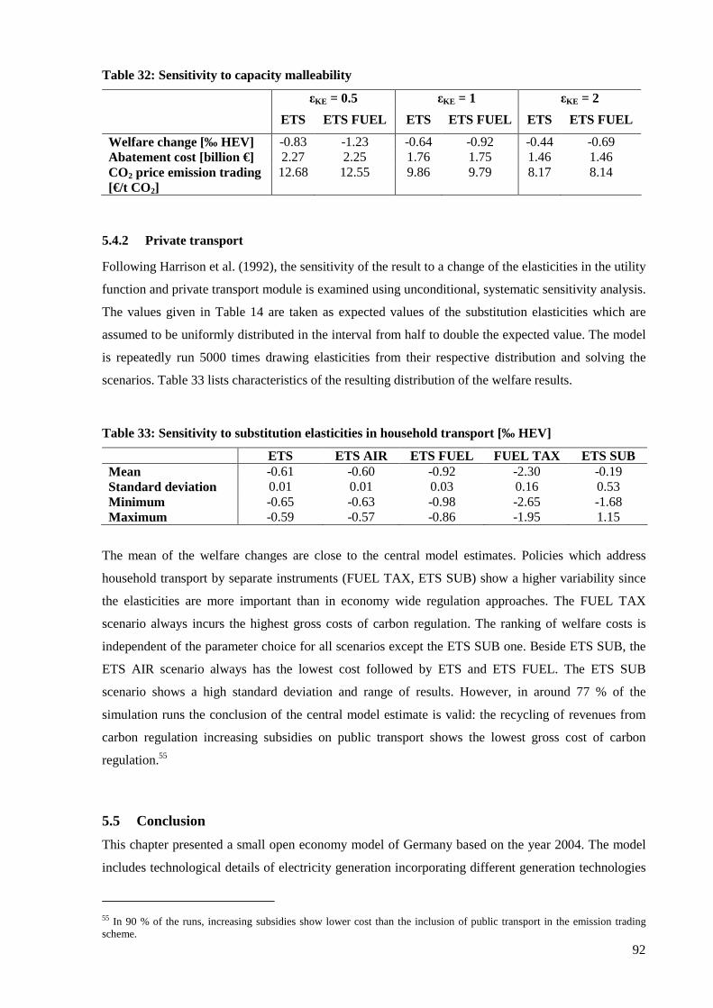
92

Table 32: Sensitivity to capacity malleability

εKE = 0.5 εKE = 1 εKE = 2

ETS ETS FUEL ETS ETS FUEL ETS ETS FUEL

Welfare change [‰ HEV] -0.83 -1.23 -0.64 -0.92 -0.44 -0.69 Abatement cost [billion €] 2.27 2.25 1.76 1.75 1.46 1.46 CO2 price emission trading [€/t CO2]

12.68 12.55 9.86 9.79 8.17 8.14

5.4.2 Private transport

Following Harrison et al. (1992), the sensitivity of the result to a change of the elasticities in the utility

function and private transport module is examined using unconditional, systematic sensitivity analysis.

The values given in Table 14 are taken as expected values of the substitution elasticities which are

assumed to be uniformly distributed in the interval from half to double the expected value. The model

is repeatedly run 5000 times drawing elasticities from their respective distribution and solving the

scenarios. Table 33 lists characteristics of the resulting distribution of the welfare results.

Table 33: Sensitivity to substitution elasticities in household transport [‰ HEV]

ETS ETS AIR ETS FUEL FUEL TAX ETS SUB Mean -0.61 -0.60 -0.92 -2.30 -0.19 Standard deviation 0.01 0.01 0.03 0.16 0.53 Minimum -0.65 -0.63 -0.98 -2.65 -1.68 Maximum -0.59 -0.57 -0.86 -1.95 1.15

The mean of the welfare changes are close to the central model estimates. Policies which address

household transport by separate instruments (FUEL TAX, ETS SUB) show a higher variability since

the elasticities are more important than in economy wide regulation approaches. The FUEL TAX

scenario always incurs the highest gross costs of carbon regulation. The ranking of welfare costs is

independent of the parameter choice for all scenarios except the ETS SUB one. Beside ETS SUB, the

ETS AIR scenario always has the lowest cost followed by ETS and ETS FUEL. The ETS SUB

scenario shows a high standard deviation and range of results. However, in around 77 % of the

simulation runs the conclusion of the central model estimate is valid: the recycling of revenues from

carbon regulation increasing subsidies on public transport shows the lowest gross cost of carbon

regulation.55

5.5 Conclusion

This chapter presented a small open economy model of Germany based on the year 2004. The model

includes technological details of electricity generation incorporating different generation technologies

55 In 90 % of the runs, increasing subsidies show lower cost than the inclusion of public transport in the emission trading scheme.

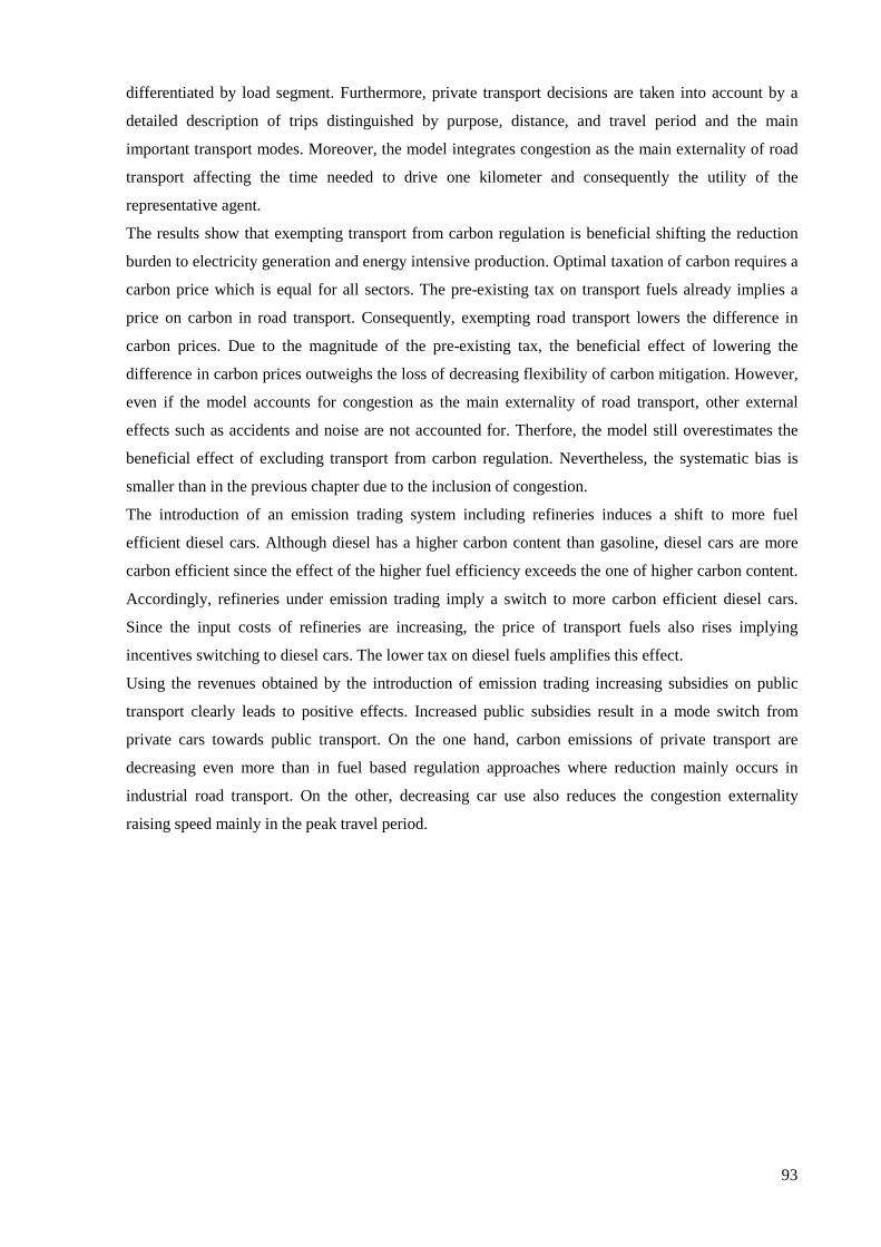
93

differentiated by load segment. Furthermore, private transport decisions are taken into account by a

detailed description of trips distinguished by purpose, distance, and travel period and the main

important transport modes. Moreover, the model integrates congestion as the main externality of road

transport affecting the time needed to drive one kilometer and consequently the utility of the

representative agent.

The results show that exempting transport from carbon regulation is beneficial shifting the reduction

burden to electricity generation and energy intensive production. Optimal taxation of carbon requires a

carbon price which is equal for all sectors. The pre-existing tax on transport fuels already implies a

price on carbon in road transport. Consequently, exempting road transport lowers the difference in

carbon prices. Due to the magnitude of the pre-existing tax, the beneficial effect of lowering the

difference in carbon prices outweighs the loss of decreasing flexibility of carbon mitigation. However,

even if the model accounts for congestion as the main externality of road transport, other external

effects such as accidents and noise are not accounted for. Therfore, the model still overestimates the

beneficial effect of excluding transport from carbon regulation. Nevertheless, the systematic bias is

smaller than in the previous chapter due to the inclusion of congestion.

The introduction of an emission trading system including refineries induces a shift to more fuel

efficient diesel cars. Although diesel has a higher carbon content than gasoline, diesel cars are more

carbon efficient since the effect of the higher fuel efficiency exceeds the one of higher carbon content.

Accordingly, refineries under emission trading imply a switch to more carbon efficient diesel cars.

Since the input costs of refineries are increasing, the price of transport fuels also rises implying

incentives switching to diesel cars. The lower tax on diesel fuels amplifies this effect.

Using the revenues obtained by the introduction of emission trading increasing subsidies on public

transport clearly leads to positive effects. Increased public subsidies result in a mode switch from

private cars towards public transport. On the one hand, carbon emissions of private transport are

decreasing even more than in fuel based regulation approaches where reduction mainly occurs in

industrial road transport. On the other, decreasing car use also reduces the congestion externality

raising speed mainly in the peak travel period.

94

6 Conclusion

6.1 Summary and conclusion

This thesis posed the question whether including road transport into the EU ETS will lower the cost of

carbon regulation. Two different CGE models are employed: an international and a small-open

economy model.

The multi-region model shows that a European-wide increase of transport fuel taxes is not a promising

option regulating the carbon emissions of transport. Including road transport into the EU ETS indeed

can lower the gross cost of carbon regulation. However, the most preferable approach is exempting

transport from regulation.

The results are confirmed by the small-open economy model which offers a far more detailed

representation of electricity generation and private transport but abstracts from term-of-trade changes.

Including transport in emission trading lowers the cost compared to an increase in fuel taxes but the

exemption is the most favorable approach.

Thus, the answer to the main question depends on the basic approach of policy makers. If governments

decide to use pricing strategies for transport fuels, then the inclusion into emission trading is the best

approach. However, generally, no carbon regulation in the road transport sector is the best strategy.

Due to already high excise taxes, the exemption of transport moves the after-regulation tax scheme

closer to the optimal one. Put differently, the exemption leads to effective carbon tax rates that are

closer to uniform across the economy. The small-open economy model shows that the result is stable

concerning congestion as a justification for high fuel tax rates. However, both models exclude further

external effects such as accidents and noise and, therefore, the results overestimate the beneficial

effext of not further increasing transport fuel prices. It is an interesting topic for future research to

include these effects in a detailed and concise manner.

The detailed model shows that including aviation in the trading scheme further lowers the cost of

regulation. Furthermore, the results indicate that subsidies on public transport may play a significant

role in addressing the carbon emission of private transport. Subsidies have two positive effects. First,

the costs of carbon regulation decrease by the induced switch to environmentally friendly public

transport. Second, the congestion externality inclines due to fewer vehicles on roads. Further welfare

gains not included in the model can be expected since the decrease in the traffic-flow also reduces

other externalities of transport such as accidents, noise, and local pollution. However, this claim has

not been tested against other revenue recycling schemes, in particular the cut of labor taxes. Whether

or not the result will prove stable is subject to future research.

6.2 Future research

This thesis neglects the spatial and network aspects of the transport problem as well as of electricity

transmission. The inclusion of the spatial dimension of transport is an important topic for future

95

research since it determines the substitution possibilities available for private cars, e.g. rural

households have less access to public transport modes and, accordingly, less substitution possibilities.

Such differences can be captured in modeling different household types with different locations of

living and utility functions (e.g. Mayeres, 1999; Kalinowska et al., 2007). However, such models are

not well suited to model households’ modes decisions or mode switches in freight transport. An

approach of explicitly including transport networks into the general equilibrium model would be

preferable. Furthermore, such models allow a better assessment of transport infrastructure

improvement. It has to be decided whether the CGE and network models are designed in an integrated

formulation or whether they are separately designed and linked in some algorithm.

Roson (1996) describes the MITER model which iteratively links three different sub-models. Ferris et

al. (1999) show a Wardop equilibrium problems can be represented in a mixed-complementarity

problem. Such a representation allows including detailed network representations into the general

equilibrium framework. A first application of integrating public and freight transport networks into a

CGE model is given by Ivanova (2003). The discussion about the mitigation of greenhouse gas

emissions of transport would benefit from such a modeling approach in order to assess interesting

topics such as improved public transport networks and freight network intermodality.

Electricity networks play a substantial role in the penetration of renewable electricity generation.

Leuthold et al. (2009) show the impact of additional wind power on the European transmission grid.

While the amount of additional grid investments in their study is modest, the integration of solar

power from the Middle East and northern Africa into the European grid imposes real challenges (DLR,

2006). In order to assess such scenarios in a general equilibrium framework, it would be useful to

integrate grid requirements. This can also be done using the MCP framework.

However, for both, transport and electricity networks, the detailed modeling implies an increase in

data requirements. For every node in the network, data on production and demand need to be

collected. Furthermore, an increased number of modeled power plants increases the number of

installed capacities in the consumers’ endowments. Accordingly, income effects become larger and

models become computably less tractable. This points into the direction of falling back to

decomposition methods and building detailed transport and energy system models. Efficient

decomposition methods for CGE models in MCP models have been demonstrated by Rausch and

Rutherford (2007) and Rutherford and Tarr (2007) a large number of consumers as well as Böhringer

and Rutherford (2009) for large scale energy system models. A combination of these approaches

would allow for the implementation of the spatial dimension into the energy system model and using

the aggregation approach for households to upscale data from the detailed geographical dimension to a

representative agent in the CGE model. A similar approach is implementable for transport system

models.

96

Literature

Aarts, L. and I. van Schagen (2006): Driving speed and the risk of road crashes: A review. Accident

Analysis and Preventions 38(2): 215-224.

Achtnicht, M., Georg Bühler, and C. Hermeling (2008): Impact of Service Station Networks on

Purchase Decisions of Alternative-fuel Vehicles. Centre for European Economic Research

Discussion Paper 08-088.

Albrecht, J. (2000): The Diffusion of Cleaner Vehicles in CO2 Emission Trading Designs.

Transportation Research Part D 5(5): 385-401.

Albrecht, J. (2001): Tradable CO2 Permits for Cars and Trucks. Journal of Cleaner Production 9(2):

179-189.

Archer, D. (2007): Global Warming: Understanding the Forecast. Oxford et al., Blackwell Publishing.

Armington, P. S. (1969): A Theory of Demand for Products Distinguished by Place of Production.

International Monetary Fund Staff Paper 16(1): 159-176.

Arrow, K. J. (1950): A Difficulty in the Concept of Social Welfare. The Journal of Political Economy

58(4): 328-346.

Arrow, K. J., H. B. Chenery, B. S. Minhas, and R. M. Solow (1961): Capital-Labor Substitution and

Economic Efficiency. The Review of Economics and Statistics 43(3): 225-250.

Arrow, K. J. and G. Debreu (1954): Existence of an Equilibrium for a Competitive Economy.

Econometrica 22(3): 265-290.

Arrow, K. J. and F. H. Hahn (1971): General Competitive Analysis. San Francisco, Holden-Day.

Auerbach, A. J. and J. R. Hines (2002): Taxation and Economic Efficiency. In: Handbook of Public

Economics, Vol. 3, Chapter 21. Ed. A. J. Auerbach and M. Feldstein, Amsterdam, North

Holland: 1347-1421.

Babiker, M. H., P. Criqui, A. D. Ellerman, J. M. Reilly and L. L. Viguier (2003). Assessing the Impact

of Carbon Tax Differentiation in the European Union. Environmental Modeling and

Assessment 8(3): 187-197.

Babiker, M., J. Reilly, and L. Viguier (2004): Is International Emissions trading always Beneficial?

The Energy Journal 25(2): 33-56.

Babiker, M., A. Gurgel, S. Paltsev, and J. Reilly (2008).: A Forward Looking Version of the MIT

Emissions Prediction and Policy Analysis (EPPA) Model. MIT Joint Program on the Science

and Policy of Global Change Report 161.

Bauer, N., L. Baumstark, M. Haller, M. Leimbach, and M. Lueken (2008): REMIND: The Equations,

Potsdam Institute for Climate Impact Research.

Baumol, W. J. and W. E. Oates (1988): The Theory of Environmental Policy. 2nd edition. New York et

al., Cambridge University Press.

Becker, G. S. (1965): A Theory of the Allocation of Time. The Economic Journal 75(299): 493-517.

Berg, C. (2007): Household Transport Demand in a CGE Framework. Environmental and Resource

Economics 37(3): 573-597.

97

Bergman, L. (2005): CGE Modeling of Environmental Policy and Resource Management. Handbook

of Environmental Economics: 1273-1306.

Bickel, P. and R. Friedrich (eds.) (2005): ExternE: Externalities of Energy - Methodology 2005

Update Luxembourg. European Commission.

Bickel, P., S. Schmid, and R. Friedrich (2005): Environmental Costs. Research in Transportation

Economics 14: 185-209.

Böhringer, C. (1995): Allgemeine Gleichgewichtsmodelle als Instrument der energie- und

umweltpolitischen Analyse. Dissertation. Frankfurt am Main, Peter Lang Verlag.

Böhringer, C. (1998): The Synthesis of Bottom-Up and Top-Down in Energy Policy Modeling.

Energy Economics 20(3): 233-248.

Böhringer, C. (2002): Industry Level Emission Trading between Power Producers in the EU. Applied

Economics 34(4): 523-533.

Böhringer, C. and K. E. Rosendahl (2009): Strategic Partitioning of Emission Allowances under the

EU Emission Trading Scheme. Resource and Energy Economics 31(3): 182-197.

Böhringer, C. and T. F. Rutherford (2002a): In Search of a Rationale for Differentiated Environmental

Taxes, Centre for European Economic Research Discussion Paper 02-30.

Böhringer, C. and T. F. Rutherford (2002b): Carbon Abatement and International Spillovers: A

Decomposition of General Equilibrium Effects. Environmental and Resource Economics

22(3): 391–417.

Böhringer, C. and T. F. Rutherford (2008): Combining Bottom-Up and Top-Down. Energy Economics

30: 574–596.

Böhringer, C. and T. F. Rutherford (2009): Integrated Assessment of Energy Policies: Decomposing

Top-Down and Bottom-Up. Journal of Economic Dynamics & Control 33(9): 1648-1661.

Böhringer, C. and C. Vogt (2003): Economic and Environmental Impacts of the Kyoto Protocol. The

Canadian Journal of Economics 36(2): 475-494.

Boiteux, M. (1956): Sur la gestion des Monopoles Publics astreints a l'equilibre budgetaire.

Econometrica 24(1): 22-40.

Bosquet, B. (2000): Environmental Tax Reform: Does it Work? A Survey of the Empirical Evidence.

Ecological Economics 34(1): 19-32.

Boveneberg, A. L. (1999): Green Tax Reforms and the Double Dividend: An Updated Reader's Guide.

International Tax and Public Finance 6(3): 421-443.

Bovenberg, A. L. and R. A. d. Mooij (1994). Environmental Levies and Distortionary Taxation. The

American Economic Review 84(4): 1085-1089.

Bovenberg, A. L. and F. van der Ploeg (1994): Environmental Policy, Public Finance and the Labor

Market in a Second-Best World. Journal of Public Economics 55(3): 349-390.

Bovenberg, L. A. and L. G. Goulder (1996): Optimal Environmental Taxation in the Presence of Other

Distortionary Taxes: General-Equilibrium Analysis. American Economic Review 86(4): 985-

1000.

98

British Petrol (2007): BP Statistical Review of World Energy. http://www.bp.com, retrieved

21.06.2008.

Brooke, A., D. Kendrick, and A. Meeraus (2008): GAMS a User’s Guide. Washington, GAMS

Development Cooperation.

Browning, E. K. (1976): The Marginal Cost of Public Fund. The Journal of Political Economy 84(2):

283-298.

Bruzelius, N. (1979): The value of travel Time: Theory and Measurement. London, Croom Helm.

Bundesministerium der Finanzen (BMF) (2009): Entwicklung der Energie- (vormals Mineralöl-) und

Stromsteuersätze in der Bundesrepublik Deutschland.

Bundesministerium für Umwelt, Naturschutz und Reaktorsicherheit (BMU) (2007): Erneuerbare

Energien in Zahlen – national und international Entwicklungen.

Burniaux, J.-M. and T. P. Truong (2002): GTAP-E: An Energy-Environmental Version of the GTAP

Model. GTAP Technical Paper 16.

Button, K. (1990): Environmental Externalities and Transport Policy. Oxford Review of Economic

Policy 6(2): 61-75.

Capros, P., P. Georgakopoulos, D. Van Regemorter, S. Proost, and C. Schmidt (1997): The GEM-E3

General Equilibrium of the European Union. Economic and Financial Modeling: 21-160.

Chiang, A. C. and K. Wainwright (2005): Fundamental Methods of Mathematical Economics. New

York, McGraw-Hill.

Christensen, L. R., D. W. Jorgenson, and L. J. Lau (1973): Transcendental Logarithmic Production

Frontiers. The Review of Economics and Statistics 55(1): 28-45.

Christensen, L. R., D. W. Jorgenson, and L. J. Lau (1975): Transcendental Logarithmic Utility

Functions. The American Economic Review 65(3): 367-383.

Choumert, F., S. Paltsev, and J. Reilly (2006): Improving the Refining Sector in EPPA. MIT Joint

Program on the Science and Policy of Global Change Technical Note 9.

Coase, R. (1960): The Problem of Social Cost. Journal of Law and Economics 3: 1-44.

Conrad, K. (1994): Applied General Equilibrium Modeling for Environmental Policy Analysis. Annals

of Operations Research 54(1): 129-142.

Conrad, K. (1997): Traffic, Transportation, Infrastructure and Externalities: A Theoretical Framework

for a CGE Analysis. The Annals of Regional Science 31(4): 369-389.

Conrad, K. and S. Heng (2002): Financing Road Infrastructure by Savings in Congestion Costs: A

CGE Analysis. The Annals of Regional Science 36(1): 107-122.

Conrad, K. and M. Schröder (1991): Demand for Durable and Nondurable Goods, Environmental

Policy and Consumer Welfare. Journal of Applied Econometrics 6(3): 271-286.

Cottle, R. W., J.-S. Pang, and R. E. Stone (1992): The Linear Complementarity Problem. San Diego,

Academic Press Inc.

99

Criqui, P., S. Mima, and L. Viguier (1999): Marginal Abatement Costs of CO2 Emission Reductions,

Geographical Flexibility and Concrete Ceilings: An Assessment using the POLES Model.

Energy Policy 27(10): 585-601.

Cropper, M. L. and W. E. Oates (1992): Environemental Economics: A Survey. Journal of Economic

Literature 30(2): 675-740.

Crutzen, P. J., A. R. Mosier, K. A. Smith, and W. Winiwarter (2008): NO2 Release from Agro-biofuel

Production Negates Global Warming Reduction by Replacing Fossil Fuels. Atmospheric

Chemistry and Physics 8(2): 389-395.

Dales, J. H. (1968): Pollution Properties and Prices. Toronto, University of Toronto Press.

David, J. and H. Herzog (2000): The Cost of Carbon Capture. Presented at: Fifth International

Conference on Greenhouse Gas Control Technologies, Cairns, Australia.

De Borger, B. and D. Swysen (1998): Optimal Pricing and Regulation of ransport Externalitites: A

welfare Comparison of Some Policy Alternatives. In: Environmental and Transport Modeling,

Ed. R. Roson and K. A. Small. Dordrecht et al., Kluwert Academic Publishers: 10-38.

De Ceuster, G. D., B. v. Herbruggen, O. Ivanova, K. Carlier, A. Martino, and D. Fiorello (2007):

TREMOVE. http://www.tremove.org, retreived: 26.07.2007.

De Jong, G. C. (1991): Utility Model of Car Ownership and Private Car Use. European Economic

Review 34(5): 971-985.

Debreu, G. (1959): Theory of Value: An Axiomatic Analysis of Economic Equilibrium. London, Yale

University Press.

Destatis (2002): Tabellenband I zur Zeitbudgeterhebung 2001/02. Aktivitäten in Stunden und Minuten

nach Geschlecht, Alter und Haushaltstyp. http://www.destatis.de, retreived 15.02.2009.

Destatis (2006): Verkehr in Deutschland 2006. http://www.destatis.de, retreived 22.01.2009.

Destatis (2008a): VGR des Bundes - Input-Output-Rechnung: http://www.destatis.de, retrieved:

30.01.2009.

Destatis (2008b): Tabellen der Umweltökonomische Gesamtrechnung. Available on request.

DeSerpa, A. C. (1971): A Theory of the Economic of Time. The Economic Journal 81(324): 828-846.

Deutscher Bundestag (2002): Gesetz zur geordneten Beendigung der Kernenergie zur gewerblichen

Erzeugung von Elektrizität, Bundesgesetzblatt, 2002(I) 26.

Deutscher Bundestag, (2009). Gesetz zur Neuregelung der Kraftfahrzeugsteuer und Änderung anderer

Gesetze, Bundesgesetzblatt (I) 29.

Deutsches Institut für Luft- und Raumfahrt (DLR) (2006): Trans-Mediterraner Solarstromverbund:

Zusammenfassung. Studie im Auftrag des Bundesminsteriums für Umwelt, Naturschutz und

Reaktorsicherheit.

Diamond, P. A. and J. A. Mirlrlees (1971a): Optimal Taxatiom and Public Production I: Production

Efficiency. The American Economic Review 61(1): 8-27.

Diamond, P. A. and J. A. Mirrlees (1971b): Optimal Taxation and Public Production II: Tax Rules.

The American Economic Review 61(3): 261-278.

100

Diewert, W. E. (1971): An Application of the Shephard Duality Theorem: A Generalized Leontief

Production Function. The Journal of Political Economy 79(3): 481-507.

Diewert, W. E. and T. J. Wales (1987): Flexible Functional Forms and Global Curvature Conditions.

Econometrica 55(1): 43-68.

Dimaranan, B. V., Ed (2006): The GTAP 6 Data Base. West Lafayette, Centre for Global Trade

Analysis, Department of Agriculture Economic, Purdue University.

Dirkse, S. P. and M. C. Ferris (1995): The PATH Solver: A Non-Monotone Stabilization Scheme for

Mixed Complementarity Problems. Optimization Methods and Software 5(2): 123-156.

Dobes, L. (1999): Kyoto: Tradable Greenhouse Emission Permits in the Transport Sector. Transport

Reviews 19(1): 81-97.

Duvall, M. (2004): Advanced Batteries for Electric-Drive Vehicles: A Technology and Cost-

Effectiveness Assessment for Battery Electric Vehicles, Power Assist Hybrid Electric

Vehicles, and Plug-In Hybrid Electric Vehicles. Electric Power Research Institute, Palo Alto.

Downing, P. B. and L. J. White (1986): Innovation in Pollution Control. Journal of Environmental

Economics and Management 13(1): 18-29.

EC (2002): Council Decision of 25 April 2002 Concerning the Approval, on Behalf of the European

Community, of the Kyoto Protocol to the United Nations Framework Convention on Climate

Change and the Joint Fulfillment of Commitments thereunder. Official Journal of the

European Union L 130/1. 2002/358/CE.

EC (2003): Directive 2003/87/EC of the European Parliament and of the Council Establishing a

Scheme for Greenhouse Gas Emission Allowance Trading within the Community and

Amending Council Directive 96/61/EC. Official Journal of the European Union L 275/32.

2003/87/EC.

EC (2008a): Directive 2008/101/EC of the European Parliament and of the Council amending

Directive 2003/87/EC so as to Include Aviation Activities in the Scheme for Greenhouse Gas

Emission Allowance Trading within the Community. Official Journal of the European Union,

L8/1. 2008/101/EC.

EC (2008b): Directive 2009/28/EC of the European Parliament and of the Council of 23 April 2009 on

the Promotion of the Use of Energy from Renewable Sources and Amending and

Subsequently Repealing Directives 2001/77/EC and 2003/30/EC, Official Journal of the

European Union, L140/16. 2009/28/EC.

EC (2009a): Decision No 406/2009/EC of the European Parliament and of the Council of 23 April

2009 on the Effort of Member States to Reduce their Greenhouse Gas Emissions to Meet the

Community’s Greenhouse Gas Emission Reduction Commitments up to 2020. Official

Journal of the European Union, L 140/136. 406/2009/EC.

EC (2009b): Directive 2009/29/EC of the European Parliament and the Council amending Directive

2003/87/EC so as to Improve and Extend the Greenhouse Gas Emission Allowance trading

Scheme of the Community. Official Journal of the European Union, L140/63. 2009/29/EC.

101

EC (2009c): Regulation (EC) No 443/2009 of the European Parliament and of the Council of 23 April

2009 Setting Emission Performance Standards for New Passenger Cars as Part of the

Community’s Integrated Approach to Reduce CO2 Emissions from Light-duty Vehicles,

Official Journal of the European Union, L140/1. 443/2009/EC.

Ellerman, D. A., H. D. Jacoby, and M. B. Zimmerman (2006): Bringing Transportation into a Cap and

Trade Regime. MIT Joint Program on the Science and Policy of Global Climate Change

Report 136.

Elmer, C.-F. and Fischer C. (2009): Designing Vehicle CO2 Emission Standards. Resources for the

Future Discussion Paper forthcoming.

European Conference of Ministers of Transport (ECMT) (2007): Cutting Transport CO2 Emissions:

What Progress? Paris, OECD.

European Energy Exchange: Sportpreise für Stundenkontrakte 2004. http://www.eex.de, retreived:

21.08.2006.

Eurostat (1999): Household Budget Survey of 1999. http://epp.eurostat.ec.europa.eu, retrieved:

10.10.2008.

Eurostat (2008a): Population Data. http://epp.eurostat.ec.europa.eu, retrieved: 10.10.2008.

Eurostat (2008b): Annual Energy Statistics. http://epp.eurostat.ec.europa.eu, retrieved: 15.10.2008.

Eurostat (2009a): Indicators for air pollution and climate change. http://epp.eurostat.ec.europa.eu,

retrieved: 14.02.2009.

Eurostat (2009b): Statistical Classification of Economic Activities in the European Community, Rev. 2

(NACE Rev. 2). http://ec.europa.eu/eurostat/ramon, retrieved 27.04.2009.

EUSUSTEL (2006): European Sustainable Electricity: Comprehensive Analysis of Future European

Demand and Generation of European Electricity and its Security of Supply.

http://www.eusustel.be.

Feldstein, M. (1976): On the Theory of Tax Reforms. Journal of Public Economics 6(1): 77-104.

Ferris, M. C., A. Meeraus, and T. F. Rutherford (1999): Computing Wardropian Equilibria in a

Complementarity Framework. Optimization Methods and Software 10(5): 669-685.

Ferris, M. C. and T. S. Munson (2000): Complementarity Problems in GAMS and the Path Solver.

Journal of Economic Dynamics and Control 24(2): 165-188.

Ferris, M. C. and J. S. Pang (1997): Engineering and Economic Applications of Complementarity

Problems. SIAM Review 39(4): 669-713.

Fischer, C., W. Harrington, and I. W. H. Parry (2007): Should Automobile Fuel Economy Standards

be Tightened? The Energy Journal 28(4): 1-29.

Galeotti, M. and C. Carraro (1996): Environmental Taxation and Unemployment: Some Evidence on

the 'Double Dividend Hypothesis' in Europe. Journal of Public Economics 62(1): 141-181.

German Institute for Economic Research (DIW) (2006): Verkehr in Zahlen 2006/2007. Hamburg,

Deutscher Verkehrsverlag.

102

Ginsburgh, V. and M. Keyzer (1997): The Structure of Applied General Equilibrium Models.

Cambridge et al., MIT Press.

Goulder, L. H. (1995): Environmental Taxation and the Double Dividend: A Reader's Guide.

International Tax and Public Finance 2: 157-183.

Graham, d. J. and S. Glaister (2002): The Demand for Automobile Fuel: A Survey of Elasticities.

Journal of Transport Economics and Policy: A Survey of Elasticities 36(1): 1-26.

Graves, P. E., D. R. Lee, and R. L. Sexton (1993): Speed Variance, Enforcement, and the Optimal

Speed Limit. Economics Letter 42(2): 237-243.

Greene, D. L., J. R. Kahn, and R. C. Gibson (1999): Fuel Economy Rebound Effect of U.S. Household

Vehicles. The Energy Journal 20(3): 1-31.

Hahn, R. W. (1984): Market Power and Transferable Property Rights. The Quarterly Journal of

Economics 99(4): 753-765.

Hammar, H., Å. Löfgren, and T. Sterner (2004): Political Economy Obstacles to Fuel Taxation. The

Energy Journal 25(3): 1-17.

Harrison, G. W. and H. D. Vinod (1992): The Sensitivity of Applied General Equilibrium Models:

Completely Randomized Factorial Sampling Designs. The Review of Economics and Statistics

74(2): 357-362.

Herry, M., N. Sedlacek, R. Tomschy, P. Bickel, and S. Schmid (2001): UNITE: The Pilot Accounts

for Austria UNIfication of accounts and marginal costs for Transport Efficiency - Working

Funded by 5th Framework RTD Programme. ITS, University of Leeds.

Hoel, M. (1996): Should a Carbon Tax be Differentiated across Sectors? Journal of Public Economics

59(1): 17-32.

Hourcarde, J.-C., M. Jaccard, C. Bataille, and F. Ghersi (2006): Hybrid Modeling: New Answers to

Old Challanges. The Energy Journal - Special Issue: Hybrid Modeling of Energy-

Environmental Policies: Reconceiling Bottom-up and Top-Down: 1-11.

Hyman, R. C., J. M. Reilly, M. H. Babiker, A. D. Masin, and H. D. Jacoby (2002): Modeling Non-

CO2 Greenhouse Gas Abatement. Environmental Modeling and Assessment 8(3): 175-186.

International Energy Agency (2008): Energy Prices and Taxes. Quarterly Statistics, 2nd Quarter 2008.

Paris, OECD.

IPCC (2006): 2006 IPCC Guidelines for National Greenhouse Gas Inventories. Ed. H. S. Eggleston, L.

Buendia, K. Miwa, T. Ngara and K. Tanabe. Institute for Global Environmental Strategy.

IPCC (2007): Climate Change 2007: The Physical Science Basis. Contribution of Working Group I to

the Fourth Assessment Report of the Intergovernmental Panel on Climate Change. Ed.

Solomon, S., D. Qin, M. Manning, Z. Chen, M. Marquis, K.B. Averyt, M. Tignor, and H.L.

Miller. Cambridge et al., Cambridge University Press.

Jaffe, A. B., R. G. Newell, and R. N. Stavins (2002a): Technological Change and the Environment. In:

Ed. K.-G. Mäler and J. Vincent: Handbook of Environmental Economics, Vol. I. Amsterdam,

Elsevier Science: Chapter 11, 461-516.

103

Jaffe, A. B., R. G. Newell, and R. N. Stavins (2002b): Environmental Policy and Technological

Change. Environmental and Resource Economics 22(1): 41-69.

Jeger, J. F., E. Quinet, D. A. R. Schwartz, J.-P. Taroux, H. Link, L. Stewart, and P. Bickel (2001).:

UNITE: Pilot Accounts - Results for France. UNIfication of accounts and marginal costs for

Transport Efficiency - Working Funded by 5th Framework RTD Programme. ITS, University

of Leeds.

Jokisch, S. and T. Mennel (2009): Hydrogen in Passenger Transport: A Macroeconomic Analysis.

Transport Reviews 59(4): 415-438.

Kalinowska, D., H. Kremers, and T. P. Truong (2007): An Assessment of Road-price Measures on

Household travel Demand in Germany Using a Computable General Equilibrium Framework.

Presented at: EconMod Conference on Energy and Environmental Modeling. Moscow.

Karplus, V. J., S. Paltsev, and J. M. Reilly (2009): Prospects for Plug-in Hybrid Electric Vehicles in

the United States and Japan: A General Equilibrium Analysis. MIT Joint Program on the

Science and Policy of Global Change Report 172.

Keller, W. J. (1976): A Nested CES-type Utility Function and its Demand and Price-Index Functions.

European Economic Review 7(2): 175-786.

Keller, W. J. (1980): Tax Incidence: A General Equilibrium Approach. Amsterdam et al., North -

Holland Publishing.

Koopman, G. J. (1995): Policies to Reduce CO2 Emissions from Cars in Europe. Journal of Transport

Economics and Policy 29(1): 53-70.

Kraftfahrt-Bundesamt (KBA) (2005a): Statistische Mittelungen: Bestand an Kraftfahrzeugen und

Kraftfahrzeuganhängern am 1. Januar 2004.

Kraftfahrt-Bundesamt (KBA) (2005b): Statistische Mittelungen: Neuzulassungen – Besitzumschrei-

bungen – Löschungen von Kraftfahrzeugen und Kraftfahrzeuganhängern im Jahr 2004.

Kremers, H. and D. Kalinowska (2009): The Distributional Effects of Car Road Charging: Application

of a Computable General Equilibrium Model Including Passenger Travel. Presented at: 17th

Annual Conference of the European Association of Environmental and Resource Economist

Amsterdam.

Krutilla, K. (1991): Environmental Regulation in an Open Economy. Journal of Environmental

Economics and Management 20(2): 127-142.

Leimbach, M., N. Bauer, L. Baumstark, and O. Edenhofer (2009): Mitigation Costs in a Globalized

World: Climate Policy Analysis with REMIND-R. Environmental Modeling and Assessment

forthcoming.

Light, M. (1999): Optimal Taxation: An Application of Mathematical Programming with Equilibrium

Constraints. University of Colorado. mimeo.

Link, H. (2004): Transport Accounts: Methodological Concepts and Empirical Results. Journal of

Transport Geography 13(1): 41-57.

104

Link, H., L. H. Stewart, C. Dol, P. Bickel, Stephan Schmid, R. Friedrich, R. Krüger, B. Droste-Franke,

and W. Krewitz (2001): UNITE: The Pilot Accounts for Germany. UNIfication of accounts

and marginal costs for Transport Efficiency - Working Funded by 5th Framework RTD

Programme. ITS, University of Leeds.

Lipsey, R. G. and K. Lancaster (1956): The General Theory of Second Best. The Review of Economic

Studies 24(1): 11-32.

Liski, M. and J.-P. Montero (2008): Market Power in an Exhaustible Resource Market: The Case of

Storable Pollution Permits.

Luo, Z.-Q., J.-S. Pang, and D. Ralph (1996): Mathematical Programs with Equilibrium Constraints.

Cambridge et al., Cambridge University Press.

Loulou, R., G. Goldstein, and K. Noble (2004): Documentation for the MARKAL Family of Models.

http://www.etsap.org/documentation.asp, retrieved: 07.08.2009.

Mansur, A. and J. Whalley (1984): Numerical Specification of Applied General Equilibrium Models:

Estimation, Calibration, and Data. In: Applied General Equilibrium Analysis. Ed. H. E. Scarf

and J. B. Shoven. Cambridge et al., Cambridge University Press: 69-126.

Mas-Colell, A., M. D. Whinston, and J. R. Green (1995): Microeconomic Theory. New York et al.,

Oxford University Press.

Mathiesen, L. (1977): Marginal Cost Pricing in a Linear Programming Model: A Case with

Constraints on Dual Variables. Scandinavian Journal of Economics 79(4): 468-477.

Mathiesen, L. (1985): Computational Experience in Solving Equilibrium Models by a Sequence of

Linear Complementarity Problems. Operations Research 33(6): 1125-1250.

Mayeres, I. (1993): The Marginal External Cost of Car Used with an Application to Belgium.

Tijdschrift voor Ecoiiomie en Management 38(3): 225-258.

Mayeres, M. (1999): The Control of Transport Externalities. PhD Thesis. Faculteit Economische en

Toegepaste Economische Wetenschappen, Katholieke Universiteit Leuven.

Mayeres, I., S. Ochelen, and S. Proost (1996): The Marginal External Costs of Urban Transport.

Transportation Research Part D 1(2): 111-130.

Mayeres, I. and S. Proost (1997): Optimal Tax and Public Investment Rules for Congestion Type of

Externalities. Scandinavian Journal of Economics 99(2): 261-279.

McFarland, J. R., J. M. Reilly, and H. J. Herzog (2004): Representing Energy Technologies in Top-

Down Economic Models using Bottom-Up Information. Energy Economics 26(4): 685-707.

Messner, S. and L. Schrattenholzer (2000): MESSAGE-MACRO: Linking an Energy Supply Model

with a Macroeconomic Module and Solving it Iteratively. Energy 25(3): 267-282.

Mineralölwirtschaftsverband (2008): Fakten und Trends: Statistischer Monatsbericht Februar 2008.

http://www.erdoel-erdgas.de/Statistischer_Monatsbericht-101-1-69b.html, retreived

12.05.2009.

Montgomery, W. D. (1972): Markets in Licenses and Efficient Pollution Control Programs. Journal of

Economic Theory 5(3): 395-418.

105

Motor Presse Stuttgart (2008): Auto Motor und Sport Spezial: Auto Katalog: Das Modellangebot

weltweit.

Munk, K. J. (2003): Computable General Equilibrium Models and their Use for Transport Policy

Analysis. Dansih Transport Research Institut Report 4.

Munk, K. J. (2005): Assessment of the introduction of road pricing using a Computable General

Equilibrium model, Economics School of Economics and Management, University of Aarhus.

Munk, K. J. (2009): The Public Economics of Agricultural Policy: A CGE Approach. Université

Catholique de Louvain, mimeo.

Navon, D. (2003): The Paradox of Driving Speed: Two Adverse Effects on Highway Accident Rates.

Accident Analysis and Preventions 35(3): 361-367.

Negishi, T. (1960): Welfare Economics and existence of Equilibrium for a Competitive Economy.

Metroeconomica 12(2): 92-97.

Newbery, D. M. (1988): Road User Charges in Britain. The Economic Journal 98(390): 161-176.

Newbery, D. M. (1990): Pricing and Congestion: Economic Principles Relevant to Pricing Roads.

Oxford Review of Economic Policy 6(2): 22-38.

Newbery, D. M. (2004): Road User and Congestion Charges. In: Theory and Practice of Excise

Taxation: Smoking, Drinking, Gambling, Polluting, and Driving. Ed. S. Cnossen. Oxford,

Oxford University Press.

OECD (2007): Revenue Statistics 1965-2006, 2007 Edition. Paris, OECD.

Östblom, G. and C. Berg (2006): The EMEC Model: Version 2.0, The National Institute of Economic

Research Working Paper.

O'Mahony, M., K. Kirwan, and S.McGrath (1997): Modeling the Internalization of External Costs of

Transport. Transportation Research Record 1576: 93-98.

Paltsev, S., L. Viguier, M. Babiker, J. Reilly, and K. H. Tay (2004): Disaggregating Household

Transport in the MIT-EPPA Model. MIT Joint Program on the Science and Policy of Global

Change Technical Note 5.

Paltsev, S., J. M. Reilly, H. D. Jacoby, R. S. Eckaus, J. McFarland, M. Sarofim, M. Asadoorian, and

M. Babiker (2005a): The MIT Emission Prediction and Policy Analysis (EPPA) model:

Version 4. MIT Joint Program on the Science and Policy of Global Change Report 125.

Paltsev, S., H. D. Jacoby, J. M. Reilly, L. Viguier, and M. Babiker (2005b): Modeling the Transport

Sector: The Role of Existing Fuel Taxes in Climate Policy. In: Energy and Environment: 25th

Anniversary of the Group for Research in Decision Analysis Vol.3., Ed. R. Loulou, J. Waaub,

and G. Zaccour. New York, Springer Verlag: 211-238.

Paltsev, S. and T. F. Rutherford (1999): From an Input-Output Table to a General Equilibrium Model:

Assessing the Excess Burden of Indirect Taxes in Russia, Department of Economics,

University of Colorado, mimeo.

Parry, I. W. (1995): Pollution Taxes and Revenue Recycling. Environmental Economics and Resource

Management 29(3): 67-77.

106

Parry, I. W. and A. Bento (2001): Revenue Recycling and the Welfare Effects of Road Pricing.

Scandinavian Journal of Economics 103(4): 645-671.

Parry, I. W. and A. Bento (2002): Estimating the Welfare Effect of Congestion Taxes: The Critical

Importance of Other Distortions within the Transport System. Journal of Urban Economics

51(2): 339-365.

Parry, I. W. and K. A. Small (2005): Does Britain or the United States Have the Right Gasoline Tax?

The American Economic Review 95(4): 1276-1289.

Parry, I. W., M. Walls, and W. Harrington (2007): Automobile Externalities and Policies. Journal of

Economic Literature XLV: 373-399.

Pearce, D. (1991): The Role of Carbon Taxes in Adjusting to Global Warming. The Economic Journal

101(407): 938-948.

Perman, R., Y. Ma, J. McGilvray, and M. Common (2003): Natural Resource and Environmnetal

Economics. 3rd edition. Essex et al., Pearson Education Lim.

Perroni, C. and T. F. Rutherford (1995): Regular Flexibility of Nested CES Functions. European

Economic Review 39(2): 335-343.

Perroni, C. and T. F. Rutherford (1998): A Comparison of the Performance of Flexible Functional

Forms for Use in Applied General Equilibrium Modelling. Computational Economics 11(3):

245-263.

Pigou, A. C. (1920): The Economics of Welfare. London, Macmillian.

Pyatt, G. and J. I. Round (1985). Social accounting matrices: A basis for planning, Washington, The

World Bank.

Ramsey, F. P. (1927): A Contribution to the Theory of Taxation. The Economic Journal 37(145): 47-

61.

Rausch, S. and T. F. Rutherford (2007): Computation of Equilibria in OLG Models with Many

Heterogeneous Households, Ruhr Economic Papers 15.

Reichmuth, M., W. Bohnenschäfer, Jaqueline Daniel, N. Fröhlich, K. Lindner, M. Müller, A. Weber,

J. Witt, F. Seefeldt, A. Kirchner, and C. Michelsen (2006): Auswirkungen der Änderungen des

Erneuerbare-Energien-Gesetzes hinsichtlich des Gesamtvolumens der Förderung, der

Belastung der Stromverbraucher sowie der Lenkungswirkung der Fördersätze für die

einzelnen Energiearten. Studie im Auftrage des Bundesministeriums für Wirtschaft und

Technologie.

Raux, C. (2004): The Use of Transferable Permits in Transport Policy. Transportation Research Part

D 9: 185-197.

Raux, C. and G. Marlot (2005): A System of tradable CO2 Permits Applied to Fuel Consumption by

Motorists. Transport Policy 12(3): 255-265.

Roson, R. (1996): The Macroeconomic Impact of traffic Congestion: A CGE Analysis. In: Recent

Advantages in Spatial Equilibrium Modeling: Methodology and Applications. Ed. N. C. J. M.

van den Bergh, P. Nijkamp and P. Rietveld. Berlin et al., Springer Verlag: 261-277.

107

Rutherford, T. F. (1993): MILES: A Mixed Inequality and Non-Linear Equation Solver.

http://www.gams.com/dd/docs/solvers/miles.pdf

Rutherford, T. F. (1995): Extension of GAMS for Complementarity Problems Arising in Applied

Economic Analysis. Journal of Economic Dynamics and Control 19(8): 1299-1324.

Rutherford, T. F. (1999): Applied General Equilibrium Modeling with MPSGE as a GAMS

Subsystem: An Overview of the Modeling Framework and Syntax. Computational Economics

14(1): 1-46.

Rutherford, T. F. (2002): Lecture notes on Constant Elasticity of Substitution Functions.

http://www.gamsworld.org/mpsge/debreu/ces.pdf, retreived 06.09.2007.

Rutherford, T. F. (2006): GTAP6inGAMS: Dataset and Model. http://www.mpsge.org/gtap6/,

retreived: 05.08.2008.

Rutherford, T. F. and D. G. Tarr (2007): Poverty Effects of Russia's WTO Accession: Modeling

"Real" Households with Endogenous Productivity Effects. Journal of International Economics

75(1): 131-150.

Sandamo, A. (1975): Optimal Taxation in the Presence of Externalities. Swedish Journal of Economics

77(1): 86-98.

Sandamo, A. (1993): Optimal Redistribution when Tastes Differ. FinanzArchiv 50(2): 149-63.

Sandoval, R., V. J. Karplus, S. Paltsev, and J. M. Reilly (2008): Modeling the Prospect for Hydrogen

Powered Transportation Through 2100. MIT Joint Program on the Science and Policy of

Global Change Report 154.

Scarf, H. E. (1984): The Computation of Equilibrium Prices. in: H. E. Scarf and J. B. Shoven (eds.)

Applied General Equilibrium. Cambridge et al., Cambridge University Press: 1-50.

Schäfer, A. and D. G. Victor (1999): Global Passenger travel: Implications for Carbon Dioxide

Emissions. Energy 24(8): 657-679.

Schäfer, A. and D. G. Victor (2000): The Future Mobility of the World Population. Transportation

Research Part A 34: 171-205.

Schäfer, A. and H. D. Jacoby (2005): Technological Details in a Multisector CGE Model: Transport

Under Climate Policy. Energy Economics 37(1): 1-24.

Schäfer, A. and H. D. Jacoby (2006): Vehicle Choice under CO2 Constraint: A General Equilibrium

Analysis. Energy Policy 34(9): 975-985.

Schallböck, K. O., M. Fischedick, B. Brouns, H.-J. Luhmann, F. Merten, H. E. Ott, A. Pastowski, and

J. Venjakob (2006). Klimawirksame Emissionen des PKW-Verkehrs und Bewertung von

Minderungsstrategien. Wuppertal Institute für Klima, Umwelt, Energie Spezial 34.

Shoven, J. B. and J. Whalley (1992): Applying General Equilibrium. Cambridge et al., Cambridge

University Press.

Small, K.A., 1992: Urban Transport Economics. Chur , Harwood Academic.

Small, K. A. and K. V. Dender (2007): Fuel Efficiency and Motor Vehicle Travel: The Declining

Rebound Effect. The Energy Journal 28(1): 25-51.

108

Springer, U. (2003): The market for tradable GHG permits under the Kyoto Protocol: a survey of

model studies. The Energy Economics 25(5): 527-551.

Starr, R. M. (1997): General Equilibrium Theory: An Introduction. Cambridge et al., Cambridge

University Press.

Steininger, K. W., B. Friedel, and B. Gebetsroither (2007): Sustainability Impacts of Car Road

Pricing: A Computable general Equilibrium Analysis for Austria. Ecological Economics

63(1): 59-69.

Sterner, T. (2007): Fuel Taxes: An Important Instrument for Climate Policy. Energy Policy 35(6):

3194-3202.

Stoft, S. (2002): Power System Economics: Designing Markets for Electricity West Sussex, UK,

Wiley & Sons.

Stronzig, M., G. Bühler, and U. Lambrecht (2002): Ansatzpunkte für einen Emissionshandel im

Verkehrssektor. Zeitschrift für Energiewirtschaft 26(3): 193-208.

Strotz, R. H. (1957): The Empirical Implications of a Utility Tree. Econometrica 25(2): 269-280.

Tietenberg, T. H. (2006): Emission Trading: Principles and Practice. Washington, RFF Press.

Todd, M. J. (1984): Efficient Methods of Computing Economic Equilibria. In: Applied General

Equilibrium. Ed. H. E. Scarf and J. B. Shoven. Cambridge et al., Cambridge University Press:

51-68.

Truong, T. P., C. Kemfert, and J.-M. Burniaux (2007): GTAP-E: An Energy-Environmental Version

of the GTAP Model with Emission Trading. German Institute for Economic Research

Discussion Paper 668.

Tweddle, G., J. Nellthorp, T. Sansom, H. Link, L. Stewart, and P. Bickel (2001): UNITE: Pilot

Accounts for the United Kingdom. UNIfication of accounts and marginal costs for Transport

Efficiency - Working Funded by 5th Framework RTD Programme. ITS, University of Leeds.

United Nations (2007). Sustainable Bioenergy: A Framework for Decision Makers. UN-Energy.

United Nations Framework Convention on Climate Change (UNFCCC) (1992): United Nations

Framework Convention on Climate Change. FCCC/INFORMAL/84. Rio de Janeiro.

UNFCCC (1998): Kyoto Protocol to the United Nations Framework Convention on Climate Change. Kyoto.

United States Environmental Protection Agency (2005): Emission Facts: Average Carbon Dioxide

Emissions Resulting from Gasoline and Diesel Fuel. Office of Transportation and Air Quality,

EPA420-F-05-001.

Van der Werf, E. (2008): Production Functions for Climate Policy Modeling: An Empirical Analysis.

Energy Economics 30(6): 2964-2979.

Verhoef, E., P. Nijkamp, and P. Rietveld (1995): The Economics of Regulatory Parking Policies: The

(Im)Possibility of Parking Policies in Traffic Regulation. Transportation Research Part A

29(2): 141-156.

Verhoef, E., P. Nijkamp and P.Rietveld (1997): Tradable Permits: Their Potential in the Regulation of

Road transport Externalities. Environment and Planning B: Planning and Design 24: 527-548.

109

Vickery, W. S. (1963): Pricing in Urban and Suburban Transport. The American Economic Review

53(2): 452-465.

Walters, A. A. (1961): The Theory and Measurement of Private and Social Cost of Highway

Congestion. Econometrica 29(4): 679-699.

Welsch, H. (2008): Armington Elasticities for Energy Policy Modeling: Evidence from Four European

Countries. Energy Economics 30: 2252-2264.

West, S. E. (2004): Distributional Effects of Alternative Vehicle Pollution Control Policies. Journal of

Public Economics 88(4): 735-757.

Wing, I. S. (2006): The Synthesis of Bottom-Up and Top-Down Approaches to Climate Policy

Modeling: Electrical Power Technologies and the Cost of Limiting US CO2 Emissions. The

Energy Journal 34(18): 3847-3869.

Wing, I. S. (2008): The Synthesis of Bottom-Up and Top-Down Approaches to Climate Policy

Modeling: Electrical Power Technologies Detail in a Social Accounting Framework. Energy

Economics 30(2): 547-573.

Wing, I. S. (2009): Computable General Equilibrium Models for the Analysis of Energy and Climate

Policies. in: Research Tools in Natural Resource and Environmental Economics, Ed. A.

Batabyal and P. Nijkamp. New Jersey et al., World Scientific Publishing.

Wissel, S., S. Rath-Nagel, M. B. U. Fahl, and A. Voß (2008). Stromerzeugungskosten im Vergleich,

Institute of Energy Economics and the Rational Use of Energy, University Stuttgart Working

Paper.

World Resource Institute (2009): Climate Analysis Indicators Tool (CAIT) Version 6.0.

http://cait.wri.org/, retrieved: 08.04.2009.

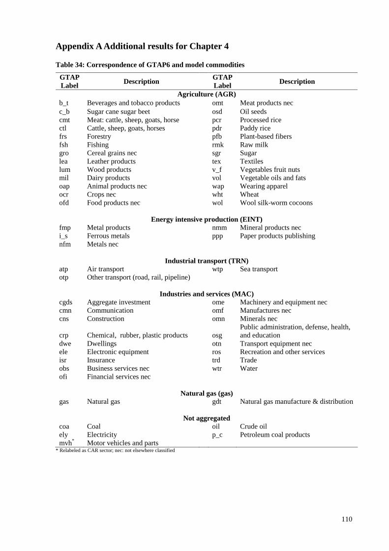
110

Appendix A Additional results for Chapter 4

Table 34: Correspondence of GTAP6 and model commodities

GTAP Label Description GTAP

Label Description

Agriculture (AGR) b_t Beverages and tobacco products omt Meat products nec c_b Sugar cane sugar beet osd Oil seeds cmt Meat: cattle, sheep, goats, horse pcr Processed rice ctl Cattle, sheep, goats, horses pdr Paddy rice frs Forestry pfb Plant-based fibers fsh Fishing rmk Raw milk gro Cereal grains nec sgr Sugar lea Leather products tex Textiles lum Wood products v_f Vegetables fruit nuts mil Dairy products vol Vegetable oils and fats oap Animal products nec wap Wearing apparel ocr Crops nec wht Wheat ofd Food products nec wol Wool silk-worm cocoons

Energy intensive production (EINT) fmp Metal products nmm Mineral products nec i_s Ferrous metals ppp Paper products publishing nfm Metals nec

Industrial transport (TRN) atp Air transport wtp Sea transport otp Other transport (road, rail, pipeline)

Industries and services (MAC) cgds Aggregate investment ome Machinery and equipment nec cmn Communication omf Manufactures nec cns Construction omn Minerals nec

crp Chemical, rubber, plastic products

osg Public administration, defense, health, and education

dwe Dwellings otn Transport equipment nec ele Electronic equipment ros Recreation and other services isr Insurance trd Trade obs Business services nec wtr Water ofi Financial services nec

Natural gas (gas) gas Natural gas gdt Natural gas manufacture & distribution

Not aggregated coa Coal oil Crude oil ely Electricity p_c Petroleum coal products mvh* Motor vehicles and parts

* Relabeled as CAR sector; nec: not elsewhere classified

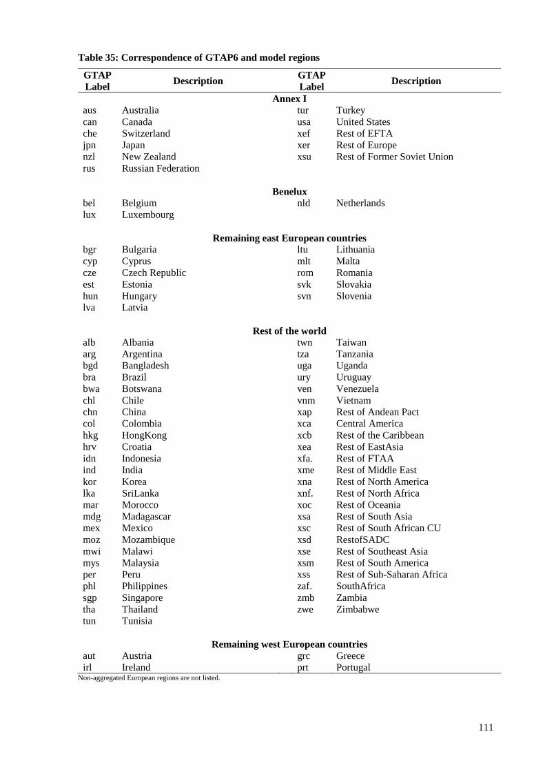
111

Table 35: Correspondence of GTAP6 and model regions

GTAP Label Description GTAP

Label Description

Annex I aus Australia tur Turkey can Canada usa United States che Switzerland xef Rest of EFTA jpn Japan xer Rest of Europe nzl New Zealand xsu Rest of Former Soviet Union rus Russian Federation

Benelux bel Belgium nld Netherlands lux Luxembourg

Remaining east European countries bgr Bulgaria ltu Lithuania cyp Cyprus mlt Malta cze Czech Republic rom Romania est Estonia svk Slovakia hun Hungary svn Slovenia lva Latvia

Rest of the world alb Albania twn Taiwan arg Argentina tza Tanzania bgd Bangladesh uga Uganda bra Brazil ury Uruguay bwa Botswana ven Venezuela chl Chile vnm Vietnam chn China xap Rest of Andean Pact col Colombia xca Central America hkg HongKong xcb Rest of the Caribbean hrv Croatia xea Rest of EastAsia idn Indonesia xfa. Rest of FTAA ind India xme Rest of Middle East kor Korea xna Rest of North America lka SriLanka xnf. Rest of North Africa mar Morocco xoc Rest of Oceania mdg Madagascar xsa Rest of South Asia mex Mexico xsc Rest of South African CU moz Mozambique xsd RestofSADC mwi Malawi xse Rest of Southeast Asia mys Malaysia xsm Rest of South America per Peru xss Rest of Sub-Saharan Africa phl Philippines zaf. SouthAfrica sgp Singapore zmb Zambia tha Thailand zwe Zimbabwe tun Tunisia

Remaining west European countries aut Austria grc Greece irl Ireland prt Portugal

Non-aggregated European regions are not listed.

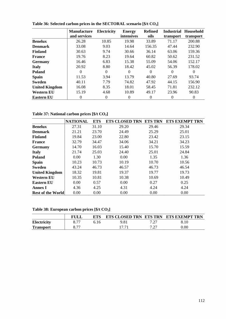
112

Table 36: Selected carbon prices in the SECTORAL scenario [$/t CO2]

Manufacture and services

Electricity Energy intensives

Refined oils

Industrial transport

Household transport

Benelux 26.28 10.85 19.98 33.89 71.17 200.88 Denmark 33.08 9.03 14.64 156.35 47.44 232.90 Finland 30.63 9.74 30.66 36.14 63.06 159.36 France 19.76 8.23 19.64 60.82 50.62 231.52 Germany 16.46 6.83 15.38 55.09 54.06 152.17 Italy 20.92 8.80 18.42 45.02 56.39 178.02 Poland 0 0 0 0 0 0 Spain 11.53 3.94 13.79 40.80 27.69 93.74 Sweden 40.11 7.79 74.82 47.92 44.15 156.90 United Kingdom 16.08 8.35 18.01 58.45 71.81 232.12 Western EU 15.19 4.68 10.89 49.17 23.96 90.83 Eastern EU 0 0 0 0 0 0

Table 37: National carbon prices [$/t CO2]

NATIONAL ETS ETS CLOSED TRN ETS TRN ETS EXEMPT TRN Benelux 27.31 31.10 29.20 29.46 29.34 Denmark 21.21 23.70 24.49 25.29 25.01 Finland 19.84 23.00 22.80 23.42 23.15 France 32.79 34.47 34.06 34.21 34.23 Germany 14.70 16.03 15.40 15.70 15.59 Italy 21.74 25.03 24.40 25.01 24.84 Poland 0.00 1.30 0.00 1.35 1.36 Spain 10.23 10.73 10.19 10.70 10.56 Sweden 43.24 46.73 46.57 46.73 46.54 United Kingdom 18.32 19.81 19.37 19.77 19.73 Western EU 10.35 10.81 10.38 10.69 10.49 Eastern EU 0.00 0.57 0.00 0.27 0.25 Annex I 4.36 4.25 4.31 4.24 4.24 Rest of the World 0.00 0.00 0.00 0.00 0.00

Table 38: European carbon prices [$/t CO2]

FULL ETS ETS CLOSED TRN ETS TRN ETS EXEMPT TRN Electricity 8.77 6.16 9.81 7.27 8.10 Transport 8.77 17.71 7.27 0.00

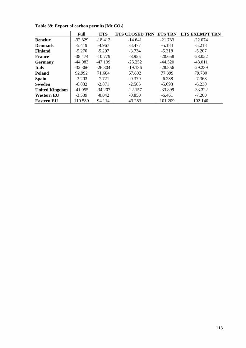
113

Table 39: Export of carbon permits [Mt CO2]

Full ETS ETS CLOSED TRN ETS TRN ETS EXEMPT TRN Benelux -32.329 -18.412 -14.641 -21.733 -22.074 Denmark -5.419 -4.967 -3.477 -5.184 -5.218 Finland -5.270 -5.297 -3.734 -5.318 -5.207 France -38.474 -10.779 -8.955 -20.658 -23.052 Germany -44.083 -47.199 -25.252 -44.520 -43.011 Italy -32.366 -26.304 -19.136 -28.856 -29.239 Poland 92.992 71.684 57.802 77.399 79.780 Spain -3.203 -7.721 -0.379 -6.288 -7.368 Sweden -6.832 -2.871 -2.505 -5.693 -6.230 United Kingdom -41.055 -34.207 -22.157 -33.899 -33.322 Western EU -3.539 -8.042 -0.850 -6.461 -7.200 Eastern EU 119.580 94.114 43.283 101.209 102.140

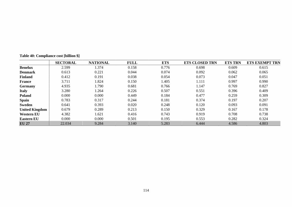
114

Table 40: Compliance cost [billion $]

SECTORAL NATIONAL FULL ETS ETS CLOSED TRN ETS TRN E TS EXEMPT TRN Benelux 2.599 1.374 0.158 0.776 0.698 0.609 0.615 Denmark 0.613 0.221 0.044 0.074 0.092 0.062 0.065 Finland 0.412 0.191 0.038 0.054 0.073 0.047 0.051 France 3.711 1.824 0.150 1.405 1.111 0.997 0.990 Germany 4.935 1.790 0.681 0.766 1.147 0.769 0.827 Italy 3.280 1.264 0.226 0.507 0.551 0.396 0.409 Poland 0.000 0.000 0.449 0.184 0.477 0.259 0.309 Spain 0.783 0.317 0.244 0.181 0.374 0.197 0.207 Sweden 0.641 0.393 0.020 0.248 0.120 0.093 0.091 United Kingdom 0.679 0.289 0.213 0.150 0.329 0.167 0.178 Western EU 4.382 1.621 0.416 0.743 0.919 0.708 0.738 Eastern EU 0.000 0.000 0.501 0.195 0.553 0.282 0.324 EU 27 22.034 9.284 3.140 5.283 6.444 4.586 4.803

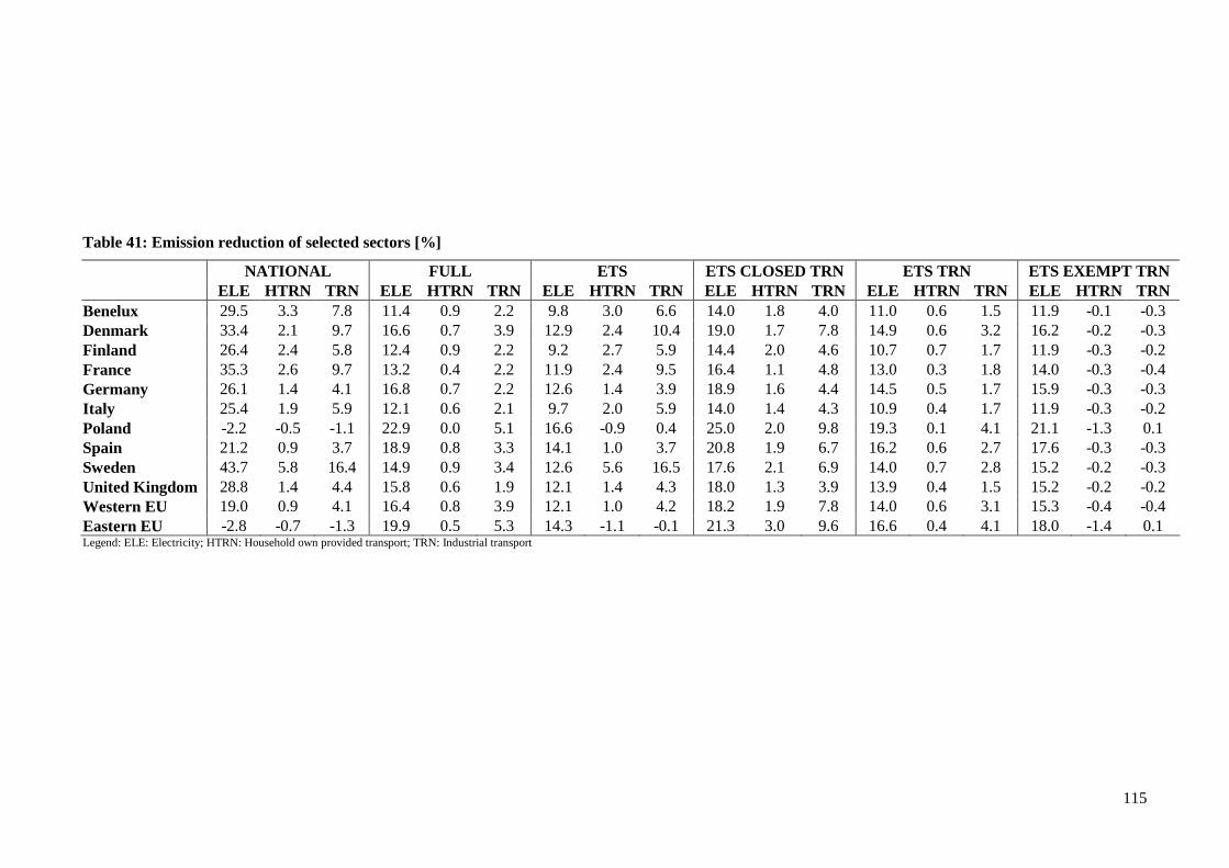
115

Table 41: Emission reduction of selected sectors [%]

NATIONAL FULL ETS ETS CLOSED TRN ETS TRN ETS EXEMPT TRN ELE HTRN TRN ELE HTRN TRN ELE HTRN TRN ELE HTRN TRN ELE HTRN TRN ELE HTRN TRN Benelux 29.5 3.3 7.8 11.4 0.9 2.2 9.8 3.0 6.6 14.0 1.8 4.0 11.0 0.6 1.5 11.9 -0.1 -0.3 Denmark 33.4 2.1 9.7 16.6 0.7 3.9 12.9 2.4 10.4 19.0 1.7 7.8 14.9 0.6 3.2 16.2 -0.2 -0.3 Finland 26.4 2.4 5.8 12.4 0.9 2.2 9.2 2.7 5.9 14.4 2.0 4.6 10.7 0.7 1.7 11.9 -0.3 -0.2 France 35.3 2.6 9.7 13.2 0.4 2.2 11.9 2.4 9.5 16.4 1.1 4.8 13.0 0.3 1.8 14.0 -0.3 -0.4 Germany 26.1 1.4 4.1 16.8 0.7 2.2 12.6 1.4 3.9 18.9 1.6 4.4 14.5 0.5 1.7 15.9 -0.3 -0.3 Italy 25.4 1.9 5.9 12.1 0.6 2.1 9.7 2.0 5.9 14.0 1.4 4.3 10.9 0.4 1.7 11.9 -0.3 -0.2 Poland -2.2 -0.5 -1.1 22.9 0.0 5.1 16.6 -0.9 0.4 25.0 2.0 9.8 19.3 0.1 4.1 21.1 -1.3 0.1 Spain 21.2 0.9 3.7 18.9 0.8 3.3 14.1 1.0 3.7 20.8 1.9 6.7 16.2 0.6 2.7 17.6 -0.3 -0.3 Sweden 43.7 5.8 16.4 14.9 0.9 3.4 12.6 5.6 16.5 17.6 2.1 6.9 14.0 0.7 2.8 15.2 -0.2 -0.3 United Kingdom 28.8 1.4 4.4 15.8 0.6 1.9 12.1 1.4 4.3 18.0 1.3 3.9 13.9 0.4 1.5 15.2 -0.2 -0.2 Western EU 19.0 0.9 4.1 16.4 0.8 3.9 12.1 1.0 4.2 18.2 1.9 7.8 14.0 0.6 3.1 15.3 -0.4 -0.4 Eastern EU -2.8 -0.7 -1.3 19.9 0.5 5.3 14.3 -1.1 -0.1 21.3 3.0 9.6 16.6 0.4 4.1 18.0 -1.4 0.1 Legend: ELE: Electricity; HTRN: Household own provided transport; TRN: Industrial transport

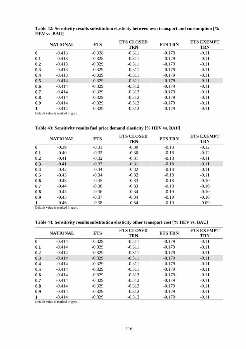
116

Table 42: Sensitivity results substitution elasticity between own transport and consumption [% HEV vs. BAU]

NATIONAL ETS ETS CLOSED TRN ETS TRN ETS EXEMPT

TRN 0 -0.413 -0.328 -0.311 -0.179 -0.11 0.1 -0.413 -0.328 -0.311 -0.179 -0.11 0.2 -0.413 -0.329 -0.311 -0.179 -0.11 0.3 -0.413 -0.329 -0.311 -0.179 -0.11 0.4 -0.413 -0.329 -0.311 -0.179 -0.11 0.5 -0.414 -0.329 -0.311 -0.179 -0.11 0.6 -0.414 -0.329 -0.312 -0.179 -0.11 0.7 -0.414 -0.329 -0.312 -0.179 -0.11 0.8 -0.414 -0.329 -0.312 -0.179 -0.11 0.9 -0.414 -0.329 -0.312 -0.179 -0.11 1 -0.414 -0.329 -0.312 -0.179 -0.11 Default value is marked in grey.

Table 43: Sensitivity results fuel price demand elasticity [% HEV vs. BAU]

NATIONAL ETS ETS CLOSED TRN ETS TRN ETS EXEMPT

TRN 0 -0.39 -0.31 -0.30 -0.18 -0.12 0.1 -0.40 -0.32 -0.30 -0.18 -0.12 0.2 -0.41 -0.32 -0.31 -0.18 -0.11 0.3 -0.41 -0.33 -0.31 -0.18 -0.11 0.4 -0.42 -0.34 -0.32 -0.18 -0.11 0.5 -0.43 -0.34 -0.32 -0.18 -0.11 0.6 -0.43 -0.35 -0.33 -0.18 -0.10 0.7 -0.44 -0.36 -0.33 -0.18 -0.10 0.8 -0.45 -0.36 -0.34 -0.19 -0.10 0.9 -0.45 -0.37 -0.34 -0.19 -0.10 1 -0.46 -0.38 -0.34 -0.19 -0.09 Default value is marked in grey.

Table 44: Sensitivity results substitution elasticity other transport cost [% HEV vs. BAU]

NATIONAL ETS ETS CLOSED TRN ETS TRN ETS EXEMPT

TRN 0 -0.414 -0.329 -0.311 -0.179 -0.11 0.1 -0.414 -0.329 -0.311 -0.179 -0.11 0.2 -0.414 -0.329 -0.311 -0.179 -0.11 0.3 -0.414 -0.329 -0.311 -0.179 -0.11 0.4 -0.414 -0.329 -0.311 -0.179 -0.11 0.5 -0.414 -0.329 -0.311 -0.179 -0.11 0.6 -0.414 -0.329 -0.312 -0.179 -0.11 0.7 -0.414 -0.329 -0.312 -0.179 -0.11 0.8 -0.414 -0.329 -0.312 -0.179 -0.11 0.9 -0.414 -0.329 -0.312 -0.179 -0.11 1 -0.414 -0.329 -0.312 -0.179 -0.11 Default value is marked in grey.

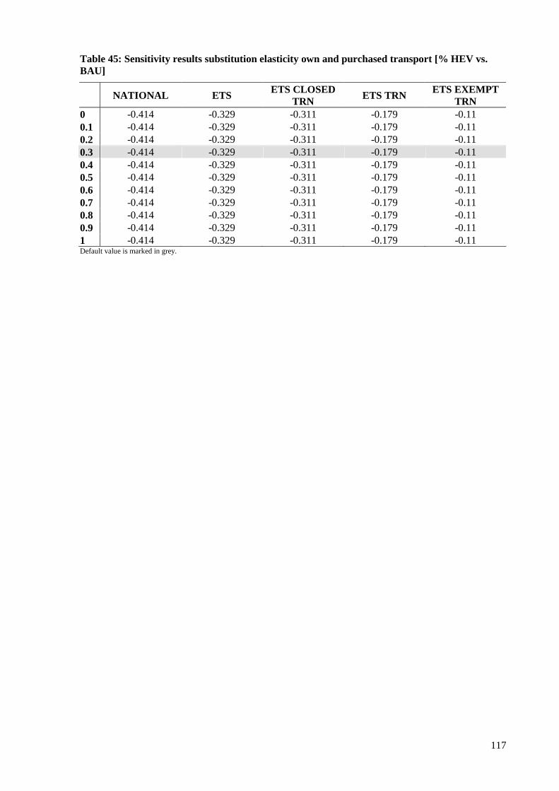
117

Table 45: Sensitivity results substitution elasticity own and purchased transport [% HEV vs. BAU]

NATIONAL ETS ETS CLOSED TRN ETS TRN ETS EXEMPT

TRN 0 -0.414 -0.329 -0.311 -0.179 -0.11 0.1 -0.414 -0.329 -0.311 -0.179 -0.11 0.2 -0.414 -0.329 -0.311 -0.179 -0.11 0.3 -0.414 -0.329 -0.311 -0.179 -0.11 0.4 -0.414 -0.329 -0.311 -0.179 -0.11 0.5 -0.414 -0.329 -0.311 -0.179 -0.11 0.6 -0.414 -0.329 -0.311 -0.179 -0.11 0.7 -0.414 -0.329 -0.311 -0.179 -0.11 0.8 -0.414 -0.329 -0.311 -0.179 -0.11 0.9 -0.414 -0.329 -0.311 -0.179 -0.11 1 -0.414 -0.329 -0.311 -0.179 -0.11 Default value is marked in grey.

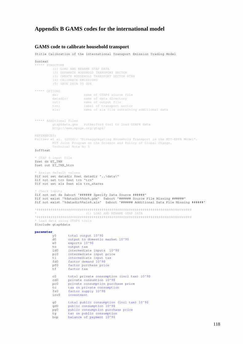
118

Appendix B GAMS codes for the international model

GAMS code to calibrate household transport $title Calibration of the International Transport E mission Trading Model $ontext ***** STRUCTURE (1) LOAD AND RENAME GTAP DATA (2) SEPARATE HOUSHOLD TRANSPORT SECTOR (3) CREATE HOUSEHOLD TRANSPORT SECTOR HTRN (4) CALIBRATE EMISSIONS (5) SAVE DATA TO GDX ***** OPTIONS ds: name of GTAP6 source file datadir: name of data directory out: name of output file trn: label of transport sector xls: name of xls file containin g additional data ***** Additional files gtap6data.gms rutherford tool to load GT AP6 data http://www.mpsge.org/gtap6/ REFERNECES: Paltsev et al. (2004): "Dissaggregating Household T ransport in the MIT-EPPA Model". MIT Joint Program on the Science and Polic y of Global Change. Technical Note No 5 $offtext * GTAP 6 input file $set ds ET_TRN $set out ET_TRN_htrn * Assign default values $if not set datadir $set datadir "..\data\" $if not set trn $set trn "trn" $if not set xls $set xls trn_shares * Check inputs $if not set ds $abort "###### Specify Data Source # #####" $if not exist "%datadir%%ds%.gdx" $abort "###### S ource File Missing ######" $if not exist "%datadir%%xls%.xls" $abort "###### Additional Data File Missing ######" *################################################## ############################# * (1) LOAD AND RENAME GTAP DATA *################################################## ############################# * Load data using GTAP6 tools $include gtap6data parameter y0 total output 10^9$ d0 output to domestic market 10^9$ e0 exports 10^9$ to output tax id0 intermediate inputs 10^9$ pi0 intermediate input price ti intermediate input tax fd0 factor demand 10^9$ pf0 factor purchase price tf factor tax c0 total private consumption (incl tax) 10^9$ cd0 private consumtion 10^9$ pc0 private consumption purchase price tc tax on private consumption fs0 factor supply 10^9$ inv0 investment g0 total public consumption (incl tax) 10^9$ gd0 public consumption 10^9$ pg0 public consumption purchase price tg tac on public consumption bop balance of payment 10^9$

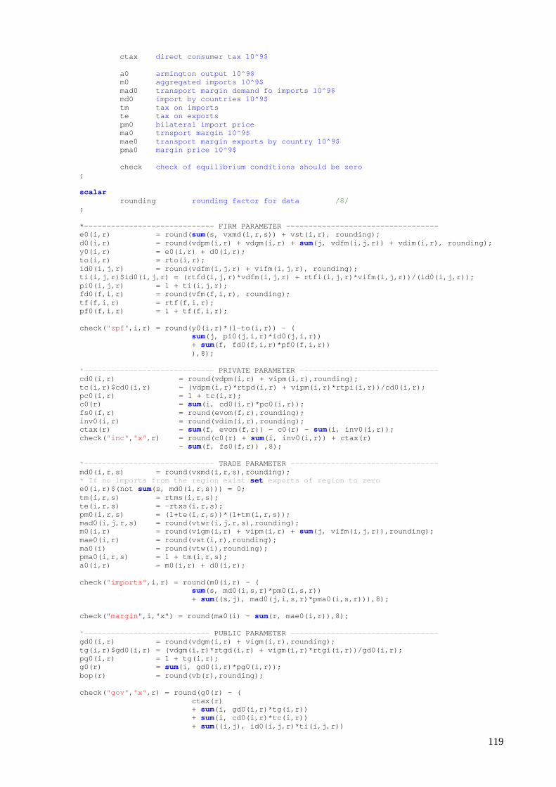
119

ctax direct consumer tax 10^9$ a0 armington output 10^9$ m0 aggregated imports 10^9$ mad0 transport margin demand fo imports 10^9$ md0 import by countries 10^9$ tm tax on imports te tax on exports pm0 bilateral import price ma0 trnsport margin 10^9$ mae0 transport margin exports by country 10^9$ pma0 margin price 10^9$ check check of equilibrium conditions should be zero ; scalar rounding rounding factor for data /8/ ; *----------------------------- FIRM PARAMETER ----- ----------------------------- e0(i,r) = round( sum(s, vxmd(i,r,s)) + vst(i,r), rounding); d0(i,r) = round(vdpm(i,r) + vdgm(i,r) + sum(j, vdfm(i,j,r)) + vdim(i,r), rounding); y0(i,r) = e0(i,r) + d0(i,r); to(i,r) = rto(i,r); id0(i,j,r) = round(vdfm(i,j,r) + vifm(i,j,r), rounding); ti(i,j,r)$id0(i,j,r) = (rtfd(i,j,r)*vdfm(i,j,r) + r tfi(i,j,r)*vifm(i,j,r))/(id0(i,j,r)); pi0(i,j,r) = 1 + ti(i,j,r); fd0(f,i,r) = round(vfm(f,i,r), rounding); tf(f,i,r) = rtf(f,i,r); pf0(f,i,r) = 1 + tf(f,i,r); check( "zpf" ,i,r) = round(y0(i,r)*(1-to(i,r)) - ( sum(j, pi0(j,i,r)*id0(j,i,r)) + sum(f, fd0(f,i,r)*pf0(f,i,r)) ),8); *----------------------------- PRIVATE PARAMETER ------------------------------- cd0(i,r) = round(vdpm(i,r) + vipm(i,r),rou nding); tc(i,r)$cd0(i,r) = (vdpm(i,r)*rtpd(i,r) + vipm(i,r )*rtpi(i,r))/cd0(i,r); pc0(i,r) = 1 + tc(i,r); c0(r) = sum(i, cd0(i,r)*pc0(i,r)); fs0(f,r) = round(evom(f,r),rounding); inv0(i,r) = round(vdim(i,r),rounding); ctax(r) = sum(f, evom(f,r)) - c0(r) - sum(i, inv0(i,r)); check( "inc" , "x" ,r) = round(c0(r) + sum(i, inv0(i,r)) + ctax(r) - sum(f, fs0(f,r)) ,8); *----------------------------- TRADE PARAMETER --------------------------------- md0(i,r,s) = round(vxmd(i,r,s),rounding); * If no imports from the region exist set exports of region to zero e0(i,r)$(not sum(s, md0(i,r,s))) = 0; tm(i,r,s) = rtms(i,r,s); te(i,r,s) = -rtxs(i,r,s); pm0(i,r,s) = (1+te(i,r,s))*(1+tm(i,r,s)); mad0(i,j,r,s) = round(vtwr(i,j,r,s),rounding); m0(i,r) = round(vigm(i,r) + vipm(i,r) + sum(j, vifm(i,j,r)),rounding); mae0(i,r) = round(vst(i,r),rounding); ma0(i) = round(vtw(i),rounding); pma0(i,r,s) = 1 + tm(i,r,s); a0(i,r) = m0(i,r) + d0(i,r); check( "imports" ,i,r) = round(m0(i,r) - ( sum(s, md0(i,s,r)*pm0(i,s,r)) + sum((s,j), mad0(j,i,s,r)*pma0(i,s,r))),8); check(" margin ",i,"x") = round(ma0(i) - sum(r, mae0(i,r)),8); *---------------------------- PUBLIC PARAMETER --------------------------------- gd0(i,r) = round(vdgm(i,r) + vigm(i,r),roun ding); tg(i,r)$gd0(i,r) = (vdgm(i,r)*rtgd(i,r) + vigm(i,r) *rtgi(i,r))/gd0(i,r); pg0(i,r) = 1 + tg(i,r); g0(r) = sum(i, gd0(i,r)*pg0(i,r)); bop(r) = round(vb(r),rounding); check( "gov" , "x" ,r) = round(g0(r) - ( ctax(r) + sum(i, gd0(i,r)*tg(i,r)) + sum(i, cd0(i,r)*tc(i,r)) + sum((i,j), id0(i,j,r)*ti(i,j,r))

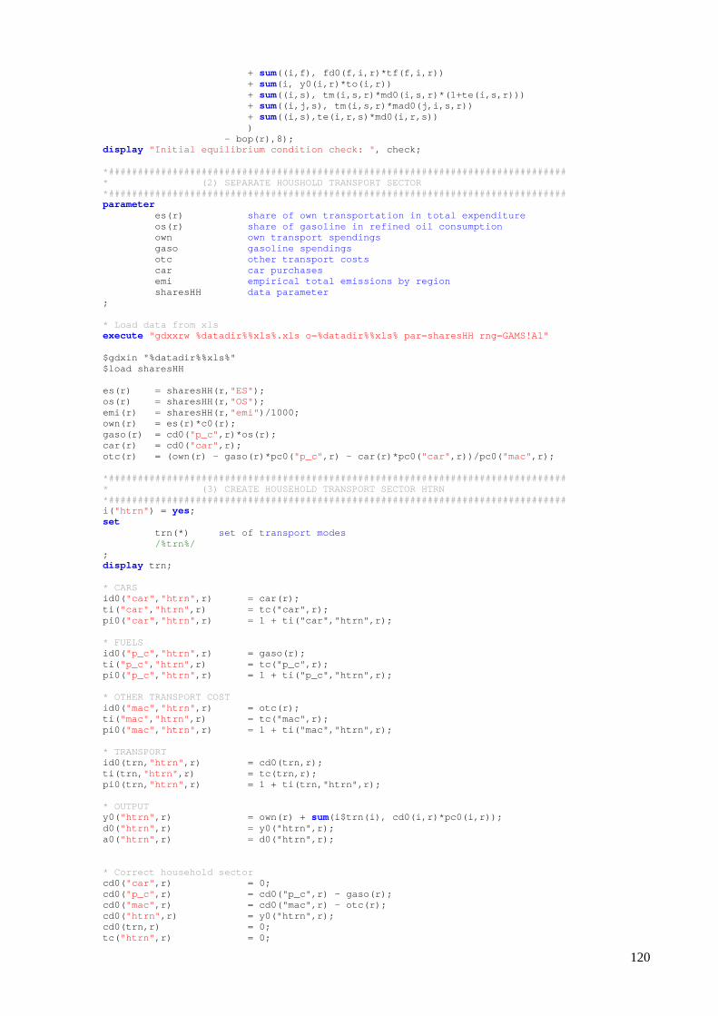
120

+ sum((i,f), fd0(f,i,r)*tf(f,i,r)) + sum(i, y0(i,r)*to(i,r)) + sum((i,s), tm(i,s,r)*md0(i,s,r)*(1+te(i,s,r))) + sum((i,j,s), tm(i,s,r)*mad0(j,i,s,r)) + sum((i,s),te(i,r,s)*md0(i,r,s)) ) - bop(r),8); display "Initial equilibrium condition check: " , check; *################################################## ############################# * (2) SEPARATE HOUSHOLD TRANSPORT SE CTOR *################################################## ############################# parameter es(r) share of own transportation in total expenditure os(r) share of gasoline in refined oil consumption own own transport spendings gaso gasoline spendings otc other transport costs car car purchases emi empirical total emissions by region sharesHH data parameter ; * Load data from xls execute "gdxxrw %datadir%%xls%.xls o=%datadir%%xls% par=sha resHH rng=GAMS!A1" $gdxin "%datadir%%xls%" $load sharesHH es(r) = sharesHH(r, "ES" ); os(r) = sharesHH(r, "OS" ); emi(r) = sharesHH(r, "emi" )/1000; own(r) = es(r)*c0(r); gaso(r) = cd0( "p_c" ,r)*os(r); car(r) = cd0( "car" ,r); otc(r) = (own(r) - gaso(r)*pc0( "p_c" ,r) - car(r)*pc0( "car" ,r))/pc0( "mac" ,r); *################################################## ############################# * (3) CREATE HOUSEHOLD TRANSPORT SEC TOR HTRN *################################################## ############################# i( "htrn" ) = yes; set trn(*) set of transport modes /%trn%/ ; display trn; * CARS id0( "car" , "htrn" ,r) = car(r); ti( "car" , "htrn" ,r) = tc("car",r); pi0( "car" , "htrn" ,r) = 1 + ti("car","htrn",r); * FUELS id0( "p_c" , "htrn" ,r) = gaso(r); ti( "p_c" , "htrn" ,r) = tc("p_c",r); pi0( "p_c" , "htrn" ,r) = 1 + ti("p_c","htrn",r); * OTHER TRANSPORT COST id0( "mac" , "htrn" ,r) = otc(r); ti( "mac" , "htrn" ,r) = tc("mac",r); pi0( "mac" , "htrn" ,r) = 1 + ti("mac","htrn",r); * TRANSPORT id0(trn, "htrn" ,r) = cd0(trn,r); ti(trn, "htrn" ,r) = tc(trn,r); pi0(trn, "htrn" ,r) = 1 + ti(trn,"htrn",r); * OUTPUT y0( "htrn" ,r) = own(r) + sum(i$trn(i), cd0(i,r)*pc0(i,r)); d0( "htrn" ,r) = y0("htrn",r); a0( "htrn" ,r) = d0("htrn",r); * Correct household sector cd0( "car" ,r) = 0; cd0( "p_c" ,r) = cd0("p_c",r) - gaso(r); cd0( "mac" ,r) = cd0("mac",r) - otc(r); cd0( "htrn" ,r) = y0("htrn",r); cd0(trn,r) = 0; tc( "htrn" ,r) = 0;

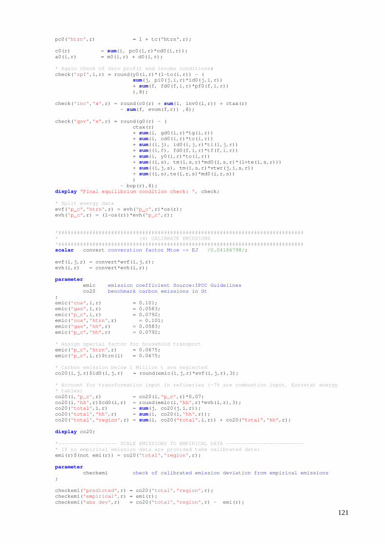
121

pc0( "htrn" ,r) = 1 + tc("htrn",r); c0(r) = sum(i, pc0(i,r)*cd0(i,r)); a0(i,r) = m0(i,r) + d0(i,r); * Again check of zero profit and income conditions : check( "zpf" ,i,r) = round(y0(i,r)*(1-to(i,r)) - ( sum(j, pi0(j,i,r)*id0(j,i,r)) + sum(f, fd0(f,i,r)*pf0(f,i,r)) ),8); check( "inc" , "x" ,r) = round(c0(r) + sum(i, inv0(i,r)) + ctax(r) - sum(f, evom(f,r)) ,8); check( "gov" , "x" ,r) = round(g0(r) - ( ctax(r) + sum(i, gd0(i,r)*tg(i,r)) + sum(i, cd0(i,r)*tc(i,r)) + sum((i,j), id0(i,j,r)*ti(i,j,r)) + sum((i,f), fd0(f,i,r)*tf(f,i,r)) + sum(i, y0(i,r)*to(i,r)) + sum((i,s), tm(i,s,r)*md0(i,s,r)*(1+te(i,s,r))) + sum((i,j,s), tm(i,s,r)*vtwr(j,i,s,r)) + sum((i,s),te(i,r,s)*md0(i,r,s)) ) - bop(r),8); display "Final equilibrium condition check: " , check; * Split energy data evf( "p_c" , "htrn" ,r) = evh( "p_c" ,r)*os(r); evh( "p_c" ,r) = (1-os(r))*evh( "p_c" ,r); *################################################## ############################# * (4) CALIBRATE EMISSIONS *################################################## ############################# scalar convert converstion factor Mtoe -> EJ /0.04186798/ ; evf(i,j,r) = convert*evf(i,j,r); evh(i,r) = convert*evh(i,r); parameter emic emission coefficient Source:IPCC Guidelines co20 benchmark carbon emissions in Gt ; emic( "coa" ,i,r) = 0.101; emic( "gas" ,i,r) = 0.0583; emic( "p_c" ,i,r) = 0.0792; emic( "coa" , "htrn" ,r) = 0.101; emic( "gas" , "hh" ,r) = 0.0583; emic( "p_c" , "hh" ,r) = 0.0792; * Assign special factor for household transport emic( "p_c" , "htrn" ,r) = 0.0675; emic( "p_c" ,i,r)$trn(i) = 0.0675; * Carbon emission below 1 Million t are neglected co20(i,j,r)$id0(i,j,r) = round(emic(i,j,r)*evf(i ,j,r),3); * Account for transformation input in refineries (~ 7% are combustion input, Eurostat energy * tables) co20(i, "p_c" ,r) = co20(i, "p_c" ,r)*0.07; co20(i, "hh" ,r)$cd0(i,r) = round(emic(i, "hh" ,r)*evh(i,r),3); co20( "total" ,i,r) = sum(j, co20(j,i,r)); co20( "total" , "hh" ,r) = sum(i, co20(i, "hh" ,r)); co20( "total" , "region" ,r) = sum(i, co20( "total" ,i,r)) + co20( "total" , "hh" ,r); display co20; *------------------- SCALE EMISSIONS TO EMPIRICAL D ATA ------------------------- * If no empirical emission data are provided take c alibrated data: emi(r)$(not emi(r)) = co20( "total" , "region" ,r); parameter checkemi check of calibrated emission deviation from empiric al emissions ; checkemi( "predicted" ,r) = co20( "total" , "region" ,r); checkemi( "empirical" ,r) = emi(r); checkemi( "abs dev" ,r) = co20( "total" , "region" ,r) - emi(r);

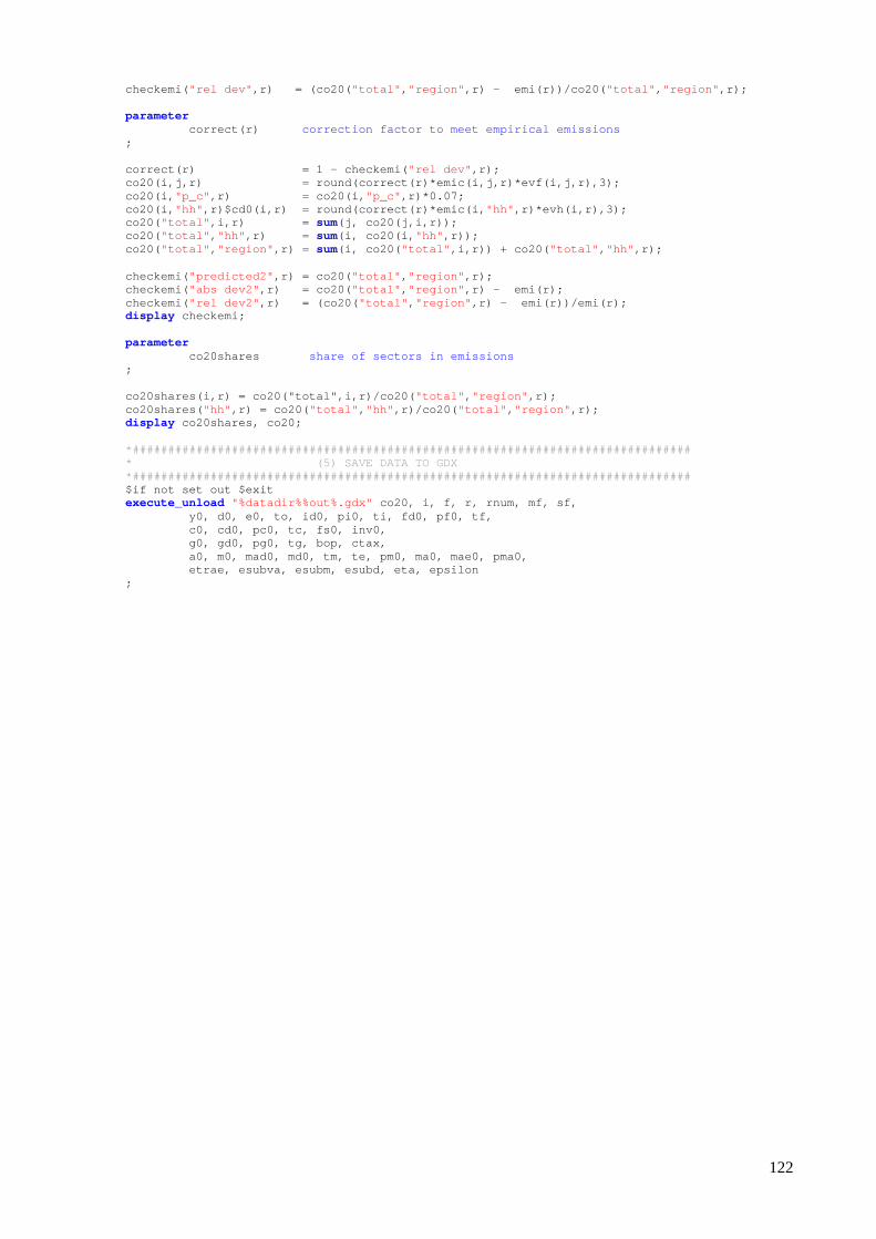
122

checkemi( "rel dev" ,r) = (co20( "total" , "region" ,r) - emi(r))/co20( "total" , "region" ,r); parameter correct(r) correction factor to meet empirical emissions ; correct(r) = 1 - checkemi( "rel dev" ,r); co20(i,j,r) = round(correct(r)*emic(i, j,r)*evf(i,j,r),3); co20(i, "p_c" ,r) = co20(i, "p_c" ,r)*0.07; co20(i, "hh" ,r)$cd0(i,r) = round(correct(r)*emic(i, "hh" ,r)*evh(i,r),3); co20( "total" ,i,r) = sum(j, co20(j,i,r)); co20( "total" , "hh" ,r) = sum(i, co20(i, "hh" ,r)); co20( "total" , "region" ,r) = sum(i, co20( "total" ,i,r)) + co20( "total" , "hh" ,r); checkemi( "predicted2" ,r) = co20( "total" , "region" ,r); checkemi( "abs dev2" ,r) = co20( "total" , "region" ,r) - emi(r); checkemi( "rel dev2" ,r) = (co20( "total" , "region" ,r) - emi(r))/emi(r); display checkemi; parameter co20shares share of sectors in emissions ; co20shares(i,r) = co20("total",i,r)/co20( "total" , "region" ,r); co20shares( "hh" ,r) = co20( "total" , "hh" ,r)/co20( "total" , "region" ,r); display co20shares, co20; *################################################## ############################# * (5) SAVE DATA TO GDX *################################################## ############################# $if not set out $exit execute_unload "%datadir%%out%.gdx" co20, i, f, r, rnum, mf, sf, y0, d0, e0, to, id0, pi0, ti, fd0, pf0, tf , c0, cd0, pc0, tc, fs0, inv0, g0, gd0, pg0, tg, bop, ctax, a0, m0, mad0, md0, tm, te, pm0, ma0, mae0, pma0, etrae, esubva, esubm, esubd, eta, epsilon ;

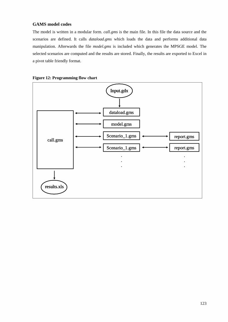
123

GAMS model codes

The model is written in a modular form. call.gms is the main file. In this file the data source and the

scenarios are defined. It calls dataload.gms which loads the data and performs additional data

manipulation. Afterwards the file model.gms is included which generates the MPSGE model. The

selected scenarios are computed and the results are stored. Finally, the results are exported to Excel in

a pivot table friendly format.

Figure 12: Programming flow chart

call.gms

Input.gdx

dataload.gms

model.gms

Scenario_1.gms

Scenario_1.gms

.

.

.

report.gms

report.gms

.

.

.

results.xls

call.gms

Input.gdxInput.gdx

dataload.gms

model.gms

Scenario_1.gms

Scenario_1.gms

.

.

.

report.gms

report.gms

.

.

.

results.xlsresults.xls

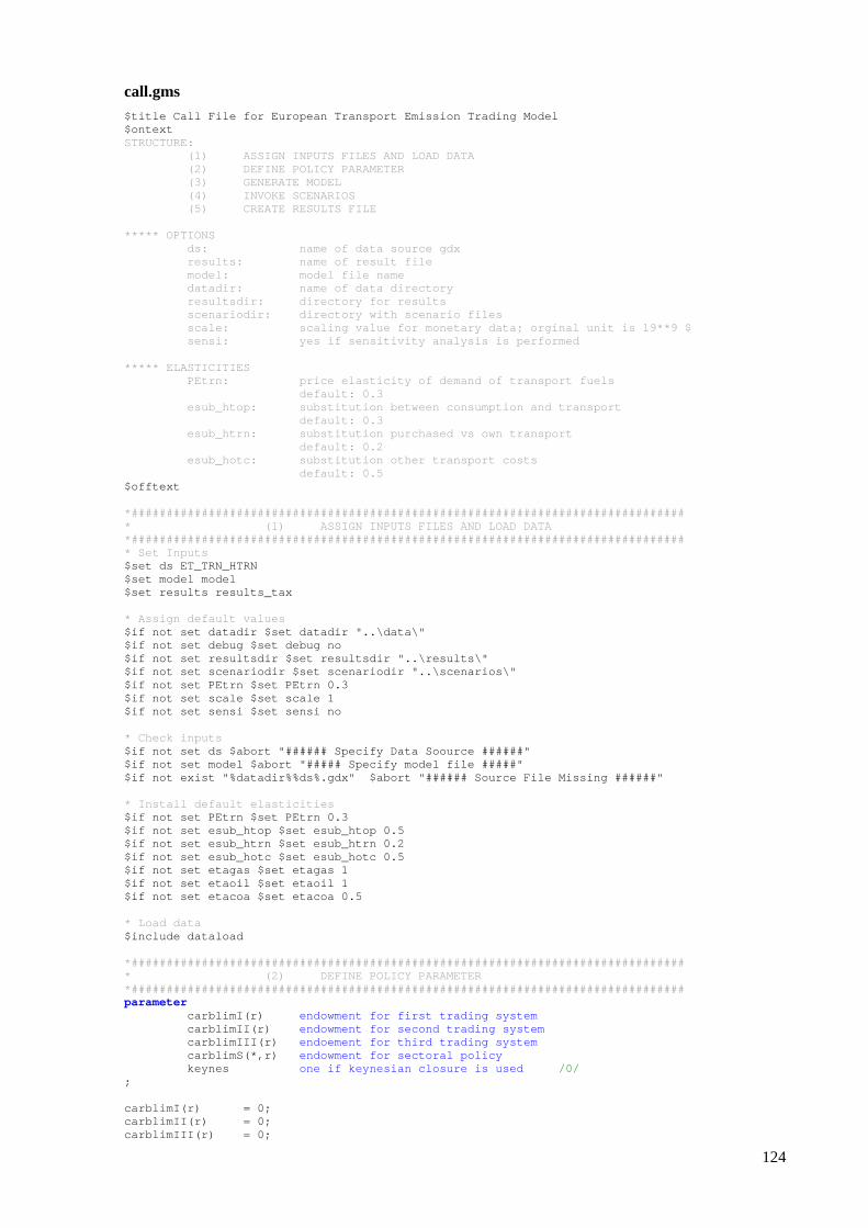
124

call.gms $title Call File for European Transport Emission Tr ading Model $ontext STRUCTURE: (1) ASSIGN INPUTS FILES AND LOAD DATA (2) DEFINE POLICY PARAMETER (3) GENERATE MODEL (4) INVOKE SCENARIOS (5) CREATE RESULTS FILE ***** OPTIONS ds: name of data source gdx results: name of result file model: model file name datadir: name of data directory resultsdir: directory for results scenariodir: directory with scenario fi les scale: scaling value for monetary data; orginal unit is 19**9 $ sensi: yes if sensitivity analysi s is performed ***** ELASTICITIES PEtrn: price elasticity of demand of transport fuels default: 0.3 esub_htop: substitution between consu mption and transport default: 0.3 esub_htrn: substitution purchased vs own transport default: 0.2 esub_hotc: substitution other transpo rt costs default: 0.5 $offtext *################################################## ############################# * (1) ASSIGN INPUTS FILES AND LOAD DATA *################################################## ############################# * Set Inputs $set ds ET_TRN_HTRN $set model model $set results results_tax * Assign default values $if not set datadir $set datadir "..\data\" $if not set debug $set debug no $if not set resultsdir $set resultsdir "..\results\ " $if not set scenariodir $set scenariodir "..\scenar ios\" $if not set PEtrn $set PEtrn 0.3 $if not set scale $set scale 1 $if not set sensi $set sensi no * Check inputs $if not set ds $abort "###### Specify Data Soource ######" $if not set model $abort "##### Specify model file #####" $if not exist "%datadir%%ds%.gdx" $abort "###### S ource File Missing ######" * Install default elasticities $if not set PEtrn $set PEtrn 0.3 $if not set esub_htop $set esub_htop 0.5 $if not set esub_htrn $set esub_htrn 0.2 $if not set esub_hotc $set esub_hotc 0.5 $if not set etagas $set etagas 1 $if not set etaoil $set etaoil 1 $if not set etacoa $set etacoa 0.5 * Load data $include dataload *################################################## ############################# * (2) DEFINE POLICY PARAMETER *################################################## ############################# parameter carblimI(r) endowment for first trading system carblimII(r) endowment for second trading system carblimIII(r) endoement for third trading system carblimS(*,r) endowment for sectoral policy keynes one if keynesian closure is used /0/ ; carblimI(r) = 0; carblimII(r) = 0; carblimIII(r) = 0;

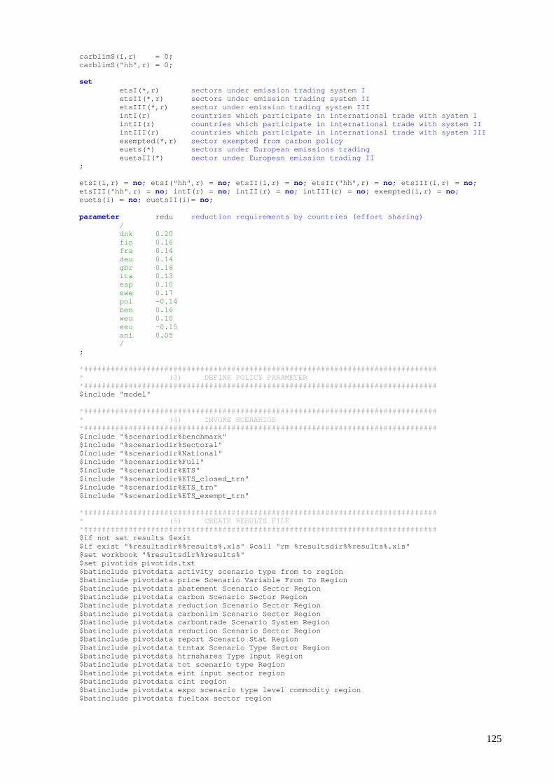
125

carblimS(i,r) = 0; carblimS("hh",r) = 0; set etsI(*,r) sectors under emission trading system I etsII(*,r) sectors under emission trading system II etsIII(*,r) sector under emission trading system III intI(r) countries which participate in international trade with system I intII(r) countries which participate in international trade with system II intIII(r) countries which participate in international trade with system III exempted(*,r) sector exempted from carbon policy euets(*) sectors under European emissions trading euetsII(*) sector under European emission trading II ; etsI(i,r) = no; etsI("hh",r) = no; etsII(i,r) = no; etsII("hh",r) = no; etsIII(i,r) = no; etsIII("hh",r) = no; intI(r) = no; intII(r) = no; intIII(r) = no; exempted(i,r) = no; euets(i) = no; euetsII(i)= no; parameter redu reduction requirements by countries (effort sharing ) / dnk 0.20 fin 0.16 fra 0.14 deu 0.14 gbr 0.16 ita 0.13 esp 0.10 swe 0.17 pol -0.14 ben 0.16 weu 0.10 eeu -0.15 ani 0.05 / ; *################################################## ############################# * (3) DEFINE POLICY PARAMETER *################################################## ############################# $include "model" *################################################## ############################# * (4) INVOKE SCENARIOS *################################################## ############################# $include "%scenariodir%benchmark" $include "%scenariodir%Sectoral" $include "%scenariodir%National" $include "%scenariodir%Full" $include "%scenariodir%ETS" $include "%scenariodir%ETS_closed_trn" $include "%scenariodir%ETS_trn" $include "%scenariodir%ETS_exempt_trn" *################################################## ############################# * (5) CREATE RESULTS FILE *################################################## ############################# $if not set results $exit $if exist "%resultsdir%%results%.xls" $call "rm %re sultsdir%%results%.xls" $set workbook "%resultsdir%%results%" $set pivotids pivotids.txt $batinclude pivotdata activity scenario type from t o region $batinclude pivotdata price Scenario Variable From To Region $batinclude pivotdata abatement Scenario Sector Reg ion $batinclude pivotdata carbon Scenario Sector Region $batinclude pivotdata reduction Scenario Sector Reg ion $batinclude pivotdata carbonlim Scenario Sector Reg ion $batinclude pivotdata carbontrade Scenario System R egion $batinclude pivotdata reduction Scenario Sector Reg ion $batinclude pivotdata report Scenario Stat Region $batinclude pivotdata trntax Scenario Type Sector R egion $batinclude pivotdata htrnshares Type Input Region $batinclude pivotdata tot scenario type Region $batinclude pivotdata eint input sector region $batinclude pivotdata cint region $batinclude pivotdata expo scenario type level comm odity region $batinclude pivotdata fueltax sector region

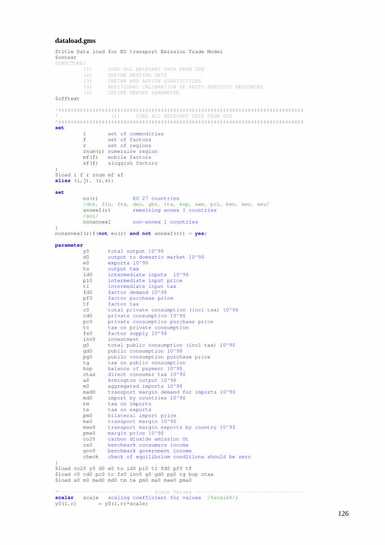
126

dataload.gms $title Data load for EU transport Emission Trade Mo del $ontext STRUCTURE: (1) LOAD ALL RELEVANT DATA FROM GDX (2) DEFINE NESTING SETS (3) DEFINE AND ASSIGN ELASTICITIES (4) ADDITIONAL CALIBRATION OF SECTO SP ECIFIC RESOURCES (5) DEFINE REPORT PARAMETER $offtext *################################################## ############################# * (1) LOAD ALL RELEVANT DATA FR OM GDX *################################################## ############################# set i set of commodities f set of factors r set of regions rnum(r) numeraire region mf(f) mobile factors sf(f) sluggish factors ; $load i f r rnum mf sf alias (i,j), (r,s); set eu(r) EU 27 countries /dnk, fin, fra, deu, gbr, ita, esp, swe, pol, ben, weu, eeu/ annexI(r) remaining annex I countries /ani/ nonannexI non-annex I countries ; nonannexI(r)$( not eu(r) and not annexI(r)) = yes; parameter y0 total output 10^9$ d0 output to domestic market 10^9$ e0 exports 10^9$ to output tax id0 intermediate inputs 10^9$ pi0 intermediate input price ti intermediate input tax fd0 factor demand 10^9$ pf0 factor purchase price tf factor tax c0 total private consumption (incl tax) 10^9$ cd0 private consumption 10^9$ pc0 private consumption purchase price tc tax on private consumption fs0 factor supply 10^9$ inv0 investment g0 total public consumption (incl tax) 10^9$ gd0 public consumption 10^9$ pg0 public consumption purchase price tg tax on public consumption bop balance of payment 10^9$ ctax direct consumer tax 10^9$ a0 Armington output 10^9$ m0 aggregated imports 10^9$ mad0 transport margin demand for imports 10^9$ md0 import by countries 10^9$ tm tax on imports te tax on exports pm0 bilateral import price ma0 transport margin 10^9$ mae0 transport margin exports by country 10^9$ pma0 margin price 10^9$ co20 carbon dioxide emission Gt ra0 benchmark consumers income gov0 benchmark government income check check of equilibrium conditions should be zero ; $load co20 y0 d0 e0 to id0 pi0 ti fd0 pf0 tf $load c0 cd0 pc0 tc fs0 inv0 g0 gd0 pg0 tg bop ctax $load a0 m0 mad0 md0 tm te pm0 ma0 mae0 pma0 *------------------------------ Scale Values ------ ----------------------------- scalar scale scaling coefficient for values /%scale%/ ; y0(i,r) = y0(i,r)*scale;

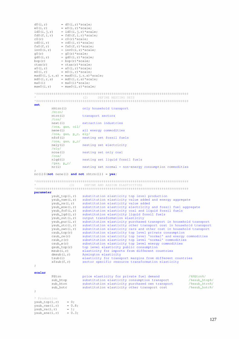
127

d0(i,r) = d0(i,r)*scale; e0(i,r) = e0(i,r)*scale; id0(i,j,r) = id0(i,j,r)*scale; fd0(f,i,r) = fd0(f,i,r)*scale; c0(r) = c0(r)*scale; cd0(i,r) = cd0(i,r)*scale; fs0(f,r) = fs0(f,r)*scale; inv0(i,r) = inv0(i,r)*scale; g0(r) = g0(r)*scale; gd0(i,r) = gd0(i,r)*scale; bop(r) = bop(r)*scale; ctax(r) = ctax(r)*scale; a0(i,r) = a0(i,r)*scale; m0(i,r) = m0(i,r)*scale; mad0(i,j,r,s) = mad0(i,j,r,s)*scale; md0(i,r,s) = md0(i,r,s)*scale; ma0(i) = ma0(i)*scale; mae0(i,r) = mae0(i,r)*scale; *################################################## ############################# * (2) DEFINE NESTING SET S *################################################## ############################# set nhtrn(i) only household transport /htrn/ ntrn(i) transport sectors /trn/ next(i) extraction industries /coa, gas, oil/ nene(i) all energy commodities /coa, gas, p_c, ely/ nfof(i) nesting set fossil fuels /coa, gas, p_c/ nely(i) nesting set electricity /ely/ ncoa(i) nesting set only coal /coa/ nlqd(i) nesting set liquid fossil fuels /gas, p_c/ nc(i) nesting set normal = non-energy consumption commodi ties ; nc(i)$( not nene(i) and not nhtrn(i)) = yes; *################################################## ############################# * (3) DEFINE AND ASSIGN ELASTIC ITIES *################################################## ############################# parameter ysub_top(i,r) substitution elasticity top level production ysub_vae(i,r) substitution elasticity value added and energy aggr egate ysub_va(i,r) substitution elasticity value added ysub_ene(i,r) substitution elasticity electricity and fossil fuel aggregate ysub_fof(i,r) substitution elasticity coal and liquid fossil fuel s ysub_lqd(i,r) substitution elasticity liquid fossil fuels ysub_out(i,r) output transformation elasticity ysub_pur(i,r) substitution elasticity purchased transport in hous ehold transport ysub_otc(i,r) substitution elasticity other transport cost in hou sehold transport ysub_own(i,r) substitution elasticity cars and other cost in hous ehold transport csub_top(r) substitution elasticity top level private consumpti on csub_ce(r) substitution elasticity top level "normal" and ener gy commodities csub_c(r) substitution elasticity top level "normal" commodit ies csub_e(r) substitution elasticity top level energy commoditie s gsub_top(r) top level elasticity public consumption msub(i,r) elasticity for imports from different countries dmsub(i,r) Armington elasticity tsub(i) elasticity for transport margins from different cou ntries sfsub(f,r) sector specific resource transformation elasticity ; scalar PEtrn price elasticity for private fuel demand /%PEtrn%/ sub_htop substitution elasticity consumption transport /%esub_htop%/ sub_htrn substitution elasticity purchased own transport /%esub_htrn%/ sub_hotc substitution elasticity other transport cost /%esub_hotc%/ ; * Production ysub_top(i,r) = 0; ysub_vae(i,r) = 0.8; ysub_va(i,r) = 1; ysub_ene(i,r) = 0.3;

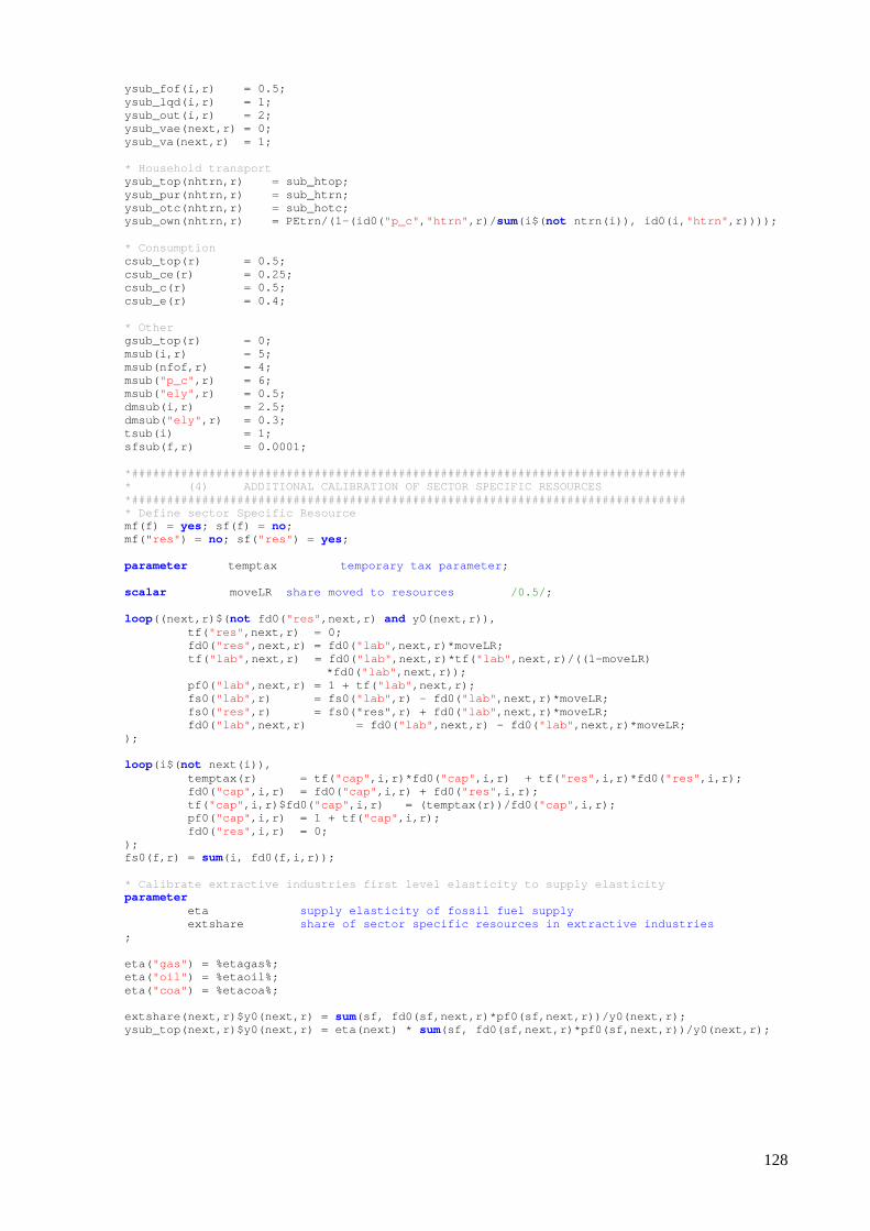
128

ysub_fof(i,r) = 0.5; ysub_lqd(i,r) = 1; ysub_out(i,r) = 2; ysub_vae(next,r) = 0; ysub_va(next,r) = 1; * Household transport ysub_top(nhtrn,r) = sub_htop; ysub_pur(nhtrn,r) = sub_htrn; ysub_otc(nhtrn,r) = sub_hotc; ysub_own(nhtrn,r) = PEtrn/(1-(id0( "p_c" , "htrn" ,r)/ sum(i$( not ntrn(i)), id0(i, "htrn" ,r)))); * Consumption csub_top(r) = 0.5; csub_ce(r) = 0.25; csub_c(r) = 0.5; csub_e(r) = 0.4; * Other gsub_top(r) = 0; msub(i,r) = 5; msub(nfof,r) = 4; msub( "p_c" ,r) = 6; msub( "ely" ,r) = 0.5; dmsub(i,r) = 2.5; dmsub( "ely" ,r) = 0.3; tsub(i) = 1; sfsub(f,r) = 0.0001; *################################################## ############################# * (4) ADDITIONAL CALIBRATION OF SECTOR S PECIFIC RESOURCES *################################################## ############################# * Define sector Specific Resource mf(f) = yes; sf(f) = no; mf(" res" ) = no; sf( "res" ) = yes; parameter temptax temporary tax parameter ; scalar moveLR share moved to resources /0.5/ ; loop((next,r)$( not fd0( "res" ,next,r) and y0(next,r)), tf( "res" ,next,r) = 0; fd0( "res" ,next,r) = fd0( "lab" ,next,r)*moveLR;

tf( "lab" ,next,r) = fd0( "lab" ,next,r)*tf( "lab" ,next,r)/((1-moveLR) *fd0( "lab" ,next,r));

pf0( "lab" ,next,r) = 1 + tf( "lab" ,next,r); fs0( "lab" ,r) = fs0( "lab" ,r) - fd0( "lab" ,next,r)*moveLR; fs0( "res" ,r) = fs0("res",r) + fd0( "lab" ,next,r)*moveLR; fd0( "lab" ,next,r) = fd0( "lab" ,next,r) - fd0( "lab" ,next,r)*moveLR; ); loop(i$( not next(i)), temptax(r) = tf( "cap" ,i,r)*fd0( "cap" ,i,r) + tf( "res" ,i,r)*fd0( "res" ,i,r); fd0( "cap" ,i,r) = fd0( "cap" ,i,r) + fd0( "res" ,i,r); tf( "cap" ,i,r)$fd0( "cap" ,i,r) = (temptax(r))/fd0( "cap" ,i,r); pf0( "cap" ,i,r) = 1 + tf( "cap" ,i,r); fd0( "res" ,i,r) = 0; ); fs0(f,r) = sum(i, fd0(f,i,r)); * Calibrate extractive industries first level elast icity to supply elasticity parameter eta supply elasticity of fossil fuel supply extshare share of sector specific resources in extractive in dustries ; eta( "gas" ) = %etagas%; eta( "oil" ) = %etaoil%; eta( "coa" ) = %etacoa%; extshare(next,r)$y0(next,r) = sum(sf, fd0(sf,next,r)*pf0(sf,next,r))/y0(next,r); ysub_top(next,r)$y0(next,r) = eta(next) * sum(sf, fd0(sf,next,r)*pf0(sf,next,r))/y0(next,r);

129

*################################################## ############################# * (5) DEFINE REPORT PARA METER *################################################## ############################# parameter activity report parameter for activities price report variable for prices carbon report variable for carbon carbonlim report of carbon limit reduction report of carbon reduction report other reports abatement report of abatement costs carbontrade report carbon trade intermediates report on intermediate demand trntax report on tax income from transport sectors tot report on terms of trade changes expo exports impo imports ;

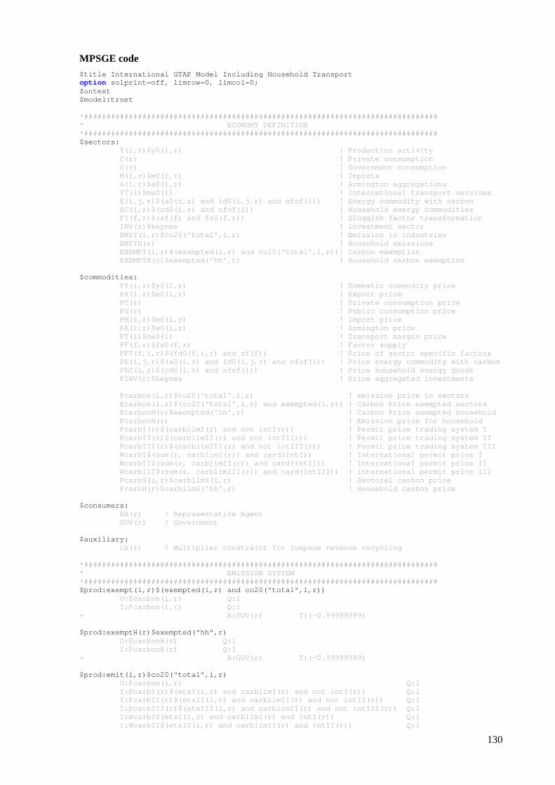
130

MPSGE code $title International GTAP Model Including Household Transport option solprint=off, limrow=0, limcol=0; $ontext $model:trnet *################################################## ############################# * ECONOMY DEFINITION *################################################## ############################# $sectors: Y(i,r)$y0(i,r) ! Production activity C(r) ! Private consumption G(r) ! Government consumption M(i,r)$m0(i,r) ! Imports A(i,r)$a0(i,r) ! Armington aggregations YT(i)$ma0(i) ! International transport services E(i,j,r)$(a0(i,r) and id0(i,j,r) and nfof( i)) ! Energy commodity with carbon EC(i,r)$(cd0(i,r) and nfof(i)) ! Household energy commodities FT(f,r)$(sf(f) and fs0(f,r)) ! Sluggish factor transformation INV(r)$keynes ! Investment sector EMIT(i,r)$co20("total",i,r) ! Emission in industries EMITH(r) ! Household emissions EXEMPT(i,r)$(exempted(i,r) and co20("total ",i,r))! Carbon exemption EXEMPTH(r)$exempted("hh",r) ! Household carbon exemption $commodities: PY(i,r)$y0(i,r) ! Domestic commodity price PX(i,r)$e0(i,r) ! Export price PC(r) ! Private consumption price PG(r) ! Public consumption price PM(i,r)$m0(i,r) ! Import price PA(i,r)$a0(i,r) ! Armington price PT(i)$ma0(i) ! Transport margin price PF(f,r)$fs0(f,r) ! Factor supply PFT(f,i,r)$(fd0(f,i,r) and sf(f)) ! Price of sector specific factors PE(i,j,r)$(a0(i,r) and id0(i,j,r) and nfof (i)) ! Price energy commodity with carbon PEC(i,r)$(cd0(i,r) and nfof(i)) ! Price household energy goods PINV(r)$keynes ! Price aggregated investments Pcarbon(i,r)$co20("total",i,r) ! emission price in sectors Ecarbon(i,r)$(co20("total",i,r) and exempt ed(i,r)) ! Carbon Price exempted sectors EcarbonH(r)$exempted("hh",r) ! Carbon Price exempted household PcarbonH(r) ! Emission price for household PcarbI(r)$(carblimI(r) and not intI(r)) ! Permit price trading system I PcarbII(r)$(carblimII(r) and not intII(r)) ! Permit price trading system II PcarbIII(r)$(carblimIII(r) and not intIII( r)) ! Permit price trading system III WcarbI$(sum(r, carblimI(r)) and card(intI) ) ! International permit price I WcarbII$(sum(r, carblimII(r)) and card(int II)) ! International permit price II WcarbIII$(sum(r, carblimIII(r)) and card(i ntIII)) ! International permit price III PcarbS(i,r)$carblimS(i,r) ! Sectoral carbon price PcarbH(r)$carblimS("hh",r) ! Household carbon price $consumers: RA(r) ! Representative Agent GOV(r) ! Government $auxiliary: LS(r) ! Multiplier constraint for lump sum revenue recycling *################################################## ############################# * EMISSION SYSTEM *################################################## ############################# $prod:exempt(i,r)$(exempted(i,r) and co20("total",i ,r)) O:Ecarbon(i,r) Q:1 I:Pcarbon(i,r) Q:1 + A:GOV(r) T: (-0.99999999) $prod:exemptH(r)$exempted("hh",r) O:EcarbonH(r) Q:1 I:PcarbonH(r) Q:1 + A:GOV(r) T: (-0.99999999) $prod:emit(i,r)$co20("total",i,r) O:Pcarbon(i,r) Q:1 I:PcarbI(r)$(etsI(i,r) and carblimI(r) and not intI(r)) Q:1 I:PcarbII(r)$(etsII(i,r) and carblimII(r) and not intII(r)) Q:1 I:PcarbIII(r)$(etsIII(i,r) and carblimII(r ) and not intIII(r)) Q:1 I:WcarbI$(etsI(i,r) and carblimI(r) and in tI(r)) Q:1 I:WcarbII$(etsII(i,r) and carblimII(r) and intII(r)) Q:1

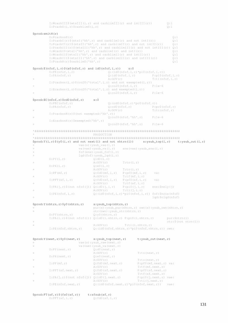
131

I:WcarbIII$(etsIII(i,r) and carblimIII(r) and intIII(r)) Q:1 I:PcarbS(i,r)$carblimS(i,r) Q:1 $prod:emitH(r) O:PcarbonH(r) Q:1 I:PcarbI(r)$(etsI("hh",r) and carblimI(r) and not intI(r)) Q:1 I:PcarbII(r)$(etsII("hh",r) and carblimII( r) and not intII(r)) Q:1 I:PcarbIII(r)$(etsIII("hh",r) and carblimI II(r) and not intIII(r)) Q:1 I:WcarbI$(etsI("hh",r) and carblimI(r) and intI(r)) Q:1 I:WcarbII$(etsII("hh",r) and carblimII(r) and intII(r)) Q:1 I:WcarbIII$(etsIII("hh",r) and carblimIII( r) and intIII(r)) Q:1 I:PcarbH(r)$carblimS("hh",r) Q:1 $prod:E(nfof,i,r)$(a0(nfof,r) and id0(nfof,i,r)) s:0 O:PE(nfof,i,r) Q:(id0(nfo f,i,r)*pi0(nfof,i,r)) I:PA(nfof,r) Q:id0(nfof ,i,r) P:pi0(nfof,i,r) + A:GOV(r) T:ti(nfof,i,r) I:Pcarbon(i,r)$(co20("total",i,r) and not exempted(i,r)) + Q:co20(nfo f,i,r) P:1e-6 I:Ecarbon(i,r)$(co20("total",i,r) and exem pted(i,r)) + Q:co20(nfo f,i,r) P:1e-6 $prod:EC(nfof,r)$cd0(nfof,r) s:0 O:PEC(nfof,r) Q:(cd0(nfo f,r)*pc0(nfof,r)) I:PA(nfof,r) Q:cd0(nfof ,r) P:pc0(nfof,r) + A:GOV(r) T:tc(nfof,r) I:PcarbonH(r)$(not exempted("hh",r)) + Q:co20(nfo f,"hh",r) P:1e-6 I:EcarbonH(r)$exempted("hh",r) + Q:co20(nfo f,"hh",r) P:1e-6 *################################################## ############################# * PRODUCTION *################################################## ############################# $prod:Y(i,r)$(y0(i,r) and not next(i) and not nhtrn (i)) s:ysub_top(i,r) t:ysub_out(i,r) + vae(s):ysub_vae(i,r) + va(vae):ysub_va(i,r) en e(vae):ysub_ene(i,r) + fof(ene):ysub_fof(i,r) + lqd(fof):ysub_lqd(i,r) O:PY(i,r) Q:d0(i,r) + A:GOV(r) T: to(i,r) O:PX(i,r) Q:e0(i,r) + A:GOV(r) T: to(i,r) I:PF(mf,r) Q:fd0(mf,i,r) P: pf0(mf,i,r) va: + A:GOV(r) T: tf(mf,i,r) I:PFT(sf,i,r) Q:fd0(sf,i,r) P: pf0(sf,i,r) va: + A:GOV(r) T: tf(sf,i,r) I:PA(j,r)$(not nfof(j)) Q:id0(j,i,r) P: pi0(j,i,r) ene:$nely(j) + A:GOV(r) T: ti(j,i,r) I:PE(nfof,i,r) Q:(id0(nfof,i,r)*p i0(nfof,i,r)) fof:$ncoa(nfof) + lqd:$nlqd(nfof) $prod:Y(nhtrn,r)$y0(nhtrn,r) s:ysub_top(nhtrn,r ) + pur(s):ysub_pur(nh trn,r) own(s):ysub_own(nhtrn,r) + otc(own):ysub_otc( nhtrn,r) O:PY(nhtrn,r) Q:y0(nhtrn,r) I:PA(i,r)$(not nfof(i)) Q:id0(i,nhtrn,r) P :pi0(i,nhtrn,r) pur:$ntrn(i) + otc:$(not ntrn(i)) + A:GOV(r) T :ti(i,nhtrn,r) I:PE(nfof,nhtrn,r) Q:(id0(nfof,nhtrn, r)*pi0(nfof,nhtrn,r)) own: $prod:Y(next,r)$y0(next,r) s:ysub_top(next,r) t:ysub_out(next,r) + vae(s):ysub_vae(next,r) + va(vae):ysub_va(next,r) O:PY(next,r) Q:d0(next,r) + A:GOV(r) T:to(next,r) O:PX(next,r) Q:e0(next,r) + A:GOV(r) T:to(next,r) I:PF(mf,r) Q:fd0(mf,next,r) P:pf0(mf,next,r) va: + A:GOV(r) T:tf(mf,next,r) I:PFT(sf,next,r) Q:fd0(sf,next,r) P:pf0(sf,next,r) + A:GOV(r) T:tf(sf,next,r) I:PA(j,r)$(not nfof(j)) Q:id0(j,next,r) P:pi0(j,next,r) vae: + A:GOV(r) T:ti(j,next,r) I:PE(nfof,next,r) Q:(id0(nfof,next,r )*pi0(nfof,next,r)) vae: $prod:FT(sf,r)$(fs0(sf,r)) t:sfsub(sf,r) O:PFT(sf,i,r) Q:fd0(sf,i,r)

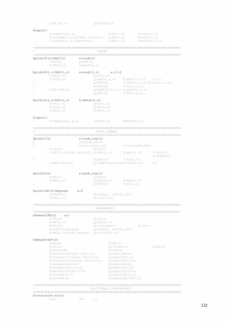
132

I:PF(sf,r) Q:fs0(sf,r) $report: V:exports(i,r) O:PX(i,r) Pr od:Y(i,r) V:intdem(i,j,r)$(not nfof(i)) I:PA(i,r) Prod:Y(j,r) V:intdem(i,j,r)$nfof(i) I:PA(i,r) Prod:E(i,j,r) *################################################## ############################# * TRADE *################################################## ############################# $prod:YT(i)$ma0(i) s:tsub(i) O:PT(i) Q:ma0(i) I:PX(i,r) Q:mae0(i,r) $prod:M(i,r)$m0(i,r) s:msub(i,r) s.tl:0 O:PM(i,r) Q:m0(i,r) I:PX(i,s) Q:md0(i,s,r) P: pm0(i,s,r) s.tl: + A:GOV(r) T: (tm(i,s,r)*(1+te(i,s,r))) + A:GOV(s) T: te(i,s,r) I:PT(j)#(s) Q:mad0(j,i,s,r) P: pma0(i,s,r) + A:GOV(r) T: tm(i,s,r) $prod:A(i,r)$a0(i,r) s:dmsub(i,r) O:PA(i,r) Q:a0(i,r) I:PY(i,r) Q:d0(i,r) I:PM(i,r) Q:m0(i,r) $report: V:Imports(i,s,r) I:PX(i,s) PR OD:M(i,r) *################################################## ############################# * FINAL DEMAND *################################################## ############################# $prod:C(r) s:csub_top(r) + ce:csub_ce(r) + c(ce):csub_c(r) e( ce):csub_e(r) O:PC(r) Q:c0(r) I:PA(i,r)$(not nfof(i)) Q:cd0(i,r) P: pc0(i,r) c:$nc(i) + e:$nene(i) + A:GOV(r) T: tc(i,r) I:PEC(nfof,r) Q:(cd0(nfof,r)*pc0 (nfof,r)) e: $prod:G(r) s:gsub_top(r) O:PG(r) Q:g0(r) I:PA(i,r) Q:gd0(i,r) P: pg0(i,r) + A:GOV(r) T: tg(i,r) $prod:INV(r)$keynes s:0 O:PINV(r) Q:(sum(i, inv0(i,r) )) I:PA(i,r) Q:inv0(i,r) *################################################## ############################# * ENDOWMENTS *################################################## ############################# $demand:RA(r) s:1 D:PC(r) Q:c0(r) E:PF(f,r) Q:fs0(f,r) E:PC(r) Q:(-ctax(r)) R:LS(r) D:PINV(r)$keynes Q:(sum(i, inv0(i,r ))) E:PA(i,r)$(not keynes) Q:(-inv0(i,r)) $demand:GOV(r) D:PG(r) Q:g0(r) E:PC(r) Q:(ctax(r) ) R:LS(r) E:PC(rnum) Q:bop(r) E:PcarbI(r)$(not intI(r)) Q:carblimI (r) E:PcarbII(r)$(not intII(r)) Q:carblimI I(r) E:PcarbIII(r)$(not intIII(r)) Q:carblimI II(r) E:WcarbI$intI(r) Q:carblimI (r) E:WcarbII$intII(r) Q:carblimI I(r) E:WcarbIII$intIII(r) Q:carblimI II(r) E:PcarbS(i,r) Q:carblimS (i,r) E:PcarbH(r) Q:carblimS ("hh",r) *################################################## ############################# * ADDITIONAL CONSTRAIN TS *################################################## ############################# $constraint:LS(r) G(r) =E= 1;

133

$offtext $sysinclude mpsgeset trnet trnet.workspace = 15; trnet.reslim = 8000; PC.FX(rnum) = 1; *################################################## ############################# * REPLICATION CHECK *################################################## ############################# LS.L(r) = 1; LS.LO(r) = - inf; Pcarbon.L(i,r) = 0; PcarbonH.L(r) = 0; PcarbI.L(r) = 0; PcarbII.L(r) = 0; PcarbIII.L(r) = 0; WcarbI.L = 0; WcarbII.L = 0; WcarbIII.L = 0; PcarbS.L(i,r) = 0; PcarbH.L(r) = 0; emit.L(i,r) = co20( "total" ,i,r); emitH.L(r) = co20( "total" , "hh" ,r); trnet.iterlim = 0; $include trnet.gen solve trnet using MCP; trnet.iterlim = 100000; display "precision of benchmark: " , trnet.objval; abort$(trnet.objval ge 1e-4) "Model does not replicate" ; * Save benchmark income values ra0(r) = RA.L(r); gov0(r)= GOV.L(r);

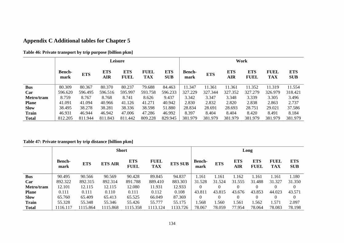
134

Appendix C Additional tables for Chapter 5

Table 46: Private transport by trip purpose [billion pkm]

Leisure Work

Bench-mark ETS ETS

AIR ETS

FUEL FUEL TAX

ETS SUB

Bench-mark ETS ETS

AIR ETS

FUEL FUEL TAX

ETS SUB

Bus 80.309 80.367 80.370 80.237 79.688 84.463 11.347 11.361 11.361 11.352 11.319 11.554 Car 596.620 596.495 596.516 595.997 593.758 596.233 327.229 327.344 327.352 327.279 326.979 318.421 Metro/tram 8.759 8.767 8.768 8.741 8.626 9.437 3.342 3.347 3.348 3.339 3.305 3.496 Plane 41.091 41.094 40.966 41.126 41.271 40.942 2.830 2.832 2.820 2.838 2.863 2.737 Slow 38.495 38.278 38.281 38.336 38.598 51.880 28.834 28.691 28.693 28.751 29.021 37.586 Train 46.931 46.944 46.942 47.006 47.286 46.992 8.397 8.404 8.404 8.420 8.491 8.184 Total 812.205 811.944 811.843 811.442 809.228 829.945 381.979 381.979 381.979 381.979 381.979 381.979

Table 47: Private transport by trip distance [billion pkm]

Short Long

Bench-mark ETS ETS AIR ETS

FUEL FUEL TAX ETS SUB Bench-

mark ETS ETS AIR

ETS FUEL

FUEL TAX

ETS SUB

Bus 90.495 90.566 90.569 90.428 89.845 94.837 1.161 1.161 1.162 1.161 1.161 1.180 Car 892.322 892.315 892.314 891.788 889.410 883.303 31.528 31.524 31.555 31.488 31.327 31.350 Metro/tram 12.101 12.115 12.115 12.080 11.931 12.933 0 0 0 0 0 0 Plane 0.111 0.111 0.110 0.111 0.112 0.108 43.811 43.815 43.676 43.853 44.023 43.571 Slow 65.760 65.409 65.413 65.525 66.049 87.369 0 0 0 0 0 0 Train 55.328 55.348 55.346 55.426 55.777 55.175 1.568 1.560 1.561 1.562 1.571 2.097 Total 1116.117 1115.864 1115.868 1115.358 1113.124 1133.726 78.067 78.059 77.954 78.064 78.083 78.198

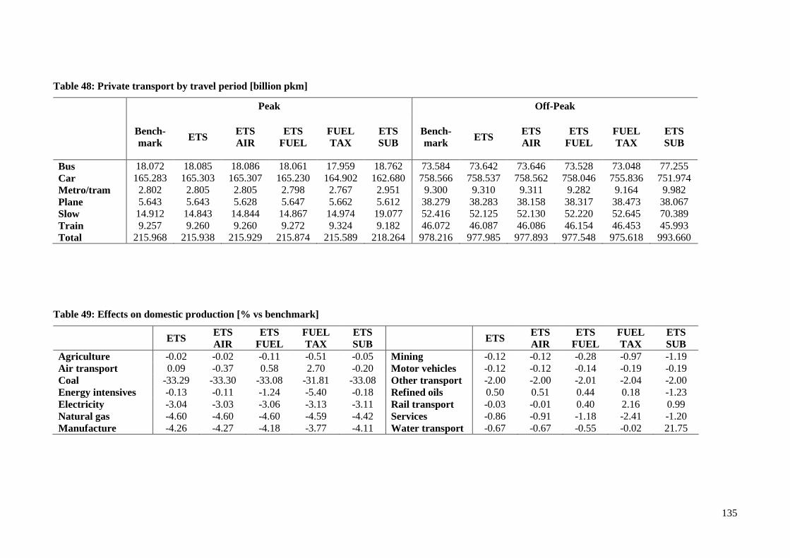
135

Table 48: Private transport by travel period [billi on pkm]

Peak Off-Peak

Bench-mark ETS ETS

AIR ETS

FUEL FUEL TAX

ETS SUB

Bench-mark ETS ETS

AIR ETS

FUEL FUEL TAX

ETS SUB

Bus 18.072 18.085 18.086 18.061 17.959 18.762 73.584 73.642 73.646 73.528 73.048 77.255 Car 165.283 165.303 165.307 165.230 164.902 162.680 758.566 758.537 758.562 758.046 755.836 751.974 Metro/tram 2.802 2.805 2.805 2.798 2.767 2.951 9.300 9.310 9.311 9.282 9.164 9.982 Plane 5.643 5.643 5.628 5.647 5.662 5.612 38.279 38.283 38.158 38.317 38.473 38.067 Slow 14.912 14.843 14.844 14.867 14.974 19.077 52.416 52.125 52.130 52.220 52.645 70.389 Train 9.257 9.260 9.260 9.272 9.324 9.182 46.072 46.087 46.086 46.154 46.453 45.993 Total 215.968 215.938 215.929 215.874 215.589 218.264 978.216 977.985 977.893 977.548 975.618 993.660

Table 49: Effects on domestic production [% vs benchmark]

ETS ETS AIR

ETS FUEL

FUEL TAX

ETS SUB

ETS ETS AIR

ETS FUEL

FUEL TAX

ETS SUB

Agriculture -0.02 -0.02 -0.11 -0.51 -0.05 Mining -0.12 -0.12 -0.28 -0.97 -1.19 Air transport 0.09 -0.37 0.58 2.70 -0.20 Motor vehicles -0.12 -0.12 -0.14 -0.19 -0.19 Coal -33.29 -33.30 -33.08 -31.81 -33.08 Other transport -2.00 -2.00 -2.01 -2.04 -2.00 Energy intensives -0.13 -0.11 -1.24 -5.40 -0.18 Refined oils 0.50 0.51 0.44 0.18 -1.23 Electricity -3.04 -3.03 -3.06 -3.13 -3.11 Rail transport -0.03 -0.01 0.40 2.16 0.99 Natural gas -4.60 -4.60 -4.60 -4.59 -4.42 Services -0.86 -0.91 -1.18 -2.41 -1.20 Manufacture -4.26 -4.27 -4.18 -3.77 -4.11 Water transport -0.67 -0.67 -0.55 -0.02 21.75

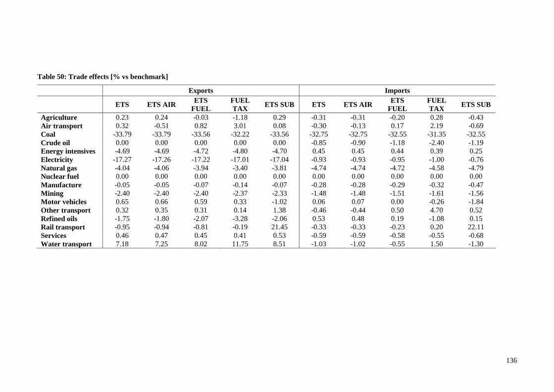
136

Table 50: Trade effects [% vs benchmark]

Exports Imports

ETS ETS AIR ETS FUEL

FUEL TAX ETS SUB ETS ETS AIR ETS

FUEL FUEL TAX ETS SUB

Agriculture 0.23 0.24 -0.03 -1.18 0.29 -0.31 -0.31 -0.20 0.28 -0.43 Air transport 0.32 -0.51 0.82 3.01 0.08 -0.30 -0.13 0.17 2.19 -0.69 Coal -33.79 -33.79 -33.56 -32.22 -33.56 -32.75 -32.75 -32.55 -31.35 -32.55 Crude oil 0.00 0.00 0.00 0.00 0.00 -0.85 -0.90 -1.18 -2.40 -1.19 Energy intensives -4.69 -4.69 -4.72 -4.80 -4.70 0.45 0.45 0.44 0.39 0.25 Electricity -17.27 -17.26 -17.22 -17.01 -17.04 -0.93 -0.93 -0.95 -1.00 -0.76 Natural gas -4.04 -4.06 -3.94 -3.40 -3.81 -4.74 -4.74 -4.72 -4.58 -4.79 Nuclear fuel 0.00 0.00 0.00 0.00 0.00 0.00 0.00 0.00 0.00 0.00 Manufacture -0.05 -0.05 -0.07 -0.14 -0.07 -0.28 -0.28 -0.29 -0.32 -0.47 Mining -2.40 -2.40 -2.40 -2.37 -2.33 -1.48 -1.48 -1.51 -1.61 -1.56 Motor vehicles 0.65 0.66 0.59 0.33 -1.02 0.06 0.07 0.00 -0.26 -1.84 Other transport 0.32 0.35 0.31 0.14 1.38 -0.46 -0.44 0.50 4.70 0.52 Refined oils -1.75 -1.80 -2.07 -3.28 -2.06 0.53 0.48 0.19 -1.08 0.15 Rail transport -0.95 -0.94 -0.81 -0.19 21.45 -0.33 -0.33 -0.23 0.20 22.11 Services 0.46 0.47 0.45 0.41 0.53 -0.59 -0.59 -0.58 -0.55 -0.68 Water transport 7.18 7.25 8.02 11.75 8.51 -1.03 -1.02 -0.55 1.50 -1.30

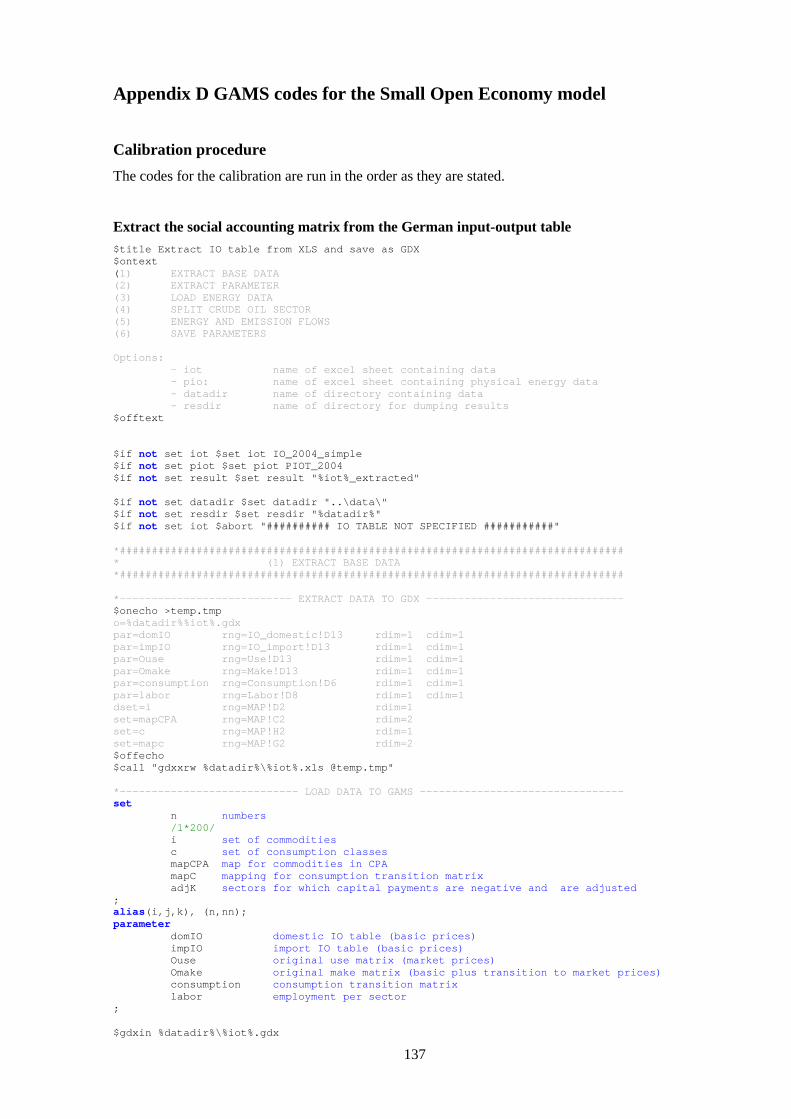
137

Appendix D GAMS codes for the Small Open Economy model

Calibration procedure

The codes for the calibration are run in the order as they are stated.

Extract the social accounting matrix from the German input-output table $title Extract IO table from XLS and save as GDX $ontext ( 1) EXTRACT BASE DATA (2) EXTRACT PARAMETER (3) LOAD ENERGY DATA (4) SPLIT CRUDE OIL SECTOR (5) ENERGY AND EMISSION FLOWS (6) SAVE PARAMETERS Options: - iot name of excel sheet contai ning data - pio: name of excel sheet contai ning physical energy data - datadir name of directory containi ng data - resdir name of directory for dump ing results $offtext $if not set iot $set iot IO_2004_simple $if not set piot $set piot PIOT_2004 $if not set result $set result "%iot%_extracted" $if not set datadir $set datadir "..\data\" $if not set resdir $set resdir "%datadir%" $if not set iot $abort "########## IO TABLE NOT SPECIFIED ###########" *################################################## ############################# * (1) EXTRACT BASE DATA *################################################## ############################# *--------------------------- EXTRACT DATA TO GDX -- ----------------------------- $onecho >temp.tmp o=%datadir%%iot%.gdx par=domIO rng=IO_domestic!D13 rdim=1 cd im=1 par=impIO rng=IO_import!D13 rdim=1 cd im=1 par=Ouse rng=Use!D13 rdim=1 cd im=1 par=Omake rng=Make!D13 rdim=1 cd im=1 par=consumption rng=Consumption!D6 rdim=1 cd im=1 par=labor rng=Labor!D8 rdim=1 cd im=1 dset=i rng=MAP!D2 rdim=1 set=mapCPA rng=MAP!C2 rdim=2 set=c rng=MAP!H2 rdim=1 set=mapc rng=MAP!G2 rdim=2 $offecho $call "gdxxrw %datadir%\%iot%.xls @temp.tmp" *---------------------------- LOAD DATA TO GAMS --- ----------------------------- set n numbers /1*200/ i set of commodities c set of consumption classes mapCPA map for commodities in CPA mapC mapping for consumption transition matrix adjK sectors for which capital payments are negative and are adjusted ; alias(i,j,k), (n,nn); parameter domIO domestic IO table (basic prices) impIO import IO table (basic prices) Ouse original use matrix (market prices) Omake original make matrix (basic plus transition to mark et prices) consumption consumption transition matrix labor employment per sector ; $gdxin %datadir%\%iot%.gdx

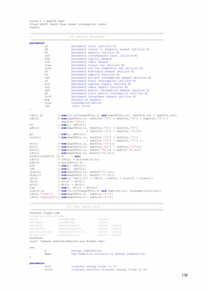
138

$load i c mapCPA mapC $load domIO impIO Ouse Omake consumption labor $gdxin *################################################## ############################# * (2) EXTRACT PARAMETER *################################################## ############################# parameter y0 benchmark total [million €] d0 benchmark output to domestic market [million €] e0 benchmark exports [million €] id0 benchmark intermediate input [million €] kd0 benchmark capital demand ld0 benchmark labor demand otax benchmark output tax [million €] utax benchmark tax for commodity use [million €] a0 benchmark Armington demand [million €] m0 benchmark imports [million €] cd0 benchmark private consumption demand [million €] c0 benchmark total consumption [million €] ks0 benchmark capital supply [million €] ls0 benchmark labor supply [million €] gd0 benchmark public consumption demand [million €] g0 benchmark total public consumption [million €] inv0 benchmark investment demand [million €] bop balance of payment cons consumption matrix lab labor force ; id0(i,j) = sum((n,nn)$(mapCPA(n,i) and mapCPA(nn,j)), domIO(n,nn) + impIO(n,nn)); cd0(i) = sum(mapCPA(n,i), domIO(n, "73" ) + domIO(n, "78" ) + impIO(n, "73" ) +

impIO(n, "78" )); c0 = sum(i, cd0(i)); gd0(i) = sum(mapCPA(n,i), domIO(n, "74" ) + domIO(n, "75" ) + impIO(n, "74" ) + impIO(n, "75" )); g0 = sum(i, gd0(i)); inv0(i) = sum(mapCPA(n,i), domIO(n, "76" ) + domIO(n, "77" ) + impIO(n, "76" ) + impIO(n, "77" ) ); e0(i) = sum(mapCPA(n,i), domIO(n, "79" )); m0(i) = sum(mapCPA(n,i), impIO(n, "82" ) - impIO(n, "79" )); kd0(i) = sum(mapCPA(n,i), domIO( "78" ,n) + domIO( "79" ,n)); ld0(i) = sum(mapCPA(n,i), domIO( "76" ,n)); adjK(i)$(kd0(i) lt 0) = yes; ld0(i) = ld0(i) + min(kd0(i),0); kd0(i) = max(kd0(i),0); ks0 = sum(i, kd0(i)); ls0 = sum(i, ld0(i)); utax(i) = sum(mapCPA(n,i), domIO( "74" ,n)); otax(i) = sum(mapCPA(n,i), domIO( "77" ,n)); y0(i) = sum(j, id0(j,i)) + ld0(i) + kd0(i) + otax(i) + utax(i) ; d0(i) = y0(i) - e0(i); a0(i) = m0(i) + d0(i); bop = sum(i, m0(i) - e0(i)); cons(i,c) = sum((n,nn)$(mapCPA(n,i) and mapc(nn,c)), consumption(n,nn)); lab(i, "total" ) = sum(mapCPA(n,i), labor(n, "1" )); lab(i, "employed" )= sum(mapCPA(n,i), labor(n, "2" )); *################################################## ############################# * (3) LOAD ENERGY DATA *################################################## ############################# $onecho >temp1.tmp o=%datadir%%piot%.gdx set=e rng=MAP!B2 rdim=1 set=mape rng=MAP!A2 rdim=2 par=eiot rng=energy!C3 rdim=1 cd im=1 par=eriot rng=eenergy!C3 rdim=1 cd im=1 par=emissions rng=emissions!C1 rdim=1 cd im=0 par=prices rng=prices!A1 rdim=1 cd im=0 $offecho $call "gdxxrw %datadir%%piot%.xls @temp1.tmp" set e energy commodities mape map numerical accounts to energy commodities ; parameter eiot original energy flows in TJ eriot original emission relevant energy flows in TJ

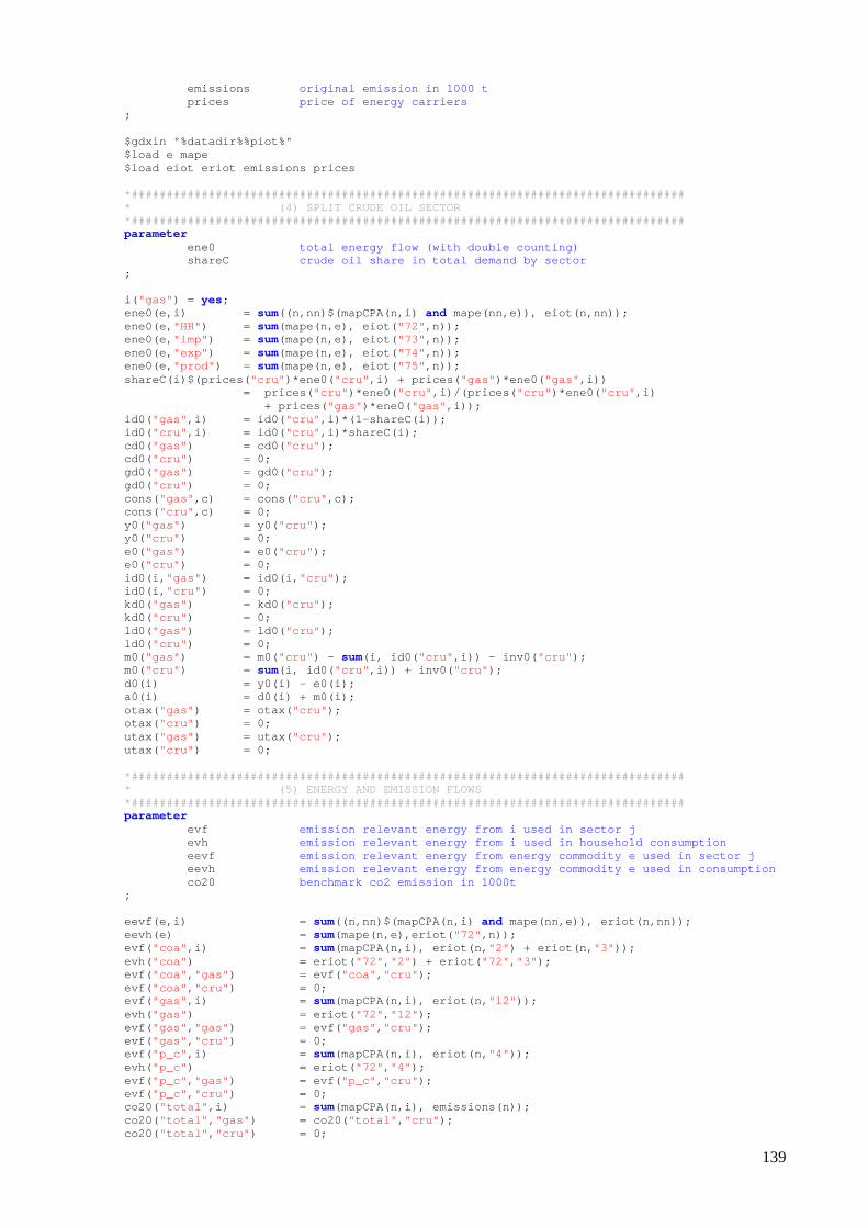
139

emissions original emission in 1000 t prices price of energy carriers ; $gdxin "%datadir%%piot%" $load e mape $load eiot eriot emissions prices *################################################## ############################# * (4) SPLIT CRUDE OIL SECTOR *################################################## ############################# parameter ene0 total energy flow (with double counting) shareC crude oil share in total demand by sector ; i( "gas" ) = yes; ene0(e,i) = sum((n,nn)$(mapCPA(n,i) and mape(nn,e)), eiot(n,nn)); ene0(e, "HH" ) = sum(mape(n,e), eiot( "72" ,n)); ene0(e, "imp" ) = sum(mape(n,e), eiot( "73" ,n)); ene0(e, "exp" ) = sum(mape(n,e), eiot( "74" ,n)); ene0(e, "prod" ) = sum(mape(n,e), eiot( "75" ,n)); shareC(i)$(prices( "cru" )*ene0( "cru" ,i) + prices( "gas" )*ene0( "gas" ,i)) = prices( "cru" )*ene0( "cru" ,i)/(prices( "cru" )*ene0( "cru" ,i) + prices( "gas" )*ene0( "gas" ,i)); id0( "gas" ,i) = id0( "cru" ,i)*(1-shareC(i)); id0( "cru" ,i) = id0( "cru" ,i)*shareC(i); cd0( "gas" ) = cd0( "cru" ); cd0( "cru" ) = 0; gd0( "gas" ) = gd0( "cru" ); gd0( "cru" ) = 0; cons( "gas" ,c) = cons( "cru" ,c); cons( "cru" ,c) = 0; y0( "gas" ) = y0( "cru" ); y0( "cru" ) = 0; e0( "gas" ) = e0( "cru" ); e0( "cru" ) = 0; id0(i, "gas" ) = id0(i, "cru" ); id0(i, "cru" ) = 0; kd0( "gas" ) = kd0( "cru" ); kd0( "cru" ) = 0; ld0( "gas" ) = ld0( "cru" ); ld0( "cru" ) = 0; m0("gas" ) = m0( "cru" ) - sum(i, id0( "cru" ,i)) - inv0( "cru" ); m0("cru" ) = sum(i, id0( "cru" ,i)) + inv0( "cru" ); d0(i) = y0(i) - e0(i); a0(i) = d0(i) + m0(i); otax( "gas" ) = otax( "cru" ); otax( "cru" ) = 0; utax( "gas" ) = utax( "cru" ); utax( "cru" ) = 0; *################################################## ############################# * (5) ENERGY AND EMISSION FLOWS *################################################## ############################# parameter evf emission relevant energy from i used in sector j evh emission relevant energy from i used in household c onsumption eevf emission relevant energy from energy commodity e us ed in sector j eevh emission relevant energy from energy commodity e us ed in consumption co20 benchmark co2 emission in 1000t ; eevf(e,i) = sum((n,nn)$(mapCPA(n,i) and mape(nn,e)), eriot(n,nn)); eevh(e) = sum(mape(n,e),eriot( "72" ,n)); evf( "coa" ,i) = sum(mapCPA(n,i), eriot(n, "2" ) + eriot(n, "3" )); evh( "coa" ) = eriot( "72" , "2" ) + eriot( "72" , "3" ); evf( "coa" , "gas" ) = evf( "coa" , "cru" ); evf( "coa" , "cru" ) = 0; evf( "gas" ,i) = sum(mapCPA(n,i), eriot(n, "12" )); evh( "gas" ) = eriot( "72" , "12" ); evf( "gas" , "gas" ) = evf( "gas" , "cru" ); evf( "gas" , "cru" ) = 0; evf( "p_c" ,i) = sum(mapCPA(n,i), eriot(n, "4" )); evh( "p_c" ) = eriot( "72" , "4" ); evf( "p_c" , "gas" ) = evf( "p_c" , "cru" ); evf( "p_c" , "cru" ) = 0; co20( "total" ,i) = sum(mapCPA(n,i), emissions(n)); co20( "total" , "gas" ) = co20( "total" , "cru" ); co20( "total" , "cru" ) = 0;

140

co20( "total" , "hh" ) = emissions( "72" ); *################################################## ############################# * (6) SAVE DATA *################################################## ############################# execute_unload " %resdir%%result% " i, c, e, y0, d0, e0, id0, kd0, ld0, otax, utax, m0, a0, cd0, gd0, inv0, bop, c0, g 0, cons, lab evf, eevf, evh, eevh, co20 , ene0 mapCPA, mapC ;

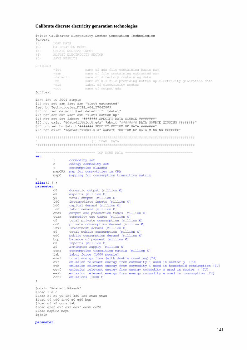
141

Calibrate discrete electricity generation technologies $title Calibrates Electricity Sector Generation Tec hnologies $ontext (1) LOAD DATA (2) CALIBRATION MODEL (3) CREATE NUCLEAR INPUT (4) ADJUST ELECTRICITY SECTOR (5) SAVE RESULTS OPTIONS: -iot name of gdx file containin g basic sam -sam name of file containing ex tracted sam -datadir name of directory containi ng data -bu name of xls file providing bottom up electricity generation data -ele label of electricity secto r -out name of output gdx $offtext $set iot IO_2004_simple $if not set sam $set sam "%iot%_extracted" $set bu Technologies_DISS_v04_27042009 $if not set datadir $set datadir "..\data\" $if not set out $set out "%iot%_Bottom_up" $if not set iot $abort "####### SPECIFY DATA SOURCE ########" $if not exist "%datadir%%iot%.gdx" $abort "######## DATA SOURCE MISSING ########" $if not set bu $abort"####### SPECIFY BOTTOM UP DAT A #######" $if not exist "%datadir%%bu%.xls" $abort "BOTTOM UP DATA MISSING #######" *################################################## ############################# * (1) LOAD DATA *################################################## ############################# *----------------------------- TOP DOWN DATA ------ ---------------------------- set i commodity set e energy commodity set c consumption classes mapCPA map for commodities in CPA mapC mapping for consumption transition matrix ; alias(i,j); parameter d0 domestic output [million €] e0 exports [million €] y0 total output [million €] id0 intermediate inputs [million €] kd0 capital demand [million €] ld0 labor demand [million €] otax output and production taxes [million €] utax commodity use taxes [million €] c0 total private consumption [million €] cd0 private consumption demand [million €] inv0 investment demand [million €] g0 total public consumption [million €] gd0 public consumption demand [million €] bop balance of payment [million €] m0 imports [million €] a0 armington supply [million €] cons consumption transition matrix [million €] lab labor force [1000 people] ene0 total energy flow (with double counting)[TJ] evf emission relevant energy from commodity i used in s ector j [TJ] evh emission relevant energy from commodity i used in h ousehold consumption [TJ] eevf emission relevant energy from energy commodity e us ed in sector j [TJ] eevh emission relevant energy from energy commodity e us ed in consumption [TJ] co20 emissions [1000 t] ; $gdxin "%datadir%%sam%" $load i e c $load d0 e0 y0 id0 kd0 ld0 otax utax $load c0 cd0 inv0 g0 gd0 bop $load m0 a0 cons lab $load ene0 evf evh eevf eevh co20 $load mapCPA mapC $gdxin parameter

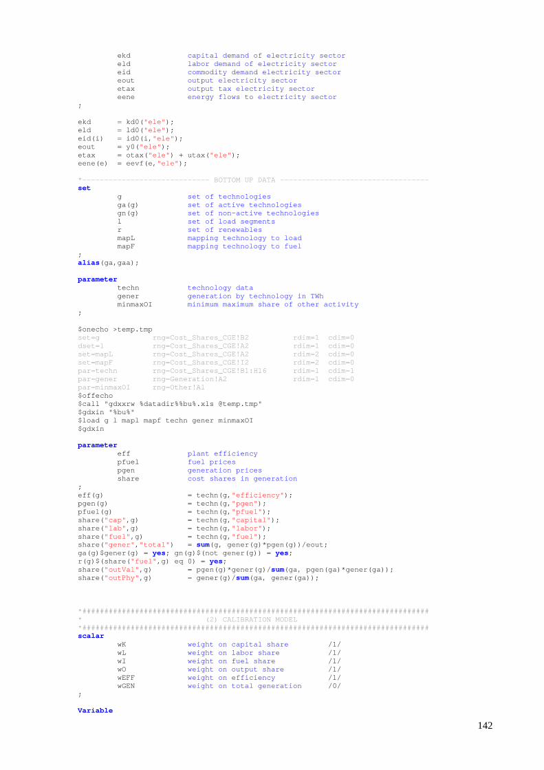
142

ekd capital demand of electricity sector eld labor demand of electricity sector eid commodity demand electricity sector eout output electricity sector etax output tax electricity sector eene energy flows to electricity sector ; ekd = kd0( "ele" ); eld = ld0( "ele" ); eid(i) = id0(i, "ele" ); eout = y0( "ele" ); etax = otax( "ele" ) + utax( "ele" ); eene(e) = eevf(e, "ele" ); *----------------------------- BOTTOM UP DATA ----- ----------------------------- set g set of technologies ga(g) set of active technologies gn(g) set of non-active technologies l set of load segments r set of renewables mapL mapping technology to load mapF mapping technology to fuel ; alias(ga,gaa); parameter techn technology data gener generation by technology in TWh minmaxOI minimum maximum share of other activity ; $onecho >temp.tmp set=g rng=Cost_Shares_CGE!B2 rd im=1 cdim=0 dset=l rng=Cost_Shares_CGE!A2 rd im=1 cdim=0 set=mapL rng=Cost_Shares_CGE!A2 rd im=2 cdim=0 set=mapF rng=Cost_Shares_CGE!I2 rd im=2 cdim=0 par=techn rng=Cost_Shares_CGE!B1:H16 rd im=1 cdim=1 par=gener rng=Generation!A2 rd im=1 cdim=0 par=minmaxOI rng=Other!A1 $offecho $call "gdxxrw %datadir%%bu%.xls @temp.tmp" $gdxin "%bu%" $load g l mapl mapf techn gener minmaxOI $gdxin parameter eff plant efficiency pfuel fuel prices pgen generation prices share cost shares in generation ; eff(g) = techn(g, "efficiency" ); pgen(g) = techn(g, "pgen" ); pfuel(g) = techn(g, "pfuel" ); share( "cap" ,g) = techn(g, "capital" ); share( "lab" ,g) = techn(g, "labor" ); share( "fuel" ,g) = techn(g, "fuel" ); share( "gener" , "total" ) = sum(g, gener(g)*pgen(g))/eout; ga(g)$gener(g) = yes; gn(g)$(not gener(g)) = yes; r(g)$(share( "fuel" ,g) eq 0) = yes; share( "outVal" ,g) = pgen(g)*gener(g)/ sum(ga, pgen(ga)*gener(ga)); share( "outPhy" ,g) = gener(g)/ sum(ga, gener(ga)); *################################################## ############################# * (2) CALIBRATION MODEL *################################################## ############################# scalar wK weight on capital share /1/ wL weight on labor share /1/ wI weight on fuel share /1/ wO weight on output share /1/ wEFF weight on efficiency /1/ wGEN weight on total generation /0/ ; Variable

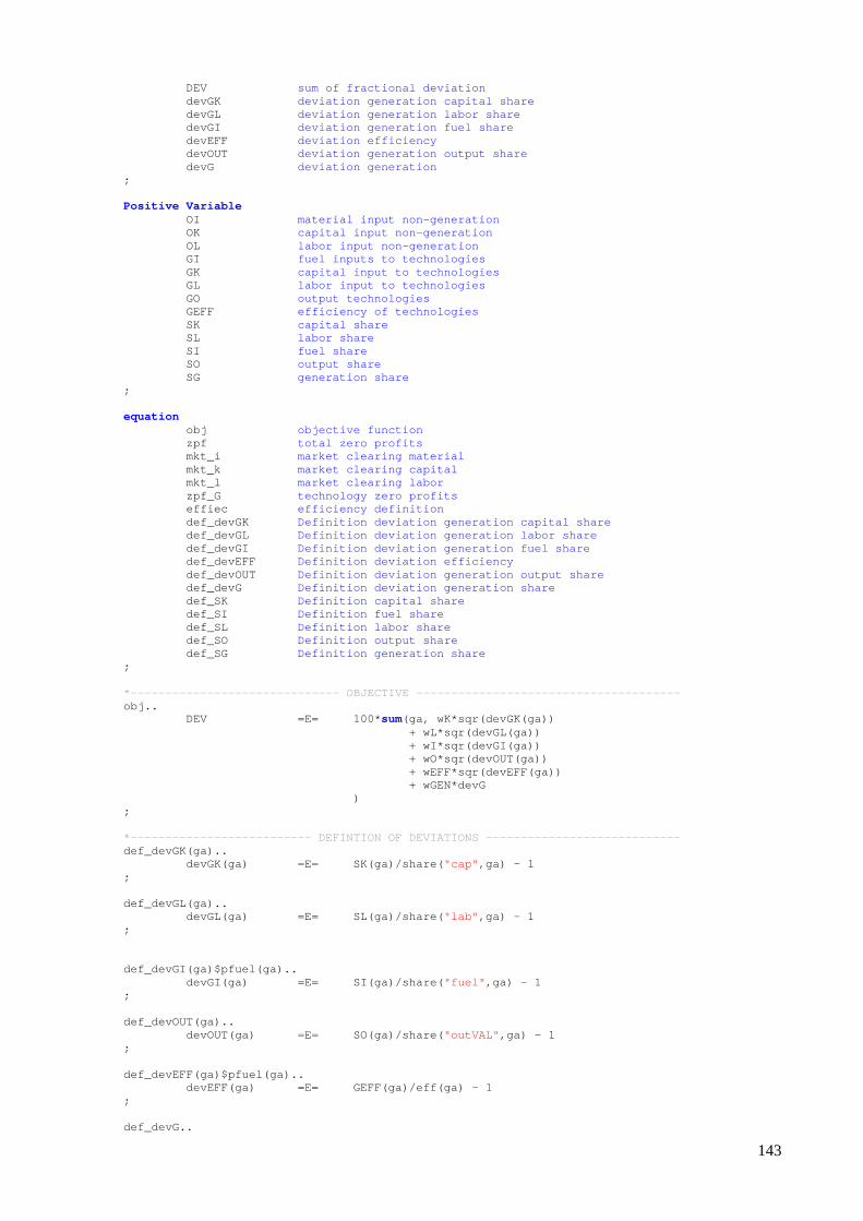
143

DEV sum of fractional deviation devGK deviation generation capital share devGL deviation generation labor share devGI deviation generation fuel share devEFF deviation efficiency devOUT deviation generation output share devG deviation generation ; Positive Variable OI material input non-generation OK capital input non-generation OL labor input non-generation GI fuel inputs to technologies GK capital input to technologies GL labor input to technologies GO output technologies GEFF efficiency of technologies SK capital share SL labor share SI fuel share SO output share SG generation share ; equation obj objective function zpf total zero profits mkt_i market clearing material mkt_k market clearing capital mkt_l market clearing labor zpf_G technology zero profits effiec efficiency definition def_devGK Definition deviation generation capital share def_devGL Definition deviation generation labor share def_devGI Definition deviation generation fuel share def_devEFF Definition deviation efficiency def_devOUT Definition deviation generation output share def_devG Definition deviation generation share def_SK Definition capital share def_SI Definition fuel share def_SL Definition labor share def_SO Definition output share def_SG Definition generation share ; *------------------------------ OBJECTIVE --------- ----------------------------- obj.. DEV =E= 100* sum(ga, wK*sqr(devGK(ga)) + wL*sqr(d evGL(ga)) + wI*sqr(d evGI(ga)) + wO*sqr(d evOUT(ga)) + wEFF*sqr (devEFF(ga)) + wGEN*dev G ) ; *-------------------------- DEFINTION OF DEVIATIONS ---------------------------- def_devGK(ga).. devGK(ga) =E= SK(ga)/share( "cap" ,ga) - 1 ; def_devGL(ga).. devGL(ga) =E= SL(ga)/share( "lab" ,ga) - 1 ; def_devGI(ga)$pfuel(ga).. devGI(ga) =E= SI(ga)/share( "fuel" ,ga) - 1 ; def_devOUT(ga).. devOUT(ga) =E= SO(ga)/share( "outVAL" ,ga) - 1 ; def_devEFF(ga)$pfuel(ga).. devEFF(ga) =E= GEFF(ga)/eff(ga) - 1 ; def_devG..

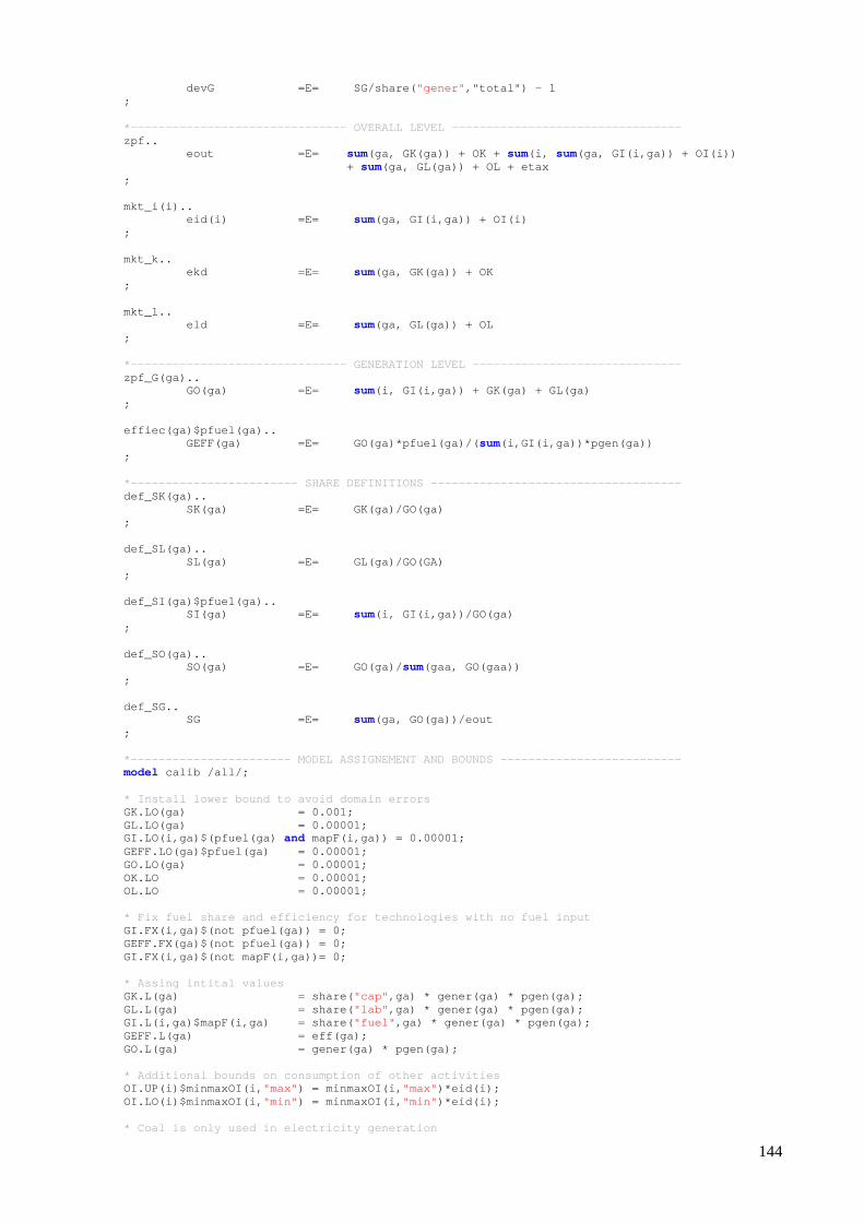
144

devG =E= SG/share( "gener" ,"total") - 1 ; *------------------------------- OVERALL LEVEL ---- ----------------------------- zpf.. eout =E= sum(ga, GK(ga)) + OK + sum(i, sum(ga, GI(i,ga)) + OI(i)) + sum(ga, GL(ga)) + OL + etax ; mkt_i(i).. eid(i) =E= sum(ga, GI(i,ga)) + OI(i) ; mkt_k.. ekd =E= sum(ga, GK(ga)) + OK ; mkt_l.. eld =E= sum(ga, GL(ga)) + OL ; *------------------------------- GENERATION LEVEL - ----------------------------- zpf_G(ga).. GO(ga) =E= sum(i, GI(i,ga)) + GK(ga) + GL(ga) ; effiec(ga)$pfuel(ga).. GEFF(ga) =E= GO(ga)*pfuel(ga)/( sum(i,GI(i,ga))*pgen(ga)) ; *------------------------ SHARE DEFINITIONS ------- ----------------------------- def_SK(ga).. SK(ga) =E= GK(ga)/GO(ga) ; def_SL(ga).. SL(ga) =E= GL(ga)/GO(GA) ; def_SI(ga)$pfuel(ga).. SI(ga) =E= sum(i, GI(i,ga))/GO(ga) ; def_SO(ga).. SO(ga) =E= GO(ga)/ sum(gaa, GO(gaa)) ; def_SG.. SG =E= sum(ga, GO(ga))/eout ; *----------------------- MODEL ASSIGNEMENT AND BOUN DS -------------------------- model calib /all/; * Install lower bound to avoid domain errors GK.LO(ga) = 0.001; GL.LO(ga) = 0.00001; GI.LO(i,ga)$(pfuel(ga) and mapF(i,ga)) = 0.00001; GEFF.LO(ga)$pfuel(ga) = 0.00001; GO.LO(ga) = 0.00001; OK.LO = 0.00001; OL.LO = 0.00001; * Fix fuel share and efficiency for technologies wi th no fuel input GI.FX(i,ga)$(not pfuel(ga)) = 0; GEFF.FX(ga)$(not pfuel(ga)) = 0; GI.FX(i,ga)$(not mapF(i,ga))= 0; * Assing intital values GK.L(ga) = share( "cap" ,ga) * gener(ga) * pgen(ga); GL.L(ga) = share( "lab" ,ga) * gener(ga) * pgen(ga); GI.L(i,ga)$mapF(i,ga) = share( "fuel" ,ga) * gener(ga) * pgen(ga); GEFF.L(ga) = eff(ga); GO.L(ga) = gener(ga) * pgen(ga); * Additional bounds on consumption of other activit ies OI.UP(i)$minmaxOI(i, "max" ) = minmaxOI(i, "max" )*eid(i); OI.LO(i)$minmaxOI(i, "min" ) = minmaxOI(i, "min" )*eid(i); * Coal is only used in electricity generation

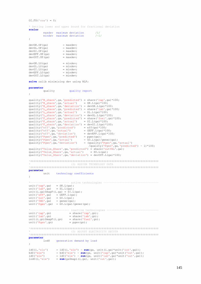
145

OI.FX( "coa" ) = 0; * Setting lower and upper bound for fractional devi ation scalar maxdev maximum deviation /1/ mindev maximum deviation /-1/ ; devGK.UP(ga) = maxdev; devGL.UP(ga) = maxdev; devGI.UP(ga) = maxdev; devEFF.UP(ga) = maxdev; devOUT.UP(ga) = maxdev; devGK.LO(ga) = mindev; devGL.LO(ga) = mindev; devGI.LO(ga) = mindev; devEFF.LO(ga) = mindev; devOUT.LO(ga) = mindev; solve calib minimizing dev using NLP; parameter quality quality report ; quality( "K_share" ,ga, "predicted" ) = share( "cap" ,ga)*100; quality( "K_share" ,ga, "actual" ) = SK.L(ga)*100; quality( "K_share" ,ga, "deviation" ) = devGK.L(ga)*100; quality( "L_share" ,ga, "predicted" ) = share( "lab" ,ga)*100; quality( "L_share" ,ga, "actual" ) = SL.L(ga)*100; quality( "L_share" ,ga, "deviation" ) = devGL.L(ga)*100; quality( "F_share" ,ga, "predicted" ) = share( "fuel" ,ga)*100; quality( "F_share" ,ga, "actual" ) = SI.L(ga)*100; quality( "F_share" ,ga, "deviation" ) = devGI.L(ga)*100; quality( "eff" ,ga, "predicted" ) = eff(ga)*100; quality( "eff" ,ga, "actual" ) = GEFF.L(ga)*100; quality( "eff" ,ga, "deviation" ) = devEFF.L(ga)*100; quality( "Pgen" ,ga, "predicted" ) = pgen(ga); quality( "Pgen" ,ga, "actual" ) = GO.L(ga)/gener(ga); quality( "Pgen" ,ga, "deviation" ) = (quality( "Pgen" ,ga, "actual" )

/quality( "Pgen" ,ga, "predicted" ) - 1)*100; quality( "Value_Share" ,ga, "predicted" ) = share( "outVAL" ,ga); quality( "Value_Share" ,ga, "actual" ) = SO.L(ga); quality( "Value_Share" ,ga, "deviation" ) = devOUT.L(ga)*100; *################################################## ############################# * (3) ASSIGN TECHNOLOGY DAT A *################################################## ############################# parameter unit technology coefficients ; *------------------------ active technologies ----- ----------------------------- unit( "cap" ,ga) = SK.L(ga); unit( "lab" ,ga) = SL.L(ga); unit(i,ga)$mapF(i,ga) = SI.L(ga); unit( "eff" ,ga) = GEFF.L(ga); unit( "out" ,ga) = GO.L(ga); unit( "TWh" ,ga) = gener(ga); unit( "Pgen" ,ga) = GO.L(ga)/gener(ga); *------------------------ inactive technologies --- ----------------------------- unit( "cap" ,gn) = share( "cap" ,gn); unit( "lab" ,gn) = share( "lab" ,gn); unit(i,gn)$mapF(i,gn) = share( "fuel" ,gn); unit( "Pgen" ,gn) = pgen(gn); *################################################## ############################# * (3) ADJUST ELECTRICITY SE COTR *################################################## ############################# parameter lod0 generation demand by load ; id0(i, "ele" ) = id0(i, "ele" ) - sum(ga, unit(i,ga)*unit( "out" ,ga)); kd0( "ele" ) = kd0( "ele" ) - sum(ga, unit( "cap" ,ga)*unit( "out" ,ga)); ld0( "ele" ) = ld0( "ele" ) - sum(ga, unit( "lab" ,ga)*unit( "out" ,ga)); lod0(l, "ele" ) = sum(ga$mapl(l,ga), unit( "out" ,ga));

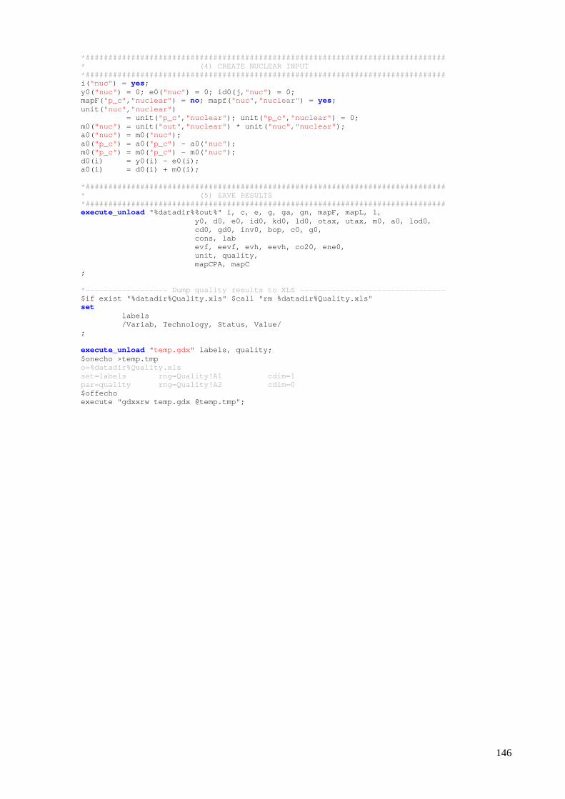
146

*################################################## ############################# * (4) CREATE NUCLEAR INPUT *################################################## ############################# i( "nuc" ) = yes; y0( "nuc" ) = 0; e0( "nuc" ) = 0; id0(j, "nuc" ) = 0; mapF("p_c" , "nuclear" ) = no; mapf( "nuc" , "nuclear" ) = yes; unit( "nuc" , "nuclear" ) = unit( "p_c" , "nuclear" ); unit( "p_c" , "nuclear" ) = 0; m0("nuc" ) = unit( "out" , "nuclear" ) * unit( "nuc" , "nuclear" ); a0( "nuc" ) = m0( "nuc" ); a0( "p_c" ) = a0( "p_c" ) - a0( "nuc" ); m0("p_c" ) = m0( "p_c" ) - m0( "nuc" ); d0(i) = y0(i) - e0(i); a0(i) = d0(i) + m0(i); *################################################## ############################# * (5) SAVE RESULTS *################################################## ############################# execute_unload "%datadir%%out%" i, c, e, g, ga, gn, mapF, mapL, l , y0, d0, e0, id0, kd0, ld0, otax, utax, m0, a0, lod0, cd0, gd0, inv0, bop, c0, g 0, cons, lab evf, eevf, evh, eevh, co20 , ene0, unit, quality, mapCPA, mapC ; *------------------ Dump quality results to XLS --- ----------------------------- $if exist "%datadir%Quality.xls" $call "rm %datadir %Quality.xls" set labels /Variab, Technology, Status, Value/ ; execute_unload " temp.gdx " labels, quality; $onecho >temp.tmp o=%datadir%Quality.xls set=labels rng=Quality!A1 cdim=1 par=quality rng=Quality!A2 cdim=0 $offecho execute "gdxxrw temp.gdx @temp.tmp";

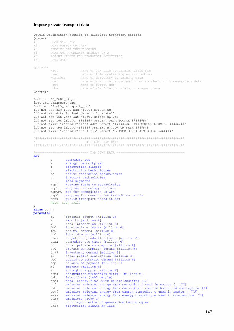
147

Impose private transport data $title Calibration routine to calibrate transport s ectors $ontext (1) LOAD SAM DATA (2) LOAD BOTTOM UP DATA (3) SPECIFY CAR TECHNOLOGIES (4) LOAD AND AGGREGATE TREMOVE DATA (5) ASSING VALUES FOR TRANSPORT ACTIVITIES (6) SAVE DATA options: -iot name of gdx file containin g basic sam -sam nema of file containing ex ttracted sam -datadir name of directory containi ng data -car name of xls file providing bottom up electricity generation data -out name of output gdx -tbu name of xls file containin g transport data $offtext $set iot IO_2004_simple $set tbu transport_one $set out "%iot%_transport_one" $if not set sam $set sam "%iot%_Bottom_up" $if not set datadir $set datadir "..\data\" $if not set out $set out "%iot%_Bottom_up_Car" $if not set iot $abort "####### SPECIFY DATA SOURCE ########" $if not exist "%datadir%%iot%.gdx" $abort "######## DATA SOURCE MISSING ########" $if not set tbu $abort"####### SPECIFY BOTTOM UP DA TA #######" $if not exist "%datadir%%tbu%.xls" $abort "BOTTOM U P DATA MISSING #######" *################################################## ############################# * (1) LOAD SAM DATA *################################################## ############################# *---------------------------- TOP DOWN DATA ------- ----------------------------- set i commodity set e energy commodity set c consumption classes g electricity technologies ga active generation technologies gn inactive technologies l load segments mapF mapping fuels to technologies mapL mapping technology to load mapCPA map for commodities in CPA mapC mapping for consumption transition matrix ptrn public transport modes in sam /otp, atp, rail/ ; alias(i,j); parameter d0 domestic output [million €] e0 exports [million €] y0 total production [million €] id0 intermediate inputs [million €] kd0 capital demand [million €] ld0 labor demand [million €] otax output and production taxes [million €] utax commodity use taxes [million €] c0 total private consumption [million €] cd0 private consumption demand [million €] inv0 investment demand [million €] g0 total public consumption [million €] gd0 public consumption demand [million €] bop balance of payment [million €] m0 imports [million €] a0 armington supply [million €] cons consumption transition matrix [million €] lab labor force [1000 people] ene0 total energy flow (with double counting)[TJ] evf emission relevant energy from commodity i used in s ector j [TJ] evh emission relevant energy from commodity i used in h ousehold consumption [TJ] eevf emission relevant energy from energy commodity e us ed in sector j [TJ] eevh emission relevant energy from energy commodity e us ed in consumption [TJ] co20 emissions [1000 t] unit unit input vector of generation technologies lod0 electricity demand by load

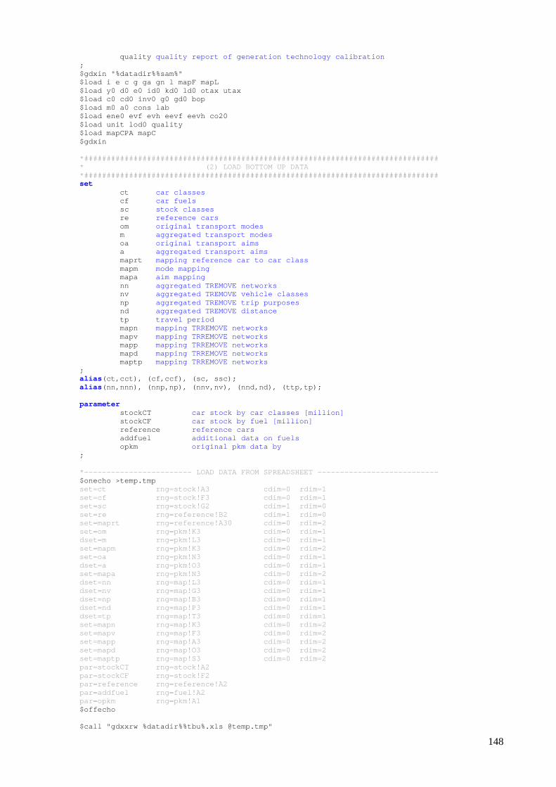
148

quality quality report of generation technology calibration ; $gdxin "%datadir%%sam%" $load i e c g ga gn l mapF mapL $load y0 d0 e0 id0 kd0 ld0 otax utax $load c0 cd0 inv0 g0 gd0 bop $load m0 a0 cons lab $load ene0 evf evh eevf eevh co20 $load unit lod0 quality $load mapCPA mapC $gdxin *################################################## ############################# * (2) LOAD BOTTOM UP DATA *################################################## ############################# set ct car classes cf car fuels sc stock classes re reference cars om original transport modes m aggregated transport modes oa original transport aims a aggregated transport aims maprt mapping reference car to car class mapm mode mapping mapa aim mapping nn aggregated TREMOVE networks nv aggregated TREMOVE vehicle classes np aggregated TREMOVE trip purposes nd aggregated TREMOVE distance tp travel period mapn mapping TRREMOVE networks mapv mapping TRREMOVE networks mapp mapping TRREMOVE networks mapd mapping TRREMOVE networks maptp mapping TRREMOVE networks ; alias(ct,cct), (cf,ccf), (sc, ssc); alias(nn,nnn), (nnp,np), (nnv,nv), (nnd,nd), (ttp,tp); parameter stockCT car stock by car classes [million] stockCF car stock by fuel [million] reference reference cars addfuel additional data on fuels opkm original pkm data by ; *------------------------ LOAD DATA FROM SPREADSHEE T --------------------------- $onecho >temp.tmp set=ct rng=stock!A3 cdim=0 rd im=1 set=cf rng=stock!F3 cdim=0 rd im=1 set=sc rng=stock!G2 cdim=1 rd im=0 set=re rng=reference!B2 cdim=1 rd im=0 set=maprt rng=reference!A30 cdim=0 rd im=2 set=om rng=pkm!K3 cdim=0 rd im=1 dset=m rng=pkm!L3 cdim=0 rd im=1 set=mapm rng=pkm!K3 cdim=0 rd im=2 set=oa rng=pkm!N3 cdim=0 rd im=1 dset=a rng=pkm!O3 cdim=0 rd im=1 set=mapa rng=pkm!N3 cdim=0 rd im=2 dset=nn rng=map!L3 cdim=0 rd im=1 dset=nv rng=map!G3 cdim=0 rd im=1 dset=np rng=map!B3 cdim=0 rd im=1 dset=nd rng=map!P3 cdim=0 rd im=1 dset=tp rng=map!T3 cdim=0 rd im=1 set=mapn rng=map!K3 cdim=0 rd im=2 set=mapv rng=map!F3 cdim=0 rd im=2 set=mapp rng=map!A3 cdim=0 rd im=2 set=mapd rng=map!O3 cdim=0 rd im=2 set=maptp rng=map!S3 cdim=0 rd im=2 par=stockCT rng=stock!A2 par=stockCF rng=stock!F2 par=reference rng=reference!A2 par=addfuel rng=fuel!A2 par=opkm rng=pkm!A1 $offecho $call "gdxxrw %datadir%%tbu%.xls @temp.tmp"

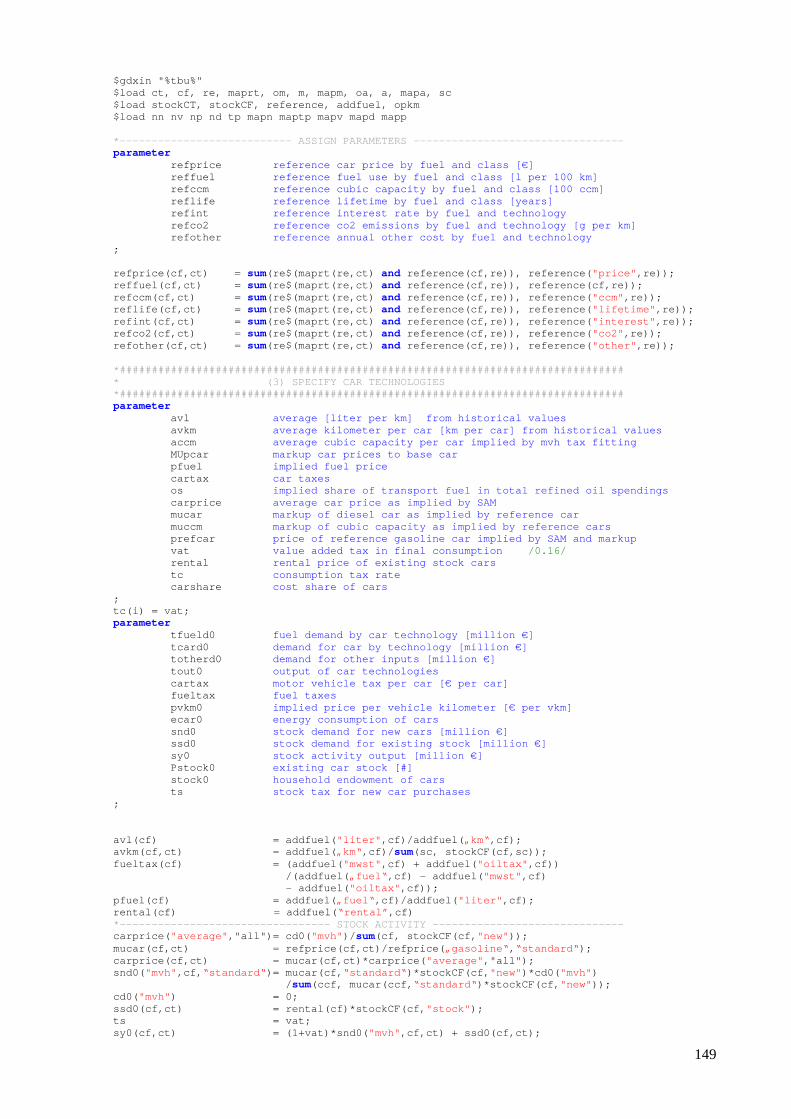
149

$gdxin "%tbu%" $load ct, cf, re, maprt, om, m, mapm, oa, a, mapa, sc $load stockCT, stockCF, reference, addfuel, opkm $load nn nv np nd tp mapn maptp mapv mapd mapp *--------------------------- ASSIGN PARAMETERS ---- ----------------------------- parameter refprice reference car price by fuel and class [€] reffuel reference fuel use by fuel and class [l per 100 km] refccm reference cubic capacity by fuel and class [100 ccm ] reflife reference lifetime by fuel and class [years] refint reference interest rate by fuel and technology refco2 reference co2 emissions by fuel and technology [g p er km] refother reference annual other cost by fuel and technology ; refprice(cf,ct) = sum(re$(maprt(re,ct) and reference(cf,re)), reference( "price" ,re)); reffuel(cf,ct) = sum(re$(maprt(re,ct) and reference(cf,re)), reference(cf,re)); refccm(cf,ct) = sum(re$(maprt(re,ct) and reference(cf,re)), reference( "ccm" ,re)); reflife(cf,ct) = sum(re$(maprt(re,ct) and reference(cf,re)), reference( "lifetime" ,re)); refint(cf,ct) = sum(re$(maprt(re,ct) and reference(cf,re)), reference( "interest" ,re)); refco2(cf,ct) = sum(re$(maprt(re,ct) and reference(cf,re)), reference( "co2" ,re)); refother(cf,ct) = sum(re$(maprt(re,ct) and reference(cf,re)), reference( "other" ,re)); *################################################## ############################# * (3) SPECIFY CAR TECHNOLOGIE S *################################################## ############################# parameter avl average [liter per km] from historical values avkm average kilometer per car [km per car] from histori cal values accm average cubic capacity per car implied by mvh tax f itting MUpcar markup car prices to base car pfuel implied fuel price cartax car taxes os implied share of transport fuel in total refined oi l spendings carprice average car price as implied by SAM mucar markup of diesel car as implied by reference car muccm markup of cubic capacity as implied by reference ca rs prefcar price of reference gasoline car implied by SAM and markup vat value added tax in final consumption /0.16/ rental rental price of existing stock cars tc consumption tax rate carshare cost share of cars ; tc(i) = vat; parameter tfueld0 fuel demand by car technology [million €] tcard0 demand for car by technology [million €] totherd0 demand for other inputs [million €] tout0 output of car technologies cartax motor vehicle tax per car [€ per car] fueltax fuel taxes pvkm0 implied price per vehicle kilometer [€ per vkm] ecar0 energy consumption of cars snd0 stock demand for new cars [million €] ssd0 stock demand for existing stock [million €] sy0 stock activity output [million €] Pstock0 existing car stock [#] stock0 household endowment of cars ts stock tax for new car purchases ; avl(cf) = addfuel( "liter" ,cf)/addfuel( „km“ ,cf); avkm(cf,ct) = addfuel( „km“ ,cf)/ sum(sc, stockCF(cf,sc)); fueltax(cf) = (addfuel( "mwst" ,cf) + addfuel( "oiltax" ,cf)) /(addfuel( „fuel“ ,cf) - addfuel( "mwst" ,cf) - addfuel( "oiltax" ,cf)); pfuel(cf) = addfuel( „fuel“ ,cf)/addfuel( "liter" ,cf); rental(cf) = addfuel( “rental” ,cf) *--------------------------------- STOCK ACTIVITY - ----------------------------- carprice( "average" ,"all")= cd0( "mvh" )/ sum(cf, stockCF(cf, "new" )); mucar(cf,ct) = refprice(cf,ct)/refprice ( „gasoline“ , “standard“ ); carprice(cf,ct) = mucar(cf,ct)*carprice( "average" ,"all"); snd0( "mvh" ,cf, “standard“ )= mucar(cf, “standard“ )*stockCF(cf, "new" )*cd0( "mvh" ) / sum(ccf, mucar(ccf, “standard“ )*stockCF(cf, "new" )); cd0( "mvh" ) = 0; ssd0(cf,ct) = rental(cf)*stockCF(cf, "stock" ); ts = vat; sy0(cf,ct) = (1+vat)*snd0( "mvh" ,cf,ct) + ssd0(cf,ct);

150

tcard0(cf,ct) = sy0(cf,ct); Pstock0(" stock" ,cf,ct) = stockCF(cf, "stock" ); Pstock0( "new" ,cf,ct) = stockCF(cf, "new" ); Pstock0( „total“ ,cf,ct) = stockCF(cf, "stock" ) + stockCF(cf, "new" ); stock0(cf,ct) = ssd0(cf,ct); tfueld0( „p_c“ ,cf,ct) = addfuel( „fuel“ ,cf) - addfuel(" mwst",cf) - addfuel(" oiltax ",cf); cd0( „p_c“ ) = cd0( „p_c“ ) - sum((cf,ct), tfueld0( „p_c“ ,cf,ct)); os = sum((cf,ct), (1+fueltax(cf))*tfueld0( „p_c“ ,cf,ct)) /( sum((cf,ct), (1+fueltax(cf))*tfueld0( „p_c“ ,cf,ct)) + 1.418*cd0( „p_c“ )); muccm(cf,ct) = refccm(cf,ct)/refccm( „gasoline“ , “standard“ ); accm(cf,ct) = refccm( „gasoline“ , “standard“ )*muccm(cf,ct); cartax(cf,ct) = Pstock0( „total“ ,cf,ct)*muccm(cf,ct) *(refccm( „gasoline“ , “standard“ )/100) *addfuel( „cartax“ ,cf); accm(cf,ct) = 100*(cartax(cf,ct)/Pstoc k0( „total“ ,cf,ct))/addfuel( „cartax“ ,cf); cartax(cf,ct) = cartax(cf,ct)*(addfuel( „cartaxtotal“ , “gasoline“ )

/ sum((ccf,cct), cartax(ccf,cct))); accm(cf,ct) = (cartax(cf,ct)/Pstock0( „total“ ,cf,ct))/addfuel( „cartax“ ,cf)*100; cartax(cf,ct) = cartax(cf,ct)/Pstock0( „total“ ,cf,ct); totherd0(i,cf,ct)$(cons(i, “total“ ) and not sameas(i, “p_c“ )) = cons(i,"wkfz")/cons(i, “total“ )*cd0(i) *Pstock0( „total“ ,cf,ct) / sum( (ccf,cct), Pstock0( „total“ ,ccf,cct)); cd0(i)$( not sameas(i, “p_c“ )) = cd0(i) - sum((cf,ct), totherd0(i,cf,ct)); *------------------------------ COMPUTE TOTAL OUTPU T --------------------------- tout0(cf,ct) = sum(i, totherd0(i,cf,ct)*(1+vat) + tfueld0(i,cf,ct)*(1+fu eltax(cf))) + tcard0(cf,ct) + Pstock 0( „total“ ,cf,ct)*cartax(cf,ct); pvkm0(cf,ct) = tout0(cf,ct)/addfuel( „km“ ,cf); carshare("car",cf,ct) = (tcard0(cf,ct) + Pstock0 ( „total“ ,cf,ct)*cartax(cf,ct)) /tout0(cf,ct); carshare("other",cf,ct) = sum(i, totherd0(i,cf,ct)*(1+vat))/tout0(cf,ct); carshare( „fuel“ ,cf,ct) = sum(i,tfueld0(i,cf,ct)*(1+fueltax(cf)))/tout0(cf,ct); *--------------------------- ASSIGN ENERGY VALUES - ----------------------------- ecar0( „p_c“ , “gasoline“ ,ct) = eevh( „gasoline“ ); ecar0( „p_c“ , “diesel“ ,ct) = eevh( „diesel“ ); evh(i) = evh(i) - sum((cf,ct), ecar0(i,cf,ct)); *################################################## ############################# * (4) LOAD AND AGGREGATE TREMOV E DATA *################################################## ############################# $include"%datadir%tremove.inc" parameter pkm person and tonne km [milli on] vkm vehicle kilometer [million ] vot value of time [€ per hour ] pce passenger car equivalents [million] speed speed on networks [km per hour] duration length of travel period [h ours] ; pkm(np,nd,tp,nv,nn) = sum((p,d,tper,v,n)$(mapn(n,nn) and mapd(d,nd) and mapv(v,nv) and mapp(p,np) and maptp(tper,tp)), Tpkm(p,d,tper,v,n)); vkm(np,nd,tp,nv,nn) = sum((p,d,tper,v,n)$(mapn(n,nn) and mapd(d,nd) and mapv(v,nv) and mapp(p,np) and maptp(tper,tp)), Tvkm(p,d,tper,v,n)); pce(np,nd,tp,nv,nn) = sum((p,d,tper,v,n)$(mapn(n,nn) and mapd(d,nd) and mapv(v,nv)

and mapp(p,np) and maptp(tper,tp)), Tvkm(p,d,tper,v,n)*Tpcu(v)); alias(v,vv), (p,pp), (d,dd); speed(nv,tp,nn)$ sum((np,nd),vkm(np,nd,tp,nv,nn)) = sum((v,tper,n)$(mapv(v,nv) and maptp(tper,tp) and mapn(n,nn)), Tspeed(v,tper,n)* sum((pp,dd), Tvkm(pp,dd,tper,v,n))) / sum((np,nd),vkm(np,nd,tp,nv,nn)); speed(nv,tp,nn)$( not sum((np,nd),vkm(np,nd,tp,nv,nn))) = sum((v,tper,n)$(mapv(v,nv) and maptp(tper,tp) and mapn(n,nn)), Tspeed(v,tper,n)); vot(np,nd,tp,nv,nn)$pkm(np,nd,tp,nv,nn) = sum((p,d,tper,v,n)$(mapn(n,nn) and mapd(d,nd) and mapv(v,nv) and mapp(p,np) and maptp(tper,tp)), Tvot(p,d,tper,v,n) *Tpkm(p,d,tper,v,n)) /pkm(np,nd,tp,nv,n n); duration(tp) = sum(maptp(tper,tp), Tduration(tper));

151

*################################################## ############################# * (5) ASSING VALUES FOR TRANSPORT ACT IVITIES *################################################## ############################# *-------------------------------- PHYSICAL VALUES - ----------------------------- parameter tact0 transport activity physical data ; tact0( „pkm“ ,np,nd,tp,nv,nn) = pkm(np,nd,tp,nv,nn); tact0( „vkm“ ,np,nd,tp,nv,nn) = vkm(np,nd,tp,nv,nn); tact0("pce",np,nd,tp,nv,nn) = pce(np,nd,tp,nv ,nn); tact0("speed",np,nd,tp,nv,nn) = speed(nv,tp,nn) ; tact0("vot",np,nd,tp,nv,nn) = vot(np,nd,tp,nv ,nn); tact0("pcu",np,nd,tp,nv,nn) = sum(mapv(v,nv), Tpcu(v)); *-------------------------- MONETARY VALUES: CARS - ----------------------------- set allm(*,*,*,*,*) set of all modes distances ... aallm(*,*,*,*,*) set of all modes distances ... ; allm(np,nd,tp,nv,nn) = yes; aallm(np,nd,tp,nv,nn) = yes; parameter vkm0 scaled vehicle kilometers of cars share_pkm share of pkm by trip class in total pkm of cars tactin0 input vectors to transport activities gross tactcarin0 input vectors to transport activities tay0 output of transport activities occup occupancy rate ; vkm0(cf,ct) = addfuel( „km“ ,cf)

* sum((nnp,nnd,ttp,nnn), tact0( „vkm“ ,nnp,nnd,ttp, "car" ,nnn)) / sum(ccf, addfuel( „km“ ,ccf));

pvkm0(cf,ct) = tout0(cf,ct)/vkm0(cf,ct); occup(allm)$tact0( „vkm“ ,allm) = tact0( „pkm“ ,allm)/tact0( „vkm“ ,allm); tactcarin0(cf,ct,np,nd,tp, "car" ,nn)

= pvkm0(cf,ct)*tact0( „vkm“ ,np,nd,tp, "car" ,nn) *vkm0(cf,ct)/ sum((ccf,cct),vkm0(ccf,cct)); parameter share_vkm share of cars' vkm in total cars' vkm ; *----------------------------- RAIL TRANSPORT ----- ----------------------------- tactin0( "rail" ,np,nd,tp, "PTRAIN" ,nn) = cd0( "rail" )* tact0( „pkm“ ,np,nd,tp, "PTRAIN" ,nn)/ sum((nnp,nnd,ttp,nnn), tact0( „pkm“ ,nnp,nnd,ttp, "PTRAIN" ,nnn)); cd0( "rail" ) = 0; *----------------------------- BUS/METRO TRANSPORT ----------------------------- set public sub set of modes which belong to public urban transport /METRAM, BUS/ ; alias(public,ppublic); tactin0( "otp" ,np,nd,tp,public,nn) = cd0( "otp" )*tact0( „pkm“ ,np,nd,tp,public,nn)/ sum((nnp,nnd,ttp,ppublic,nnn), tact0( „pkm“ ,nnp,nnd,ttp,ppublic,nnn)); cd0( "otp" ) = 0; *----------------------------- AIR TRANSPORT ------ ---------------------------- - tactin0( "atp" ,np,nd,tp,"PLANE",nn) = cd0( "atp" )*tact0( „pkm“ ,np,nd,tp, "PLANE" ,nn)/ sum((nnp,nnd,ttp,nnn), tact0( „pkm“ ,nnp,nnd,ttp, "PLANE" ,nnn)); cd0( "atp" ) = 0; *----------------------------- CREATE MONETARY INPU TS -------------------------- tay0(np,nd,tp,nv,nn) = sum(i, tactin0(i,np,nd,tp,nv,nn)) + sum((cf,ct), tactcarin0(cf,ct,np,nd,tp,nv,nn)); *################################################## ############################# * (6) SAVE DATA *################################################## ############################# execute_unload " %datadir%%out% " i, c, e, g, ga, gn, mapF, mapL, l, y0, d0, e0, id0, kd0, ld0, otax, utax, m0, a0, lod0, cd0, gd0, inv0, bop, c0, g 0, cons, lab evf, eevf, evh, eevh, co20 , ene0, ecar0 unit, quality, mapCPA, mapC, tactin0=taid0, tactcarin0= tacard0, tact0, tay0, tout0=cy0, totherd0=cid0, tcard0=ccd0, tfueld0=cfd0 stock0, snd0, ssd0, sy0=sy 0, Pstock0,

152

nn=n, nv=m, np=p, nd=d, tp lavmohr, cf, ct fueltax=tfuel cartax tc=to ther refco2 tnew ts pvkm0 vkm0;

153

Impose tax system $title Program to impose tax system on the transpor t dataset $set data IO_2004_simple_transport_one $if not set datadir $set datadir "..\data\" $if not set out $set out "%data%_tax" $if not set data $abort "###### NO SOURCE FILE SPEC IFIED ######" $if not exist "%datadir%%data%.gdx" $abort "##### S OURCE FILE DOES NOT EXIST #####" *################################################## ############################# * (1) LOAD DATA *################################################## ############################# set i set of commodities c set of consumption account in transition matrix g set of generation technologies e energy commodities ga set of active generation technologies gn set of inactive generation technologies mapF mapping fuels to technologies mapL mapping technology to load l load segments n set of transport networks m set of transport modes p set of transport purposes d set of transport distances tp set of travel periods cf set of car fuels ct set of car technologies ; allias(i,j); parameter y0 total production [million €] d0 production for domestic market [million €] e0 production for exports [million €] id0 intermediate demand [million €] kd0 capital demand [million €] ld0 labor demand [million €] otax output tax [million €] utax use taxes [million €] lod0 demand by load [million €] m0 imports [million €] a0 armington supply [million €] unit unit netput vector for generation technologies c0 total private consumption [million €] g0 total public consumption [million €] inv0 investment demand [million €] bop balance of payment [million €] cd0 private demand [million €] gd0 public demand [million €] ls0 labor supply [million €] ks0 capital supply [million €] cons consumption matrix taid0 intermediate inputs transport activities [million € ] tacard0 car demand by transport activities [million €] tay0 output of transport activities [million €] tact0 physical data on transport activities [pkm vkm pce in million - km per hour] lavmohr average kilometer per trip for public transport [km ] cy0 output of car technologies [million €] cid0 input of car technologies [million €] ccd0 car input of car technologies [million €] cfd0 fuel demand by car technology [million €] refco2 reference emissions [g c02 per km] vkm0 of cars by class [million vkm] stock0 stock of car technologies [million €] snd0 demand for new cars [million €] ssd0 demand for car stock [million €] sy0 output of stock activity Pstock0 stock of cars [million] ts tax on new car purchases evh energy demand household [TJ] eevh enery demand household by energy commodities [TJ] evf energy demand firms [TJ] eevf energy demand firms by energy commodity [TJ] ecar0 energy demand by cars [TJ] co20 emissions [1000 t] tfuel fuel tax payments [rate] cartax car tax payments [million €]

154

tother tax on other inputs in car technologies [rate] pvkm0 price per vehicle kilometer kmpercat kilometers per car category [million] ; $gdxin "%datadir%%data%" $load i c g ga gn mapF mapL l n m p tp cf ct d e $load y0 d0 e0 id0 kd0 ld0 otax utax lod0 m0 a0 uni t $load c0 g0 inv0 bop cd0 gd0 $load taid0 tay0 tacard0 tact0 lavmohr $load cy0 cid0 ccd0 cfd0 $load stock0 snd0 ssd0 sy0 Pstock0 $load evh eevh evf eevf ecar0 co20 $load cartax tfuel tother cons refco2 $load pvkm0 ts vkm0 *################################################## ############################# * (2) TRANSPORT TECHNOLOGY TAX ES *################################################## ############################# parameter tcar tax on cars pcar0 benchmark price of cars pfuel0 benchmark price on fuels pother0 benchmark price of other inputs ; tcar(cf,ct) = cartax(cf,ct)*Pstock0( "total" ,cf,ct)/ccd0(cf,ct); pcar0(cf,ct) = 1 + tcar(cf,ct); pfuel0(i,cf) = 1 + tfuel(cf); pother0(i) = 1 + tother(i); *################################################## ############################# * (3) TRANSPORT ACTIVITY TAXES *################################################## ############################# parameter tta tax on transport activity inputs pta0 benchmark price for transport activity inputs ; parameter costcover cost coverage of public transport [Source TREMOVE p. 39] /BUS 0.817 METRAM 0.817 PTRAIN 0.552 FTRAIN 1 PLANE 1 SHIP 1 SLOW 1 CAR 1/; tta(i,m)$( sum((p,d,tp,n), taid0(i,p,d,tp,m,n))) = (costcover(m ) - 1); pta0(i,m) = 1 + tta(i,m); tay0(p,d,tp,m,n) = sum(i, pta0(i,m)*taid0(i,p,d,tp,m,n)) + sum((cf,ct), tacard0(cf,ct,p,d,tp,m,n)); *################################################## ############################# * (4) CONSUMPTION TAXES *################################################## ############################# parameter tc consumption taxes pc0 benchmark consumer prices ; tc(i)$(cd0(i) and cons(i, "total" )) = (cons(i, "total" ) - cd0(i))/cd0(i); pc0(i) = 1 + tc(i); *################################################## ############################# * (5) PRODUCTION TAXES *################################################## ############################# parameter ty ouput tax ti input tax pi0 intermediat input price ; set p_c set to identify refined oils /p_c/ ; allias(i,jj); ti(i,j)$utax(j) = utax(j)/ sum(jj, id0(jj,j)); ti(i, "otp" ) = 0; ti( "p_c" , "otp" ) = tfuel( "diesel" ); ti(i, "otp" )$(not p_c(i)) = (utax( "otp" )- id0( "p_c" , "otp" )*ti( "p_c" , "otp" ))

155

/ sum(jj$(not p_c(jj)), id0(jj, "otp" )); pi0(j,i) = 1+ ti(j,i); ty(i)$y0(i) = otax(i)/y0(i); *################################################## ############################# * (6) INCOME AND SOCIAL SECURI TY *################################################## ############################# scalar * Source: Source: OECD 2007 Revenue Statisti c incometax tax on household income /175558/ hhsov social insurance contribution household /135280/ unsov social insurance contribution firms /152530/ ; parameter tl tax on labor use pl0 benchmark labor price tw tax on wage pw0 gross wage timeL0 time supplied to labor ; tl(i) = unsov/( sum(j, ld0(j)) - unsov); pl0(i) = 1 + tl(i); ld0(i) = ld0(i)/pl0(i); ls0 = sum(i, ld0(i)) + sum(ga, unit( "lab" ,ga)*unit( "out" ,ga)); ks0 = sum(i, kd0(i)) + sum(ga, unit( "cap" ,ga)*unit( "out" ,ga)); tw = (incometax + hhsov)/(ls0 - incometax - h hsov); pw0 = 1 + tw; timeL0 = ls0/pw0; *################################################## ############################# * (7) DERIVE DIRECT TRANSFER *################################################## ############################# parameter trans0 benchmark direct transfer [million €] ; trans0 = - (ks0 + timeL0 - sum(i, pc0(i)*cd0(i) + inv0(i)) + sum((cf,ct), + stock0(cf,ct)) - sum((p,d,tp,m,n), tay0(p,d,tp,m,n))) ; c0 = sum(i, cd0(i) + inv0(i)) + sum((p,d,tp,m,n), tay0(p,d,tp,m,n)); g0 = sum(i, gd0(i)); *################################################## ############################# * (8) SAVE DATA TO GDX *################################################## ############################# execute_unload "%datadir%%out%" i, g, e, ga, gn, mapF, mapL, l, n , p, m, d, tp, cf, ct, y0, d0, e0, id0, kd0, ld0, lod0, m0, a0, u nit, evf, eevf, tl, pl0, ty, ti, pi0, c0, g0, inv0, bop, cd0, gd0, ls0, ks0, evh , eevh, timeL0, trans0, tc, pc0, tw, pw0 taid0, tay0, tacard0, tact0, lavmohr, tta, pta0 cy0, cid0, ccd0, cfd0, ecar0, tfuel, tcar, tother, pcar0, pfuel0, pother0, refco2, stock0, snd0, ssd0, sy0, Pstock0, co20, otax, utax, ts, pvkm0, vkm0 ;

156

Codes for the simulations

Files for the simulation are organized in the same manner as in the international model. Since the

call.gms file is similar to the international model, it is not stated. In the dataload.gms file data are

loaded, the congestion function is calibrated, and the tax system is additionally manipulated.

dataload.gms $ontext Programm to load all relevant benchmark data Also serves as overview over all parameters, sets, and equilibrium conditions. (1) LOAD DATA (2) DATA SCALING (3) CALIBRATION ELECTRICITY TECHNOLOGIES (4) SEPARATING FUEL INPUTS (5) CALIBRATION TRANSPORT ACTIVITIES (6) CONGESTION FUNCTION (6) CARBON EMISSIONS (7) CONSUMPTION TAXES (8) INITALIZE POLICY PARAMETERS OPTIONS: ------------------------ SCALING AND DATA LOAD ---- ----------------------------- data name of gdx file containin g data datadir name of data directory scalev scalinf for monetary units scalet scaling for emission scalee scaling of energy values scalepkm scaling of transport data ------------------------ MARKUPS INACTIVE TECHNOLOG IES ------------------------- muCoalCCS markup coal ccs technology muGASCCS markup gas ccs technology muWindOff markup offshore wind techn ology muPV markup pV technology muBhcoaPC markup hcoa in base muBCCGT markup CCGT in base muhybrid markup on hybrid cars $offtext $eolcom ! $if not set data $set data IO_2004_one $if not set datadir $set datadir "..\data\" $if not set scalev $set scalev 0.001 $if not set scalet $set scalet 0.000001 $if not set scalee $set scalee 0.001 $if not set scalepkm $set scalepkm 0.001 $if not set muCoalCCS $set muCoalCCS 0.25 $if not set muGASCCS $set muGASCCS 0.15 $if not set muWindOff $set muWindOff 0.1 $if not set muPV $set muPV 1.5 $if not set muBhcoaPC $set muBhcoaPC 0.19 $if not set muBCCGT $set muBCCGT 0.19 $if not set muhybrid $set muhybrid 0.03 $if not exist "%datadir%%data%.gdx" $abort "###### SOURCE DATA MISSING ######" option solprint=silent; *################################################## ############################# * (1) LOAD DATA *################################################## ############################# set i set of commodities e set of energy commodities l set of load segments mapL mapping technologies to load g set of generation technologies ga set of active generation technologies gn set of in active generation technologies cf set of transport fuels ct set of transport technologies n set of transport networks m set of transport modes d set of transport distances p set of transport purposes tp set of travel periods glo global set

157

gloe global set of all energy and fuel inputs ; alias(i,j,ii), (g,gg), (ga,gga), (gn,ggn), (n,nn), (d,dd ), (p,pp), (m,mm), (tp,ttp), (cf,ccf), (ct,cct), (l,ll); *------------------------------- NESTING SETS ----- ----------------------------- set ele electricity sector /ele/ fof fossil fuels /coa, gas, p_c/ p_c refined oils /p_c/ coa only coal /coa/ otp other transport sector /otp/ work only work transport /work/ leis only leisure trips /cons/ pub set of public transport modes /bus, metram/ ptrain only private trains /ptrain/ pur purchased transportation modes /bus, metram, ptrain, plane/ busm busses and metro /bus, metram/ trpl train and plane /ptrain, plane/ own own transportation modes /car, slow/ roadv road vehicles /bus, car/ busses only busses /bus/ cars only car mode /car/ lkws only lkws /lkw/ slow only slow mode /slow/ roads set of road networks /URBAN, NURBAN/ nroad non road modes in production /atp, wtp/ public all public transport production sectors /bus, rail, metram/ gaso only gasoline cars /gasoline/ prodtrn transport production sectors /otp, atp, wtp/ ; *----------------------------- SETS FOR POLICIES -- ----------------------------- set exempted set to indicate if commodity i in j is exempted fro m carbon regulation tradeI input i in sector j is part of trading scheme I tradeII input i in sector j is part of trading scheme II tradeIII input i in sector j is part of trading scheme III tradeIV input i in sector j is part of trading scheme IV tradeS input i in sector j is part of sectoral regulation ets sector in emission trading scheme ; *-------------------------- BENCHMARK PARAMETERS -- ----------------------------- parameter y0 total production [million €] d0 production for domestic market [million €] e0 production for exports [million €] id0 intermediate inputs [million €] kd0 capital inputs [million €] fd0 benchmark transport fuel demand tf tax on transport fuel inputs pf0 benchmark price on fuel inputs ld0 labor inputs [million €] lod0 electricity demand by load [million €] ti intermediate input tax pi0 intermediate inputs reference price

158

ty output tax tl labor tax pl0 reference labor price unit unit input vector generation technologies phyld0 physical electricity demand by load fuely0 transportation fuel output fuelid0 transportation fuel input a0 armington supply [million €] m0 imports [million €] g0 total government consumption [million €] gd0 public commodity consumption [million €] bop balance of payments [million €] trans0 direct transfers to household [million €] c0 total private consumption [million €] cd0 private commodity consumption [million €] inv0 investments [million €] ks0 capital endowment [million €] ls0 labor supplied [million €] timeL0 time supplied to labor [million €] tw tax on labor income pw0 reference household wage stock0 stock of cars [million €] Pstock0 stock of cars [number] tc tax on private consumption pc0 reference private consumption ts0 supply of travel "speed" timeT0 benchmark travel time budget time0 total consumption and transport time endowment leis0 benchmark leisure consumption tay0 output of transport activity [million €] taid0 intermediate demand transport activity [million €] tacard0 car demand of transport activity [million €] tta tax on intermediate demand of transport activities pta0 reference price intermediate demand transport activ ities tat0 time input [million €] tast0 time input for congestion link [million €] speed0 speed of mode on network in travel period duration duration of travel periods [hours] /opeak 7320 peak 1440/ pce0 passenger car equivalents in benchmark [million] pkm0 benchmark person or tone kilometer [million] vkm0 vehicle kilometer in benchmark [million] pcu passenger car conversion factors /car 1 bus 2 lkw 2/ occup occupancy rates [persons per vehicle] bpr parameters in BRP function shcom committed value share in total mileage output tacom0 demand committed mileage tasup0 demand supplementary mileage tcirc0 circulation tax in benchmark tcirc circulation tax in scenario vot0 value of time of trips costcov cost coverage rates for public transport [TREMOVE p . 39] /bus 0.817 metram 0.817/ cy0 output of car technologies [million €] cid0 intermediate demand car technologies [million €] cfd0 fuel demand by car technologies [million €] ccd0 car demand [million €] tfuel transport fuel tax tcar car tax pfuel0 reference fuel price pcar0 reference car rental price tother tax on intermediate inputs pother0 reference price car intermediate inputs refco2 reference specific emissions [g per km] kmpercat kilometer per car category pvkm price of vehicle km shcomitted percentage of committed mileage /diesel 0.65 gasoline 0.65/ totalvkmcar total pkm by cars comy0 output of committed millage activity comid0 maintenance input of committed mileage comcar0 car input to committed mileage comfd0 committed fuel input supy0 output of supplementary millage activity

159

supid0 maintenance input of supplementary inputs supfd0 supplementary fuel input carvkm0 vkm by car class [Million] pvkm0 price per vehicle kilometer by car class [€ per vk m] snd0 demand for new cars [million €] ssd0 demand for car stock [million €] sy0 output of stock activity [million €] stax tax on new car purchases ps0 reference price new car purchases co20 carbon emission [1000 t] evh household emission relevant energy [TJ] eevh household emission relevant energy by energy commo dity [TJ] evf firms emission relevant energy [TJ] eevf firms emission relevant energy by energy commodity [TJ] ecar energy demand by cars [TJ] tact0 transport activity data [pkm vkm pce in million - speed:km per hour] carblim0 initial carbon emissions ; $gdxin "%datadir%%data%" $load i l mapl g ga gn cf ct n m d p tp e $load y0 d0 e0 id0 kd0 ld0 lod0 ti pi0 ty tl pl0 un it $load a0 m0 $load g0 gd0 bop trans0 $load c0 cd0 ks0 ls0 timeL0 tw pw0 stock0 Pstock0 i nv0 tc pc0 $load tay0 taid0 tacard0 tta pta0 $load cy0 cfd0 cid0 tfuel tcar pfuel0 tother pother 0 pcar0 refco2 ccd0 carvkm0 pvkm0 $load snd0 ssd0 sy0 ps0 stax=ts $load co20 evh eevh evf eevf ecar tact0 *$load pvkm0 $gdxin glo(i) = yes; glo(pub) = yes; glo( "hh" ) = yes; glo(ct) = yes; gloe(fof) = yes; gloe(cf) = yes; *---------------------------- ELECTRICITY PARAMETER ---------------------------- parameter markupG markup of inactive generation technologies /gasCCS %muGasCCS% windOff %muWindOff% PV %muPV% coalCCS %muCoalCCS% BhcoaPC %muBhcoaPC% BCCGT %muBCCGT%/ capacities estimated capacities in TWh * 0 : no capacity expansion possible * +inf : unlimited capacity possible * Source: BMU erneuraber energien in zahlen p. 44 /CCGT +inf BCCGT +inf OCOT +inf OCGT +inf windOn 68 windOff 135 PV 105 nuclear 0 hcoaPC +inf BhcoaPC +inf ligniteST +inf hydro 0 other 0 gasCCS +inf coalCCS +inf/ relgen0 relative generation in % cap capacity limit for technology g relcap capacity relative to benchmark output convTWhTJ conversion factor from TWH to TJ /3599.99712/ co2gen0 benchmark emission of generation technologies cpr capture rate for ccs technologies /gasCCS 0.9 coalCCS 0.9/ ; *---------------------------- TRANSPORT PARAMETER - ----------------------------- parameter trn_p total transport by purpose trn_pd transport by purpose and distance trn_pdtp transport by period purpose and distance trn_pdtpm transport by mode period purpose and distance py0 output of public transport modes pid0 intermediate inputs public transport modes

160

pkd0 capital demand public transport modes pld0 labor demand public transport modes pti intermediate input tax public transport ppi0 intermediate input reference price public transport ptl public transport labor tax ppl0 public transport labor price pty public transport output tax tapubd0 transport activities public transport demand ttapub tax on public transport inputs ptapub0 reference price public transport inputs co2pub0 carbon emissions public transport ptf tax on transportation fuel inputs ppf0 reference price transportation fuel inputs pfd0 public transport fuel demand ra0 supply of available road capacity in benchmark tad0(p,d,tp,m,n) demand for road time aggregate tara0(p,d,tp,m,n) demand for road availability congpce million pce per hour of travel period [million pcu ] occup occupancy rates [persons per vehicle] co2car0 carbon emissions by cars ; *----------------------------- CARBON EMISSIONS --- ----------------------------- parameter emicoef emission coefficient in [kg per TJ] [Source IPCC 20 06] /coa 101000 p_c 74100 gas 56100 diesel 74100 gasoline 69300 CCGT 56100 hcoaPC 98300 !Anthracit e value OCGT 56100 OCOT 74100 !gas diese l oil ligniteST 101000/ ; *---------------------------- POLICY PARAMETERS --- ----------------------------- parameter carblimI carbon limit trading scheme I carblimII carbon limit trading scheme II carblimIII carbon limit trading scheme III carblimIV carbon limit trading scheme IV carblimS carbon limit sectoral regulation carblimTRN carbon limit private transportation in circulation tax case redu reduction level of economy’s emissions /0/ ; * FLAGS scalar congestion one if congestion is used /1/ endogL endogenous labor /0/ circulation endogenous circulation tax on cars /0/ lump one if lumpsum recycling /1/ keynes one if marginal propensity to save is one /0/ pubsub one if revenues are recycled using public transport subsidy /0/ ; *################################################## ############################# * (2) DATA SCALING *################################################## ############################# scalar scalev scaling factor monetary units /%scalev%/ scalet scaling factor emission units /%scalet%/ scalee scaling factor energy units /%scalee%/ scalepkm scaling factor pkm units /%scalepkm%/ rounding rounding factor /8/ ; *-------------------------- SCALE MONETARY UNITS -- ----------------------------- y0(i) = round(y0(i)*scalev, rounding); d0(i) = round(d0(i)*scalev, rounding); e0(i) = round(e0(i)*scalev, rounding); m0(i) = round(m0(i)*scalev, rounding); a0(i) = round(a0(i)*scalev, rounding); kd0(i) = round(kd0(i)*scalev, rounding); ld0(i) = round(ld0(i)*scalev, rounding); id0(j,i) = round(id0(j,i)*scalev, rounding) ; lod0(l,i) = round(lod0(l,i)*scalev, rounding ); cd0(i) = round(cd0(i)*scalev, rounding);

161

inv0(i) = round(inv0(i)*scalev, rounding); trans0 = round(trans0*scalev, rounding); ks0 = round(ks0*scalev, rounding); timeL0 = round(timeL0*scalev, rounding); ls0 = round(ls0*scalev, rounding); stock0(cf,ct) = round(stock0(cf,ct)*scalev, roun ding); tay0(p,d,tp,m,n) = round(tay0(p,d,tp,m,n)*s calev, rounding); taid0(i,p,d,tp,m,n) = round(taid0(i,p,d,tp,m,n )*scalev, rounding); tacard0(cf,ct,p,d,tp,m,n)= round(tacard0(cf,ct,p,d, tp,m,n)*scalev, rounding); cy0(cf,ct) = round(cy0(cf,ct)*scalev, roundin g); cid0(i,cf,ct) = round(cid0(i,cf,ct)*scalev, roun ding); cfd0(i,cf,ct) = round(cfd0(i,cf,ct)*scalev, roun ding); ccd0(cf,ct) = round(ccd0(cf,ct)*scalev, roundi ng); ssd0(cf,ct) = round(ssd0(cf,ct)*scalev, roundi ng); snd0(i,cf,ct) = round(snd0(i,cf,ct)*scalev, roun ding); sy0(cf,ct) = round(sy0(cf,ct)*scalev, roundin g); unit( "out" ,g) = round(unit( "out" ,g)*scalev, rounding); unit( "pgen" ,g) = round(unit( "pgen" ,g)*scalev, rounding); gd0(i) = round(gd0(i)*scalev, rounding); g0 = round(g0*scalev, rounding); bop = round(bop*scalev, rounding); c0 = sum(i,cd0(i)*pc0(i)) + sum((p,d,tp,m,n), tay0(p,d,tp,m,n)); *--------------------------- SCALE PHYSICAL UNITS - ----------------------------- co20( "total" ,i) = round(co20( "total" ,i)*scalet, 3); co20( "total" , "hh" ) = round(co20( "total" , "hh" )*scalet, 3); evh(i) = round(evh(i)*scalee, 3); eevh(e) = round(eevh(e)*scalee, 3) ; evf(j,i) = round(evf(j,i)*scalee, 3 ); eevf(e,i) = round(eevf(e,i)*scalee, 3); ecar(i,cf,ct) = round(ecar(i,cf,ct)*scal ee, 8); tact0( "pkm" ,p,d,tp,m,n) = round(tact0( "pkm" ,p,d,tp,m,n)*scalepkm, 8); tact0( "vkm" ,p,d,tp,m,n) = round(tact0( "vkm" ,p,d,tp,m,n)*scalepkm, 8); tact0( "pce" ,p,d,tp,m,n) = round(tact0( "pce" ,p,d,tp,m,n)*scalepkm, 8); carvkm0(cf,ct) = round(carvkm0(cf,ct)*sca lepkm,8); pvkm0(cf,ct) = round(pvkm0(cf,ct)*scale v/scalepkm, 8); unit( " TJ" ,g) = round(unit( "TWh" ,g)*convTWhTJ*scalee, 8); *################################################## ############################# * (3) CALIBRATION ELECTRICITY TECHN OLOGIES *################################################## ############################# markupG(gn) = 1 + markupG(gn); cap(g)$(capacities(g) and capacities(g) lt +inf) = unit( "pgen" ,g)*capacities(g); cap(g)$( not capacities(g)) = unit( "out" ,g); cap(g)$(capacities(g) eq +inf) = +inf; cap( "nuclear" ) = unit( "pgen" , "nuclear" )*unit( "TWh" , "nuclear" ); phyld0( "TWh" ,l) = sum(g$mapl(l,g), unit( "TWh" ,g)); phyld0( "out" ,l) = sum(g$mapl(l,g), unit( "out" ,g)); *################################################## ############################# * (4) SEPARATING FUEL INP UTS *################################################## ############################# * Fuel inputs are separated using the emission rele vant energy flows * which identify diesel and gasoline consumption in total refined oil consumption * In order to convert energy flows to monetary unit s prices of transportation * fuels and the light fuel oil are used which are g iven in oecd energy prices * and taxes parameter oilprice prices of refined oils [$ per toe in 2004] /gasoline 1748.7 diesel 1155 lfo 483.2/ temptax temporary tax parameter lkwtax total taxes paid by freight transport [Mio € - DIW p. 274] /37231/ ; temptax( "old" ,i) = sum(j, ti(j,i)*id0(j,i)); temptax( "out" ,i) = ty(i)*y0(i); fd0(cf,j)$id0( "p_c" ,j) = id0( "p_c" ,j)*oilprice(cf)*eevf(cf,j) /( sum(ccf, oilprice(ccf)*eevf(ccf,j)) + (eevf( "toil" ,j) - sum(ccf, eevf(ccf,j)))*oilprice( "lfo" )); fd0(cf, "gas" ) = id0( "p_c" , "gas" )*oilprice(cf)*eevf(cf, "cru" ) /( sum(ccf, oilprice(ccf)*eevf(ccf, "cru" )) + (eevf( "toil" , "cru" ) - sum(ccf, eevf(ccf, "cru" )))

*oilprice( "lfo" )); * Industries does not pay the value added tax (16%) on top of eco and mineral * oil tax tf(cf,i) = tfuel(cf)/(1.16); * Ships do not pay taxes on diesel

162

tf( "diesel" , " wtp " ) = 0; temptax( "fuel" ,i) = sum(cf, tf(cf,i)*fd0(cf,i)); * Correct intermediate demands id0( "p_c" ,i) = round(id0( "p_c" ,i) - sum(cf, fd0(cf,i)), rounding); *--------------------------------- Tax system for p roduction ------------------- ti(i,j) = 0; * according to IEA 2008 tax on refined oil inputs i s around 20% ti( "p_c" ,i) = 0.2; ti( "p_c" , "p_c" ) = 0; ti( "p_c" , "atp" ) = 0; temptax( "fuel" ,i) = temptax( "fuel" ,i) + ti( "p_c" ,i)*id0( "p_c" ,i); ti(j,i)$( sum(ii, id0(ii,i)) and not ti(j,i)) = (temptax( "old" ,i) - temptax( "fuel" ,i)) / sum(ii$( not ti(ii,i)), id0(ii,i)); temptax( "new" ,i) = sum(j, ti(j,i)*id0(j,i)) + sum(cf, tf(cf,i)*fd0(cf,i)); temptax( "test" ,i) = temptax( "new" ,i) - temptax( "old" ,i); pf0(cf,i) = 1 + tf(cf,i); pi0(i,j) = 1 + ti(i,j); *------------------------ Create transportation fue l activity ------------------ fuely0(cf) = sum(i, fd0(cf,i)) + sum(ct, cfd0( "p_c" ,cf,ct)); fuelid0( "p_c" ,cf)= fuely0(cf); * Adjust energy flows to faciliate carbon calibrati on evf(cf,i) = eevf(cf,i); evf( "p_c" ,i) = round(evf( "p_c" ,i) - sum(cf, eevf(cf,i)), 8); evf(i, "cru" ) = 0; evf(cf, "cru" ) = 0; evf(cf, "gas" ) = eevf(cf, "cru" ); evf( "p_c" , "gas" ) = max(evf( "p_c" , "gas" ) - sum(cf, eevf(cf, "cru" )), 0); *################################################## ############################# * (5) CALIBRATION TRANSPORT ACTIVIT IES *################################################## ############################# trn_p(p) = sum((d,tp,m,n), tay0(p,d,tp,m,n)); trn_pd(p,d) = sum((tp,m,n), tay0(p,d,tp,m,n)); trn_pdtp(p,d,tp) = sum((m,n), tay0(p,d,tp,m,n)); trn_pdtpm(p,d,tp,m) = sum((n), tay0(p,d,tp,m,n)); * Adjust total final consumption since work trips a re implemented using rationing c0 = c0 - trn_p( " work " ); *################################################## ############################# * (6) CONGESTION FUNCTI ON *################################################## ############################# *--------------------- CALIBRATION CONGESTION FUNCT ION (BPR) ------------------- speed0(m,n,tp) = tact0( "speed" , "cons" , "short" ,tp,m,n); speed0( " METRAM" ,n,tp) = 30.78253; !TREMOVE occup(p,d,tp,m,n)$tact0( "vkm" ,p,d,tp,m,n) = tact0( "pkm" ,p,d,tp,m,n)/tact0( "vkm" ,p,d,tp,m,n); pkm0(p,d,tp,m,n) = tact0( "pkm" ,p,d,tp,m,n); vkm0(p,d,tp,m,n)$occup(p,d,tp,m,n) = pkm0(p, d,tp,m,n)/occup(p,d,tp,m,n); pce0(p,d,tp,m,n) = vkm0(p, d,tp,m,n)*pcu(m); congpce(tp,n) = sum((p,d,m), pce0(p,d,tp,m,n)) /durati on(tp); Positive Variable freeflow calibrated free flow speed capacity calibrated capacity of road net work ; Variable dummy dummy objective ; Eqaution objII dummy objective eq_bpr BPR function to be calibrated ; objII.. dummy =E= 0 ; eq_bpr(tp,n)$(roads(n)).. 1/speed0( "car" ,n,tp) =E= freeflow(n) * (1 + 0.15* (congpce(tp,n)/capacity(n))**4) ; capacity.LO(n) = 0.0001; freeflow.LO(n) = 0.0001; capacity.FX(n)$( not sum(tp, congpce(tp,n))) = 0;

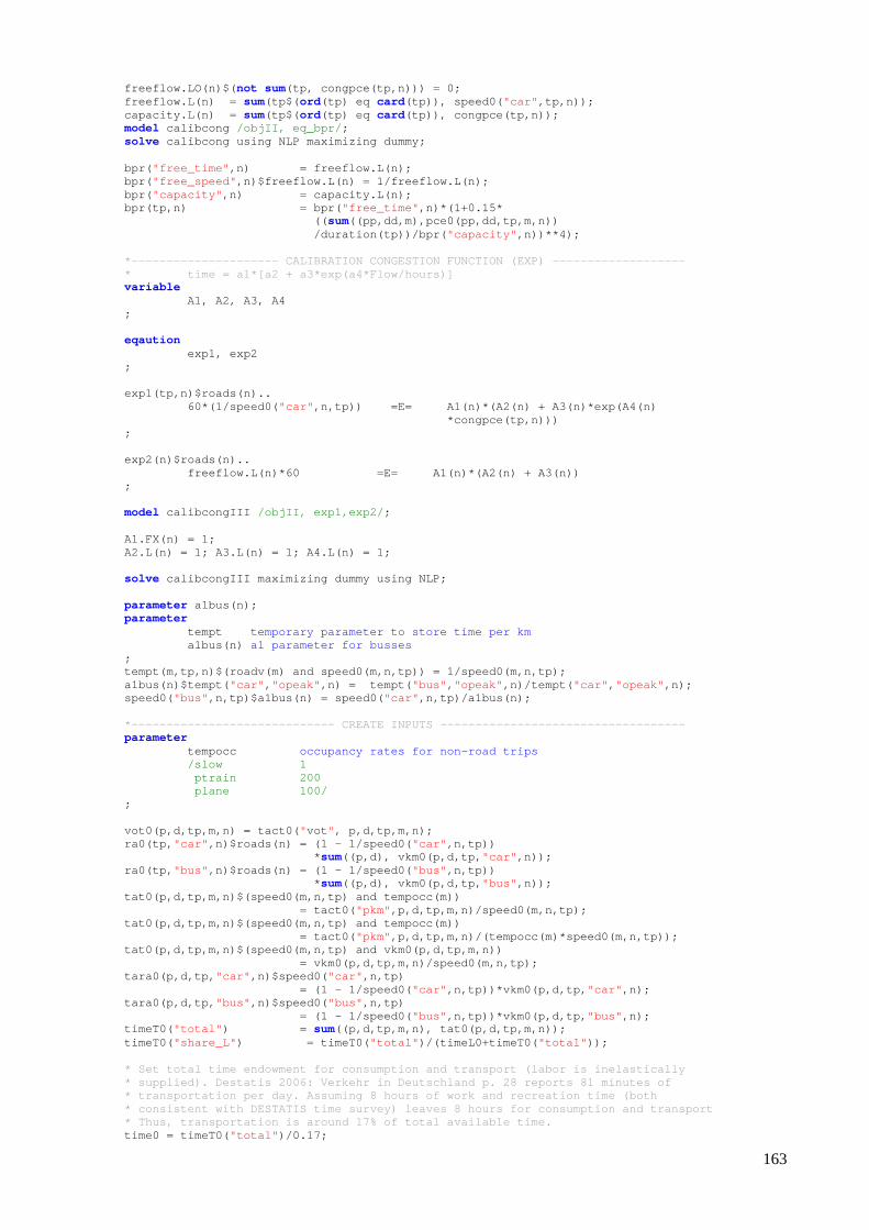
163

freeflow.LO(n)$( not sum(tp, congpce(tp,n))) = 0; freeflow.L(n) = sum(tp$( ord(tp) eq card(tp)), speed0( "car" ,tp,n)); capacity.L(n) = sum(tp$( ord(tp) eq card(tp)), congpce(tp,n)); model calibcong /objII, eq_bpr/ ; solve calibcong using NLP maximizing dummy; bpr( "free_time" ,n) = freeflow.L(n); bpr( "free_speed" ,n)$freeflow.L(n) = 1/freeflow.L(n); bpr( "capacity" ,n) = capacity.L(n); bpr(tp,n) = bpr( "free_time" ,n)*(1+0.15* (( sum((pp,dd,m),pce0(pp,dd,tp,m,n)) /duration(tp))/bpr( "capacity" ,n))**4); *--------------------- CALIBRATION CONGESTION FUNCT ION (EXP) ------------------- * time = a1*[a2 + a3*exp(a4*Flow/hours)] variable A1, A2, A3, A4 ; eqaution exp1, exp2 ; exp1(tp,n)$roads(n).. 60*(1/speed0( "car" ,n,tp)) =E= A1(n)*(A2(n) + A3(n)*exp(A4(n) *cong pce(tp,n))) ; exp2(n)$roads(n).. freeflow.L(n)*60 =E= A1(n)*( A2(n) + A3(n)) ; model calibcongIII /objII, exp1,exp2/ ; A1.FX(n) = 1; A2.L(n) = 1; A3.L(n) = 1; A4.L(n) = 1; solve calibcongIII maximizing dummy using NLP; parameter a1bus(n); parameter tempt temporary parameter to store time per km a1bus(n) a1 parameter for busses ; tempt(m,tp,n)$(roadv(m) and speed0(m,n,tp)) = 1/spe ed0(m,n,tp); a1bus(n)$tempt( "car" , "opeak" ,n) = tempt( "bus" , "opeak" ,n)/tempt( "car" , "opeak" ,n); speed0( "bus" ,n,tp)$a1bus(n) = speed0( "car" ,n,tp)/a1bus(n); *----------------------------- CREATE INPUTS ------ ----------------------------- parameter tempocc occupancy rates for non-road trips /slow 1 ptrain 200 plane 100/ ; vot0(p,d,tp,m,n) = tact0( " vot " , p,d,tp,m,n); ra0(tp, "car" ,n)$roads(n) = (1 - 1/speed0( "car" ,n,tp)) * sum((p,d), vkm0(p,d,tp, "car" ,n)); ra0(tp, "bus" ,n)$roads(n) = (1 - 1/speed0( "bus" ,n,tp)) * sum((p,d), vkm0(p,d,tp, "bus" ,n)); tat0(p,d,tp,m,n)$(speed0(m,n,tp) and tempocc(m)) = tact0( "pkm" ,p,d,tp,m,n)/speed0(m,n,tp); tat0(p,d,tp,m,n)$(speed0(m,n,tp) and tempocc(m)) = tact0( "pkm" ,p,d,tp,m,n)/(tempocc(m)*speed0(m,n,tp)); tat0(p,d,tp,m,n)$(speed0(m,n,tp) and vkm0(p,d,tp,m, n)) = vkm0(p,d,tp,m,n)/speed0( m,n,tp); tara0(p,d,tp, "car" ,n)$speed0( "car" ,n,tp) = (1 - 1/speed0( "car" ,n,tp))*vkm0(p,d,tp, "car" ,n); tara0(p,d,tp, "bus" ,n)$speed0( "bus" ,n,tp) = (1 - 1/speed0( "bus" ,n,tp))*vkm0(p,d,tp, "bus" ,n); timeT0( "total" ) = sum((p,d,tp,m,n), tat0(p,d,tp,m,n)); timeT0( "share_L" ) = timeT0( "total" )/(timeL0+timeT0( "total" )); * Set total time endowment for consumption and tran sport (labor is inelastically * supplied). Destatis 2006: Verkehr in Deutschland p. 28 reports 81 minutes of * transportation per day. Assuming 8 hours of work and recreation time (both * consistent with DESTATIS time survey) leaves 8 ho urs for consumption and transport * Thus, transportation is around 17% of total avail able time. time0 = timeT0( "total" )/0.17;

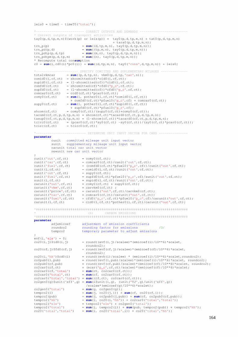
164

leis0 = time0 - timeT0( "total" ); *------------------------- CORRECT OUTPUTS AND DEMA NDS ------------------------- * Correct outputs of transport activities tay0(p,d,tp,m,n)$(work(p) or leis(p)) = tay0(p,d,t p,m,n) + tat0(p,d,tp,m,n) + tara0(p, d,tp,m,n); trn_p(p) = sum((d,tp,m,n), tay0(p,d,tp,m,n)); trn_pd(p,d) = sum((tp,m,n), tay0(p,d,tp,m,n)); trn_pdtp(p,d,tp) = sum((m,n), tay0(p,d,tp,m,n)); trn_pdtpm(p,d,tp,m) = sum((n), tay0(p,d,tp,m,n)); * Recompute total con sumption c0 = sum(i,cd0(i)*pc0(i)) + sum((d,tp,m,n), tay0( "cons" ,d,tp,m,n)) + leis0; *---------------------- SPECIFY COMIITED AND SUPLEM ENTARY MILAGES -------------- totalvkmcar = sum((p,d,tp,n), vkm0(p,d,tp, "car" ,n)); comid0(i,cf,ct) = shcomitted(cf)*cid0(i,cf,ct); supid0(i,cf,ct) = (1-shcomitted(cf))*cid0(i,cf,ct) ; comfd0(cf,ct) = shcomitted(cf)*cfd0( "p_c" ,cf,ct); supfd0(cf,ct) = (1-shcomitted(cf))*cfd0( "p_c" ,cf,ct); comcar0(cf,ct) = ccd0(cf,ct)*pcar0(cf,ct); comy0(cf,ct) = sum(i, pother0(i,cf,ct)*comid0(i,cf,ct)) + comfd0(cf,ct)*pfuel0( "p_c" ,cf) + comcar0(cf,ct); supy0(cf,ct) = sum(i, pother0(i,cf,ct)*supid0(i,cf,ct)) + supfd0(cf,ct)*pfuel0( "p_c" ,cf); shcom(cf,ct) = comy0(cf,ct)/(supy0(cf,ct)+comy0 (cf,ct)); tacom0(cf,ct,p,d,tp,m,n) = shcom(cf,ct)*tacard0(cf, ct,p,d,tp,m,n); tasup0(cf,ct,p,d,tp,m,n) = (1-shcom(cf,ct))*tacard0 (cf,ct,p,d,tp,m,n); tcirc0(cf,ct) = (pcar0(cf,ct)*sy0(cf,ct) -sy0(cf ,ct))/(sy0(cf,ct)*pcar0(cf,ct)); tcirc(cf,ct) = tcirc0(cf,ct); *-------------------------- DETERMINE UNIT INPUT VE CTOR FOR CARS --------------- parameter cunit committed mileage unit input vector sunit supplementary mileage unit input vector carunit total car unit vector newunit new car unit vector ; cunit( "out" ,cf,ct) = comy0(cf,ct); cunit( "car" ,cf,ct) = comcar0(cf,ct)/cunit( "out" ,cf,ct); cunit( "fuel" ,cf,ct) = (comfd0(cf,ct)*pfuel0( "p_c" ,cf))/cunit( "out" ,cf,ct); cunit(i,cf,ct) = comid0(i,cf,ct)/cunit( "out" ,cf,ct); sunit( "out" ,cf,ct) = supy0(cf,ct); sunit( "fuel" ,cf,ct) = supfd0(cf,ct)*pfuel0( "p_c" ,cf)/sunit( "out" ,cf,ct); sunit(i,cf,ct) = supid0(i,cf,ct)/sunit( "out" ,cf,ct); carunit( "out" ,cf,ct) = comy0(cf,ct) + supy0(cf,ct); carunit( "vkm" ,cf,ct) = carvkm0(cf,ct) ; carunit( " price " ,cf,ct) = carunit( "out" ,cf,ct)/carvkm0(cf,ct); carunit( "car" ,cf,ct) = comcar0(cf,ct)/carunit( "out" ,cf,ct); carunit( "fuel" ,cf,ct) = cfd0( "p_c" ,cf,ct)*pfuel0( "p_c" ,cf)/carunit( "out" ,cf,ct); carunit(i,cf,ct) = cid0(i,cf,ct)*pother0(i, cf,ct)/carunit( "out" ,cf,ct); *################################################## ############################# * (6) CARBON EMISSIO NS *################################################## ############################# parameter adjemicoef adjustment of emission coefficients roundco2 rounding factor for emissions /3/ tempco2 temporary parameter to adjust emissions ; evf(i, "ele" ) = 0; co20(i,j)$id0(i,j) = round((evf(i,j)/scalee)* (emicoef(i)/10**6)*scalet, roundco2); co20(cf,j)$fd0(cf,j) = round((evf(cf,j)/scalee) *(emicoef(cf)/10**6)*scalet, roundco2); co20(i, "hh" )$cd0(i) = round((evh(i)/scalee) * (emicoef(i) /10**6)*scalet,roundco2); co2pub0(i,pub) = round((evf(i,pub)/scalee )*(emicoef(i)/10**6)*scalet, roundco2); co2pub0(cf,pub) = round((evf(cf,pub)/scale e)*(emicoef(cf)/10**6)*scalet, roundco2); co2car0(cf,ct) = (ecar( "p_c" ,cf,ct)/scalee)*(emicoef(cf)/10**6)*scalet; co2car0(cf, "total" ) = sum(ct, co2car0(cf,ct)); co2car0( "total" ,ct) = sum(cf, co2car0(cf,ct)); co2car0( "total" , "total" ) = sum((cf,ct), co2car0(cf,ct)); co2gen0(g)$unit( " eff " ,g) = sum(i$unit(i,g), (unit( " TJ" ,g)/unit( " eff " ,g)) /scalee*(emicoef(g)/10** 6)*scalet); co2gen0( "total" ) = sum(g, co2gen0(g)); tempco2(i) = sum(j, co20(j,i)) + sum(cf, co20(cf,i)); tempco2(pub) = sum(j, co2pub0(j,pub)) + sum(cf, co2pub0(cf,pub)); tempco2( "hh" ) = sum(i, co20(i, "hh" )) + co2car0( "total" , "total" ); tempco2( "ele" ) = tempco2( "ele" ) + co2gen0( "total" ); tempco2( "total" ) = sum(i, tempco2(i)) + sum(pub, tempco2(pub)) + tempco2( "hh" ); co20( "total" , "total" ) = sum(i, co20( "total" ,i)) + co20( "total" , "hh" );

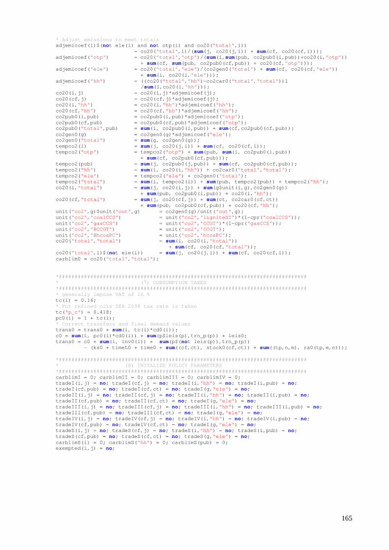
165

* Adjust emissions to meet totals adjemicoef(i)$( not ele(i) and not otp(i) and co20( "total" ,i)) = co20( "total" ,i)/( sum(j, co20(j,i)) + sum(cf, co20(cf,i))); adjemicoef( "otp" ) = co20( "total" , "otp" )/( sum(i, sum(pub, co2pub0(i,pub))+co20(i, "otp" )) + sum(cf, sum(pub, co2pub0(cf,pub)) + co20(cf, "otp" ))); adjemicoef( "ele" ) = co20( "total" , "ele" )/(co2gen0( "total" ) + sum(cf, co20(cf, "ele" )) + sum(i, co20(i, "ele" ))); adjemicoef( "hh" ) = ((co20( "total" , "hh" )-co2car0( "total" , "total" ))1

/ sum(i,co20(i, "hh" ))); co20(i,j) = co20(i,j)*adjemicoef(j); co20(cf,j) = co20(cf,j)*adjemicoef(j) ; co20(i, "hh" ) = co20(i, "hh" )*adjemicoef( "hh" ); co20(cf, "hh" ) = co20(cf, "hh" )*adjemicoef( "hh" ); co2pub0(i,pub) = co2pub0(i,pub)*adjemicoe f( "otp" ); co2pub0(cf,pub) = co2pub0(cf,pub)*adjemico ef( "otp" ); co2pub0( "total" ,pub) = sum(i, co2pub0(i,pub)) + sum(cf,co2pub0(cf,pub)); co2gen0(g) = co2gen0(g)*adjemicoef( "ele" ); co2gen0( "total" ) = sum(g, co2gen0(g)); tempco2(i) = sum(j, co20(j,i)) + sum(cf, co20(cf,i)); tempco2( "otp" ) = tempco2( "otp" ) + sum(pub, sum(i, co2pub0(i,pub)) + sum(cf, co2pub0(cf,pub))); tempco2(pub) = sum(j, co2pub0(j,pub)) + sum(cf, co2pub0(cf,pub)); tempco2( "hh" ) = sum(i, co20(i, "hh" )) + co2car0( "total" , "total" ); tempco2( "ele" ) = tempco2( "ele" ) + co2gen0( "total" ); tempco2( "total" ) = sum(i, tempco2(i)) + sum(pub, tempco2(pub)) + tempco2( "hh" ); co20(i, "total" ) = sum(j, co20(i,j)) + sum(g$unit(i,g),co2gen0(g)) + sum(pub, co2pub0(i,pub)) + co20(i, "hh" ); co20(cf, "total" ) = sum(j, co20(cf,j)) + sum(ct, co2car0(cf,ct)) + sum(pub, co2pub0(cf,pub)) + co20(cf, "hh" ); unit( "co2" ,g)$unit( "out" ,g) = co2gen0(g)/unit( "out" ,g); unit( "co2" , "coalCCS" ) = unit( "co2" , "ligniteST" )*(1-cpr( "coalCCS" )); unit( "co2" , "gasCCS" ) = unit( "co2" , "CCGT")*(1-cpr( "gasCCS" )); unit( "co2" , "BCCGT") = unit( "co2" , "CCGT"); unit( "co2" , "BhcoaPC" ) = unit( "co2" , "hcoaPC" ); co20( "total" , "total" ) = sum(i, co20(i, "total" )) + sum(cf, co20(cf, "total" )); co20( "total" ,i)$( not ele(i)) = sum(j, co20(j,i)) + sum(cf, co20(cf,i)); carblim0 = co20( "total" , "total" ); *################################################## ############################# * (7) CONSUMPTION TAXES *################################################## ############################# * generally impose VAT of 16 % tc(i) = 0.16; * For refined oils IEA 2008 tax rate is taken tc( "p_c" ) = 0.418; pc0(i) = 1 + tc(i); * Correct transfers and final demand values trans0 = trans0 + sum(i, tc(i)*cd0(i)); c0 = sum(i, pc0(i)*cd0(i)) + sum(p$leis(p),trn_p(p)) + leis0; trans0 = c0 + sum(i, inv0(i)) + sum(p$( not leis(p)),trn_p(p)) - (ks0 + timeL0 + time0 + sum((cf,ct), stock0(cf,ct)) + sum((tp,n,m), ra0(tp,m,n))); *################################################## ############################# * (8) INITALIZE POLICY PARAMETE RS *################################################## ############################# carblimI = 0; carblimII = 0; carblimIII = 0; carbli mIV = 0; tradeI(i,j) = no; tradeI(cf,j) = no; tradeI(i, "hh" ) = no; tradeI(i,pub) = no; tradeI(cf,pub) = no; tradeI(cf,ct) = no; tradeI(g, "ele" ) = no; tradeII(i,j) = no; tradeII(cf,j) = no; tradeII(i, "hh" ) = no; tradeII(i,pub) = no; tradeII(cf,pub) = no; tradeII(cf,ct) = no; tradeI(g, "ele" ) = no; tradeIII(i,j) = no; tradeIII(cf,j) = no; tradeIII(i, "hh" ) = no; tradeIII(i,pub) = no; tradeIII(cf,pub) = no; tradeIII(cf,ct) = no; tradeI(g, "ele" ) = no; tradeIV(i,j) = no; tradeIV(cf,j) = no; tradeIV(i, "hh" ) = no; tradeIV(i,pub) = no; tradeIV(cf,pub) = no; tradeIV(cf,ct) = no; tradeI(g, "ele" ) = no; tradeS(i,j) = no; tradeS(cf,j) = no; tradeS(i, "hh" ) = no; tradeS(i,pub) = no; tradeS(cf,pub) = no; tradeS(cf,ct) = no; tradeS(g, "ele" ) = no; carblimS(i) = 0; carblimS( "hh" ) = 0; carblimS(pub) = 0; exempted(i,j) = no;

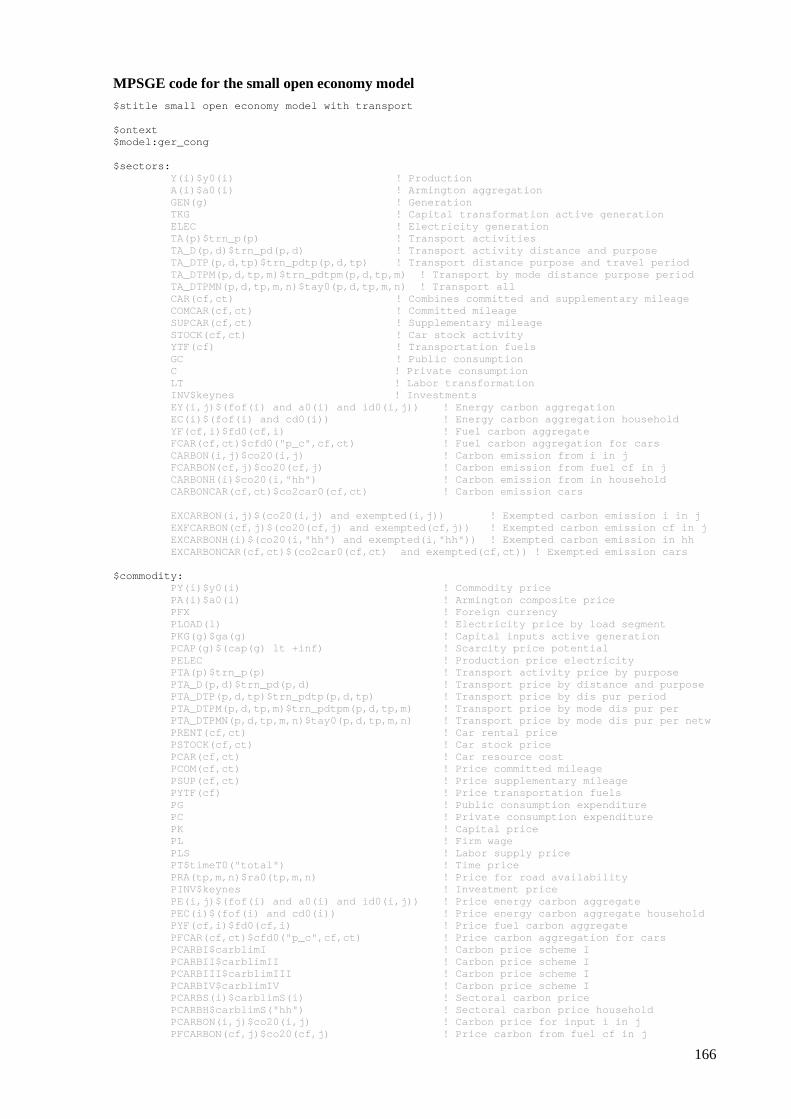
166

MPSGE code for the small open economy model $stitle small open economy model with transport $ontext $model:ger_cong $sectors: Y(i)$y0(i) ! Production A(i)$a0(i) ! Armington aggrega tion GEN(g) ! Generation TKG ! Capital transform ation active generation ELEC ! Electricity gener ation TA(p)$trn_p(p) ! Transport activit ies TA_D(p,d)$trn_pd(p,d) ! Tran sport activity distance and purpose TA_DTP(p,d,tp)$trn_pdtp(p,d,tp) ! Tran sport distance purpose and travel period TA_DTPM(p,d,tp,m)$trn_pdtpm(p,d,tp,m) ! T ransport by mode distance purpose period TA_DTPMN(p,d,tp,m,n)$tay0(p,d,tp,m,n) ! T ransport all CAR(cf,ct) ! Combi nes committed and supplementary mileage COMCAR(cf,ct) ! Committed mi leage SUPCAR(cf,ct) ! Supp lementary mileage STOCK(cf,ct) ! Car stock activity YTF(cf) ! Tran sportation fuels GC ! Public consumption C ! Priva te consumption LT ! Labor transformation INV$keynes ! Inves tments EY(i,j)$(fof(i) and a0(i) and id0(i,j)) ! Energy carbon aggregation EC(i)$(fof(i) and cd0(i)) ! Energy carbon aggregation household YF(cf,i)$fd0(cf,i) ! Fuel carbon aggregate FCAR(cf,ct)$cfd0("p_c",cf,ct) ! Fuel carbon aggregation for cars CARBON(i,j)$co20(i,j) ! Carbon emission from i in j FCARBON(cf,j)$co20(cf,j) ! Carbon emission from fuel cf in j CARBONH(i)$co20(i,"hh") ! Carbon emission from in household CARBONCAR(cf,ct)$co2car0(cf,ct) ! Carbon emission cars EXCARBON(i,j)$(co20(i,j) and exempted(i,j) ) ! Exempted carbon emission i in j EXFCARBON(cf,j)$(co20(cf,j) and exempted(c f,j)) ! Exempted carbon emission cf in j EXCARBONH(i)$(co20(i,"hh") and exempted(i, "hh")) ! Exempted carbon emission in hh EXCARBONCAR(cf,ct)$(co2car0(cf,ct) and ex empted(cf,ct)) ! Exempted emission cars $commodity: PY(i)$y0(i) ! Commodity price PA(i)$a0(i) ! Armington composite price PFX ! Foreign currency PLOAD(l) ! Electricity price by load segment PKG(g)$ga(g) ! Capital inputs active generation PCAP(g)$(cap(g) lt +inf) ! Scarcity price potential PELEC ! Production price electricity PTA(p)$trn_p(p) ! Transport activity price by purpose PTA_D(p,d)$trn_pd(p,d) ! Transport price by distance and purpose PTA_DTP(p,d,tp)$trn_pdtp(p,d,tp) ! Transport price by dis pur period PTA_DTPM(p,d,tp,m)$trn_pdtpm(p,d,tp,m) ! Transport price by mode dis pur per PTA_DTPMN(p,d,tp,m,n)$tay0(p,d,tp,m,n) ! Transport price by mode dis pur per netw PRENT(cf,ct) ! Car rental price PSTOCK(cf,ct) ! Car stock price PCAR(cf,ct) ! Car resource cost PCOM(cf,ct) ! Price committed mileage PSUP(cf,ct) ! Price supplementary mileage PYTF(cf) ! Price transportation fuels PG ! Public c onsumption expenditure PC ! Private consumption expenditure PK ! Capital price PL ! Firm wag e PLS ! Labor su pply price PT$timeT0("total") ! Time pri ce PRA(tp,m,n)$ra0(tp,m,n) ! Price fo r road availability PINV$keynes ! Investme nt price PE(i,j)$(fof(i) and a0(i) and id0(i,j)) ! Price energy carbon aggregate PEC(i)$(fof(i) and cd0(i)) ! Price energy carbon aggregate household PYF(cf,i)$fd0(cf,i) ! Price fuel carbon aggregate PFCAR(cf,ct)$cfd0("p_c",cf,ct) ! Price carbon aggregation for cars PCARBI$carblimI ! Carbo n price scheme I PCARBII$carblimII ! Carbo n price scheme I PCARBIII$carblimIII ! Carbo n price scheme I PCARBIV$carblimIV ! Carbo n price scheme I PCARBS(i)$carblimS(i) ! Secto ral carbon price PCARBH$carblimS("hh") ! Secto ral carbon price household PCARBON(i,j)$co20(i,j) ! Carbo n price for input i in j PFCARBON(cf,j)$co20(cf,j) ! Price carbon from fuel cf in j

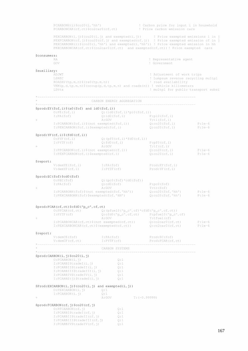
167

PCARBONH(i)$co20(i,"hh") ! Carbo n price for input i in household PCARBONCAR(cf,ct)$co2car0(cf,ct) ! Price carbon emission cars PEXCARBON(i,j)$(co20(i,j) and exempted(i,j )) ! Price exempted emissions i in j PEXFCARBON(cf,j)$(co20(cf,j) and exempted( cf,j)) ! Price exempted emission cf in j PEXCARBONH(i)$(co20(i,"hh") and exempted(i ,"hh")) ! Price exempted emission in hh PEXCARBONCAR(cf,ct)$(co2car0(cf,ct) and e xempted(cf,ct)) ! Price exempted cars $consumers: RA ! Representative agen t GOV ! Government $auxiliary: ADJWT ! Adjustment of work trips LSREC ! Lumpsum revenue recycling multpl ROADAV(tp,m,n)$(ra0(tp,m,n)) ! road availability VKM(p,d,tp,m,n)$(occup(p,d,tp,m,n) and roa ds(n)) ! vehicle kiliometers LStta ! multpl for public transport subsi *-------------------------------------------------- ----------------------------- * CARBON ENERGY AGGREGATI ON *-------------------------------------------------- ----------------------------- $prod:EY(fof,i)$(a0(fof) and id0(fof,i)) O:PE(fof,i) Q:(id0(fof,i)*pi0( fof,i)) I:PA(fof) Q:id0(fof,i) P:pi0(fof,i) + A:GOV T:ti(fof,i) I:PCARBON(fof,i)$(not exempted(fof,i)) Q:co20(fof,i) P:1e-6 I:PEXCARBON(fof,i)$exempted(fof,i) Q:co20(fof,i) P:1e-6 $prod:YF(cf,i)$(fd0(cf,i)) O:PYF(cf,i) Q:(pf0(cf,i)*fd0(c f,i)) I:PYTF(cf) Q:fd0(cf,i) P:pf0(cf,i) + A:GOV T:tf(cf,i) I:PFCARBON(cf,i)$(not exempted(cf,i)) Q:co20(cf,i) P:1e-6 I:PEXFCARBON(cf,i)$exempted(cf,i) Q:co20(cf,i) P:1e-6 $report: V:demYE(fof,i) I:PA(fof) Prod:EY(fof,i) V:demYF(cf,i) I:PYTF(cf) Prod:YF(cf,i) $prod:EC(fof)$cd0(fof) O:PEC(fof) Q:(pc0(fof)*cd0(fo f)) I:PA(fof) Q:cd0(fof) P:pc0(fof) + A:GOV T:tc(fof) I:PCARBONH(fof)$(not exempted(fof,"hh")) Q:co20(fof,"hh") P:1e-6 I:PEXCARBONH(fof)$exempted(fof,"HH") Q:co20(fof,"hh") P:1e-6 $prod:FCAR(cf,ct)$cfd0("p_c",cf,ct) O:PFCAR(cf,ct) Q:(pfuel0("p_c",cf )*cfd0("p_c",cf,ct)) I:PYTF(cf) Q:cfd0("p_c",cf,ct ) P:pfuel0("p_c",cf) + A:GOV T:tfuel(cf) I:PCARBONCAR(cf,ct)$(not exempted(cf,ct)) Q:co2car0(cf,ct) P:1e-6 I:PEXCARBONCAR(cf,ct)$(exempted(cf,ct)) Q:co2car0(cf,ct) P:1e-6 $report: V:demCE(fof) I:PA(fof) Prod:EC(fof) V:demCF(cf,ct) I:PYTF(cf) Prod:FCAR(cf,ct) *-------------------------------------------------- ----------------------------- * CARBON SYSTEMS *-------------------------------------------------- ----------------------------- $prod:CARBON(i,j)$co20(i,j) O:PCARBON(i,j) Q:1 I:PCARBI$tradeI(i,j) Q:1 I:PCARBII$tradeII(i,j) Q:1 I:PCARBIII$tradeIII(i,j) Q:1 I:PCARBIV$tradeIV(i,j) Q:1 I:PCARBS(j)$tradeS(i,j) Q:1 $Prod:EXCARBON(i,j)$(co20(i,j) and exempted(i,j)) O:PEXCARBON(i,j) Q:1 I:PCARBON(i,j) Q:1 + A:GOV T: (-0.99999) $prod:FCARBON(cf,j)$co20(cf,j) O:PFCARBON(cf,j) Q:1 I:PCARBI$tradeI(cf,j) Q:1 I:PCARBII$tradeII(cf,j) Q:1 I:PCARBIII$tradeIII(cf,j) Q:1 I:PCARBIV$tradeIV(cf,j) Q:1

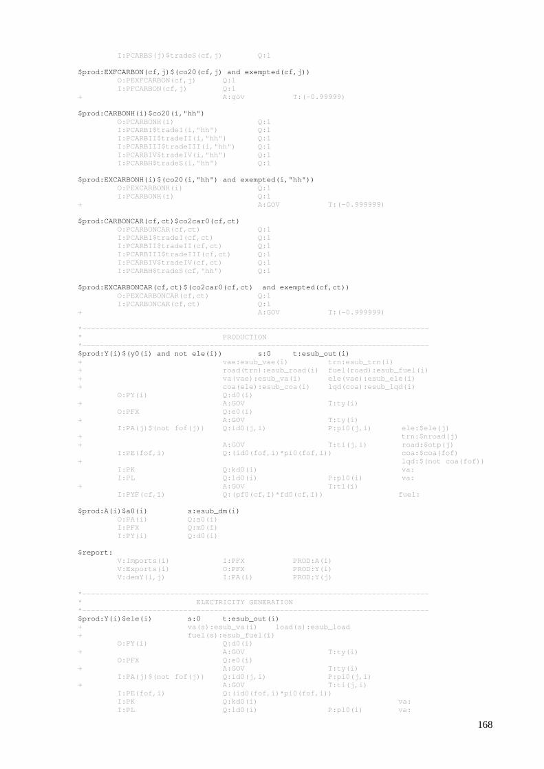
168

I:PCARBS(j)$tradeS(cf,j) Q:1 $prod:EXFCARBON(cf,j)$(co20(cf,j) and exempted(cf,j )) O:PEXFCARBON(cf,j) Q:1 I:PFCARBON(cf,j) Q:1 + A:gov T: (-0.99999) $prod:CARBONH(i)$co20(i,"hh") O:PCARBONH(i) Q:1 I:PCARBI$tradeI(i,"hh") Q:1 I:PCARBII$tradeII(i,"hh") Q:1 I:PCARBIII$tradeIII(i,"hh") Q:1 I:PCARBIV$tradeIV(i,"hh") Q:1 I:PCARBH$tradeS(i,"hh") Q:1 $prod:EXCARBONH(i)$(co20(i,"hh") and exempted(i,"hh ")) O:PEXCARBONH(i) Q:1 I:PCARBONH(i) Q:1 + A:GOV T:(-0.999999) $prod:CARBONCAR(cf,ct)$co2car0(cf,ct) O:PCARBONCAR(cf,ct) Q:1 I:PCARBI$tradeI(cf,ct) Q:1 I:PCARBII$tradeII(cf,ct) Q:1 I:PCARBIII$tradeIII(cf,ct) Q:1 I:PCARBIV$tradeIV(cf,ct) Q:1 I:PCARBH$tradeS(cf,"hh") Q:1 $prod:EXCARBONCAR(cf,ct)$(co2car0(cf,ct) and exemp ted(cf,ct)) O:PEXCARBONCAR(cf,ct) Q:1 I:PCARBONCAR(cf,ct) Q:1 + A:GOV T:(-0.999999) *-------------------------------------------------- ----------------------------- * PRODUCTION *-------------------------------------------------- ----------------------------- $prod:Y(i)$(y0(i) and not ele(i)) s:0 t: esub_out(i) + vae:esub_vae(i) trn:esub_trn(i) + road(trn):esub_roa d(i) fuel(road):esub_fuel(i) + va(vae):esub_va(i) ele(vae):esub_ele(i) + coa(ele):esub_coa( i) lqd(coa):esub_lqd(i) O:PY(i) Q:d0(i) + A:GOV T:ty(i) O:PFX Q:e0(i) + A:GOV T:ty(i) I:PA(j)$(not fof(j)) Q:id0(j,i) P:pi0(j,i) ele:$ele(j) + trn:$nroad(j) + A:GOV T:ti(j,i) road:$otp(j) I:PE(fof,i) Q:(id0(fof,i)*pi0( fof,i)) coa:$coa(fof) + lqd:$(not coa(fof)) I:PK Q:kd0(i) va: I:PL Q:ld0(i) P:pl0(i) va: + A:GOV T:tl(i) I:PYF(cf,i) Q:(pf0(cf,i)*fd0(c f,i)) fuel: $prod:A(i)$a0(i) s:esub_dm(i) O:PA(i) Q:a0(i) I:PFX Q:m0(i) I:PY(i) Q:d0(i) $report: V:Imports(i) I:PFX PR OD:A(i) V:Exports(i) O:PFX PR OD:Y(i) V:demY(i,j) I:PA(i) PR OD:Y(j) *-------------------------------------------------- ----------------------------- * ELECTRICITY GENERATION *-------------------------------------------------- ----------------------------- $prod:Y(i)$ele(i) s:0 t:esub_out(i) + va(s):esub_va(i) load(s ):esub_load + fuel(s):esub_fuel(i) O:PY(i) Q:d0(i) + A:GOV T:ty(i) O:PFX Q:e0(i) + A:GOV T:ty(i) I:PA(j)$(not fof(j)) Q:id0(j,i) P:pi0(j,i) + A:GOV T:ti(j,i) I:PE(fof,i) Q:(id0(fof,i)*pi0( fof,i)) I:PK Q:kd0(i) va: I:PL Q:ld0(i) P:pl0(i) va:

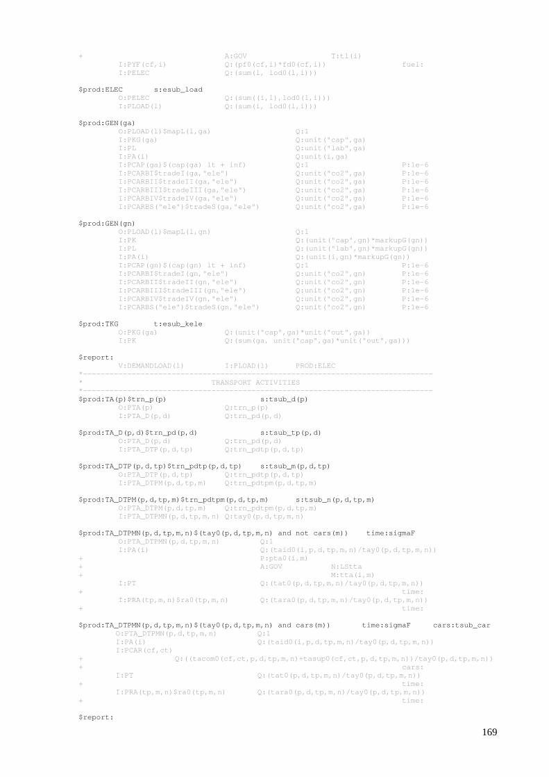
169

+ A:GOV T:tl(i) I:PYF(cf,i) Q:(pf0(cf,i)*fd0(c f,i)) fuel: I:PELEC Q:(sum(l, lod0(l,i ))) $prod:ELEC s:esub_load O:PELEC Q:(sum((i,l),lod0( l,i))) I:PLOAD(l) Q:(sum(i, lod0(l,i ))) $prod:GEN(ga) O:PLOAD(l)$mapL(l,ga) Q: 1 I:PKG(ga) Q: unit("cap",ga) I:PL Q: unit("lab",ga) I:PA(i) Q: unit(i,ga) I:PCAP(ga)$(cap(ga) lt + inf) Q: 1 P:1e-6 I:PCARBI$tradeI(ga,"ele") Q: unit("co2",ga) P:1e-6 I:PCARBII$tradeII(ga,"ele") Q: unit("co2",ga) P:1e-6 I:PCARBIII$tradeIII(ga,"ele") Q: unit("co2",ga) P:1e-6 I:PCARBIV$tradeIV(ga,"ele") Q: unit("co2",ga) P:1e-6 I:PCARBS("ele")$tradeS(ga,"ele") Q: unit("co2",ga) P:1e-6 $prod:GEN(gn) O:PLOAD(l)$mapL(l,gn) Q: 1 I:PK Q: (unit("cap",gn)*markupG(gn)) I:PL Q: (unit("lab",gn)*markupG(gn)) I:PA(i) Q: (unit(i,gn)*markupG(gn)) I:PCAP(gn)$(cap(gn) lt + inf) Q: 1 P:1e-6 I:PCARBI$tradeI(gn,"ele") Q: unit("co2",gn) P:1e-6 I:PCARBII$tradeII(gn,"ele") Q: unit("co2",gn) P:1e-6 I:PCARBIII$tradeIII(gn,"ele") Q: unit("co2",gn) P:1e-6 I:PCARBIV$tradeIV(gn,"ele") Q: unit("co2",gn) P:1e-6 I:PCARBS("ele")$tradeS(gn,"ele") Q: unit("co2",gn) P:1e-6 $prod:TKG t:esub_kele O:PKG(ga) Q:(unit("cap",ga)* unit("out",ga)) I:PK Q:(sum(ga, unit("c ap",ga)*unit("out",ga))) $report: V:DEMANDLOAD(l) I:PLOAD(l) PR OD:ELEC *-------------------------------------------------- ----------------------------- * TRANSPORT ACTIVITIES *-------------------------------------------------- ----------------------------- $prod:TA(p)$trn_p(p) s:tsub_d(p ) O:PTA(p) Q:trn_p(p) I:PTA_D(p,d) Q:trn_pd(p,d) $prod:TA_D(p,d)$trn_pd(p,d) s:tsub_tp( p,d) O:PTA_D(p,d) Q:trn_pd(p,d) I:PTA_DTP(p,d,tp) Q:trn_pdtp(p,d,tp) $prod:TA_DTP(p,d,tp)$trn_pdtp(p,d,tp) s:tsub_m(p ,d,tp) O:PTA_DTP(p,d,tp) Q:trn_pdtp(p,d,tp) I:PTA_DTPM(p,d,tp,m) Q:trn_pdtpm(p,d,tp ,m) $prod:TA_DTPM(p,d,tp,m)$trn_pdtpm(p,d,tp,m) s: tsub_n(p,d,tp,m) O:PTA_DTPM(p,d,tp,m) Q:trn_pdtpm(p,d,tp ,m) I:PTA_DTPMN(p,d,tp,m,n) Q:tay0(p,d,tp,m,n) $prod:TA_DTPMN(p,d,tp,m,n)$(tay0(p,d,tp,m,n) and no t cars(m)) time:sigmaF O:PTA_DTPMN(p,d,tp,m,n) Q:1 I:PA(i) Q:(taid0(i ,p,d,tp,m,n)/tay0(p,d,tp,m,n)) + P:pta0(i,m ) + A:GOV N:LStta + M:tta(i,m) I:PT Q:(tat0(p, d,tp,m,n)/tay0(p,d,tp,m,n)) + time: I:PRA(tp,m,n)$ra0(tp,m,n) Q:(tara0(p ,d,tp,m,n)/tay0(p,d,tp,m,n)) + time: $prod:TA_DTPMN(p,d,tp,m,n)$(tay0(p,d,tp,m,n) and ca rs(m)) time:sigmaF cars:tsub_car

O:PTA_DTPMN(p,d,tp,m,n) Q:1 I:PA(i) Q:(taid0(i,p,d,tp, m,n)/tay0(p,d,tp,m,n)) I:PCAR(cf,ct)

+ Q:((tacom0(cf,ct,p,d,tp,m,n)+tasup0(cf,ct ,p,d,tp,m,n))/tay0(p,d,tp,m,n)) + cars:

I:PT Q:(tat0(p,d,tp,m,n )/tay0(p,d,tp,m,n)) + time:

I:PRA(tp,m,n)$ra0(tp,m,n) Q:(tara0(p,d,tp,m, n)/tay0(p,d,tp,m,n)) + time: $report:

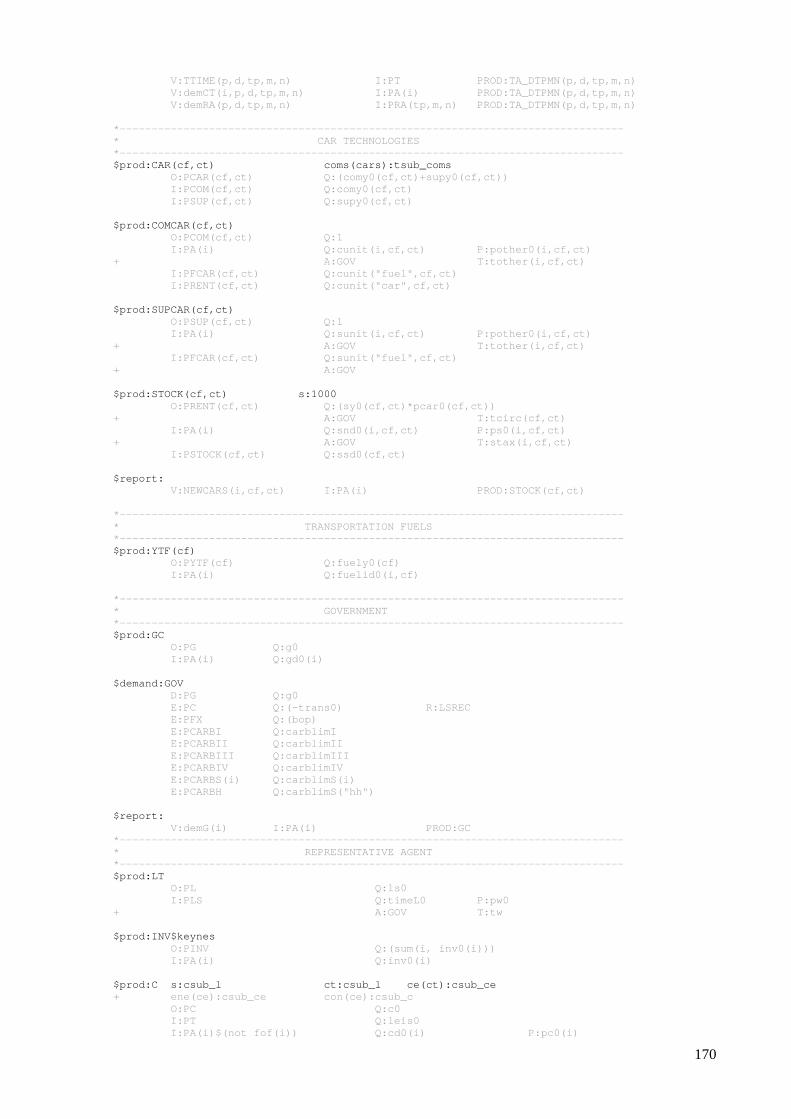
170

V:TTIME(p,d,tp,m,n) I:PT PROD:TA_DTPMN(p,d,tp,m,n) V:demCT(i,p,d,tp,m,n) I:PA(i) PROD:TA_DTPMN(p,d,tp,m,n) V:demRA(p,d,tp,m,n) I:PRA(tp,m ,n) PROD:TA_DTPMN(p,d,tp,m,n) *-------------------------------------------------- ----------------------------- * CAR TECHNOLOGIES *-------------------------------------------------- ----------------------------- $prod:CAR(cf,ct) coms(cars):tsub_co ms O:PCAR(cf,ct) Q:(comy0(cf,ct)+su py0(cf,ct)) I:PCOM(cf,ct) Q:comy0(cf,ct) I:PSUP(cf,ct) Q:supy0(cf,ct) $prod:COMCAR(cf,ct) O:PCOM(cf,ct) Q:1 I:PA(i) Q:cunit(i,cf,ct) P:pother0(i,cf,ct) + A:GOV T:tother(i,cf,ct) I:PFCAR(cf,ct) Q:cunit("fuel",cf, ct) I:PRENT(cf,ct) Q:cunit("car",cf,c t) $prod:SUPCAR(cf,ct) O:PSUP(cf,ct) Q:1 I:PA(i) Q:sunit(i,cf,ct) P:pother0(i,cf,ct) + A:GOV T:tother(i,cf,ct) I:PFCAR(cf,ct) Q:sunit("fuel",cf, ct) + A:GOV $prod:STOCK(cf,ct) s:1000 O:PRENT(cf,ct) Q:(sy0(cf,ct)*pcar 0(cf,ct)) + A:GOV T:tcirc(cf,ct) I:PA(i) Q:snd0(i,cf,ct) P:ps0(i,cf,ct) + A:GOV T:stax(i,cf,ct) I:PSTOCK(cf,ct) Q:ssd0(cf,ct) $report: V:NEWCARS(i,cf,ct) I:PA(i) PROD:STOCK(cf,ct) *-------------------------------------------------- ----------------------------- * TRANSPORTATION FUELS *-------------------------------------------------- ----------------------------- $prod:YTF(cf) O:PYTF(cf) Q:fuely0(cf) I:PA(i) Q:fuelid0(i,cf) *-------------------------------------------------- ----------------------------- * GOVERNMENT *-------------------------------------------------- ----------------------------- $prod:GC O:PG Q:g0 I:PA(i) Q:gd0(i) $demand:GOV D:PG Q:g0 E:PC Q:(-trans0) R: LSREC E:PFX Q:(bop) E:PCARBI Q:carblimI E:PCARBII Q:carblimII E:PCARBIII Q:carblimIII E:PCARBIV Q:carblimIV E:PCARBS(i) Q:carblimS(i) E:PCARBH Q:carblimS("hh") $report: V:demG(i) I:PA(i) PR OD:GC *-------------------------------------------------- ----------------------------- * REPRESENTATIVE AGENT *-------------------------------------------------- ----------------------------- $prod:LT O:PL Q:ls0 I:PLS Q:timeL0 P:pw0 + A:GOV T:tw $prod:INV$keynes O:PINV Q:(sum(i, inv0(i))) I:PA(i) Q:inv0(i) $prod:C s:csub_l ct:csub_l ce(ct ):csub_ce + ene(ce):csub_ce con(ce):csub_c O:PC Q:c0 I:PT Q:leis0 I:PA(i)$(not fof(i)) Q:cd0(i) P:pc0(i)

171

+ con:$(not ele(i)) + A:GOV T:tc(i) ene:$ele(i) I:PEC(fof) Q:(cd0(fof )*pc0(fof)) ene: I:PTA(p)$leis(p) Q:trn_p(p) ct: $demand:RA s:1 D:PC Q: c0 D:PINV$keynes Q: (sum(i, inv0(i))) E:PA(i)$(not keynes) Q: (-inv0(i)) E:PK Q: ks0 E:PLS Q: timeL0 E:PSTOCK(cf,ct) Q: stock0(cf,ct) E:PCAP(g)$(cap(g) lt + inf) Q: cap(g) E:PTA(p)$work(p) Q: (-trn_p(p)) R:ADJWT E:PC Q: trans0 R:LSREC E:PT Q: time0 E:PRA(tp,m,n)$ra0(tp,m,n) Q: 1 R:ROADAV(tp,m,n) $report: V:LEISURE I:PT PR OD:C V:demC(i) I:PA(i) PR OD:C *-------------------------------------------------- ----------------------------- * CONSTRAINTS *-------------------------------------------------- ----------------------------- $constraint:ADJWT

sum((d,tp,m,n)$tay0("work",d,tp,m,n), TA_DTPMN("work",d,tp,m,n)*(pkm0("work",d,tp,m,n)/ta y0("work",d,tp,m,n)))

=E= sum((d,tp,m,n),pkm 0("work",d,tp,m,n))*LT; $constraint:LSREC$lump GC =E= 1; $constraint:LSREC$(not lump) LSREC =E= 1; $constraint:LStta$pubsub GC =E= 1; $constraint:LStta$(not pubsub) LStta =E= 1; $constraint:VKM(p,d,tp,m,n)$(occup(p,d,tp,m,n) and roads(n) and not lkws(m)) VKM(p,d,tp,m,n) =E= (pkm0(p,d,tp,m,n)/tay0(p,d,tp,m,n))*TA_DTPMN(p,d,tp ,m,n)/occup(p,d,tp,m,n); $constraint:VKM(p,d,tp,m,n)$(occup(p,d,tp,m,n) and roads(n) and lkws(m)) VKM(p,d,tp,m,n) =E= vkm0(p,d,tp,m,n); $constraint:ROADAV(tp,m,n)$(ra0(tp,m,n) and congest ion and cars(m))

ROADAV(tp,m,n) =E= (1- (A2.L(n) + A3.L(n)*exp(A4.L(n)*sum((p,d,mm)$(occup(p,d,tp,mm,n )), VKM(p,d,tp,mm,n)*pcu(mm)/duration(tp))))/60) *sum((p,d,mm)$(occup(p,d,tp,mm,n) and cars(mm)), VKM(p,d,tp,mm,n));

$constraint:ROADAV(tp,m,n)$(ra0(tp,m,n) and congest ion and busses(m))

ROADAV(tp,m,n) =E= (1- (a1bus(n)*(A2.L(n) + A3.L(n)*exp(A4.L(n)*sum((p,d,mm)$(occup(p,d,tp,mm,n )), VKM(p,d,tp,mm,n)*pcu(mm)/duration(tp))))/60)) *sum((p,d,mm)$(occup(p,d,tp,mm,n) and busses(mm)), VKM(p,d,tp,mm,n));

$constraint:ROADAV(tp,m,n)$(ra0(tp,m,n) and not con gestion and cars(m)) ROADAV(tp,m,n) =E= ra0(tp,m,n)*sum((p, d,mm)$(occup(p,d,tp,mm,n) and cars(mm)),

VKM(p,d,tp,mm,n)) /sum((p,d,mm)$(occup(p,d,tp,mm,n) and cars(mm)), vkm0(p,d,tp,mm,n));

$constraint:ROADAV(tp,m,n)$(ra0(tp,m,n) and not con gestion and busses(m)) ROADAV(tp,m,n) =E= ra0(tp,m,n)*sum((p, d,mm)$(occup(p,d,tp,mm,n) and busses(mm)),

VKM(p,d,tp,mm,n)) /sum((p,d,mm)$(occup(p,d,tp,mm,n) and busses(mm)),

vkm0(p,d,tp,mm,n)); $offtext $sysinclude mpsgeset ger_cong