Embed Size (px)
Citation preview
Treball Final de Grau
tutor/s Dr. Ricard Torres Castillo
Dra. Alexandra Bonet Ruiz Departament d’enginyeria química i
química analítica
Simulation of the Reynold experiment.
Raül Álvarez López June 2019


Aquesta obra està subjecta a la llicència de: Reconeixement–NoComercial-SenseObraDerivada
http://creativecommons.org/licenses/by-nc-nd/3.0/es/

"En teoría, no existe diferencia entre teoría y práctica; en la práctica sí la hay"
Jan L.A. van de Snepscheut
Un cop finalitzat el treball i mirant enrere veig tot l'esforç dedicat i no puc més que reconèixer l'ajuda que m'han brindat i sense la qual no hagués obtingut un resultat satisfactori.
En primer lloc m'agradaria agrair als meus tutors, Ricard Torres i Alexandra Bonet pel seu suport al llarg d'aquests mesos. Han estat presents en qualsevol moment que els he necessitat o he tingut cap dubte per ajudar-me en tot el que podien i més.
També m'agradaria donar les gràcies a la meva germana així com als meus pares que m’han ajudat en tot moment amb tot el que han pogut.
Per últim, agrair a diverses persones que m’han brindat la seva ajuda sense cap tipus d’interès .

Tabla de contenido
SUMMARY I
RESUM III
1. INTRODUCTION 1 THEORETICAL BASIS 3
1.1.1. LAMINAR FLOW 3 1.1.2. TURBULENT FLOW 4
CLASSICAL MODEL 4 COMPUTATIONAL FLUID DYNAMICS (CFD) MODELS 6
1.3.1. GENERAL EQUATIONS FOR CFD 7 1.3.2. TURBULENCE MODEL 8
ANSYS 9 1.4.1. GEOMETRY 10 1.4.2. MESH 10 1.4.3. SETUP 10 1.4.4. SOLUTION 11 1.4.5. RESULTS 11
2. OBJECTIVE 13
3. MATERIAL AND METHODS 15 GEOMETRY DESIGN 15 MESH GENERATION 17 SIMULATION SETUP AND POSTPROCESSING 17
3.3.1. MODELS PHASES 18 3.3.2. BOUNDARY CONDITIONS 18 3.3.3. INITIALIZATION AND CALCULATION 18
4. RESULTS AND DISCUSSION 19 RESULTS OBTAINED IN LABORATORY 19 VALIDATION OF THE CFD MODEL 22 RESULTS OBTAINED USING CFD 22
8 Álvarez López, Raül
4.3.1. CONTOUR PLOT OF VELOCITY 23 4.3.2. DISCUSSION ABOUT THE CONTOUR PLOTS OF VELOCITY 25 4.3.3. CONTOUR PLOTS OF VELOCITY IN THE Y AXIS 25 4.3.4. DISCUSSION ABOUT THE CONTOUR PLOTS OF VELOCITY IN THE Y AXIS 27 4.3.5. PROFILES OF VELOCITY 28 4.3.6. DISCUSSION ABOUT THE PROFILES OF VELOCITY 30 4.3.7. VISUAL SIMULATION OF THE REYNOLDS EXPERIMENT 30 4.3.8. DISCUSSION ABOUT THE VISUAL SIMULATION 32 4.3.9. DETERMINATION OF THE CRITICAL POINT 33
5. CONCLUSIONS 34
REFERENCES AND NOTES 35
ACRONYMS 37
Simulation of the Reynolds experiment i
SUMMARY In this end-of-degree project, the practice performed in the laboratory of chemical
engineering experimentation "Fluid flow regime for pipes: Reynolds number" is reproduced through the use of a computer program for fluid dynamics.
The experiment consists of making a fluid flow through a glass tube where a tracer is injected to distinguish the different flow regimes. The flow regime and the loss of charge for different values of the Reynolds number are observed.
To reproduce this experiment the following steps have been followed: Firstly, a scheme and the mesh of this scheme was made to represent the real situation. Secondly, a validation of the model was carried out to show that the values obtained through the simulation were consistent with those obtained in the laboratory. Finally, several simulations were carried out for different values of the Reynolds number in order to observe different parameters of interest and the determination of the critical point.
These simulations have been made using the CFS ANSYS program, where water was used instead of a tracer. This is because the program itself allows you to distinguish water depending on the surface through which it has been introduced to the system.
When performing these simulations, we have been able to observe the different flow regimes using different speed profiles, and determine a range where the critical point is present.
The conclusions that we have obtained are that it is possible to carry out the simulations using the CFD program. When using the k-epsilon model this program is consistent when we are not close to the critical point.
Keywords: ANSYS, Turbulence, Mesh, Pressure drop, Injection, Flow, Laminar.

Simulation of the Reynolds experiment iii
RESUM En aquest projecte de fi de grau, es reprodueix la pràctica realitzada al laboratori
d’experimentació en enginyeria química (1) “Règims de circulació de fluids per canonades: Nombre de Reynolds” mitjançant l’ús d’un programa computacional per a la dinàmica de fluids.
L’experiment consisteix a fer circular un fluid per un tub de vidre on s’injecta un traçador que permet distingir els diferents règims de circulació. S’observa el règim de circulació i la pèrdua de càrrega per a diferents valors del nombre de Reynolds.
Per a reproduir aquest experiment en primer lloc s’ha realitzat un esquema que representes la situació real i el mallat d’aquest esquema. A continuació, s’ha dut a terme una validació del model on s’ha comprovat que els valors obtinguts mitjançant la simulació fossin coherents amb els obtinguts al laboratori. Per últim, s’han dut a terme diverses simulacions per a diferents valors del nombre de Reynolds amb la finalitat d’observar diferents paràmetres d’interès i la determinació del punt crític.
Aquestes simulacions s’han realitzat utilitzant el programa de CFD ANSYS on, en compte d’utilitzar un traçador, s’ha utilitzat la mateixa aigua. Això és pel fet que el mateix programa et permet distingir l’aigua depenent de la superfície per on s’ha introduït al sistema.
En realitzar aquestes simulacions s’han pogut observar els diferents règims de circulació mitjançant els perfils de velocitat i s’ha determinat un rang on està present el punt crític.
Les conclusions que s’han obtingut són que s’ha pogut fer utilitzant el programa de CFD i que aquest programa a l’utilitzar el model k-epsilon és coherent quan no ens trobem pròxims al punt crític.
Paraules clau: ANSYS, Turbulència, Mesh, Pèrdua de càrrega, Règim de circulació, injecció, Laminar.

Simultaion of the Reynolds experiment 1
1. INTRODUCTION It was around 1830 that it had only been able to identify two different kinds of flow that were
only differentiated because of the different behavior in front of the loss of energy. Around 1839, Hagen found experimentally the principles of laminar flow. It was one year later when Poiseuille made it analytically, developing equation of Hagen-Poiseuille for the laminar flow. The correct description and formulation of both types of flow arrived at 1880 and 1884 by Osborne Reynolds at the university of Cambridge.
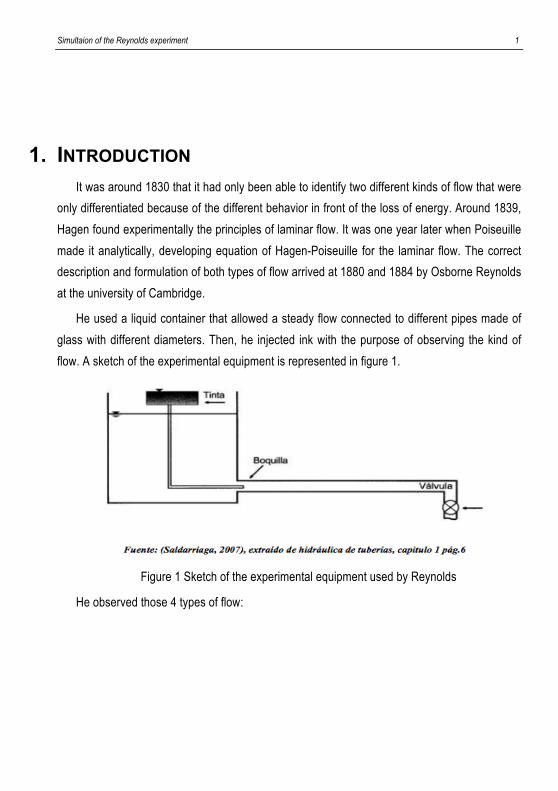
He used a liquid container that allowed a steady flow connected to different pipes made of glass with different diameters. Then, he injected ink with the purpose of observing the kind of flow. A sketch of the experimental equipment is represented in figure 1.
Figure 1 Sketch of the experimental equipment used by Reynolds
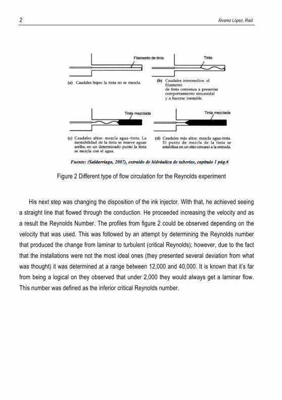
He observed those 4 types of flow:
2 Álvarez López, Raül
Figure 2 Different type of flow circulation for the Reynolds experiment
His next step was changing the disposition of the ink injector. With that, he achieved seeing a straight line that flowed through the conduction. He proceeded increasing the velocity and as a result the Reynolds Number. The profiles from figure 2 could be observed depending on the velocity that was used. This was followed by an attempt by determining the Reynolds number that produced the change from laminar to turbulent (critical Reynolds); however, due to the fact that the installations were not the most ideal ones (they presented several deviation from what was thought) it was determined at a range between 12,000 and 40,000. It is known that it’s far from being a logical on they observed that under 2,000 they would always get a laminar flow. This number was defined as the inferior critical Reynolds number.
Simultaion of the Reynolds experiment 3
THEORETICAL BASIS The Reynolds number shows the relation between the forces of inertia and the forces of
viscosity. The inertial forces, according to the first law of newton make the fluid maintain their velocity and direction while the viscous forces stop the movement of the fluid mainly because of its friction. If the forces of inertia are large it will be in a turbulent flow, in the case that the inertial forces are small it will be in a laminar flow. Between those two it is found the critical zone.
The Reynolds number can be calculated using:
Re=ρ·v'·Dµμ
(1)
Where ρ is the density of the fluid, vm the average speed that flows through the pipe, µ the viscosity and D the diameter of the conduction.
This dimensionless number will allow us to know numerically the kind of flow that it is expected to get. For a Reynolds number under 2100, a laminar state. Between 2,100 and 4,000, the critical zone. Between 4,000 and 10,000, the transient zone where the properties of laminar and turbulent could be found. Finally over 10,000, it would be in a clear turbulent flow.
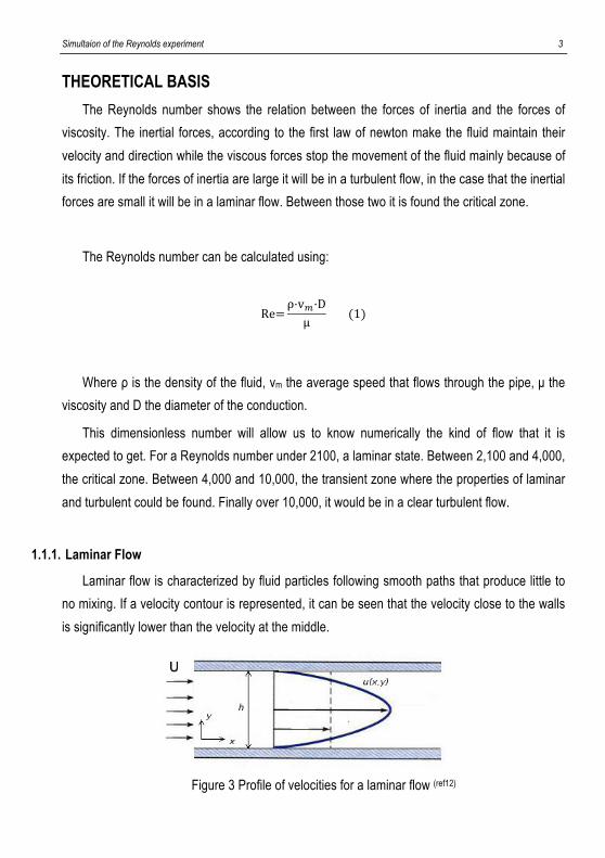
1.1.1. Laminar Flow
Laminar flow is characterized by fluid particles following smooth paths that produce little to no mixing. If a velocity contour is represented, it can be seen that the velocity close to the walls is significantly lower than the velocity at the middle.
Figure 3 Profile of velocities for a laminar flow (ref12)
4 Álvarez López, Raül
This profile can be represented using:
𝑣 = 𝑣'/0 · (1 −𝑟𝑅)4 (2)
Where v is the velocity at a given radius, vmax is the maximum velocity (usually at the middle since is the one with less interaction with the walls that stop it), r is the radius where the velocity wants to be known and R is the Radius of the conduction.
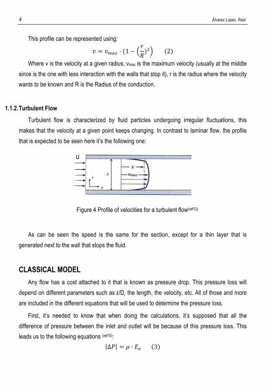
1.1.2. Turbulent Flow
Turbulent flow is characterized by fluid particles undergoing irregular fluctuations, this makes that the velocity at a given point keeps changing. In contrast to laminar flow, the profile that is expected to be seen here it’s the following one:
Figure 4 Profile of velocities for a turbulent flow(ref12)
As can be seen the speed is the same for the section, except for a thin layer that is generated next to the wall that stops the fluid.
CLASSICAL MODEL Any flow has a cost attached to it that is known as pressure drop. This pressure loss will
depend on different parameters such as ε/D, the length, the velocity, etc. All of those and more are included in the different equations that will be used to determine the pressure loss.
First, it’s needed to know that when doing the calculations, it’s supposed that all the difference of pressure between the inlet and outlet will be because of this pressure loss. This leads us to the following equations (ref10):
Δ𝑃 = 𝜌 · 𝐸: (3)
Simultaion of the Reynolds experiment 5
The term Ev represents the pressure loss, that can be developed to:
𝐸: = 4𝑓 ·𝑣'4
2·𝐿𝐷 (4)
Where L is the length of the pipe and 4f the friction factor. This friction factor can be furthermore developed into the following equation only if the roughness (ε/D) is equal to 0 (this means that the surface of the pipe is smooth)
4𝑓 =0.316𝑅𝑒D.4E
(5)
As can be seen this factor will be inversely proportional to the Reynolds, this means that the slower the fluid flows, the bigger the pressure loss will be. Depending if it’s in a laminar state or turbulent it can analytically get to:
For laminar:
𝑣' =∆𝑃 · 𝐷4
32𝜇 · 𝐿 (6)
Combining (1) (3) and (4). For a laminar flow it leads to:
4𝑓 =64𝑅𝑒 (7)
This one can also be arranged to find Ev directly giving:
𝐸: =32𝜇4 · 𝐿𝜌4𝐷J
· 𝑅𝑒 (8)
With a similar approach to the turbulent flow the different equations for the functions Ev=f(Re), Ev/vm=f(Re), Ev/(vm2)=f(Re) can be easily found using:
Laminar:
𝐸: =32𝜇4 · 𝐿𝜌4𝐷J
· 𝑅𝑒 (9)
𝐸:𝑣'
=32𝜇𝐿𝜌 · 𝐷4
(10)
6 Álvarez López, Raül
𝐸:𝑣'4 =
32𝐿𝐷 · 𝑅𝑒
(11)
Turbulent:
𝐸: =0.316𝜇 · 𝐿2𝜌4 · 𝐷J
· 𝑅𝑒M.NE (12)
𝐸:𝑣'
=0.316𝐿 · 𝜇2𝜌 · 𝐷4
· 𝑅𝑒D.NE (13)
𝐸:𝑣'4 =
0.316 · 𝐿2𝐷
· 𝑅𝑒OD.4E (14)
Apart from those equations it will also be needed some relations that might be of basic knowledge like:
𝑞 =𝑉𝑡 (15)
𝑣' =𝑞𝑆 (16)
𝑆 =𝜋𝐷4
4 (17)
COMPUTATIONAL FLUID DYNAMICS (CFD) MODELS Computational fluid dynamics is a part of fluid mechanics that uses numerical analysis to
solve problems that involve fluid flows. Those are used by computers that will simulate the flow of the fluid taking into account any kind of interactions. This kind of programs makes it easier as they provide faster and more accurate solutions. They also allow to work either in 2D or 3D.
They can be found in a wide variety of fields such as flight tests, weather simulation or biomedical engineering. However, they all rely on the same principles, they do a discretization of the space of ordinary differential equations for unsteady problems and algebraic equations for
Simultaion of the Reynolds experiment 7
steady problems. There will also be 2 more methods depending on how we want to integrate ordinary differential equations (Implicit or semi-implicit).
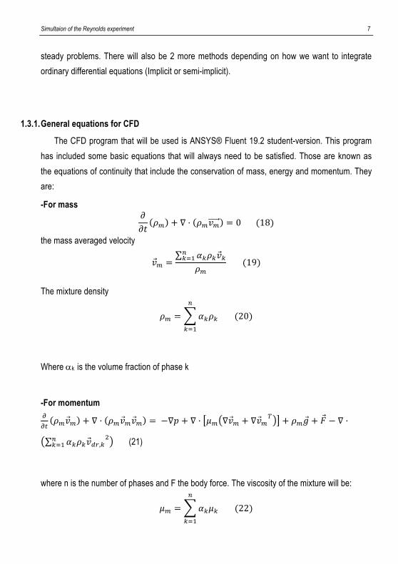
1.3.1. General equations for CFD
The CFD program that will be used is ANSYS® Fluent 19.2 student-version. This program has included some basic equations that will always need to be satisfied. Those are known as the equations of continuity that include the conservation of mass, energy and momentum. They are:
-For mass 𝜕𝜕𝑡
𝜌' + ∇ · 𝜌'𝑣' = 0 (18)
the mass averaged velocity
𝑣' =𝛼Y𝜌Y𝑣YZ
Y[M
𝜌' (19)
The mixture density
𝜌' = 𝛼Y𝜌Y
Z
Y[M
(20)
Where ak is the volume fraction of phase k
-For momentum \\]
𝜌'𝑣' + ∇ · 𝜌'𝑣'𝑣' = −∇𝑝 + ∇ · 𝜇' ∇𝑣' + ∇𝑣'_ + 𝜌'𝑔 + 𝐹 − ∇ ·
𝛼Y𝜌Y𝑣bc,Y4Z
Y[M (21)
where n is the number of phases and F the body force. The viscosity of the mixture will be:
𝜇' = 𝛼Y𝜇Y
Z
Y[M
(22)
8 Álvarez López, Raül
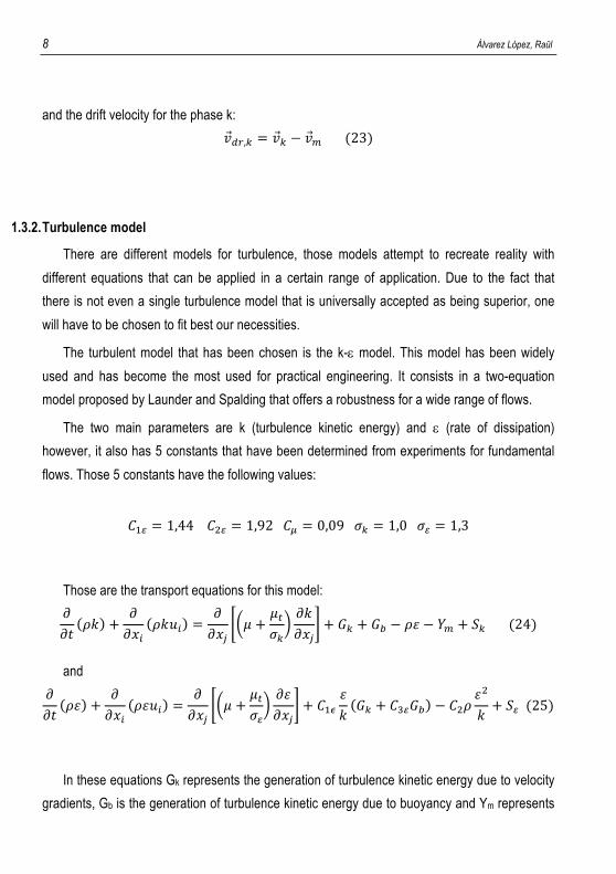
and the drift velocity for the phase k: 𝑣bc,Y = 𝑣Y − 𝑣' (23)
1.3.2. Turbulence model
There are different models for turbulence, those models attempt to recreate reality with different equations that can be applied in a certain range of application. Due to the fact that there is not even a single turbulence model that is universally accepted as being superior, one will have to be chosen to fit best our necessities.
The turbulent model that has been chosen is the k-e model. This model has been widely used and has become the most used for practical engineering. It consists in a two-equation model proposed by Launder and Spalding that offers a robustness for a wide range of flows.
The two main parameters are k (turbulence kinetic energy) and e (rate of dissipation) however, it also has 5 constants that have been determined from experiments for fundamental flows. Those 5 constants have the following values:
𝐶Mf = 1,44 𝐶4f = 1,92 𝐶g = 0,09 𝜎Y = 1,0 𝜎f = 1,3
Those are the transport equations for this model: 𝜕𝜕𝑡
𝜌𝑘 +𝜕𝜕𝑥k
𝜌𝑘𝑢k =𝜕𝜕𝑥m
𝜇 +𝜇]𝜎Y
𝜕𝑘𝜕𝑥m
+ 𝐺Y + 𝐺o − 𝜌𝜀 − 𝑌' + 𝑆Y (24)
and 𝜕𝜕𝑡
𝜌𝜀 +𝜕𝜕𝑥k
𝜌𝜀𝑢k =𝜕𝜕𝑥m
𝜇 +𝜇]𝜎f
𝜕𝜀𝜕𝑥m
+ 𝐶Mr𝜀𝑘𝐺Y + 𝐶Jf𝐺o − 𝐶4𝜌
𝜀4
𝑘+ 𝑆f (25)
In these equations Gk represents the generation of turbulence kinetic energy due to velocity gradients, Gb is the generation of turbulence kinetic energy due to buoyancy and Ym represents
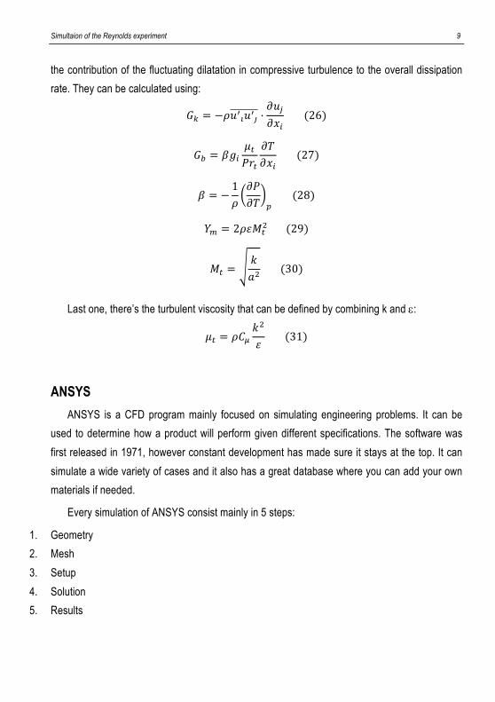
Simultaion of the Reynolds experiment 9
the contribution of the fluctuating dilatation in compressive turbulence to the overall dissipation rate. They can be calculated using:
𝐺Y = −𝜌𝑢st𝑢su ·𝜕𝑢m𝜕𝑥k
(26)
𝐺o = 𝛽𝑔k𝜇]𝑃𝑟]
𝜕𝑇𝜕𝑥k
(27)
𝛽 = −1𝜌𝜕𝑃𝜕𝑇 x
(28)
𝑌' = 2𝜌𝜀𝑀]4 (29)
𝑀] =𝑘𝑎4 (30)
Last one, there’s the turbulent viscosity that can be defined by combining k and e:
𝜇] = 𝜌𝐶g𝑘4
𝜀 (31)
ANSYS ANSYS is a CFD program mainly focused on simulating engineering problems. It can be
used to determine how a product will perform given different specifications. The software was first released in 1971, however constant development has made sure it stays at the top. It can simulate a wide variety of cases and it also has a great database where you can add your own materials if needed.
Every simulation of ANSYS consist mainly in 5 steps:
1. Geometry 2. Mesh 3. Setup 4. Solution 5. Results
10 Álvarez López, Raül
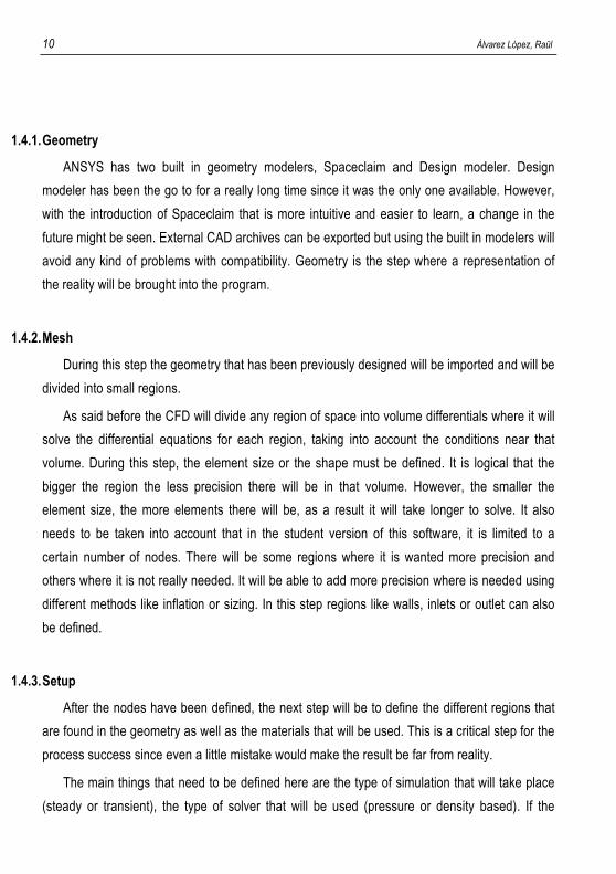
1.4.1. Geometry
ANSYS has two built in geometry modelers, Spaceclaim and Design modeler. Design modeler has been the go to for a really long time since it was the only one available. However, with the introduction of Spaceclaim that is more intuitive and easier to learn, a change in the future might be seen. External CAD archives can be exported but using the built in modelers will avoid any kind of problems with compatibility. Geometry is the step where a representation of the reality will be brought into the program.
1.4.2. Mesh
During this step the geometry that has been previously designed will be imported and will be divided into small regions.
As said before the CFD will divide any region of space into volume differentials where it will solve the differential equations for each region, taking into account the conditions near that volume. During this step, the element size or the shape must be defined. It is logical that the bigger the region the less precision there will be in that volume. However, the smaller the element size, the more elements there will be, as a result it will take longer to solve. It also needs to be taken into account that in the student version of this software, it is limited to a certain number of nodes. There will be some regions where it is wanted more precision and others where it is not really needed. It will be able to add more precision where is needed using different methods like inflation or sizing. In this step regions like walls, inlets or outlet can also be defined.
1.4.3. Setup
After the nodes have been defined, the next step will be to define the different regions that are found in the geometry as well as the materials that will be used. This is a critical step for the process success since even a little mistake would make the result be far from reality.
The main things that need to be defined here are the type of simulation that will take place (steady or transient), the type of solver that will be used (pressure or density based). If the
Simultaion of the Reynolds experiment 11
regions have been defined before, the boundary conditions will have to be defined too. This includes the approach for the simulation, for example if the parameters are pressures or velocity. This will also include defining the properties of the wall, the kind of rigidity and how it will affect the loss of charge.
1.4.4. Solution
It is at this point that it’s needed to indicate what kind of simplifications the program will perform and how it will approach the solution for every time-step. Here it is also defined what range of time wants to be analysed and the parameters that want to be recorded.
Once the process has been initialized the numeric method will try to converge calculating residuals that will indicate if the system has converged or not. Those residuals can be specified to match the amount of the precision that is wanted.
1.4.5. Results
ANSYS has its own software for data presentation. After the simulation has been completed with success, there is the possibility to represent the results in a wide variety of graphics. On those graphics, if they have been defined previously you can set it up so it forms an animation.
This step also allows for post processing, this includes the option of defining charts or graphics for different parameters as well as doing iso-surfaces or section cuts.

Simultaion of the Reynolds experiment 13
2. OBJECTIVE The main aim of this project is comparing the results obtained experimentally with the
results obtained using the simulation software ANSYS fluent. However, all the objectives that want to be achieved are:
• Learning how to use and get used to working with ANSYS as well as the options that it can offer to represent different geometries.
• Generate a simulation that can be used for a wide variety of parameters. • Compare the results obtained in the laboratory with the ones obtained using CFD. • Differentiate the kinds of flows as would be done in the laboratory. • Determine the critical point using the CFD data.

Simultaion of the Reynolds experiment 15
3. MATERIAL AND METHODS This simulation has been done using a fluid dynamics modelling (ANSYS). In the following
subsections details about the methods that have been chosen can be found.
GEOMETRY DESIGN The first step that needs to be done when starting a new simulation is generating a
geometry. This geometry needs to be a general or a more accurate sketch that represents reality.
In this case there is a tube and an interior injection of a fluid that will introduce a tracing fluid. To represent this, it was decided to do it in 2D over 3D, this would allow to make it way simpler and reduce the number of nodes needed. Due to the fact that we are using the student version of ANSYS, we have a limitation for the amount of nodes we can work with. It should be clear that if we solve the 2D problem, because of the geometry, it would be a really similar representation for 3D because of the symmetry of the system.
Once it has been decided to work in 2D over 3D, ANSYS allows you to design your geometry with either SpaceClaim or DesignModeler (there is also the possibility of importing the geometry from other geometry designers such as CAD).
SpaceClaim was chosen since it’s more intuitive and has several functions like undo that the other may not have or are not as intuitive to use.
To represent both tubes, rectangles will be used. As can be expected the edges of this rectangle will represent:
• The inlet at the left edge, being the surface where the fluid will enter the system • The outlet at the right edge, being the surface where the fluid will exit the system • The walls, both top and bottom edges will represent the walls of the tube that will keep the fluid
in the system.
16 Álvarez López, Raül
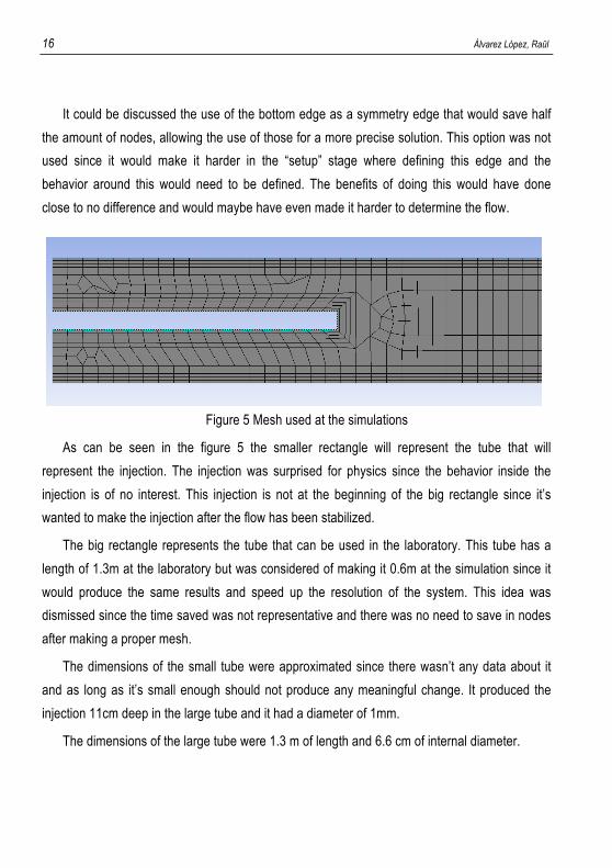
It could be discussed the use of the bottom edge as a symmetry edge that would save half the amount of nodes, allowing the use of those for a more precise solution. This option was not used since it would make it harder in the “setup” stage where defining this edge and the behavior around this would need to be defined. The benefits of doing this would have done close to no difference and would maybe have even made it harder to determine the flow.
Figure 5 Mesh used at the simulations
As can be seen in the figure 5 the smaller rectangle will represent the tube that will represent the injection. The injection was surprised for physics since the behavior inside the injection is of no interest. This injection is not at the beginning of the big rectangle since it’s wanted to make the injection after the flow has been stabilized.
The big rectangle represents the tube that can be used in the laboratory. This tube has a length of 1.3m at the laboratory but was considered of making it 0.6m at the simulation since it would produce the same results and speed up the resolution of the system. This idea was dismissed since the time saved was not representative and there was no need to save in nodes after making a proper mesh.
The dimensions of the small tube were approximated since there wasn’t any data about it and as long as it’s small enough should not produce any meaningful change. It produced the injection 11cm deep in the large tube and it had a diameter of 1mm.
The dimensions of the large tube were 1.3 m of length and 6.6 cm of internal diameter.
Simultaion of the Reynolds experiment 17
MESH GENERATION After the geometry has been imported (either by an ANSYS modeler or any other that is
supported), it will be proceeded with the discretization of the system. In this step, it will be defined how small the differentials of volume will be. In each of this element the differential equations will be solved taking into account the surroundings until it converges into a solution.
To make sure the precision of this model is good enough, a great meshing is a critical step especially closer to the walls when simulating any type of turbulent flows (ref 7). To make sure there are no problems close to the walls an inflation is inserted close to the edges.
The main properties of the mesh are:
• Surface (8.565·10-3) [m2] • Number of nodes (27,800) • Element size (8·10-4)m
The main properties of the inflation are:
• Number of layers (5) • Growth rate (1.2) • Tension ratio (0.272)
The last step before exiting the mesh system will be to generate named selections in order to simplify and ensure that the resolution will be done properly. Those selections that need to be named are the inlet of both tubes and the outlet of those. The wall will be automatically detected by the CFD and assigned as a wall.
SIMULATION SETUP AND POSTPROCESSING After the geometry has been meshed, the next step will be to define all the boundary
conditions as well as the models including the parameters that will be used.
18 Álvarez López, Raül
3.3.1. Models phases
First, at this stage the solver method that will be used needs to be specified. It has been chosen a pressure-based and steady state method so that there are no problems and the profiles should remain constant at any time.
In the simulation it is needed to define two different phases the fluid that would be flowing through the exterior pipe and the one that will be injected. By using the multiphase model those 2 phases will be defined and allow to differentiate the water according to the surface they were injected from.
It will also be defined in here the model of turbulence that wants to be used, as mentioned before in this simulation, k-epsilon model was used. The parameters used for these simulations, where the standard ones without making any changes to the constants that are used.
3.3.2. Boundary conditions
For the boundary conditions, it has been specified the velocity for each simulation as well as the pressure of exit. The velocity has been calculated in order to get Reynolds numbers from 1,000 to 15,000. In this range it’s expected to be able to see all different types of flow.
On this step, it also needs to be defined the fluid, in this case it’s water for both phases. It will also be defined for the injection a 100% of phase 2 and for the exterior tube a 0%.
Here it will also be defined the type of walls that will be used, defining how smooth they are and how they behave.
3.3.3. Initialization and calculation
Once the boundary conditions have been defined, the convergence criteria can be modified in the solution menu. The convergence conditions have been defined to 1x10⁻⁶ for each one of the different parameters. After performing a Standard initialization where there are no extra parameters needed, parameters that want to be tracked can be defined as well as different contour plots or different type of graphics that will allow to generate the animation after the simulation has been solved.
The last step before running the simulation will be to give a maximum number of iterations so that the system will converge.
Simultaion of the Reynolds experiment 19
4. RESULTS AND DISCUSSION In the following sections it will be explained in detail all the data that were obtained. This
includes how it’s been used to find different parameters as well as the information they provide us with.
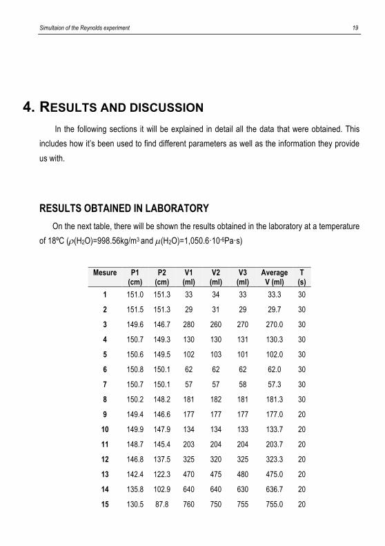
RESULTS OBTAINED IN LABORATORY On the next table, there will be shown the results obtained in the laboratory at a temperature
of 18ºC (r(H2O)=998.56kg/m3 and µ(H2O)=1,050.6·10-6Pa·s)
Mesure P1
(cm) P2
(cm) V1
(ml) V2
(ml) V3
(ml) Average
V (ml) T
(s) 1 151.0 151.3 33 34 33 33.3 30
2 151.5 151.3 29 31 29 29.7 30
3 149.6 146.7 280 260 270 270.0 30
4 150.7 149.3 130 130 131 130.3 30
5 150.6 149.5 102 103 101 102.0 30
6 150.8 150.1 62 62 62 62.0 30
7 150.7 150.1 57 57 58 57.3 30
8 150.2 148.2 181 182 181 181.3 30
9 149.4 146.6 177 177 177 177.0 20
10 149.9 147.9 134 134 133 133.7 20
11 148.7 145.4 203 204 204 203.7 20
12 146.8 137.5 325 320 325 323.3 20
13 142.4 122.3 470 475 480 475.0 20
14 135.8 102.9 640 640 630 636.7 20
15 130.5 87.8 760 750 755 755.0 20
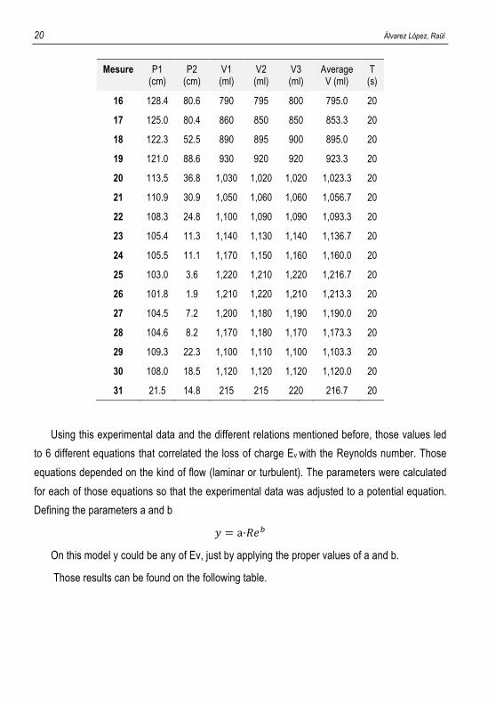
20 Álvarez López, Raül
Mesure P1 (cm)
P2 (cm)
V1 (ml)
V2 (ml)
V3 (ml)
Average V (ml)
T (s)
16 128.4 80.6 790 795 800 795.0 20
17 125.0 80.4 860 850 850 853.3 20
18 122.3 52.5 890 895 900 895.0 20
19 121.0 88.6 930 920 920 923.3 20
20 113.5 36.8 1,030 1,020 1,020 1,023.3 20
21 110.9 30.9 1,050 1,060 1,060 1,056.7 20
22 108.3 24.8 1,100 1,090 1,090 1,093.3 20
23 105.4 11.3 1,140 1,130 1,140 1,136.7 20
24 105.5 11.1 1,170 1,150 1,160 1,160.0 20
25 103.0 3.6 1,220 1,210 1,220 1,216.7 20
26 101.8 1.9 1,210 1,220 1,210 1,213.3 20
27 104.5 7.2 1,200 1,180 1,190 1,190.0 20
28 104.6 8.2 1,170 1,180 1,170 1,173.3 20
29 109.3 22.3 1,100 1,110 1,100 1,103.3 20
30 108.0 18.5 1,120 1,120 1,120 1,120.0 20
31 21.5 14.8 215 215 220 216.7 20
Using this experimental data and the different relations mentioned before, those values led to 6 different equations that correlated the loss of charge Ev with the Reynolds number. Those equations depended on the kind of flow (laminar or turbulent). The parameters were calculated for each of those equations so that the experimental data was adjusted to a potential equation. Defining the parameters a and b
𝑦 = a·𝑅𝑒o
On this model y could be any of Ev, just by applying the proper values of a and b.
Those results can be found on the following table.
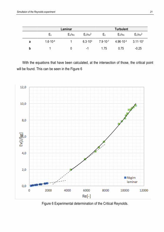
Simultaion of the Reynolds experiment 21
Laminar Turbulent Ev Ev/vm Ev/vm2 Ev Ev/vm Ev/vm2
a 1.6·10-4 1 6.3·103 7.9·10-7 4.96·10-3 3.11·101
b 1 0 -1 1.75 0.75 -0.25
With the equations that have been calculated, at the intersection of those, the critical point will be found. This can be seen in the Figure 6
Figure 6 Experimental determination of the Critical Reynolds.
22 Álvarez López, Raül
As can be seen the value for the critical Reynolds is around the 2,780 value. This is a coherent value since it is inside the critical zone.
VALIDATION OF THE CFD MODEL Before doing any simulation, it is needed to validate that the model that has been designed
works properly. A difference of pressure is applied at the tube and compared with the experimental data.
This is done by using a certain difference of pressure between entry and exit at the CFD that it’s the same as the one that was used at the laboratory. For doing this the cm of the columns that were calculated observed in the laboratory will be converted into Pascals multiplying for 9.8·103. After the pressure is applied and the simulation run, the average velocity is compared using ANSYS and the one in the laboratory.
Those two will show some difference because the wall used in ANSYS will not behave exactly the same as the one of the laboratory since the glass material couldn’t be added. And it’s not as ideal as the one in ANSYS, that is why it’s always obtained a velocity slightly higher than in the laboratory.
RESULTS OBTAINED USING CFD In this section will be described the results obtained using ANSYS. As mentioned before,
these are the results obtained from a transient state where there was a continuous injection.
The simulation was done in the range between 1,000 and 15,000 for the Reynolds number using an increment of 1,000. Here, there will only be displayed one simulation for each kind of flow (All the simulations can be found in the annex). This should allow for a proper determination of the kind of flow that is happening on that Reynolds number. However, using the profile of velocity to determine it as well as in the experimental method there are some kind of flows that are difficult to determine.
Simultaion of the Reynolds experiment 23
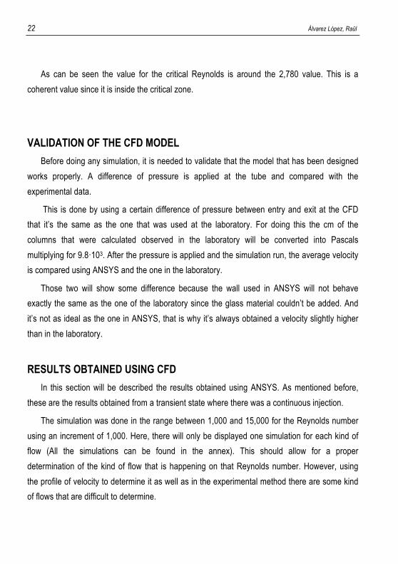
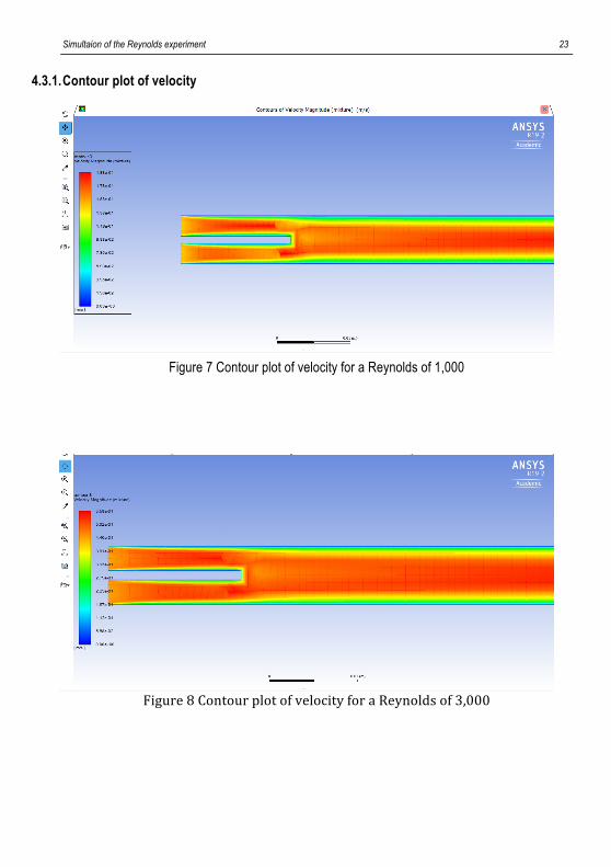
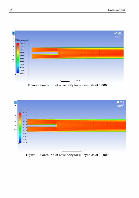
4.3.1. Contour plot of velocity
Figure 7 Contour plot of velocity for a Reynolds of 1,000
Figure 8 Contour plot of velocity for a Reynolds of 3,000
24 Álvarez López, Raül
Figure 9 Contour plot of velocity for a Reynolds of 7,000
Figure 10 Contour plot of velocity for a Reynolds of 15,000
Simultaion of the Reynolds experiment 25
4.3.2. Discussion About the contour plots of velocity
All of the graphics that have been represented have been cut, this is because of inserting the full length (1.3m) of the tube with such small diameter nothing would be noticeable. However, the section that has been cut follows the same patter as the one shown, so no relevant information has been lost.
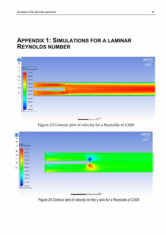
As can be seen on those graphics as we increase The Reynolds number, the layers that are close to the wall become thinner. This is because, as it increases so it does the region that is in the plateau of velocity. It can also be seen the effect that has the section. At the beginning when ANSYS considers the exterior side as individual conductions, the layer is thinner and is clearly increased as soon as the diameter increases.
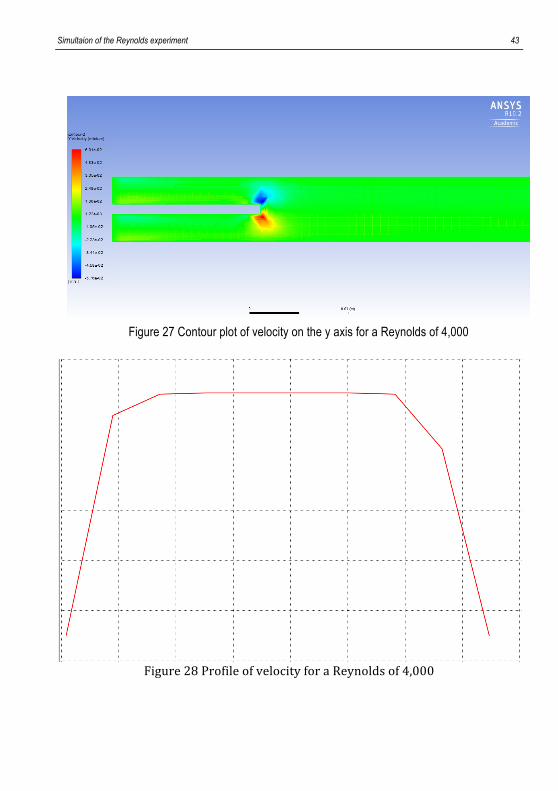
On those contours could be seen the variation of the thickness of the layer next to the wall as the Reynolds number is increased.
4.3.3. Contour plots of velocity in the y axis
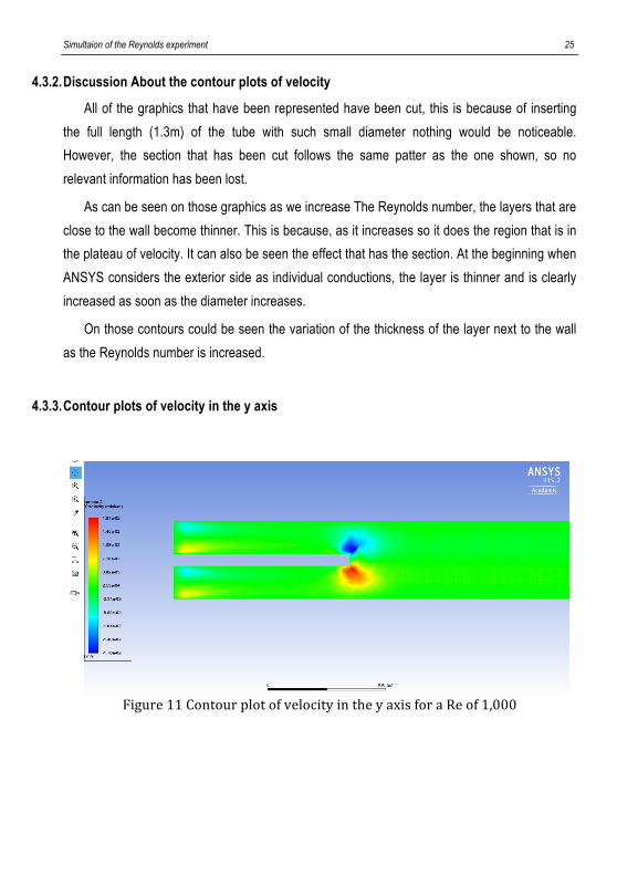
Figure 11 Contour plot of velocity in the y axis for a Re of 1,000
26 Álvarez López, Raül
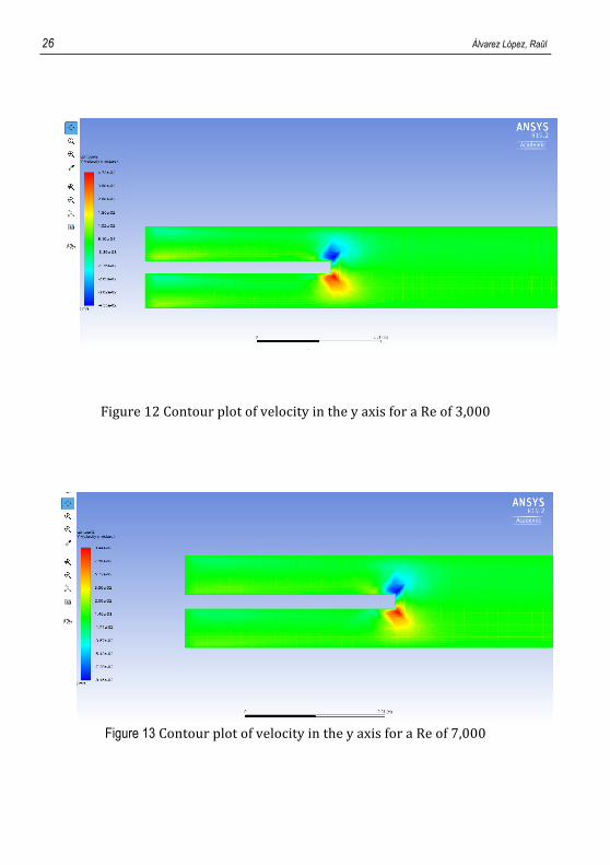
Figure 12 Contour plot of velocity in the y axis for a Re of 3,000
Figure 13 Contour plot of velocity in the y axis for a Re of 7,000
Simultaion of the Reynolds experiment 27
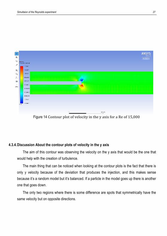
Figure 14 Contour plot of velocity in the y axis for a Re of 15,000
4.3.4. Discussion About the contour plots of velocity in the y axis
The aim of this contour was observing the velocity on the y axis that would be the one that would help with the creation of turbulence.
The main thing that can be noticed when looking at the contour plots is the fact that there is only y velocity because of the deviation that produces the injection, and this makes sense because it’s a random model but it’s balanced. If a particle in the model goes up there is another one that goes down.
The only two regions where there is some difference are spots that symmetrically have the same velocity but on opposite directions.
28 Álvarez López, Raül
4.3.5. Profiles of velocity
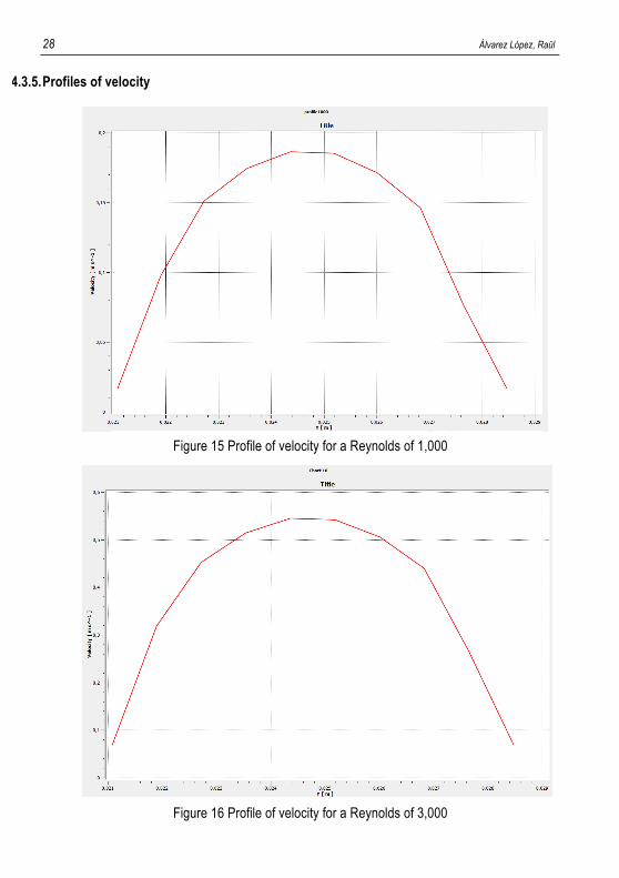
Figure 15 Profile of velocity for a Reynolds of 1,000
Figure 16 Profile of velocity for a Reynolds of 3,000
Simultaion of the Reynolds experiment 29
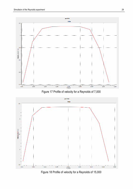
Figure 17 Profile of velocity for a Reynolds of 7,000
Figure 18 Profile of velocity for a Reynolds of 15,000
30 Álvarez López, Raül
4.3.6. Discussion About the profiles of velocity
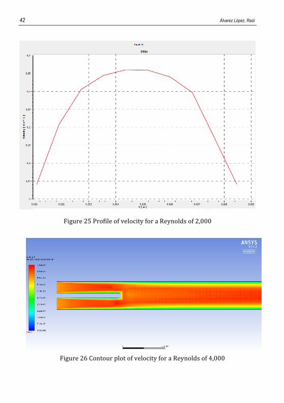
The aim of this chart was to visualize the profiles of velocity that were easily differentiable. On figure 15 and 16 it can be seen the profile expected for a laminar flow (a parabolic shape). As well, for figures 17 and 18 the turbulent flow can be distinguished as a result of being able to observe a clear plateau zone in the middle where all the points have very similar velocity.
If compared figure 15 to 16 it can be noticed that 16 is just by a little wider than 15 (this can be observed taking as a reference the squared background).
Comparing 17 and 18 as before, here it can be observed that the plateau of velocities is wider as the Reynolds number is increased.
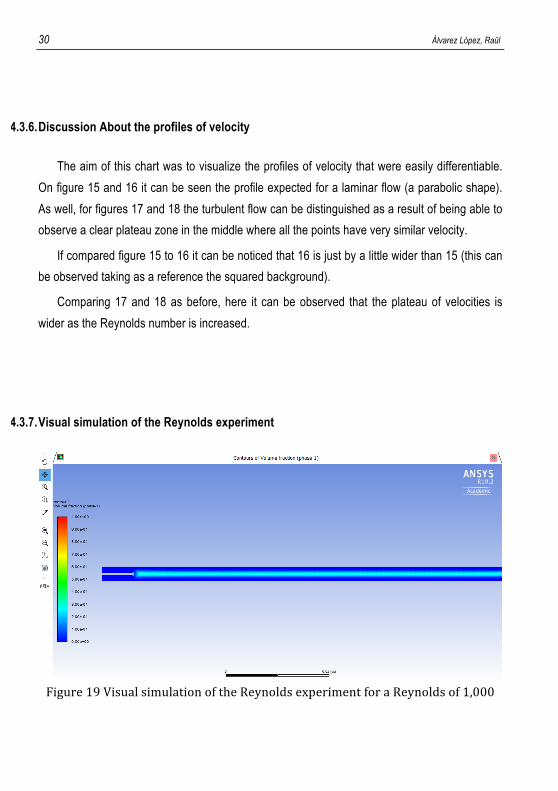
4.3.7. Visual simulation of the Reynolds experiment
Figure 19 Visual simulation of the Reynolds experiment for a Reynolds of 1,000
Simultaion of the Reynolds experiment 31
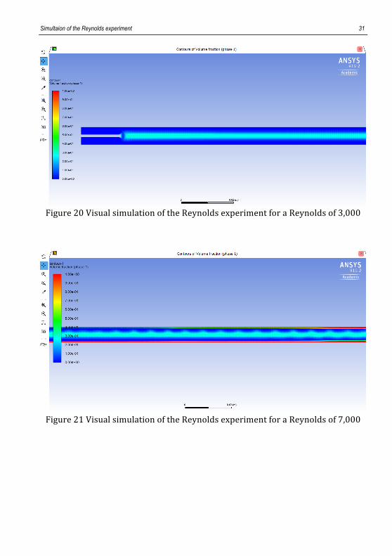
Figure 20 Visual simulation of the Reynolds experiment for a Reynolds of 3,000
Figure 21 Visual simulation of the Reynolds experiment for a Reynolds of 7,000
32 Álvarez López, Raül
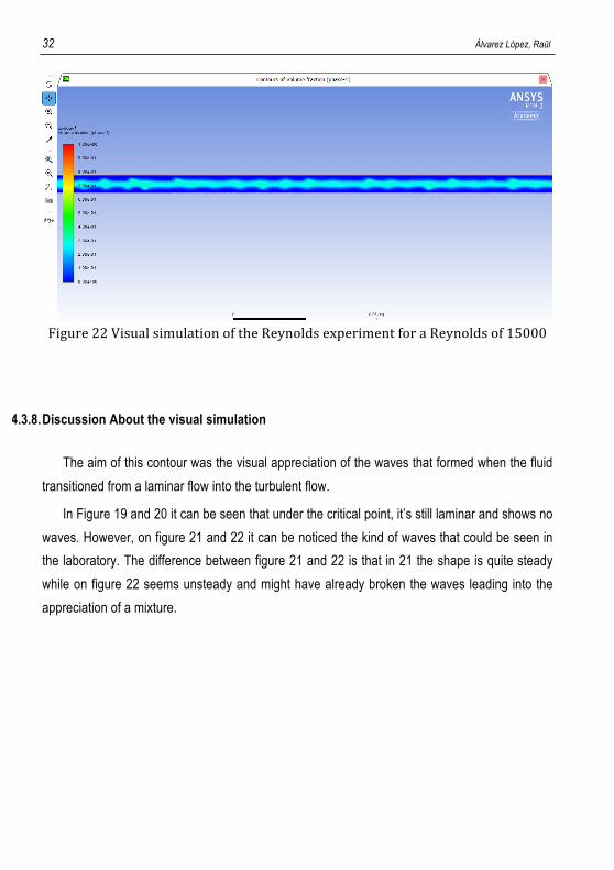
Figure 22 Visual simulation of the Reynolds experiment for a Reynolds of 15000
4.3.8. Discussion About the visual simulation
The aim of this contour was the visual appreciation of the waves that formed when the fluid transitioned from a laminar flow into the turbulent flow.
In Figure 19 and 20 it can be seen that under the critical point, it’s still laminar and shows no waves. However, on figure 21 and 22 it can be noticed the kind of waves that could be seen in the laboratory. The difference between figure 21 and 22 is that in 21 the shape is quite steady while on figure 22 seems unsteady and might have already broken the waves leading into the appreciation of a mixture.
Simultaion of the Reynolds experiment 33
4.3.9. Determination of the critical point
The determination of the critical point has been done by performing different simulations (that can be seen in the Appendix 2) between 3,000-4,000. The objective was to define a critical point within a range of 50. Taking advantage that when using ANSYS the change from laminar into turbulent is not smooth doing a few simulations, it will be achieved.
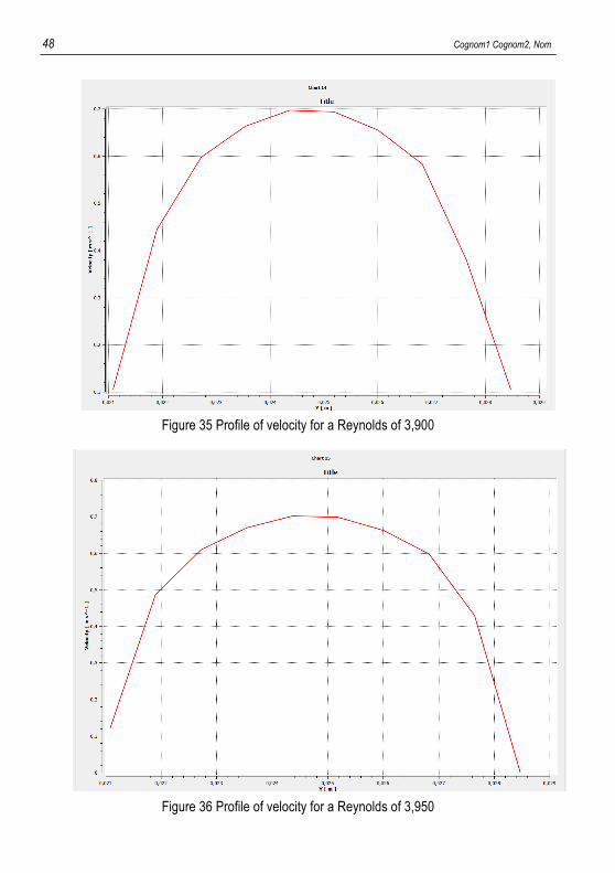
By using the iterative method was obtained a range between 3,950 and 4,000. This is an expected result (on the critical zone between 2,100-4,000), however is still very close to the superior limit. This might be because the change that ANSYS uses it at a given value instead of a smooth approach, as can be seen in the simulations the change from 3,950 to 4,000.
34 Álvarez López, Raül
5. CONCLUSIONS
• Using ANSYS it has been possible to carry out a simulation of the Reynolds experiment • The model used by ANSYS could be used for future simulations since it has been checked that
it behaves as in the laboratory. • The profiles of velocity can be observed and are reliable when it’s not too close to the critical
point. This is because, as it can be seen, the change from laminar is not as smooth as it can be seen in the change from 3,950 to 4,000.
• The critical point that has been calculated using ANSYS is in the range between 3,950 and 4,000.
• The waves that could be observed in the laboratory can be observed in the model used.
Simultaion of the Reynolds experiment 35
REFERENCES AND NOTES 1. Dr. Llorenç Llacuna, Joan. Notes from the subject “transport phenomena” and flow circulation (2018 and
2016) 2. ANSYS Fluent 19.2 Workbench User’s guide. ANSYS, Inc. License Manager Release 19.2 (2019a) 3. ANSYS Meshing User’s guide. ANSYS, Inc. License Manager Release 19.2 (2019b) 4. ANSYS Fluent Theory Guide. ANSYS, Inc. License Manager Release 19.2 (2019c) 5. Levenspiel, O. Flujo de fluidos e intercambio de calor. Barcelona: Reverté (1993) 6. M.Afkhami, A. Hassanpour, M. Fairweather “Effect of Reynolds number on particle interaction”(2018) 7. Willcox, David “Formulation of the k-w turbulence model revisited” (2008) 8. F.M.C. Silva; M.F.Apolinário; A.M.O.Siqueira ; A.L.M. Candian, L.A.F Moreira, M.R. Sarti. “Reynolds
experiment and fundamentals of fluid mechanics” (2017) 9. Perry, R.H. ; Green, D.W. Perry’s Chemical Engineers’ Handbook, 8th Editio. McGraw-Hill: United States of
America (2008) 10. Secció departamental d’enginyeria química, guió de practiques (Experimentació en enginyeria química 1) 11. A. Calderon, G.Vargas, Y. Morales “Construcción de prototipo del experimento de Reynolds”(2017) 12. A. Cubillos CFD con Openfoam (2013)

Simultaion of the Reynolds experiment 37
ACRONYMS ak àVolume fraction of phase k
C1e à Constant used for the turbulence model k-epsilon
C2e àConstant used for the turbulence model k-epsilon
Cµ à Constant used for the turbulence model k-epsilon
D à Diameter of the conduction
e à Rate of dissipation for kinetic energy
Ev àLoss of charge
f à Factor of friction
g à Gravitational acceleration
Gk à Generation of turbulence kinetic energy due to velocity gradients
Gb à Generation of turbulence kinetic energy due to buoyancy
k à Turbulence kinetic energy
L à Length of the conduction
µ à Viscosity
DP à Difference of pressure or pressure drop.
q à Volumetric flow
r à Radius of the interior conduction
38 Álvarez López, Raül
R à�Radius of the external conduction
Re à Number of Reynolds
r à Density
S à Surface
t à Time
sk à Constant used for the turbulence model k-epsilon
se à Constant used for the turbulence model k-epsilon
u à�Velocity
V à Volume
vdr,k �Drift velocity for the phase k�����������������������������
vk à Velocity of the phase k
vmax à Max velocity in a given section
Ym à Contribution of the fluctuating dilatation in compressive turbulence to the overall dissipation rate

Simultaion of the Reynolds experiment 39
APPENDICES

Simultaion of the Reynolds experiment 41
APPENDIX 1: SIMULATIONS FOR A LAMINAR REYNOLDS NUMBER
Figure 23 Contour plot of velocity for a Reynolds of 2,000
Figure 24 Contour plot of velocity on the y axis for a Reynolds of 2,000
42 Álvarez López, Raül
Figure 25 Profile of velocity for a Reynolds of 2,000
Figure 26 Contour plot of velocity for a Reynolds of 4,000
Simultaion of the Reynolds experiment 43
Figure 27 Contour plot of velocity on the y axis for a Reynolds of 4,000
Figure 28 Profile of velocity for a Reynolds of 4,000

44 Álvarez López, Raül
Simulation of the Reynolds experiment 45
APPENDIX 2: PROFILES OBTAINED FOR THE DETERMINATION OF THE CRITICAL POINT
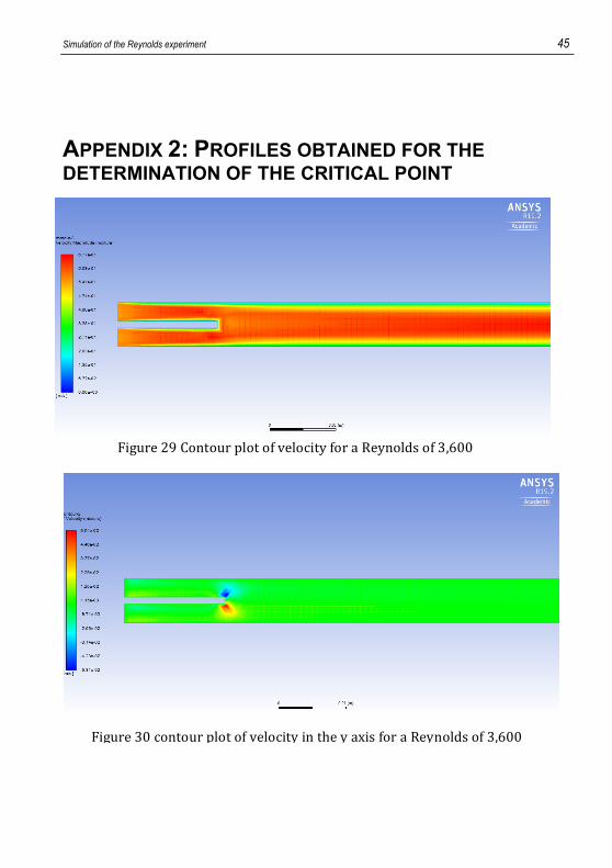
Figure 29 Contour plot of velocity for a Reynolds of 3,600
Figure 30 contour plot of velocity in the y axis for a Reynolds of 3,600
46 Cognom1 Cognom2, Nom
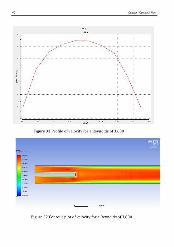
Figure 31 Profile of velocity for a Reynolds of 3,600
Figure 32 Contour plot of velocity for a Reynolds of 3,800
Simulation of the Reynolds experiment 47
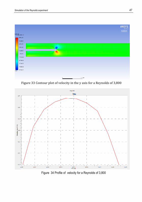
Figure 34 Profile of velocity for a Reynolds of 3,800
Figure 33 Contour plot of velocity in the y axis for a Reynolds of 3,800
48 Cognom1 Cognom2, Nom
Figure 35 Profile of velocity for a Reynolds of 3,900
Figure 36 Profile of velocity for a Reynolds of 3,950

Simulation of the Reynolds experiment 49


![Engineered RNase P Ribozymes Effectively Inhibit the ... · ribozymes were injected into SCID mice by a modified “hydrodynamic transfection” procedure 31], AS [29-expression and](https://img.pdfslide.tips/doc/110x75/5fad68d2a18a2641857d0626/engineered-rnase-p-ribozymes-effectively-inhibit-the-ribozymes-were-injected.jpg)


![Research Article Influence of a Diester …downloads.hindawi.com/journals/jvm/2014/492735.pdfichi Sankyo, Tokyo) ug/kg was injected intravenously [ ]. e serum was collected before](https://img.pdfslide.tips/doc/110x75/5f7ba9d22a14f7750765cf5a/research-article-influence-of-a-diester-ichi-sankyo-tokyo-ugkg-was-injected-intravenously.jpg)