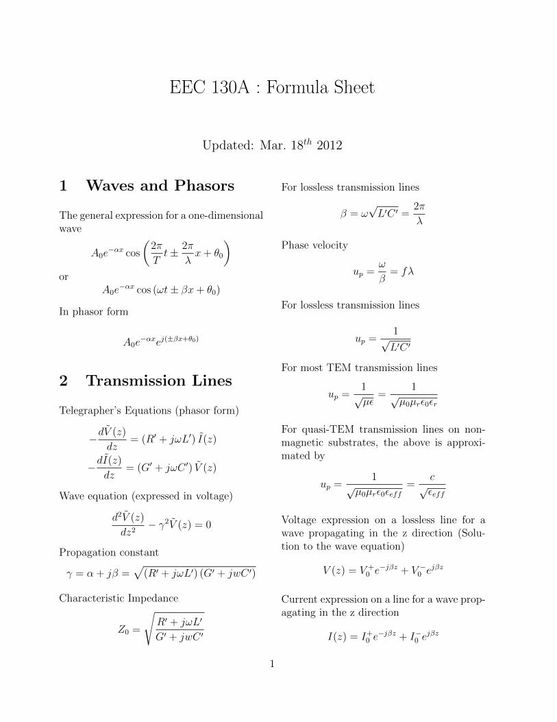
EEC 130A : Formula Sheet

Updated: Mar. 18th 2012

1 Waves and Phasors

The general expression for a one-dimensionalwave

A0e−αx cos

(2π

Tt± 2π

λx+ θ0

)or

A0e−αx cos (ωt± βx+ θ0)

In phasor form

A0e−αxej(±βx+θ0)

2 Transmission Lines

Telegrapher’s Equations (phasor form)

−dV (z)

dz= (R′ + jωL′) I(z)

−dI(z)

dz= (G′ + jωC ′) V (z)

Wave equation (expressed in voltage)

d2V (z)

dz2− γ2V (z) = 0

Propagation constant

γ = α + jβ =√

(R′ + jωL′) (G′ + jwC ′)

Characteristic Impedance

Z0 =

√R′ + jωL′

G′ + jwC ′

For lossless transmission lines

β = ω√L′C ′ =

2π

λ

Phase velocity

up =ω

β= fλ

For lossless transmission lines

up =1√L′C ′

For most TEM transmission lines

up =1√µε

=1

√µ0µrε0εr

For quasi-TEM transmission lines on non-magnetic substrates, the above is approxi-mated by

up =1

√µ0µrε0εeff

=c

√εeff

Voltage expression on a lossless line for awave propagating in the z direction (Solu-tion to the wave equation)

V (z) = V +0 e−jβz + V −0 e

jβz

Current expression on a line for a wave prop-agating in the z direction

I(z) = I+0 e−jβz + I−0 e

jβz

1

Reflection coefficient from load ZL

ΓL =ZL − Z0

ZL + Z0

Voltage standing wave ratio on a line withreflection coefficient ΓL

SWR =|V |max|V |min

=1 + |Γ|1− |Γ|

Position of voltage maximum

dmax =θrλ

4π+nλ

2,

where n = 0, 1, 2, . . . if θr ≥ 0, and n =1, 2, . . . if θr < 0.

Position of voltage minimum

dmin = dmax ±λ

4.

depending on whether dmax is greater or lessthan λ/4.

Input impedance of a transmission line seenat a distance l from a load ZL

Z(l) = Z0ZL + jZ0 tan(βl)

Z0 + jZL tan(βl)

Input reflection coefficient of a lossless trans-mission line seen at a distance l from a loadZL

Γin = Γe−j2βl

3 Electrostatics

Force on a point charge q inside a static elec-tric field

F = qE

Gauss’s law∮S

D · dS = Q or ∇ ·D = ρ

Electrostatic fields are conservative

∇× E = 0 or

∮C

E · dl = 0

Electric field produced by a point charge qin free space

E =q (R−Ri)

4πε0 |R−Ri|3

Electric field produced by a volume chargedistribution

E =1

4πε

∫V ′

R′ρv dV

′

R′2

Electric field produced by a surface chargedistribution

E =1

4πε

∫S′R′ρs ds

′

R′2

Electric field produced by a line charge dis-tribution

E =1

4πε

∫l′R′ρl dl

′

R′2

Electric field produced by an infinite sheetof charge

E = zρs2ε

Electric field produced by an infinite line ofcharge

E =D

ε= r

Dr

ε= r

ρl2πεr

Electric field - scalar potential relationship

E = −∇V or V2 − V1 = −∫ P2

P1

E · dl

2

Electric potential due to a point charge(with infinity chosen as the reference)

V =q

4πε0 |R−Ri|

Poisson’s equation

∇2V = −ρε

Constitutive relationship in dielectric mate-rials

D = ε0E + P

where P is the polarization.

P = ε0χeE

Electrostatic energy density

we =1

2εE2

Boundary conditions

E1t = E2t or n× (E1 − E2) = 0

D1n −D2n = ρs or n · (D1 −D2) = ρs

Ohm’s law

J = σE

Conductivity

σ = ρvµ

where µ stands for charge mobility.

Joule’s law

P =

∫E · J dv

4 Magnetostatics

Force on a moving charge q inside a magneticfield

F = qu×B

Force on an infinitesimally small current el-ement Idl inside a magnetic field

dFm = Idl×B

Torque on a N -turn loop carrying current Iinside a uniform magnetic field

T = m×B

where m = nNIA.

Gauss’s law for magnetism

∇ ·B = 0 or

∮S

B · dS = 0

Ampere’s law

∇×H = J or

∮C

H · dl = I

Magnetic flux density — magnetic vectorpotential relationship

B = ∇×A

Magnetic potential produced by a currentdistribution

A =µ

4π

∫V ′

J

R′dV ′

Vector Poisson’s Equation

∇2A = −µJ

Magnetic field intensity produced by an in-finitesimally small current element (Biot-Savart law)

3

dH =I

4π

dl× R

R2

Magnetic field produced by an infinitely longwire of current in the z-direction

H = φI

2πr

Magnetic field produced by a circular loopof current in the φ-direction

H = zIa2

2(a2 + z2)3/2

Constitutive relationship in magnetic mate-rials

B = µ0H + µ0M

Magnetization

M = χmH

Boundary conditions

B1n = B2n or n · (B1 −B2) = 0

H1t −H2t = Js or n× (H1 −H2) = Js

Magnetostatic energy density

wm =1

2µH2

5 Maxwell’s Equations

Integral form ∮S

D · ds = Q

∮C

E · dl = −∫S

∂B

∂t· ds

∮S

B · ds = 0

∮C

H · dl =

∫S

(J +

∂D

∂t

)· ds

6 Useful Integrals

∫dx√x2 + c2

= ln(x+√x2 + c2)∫

dx

x2 + c2=

1

ctan−1

x

c∫dx(

x2 + c2)3/2 =

1

c2x√

x2 + c2∫x dx√x2 + c2

=√x2 + c2∫

x dx

x2 + c2=

1

2ln (x2 + c2)∫

x dx

(x2 + c2)3/2= − 1√

x2 + c2∫dx

(a+ bx)2= − 1

b(a+ bx)

7 Constants

Free space permittivity

ε0 = 8.85× 10−12 F/m

Free space permeability

µ0 = 4π × 10−7 H/m

4