WORKING PAPER SERIES - · PDF fileThe views expressed in the Working Paper Series are those of the author(s ... North American Free Trade Agreement ... METRs are computed for hypothetical

WORKING PAPER NO. 2011‐18

THE IMPACTS OF VARIOUS TAXES ON FOREIGN DIRECT INVESTMENT By

Stacie Beck and Alexis Chaves

WORKING PAPER SERIES

The views expressed in the Working Paper Series are those of the author(s) and do not necessarily reflect those of the Department of Economics or of the University of Delaware. Working Papers have not undergone any formal review and approval and are circulated for discussion purposes only and should not be quoted without permission. Your comments and suggestions are welcome and should be directed to the corresponding author. Copyright belongs to the author(s).

THE IMPACTS OF VARIOUS TAXES ON FOREIGN DIRECT INVESTMENT

By Stacie Beck* and Alexis Chaves**

ABSTRACT

Previous work on the effect of taxes on foreign direct investment (FDI) focused

primarily on capital income taxes. We investigate the proposition that other forms of taxation

may also deter FDI. We use tax ratios, i.e., average effective tax rates, on consumption, labor and

capital income for a panel of 25 OECD countries from 1975-2006. We find that increases in

relative tax rates on capital income encourage net FDI outflow whereas increases in labor income

tax rates have the opposite effect. Increases in relative consumption tax rates have insignificant

impacts.

JEL: F21, H20, C33

Keywords: Tax Ratio, Foreign Direct Investments

*Department of Economics, University of Delaware, Newark, DE 19716 **Bureau of Economic Analysis, 1441 L Street, NW,Washington, DC 20230. The authors can be reached at [email protected] or [email protected] or (302)831-1915. The views expressed in this paper are solely those of the authors and not necessarily those of the U.S. Bureau of Economic Analysis or the U.S. Department of Commerce.

2

THE IMPACTS OF VARIOUS TAXES ON FOREIGN DIRECT INVESTMENT

Tax policy typically emerges as one of the leading points in a discussion of factors

that can either attract or drive away foreign direct investment (FDI). However, most previous

studies of tax impact on FDI are concerned with taxes levied on corporations or on capital

income. Less attention has been paid to other types of taxes, such as those exacted on workers or

consumers. However, it is possible that other taxes have an influence on FDI as well. Taxes on

labor income and consumption impact the return on work effort. While labor supply may be

inelastic in the short run, so that tax incidence falls on workers, in the longer run labor supply

elasticity is higher. If so, labor income and consumption taxes raise wage costs to employers.

High wage costs could cause domestic firms to substitute capital for labor, thus reducing their

funds for investment abroad. On the other hand, an economy with high wages costs may

experience outflows of investment funds as corporations outsource their production.

In a previous study, Beck and Coskuner (2007) found that taxes impact relative

price, i.e., the real exchange rate, in the direction indicated by theory. A follow-up study found

that export volumes respond to price changes caused by tax changes (Beck and Chaves, 2011).

However, financial flows induced by tax changes may offset their effect on exports. The

objective of this paper is to determine the extent to which this true for three types of taxes:

consumption, labor income and capital income. We find that the impact of increased capital

income tax rates on export volume is partly offset by the investment outflows they induce. The

impact of increased labor income tax rates is significantly negative, suggesting that the capital

substitution effect dominates the outsourcing effect. The impact of increased consumption taxes

is insignificant. Moreover, our estimates of the impact of capital income tax changes is larger

than that found elsewhere in the literature when labor income and consumption tax changes are

taken into account.

3

I. Previous Literature

Previous literature has established a relationship between FDI and one category of

taxes: capital income taxes. De Mooij and Ederveen (2003; 2008) provide useful overviews.

After removing outliers, they calculate a mean value tax elasticity of -3.3, suggesting that a 1

percent reduction in the host country rate of tax on capital would increase total FDI inflows by

3.3 percent. Studies of the impacts of other forms of taxation on FDI are scarce. Egger and

Radulescu (2008) examine labor tax impacts on the location of foreign subsidiaries and find that

both the capital income tax rate and the constructed labor income tax rate have a negative

relationship to the prevalence of subsidiaries or branches of foreign owned corporations. Deasi,

et al. (2004) also find evidence that indirect taxes (taxes other than payroll and corporate income

taxes) depress FDI. However, their study does not distinguish between taxes on capital, labor and

consumption as ours does.

II. Model Specification

We use a gravity model specification to model bilateral FDI outflows, based upon their

success elsewhere in the literature (e.g., Eaton and Tamura, 1994; Razin, et al., 2002; Bénassy-

Quéré et al., 2001). Although the theoretical foundation of the gravity model of FDI is not as

fully developed as it is for trade (by, e.g., Bergstrand, 1985; 1989), there is justification for using

a gravity model to represent horizontal FDI. Most studies that have tested the relationship

between FDI and trade support this idea (Brainard, 1993; Eaton and Tamura, 1994; Ramkishen

and Reinert, 2008).

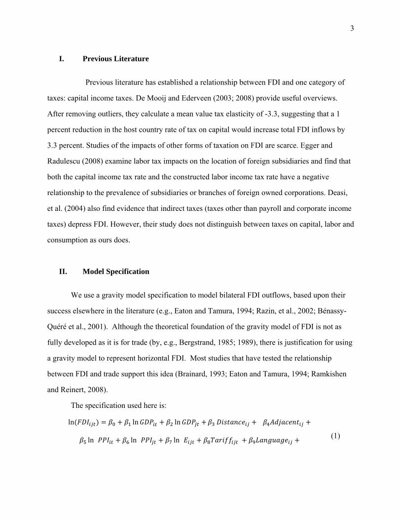
The specification used here is:

ln ln ln

ln ln ln (1)

4

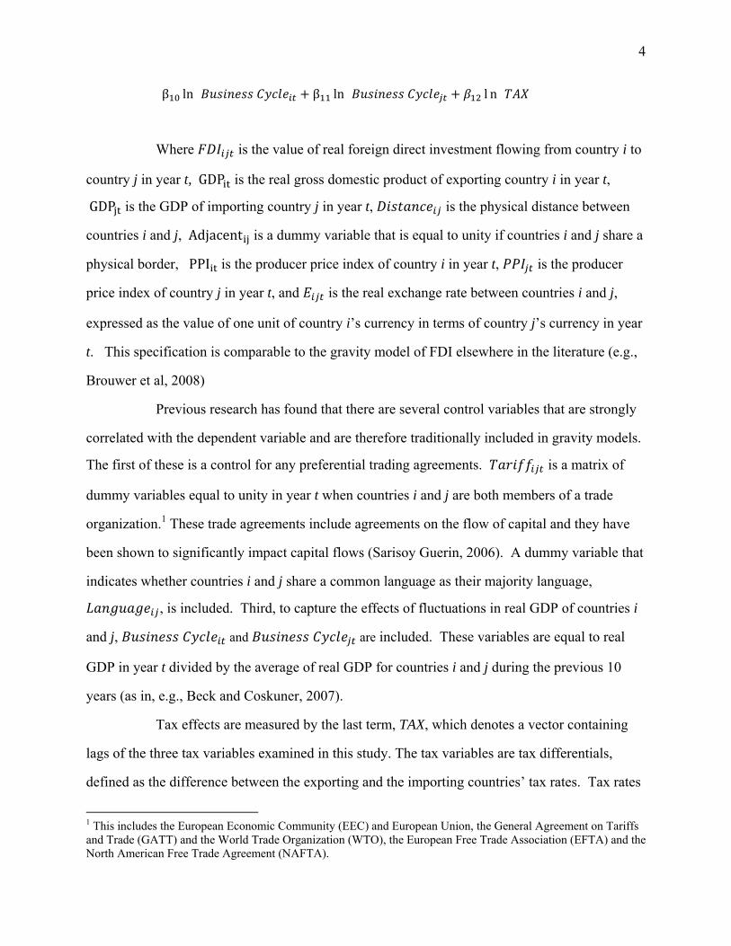
β ln β ln l n

Where is the value of real foreign direct investment flowing from country i to

country j in year t, GDP is the real gross domestic product of exporting country i in year t,

GDP is the GDP of importing country j in year t, is the physical distance between

countries i and j, Adjacent is a dummy variable that is equal to unity if countries i and j share a

physical border, PPI is the producer price index of country i in year t, is the producer

price index of country j in year t, and is the real exchange rate between countries i and j,

expressed as the value of one unit of country i’s currency in terms of country j’s currency in year

t. This specification is comparable to the gravity model of FDI elsewhere in the literature (e.g.,

Brouwer et al, 2008)

Previous research has found that there are several control variables that are strongly

correlated with the dependent variable and are therefore traditionally included in gravity models.

The first of these is a control for any preferential trading agreements. is a matrix of

dummy variables equal to unity in year t when countries i and j are both members of a trade

organization.1 These trade agreements include agreements on the flow of capital and they have

been shown to significantly impact capital flows (Sarisoy Guerin, 2006). A dummy variable that

indicates whether countries i and j share a common language as their majority language,

, is included. Third, to capture the effects of fluctuations in real GDP of countries i

and j, and are included. These variables are equal to real

GDP in year t divided by the average of real GDP for countries i and j during the previous 10

years (as in, e.g., Beck and Coskuner, 2007).

Tax effects are measured by the last term, TAX, which denotes a vector containing

lags of the three tax variables examined in this study. The tax variables are tax differentials,

defined as the difference between the exporting and the importing countries’ tax rates. Tax rates

1 This includes the European Economic Community (EEC) and European Union, the General Agreement on Tariffs and Trade (GATT) and the World Trade Organization (WTO), the European Free Trade Association (EFTA) and the North American Free Trade Agreement (NAFTA).

5

include , which is the difference between consumption tax rates levied by countries i and j

in year t, , for the difference in labor income tax rates and , for the difference in capital

income tax rates. We hypothesize that an increase in the capital income tax rate differential will

increase foreign direct investment outflows so we expect the coefficients of and its lags to

be positive. Labor income taxes and consumption taxes represent taxes on work effort. There are

two possible responses by producers to increases in these taxes. One is to move production

overseas in search of lower labor costs, thus increasing foreign direct investment outflows. The

other is to divert funds toward domestic operations in order to reduce labor costs by increasing

capital intensity, thus reducing investment outflows. Hence, the coefficients of and of

and their lags could have either sign.

In order to capture the cumulative impact of the tax, each specification uses eight

lags of the respective tax variable. We choose eight years as the maximum for the long-term lag

based on the observation that the t-statistics of tax ratios lagged up to eight years were

statistically significant whereas they were insignificant beyond eight years in the vast majority of

models tested.

III. Data

Three methods of calculating tax rates have been used in the literature: statutory tax rates,

tax ratios, i.e., average effective tax rates (AETRs), and marginal effective tax rates (METRs)

(Hajkova et al., 2006; de Mooij and Ederveen, 2008). Statutory tax rates have been widely

viewed as unsatisfactory compared to AETRs (e.g., Egger and Radulescu, 2008; Hajkova, 2006;

Wolff, 2007; de Mooij and Ederveen, 2008). METRs are computed for hypothetical cases and

therefore take into account firms’ expectations of tax burdens.2 However, the advantage of tax

ratios is that they provide data on taxes actually paid, and so incorporate firms’ tax minimizing 2 Bénassy-Quéré et al. (2001) use several measures including tax ratios and METRs. All four measures of capital income taxes are shown to have significant impacts. Papers that have used tax ratios to calculate the tax rate at the microeconomic level are Altshuler and Newlon, (1993), Büttner (2001) and Stowhase (2002). In their survey De Mooij and Ederveen (2008) note that estimates using AETRs are generally larger than those using METRs.

6

strategies. Although they are far from perfect, they are reasonable proxies for marginal tax rates

and therefore, they are used here. We describe these data further below as well as our extensions.

Tax Rates

Mendoza et al. (1994) first calculated tax ratios for the G-7 countries between 1965

and 1988.4 Carey and Rabesona (2002) updated these tax ratio data to include 25 countries

between 1975 and 2000 using the SNA93 National Accounts data. We use their methods,

described in Cary and Tchilinguirian (2000), to extend the tax ratio data to include 25 OECD

countries between 1975 and 2006. To construct the tax ratios, tax revenue data published by the

OECD are divided into components which are levied on consumption, labor, and capital. These

revenues form the numerators of the tax ratios. The denominators are formed by the base on

which each of these taxes were levied and are determined by using each country’s national

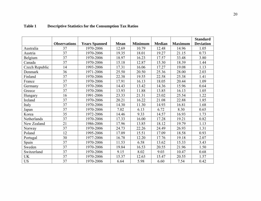
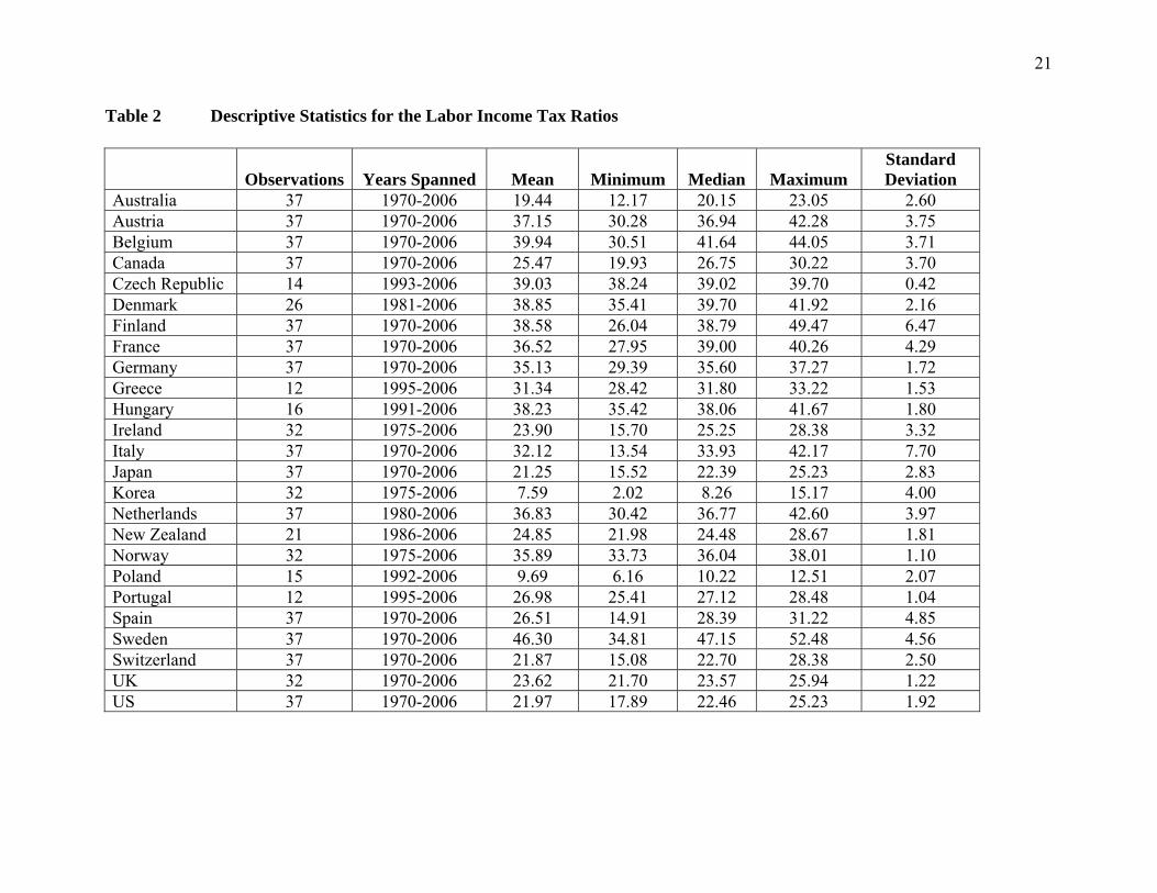
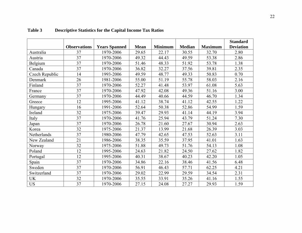
accounts data.5 Tables 1-3 contain descriptive statistics of our updated tax ratio dataset.6

Foreign Direct Investment

Foreign direct investment data are obtained from the Foreign Direct Investment

Statistics published by the OECD.stat database. These data are an unbalanced panel of annual

data containing FDI outward flows between each pair of countries included in this study in

nominal US dollars for 1985 through 2006. These data are converted to real US dollar values

using the OECD’s annual exchange rates and gross total fixed capital formation deflators.

Included in the measure of FDI are earnings from investments by foreign entities that are

retained by some part of the parent organization and transfers of funds from the parent

organization to its foreign entities (either in the form of debt or equity). These data also include

purchases of existing assets and exclude investment funds that are obtained in the host country or

from a third country, hence they are not a perfect measure of foreign direct investment.

4 Volkerink and de Haan (2000) provide an organized and thorough overview of the literature on tax ratio computations alongside of their own calculations of Mendoza, et al. (1997)’s. 5 A detailed description of these calculations can be found in an Appendix supplied upon request. 6 Slight discrepancies with Carey and Rabesona (2002) where our data overlap can be attributed to slightly different data sources and updated revenue and national accounts data.

7

Nevertheless, they are close proxies and, as such, are often used to represent international

investment flows.

Other Explanatory Variables

Most additional data were obtained from the OECD.stat database, with a few

exceptions. is real annual GDP obtained from the OECD national accounts. is a

variable which estimates the physical distance between the two most populous cities for any two

country pairs. Listings for membership in trade organization were found on the WTO website

and the WTO Regional Trade Agreements Information System. The real exchange rate, was

calculated using the nominal exchange rate from the OECD’s Reference Series for Revenue

Statistics and was adjusted using the exporter and importer producer price index as suggested by

Chinn (2006) in the following way:

is the industrial producer price index obtained from the IMF’s International Financial

Statistics Database with missing values in some cases filled in using OECD.stat. This measure

of the price level is based on the revenue received by producers of goods and services so it is free

from sales and excise taxes that are included in other measures of the price level such as the

consumer price index.

IV. Estimation

The proper specification of a panel gravity model is one that contains exporter and

importer country fixed effects, time fixed effects, as well as time-invariant bilateral effects

(Egger and Pfaffermayr, 2003). However, including fixed bilateral effects means that several

time-invariant parameters familiar to gravity models cannot be included in the specification,

including distance, adjacency, whether the countries share a common language, shared

membership in some long-standing trade agreements, etc. According to Egger and Pfaffermayr

(2003), including the fixed bilateral effects in lieu of these types of variables is often a better

8

option. However, to ensure that it is the best option in this particular model, we follow Egger

and Pfaffermayr and empirically test whether including fixed effects is superior to the set of

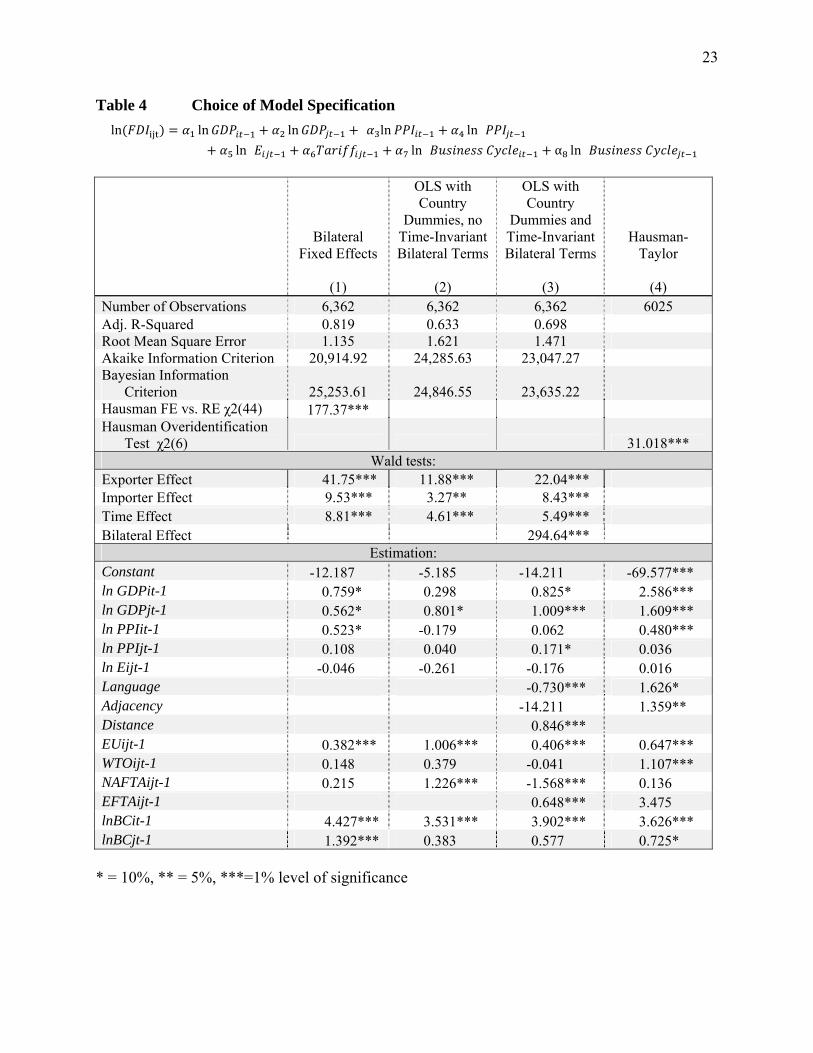
time-invariant bilateral variables mentioned above. We compare three versions of our baseline

gravity model in Table 4. The first model in column 1 includes fixed effects for each country

pair and contains no time-invariant bilateral terms. The second model in column 2 is ordinary

least squares (OLS) that also excludes time-invariant bilateral terms and contains only main

country fixed effects, which are essentially two sets of dummy variables: one for exporting (i)

country and one for importing (j) country. The third model in column 3 also includes main

country fixed effects and is identical to the second but adds in the time-invariant bilateral terms

of distance, adjacency, language and a dummy variable for membership in the European Trade

Association (the only time-invariant trade agreement used in the baseline specification). The

results of several Wald tests lead to the conclusion that the bilateral fixed effects model is the

superior model of these three, as it was in Egger and Pfaffermayr (2003).

In a subsequent paper, Egger (2005) suggests additional criteria to use to determine

whether a fixed effects model is appropriate.7 Following Egger, we first perform a Hausman test

which results in a highly significant χ2 statistic, indicating that the fixed effects model is

consistent while the random effects model is inconsistent. Second, we perform a Wald test that

results in a rejection of the null hypothesis that the set of bilateral fixed effects is equal to zero.8

Third, we determine that a fixed effects model is preferred over a Hausman-Taylor model by

testing whether the instruments, or the exogenous variables in the model, are uncorrelated with

the error term using a Hausman-Taylor over-identification test of the following specification:

7 Under Egger’s criteria, the fixed effects model is appropriate if: (i) the Hausman test rejects the random effects model, (ii) “at least one of the tests of zero exporter and zero importer fixed effects rejects zero” and (iii) the H-T over-identification test rejects (the null hypothesis of which states that the instruments, or the exogenous variables in the model, are uncorrelated with the error term). Our fixed effects model differs slightly from that of Egger in that a full set of bilateral fixed effects is used rather than just fixed effects for exporter and importer countries per the conclusions following Egger and Pfaffermeyer (2003). 8 This fixed effects model differs from that of Egger in that a full set of bilateral fixed effects is used rather than just fixed effects for exporter and importer countries. This is per the conclusions following Egger and Pfaffermeyer (2003).

9

ln FDI ln ln ln

ln ln

α ln α ln

Where the endogenous variables are , , , , and in

some specifications, also any of the tax ratios. The remaining variables are classified as

exogenous and as such, in the H-T model they are used as instruments in order to calculate

values for the endogenous variables. The over-identification tests reject the null hypothesis that

the extra instruments are uncorrelated with the error term (column 4 of Table 4). Therefore, the

fixed effects model is appropriate in this case.

Time Effects

Following Egger (2000), time effects are tested in this model. The results of

likelihood ratio tests performed on each of the three models described above appear in Table 4.

These results show that the χ2 statistic is highly significant in all three cases—indicating that the

null hypothesis of restricting the year effects to zero is rejected. Therefore, time effects are

included in this model although not reported in the following tables.

Endogeneity

There is reason to believe that the dependent variable, FDI in year t, could influence

some of the independent variables in year t. For example, a large increase in FDI from country i

in year t could lead to a significant increase in GDP of country j. To deal with the issue of

endogeneity in the specification, Mendoza et. al. (1997) and Bénassy-Quéré et al. (2001) lagged

all of the time-varying independent variables; we follow this practice as well. Theoretically this

is justified since these variables are likely to affect FDI outflow with a delay. There is also likely

to be a significant lag in the relationship between the exchange rate and FDI. To determine the

appropriate lag of the exchange rate, we used the baseline model below and compared the same

specification with the exchange rate lagged 1, 2 and 3 years. The value of the exchange rate

lagged one year had the highest level of significance based on the t-statistic and thus we chose to

use this for the final specification.

10

Multicollinearity

Tax ratios are possibly correlated with real GDP because they are constructed using

a portion of GDP as the tax base.9 Mendoza et al. (1997) use a lagged value of tax ratios as

instruments in order to avoid this issue. Because the time-variant terms have already been

lagged in order to avoid concerns over endogeneity, following this solution would require that

the tax ratios be lagged by two time periods if it was determined that the multicollinearity

between taxes and GDP was of significant magnitude. This is avoided, however, because

analysis of the data shows that although there is significant correlation between GDP and the tax

ratios, the impact that this correlation has on the estimates from the model appear to be

minimal.10

Tax ratios themselves maybe collinear, i.e., either positively or negatively correlated.

The positive correlation would result if a government decided to use an expansionary or

contractionary policy and thereby decreased or increased all types of taxes. A negative

correlation would result from a government attempting to shift the tax burden from one base to

another if minimum revenue is desired. Analysis of the data shows that either of these

explanations is plausible for different countries. Countries that have positively correlated labor

and capital tax ratios, which are each negatively correlated with the consumption tax ratio,

include: Austria, Belgium, Canada, France, Greece, Japan, the Netherlands, Portugal and the US.

Countries for which all three tax ratios are positively correlated include: Australia, Finland,

Germany, Hungary, Iceland, Ireland, Italy, Korea, New Zealand, Norway, Poland, the Slovak

Republic, Spain and Sweden. Further robustness checks were performed. These involve

comparing estimates when one or more tax variables is removed or when small portions of data

are removed. The overall conclusions regarding sign and significance are unchanged with two

9 This problem does not seem to be a concern to those who have used both tax ratios and a measure of GDP as explanatory variables within the same equation, such as Bénassy-Quéré et al. (2001). 10 The analysis involved the comparison of several versions of the basic model each including combinations of tax ratios lagged by between one and ten years. Based on the fact that the t-statistics of the GDP and tax ratio coefficients and the R2 value were little changed by these variations, there is little evidence that correlation between GDP and the tax ratios has a meaningful impact on the results.

11

exceptions. The cumulative impact of an increase in the labor income tax variable is significantly

negative when either the capital income tax variable is included or a measure of the overall tax

burden is included, whereas it is insignificant alone. Also, the cumulative impact of capital

income taxes is always significantly positive whether included singly or together, but the

magnitude is greater when labor income tax rates are controlled for. Since our results along with

those in previous studies indicate that the capital income tax variable is significant, we concluded

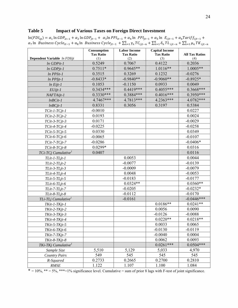
that the specification which includes all three tax variables is most appropriate. Table 5 provides

estimates when tax ratios included singly and together.11 Later tables include all three tax ratios.

Heteroskedasticity

The main specification for the gravity model is also tested for the presence of

heteroskedasticity by calculating a modified Wald statistic for groupwise heteroskedasticity in

the residuals of the fixed effect regression models. In all three cases, the null hypothesis of

homoskedasticity is rejected. As a result, all of the estimations included in this research are

reported with heteroskedasticity-robust standard errors.

Serial Correlation

The specification was tested for evidence of first order serial correlation in the

residuals of the heteroskedasticity-robust fixed effect regression models. Without serial

correlation present, the residuals from the regression of the first-differenced variables should

have an autocorrelation of -0.5 (Wooldridge, 2002). To determine whether this is the case, we

use a Wald test of whether in a regression of the lagged residuals on the current residuals the

coefficient of the lagged residuals is equal to -0.5. In all three cases, the null hypothesis of no

serial correlation was rejected. A fixed effects model assumes that error components within a

group (or country in the current case) are equally-well correlated with every other observation

within the group (Nichols and Schaffer, 2007). However, the presence of serial correlation in the

fixed effects model shows that in this case that assumption is not valid. Instead, there is

11 Results including pairwise comparisons for full sample and subsamples and comparisons with and without a measure of overall tax burden are available upon request.

12

evidence that the errors are clustered, meaning that observations for each exporting country are

correlated, although they are not correlated across country pairs. The same is true for the

importing countries. Since these groups overlap (one is not contained within another), the errors

in the current research are subject to non-nested two-way clustering. The assumptions under a

model with clustered errors are more relaxed than under the fixed effects model since one still

assumes that there is no correlation of the error terms across groups, but the errors within each

group may have any correlation (Nichols and Schaffer, 2007).

Cluster-robust standard error estimators only converge to their true values as the

number of clusters approaches infinity, which in practice has been shown to be around 50

(Nichols and Schaffer, 2007). In addition, these estimators have been shown to be less accurate

in cases when the cluster sizes are unequal. Both of these issues pose difficulties in the current

study where there are 25 countries (hence 25 clusters) and some countries have more complete

time series than others. Therefore, it is quite possible that cluster-robust standard error estimates

are less accurate than those produced by the model that does not account for serial correlation.

To evaluate how cluster-robust standard errors perform in a setting similar to our

own, we turn to a paper by Cameron et al. (2006). In it, the authors evaluate a method of

estimating cluster-robust standard errors in the presence of multi-level clustering by comparing

its hypothesis test rejection rates with those of other estimation methods for different numbers of

clusters. The results most relevant to the current research are those produced for a model with

random effects common to each group and a heteroskedastic error term where the number of

two-way clusters is equal to 30. Although this analysis is not perfectly analogous to the current

research, it sheds some light on the appropriateness of using this type of estimation procedure.

The authors find the most accurate rejection rates for the estimation models that assume

independently and identically distributed errors (no serial correlation) or that allow for only one-

way clustered errors. This result implies that the standard errors produced by a two-way cluster-

robust model would be further from their true values than if the clustered errors are ignored.

Hence we ignore serial correlation in the current study.

13

V. Results

Estimates with tax ratios included singly and together appear in Table 5. Subsequent

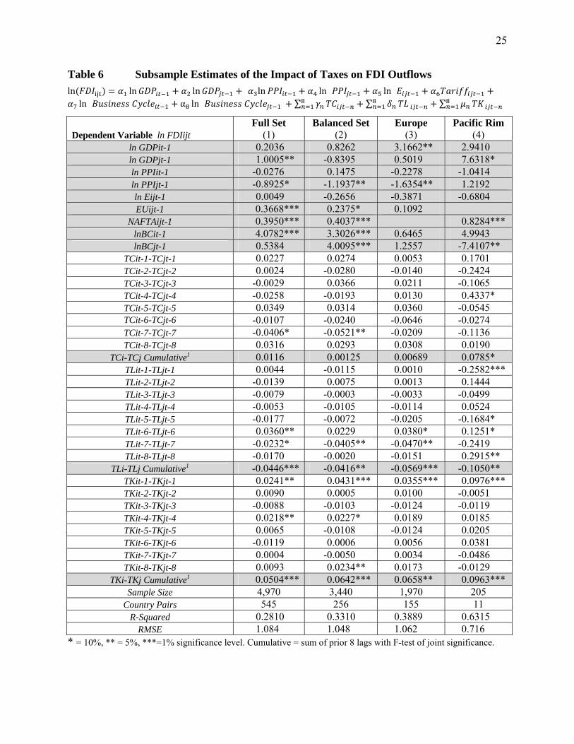
tables include all three tax ratios. Tables 6 reports estimates for subsamples and Table 7 lists

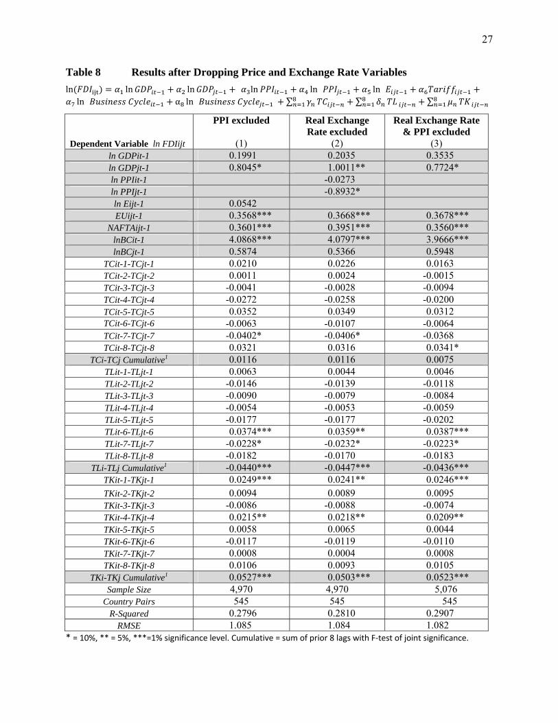
countries included in each subsample. Tables 8 and 9 report estimates for variations of the base

specification.

Most of the coefficients of the explanatory variables have the hypothesized signs.

Real GDP for both the source and destination country have consistently positive signs as

expected, although generally only the coefficient of the GDP of the destination country is

significant. In most specifications tested, the price level of the destination country has a

statistically significant negative impact, indicating that countries with rising prices are less likely

to attract FDI. This result is consistent with the findings of Stein and Daude (2001) who showed

that inflation in the destination country decreases FDI flows. The real exchange rate has no

statistically significant impact on FDI flows, which is similar to results found by Brouwer et al.

(2008). The business cycle of the home country has a positive effect on outflows of FDI in most

cases whereas the business cycle of the destination country generally has an insignificant effect

on FDI flows. Two exceptions occur in subsamples, where the balanced panel regression shows a

significant positive effect whereas the Pacific Rim shows a significant negative effect of the

destination country’s business cycle on FDI outflows. This finding is consistent with mixed

results found by Frenkel et al. (2004). Common membership in the EU and NAFTA was shown

to increase FDI outflows, which is consistent with the findings of Frankel and Wei (1996). The

dummy variables for WTO and EFTA membership do not appear in the results because

membership does not vary across the time and mix of countries included in the dataset, which

was constrained by the availability of bilateral FDI data.

In our discussion below, the cumulative impact of tax changes on FDI refers to the

sum of the coefficients of the lagged tax variables from one to eight years (∑ ) and the

14

statistical significance is determined by a test of joint significance on those lags. The coefficients

are semi-elasticities, i.e., the percentage change in outflows of FDI with respect to a one

percentage point change in the difference between the source and destination countries’ taxes.

To illustrate, the coefficient of the capital income tax ratio differential lagged one year is 0.024

and the long-run coefficient is 0.050 (column 4 of Table 4). If a country increases its average

effective capital income tax by one percentage point while its trading partners keep its capital

income taxes constant, the result will be an increase in FDI outflows of 2.4 percent in the current

year and a cumulative increase in FDI outflows of 5 percent over the eight year period. To put

this into perspective using the example of the US, which had total FDI outflows of $224 billion

in 2006, assuming a US capital income tax ratio that is increased from 27 to 28 percent, US FDI

outflows would increase by 0.024 X $224 billion, or $5.4 billion in the year of the tax increase.

Over an eight year period, an estimate of the increase in FDI outflows would be 0.05 X $224

billion, or $11.2 billion. Below we discuss the estimated impact of each type of tax.

Capital Income Tax

The capital income tax has a statistically significant positive effect on outflows of

FDI in all regressions, confirming the results of numerous prior studies. Significant coefficients

occur in the lags of the first four years. Table 5 shows that the cumulative effect is 0.026 when

the capital income tax is included alone. However, the cumulative effect appears higher, at

0.050, when the effects of labor income and consumption tax changes are included. The

magnitudes of our estimated semi-elasticities are similar to the average semi-elasticity of .033

cited in the survey by de Mooij and Ederveen (2008) and Bénassy-Quéré et al. (2001) who found

.042 using the corporate tax rate differential. Table 6 shows estimates for subsamples; these

include FDI flows to other members of the same subsample. Subsample members are listed in

Table 7. The estimated semi-elasticities for FDI flows between countries in the subsamples are

higher: for the European subsample it is .067 and for the Pacific Rim subsample it is .096. The

conclusion that changes in capital income tax rates have a significant positive impact on FDI

outflows is unchanged by variations in specifications as shown in Tables 8 and 9.

15

Labor Income Tax

The effect of changes in the labor income tax rate differential is more ambiguous, as

theory suggests. There appears to be a significant positive effect on outflows after a lag of six

years, possibly reflecting low labor supply elasticity in the short run that initially keeps wage

increases in check. Overall, the cumulative effect is significantly negative when controlling for

the impact of the other taxes. This would seem to indicate that the dominant impact of

increasing labor income taxes is to reduce FDI outflows, possibly because firms are spending

funds to substitute capital for labor domestically; a more definitive answer awaits further

research. This result is consistent across subsamples and alternative specifications. The effect is

stronger for the Pacific Rim subsample, possibly reflecting less rigid labor markets in these

countries relative to European labor markets.

Consumption Tax

Estimates of the impact of changes in the consumption tax rate differential do not

consistently show a significant impact on FDI outflows. Estimates of the cumulative effect of

changes in consumption tax are likewise insignificant. We conclude that consumption taxes do

not affect FDI outflows.

VI. Conclusions

Our study finds that higher capital income taxes encourage international investment

outflow from high-tax countries to low-tax countries, as in previous studies. Our estimate of the

impact of capital income tax changes is higher than previous studies when changes in labor

income taxes and consumption taxes are controlled for. Additionally, we estimate the impact of

capital income tax changes to be much higher in a subsample of Pacific Rim countries.

We find that higher labor income taxes reduce international investment outflow from

high-tax countries. We conjecture that this is because the incentive to replace labor with capital

causes firms to redirect investment toward domestic operations, at least in the near term. The

16

effect appears to outweigh the incentive to outsource operations abroad. This is a hypothesis that

remains to be investigated further. We find that consumption taxes, which might also be viewed

as taxes on work effort, have little impact on international investment flows.

This paper answers a question raised in Beck and Chaves (2010) which estimated the

impact of changes in these three taxes: capital income, labor income and consumption, on

exports. The question there was: do tax increases induce increases in investment outflow that

mask their impact on export competitiveness? We conclude that the effect of increases in capital

income taxes on exports is indeed offset by investment outflows whereas the effect of increases

in labor income taxes or consumption taxes on exports is not.

Governments that establish relatively high capital income taxes will drive more

investment abroad and attract less international investment. This evidence adds even more

support to the idea that when reforming tax policies, there is good reason for governments to take

account of the impacts of tax policy on its country’s attractiveness to investment flows.

17

REFERENCES

Altshuler, R., H. Grubert and T. S. Newlon. “Has US Investment Abroad become more Sensitive to Tax Rates?” In James R. Hines, Jr. (ed.), International Taxation and Multinational Activity. Chicago, IL: University of Chicago Press. (2001)

Beck, Stacie, and Alexis Chaves "The Impact of Taxes on Trade Competitiveness." Working Paper, University of Delaware Economics Dept. (2011).

Beck, Stacie, and Cagay Coskuner "Tax Effects on the Real Exchange Rate." Review of International Economics 15, no. 5 (2007): 854-868.

Bénassy-Quéré, Agnès, Lionel Fontagné and Amina Lahrèche-Révil. “Tax Competition and Foreign Direct Investment,” Mimeo, CEPII, Paris. (2001).

Bergstrand, Jeffrey H. “The Generalized Gravity Equation, Monopolistic Competition, and the Factor-Proportions Theory in International Trade.” Review of Economics and Statistics. 71, no. 1 (Feb. 1989): 143-153.

Bergstrand, Jeffrey H. “The Gravity Equation in International Trade: Some Microeconomic Foundations and Empirical Evidence.” Review of Economics and Statistics. 67, no. 3 (Aug. 1985): 474-481.

Brainard, S. Lael. “An Empirical Assessment of the Factor Proportions Explanation of Multinational Sales.” NBER Working Paper No. 4583. (Dec. 1993).

Brouwer, Jelle, Richard Paap and Jean-Marie Viaene. “The Trade and FDI Effects of EMU Enlargement.” Journal of International Money and Finance. No. 27 (2008): 188-208.

Büttner, Thiess “The impact of taxes and public spending on FDI: an empirical analysis of FDI-flows within Europe.” ZEW Discussion Paper 02-17 (2001).

Cameron, A. Colin, Jonah B. Gelbach and Douglas L. Miller. “Robust Inference with Multi-way Clustering.” NBER Technical Working Paper No. 327. (Sept. 2006).

Carey, David, and Josette Rabesona.. "Tax Ratios on Labour and Capital Income and on Consumption." OECD Economic Studies No. 35 (2002): 129-174.

Carey, David, and Harry Tchilinguirian. "Average Effective Tax Rates on Capital, Labour and Consumption." OECD Economics Department Working Papers, No. 258, OECD Publishing. (2000).

de Mooij, Ruud A., and Sjef Ederveen. "Taxation and Foreign Direct Investment: A Synthesis of Empirical Research." International Tax and Public Finance 10, no. 6 (Nov. 2003): 673-693.

de Mooij, Ruud A., and Sjef Ederveen. "Corporate Tax Elasticities: A Reader’s Guide to Empirical Findings." Oxford Review of Economic Policy 24, no. 4 (2008): 680-697.

18

Desai, Mihir A., Fritz Foley, and James R. Hines. "Foreign Direct Investment in a World of Multiple Taxes." Journal of Public Economics 88, (2004): 2727-2744.

Eaton, Jonathan, and Akiko Tamura. "Bilateralism and Regionalism in Japanese and U.S. Trade and Direct Foreign Investment Patterns." Journal of the Japanese and International Economies 8, no. 4 (Dec. 1994): 478-510.

Egger, Peter. "Alternative Techniques for Estimation of Cross-Section Gravity Models." Review of International Economics 13, no. 5 (2005): 881-891.

Egger, Peter. "A Note on the Proper Econometric Specification of the Gravity Equation." Economics Letters 66, no. 1 (Jan. 2000): 25-31.

Egger, Peter, and Michael Pfaffermayr. "The Proper Panel Econometric Specification of the Gravity Equation: A Three-Way Model with Bilateral Interaction Effects." Empirical Economics 28, no. 3 (Jun. 2003): 571-580.

Egger, Peter, and Doina Maria Radulescu. "Labour Taxation and Foreign Direct Investment."

CESifo Working Paper No. 2309 (May 2008).

Frankel, Jeffrey, and Shang-Jin Wei. "ASEAN in a regional perspective." In Hicklin, J., Robinson, D., and Singh, A. (eds) Macroeconomic Issues Facing ASEAN Countries. Washington, DC: International Monetary Fund, (1996): 311-365.

Frenkel, Michael, Katja Funke and Geor Stadtmann. “A Panel Analysis of Bilateral FDI Flows to Emerging Economies.” Economic Systems 28 (2004): 281-300.

Hajkova, Dana, Giuseppi Nicoletti, Laura Vartia, and Kwang-Yeol Yoo. "Taxation and Business Environment as Drivers of Foreign Direct Investment in OECD Countries." OECD Economic Studies (2006): 7-38.

King, Mervyn A., and Don Fullerton, eds. The Taxation of Income from Capital: A Comparative Study of the United States, United Kingdom, Sweden and West Germany, The National Bureau of Economic Research (1984).

Mendoza, Enrique G., Gian Maria Milesi-Ferretti, and Patrick Asea. "On the Ineffectiveness of Tax Policy in Altering Long-Run Growth: Harberger's Superneutrality Conjecture." Journal of Public Economics 66, no. 1 (Oct. 1997): 99-126.

Mendoza, Enrique G., Razin, Assaf, and Linda L. Tesar. "Effective Tax Rates in Macroeconomics: Cross-Country Estimates of Tax Rates on Factor Incomes and Consumption." Journal of Monetary Economics 34, no. 3 (Dec. 1994): 297-323.

Nichols, Austin and Mark Schaffer. “Clustered Errors in Stata.” Research Papers in Economics (Sept. 2007): http://repec.org/usug2007/crse.pdf.

Ramkishen S. Rajan and Kenneth A. Reinert, eds. “Vertical Versus Horizontal FDI” Princeton Encyclopedia of the World Economy, Princeton University Press (2008).

19

Razin, Assaf, Ashoka Mody, and Efraim Sadka. "The Role of Information in Driving FDI: Theory and Evidence." NBER Working Paper No. 9255 (Oct. 2002).

Sarisoy Guerin, Selen. "The Role of Geography in Financial and Economic Integration: A Comparative Analysis of Foreign Direct Investment, Trade and Portfolio Investment Flows." World Economy 29, no. 2 (Feb. 2006): 189-209.

Stowhase, Sven. "Tax-Rate Differentials and Sector-Specific Foreign Direct Investment: Empirical Evidence from the EU." FinanzArchiv 61, no. 4 (Feb. 2002): 535-558.

Stein, Ernesto and Christian Daude. “Institutions, Integration and the Location of Foreign Direct Investment.” Global Forum on International Investment: New Horizons for Foreign Direct Investment. (2001): 101-128.

Volkerink, Bjorn and Jakob de Haan. “Tax Ratios: A Critical Survey.” OECD Tax Policy Studies No. 5 (2000).

Wooldridge, J. M. Econometric Analysis of Cross Section and Panel Data. Cambridge, Massachusetts: The MIT Press (2002).

20

Table 1 Descriptive Statistics for the Consumption Tax Ratios

Observations Years Spanned Mean Minimum Median MaximumStandard Deviation

Australia 37 1970-2006 12.69 10.79 12.48 14.96 1.05 Austria 37 1970-2006 19.35 18.01 19.27 21.15 0.73 Belgium 37 1970-2006 18.97 16.23 17.57 33.48 3.80 Canada 37 1970-2006 15.18 12.87 15.30 18.39 1.44 Czech Republic 14 1993-2006 17.31 16.06 17.27 19.08 1.13 Denmark 36 1971-2006 25.50 20.50 25.36 28.00 2.03 Finland 37 1970-2006 22.38 19.55 22.58 25.38 1.41 France 37 1970-2006 17.91 16.13 18.05 20.44 1.09 Germany 37 1970-2006 14.43 13.42 14.36 15.96 0.64 Greece 37 1970-2006 13.93 11.88 13.85 16.13 1.05 Hungary 16 1991-2006 23.33 21.31 23.02 25.54 1.22 Ireland 37 1970-2006 20.21 16.22 21.08 22.88 1.85 Italy 37 1970-2006 14.30 11.30 14.93 16.81 1.68 Japan 37 1970-2006 7.02 6.13 6.72 8.30 0.65 Korea 35 1972-2006 14.46 9.33 14.57 16.93 1.73 Netherlands 37 1970-2006 17.33 16.00 17.28 19.21 0.82 New Zealand 21 1986-2006 17.96 13.85 18.12 19.79 1.13 Norway 37 1970-2006 24.73 22.26 24.49 26.93 1.31 Poland 12 1995-2006 17.09 15.51 17.09 18.58 0.93 Portugal 30 1977-2006 16.78 12.20 17.76 19.18 2.07 Spain 37 1970-2006 11.53 6.58 13.62 15.33 3.43 Sweden 37 1970-2006 19.84 16.53 20.55 21.96 1.50 Switzerland 37 1970-2006 9.15 8.02 9.03 10.47 0.68 UK 37 1970-2006 15.37 12.63 15.47 20.55 1.57 US 37 1970-2006 6.64 5.98 6.60 7.54 0.42

21

Table 2 Descriptive Statistics for the Labor Income Tax Ratios

Observations Years Spanned Mean Minimum Median Maximum Standard Deviation


22

Table 3 Descriptive Statistics for the Capital Income Tax Ratios

Observations Years Spanned Mean Minimum Median Maximum Standard Deviation


23

Table 4 Choice of Model Specification

ln ln ln ln ln

ln ln α ln

Bilateral Fixed Effects

(1)

OLS with Country

Dummies, no Time-Invariant Bilateral Terms

(2)

OLS with Country

Dummies and Time-Invariant Bilateral Terms

(3)

Hausman-Taylor

(4)

Number of Observations 6,362 6,362 6,362 6025 Adj. R-Squared 0.819 0.633 0.698 Root Mean Square Error 1.135 1.621 1.471 Akaike Information Criterion 20,914.92 24,285.63 23,047.27 Bayesian Information

Criterion 25,253.61 24,846.55 23,635.22 Hausman FE vs. RE χ2(44) 177.37*** Hausman Overidentification

Test χ2(6) 31.018*** Wald tests:

Exporter Effect 41.75*** 11.88*** 22.04*** Importer Effect 9.53*** 3.27** 8.43*** Time Effect 8.81*** 4.61*** 5.49*** Bilateral Effect 294.64***

Estimation: Constant -12.187 -5.185 -14.211 -69.577*** ln GDPit-1 0.759* 0.298 0.825* 2.586*** ln GDPjt-1 0.562* 0.801* 1.009*** 1.609*** ln PPIit-1 0.523* -0.179 0.062 0.480*** ln PPIjt-1 0.108 0.040 0.171* 0.036 ln Eijt-1 -0.046 -0.261 -0.176 0.016 Language -0.730*** 1.626* Adjacency -14.211 1.359** Distance 0.846*** EUijt-1 0.382*** 1.006*** 0.406*** 0.647*** WTOijt-1 0.148 0.379 -0.041 1.107*** NAFTAijt-1 0.215 1.226*** -1.568*** 0.136 EFTAijt-1 0.648*** 3.475 lnBCit-1 4.427*** 3.531*** 3.902*** 3.626*** lnBCjt-1 1.392*** 0.383 0.577 0.725*

* = 10%, ** = 5%, ***=1% level of significance

24

Table 5 Impact of Various Taxes on Foreign Direct Investment

ln ln ln ln ln ln ln α ln

∑ ∑

∑

Dependent Variable ln FDIijt

Consumption Tax Ratio

(1)

Labor Income Tax Ratio

(2)

Capital Income Tax Ratio

(3) All Tax Ratios

(4)

ln GDPit-1 0.5249 0.7067 0.4122 0.2036 ln GDPjt-1 0.7511* 0.9645** 1.0116** 1.0005** ln PPIit-1 0.3515 0.3269 0.1232 -0.0276 ln PPIjt-1 -0.8433* -0.9840** -0.9060** -0.8925* ln Eijt-1 0.1053 -0.1150 0.0933 0.0049 EUijt-1 0.3434*** 0.4419*** 0.4055*** 0.3668***

NAFTAijt-1 0.3330*** 0.3884*** 0.4016*** 0.3950*** lnBCit-1 4.7467*** 4.7813*** 4.2363*** 4.0782*** lnBCjt-1 0.8331 0.3056 0.3197 0.5384

TCit-1-TCjt-1 -0.0010 0.0227 TCit-2-TCjt-2 0.0193 0.0024 TCit-3-TCjt-3 0.0171 -0.0029 TCit-4-TCjt-4 -0.0225 -0.0258 TCit-5-TCjt-5 0.0330 0.0349 TCit-6-TCjt-6 -0.0065 -0.0107 TCit-7-TCjt-7 -0.0286 -0.0406* TCit-8-TCjt-8 0.0299* 0.0316

TCi-TCj Cumulative1 0.0407 0.0116 TLit-1-TLjt-1 0.0053 0.0044 TLit-2-TLjt-2 -0.0077 -0.0139 TLit-3-TLjt-3 -0.0009 -0.0079 TLit-4-TLjt-4 0.0048 -0.0053 TLit-5-TLjt-5 -0.0183 -0.0177 TLit-6-TLjt-6 0.0324** 0.0360** TLit-7-TLjt-7 -0.0205 -0.0232* TLit-8-TLjt-8 -0.0112 -0.0170

TLi-TLj Cumulative1 -0.0161 -0.0446*** TKit-1-TKjt-1 0.0186** 0.0241** TKit-2-TKjt-2 0.0056 0.0090 TKit-3-TKjt-3 -0.0126 -0.0088 TKit-4-TKjt-4 0.0220** 0.0218** TKit-5-TKjt-5 0.0033 0.0065 TKit-6-TKjt-6 -0.0130 -0.0119 TKit-7-TKjt-7 -0.0040 0.0004 TKit-8-TKjt-8 0.0062 0.0093

TKi-TKj Cumulative1 0.0261*** 0.0504*** Sample Size 5,510 5,129 5,033 4,970

Country Pairs 549 545 545 545 R-Squared 0.2733 0.2665 0.2700 0.2810

RMSE 1.122 1.107 1.100 1.084 * = 10%, ** = 5%, ***=1% significance level. Cumulative = sum of prior 8 lags with F-test of joint significance.

25

Table 6 Subsample Estimates of the Impact of Taxes on FDI Outflows


∑ ∑

∑

Dependent Variable ln FDIijt Full Set

(1) Balanced Set

(2) Europe

(3) Pacific Rim

(4) ln GDPit-1 0.2036 0.8262 3.1662** 2.9410 ln GDPjt-1 1.0005** -0.8395 0.5019 7.6318* ln PPIit-1 -0.0276 0.1475 -0.2278 -1.0414 ln PPIjt-1 -0.8925* -1.1937** -1.6354** 1.2192 ln Eijt-1 0.0049 -0.2656 -0.3871 -0.6804 EUijt-1 0.3668*** 0.2375* 0.1092

NAFTAijt-1 0.3950*** 0.4037*** 0.8284*** lnBCit-1 4.0782*** 3.3026*** 0.6465 4.9943 lnBCjt-1 0.5384 4.0095*** 1.2557 -7.4107**

TCit-1-TCjt-1 0.0227 0.0274 0.0053 0.1701 TCit-2-TCjt-2 0.0024 -0.0280 -0.0140 -0.2424 TCit-3-TCjt-3 -0.0029 0.0366 0.0211 -0.1065 TCit-4-TCjt-4 -0.0258 -0.0193 0.0130 0.4337* TCit-5-TCjt-5 0.0349 0.0314 0.0360 -0.0545 TCit-6-TCjt-6 -0.0107 -0.0240 -0.0646 -0.0274 TCit-7-TCjt-7 -0.0406* -0.0521** -0.0209 -0.1136 TCit-8-TCjt-8 0.0316 0.0293 0.0308 0.0190

TCi-TCj Cumulative1 0.0116 0.00125 0.00689 0.0785* TLit-1-TLjt-1 0.0044 -0.0115 0.0010 -0.2582*** TLit-2-TLjt-2 -0.0139 0.0075 0.0013 0.1444 TLit-3-TLjt-3 -0.0079 -0.0003 -0.0033 -0.0499 TLit-4-TLjt-4 -0.0053 -0.0105 -0.0114 0.0524 TLit-5-TLjt-5 -0.0177 -0.0072 -0.0205 -0.1684* TLit-6-TLjt-6 0.0360** 0.0229 0.0380* 0.1251* TLit-7-TLjt-7 -0.0232* -0.0405** -0.0470** -0.2419 TLit-8-TLjt-8 -0.0170 -0.0020 -0.0151 0.2915**

TLi-TLj Cumulative1 -0.0446*** -0.0416** -0.0569*** -0.1050** TKit-1-TKjt-1 0.0241** 0.0431*** 0.0355*** 0.0976*** TKit-2-TKjt-2 0.0090 0.0005 0.0100 -0.0051 TKit-3-TKjt-3 -0.0088 -0.0103 -0.0124 -0.0119 TKit-4-TKjt-4 0.0218** 0.0227* 0.0189 0.0185 TKit-5-TKjt-5 0.0065 -0.0108 -0.0124 0.0205 TKit-6-TKjt-6 -0.0119 0.0006 0.0056 0.0381 TKit-7-TKjt-7 0.0004 -0.0050 0.0034 -0.0486 TKit-8-TKjt-8 0.0093 0.0234** 0.0173 -0.0129

TKi-TKj Cumulative1 0.0504*** 0.0642*** 0.0658** 0.0963*** Sample Size 4,970 3,440 1,970 205

Country Pairs 545 256 155 11 R-Squared 0.2810 0.3310 0.3889 0.6315

RMSE 1.084 1.048 1.062 0.716 * = 10%, ** = 5%, ***=1% significance level. Cumulative = sum of prior 8 lags with F-test of joint significance.

26

Table 7 Subsample Composition

Subsamples Countries Included Countries Dropped Australia, Austria, Belgium, Canada,

Czech Republic, Denmark, Finland, France, Germany, Greece, Hungary, Ireland, Italy, Japan, Korea, Netherlands, New Zealand, Norway, Poland, Portugal, Spain, Sweden, Switzerland, United Kingdom, United States.

Full (25 countries)

Australia, Austria, Finland, France, Germany, Italy, Japan, Netherlands, Norway, Spain, Sweden, United Kingdom, United States

Czech Republic, Denmark, Greece, Hungary, New Zealand, Poland, Portugal.

Balanced (13 countries)

Europe (13 countries)

Austria, Belgium, Finland, France, Germany, Ireland, Italy, Netherlands, Norway, Spain, Sweden, Switzerland, United Kingdom.

Australia, Canada, Czech Republic, Denmark, Greece, Hungary, Japan, Korea, New Zealand, Poland, Portugal and U.S.

Pacific Rim (5 countries)

Australia, Canada, Japan, Korea, and U.S.

Austria, Belgium, Czech Republic, Denmark, Finland, France, Germany, Greece, Hungary, Ireland, Italy, Netherlands, New Zealand, Norway, Poland, Portugal, Spain, Sweden, Switzerland, United Kingdom.

27

Table 8 Results after Dropping Price and Exchange Rate Variables


∑ ∑

∑

Dependent Variable ln FDIijt

PPI excluded

(1)

Real Exchange Rate excluded

(2)

Real Exchange Rate & PPI excluded

(3) ln GDPit-1 0.1991 0.2035 0.3535 ln GDPjt-1 0.8045* 1.0011** 0.7724* ln PPIit-1 -0.0273 ln PPIjt-1 -0.8932* ln Eijt-1 0.0542 EUijt-1 0.3568*** 0.3668*** 0.3678***

NAFTAijt-1 0.3601*** 0.3951*** 0.3560*** lnBCit-1 4.0868*** 4.0797*** 3.9666*** lnBCjt-1 0.5874 0.5366 0.5948

TCit-1-TCjt-1 0.0210 0.0226 0.0163 TCit-2-TCjt-2 0.0011 0.0024 -0.0015 TCit-3-TCjt-3 -0.0041 -0.0028 -0.0094 TCit-4-TCjt-4 -0.0272 -0.0258 -0.0200 TCit-5-TCjt-5 0.0352 0.0349 0.0312 TCit-6-TCjt-6 -0.0063 -0.0107 -0.0064 TCit-7-TCjt-7 -0.0402* -0.0406* -0.0368 TCit-8-TCjt-8 0.0321 0.0316 0.0341*

TCi-TCj Cumulative1 0.0116 0.0116 0.0075 TLit-1-TLjt-1 0.0063 0.0044 0.0046 TLit-2-TLjt-2 -0.0146 -0.0139 -0.0118 TLit-3-TLjt-3 -0.0090 -0.0079 -0.0084 TLit-4-TLjt-4 -0.0054 -0.0053 -0.0059 TLit-5-TLjt-5 -0.0177 -0.0177 -0.0202 TLit-6-TLjt-6 0.0374*** 0.0359** 0.0387*** TLit-7-TLjt-7 -0.0228* -0.0232* -0.0223* TLit-8-TLjt-8 -0.0182 -0.0170 -0.0183

TLi-TLj Cumulative1 -0.0440*** -0.0447*** -0.0436*** TKit-1-TKjt-1 0.0249*** 0.0241** 0.0246*** TKit-2-TKjt-2 0.0094 0.0089 0.0095 TKit-3-TKjt-3 -0.0086 -0.0088 -0.0074 TKit-4-TKjt-4 0.0215** 0.0218** 0.0209** TKit-5-TKjt-5 0.0058 0.0065 0.0044 TKit-6-TKjt-6 -0.0117 -0.0119 -0.0110 TKit-7-TKjt-7 0.0008 0.0004 0.0008 TKit-8-TKjt-8 0.0106 0.0093 0.0105

TKi-TKj Cumulative1 0.0527*** 0.0503*** 0.0523*** Sample Size 4,970 4,970 5,076

Country Pairs 545 545 545 R-Squared 0.2796 0.2810 0.2907

RMSE 1.085 1.084 1.082 * = 10%, ** = 5%, ***=1% significance level. Cumulative = sum of prior 8 lags with F‐test of joint significance.

28

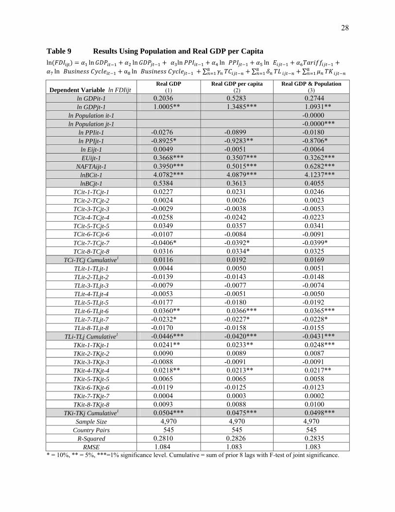
Table 9 Results Using Population and Real GDP per Capita


∑ ∑

∑

Dependent Variable ln FDIijt Real GDP

(1) Real GDP per capita

(2) Real GDP & Population

(3)

ln GDPit-1 0.2036 0.5283 0.2744 ln GDPjt-1 1.0005** 1.3485*** 1.0931**

ln Population it-1 -0.0000 ln Population jt-1 -0.0000***

ln PPIit-1 -0.0276 -0.0899 -0.0180 ln PPIjt-1 -0.8925* -0.9283** -0.8706* ln Eijt-1 0.0049 -0.0051 -0.0064 EUijt-1 0.3668*** 0.3507*** 0.3262***

NAFTAijt-1 0.3950*** 0.5015*** 0.6282*** lnBCit-1 4.0782*** 4.0879*** 4.1237*** lnBCjt-1 0.5384 0.3613 0.4055

TCit-1-TCjt-1 0.0227 0.0231 0.0246 TCit-2-TCjt-2 0.0024 0.0026 0.0023 TCit-3-TCjt-3 -0.0029 -0.0038 -0.0053 TCit-4-TCjt-4 -0.0258 -0.0242 -0.0223 TCit-5-TCjt-5 0.0349 0.0357 0.0341 TCit-6-TCjt-6 -0.0107 -0.0084 -0.0091 TCit-7-TCjt-7 -0.0406* -0.0392* -0.0399* TCit-8-TCjt-8 0.0316 0.0334* 0.0325

TCi-TCj Cumulative1 0.0116 0.0192 0.0169 TLit-1-TLjt-1 0.0044 0.0050 0.0051 TLit-2-TLjt-2 -0.0139 -0.0143 -0.0148 TLit-3-TLjt-3 -0.0079 -0.0077 -0.0074 TLit-4-TLjt-4 -0.0053 -0.0051 -0.0050 TLit-5-TLjt-5 -0.0177 -0.0180 -0.0192 TLit-6-TLjt-6 0.0360** 0.0366*** 0.0365*** TLit-7-TLjt-7 -0.0232* -0.0227* -0.0228* TLit-8-TLjt-8 -0.0170 -0.0158 -0.0155

TLi-TLj Cumulative1 -0.0446*** -0.0420*** -0.0431*** TKit-1-TKjt-1 0.0241** 0.0233** 0.0248*** TKit-2-TKjt-2 0.0090 0.0089 0.0087 TKit-3-TKjt-3 -0.0088 -0.0091 -0.0091 TKit-4-TKjt-4 0.0218** 0.0213** 0.0217** TKit-5-TKjt-5 0.0065 0.0065 0.0058 TKit-6-TKjt-6 -0.0119 -0.0125 -0.0123 TKit-7-TKjt-7 0.0004 0.0003 0.0002 TKit-8-TKjt-8 0.0093 0.0088 0.0100

TKi-TKj Cumulative1 0.0504*** 0.0475*** 0.0498*** Sample Size 4,970 4,970 4,970

Country Pairs 545 545 545 R-Squared 0.2810 0.2826 0.2835

RMSE 1.084 1.083 1.083 * = 10%, ** = 5%, ***=1% significance level. Cumulative = sum of prior 8 lags with F-test of joint significance.

Documents

WORKING PAPER SERIES - · PDF fileThe views expressed in the Working Paper Series are those of the author(s ... North American Free Trade Agreement ... METRs are computed for hypothetical