NBER WORKING PAPER SERIES

WHAT PROMOTES JAPAN TOINTERVENE IN THE FOREX MARKET?

A NEW APPROACH TO A REACTION FUNCTION

Takatoshi ItoTomoyoshi Yabu

Working Paper 10456http://www.nber.org/papers/w10456

NATIONAL BUREAU OF ECONOMIC RESEARCH1050 Massachusetts Avenue

Cambridge, MA 02138April 2004

We thank Graham Elliott, Eli Kollman, Eiji Kurozumi, Kenji Miyazaki, Akiko Tamura, Tatsuma Wada, andAi Deng for many helpful comments. Needless to say, the authors are solely responsible for any remainingerrors. The views and opinions expressed in this paper are those of authors.The views expressed herein arethose of the author(s) and not necessarily those of the National Bureau of Economic Research.

©2004 by Takatoshi Ito and Tomoyoshi Yabu. All rights reserved. Short sections of text, not to exceed twoparagraphs, may be quoted without explicit permission provided that full credit, including © notice, is givento the source.

What Prompts Japan to Intervene in the Forex Market? A New Approach to a Reaction FunctionTakatoshi Ito and Tomoyoshi YabuNBER Working Paper No. 10456April 2004JEL No. F31, E58, G15

ABSTRACT

This paper analyzes and estimates the reaction function of the Japanese monetary authorities in

deciding when to intervene in the foreign exchange (forex) markets, using daily Japanese

intervention data from April 1, 1991 to December 31, 2002. This paper is the first in estimating the

reaction function of the monetary authorities in the forex market intervention with following new

methods. First, a theoretical friction model is presented to describe the intervention as cost-

minimizing behavior. Second, the ordered probit analysis, which is consistent with the theoretical

model, was carried out to predict authorities’ reaction function. The regime change from frequent,

small-size intervention before June 1995 and infrequent, large-size intervention after June 1995 is

established and estimations are conducted for two different regimes separately. Third, a noise-to-

signal ratio is applied in selecting the optimal cutoff point in estimated ordered probit function to

use the model for predicting interventions. Major findings are as follows: (1) There was a regime

change in June 1995 from small-scale frequent interventions to large-scale infrequent interventions;

(2) the first half of the sample period had lower friction costs than the second half of the sample

period; (3) Judging from the model and data, the optimum cutoff was higher in the first half than the

second half.

Takatoshi ItoDepartment of EconomicsThe University of Tokyo7-3-1 Hongo, Bunkyo-kuTokyo, 153-8904, Japanand NBERtito@e.u-tokyo.ac.jp

Tomoyoshi YabuDepartment of EconomicsBoston University270 Bay State RoadBoston, MA 02215tyabu@bu.edu

2

1. Introduction The monetary authorities of Japan have intervened in the foreign exchange market more frequently than other G7 countries in, at least, the past thirteen years.1 Between April 1991 and December 2002, the Japanese authorities intervened in 214 days (7% of business days), of which 32 days were in the direction of purchasing the yen and selling the dollar, and 182 days in the opposite direction. (The Japanese Ministry of Finance, under a new Vice Minister of Finance for International Affairs, conducted much more frequent and large-scale interventions from January 2003 to March 2004, but that episode will be left for our future analysis.) The Japanese Ministry of Finance has disclosed the intervention days and amounts from April 1, 1991 to recent months. Ito (2003) described the institutional aspects and the data as well as making a first attempt of analyzing effectiveness, profits, and a reaction function. This paper, improving significantly over Ito (2003), analyzes and estimates the reaction function of the Japanese monetary authorities in deciding when to intervene in the yen/dollar market, using daily intervention data from April 1, 1991 to December 31, 2002. The paper is intended to analyze objectively the intervention reaction function without a value or normative judgment.

The disclosure of new data set stimulated several detailed studies. Ito (2003) investigated the effectiveness of the intervention, considering various criteria that are derived from possible motivations. He found that interventions before June 1995 was broadly ineffective in moving the exchange rate of the intervention days in the intended direction, while interventions after June 1995 to March 2001 were judged to be effective. He also estimated profits, realized income and unrealized capital gains, made by intervention, that amounted to 8.6 trillion yen over the ten year period. Fatum and Hutchison (2003) investigated the effectiveness of intervention using an event study methodology. They found strong evidence that sterilized intervention affected the exchange rate. Kearns and Rigobon (2003) estimated the effectiveness of intervention, that is, the impact of interventions on the exchange rate, using Australian and Japanese intervention data. Dominguez (2003) also analyzed the effectiveness of the Japanese intervention and compared to Federal Reserve Bank interventions. Frenkel, Pierdzioch,

1 The intervention decision in Japan is under jurisdiction of the Ministry of Finance and the Bank of Japan acts as an agent for implementation. The yen for intervention is obtained by issues of short-term government securities (Financial Bills) and listed as the liability in the special budget for intervention, while the acquired dollars are on the asset side of the special budget. See Ito (2003) for details of institutional aspects.

3

and Stadtmann (2002) used the Japanese disclosed data and estimated the reaction function. Their specification and estimation method are different from ours. Hillebrand and Schnabl (2003) also used the Japanese intervention data and found effectiveness after 1999. Galati and Melick (2002) analyzed the effectiveness of interventions on market expectations and found some evidence of effectiveness in the mark/dollar and yen/dollar markets.

This paper is the first in estimating the reaction function of the monetary authorities in the foreign exchange market intervention with the following new features. First, a general reaction function is derived from the cost-minimizing behavior of the monetary authorities that takes into account political costs associated with intervention. The model predicts a neutral band (no intervention) for wide range of state variables. Second, the ordered probit model is applied to estimate the equation derived from the theoretical model. Third, the model is applied to the Japanese data that were disclosed in 2001 for the period since April 1991, with a careful consideration to a possible regime change after 1995. Fourth, a method to choose the optimal cutoff in predicting intervention is proposed. In the literature, the cutoff is chosen arbitrarily, such as 0.5 in probit equation fitted valued. In order to choose the threshold more rationally, we propose to find the optimal cutoff by minimizing the noise-to-signal ratio.

Ito (2003) has estimated the reaction function of the Japanese authorities using the usual OLS. However, interventions were carried out only less than 10 percent of the business days on average during the sample period. Therefore, for more than 90 percent of the time, obvious zeros of interventions are not well predicted. A small amount of intervention predictions are most of the time turned out to be exactly the forecast errors of opposite signs. In order to rectify this problem, two estimation methods have been proposed in the literature. One method is based on the Probit model with a binary choice dependent variable, intervention or no intervention. (See Baillie and Osterberg (1997) and Dominguez (1998)). However, no theoretical model was presented. Another is based on the ''friction'' model. Almekinders and Eijffinger (1996) proposed a model with political frictions that no intervention is required when deviation from an optimal is small. The reaction function of intervention was derived formally rather than in ad hoc way. The Almekinders and Eijffinger model uses intervention amount as the dependent variable.

This paper extends the Almekinders and Eijffinger paper to show explicitly the target exchange rate, the loss function, and cost-minimizing behavior of the monetary authorities. However, our estimation method is the Ordered Probit in which the dependent variable is the indicator function (-1, 0 or 1) of intervention, not intervention amount in Almekinders and Eijffinger (1996). One choice that an economist has to face in

4

the literature of intervention is whether to use the actual dollar (or yen) amount of intervention or the indicator function of intervention. If the fact that intervention is carried out, which the market almost always knows within an hour as a market rumor, is more important than the precise amount, then the indicator function is appropriate. If the amount makes the difference in the impact on the exchange rate movement, the amount should be used. One drawback on using the precise amounts of interventions is the fact that the market usually does not know the amount of intervention on the day of intervention.

In the analysis of a reaction function of the monetary authorities, the indicator function is more appropriate, if an impact on the exchange rate is due more to the fact that there is an intervention than to how large it is, then authority's decision on whether or not to intervene is more important than how much to intervene. Moreover, when the monetary authorities decide to intervene, which the paper attempts to capture, the authorities may not know how much to spend that day. They may buy/sell more foreign exchanges as hours progress and the impacts become known. For these reasons, we will use the indicator function of intervention, whether the yen was sold or bought, or no intervention, in this paper.

The model of reaction function can be seen as a prediction of intervention. The literature on the prediction has been developed in the financial crisis literature. One strand of the early warning model of currency crises, such as Kaminsky and Reinhart (1999), uses a model to predict a crisis and evaluate alternative model specifications by calculating the noise-to-signal ratio. We apply the noise-to-signal ratio method to evaluation of various specifications of the intervention reaction function. The evaluation can lead to the choice of the optimal cutoff in the probit estimation of predicting intervention. This is a new insight in the intervention reaction function literature. The often-cited motivation for intervention is to prevent too much appreciation or depreciation, both as a level and as a speed. (See Edison (1993), Dominguez and Frankel (1993), Almekinders (1995), and Sarno and Taylor (2001, 2003) for surveys.) Too much appreciation (in a short period time) would harm exporters, while too much depreciation (in a short period time) would harm importers and confidence of financial market in general. To maintain a stable exchange rate that are broadly consistent with fundamentals is an aim of the monetary authorities.

This paper will ask a question when the authorities decide to intervene in the 1991-2002 time period. Considering that the frequency of interventions had changed greatly before and after June 1995, all regressions will be conducted for the whole sample, the earlier period (before June 1995), and the latter period (after June 1995).

5

To anticipate, major findings are as follows: (1) A regime change in June 1995 from small-scale frequent interventions to large-scale infrequent interventions was found to have occurred, as found by Ito (2003), and attributed to the change in personnel who was in charge of intervention at the Ministry of Finance; (2) the first half of the sample period had lower friction costs than the second half of the sample period; and (3) For the econometrician who cannot directly observe the authorities’ friction costs, the optimum cutoff is estimated to be higher in the first half than the second half.

The rest of the paper is organized as follows. Section 2 gives an overview of the yen/dollar exchange rate movement and intervention incidents from April 1991 to December 2002. Section 3 gives the specification of reaction function derived from a model. Section 4 estimates the model of interventions and analyzes the estimation results. Section 5 evaluates the predictability of interventions. Section 6 concludes the paper. 2. Overview of the yen/dollar movement In Figure 1, the yen/dollar movement is shown. The yen had fluctuated between 147 yen/dollar (on August 1, 1998) and 80 yen/dollar (on April 19, 1995). From 1991 to April 1995, the yen appreciation trend was observed, followed by the yen depreciation trend from April 1995 to August 1998. The yen appreciated from August 1998 to January 2000, when the yen has just above 100 yen/dollar. The yen depreciated after that, until the yen reached the mid-120s in March 2001.

Figure 1 about here Figure 2 shows the monthly-aggregated amounts of interventions. All

interventions to purchase the yen were conducted when the yen/dollar rate was higher (yen being more depreciated) than 125 yen, while all interventions to sell yen were conducted when the yen/dollar rate was lower (yen being more appreciated) than 125 yen. The fact that the dollar was bought when it was relatively cheap vis-à-vis the yen, and that the dollar was sold when it was relatively expensive means great profits to the monetary authorities. From April 1991 to December 2002, the realized gains (by purchasing the dollar and selling the matching amount) amounted to 1 trillion yen, and the net interest income (the interest income earned on the accumulated foreign reserves due to interventions minus the interest payments on the yen securities) amounted to 4.9 trillion yen. At the end of December 2002, the accumulated net intervention amounts in terms of the dollars, 225 billion dollars, have the inventory unit price of 108.8 yen/dollar, while the market price was 118.7 yen/dollar, suggesting the unrealized gains of 2.3 trillion yen. The gains suggest that the interventions were rather stabilizing in the notion of Milton Friedman, as argued in Ito (2003). (After the first draft of paper was written,

6

the intervention amounts have soared and the yen appreciated despite the frequent and large-scale intervention. At the time of this writing, the yen/dollar level is below 110 yen/dollar. And the authorities are estimated to carry unrealized losses. However, the analysis of interventions in 2003-2004 will be left to a future research.)

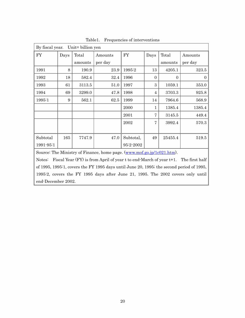
Figure 2 about here The intervention size and frequencies greatly changed before and after June 21, 1995, when Dr. Sakakibara became Director General of the International Finance Bureau of Ministry of Finance. Table 1 shows the number of intervention days, the total yen amount of intervention, the average (per-day) size of intervention for each year. In the first half of sample (April 1991-June 20, 1995), 165 interventions were conducted, while only 49 interventions were conducted in the second half (June 21, 1995—December 2002) of the sample. The total intervention amount was 8 trillion yen in the first half, while it was 25 trillion yen in the second half. The average intervention size was about 47 billion yen in the first half, but the average size of intervention increased by more than ten times in the second half of the sample. In summary, the first half was characterized by frequent, small-size interventions, while the second half by infrequent, but large-size interventions.

Table 1 about here Dr. Sakakibara himself noted the difference, emphasizing that it was a deliberate choice. Talking of interventions by his predecessor, Dr. Sakakibara writes, “The market was accustomed to interventions, because they were too frequent. The interventions were taken as given. Most interventions, including joint interventions, were predictable, so that interventions, even joint ones, had only small, short-term effects, and could not change the sentiment of the market.” (Sakakibara (2000), p.119) “[T]he change in intervention philosophy and technique [was introduced]. For this, all I have to do was to make a decision and convince the Vice Minister and the Minister of [its desirability]. For one, the frequency of interventions was reduced substantially, and per-intervention amount was increased, in order to push up the level [of the dollar vis-à-vis the yen]” (ibid., p.120) Words and deeds of Dr. Sakakibara seem to show the deliberate changes in the intervention style in order to change the level of the exchange rate by influencing the expectation of the market. Less frequent, but large-scale each time, interventions were a hallmark of the period from June 1995 to end-2002.2 In the next section, we rigorously

2 Dr. Sakakibara retired in July 1999. But, his successor, Mr. Kuroda was widely regarded as a person who inherited the same philosophy toward the exchange rate market function and intervention policy.

7

examine the monetary authority’s decision to intervene using an econometric model that takes into account the feature that interventions are infrequent events. 3. Model of Infrequent Intervention 3.1. Loss Function In most of papers in the literature, the intervention reaction function is typically assumed rather than derived. An exception is Almekinders and Eijffinger (1996) that derived a reaction function from the loss function of the monetary authorities.3 We follow their approach, with more realistic formulation of the target exchange rate and the cost function of intervention. The monetary authorities are assumed to have a loss function that should be minimized using interventions. The loss function is assumed to be:

Min ]|)[(]|[ 12

1 −− Ω−=Ω tTtttt ssELossE (1)

where st denotes the log of the yen/dollar rate at the close of the New York market (time t); sT

t denotes the target of the yen/dollar rate for the monetary authorities at time t; and Ωt-1 denotes the information available to the monetary authorities and market participants at the end of date t-1.4 The specification means that the loss is defined by squared deviation of the actual exchange rate from the target rate at date t. In addition, the monetary authorities are assumed to believe that the exchange rate is a random walk if there is no intervention and the date t intervention has impacts on the actual exchange rate process. The process of exchange rate is as follows:

tttt uIntss ++= − ρ1 (2) where ut is a white noise. Effectiveness of intervention on exchange rate implies the negative sign of ρ. For example, the yen-purchasing intervention (Intt>0) by the monetary authorities tends to appreciate the yen (st -st-1<0), then the negative sign of ρ should be obtained.

The pattern of intervention by Mr. Kuroda does not show an apparent change from the one by Dr. Sakakibara. 3 The objective of the Frenkel, Pierdzioch, and Stadtmann (2002) paper is similar to ours. The difference is specification and methodology. They have defined the loss function as a weighted sum of the deviation from the target exchange rate and the deviation from the target intervention amount, and applied the model to the Japanese intervention data. The former is simply the moving average or PPP. We think that using the intervention target in the loss function is not convincing. Their paper is not using the friction model, unlike Almekinders and Eijffinger (1996) and this paper. The Frekel, Pierdzioch, and Stadtmann paper did not check a possible regime change in the middle of the sample period, unlike Ito (2003) or this paper. 4 The New York close rate, instead of the Tokyo market, is used because Janapese intervention of day t can be carried out in the Tokyo market, European market, or New York market. See Ito (2003) for a detailed time line for this.

8

Minimizing the loss function (1) by choosing Intt subject to the constraint (2) leads to the following intervention reaction function:

)(11

* Tttt ssInt −−= −ρ

(3)

Intt* denotes the optimal intervention. The authorities have a target exchange rate that is defined by the weighted average of the past exchange rates. We pick up three representatives from the past exchange rates; the yen/dollar rate in the previous day, the yen/dollar rate in the previous month (21 business days), the past-one-year moving average of the yen/dollar rate. Therefore, the target exchange rate is

MAttt

Tt ssss 1321221 −−− ++= ααα (4)

where α 1+α 2+α 3=1. 5 For example, when the monetary authorities pay greater attention to long-run stability than to other factors, α3 takes a value close to one. This represents the desire by the monetary authorities for mean reversion. On the other hand, when they attach greater importance to short-run stability than to others, α1 takes a value close to one. This is the case when a short-run movement (st-2 to st-1) is to be reversed, or at least to be moderated in speed. Coefficientα2 represents the medium term target of the authorities, that is mean reversion to the trend of the past one month. In the case they attach equal importance, each αi takes 1/3. Using (3) and (4), the optimal intervention can be written as

)()()( 11211211* MA

ttttttt ssssssInt −−−−−− −−−−−−=ρ

αρ

αρα ３２

)()()( 1132112211MAtttttt ssssss −−−−−− −+−+−= βββ (5)

That is, the optimal intervention is a function of three explanatory variables; the change in the yen/dollar rate on day t-1; the change in the yen/dollar rate in the previous 21 (business) days; the percent deviation of the current (day before) level from the past-one-year moving average. Note that the relationships among parameters are written as follows: αi=βi/(β1+β2+β3) and ρ= -1/(β1+β2+β3). This means that once we can estimateβi, we can identify αi and ρ, respectively. As we will see, however, this is not the case.

5α3 is assumed to be one in Almekinders and Eijffinger (1996). Thus, our target rate may be considered as a general form of their target rate. Another approach is to use the PPP rate instead of equation (4). However, given the availability of the data in the monthly base, it leads to a sticky target rate in the daily model of intervention.

9

3.2. Political Cost The specification of intervention (5), when taken literally, implies that intervention should take place almost everyday. This is inconsistent with the fact that interventions were actually carried out only less than 10 percent of the business days on average. One way to rectify this problem is to model explicitly the political cost for intervention, that is incurred during decision-making process for designing the optimal intervention strategy (see Almekinders (1995) and Almekinders and Eijffinger (1996)). Political costs reflect costs of discussion with Minister of Finance of own country and other major countries of intervention currencies. In order to carry out intervention, an explanation to the Minister of Finance, and in some cases to other ministers, including Prime Minister, is necessary and a tacit approval of other countries has to be sought after. Political costs are most likely independent of the size of intervention. However, once the approval is secured, then intervention can be carried out in several days in a row, if the situation does not change dramatically. What is called political cost may reflect aversion to intervention by those who are in charge of interventions, namely, officials at the Ministry of Finance. Those who believe that the market will have power to restore an equilibrium sooner than later, they find costs to be high, while those who believe that the market can overshoot and get misaligned for a long time tend to find political costs low. Any consideration that is not captured by the specification of the target rate will show up as the political costs.

With the presence of political costs, intervention takes place if and only if benefits of intervention are higher than costs. Usually, political costs are assumed to be a function of intervention at date t. If intervention was carried out the day before, then the political cost is less, because the decision by the Minister was already secured once, so that an additional cost on the day after is much less. Therefore, we assume that political costs are a function of interventions not only at date t but also at date t-1. Under this assumption, we can explain why intervention tends to be correlated (once intervened, another intervention is likely to occur the day later). Therefore, a cost function of intervention is defined as

<<−>>−

=−

−−

+

0)0(10)0(1

121

121

tt

ttt IntifIntFCFC

IntifIntFCFCFC (6)

where FC1j>0, FC2>0, and 1(.) is the indicator function. For example, FC1

- may be smaller than FC1

+, implying that the yen-selling intervention takes fewer costs than the yen-purchasing intervention. The opposite situation may be possible. FC2>0 implies that intervention at date t-1 reduces political costs of intervention at date t.

10

3.3. Ordered Probit The monetary authorities compare benefits of reducing losses of no intervention to fixed costs of intervention, and carry out interventions only when benefits are higher than costs. Note that the greater the optimal intervention the greater the loss of no intervention. Therefore, once the optimal intervention crosses the thresholds, the monetary authorities intervene in the foreign exchange market. The actual intervention can be written as:

+<>−+>−<+<<+

<+<+−=

−

−−

−

ttt

tttt

ttt

t

IntIntifIntIntIntif

IntIntifIInt

εβµβµεβµ

βµε

*142

142*

141

141*

)0(11)0(1)0(10

)0(11 (7)

μ1<0，μ2>0, β4>0 and εt～i.i.d.N(0,σ2). Given the observation that the direction of intervention at date t was never

different from that of date t-1, the equation (7) can be replaced by the equation (8):

<+<<

<−=

*2

2*

1

1*

101

t

t

t

t

yifyif

yifIInt

µµµ

µ (8)

where yt * =Χtβ+εt withεt～i.i.d.N(0,σ2) and

141132112211 )()()( −−−−−−− +−+−+−= tMAttttttt IIntssssssX βββββ .

This model is considered as an Ordered Probit Model and can be estimated by the maximum likelihood method. However, we estimate βi*=βi/σ and μi*=μi/σ, not βi and μi directly. This means that we can estimate αi=βi*/(β1*+β2*+β3*) but there is no way to identify ρ without additional assumptions. The model can be regarded as a reaction function with a “neutral band” of no-intervention. 3.4. Relationship to Conventional Specification

The conventional reaction function of the monetary authorities, without the neutral band of no-intervention, is presented here for comparison. Let us recall that Ito (2003) defined a reaction function that was conventional in the literature and estimated it. The intervention, either size (amount) of intervention (Int) or the indicator, IInt = (1,0, or -1), is regressed on the daily exchange rate change, the monthly change, the deviation from a long-run equilibrium, and the intervention of the day before. In the indicator

11

specification, the following regression can be estimated:6

ttMAttttttt IIntssssssIInt νφφφφφ ++−+−+−+= −−−−−−− 1411321122110 )()()( (9)

The equation (9) can be interpreted as a linearlization of the general intervention reaction function (8). Therefore, the conventional regression has a constant term while the ordered probit function has no constant term. Furthermore, vt has heteroskedasticity and thus heteroskedasticity-and-autocorrelation-consistent (HAC) standard errors should be used for inference. 4. Estimating a Reaction Function 4.1. Structural Break Structural changes are suspected from observations of intervention patterns, as described in Section 2. In this section, a structural break for the reaction function is tested first in order to examine whether our observation, supported by Dr. Sakakibara’s own assertion, is confirmed by data.

The regression analysis will be conducted to test rigorously the possible break at around the time of June 1995, when Dr. Sakakibara became in charge of intervention. First, the null hypothesis of no break at June 21, 1995, for the ordered probit regression, eq. (8) is rejected at the 1% significance. Therefore, our prior of structural changes due to a personnel change is confirmed by the statistical test. For the linear version, (9), the Supτ (F(τ)) test, a la Andrews (1993), is conducted to search for a (unknown) date of structural break. For possible (known) dates of a structural break, the Chow test was conducted. The F-statistic for the structural break is plotted in Figure 3. Possible structural break dates are tested, and the single peak of the F-statistic is found to be on April 18, 1995.7 The break date is two months earlier than the date we identify by the personnel change, June 21. The reason for this deviation is based on the following pattern of intervention during the two-month period between the two dates. Although continuous interventions, a hallmark of pre-Sakakibara era, seemed to have ended on April 18. The only intervention after this date before June 21 was May 31. Therefore, according to statistical analysis, the policy

6 Ito (2003) used the intervention amount instead of the indicator functions: with the size of intervention, the following regression was estimated:

ttMAttttttt IntssssssInt ωθθθθθ ++−+−+−+= −−−−−−− 1411321122110 )()()(

7 The possible structural break days to be tested are the middle 70% of the sample period. Namely the first 15% and the last 15% of days are excluded from test for a structural break. For the large-sample approximation to the distribution of the Supτ (F(τ)) test to be good, the subsample endpoints should not be close to zero so that 15% trimming is a common choice in practice.

12

switch from frequent interventions to infrequent interventions occurred on April 18. Insert Figure 3 about here

The F-statistic for a hypothesis of structural break on April 18 is 45, and the null is rejected with 1 percent significance. Moreover, the F-statistic on June 21, which is 33, is also large enough to reject the null with 1 percent significance. Since we have prior knowledge of regime change due to a personnel change, supported by a memoir of Dr. Sakakibara, we will adopt June 21 as the structural break date. Below, all models are estimated for the entire period, before June 21, 1995 (pre-June 1995), and after June 21, 1995 (post-June 1995).8 4.2. Conventional Regressions The conventional reaction function, equation (9), is estimated. This is basically an update of the reaction function estimated in Ito (2003), extending the sample period by one year, with a modification of replacing Intervention amount (Int) with the intervention indicator (IInt) as a dependent variable. Results are shown in Table 2. The reaction function gives different estimates and explanatory power in the first half and second half of the sample. Reactions to the previous day changes (φ1), to the medium-term trend (φ2) , and to the deviation from the long-run trend (φ 3), were all much stronger in the first half. Of these, the medium-term trend seemed to have been ignored by the authorities in post-1995:06 period. This reflects the fact that there were much more frequent interventions in the first half. The coefficient of lagged intervention (φ4) was also found to be significant in both periods, with a larger coefficient in the first period.

Insert Table 2 The explanatory power of the regression was significantly lower in the second half of the sample, but this is consistent with the reputation that Dr. Sakakibara wanted the intervention to be unpredictable. He believed that a surprise intervention would be more effective than a predictable one. 4.3. Ordered Probit Regressions Estimates of the ordered probit model are summarized in Table 3. The following six observations stand out. First, a tendency of lean-against-the-wind interventions is confirmed for the daily and medium-term considerations. For the daily

8 Even if we adopt April 18 as the regime change date, most of the findings comparing the first regime and second regime remain valid.

13

reaction, β1*>0 holds true for the entire, pre-June 1995, and the post-June 1995 periods. The positive coefficient means that yen appreciation (depreciation) on the day before tends to trigger an intervention to sell (buy, respectively) the yen. There was also a tendency of lean-against-the-wind interventions when there is trend of appreciation (depreciation) in the medium term (preceding 21 days), asβ2*>0 is confirmed for the entire and pre-June 1995 periods. Namely, if the yen appreciation (depreciation) occurred in the last 21 days, then it is more likely to intervene and sell (buy, respectively) the yen.9

Insert Table 3 about here Second, intervention is more likely to occur when the exchange rate is more deviated from a long-run moving average, as β3* > 0 holds for the entire, pre-June 1995, and post-June1995 periods. Therefore, the monetary authorities tend to intervene when the exchange rate deviates more from the long-run equilibrium that is defined by the moving average of past one year.

By construction, the original weights of the three components of the target exchange rate are calculated. Using α1+α2 +α3 =1, we can calculate each component, (α1 , α2 , α3). In the pre-June 1995, period, (α1 , α2 , α3) = (0.62, 0.20, 0.18), while in the post-June 1995 period, (α1 , α2 , α3) = (0.88, 0.00, 0.12), with a restriction that non-significant estimate being set to zero. In the pre-June 1995 period, the monetary authorities were mindful of the daily, medium-term, long-term exchange rate movements. In the post-June 1995 period, the monetary authorities attached importance almost solely to the daily exchange rate movements, with a minor consideration to the long-term misalignment.

Third, the coefficient of interventions of day before is estimated as significant, β4*>0. This implies that the likelihood of interventions does increase if there was an intervention the day before. This reflects the lower political costs of continuous interventions. The result does hold for the entire, pre-1995:06, and post-1995:06 periods. The magnitude of increasing likelihood of intervention is 1.6 and 1.7, respectively.

Fourth, the neutral band of no intervention was estimated to be (-2.1, +1.9) for the first subsample, and (-2.2, +3.0) for the second subsample. That is, the neutral band was much wider in the second half than the first half. The difference in the neutral band

9 Dr. Sakakibara has a reputation of carrying out the lean-in interventions (β*2<0). The reputation partly comes from his own writings. This reputation is not proven by the estimation. For the medium term (β*2), however, neither lean-in or lean-against interventions was not proved for the post-June 1995, that is, the Sakakibara period.

14

gives quite a different prediction on interventions, and this is consistent with casual observations of the frequency of interventions, as shown in Table 1. Figures 4, 5, and 6 show the estimated neutral band and the fitted value of the latent variable y*. For the entire period, Figure 4 shows the relationship between the neutral band and the fitted value. When estimated separately, Figures 5 and 6 show the relationship of the two subperiods. With the narrow band in the first half, it was predicted as shown in Figure 5, that interventions are frequent, while with the wide band in the second half, the frequency of interventions was predicted as low as in Figure 6.

Figures 4, 5, and 6 about here Fifth, there are asymmetries in the neutral bands, that is the magnitudes of upper

band and lower band are different only in the second half. It is often said that the Japanese monetary authorities are much more tolerant to yen depreciation than yen appreciation. One way to formalize this asymmetry hypothesis would be to compare the ceiling and floor of the neutral band. In the first period, the band was symmetric in positive and negative directions as the band was estimated to be (-2.1, +1.8). In the second period, it was shown that the monetary authorities were much more tolerant toward the yen depreciation than the yen appreciation. This shows that political costs were quite symmetric in both directions in the first period, but were biased in preference for yen depreciation in the post-June 1995, the Sakakibara period. Sixth, although the regression of the second half still has lower explanatory power (McFadden’s R2) than the first half, the difference between the two period is greatly narrowed in the regression with the neutral band (Table 3) compared to the conventional regression (Table 2). The R2 increases from 0.078 to 0.178 in the second half. This is due to the fact that the model is rich enough to allow prediction of zero intervention in the model. 4.4 Difference between the two subsamples It has been established in reviewing the Japanese interventions in the 1990s that the pre-June 1995 period was characterized by frequent, small-scale interventions, while the post-June 1995 period was characterized by infrequent, large-scale interventions. By the conventional reaction function, a la Ito (2003), showed that the reaction function was estimated badly in the second sub-sample. Coefficients of the past exchange rate changes and the deviation from an equilibrium level are smaller in the second period than the first period. The smaller estimated coefficients reflects the fact that most of the days, the regressions were fit to predict the zero of the dependent variable. Those who were in charge of interventions in the second period are estimated to be quite insensitive to the

15

exchange rate changes. Infrequent, but large-scale interventions in the second period produced the large forecast errors. By introducing political costs that lead to a neutral band of no-intervention, it is possible to distinguish whether the monetary authorities of the second period was insensitive to the exchange rate changes—that is the target exchange rate was low—or the political costs were high for some reasons. 5．Minimizing a surprise or a false alarm? One way to judge how well the reaction function is tracing the intervention indicator variable is to regard the model as a prediction of intervention, and evaluate the accuracy of prediction. Suppose that an econometrician (or a private-sector market participant) is interested in predicting whether there is intervention on day t at the beginning of the Tokyo market, then the probit model can be used for this purpose. The market participant does not like a surprise (i.e., an actual intervention without a warning from a model) or a false alarm (i.e., a model predicts an intervention, which would not take place). The ordered probit model gives the fitted value of probability for intervention. Then, by choosing the cutoff for the indicator in [0,1], the econometrician can either predict, at the beginning of the Tokyo market, that the intervention will take place or not on that day. If the fitted value of probability exceeds the chosen cutoff value, then an intervention is predicted, while the lower fitted value is ignored for prediction. If the cutoff is too low, then too many interventions are predicted, and most of them will turn out to be false alarms. If the cutoff is too high, then too few interventions are predicted so that actual interventions would take place without the warning call. The task is a well-known problem of balancing minimization of the type one errors vs. the type two errors. Table 4 summarizes the 2x2 matrix of the prediction and actual interventions: correct prediction, the type one errors, and type two errors. Cell A is the number of days when the signal (warning/prediction) of intervention was issued, and actual intervention was observed. Cell B is the number of days when a warning was issued but turned out to be a false alarm. Cell C is the count of days when actual intervention takes place without a warning by the model. This is the event of surprise intervention. Cell D is the number of days when a model predicts no intervention that turned out to be true. 10

10 We implicitly ignore the possibilities that the probability of the yen-purchasing (selling) intervention is higher than that of the yen-selling (purchasing) intervention, when the yen-selling (purchasing) intervention takes place. In our argument, this case is counted as a correct signal, though it is a noise. However, this is not a problem because these cases do not happen in our data. The monetary authorities always have some economic reasons to intervene in the forex market so that we

16

The currency crisis literature has developed a way to evaluate the so-called early warning model of the crisis. (See Kaminsky and Reinhart (1999) for the seminal work.) They have proposed to use the noise-to-signal ratio. Note that A/(A+C) is the ratio of correct signal of the actual intervention (crisis in the early warning literature) days, while B/(B+D) is the ratio of false alarms of the no-intervention days. When a very low cutoff is chosen, then the ratio of correct signals A/(A+C) will increase, but the ratio of false alarm B/(B+D) will increase as well. When a very high cutoff is chosen, the ratio of correct signal decreases, making interventions are surprises, although the ratio of false alarms would decrease. The noise-to-signal ratio is defined as ([B/(B+D)]/[A/(A+C)]). The optimal cutoff, as proposed by Kaminsky and Reinhart, is chosen to minimize this ratio. Since A+C and B+D are constant, the optimal cutoff can be chosen to minimize B/A. Tables 5-1, 5-2, and 5-3 show the optimal cutoff and the resulting counts in the format of Table 4, for the entire sample, the first half, and the second half, respectively. For the first half, the optimal cutoff was 0.72, but the correct signal was issued 50 times out of 165 interventions. The ratio of correct signal was 30%, while about 70% of interventions were surprise interventions. The false alarm was issued only 8 times out of 936 no-intervention days. The noise ratio was only 0.8%. The noise-to-signal ratio was 0.0282. The intervention was in the sense quite predictable. For the second half, the optimal cutoff was 0.30. With this cutoff, the correct signal was only 5 times out of 49 interventions. The correct signal ratio was about 10%, that is, about 90% of interventions were surprises. The false alarm was issued 13 times out of 1905 no-intervention days; the noise ratio was 0.7%. The noise-to-signal ratio was 0.0669 that is much higher than the first half. The main difficulty was the low ratio of correct signal. The signal ratio was 30% in the first half of the sample, while it was 10% in the second half of the sample. In other words, the signal turned on 58 times, in which 8 turned out to be false (13% of false signal ratio) in the first period. In the second period, the false signals were 13 out of 18 (72% of false signal ratio). This confirms the conventional wisdom, as documented in Ito (2003) that interventions in the second half of the sample were quite unpredictable, and that was intended by Dr. Sakakibara. It should be noted that the reaction function in this section is of the in-sample prediction type. If the model is seriously used for prediction, the out-of-sample prediction model should be developed. However, it is not

do not have a situation in which the econometrician expects the yen-purchasing (selling) intervention when the yen-selling (purchasing) intervention takes place.

17

straight-forward, as both regression and the cutoff point should be optimized everyday. This is left for future research. 6．Conclusion This paper has proposed and estimated a new model of intervention activities of the Japanese monetary authorities. The reaction function of intervention has been typically estimated with a regular OLS regression. However, the conventional model has a shortcoming of predicting interventions almost always that turned out to be false. The new model is based on a theoretical model of interventions with political fixed costs of intervention. The ordered probit model with a neutral band of no-intervention, is derived from theory, and estimated for the 1991-2002 period. The frequency and size of intervention changed, from frequent, small-size interventions to infrequent, large-size interventions, in June 1995 when Dr. Sakakibara became in charge of intervention policy. The ordered probit reaction function with a neutral band was estimated for the entire, first-half, and second-half of the sample. The following points stand out. The interventions were of the lean-against type, in that large changes in the previous days tended to prompt interventions to counter the movement. The authorities tended to intervene when the exchange rate deviated large from a long-term moving average. When there was an intervention a day before, it is more likely, other things being equal, for the authorities to intervene. The neutral band was much wider in the second half than the first half. In the second half, the neutral band was asymmetric, in that the yen depreciation was more tolerated than yen appreciation. The ordered probit function can be viewed as a forecasting model of intervention indicator. When a cutoff level is chosen, the prediction of intervention is generated, that may turn out to be true or false. The optimal cutoff level was chosen to minimize the noise-to-signal ratio. The optimal cutoff was higher in the first half than the second half. The noise-to-signal ratio was higher in the second half, as many interventions were surprises. According to the writings of the Dr. Sakakibara, this was a deliberate policy of the authorities. The newly proposed model of interventions is successfully estimated. It remains to be a future task to refine the specification, and introduce a concept of out-of-sample forecasts in calculating the noise-to-signal ratio.

18

Reference Andrews, D.W.K. (1993). “Tests for Parameter Instability and Structural Change with Unknown Change Point,“ Econometrica: 821-856. Almekinders, Geert J. (1995). Foreign Exchange Intervention: Theory and Evidence, Cheltenham: Edward Elgar Publishing Ltd. Almekinders, Geert J. and Sylvester C. W. Eijffinger (1996). “A Friction Model of Daily Bundesbank and Federal Reserve Intervention,“ Journal of Banking and Finance: 1365-1380. Baillie, Richard T. and William P. Osterberg, (1997). “Why Do Central Banks Intervene?” Journal of International Money and Finance, vol. 16, no. 6: 909-919. Dominguez, Kathryn and Jeffrey Frankel (1993). Does Foreign Exchange Intervention Work? Washington DC: Institute for International Economics. Dominguez, Kathryn (1998). “Central bank intervention and exchange rate volatility,“ Journal of International Money and Finance, Vol.17, 161-190. Dominguez, Kathryn (2003). “Foreign Exchange Intervention: Did it Work in the 1990s?” in F. Bergsten and J. Williamson, (eds.), Dollar Overvaluation and the World Economy, Special Report vol. 15, Institute for International Economics, Washington, D.C.,: 217-245. Edison, Hali J. (1993). The Effectiveness of Central-Bank Intervention: A Survey of the Literature After 1982, Special Papers in International Economics, no. 18, Princeton, N.J.: Princeton University, July 1993. Fatum, Rasmus and Michael Hutchison (2003). “Is sterilized foreign exchange intervention effective after all? An event study approach,” The Economic Journal, Vol. 113, 390-411. Frenkel, Michael, Christian Pierdzioch, and Georg Stadtmann, (2002). “Bank of Japan

19

and Federal Reserve Interventions in the Yen/U.S. Dollar market: Estimating the Central Banks’ Reaction Functions” Kiel Institute for World Economics, photocopy. http://papers.ssrn.com/sol3/PaperDownload Galati, Gabriele and Will Melick, (2002). “Central Bank Intervention and Market Expectations,” BIS Papers, no. 10. http://www.bis.org/publ/bispap10.htm#pgtop Hillebrand, Eric and Gunter Schnabl (2003). “The Effects of Japanese Foreign Exchange Intervention: GARCH Estimation and Change Point Detection” Japan Bank for International Cooperation, Discussion Paper No. 6, October. Ito, Takatoshi (2003). “Is Foreign Exchange Intervention Effective? the Japanese experiences in the 1990s,” in Paul Mizen (ed.), Monetary History, Exchange Rates and Financial Markets, Essays in Honour of Charles Goodhart, Volume 2, CheltenhamU.K.; Edward Elgar Pub. 2003: 126-153. [NBER working paper no. 8914, April 2002] Kaminsky, Graciela and Carmen Reinhart (1998). “The Twin Crises: The Causes of Banking and Balance-Of-Payments Problems,” American Economic Review, Vol. 89, 473-500. Kearns, Jonathan and Roberto Rigobon, (2003). “Identifying the Efficacy of Central Bank Interventions: Evidence from Australia and Japan” February 2003, available at http://web.mit.edu/rigobon/www/Papers/cbi.htm. An earlier version without the Japanese data and associated analysis was in NBER wp no. 9062, July 2002. Sakakibara, Eisuke (2000). The day Japan and the World shuddered: establishment of Cyber-capitalism, Chuo-Koron Shin Sha, April. Sarno, Lucio and Mark P. Taylor, (2001). “Official Intervention in the Foreign Exchange Market: Is It Effective and, If So, How Does It Work?” Journal of Economic Literature, vol. XXXIX, September: 839-868. Sarno, Lucio and Mark P. Taylor, (2003). Economics of Exchange Rates, Cambridge: Cambridge University Press.

20

Table1. Frequencies of interventions

By fiscal year. Unit= billion yen

FY Days Total amounts

Amounts per day

FY Days Total amounts

Amounts per day

1991 8 190.9 23.9 1995:2 13 4205.1 323.51992 18 582.4 32.4 1996 0 0 01993 61 3113.5 51.0 1997 3 1059.1 353.01994 69 3299.0 47.8 1998 4 3703.3 925.81995:1 9 562.1 62.5 1999 14 7964.6 568.9 2000 1 1385.4 1385.4 2001 7 3145.5 449.4 2002 7 3992.4

570.3

Subtotal 1991-95:1

165 7747.9 47.0 Subtotal, 95:2-2002

49 25455.4 519.5

Source: The Ministry of Finance, home page. (www.mof.go.jp/1c021.htm). Notes: Fiscal Year (FY) is from April of year t to end-March of year t+1. The first half of 1995, 1995:1, covers the FY 1995 days until June 20, 1995; the second period of 1995, 1995:2, covers the FY 1995 days after June 21, 1995. The 2002 covers only until end-December 2002.

21

Table2: Conventional Reaction Function with No neutral band, OLS

ttMAttttttt IIntssssssIInt νφφφφφ ++−+−+−+= −−−−−−− 1411321122110 )()()(

FULL 91/4/1-95/6/20 95/6/21-02/12/31 φ0

-0.0232

(0.005)** 0.0178

(0.0174) -0.0178

(0.0056)** φ1

4.056

(0.836)** 5.439

(1.967)** 2.437

(0.774)** φ2

0.503

(0.238) * 1.607

(0.666)* 0.116

(0.143) φ3

0.325

(0.078)** 1.165

(0.366)** 0.153

(0.075)* φ4

0.481

(0.041)** 0.478

(0.045)** 0.247

(0.068)** R2 Bar 0.293 0.387 0.078

OBS 3055 1101 1954

Note: Heteroskedasticity-and-autocorrelation-consistent (HAC) standard errors are given in parentheses. †Statistically significant at the 10-percent level. *Statistically significant at the 5-percent level. **Statistically significant at the 1-percent level. φ1 > 0, φ2 > 0: Lean against the wind. φ3 > 0, further the rate is away from sMA, more likely to have a larger intervention. φ4 > 0, there is a tendency to have subsequent interventions

Table3:Ordered Probit

<+<<

<−=

*2

2*

1

1*

101

t

t

t

t

yifyif

yifIInt

µµµ

µ

where ttt Xy εβ +=* with tε ～i.i.d.N(0,σ2) and

141132112211 )()()( −−−−−−− +−+−+−= tMAttttttt IIntssssssX βββββ .

FULL 91/4/1-95/6/20 95/6/21-02/12/31 *1β

26.19 (5.650)**

24.25 (8.746)**

27.813 (6.053)**

*2β

3.905 (2.117) †

7.788 (3.631)*

1.373 (2.343)

*3β

3.276 (0.816)**

6.624 (1.952)**

3.475 (1.247)**

*4β

1.911 (0.128)**

1.619 (0.161)**

1.725 (0.232)**

Threshold *1µ

-2.064

(0.073)**

-2.111

(0.155)**

-2.207

(0.090)** *2µ

2.507 (0.126)**

1.885 (0.163)**

3.018 (0.167)**

McFadden’s R2 0.328 0.366 0.176

OBS 3055 1101 1954

Note: Heteroskedasticity-and-autocorrelation-consistent (HAC) standard errors are given in parentheses. †Statistically significant at the 10-percent level. *Statistically significant at the 5-percent level. **Statistically significant at the 1-percent level. β1*> 0, β2* > 0: Lean against the wind. β3* > 0, further the rate is away from sMA, more likely to have a larger intervention. β4* > 0, there is a tendency to have subsequent interventions

23

Table 4: Conceptual Framework: Surprise vs. False Alarm Intervention occurred No intervention occurred

Signal was issued A B Signal was not issued C D

Total A+C B+D

Table 5: Optimal Noise to signal ratio Table 5-1: Full Sample

Intervention No Intervention Signal was issued 63 14

No signal was issued 151 2827 Total 214 2841

Cutoff: 62% Signal: 63/214= 0.2943 Noise: 14/2841= 0.00492 Noise to Signal Ratio: 0.0167

Table5-2: The First Half

Intervention No Intervention Signal was issued 50 8

No signal was issued 115 928 Total 165 936

Cutoff: 72% Signal: 50/165= 0.3030 Noise: 8/936= 0.0085 Noise to Signal Ratio: 0.0282

Table5-3: The Second Half

Intervention No Intervention Signal was issued 5 13

No signal was issued 44 1892 Total 49 1905

Cutoff: 30% Signal: 5/49= 0.10204 Noise: 13/1905= 0.0068 Noise to Signal Ratio: 0.0669

24

Figure 1: Yen/Dollar Exchange Rate Apr1991-Dec2002 NY close

Figure 2: Amounts of Intervention (monthly aggregation)

70

80

90

100

110

120

130

140

150

91/4 92/4 93/4 94/4 95/4 96/4 97/4 98/4 99/4 00/4 01/4 02/4

Yen/US$

-40000

-30000

-20000

-10000

0

10000

20000

30000

40000

91/4 92/4 93/4 94/4 95/4 96/4 97/4 98/4 99/4 00/4 01/4 02/4

Sell $, buy yen

Buy $, sell yen

yen 100mil

25

Figure 3: F-Statistics Testing for a Break in Equation (9) at Different Dates

Figure 4: Full Sample

0

5

10

15

20

25

30

35

40

45

50

91/4 92/4 93/4 94/4 95/4 96/4 97/4 98/4 99/4 00/4 01/4 02/4

F-Statistic

c

-5

-4

-3

-2

-1

0

1

2

3

4

5

91/4 92/4 93/4 94/4 95/4 96/4 97/4 98/4 99/4 00/4 01/4 02/4

μ2

μ1

26

Figure 5: The First Half

Figure 6: The Second Half

-5

-4

-3

-2

-1

0

1

2

3

4

5

91/4 91/10 92/4 92/10 93/4 93/10 94/4 94/10 95/4

μ1

μ2

-5

-4

-3

-2

-1

0

1

2

3

4

5

95/6 96/6 97/6 98/6 99/6 00/6 01/6 02/6

μ2

μ1