Embed Size (px)
Citation preview

www.iran-mavad.com مرجع علمی مھندسی مواد
P1: FDG/FGA P2: FDG
CB381-Davis-FM CB381-Davis May 17, 2001 19:31 Char Count= 0
Theory of Solidification
The processes of freezing and melting were present at the beginnings of theEarth and continue to affect the natural and industrial worlds. The solidificationof a liquid or the melting of a solid involves a complex interplay of many physicaleffects. This book systematically presents the field of continuum solidificationtheory based on instability phenomena. An understanding of the physics is de-veloped by using examples of increasing complexity with the object of creatinga deep physical insight applicable to more complex problems.
Applied mathematicians, engineers, physicists and materials scientists willall find this volume of interest.
Stephen H. Davis is McCormick Professor and Walter P. Murphy Professor ofApplied Mathematics at Northwestern University.
i
www.iran-mavad.com مرجع علمی مھندسی مواد

P1: FDG/FGA P2: FDG
CB381-Davis-FM CB381-Davis May 17, 2001 19:31 Char Count= 0
ii
This page intentionally left blank
www.iran-mavad.com مرجع علمی مھندسی مواد
P1: FDG/FGA P2: FDG
CB381-Davis-FM CB381-Davis May 17, 2001 19:31 Char Count= 0
CAMBRIDGE MONOGRAPHS ON MECHANICS
FOUNDING EDITOR
G. K. Batchelor
GENERAL EDITORS
S. H. DavisMcCormick Professor and Walter P. Murphy Professor
Applied MathematicsNorthwestern University
L. B. FreundHenry Ledyard Goddard University Professor
Division of EngineeringBrown University
S. LeibovichSibley School of Mechanical and Aerospace Engineering
Cornell University
V. TvergaardDepartment of Solid Mechanics
The Technical University of Denmark
iii
www.iran-mavad.com مرجع علمی مھندسی مواد

P1: FDG/FGA P2: FDG
CB381-Davis-FM CB381-Davis May 17, 2001 19:31 Char Count= 0
iv
This page intentionally left blank
www.iran-mavad.com مرجع علمی مھندسی مواد
P1: FDG/FGA P2: FDG
CB381-Davis-FM CB381-Davis May 17, 2001 19:31 Char Count= 0
T H E O R Y O FS O L I D I F I C A T I O N
STEPHEN H. DAVISNorthwestern University
v
www.iran-mavad.com مرجع علمی مھندسی مواد
PUBLISHED BY CAMBRIDGE UNIVERSITY PRESS (VIRTUAL PUBLISHING) FOR AND ON BEHALF OF THE PRESS SYNDICATE OF THE UNIVERSITY OF CAMBRIDGEThe Pitt Building, Trumpington Street, Cambridge CB2 IRP 40 West 20th Street, New York, NY 10011-4211, USA 477 Williamstown Road, Port Melbourne, VIC 3207, Australia
http://www.cambridge.org
© Cambridge University Press 2001 This edition © Cambridge University Press (Virtual Publishing) 2003
First published in printed format 2001
A catalogue record for the original printed book is available from the British Library and from the Library of Congress Original ISBN 0 521 65080 1 hardback
ISBN 0 511 01924 6 virtual (netLibrary Edition)
www.iran-mavad.com مرجع علمی مھندسی مواد
P1: FDG/FGA P2: FDG
CB381-Davis-FM CB381-Davis May 17, 2001 19:31 Char Count= 0
I dedicate this book to the wonderful women in my life,my mother Eva
andmy wife Suellen
vii
www.iran-mavad.com مرجع علمی مھندسی مواد

P1: FDG/FGA P2: FDG
CB381-Davis-FM CB381-Davis May 17, 2001 19:31 Char Count= 0
viii
This page intentionally left blank
www.iran-mavad.com مرجع علمی مھندسی مواد
P1: FDG/FGA P2: FDG
CB381-Davis-FM CB381-Davis May 17, 2001 19:31 Char Count= 0
Contents
Preface page xiii
1 Introduction 1
2 Pure Substances 72.1 Planar interfaces 7
2.1.1 Mathematical model 72.1.2 One-dimensional freezing from a cold
boundary 92.1.3 One-dimensional freezing from a cold
boundary: Small undercooling 132.1.4 One-dimensional freezing into an
undercooled melt 152.1.5 One-dimensional freezing into an
undercooled melt: Effect of kineticundercooling 18
2.2 Curved interfaces 212.2.1 Boundary conditions 212.2.2 Growth of a nucleus in an undercooled melt 262.2.3 Linearized instability of growing nucleus 322.2.4 Linearized instability of a plane front
growing into an undercooled melt 352.2.5 Remarks 39
3 Binary Substances 423.1 Mathematical model 423.2 Directional solidification 45
ix
www.iran-mavad.com مرجع علمی مھندسی مواد
P1: FDG/FGA P2: FDG
CB381-Davis-FM CB381-Davis May 17, 2001 19:31 Char Count= 0
x Contents
3.3 Basic state and approximate models 463.4 Linearized instability of a moving front in
directional solidification 483.5 Mechanism of morphological instability 563.6 More general models 573.7 Remarks 59
4 Nonlinear theory for directional solidification 624.1 Bifurcation theory 62
4.1.1 Two-dimensional theory 624.1.2 Two-dimensional theory for wave number se-
lection 664.1.3 Three-dimensional theory 72
4.2 Long-scale theories 764.2.1 Small segregation coefficient 774.2.2 Small segregation coefficient and large
surface energy 784.2.3 Near absolute stability 80
4.3 Remarks 82
5 Anisotropy 865.1 Surface energy and kinetics 865.2 Directional solidification with “small” anisotropy 915.3 Directional solidification with “small” anisotropy:
Stepwise growth 975.4 Unconstrained growth with “small” anisotropy 105
5.4.1 Two-dimensional crystal andone-dimensional front 110
5.4.2 Three-dimensional crystal andtwo-dimensional front 111
5.5 Unconstrained growth with “large” anisotropy –One-dimensional interfaces 121
5.6 Unconstrained growth with “large” anisotropy –Two-dimensional interfaces 135
5.7 Faceting with constant driving force 1395.8 Coarsening 1525.9 Remarks 156
6 Disequilibrium 1626.1 Model of rapid solidification 1646.2 Basic state and linear stability theory 167
www.iran-mavad.com مرجع علمی مھندسی مواد
P1: FDG/FGA P2: FDG
CB381-Davis-FM CB381-Davis May 17, 2001 19:31 Char Count= 0
Contents xi
6.3 Thermal effects 1716.4 Linear-stability theory with thermal effects 172
6.4.1 Steady mode 1736.4.2 Oscillatory mode 1736.4.3 The two modes 177
6.5 Cellular modes in the FTA: Two-dimensionalbifurcation theory 181
6.6 Oscillatory modes in the FTA: Two-dimensionalbifurcation theory 183
6.7 Strongly nonlinear pulsations 1896.7.1 Small β 1906.7.2 Large β 1986.7.3 Numerical simulation 203
6.8 Mode coupling 2046.8.1 Pulsatile–cellular interactions 2046.8.2 Oscillatory–cellular interactions 2056.8.3 Oscillatory–pulsatile interactions 206
6.9 Phenomenological models 2086.10 Remarks 211
7 Dendrites 2157.1 Isolated needle crystals 2177.2 Approximate selection arguments 2217.3 Selection theories 2297.4 Arrays of needles 2377.5 Remarks 251
8 Eutectics 2558.1 Formulation 2568.2 Approximate theories for steady growth
and selection 2618.3 Instabilities 2678.4 Remarks 270
9 Microscale Fluid Flow 2749.1 Formulation 2769.2 Prototype flows 279
9.2.1 Free convection 2799.2.2 Benard convection 280
9.3 Directional solidification and volume-changeconvection 283
www.iran-mavad.com مرجع علمی مھندسی مواد
P1: FDG/FGA P2: FDG
CB381-Davis-FM CB381-Davis May 17, 2001 19:31 Char Count= 0
xii Contents
9.4 Directional solidification and buoyancy-drivenconvection 287
9.5 Directional solidification and forced flows 2929.6 Directional solidification with imposed
cellular convection 3049.7 Flows over Ivantsov needles 3119.8 Remarks 319
10 Mesoscale Fluid Flow 32410.1 Formulation 32510.2 Planar solidification between horizontal planes 32610.3 Mushy-zone models 33110.4 Mushy zones with volume-change convection 33610.5 Mushy zones with buoyancy-driven convective
instability 34110.6 An oscillatory mode of convective instability 34910.7 Weakly nonlinear convection 35610.8 Chimneys 35710.9 Remarks 363
11 Phase-Field Models 36611.1 Pure materials – A model system 36711.2 Pure materials – A deduced system 37211.3 Pure materials – Computations 37411.4 Remarks 376
Index 379
www.iran-mavad.com مرجع علمی مھندسی مواد
P1: FDG/FGA P2: FDG
CB381-Davis-FM CB381-Davis May 17, 2001 19:31 Char Count= 0
Preface
Materials Science is an extremely broad field covering metals, semiconductors,ceramics, and polymers, just to mention a few. Its study is dominated by thefabrication of specimens and the characterization of their properties. A rela-tively small portion of the field is devoted to phase transformation, the dynamicprocess by which in the present context a liquid is frozen or a solid is melted.
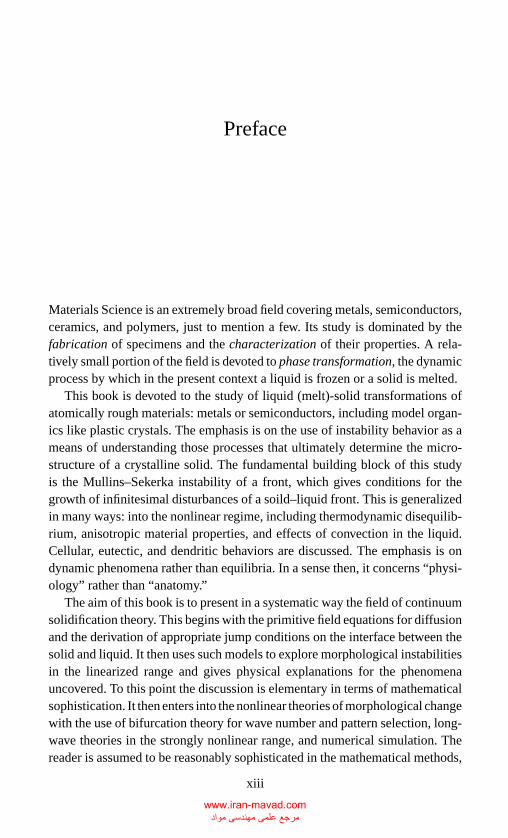
This book is devoted to the study of liquid (melt)-solid transformations ofatomically rough materials: metals or semiconductors, including model organ-ics like plastic crystals. The emphasis is on the use of instability behavior as ameans of understanding those processes that ultimately determine the micro-structure of a crystalline solid. The fundamental building block of this studyis the Mullins–Sekerka instability of a front, which gives conditions for thegrowth of infinitesimal disturbances of a soild–liquid front. This is generalizedin many ways: into the nonlinear regime, including thermodynamic disequilib-rium, anisotropic material properties, and effects of convection in the liquid.Cellular, eutectic, and dendritic behaviors are discussed. The emphasis is ondynamic phenomena rather than equilibria. In a sense then, it concerns “physi-ology” rather than “anatomy.”
The aim of this book is to present in a systematic way the field of continuumsolidification theory. This begins with the primitive field equations for diffusionand the derivation of appropriate jump conditions on the interface between thesolid and liquid. It then uses such models to explore morphological instabilitiesin the linearized range and gives physical explanations for the phenomenauncovered. To this point the discussion is elementary in terms of mathematicalsophistication. It then enters into the nonlinear theories of morphological changewith the use of bifurcation theory for wave number and pattern selection, long-wave theories in the strongly nonlinear range, and numerical simulation. Thereader is assumed to be reasonably sophisticated in the mathematical methods,
xiii
www.iran-mavad.com مرجع علمی مھندسی مواد
P1: FDG/FGA P2: FDG
CB381-Davis-FM CB381-Davis May 17, 2001 19:31 Char Count= 0
xiv Preface
that is, stability theory and its nonlinear extensions and some asymptotic andperturbation theory, but having little background in materials science. Thus,the book is deliberately nonuniform in its “degree of difficulty.” Those withlimited mathematical background can skip the nonlinear theories and read aboutthe physical phenomena and the linearized theories in the various chapters.The text should take the reader from the elements of the physics to the latestdevelopments of the theory. It would be hoped that applied mathematicians,engineers, and physicists would profit from the material presented as wouldtheoretically inclined materials scientists who could see how mathematics cangenerate understanding of relevant physical phenomena. An understanding ofthe physics is developed by using examples of increasing complexity withthe objective of creating a deep physical insight applicable to more complexproblems.
My interest in solidification was first stimulated by Jon Dantzig in his Ph.D.thesis of 1977 and permanently triggered by Ulrich Muller in our 1984 workon Benard convection coupled to a freezing front. When learning a new subjectas an “adult,” one leans heavily on the expertise of senior colleagues for theirwisdom. I thus wish to publicly thank Sam Coriell, Jon Dantzig, Paul Fife,Marty Glicksman, Wilfried Kurz, Jeff McFadden, Uli Muller, Bob Sekerka,Peter Voorhees, and Grae Worster for their contributions to my education.
I have always learned more from my graduate students, post-doctoral fellows,and visiting scientists than they have from me. I wish to thank them for theirwillingness to try something new. They are V. S. Ajaev, K. Brattkus, R. J.Braun, L. Buhler, D. J. Canright, Y.-J. Chen, J. A. Dantzig, A. A. Golovin, H.-P.Grimm, D. A. Huntley, P.-Q. Luo, G. B. McFadden, G. J. Merchant, P. Metzener,U. Muller, D. S. Riley, T. P. Schulze, B. J. Spencer, A. Umantsev, G. W. Young,and J.-J. Xu.
I am grateful to several people for reading selected chapters of the bookand making important suggestions. They are Dan Anderson, Kirk Brattkus,Yi-Ju Chen, Jon Dantzig, Sasha Golovin, Jeff McFadden, Tim Schulze, PeterVoorhees, Grae Worster, and J.-J. Xu.
This book could not have been written without the generous support ofthe National Aeronautics and Space Administration Microgravity Sciences andApplications Program.
Finally, I would like to thank my secretary, Judy Piehl, not only for herimpeccable typing, but for her sense of joy in her work. Her presence in thedepartment makes it possible for all of us to do better what we do.
www.iran-mavad.com مرجع علمی مھندسی مواد
P1: GFZ
CB381-01 CB381-Davis May 15, 2001 14:39 Char Count= 0
1
Introduction
The processes of freezing and melting were present at the beginning of theEarth and continue to affect the natural and industrial worlds. These processescreated the Earth’s crust and affect the dynamics of magmas and ice floes,which in turn affect the circulation of the oceans and the patterns of climate andweather. A huge majority of commercial solid materials were “born” as liquidsand frozen into useful configurations. The systems in which solidification isimportant range in scale from nanometers to kilometers and couple with a vastspectrum of other physics.
The solidification of a liquid or the melting of a solid involves a complex-interplay of many physical effects. The solid–liquid interface is an active freeboundary from which latent heat is liberated during phase transformation. Thisheat is conducted away from the interface through the solid and liquid, result-ing in the presence of thermal boundary layers near the interface. Across theinterface, the density changes, say, from ρ� to ρs. Thus, if ρs > ρ�, so that thematerial shrinks upon solidification, a flow is induced toward the interface from“infinity.”
If the liquid is not pure but contains solute, preferential rejection or incor-poration of solute occurs at the interface. For example, if a single solute ispresent and its solubility is smaller in the (crystalline) solid than it is in theliquid, the solute will be rejected at the interface. This rejected material willbe diffused away from the interface through the solid, the liquid, or both, re-sulting in the presence of concentration boundary layers near the interface. Thethermal and concentration boundary layer structures determine, in large part,whether morphological instabilities of the interface exist and what the ultimatemicrostructure of the solid becomes. Many a solidification problem of interestcouples the preceding purely diffusive effects with effects of thermodynamicdisequilibrium, crystalline anisotropy, and convection in the melt.
1
www.iran-mavad.com مرجع علمی مھندسی مواد
P1: GFZ
CB381-01 CB381-Davis May 15, 2001 14:39 Char Count= 0
2 1. Introduction
On the coarsest level of understanding, freezing is of concern only as a heat ormass transfer process. Thus, one cools a glass of bourbon by inserting ice cubesthat extract heat by melting. Likewise, one places salt on icy roads in Evanstonto facilitate melting because salt water has a lower melting temperature thanpure water.
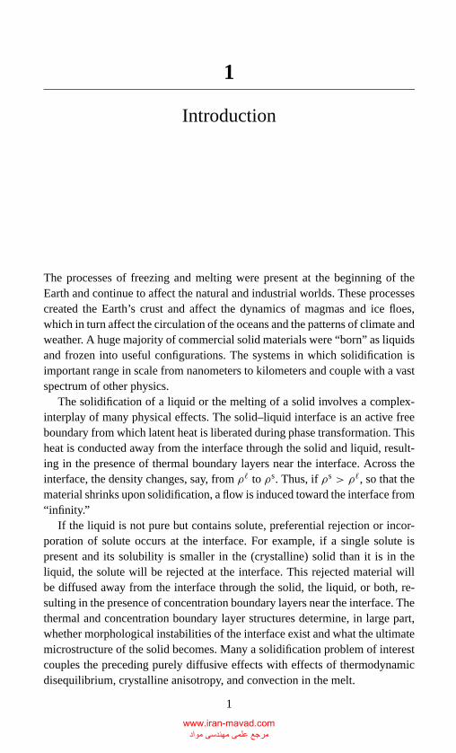
On a finer level of understanding, freezing can create solids whose mi-crostructures are determined by the process parameters and the intrinsic insta-bilities of the solid–liquid front. Figure 1.1 shows a longitudinal section of aZn–Al alloy casting. Notice the dendritic structures that extend inward fromthe cold boundary and a core region in which no microstructure is visible. Atlater times, spontaneous nucleation in the core can cause “snowflakes” to growin the core. The coarseness or fineness of the microstructure helps determinewhether mechanical and thermal reprocessing can be accomplished without theappearance of cracks.
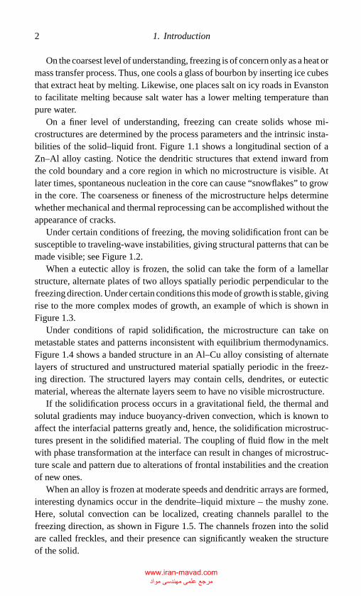
Under certain conditions of freezing, the moving solidification front can besusceptible to traveling-wave instabilities, giving structural patterns that can bemade visible; see Figure 1.2.
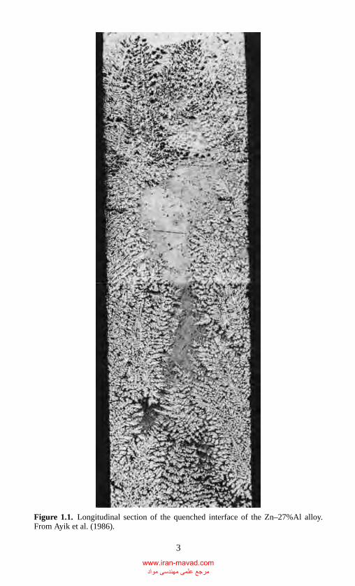
When a eutectic alloy is frozen, the solid can take the form of a lamellarstructure, alternate plates of two alloys spatially periodic perpendicular to thefreezing direction. Under certain conditions this mode of growth is stable, givingrise to the more complex modes of growth, an example of which is shown inFigure 1.3.
Under conditions of rapid solidification, the microstructure can take onmetastable states and patterns inconsistent with equilibrium thermodynamics.Figure 1.4 shows a banded structure in an Al–Cu alloy consisting of alternatelayers of structured and unstructured material spatially periodic in the freez-ing direction. The structured layers may contain cells, dendrites, or eutecticmaterial, whereas the alternate layers seem to have no visible microstructure.
If the solidification process occurs in a gravitational field, the thermal andsolutal gradients may induce buoyancy-driven convection, which is known toaffect the interfacial patterns greatly and, hence, the solidification microstruc-tures present in the solidified material. The coupling of fluid flow in the meltwith phase transformation at the interface can result in changes of microstruc-ture scale and pattern due to alterations of frontal instabilities and the creationof new ones.
When an alloy is frozen at moderate speeds and dendritic arrays are formed,interesting dynamics occur in the dendrite–liquid mixture – the mushy zone.Here, solutal convection can be localized, creating channels parallel to thefreezing direction, as shown in Figure 1.5. The channels frozen into the solidare called freckles, and their presence can significantly weaken the structureof the solid.
www.iran-mavad.com مرجع علمی مھندسی مواد
P1: GFZ
CB381-01 CB381-Davis May 15, 2001 14:39 Char Count= 0
Figure 1.1. Longitudinal section of the quenched interface of the Zn–27%Al alloy.From Ayik et al. (1986).
3
www.iran-mavad.com مرجع علمی مھندسی مواد
P1: GFZ
CB381-01 CB381-Davis May 15, 2001 14:39 Char Count= 0
4 1. Introduction
Figure 1.2. Etched longitudinal section of a Ga-doped Ge single crystal showing trav-eling waves on the interface. The arrow indicates the growth direction. From Singh,Witt, and Gatos (1974).
Figure 1.3. TEM micrographs of laser rapidly solidified Al–40 wt % Cu alloy oscillatoryinstabilities. V = 0.03 m/s. From Gill and Kurz (1993).
Given that the solid has crystalline structure, intrinsic symmetries in thematerial properties help define the continuum material. The surface energy andthe kinetic coefficient on the interface as well as the bulk transport propertiesinherit the directional properties of the crystal, and thus anisotropies are oftensignificant in determining the cellular or dendritic patterns that emerge. If theanisotropy is strong enough, the front can exhibit facets and corners.
www.iran-mavad.com مرجع علمی مھندسی مواد
P1: GFZ
CB381-01 CB381-Davis May 15, 2001 14:39 Char Count= 0
1. Introduction 5
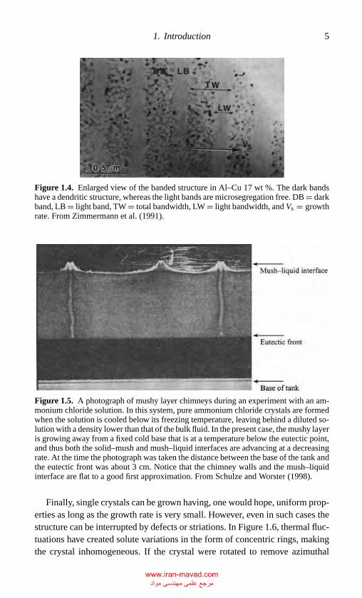
Figure 1.4. Enlarged view of the banded structure in Al–Cu 17 wt %. The dark bandshave a dendritic structure, whereas the light bands are microsegregation free. DB = darkband, LB = light band, TW = total bandwidth, LW = light bandwidth, and Vs = growthrate. From Zimmermann et al. (1991).
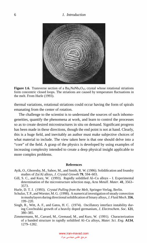
Figure 1.5. A photograph of mushy layer chimneys during an experiment with an am-monium chloride solution. In this system, pure ammonium chloride crystals are formedwhen the solution is cooled below its freezing temperature, leaving behind a diluted so-lution with a density lower than that of the bulk fluid. In the present case, the mushy layeris growing away from a fixed cold base that is at a temperature below the eutectic point,and thus both the solid–mush and mush–liquid interfaces are advancing at a decreasingrate. At the time the photograph was taken the distance between the base of the tank andthe eutectic front was about 3 cm. Notice that the chimney walls and the mush–liquidinterface are flat to a good first approximation. From Schulze and Worster (1998).
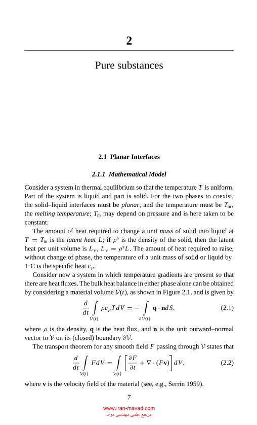
Finally, single crystals can be grown having, one would hope, uniform prop-erties as long as the growth rate is very small. However, even in such cases thestructure can be interrupted by defects or striations. In Figure 1.6, thermal fluc-tuations have created solute variations in the form of concentric rings, makingthe crystal inhomogeneous. If the crystal were rotated to remove azimuthal
www.iran-mavad.com مرجع علمی مھندسی مواد
P1: GFZ
CB381-01 CB381-Davis May 15, 2001 14:39 Char Count= 0
6 1. Introduction
Figure 1.6. Transverse section of a Ba2NaNb5O15 crystal whose rotational striationsform concentric closed loops. The striations are caused by temperature fluctuations inthe melt. From Hurle (1993).
thermal variations, rotational striations could occur having the form of spiralsemanating from the center of rotation.
The challenge to the scientist is to understand the sources of such inhomo-geneities, quantify the phenomena at work, and learn to control the processesso as to create desired microstructures in situ on demand. Significant progresshas been made in these directions, though the end point is not at hand. Clearly,this is a huge field, and inevitably an author must make subjective choices ofwhat material to include. The view taken here is that one should delve into a“core” of the field. A grasp of the physics is developed by using examples ofincreasing complexity intended to create a deep physical insight applicable tomore complex problems.
References
Ayik, O., Ghoreshy, M., Sahoo, M., and Smith, R. W. (1986). Solidification and foundrystudies of Zn/Al alloys, J. Crystal Growth 79, 594–603.
Gill, S. C., and Kurz, W. (1993). Rapidly solidified Al–Cu alloys – I. Experimentaldetermination of the microstructure selection map, Acta Metall. Mater. 41, 3563–3573.
Hurle, D. T. J. (1993). Crystal Pulling from the Melt, Springer-Verlag, Berlin.Schulze, T. P., and Worster, M. G. (1998). A numerical investigation of steady convection
in mushylayers during directional solidification of binary alloys, J. Fluid Mech. 356,199–220.
Singh, R., Witt, A. F., and Gatos, H. C. (1974). Oscillatory interface instability dur-ing Czochralski growth of a heavily doped germanium, J. Electrochem. Soc. 121,380–385.
Zimmermann, M., Carrard, M., Gremaud, M., and Kurz, W. (1991). Characterizationof a banded structure in rapidly solidified Al–Cu alloys, Mater. Sci. Eng. A134,1279–1282.
www.iran-mavad.com مرجع علمی مھندسی مواد
P1: GKW/FYX P2: GKW
CB381-02 CB381-Davis May 17, 2001 15:45 Char Count= 0
2
Pure substances
2.1 Planar Interfaces
2.1.1 Mathematical Model
Consider a system in thermal equilibrium so that the temperature T is uniform.Part of the system is liquid and part is solid. For the two phases to coexist,the solid–liquid interfaces must be planar, and the temperature must be Tm,
the melting temperature; Tm may depend on pressure and is here taken to beconstant.
The amount of heat required to change a unit mass of solid into liquid atT = Tm is the latent heat L; if ρs is the density of the solid, then the latentheat per unit volume is LV , LV = ρsL . The amount of heat required to raise,without change of phase, the temperature of a unit mass of solid or liquid by1◦C is the specific heat cp.
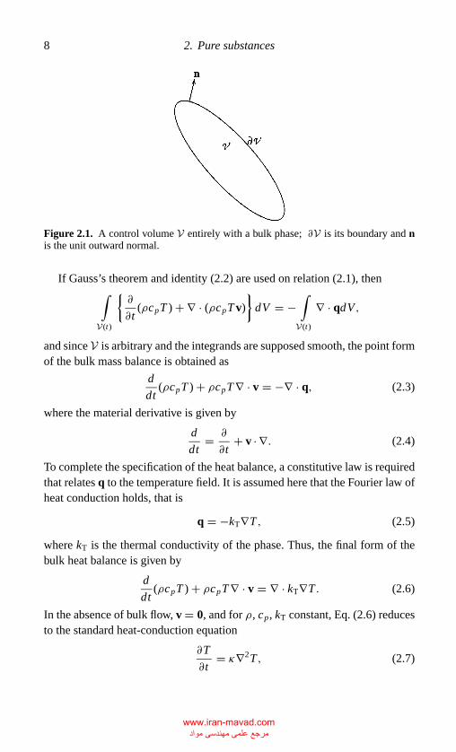
Consider now a system in which temperature gradients are present so thatthere are heat fluxes. The bulk heat balance in either phase alone can be obtainedby considering a material volume V(t), as shown in Figure 2.1, and is given by
d
dt
∫V(t)
ρcpT dV = −∫
∂V(t)
q · ndS, (2.1)
where ρ is the density, q is the heat flux, and n is the unit outward–normalvector to V on its (closed) boundary ∂V .
The transport theorem for any smooth field F passing through V states that
d
dt
∫V(t)
FdV =∫
V(t)
[∂F
∂t+ ∇ · (Fv)
]dV, (2.2)
where v is the velocity field of the material (see, e.g., Serrin 1959).
7
www.iran-mavad.com مرجع علمی مھندسی مواد
P1: GKW/FYX P2: GKW
CB381-02 CB381-Davis May 17, 2001 15:45 Char Count= 0
8 2. Pure substances
Figure 2.1. A control volume V entirely with a bulk phase; ∂V is its boundary and nis the unit outward normal.
If Gauss’s theorem and identity (2.2) are used on relation (2.1), then∫V(t)
{∂
∂t(ρcpT ) + ∇ · (ρcpT v)
}dV = −
∫V(t)
∇ · qdV,
and since V is arbitrary and the integrands are supposed smooth, the point formof the bulk mass balance is obtained as
d
dt(ρcpT ) + ρcpT∇ · v = −∇ · q, (2.3)
where the material derivative is given by
d
dt= ∂
∂t+ v · ∇. (2.4)
To complete the specification of the heat balance, a constitutive law is requiredthat relates q to the temperature field. It is assumed here that the Fourier law ofheat conduction holds, that is
q = −kT∇T, (2.5)
where kT is the thermal conductivity of the phase. Thus, the final form of thebulk heat balance is given by
d
dt(ρcpT ) + ρcpT∇ · v = ∇ · kT∇T . (2.6)
In the absence of bulk flow, v = 0, and for ρ, cp, kT constant, Eq. (2.6) reducesto the standard heat-conduction equation
∂T
∂t= κ∇2T, (2.7)
www.iran-mavad.com مرجع علمی مھندسی مواد
P1: GKW/FYX P2: GKW
CB381-02 CB381-Davis May 17, 2001 15:45 Char Count= 0
2.1 Planar interfaces 9
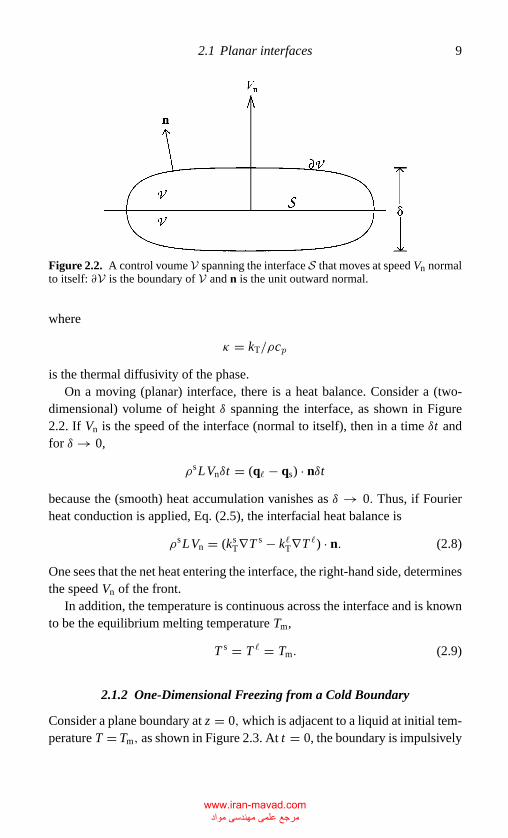
Figure 2.2. A control voume V spanning the interface S that moves at speed Vn normalto itself: ∂V is the boundary of V and n is the unit outward normal.
where
κ = kT/ρcp
is the thermal diffusivity of the phase.On a moving (planar) interface, there is a heat balance. Consider a (two-
dimensional) volume of height δ spanning the interface, as shown in Figure2.2. If Vn is the speed of the interface (normal to itself), then in a time δt andfor δ → 0,
ρsLVnδt = (q� − qs) · nδt
because the (smooth) heat accumulation vanishes as δ → 0. Thus, if Fourierheat conduction is applied, Eq. (2.5), the interfacial heat balance is
ρsLVn = (ksT∇T s − k�T∇T �) · n. (2.8)
One sees that the net heat entering the interface, the right-hand side, determinesthe speed Vn of the front.
In addition, the temperature is continuous across the interface and is knownto be the equilibrium melting temperature Tm,
T s = T � = Tm. (2.9)
2.1.2 One-Dimensional Freezing from a Cold Boundary
Consider a plane boundary at z = 0,which is adjacent to a liquid at initial tem-perature T = Tm, as shown in Figure 2.3. At t = 0, the boundary is impulsively
www.iran-mavad.com مرجع علمی مھندسی مواد
P1: GKW/FYX P2: GKW
CB381-02 CB381-Davis May 17, 2001 15:45 Char Count= 0
10 2. Pure substances
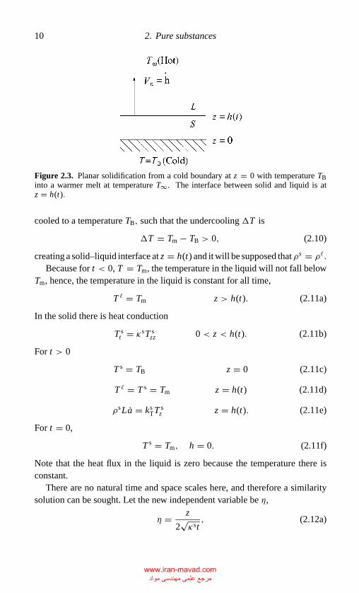
Figure 2.3. Planar solidification from a cold boundary at z = 0 with temperature TBinto a warmer melt at temperature T∞. The interface between solid and liquid is atz = h(t).
cooled to a temperature TB, such that the undercooling �T is
�T = Tm − TB > 0, (2.10)
creating a solid–liquid interface at z = h(t) and it will be supposed thatρs = ρ�.
Because for t < 0, T = Tm, the temperature in the liquid will not fall belowTm, hence, the temperature in the liquid is constant for all time,
T � = Tm z > h(t). (2.11a)
In the solid there is heat conduction
T st = κsT s
zz 0 < z < h(t). (2.11b)
For t > 0
T s = TB z = 0 (2.11c)
T � = T s = Tm z = h(t) (2.11d)
ρsLa = ksTT s
z z = h(t). (2.11e)
For t = 0,
T s = Tm, h = 0. (2.11f)
Note that the heat flux in the liquid is zero because the temperature there isconstant.
There are no natural time and space scales here, and therefore a similaritysolution can be sought. Let the new independent variable be η,
η = z
2√κst, (2.12a)
www.iran-mavad.com مرجع علمی مھندسی مواد
P1: GKW/FYX P2: GKW
CB381-02 CB381-Davis May 17, 2001 15:45 Char Count= 0
2.1 Planar interfaces 11
define the nondimensional temperature by θ,
T s = Tb + (�T )θ (η), (2.12b)
and thus θ = 0 at the base and θ = 1 at the front. Finally, consistent with thepreceding equations, the interface position is written as
h(t) = 2�√κst, (2.12c)
where the value of�, as yet unknown, determines the speed and position of thefront. Through the use of these forms, system (2.11a) becomes
θ ′′ + 2ηθ ′ = 0 0 < η < � (2.13a)
θ = 0 η = 0 (2.13b)
θ = 1 η = � (2.13c)
θ ′ = 2S� η = � (2.13d)
where the Stefan number S is
S = L
csp�T
. (2.14)
Notice that the initial conditions (2.11f) applied at t = 0 corresponds to η → ∞and that the temperature is constant in (h,∞). Thus, the thermal condition canbe applied at η = �, as shown in Eq. (2.13c). One integral of Eq. (2.13a) gives
θ ′ = Ae−η2, (2.15a)
where the integration constant A satisfies
2S� = Ae−�2. (2.15b)
A second integral that satisfies Eqs. (2.13b,c) is
θ =
∫ η
0e−s2
ds∫ �
0e−s2
ds
= erf (η)
erf (�), (2.15c)
where the error function is defined by
erf (z) ≡ 2√π
∫ z
0e−s2
ds. (2.16)
www.iran-mavad.com مرجع علمی مھندسی مواد
P1: GKW/FYX P2: GKW
CB381-02 CB381-Davis May 17, 2001 15:45 Char Count= 0
12 2. Pure substances
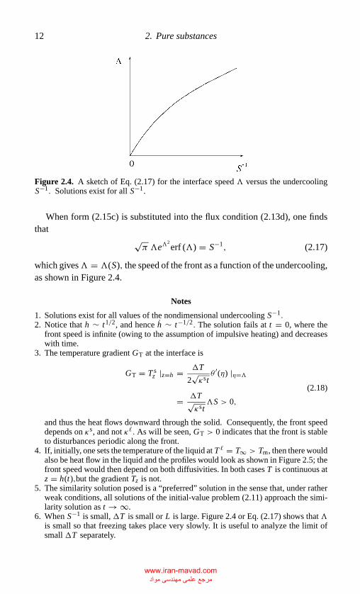
Figure 2.4. A sketch of Eq. (2.17) for the interface speed � versus the undercoolingS−1. Solutions exist for all S−1.
When form (2.15c) is substituted into the flux condition (2.13d), one findsthat
√π �e�
2erf (�) = S−1, (2.17)
which gives� = �(S), the speed of the front as a function of the undercooling,as shown in Figure 2.4.
Notes
1. Solutions exist for all values of the nondimensional undercooling S−1.2. Notice that h ∼ t1/2, and hence h ∼ t−1/2. The solution fails at t = 0, where the
front speed is infinite (owing to the assumption of impulsive heating) and decreaseswith time.
3. The temperature gradient GT at the interface is
GT = T sz |z=h = �T
2√κstθ ′(η) |η=�
= �T√κst�S > 0,
(2.18)
and thus the heat flows downward through the solid. Consequently, the front speeddepends on κs, and not κ�. As will be seen, GT > 0 indicates that the front is stableto disturbances periodic along the front.
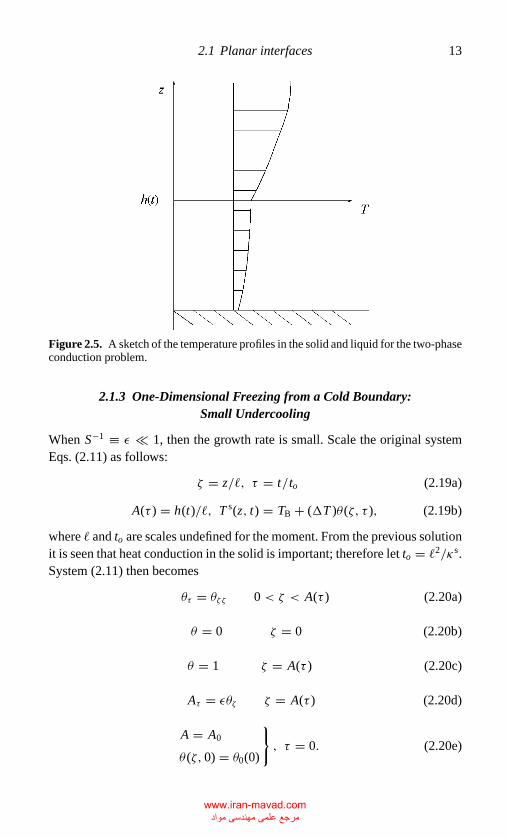
4. If, initially, one sets the temperature of the liquid at T � = T∞ > Tm, then there wouldalso be heat flow in the liquid and the profiles would look as shown in Figure 2.5; thefront speed would then depend on both diffusivities. In both cases T is continuous atz = h(t),but the gradient Tz is not.
5. The similarity solution posed is a “preferred” solution in the sense that, under ratherweak conditions, all solutions of the initial-value problem (2.11) approach the simi-larity solution as t → ∞.
6. When S−1 is small, �T is small or L is large. Figure 2.4 or Eq. (2.17) shows that �is small so that freezing takes place very slowly. It is useful to analyze the limit ofsmall �T separately.
www.iran-mavad.com مرجع علمی مھندسی مواد
P1: GKW/FYX P2: GKW
CB381-02 CB381-Davis May 17, 2001 15:45 Char Count= 0
2.1 Planar interfaces 13
Figure 2.5. A sketch of the temperature profiles in the solid and liquid for the two-phaseconduction problem.
2.1.3 One-Dimensional Freezing from a Cold Boundary:Small Undercooling
When S−1 ≡ ε 1, then the growth rate is small. Scale the original systemEqs. (2.11) as follows:
ζ = z/�, τ = t/to (2.19a)
A(τ ) = h(t)/�, T s(z, t) = TB + (�T )θ (ζ, τ ), (2.19b)
where � and to are scales undefined for the moment. From the previous solutionit is seen that heat conduction in the solid is important; therefore let to = �2/κs.System (2.11) then becomes
θτ = θζζ 0 < ζ < A(τ ) (2.20a)
θ = 0 ζ = 0 (2.20b)
θ = 1 ζ = A(τ ) (2.20c)
Aτ = εθζ ζ = A(τ ) (2.20d)
A = A0
θ (ζ, 0) = θ0(0)
}, τ = 0. (2.20e)
www.iran-mavad.com مرجع علمی مھندسی مواد
P1: GKW/FYX P2: GKW
CB381-02 CB381-Davis May 17, 2001 15:45 Char Count= 0
14 2. Pure substances
In the preceding, the problem has been generalized to allow nonzero initialtemperature distributions θ0(ζ ) and initial-front positions A0.
If ∂/∂τ = O(1) and ε → 0, the resulting system remains second orderin time and hence is capable of satisfying both initial conditions. However, atfirst approximation Aτ ∼ 0, and thus from time zero to τ = O(1) the interfaceis stationary at its initial position and solidification does not occur. In thistime interval one then has a standard heat-conduction problem for θ on a fixeddomain, 0<ζ < A. This represents the inner solution in time. The outer solutionin time, valid for long periods, requires a rescaling of time
τ = ετ, (2.21)
which represents a time scale based on latent heat and undercooling, namelyρsL�2/kT�T , and so describes the solidification process. In this case, system(2.11) becomes
εθτ = θζζ 0 < ζ < A(τ ) (2.22a)
θ = 0 ζ = 0 (2.22b)
θ = 1 ζ = A(τ ) (2.22c)
Aτ = θζ ζ = A(τ ) (2.22d)
A = A0, θ = θ0 τ = 0. (2.22e)
The limit ∂/∂τ = O(1) and ε → 0 is a singular perturbation; it is seen that atfirst approximation the temperature is quasi-steady,
θζζ = 0. (2.23)
The solution that satisfies Eqs. (2.22b,c) is
θ = ζ/A. (2.24)
Now the flux condition (2.22d) gives
AAτ = 1, (2.25)
which is a nonlinear evolution equation for A (Young 1994). Thus, with thefirst of condition (2.22e),
A2(τ ) − A20 = 2τ . (2.26)
In dimensional terms,
h2 − h20 = 2εκst = 2ks
T(�T )t
ρsL. (2.27)
The inner and outer solutions automatically match asymptotically.
www.iran-mavad.com مرجع علمی مھندسی مواد
P1: GKW/FYX P2: GKW
CB381-02 CB381-Davis May 17, 2001 15:45 Char Count= 0
2.1 Planar interfaces 15
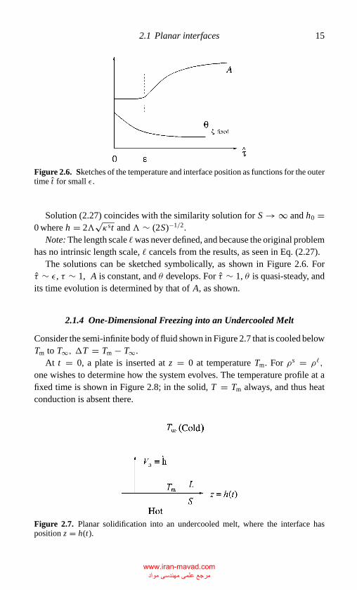
Figure 2.6. Sketches of the temperature and interface position as functions for the outertime t for small ε.
Solution (2.27) coincides with the similarity solution for S → ∞ and h0 =0 where h = 2�
√κst and � ∼ (2S)−1/2.
Note: The length scale �was never defined, and because the original problemhas no intrinsic length scale, � cancels from the results, as seen in Eq. (2.27).
The solutions can be sketched symbolically, as shown in Figure 2.6. Forτ ∼ ε, τ ∼ 1, A is constant, and θ develops. For τ ∼ 1, θ is quasi-steady, andits time evolution is determined by that of A, as shown.
2.1.4 One-Dimensional Freezing into an Undercooled Melt
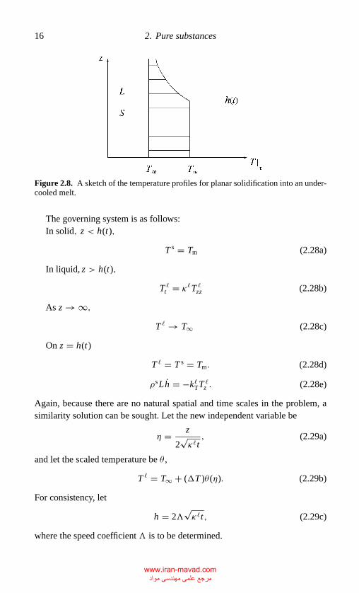
Consider the semi-infinite body of fluid shown in Figure 2.7 that is cooled belowTm to T∞, �T = Tm − T∞.
At t = 0, a plate is inserted at z = 0 at temperature Tm. For ρs = ρ�,
one wishes to determine how the system evolves. The temperature profile at afixed time is shown in Figure 2.8; in the solid, T = Tm always, and thus heatconduction is absent there.
Figure 2.7. Planar solidification into an undercooled melt, where the interface hasposition z = h(t).
www.iran-mavad.com مرجع علمی مھندسی مواد
P1: GKW/FYX P2: GKW
CB381-02 CB381-Davis May 17, 2001 15:45 Char Count= 0
16 2. Pure substances
Figure 2.8. A sketch of the temperature profiles for planar solidification into an under-cooled melt.
The governing system is as follows:In solid, z < h(t),
T s = Tm (2.28a)
In liquid, z > h(t),
T �t = κ�T �zz (2.28b)
As z → ∞,T � → T∞ (2.28c)
On z = h(t)
T � = T s = Tm. (2.28d)
ρsLh = −k�TT �z . (2.28e)
Again, because there are no natural spatial and time scales in the problem, asimilarity solution can be sought. Let the new independent variable be
η = z
2√κ�t, (2.29a)
and let the scaled temperature be θ ,
T � = T∞ + (�T )θ (η). (2.29b)
For consistency, let
h = 2�√κ�t, (2.29c)
where the speed coefficient � is to be determined.
www.iran-mavad.com مرجع علمی مھندسی مواد
P1: GKW/FYX P2: GKW
CB381-02 CB381-Davis May 17, 2001 15:45 Char Count= 0
2.1 Planar interfaces 17
The solution for the temperature is
θ (η) = erfc(η)
erfc(�), (2.30)
where the complementary error function is defined by
erfc(z) = 2√π
∫ ∞
ze−s2
ds. (2.31)
The flux condition (2.28e) then gives the characteristic equation√π�e�
2erfc(�) = S−1. (2.32)
Note: The temperature gradient GT in the liquid at the interface
GT = Tz[h(t), t] < 0
always, and thus the heat flows through the liquid. Consequently, the frontspeed depends on κ� and not κs. As will be seen, GT < 0 indicates that thefront is unstable to disturbances periodic along the front.
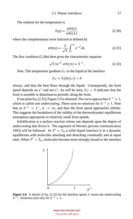
If one plots Eq. (2.32), Figure 2.9 is obtained. The curve approaches S−1 = 1,which is called unit undercooling. There exist no solutions for S−1 ≥ 1. Notethat as S−1 → 1−, � → ∞, and thus the front speed approaches infinity.This suggests the breakdown of the validity of the thermodynamic equilibriumassumption appropriate to relatively small front speeds.
Solidification is a surface reaction whose rate depends upon the degree ofundercooling that drives it. The argument of Worster (private communication1993) will be followed. At T I = Tm a solid–liquid interface is in a dynamicequilibrium with molecules attaching and detaching continually and at equalrates. When T I < Tm, molecules become more strongly bound to the interface
Figure 2.9. A sketch of Eq. (2.32) for the interface speed � versus the undercoolingS−1. Solutions exist only for S−1 < 1.
www.iran-mavad.com مرجع علمی مھندسی مواد
P1: GKW/FYX P2: GKW
CB381-02 CB381-Davis May 17, 2001 15:45 Char Count= 0
18 2. Pure substances
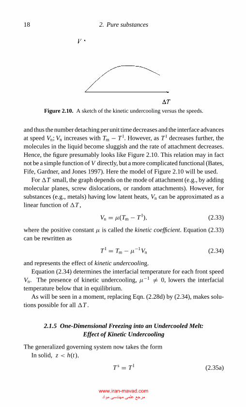
Figure 2.10. A sketch of the kinetic undercooling versus the speeds.
and thus the number detaching per unit time decreases and the interface advancesat speed Vn; Vn increases with Tm − T I. However, as T I decreases further, themolecules in the liquid become sluggish and the rate of attachment decreases.Hence, the figure presumably looks like Figure 2.10. This relation may in factnot be a simple function of V directly, but a more complicated functional (Bates,Fife, Gardner, and Jones 1997). Here the model of Figure 2.10 will be used.
For�T small, the graph depends on the mode of attachment (e.g., by addingmolecular planes, screw dislocations, or random attachments). However, forsubstances (e.g., metals) having low latent heats, Vn can be approximated as alinear function of �T ,
Vn = µ(Tm − T I), (2.33)
where the positive constant µ is called the kinetic coefficient. Equation (2.33)can be rewritten as
T I = Tm − µ−1Vn (2.34)
and represents the effect of kinetic undercooling.Equation (2.34) determines the interfacial temperature for each front speed
Vn. The presence of kinetic undercooling, µ−1 �= 0, lowers the interfacialtemperature below that in equilibrium.
As will be seen in a moment, replacing Eqn. (2.28d) by (2.34), makes solu-tions possible for all �T .
2.1.5 One-Dimensional Freezing into an Undercooled Melt:Effect of Kinetic Undercooling
The generalized governing system now takes the formIn solid, z < h(t),
T s = T I (2.35a)
www.iran-mavad.com مرجع علمی مھندسی مواد
P1: GKW/FYX P2: GKW
CB381-02 CB381-Davis May 17, 2001 15:45 Char Count= 0
2.1 Planar interfaces 19
In liquid, z > h(t)
T �t = κ�T �zz (2.35b)
As z → ∞T � → T∞ (2.35c)
On z = h(t),
T � = T I, (2.35d)
ρsLh = −k�T �z , (2.35e)
h = µ(Tm − T I). (2.35f)
Notice here that T I is now unknown and must be determined as part of thesolution.
An important difference between the equilibrium and nonequilibrium for-mulations is seen by dimensional analysis. Previously, the scales of length �and time to were arbitrary, and a relation between them associated with heatconduction, to = �2/κ�, was used; however, �was still arbitrary. Now, however,� is determined by the kinetic undercooling, namely
�
(κ�
�2
)= µ�T,
and thus
� = κ�
µ�T; (2.36a)
hence, using to = �2/κ�, we obtain
to = κ�
µ2(�T )2. (2.36b)
Write again
T � = T∞ + (�T )θ, (2.37)
and the scaled system becomes
θt = θzz z > A(t) (2.38a)
θ → 0 z → ∞ (2.38b)
θ = θ I
S A = −θz
A = 1 − θ I
, z = A(t) (2.38c)
www.iran-mavad.com مرجع علمی مھندسی مواد
P1: GKW/FYX P2: GKW
CB381-02 CB381-Davis May 17, 2001 15:45 Char Count= 0
20 2. Pure substances
The kinetic condition suggests seeking a solution with θ I constant; hence,A(t) = V . Let us seek a traveling-wave solution
θ = θ (ζ ), (2.39a)
where
ζ = z − V t, (2.39b)
and so the interface lies at ζ = 0. Here V is a constant and ζ is measured in amoving frame of reference. The diffusion equation (2.38a) then becomes
−V θ ′ = θ ′′, (2.40)
where a prime denotes d/dζ .The solution of Eq. (2.40), subject to conditions (2.38b) and the first of
(2.38c), is
θ = θ Ie−V ζ . (2.41)
The Stefan and kinetic conditions, the second and third of Eqs. (2.38c) thengive
θ I = S (2.42)
and
V = 1 − S, S < 1. (2.43)
Thus, for all S < 1,
θ = Se−(1−S)(z−V t), (2.44)
and solutions for S−1 > 1 have been found (Glicksman and Schaefer 1967).Note: Again, GT < 0.When there is unit undercooling, S = 1, yet a different solution exists
(Umantsev 1985) with h(t) ∼ t2/3. With kinetic undercooling present, thereare solutions for all S:
S−1 < 1, h ∼ t12
S−1 = 1, h ∼ t23
S−1 > 1, h ∼ t
. (2.45)
www.iran-mavad.com مرجع علمی مھندسی مواد

P1: GKW/FYX P2: GKW
CB381-02 CB381-Davis May 17, 2001 15:45 Char Count= 0
2.2 Curved interfaces 21
2.2 Curved Interfaces
2.2.1 Boundary Conditions
Consider a two-dimensional solid “drop” on a substrate, as shown in Figure2.11; no phase transformation is present. Thermodynamic equilibrium impliesthat the Helmholtz free energy E of the system, the sum of the surface energies,must be at a minimum for an equilibrium state to exist. Note that other energies,such as the elastic energy of “drop” and substrate, are ignored here, as is usual.The analysis follows Mullins (1963).
Let the system be uniform in the direction normal to the page and let w bea unit of length in that direction. The Helmholtz free energy is then
E = w
{∫ �2
�1
γ(1 + h2
x
)1/2dx + γ1(�2 − �1) + γ2[�− (�2 − �1)]
}, (2.46a)
where z = h(x) is the height of the interface, γ is the energy per unit area on thedrop–liquid interface, and γ1 and γ2 are the corresponding surface energies perunit area on the solid–substrate and liquid–substrate interfaces, respectively; allof these are taken to be constants, � is a fixed length, always larger than dropwidth, which is introduced to keep the energies finite; x = �1and �2 are theendpoints of the drop, and θ, measured within the drop, is called the contactangle. Consider variations in h, �1, and �2 such that the volume V of the dropis preserved, where
V = w
∫ �2
�1
hdx . (2.46b)
For a discussion of the variational calculus needed for this section, see Courantand Hilbert (1953), Chap. 4.
Figure 2.11. A solid, two-dimensional drop on a substrate; z = h(x) is the drop shape,x = �1 and �2 are the locations of the contact lines, � indicates an expanse larger thanthe drop, and θ is the contact angle.
www.iran-mavad.com مرجع علمی مھندسی مواد
P1: GKW/FYX P2: GKW
CB381-02 CB381-Davis May 17, 2001 15:45 Char Count= 0
22 2. Pure substances
The constrained problem defined above can be written as an unconstrainedvariational problem by introducing the Lagrange multiplier λ and writing
E ′ = E + λw∫ �2
�1
hdx
= w
{∫ �2
�1
[γ(1 + h2
x
)1/2 + λh]
dx + γ1(�2 − �1) + γ2 [�− (�2 − �1)]
}.
(2.47)
In order for E ′ to be minimum, it is necessary for the first variation, δE ′, to bezero,
w−1δE ′ =�2∫�1
{γ hxδ(hx )(1 + h2
x
)1/2 + λδh}
dx
+{γ[(
1 + h2x
)1/2]+ λh∣∣∣�2
+ γ1 − γ2
}δ�2
+{
−γ[(
1 + h2x
)1/2]− λh∣∣∣�1
− γ1 + γ2
}δ�1 = 0 (2.48)
Formally, one writes that
δ(hx ) = (δh)x (2.49)
and uses integration by parts to obtain∫ �
�1
hxδhx(1 + h2
x
)1/2 dx = −∫ �2
�1
{hx(
1 + h2x
)1/2}
x
δh dx + hxδh(1 + h2
x
)1/2∣∣∣∣∣�2
�1
.
(2.50)
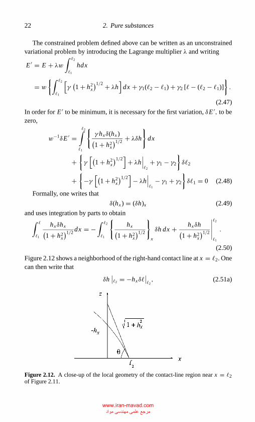
Figure 2.12 shows a neighborhood of the right-hand contact line at x = �2. Onecan then write that
δh∣∣�2 = −hxδ�
∣∣�2, (2.51a)
Figure 2.12. A close-up of the local geometry of the contact-line region near x = �2of Figure 2.11.
www.iran-mavad.com مرجع علمی مھندسی مواد
P1: GKW/FYX P2: GKW
CB381-02 CB381-Davis May 17, 2001 15:45 Char Count= 0
2.2 Curved interfaces 23
and similarly at the other contact line
δh∣∣�1 = −hxδ�
∣∣�1
(2.51b)
Thus,
hxδh(1 + h2
x
)1/2∣∣∣∣∣�2
�1
= − h2xδ�(
1 + h2x
)1/2∣∣∣∣∣�2
�1
. (2.52)
Finally,
w−1δE ′ =�2∫�1
{−γ[
hx(1 + h2
x
)1/2]
x
+ λ}δh dx
+ γ(
1 + h2x
)1/2∣∣∣∣∣�2
+ λh + γ1 − γ2
δ�2
− γ(
1 + h2x
)1/2∣∣∣∣∣�1
+ λh + γ1 − γ2
δ�1 = 0, (2.53)
where the boundary terms have been combined.Consider first variations in which the endpoints are fixed, that is, δ�1 =
δ�2 = 0. Given that the integrand of Eq. (2.53) is smooth and δh is otherwisearbitrary, that integrand must vanish. This gives the Euler–Lagrange equation
−γ[
hx(1 + h2
x
)1/2]
x
+ λ = 0
or
2Hγ = λ (2.54)
Here, for a one-dimensional interface the mean curvature H is defined by
2H = hxx(1 + h2
x
)3/2 . (2.55)
The interfacial shape h has constant curvature, and thus in two dimensions isan arc of a circle. By this definition a solid finger extending into the liquid hasH < 0. The Lagrange multiplier is a constant that cannot be determined byvariational calculus but requires some additional physical statement (Hills andRoberts 1993).
Let the Gibbs free energy� of the system depend on the pressure p and thetemperature T . Let � on the solid side of the interface be equal to that on the
www.iran-mavad.com مرجع علمی مھندسی مواد
P1: GKW/FYX P2: GKW
CB381-02 CB381-Davis May 17, 2001 15:45 Char Count= 0
24 2. Pure substances
liquid side. Expand this equation about p = p�, the pressure on the liquid side,let T = Tm and identify ∂�/∂p by 1/ps, and let ∂�/∂T = −s, the entropy,and �s = LV/Tm,; then one can write
λ = LV�T/Tm, (2.56a)
where
�T = T I − Tm. (2.56b)
Here T I is the drop–liquid interface temperature and Tm is the equilibriummelting temperature of the material in the drop.
The results above can be obtained by using the total grand potential (Gibbs1948, p. 229; Wettlaufer and Worster 1995), and this approach has the advantageof easy generalization to multicomponent systems.
Equation (2.54) is the Laplace relation for the interface, and the followingis the Gibbs–Thomson relation giving capillary undercooling:
T I = Tm
[1 + 2H
γ
LV
](2.57)
If H is replaced by its generalization to a two-dimensional surface, then Eq.(2.57) holds for three-dimensional systems. See Chapter 5 for generalizationsto systems where γ depends on the orientation of the surface.
Consider next variations in which the endpoints may move. Because Eq.(2.54) holds already, one has at each endpoint x = �i , i = 1, 2, that
γ(1 + h2
x
)1/2 + γ1 − γ2 = 0, (2.58)
because h is zero at the endpoints. If Figure 2.12 is used to evaluate this,(1 + h2
x
)−1/2 = cos θ, and thus the Young–Laplace relation emerges,
γ cos θ = γ2 − γ1. (2.59)
At equilibrium at each contact line the contact angle θ adjusts itself to give thissurface–energy balance. See Chapter 5 for generalizations to systems where γdepends on the orientation of the surface.
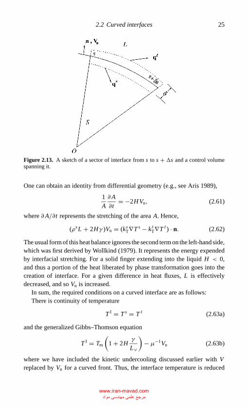
On a moving interface, there is a heat balance, applied to the domain shownin Figure 2.13. Call Vn the speed of the interface normal to itself and s the arclength. In Figure 2.13 as δ → 0 in a time δt,
ρsLVn Aδt − γ A |s+δs + γ A|s = (q� − qs) · nAδt
or
ρsLVn − 1
A
∂
∂t(γ A) = ks
TT sn − k�TT �n . (2.60)
www.iran-mavad.com مرجع علمی مھندسی مواد
P1: GKW/FYX P2: GKW
CB381-02 CB381-Davis May 17, 2001 15:45 Char Count= 0
2.2 Curved interfaces 25
Figure 2.13. A sketch of a sector of interface from s to s + �s and a control volumespanning it.
One can obtain an identity from differential geometry (e.g., see Aris 1989),
1
A
∂A
∂t= −2HVn, (2.61)
where ∂A/∂t represents the stretching of the area A. Hence,
(ρsL + 2Hγ )Vn = (ksT∇T s − k�T∇T �) · n. (2.62)
The usual form of this heat balance ignores the second term on the left-hand side,which was first derived by Wollkind (1979). It represents the energy expendedby interfacial stretching. For a solid finger extending into the liquid H < 0,and thus a portion of the heat liberated by phase transformation goes into thecreation of interface. For a given difference in heat fluxes, L is effectivelydecreased, and so Vn is increased.
In sum, the required conditions on a curved interface are as follows:There is continuity of temperature
T I = T s = T � (2.63a)
and the generalized Gibbs–Thomson equation
T I = Tm
(1 + 2H
γ
LV
)− µ−1Vn (2.63b)
where we have included the kinetic undercooling discussed earlier with Vreplaced by Vn for a curved front. Thus, the interface temperature is reduced
www.iran-mavad.com مرجع علمی مھندسی مواد
P1: GKW/FYX P2: GKW
CB381-02 CB381-Davis May 17, 2001 15:45 Char Count= 0
26 2. Pure substances
for “fingers” of solid growing into melt (H < 0) and for increased speed Vn ofthe interface. In addition, there is the heat balance
ksT∇T s − k�T∇T � = LVVn
(1 + 2H
γ
LV
). (2.63c)
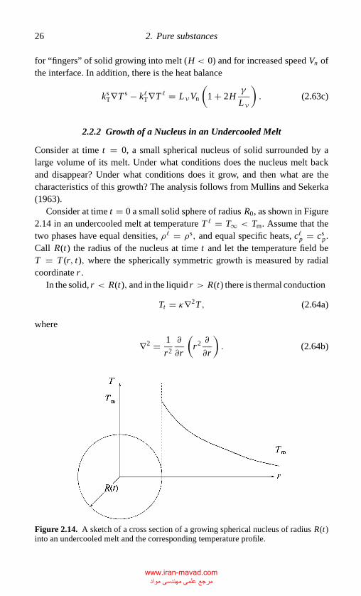
2.2.2 Growth of a Nucleus in an Undercooled Melt
Consider at time t = 0, a small spherical nucleus of solid surrounded by alarge volume of its melt. Under what conditions does the nucleus melt backand disappear? Under what conditions does it grow, and then what are thecharacteristics of this growth? The analysis follows from Mullins and Sekerka(1963).
Consider at time t = 0 a small solid sphere of radius R0, as shown in Figure2.14 in an undercooled melt at temperature T � = T∞ < Tm. Assume that thetwo phases have equal densities, ρ� = ρs, and equal specific heats, c�p = cs
p.Call R(t) the radius of the nucleus at time t and let the temperature field beT = T (r, t), where the spherically symmetric growth is measured by radialcoordinate r .
In the solid, r < R(t), and in the liquid r > R(t) there is thermal conduction
Tt = κ∇2T, (2.64a)
where
∇2 = 1
r2
∂
∂r
(r2 ∂
∂r
). (2.64b)
Figure 2.14. A sketch of a cross section of a growing spherical nucleus of radius R(t)into an undercooled melt and the corresponding temperature profile.
www.iran-mavad.com مرجع علمی مھندسی مواد
P1: GKW/FYX P2: GKW
CB381-02 CB381-Davis May 17, 2001 15:45 Char Count= 0
2.2 Curved interfaces 27
Far from the sphere, r → ∞,
T � → T∞, (2.64c)
whereas at the origin, r = 0, the temperature is bounded,∣∣T s∣∣ < ∞. (2.64d)
On the sphere r = R(t), there is the continuity of temperature, the Gibbs–Thomson equation, and the heat balance,
T � = T s = T I = Tm
[1 + 2H
γ
LV
](2.64e)
and
LVd R
dt= [ks
T∇T s − k�T∇T �] · n, (2.64f)
where n is the unit vector pointing out of the nucleus. The curvature-dependentheat rise in the heat balance, usually small, and the kinetic undercooling, haveboth been ignored for simplicity. Here the mean curvature is
H = − 1
R(2.64g)
and
n·∇ = ∂
∂r. (2.64h)
Finally, there are initial conditions,
R(0) = R0
T �(r, 0) = T �o (r )
T s(r, 0) = T so (r )
, t = 0. (2.64i)
Define scales as follows:
length → R0
temperature → �T = Tm − T∞
speed → vp = k�T�T
R0LV
time → tp = R0/vp = R20 LV
k�T�T.
(2.65)
Here �T is the undercooling and vp is determined by the heat balance at theinterface.
www.iran-mavad.com مرجع علمی مھندسی مواد
P1: GKW/FYX P2: GKW
CB381-02 CB381-Davis May 17, 2001 15:45 Char Count= 0
28 2. Pure substances
Define now the following nondimensional variables:
r = r/R0, T = (T − Tm)/�T, t = t/tp. (2.66)
The governing system (2.64) can be written as follows:
εT �t = ∇2T � r > R(t) (2.67a)
εT st = κ∇2T s r < R(t) (2.67b)
T � = −1 r → ∞ (2.67c)
|T s| < ∞ r → 0 (2.67d)
T � = T s = − �R
d R
dt= kTT s
r − T �r
r = R(t)
(2.67e)
R = 1
T � = T �o
T s = T so
t = 0, (2.67f)
where the carets have been dropped. The nondimensional parameters presentare the modified Stefan number S,
S−1 = k�T�T
LVκ�= c�p�T
L≡ ε, (2.68a)
the surface energy parameter �,
� = 2γ
R0LV
Tm
�T(2.68b)
and the thermal parameters κ and kT,
κ = κs
κ�
kT = ksT
k�T
. (2.68c)
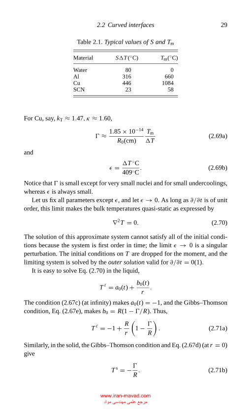
Let us estimate the values of the physical constants for typical materials.These are shown in Table 2.1.
www.iran-mavad.com مرجع علمی مھندسی مواد
P1: GKW/FYX P2: GKW
CB381-02 CB381-Davis May 17, 2001 15:45 Char Count= 0
2.2 Curved interfaces 29
Table 2.1. Typical values of S and Tm
Material S�T (◦C) Tm(◦C)
Water 80 0Al 316 660Cu 446 1084SCN 23 58
For Cu, say, kT ≈ 1.47, κ ≈ 1.60,
� ≈ 1.85 × 10⁻¹⁴
R0(cm)
Tm
�T(2.69a)
and
ε = �T ◦C409◦C
. (2.69b)
Notice that � is small except for very small nuclei and for small undercoolings,whereas ε is always small.
Let us fix all parameters except ε, and let ε → 0. As long as ∂/∂t is of unitorder, this limit makes the bulk temperatures quasi-static as expressed by
∇2T = 0. (2.70)
The solution of this approximate system cannot satisfy all of the initial condi-tions because the system is first order in time; the limit ε → 0 is a singularperturbation. The initial conditions on T are dropped for the moment, and thelimiting system is solved by the outer solution valid for ∂/∂t = 0(1).
It is easy to solve Eq. (2.70) in the liquid,
T � = a0(t) + b0(t)
r.
The condition (2.67c) (at infinity) makes a0(t) = −1, and the Gibbs–Thomsoncondition, Eq. (2.67e), makes b0 = R(1 − �/R). Thus,
T � = −1 + R
r
(1 − �
R
). (2.71a)
Similarly, in the solid, the Gibbs–Thomson condition and Eq. (2.67d) (at r = 0)give
T s = −�R. (2.71b)
www.iran-mavad.com مرجع علمی مھندسی مواد
P1: GKW/FYX P2: GKW
CB381-02 CB381-Davis May 17, 2001 15:45 Char Count= 0
30 2. Pure substances
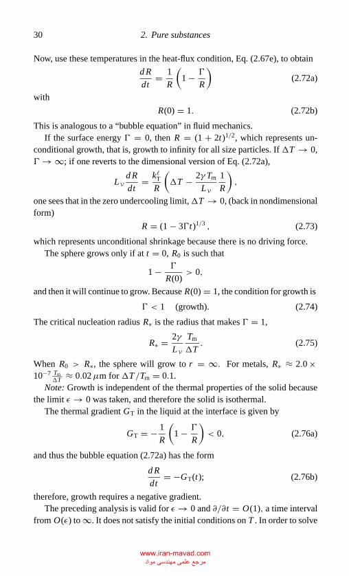
Now, use these temperatures in the heat-flux condition, Eq. (2.67e), to obtain
d R
dt= 1
R
(1 − �
R
)(2.72a)
with
R(0) = 1. (2.72b)
This is analogous to a “bubble equation” in fluid mechanics.If the surface energy � = 0, then R = (1 + 2t)1/2, which represents un-
conditional growth, that is, growth to infinity for all size particles. If�T → 0,� → ∞; if one reverts to the dimensional version of Eq. (2.72a),
LVd R
dt= k�T
R
(�T − 2γ Tm
LV
1
R
),
one sees that in the zero undercooling limit,�T → 0, (back in nondimensionalform)
R = (1 − 3�t)1/3 , (2.73)
which represents unconditional shrinkage because there is no driving force.The sphere grows only if at t = 0, R0 is such that
1 − �
R(0)> 0,
and then it will continue to grow. Because R(0) = 1, the condition for growth is
� < 1 (growth). (2.74)
The critical nucleation radius R∗ is the radius that makes � = 1,
R∗ = 2γ
LV
Tm
�T. (2.75)
When R0 > R∗, the sphere will grow to r = ∞. For metals, R∗ ≈ 2.0 ×10⁻⁷ Tm
�T ≈ 0.02µm for �T /Tm = 0.1.Note: Growth is independent of the thermal properties of the solid because
the limit ε → 0 was taken, and therefore the solid is isothermal.The thermal gradient GT in the liquid at the interface is given by
GT = − 1
R
(1 − �
R
)< 0, (2.76a)
and thus the bubble equation (2.72a) has the form
d R
dt= −GT(t); (2.76b)
therefore, growth requires a negative gradient.The preceding analysis is valid for ε → 0 and ∂/∂t = O(1), a time interval
from O(ε) to ∞. It does not satisfy the initial conditions on T . In order to solve
www.iran-mavad.com مرجع علمی مھندسی مواد
P1: GKW/FYX P2: GKW
CB381-02 CB381-Davis May 17, 2001 15:45 Char Count= 0
2.2 Curved interfaces 31
for this early-time behavior, one must rescale time and hence seek the innersolution.
Let t be the dimensional time and t be the “outer” time. Then
t∗ = t
ε= t
εtp= t(
R20/κ
�) . (2.77a)
Thus, t , the outer time, derives its scale from the interfacial balance of heat, andt∗, the inner time, is determined by thermal conduction. In fact it is seen that
t
t∗= ε. (2.77b)
When the change of variable (2.77a) is made, the bulk diffusion equationsbecome free of ε, but now the interfacial heat balance is as follows:
d R
dt∗= ε(kTT s
r − T �r)
(2.78)
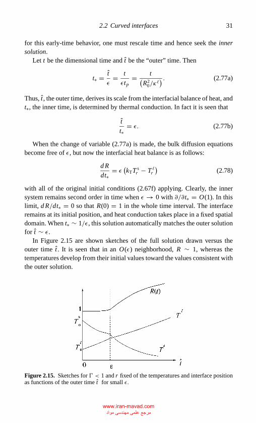
with all of the original initial conditions (2.67f) applying. Clearly, the innersystem remains second order in time when ε → 0 with ∂/∂t∗ = O(1). In thislimit, d R/dt∗ = 0 so that R(0) = 1 in the whole time interval. The interfaceremains at its initial position, and heat conduction takes place in a fixed spatialdomain. When t∗ ∼ 1/ε, this solution automatically matches the outer solutionfor t ∼ ε.
In Figure 2.15 are shown sketches of the full solution drawn versus theouter time t . It is seen that in an O(ε) neighborhood, R ∼ 1, whereas thetemperatures develop from their initial values toward the values consistent withthe outer solution.
Figure 2.15. Sketches for � < 1 and r fixed of the temperatures and interface positionas functions of the outer time t for small ε.
www.iran-mavad.com مرجع علمی مھندسی مواد
P1: GKW/FYX P2: GKW
CB381-02 CB381-Davis May 17, 2001 15:45 Char Count= 0
32 2. Pure substances
2.2.3 Linearized Instability of Growing Nucleus
As the spherical nucleus grows in time, as given by Eq. (2.72a), there is thepossibility that at some time (or equivalently at some radius) an instability willoccur that destroys the spherical symmetry of the particle. In order to determinewhether instabilities occur, begin with the full time-dependent system (2.67),the exact solution given asymptotically for ε → 0 in the last section, namely
T = T (r, t), R = R(t),
and disturb the system by small disturbances T ′ and R′ as follows:
T = T (r, t) + T ′(r, θ, φ, t), R = R(t) + R′(θ, φ, t). (2.79)
Substitute these into the system, and linearize in primed quantities. The resultinglinear system as follows:
εT �′
t = ∇2T �′, r > R (2.80a)
εT s′t = κ∇2T s′
, r < R (2.80b)
T ′ → 0, r → ∞ (2.80c)∣∣T ′∣∣ < ∞, r → 0 (2.80d)
R′t = kTT s′
r − T �′
r + (kTT srr − T �rr
)R′
T �′ + T �r R′ = T s′ + T s
r R′ = H ′�
}, r = R, (2.80e)
where
∇2 = ∂2
∂r2+ 2
r
∂
∂r+ 1
r2L (2.80f)
L = ∂2
∂θ2+ cot θ
∂
∂θ+ 1
sin2 θ
∂2
∂ϕ2(2.80g)
n =(
1, − 1
RRθ , − 1
R sin θR
)(1 + R2
θ
R2+ R2
ϕ
R2 sin2 θ
)−1/2
(2.80h)
2H = − 2
R+ 2R′
R2 + L R′
R2 ∼ − 2
R+ (L + 2)R′
R2 + · · ·. (2.80i)
Notice that all interfacial conditions apply on r = R rather than on r = R + R′
because Taylor series have been used to transfer the site of their application tothe undisturbed interface. In the second of Eqs. (2.80e), H ′ is the disturbedcurvature that is defined in Eq. (2.80i).
www.iran-mavad.com مرجع علمی مھندسی مواد
P1: GKW/FYX P2: GKW
CB381-02 CB381-Davis May 17, 2001 15:45 Char Count= 0
2.2 Curved interfaces 33
Notice, as well, that the initial conditions have been dropped because theinterest lies in the long-time behavior of disturbances, that is, if (T ′, R′) growswith time as t → ∞, then the interface is unstable. If (T ′, R′) decays always,then the interface is stable.
Given that the long-time behavior is of interest, consider only the outersolution and set ε = 0. Thus, the temperatures in each phase are quasi-steady.
For r > R(t) then,
∇2T �′ = 0. (2.81a)
Let us consider normal-mode solutions (separation of variables) and write
T �′ = f (r )Y�m, (2.81b)
where Y�m are spherical harmonics that satisfy
LY�m = −�(�+ 1)Y�m (2.81c)
(see Morse and Feshbach 1953, 1264ff.). Then, the function f satisfies
f ′′ + 2
rf ′ − �(�+ 1)
r2f = 0. (2.81d)
This is an equidimensional equation whose solutions have the form f ∝ rk ,where k = �, −�− 1. Thus, here
T ′� = AO(t)r−�−1Y�m(θ, φ), (2.81e)
which satisfies the condition (2.80c) at infinity.For r < R(t),
∇T ′s = 0 (2.82a)
and
T ′s = AI(t)r�Y�m(θ, ϕ), (2.82b)
which satisfies the condition (2.80d) as r → 0.Let R′ = R(t)Y�m and substitute forms (2.81e) and (2.82b) into the Gibbs–
Thomson equation (2.80e) to obtain
AO(t) =[
R� − 1
2��(�+ 1)R�−1
]R. (2.82c)
Finally, use the flux condition, the first part of Eq. (2.80e), to find after somealgebra that
d R
dt={
1 − �
2R(t)[(�+ 1)(�+ 2) + 2 + kT�(�+ 2)]
}(�− 1)
R2 R. (2.83)
www.iran-mavad.com مرجع علمی مھندسی مواد
P1: GKW/FYX P2: GKW
CB381-02 CB381-Davis May 17, 2001 15:45 Char Count= 0
34 2. Pure substances
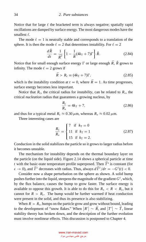
Notice that for large � the bracketed term is always negative; spatially rapidoscillations are damped by surface energy. The most dangerous modes have thesmallest �.
The mode � = 1 is neutrally stable and corresponds to a translation of thesphere. It is then the mode � = 2 that determines instability. For � = 2
d R
dt= 1
R2
{1 − 1
R(4kT + 7)�
}R. (2.84)
Notice that for small enough surface energy � or large enough R, R grows toinfinity. The mode � = 2 grows if
R > Rc ≡ (4kT + 7)�, (2.85)
which is the instability condition at t = 0, where R = 1. As time progresses,surface energy becomes less important.
Notice that Rc, the critical radius for instability, can be related to R∗, thecritical nucleation radius that guarantees a growing nucleus, by
Rc
R∗= 4kT + 7, (2.86)
and thus for a typical metal Rc ≈ 0.30µm, whereas R∗ ≈ 0.02µm.Three interesting cases are
Rc
R∗=
7 if kT = 0
11 if kT = 1
15 if kT = 2.
(2.87)
Conduction in the solid stabilizes the particle so it grows to larger radius beforeit becomes unstable.
The mechanism for instability depends on the thermal boundary layer onthe particle (on the liquid side). Figure 2.14 shows a spherical particle at timet with the basic-state temperature profile superposed. Then T s is constant (forε → 0), and T � decreases with radius. Thus, always dT �/dr = −G�(t) < 0.
Consider now a shape perturbation on the sphere as shown. A solid bumppushes further into the liquid, steepens the magnitude of the gradient G�, which,by the flux balance, causes the bump to grow faster. The surface energy isavailable to oppose this growth. It is able to do this for R∗ < R < Rc, but itcannot for R > Rc. The bump would be further warmed if heat conductionwere present in the solid, and thus its presence is also stabilizing.
When R > Rc, bumps on the particle grow and grow without bound, leadingto the development of “snow flakes.” When
∣∣R′∣∣ ∼ R, and∣∣T ′∣∣ ∼ T , linear
stability theory has broken down, and the description of the further evolutionmust involve nonlinear effects. This discussion is postponed to Chapter 4.
www.iran-mavad.com مرجع علمی مھندسی مواد
P1: GKW/FYX P2: GKW
CB381-02 CB381-Davis May 17, 2001 15:45 Char Count= 0
2.2 Curved interfaces 35
2.2.4 Linearized Instability of a Plane Front Growinginto an Undercooled Melt
In Section 2.1.4 the solution is given for a moving planar front. If and whenthe front becomes unstable to cellular modes, periodic along the interface, thestability problem becomes one in which curved interfaces are important. Onlythe case of larger undercooling, S−1 > 1, (called hypercooled) will be givenhere, and hence kinetic undercooling is retained.
Consider a front moving in the z-direction, z = h(x, t) and only the two-dimensional problem.
The governing system is as follows:In liquid, z > h,
T �t = κ�∇2T �. (2.88a)
In solid, z < h,
T s = T I. (2.88b)
where T I(x, t) is unknown a priori. As z → ∞T � → T∞. (2.88c)
On z = h(x, t)
T s = T � = T I = Tm
(1 + 2H
γ
LV
)− µ−1Vn (2.88d)
(LV + 2Hγ )Vn = −k�T∇T � · n, (2.88e)
where
Vn = ht(1 + h2
x
)1/2 (2.88f)
is the speed of the front normal to itself, and the effects of kinetic undercoolingare included in the Gibbs–Thomson relation (2.88e) through coefficient µ.
Introduce scales as follows: length ∼ �, time ∼ to, temperature ∼ �T =Tm − T∞ > 0, and define θ through T = T∞ + (�T )θ . Here
� = κ�
µ�T, and to = κ�
µ2(�T )2. (2.89)
The scaled equations now have the form:In liquid z > h,
θt = ∇2θ. (2.90a)
www.iran-mavad.com مرجع علمی مھندسی مواد
P1: GKW/FYX P2: GKW
CB381-02 CB381-Davis May 17, 2001 15:45 Char Count= 0
36 2. Pure substances
In solid z < h,
θ = θ I, (2.90b)
where
θ I = (T I − T∞)/�T (2.90c)
As z → ∞θ → 0. (2.90d)
On the interface z = h(x, t)(S + 2HC−1
)Vn = −∇θ · n (2.90e)
1 + 2H�1 − Vn = θ, (2.90f)
where
C = k�Tµγ, S = L
c�p�T, �1 = γ
L
Tmc�pµ
k�T. (2.91)
The first step is defining a basic state, the solution that was obtained inSection 2.1.4, as follows:
θ = Se−V z (2.92a)
h = V t, (2.92b)
where
z = z − V t (2.92c)
and
S = 1 − V . (2.92d)
One changes coordinates (x, z, t) → (x, z, t), where x = x, z = z −V t, t = t , and Eq . (2.90b) becomes
θt − V θz = ∇2θ ; (2.93)
the carats have been dropped.Disturb this exact solution as follows:
θ = θ + θ ′, h = h′. (2.94)
If one substitutes forms (2.94) into system (2.90) and linearizes in primedquantities, the linearized stability problem results. In liquid, z > 0
θ ′t − V θ ′
z = ∇2θ ′ (2.95a)
www.iran-mavad.com مرجع علمی مھندسی مواد
P1: GKW/FYX P2: GKW
CB381-02 CB381-Davis May 17, 2001 15:45 Char Count= 0
2.2 Curved interfaces 37
At z → ∞,θ ′ → 0 (2.95b)
On z = 0,
Sh′t + C−1V h′
xx + V 2Sh′ = −θ ′z (2.95c)
�1h′xx − h′
t + V Sh′ = 0, (2.95d)
where the interfacial-boundary conditions have been linearized, as discussedearlier. Note that because θ s = θ I, the temperature in the solid decouples fromthis system and hence can be determined after (2.95) is solved.
To solve system (2.95), use normal modes
[θ ′(x, t), h′(t)] = [θ (z), h]eσ t+ia1x . (2.96)
Note that because time does not appear explicitly in the coefficients of system(2.95), exponential variations in time occur in the disturbances; this contraststo the case of the nucleus that grows like t1/2.
The heat equation (2.95a) becomes(σ − V
d
dz
)θ =(
d2
dz2− a2
1
)θ , (2.97a)
which has solutions θ = e−pz, Re p > ∞ that satisfy the condition at z → ∞.Here
p2 − pV − (a21 + σ ) = 0
so that
p = 1
2
{V + [V 2 + 4
(a2
1 + σ )]1/2} . (2.97b)
The interfacial conditions are
(σ S − C−1V a21 + V 2S)h = pθ (0) (2.97c)
and
(−�1a21 − σ + V S)h = θ (0). (2.97d)
This linear, homogeneous system has nontrivial solutions only when the de-terminant of the matrix of coefficients is zero. This gives the characteristicequation
σ (S + p) = p(V S − �a21) + C−1a2
1 − V 2S (2.97e)
with
V = 1 − S. (2.97f)
www.iran-mavad.com مرجع علمی مھندسی مواد
P1: GKW/FYX P2: GKW
CB381-02 CB381-Davis May 17, 2001 15:45 Char Count= 0
38 2. Pure substances
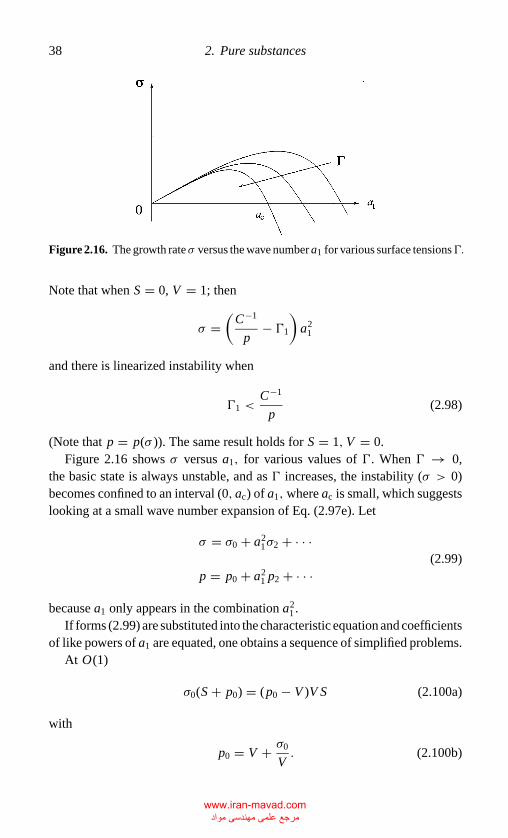
Figure 2.16. The growth rateσ versus the wave number a1 for various surface tensions�.
Note that when S = 0, V = 1; then
σ =(
C−1
p− �1
)a2
1
and there is linearized instability when
�1 <C−1
p(2.98)
(Note that p = p(σ )). The same result holds for S = 1, V = 0.Figure 2.16 shows σ versus a1, for various values of �. When � → 0,
the basic state is always unstable, and as � increases, the instability (σ > 0)becomes confined to an interval (0, ac) of a1,where ac is small, which suggestslooking at a small wave number expansion of Eq. (2.97e). Let
σ = σ0 + a21σ2 + · · ·
p = p0 + a21 p2 + · · ·
(2.99)
because a1 only appears in the combination a21 .
If forms (2.99) are substituted into the characteristic equation and coefficientsof like powers of a1 are equated, one obtains a sequence of simplified problems.
At O(1)
σ0(S + p0) = (p0 − V )V S (2.100a)
with
p0 = V + σ0
V. (2.100b)
www.iran-mavad.com مرجع علمی مھندسی مواد
P1: GKW/FYX P2: GKW
CB381-02 CB381-Davis May 17, 2001 15:45 Char Count= 0
2.2 Curved interfaces 39
The leading-order solutions are σ0 = 0, −V 2. A small perturbation will notchange the sign of σ ∼ −V 2, which will always correspond to a decayingmode. Thus, consider σ0 = 0. At O(a2
1), one can find σ2,
σ2 = −�1 + S + C−1
1 − S. (2.101)
The neutral stability curve is obtained for σ ∼ σ0 + a2σ2 = 0, giving S = Sc,
S−1c = �1c + 1
�1c − C−1. (2.102)
Equation (2.102) gives a critical value� for neutral stability. One can then writeit as
σ2 = S−1c − S−1
S−1 − 1(1 − C−1) + O[(Sc − S)2]
so that as the undercooling is decreased from S−1c , the planar front becomes
unstable; there is instability for
S−1 < S−1c . (2.103)
One can estimate the size of C−1 and hence the magnitude of the curvatureeffect in the flux condition: S−1 is large in metals and C−1/�1 = L/Tmcp ≈409/Tm ≈ 0.3–0.5, even at these large undercoolings.
When S−1< 1, the planar growth has h ∼ t1/2, and thus the linearizeddisturbance equations have time-dependent coefficients, and normal modes canreduce this system only to a set of partial differential equations in z and t .One must then use numerical methods to solve these as initial value problems.However, there is no convenient representation for the solutions, and somewhatodd initial conditions can give rather large growth rates; moreover, no simplebasis exists for judging the criteria for stability. See Davis (1976) for a discussionof this matter in fluid-dynamical systems.
2.2.5 Remarks
The equations governing a solidifying pure melt have been derived. In particu-lar, across the interface between solid and liquid, there is the heat balance, Eq.(2.62),
LV
(1 + 2H
γ
LV
)Vn = (ks
T∇T s − k�T∇T �) · n, (2.104a)
continuity of temperature
T I = T s = T �, (2.104b)
www.iran-mavad.com مرجع علمی مھندسی مواد
P1: GKW/FYX P2: GKW
CB381-02 CB381-Davis May 17, 2001 15:45 Char Count= 0
40 2. Pure substances
and the Gibbs–Thomson equation
T I = Tm
(1 + 2H
γ
LV
)− µ−1Vn. (2.104c)
Condition (2.104a) shows that the magnitudes of the temperature gradientsat the interface determine the propagation speed Vn, and their signs determinewhether planar or spherical propagation is susceptible to instabilities periodicalong the fronts.
Consider the same geometries that have been discussed above, except now aboundary temperature is raised above Tm. A block of solid at T s = Tm is thenmelted, and the interface moves like h(t) = 2�
√κ�t, where now h depends
on κ� rather than κs (see Eq. (2.12c)); the heat conduction is principally in theliquid. Thus, the times it takes to freeze a liquid and melt a solid are intrinsicallydifferent because their ratio depends on κs/κ�.
In this chapter, pure liquids and thermal gradients have been studied. Thereis an analogous problem in which the temperature is uniform and a solid iscreated by growth from a saturated liquid. The same systems govern both if themass flux is Fickian, that is qc = −D∇C, cross-diffusion is absent, C replacesT , and D replaces κ and kT.
References
Aris, R. (1989). Vectors, Tensors, and the Basic Equations of Fluid Mechanics, Dover,New York.
Bates, P. W., Fife, P. C., Gardner, R. A., and Jones, C. K. R. T. (1997). Phase fieldmodels for hypercooled solidification, Physica D 104, 1–31.
Courant, R., and Hilbert, D. (1953). Methods of Mathematical Physics, Vol. 1, Inter-science, New York.
Davis, S. H. (1976). The stability of time-periodic flows, Ann. Rev. Fluid Mech. 8,57–74.
Gibbs, J. W. (1948). The Collected Works of J. Willard Gibbs, Vol. 1, Yale UniversityPress, New Haven.
Glicksman, M. E., and Schaefer, R. J. (1967). Investigation of solid/liquid interfacetemperatures via isenthalpic solidification, J. Crystal Growth 1, 297–310.
Hills, R. N., and Roberts, P. H. (1993). A note on the kinetic conditions at a supercooledinterface, Intern. Comm. Heat Mass Transf. 20, 407–416.
Morse, P. M., and Feshbach, H. (1953). Methods of Theoretical Physics, Part II,McGraw–Hill, New York.
Mullins, W. W. (1963). Solid surface morphologies governed by capillarity, in MetalSurfaces, pages 17–66, Chap. 2, American Society for Metals, Metals Park, Ohio.
Mullins, W. W., and Sekerka, R. (1963). Morphological stability of a particle growingby diffusion or heat flow, J. Appl. Phys. 34, 323–329.
Serrin, J. (1959). Principles of classical fluid mechanics, in Handbuch der Physik Vol.VIII/1 Mathematical, 125–263, Springer-Verlag, Berlin.
Umantsev, A. (1985). Motion of a plane front during cyrstallization, Sov. Phys. Crys-tallogr. 30, 87–91.
www.iran-mavad.com مرجع علمی مھندسی مواد
P1: GKW/FYX P2: GKW
CB381-02 CB381-Davis May 17, 2001 15:45 Char Count= 0
References 41
Wettlaufer, J. S., and Worster, M. G. (1995). Dynamics of premelted films: Frost heavein a capillary, Phys. Rev. E 51, 4679–4689.
Wollkind, D. J. (1979). A deterministic continuum mechanical approach to morpho-logical stability of the solid–liquid interfaces, in W. R. Wilcox, editor, Preparationand Properties of Solid State Materials 4, 111–191, Dekker, New York.
Young, G. W. (1994). Mathematical description of viscous free surface flows, in FreeBoundaries in Viscous Flows: IMA Volumes in Mathematics and Its Applications61, 1–27, Springer-Verlag, New York.
www.iran-mavad.com مرجع علمی مھندسی مواد
P1: GKE/fcw P2: GKW
CB381-03 CB381-Davis May 17, 2001 15:56 Char Count= 0
3
Binary substances
3.1 Mathematical Model
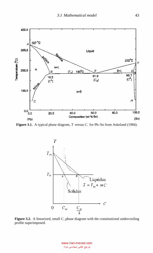
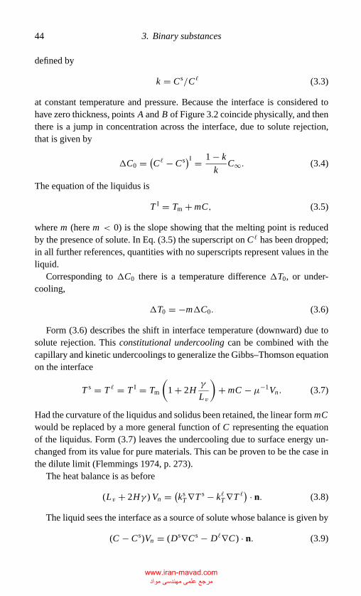
When a binary liquid is frozen, it usually rejects some or all of its solute becausethat solute is more soluble in the liquid than in the crystalline solid. The degreeof rejection can be obtained from the phase diagram for systems in thermody-namical equilibrium, an example of which is shown in Figure 3.1. The rejectedsolute in the liquid is subject to diffusion, and thus, a major difference betweenthe dynamics of pure material and that of alloys is the need to track both thetemperature and concentration fields.
In the bulk liquid or solid there is again the heat conduction
Tt = κ∇2T . (3.1)
Consider that the solute is dilute; thus the solute diffusion equation valid inboth phases is
Ct = D∇2C, (3.2)
where D is the solute diffusivity andC is the solute concentration. Equation (3.2)can be derived exactly as was Eq. (3.1) if one makes the following replacements:T → C, κ → D, assumes that there is no cross diffusion and that the soluteflux satisfies the relation qs = −D∇C , a Fickian model. In the far fields thereare appropriate conditions on both T and C.
Figure 3.2 shows a phase diagram near its left-hand side, where C is small.The curved liquidus and solidus have been represented by straight lines. Abovethe liquidus all material is liquid, and below the solidus, all is solid. At afixed interface temperature T0, as shown, the interface has concentration C s onthe solid side equal to C∞, and C�, the concentration at the interface on theliquid side is given by C∞/k; k is the segregation or distribution coefficient
42
www.iran-mavad.com مرجع علمی مھندسی مواد
P1: GKE/fcw P2: GKW
CB381-03 CB381-Davis May 17, 2001 15:56 Char Count= 0
3.1 Mathematical model 43
Figure 3.1. A typical phase diagram, T versus C, for Pb–Sn from Askeland (1984).
Figure 3.2. A linearized, small C , phase diagram with the constitutional undercoolingprofile superimposed.
www.iran-mavad.com مرجع علمی مھندسی مواد
P1: GKE/fcw P2: GKW
CB381-03 CB381-Davis May 17, 2001 15:56 Char Count= 0
44 3. Binary substances
defined by
k = C s/C� (3.3)
at constant temperature and pressure. Because the interface is considered tohave zero thickness, points A and B of Figure 3.2 coincide physically, and thenthere is a jump in concentration across the interface, due to solute rejection,that is given by
�C0 = (C� − C s)I = 1 − k
kC∞. (3.4)
The equation of the liquidus is
T I = Tm + mC, (3.5)
where m (here m < 0) is the slope showing that the melting point is reducedby the presence of solute. In Eq. (3.5) the superscript on C� has been dropped;in all further references, quantities with no superscripts represent values in theliquid.
Corresponding to �C0 there is a temperature difference �T0, or under-cooling,
�T0 = −m�C0. (3.6)
Form (3.6) describes the shift in interface temperature (downward) due tosolute rejection. This constitutional undercooling can be combined with thecapillary and kinetic undercoolings to generalize the Gibbs–Thomson equationon the interface
T s = T � = T I = Tm
(1 + 2H
γ
Lv
)+ mC − µ−1Vn. (3.7)
Had the curvature of the liquidus and solidus been retained, the linear form mCwould be replaced by a more general function of C representing the equationof the liquidus. Form (3.7) leaves the undercooling due to surface energy un-changed from its value for pure materials. This can be proven to be the case inthe dilute limit (Flemmings 1974, p. 273).
The heat balance is as before
(Lv + 2Hγ ) Vn = (ksT ∇T s − k�T ∇T �
) · n. (3.8)
The liquid sees the interface as a source of solute whose balance is given by
(C − C s)Vn = (Ds∇C s − D�∇C) · n. (3.9)
www.iran-mavad.com مرجع علمی مھندسی مواد
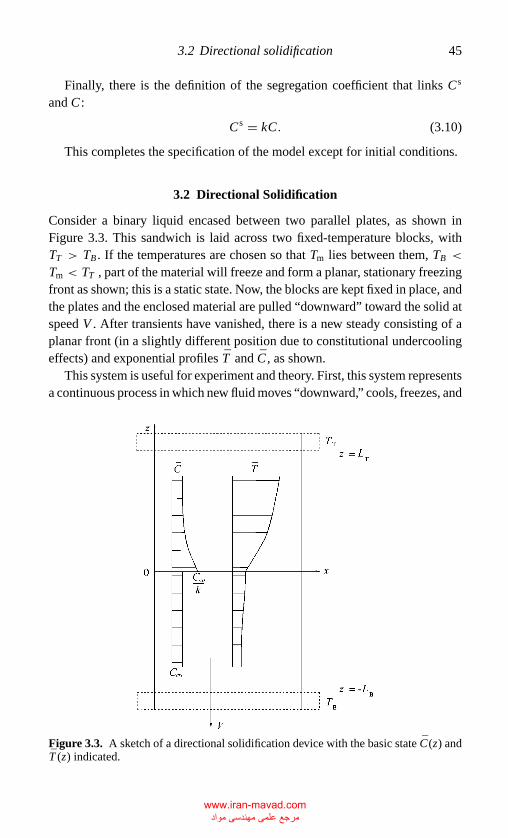
P1: GKE/fcw P2: GKW
CB381-03 CB381-Davis May 17, 2001 15:56 Char Count= 0
3.2 Directional solidification 45
Finally, there is the definition of the segregation coefficient that links C s
and C :
C s = kC. (3.10)
This completes the specification of the model except for initial conditions.
3.2 Directional Solidification
Consider a binary liquid encased between two parallel plates, as shown inFigure 3.3. This sandwich is laid across two fixed-temperature blocks, withTT > TB . If the temperatures are chosen so that Tm lies between them, TB <
Tm < TT , part of the material will freeze and form a planar, stationary freezingfront as shown; this is a static state. Now, the blocks are kept fixed in place, andthe plates and the enclosed material are pulled “downward” toward the solid atspeed V . After transients have vanished, there is a new steady consisting of aplanar front (in a slightly different position due to constitutional undercoolingeffects) and exponential profiles T and C , as shown.
This system is useful for experiment and theory. First, this system representsa continuous process in which new fluid moves “downward,” cools, freezes, and
Figure 3.3. A sketch of a directional solidification device with the basic state C(z) andT (z) indicated.
www.iran-mavad.com مرجع علمی مھندسی مواد
P1: GKE/fcw P2: GKW
CB381-03 CB381-Davis May 17, 2001 15:56 Char Count= 0
46 3. Binary substances
moves onward. Second, it turns out that the C-field can cause morphologicalinstabilities of the front while the thermal field stabilizes the front. These op-posing effects lead to frontal instabilities that equilibrate in amplitude, makingthis system an excellent vehicle for the careful study of phase transformationdynamics. Third, the thinness of the Hele–Shaw cell and the use of transparentmodel fluids make for the easy viewing of the interface morphology through amicroscope.
A model describing this uses a coordinate system, z → z − V t, that ismoving with the interface at speed V , and thus the diffusion fields satisfy thefollowing equations:
Tt − V Tz = κ∇2T (3.11a)
Ct − V Cz = D∇2C. (3.11b)
In the two phases Eqs. (3.11a,b) apply on the two sides of the interface, whichis located at z = h(x, y, t) and +z points into the liquid. At z = LT , say,
T � = TT (3.11c)
C�z = 0 (3.11d)
and at z = −L B ,
T s = TB (3.11e)
C sz = 0. (3.11f)
On the interface, Eqs. (3.7)–(3.10) hold.
3.3 Basic State and Approximate Models
In the laboratory frame one seeks a solution independent of x, y, and t and,hence, dependent on z only.
As seen from Eq. (3.11a),
−V Tz = κTzz, (3.12)
whose solutions are a constant and exp(−V z/κ). With conditions at z =LT , −L B , one can obtain appropriate solutions for T (and C) with h = h0
(constant).For a well-designed experiment, LT , L B are very large, and the numerical
values of these are expected to have very little effect on instabilities of unit-order wavelength at the interface, and thus it would be convenient to replacethese by infinity. This is justified in the liquid phase, for as z → ∞, theexponential decays, and only exponentially small errors are made by taking
www.iran-mavad.com مرجع علمی مھندسی مواد
P1: GKE/fcw P2: GKW
CB381-03 CB381-Davis May 17, 2001 15:56 Char Count= 0
3.3 Basic state and approximate models 47
LT → ∞. In the solid phase, however, as z → −∞, the exponentials grow. Ifκs (and Ds) are small in some sense, it is possible to show (see, e.g., Huntley1993) for κs → 0, that T s develops nonuniformities not at the interface but atthe lower boundary z = −L B . This “boundary layer” is thin and far removedfrom the interface, and thus it can be permissible to ignore these boundary-layerbehaviors and use as approximate solutions in the solid phase that are unboundedat z → −∞. A similar argument holds for concentration and Ds → 0.
If Ds = D�, one has the symmetric model, which is appropriate for certainphase transformation studies of liquid crystals, for example. If Ds D�, onehas the one-sided model. Here Ds can be set to zero and LT can be set to infinity,as discussed above. The one-sided model is appropriate for solidification inmetals, semiconductors, and many transparent organics. The one-sided andextended model will be discussed here.
If the Stefan number S (latent heat) is set to zero in the heat-flux conditionand � = O(1) elsewhere, the thermal properties (e.g., kT , κ, cp) in the twophases are assumed to be equal, and, as is usual, D κ everywhere, then onecan replace T and T s by a single linear variation valid in both phases,
T = T0 + GT z, (3.13)
where GT is the constant temperature gradient. Conditions in the far field aredeemed not to influence the dynamics of the front strongly. This combinationof limits gives the FTA, the frozen temperature approximation (Langer 1980).It comes about by scaling lengths on the concentration-boundary-layer thick-ness δc,
δc = D
V, (3.14a)
which is much smaller than the thermal-boundary-layer thickness δT,
δT = κ
V. (3.14b)
The scaled transport equations in nondimensional form are then
D
κ(Tt − Tz) = ∇2T (3.15a)
and
Ct − Cz = ∇2C, (3.15b)
and when D/κ → 0, the thermal-steady-state approximation (see Coriell andMcFadden 1993) is enforced, a linear temperature distribution, the “small” zapproximation to the exponential behavior, is obtained. As will be seen, suchapproximations are very good in many systems.
www.iran-mavad.com مرجع علمی مھندسی مواد
P1: GKE/fcw P2: GKW
CB381-03 CB381-Davis May 17, 2001 15:56 Char Count= 0
48 3. Binary substances
The basic state that will be considered next applies to the one-sided modelwith the FTA.
Here T is given by Eq. (3.13), and
C = C∞
[1 + 1 − k
ke− V z
D
], (3.16a)
C s = C∞, (3.16b)
h = 0, (3.16c)
where
T0 = Tm + mC∞k
− µ−1V, (3.16d)
and
C → C∞ as z → ∞. (3.16e)
The concentration profile balances rejection of solute at the front, a source,with diffusion in the liquid. Equation (3.16d) defines T0, the temperature at theinterface in terms of the concentration and the speed. Both the presence of theconstitutional undercooling (recall that m < 0) and the kinetic undercoolingtend to reduce T0 from Tm. Note that at the interface (on the liquid side) theconcentration gradient Gc is given from Eq. (3.16a) by
Gc = (k − 1)
kC∞
V
D, (3.17)
which is negative for k < 1.
3.4 Linearized Instability of a Moving Frontin Directional Solidification
Consider directional solidification in two dimensions via the one-sided modelwith the FTA with kinetics ignored; all quantities are independent of y.
Let us introduce nondimensional variables. Scale all lengths on δc
(x, z) = 1
δc(x, z), h = h
δc
t = V 2
Dt, C = C − C∞/k
DGc/V
T = (T − T0 − mC∞/k)
δcGT,
(3.18)
www.iran-mavad.com مرجع علمی مھندسی مواد
P1: GKE/fcw P2: GKW
CB381-03 CB381-Davis May 17, 2001 15:56 Char Count= 0
3.4 Linearized instability of a moving front in directional solidification 49
and then drop the carets. The temperature field is permanent at
T = z. (3.19a)
For z > h(x, t),
Ct − Cz = ∇2C. (3.19b)
As z → ∞,
C → 1. (3.19c)
On z = h(x, t),
M−1T = C + 2H� (3.19d)
and
[C(k − 1) + 1](1 + ht ) = Cz − hxCx , (3.19e)
where
M = mGc
GT= m(k − 1)C∞V
kGT D(3.20a)
is the morphological number and
� = γ Tm
LvmGc
V 2
D2= γ TmV
C∞LvD
k
m(k − 1)(3.20b)
is a measure of the surface energy. As can be seen, the problem reduces onlyto the tracking of solute in the liquid and the shape of the interface.
The basic state, as before, consists of a planar interface and an exponentialsolute field
h = 0 (3.21a)
C = 1 − e−z (3.21b)
with
T = z (3.21c)
everywhere.Let the system be disturbed as follows:
h = h + h′, C = C + C ′. (3.22)
There is no need to perturb the thermal field because, in the present approxi-mation, thermal disturbances always decay to zero.
If forms (3.22) are substituted into system (3.19) and linearized in primedquantities, the linearized disturbance equations are obtained.
www.iran-mavad.com مرجع علمی مھندسی مواد
P1: GKE/fcw P2: GKW
CB381-03 CB381-Davis May 17, 2001 15:56 Char Count= 0
50 3. Binary substances
For z > 0,
C ′t − C ′
z = ∇2C ′. (3.23a)
As z → ∞,
C ′ → 0. (3.23b)
On z = 0,
C ′z = (k − 1)C ′ + kh′ + h′
t (3.23c)
C ′ = (M−1 − 1 − �∇2)h′. (3.23d)
This linear system has coefficients independent of x and t , and thus one canintroduce normal modes
(C ′, h′) = (c1(z), h1)eσ t+ia1x , (3.24)
where σ is the growth rate and a1 is the wave number along the interface. Whenthese are substituted into system (3.23a), one obtains
σc1 =(
d2
dz2− a2
1 + d
dz
)c1, z > 0. (3.25a)
On the interface z = 0 the linearized boundary conditions are
dc1
dz= (k − 1)c1 + (k + σ )h1, (3.25b)
c1 = (M−1 − 1 + a21�)
h1, (3.25c)
and
c1 → 0 as z → ∞. (3.25d)
The solution of Eq. (3.25a) that satisfies condition (3.25d) is
c1(z) = Ae− 1
2
{1+
√1+4(σ+a2
1 )}
z. (3.25e)
If Eq. (3.25e) is substituted in conditions (3.25b,c), a homogeneous, linear setof algebraic equations is obtained. To guarantee the existence of nontrivialsolutions, the determinant of the matrix of coefficients must be set to zero; thisyields the characteristic equation√
1 + 4(σ + a2
1
) = 1 − 2k − 2(σ + k)(M−1 − 1 + a2
1�)−1. (3.26)
This equation of the form F(σ, a21 ; M, �, k) = 0 determines the stability
www.iran-mavad.com مرجع علمی مھندسی مواد
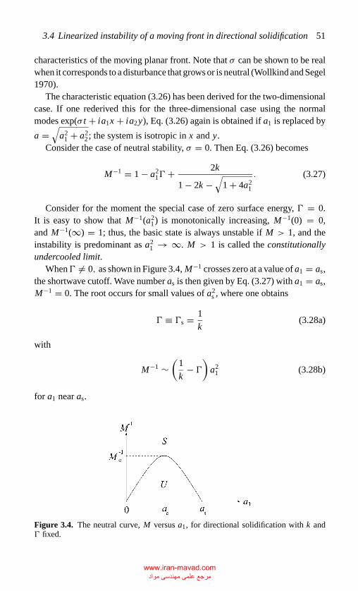
P1: GKE/fcw P2: GKW
CB381-03 CB381-Davis May 17, 2001 15:56 Char Count= 0
3.4 Linearized instability of a moving front in directional solidification 51
characteristics of the moving planar front. Note that σ can be shown to be realwhen it corresponds to a disturbance that grows or is neutral (Wollkind and Segel1970).
The characteristic equation (3.26) has been derived for the two-dimensionalcase. If one rederived this for the three-dimensional case using the normalmodes exp(σ t + ia1x + ia2y), Eq. (3.26) again is obtained if a1 is replaced by
a =√
a21 + a2
2 ; the system is isotropic in x and y.Consider the case of neutral stability, σ = 0. Then Eq. (3.26) becomes
M−1 = 1 − a21� + 2k
1 − 2k −√
1 + 4a21
. (3.27)
Consider for the moment the special case of zero surface energy, � = 0.It is easy to show that M−1(a2
1) is monotonically increasing, M−1(0) = 0,and M−1(∞) = 1; thus, the basic state is always unstable if M > 1, and theinstability is predominant as a2
1 → ∞. M > 1 is called the constitutionallyundercooled limit.
When� �= 0, as shown in Figure 3.4, M−1 crosses zero at a value of a1 = as,the shortwave cutoff. Wave number as is then given by Eq. (3.27) with a1 = as,M−1 = 0. The root occurs for small values of a2
s , where one obtains
� ≡ �s = 1
k(3.28a)
with
M−1 ∼(
1
k− �)
a21 (3.28b)
for a1 near as.
Figure 3.4. The neutral curve, M versus a1, for directional solidification with k and� fixed.
www.iran-mavad.com مرجع علمی مھندسی مواد
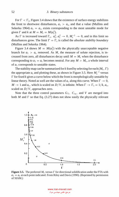
P1: GKE/fcw P2: GKW
CB381-03 CB381-Davis May 17, 2001 15:56 Char Count= 0
52 3. Binary substances
For � < �s, Figure 3.4 shows that the existence of surface energy stabilizesthe front to shortwave disturbances, a1 > as, and that a value (Mullins andSekerka 1964) a1 = ac, exists corresponding to the most unstable mode forgiven � and k at M = Mc = M(a2
c ).As � is increased toward �s, a2
s , a2c → 0,M−1
c → 0, and in this limit nodisturbances grow. The limit � = �s is called the absolute stability boundary(Mullins and Sekerka 1964).
Figure 3.4 shows M = M(a21) with the physically unacceptable negative
branch for a1 > as removed. As M , the measure of solute rejection, is in-creased from zero, all disturbances decay until M = Mc when the disturbancecorresponding to a1 = ac becomes neutral. For any M > Mc, a whole intervalof a1 corresponds to unstable states.
The stability map can be summarized for k fixed by selecting for each (Mc, �)the appropriate ac and plotting these, as shown in Figure 3.5. Here M−1
c versus� for fixed k gives a curve below which the front is morphologically unstable bylinear theory. Noted as well are the values of ac along this curve. When � → 0,M → 1 and ac, which is scaled on D/V , is infinite. When � → �s = 1/k, ac,scaled on D/V , approaches zero.
Note that the three control parameters GT, C∞, and V are merged intoboth M and � so that Eq. (3.27) does not show easily the physically relevant
Figure 3.5. The preferred Mc versus � for directional solidification under the FTA witha1 = ac at each point indicated. From Riley and Davis (1990). (Reprinted by permissionof SIAM.)
www.iran-mavad.com مرجع علمی مھندسی مواد
P1: GKE/fcw P2: GKW
CB381-03 CB381-Davis May 17, 2001 15:56 Char Count= 0
3.4 Linearized instability of a moving front in directional solidification 53
situation of GT fixed as V and C∞ increase,
� ∝ V
C∞, M ∝ V C∞, a ∝ 1
V. (3.29)
This dilemma can be overcome if one defines new measures that separatethe control parameters (Merchant and Davis 1990), or, alternatively, one canreturn to the dimensional system. In either case the new figures have similarshapes.
The previous results can be recast into a set of velocity and concentrationcurves using nondimensional parameters that isolate V and C∞ as indepen-dently controllable parameters; call these natural parameters. The appropriatescalings are described in Merchant and Davis (1990) where, instead of diffusionscales, capillary scales are used. These scales for length and time are
δL = (γ TM/LGT)1/2
δT = γ TM/LGT D.
}(3.30)
The control parameters M and � are replaced by nondimensional speed andconcentration parameters V and C, respectively. These are defined by
V2 = γ TMV 2
LGT D2
C2 = m2E (kE − 1)2LC2
∞k2
E GTγ TM.
(3.31)
For the easy switching from the old parameters M and � to the natural ones Vand C, the following transformations can be used:
M → VC, � → V/C;
a → a/V, σ → σ/V2,(3.32)
which can be inserted into the characteristic equation.Let us plot the neutral stability curve given by Eq. (3.27) when the dimen-
sional wave number a∗, and dimensional growth rate σ∗ are introduced,
a = a∗D
V, σ = σ∗
D
V 2. (3.33)
Fix GT and let C∞ and V be the control variables of interest. For a given setof material constants, the neutral curve is as shown in Figure 3.6, �nV versus�n C∞. To the left of the curve the basic state is linearly stable, and to the rightit is unstable.
www.iran-mavad.com مرجع علمی مھندسی مواد
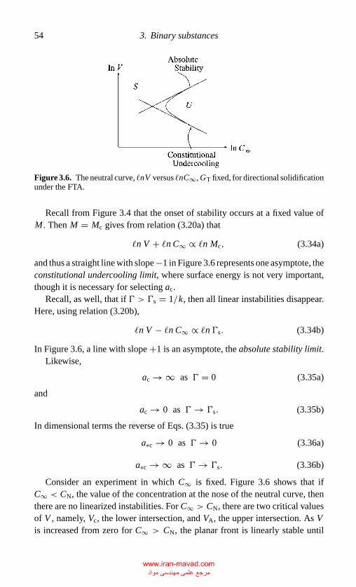
P1: GKE/fcw P2: GKW
CB381-03 CB381-Davis May 17, 2001 15:56 Char Count= 0
54 3. Binary substances
Figure 3.6. The neutral curve, �nV versus �nC∞, GT fixed, for directional solidificationunder the FTA.
Recall from Figure 3.4 that the onset of stability occurs at a fixed value ofM . Then M = Mc gives from relation (3.20a) that
�n V + �n C∞ ∝ �n Mc, (3.34a)
and thus a straight line with slope −1 in Figure 3.6 represents one asymptote, theconstitutional undercooling limit, where surface energy is not very important,though it is necessary for selecting ac.
Recall, as well, that if � > �s = 1/k, then all linear instabilities disappear.Here, using relation (3.20b),
�n V − �n C∞ ∝ �n �s. (3.34b)
In Figure 3.6, a line with slope +1 is an asymptote, the absolute stability limit.Likewise,
ac → ∞ as � = 0 (3.35a)
and
ac → 0 as � → �s. (3.35b)
In dimensional terms the reverse of Eqs. (3.35) is true
a∗c → 0 as � → 0 (3.36a)
a∗c → ∞ as � → �s. (3.36b)
Consider an experiment in which C∞ is fixed. Figure 3.6 shows that ifC∞ < CN, the value of the concentration at the nose of the neutral curve, thenthere are no linearized instabilities. For C∞ > CN, there are two critical valuesof V , namely, Vc, the lower intersection, and VA, the upper intersection. As Vis increased from zero for C∞ > CN, the planar front is linearly stable until
www.iran-mavad.com مرجع علمی مھندسی مواد
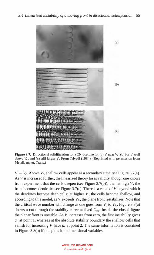
P1: GKE/fcw P2: GKW
CB381-03 CB381-Davis May 17, 2001 15:56 Char Count= 0
3.4 Linearized instability of a moving front in directional solidification 55
Figure 3.7. Directional solidification for SCN-acetone for (a) V near Vc, (b) for V wellabove Vc, and (c) still larger V . From Trivedi (1984). (Reprinted with permission fromMetall. mater. Trans.)
V = Vc. Above Vc, shallow cells appear as a secondary state; see Figure 3.7(a).As V is increased further, the linearized theory loses validity, though one knowsfrom experiment that the cells deepen (see Figure 3.7(b)); then at high V , thefront becomes dendritic; see Figure 3.7(c). There is a value of V beyond whichthe dendrites become deep cells; at higher V , the cells become shallow, andaccording to this model, as V exceeds VA, the plane front restabilizes. Note thatthe critical wave number will change as one goes from Vc to VA. Figure 3.8(a)shows a cut through the stability curve at fixed C∞. Inside the closed figurethe planar front is unstable. As V increases from zero, the first instability givesac at point 1, whereas at the absolute stability boundary the shallow cells thatvanish for increasing V have ac at point 2. The same information is containedin Figure 3.8(b) if one plots it in dimensional variables.
www.iran-mavad.com مرجع علمی مھندسی مواد
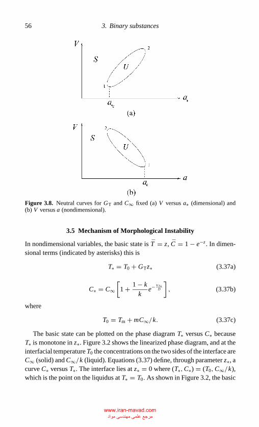
P1: GKE/fcw P2: GKW
CB381-03 CB381-Davis May 17, 2001 15:56 Char Count= 0
56 3. Binary substances
Figure 3.8. Neutral curves for GT and C∞ fixed (a) V versus a∗ (dimensional) and(b) V versus a (nondimensional).
3.5 Mechanism of Morphological Instability
In nondimensional variables, the basic state is T = z, C = 1 − e−z . In dimen-sional terms (indicated by asterisks) this is
T∗ = T0 + GTz∗ (3.37a)
C∗ = C∞
[1 + 1 − k
ke− V z∗
D
], (3.37b)
where
T0 = Tm + mC∞/k. (3.37c)
The basic state can be plotted on the phase diagram T∗ versus C∗ becauseT∗ is monotone in z∗. Figure 3.2 shows the linearized phase diagram, and at theinterfacial temperature T0 the concentrations on the two sides of the interface areC∞ (solid) and C∞/k (liquid). Equations (3.37) define, through parameter z∗, acurve C∗ versus T∗. The interface lies at z∗ = 0 where (T∗,C∗) = (T0,C∞/k),which is the point on the liquidus at T∗ = T0. As shown in Figure 3.2, the basic
www.iran-mavad.com مرجع علمی مھندسی مواد
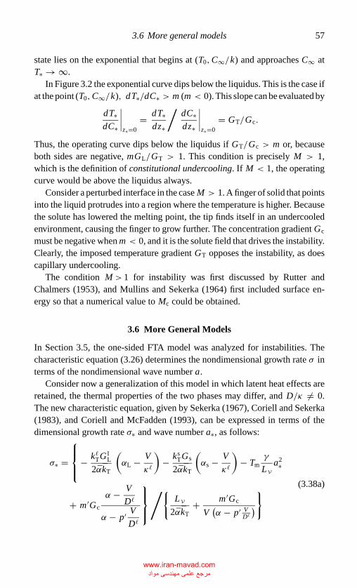
P1: GKE/fcw P2: GKW
CB381-03 CB381-Davis May 17, 2001 15:56 Char Count= 0
3.6 More general models 57
state lies on the exponential that begins at (T0,C∞/k) and approaches C∞ atT∗ → ∞.
In Figure 3.2 the exponential curve dips below the liquidus. This is the case ifat the point (T0,C∞/k), dT∗/dC∗ > m (m < 0). This slope can be evaluated by
dT∗dC∗
∣∣∣∣z∗=0
= dT∗dz∗
/dC∗dz∗
∣∣∣∣z∗=0
= GT/Gc.
Thus, the operating curve dips below the liquidus if GT/Gc > m or, becauseboth sides are negative, mGL/GT > 1. This condition is precisely M > 1,which is the definition of constitutional undercooling. If M < 1, the operatingcurve would be above the liquidus always.
Consider a perturbed interface in the case M > 1. A finger of solid that pointsinto the liquid protrudes into a region where the temperature is higher. Becausethe solute has lowered the melting point, the tip finds itself in an undercooledenvironment, causing the finger to grow further. The concentration gradient Gc
must be negative when m < 0, and it is the solute field that drives the instability.Clearly, the imposed temperature gradient GT opposes the instability, as doescapillary undercooling.
The condition M > 1 for instability was first discussed by Rutter andChalmers (1953), and Mullins and Sekerka (1964) first included surface en-ergy so that a numerical value to Mc could be obtained.
3.6 More General Models
In Section 3.5, the one-sided FTA model was analyzed for instabilities. Thecharacteristic equation (3.26) determines the nondimensional growth rate σ interms of the nondimensional wave number a.
Consider now a generalization of this model in which latent heat effects areretained, the thermal properties of the two phases may differ, and D/κ �= 0.The new characteristic equation, given by Sekerka (1967), Coriell and Sekerka(1983), and Coriell and McFadden (1993), can be expressed in terms of thedimensional growth rate σ∗ and wave number a∗, as follows:
σ∗ =
− k�TGI
L
2αkT
(αL − V
κ�
)− ks
TGs
2αkT
(αs − V
κ�
)− Tm
γ
LVa2
∗
+ m ′Gc
α − V
D�
α − p′ V
D�
/{
LV
2αkT+ m ′Gc
V(α − p′ V
D�)} (3.38a)
www.iran-mavad.com مرجع علمی مھندسی مواد
P1: GKE/fcw P2: GKW
CB381-03 CB381-Davis May 17, 2001 15:56 Char Count= 0
58 3. Binary substances
where
α = V
2D�+[(
V
2D�
)2
+ a2∗ + σ∗
D�
] 12
αL = V
2κ�+[(
V
2κ�
)2
+ a2∗ + σ∗
κ�
] 12
αs = V
2κs+[(
V
2κs
)2
+ a2∗ + σ∗
κs
] 12
α = (ksTαs + k�Tα�
)/(2kT)
kT = 12
(ks
T + k�T)
m ′ = ∂TE
∂Cp′ = 1 − k ′
k ′ = ∂Cs
∂C= k + C∞
k
∂k
∂C
. (3.38b)
The quantities k ′ and m ′ allow the solidus and liquidus to be curved.The heat balance at the interfaces requires that
ksTGS − k�TGL = V LV, (3.38c)
where GS and GL are the temperature gradients at the interface on the solid andliquid sides, respectively.
In the thermal steady-state approximation, D, Ds κ�, κs.Let κ�, κs → ∞as formally in forms (3.38), α, αs, αL → a∗, and the neutral curve, σ∗ = 0 hasthe form
−GT + Tmγ
Lva2
∗ + m ′Gcα − V/D
α − p′V/D, (3.39a)
where G is the conductivity-weighted temperature gradient
GT = k�TGL + ksTGS
k�T + ksT
. (3.39b)
If now, one lets ksT = k�T and LV → 0 with γ /LV = O(1), then condition
(3.38c) gives GS = GL ≡ GT, constant, consistent with the FTA.The results of Section 3.4 hold qualitatively in the more general cases. The ad-
dition of latent heat slightly stabilizes the front against morphological changes.Figure 3.9 compares the neutral curves for two one-sided models, one in theFTA and the other generalized to include the full thermal fields. The two asymp-totes for constitutional undercooling and absolute instability are unchanged by
www.iran-mavad.com مرجع علمی مھندسی مواد
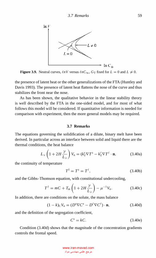
P1: GKE/fcw P2: GKW
CB381-03 CB381-Davis May 17, 2001 15:56 Char Count= 0
3.7 Remarks 59
Figure 3.9. Neutral curves, �nV versus �nC∞, GT fixed for L = 0 and L �= 0.
the presence of latent heat or the other generalizations of the FTA (Huntley andDavis 1993). The presence of latent heat flattens the nose of the curve and thusstabilizes the front near the nose.
As has been shown, the qualitative behavior in the linear stability theoryis well described by the FTA in the one-sided model, and for most of whatfollows this model will be considered. If quantitative information is needed forcomparison with experiment, then the more general models may be required.
3.7 Remarks
The equations governing the solidification of a dilute, binary melt have beenderived. In particular across an interface between solid and liquid there are thethermal conditions, the heat balance
LV
(1 + 2H
γ
LV
)Vn = (ks
T∇T s − k�T∇T � · n, (3.40a)
the continuity of temperature
T I = T s = T �, (3.40b)
and the Gibbs–Thomson equation, with constitutional undercooling,
T I = mC + Tm
(1 + 2H
γ
LV
)− µ−1Vn. (3.40c)
In addition, there are conditions on the solute, the mass balance
(1 − k)CVn = (Ds∇C s − D�∇C�) · n, (3.40d)
and the definition of the segregation coefficient,
C s = kC. (3.40e)
Condition (3.40d) shows that the magnitude of the concentration gradientscontrols the frontal speed.
www.iran-mavad.com مرجع علمی مھندسی مواد
P1: GKE/fcw P2: GKW
CB381-03 CB381-Davis May 17, 2001 15:56 Char Count= 0
60 3. Binary substances
The mechanism of morphological instability in a dilute binary alloy has beendiscussed as well as models for the prediction of Mc and ac. Experiments ofde Cheveigne, Guthmann, and Lebrun (1985) on CB4 with about 0.1% Br as acontaminant show that, on the low-speed branch, theory and experiment agreereasonably well on Mc, but the critical wave numbers can differ by a factorof two or more. Several possible explanations exist for this disagreement, andthese are discussed in Chapter 4.
One possibility for the disagreement is that the growth of the instability be-gins early, when the basic state has not yet approached its final steady form. Theanalysis of the instabilities of unsteady states is quite difficult; consequently,Warren and Langer (1993) examined a model version of the problem by pa-rameterizing the time dependence through an unsteady solute boundary layerthickness �(t) such that �(t) → δc as t → ∞. They then found the criticala∗c smaller than those of the previous theory, which has � = δc forever, andobtained predictions qualitatively in agreement with the observations of Trivediand Somboonsuk (1985) in SCN–acetone. Losert, Shi, and Cummins (1998)used SCN with coumarin 152 as a contaminant and found good agreement withthe Warren–Langer predictions (SCN is the transparent organic succinonitrile).
References
Askeland, D. R. (1984). The Science and Engineering of Materials, Book-ColeEngineering Division.
Coriell, S. R., and McFadden, G. B. (1993). Morphological stability, in D. T. J. Hurle,editor, Handbook of Crystal Growth. 16, 785–857, North-Holland, Amsterdam.
Coriell, S. R., and Sekerka, R. F. (1983). Oscillatory morphological instabilities due tonon-equilibrium segregation, J. Crystal Growth 61, 499–508.
de Cheveigne, S., Guthmann, C., and Lebrun, M.-M. (1985). Nature of the transition ofthe solidification front of a binary mixture from a plane to a cellular morphology,J. Crystal Growth 73, 242–244.
Flemmings, M. C. (1974). Solidification Processing, McGraw–Hill, New York.Huntley, D. A. (1993). Thermal effects in rapid directional solidification. Ph.D. thesis,
Northwestern University.Huntley, D. A., and Davis, S. H. (1993). Thermal effects in rapid directional solidifica-
tion: Linear theory, Acta Metall. Mater. 41, 2025–2043.Langer, J. S. (1980). Instabilities and pattern formation in crystal growth, Rev. Mod.
Phys. 52, 1–28.Losert, W., Shi, B. Q., and Cummins, J. Z. (1998). Evolution of dendritic patterns during
alloy solidification: Onset of the initial instability, Proc. Natl. Acad. Sci. U.S.A. 95,431–438.
Merchant, G. J., and Davis, S. H. (1990). Morphological instability in rapid directionalsolidification, Acta Metall. Mater. 38, 2683–2693.
Mullins, W. W., and Sekerka, R. F. (1964). Stability of a planar interface during solidi-fication of a dilute binary alloy, J. Appl. Phys. 35, 444–451.
Riley, D. S., and Davis, S. H. (1990). Long-wave morphological instabilities in the direc-tional solidification of a dilute binary mixture, SIAM J. Appl. Math. 50, 420–436.
www.iran-mavad.com مرجع علمی مھندسی مواد
P1: GKE/fcw P2: GKW
CB381-03 CB381-Davis May 17, 2001 15:56 Char Count= 0
References 61
Rutter, J. W., and Chalmers, B. (1953). A prismatic substructure formed during solidi-fication of metals, Can. J. Phys. 31, 15–49.
Sekerka, R. F. (1967). Time-dependent theory of stability of a planar interface duringdilute binary alloy solidification, in H. S. Perser, editor, Crystal Growth, pages691–702, Pergamon Press, Oxford.
Trivedi, R. (1984). Interdendritic spacing: Part II. A comparison of theory and experi-ment, Metall. mater. Trans. 15A, 977–982.
Trivedi, R., and Somboonsuk, K. (1985). Pattern formation during the solidification ofbinary systems, Acta Metall. Mater. 33, 1061–1068.
Warren, J. A., and Langer, J. S. (1993). Prediction of dendritic spacings in a directionalsolidification experiment, Phys. Rev. E 47, 2702–2712.
Wollkind, D. G., and Segel, L. A. (1970). A nonlinear stability analysis of the freezingof a dilute binary alloy, Phil. Trans. Roy. Soc. London A268, 351–380.
www.iran-mavad.com مرجع علمی مھندسی مواد
P1: GGH
CB381-04 CB381-Davis May 17, 2001 15:59 Char Count= 0
4
Nonlinear theory for directional solidification
In Chapter 2 we saw that a spherical front in a pure material in an undercooledliquid is either unstable or not, depending on the size of the sphere. There is nosecondary control that allows one to mediate the growth. In Chapter 3, we sawthat, in directional solidification of a binary liquid, the concentration gradientat the interface creates an instability; however, there is a secondary parameter,the temperature gradient, that opposes the instability and thus can be usedto control the local growth beyond the linearized stability limit. Thus, muchattention has been given to directional solidification both experimentally andtheoretically, and it is in this chapter that nonlinear theory will be discussed.
There are two approaches to the nonlinear theory, depending upon whetherthe critical wave number ac of linear theory is of unit order, or is small (i.e.,asymptotically zero). In the former case one can construct Landau, Ginzburg–Landau, or Newell–Whitehead–Segel equations to study (weakly nonlinear)bifurcation behavior. This gives information regarding the nature of the bi-furcation (sub- or supercritical), the question of wave number selection, thepreferred pattern of the morphology, and hence the resulting microstructure. Ifac is small one must use a longwave theory that generates evolution equationsgoverning the nonlinear development. Such longwave theories can be weakly orstrongly nonlinear, depending on the particular situation. They, too, can then beanalyzed to discover the nature of the bifurcation and the selection of preferredwave number and pattern.
4.1 Bifurcation Theory
4.1.1 Two-Dimensional Theory
When directional solidification is performed in a Hele–Shaw cell, a regionbounded by two parallel, closely spaced plates, the instability can readily be
62
www.iran-mavad.com مرجع علمی مھندسی مواد
P1: GGH
CB381-04 CB381-Davis May 17, 2001 15:59 Char Count= 0
4.1 Bifurcation theory 63
observed if the plates and the fluid are transparent. The instability is sensiblytwo-dimensional as long as the curvature of the interface across the gap isnegligible.
Bifurcation theory in two dimensions in the FTA proceeds as follows. Fromthe linearized theory one has Mc, ac and the corresponding eigenfunctions. Thegrowth rate σ can be written as
σ = σ0(M − Mc) + O[(M − Mc)
2]
(4.1)
valid near the neutral curve, say for a1 = ac σ0 = O(1). Because linearizedgrowth has the form exp (σ t) ∼ exp [σ0(M − Mc)t], one can identify the slowtime t by t = σ t .
If one defines the small parameter ε ≡ |σ |1/2 as M → Mc, then
t = ε2t (4.2a)
and it follows that
M ∼ Mc + δε2, (4.2b)
where, for convenience, the factor δ = sgn(M − Mc) has been introduced sothat both signs of M − Mc can be treated simultaneously.
Forms (4.2) are introduced into Eqs. (3.19) governing directional solidifica-tion subject to the FTA and the one-sided model. The dependent variables arewritten as asymptotic expansions
[C(x, z, t), h(x, t)] ∼ [C(z), h]
+ ε {A( t)[C1(z), h1]eia1x + A∗( t)[C∗1 (z), h∗
1]e−ia1x},
(4.2c)
where the amplitude A is for the moment unknown and an asterisk denotescomplex conjugate. The forms (4.2) are substituted into the governing system,and coefficients of equal powers of ε are equated to zero.
At O(1), [C(z), h] turns out to be the basic state already calculated. At O(ε),one obtains the linear theory for M = Mc. At O(ε2) an inhomogeneous linearsystem for [C2(z), h2], which can be solved explicitly, is obtained. Finally,at O(ε3) the inhomogeneous linear system for [C3(z), h3] cannot be solvedunless the right-hand side satisfies an orthogonality condition. The result of thisFredholm condition is an equation for A( t), which until now, was undefined; Asatisfies a Landau equation
d A
d t= [δ − b1 |A|2] A. (4.3)
Here b1, the Landau coefficient, is a real, computable quantity that depends on
www.iran-mavad.com مرجع علمی مھندسی مواد
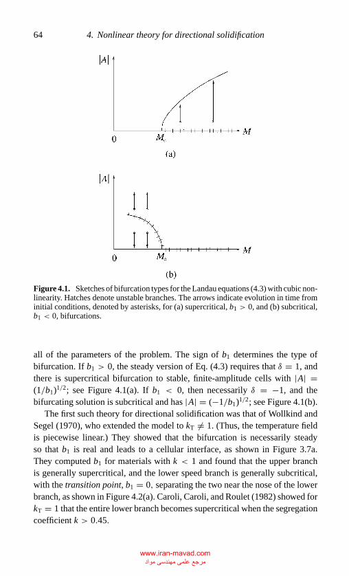
P1: GGH
CB381-04 CB381-Davis May 17, 2001 15:59 Char Count= 0
64 4. Nonlinear theory for directional solidification
Figure 4.1. Sketches of bifurcation types for the Landau equations (4.3) with cubic non-linearity. Hatches denote unstable branches. The arrows indicate evolution in time frominitial conditions, denoted by asterisks, for (a) supercritical, b1 > 0, and (b) subcritical,b1 < 0, bifurcations.
all of the parameters of the problem. The sign of b1 determines the type ofbifurcation. If b1 > 0, the steady version of Eq. (4.3) requires that δ = 1, andthere is supercritical bifurcation to stable, finite-amplitude cells with |A| =(1/b1)1/2; see Figure 4.1(a). If b1 < 0, then necessarily δ = −1, and thebifurcating solution is subcritical and has |A| = (−1/b1)1/2; see Figure 4.1(b).
The first such theory for directional solidification was that of Wollkind andSegel (1970), who extended the model to kT �= 1. (Thus, the temperature fieldis piecewise linear.) They showed that the bifurcation is necessarily steadyso that b1 is real and leads to a cellular interface, as shown in Figure 3.7a.They computed b1 for materials with k < 1 and found that the upper branchis generally supercritical, and the lower speed branch is generally subcritical,with the transition point, b1 = 0, separating the two near the nose of the lowerbranch, as shown in Figure 4.2(a). Caroli, Caroli, and Roulet (1982) showed forkT = 1 that the entire lower branch becomes supercritical when the segregationcoefficient k > 0.45.
www.iran-mavad.com مرجع علمی مھندسی مواد
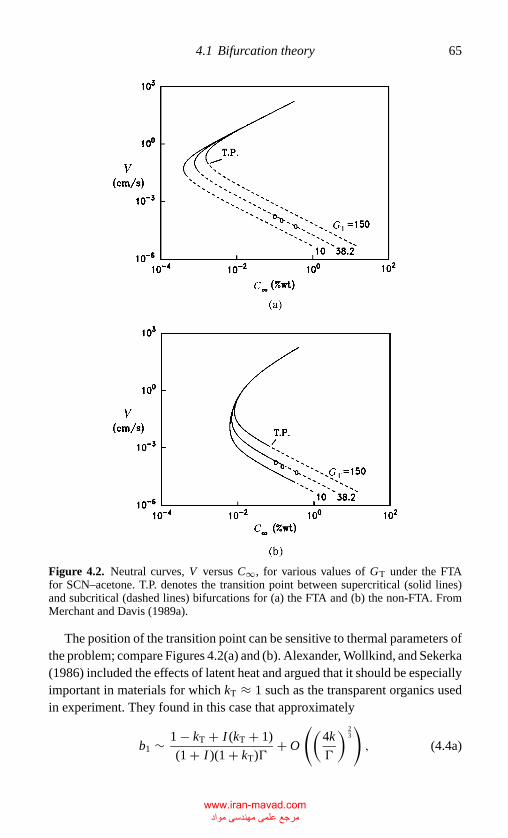
P1: GGH
CB381-04 CB381-Davis May 17, 2001 15:59 Char Count= 0
4.1 Bifurcation theory 65
Figure 4.2. Neutral curves, V versus C∞, for various values of GT under the FTAfor SCN–acetone. T.P. denotes the transition point between supercritical (solid lines)and subcritical (dashed lines) bifurcations for (a) the FTA and (b) the non-FTA. FromMerchant and Davis (1989a).
The position of the transition point can be sensitive to thermal parameters ofthe problem; compare Figures 4.2(a) and (b). Alexander, Wollkind, and Sekerka(1986) included the effects of latent heat and argued that it should be especiallyimportant in materials for which kT ≈ 1 such as the transparent organics usedin experiment. They found in this case that approximately
b1 ∼ 1 − kT + I (kT + 1)
(1 + I )(1 + kT)�+ O
((4k
�
) 23
), (4.4a)
www.iran-mavad.com مرجع علمی مھندسی مواد
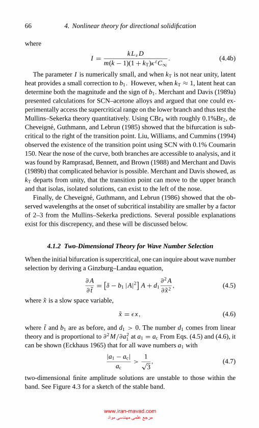
P1: GGH
CB381-04 CB381-Davis May 17, 2001 15:59 Char Count= 0
66 4. Nonlinear theory for directional solidification
where
I = kLvD
m(k − 1)(1 + kT)κ�C∞. (4.4b)
The parameter I is numerically small, and when kT is not near unity, latentheat provides a small correction to b1. However, when kT ≈ 1, latent heat candetermine both the magnitude and the sign of b1. Merchant and Davis (1989a)presented calculations for SCN–acetone alloys and argued that one could ex-perimentally access the supercritical range on the lower branch and thus test theMullins–Sekerka theory quantitatively. Using CBr4 with roughly 0.1%Br2, deCheveigne, Guthmann, and Lebrun (1985) showed that the bifurcation is sub-critical to the right of the transition point. Liu, Williams, and Cummins (1994)observed the existence of the transition point using SCN with 0.1% Coumarin150. Near the nose of the curve, both branches are accessible to analysis, and itwas found by Ramprasad, Bennett, and Brown (1988) and Merchant and Davis(1989b) that complicated behavior is possible. Merchant and Davis showed, askT departs from unity, that the transition point can move to the upper branchand that isolas, isolated solutions, can exist to the left of the nose.
Finally, de Cheveigne, Guthmann, and Lebrun (1986) showed that the ob-served wavelengths at the onset of subcritical instability are smaller by a factorof 2–3 from the Mullins–Sekerka predictions. Several possible explanationsexist for this discrepency, and these will be discussed below.
4.1.2 Two-Dimensional Theory for Wave Number Selection
When the initial bifurcation is supercritical, one can inquire about wave numberselection by deriving a Ginzburg–Landau equation,
∂A
∂ t= [δ − b1 |A|2] A + d1
∂2 A
∂ x2, (4.5)
where x is a slow space variable,
x = εx, (4.6)
where t and b1 are as before, and d1 > 0. The number d1 comes from lineartheory and is proportional to ∂2M/∂a2
1 at a1 = ac From Eqs. (4.5) and (4.6), itcan be shown (Eckhaus 1965) that for all wave numbers a1 with
|a1 − ac|ac
>1√3, (4.7)
two-dimensional finite amplitude solutions are unstable to those within theband. See Figure 4.3 for a sketch of the stable band.
www.iran-mavad.com مرجع علمی مھندسی مواد
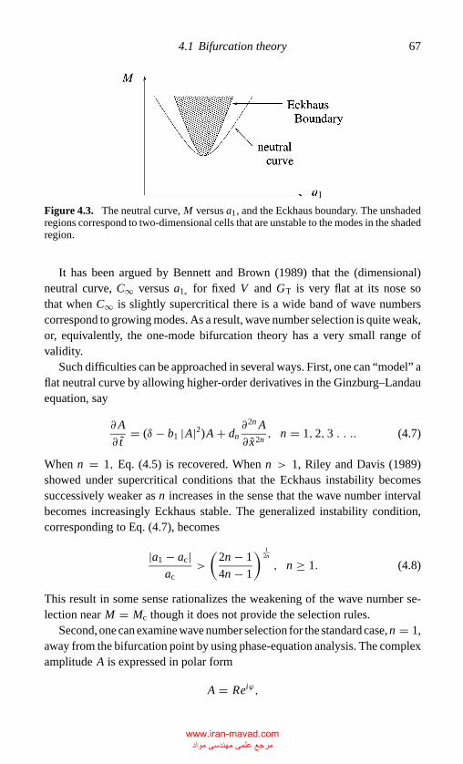
P1: GGH
CB381-04 CB381-Davis May 17, 2001 15:59 Char Count= 0
4.1 Bifurcation theory 67
Figure 4.3. The neutral curve, M versus a1, and the Eckhaus boundary. The unshadedregions correspond to two-dimensional cells that are unstable to the modes in the shadedregion.
It has been argued by Bennett and Brown (1989) that the (dimensional)neutral curve, C∞ versus a1∗ for fixed V and GT is very flat at its nose sothat when C∞ is slightly supercritical there is a wide band of wave numberscorrespond to growing modes. As a result, wave number selection is quite weak,or, equivalently, the one-mode bifurcation theory has a very small range ofvalidity.
Such difficulties can be approached in several ways. First, one can “model” aflat neutral curve by allowing higher-order derivatives in the Ginzburg–Landauequation, say
∂A
∂ t= (δ − b1 |A|2)A + dn
∂2n A
∂ x2n, n = 1, 2, 3 . . .. (4.7)
When n = 1, Eq. (4.5) is recovered. When n > 1, Riley and Davis (1989)showed under supercritical conditions that the Eckhaus instability becomessuccessively weaker as n increases in the sense that the wave number intervalbecomes increasingly Eckhaus stable. The generalized instability condition,corresponding to Eq. (4.7), becomes
|a1 − ac|ac
>
(2n − 1
4n − 1
) 12n
, n ≥ 1. (4.8)
This result in some sense rationalizes the weakening of the wave number se-lection near M = Mc though it does not provide the selection rules.
Second, one can examine wave number selection for the standard case,n = 1,away from the bifurcation point by using phase-equation analysis. The complexamplitude A is expressed in polar form
A = Reiϕ,
www.iran-mavad.com مرجع علمی مھندسی مواد
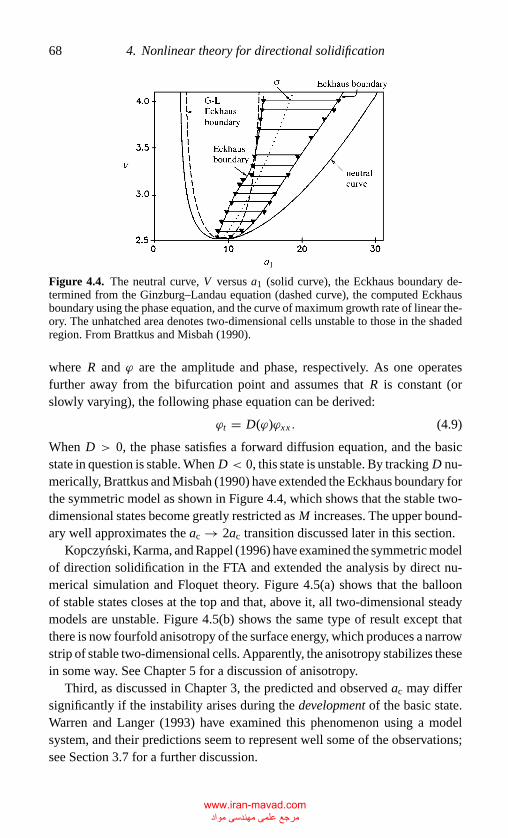
P1: GGH
CB381-04 CB381-Davis May 17, 2001 15:59 Char Count= 0
68 4. Nonlinear theory for directional solidification
Figure 4.4. The neutral curve, V versus a1 (solid curve), the Eckhaus boundary de-termined from the Ginzburg–Landau equation (dashed curve), the computed Eckhausboundary using the phase equation, and the curve of maximum growth rate of linear the-ory. The unhatched area denotes two-dimensional cells unstable to those in the shadedregion. From Brattkus and Misbah (1990).
where R and ϕ are the amplitude and phase, respectively. As one operatesfurther away from the bifurcation point and assumes that R is constant (orslowly varying), the following phase equation can be derived:
ϕt = D(ϕ)ϕxx . (4.9)
When D > 0, the phase satisfies a forward diffusion equation, and the basicstate in question is stable. When D < 0, this state is unstable. By tracking D nu-merically, Brattkus and Misbah (1990) have extended the Eckhaus boundary forthe symmetric model as shown in Figure 4.4, which shows that the stable two-dimensional states become greatly restricted as M increases. The upper bound-ary well approximates the ac → 2ac transition discussed later in this section.
Kopczynski, Karma, and Rappel (1996) have examined the symmetric modelof direction solidification in the FTA and extended the analysis by direct nu-merical simulation and Floquet theory. Figure 4.5(a) shows that the balloonof stable states closes at the top and that, above it, all two-dimensional steadymodels are unstable. Figure 4.5(b) shows the same type of result except thatthere is now fourfold anisotropy of the surface energy, which produces a narrowstrip of stable two-dimensional cells. Apparently, the anisotropy stabilizes thesein some way. See Chapter 5 for a discussion of anisotropy.
Third, as discussed in Chapter 3, the predicted and observed ac may differsignificantly if the instability arises during the development of the basic state.Warren and Langer (1993) have examined this phenomenon using a modelsystem, and their predictions seem to represent well some of the observations;see Section 3.7 for a further discussion.
www.iran-mavad.com مرجع علمی مھندسی مواد
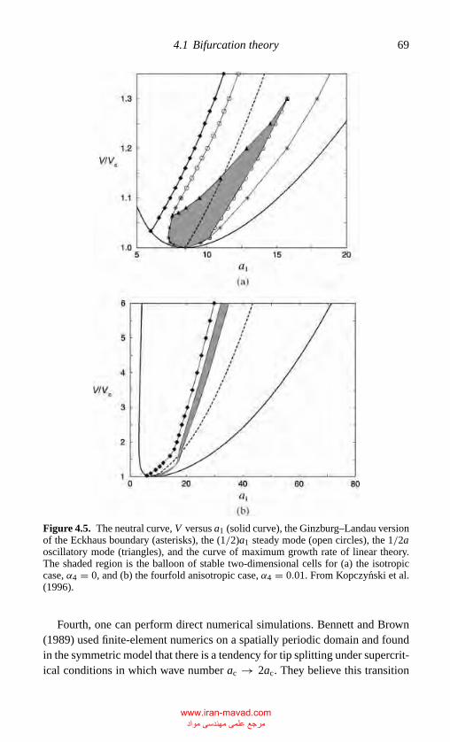
P1: GGH
CB381-04 CB381-Davis May 17, 2001 15:59 Char Count= 0
4.1 Bifurcation theory 69
Figure 4.5. The neutral curve, V versus a1 (solid curve), the Ginzburg–Landau versionof the Eckhaus boundary (asterisks), the (1/2)a1 steady mode (open circles), the 1/2aoscillatory mode (triangles), and the curve of maximum growth rate of linear theory.The shaded region is the balloon of stable two-dimensional cells for (a) the isotropiccase, α4 = 0, and (b) the fourfold anisotropic case, α4 = 0.01. From Kopczynski et al.(1996).
Fourth, one can perform direct numerical simulations. Bennett and Brown(1989) used finite-element numerics on a spatially periodic domain and foundin the symmetric model that there is a tendency for tip splitting under supercrit-ical conditions in which wave number ac → 2ac. They believe this transition
www.iran-mavad.com مرجع علمی مھندسی مواد
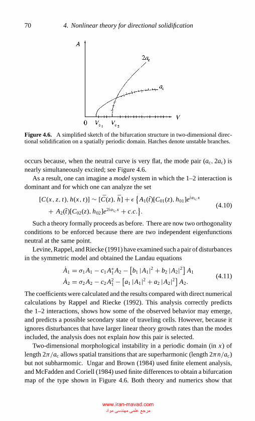
P1: GGH
CB381-04 CB381-Davis May 17, 2001 15:59 Char Count= 0
70 4. Nonlinear theory for directional solidification
Figure 4.6. A simplified sketch of the bifurcation structure in two-dimensional direc-tional solidification on a spatially periodic domain. Hatches denote unstable branches.
occurs because, when the neutral curve is very flat, the mode pair (ac, 2ac) isnearly simultaneously excited; see Figure 4.6.
As a result, one can imagine a model system in which the 1–2 interaction isdominant and for which one can analyze the set
[C(x, z, t), h(x, t)] ∼ [C(z), h] + ε {A1(t)[C01(z), h01]eia1c x
+ A2(t)[C02(z), h02]e2ia1c x + c.c.}.
(4.10)
Such a theory formally proceeds as before. There are now two orthogonalityconditions to be enforced because there are two independent eigenfunctionsneutral at the same point.
Levine, Rappel, and Riecke (1991) have examined such a pair of disturbancesin the symmetric model and obtained the Landau equations
A1 = σ1 A1 − c1 A∗1 A2 − [b1 |A1|2 + b2 |A2|2
]A1
A2 = σ2 A2 − c2 A21 − [a1 |A1|2 + a2 |A2|2
]A2.
(4.11)
The coefficients were calculated and the results compared with direct numericalcalculations by Rappel and Riecke (1992). This analysis correctly predictsthe 1–2 interactions, shows how some of the observed behavior may emerge,and predicts a possible secondary state of traveling cells. However, because itignores disturbances that have larger linear theory growth rates than the modesincluded, the analysis does not explain how this pair is selected.
Two-dimensional morphological instability in a periodic domain (in x) oflength 2π/ac allows spatial transitions that are superharmonic (length 2πn/ac)but not subharmomic. Ungar and Brown (1984) used finite element analysis,and McFadden and Coriell (1984) used finite differences to obtain a bifurcationmap of the type shown in Figure 4.6. Both theory and numerics show that
www.iran-mavad.com مرجع علمی مھندسی مواد
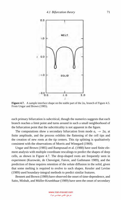
P1: GGH
CB381-04 CB381-Davis May 17, 2001 15:59 Char Count= 0
4.1 Bifurcation theory 71
Figure 4.7. A sample interface shape on the stable part of the 2ac branch of Figure 4.5.From Ungar and Brown (1985).
each primary bifurcation is subcritical, though the numerics suggests that eachbranch reaches a limit point and turns around in such a small neighborhood ofthe bifurcation point that the subcriticality is not apparent in the figure.
The computations show a secondary bifurcation from mode ac → 2ac atfinite amplitude, and the process exhibits the flattening of the cell tips andthe creation of new roots at the tip centers. This tip splitting is qualitativelyconsistent with the observations of Morris and Winegard (1969).
Ungar and Brown (1985) and Ramprasad et al. (1988) have used finite ele-ment analysis with multiple coordinate rescalings to predict the shapes of deepcells, as shown in Figure 4.7. The drop-shaped roots are frequently seen inexperiment (Kurowski, de Cheveigne, Faivre, and Guthmann 1989), and theprediction of these requires retention of the solute diffusion in the solid, giventhat some melting is required to evolve to such shapes. Kessler and Levine(1989) used boundary-integral methods to predict similar features.
Bennett and Brown (1989) have observed the onset of time-dependence, andSaito, Misbah, and Muller-Krumbhaar (1989) have seen the onset of secondary
www.iran-mavad.com مرجع علمی مھندسی مواد
P1: GGH
CB381-04 CB381-Davis May 17, 2001 15:59 Char Count= 0
72 4. Nonlinear theory for directional solidification
side arms of deep cells. Various calculations in two dimensions have been doneusing the FTA and their generalizations. See Coriell and McFadden (1993) fora detailed summary.
4.1.3 Three-Dimensional Theory
When directional solidification is performed in general applications, the mate-rial is not confined to a Hele–Shaw geometry but occupies a three-dimensionalspace. In this case, the concentration, temperature, and interface position dependon two transverse spatial variables x and y.
One approach to the description of three-dimensional instabilities is thederivation, valid near the bifurcation point, of an amplitude equation that allowslong-scale modulations in both x and y to two-dimensional solutions. Such anequation, the Newell–Whitehead–Segel equation, was derived by Segel (1969)and Newell and Whitehead (1969) in the context of Benard convection.
If the basic two-dimensional solution treated in Section 4.1.1 depends onx, t only, then one lets x = εx, t = ε2t, as before, but now lets y = ε1/2y.The result is the equation for A(x, y, t)
∂A
∂ t− d1
[∂
∂ x− i
∂2
∂ y2
]2
A = (δ − b1 |A|2)A, (4.12)
where d1, δ, and b1 are the same constants as before. From this equation the sta-bility of two-dimensional solutions to the Eckhaus instabilities can be examinedfor (∂/∂ y = 0), as well as, three-dimensional corrugations.
When in fact three-dimensional states are present, one can directly exam-ine the competition among regular planforms by deriving appropriate sets ofLandau equations.
In the FTA, the dependent variables are written
[C(x, y, z, t), h(x, y, t)] ∼ (C(z), h) + ε f0[C1(z), h1], (4.13a)
where
f0 =J∑
j=1
{A j ( t)e
ia j ·r + cc}, (4.13b)
A j is a complex coefficient and the vector wave number a j = (a1, a2); in theplane r = (x, y). The number of modes J depends upon the interaction beingconsidered and determines the number of orthogonality conditions that mustbe enforced.
When two-dimensional cells are considered, J = 1 so that, say a = (1, 0)ac
and the amplitude A1 satisfies Eq. (4.3) When one interacts two-dimensional
www.iran-mavad.com مرجع علمی مھندسی مواد
P1: GGH
CB381-04 CB381-Davis May 17, 2001 15:59 Char Count= 0
4.1 Bifurcation theory 73
cells and allows squares, J = 2, a = (1/√
2, 1/√
2)ac, and the amplitudesA1, A2 satisfy
d A1
d t= {δ − b1 |A1|2 − b2 |A2|2}A1 (4.14a)
d A2
d t= {δ − b2 |A1|2 − b1 |A2|2}A2. (4.14b)
When one interacts two-dimensional cells and allows hexagons, J = 3,a = (a1 cos 1/3 ( j − 1)π, a2 sin 1/3 ( j − 1)π ) , j = 1, 2, 3, and
∣∣a j
∣∣ = ac.
In this case
d A1
d t= δA1 − b0 A2 A∗
3 − A1{b1 |A1|2 + b3
[|A2|2 + |A3|2]}
(4.15a)
d A2
d t= δA2 − b0 A∗
1 A3 − A2{b1 |A2|2 + b3
[|A3|2 + |A1|2]}
(4.15b)
d A3
d t= δA3 − b0 A∗
1 A2 − A3{b1 |A3|2 + b3
[|A1|2 + |A2|2]}. (4.15c)
Equation (4.3) governs the growth of two-dimensional cells. As discussedearlier, b1, the Landau coefficient, determines whether the bifurcation is su-percritical (b1 > 0) or subcritical (b1 < 0). The point where b1 = 0 is thetransition point separating the two behaviors.
Equations (4.14) govern the competition between two-dimensional cells(A1 = 0, A2 �= 0, or A1 �= 0, A2 = 0) and squares (A1, A2 �= 0). The coef-ficient b2 has not been calculated for directional solidification likely becauselimited observations indicate that hexagonal arrays are the principal patternseen. For example if both b1, b2 > 0, then either rolls or squares, but not both,are stable depending upon whether b1/b2 < 1 or b1/b2 > 1, respectively.
Experiments by Cole and Winegard (1963) on tin alloys and Morris andWinegard (1969) show hexagonal structures. As a result, system (4.15) hasdrawn more attention. The cubic interaction coefficient b3, is required as wellas the quadratic interaction coefficient b0.
In all of the preceding equations the primitive (unscaled) amplitude is scaledby ε1/2, the time by ε and the cubic coefficients are of unit order. When quadraticterms are present, as in Eqs. (4.15), and the primitive quadratic coefficient b0
is of unit order, the cubic terms are negligible. To retain both the cubic andquadratic terms, b0 must be order ε in magnitude. Thus, the coefficient b0 inEqs. (4.15) is defined by b0 = b0ε, b0 = O(1).
When b0 �= 0, the hexagonal planforms can exist and be stable.Figures 4.8(a) and (b) from McFadden, Boisvert, and Coriell (1987) showphysically distinct configurations that depend on sgn b0 and the relative
www.iran-mavad.com مرجع علمی مھندسی مواد
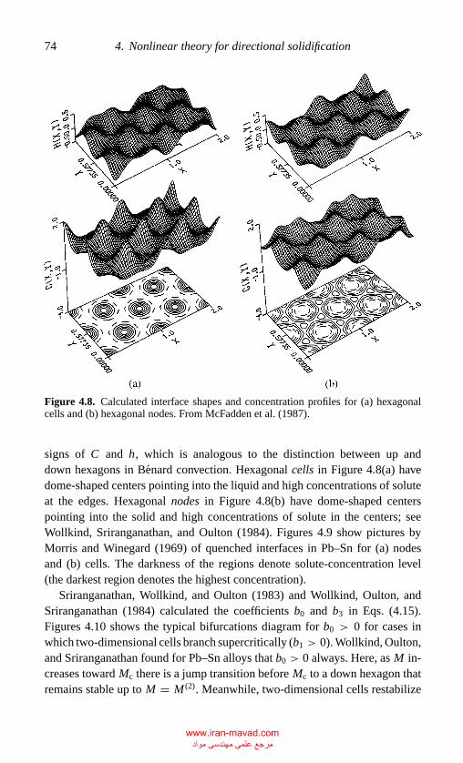
P1: GGH
CB381-04 CB381-Davis May 17, 2001 15:59 Char Count= 0
74 4. Nonlinear theory for directional solidification
Figure 4.8. Calculated interface shapes and concentration profiles for (a) hexagonalcells and (b) hexagonal nodes. From McFadden et al. (1987).
signs of C and h, which is analogous to the distinction between up anddown hexagons in Benard convection. Hexagonal cells in Figure 4.8(a) havedome-shaped centers pointing into the liquid and high concentrations of soluteat the edges. Hexagonal nodes in Figure 4.8(b) have dome-shaped centerspointing into the solid and high concentrations of solute in the centers; seeWollkind, Sriranganathan, and Oulton (1984). Figures 4.9 show pictures byMorris and Winegard (1969) of quenched interfaces in Pb–Sn for (a) nodesand (b) cells. The darkness of the regions denote solute-concentration level(the darkest region denotes the highest concentration).
Sriranganathan, Wollkind, and Oulton (1983) and Wollkind, Oulton, andSriranganathan (1984) calculated the coefficients b0 and b3 in Eqs. (4.15).Figures 4.10 shows the typical bifurcations diagram for b0 > 0 for cases inwhich two-dimensional cells branch supercritically (b1 > 0). Wollkind, Oulton,and Sriranganathan found for Pb–Sn alloys that b0 > 0 always. Here, as M in-creases toward Mc there is a jump transition before Mc to a down hexagon thatremains stable up to M = M (2). Meanwhile, two-dimensional cells restabilize
www.iran-mavad.com مرجع علمی مھندسی مواد
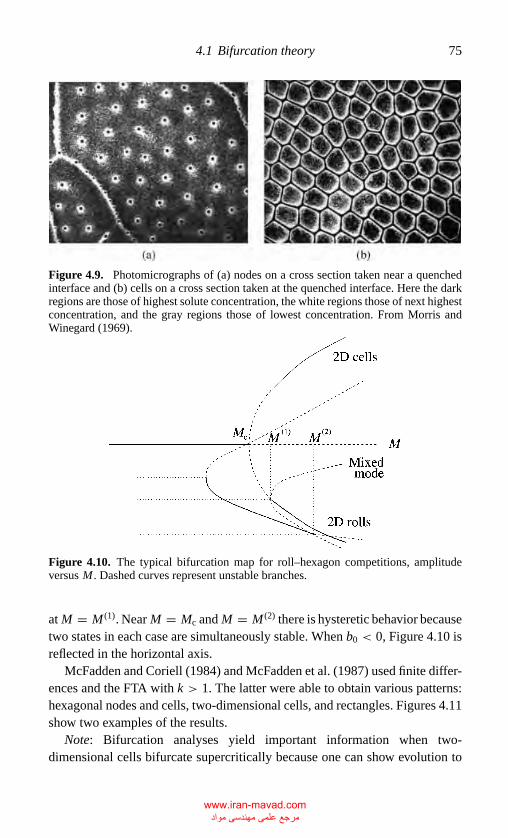
P1: GGH
CB381-04 CB381-Davis May 17, 2001 15:59 Char Count= 0
4.1 Bifurcation theory 75
Figure 4.9. Photomicrographs of (a) nodes on a cross section taken near a quenchedinterface and (b) cells on a cross section taken at the quenched interface. Here the darkregions are those of highest solute concentration, the white regions those of next highestconcentration, and the gray regions those of lowest concentration. From Morris andWinegard (1969).
Figure 4.10. The typical bifurcation map for roll–hexagon competitions, amplitudeversus M . Dashed curves represent unstable branches.
at M = M (1). Near M = Mc and M = M (2) there is hysteretic behavior becausetwo states in each case are simultaneously stable. When b0 < 0, Figure 4.10 isreflected in the horizontal axis.
McFadden and Coriell (1984) and McFadden et al. (1987) used finite differ-ences and the FTA with k > 1. The latter were able to obtain various patterns:hexagonal nodes and cells, two-dimensional cells, and rectangles. Figures 4.11show two examples of the results.
Note: Bifurcation analyses yield important information when two-dimensional cells bifurcate supercritically because one can show evolution to
www.iran-mavad.com مرجع علمی مھندسی مواد
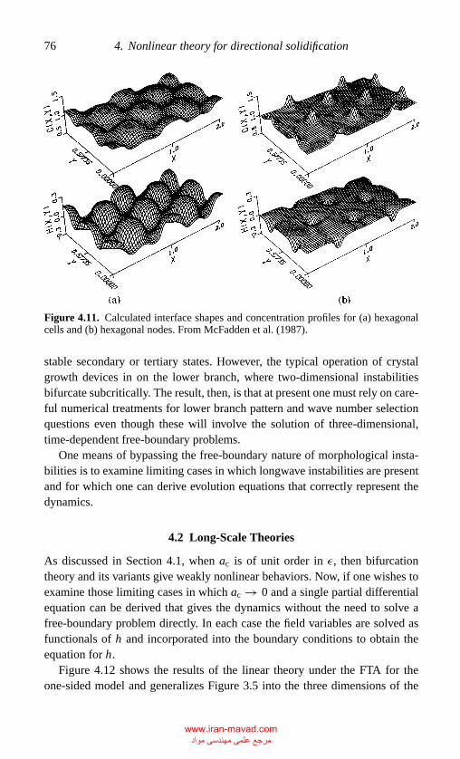
P1: GGH
CB381-04 CB381-Davis May 17, 2001 15:59 Char Count= 0
76 4. Nonlinear theory for directional solidification
Figure 4.11. Calculated interface shapes and concentration profiles for (a) hexagonalcells and (b) hexagonal nodes. From McFadden et al. (1987).
stable secondary or tertiary states. However, the typical operation of crystalgrowth devices in on the lower branch, where two-dimensional instabilitiesbifurcate subcritically. The result, then, is that at present one must rely on care-ful numerical treatments for lower branch pattern and wave number selectionquestions even though these will involve the solution of three-dimensional,time-dependent free-boundary problems.
One means of bypassing the free-boundary nature of morphological insta-bilities is to examine limiting cases in which longwave instabilities are presentand for which one can derive evolution equations that correctly represent thedynamics.
4.2 Long-Scale Theories
As discussed in Section 4.1, when ac is of unit order in ε, then bifurcationtheory and its variants give weakly nonlinear behaviors. Now, if one wishes toexamine those limiting cases in which ac → 0 and a single partial differentialequation can be derived that gives the dynamics without the need to solve afree-boundary problem directly. In each case the field variables are solved asfunctionals of h and incorporated into the boundary conditions to obtain theequation for h.
Figure 4.12 shows the results of the linear theory under the FTA for theone-sided model and generalizes Figure 3.5 into the three dimensions of the
www.iran-mavad.com مرجع علمی مھندسی مواد
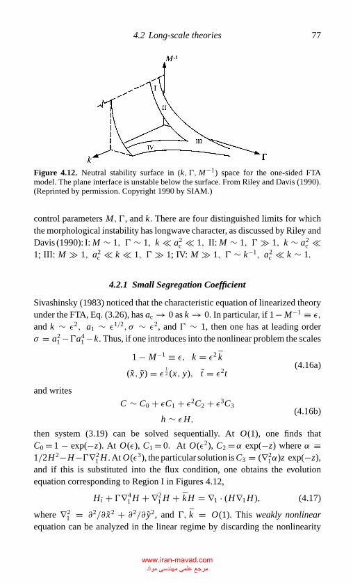
P1: GGH
CB381-04 CB381-Davis May 17, 2001 15:59 Char Count= 0
4.2 Long-scale theories 77
Figure 4.12. Neutral stability surface in (k, �,M−1) space for the one-sided FTAmodel. The plane interface is unstable below the surface. From Riley and Davis (1990).(Reprinted by permission. Copyright 1990 by SIAM.)
control parameters M, �, and k. There are four distinguished limits for whichthe morphological instability has longwave character, as discussed by Riley andDavis (1990): I: M ∼ 1, � ∼ 1, k a2
c 1, II: M ∼ 1, � � 1, k ∼ a2c
1; III: M � 1, a2c k 1, � � 1; IV: M � 1, � ∼ k−1, a2
c k ∼ 1.
4.2.1 Small Segregation Coefficient
Sivashinsky (1983) noticed that the characteristic equation of linearized theoryunder the FTA, Eq. (3.26), has ac → 0 as k → 0. In particular, if 1− M−1 ≡ ε,
and k ∼ ε2, a1 ∼ ε1/2, σ ∼ ε2, and � ∼ 1, then one has at leading orderσ = a2
1 −�a41 −k. Thus, if one introduces into the nonlinear problem the scales
1 − M−1 ≡ ε, k = ε2 k
(x, y) = ε12 (x, y), t = ε2t
(4.16a)
and writes
C ∼ C0 + εC1 + ε2C2 + ε3C3
h ∼ εH,(4.16b)
then system (3.19) can be solved sequentially. At O(1), one finds thatC0 = 1 − exp(−z). At O(ε), C1 = 0. At O(ε2), C2 =α exp(−z) where α ≡1/2H 2−H−�∇2
1 H . At O(ε3), the particular solution is C3 = (∇21α)z exp(−z),
and if this is substituted into the flux condition, one obtains the evolutionequation corresponding to Region I in Figures 4.12,
Ht + �∇41 H + ∇2
1 H + kH = ∇1 · (H∇1 H ), (4.17)
where ∇21 = ∂2/∂ x2 + ∂2/∂ y2, and �, k = O(1). This weakly nonlinear
equation can be analyzed in the linear regime by discarding the nonlinearity
www.iran-mavad.com مرجع علمی مھندسی مواد
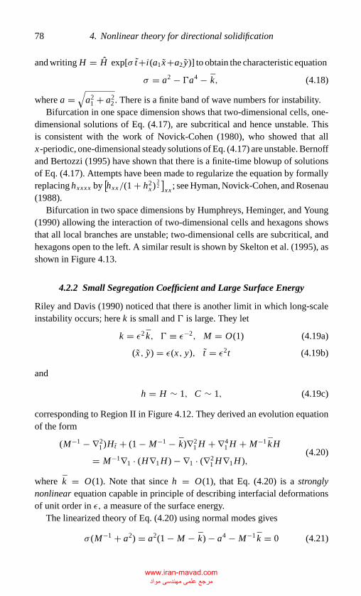
P1: GGH
CB381-04 CB381-Davis May 17, 2001 15:59 Char Count= 0
78 4. Nonlinear theory for directional solidification
and writing H = H exp[σ t+i(a1 x+a2 y)] to obtain the characteristic equation
σ = a2 − �a4 − k, (4.18)
where a =√
a21 + a2
2 . There is a finite band of wave numbers for instability.Bifurcation in one space dimension shows that two-dimensional cells, one-
dimensional solutions of Eq. (4.17), are subcritical and hence unstable. Thisis consistent with the work of Novick-Cohen (1980), who showed that allx-periodic, one-dimensional steady solutions of Eq. (4.17) are unstable. Bernoffand Bertozzi (1995) have shown that there is a finite-time blowup of solutionsof Eq. (4.17). Attempts have been made to regularize the equation by formallyreplacing hxxxx by
[hxx/(1 + h2
x )32]
xx; see Hyman, Novick-Cohen, and Rosenau
(1988).Bifurcation in two space dimensions by Humphreys, Heminger, and Young
(1990) allowing the interaction of two-dimensional cells and hexagons showsthat all local branches are unstable; two-dimensional cells are subcritical, andhexagons open to the left. A similar result is shown by Skelton et al. (1995), asshown in Figure 4.13.
4.2.2 Small Segregation Coefficient and Large Surface Energy
Riley and Davis (1990) noticed that there is another limit in which long-scaleinstability occurs; here k is small and � is large. They let
k = ε2 k, � ≡ ε−2, M = O(1) (4.19a)
(x, y) = ε(x, y), t = ε2t (4.19b)
and
h = H ∼ 1, C ∼ 1, (4.19c)
corresponding to Region II in Figure 4.12. They derived an evolution equationof the form
(M−1 − ∇21 )Ht + (1 − M−1 − k)∇2
1 H + ∇41 H + M−1 kH
= M−1∇1 · (H∇1 H ) − ∇1 · (∇21 H∇1 H ),
(4.20)
where k = O(1). Note that since h = O(1), that Eq. (4.20) is a stronglynonlinear equation capable in principle of describing interfacial deformationsof unit order in ε, a measure of the surface energy.
The linearized theory of Eq. (4.20) using normal modes gives
σ (M−1 + a2) = a2(1 − M − k) − a4 − M−1 k = 0 (4.21)
www.iran-mavad.com مرجع علمی مھندسی مواد
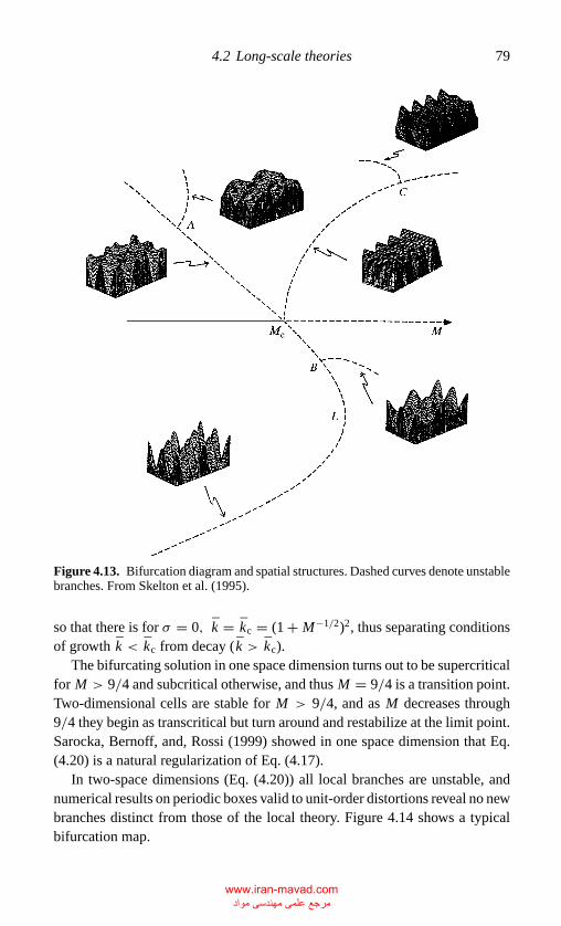
P1: GGH
CB381-04 CB381-Davis May 17, 2001 15:59 Char Count= 0
4.2 Long-scale theories 79
Figure 4.13. Bifurcation diagram and spatial structures. Dashed curves denote unstablebranches. From Skelton et al. (1995).
so that there is for σ = 0, k = kc = (1 + M−1/2)2, thus separating conditionsof growth k < kc from decay ( k > kc).
The bifurcating solution in one space dimension turns out to be supercriticalfor M > 9/4 and subcritical otherwise, and thus M = 9/4 is a transition point.Two-dimensional cells are stable for M > 9/4, and as M decreases through9/4 they begin as transcritical but turn around and restabilize at the limit point.Sarocka, Bernoff, and, Rossi (1999) showed in one space dimension that Eq.(4.20) is a natural regularization of Eq. (4.17).
In two-space dimensions (Eq. (4.20)) all local branches are unstable, andnumerical results on periodic boxes valid to unit-order distortions reveal no newbranches distinct from those of the local theory. Figure 4.14 shows a typicalbifurcation map.
www.iran-mavad.com مرجع علمی مھندسی مواد
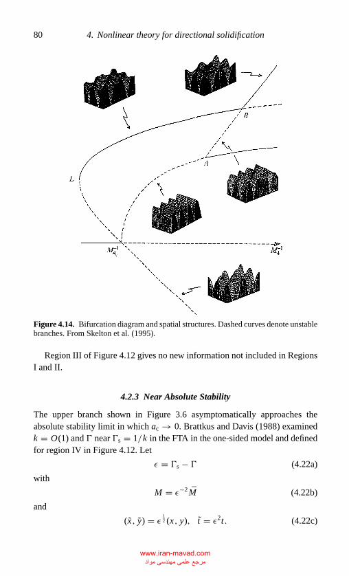
P1: GGH
CB381-04 CB381-Davis May 17, 2001 15:59 Char Count= 0
80 4. Nonlinear theory for directional solidification
Figure 4.14. Bifurcation diagram and spatial structures. Dashed curves denote unstablebranches. From Skelton et al. (1995).
Region III of Figure 4.12 gives no new information not included in RegionsI and II.
4.2.3 Near Absolute Stability
The upper branch shown in Figure 3.6 asymptomatically approaches theabsolute stability limit in which ac → 0. Brattkus and Davis (1988) examinedk = O(1) and � near �s = 1/k in the FTA in the one-sided model and definedfor region IV in Figure 4.12. Let
ε = �s − � (4.22a)
with
M = ε−2M (4.22b)
and
(x, y) = ε12 (x, y), t = ε2t. (4.22c)
www.iran-mavad.com مرجع علمی مھندسی مواد
P1: GGH
CB381-04 CB381-Davis May 17, 2001 15:59 Char Count= 0
4.2 Long-scale theories 81
Here M = O(1) and k is arbitrary. The asymptotic expansion for the interfaceposition has the form h ∼ H , and thus unit-order distortions are allowed.Brattkus and Davis derived the strongly nonlinear equation
Ht t − ∇21 Ht + 1
4(1 − ν2)∇4
1 H + ∇21 H + µ−1 H = Ht∇2
1 H + |∇1 H |2t− 1
2(1 − ν)∇2
1
(|∇1 H |2)− ν∇1 · (∇21 H∇1 H
)− 1
2∇1 · (|∇1 H |2 ∇1 H
),
(4.23)
where
M = µ(1 + 2k)/k3 (4.24a)
and
ν = (1 + 2k)−1. (4.24b)
In the linearized theory, the characteristic equation takes the form
σ 2 + a2(2 + k−1)σ + [kM−1 − ka2 + a4(1 + k−1)] = 0. (4.25)
Notice that the growth rate σ satisfies a quadratic equation, and hence both firstand second derivatives are inherited by the evolution equation (4.23). Note,too, that the nonlinearities of Eq. (4.23) are both cubic and quadratic, which ispossible because the equation is strongly nonlinear.
In one space dimension the bifurcations are supercritical, and two-dimensional cells equilibrate to finite-amplitude forms. In two space dimen-sions, all two-dimensional states are initially unstable. Brattkus and Davis foundfor µ fixed and k → 1 that pattern selection gives a normal two-dimensional-cell–hexagonal interaction, as shown in Figure 4.10. Skelton et al. (1995) foundnumerically that no new branches or instabilities are obtained in a numericaldomain substantially larger than that covered by the local theory and for k assmall as 0.90.
That the evolution equation (4.23) contains both first and second time deriva-tives suggests that it might be possible to excite secondary bifurcations to time-periodic states. Brattkus (1990) attempted this in the case of a single spacedimension. In this case Eq. (4.23) has the form
L(H ) = Ht t − Hxx t + 1
4(1 − ν2)Hxx x x + Hxx + µ−1 H = N (H ), (4.26a)
where
N (H ) = Hxx Ht + 2Hx Hxt − Hx Hx x x − H 2x − 1
2
(H 2
x
)x x . (4.26b)
Brattkus (1990) was not able to find time-dependent instabilities of two-dimensional cells (using Floquet theory). However, he rederived the two-dimensional evolution equation for the symmetric model. He found that
www.iran-mavad.com مرجع علمی مھندسی مواد
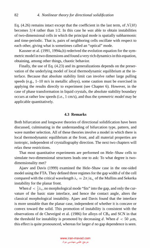
P1: GGH
CB381-04 CB381-Davis May 17, 2001 15:59 Char Count= 0
82 4. Nonlinear theory for directional solidification
Eq. (4.26) remains intact except that the coefficient in the last term, of N (H )becomes 3/4 rather than 1/2. In this case he was able to obtain instabilitiesof two-dimensional cells in which the principal mode is spatially subharmonicand time-periodic. That is, pairs of neighboring cells oscillate with respect toeach other, giving what is sometimes called an “optical” mode.
Kassner et al. (1991, 1994a,b) rederived the evolution equation for the sym-metric model in two dimensions and found a very rich dynamics in this equation,obtaining, among other things, chaotic behavior.
Finally, the use of Eq. (4.23) and its generalizations depends on the preser-vation of the underlying model of local thermodynamic equilibrium at the in-terface. Because that absolute stability limit can involve rather large pullingspeeds (e.g., 1–10 m/s in metallic alloys), some caution must be exercised inapplying the results directly to experiment (see Chapter 6). However, in thecase of phase transformation in liquid crystals, the absolute stability boundaryoccurs at rather low speeds (i.e., 1 cm/s), and thus the symmetric model may beapplicable quantitatively.
4.3 Remarks
Both bifurcation and longwave theories of directional solidification have beendiscussed, culminating in the understanding of bifurcation type, pattern, andwave number selection. All of these theories involve a model in which there islocal thermodynamic equilibrium at the front, and all material properties areisotropic, independent of crystallography direction. The next two chapters willrelax these restrictions.
That most quantitative experiments are performed on Hele–Shaw cells tosimulate two-dimensional structures leads one to ask: To what degree is two-dimensionality met?
Ajaev and Davis (1999) examined the Hele–Shaw case in the one-sidedmodel using the FTA. They defined three regimes for the gap width d of the cellcompared with the critical wavelength λc = 2π/a∗c of the Mullins and Sekerkainstability for the planar front.
When d < 12λc, no morphological mode “fits” into the gap, and only the cur-
vature of the basic state interface, and hence the contact angle, alters theclassical morphological instability. Ajaev and Davis found that the interfaceis more unstable than the planar case, independent of whether it is concave orconvex toward the solid. This promotion of instability is consistent with theobservations of de Cheveigne et al. (1986) for alloys of CB4 and SCN in thatthe threshold for instability is promoted by decreasing d. When d < 50 µm,this effect is quite pronounced, whereas for larger d no gap dependence is seen.
www.iran-mavad.com مرجع علمی مھندسی مواد
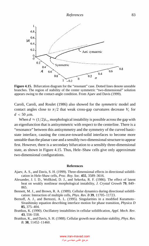
P1: GGH
CB381-04 CB381-Davis May 17, 2001 15:59 Char Count= 0
References 83
Figure 4.15. Bifurcation diagram for the “resonant” case. Dotted lines denote unstablebranches. The region of stability of the center symmetric “two-dimensional” solutionappears owing to the contact-angle condition. From Ajaev and Davis (1999).
Caroli, Caroli, and Roulet (1986) also showed for the symmetric model andcontact angles close to π/2 that weak cross-gap curvatures decrease Vc ford < 50 µm.
When d ≈ (1/2)λc, morphological instability is possible across the gap withan eigenfunction that is antisymmetric with respect to the centerline. There is a“resonance” between this antisymmetry and the symmetry of the curved basic-state interface, causing the concave-toward-solid interfaces to become moreunstable than the planar case and a sensibly two-dimensional structure to appearfirst. However, there is a secondary bifurcation to a sensibly three-dimensionalstate, as shown in Figure 4.15. Thus, Hele–Shaw cells give only approximatetwo-dimensional configurations.
References
Ajaev, A. S., and Davis, S. H. (1999). Three-dimensional effects in directional solidifi-cation in Hele-Shaw cells, Proc. Roy. Soc. 455, 3589–3616.
Alexander, J. I. D., Wollkind, D. J., and Sekerka, R. F. (1986). The effect of latentheat on weakly nonlinear morphological instability, J. Crystal Growth 79, 849–865.
Bennett, M. J., and Brown, R. A. (1989). Cellular dynamics during directional solidifi-cation: Interaction of multiple cells, Phys. Rev. B 39, 11705–11723.
Bernoff, A. J., and Bertozzi, A. L. (1995). Singularities in a modified Kuramoto–Sivashinsky equation describing interface motion for phase transition, Physica D85, 375–404.
Brattkus, K. (1990). Oscillatory instabilities in cellular solidification, Appl. Mech. Rev.43, 556–558.
Brattkus, K., and Davis, S. H. (1988). Cellular growth near absolute stability, Phys. Rev.B. 38, 11452–11460.
www.iran-mavad.com مرجع علمی مھندسی مواد
P1: GGH
CB381-04 CB381-Davis May 17, 2001 15:59 Char Count= 0
84 4. Nonlinear theory for directional solidification
Brattkus, K., and Misbah, C. (1990). Phase dynamics in directional solidification, Phys.Rev. Lett. 64, 1935–1938.
Caroli, B., Caroli, C., and Roulet, B. (1982). On the emergence of one dimensional frontinstabilities in directional solidification and fusion of binary mixtures, J. de Phys.(Paris) 43, 1767–1780.
. (1986). The Mullins–Sekerka instability in thin samples, J. Crystal Growth 76,31–49.
de Cheveigne, S., Guthmann, C., and Lebrun, M.-M. (1985). Nature of the transition ofthe solidification front of a binary mixture from a planar to a cellular morphology,J. Crystal Growth 73, 242–244.
. (1986). Cellular instabilities in directional solidification, J. de Phys. (Paris) 47,2095–2103.
Cole, G. S., and Winegard, W. C. (1963). The transition from plane to cellular interfacein solidifying tin-lead-antimony alloys, J. Inst. Metals 92, 322–326.
Coriell, S. R., and McFadden, G. J. (1993). Morphological stability, D. T. J. Hurle,editor, in Handbook of Crystal Growth 1b, Chap. 12, 785–857, North-Holland,Amsterdam.
Eckhaus, W. (1965), Studies in Nonlinear Stability Theory, Springer–Verlag, Berlin.Humphreys, L. B., Heminger, J. A., and Young, G. W. (1990). Morphological stability
in a float zone, J. Crystal Growth 100, 31–50.Hyman, J. M., Novick-Cohen, A., and Rosenau, P. (1988). Modified asymptotic approach
to modeling a dilute-binary-alloy solidification front, Phys. Rev. B 37, 7603–7608.Kassner, K., Misbah, C., and Muller-Krumbhaar, H. (1991). Transition to chaos in
directional solidification, Phys. Rev. Lett. 67, 1551–1553.Kassner, K., Misbah, C., Muller-Krumbhaar, H., and Valance, A. (1994a). Directional
solidification at high speed. I. Secondary instabilities, Phys. Rev. E 49, 5477–5494.
. (1994b). Directional solidification at high speed. II. Transition to chaos, Phys.Rev. E 49, 5495–5515.
Kessler, D. A., and Levine, H. (1989). Steady-state cellular growth during directionalsolidification, Phys. Rev. A 39, 3041–3052.
Kopczynski, P., Rappel, W.-J., and Karma, A. (1996). Critical role of crystallineanisotropy in the stability of cellular array structures in directional solidification,Phys. Rev. Lett. 77, 3387–3390.
Kurowski, P., de Cheveigne, S., Faive, G., and Guthmann, C. (1989). Cusp instability incellular growth, J. de Phys. 50, 3007–3019.
Levine, H., Rappel, W.-J., and Riecke, H. (1991). Resonant interactions and travelingsolidification cells, Phys. Rev. A 43, 1122–1125.
Liu, D., Williams, L. M., and Cummins, H. Z. (1994). Subcritical–supercritical bifurca-tion crossover in directional solidification, Phys. Rev. E 50, R4286–R4289.
McFadden, G. B., and Coriell, S. R. (1984). Nonplanar interface morphologies duringunidirectional solidification of a binary alloy, Physica D 12, 253–261.
McFadden, G. B., Boisvert, R. F., and Coriell, S. R. (1987). Nonplanar interfacemorphologies during unidirectional solidification of a binary alloy II. Three-dimensional computations, J. Crystal Growth 84, 371–388.
Merchant, G. J., and Davis, S. H. (1989a). Shallow cells in directional solidification,Phys. Rev. Lett. 63, 573–575.
. (1989b). Directional solidification near minimum c∞: Two-dimensional isolasand multiple solutions, Phys. Rev. B 40, 11140–11152.
Morris, L. R., and Winegard, W. C. (1969). The development of cells during the solidi-fication of a dilute Pb–Sn alloy, J. Crystal Growth 5, 361–375.
www.iran-mavad.com مرجع علمی مھندسی مواد
P1: GGH
CB381-04 CB381-Davis May 17, 2001 15:59 Char Count= 0
References 85
Newell, A. C., and Whitehead, J. A. (1969). Finite bandwith, finite amplitude convection,J. Fluid Mech. 38, 279–303.
Novick-Cohen, A. (1980). Instability of periodic states for the Sivashinsky equation,Q. Appl. Math. 48, 217–224.
Ramprasad, N., Bennett, M. J., and Brown, R. A. (1988). Wavelength dependence ofcells of finite depth in directional solidification, Phys. Rev. B 38, 583–592.
Rappel, W.-J., and Riecke, H. (1992). Parity-breaking in directional solidification: Nu-merics versus amplitude equations, Phys. Rev. A 45, 846–859.
Riley, D. S., and Davis, S. H. (1989). Eckhaus instabilities in generalized Landau–Ginzburg equations, Phys. Fluids A 1, 1745–1747.
. (1990). Long-wave morphological instabilities in the directional solidificationof a dilute binary mixture, SIAM J. Appl. Math. 50, 420–436.
Saito, Y., Misbah, C., and Muller-Krumbhaar, H. (1989). Directional solidification:Transition from cell to dendrites, Phys. Rev. Lett. 63, 2377–2380.
Sarocka, D. S., Bernoff, A. J., and Rossi, L. F. (1999). Large-amplitude solutions tothe Sivashinsky and Riley–Davis equations for directional solidification, PhysicaD 127, 146–176.
Segel, L. A. (1969). Distant side-walls cause slow amplitude modulation of cellularconvection, J. Fluid Mech. 38, 203–224.
Sivashinsky, G. I. (1983). On cellular instability in the solidification of a dilute binaryalloy, Physica D 8, 243–248.
Skelton, A. C., McFadden, G. B., Impey, M. D., Riley, D. S., Cliffe, K. A., Wheeler, A.A., and Davis, S. H. (1995). On long-wave morphological instabilities in directionalsolidification, Eur. J. Appl. Math. 6, 639–652.
Sriranganathan, R., Wollkind, D. J., and Oulton, D. B. (1983). A theoretical investigationof the development of interfacial cells during the solidification of a binary alloy:Comparison with the experiments of Morris and Winegard, J. Crystal Growth 62,265–283.
Ungar, L. H., and Brown, R. A. (1984). Cellular interface morphologies in directionalsolidification: The one-sided model, Phys. Rev. B 29, 1367–1380.
. (1985). Cellular morphologies in directional solidification. IV. The formationof deep cells, Phys. Rev. B 31, 5931–5940.
Warren, J. A., and Langer, J. S. (1993). Prediction of dendrite spacing in a directionalsolidification experiment, Phys. Rev. E 47, 2702–2712.
Wollkind, D. J., Oulton, D. B., and Sriranganathan, R. (1984). A nonlinear stabilityanalysis of a model equation for alloy solidification, J. de Phys. 45, 505–516.
Wollkind, D. J., and Segel, L. A. (1970). A nonlinear stability analysis of the freezingof a dilute binary alloy, Philos. Trans. Roy. Soc. London A 268, 351–380.
Wollkind, D. J., Sriranganathan, R., and Oulton, D. B. (1984). Interfacial patterns duringplane front alloy solidification, Physica 12D, 215–240.
www.iran-mavad.com مرجع علمی مھندسی مواد
P1: GKE
Chap-05 CB381-Davis May 17, 2001 17:3 Char Count= 0
5
Anisotropy
The modern theory of morphological instability began with the work of Mullinsand Sekerka (1963, 1964), as discussed in Chapter 3, who modeled the solidas an isotropic, continuous medium whose only “memory” of its crystallinestructure is the presence of latent heat. They used linear stability theoryto show that adverse gradients of temperature or solute concentration at amoving front drives an instability, and the surface energy cuts off the short-scale corrugations. The nonlinear extensions of this model were discussed inChapter 4.
The preceding developments have had broad impact on the field, which isremarkable given that no account had been taken of the details of the crys-tallographic properties of the solid. One would expect the crystal structure toimpress geometrical symmetries on the system that compete with nonlinearitiesfor the determination of morphological pattern and hence the microstructure ofthe solid. In principle, all of the bulk material properties (e.g., ks
T, csp, ρ
s, Ds)and the interfacial properties (e.g., γ, µ) possess the same orientational infor-mation, though some of the anisotropies may be more important than others inparticular situations.
5.1 Surface Energy and Kinetics
Consider first the anisotropy of surface energy γ . Now, instead of γ beingconstant, it depends on the orientation of the interface with respect to the un-derlying crystal structure. This information is transmitted to the surface energyby allowing γ = γ (n), where n is the unit outward normal vector to the body.The formulation of a two-dimensional drop on a substrate of Section 2.2 still
86
www.iran-mavad.com مرجع علمی مھندسی مواد
P1: GKE
Chap-05 CB381-Davis May 17, 2001 17:3 Char Count= 0
5.1 Surface energy and kinetics 87
holds, and Eq. (2.47) is still correct, namely,
w−1 E ′ =�2∫�1
I dx + γ1(�2 − �1) + γ2[�− (�2 − �1)], (5.1)
where now
I = γ (hx )(1 + h2x )
12 + λh. (5.2)
The geometrical quantities are shown in Figure 2.11.To evaluate the variation of E ′, one needs some notation and several relations:
∂
∂hxγ ≡ γ,x,
∂2
∂h2x
γ = γ,xx ,∂
∂xγ,x = γ,xxhxx . (5.3)
The variation of E ′ is then given by
w−1δE ′ =�2∫�1
[Ihδh + Ihx (δh)x
]+ (I + γ1 − γ2) δ�|�2�1
(5.4)
and using integration by parts, one obtains
w−1δE ′ =�2∫�1
[Ih − (Ihx
)x
]δh dx + Ihx δh
∣∣�2
�1+ (I + γ1 − γ2) δ�|�2
�1. (5.5)
Again, use endpoint relations (2.51), δh|�1,�2= −hxδ�|�1,�2
, to obtain the finalform of the first variation
w−1δE ′ =�2∫�1
[Ih − (Ihx
)x
]δh dx + [I − hx Ihx + γ1 − γ2
]δ�|�2
�1. (5.6)
The Euler–Lagrange equation becomes
Ih − (Ihx
)x
= 0
or
λ = hxx
(1 + h2x )3/2
{γ + 2γ,xhx (1 + h2
x ) + γ,xx (1 + h2x )2}. (5.7)
It is convenient to define θ to be the angle between the z-axis and n, n =(sin θ, cos θ ). In terms of θ, −hx = tan θ , and thus at the contact line θ is thecontact angle. Further,
(1 + h2
x
)1/2 = sec θ and γ,x = γθ cos2 θ . After a bitof manipulation, form (5.7) becomes
λ = 2H (γ + γθθ ), (5.8)
www.iran-mavad.com مرجع علمی مھندسی مواد
P1: GKE
Chap-05 CB381-Davis May 17, 2001 17:3 Char Count= 0
88 5. Anisotropy
which is a generalization of Eq. (2.54) made by Herring (1951) to situations inwhich γ varies with the orientation of the front. Equation (5.8), derived in twodimensions, is valid in three dimensions if the mean curvature H is replacedby its appropriate form. The corresponding Gibbs–Thomson equation is then
T I = Tm
[1 + 2H
γ + γθθLv
]; (5.9)
compare this with Eq. (2.57).If one returns to Eq. (5.6), the end conditions for the first variation are
I − hx Ihx + γ1 − γ2 = 0, x = �1, �2
or
γ
(1 + h2x )
12
= γ2 − γ1 + γ,xhx (1 + h2x )
12 . (5.10)
From the definition of θ , Eq. (5.10) becomes
γ cos θ = γ2 − γ1 − γθ sin θ, (5.11)
which is the generalization to orientational dependence of the Young–Laplaceequation (2.59) made by Herring (1951). Again, at the contact line θ is thecontact angle.
Consider a single crystal of fixed volume (no phase transformation) and seekits shape at thermodynamic equilibrium. From surface energy minimization,Eq. (5.8), 2H (γ + γθθ ) is constant. Clearly, if γ were isotropic, as it wouldbe for a drop of liquid or a glass, γ would be constant, and hence H would beconstant. In two or three dimensions, the equilibrium figure would be a circleor a sphere, respectively.
Consider a rectangular parallelpiped shown in Figure 5.1 of dimensions 2(�1, �2, �3) in the direction (x, y, z) in which each face parallel to a differentcoordinate axis has a different γ, as shown. If one minimizes E = 2 (γ1�2�3+γ2�1�3 + γ3�1�2) subject to V= �1�2�3 fixed, one finds (Mullins 1963)that
γ1
�1= γ2
�2= γ3
�3= constant. (5.12)
Thus, the γ of any face is proportional to the distance of that face from thecenter of the parallelpiped. The equilibrium shape, because it minimizes surfaceenergy, makes the face with the largest γ have the smallest area. More generally,it is found that the shape will form so as to preferentially expose crystallographicorientations of low γ .
www.iran-mavad.com مرجع علمی مھندسی مواد
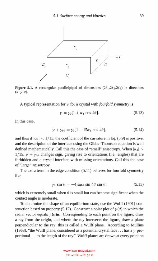
P1: GKE
Chap-05 CB381-Davis May 17, 2001 17:3 Char Count= 0
5.1 Surface energy and kinetics 89
Figure 5.1. A rectangular parallelpiped of dimensions (2�1,2�2,2�3) in directions(x, y, z).
A typical representation for γ for a crystal with fourfold symmetry is
γ = γ0[1 + α4 cos 4θ ]. (5.13)
In this case,
γ + γθθ = γ0[1 − 15α4 cos 4θ ], (5.14)
and thus if |α4| < 1/15, the coefficient of the curvature in Eq. (5.9) is positive,and the description of the interface using the Gibbs–Thomson equation is welldefined mathematically. Call this the case of “small” anisotropy. When |α4| >1/15, γ + γθθ changes sign, giving rise to orientations (i.e., angles) that areforbidden and a crystal interface with missing orientations. Call this the caseof “large” anisotropy.
The extra term in the edge condition (5.11) behaves for fourfold symmetrylike
γθ sin θ = −4γ0α4 sin 4θ sin θ, (5.15)
which is extremely small when θ is small but can become significant when thecontact angle is moderate.
To determine the shape of an equilibrium state, use the Wulff (1901) con-struction based on property (5.12). Construct a polar plot of γ (θ ) in which theradial vector equals γ (n)n. Corresponding to each point on the figure, drawa ray from the origin, and where the ray intersects the figure, draw a planeperpendicular to the ray; this is called a Wulff plane. According to Mullins(1963), “the Wulff plane, considered as a potential crystal face . . . has a γ pro-portional . . . to the length of the ray.” Wulff planes are drawn at every point on
www.iran-mavad.com مرجع علمی مھندسی مواد
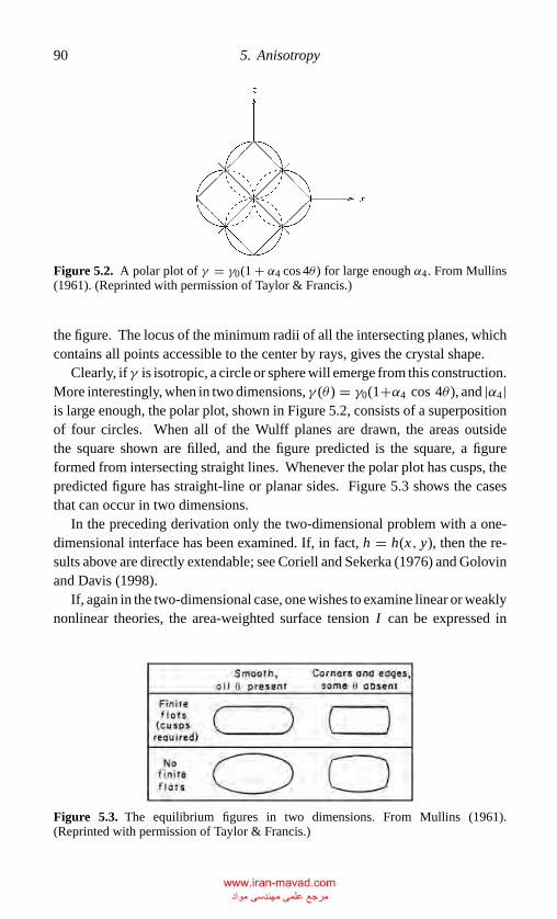
P1: GKE
Chap-05 CB381-Davis May 17, 2001 17:3 Char Count= 0
90 5. Anisotropy
Figure 5.2. A polar plot of γ = γ0(1 + α4 cos 4θ ) for large enough α4. From Mullins(1961). (Reprinted with permission of Taylor & Francis.)
the figure. The locus of the minimum radii of all the intersecting planes, whichcontains all points accessible to the center by rays, gives the crystal shape.
Clearly, if γ is isotropic, a circle or sphere will emerge from this construction.More interestingly, when in two dimensions, γ (θ ) = γ0(1+α4 cos 4θ ), and |α4|is large enough, the polar plot, shown in Figure 5.2, consists of a superpositionof four circles. When all of the Wulff planes are drawn, the areas outsidethe square shown are filled, and the figure predicted is the square, a figureformed from intersecting straight lines. Whenever the polar plot has cusps, thepredicted figure has straight-line or planar sides. Figure 5.3 shows the casesthat can occur in two dimensions.
In the preceding derivation only the two-dimensional problem with a one-dimensional interface has been examined. If, in fact, h = h(x, y), then the re-sults above are directly extendable; see Coriell and Sekerka (1976) and Golovinand Davis (1998).
If, again in the two-dimensional case, one wishes to examine linear or weaklynonlinear theories, the area-weighted surface tension I can be expressed in
Figure 5.3. The equilibrium figures in two dimensions. From Mullins (1961).(Reprinted with permission of Taylor & Francis.)
www.iran-mavad.com مرجع علمی مھندسی مواد
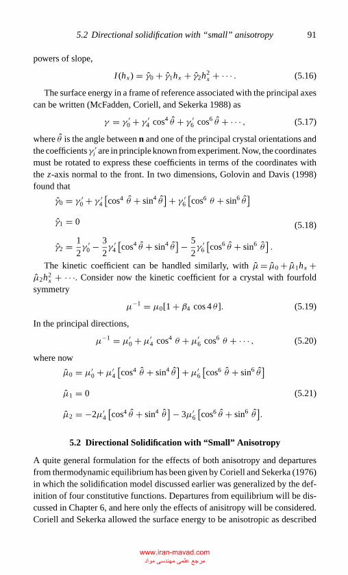
P1: GKE
Chap-05 CB381-Davis May 17, 2001 17:3 Char Count= 0
5.2 Directional solidification with “small” anisotropy 91
powers of slope,
I (hx ) = γ0 + γ1hx + γ2h2x + · · · . (5.16)
The surface energy in a frame of reference associated with the principal axescan be written (McFadden, Coriell, and Sekerka 1988) as
γ = γ ′0 + γ ′
4 cos4 θ + γ ′6 cos6 θ + · · · , (5.17)
where θ is the angle between n and one of the principal crystal orientations andthe coefficientsγ ′
i are in principle known from experiment. Now, the coordinatesmust be rotated to express these coefficients in terms of the coordinates withthe z-axis normal to the front. In two dimensions, Golovin and Davis (1998)found that
γ0 = γ ′0 + γ ′
4
[cos4 θ + sin4 θ
]+ γ ′6
[cos6 θ + sin6 θ
]γ1 = 0
γ2 = 1
2γ ′
0 − 3
2γ ′
4
[cos4 θ + sin4 θ
]− 5
2γ ′
6
[cos6 θ + sin6 θ
].
(5.18)
The kinetic coefficient can be handled similarly, with µ= µ0 + µ1hx +µ2h2
x + · · ·. Consider now the kinetic coefficient for a crystal with fourfoldsymmetry
µ−1 = µ0[1 + β4 cos 4 θ ]. (5.19)
In the principal directions,
µ−1 = µ′0 + µ′
4 cos4 θ + µ′6 cos6 θ + · · · , (5.20)
where now
µ0 = µ′0 + µ′
4
[cos4 θ + sin4 θ
]+ µ′6
[cos6 θ + sin6 θ
]µ1 = 0
µ2 = −2µ′4
[cos4 θ + sin4 θ
]− 3µ′6
[cos6 θ + sin6 θ
].
(5.21)
5.2 Directional Solidification with “Small” Anisotropy
A quite general formulation for the effects of both anisotropy and departuresfrom thermodynamic equilibrium has been given by Coriell and Sekerka (1976)in which the solidification model discussed earlier was generalized by the def-inition of four constitutive functions. Departures from equilibrium will be dis-cussed in Chapter 6, and here only the effects of anisitropy will be considered.Coriell and Sekerka allowed the surface energy to be anisotropic as described
www.iran-mavad.com مرجع علمی مھندسی مواد
P1: GKE
Chap-05 CB381-Davis May 17, 2001 17:3 Char Count= 0
92 5. Anisotropy
above. They wrote the kinetic undercooling as
Vn = f (Te − T I, hx , hxx ). (5.22)
The function f is not known in general, but if f is smooth, and in the case oflinear stability theory about a planar interface, this relation can be linearizedas
V ′n ∼ f (T 0
e − T I0, 0, 0) + µT (T ′e − T I′ ) + µxhx + µxxhxx , (5.23)
where now only constant coefficients µT, µx , and µxx need to be measuredand f (T 0
e −T I0, 0, 0) is part of the basic state. Equation (5.23) for linear theorycan then be written
T I′ = T ′e + µ−1
T V ′n + µ−1
T [µxhx + µxxhxx ], (5.24)
and T ′e contains the constitutional and capillary undercooling. In dimensional
terms the linearized Gibbs–Thomson relation is now
Gh = mC + Tm2Hγ ′ + µ−1T V ′
n + µ−1T [µxhx + µxxhxx ]. (5.25)
Coriell and Sekerka (1976) examined the one-sided model under the frozentemperature approximation and found, for “small” anisotropy, linear instabilitymodes that have complex growth rates σ = σR + iσI indicating the presence oftraveling or standing waves with angular frequencies ω ≡ σI �= 0.
They explained the presence of these waves as follows: If, say, µT ,µx > 0and a normal mode exp[i(ax + ωt)] is defined, there is a wave traveling in thenegative x-direction (forω > 0). Parts of the front for which hx > 0 have larger∣∣V ′
n
∣∣ than those for when hx < 0, and a wave motion can ensue. Coriell andSekerka argued that when the disturbance reaches finite amplitude, the cellsthat grow will be tilted at an angle tan−1(c/V ) with respect to the heat flow,where c = ω/a is the phase speed of the wave.
A nonlinear analysis in the Sivashinsky limit, k → 0, � = O(1) is validfor long-scale weakly nonlinear states. As shown in Section 4.3, M−1 = 1 − ε,and the wave number is O(ε1/2). When the preceding model of anisotropy isinserted and
µT ≡ V 2
mGc DµT, µx ≡ µx
µT
V
mGc D, (5.26)
the theory can be extended (Young, Davis, and Brattkus 1987) if µT =ε1/2µT , µx = ε1/2µx , where the barred quantities are of unit order. Theevolution equation, written for the two-dimensional case as a generalization ofEq. (4.17) is
Ht + �∇41 H + ∇2
1 H + µ·∇ · (∇2 H ) + kH = ∇1 · (H∇1 H ) (5.27)
where µ = (µx , µy)T and µy has the expected definition.
www.iran-mavad.com مرجع علمی مھندسی مواد
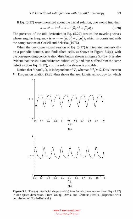
P1: GKE
Chap-05 CB381-Davis May 17, 2001 17:3 Char Count= 0
5.2 Directional solidification with “small” anisotropy 93
If Eq. (5.27) were linearized about the trivial solution, one would find that
σ = a2 − �a4 − k − i(µxa21 + µya
22). (5.28)
The presence of the odd derivative in Eq. (5.27) creates the traveling waveswhose angular frequency is ω = − (µxa2
1 + µya22
), which is consistent with
the computations of Coriell and Sekerka (1976).When the one-dimensional version of Eq. (5.27) is integrated numerically
on a periodic domain, one finds tilted cells, as shown in Figure 5.4(a), withthe corresponding concentration distribution shown in Figure 5.4(b). It is alsoevident that the solution bifurcates subcritically and thus suffers from the samedefect as does Eq. (4.17), viz. the solution shown is unstable.
Notice that V/mGc D, is independent of V , whereas V 2/mGc D is linear inV . Dispersion relation (5.28) thus shows that any kinetic anisotropy for which
Figure 5.4. The (a) interfacial shape and (b) interfacial concentration from Eq. (5.27)in one space dimension. From Young, Davis, and Brattkus (1987). (Reprinted withpermission of North-Holland.)
www.iran-mavad.com مرجع علمی مھندسی مواد
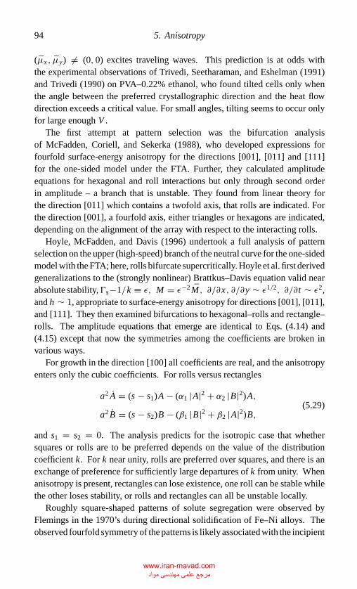
P1: GKE
Chap-05 CB381-Davis May 17, 2001 17:3 Char Count= 0
94 5. Anisotropy
(µx , µy) �= (0, 0) excites traveling waves. This prediction is at odds withthe experimental observations of Trivedi, Seetharaman, and Eshelman (1991)and Trivedi (1990) on PVA–0.22% ethanol, who found tilted cells only whenthe angle between the preferred crystallographic direction and the heat flowdirection exceeds a critical value. For small angles, tilting seems to occur onlyfor large enough V .
The first attempt at pattern selection was the bifurcation analysisof McFadden, Coriell, and Sekerka (1988), who developed expressions forfourfold surface-energy anisotropy for the directions [001], [011] and [111]for the one-sided model under the FTA. Further, they calculated amplitudeequations for hexagonal and roll interactions but only through second orderin amplitude – a branch that is unstable. They found from linear theory forthe direction [011] which contains a twofold axis, that rolls are indicated. Forthe direction [001], a fourfold axis, either triangles or hexagons are indicated,depending on the alignment of the array with respect to the interacting rolls.
Hoyle, McFadden, and Davis (1996) undertook a full analysis of patternselection on the upper (high-speed) branch of the neutral curve for the one-sidedmodel with the FTA; here, rolls bifurcate supercritically. Hoyle et al. first derivedgeneralizations to the (strongly nonlinear) Brattkus–Davis equation valid nearabsolute stability,�s−1/k ≡ ε, M = ε−2M, ∂/∂x, ∂/∂y ∼ ε1/2, ∂/∂t ∼ ε2,and h ∼ 1, appropriate to surface-energy anisotropy for directions [001], [011],and [111]. They then examined bifurcations to hexagonal–rolls and rectangle–rolls. The amplitude equations that emerge are identical to Eqs. (4.14) and(4.15) except that now the symmetries among the coefficients are broken invarious ways.
For growth in the direction [100] all coefficients are real, and the anisotropyenters only the cubic coefficients. For rolls versus rectangles
a2 A = (s − s1)A − (α1 |A|2 + α2 |B|2)A,
a2 B = (s − s2)B − (β1 |B|2 + β2 |A|2)B,(5.29)
and s1 = s2 = 0. The analysis predicts for the isotropic case that whethersquares or rolls are to be preferred depends on the value of the distributioncoefficient k. For k near unity, rolls are preferred over squares, and there is anexchange of preference for sufficiently large departures of k from unity. Whenanisotropy is present, rectangles can lose existence, one roll can be stable whilethe other loses stability, or rolls and rectangles can all be unstable locally.
Roughly square-shaped patterns of solute segregation were observed byFlemings in the 1970’s during directional solidification of Fe–Ni alloys. Theobserved fourfold symmetry of the patterns is likely associated with the incipient
www.iran-mavad.com مرجع علمی مھندسی مواد
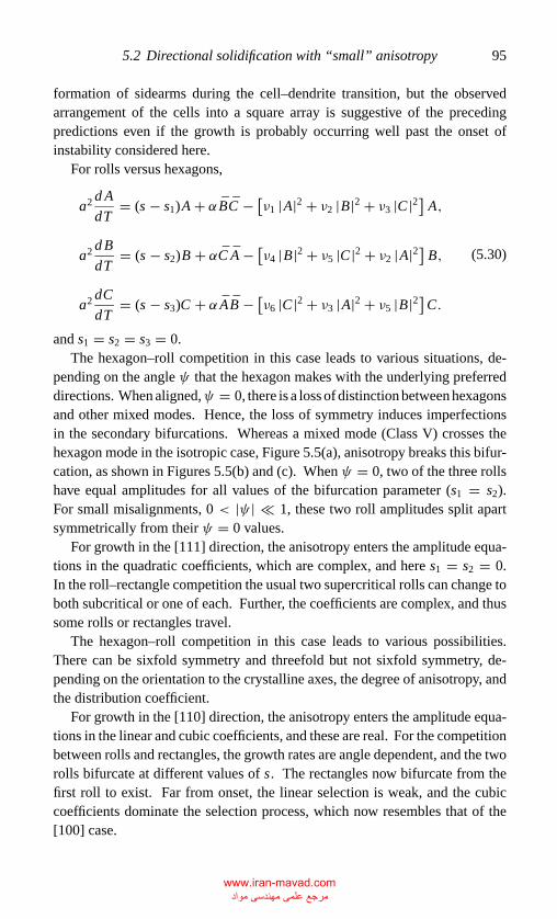
P1: GKE
Chap-05 CB381-Davis May 17, 2001 17:3 Char Count= 0
5.2 Directional solidification with “small” anisotropy 95
formation of sidearms during the cell–dendrite transition, but the observedarrangement of the cells into a square array is suggestive of the precedingpredictions even if the growth is probably occurring well past the onset ofinstability considered here.
For rolls versus hexagons,
a2 d A
dT= (s − s1)A + α BC − [ν1 |A|2 + ν2 |B|2 + ν3 |C |2] A,
a2 d B
dT= (s − s2)B + αC A − [ν4 |B|2 + ν5 |C |2 + ν2 |A|2] B,
a2 dC
dT= (s − s3)C + α A B − [ν6 |C |2 + ν3 |A|2 + ν5 |B|2]C.
(5.30)
and s1 = s2 = s3 = 0.The hexagon–roll competition in this case leads to various situations, de-
pending on the angle ψ that the hexagon makes with the underlying preferreddirections. When aligned,ψ = 0, there is a loss of distinction between hexagonsand other mixed modes. Hence, the loss of symmetry induces imperfectionsin the secondary bifurcations. Whereas a mixed mode (Class V) crosses thehexagon mode in the isotropic case, Figure 5.5(a), anisotropy breaks this bifur-cation, as shown in Figures 5.5(b) and (c). When ψ = 0, two of the three rollshave equal amplitudes for all values of the bifurcation parameter (s1 = s2).For small misalignments, 0 < |ψ | 1, these two roll amplitudes split apartsymmetrically from their ψ = 0 values.
For growth in the [111] direction, the anisotropy enters the amplitude equa-tions in the quadratic coefficients, which are complex, and here s1 = s2 = 0.In the roll–rectangle competition the usual two supercritical rolls can change toboth subcritical or one of each. Further, the coefficients are complex, and thussome rolls or rectangles travel.
The hexagon–roll competition in this case leads to various possibilities.There can be sixfold symmetry and threefold but not sixfold symmetry, de-pending on the orientation to the crystalline axes, the degree of anisotropy, andthe distribution coefficient.
For growth in the [110] direction, the anisotropy enters the amplitude equa-tions in the linear and cubic coefficients, and these are real. For the competitionbetween rolls and rectangles, the growth rates are angle dependent, and the tworolls bifurcate at different values of s. The rectangles now bifurcate from thefirst roll to exist. Far from onset, the linear selection is weak, and the cubiccoefficients dominate the selection process, which now resembles that of the[100] case.
www.iran-mavad.com مرجع علمی مھندسی مواد
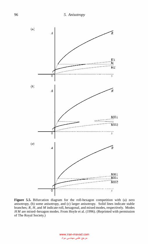
P1: GKE
Chap-05 CB381-Davis May 17, 2001 17:3 Char Count= 0
96 5. Anisotropy
Figure 5.5. Bifurcation diagram for the roll-hexagon competition with (a) zeroanisotropy, (b) some anisotropy, and (c) larger anisotropy. Solid lines indicate stablebranches; R, H , and M indicate roll, hexagonal, and mixed modes, respectively. ModesH M are mixed–hexagon modes. From Hoyle et al. (1996). (Reprinted with permissionof The Royal Society.)
www.iran-mavad.com مرجع علمی مھندسی مواد
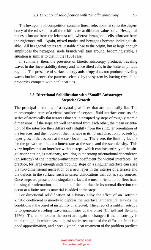
P1: GKE
Chap-05 CB381-Davis May 17, 2001 17:3 Char Count= 0
5.3 Directional solidification with “small” anisotropy 97
The hexagon–roll competition contains linear selection that splits the degen-eracy of the rolls so that all three bifurcate at different values of s. Hexagonalnodes bifurcate from the leftmost roll, whereas hexagonal cells bifurcate fromthe rightmost roll. Again, mixed modes and hexagons become indistinguish-able. All hexagonal states are unstable close to the origin, but at large enoughamplitudes the hexagonal node branch will turn around, becoming stable, asituation is similar to that in the [100] case.
In summary, then, the presence of kinetic anisotropy produces travelingwaves in the linear stability theory and hence tilted cells in the finite amplituderegime. The presence of surface-energy anisotropy does not produce travelingwaves but influences the patterns selected by the system by having crystallineproperties compete with nonlinearities.
5.3 Directional Solidification with “Small” Anisotropy:Stepwise Growth
The principal directions of a crystal give faces that are atomically flat. Themicroscopic picture of a vicinal surface of a crystal–fluid interface consists of aseries of atomically flat terraces that are interrupted by steps of roughly atomicdimensions. If the steps are well separated from each other, the mean orienta-tion of the interface then differs only slightly from the singular orientation ofthe terraces, and the motion of the interface in its normal direction proceeds bylayer growth that occurs at the step locations. Therefore, the limiting factorsfor the growth are the attachment rate at the steps and the step density. Thisview implies that an interface without steps, which consists entirely of the sin-gular orientation, is stationary, resulting in the strong orientational dependence(anisotropy) of the interface–attachment coefficient for vicinal interfaces. Inpractice, for large enough undercooling, steps on a singular interface can arisevia two-dimensional nucleation of a new layer in the interior of a terrace andvia defects in the surface, such as screw dislocations that act as step sources.Once steps are present on a singular surface, the mean orientation differs fromthe singular orientation, and motion of the interface in its normal direction canoccur at a finite rate as material is added at the steps.
For directional solidification of a binary alloy the effect of an isotropickinetic coefficient is merely to depress the interface temperature, leaving theconditions at the onset of instability unaffected. The effect of a mild anisotropyis to generate traveling-wave instabilities at the onset (Coriell and Sekerka1976). The conditions at the onset are again unchanged if the anisotropy ismild enough, in which case a quasi-static treatment of the diffusion field is agood approximation, and a weakly nonlinear treatment of the problem predicts
www.iran-mavad.com مرجع علمی مھندسی مواد
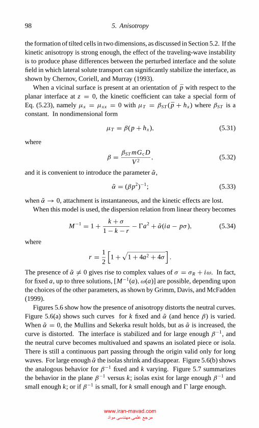
P1: GKE
Chap-05 CB381-Davis May 17, 2001 17:3 Char Count= 0
98 5. Anisotropy
the formation of tilted cells in two dimensions, as discussed in Section 5.2. If thekinetic anisotropy is strong enough, the effect of the traveling-wave instabilityis to produce phase differences between the perturbed interface and the solutefield in which lateral solute transport can significantly stabilize the interface, asshown by Chernov, Coriell, and Murray (1993).
When a vicinal surface is present at an orientation of p with respect to theplanar interface at z = 0, the kinetic coefficient can take a special form ofEq. (5.23), namely µx = µxx = 0 with µT = βST ( p + hx ) where βST is aconstant. In nondimensional form
µT = β(p + hx ), (5.31)
where
β = βST mGc D
V 2, (5.32)
and it is convenient to introduce the parameter α,
α = (βp2)−1; (5.33)
when α → 0, attachment is instantaneous, and the kinetic effects are lost.When this model is used, the dispersion relation from linear theory becomes
M−1 = 1 + k + σ1 − k − r
− �a2 + α(ia − pσ ), (5.34)
where
r = 1
2
[1 +√
1 + 4a2 + 4σ].
The presence of α �= 0 gives rise to complex values of σ = σR + iω. In fact,for fixed a, up to three solutions, [M−1(a), ω(a)] are possible, depending uponthe choices of the other parameters, as shown by Grimm, Davis, and McFadden(1999).
Figures 5.6 show how the presence of anisotropy distorts the neutral curves.Figure 5.6(a) shows such curves for k fixed and α (and hence β) is varied.When α = 0, the Mullins and Sekerka result holds, but as α is increased, thecurve is distorted. The interface is stabilized and for large enough β−1, andthe neutral curve becomes multivalued and spawns an isolated piece or isola.There is still a continuous part passing through the origin valid only for longwaves. For large enough α the isolas shrink and disappear. Figure 5.6(b) showsthe analogous behavior for β−1 fixed and k varying. Figure 5.7 summarizesthe behavior in the plane β−1 versus k; isolas exist for large enough β−1 andsmall enough k; or if β−1 is small, for k small enough and � large enough.
www.iran-mavad.com مرجع علمی مھندسی مواد
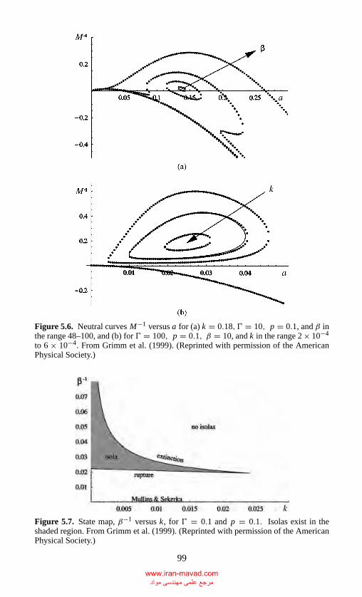
P1: GKE
Chap-05 CB381-Davis May 17, 2001 17:3 Char Count= 0
Figure 5.6. Neutral curves M−1 versus a for (a) k = 0.18, � = 10, p = 0.1, and β inthe range 48–100, and (b) for � = 100, p = 0.1, β = 10, and k in the range 2 × 10⁻⁴
to 6 × 10⁻⁴. From Grimm et al. (1999). (Reprinted with permission of the AmericanPhysical Society.)
Figure 5.7. State map, β−1 versus k, for � = 0.1 and p = 0.1. Isolas exist in theshaded region. From Grimm et al. (1999). (Reprinted with permission of the AmericanPhysical Society.)
99
www.iran-mavad.com مرجع علمی مھندسی مواد
P1: GKE
Chap-05 CB381-Davis May 17, 2001 17:3 Char Count= 0
100 5. Anisotropy
Necessary conditions for the prediction of isolas are small k and large �.As long as α is taken to be small, it is the term −�a2 that dominates theneutral curve for large a. If k is even smaller (and � is no longer large),the stabilization at large wave numbers can be dominated by anisotropy. Or,expressed in physical terms, anisotropy plays a role analogous to that of surfaceenergy, and its influence is strongly stabilizing. However, it is not possible toreplace completely the effect of capillarity by anisotropy; if � = 0, large wavenumbers are not stabilized.
It is worthwhile noting that in some cases linear theory predicts a “stabilitywindow,” meaning that the domain of M−1 for which there is linear stability forall wave numbers is not necessarily the semi-infinite interval as was true in theisotropic case, but can now be composed of a semi-infinite interval and a finiteinterval (the “window”). This can be easily understood by following verticallines in Figure 5.6(a). Note that the physically relevant part of the continuousbranch of the neutral stability curve is not clearly visible in this figure.
In Section 5.2, the Sivashinsky limit, k → 0, � ∼ 1, |M − 1| → 0, wasextended by allowing the anisotropy to be O(ε1/2). It was found that the onsetof instability is unchanged, but now traveling waves that bifurcate subcriticallyare predicted.
Grimm et al. (1999) have found a new limit with α = O(1). As before, theylet M−1 = 1 −µε, k = κε2, κ = O(1), � = O(1), ∂/∂x = O(ε1/2), but nowbecause α is of unit order, they took ∂/∂t = ε3/2 (rather than ε2). They wroteh ∼ h0 + ε1/2h1 and found that
h0t + αh0xxx − 1
2
(h2
0
)xx = 0. (5.35a)
This is an equation for nondissipative dispersive waves that exhibit no instability.At the next order they found that
h1t + αh1xxx − (h0h1)xx = − h0T − κh0 − µh0xx − �h0xxxx +αh0xt − α(h20x
)x .
(5.35b)
One can recompose Eqs. (5.35) for h ∼ h0 + ε1/2h1 and find that
ht + αhxxx − 1
2(h2)xx + ε {κh + �hxxxx + µhxx − αhxt +α (h2
x
)x
} = O(ε2).
(5.36)To analyze Eq. (5.36), write ∂/∂t = ∂/∂t0 + ε1/2∂/∂t2 +ε∂/∂t4 +· · · , µ =
µc + ε1/2µ2 + · · · and h = ε1/4v1 + ε1/2v2 + · · · . From linear theory,
a2c =√
κ
� + α2, ωc = αa3
c , µc = 2√κ(� + α2
)with phase speed c = ω/ac.
www.iran-mavad.com مرجع علمی مھندسی مواد
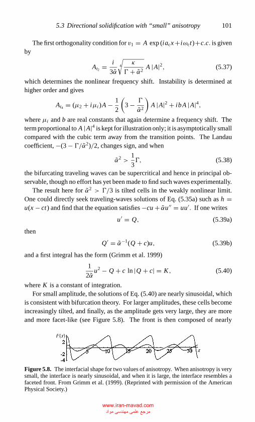
P1: GKE
Chap-05 CB381-Davis May 17, 2001 17:3 Char Count= 0
5.3 Directional solidification with “small” anisotropy 101
The first orthogonality condition for v1 = A exp (iacx +iωct)+c.c. is givenby
At2 = i
3α4
√κ
� + α2A |A|2, (5.37)
which determines the nonlinear frequency shift. Instability is determined athigher order and gives
At4 = (µ2 + iµi )A − 1
2
(3 − �
α2
)A |A|2 + ibA |A|4,
where µi and b are real constants that again determine a frequency shift. Theterm proportional to A |A|4 is kept for illustration only; it is asymptotically smallcompared with the cubic term away from the transition points. The Landaucoefficient, −(3 − �/α2)/2, changes sign, and when
α2 >1
3�, (5.38)
the bifurcating traveling waves can be supercritical and hence in principal ob-servable, though no effort has yet been made to find such waves experimentally.
The result here for α2 > �/3 is tilted cells in the weakly nonlinear limit.One could directly seek traveling-waves solutions of Eq. (5.35a) such as h =u(x − ct) and find that the equation satisfies −cu + αu′′ = uu′. If one writes
u′ = Q, (5.39a)
then
Q′ = α−1(Q + c)u, (5.39b)
and a first integral has the form (Grimm et al. 1999)
1
2αu2 − Q + c ln |Q + c| = K , (5.40)
where K is a constant of integration.For small amplitude, the solutions of Eq. (5.40) are nearly sinusoidal, which
is consistent with bifurcation theory. For larger amplitudes, these cells becomeincreasingly tilted, and finally, as the amplitude gets very large, they are moreand more facet-like (see Figure 5.8). The front is then composed of nearly
Figure 5.8. The interfacial shape for two values of anisotropy. When anisotropy is verysmall, the interface is nearly sinusoidal, and when it is large, the interface resembles afaceted front. From Grimm et al. (1999). (Reprinted with permission of the AmericanPhysical Society.)
www.iran-mavad.com مرجع علمی مھندسی مواد
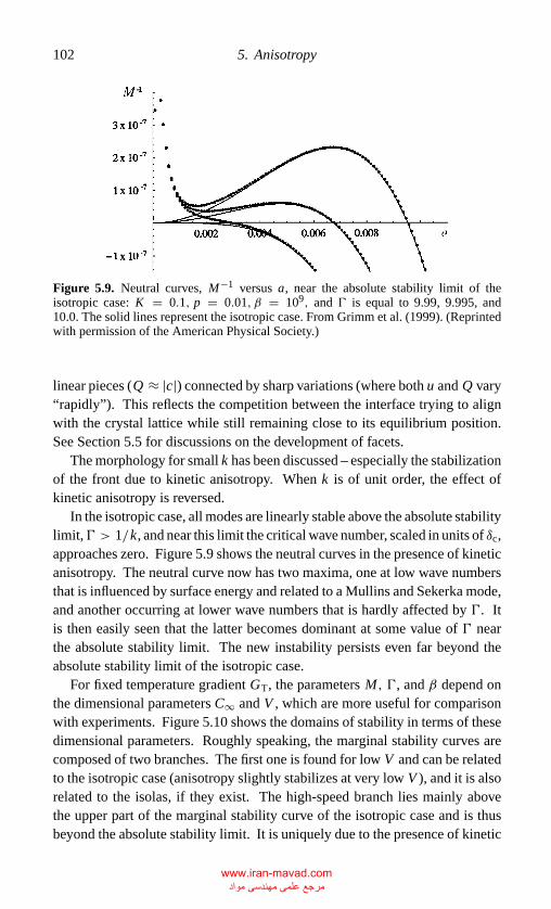
P1: GKE
Chap-05 CB381-Davis May 17, 2001 17:3 Char Count= 0
102 5. Anisotropy
Figure 5.9. Neutral curves, M−1 versus a, near the absolute stability limit of theisotropic case: K = 0.1, p = 0.01, β = 109, and � is equal to 9.99, 9.995, and10.0. The solid lines represent the isotropic case. From Grimm et al. (1999). (Reprintedwith permission of the American Physical Society.)
linear pieces (Q ≈ |c|) connected by sharp variations (where both u and Q vary“rapidly”). This reflects the competition between the interface trying to alignwith the crystal lattice while still remaining close to its equilibrium position.See Section 5.5 for discussions on the development of facets.
The morphology for small k has been discussed – especially the stabilizationof the front due to kinetic anisotropy. When k is of unit order, the effect ofkinetic anisotropy is reversed.
In the isotropic case, all modes are linearly stable above the absolute stabilitylimit,� > 1/k, and near this limit the critical wave number, scaled in units of δc,approaches zero. Figure 5.9 shows the neutral curves in the presence of kineticanisotropy. The neutral curve now has two maxima, one at low wave numbersthat is influenced by surface energy and related to a Mullins and Sekerka mode,and another occurring at lower wave numbers that is hardly affected by �. Itis then easily seen that the latter becomes dominant at some value of � nearthe absolute stability limit. The new instability persists even far beyond theabsolute stability limit of the isotropic case.
For fixed temperature gradient GT, the parameters M, �, and β depend onthe dimensional parameters C∞ and V , which are more useful for comparisonwith experiments. Figure 5.10 shows the domains of stability in terms of thesedimensional parameters. Roughly speaking, the marginal stability curves arecomposed of two branches. The first one is found for low V and can be relatedto the isotropic case (anisotropy slightly stabilizes at very low V ), and it is alsorelated to the isolas, if they exist. The high-speed branch lies mainly abovethe upper part of the marginal stability curve of the isotropic case and is thusbeyond the absolute stability limit. It is uniquely due to the presence of kinetic
www.iran-mavad.com مرجع علمی مھندسی مواد
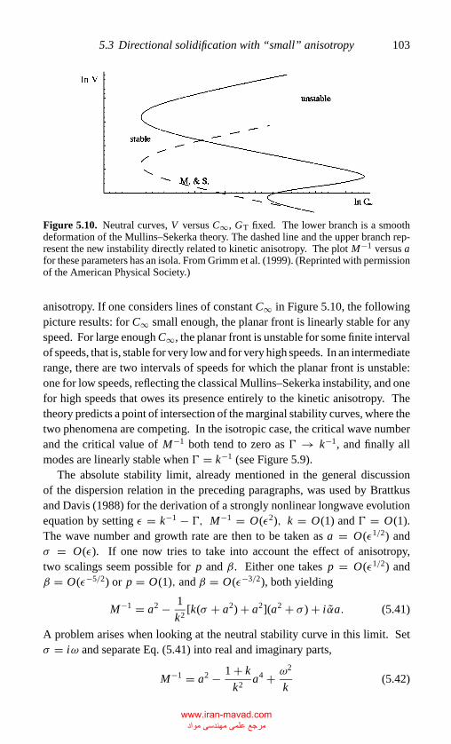
P1: GKE
Chap-05 CB381-Davis May 17, 2001 17:3 Char Count= 0
5.3 Directional solidification with “small” anisotropy 103
Figure 5.10. Neutral curves, V versus C∞, GT fixed. The lower branch is a smoothdeformation of the Mullins–Sekerka theory. The dashed line and the upper branch rep-resent the new instability directly related to kinetic anisotropy. The plot M−1 versus afor these parameters has an isola. From Grimm et al. (1999). (Reprinted with permissionof the American Physical Society.)
anisotropy. If one considers lines of constant C∞ in Figure 5.10, the followingpicture results: for C∞ small enough, the planar front is linearly stable for anyspeed. For large enough C∞, the planar front is unstable for some finite intervalof speeds, that is, stable for very low and for very high speeds. In an intermediaterange, there are two intervals of speeds for which the planar front is unstable:one for low speeds, reflecting the classical Mullins–Sekerka instability, and onefor high speeds that owes its presence entirely to the kinetic anisotropy. Thetheory predicts a point of intersection of the marginal stability curves, where thetwo phenomena are competing. In the isotropic case, the critical wave numberand the critical value of M−1 both tend to zero as � → k−1, and finally allmodes are linearly stable when � = k−1 (see Figure 5.9).
The absolute stability limit, already mentioned in the general discussionof the dispersion relation in the preceding paragraphs, was used by Brattkusand Davis (1988) for the derivation of a strongly nonlinear longwave evolutionequation by setting ε = k−1 − �, M−1 = O(ε2), k = O(1) and � = O(1).The wave number and growth rate are then to be taken as a = O(ε1/2) andσ = O(ε). If one now tries to take into account the effect of anisotropy,two scalings seem possible for p and β. Either one takes p = O(ε1/2) andβ = O(ε−5/2) or p = O(1), and β = O(ε−3/2), both yielding
M−1 = a2 − 1
k2[k(σ + a2) + a2](a2 + σ ) + i αa. (5.41)
A problem arises when looking at the neutral stability curve in this limit. Setσ = iω and separate Eq. (5.41) into real and imaginary parts,
M−1 = a2 − 1 + k
k2a4 + ω2
k(5.42)
www.iran-mavad.com مرجع علمی مھندسی مواد
P1: GKE
Chap-05 CB381-Davis May 17, 2001 17:3 Char Count= 0
104 5. Anisotropy
and
ω = αk2
1 + 2ka−1.
One sees that the scaling is inappropriate for a → 0 because ω ∝ a−1.
There is a new limit in the neighborhood of the second maximum of the neu-tral curve that can be defined and describes unstable fronts beyond the absolutestability limit, that is, for � > 1/k. Let M−1 = O(ε2), p = O(ε), µT =O(ε−4), a = O(ε) andω = O(ε). On the neutral curve at order ε2 one obtains
M−1 = (k−1 − �)a2 + ω2
k, (5.43a)
with ω given by
ω3 + a2ω − αk2
1 + 2ka = 0. (5.43b)
The resulting curve ω = ω(a) then grows as a1/3 at the origin, and, after havingreached a maximum, decays like a−1. The neutral stability curve in terms ofM−1 therefore has a vertical tangent at the origin, which is rather unusual. Thisis corrected by terms of the following order that introduce a singular perturbationnear the origin. A more important observation is that one must have � ≥ k−1
for this limit to apply (although an accurate description of the neutral stabilitycurve near the origin when � < k−1 may be obtained).
For h ∼ h0 + εh1, and c ∼ c + εc1, and ∂/∂t → ε∂/∂t + ε2∂/∂T , Grimmet al. (1999) found that
h0(t, T, x) = A(T, x)eiω0t + A(T, x)e−iω0t (5.44)
and
h1t t + kM−1h1 + Lh0 + N (h0) − αh1x
1 + h1x/p= 0, (5.45)
where
ω0 =√
kM−1
Lh = 2hT t + (1 + 2k)M−1ht − 1 + 2k
khtxx + khxx
N (h) = hthxx + 3kM−1hht − 2hxhtx .
(5.46)
The amplitude A of Eq. (5.44) is determined by an orthogonality conditionon Eq. (5.45). The result is
2ω0 AT + 1 + 2k
kω3
0 A − 1 + 2k
kω0 Axx + ikαAx R(|Ax |) = 0, (5.47)
www.iran-mavad.com مرجع علمی مھندسی مواد
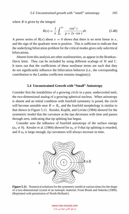
P1: GKE
Chap-05 CB381-Davis May 17, 2001 17:3 Char Count= 0
5.4 Unconstrained growth with “small” anisotropy 105
where R is given by the integral
R(x) = 1
π
∫ 2π
0
cos2 t
p + 2x cos tdt. (5.48)
A power series of R(x) about x = 0 shows that there is no term linear in x ,and the sign of the quadratic term is positive. This is sufficient to indicate thatthe underlying bifurcation problem for the critical modes gives only subcriticalbifurcations.
Absent from this analysis are other nonlinearities, as appear in the Brattkus–Davis limit. They can be included by using different scalings of H and C.It turns out that the coefficients of these nonlinear terms are such that theydo not significantly influence the bifurcation behavior (i.e., the correspondingcontribution to the Landau coefficient remains imaginary).
5.4 Unconstrained Growth with “Small” Anisotropy
Consider first the instabilities of a growing circle in a pure, undercooled melt,the two-dimensional analog of a growing spherical nucleus. When anisotropyis absent and an initial condition with fourfold symmetry is posed, the circlewill become unstable near R = Rc, and the fourfold morphology is similar tothat shown in Figure 5.11. Kessler, Koplik, and Levine (1984) showed for thesymmetric model that the curvature at the tips decreases with time and passesthrough zero, indicating that tip splitting has begun.
Consider now the influence of fourfold anisotropy of the surface energy(α4 �= 0). Kessler et al. (1984) showed for α4 �= 0 that tip splitting is retarded,and if α4 is large enough, tip curvatures will always increase in time.
Figure 5.11. Numerical solutions for the symmetric model at various times for the shapeof a two-dimensional crystal of an isotropic material. From Brush and Sekerka (1989).(Reprinted with permission of North-Holland.)
www.iran-mavad.com مرجع علمی مھندسی مواد
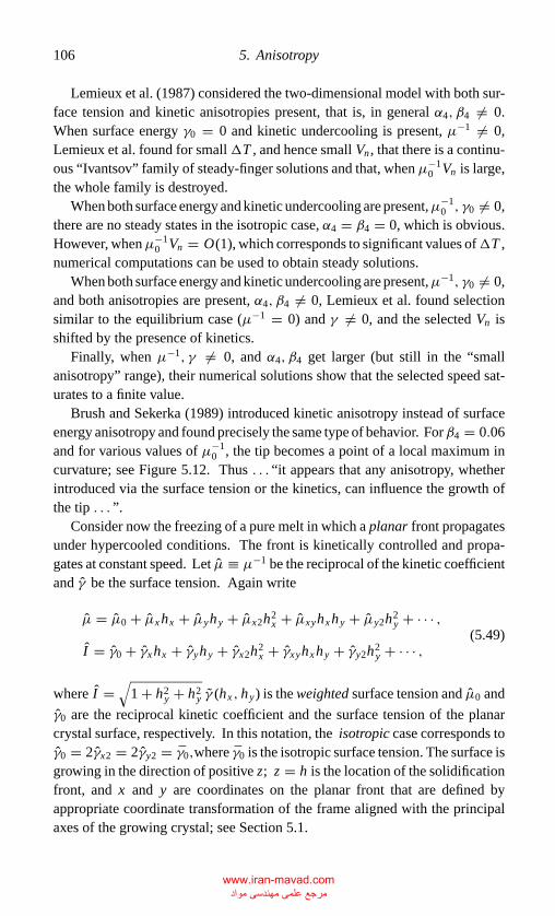
P1: GKE
Chap-05 CB381-Davis May 17, 2001 17:3 Char Count= 0
106 5. Anisotropy
Lemieux et al. (1987) considered the two-dimensional model with both sur-face tension and kinetic anisotropies present, that is, in general α4, β4 �= 0.When surface energy γ0 = 0 and kinetic undercooling is present, µ−1 �= 0,Lemieux et al. found for small�T , and hence small Vn , that there is a continu-ous “Ivantsov” family of steady-finger solutions and that, when µ−1
0 Vn is large,the whole family is destroyed.
When both surface energy and kinetic undercooling are present,µ−10 , γ0 �= 0,
there are no steady states in the isotropic case, α4 = β4 = 0, which is obvious.However, whenµ−1
0 Vn = O(1), which corresponds to significant values of�T ,numerical computations can be used to obtain steady solutions.
When both surface energy and kinetic undercooling are present,µ−1, γ0 �= 0,and both anisotropies are present, α4, β4 �= 0, Lemieux et al. found selectionsimilar to the equilibrium case (µ−1 = 0) and γ �= 0, and the selected Vn isshifted by the presence of kinetics.
Finally, when µ−1, γ �= 0, and α4, β4 get larger (but still in the “smallanisotropy” range), their numerical solutions show that the selected speed sat-urates to a finite value.
Brush and Sekerka (1989) introduced kinetic anisotropy instead of surfaceenergy anisotropy and found precisely the same type of behavior. Forβ4 = 0.06and for various values of µ−1
0 , the tip becomes a point of a local maximum incurvature; see Figure 5.12. Thus . . . “it appears that any anisotropy, whetherintroduced via the surface tension or the kinetics, can influence the growth ofthe tip . . . ”.
Consider now the freezing of a pure melt in which a planar front propagatesunder hypercooled conditions. The front is kinetically controlled and propa-gates at constant speed. Let µ ≡ µ−1 be the reciprocal of the kinetic coefficientand γ be the surface tension. Again write
µ = µ0 + µxhx + µyhy + µx2h2x + µxyhxhy + µy2h2
y + · · · ,
I = γ0 + γxhx + γyhy + γx2h2x + γxyhxhy + γy2h2
y + · · · ,(5.49)
where I =√
1 + h2y + h2
y γ (hx , hy) is the weighted surface tension and µ0 and
γ0 are the reciprocal kinetic coefficient and the surface tension of the planarcrystal surface, respectively. In this notation, the isotropic case corresponds toγ0 = 2γx2 = 2γy2 = γ0,where γ0 is the isotropic surface tension. The surface isgrowing in the direction of positive z; z = h is the location of the solidificationfront, and x and y are coordinates on the planar front that are defined byappropriate coordinate transformation of the frame aligned with the principalaxes of the growing crystal; see Section 5.1.
www.iran-mavad.com مرجع علمی مھندسی مواد
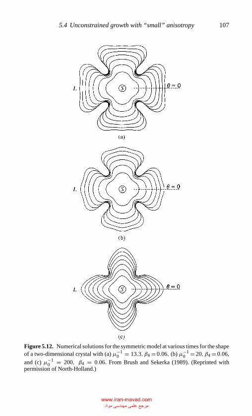
P1: GKE
Chap-05 CB381-Davis May 17, 2001 17:3 Char Count= 0
5.4 Unconstrained growth with “small” anisotropy 107
Figure 5.12. Numerical solutions for the symmetric model at various times for the shapeof a two-dimensional crystal with (a) µ−1
0 = 13.3, β4 = 0.06, (b) µ−10 = 20, β4 = 0.06,
and (c) µ−10 = 200, β4 = 0.06. From Brush and Sekerka (1989). (Reprinted with
permission of North-Holland.)
www.iran-mavad.com مرجع علمی مھندسی مواد
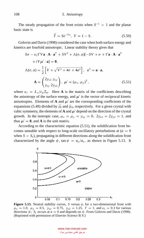
P1: GKE
Chap-05 CB381-Davis May 17, 2001 17:3 Char Count= 0
108 5. Anisotropy
The steady propagation of the front exists when S−1 > 1 and the planarbasic state is
T = Se−V z, V = 1 − S. (5.50)
Golovin and Davis (1998) considered the case when both surface energy andkinetics are fourfold anisotropic. Linear stability theory gives that
Sσ − κ1�V a · A · aT + SV 2 +�(σ, a)[−SV + σ + �a · A · aT
+ iVµ′ · a] = 0,
�(σ, a) = 1
2
[V +√
V 2 + 4σ + 4a2], a2 = a · a,
A =(
2γx2 γxy
γxy 2γy2
), µ′ = (µx , µy)T , (5.51)
where κ1 = Lv/cpTm . Here A is the matrix of the coefficients describingthe anisotropy of the surface energy, and µ′ is the vector of reciprocal kineticanisotropies. Elements of A and µ′ are the corresponding coefficients of theexpansions (5.49) divided by γ0 and µ0, respectively. For a given crystal withcubic symmetry, the elements of A and µ′ depend on the direction of the crystalgrowth. In the isotropic case, µx = µy = γxy = 0, 2γx2 = 2γy2 = 1, andthus µ′ = 0, and A is the unit matrix.
According to the characteristic equation (5.51), the solidification front be-comes unstable with respect to long-scale oscillatory perturbations at (a = 0when S > Sc), propagating in different directions along the solidification frontcharacterized by the angle ψ , tanψ = ay/ax , as shown in Figure 5.13. It
Figure 5.13. Neutral stability curves, S versus a, for a two-dimensional front withµx = 1.0, µy = 0.5, γxy = 0.75, γy2 = 1.25, � = 1, and κ1 = 0.3 for variousdirections ψ ; Sc occurs at a = 0 and depends on ψ . From Golovin and Davis (1998).(Reprinted with permission of Elsevier Science B.V.)
www.iran-mavad.com مرجع علمی مھندسی مواد
P1: GKE
Chap-05 CB381-Davis May 17, 2001 17:3 Char Count= 0
5.4 Unconstrained growth with “small” anisotropy 109
can be seen that the critical Stefan number Sc depends on the direction of thedisturbance wave vector, namely,
Sc = α(ψ)�(1 − κ1)
1 + α(ψ)�(1 − κ1) + m2(ψ),
α(ψ) = 2γx2 cos2 ψ + γxy sin 2ψ + 2γy2 sin2 ψ,
m(ψ) = µx cos ψ + µy sin ψ. (5.52)
The (constant) front speed corresponding to the onset of the instability isVc = 1 − Sc. In the general case, when both surface tension and kineticsanisotropies are present, this instability gives rise to the propagation of longwaves along the solidification front with the following phase velocity, vp, andthe group velocity vg:
vp = ωa/a2 = Vc(ψ)(µ′ · a)a/a2,
vg = Vc(ψ)µ′.(5.53)
These long waves manifest themselves as periodic cells traveling along the so-lidification front. Thus, the existence of traveling cells depends on the presenceof kinetic anisotropy. If there is no kinetic anisotropy, µ′ = 0, the instability isthen monotonic, leading to stationary, spatially periodic structures: stationarycells.
In general, with the increase of S, the traveling cells that first start to growtravel in the directions given by an angleψ0 that is determined by the coefficientsof surface tension and kinetic anisotropies and that satisfies the equation
[1 + m2(ψ0)]α′(ψ0) = 2α(ψ0)m(ψ0)m ′(ψ0) (5.54)
together with the following inequality:
[(α′′(1 + m2) − 2α(m ′)2 + mm ′′)][1 + α�(1 − κ1) + m2]
− 2[α′(1 + m2) − 2αmm ′][α′�(1 − κ1) + 2mm ′] > 0.(5.55)
Here m(ψ) and α(ψ) are defined in Eq. (5.52), and the prime denotes dif-ferentiation with respect to ψ . The angle ψ0 gives the minimum value ofSc = Sc(ψ0) = S0, V0 = 1 − S0. In a particular case, when only a kineticanisotropy is present, the preferred direction of the traveling-cell propagationis given by an angle ψk
0
tan 2ψk0 = µy
µx. (5.56)
www.iran-mavad.com مرجع علمی مھندسی مواد
P1: GKE
Chap-05 CB381-Davis May 17, 2001 17:3 Char Count= 0
110 5. Anisotropy
In the case when only surface tension anisotropy is present, the stationary roll-like periodic structure forms in the preferred direction given by an angle ψ s
0
such that
tan 2ψ s0 = γxy
γx2 − γy2. (5.57)
In the general case there also exists a specific direction characterized by an angleψn
0 at which the group velocity of the waves is normal to their wave vector (inthe frame moving with the planar front with the velocity Vc(ψn
0 )), and the phasevelocity is zero:
tan ψn0 = −µx
µy, (5.58)
and thusψn0 = π/2+ψk
0 . When the surface tension and the kinetic anisotropiessatisfy the relation
γxy(µ2y − µ2
x ) + 2µxµy(γx2 − γy2) = 0, (5.59)
ψn0 can give a minimum of Sc, and the instability first occurs in the direction
determined byψn0 , so that the wave, whose group velocity is normal to its wave
vector, is first to appear. Notice that if either anisotropy, kinetic or capillary, iszero, then relation (5.59) is an identity. If only the kinetic anisotropy is present,the angle ψn
0 always corresponds to a maximum of the dependence Sc(ψ).Typically, variations of the instability threshold Sc depend on the direction
of cell propagation at the front (on the angle ψ), given by Eq. (5.52).Owing to the presence of anisotropy, the instability threshold S0 = Sc(ψ0)
given by relation (5.59), at which the traveling (or stationary) cells first appearin the preferred direction on the propagating solidification front, depends inturn on the direction of the propagation of the front compared with the princi-pal directions. This dependence is illustrated in two cases below for crystalswith cubic symmetry: when a crystal grows in a Hele–Shaw cell, so that thesolidification front is effectively one-dimensional, and in a three-dimensionalcase with a two-dimensional front.
5.4.1 Two-Dimensional Crystal and One-Dimensional Front
It is natural to consider the dimensional surface tension and the dimensionalkinetic coefficient to be dependent on the direction of a crystal growth in thefollowing form:
γ0 = γ0(1 + α4 cos 4φ), µ0 = µ0(1 + β4 cos 4φ), (5.60)
www.iran-mavad.com مرجع علمی مھندسی مواد
P1: GKE
Chap-05 CB381-Davis May 17, 2001 17:3 Char Count= 0
5.4 Unconstrained growth with “small” anisotropy 111
where now φ is an angle between the [10] direction and the direction of thecrystal growth; γ0 and µ0 are the mean surface tension and the reciprocal ofmean kinetic coefficients, respectively. Consider a local perturbation of thefront with the normal vector at the angle φ + δφ with respect to the [10]direction, so that cos δφ = (1 + hx )−1/2, sin δφ = −hx (1 + h2
x )−1/2. If oneuses Eq. (5.59) and expands E(h) and µ(h) for small |hx |, one gets γx2 and µx
for the dimensionless parameters (only parameters with x indices are relevantin two-dimensional case)
γx2 = 1
2(1 − 15α4 cos 4φ), µx = 4β4 sin 4φ
1 + β4 cos 4φ. (5.61)
If one sets ψ = 0 in Eq. (5.52) for two-dimensional case, and substitutesEqs. (5.60) and (5.61) into Eq. (5.52), the instability threshold is obtained asa function of the growth direction φ and of the coefficients of surface-tensionand kinetic anisotropies, α4 and β4.
The variation of Sc(φ) at different anisotropies of the surface tensionand of the kinetic coefficient has extrema at φ = nπ/4 designating thecrystallographic directions [10], [01], and [11]; in these directions µx = 0,and morphological instability is monotonic, leading to formation of stationarycells; there are no traveling cells when a crystal grows in one of the principalcrystallographic directions.
If different crystals grow in the direction [10] or [11], their kinetic anisotropycoefficientsµx are equal to zero, and the instability is monotonic, leading to theformation of stationary cells. However, the instability threshold correspondingto different crystals still depends on the coefficients of the kinetic anisotropyβ4 because the parameter � depends on the anisotropic kinetic coefficient µ0.
Owing to this dependence, when crystals grow in the [10] direction, the criticalStefan number will be maximal for a crystal with minimal negative kinetic andsurface-tension anisotropy coefficients β4 and α4, and when various crystalsgrow in the [11] direction, the critical Stefan number will be maximal for crystalswith maximal positive values of the kinetic and surface-tension anisotropycoefficients. The critical Stefan number can be maximal for a crystal that hassome intermediate value of β4, and this value does not depend on α4.
5.4.2 Three-Dimensional Crystal and Two-Dimensional Front
The anisotropies of the surface tension and of the kinetic coefficient are de-scribed by Eqs. (5.49), whose coefficients depend on the direction of the crystalgrowth, and can be expressed in terms of two angles, θ and φ, that are spherical
www.iran-mavad.com مرجع علمی مھندسی مواد
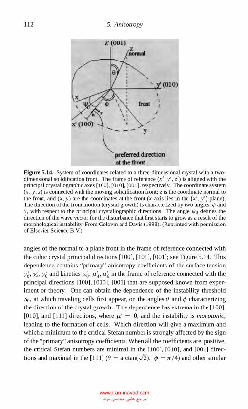
P1: GKE
Chap-05 CB381-Davis May 17, 2001 17:3 Char Count= 0
112 5. Anisotropy
Figure 5.14. System of coordinates related to a three-dimensional crystal with a two-dimensional solidification front. The frame of reference (x ′, y′, z′) is aligned with theprincipal crystallographic axes [100], [010], [001], respectively. The coordinate system(x, y, z) is connected with the moving solidification front; z is the coordinate normal tothe front, and (x, y) are the coordinates at the front (x-axis lies in the
(x ′, y′)-plane).
The direction of the front motion (crystal growth) is characterized by two angles, φ andθ , with respect to the principal crystallographic directions. The angle ψ0 defines thedirection of the wave vector for the disturbance that first starts to grow as a result of themorphological instability. From Golovin and Davis (1998). (Reprinted with permissionof Elsevier Science B.V.)
angles of the normal to a plane front in the frame of reference connected withthe cubic crystal principal directions [100], [101], [001]; see Figure 5.14. Thisdependence contains “primary” anisotropy coefficients of the surface tensionγ ′
0, γ′4, γ
′6 and kinetics µ′
0, µ′4, µ
′6 in the frame of reference connected with the
principal directions [100], [010], [001] that are supposed known from exper-iment or theory. One can obtain the dependence of the instability thresholdS0, at which traveling cells first appear, on the angles θ and φ characterizingthe direction of the crystal growth. This dependence has extrema in the [100],[010], and [111] directions, where µ′ = 0, and the instability is monotonic,leading to the formation of cells. Which direction will give a maximum andwhich a minimum to the critical Stefan number is strongly affected by the signof the “primary” anisotropy coefficients. When all the coefficients are positive,the critical Stefan numbers are minimal in the [100], [010], and [001] direc-tions and maximal in the [111] (θ = arctan(
√2), φ = π/4) and other similar
www.iran-mavad.com مرجع علمی مھندسی مواد
P1: GKE
Chap-05 CB381-Davis May 17, 2001 17:3 Char Count= 0
5.4 Unconstrained growth with “small” anisotropy 113
directions. When some of the coefficients are negative, the maximal criticalStefan number can be in the [100], [010], and [001] directions. In the follow-ing the nonlinear evolution of the waves (traveling cells) in the vicinity of theinstability threshold will be considered.
To derive an equation describing nonlinear evolution of the traveling cellsgenerated by the instability of the solidification front described above newcoordinates are introduced connected, with the direction at the front in whichthe instability first appears, which is characterized by the angleψ0: X = ε(r·n),Y = ε2(r · τ ), where n = ( cos ψ0, sin ψ0) and τ = (− sin ψ0, cos ψ0) are theunit vectors in the direction of the most rapidly growing perturbations (n) andnormal to the direction (τ ), (see Fig. 5.14), and ε is defined by the degree of thesupercriticality, ε2 = (S − S0)/S2; S2 is an arbitrary number that can be fixedby choosing a convenient scaling for ε. Thus, the new long-scale coordinatesX and Y are along the preferred direction and normal to it, respectively. Forthe anisotropic problem the details of the derivation are given in Appendix Cof Golovin and Davis (1998). For the front deformations h = O(ε), in theframe of reference moving with the group velocity of the waves, one obtainsthe following anisotropic evolution equation;
hτ + a1hξξξ + a2h2ξ + ε(a3S2hξξ − a4hηη + a5hξξη
+ a6hξξξξ − g1hξhξξ − g2hξhη) = 0, (5.62)
where τ = (ε3 + ε4)t, ξ = X − (εV0 − ε2S2)m0t, η = Y − (ε2V0 − ε4S2)m ′0t ,
and the coefficients are given in Golovin and Davis (1998). It can be shown thatcoefficients a4 and a6 are always positive.
Equation (5.62) describes the generic long waves (traveling cells) broughtabout by the oscillatory, long-scale morphological instability of a planar so-lidification front that propagate in the preferred direction determined by Eqs.(5.55) and (5.56). It can be seen that the main part of the equation involves aKorteweg–de Vries (KdV) operator and is modified by smaller terms describingthe effect of instability and dissipation. The specific case, when the group ve-locity of the waves is normal to their wave vector and the phase velocity is equalto zero, is described by the following equation with the physical h = O(ε2)and T = ε4t :
hT + a5hηX X + a2h2X + a3S2hX X − a4hηη + a6hX X X X = 0, (5.63)
where the coefficients ai are related to the respective coefficients ai in Eq. (5.62),and the coordinate η is a translation in time of Y . In one dimension,Eq. (5.63) is the Kuramoto–Sivashinsky equation, and in two dimensions it
www.iran-mavad.com مرجع علمی مھندسی مواد
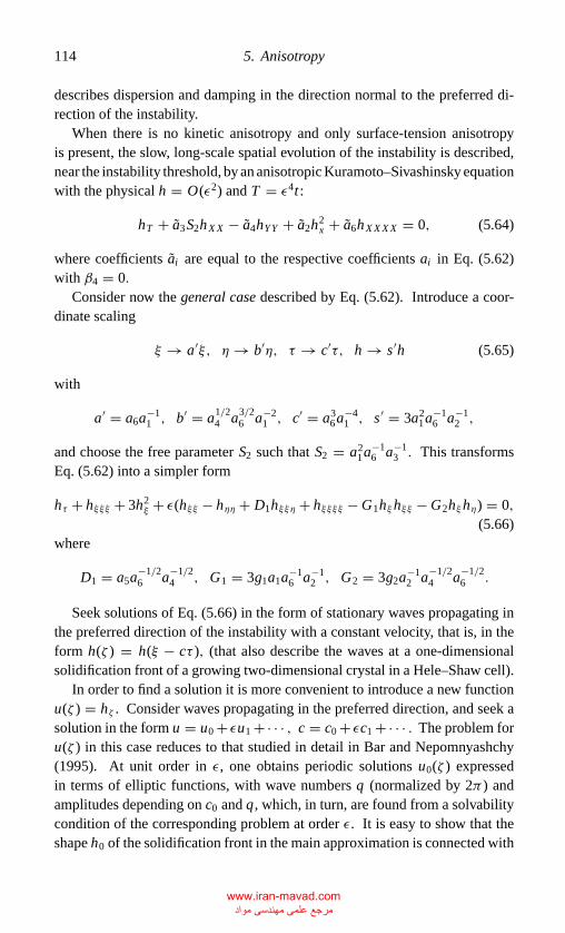
P1: GKE
Chap-05 CB381-Davis May 17, 2001 17:3 Char Count= 0
114 5. Anisotropy
describes dispersion and damping in the direction normal to the preferred di-rection of the instability.
When there is no kinetic anisotropy and only surface-tension anisotropyis present, the slow, long-scale spatial evolution of the instability is described,near the instability threshold, by an anisotropic Kuramoto–Sivashinsky equationwith the physical h = O(ε2) and T = ε4t :
hT + a3S2hX X − a4hY Y + a2h2x + a6hX X X X = 0, (5.64)
where coefficients ai are equal to the respective coefficients ai in Eq. (5.62)with β4 = 0.
Consider now the general case described by Eq. (5.62). Introduce a coor-dinate scaling
ξ → a′ξ, η → b′η, τ → c′τ, h → s ′h (5.65)
with
a′ = a6a−11 , b′ = a1/2
4 a3/26 a−2
1 , c′ = a36a−4
1 , s ′ = 3a21a−1
6 a−12 ,
and choose the free parameter S2 such that S2 = a21a−1
6 a−13 . This transforms
Eq. (5.62) into a simpler form
hτ + hξξξ + 3h2ξ + ε(hξξ − hηη + D1hξξη + hξξξξ − G1hξhξξ − G2hξhη) = 0,
(5.66)where
D1 = a5a−1/26 a−1/2
4 , G1 = 3g1a1a−16 a−1
2 , G2 = 3g2a−12 a−1/2
4 a−1/26 .
Seek solutions of Eq. (5.66) in the form of stationary waves propagating inthe preferred direction of the instability with a constant velocity, that is, in theform h(ζ ) = h(ξ − cτ ), (that also describe the waves at a one-dimensionalsolidification front of a growing two-dimensional crystal in a Hele–Shaw cell).
In order to find a solution it is more convenient to introduce a new functionu(ζ ) = hζ . Consider waves propagating in the preferred direction, and seek asolution in the form u = u0 + εu1 +· · · , c = c0 + εc1 +· · · . The problem foru(ζ ) in this case reduces to that studied in detail in Bar and Nepomnyashchy(1995). At unit order in ε, one obtains periodic solutions u0(ζ ) expressedin terms of elliptic functions, with wave numbers q (normalized by 2π ) andamplitudes depending on c0 and q, which, in turn, are found from a solvabilitycondition of the corresponding problem at order ε. It is easy to show that theshape h0 of the solidification front in the main approximation is connected with
www.iran-mavad.com مرجع علمی مھندسی مواد
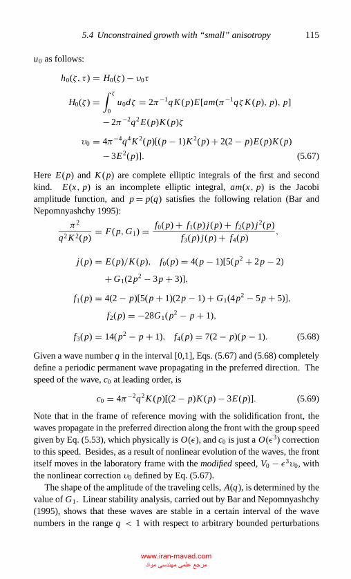
P1: GKE
Chap-05 CB381-Davis May 17, 2001 17:3 Char Count= 0
5.4 Unconstrained growth with “small” anisotropy 115
u0 as follows:
h0(ζ, τ ) = H0(ζ ) − υ0τ
H0(ζ ) =∫ ζ
0u0dζ = 2π−1qK (p)E[am(π−1qζK (p), p), p]
− 2π−2q2 E(p)K (p)ζ
υ0 = 4π−4q4K 2(p)[(p − 1)K 2(p) + 2(2 − p)E(p)K (p)
− 3E2(p)]. (5.67)
Here E(p) and K (p) are complete elliptic integrals of the first and secondkind. E(x, p) is an incomplete elliptic integral, am(x, p) is the Jacobiamplitude function, and p = p(q) satisfies the following relation (Bar andNepomnyashchy 1995):
π2
q2K 2(p)= F(p,G1) = f0(p) + f1(p) j(p) + f2(p) j2(p)
f3(p) j(p) + f4(p),
j(p) = E(p)/K (p), f0(p) = 4(p − 1)[5(p2 + 2p − 2)
+ G1(2p2 − 3p + 3)],
f1(p) = 4(2 − p)[5(p + 1)(2p − 1) + G1(4p2 − 5p + 5)],
f2(p) = −28G1(p2 − p + 1),
f3(p) = 14(p2 − p + 1), f4(p) = 7(2 − p)(p − 1). (5.68)
Given a wave number q in the interval [0,1], Eqs. (5.67) and (5.68) completelydefine a periodic permanent wave propagating in the preferred direction. Thespeed of the wave, c0 at leading order, is
c0 = 4π−2q2K (p)[(2 − p)K (p) − 3E(p)]. (5.69)
Note that in the frame of reference moving with the solidification front, thewaves propagate in the preferred direction along the front with the group speedgiven by Eq. (5.53), which physically is O(ε), and c0 is just a O(ε3) correctionto this speed. Besides, as a result of nonlinear evolution of the waves, the frontitself moves in the laboratory frame with the modified speed, V0 − ε3υ0, withthe nonlinear correction υ0 defined by Eq. (5.67).
The shape of the amplitude of the traveling cells, A(q), is determined by thevalue of G1. Linear stability analysis, carried out by Bar and Nepomnyashchy(1995), shows that these waves are stable in a certain interval of the wavenumbers in the range q < 1 with respect to arbitrary bounded perturbations
www.iran-mavad.com مرجع علمی مھندسی مواد
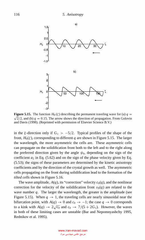
P1: GKE
Chap-05 CB381-Davis May 17, 2001 17:3 Char Count= 0
116 5. Anisotropy
Figure 5.15. The function H0 (ζ ) describing the permanent traveling wave for (a) q =√2/2, and (b) q = 0.15. The arrow shows the direction of propagation. From Golovin
and Davis (1998). (Reprinted with permission of Elsevier Science B.V.)
in the ξ -direction only if G1 > −5/2. Typical profiles of the shape of thefront, H0(ζ ), corresponding to different q are shown in Figure 5.15. The largerthe wavelength, the more asymmetric the cells are. These asymmetric cellscan propagate on the solidification front both to the left and to the right alongthe preferred direction given by the angle ψ0, depending on the sign of thecoefficient a2 in Eq. (5.62) and on the sign of the phase velocity given by Eq.(5.53); the signs of these parameters are determined by the kinetic anisotropycoefficients and by the direction of the crystal growth as well. The asymmetriccells propagating on the front during solidification lead to the formation of thetilted cells shown in Figure 5.16.
The wave amplitude, A(q), its “correction” velocity c0(q), and the nonlinearcorrection for the velocity of the solidification front υ0(q) are related to thewave number q. The larger the wavelength, the greater is the amplitude (seeFigure 5.15). When q → 1, the traveling cells are nearly sinusoidal near thebifurcation point, with A(q) → 0 and c0 → −1; the case q → 0 correspondsto a kink with A(q) → 2
√c0 and c0 → 7/(5 + 2G1). However, the waves
in both of these limiting cases are unstable (Bar and Nepomnyashchy 1995,Rednikov et al. 1995).
www.iran-mavad.com مرجع علمی مھندسی مواد
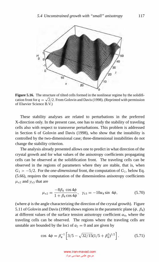
P1: GKE
Chap-05 CB381-Davis May 17, 2001 17:3 Char Count= 0
5.4 Unconstrained growth with “small” anisotropy 117
Figure 5.16. The structure of tilted cells formed in the nonlinear regime by the solidifi-cation front for q = √
2/2. From Golovin and Davis (1998). (Reprinted with permissionof Elsevier Science B.V.)
These stability analyses are related to perturbations in the preferredX-direction only. In the present case, one has to study the stability of travelingcells also with respect to transverse perturbations. This problem is addressedin Section 6 of Golovin and Davis (1998), who show that the instability iscontrolled by the two-dimensional case; three-dimensional instabilities do notchange the stability criterion.
The analysis already presented allows one to predict in what direction of thecrystal growth and for what values of the anisotropy coefficients propagatingcells can be observed at the solidification front. The traveling cells can beobserved in the regions of parameters where they are stable, that is, whenG1 > −5/2. For the one-dimensional front, the computation of G1, below Eq.(5.66), requires the computation of the dimensionless anisotropy coefficientsµx2 and γx3 that are
µx2 = −8β4 cos 4φ
1 + β4 cos 4φ, γx3 = −10α4 sin 4φ, (5.70)
(where φ is the angle characterizing the direction of the crystal growth). Figure5.11 of Golovin and Davis (1998) shows regions in the parametric plane (φ, β4)at different values of the surface tension anisotropy coefficient α4, where thetraveling cells can be observed. The regions where the traveling cells areunstable are bounded by the loci of a2 = 0 and are given by
cos 4φ = β−14
[3/5 −
√32/15(1/5 + β2
4 )1/2]. (5.71)
www.iran-mavad.com مرجع علمی مھندسی مواد
P1: GKE
Chap-05 CB381-Davis May 17, 2001 17:3 Char Count= 0
118 5. Anisotropy
If 0 < |β4| < 1/17, stable traveling cells exist at any direction of a crystalgrowth. If 1/17 < |β4| < 1, there exist certain intervals of the directions ofa crystal growth at which traveling cells are unstable and where the instabilityof a one-dimensional solidification front results in a more complex behavior.When β4 → 0, the traveling cells are still stable, but their velocity tends tozero, and thus at β4 = 0 traveling cells are replaced by stationary cells, whichare described by a Kuramoto–Sivashinsky equation.
For a two-dimensional solidification front, the parameter G1 is computedusing the expressions for anisotropy coefficients given in Golovin and Davis(1998). One can exhibit regions in the parametric plane of spherical angles(φ, θ ) defining the crystal growth direction at which the traveling cells arestable (at fixed particular values of the primed anisotropy coefficients).
Characteristics of traveling cells resulting from the morphological instabilityof a rapid solidification front depend on the degree of supercriticality (thedistance from the instability threshold), the direction of the crystal growth,and the amplitude of the wave, which is the function of its wave number. Ifone supposes that the system selects a most rapidly growing mode of lineartheory with the dimensionless wave number q = √
2/2, then, in the simplestcase of one-dimensional solidification fronts, dimensional characteristics of thewaves – their speed υ (the phase and the group speeds are the same in one-dimensional case), the wavelength λ, and the amplitude A can, in the mainapproximation, be expressed as follows:
υ = �T
µ0W (φ), λ = χµ0
�Tε−1�(φ), A = χµ0
�Tε−1 Q(φ), (5.72)
and
ε2 = S − S0
S0= ε2 S2
S0, W (φ) = 4V0(φ) β4 sin 4φ
(1 + β4 cos 4φ)2,
�(φ) = 2π√
2√S0(φ)
(1 + β4 cos 4φ)
√a6
a3,
Q(φ) = 3√
S0(φ)(1 + β4 cos 4φ)a1
a2
√a3
a6A(1/
√2). (5.73)
A plot of Q(φ) (Golovin and Davis 1998, Figure 13) for q = √2/2 shows
that the cells are unstable in certain intervals of φ, depending on α4 and β4; thisis where G1 < −5/2.
When there is no kinetic anisotropy and only anisotropy of surface tension ispresent, the morphological instability of a rapidly solidifying front is monotonicand yields the formation of a pattern of stationary cells (rolls) with the wave
www.iran-mavad.com مرجع علمی مھندسی مواد
P1: GKE
Chap-05 CB381-Davis May 17, 2001 17:3 Char Count= 0
5.4 Unconstrained growth with “small” anisotropy 119
vector oriented at the solidification front in the direction given by Eq. (5.57).These cells are described by a stationary periodic solution of the anisotropicKuramoto–Sivashinsky Eq. (5.64) that can be written in a rescaled form as
hT + hX X − hY Y + h2X + hX X X X = 0 (5.74)
with the physical h = O(ε2), T = O(ε4), and the coordinates X and Y de-fined along and normal to the preferred direction of the instability, respectively.Equation (5.74) is a particular case of the following more general anisotropicKuramoto–Sivashinsky equation of
hT + hX X + αhY Y + ∇41 h + h2
X + βh2Y = 0 (5.75)
studied by Chang, Demekhin, and Kopelevich (1993) and Rost and Krug (1995)as a model for nonlinear evolution of three-dimensional perturbations of a fluidfilm flowing down an inclined plane, nonlinear evolution of sputter-erodedsurfaces in the course of an electron beam treatment, and epitaxial growth of avicinal surface. Equation (5.75) transforms into Eq. (5.74) as α → −∞ withthe rescaling Y → Y/
√−α.It was shown in Chang et al. (1993) and Rost and Krug (1995) that, in
spite of the apparently stabilizing diffusional term in the Y -direction, the one-dimensional solutions of Eq. (5.76) periodic in the X -direction can, owing tothe nonlinearity, become unstable with respect to perturbations normal to thepreferred direction. Numerical simulations (Kawahara and Toh 1988) showthat this instability leads to formation of stripes whose widths are modulated inthe Y -direction that slowly vary in space and time – often in a chaotic manner.Such modulated stripes can manifest themselves in experiment as a structureof strongly elongated cells (“sausages”) with the larger side aligned normal tothe preferred direction of morphological instability.
In summary, then, results have been obtained on the effects of anisotropyof surface tension and kinetic coefficients on the morphological instability ofa solidification front rapidly propagating in a hypercooled melt in which thesolidification process is controlled by kinetics. Because of the anisotropy, thethreshold of the instability (the critical undercooling or the critical Stefan num-ber) depends on the direction of the crystal growth and on the anisotropy coef-ficient. In the general case, when both anisotropies are present, the instabilitygenerates traveling cells (waves) that travel on the two-dimensional front in apreferred direction determined by the coefficients of anisotropy. In a particularcase, when there is no kinetic anisotropy and only the surface tension anisotropyis present, the instability is monotonic and leads to the formation of stationarycells (that are also oriented on the front in the preferred direction. It should benoted that the anisotropy coefficients in Eqs. (5.49) depend on the direction of
www.iran-mavad.com مرجع علمی مھندسی مواد
P1: GKE
Chap-05 CB381-Davis May 17, 2001 17:3 Char Count= 0
120 5. Anisotropy
the crystal growth. For instance, when a crystal with cubic symmetry grows inone of the principal cyrstallographic directions, [100], [110], or [111] (or in thedirections [10] and [11] in the two-dimensional case), µx = µy = 0, and themorphological instability is monotonic and will lead to formation of stationarycells in this case, not to traveling ones.
A weakly nonlinear analysis of the instability near the threshold showsthat, in the general case, the evolution of the traveling cells is described bya dissipation-modified anisotropic KdV equation, Eq. (5.62). When there isno kinetic anisotropy, the nonlinear evolution of the instability is governedby anisotropic Kuramoto–Sivashinsky Eq. (5.63). In an “exotic” case, whenthe anisotropy coefficients satisfy relation (5.59), the morphological instabil-ity creates cells traveling along the solidification front with the group velocitynormal to the wave vector. These cells are described by Eq. (5.64), whichis a Kuramoto–Sivashinsky equation “in the preferred direction,” but one thatencompasses dispersion and diffusional damping in the direction normal to thepreferred one.
In the general case when both anisotropies are present, the dissipation-modified anisotropic KdV equation has the solutions in the form of cells thattravel at constant speed. Propagation of the cells along the front changes thespeed of the front itself.
Stability analysis shows that these waves are stable only if the nonlinearcoefficient in Eq. (5.67) G1 is greater than −5/2 and if the wave number is ina certain finite interval depending on G1. This interval does not include thezero wave number; hence, the solitary wave, corresponding to a single “step”propagating along the solidification front, is unstable. The stability conditionimposes restrictions on the values of the anisotropy coefficients as well as onthe directions of the crystal growth at which these cells can be observed inexperiments. Owing to anisotropy, the characteristics of stable traveling cellsdepend on the direction of the crystal growth. If the traveling cells are unstable,one would expect more complex wavy patterns to appear such as wave trainsor chaotic wavy patterns.
In the particular case when only surface tension anisotropy is present, thenonlinear evolution of stationary cells governed by the anisotropic Kuramoto–Sivashinsky equation can lead to formation of a spatially irregular structure ofstrongly elongated cells (“sausages”) whose long sides are aligned normal tothe preferred direction of the morphological instability.
It is important to say that the analysis presented is valid only if the anisotropyof surface tension (the coefficients γ ′
0, γ′2, γ
′4 for a three-dimensional cubic crys-
tal or the coefficient α4 for a two-dimensional cubic crystal growing in a Hele–Shaw cell) is smaller than a certain threshold; in the two-dimensional case with
www.iran-mavad.com مرجع علمی مھندسی مواد
P1: GKE
Chap-05 CB381-Davis May 17, 2001 17:3 Char Count= 0
5.5 Unconstrained growth with “large” anisotropy 121
fourfold symmetry, |α4| < 1/15. Otherwise, the weighted surface energy be-comes negative, and the solidification front becomes unstable at all values ofundercooling. It can be shown using the dispersion relation that in this case thelinear growth rate of the perturbations with the wave vector a is σ = |�| a2,and there is no shortwave cutoff in the linear terms. This situation is believedto cause the formation of facets and corners that cannot be described by thisweakly nonlinear theory but will be discussed in the next section.
5.5 Unconstrained Growth with “Large” Anisotropy –One-Dimensional Interfaces
In the previous discussion of anisotropic surface tension, the anisotropy was“small” in the sense thatF ≡ γ +γθθ > 0 everywhere, and hence the capillary-undercooling effect is well defined. In this section it will be assumed thatF < 0 for certain angles, which will lead in the case of static equilibrium tosolid particles with missing orientations. The figures will have sharp corners,and their shapes will be describable by the Wulff construction (Wulff 1901,Herring 1951), as discussed in Section 5.1.
When the interface is not in equilibrium but is evolving with time, the condi-tion F < 0 somewhere makes the evolution ill-conditioned; the coefficient ofthe curvature in the Gibbs–Thomson equation changes sign. One must “regu-larize” the model in some way, the most natural means being the introduction ofnew physics by endowing the edges with “line tension,” which can be ascribedto the dynamics of steps (Nozieres 1992).
The energy of steps is usually considered to be a function of the step density,the latter depending on the orientation of the crystal surface with respect to theprincipal crystal direction (x-axis); see Figure 5.17. If λ is the crystal latticespacing, and d is the step length, then for the density of steps n(x) and theirenergy E(n) for a unit length in the x-direction one has (Nozieres 1992)
nλ = λ
d= tan θ = hx , E(n) = γ
cos θ= γ
√1 + h2
x . (5.76)
Equations (5.76) are valid for vicinal surfaces when |θ | is small and the steps arewell-defined (Nozieres 1992). In the corner region, where the mean curvatureH is high, the orientation of the surface varies very rapidly, leading to a largevariation of n(x); in fact
dn
dx= 1
λhxx = 1
λ
2H
cos3 θ(5.77)
(the curvature is positive for a convex crystal surface). In this case, when |nx |
www.iran-mavad.com مرجع علمی مھندسی مواد
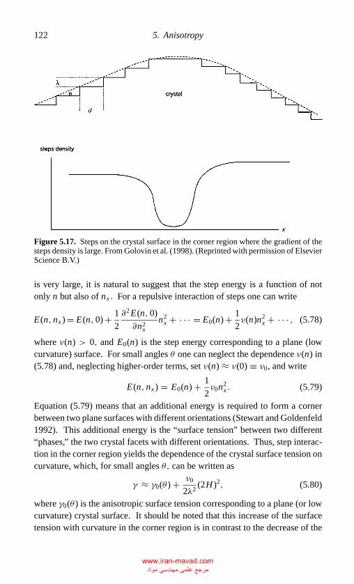
P1: GKE
Chap-05 CB381-Davis May 17, 2001 17:3 Char Count= 0
122 5. Anisotropy
Figure 5.17. Steps on the crystal surface in the corner region where the gradient of thesteps density is large. From Golovin et al. (1998). (Reprinted with permission of ElsevierScience B.V.)
is very large, it is natural to suggest that the step energy is a function of notonly n but also of nx . For a repulsive interaction of steps one can write
E(n, nx ) = E(n, 0) + 1
2
∂2 E(n, 0)
∂n2x
n2x + · · · = E0(n) + 1
2ν(n)n2
x + · · · , (5.78)
where ν(n) > 0, and E0(n) is the step energy corresponding to a plane (lowcurvature) surface. For small angles θ one can neglect the dependence ν(n) in(5.78) and, neglecting higher-order terms, set ν(n) ≈ ν(0) ≡ ν0, and write
E(n, nx ) = E0(n) + 1
2ν0n2
x . (5.79)
Equation (5.79) means that an additional energy is required to form a cornerbetween two plane surfaces with different orientations (Stewart and Goldenfeld1992). This additional energy is the “surface tension” between two different“phases,” the two crystal facets with different orientations. Thus, step interac-tion in the corner region yields the dependence of the crystal surface tension oncurvature, which, for small angles θ, can be written as
γ ≈ γ0(θ ) + ν0
2λ2(2H )2, (5.80)
where γ0(θ ) is the anisotropic surface tension corresponding to a plane (or lowcurvature) crystal surface. It should be noted that this increase of the surfacetension with curvature in the corner region is in contrast to the decrease of the
www.iran-mavad.com مرجع علمی مھندسی مواد
P1: GKE
Chap-05 CB381-Davis May 17, 2001 17:3 Char Count= 0
5.5 Unconstrained growth with “large” anisotropy 123
surface tension of a very small liquid droplet when the surface-layer thicknessbecomes comparable with the droplet radius (Rowlinson and Widom 1989).
The equilibrium at the crystal surface can be viewed as an equilibriumof a system of steps (Nozieres 1992). The “chemical potential” µs of suchnonuniform system of steps can be computed as µs = δF/δn, where F =∫
E(n, nx )dx is the free energy of a surface with a nonuniform distribution ofsteps (Cahn and Hilliard 1958). Using Eq. (5.79), one gets for the chemicalpotential per unit length in the x-direction
µs = d E0
dn− ν0nxx . (5.81)
In equilibrium, the thermodynamic force caused by the repulsion of steps,−dµs/dx , should be balanced by a “supercooling” force, −λLvδT/Tm, thatmakes the steps move in such a way that the surface would grow; here δT =Te − Tm is the departure of the equilibrium temperature Te corresponding to acurved surface from the equilibrium melting temperature of the plane surfaceTm. Using Eqs. (5.76) and (5.77), as well as hx = tan θ , one obtains, as anequilibrium condition, the following modified Gibbs–Thomson relation:
(Tm − Te)
TmLv = −1
λ
d2 E0
dn2nx + ν0
λnxxx = −
∂2[γ0(hx )
√1 + h2
x
]∂h2
x
hxx + ν0
λ2hxxxx .
(5.82)
The modified Gibbs–Thomson relation (5.82) can be also derived, if, as it isfound in Mullins (1963), one considers a variation δh of the crystal surface inequilibrium that conserves the volume, so that
∫ l0 δh dx = 0. In this case, the
variation of the surface free energy,
F =l∫
0
[E0(n) + 1
2ν0n2
x
]dx =
l∫0
γ0(hx )√
1 + h2xdx + ν0
2λ2
l∫0
h2xxdx .
is
δF =l∫
0
∂(γ0(hx )
√1 + h2
x
)∂hx
δhx + ν0
λ2hxxδhxx
dx
=l∫
0
−∂2[γ0
√1 + h2
x
]∂h2
x
hxx + ν0
λ2hxxxx
δh dx
+∂(γ0
√1 + h2
x
)∂hx
− ν0
λ2hxxx
δh∣∣∣∣∣∣l
0
+ ν0
λ2hxxδhx
∣∣∣l0. (5.83)
www.iran-mavad.com مرجع علمی مھندسی مواد
P1: GKE
Chap-05 CB381-Davis May 17, 2001 17:3 Char Count= 0
124 5. Anisotropy
In equilibrium, the sum of the variations of the surface free energy (Eq.(5.83)) and the bulk free energy must be zero. Because the volume is conservedand∫ l
0 δh dx = 0, the variation of the bulk free energy is equal to the total
change of the bulk chemical potential, which is∫ l
0 Lv(δT/Tm)δh dx . (Thebulk chemical potential plays the role of the Lagrange multiplier; Coriell andSekerka 1976). Taking δh(0) = δh(l) = 0 and neglecting the term with hxx atthe boundaries of the corner region, one obtains the modified Gibbs–Thomsonrelation (5.82) valid for |hx | 1.
Consider now a planar interface moving at constant speed in a hypercooledmelt. The kinetic undercooling is taken to be isotropic, and the expression forthe fourfold symmetric surface energy E(hx ) is written for small |hx | as
E = f0(θ ) + f1(θ )hx + f2(θ )h2x + · · · (5.84)
with
f0 = 1 − 15α4 cos 4θ, f1 = 60α4 sin 4θ, f2 = 3
2(95α4 cos 4θ − 1).
In scaled coordinates the governing system has the form
�t − V�z = ∇2� for z > h(x, t).
On z = h(x, t)
S(V + ht ) = −�z + hx�x (5.85)
� = 1 + �E(hx )hxx − K hxxxx − V + ht
(1 + h2x )1/2
.
As z → ∞,C → 0.
Notice that the Gibbs–Thomson relation now contains a fourth-order spatialderivative that regularizes the “large” anisotropy case where E has zeros. Inthe preceding
E(h) = ∂2
∂h2x
(σ0
√1 + h2
x
)(5.86)
and
K = ν0Tm/λ2κµ0Lv.
A weakly nonlinear evolution equation can be derived by introducing thelong-scale X = εx, the hierarchy of slow times T2, T3, T4, . . . such thatTk = εk t, k = 2, 3, . . . , and consider h(X, T2, T3, T4, . . .) = O(1), �(Z , X ,T2, T3, T4. . . .) = �(0)(Z , X, T2, T3, T4, . . .) + ε2�(2) (Z , X, T2, T3, T4, . . .) +
www.iran-mavad.com مرجع علمی مھندسی مواد
P1: GKE
Chap-05 CB381-Davis May 17, 2001 17:3 Char Count= 0
5.5 Unconstrained growth with “large” anisotropy 125
ε3�(3)(Z , X, T2, T3, T4, . . .) + ε4�(4)(Z , X, T2, T3, T4, . . .) + · · ·; functions�(i) must decay at infinity; the expansion of the effective surface tension E(hx )is given by Eqs. (5.84).
After a good deal of analysis, Golovin, Davis, and Nepomnyashchy (1998)found that, in reconstituted form,
ht − 1
2V h2
x + 1
8V h4
x = (−µ+ αhx + βh2x )hxx − (|s4| + K )hxxxx , (5.87)
where
µ = S
V− � f0 = S
V− �(1 − 15α4 cos 4θ ),
α = � f1 = 60�α4 sin 4θ,
β = S
V− �(
1
2f0 + f2
)= S
V+ �(135α4 cos 4θ − 1),
(5.88)
and s4 is defined by σ ∼ s2a2 + s4a4 as a → 0.Notice that the regularization imposed by the interaction of steps in the corner
region leads to the curvature-dependent surface tension, which augments thecoefficient of the fourth-order term in Eq. (5.87). It does not alter the structureof the equation. The form of Eq. (5.87) has been derived by Angenent andGurtin (1989) and Gurtin (1993).
Note that the mean value of h over one wavelength is nonzero because thereis continuous crystal growth. If the effect of step interaction in the cornerregion is large enough, then Eq. (5.87) governs the dynamics of facet formationin hypercooled solidification. If the effect is small, as might be expected onphysical grounds, the band of unstable wave numbers is not necessarily small,and we should consider this as a model equation for describing the process ofthe formation of corners and facets caused by anisotropic surface tension.
Equation (5.87) can be written in a canonical form by introducing newvariables
ξ = 3V
β√
2x, τ = 3V 2
βt, q = hx/
√2,
and finding the following equation for the slope q of the interface:
qτ − qqξ + q3qξ = (−mq + bq2 + q3 − χqξξ )ξξ , (5.89)
where
m = 3µ
2β, b = 3α
2√
2β, χ = 27V 2(|s4| + K )
4β3. (5.90)
www.iran-mavad.com مرجع علمی مھندسی مواد
P1: GKE
Chap-05 CB381-Davis May 17, 2001 17:3 Char Count= 0
126 5. Anisotropy
Equation (5.89) is essentially a convective Cahn–Hilliard equation 1958.The Cahn–Hilliard equation, absent the convective terms, describes the processof spinodal decomposition and has the following form:
uτ = (−u + bu2 + u3 − uξξ )ξξ = 0, (5.91)
where u is the order parameter (e.g., the concentration of one of the componentsof an alloy). This equation has been intensively studied (see Novick-Cohen1998 for the review). It has the solution (Novick-Cohen and Segel 1984)
u = −b/3 ± (b2/3 + 1)1/2 tanh[(b2/3 + 1)1/2ξ/
√2]
(5.92)
that describes the final stage of the spinodal decomposition, the formation ofthe interface between two thermodynamically stable states of an alloy withdifferent concentrations. The form of Eq. (5.91) originates from the alloydouble-well free energy F(u) given by F = −u2/2 + bu3/3 + u4/4 and alsotakes into account the stabilizing effect of the excess energy of the interfacebetween the two separated phases (Novick-Cohen and Segel 1984). Solution(5.92) describes the interface between the two stable compositions of the alloycorresponding to the binodal, that is, the points of the bitangent to the graphF(u), that give the values of the concentrations at which the chemical potentialsof each component are equal in both phases.
With convective terms, −qqξ + q3qξ , Eq. (5.89) is similar to the so-calleddriven Cahn–Hilliard equation (Emmott and Bray 1996)
ut − E(u2)x = (−u + u3 − uxx )xx , (5.93)
that describes a spinodal decomposition in the presence of an external (e.g.,gravitational or electric) field when the dependence of the mobility factor onthe order parameter is important (Leung 1990 and Yeung et al. 1992). Equation(5.93) has an exact solution u = u∞ tanh(u∞x/
√2) with u2
∞ = 1 + √2E
(Leung 1990, Emmott and Bray 1996) that shows the broken symmetry due tothe convective term, leading to different amplitudes of kinks and antikinks (akink has a positive derivative, and an antikink has a negative one).∗
In the present case, the “order parameter” corresponds to the slope of theinterface, and convective terms −qqξ + q3qξ stem from the effect of kinetics(the finite rate of atoms or molecules attaching to the crystal surface) that
∗ By using another scaling, ξ = [(|s4| + K )/µ]1/2 x, τ = [(|s4| + K )/µ2]
t, q = [3µ/β]1/2 hx ,
Eq. (5.87) can be written in the form qτ − ((1/2)v1q2 − (1/4)v2q4)ξ = (−q +bq2 +q3 −qξξ )ξξ ,where v1 = (V/µ)[3 |s4| + K )/β]1/2, v2 = 3v1µ/β, b = (α/2)[3/(βµ)]1/2, that is analogousto Eq. (5.93). Thus, the convective terms are seen to be proportional to the speed V of theunperturbed front. The form of Eq. (5.89) is physically clearer and more convenient for numericalcomputations.
www.iran-mavad.com مرجع علمی مھندسی مواد
P1: GKE
Chap-05 CB381-Davis May 17, 2001 17:3 Char Count= 0
5.5 Unconstrained growth with “large” anisotropy 127
provides an independent flux of the order parameter similar to the effect of anexternal field in spinodal decomposition of a driven system. Equation (5.89)can be written in the conservation form
qτ +[−1
2q2 + 1
4q4
]ξ
+[−∂G
∂q+ χqξξ
]ξξ
= 0, (5.94)
where the nonlinear term with the first derivative represents the flux of the“order parameter” caused by kinetics, and G(q) is the effective double-well“free energy”
G = −1
2mq2 + 1
3bq3 + 1
4q4. (5.95)
The coefficients m and b, defining the shape of G, depend not only on thefunctions f0(θ ), f1(θ ), and f2(θ ) from the expansion of the anisotropic surfacetension but also on the Stefan number S characterizing the undercooling, andhence on the front velocity V = 1−S. This is because the local thermodynamicequilibrium is absent on the surface of a crystal whose rapid growth from thehypercooled melt is controlled by the attachment kinetics. The effective double-well “free energy” is symmetric when the direction of the crystallization frontmotion coincides with one of the principal crystal directions (b = 0), and it isasymmetric otherwise.
The similarity between the process of spinodal decomposition and the for-mation of facets from energetically unstable crystal surfaces was noticed longago (Mullins 1961, Cabrera 1963, Cahn and Hoffman 1974) as well as in somerecent works (Gurtin 1993; Carlo, Gurtin, and Podio-Guidugli 1992; Stewartand Goldenfeld 1992; Liu and Metiu 1993). It was shown that the slope ofthe equilibrium facets grown from the unstable surface corresponds to bitan-gent (binodal) points of the surface free energy in a complete analogy with thespinodal decomposition. However, when convective effects are present, thisbitangent construction is destroyed (see also Leung 1990).
In Eq. (5.89), the parameter m measures the magnitude of the instability,and the coefficient b characterizes the anisotropic effect of the crystal growthdirection. The relative effects of the attachment kinetics and of the surfacetension dependence on curvature (the “line tension” between two facets) ischaracterized by the parameter χ.
Golovin et al. (1998) found a solution of Eq. (5.89) in the form
q = A + B tanh
[φB(ξ − cτ )√
χ
](5.96)
corresponding to a kink moving with a constant speed c. Such a kink in theslope of a surface would correspond to two almost flat faces (facets) separated
www.iran-mavad.com مرجع علمی مھندسی مواد
P1: GKE
Chap-05 CB381-Davis May 17, 2001 17:3 Char Count= 0
128 5. Anisotropy
by a corner. By substituting Eq. (5.96), one finds the following equationfor φ:
φ3 − 1
2φ −
√χ
24= 0, (5.97)
and the following relations for A and B:
A = − 2bφ
6φ + √χ, B2 = 2mφ + √
χ
2(φ + √χ/3)
+ 2b2φ2(6φ − √χ )(
6φ + √χ)2 (φ + √
χ/3)
(5.98)
(it is sufficient to take B > 0), and the speed of the kink motion c:
c = A(A2 + B2 − 1). (5.99)
The case when the coefficient χ is small, χ 1, corresponds to either smallspeed of the crystallization front or to weak interaction of steps in the cornerregion (i.e., weak surface-tension dependence on curvature). For χ 1, Eq.(5.97) has the following approximate solutions:
φ± = ± 1√2
+√χ
24∓ χ
3 · 213/2+ O(χ3/2), (5.100)
φ0 = −√χ
12− χ3/2
864+ O(χ5/2). (5.101)
Solutions φ± for χ 1 defined by Eq. (5.100) correspond to kinks (φ+)and antikinks (φ−) described by Eqs. (5.98) and (5.99), and the slowly varyingsolution, Eq. (5.101) corresponding to φ0, divides the regions of their attraction.Consider solutions φ±.
For χ 1,
A = −b
3± b
9√
2
√χ − 5b
216χ + O(χ3/2), (5.102)
B =√
m + b2/3 ± 9 − 5b2 − 6m
6√
18m + 6b2
√χ
+ 126m2 + 189mb2 − 135m + 40b4 + 9b2 − 81
12√
2(18m + 6b2)3/2χ + O(χ3/2),
(5.103)and the speed of the kinks c is
c = b
3
(1 − m − 4
9b2
)∓ b
27√
2(12 − 7b2 − 9m)
√χ
+ b
216(44 − 33b2 − 31m)χ + O(χ3/2). (5.104)
www.iran-mavad.com مرجع علمی مھندسی مواد
P1: GKE
Chap-05 CB381-Davis May 17, 2001 17:3 Char Count= 0
5.5 Unconstrained growth with “large” anisotropy 129
In Eqs. (5.102)–(5.104), the upper signs correspond to kinks, and the lowerones correspond to antikinks.
The limiting values of the surface slopes at ± ∞, q (k,a)± are different for
kinks (k) and antikinks (a), namely,
q (k)± = q (0)
± + √χq (1)
± + χq (2)± + O(χ3/2),
q (a)± = q (0)
∓ − √χq (1)
∓ + χq (2)∓ + O(χ3/2),
(5.105)
where
q (0)± = ±
√m + b2/3 − b/3, q (1)
± = ± 9 − 5b2 − 6m
6√
18m + 6b2+ b
9√
2,
q (2)± = ±126m2 + 189mb2 − 135m + 40b4 + 9b2 − 81
12√
2(18m + 6b2)3/2− 5b
216.
(5.106)
By integrating Eq. (5.89) from −∞ to ∞, one can easily show that the speedof the kinks and antikinks motion is related to q± by
c = 1
4(q+ + q−)
(q2
+ + q2− − 2
). (5.107)
The kink solution (5.96) for the slope of the crystal surface corresponds tothe surface in the form of two plane facets connected by a rounded corner. Thekink with q− < 0, q+ > 0 corresponds to a valley, and the antikink withq− > 0, q+ < 0 corresponds to a hill. The shape of the solid–liquid interfacecan easily be obtained by integrating Eq. (5.89) and solution (5.96) as
h = A(ξ − cτ ) +√χ
φln
[cosh
(φB(ξ − cτ )√
χ
)]+ Cτ, (5.108)
where C = (B2 − A2)(2 − 3A2 − B2)/4 is the correction to the mean speed ofthe solidification front.
Figure 5.18 shows the formation of two facets connected by a roundedcorner. The angle between the facets is ϕ = π − arctan
√2q− + arctan
√2q+,
and the corner radius of curvature ρ is of the order of the kink transitionallayer, ρ ∼ 2π
√2χ/m, which gives the length of the most rapidly growing
perturbation. The kinks (antikinks) are symmetric, and they correspond tosymmetric valleys (hills) in the crystallization front shape, if b = 0, that is, if thedirection of the crystal growth (orientation of the crystallization front) coincideswith one of the principal crystal directions. Otherwise, the kinks and antikinksare asymmetric and correspond to valleys and hills whose sides have differentslopes. Such asymmetric hills and valleys move along the solidification front
www.iran-mavad.com مرجع علمی مھندسی مواد
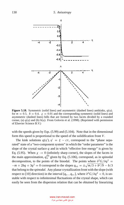
P1: GKE
Chap-05 CB381-Davis May 17, 2001 17:3 Char Count= 0
130 5. Anisotropy
Figure 5.18. Symmetric (solid lines) and asymmetric (dashed lines) antikinks, q(η),for m = 0.5, b = 0.4, χ = 0.01 and the corresponding symmetric (solid lines) andasymmetric (dashed lines) hills that are formed by two facets divided by a roundedcorner, (a) q(η) and (b) h(η). From Golovin et al. (1998). (Reprinted with permissionof Elsevier Science B.V.)
with the speeds given by Eqs. (5.99) and (5.104). Note that in the dimensionalform this speed is proportional to the speed of the solidification front V .
The kink solutions q(η′), η′ = ξ − cτ , correspond to the “phase sepa-rated” state of a “two-component system” in which the “order parameter” is theslope of the crystal surface q and in which “effective free energy” is given byEq. (5.95). When χ → 0 (infinitely sharp corner), the slopes of the facets inthe main approximation, q (0)
± given by Eq. (5.106), correspond, as in spinodaldecomposition, to the points of the binodal. The points where ∂2G/∂q2 =−m + 2bq + 3q2 = 0 correspond to the slopes qs± = ±
√m/3 + b2/9 − b/3
that belong to the spinodal. Any planar crystallization front with the slope (withrespect to [10] direction) in the interval [qs−, qs+], where ∂2G/∂q2 < 0, is un-stable with respect to infinitesimal fluctuations of the crystal shape, which caneasily be seen from the dispersion relation that can be obtained by linearizing
www.iran-mavad.com مرجع علمی مھندسی مواد
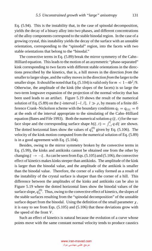
P1: GKE
Chap-05 CB381-Davis May 17, 2001 17:3 Char Count= 0
5.5 Unconstrained growth with “large” anisotropy 131
Eq. (5.94). This is the instability that, in the case of spinodal decomposition,yields the decay of a binary alloy into two phases, and different concentrationsof the alloy components correspond to the stable binodal region. In the case of agrowing crystal, this instability yields the decay of the surface with an unstableorientation, corresponding to the “spinodal” region, into the facets with twostable orientations that belong to the “binodal.”
The convective terms in Eq. (5.89) break the mirror symmetry of the Cahn–Hilliard equation. This leads to the motion of an asymmetric “phase-separated”kink corresponding to two facets with different stable orientations in the direc-tions prescribed by the kinetics, that is, a hill moves in the direction from thesmaller to larger slope, and the valley moves in the direction from the larger to thesmaller slope. It should be noted that Eq. (5.104) is valid only for m < 1−4b2/9.Otherwise, the amplitude of the kink (the slopes of the facets) is so large thetwo-term longwave expansion of the projection of the normal velocity that hasbeen used leads to an artifact. Figure 5.19 shows the result of the numericalsolution of Eq. (5.89) on the ξ -interval [−l, l], l � ρ, by means of a finite dif-ference Crank–Nickolson scheme with the boundary conditions qξ = qξξξ = 0at the ends of the interval appropriate to the simulating of the Cahn–Hilliardequation (Bates and Fife 1993). Both the numerical solution q (ξ, t) for the sur-face slope and the corresponding surface shape h(ξ, t) = ∫ ξ−l q dξ are shown.
The dotted horizontal lines show the values of q (0)± given by Eq. (5.106). The
velocity of the kink motion computed from the numerical solution of Eq. (5.89)is in a good agreement with Eq. (5.104).
Besides, owing to the mirror symmetry broken by the convective terms inEq. (5.99), the kinks and antikinks cannot be obtained one from the other bychanging ξ → −ξ . As can be seen from Eqs. (5.105) and (5.106), the convectiveeffect of kinetics makes kinks steeper than antikinks. The amplitude of the kinkis larger than the binodal value, and the amplitude of the antikink is smallerthan the binodal value. Therefore, the corner of a valley formed as a result ofthe instability of the crystal surface is sharper than the corner of a hill. Thisdifference between the amplitudes of the kinks and antikinks can be also inFigure 5.19 where the dotted horizontal lines show the binodal values of thesurface slope, q (0)
± . Thus, owing to the convective effect of kinetics, the slopes ofthe stable surfaces resulting from the “spinodal decomposition” of the unstablesurface depart from the binodal. Using the definition of the small parameter χ,it is easy to see from Eqs. (5.105) and (5.106) that these deviations grow withthe speed of the front V .
Such an effect of kinetics is natural because the evolution of a curve whosepoints move with the same constant normal velocity tends to produce caustics
www.iran-mavad.com مرجع علمی مھندسی مواد
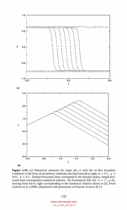
P1: GKE
Chap-05 CB381-Davis May 17, 2001 17:3 Char Count= 0
Figure 5.19. (a) Numerical solutions for slope q(ξ, t) with the no-flux boundaryconditions in the form of asymmetric antikinks moving from left to right, m = 0.5, χ =0.01, b = 0.2. Dashed horizontal lines correspond to the binodal slopes; dotted hori-zontal lines correspond to analytical solution. (b) Asymmetric hill, h(ξ, t) = ∫ ξ−1 q dξ ,moving from left to right corresponding to the numerical solution shown in (a). FromGolovin et al. (1998). (Reprinted with permission of Elsevier Science B.V.)
132
www.iran-mavad.com مرجع علمی مھندسی مواد
P1: GKE
Chap-05 CB381-Davis May 17, 2001 17:3 Char Count= 0
5.5 Unconstrained growth with “large” anisotropy 133
in the case of a concave curve and tends to reduce the curvature when the curveis convex.
Equation (5.89) is nonlinear, and its solution in a finite domain is very closeto the analytical solution of Eq. (5.96) if the width of the interfacial region issmall in comparison with the width of the computational domain, though thissolution is not necessarily unique. As shown by Emmott and Bray (1996) forEq. (5.93), if the symmetry conditions are used, qxx (0) = 0, q(l) = −q(−l),the antikink is unique, but there is a family of kinks parameterized by the valueq(l). In the computations shown above, the boundary conditions used wereqx = qxxx = 0 at x = ± l, and these ensure the uniqueness of the solutions.
In order to study the dynamics of the formation of facets on the surface of acrystal growing in a hypercooled melt, a numerical solution of Eq. (5.89) wasobtained by means of a pseudospectral code with periodic boundary conditions.Figure 5.20 shows different stages of the instability of a plane crystal surface
Figure 5.20. Different stages of the faceting of an unstable solidification front obtainedby numerical solution for q and h with periodic boundary conditions, m = 0.25, χ =0.001, and b = 0. (a) Formation of periodic structure of hills and valleys, (b) and (c)the coarsening process, (d) final state; two facets separated by a rounded corner. FromGolovin et al. (1998). (Reprinted with permission of Elsevier Science B.V.)
www.iran-mavad.com مرجع علمی مھندسی مواد
P1: GKE
Chap-05 CB381-Davis May 17, 2001 17:3 Char Count= 0
134 5. Anisotropy
when the direction of the growth coincides with one of the principal crystaldirections, and thus in Eq. (5.90) b = 0. Both the numerical solution q(ξ, t)for the surface slope and the corresponding surface shape h(ξ, t) = ∫ q dξ , areshown. Starting from small random initial perturbations, the system first devel-ops into a spatially periodic hill-and-valley structure (“teeth”) (Figure 5.20(a))with the spatial period corresponding to the wavelength of the most rapidlygrowing mode. Each tooth consists of two facets corresponding to the wave-length of the most rapidly growing mode. Each tooth of this structure consistsof two facets corresponding to the stable orientation close to the “binodal” one.In the course of further evolution the system exhibits coarsening: small teethmerge (Figure 5.20(b)) and form larger ones with larger spatial period (Figure5.20(c)). This corresponds to the formation of several larger kinks of the sur-face slope. In a system with periodic boundary conditions, the final state isa single kink–antikink pair corresponding to a periodic structure of hills andvalleys composed of facets with stable orientations with the period equal to theperiod of the computation domain (Figure 5.20(d)).
If the crystal growth direction differs from one of the crystal principal direc-tions (b �= 0), the “teeth” resulting from the instability will be tilted, and thewhole hill-and-valley system will move along the crystal surface. In the courseof this drift of the whole structure, the coarsening proceeds, and thus finallythere will be one moving hill and valley.
It is important to know how the convective effect of kinetics influencesthe rate of coarsening. Usually, when the coarsening process is governed bydiffusion and capillarity, as described by the Cahn–Hilliard equation, the ratesof coarsening in two-dimensional and three-dimensional problems obey thewell-known Lifshitz–Slyozov–Wagner law (Lifshitz and Slyozov 1961, Wagner1961), namely, at the late stage of coarsening, the mean scale of the new phasegrowing from the other, larger phase (e.g., liquid droplets growing from theirvapor) increases as t1/3, where t is time (see Shinozaki and Oono 1993, Kupperand Masbaum 1994 and references therein). In one dimension, the solutionsof the Cahn–Hilliard equation exhibit logarithmically slow rates of coarsening(see Kawakatsu and Munakata 1985; Alikakos, Bates, and Fusco 1991; Batesand Xun 1994, 1995).
However, the coarsening can go much faster if the flux of the order pa-rameter is governed by some independent velocity scale present in the system(e.g., resulting from hydrodynamic effects); in this case the mean scale ofthe new phase can increase ∝ tn, 1/3 < n ≤ 1 (Siggia 1979; Tanaka 1997;Ratke and Thieringer 1985; Wan and Sahm 1990; Akaiwa, Hardy, and Voorhees1991). In the present case the kinetics controlling the crystal growth from the
www.iran-mavad.com مرجع علمی مھندسی مواد
P1: GKE
Chap-05 CB381-Davis May 17, 2001 17:3 Char Count= 0
5.6 Unconstrained growth with “large” anisotropy 135
hypercooled melt sets an independent velocity scale for the order parameter,the surface slope, and this leads to much faster coarsening dynamics. In a one-dimensional case the initial stage the coarsening goes like ∼ t, and at the laststage the mean scale of the system increases ∼ t1/2. This result coincideswith the results of the numerical simulation of a model dynamical system in-troduced in Emmott and Bray (1996) for governing the interaction of kinksin the driven Cahn–Hilliard equation (Eq. (5.93)). This coarsening dynamicsimplies that the interaction of kinks in Eq. (5.89) at the late stages, when thedistance between the kinks is large, leads to their attractive motion with thespeed inversely proportional to the distance between the kinks. At the initialstage, when the distance between the kinks is small, the speed of their attractivemotion probably tends to a constant value as is suggested by the coarsening∼ t at this stage. However, a separate investigation of the interaction of thekinks is required in the spirit of the theory developed in Kawasaki and Ohta(1982).
5.6 Unconstrained Growth with “Large” Anisotropy –Two-Dimensional Interfaces
Consider now the case of three-dimensional crystal growth in which h =h(x, y, t). Golovin et al. (1999) obtained the evolution equation
ht(1 + |∇h|2)−1/2 = µ [�(h) + E(h)] (5.109)
where E given by
E(h) = ∂2 I
∂(hx )2hxx + 2
∂2 I
∂hx∂hyhxy + ∂2 I
∂(hy)2hyy − ∂2 I
∂(hxx )2hxxxx
− 2∂2 I
∂hxy∂hxxhxxxy −
(∂2 I
∂(hxy)2+ 2
∂2 I
∂hxx∂hyy
)hxxyy
− 2∂2 I
∂hxy∂hyyhxyyy − ∂2 I
∂(hyy)2hyyyy, (5.110)
where
I = γ
√1 + |∇h|2, (5.111)
and� represents the driving force of the crystal growth. Golovin et al. (1999)considered two cases, (1) � is a constant that holds when the driving forceis independent of the local temperature field, and (2) � is local in the sense
www.iran-mavad.com مرجع علمی مھندسی مواد
P1: GKE
Chap-05 CB381-Davis May 17, 2001 17:3 Char Count= 0
136 5. Anisotropy
that the boundary-layer thickness is small compared with the curvature of thecrystal. When the driving force is local, then �(h) would be represented bya nonlinear differential operator. When it is nonlocal, it is represented by anonlinear integro–differential operator.
For constant driving force, �(h) = �0, and for a cubic crystal
γ = γ0[1 + α4
(n4
x + n4y + n4
z
)+ α6(n6
x + n6y + n6
z
)+ · · ·]+ 1
2δ(2H )2,
(5.112)
where nx , ny, nz are the coordinates of the local unit normal to the crystalsurface in the frame of reference of the principal directions [100], [101], and[001] that can be expressed in terms of the angular spherical coordinates θand φ as nx = sin θ cosφ, ny = sin θ sinφ, nz = cos θ, γ0 is a constantcharacterizing mean surface tension of the crystal,α4, α6, . . . are the coefficientsof the surface tension anisotropy, and δ = const > 0. Consider a planarcrystal surface growing with the orientation characterized by a normal vectorez = (sin θ cos φ, sin θ sinφ, cos θ ) and choose the other two basis vectorsin the surface plane to be ex = ez×e0
z/∣∣ez × e0
z
∣∣ , ey = ez×ex/ |ez × ex |, wheree0
z is aligned along the [001] direction. In the coordinate system {ex , ey, ez} theposition of the crystal surface is given by z = h(x, y, t). The weighed surfacetension I defined by Eq. (5.2) with λ = 0 can be expanded for |hx | 1,∣∣hy
∣∣ 1 as
I (hx , hy, hxx , hxy, hyy) = γ0
∞∑m,n = 0
emn(α4, α6, θ, φ)hmx hn
y
+ 1
2δ(h2
xx + 2hxxhyy + h2yy
)+ · · · . (5.113)
Here the coefficients ei j are the functions of the direction of the crystal growthand of the anisotropy coefficients which were computed in Golovin and Davis(1998).
After the transformation t → t/(κ�0), Eq. (5.109) reads
ht = .
√1 + |∇h|2[1 + �E(h)], (5.114)
where � = γ0/�0.
Equation (5.114) has a solution corresponding to a planar, uniformly growingsurface (uniformly propagating crystallization front) h = t (the dimensionalspeed of the front is κ�0). Transform to the frame moving with the planar front,change the variable h → h + t , and expand Eq. (5.114) for |ht | 1, |∇h| 1.
www.iran-mavad.com مرجع علمی مھندسی مواد
P1: GKE
Chap-05 CB381-Davis May 17, 2001 17:3 Char Count= 0
5.6 Unconstrained growth with “large” anisotropy 137
Keeping the terms up to the second order, one obtains
ht − 1
2|∇h|2 − �E2(h) = 0, (5.115)
where E2 is the linear differential operator
E2 = ∇ A∇T , A = 2e20 e11
e11 2e02
. (5.116)
Equation (5.115) is an anisotropic Burgers equation. It can also be called theanisotropic, deterministic Kardar–Parisi–Zhang (AKPZ) equation (Wolf 1991;Barabasi, Araujo, and Stanley 1992). With noise added, this equation describeskinetic roughening of vicinal surfaces (Wolf 1991) and epitaxial growth (seeKrug 1997 for review). If the eigenvalues of the anisotropy matrix A are positive,Eq. (5.116) describes a hill-and-valley structure propagating along the interfacewith the amplitude determined by initial conditions (Fogedby 1998). In thiscase the anisotropic surface tension prevents the formation of sharp corners inthe course of kinetically controlled crystal growth (Uwaha 1987, Yokohamaand Sekerka 1992).
When at least one of the eigenvalues of A is negative, the crystal surfacewith the orientation characterized by the anisotropy matrix A is thermody-namically unstable. This instability results in the formation of facets and cor-ners. However, in this case Eq. (5.115) is ill-posed because it does not have ashortwave cutoff. In order to describe the dynamics of the formation of facetsand corners, one has to keep higher-order terms in the evolution equation forthe crystal surface.
Keeping the terms up to the fourth order, one obtains for the shape of thecrystal surface in the moving frame the following evolution equation:
ht = 1
2|∇h|2 − 1
8|∇h|4 + �
(1 + 1
2|∇h|2
)E2(h) + �E3(h)
+�E4(h) + O(|∇h|6). (5.117)
The nonlinear terms |∇h|2 /2−|∇h|4 /8 on the right-hand side of Eq. (5.118)stem from the projection of the local normal velocity of the crystallization fronton the z-axis. Usually, only a |∇h|2 term is present in this type of equationbecause it already describes the kinematic effect of the interfacial slope (Krug1997). Moreover, although the two-term expansion that includes also the |∇h|4term is more accurate for small surface slopes, it can lead to artifacts if the slopeof the interface is too large. Therefore, the fourth-order kinematic term in the
www.iran-mavad.com مرجع علمی مھندسی مواد
P1: GKE
Chap-05 CB381-Davis May 17, 2001 17:3 Char Count= 0
138 5. Anisotropy
evolution equation is omitted. Thus, Eq. (5.117) is written in the following form:
ht = 1
2|∇h|2 + hxx [µ11 + κ11hx + λ11hy + a11h2
x + b11h2y + c11hxhy]
+ hxy[µ12 + κ12hx + λ12hy + a12h2x + b12h2
y + c12hxhy]
+ hyy[µ22 + κ22hx + λ22hy + a22h2x + b22h2
y + c22hxhy] − ν∇4h.(5.118)
Equation (5.118) is related to those derived in Stewart and Goldenfeld (1992)and Liu and Metiu (1993) for the faceting of crystal surfaces with unstable ori-entations when there is no surface growth. The coefficients µi j characterizethe linear faceting instability of the thermodynamically unstable surface, andthe coefficients of the nonlinear terms determine the stable orientations of theappearing facets and the symmetry of the faceted structure. The linear damp-ing coefficient ν characterizes the stabilizing effect of the additional energyof edges and determines their widths. The new feature is that Eq. (5.118) de-scribes the faceting instability in the course of kinetically controlled crystalgrowth, which accounts for the presence of the “convective” term 1
2 |∇h|2. Onthe other hand, this feature can be considered as a generalization of isotropicgrowth models reviewed by Krug for the case of an evaporation–condensationgrowth mechanism. Equation (5.118) is considered in the present case to be aphenomenological model for the formation of facets and corners in the kineti-cally controlled growth of a thermodynamically unstable surface in the simplestcase of a constant driving force.
A related evolution equation is derived for a more complicated case, whenthe difference between the crystal and liquid chemical potentials is not constant,but it is locally coupled to the temperature field in a thermal diffusion boundarylayer near the crystal surface.
As an example, consider the solidification of a hypercooled melt. For a local�(h), the growth is controlled by attachment kinetics
Vn ∝ T e − T I
valid for small deviations from equilibrium. (Bates et al. 1997 have discussedmodels valid at substantial undercoolings.) Golovin et al. (1999) obtained thefollowing equation:
ht − 1
2V |∇h|2 = hxx [µs
11 + κ11hx + λ11hy + as11h2
x + b11h2y + c11hxhy]
+ hxy[µ12 + κ12hx + λ12hy + a12h2x + b12h2
y + cs12hxhy]
+ hyy[µs22 + κ22hx + λ22hy + a22h2
x + bs22h2
y + c22hxhy]
+ g∂(hx , hy)
∂(x, y)− χi jklhxi x j xk xl , (5.119)
www.iran-mavad.com مرجع علمی مھندسی مواد
P1: GKE
Chap-05 CB381-Davis May 17, 2001 17:3 Char Count= 0
5.7 Faceting with constant driving force 139
where all coefficients are exhibited there and with terms O(|∇h|4) in Vn ne-glected.
Equation (5.119) is asymptotically correct if µi j = O(ε2) and κi j , λi j =O(ε). Otherwise, it should be considered as a model equation for describingformation of corners and facets caused by anisotropic surface tension in thecourse of kinetically controlled crystal growth when the effect of the thermalboundary layer near the crystal surface is important. The coefficients are de-termined not only by the anisotropy of the crystal surface tension but also bythe temperature field near the crystal surface, that is, they depend also on theundercooling S−1.
Equation (5.119) also contains a new term g∂(hx , hy)/∂(x, y), which is themain part of the Gaussian curvature G = (hxx , hyy − h2
xy)/(1 + |∇h|2)2 in thelong-wave approximation. This term was first seen in Sarocka and Bernoff(1995) as part of the intrinsic equation of interfacial motion for solidification ina hypercooled melt in the case of isotropic surface tension; in the isotropic casethe coefficient g coincides with the corresponding coefficient derived there.Note that the evolution equation derived by Sarocka and Bernoff (1995) alsocontains a nonlinear term proportional to the square H 2 of the mean curva-ture, which arises if one takes into account thermal diffusion in the crystal (thetwo-sided model). In the one-dimensional case the term with the Gaussian cur-vature disappears, and Eq. (5.119) is reduced to the evolution equation derivedearlier.
On the one hand, physical effects that would lead to the appearance of theterm with the Gaussian curvature in the equation describing the evolution ofthe crystal surface are not clear. On the other hand, the Gaussian curvature is thesurface invariant, and one might expect it to appear naturally in the expansionwith respect to small surface slopes. In the next section it is shown that thepresence of this term leads, within the framework of the present model, to theformation of some of the patterns observed in crystal-growth experiments.
5.7 Faceting with Constant Driving Force
Consider now the faceting of kinetically growing crystal surfaces with differentorientations when the effects of the temperature variations in the diffusionboundary layer can be neglected (constant driving force).
For growth in direction [001], Eq. (5.118) becomes
ht = −m∇2h − ν∇4h + 1
2|∇h|2 + hxx
[ah2
x + bh2y
]+ hyy
[bh2
x + ah2y
]+ chxyhxhy,
www.iran-mavad.com مرجع علمی مھندسی مواد
P1: GKE
Chap-05 CB381-Davis May 17, 2001 17:3 Char Count= 0
140 5. Anisotropy
where
m = �(3α4 + 5α6 − 1), a = �(33α4 + 50α6 − 1),
b = �(6α4 + 15α6), c = �(30α4 + 70α6 − 2),(5.120)
and ν = δ/�0 > 0. Consider the anisotropy coefficients α4, α6 to be suchthat m > 0, and thus the [001] surface is thermodynamically unstable andfaceting occurs. The coefficients a, b, and c characterizing the stable orienta-tion of facets are taken to be positive, and the coefficient ν is taken to be smallin order to get sharp corners. Equations (5.120) do not have a rotational sym-metry but are symmetric with respect to the transformations x → −x, y →−y, x → y. This corresponds to the fourfold symmetry of the [001] crystalsurface.
Figure 5.21 shows the results of the numerical solution of Eqs. (5.120)for b/a 1, that is, for large anisotropy, and exhibits the shapes of thecrystal surface at different times. First one observes the formation of a hill-and-valley structure in the form of square pyramids. Note that the squareshape of the pyramids can be distorted by their interaction. Such pyramidsare often seen on the [001] surfaces growing by chemical-vapor deposition(Bloem et al. 1983), liquid phase epitaxy (Bauser and Lochner 1981), molec-ular beam epitaxy (van Nostrand et al. 1995, and van Nostrand, Chey andCahill 1995), and so forth. The pyramids with a characteristic horizontalscale λ∗ corresponding to the most rapidly growing mode given by the lin-ear stability analysis, λ∗ = 2π
√2ν/m, are formed in a characteristic time,
τ∗ = m2/(4ν), and they have a characteristic slope. This slope is determinedby the anisotropy of the surface energy as well as by the surface growth speed;the curvatures of the pyramid edges and vertex are determined by their addi-tional energy. After the pyramids have been formed, their slopes no longerchange, but the structure coarsens in time, forming square pyramids withlarger horizontal scales, which is typical of faceting instability of thermody-namically unstable surfaces whose slopes are determined by anisotropic freeenergy.
In the case of a kinetically controlled growth, when the evolution equation forthe surface shape contains the nonlinear growth term |∇h|2, the double tangentconstruction is destroyed, but the slopes of facets remain fixed. (Golovin et al.1999). In the present case far from the vertices, the slopes can be obtainedanalytically.
Consider a square pyramid oriented in such a way that the projections of itsedges on the basis plane coincide with x and y axes. In this case, the pyramidal
www.iran-mavad.com مرجع علمی مھندسی مواد
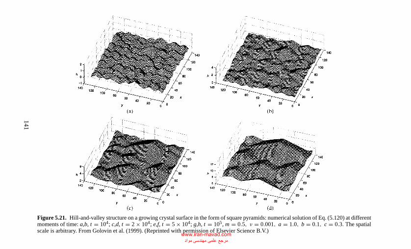
P1:GK
E
Chap-05
CB
381-Davis
May
17,200117:3
Char
Count=
0
Figure 5.21. Hill-and-valley structure on a growing crystal surface in the form of square pyramids: numerical solution of Eq. (5.120) at differentmoments of time: a,b, t = 104; c,d, t = 2 × 10⁴; e,f, t = 5 × 10⁴; g,h, t = 105, m = 0.5, ν = 0.001, a = 1.0, b = 0.1, c = 0.3. The spatialscale is arbitrary. From Golovin et al. (1999). (Reprinted with permission of Elsevier Science B.V.)
141
www.iran-mavad.com مرجع علمی مھندسی مواد
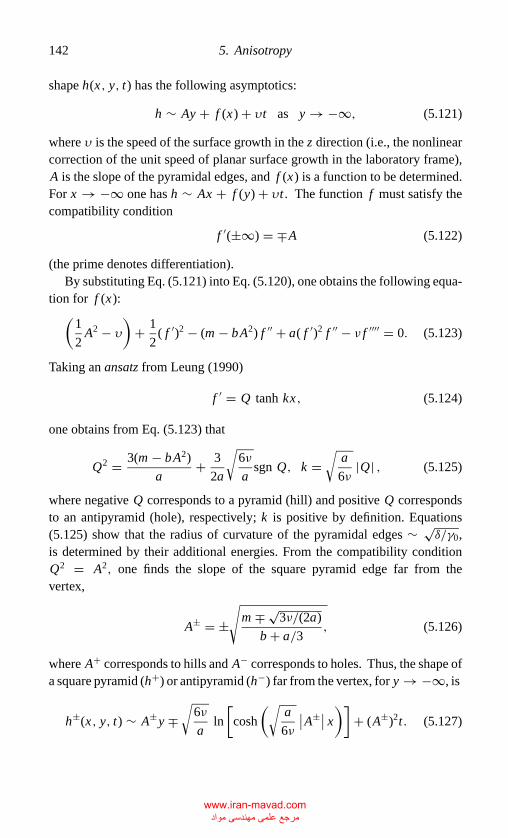
P1: GKE
Chap-05 CB381-Davis May 17, 2001 17:3 Char Count= 0
142 5. Anisotropy
shape h(x, y, t) has the following asymptotics:
h ∼ Ay + f (x) + υt as y → −∞, (5.121)
where υ is the speed of the surface growth in the z direction (i.e., the nonlinearcorrection of the unit speed of planar surface growth in the laboratory frame),A is the slope of the pyramidal edges, and f (x) is a function to be determined.For x → −∞ one has h ∼ Ax + f (y) + υt . The function f must satisfy thecompatibility condition
f ′(±∞) = ∓A (5.122)
(the prime denotes differentiation).By substituting Eq. (5.121) into Eq. (5.120), one obtains the following equa-
tion for f (x):(1
2A2 − υ
)+ 1
2( f ′)2 − (m − bA2) f ′′ + a( f ′)2 f ′′ − ν f ′′′′ = 0. (5.123)
Taking an ansatz from Leung (1990)
f ′ = Q tanh kx, (5.124)
one obtains from Eq. (5.123) that
Q2 = 3(m − bA2)
a+ 3
2a
√6ν
asgn Q, k =
√a
6ν|Q| , (5.125)
where negative Q corresponds to a pyramid (hill) and positive Q correspondsto an antipyramid (hole), respectively; k is positive by definition. Equations(5.125) show that the radius of curvature of the pyramidal edges ∼ √
δ/γ0,is determined by their additional energies. From the compatibility conditionQ2 = A2, one finds the slope of the square pyramid edge far from thevertex,
A± = ±√
m ∓ √3ν/(2a)
b + a/3, (5.126)
where A+ corresponds to hills and A− corresponds to holes. Thus, the shape ofa square pyramid (h+) or antipyramid (h−) far from the vertex, for y → −∞, is
h±(x, y, t) ∼ A±y ∓√
6ν
aln
[cosh
(√a
6ν
∣∣A±∣∣ x)]+ (A±)2t. (5.127)
www.iran-mavad.com مرجع علمی مھندسی مواد
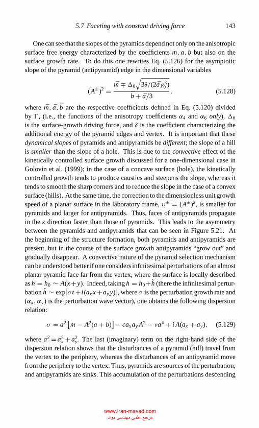
P1: GKE
Chap-05 CB381-Davis May 17, 2001 17:3 Char Count= 0
5.7 Faceting with constant driving force 143
One can see that the slopes of the pyramids depend not only on the anisotropicsurface free energy characterized by the coefficients m, a, b but also on thesurface growth rate. To do this one rewrites Eq. (5.126) for the asymptoticslope of the pyramid (antipyramid) edge in the dimensional variables
(A±)2 =m ∓�0
√3δ/(2aγ 3
0 )
b + a/3, (5.128)
where m, a, b are the respective coefficients defined in Eq. (5.120) dividedby �, (i.e., the functions of the anisotropy coefficients α4 and α6 only), �0
is the surface-growth driving force, and δ is the coefficient characterizing theadditional energy of the pyramid edges and vertex. It is important that thesedynamical slopes of pyramids and antipyramids be different; the slope of a hillis smaller than the slope of a hole. This is due to the convective effect of thekinetically controlled surface growth discussed for a one-dimensional case inGolovin et al. (1999); in the case of a concave surface (hole), the kineticallycontrolled growth tends to produce caustics and steepens the slope, whereas ittends to smooth the sharp corners and to reduce the slope in the case of a convexsurface (hills). At the same time, the correction to the dimensionless unit growthspeed of a planar surface in the laboratory frame, υ± = (A±)2, is smaller forpyramids and larger for antipyramids. Thus, faces of antipyramids propagatein the z direction faster than those of pyramids. This leads to the asymmetrybetween the pyramids and antipyramids that can be seen in Figure 5.21. Atthe beginning of the structure formation, both pyramids and antipyramids arepresent, but in the course of the surface growth antipyramids “grow out” andgradually disappear. A convective nature of the pyramid selection mechanismcan be understood better if one considers infinitesimal perturbations of an almostplanar pyramid face far from the vertex, where the surface is locally describedas h = h0 ∼ A(x+y). Indeed, taking h = h0+h (there the infinitesimal pertur-bation h ∼ exp[σ t + i(ax x +ay y)], where σ is the perturbation growth rate and(αx , αy) is the perturbation wave vector), one obtains the following dispersionrelation:
σ = a2[m − A2(a + b)
]− caxay A2 − νa4 + i A(ax + ay), (5.129)
where a2 = a2x + a2
y . The last (imaginary) term on the right-hand side of thedispersion relation shows that the disturbances of a pyramid (hill) travel fromthe vertex to the periphery, whereas the disturbances of an antipyramid movefrom the periphery to the vertex. Thus, pyramids are sources of the perturbation,and antipyramids are sinks. This accumulation of the perturbations descending
www.iran-mavad.com مرجع علمی مھندسی مواد
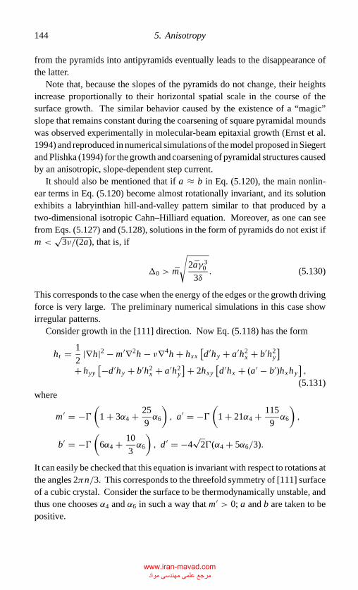
P1: GKE
Chap-05 CB381-Davis May 17, 2001 17:3 Char Count= 0
144 5. Anisotropy
from the pyramids into antipyramids eventually leads to the disappearance ofthe latter.
Note that, because the slopes of the pyramids do not change, their heightsincrease proportionally to their horizontal spatial scale in the course of thesurface growth. The similar behavior caused by the existence of a “magic”slope that remains constant during the coarsening of square pyramidal moundswas observed experimentally in molecular-beam epitaxial growth (Ernst et al.1994) and reproduced in numerical simulations of the model proposed in Siegertand Plishka (1994) for the growth and coarsening of pyramidal structures causedby an anisotropic, slope-dependent step current.
It should also be mentioned that if a ≈ b in Eq. (5.120), the main nonlin-ear terms in Eq. (5.120) become almost rotationally invariant, and its solutionexhibits a labryinthian hill-and-valley pattern similar to that produced by atwo-dimensional isotropic Cahn–Hilliard equation. Moreover, as one can seefrom Eqs. (5.127) and (5.128), solutions in the form of pyramids do not exist ifm <
√3ν/(2a), that is, if
�0 > m
√2aγ 3
0
3δ. (5.130)
This corresponds to the case when the energy of the edges or the growth drivingforce is very large. The preliminary numerical simulations in this case showirregular patterns.
Consider growth in the [111] direction. Now Eq. (5.118) has the form
ht = 1
2|∇h|2 − m ′∇2h − ν∇4h + hxx
[d ′hy + a′h2
x + b′h2y
]+ hyy
[−d ′hy + b′h2x + a′h2
y
]+ 2hxy[d ′hx + (a′ − b′)hxhy
],
(5.131)where
m ′ = −�(
1 + 3α4 + 25
9α6
), a′ = −�
(1 + 21α4 + 115
9α6
),
b′ = −�(
6α4 + 10
3α6
), d ′ = −4
√2�(α4 + 5α6/3).
It can easily be checked that this equation is invariant with respect to rotations atthe angles 2πn/3. This corresponds to the threefold symmetry of [111] surfaceof a cubic crystal. Consider the surface to be thermodynamically unstable, andthus one chooses α4 and α6 in such a way that m ′ > 0; a and b are taken to bepositive.
www.iran-mavad.com مرجع علمی مھندسی مواد
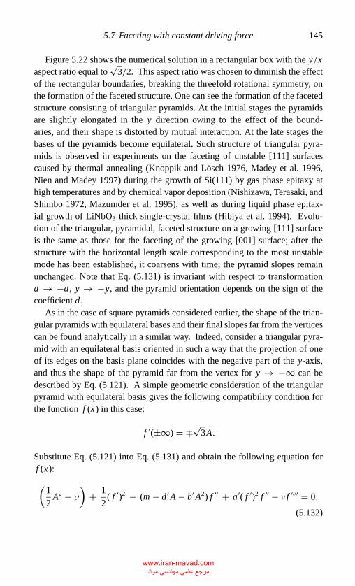
P1: GKE
Chap-05 CB381-Davis May 17, 2001 17:3 Char Count= 0
5.7 Faceting with constant driving force 145
Figure 5.22 shows the numerical solution in a rectangular box with the y/xaspect ratio equal to
√3/2. This aspect ratio was chosen to diminish the effect
of the rectangular boundaries, breaking the threefold rotational symmetry, onthe formation of the faceted structure. One can see the formation of the facetedstructure consisting of triangular pyramids. At the initial stages the pyramidsare slightly elongated in the y direction owing to the effect of the bound-aries, and their shape is distorted by mutual interaction. At the late stages thebases of the pyramids become equilateral. Such structure of triangular pyra-mids is observed in experiments on the faceting of unstable [111] surfacescaused by thermal annealing (Knoppik and Losch 1976, Madey et al. 1996,Nien and Madey 1997) during the growth of Si(111) by gas phase epitaxy athigh temperatures and by chemical vapor deposition (Nishizawa, Terasaki, andShimbo 1972, Mazumder et al. 1995), as well as during liquid phase epitax-ial growth of LiNbO3 thick single-crystal films (Hibiya et al. 1994). Evolu-tion of the triangular, pyramidal, faceted structure on a growing [111] surfaceis the same as those for the faceting of the growing [001] surface; after thestructure with the horizontal length scale corresponding to the most unstablemode has been established, it coarsens with time; the pyramid slopes remainunchanged. Note that Eq. (5.131) is invariant with respect to transformationd → −d, y → −y, and the pyramid orientation depends on the sign of thecoefficient d.
As in the case of square pyramids considered earlier, the shape of the trian-gular pyramids with equilateral bases and their final slopes far from the verticescan be found analytically in a similar way. Indeed, consider a triangular pyra-mid with an equilateral basis oriented in such a way that the projection of oneof its edges on the basis plane coincides with the negative part of the y-axis,and thus the shape of the pyramid far from the vertex for y → −∞ can bedescribed by Eq. (5.121). A simple geometric consideration of the triangularpyramid with equilateral basis gives the following compatibility condition forthe function f (x) in this case:
f ′(±∞) = ∓√
3A.
Substitute Eq. (5.121) into Eq. (5.131) and obtain the following equation forf (x):
(1
2A2 − υ
)+ 1
2( f ′)2 − (m − d ′ A − b′ A2) f ′′ + a′( f ′)2 f ′′ − ν f ′′′′ = 0.
(5.132)
www.iran-mavad.com مرجع علمی مھندسی مواد
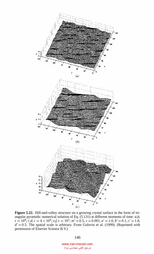
P1: GKE
Chap-05 CB381-Davis May 17, 2001 17:3 Char Count= 0
Figure 5.22. Hill-and-valley structure on a growing crystal surface in the form of tri-angular pyramids: numerical solution of Eq. (5.131) at different moments of time: a,b,t = 104; c,d, t = 4 × 10⁴; e,f, t = 105; m′ = 0.5, ν= 0.001, a′ = 1.0, b′ = 0.1, c′ = 1.8,d ′ = 0.5. The spatial scale is arbitrary. From Golovin et al. (1999). (Reprinted withpermission of Elsevier Science B.V.)
146
www.iran-mavad.com مرجع علمی مھندسی مواد
P1: GKE
Chap-05 CB381-Davis May 17, 2001 17:3 Char Count= 0
5.7 Faceting with constant driving force 147
Using the same ansatz (5.124) as before for f ′, one obtains fromEq. (5.132)
Q2 = 3(m − d ′ A − b′ A2)
a′ + 3
2a′
√6ν
a′ sgn Q,
k =√
a′
6ν|Q|, (5.133)
where, as in the case considered in the preceding section, negative Q corre-sponds to a pyramid, and positive Q corresponds to an antipyramid, respectively.From the compatibility condition, Q2 = 3A2, one obtains a quadratic equa-tion for the slope of the triangular pyramid edge far from the vertex. A sta-ble solution of this equation is determined by the sign of the coefficient d ′,namely,
A± =−d ′ −
√(d ′)2 + 4(a′ + b′)
[m ′ ∓ √
3ν/(2a′)]
2(a′ + b′)
for d ′ > 0,
A± =−d ′ +
√(d ′)2 + 4(a′ + b′)
[m ′ ∓ √
3ν/(2a′)]
2(a′ + b′)
for d ′ < 0,
(5.134)
where A± corresponds to the hills (A+) and holes (A−), respectively. Thus, theshape of the triangular pyramids (antipyramids) for y → −∞ is
h±(x, y, t) ∼ A±y ∓√
6ν
aln
[cosh
(√a
2ν
∣∣A±∣∣ x)]+ 2(A±)2t. (5.135)
One can see that the parameters and evolution of triangular pyramids andantipyramids are distinguished, as discussed in the preceding section for thecase of square pyramids. The solution in the form of triangular pyramids existsif (d ′)2 + 4(a′ + b′)[m ′ − √
3ν/(2a′)] > 0, that is, as in the case of the squarepyramids, the triangular pyramids cannot form for large ν corresponding toeither very fast surface growth or to a large edge energy; these cases are notconsidered here.
Consider now growth in the [110] direction. Equation (5.118) reads
ht = 1
2|∇h|2 + hxx
[−mx + axh2x + bxh2
y
]+ hyy[−my + ayh2
x + byh2y
]+ chxyhxhy − v∇4h,
www.iran-mavad.com مرجع علمی مھندسی مواد
P1: GKE
Chap-05 CB381-Davis May 17, 2001 17:3 Char Count= 0
148 5. Anisotropy
where
mx = −�(
9
2α4 + 25
4α6 + 1
), my = �
(3
2α4 + 5
4α6 − 1
),
ax = −�(
69
2α4 + 205
4α6 + 1
), bx = −�
(3α4 + 45
4α6
),
ay = −�(6α4 + 15α6), by = �
(45
2α4 + 25
2α6 − 1
),
c = −�(
21α4 + 115
2α6 + 2
).
(5.136)
Here consider the anisotropy coefficients α4 and α6 to be such that the [110]surface is thermodynamically unstable in both x and y directions, that is, my >
0. The other coefficients are also taken to be positive in the simulations.Equation (5.136) is invariant with respect to transformations x → −x,
y → −y, but it is not invariant with respect to the transformation x → y. Thisreflects the twofold symmetry of the [110] surface. Thus, one can expect thefaceting instability of this surface to result in the structure of either rhombicpyramids or grooves. One observes that the resulting structure depends on thedegree of anisotropy. Figure 5.23 shows the evolution of the faceted surface inthe case when the asymmetry between the x and y directions is not very large butthe anisotropy is still large so that bx/ax and ay/by are small. First, one observesthe formation of a system of grooves (Figure 5.23(a)). Later, the grooves decayinto islands in the form of rhombic pyramids (Figure 5.23(b)). Similar rhombicpyramids are observed such as during the epitaxial growth of an In–Ga–As alloyon the InP(001) surface (Jacob et al. 1997). The rhombic pyramids coarsen intime (Figure 5.23(c)), but although the shapes of the square and triangularpyramids remain self-similar during the coarsening, the coarsening rates of therhombic pyramids are different in the x and y directions. Namely, one observesthat the coarsening in the y direction goes a little faster, and thus the rhombicpyramids gradually thicken in the y direction and tend to a limiting rhombicshape that can be found analytically for regions far from the vertex in a waysimilar to that described in the preceding sections for the square and triangularpyramids. Indeed, consider a rhombic pyramid oriented in such a way that theprojections of its edges on the basis plane coincide with the x- and y-axes. Forthe asymptotics of the pyramid shape far from the vertex, one has
h ∼ Ax + f (y) + υt, f ′(±∞) = ∓B as x → −∞,
h ∼ By + g(x) + υt, g′(±∞) = ∓A as y → −∞.(5.137)
www.iran-mavad.com مرجع علمی مھندسی مواد
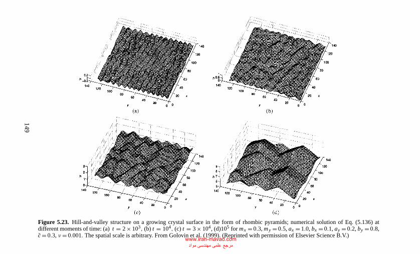
P1:GK
E
Chap-05
CB
381-Davis
May
17,200117:3
Char
Count=
0
Figure 5.23. Hill-and-valley structure on a growing crystal surface in the form of rhombic pyramids; numerical solution of Eq. (5.136) atdifferent moments of time: (a) t = 2 × 10³, (b) t = 104, (c) t = 3 × 10⁴, (d)105 for mx = 0.3, my = 0.5, ax = 1.0, bx = 0.1, ay = 0.2, by = 0.8,c = 0.3, ν= 0.001. The spatial scale is arbitrary. From Golovin et al. (1999). (Reprinted with permission of Elsevier Science B.V.)
149
www.iran-mavad.com مرجع علمی مھندسی مواد
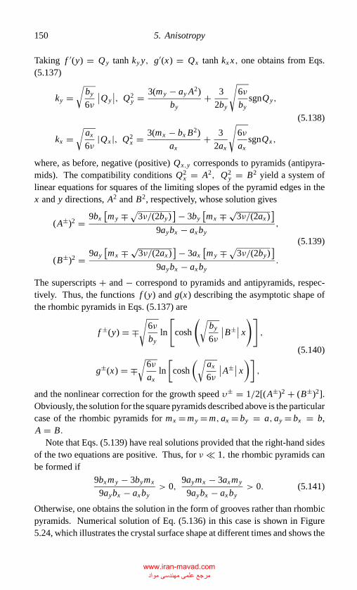
P1: GKE
Chap-05 CB381-Davis May 17, 2001 17:3 Char Count= 0
150 5. Anisotropy
Taking f ′(y) = Qy tanh ky y, g′(x) = Qx tanh kx x, one obtains from Eqs.(5.137)
ky =√
by
6ν
∣∣Qy
∣∣, Q2y = 3(my − ay A2)
by+ 3
2by
√6ν
bysgnQy,
kx =√
ax
6ν|Qx |, Q2
x = 3(mx − bx B2)
ax+ 3
2ax
√6ν
axsgnQx ,
(5.138)
where, as before, negative (positive) Qx,y corresponds to pyramids (antipyra-mids). The compatibility conditions Q2
x = A2, Q2y = B2 yield a system of
linear equations for squares of the limiting slopes of the pyramid edges in thex and y directions, A2 and B2, respectively, whose solution gives
(A±)2 = 9bx[my ∓√3ν/(2by)
]− 3by[mx ∓ √
3ν/(2ax )]
9aybx − axby,
(B±)2 = 9ay[mx ∓ √
3ν/(2ax )]− 3ax
[my ∓√3ν/(2by)
]9aybx − axby
.
(5.139)
The superscripts + and − correspond to pyramids and antipyramids, respec-tively. Thus, the functions f (y) and g(x) describing the asymptotic shape ofthe rhombic pyramids in Eqs. (5.137) are
f ±(y) = ∓√
6ν
byln
[cosh
(√by
6ν
∣∣B±∣∣ x)],
g±(x) = ∓√
6ν
axln
[cosh
(√ax
6ν
∣∣A±∣∣ x)] ,(5.140)
and the nonlinear correction for the growth speed υ± = 1/2[(A±)2 + (B±)2].Obviously, the solution for the square pyramids described above is the particularcase of the rhombic pyramids for mx = my = m, ax = by = a, ay = bx = b,A = B.
Note that Eqs. (5.139) have real solutions provided that the right-hand sidesof the two equations are positive. Thus, for ν 1, the rhombic pyramids canbe formed if
9bxmy − 3bymx
9aybx − axby> 0,
9aymx − 3axmy
9aybx − axby> 0. (5.141)
Otherwise, one obtains the solution in the form of grooves rather than rhombicpyramids. Numerical solution of Eq. (5.136) in this case is shown in Figure5.24, which illustrates the crystal surface shape at different times and shows the
www.iran-mavad.com مرجع علمی مھندسی مواد
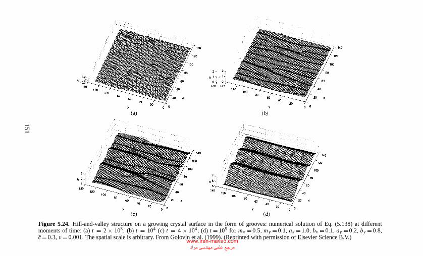
P1:GK
E
Chap-05
CB
381-Davis
May
17,200117:3
Char
Count=
0
Figure 5.24. Hill-and-valley structure on a growing crystal surface in the form of grooves: numerical solution of Eq. (5.138) at differentmoments of time: (a) t = 2 × 10³, (b) t = 104 (c) t = 4 × 10⁴; (d) t = 105 for mx = 0.5, my = 0.1, ax = 1.0, bx = 0.1, ay = 0.2, by = 0.8,c = 0.3, ν= 0.001. The spatial scale is arbitrary. From Golovin et al. (1999). (Reprinted with permission of Elsevier Science B.V.)
151
www.iran-mavad.com مرجع علمی مھندسی مواد
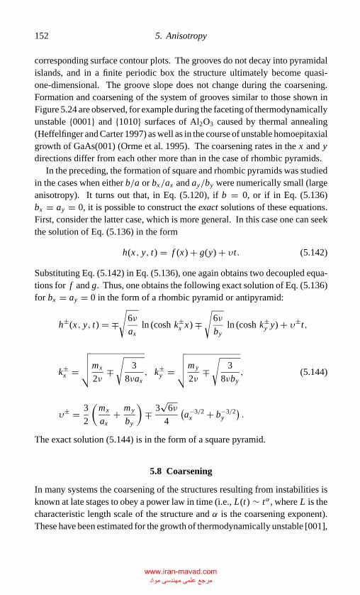
P1: GKE
Chap-05 CB381-Davis May 17, 2001 17:3 Char Count= 0
152 5. Anisotropy
corresponding surface contour plots. The grooves do not decay into pyramidalislands, and in a finite periodic box the structure ultimately become quasi-one-dimensional. The groove slope does not change during the coarsening.Formation and coarsening of the system of grooves similar to those shown inFigure 5.24 are observed, for example during the faceting of thermodynamicallyunstable {0001} and {1010} surfaces of Al2O3 caused by thermal annealing(Heffelfinger and Carter 1997) as well as in the course of unstable homoepitaxialgrowth of GaAs(001) (Orme et al. 1995). The coarsening rates in the x and ydirections differ from each other more than in the case of rhombic pyramids.
In the preceding, the formation of square and rhombic pyramids was studiedin the cases when either b/a or bx/ax and ay/by were numerically small (largeanisotropy). It turns out that, in Eq. (5.120), if b = 0, or if in Eq. (5.136)bx = ay = 0, it is possible to construct the exact solutions of these equations.First, consider the latter case, which is more general. In this case one can seekthe solution of Eq. (5.136) in the form
h(x, y, t) = f (x) + g(y) + υt. (5.142)
Substituting Eq. (5.142) in Eq. (5.136), one again obtains two decoupled equa-tions for f and g. Thus, one obtains the following exact solution of Eq. (5.136)for bx = ay = 0 in the form of a rhombic pyramid or antipyramid:
h±(x, y, t) = ∓√
6ν
axln (cosh k±
x x) ∓√
6ν
byln (cosh k±
y y) + υ±t,
k±x =
√√√√mx
2ν∓√
3
8νax, k±
y =√√√√my
2ν∓√
3
8νby, (5.144)
υ± = 3
2
(mx
ax+ my
by
)∓ 3
√6ν
4
(a−3/2
x + b−3/2y
).
The exact solution (5.144) is in the form of a square pyramid.
5.8 Coarsening
In many systems the coarsening of the structures resulting from instabilities isknown at late stages to obey a power law in time (i.e., L(t) ∼ tα , where L is thecharacteristic length scale of the structure and α is the coarsening exponent).These have been estimated for the growth of thermodynamically unstable [001],
www.iran-mavad.com مرجع علمی مھندسی مواد
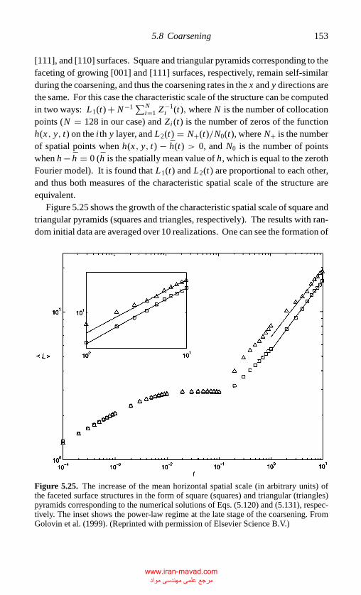
P1: GKE
Chap-05 CB381-Davis May 17, 2001 17:3 Char Count= 0
5.8 Coarsening 153
[111], and [110] surfaces. Square and triangular pyramids corresponding to thefaceting of growing [001] and [111] surfaces, respectively, remain self-similarduring the coarsening, and thus the coarsening rates in the x and y directions arethe same. For this case the characteristic scale of the structure can be computedin two ways: L1(t) + N−1∑N
i=1 Z−1i (t), where N is the number of collocation
points (N = 128 in our case) and Zi (t) is the number of zeros of the functionh(x, y, t) on the i th y layer, and L2(t) = N+(t)/N0(t), where N+ is the numberof spatial points when h(x, y, t) − h(t) > 0, and N0 is the number of pointswhen h − h = 0 (h is the spatially mean value of h, which is equal to the zerothFourier model). It is found that L1(t) and L2(t) are proportional to each other,and thus both measures of the characteristic spatial scale of the structure areequivalent.
Figure 5.25 shows the growth of the characteristic spatial scale of square andtriangular pyramids (squares and triangles, respectively). The results with ran-dom initial data are averaged over 10 realizations. One can see the formation of
Figure 5.25. The increase of the mean horizontal spatial scale (in arbitrary units) ofthe faceted surface structures in the form of square (squares) and triangular (triangles)pyramids corresponding to the numerical solutions of Eqs. (5.120) and (5.131), respec-tively. The inset shows the power-law regime at the late stage of the coarsening. FromGolovin et al. (1999). (Reprinted with permission of Elsevier Science B.V.)
www.iran-mavad.com مرجع علمی مھندسی مواد
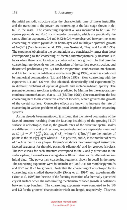
P1: GKE
Chap-05 CB381-Davis May 17, 2001 17:3 Char Count= 0
154 5. Anisotropy
the initial periodic structure after the characteristic time of linear instabilityand the transition to the power-law coarsening at the late stage shown in de-tail in the inset. The coarsening exponent α was measured to be 0.47 forsquare pyramids and 0.45 for triangular pyramids, which are practically thesame. Similar exponents, 0.4 and 0.42 ± 0.4, were observed in experiments oncoarsening of square pyramids in homolayer and multilayer epitaxial growthof Ge(001) (Van Nostrand et al. 1995, van Nostrand, Chey, and Cahill 1995).The exponents obtained in the computations are considerably larger than thosecorresponding to the coarsening of faceted thermodynamically unstable sur-faces when there is no kinetically controlled surface growth. In that case thecoarsening rate depends on the mechanism of the surface reconstruction, andtheoretical predictions give 1/4 for the evaporation–condensation mechanismand 1/6 for the surface-diffusion mechanism (Krug 1997), which is confirmedby numerical computations (Liu and Metiu 1993). Slow coarsening with theexponents 1/4 and 1/6 was also obtained, theoretically and experimentally,in different problems of epitaxial growth and molecular-beam epitaxy. Thepresent exponents are closer to those predicted by Mullins for the evaporation–condensation mechanism, that is, 1/2 (Mullins 1961). One can attribute the fastcoarsening here to the convective effect of kinetics, which governs the growthof the crystal surface. Convective effects are known to increase the rate ofcoarsening in various problems of spinodal decomposition in phase-separatingsystems.
As has already been mentioned, it is found that the rate of coarsening of thefaceted structure resulting from the faceting instability of the growing [110]surface is anisotropic, that is, the growth rates of the structure spatial scalesare different in x and y directions, respectively, and are separately measuredas 〈Lx,y〉 = N−1∑N
i=1 2(nx , ny)+i /Zi , where (nx )+i [(nx )+i ] are the number ofpoints in the i th x[y] layer where h− h is positive, and Zi is the number of zerosof h − h in the i th x or y layer. Figure 5.26 shows the coarsening of anisotropicfaceted structures for rhombic pyramids (diamonds) and for grooves (circles).The two curves for each structure correspond to the x and y directions in thesurface plane; the results are averaged over 10 realizations with different randominitial data. The power-law coarsening regime is shown in detail in the inset.The coarsening exponents were found to be 0.61 and 0.41 for rhombic pyramidsand 0.57 and 0.23 for grooves. Note that the coarsening of anisotropic facetscoarsening was studied theoretically (Song et al. 1997) and experimentally(Yoon et al. 1998) for the case of the faceting transition of a thermally quenchedcrystal surface when the rate-limiting mechanism of facet growth is collisionsbetween step bunches. The coarsening exponents were computed to be 1/6and 1/2 for the grooves’ characteristic width and length, respectively. This was
www.iran-mavad.com مرجع علمی مھندسی مواد
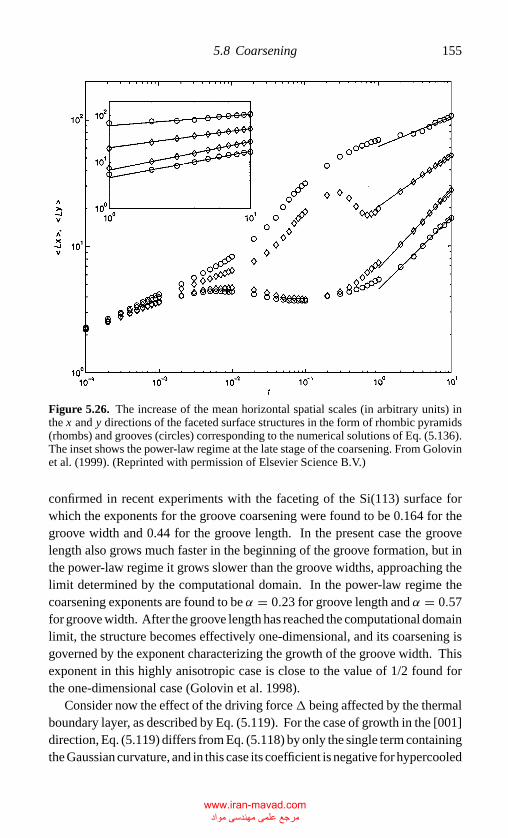
P1: GKE
Chap-05 CB381-Davis May 17, 2001 17:3 Char Count= 0
5.8 Coarsening 155
Figure 5.26. The increase of the mean horizontal spatial scales (in arbitrary units) inthe x and y directions of the faceted surface structures in the form of rhombic pyramids(rhombs) and grooves (circles) corresponding to the numerical solutions of Eq. (5.136).The inset shows the power-law regime at the late stage of the coarsening. From Golovinet al. (1999). (Reprinted with permission of Elsevier Science B.V.)
confirmed in recent experiments with the faceting of the Si(113) surface forwhich the exponents for the groove coarsening were found to be 0.164 for thegroove width and 0.44 for the groove length. In the present case the groovelength also grows much faster in the beginning of the groove formation, but inthe power-law regime it grows slower than the groove widths, approaching thelimit determined by the computational domain. In the power-law regime thecoarsening exponents are found to be α = 0.23 for groove length and α = 0.57for groove width. After the groove length has reached the computational domainlimit, the structure becomes effectively one-dimensional, and its coarsening isgoverned by the exponent characterizing the growth of the groove width. Thisexponent in this highly anisotropic case is close to the value of 1/2 found forthe one-dimensional case (Golovin et al. 1998).
Consider now the effect of the driving force� being affected by the thermalboundary layer, as described by Eq. (5.119). For the case of growth in the [001]direction, Eq. (5.119) differs from Eq. (5.118) by only the single term containingthe Gaussian curvature, and in this case its coefficient is negative for hypercooled
www.iran-mavad.com مرجع علمی مھندسی مواد
P1: GKE
Chap-05 CB381-Davis May 17, 2001 17:3 Char Count= 0
156 5. Anisotropy
solidification in a thermodynamically unstable direction. However, for othersystems the coefficient may be positive.
For g > 0 the pyramids are more rounded and look more like “square” cones.Such rounded square pyramids as well as almost rounded cones are observedin some epitaxial growth systems (van Erk et al. 1980). It is thus conceivablethat the rounding of the pyramid edges in the course of epitaxial growth canbe caused by the effect of interaction between the thermal or concentrationfield and the shape of the crystal surface (if the growth is controlled by theevaporation–condensation mechanism).
For g < 0, instead of cones there are now square rounded holes formingon a growing thermodynamically unstable surface. Square, triangular, andspiral holes on the crystal surface are observed in experiments when the crystalsurface is evaporating (Bethge and Keller 1974, Lampert and Reichelt 1981,Surek, Hirth, and Pound 1973), and they are believed to be caused by thedislocations meeting the crystal surface. It seems that there are no experimentalobservations of the formation of holes on a growing crystal surface. However,because the considered model of surface growth is proposed for the evaporation–condensation mechanism, such effects of mass or heat transfer in diffusionboundary layers near the crystal surface are conceivable.
5.9 Remarks
The influence of morphological instability on the anisotropy of surface energy γand attachment kinetics µ is induced by the presence of crystallographic struc-ture and sets the stage for a competition with the imposed heat-flow direction.
In the case of equilibrium figures, the case of surface-energy anisotropybeing “small,” F = γ + γθθ > 0 always, gives rise to distorted but smoothshapes. When the anisotropy is “large,” F < 0 somewhere, the shapes havemissing orientations and hence corners where the slope is discontinuous.
The remaining discussion concerned instability and dynamic evolution ofinterfaces. For “small” anisotropies the bifurcations to squares or hexagonsinvolve imperfections, traveling cells, and new branches that depend on theanisotropy for the existence and stability. Anisotropy of either γ and µ candelay or remove the tendency in two dimensions for tip splitting present in theisotropic case.
For a plane front in one dimension in a hypercooled melt, evolution equa-tions valid in the longwave limit show traveling, asymmetric cells that displayanomolous coarsening due to the convective nature of the evolution driven byphase transformation. Here the coarsening rate is t1/2 for very long times andt for earlier times, compared with the classical result lnt , for nonconvectivesystems.
www.iran-mavad.com مرجع علمی مھندسی مواد
P1: GKE
Chap-05 CB381-Davis May 17, 2001 17:3 Char Count= 0
References 157
For a planar front in a hypercooled melt of a material with “large” surfacetension anisotropy, convective Cahn–Hilliard equations govern the evolution ofpyramids and grooves and again lead to anomalously rapid coarsening.
In the process of analyzing such evolutions, Golovin et al. (1998) obtaineda general expression for the Gibbs–Thomson equation for pure materials thatdisplay surface tension anisotropy. They found that the equilibrium temperatureT e on the interface has the form
T e = Tm
[1 − K
Lv(F − F1)
], (5.145a)
where
F = γ + γθθ (5.145b)
F1 = K
(1 + ∂2
∂θ2
)∂γ
∂K+ ∂2γ
∂K 2
(∂K
∂θ2
)2
(5.145c)
and
K = −2H (5.145d)
This form can be used to write down the chemical potential and hence can beused in problems other than hypercooled solidification such as surface diffusionon thin films.
References
Akaiwa, N., Hardy, S. C., and Voorhees, P. W. (1991). The effect of convection onOstwald ripening in solid–liquid mixtures, Acta Metall. Mater. 39, 2931–2942.
Alikakos, N., Bates, P. W., and Fusco, G. (1991). Slow motion for the Cahn–Hilliardequation in one space dimension, J. Diff. Eqs. 90, 81–135.
Angenent, S., and Gurtin, M. E. (1989). Multiphase thermomechanics with interfacialstructure. 2. Evolution of an isothermal interface, Arch. Rational Mech. Anal. 108,323–391.
Bar, D. E., and Nepomnyashchy, A. A. (1995). Stability of periodic waves governed bythe modified Kawahara equation, Physica D 86, 586–602.
Barabasi, A.-L., Araujo, M., and Stanley, H. E. (1992). Three-dimensional Toom model:Convection to the anisotropic Kardar–Parisi–Zhang equation, Phys. Rev. Lett. 68,3729–3732.
Bates, P. W., and Fife, P. C. (1993). The dynamics of nucleation for the Cahn–Hilliardequation, SIAM J. Appl. Math. 53, 990–1008.
Bates, P. W., and Xun, J. P. (1994). Metastable patterns for the Cahn–Hilliard equation,Part I, J. Diff. Eqs. 111, 421–457.
. (1995). Metastable patterns for the Cahn–Hilliard equation, Part 2: Layer dy-namics and slow invariant manifold, J. Diff. Eqs. 117, 165–216.
Bates, P. W., Fife, P. C., Gardner, R. A., and Jones, C. K. R. T. (1997). Phase field modelsfor hypercooled solidification, Physica D 104, 1–31.
www.iran-mavad.com مرجع علمی مھندسی مواد
P1: GKE
Chap-05 CB381-Davis May 17, 2001 17:3 Char Count= 0
158 5. Anisotropy
Bauser, E., and Lochner, K. S. (1981). Steps on facets of solution grown GaAs epitaxiallayers, J. Crystal Growth 55, 457–464.
Bethge, H., and Keller, K. W. (1974). Evaporation rate of NaC�–H in a vacuum, J.Crystal Growth 23, 105–112.
Bloem, J., Oei, Y. S., de Moor, H. H. C., Hanssen, J. H. L., and Giling, L. J. (1983). Nearequilibrium growth of silicon by CVD. 1. The Si-C�–H system, J. Crystal Growth65, 399–405.
Brattkus, K., and Davis, S. H. (1988). Cellular growth near absolute stability Phys. Rev.B 38, 11452–11460.
Brush, L. N., and Sekerka, R. F. (1989). A numerical study of two-dimensional crystalgrowth forms in the presence of anisotropic growth kinetics, J. Crystal Growth 96,419–441.
Cabrera, N. (1963). On stability of structure of crystal surfaces, in Symposium on Proper-ties of Surfaces, 24-31, American Society for Testing and Materials, Philadelphia.
Cahn, J. W., and Hilliard, J. E. (1958). Free energy of a nonuniform systems. III. Nu-cleation in a two-component incompressible fluid, J. Chem. Phys. 31, 688–699.
Cahn, J. W., and Hoffman, D. W. (1974). A vector thermodynamics for anisotropicsurfaces–II. Curved and facetted surfaces, Acta Metall. Mater. 22, 1205–1214.
Carlo, A. D., Gurtin, M. E., and Podio-Guidugli, P. (1992). A regularized equation foranisotropic motion-by-curvature, SIAM J. Appl. Math. 52, 1111–1119.
Chang, H.-C., Demekhin, E. A., and Kopelevich, D. I. (1993). Laminarizing effect ofdispersion in an active–dissipative nonlinear medium, Physica D 63, 299–320.
Chernov, A. A., Coriell, S. R., and Murray, B. T. (1993). Morphological stability of avicinal face induced by step flow, J. Crystal Growth 132, 405–413.
Coriell, S. R., and Sekerka, R. F. (1976). The effect of the anisotropy of surface tensionand interface kinetics on morphological instability, J. Crystal Growth 34, 157–163.
Emmott, C. L., and Bray, A. J. (1996). Coarsening dynamics of a one-dimensional drivenCahn–Hilliard system. Phys. Rev. E 54, 4568–4575.
Ernst, H.-J., Fabre, F., Folkerts, R., and Lapujoulade, J. (1994). Observation of a growthinstability during low-temperature molecular-beam epitaxy, Phys. Rev. Lett. 72,112–115.
Fogedby, H. C. (1998). Solitons and diffusive modes in the noiseless Burgers equation:Stability analysis, Phys. Rev. E 57, 2331–2337.
Golovin, A. A., and Davis, S. H. (1998). Effect of anisotropy on morphological instabilityin the freezing of a hypercooled melt, Physica D 116, 363–391.
Golovin, A. A., Davis, S. H., and Nepomnyashchy, A. A. (1998). A convective Cahn–Hilliard formation of facets and corners in crystal growth, Physica D 122, 202–230.
Golovin, A. A., Davis, S. H., and Nepomnyashchy, A. A. (1999). Model for faceting ina kinetically controlled crystal growth, Phys. Rev. E 59, 803–825.
Grimm, H. P., Davis, S. H., and McFadden, G. B. (1999). Steps, kinetic anisotropy, andlong-wave instabilities in directional solidification, Phys. Rev. E 59, 5629–5640.
Gurtin, M. E. (1993). Thermomechanics of Evolving Phase Boundaries in the Plane,Clarendon Press, Oxford.
Heffelfinger, J. R., and Carter, C. B. (1997). Mechanisms of surface faceting and coars-ening, Surf. Sci 389, 188–200.
Herring, C. (1951). Surface tension as a motivation for sintering, in W. E. Kingston,editor, Physics of Powder Metall., Chap. 8, McGraw–Hill, New York.
Hibiya, T., Suzuki, H., Yonenaga, L., Kimura, S., Kawaguchi, T., Shishido, T., andFukuda, T. (1994). Liquid phase epitaxial growth and characterization of LiNO3single crystal films, J. Crystal Growth 144, 213–217.
www.iran-mavad.com مرجع علمی مھندسی مواد
P1: GKE
Chap-05 CB381-Davis May 17, 2001 17:3 Char Count= 0
References 159
Hoyle, R. B., McFadden, G. B., and Davis, S. H. (1996). Pattern selection with anisotropyduring directional solidification, Phil. Trans. Roy. Soc. Lond. A 354, 2915–2949.
Jacob, D., Androussi, Y., Benabbas, T., Francois, P., Ferre, D., Lefebvre, A., Gendry, M.,and Robach, Y. (1997). Elastic misfit stress relaxation in In 1
4Ga 3
4As layers grown
under tension on InP(001), J. Crystal Growth 179, 331–338.Kawahara, T., and Toh, S. (1988). Pulse interactions in an unstable dissipative–dispersive
nonlinear system, Phys. Fluids 31, 2103–2111.Kawakatsu, T., and Munakata, T. (1985). Kink dynamics in a one-dimensional conserved
TDGL system, Prog. Theor. Phys. 74, 11–19.Kawasaki, K., and Ohta, T. (1982). Kink dynamics in one-dimensional nonlinear sys-
tems, Physica A 116, 573–593.Kessler, D., Koplik, J., and Levine, H. (1984). Geometrical models of interface evolution.
II. Numerical simulation, Phys. Rev. A 30, 3161–3174.Knoppik, D., and Losch, A. (1976). Surface structure and degree of coarsening of {111}
NaCl surfaces near the thermodynamic equilibrium between crystal and vapor,J. Crystal Growth 34, 332–336.
Krug, J. (1997). Origin of scale invariance in growth processes, Adv. Phys. 46, 139–282.Kupper, T., and Masbaum, N. (1994). Simulation of particle growth and Ostwald ripening
via the Cahn–Hilliard equation, Acta Metall. Mater. 42, 1847–1858.Lampert, B., and Reichelt, K. (1981). The investigation of cleavage faces of Sb2Te3 by
surface decoration, J. Crystal Growth 51, 203–212.Lemieux, M.-A., Lin, J., and Kotliar, G. (1987). Effects of nonequilibrium kinetics on
velocity selection in dendritic growth, Phys. Rev. A 36, 1849–1854.Leung, K. (1990). Theory of morphological instability in driven systems, J. Stat. Phys.
61, 345–364.Lifshitz, I. M., and Slyozov, V. V. (1961). The kinetics of precipitation from supersatu-
rated solid solutions, J. Phys. Chem. Solids 19, 35–50.Liu, F., and Metiu, H. (1993). Dynamics of phase separation of crystal surfaces, Phys.
Rev. B 48, 5808–5817.Madey, T. E., Guan, J., Nien, C.-H., Dong, C.-Z., Tao, H.-S., and Campbell, R. A. (1996).
Faceting induced by ultra-thin metal films on W(111) and Mo(111): structures,reactivity, and properties, Surf. Rev. Lett. 3, 1315–1328.
Mazumder, M. K., Mashiko, Y., Koyama, M. H., Takakuwa, Y., and Miyamoto, N.(1995). Generation kinetics of pyramidal hillock and crystallographic defect onSi(111) vicinal surfaces growth with SiH2C�2, J. Crystal Growth 155, 183–192.
McFadden, G. B., Coriell, S. R., and Sekerka, R. F. (1988). Effect of surface tensionanisotropy on cellular morphologies, J. Crystal Growth 91, 180–198.
Mullins, W. W. (1961). Theory of linear facet growth during thermal etching, Philos.Mag. 6, 1313–1341.
. (1963). Solid surface morphologies governed by capillarity, in Metal Surfaces,pages 17–66, American Society for Metals, Metals Park, OH.
Mullins, W. W., and Sekerka, R. F. (1963). Morphological stability of a particle growingby diffusion or heat flow, J. Appl. Phys. 34, 323–329.
. (1964). Stability of a planar interface during directional solidification of a dilutebinary alloy J. Appl. Phys. 35, 444–451.
Nien, C.-H., and Madey, T. E. (1997). Atomic structures on faceted W(111) surfacesinduced by ultra thin films of Pd, Surf. Sci. 380, L527–L532.
Nishizawa, J.-I., Terasaki, T., and Shimbo, M. (1972). Silicon epitaxial growth,J. Crystal Growth 17, 241–248.
www.iran-mavad.com مرجع علمی مھندسی مواد
P1: GKE
Chap-05 CB381-Davis May 17, 2001 17:3 Char Count= 0
160 5. Anisotropy
Novick-Cohen, A. (1998). The Cahn–Hilliard equation: Mathematical and modelingperspectives, Adv. Math. Sci. Appl. 8, 965–985.
Novick-Cohen, A., and Segel, L. A. (1984). Nonlinear aspects of the Cahn–Hilliardequation, Physica D 10, 277–298.
Nozieres, P. (1992). Shape and growth of crystals, in C. Godreche, editor, Solids Farfrom Equilibrium, pages 1–154, Cambridge University Press, Cambridge.
Orme, C., Johnson, M. D., Leung, K.-T., Orr, B. G., Smilauer, P., and Vvedensky, D.(1995). Studies of large-scale unstable growth formed during GaAs (001) homoepi-taxy, J. Crystal Growth 150, 128–135.
Ratke, L., and Thieringer, W. K. (1985). The influence of particle motion on Ostwaldripening in liquids, Acta Metall. Mater. 33, 1793–1802.
Rednikov, A. Ye., Velarde, M. G., Ryazantsev, Yu. S., Nepomnyashchy, A. A., andKurdjumov, V. N. (1995). Cnoidal wave-trains and solitary waves in a dissipative-modified Kortweg–de Vries equation, Acta Appl. Math. 39, 457–475.
Rost, M., and Krug, J. (1995). Anisotropic Kuramoto–Sivashinsky equation for surfacegrowth and erosion, Phys. Rev. Lett. 75, 3894–3897.
Rowlinson, J. S., and Widom, B. (1989). Molecular Theory of Capillarity, ClarendonPress, Oxford.
Sarocka, D. C., and Bernoff, A. J. (1995). An intrinsic equation of interfacial motion forthe solidification of a pure hypercooled melt, Physica D 85, 348–374.
Shinozaki, A., and Oono, Y. (1993). Dispersion relation around the kink solution of theCahn–Hilliard equation, Phys. Rev. E 47, 804–811.
Siegert, M., and Plishke, M. (1994). Slope selection and coarsening in molecular beanepitaxy, Phys. Rev. Lett. 73, 1517–1520.
Siggia, E. D. (1979). Late stages of spinodal decomposition in binary mixtures, Phys.Rev. A 20, 595–605.
Song, S., Yoon, M., Mochrie, S. G. J., Stephenson, G. B., and Milner, S. T. (1997).Faceting kinetics of stopped Si(113) surfaces: Dynamic scaling and nano-scalegrooves, Surf. Sci. 372, 37–63.
Stewart, J., and Goldenfeld, N. (1992). Spinodal decomposition of a crystal surface,Phys. Rev. A 46, 6505–6512.
Surek, T., Hirth, J. P., and Pound, G. M. (1973). The back-force effect at repeated nucle-ation sources in crystal evaporation and dissolution processes, J. Crystal Growth18, 20–28.
Tanaka, H. (1997). New mechanism of droplet coarsening in phase-separating fluidmixtures, J. Chem. Phys. 107, 3734–3737.
Trivedi, R. (1990). Effects of anisotropy properties on interface pattern formation, Appl.Mech. Rev. 43, 579–584.
Trivedi, R., Seetharaman, V., and Eshelman, M. A. (1991). The effect of interface at-tachment kinetics on solidification interface morphologies, Metall. Trans. A 22,585–593.
Uwaha, M. (1987). Asymptotic growth shapes developed from two-dimensional nuclei,J. Crystal Growth 80, 84–90.
van Erk, W., van Hoek-Martens, H. J. G. J., and Bartals, G. (1980). The effect of substrateorientation of the growth kinetics of garnet liquid phase epitaxy, J. Crystal Growth48, 621–634.
van Nostrand, J. E., Chey, S. J., and Cahill, D. G. (1995). Surface roughness and patternformation during homoepitaxial growth of Ge(001) at low temperatures, J. Vac.Sci. Technol. B 13, 1816–1819.
van Nostrand, J. E., Chey, S. J., Hasan, M.-A., Cahill, D. G., and Greene, J. E. (1995).Surface morphology during multilayer epitaxial growth of Ge(001), Phys. Rev. Lett.74, 1127–1130.
www.iran-mavad.com مرجع علمی مھندسی مواد
P1: GKE
Chap-05 CB381-Davis May 17, 2001 17:3 Char Count= 0
References 161
Wagner, C. (1961). Theorie der Alterung von Niederschlagen durch Umlosen (Ostwald-Reifung), Z. Elektrochem. 65, 581–591.
Wan, G., and Sahm, P. R. (1990). Ostwald ripening in the isothermal rheocasting process,Acta Metall. Mater. 38, 967–972.
Wolf, D. E. (1991). Kinetic roughening of vicinal surfaces, Phys. Rev. Lett. 67, 1783–1786.
Wulff, G. (1901). Zur Frage der Geschwindigkeit des Wachsthums und der Auflosungder Krystallflachen, Z. Kryst. Min. 34, 449–530.
Yeung, C., Rogers, T., Hernandez-Machado, A., and Jasnow, D. (1992). Phase-separationdynamics in driven diffusive systems, J. Stat. Phys. 66, 1071–1088.
Yokoyama, E., and Sekerka, R. F. (1992). A numerical study of the combined effect ofanisotropic surface energy and interface kinetics on pattern formation during thegrowth of two-dimensional crystals, J. Crystal Growth 125, 398–403.
Yoon, M., Mochrie, S. G. J., Tate, M. W., Gruner, S. M., and Eikenberry, E. F. (1998).Anisotropic coarsening of periodic grooves: Time-resolved X-ray scattering, Phys.Rev. Lett. 80, 337–340.
Young, G. W., Davis, S. H., and Brattkus, K. (1987). Anisotropic interface kinetics andtilted cells in unidirectional solidification, J. Crystal Growth 83, 560–571.
www.iran-mavad.com مرجع علمی مھندسی مواد
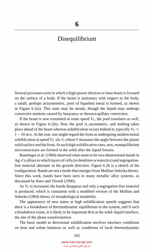
P1: LGD
CB381-06 CB381-Davis May 17, 2001 18:10 Char Count= 0
6
Disequilibrium
Several processes exist in which a high-power electron or laser beam is focusedon the surface of a body. If the beam is stationary with respect to the body,a small, perhaps axisymmetric, pool of liquefied metal is formed, as shownin Figure 6.1(a). This state may be steady, though the liquid may undergoconvective motions caused by buoyancy or thermocapillary convection.
If the beam is now translated at some speed VT, the pool translates as well,as shown in Figure 6.1(b). Now the pool is asymmetric, and melting takesplace ahead of the beam whereas solidification occurs behind it; typically VT ≈1−10 m/s. At the rear, one might regard the front as undergoing unidirectionalsolidification at speed VT sin θ , where θ measures the angle between the planersolid surface and the front. At such high solidification rates, new, nonequilibriummicrostructures are formed in the solid after the liquid freezes.
Boettinger et al. (1984) observed what seem to be two-dimensional bands inAg–Cu alloys in which layers of cells (or dendrites or eutectics) and segregation-free material alternate in the growth direction. Figure 6.2b is a sketch of theconfiguration. Bands are not a mode that emerges from Mullins-Sekerka theory.Since this work, bands have been seen in many metallic alloy systems, asdiscussed by Kurz and Trivedi (1990).
As VT is increased, the bands disappear and only a segregation-free materialis produced, which is consistent with a modified version of the Mullins andSekerka (1964) theory of morphological instability.
The appearance of new states at high solidification speeds suggests thatthere is a breakdown of thermodynamic equilibrium in the system, and if sucha breakdown exists, it is likely to be important first at the solid–liquid interface,the site of the phase transformation.
The basic model in directional solidification involves interface conditionson heat and solute balances as well as conditions of local thermodynamic
162
www.iran-mavad.com مرجع علمی مھندسی مواد
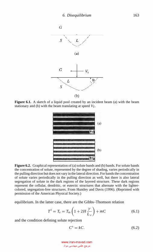
P1: LGD
CB381-06 CB381-Davis May 17, 2001 18:10 Char Count= 0
6. Disequilibrium 163
Figure 6.1. A sketch of a liquid pool created by an incident beam (a) with the beamstationary and (b) with the beam translating at speed VT.
Figure 6.2. Graphical representation of (a) solute bands and (b) bands. For solute bandsthe concentration of solute, represented by the degree of shading, varies periodically inthe pulling direction but does not vary in the lateral direction. For bands the concentrationof solute varies periodically in the pulling direction as well, but there is also lateralsegregation of solute in the dark regions of the layered structure. These dark regionsrepresent the cellular, dendritic, or eutectic structures that alternate with the lighter-colored, segregation-free structures. From Huntley and Davis (1996). (Reprinted withpermission of the American Physical Society.)
equilibrium. In the latter case, there are the Gibbs–Thomson relation
T I = Te = Tm
(1 + 2H
γ
LV
)+ mC (6.1)
and the condition defining solute rejection
C s = kC. (6.2)
www.iran-mavad.com مرجع علمی مھندسی مواد
P1: LGD
CB381-06 CB381-Davis May 17, 2001 18:10 Char Count= 0
164 6. Disequilibrium
This model is capable of describing, over a wide range of conditions, the for-mation and evolution of cells and, in principle, the behavior of dendrites. Whenprocess conditions are moderate (e.g., V is not too large), one would expect theassumption of local equilibrium to be a good approximation.
In Chapter 2, kinetic undercooling was introduced in situations of pureliquids in which large undercoolings produce large speeds. Thus, additionalundercooling
T I − Te ∝ Vn
becomes important at high speeds and, as was seen, in hypercooled liquids.When binary alloys are rapidly solidified, one has to augment the interfaceconditions on the solute as well. This chapter describes such models and theirconsequences.
6.1 Model of Rapid Solidification
Mullins and Sekerka (1964) posed local thermodynamic equilibrium at thesolid–liquid interface and studied the linear instability of the planar front indirectional solidification. They found theoretically that the interface is suscep-tible to steady cellular instabilities (MS instability) that disappear at sufficientlyhigh pulling speeds at which the instability is suppressed by surface energy atthe absolute stability boundary. When the pulling speeds are high enough, thevalidity of the assumption of local equilibrium at the solid–liquid interface mustsurely be violated. One would expect here that kinetic undercooling is important.
Because solute rejection is present, one would further expect informationderived from the phase diagram to be altered as well. This information incor-porated into conditions (6.1) and (6.2) is given by Tm, k, and m. When disequi-librium is present, k and m likely will no longer be take their low-speed values.
Coriell and Sekerka (1983) proposed a model of nonequilibrium interfaceswith attachment kinetics in which several functionals of speed, concentration,and temperature replace segregation parameters normally taken from phasedisgrams. They posed
C s = k(Vn,C, TI)C (6.3a)
and
Vn = f (T e − T I,C, T I). (6.3b)
More recently, models have been developed that are simplifications of thisgeneral theory in which only the local speed Vn generates disequilibrium; thismodel will now be discussed.
www.iran-mavad.com مرجع علمی مھندسی مواد
P1: LGD
CB381-06 CB381-Davis May 17, 2001 18:10 Char Count= 0
6.1 Model of rapid solidification 165
Consider a planar interface moving at speed V and rejecting solute as phasetransformation occurs. When V is small enough, the rejected solute has time todiffuse in the liquid, establishing the exponential basic state profile of lengthscale δc = D/V . One describes such a process using the equilibrium distribu-tion coefficient, which will now be denoted by kE.
As V increases, the material rejected has relatively less time to diffuse; if V iscomparable to some new speedβ−1
0 , the interface overtakes a significant amountof rejected solute and incorporates this into the crystal structure of the solid.This solute trapping, or partial solute trapping, is a nonequilibrium processbecause the solute cannot “fit” in the crystalline matrix, and a nonequilibriumsolid phase is formed.
The process of solute trapping effectively modifies the rejection process bychanging kE to k(V ). To be sure, k(V ) ∼ kE as V → 0. A form for k(V ) wasproposed by Aziz (1982) and Jackson, Gilmer, and Leamy (1980) by examiningthermodynamics away from equilibrium. They found that
k(Vn) = kE + β0Vn
1 + β0Vn, (6.4)
where
Vn = (V + ht)
/√1 + |∇h|2, (6.5)
and now the interface is allowed to be nonplanar but not “too” curved.In Eq. (6.5), as |Vn| → ∞, k → 1, which is called complete solute trapping.
All the rejected solute is overtaken by the front and incorporated in the solid;there is no solute rejection. Typically, in metals or semiconductors,β−1
0 ≈ 5 m/s.Aziz et al. (1986) confirmed form (6.4) quantitatively in silicon alloys for casesin which the planar front is stable. See Table 6.1 for measured values of β0 invarious systems.
Baker and Cahn (1971), Boettinger and Perepezko (1985), and Boettingerand Coriell (1986) argued that if one replaces kE by k(Vn), then to be self-consistent one should likewise replace the equilibrium liquidus slope mE bysome m(Vn).
Boettinger and Perepezko (1985) and Boettinger and Coriell (1986) derived athermodynamically consistent expression for m(V ) that is represented in termsof the same parameter β0, namely,
m(Vn)/mE = 1 − 1
(kE − 1)
{kE − k(Vn)
[1 − �n k(Vn)
kE
]}, (6.6)
where again V has been replaced by Vn. Here m ∼ mE as Vn → 0 and m ∼�nkE/kE − 1 as |Vn| → ∞.
www.iran-mavad.com مرجع علمی مھندسی مواد
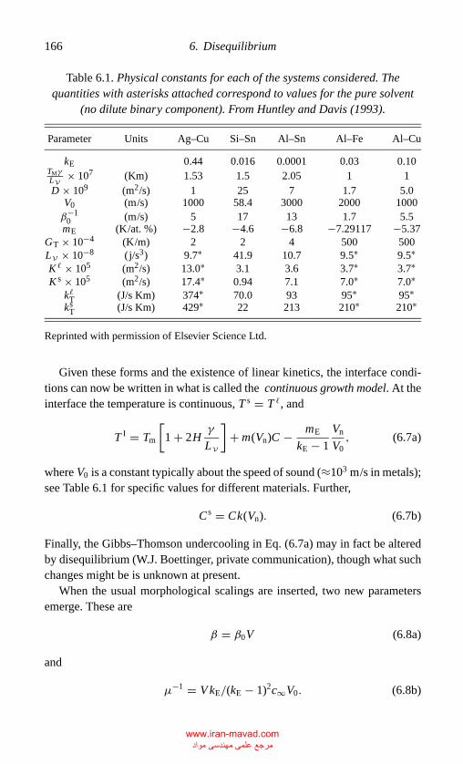
P1: LGD
CB381-06 CB381-Davis May 17, 2001 18:10 Char Count= 0
166 6. Disequilibrium
Table 6.1. Physical constants for each of the systems considered. Thequantities with asterisks attached correspond to values for the pure solvent
(no dilute binary component). From Huntley and Davis (1993).
Parameter Units Ag–Cu Si–Sn Al–Sn Al–Fe Al–Cu
kE 0.44 0.016 0.0001 0.03 0.10TMγLV × 107 (Km) 1.53 1.5 2.05 1 1D × 109 (m2/s) 1 25 7 1.7 5.0
V0 (m/s) 1000 58.4 3000 2000 1000β−1
0 (m/s) 5 17 13 1.7 5.5mE (K/at. %) −2.8 −4.6 −6.8 −7.29117 −5.37
GT × 10−4 (K/m) 2 2 4 500 500LV × 10−8 (j/s3) 9.7∗ 41.9 10.7 9.5∗ 9.5∗K � × 105 (m2/s) 13.0∗ 3.1 3.6 3.7∗ 3.7∗K s × 105 (m2/s) 17.4∗ 0.94 7.1 7.0∗ 7.0∗
k�T (J/s Km) 374∗ 70.0 93 95∗ 95∗ks
T (J/s Km) 429∗ 22 213 210∗ 210∗
Reprinted with permission of Elsevier Science Ltd.
Given these forms and the existence of linear kinetics, the interface condi-tions can now be written in what is called the continuous growth model. At theinterface the temperature is continuous, T s = T �, and
T I = Tm
[1 + 2H
γ
LV
]+ m(Vn)C − mE
kE − 1
Vn
V0, (6.7a)
where V0 is a constant typically about the speed of sound (≈103 m/s in metals);see Table 6.1 for specific values for different materials. Further,
C s = Ck(Vn). (6.7b)
Finally, the Gibbs–Thomson undercooling in Eq. (6.7a) may in fact be alteredby disequilibrium (W.J. Boettinger, private communication), though what suchchanges might be is unknown at present.
When the usual morphological scalings are inserted, two new parametersemerge. These are
β = β0V (6.8a)
and
µ−1 = V kE/(kE − 1)2c∞V0. (6.8b)
www.iran-mavad.com مرجع علمی مھندسی مواد
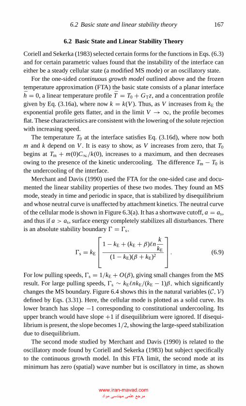
P1: LGD
CB381-06 CB381-Davis May 17, 2001 18:10 Char Count= 0
6.2 Basic state and linear stability theory 167
6.2 Basic State and Linear Stability Theory
Coriell and Sekerka (1983) selected certain forms for the functions in Eqs. (6.3)and for certain parametric values found that the instability of the interface caneither be a steady cellular state (a modified MS mode) or an oscillatory state.
For the one-sided continuous growth model outlined above and the frozentemperature approximation (FTA) the basic state consists of a planar interfaceh = 0, a linear temperature profile T = T0 + GTz, and a concentration profilegiven by Eq. (3.16a), where now k = k(V ). Thus, as V increases from kE theexponential profile gets flatter, and in the limit V → ∞, the profile becomesflat. These characteristics are consistent with the lowering of the solute rejectionwith increasing speed.
The temperature T0 at the interface satisfies Eq. (3.16d), where now bothm and k depend on V . It is easy to show, as V increases from zero, that T0
begins at Tm + m(0)C∞/k(0), increases to a maximum, and then decreasesowing to the presence of the kinetic undercooling. The difference Tm − T0 isthe undercooling of the interface.
Merchant and Davis (1990) used the FTA for the one-sided case and docu-mented the linear stability properties of these two modes. They found an MSmode, steady in time and periodic in space, that is stabilized by disequilibriumand whose neutral curve is unaffected by attachment kinetics. The neutral curveof the cellular mode is shown in Figure 6.3(a). It has a shortwave cutoff, a = as,and thus if a > as, surface energy completely stabilizes all disturbances. Thereis an absolute stability boundary � = �s,
�s = kE
1 − kE + (kE + β)�nk
kE
(1 − kE)(β + kE)2
. (6.9)
For low pulling speeds, �s = 1/kE + O(β), giving small changes from the MSresult. For large pulling speeds, �s ∼ kE�nkE/(kE − 1)β, which significantlychanges the MS boundary. Figure 6.4 shows this in the natural variables (C,V)defined by Eqs. (3.31). Here, the cellular mode is plotted as a solid curve. Itslower branch has slope −1 corresponding to constitutional undercooling. Itsupper branch would have slope +1 if disequilibrium were ignored. If disequi-librium is present, the slope becomes 1/2, showing the large-speed stabilizationdue to disequilibrium.
The second mode studied by Merchant and Davis (1990) is related to theoscillatory mode found by Coriell and Sekerka (1983) but subject specificallyto the continuous growth model. In this FTA limit, the second mode at itsminimum has zero (spatial) wave number but is oscillatory in time, as shown
www.iran-mavad.com مرجع علمی مھندسی مواد
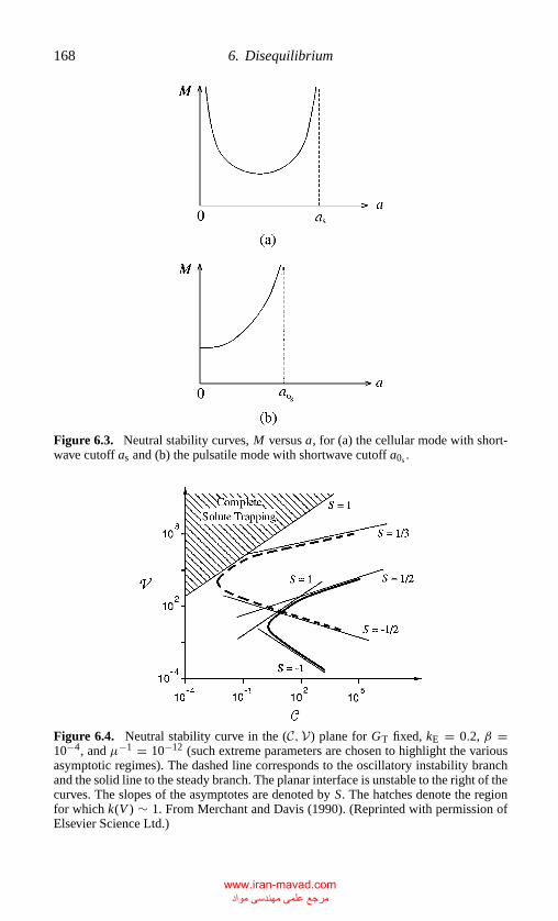
P1: LGD
CB381-06 CB381-Davis May 17, 2001 18:10 Char Count= 0
168 6. Disequilibrium
Figure 6.3. Neutral stability curves, M versus a, for (a) the cellular mode with short-wave cutoff as and (b) the pulsatile mode with shortwave cutoff a0s .
Figure 6.4. Neutral stability curve in the (C,V) plane for GT fixed, kE = 0.2, β =10−4, and µ−1 = 10−12 (such extreme parameters are chosen to highlight the variousasymptotic regimes). The dashed line corresponds to the oscillatory instability branchand the solid line to the steady branch. The planar interface is unstable to the right of thecurves. The slopes of the asymptotes are denoted by S. The hatches denote the regionfor which k(V ) ∼ 1. From Merchant and Davis (1990). (Reprinted with permission ofElsevier Science Ltd.)
www.iran-mavad.com مرجع علمی مھندسی مواد
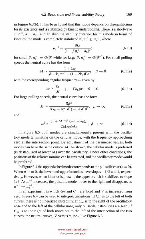
P1: LGD
CB381-06 CB381-Davis May 17, 2001 18:10 Char Count= 0
6.2 Basic state and linear stability theory 169
in Figure 6.3(b). It has been found that this mode depends on disequilibriumfor its existence and is stabilized by kinetic undercooling. There is a shortwavecutoff, a = a0s, and an absolute stability criterion for this mode in terms ofkinetics; the mode is completely stabilized if µ−1 ≥ µ−1
s , where
µ−1s = βkE
(1 + β)(β + kE)2; (6.10)
for small β, µ−1s = O(β) while for large β, µ−1
s = O(β−2). For small pullingspeeds the neutral curve has the form
M ∼ 1 + 2kE
β − kEµ−1 − (1 + 2kE)�a2, β → 0 (6.11a)
with the corresponding angular frequency ω given by
ω2 ∼ kE
M− (1 − �kE)a2, β → 0. (6.11b)
For large pulling speeds, the neutral curve has the form
M ∼ 5β2
2(kE − µ−1β2) − 5�a2β2, β → ∞ (6.11c)
and
ω2 ∼ (1 + M�a2)(−1 + kE)β
2MkE�nkE, β → ∞. (6.11d)
In Figure 6.5 both modes are simultaneously present with the oscilla-tory mode terminating on the cellular mode, with the frequency approachingzero at the intersection point. By adjustment of the parametric values, bothmodes can have the same critical M . As shown, the cellular mode is preferred(is destabilized at lower M) over the oscillatory. Under other conditions, thepositions of the relative minima can be reversed, and the oscillatory mode wouldbe preferred.
In Figure 6.4 the upper dashed mode corresponds to the pulsatile case (a = 0).When µ−1 = 0, the lower and upper branches have slopes −1/2 and 1, respec-tively. However, when kinetics is present, the upper branch is stabilized to slope1/3. As µ−1 increases, the pulsatile mode moves to the right and disappears asµ−1 → µ−1
s .In an experiment in which GT and C∞ are fixed and V is increased from
zero, Figure 6.4 can be used to interpret transitions. If C∞ is to the left of bothcurves, there is no linearized instability. If C∞ is to the right of the oscillatorynose and to the left of the cellular nose, only pulsatile instabilities are seen. IfC∞ is to the right of both noses but to the left of the intersection of the twocurves, the neutral curves, V versus a, look like Figure 6.6.
www.iran-mavad.com مرجع علمی مھندسی مواد
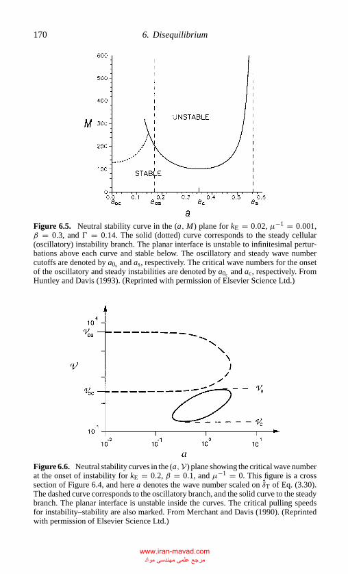
P1: LGD
CB381-06 CB381-Davis May 17, 2001 18:10 Char Count= 0
170 6. Disequilibrium
Figure 6.5. Neutral stability curve in the (a,M) plane for kE = 0.02, µ−1 = 0.001,β = 0.3, and � = 0.14. The solid (dotted) curve corresponds to the steady cellular(oscillatory) instability branch. The planar interface is unstable to infinitesimal pertur-bations above each curve and stable below. The oscillatory and steady wave numbercutoffs are denoted by a0s and as, respectively. The critical wave numbers for the onsetof the oscillatory and steady instabilities are denoted by a0c and ac, respectively. FromHuntley and Davis (1993). (Reprinted with permission of Elsevier Science Ltd.)
Figure 6.6. Neutral stability curves in the (a,V) plane showing the critical wave numberat the onset of instability for kE = 0.2, β = 0.1, and µ−1 = 0. This figure is a crosssection of Figure 6.4, and here a denotes the wave number scaled on δT of Eq. (3.30).The dashed curve corresponds to the oscillatory branch, and the solid curve to the steadybranch. The planar interface is unstable inside the curves. The critical pulling speedsfor instability–stability are also marked. From Merchant and Davis (1990). (Reprintedwith permission of Elsevier Science Ltd.)
www.iran-mavad.com مرجع علمی مھندسی مواد

P1: LGD
CB381-06 CB381-Davis May 17, 2001 18:10 Char Count= 0
6.3 Thermal effects 171
As V crosses Vc, steady cells appear whose wave numbers are near thatof the minimum of the solid loop in Figure 6.6, ac ≈ 0.3. As V is increasedfurther, the cells should deepen, and a should increase; there may be a cellular–dendritic transition (not covered by the present linear theory), and the cellsreturn as the absolute stability boundary V = VA is approached. As V increasesfurther, the cells become shallow and finally disappear at V = VA where thewave number aA ≈ 2.2 corresponds to the top of the solid loop in Figure 6.6.Now, since VA < V0c, the planar interface regains stability. The range, VA <
V < V0c, where the planar state is stable, is a window of stability. As Vis increased to V = V0c, the oscillatory mode becomes excited with wavenumber a0c = 0. The instability produces solute bands shown in Figure 6.2(a),which are solute distributions periodic in the direction of solidification freeof lateral segregation. The angular frequency ω0c of the oscillatory instabilityand the spatial wavelength of the solute band should decrease as V increases.As V is increased further, some nonlinear selection mechanism determines theoscillatory mode in the range V0c< V < V0A. It may continue to give solutebanding, or some cellular structure may emerge. When V < V0A, solute bandsare certainly present because the top of the dashed loop in Figure 6.6 has a0c = 0.At V = V0A the planar state regains stability. What the system selects away fromthe linear stability regime is, presumably, determined nonlinear interactions,which are outside the realm of the present theory given that they correspond toparametric regions deep in the unstable regions of the loops.
6.3 Thermal Effects
When the pulling speeds are large, if both D/V and κ/V become very small,and if large wave number instability is important, say, for the oscillatory mode,then the thermal boundary layer likely becomes important and latent heat effectsshould not be neglected.
Huntley and Davis (1993) generalized the linear stability theory to the case inwhich the full thermal effects are included subject to the cold boundary condi-tion. In addition to the parameters M, �, kE,mE, β, and µ, the new parametersthat emerge are latent heat
L = LVV
k�TGT, (6.12a)
the thermal conductivity ratio
kT = ksT
k�T, (6.12b)
www.iran-mavad.com مرجع علمی مھندسی مواد
P1: LGD
CB381-06 CB381-Davis May 17, 2001 18:10 Char Count= 0
172 6. Disequilibrium
the temperature gradients
GL = GL
GT, Gs = Gs
GT(6.12c)
and the diffusivity ratios
D(�) = D
κ�, D(s) = D
κs, (6.12d)
where the heat balance requires that
L = kTGS − GL. (6.13)
The FTA is recovered when kT = 1, L = 0 and D(s) = D(�) = 0.There is a steady basic state solution of the system as follows:
CL = CL(z) = 1 − kE
(kE + β)exp(−z) (6.14a)
CS = CS(z) = 0 (6.14b)
T L = T L(z) = T0 +(
GL
D(�)
)[1 − exp(−D(�)z)] (6.14c)
T S = T S(z) = T0 +(
L + GL
nD(s)
)[1 − exp(−D(s)z)] (6.14d)
h = h = 0. (6.14e)
Here the planar interfacial temperature T0 is given by
T0 = −Mµ−1 + M
(kE − 1)
[m(1)kE
k(1)− 1
]. (6.14f)
This steady state solution will be used as the basic state solution in the linearstability analysis.
6.4 Linear-Stability Theory with Thermal Effects
The linear-stability theory results in the following rather complicated charac-teristic equation derived by Huntley and Davis (1993):
(kT RS + RL)
{kE
1 + β(
1 + σ
kE + β)
m(1) − (R + k − 1)
·[− GLM−1 − �a2 + + kEβσ�n(k/kE)
(kT + β)(kT − 1)(1 + β)− µ−1σ + m(1)kE
kE + β]}
+ M−1(R + k − 1){Lσ + [L + (1 − kT)GL]RS
+ GL(D(s) − D(�)) + L D(s)} = 0, (6.15a)
www.iran-mavad.com مرجع علمی مھندسی مواد
P1: LGD
CB381-06 CB381-Davis May 17, 2001 18:10 Char Count= 0
6.4 Linear-stability theory with thermal effects 173
where
k = kE + β1 + β (6.15b)
m(1) = 1 − 1
kE − 1{kE − k[1 − �n(k/kE)]} (6.15c)
R = 1
2+ 1
2
√1 + 4σ + 4a2 (6.15d)
RS = − D(s)
2+ 1
2
√D(s)2 + 4σD(s) + 4a2 (6.15e)
RL = D(�)
2+ 1
2
√D(�)2 + 4σD(�) + 4a2. (6.15f)
In what follows, some simplifications are made, namely,
kT = 1 (6.16a)
and
D(s) = D(�) ≡ D (6.16b)
so that
GL = 1 − 1
2L. (6.17)
In this simplified case the two phases have equal thermal properties. Then, Dmeasures departures for the temperature field from the linear form (nonthermalsteady state), and L measures the latent heat liberated. The aim is to determinehow the instabilities found earlier are modified by these thermal effects.
6.4.1 Steady Mode
The steady cellular mode is stabilized by disequilibrium, and the critical con-ditions are unaffected by kinetics in the FTA. When either D or L is increasedfrom zero, the mode is stabilized, but the shortwave cutoff as is independentof the parameters D and L , as shown in Figure 6.7. The curve of Figure 6.8shows for a = ac the stabilization due to thermal effects and the absence ofstabilization in the constitutional undercooling and absolute stability limits.
6.4.2 Oscillatory Mode
In the FTA, the preferred oscillatory mode always has a → 0, and thus it firstoccurs as a pulsatile mode with frequencyω �= 0, as shown in Figure 6.5. When
www.iran-mavad.com مرجع علمی مھندسی مواد
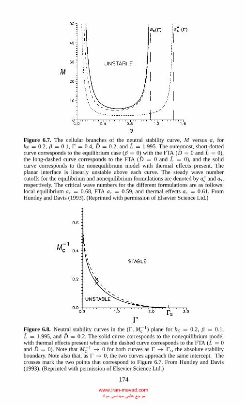
P1: LGD
CB381-06 CB381-Davis May 17, 2001 18:10 Char Count= 0
Figure 6.7. The cellular branches of the neutral stability curve, M versus a, forkE = 0.2, β = 0.1, � = 0.4, D = 0.2, and L = 1.995. The outermost, short-dottedcurve corresponds to the equilibrium case (β = 0) with the FTA (D = 0 and L = 0),the long-dashed curve corresponds to the FTA (D = 0 and L = 0), and the solidcurve corresponds to the nonequilibrium model with thermal effects present. Theplanar interface is linearly unstable above each curve. The steady wave numbercutoffs for the equilibrium and nonequilibrium formulations are denoted by ae
s and as,respectively. The critical wave numbers for the different formulations are as follows:local equilibrium ac = 0.68, FTA ac = 0.59, and thermal effects ac = 0.61. FromHuntley and Davis (1993). (Reprinted with permission of Elsevier Science Ltd.)
Figure 6.8. Neutral stability curves in the (�,M−1c ) plane for kE = 0.2, β = 0.1,
L = 1.995, and D = 0.2. The solid curve corresponds to the nonequilibrium modelwith thermal effects present whereas the dashed curve corresponds to the FTA (L = 0and D = 0). Note that M−1
c → 0 for both curves as � → �s, the absolute stabilityboundary. Note also that, as � → 0, the two curves approach the same intercept. Thecrosses mark the two points that correspond to Figure 6.7. From Huntley and Davis(1993). (Reprinted with permission of Elsevier Science Ltd.)
174
www.iran-mavad.com مرجع علمی مھندسی مواد
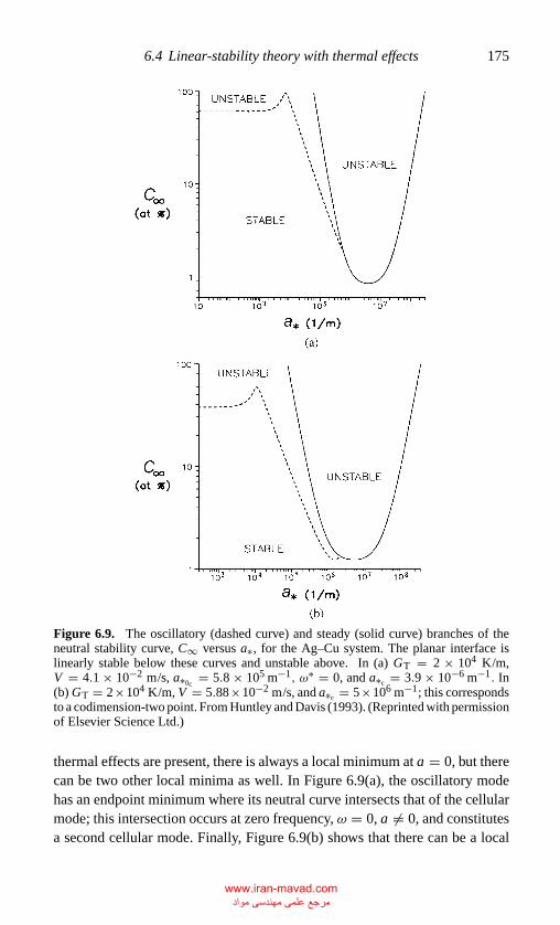
P1: LGD
CB381-06 CB381-Davis May 17, 2001 18:10 Char Count= 0
6.4 Linear-stability theory with thermal effects 175
Figure 6.9. The oscillatory (dashed curve) and steady (solid curve) branches of theneutral stability curve, C∞ versus a∗, for the Ag–Cu system. The planar interface islinearly stable below these curves and unstable above. In (a) GT = 2 × 10⁴ K/m,V = 4.1 × 10⁻² m/s, a∗0c
= 5.8 × 10⁵ m−1, ω∗ = 0, and a∗c = 3.9 × 10⁻⁶ m−1. In(b) GT = 2×10⁴ K/m, V = 5.88×10⁻² m/s, and a∗c = 5×10⁶ m−1; this correspondsto a codimension-two point. From Huntley and Davis (1993). (Reprinted with permissionof Elsevier Science Ltd.)
thermal effects are present, there is always a local minimum at a = 0, but therecan be two other local minima as well. In Figure 6.9(a), the oscillatory modehas an endpoint minimum where its neutral curve intersects that of the cellularmode; this intersection occurs at zero frequency, ω = 0, a �= 0, and constitutesa second cellular mode. Finally, Figure 6.9(b) shows that there can be a local
www.iran-mavad.com مرجع علمی مھندسی مواد
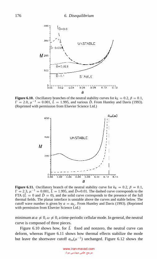
P1: LGD
CB381-06 CB381-Davis May 17, 2001 18:10 Char Count= 0
176 6. Disequilibrium
Figure 6.10. Oscillatory branches of the neutral stability curves for kE = 0.2, β = 0.1,� = 2.0, µ−1 = 0.001, L = 1.995, and various D. From Huntley and Davis (1993).(Reprinted with permission from Elsevier Science Ltd.)
Figure 6.11. Oscillatory branch of the neutral stability curve for kE = 0.2, β = 0.1,� = 2.3, µ−1 = 0.001, L = 1.995, and D=0.01. The dashed curve corresponds to theFTA (L = 0 and D = 0), and the solid curve corresponds to the presence of the fullthermal fields. The planar interface is unstable above the curves and stable below. Thecutoff wave number is given by a = a0s . From Huntley and Davis (1993). (Reprintedwith permission from Elsevier Science Ltd.)
minimum at a �= 0,ω �= 0, a time-periodic cellular mode. In general, the neutralcurve is composed of three pieces.
Figure 6.10 shows how, for L fixed and nonzero, the neutral curve candeform, whereas Figure 6.11 shows how thermal effects stabilize the modebut leave the shortwave cutoff aos(µ−1) unchanged. Figure 6.12 shows the
www.iran-mavad.com مرجع علمی مھندسی مواد
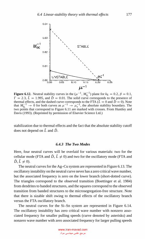
P1: LGD
CB381-06 CB381-Davis May 17, 2001 18:10 Char Count= 0
6.4 Linear-stability theory with thermal effects 177
Figure 6.12. Neutral stability curves in the (µ−1,M−10c
) plane for kE = 0.2, β = 0.1,� = 2.3, L = 1.995, and D = 0.01. The solid curve corresponds to the presence ofthermal effects, and the dashed curve corresponds to the FTA (L = 0 and D = 0). Notethat M−1
0c→ 0 for both curves as µ−1 → µ−1
s , the absolute stability boundary. Thetwo points that correspond to Figure 6.11 are marked with crosses. From Huntley andDavis (1993). (Reprinted by permission of Elsevier Science Ltd.)
stabilization due to thermal effects and the fact that the absolute stability cutoffdoes not depend on L and D.
6.4.3 The Two Modes
Here, four neutral curves will be overlaid for various materials: two for thecellular mode (FTA and D, L �= 0) and two for the oscillatory mode (FTA andD, L �= 0).
The neutral curves for the Ag–Cu system are represented in Figure 6.13. Theoscillatory instability on the neutral curve never has a zero critical wave number,but the associated frequency is zero on the lower branch (short-dotted curve).The triangles correspond to the observed transition (Boettinger et al. 1984)from dendrites to banded structures, and the squares correspond to the observedtransition from banded structures to the microsegregation-free structure. Notethat there is sizable shift owing to thermal effects of the oscillatory branchversus the FTA oscillatory branch.
The neutral curves for the Si–Sn system are represented in Figure 6.14.The oscillatory instability has zero critical wave number with nonzero asso-ciated frequency for smaller pulling speeds (curve denoted by asterisks) andnonzero wave number with zero associated frequency for larger pulling speeds
www.iran-mavad.com مرجع علمی مھندسی مواد
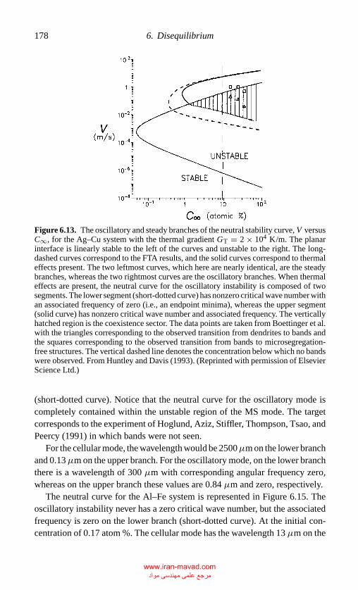
P1: LGD
CB381-06 CB381-Davis May 17, 2001 18:10 Char Count= 0
178 6. Disequilibrium
Figure 6.13. The oscillatory and steady branches of the neutral stability curve, V versusC∞, for the Ag–Cu system with the thermal gradient GT = 2 × 10⁴ K/m. The planarinterface is linearly stable to the left of the curves and unstable to the right. The long-dashed curves correspond to the FTA results, and the solid curves correspond to thermaleffects present. The two leftmost curves, which here are nearly identical, are the steadybranches, whereas the two rightmost curves are the oscillatory branches. When thermaleffects are present, the neutral curve for the oscillatory instability is composed of twosegments. The lower segment (short-dotted curve) has nonzero critical wave number withan associated frequency of zero (i.e., an endpoint minima), whereas the upper segment(solid curve) has nonzero critical wave number and associated frequency. The verticallyhatched region is the coexistence sector. The data points are taken from Boettinger et al.with the triangles corresponding to the observed transition from dendrites to bands andthe squares corresponding to the observed transition from bands to microsegregation-free structures. The vertical dashed line denotes the concentration below which no bandswere observed. From Huntley and Davis (1993). (Reprinted with permission of ElsevierScience Ltd.)
(short-dotted curve). Notice that the neutral curve for the oscillatory mode iscompletely contained within the unstable region of the MS mode. The targetcorresponds to the experiment of Hoglund, Aziz, Stiffler, Thompson, Tsao, andPeercy (1991) in which bands were not seen.
For the cellular mode, the wavelength would be 2500µm on the lower branchand 0.13µm on the upper branch. For the oscillatory mode, on the lower branchthere is a wavelength of 300 µm with corresponding angular frequency zero,whereas on the upper branch these values are 0.84 µm and zero, respectively.
The neutral curve for the Al–Fe system is represented in Figure 6.15. Theoscillatory instability never has a zero critical wave number, but the associatedfrequency is zero on the lower branch (short-dotted curve). At the initial con-centration of 0.17 atom %. The cellular mode has the wavelength 13 µm on the
www.iran-mavad.com مرجع علمی مھندسی مواد
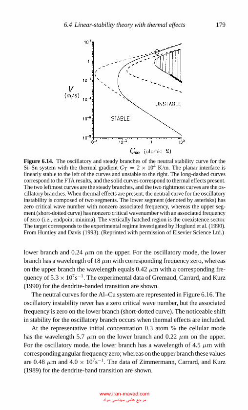
P1: LGD
CB381-06 CB381-Davis May 17, 2001 18:10 Char Count= 0
6.4 Linear-stability theory with thermal effects 179
Figure 6.14. The oscillatory and steady branches of the neutral stability curve for theSi–Sn system with the thermal gradient GT = 2 × 10⁴ K/m. The planar interface islinearly stable to the left of the curves and unstable to the right. The long-dashed curvescorrespond to the FTA results, and the solid curves correspond to thermal effects present.The two leftmost curves are the steady branches, and the two rightmost curves are the os-cillatory branches. When thermal effects are present, the neutral curve for the oscillatoryinstability is composed of two segments. The lower segment (denoted by asterisks) haszero critical wave number with nonzero associated frequency, whereas the upper seg-ment (short-dotted curve) has nonzero critical wavenumber with an associated frequencyof zero (i.e., endpoint minima). The vertically hatched region is the coexistence sector.The target corresponds to the experimental regime investigated by Hoglund et al. (1990).From Huntley and Davis (1993). (Reprinted with permission of Elsevier Science Ltd.)
lower branch and 0.24 µm on the upper. For the oscillatory mode, the lowerbranch has a wavelength of 18µm with corresponding frequency zero, whereason the upper branch the wavelength equals 0.42 µm with a corresponding fre-quency of 5.3 × 10⁷s−1. The experimental data of Gremaud, Carrard, and Kurz(1990) for the dendrite-banded transition are shown.
The neutral curves for the Al–Cu system are represented in Figure 6.16. Theoscillatory instability never has a zero critical wave number, but the associatedfrequency is zero on the lower branch (short-dotted curve). The noticeable shiftin stability for the oscillatory branch occurs when thermal effects are included.
At the representative initial concentration 0.3 atom % the cellular modehas the wavelength 5.7 µm on the lower branch and 0.22 µm on the upper.For the oscillatory mode, the lower branch has a wavelength of 4.5 µm withcorresponding angular frequency zero; whereas on the upper branch these valuesare 0.48 µm and 4.0 × 10⁷s−1. The data of Zimmermann, Carrard, and Kurz(1989) for the dendrite-band transition are shown.
www.iran-mavad.com مرجع علمی مھندسی مواد
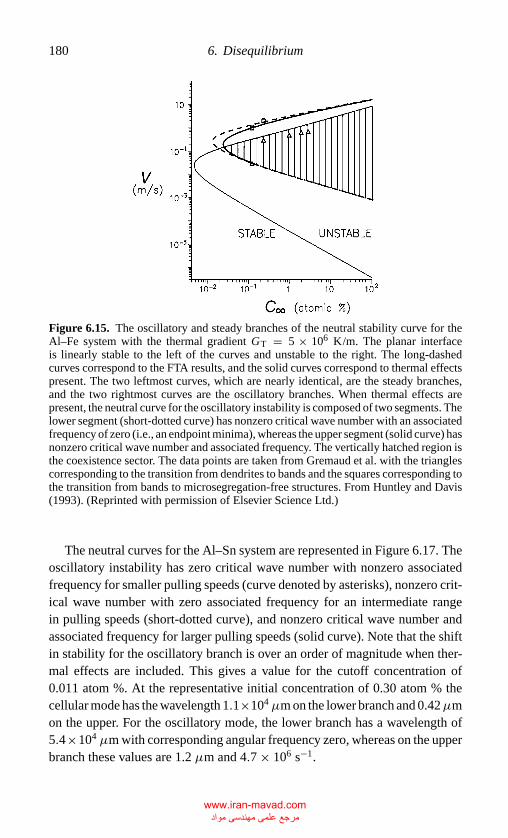
P1: LGD
CB381-06 CB381-Davis May 17, 2001 18:10 Char Count= 0
180 6. Disequilibrium
Figure 6.15. The oscillatory and steady branches of the neutral stability curve for theAl–Fe system with the thermal gradient GT = 5 × 10⁶ K/m. The planar interfaceis linearly stable to the left of the curves and unstable to the right. The long-dashedcurves correspond to the FTA results, and the solid curves correspond to thermal effectspresent. The two leftmost curves, which are nearly identical, are the steady branches,and the two rightmost curves are the oscillatory branches. When thermal effects arepresent, the neutral curve for the oscillatory instability is composed of two segments. Thelower segment (short-dotted curve) has nonzero critical wave number with an associatedfrequency of zero (i.e., an endpoint minima), whereas the upper segment (solid curve) hasnonzero critical wave number and associated frequency. The vertically hatched region isthe coexistence sector. The data points are taken from Gremaud et al. with the trianglescorresponding to the transition from dendrites to bands and the squares corresponding tothe transition from bands to microsegregation-free structures. From Huntley and Davis(1993). (Reprinted with permission of Elsevier Science Ltd.)
The neutral curves for the Al–Sn system are represented in Figure 6.17. Theoscillatory instability has zero critical wave number with nonzero associatedfrequency for smaller pulling speeds (curve denoted by asterisks), nonzero crit-ical wave number with zero associated frequency for an intermediate rangein pulling speeds (short-dotted curve), and nonzero critical wave number andassociated frequency for larger pulling speeds (solid curve). Note that the shiftin stability for the oscillatory branch is over an order of magnitude when ther-mal effects are included. This gives a value for the cutoff concentration of0.011 atom %. At the representative initial concentration of 0.30 atom % thecellular mode has the wavelength 1.1×104µm on the lower branch and 0.42µmon the upper. For the oscillatory mode, the lower branch has a wavelength of5.4×104 µm with corresponding angular frequency zero, whereas on the upperbranch these values are 1.2 µm and 4.7 × 10⁶ s−1.
www.iran-mavad.com مرجع علمی مھندسی مواد
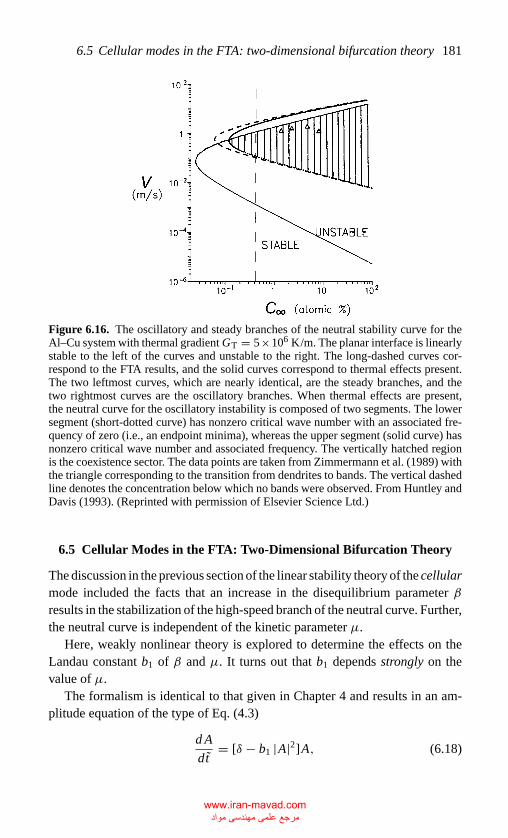
P1: LGD
CB381-06 CB381-Davis May 17, 2001 18:10 Char Count= 0
6.5 Cellular modes in the FTA: two-dimensional bifurcation theory 181
Figure 6.16. The oscillatory and steady branches of the neutral stability curve for theAl–Cu system with thermal gradient GT = 5×10⁶ K/m. The planar interface is linearlystable to the left of the curves and unstable to the right. The long-dashed curves cor-respond to the FTA results, and the solid curves correspond to thermal effects present.The two leftmost curves, which are nearly identical, are the steady branches, and thetwo rightmost curves are the oscillatory branches. When thermal effects are present,the neutral curve for the oscillatory instability is composed of two segments. The lowersegment (short-dotted curve) has nonzero critical wave number with an associated fre-quency of zero (i.e., an endpoint minima), whereas the upper segment (solid curve) hasnonzero critical wave number and associated frequency. The vertically hatched regionis the coexistence sector. The data points are taken from Zimmermann et al. (1989) withthe triangle corresponding to the transition from dendrites to bands. The vertical dashedline denotes the concentration below which no bands were observed. From Huntley andDavis (1993). (Reprinted with permission of Elsevier Science Ltd.)
6.5 Cellular Modes in the FTA: Two-Dimensional Bifurcation Theory
The discussion in the previous section of the linear stability theory of the cellularmode included the facts that an increase in the disequilibrium parameter βresults in the stabilization of the high-speed branch of the neutral curve. Further,the neutral curve is independent of the kinetic parameter µ.
Here, weakly nonlinear theory is explored to determine the effects on theLandau constant b1 of β and µ. It turns out that b1 depends strongly on thevalue of µ.
The formalism is identical to that given in Chapter 4 and results in an am-plitude equation of the type of Eq. (4.3)
d A
dt= [δ − b1 |A|2]A, (6.18)
www.iran-mavad.com مرجع علمی مھندسی مواد
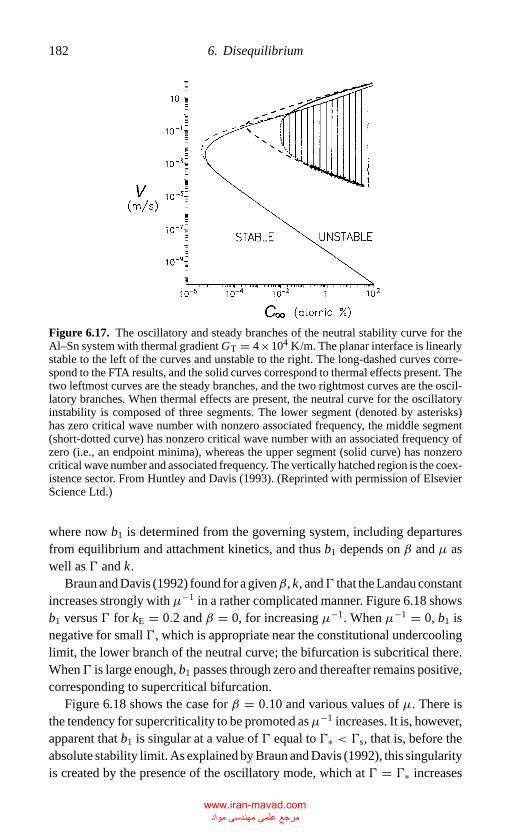
P1: LGD
CB381-06 CB381-Davis May 17, 2001 18:10 Char Count= 0
182 6. Disequilibrium
Figure 6.17. The oscillatory and steady branches of the neutral stability curve for theAl–Sn system with thermal gradient GT = 4×10⁴ K/m. The planar interface is linearlystable to the left of the curves and unstable to the right. The long-dashed curves corre-spond to the FTA results, and the solid curves correspond to thermal effects present. Thetwo leftmost curves are the steady branches, and the two rightmost curves are the oscil-latory branches. When thermal effects are present, the neutral curve for the oscillatoryinstability is composed of three segments. The lower segment (denoted by asterisks)has zero critical wave number with nonzero associated frequency, the middle segment(short-dotted curve) has nonzero critical wave number with an associated frequency ofzero (i.e., an endpoint minima), whereas the upper segment (solid curve) has nonzerocritical wave number and associated frequency. The vertically hatched region is the coex-istence sector. From Huntley and Davis (1993). (Reprinted with permission of ElsevierScience Ltd.)
where now b1 is determined from the governing system, including departuresfrom equilibrium and attachment kinetics, and thus b1 depends on β and µ aswell as � and k.
Braun and Davis (1992) found for a givenβ, k, and� that the Landau constantincreases strongly with µ−1 in a rather complicated manner. Figure 6.18 showsb1 versus � for kE = 0.2 and β = 0, for increasing µ−1. When µ−1 = 0, b1 isnegative for small �, which is appropriate near the constitutional undercoolinglimit, the lower branch of the neutral curve; the bifurcation is subcritical there.When� is large enough, b1 passes through zero and thereafter remains positive,corresponding to supercritical bifurcation.
Figure 6.18 shows the case for β = 0.10 and various values of µ. There isthe tendency for supercriticality to be promoted asµ−1 increases. It is, however,apparent that b1 is singular at a value of � equal to �∗ < �s, that is, before theabsolute stability limit. As explained by Braun and Davis (1992), this singularityis created by the presence of the oscillatory mode, which at � = �∗ increases
www.iran-mavad.com مرجع علمی مھندسی مواد
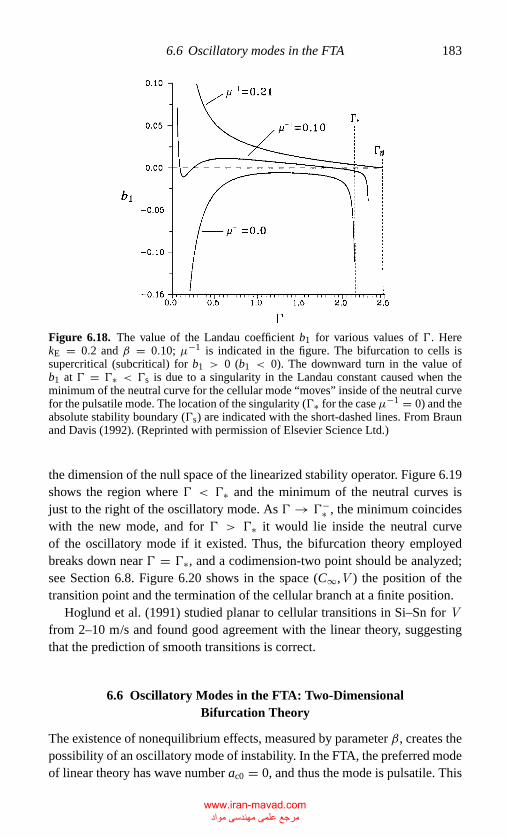
P1: LGD
CB381-06 CB381-Davis May 17, 2001 18:10 Char Count= 0
6.6 Oscillatory modes in the FTA 183
Figure 6.18. The value of the Landau coefficient b1 for various values of �. HerekE = 0.2 and β = 0.10; µ−1 is indicated in the figure. The bifurcation to cells issupercritical (subcritical) for b1 > 0 (b1 < 0). The downward turn in the value ofb1 at � = �∗ < �s is due to a singularity in the Landau constant caused when theminimum of the neutral curve for the cellular mode “moves” inside of the neutral curvefor the pulsatile mode. The location of the singularity (�∗ for the case µ−1 = 0) and theabsolute stability boundary (�s) are indicated with the short-dashed lines. From Braunand Davis (1992). (Reprinted with permission of Elsevier Science Ltd.)
the dimension of the null space of the linearized stability operator. Figure 6.19shows the region where � < �∗ and the minimum of the neutral curves isjust to the right of the oscillatory mode. As � → �−
∗ , the minimum coincideswith the new mode, and for � > �∗ it would lie inside the neutral curveof the oscillatory mode if it existed. Thus, the bifurcation theory employedbreaks down near � = �∗, and a codimension-two point should be analyzed;see Section 6.8. Figure 6.20 shows in the space (C∞,V ) the position of thetransition point and the termination of the cellular branch at a finite position.
Hoglund et al. (1991) studied planar to cellular transitions in Si–Sn for Vfrom 2–10 m/s and found good agreement with the linear theory, suggestingthat the prediction of smooth transitions is correct.
6.6 Oscillatory Modes in the FTA: Two-DimensionalBifurcation Theory
The existence of nonequilibrium effects, measured by parameter β, creates thepossibility of an oscillatory mode of instability. In the FTA, the preferred modeof linear theory has wave number ac0 = 0, and thus the mode is pulsatile. This
www.iran-mavad.com مرجع علمی مھندسی مواد
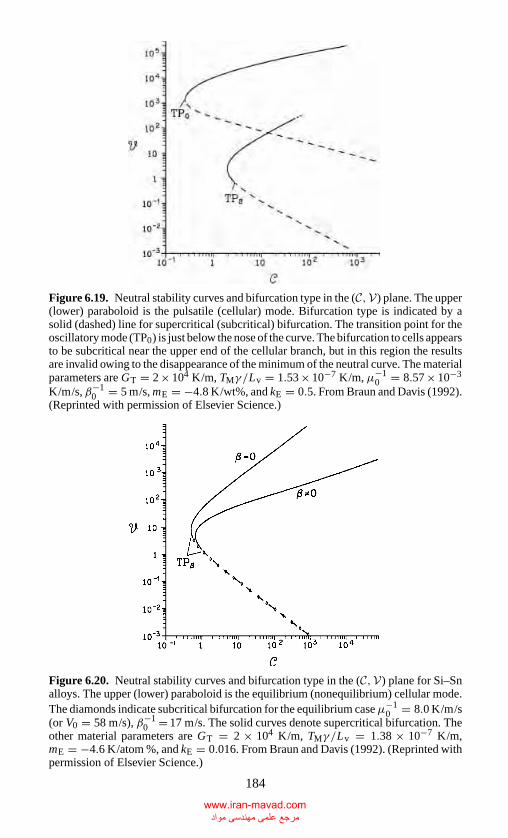
P1: LGD
CB381-06 CB381-Davis May 17, 2001 18:10 Char Count= 0
Figure 6.19. Neutral stability curves and bifurcation type in the (C,V) plane. The upper(lower) paraboloid is the pulsatile (cellular) mode. Bifurcation type is indicated by asolid (dashed) line for supercritical (subcritical) bifurcation. The transition point for theoscillatory mode (TP0) is just below the nose of the curve. The bifurcation to cells appearsto be subcritical near the upper end of the cellular branch, but in this region the resultsare invalid owing to the disappearance of the minimum of the neutral curve. The materialparameters are GT = 2 × 10⁴ K/m, TMγ /Lv = 1.53 × 10⁻⁷ K/m, µ−1
0 = 8.57 × 10⁻³
K/m/s, β−10 = 5 m/s, mE = −4.8 K/wt%, and kE = 0.5. From Braun and Davis (1992).
(Reprinted with permission of Elsevier Science.)
Figure 6.20. Neutral stability curves and bifurcation type in the (C,V) plane for Si–Snalloys. The upper (lower) paraboloid is the equilibrium (nonequilibrium) cellular mode.The diamonds indicate subcritical bifurcation for the equilibrium caseµ−1
0 = 8.0 K/m/s(or V0 = 58 m/s), β−1
0 = 17 m/s. The solid curves denote supercritical bifurcation. Theother material parameters are GT = 2 × 10⁴ K/m, TMγ /Lv = 1.38 × 10⁻⁷ K/m,mE = −4.6 K/atom %, and kE = 0.016. From Braun and Davis (1992). (Reprinted withpermission of Elsevier Science.)
184
www.iran-mavad.com مرجع علمی مھندسی مواد
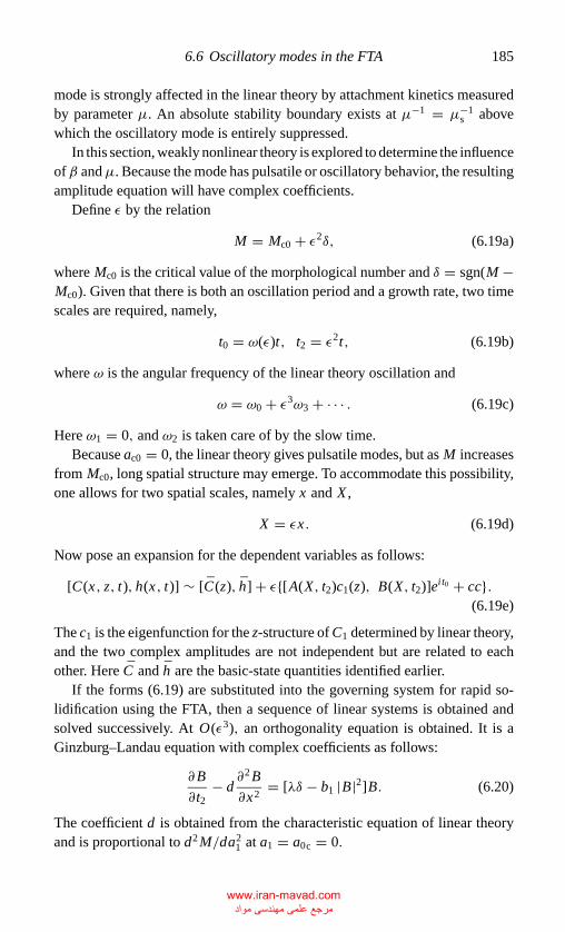
P1: LGD
CB381-06 CB381-Davis May 17, 2001 18:10 Char Count= 0
6.6 Oscillatory modes in the FTA 185
mode is strongly affected in the linear theory by attachment kinetics measuredby parameter µ. An absolute stability boundary exists at µ−1 = µ−1
s abovewhich the oscillatory mode is entirely suppressed.
In this section, weakly nonlinear theory is explored to determine the influenceof β andµ. Because the mode has pulsatile or oscillatory behavior, the resultingamplitude equation will have complex coefficients.
Define ε by the relation
M = Mc0 + ε2δ, (6.19a)
where Mc0 is the critical value of the morphological number and δ = sgn(M −Mc0). Given that there is both an oscillation period and a growth rate, two timescales are required, namely,
t0 = ω(ε)t, t2 = ε2t, (6.19b)
where ω is the angular frequency of the linear theory oscillation and
ω = ω0 + ε3ω3 + · · · . (6.19c)
Here ω1 = 0, and ω2 is taken care of by the slow time.Because ac0 = 0, the linear theory gives pulsatile modes, but as M increases
from Mc0, long spatial structure may emerge. To accommodate this possibility,one allows for two spatial scales, namely x and X ,
X = εx . (6.19d)
Now pose an expansion for the dependent variables as follows:
[C(x, z, t), h(x, t)] ∼ [C(z), h] + ε{[A(X, t2)c1(z), B(X, t2)]eit0 + cc}.(6.19e)
The c1 is the eigenfunction for the z-structure of C1 determined by linear theory,and the two complex amplitudes are not independent but are related to eachother. Here C and h are the basic-state quantities identified earlier.
If the forms (6.19) are substituted into the governing system for rapid so-lidification using the FTA, then a sequence of linear systems is obtained andsolved successively. At O(ε3), an orthogonality equation is obtained. It is aGinzburg–Landau equation with complex coefficients as follows:
∂B
∂t2− d
∂2 B
∂x2= [λδ − b1 |B|2]B. (6.20)
The coefficient d is obtained from the characteristic equation of linear theoryand is proportional to d2M/da2
1 at a1 = a0c = 0.
www.iran-mavad.com مرجع علمی مھندسی مواد
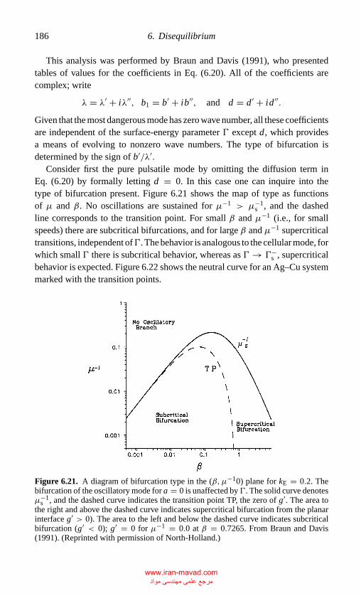
P1: LGD
CB381-06 CB381-Davis May 17, 2001 18:10 Char Count= 0
186 6. Disequilibrium
This analysis was performed by Braun and Davis (1991), who presentedtables of values for the coefficients in Eq. (6.20). All of the coefficients arecomplex; write
λ = λ′ + iλ′′, b1 = b′ + ib′′, and d = d ′ + id ′′.
Given that the most dangerous mode has zero wave number, all these coefficientsare independent of the surface-energy parameter � except d, which providesa means of evolving to nonzero wave numbers. The type of bifurcation isdetermined by the sign of b′/λ′.
Consider first the pure pulsatile mode by omitting the diffusion term inEq. (6.20) by formally letting d = 0. In this case one can inquire into thetype of bifurcation present. Figure 6.21 shows the map of type as functionsof µ and β. No oscillations are sustained for µ−1 > µ−1
s , and the dashedline corresponds to the transition point. For small β and µ−1 (i.e., for smallspeeds) there are subcritical bifurcations, and for large β and µ−1 supercriticaltransitions, independent of�. The behavior is analogous to the cellular mode, forwhich small � there is subcritical behavior, whereas as � → �−
s , supercriticalbehavior is expected. Figure 6.22 shows the neutral curve for an Ag–Cu systemmarked with the transition points.
Figure 6.21. A diagram of bifurcation type in the (β,µ−10) plane for kE = 0.2. Thebifurcation of the oscillatory mode for a = 0 is unaffected by�. The solid curve denotesµ−1
s , and the dashed curve indicates the transition point TP, the zero of g′. The area tothe right and above the dashed curve indicates supercritical bifurcation from the planarinterface g′ > 0). The area to the left and below the dashed curve indicates subcriticalbifurcation (g′ < 0); g′ = 0 for µ−1 = 0.0 at β = 0.7265. From Braun and Davis(1991). (Reprinted with permission of North-Holland.)
www.iran-mavad.com مرجع علمی مھندسی مواد
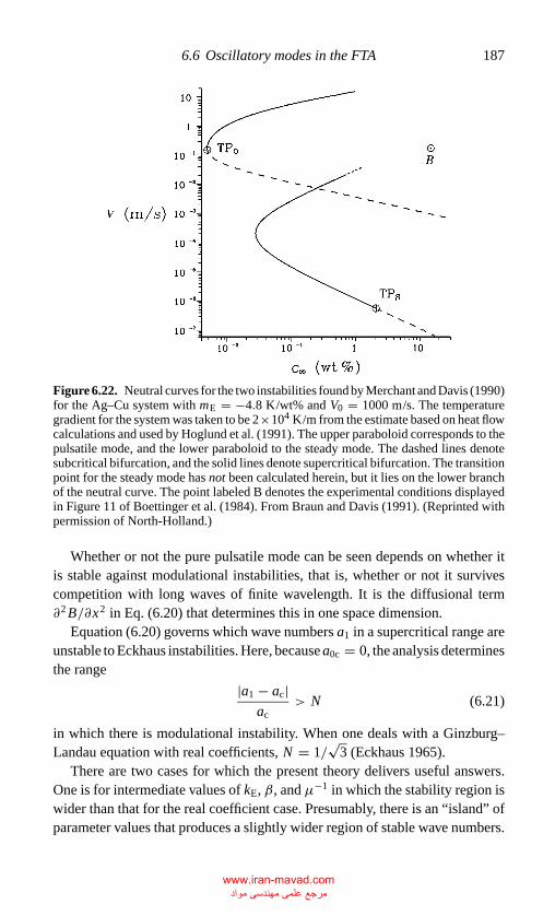
P1: LGD
CB381-06 CB381-Davis May 17, 2001 18:10 Char Count= 0
6.6 Oscillatory modes in the FTA 187
Figure 6.22. Neutral curves for the two instabilities found by Merchant and Davis (1990)for the Ag–Cu system with mE = −4.8 K/wt% and V0 = 1000 m/s. The temperaturegradient for the system was taken to be 2×10⁴ K/m from the estimate based on heat flowcalculations and used by Hoglund et al. (1991). The upper paraboloid corresponds to thepulsatile mode, and the lower paraboloid to the steady mode. The dashed lines denotesubcritical bifurcation, and the solid lines denote supercritical bifurcation. The transitionpoint for the steady mode has not been calculated herein, but it lies on the lower branchof the neutral curve. The point labeled B denotes the experimental conditions displayedin Figure 11 of Boettinger et al. (1984). From Braun and Davis (1991). (Reprinted withpermission of North-Holland.)
Whether or not the pure pulsatile mode can be seen depends on whether itis stable against modulational instabilities, that is, whether or not it survivescompetition with long waves of finite wavelength. It is the diffusional term∂2 B/∂x2 in Eq. (6.20) that determines this in one space dimension.
Equation (6.20) governs which wave numbers a1 in a supercritical range areunstable to Eckhaus instabilities. Here, because a0c = 0, the analysis determinesthe range
|a1 − ac|ac
> N (6.21)
in which there is modulational instability. When one deals with a Ginzburg–Landau equation with real coefficients, N = 1/
√3 (Eckhaus 1965).
There are two cases for which the present theory delivers useful answers.One is for intermediate values of kE, β, and µ−1 in which the stability region iswider than that for the real coefficient case. Presumably, there is an “island” ofparameter values that produces a slightly wider region of stable wave numbers.
www.iran-mavad.com مرجع علمی مھندسی مواد
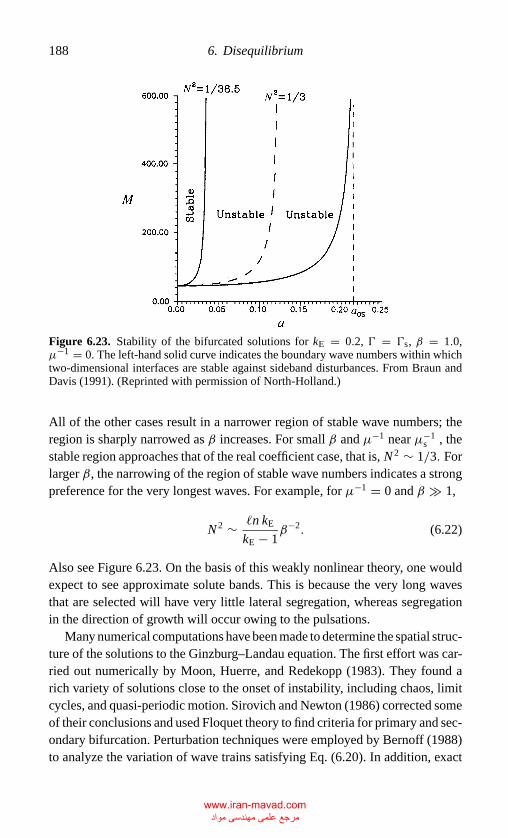
P1: LGD
CB381-06 CB381-Davis May 17, 2001 18:10 Char Count= 0
188 6. Disequilibrium
Figure 6.23. Stability of the bifurcated solutions for kE = 0.2, � = �s, β = 1.0,µ−1 = 0. The left-hand solid curve indicates the boundary wave numbers within whichtwo-dimensional interfaces are stable against sideband disturbances. From Braun andDavis (1991). (Reprinted with permission of North-Holland.)
All of the other cases result in a narrower region of stable wave numbers; theregion is sharply narrowed as β increases. For small β and µ−1 near µ−1
s , thestable region approaches that of the real coefficient case, that is, N 2 ∼ 1/3. Forlarger β, the narrowing of the region of stable wave numbers indicates a strongpreference for the very longest waves. For example, for µ−1 = 0 and β � 1,
N 2 ∼ �n kE
kE − 1β−2. (6.22)
Also see Figure 6.23. On the basis of this weakly nonlinear theory, one wouldexpect to see approximate solute bands. This is because the very long wavesthat are selected will have very little lateral segregation, whereas segregationin the direction of growth will occur owing to the pulsations.
Many numerical computations have been made to determine the spatial struc-ture of the solutions to the Ginzburg–Landau equation. The first effort was car-ried out numerically by Moon, Huerre, and Redekopp (1983). They found arich variety of solutions close to the onset of instability, including chaos, limitcycles, and quasi-periodic motion. Sirovich and Newton (1986) corrected someof their conclusions and used Floquet theory to find criteria for primary and sec-ondary bifurcation. Perturbation techniques were employed by Bernoff (1988)to analyze the variation of wave trains satisfying Eq. (6.20). In addition, exact
www.iran-mavad.com مرجع علمی مھندسی مواد
P1: LGD
CB381-06 CB381-Davis May 17, 2001 18:10 Char Count= 0
6.7 Strongly nonlinear pulsations 189
solutions have been found by Nozaki and Bekki (1984) and Bekki and Nozaki(1985). These exact solutions are solitary waves, shocklike waves ( jumps inwave number), and holes ( jumps in phase). The shocklike solutions come aboutwhen two regions of different wave number meet (see Bekki and Nozaki 1985and Bernoff 1988) and a region of rapid transition occurs from one wave numberto the other. The hole solutions form when two shocklike solutions meet. Forthese types of solutions to exist, the wave numbers for the parts of the uniformwave train must be modulationally stable to sideband disturbances accordingto Stuart and DiPrima (1978). One may expect to see these regions of wavenumber transition experimenally in stable wave number regimes.
As discussed in Moon et al. (1983) and Kuramoto (1984), for the case whenthe critical wave number for a Ginzburg–Landau equation is zero, a Kuramoto–Sivashinsky equation may be derived in which the amplitude of the solutionremains constant but the phase may vary on the slow time and space scales. Ifd ′ < 0 in Eq. (6.23), Kuramoto (1984) found that diffusion-induced phase tur-bulence results. The Ginzburg–Landau equation (6.20) for rapid solidificationalways has d ′ > 0, and thus one would not expect to see phase turbulence inthe present applications.
The form of the evolution equation for the case when a second spatial dimen-sion is present will also be a Ginzburg–Landau equation; the only difference willbe that the BX X term becomes BX X + BY Y with the same coefficient. The mostdangerous mode would still occur at zero wave number. In this case, the analysisof Kuramoto (1984) also applies, but the extra spatial dimension now admitsrotating spiral waves as solutions. It is interesting to note that rotating spiralwaves have been observed in solidification in the melt-spinning experimentsby Thoma et al. (1988). They performed experiments with Ag-19 wt % Cu atwheel speeds of 10–40 m/s and calculated that the average growth rate did notexceed 6 m/s. The wavelength of the spiral far from the core appears to be about2 µm. The Ginzburg–Landau equation derived above requires that the wave-length of the spiral be long compared with the solute–boundary-layer thickness.The solute diffusivity in the liquid for Ag–Cu is near 10−9 m2/s, whereas thegrowth rate is near 1 m/s; the solute–boundary-layer thickness is near 10−9 mor 10−3 µm. Thus, the helical growth observed has a wavelength that is verylong compared with the solute boundary layer, and the described model may,indeed, contain the physics necessary to describe this helical growth.
6.7 Strongly Nonlinear Pulsations
In Section 6.6 the weakly nonlinear theory showed that the bifurcation ofspatially uniform oscillations from the planar interface is subcritical when
www.iran-mavad.com مرجع علمی مھندسی مواد
P1: LGD
CB381-06 CB381-Davis May 17, 2001 18:10 Char Count= 0
190 6. Disequilibrium
nonequilibrium effects are small and supercritical when either β is large orwhen µ−1 is near µ−1
s . When β is small, the nonlinearly stable band of wavenumbers has N = 1/
√3, the Eckhaus limit for the real Ginzburg–Landau equa-
tion. As β becomes large, N → 0, and thus very long waves are selected. Inboth limits of β, the pulsatile mode, a = 0, remains stable.
In this section the pulsatile mode will be examined, and it will be demon-strated that strongly nonlinear behavior can be described analytically, as shownby Merchant et al. (1992).
6.7.1 Small β
Consider the rapid solidification system with ∂/∂x, ∂/∂y = 0, and let β 1.From Eqs. (6.11a,b) for a = 0
M ∼ 1 + 2kE
β − kEµ−1, ω2
0 = kE/M as β → 0, (6.23)
where ω0 is the angular frequency according to linear theory.If the two terms in the denominator of Eq. (6.23) are balanced, one can define
µ−1 = β
kE− (1 + µ−1)
2 + kE
k2E
β2, M = Mβ−2, M = O(1) (6.24)
consistent with the characteristic equation. Here µ−1 is a detuning parameterforµ−1 nearµ−1
s . An increase in µ−1 results in a decrease inµ−1, and thus µ−1
measures the deviation from the absolute stability boundary for the pulsatilemode. Here, if µ−1 = 0, µ−1 =µ−1
s .The restriction ofµ−1 to∣∣µ−1 − µ−1
s
∣∣ 1leads to a uniform description of the bifurcation, even in the subcritical case.
From Eq. (6.23), the critical morphological number corresponds to
M ∼ (1 + 2kE)kE
(2 + kE)µ−1. (6.25)
Asymptotic analysis of the full characteristic equation suggests that there aretwo time scales
t1 = βt and t2 = β2t. (6.26a)
The coordinate in the direction of growth remains unchanged, Z = z.Map theinterface into a fixed domain by letting ζ = Z − H (t1, t2). In the liquid ζ > 0,
Cζ ζ + Cζ − β[Ct1 − Ht1Cζ ] − β2[Ct1 − Ht1Cζ ] = 0; (6.26b)
www.iran-mavad.com مرجع علمی مھندسی مواد
P1: LGD
CB381-06 CB381-Davis May 17, 2001 18:10 Char Count= 0
6.7 Strongly nonlinear pulsations 191
on the interface at ς = 0,
Cζ − (1 + βHt1 + β2 Ht2 )[(kE − 1)C + 1](k − 1)
kE − 1)= 0,
β2M−1 H +[β
kE− (µ−1 + 1)
2 + kE
k2E
β2
](V − 1) − Cm(V )
− kE
(kE − 1)
[m(V )
kE− m(V )
k
]= 0;
(6.26c)
and as ζ → 0,
C → 1. (6.26d)
The domain of the problem is now 0 < ζ < ∞. Also,
k(V ) = kE + β V
1 + β V, (6.26e)
V = 1 + βHt1 + β2 Ht2 . (6.26f)
Pose the following expansions:
C(z, t) = C0 + βC1 + · · · , (6.26g)
h(t) = 1
β(H0 + βH1 + · · ·). (6.26h)
The latter form indicates that the presence of disequilibrium effects drives verylarge amplitude oscillations compared with the steady-solute boundary-layerthickness δc.
At leading order, one obtains, for ζ > 0
C0ζ ζ + C0ζ (1 + H0t1 ) = 0; (6.27a)
on ζ = 0,
C0ς − (1 + H0t1 )[1 + C0(kE − 1)] = 0, (6.27b)
C0 = 0; (6.27c)
and, as ζ → ∞,C0 → 1. (6.27d)
The solution to problem (6.27) is
C0 = 1 − exp[−(1 + H0t1 )ζ ], (6.28)
www.iran-mavad.com مرجع علمی مھندسی مواد
P1: LGD
CB381-06 CB381-Davis May 17, 2001 18:10 Char Count= 0
192 6. Disequilibrium
where the interface position H0 is arbitrary at this order. Note that the solutefield is explicitly quasi-steady but depends strongly on time through H0t1 .
Define W ≡ 1 + H0t1 and, at O(β) obtain, for ζ > 0,
C1ζ ζ + C1ζW = −(H1t1 + H0t1 )C0ζ + C0t1 ; (6.29a)
on ζ = 0
C1ζ − W (kE − 1)C1 − H1t1 = H0t2 − W 2, (6.29b)
− C1 + M−1 H0 + 1
kEW = 0; (6.29c)
and, as ζ → ∞,C1 → 0. (6.29d)
The Fredholm alternative must be enforced in order to eliminate secular termsthat grow algebraically in ζ . This is most easily done by integrating Eq. (6.29a)over the domain in ζ and using the boundary conditions to obtain the compati-bility condition
∂2 H0
∂t21
+ ω20 H0
(1 + ∂H0
∂t1
)3
= 0, (6.30)
where ω20 is given by Eq.(6.23). To leading order, the location of the interface is
thus governed by the preceding nonlinear oscillator equation. The first integralmay be calculated by multiplying Eq. (6.30) by H0t1 and integrating to obtain
ω20 H 2
0 + (H0t1 )2
(1 + H0t1 )2≡ A2(t2). (6.31)
The phase plane for Eq. (6.31) is shown in Figure 6.24. For amplitudes A < 1,the orbits form closed curves, indicating periodic behavior. As the amplitudeapproaches unity, the velocity becomes unbounded. For A ≥ 1, the curves areno longer closed, indicating nonperiodic behavior. The energy (or amplitude)evolves on the slow time, and, generally, the frequency is amplitude dependentand thus also evolves on the slow time.
An implicit solution to Eq. (6.31) may be found by integrating once more,
H0 = [A(t2)/ω0] sin[ω0(t1 + H0) + φ(t2)]. (6.32)
Some results of the numerical calculations of H0 are shown in Figure 6.25. Notethat the velocity profiles become more peaked as the amplitude increases towardunity. The motion becomes more like a relaxation oscillation as the amplitude
www.iran-mavad.com مرجع علمی مھندسی مواد
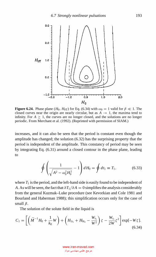
P1: LGD
CB381-06 CB381-Davis May 17, 2001 18:10 Char Count= 0
6.7 Strongly nonlinear pulsations 193
Figure 6.24. Phase plane (H0, H0T) for Eq. (6.34) with ω0 = 1 valid for β 1. Theclosed curves near the origin are nearly circular, but as A → 1, the maxima tend toinfinity. For A ≥ 1, the curves are no longer closed, and the solutions are no longerperiodic. From Merchant et al. (1992). (Reprinted with permission of SIAM.)
increases, and it can also be seen that the period is constant even though theamplitude has changed; the solution (6.32) has the surprising property that theperiod is independent of the amplitude. This constancy of period may be seenby integrating Eq. (6.31) around a closed contour in the phase plane, leadingto
∮ 1√A2 − ω2
0 H 20
− 1
d H0 =
∮dt1 ≡ T1, (6.33)
where T1 is the period, and the left-hand side is easily found to be independent ofA. As will be seen, the fact that ∂T1/∂A = 0 simplifies the analysis considerablyfrom the general Kuzmak–Luke procedure (see Kevorkian and Cole 1981 andBourland and Haberman 1988); this simplification occurs only for the case ofsmall β.
The solution of the solute field in the liquid is
C1 =[(
M−1 H0 + 1
kEW
)+(
H1t1 + H0t2 − Wt1
W 2
)ζ − Wt1
2Wζ 2
]exp[−Wζ ].
(6.34)
www.iran-mavad.com مرجع علمی مھندسی مواد
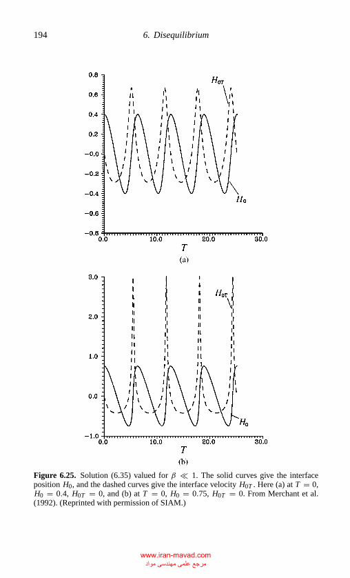
P1: LGD
CB381-06 CB381-Davis May 17, 2001 18:10 Char Count= 0
194 6. Disequilibrium
Figure 6.25. Solution (6.35) valued for β 1. The solid curves give the interfaceposition H0, and the dashed curves give the interface velocity H0T . Here (a) at T = 0,H0 = 0.4, H0T = 0, and (b) at T = 0, H0 = 0.75, H0T = 0. From Merchant et al.(1992). (Reprinted with permission of SIAM.)
www.iran-mavad.com مرجع علمی مھندسی مواد
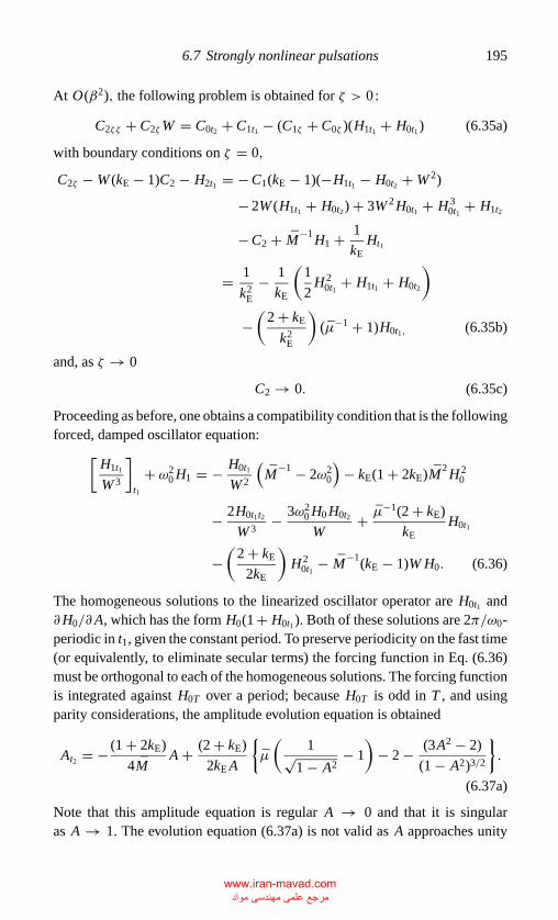
P1: LGD
CB381-06 CB381-Davis May 17, 2001 18:10 Char Count= 0
6.7 Strongly nonlinear pulsations 195
At O(β2), the following problem is obtained for ζ > 0:
C2ζ ζ + C2ζW = C0t2 + C1t1 − (C1ζ + C0ζ )(H1t1 + H0t1 ) (6.35a)
with boundary conditions on ζ = 0,
C2ζ − W (kE − 1)C2 − H2t1 = − C1(kE − 1)(−H1t1 − H0t2 + W 2)
− 2W (H1t1 + H0t2 ) + 3W 2 H0t1 + H 30t1 + H1t2
− C2 + M−1 H1 + 1
kEHt1
= 1
k2E
− 1
kE
(1
2H 2
0t1 + H1t1 + H0t2
)
−(
2 + kE
k2E
)(µ−1 + 1)H0t1, (6.35b)
and, as ζ → 0
C2 → 0. (6.35c)
Proceeding as before, one obtains a compatibility condition that is the followingforced, damped oscillator equation:[
H1t1
W 3
]t1
+ ω20 H1 = − H0t1
W 2
(M−1 − 2ω2
0
)− kE(1 + 2kE)M2 H 2
0
− 2H0t1t2
W 3− 3ω2
0 H0 H0t2
W+ µ−1(2 + kE)
kEH0t1
−(
2 + kE
2kE
)H 2
0t1 − M−1(kE − 1)W H0. (6.36)
The homogeneous solutions to the linearized oscillator operator are H0t1 and∂H0/∂A, which has the form H0(1 + H0t1 ). Both of these solutions are 2π/ω0-periodic in t1, given the constant period. To preserve periodicity on the fast time(or equivalently, to eliminate secular terms) the forcing function in Eq. (6.36)must be orthogonal to each of the homogeneous solutions. The forcing functionis integrated against H0T over a period; because H0T is odd in T , and usingparity considerations, the amplitude evolution equation is obtained
At2 = − (1 + 2kE)
4MA + (2 + kE)
2kE A
{µ
(1√
1 − A2− 1
)− 2 − (3A2 − 2)
(1 − A2)3/2
}.
(6.37a)
Note that this amplitude equation is regular A → 0 and that it is singularas A → 1. The evolution equation (6.37a) is not valid as A approaches unity
www.iran-mavad.com مرجع علمی مھندسی مواد
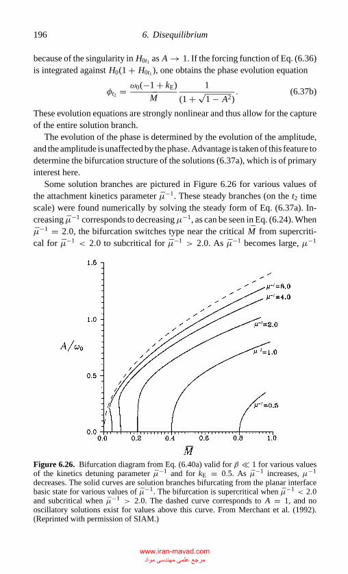
P1: LGD
CB381-06 CB381-Davis May 17, 2001 18:10 Char Count= 0
196 6. Disequilibrium
because of the singularity in H0t1 as A → 1. If the forcing function of Eq. (6.36)is integrated against H0(1 + H0t1 ), one obtains the phase evolution equation
φt2 = ω0(−1 + kE)
M
1
(1 + √1 − A2)
. (6.37b)
These evolution equations are strongly nonlinear and thus allow for the captureof the entire solution branch.
The evolution of the phase is determined by the evolution of the amplitude,and the amplitude is unaffected by the phase. Advantage is taken of this feature todetermine the bifurcation structure of the solutions (6.37a), which is of primaryinterest here.
Some solution branches are pictured in Figure 6.26 for various values ofthe attachment kinetics parameter µ−1. These steady branches (on the t2 timescale) were found numerically by solving the steady form of Eq. (6.37a). In-creasing µ−1 corresponds to decreasingµ−1, as can be seen in Eq. (6.24). Whenµ−1 = 2.0, the bifurcation switches type near the critical M from supercriti-cal for µ−1 < 2.0 to subcritical for µ−1 > 2.0. As µ−1 becomes large, µ−1
Figure 6.26. Bifurcation diagram from Eq. (6.40a) valid for β 1 for various valuesof the kinetics detuning parameter µ−1 and for kE = 0.5. As µ−1 increases, µ−1
decreases. The solid curves are solution branches bifurcating from the planar interfacebasic state for various values of µ−1. The bifurcation is supercritical when µ−1 < 2.0and subcritical when µ−1 > 2.0. The dashed curve corresponds to A = 1, and nooscillatory solutions exist for values above this curve. From Merchant et al. (1992).(Reprinted with permission of SIAM.)
www.iran-mavad.com مرجع علمی مھندسی مواد
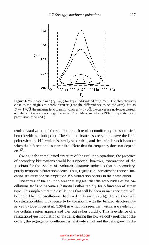
P1: LGD
CB381-06 CB381-Davis May 17, 2001 18:10 Char Count= 0
6.7 Strongly nonlinear pulsations 197
Figure 6.27. Phase plane (Y0, Y0ψ ) for Eq. (6.56) valued for β � 1. The closed curvesclose to the origin are nearly circular (note the different scales on the axes), but asB → 1/
√3, the maxima tend to infinity. For B ≥ 1/
√3, the curves are no longer closed,
and the solutions are no longer periodic. From Merchant et al. (1992). (Reprinted withpermission of SIAM.)
tends toward zero, and the solution branch tends nonuniformly to a subcriticalbranch with no limit point. The solution branches are stable above the limitpoint when the bifurcation is locally subcritical, and the entire branch is stablewhen the bifurcation is supercritical. Note that the frequency does not dependon M .
Owing to the complicated structure of the evolution equations, the presenceof secondary bifurcations would be suspected; however, examination of theJacobian for the system of evolution equations indicates that no secondary,purely temporal bifurcation occurs. Thus, Figure 6.27 contains the entire bifur-cation structure for the amplitude. No bifurcation occurs in the phase either.
The forms of the solution branches suggest that the amplitudes of the os-cillations tends to become substantial rather rapidly for bifurcation of eithertype. This implies that the oscillations that will be seen in an experiment willbe more like the oscillations displayed in Figure 6.25(b); that is, they willbe relaxation-like. This seems to be consistent with the banded structure ob-served by Boettinger et al. (1984) in which it is seen that, within a wavelength,the cellular region appears and dies out rather quickly. This is evidence of arelaxation-type modulation of the cells; during the low-velocity portions of thecycles, the segregation coefficient is relatively small and the cells grow. In the
www.iran-mavad.com مرجع علمی مھندسی مواد
P1: LGD
CB381-06 CB381-Davis May 17, 2001 18:10 Char Count= 0
198 6. Disequilibrium
relatively short portion of the cycle when the velocity is high, the segregationcoefficient rapidly approaches unity, and relatively little solute is rejected.
For this analysis to be physically relevant, one would expect to see thefrequency ω observed experimentally, perhaps as the frequency of the cellmodulation noted in banding phenomena as studied by Boettinger et al. (1984).On the basis of the material properties and experimental conditions, the cellsobserved occur at β = 0.034, and the period of the bands is about 170 diffusiontimes. The period of the oscillations here is expected to be on the T = βt timescale, or a scale of about 30 diffusion times. Using the asymptotic form of thefrequency from the linear theory
ω20 = 2 + kE
µ−1(1 + 2kE), (6.38)
and assuming that V0 = 1000 m/s, one should obtain a period of 2π/βω0 ≈ 80diffusion times. The period increases with morphological number to the power1/2. The characteristic time for growth or decay of the oscillations is on thet2 = β2t time scale and is expected to be on the order of 900 diffusion times.The time scales are of roughly the correct order.
For completeness, the results are discussed in experimentally relevant terms.Experimentally controllable parameters are the speed of the front V and theconcentration of the solute C . Typical results of linear stability analysis ofthe planar interface basic state are shown in Figure 6.4. Small β correspondsto “low” speed, and thus this analysis operates near the lower branch of theoscillatory curve. The experimental conditions under which Boettinger et al.observed bands is just the region where the oscillatory instability may in-teract with the steady cellular instability (Section 6.8), and this may be thecause of banding phenomena, as suggested by Merchant and Davis (1990).Time scale estimates seem to support this speculation. Furthermore, the period(in dimensional terms) decreases with increasing pulling speed, as observedexperimentally by Gremaud et al. (1990).
6.7.2 Large β
Asβ→ ∞, the segregation coefficient approaches unity to leading order, yet thepulsatile instability remains. A different nonlinear oscillator governs locationof the interface, and the period of the oscillation is amplitude dependent.
The asymptotic forms for β → ∞ for the critical morphological numberand frequency of linear stability theory, are seen by Eqs. (6.11c,d), which fora = 0 are the following:
M ∼ 5β2
2(kE − µ−1β2)and ω2
0 = (kE − 1)β
2kEM �n kE. (6.39)
www.iran-mavad.com مرجع علمی مھندسی مواد
P1: LGD
CB381-06 CB381-Davis May 17, 2001 18:10 Char Count= 0
6.7 Strongly nonlinear pulsations 199
The terms in the denominator of Eq. (6.39) are balanced by choosing µ−1 to beO(β−2) and kE to be O(1). The following scales emerge:
β ≡ 1
ε2, M = M
ε4, µ−1 = ε4µ−1, (6.40)
as ε → 0. The value of µ−1 need not be near µ−1s here because the bifurcation
is supercritical (Braun and Davis 1991), and thus a uniform description of thebifurcation is expected even for weak kinetics. Relation (6.39) suggests theexistence of a time scale εt , and asymptotic analysis of the full dispersionrelation suggests a second slow time ε2t . However, as is often the case foroscillators with slowly varying period, a more general time scale is required(see Kevorkian and Cole 1981 and Bourland and Haberman 1988). In the presentcase, the appropriate time variables are
ψ = θ (t2)
ε+ φ(t2) (6.41a)
t2 = ε2t (6.41b)
These are required because the period in this limit is affected by the amplitudeof the oscillator, and perturbations in amplitude affect the functional form ofthe period. The coordinate in the direction of growth remains unscaled, Z = z.
One poses, for ε → 0,
C(z, t ; ε) = C(ξ, ψ, t2) = C0 + ε2C2 + ε3C3 + · · · , (6.42a)
h(t ; ε) = H (ψ, t2) = 1
ε(H0 + εH1 + · · ·) (6.42b)
and proceeds as before. Again, the presence of disequilibrium effects drives avery large amplitude oscillation.
At leading order,
C0 = 1. (6.43)
The solute field is constant to leading order owing to the near absence of soluterejection in the high-speed limit. The interface position H0 is again arbitrary atleading order. The O(ε) problem is trivial.
At O(ε2)
C2 = −kE
Xexp[−Xξ ], (6.44a)
where
X = 1 + H0ψ and (t2) = θ ′(t2). (6.44b)
www.iran-mavad.com مرجع علمی مھندسی مواد
P1: LGD
CB381-06 CB381-Davis May 17, 2001 18:10 Char Count= 0
200 6. Disequilibrium
The correction to the leading order (constant) solute field is strongly dependenton time through H0ψ .
At O(ε3) the integration over the domain yields the compatibility condition
2 ∂2 H0
∂ψ2+ 2
0 H0
(1 + ∂H0
∂ψ
)4
= 0, (6.45)
where 20 ≡ (kE − 1)/(2kEM �n kE). As in the previous case, the location of
the interface is given to leading order by a nonlinear oscillator equation, nowwith exponent four. Here the frequency does vary with the amplitude of theoscillation. Rescale the amplitude as Y0ψ ≡ H0/ 0 and define ρ ≡ / 0;Eq. (6.45) then becomes
ρ2 ∂2Y0
∂ψ2+ Y0
(1 + ρ ∂Y0
∂ψ
)4
= 0. (6.46)
The first integral may be calculated by multiplying Eq. (6.46) by ρY0ψ andintegrating; the result is
Y 20 + ρ2Y 2
0ψ (1 + ρY0ψ/3)
(1 + ρY0ψ )3≡ B2(t2). (6.47)
The phase plane for Eq. (6.47) is shown in Figure 6.27. For amplitudesB < 1/
√3, the orbits form closed curves, indicating periodic behavior. As
the amplitudes approach 1/√
3, the velocity Y0ψ becomes unbounded, and, forB ≥ 1/
√3, the curves are no longer closed, indicating nonperiodic behavior in
the same way. The energy B evolves on the slow time; because the frequencydepends on the amplitude in this limit, the frequency will also evolve on theslow time.
The first integral (6.47) can not be conveniently integrated again. It is asimple matter, however, to integrate Eq. (6.46) numerically. The solutions arevery similar in character to the solutions in the small β case. The velocityprofile again becomes very peaked as the amplitude approaches its limitingvalue, here 1/
√3, and the oscillation becomes more relaxation-like. The period
of the oscillation can be normalized to be 2π for a given amplitude by find-ing the appropriate ρ; this is accomplished by iterating on ρ until the correctvalue of Y0 at ψ = 2π is obtained; ρ increases monotonically with increasingenergy.
www.iran-mavad.com مرجع علمی مھندسی مواد
P1: LGD
CB381-06 CB381-Davis May 17, 2001 18:10 Char Count= 0
6.7 Strongly nonlinear pulsations 201
The compatibility condition at O(ε4) gives the following forced, dampedoscillator equation:
[ H1ψ
X4
]ψ
+ 20 H1 =
X4(φ′H0ψψ − 2H0ψ t2 + 3 H0ψψ
X5(−φ′ + H0t2 )
+ 3 3
2X6H0ψψψ − 15 4
2X7H 2
0ψψ − 20
×[kEM
2
(1
X2− 1
)+ Mµ−1 H0ψψ − 2 H0 H0ψψ
X3
− 1 + H0 H0t2
X− 1
X2+ φ′H0
(1 − 1
X4
)].
(6.48)
One of the two homogeneous solutions to Eq. (6.48) is periodic on the ψ scalewith period 2π , and it is given by H0ψ . The other homogeneous solution isnot periodic. To preserve periodicity on the fast time, the forcing function inEq. (6.48) must be orthogonal to the periodic homogeneous solution. Integratethe forcing function against H0ψ over a period and use the fact that H0 isodd in ψ , as well as parity considerations, to obtain the (rescaled) amplitudeevolution equation
1
2
d(B2)
dt2= (kE − 1)ρ2
2kE �n kE
·{(
kE − 52M
) [ Y 20ψ
(1 + ρY0ψ )2
]− µ−1Y 2
0ψ − 12
(kE − 5
M
)Y 2
0 Y 20ψ
}.
(6.49)Here
f ≡∫ 2π
0f (ψ)dψ. (6.50)
The procedure used here is identical (except for the choice of the slowesttime scale) to a procedure discussed in Bourland and Haberman (1988) forthe analysis of weakly dissipative nonlinear oscillators. The form of theamplitude evolution equation (6.49) is an intermediate one for the derivationof the equivalent of Eq. (6.37); there, a closed-form implicit solution is knownthat allows one to evaluate the mean terms. Here, no such closed-form solutionis known, and further simplification is not possible.
It is necessary to proceed to one higher order after completely solvingthe linear oscillator Eq. (6.48) to obtain the slow-time evolution of φ′. The
www.iran-mavad.com مرجع علمی مھندسی مواد
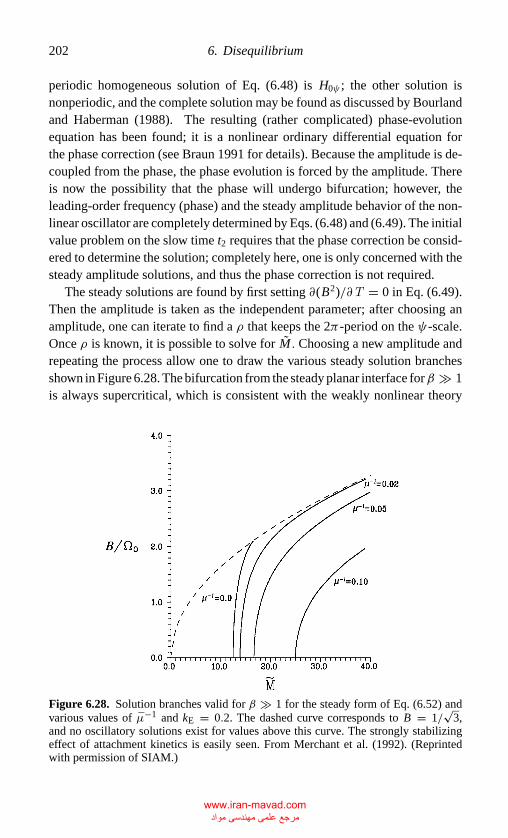
P1: LGD
CB381-06 CB381-Davis May 17, 2001 18:10 Char Count= 0
202 6. Disequilibrium
periodic homogeneous solution of Eq. (6.48) is H0ψ ; the other solution isnonperiodic, and the complete solution may be found as discussed by Bourlandand Haberman (1988). The resulting (rather complicated) phase-evolutionequation has been found; it is a nonlinear ordinary differential equation forthe phase correction (see Braun 1991 for details). Because the amplitude is de-coupled from the phase, the phase evolution is forced by the amplitude. Thereis now the possibility that the phase will undergo bifurcation; however, theleading-order frequency (phase) and the steady amplitude behavior of the non-linear oscillator are completely determined by Eqs. (6.48) and (6.49). The initialvalue problem on the slow time t2 requires that the phase correction be consid-ered to determine the solution; completely here, one is only concerned with thesteady amplitude solutions, and thus the phase correction is not required.
The steady solutions are found by first setting ∂(B2)/∂T = 0 in Eq. (6.49).Then the amplitude is taken as the independent parameter; after choosing anamplitude, one can iterate to find a ρ that keeps the 2π -period on the ψ-scale.Once ρ is known, it is possible to solve for M . Choosing a new amplitude andrepeating the process allow one to draw the various steady solution branchesshown in Figure 6.28. The bifurcation from the steady planar interface forβ � 1is always supercritical, which is consistent with the weakly nonlinear theory
Figure 6.28. Solution branches valid for β � 1 for the steady form of Eq. (6.52) andvarious values of µ−1 and kE = 0.2. The dashed curve corresponds to B = 1/
√3,
and no oscillatory solutions exist for values above this curve. The strongly stabilizingeffect of attachment kinetics is easily seen. From Merchant et al. (1992). (Reprintedwith permission of SIAM.)
www.iran-mavad.com مرجع علمی مھندسی مواد
P1: LGD
CB381-06 CB381-Davis May 17, 2001 18:10 Char Count= 0
6.7 Strongly nonlinear pulsations 203
of Braun and Davis (1991). The strongly stabilizing influence of attachmentkinetics (µ) is evident in the behavior of the solution branches. For increasingµ−1, the steady-state amplitude of the oscillations decreases, which we wouldexpect if atoms were attaching more sluggishly to the interface. Whenµ−1 = 0,the amplitude rises very quickly to within a very small neighborhood of thelimiting amplitude for oscillations to exist. Note that when the solution becomesclose enough to the limiting amplitude, the oscillations develop very steepgradients as the velocity H0ψ becomes more sharply peaked, and the multiplescale analysis performed here is no longer valid. A new, faster time scale mustbe allowed near the limiting amplitude.
One should again expect the amplitude of the oscillations to become sub-stantial very quickly as the morphological number is increased and thus to seerelaxation-type oscillations experimentally. The oscillations would be respon-sible for striations in the solute frozen into the solid.
Attachment kinetics become very important at high speeds, and, for β = 10,the attachment kinetics for Ag–Cu, one of the best characterized alloys at highsolidification rates, are too sluggish to allow the oscillations described here. Amaterial with higher C∞, smaller kE, a very large V0, and a large β0 is mostlikely to have experimentally observable solute bands at high speeds; in short,the effect of attachment kinetics µ must be small. Large V0 implies very rapidattachment of atoms to the solid at the solid–liquid interface, and large β0
implies that solute rejection at the interface deviates from its equilibrium valueat relatively low speeds. Materials without these properties do not exhibit thesolute bands analyzed here.
6.7.3 Numerical Simulation
As just seen, for limiting values of β, the pulsatile mode satisfies a stronglynonlinear oscillation equation, whereas instability is determined at higher order.A numerical simulation of the system can be difficult because representationsof the interface (boundary integrals, boundary elements, etc.) involve integralswith history-dependent kernels that require cumulative evolution cost. Brattkusand Meiron (1992) have used a method of Greengard and Strain’s (1990) to splitthe kernel into two portions: a regular piece that delivers the history effect anda singular piece. Each portion is uniformly bounded, and the cost of evolutionis limited because the singular part is fixed and the remainder can be written asa rapidly convergent series with easily updated coefficients.
Brattkus and Meiron (1992) analyzed the pulsations discussed above. Theyverified the critical conditions for linearized instability for Mc within 1 percent,ω0 within a fraction of a percent, and the growth rate.
www.iran-mavad.com مرجع علمی مھندسی مواد
P1: LGD
CB381-06 CB381-Davis May 17, 2001 18:10 Char Count= 0
204 6. Disequilibrium
In the nonlinear range above Mc with instantaneous kinetics, µ−1 = 0, am-plitudes grow without bound, consistent with the analyses, likely showing theformation of finite-time singularities. When µ−1 > 0, the amplitudes equili-brate and give phase portraits for β = 50 similar to those in Figure 6.27. Theproperties of the solution for β → ∞ show that ω0 ∼ β−1/2, and the amplitudeB ∼ β1/2, which is consistent with the asymptotics. However, the amplitudeitself differs from the asymptotics. Similar conclusions hold for small β. At thistime the discrepancy between asymptotic and numerical solutions has not beenresolved.
6.8 Mode Coupling
There are parameter values for which the oscillatory and cellular modes havesimultaneous onsets of instability (codimension-two points). In Figure 6.4 thisoccurs at the intersection of the two neutral curves. The equivalent case is shownin Figure 6.5 in which, in nondimensional terms, the two modes have about thesame Mc, although the ac = 0 for one and ac ≈ 0.35 for the other. Figure6.9(b) shows a case in which the critical values of C∞ are equal and a∗
c ≈ 106
and a∗c ≈ 7 × 10⁶ for the two modes. A local minimum exists at a∗ = 0. It
is also possible to vary the parameters so that both of these modes have thesame critical C∞ and hence produce a codimension-two interaction betweentwo time-periodic modes, respectively, one with a∗
c = 0 and one with a∗c �= 0.
Given these possibilities, one wishes to determine the possible nonlinearinteractions that occur near the codimension-two points and predict, if possible,the conditions for banding.
Bands are alternate strips of cells (or dendrites) and segregation-free material.One can envision these occurring when, say, a cellular mode is modulated bya coexisting pulsation. In the part of the cycle that the speed is maximum,segregation-free states would be stable, whereas in the part of the cycle that thespeed is minimum, the cells would be preferred. Such a nonlinear interactioncould appear (Braun and Davis 1992) as a tertiary bifurcation from a mixedmode, as shown in Figure 6.29. These possibilities are now considered.
6.8.1 Pulsatile–Cellular Interactions
The oscillatory mode has a0c = 0 in the FTA. In this case, Braun, Merchant,and Davis (1992) wrote
� = �0 + νε2, M ∼ M0 + ε2M2, t1 = ω0t, t2 = ε2t, (x, z) = (X, Z )(6.50a)
www.iran-mavad.com مرجع علمی مھندسی مواد
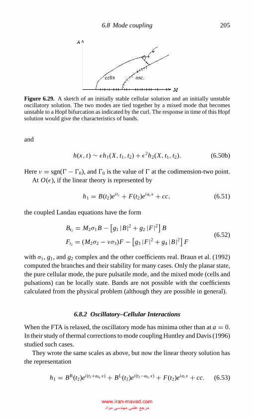
P1: LGD
CB381-06 CB381-Davis May 17, 2001 18:10 Char Count= 0
6.8 Mode coupling 205
Figure 6.29. A sketch of an initially stable cellular solution and an initially unstableoscillatory solution. The two modes are tied together by a mixed mode that becomesunstable to a Hopf bifurcation as indicated by the curl. The response in time of this Hopfsolution would give the characteristics of bands.
and
h(x, t) ∼ εh1(X, t1, t2) + ε2h2(X, t1, t2). (6.50b)
Here ν = sgn(� − �0), and �0 is the value of � at the codimension-two point.At O(ε), if the linear theory is represented by
h1 = B(t2)eit1 + F(t2)eiacx + cc, (6.51)
the coupled Landau equations have the form
Bt2 = M2σ1 B − [g1 |B|2 + g2 |F |2] B
Ft2 = (M2σ2 − νσ3)F − [g3 |F |2 + g4 |B|2] F(6.52)
with σ1, g1, and g2 complex and the other coefficients real. Braun et al. (1992)computed the branches and their stability for many cases. Only the planar state,the pure cellular mode, the pure pulsatile mode, and the mixed mode (cells andpulsations) can be locally state. Bands are not possible with the coefficientscalculated from the physical problem (although they are possible in general).
6.8.2 Oscillatory–Cellular Interactions
When the FTA is relaxed, the oscillatory mode has minima other than at a = 0.In their study of thermal corrections to mode coupling Huntley and Davis (1996)studied such cases.
They wrote the same scales as above, but now the linear theory solution hasthe representation
h1 = BR(t2)ei(t2+a0c x) + BL(t2)ei(t2−a0c x) + F(t2)eiacx + cc. (6.53)
www.iran-mavad.com مرجع علمی مھندسی مواد
P1: LGD
CB381-06 CB381-Davis May 17, 2001 18:10 Char Count= 0
206 6. Disequilibrium
Orthogonality at O(ε3) gives the complex Landau equations
BLt2 = (M2σ0 − σ1ν)BL −
[g1
∣∣BL∣∣2 + g2 |F |2 + g5
∣∣BR∣∣2] BL
BRt2 = (M2σ0 − σ1ν)BR −
[g5
∣∣BL∣∣2 + g2 |F |2 + g1
∣∣BR∣∣2] BR
Ft2 = (M2σ2 − σ3ν)F −[g3 |F |2 + g4
∣∣BL∣∣2 + g∗
4
∣∣BR∣∣2] F.
(6.54)
Hereσ2, σ3, and g3 are real andσ0, σ1, g1, g2, g4, and g5 are complex; an asteriskdenotes a complex conjugate.
Huntley and Davis (1996) computed the branches and their stability for thesystems Ag–Cu, Al–Cu, Al–Fe, and Al–Sn. Only the planar state, the purecellular mode, and pure traveling waves can be locally stable. Again, bands arenot possible with the physically determined coefficients.
6.8.3 Oscillatory–pulsatile interactions
When the FTA is relaxed, the principal interaction can be between a pulsatilemode, frequency ω0, and an oscillatory mode, frequency ω1, with a0c �= 0. Thisinteraction has been considered by Grimm and Metzener (1998) in two cases:(1) the nonresonant case in which ω0 and ω1 are unrelated, and (2) ω0 = 2ω1,a resonant case.
In the nonresonant case, the interface is represented by
h(t1, t2, x) = A(t2)ei(acx+ω1t1) + B(t2)ei(acx−ω1t1) + W (t2)eiω0t1 + cc (6.55)
and by the usual methods a set of Landau equations is determined as follows:
Wt2 = λ1W + W[a |W |2 + b |A|2 + b |B|2]
At2 = λ2 A + A[c |W |2 + d |A|2 + e |B|2]
Bt2 = λ2 B + B[c |W |2 + e |A|2 + d |B|2] ,
(6.56)
where all coefficients are complex. The cases chosen and the values of thecoefficients are given in their tables. The phases are passive in this system, andthus each complex amplitude can be replaced by its real amplitude. These realequations have the usual equilibrium states: the basic state, pure modes, mixed(traveling) modes with W and A or W and B, and mixed (standing) modes withW �= 0 and A = B. Time-periodic solutions may arise as Hopf bifurcationsfrom the mixed modes. Grimm and Metzener (1998) give conditions for theexistence of this degenerate bifurcation (at the point, an infinity of periodicorbits exists; if the conditions are perturbed, no periodic orbits exist). Higherorder corrections are necessary to remove the degeneracy. Periodic solutions
www.iran-mavad.com مرجع علمی مھندسی مواد
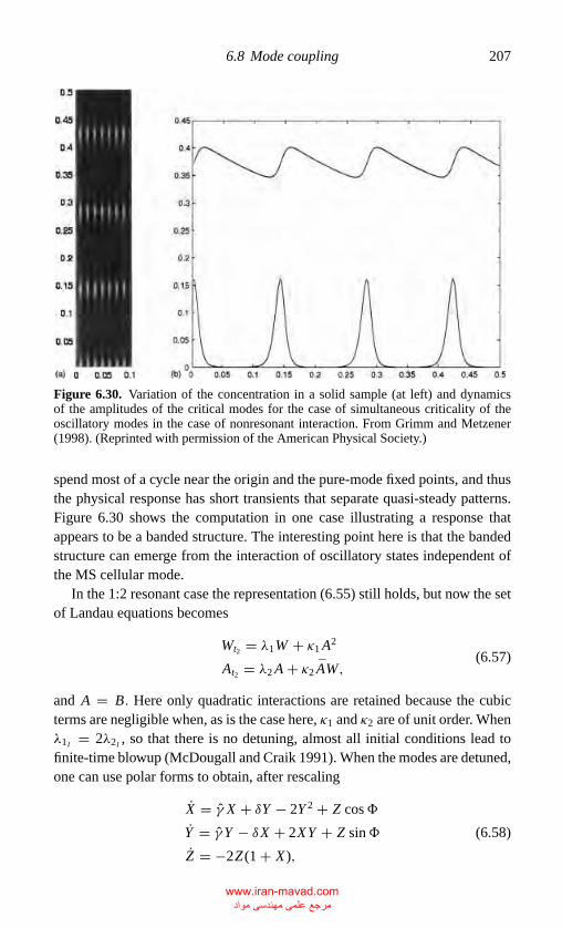
P1: LGD
CB381-06 CB381-Davis May 17, 2001 18:10 Char Count= 0
6.8 Mode coupling 207
Figure 6.30. Variation of the concentration in a solid sample (at left) and dynamicsof the amplitudes of the critical modes for the case of simultaneous criticality of theoscillatory modes in the case of nonresonant interaction. From Grimm and Metzener(1998). (Reprinted with permission of the American Physical Society.)
spend most of a cycle near the origin and the pure-mode fixed points, and thusthe physical response has short transients that separate quasi-steady patterns.Figure 6.30 shows the computation in one case illustrating a response thatappears to be a banded structure. The interesting point here is that the bandedstructure can emerge from the interaction of oscillatory states independent ofthe MS cellular mode.
In the 1:2 resonant case the representation (6.55) still holds, but now the setof Landau equations becomes
Wt2 = λ1W + κ1 A2
At2 = λ2 A + κ2 AW,(6.57)
and A = B. Here only quadratic interactions are retained because the cubicterms are negligible when, as is the case here, κ1 and κ2 are of unit order. Whenλ1I = 2λ2I , so that there is no detuning, almost all initial conditions lead tofinite-time blowup (McDougall and Craik 1991). When the modes are detuned,one can use polar forms to obtain, after rescaling
X = γ X + δY − 2Y 2 + Z cos�
Y = γY − δX + 2XY + Z sin�
Z = −2Z (1 + X ),
(6.58)
www.iran-mavad.com مرجع علمی مھندسی مواد
P1: LGD
CB381-06 CB381-Davis May 17, 2001 18:10 Char Count= 0
208 6. Disequilibrium
where γ measures λ1R/λ2R , δ is the detuning parameter, and� is related to thephase difference between the two modes; all the coefficients are real.
Hughes and Proctor (1992) showed that when X = −1, there are two fixedpoints, one stable and one unstable. The state
Y = 12δ +
tan�+ 1
22 − δ tan�
γ + O(γ 2)
Z = 2 + 12δ
2
(2 − δ tan�) cos�γ + O(γ 2)
(6.59)
is stable if to O(γ ),
4 − δ2
12 + δ2<
1
2δ tan� < 1. (6.60)
It ceases to exist at unity and undergoes a Hopf bifurcation at the lower bound.Hughes and Proctor (1992) found that periodic orbits exist beyond the Hopfbifurcation point, and they undergo a cascade of period doublings as the pa-rameters are varied. The dynamics is characterized by the alternation of slowand fast phases. During the slow Z phase, the standing waves have small am-plitude, and in the fast phase all variables are important. Again, this suggeststhe possibility of the prediction of banded structures, as shown in Figure 6.31.
In both of the cases studied involving the interactions of oscillatory modes,the responses suggest banded structures. However, these theories have not yetbeen tested quantitatively against experiment and hence remain only a possiblescenario.
6.9 Phenomenological Models
In Section 6.8 weakly nonlinear interactions of cells and oscillations werediscussed for situations near the crossings of the two neutral curves. Thesecodimension-two analyses can in principle give conditions under which band-like structures would emerge. However, to this point these structures are notpredicted when the coefficients of the appropriate Landau equations are com-puted from the material and processing parameters of the system.
An alternative approach is to examine certain physical quantities such astemperature versus speed on interfaces undergoing steady growth and to posean ansatz that, if correct, selects the morphology the system favors.
Gremaud et al. (1991) and Carrard et al. (1992) have posed such a model inthe FTA. Figure 6.32 shows plots of the interface temperature for steady growthin two cases. In the first case, as discussed in Section 6.2, there is the interface
www.iran-mavad.com مرجع علمی مھندسی مواد
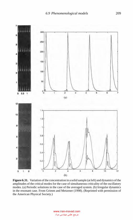
P1: LGD
CB381-06 CB381-Davis May 17, 2001 18:10 Char Count= 0
6.9 Phenomenological models 209
Figure 6.31. Variation of the concentration in a solid sample (at left) and dynamics of theamplitudes of the critical modes for the case of simultaneous criticality of the oscillatorymodes. (a) Periodic solutions in the case of the averaged system. (b) Irregular dynamicsin the resonant case. From Grimm and Metzener (1998). (Reprinted with permission ofthe American Physical Society.)
www.iran-mavad.com مرجع علمی مھندسی مواد
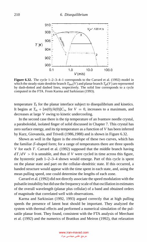
P1: LGD
CB381-06 CB381-Davis May 17, 2001 18:10 Char Count= 0
210 6. Disequilibrium
Figure 6.32. The cycle 1–2–3–4–1 corresponds to the Carrard et al. (1992) model inwhich the steady-state dendrite branch Tden(V ) and planar branch Tpl(V ) are representedby dash-dotted and dashed lines, respectively. The solid line corresponds to a cyclecomputed in the FTA. From Karma and Sarkissian (1993).
temperature T0 for the planar interface subject to disequilibrium and kinetics.It begins at Tm + [m(0)/k(0)]C∞ for V = 0, increases to a maximum, anddecreases at large V owing to kinetic undercooling.
In the second case there is the tip temperature of an Ivantsov needle crystal,a paraboloidal, isolated finger of solid discussed in Chapter 7. This crystal haszero surface energy, and its tip temperature as a function of V has been inferredby Kurz, Giovanola, and Trivedi (1986,1988) and is shown in Figure 6.32.
Shown as well in the figure is the envelope of these two curves, which hasthe familiar S-shaped form; for a range of temperatures there are three speedsV for each T . Carrard et al. (1992) supposed that the middle branch havingdT /dV > 0 is unstable, and thus if V were cycled in time across this figure,the hysteretic path 1–2–3–4 shown would emerge. Part of this cycle is spenton the planar state and part on the cellular–dendritic state. If this occurred, abanded structure would appear with the time spent in each state, and, using themean pulling speed, one could determine the lengths of each zone.
Carrard et al. (1992) did not directly associate the speed modulation with thepulsatile instability but did use the frequency scale of that oscillation in estimatesof the overall wavelength (planar plus cellular) of a band and obtained ordersof magnitude that correlated well with observations.
Karma and Sarkissian (1992, 1993) argued correctly that at high pullingspeeds the presence of latent heat should be important. They analyzed thesystem with thermal effects and performed a numerical simulation of the pul-satile planar front. They found, consistent with the FTA analysis of Merchantet al. (1992) and the numerics of Brattkus and Meiron (1992), that relaxation
www.iran-mavad.com مرجع علمی مھندسی مواد
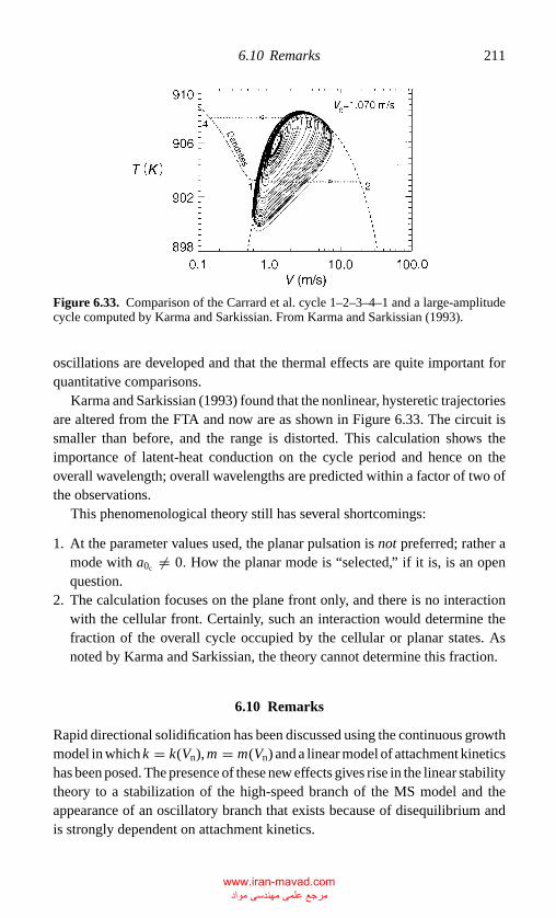
P1: LGD
CB381-06 CB381-Davis May 17, 2001 18:10 Char Count= 0
6.10 Remarks 211
Figure 6.33. Comparison of the Carrard et al. cycle 1–2–3–4–1 and a large-amplitudecycle computed by Karma and Sarkissian. From Karma and Sarkissian (1993).
oscillations are developed and that the thermal effects are quite important forquantitative comparisons.
Karma and Sarkissian (1993) found that the nonlinear, hysteretic trajectoriesare altered from the FTA and now are as shown in Figure 6.33. The circuit issmaller than before, and the range is distorted. This calculation shows theimportance of latent-heat conduction on the cycle period and hence on theoverall wavelength; overall wavelengths are predicted within a factor of two ofthe observations.
This phenomenological theory still has several shortcomings:
1. At the parameter values used, the planar pulsation is not preferred; rather amode with a0c �= 0. How the planar mode is “selected,” if it is, is an openquestion.
2. The calculation focuses on the plane front only, and there is no interactionwith the cellular front. Certainly, such an interaction would determine thefraction of the overall cycle occupied by the cellular or planar states. Asnoted by Karma and Sarkissian, the theory cannot determine this fraction.
6.10 Remarks
Rapid directional solidification has been discussed using the continuous growthmodel in which k = k(Vn), m = m(Vn) and a linear model of attachment kineticshas been posed. The presence of these new effects gives rise in the linear stabilitytheory to a stabilization of the high-speed branch of the MS model and theappearance of an oscillatory branch that exists because of disequilibrium andis strongly dependent on attachment kinetics.
www.iran-mavad.com مرجع علمی مھندسی مواد
P1: LGD
CB381-06 CB381-Davis May 17, 2001 18:10 Char Count= 0
212 Disequilibrium
These modes have been traced into the weakly nonlinear regime, and theirinteractions trigger the appearance of nonequilibrium solids called banded struc-tures. As of yet, such microstructures have not been predicted from first prin-ciples using measured values of the physical properties of known alloys.
All of the preceding characteristics depend on a particular functional form,Eq. (6.4), for k(Vn), which has a good deal of theoretical and experimental sup-port. However, the case is not closed in this regard. There are other possibilitiesin the literature. In any case k(0) = kE , k(∞) = 1, and k is monotonic. Forall the cases, m(Vn) is a given functional of k, and this functional should stillstand.
Likewise, the linear model of kinetics, Vn = µ(Tm − T I
), might be more
accurately described by a more general Vn = F(Tm − T I
)or a nonexplicit
functional, as suggested by Bates et al. (1997).
References
Aziz, M. J. (1982). Model for solute redistribution during rapid solidification, J. Appl.Phys. 53, 1158–1168.
Aziz, M. J., Tsao, J. Y., Thompson, M. O., Peercy, P. S., and White, C. W. (1986). Solutetrapping: Comparison of theory with experiment, Phys. Rev. Lett. 56, 2489–2492.
Baker, J. C., and Cahn, J. W. (1971). Thermodynamics of solidification, in Solidification,pages 23–58, American Society for Metals, Metals Park, OH.
Bates, P. W., Fife, P. C., Gardner, R. A., and Jones, C. K. R. T. (1997). Phase field modelsfor hypercooled solidification, Physica D 104, 1–31.
Bekki, N., and Nozaki, K. (1985). Formation of spatial patterns and holes in the gener-alized Ginzburg-Landau equation, Phys. Letters A110, 133–135.
Bernoff, A. J. (1988). Slowly varying fully nonlinear wavetrains in the Ginzburg–Landauequations, Physica D 30, 363–381.
Boettinger, W. J., and Coriell, S. R. (1986). Microstructure formation in rapidly solidfiedalloys, in P. R. Sahm, H. Jones, and C. M. Adam, editors, Rapid SolidificationMaterials and Technologies, pages 81–108, Nijhoff Publishers, Dordrecht, TheNetherlands.
Boettinger, W. J., and Perepezko, J. H. (1985). Fundamentals of rapid solidification,in S. K. Das, B. H. Kear, and C. M. Adam, editors, Rapid Solidified CrystallineAlloys, Proc. TMS–AIME Northeast Regionional Meeting, Morrison, NJ., pages21–58, The Metallurgical Society, Warrenton, PA.
Boettinger, W. J., Schechtman, D., Schaefer, R. J., and Biancaneillo, F. S. (1984). Theeffect of rapid solidification velocity on the microstructure of Ag–Cu alloys, Metall.Trans. A15, 55–66.
Bourland, F. J., and Haberman, R. (1988). The modulated phase shift for strongly non-linear, slowly varying, and weakly nonlinear damped oscillators, SIAM J. Appl.Math. 48, 737–748.
Brattkus, K., and Meiron, D. I. (1992). Numerical simulations of unsteady crystal growth,SIAM J. Appl. Math. 52, 1303–1320.
Braun, R. J. (1991). Nonlinear analysis in directional solidification, Ph.D. thesis, North-western University, Evanston, IL.
Braun, R. J., and Davis, S. H. (1991). Oscillatory instability in rapid solidification,J. Crystal Growth 112, 670–690.
www.iran-mavad.com مرجع علمی مھندسی مواد
P1: LGD
CB381-06 CB381-Davis May 17, 2001 18:10 Char Count= 0
References 213
. (1992). Cellular instability in rapid directional solidification: Bifurcation theory,Acta Metall. Mater. 40, 2617–2628.
Braun, R. J., Merchant, G. J., and Davis, S. H. (1992). Pulsatile- and cellular-modeinteraction in rapid directional solidification, Phys. Rev. B 45, 7002–7016.
Carrard, M., Gremaud, M., Zimmermann, M., and Kurz, W. (1992). About the bandedstructure in rapidly solidified dendritic and eutectic alloys, Acta Metall. mater. 40,983–996.
Coriell, S. R., and Sekerka, R. F. (1983). Oscillatory morphological instability due tononequilibrium segregation, J. Crystal Growth 61, 499–508.
Eckhaus, W. (1965). Studies in Non-Linear Stability Theory, Springer-Verlag, NewYork.
Greengard, L., and Strain, J. (1990). A fast algorithm for the evaluation of heat potentials,Comm. Pure Appl. Math. 43, 949–963.
Gremaud, M., Carrard, M., and Kurz, W. (1990). The microstructure of rapidly solidifiedAl–Fe alloys subjected to laser surface treatment, Acta Metall. Mater. 38, 2587–2599.
. (1991). Banding phenomena in Al–Fe alloys subjected to laser surface treat-ment, Acta Metall. Mater. 39, 1431–1443.
Grimm, H. P., and Metzener, P. (1998). Oscillatory phenomena in directional solidifi-cation, Phys. Rev. B 58, 144–155.
Hoglund, D. E., Aziz, M. J., Stiffler, S. R., Thompson, M. O., Tsao, J. Y., and Peercy,P. S. (1991). Effect of nonequilibrium interface kinetics on cellular breakdownof planar interfaces during rapid solidification of Si–Sn, J. Crystal Growth 109,107–112.
Hughes, D. W., and Proctor, M. R. E. (1992). Nonlinear three-wave interaction withnon-conservative coupling, J. Fluid Mech. 244, 583–604.
Huntley, D. A., and Davis, S. H. (1993). Thermal effects in rapid directional solidifica-tion: Linear theory, Acta metall. mater. 41, 2025–2043.
Huntley D. A., and Davis, S. H. (1996). Effect of latent heat on oscillatory and cel-lular mode coupling in rapid directional solidification, Phys. Rev. B 53, 3132–3144.
Jackson, K. A., Gilmer, G. H., and Leamy, H. J. (1980). Solute trapping, in C. W.White and P. S. Peercy, editors, Laser and Electronic Beam Processing of Materials,Proceedings of the Symposium of the Materials Research Society, Academic Press,New York, 104–110.
Karma, A., and Sarkissian, A. (1992). Dynamics of banded structure formation in rapidsolidification, Phys. Rev. Lett. 68, 2616–2619.
. (1993). Interface dynamics and banding in rapid solidification, Phys. Rev. E47, 513–533.
Kevorkian, J., and Cole, J. D. (1981). Perturbation Methods in Applied Mathematics,Springer-Verlag, New York.
Kuramoto, Y. (1984). Chemical Oscillations, Waves, and Turbulence, Springer-Verlag,New York.
Kurz, W., Giovanola, B., and Trivedi, R. (1986). Theory of microstructural developmentduring rapid solidification, Acta Metall. Mater. 34, 823–830.
. (1988). Microsegregation in rapidly solidified Ag–15wt% –Cu, J. CrystalGrowth 91, 123–125.
Kurz, W., and Trivedi, R. (1990). Solidification microstructures-Recent developmentsand future directions, Acta Metall. Mater. 38, 1–17.
McDougall, S. R., and Craik, A. D. D. (1991). Blow-up in non-conservative second-harmonic resonance, Wave Motion 13, 155–165.
www.iran-mavad.com مرجع علمی مھندسی مواد
P1: LGD
CB381-06 CB381-Davis May 17, 2001 18:10 Char Count= 0
214 Disequilibrium
Merchant, G. J., Braun, R. J., Brattkus, K., and Davis, S. H. (1992). Pulsatile instabilityin rapid solidification, SIAM J. Appl. Math. 52, 1279–1302.
Merchant, G. J., and Davis, S. H. (1990). Morphological instability in rapid directionalsolidification, Acta Metall. Mater. 38, 2683–2693.
Moon, H. T., Huerre, P., and Redekopp, L. G. (1983). Transitions to chaos in theGinzburg-Landau equation, Physica 7D, 135–150.
Mullins, W. W., and Sekerka, R. F. (1964). Stability of a planar interface during solidi-fication of a dilute binary alloy, J. Appl. Phys. 35, 444–451.
Nozaki, K., and Bekki, N. (1984). Exact solutions of the generalized Ginzburg-Landauequation, J. Phys. Soc. Japan 53, 1581–1582.
Sirovich, L., and Newton, P. (1986). Periodic solutions of the Ginzburg-Landau equation,Physica 21D, 115–125.
Stuart, J. T., and DiPrima, R. C. (1978). The Eckhaus and Benjamin–Feir resonancemechanisms, Proc. Roy. Soc. Lond. A362, 27–41.
Thoma, D. J., Glascow, J. K., Tewari, S. N., Perepezko, J. H., and Jayaraman, N. (1988).Effects of process parameters on melt-spun Ag–Cu, Mater. Sci. Eng. 98, 89–73.
Zimmermann, M., Carrard, M., and Kurz, W. (1989). Rapid solidification of Al–Cueutectic alloy by laser remelting, Acta Metall. Mater. 37, 3305–3313.
www.iran-mavad.com مرجع علمی مھندسی مواد
P1: GKW/FYX P2: GKW/FYX QC: GKW/UKS T1: GKW
CB381-07 CB381-Davis May 17, 2001 18:43 Char Count= 0
7
Dendrites
Chapter 2 addresses nucleate growth. It was found that a spherical nucleus inan undercooled liquid will melt and disappear if its radius R is smaller than thecritical nucleation radius R∗. In this case, the curvature is so large that surfaceenergy effects dominate those of undercooling. When R > R∗, the spherewill continue to grow, and, as time increases, the effects of surface energy willdecrease. When R reaches Rc, a morphological instability causes the sphericalinterface to become unstable to spatially periodic disturbances, leading to thegrowth of “bumps” on the interface. Experimental observation shows that the“bumps” grow, become dendritic, and continue to grow until they impact eachother or a system boundary. Figure 7.1 shows a single bump that has becomedendritic.
The term dendrite does not seem to have an accepted definition in the litera-ture though it does refer to a treelike structure. Here it will be used to denote atwo- or three-dimensional structure with side arms. Cells can, as well, be eithertwo- or three-dimensional.
Dendritic growth is likely the most common form of microstructure, beingpresent in all macroscopic castings. In fact, unless limitations of speed (orundercooling) are taken, a melt will usually freeze dendritically. If a sample ofdendritically structured material having coarse microstructure is reprocessed,it will crack or otherwise produce defects. However, if the microstructure werefine enough, the reprocessing could proceed without ill effects. In either case, the“ghost” of the dendrites will remain after reprocessing. One of the key questionsin materials science is: How does one predict the microstructure of a solidifiedsample? Further, how can one control the process to deliver the microstructurethat is desired? These questions cannot presently be fully answered, thoughthey do motivate the study of dendritic growth.
215
www.iran-mavad.com مرجع علمی مھندسی مواد
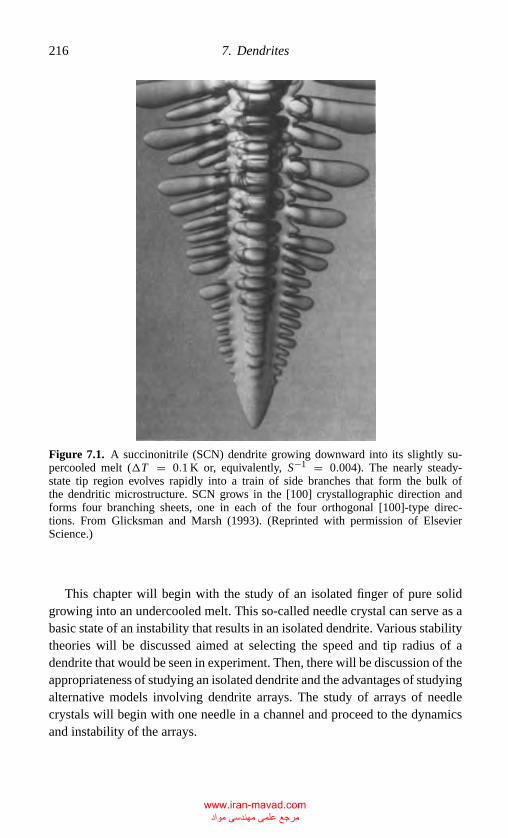
P1: GKW/FYX P2: GKW/FYX QC: GKW/UKS T1: GKW
CB381-07 CB381-Davis May 17, 2001 18:43 Char Count= 0
216 7. Dendrites
Figure 7.1. A succinonitrile (SCN) dendrite growing downward into its slightly su-percooled melt (�T = 0.1 K or, equivalently, S−1 = 0.004). The nearly steady-state tip region evolves rapidly into a train of side branches that form the bulk ofthe dendritic microstructure. SCN grows in the [100] crystallographic direction andforms four branching sheets, one in each of the four orthogonal [100]-type direc-tions. From Glicksman and Marsh (1993). (Reprinted with permission of ElsevierScience.)
This chapter will begin with the study of an isolated finger of pure solidgrowing into an undercooled melt. This so-called needle crystal can serve as abasic state of an instability that results in an isolated dendrite. Various stabilitytheories will be discussed aimed at selecting the speed and tip radius of adendrite that would be seen in experiment. Then, there will be discussion of theappropriateness of studying an isolated dendrite and the advantages of studyingalternative models involving dendrite arrays. The study of arrays of needlecrystals will begin with one needle in a channel and proceed to the dynamicsand instability of the arrays.
www.iran-mavad.com مرجع علمی مھندسی مواد
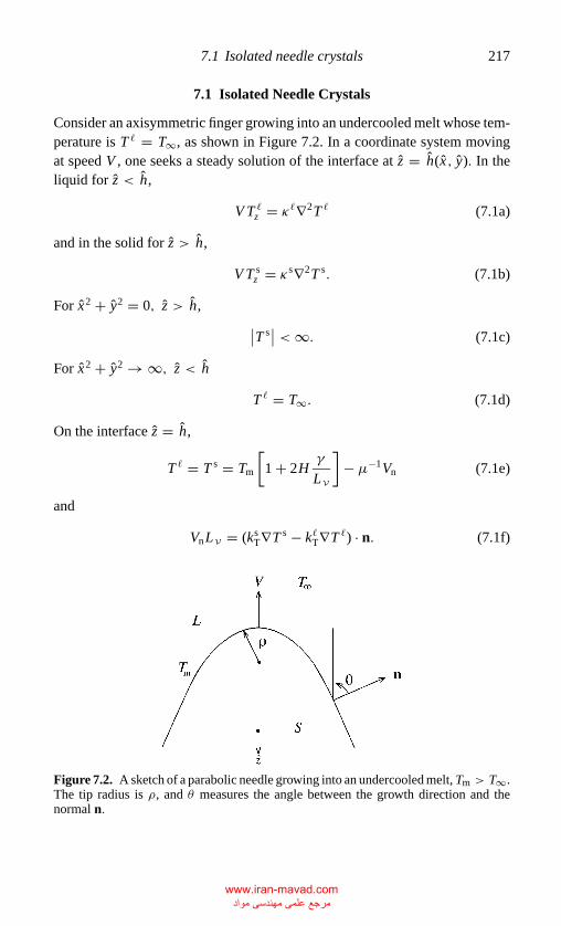
P1: GKW/FYX P2: GKW/FYX QC: GKW/UKS T1: GKW
CB381-07 CB381-Davis May 17, 2001 18:43 Char Count= 0
7.1 Isolated needle crystals 217
7.1 Isolated Needle Crystals
Consider an axisymmetric finger growing into an undercooled melt whose tem-perature is T � = T∞, as shown in Figure 7.2. In a coordinate system movingat speed V , one seeks a steady solution of the interface at z = h(x, y). In theliquid for z < h,
V T �z = κ�∇2T � (7.1a)
and in the solid for z > h,
V T sz = κs∇2T s. (7.1b)
For x2 + y2 = 0, z > h, ∣∣T s∣∣ < ∞. (7.1c)
For x2 + y2 → ∞, z < h
T � = T∞. (7.1d)
On the interface z = h,
T � = T s = Tm
[1 + 2H
γ
LV
]− µ−1Vn (7.1e)
and
VnLV = (ksT∇T s − k�T∇T �) · n. (7.1f)
Figure 7.2. A sketch of a parabolic needle growing into an undercooled melt, Tm > T∞.The tip radius is ρ, and θ measures the angle between the growth direction and thenormal n.
www.iran-mavad.com مرجع علمی مھندسی مواد
P1: GKW/FYX P2: GKW/FYX QC: GKW/UKS T1: GKW
CB381-07 CB381-Davis May 17, 2001 18:43 Char Count= 0
218 7. Dendrites
Equation (7.1e) is the Gibbs–Thomson equation with kinetic undercooling, Eq.(7.1f) is the interfacial heat balance, and n = ( hx , h y,−1)(1 + h2
x + h2y)−1/2.
Scale lengths on δT = κ�/V , and T − T∞ on �T = Tm − T∞. The non-dimensional system then has the form
θ�z = ∇2θ�, z < h (7.2a)
θ sz = κ∇2θ s, z > h (7.2b)
∣∣θ s∣∣ < ∞, x2 + y2 = 0, z > h (7.2c)
θ� = 0, x2 + y2 → ∞, z < h (7.2d)
θ� = θ s = 1 + H� − µ−1Vn, z = h (7.2e)
SVn = (kT∇θ s − ∇θ�) · n, z = h, (7.2f)
where
κ = κs/κ�, kT = ksT/k�T
� = 2γ
δTLV
Tm
�T, S−1 = cs
p�T
L, µ−1 = µ−1V
�T
(7.3)
Ivantsov (1947) noticed that a solution of this system could be found whenthe kinetics is instantaneous, µ−1 = 0, and when the surface energy is zero,� = 0. In this case Eq. (7.2e) shows that the interface is isothermal, θ I ≡ 1.Ivantsov then obtained a similarity solution for θ� and h in the form
θ� = E1[
12 s(x, y, z)
]E1[Pe0]
(7.4a)
and
h = 1
4Pe0[4ρ2 − x2 − y2]. (7.4b)
Here E1 is the exponential integral
E1(ξ ) =∫ ∞
ξ
z−1e−zdz,
s = z +√
x2 + y2 + z2,
(7.5a)
and the Peclet number Pe0 is
Pe0 = ρ
2δT, (7.5b)
www.iran-mavad.com مرجع علمی مھندسی مواد
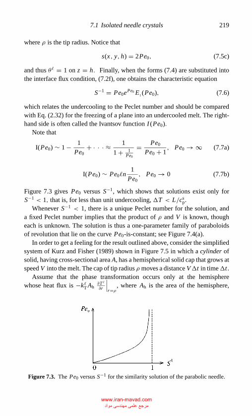
P1: GKW/FYX P2: GKW/FYX QC: GKW/UKS T1: GKW
CB381-07 CB381-Davis May 17, 2001 18:43 Char Count= 0
7.1 Isolated needle crystals 219
where ρ is the tip radius. Notice that
s(x, y, h) = 2Pe0, (7.5c)
and thus θ� = 1 on z = h. Finally, when the forms (7.4) are substituted intothe interface flux condition, (7.2f), one obtains the characteristic equation
S−1 = Pe0ePe0 E1 (Pe0), (7.6)
which relates the undercooling to the Peclet number and should be comparedwith Eq. (2.32) for the freezing of a plane into an undercooled melt. The right-hand side is often called the Ivantsov function I (Pe0).
Note that
I(Pe0) ∼ 1 − 1
Pe0+ · · · ≈ 1
1 + 1Pe0
= Pe0
Pe0 + 1, Pe0 → ∞ (7.7a)
I(Pe0) ∼ Pe0�n1
Pe0, Pe0 → 0 (7.7b)
Figure 7.3 gives Pe0 versus S−1, which shows that solutions exist only forS−1 < 1, that is, for less than unit undercooling, �T < L/cs
p.Whenever S−1 < 1, there is a unique Peclet number for the solution, and
a fixed Peclet number implies that the product of ρ and V is known, thougheach is unknown. The solution is thus a one-parameter family of paraboloidsof revolution that lie on the curve Pe0-is-constant; see Figure 7.4(a).
In order to get a feeling for the result outlined above, consider the simplifiedsystem of Kurz and Fisher (1989) shown in Figure 7.5 in which a cylinder ofsolid, having cross-sectional area A, has a hemispherical solid cap that grows atspeed V into the melt. The cap of tip radius ρ moves a distance V�t in time�t .
Assume that the phase transformation occurs only at the hemispherewhose heat flux is −k�T Ah
∂T �
∂r
∣∣∣r=ρ
, where Ah is the area of the hemisphere,
Figure 7.3. The Pe0 versus S−1 for the similarity solution of the parabolic needle.
www.iran-mavad.com مرجع علمی مھندسی مواد
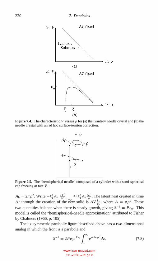
P1: GKW/FYX P2: GKW/FYX QC: GKW/UKS T1: GKW
CB381-07 CB381-Davis May 17, 2001 18:43 Char Count= 0
220 7. Dendrites
Figure 7.4. The characteristic V versus ρ for (a) the Ivantsov needle crystal and (b) theneedle crystal with an ad hoc surface-tension correction.
Figure 7.5. The “hemispherical needle” composed of a cylinder with a semi-sphericalcap freezing at rate V .
Ah = 2πρ2. Write −k�T Ah∂T �
∂r
∣∣∣r=ρ
≈ k�T Ah�Tρ
. The latent heat created in time�t through the creation of the new solid is AV Lv
csp, where A = πρ2. These
two quantities balance when there is steady growth, giving S−1 = Pe0. Thismodel is called the “hemispherical-needle approximation” attributed to Fisherby Chalmers (1966, p. 105).
The axisymmetric parabolic figure described above has a two-dimensionalanalog in which the front is a parabola and
S−1 = 2Pe0ePe0
∫ ∞
1e−Pe0z2
dz. (7.8)
www.iran-mavad.com مرجع علمی مھندسی مواد
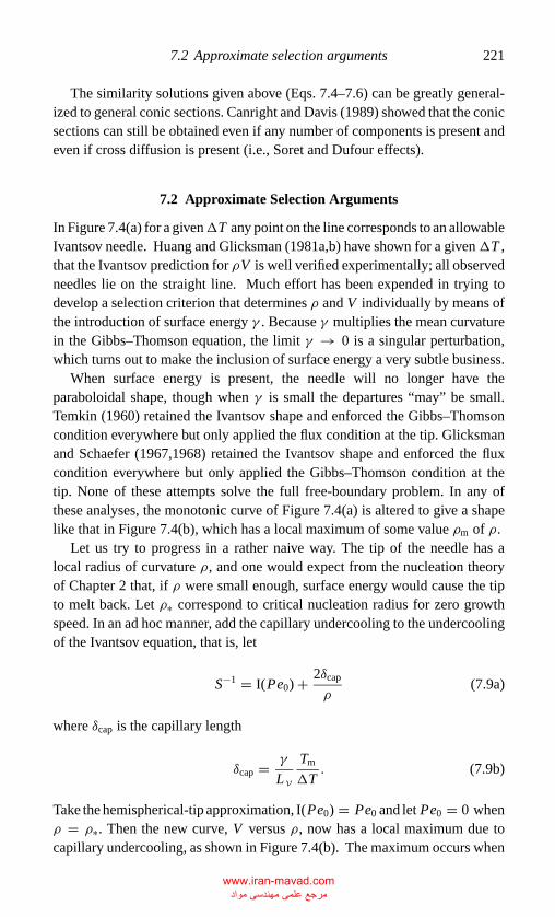
P1: GKW/FYX P2: GKW/FYX QC: GKW/UKS T1: GKW
CB381-07 CB381-Davis May 17, 2001 18:43 Char Count= 0
7.2 Approximate selection arguments 221
The similarity solutions given above (Eqs. 7.4–7.6) can be greatly general-ized to general conic sections. Canright and Davis (1989) showed that the conicsections can still be obtained even if any number of components is present andeven if cross diffusion is present (i.e., Soret and Dufour effects).
7.2 Approximate Selection Arguments
In Figure 7.4(a) for a given�T any point on the line corresponds to an allowableIvantsov needle. Huang and Glicksman (1981a,b) have shown for a given�T ,that the Ivantsov prediction for ρV is well verified experimentally; all observedneedles lie on the straight line. Much effort has been expended in trying todevelop a selection criterion that determines ρ and V individually by means ofthe introduction of surface energy γ . Because γ multiplies the mean curvaturein the Gibbs–Thomson equation, the limit γ → 0 is a singular perturbation,which turns out to make the inclusion of surface energy a very subtle business.
When surface energy is present, the needle will no longer have theparaboloidal shape, though when γ is small the departures “may” be small.Temkin (1960) retained the Ivantsov shape and enforced the Gibbs–Thomsoncondition everywhere but only applied the flux condition at the tip. Glicksmanand Schaefer (1967,1968) retained the Ivantsov shape and enforced the fluxcondition everywhere but only applied the Gibbs–Thomson condition at thetip. None of these attempts solve the full free-boundary problem. In any ofthese analyses, the monotonic curve of Figure 7.4(a) is altered to give a shapelike that in Figure 7.4(b), which has a local maximum of some value ρm of ρ.
Let us try to progress in a rather naive way. The tip of the needle has alocal radius of curvature ρ, and one would expect from the nucleation theoryof Chapter 2 that, if ρ were small enough, surface energy would cause the tipto melt back. Let ρ∗ correspond to critical nucleation radius for zero growthspeed. In an ad hoc manner, add the capillary undercooling to the undercoolingof the Ivantsov equation, that is, let
S−1 = I(Pe0) + 2δcap
ρ(7.9a)
where δcap is the capillary length
δcap = γ
LV
Tm
�T. (7.9b)
Take the hemispherical-tip approximation, I(Pe0) = Pe0 and let Pe0 = 0 whenρ = ρ∗. Then the new curve, V versus ρ, now has a local maximum due tocapillary undercooling, as shown in Figure 7.4(b). The maximum occurs when
www.iran-mavad.com مرجع علمی مھندسی مواد
P1: GKW/FYX P2: GKW/FYX QC: GKW/UKS T1: GKW
CB381-07 CB381-Davis May 17, 2001 18:43 Char Count= 0
222 7. Dendrites
ddρ (S−1) is zero, that is, when ρm = 2
√δT δcap, proportional to the geometrical
mean of δT and δcap.The appearance of the maximum suggested to researchers that the operating
point might be at (ρm, Vm); this is the “maximum velocity hypothesis.” Un-fortunately, as Glicksman and Marsh (1993, p. 1088) explained, “the disparitybetween the predicted and observed dendritic [tip] scales . . . [turn out to be] aslarge as 1–2 orders of magnitude.” The predicted tip radii are much too small.
The experiments of Schaefer, Glicksman, and Ayers (1975) and Glicksman,Schaefer, and Ayers (1976) on the transparent organic succinonitrile (SCN)show that, if
� ≡ δT
2δ(1)cap
(= 1
2�S−1
), (7.10a)
where
δ(1)cap = 2Tmcs
pγ
L2V
,
one can only find solutions up to � = �max. The Temkin–Trivedi value is
�max = 0.0254 S−2.65. (7.10b)
Nash and Glicksman (1974) were able to convert system (7.2) into a singleintegral equation using Green’s functions and were able to compute a value of�max, namely,
�max = 0.064 S−2.65. (7.10c)
Both of these results seem to predict the exponent well, though the multiplicativefactor is significantly different from experiment, as shown in Figure 7.6. Thus,V of the theory is too large by an order of magnitude. The implication is that themaximum velocity hypothesis is not correct. See Glicksman and Marsh (1993)for a more extensive discussion.
The inclusion of surface energy is thus much more subtle than the preceding“fixes” suggest. Because the ρ selected is orders of magnitude larger than ρm,it occurs well down the sloped portion of Figure 7.4(a), where ρ is so large thatsurface energy seems to have a rather small influence on the shape of the finger.
The selection criterion then involves more than the inclusion of surface en-ergy for steady growth. Oldfield (1973) and Langer and Muller-Krumbhaar(1978a) suggested that even given a steady needle with surface energy, a condi-tion of stability should be invoked. When surface energy γ is present and kinetic
www.iran-mavad.com مرجع علمی مھندسی مواد
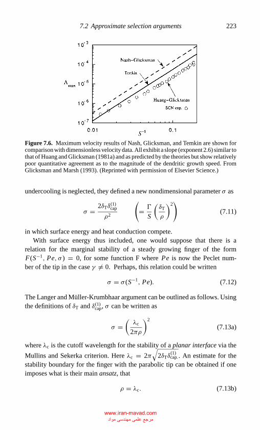
P1: GKW/FYX P2: GKW/FYX QC: GKW/UKS T1: GKW
CB381-07 CB381-Davis May 17, 2001 18:43 Char Count= 0
7.2 Approximate selection arguments 223
Figure 7.6. Maximum velocity results of Nash, Glicksman, and Temkin are shown forcomparison with dimensionless velocity data. All exhibit a slope (exponent 2.6) similar tothat of Huang and Glicksman (1981a) and as predicted by the theories but show relativelypoor quantitative agreement as to the magnitude of the dendritic growth speed. FromGlicksman and Marsh (1993). (Reprinted with permission of Elsevier Science.)
undercooling is neglected, they defined a new nondimensional parameter σ as
σ = 2δTδ(1)cap
ρ2
(= �
S
(δT
ρ
)2)
(7.11)
in which surface energy and heat conduction compete.With surface energy thus included, one would suppose that there is a
relation for the marginal stability of a steady growing finger of the formF(S−1, Pe, σ ) = 0, for some function F where Pe is now the Peclet num-ber of the tip in the case γ �= 0. Perhaps, this relation could be written
σ = σ (S−1, Pe). (7.12)
The Langer and Muller-Krumbhaar argument can be outlined as follows. Usingthe definitions of δT and δ(1)
cap, σ can be written as
σ =(λc
2πρ
)2
(7.13a)
where λc is the cutoff wavelength for the stability of a planar interface via the
Mullins and Sekerka criterion. Here λc = 2π√
2δTδ(1)cap.. An estimate for the
stability boundary for the finger with the parabolic tip can be obtained if oneimposes what is their main ansatz, that
ρ = λc. (7.13b)
www.iran-mavad.com مرجع علمی مھندسی مواد
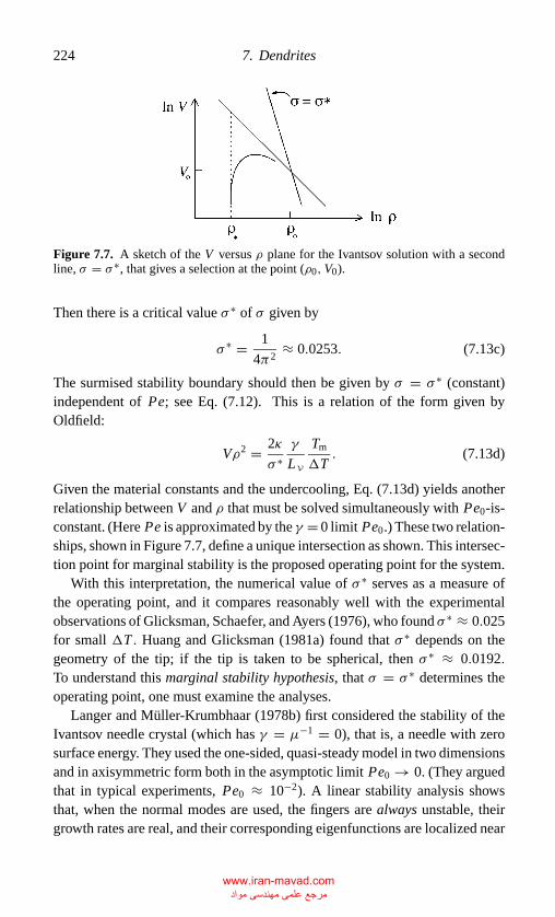
P1: GKW/FYX P2: GKW/FYX QC: GKW/UKS T1: GKW
CB381-07 CB381-Davis May 17, 2001 18:43 Char Count= 0
224 7. Dendrites
Figure 7.7. A sketch of the V versus ρ plane for the Ivantsov solution with a secondline, σ = σ ∗, that gives a selection at the point (ρ0, V0).
Then there is a critical value σ ∗ of σ given by
σ ∗ = 1
4π2≈ 0.0253. (7.13c)
The surmised stability boundary should then be given by σ = σ ∗ (constant)independent of Pe; see Eq. (7.12). This is a relation of the form given byOldfield:
Vρ2 = 2κ
σ ∗γ
LV
Tm
�T. (7.13d)
Given the material constants and the undercooling, Eq. (7.13d) yields anotherrelationship between V and ρ that must be solved simultaneously with Pe0-is-constant. (Here Pe is approximated by the γ = 0 limit Pe0.) These two relation-ships, shown in Figure 7.7, define a unique intersection as shown. This intersec-tion point for marginal stability is the proposed operating point for the system.
With this interpretation, the numerical value of σ ∗ serves as a measure ofthe operating point, and it compares reasonably well with the experimentalobservations of Glicksman, Schaefer, and Ayers (1976), who found σ ∗ ≈ 0.025for small �T . Huang and Glicksman (1981a) found that σ ∗ depends on thegeometry of the tip; if the tip is taken to be spherical, then σ ∗ ≈ 0.0192.To understand this marginal stability hypothesis, that σ = σ ∗ determines theoperating point, one must examine the analyses.
Langer and Muller-Krumbhaar (1978b) first considered the stability of theIvantsov needle crystal (which has γ = µ−1 = 0), that is, a needle with zerosurface energy. They used the one-sided, quasi-steady model in two dimensionsand in axisymmetric form both in the asymptotic limit Pe0 → 0. (They arguedthat in typical experiments, Pe0 ≈ 10−2). A linear stability analysis showsthat, when the normal modes are used, the fingers are always unstable, theirgrowth rates are real, and their corresponding eigenfunctions are localized near
www.iran-mavad.com مرجع علمی مھندسی مواد
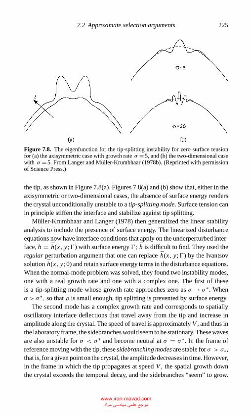
P1: GKW/FYX P2: GKW/FYX QC: GKW/UKS T1: GKW
CB381-07 CB381-Davis May 17, 2001 18:43 Char Count= 0
7.2 Approximate selection arguments 225
Figure 7.8. The eigenfunction for the tip-splitting instability for zero surface tensionfor (a) the axisymmetric case with growth rate σ = 5, and (b) the two-dimensional casewith σ = 5. From Langer and Muller-Krumbhaar (1978b). (Reprinted with permissionof Science Press.)
the tip, as shown in Figure 7.8(a). Figures 7.8(a) and (b) show that, either in theaxisymmetric or two-dimensional cases, the absence of surface energy rendersthe crystal unconditionally unstable to a tip-splitting mode. Surface tension canin principle stiffen the interface and stabilize against tip splitting.
Muller-Krumbhaar and Langer (1978) then generalized the linear stabilityanalysis to include the presence of surface energy. The linearized disturbanceequations now have interface conditions that apply on the underperturbed inter-face, h = h(x, y;�) with surface energy �; h is difficult to find. They used theregular perturbation argument that one can replace h(x, y;�) by the Ivantsovsolution h(x, y; 0) and retain surface energy terms in the disturbance equations.When the normal-mode problem was solved, they found two instability modes,one with a real growth rate and one with a complex one. The first of theseis a tip-splitting mode whose growth rate approaches zero as σ → σ ∗. Whenσ >σ ∗, so that ρ is small enough, tip splitting is prevented by surface energy.
The second mode has a complex growth rate and corresponds to spatiallyoscillatory interface deflections that travel away from the tip and increase inamplitude along the crystal. The speed of travel is approximately V , and thus inthe laboratory frame, the sidebranches would seem to be stationary. These wavesare also unstable for σ < σ ∗ and become neutral at σ = σ ∗. In the frame ofreference moving with the tip, these sidebranching modes are stable for σ > σ∗,that is, for a given point on the crystal, the amplitude decreases in time. However,in the frame in which the tip propagates at speed V , the spatial growth downthe crystal exceeds the temporal decay, and the sidebranches “seem” to grow.
www.iran-mavad.com مرجع علمی مھندسی مواد
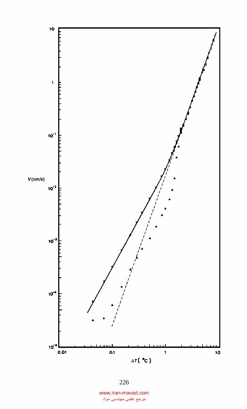
P1: GKW/FYX P2: GKW/FYX QC: GKW/UKS T1: GKW
CB381-07 CB381-Davis May 17, 2001 18:43 Char Count= 0
226
www.iran-mavad.com مرجع علمی مھندسی مواد
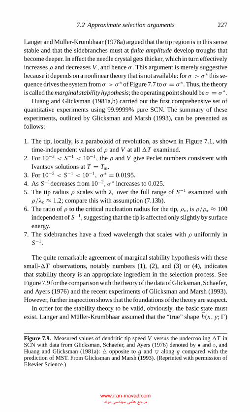
P1: GKW/FYX P2: GKW/FYX QC: GKW/UKS T1: GKW
CB381-07 CB381-Davis May 17, 2001 18:43 Char Count= 0
7.2 Approximate selection arguments 227
Langer and Muller-Krumbhaar (1978a) argued that the tip region is in this sensestable and that the sidebranches must at finite amplitude develop troughs thatbecome deeper. In effect the needle crystal gets thicker, which in turn effectivelyincreases ρ and decreases V , and hence σ . This argument is merely suggestivebecause it depends on a nonlinear theory that is not available: for σ > σ ∗ this se-quence drives the system fromσ > σ ∗ of Figure 7.7 toσ = σ ∗.Thus, the theoryis called the marginal stability hypothesis; the operating point should beσ = σ ∗.
Huang and Glicksman (1981a,b) carried out the first comprehensive set ofquantitative experiments using 99.9999% pure SCN. The summary of theseexperiments, outlined by Glicksman and Marsh (1993), can be presented asfollows:
1. The tip, locally, is a paraboloid of revolution, as shown in Figure 7.1, withtime-independent values of ρ and V at all �T examined.
2. For 10−3 < S−1 < 10−1, the ρ and V give Peclet numbers consistent withIvantsov solutions at T = Tm.
3. For 10−2 < S−1 < 10−1, σ ∗ = 0.0195.4. As S−1decreases from 10−2, σ ∗ increases to 0.025.5. The tip radius ρ scales with λc over the full range of S−1 examined withρ/λc ≈ 1.2; compare this with assumption (7.13b).
6. The ratio of ρ to the critical nucleation radius for the tip, ρ∗, is ρ/ρ∗ ≈ 100independent of S−1, suggesting that the tip is affected only slightly by surfaceenergy.
7. The sidebranches have a fixed wavelength that scales with ρ uniformly inS−1.
The quite remarkable agreement of marginal stability hypothesis with thesesmall-�T observations, notably numbers (1), (2), and (3) or (4), indicatesthat stability theory is an appropriate ingredient in the selection process. SeeFigure 7.9 for the comparison with the theory of the data of Glicksman, Schaefer,and Ayers (1976) and the recent experiments of Glicksman and Marsh (1993).However, further inspection shows that the foundations of the theory are suspect.
In order for the stability theory to be valid, obviously, the basic state mustexist. Langer and Muller-Krumbhaar assumed that the “true” shape h(x, y;�)
Figure 7.9. Measured values of dendritic tip speed V versus the undercooling �T inSCN with data from Glicksman, Schaefer, and Ayers (1976) denoted by • and ◦, andHuang and Glicksman (1981a): � opposite to g and � along g compared with theprediction of MST. From Glicksman and Marsh (1993). (Reprinted with permission ofElsevier Science.)
www.iran-mavad.com مرجع علمی مھندسی مواد
P1: GKW/FYX P2: GKW/FYX QC: GKW/UKS T1: GKW
CB381-07 CB381-Davis May 17, 2001 18:43 Char Count= 0
228 7. Dendrites
can be replaced by h(x, y; 0), the Ivantsov solution. Certainly, h(x, y; 0) is well-defined. As will be seen in a moment, for� �= 0, h(x, y;�) does not exist if oneassumes that, as the roots of the crystal are approached, the behavior is Ivantsov-like! A small amount of surface energy produces a singular perturbation thatdestroys the existence of shapes uniformly close to the Ivantsov needle crystal.
The question arises then of how to pose the problem with � �= 0. Forconvenience, the two-dimensional case will be discussed. The approximatesolutions of the problem, for example, Nash and Glicksman (1974), are normallysought on half of a symmetric needle, say, from the tip at s = 0 to the root ats = ∞, where s is the arc length. Among the boundary conditions are that thetip have a horizontal tangent
∂h
∂s
∣∣∣∣s=0
= 0 (7.14a)
and that the root be Ivantsov-like,
h → h(x ; 0) as s → ∞. (7.14b)
It was shown by Meiron (1986) and Kessler and Levine (1986) that the steadyproblem with end conditions (7.14) has no solutions. Specifically, if condition(7.14b) holds, then as� → 0, ∂h
∂s
∣∣s=0
∼ exp(−1/�).The slope at the tip is neverzero for any � > 0. This surprising result took many years to establish usinganalytical continution and asymptotic methods that retain exponentially smallterms; see Langer (1987) for a comprehensive review. Because the problem for� �= 0 has no solution, the Langer–Muller-Krumbhaar stability analysis of itloses meaning.
In posing the steady needle without kinetics, it was assumed that (1) surfaceenergy is isotropic, (2) the needle is steady, (3) the tip is smooth, and (4) the rootis Ivantsov-like. Because solutions of this system do not exist, one or more ofthese assumptions must be relaxed. Such relaxations have given rise to furtherattempts at solutions to the isolated needle problem.
If assumptions (2)-(4) are accepted one must include additional physics inthe mathematical description. If (1) is relaxed and the surface energy is madeanisotropic, then one is led to microscopic solvability theory (MST). If (1) and(3), are retained, smooth-tipped fingers can be found that misbehave as s → ∞,and one is led to interfacial wave theory (IWT) in which an unstable interfacecan lead to unsteady tip motions. In Section 7.3, these generalizations will bediscussed.
Before continuing with surface–energy-based selection criteria, it shouldbe noted that, if one enforces zero surface energy and anisotropic attachmentkinetics, there are solutions for a finger valid for small S−1 and β4. Brener,
www.iran-mavad.com مرجع علمی مھندسی مواد
P1: GKW/FYX P2: GKW/FYX QC: GKW/UKS T1: GKW
CB381-07 CB381-Davis May 17, 2001 18:43 Char Count= 0
7.3 Selection theories 229
Geilikman, and Temkin (1988) found that V ∝ β5/44 S−2. This suggests that
“any” anisotropy may suffice for the existence of steady needles in the casewhen added physics is allowed.
7.3 Selection Theories
Consider first the possibility that conditions (7.14) hold, but now the surfaceenergy is anisotropic. In this case the capillary undercooling is modified from2HTmγ /LV to 2H Tm
Lv(γ + γθθ ), as discussed in Chapter 5. Here θ is the angle
between the normal to the interface and the growth direction. If one consider amaterial with fourfold symmetry, γ can be written as γ = γ0[1 + α4 cos 4θ ],and thus γ + γθθ = γ0[1 − 15α4 cos 4θ ].
It has been shown by Kruskal and Segur (1991) for a model equation withsuch anisotropy that the steady needle exists, satisfying conditions (7.14) aslong as α4 �= 0. Ben Amar and Pomeau (1986) and Barbieri, Hong, and Langer(1987) have extended the analyses from model equations to the physical modeland obtained results consistent with the numerical simulations of Meiron (1986)and Kessler and Levine (1986). Langer (1987) showed for small �T that, intwo dimensions,
σ ∗ ≈ σ α7/44 (7.15)
where σ is a unit order constant. Again, this is a criterion in which σ ∗ is a con-stant, independent of Pe. A countable infinity of steady needle solutions withsufficiently large anisotropy exists (Meiron 1986, Kessler and Levine 1986).Condition (7.15) corresponds to that one having the largest V , which is foundto be the one that is not unstable; it is neutrally stable. In order that this neu-trally stable needle exhibit sidebranching instabilities, it is necessary that thereis persistant noise at the tip.
The prediction of this microscopic solvability theory for the symmetric modelin two dimensions is given by Pe ≈ (�T/π )2 so that
V ≈ 2κ
δ(1)cap
σ ∗ Pe2 ≈ σ ∗ 2κ
�c
(�T )4
π2(7.16a)
and
ρ ≈ �c
σ ∗ Pe≈ �c
σ ∗π
(�T )2, (7.16b)
where δ(1)cap is δ(1)
cap times a scale factor dependent on the anisotropy. A similarresult holds for the axisymmetric case.
www.iran-mavad.com مرجع علمی مھندسی مواد
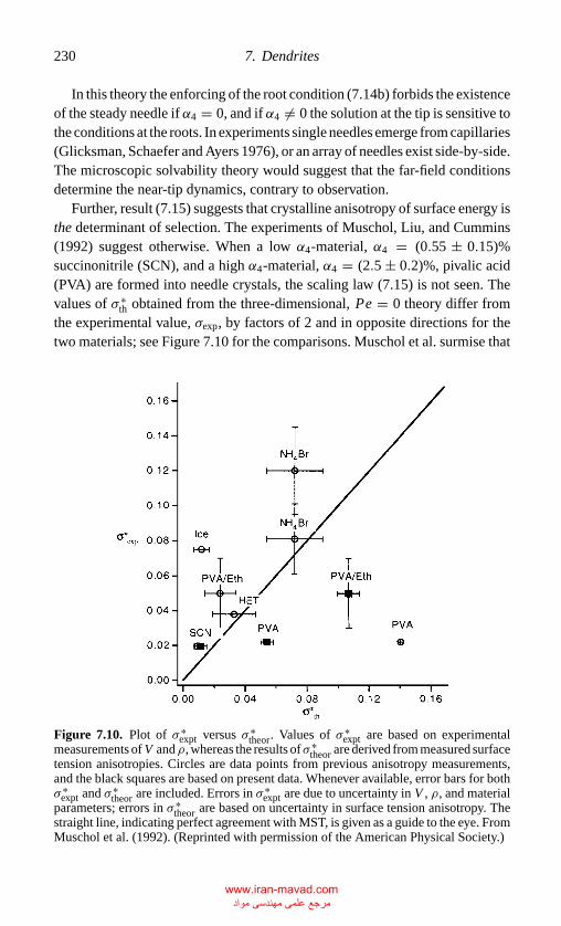
P1: GKW/FYX P2: GKW/FYX QC: GKW/UKS T1: GKW
CB381-07 CB381-Davis May 17, 2001 18:43 Char Count= 0
230 7. Dendrites
In this theory the enforcing of the root condition (7.14b) forbids the existenceof the steady needle if α4 = 0, and if α4 �= 0 the solution at the tip is sensitive tothe conditions at the roots. In experiments single needles emerge from capillaries(Glicksman, Schaefer and Ayers 1976), or an array of needles exist side-by-side.The microscopic solvability theory would suggest that the far-field conditionsdetermine the near-tip dynamics, contrary to observation.
Further, result (7.15) suggests that crystalline anisotropy of surface energy isthe determinant of selection. The experiments of Muschol, Liu, and Cummins(1992) suggest otherwise. When a low α4-material, α4 = (0.55 ± 0.15)%succinonitrile (SCN), and a high α4-material, α4 = (2.5 ± 0.2)%, pivalic acid(PVA) are formed into needle crystals, the scaling law (7.15) is not seen. Thevalues of σ ∗
th obtained from the three-dimensional, Pe = 0 theory differ fromthe experimental value, σexp, by factors of 2 and in opposite directions for thetwo materials; see Figure 7.10 for the comparisons. Muschol et al. surmise that
Figure 7.10. Plot of σ ∗expt versus σ ∗
theor. Values of σ ∗expt are based on experimental
measurements of V andρ, whereas the results ofσ ∗theor are derived from measured surface
tension anisotropies. Circles are data points from previous anisotropy measurements,and the black squares are based on present data. Whenever available, error bars for bothσ ∗
expt and σ ∗theor are included. Errors in σ ∗
expt are due to uncertainty in V , ρ, and materialparameters; errors in σ ∗
theor are based on uncertainty in surface tension anisotropy. Thestraight line, indicating perfect agreement with MST, is given as a guide to the eye. FromMuschol et al. (1992). (Reprinted with permission of the American Physical Society.)
www.iran-mavad.com مرجع علمی مھندسی مواد
P1: GKW/FYX P2: GKW/FYX QC: GKW/UKS T1: GKW
CB381-07 CB381-Davis May 17, 2001 18:43 Char Count= 0
7.3 Selection theories 231
“. . . in view of the results for SCN and PVA . . . , the correctness of MST in itspresent form cannot realistically be viewed as being confirmed by experiment.”
Consider again the needle crystal with isotropic surface energy. When bothconditions (7.14) are imposed, no solution exists for � > 0, whereas infinitelymany are present for � = 0. The limit � → 0 is a singular perturbation.Because the curvature of a needle crystal is significant near the tip, one wouldthink that the reduction of order of the differential system when � → 0 wouldrequire a boundary-layer correction near the tip, whereas the “outer” solution inwhich � → 0 is a regular limit would encompass the remainder of the needle,including the roots. With root condition (7.14b) satisfied, no surface-energycorrection near the tip would yield a solution; the tip for � �= 0 is not smooth.
Xu (1997) has taken the point of view that the surface-energy correctionshould not be at the tip but at the roots. He thus sought an “outer” solution,satisfying condition (7.14a), valid everywhere outside a neighborhood of theroots and an inner surface energy correction at the roots.
His strategy is to express, say in two dimensions, the shape of the needleh(x ;�) as an asymptotic series composed of two parts: a regular perturbationseries hR,
h R ∼ h(x, y; 0) + ε2h1 + ε4h2 + · · · (7.17a)
valid for, say, arc lengths in the range 0 ≤ s ≤ L0(ε, t), and a surface-tensioncorrection obtained by a WKB approximation,
hS ∼ f (ε) sin( s
ε
) ( cosh s
2 cosh L0
)1/2
; (7.17b)
h is given by
h ∼ hR + hS. (7.17c)
A parameter Pe0 is used and represents the Ivantsov–Peclet number at whichthe length scale is ρ0, the tip radius of a needle without surface tension. HereXu uses a parameter ε defined in terms of ρ without surface tension. When�T → 0
ε = 1
Pe0
√�/S, (7.17d)
which is about 2√σ , where σ is the parameter introduced by Oldfield (1973)
and Langer and Muller-Krumbhaar (1978a). When �T is not small, ε is nolonger related directly to σ .
In form (7.17a) h(x, y; 0) represents the Ivantsov solution and hR is a regularseries in� , which if hS were omitted, would fail to satisfy root condition (7.14b).
www.iran-mavad.com مرجع علمی مھندسی مواد
P1: GKW/FYX P2: GKW/FYX QC: GKW/UKS T1: GKW
CB381-07 CB381-Davis May 17, 2001 18:43 Char Count= 0
232 7. Dendrites
Form (7.17b) represents strongly oscillatory corrections that enable condition(7.14b) to be satisfied but which becomes negligible (exponentially) as the tipis approached. In particular, if s is fixed and ε → 0, then the Ivantsov solutiongoverns the near-tip needle structure independent of near-root conditions. Thefunction f is chosen to satisfy the root conditions.
Finally, the L0(ε, t) is a slowly varying increasing function of time thatapproaches infinity as ε → 0; the asymptotic properties can be chosen tovalidate the approximate solution (7.17c). Xu calls this a generalized steadystate, though the terminology “steady” is misleading.
The Xu basic state (7.17) has the attractive feature that the near-tip propertiesof the needle are very weakly dependent on the root conditions – a characteristicrecognized to be present by every experimentalist.
In order to examine linear stability theory, Xu perturbs the basic state h,symbolically, as
h(x, t) = h + h′. (7.18)
He linearizes in primed quantities and then represents h as h(x, y, 0) + O(ε2)and retains only terms of O(ε). Thus, he retains as the basic state the Ivantsovparaboloid without near-tip corrections and without the oscillatory tail near theroots. In effect he returns to the Langer–Muller-Krumbhaar supposition thatsurface energy is negligible in the basic state but not in the disturbances. UnlikeLanger–Muller-Krumbhaar, Xu derives this result and applies it only far fromthe roots. What allows Xu to ignore the root region is his decision to focus onthe spatial growth of disturbances.
Xu seeks a solution using the WKB approximation in ε, where the growthrate σ ∼ σ0 + εσ1 and the wave number k ∼ k0 + εk1. At leading order in ε,Xu finds a local form of the characteristic equation
σ0 = k0
g2
[1 − 2k2
0
g
]− isk0
g2, (7.19)
where g is a geometrical scale factor.Form (7.19) generalizes that of Mullins and Sekerka (1964) to the present
situation in which a curved front moves through the melt. At the tip the normalvelocity Vn is V . However, as one moves away from the tip, Vn = V cos θ ,and each point experiences a different freezing rate. In a frame moving withthe tip, the melt “flows” by like a liquid past a curved body. The result (7.19)shows that Re σ0 indicates growth for a range of wave numbers k0. In additionIm σ0 gives the angular speed of the traveling disturbance, a wave that travelsfrom the tip toward the root.
www.iran-mavad.com مرجع علمی مھندسی مواد
P1: GKW/FYX P2: GKW/FYX QC: GKW/UKS T1: GKW
CB381-07 CB381-Davis May 17, 2001 18:43 Char Count= 0
7.3 Selection theories 233
Rather than regarding Eq. (7.19) as determining a growth rate as a functionof a wave number, Xu takes the view that a disturbance of fixed frequency growsspatially (toward the root), and thus Eq. (7.19) gives three complex roots k0 asfunctions of the given σ0. Two of these local solutions have Re k0 > 0 andhence are physically relevant, and these correspond to a long- and a shortwavemode. At a fixed time, the amplitude of the shortwave mode first decreasesin s and then increases exponentially. The longwave mode first increases ins and then decreases exponentially. Thus, the matching as s → ∞ requiresh′ to behave like the longwave mode, which is a spatially oscillatory behaviordifferent from the Ivantsov root.
At O(ε), a similar procedure is applied, and the first correction is obtained.Here it is noted that the asymptotics break down at two points: (1) a turningpoint rc, which is near the tip but separated from it, and (2) at the tip. Thepoint rc is conveniently analyzed in the complex plane and represents a criticallayer across which different representations must be matched. To ensure asmooth tip, the near-tip solution must be matched to the outer solution. Thesesubtle analyses yield a characteristic equation for the instability over the entirespatial range excluding a neighborhood of the root. Xu finds a discrete set,{σ
(n)0 , 0,±1,±2, · · · }, of complex growth rates. Figure 7.11 shows both Re σ0
and Im σ0 ≡ ω0 versus ε for a particular case. In Figure 7.11(a) when ε > ε∗,all disturbances decay and the first mode to be destabilized is n = 0; thisoccurs ε = ε∗. Figure 7.11b, gives the corresponding angular frequency ω0.At leading order in ε, ω0 = −0.21291 at a critical ε, ε∗ = 0.1590. WhenO(ε) terms are included, the first corrections of these are ω1 ≈ −0.2183 withε(1) ≈ 0.1108, which valid for Pe → 0. Xu finds two classes of solutions:symmetric with respect to the center line and antisymmetric.
At distances well beyond the critical layer, one can use the wave number toconvert ω0 to the phase speed c of an instability wave that could be seen by anobserver. Xu finds for the whole range 2×10⁻³ < Pe < 20 that c = 1±0.025,suggesting that in a laboratory frame the wave crests, the side arms, wouldappear to be nearly stationary, c = 1, consistent with observation. Figure 7.12(a)shows a graphical view of a time sequence of interfacial shapes for a fixed ε,which looks very close to the observed measured sequences. Figure 7.12(b)shows the disturbance only for the instability mode. It is concentrated near thecritical layer and dies away in both directions.
Xu explained the role played by the critical layer as a “barrier” that takesinstability waves arising from the tip, and partially reflects them back towardthe tip, effectively trapping waves in the region. The matching across the layerdetermines the wave that is transmitted and produces the sidebranches.
www.iran-mavad.com مرجع علمی مھندسی مواد
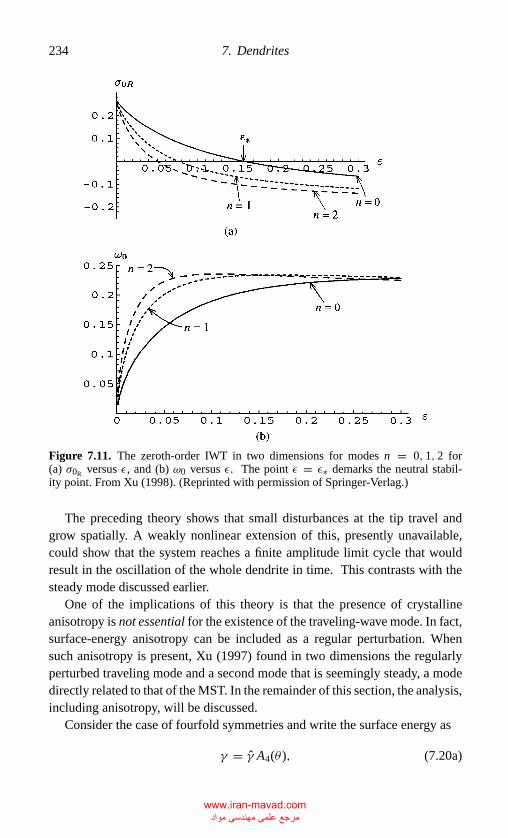
P1: GKW/FYX P2: GKW/FYX QC: GKW/UKS T1: GKW
CB381-07 CB381-Davis May 17, 2001 18:43 Char Count= 0
234 7. Dendrites
Figure 7.11. The zeroth-order IWT in two dimensions for modes n = 0, 1, 2 for(a) σ0R versus ε, and (b) ω0 versus ε. The point ε = ε∗ demarks the neutral stabil-ity point. From Xu (1998). (Reprinted with permission of Springer-Verlag.)
The preceding theory shows that small disturbances at the tip travel andgrow spatially. A weakly nonlinear extension of this, presently unavailable,could show that the system reaches a finite amplitude limit cycle that wouldresult in the oscillation of the whole dendrite in time. This contrasts with thesteady mode discussed earlier.
One of the implications of this theory is that the presence of crystallineanisotropy is not essential for the existence of the traveling-wave mode. In fact,surface-energy anisotropy can be included as a regular perturbation. Whensuch anisotropy is present, Xu (1997) found in two dimensions the regularlyperturbed traveling mode and a second mode that is seemingly steady, a modedirectly related to that of the MST. In the remainder of this section, the analysis,including anisotropy, will be discussed.
Consider the case of fourfold symmetries and write the surface energy as
γ = γ A4(θ ), (7.20a)
www.iran-mavad.com مرجع علمی مھندسی مواد
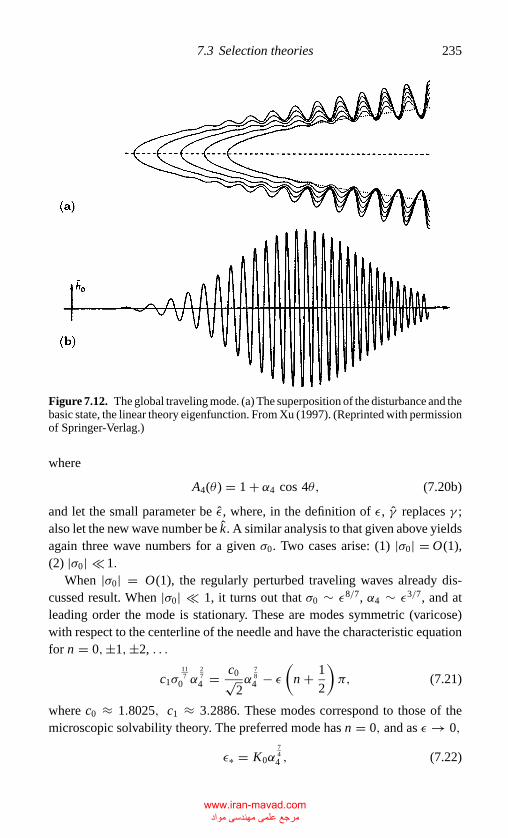
P1: GKW/FYX P2: GKW/FYX QC: GKW/UKS T1: GKW
CB381-07 CB381-Davis May 17, 2001 18:43 Char Count= 0
7.3 Selection theories 235
Figure 7.12. The global traveling mode. (a) The superposition of the disturbance and thebasic state, the linear theory eigenfunction. From Xu (1997). (Reprinted with permissionof Springer-Verlag.)
where
A4(θ ) = 1 + α4 cos 4θ, (7.20b)
and let the small parameter be ε, where, in the definition of ε, γ replaces γ ;also let the new wave number be k. A similar analysis to that given above yieldsagain three wave numbers for a given σ0. Two cases arise: (1) |σ0| = O(1),(2) |σ0| 1.
When |σ0| = O(1), the regularly perturbed traveling waves already dis-cussed result. When |σ0| 1, it turns out that σ0 ∼ ε8/7, α4 ∼ ε3/7, and atleading order the mode is stationary. These are modes symmetric (varicose)with respect to the centerline of the needle and have the characteristic equationfor n = 0,±1,±2, . . .
c1σ117
0 α274 = c0√
2α
784 − ε
(n + 1
2
)π, (7.21)
where c0 ≈ 1.8025, c1 ≈ 3.2886. These modes correspond to those of themicroscopic solvability theory. The preferred mode has n = 0, and as ε → 0,
ε∗ = K0α744 , (7.22)
www.iran-mavad.com مرجع علمی مھندسی مواد
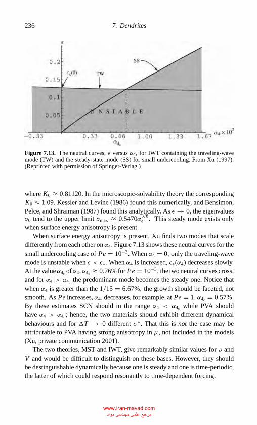
P1: GKW/FYX P2: GKW/FYX QC: GKW/UKS T1: GKW
CB381-07 CB381-Davis May 17, 2001 18:43 Char Count= 0
236 7. Dendrites
Figure 7.13. The neutral curves, ε versus α4, for IWT containing the traveling-wavemode (TW) and the steady-state mode (SS) for small undercooling. From Xu (1997).(Reprinted with permission of Springer-Verlag.)
where K0 ≈ 0.81120. In the microscopic-solvability theory the correspondingK0 ≈ 1.09. Kessler and Levine (1986) found this numerically, and Bensimon,Pelce, and Shraiman (1987) found this analytically. As ε → 0, the eigenvaluesσ0 tend to the upper limit σmax ≈ 0.5470α3/8
4 . This steady mode exists onlywhen surface energy anisotropy is present.
When surface energy anisotropy is present, Xu finds two modes that scaledifferently from each other on α4. Figure 7.13 shows these neutral curves for thesmall undercooling case of Pe = 10−3. When α4 = 0, only the traveling-wavemode is unstable when ε < ε∗. When α4 is increased, ε∗(α4) decreases slowly.At the valueα4c ofα4,α4c ≈ 0.76% for Pe = 10−3, the two neutral curves cross,and for α4 > α4c the predominant mode becomes the steady one. Notice thatwhen α4 is greater than the 1/15 = 6.67%, the growth should be faceted, notsmooth. As Pe increases, α4c decreases, for example, at Pe = 1, α4c = 0.57%.By these estimates SCN should in the range α4 < α4c while PVA shouldhave α4 > α4c ; hence, the two materials should exhibit different dynamicalbehaviours and for �T → 0 different σ ∗. That this is not the case may beattributable to PVA having strong anisotropy in µ, not included in the models(Xu, private communication 2001).
The two theories, MST and IWT, give remarkably similar values for ρ andV and would be difficult to distinguish on these bases. However, they shouldbe destinguishable dynamically because one is steady and one is time-periodic,the latter of which could respond resonantly to time-dependent forcing.
www.iran-mavad.com مرجع علمی مھندسی مواد
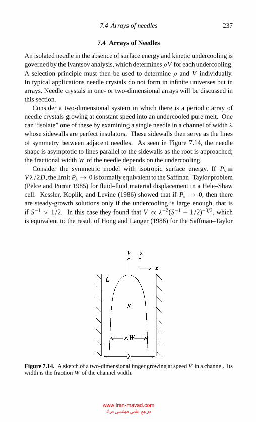
P1: GKW/FYX P2: GKW/FYX QC: GKW/UKS T1: GKW
CB381-07 CB381-Davis May 17, 2001 18:43 Char Count= 0
7.4 Arrays of needles 237
7.4 Arrays of Needles
An isolated needle in the absence of surface energy and kinetic undercooling isgoverned by the Ivantsov analysis, which determines ρV for each undercooling.A selection principle must then be used to determine ρ and V individually.In typical applications needle crystals do not form in infinite universes but inarrays. Needle crystals in one- or two-dimensional arrays will be discussed inthis section.
Consider a two-dimensional system in which there is a periodic array ofneedle crystals growing at constant speed into an undercooled pure melt. Onecan “isolate” one of these by examining a single needle in a channel of width λwhose sidewalls are perfect insulators. These sidewalls then serve as the linesof symmetry between adjacent needles. As seen in Figure 7.14, the needleshape is asymptotic to lines parallel to the sidewalls as the root is approached;the fractional width W of the needle depends on the undercooling.
Consider the symmetric model with isotropic surface energy. If Pλ≡Vλ/2D, the limit Pλ → 0 is formally equivalent to the Saffman–Taylor problem(Pelce and Pumir 1985) for fluid–fluid material displacement in a Hele–Shawcell. Kessler, Koplik, and Levine (1986) showed that if Pλ → 0, then thereare steady-growth solutions only if the undercooling is large enough, that isif S−1 > 1/2. In this case they found that V ∝ λ−2(S−1 − 1/2)−3/2, whichis equivalent to the result of Hong and Langer (1986) for the Saffman–Taylor
Figure 7.14. A sketch of a two-dimensional finger growing at speed V in a channel. Itswidth is the fraction W of the channel width.
www.iran-mavad.com مرجع علمی مھندسی مواد
P1: GKW/FYX P2: GKW/FYX QC: GKW/UKS T1: GKW
CB381-07 CB381-Davis May 17, 2001 18:43 Char Count= 0
238 7. Dendrites
problem. When surface energy anisotropy is present, then steady needles existeven for S−1 < 1/2.
The preceding results for Pλ → 0 are for a case distant from that of thefree needle crystal, which would have Pλ → ∞. To understand how the needlepasses to this limit, Brener, et al. (1988) considered the case of Pλ arbitrary.They defined � to be
� = λ/d0, (7.23a)
where
d0 = F(θ )Tmcp
L2v
, (7.23b)
F(θ ) = γ + γθθ = γ A4(θ ), (7.23c)
A4 = 1 + α4 cos 4θ. (7.23d)
Brener, et al. (1998) solved the problem directly using the techniques ofmicroscopic solvability theory. For isotropic surface energy they, too, foundsolutions only for S−1 > 1/2, which translates into solutions existing only for�greater than a critical value. Figure 7.15(a) shows the case S−1 = 0.6 in whichthere are two branches of solutions. The lower branch is equivalent to that foundby Kessler et al. (1986), whereas the upper branch is new. Figure 7.15(b) showsV versus S−1 for a pair of separations�. Solutions exist only for S−1 > S−1
∗ (�),where S−1
∗ decreases with increasing� . The upper branch corresponds to thewidth W of a finger increasing with undercooling S−1, and hence it is thisbranch that corresponds to the isolated needle as � → ∞. The symbol ⊗denotes points calculated by Karma (1986) for S−1 = 1.
When the surface energy is anisotropic, α4 �= 0, solutions exist below S−1 =1/2. Figure 7.16 shows for α4 = 10−2 that there are again two branches,and as � → ∞ a single branch emerges from the origin, which consistentwith both microscopic solrability theory (MST) and interfacial wave theory(IWT).
In the preceding the solutions are symmetric with respect to the centerlineof the channel. It turns out that in addition to center-symmetric solutions, thereexist pairs of solutions that have this symmetry broken; see Brener et al. (1993)and Ihle and Muller-Krumbhaar (1994). Kupferman, Kessler, and Ben-Jacob(1995) reexamined the two-dimensional problem for the one-sided model andfound solutions for both α4 = 0 and α4 �= 0, as shown in Figure 7.17, butnow they found symmetry-breaking solutions as well that bifurcate from the
www.iran-mavad.com مرجع علمی مھندسی مواد
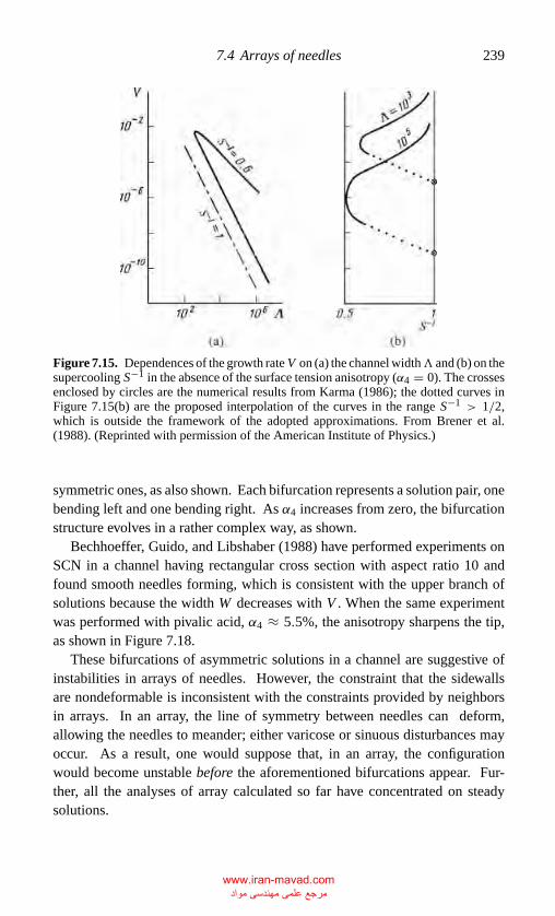
P1: GKW/FYX P2: GKW/FYX QC: GKW/UKS T1: GKW
CB381-07 CB381-Davis May 17, 2001 18:43 Char Count= 0
7.4 Arrays of needles 239
Figure 7.15. Dependences of the growth rate V on (a) the channel width� and (b) on thesupercooling S−1 in the absence of the surface tension anisotropy (α4 = 0). The crossesenclosed by circles are the numerical results from Karma (1986); the dotted curves inFigure 7.15(b) are the proposed interpolation of the curves in the range S−1 > 1/2,which is outside the framework of the adopted approximations. From Brener et al.(1988). (Reprinted with permission of the American Institute of Physics.)
symmetric ones, as also shown. Each bifurcation represents a solution pair, onebending left and one bending right. As α4 increases from zero, the bifurcationstructure evolves in a rather complex way, as shown.
Bechhoeffer, Guido, and Libshaber (1988) have performed experiments onSCN in a channel having rectangular cross section with aspect ratio 10 andfound smooth needles forming, which is consistent with the upper branch ofsolutions because the width W decreases with V . When the same experimentwas performed with pivalic acid, α4 ≈ 5.5%, the anisotropy sharpens the tip,as shown in Figure 7.18.
These bifurcations of asymmetric solutions in a channel are suggestive ofinstabilities in arrays of needles. However, the constraint that the sidewallsare nondeformable is inconsistent with the constraints provided by neighborsin arrays. In an array, the line of symmetry between needles can deform,allowing the needles to meander; either varicose or sinuous disturbances mayoccur. As a result, one would suppose that, in an array, the configurationwould become unstable before the aforementioned bifurcations appear. Fur-ther, all the analyses of array calculated so far have concentrated on steadysolutions.
www.iran-mavad.com مرجع علمی مھندسی مواد
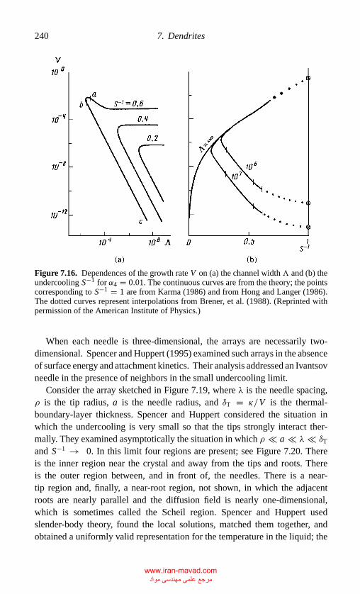
P1: GKW/FYX P2: GKW/FYX QC: GKW/UKS T1: GKW
CB381-07 CB381-Davis May 17, 2001 18:43 Char Count= 0
240 7. Dendrites
Figure 7.16. Dependences of the growth rate V on (a) the channel width� and (b) theundercooling S−1 for α4 = 0.01. The continuous curves are from the theory; the pointscorresponding to S−1 = 1 are from Karma (1986) and from Hong and Langer (1986).The dotted curves represent interpolations from Brener, et al. (1988). (Reprinted withpermission of the American Institute of Physics.)
When each needle is three-dimensional, the arrays are necessarily two-dimensional. Spencer and Huppert (1995) examined such arrays in the absenceof surface energy and attachment kinetics. Their analysis addressed an Ivantsovneedle in the presence of neighbors in the small undercooling limit.
Consider the array sketched in Figure 7.19, where λ is the needle spacing,ρ is the tip radius, a is the needle radius, and δT = κ/V is the thermal-boundary-layer thickness. Spencer and Huppert considered the situation inwhich the undercooling is very small so that the tips strongly interact ther-mally. They examined asymptotically the situation in which ρ a λ δT
and S−1 → 0. In this limit four regions are present; see Figure 7.20. Thereis the inner region near the crystal and away from the tips and roots. Thereis the outer region between, and in front of, the needles. There is a near-tip region and, finally, a near-root region, not shown, in which the adjacentroots are nearly parallel and the diffusion field is nearly one-dimensional,which is sometimes called the Scheil region. Spencer and Huppert usedslender-body theory, found the local solutions, matched them together, andobtained a uniformly valid representation for the temperature in the liquid; the
www.iran-mavad.com مرجع علمی مھندسی مواد
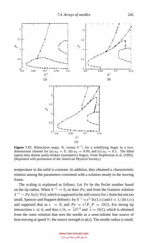
P1: GKW/FYX P2: GKW/FYX QC: GKW/UKS T1: GKW
CB381-07 CB381-Davis May 17, 2001 18:43 Char Count= 0
7.4 Arrays of needles 241
Figure 7.17. Bifurcation maps, Pλ versus S−1, for a solidifying finger in a two-dimensional channel for (a) α4 = 0, (b) α4 = 0.09, and (c) α4 = 0.1. The filled(open) dots denote parity-broken (symmetric) fingers. From Kupferman et al. (1995).(Reprinted with permission of the American Physical Society.)
temperature in the solid is constant. In addition, they obtained a characteristicrelation among the parameters consistent with a solution steady in the movingframe.
The scaling is explained as follows. Let Pe be the Peclet number basedon the tip radius. When S−1 → 0, so does Pe, and from the Ivantsov solutionS−1 ∼ Pe ln (1/Pe), which is supposed to be still correct for λ finite but not toosmall. Spencer and Huppert defined ε by S−1 = ε2 ln (1/ε) and δ = 1/ (ln 1/ε)and supposed that as ε → 0, and Pe = ε2 P, P = O(1). For strong tipinteractions λ δT and thus λ/δT = λδ1/2 and λ = O(1), which is obtainedfrom the outer solution that sees the needle as a semi-infinite line source ofheat moving at speed V ; the source strength is φ(z). The needle radius is small,
www.iran-mavad.com مرجع علمی مھندسی مواد
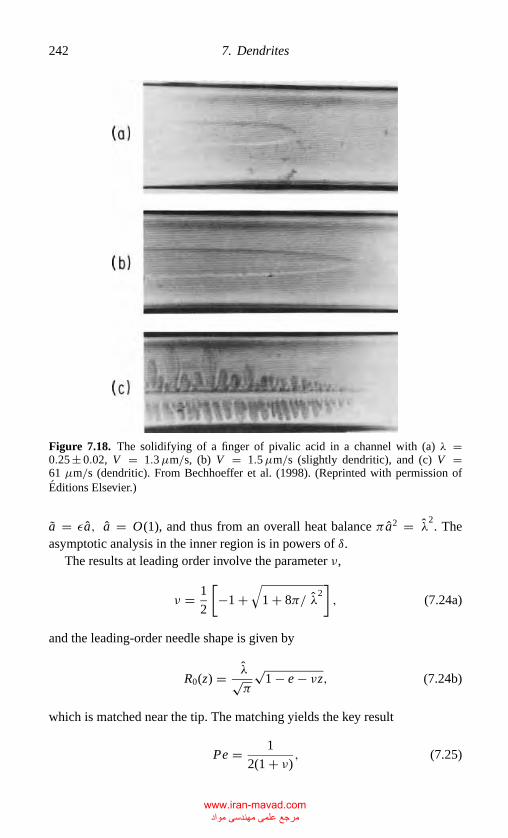
P1: GKW/FYX P2: GKW/FYX QC: GKW/UKS T1: GKW
CB381-07 CB381-Davis May 17, 2001 18:43 Char Count= 0
242 7. Dendrites
Figure 7.18. The solidifying of a finger of pivalic acid in a channel with (a) λ =0.25 ± 0.02, V = 1.3µm/s, (b) V = 1.5µm/s (slightly dendritic), and (c) V =61 µm/s (dendritic). From Bechhoeffer et al. (1998). (Reprinted with permission ofEditions Elsevier.)
a = εa, a = O(1), and thus from an overall heat balance π a2 = λ2. The
asymptotic analysis in the inner region is in powers of δ.The results at leading order involve the parameter ν,
ν = 1
2
[−1 +
√1 + 8π/ λ
2], (7.24a)
and the leading-order needle shape is given by
R0(z) = λ√π
√1 − e − νz, (7.24b)
which is matched near the tip. The matching yields the key result
Pe = 1
2(1 + ν) , (7.25)
www.iran-mavad.com مرجع علمی مھندسی مواد
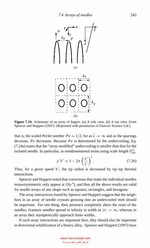
P1: GKW/FYX P2: GKW/FYX QC: GKW/UKS T1: GKW
CB381-07 CB381-Davis May 17, 2001 18:43 Char Count= 0
7.4 Arrays of needles 243
Figure 7.19. Schematic of an array of fingers. (a) A side view. (b) A top view. FromSpencer and Huppert (1997). (Reprinted with permission of Elsevier Science Ltd.)
that is, the scaled Peclet number Pe = 1/2, for as λ → ∞ and as the spacingsdecrease, Pe decreases. Because Pe is determined by the undercooling, Eq.(7.24a) states that the “array-modified” undercooling is smaller than that for theisolated needle. In particular, in nondimensional terms using scale length δ(1)
cap,
ρ ′V ′ = 1 − 2π
(ρ ′
λ′
)2
. (7.26)
Thus, for a given speed V ′, the tip radius is decreased by tip–tip thermalinteractions.
Spencer and Huppert noted that corrections that make the individual needlesnonaxisymmetric only appear at O(ε4), and thus all the above results are validfor needle arrays of any shape such as squares, rectangles, and hexagons.
The array interactions found by Spencer and Huppert suggest that the neigh-bors in an array of needle crystals growing into an undercooled melt shouldbe important. For one thing, their presence completely alters the roots of theneedles; Ivantsov needles spread to infinity in width as |z| → ∞, whereas inan array they asymptotically approach finite widths.
If such array interactions are important here, they should also be importantin directional solidification of a binary alloy. Spencer and Huppert (1997) have
www.iran-mavad.com مرجع علمی مھندسی مواد
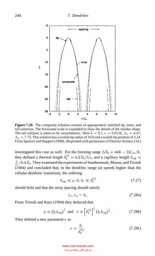
P1: GKW/FYX P2: GKW/FYX QC: GKW/UKS T1: GKW
CB381-07 CB381-Davis May 17, 2001 18:43 Char Count= 0
244 7. Dendrites
Figure 7.20. The composite solution consists of appropriately matched tip, inner, andtail solutions. The horizontal scale is expanded to show the details of the slender shape.The tail solution is taken to be axisymmetric. Here k = 0.1, ε = 0.0116, �x = 6.47,�y = 7.75. This solution has a scaled-tip radius of 10.8 and a scaled-tip position of 2.24.From Spencer and Huppert (1998). (Reprinted with permission of Elsevier Science Ltd.)
investigated this case as well. For the freezing range �T0 = m(k − 1)C∞/k,they defined a thermal length δ(1)
T = k�T0/GT, and a capillary length δcap =γ
Lv/k�T0. They examined the experiments of Somboonsuk, Mason, and Trivedi
(1984) and concluded that, in the dendritic range (at speeds higher than thecellular-dendritic transition), the ordering
δcap ρ δc δ(1)T (7.27)
should hold and that the array spacing should satisfy
λx , λy ∼ δc. (7.28a)
From Trivedi and Kurz (1994) they deduced that
ρ ∝ (δcδcap) 1
2 and λ ∝[δ
(1)T
] 12 (δcδcap
) 14 . (7.28b)
They defined a new parameter ε as
ε = δc
δ(1)T
, (7.28c)
www.iran-mavad.com مرجع علمی مھندسی مواد
P1: GKW/FYX P2: GKW/FYX QC: GKW/UKS T1: GKW
CB381-07 CB381-Davis May 17, 2001 18:43 Char Count= 0
7.4 Arrays of needles 245
which satisfies ε = k−1M−1, and sought solutions for ε → 0 (large speed),
Pe = ρ
δc≡ ε P, P = O(1), (7.28d)
and
δcap
δc= O(ε2). (7.28e)
Typically, in the experiments of Somboonsuk et al. (1984), ε < 0.1, except nearthe cellular–dendritic transition.
In scaled form they solved the following system: In the liquid
∇2C − Cζ = 0 (7.29a)
on the interface
C = ε�+ εζ (7.29b)
n · k [1 + (1 − k)C] = −Cn, (7.29c)
where
� = T0 − Ttip
k�T0= ctip − c∞
c∞(1 − k)≡ ε� (7.30)
is the solute undercooling of the tip relative to the liquidus, ζ = z − ztip, n andk are unit vectors normal to the interface and in the ζ -direction, respectively,and the O(ε2) capillary undercooling has been omitted.
They decomposed the solution into four regions; see Figure 7.20. In theouter region, r ∼ 1, ζ ∼ 1, and the needle appears to be a line source ofstrength Q(ζ ) ∼ ε from 0 < ζ < ∞. The tip solution is given by the Ivantsovneedle, ζ ∼ ε, r = Rtip(ζ ), where
R2tip = 2Pζ. (7.31)
The root solution corresponds to radial diffusion with r ∼ 1, and ζ ∼1/ε(ζ > 0). The “unit cell” encompasses a nonaxisymmetric needle whosecross-sectional area AR is
AR = �x�y {1 − [1 + (1 − k)εζ ]}− 11−k . (7.32)
The inner solution r ∼ ε1/2 and ζ ∼ 1 ties all of these together becauseit contains effects of the tip, the neighbors, and the roots. For the case of�x = �y, Rin is axisymmetric at leading order and satisfies
πR2in =∫ ζ
0Q(s)ds. (7.33)
www.iran-mavad.com مرجع علمی مھندسی مواد
P1: GKW/FYX P2: GKW/FYX QC: GKW/UKS T1: GKW
CB381-07 CB381-Davis May 17, 2001 18:43 Char Count= 0
246 7. Dendrites
Finally, the strength Q(ζ ) of the line source is determined by local equilib-rium on the surface of the slender needle; it requires that the C generated byQ vary linearly in z as given by the temperature field. Thus, after matching,Somboonsuk et al. found that
�+ δζ = Q(ζ )
4πδ− 1
4πQ(ζ )
[ln
(R2
in
4ζ
)+ γE
]
+∫ ∞
0[Q(s) − Q(ζ )]G00(ζ ; s)ds +
∞∑i=−∞
i2+ j2 �=0
∞∑j=−∞
∫ ∞
0Q(s)Gi j (ζ, s)ds,
(7.34a)
where
δ = 1
�n(
1ε
) , (7.34b)
γE is Euler’s constant, and
Gi j (ζ, s) = exp
{−1
2[di j + s − ζ ]
}/4πdi j ,
di j = {(i�x )2 + ( j�y)2 + (s − ζ )2}1/2
.
(7.34c)
For ε ζ 1, the inner solution must match the Ivantsov tip,
Q(0) = 2π P, (7.35a)
and for 1 ζ 1/ε, the inner solution must match the (quasi–one-dimensional) Scheil-like solution
Q(∞) = �x�y . (7.35b)
Given ε and (�x ,�y), the unknown � and Q(ζ ) are simultaneously deter-mined by a nonlinear solvability condition. The constraint (7.35b) is satisfiedautomatically, and the tip radius through P is determined from Eq. (7.35a).
Spencer and Huppert (1998) subsequently solved this nonlinear integral sys-tem. They found that the parabolic tip extends back at a distance δc, after whichthe cross section becomes thinner than the Ivantsov needle. They also foundthat the inner region extends back from the tip a distance of 10δc. Figure 7.20shows the computed solutions in each region and the composite solution. Again,note that the Ivantsov tip occupies a very small region. For small ε, the tip radiusagrees well with experiment. One can convert this to the tip undercooling� andhence relate the results to the single isothermal solutal dendrite (Figure 7.21).
Spencer and Huppert suggested that there is a type of selection in the steadygrowth problem. Two parameters are present, say the spacing λ and either ρ
www.iran-mavad.com مرجع علمی مھندسی مواد
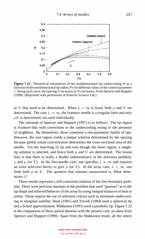
P1: GKW/FYX P2: GKW/FYX QC: GKW/UKS T1: GKW
CB381-07 CB381-Davis May 17, 2001 18:43 Char Count= 0
7.4 Arrays of needles 247
Figure 7.21. Theoretical calculations of the nondimensional tip undercooling � as afunction of the nondimensional tip radius Pe for different values of the control parameterε. Along each curve, the spacing� increases as Pe increases. From Spencer and Huppert(1998). (Reprinted with permission of Elsevier Science Ltd.)
or V that need to be determined. When λ < ∞ is fixed, both ρ and V aredetermined. The case λ → ∞, the Ivantsov needle is a singular limit and onlyρV is determined, not each individually.
The rationale of Spencer and Huppert (1997) is as follows: The tip regionis Ivantsov-like with corrections to the undercooling owing to the presenceof neighbors. By themselves, these constitute a one-parameter family of tips.However, the root region yields a unique solution determined by the spacingbecause global solute concentration determines the cross-sectional area of theneedle. Via the matching of tip and root though the inner region, a single-tip solution is selected, and hence both ρ and V are determined. The lessonhere is that there is really a double indeterminacy in the selection problem,λ and ρ (or V ). In the free-needle case, one specifies λ = ∞ and requiresan extra selection theory to give ρ (or V ). In the array case, λ < ∞, onefinds both ρ or V . The question that remains unanswered is, What deter-mines λ?
These results represent a self-consistent solution of the free-boundary prob-lem. There were previous attempts at the problem that used “guesses” as to thetip shape and inferred behavior of the array by using integral balances of heat orsolute. These require the use of selection criteria such as minimum undercool-ing or marginal stability. Hunt (1991) and Trivedi (1984) used a spherical tipand a Scheil approximation. Makkonen (1991) used a parabolic tip. Figure 7.22is the comparison of these partial theories with the present case, as taken fromSpencer and Huppert (1999). Apart from the Makkonen result, all the others
www.iran-mavad.com مرجع علمی مھندسی مواد
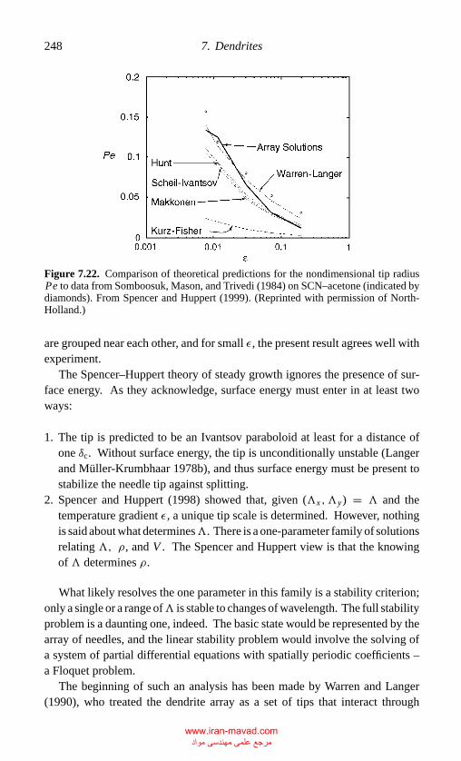
P1: GKW/FYX P2: GKW/FYX QC: GKW/UKS T1: GKW
CB381-07 CB381-Davis May 17, 2001 18:43 Char Count= 0
248 7. Dendrites
Figure 7.22. Comparison of theoretical predictions for the nondimensional tip radiusPe to data from Somboosuk, Mason, and Trivedi (1984) on SCN–acetone (indicated bydiamonds). From Spencer and Huppert (1999). (Reprinted with permission of North-Holland.)
are grouped near each other, and for small ε, the present result agrees well withexperiment.
The Spencer–Huppert theory of steady growth ignores the presence of sur-face energy. As they acknowledge, surface energy must enter in at least twoways:
1. The tip is predicted to be an Ivantsov paraboloid at least for a distance ofone δc. Without surface energy, the tip is unconditionally unstable (Langerand Muller-Krumbhaar 1978b), and thus surface energy must be present tostabilize the needle tip against splitting.
2. Spencer and Huppert (1998) showed that, given (�x ,�y) = � and thetemperature gradient ε, a unique tip scale is determined. However, nothingis said about what determines�. There is a one-parameter family of solutionsrelating �, ρ, and V . The Spencer and Huppert view is that the knowingof � determines ρ.
What likely resolves the one parameter in this family is a stability criterion;only a single or a range of� is stable to changes of wavelength. The full stabilityproblem is a daunting one, indeed. The basic state would be represented by thearray of needles, and the linear stability problem would involve the solving ofa system of partial differential equations with spatially periodic coefficients –a Floquet problem.
The beginning of such an analysis has been made by Warren and Langer(1990), who treated the dendrite array as a set of tips that interact through
www.iran-mavad.com مرجع علمی مھندسی مواد
P1: GKW/FYX P2: GKW/FYX QC: GKW/UKS T1: GKW
CB381-07 CB381-Davis May 17, 2001 18:43 Char Count= 0
7.4 Arrays of needles 249
the concentration field. These tips are local sources of rejected solute thatdepend on the local speeds Vi and local radii of curvature ρi . The tips are wellseparated so that ρi λ, d, where d is the gap width of the Hele–Shaw cellif one considers a single row of needles. The position zi of each tip is on theliquidus, Ci = −Gc/mzi so that capillary undercooling is neglected. Warrenand Langer presumed that the tips each behave as isolated needles growingslowly in a homogeneous melt.
Because the work of Warren and Langer was done before that of Spencerand Huppert, they were not aware that each Vi and ρi can be determined byarray interactions. By examining tips only they needed an extra condition todetermine these. They used the condition given by MST (dependent on surfaceenergy), namely,
2Dd0
Viρ2i
= σ ∗,
where for this one-sided model they take σ ∗ = 0.04. The result is a lineardynamical system for the zi , and they found conditions for marginal stability.In the experiments of Somboonsuk et al. (1984), d < λ, and thus no instabilitymodes “fit” across the gap. The result of Warren and Langer is that the mostdangerous instability is spatially subharmonic, that is, alternate needles growat the expense of the nearest neighbors. Figure 7.22 compares these results forlarge M ∝ ε−1. The tip radius given compares quite well for ε 1 with theSpencer–Huppert theory and for ε not so small is better than theirs.
A possible explanation for the fine comparison of this theory is that the arrayinteractions do determine ρi and Vi for fixed λ but that the instability of thesteady growth is determined by effects only local to the tips. The selectionquestion awaits a full stability theory.
The results of Warren and Langer allow for the existence of a whole rangeof spacings that correspond to stable needle arrays. The situation that seems toexist is that “all” spacings λ are allowable for the existence of steady growth; seeFigure 7.23. When λ is small enough, the front becomes unstable to an over-growth effect in which alternate needles run ahead, suppressing their neighborsand effectively increasing λ. This is the Warren–Langer subharmonic instabil-ity. When λ is large enough, so that ρ is large, the “flattened” tip becomessusceptible to a morphological instability locally, which results in the splittingof the tip. The arrays would then be stable in between these limits. In ex-periments, however, the tip-splitting limit is never reached. Instead, anotherinstability intervenes. Han and Trivedi (1994) showed that the needles developsidearms that develop orthogonally to the main needles, and these side branchesthemselves grow side branches, called tertiary arms, that grow in the pulling
www.iran-mavad.com مرجع علمی مھندسی مواد
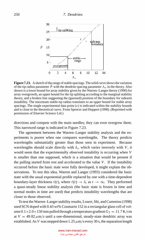
P1: GKW/FYX P2: GKW/FYX QC: GKW/UKS T1: GKW
CB381-07 CB381-Davis May 17, 2001 18:43 Char Count= 0
250 7. Dendrites
Figure 7.23. A sketch of the range of stable spacings. The solid curve shows the variationof the tip radius parameter P with the dendrite spacing parameter�x in the theory. Alsoshown is a lower bound for array stability given by the Warren–Langer theory (1990) forarray overgrowth, an upper bound for the tip splitting according to the marginal stabilitytheory, and a broken line suggesting the (guessed) position of the boundary for sidearminstability. The maximum stable-tip radius translates to an upper bound for stable arrayspacings. The single experimental data point (x) is indicated within the stability boundsand is close to the theoretical curve. From Spencer and Huppert (1998). (Reprinted withpermission of Elsevier Science Ltd.)
directions and compete with the main needles; they can even overgrow them.This narrowed range is indicated in Figure 7.23.
The agreement between the Warren–Langer stability analysis and the ex-periments is poorer when one compares wavelengths. The theory predictswavelengths substantially greater than those seen in experiment. Becausewavelengths should scale directly with δc, which varies inversely with V , itwould seem that the experimentally observed instability is occurring when Vis smaller than one supposed, which is a situation that would be present ifthe pulling started from rest and accelerated to the value V . If the instabilityoccurred before the basic state were fully developed, it might explain the ob-servations. To test this idea, Warren and Langer (1993) considered the basicstate with the usual exponential profile replaced by one with a time-dependentboundary-layer thickness �(t), where �(t) → δc as t → ∞. They performeda quasi-steady linear stability analysis (the basic state is frozen in time andnormal modes in time are used) that predicts instability wavelengths that arecloser to those observed.
To test the Warren–Langer stability results, Losert, Shi, and Cummins (1998)used SCN doped with 0.43 wt% Coumarin 152 in a rectangular glass cell of vol-ume 0.1×2.0×150 mm pulled through a temperature gradient GT = 11.7 K/cmat V = 49.82µm/s until a one-dimensional, steady-state dendritic array wasestablished. As V was stepped down 1.25µm/s every 30 s, the separation length
www.iran-mavad.com مرجع علمی مھندسی مواد
P1: GKW/FYX P2: GKW/FYX QC: GKW/UKS T1: GKW
CB381-07 CB381-Davis May 17, 2001 18:43 Char Count= 0
7.5 Remarks 251
λ remained at 170µm until V = 17.4µm/s, when the array became unstablethrough alternate dendrites that began to overgrow their neighbors. The Warrenand Langer (1990) critical speed is given by V = 14.0µm/s.
Losert, Mesquita, Figeiredo, and Cummins (1998) reconsidered the samesystem in the same channel. Coumarin 152 is a laser dye that has fluorescenceabsorption in the ultraviolet range so that if one illuminates the sample along theinterface with a mercury ultraviolet lamp, the sample will be heated locally andthe interface will melt back. This allows one to select a uniform wavelength forstudy. Here V = 19.8µm/s initially, and a row of ultraviolet spots is appliedcontinuously until a uniform array of dendrites is created with λ ≈ 150µm.The ultraviolet forcing is then turned off. In order to test for subharmonicinstability, the ultraviolet spots are focused on the tips of alternate dendrites,creating an amplitude modulation equal to 2λ, which decays at a measuredrate. This process is repeated at several different V values between 19.8 and6.6µm/s, and the decay rates are calculated. When these are extrapolated tozero, the apparent critical V for stability is V ≈ 4µm/s. (When no ultravioletmodulation is introduced, the array seems to become unstable at the same criticalV ). The measured decay rates are those predicted by Warren and Langer occurat pulling speeds about three times greater than those in the experiments.
Losert, Mesquita, Figeiredo, and Cummins (1998) found a quantitative fitfor this instability in the weakly nonlinear range to a Landau equation for theamplitude of the modulation,
A = σ0 A − b1 |A|2 A (7.36a)
with
σ0 = −0.090S−1 and b1 = −1.1 × 10⁻⁵µm−2S−1. (7.36b)
As V is decreased, there is a bifurcation that is subcritical with a deep range ofsubcriticality.
This remarkable study documenting the overgrowth instability shows howovergrowth occurs at the left-hand boundary of Figure 7.23. There is no com-parable study for the instability on the right-hand boundary. The significanceof Figure 7.23 is that no single spacing is globally preferred; there is an intervalof λ that corresponds to stable, regular needle arrays, and these presumably canbe accessed by the system through varying the history of the process.
7.5 Remarks
The Ivantsov solution for zero surface energy and zero attachment kineticspresents a parabola (two-dimensional) or paraboloid (three-dimensional) validfor steady growth. This deceptively simple solution is difficult to extend to sit-uations with small surface tension. The implied singular perturbation destroys
www.iran-mavad.com مرجع علمی مھندسی مواد
P1: GKW/FYX P2: GKW/FYX QC: GKW/UKS T1: GKW
CB381-07 CB381-Davis May 17, 2001 18:43 Char Count= 0
252 7. Dendrites
the uniform validity of the Ivantsov solution. If one preserves the Ivantsovroot, no solution is present unless one makes the system anisotropic, say, in thesurface tension. If one abandons the Ivantsov-root behavior, a solution with asmooth tip and isotropic surface energy can be found.
The stability of the isolated needle is summarized in Figure 7.13. When0 ≤ α4 < α4c , the traveling wave predominates, and when α4 exceeds α4c , thesteady-needle predominates. Every numerical simulation to date applies to thelatter range, and the MST seems well tested. In some of these simulations,when α4 < α4c , no MST solution could be found in anecdotal agreement withthe picture shown. No comprehensive numerical test of IWT has yet appeared.
It seems to be the case that all the theories give tip radii and tip speedsof remarkably similar magnitudes, and thus by these measures it would bevery difficult to distinguish these experimentally. Because the theories predictintrinsically different behaviors, steady versus time-periodic, and persistentnoise required versus persistent noise not required, more dynamically basedexperiments are needed. Further, experiments, physical and numerical, cannotapproach the small undercooling limit most accessible to analysis since in thisvicinity V is very small and hence δT is very large, and the presence of “distant”boundaries affects the thermal field.
An array of needles possesses root regions significantly different from thoseof isolated needles, and their stability behavior differs markedly. In this case,the presence of neighbors induces collective instabilities as summarized inFigure 7.23. Regular arrays with separation distancesλ too small are susceptibleto overgrowth instabilities, whereas those with λ too large are made unstable bytip splitting or tertiary-sidearm overgrowth. The largeλ instabilities are not wellunderstood theoretically. When λ is between these critical values, the regulararray is seemingly stable, and any value in this range is in principle accessible.Cummins et al. have addressed overgrowth instabilities, but much more needsto be done experimentally to demark the range of λ that must be accessed.No theory exists in the literature that addresses the conceivable appearance ofirregular arrays.
References
Barbieri, A., Hong, D. C., and Langer, J. S. (1987). Velocity selection in the symmetricalmodels of dendritic crystal growth, Phys. Rev. A 35, 1802–1808.
Bechhoeffer, J., Guido, H., and Libshaber, A. (1988). Solidification dans un capillairerectangulaire, Comptes Rendus 306, 619–625.
Ben Amar, M., and Pomeau, Y. (1986). “Theory of dendritic growth in a weakly undercooled melt.” Europhys. Lett. 2, 307–314.
Bensimon, D., Pelce, P., and Shraiman, B. I. (1987). Dynamics of curved fronts andpattern selection, J. Physique (Paris) 48, 2081–2087.
www.iran-mavad.com مرجع علمی مھندسی مواد
P1: GKW/FYX P2: GKW/FYX QC: GKW/UKS T1: GKW
CB381-07 CB381-Davis May 17, 2001 18:43 Char Count= 0
References 253
Brener, E. A., Geilikman, M. B., and Temkin, D. E. (1988). Growth of a needle-shapedcrystal in a channel, Sov. Phys. JETP 67, 1002–1009.
Brener, E. A., Muller-Krumbhaar, H., Saito, Y., and Temkin, D. E. (1993). Crystalgrowth in a channel: Numerical study of the one-sided model, Phys. Rev. E 47,1151–1155.
Canright, D., and Davis, S. H. (1989). Similarity solutions to phase-change problems,Metall. Trans. 20A, 225–235.
Chalmers, B. (1966). Principles of Solidification, Wiley, New York.Glicksman, M. E., and Marsh, S. P. (1993). The dendrite, in D. T. J. Hurle, editor,
Handbook of Crystal Growth, Chap.15, North-Holland, Amsterdam.Glicksman, M. E., and Schaefer, R. J. (1967). Investigation of solid-liquid interface
temperature via isenthalpic solidification, J. Crystal Growth 1, 297–310.. (1968). Comments on theoretical analyses of isenthalpic solidification, J. Crys-
tal Growth 2, 239–242.Glicksman, M. E., Schaefer, R. J., and Ayers, J. D. (1976). Dendritic growth – a test of
theory, Metall. Trans. A7, 1747–1759.Han, S. H., and Trivedi, R. (1994). Primary spacing selection in directionally solidified
alloys, Acta Metall. Mater. 42, 25–41.Hong, D. C., and Langer, J. S. (1986). Analytic theory of the selection mechanism in
the Saffman–Taylor problem, Phys. Rev. Lett. 56, 2032–2035.Huang, S.-C., and Glicksman, M. E. (1981a). Fundamentals of dendritic solidification:
I. Steady-state tip-growth, Acta Metall. Mater. 29, 701–716.. (1981b). Fundamentals of dendritic solidification: Development of sidebranch
structure, Acta Metall. Mater. 29, 717–731.Hunt, J. D. (1991). A numerical analysis of dendritic and cellular growth of a pure
material investigating the transition from array to isolated growth, Acta Metall.Mater. 39, 2117–2133.
Ihle, T., and Muller-Krumbhaar, H. (1994). Diffusion-limited fractal growth morphologyin thermodynamical 2-phase systems, Phys. Rev. Lett. 70, 3083–3086.
Ivantsov, G. P. (1947). Temperature field around spherical, cylindrical, and needle-shaped crystals which grow in supercooled melt, Dokl. Akad. Nauk SSSR 558,567–569.
Karma, A. (1986). “Solidification cells at low velocity – The moving symmetric model”Phys. Rev. A 34, 4353–4362.
Kessler, D. A., and Levine, H. (1986). Stability of dendritic crystals, Phys. Rev. Lett.57, 3069–3072.
Kessler, D. A., Koplik, J., and Levine, H. (1986). Dendritic growth in a channel, Phys.Rev. A 34, 4980–4987.
Kruskal, H., and Segur, H. (1991). Asymptotics beyond all orders in a. model of crystalgrowth, Stud. Appl. Math. 85, 129–181.
Kupferman, R., Kessler, D. A., and Ben-Jacob, E. (1995). Coexistence of symmetricand parity-broken dendrites in a channel, Physics A 213, 451–464.
Kurz, W., and Fisher, D. J. (1989). Fundamentals of Solidification, Trans Tech, Aed-ermannsdorf, Switzerland.
Langer, J. S. (1987). Lectures in the theory of pattern formation, in, J. Souletie, J.Vannimeus, and R. Stora, editors Le hasard et la matiere, Les Houches sessionXLVI, pages 629–712, North-Holland, Amsterdam.
Langer, J. S., and Muller-Krumbhaar, H. (1978a). Theory of dendritic growth – I.Elements of a stability analysis, Acta Metall. Mater. 26, 1681–1688.
Langer, J. S., and Muller-Krumbhaar, H. (1978b). Theory of dendritic growth – II.Instabilities in the limit of vanishing surface tension, Acta Metall. Mater. 26, 1689–1696.
www.iran-mavad.com مرجع علمی مھندسی مواد
P1: GKW/FYX P2: GKW/FYX QC: GKW/UKS T1: GKW
CB381-07 CB381-Davis May 17, 2001 18:43 Char Count= 0
254 7. Dendrites
Losert, W., Mesquita, O. N., Figeiredo, J. M. A., and Cummins, H. Z. (1998). Directmeasurement of dendritic array stability, Phys. Rev. Lett. 81, 409–412.
Losert, W., Shi, B. Q., and Cummins, H. Z. (1998). Evolution of dendritic patternsduring alloy solidification: Onset of the initial instability, Proc. Nat. Acad. Sci. 95,431–438.
Makkonen, L. (1991). Primary dendrite spacing in constrained solidification, Mat. Sci.Eng. A-Struct. 148, 141–143.
Meiron, D. I. (1986). Selection of steady states in the two-dimensional symmetricmodel of dendritic growth, Phys. Rev. A 33, 2704–2715.
Muller-Krumbhaar, H., and Langer, J. S. (1978). Theory of dendritic growth – III.Effects of surface tension, Acta Metall. Mater. 26 , 1697–1708.
Mullins, W. W., and Sekerka, R. F. (1964). Stability of a planar interface during solidi-fication of a dilute binary alloy, J. Appl. Phys. 35, 444–451.
Muschol, M., Liu, D., and Cummins, H. Z. (1992). Surface-tension-anisotropy measure-ments of succinonitrile and pivalic acid: Comparison with microscopic solvabilitytheory, Phys. Rev. A 46, 1038–1050.
Nash, G. E., and Glicksman, M. E. (1974). Capillary-limited steady-state dendriticgrowth – I. Theoretical developments, Acta Metall. mater. 22, 1283–1290.
Oldfield, W. (1973). “Computer model studies of dendritic growth.” Mater. Sci. Eng.11, 211–218.
Pelce, P., and Pumir, A. (1985). Cell shape in directional solidification in the smallPeclet limit, J. Crystal Growth 73, 337.
Schaefer, R. J., Glicksman, M. E., and Ayers, J. D. (1975). High-confidence measure-ments of solid–liquid surface energy in a pure metal, Philos. Mag. 32, 725–743.
Somboonsuk, K., Mason, J. T., and R. Trivedi (1984). Interdendritic spacing: Part I.Experimental studies, Metall. Trans. A 15A, 967.
Spencer, B. J., and Huppert, H. E. (1995). State–state solutions for an array of strongly-interacting needle crystals in the limit of small undercooling, J. Crystal Growth148, 305–323.
. (1997). On the solidification of dendritic arrays: An asymptotic theory for thedirectional solidification of slender needle crystals, Acta Metall. Mater 45, 1535–1549.
. (1998). On the solidification of dendritic arrays: Selection of the tip charac-teristics of slender needle crystals by array interactions, Acta Metall. Mater 46,2645–2662.
. (1999). The relationship between dendrite tip characteristics and dendrite spac-ings in alloy directional solidification, J. Crystal Growth 200, 287–296.
Temkin, D. E. (1960). Growth rate of a needle crystal formed in a supercooled melt,Dokl. Akad. Nauk SSSR 132, 609–613.
Trivedi, R. (1984). Interdendritic spacingz. A comparison of theory and experiment,Metall Trans A 15, 977–982.
Trivedi, R., and Kurz, W. (1994). Solidification microstructures – A conceptual ap-proach, Acta Metall. Mater. 42, 15–23.
Warren, J. A., and Langer, J. S. (1990). Stability of dendritic arrays, Phys. Rev. A 42,3518–3525.
.(1993). Prediction of dendritic spacings in a directional-solidification experi-ment, Phys. Rev. E 47, 2702–2712.
Xu, J.-J. (1997). Interfacial Wave Theory of Pattern Formation, Springer-Verlag, NewYork.
www.iran-mavad.com مرجع علمی مھندسی مواد
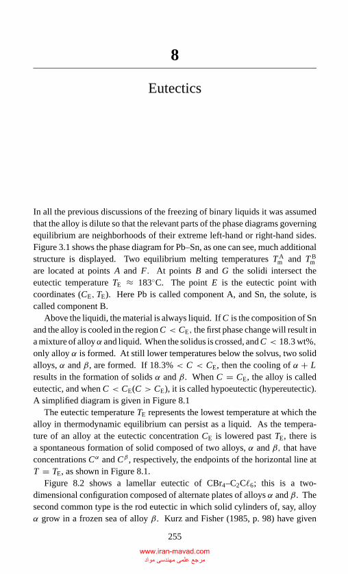
P1: GKE
CB381-08 CB381-Davis May 17, 2001 18:59 Char Count= 0
8
Eutectics
In all the previous discussions of the freezing of binary liquids it was assumedthat the alloy is dilute so that the relevant parts of the phase diagrams governingequilibrium are neighborhoods of their extreme left-hand or right-hand sides.Figure 3.1 shows the phase diagram for Pb–Sn, as one can see, much additionalstructure is displayed. Two equilibrium melting temperatures T A
m and T Bm
are located at points A and F. At points B and G the solidi intersect theeutectic temperature TE ≈ 183◦C. The point E is the eutectic point withcoordinates (CE, TE). Here Pb is called component A, and Sn, the solute, iscalled component B.
Above the liquidi, the material is always liquid. If C is the composition of Snand the alloy is cooled in the region C < CE, the first phase change will result ina mixture of alloyα and liquid. When the solidus is crossed, and C < 18.3 wt%,only alloy α is formed. At still lower temperatures below the solvus, two solidalloys, α and β, are formed. If 18.3% < C < CE, then the cooling of α + Lresults in the formation of solids α and β. When C = CE, the alloy is calledeutectic, and when C < CE(C > CE), it is called hypoeutectic (hypereutectic).A simplified diagram is given in Figure 8.1
The eutectic temperature TE represents the lowest temperature at which thealloy in thermodynamic equilibrium can persist as a liquid. As the tempera-ture of an alloy at the eutectic concentration CE is lowered past TE, there isa spontaneous formation of solid composed of two alloys, α and β, that haveconcentrations Cα and Cβ , respectively, the endpoints of the horizontal line atT = TE, as shown in Figure 8.1.
Figure 8.2 shows a lamellar eutectic of CBr4–C2C�6; this is a two-dimensional configuration composed of alternate plates of alloys α and β. Thesecond common type is the rod eutectic in which solid cylinders of, say, alloyα grow in a frozen sea of alloy β. Kurz and Fisher (1985, p. 98) have given
255
www.iran-mavad.com مرجع علمی مھندسی مواد
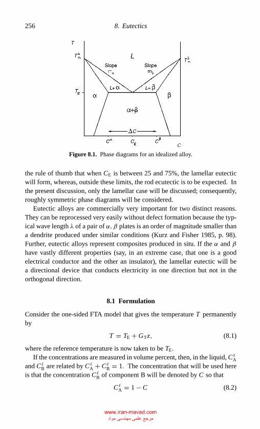
P1: GKE
CB381-08 CB381-Davis May 17, 2001 18:59 Char Count= 0
256 8. Eutectics
Figure 8.1. Phase diagrams for an idealized alloy.
the rule of thumb that when CE is between 25 and 75%, the lamellar eutecticwill form, whereas, outside these limits, the rod ecutectic is to be expected. Inthe present discussion, only the lamellar case will be discussed; consequently,roughly symmetric phase diagrams will be considered.
Eutectic alloys are commercially very important for two distinct reasons.They can be reprocessed very easily without defect formation because the typ-ical wave length λ of a pair of α, β plates is an order of magnitude smaller thana dendrite produced under similar conditions (Kurz and Fisher 1985, p. 98).Further, eutectic alloys represent composites produced in situ. If the α and βhave vastly different properties (say, in an extreme case, that one is a goodelectrical conductor and the other an insulator), the lamellar eutectic will bea directional device that conducts electricity in one direction but not in theorthogonal direction.
8.1 Formulation
Consider the one-sided FTA model that gives the temperature T permanentlyby
T = TE + GTz, (8.1)
where the reference temperature is now taken to be TE.If the concentrations are measured in volume percent, then, in the liquid, C�
A
and C�B are related by C�
A + C�B = 1. The concentration that will be used here
is that the concentration C�B of component B will be denoted by C so that
C�A = 1 − C (8.2)
www.iran-mavad.com مرجع علمی مھندسی مواد
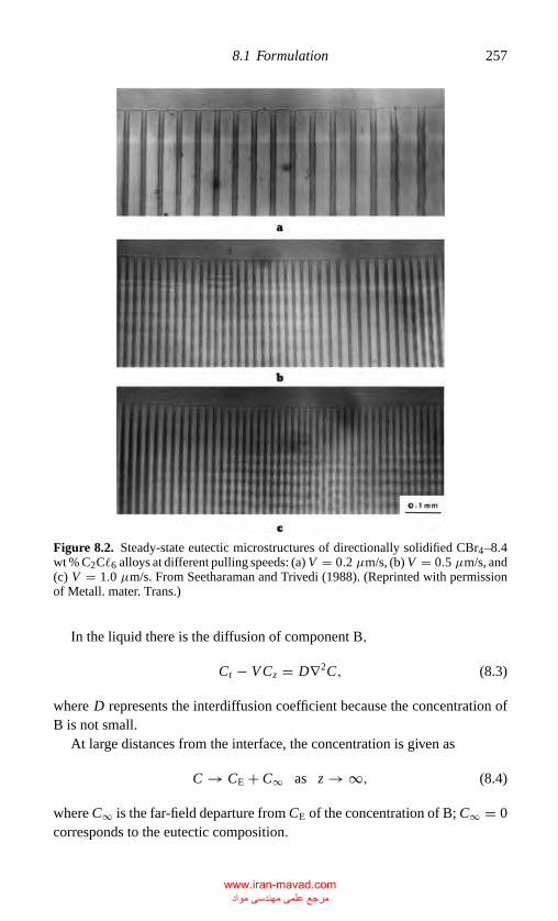
P1: GKE
CB381-08 CB381-Davis May 17, 2001 18:59 Char Count= 0
8.1 Formulation 257
Figure 8.2. Steady-state eutectic microstructures of directionally solidified CBr4–8.4wt % C2C�6 alloys at different pulling speeds: (a) V = 0.2 µm/s, (b) V = 0.5 µm/s, and(c) V = 1.0 µm/s. From Seetharaman and Trivedi (1988). (Reprinted with permissionof Metall. mater. Trans.)
In the liquid there is the diffusion of component B,
Ct − V Cz = D∇2C, (8.3)
where D represents the interdiffusion coefficient because the concentration ofB is not small.
At large distances from the interface, the concentration is given as
C → CE + C∞ as z → ∞, (8.4)
where C∞ is the far-field departure from CE of the concentration of B; C∞ = 0corresponds to the eutectic composition.
www.iran-mavad.com مرجع علمی مھندسی مواد
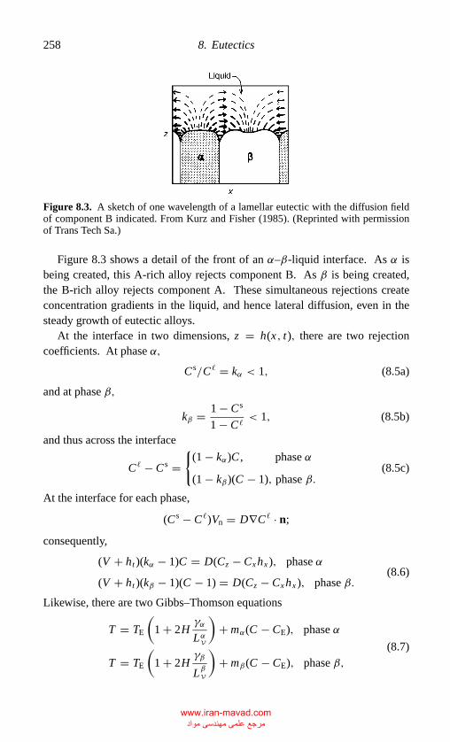
P1: GKE
CB381-08 CB381-Davis May 17, 2001 18:59 Char Count= 0
258 8. Eutectics
Figure 8.3. A sketch of one wavelength of a lamellar eutectic with the diffusion fieldof component B indicated. From Kurz and Fisher (1985). (Reprinted with permissionof Trans Tech Sa.)
Figure 8.3 shows a detail of the front of an α–β-liquid interface. As α isbeing created, this A-rich alloy rejects component B. As β is being created,the B-rich alloy rejects component A. These simultaneous rejections createconcentration gradients in the liquid, and hence lateral diffusion, even in thesteady growth of eutectic alloys.
At the interface in two dimensions, z = h(x, t), there are two rejectioncoefficients. At phase α,
C s/C� = kα < 1, (8.5a)
and at phase β,
kβ = 1 − C s
1 − C�< 1, (8.5b)
and thus across the interface
C� − C s ={
(1 − kα)C , phase α
(1 − kβ)(C − 1), phase β.(8.5c)
At the interface for each phase,
(C s − C�)Vn = D∇C� · n;
consequently,
(V + ht )(kα − 1)C = D(Cz − Cxhx ), phase α
(V + ht )(kβ − 1)(C − 1) = D(Cz − Cxhx ), phase β.(8.6)
Likewise, there are two Gibbs–Thomson equations
T = TE
(1 + 2H
γα
LαV
)+ mα(C − CE), phase α
T = TE
(1 + 2H
γβ
LβV
)+ mβ(C − CE), phase β,
(8.7)
www.iran-mavad.com مرجع علمی مھندسی مواد
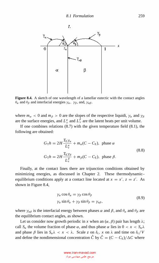
P1: GKE
CB381-08 CB381-Davis May 17, 2001 18:59 Char Count= 0
8.1 Formulation 259
Figure 8.4. A sketch of one wavelength of a lamellar eutectic with the contact anglesθα and θβ and interfacial energies γα, γβ , and, γαβ .
where mα < 0 and mβ > 0 are the slopes of the respective liquidi, γα and γβare the surface energies, and LαV and LβV are the latent heats per unit volume.
If one combines relations (8.7) with the given temperature field (8.1), thefollowing are obtained:
GTh = 2HTEγα
Lαv+ mα(C − CE), phase α
GTh = 2HTEγβ
Lβv+ mβ(C − CE), phase β.
(8.8)
Finally, at the contact lines there are trijunction conditions obtained byminimizing energies, as discussed in Chapter 2. These thermodynamic–equilibrium conditions apply at a contact line located at x = x ′, z = z′. Asshown in Figure 8.4,
γα cos θα = γβ cos θβ
γα sin θα + γβ sin θβ = γαβ,(8.9)
where γαβ is the interfacial energy between phases α and β, and θα and θβ arethe equilibrium contact angles, as shown.
Let us consider now growth periodic in x when an (α, β) pair has length λ;call Sα the volume fraction of phase α, and thus phase α lies in 0 < x < Sαλand phase β lies in Sαλ < x < λ. Scale z on δc, x on λ and time on δc/Vand define the nondimensional concentration C by C = (C − CE)/�C where
www.iran-mavad.com مرجع علمی مھندسی مواد
P1: GKE
CB381-08 CB381-Davis May 17, 2001 18:59 Char Count= 0
260 8. Eutectics
�C = Cβ − Cα , as shown in Figure 8.1. If the carets are dropped, system(8.3)–(8.9) takes the form
Ct − Cz = Czz +�−2Cxx , z > h(x, t). (8.10a)
On z = h(x, t), 0 < x < Sα,
(1 + ht ) [(1 − kα) C +�] = −(Cz −�−2hxCx), (8.10b)
M−1α h = −C + 2H�α. (8.10c)
On z = h(x, t), Sα < x < 1,
(1 + ht )[(
1 − kβ)
C +�− 1] = −(Cz −�2hxCz
), (8.10d)
M−1β h = C + 2H�β. (8.10e)
At the trijunctions,
m�α cos θα = �β cos θβ, (8.10f)
m�α sin θα + �β sin θβ = �αβ, (8.10g)
and as z → ∞,
C → C∞, (8.10h)
where
Mα = −mα�C
GTδcMβ = mβ�C
GTδc
�α = − γαTE
mα(�C)LαVδc�β = − γβTE
mβ(�C)LβVδc
�αβ = γαβTE
mβ(�C)LβVδcm = −mα
mβ
LαVLβV
� = CE − Csα
�CC∞ = C∞ − CE
�C
� = λ
δc.
(8.11)
www.iran-mavad.com مرجع علمی مھندسی مواد
P1: GKE
CB381-08 CB381-Davis May 17, 2001 18:59 Char Count= 0
8.2 Approximate theories for steady growth and selection 261
8.2 Approximate Theories for Steady Growth and Selection
The central analysis of steady growth was undertaken by Jackson and Hunt(1966), who solved the steady growth problem with rather severe approxima-tions.
(1) They sought solutions for the concentration C with the interface replacedby a plane. In effect they obtained an “outer” solution valid where the interfacialcorrugations are negligible. To do this, (2) they approximated the left-handside of the conditions (8.10b,d) with constants obtained by presuming that theconcentration departs from CE by a negligibly small amount. Because C = 0corresponds to the eutectic concentration, the new flux balances become
� = Cz, 0 ≤ x < Sα (8.12a)
and
�− 1 = Cz, Sα < x ≤ 1. (8.12b)
On the right-hand sides of balances (8.10b,d), hx is replaced by zero.Jackson and Hunt solved (8.10a) for the concentration by writing
C(x, g) = C∞ + B0e−z +∞∑
n=1
Bne−[
12 +
√14 +n2π2�−2
]zcos nπ
(x − 1
2Sα
).
(8.13)
For purposes of simplicity, (3) they utilized the condition that for n =1, 2, . . . , nπ � (1/2)�, which means that λ δc is valid for all cases inwhich the solidification is not too “rapid.” As a result
C(x, z) ≈ C∞ + B0e−z +∞∑
n=1
Bne− nπ z� cos nπ
(x − 1
2Sα
). (8.14)
They then obtained the coefficients Bn using the orthogonality of the Fouriermodes to find that
− B0 = Sα�+ (1 − Sα) (�− 1), (8.15a)
which is a scaled version of the lever law, and
Bn = − 2�
n2π2sin nπ Sα, (8.15b)
which represents the ratio of � to �C. Thus,
C(x, z) ≈ C∞ − [Sα�+ (1 − Sα) (�− 1)] e−z
− 2�∞∑
n=1
1
n2π2e− nπ z
� sin nπ Sα cos nπ
(x − 1
2Sα
). (8.16)
www.iran-mavad.com مرجع علمی مھندسی مواد
P1: GKE
CB381-08 CB381-Davis May 17, 2001 18:59 Char Count= 0
262 8. Eutectics
This approximated distribution of solute represents a concentration boundarylayer of thickness δc (the first two terms), similar to that for directional solid-ification of a dilute alloy, corrected by x-periodic distributions that reflect theplate-like structure of eutectic growth. The boundary layer has constant thick-ness, but the coefficient B0 varies with concentration; it is zero at the eutecticconcentration that reflects the fact in this case that there is no net rejection overone wavelength. What α rejects, β incorporates.
Given the approximate C(x, z), Eq. (8.16), one can now turn to shape of theinterface. From Eq. (8.10c),
2H�α − M−1α h = C(x, 0)
= C∞ + [Sα�+ (1 − Sα) (�− 1)]
− 2�∞∑
n=1
1
n2π2sin nπ Sα sin nπx
≡ f (x). (8.17)
Jackson and Hunt (1966) ignored the term M−1h and solved Eq. (8.17) subjectto the edge conditions. For present purposes, it is sufficient to replace 2H byits linearization hxx appropriate to small contact angles θα and θβ . Thus,
�αhxx = f (x), (8.18a)
and thus
�αhx =∫ x
0f (s)ds + θα (8.18b)
(tan θα ≈ θα), and
�αh =∫ x
0
∫ ξ
0f (s)ds dξ + θαx, (8.18c)
which satisfies h(0) = 0. Likewise, from Eq. (8.10e) with similar approxima-tions,
�βhxx = − f (x) (8.19a)
so that
�βhx = −∫ x
Sa
f (s)ds + θβ (8.19b)
and
�βh = −∫ x
Sα
∫ ξ
Sα
f (s)ds dξ + θβ (x − Sα), (8.19c)
which satisfies h(Sα) = 0. The shapes (8.18c) and (8.19c) are concave down-ward segments that meet at the trijunctions at prescribed angles.
www.iran-mavad.com مرجع علمی مھندسی مواد
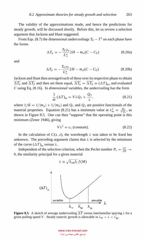
P1: GKE
CB381-08 CB381-Davis May 17, 2001 18:59 Char Count= 0
8.2 Approximate theories for steady growth and selection 263
The validity of the approximations made, and hence the predictions forsteady growth, will be discussed shortly. Before this, let us review a selectionargument that Jackson and Hunt suggested.
From Eqs. (8.7) the dimensional undercoolings TE − T I on each phase havethe forms
�Tα = −TEγα
LαV2H − mα(C − CE) (8.20a)
and
�Tβ = −TEγβ
LαV2H − mβ(C − CE). (8.20b)
Jackson and Hunt then averaged each of these over its respective phase to obtain�Tα and �Tβ and then set them equal, �Tα = �Tβ ≡ (�T )m, and evaluatedC using Eq. (8.16). In dimensional variables, the undercooling has the form
1
m(�T )m = VλQ1 + Q2
λ, (8.21)
where 1/m = 1/|mα| + 1/|mβ | and Q1 and Q2 are positive functionals of thematerial properties. Equation (8.21) has a minimum value at λ2
m = Q2V Q1
, asshown in Figure 8.5. One can then “suppose” that the operating point is thisminimum (Zener 1946), giving
Vλ2 = c1 (constant). (8.22)
In the calculation of C(x, z), the wavelength λ was taken to be fixed butunknown. The preceding argument claims that λ is selected by the minimumof the curve (�T )m versus λ.
Independent of the selection criterion, when the Peclet number Pλ = λV2D →
0, the similarity principal for a given material
λ ∝ √δcapδc f (M)
Figure 8.5. A sketch of average undercooling �T versus interlamellar spacing λ for agiven pulling speed V . Steady eutectic growth is allowable in λm < λ < λ
′M.
www.iran-mavad.com مرجع علمی مھندسی مواد
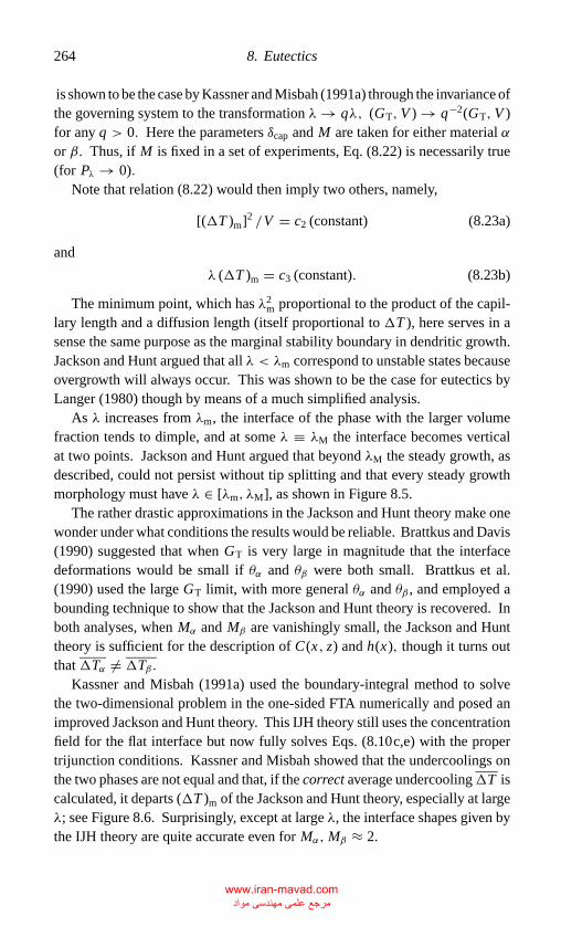
P1: GKE
CB381-08 CB381-Davis May 17, 2001 18:59 Char Count= 0
264 8. Eutectics
is shown to be the case by Kassner and Misbah (1991a) through the invariance ofthe governing system to the transformation λ → qλ, (GT, V ) → q−2(GT, V )for any q > 0. Here the parameters δcap and M are taken for either material αor β. Thus, if M is fixed in a set of experiments, Eq. (8.22) is necessarily true(for Pλ → 0).
Note that relation (8.22) would then imply two others, namely,
[(�T )m]2 /V = c2 (constant) (8.23a)
and
λ (�T )m = c3 (constant). (8.23b)
The minimum point, which has λ2m proportional to the product of the capil-
lary length and a diffusion length (itself proportional to �T ), here serves in asense the same purpose as the marginal stability boundary in dendritic growth.Jackson and Hunt argued that all λ < λm correspond to unstable states becauseovergrowth will always occur. This was shown to be the case for eutectics byLanger (1980) though by means of a much simplified analysis.
As λ increases from λm, the interface of the phase with the larger volumefraction tends to dimple, and at some λ ≡ λM the interface becomes verticalat two points. Jackson and Hunt argued that beyond λM the steady growth, asdescribed, could not persist without tip splitting and that every steady growthmorphology must have λ ∈ [λm, λM], as shown in Figure 8.5.
The rather drastic approximations in the Jackson and Hunt theory make onewonder under what conditions the results would be reliable. Brattkus and Davis(1990) suggested that when GT is very large in magnitude that the interfacedeformations would be small if θα and θβ were both small. Brattkus et al.(1990) used the large GT limit, with more general θα and θβ , and employed abounding technique to show that the Jackson and Hunt theory is recovered. Inboth analyses, when Mα and Mβ are vanishingly small, the Jackson and Hunttheory is sufficient for the description of C(x, z) and h(x), though it turns outthat �Tα �= �Tβ.
Kassner and Misbah (1991a) used the boundary-integral method to solvethe two-dimensional problem in the one-sided FTA numerically and posed animproved Jackson and Hunt theory. This IJH theory still uses the concentrationfield for the flat interface but now fully solves Eqs. (8.10c,e) with the propertrijunction conditions. Kassner and Misbah showed that the undercoolings onthe two phases are not equal and that, if the correct average undercooling�T iscalculated, it departs (�T )m of the Jackson and Hunt theory, especially at largeλ; see Figure 8.6. Surprisingly, except at large λ, the interface shapes given bythe IJH theory are quite accurate even for Mα,Mβ ≈ 2.
www.iran-mavad.com مرجع علمی مھندسی مواد
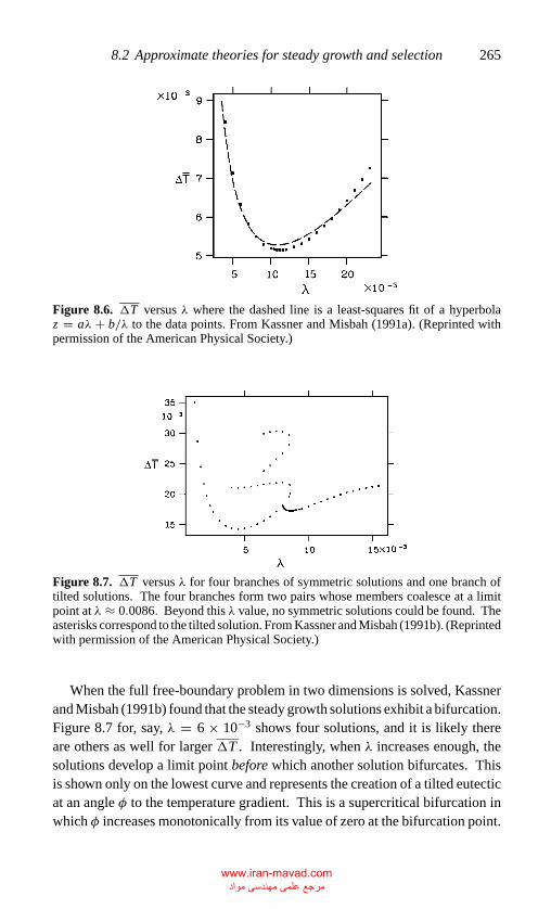
P1: GKE
CB381-08 CB381-Davis May 17, 2001 18:59 Char Count= 0
8.2 Approximate theories for steady growth and selection 265
Figure 8.6. �T versus λ where the dashed line is a least-squares fit of a hyperbolaz = aλ + b/λ to the data points. From Kassner and Misbah (1991a). (Reprinted withpermission of the American Physical Society.)
Figure 8.7. �T versus λ for four branches of symmetric solutions and one branch oftilted solutions. The four branches form two pairs whose members coalesce at a limitpoint at λ ≈ 0.0086. Beyond this λ value, no symmetric solutions could be found. Theasterisks correspond to the tilted solution. From Kassner and Misbah (1991b). (Reprintedwith permission of the American Physical Society.)
When the full free-boundary problem in two dimensions is solved, Kassnerand Misbah (1991b) found that the steady growth solutions exhibit a bifurcation.Figure 8.7 for, say, λ = 6 × 10⁻³ shows four solutions, and it is likely thereare others as well for larger �T . Interestingly, when λ increases enough, thesolutions develop a limit point before which another solution bifurcates. Thisis shown only on the lowest curve and represents the creation of a tilted eutecticat an angle φ to the temperature gradient. This is a supercritical bifurcation inwhich φ increases monotonically from its value of zero at the bifurcation point.
www.iran-mavad.com مرجع علمی مھندسی مواد
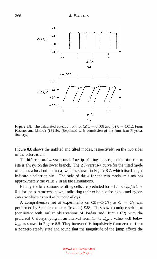
P1: GKE
CB381-08 CB381-Davis May 17, 2001 18:59 Char Count= 0
266 8. Eutectics
Figure 8.8. The calculated eutectic front for (a) λ = 0.008 and (b) λ = 0.012. FromKassner and Misbah (1991b). (Reprinted with permission of the American PhysicalSociety.)
Figure 8.8 shows the untilted and tilted modes, respectively, on the two sidesof the bifurcation.
The bifurcation always occurs before tip splitting appears, and the bifurcationsite is always on the lower branch. The�T-versus-λ curve for the tilted modeoften has a local minimum as well, as shown in Figure 8.7, which itself mightindicate a selection site. The ratio of the λ for the two modal minima hasapproximately the value 2 in all the simulations.
Finally, the bifurcations to tilting cells are predicted for −1.4 < C∞/�C <0.1 for the parameters shown, indicating their existence for hypo- and hyper-eutectic alloys as well as eutectic alloys.
A comprehensive set of experiments on CB4–C2C�6 at C = CE wasperformed by Seetharaman and Trivedi (1988). They saw no unique selection(consistent with earlier observations of Jordan and Hunt 1972) with thepreferred λ always lying in an interval from λm to λ′
M, a value well belowλM, as shown in Figure 8.5. They increased V impulsively from zero or froma nonzero steady state and found that the magnitude of the jump affects the
www.iran-mavad.com مرجع علمی مھندسی مواد
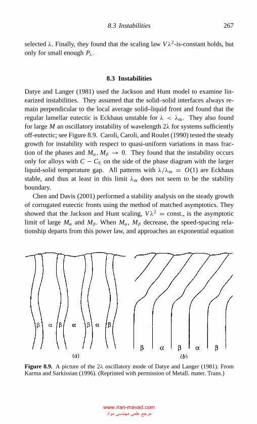
P1: GKE
CB381-08 CB381-Davis May 17, 2001 18:59 Char Count= 0
8.3 Instabilities 267
selected λ. Finally, they found that the scaling law Vλ2-is-constant holds, butonly for small enough Pλ.
8.3 Instabilities
Datye and Langer (1981) used the Jackson and Hunt model to examine lin-earized instabilities. They assumed that the solid–solid interfaces always re-main perpendicular to the local average solid–liquid front and found that theregular lamellar eutectic is Eckhaus unstable for λ < λm. They also foundfor large M an oscillatory instability of wavelength 2λ for systems sufficientlyoff-eutectic; see Figure 8.9. Caroli, Caroli, and Roulet (1990) tested the steadygrowth for instability with respect to quasi-uniform variations in mass frac-tion of the phases and Mα,Mβ → 0. They found that the instability occursonly for alloys with C − CE on the side of the phase diagram with the largerliquid-solid temperature gap. All patterns with λ/λm = O(1) are Eckhausstable, and thus at least in this limit λm does not seem to be the stabilityboundary.
Chen and Davis (2001) performed a stability analysis on the steady growthof corrugated eutectic fronts using the method of matched asymptotics. Theyshowed that the Jackson and Hunt scaling, Vλ2 = const., is the asymptoticlimit of large Mα and Mβ . When Mα , Mβ decrease, the speed-spacing rela-tionship departs from this power law, and approaches an exponential equation
Figure 8.9. A picture of the 2λ oscillatory mode of Datye and Langer (1981). FromKarma and Sarkissian (1996). (Reprinted with permission of Metall. mater. Trans.)
www.iran-mavad.com مرجع علمی مھندسی مواد
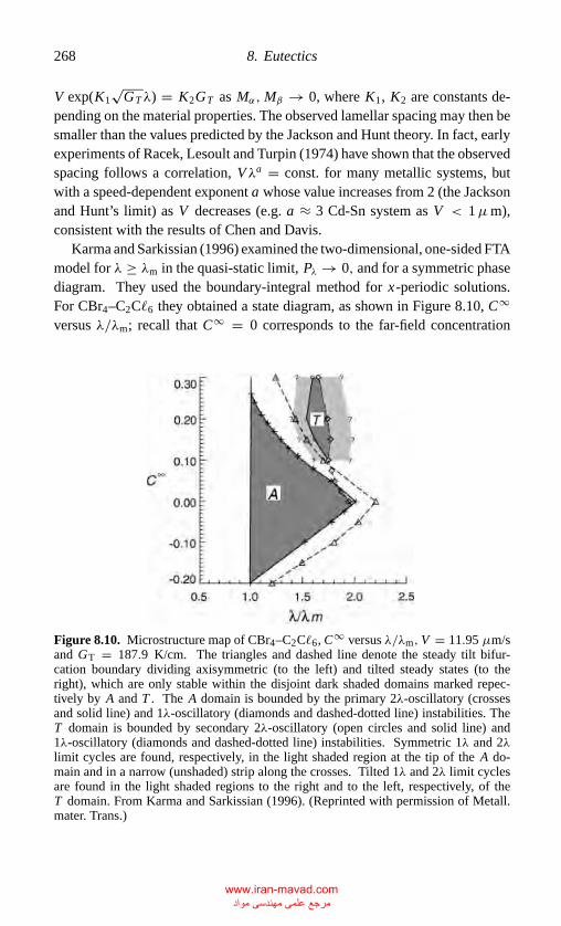
P1: GKE
CB381-08 CB381-Davis May 17, 2001 18:59 Char Count= 0
268 8. Eutectics
V exp(K1√
GTλ) = K2GT as Mα,Mβ → 0, where K1, K2 are constants de-pending on the material properties. The observed lamellar spacing may then besmaller than the values predicted by the Jackson and Hunt theory. In fact, earlyexperiments of Racek, Lesoult and Turpin (1974) have shown that the observedspacing follows a correlation, Vλa = const. for many metallic systems, butwith a speed-dependent exponent a whose value increases from 2 (the Jacksonand Hunt’s limit) as V decreases (e.g. a ≈ 3 Cd-Sn system as V < 1µm),consistent with the results of Chen and Davis.
Karma and Sarkissian (1996) examined the two-dimensional, one-sided FTAmodel for λ ≥ λm in the quasi-static limit, Pλ → 0, and for a symmetric phasediagram. They used the boundary-integral method for x-periodic solutions.For CBr4–C2C�6 they obtained a state diagram, as shown in Figure 8.10, C∞
versus λ/λm; recall that C∞ = 0 corresponds to the far-field concentration
Figure 8.10. Microstructure map of CBr4–C2C�6, C∞ versus λ/λm, V = 11.95 µm/sand GT = 187.9 K/cm. The triangles and dashed line denote the steady tilt bifur-cation boundary dividing axisymmetric (to the left) and tilted steady states (to theright), which are only stable within the disjoint dark shaded domains marked repec-tively by A and T . The A domain is bounded by the primary 2λ-oscillatory (crossesand solid line) and 1λ-oscillatory (diamonds and dashed-dotted line) instabilities. TheT domain is bounded by secondary 2λ-oscillatory (open circles and solid line) and1λ-oscillatory (diamonds and dashed-dotted line) instabilities. Symmetric 1λ and 2λlimit cycles are found, respectively, in the light shaded region at the tip of the A do-main and in a narrow (unshaded) strip along the crosses. Tilted 1λ and 2λ limit cyclesare found in the light shaded regions to the right and to the left, respectively, of theT domain. From Karma and Sarkissian (1996). (Reprinted with permission of Metall.mater. Trans.)
www.iran-mavad.com مرجع علمی مھندسی مواد
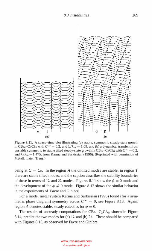
P1: GKE
CB381-08 CB381-Davis May 17, 2001 18:59 Char Count= 0
8.3 Instabilities 269
Figure 8.11. A space–time plot illustrating (a) stable, symmetric steady-state growthin CBr4–C2C�6 with C∞ = 0.2, and λ/λm = 1.09, and (b) a dynamical transient fromunstable symmetric to stable tilted steady-state growth in CBr4–C2C�6 with C∞ = 0.2,and λ/λm = 1.475, from Karma and Sarkissian (1996). (Reprinted with permission ofMetall. mater. Trans.)
being at C = CE. In the region A the untilted modes are stable; in region Tthere are stable tilted modes, and the caption describes the stability boundariesof these in terms of 1λ and 2λ modes. Figures 8.11 show the φ = 0 mode andthe development of the φ �= 0 mode. Figure 8.12 shows the similar behaviorin the experiments of Favre and Ginibre.
For a model metal system Karma and Sarkissian (1996) found (for a sym-metric phase diagram) symmetry across C∞ = 0; see Figure 8.13. Again,region A denotes stable, steady eutectics for φ = 0.
The results of unsteady computations for CBr4–C2C�6, shown in Figure8.14, predict the two modes for (a) 1λ and (b) 2λ. These should be comparedwith Figures 8.15, as observed by Favre and Ginibre.
www.iran-mavad.com مرجع علمی مھندسی مواد
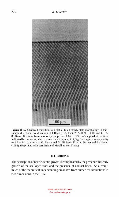
P1: GKE
CB381-08 CB381-Davis May 17, 2001 18:59 Char Count= 0
270 8. Eutectics
Figure 8.12. Observed transition to a stable, tilted steady-state morphology in thin-sample directional solidification of CBr4–C2C�6 for C∞ ≈ 0.21 ± 0.02 and GT ≈80 K/cm. It results from a velocity jump from 0.85 to 3.3 µm/s applied at the timeindicated by the arrow, which corresponds to a jump in λ/λm from approximately unityto 1.9 ± 0.1 (courtesy of G. Faivre and M. Ginigre). From to Karma and Sarkissian(1996). (Reprinted with permission of Metall. mater. Trans.)
8.4 Remarks
The description of near-eutectic growth is complicated by the presence in steadygrowth of the scalloped front and the presence of contact lines. As a result,much of the theoretical understanding emanates from numerical simulations intwo dimensions in the FTA.
www.iran-mavad.com مرجع علمی مھندسی مواد
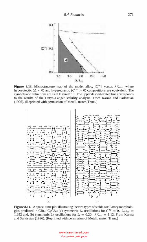
P1: GKE
CB381-08 CB381-Davis May 17, 2001 18:59 Char Count= 0
8.4 Remarks 271
Figure 8.13. Microstructure map of the model alloy, |C∞| versus λ/λm, wherehypoeutectic (� < 0) and hypereutectic (C∞ > 0) compositions are equivalent. Thesymbols and definitions are as in Figure 8.10. The upper dashed-dotted line correspondsto the results of the Datye–Langer stability analysis. From Karma and Sarkissian(1996). (Reprinted with permission of Metall. mater. Trans.)
Figure 8.14. A space–time plot illustrating the two types of stable oscillatory morpholo-gies predicted in CBr4–C2C�6: (a) symmetric 1λ oscillations for C∞ = 0, λ/λm =1.952 and, (b) symmetric 2λ oscillations for � = 0.20, λ/λm = 1.12. From Karmaand Sarkissian (1996). (Reprinted with permission of Metall. mater. Trans.)
www.iran-mavad.com مرجع علمی مھندسی مواد
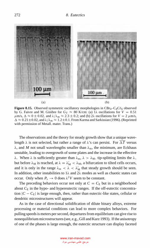
P1: GKE
CB381-08 CB381-Davis May 17, 2001 18:59 Char Count= 0
272 8. Eutectics
Figure 8.15. Observed symmetric oscillatory morphologies in CBr4–C4C�6 observedby G. Faivre and M. Ginibre for GT ≈ 80 K/cm: (a) 1λ oscillations for V = 0.51µm/s, � ≈ 0 ± 0.02, and λ/λm ≈ 2.3 ± 0.2; and (b) 2λ oscillations for V = 2 µm/s,� ≈ 0.21±0.02, and λ/λm ≈ 1.2±0.1. From Karma and Sarkissian (1996). (Reprintedwith permission of Metall. mater. Trans.)
The observations and the theory for steady growth show that a unique wave-length λ is not selected, but rather a range of λ’s can persist. For �T versusλ, and M not small wavelengths smaller than λm, the minimum, are Eckhausunstable, leading to overgrowth of some plates and the increase in the effectiveλ. When λ is sufficiently greater than λm, λ > λM, tip-splitting limits the λ,but before λM is reached, at λ = λ′
M < λM, a bifurcation to tilted cells occurs,and it is only in the range λm < λ < λ
′M that steady growth should be seen.
In addition, other instabilities to 1λ and 2λ modes as well as chaotic states canoccur. Only when Pλ → 0 does λ2V seem to be constant.
The preceding behaviors occur not only at C = CE but in a neighborhoodabout CE in the hypo- and hypereutectic ranges. If the off-eutectic concentra-tion |C − CE| is large enough, then, rather than eutectic-like states, cellular ordendritic microstructures will appear.
As in the case of directional solidification of dilute binary alloys, extremeprocessing or material conditions can lead to more complex behaviors. Forpulling speeds is meters per second, departures from equilibrium can give rise tononequilibrium microstructures (see, e.g., Gill and Kurz 1993). If the anisotropyof one of the phases is large enough, the eutectic structure can display faceted
www.iran-mavad.com مرجع علمی مھندسی مواد
P1: GKE
CB381-08 CB381-Davis May 17, 2001 18:59 Char Count= 0
References 273
behavior. If significant convection is present in the melt, the range of preferredλ will be altered.
References
Brattkus, K., Caroli, B., Caroli, C., and Roulet, B. (1990). Lamellar eutectic growth atlarge thermal gradient: I. Stationary patterns. J. Phys. (France) 51, 1847–1864.
Brattkus, K., and Davis, S. H. (1989). Steady and dynamic lamellar-eutectic growth.Preprint cited as Brattkus in Kurz, W., and Trivedi, R. (1990). Solidification mi-crostructure: Recent developments and future directions. Acta Metall. Mater. 38,1–17.
Caroli, B., Caroli, C., and Roulet, B. (1990). Lamellar eutectic growth at large thermalgradient, II. Linear stability, J. Phys. (France) 51, 1865–1876.
Chen, Y.-J., and Davis, S. H. (2001). Instability of triple junctions in lamellar eutecticgrowth, Acta Mater. (in press).
Datye, V., and Langer, J. S. (1981). Stability of thin eutectic growth, Phys. Rev. B 24,4155–4169.
Gill, S. C., and Kurz, W. (1993). Rapidly solidified Al–Cu alloys – I. Experimentaldetermination of the microstructure selection map, Acta Metall. Mater. 41, 3563–3573.
Jackson, K. A., and Hunt, J. D. (1966). Lamellar and rod eutectic growth, Trans. Metall.Soc. AIME 236, 1128–1142.
Jordan, R. M., and Hunt, J. D. (1972). Interface under coolings during the growth ofPb-Sn eutectics, Met. Trans. 3, 1385–1390.
Karma, A., and Sarkissian, A. (1996). Morphological instabilities of lamellar eutectics,Metall. mater. Trans. A 27, 635–656.
Kassner, K., and Misbah, C. (1991a). Growth of lamellar eutectic structures: The ax-isymmetric state, Phys. Rev. A 44, 6513–6532.
. (1991b). Spontaneous parity-breaking transition in directional growth of lamel-lar eutectic structures, Phys. Rev. A 44, 6533–6543.
Kurz, W., and Fisher, D. J. (1985). Fundamentals of Solidification, Trans. Tech. Publ.,Aedermannsdorf, Switzerland.
Langer, J. S. (1980). Eutectic solidification and marginal stability, Phys. Rev. Lett. 44,1023–1026.
Racek, R., Lesoult, G., and Turpin, M. (1974). The Cd-Sn eutectic structures at lowgrowth rates, Cryst. Growth 22, 210–218.
Seetharaman, V., and Trivedi, R. (1988). Eutectic growth: Selection of interlamellarspacings, Metall. mater. Trans. A 19, 2955–2964.
Zener (1946). Kinetics of the decomposition of austenite, Trans. Metall. Soc. AIME 167,550–595.
www.iran-mavad.com مرجع علمی مھندسی مواد
P1: GMD
CB381-09 CB381-Davis May 17, 2001 19:20 Char Count= 0
9
Microscale fluid flow
In all the earlier discussions of morphological instabilities, the driver of themorphological changes was the gradient at the front of a diffusive quantity. Forthe pure material it was an adverse temperature gradient, and for the binary alloyin directional solidification it was an adverse concentration gradient. It seemsclear if fluid flow is present in the liquid (melt) that the heat or solute can beconvected and hence that its distribution can be altered. Such alterations wouldnecessarily change the conditions for instability. What makes the situation moresubtle is that flow over a disturbed (i.e., corrugated) interface will not only alter“vertical” distributions but will also create means of lateral transport, whichcan stabilize or destabilize the front. The allowance of fluid flow can createnew frontal instabilities, flow-induced instabilities, that can preempt the alteredmorphological instability and dominate the behavior of the front.
It has been known since time immemorial that fluid flow can affect solidifi-cation; cases range from the stirring of a partially frozen lake to the agitationof “scotch on the rocks.” Crystal growers are keenly aware of the importanceof fluid flows. Rosenberger (1979) states that “non-steady convection is nowrecognized as being largely responsible for inhomogeneity in solids.”
When one attempts to grow single crystals, the state of pure diffusion rarelyexists. Usually, flow is present in the melt; it may be created by direct forcingor it may be due to the presence of convection. Brown (1988) has given a broadsurvey of the processing configurations and the types of flows that occur.
There are many examples of forced flows. The crystal may be rotated to erasenonaxially symmetric thermal effects, but it creates a von Karman swirl flow.The use of microgravity environments for the growth of crystals suppressesmajor buoyancy effects, but the lurching of the spacecraft creates transientaccelerations, called g-jitter, that stir the liquid.
274
www.iran-mavad.com مرجع علمی مھندسی مواد
P1: GMD
CB381-09 CB381-Davis May 17, 2001 19:20 Char Count= 0
9. Microscale fluid flow 275
There are three types of convection that can occur in the liquid:
1. If the density of the liquid and solid are different, bulk flows in the liquidare driven normal to the interface; this is volume-change convection presenteven in the absence of gravity.
2. There is buoyancy-driven convection created by density gradients. In binaryliquids, the double-diffusive convection can be steady when Rayleigh num-bers exceed critical values or at arbitrarily small Rayleigh numbers owingto the presence of, say, heat losses at the sidewalls of the container. If theRayleigh numbers are high enough, the steady convection can become unsta-ble and, perhaps, unsteady. This is often the case in metallic or semiconductormaterials that have very small Prandtl numbers.
3. When fluid–fluid interfaces are present, as in the case of containerless pro-cessing by float zone methods or the reprocessing of surfaces by lasers, steeptemperature and concentration gradients on these interfaces can drive steadythermosoluto–capillary convection. If these steady flows become unstable,unsteady states can occur.
All of the aforementioned flows are in a sense accidental or at any rateunintentional. They cannot be prevented or else are present, as in the caseof the swirl, because the motion is necessary for other reasons. There canalso be intentionally imposed flows. In the 1960s Hurle suggested that crystalgrowers, rather than bemoaning the presence of convection as a source of crystalnonuniformities, should try to “design” natural convection (or forced flows)that would homogenize the solute boundary layer at the interface. In effect,this would decrease the local gradient |Gc| enough to eliminate the possibilityof morphological instabilities. This attractive possibility has motivated a gooddeal of work on the coupling of flow and morphology.
In this chapter, a general formulation of solidification and convection willbe given, special cases of which will be studied in subsequent sections. Theseinclude prototype flows in which standard hydrodynamic-instability modelshave one or more rigid boundaries replaced with crystal fronts that can meltor freeze. There is also directional solidification in the presence of imposedflows, either parallel or non-parallel. There is the interaction of directionalsolidification and convection. If the solid and liquid have different densities, theinterface drives a flow. If one solidifies upward and rejects solute of low density,then the liquid is stably stratified thermally but unstably stratified solutally.Thus, there can be convective as well as morphological instabilities. Thesecan occur simultaneously, or the convective field can already be present whenthe morphological instability begins. Finally, the convection can be turbulent,and this mesoscale convection can strongly affect the gross morphologies of
www.iran-mavad.com مرجع علمی مھندسی مواد
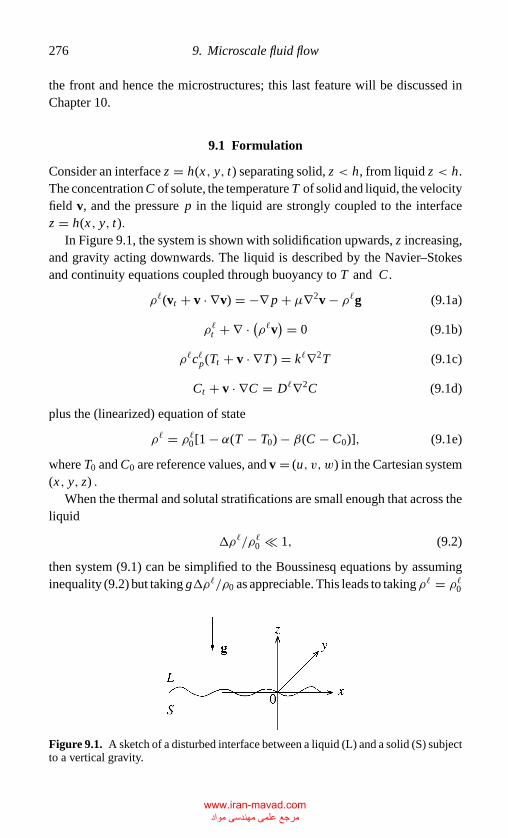
P1: GMD
CB381-09 CB381-Davis May 17, 2001 19:20 Char Count= 0
276 9. Microscale fluid flow
the front and hence the microstructures; this last feature will be discussed inChapter 10.
9.1 Formulation
Consider an interface z = h(x, y, t) separating solid, z < h, from liquid z < h.The concentration C of solute, the temperature T of solid and liquid, the velocityfield v, and the pressure p in the liquid are strongly coupled to the interfacez = h(x, y, t).
In Figure 9.1, the system is shown with solidification upwards, z increasing,and gravity acting downwards. The liquid is described by the Navier–Stokesand continuity equations coupled through buoyancy to T and C .
ρ�(vt + v · ∇v) = −∇ p + µ∇2v − ρ�g (9.1a)
ρ�t + ∇ · (ρ�v) = 0 (9.1b)
ρ�c�p(Tt + v · ∇T ) = k�∇2T (9.1c)
Ct + v · ∇C = D�∇2C (9.1d)
plus the (linearized) equation of state
ρ� = ρ�0[1 − α(T − T0) − β(C − C0)], (9.1e)
where T0 and C0 are reference values, and v = (u, v, w) in the Cartesian system(x, y, z) .
When the thermal and solutal stratifications are small enough that across theliquid
�ρ�/ρ�0 1, (9.2)
then system (9.1) can be simplified to the Boussinesq equations by assuminginequality (9.2) but taking g�ρ�/ρ0 as appreciable. This leads to takingρ� = ρ�0
Figure 9.1. A sketch of a disturbed interface between a liquid (L) and a solid (S) subjectto a vertical gravity.
www.iran-mavad.com مرجع علمی مھندسی مواد
P1: GMD
CB381-09 CB381-Davis May 17, 2001 19:20 Char Count= 0
9.1 Formulation 277
everywhere in the system except in the buoyancy term of Eq. (9.1a). If one writesk�T/ρ
�0c�p = κ� and ν = µ/ρ�0, then system (9.3) becomes
vt + v · ∇v = −∇(p/ρ�0) + ν∇2v + [α(T − T0) + β(C − C0)]g (9.3a)
∇ · v = 0 (9.3b)
Tt + v · ∇ · T = κ�∇2T (9.3c)
Ct + v · ∇C = D�∇2C, (9.3d)
where the constant portion of ρ� in ρ�g has been included in p.This Boussinesq approximation so simplifies the fluid mechanics that it is
used by many even when inequality (9.2) is violated. In such cases system (9.3)should be regarded as a model system.
In the solid,
T st = κs∇2T s (9.4a)
C st = Ds∇2C s. (9.4b)
On the interface z = h(x, y, t), there is the Gibbs–Thomson equation (in theabsence of kinetic undercooling, say)
T s = T � = mC + Tm
[1 + 2H
γ
LV
](9.5a)
and the flux conditions
(1 − k)CVn = [Ds∇C s − D�∇C] · n (9.5b)
LVVn = (ksT ∇T s − k�T ∇T ) · n (9.5c)
where the unit normal n points out of the solid, and Vn is the normal speed ofthe interface.
Finally, on z = h, for each unit tangent ti , i = 1, 2,
v · ti = 0, (9.5d)
because the front is a no-slip surface and(ρ� − ρs
)ht = ρ�(w − uhx − vhy), (9.5e)
a statement of mass conservation that allows for changes in density upon phasetransformation.
In the following, only the one-sided FTA will be discussed so that the tem-perature T is everywhere given by
T = T0 + GTz, (9.6)
www.iran-mavad.com مرجع علمی مھندسی مواد
P1: GMD
CB381-09 CB381-Davis May 17, 2001 19:20 Char Count= 0
278 9. Microscale fluid flow
Ds/D� → 0, and for each phase D/κ → 0. In this case, Eqs. (9.4a,b) and(9.5c) become redundant.
The remaining system can be scaled as follows: length d, speed Vs, timed/Vs , pressure µVs/d, temperature GTd, and concentration is written asC∞[1 + (k − 1)C]; d and Vs will be defined later when specific systems arestudied. Then, system (9.3) has the form
Re(vt + v · ∇v) = −∇ p + ∇2v + RCCe3 (9.7a)
∇ · v = 0 (9.7b)
ScRe(Ct + v · ∇C) = ∇2C, (9.7c)
where e3 = (0, 0, 1), the reference concentration C0 is taken to be C∞, thethermal buoyancy, proportional to z, is included in p and
Re = Vsd
νReynolds number
Sc = κ�
D�Schmidt number (9.8)
RC = gβC∞(1 − k)d2
κ�νVssolutal Rayleigh number.
Equations (9.5a,b) become
M−1h = C + 2H�1 (9.9a)
and
[1 + (k − 1)C]Vn = D�
Vsd∇C · n (9.9b)
where
M = m(k − 1)C∞GT d
, �1 = Tmγ
LVd
1
m(k − 1)C∞. (9.9c)
Equation (9.5d) remains unaltered
v · ti = 0, i = 1, 2 (9.9d)
and equation (9.5e) becomes
(1 − ρ)ht = w − uhx − vhy, (9.9e)
where
ρ = ρs
ρ�. (9.10)
Finally, both C and v need to be prescribed at z → ∞.
www.iran-mavad.com مرجع علمی مھندسی مواد
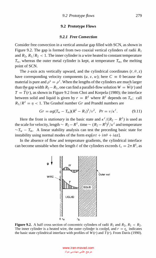
P1: GMD
CB381-09 CB381-Davis May 17, 2001 19:20 Char Count= 0
9.2 Prototype flows 279
9.2 Prototype Flows
9.2.1 Free Convection
Consider free convection in a vertical annular gap filled with SCN, as shown inFigure 9.2. The gap is formed from two coaxial vertical cylinders of radii R1
and R2, R1/R2 < 1. The inner cylinder is a wire heated to constant temperatureTw, whereas the outer metal cylinder is kept, at temperature Tm, the meltingpoint of SCN.
The z-axis acts vertically upward, and the cylindrical coordinates (r, θ, z)have corresponding velocity components (u, v, w); here C ≡ 0 because thematerial is pure and ρs = ρ�. When the lengths of the cylinders are much largerthan the gap width R2− R1, one can find a parallel-flow solution W = W (r ) andT = T (r ), as shown in Figure 9.2 from Choi and Korpela (1980); the interfacebetween solid and liquid is given by r = RI where RI depends on Tw; callR1/RI = η < 1. The Grashof number Gr and Prandtl numbers are
Gr = αg(Tw − Tm)(RI − R1)3/ν2, Pr = ν/κ�. (9.11)
Here the front is stationary in the basic state and κ�/(R2 − RI ) is used asthe scale for velocity, length ∼ R2 − RI , time ∼ (R2 − RI)2/κ� and temperature∼Tw − Tm. A linear stability analysis can test the preceding basic state forinstability using normal modes of the form exp[σ t + inθ + iaz].
In the absence of flow and temperature gradients, the cylindrical interfacecan become unstable when the length � of the cylinders exceeds �c = 2πRI, as
Figure 9.2. A half cross section of concentric cylinders of radii R1 and R2, R1 < R2.The inner cylinder is a heated wire, the outer cylinder is cooled, and r = rSL indicatesthe basic state cylindrical interface with profiles of W (r ) and T (r ). From Davis (1990).
www.iran-mavad.com مرجع علمی مھندسی مواد
P1: GMD
CB381-09 CB381-Davis May 17, 2001 19:20 Char Count= 0
280 9. Microscale fluid flow
shown by Rayleigh (1879). This capillary instability is axisymmetric, that is,n = 0, and leads to the breakup of the cylinder into “droplets.” In the presenceof the radial temperature gradient as prescribed, bulges of solid are melted backowing to the Gibbs–Thomson effect, and thus the capillary instability is delayedor entirely suppressed. Coriell and McFadden (1992, private communication)found that capillary instabilities do not occur in the range of the experimentsdescribed below.
In the absence of interfacial deformation, the parallel flow W (r ) has a pointof inflection, where d/dr
[r−1dW/dr
] = 0 at a point r = rs,which triggers aninviscid instability that is present even at finite Reynolds numbers. Furthermore,the temperature distribution T (r ) implies the presence of horizontal density gra-dients and so is susceptible to buoyancy-driven instabilities. Choi and Korpela(1980) and Shaaban and Ozisik (1982) examined the case for n = 0, whereasMcFadden et al. (1984) examined the spiral modes n = ±1.
For small Prandtl numbers, convection is weak, and the dominant insta-bility comes from the shear mode in the form of upward propagating waves(opposite in sense to the flow near the interface). For small gaps, n = 0 dom-inates, whereas for larger gaps n = ±1 does. The buoyancy-driven mode hasGrc → ∞ as Pr → ∞ and, at least for small gaps, has Grc ∼ Pr−1/2 as Pr → 0.
Now allow the interface to deform. McFadden et al. (1984) neglected surfaceenergy because the disturbance wavelengths are much larger than those, forexample, in morphological instability. They found that the ability of the interfaceto deform by melting or freezing drastically promotes the growth of the shearmodes. For example, for small gap, η = 0.02, Pr = 22.8, the thermal mode hasGrc = 2150, whereas the shear mode has Grc = 176 for n = ±1 (comparedwith 2152 without deformation). The wave propagates upward with phase speedσIa = c ≈ 7.24 × 10⁻³ in units of ν/(RI − R1), which is consistent with theidea that melting and freezing are sluggish processes. The physical mechanismfor this destabilization has not yet been explained.
Experimental observations on SCN by Glicksman and Mickalonis (1982)and Fang et al. (1985) and the preceding predictions are in close accord. Figure9.3 shows photographs of the spiral modes.
9.2.2 Benard Convection
In the preceding discussion, the phase transformation at the solid–liquid inter-face drastically promotes instability and the preferred pattern of instability isdetermined from linear stability theory. In the Benard convection problem to bediscussed now, linear theory fails to predict the pattern, and the freezing–meltingof the interface alters the pattern predicted by a weakly nonlinear theory.
www.iran-mavad.com مرجع علمی مھندسی مواد
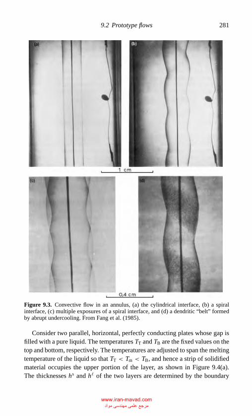
P1: GMD
CB381-09 CB381-Davis May 17, 2001 19:20 Char Count= 0
9.2 Prototype flows 281
Figure 9.3. Convective flow in an annulus, (a) the cylindrical interface, (b) a spiralinterface, (c) multiple exposures of a spiral interface, and (d) a dendritic “belt” formedby abrupt undercooling. From Fang et al. (1985).
Consider two parallel, horizontal, perfectly conducting plates whose gap isfilled with a pure liquid. The temperatures TT and TB are the fixed values on thetop and bottom, respectively. The temperatures are adjusted to span the meltingtemperature of the liquid so that TT < Tm < TB, and hence a strip of solidifiedmaterial occupies the upper portion of the layer, as shown in Figure 9.4(a).The thicknesses hs and h� of the two layers are determined by the boundary
www.iran-mavad.com مرجع علمی مھندسی مواد
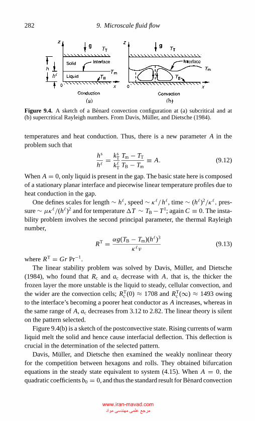
P1: GMD
CB381-09 CB381-Davis May 17, 2001 19:20 Char Count= 0
282 9. Microscale fluid flow
Figure 9.4. A sketch of a Benard convection configuration at (a) subcritical and at(b) supercritical Rayleigh numbers. From Davis, Muller, and Dietsche (1984).
temperatures and heat conduction. Thus, there is a new parameter A in theproblem such that
hs
h�= ks
T
k�T
Tm − TT
TB − Tm≡ A. (9.12)
When A = 0, only liquid is present in the gap. The basic state here is composedof a stationary planar interface and piecewise linear temperature profiles due toheat conduction in the gap.
One defines scales for length ∼ h�, speed ∼ κ�/h�, time ∼ (h�)2/κ�, pres-sure ∼ µκ�/(h�)2 and for temperature�T ∼ TB − T I; again C ≡ 0. The insta-bility problem involves the second principal parameter, the thermal Rayleighnumber,
RT = αg(TB − Tm)(h�)3
κ�ν(9.13)
where RT = Gr Pr−1.The linear stability problem was solved by Davis, Muller, and Dietsche
(1984), who found that Rc and ac decrease with A, that is, the thicker thefrozen layer the more unstable is the liquid to steady, cellular convection, andthe wider are the convection cells; RT
c (0) ≈ 1708 and RTc (∞) ≈ 1493 owing
to the interface’s becoming a poorer heat conductor as A increases, whereas inthe same range of A, ac decreases from 3.12 to 2.82. The linear theory is silenton the pattern selected.
Figure 9.4(b) is a sketch of the postconvective state. Rising currents of warmliquid melt the solid and hence cause interfacial deflection. This deflection iscrucial in the determination of the selected pattern.
Davis, Muller, and Dietsche then examined the weakly nonlinear theoryfor the competition between hexagons and rolls. They obtained bifurcationequations in the steady state equivalent to system (4.15). When A = 0, thequadratic coefficients b0 = 0, and thus the standard result for Benard convection
www.iran-mavad.com مرجع علمی مھندسی مواد
P1: GMD
CB381-09 CB381-Davis May 17, 2001 19:20 Char Count= 0
9.3 Directional solidification and volume-change convection 283
is recovered; only rolls are stable for RT > RTc , and no subcritical convection
is present (Schluter, Lortz, and Busse 1965). As A is increased, |b0| increases.This situation is analogous to the work of Davis and Segel (1968), who studiedBenard convection with an upper free surface. The surface deflections giverise to non-Boussinesq effects reflected in b0 �= 0. Now hexagons, hexagonsand rolls, and rolls are successively stable; see Section 4.1.3. This sequenceof transitions is seen in the experiment of Davis, Muller, and Dietsche (1984),as shown in Figure 9.5. For technical reasons, only qualitative comparisonsbetween theory and experiment are possible. These comparisons show that thethicker the solid, the larger the interface deflection and the more likely one isto see hexagonal states.
There is one prediction of the theory that was not verifiable in the experiment.As RT is increased, the onset of hexagons from pure conduction occurs via asubcritical bifurcation and hence a jump transition. When this occurs, the rapidrise in vertical heat transport will increase the mean height of the interface.Further, RT must be decreased below RT
c before there is a jump transitionback to pure conduction. Dietsche and Muller (1985) performed another set ofexperiments on a layer, one of whose horizontal dimensions was comparableto its gap width. Hexagons are not regular, but Dietsche and Muller observedthe hysteresis predicted and the jump-like nature of the onset of polygonalconvection. At higher RT, bimodal patterns are seen.
If the two plates of the original configuration are poor heat conductors, thepattern selection is different. Hadji, Schell, and Riahi (1990) predicted squarepatterns for small A and squares and rolls at higher A.
Many other systems involving hydrodynamic instabilities with freezing–melting boundaries exist. Zimmermann, Muller, and Davis (1992) includedSoret effects in the liquid in the Benard cell. McFadden et al. (1989) haveexamined Couette flow in which the free convection configuration discussedearlier has the inner cylinder rotating. Other examples can be found in theconference proceedings of Davis et al. (1992).
9.3 Directional Solidification and Volume-Change Convection
The interface at z = h(x, y, t) is the site of a phase transformation in which theliquid of density ρ� changes to solid of density ρs. Morphological changes aredriven by solute rejection there and, in addition, if ρ� �= ρs, the interface drives aconvective flow. For example, a dilute lead–tin alloy shrinks upon solidification,ρs/ρ� ≈ 1.05, and a weak flow from “infinity” is generated to conserve mass.On the other hand, silicon expands upon solidification, ρs/ρ� ≈ 0.91, and thegenerated flow is from the interface to “infinity.”
www.iran-mavad.com مرجع علمی مھندسی مواد
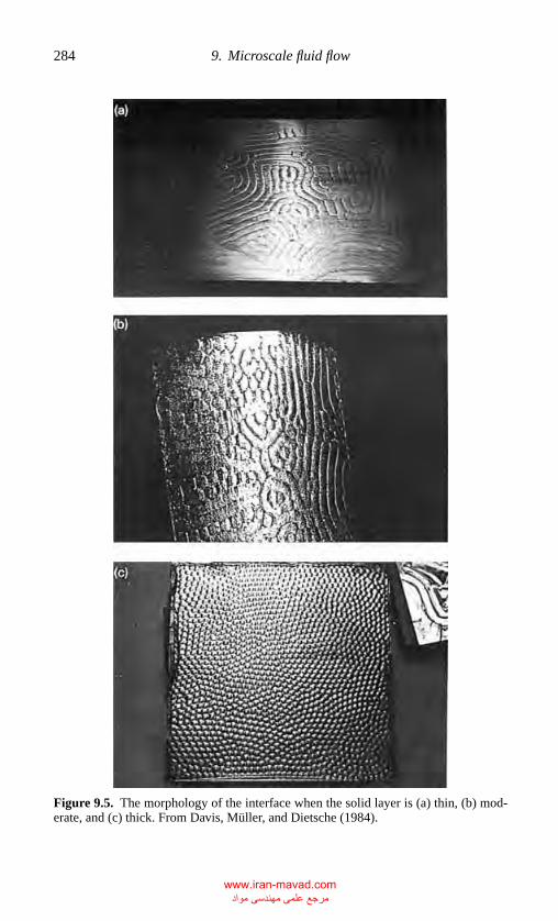
P1: GMD
CB381-09 CB381-Davis May 17, 2001 19:20 Char Count= 0
284 9. Microscale fluid flow
Figure 9.5. The morphology of the interface when the solid layer is (a) thin, (b) mod-erate, and (c) thick. From Davis, Muller, and Dietsche (1984).
www.iran-mavad.com مرجع علمی مھندسی مواد
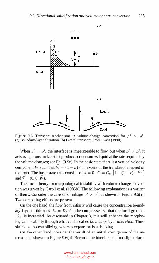
P1: GMD
CB381-09 CB381-Davis May 17, 2001 19:20 Char Count= 0
9.3 Directional solidification and volume-change convection 285
Figure 9.6. Transport mechanisms in volume-change convection for ρs > ρ�.(a) Boundary-layer alteration. (b) Lateral transport. From Davis (1990).
When ρ� = ρs, the interface is impermeable to flow, but when ρ� �= ρs, itacts as a porous surface that produces or consumes liquid at the rate required bythe volume changes; see Eq. (9.9e). In the basic state there is a vertical velocitycomponent W such that W = (1 − ρ)V in excess of the translational speed ofthe front. The basic state thus consists of h = 0, C = C∞
[1 + (1 − k)e−z/δc
]and v = (0, 0, W ).
The linear theory for morphological instability with volume change convec-tion was given by Caroli et al. (1985b). The following explanation is a variantof theirs. Consider the case of shrinkage ρs > ρ�, as shown in Figure 9.6(a).Two competing effects are present.
On the one hand, the flow from infinity will cause the concentration bound-ary layer of thickness δc = D/V to be compressed so that the local gradient|Gc| is increased. As discussed in Chapter 3, this will enhance the morpho-logical instability through what can be called boundary-layer alteration. Thus,shrinkage is destabilizing, whereas expansion is stabilizing.
On the other hand, consider the result of an initial corrugation of the in-terface, as shown in Figure 9.6(b). Because the interface is a no-slip surface,
www.iran-mavad.com مرجع علمی مھندسی مواد
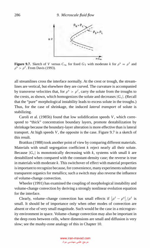
P1: GMD
CB381-09 CB381-Davis May 17, 2001 19:20 Char Count= 0
286 9. Microscale fluid flow
Figure 9.7. Sketch of V versus C∞ for fixed GT with moderate k for ρs = ρ� andρs > ρ�. From Davis (1993).
all streamlines cross the interface normally. At the crest or trough, the stream-lines are vertical, but elsewhere they are curved. The curvature is accompaniedby transverse velocities that, for ρs > ρ�, carry the solute from the troughs tothe crests, as shown, which homogenizes the solute and decreases |Gc|. (Recallthat the “pure” morphological instability leads to excess solute in the troughs.)Thus, for the case of shrinkage, the induced lateral transport of solute isstabilizing.
Caroli et al. (1985b) found that low solidification speeds V , which corre-spond to “thick” concentration boundary layers, promote destabilization byshrinkage because the boundary-layer alteration is more effective than is lateraltransport. At high speeds V , the opposite is the case. Figure 9.7 is a sketch ofthis result.
Brattkus (1988) took another point of view by comparing different materials.Materials with small segregation coefficient k reject nearly all their solute.Because |Gc| is monotonically decreasing with k, systems with small k aredestabilized when compared with the constant-density case; the reverse is truein materials with moderate k. This switchover of effect with material propertiesis important to recognize because, for convenience, many experiments substitutetransparent organics for metallics; such a switch may also reverse the influenceof volume-change convection.
Wheeler (1991) has examined the coupling of morphological instability andvolume-change convection by deriving a strongly nonlinear evolution equationfor the interface.
Clearly, volume–change convection has small effects if∣∣ρ� − ρs
∣∣ /ρ� issmall. It should be of importance only when other modes of convection areabsent or else of very small magnitude. Such would be the case in a micrograv-ity environment in space. Volume–change convection may also be important inthe deep roots between cells, where dimensions are small and diffusion is veryslow; see the mushy-zone analogy of this in Chapter 10.
www.iran-mavad.com مرجع علمی مھندسی مواد
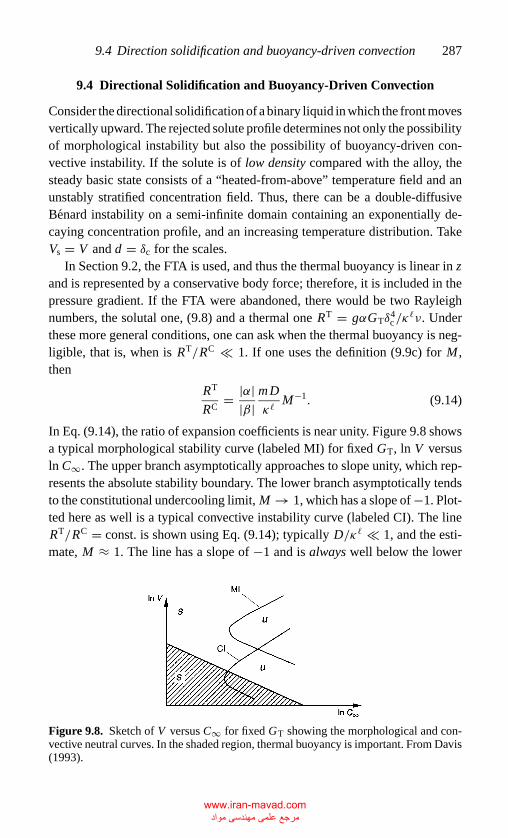
P1: GMD
CB381-09 CB381-Davis May 17, 2001 19:20 Char Count= 0
9.4 Direction solidification and buoyancy-driven convection 287
9.4 Directional Solidification and Buoyancy-Driven Convection
Consider the directional solidification of a binary liquid in which the front movesvertically upward. The rejected solute profile determines not only the possibilityof morphological instability but also the possibility of buoyancy-driven con-vective instability. If the solute is of low density compared with the alloy, thesteady basic state consists of a “heated-from-above” temperature field and anunstably stratified concentration field. Thus, there can be a double-diffusiveBenard instability on a semi-infinite domain containing an exponentially de-caying concentration profile, and an increasing temperature distribution. TakeVs = V and d = δc for the scales.
In Section 9.2, the FTA is used, and thus the thermal buoyancy is linear in zand is represented by a conservative body force; therefore, it is included in thepressure gradient. If the FTA were abandoned, there would be two Rayleighnumbers, the solutal one, (9.8) and a thermal one RT = gαGTδ
4c/κ
�ν. Underthese more general conditions, one can ask when the thermal buoyancy is neg-ligible, that is, when is RT/RC 1. If one uses the definition (9.9c) for M ,then
RT
RC= |α|
|β|mD
κ�M−1. (9.14)
In Eq. (9.14), the ratio of expansion coefficients is near unity. Figure 9.8 showsa typical morphological stability curve (labeled MI) for fixed GT, ln V versusln C∞. The upper branch asymptotically approaches to slope unity, which rep-resents the absolute stability boundary. The lower branch asymptotically tendsto the constitutional undercooling limit, M → 1, which has a slope of −1. Plot-ted here as well is a typical convective instability curve (labeled CI). The lineRT/RC = const. is shown using Eq. (9.14); typically D/κ� 1, and the esti-mate, M ≈ 1. The line has a slope of −1 and is always well below the lower
Figure 9.8. Sketch of V versus C∞ for fixed GT showing the morphological and con-vective neutral curves. In the shaded region, thermal buoyancy is important. From Davis(1993).
www.iran-mavad.com مرجع علمی مھندسی مواد
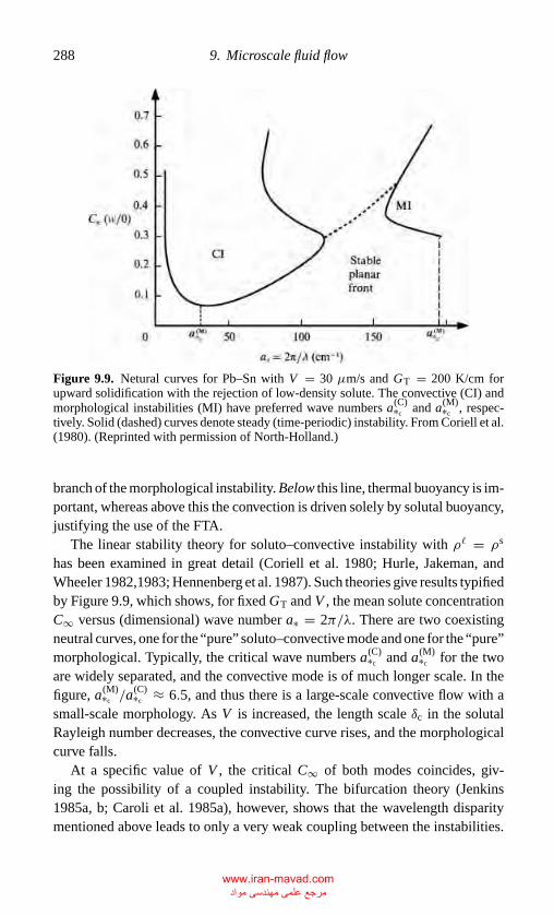
P1: GMD
CB381-09 CB381-Davis May 17, 2001 19:20 Char Count= 0
288 9. Microscale fluid flow
Figure 9.9. Netural curves for Pb–Sn with V = 30 µm/s and GT = 200 K/cm forupward solidification with the rejection of low-density solute. The convective (CI) andmorphological instabilities (MI) have preferred wave numbers a(C)
∗c and a(M)∗c , respec-
tively. Solid (dashed) curves denote steady (time-periodic) instability. From Coriell et al.(1980). (Reprinted with permission of North-Holland.)
branch of the morphological instability. Below this line, thermal buoyancy is im-portant, whereas above this the convection is driven solely by solutal buoyancy,justifying the use of the FTA.
The linear stability theory for soluto–convective instability with ρ� = ρs
has been examined in great detail (Coriell et al. 1980; Hurle, Jakeman, andWheeler 1982,1983; Hennenberg et al. 1987). Such theories give results typifiedby Figure 9.9, which shows, for fixed GT and V , the mean solute concentrationC∞ versus (dimensional) wave number a∗ = 2π/λ. There are two coexistingneutral curves, one for the “pure” soluto–convective mode and one for the “pure”morphological. Typically, the critical wave numbers a(C)
∗c and a(M)∗c for the two
are widely separated, and the convective mode is of much longer scale. In thefigure, a(M)
∗c /a(C)∗c ≈ 6.5, and thus there is a large-scale convective flow with a
small-scale morphology. As V is increased, the length scale δc in the solutalRayleigh number decreases, the convective curve rises, and the morphologicalcurve falls.
At a specific value of V , the critical C∞ of both modes coincides, giv-ing the possibility of a coupled instability. The bifurcation theory (Jenkins1985a, b; Caroli et al. 1985a), however, shows that the wavelength disparitymentioned above leads to only a very weak coupling between the instabilities.
www.iran-mavad.com مرجع علمی مھندسی مواد
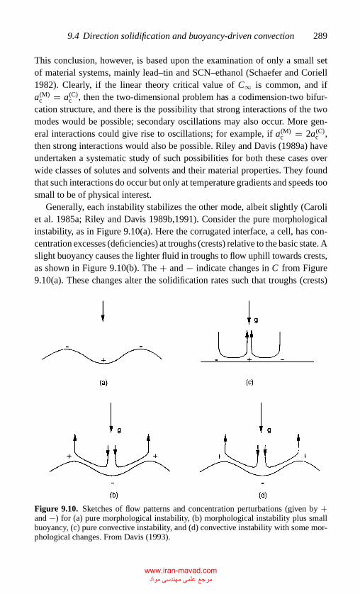
P1: GMD
CB381-09 CB381-Davis May 17, 2001 19:20 Char Count= 0
9.4 Direction solidification and buoyancy-driven convection 289
This conclusion, however, is based upon the examination of only a small setof material systems, mainly lead–tin and SCN–ethanol (Schaefer and Coriell1982). Clearly, if the linear theory critical value of C∞ is common, and ifa(M)
c = a(C)c , then the two-dimensional problem has a codimension-two bifur-
cation structure, and there is the possibility that strong interactions of the twomodes would be possible; secondary oscillations may also occur. More gen-eral interactions could give rise to oscillations; for example, if a(M)
c = 2a(C)c ,
then strong interactions would also be possible. Riley and Davis (1989a) haveundertaken a systematic study of such possibilities for both these cases overwide classes of solutes and solvents and their material properties. They foundthat such interactions do occur but only at temperature gradients and speeds toosmall to be of physical interest.
Generally, each instability stabilizes the other mode, albeit slightly (Caroliet al. 1985a; Riley and Davis 1989b,1991). Consider the pure morphologicalinstability, as in Figure 9.10(a). Here the corrugated interface, a cell, has con-centration excesses (deficiencies) at troughs (crests) relative to the basic state. Aslight buoyancy causes the lighter fluid in troughs to flow uphill towards crests,as shown in Figure 9.10(b). The + and − indicate changes in C from Figure9.10(a). These changes alter the solidification rates such that troughs (crests)
Figure 9.10. Sketches of flow patterns and concentration perturbations (given by +and −) for (a) pure morphological instability, (b) morphological instability plus smallbuoyancy, (c) pure convective instability, and (d) convective instability with some mor-phological changes. From Davis (1993).
www.iran-mavad.com مرجع علمی مھندسی مواد
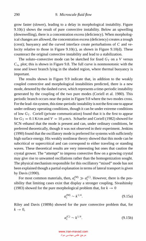
P1: GMD
CB381-09 CB381-Davis May 17, 2001 19:20 Char Count= 0
290 9. Microscale fluid flow
grow faster (slower), leading to a delay in morphological instability. Figure9.10(c) shows the result of pure convective instability. Below an upwelling(downwelling), there is a concentration excess (deficiency). When morpholog-ical changes are allowed, the concentration excess (deficiency) creates a trough(crest); buoyancy and the curved interface create perturbations of C and ve-locity relative to those in Figure 9.10(c), as shown in Figure 9.10(d). Thesecounteract the original convective instability and lead to a stabilization.
The soluto–convective mode can be sketched for fixed GT on a V versusC∞ plot; this is shown in Figure 9.8. The full curve is nonmonotonic with thenose and lower branch lying in the shaded region, where thermal buoyancy isimportant.
The results shown in Figure 9.9 indicate that, in addition to the weaklycoupled convective and morphological instabilities predicted, there is a newmode, denoted by the dashed curve, which represents a time-periodic instabilitygenerated by the coupling of the two pure modes (Coriell et al. 1980). Thisperiodic branch occurs near the point in Figure 9.8 where the two modes cross.For the lead–tin system, this time-periodic instability is not the first one to appearunder ordinary operating conditions, though it can be under extreme conditionsof low GT. Coriell (private communication) found that it is the first to appearfor GT = 0.1 K/cm and V = 10µm/s. Schaefer and Coriell (1982) showed forSCN–ethanol that the mode is present and can, under ordinary conditions, bepreferred theoretically, though it was not observed in their experiment. Jenkins(1990) found that the oscillatory mode is preferred for systems with sufficientlyhigh surface energy. His weakly nonlinear theory showed that this mode can besubcritical or supercritical and can correspond to either traveling or standingwaves. These theoretical results are very interesting but ones that caution thecrystal grower. The “attempt” to impress convective flow on a growing crystalmay give rise to unwanted oscillations rather than the homogenization sought.The physical mechanism responsible for this oscillatory “mixed” mode has notbeen explained though a partial explanation in terms of lateral transport is givenby Davis (1990).
For most common materials, then, a(M)c � a(C)
c . However, there is the pos-sibility that limiting cases exist that display a stronger coupling. Sivashinsky(1983) showed for the pure morphological problem that, for k → 0
a(M)c ∼ k1/4. (9.15a)
Riley and Davis (1989b) showed for the pure convective problem that, fork → 0,
a(C)c ∼ k1/4. (9.15b)
www.iran-mavad.com مرجع علمی مھندسی مواد
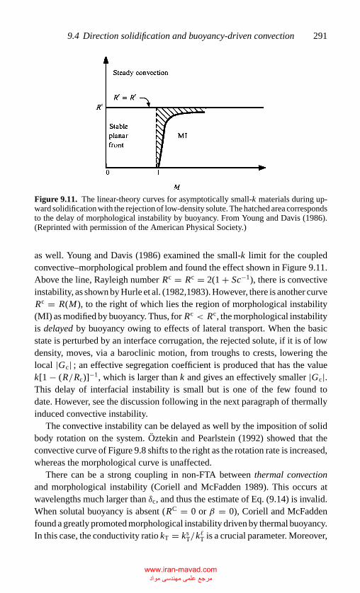
P1: GMD
CB381-09 CB381-Davis May 17, 2001 19:20 Char Count= 0
9.4 Direction solidification and buoyancy-driven convection 291
Figure 9.11. The linear-theory curves for asymptotically small-k materials during up-ward solidification with the rejection of low-density solute. The hatched area correspondsto the delay of morphological instability by buoyancy. From Young and Davis (1986).(Reprinted with permission of the American Physical Society.)
as well. Young and Davis (1986) examined the small-k limit for the coupledconvective–morphological problem and found the effect shown in Figure 9.11.Above the line, Rayleigh number Rc = Rc = 2(1 + Sc−1), there is convectiveinstability, as shown by Hurle et al. (1982,1983). However, there is another curveRc = R(M), to the right of which lies the region of morphological instability(MI) as modified by buoyancy. Thus, for Rc < Rc, the morphological instabilityis delayed by buoyancy owing to effects of lateral transport. When the basicstate is perturbed by an interface corrugation, the rejected solute, if it is of lowdensity, moves, via a baroclinic motion, from troughs to crests, lowering thelocal |Gc| ; an effective segregation coefficient is produced that has the valuek[1 − (R/Rc)]−1, which is larger than k and gives an effectively smaller |Gc|.This delay of interfacial instability is small but is one of the few found todate. However, see the discussion following in the next paragraph of thermallyinduced convective instability.
The convective instability can be delayed as well by the imposition of solidbody rotation on the system. Oztekin and Pearlstein (1992) showed that theconvective curve of Figure 9.8 shifts to the right as the rotation rate is increased,whereas the morphological curve is unaffected.
There can be a strong coupling in non-FTA between thermal convectionand morphological instability (Coriell and McFadden 1989). This occurs atwavelengths much larger than δc, and thus the estimate of Eq. (9.14) is invalid.When solutal buoyancy is absent (RC = 0 or β = 0), Coriell and McFaddenfound a greatly promoted morphological instability driven by thermal buoyancy.In this case, the conductivity ratio kT = ks
T/k�T is a crucial parameter. Moreover,
www.iran-mavad.com مرجع علمی مھندسی مواد
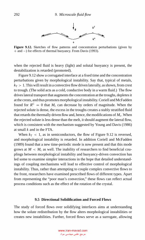
P1: GMD
CB381-09 CB381-Davis May 17, 2001 19:20 Char Count= 0
292 9. Microscale fluid flow
Figure 9.12. Sketches of flow patterns and concentration perturbations (given by+ and −) for effects of thermal buoyancy. From Davis (1993).
when the rejected fluid is heavy (light) and solutal buoyancy is present, thedestabilization is retarded (promoted).
Figure 9.12 show a corrugated interface at a fixed time and the concentrationperturbations given by morphological instability. Say that, typical of metals,kT > 1. This will result in a convective flow driven laterally, as shown, from crestto trough. (The solid acts as a cold, conductive body in a warm fluid.) The flowdrives lateral transport that augments the concentration at the troughs, depletes itat the crests, and thus promotes morphological instability. Coriell and McFaddenfound for RC = 0 that Mc can decrease by orders of magnitude. When therejected solute is dense, the excess in the troughs creates a stably stratified fluidthat retards the thermally driven flow and, hence, the modifications of Mc. Whenthe rejected solute is less dense than the melt, it should augment the lateral flow,which is consistent with the mechanism suggested by Young and Davis (1986)at small k and in the FTA.
When kT < 1, as in semiconductors, the flow of Figure 9.12 is reversed,and morphological instability is retarded. In addition Coriell and McFadden(1989) found that a new time-periodic mode is now present and that this modegrows at M < Mc as well. The inability of researchers to find beneficial cou-plings between morphological instability and buoyancy-driven convection hasled some to examine simpler interactions in the hope that detailed understand-ings of coupling mechanisms will lead to effective control of morphologicalinstability. Thus, rather than attempting to couple complex convective flows tothe front, researchers have examined prescribed flows of different types. Apartfrom representing the “poor man’s convection,” these flows can reflect actualprocess conditions such as the effect of the rotation of the crystal.
9.5 Directional Solidification and Forced Flows
The study of forced flows over solidifying interfaces aims at understandinghow the solute redistribution by the flow alters morphological instabilities orcreates new instabilities. Further, forced flows serve as a surrogate, allowing
www.iran-mavad.com مرجع علمی مھندسی مواد
P1: GMD
CB381-09 CB381-Davis May 17, 2001 19:20 Char Count= 0
9.5 Directional solidification and forced flows 293
one to isolate certain effects of convection in the melt and to focus on one-waycouplings.
The first studies of forced flows were those of Delves (1968,1971), whoimposed a Blasius boundary layer on the interface, but, by examining wave-lengths that were short compared with the spreading length of the boundarylayer, he really focused on locally parallel flow. Arguments of local parallelismled Coriell et al. (1984) to impose plane Couette flow upon the interface.
If one pictures an constant imposed flow across an interface at “infinity”and allows the solidification to proceed, the forced flow has the asymptoticsuction profile, a boundary-layer flow on the scale δv, the viscous boundarylayer thickness,
δv = ν/V . (9.16)
The velocity component along the interface has the form of the asymptoticsuction profile, u ∝ 1 − e−z/δ, which couples with morphological instability(Forth and Wheeler 1989). Given that the concentration and thermal boundarylayers scale on δc and δT, three lengths are involved in such problems.
In the case of an organic alloy,
δc δT δv (9.17a)
because δv/δT = Pr, and Pr is large. However, for a small-Prandtl-numbermetallic alloy,
δc δv δT. (9.17b)
These inequalities are relevant when one considers disturbances of variouswavelengths λ. The “normal” situation described has λ < δc and thus thethermal field and the velocity field can be represented in locally linear form by
T = T0 + GTz (9.18a)
and
u ∼ V
νz, (9.18b)
the latter being the plane Couette flow considered by Coriell et al. (1984).However, when λ becomes large enough, these localizations are no longer validbecause the disturbances are affected by the curvatures of the profiles. Thedistance L+ from the interface to the upper heat source can then be a relevantlength scale as well.
Coriell et al. (1984) examined two-dimensional disturbances (periodic inthe flow direction) and found that the flow stabilizes the interface because thepresence of the flow increases Mc. However, if one considers longitudinal-roll
www.iran-mavad.com مرجع علمی مھندسی مواد
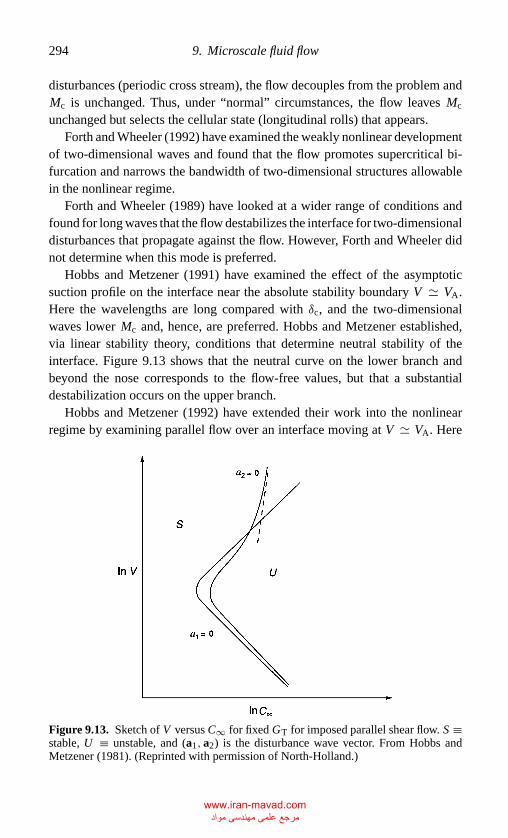
P1: GMD
CB381-09 CB381-Davis May 17, 2001 19:20 Char Count= 0
294 9. Microscale fluid flow
disturbances (periodic cross stream), the flow decouples from the problem andMc is unchanged. Thus, under “normal” circumstances, the flow leaves Mc
unchanged but selects the cellular state (longitudinal rolls) that appears.Forth and Wheeler (1992) have examined the weakly nonlinear development
of two-dimensional waves and found that the flow promotes supercritical bi-furcation and narrows the bandwidth of two-dimensional structures allowablein the nonlinear regime.
Forth and Wheeler (1989) have looked at a wider range of conditions andfound for long waves that the flow destabilizes the interface for two-dimensionaldisturbances that propagate against the flow. However, Forth and Wheeler didnot determine when this mode is preferred.
Hobbs and Metzener (1991) have examined the effect of the asymptoticsuction profile on the interface near the absolute stability boundary V � VA.Here the wavelengths are long compared with δc, and the two-dimensionalwaves lower Mc and, hence, are preferred. Hobbs and Metzener established,via linear stability theory, conditions that determine neutral stability of theinterface. Figure 9.13 shows that the neutral curve on the lower branch andbeyond the nose corresponds to the flow-free values, but that a substantialdestabilization occurs on the upper branch.
Hobbs and Metzener (1992) have extended their work into the nonlinearregime by examining parallel flow over an interface moving at V � VA. Here
Figure 9.13. Sketch of V versus C∞ for fixed GT for imposed parallel shear flow. S ≡stable, U ≡ unstable, and (a1, a2) is the disturbance wave vector. From Hobbs andMetzener (1981). (Reprinted with permission of North-Holland.)
www.iran-mavad.com مرجع علمی مھندسی مواد
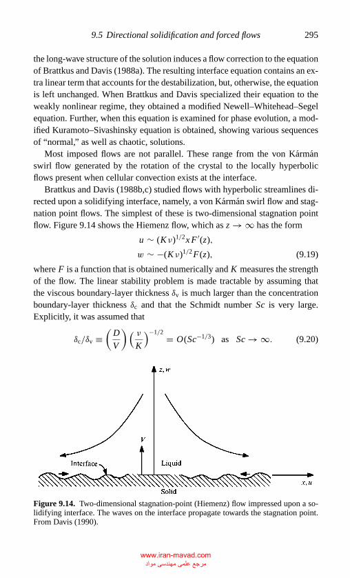
P1: GMD
CB381-09 CB381-Davis May 17, 2001 19:20 Char Count= 0
9.5 Directional solidification and forced flows 295
the long-wave structure of the solution induces a flow correction to the equationof Brattkus and Davis (1988a). The resulting interface equation contains an ex-tra linear term that accounts for the destabilization, but, otherwise, the equationis left unchanged. When Brattkus and Davis specialized their equation to theweakly nonlinear regime, they obtained a modified Newell–Whitehead–Segelequation. Further, when this equation is examined for phase evolution, a mod-ified Kuramoto–Sivashinsky equation is obtained, showing various sequencesof “normal,” as well as chaotic, solutions.
Most imposed flows are not parallel. These range from the von Karmanswirl flow generated by the rotation of the crystal to the locally hyperbolicflows present when cellular convection exists at the interface.
Brattkus and Davis (1988b,c) studied flows with hyperbolic streamlines di-rected upon a solidifying interface, namely, a von Karman swirl flow and stag-nation point flows. The simplest of these is two-dimensional stagnation pointflow. Figure 9.14 shows the Hiemenz flow, which as z → ∞ has the form
u ∼ (Kν)1/2x F ′(z),
w ∼ −(Kν)1/2 F(z), (9.19)
where F is a function that is obtained numerically and K measures the strengthof the flow. The linear stability problem is made tractable by assuming thatthe viscous boundary-layer thickness δv is much larger than the concentrationboundary-layer thickness δc and that the Schmidt number Sc is very large.Explicitly, it was assumed that
δc/δv ≡(
D
V
)( νK
)−1/2= O(Sc−1/3) as Sc → ∞. (9.20)
Figure 9.14. Two-dimensional stagnation-point (Hiemenz) flow impressed upon a so-lidifying interface. The waves on the interface propagate towards the stagnation point.From Davis (1990).
www.iran-mavad.com مرجع علمی مھندسی مواد
P1: GMD
CB381-09 CB381-Davis May 17, 2001 19:20 Char Count= 0
296 9. Microscale fluid flow
Note that the δv here, is distinct from that in Eq. (9.16). Given the smallness ofδc, the interface senses only the local forms of the imposed flow, and the flowsenses a flat interface; thus,
u ∼ βxζ, w ∼ −1
2βζ 2, (9.21)
where ζ = z/δc, and β measures F ′′(0), the local shear. Finally, Brattkus andDavis considered waves long compared with δc though smaller than δv. Theysolved the modified diffusion problem
Cζ ζ +(
1 + 1
2βζ 2
)Cζ − βxζCx = Cτ , 0 ζ < ∞,
Cζ + (1 − M−1)−1
Cτ + [k(1 − M−1)−1 + (1 − k)]
C = 0, ζ = 0,
C(∞) = 0,(9.22)
where τ is a scaled (slow) time. Note that the longwave approximation leadsto the neglect of the lateral diffusion term Cxx . This neglect is justified onlyfar away from the stagnation point at x = 0 but makes the solution of thelinear-stability problem (9.22) tractable.
The nonparallel flow gives rise to the term xCx , which is scale invariant andthus survives the longwave approximation. The system (9.22) can be solved byemploying quasi-normal modes as follows:
C(x, ζ, τ ) = eστ+ia ln x C(ζ ), (9.23)
which converts system (9.22) into a constant-coefficient eigenvalue problemfor growth rate σ = σ (k; M ; a). The system is solved numerically, and Figure9.15 shows the neutral curves.
The flow produces a longwave instability that creates waves that travel inwardtoward the stagnation point, as shown in Figure 9.14. The flow is locally periodicin x but by the structure of the normal modes is not globally so. The instabilityexists for long waves in a region where the Mullins and Sekerka conditiongives only stability. Thus, it is called flow-induced morphological instability.The largest growth rate Reσ occurs for a → ∞, where the longwave theory isinvalid and surface energy should help stabilize the interface. Thus, “longish”waves would be preferred, and these would grow for M just above unity, thatis, for any degree of constitutional undercooling; thus, it is a morphologicalinstability. The neutral stability curve, sketched for all wave numbers, would beas shown in Figure 9.16. When the wave numbers are large, the disturbances seeonly the local velocities, and the flow appears to be locally parallel. The dashedcurve of Figure 9.16 shows the analog of the results of Coriell et al. (1984)
www.iran-mavad.com مرجع علمی مھندسی مواد
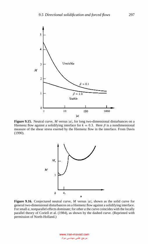
P1: GMD
CB381-09 CB381-Davis May 17, 2001 19:20 Char Count= 0
9.5 Directional solidification and forced flows 297
Figure 9.15. Neutral curve, M versus |a|, for long two-dimensional disturbances on aHiemenz flow against a solidifying interface for k = 0.3. Here β is a nondimensionalmeasure of the shear stress exerted by the Hiemenz flow in the interface. From Davis(1990).
Figure 9.16. Conjectured neutral curve, M versus |a|, shown as the solid curve forgeneral two-dimensional disturbances on a Hiemenz flow against a solidifying interface.For small a, nonparallel effects dominate; for other a the curve coincides with the locallyparallel theory of Coriell et al. (1984), as shown by the dashed curve. (Reprinted withpermission of North-Holland.)
www.iran-mavad.com مرجع علمی مھندسی مواد
P1: GMD
CB381-09 CB381-Davis May 17, 2001 19:20 Char Count= 0
298 9. Microscale fluid flow
appropriate to locally parallel flows. When the wave numbers are small, thedisturbances see the curvature of the streamlines and, hence, the nonparallel floweffects, as shown in the solid curve of Figure 9.16. The connection between thesmall-|a| loop and the ordinary morphological instability loop is conjectured.
The destabilization by nonparallel flow depends on both velocity compo-nents. The component normal to the mean position of the interface is di-rected inward. Its presence causes boundary-layer alteration. The concentrationboundary layer is compressed, steepening the local gradient |Gc|. The lateralcomponent of velocity (linear in x) varies with distance from the stagnationpoint and produces horizontal concentration gradients that drive the travelingcells propagating into the oncoming flow.
The destabilization of long waves in the x-direction may be negated by “end”effects that disallow the “fitting” of such waves in the system. In this case, theresults of McFadden, Coriell, and Alexander (1988) would be regained. Onecould then allow disturbances of the form
C(y, z, t) = eσ t+ibyC(z) (9.24)
for cross-stream periodic waves that are x-independent (a = 0). The fullstagnation-point flow linear stability problem has been examined in this caseby McFadden et al. (1988). They found in this case that the flow would slightlydelay morphological instability.
The effects of unsteadiness in the melt flow have been investigated byMerchant and Davis (1989). They considered plane stagnation-point flowagainst the interface but allowed the flow at infinity to be time periodic, wherethe strength K of the flow in Eq. (9.21) is replaced by a time-periodic functionas follows:
K → K�(ωt) = K [1 + δ cosωt]. (9.25)
Merchant and Davis again considered longwave, two-dimensional disturbancesand found that system (9.22) is replaced by the following:
Cζ ζ +[1 + 1
2β�3/2(τ )ζ 2
]Cζ − β�3/2(τ )xζCx = Ct ,
Cζ + (1 − M−1)−1Ct + [k(1 − M−1)−1 + (1 − k)]C = 0, ζ = 0,
C(∞) = 0, (9.26)
where = ωD/V 2 is the scaled forcing frequency. They found that modulationat low frequency stabilizes the interface against flow-induced morphologicalinstabilities, whereas high frequency promotes the instabilities. The response
www.iran-mavad.com مرجع علمی مھندسی مواد
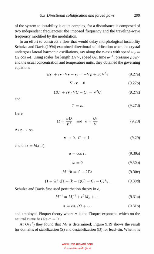
P1: GMD
CB381-09 CB381-Davis May 17, 2001 19:20 Char Count= 0
9.5 Directional solidification and forced flows 299
of the system to instability is quite complex, for a disturbance is composed oftwo independent frequencies: the imposed frequency and the traveling-wavefrequency modified by the modulation.
In an effort to construct a flow that would delay morphological instabilitySchulze and Davis (1994) examined directional solidification when the crystalundergoes lateral harmonic oscillations, say along the x-axis with speed uw =U0 cos ωt . Using scales for length D/V , speed U0, time ω−1, pressure ρU0Vand the usual concentration and temperature units, they obtained the governingequations
vt + εv · ∇v − vz = −∇ p + Sc∇2v (9.27a)
∇ · v = 0 (9.27b)
Ct + εv · ∇C − Cz = ∇2C (9.27c)
and
T = z. (9.27d)
Here,
= ωD
V 2and ε = U0
V(9.28)
As z → ∞v → 0, C → 1, (9.29)
and on z = h(x, t)
u = cos t, (9.30a)
w = 0 (9.30b)
M−1h = C + 2�h (9.30c)
(1 + ht )[1 + (k − 1)C] = Cz − Cxhx . (9.30d)
Schulze and Davis first used perturbation theory in ε,
M−1 = M−1c + ε2M2 + · · · (9.31a)
σ = εσ1/ + · · · (9.31b)
and employed Floquet theory where σ is the Floquet exponent, which on theneutral curve has Re σ = 0.
At O(ε2) they found that M2 is determined; Figure 9.19 shows the resultfor domains of stabilization (S) and destabilization (D) for lead–tin. When ε is
www.iran-mavad.com مرجع علمی مھندسی مواد
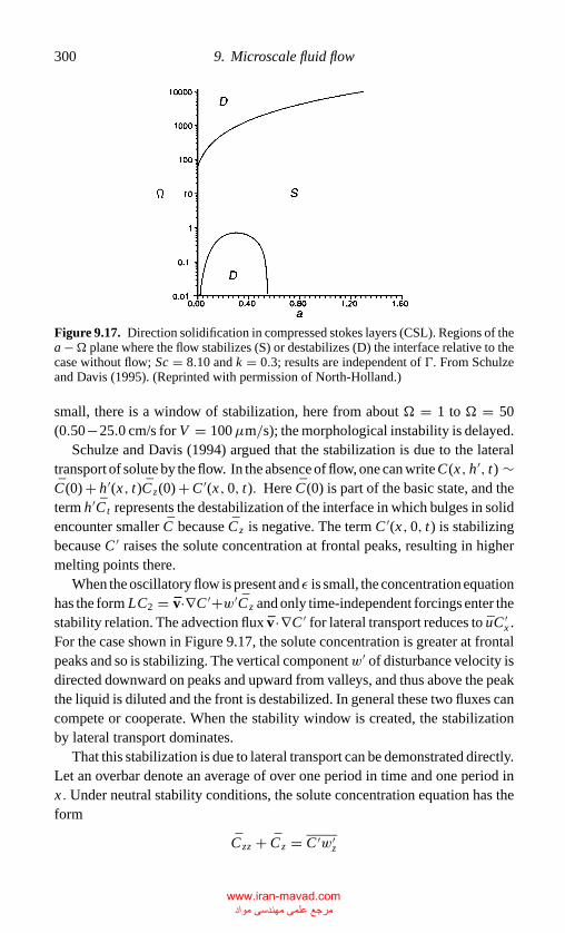
P1: GMD
CB381-09 CB381-Davis May 17, 2001 19:20 Char Count= 0
300 9. Microscale fluid flow
Figure 9.17. Direction solidification in compressed stokes layers (CSL). Regions of thea − plane where the flow stabilizes (S) or destabilizes (D) the interface relative to thecase without flow; Sc = 8.10 and k = 0.3; results are independent of �. From Schulzeand Davis (1995). (Reprinted with permission of North-Holland.)
small, there is a window of stabilization, here from about = 1 to = 50(0.50−25.0 cm/s for V = 100µm/s); the morphological instability is delayed.
Schulze and Davis (1994) argued that the stabilization is due to the lateraltransport of solute by the flow. In the absence of flow, one can write C(x, h′, t) ∼C(0) + h′(x, t)C z(0) + C ′(x, 0, t). Here C(0) is part of the basic state, and theterm h′C t represents the destabilization of the interface in which bulges in solidencounter smaller C because C z is negative. The term C ′(x, 0, t) is stabilizingbecause C ′ raises the solute concentration at frontal peaks, resulting in highermelting points there.
When the oscillatory flow is present and ε is small, the concentration equationhas the form LC2 = v·∇C ′+w′C z and only time-independent forcings enter thestability relation. The advection flux v ·∇C ′ for lateral transport reduces to uC ′
x .For the case shown in Figure 9.17, the solute concentration is greater at frontalpeaks and so is stabilizing. The vertical componentw′ of disturbance velocity isdirected downward on peaks and upward from valleys, and thus above the peakthe liquid is diluted and the front is destabilized. In general these two fluxes cancompete or cooperate. When the stability window is created, the stabilizationby lateral transport dominates.
That this stabilization is due to lateral transport can be demonstrated directly.Let an overbar denote an average of over one period in time and one period inx . Under neutral stability conditions, the solute concentration equation has theform
C zz + C z = C ′w′z
www.iran-mavad.com مرجع علمی مھندسی مواد
P1: GMD
CB381-09 CB381-Davis May 17, 2001 19:20 Char Count= 0
9.5 Directional solidification and forced flows 301
If one substitutes the calculated C ′ and w subject to C = 0 at z = 0 and ∞,one finds that the local gradient at the front C z
∣∣0 actually steepens because of
the flow – even when stabilization is obtained.The modulation of the crystal, as described, creates a window of stability
for small ε and two-dimensional disturbances. However, if three-dimensionaldisturbances were allowed, as before, longitudinal rolls would be unaffected bythe flow and hence preferred.
In the three-dimensional case, in order to obtain stabilization one must “con-fuse” the system so that longitudinal rolls cannot be defined. This can be doneby following a suggestion of Kelly and Hu (1993), who considered nonpla-nar modulations in Benard convection and succeeded in delaying the onset ofconvection. One thus imposes velocities on the crystal, relative to the liquid atinfinity, in two orthogonal components, namely,
uW = U0 cos ωt, vW = βU0 cos(ωt − δ). (9.32)
Schulze and Davis (1994) examined the linearized system for small ε and foundthat the modification M2 to the critical morphological number has the form
M2 = [(cos θ + β cos δ sin θ )2 + β2 sin2 θ sin2 δ]
M2D2 , (9.33)
where M2D2 is that obtained earlier (see Figure 9.17), and θ = tan−1(a2/a1) is
the angle of the disturbance wave vector with the x-axis. This 2D→3D relationhas the same form as that found by Kelly and Hu in the Benard problem. Therange of stabilization shown in Figure 9.17 for the two-dimensional case nowapplies to the three-dimensional case as long as δ is not an integral multiple ofπ . The maximal stabilization occurs when δ = π/2, and if β is unity, the crystalis translating on circular orbits and no preferred direction is distinguished forthe cellular morphology.
Schulze and Davis (1995) then examined the linearized stability for arbitraryε by representing the eigenfunctions as (C ′, w′) =∑∞
m=−∞[Cm(z), wm(z)]eimt
times a Floquet multiplier.Figure 9.18 shows M−1 versus ε for a = ac(no flow) in the case of lead–tin.
In the window of stability, as ε increases, M−1c decreases through zero, which
corresponds to complete stabilization. Note that if ε is increased even further,the tendency to stabilization can be reversed. Figure 9.19 shows the stabilityboundary in the M−1 versus� plane for fixed k and . Notice that the intercept at(0,1) never changes but that there is a substantial stabilization near the absolutestability limit. Figure 9.20 shows the same information in physical coordinates.The stabilization is substantial near the nose of the curve and near the absolutestability boundary. Table 9.1 shows the values calculated for top and bottom
www.iran-mavad.com مرجع علمی مھندسی مواد
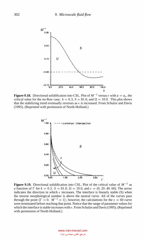
P1: GMD
CB381-09 CB381-Davis May 17, 2001 19:20 Char Count= 0
302 9. Microscale fluid flow
Figure 9.18. Directional solidification into CSL. Plot of M−1 versus ε with a = ac, thecritical value for the no-flow case; k = 0.3, S = 81.0, and = 10.0. This plot showsthat the stabilizing trend eventually reverses as ε is increased. From Schulze and Davis(1995). (Reprinted with permission of North-Holland.)
Figure 9.19. Directional solidification into CSL. Plot of the critical value of M−1 asa function of � for k = 0.3, S = 81.0, = 10.0, and ε = (0, 20, 40, 60). The arrowindicates the direction in which ε increases. The interface is linearly stable (S) whenthe inverse morphological number is above the neutral curve. All of the curves passthrough the point
(� = 0, M−1 = 1
); however, the calculations for the ε = 60 curve
were terminated before reaching that point. Notice that the range of parameter values forwhich the interface is stable increases with ε. From Schulze and Davis (1995). (Reprintedwith permission of North-Holland.)
www.iran-mavad.com مرجع علمی مھندسی مواد
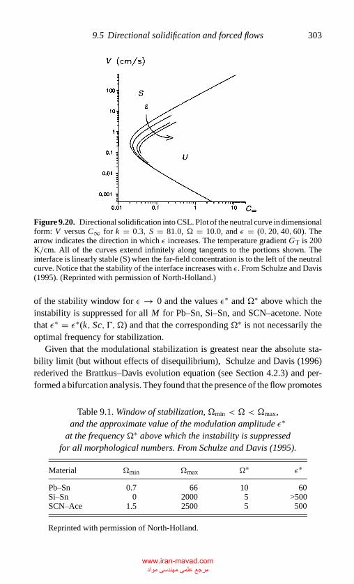
P1: GMD
CB381-09 CB381-Davis May 17, 2001 19:20 Char Count= 0
9.5 Directional solidification and forced flows 303
Figure 9.20. Directional solidification into CSL. Plot of the neutral curve in dimensionalform: V versus C∞ for k = 0.3, S = 81.0, = 10.0, and ε = (0, 20, 40, 60). Thearrow indicates the direction in which ε increases. The temperature gradient GT is 200K/cm. All of the curves extend infinitely along tangents to the portions shown. Theinterface is linearly stable (S) when the far-field concentration is to the left of the neutralcurve. Notice that the stability of the interface increases with ε. From Schulze and Davis(1995). (Reprinted with permission of North-Holland.)
of the stability window for ε → 0 and the values ε∗ and ∗ above which theinstability is suppressed for all M for Pb–Sn, Si–Sn, and SCN–acetone. Notethat ε∗ = ε∗(k, Sc, �, ) and that the corresponding ∗ is not necessarily theoptimal frequency for stabilization.
Given that the modulational stabilization is greatest near the absolute sta-bility limit (but without effects of disequilibrium), Schulze and Davis (1996)rederived the Brattkus–Davis evolution equation (see Section 4.2.3) and per-formed a bifurcation analysis. They found that the presence of the flow promotes
Table 9.1. Window of stabilization, min < < max,and the approximate value of the modulation amplitude ε∗
at the frequency ∗ above which the instability is suppressedfor all morphological numbers. From Schulze and Davis (1995).
Material min max ∗ ε∗
Pb–Sn 0.7 66 10 60Si–Sn 0 2000 5 >500SCN–Ace 1.5 2500 5 500
Reprinted with permission of North-Holland.
www.iran-mavad.com مرجع علمی مھندسی مواد
P1: GMD
CB381-09 CB381-Davis May 17, 2001 19:20 Char Count= 0
304 9. Microscale fluid flow
subcritical instability. Hence, a portion of the predicted stabilization may be lostat finite amplitude.
These analyses in some sense validate the comment made by Delves (1971),who considered steady flow over a crystal that “it might be possible to ensurecomplete stability of the interface by rapid and continuous changes in the flowpattern.”
9.6 Directional Solidification with Imposed Cellular Convection
The interaction of simultaneous instabilities discussed in Section 9.4, validnear the codimension-two point, the intersection point of the two neutral curvesof Figure 9.8, yielded only small mutual stabilizations of the morphologicaland convective instabilities. This smallness is due to the disparity of the criticalwave numbers; see Figure 9.9. The common situation in crystal growth involvessystems, shown in Figure 9.8, in which one operates at values of C∞ well to theright of the intersection of the two neutral curves. In such cases, as V is increasedfrom zero, there is first a convective instability whose convective amplitudesincrease to well-developed cellular convection. It is in this convective region thatthe neutral curve for morphological instability lies. Thus, the normal situationhas the onset of morphological instability occurring in the presence of a pre-existing long-scale convective field.
One can “manufacture” a convective field from the Boussinesq equationswith the solutal buoyancy removed and replaced by a “fictitious” body forcethat generates the convection. Given this convection, one can then determinethe interfacial response by analyzing the convection–diffusion equation for C .Suppose that ρs = ρ� and that the one-sided model using the FTA is used,and consider the two-dimensional problem. A solution of the Navier–Stokesequations for a particular choice of body force 2π/α-periodic in x is
u = −U0(1 − e−z/s) sin αx (9.34a)
w = αU0[z − s(1 − e−z/s)
]cos αx, (9.34b)
where V and δc are chosen as speed and length scales and the parameter s mea-sures the decay length normal to the interface – in effect the viscous boundary-layer thickness in units of δc (Schulze and Davis 1994). It is convenient to mapthe interface to a plane by writing ζ = eH−z . Then, the streamfunction forEqs. (9.34) is
ψ(x, ζ ) = [−s + ln ζ − sζ 1/s]U0 sin αx . (9.34c)
www.iran-mavad.com مرجع علمی مھندسی مواد
P1: GMD
CB381-09 CB381-Davis May 17, 2001 19:20 Char Count= 0
9.6 Directional solidification with imposed cellular convection 305
Write asymptotic expansions for C and H valid for αδ small
C(αx, ζ ) ∼ ζ + αδC1(ζ ) cos αx
H (αx) ∼ 0 + αδ H 1 cos αx,(9.35)
where
δ = U0
1 + s. (9.36)
When these are substituted into the governing system, one finds that
C1 = ζ
[1
k+ (s2 − 1) ln ζ + 1
2(s + 1) ln2 ζ + s3(1 − ζ 1/s)
]
H 1 = − M
k,
(9.37)
which describe the solute and interface as forced by the flow.To describe the morphological instability, as altered by the presence of the
flow, write
M−1 = M−1c − µ1ε
2m, δ = µ2ε2δ
T = µ3ε2t, X = εβcx, α/βc = εα
(9.38)
so that δ represents the convective amplitude and α represents the unit-orderscaled α/βc. The parameter ε measures the ratio of the wave numbers andε → 0 governs the system of long-scale convection forcing small-scale mor-phology. Here the X represents a slow spatial scale, and T represents the slowtime. When m > 0, then the flow delays the morphological instability. The µi
are unit order real and positive coefficients to be determined later.Now write
v = v+ {εv1(T, Xi , ζ ) + ε2v2 + ε3v3 + · · ·} eiβc·(x,y) (9.39)
where v = (C, H, v); v0 is taken to be O(ε2), namely U0 = ε2v0. At O(ε) oneobtains the no-flow linear problem, symbolically Lv1 = 0,which gives (βc,Mc)and v1. At O(ε2), Lv2 = F2(v1) can be solved directly. At O(ε2), Lv3 =F3(v1, v2) has solutions only if an orthogonality condition holds, namely (withthe subscript dropped),
HT = [m + iδ sin αx] H + HX X − b1 H |H |2
+O(εαδH cos αx, εδHX sin αX ) = 0. (9.40)
Here b1 is the Landau coefficient for the case with no flow, as first computedby Wollkind and Segel (1970). Notice that when δ = 0 (no flow) that m = 0
www.iran-mavad.com مرجع علمی مھندسی مواد
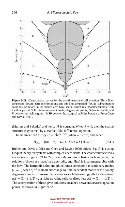
P1: GMD
CB381-09 CB381-Davis May 17, 2001 19:20 Char Count= 0
306 9. Microscale fluid flow
Figure 9.21. Characteristic curves for the two-dimensional-cell equation. Thick linesare period-(2π/a) (harmonic) solutions, and thin lines are period-(4π/a) (subharmonic)solutions. Solutions in the shaded area have spatial structures incommensurable withthe flow period. Solid circles represent doubly degenerate points; S denotes stable, andU denotes unstable regions; MSB denotes the marginal stability boundary. From Chenand Davis (1999).
(Mullins and Sekerka) and hence H is constant. When δ �= 0, then the spatialstructure is governed by a Mathieu-like differential operator.
In the linearized theory H = He(σ+iω)t , where σ is real, and hence
H X X + [(m − σ ) − iω + iδ sin αX ] H = 0. (9.41)
Buhler and Davis (1998) and Chen and Davis (1999) solved Eq. (9.41) usingFloquet theory for systems with complex coefficients. The characteristic curvesare shown in Figure 9.21 for 2π/α-periodic solutions. Inside the boundaries, thesolutions (shown as shaded) are aperiodic, and H (x) is incommensurable withthe flow. The harmonic solutions (thick lines) correspond to stationary modes(ω = 0) when δ/α2 is small but change to time-dependent modes at the doublydegenerate points. These oscillatory modes are left-traveling cells localized nearαX = (2n + 1/2)π , or right-traveling cells localized nearαX = (2n − 1/2)π.The superposition of these gives solutions localized between surface stagnationpoints, as shown in Figure 9.22.
www.iran-mavad.com مرجع علمی مھندسی مواد
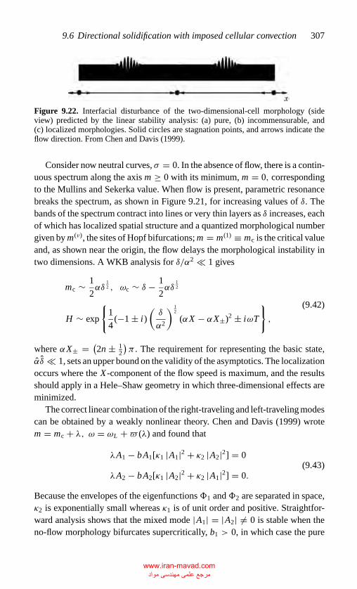
P1: GMD
CB381-09 CB381-Davis May 17, 2001 19:20 Char Count= 0
9.6 Directional solidification with imposed cellular convection 307
Figure 9.22. Interfacial disturbance of the two-dimensional-cell morphology (sideview) predicted by the linear stability analysis: (a) pure, (b) incommensurable, and(c) localized morphologies. Solid circles are stagnation points, and arrows indicate theflow direction. From Chen and Davis (1999).
Consider now neutral curves, σ = 0. In the absence of flow, there is a contin-uous spectrum along the axis m ≥ 0 with its minimum, m = 0, correspondingto the Mullins and Sekerka value. When flow is present, parametric resonancebreaks the spectrum, as shown in Figure 9.21, for increasing values of δ. Thebands of the spectrum contract into lines or very thin layers as δ increases, eachof which has localized spatial structure and a quantized morphological numbergiven by m(ν), the sites of Hopf bifurcations; m = m(1) ≡ mc is the critical valueand, as shown near the origin, the flow delays the morphological instability intwo dimensions. A WKB analysis for δ/α2 1 gives
mc ∼ 1
2αδ
12 , ωc ∼ δ − 1
2αδ
12
H ∼ exp
{1
4(−1 ± i)
(δ
α2
) 12
(αX − αX±)2 ± iωT
},
(9.42)
where αX± = (2n ± 12
)π . The requirement for representing the basic state,
αδ 1, sets an upper bound on the validity of the asymptotics. The localizationoccurs where the X -component of the flow speed is maximum, and the resultsshould apply in a Hele–Shaw geometry in which three-dimensional effects areminimized.
The correct linear combination of the right-traveling and left-traveling modescan be obtained by a weakly nonlinear theory. Chen and Davis (1999) wrotem = mc + λ, ω = ωL +! (λ) and found that
λA1 − bA1[κ1 |A1|2 + κ2 |A2|2] = 0
λA2 − bA2[κ1 |A2|2 + κ2 |A1|2] = 0.(9.43)
Because the envelopes of the eigenfunctions�1 and�2 are separated in space,κ2 is exponentially small whereas κ1 is of unit order and positive. Straightfor-ward analysis shows that the mixed mode |A1| = |A2| �= 0 is stable when theno-flow morphology bifurcates supercritically, b1 > 0, in which case the pure
www.iran-mavad.com مرجع علمی مھندسی مواد
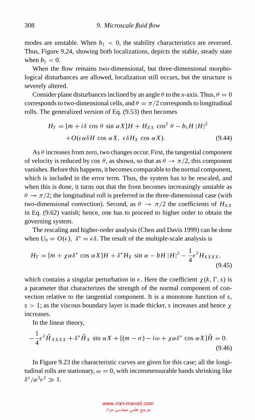
P1: GMD
CB381-09 CB381-Davis May 17, 2001 19:20 Char Count= 0
308 9. Microscale fluid flow
modes are unstable. When b1 < 0, the stability characteristics are reversed.Thus, Figure 9.24, showing both localizations, depicts the stable, steady statewhen b1 < 0.
When the flow remains two-dimensional, but three-dimensional morpho-logical disturbances are allowed, localization still occurs, but the structure isseverely altered.
Consider plane disturbances inclined by an angle θ to the x-axis. Thus, θ = 0corresponds to two-dimensional cells, and θ = π/2 corresponds to longitudinalrolls. The generalized version of Eq. (9.53) then becomes
HT = [m + iδ cos θ sin αX ]H + HX X cos2 θ − b1 H |H |2
+O(εαδH cos αX, εδHX cos αX ). (9.44)
As θ increases from zero, two changes occur. First, the tangential componentof velocity is reduced by cos θ , as shown, so that as θ → π/2, this componentvanishes. Before this happens, it becomes comparable to the normal component,which is included in the error term. Thus, the system has to be rescaled, andwhen this is done, it turns out that the front becomes increasingly unstable asθ → π/2; the longitudinal roll is preferred in the three-dimensional case (withtwo-dimensional convection). Second, as θ → π/2 the coefficients of HX X
in Eq. (9.62) vanish; hence, one has to proceed to higher order to obtain thegoverning system.
The rescaling and higher-order analysis (Chen and Davis 1999) can be donewhen U0 = O(ε), δ∗ = εδ. The result of the multiple-scale analysis is
HT = [m + χαδ∗ cos αX ]H + δ∗HX sin α − bH |H |2 − 1
4ε2 HX X X X ,
(9.45)
which contains a singular perturbation in ε. Here the coefficient χ (k, �, s) isa parameter that characterizes the strength of the normal component of con-vection relative to the tangential component. It is a monotone function of s,s > 1; as the viscous boundary layer is made thicker, s increases and hence χincreases.
In the linear theory,
−1
4ε2 H X X X X + δ∗ H X sin αX + [(m − σ ) − iω + χαδ∗ cos αX ]H = 0.
(9.46)
In Figure 9.23 the characteristic curves are given for this case; all the longi-tudinal rolls are stationary, ω = 0, with incommensurable bands shrinking likeδ∗/α3ε2 � 1.
www.iran-mavad.com مرجع علمی مھندسی مواد
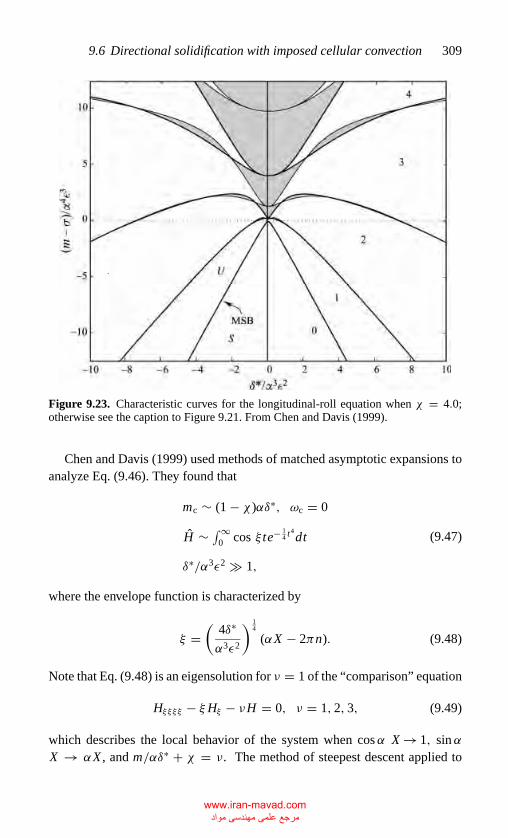
P1: GMD
CB381-09 CB381-Davis May 17, 2001 19:20 Char Count= 0
9.6 Directional solidification with imposed cellular convection 309
Figure 9.23. Characteristic curves for the longitudinal-roll equation when χ = 4.0;otherwise see the caption to Figure 9.21. From Chen and Davis (1999).
Chen and Davis (1999) used methods of matched asymptotic expansions toanalyze Eq. (9.46). They found that
mc ∼ (1 − χ )αδ∗, ωc = 0
H ∼ ∫∞0 cos ξ te− 1
4 t4dt
δ∗/α3ε2 � 1,
(9.47)
where the envelope function is characterized by
ξ =(
4δ∗
α3ε2
) 14
(αX − 2πn). (9.48)
Note that Eq. (9.48) is an eigensolution for ν = 1 of the “comparison” equation
Hξξξξ − ξHξ − νH = 0, ν = 1, 2, 3, (9.49)
which describes the local behavior of the system when cosα X → 1, sinαX → αX , and m/αδ∗ + χ = ν. The method of steepest descent applied to
www.iran-mavad.com مرجع علمی مھندسی مواد
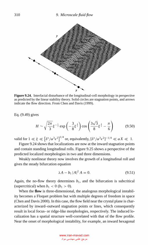
P1: GMD
CB381-09 CB381-Davis May 17, 2001 19:20 Char Count= 0
310 9. Microscale fluid flow
Figure 9.24. Interfacial disturbance of the longitudinal-cell morphology in perspectiveas predicted by the linear stability theory. Solid circles are stagnation points, and arrowsindicate the flow direction. From Chen and Davis (1999).
Eq. (9.49) gives
H ∼√
2π
3ξ− 1
3 exp
(−3
8ξ
43
)cos
(3√
3
8ξ
43 − π
6
)(9.50)
valid for 1 ξ [δ∗/α3ε2]1/4
or, equivalently, [δ∗/α3ε2]−1/4 αX 1.Figure 9.24 shows that localizations are now at the inward stagnation points
and contain standing longitudinal rolls. Figure 9.25 shows a perspective of thepredicted localized morphologies in two and three dimensions.
Weakly nonlinear theory now involves the growth of a longitudinal roll andgives the steady bifurcation equation
λA − b1 |A|2 A = 0. (9.51)
Again, the no-flow theory determines b1, and the bifurcation is subcritical(supercritical) when b1 < 0 (b1 > 0).
When the flow is three-dimensional, the analogous morphological instabil-ity becomes a Floquet problem but with multiple degrees of freedom in space(Chen and Davis 2000). In this case, the flow field near the crystal plane is char-acterized by inward–outward stagnation points or lines, which consequentlyresult in local focus- or ridge-like morphologies, respectively. The induced lo-calization has a spatial structure well-correlated with that of the flow profile.Near the onset of morphological instability, for example, an inward hexagonal
www.iran-mavad.com مرجع علمی مھندسی مواد
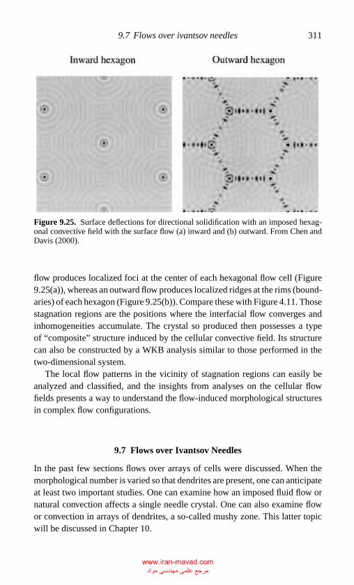
P1: GMD
CB381-09 CB381-Davis May 17, 2001 19:20 Char Count= 0
9.7 Flows over ivantsov needles 311
Figure 9.25. Surface deflections for directional solidification with an imposed hexag-onal convective field with the surface flow (a) inward and (b) outward. From Chen andDavis (2000).
flow produces localized foci at the center of each hexagonal flow cell (Figure9.25(a)), whereas an outward flow produces localized ridges at the rims (bound-aries) of each hexagon (Figure 9.25(b)). Compare these with Figure 4.11. Thosestagnation regions are the positions where the interfacial flow converges andinhomogeneities accumulate. The crystal so produced then possesses a typeof “composite” structure induced by the cellular convective field. Its structurecan also be constructed by a WKB analysis similar to those performed in thetwo-dimensional system.
The local flow patterns in the vicinity of stagnation regions can easily beanalyzed and classified, and the insights from analyses on the cellular flowfields presents a way to understand the flow-induced morphological structuresin complex flow configurations.
9.7 Flows over Ivantsov Needles
In the past few sections flows over arrays of cells were discussed. When themorphological number is varied so that dendrites are present, one can anticipateat least two important studies. One can examine how an imposed fluid flow ornatural convection affects a single needle crystal. One can also examine flowor convection in arrays of dendrites, a so-called mushy zone. This latter topicwill be discussed in Chapter 10.
www.iran-mavad.com مرجع علمی مھندسی مواد
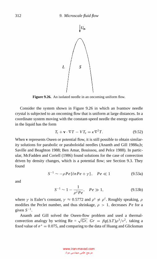
P1: GMD
CB381-09 CB381-Davis May 17, 2001 19:20 Char Count= 0
312 9. Microscale fluid flow
Figure 9.26. An isolated needle in an oncoming uniform flow.
Consider the system shown in Figure 9.26 in which an Ivantsov needlecrystal is subjected to an oncoming flow that is uniform at large distances. In acoordinate system moving with the constant-speed needle the energy equationin the liquid has the form
Tt + v · ∇T − V Tz = κ∇2T . (9.52)
When v represents Oseen or potential flow, it is still possible to obtain similar-ity solutions for parabolic or paraboloidal needles (Ananth and Gill 1988a,b;Saville and Beaghton 1988; Ben Amar, Bouissou, and Pelce 1988). In partic-ular, McFadden and Coriell (1986) found solutions for the case of convectiondriven by density changes, which is a potential flow; see Section 9.3. Theyfound
S−1 ∼ −ρPe [�nPe + γ ] , Pe 1 (9.53a)
and
S−1 ∼ 1 − 1
ρ2 Pe, Pe � 1, (9.53b)
where γ is Euler’s constant, γ ≈ 0.5772 and ρs �= ρ�. Roughly speaking, ρmodifies the Peclet number, and thus shrinkage, ρ > 1, decreases Pe for agiven S−1.
Ananth and Gill solved the Oseen-flow problem and used a thermal-convection analogy by writing Re =
√Gr, Gr = βg(�T )ρ3/ν2, taking a
fixed value of σ ∗ = 0.075, and comparing to the data of Huang and Glicksman
www.iran-mavad.com مرجع علمی مھندسی مواد
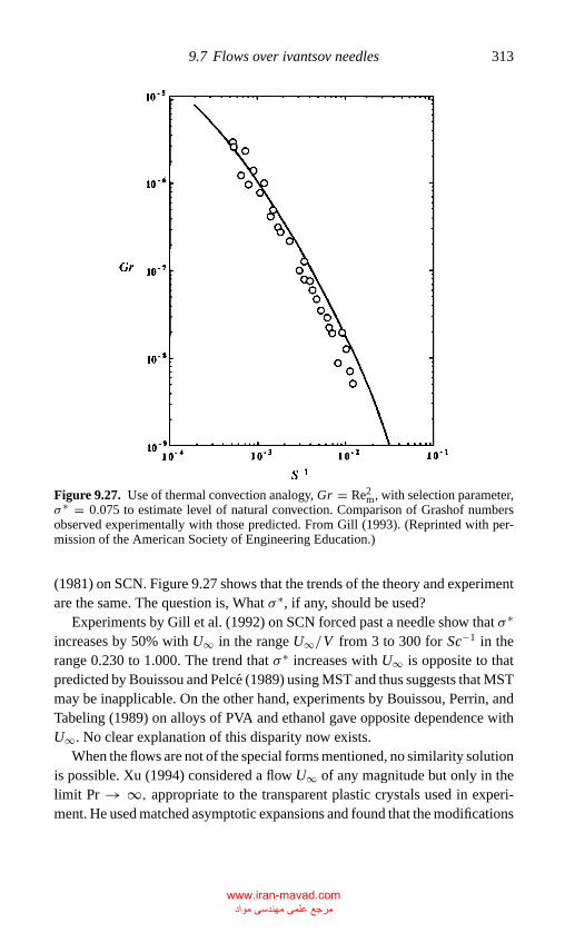
P1: GMD
CB381-09 CB381-Davis May 17, 2001 19:20 Char Count= 0
9.7 Flows over ivantsov needles 313
Figure 9.27. Use of thermal convection analogy, Gr = Re2m, with selection parameter,
σ ∗ = 0.075 to estimate level of natural convection. Comparison of Grashof numbersobserved experimentally with those predicted. From Gill (1993). (Reprinted with per-mission of the American Society of Engineering Education.)
(1981) on SCN. Figure 9.27 shows that the trends of the theory and experimentare the same. The question is, What σ ∗, if any, should be used?
Experiments by Gill et al. (1992) on SCN forced past a needle show that σ ∗
increases by 50% with U∞ in the range U∞/V from 3 to 300 for Sc−1 in therange 0.230 to 1.000. The trend that σ ∗ increases with U∞ is opposite to thatpredicted by Bouissou and Pelce (1989) using MST and thus suggests that MSTmay be inapplicable. On the other hand, experiments by Bouissou, Perrin, andTabeling (1989) on alloys of PVA and ethanol gave opposite dependence withU∞. No clear explanation of this disparity now exists.
When the flows are not of the special forms mentioned, no similarity solutionis possible. Xu (1994) considered a flow U∞ of any magnitude but only in thelimit Pr → ∞, appropriate to the transparent plastic crystals used in experi-ment. He used matched asymptotic expansions and found that the modifications
www.iran-mavad.com مرجع علمی مھندسی مواد
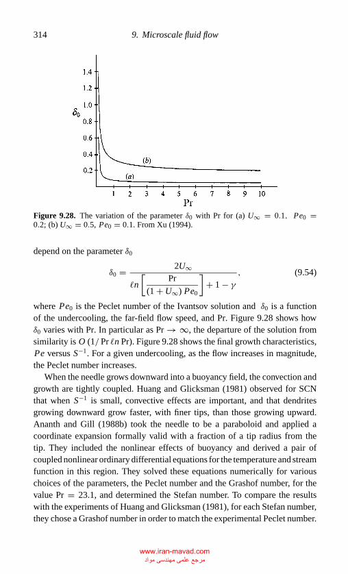
P1: GMD
CB381-09 CB381-Davis May 17, 2001 19:20 Char Count= 0
314 9. Microscale fluid flow
Figure 9.28. The variation of the parameter δ0 with Pr for (a) U∞ = 0.1, Pe0 =0.2; (b) U∞ = 0.5, Pe0 = 0.1. From Xu (1994).
depend on the parameter δ0
δ0 = 2U∞
�n
[Pr
(1 + U∞) Pe0
]+ 1 − γ
, (9.54)
where Pe0 is the Peclet number of the Ivantsov solution and δ0 is a functionof the undercooling, the far-field flow speed, and Pr. Figure 9.28 shows howδ0 varies with Pr. In particular as Pr → ∞, the departure of the solution fromsimilarity is O (1/ Pr �n Pr). Figure 9.28 shows the final growth characteristics,Pe versus S−1. For a given undercooling, as the flow increases in magnitude,the Peclet number increases.
When the needle grows downward into a buoyancy field, the convection andgrowth are tightly coupled. Huang and Glicksman (1981) observed for SCNthat when S−1 is small, convective effects are important, and that dendritesgrowing downward grow faster, with finer tips, than those growing upward.Ananth and Gill (1988b) took the needle to be a paraboloid and applied acoordinate expansion formally valid with a fraction of a tip radius from thetip. They included the nonlinear effects of buoyancy and derived a pair ofcoupled nonlinear ordinary differential equations for the temperature and streamfunction in this region. They solved these equations numerically for variouschoices of the parameters, the Peclet number and the Grashof number, for thevalue Pr = 23.1, and determined the Stefan number. To compare the resultswith the experiments of Huang and Glicksman (1981), for each Stefan number,they chose a Grashof number in order to match the experimental Peclet number.
www.iran-mavad.com مرجع علمی مھندسی مواد
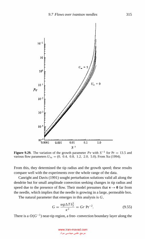
P1: GMD
CB381-09 CB381-Davis May 17, 2001 19:20 Char Count= 0
9.7 Flows over ivantsov needles 315
Figure 9.29. The variation of the growth parameter Pe with S−1 for Pr = 13.5 andvarious flow parameters U∞ = (0, 0.4, 0.8, 1.2, 2.0, 5.0). From Xu (1994).
From this, they determined the tip radius and the growth speed; these resultscompare well with the experiments over the whole range of the data.
Canright and Davis (1991) sought perturbation solutions valid all along thedendrite but for small amplitude convection seeking changes in tip radius andspeed due to the presence of flow. Their model presumes that v → 0 far fromthe needle, which implies that the needle is growing in a large, permeable box.
The natural parameter that emerges in this analysis is G,
G = αg�T δ3T
κ2= Gr Pr−2. (9.55)
There is a O(G−1) near-tip region, a free- convection boundary layer along the
www.iran-mavad.com مرجع علمی مھندسی مواد
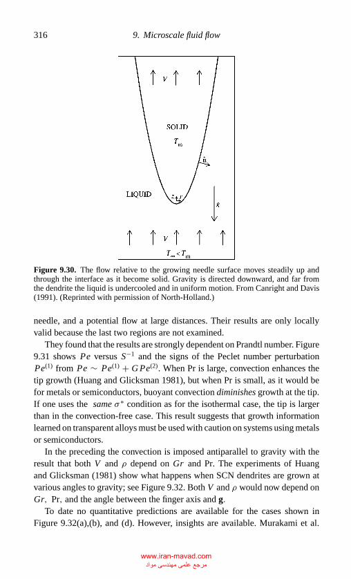
P1: GMD
CB381-09 CB381-Davis May 17, 2001 19:20 Char Count= 0
316 9. Microscale fluid flow
Figure 9.30. The flow relative to the growing needle surface moves steadily up andthrough the interface as it become solid. Gravity is directed downward, and far fromthe dendrite the liquid is undercooled and in uniform motion. From Canright and Davis(1991). (Reprinted with permission of North-Holland.)
needle, and a potential flow at large distances. Their results are only locallyvalid because the last two regions are not examined.
They found that the results are strongly dependent on Prandtl number. Figure9.31 shows Pe versus S−1 and the signs of the Peclet number perturbationPe(1) from Pe ∼ Pe(1) + G Pe(2). When Pr is large, convection enhances thetip growth (Huang and Glicksman 1981), but when Pr is small, as it would befor metals or semiconductors, buoyant convection diminishes growth at the tip.If one uses the same σ ∗ condition as for the isothermal case, the tip is largerthan in the convection-free case. This result suggests that growth informationlearned on transparent alloys must be used with caution on systems using metalsor semiconductors.
In the preceding the convection is imposed antiparallel to gravity with theresult that both V and ρ depend on Gr and Pr. The experiments of Huangand Glicksman (1981) show what happens when SCN dendrites are grown atvarious angles to gravity; see Figure 9.32. Both V and ρ would now depend onGr, Pr, and the angle between the finger axis and g.
To date no quantitative predictions are available for the cases shown inFigure 9.32(a),(b), and (d). However, insights are available. Murakami et al.
www.iran-mavad.com مرجع علمی مھندسی مواد
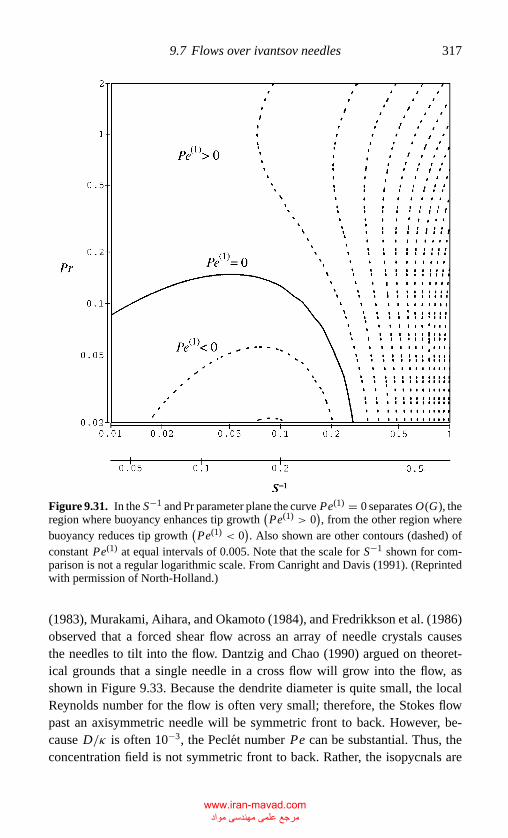
P1: GMD
CB381-09 CB381-Davis May 17, 2001 19:20 Char Count= 0
9.7 Flows over ivantsov needles 317
Figure 9.31. In the S−1 and Pr parameter plane the curve Pe(1) = 0 separates O(G), theregion where buoyancy enhances tip growth
(Pe(1) > 0
), from the other region where
buoyancy reduces tip growth(Pe(1) < 0
). Also shown are other contours (dashed) of
constant Pe(1) at equal intervals of 0.005. Note that the scale for S−1 shown for com-parison is not a regular logarithmic scale. From Canright and Davis (1991). (Reprintedwith permission of North-Holland.)
(1983), Murakami, Aihara, and Okamoto (1984), and Fredrikkson et al. (1986)observed that a forced shear flow across an array of needle crystals causesthe needles to tilt into the flow. Dantzig and Chao (1990) argued on theoret-ical grounds that a single needle in a cross flow will grow into the flow, asshown in Figure 9.33. Because the dendrite diameter is quite small, the localReynolds number for the flow is often very small; therefore, the Stokes flowpast an axisymmetric needle will be symmetric front to back. However, be-cause D/κ is often 10−3, the Peclet number Pe can be substantial. Thus, theconcentration field is not symmetric front to back. Rather, the isopycnals are
www.iran-mavad.com مرجع علمی مھندسی مواد
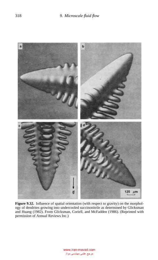
P1: GMD
CB381-09 CB381-Davis May 17, 2001 19:20 Char Count= 0
318 9. Microscale fluid flow
Figure 9.32. Influence of spatial orientation (with respect to gravity) on the morphol-ogy of dendrites growing into undercooled succinonitrile as determined by Glicksmanand Huang (1982). From Glicksman, Coriell, and McFadden (1986). (Reprinted withpermission of Annual Reviews Inc.)
www.iran-mavad.com مرجع علمی مھندسی مواد
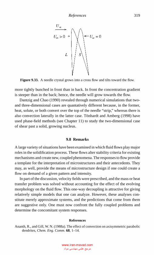
P1: GMD
CB381-09 CB381-Davis May 17, 2001 19:20 Char Count= 0
References 319
Figure 9.33. A needle crystal grows into a cross flow and tilts toward the flow.
more tightly bunched in front than in back. In front the concentration gradientis steeper than in the back; hence, the needle will grow towards the flow.
Dantzig and Chao (1990) revealed through numerical simulations that two-and three-dimensional cases are quantatively different because, in the former,heat, solute, or both convert over the top of the needle “strip,” whereas there isalso convection laterally in the latter case. Tonhardt and Amberg (1998) haveused phase-field methods (see Chapter 11) to study the two-dimensional caseof shear past a solid, growing nucleus.
9.8 Remarks
A large variety of situations have been examined in which fluid flows play majorroles in the solidification process. These flows alter stability criteria for existingmechanisms and create new, coupled phenomena. The responses to flow providea template for the interpretation of microstructures and their antecedents. Theymay, as well, provide the means of microstructure design if one could create aflow on demand of a given pattern and intensity.
In part of the discussion, velocity fields were prescribed, and the mass or heattransfer problem was solved without accounting for the effect of the evolvingmorphology on the fluid flow. This one-way decoupling is attractive for givingrelatively simple models that one can analyze. However, these analyses con-stitute merely approximate systems, and the predictions that come from themare suggestive only. One must now confront the fully coupled problems anddetermine the concomitant system responses.
References
Ananth, R., and Gill, W. N. (1988a). The effect of convection on axisymmetric parabolicdendrites, Chem. Eng. Comm. 68, 1–14.
www.iran-mavad.com مرجع علمی مھندسی مواد
P1: GMD
CB381-09 CB381-Davis May 17, 2001 19:20 Char Count= 0
320 9. Microscale fluid flow
Ananth, R., and Gill, W. N. (1988b). Dendritic growth with thermal convection, J. CrystalGrowth 91, 587–598.
Ben Amar, M., Bouissou, P. H., and Pelce, P. (1988). An exact solution for the shape ofa crystal growing in a forced flow, J. Crystal Growth 92, 97–100.
Bouissou, P., and Pelce, P. (1989). Effect of a forced flow on dendritic growth Phys. Rev.A 40, 6673–6680.
Bouissou, P., Perrin, B., and Tabeling, P. (1989). Influence of an external flow on dendriticcrystal growth, Phys. Rev. A 40, 509–512.
Brattkus, K. (1988). Directional solidification of dilute binary alloy, Ph.D. Dissertation,Northwestern University, Evanston, IL.
Brattkus, K., and Davis, S. H. (1988a). Cellular growth near absolute stability, Phys.Rev. B 38, 11452–11460.
————. (1988b). Flow-induced morphological instabilities: The rotating disc. J. Crys-tal Growth 87, 385–396.
————. (1988c). Flow-induced morphological instabilities: Stagnation-point flows,J. Crystal Growth 89, 423–427.
Brown, R. A. (1988). Theory of transport processes in single crystal growth from themelt, AIChE J. 34, 881–911.
Buhler, L., and Davis, S. H. (1998). Flow-induced changes of morphological instabilityin directional solidification: Localized morphologies, J. Crystal Growth 186, 629–647.
Canright, D., and Davis, S. H. (1991). Buoyancy effects of a growing, isolated dendrite,J. Crystal Growth 114, 153–185.
Caroli B., Caroli, C., Misbah C., and Roulet, B. (1985a). Solutal convection and mor-phological instability in directional solidification of binary alloys, J. Phys. (Paris)46, 401–413.
————. (1985b). Solutal convection and morphological instability in directional solid-ification of binary alloys. II. Effect of the density difference between the phases,J. Phys. (Paris) 46, 1657–1665.
Chen, Y.-J., and Davis, S. H. (1999). Directional solidification of a binary alloy intoa cellular convective flow: Localized morphologies, J. Fluid Mech. 395, 253–270.
————. (2000). Flow-induced patterns in directional solidification: Localized mor-phologies in three-dimensional flows J. Fluid Mech. 421, 369–380.
Choi, I. G., and Korpela, A. A. (1980). Stability of the conduction regime of naturalconvection in a tall vertical annulus, J. Fluid Mech. 99, 725–738.
Coriell, S. R., Cordes, M. R., Boettinger, W. S., and Sekerka, R. F. (1980). Convec-tive and interfacial instability during unidirectional solidification in a binary alloy,J. Crystal Growth 49, 13–28.
Coriell, S. R., and McFadden, G. B. (1989). Buoyancy effects on morphological insta-bility during directional solidification, J. Crystal Growth 94, 513–521.
Coriell, S. R., McFadden, G. B., Boisvert, R. F., and Sekerka, R. F. (1984). Effect of aforced Couette flow on coupled convective and morphological instabilities duringunidirectional solidification, J. Crystal Growth 69, 15–22.
Dantzig, J. A., and Chao, L. S. (1990). The effect of shear flows on solidification mi-crostructure, in C. F. Chen, editor, Proc. 10th U.S. Nat. Cong. of Appl. Mech., pages249–255. ASME Press, N.Y.
Davis, S. H. (1990). Hydrodynamic interactions in directional solidification, J. FluidMech. 212, 241–262.
————. (1993). Effects of flow on morphological instability, in Handbook of CrystalGrowth, Vol. 1b, pp. 861–897, North-Holland, Amsterdam.
www.iran-mavad.com مرجع علمی مھندسی مواد
P1: GMD
CB381-09 CB381-Davis May 17, 2001 19:20 Char Count= 0
References 321
Davis, S. H., Huppert, H. E., Muller, U., and Worster, M. G. (1992). Interactive dynamicson convection and solidification, NATO ASI Series E, Vol. 219, Kluwer Publishers,Dordrecht.
Davis, S. H., Muller, U., and Dietsche, C. (1984). Pattern selection in single-componentsystems coupling Benard convection and solidification, J. Fluid Mech. 144, 133–151.
Davis, S. H., and Segel, L. A. (1968). Effects of surface curvature and property variationon cellular convection. Phys. Fluids 11, 470–476.
Delves, R. T. (1968). Theory of stability of a solid liquid interface during growth fromstirred melts, J. Crystal Growth 3–4, 562–568.
————. (1971). Theory of the stability of a solid liquid interface during growth fromstirred melts II, J. Crystal Growth 8, 13–25.
Dietsche, C., and Muller, U. (1985). Influence of Benard convection on solid–liquidinterfaces, J. Fluid Mech. 161, 249–268.
Fang, Q. T., Glicksman, M. E., Coriell, S. R., McFadden, G. B., and Boisvert, R. F.(1985). Convective influence on the stability of a cylindrical solid–liquid interface,J. Fluid Mech. 151, 121–140.
Forth, S. A., and Wheeler, A. A. (1989). Hydrodynamic and morphological stability ofthe unidirectional solidification of a freezing binary alloy: A simple model, J. FluidMech. 202, 339–366.
————. (1992). Coupled convective and morphological instability in a simple modelof the solidification of a binary alloy, including a shear flow, J. Fluid Mech. 236,61–94.
Fredriksson, H., El Mahallawy, N., Taha, M., Liu, X., and Wanglow, G. (1986). Scand.J. Metall. 15, 127–137.
Gill, W. N. (1993). Interactive dynamics of convection and crystal growth, Chem. Eng.Educ. 27, 198–205.
Gill, W. N., Lee, Y. W., Koo, K. K., and Ananth, R. (1992). Interaction of thermaland forced convection with the growth of dendritic crystals, in S. H. Davis, H. E.Huppert, U. Muller, and M. G. Worster, editors, Interactive Dynamics of Convectionand Solidification, Kluwer Academic Publishers, Dordrecht.
Glicksman, M. E., and Mickalonis, J. I. (1982). Convective coupling of a solid–liquidinterface in an internally heated vertical cylinder, in T. Negat Veziroglon, editor,Thermal Sciences, 16, 505–515, Hemisphere Publications, Washington, DC.
Glicksman, M. E., Coriell, S. R. and McFadden, G. B. (1986). Interaction of flows withthe crystal-melt interface, Ann. Rev. Fluid Mech. 18, 307–335.
Hadji, L., Schell, M., and Riahi, D. N. (1990). Interfacial pattern formation in thepresence of solidification and thermal convection, Phys. Rev. A 41, 863–873.
Hennenberg, M., Rouzaud, A., Favier, J. J., and Camel, D. (1987). Morphological andthermosolutal instabilities inside a deformable boundary layer during directionalsolidification. I. Theoretical methods, J. Phys. (Paris) 48, 173–183.
Hobbs, A. K., and Metzener, P. (1991). Long-wave instabilities in directional solidifica-tion with remote flow, J. Crystal Growth 112, 539–553.
————. (1992). Directional solidification: Interface dynamics and weak remote flow,J. Crystal Growth 118, 319–332.
Huang, S. C., and Glicksman, M. E. (1981). Fundamentals of dendritic solidification-I.Steady–state growth, Acta Metall. Mater. 29, 701–717.
Hurle, D. T. J., Jakeman E., and Wheeler, A. A. (1982). Effect of solutal convection onthe morphological stability of a binary alloy J. Crystal Growth 58, 163–179.
————. (1983). Hydrodynamic stability of the melt during solidification of a binaryalloy Phys. Fluids 26, 624–626.
www.iran-mavad.com مرجع علمی مھندسی مواد
P1: GMD
CB381-09 CB381-Davis May 17, 2001 19:20 Char Count= 0
322 9. Microscale fluid flow
Jenkins, D. R. (1985a). Nonlinear interaction of morphological convective instabi-ities during solidification of a dilute binary alloy, IMA J. Appl. Math. 35, 145–147.
————. (1985b). Nonlinear analysis of convective and morphological instability duringsolidification of a dilute binary alloy, Physiochem. Hydrodyn. 6, 521–537.
————. (1990). Oscillatory instability in a model of direction of solidification, J. CrystalGrowth 102, 481–490.
Kelly, R. E., and Hu, H.-C. (1993). The onset of Rayleigh–Binard convection in non-planar oscillatory flows, J. Fluid Mech. 249, 373–390.
McFadden, G. B., and Coriell, S. R. (1986). The effect of fluid flow due to the crystal-melt density change on the growth of a parabolic isothermal dendrite, J. CrystalGrowth 74, 507–512.
McFadden, G. B., Coriell, S. R., and Alexander, J. I. D. (1988). ‘Hydrodynamic andfree-boundary instabilities during crystal growth – The effect of a plane stagnationflow, Comm. Pure Appl. Math. 41, 683–706.
McFadden, G. B., Coriell, S. R., Boisvert, R. F., Glicksman, M. E., and Fang, Q. T.(1984). Morphological stability in the presence of fluid flow in the melt, Metall.Trans. A15, 2117–2124.
McFadden, G. B., Coriell, S. R., Boisvert, R. F., Glicksman, M. E., and Selleck, M. E.(1989). PhysicoChem. Hydrodyn. 11, 387.
Merchant, G. J., and Davis, S. H. (1989). Flow-indiced morphological instabilities dueto temporally-modulated stagnation-point flow, J. Crystal Growth 96, 737–746.
Murakami, K., Fujiyama, T., Koike, A., and Okamoto, T. (1983). Influence of melt flowon the growth directionals of columnar grains and columnar dendrites, Acta Metall.Mater. 31, 1425–1432.
Murakami, K., Aihara, H., and Okamoto, T. (1984). Growth direction of columnarcrystals solidified in a flowing melt, Acta Metall. 32, 933–939.
Ozetkin, A., and Pearlstein, A. J. (1992). Coriolis effects on the stability of plane-frontsolidification of dilue Pb–Sn binary alloys, Metall. Trans. B23, 73–80.
Lord Rayleigh (1879). On the instability of jets, Proc. Lond. Math. Soc. 10, 4–13.Riley, D. S., and Davis, S. H. (1989a). Applied Mathematics Technical Report No. 8838
(Northwestern University).————. (1989b). Hydrodynamic stability of the melt during the solidification of a binary
alloy with small segregation coefficient, Physica D. 39, 231–238.————. (1991). Long-wave interactions in morphological and convective, instabilities
IMA J. Appl. Math. 45, 267–285.Rosenberger, F. (1979). Fundamentals of Crystal Growth I, Springer-Verlag, New York.Saville, D. A., and Beaghton, P. J. (1988). Growth of needle-shaped crystals in the
presence of convection, Phys. Rev. A 37, 3423–3430.Schaefer, R. J., and Coriell, S. R. (1982). Convective and interfacial instabilities during
solidification of succinonitrile containing ethanol, in G. E. Rindone, editor, Ma-terials Processing in the Reduced Gravity Environment of Space, pages 479–489,Materials Research Society Symposium Proceedings, Vol. 9, North-Holland Press,New York.
Schluter, A., Lortz, and Busse, F. H. (1965). On the stability of steady finite amplitudeconvection, J. Fluid Mech. 23, 129–144.
Schulze, T. P., and Davis, S. H. (1994). The influence of oscillating and steady shearson interfacial instability during directional solidification, J. Crystal Growth 143,317–333.
————. (1995). Shear stabilization of morphological instability during directional so-lidification, J. Crystal Growth 149, 253–265.
www.iran-mavad.com مرجع علمی مھندسی مواد
P1: GMD
CB381-09 CB381-Davis May 17, 2001 19:20 Char Count= 0
References 323
————. (1996). Shear stabiligation of a solidifying front: Weakly nonlinear analysis inthe long-wave limit Phys. Fluids 9, 2319–2336.
Shaaban, A. H., and Ozisik, M. N. (1982). Effect of curvature on the thermal stabilityof a fluid between two long vertical coaxial cylinders, in U. Grigull, E. Hahne,K. Stephan and J. Straub, editor, Heat Trans. for 1982, Munich, Vol. 2, 281–286,Hemisphere Publishers, Washington, DC.
Sivashinsky G. I. (1983). On cellular instability in the solidification of a dilute binaryalloy, Physica D. 8, 243–248.
Tonhardt, R., and Amberg, G. (1998). Phase-field simulation of dendritic growth in ashear flow, J. Crystal Growth 194, 406–425.
Wheeler, A. A. (1991). A strongly nonlinear analysis of the morphological instabilityof a freezing binary alloy–solutal convection, density changes, and nonequilibriumeffects, IMA J. Appl. Math. 47, 173–192.
Wollkind, D. J., and Segel, L. A. (1970). A nonlinear stability analysis of the freezingof a dilute binary alloy, Philos. Trans. Roy. Soc. London A 268, 351–380.
Young, G. W., and Davis, S. H. (1986). Directional solidification with buoyancy insystems with small segregation coefficient, Phys. Rev. B 34, 3388–3396.
Xu, J.-J. (1994). Dendritic growth from a melt in an external flow: Uniformly validasymptotic solution for the steady state, J. Fluid Mech. 263, 227–243.
Zimmermann, G., Muller, U., and Davis, S. H. (1992). Benard convection in binarymixtures with Soret effects and solidification, J. Fluid Mech. 238, 657–682 andCorrigendum 254, 720.
www.iran-mavad.com مرجع علمی مھندسی مواد
P1: GKE
CB381-10 CB381-Davis May 17, 2001 18:58 Char Count= 0
10
Mesoscale fluid flow
In Chapter 9 the discussion of the interaction of fluid flows with solidificationfronts focused on how individual cells or dendrites are affected by the motionof the melt. The discussion was confined to the onset, or near onset, of mor-phological instability and the influence of laminar flows because the systemshad small scale and the rate of solidification could be readily controlled. Thereare many situations in industrial or natural situations in which the systems havelarge scale and the freezing rates are externally provided.
When the freezing rate is not carefully controlled near M = Mc, the typicalmorphology present is dendritic (or eutectic) and strongly nonlinear in theparameter space V − C∞ of Figure 3.6. The region within which there are bothdendrites and interstitial liquid is called a mushy zone. Such zones should not bedescribed pointwise in the same sense that one would not want to describe flowpointwise in a porous rock. Instead, the zone is treated as a porous region thatis reactive in the sense that the matrix melts and the liquid freezes and whoseproperties are described in terms of quantities averaged over many dendritespacings. There still is a purely liquid region and a purely solid region, but nowthey are separated by an intermediate layer, the mushy zone.
When the length scale of the system is large and the fluid is subjected to grav-ity, the fluid in the fully liquid system will undergo buoyancy-driven convection.The large scale may imply that the Rayleigh number is large enough that theconvection is unsteady, laminar, or turbulent.
If one simultaneously has strongly supercritical morphological instability,turbulent flow in the liquid, and finally (weaker) convective flow in the mush,the dynamics is so complex that direct large-scale numerical simulations givetoo much data and not enough information. Alternatively, one can attemptto understand dominant balances by drastically simplifying the systems andlearning the underlying physics step-by-step.
324
www.iran-mavad.com مرجع علمی مھندسی مواد
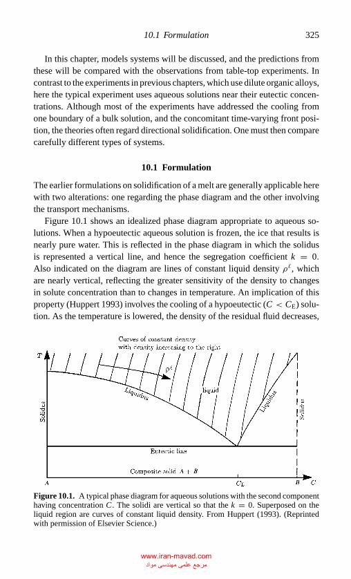
P1: GKE
CB381-10 CB381-Davis May 17, 2001 18:58 Char Count= 0
10.1 Formulation 325
In this chapter, models systems will be discussed, and the predictions fromthese will be compared with the observations from table-top experiments. Incontrast to the experiments in previous chapters, which use dilute organic alloys,here the typical experiment uses aqueous solutions near their eutectic concen-trations. Although most of the experiments have addressed the cooling fromone boundary of a bulk solution, and the concomitant time-varying front posi-tion, the theories often regard directional solidification. One must then comparecarefully different types of systems.
10.1 Formulation
The earlier formulations on solidification of a melt are generally applicable herewith two alterations: one regarding the phase diagram and the other involvingthe transport mechanisms.
Figure 10.1 shows an idealized phase diagram appropriate to aqueous so-lutions. When a hypoeutectic aqueous solution is frozen, the ice that results isnearly pure water. This is reflected in the phase diagram in which the solidusis represented a vertical line, and hence the segregation coefficient k = 0.Also indicated on the diagram are lines of constant liquid density ρ�, whichare nearly vertical, reflecting the greater sensitivity of the density to changesin solute concentration than to changes in temperature. An implication of thisproperty (Huppert 1993) involves the cooling of a hypoeutectic (C < CE) solu-tion. As the temperature is lowered, the density of the residual fluid decreases,
Figure 10.1. A typical phase diagram for aqueous solutions with the second componenthaving concentration C . The solidi are vertical so that the k = 0. Superposed on theliquid region are curves of constant liquid density. From Huppert (1993). (Reprintedwith permission of Elsevier Science.)
www.iran-mavad.com مرجع علمی مھندسی مواد
P1: GKE
CB381-10 CB381-Davis May 17, 2001 18:58 Char Count= 0
326 10. Mesoscale fluid flow
contrary to the “normal” behavior. This is because the liquid becomes depletedof the heavy component (B) and the density is more sensitive to concentrationdecreases than to temperature decreases. Similarly, the cooling of a hypereu-tectic, (C > CE) solution results in successively decreasing densities of therejected material.
When vigorous convection is present and only large-scale properties of theinterface are sought, it is sufficient to represent the thermal transport (beyondconduction) by a simplified functional. In this case the interfacial thermal bal-ance might be written as[
c�p(T − Tm) + Lv]
ht = −ksT sn − FT, (10.1)
where FT is a correlation for convective heat transport (Turner 1979) of theform
FT = ck�( αg
κ�ν
) 13
(T − Tm)43 , (10.2)
T is the mean temperature of the liquid, and c is an empirical constant, c ≈ 0.14.In addition, it turns out that effects of attachment kinetics, important in melts
only at high pulling speeds, enter the description of aqueous solutions at muchlower speeds, and thus at the interface
Vn = µ(T � − T I) (10.3)
where, for example in aqueous isopropanol, µ ≈ 2.2 × 10⁻⁴ cm s−1(C0)−1
(Kerr et al. 1990).
10.2 Planar Solidification between Horizontal Planes
Consider two horizontal plates that enclose an aqueous solution. Huppert andWorster (1985) classified the various possibilities as functions of compositionand cooling position into six cases; Table 10.1 from Huppert (1993) summarizesthese.
When a eutectic solution is cooled from below, Case A, Figure 10.2(a), onehas a classical, one-component, Stefan problem, as discussed in Section 2.1.Solutions exist for all values of the Stefan number S, the planar front h(t)moves with speed proportional to
√t, and the configuration is thermally and
morphologically stable.When a eutectic solution is cooled from above, Case B, one has a eutectic
solid created above liquid, precisely the problem studied by Davis, Muller, andDietsche (1984) and discussed in Section 9.2.2; no solute is rejected. Becausethe liquid is heated from below, the system is susceptible to Benard instabilities
www.iran-mavad.com مرجع علمی مھندسی مواد
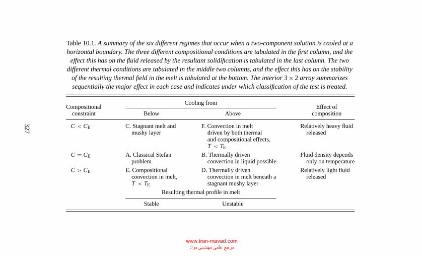
P1:GK
E
CB
381-10C
B381-D
avisM
ay17,2001
18:58C
harC
ount=0
Table 10.1. A summary of the six different regimes that occur when a two-component solution is cooled at ahorizontal boundary. The three different compositional conditions are tabulated in the first column, and theeffect this has on the fluid released by the resultant solidification is tabulated in the last column. The two
different thermal conditions are tabulated in the middle two columns, and the effect this has on the stabilityof the resulting thermal field in the melt is tabulated at the bottom. The interior 3 × 2 array summarizessequentially the major effect in each case and indicates under which classification of the test is treated.
Cooling fromCompositional
constraint Below AboveEffect of
composition
C < CE C. Stagnant melt and F. Convection in melt Relatively heavy fluidmushy layer driven by both thermal released
and compositional effects,T < TE
C = CE A. Classical Stefan B. Thermally driven Fluid density dependsproblem convection in liquid possible only on temperature
C > CE E. Compositional D. Thermally driven Relatively light fluidconvection in melt, convection in melt beneath a releasedT < TE stagnant mushy layer
Resulting thermal profile in melt
Stable Unstable
327
www.iran-mavad.com مرجع علمی مھندسی مواد
P1: GKE
CB381-10 CB381-Davis May 17, 2001 18:58 Char Count= 0
328 10. Mesoscale fluid flow
for Rayleigh number RT ≈ RTc . Turner, Huppert, and Sparks (1986) and
Huppert and Worster (1991) studied situations in which RT � RTc and the
lower boundary is changed from a perfect conductor to a perfect insulator(Figure 10.2(b)). This change results in a system that completely solidifies. Byusing thermal condition (10.1), Huppert and Worster (1991) identified threedistinct asymptotic ranges for the solid thickness h/d versus time τ = κ�t/d2,where d is the spacing between the plates. The changes occur at τ ∼ [cR1/3
0
]−2
and τ ∼ [cR1/30
]−6/7, where R0 is the Rayleigh number at t = 0. There is no
morphological instability in this case.When a hypoeutectic aqueous solution is cooled from below, Case C,
Figure 10.2(c), the thermal field is stably stratified, and the rejection createsa negative solute gradient at the front. Thus, the front is morphologically unsta-ble. Because C < CE, the solutal field is also stably stratified. When M � Mc,
the front becomes dendritic, and a mushy layer is formed, as shown in Figure10.2(d). The interest, then, is the prediction of the thickness h(t) of the mush.
When a hypereutectic solution is cooled from above, Case D, Figure 10.2(e),the picture is superficially the same as that of Case B, Figure 10.2(b), where iceis above liquid, but now there is solute rejection, a morphological instability,and a mushy zone above the interface. When RT � RT
c , the interface betweenmush and liquid is subjected to augmented heat transfer like that representedby condition (10.2).
When a hypereutectic solution is cooled from below, TB < TE, Case E,Figure 10.2(f), the thermal field is stably stratified, but there is solutal convec-tion. Woods and Huppert (1989) estimated by analogy with the thermal casethat the convective compositional flux Fc has the form
Fc = cc(gβD2/ν)13 (�C)
43 (10.4)
where �C is the change in composition across the boundary layer above themush-liquid interface and cc is an empirical constant. Both the thickness of themush and the microstructure are affected by the convection.
When a hypoeutectic solution is cooled from above, TB < TE, Case F,Figure 10.2(g), both the compositional and thermal fields are unstably stratified,and strong double-diffusion convection occurs under a mushy layer formed atthe top. This convection is dominated by the solutal buoyancy, because, ifthe thermal-equilibrium assumption is valid, the buoyancy g�ρ has the form(Worster 1992b)
g�ρ = −g[α�T + β�c] = −g(αm + β)�c, (10.5)
where m < 0. Generally speaking |β| � |mα|, and thus thermal buoyancy is
www.iran-mavad.com مرجع علمی مھندسی مواد
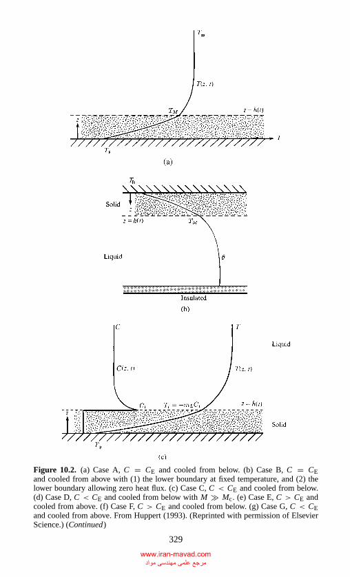
P1: GKE
CB381-10 CB381-Davis May 17, 2001 18:58 Char Count= 0
Figure 10.2. (a) Case A, C = CE and cooled from below. (b) Case B, C = CEand cooled from above with (1) the lower boundary at fixed temperature, and (2) thelower boundary allowing zero heat flux. (c) Case C, C < CE and cooled from below.(d) Case D, C < CE and cooled from below with M � Mc. (e) Case E, C > CE andcooled from above. (f) Case F, C > CE and cooled from below. (g) Case G, C < CEand cooled from above. From Huppert (1993). (Reprinted with permission of ElsevierScience.) (Continued)
329
www.iran-mavad.com مرجع علمی مھندسی مواد
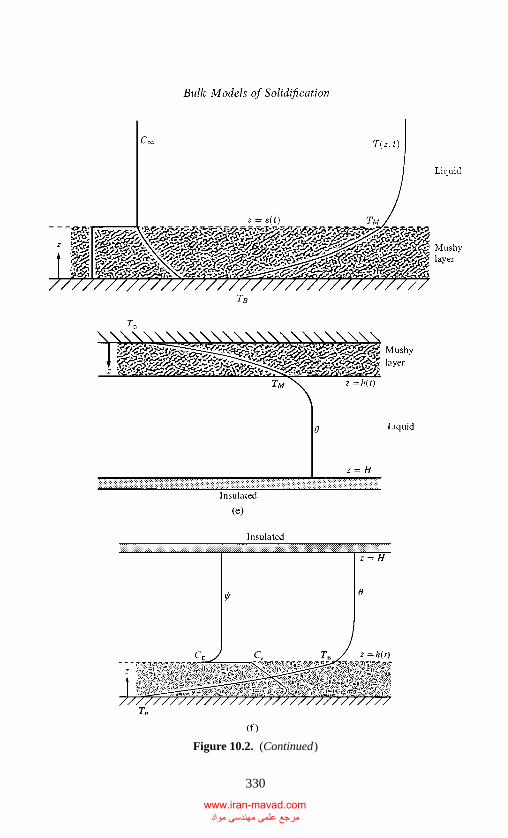
P1: GKE
CB381-10 CB381-Davis May 17, 2001 18:58 Char Count= 0
Figure 10.2. (Continued)
330
www.iran-mavad.com مرجع علمی مھندسی مواد
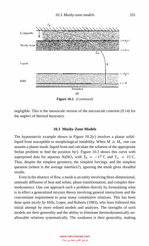
P1: GKE
CB381-10 CB381-Davis May 17, 2001 18:58 Char Count= 0
10.3 Mushy-zone models 331
Figure 10.2. (Continued)
negligible. This is the mesoscale version of the microscale criterion (9.14) forthe neglect of thermal buoyancy.
10.3 Mushy-Zone Models
The hypoeutectic example shown in Figure 10.2(c) involves a planar solid–liquid front susceptible to morphological instability. When M � Mc, one canassume a planar mush–liquid front and calculate the solution of the appropriateStefan problem to find the position h(t). Figure 10.3 shows this curve withsuperposed data for aqueous NaNO3 with TB = −17◦C and T∞ = 15◦C.Thus, despite the simplest geometry, the simplest forcings, and the simplestquestion (where is the average interface?), ignoring the mush gives dreadfulresults.
Even in the absence of flow, a mush is an entity involving three-dimensional,unsteady diffusion of heat and solute, phase transformation, and complex ther-modynamics. One can approach such a problem directly by formulating whatis in effect a generalized mixture theory involving general interactions and theconcomitant requirement to pose many constitutive relations. This has beendone quite nicely by Hills, Loper, and Roberts (1983), who have followed thisinitial attempt by more refined models and analyses. The strengths of suchmodels are their generality and the ability to eliminate thermodynamically un-allowable relations systematically. The weakness is their generality, making
www.iran-mavad.com مرجع علمی مھندسی مواد
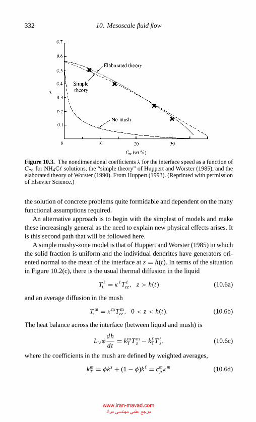
P1: GKE
CB381-10 CB381-Davis May 17, 2001 18:58 Char Count= 0
332 10. Mesoscale fluid flow
Figure 10.3. The nondimensional coefficients λ for the interface speed as a function ofC∞ for NH4C� solutions, the “simple theory” of Huppert and Worster (1985), and theelaborated theory of Worster (1990). From Huppert (1993). (Reprinted with permissionof Elsevier Science.)
the solution of concrete problems quite formidable and dependent on the manyfunctional assumptions required.
An alternative approach is to begin with the simplest of models and makethese increasingly general as the need to explain new physical effects arises. Itis this second path that will be followed here.
A simple mushy-zone model is that of Huppert and Worster (1985) in whichthe solid fraction is uniform and the individual dendrites have generators ori-ented normal to the mean of the interface at z = h(t). In terms of the situationin Figure 10.2(c), there is the usual thermal diffusion in the liquid
T �t = κ�T �zz, z > h(t) (10.6a)
and an average diffusion in the mush
T mt = κmT m
zz , 0 < z < h(t). (10.6b)
The heat balance across the interface (between liquid and mush) is
LVφdh
dt= km
T T mz − k�TT �z, (10.6c)
where the coefficients in the mush are defined by weighted averages,
kmT = φks + (1 − φ)k� = cm
p κm (10.6d)
www.iran-mavad.com مرجع علمی مھندسی مواد
P1: GKE
CB381-10 CB381-Davis May 17, 2001 18:58 Char Count= 0
10.3 Mushy-zone models 333
and
cmp = φcs
p + (1 − φ)c�p. (10.6e)
Here φ is the (constant) volume fraction of solid and cp is the specific heat perunit volume. Huppert and Worster argued that (10.6d) well describes a randomarray of dendrites whose phase boundares are sensibly vertical and whose solidfraction is uniform; relation (10.6e) is exact.
The model involves the assumption that “all” the rejected solute producedby growth is trapped within the mush and that the boundary layer above themush accounts for “zero” rejected solute, which is consistent with D� κ�.As will be seen, this implies that the overall thickness of the mushy zone scaleswith thermal – rather than solutal – diffusion rates.
A major assumption in these theories is that the mush is in thermodynamicequilibrium because the concentration and the temperature are always confinedto lie on the liquidus,which is consistent with the intimate intermingling of solidand liquid and the mush’s being described on scales of many dendrites. Thus,
Cm = T m/m, 0 < z < h(t) (10.6f)
and
C� = C∞, z ≥ h(t). (10.6g)
Equation (10.6g) is consistent with a thin concentration boundary layer.Finally, there is a global solute balance,
(1 − φ)∫ h(t)
0Cm(z, t)dz = h(t)C∞. (10.6h)
Huppert and Worster solved the Stefan problem for this system in whichh(t) = 2λm
√κ�t . For the conditions of their experiment, their predictions,
shown in Figure 10.3 and labelled “simply” theory, are quite good. The successof this model in predicting the depth of the mushy layer with h(t) ∝
√κ�t
establishes that the depth of the mush scales on thermal properties of the fluideven though it is the solute distribution in the boundary layer that produces theinitial morphological instability and hence the dendrites.
If all that needed predicting were h(t), one would be finished. However, themicrostructure in the resulting solid is also of interest. In this case, one wouldneed to allowφ = φ(x), and if one were to consider the approach to steady state,then one would need φ = φ(x, t). Finally, many features of the microstructureare created by instabilities in the mush, and any consideration of stability theoryrequires a model in which φ = φ(x, t), as well.
www.iran-mavad.com مرجع علمی مھندسی مواد
P1: GKE
CB381-10 CB381-Davis May 17, 2001 18:58 Char Count= 0
334 10. Mesoscale fluid flow
One such elaborated theory was given by Worster (1990). He wrote
ρm = φρs + (1 − φ)ρ�, (10.7a)
where now φ is the (variable) volume fraction, and if V is the Darcy velocityfield (valid over many dendrite spacings), then mass conservation in the liquidin the mush requires that
ρmt + ∇ · (ρ�V) = 0. (10.7b)
If one defines again ρ = ρs/ρ�, then Eq. (10.7b) implies that
∇ · V = (1 − ρ)φt, (10.7c)
and thus expansion or contraction upon phase transformation destroys thesolenoidal nature of V, as discussed in Section 9.3.
The local average concentration Cm in the mush is given by
ρmCm = ρs∫ φ
0C s(φ′)dφ′ + ρ�(1 − φ)C, (10.7d)
and the balance equation for solute takes the form
(ρmCm)t + ∇ · (ρ�CV) = ρ�∇ · (Dm∇C), (10.7e)
where Dm is the local (average) solute diffusivity in the mush. One can simplifyequation (10.7e), using Eq. (10.7c), to yield
(1 − φ)Ct + V · ∇C = ∇ · (Dm∇C) + ρ(1 − k)Cφt. (10.7f)
Notice in Eq. (10.7f) that the last term represents a sink of solute driven byrejection.
The temperature field in the mush has an enthalpy Hm
such that
ρm Hm = φρs H
s + (1 − φ)ρ� H�, (10.7g)
and the heat balance has the form
(ρm Hm
)t + ∇ · (ρ� H�V) = ∇ · (km
T ∇T ), (10.7h)
where kmT is the mean thermal conductivity in the mush. One can simplify
equation (10.7h) (Worster 1992a), using Eqs. (10.7b,g), giving
cmp Tt + c�pV · ∇T = ∇ · (km
T ∇T ) + ρsLφt (10.7i)
where
cmp = φcs
p + (1 − φ)c�p (10.7j)
www.iran-mavad.com مرجع علمی مھندسی مواد
P1: GKE
CB381-10 CB381-Davis May 17, 2001 18:58 Char Count= 0
10.3 Mushy-zone models 335
and in both the solid and liquid cp is the density times d H/dT . The latent heatper unit mass L can be identified with H
� − Hs
and is generally a function ofthe dependent variables.
Equations (10.7c,f,i) constitute a coupled system through the following as-sumption: if the mush obeys the equilibrium relationship, T m = TL (C), alwayslying on the liquidus, then the two fields T and C are required to vary in tandemand in effect are no longer independent functions.
Finally, the flow field is defined in the porous mush by Darcy’s equation
µ�V = "[(ρ� − ρ0)g − ∇ p] (10.7k)
where ρ0 is a reference density and" is the permeability of the medium. All themush properties, Dm, km
T , and", depend on φ, and some assumptions need tobe made regarding these variations. Typically, one takes Dm = (1 − φ)D�, theone-sided model, and km
T = (1 − φ)k�T + φksT and some relation is required for
" = "(φ). The permeability " has units of length squared, where the lengthscales with the pore diameter (dendrite spacing) of the mush.
Given these bulk equations, one can use “pillbox” arguments to obtain jumpconditions across the liquid–mush interface. If [J ] ≡ J � − J m, then
[V · n] = −(1 − ρ)vn [φ] , (10.7l)
ρ (1 − k) C [φ] vn = [Dm∇C · n] (10.7m)
ρsLv [φ] vn = [km∇T · n], (10.7n)
if it is assumed that T is continuous across the boundary. Worster (1986) sug-gested that the equilibrium relation T = TL(C) be used at the interface andinternal equilibrium applied, in which case
[∇T · n] = m [∇C · n]. (10.7o)
Commonly, Eqs. (10.7m–o) imply that [φ] = 0, but not always. In the limitD/κ → 0, Eq. (10.7o) implies that C and T are comparable, and thus Eq.(10.7m) becomes on this limit
ρ (1 − k) C [φ] vn = 0,
and thus,
[φ] = 0. (10.7p)
Equation (10.7n) then shows that ∇T · n is continuous across the interface.
www.iran-mavad.com مرجع علمی مھندسی مواد
P1: GKE
CB381-10 CB381-Davis May 17, 2001 18:58 Char Count= 0
336 10. Mesoscale fluid flow
In the limit D/κ → 0 then, the governing system is Eqs. (10.7c,f) withsolute diffusivity neglected,
(1 − φ) Ct + V · ∇C = ρ (1 − k) Cφt , (10.8)
and Eqs. (10.7i, k).This elaborated model should of course be consistent with the simple exper-
iment of Figure 10.2d. Worster (1986) re-solved the Stefan problem using thisnew formulation. Figure 10.3 shows the position of the front, which predictsthe data for NaNO3 about as well as the simple theory.
10.4 Mushy Zones with Volume-Change Convection
The elaborated system includes the possibility that ρ �= 1. For example ifρ > 1, so that material shrinks upon solidification, small changes will occur inthe system, including an additional “flow from infinity” of magnitude |1 − ρ|.In the absence of mush, such effects are normally quite small – perhaps a fewpercent change in the stability conditions; see Section 9.3. However, in a mushthe changes are potentially more important because shrinkage can alter thepermeability of the mush and substantially redirect the interstitial flows.
Chiareli, Huppert, and Worster (1994) recalculated the solution to the Stefanproblem with ρ arbitrary, using the similarity variable η = z/2
√κ�t and inter-
face position h(t) = 2λ√κ�t , and applied the results to the measurements of
Chen and Chen (1991) and Shirtcliffe, Huppert, and Worster (1991). In the caseof the latter data on aqueous NaNO3, Figure 10.4 shows that the accounting fordensity changes can give remarkable quantitative agreement between theoryand experiment for the volume-fraction distribution as a function of z and t .
Chiareli and Worster have shown that a mushy layer is susceptible to aflow-focusing instability due to shrinkage. A binary alloy undergoes directionalsolidification at speed V subject to the FTA and one-sided solute diffusion. Thespeeds are scaled on V, the lengths on thermal length δT = κ�/V, and timeon δT/V . The pressure is scaled on µV δT/"
∗, where "
∗characterizes the
permeability.The height z = 0 is taken to be at the eutectic temperature TE and concen-
tration CE; the temperature is T∞ and the concentration is C∞ far from z = 0.If the liquidus is taken to be a straight line, then, for this hypereutectic case, theliquidus has the form
T = TE + m(C − CE), m > 0. (10.9a)
At large z, T (C∞) = TE + m�C , where
�C = C∞ − CE (10.9b)
www.iran-mavad.com مرجع علمی مھندسی مواد
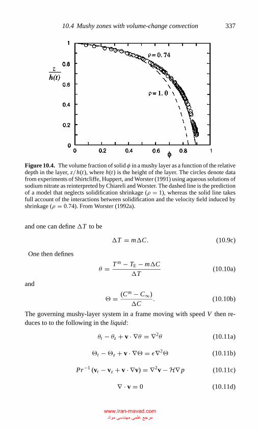
P1: GKE
CB381-10 CB381-Davis May 17, 2001 18:58 Char Count= 0
10.4 Mushy zones with volume-change convection 337
Figure 10.4. The volume fraction of solidφ in a mushy layer as a function of the relativedepth in the layer, z/h(t), where h(t) is the height of the layer. The circles denote datafrom experiments of Shirtcliffe, Huppert, and Worster (1991) using aqueous solutions ofsodium nitrate as reinterpreted by Chiareli and Worster. The dashed line is the predictionof a model that neglects solidification shrinkage (ρ = 1), whereas the solid line takesfull account of the interactions between solidification and the velocity field induced byshrinkage (ρ = 0.74). From Worster (1992a).
and one can define �T to be
�T = m�C. (10.9c)
One then defines
θ = T m − TE − m�C
�T(10.10a)
and
� = (Cm − C∞)
�C. (10.10b)
The governing mushy-layer system in a frame moving with speed V then re-duces to to the following in the liquid:
θt − θz + v · ∇θ = ∇2θ (10.11a)
�t −�z + v · ∇� = ε∇2� (10.11b)
Pr−1 (vt − vz + v · ∇v) = ∇2v − H∇ p (10.11c)
∇ · v = 0 (10.11d)
www.iran-mavad.com مرجع علمی مھندسی مواد
P1: GKE
CB381-10 CB381-Davis May 17, 2001 18:58 Char Count= 0
338 10. Mesoscale fluid flow
with the interface conditions on z = h,
θ = � (10.11e)
∇θ · n = ∇� · n (10.11f)
[V · n] = 0 (10.11g)[V · ti] = 0, i = 1, 2 (10.11h)
and as z → ∞� → 0; θ = θ∞, v → (1 − ρ)z. (10.11i)
The nondimensional parameters are the Prandtl number Pr , the permeabilityratio
H = δ2T /"
∗ (10.12a)
the far-field transport θ∞,
θ∞ = T∞ − TE
�T+ 1 (10.12b)
and
ε = D�/κ�. (10.12c)
In the mush, the assumption of thermodynamic equilibrium gives in 0 <z < h,
θ ≡ � (10.13a)
θt − θz + V · ∇θ = ∇2θ + S1 (φt − φz) (10.13b)
(1 − φ) (θt − θz) + V · ∇θ = ρ (θ − C) (φt − φz) (10.13c)
∇ · V = (1 − ρ) (φt − φz) (10.13d)
and Darcy’s law
V = −"(φ)∇ p. (10.13e)
Here,
S1 = ρsL
ρ�cp�T, (10.14a)
and
C = Cs − CE
�C− 1, (10.14b)
www.iran-mavad.com مرجع علمی مھندسی مواد
P1: GKE
CB381-10 CB381-Davis May 17, 2001 18:58 Char Count= 0
10.4 Mushy zones with volume-change convection 339
where Cs is the solute concentration in the solid matrix, and V = (1 − φ) v.Chiareli and Worster chose the empirical law for permeability,
"(φ) = (1−φ)q (10.15)
where q indicates the sensitivity to changes in permeability.Finally, at z = 0,
θ = −1, V · z = (1 − ρ) (1 − φ) (10.16)
and at z = h
[θ ] = 0, φ = 0, [∇θ · n] = 0, [p] = 0. (10.17)
As seen in Section 9.3, the flow produced by density changes is determinedby the continuity equation only. The Navier–Stokes equation, not shown, merelydetermines the pressure field.
A basic state for this system is
v = (0, 0, 1 − ρ) in the liquid (10.18a)
V = {0, 0, (1 − ρ)(1 − φ)} in the mush. (10.18b)
In the liquid,
θ = θ∞ + (θ I − θ∞)
e−ρ(z−h) (10.18c)
and
θ = θ Ie−ρ(z−h)/ε. (10.18d)
The interfacial temperature is θ I,
θ I = − ε
1 − ε θ∞. (10.18e)
In the mush,
φ = θ
C − θ (10.18f)
and so
d θ
dz= ρθ∞ − θ − S1θ
C − θ − (1 − ρ) C ln
(C − θC), (10.18g)
which determines h. Finally,
d p
dz= − (1 − ρ)
1 − φ" (φ)
. (10.18h)
www.iran-mavad.com مرجع علمی مھندسی مواد
P1: GKE
CB381-10 CB381-Davis May 17, 2001 18:58 Char Count= 0
340 10. Mesoscale fluid flow
In the basic state the flow is vertical; in the liquid there are exponential profilesof temperature and concentration, and in the mush the profiles are given by Eqs.(10.18f–h).
Chiareli and Worster (1995) identified a near-eutectic limit that simplifiesthe dynamics. When �C → 0, then C∞ → CE and one obtains the limitingforms of the Fowler (1985) model generalized to q �= 1.
The basic state suggests considering ( for �C → 0)
C → ∞, θ∞ → ∞, C/θ∞ = O(1), q = q/C (10.19a)
and rescaling as follows:
φ = Cφ and z = ρθ∞z. (10.19b)
If one considers the linear stability problem in the unscaled variables and usesnormal modes exp (σ t + iax), then
a = a
ρθ∞, σ = σ
ρθ∞. (10.19c)
The leading-order linear stability problem reduces in the mushy layer to(D
2 − a2)θ = 0 (10.20a)
(σ − ρ D
)θ + W = ρ
(D − σ ) φ (10.20b)
(D
2 − q D − a2)
W = a2 (1 − ρ) pφ. (10.20c)
A special case is considered in which the mush–liquid interface is unperturbed.This decouples the mush from the bulk liquid. The boundary conditions on themush are then
θ = 0, W = 0 at z = 0. (10.20d)
θ = 0, DW = 0, φ = 0 at z = 1. (10.20e)
In conditions (10.20 d,e), θ,W , and φ represent normal-mode amplitudes, andD = d/dz.
Clearly, Eq. (10.20a) and θ = 0 on z = 0, 1 imply that θ ≡ 0. The remainingsystem is solved numerically. The results are shown in Figure 10.5. Only whenq is sufficiently large is there an instability justifying the rescaling (10.19a).Extreme changes in permeability result in an instability that has the streamlinesshown in Figure 10.6 and is suggestive as a precursor to the formation of achanneled mush. Chiareli and Worster (1995) verified that the more generalmodel gives qualitatively the same instability.
www.iran-mavad.com مرجع علمی مھندسی مواد
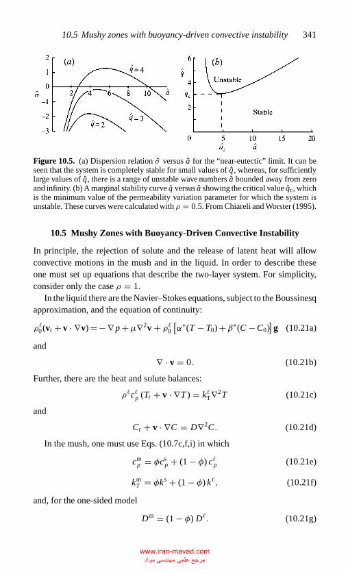
P1: GKE
CB381-10 CB381-Davis May 17, 2001 18:58 Char Count= 0
10.5 Mushy zones with buoyancy-driven convective instability 341
Figure 10.5. (a) Dispersion relation σ versus a for the “near-eutectic” limit. It can beseen that the system is completely stable for small values of q , whereas, for sufficientlylarge values of q , there is a range of unstable wave numbers a bounded away from zeroand infinity. (b) A marginal stability curve q versus a showing the critical value qc, whichis the minimum value of the permeability variation parameter for which the system isunstable. These curves were calculated with ρ = 0.5. From Chiareli and Worster (1995).
10.5 Mushy Zones with Buoyancy-Driven Convective Instability
In principle, the rejection of solute and the release of latent heat will allowconvective motions in the mush and in the liquid. In order to describe theseone must set up equations that describe the two-layer system. For simplicity,consider only the case ρ = 1.
In the liquid there are the Navier–Stokes equations, subject to the Boussinesqapproximation, and the equation of continuity:
ρ�0(vt + v · ∇v) = − ∇ p +µ∇2v + ρ�0[α∗(T − T0) +β∗(C − C0)
]g (10.21a)
and
∇ · v = 0. (10.21b)
Further, there are the heat and solute balances:
ρ�c�p (Tt + v · ∇T ) = k�T∇2T (10.21c)
and
Ct + v · ∇C = D∇2C. (10.21d)
In the mush, one must use Eqs. (10.7c,f,i) in which
cmp = φcs
p + (1 − φ) c�p (10.21e)
kmT = φks + (1 − φ) k�, (10.21f)
and, for the one-sided model
Dm = (1 − φ) D�. (10.21g)
www.iran-mavad.com مرجع علمی مھندسی مواد
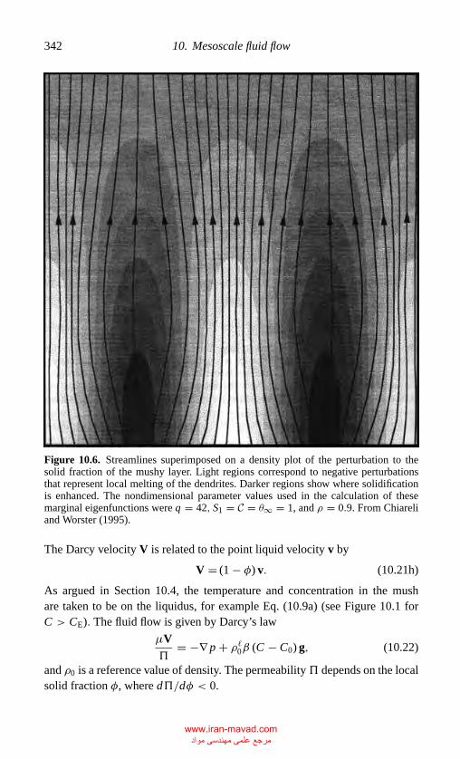
P1: GKE
CB381-10 CB381-Davis May 17, 2001 18:58 Char Count= 0
342 10. Mesoscale fluid flow
Figure 10.6. Streamlines superimposed on a density plot of the perturbation to thesolid fraction of the mushy layer. Light regions correspond to negative perturbationsthat represent local melting of the dendrites. Darker regions show where solidificationis enhanced. The nondimensional parameter values used in the calculation of thesemarginal eigenfunctions were q = 42, S1 = C = θ∞ = 1, and ρ = 0.9. From Chiareliand Worster (1995).
The Darcy velocity V is related to the point liquid velocity v by
V = (1 − φ) v. (10.21h)
As argued in Section 10.4, the temperature and concentration in the mushare taken to be on the liquidus, for example Eq. (10.9a) (see Figure 10.1 forC > CE). The fluid flow is given by Darcy’s law
µV"
= −∇ p + ρ�0β (C − C0) g, (10.22)
and ρ0 is a reference value of density. The permeability" depends on the localsolid fraction φ, where d"/dφ < 0.
www.iran-mavad.com مرجع علمی مھندسی مواد
P1: GKE
CB381-10 CB381-Davis May 17, 2001 18:58 Char Count= 0
10.5 Mushy zones with buoyancy-driven convective instability 343
Notice that condition (10.22) implies that, in the mush,
β = β∗ + mα∗ (10.23)
and β > 0, usually.Introduce the following scaled quantities. In the mush z < h(x, y, t),
θ = T − TL(C0)
�T, � = C − C0
�C, (10.24)
where �T = m�C = TL(C0) − TE. Scale speeds on V, lengths on δT ,
time on δT /V , and pressure on β�Cρ�0gκ/V , where V is the constant rate ofsolidification.
The nondimensional governing system (Worster 1992b) is then as follows:liquid (z > h):
θt − θz + v · ∇θ = ∇2θ (10.25a)
�t −�z + v · ∇� = ε∇2� (10.25b)
Pr−1(vt − uz + v · ∇v) = ∇2u + RTθk − RC
[�k + β
β∗ ∇ p
](10.25c)
mush (z < h):(∂
∂t− ∂
∂z
)[θ + S
C − ξC − θ
]+ V · ∇θ = ∇2θ (10.25d)
(∂
∂t− ∂
∂z
)ξ + V · ∇θ = 0 (10.25e)
V"
= −Rm [∇ p + θk] (10.25f)
∇ · V = 0 (10.25g)
Interface (z = h):
θ = � (10.25h)
n · ∇θ = n · ∇� (10.25i)
[n · V] = 0 (10.25j)
[t · V] = 0 (10.25k)
www.iran-mavad.com مرجع علمی مھندسی مواد
P1: GKE
CB381-10 CB381-Davis May 17, 2001 18:58 Char Count= 0
344 10. Mesoscale fluid flow
Infinity (z → ∞):
θ = θ∞ (10.25l)
� → 0 (10.25m)
V → 0. (10.25n)
In the preceding, the velocity is written in terms of V = (1 − φ) v, and thusin the liquid region φ = 0 and V = v.
Here
RT = α∗�T gδ3T
/κν
RC = β∗�Cgδ3T
/κν
Rm = β�Cg"∗δT/κν
S = LV/
cp�T
C = (Cs − C0)/�C
ε = D/κ
ξ = (1 − φ)�+ φC
(10.26)
In the coordinate system moving with the interface, there is a static basicstate. In the liquid,
θ = θ∞ + (θ I − θ∞)
e−(z−h) (10.27a)
θ = θ Ie−(z−h)/ε (10.27b)
with
θ I = − ε
1 − ε θ∞. (10.27c)
In the mush,
z = α − Cα − β ln
(α + 1
α − θ)
+ C − βα − β ln
(β + 1
β − θ), (10.27d)
where
α = A + B, β = A − B, A = 1/2 (C + θ∞ + S), B2 = A2 − Cθ∞ − Sθ I
(10.27e)
www.iran-mavad.com مرجع علمی مھندسی مواد
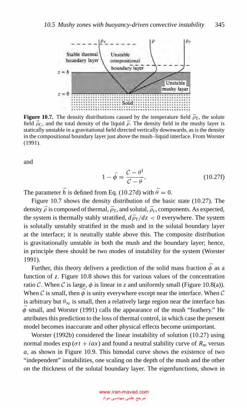
P1: GKE
CB381-10 CB381-Davis May 17, 2001 18:58 Char Count= 0
10.5 Mushy zones with buoyancy-driven convective instability 345
Figure 10.7. The density distributions caused by the temperature field ρT, the solutefield ρC, and the total density of the liquid ρ. The density field in the mushy layer isstatically unstable in a gravitational field directed vertically downwards, as is the densityin the compositional boundary layer just above the mush–liquid interface. From Worster(1991).
and
1 − φ = C − θ I
C − θ , (10.27f)
The parameter h is defined from Eq. (10.27d) with θ = 0.Figure 10.7 shows the density distribution of the basic state (10.27). The
density ρ is composed of thermal, ρT, and solutal, ρc, components. As expected,the system is thermally stably stratified, dρT/dz < 0 everywhere. The systemis solutally unstably stratified in the mush and in the solutal boundary layerat the interface; it is neutrally stable above this. The composite distributionis gravitationally unstable in both the mush and the boundary layer; hence,in principle there should be two modes of instability for the system (Worster1991).
Further, this theory delivers a prediction of the solid mass fraction φ as afunction of z. Figure 10.8 shows this for various values of the concentrationratio C.When C is large, φ is linear in z and uniformly small (Figure 10.8(a)).When C is small, then φ is unity everywhere except near the interface. When Cis arbitrary but θ∞ is small, then a relatively large region near the interface hasφ small, and Worster (1991) calls the appearance of the mush “feathery.” Heattributes this prediction to the loss of thermal control, in which case the presentmodel becomes inaccurate and other physical effects become unimportant.
Worster (1992b) considered the linear instability of solution (10.27) usingnormal modes exp (σ t + iax) and found a neutral stability curve of Rm versusa, as shown in Figure 10.9. This bimodal curve shows the existence of two“independent” instabilities, one scaling on the depth of the mush and the otheron the thickness of the solutal boundary layer. The eigenfunctions, shown in
www.iran-mavad.com مرجع علمی مھندسی مواد
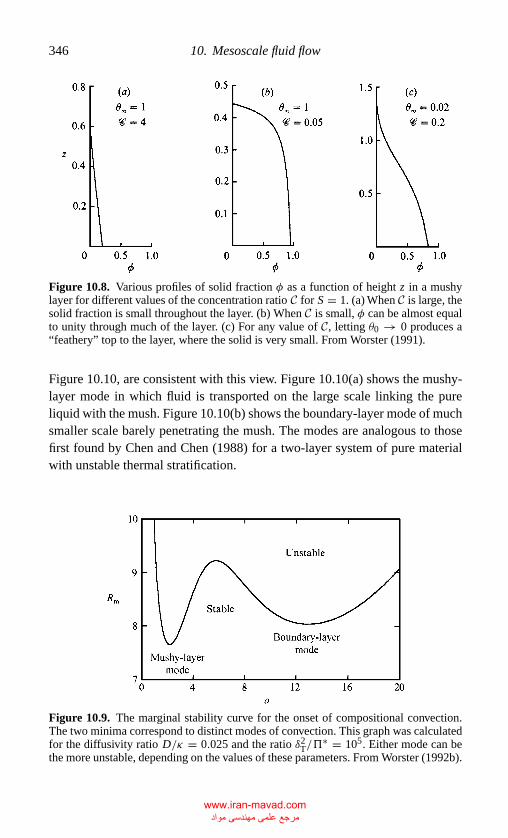
P1: GKE
CB381-10 CB381-Davis May 17, 2001 18:58 Char Count= 0
346 10. Mesoscale fluid flow
Figure 10.8. Various profiles of solid fraction φ as a function of height z in a mushylayer for different values of the concentration ratio C for S = 1. (a) When C is large, thesolid fraction is small throughout the layer. (b) When C is small, φ can be almost equalto unity through much of the layer. (c) For any value of C, letting θ0 → 0 produces a“feathery” top to the layer, where the solid is very small. From Worster (1991).
Figure 10.10, are consistent with this view. Figure 10.10(a) shows the mushy-layer mode in which fluid is transported on the large scale linking the pureliquid with the mush. Figure 10.10(b) shows the boundary-layer mode of muchsmaller scale barely penetrating the mush. The modes are analogous to thosefirst found by Chen and Chen (1988) for a two-layer system of pure materialwith unstable thermal stratification.
Figure 10.9. The marginal stability curve for the onset of compositional convection.The two minima correspond to distinct modes of convection. This graph was calculatedfor the diffusivity ratio D/κ = 0.025 and the ratio δ2
T/"∗ = 105. Either mode can be
the more unstable, depending on the values of these parameters. From Worster (1992b).
www.iran-mavad.com مرجع علمی مھندسی مواد
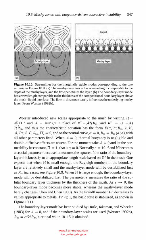
P1: GKE
CB381-10 CB381-Davis May 17, 2001 18:58 Char Count= 0
10.5 Mushy zones with buoyancy-driven convective instability 347
Figure 10.10. Streamlines for the marginally stable modes corresponding to the twominima in Figure 10.9. (a) The mushy-layer mode has a wavelength comparable to thedepth of the mushy layer, and the flow penetrates the layer. (b) The boundary-layer modehas a wavelength comparable to the thickness of the compositional boundary layer abovethe mush–liquid interface. The flow in this mode barely influences the underlying mushylayer. From Worster (1992b).
Worster introduced new scales appropriate to the mush by writing H=δ2
T
/"∗ and A = ma∗/β in place of RT =AHRm , and RC = (1 +A)
HRm , and thus the characteristic equation has the form F(σ , a; Rm , ε,H,A, Pr, S, C, θ∞,") = 0, and on the neutral curve,σ = 0, Rm = Rm (σ ; a),withall other parameters fixed. When A = 0, thermal buoyancy is negligible anddouble-diffusive effects are absent. For the moment take A = 0 and let the per-meability be constant," ≡ 1, that is q = 0. Normally ε ≡ 10−2 andH becomesa crucial parameter because it measures the square of the ratio of the boundary-layer thickness δT to an appropriate length scale based on"∗ in the mush. Oneexpects that when H is small enough, the Rayleigh numbers in the boundarylayer are relatively small and the mushy-layer mode will be destabilized firstas Rm increases; see Figure 10.9. When H is large enough, the boundary-layermode will be destabilized first. The parameter ε measures the ratio of the so-lutal boundary layer thickness by the thickness of the mush. As ε → 0, theboundary-layer mode becomes more stable, whereas the mushy-layer modebarely changes (Chen and Chen 1988). As the Prandtl number Pr decreases tovalues appropriate to metals, Pr 1, the basic state is stabilized, as shown inFigure 10.11.
The boundary-layer mode has been studied by Hurle, Jakeman, and Wheeler(1983) for A = 0, and if the boundary-layer scales are used (Worster 1992b),Rδc = ε3HRm , a critical value 10–15 is obtained.
www.iran-mavad.com مرجع علمی مھندسی مواد
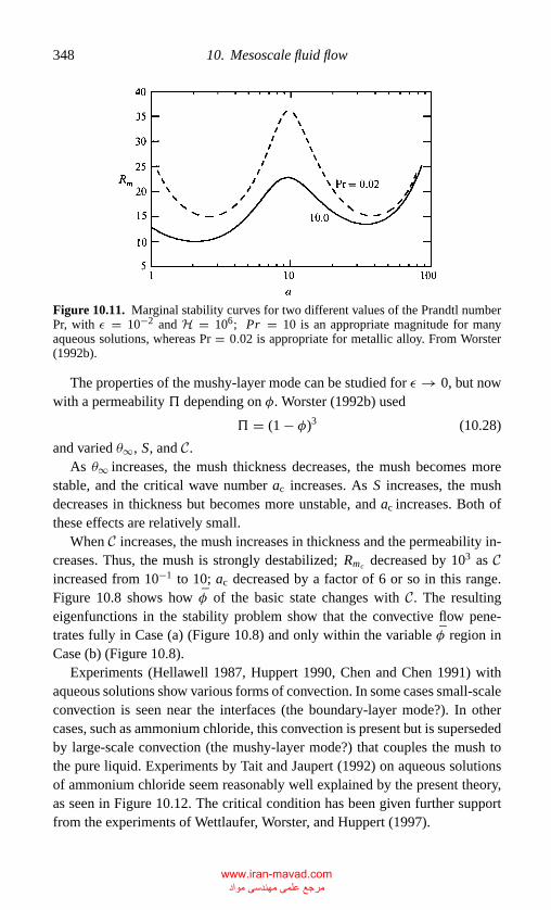
P1: GKE
CB381-10 CB381-Davis May 17, 2001 18:58 Char Count= 0
348 10. Mesoscale fluid flow
Figure 10.11. Marginal stability curves for two different values of the Prandtl numberPr, with ε = 10−2 and H = 106; Pr = 10 is an appropriate magnitude for manyaqueous solutions, whereas Pr = 0.02 is appropriate for metallic alloy. From Worster(1992b).
The properties of the mushy-layer mode can be studied for ε → 0, but nowwith a permeability " depending on φ. Worster (1992b) used
" = (1 − φ)3 (10.28)
and varied θ∞, S, and C.As θ∞ increases, the mush thickness decreases, the mush becomes more
stable, and the critical wave number ac increases. As S increases, the mushdecreases in thickness but becomes more unstable, and ac increases. Both ofthese effects are relatively small.
When C increases, the mush increases in thickness and the permeability in-creases. Thus, the mush is strongly destabilized; Rmc decreased by 103 as Cincreased from 10−1 to 10; ac decreased by a factor of 6 or so in this range.Figure 10.8 shows how φ of the basic state changes with C. The resultingeigenfunctions in the stability problem show that the convective flow pene-trates fully in Case (a) (Figure 10.8) and only within the variable φ region inCase (b) (Figure 10.8).
Experiments (Hellawell 1987, Huppert 1990, Chen and Chen 1991) withaqueous solutions show various forms of convection. In some cases small-scaleconvection is seen near the interfaces (the boundary-layer mode?). In othercases, such as ammonium chloride, this convection is present but is supersededby large-scale convection (the mushy-layer mode?) that couples the mush tothe pure liquid. Experiments by Tait and Jaupert (1992) on aqueous solutionsof ammonium chloride seem reasonably well explained by the present theory,as seen in Figure 10.12. The critical condition has been given further supportfrom the experiments of Wettlaufer, Worster, and Huppert (1997).
www.iran-mavad.com مرجع علمی مھندسی مواد
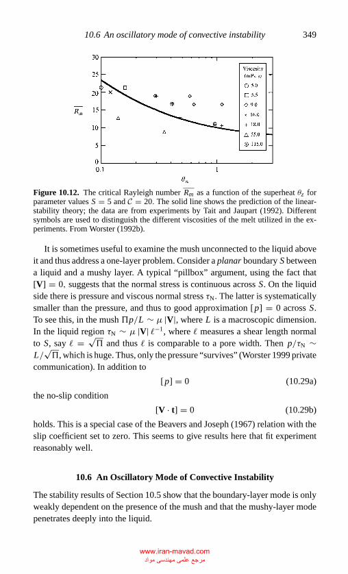
P1: GKE
CB381-10 CB381-Davis May 17, 2001 18:58 Char Count= 0
10.6 An oscillatory mode of convective instability 349
Figure 10.12. The critical Rayleigh number Rm as a function of the superheat θz forparameter values S = 5 and C = 20. The solid line shows the prediction of the linear-stability theory; the data are from experiments by Tait and Jaupart (1992). Differentsymbols are used to distinguish the different viscosities of the melt utilized in the ex-periments. From Worster (1992b).
It is sometimes useful to examine the mush unconnected to the liquid aboveit and thus address a one-layer problem. Consider a planar boundary S betweena liquid and a mushy layer. A typical “pillbox” argument, using the fact that[V] = 0, suggests that the normal stress is continuous across S. On the liquidside there is pressure and viscous normal stress τN. The latter is systematicallysmaller than the pressure, and thus to good approximation [p] = 0 across S.To see this, in the mush "p/L ∼ µ |V|, where L is a macroscopic dimension.In the liquid region τN ∼ µ |V| �−1, where � measures a shear length normalto S, say � = √
" and thus � is comparable to a pore width. Then p/τN ∼L/
√", which is huge. Thus, only the pressure “survives” (Worster 1999 private
communication). In addition to
[p] = 0 (10.29a)
the no-slip condition
[V · t] = 0 (10.29b)
holds. This is a special case of the Beavers and Joseph (1967) relation with theslip coefficient set to zero. This seems to give results here that fit experimentreasonably well.
10.6 An Oscillatory Mode of Convective Instability
The stability results of Section 10.5 show that the boundary-layer mode is onlyweakly dependent on the presence of the mush and that the mushy-layer modepenetrates deeply into the liquid.
www.iran-mavad.com مرجع علمی مھندسی مواد
P1: GKE
CB381-10 CB381-Davis May 17, 2001 18:58 Char Count= 0
350 10. Mesoscale fluid flow
When δT is much larger than the average spacing between the dendrites,Emms and Fowler (1994) showed that the interfacial condition [p] = 0 reducesto p-is-constant for the mush. In the present analysis a model system is usedin which the liquid–mush interface is a fixed plane and p-is-constant is re-placed with W = 0. This model, introduced by Amberg and Homsy (1993),permits analysis of the dynamics within the mush, free from coupling with theliquid.
This model further restricts the mush thickness, now called d, by lettingδ = d/δT 1. Anderson and Worster (1995) equated the heat fluxes at theinterface �T/d ∼ [T∞ − TL(C0)] /δT and found that
θ∞ ≡ T∞ − TL(C0)
�T∼ 1
δ. (10.30a)
Amberg and Homsy (1993) likewise showed that, when δ is small, C is large,namely.
C = C
δ(10.30b)
where C = O(1) as δ → 0, which corresponds to the near-eutectic approxima-tion used by Fowler (1985).
Emms and Fowler (1994) further assumed that the Stefan number is large,that is,
S = S
δ, (10.30c)
where S = O(1) as δ → 0.Through this model, a term in Eq. (10.25d) can be simplified,
C − ξC − θ = C − (1 − φ)θ − Cφ
C − θ = 1 − φ, (10.31)
and in Eq. (10.27d), the constant, unity, is annihilated by the derivatives. Themodel system related to Eq. (10.28) then becomes
(∂
∂t− ∂
∂z
)(θ − Sφ) + V · ∇θ = ∇2θ (10.32a)
(∂
∂t− ∂
∂z
){(1 − φ)θ + Cφ} + V · ∇θ = 0 (10.32b)
"−1(φ)V = −∇ p − Rmθk (10.32c)
∇ · V = 0 (10.32d)
www.iran-mavad.com مرجع علمی مھندسی مواد
P1: GKE
CB381-10 CB381-Davis May 17, 2001 18:58 Char Count= 0
10.6 An oscillatory mode of convective instability 351
with the boundary conditions
θ = −1, W = 0 on z = 0 (10.33a,b)
θ = 0, W = 0, φ = 0 on z = δ. (10.33c,d,e)
Introduce the rescalings
(X, Y, Z ) = (x, y, z)
δ, T = t/δ2, R2 = δRm (10.34)
p1 = p/R, V1 = δ
RV
as suggested by Amberg and Homsy (1993). The subscript unity is now dropped.The basic state is steady and horizontally uniform and satisfies
−δ[θ − S
δφ
]′= θ
′′ (10.35a)
−δ[(1 − φ)θ + C
δφ
]′= 0 (10.35b)
− p′ − Rθ = 0 (10.35c)
with
θ = −1 on Z = 0 (10.36a)
and
θ = φ = 0 on Z = 1, (10.36b,c)
where a prime denotes d/d Z .Approximate solutions to systems (10.35) and (10.36) can be obtained in
powers of δ,namely.
θ = Z − 1 − 1
2δ (Z2 − Z
)+ · · · (10.37a)
φ = δφ = −δ Z − 1
C+ δ2
[− (Z − 1)2
C2+
2C(Z2 − Z )
]+ · · ·, (10.37b)
where
= 1 + S/C . (10.37c)
Note that φ is small, and θ is linear to leading order, which is directly relatedto convection in a passive porous layer as considered by Palm, Weber, and
www.iran-mavad.com مرجع علمی مھندسی مواد
P1: GKE
CB381-10 CB381-Davis May 17, 2001 18:58 Char Count= 0
352 10. Mesoscale fluid flow
Kvernvold (1972). It is the higher-order term, O(δ) that models the “mushiness.”Anderson and Worster (1996) examined the linear instabilities of the basic stateusing normal modes exp (σT + iaX ). They wrote
"−1(δφ) = 1 + δφ0K1 + · · ·
σ = σ0 + δσ1 + · · ·R = R0 + δR1 + · · ·θ = θ0 + δθ1 + · · ·φ = φ0 + δφ1 + · · ·V = V0 + δV1 + · · ·,
(10.38)
where carets denote normal-mode amplitudes, and from Eq. (10.37b)
φ0 = (1 − Z ) /C . (10.39)
The constant K1 characterizes variations in permeability with solid fraction:At O(δ) an orthogonality condition determinesσ1 = σ1R+iω1 and R1.When
conditions are neutral, σ1R = 0, the orthogonality condition has a real part
R1
R0= 1
4
K1
C+ S
C2
[1
4+ π2(1 + cos ω1)(
π2 − ω21
)2]
(10.40a)
and an imaginary part
ω1
{1 + S
C2 2
π2 + a2
π2 − ω21
[1 − 2π2
π2 − ω21
sin ω1
ω1
]}= 0 (10.40b)
There is the steady mode with ω1 = 0 and
R = R0
[1 + δ R1
R0
]+ O(δ2)
= a2 + π2
a 1/2
{1 + δ
[K1
4C+(
1
4+ 2
π2
)S
C2
]}+ O(δ2), (10.41)
where R20 = (a2 + π2)2/ a2 has been used. Result (10.41) agrees with that
of Amberg and Homsy (1993) when proper regard is taken of the differentscalings as well as the results in Section 10.5.
When conditions allow oscillations, ω1 �= 0, (Anderson and Worster 1996).Figure 10.13 shows ω1 versus a/π for fixed values of S/C2
2 = S/(C + S)2δ.When S/C2
2 < 1, the oscillatory mode exists only for a large enough. WhenS/C2
2 ≥ 1, it exists for all a ≥ 0.
www.iran-mavad.com مرجع علمی مھندسی مواد
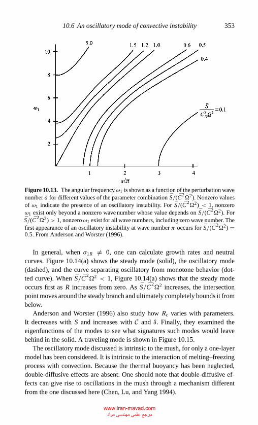
P1: GKE
CB381-10 CB381-Davis May 17, 2001 18:58 Char Count= 0
10.6 An oscillatory mode of convective instability 353
Figure 10.13. The angular frequencyω1 is shown as a function of the perturbation wavenumber a for different values of the parameter combination S/(C2
2). Nonzero valuesof ω1 indicate the presence of an oscillatory instability. For S/(C2
2) < 1, nonzeroω1 exist only beyond a nonzero wave number whose value depends on S/(C2
2). ForS/(C2
2) > 1, nonzeroω1 exist for all wave numbers, including zero wave number. Thefirst appearance of an oscillatory instability at wave number π occurs for S/(C2
2) =0.5. From Anderson and Worster (1996).
In general, when σ1R �= 0, one can calculate growth rates and neutralcurves. Figure 10.14(a) shows the steady mode (solid), the oscillatory mode(dashed), and the curve separating oscillatory from monotone behavior (dot-ted curve). When S/C2
2 < 1, Figure 10.14(a) shows that the steady modeoccurs first as R increases from zero. As S/C2
2 increases, the intersectionpoint moves around the steady branch and ultimately completely bounds it frombelow.
Anderson and Worster (1996) also study how Rc varies with parameters.It decreases with S and increases with C and δ. Finally, they examined theeigenfunctions of the modes to see what signatures such modes would leavebehind in the solid. A traveling mode is shown in Figure 10.15.
The oscillatory mode discussed is intrinsic to the mush, for only a one-layermodel has been considered. It is intrinsic to the interaction of melting–freezingprocess with convection. Because the thermal buoyancy has been neglected,double-diffusive effects are absent. One should note that double-diffusive ef-fects can give rise to oscillations in the mush through a mechanism differentfrom the one discussed here (Chen, Lu, and Yang 1994).
www.iran-mavad.com مرجع علمی مھندسی مواد
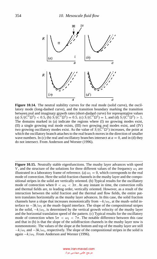
P1: GKE
CB381-10 CB381-Davis May 17, 2001 18:58 Char Count= 0
354 10. Mesoscale fluid flow
Figure 10.14. The neutral stability curves for the real mode (solid curve), the oscil-latory mode (long-dashed curve), and the transition boundary marking the transitionbetween real and imaginary growth rates (short-dashed curve) for representative values(a) S/(C2
2) < 0.5, (b) S/(C2 2) = 0.5, (c) S/(C2
2) = 1, and (d) S/(C2 2) > 1.
The domains marked in (a) indicate the regions where (I) no growing modes exist,(II) a single growing real mode exists, (III) two growing real modes exist, and (IV)two growing oscillatory modes exist. As the value of S/(C2
2) increases, the point atwhich the oscillatory branch attaches to the real branch moves in the direction of smallerwave numbers. In (c) the real and oscillatory branches intersect at a = 0, and in (d) theydo not intersect. From Anderson and Worster (1996).
Figure 10.15. Neutrally stable eigenfunctions. The mushy layer advances with speedV , and the structure of the solutions for three different values of the frequency ω1 areillustrated in a laboratory frame of reference. (a) ω1 = 0, which corresponds to the realmode of convection. Here the solid-fraction channels in the mushy layer and the compo-sitional stripes in the solid are vertically oriented. (b) Typical results for the oscillatorymode of convection when 0 < ω1 < 3π . At any instant in time, the convection rollsand thermal fields are, to leading order, vertically oriented. However, as a result of theinteraction between the solid fraction and the thermal and flow fields, the entire pat-tern translates horizontally as the mushy layer advances. In this case, the solid fractionchannels have a slope that increases monotonically from −k/ω1, at the mush–solid in-terface to −3k/ω1 at the mush–liquid interface. The slope of the compositional stripesin the solid, −k/ω1, is determined by the vertical growth velocity of the mushy layerand the horizontal translation speed of the pattern. (c) Typical results for the oscillatorymode of convection when 5π < ω1 < 7π . The notable difference between this caseand that in (b) is that the slope of the solidfraction channels in the mushy layer now isnonmonotonic. The values of the slope at the bottom and top of the mushy layer are still−k/ω1 and −3k/ω1, respectively. The slope of the compositional stripes in the solid isagain −k/ω1. From Anderson and Worster (1996).
www.iran-mavad.com مرجع علمی مھندسی مواد
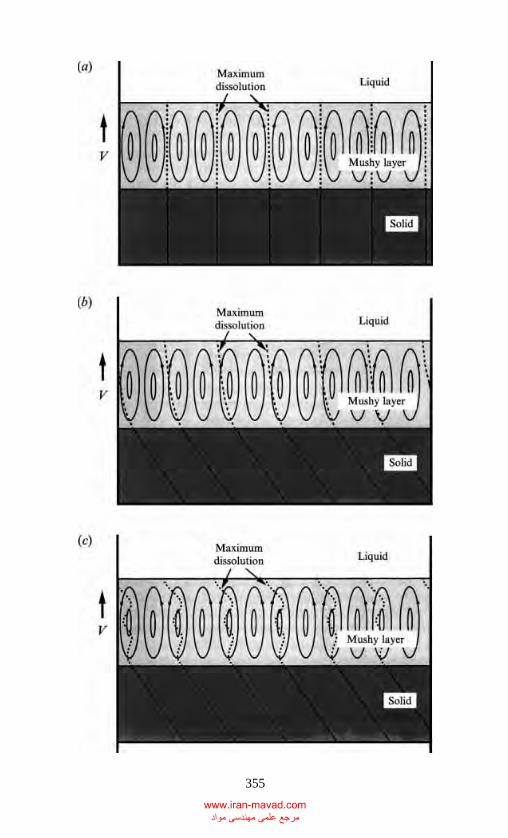
P1: GKE
CB381-10 CB381-Davis May 17, 2001 18:58 Char Count= 0
355
www.iran-mavad.com مرجع علمی مھندسی مواد
P1: GKE
CB381-10 CB381-Davis May 17, 2001 18:58 Char Count= 0
356 10. Mesoscale fluid flow
10.7 Weakly Nonlinear Convection
In Section 10.6 a model appropriate to thin mushy layers, δ → 0, was examined,particularly for C ∼ δ−1, S ∼ δ−1 as δ → 0. The governing system for thismodel is Eq. (10.32) with rescaling (10.34) for X , Y , Z , T , and R, and this willbe used to examine pattern selection for the steady mode in the one-layer case.
Anderson and Worster (1995) used a double expansion in δ and ε, the dis-turbance amplitude for the limiting case 0 ≤ ε δ 1. The basic stateis given by the analysis of Section 10.6 and is of the form (θ, φ,V, p) =[θ (z), φ(z), 0, R p(z)] where each element depends on δ. Because φ ∼ δ, onecan represent the permeability as follows:
"−1(φ) = 1 + K1φ + K2φ2 + K3φ
3 + · · · (10.42)
with K1 > 0 and K2, K3, . . . characterizing variations in permeability withsolid fraction.
The disturbed fields are written
θ = θ + εθ (X, Y, Z , T )
φ = φ + εφ(X, Y, Z , T )
V = 0 + εR
δV(X, Y, Z , T )
p = R p + εR p(X, Y, Z , T )
(10.43)
Note that the asymptotic representation for V ∼ ε/δ is well defined. AtO(1) in ε, the basic state is recovered. At O(ε), the linear theory of Sec-tion 10.6 is recovered. At O(ε2), one obtains an integrable system, and atO(ε3), an orthogonality condition that produces a set of amplitude equations isenforced.
Anderson and Worster (1995) investigated the competition between rolls andhexagons, for a = ac, where the linear theory eigenfunctions are proportionalto η(X, Y ),
η =3∑
j=1
A j (τ )eia j ·r + A∗j (τ )e−ia j ·r (10.44)
where τ = ε2T and
a j ={
(0, π ),
(1
2π
√3,
1
2π
),
(1
2π
√3,−1
2π
)}, r = (X, Y ).
This gives rise to amplitude equations of the form (4.18). Most important, thecoefficient b0 of the quadratic terms determines the character of the hexagonal
www.iran-mavad.com مرجع علمی مھندسی مواد
P1: GKE
CB381-10 CB381-Davis May 17, 2001 18:58 Char Count= 0
10.8 Chimneys 357
pattern that is stable. Here, in unscaled variables
−εb0 = 6π3
{K1
Cδ + 2δ
3π2
[4
3 2 +
(44
9+ 3π2
2
)K2
C2δ2− 26
7
S
C2δ
]},
(10.45)
and all terms here are O(δ).Figure 4.11 shows the bifurcation diagrams for εb0 < 0 and εb0 > 0
(downflow at the center), respectively. As R increases, there is a jump transitionto hexagons, and as R is further increased, rolls become stable as well. For Rsufficiently large, the hexagons become unstable, and only rolls persist.
The first analysis of this system was that of Amberg and Homsy (1993), whoconsidered the case S = O(1), and took into account nonlinear perturbations in"(φ). By taking S/C ∼ 1 as δ → 0,Anderson and Worster were able to accountfor additional physical effects such as nonlinear variations in θ (z), higher-ordereffects in " (φ), and interactions between the temperature and φ. It is this lasteffect that gives rise to the last term in Eq. (10.45) and allows the possibility thatεb0 can be positive. When S ∼ 1, this term disappears. Further, Amberg andHomsy found that rolls bifurcate supercritically only when K1/C < 0.226. Inthe present analysis, K1/C = O(δ), and thus the rolls are as pictured in Figure4.11.
Amberg and Homsy found that εb0 < 0, and thus only upflow hexagons canbe stable. The inclusion of further physical effects by Anderson and Worstershows that upflow or downflow hexagons are physically possible. Figure 10.16for K2 = 0 shows where one expects either up or down hexagons at onset andwhere the oscillatory mode, discussed in Section 10.7, is present. The weaklynonlinear analysis here describes only the steady bifurcations. Stable downhexagons can be found only for K2 < 0.131.
These results can be compared qualitatively with the observations of Tait,Jahrling, and Jaupart (1992) on ammonium chloride solutions in a tank cooledfrom below. They saw arrays with the hexagonal pattern of chimneys (see Sec-tion10.8) with downflow at the centers consistent with the preceding theory forK2 < 0.131. Without accounting for temperature–φ interactions, only upflowat centers would be predicted (Amberg and Homsy 1993).
10.8 Chimneys
When alloys are directionally solidified at speeds well within the regionwhere dendrites are present, certain defects can occur. One of these is the“freckle,” which is a long solid-free channel parallel to the pulling direction. The
www.iran-mavad.com مرجع علمی مھندسی مواد
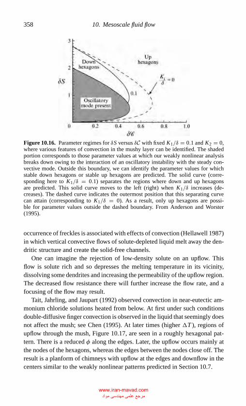
P1: GKE
CB381-10 CB381-Davis May 17, 2001 18:58 Char Count= 0
358 10. Mesoscale fluid flow
Figure 10.16. Parameter regimes for δS versus δC with fixed K1/δ = 0.1 and K2 = 0,where various features of convection in the mushy layer can be identified. The shadedportion corresponds to those parameter values at which our weakly nonlinear analysisbreaks down owing to the interaction of an oscillatory instability with the steady con-vective mode. Outside this boundary, we can identify the parameter values for whichstable down hexagons or stable up hexagons are predicted. The solid curve (corre-sponding here to K1/δ = 0.1) separates the regions where down and up hexagonsare predicted. This solid curve moves to the left (right) when K1/δ increases (de-creases). The dashed curve indicates the outermost position that this separating curvecan attain (corresponding to K1/δ = 0). As a result, only up hexagons are possi-ble for parameter values outside the dashed boundary. From Anderson and Worster(1995).
occurrence of freckles is associated with effects of convection (Hellawell 1987)in which vertical convective flows of solute-depleted liquid melt away the den-dritic structure and create the solid-free channels.
One can imagine the rejection of low-density solute on an upflow. Thisflow is solute rich and so depresses the melting temperature in its vicinity,dissolving some dendrites and increasing the permeability of the upflow region.The decreased flow resistance there will further increase the flow rate, and afocusing of the flow may result.
Tait, Jahrling, and Jaupart (1992) observed convection in near-eutectic am-monium chloride solutions heated from below. At first under such conditionsdouble-diffusive finger convection is observed in the liquid that seemingly doesnot affect the mush; see Chen (1995). At later times (higher �T ), regions ofupflow through the mush, Figure 10.17, are seen in a roughly hexagonal pat-tern. There is a reduced φ along the edges. Later, the upflow occurs mainly atthe nodes of the hexagons, whereas the edges between the nodes close off. Theresult is a planform of chimneys with upflow at the edges and downflow in thecenters similar to the weakly nonlinear patterns predicted in Section 10.7.
www.iran-mavad.com مرجع علمی مھندسی مواد
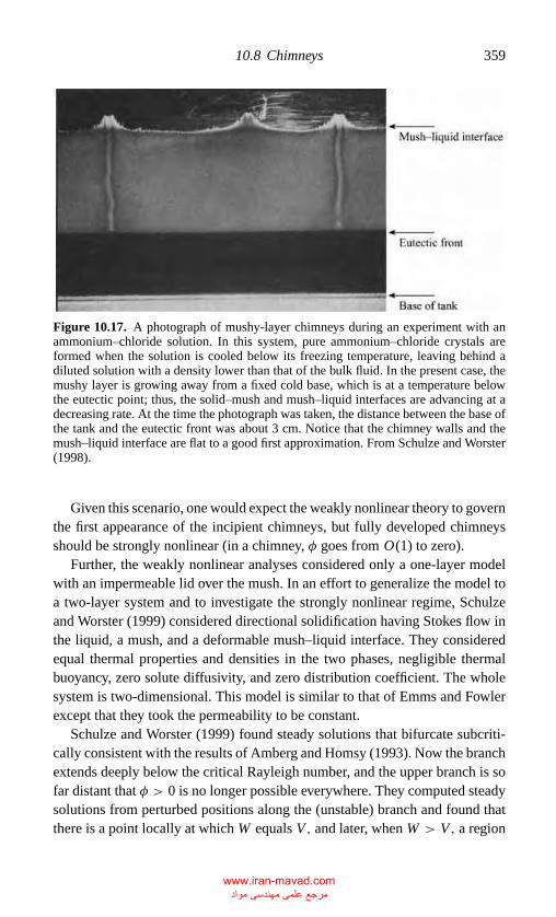
P1: GKE
CB381-10 CB381-Davis May 17, 2001 18:58 Char Count= 0
10.8 Chimneys 359
Figure 10.17. A photograph of mushy-layer chimneys during an experiment with anammonium–chloride solution. In this system, pure ammonium–chloride crystals areformed when the solution is cooled below its freezing temperature, leaving behind adiluted solution with a density lower than that of the bulk fluid. In the present case, themushy layer is growing away from a fixed cold base, which is at a temperature belowthe eutectic point; thus, the solid–mush and mush–liquid interfaces are advancing at adecreasing rate. At the time the photograph was taken, the distance between the base ofthe tank and the eutectic front was about 3 cm. Notice that the chimney walls and themush–liquid interface are flat to a good first approximation. From Schulze and Worster(1998).
Given this scenario, one would expect the weakly nonlinear theory to governthe first appearance of the incipient chimneys, but fully developed chimneysshould be strongly nonlinear (in a chimney, φ goes from O(1) to zero).
Further, the weakly nonlinear analyses considered only a one-layer modelwith an impermeable lid over the mush. In an effort to generalize the model toa two-layer system and to investigate the strongly nonlinear regime, Schulzeand Worster (1999) considered directional solidification having Stokes flow inthe liquid, a mush, and a deformable mush–liquid interface. They consideredequal thermal properties and densities in the two phases, negligible thermalbuoyancy, zero solute diffusivity, and zero distribution coefficient. The wholesystem is two-dimensional. This model is similar to that of Emms and Fowlerexcept that they took the permeability to be constant.
Schulze and Worster (1999) found steady solutions that bifurcate subcriti-cally consistent with the results of Amberg and Homsy (1993). Now the branchextends deeply below the critical Rayleigh number, and the upper branch is sofar distant that φ > 0 is no longer possible everywhere. They computed steadysolutions from perturbed positions along the (unstable) branch and found thatthere is a point locally at which W equals V, and later, when W > V, a region
www.iran-mavad.com مرجع علمی مھندسی مواد
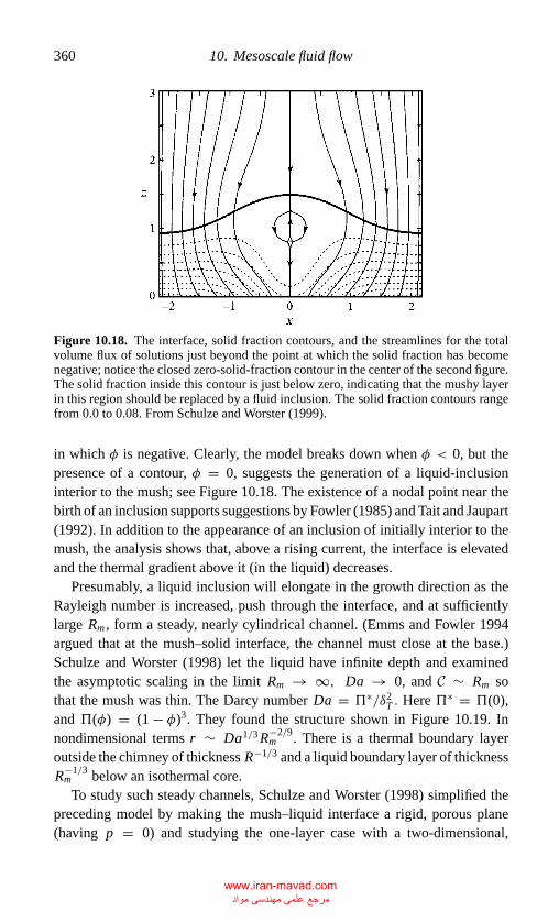
P1: GKE
CB381-10 CB381-Davis May 17, 2001 18:58 Char Count= 0
360 10. Mesoscale fluid flow
Figure 10.18. The interface, solid fraction contours, and the streamlines for the totalvolume flux of solutions just beyond the point at which the solid fraction has becomenegative; notice the closed zero-solid-fraction contour in the center of the second figure.The solid fraction inside this contour is just below zero, indicating that the mushy layerin this region should be replaced by a fluid inclusion. The solid fraction contours rangefrom 0.0 to 0.08. From Schulze and Worster (1999).
in which φ is negative. Clearly, the model breaks down when φ < 0, but thepresence of a contour, φ = 0, suggests the generation of a liquid-inclusioninterior to the mush; see Figure 10.18. The existence of a nodal point near thebirth of an inclusion supports suggestions by Fowler (1985) and Tait and Jaupart(1992). In addition to the appearance of an inclusion of initially interior to themush, the analysis shows that, above a rising current, the interface is elevatedand the thermal gradient above it (in the liquid) decreases.
Presumably, a liquid inclusion will elongate in the growth direction as theRayleigh number is increased, push through the interface, and at sufficientlylarge Rm , form a steady, nearly cylindrical channel. (Emms and Fowler 1994argued that at the mush–solid interface, the channel must close at the base.)Schulze and Worster (1998) let the liquid have infinite depth and examinedthe asymptotic scaling in the limit Rm → ∞, Da → 0, and C ∼ Rm sothat the mush was thin. The Darcy number Da = "∗/δ2
T . Here "∗ = "(0),and "(φ) = (1 − φ)3. They found the structure shown in Figure 10.19. Innondimensional terms r ∼ Da1/3 R−2/9
m . There is a thermal boundary layeroutside the chimney of thickness R−1/3 and a liquid boundary layer of thicknessR−1/3
m below an isothermal core.To study such steady channels, Schulze and Worster (1998) simplified the
preceding model by making the mush–liquid interface a rigid, porous plane(having p = 0) and studying the one-layer case with a two-dimensional,
www.iran-mavad.com مرجع علمی مھندسی مواد
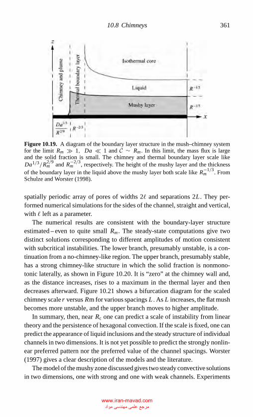
P1: GKE
CB381-10 CB381-Davis May 17, 2001 18:58 Char Count= 0
10.8 Chimneys 361
Figure 10.19. A diagram of the boundary layer structure in the mush–chimney systemfor the limit Rm � 1, Da 1 and C ∼ Rm . In this limit, the mass flux is largeand the solid fraction is small. The chimney and thermal boundary layer scale likeDa1/3/R2/9
m and R−2/3m , respectively. The height of the mushy layer and the thickness
of the boundary layer in the liquid above the mushy layer both scale like R−1/3m . From
Schulze and Worster (1998).
spatially periodic array of pores of widths 2� and separations 2L . They per-formed numerical simulations for the sides of the channel, straight and vertical,with � left as a parameter.
The numerical results are consistent with the boundary-layer structureestimated – even to quite small Rm . The steady-state computations give twodistinct solutions corresponding to different amplitudes of motion consistentwith subcritical instabilities. The lower branch, presumably unstable, is a con-tinuation from a no-chimney-like region. The upper branch, presumably stable,has a strong chimney-like structure in which the solid fraction is nonmono-tonic laterally, as shown in Figure 10.20. It is “zero” at the chimney wall and,as the distance increases, rises to a maximum in the thermal layer and thendecreases afterward. Figure 10.21 shows a bifurcation diagram for the scaledchimney scale r versus Rm for various spacings L .As L increases, the flat mushbecomes more unstable, and the upper branch moves to higher amplitude.
In summary, then, near Rc one can predict a scale of instability from lineartheory and the persistence of hexagonal convection. If the scale is fixed, one canpredict the appearance of liquid inclusions and the steady structure of individualchannels in two dimensions. It is not yet possible to predict the strongly nonlin-ear preferred pattern nor the preferred value of the channel spacings. Worster(1997) gives a clear description of the models and the literature.
The model of the mushy zone discussed gives two steady convective solutionsin two dimensions, one with strong and one with weak channels. Experiments
www.iran-mavad.com مرجع علمی مھندسی مواد
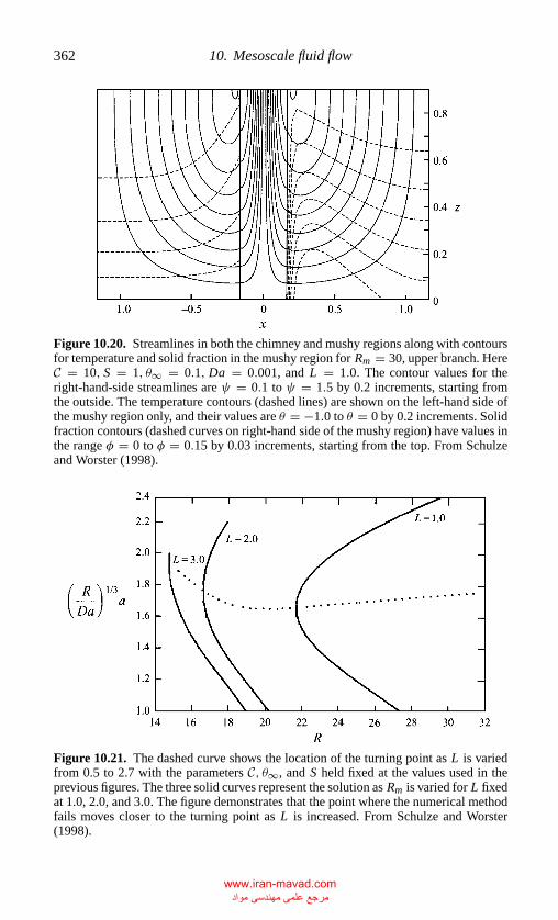
P1: GKE
CB381-10 CB381-Davis May 17, 2001 18:58 Char Count= 0
362 10. Mesoscale fluid flow
Figure 10.20. Streamlines in both the chimney and mushy regions along with contoursfor temperature and solid fraction in the mushy region for Rm = 30, upper branch. HereC = 10, S = 1, θ∞ = 0.1, Da = 0.001, and L = 1.0. The contour values for theright-hand-side streamlines are ψ = 0.1 to ψ = 1.5 by 0.2 increments, starting fromthe outside. The temperature contours (dashed lines) are shown on the left-hand side ofthe mushy region only, and their values are θ = −1.0 to θ = 0 by 0.2 increments. Solidfraction contours (dashed curves on right-hand side of the mushy region) have values inthe range φ = 0 to φ = 0.15 by 0.03 increments, starting from the top. From Schulzeand Worster (1998).
Figure 10.21. The dashed curve shows the location of the turning point as L is variedfrom 0.5 to 2.7 with the parameters C, θ∞, and S held fixed at the values used in theprevious figures. The three solid curves represent the solution as Rm is varied for L fixedat 1.0, 2.0, and 3.0. The figure demonstrates that the point where the numerical methodfails moves closer to the turning point as L is increased. From Schulze and Worster(1998).
www.iran-mavad.com مرجع علمی مھندسی مواد
P1: GKE
CB381-10 CB381-Davis May 17, 2001 18:58 Char Count= 0
References 363
with ammonium chloride solutions exhibit channels, though experiments onother salt solutions (Huppert 1990) often do not exhibit channels. Huppert,Hallworth, and Lipson (1993) obtained insight into this discrepancy by dopingNH4Cl with CuSO4. When the dopant had concentrations over 0.3 wt % CuSO4,chimneys did not form. The addition of CuSO4 makes the crystals more faceted(Mellor 1981) and hence increases the importance of the kinetic undercooling.Worster and Kerr (1994) measured µ in the relation vn = µ[TL(C0) − T I]2
and found that µ is a strong function of the concentration of CuSO4 and thatits increase strengthens the boundary-layer convective mode, which retards thegrowth of the mush, increases its solid reaction, and decreases �C across it.All of these reduce R and may prevent R from rising to values necessary forthe onset of channels (Worster 1997).
10.9 Remarks
Mushy zones have been modeled as porous media whose matrices can grow orshrink by phase transformation. The model, coupled with convection, has beenused as a basis of instability theory that yields three distinct modes: a steadyboundary-layer mode in the liquid, a steady mushy-layer mode, and a time-periodic mushy-layer mode. The three-dimensional, weakly nonlinear theoryfor the steady mushy-layer mode shows a preference for hexagonal convectionnear the onset of motion.
The mushy-layer models yield predictions for mushy-layer thickness andplanform preference in good agreement with observation, though all the exper-iments have been done with various salt solutions. What remains to be done areexperiments on metallic alloys, which have low Prandtl numbers and negligi-ble kinetic undercoolings, in order to see whether the mushy-layer theory forpreferred microstructure compares well with observation.
References
Amberg, G., and Homsy, G. M. (1993). Nonlinear analysis of buoyant convection inbinary solidification with application to channel formation, J. Fluid Mech. 252,79–98.
Anderson, D. M., and Worster, M. G. (1995). Weakly nonlinear analysis of convectionin mushy layers during the solidification of binary alloys, J. Fluid Mech. 302,307–331.
. (1996). A new oscillatory instability in a mushy layer during the solidificationof binary alloys, J. Fluid Mech. 307, 245–267.
Beavers, G. S., and Joseph, D. D. (1967). Boundary conditions at a naturally permeablewall, J. Fluid Mech. 30, 197–207.
Chen, C. F. (1995). Experimental study of convection in a mushy layer during directionalsolidification, J. Fluid Mech. 293, 81–98.
www.iran-mavad.com مرجع علمی مھندسی مواد
P1: GKE
CB381-10 CB381-Davis May 17, 2001 18:58 Char Count= 0
364 10. Mesoscale fluid flow
Chen, F., and Chen, C. F. (1988). Onset of finger convection in a horizontal porous layerunderlying a fluid layer, Trans. ASME C: Heat Transfer 110, 403–407.
. (1991). Experimental study of directional solidification of aqueous ammoniumchloride solution, J. Fluid Mech. 227, 567–586.
Chen, F., Lu, J. W., and Yang, T. L. (1994). Convective instability in ammonium chloridesolution directionally solidified from below, J. Fluid Mech. 276, 163–187.
Chiareli, A. O. P., Huppert, H. E., and Worster, M. G. (1994). Segregation and flowduring the solidification of alloys, J. Crystal Growth 139, 134–146.
Chiareli, A. O. P., and Worster, M. G. (1995). Flow focusing instability in a solidifyingmush, J. Fluid Mech. 297, 293–306.
Davis, S. H., Muller, U., and Dietsche, C. (1984). Pattern selection in single-componentsystems coupling Benard convection and solidification, J. Fluid Mech. 144, 133–151.
Emms, P. W., and Fowler, A. C. (1994). Compositional convection in the solidificationof binary alloys J. Fluid Mech. 262, 111–139.
Fowler, A. C. (1985). The formation of freckles in binary alloys, IMA J. Appl. Math. 35,159–174.
Hellawell, A. (1987). Local convective flows in partially solidified systems, in D. E.Loper, editor, Structure and Dynamics of Partially Solidified Systems, pp. 5–22,Martinus Nijhoff, Dordrecht.
Hills, R. N., Loper, D. E., and Roberts, P. H. (1983). A thermodynamically consistentmodel of a mushy zone, Q. J. Appl. Math. 36, 505–539.
Huppert, H. E. (1990). The fluid dynamics of solidification, J. Fluid Mech. 212, 209–240.. (1993). Bulk models of solidification, in D. T. J. Hurle, editor, Handbook of
Crystal Growth, Vol. 1b, pp. 741–784, North-Holland, Amsterdam.Huppert, H. E., Hallworth, M. A., and Lipson, S. G. (1993). Solidification of NH4Cl
and NH4Br from aqueous solutions contaminated by CuSO4: The extinction ofchimneys, J. Crystal Growth 130, 495–506.
Huppert, H. E., and Worster, M. G. (1985). Dynamic solidification of a binary melt,Nature 314, 703–707.
. (1991). Vigorous motions in magma chambers and lava lakes, in D. A. Yuen,editor, Chaotic Processes in the Geological Sciences, IMA Series 41, p. 41.
Hurle, D. T. J., Jakeman, E., and Wheeler, A. A. (1983). Hydrodynamic stability of themelt during the solidification of a binary alloy, Phys. Fluids 26, 624–626.
Kerr, R. C., Woods, A. W., Worster, M. G., and Huppert, H. E. (1990). Solidificationof an alloy cooled from above. Part 1. Equilibrium growth, J. Fluid Mech. 216,323–342.
Mellor, J. W. (1981). A Comprehensive Treatise on Inorganic and Theoretical Chemistry,pp. 383–389, Longmans, London.
Palm, E., Weber, J. E., and Kvernvold, O. (1972). On steady convection in a porousmedium, J. Fluid Mech. 54, 153–161.
Schulze, T. P., and Worster, M. G. (1998). A numerical investigation of steady convectionin mushy layers during the directional solidification of binary alloys, J. Fluid Mech.356, 199–202.
. (1999). Weak convection, liquid inclusions and the formation of chimneys inmushy layers, J. Fluid Mech. 388, 197–215.
Shirtcliffe, T. G. L., Huppert, H. E., and Worster, M. G. (1991). Measurement of solidfraction in the crystallization of a binary melt, J. Crystal Growth 113, 566–574.
Tait, S., Jahrling, K., and Jaupart, C. (1992). The planform of composition convectionand chimney formation in a mushy layer, Nature 359, 406–408.
Tait, S., and Jaupart, C. (1992). Compositional convection in a reactive crystalline mushand melt differentiation, J. Geophys. Res. 97, 6735–6756.
www.iran-mavad.com مرجع علمی مھندسی مواد
P1: GKE
CB381-10 CB381-Davis May 17, 2001 18:58 Char Count= 0
References 365
Turner, J. S. (1979). Buoyancy Effects in Fluids, Cambridge University Press, New York.Turner, J. S., Huppert, H. E., and Sparks, R. S. J. (1986). Komatiites II: Experimen-
tal and theoretical investigations of post-emplacement cooling and crystallization,J. Petrol. 27, 397–437.
Wettlaufer, J. S., Worster, M. G., and Huppert, H. E. (1997). Natural convection duringsolidification of an alloy from above with application to the evolution of sea ice,J. Fluid Mech. 344, 291–316.
Woods, A. W., and Huppert, H. E. (1989). The growth of compositionally stratified solidabove a horizontal boundary, J. Fluid Mech. 199, 29–53.
Worster, M. G. (1986). Solidification of an alloy from a cooled boundary, J. Fluid Mech.167, 481–502.
. (1990). Structure of a convecting mushy layer, Appl. Mech. Rev. 43, S59–S62.
. (1991). Natural convection in a mushy layer, J. Fluid Mech. 224, 335–339.
. (1992a). The dynamics of mushy layers, in S. H. Davis, H. E. Huppert, U. Muller,and M. G. Worster, editors, Interactive Dynamics of Convection and Solidification,pp. 113–138, NATO ASO E219, Dordrecht, Kluwer.
. (1992b). Instabilities of the liquid and mushy regions during solidification ofalloys, J. Fluid Mech. 237, 649–669.
. (1997). Convection in mushy layers, Ann. Rev. Fluid Mech. 29, 91–122.Worster, M. G., and Kerr, R. C. (1994). The transient behavior of alloys solidified from
below prior to the formation of chimneys, J. Fluid Mech. 269, 23–44.
www.iran-mavad.com مرجع علمی مھندسی مواد
P1: GMD
CB381-11 CB381-Davis May 16, 2001 19:5 Char Count= 0
11
Phase-field models
In all the systems discussed heretofore the solidification front was considered tobe a mathematical interface of zero thickness endowed with surface propertiesdeemed appropriate to the physics. In this chapter, another approach is taken.The front is allowed to be diffuse, and the fields of interest, such as T andC , are supposed to have well-defined bulk behaviors away from the interfacialregion and rapid, though continuous, variations within it. Minimally, one wouldwish the model to satisfy the laws of thermodynamics, appropriately extendedinto the nonequilibrium regions, and regain the interfacial properties and jumpconditions appropriate to the thin-interface limit when the interfacial thicknessapproaches zero.
On the one hand one would anticipate that an infinite number of such modelslikely exists. On the other hand one would anticipate that the thin-interface limitmight be taken a number of ways, each giving distinct properties to the front.Nonetheless, conceptually there are two possible virtues of the diffuse-interfaceapproach. If the models are well chosen on the basis of some underlying frame-work, then there would be a systematic means of generalizing the models tosystems such as rapid solidification. In Chapter 6 high rates of solidification weremodeled by appending to the standard model variations k = k(Vn), m = m(Vn)with, for example, the equilibrium Gibbs–Thomson undercooling. A systematicgeneralization could indicate how the relationships for k and m emerge, andwhat other alterations to the model should simultaneously be included. Call this“model building.”
The second virtue is the practical one of being able to compute complexmicrostructures. Given the sharp interface model, one can track the front whendendrites begin to appear, but as a dendrite develops secondary and tertiarysidearms, front tracking becomes impossible. The “diffuse” interface modeltreats all the phases as one with spatially varying properties, and thus it may
366
www.iran-mavad.com مرجع علمی مھندسی مواد
P1: GMD
CB381-11 CB381-Davis May 16, 2001 19:5 Char Count= 0
11.1 Pure materials – A model system 367
be possible to simulate more complex structures numerically for longer times.Call this “simulation building.”
Consider a system in which an interfacial region of thickness W is includedbetween two bulk phases, solid and liquid. To identify the phases one definesa “marker function” φ, called the phase field, which takes on two differentconstant values (say ±1) in the bulks but varies smoothly between them. Thetask is to find a system of continuum equations that govern C , T , and φ. Onetakes the convention that the interface lies at φ = 0. A simulation of theinterface then involves the location of the zeros of φ and not the solution of afree-boundary problem.
The discussion will begin with a model system for a simple pure-materialsystem. This will be generalized to a deduced system, and then the results ofnumerical computation will be discussed.
11.1 Pure Materials – A Model System
Consider first a model solid–liquid system in which the thermal properties ofthe two phases are identical. For the nondimensional temperature θ and thephase field φ in planar growth write
αp2φt = p2φzz − f ′(φ) − λg′(φ)θ (11.1a)
θt = θzz + 1
2φt , (11.1b)
where
f (φ) = − [ 12φ2 − 14φ
4]
g(φ) = φ − 23φ
3 + 15φ
5.(11.2)
Here, a Peclet number p represents the ratio of the thickness W of the interfacialregion to δT = κ/v and hence is considered to be small; α and the linkingparameter λ are constants. Here v is some estimate of the freezing rate.
In this model φ = +1 in the solid and −1 in the liquid, and it variescontinuously in between them. One then sees that the temperature θ in eachbulk phase satisfies the heat-conduction equation (11.1b) in which (1/2)φt
represents a source of heat localized to the interfacial region and is relatedto the liberation of latent heat. The sources f ′(φ) and g′(φ) in Eq. (11.1a) ref-lect the phase change alterations as the temperature field is varied. When λ = 0,the phase-field decouples from the temperature and develops independently,though the temperature continues to depend on φ. As the interface thicknessW → 0, p → 0, and the thin-interface limit should be approached though, asis clear, p → 0 is a singular perturbation.
www.iran-mavad.com مرجع علمی مھندسی مواد
P1: GMD
CB381-11 CB381-Davis May 16, 2001 19:5 Char Count= 0
368 11. Phase-field models
One would expect that if system (11.1) represents the standard solidificationequations, it should do so in a limit that involves p → 0, or λ → 0, or both.Two of the possibilities have been used extensively in the literature and will bediscussed now.
Consider first the case p → 0 with λ = O(1), which was posed by Fife andPenrose (1995) and elaborated by Karma and Rappel (1998).
In the outer region, far from the interface, write
θ = θ0 + pθ1 + · · · ; (11.3)
one finds that at all orders
θi t = θi zz, i = 0, 1, 2, . . . (11.4)
as expected; the temperature satisfies a heat-conduction equation.To analyze the inner region it is convenient to introduce a coordinate z
moving with the front whose speed is v(t),
z = z −∫ t
0v(t ′) dt ′. (11.5)
One can then introduce the inner variable η,
η = z/p. (11.6)
In terms of η, the system (11.1) and (11.2) becomes
αp2
(φt − v
pφη
)= φηη + φ(1 − φ2) + λ(1 − φ2)2θ (11.7a)
p2
(θt − v
pθη
)= θηη + 1
2p2
(φt − v
pφη
). (11.7b)
Write an asymptotic expansion in the inner region
(θ, φ) = (�0,�0) + p(�1,�1) + · · · . (11.8)
When this is substituted into system (11.7), one obtains at leading order in p
�0ηη +�0(1 −�20) + λ(1 −�2
0)2�0 = 0 (11.9a)
�0ηη = 0. (11.9b)
It is immediately evident that�0 must be constant in order to match to the outerfields, and hence one can take
�0 ≡ 0. (11.10)
www.iran-mavad.com مرجع علمی مھندسی مواد
P1: GMD
CB381-11 CB381-Davis May 16, 2001 19:5 Char Count= 0
11.1 Pure materials – A model system 369
Equation (11.9a) can then be solved, giving
�0η = −tanhη√2, (11.11)
which gives the principal behavior of the phase-field structure. At O(p) onehas, using result (11.10), that
�1ηη + (1 − 3�20)�1 = −αv�0η − λ(1 −�2
0)�1 (11.12a)
�1ηη − 1
2v�0η = 0. (11.12b)
Equation (11.12b) can be integrated directly twice, giving
�1η − 1
2v�0 = A (11.13a)
and
�1 = θ1 + Aη + 1
2v
∫ η
0�0(η′) dη′, (11.13b)
where A and θ1 are constants of integration. Notice that at η = 0, �1 = θ1.The linear operator on the left-hand side of Eq. (11.12a) is self-adjoint and is
the Frechet derivative of that of Eq. (11.9a). Hence, a complementary solutionof Eq. (11.12a) is �0η, and its right-hand side must be orthogonal to this forsolutions to exist. This Fredholm condition gives∫ ∞
−∞
[αv�0η + λ(1 −�2
0)2�1]�0η dη = 0. (11.14)
The condition (11.14) determines the constant θ1. To see this, eliminate �1
using Eq. (11.13b) to obtain
αv
∫ ∞
−∞�2
0η dη + λθ1
∫ ∞
−∞(1 −�2
0)2�0η dη
+ 1
2λv
∫ ∞
−∞(1 −�2
0)2�0η
[∫ η
0�0(η′) dη′
]dη = 0. (11.15)
Notice that the constant A is not present because it multiplies the integral of anodd function.
Now let us turn to matching. The heat fluxes match if
limη→±∞�1η = lim
z→0±θ0z ≡ θ±
0z . (11.16)
Using solution (11.13a) on each side of the region gives, in the solid,
θ+0z − 1
2v = A, (11.17a)
www.iran-mavad.com مرجع علمی مھندسی مواد
P1: GMD
CB381-11 CB381-Davis May 16, 2001 19:5 Char Count= 0
370 11. Phase-field models
and in the liquid,
θ−0z + 1
2v = A (11.17b)
By eliminating A between these, one obtains the first condition satisfied by theouter field,
v = θ+0z − θ−
0z, (11.18a)
which is the scaled thin-interface heat balance.One can also solve for the integration constant A,
A = θ±0z ∓ 1
2v. (11.18b)
Now consider the temperature itself. Because �0 ≡ 0, one can write nearη = 0, that
θouter ∼ pθ±1 + θ±
0z z (11.19)
and using Eq. (11.13b), one obtains
θinner ∼ p
[θ1 + Aη + 1
2v
∫ η
0�0(η′) dη′
]
= p
[θ1 + 1
2v
∫ η
0�0(η′) dη′
]+ Az. (11.20)
Now, from relation (11.18b), one obtains
θinner ∼ p
{θ1 + 1
2v
∫ η
0[�0(η′) ± 1] dη′ + θ±
0z z
}. (11.21)
When relations (11.19) and (11.21) are matched, one finds that
θ±1 = θ1 + 1
2v + I, (11.22)
where
I =∫ ∞
0[�0(η′) + 1] dη′ =
∫ −∞
0[�0(η′) − 1] dη′, (11.23)
and thus from relation (11.19) one finds
θouter ∼ p
(θ1 + 1
2I
)+ θ±
0z z. (11.24)
The temperature θ I at the interface, θouter|z=0, is thus continuous. Given thevalues of θ1 from Eq. (11.22), the interfacial temperature through O(p) becomes
θ I ∼ −a1α
λ
[1 − a4
λ
α
]pv, (11.25)
www.iran-mavad.com مرجع علمی مھندسی مواد
P1: GMD
CB381-11 CB381-Davis May 16, 2001 19:5 Char Count= 0
11.1 Pure materials – A model system 371
where the ai are positive constants obtained by definite integrations and
a4 = 1 + 1
2
a2
a1. (11.26)
Equation (11.25) shows that as p → 0, the interface temperature recoversthe form
θ I = −µ−1vp, (11.27)
and µ is the nondimensional kinetic coefficient appropriate to the planarinterface.
Karma and Rappel (1998) considered the more general case of a curvedinterface and found that Eqs. (11.25) and (11.27) become, respectively,
θ I ∼{
2Ha1
λ− a1α
λ
[1 − a4
λ
α
]v
}p (11.28)
and
θI = 2H� − µ−1v, (11.29)
where � denotes nondimensional surface energy.Thus, at O(p) one recovers the appropriate jump conditions. Karma and
Rappel (1998) noted that µ−1 can be controlled by the choice of λ becauseso far λ is arbitrary. For example, to examine solidification with instantaneouskinetics appropriate to small undercooling, one merely chooses λ = α/a4.
The second limit appropriate to thin interfaces dates back to the work ofCaginalp (1989) and is related to a vanishingly small linking parameter λ. Inthe present notation, p → 0, λ → 0 such that p/λ = O(1). The asymptoticsfollow as before, and the result for a curved front is condition (11.25) butwith the term a4λ/α neglected compared with unity. Now µ−1 is no longercontrollable; it cannot be chosen to be zero.
Karma and Rappel (1998) discussed, on dimensional grounds, the impli-cations for numerical computation. In the small-linking-parameter limit, theratio of the thickness W to the capillary length δcap = γ Tmcp/L2
V must be verysmall, whereas this ratio need only be of unit order in the small-Peclet num-ber limit, which is a huge advantage given that δcap is typically of moleculardimensions.
Note: The equations involving the phase-field approach look startlingly simi-lar to those of the mushy zone, as discussed in Chapter 10. A contrast is betweenphase-field models in which one takes p → 0 and mushy models in which oneallows the equivalant of p to remain of unit order.
www.iran-mavad.com مرجع علمی مھندسی مواد
P1: GMD
CB381-11 CB381-Davis May 16, 2001 19:5 Char Count= 0
372 11. Phase-field models
11.2 Pure Materials – A Deduced System
The system examined in Section 11.1 was asserted with only verbal justification.In this section, a more elaborate system will be deduced using the ideas ofthermodynamics for systems out of equilibrium.
Phase-field theory for the solidification can be traced to 1978 when Langerextracted from analysis of critical phenomena a model for the freezing of anundercooled melt (later published in Langer 1986). Caginalp (1985), Collinsand Levine (1985), and Umantsev and Roitburd (1988) did so as well. The issueof “thermodynamic self-consistency” was treated by Penrose and Fife (1990)and Wang et al. (1993).
The necessity of including anisotropy follows in part from the MST fordendrites. Caginalp and Fife (1986) and Caginalp (1986) replaced the magnitudeof the gradient by anisotropic quadratic forms. Langer (1986) added higher-order gradients. Kobayashi (1993) and Wheeler, Murray, and Schaefer (1993)allowed the coefficient of the gradient energy to depend on orientation throughn = ∇φ/|∇φ|.
Consider
F(θ, φ) =∫
[1
2W 2|∇φ|2 + f (φ) + 1
2bλθ2
]dV, (11.30)
where W is the interfacial thickness, θ = (T − Tm)cp/L is the scaled tempera-ture, φ is the phase field, is the volume occupied by the material, and ∂ isits zero-flux boundary. Here
f (φ) = −1
2φ2 + 1
4φ4, (11.31)
which has a local maximum at φ = 0 and local minima at φ = ±1.One supposes that θ and φ evolve by the rules
τφt = −δFδφ
(11.32a)
and
bλ�t = κ∇2 δFδ�, (11.32b)
where δ denotes the variational derivative. The mobility parameter τ−1 and b,λ, and κ are positive. Here the enthalpy � is related to the temperature by
� = θ − 1
2h(φ) (11.33)
and 12 [h(1) + h(−1)] = 1 for reasons of normalization.
www.iran-mavad.com مرجع علمی مھندسی مواد
P1: GMD
CB381-11 CB381-Davis May 16, 2001 19:5 Char Count= 0
11.2 Pure materials – A deduced system 373
This formulation guarantees that the free energy decreases locally and thatthe enthalpy balance holds (Warren and Boettinger 1995; Wheeler, Boettinger,and McFadden 1992)
When
g(φ) = 1
2bh(φ), (11.34)
Eqs. (11.32) reduce to
τφt = W 2∇2φ − ∂
∂φF(φ, λθ ) (11.35a)
θt = κ∇2θ + 1
2[h(φ)]t (11.35b)
and
F(φ, λθ ) = f (φ) + λg(φ)θ. (11.35c)
The models in the literature differ by their choices of f , g, and h, and reasonablywide ranges of choices give consistent results for p → 0. Caginalp and Chen(1992) and Wang et al. (1993) took
g(φ) = φ − 2
3φ3 + 1
5φ5 (11.36)
When τ ,λ,κ , and W are constants, the system describes an isotropic material.Following Karma and Rappel (1998), scale lengths on δT = κ/V , time onδT /V , and system (11.35) becomes
αp2φt = p2∇2φ + φ − φ3 − λ(1 − φ2)2θ (11.37a)
θt = ∇2θ + 1
2[h(φ)]t , (11.37b)
where either
h = 15
8
(φ − 2
3φ3 + 1
5φ5
),
(b = 15
16
)(11.37c)
or
h = φ. (11.37d)
The latter is not a special case of Eq. (11.34). Here p is the interfacial Pecletnumber,
p = W V
κ, (11.38)
which is presumed to be very small.
www.iran-mavad.com مرجع علمی مھندسی مواد
P1: GMD
CB381-11 CB381-Davis May 16, 2001 19:5 Char Count= 0
374 11. Phase-field models
This system can be seen to be related directly to Eq. (11.1) and the limitp → 0, λ = O(1), one regains the first thin-interface limit.
When the material is anisotropic, and τ and W depend on the local unitnormal n, then, with choice (11.37d), system (11.37) becomes
A2(n)φt = ∇ · [A2(n)∇φ] + [φ − λθ (1 − φ2)](1 − φ2) (11.39a)
+[|∇φ|2 A(n)
∂
∂φxA(n)
]x
+[∇φ|2 A(n)
∂
∂φyA(n)
]y
θt = D∇2θ + 1
2φt (11.39b)
and
D = κτ0/W 20 . (11.39c)
The anisotropy is defined by W (n) = W0 A(n), where W0 is a scale for theinterface width and τ (n) ≡ τ0 A2(n), A is in the range [0, 1], and
A(n) = (1 − 3α)
[1 + 4α
1 − 3α
φ4x + φ4
y
|∇φ|4]. (11.40)
Equation (11.40) defines α, which is zero in the isotropic case and is related toα4 in the case of fourfold symmetry.
11.3 Pure Materials – Computations
The systems (11.37) and (11.39) can be integrated numerically in a variety ofways given that a free boundary need not be tracked. The earliest numericalsimulations derive from Fix (1983), from whom the questions of adequateresolution and sufficiently small W arose. Langer (1986) and Caginalp (1989)obtained expressions for λ → 0 of the form
d0 = a1W
λ, µ−1 = a1
τ
λW(11.41)
that relate the sharp-interface parameters d0 and µ to the limiting forms ofthe phase field. Kobayashi (1993) and McFadden et al. (1993) extended theseto systems with anisotropy. Following Karma and Rappel (1998), d0 and µ−1
must scale W/λ and τ/Wλ, respectively. Relations (11.41) only fix W/λ andτ/Wλ and not W and τ independently. Hence, numerical convergence requiresdecreasing W ∼ λ and τ ∼ λ2 until the results become W independent. Thisrequires, W → 0, τ → 0, λ → 0 such that d0 and µ remain fixed. In the limit,one wishes the variation δθ across the interfacial region to vanish, as seen from
www.iran-mavad.com مرجع علمی مھندسی مواد
P1: GMD
CB381-11 CB381-Davis May 16, 2001 19:5 Char Count= 0
11.3 Pure materials – computations 375
the outer region. Here δθ ∼ W/δT , and if the computation is done at unit-orderundercooling, then necessarily µ−1V � d0(2H ); the kinetic undercooling isdominant. Now, if W/δT is small compared with the interfacial temperature,one wishes that W/δT µ−1V , and thus, using Eq. (11.41) one finds that thelimitation is
W
d0 κτ
W 2(11.42)
and, because κτ/W 2 is of unit order, W must be much smaller than the capillarylength, which is exactly the same conclusion derived by Brattkus, Meiron, andSpencer (1993) and Braun, McFadden, and Coriell (1994).
The asymptotics of Section 11.2 take the linking parameter of unit orderand allow the interfacial Peclet number p → 0. Fife and Penrose (1995) firstaddressed this limit, but it was Karma and Rappel (1996) who extended it appro-priately to numerical computation. Karma and Rappel found that, correspondingto relations (11.41), the new relations become
d0 = a1W
λ, µ−1 = a1
(τ
λW− a2
W
D
)(11.43)
Constraint (11.42) no longer applies because the inequality W/κ τ/λW nec-essarily applies as well; if one chooses λ = τκ/W 2a2, then µ−1 = 0. Nolonger must W/δT µ−1V , but now W/δT d0, and thus W/d0 δT , whichis a much weaker requirement.
The most recent and accurate computations entail the use of a finite-elementmethod using adaptive grids. Provatas, Goldenfeld, and Dantzig (1998) consid-ered in two dimensions the growth and instability of an initially circular nucleus.Figure 11.1 shows their typical result for the case of fourfold symmetry withα4 = 0.05 and undercooling S−1 = cp�T/L = 0.55. Notice that sidearmshave appeared and that the thermal boundary layer is thin because S−1 islarge. In order to get numerical convergence, the ratios of the sizes of thelargest to the smallest elements are made 2n. For S−1 = 0.25 they can usen = 12, whereas for S−1 = 0.10 they require n = 17. For S−1 ≥ 0.30the computations give equilibration to a steady state consistent with MST. Atlower S−1, such approach is inconsistent with the theory for an isolated fin-ger because the thermal boundary layer overlaps neighboring arms; the MSTresult is not recovered. Kim et al. (1999) examined the phase-field solutionsfor large S−1, but for various choices of g(φ) and h(φ). They found that thesame long-time asymptotic state is obtained for all cases, verifying numeri-cally that, for sufficient resolution, the MST prediction is obtained for largeenough S−1.
www.iran-mavad.com مرجع علمی مھندسی مواد
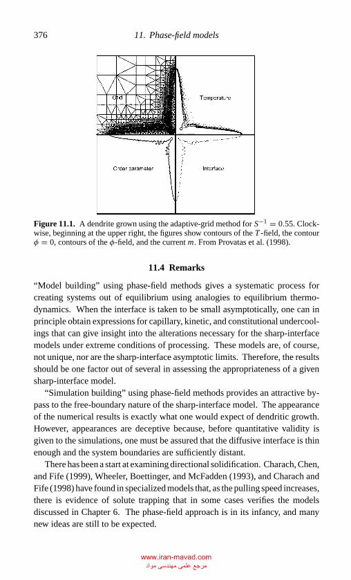
P1: GMD
CB381-11 CB381-Davis May 16, 2001 19:5 Char Count= 0
376 11. Phase-field models
Figure 11.1. A dendrite grown using the adaptive-grid method for S−1 = 0.55. Clock-wise, beginning at the upper right, the figures show contours of the T -field, the contourφ = 0, contours of the φ-field, and the current m. From Provatas et al. (1998).
11.4 Remarks
“Model building” using phase-field methods gives a systematic process forcreating systems out of equilibrium using analogies to equilibrium thermo-dynamics. When the interface is taken to be small asymptotically, one can inprinciple obtain expressions for capillary, kinetic, and constitutional undercool-ings that can give insight into the alterations necessary for the sharp-interfacemodels under extreme conditions of processing. These models are, of course,not unique, nor are the sharp-interface asymptotic limits. Therefore, the resultsshould be one factor out of several in assessing the appropriateness of a givensharp-interface model.
“Simulation building” using phase-field methods provides an attractive by-pass to the free-boundary nature of the sharp-interface model. The appearanceof the numerical results is exactly what one would expect of dendritic growth.However, appearances are deceptive because, before quantitative validity isgiven to the simulations, one must be assured that the diffusive interface is thinenough and the system boundaries are sufficiently distant.
There has been a start at examining directional solidification. Charach, Chen,and Fife (1999), Wheeler, Boettinger, and McFadden (1993), and Charach andFife (1998) have found in specialized models that, as the pulling speed increases,there is evidence of solute trapping that in some cases verifies the modelsdiscussed in Chapter 6. The phase-field approach is in its infancy, and manynew ideas are still to be expected.
www.iran-mavad.com مرجع علمی مھندسی مواد
P1: GMD
CB381-11 CB381-Davis May 16, 2001 19:5 Char Count= 0
References 377
Clearly, carefully controlled use of phase-field simulations can be extraor-dinarily useful in assessing and predicting complex microstructures.
References
Brattkus, K., Meiron, D. I., and Spencer, B. J. (1993). Consistent nucleation in diffusivephase-field models, unpublished.
Braun, R. J., McFadden, G. B., and Coriell, S. R. (1994). Morphological instability inphase-field models of solidification, Phys. Rev. E 49, 4336–4352.
Caginalp, G. (1985). Surface tension and supercooling in solidification theory, inL. Garrido, editor, Applications of Field Theory to Statistical Mechanics, pages216–226, Notes in Physics 216, Springer-Verlag, Berlin.
. (1986). An analysis of a phase field model of a free boundary, Arch. Rat. Mech.Anal. 92, 205–245.
. (1989). Stefan and Hele–Shaw type models as asymptotic limits of the phase-field equations, Phys. Rev. A 39, 5887–5896.
Caginalp, G., and Chen (1992). Phase field equations in the singular limit of sharp inter-face problems, in M. E. Gwinn and G. B. McFadden, editors, On the Evolution ofPhase Boundaries, pages 1–27, IMA Volumes in Mathematics and Its Applications43, Springer Verlag, Berlin.
Caginalp, G., and Fife, P. C. (1986). Phase field methods of interfacial boundaries, Phys.Rev. B 33, 7792–7794.
Charach, C., Chen, C. K., and Fife, P. C. (1999). Developments in phase-field modelingof thermoelastic and two-component materials, J. Stat. Phys. 95, 1141–1164.
Charach, C., and Fife, P. C. (1998). Solidification fronts and solute trapping in a binaryalloy, SIAM J. Appl. Math. 58, 1826–1851.
Collins, J. B., and Levine, H. (1985). Diffuse interface model of diffusion-limited cyrstalgrowth, Phys. Rev. B 31, 6119–6122.
Fife, P. C., and Penrose, O. (1995). Interfacial dynamics for thermodynamically con-sistent phase-field models with non-conserved order parameter, Electronic J. Diff.Eqns. 16, 1–19.
Fix, G. J. (1983). Phase field methods for free boundary problems, in A. Fasano and M.Primicerio, editors Free boundary Problems: Theory and Applications.
Kim, Y.-T., Provatos, N., Goldenfeld, N., and Dantzig, J. A. (1999). Universal dynamicsof phase-field models for dendritic growth, Phys. Rev. E 59, R2546–R2549.
Karma A., and Rappel, W.-J. (1996). Numerical simulation of three-dimensional den-dritic growth, Phys. Rev. Lett. 77, 4050–4053.
. (1998). Quantitative phase-field modeling of dendritic growth in two and threedimensions, Phys. Rev. E 57, 4323–4339.
Kobayashi, R. (1993). Modeling and numerical simulations of dendritic crystal growth,Physica D 63, 410–423.
Langer, J. S. (1986). Models of pattern formation in first-order phase transitions, inDirections in Condensed Matter, World Scientific, Singapore, 165–186.
McFadden, G. B., Wheeler, A. A., Braun, R. J., and Coriell, S. R., and Sekerka,R. F. (1993). Phase-field models for anisotropic interfaces, Phys. Rev. E 48, 2016–2024.
Penrose, O., and Fife, P. C. (1990). Thermodynamically consistent model of phase-fieldtype for the kinetics of phase transitions, Physica D 43, 44–62.
Provatas, N., Goldenfeld, N., and Dantzig, J. A. (1998). Efficient computation ofdendritic microstructures using adaptive mesh refinement, Phys. Rev. Lett. 80,3308–3311.
www.iran-mavad.com مرجع علمی مھندسی مواد
P1: GMD
CB381-11 CB381-Davis May 16, 2001 19:5 Char Count= 0
378 11. Phase-field models
Umantsev, A. R., and Roitburd, A. L. (1988). Non-isothermal relaxation in a nonlocalmedium, Sov. Phys. Solid State 30, 594–598.
Wang, S.-L., Sekerka, R. F., Wheeler, A. A., Murray, B. T., Coriell, S. R., Braun, R. J.,and McFadden, G. B. (1993). Thermodynamically consistent phase-field modelsfor solidification, Physica D 69, 189–200.
Warren, J. A., and Boettinger, W. J. (1995). Prediction of dendritic growth and microseg-regation on patterns in a binary alloy using the phase-field model, Acta Metall.Mater. 43, 689–703.
Wheeler, A. A., Boettinger, W. J., and McFadden, G. B. (1992). Phase-field model forisothermal phase transitions in binary alloys, Phys. Rev. A 45, 7424–7439.
. (1993). A phase-field model of solute trapping during solidification, Phys. Rev.E 47, 1893–1909.
Wheeler, A. A., Murray, B. T., and Schaefer, R. J. (1993). Computation of dendritesusing a phase field model, Physica D 66, 243–262.
www.iran-mavad.com مرجع علمی مھندسی مواد
P1: JSN
Cb381-Index CB381-Davis June 9, 2001 13:54 Char Count= 0
Index
A
Amberg–Homsy model, 350, 359Anderson–Worster model, 352–357Anisotropy, 86–161
attachment kinetics, 92, 98, 102–103,106–110, 124, 228–229
Brattkus–Davis equation, 94, 103, 105Burgers equation, 137capillarity and, 100coarsening and, 152–156coefficients of, 94, 102, 117–119corners and, 121, 125,130dendrites and, 228faceting and, 139–152fingers and, 228fourfold, 68, 89–94, 106–108Kuramoto–Sivashinsky equation, 119–120large, 89, 121–139, 229microscopic solvability theory (MST) and,
229–230, 238–239, 372needles and, 229–230phase-field, theory and, 372–374Sivashinsky equation, 92, 100small, 89, 91–121step-wise growth, 97–105, 121–124surface energy, 86–91, 97, 105, 110–122,
138–146, 230, 236–238symmetry and, 82–83, 131, 145, 238thin-interface limit and, 374–375travelling waves and, 234–237unconstrained growth and, 105–139See also specific models, parameters
Antikinks, 126, 128–129Approximate selection of dendrites,
221–229of eutectics, 261–267
Aqueous solutions, 325–326Asymptotic suction profile, 293–294
Attachment kinetics, 18, 164, 181–183, 196anisotropy and. See Anisotropyfingers and, 228growth and, 138high speeds and, 203Ivantsov solution, 251–252step density and, 97See also specific model, parameters
B
Bands, 162–163, 171, 177, 204, 205, 208Benard convection, 72, 74, 280–283, 301
pulsations, 190–203Bifurcation, 62, 94, 265
anisotropy on, 94–97coupling and, 288–289degenerate, 206dimension and, 78–89directional solidification and, 62–85free boundary problems and, 76interfacial shape and, 101Landau coefficient and, 70, 73, 101,
181–183nonlinear theory, 62–85subcritical, 64, 76, 199, 265, 283three-dimensional theory, 72–75tilting cells and, 266tip-splitting and, 265transition point, 64two-dimensional theory, 62–71, 181–183
Binary substances, 42–61approximate models, 46–48directional solidification, 45–56linear instability, 48–56model for, 42–45morphological instability, 56–57See also specific alloys, effects
Binodal points, 126–127
379
www.iran-mavad.com مرجع علمی مھندسی مواد
P1: JSN
Cb381-Index CB381-Davis June 9, 2001 13:54 Char Count= 0
380 Index
Boundary conditions, 21–26Boundary-integral methods, 71Boundary-layer effects, 285, 293, 346.
See also specific effects, parametersBoundary-layer mode, 346Boussinesq approximation, 276–277,
304, 341Brattkus-Davis equation, 80–82, 94, 303
anisotropy, 103, 105Buoyancy, 331
convective effects, 162, 275, 287, 341–349directional solidification and, 287–292instabilities, 280, 341–349mushy zones and, 341–349solutal, 288, 289
C
Cahn-Hilliard equation, 126, 131, 134,144, 157
Capillarity, anisotropy and, 100Capillary number (C), 36Capillary undercooling, 24, 57Cellular-dendritic transition, 245Cellular modes, in FTA, 181–183Chaotic states, 82, 188, 272, 295Chemical potential, 123Chiareli–Worster limit, 340Chimneys, 5, 357–363Coarsening, 134, 144, 152–156Cold-boundary condition, 171Compatibility conditions, 142, 145, 192, 195,
199–200Composite structures, 311Concentration boundary-layer thickness, 47Constitutional undercooling, 44, 51, 54, 57,
59, 287Contact angle, 21, 82–83, 259Continuity, equation of, 341Continuity of temperature, 39, 59Continuous-growth model, 166–167Convection
Benard, 280–283binodal points, 127buoyancy and, 3, 275, 287–292, 341–349cellular, 304–311coarsening and, 134–135, 154directional solidification and, 283–287free, 279–280mesoscale fluid flow, 341–357oscillatory instability, 341–356thermal boundary layer and, 289–291thermocapillary, 275volume-change, 275, 283–287weakly nonlinear, 356–357
Corners, 121, 125, 130Couette flow, 283, 293Coupling effects, 205, 288–270, 205, 288
Critical nucleation radius, 30, 34, 215–221Cross-gap curvatures, 83Curved interfaces, 21–39
boundary conditions, 21–26undercooling and, 26–39
D
Darcy’s law, 334–335, 338, 342Darcy number, 360Dendrites, 215–254
approximate selection, 221–229banded transition, 179critical radius, 215–221crystals, 217–221definition of, 215mushy zones and, 330–334, 350–352needles. See Needlesprediction of, 215selection theories, 221–237See specific types, conditions, parameters
Diffusiondiffusivity ratios, 172double-diffusive effects, 353interdiffusion coefficient, 257modified problem of, 296thermodynamics and, 1
Directional solidification, 45–46, 275anisotropy and, 91–105binary substances and, 45–46, 48–56buoyancy-driven convection, 287–292cellular convection and, 304–311forced flows and, 292–304microscale fluid flow and, 283–311nonlinear theory for, 62–85volume-change convection, 283–287
Disequilibrium, 156, 190, 199, 162–214bifurcation theory, 181–189cellular modes, in FTA, 181–183linear stability theory, 167–181mode coupling, 204–208nonlinear pulsations, 189–204oscillatory–cellular interactions, 204–206oscillatory modes, in FTA, 183–189oscillatory–pulsatile interactions, 206–208parameter, 181phenomenological models, 208–211pulsatile–cellular interactions, 204–205rapid solidification and, 164–167thermal effects, 171–181undercooling and, 166
Distribution coefficient. See segregationcoefficient
Double-diffusive effects, 353Double-well free energy, 126–127Drop-shaped roots, 71Droplets, 280Dufour effect, 221
www.iran-mavad.com مرجع علمی مھندسی مواد
P1: JSN
Cb381-Index CB381-Davis June 9, 2001 13:54 Char Count= 0
Index 381
E
Eckhaus instability, 67–68, 72, 187–190,267–268
Emms-Fowler model, 359End effects, 298Epitaxial growth, 156Equilibrium distribution coefficient, 165Equilibrium shape, 88, 89Euler–Lagrange equation, 23, 87Eutectics, 255–273
approximate theories for, 261–267eutectic point, 255hypereutectic, 272, 326–328hypoeutectic, 272, 326–328lamellar, 255rod, 255selection models, 261–267See also specific effects
Evaporation–condensation model, 138,152, 156
Evolution equations, 14, 62, 77, 82,113, 124
anisotropic, 92, 101, 113–114, 119,125–126, 137–139, 144, 147
SeeKardar–Parisi–ZhangKorteweg–de VriesCahn–HilliardBrattkus–DavisRiley–DavisSivashinskyKuramoto–Sivashinsky
F
Faceting, 138anisotropy and, 139–152constant driving force, 139–152line tension and, 127spinodal decomposition and, 127, 130
Fickian law, 42Finger growth, 25–26, 106, 228. See also
NeedlesFisher approximation, 220Floquet theory, 69, 81, 188, 247,
299, 306Flow-induced instabilities, 274, 296Forced flows, 274, 292–304Fourfold symmetry, 68, 89–91, 108Fourier’s law, 8Fowler model, 340Freckles, 3, 357Free convection, 279–280Free energy, 127Frozen temperature approximation (FTA), 47,
55–57, 76, 92, 181–189, 287–288FTA. See Frozen temperature approximation
G
G-jitter effect, 274Gaussian curvature, 139Gibbs free energy, 23Gibbs-Thomson equation, 24–25, 27, 29, 40,
44, 59anisotropy and, 88, 157disequilibrium, 166
Ginzburg–Landau equationbifurcation and, 66Eckhaus limit for, 190
Grashof number, 279, 314Greengard–Strain method, 203Groove structures, 148Growth models, 30–39, 166–167, 261–267.
See specific models
H
Heat balance, 26, 39, 44, 59Heat equation, 8–10, 37, 42Hele–Shaw cell, 46, 62, 72, 82–83, 237Helical growth, 189Helmholtz free energy, 21Hemispherical-needle approximation, 220Herring model, 88Hexagonal structures, 73–75, 79–82, 95–97,
282, 356–358Hole solutions, 189Hong–Langer model, 238Hopf bifurcations, 206–208Hydrodynamic effects, 134Hypercooling, 20, 35, 106–161, 138–139
I
Imposed cellular convection, 304Imposed flows, 275Instabilities
absolute-stability limit, 52–58, 80–82,102–104, 169, 177, 294, 303
buoyancy-driven, 280, 292chaotic states, 82, 188, 272, 295coarsening and, 152–156convective, 291critical radius for, 34Eckhaus, 67–68, 72, 187–190,
267–268eutectics, 267–269flow-induced, 274latent-heat effects, 57–59, 172–183long-scale theories, 76–82mechanism of, 56–57morphological, 46–49, 55–60, 271, 292,
302–303mushy zones and, 340–347shrinkage and, 285soluto-convective, 288
www.iran-mavad.com مرجع علمی مھندسی مواد
P1: JSN
Cb381-Index CB381-Davis June 9, 2001 13:54 Char Count= 0
382 Index
Instabilities (Cont.)subharmonic, 251See also Linear stability theory
Interdiffusion coefficient, 257Interfaces
anisotropy. See Anisotropyboundary conditions, 37–40, 59, 88,
164–166attachment coefficient, 97heat balance at, 25, 58diffuse, 366–378no-slip condition, 277, 285, 349stretching, 25thin-interface limit, 366–367See also specific parameters, effects
Interfacial wave theory (IWT), 228, 236–238,252
Isolated needles, 217–221, 228IWT. See Interfacial wave theoryIvantsov solutions, 251–252
needles and, 210, 246–247, 311–319Peclet number and, 231, 314Xu basic state and, 232
J
Jackson–Hunt model, 261, 264–267
K
Kardar–Parisi–Zhang (KPZ) equation, 137KPZ. See Kardar–Parisi–Zhang equationKdV. See Korteweg–de Vries operatorKinetic coefficient, 17, 371Kinks, 126, 128–130
antikinks and, 129coarsening and, 134–135facets and, 127phase separation and, 131symmetry and, 131
Korteweg–deVries (KdV) equation, 113, 120Kuramoto–Sivashinsky equation, 113, 114,
118–119, 295Kurz–Fisher system, 219Kuzmak–Luke procedure, 193
L
Lamellar eutectics, 255Landau coefficient, 63, 70–73, 101, 181–183Landau equations, 251, 304
bifurcation types, 62–64coupled, 205regular planforms and, 72
Langer–Muller–Krumbhaar model, 224, 228,231
Large anisotropy, 89, 121–139, 229Latent heat effects, 7, 57–58, 171
pulling speed and, 210
Lateral transport effects, 274, 286convective effects, 288
Leading-order problem, 340Line tension, 121, 127Linear stability theory, 36, 38, 108, 282
basic state, 167–171curved interfaces and, 32–35directional solidification, 48–56disequilibrium, 167–181fingers and, 223–225Floquet theory and, 301Jackson–Hunt model and, 267–268marginal stability, 224Warren–Langer model, 250See also Instabilities
Liquid phase epitaxy, 140Long-scale theoriesSee Evolution equations, 82
M
Maximum velocity hypothesis, 222Mesoscale fluid flow, 324–365
buoyancy effects, 341–349chimneys, 357–363convective instability, 341–356formulation, 325–326mushy-zone models, 331–349nonlinear convection, 356–357oscillatory mode, 349–356volume-change convection, 336–341
Microscale fluid flow, 274–323Benard convection, 280–283buoyancy-driven convection, 287–292cellular convection, 304–311directional solidification, 283–311equations for, 276–279forced flows, 292–304free convection, 279–280Ivantsov needles, 311–319prototype flows, 276–279volume-change convection, 283–287
Microscopic solvability theory (MST),234–238, 249
Mobility parameter, 126, 372Mode coupling
disequilibrium, 204–208oscillatory–cellular interactions, 204–206oscillatory–pulsatile interactions, 206–208pulsatile-cellular interactions, 204–205
Models, 70binary substances, 42–48, 57–59disequilibrium, 208–211phase-field, 366–376phenomenological, 208–211See also specific effects, models
Modulational stability, 187–189Morphological instability. See Instabilities
www.iran-mavad.com مرجع علمی مھندسی مواد
P1: JSN
Cb381-Index CB381-Davis June 9, 2001 13:54 Char Count= 0
Index 383
Morphological number, 49, 260MST. See Microscopic solvability theoryMullins–Sekerka theory, 66, 103, 162, 223,
232, 296Mushy zones, 311, 324
buoyancy and, 341–349convective instability, 341–349mesoscale fluid flow, 336–349models for, 331–336with volume-change convection, 336–341
N
Natural parameters, 53Needles, 210, 216, 228, 231
arrays of, 237–251dendrites, 216–221, 237–251hemispherical-needle approximation, 220Ivantsov needles, 220, 311–319kinetics and, 228–230See Isolated needlessidebranching, 225–227, 233, 249Stokes flow, 317tilting, 317–318See also specific effects, systems
Newell–Whitehead-Segel equation, 62, 72,295
Nucleate growth, 7–40, 215critical nucleation radius, 30, 34, 215–221linearized instability, 32–35
Numerical simulation methods, 69–70,190–203, 367, 375
O
Oldfield model, 224, 231Optical mode, 82Order parameter, 126, 127, 134
phase separation and, 130Oscillatory behavior, 167–173, 177, 182, 299,
353bifurcation and, 183–189cellular interactions, 204–206convective instability, 341–356disequilibrium, 183–189, 204–208FTA and, 183–189mesoscale fluid flow, 349–356mode coupling, 204–208pulsatile interactions, 206–208
Overgrowth instability, 251
P
Partial solute trapping, 165Peclet number, 223, 227, 241
interfacial, 373Ivantsov solution, 312–314selection criteria and, 263undercooling and, 218–219
Permeability, 338–3399Phase-evolution equation, 67, 196Phase–field models, 366–376Phase separation, 130Prandtl number, 275, 279, 280, 293, 347Prototype flows, 275Pulsatile instabilities, 169Pulsatile modes, 184–186, 204–208Pulsatile–oscillatory interactions, 206–208Pulsations, 190–203Pyramids, 140–143
cones and, 156magic slopes, 144rhombic, 148, 150–154
Q
Quasi-periodic motion, 188Quasi-steady linear stability analysis, 250Quenched interfaces, 74
R
Rapid solidification, 164, 189–214Rayleigh numbers, 275, 278, 282, 288, 347Rejection, of solute, 163Reynolds number, 278Riley–Davis equation, 78–80Rhombic pyramids, 150–154Rod eutectics, 255Roots, 71Rounded corners, 129–130
S
Saffman–Taylor problem, 237, 238Sausage structures, 119Scheil approximation, 246–247Scheil region, 240Schmidt number, 278, 295Schulze–Davis model, 299Schulze–Worster model, 360SCN. See SuccinonitrileSegregation coefficient, 42, 45, 59, 197, 198,
286, 289Semiconductors, 165, 256, 292, 316Shocklike solutions, 189Shortwave cutoff, 121, 137, 167, 169Shrinkage, instability and, 285Sideband disturbances, 189Sidebranches, 225–227, 233, 249Similarity solutions, 10, 12, 15–16, 221Simulation methods, 69–70, 190–203,
367, 375Sivashinsky equation, 77–78, 92, 100Slender-body theory, 240Snowflake formation, 2, 34Solitary waves, 189Solute balance, 44
www.iran-mavad.com مرجع علمی مھندسی مواد
P1: JSN
Cb381-Index CB381-Davis June 9, 2001 13:54 Char Count= 0
384 Index
Solute bands, 171Solute rejection, 44, 163–165Solute trapping, 165Soluto-convective instability, 288Soret effect, 221, 283Spencer–Huppert model, 243–248, 249Spinodal decomposition, 126–127,
130–131Spiral modes, 280Square patterns, 283Square pyramids, 145Squares, 73, 94Stability
absolute-stability limit, 52–58, 80–82,102–104, 164, 177, 294
Datye–Langer theory, 271modulational, 189nearly absolute, 80–82window of, 171See Instabilities
Stagnation-point flow, 295–296, 298Stationary cells, 109, 111, 120Steady cellular mode, 173Steady growth, 261–267Stefan number, 11, 28, 47, 111, 112, 119, 127,
314, 350anisotropy and, 112
Stefan problem, 333, 336Step density, 97, 121Stepwise growth, 97–105Stretching, interfacial, 25Subharmonic instability, 251Succinonitrile (SCN), 29, 222
acetone alloys, 55, 66ethanol and, 289
Surface energy, 34, 109anisotropy and, 86–91, 97, 100, 105, 106,
111–112, 117, 122, 230, 236corners and, 121curvature-dependent, 125diffusion and, 154homogenization and, 288Ivantsov function, 252kinetics and, 86–91parameter, 28, 36, 49, 260segregation coefficient and, 78–80Spencer–Huppert theory and, 248undercooling and, 44weighted, 90, 106WKB approximation, 231Xu basic state and, 232zero value, 151
Swirl, 275Symmetry, 42, 82–83, 268
aspect ratio and, 145Cahn–Hilliard equation and, 131kinks and, 131
surface energy and, 237–238symmetry-breaking, 238See also Anisotropy
T
Tertiary arms, 249Thermal boundary layer, 155Thermal conductivity ratio, 28, 171Thermal-diffusivity ratio, 28Thermal length, 336Thermodynamically instability, 137, 138Thermosoluto-capillary convection, 275Thin-interface limit, 367Tilted cells, 94, 97, 116Tip splitting
anisotropy and, 105bifurcation and, 265chaotic states and, 272instabilities and, 249Jackson–Hunt theory, 264steady growth and, 264supercriticality and, 69–70surface tension and, 225symmetry and, 69–70
Total grand potential, 24Transition point, 64Trapping, of solute, 165Travelling-wave mode, 20, 93, 97, 109–120,
234–237Triangular pyramids, 145Trijunction conditions, 259Trivedi–Kurz parameter, 244
U
Ultraviolet forcing, 251Unconstrained growth, 26–34, 105–161
large anisotropy, 121–139, 161Undercooling, 13, 17
anisotropy and, 92, 98, 102–103, 106, 109,124
capillary, 57constitutional, 44, 51, 59, 287curved interfaces and, 26–32, 35–39equilibrium and, 166Gibbs–Thomson relation and, 25, 35, 44,
218instability and, 35Ivantsov analysis and, 237kinetic, 18–20, 25, 35, 92, 124linearized instability, 35–39nucleus growth, 26–32Peclet number, 218solute rejection, 163surface energy and, 17, 44, 92unit undercooling, 17See specific models
www.iran-mavad.com مرجع علمی مھندسی مواد
P1: JSN
Cb381-Index CB381-Davis June 9, 2001 13:54 Char Count= 0
Index 385
V
Volume-change convection, 275, 286mushy-zones and, 334–341
W
Warren–Langer model, 60, 249–250Weakly nonlinear systems, 62, 77, 124,
356–357WKB approximation, 231, 232
Wollkind–Segel model, 64Wulff construction, 89–90, 121
X
Xu model, 231–237
Y
Young–Laplace equation, 24, 88
www.iran-mavad.com مرجع علمی مھندسی مواد


![최장9일추석황금연휴백태 해외여행러시 병원들도특수pdf.kjdaily.com/sectionpdf/201309/20130917-06.pdf94$ 91 . #(© #(© #63:09+49], 395,8480457](https://img.pdfslide.tips/doc/110x75/5e050b318f85a44a0e6cacde/oe9eoeefoe-eoe-eeepdf-91.jpg)