Morphology and dynamics of midlatitude sporadic-E
from GPS total electron content observations
by
Jun Maeda
A dissertation submitted in partial fulfillment
of the requirements for the degree of
Doctor of Philosophy
Department of Natural History Sciences
Hokkaido University
February 2015

i
Table of Contents
Abstract ............................................................................................................. iv
Acknowledgments .............................................................................................. vi
Chapter 1: Introduction
1.1. Midlatitude sporadic-E ................................................................................. 2
1.1.1. General introduction ........................................................................................... 2
1.1.2. Seasonal variation of Es occurrence ................................................................... 6
1.1.3. Global distribution of Es occurrences ................................................................. 7
1.1.4. Wind shear theory ............................................................................................... 9
1.2. Unsolved problems on midlatitude sporadic-E ............................................... 13
1.2.1. Morphology ....................................................................................................... 13
1.2.2. Dynamics .......................................................................................................... 14
1.3. Current observation methods and instruments ................................................ 16
1.3.1. Ionosonde .......................................................................................................... 16
1.3.2. Coherent scatter radar ....................................................................................... 17
1.3.3. Incoherent scatter radar ..................................................................................... 18
1.3.4. Rocket experiment ............................................................................................ 19
1.3.4.1. Trimethyl aluminum release experiment ............................................... 20
1.3.4.2. Magnesium ion imager ....................................................................... 20
1.3.5. Remote sensing of the ionosphere from space .................................................. 20
1.3.5.1. GPS radio occultation observation ....................................................... 21
1.3.5.2. GNSS total electron content observation .............................................. 22
1.4. The objectives of the present work .................................................................. 23
ii
Chapter 2: Application of GPS total electron content observation
on sporadic-E detection
2.1. Global Positioning System ........................................................................... 25
2.2. Total electron content (TEC) observation ...................................................... 26
2.3. Basic idea of sporadic-E detection with GPS-TEC .......................................... 28
2.4. GPS data collection ..................................................................................... 30
2.5. GPS data processing .................................................................................... 31
2.5.1. Derivation of TEC and model fitting ................................................................ 31
2.5.2. Derivation and mapping of vertical TEC anomaly ........................................... 36
2.6. Altitude constraint of vertical TEC anomaly .................................................. 39
2.7. Spatial resolution: comparison with ionosonde observation ............................. 42
2.8. Estimation of the thickness of sporadic-E ...................................................... 45
2.9. Advantages and limitations of GPS-TEC method on sporadic-E observations .... 46
2.10. Concluding remarks .................................................................................. 48
Chapter 3: Morphology and dynamics of midlatitude sporadic-E
Large-scale structure
3.1. Introduction ................................................................................................ 50
3.2. Definition of sporadic-E .............................................................................. 53
3.3. Frontal structure .......................................................................................... 55
3.3.1. Latitudinal independence .................................................................................. 58
3.3.2. Length, width, and azimuth alignment .............................................................. 60
3.4. Dynamics of frontal structure .......................................................................... 63
3.4.1. Simultaneous occurrence .................................................................................. 63
3.4.2. Movement ......................................................................................................... 66
3.4.3. Atmospheric tidal effect on Es movement ........................................................ 75
3.4.4. Estimation of direction of plasma transportation .............................................. 78

iii
3.4.5. Role of gravity waves ....................................................................................... 81
3.5. Concluding remarks .................................................................................... 84
Chapter 4: Morphology and dynamics of midlatitude sporadic-E
Small-scale structure
4.1. Introduction ................................................................................................ 86
4.2. Quasi-periodic (QP) TEC signature ............................................................... 90
4.3. Morphology and dynamics of QP structure .................................................... 91
4.3.1. Leading and trailing edge of frontal structure ................................................... 91
4.3.2. QP plasma structure along the elongation ......................................................... 96
4.3.3. Discussion ......................................................................................................... 99
4.3.3.1. QP structure in the across-the-elongation direction ................................ 99
4.3.3.2. QP structure in the along-the-elongation direction ............................... 101
4.4. Concluding remarks .................................................................................. 104
Chapter 5: Conclusions and Future work
5.1. Conclusions .............................................................................................. 106
5.1.1. Application of GPS-TEC observation on sporadic-E detection ...................... 106
5.1.2. Morphology and dynamics of midlatitude sporadic-E .................................... 107
5.2. Future work .............................................................................................. 109
References ............................................................................................... 110
iv
Abstract
Two-dimensional (2-D) horizontal structures of midlatitude sporadic-E (Es) are
studied by using total electron content (TEC) observations with a dense array of Global
Positioning System (GPS) receivers in Japan. 2-D TEC maps made it possible to study
morphological properties of horizontal shapes of Es. Here we focus on 2-D structure
and time evolution of ionospheric irregularities caused by midlatitude Es over the
Japanese Islands.
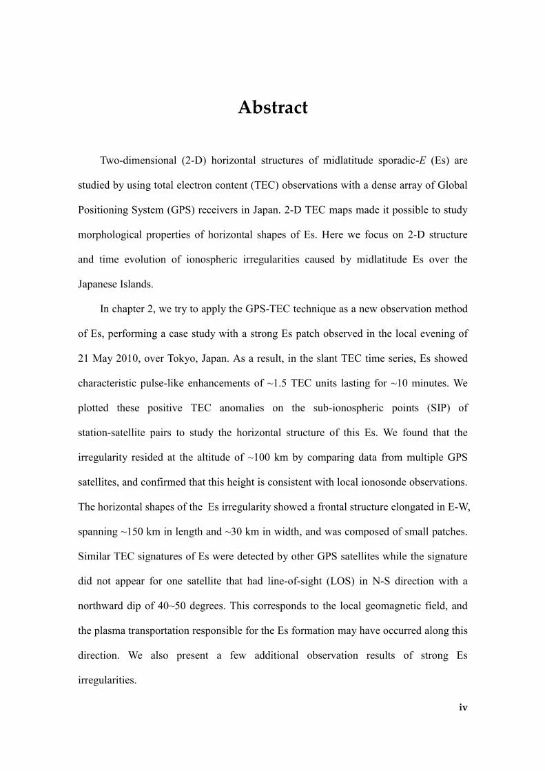
In chapter 2, we try to apply the GPS-TEC technique as a new observation method
of Es, performing a case study with a strong Es patch observed in the local evening of
21 May 2010, over Tokyo, Japan. As a result, in the slant TEC time series, Es showed
characteristic pulse-like enhancements of ~1.5 TEC units lasting for ~10 minutes. We
plotted these positive TEC anomalies on the sub-ionospheric points (SIP) of
station-satellite pairs to study the horizontal structure of this Es. We found that the
irregularity resided at the altitude of ~100 km by comparing data from multiple GPS
satellites, and confirmed that this height is consistent with local ionosonde observations.
The horizontal shapes of the Es irregularity showed a frontal structure elongated in E-W,
spanning ~150 km in length and ~30 km in width, and was composed of small patches.
Similar TEC signatures of Es were detected by other GPS satellites while the signature
did not appear for one satellite that had line-of-sight (LOS) in N-S direction with a
northward dip of 40~50 degrees. This corresponds to the local geomagnetic field, and
the plasma transportation responsible for the Es formation may have occurred along this
direction. We also present a few additional observation results of strong Es
irregularities.
v
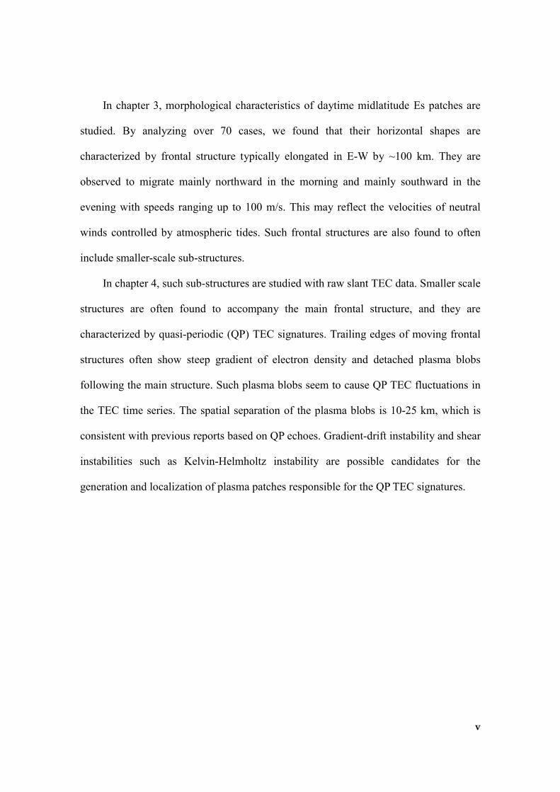
In chapter 3, morphological characteristics of daytime midlatitude Es patches are
studied. By analyzing over 70 cases, we found that their horizontal shapes are
characterized by frontal structure typically elongated in E-W by ~100 km. They are
observed to migrate mainly northward in the morning and mainly southward in the
evening with speeds ranging up to 100 m/s. This may reflect the velocities of neutral
winds controlled by atmospheric tides. Such frontal structures are also found to often
include smaller-scale sub-structures.
In chapter 4, such sub-structures are studied with raw slant TEC data. Smaller scale
structures are often found to accompany the main frontal structure, and they are
characterized by quasi-periodic (QP) TEC signatures. Trailing edges of moving frontal
structures often show steep gradient of electron density and detached plasma blobs
following the main structure. Such plasma blobs seem to cause QP TEC fluctuations in
the TEC time series. The spatial separation of the plasma blobs is 10-25 km, which is
consistent with previous reports based on QP echoes. Gradient-drift instability and shear
instabilities such as Kelvin-Helmholtz instability are possible candidates for the
generation and localization of plasma patches responsible for the QP TEC signatures.
vi
Acknowledgments
On submitting this dissertation, I would like to show my sincere gratitude to all of
the people who encouraged and advised me in the course of my study.
First, my hearty gratitude goes to Professor Kosuke Heki who has patiently guided
and assisted me throughout the work. He always welcomed me to ask any question and
helped me to solve problems I faced. Also he encouraged me to attend a number of
international and domestic conferences, where I discussed with many researchers. These
experiences substantially improved not only my knowledge but also imagination to read
data and results. I wish to thank Professor Masato Furuya for giving me opportunities to
learn data processing of synthetic aperture radar (SAR). Direct imaging of sporadic-E
with SAR observation will definitely be the next challenge, at which I am excited. I
would like to express my hearty appreciation to Prof. Junji Koyama, Prof. Kiyoshi
Yomogida, and Prof. Kazunori Yoshizawa for their constructive comments and advices.
My hearty appreciation goes to Professor Shigeto Watanabe and Dr. Junichi Kurihara
for their helpful discussion and comments which greatly improved this dissertation.
I wish to show my sincere gratitude to Prof. Mamoru Yamamoto of Kyoto
University, Dr. Takashi Maruyama of National Institute of Information and
Communications Technology, and Dr. Susumu Saito of Electronic Navigation Research
Institute for their constructive discussion and warm encouragement at every science
meeting.
Last but not least, I thank my family for all of the ‘continuous’ support given to me
who has been always chasing a so-called ‘sporadic’ thing.

1
Chapter 1
Introduction
Chapter 1: Introduction
2
1.1. Midlatitude sporadic-E
1.1.1. General introduction
Sporadic-E (Es) is a densely ionized plasma patch which occasionally appears at
altitudes around 100 km in the E-region of the ionosphere. It is characterized by
anomalously high electron densities that often exceed those in the F-region (alt. ~300
km). Since the era of telecommunication utilizing ionosphere, Es has been a
long-standing puzzling problem for the society of radio communications. Its
unpredictable appearance often causes irregular propagation of high frequency (HF) and
very high frequency (VHF) radio waves. Nowadays, the means of telecommunication
shifted from HF to satellite communications with microwaves. Nevertheless, Es still
remains an important issue because it often causes scintillations in microwaves and
degrades the positioning accuracy of Global Navigation Satellite System (GNSS).
Es is often divided into three categories by geographical regions; polar-,
midlatitude-, and equatorial-types. These are also characterized by different generation
mechanisms. In the polar region, Es is triggered and accompanied by aurora activities
during nighttime. Equatorial Es occurs near the magnetic equator during daytime
[Whitehead, 1970, and references therein]. Midlatitude Es, the main target of the present
work, is formed in the midlatitude regions of both hemispheres primarily by vertical
shears in the neutral winds in the lower thermosphere [Whitehead, 1989].
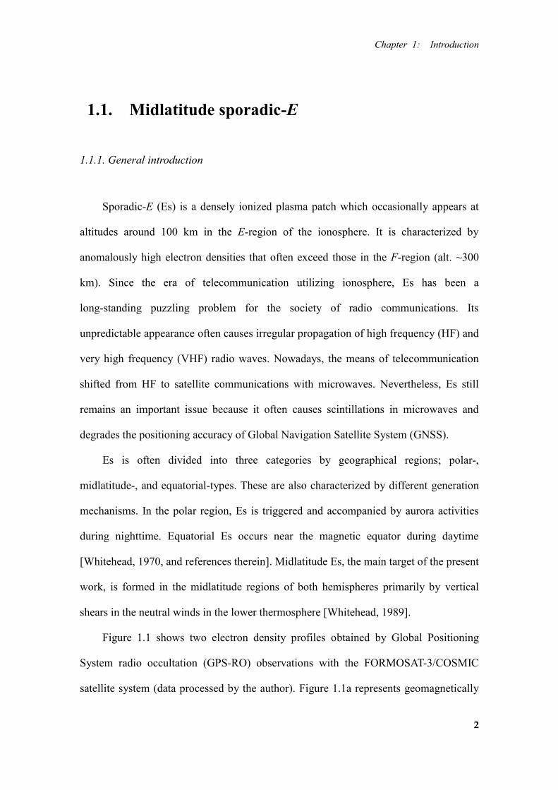
Figure 1.1 shows two electron density profiles obtained by Global Positioning
System radio occultation (GPS-RO) observations with the FORMOSAT-3/COSMIC
satellite system (data processed by the author). Figure 1.1a represents geomagnetically
Chapter 1: Introduction
3
quiet time ionosphere without Es. The profiles were obtained over the central part of
Japan in May 2009, the early summer in the Northern Hemisphere (NH). Black and
gray lines show daytime and nighttime profiles, respectively. There we can see clear F2
peaks both in daytime and nighttime. During daytime, F1- and E-regions are evident
between altitudes ~100 km and ~200 km, which almost disappear in nighttime. In
Figure 1.1b, a densely ionized thin layer can be seen at an altitude of ~110 km. The
profile is obtained over the northern Pacific Ocean in May 2012. This is a typical
electron density profile of a midlatitude Es layer. The peak electron density of this thin
layer reaches 8.0 x 10⁵ el/cm
3 which is equivalent to the critical frequency (foEs) of 8.0
Figure 1.1. Electron density profiles from GPS-RO of (a) daytime (black) and
nighttime (gray) ionosphere without Es and (b) daytime ionosphere with a typical
Es layer at midlatitudes. The profiles are measured over central Japan in May 2009
(Fig1.1a) and northern Pacific Ocean in May 2012 (Fig1.1b), respectively.
Chapter 1: Introduction
4
MHz. As shown in Figure 1.1b, the electron density in an Es layer often exceeds that of
the F-region. The mean thickness of layers is reported to be in the range of 0.5-2.0 km
[Kantarizis, 1971], and this is extremely thin compared to that of the F2 layer.
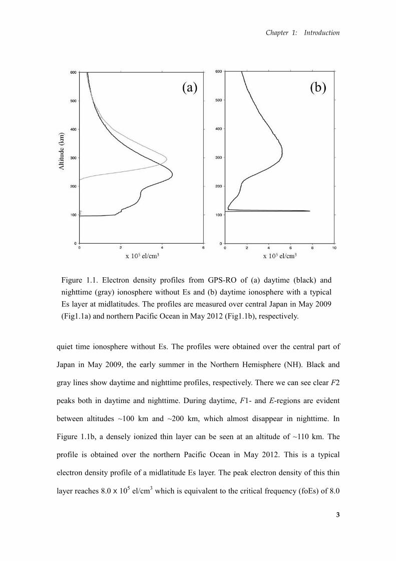
Figure 1.2 is an ionogram showing typical example of intensely ionized Es
observed by an ionosonde at Kokubunji, Tokyo, Japan on 6 June 2013. Such an
ionogram is routinely published online by National Institute of Information and
Communications Technology (NICT). As seen in Figure 1.1, the peak electron density is
dominated by F2 layer during daytime. In the ionogram, however, F2 layer is absent,
being blanketed by the Es layer underneath. This is called blanket Es, and indicates that
the layer is uniformly formed to cover the entire horizontal field of view of the
Figure 1.2. Typical Es trace in an ionogram obtained at Kokubunji ionosonde.
Courtesy of National Institute of Information and Communications Technology
(NICT).
Chapter 1: Introduction
5
ionosonde. If the layer is patchy, then an F2 trace can be seen together with Es trace, i.e.,
transparent Es. The ionosonde, or bottom side sounding, is one of the oldest observation
methods of Es which provides a number of parameters such as foEs, fbEs (blanketing
frequency), and h’Es (height of Es). Blanketing/transparent signatures are also read
directly from the backscatter traces in the ionograms.
In the present study, we will focus on midlatitude Es. In the next section, we will
review our current knowledge of midlatitude Es.
Chapter 1: Introduction
6
1.1.2 Seasonal variation of Es occurrence
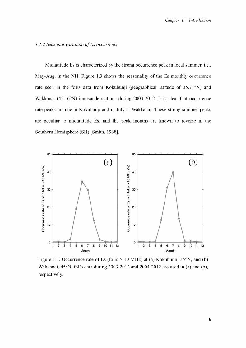
Midlatitude Es is characterized by the strong occurrence peak in local summer, i.e.,
May-Aug, in the NH. Figure 1.3 shows the seasonality of the Es monthly occurrence
rate seen in the foEs data from Kokubunji (geographical latitude of 35.71°N) and
Wakkanai (45.16°N) ionosonde stations during 2003-2012. It is clear that occurrence
rate peaks in June at Kokubunji and in July at Wakkanai. These strong summer peaks
are peculiar to midlatitude Es, and the peak months are known to reverse in the
Southern Hemisphere (SH) [Smith, 1968].
Figure 1.3. Occurrence rate of Es (foEs > 10 MHz) at (a) Kokubunji, 35°N, and (b)
Wakkanai, 45°N. foEs data during 2003-2012 and 2004-2012 are used in (a) and (b),
respectively.
Chapter 1: Introduction
7
1.1.3. Global distribution of Es occurrences
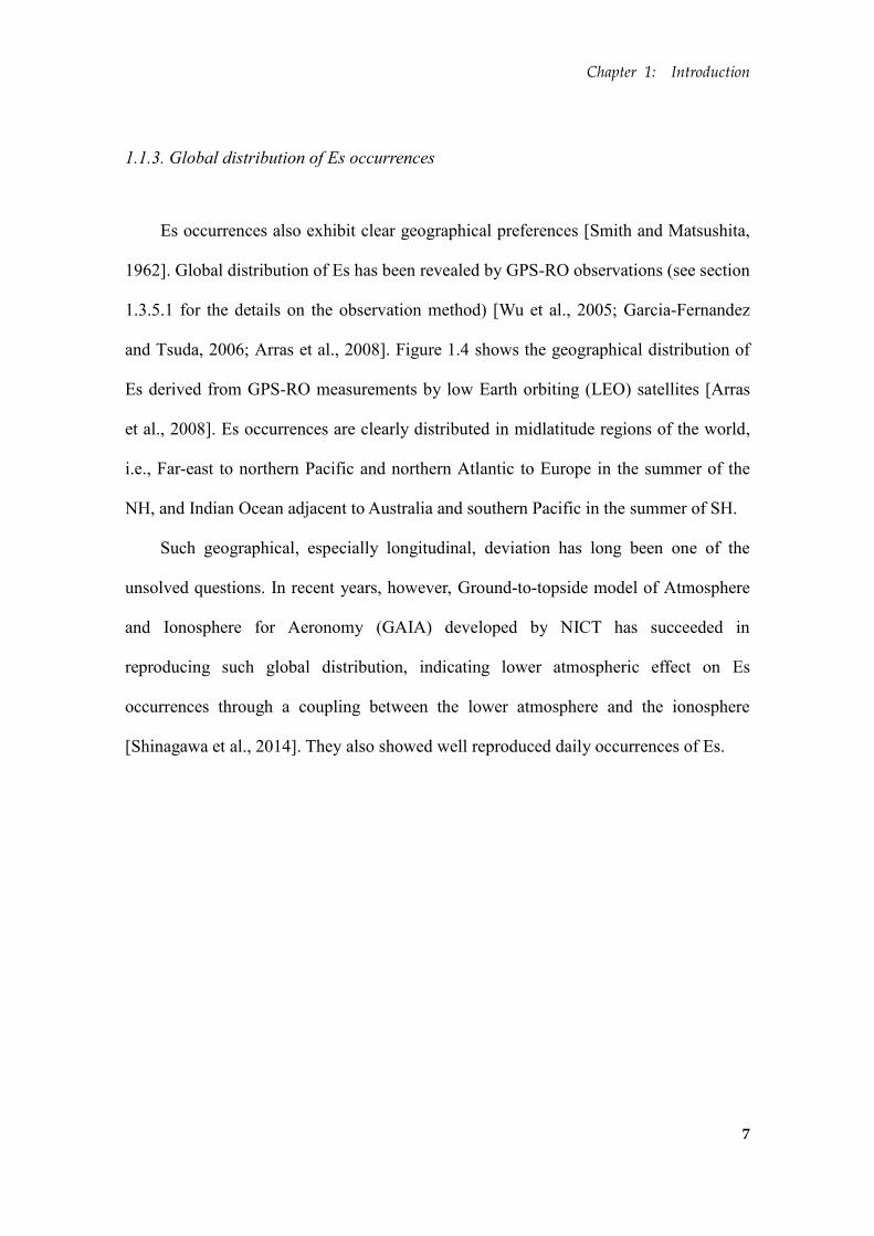
Es occurrences also exhibit clear geographical preferences [Smith and Matsushita,
1962]. Global distribution of Es has been revealed by GPS-RO observations (see section
1.3.5.1 for the details on the observation method) [Wu et al., 2005; Garcia-Fernandez
and Tsuda, 2006; Arras et al., 2008]. Figure 1.4 shows the geographical distribution of
Es derived from GPS-RO measurements by low Earth orbiting (LEO) satellites [Arras
et al., 2008]. Es occurrences are clearly distributed in midlatitude regions of the world,
i.e., Far-east to northern Pacific and northern Atlantic to Europe in the summer of the
NH, and Indian Ocean adjacent to Australia and southern Pacific in the summer of SH.
Such geographical, especially longitudinal, deviation has long been one of the
unsolved questions. In recent years, however, Ground-to-topside model of Atmosphere
and Ionosphere for Aeronomy (GAIA) developed by NICT has succeeded in
reproducing such global distribution, indicating lower atmospheric effect on Es
occurrences through a coupling between the lower atmosphere and the ionosphere
[Shinagawa et al., 2014]. They also showed well reproduced daily occurrences of Es.
Chapter 1: Introduction
8
Figure 1.4. Global distribution of Es occurrences retrieved from GPS-RO
measurements by low Earth orbiting satellites, such as CHAMP, GRACE, and
FORMOSAT-3/COSMIC [Arras et al., 2008]. Panels represent autumn, winter,
spring, and summer (in the Northern Hemisphere) in clockwise from top left.
Chapter 1: Introduction
9
1.1.4. Wind shear theory
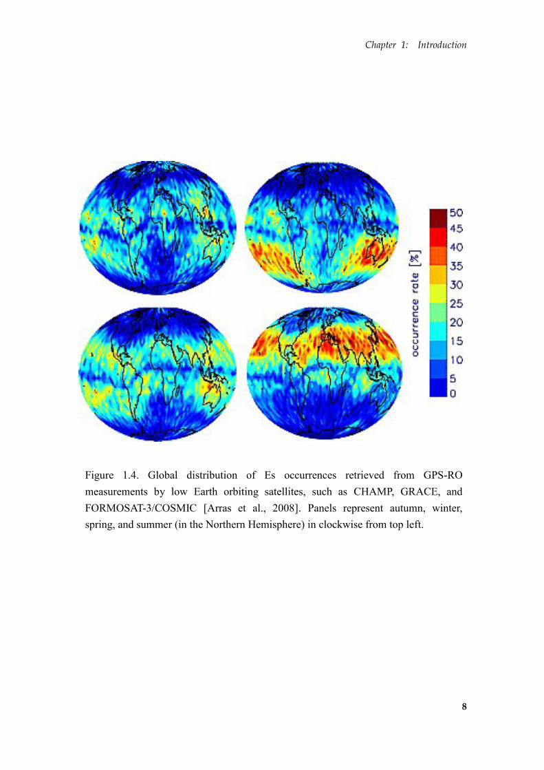
Vertical wind shear is a widely accepted mechanism that explains the formation of
midlatitude Es [Dungey, 1959; Whitehead, 1960, 1961]. Figure 1.5 shows the schematic
illustration of ion convergence in the E-region of the ionosphere by zonal and
meridional wind shears in the presence of inclined geomagnetic fields. Although the
possible shear nodes can be caused by both zonal and meridional winds, the primary
driver of ion convergence in the altitude below 115 km is considered to be zonal winds
[Haldoupis, 2012]. Associated with the convergence process of positive ions into a
thin layer, electrons move along the geomagnetic field lines to neutralize the positive
charge. Consequently, a densely ionized layer is formed at the altitude of wind shear
null. It should be noticed that this wind shear theory only explains the principle of layer
formation in the vertical plane but not in the horizontal plane.
Figure 1.5. Principal ion convergence mechanisms in (a) zonal and (b) meridional
wind shear node [Haldoupis, 2012]. In the lower E-region (altitudes below 115 km),
zonal wind shear is the primary driver of ion convergence.
Chapter 1: Introduction
10
What is the source of the positive ion? In the daytime E-region, N2 and O2 are the
dominant molecules for ionization. However, their rapid recombination leads E-region
ionization to photo-equilibrium, which is the reason why a normal E-layer almost
disappears at night. On the other hand, Es often occurs at night and it is common that
their appearances last for several hours. These facts immediately contradict with the
normal E-region photo-equilibrium and exclude it from the possible source of positive
ions responsible for the Es ionization.
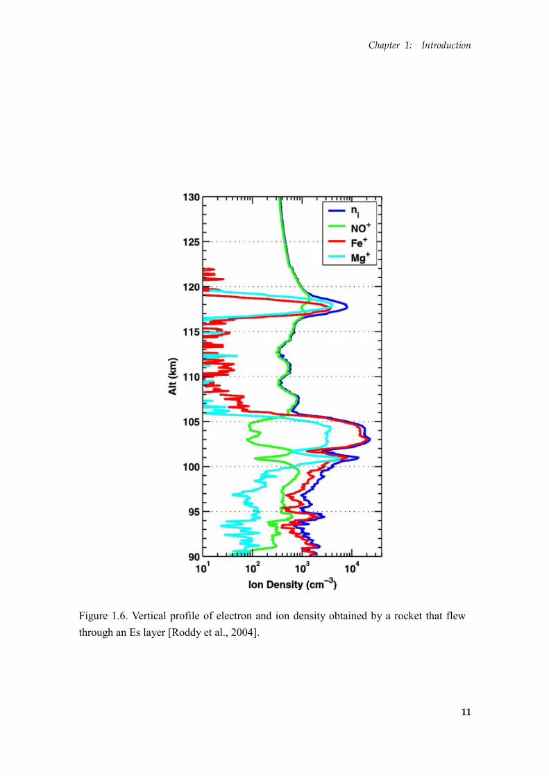
Later on, rocket observations have directly measured the electron and ion density
profile to confirm that metallic ions, e.g., Fe+ and Mg
+, are the primary source of Es
ionization [e.g., Roddy et al., 2004]. As the theory predicts, recombination rates of these
metallic ions are much lower than those of NO+ and O2
+. Metallic ions have long
lifetimes depending on altitudes, e.g., a few days at ~120 km and a few hours at ~95 km
[Haldoupis, 2012]. In Figure 1.6, it is evident that twin-peak of electron density at the
altitudes of 103-105 km and 117-118 km well corresponds to those of Fe+ and Mg
+.
These metallic atoms are considered to be of meteoric origin and it is natural to consider
that the formation of these thin layers is attributed to the ion convergence by the neutral
wind shears in the presence of geomagnetic field.
It should be noticed that although meteor is the source of the metallic ions, it does
not immediately mean that meteor itself is the direct cause of Es. Although, in some
observations, meteor is observed to be trapped in the wind shear node to produce
enhanced Es (Figure 1.7 and 1.8), the primary mechanism is considered to be the
existence of shears in the neutral winds [Maruyama et al., 2003, 2008; Malhotra et al.,
2008].
Chapter 1: Introduction
11
Figure 1.6. Vertical profile of electron and ion density obtained by a rocket that flew
through an Es layer [Roddy et al., 2004].

Chapter 1: Introduction
12
Figure 1.7. A schematic illustration of meteor trail, its condensation into a thin layer
by wind shear, and development of Es patch [Maruyama et al., 2003]
Figure 1.8. Range-time-intensity (RTI) plot of meteor induced enhancement in
sporadic-E ionization [Malhotra et al., 2008]. SNR stands for signal-to-noise ratio
(in dB).
Chapter 1: Introduction
13
1.2. Unsolved problems on midlatitude sporadic-E
There are a number of issues that remain unsolved regarding midlatitude Es. They
are classified into either of the two categories, i.e., morphology and dynamics. The
former is about the shapes of Es plasma patches. The morphological properties such as
length, width, alignment azimuth, and structures are yet to be investigated. The latter is
related to the generation mechanism, temporal evolution, and movements of dense Es
patches. Although several hypotheses have been proposed, insufficient number of Es
observations prohibits conclusive discussions.
1.2.1. Morphology
Since its discovery, structure of Es has been drawing attention of researchers.
Nevertheless, its two-dimensional (2-D) horizontal shape has long been ambiguous due
to the lack of appropriate observation means. In recent years, their 2-D horizontal
shapes have been successfully imaged with ground-based radar observations during
nighttime [Hysell et al., 2002; 2004; Larsen et al., 2007]. For example, Hysell et al.
[2009] used a coherent scatter radar (CSR) at St. Croix, US Virgin Islands (USVI) in the
Caribbean Sea, to observe low- and mid-latitude Es. They revealed patchy structures of
Es elongated in E-W and/or NW-SE, and their movements in the directions
perpendicular to the elongation azimuths. Kurihara et al. [2010] revealed the 2-D image
of an Es patch by the magnesium ion imager (MII) on board a rocket flying over
southwestern Japan. The patch had a horizontal dimension of 30 x 10 km and showed
elongation in NW-SE.
Chapter 1: Introduction
14
Numerical simulations suggested that Es patches are preferably aligned in NW-SE
and propagate southwestward in the NH [Cosgrove and Tsunoda, 2002, 2004;
Yokoyama et al., 2009]. However, there have not been sufficient number of
observations on the horizontal structure, temporal evolution, and movement of Es to
substantiate such simulation results. Thus morphological properties of midlatitude Es
have remained vague to a large extent until now.
1.2.2. Dynamics
Widely accepted structuring mechanisms of Es under the presence of vertical wind
shear include, atmospheric gravity waves [Woodman et al., 1991; Didebulidze and
Lomidze, 2010; Chu et al., 2011], shear instability [Larsen, 2000; Bernhardt, 2002;
Larsen et al., 2007; Hysell et al., 2009], and Es-layer instability [Cosgrove and Tsunoda,
2002; 2004]. The atmospheric gravity waves are suggested to modulate Es layer
vertically, which would cause quasi-periodic (QP) radar echoes. However, even the
intensive rocket experiments combined with ground-based radar observations during the
Sporadic-E Experiment over Kyushu (SEEK) campaign failed to confirm their effect
[Larsen et al., 1998].
The shear instabilities such as Kelvin-Helmholtz (K-H) instability in the neutral
atmosphere are also proposed to create a densely ionized billow structure [Bernhardt,
2002]. In fact, such billow structure in the E-region of the ionosphere is imaged as a
trimethyl aluminum (TMA) trail in the up-leg portion of a rocket experiment conducted
in the SEEK-2 campaign [Larsen et al., 2005].
Es-layer instability has a unique characteristic that maximum growth rate is
Chapter 1: Introduction
15
achieved when the ionized patches are aligned in the NW-SE and is also characterized
by preferred southwestward propagation in the NH [Cosgrove and Tsunoda, 2002].
At the moment, it is difficult to tell which mechanism is dominant for Es
structuring because of the scarcity of observations. Hence, studies of morphology and
dynamics of Es, e.g., horizontal shapes and movements, are indispensable to discuss
their generation mechanisms. The morphological properties of Es would serve as a key
to evaluate the proposed theories. This is the primary motivation of the present work, to
study 2-D images of midlatitude Es plasma patches.
Chapter 1: Introduction
16
1.3. Current observation methods and instruments
In this section, we briefly introduce current observation instruments and methods.
1.3.1. Ionosonde
As mentioned in the previous section, one of the oldest observation methods of Es
is the bottom-side sounding by ionosondes. In Japan, four ionosonde stations are
currently operational, i.e., Wakkanai, Kokubunji, Yamagawa, and Okinawa, and NICT
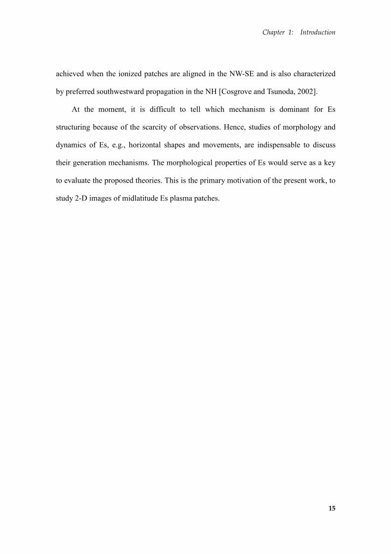
conduct routine observations every 15 min. Figure 1.9 shows the picture of the antenna
site of the Okinawa ionosonde. Ionograms (Figure 1.2) obtained by these ionosondes
are made available online (http://wdc.nict.go.jp/ionog/js_viewer/js_01.html). These four
ionosondes perform oblique incidence sounding as well as vertical incidence sounding.
Figure 1.9. Delta-loop antenna of ionosonde station at Ohgimi, Okinawa.
Chapter 1: Introduction
17
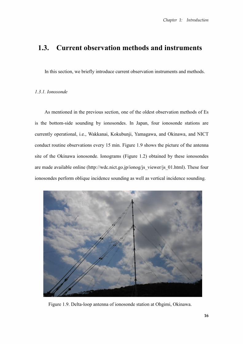
Figure 1.10. Part of the array composed of eight Yagi-Uda antenna of the CSR at St.
Croix, USVI [Cornell University, http://landau.geo.cornell.edu/].
1.3.2. Coherent scatter radar
A coherent scatter radar (CSR) is a ground-based radar. CSR is often used to
observe plasma irregularities with radio imaging technique. In the Es study, CSR at St.
Croix, US Virgin Island (USVI), is well known. The radar transmits in 29.8 MHz (HF
wave) with a peak output power of 8 kW using an array of eight 5-element Yagi-Uda
antennas (Figure 1.10). This CSR is often operated in combination with incoherent
scatter radar (ISR) at Arecibo, Puerto Rico, to conduct simultaneous observations on
plasma structures and various parameters of plasma of the low- and mid-latitude Es
irregularities [Hysell et al., 2004; 2009].
Chapter 1: Introduction
18
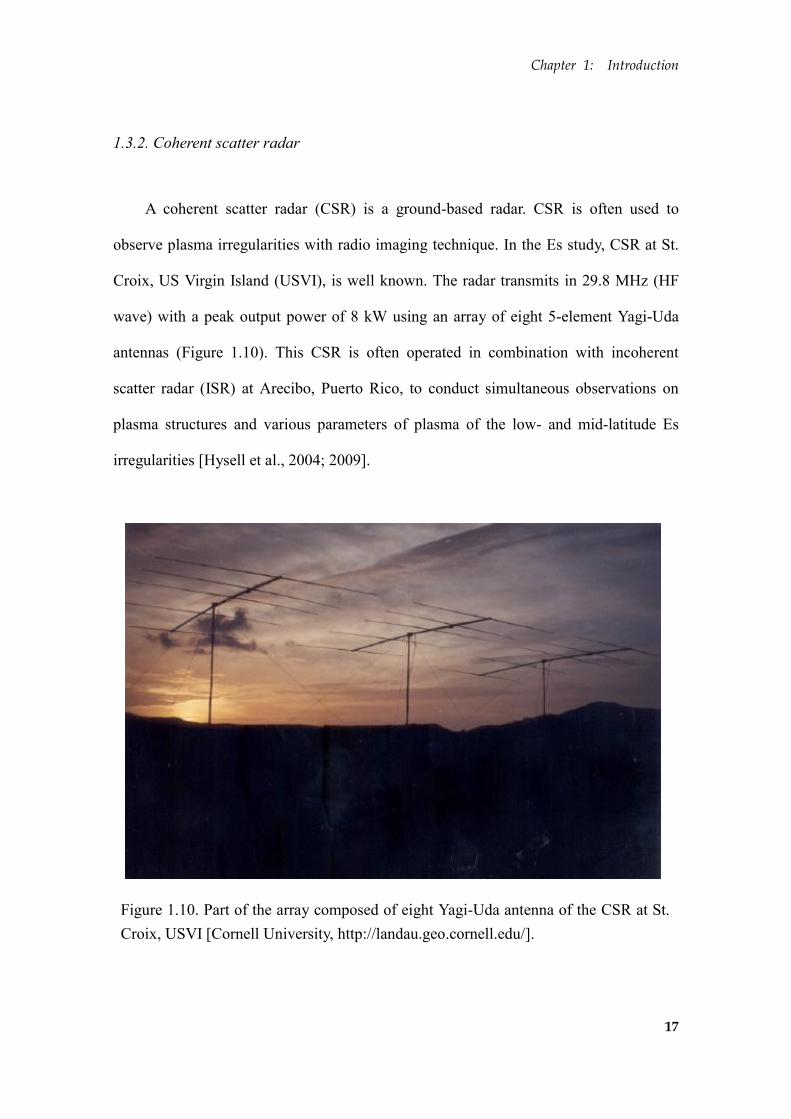
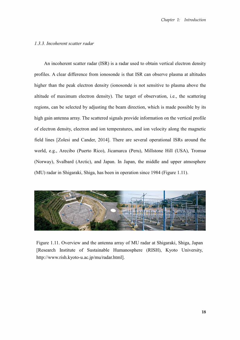
Figure 1.11. Overview and the antenna array of MU radar at Shigaraki, Shiga, Japan
[Research Institute of Sustainable Humanosphere (RISH), Kyoto University,
http://www.rish.kyoto-u.ac.jp/mu/radar.html].
1.3.3. Incoherent scatter radar
An incoherent scatter radar (ISR) is a radar used to obtain vertical electron density
profiles. A clear difference from ionosonde is that ISR can observe plasma at altitudes
higher than the peak electron density (ionosonde is not sensitive to plasma above the
altitude of maximum electron density). The target of observation, i.e., the scattering
regions, can be selected by adjusting the beam direction, which is made possible by its
high gain antenna array. The scattered signals provide information on the vertical profile
of electron density, electron and ion temperatures, and ion velocity along the magnetic
field lines [Zolesi and Cander, 2014]. There are several operational ISRs around the
world, e.g., Arecibo (Puerto Rico), Jicamarca (Peru), Millstone Hill (USA), Tromsø
(Norway), Svalbard (Arctic), and Japan. In Japan, the middle and upper atmosphere
(MU) radar in Shigaraki, Shiga, has been in operation since 1984 (Figure 1.11).
Chapter 1: Introduction
19
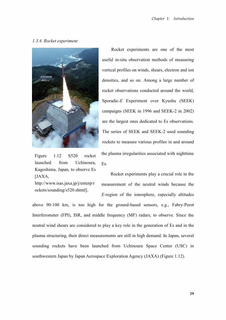
Figure 1.12 S520 rocket
launched from Uchinoura,
Kagoshima, Japan, to observe Es
[JAXA,
http://www.isas.jaxa.jp/j/enterp/r
ockets/sounding/s520.shtml].
1.3.4. Rocket experiment
Rocket experiments are one of the most
useful in-situ observation methods of measuring
vertical profiles on winds, shears, electron and ion
densities, and so on. Among a large number of
rocket observations conducted around the world,
Sporadic-E Experiment over Kyushu (SEEK)
campaigns (SEEK in 1996 and SEEK-2 in 2002)
are the largest ones dedicated to Es observations.
The series of SEEK and SEEK-2 used sounding
rockets to measure various profiles in and around
the plasma irregularities associated with nighttime
Es.
Rocket experiments play a crucial role in the
measurement of the neutral winds because the
E-region of the ionosphere, especially altitudes
above 90-100 km, is too high for the ground-based sensors, e.g., Fabry-Perot
Interferometer (FPI), ISR, and middle frequency (MF) radars, to observe. Since the
neutral wind shears are considered to play a key role in the generation of Es and in the
plasma structuring, their direct measurements are still in high demand. In Japan, several
sounding rockets have been launched from Uchinoura Space Center (USC) in
southwestern Japan by Japan Aerospace Exploration Agency (JAXA) (Figure 1.12).
Chapter 1: Introduction
20
1.3.4.1. Trimethyl aluminum release experiment
In addition to the measurement of vertical profiles, trimethyl aluminum (TMA)
release experiments have been conducted to provide pictorial images of neutral winds in
the E-region of the ionosphere. With a triangular survey, the detailed structure of TMA
trails can provide information on, e.g., wavelength of perturbations in neutral wind. The
results of TMA release experiments are discussed in the section 4.4.
1.3.4.2. Magnesium ion imager
Magnesium ion imager (MII) was launched on board a rocket from USC in the
summer of 2009, to image the horizontal structure of Es irregularities. Since the
magnesium ions are one of the dominant long-life metallic ions that are responsible for
Es ionization (Figure 1.6), MII captures the scattering from Mg+ ions to enable 2-D
mapping of Es patches. This is currently the only observation method, except GPS-TEC,
that directly images the horizontal shape of Es. The results of an MII experiment are
discussed in the chapter 3.1.
1.3.5. Remote sensing of the ionosphere from space
Top-side soundings by satellites were conducted in the earlier period back in the
1980s, which may be the first remote sensing of the ionosphere from space. In recent
years, ionosphere observations have come to see a new remote sensing method, that is,
Global Navigation Satellite System (GNSS). Using such navigation satellites, the
Earth’s ionosphere can be observed more globally and continuously than previous days.
Chapter 1: Introduction
21
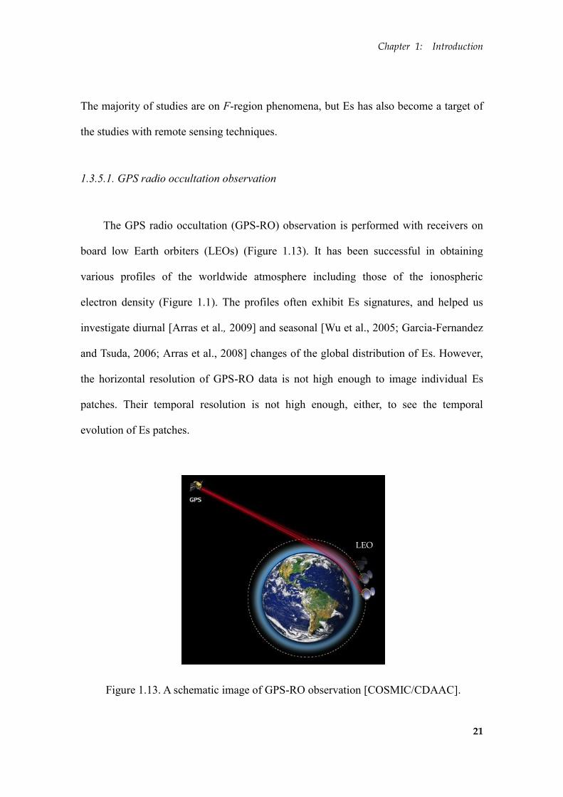
Figure 1.13. A schematic image of GPS-RO observation [COSMIC/CDAAC].
The majority of studies are on F-region phenomena, but Es has also become a target of
the studies with remote sensing techniques.
1.3.5.1. GPS radio occultation observation
The GPS radio occultation (GPS-RO) observation is performed with receivers on
board low Earth orbiters (LEOs) (Figure 1.13). It has been successful in obtaining
various profiles of the worldwide atmosphere including those of the ionospheric
electron density (Figure 1.1). The profiles often exhibit Es signatures, and helped us
investigate diurnal [Arras et al., 2009] and seasonal [Wu et al., 2005; Garcia-Fernandez
and Tsuda, 2006; Arras et al., 2008] changes of the global distribution of Es. However,
the horizontal resolution of GPS-RO data is not high enough to image individual Es
patches. Their temporal resolution is not high enough, either, to see the temporal
evolution of Es patches.
LEO
Chapter 1: Introduction
22
1.3.5.2. GNSS total electron content observation
In recent years, various GNSS has been launched. Although their primary purpose
is positioning and measurements of crustal deformation, they are also useful to
investigate the Earth’s ionosphere.
GNSS satellites use microwave carriers in two different frequencies. Since the
ray-path, or line-of-sight, between a satellite and a ground-based receiver go through the
ionosphere, GNSS signal reaches the receiver with phase delays depending on the
carrier wave frequencies. Such ionospheric delay is inversely proportional to the square
of the frequency as the first approximation [Kedar et al., 2003], and the temporal change
of the phase difference between the two carrier waves is proportional to the change in
total electron content (TEC) along the line-of-sight. In short, this method can measure
the total number of electrons along the ray-path between a satellite and a receiver.
Global Positioning System (GPS), the American GNSS, has been widely used for
TEC measurements, and the technique is often called GPS-TEC. Since the TEC is
dominated by the electrons in the F-region of the ionosphere and has no vertical
resolution in principle, it has been used mostly to study ionospheric phenomena in the
F-region. If the GNSS receiver network is dense enough, it can perform 2-D mapping of
TEC and enables us to investigate horizontal distributions of various kinds of
ionospheric irregularities, e.g., medium-scale traveling ionospheric disturbances
(MSTIDs) [Saito et al., 1998, 2002], spread-F [Mendillo et al., 2001], plasma bubbles
[Otsuka et al., 2002; Ma and Maruyama, 2006], storm enhanced densities (SED) [Foster
et al., 2002] and so on. However, Es have never been studied with this method. In the
present study, we apply this method to study Es and perform systematic investigations

Chapter 1: Introduction
23
of its 2-D horizontal structures for the first time. Further details of this observation
technique and its application to Es observations are given in the next chapter.
1.4. The objectives of the present work
With the background explained in the previous section, this study aims to
(1) establish GPS-TEC as a new observation method to image 2-D horizontal structures
(2) reveal morphological properties of horizontal structures
(3) provide insights into the dynamics of the generation and time evolution
of midlatitude Es irregularities above the Japanese Islands.
24
Chapter 2
Application of GPS total electron content
observation on sporadic-E detection
The contents of this chapter have been published in Radio Science,
Maeda, J. and K. Heki (2014), Two-dimensional observations of mid-latitude
sporadic-E irregularities with a dense GPS array in Japan, Radio Sci., 49, 28-35,
doi:10.1002/2013RS005295.
Chapter 2: Application of GPS-TEC observation on sporadic-E detection
25
2.1. Global Positioning System
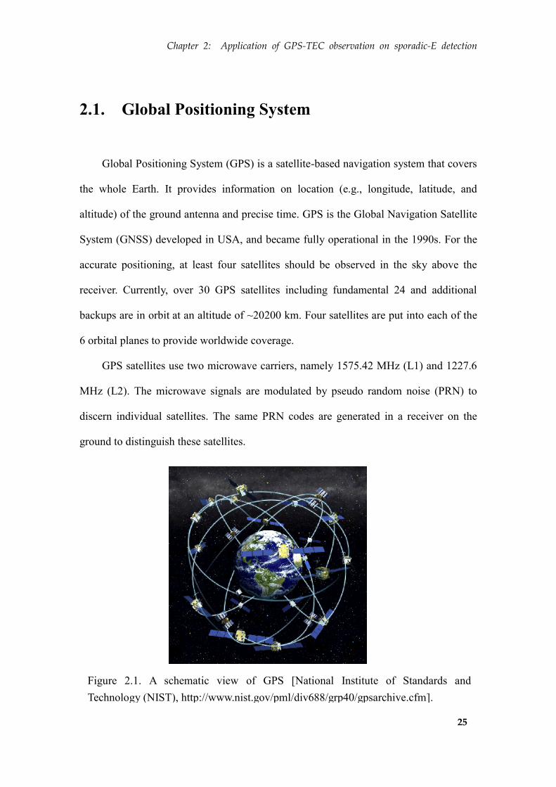
Global Positioning System (GPS) is a satellite-based navigation system that covers
the whole Earth. It provides information on location (e.g., longitude, latitude, and
altitude) of the ground antenna and precise time. GPS is the Global Navigation Satellite
System (GNSS) developed in USA, and became fully operational in the 1990s. For the
accurate positioning, at least four satellites should be observed in the sky above the
receiver. Currently, over 30 GPS satellites including fundamental 24 and additional
backups are in orbit at an altitude of ~20200 km. Four satellites are put into each of the
6 orbital planes to provide worldwide coverage.
GPS satellites use two microwave carriers, namely 1575.42 MHz (L1) and 1227.6
MHz (L2). The microwave signals are modulated by pseudo random noise (PRN) to
discern individual satellites. The same PRN codes are generated in a receiver on the
ground to distinguish these satellites.
Figure 2.1. A schematic view of GPS [National Institute of Standards and
Technology (NIST), http://www.nist.gov/pml/div688/grp40/gpsarchive.cfm].
Chapter 2: Application of GPS-TEC observation on sporadic-E detection
26
2.2. Total electron content (TEC) observation
In this study, we used GPS satellites and the Japanese nationwide dense array of
continuous GNSS receivers, called GNSS Earth Observation Network (GEONET), to
measure ionospheric total electron content (TEC) over the Japanese Islands. TEC is the
number of electrons along the path between a GNSS satellite and a ground-based
receiver. GEONET is composed of ~1200 stations throughout Japan and is operated by
Geospatial Information Authority of Japan (GSI). Its high spatial density (typical
horizontal separation of GNSS stations is 15-25 km) and time resolution (regularly
sampled every 30 seconds) enables imaging of the two-dimensional (2-D) horizontal
structure and temporal evolution of various ionospheric irregularities. Since we mainly
use GPS to derive TEC, this method is often referred to as GPS-TEC observation. It has
been applied to investigate travelling ionospheric disturbances (TIDs) [Saito et al., 1998,
2002; Tsugawa et al., 2004; Hayashi et al., 2010] and plasma bubbles [Otsuka et al.,
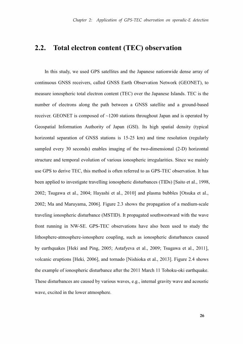
2002; Ma and Maruyama, 2006]. Figure 2.3 shows the propagation of a medium-scale
traveling ionospheric disturbance (MSTID). It propagated southwestward with the wave
front running in NW-SE. GPS-TEC observations have also been used to study the
lithosphere-atmosphere-ionosphere coupling, such as ionospheric disturbances caused
by earthquakes [Heki and Ping, 2005; Astafyeva et al., 2009; Tsugawa et al., 2011],
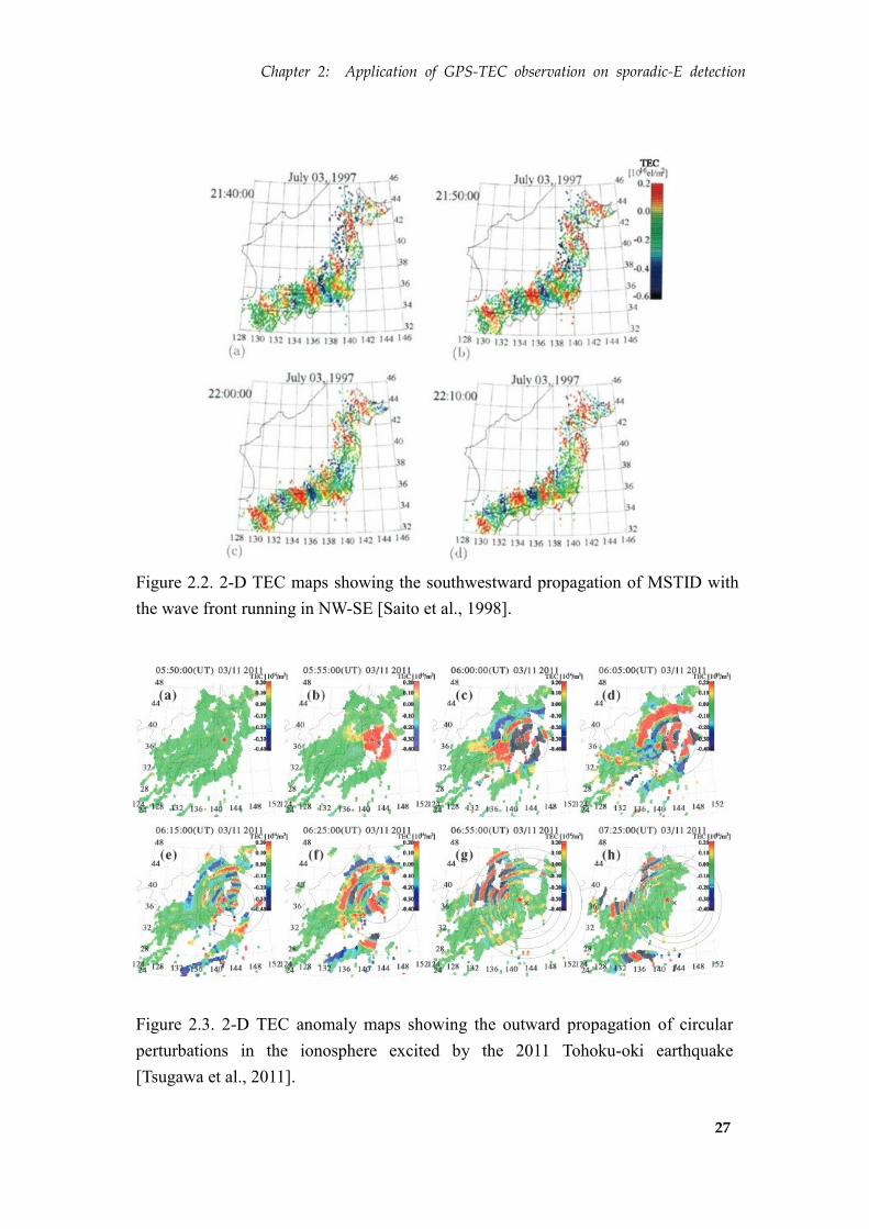
volcanic eruptions [Heki, 2006], and tornado [Nishioka et al., 2013]. Figure 2.4 shows
the example of ionospheric disturbance after the 2011 March 11 Tohoku-oki earthquake.
These disturbances are caused by various waves, e.g., internal gravity wave and acoustic
wave, excited in the lower atmosphere.
Chapter 2: Application of GPS-TEC observation on sporadic-E detection
27
Figure 2.2. 2-D TEC maps showing the southwestward propagation of MSTID with
the wave front running in NW-SE [Saito et al., 1998].
Figure 2.3. 2-D TEC anomaly maps showing the outward propagation of circular
perturbations in the ionosphere excited by the 2011 Tohoku-oki earthquake
[Tsugawa et al., 2011].

Chapter 2: Application of GPS-TEC observation on sporadic-E detection
28
2.3. Basic idea of sporadic-E detection with GPS-TEC
With its high spatial and temporal resolution of GEONET, GPS-TEC observation
has a high potential as a new method to study Es. It will enable 2-D mapping of
horizontal structure of Es, a long-standing issue in ionospheric physics. As already
shown in Figure 2.2 and 2.3, high temporal resolution makes GPS-TEC also useful to
study temporal evolution of ionospheric irregularities.
When applying this method to detect Es, there is one problem, i.e., the lack of
vertical resolution. Basically, GPS-TEC observations let us know the number of
electrons integrated along the line-of-sight between a satellite and a receiver without
recognizing altitudes where electrons exist (see Figure 2.6). Generally speaking, TEC is
dominated by electrons in the F-region of the ionosphere. Hence the GPS-TEC method
has little been used to study phenomena in the ionospheric E-region. Strong Es
irregularities are, however, expected to show TEC signals large enough to be detected in
its time series. In fact, the critical frequency of Es often exceeds that of F-region and
sometimes reaches ~20 MHz.
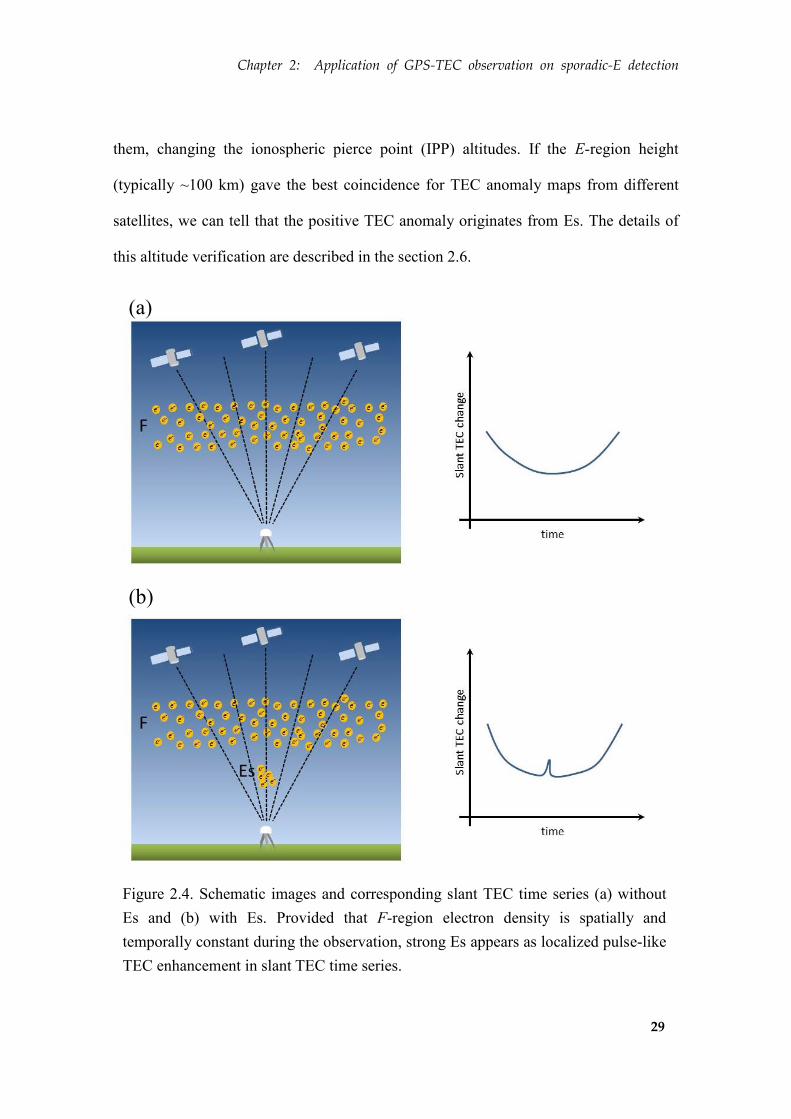
In Figure 2.4, the principle of Es detection with GPS-TEC technique is sketched.
An intensely ionized plasma patch associated with Es will cause sudden and localized
TEC enhancement when the line-of-sight penetrates it. This can be recognized as a
transient positive TEC pulse if the F-region is calm enough. However, we should verify
that the electron density enhancement occurred in the E-region of the ionosphere.
Because GPS-TEC only gives vertically integrated number of electrons, we have to rely
upon a special technique to constrain the altitude of TEC anomaly. In the present study,
we used multiple TEC maps derived from different satellites. Then we superimposed
Chapter 2: Application of GPS-TEC observation on sporadic-E detection
29
them, changing the ionospheric pierce point (IPP) altitudes. If the E-region height
(typically ~100 km) gave the best coincidence for TEC anomaly maps from different
satellites, we can tell that the positive TEC anomaly originates from Es. The details of
this altitude verification are described in the section 2.6.
Figure 2.4. Schematic images and corresponding slant TEC time series (a) without
Es and (b) with Es. Provided that F-region electron density is spatially and
temporally constant during the observation, strong Es appears as localized pulse-like
TEC enhancement in slant TEC time series.
(a)
(b)
Chapter 2: Application of GPS-TEC observation on sporadic-E detection
30
2.4. GPS data collection
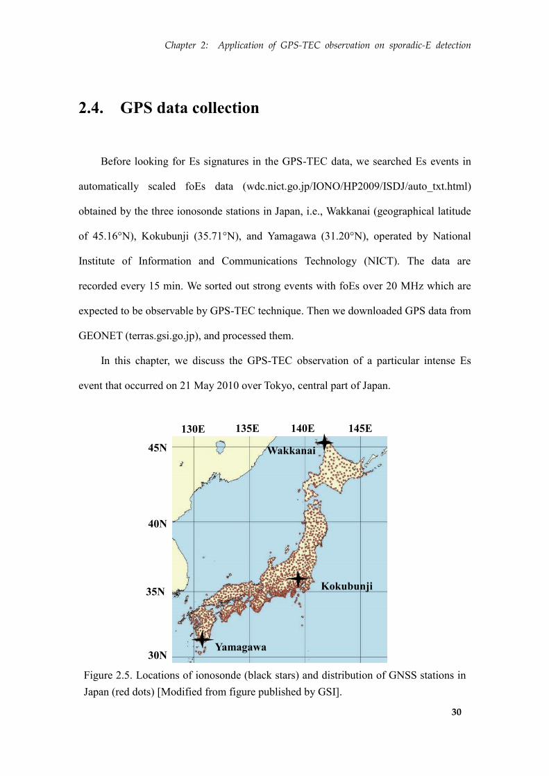
Before looking for Es signatures in the GPS-TEC data, we searched Es events in
automatically scaled foEs data (wdc.nict.go.jp/IONO/HP2009/ISDJ/auto_txt.html)
obtained by the three ionosonde stations in Japan, i.e., Wakkanai (geographical latitude
of 45.16°N), Kokubunji (35.71°N), and Yamagawa (31.20°N), operated by National
Institute of Information and Communications Technology (NICT). The data are
recorded every 15 min. We sorted out strong events with foEs over 20 MHz which are
expected to be observable by GPS-TEC technique. Then we downloaded GPS data from
GEONET (terras.gsi.go.jp), and processed them.
In this chapter, we discuss the GPS-TEC observation of a particular intense Es
event that occurred on 21 May 2010 over Tokyo, central part of Japan.
Figure 2.5. Locations of ionosonde (black stars) and distribution of GNSS stations in
Japan (red dots) [Modified from figure published by GSI].
Wakkanai
Kokubunji
Yamagawa
45N
35N
40N
30N
140E 145E 135E 130E
Chapter 2: Application of GPS-TEC observation on sporadic-E detection
31
2.5. GPS data processing
2.5.1. Derivation of TEC and model fitting
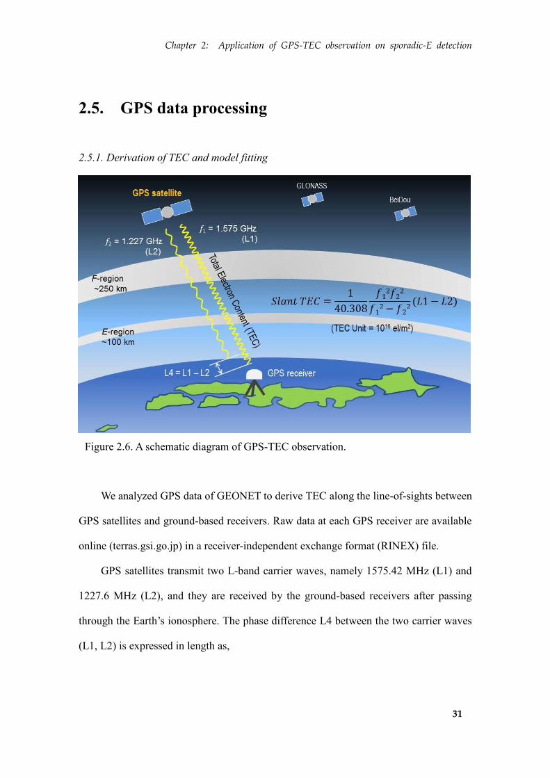
We analyzed GPS data of GEONET to derive TEC along the line-of-sights between
GPS satellites and ground-based receivers. Raw data at each GPS receiver are available
online (terras.gsi.go.jp) in a receiver-independent exchange format (RINEX) file.
GPS satellites transmit two L-band carrier waves, namely 1575.42 MHz (L1) and
1227.6 MHz (L2), and they are received by the ground-based receivers after passing
through the Earth’s ionosphere. The phase difference L4 between the two carrier waves
(L1, L2) is expressed in length as,
Figure 2.6. A schematic diagram of GPS-TEC observation.
Chapter 2: Application of GPS-TEC observation on sporadic-E detection
32
L4 L1 − L2,
whose changes are proportional to those in TEC along the line-of-sight (slant TEC).
Slant TEC is calculated from the following formula,
Slant TEC = 40.308−1 (𝑓1
2𝑓22
𝑓12 − 𝑓2
2) (L1 − L2)
where f1 and f2 represent the frequencies of L1 and L2 microwave carriers (Figure 2.6).
Provided that the F-layer is spatially and temporally calm during the measurement, slant
TEC time series show U-shaped curves because the incident angle of line-of-sights into
the ionosphere changes as the satellite moves in the sky (Figure 2.7).
Next we draw a model curve by assuming the temporal change of vertical TEC as a
polynomial of time t which is determined by least-squares method [Ozeki and Heki,
2010],
Slant TEC(𝑡, 𝜁) =Vertical TEC
cos𝜁+ 𝑑
where t, ζ, and d represent time, the zenith angle at IPP altitude, and constant bias
specific to each satellite-receiver pairs, respectively. Vertical TEC change over a few
hours period can be well approximated with a quadratic function of time t,
Vertical TEC(𝑡) = 𝑎𝑡2 + 𝑏𝑡 + 𝑐
Chapter 2: Application of GPS-TEC observation on sporadic-E detection
33
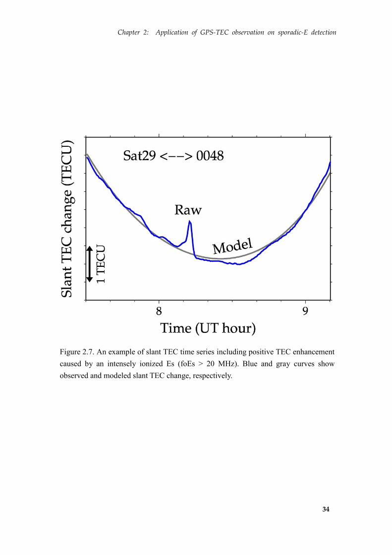
where a, b, and c are the variables to be estimated using least-squares adjustment. A
model curve is shown as a gray curve in Figure 2.7.
The typical Es signature in slant TEC (blue curve in Figure 2.7) appears at around
08:11 UT (17:11 LT) as a relatively sharp positive pulse of ~1 TECU (TEC Unit, 1
TECU 1016
electrons m-2
) lasting for ~10 minutes. At this time, the line-of-sight is
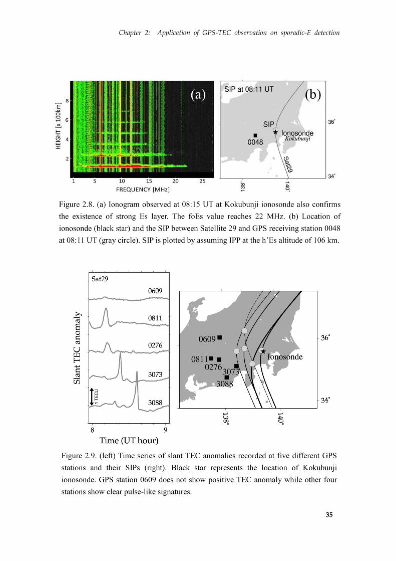
considered to have passed through one of the Es patches of very high electron density.
Almost at the same time (08:15 UT), the Kokubunji ionosonde station recorded a strong
Es with the maximum foEs of 22 MHz (Figure 2.8a). The positions of ionospheric
penetration point (IPP) of line-of-sights are calculated by assuming a thin layer at the
height of 106 km, which corresponds to the h’ Es value observed at the ionosonde. The
sub-ionospheric point (SIP), the ground projection of IPP, is close to the ionosonde (a
gray circle in Figure 2.8b), suggesting that the ionosonde and GPS-TEC detected the
same patch of Es. This comparison with a local ionosonde station supports that the
pulse-like positive TEC anomaly originates from the E-region of the ionosphere.
Chapter 2: Application of GPS-TEC observation on sporadic-E detection
34
Figure 2.7. An example of slant TEC time series including positive TEC enhancement
caused by an intensely ionized Es (foEs > 20 MHz). Blue and gray curves show
observed and modeled slant TEC change, respectively.
Chapter 2: Application of GPS-TEC observation on sporadic-E detection
35
Figure 2.8. (a) Ionogram observed at 08:15 UT at Kokubunji ionosonde also confirms
the existence of strong Es layer. The foEs value reaches 22 MHz. (b) Location of
ionosonde (black star) and the SIP between Satellite 29 and GPS receiving station 0048
at 08:11 UT (gray circle). SIP is plotted by assuming IPP at the h’Es altitude of 106 km.
Figure 2.9. (left) Time series of slant TEC anomalies recorded at five different GPS
stations and their SIPs (right). Black star represents the location of Kokubunji
ionosonde. GPS station 0609 does not show positive TEC anomaly while other four
stations show clear pulse-like signatures.

Chapter 2: Application of GPS-TEC observation on sporadic-E detection
36
The left panel of Figure 2.9 shows time series of slant TEC anomalies observed at
five different GPS stations, with which we can confirm the geographical localization of
the TEC anomaly. Four of them show positive TEC anomalies, including the one with
SIP near the ionosonde (3073). The GPS stations with pulse-like anomalies are located
to the south of 36°N. The station 0609, located to the north of the boundary, does not
show such an anomaly. Such highly-localized nature of the TEC anomaly is peculiar to
Es, and rules out other possibilities such as TIDs and solar flares. TIDs would have
much larger spatial scales and longer periods, and solar flares would have left similar
signatures over the whole sun-lit hemisphere at a certain time (there were no reports of a
solar flare at this time). Thus we consider this a signature of Es.
2.5.2. Derivation and mapping of vertical TEC anomaly
In this section we describe how the vertical TEC anomaly is calculated and
mapped to its ground projection. First, the vertical TEC anomalies are derived by
multiplying the residual of slant TEC with the cosine of the incident angle, i.e., the
zenith angle of a line-of-sight at an IPP point assuming a thin layer at an altitude of 100
km. Navigation files that contain orbital elements of GPS satellites are used to calculate
IPPs. SIP positions are calculated by assuming IPP altitude also at 100 km. Then
vertical TEC anomalies are mapped onto them, which will consequently show the 2-D
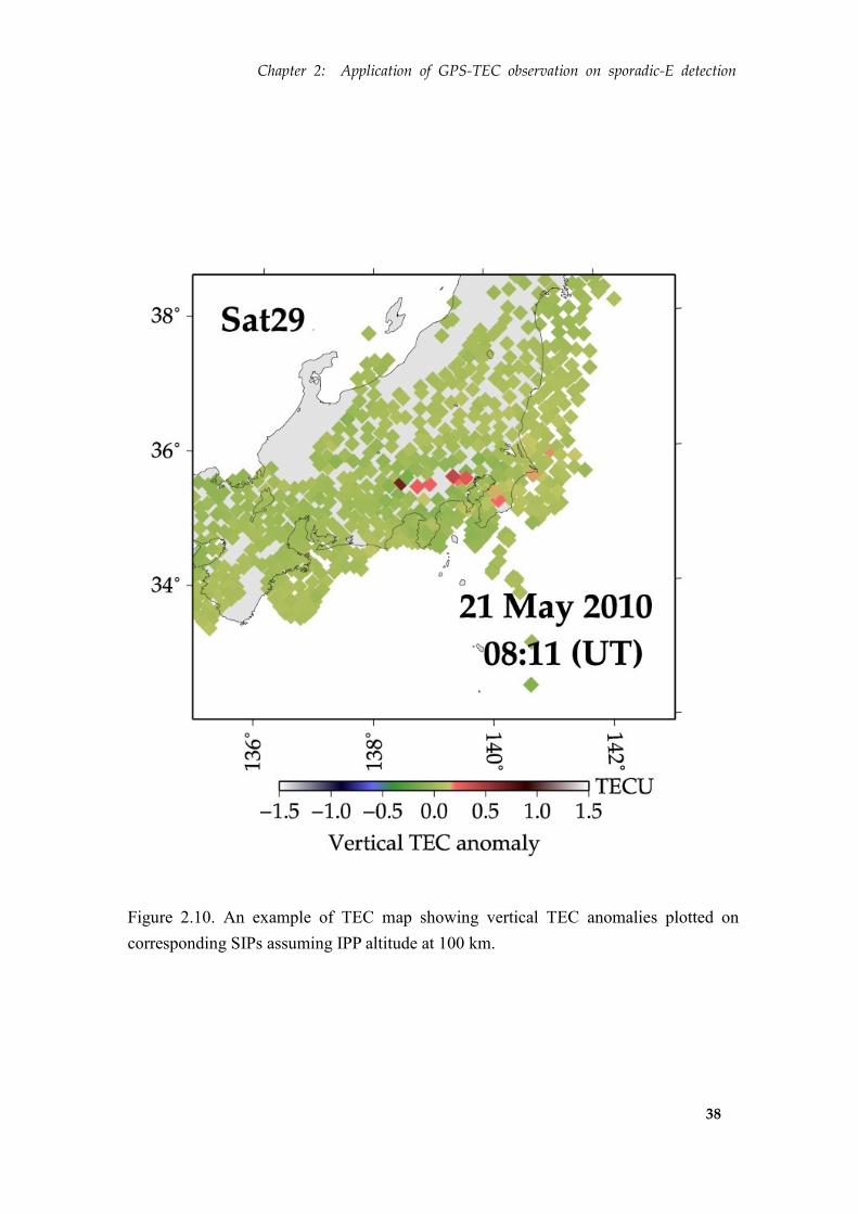
horizontal structure of Es. Figure 2.10 shows the snapshot of vertical TEC anomalies at
08:11 UT around the central Japan drawn with the IPP height of 100 km. In Figure 2.10,
we can see several red dots (positive anomaly) in the region where green dots (normal
region) are dominant. As previously discussed, positive anomaly is attributed to a
Chapter 2: Application of GPS-TEC observation on sporadic-E detection
37
plasma patch associated with Es. Thus the overview of the red dots should represent the
2-D horizontal shape of Es patches. Figure 2.10 shows that the Es irregularity has a
frontal structure elongated in the east-west (E-W) direction with the dimension of ~150
km in E-W and ~30 km in north-south (N-S).
Since the distances between GEONET stations are 15-25 km, the spatial resolution
of the vertical TEC anomaly maps is approximately ~25 km. This map shows relatively
large-scale structure having a horizontal scale size of tens to several hundreds of
kilometers with a typical spatial resolution of 15-25 km. Hence small-scale structures
with a horizontal scale size less than that are not included in the map.
Chapter 2: Application of GPS-TEC observation on sporadic-E detection
38
Figure 2.10. An example of TEC map showing vertical TEC anomalies plotted on
corresponding SIPs assuming IPP altitude at 100 km.

Chapter 2: Application of GPS-TEC observation on sporadic-E detection
39
2.6. Altitude constraint of vertical TEC anomaly
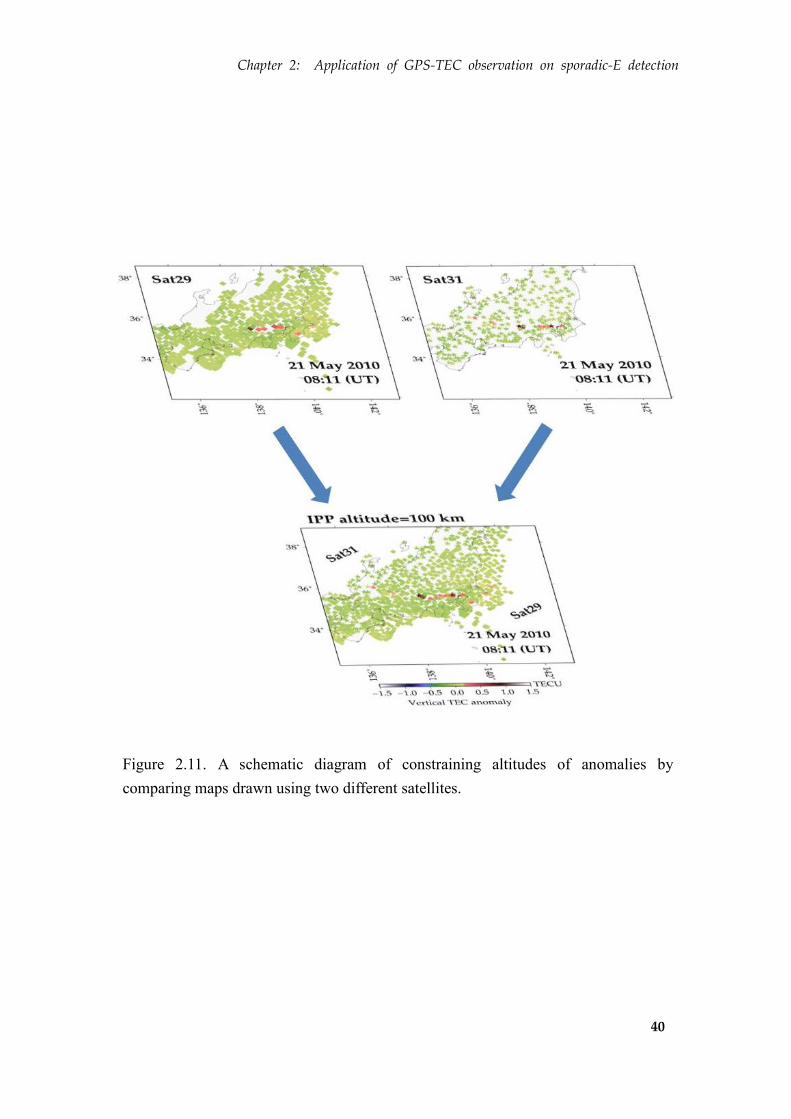
In Figure 2.11, among the majority of SIP points of green color indicating no
anomalies, there are some red and blue points indicating positive and negative
anomalies, respectively. The positive anomaly (red dots) at 08:11 UT observed with
Satellites 29 and 31 shows simple linear structures running in the E-W direction, an
ideal situation to make it possible to constrain the altitude of this linear anomaly.
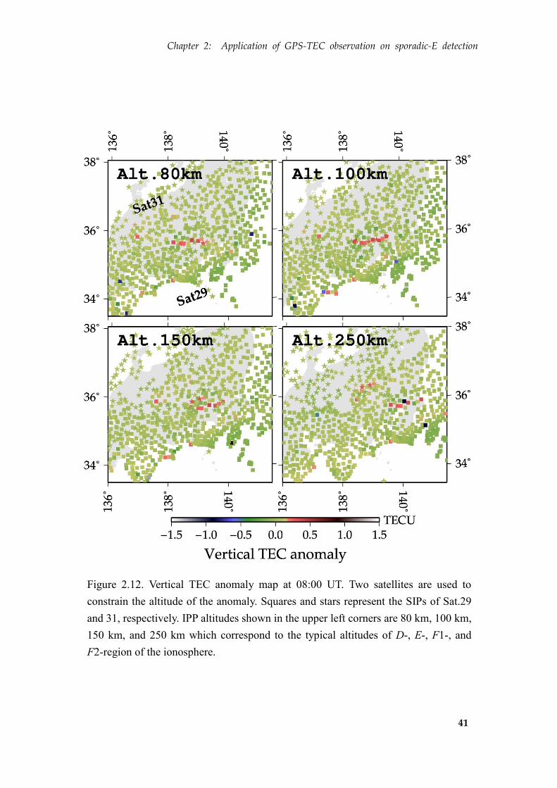
In Figure 2.12, we mapped the vertical TEC anomalies at 08:00 UT using two
different satellites. There we assume four different IPP heights in order to constrain the
altitude of the TEC anomalies. IPP height of 80 km corresponds to the D-region of the
ionosphere, and 100 km, 150 km and 250 km correspond to the E-, F1-, and F2-regions,
respectively. In Figure 2.12, two linear structures obtained from the two satellites
coincide with each other when the IPP height is assumed as 100 km. On the other hand,
large gaps emerge with higher and lower IPP heights. Considering that the h’Es at
Kokubunji ionosonde was 106 km, we can conclude with confidence that the observed
TEC anomalies are the signature of irregularities at the E-region of the ionosphere.
Chapter 2: Application of GPS-TEC observation on sporadic-E detection
40
Figure 2.11. A schematic diagram of constraining altitudes of anomalies by
comparing maps drawn using two different satellites.
Chapter 2: Application of GPS-TEC observation on sporadic-E detection
41
Figure 2.12. Vertical TEC anomaly map at 08:00 UT. Two satellites are used to
constrain the altitude of the anomaly. Squares and stars represent the SIPs of Sat.29
and 31, respectively. IPP altitudes shown in the upper left corners are 80 km, 100 km,
150 km, and 250 km which correspond to the typical altitudes of D-, E-, F1-, and
F2-region of the ionosphere.
Chapter 2: Application of GPS-TEC observation on sporadic-E detection
42
2.7. Spatial resolution: comparison with ionosonde
observation
Here we compare the Es movements shown in vertical TEC anomaly maps with
ionosonde observations. Figure 2.12 shows time series of vertical TEC maps in the left
panel, and ionograms at the corresponding time epochs obtained at the Kokubunji
ionosonde in the right panel. The ionosonde observations are much more sensitive to
‘weak’ Es layers since they transmit high-frequency (HF) radio waves up to 30 MHz at
these stations. On the other hand, GPS satellites use L-band microwaves, i.e., 1.2 and
1.5 GHz, which is not much affected by weak Es layers, e.g., with foEs less than ~10
MHz. Therefore TEC and ionosonde observations should not be compared directly, and
one should pay attention to the foEs values.
With our observation experiences, the threshold of foEs for the Es detectable with
GPS-TEC observations seems to be around 16-17 MHz. If the foEs value exceeds the
17 MHz, we can expect positive TEC pulse signatures in slant TEC time series (e.g.,
Figure 2.6), and we can draw their 2-D maps. Provided the antenna pattern is the same
as designed, the horizontal coverage of ionosonde observation, projected at an altitude
of 100 km, is assumed to be ~80 km in diameter. From that point of view, the TEC
observations and ionosonde observations coincide with each other in Figure 2.13, i.e.,
the positive TEC anomaly regions are within the horizontal scope of the ionosonde.
This comparison shows not only the better spatial resolution of the TEC map
compared to ionosonde observation, but also the usefulness of GPS-TEC observations
on knowing what caused the foEs time variation. For example, without GPS-TEC
Chapter 2: Application of GPS-TEC observation on sporadic-E detection
43
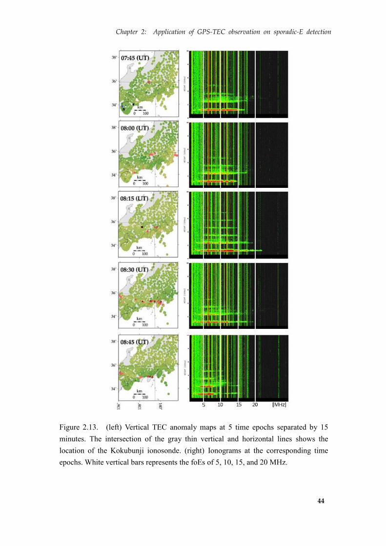
observations, the ionograms shown in Figure 2.13 only show the temporal change of
foEs and cannot tell why they changed. We cannot rule out the possibility of appearance
and disappearance of Es above the ionosonde. However, with GPS-TEC observation,
the temporal change of foEs can be interpreted simply as the southward passage of an
Es patch.
Chapter 2: Application of GPS-TEC observation on sporadic-E detection
44
Figure 2.13. (left) Vertical TEC anomaly maps at 5 time epochs separated by 15
minutes. The intersection of the gray thin vertical and horizontal lines shows the
location of the Kokubunji ionosonde. (right) Ionograms at the corresponding time
epochs. White vertical bars represents the foEs of 5, 10, 15, and 20 MHz.
Chapter 2: Application of GPS-TEC observation on sporadic-E detection
45
2.8. Estimation of the thickness of sporadic-E
The peak electron density of an Es patch can be inferred by comparing foEs and
the amplitude of the TEC changes. The former is observed by ionosondes, and the
vertically integrated number of electrons of the same Es patch can be inferred from the
latter. For the Es irregularity of Figure 2.6, the peak foEs was ~20 MHz at 08:15 UT
(Fig. 2.7a). This corresponds to the peak plasma density of 5.0 × 10¹²
electrons m-3
according to the equation in Reddy and Rao [1968], i.e.,
fo ≈ 8.98 ×√ Ne,
where fo is the critical frequency (Hz) and Ne is the electron density (electrons m-3
). As
the TEC enhancement above the ionosonde was ~1.0 TECU (1.0 ×10¹⁶
electrons m-2
),
the thickness of Es layer is estimated as ~2 km. This is consistent with earlier reports by
GPS radio occultation observations [Garcia-Fernandez and Tsuda, 2006] and rocket
experiments [Wakabayashi and Ono, 2005].
Chapter 2: Application of GPS-TEC observation on sporadic-E detection
46
2.9. Advantages and limitations of GPS-TEC method
on sporadic-E observations
One of the advantages of GPS-TEC over conventional radar observations is its
high spatial (15-25 km) and temporal (30 seconds) resolution. This technique is useful
to detect relatively large Es irregularities with spatial scale of a few hundreds of
kilometers as well as small Es patches of a few tens of kilometers. It is also important to
note that the 30-second time resolution of GPS-TEC is useful to study their dynamics,
i.e., movements of Es patches. By using multiple satellites to cover large area,
GPS-TEC could capture the whole process of Es formation and decay.
One of the limitations of GPS-TEC technique on Es observations would be that we
can see only strong Es, i.e., with foEs more than 16-17 MHz. Because the background
TEC is dominated by the electrons in the F-region, even a small perturbation in the
F-region electron density can easily mask the Es signatures in the time series.
While a number of observations and theoretical models suggest that Es layer is
modulated in altitude [Woodman et al., 1991; Larsen, 2000; Bernhardt, 2002; Cosgrove
and Tsunoda, 2002; Yokoyama et al., 2009], the GPS-TEC technique is not good at
detecting such small-scale vertical structures. This may be another potential limitation
of this technique.
In Figure 2.12, we demonstrated that the Es height could be constrained by
GPS-TEC technique by matching the frontal structure of Es with using multiple
satellites. The height resolution depends on the incident angles of the line-of-sight into
the Es layer, i.e., lager incident angles give higher height resolution. In the case of

Chapter 2: Application of GPS-TEC observation on sporadic-E detection
47
Figure 2.12, the incident angles are ~45 degrees for Satellite 29 and ~70 degrees for
Satellite 31. Then the height resolution would be ~20 km, i.e., changing the Es height by
this amount results in significant inconsistency of the ground projections of Es from the
two satellites. In other words, GPS-TEC has height resolution sufficient to distinguish
the irregularities at altitudes of D- (80 km), E- (100 km), F1- (150 km), and F2-layer
(250 km) without relying upon ionosonde observations. This suggests the possibility of
automatic detection of Es by GPS-TEC in the future.
Further densification of SIP with GEONET will be realized by incorporating data
from GNSS other than GPS, which is under progress now by GSI by replacing receivers
to new models compatible with multiple GNSS. Hybrid observations by GPS-TEC
combined with the radio tomography technique [e.g., Bernhardt et al., 2005] or rocket
experiments [e.g., Kurihara et al., 2010] would enable 3-D mapping of Es structures in
the future.
Chapter 2: Application of GPS-TEC observation on sporadic-E detection
48
2.10. Concluding remarks
In this chapter we have evaluated the GPS-TEC method as a new mean to observe
Es. Here we will conclude this chapter as follows:
(1) Es can be detected by GPS-TEC observation if the foEs exceeds 16-17 MHz. In
slant TEC time series, Es signature is characterized by a pulse-like positive TEC
anomaly.
(2) TEC map can be generated to image the large-scale horizontal structure of Es. TEC
maps can also be used to constrain its altitude. With this technique, we confirmed
that the Es exists at the altitude ~100 km, the E-region of the ionosphere.
(3) GPS-TEC observation can provide additional information on the movement of Es
patches. This helps us interpret the change in foEs by ionosonde, i.e., whether it
shows development and decay, or just passing-by of an Es patch.
(4) Layer thickness can be inferred by comparing the magnitudes of TEC anomaly and
foEs. We found that they are in the range of 1.0-2.5 km, which is roughly consistent
with the previous studies.
49
Chapter 3
Morphology and dynamics of
midlatitude sporadic-E
Large-scale structure
The contents of this chapter have been submitted to Earth, Planets and Space.
Chapter 3: Morphology and dynamics, Large-scale structure
50
3.1. Introduction
Two-dimensional (2-D) horizontal structure of midlatitude sporadic-E (Es) had
long been enigmatic before radio imaging technique using coherent scatter radar (CSR)
and magnesium ion imager (MII) were developed recently. Radio imaging conducted
over Puerto Rico provided 2-D horizontal shapes of patchy structure of nighttime Es in
low- and mid-latitudes (the Caribbean Sea) [Hysell et al., 2002, 2004, 2009; Larsen et
al., 2007] (Figure 3.1). A rocket experiment conducted in midlatitude (southwestern
Japan) provided a composite image of MII observations showing 30 10 km scale
patchy structure in evening twilight hours [Kurihara et al., 2010] (Figure 3.2). Saito et al.
[2006] revealed 3-D structure of nighttime Es during a quasi-periodic (QP) echo event
by using the MU radar in Japan. All these pioneer studies were done for nighttime Es,
and there have been few observations of daytime Es.
Cathey [1969] found Es cloud sizes 10-1000 km, with a mean of 170 km, by the
Explorer satellite observations over the southern Argentina. The observation was made
using high frequency (HF) radio waves. Tanaka [1979] conducted backscatter radar
observations to investigate the morphology of Es structure over the central part of Japan.
In his results, large-scale backscatter regions, i.e., Es structure, are evident. The regions
are estimated to elongate ~300 km in winter and ~500 km in summer. These reports
suggest that Es clouds are often formed over large horizontal scales. On the other hands,
previous imaging results seem to show only a part of such large-scale structure. To our
knowledge, there have been no reports, i.e., 2-D imaging results, on the entire Es
structure over several hundreds of kilometers.
Hence the principal objective in this chapter is to reveal the large-scale structure of
Chapter 3: Morphology and dynamics, Large-scale structure
51
Es clouds as a whole. Several examples of 2-D horizontal structures are presented. Also,
the morphology of the structures is analyzed from statistical point of view. Possible
interpretations on the dynamic behaviors of Es will also be discussed.
Chapter 3: Morphology and dynamics, Large-scale structure
52
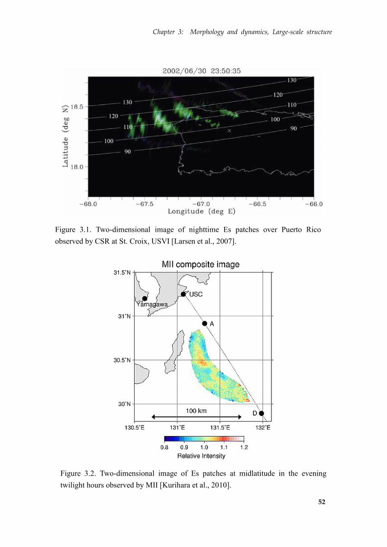
Figure 3.1. Two-dimensional image of nighttime Es patches over Puerto Rico
observed by CSR at St. Croix, USVI [Larsen et al., 2007].
Figure 3.2. Two-dimensional image of Es patches at midlatitude in the evening
twilight hours observed by MII [Kurihara et al., 2010].

Chapter 3: Morphology and dynamics, Large-scale structure
53
3.2. Definition of sporadic-E
As Mathews [1998] pointed out, the term ‘sporadic-E’ has been in semantic
difficulties in that the word includes various layers in the ionospheric E-region caused
by wind shear and atmospheric tides. It makes Es a general term for mixed phenomena.
One of such phenomena is a tidal ion layer (TIL) that prefers relatively higher altitudes
above ~110 km and is less ionized than dominant Es. TILs are often referred to as
intermediate-layers or descending ion layers (DILs) from the temporal change in its
altitude. Field aligned irregularities (FAIs) are also weakly ionized and appear at higher
altitudes with a different generation mechanism from that of TIL. Both phenomena are
often observed by radar observations during Es events.
In addition, Kelly [2013] have pointed out that slant echoes which are often
observed in QP radar echo do not actually represent the layer descent. Various kinds of
ground-based radars have long been observing these phenomena, and different
sensitivities of these instruments gave different definitions of what is sporadic among
various types of the E-region echoes. However, the sporadic nature should not depend
on the type of observation instruments.
We have to take particular care on this problem. Here we study Es layers using
GPS-TEC observations, which is not sensitive to weakly ionized layers or irregularities
in the E-region of the ionosphere, e.g., TILs and FAIs. This method helps us exclude
confusing layers and irregularities (which are generally weakly ionized), and isolate
only and truly ‘sporadic’ layers (which are intensely ionized, i.e., foEs > 16-17 MHz) to
be investigated.
Chapter 3: Morphology and dynamics, Large-scale structure
54
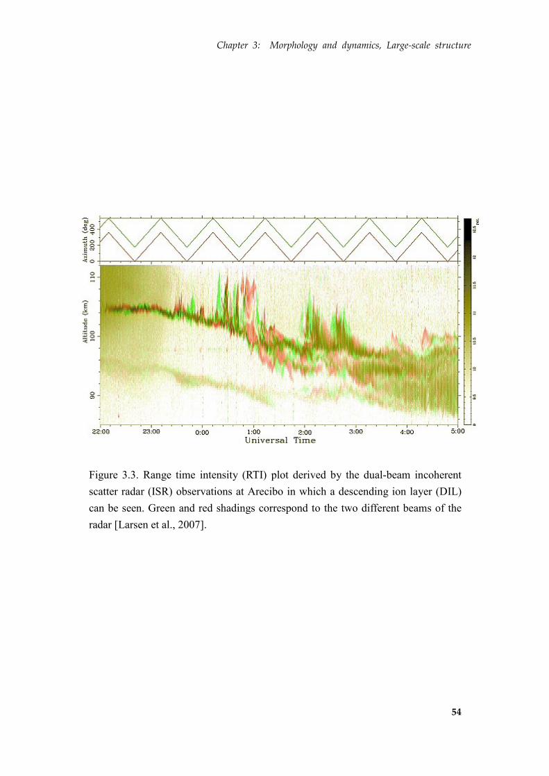
Figure 3.3. Range time intensity (RTI) plot derived by the dual-beam incoherent
scatter radar (ISR) observations at Arecibo in which a descending ion layer (DIL)
can be seen. Green and red shadings correspond to the two different beams of the
radar [Larsen et al., 2007].
Chapter 3: Morphology and dynamics, Large-scale structure
55
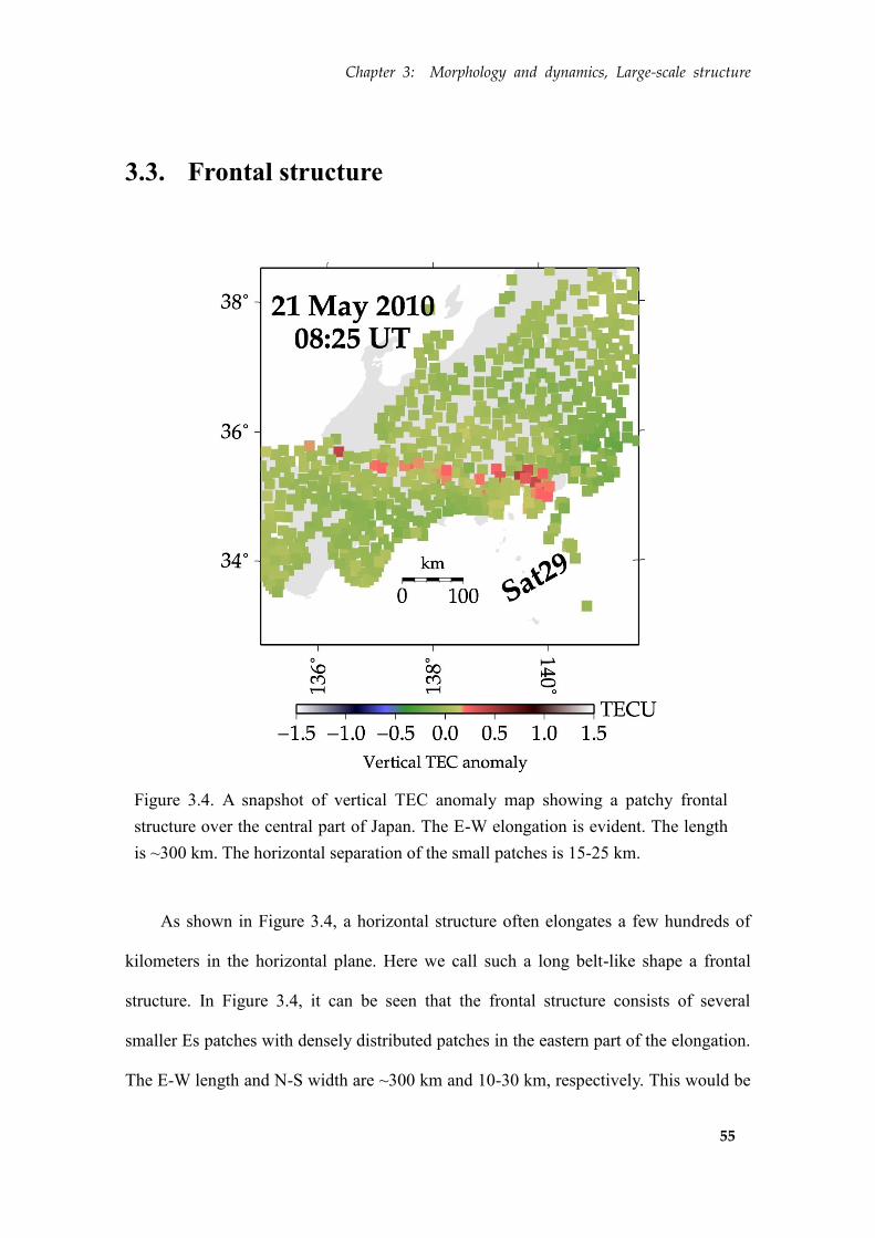
Figure 3.4. A snapshot of vertical TEC anomaly map showing a patchy frontal
structure over the central part of Japan. The E-W elongation is evident. The length
is ~300 km. The horizontal separation of the small patches is 15-25 km.
3.3. Frontal structure
As shown in Figure 3.4, a horizontal structure often elongates a few hundreds of
kilometers in the horizontal plane. Here we call such a long belt-like shape a frontal
structure. In Figure 3.4, it can be seen that the frontal structure consists of several
smaller Es patches with densely distributed patches in the eastern part of the elongation.
The E-W length and N-S width are ~300 km and 10-30 km, respectively. This would be
Chapter 3: Morphology and dynamics, Large-scale structure
56
the first successful imaging of the whole Es irregularity with a large-scale E-W frontal
structure.
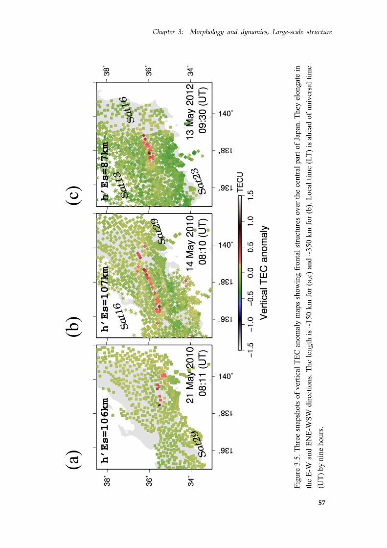
Similar structures have been observed for strong Es irregularities (with foEs > 20
MHz) observed on other days, e.g., 14 May 2010 (Fig.3.5b), and 13 May 2012
(Fig.3.5c). There we can see similar frontal structures running roughly ENE-WSW.
These anomalies have also been confirmed to be Es by constraining the anomaly
altitudes in the same way as described in the chapter 2, i.e., comparison of vertical TEC
anomaly maps from two satellites and h’Es from ionosonde. The lengths of the positive
anomalies are ~ 350 km for the case on 14 May 2010, and ~150 km for the other two
cases.
Chapter 3: Morphology and dynamics, Large-scale structure
57
Fig
ure
3.5
. T
hre
e sn
apsh
ots
of
ver
tica
l T
EC
anom
aly m
aps
sho
win
g f
ronta
l st
ruct
ure
s o
ver
the
centr
al p
art
of
Japan
. T
hey
elo
ngat
e in
the
E-W
and E
NE
-WS
W d
irec
tions.
The
length
is
~150 k
m f
or
(a,c
) an
d ~
350 k
m f
or
(b).
Loca
l ti
me
(LT
) is
ahea
d o
f univ
ersa
l ti
me
(UT
) by n
ine
hours
.
(a)
(b)
(c)
Chapter 3: Morphology and dynamics, Large-scale structure
58
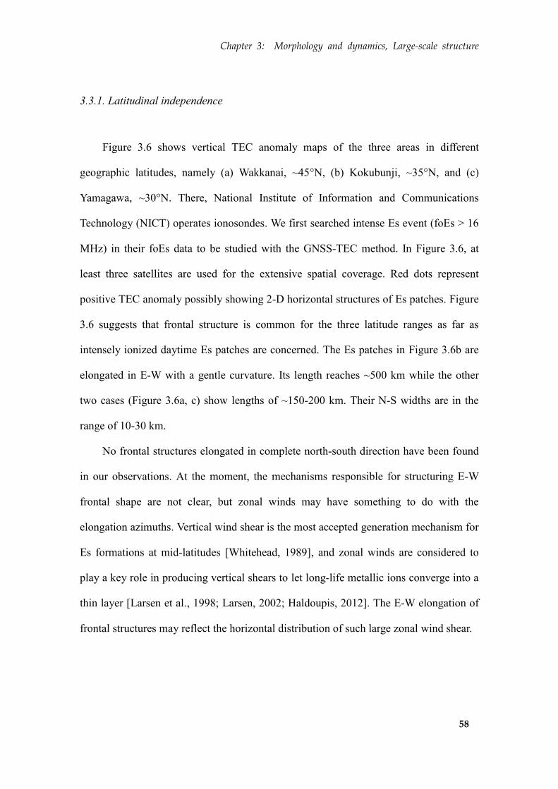
3.3.1. Latitudinal independence
Figure 3.6 shows vertical TEC anomaly maps of the three areas in different
geographic latitudes, namely (a) Wakkanai, ~45°N, (b) Kokubunji, ~35°N, and (c)
Yamagawa, ~30°N. There, National Institute of Information and Communications
Technology (NICT) operates ionosondes. We first searched intense Es event (foEs > 16
MHz) in their foEs data to be studied with the GNSS-TEC method. In Figure 3.6, at
least three satellites are used for the extensive spatial coverage. Red dots represent
positive TEC anomaly possibly showing 2-D horizontal structures of Es patches. Figure
3.6 suggests that frontal structure is common for the three latitude ranges as far as
intensely ionized daytime Es patches are concerned. The Es patches in Figure 3.6b are
elongated in E-W with a gentle curvature. Its length reaches ~500 km while the other
two cases (Figure 3.6a, c) show lengths of ~150-200 km. Their N-S widths are in the
range of 10-30 km.
No frontal structures elongated in complete north-south direction have been found
in our observations. At the moment, the mechanisms responsible for structuring E-W
frontal shape are not clear, but zonal winds may have something to do with the
elongation azimuths. Vertical wind shear is the most accepted generation mechanism for
Es formations at mid-latitudes [Whitehead, 1989], and zonal winds are considered to
play a key role in producing vertical shears to let long-life metallic ions converge into a
thin layer [Larsen et al., 1998; Larsen, 2002; Haldoupis, 2012]. The E-W elongation of
frontal structures may reflect the horizontal distribution of such large zonal wind shear.
Chapter 3: Morphology and dynamics, Large-scale structure
59
Fig
ure
3.6
. V
erti
cal
TE
C a
nom
aly m
aps
show
ing E
s pat
ches
that
app
eare
d i
n t
hre
e dif
fere
nt
lati
tude
regio
ns,
(a)
Wak
kan
ai ~
45
°N,
(b)
Kokubunji
~35°N
, an
d (
c) Y
amag
awa
~30
°N.
Fro
nta
l st
ruct
ure
s ar
e co
mm
only
see
n a
lth
ough t
hei
r le
ngth
s ra
nge
from
100
to 5
00 k
m.
Loca
l ti
me
(LT
) is
ahea
d o
f univ
ersa
l ti
me
(UT
) b
y n
ine
hours
.
Chapter 3: Morphology and dynamics, Large-scale structure
60
3.3.2. Length, width, and azimuth alignment
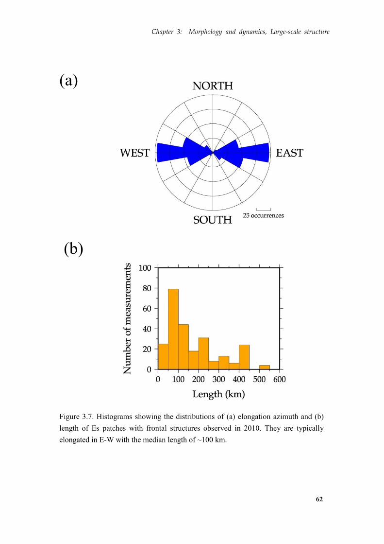
Figure 3.7 compares number of occurrences of (a) elongation azimuth and (b)
length for the ~70 Es cases observed in 2010. We counted one Es patch several times
(with 5 minutes intervals) because it changes its shape rapidly. The rose diagram shows
preferred elongation in the E-W direction. The histogram shows that the lengths of the
frontal structures are distributed over a wide range (50-500 km) with the average of
~160 km. Although the median is ~100 km, smaller distribution peaks exist around 250
km and 450 km.
The average length in the present study is ~160 km, which is consistent with
Cathey [1969], who used 5-7 MHz HF radio wave for the backscatter observation. Our
observations, on the other hand, use microwave that is sensitive only to intensely
ionized Es (foEs > 16-17 MHz). Thus our results show the morphological properties of
intensely ionized Es.
Numerical simulations predict NW-SE aligned frontal shape [Cosgrove and
Tsunoda, 2002, 2004; Yokoyama et al., 2009]. Although the Es images from our
GPS-TEC observations showed preferred elongation in E-W, our observations would
not contradict with these works because we discuss here the morphology of larger-scale
structures. The spatial resolution of our TEC maps (15-25 km) is not fine enough to
image such small-scale plasma patches dealt with in the numerical simulations. On the
other hand, Maruyama et al. [2000] inferred large-scale frontal structure elongated in
E-W from an analysis of QP scintillation, which is consistent with those presented in
this study. Their results are more supportive in that the observation is done in Japan. At
this moment we can conclude that, as far as the large-scale structures in Japan are
Chapter 3: Morphology and dynamics, Large-scale structure
61
concerned, the frontal structures prefer the E-W elongation.
Chapter 3: Morphology and dynamics, Large-scale structure
62
Figure 3.7. Histograms showing the distributions of (a) elongation azimuth and (b)
length of Es patches with frontal structures observed in 2010. They are typically
elongated in E-W with the median length of ~100 km.
(a)
(b)
Chapter 3: Morphology and dynamics, Large-scale structure
63
3.4. Dynamics of frontal structure
3.4.1. Simultaneous occurrence
Figure 3.8a shows 5-minute snapshots of vertical TEC anomaly map generated for
08:00-08:35 UT. Two separate frontal structures, labeled as A and B in the third
snapshot, are evident over southwestern and central Japan, respectively. Their
elongation directions at 08:10 UT are different, i.e., the structure A elongates in E-W
while the structure B elongates in NE-SW. The structure A is the longest (~200 km) at
08:03 UT (Figure 3.8b) while the structure B is the longest (~400 km) at 08:12 UT
(Figure 3.8c).
The two structures show different temporal evolution. During 08:00-08:10 UT, the
two structures change like see-saw, i.e., the structure A decays while the structure B gets
conspicuous. As for frontal structure A, it intermittently repeats cycles of appearance
and decay, e.g., it is clear in 08:00-08:10 UT but becomes obscure 5 min later (08:15
UT). The elongation of the structure A changed from E-W to NW-SE around 08:20 UT
and then to WNW-ESE during 08:30-08:35 UT. After 08:35 UT, it became obscure in
shape. The structure B was more stable during 08:05-08:25 UT. Its elongation azimuth
remained ENE-WSW, and its length changed little. After 08:30 UT, however, the
structure B dissolved into small patches. At 08:35 UT, it split into two smaller frontal
structures with the boundary at ~138°E keeping their elongation azimuths.
Simultaneous occurrence and different temporal evolution of the two frontal
structures in Figure 3.8 suggest diversity in the developing process and the structures of
Es patches. There the structure A is shorter in length and lifetime than the structure B.

Chapter 3: Morphology and dynamics, Large-scale structure
64
The structure A changed its shape more rapidly than B, i.e., its frontal structure appeared
intermittently with unstable elongation azimuth. The wind shear in the region around
the structure A may have been more unstable than that of the structure B. In the
snapshots during 08:00-08:10 UT (Figure 3.8a), it is clear that the two frontal structures
were in the opposite phase, i.e., the structure A was decaying while the structure B was
growing in length. The two structures would have been created by two different wind
shear systems which were strong enough to form intensely ionized Es patches. Since
zonal winds are the primary driver of vertical shears below an altitude of 115 km
[Haldoupis, 2012], the horizontal scale sizes of zonal wind shears are inferred to be
several hundreds of kilometers in E-W and a few tens of kilometers in N-S.
In addition, GPS-TEC results provide a better understanding of ionosonde data.
Although ionosondes are separated from other ionosondes by over 1000 km in Japan,
they often observe simultaneous occurrences of Es. It has long been a puzzling problem
whether the simultaneous rise of foEs at different observatories represents the
appearance of one Es patch or simultaneous emergence of multiple Es patches. In the
latter case, it would also be an interesting issue if there is any causal relationship
between the emergences of the two patches. TEC maps can distinguish these cases, and
will enable more realistic interpretation of ionosonde data.
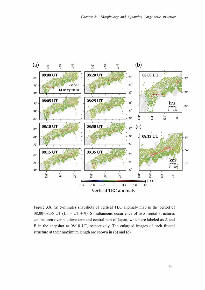
Chapter 3: Morphology and dynamics, Large-scale structure
65
Figure 3.8. (a) 5-minutes snapshots of vertical TEC anomaly map in the period of
08:00-08:35 UT (LT = UT + 9). Simultaneous occurrence of two frontal structures
can be seen over southwestern and central part of Japan, which are labeled as A and
B in the snapshot at 08:10 UT, respectively. The enlarged images of each frontal
structure at their maximum length are shown in (b) and (c).

Chapter 3: Morphology and dynamics, Large-scale structure
66
3.4.2. Movement
Figure 3.9 shows snapshots at four time epochs and the movement of an Es patch
with a frontal structure aligned in E-W direction. Although its eastern and western ends
are out of the GEONET coverage (e.g., 03:45 UT), its northward migration can be seen.
Such movements perpendicular to the elongation are often observed.
Next we have a look at the vertical TEC anomaly maps on 21 May 2010, at various
time epochs (Figure 3.10), and study the time evolution of the horizontal structure of the
Es irregularity. The frontal structures are clearly seen at 08:00, 08:10, and at 08:20 UT.
The Es patches line up in the ENE-WSW direction at 08:00 UT and in the E-W
direction during 08:10 ~08:20 UT. In the snapshots after 08:25 UT, the characteristic
E-W frontal structure seems to have dissolved into smaller patches of a size of ~80 km
aligned in the NW-SE direction. These snapshots suggest that the lifetime of this
frontal structure of Es irregularities was not much longer than a few tens of minutes.
After 08:25 UT, the E-W frontal structure broke into smaller patches and moved
southwestward at the speed of ~80 m/s. These southwestward movements of NW-SE
aligned patches are typically seen at 08:35, 08:40 and 08:50 UT.
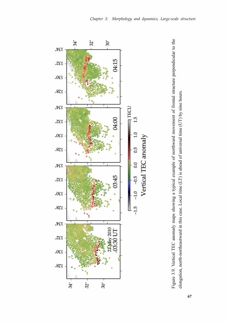
Chapter 3: Morphology and dynamics, Large-scale structure
67
Fig
ure
3.9
. V
erti
cal
TE
C a
nom
aly m
aps
show
ing a
typic
al e
xam
ple
of
no
rthw
ard m
ov
emen
t of
fronta
l st
ruct
ure
per
pen
dic
ula
r to
the
elongat
ion,
nort
h-n
ort
hea
stw
ard i
n t
his
cas
e. L
oca
l ti
me
(LT
) is
ahea
d o
f univ
ersa
l ti
me
(UT
) by n
ine
hours
.
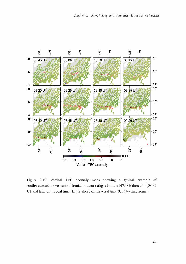
Chapter 3: Morphology and dynamics, Large-scale structure
68
Figure 3.10. Vertical TEC anomaly maps showing a typical example of
southwestward movement of frontal structure aligned in the NW-SE direction (08:35
UT and later on). Local time (LT) is ahead of universal time (UT) by nine hours.
Chapter 3: Morphology and dynamics, Large-scale structure
69
Figure 3.11 shows northward migration of Es in the early afternoon over
southwestern Japan. It took almost 2 hours for the Es to migrate by ~400 km. During the
migration, the Es keeps E-W frontal structure although the shape slightly changes. It
should be noticed that the change in the elongation azimuth accompanies the change in
the migration direction. For example, before 03:35 UT, the frontal structure is elongated
in E-W direction. After that time, the elongation azimuth rotated to become W-NW to
E-SE. At the same time, the migration direction appears to have changed from precise
northward to toward NNE. Then, after 04:20 UT, the frontal structure moved
northeastward maintaining the elongation in NW-SE. This suggests that the migration
tends to move perpendicular to the elongation direction.
Figure 3.12 also shows the migration in the direction normal to the elongation. In
this case, an E-W elongated frontal structure moved southward over the northern part of
Japan. It decays just before the local noon. In the decay process imaged by GPS-TEC,
the structure seems to have kept its frontal shape, e.g., those shown in 02:20-02:55 UT.
On the migration speeds, it is 70-80 m/s in Figure 3.10 and Figure 3.11, and 40-50 m/s
in Figure 3.12.
Actually, substantial portion of the observed Es did not show significant
movements. In the present study, 24 out of 71 cases showed clear movements, while the
others stayed above the same places until they disappear. We analyzed these 24 cases
observed over Wakkanai, Kokubunji, and Yamagawa, and inferred the migration speeds
of Es patches.
Figure 3.13 shows the distribution of migration speeds normal to the elongation
azimuths. There we neglected the movements in the elongation direction because they
cannot be clearly distinguished from the temporal growth of Es patches in the
Chapter 3: Morphology and dynamics, Large-scale structure
70
elongation direction. Because the structures are elongated preferably in E-W, their
migration speeds are either northward or southward. We also considered Es speed less
than 25 m/s as stationary, so only the velocities larger than that value are counted there.
Figure 3.13 suggests that the speeds range up to 100 m/s with the average of ~60 m/s for
both directions (the velocity is measured every 15 minutes, often multiple times for a
single Es patch), which is considered to reflect the speed of neutral winds in the
E-region of the ionosphere.
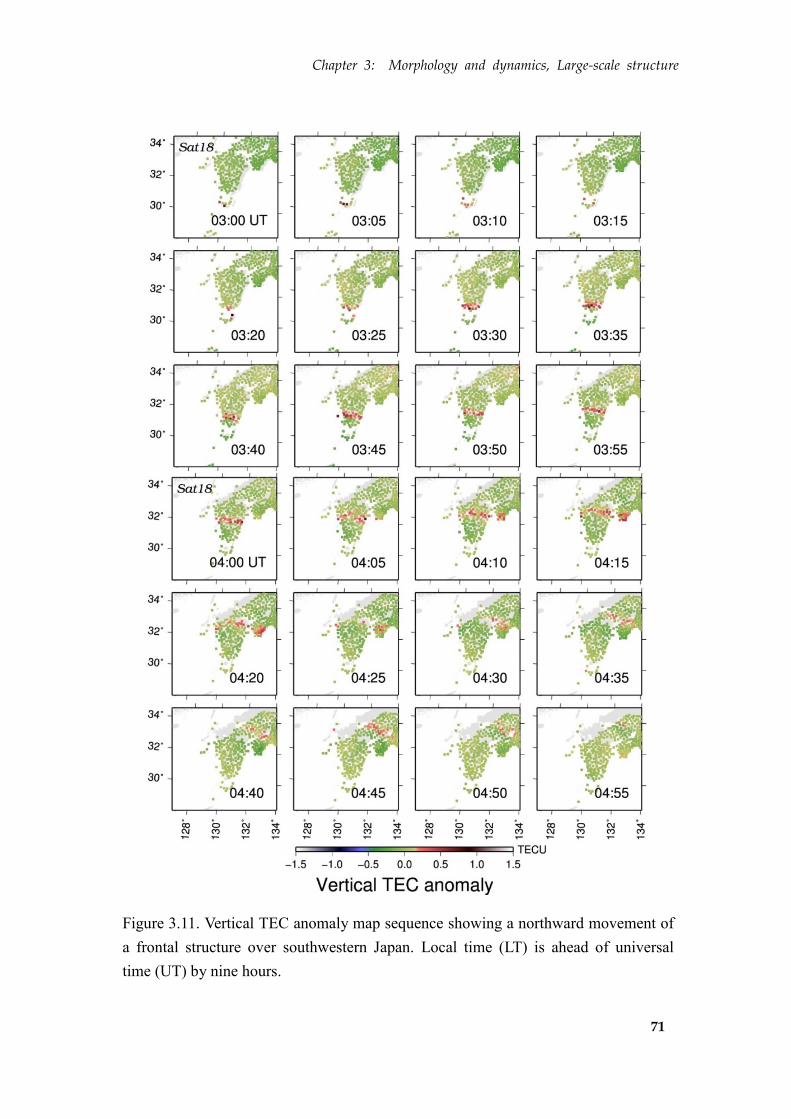
Chapter 3: Morphology and dynamics, Large-scale structure
71
Figure 3.11. Vertical TEC anomaly map sequence showing a northward movement of
a frontal structure over southwestern Japan. Local time (LT) is ahead of universal
time (UT) by nine hours.
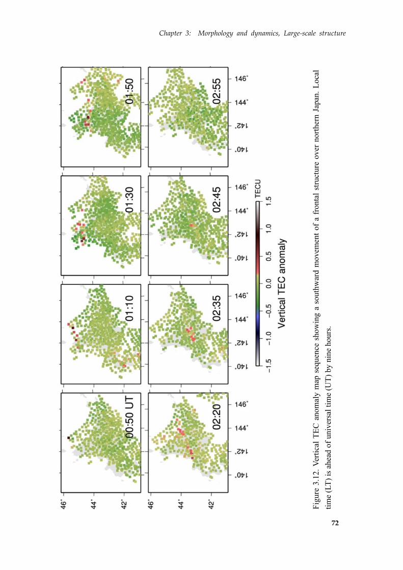
Chapter 3: Morphology and dynamics, Large-scale structure
72
Fig
ure
3.1
2.
Ver
tica
l T
EC
anom
aly m
ap s
equ
ence
show
ing a
south
war
d m
ovem
ent
of
a fr
onta
l st
ruct
ure
ov
er n
ort
her
n J
apan
. L
oca
l
tim
e (L
T)
is a
hea
d o
f univ
ersa
l ti
me
(UT
) by n
ine
hours
.
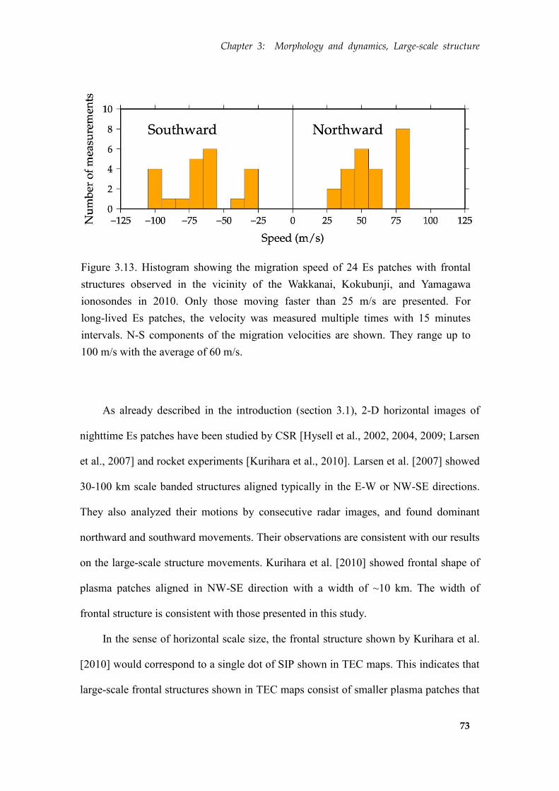
Chapter 3: Morphology and dynamics, Large-scale structure
73
Figure 3.13. Histogram showing the migration speed of 24 Es patches with frontal
structures observed in the vicinity of the Wakkanai, Kokubunji, and Yamagawa
ionosondes in 2010. Only those moving faster than 25 m/s are presented. For
long-lived Es patches, the velocity was measured multiple times with 15 minutes
intervals. N-S components of the migration velocities are shown. They range up to
100 m/s with the average of 60 m/s.
As already described in the introduction (section 3.1), 2-D horizontal images of
nighttime Es patches have been studied by CSR [Hysell et al., 2002, 2004, 2009; Larsen
et al., 2007] and rocket experiments [Kurihara et al., 2010]. Larsen et al. [2007] showed
30-100 km scale banded structures aligned typically in the E-W or NW-SE directions.
They also analyzed their motions by consecutive radar images, and found dominant
northward and southward movements. Their observations are consistent with our results
on the large-scale structure movements. Kurihara et al. [2010] showed frontal shape of
plasma patches aligned in NW-SE direction with a width of ~10 km. The width of
frontal structure is consistent with those presented in this study.
In the sense of horizontal scale size, the frontal structure shown by Kurihara et al.
[2010] would correspond to a single dot of SIP shown in TEC maps. This indicates that
large-scale frontal structures shown in TEC maps consist of smaller plasma patches that
Chapter 3: Morphology and dynamics, Large-scale structure
74
have individual structure. Hence it is natural to consider large-scale frontal structures as
an assemblage of such small scale patches. Larsen et al. [2007] reported complex
propagation of multiple small-scale structures in a banded structure, e.g., one small
patch moved toward N-NW while another moved eastward simultaneously. The spatial
resolution of our TEC maps (15-25 km) is not high enough to study movements of such
small-scale plasma patches. Further morphological analyses of small-scale plasma
structures should be done with enhanced spatial resolution.

Chapter 3: Morphology and dynamics, Large-scale structure
75
Figure 3.14. Local time dependence of the directions of N-S movements of Es patches
observed in 2010 (histogram). We only show observations made in central Japan
where GPS-TEC data have a better spatial coverage and resolution. Curves show
occurrence rates of Es from foEs data during 2003-2012 (dashed) and 2010 (solid) by
the Kokubunji ionosonde (we show only the cases with foEs > 10 MHz).
3.4.3. Atmospheric tidal effect on Es movement
Figure 3.14 shows local time dependence of the number of elongation-normal
movements (either northward or southward) of the Es frontal structures observed in
2010. Northward and southward components are colored in orange and gray,
respectively. There we also compare the hourly occurrence rates of strong Es (foEs > 10

Chapter 3: Morphology and dynamics, Large-scale structure
76
MHz) observed by the Kokubunji ionosonde during 2010 and during 2003-2012. Here
we exclude Es observed in the northern and southern Japan, and discuss 24 cases
observed over the central part of Japan where a larger latitudinal coverage of densely
distributed GPS stations enables us to analyze the migration of Es patches (Figure 3.6b).
The Kokubunji ionosonde (35.71°N, 139.49°E) is included in this region. As stated in
the caption of Figure 3.13, the velocities are measured multiple times (with 15 minutes
interval) for long-lived Es patches.
The histogram in Figure 3.14 suggests that Es patches move mainly northward in
10-14 LT and mainly southward in 17-19 LT. The Es occurrence rates from the
ionosonde during 2003-2012 show maxima around 10 LT and 17 LT and a minimum in
13-15 LT. The peak in northward moving Es from GPS-TEC lags behind the
morning-peak of the Es occurrence rate from the ionosonde by ~2 hours. The same is
true for the minimum occurrence hour in the afternoon. The peak of southward
movement from GPS-TEC coincides with that of the occurrence rate from the
ionosonde. The distribution of the occurrence hour from the ionosonde during 2010, the
same period as the GPS-TEC study, shows morning peaks at 10 LT and 12 LT followed
by a drop in 13-15 LT and the evening peak at 17 LT. The peaks of northward and
southward movements coincide with those of the morning and evening peaks of the Es
occurrence hours in 2010.
In Figure 3.14, northward movements dominate from late morning to early
afternoon, and southward movements dominate from late afternoon to evening. The
reversal from southward to northward seems to occur during a ~6 hour period at night.
This transition is, however, unclear because of the lack of Es observations during that
period. Tanaka [1979] investigated Es movements by backscatter radar observations in
Chapter 3: Morphology and dynamics, Large-scale structure
77
central Japan. His results show dominant northward and southward movements at 12-14
LT and 16-21 LT, respectively, which are consistent with those presented in our study.
Between the periods of northward and southward movements, there is a ‘silent
period’ at ~15 LT. This period would represent the transition of meridional wind
direction from northward to southward. In fact, Tanaka [1979] has found a clockwise
rotation of Es drift vectors in the local time variation, i.e., northward to westward, and
then to southward. The westward drifts peaks at around 15 LT, which roughly coincides
with the silent period in Figure 5 (please note that we neglect E-W movements here).
The northward Es migration in the local morning is consistent with the E-region
horizontal wind vectors at midlatitudes inferred from diurnal (Sq) geomagnetic
variation [Kato, 1956]. Southward Es movements in the local evening might be driven
by semidiurnal tide [Maeda, 1957; Elford, 1959], although the tidal winds are generally
slower than the Es migration speeds observed in our study. The whole wind system,
including the wind shear region responsible for Es generation, might have moved
together with the global-scale atmospheric tidal winds.
The foEs data over a ten-year period in Figure 5 suggest 8 hour periodicities in the
Es occurrences. According to Haldoupis and Pancheva [2006], foEs data show peaks at
6 and 8 hour periods in the Es occurrence. They found the 8 hour periodicity more
regular and significant, and attributed it to atmospheric tides. Both the reversal of Es
migration directions and 8 hour Es occurrence periodicity in Figure 3.14 suggest
atmospheric tidal wind in the neutral atmosphere may control the occurrence and drifts
of Es patches.
Chapter 3: Morphology and dynamics, Large-scale structure
78
3.4.4. Estimation of direction of plasma transportation
In this section, we try to estimate the direction of plasma transportation by
comparing signatures with multiple satellites. Because the incident angles and azimuth
of the line-of-sight are different among satellites, amplitudes of the positive TEC
anomaly associated with Es patch also look different to some extent. Investigating such
differences would help us estimate how plasma has been transported to form the Es
structure.
Figure 3.15 shows the vertical TEC anomaly maps at 08:07 UT, 08:21 UT, and
08:35 UT derived with five different GPS satellites available during the period of the Es
appearance. In Figure 3.15, we can see that the same Es irregularity looks fairly
different when viewed with different satellites. Satellite 29 provides the clearest image
of the whole horizontal structure of the Es irregularity. One of the reasons that Satellite
29 gives the best image is that the line-of-sight passes through the Es structure with a
low elevation angle from the same direction of the frontal structure elongation. This
causes the largest phase delays, which would result in clear and large TEC anomaly.
The temporal evolution of its horizontal structure also looks fairly different with
different satellites. For example, Satellite 16 captured E-W frontal structure at later time
epochs, e.g., at 08:35 UT. On the other hand, Satellite 31 seems to have lost sight of the
E-W frontal structure after 08:21 UT. Such satellite dependent amplitudes of the Es
signatures seem to reflect its three-dimensional (3-D) structure. The Kokubunji
ionogram at 08:15 UT (Fig. 2.8a) shows ‘blanket-Es’, i.e., the highly ionized Es layer
makes a continuous flat plane, which seems inconsistent with the highly patchy
structure suggested by the GPS-TEC observations. We consider that such patches may
Chapter 3: Morphology and dynamics, Large-scale structure
79
correspond to regions with very high electron density (i.e., foEs > 20 MHz) for which
only GPS-TEC observations are sensitive.
It is noteworthy that only Satellite 14, among the five satellites, failed to detect the
Es frontal structure in the period 08:07- 08:35 UT. Although the ionosonde at Kokubunji
show that strong Es signatures at 08:15 UT and 08:30 UT, Satellite 14 does not show
positive TEC anomalies anywhere in the entire network including stations with SIP
close to Kokubunji. Such a lack of the Es signature may reflect the direction of plasma
transportation responsible for the Es formation. Since TEC corresponds to the integrated
number of electrons along the line-of-sight, no anomaly would be seen if the plasmas
have moved along the line-of-sight. In this case, plasmas might have been transported in
the direction close to the Satellite 14 line-of-sight, that is, nearly N-S in azimuth with
the dip of 40~50 degrees toward north.
This suggests that the transportation may have occurred along the local
geomagnetic field direction, although further studies are necessary to see if this is a
general phenomenon. Our result shows that GPS-TEC can be used to infer the plasma
movements that caused the Es formation. Owing to spatial density of ground GPS
stations and availability of multiple satellites in the sky, GPS-TEC has a strong potential
of investigating the dynamics of formation and decay of Es irregularities through 3-D
observations of the plasma movements.
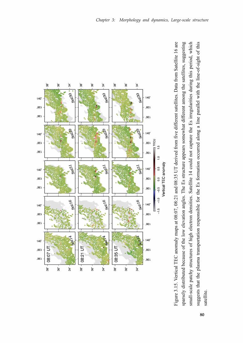
Chapter 3: Morphology and dynamics, Large-scale structure
80
Fig
ure
3.1
5. V
erti
cal
TE
C a
nom
aly m
aps
at 0
8:0
7, 08:2
1 a
nd 0
8:3
5 U
T d
eriv
ed f
rom
fiv
e dif
fere
nt
sate
llit
es. D
ata
from
Sat
elli
te 1
6 a
re
spar
sely
dis
trib
ute
d b
ecau
se o
f th
e lo
w e
levat
ion a
ngle
s. T
he
Es
stru
cture
appea
rs s
om
ewh
at d
iffe
rent
among t
he
sate
llit
es,
sugges
ting
smal
l-sc
ale
pat
chy s
tru
cture
s of
hig
h e
lect
ron d
ensi
ties
. S
atell
ite
14 c
ould
not
captu
re t
he
Es
irre
gula
riti
es d
uri
ng t
his
per
iod,
wh
ich
sugges
ts t
hat
the
pla
sma
tran
sport
atio
n r
esponsi
ble
for
the
Es
form
atio
n o
ccurr
ed a
long a
lin
e par
alle
l w
ith t
he
line-
of-
sight
of
this
sate
llit
e.
Chapter 3: Morphology and dynamics, Large-scale structure
81
3.4.5. Role of gravity waves
In Figure 3.9-12, Es movements normal to the elongation azimuth are evident. As
shown in Figure 3.13, their speeds range up to 100 m/s, which are often found in those
of the neutral winds in the E-region of the ionosphere. Zonal wind profiles were
obtained from an experiment called the Sporadic-E Experiment over Kyushu (SEEK)
[Larsen et al., 1998], and the wind speeds at an Es altitude is consistent with those
presented in this study. Es movements are considered to reflect the general tendency of
the neutral wind direction in the ionospheric E-region [Tanaka, 1979]. Although the
neutral wind data are not available for the Es studied here, it may be possible to estimate
the approximate neutral wind velocity from the velocity of these Es patches.
In Figure 3.10, after the dissipation of the E-W frontal structure, at least two
smaller band-like patches that aligned in NW-SE appeared and moved southwestward at
~80 m/s (typically seen in the snapshots at 08:35 and 08:40 UT in Figure 3.10).
Previous studies have reported that such southwestward movements of NW-SE aligned
band structures frequently occur for midlatitude Es in the Northern Hemisphere (NH)
[Tsunoda and Cosgrove, 2001; Cosgrove and Tsunoda, 2002; Tsunoda et al., 2004]. In
the snapshot of vertical TEC map at 08:35 UT and 08:40 UT in Figure 3.10, the two
individual Es bands seem to form a wave-like structure. In fact, the bands are
horizontally separated by 30-40 km, which is similar to the wave length of internal
gravity waves observed at an altitude of 100 km in this region. Cosgrove [2007] have
pointed out that the polarization electric field modulated by gravity waves in the
F-region can modulate the E-region background plasma through the electrodynamic
coupling. This suggests that the observed southwestward movements of NW-SE aligned
Chapter 3: Morphology and dynamics, Large-scale structure
82
Es irregularities might be driven by the atmospheric gravity waves.
In the midlatitude region of the NH, medium-scale traveling ionospheric
disturbances (MSTIDs) often appear at night and propagate southwestward keeping the
phase front aligned in NW-SE[Saito et al., 2002]. Considering the electrodynamic
coupling between the F- and E-region of the ionosphere, Tsunoda and Cosgrove [2001]
suggested the influence of TIDs on Es generation in the nighttime midlatitude
ionosphere. Bowman [1960, 1968] pointed out that an Es band is often accompanied by
TIDs, and this was true in 11 cases out of 13 (85 percent). Although we did not find
simultaneous MSTID activities with all Es events detected by GPS-TEC, we found
MSTID followed Es activities 30 minutes later in the case of Figure 3.10. In this case,
the wave fronts of the MSTIDs are typically aligned in NW-SE and propagated
southwestward. Because MSTIDs frequently appear at night in this region, the
subsequent MSTID may not have had any causal relationship with the Es. Because
GPS-TEC can observe both Es and MSTID, we could perform statistical studies on
evening type Es irregularities in the future in order to examine the causal relationship
between Es and MSTIDs.
The possible relationship of Es and MSTID suggests that we should take gravity
waves into account in discussing the evening southward movement of Es patches. Liu et
al. [2014] have reported that the large winds and shears are produced by the migrating
tidal background winds by an interaction with gravity waves. As mentioned above, we
found the fragmentation of frontal structure preceding MSTID passage, i.e., Es with an
E-W elongated structure dissolved into smaller wave-like pieces aligned in NW-SE
[Maeda and Heki, 2014]. The horizontal separation of these pieces is 30-40 km and they
moved southwestward by ~80 m/s in the local evening. These observations suggest
Chapter 3: Morphology and dynamics, Large-scale structure
83
possible interaction of gravity waves in the destruction of large-scale frontal structure
and following southward migration of smaller pieces. Such interaction of two
ionospheric phenomena has been found in the F-region. For example, Otsuka et al.
[2012] showed disappearance of equatorial plasma bubbles after the interaction with an
MSTID.
As shown in Figure 3.13, speeds of frontal structure movement agree well with
neutral winds and gravity waves. Further investigations on Es movement, such as
simultaneous measurement of E-region winds and Es movement using 2-D mapping,
are needed to reveal the detailed dynamics of the E-region neutral
atmosphere/ionosphere. The result shown in Figure 3.14 would serve as the
observational evidence that demonstrates coupling between the neutral atmosphere and
plasma movement in the E-region of the ionosphere.
Chapter 3: Morphology and dynamics, Large-scale structure
84
3.5. Concluding remarks
In this chapter, we have shown morphological properties of large-scale Es
structures and discussed their dynamics. This chapter can be concluded as follows:
(1) In the vertical TEC anomaly maps, Es often shows large-scale frontal structures
elongated in E-W direction and spanning more than 100 km.
(2) Intensely ionized daytime Es patches show frontal structures with typical elongation
in E-W over the latitude range of 30°N-45°N.
(3) Lengths and widths of Es frontal structures range in 50-500 km and 10-30 km,
respectively.
(4) Northward and southward movements, perpendicular to the elongation azimuths, are
observed. They range up to 100 m/s with the average of 60 m/s in both directions.
(5) We also observed the fragmentation of the E-W frontal structure into smaller
patches and its migration.
(6) Tidal winds in neutral atmosphere may control the migration direction of Es frontal
structures.
(7) Observations with multiple satellites suggested that the plasma transportation
responsible for the Es formation in the case of 21 May 2010 appears to have
occurred in a direction close to the local geomagnetic field.
85
Chapter 4
Morphology and dynamics of
midlatitude sporadic-E
Small-scale structure
The contents of this chapter have been submitted to Earth, Planets and Space.
Chapter 4: Morphology and dynamics, Small-scale structure
86
4.1. Introduction
Existence of patches forming small-scale structures is suggested by quasi-periodic
(QP) echoes in the traditional backscatter radar observations (Figure 4.1). Yamamoto et
al. [1991, 1992] discovered QP echoes from field aligned irregularities (FAIs) in the
nighttime E-region of the ionosphere by using the Middle and Upper atmosphere (MU)
radar. This finding gave rise to interests in the dynamics in the Es patches and
instabilities responsible for generating such QP echoes. Maruyama [1991, 1995]
analyzed QP scintillations in 136 MHz radio waves transmitted from a geostationary
satellite (Figure 4.2) and showed that linear shaped Es structures drifted in the direction
perpendicular to the elongation.
Maruyama et al. [2000] found morphological similarity between QP echoes
observed with the MU radar and QP scintillations in 136 MHz radio wave from a
geostationary satellite. They proposed a model that the gradient drift instability
produces secondary sheet-like irregularities along B fields, possibly responsible for the
generation of QP echoes. The wavelengths of small-scale irregularities inferred from QP
echoes at low- and mid-latitudes are reported in the range of 8-30 km [Tsunoda et al.,
2000; Hysell et al., 2004; Saito et al., 2005] with typical time periods of 2-10 min
[Larsen et al., 2007]. Radar imaging experiments over Arecibo together with numerical
simulation have also revealed kilometer-scale fine structures in Es [Hysell et al, 2013;
Huba et al., 2014].
Among various kinds of observation methods, Maeda and Heki [2014] detected Es
layers by analyzing Global Positioning System (GPS) data. They found positive
anomalies in the total electron content (TEC) caused by Es irregularities, and succeeded
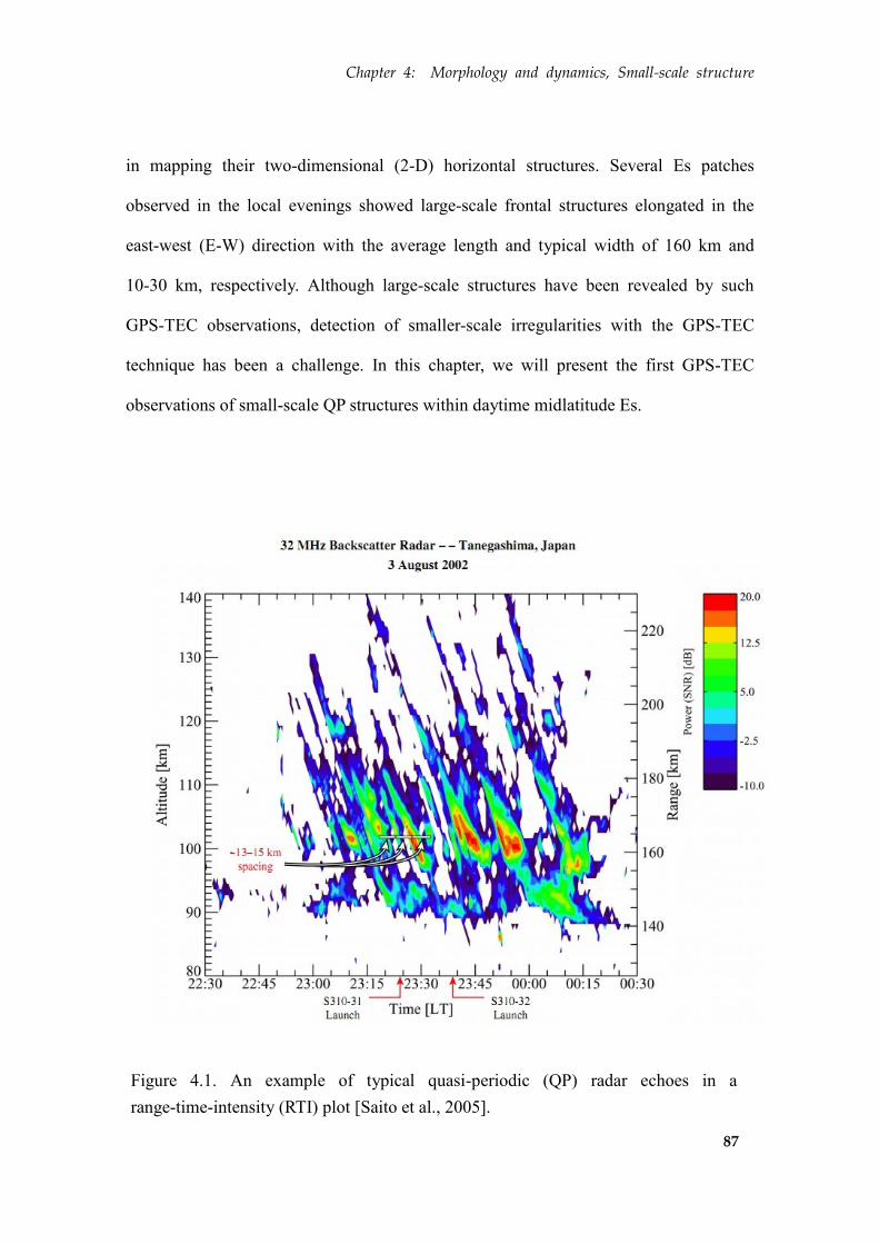
Chapter 4: Morphology and dynamics, Small-scale structure
87
in mapping their two-dimensional (2-D) horizontal structures. Several Es patches
observed in the local evenings showed large-scale frontal structures elongated in the
east-west (E-W) direction with the average length and typical width of 160 km and
10-30 km, respectively. Although large-scale structures have been revealed by such
GPS-TEC observations, detection of smaller-scale irregularities with the GPS-TEC
technique has been a challenge. In this chapter, we will present the first GPS-TEC
observations of small-scale QP structures within daytime midlatitude Es.
Figure 4.1. An example of typical quasi-periodic (QP) radar echoes in a
range-time-intensity (RTI) plot [Saito et al., 2005].
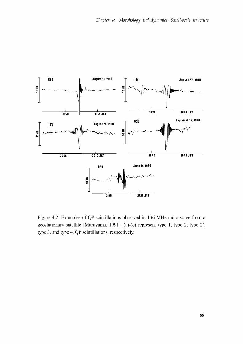
Chapter 4: Morphology and dynamics, Small-scale structure
88
Figure 4.2. Examples of QP scintillations observed in 136 MHz radio wave from a
geostationary satellite [Maruyama, 1991]. (a)-(e) represent type 1, type 2, type 2’,
type 3, and type 4, QP scintillations, respectively.

Chapter 4: Morphology and dynamics, Small-scale structure
89
To reveal horizontal structures of Es, Maeda and Heki [2014] first performed
detection and imaging of large-scale structures of Es with GPS-TEC observations. A
dense array of GNSS receivers in Japan, GEONET, enabled us to draw 2-D maps
covering the whole Es irregularity extending by several hundreds of kilometers with
spatial resolution of ~25 km. However, Maeda and Heki [2014] did not perform the
detection of smaller-scale structures. Such sub-structures are of great interests and
importance, considering a number of previous studies that report QP echoes or
scintillation. Further detailed analyses based on morphological characteristics as well as
quantities from conventional observations such as electron density and wind profiles
will provide better understanding of the formation and development processes of plasma
structures in Es.
For the detection of small-scale structures, we will simply use raw slant TEC time
series instead of 2-D TEC maps. In this method, the spatial resolution is determined by
the sampling interval of GPS data and the speed of a satellite motion. With 30 seconds
sampling interval, spatial resolution would typically be less than ~2 km. This is
sufficient for the detection of small-scale plasma structures represented by QP radar
echoes.

Chapter 4: Morphology and dynamics, Small-scale structure
90
4.2. Quasi-periodic (QP) TEC signature
In slant TEC time series, Es signature is principally represented by a positive
pulse-like TEC enhancement with a single peak. However, it is often seen that the main
pulse is accompanied by a few smaller positive TEC pulses. They are smaller in
amplitude than those of the main pulse, e.g., ~0.5 TECU or much less when the main
pulse is ~1.0 TECU. What is more characteristic is that they often appear
quasi-periodically in time. This suggests quasi-periodical separation of less ionized
plasma blobs lined up in a certain direction.
Such signature is very similar to those reported by traditional radar observations
[Tsunoda et al., 2000; Hysell et al., 2004; Saito et al., 2005]. However, our observations
are in daytime and most of the previous studies are during nighttime. According to
Maruyama [1991], QP scintillation in 136 MHz radio wave from a geostationary
satellite also concentrates in nighttime. Thus QP echo and scintillation are considered to
occur more frequently in nighttime when E-region plasma irregularities are unstable.
The electron density gradient in the plasma blobs are thought to be the primary
cause of QP scintillation [Maruyama 1991; Maruyama et al., 2000]. QP echoes are at
first considered to originate from field-aligned irregularities (FAI) by Yamamoto et al.
[1991, 1992]. On the other hand, Kelly [2013] pointed out that slant QP echoes should
be understood considering the horizontal shape of plasma blob. Descending layers as
characterized by slant QP echoes, can also be seen when the blob is azimuthally aligned
rather than it actually descending in altitude, due to the ambiguity in the radars’ locus of
the perpendicularity. This suggests that horizontal shapes of small-scale plasma blob can
provide better insights into the QP echo/scintillation events.
Chapter 4: Morphology and dynamics, Small-scale structure
91
4.3. Morphology and dynamics of QP structure
4.3.1. Leading and trailing edge of frontal structure
In addition to large-scale structures of Es, here we show smaller plasma structures
in the leading and trailing edges of frontal structures. They are inferred from slant TEC
time series obtained by satellites that move perpendicular to the direction of elongation.
Here we report two cases of QP patch structures. Figure 4.3 and 4.4 show
southward- and northward-drifting Es, respectively. For the northward (southward) Es,
we used satellites moving in the opposite directions, i.e., southward (northward), to
examine the slant TEC time series across the frontal structure. Hence, in Figure 4.3a, the
earlier part of TEC anomaly in the time series represents plasma patches in the leading
edge and the latter part represents those of the trailing edge of the frontal structure. It is
clear in Figure 4.3a that the leading edge is characterized by smooth and gradual TEC
increase in contrast to a steep drop of TEC in the trailing edge. In addition to this, the
trailing edge is characterized by multiple short TEC pulses, i.e., QP TEC signature,
possibly due to small plasma patches spaced somewhat quasi-periodically, i.e., 20-25
km, behind the main Es patch.
Figure 4.3 shows non-uniform QP signatures within a single Es frontal structure.
The waveform of the slant TEC time series from the western and eastern GPS stations
appear much different. The QP signatures are clearer in the eastern part of the
elongation than those in the western part. It is also noteworthy that the QP signature
recorded with eastern GPS stations (0877 and 0007) show constant amplitudes. In the
western GPS station 0102, the QP regions seem to be merged with the main frontal

Chapter 4: Morphology and dynamics, Small-scale structure
92
structure, making it difficult to identify the original main patch.
Similar QP TEC signature can be found in Figure 4.4. In this case, Es moved
northward. We used southward satellite (Satellite 18) to measure the across-structure
TEC time series of the E-W elongated frontal structure. The earlier part of the time
series shows the leading edge of the frontal structure. In Figure 4.4, it can be seen that
QP signatures are evident in the main TEC pulse in addition to the trailing edge. This
‘inhabitancy’ of QP signature in the dominant Es patch indicates that the frontal
structure itself is unstable and modulated by some kind of instabilities. The broken
blobs following the frontal structure from the trailing edge are similar to those reported
in Figure 4.3, and possibly generated by gradient drift instability.
In both Figure 4.3 and 4.4 cases, the distribution of QP signature is localized in the
elongation direction. This may be attributed to the difference in the electron density
gradient, which consequently determines the growth rate of gradient-drift instability.
Another possibility is the difference in the wind shear which causes the neutral shear
instability. If the winds and shears are not uniform in the E-W elongation direction,
which is very natural, each plasma blob is supposed to be under different instability
condition. One plasma blob would be under the condition of low Richardson number,
i.e., Ri < 1/4, where it is sensitive to the Kelvin-Helmholtz (K-H) instability, and
another blob might not. Combined observations of GPS-TEC and ground-based radar,
and/or rocket experiments will provide more insights into various kinds of plasma
and/or neutral instabilities in the frontal structure.
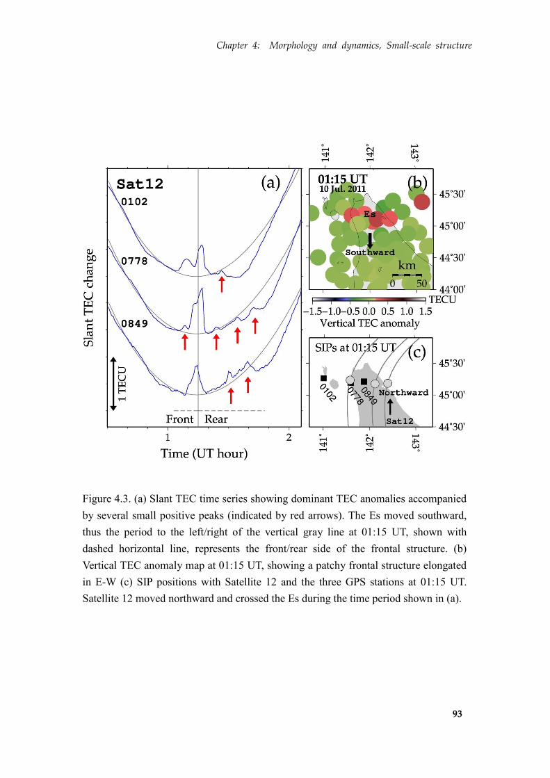
Chapter 4: Morphology and dynamics, Small-scale structure
93
Figure 4.3. (a) Slant TEC time series showing dominant TEC anomalies accompanied
by several small positive peaks (indicated by red arrows). The Es moved southward,
thus the period to the left/right of the vertical gray line at 01:15 UT, shown with
dashed horizontal line, represents the front/rear side of the frontal structure. (b)
Vertical TEC anomaly map at 01:15 UT, showing a patchy frontal structure elongated
in E-W (c) SIP positions with Satellite 12 and the three GPS stations at 01:15 UT.
Satellite 12 moved northward and crossed the Es during the time period shown in (a).
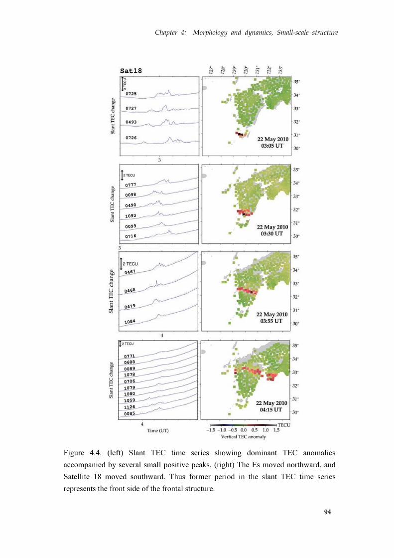
Chapter 4: Morphology and dynamics, Small-scale structure
94
Figure 4.4. (left) Slant TEC time series showing dominant TEC anomalies
accompanied by several small positive peaks. (right) The Es moved northward, and
Satellite 18 moved southward. Thus former period in the slant TEC time series
represents the front side of the frontal structure.
Chapter 4: Morphology and dynamics, Small-scale structure
95
The gradient drift instability can make plasma patches unstable when the direction
of the plasma propagation coincides with the gradient of electron density within the
patches. Thus it could form smooth/undulated leading/trailing edges. Densely ionized
plasma patches can produce rather strong polarization electric fields and currents, which
would then trigger the gradient drift and other plasma instabilities [Hysell et al., 2002].
As far as the drifting strong Es patches (i.e., large foEs) are concerned, gradient drift
instability may play an important role in the formation of peculiar shapes of leading and
trailing edges.
In slant TEC time series, main patches represented by the largest amplitude of TEC
anomalies are often accompanied by QP TEC signatures. Our observations confirmed
that QP TEC enhancements can appear both in the leading and trailing edges of moving
frontal structures. This result excludes the simple assumption that the gradient drift
instability is the only generation mechanism responsible for them. Nevertheless, at least
for the case shown in Figure 4.3, it seems appropriate to assume that the gradient drift
instability generated QP plasma patches in the trailing edges of frontal structures.
The results shown in Figure 4.4 indicate that the frontal structure is characterized
by a smooth leading edge with gradual increase in electron density and a steep trailing
edge with a sudden drop of electron density. In addition, the trailing edges are followed
by some broken plasma patches. This feature is observed during the northward drift of
the frontal structure, and the plasma patches in the leading/trailing edge are considered
to be relatively stable/unstable. Thus the gradient drift instability is one of the possible
candidates responsible for the QP TEC signature.
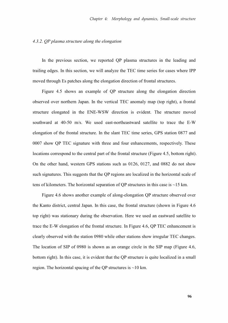
Chapter 4: Morphology and dynamics, Small-scale structure
96
4.3.2. QP plasma structure along the elongation
In the previous section, we reported QP plasma structures in the leading and
trailing edges. In this section, we will analyze the TEC time series for cases where IPP
moved through Es patches along the elongation direction of frontal structures.
Figure 4.5 shows an example of QP structure along the elongation direction
observed over northern Japan. In the vertical TEC anomaly map (top right), a frontal
structure elongated in the ENE-WSW direction is evident. The structure moved
southward at 40-50 m/s. We used east-northeastward satellite to trace the E-W
elongation of the frontal structure. In the slant TEC time series, GPS station 0877 and
0007 show QP TEC signature with three and four enhancements, respectively. These
locations correspond to the central part of the frontal structure (Figure 4.5, bottom right).
On the other hand, western GPS stations such as 0126, 0127, and 0882 do not show
such signatures. This suggests that the QP regions are localized in the horizontal scale of
tens of kilometers. The horizontal separation of QP structures in this case is ~15 km.
Figure 4.6 shows another example of along-elongation QP structure observed over
the Kanto district, central Japan. In this case, the frontal structure (shown in Figure 4.6
top right) was stationary during the observation. Here we used an eastward satellite to
trace the E-W elongation of the frontal structure. In Figure 4.6, QP TEC enhancement is
clearly observed with the station 0980 while other stations show irregular TEC changes.
The location of SIP of 0980 is shown as an orange circle in the SIP map (Figure 4.6,
bottom right). In this case, it is evident that the QP structure is quite localized in a small
region. The horizontal spacing of the QP structures is ~10 km.
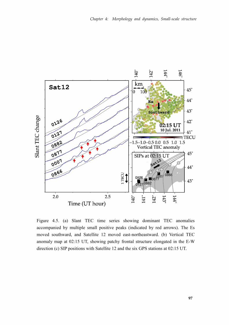
Chapter 4: Morphology and dynamics, Small-scale structure
97
Figure 4.5. (a) Slant TEC time series showing dominant TEC anomalies
accompanied by multiple small positive peaks (indicated by red arrows). The Es
moved southward, and Satellite 12 moved east-northeastward. (b) Vertical TEC
anomaly map at 02:15 UT, showing patchy frontal structure elongated in the E-W
direction (c) SIP positions with Satellite 12 and the six GPS stations at 02:15 UT.
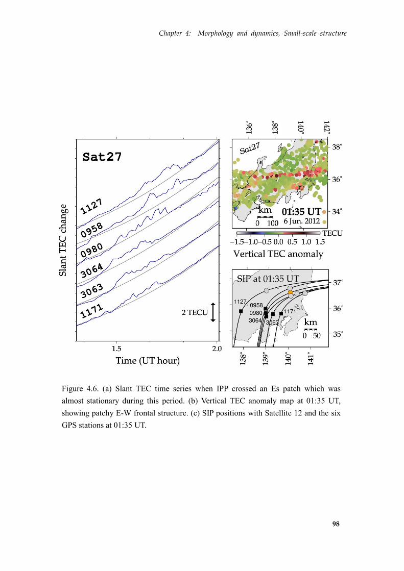
Chapter 4: Morphology and dynamics, Small-scale structure
98
Figure 4.6. (a) Slant TEC time series when IPP crossed an Es patch which was
almost stationary during this period. (b) Vertical TEC anomaly map at 01:35 UT,
showing patchy E-W frontal structure. (c) SIP positions with Satellite 12 and the six
GPS stations at 01:35 UT.
Chapter 4: Morphology and dynamics, Small-scale structure
99
4.3.3. Discussion
4.3.3.1. QP structure in the across-the-elongation direction
Maruyama [1991] conducted a beacon experiment at Wakkanai (very close to the
current NICT ionosonde site), and had observed QP scintillations in 136 MHz radio
waves transmitted from a geostationary satellite. He reported multiple linear-shaped Es
layers aligned in E-W which are horizontally separated in the N-S direction by 8-17 km.
Although Maruyama [1991] mainly examined nighttime QP scintillations, the horizontal
shape and spacing are consistent with those presented in our study. The SEEK-2
campaign performed in southwestern Japan also showed a similar result, i.e., they
observed QP echoes horizontally separated by 13-15 km in N-S direction [Saito et al.,
2005] (Figure 4.1). According to the CSR observations of the nighttime E-region of the
ionosphere over the Caribbean Sea, wavelike behavior with the horizontal spacing of
~15 km was also evident in a banded structure [Hysell et al., 2009].
Our results show 10-25 km horizontal spacing for the QP regions, and this is
consistent with these past observations. Although QP events are less frequent in daytime,
our observations suggest that QP structures are often seen in daytime Es patches. The
condition for the development of the QP structure is not clear at this moment, but
further case studies and statistical studies will reveal detailed characteristics of daytime
QP structures. This will eventually lead to better understanding of the instability process
working in the primary frontal structure.
Maruyama [1991] inferred that the plasma patch of drifting Es is elongated in a
direction with higher electron density in the trailing edge (Figure 4.7). Our observations
also show that leading and trailing edges of drifting Es have such gradient in electron
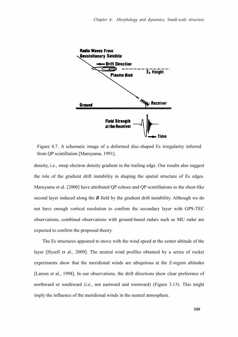
Chapter 4: Morphology and dynamics, Small-scale structure
100
Figure 4.7. A schematic image of a deformed disc-shaped Es irregularity inferred
from QP scintillation [Maruyama, 1991].
density, i.e., steep electron density gradient in the trailing edge. Our results also suggest
the role of the gradient drift instability in shaping the spatial structure of Es edges.
Maruyama et al. [2000] have attributed QP echoes and QP scintillations to the sheet-like
second layer induced along the B field by the gradient drift instability. Although we do
not have enough vertical resolution to confirm the secondary layer with GPS-TEC
observations, combined observations with ground-based radars such as MU radar are
expected to confirm the proposed theory.
The Es structures appeared to move with the wind speed at the center altitude of the
layer [Hysell et al., 2009]. The neutral wind profiles obtained by a series of rocket
experiments show that the meridional winds are ubiquitous at the E-region altitudes
[Larsen et al., 1998]. In our observations, the drift directions show clear preference of
northward or southward (i.e., not eastward and westward) (Figure 3.13). This might
imply the influence of the meridional winds in the neutral atmosphere.
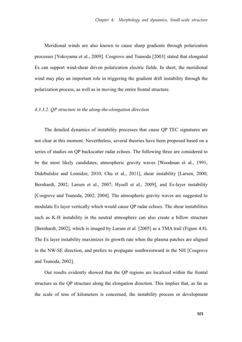
Chapter 4: Morphology and dynamics, Small-scale structure
101
Meridional winds are also known to cause sharp gradients through polarization
processes [Yokoyama et al., 2009]. Cosgrove and Tsunoda [2003] stated that elongated
Es can support wind-shear driven polarization electric fields. In short, the meridional
wind may play an important role in triggering the gradient drift instability through the
polarization process, as well as in moving the entire frontal structure.
4.3.3.2. QP structure in the along-the-elongation direction
The detailed dynamics of instability processes that cause QP TEC signatures are
not clear at this moment. Nevertheless, several theories have been proposed based on a
series of studies on QP backscatter radar echoes. The following three are considered to
be the most likely candidates; atmospheric gravity waves [Woodman et al., 1991;
Didebulidze and Lomidze, 2010; Chu et al., 2011], shear instability [Larsen, 2000;
Bernhardt, 2002; Larsen et al., 2007; Hysell et al., 2009], and Es-layer instability
[Cosgrove and Tsunoda, 2002; 2004]. The atmospheric gravity waves are suggested to
modulate Es layer vertically which would cause QP radar echoes. The shear instabilities
such as K-H instability in the neutral atmosphere can also create a billow structure
[Bernhardt, 2002], which is imaged by Larsen et al. [2005] as a TMA trail (Figure 4.8).
The Es layer instability maximizes its growth rate when the plasma patches are aligned
in the NW-SE direction, and prefers to propagate southwestward in the NH [Cosgrove
and Tsunoda, 2002].
Our results evidently showed that the QP regions are localized within the frontal
structure as the QP structure along the elongation direction. This implies that, as far as
the scale of tens of kilometers is concerned, the instability process or development
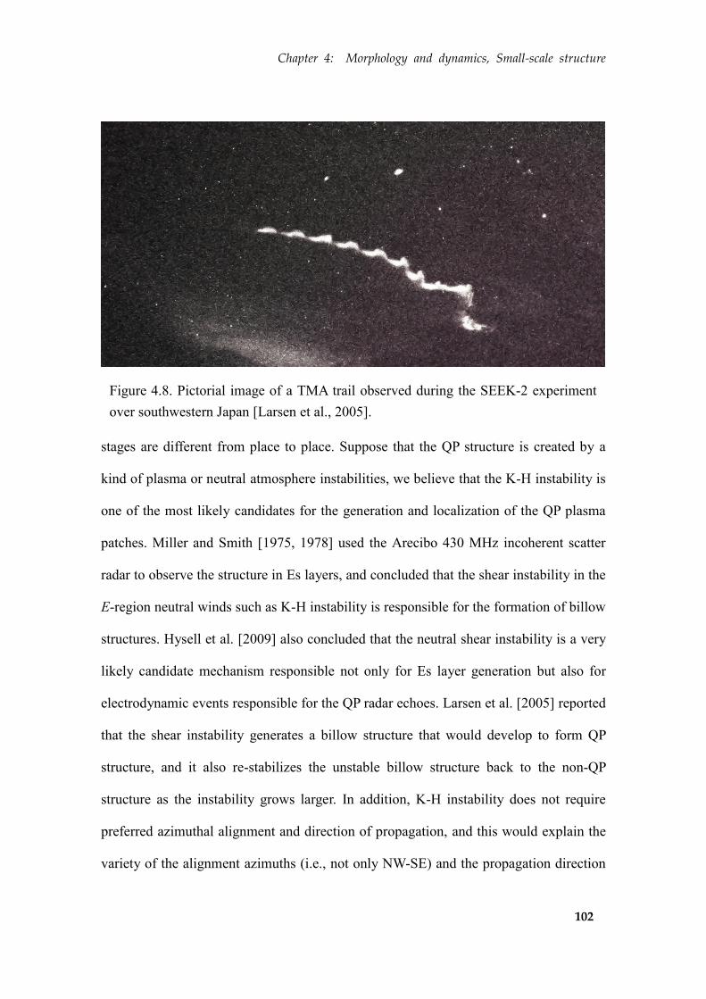
Chapter 4: Morphology and dynamics, Small-scale structure
102
stages are different from place to place. Suppose that the QP structure is created by a
kind of plasma or neutral atmosphere instabilities, we believe that the K-H instability is
one of the most likely candidates for the generation and localization of the QP plasma
patches. Miller and Smith [1975, 1978] used the Arecibo 430 MHz incoherent scatter
radar to observe the structure in Es layers, and concluded that the shear instability in the
E-region neutral winds such as K-H instability is responsible for the formation of billow
structures. Hysell et al. [2009] also concluded that the neutral shear instability is a very
likely candidate mechanism responsible not only for Es layer generation but also for
electrodynamic events responsible for the QP radar echoes. Larsen et al. [2005] reported
that the shear instability generates a billow structure that would develop to form QP
structure, and it also re-stabilizes the unstable billow structure back to the non-QP
structure as the instability grows larger. In addition, K-H instability does not require
preferred azimuthal alignment and direction of propagation, and this would explain the
variety of the alignment azimuths (i.e., not only NW-SE) and the propagation direction
Figure 4.8. Pictorial image of a TMA trail observed during the SEEK-2 experiment
over southwestern Japan [Larsen et al., 2005].
Chapter 4: Morphology and dynamics, Small-scale structure
103
of QP structures (i.e., not only toward SW) observed in this study.
Chapter 4: Morphology and dynamics, Small-scale structure
104
4.4. Concluding remarks
In this chapter, we have shown small-scale plasma structures associated with Es
patches with frontal structure, and discussed instability processes possibly responsible
for them. Conclusions of this chapter are as follows:
(1) Small scale sub-structures are found to accompany the main Es frontal structure.
They are characterized by quasi-periodic (QP) TEC signatures.
(2) QP TEC signatures are observed in daytime strong Es.
(3) Leading edges of propagating Es frontal structures show a gentle spatial gradient of
electron density and smooth edge shapes. On the other hand, their trailing edges
show steep gradients and often accompany several broken plasma patches. Plasma
instability such as gradient drift instability is one of the possible candidates
responsible for the undulated trailing edge.
(4) QP plasma patches in a frontal structure can cause QP TEC fluctuations. The spatial
separation is 10-25 km, which is consistent with previous studies based on QP
echoes.
(5) Frontal structures often consist of both QP and non-QP regions. Shear instabilities
such as Kelvin-Helmholtz instability is the most likely candidate to explain the
generation and localization of small plasma patches.

105
Chapter 5
Conclusions and Future work
Chapter 5: Conclusions and Future work
106
5.1. Conclusions
We have shown and discussed two principal issues in the present dissertation, i.e.,
application of the GPS-TEC method for the observation of sporadic E (Es), and the
morphological and dynamical characteristics of midlatitude Es observed with this new
method in Japan. Here we summarize our study into the following concluding remarks.
5.1.1. Application of GPS-TEC observation on sporadic-E detection
GPS-TEC observations can detect Es patches if their foEs values exceed 16-17
MHz. In slant TEC time series, Es signatures are characterized by pulse-like positive
TEC anomalies. TEC anomalies can be mapped to image the large-scale horizontal
structure of Es patches. Matching of TEC maps drawn with multiple GPS satellites can
be used to constrain Es altitudes, and several Es patches have been proved to exist at the
E-region altitude of ~100 km. GPS-TEC observation can also provide information on Es
movements. High temporal resolution (30 seconds) two-dimensional imaging of Es
makes it possible to observe temporal evolution of individual Es patches. This would be
a breakthrough of Es observations considering the spatial resolution 400 times as high
(1200 stations versus 3 stations) and the temporal resolution 30 times as high (30
seconds versus 15 minutes) as conventional sensors such as ionosondes. The thickness
of Es patches, inferred by comparing the amplitudes of TEC anomalies and foEs values,
fell in the range of 1.0-2.5 km, which is consistent with previous studies.
Chapter 5: Conclusions and Future work
107
5.1.2. Morphology and dynamics of midlatitude sporadic-E
In the vertical TEC anomaly maps, intensely ionized daytime Es patches often
show large-scale frontal structures elongated in E-W by more than 100 km. This was the
case over the latitude range covered by this study, 30°N-45°N. Observations of over 70
Es patches showed the lengths and widths of their frontal structures are 50-500 km and
10-30 km, respectively. Northward and southward movements, perpendicular to the
elongation azimuths, are observed. They range up to 100 m/s with the average of 60 m/s
in both directions. We also observed the fragmentation of the E-W frontal structure into
smaller patches and their migration. Tidal winds in neutral atmosphere may control the
migration direction of Es frontal structures.
Observations with multiple satellites suggested that the E-W frontal structure is
composed of small patches with very high electron density. In the case of Es on 21 May
2010, the plasma transportation responsible for the Es formation is found to have
occurred in a direction close to the local geomagnetic field.
Small scale sub-structures are found to accompany the main frontal structure. They
are characterized by quasi-periodic (QP) TEC signatures. Leading edges of drifting
frontal structures show moderate gradients of electron density represented by smooth
and uniform transitions. On the other hands, the trailing edges show steep gradient of
electron density represented by clear boundaries, and they are often accompanied by
several smaller plasma patches possibly torn from the main patch. QP plasma patches
within a frontal structure can also cause QP TEC fluctuations. The spatial separation of
the plasma blobs is 10-25 km, which is consistent with past radar observations of QP
echoes. Frontal structures are found to consist of QP and non-QP regions. Shear

Chapter 5: Conclusions and Future work
108
instability as represented by the Kelvin-Helmholtz instability might be able to explain
the generation and localization of plasma patches responsible for the QP signatures.
Here we investigated both morphological and dynamical characteristics of daytime
midlatitude Es. The results of our GPS-TEC observations provide systematic
understanding of past observation results which have been obtained as small fragments
by conventional radar and rocket observations. 2-D TEC maps enable us to draw
horizontal images of the whole Es irregularities. At the same time, studies of raw TEC
time series give us opportunities to study even smaller-scale patches, and we could, for
the first time, show that large-scale frontal structures are composed of smaller plasma
blobs. QP TEC signatures are often found in daytime strong Es in both the across- and
along-elongation directions of the frontal structures. This suggests that neutral and/or
plasma instabilities let large-scale Es patches evolve in time, making sub-structures
composed of smaller-scale blobs.
Chapter 5: Conclusions and Future work
109
5.2. Future work
While we have revealed morphological and dynamical properties of daytime
midlatitude Es to a large extent, there are still rooms for future investigations. Here we
discuss possible targets of future work as follows:
Nighttime observations: From the viewpoint of electrodynamic coupling between the
E- and F-region of the ionosphere at night, we need more nighttime GPS-TEC
observations. In addition, observations on Es movements during the nighttime will
further substantiate their link with the neutral atmospheric effect, i.e., tidal winds, in
the E-region of the ionosphere.
TEC tomography studies: It is still ambiguous how plasmas are transported in space
during the formation of intense Es at midlatitudes. To infer the detailed vertical
structure of Es, tomographic analysis is a promising numerical technique.
Tomographic studies of the 3-D structure of Es using the GPS-TEC data would need
to be incorporated into other tomography techniques, e.g., radio tomography.
Further analyses of QP TEC signatures: Since small-scale plasma structures are
important to discuss instabilities and structuring process of Es plasma patches, we
should analyze more cases of Es with QP TEC signatures. Morphological properties,
e.g., elongation direction, horizontal scale size, horizontal separation, drift speed,
will also provide observational insight into plasma and/or neutral atmospheric
instabilities involved in the temporal evolution of Es patches at midlatitudes.
References
110
References
Arras, C., J. Wickert, G. Beyerle, S. Heise, T. Schmidt, and C. Jacobi (2008), A global
climatology of ionospheric irregularities derived from GPS radio occultation,
Geophys. Res. Lett., 35, L14809, doi:10.1029/2008GL034158.
Arras, C., C. Jaobi, and J. Wickhert (2009), Semidiurnal tidal signature in sporadic E
occurrence rates derived from GPS radio occultation measurements at higher
midlatitudes, Ann. Geophys., 27, 2555-2563, doi:10.5194/angeo-27-2555-2009.
Astafyeva, E., K. Heki, V. Kiryushkin, E. Afraimovich, and S. Shalimov (2009),
Two-mode long-distance propagation of coseismic ionosphere disturbances, J.
Geophys. Res., 114, A10307, doi:10.1029/2008JA013853.
Bernhardt, P. A. (2002), The modulation of sporadic-E layers by Kelvin-Helmholtz
billows in the neutral atmosphere, J. Atmos Sol. Terr. Phys., 64, 1487-1504.
Bernhardt, P. A., C. A. Selcher, C. Siefring, M. Wilkens, C. Compton, G. Bust, M.
Yamamoto, S. Fukao, O. Takayuki, M. Wakabayashi, and H. Mori (2005), Radio
tomographic imaging of sporadic-E layers during SEEK-2, Ann. Geophys., 23,
2357-2368.
Bowman, G. G. (1960), Some aspects of sporadic E at mid-latitudes, Planet. Space Sci.,
2, 195.
Bowman, G. G. (1968), Movements of ionospheric irregularities and gravity waves, J.
Atmos Terr. Phys., 630, 721.
Cathey, E. H. (1969), Some midlatitude sporadic-E results from the Explorer 20 satellite,
J. Geophys. Res., 74(9), 2240–2247, doi:10.1029/JA074i009p02240.

References
111
Chu, Y.-H., P. S. Brahmanandam, C.-Y. Wang, Ching-Lun S., and R.-M. Kuong (2011),
Coordinated sporadic E layer observations made with Chung-Li 30 MHz radar,
ionosonde and FORMOSAT-3/COSMIC satellites, J. Atmos. Solar-Terr Phys., 73,
883–894.
Cosgrove, R. B., and R. T. Tsunoda (2002), A direction-dependent instability of
sporadic-E layers in the nighttime midlatitude ionosphere, Geophys. Res. Lett.,
29(18), 1864, doi:10.1029/2002GL014669.
Cosgrove, R. B., and R. T. Tsunoda (2003), Simulation of the nonlinear evolution of the
sporadic-E layer instability in the nighttime midlatitude ionosphere, J. Geophys.
Res., 108, 1283, doi:10.1029/2002JA009728, A7.
Cosgrove, R. B., and R. T. Tsunoda (2004), Instability of the E-F coupled nighttime
midlatitude ionosphere, J. Geophys. Res., 109, A04305,
doi:10.1029/2003JA010243.
Cosgrove, R. B. (2007), Wavelength dependence of the linear growth rate of the Es layer
instability, Ann. Geophys., 25, 1311-1322, doi:10.5194/angeo-25-1311-2007.
Dungey, J. W. (1959), The effect of a magnetic field on turbulence in an ionized gas, J.
Geophys. Res., 64, 2188.
Didebulidze, G. G., and L. N. Lomidze (2010), Double atmospheric gravity wave
frequency oscillations of sporadic E formed in a horizontal shear flow, Physics
Letters, A 374.7, 952-969.
Elford, W. G. (1959), A study of winds between 80 and 100 km in medium latitudes,
Planetary and Space Science, 1, 94–101.
Foster, J. C., P. J. Erickson, A. J. Coster, J. Goldstein, and F. J. Rich (2002), Ionospheric
signatures of plasmaspheric tails, Geophys. Res. Lett., 29(13),

References
112
doi:10.1029/2002GL015067.
Garcia-Fernandez, M., and T. Tsuda (2006), A global distribution of sporadic E events
revealed by means of CHAMP-GPS occultations, Earth Planets Space, 58, 33–36.
Haldoupis, C., and D. Pancheva (2006), Terdiurnal tidelike variability in sporadic E
layers, J. Geophys. Res., 111, A07303, doi:10.1029/2005JA011522.
Haldoupis, C. (2012), Midlatitude Sporadic E layers. A typical paradigm of
atmosphere–ionosphere coupling, Space Sci. Rev., 168, 441–461.
Hayashi, H., N. Nishitani, T. Ogawa, Y. Otsuka, T. Tsugawa, K. Hosokawa, and A. Saito
(2010), Large-scale traveling ionospheric disturbance observed by superDARN
Hokkaido HF radar and GPS networks on 15 December 2006, J. Geophys. Res., 115,
A06309, doi:10.1029/2009JA014297.
Heki, K., and J.-S. Ping (2005), Directivity and apparent velocity of the coseismic
ionospheric disturbances observed with a dense GPS array, Earth Planet. Sci. Lett.,
236, 845-855.
Heki, K. (2006), Explosion energy of the 2004 eruption of the Asama Volcano, central
Japan, inferred from ionospheric disturbances, Geophys. Res. Lett., 33, L14303,
doi:10.1029/2006GL026249.
Huba, J. D., R. W. Schunk, and G. V. Khazanov (2014), Modeling the
Ionosphere-Thermosphere System, American Geophysical Union, Washington,
D.C.
Hysell, D. L., M. Yamamoto, and S. Fukao (2002), Imaging radar observations and
theory of type I and type II quasi-periodic echoes, J. Geophys. Res., 107(A11),
1360, doi:10.1029/2002JA009292.
References
113
Hysell, D. L., M. F. Larsen, and Q. H. Zhou (2004), Common volume coherent and
incoherent scatter radar observations of mid-latitude sporadic E-layers and QP
echoes, Ann. Geophys., 22, 3277-3290, doi:10.5194/angeo-22-3277-2004.
Hysell, D. L., E. Nossa, M. F. Larsen, J. Munro, M. P. Sulzer, and S. A. González
(2009), Sporadic E layer observations over Arecibo using coherent and incoherent
scatter radar: Assessing dynamic stability in the lower thermosphere, J. Geophys.
Res., 114, A12303, doi:10.1029/2009JA014403.
Hysell, D. L., E. Nossa, H. C. Aveiro, M. F. Larsen, J. Munro, M. P. Sulzer, and S. A.
González (2013), Fine structure in midlatitude sporadic E layers, J. Atm.
Solar-Terr. Phys., 103, 16-23, doi:10.1016/j.jastp.2012.12.005.
Kantarizis, E. (1971), Measurement of the thickness of a sporadic E-layer, J. Atmos. Terr.
Phys., 33, 1651-1656.
Kato, S. (1956), Horizontal wind systems in the ionospheric E region deduced from the
dynamo theory of the geomagnetic Sq Variation Part II, J. Geomag. Geoelectr., 8,
24-37.
Kedar, S., G. A. Hajj, B. D. Wilson, and M. B. Heflin (2003), The effect of the second
order GPS ionospheric correction on receiver positions, Geophys. Res. Lett., 30, 1829,
doi:10.1029/2003GL017639.
Kelly, M. C. (2009), The Earth’s Ionosphere: Plasma Physics and Electrodynamics,
International Geophysics Series, Vol. 96, Academic, San Diego, California.
Kurihara, J., et al. (2010), Horizontal structure of sporadic E layer observed with a
rocket-borne magnesium ion imager, J. Geophys. Res., 115, A12318,
doi:10.1029/2009JA014926.
Larsen, M. F., S. Fukao, M. Yamamoto, R. Tsunoda, K. Igarashi, and T. Ono (1998),
References
114
The SEEK chemical release experiment: Observed neutral wind profile in a region
of sporadic-E, Geophys. Res. Lett., 25, 1789.
Larsen, M. F. (2000), A shear instability seeding mechanism for quasiperiodic radar
echoes, J. Geophys. Res., 105(A11), 24931–24940, doi:10.1029/1999JA000290.
Larsen, M. F. (2002), Winds and shears in the mesosphere and lower thermosphere:
Results from four decades of chemical release wind measurements, J. Geophys.
Res., 107(A8), doi:10.1029/2001JA000218.
Larsen, M. F., M. Yamamoto, S. Fukao, and R. T. Tsunoda (2005), SEEK 2:
Observations of neutral winds, wind shears, and wave structure during a sporadic
E/QP event, Ann. Geophys., 23, 2369-2375.
Larsen, M. F., D. L. Hysell, Q. H. Zhou, S. M. Smith, J. Friedman, and R. L. Bishop
(2007), Imaging coherent scatter radar, incoherent scatter radar, and optical
observations of quasiperiodic structures associated with sporadic E layers, J.
Geophys. Res., 112, A06321, doi:10.1029/2006JA012051.
Liu, X., J. Xu, J. Yue, H. L. Liu, and W. Yuan (2014), Large winds and wind shears
caused by the nonlinear interactions between gravity waves and tidal backgrounds
in the mesosphere and lower thermosphere, J. Geophys. Res. Space Physics, 119,
7698–7708, doi:10.1002/2014JA020221.
Ma, G., and T. Maruyama (2006), A super bubble detected by dense GPS network at
east Asian longitudes, Geophys. Res. Lett., 33, L21103,
doi:10.1029/2006GL027512.
Maeda, H. (1957), Horizontal wind systems in the ionospheric E region deduced from
the dynamo theory of the geomagnetic Sq Variation Part III, J. Geomag. Geoelectr.,
9, 86-93.
References
115
Maeda, J., and K. Heki (2014), Two-dimensional observations of midlatitude sporadic E
irregularities with a dense GPS array in Japan, Radio Sci., 49, 28–35,
doi:10.1002/2013RS005295.
Malhotra, A., J. D. Mathews, and J. Urbina (2008), Effect of meteor ionization on
sporadic-E observed at Jicamarca, Geophys. Res. Lett., 35, L15106,
doi:10.1029/2008GL034661.
Maruyama, T. (1991), Observations of quasi-periodic scintillations and their possible
relation to the dynamics of Es plasma blobs, Radio Sci., 26(3), 691–700,
doi:10.1029/91RS00357.
Maruyama, T. (1995), Shapes of irregularities in the sporadic E layer producing
quasi-periodic scintillations, Radio Sci., 30(3), 581–590, doi:10.1029/95RS00830.
Maruyama, T., S. Fukao, and M. Yamamoto (2000), A possible mechanism for echo
striation generation of radar backscatter from midlatitude sporadic E, Radio Sci.,
35(5), 1155–1164, doi:10.1029/1999RS002296.
Maruyama, T., H. Kato, and M. Nakamura (2003), Ionospheric effects of the Leonid
meteor shower in November 2001 as observed by rapid run ionosondes, J.
Geophys. Res., 108, 1324, doi:10.1029/2003JA009831, A8.
Maruyama, T., H. Kato, and M. Nakamura (2008), Meteor-induced transient sporadic E
as inferred from rapid-run ionosonde observations at midlatitudes, J. Geophys. Res.,
113, A09308, doi:10.1029/2008JA013362.
Mathews, J. D. (1998), Sporadic E: current views and recent progress, J. Atmos.
Solar‐Terr. Phys., 60, 413–435.
Mendillo, M., J. Meriwether, and M. Biondi (2001), Testing the thermospheric neutral
wind suppression mechanism for day-to-day variability of equatorial spread F, J.
References
116
Geophys. Res., 106(A3), 3655–3663, doi:10.1029/2000JA000148.
Miller, K. L., and L. G. Smith (1975), Horizontal structure of mid-latitude sporadic E
layers observed by incoherent scatter radar, Radio Sci., 10, 271.
Miller, K. L., and L. G. Smith (1978), Incoherent scatter radar observations of irregular
structure in mid-latitude sporadic E layers, J. Geophys. Res., 33, 3761.
Nishioka, M., T. Tsugawa, M. Kubota, and M. Ishii (2013), Concentric waves and
short-period oscillations observed in the ionosphere after the 2013 Moore EF5
tornado, Geophys. Res. Lett., 40, 5581–5586, doi:10.1002/2013GL057963.
Otsuka, Y., T. Ogawa, A. Saito, T. Tsugawa, S. Fukao, and S. Miyazaki (2002), A new
technique for mapping of total electron content using GPS network in Japan, Earth
Planets Space, 54, 63–70.
Otsuka, Y., K. Shiokawa, and T. Ogawa (2012), Disappearance of equatorial plasma
bubble after interaction with mid-latitude medium-scale traveling ionospheric
disturbance, Geophys. Res. Lett., 39, L14105, doi:10.1029/2012GL052286.
Ozeki, M., and K. Heki (2010), Ionospheric holes made by ballistic missiles from North
Korea detected with a Japanese dense GPS array, J. Geophys. Res., 115, A09314,
doi:10.1029/2010JA015531.
Reddy, C. A., and M. M. Rao (1968), On the physical significance of the Es parameters
fbEs, fEs, and foEs, J. Geophys. Res., 73(1), 215–224,
doi:10.1029/JA073i001p00215.
Roddy, P. A., G. D. Earle, C. M. Swenson, C. G. Carlson, and T. W. Bullett (2004),
Relative concentrations of molecular and metallic ions in midlatitude intermediate
and sporadic-E layers, Geophys. Res. Lett., 31, L19807,
doi:10.1029/2004GL020604.
References
117
Saito, A., S. Fukao, and S. Miyazaki (1998), High resolution mapping of TEC
perturbations with the GSI GPS network over Japan, Geophys. Res. Lett., 25(16),
3079–3082, doi:10.1029/98GL52361.
Saito, A., M. Nishimura, M. Yamamoto, S. Fukao, T. Tsugawa, Y. Otsuka, S. Miyazaki,
and M. C. Kelley (2002), Observations of traveling ionospheric disturbances and
3-m scale irregularities in the nighttime F-region ionosphere with the MU radar and
a GPS network, Earth Planets Space, 54, 31–44.
Saito, S., M. Yamamoto, S. Fukao, M. Marumoto, and R. T. Tsunoda (2005), Radar
observations of field-aligned plasma irregularities in the SEEK-2 campaign, Ann.
Geophys., 23, 2307-2318, doi:10.5194/angeo-23-2307-2005.
Saito, S., M. Yamamoto, H. Hashiguchi, and A. Maegawa (2006), Observation of
three-dimensional structures of quasi-periodic echoes associated with mid-latitude
sporadic-E layers by MU radar ultra-multi-channel system, Geophys. Res. Lett., 33,
L14109, doi:10.1029/2005GL025526.
Shinagawa H., H. Jin, Y. Miyoshi, H. Fujiwara, and T. Yokoyama (2014), Prediction of
the occurrence of sporadic E layers and plasma bubbles using GAIA, R010-02,
SGEPSS fall meeting, Nagano, Japan.
Smith, E. K. Jr., and S. Matsushita (1962), Ionospheric sporadic E, Pergamon, New
York.
Smith, E. K. (1968), Some unexplained features in the statistics for intense sporadic E,
Second Seminar on the Cause and Structure of Temperate Latitude Sporadic-E,
Vail, Colorado, paper 12.
Tanaka, T. (1979), Sky-wave backscatter observations of sporadic-E over Japan, J.
Atmos Terr. Phys., 41, 203-215.
References
118
Tsugawa, T., A. Saito, and Y. Otsuka (2004), A statistical study of large-scale traveling
ionospheric disturbances using the GPS network in Japan, J. Geophys. Res., 109,
A06302, doi:10.1029/2003JA010302.
Tsugawa, T., A. Saito, Y. Otsuka, M. Nishioka, T. Maruyama, H. Kato, and K. T.
Murata (2011), Ionospheric disturbances detected by GPS total electron content
observation after the 2011 off the Pacific coast of Tohoku Earthquake, Earth,
planets and space, 63(7), 875-879.
Tsunoda, R. T., M. Yamamoto, H. Mori, and S. Fukao (2000), SEEK S310-25:
Quasi-periodic echoes and polarization electric fields, Geophys. Res. Lett., 27,
3281.
Tsunoda, R. T., and R. B. Cosgrove (2001), Coupled electrodynamics in the nighttime
midlatitude ionosphere, Geophys. Res. Lett., 28, 4171-4174.
Tsunoda, R. T., R. B. Cosgrove, and T. Ogawa (2004), Azimuth-dependent Es layer
instability: A missing link found, J. Geophys. Res., 109, A12303,
doi:10.1029/2004JA010597.
Wakabayashi, M., T. Ono, T. Mori, and P. A. Bernhardt (2005), Electron density and
plasma waves measurement in mid-latitude sporadic-E layer observed during the
SEEK-2 campaign, Ann. Geophys., 23, 2335-2345.
Wakabayashi, M., and T. Ono (2005), Multi-layer structure of mid-latitude sporadic-E
observed during the SEEK-2 campaign, Ann. Geophys., 23, 2347-2355.
Whitehead, J. D. (1960), Formation of the sporadic E layer in the temperate zones,
Nature, 188, 567.
Whitehead, J. D. (1961), The formation of the sporadic E layer in the temperate zones, J.
Atmos. Terr. Phys., 20, 49.
References
119
Whitehead, J. D. (1970), Production and prediction of sporadic E, Rev. Geophys. Space
Phys., 8, 65-144.
Whitehead, J. D. (1989), Recent work on mid-latitude and equatorial sporadic E, J.
Atmos. Terr. Phys., 51, 401-424.
Woodman, R. F., M. Yamamoto, and S. Fukao (1991), Gravity wave modulation of
gradient drift instabilities in mid-latitude sporadic E irregularities, Geophys. Res.
Lett., 18, 1197–1200, doi: 10.1029/91GL01159.
Wu, D. L., C. O. Ao, G. A. Hajj, M. de la Torre Juarez, and A. J. Mannucci (2005),
Sporadic E morphology from GPS-CHAMP radio occultation, J. Geophys. Res.,
110, A01306, doi:10.1029/2004JA010701.
Yamamoto, M., S. Fukao, R. F. Woodman, T. Ogawa, T. Tsuda, and K. Kato (1991),
Mid-latitude E-region field aligned irregularities observed with the MU radar, J.
Geophys. Res., 96, 15,943.
Yamamoto, M., S. Fukao, T. Ogawa, T. Tsuda, and S. Kato (1992), A morphological
study of mid-latitude E-region field-aligned irregularities observed with the MU
radar, J. Atmos. Terr. Phys., 54, 769–777.
Yokoyama, T., D. L. Hysell, Y. Otsuka, and M. Yamamoto (2009), Three-dimensional
simulation of the coupled Perkins and Es-layer instabilities in the nighttime
midlatitude ionosphere, J. Geophys. Res., 114, A03308,
doi:10.1029/2008JA013789.
Zolesi, B., and L. R. Cander (2014), Ionospheric prediction and forecasting, Springer,
Heiderberg.
Recommended