Download pdf - Numerical (error) issues on compressible multicomponent flows using a high-order differencing scheme: Weighted compact nonlinear scheme

Journal of Computational Physics 231 (2012) 3181–3210

Contents lists available at SciVerse ScienceDirect

Journal of Computational Physics

journal homepage: www.elsevier .com/locate / jcp

Numerical (error) issues on compressible multicomponent flows usinga high-order differencing scheme: Weighted compact nonlinear scheme

Taku Nonomura a,⇑, Seiichiro Morizawa b, Hiroshi Terashima c, Shigeru Obayashi b, Kozo Fujii a

a JAXA/Institute of Space and Astronautical Science, Yoshinodai 3-1-1 1813, Sagamihara, Kanagawa, Japanb Tohoku University, Katahira 2-1-1, Aoba-ku Sendai, Miyagi, Japanc The University of Tokyo, Hongo 7-3-1, Bunkyo, Tokyo, Japan

a r t i c l e i n f o

Article history:Received 27 August 2011Received in revised form 20 December 2011Accepted 29 December 2011Available online 10 January 2012

Keywords:Weighted compact nonlinear schemeMulti-component compressible flowResolution

0021-9991/$ - see front matter � 2012 Elsevier Incdoi:10.1016/j.jcp.2011.12.035

⇑ Corresponding author. Tel./fax: +81 42 759 825E-mail address: [email protected] (T. N

a b s t r a c t

A weighted compact nonlinear scheme (WCNS) is applied to numerical simulations of com-pressible multicomponent flows, and four different implementations (fully or quasi-con-servative forms and conservative or primitive variables interpolations) are examined inorder to investigate numerical oscillation generated in each implementation. The resultsshow that the different types of numerical oscillation in pressure field are generated whenfully conservative form or interpolation of conservative variables is selected, while quasi-conservative form generally has poor mass conservation property. The WCNS implementa-tion with quasi-conservative form and interpolation of primitive variables can suppressthese oscillations similar to previous finite volume WENO scheme, despite the presentscheme is finite difference formulation and computationally cheaper for multi-dimensionalproblems. Series of analysis conducted in this study show that the numerical oscillationdue to fully conservative form is generated only in initial flow fields, while the numericaloscillation due to interpolation of conservative variables exists during the computations,which leads to significant spurious numerical oscillations near interfaces of different com-ponent of fluids. The error due to fully conservative form can be greatly reduced bysmoothing interface, while the numerical oscillation due to interpolation of conservativevariables cannot be significantly reduced. The primitive variable interpolation is, therefore,considered to be better choice for compressible multicomponent flows in the framework ofWCNS. Meanwhile better choice of fully or quasi-conservative form depends on a situationbecause the error due to fully conservative form can be suppressed by smoothed interfaceand because quasi-conservative form eliminates all the numerical oscillation but has poormass conservation.

� 2012 Elsevier Inc. All rights reserved.

1. Introduction

Mixing of multiple gases in compressible flowfields including shock waves is of importance in various engineering fields.For example, the accurate prediction of acoustic waves from a rocket plume is required for rocket launching, where the gas ofrocket plume is different from ambient. Several researchers conducted numerical simulations of rocket plumes under anassumption of single-species flows, to predict acoustic environments for satellite or launch fields, even though the gas ofrocket plumes is different from that of ambient [1,2]. The effects of mixing of different gas components on acoustic wavesfrom rocket plume possibly affect the generation of acoustic waves. However, simulations for multi-component flows have

. All rights reserved.

9.onomura).

http://dx.doi.org/10.1016/j.jcp.2011.12.035

mailto:[email protected]

http://dx.doi.org/10.1016/j.jcp.2011.12.035

http://www.sciencedirect.com/science/journal/00219991

http://www.elsevier.com/locate/jcp

3182 T. Nonomura et al. / Journal of Computational Physics 231 (2012) 3181–3210

several problems discussed later, and it is important to clarify the characteristics of schemes for such flows. We are now con-sidering application of a weighted compact nonlinear scheme, which is adopted in the study by Nonomura and Fujii [1,2], tosuch problems.

Here, WCNS is a variation of weighted-essentially-nonoscillatory (WENO) [3,4] type scheme, and has three advantagescompared with the original WENO: (1) WCNS has higher resolution than WENO [5,6]; (2) various flux evaluation methodscan be applied [5], e.g., Roe’s flux difference splitting method (FDS) [7]; and (3) freestream and vortex preservation proper-ties are very good on a wavy grid [8,9]. These advantages are basically owing to that the variable interpolation used in finitevolume method can be used in the WCNS procedure despite WCNS is a finite difference method. Considering these advan-tages, high-order WCNS was developed by Nonomura et al. [10] and by Zhang et al. [6], independently.

Numerical methods for compressible multicomponent flows can be decomposed into two types: (1) sharp interfacemethod and (2) diffused interface method. In the sharp interface method, immiscible flows are assumed. Interfaces betweendifferent fluids (hereafter we call simply ‘‘interface’’) are captured by volume of fluid method [11], level-set method [12–14]or front tracking method [15–17] and each fluid is solved independently. Here, boundary conditions at interface are given byghost-fluid method [16,18] or application of exact Riemann solver at the interface [17,19]. Although interface can be resolvedsharply, it is difficult to apply these methods to the complex shape of interface. On the other hand, diffused interface meth-ods [20–24] assumes that the fluid is miscible with introducing equations of mass fraction, and the interface is not treateddirectly. Due to the easiness of implementation and complicated interfaces expected to be generated, diffused interfacemethod is adopted in the framework of WCNS for the application to multicomponent flows.

Abgrall [20] applied diffused interface methods to convection problems of fluids with different specific heat ratio, and hereported that the numerical oscillation is observed when a fully conservative form of the governing equations was used. Thisproblem is because pressure equilibrium is violated at the interface, owing to mismatch of evaluations of energy and specificheat ratio. Abgrall and other researchers [20] showed that this numerical oscillation can be eliminated by nonconservativeform of mass fraction equation (or energy equation [21]). This type of formulation is so-called a quasi-conservative form.Recently, Johnsen and Colonius [22] extended this idea to a higher-order finite volume WENO scheme. They demonstratedthat the characteristic interpolation of primitive variables is a key for eliminating numerical oscillations in compressiblemulticomponent flows, while the general WENO uses the conservative variables. This technique cannot be applied to thefinite difference WENO because finite difference WENO does not include the variable interpolation, but conservative fluxinterpolation. With regard to applications of high-order scheme to compressible multicomponent flows, Kawai and Terashi-ma [24] conducted compressible multi-component flow simulations with high-order compact scheme and localized artificialdiffusivity. They demonstrated that the scheme works effectively for reducing spurious oscillations at interfaces, showingthe good mass conservation property due to the use of the fully conservation form. They also suggested that the use ofsmooth initial interface is effective to eliminate the startup error and the subsequent spurious oscillations related to com-pressible multicomponent flow simulations.

The finite volume WENO by Johnsen and Colonius [22] seems to be a good way while it has following two problems; (1)computationally expensive due to its multi-dimensional reconstruction inherently adopted in finite volume scheme and (2)mass conservation of each species is not fully satisfied due to quasi-conservative formulation [25]. With regard to the formerproblem, WCNS is able to use variable interpolation despite finite difference formulation. Thus, the characteristic interpola-tion of primitive variable adopted in Johnsen and Colonius [22] can be implemented in finite difference formulation, and theerror indicated by Johnsen and Colonius can be eliminated while keeping computational costs cheaper, because the finitedifference scheme has lower computational costs than finite volume scheme, which is reported in Ref. [26,27] and shortlydiscussed in Appendix B. On the other hand, the latter problem relates to the selection of fully conservative or quasi-conser-vative forms. Although there is a trade-off between this problem and the error indicated by Abgrall [20] the discussionincluding this trade-off has not been conducted in detail. It should be noted that there are limited studies on implementationof high-order scheme to compressible multi-component flows.

More recently, Johnsen and his colleague [28] proposed the formulation for keeping the pressure, velocity, and temperatureequilibrium with the fully conservative equations. In their formulation, the fully conservative equations and specific heat ratioare simultaneously solved, and the specific heat ratio is used for the estimation of pressure, though this method considers theoverestimation system because the specific heat ratio can be also estimated by the mass fraction which is solved in the conser-vative form. Although the method by Johnsen is very attractive for keeping the equilibrium and conservation, it still has thedisadvantage of high computational cost and further discussion should be needed for the disadvantage of using overestimationsystem. Therefore, we do not introduce this technique for the discussion in this paper, while it should be noted that this tech-nique also can be used for the WCNS without losing its advantage of the finite difference formulation.

Also, Shukla et al. [29] introduced the artificial compression technique for the diffused interface method. Their resultshows that this method is good to capture the interface. It should be noted that this technique is also applicable to the WCNSwhile maintaining the advantage of WCNS to WENO, but it is not discussed in this paper because it is out of scope of thispaper discussed below.

The objective of the present study is to understand the preferable implementation of WCNS to compressible multi-component flows; especially to understand effects of the choice of fully conservative or quasi-conservative forms and thechoice of characteristic interpolation of conservative variables or primitive variables. To investigate effects and trade-offrelationship of these choices, four different implementations of WCNS is evaluated throughout various test cases. Theimplementation with quasi-conservative forms and characteristic interpolation of primitive variable is expected to be the

T. Nonomura et al. / Journal of Computational Physics 231 (2012) 3181–3210 3183

error-free implementation like the finite volume WENO adopted by Johnsen and Colonius despite it is finite differencescheme. This is simply analyzed based on formulations and computationally verified through the test cases. Also, the effectsof initial condition (smoothness of interface) for each error are investigated as in the study by Kawai and Terashima [24]. Inaddition, we demonstrate the high resolution of WCNS compared with conventional upwind scheme and the high efficiency(low computational costs) of WCNS compared with finite volume WENO in Appendixes A and B, respectively.

2. Numerical methods

In this study, four possible implementations of WCNS are conducted. The choice of fully conservative or quasi-conserva-tive forms and the choice of characteristic interpolation of conservative variable or primitive variable are investigated. Theseimplementations are constructed on the well-validated in-house code. The implementation of fully conservative from withcharacteristic interpolation of conservative variable is named Fcnsv. The implementation of fully conservative from withcharacteristic interpolation of primitive variable is named Fprim. The implementation of quasi-conservative from with char-acteristic interpolation of conservative variable is named Qcnsv. The implementation of quasi-conservative from with char-acteristic interpolation of primitive variable is named Qprim. In all the implementations, we use characteristic interpolationinstead of componentwise interpolation because componentwise interpolation generates spurious oscillation near shockwaves. It should be noted that componentwise interpolation is almost the same as characteristic interpolation for capturinginterface of two-components in our a priori test.

2.1. Governing equations

In this section, details of implementations for two-component flows are presented. The compressible Euler equations andmass fraction equations are solved as the governing equations. A conservative form of the compressible Euler equations is asfollows:

@q@tþ @quj

@xj¼ 0;

@qui

@tþ @ðquiuj þ pdijÞ

@xj¼ 0;

@qe@tþ @ðqeþ pÞuj

@xj¼ 0; ð1Þ

where q, ui, p, e, xi and t are the density, velocity vector, pressure, energy per unit mass, position vector, and time, respec-tively. Here, dij denotes Kronecker delta.

A fully conservative form means that a following conservative form of equation of mass fraction is added to Eq. (1):

@qY1

@tþ @qujY1

@xj¼ 0; ð2Þ

where Y1 is the mass fraction of gas 1. The mass fraction of gas 0 is written as follows:

Y0 ¼ 1� Y1: ð3Þ

On the other hand, a quasi-conservative form means the following nonconservative form of the mass fraction equations isused instead of Eq. (2)

@Y1

@tþ @ujY1

@xj� Y1

@ui

@xi¼ 0: ð4Þ

It is noted that, although the standard nonconservative form of mass fraction equation is written as

@Y1

@tþ u1

@Yi

@xi¼ 0; ð5Þ

Eq. (4) is employed to obtain the same convection velocity for density, energy and mass fraction, as discussed in Johnsen andColonius [22]. Assuming temperature equilibrium at the interface, the specific heat ratio of mixture is defined as follows:

c ¼ 1Y1

c1�1þY0

c0�1

þ 1; ð6Þ

where c, c0, and c1 are specific heat ratio of mixed gas, gas 0 and gas 1, respectively. The ideal gas equation of state is writtenas follows, using the specific heat ratio of mixed gas:

qe ¼ pc� 1

þ 12quiui: ð7Þ

Table 1 also summarizes equations employed in each implementation.

Table 1Four implementations tested in this study.

Case Fully/quasi conservative form Interpolation Governing equations

Fcnsv Fully conservative form Conservative variables Eqs. (1)–(3), (6) and (7)Fprim Fully conservative form Primitive variables Eqs. (1)–(3), (6) and (7)Qcnsv Quasi-conservative form Conservative variables Eqs. (1), (3), (4), (6) and (7)Qprim Quasi-conservative form Primitive variables Eqs. (1), (3), (4), (6) and (7)


2.2. Finite difference scheme

In this study, WCNS based on seventh-order variable interpolation and eighth-order explicit difference scheme is used,whereas WCNS has several advantages compared with WENO: (1) applicability of various flux evaluation method; (2) higherresolution; (3) preservation of freestream and vortex in a wavy grid as discussed before. With regard to the flux evaluation,Harten-Lax-Leer contact capturing (HLLC) scheme [30] is adopted. In this section, procedures of WCNS are described in de-tail. There are three procedures of WCNS; nonlinear interpolation, flux evaluation and linear differencing.

2.2.1. Nonlinear interpolationHere, nonlinear interpolation of Q L

jþ1=2 in j direction is presented, where Qj is a conservative/primitive variable vector atnode j and the superscript L is value at the left side. First, the conservative/primitive variables inside the stencil used for non-linear interpolation are transformed into characteristic variables as follows:

qjþn;m ¼ lj;mQjþn;m; ðn ¼ �3; . . . ;3Þ; ð8Þ

where qj+n,m is mth component of characteristic variable at node j + n, lj,m is the mth left eigenvector for the center node j forthe stencil. Here, a left eigenvector represents one for flux Jacobian when conservative variables are interpolated, while itrepresents one for coefficient matrix of Euler equations written by primitive variables when primitive variables areinterpolated.

Then, interpolations qL;kjþ1=2;m; ðk ¼ 1; . . . ;4Þ of mth characteristic variables are constructed from four-points substensil as

follows:

qL;1jþ1=2;m ¼ �

516

qj�3;m þ2116

qj�2;m �3516

qj�1;m þ3516

qj;m; ð9Þ

qL;2jþ1=2;m ¼

116

qj�2;m �5

16qj�1;m þ

1516

qj;m þ5

16qjþ1;m; ð10Þ

qL;3jþ1=2;m ¼ �

116

qj�1;m þ9

16qj;m þ

916

qjþ1;m �1

16qjþ2;m; ð11Þ

qL;4jþ1=2;m ¼

516

qj;m þ1516

qjþ1;m �5

16qjþ2;m þ

116

qjþ3;m: ð12Þ

Next, qLjþ1=2;m is computed as weighted averaging of qL;k

jþ1=2;m:

qLjþ1=2;m ¼ w1;mqL;1

jþ1=2;m þw2;mqL;2jþ1=2;m þw3;mqL;3

jþ1=2;m þw4;mqL;4jþ1=2;m; ð13Þ

where wk,m is nonlinear weight computed as

wk;m ¼ak;mP

lal;m; ð14Þ

ak;m ¼Ck

ðISk;m þ eÞ2: ð15Þ

Here,

ðC1;C2;C3;C4Þ ¼1

64;2164

;3564

;7

64

� �ð16Þ

are optimal weights, and ISk,m is the smooth indicator defined as follows:

ISk;m ¼X4

n¼1

X4

l¼1

cn;k;lqmjþkþl�5

!ð17Þ

where cn,k,l is a coefficient for a smooth indicator. In seventh-order WCNS by Nonomura et al. [10], Eqs. (9)–(12), (17) aresimply computed using approximate derivatives to reduce computational cost. See Ref. [10] for more details. Finally,qL

jþ1=2 is transformed into Q Ljþ1=2 as follows:


Q Ljþ1=2 ¼

Xm

rj;mqLjþ1=2;m; ð18Þ

where rj,m is right eigenvector corresponding to lj,m. Here, QRjþ1=2 can be computed symmetrically. The two interpolations

(conservative or primitive variables) are used, coupled with the fully conservative or quasi-conservative forms of the gov-erning equations. Table 1 summarizes the equations in each implementation used in this study.

2.2.2. Flux evaluationNext, the flux at the cell-center, EWCNS, is evaluated based on QL and QR. In this study, HLLC scheme [30] is adopted similar

to the study by Johnsen and Colonius [22].

2.2.3. Linear differencingFinally, first derivative of flux is computed with a high-order linear difference scheme. Earlier studies [5,31] showed that

the resolution of WCNS are not affected by the choice of difference schemes (e.g., explicit or implicit). In this study, aneighth-order explicit difference scheme is used as follows:

E0j ¼1Dx

12251024

EWCNSjþ1=2 � EWCNS

j�1=2

� �� 1

Dx245

3072EWCNS

jþ3=2 � EWCNSj�3=2

� �þ 1

Dx49

5120ðEWCNS

jþ5=2 � EWCNSj�5=2Þ

� 1Dx

57168

EWCNSjþ7=2 � EWCNS

j�7=2

� �: ð19Þ

2.2.4. Time integrationThe third-order total variation diminishing Runge–Kutta scheme [32] is adopted for the time integration.

2.2.5. Pressure equilibrium for quasi-conservative form with interpolation of primitive variablesIn this subsection, we present that Qprim implementation (which is based on quasi-conservative form with interpolation

of primitive variables) can keep its pressure equilibrium, similar to finite volume WENO by Johnsen and Colonius [22]. Giventhe one-dimensional flow with constant u > 0 and p, we have uL = u and pL = p through the interpolation of primitivevariables (whereas they are not always satisfied through the interpolation of conservative variables). Then, HLLC fluxevaluation and linear differencing are conducted with Euler explicit time integration for simplicity, and the variations indensity, velocity, and pressure are as follows:

qnþ1j ¼ qn

j þDxDt

uXs�1

k¼0

bk qLiþ1=2þk � qL

i�1=2�k

� � !; ð20Þ

ðquÞnþ1j ¼ ðquÞnj �

DxDt

u2Xs�1

k¼0


i�1=2�k

� � !; ð21Þ

ðqeÞnþ1j ¼ ðqeÞnj �

DxDt

uu2

2

Xs�1

k¼0


i�1=2�k

� �þ p

Xs�1

k¼0

bk1

cLjþ1=2þk � 1

� 1cL

j�1=2�k � 1

!" #; ð22Þ

Ynþ1j ¼ Yn

j þDxDt

uXs�1

k¼0

bk YLiþ1=2þk � YL

i�1=2�k

� � !; ð23Þ

where superscript n denotes the value for the time step n and bk is coefficient for the linear difference scheme in WCNS pro-cedure. In this discussion, we choose explicit difference scheme for simplicity. Based on Eqs. (20) and (21), we obtain

unþ1j ¼

ðquÞnþ1j

qnj

¼ u: ð24Þ

From the equation of state and Eq. (24), pressure at (n + 1) time step is written as follows:

pnþ1j ¼ ðcnþ1 � 1Þ ðqeÞnþ1

j �ðquÞnþ1

j

h i2

2qnþ1

j

8><>:

9>=>; ¼ ðcnþ1 � 1Þ ðqeÞnþ1

j �u2qnþ1

j

2

" #: ð25Þ

After the substitution of Eqs. (6), (20), (22)–(24) into Eq. (25) and the cumbersome calculation, we have

pnþ1 ¼ p: ð26Þ

This analysis shows that Qprim can keep velocity and pressure equilibrium for one-dimensional flow.

Fig. 1. Initial distributions of the test examining order of accuracy.

Fig. 2. L2 error for each implementation with original weight computation.

Fig. 3. L2 error for each implementation with mapped technique for weight computation.



3. One-dimensional test cases

3.1. A test for order of accuracy

The order of accuracy for each implementation is examined. A sufficiently smooth initial profile, shown in Fig. 1, is gen-erated as:

U ¼ ðq;u; p;Y1Þt ¼ ð5:5þ 0:9 sinð2pxÞ;0:5;1=1:4;0:5þ 0:1 sinð2pxÞÞt ;c0 ¼ 1:4; c1 ¼ 1:6;� 0:5 6 x 6 0:5: ð27Þ

The periodic condition is imposed at the boundary. Time step size Dt is set to Dx3, where Dx is grid spacing. Computationsare conducted until time t = 2.0. The exact solution is the same as the initial profile. Grid points are set to 8, 16, 32 and 64.

Fig. 2 shows the L2 error varied with grid spacing. All the implementations guarantee 5.5–6.5th-order of accuracy. Thereason why they cannot exactly guarantee seventh-order accuracy is that the nonlinear weights do not become optimal val-ues near the critical points [33]. A mapped technique [33] efficiently recovers the order of accuracy to the formal order ofaccuracy as shown in Fig. 3, demonstrating that the four implementations are properly constructed to be the seventh-orderof accuracy.

In the test problems shown later, the standard way for computing nonlinear weights without the mapped technique isused, because it is not expected to affect the conclusion in the following discussions.

3.2. A material convection problem

A one-dimensional material convection problem, similar to those by Johnsen and Colonius [22] or by Kawai and Terashi-ma [24], is simulated. Initial conditions are set as

U ¼Umaterial 0:25 < x < 0:75;Uambient otherwise;

�

Umaterial ¼ ðqm;um; pm;Y1;mÞt ¼ ð10;0:5;1=1:4;1:0Þt ;Uambient ¼ ðqa;ua;pa;Y1;aÞt ¼ ð1;0:5;1=1:4;0:0Þt ;c0 ¼ 1:4; c1 ¼ 1:6;0 6 x 6 1: ð28Þ

When the initial condition of smoothed interface is introduced in order to reduce the numerical oscillations at the interface,the initial condition is defined using the error function as follows, similar to Kawai and Terashima [24]:

U ¼ ð1� fsmoothÞUambient þ fsmoothUmaterial;

fsmooth ¼ 0:5þ 0:5erfs

CeDx

� �; ð29Þ

where fsmooth is a switching function, s is signed distance from the interface, erf is the Gauss error function, and Ce is a freeparameter for adjusting the smoothness of the interface. Effects of Ce on the initial profile are shown in Fig. 4.

The periodic boundary condition is imposed. The CFL number is set to 0.6 and computation is conducted until t = 2.0.First, the solutions for the sharp-interface initial condition are discussed. Fig. 5 shows distributions of density, pressure,

mass fraction for gas 1 at t = 2.0 when the sharp-interface initial condition is adopted. The pressure equilibrium is perfectly

Fig. 4. Effects of Ce on the initial profile of material convection problem.

Fig. 5. Results of material convection problem with sharp initial interface (t = 2.0).


achieved with Qprim. Small numerical oscillations are observed for Qcnsv and large ones are observed for both Fcnsv andFprim. This shows that the error caused by fully conservative form is larger than that of interpolation of conservative vari-ables. There are no major numerical oscillations in the distributions of density and mass fraction.

Fig. 6 shows the time history of normalized error in the mass conservation of gas 1, and L2 errors of pressure and velocity.The error in mass conservation of gas 1 are almost machine zero for Fcnsv and Fprim while Qcnsv and Qprim have errors of�102 in mass conservation.

Errors in the distributions of pressure and velocity shows that Qprim keeps pressure (velocity) equilibrium, Qcnsv gen-erates small error, and both Fcnsv and Fprim produce large error. The error caused by fully conservative form is larger thanthat caused by the interpolation of conservative variables.

Fig. 7 shows the distributions of density, pressure, and mass fraction for gas 1 at t = 2.0 using the smoothed-interface ini-tial condition with Ce = 3. The pressure equilibrium is perfectly achieved with Qprim. Also, Fprim does not seem to have anynumerical oscillation in this axis range, though the one- or two-order smaller error compared with Fcnsv or Qcnsv is

Fig. 6. Time history of error in material convection problem with sharp initial interface (t = 2.0).


generated. Here, Fcnsv and Qcnsv still generate large numerical errors, though they become smaller than those producedusing the sharp initial interface. This indicates that the error caused by interpolation of conservative variables relatively be-comes larger than that caused by the fully conservative forms. The distributions of density and mass fraction do not showany differences among all the implementations.

Fig. 8 shows the time history of mass of gas 1, the L2 errors of pressure and velocity with the smoothed-interface initialcondition. The mass conservation error is almost machine zero for Fcnsv and Fprim, while Qcnsv and Qprim produce themass conservation errors of �104–103 which are smaller than those with the sharp initial interface. The errors in distribu-tions of pressure and velocity show that Qprim keeps pressure (velocity) equilibrium, Fprim produces very small errors, and

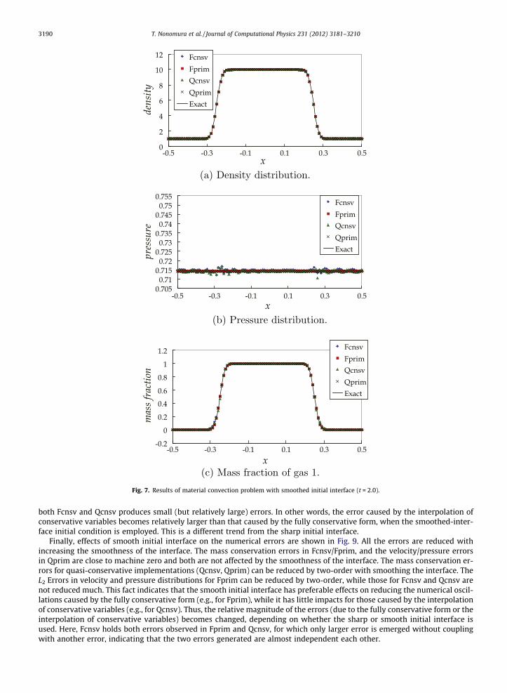
Fig. 7. Results of material convection problem with smoothed initial interface (t = 2.0).


both Fcnsv and Qcnsv produces small (but relatively large) errors. In other words, the error caused by the interpolation ofconservative variables becomes relatively larger than that caused by the fully conservative form, when the smoothed-inter-face initial condition is employed. This is a different trend from the sharp initial interface.

Finally, effects of smooth initial interface on the numerical errors are shown in Fig. 9. All the errors are reduced withincreasing the smoothness of the interface. The mass conservation errors in Fcnsv/Fprim, and the velocity/pressure errorsin Qprim are close to machine zero and both are not affected by the smoothness of the interface. The mass conservation er-rors for quasi-conservative implementations (Qcnsv, Qprim) can be reduced by two-order with smoothing the interface. TheL2 Errors in velocity and pressure distributions for Fprim can be reduced by two-order, while those for Fcnsv and Qcnsv arenot reduced much. This fact indicates that the smooth initial interface has preferable effects on reducing the numerical oscil-lations caused by the fully conservative form (e.g., for Fprim), while it has little impacts for those caused by the interpolationof conservative variables (e.g., for Qcnsv). Thus, the relative magnitude of the errors (due to the fully conservative form or theinterpolation of conservative variables) becomes changed, depending on whether the sharp or smooth initial interface isused. Here, Fcnsv holds both errors observed in Fprim and Qcnsv, for which only larger error is emerged without couplingwith another error, indicating that the two errors generated are almost independent each other.

Fig. 8. Time history of error in material convection problem with smoothed initial interface (t = 2.0).


The results above are summarized in Table 2. The insights obtained in this problem are as follows:

� A high-order finite difference scheme which achieves pressure and velocity equilibriums can be constructed using thequasi-conservative form and the primitive variable interpolation.� The errors in mass conservation, pressure and velocity distributions can be reduced with smoothing the interface of the

initial condition.

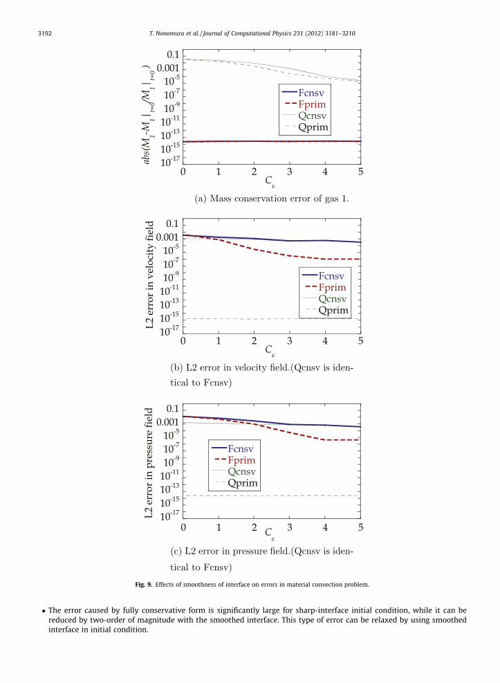
Fig. 9. Effects of smoothness of interface on errors in material convection problem.


� The error caused by fully conservative form is significantly large for sharp-interface initial condition, while it can bereduced by two-order of magnitude with the smoothed interface. This type of error can be relaxed by using smoothedinterface in initial condition.

Table 2Errors in material convection problem. Here, circle denotes that the error isnot generated, triangle denoted that the error is generated but suppressedwith smoothing interface and cross shows that the error is generated evenwith the smoothed interface.

Case Error due toconservative form

Error due to interpolation ofconservative variables

Fcnsv M �Fprim M s

Qcnsv s �Qprim s s


� The error caused by interpolation of conservative variables cannot be reduced much by using the smooth initial interface.Therefore, the interpolation of primitive variables is preferred with any initial interfaces.� The two types of the numerical oscillations, one caused by fully conservative form and the other caused by interpolation

of conservative variables, are almost independent each other.

This problem is used for the comparison of resolution and efficiency between WCNS and the existing schemes in Appen-dixes A and B.

Fig. 10. Density and pressure distributions of multi-component Sod problem (t = 0.2).


3.3. Shock-tube problems

The following two-component Sod problem [21,22,24] is solved.

U ¼UL x 6 0:5;UR x > 0:5;

�

Fig. 11. Initial condition of one-dimensional shock–bubble interaction problem.

Table 3Errors in shock-tube problem. Here, circle denotes that the error is not generated, triangle denotedthat the error is generated but suppressed with smoothing interface and cross shows that the error isgenerated even with the smoothed interface.

Case Error at the edge of expansionwave

Error at contactsurface

Error at shockwave

Fcnsv M � s

Fprim M s �Qcnsv s � s

Qprim s s �


UL ¼ ðqL;uL;pL;Y1;LÞt ¼ ð1;0;1; 0Þt;UR ¼ ðqR;uR;pR;Y1;RÞt ¼ ð0:125;0; 0:1;1Þt ;c0 ¼ 1:4; c1 ¼ 1:6;0 6 x 6 1: ð30Þ

Sharp-interface initial condition is adopted, where number of grid points is 201 and the CFL number is 0.6. The density and pres-sure profiles at t = 0.2 are shown in Fig. 10. First, the numerical oscillations produced in this problem are quite small compared tothose in the advection problem and the implementation does not strongly affect their magnitude and frequency. The enlargedview (Fig. 10(c)) shows that (1) the fully conservative form (Fcnsv and Fprim) generates a little larger oscillations at the edgeof the expansion fan as compared with the quasi-conservative form (Qcnsv and Fcnsv); (2) the interpolation of primitive variables(Fprim and Qprim) avoids the numerical spike at the contact surface; and (3) the interpolation of primitive variables generatessome oscillations at the shock wave. The interpolation of primitive variables is preferable for capturing contact surface withoutsignificant oscillations, while producing small oscillations at the shock wave. The result with the smoothed-interface initial con-dition shows that numerical oscillations at the edge of expansion wave can be reduced, while the other oscillations remain.

The results above are summarized in Table 3. The insights obtained in the shock-tube problems are as follows:

� There are no significant differences in the solution of two-component shock tube problems due to implementations.� Interpolation of primitive variables avoids the numerical oscillations at the contact surface, while generating numerical

oscillation at the shock waves.� Fully conservative form generates numerical oscillations at the edge to the expansion wave, while it can be reduced by

smoothing the interface.

3.4. Shock–bubble interaction problem

The following shock–bubble interaction problem is solved because the interaction of shock waves and contact surface canbe observed in this problem. The initial condition is as follows:

U ¼Ububble ð4þ xÞ2 < 0:5;Upreshock x < �3;Upostshock otherwise;

8<:

Ububble ¼ ðqb;ub;pb;Y1;bÞt ¼ ð0:1819;1:22;1=1:4;1Þt;Upreshock ¼ ðqpre;upre;ppre; Y1;preÞt ¼ ð1;1:22;1=1:4; 0Þt;Upostshock ¼ ðqpost;upost;ppost; Y1;postÞt ¼ ð1:3764;0:8864;1:5698=1:4;0Þt;c0 ¼ 1:4; c1 ¼ 1:648;� 5 6 x 6 5: ð31Þ

Fig. 12. Schematic of one-dimensional shock–bubble interaction problem. Here, the x–t diagram of the density distribution is shown.

Fig. 13. Density and pressure distribution of the one-dimensional shock–bubble interaction problem with sharp initial interface (t = 4.0) Here, thenumerical oscillations generated in pressure fields for Fcnsv, Fprim and Qcnsv are depicted.

Fig. 14. Time history of error in the mass conservation of the one-dimensional shock–bubble interaction problem with sharp initial interface.



Fig. 11 shows the initial condition above. In this problem, the coordinate system in which the shock wave stands stationallyis adopted while most of earlier studies employ the coordinate system in which the preshock gas is stationary [21,22]. Thecoordinate system in which the shock wave stands stationally is appropriate for dividing two numerical oscillations (due tothe conservative form and the interpolation procedures, respectively).

The x–t diagram of density obtained by Qprim with 5001 grid points is shown in Fig. 12. The bubble goes into the shockwaves, and expansion and compression waves are generated. After that, the weak compression waves are generated at theinterface of bubble as a result of the interaction between the interface and the shock wave.

This problem is solved with sharp-interface initial condition, 1001 grid points, and CFL number of 0.6. It should be notedthat the analyses with 201 grid points were also conducted, but it is not good for dividing two numerical oscillations becausethe oscillations due to different factor are located similar position due to lack of grid resolution. The computational resultswith 1001 grid points at t = 4.0 are shown in Fig. 13. Comparison between Fprim and Qprim (effect of the conservation form)shows the numerical oscillations caused by fully conservative form which are caused by sudden movement of the sharpinterface at the very early stage of the computation and are propagated with the speed of sound. This type of oscillationis not significantly generated in later stage. This is because the interface becomes smooth and the smoothed interface doesnot generate this kind of numerical oscillations. On the other hand, comparison between Qcnsv and Qprim (effect of theinterpolation) shows that the numerical oscillations caused by the interpolation of conservative variables are observed inside

Fig. 15. Density and pressure distribution of the one-dimensional shock–bubble interaction problem with smoothed initial interface (t = 4.0). Here, thenumerical oscillations generated in pressure fields for Fcnsv, Fprim and Qcnsv are depicted.


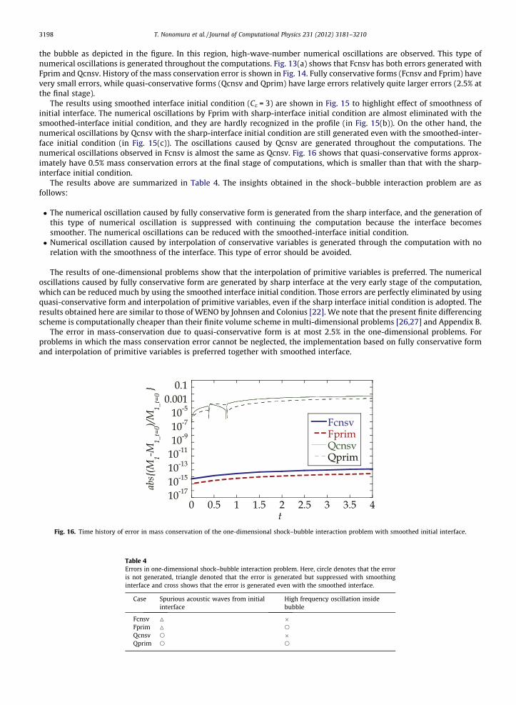
the bubble as depicted in the figure. In this region, high-wave-number numerical oscillations are observed. This type ofnumerical oscillations is generated throughout the computations. Fig. 13(a) shows that Fcnsv has both errors generated withFprim and Qcnsv. History of the mass conservation error is shown in Fig. 14. Fully conservative forms (Fcnsv and Fprim) havevery small errors, while quasi-conservative forms (Qcnsv and Qprim) have large errors relatively quite larger errors (2.5% atthe final stage).

The results using smoothed interface initial condition (Ce = 3) are shown in Fig. 15 to highlight effect of smoothness ofinitial interface. The numerical oscillations by Fprim with sharp-interface initial condition are almost eliminated with thesmoothed-interface initial condition, and they are hardly recognized in the profile (in Fig. 15(b)). On the other hand, thenumerical oscillations by Qcnsv with the sharp-interface initial condition are still generated even with the smoothed-inter-face initial condition (in Fig. 15(c)). The oscillations caused by Qcnsv are generated throughout the computations. Thenumerical oscillations observed in Fcnsv is almost the same as Qcnsv. Fig. 16 shows that quasi-conservative forms approx-imately have 0.5% mass conservation errors at the final stage of computations, which is smaller than that with the sharp-interface initial condition.

The results above are summarized in Table 4. The insights obtained in the shock–bubble interaction problem are asfollows:

� The numerical oscillation caused by fully conservative form is generated from the sharp interface, and the generation ofthis type of numerical oscillation is suppressed with continuing the computation because the interface becomessmoother. The numerical oscillations can be reduced with the smoothed-interface initial condition.� Numerical oscillation caused by interpolation of conservative variables is generated through the computation with no

relation with the smoothness of the interface. This type of error should be avoided.

The results of one-dimensional problems show that the interpolation of primitive variables is preferred. The numericaloscillations caused by fully conservative form are generated by sharp interface at the very early stage of the computation,which can be reduced much by using the smoothed interface initial condition. Those errors are perfectly eliminated by usingquasi-conservative form and interpolation of primitive variables, even if the sharp interface initial condition is adopted. Theresults obtained here are similar to those of WENO by Johnsen and Colonius [22]. We note that the present finite differencingscheme is computationally cheaper than their finite volume scheme in multi-dimensional problems [26,27] and Appendix B.

The error in mass-conservation due to quasi-conservative form is at most 2.5% in the one-dimensional problems. Forproblems in which the mass conservation error cannot be neglected, the implementation based on fully conservative formand interpolation of primitive variables is preferred together with smoothed interface.

Table 4Errors in one-dimensional shock–bubble interaction problem. Here, circle denotes that the erroris not generated, triangle denoted that the error is generated but suppressed with smoothinginterface and cross shows that the error is generated even with the smoothed interface.

Case Spurious acoustic waves from initialinterface

High frequency oscillation insidebubble

Fcnsv M �Fprim M s

Qcnsv s �Qprim s s

Fig. 16. Time history of error in mass conservation of the one-dimensional shock–bubble interaction problem with smoothed initial interface.


4. Test problems for two-dimensional flow

Two problems, typically used in earlier studies about compressible multicomponent flows [22,24,14,16], were carried outin order to examine the impact of each implementation on multidimensional flow fields.

Fig. 17. Schematic of initial condition of the two-dimensional shock–bubble interaction problem.

Fig. 18. Example of computational results of the two-dimensional shock–bubble interaction problem. Density distribution is shown. The result is computedby Qprim. Top to bottom; t = 0.410, 0.622, 0.821, 1.086, 2.002, 3.242. 4.880 and 6.929. The figures show the regions at 0.9 < x < 11.7.


4.1. Shock–bubble interaction problem

The following two-dimensional shock–bubble interaction problem is solved.

Fig. 19.at t = 1

U ¼Ubublle ðx� 1Þ2 þ ðy� 1Þ2 < 0:5;Upreshock x < 2;Upostshock otherwise;

8><>:

Divergence of velocity fields of the two-dimensional shock–bubble interaction problem. Top to bottom: Fcnsv, Fprim, Qcnsv and Qprim. The results.086 are shown. Contour range normalized by initial bubble diameter is set from �1 to 1. The figures show the regions at 0.9 < x < 11.7.

Fig. 20.are sho


Ububble ¼ ðqb;ub;vb; pb; Y1;bÞt ¼ ð0:1819;1:22; 0;1=1:4;1Þt;Upreshock ¼ ðqpre;upre;vpre;ppre; Y1;preÞt ¼ ð1;1:22;0;1=1:4;0Þt ;Upostshock ¼ ðqpost;upost;vpost;ppost;Y1;postÞt ¼ ð1:3764;0:8864;0;1:5698=1:4;0Þt ;c0 ¼ 1:4; c1 ¼ 1:648;0 6 x 6 16; �0:89 6 y 6 0:89: ð32Þ

Density fields of the two-dimensional shock–bubble interaction problem. Top to bottom: Fcnsv, Fprim, Qcnsv and Qprim. The results at t = 6.929wn. Contour range is set from 0.2 to 1.4. The figures show the regions at 0.9 < x < 11.7.


The schematic is shown in Fig. 17.In this problem, the coordinate system in which the shock wave stands stationally is adopted for dividing the numerical

oscillations similar to one-dimensional version, while the earlier studies employ the coordinate system in which the pre-shock gas is stationary [22,24]. Grid points are set to 1601 � 179. The slip wall condition is adopted at the top and bottomwall conditions and the initial values are fixed at the left and right boundaries. Sharp-interface and smoothed-interface ini-tial conditions are adopted and the CFL number is 0.6.

The results of Qprim with the sharp-interface initial condition are shown in Fig. 18. Bubble goes into the shock waves, andthen its interface is deformed due to the baroclinic torque (due to the misalignment between the density and pressure gra-dients). The deformation of the bubble is similar to those of experimental observations and the earlier computations.

Then, the numerical oscillations generated in this problem are discussed. The distributions of velocity divergence att = 1.086 are presented in Fig. 19. The velocity divergence is used in order to highlights numerical oscillations produceddue to each implementation.

Comparing Fprim with Qprim, the numerical oscillations caused by fully conservative form are discussed. The differencebetween Fprim and Qprim appears only in the generation of the sound wave observed outside the bubble (as depicted inFig. 19(a)). This wave is generated due to the violation of pressure equilibrium at the interface. Except for this, any othersignificant numerical oscillations are not observed. As demonstrated in the one-dimensional case, this type of numericaloscillations can be significantly suppressed by adopting the smoothed-interface initial condition as shown in Fig. 19(b).

Comparing Qcnsv with Qprim, the numerical oscillation caused by interpolation of conservative variables are discussed. Thedifference between Qcnsv and Qprim appears numerical oscillations inside the bubble. Unlike the spurious sound waves due tothe conservation form, they are generated not only at the early stage of computation but also throughout the whole computa-tion. These errors are still produced even with smoothed-interface initial condition, though they are slightly reduced. Therefore,the interpolation of primitive variables is preferable for accurate interface simulations in compressible flows.

Numerical oscillations of Fcnsv are superimposition of numerical oscillations of Qcnsv and Fprim. This illustrates that thenonlinear effects of these two numerical oscillations are not observed and they are almost independent each other.

Next, the effects on the bubble shape are discussed. The density distributions at t = 6.929 are shown in Fig. 20. It showsthat Fcnsv and Qcnsv produce spuriously oscillated interfaces. This trend does not change even with the smoothed-interfaceinitial condition. On the other hand, interface shape of Fprim is almost the same as that of Qprim. The numerical oscillation ofFprim, i.e. one caused by the fully conservative form, is limited to the spurious acoustic wave generated at the very earlystage of computation, and Fprim keeps good accuracy through the computation except for the spurious acoustic waves.

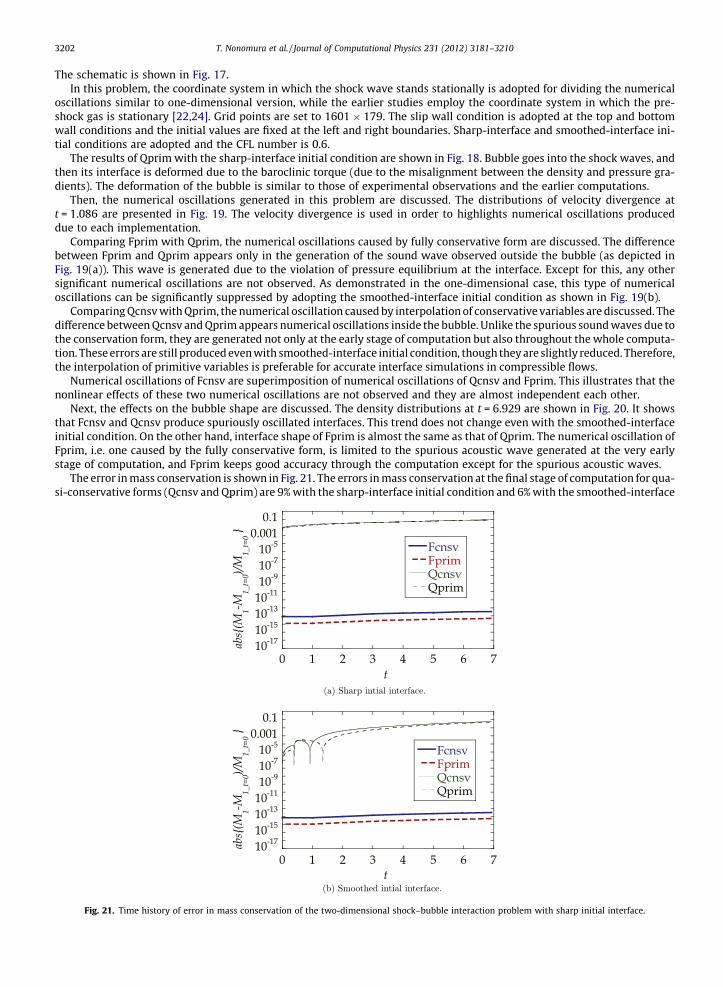
The error in mass conservation is shown in Fig. 21. The errors in mass conservation at the final stage of computation for qua-si-conservative forms (Qcnsv and Qprim) are 9% with the sharp-interface initial condition and 6% with the smoothed-interface

Fig. 21. Time history of error in mass conservation of the two-dimensional shock–bubble interaction problem with sharp initial interface.


initial conditions. Obviously, the errors in mass conservation for Fcnsv and Fprim are very close to the machine zero. If the errorin mass conservation due to quasi-conservative form is not in acceptable range, Fprim with smoothed-interface initialcondition is preferred. Meanwhile, if the error in mass conservation for quasi-conservative form is in acceptable range, Qprimis preferred because Qprim does not produce any kind of numerical oscillations even with the sharp interface.

The results above are summarized in Table 5.

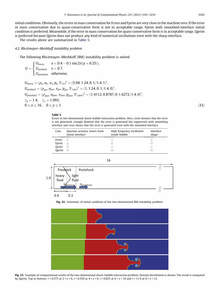
4.2. Rhcitmayer–Meshkoff instability problem

The following Rhcitmayer–Meshkoff (RM) instability problem is solved

Fig. 23.by Qpri

U ¼Uheavy x < 0:4� 0:1 sinð2pðyþ 0:25ÞÞ;Upreshock x < 0:7;Upostshock otherwise;

8><>:

Uheavy ¼ ðqh;uh; vh;ph;Y1;hÞt ¼ ð5:04;1:24;0;1=1:4;1Þt;Upreshock ¼ ðqpre;upre;vpre;ppre; Y1;preÞt ¼ ð1;1:24;0;1=1:4;0Þt ;Upostshock ¼ ðqpost;upost;vpost;ppost;Y1;postÞt ¼ ð1:4112;0:8787;0;1:6272=1:4;0Þt ;c0 ¼ 1:4; c1 ¼ 1:093;0 6 x 6 16; 0 6 y 6 1: ð33Þ

Example of computational results of the two-dimensional shock–bubble interaction problem. Density distribution is shown. The result is computedm. Top to bottom; t = 0.275 at 2 < x < 6, t = 0.550 at 4 < x < 8, t = 0.825 at 6 < x < 10 and t = 11.0 at 8 < x < 12.

Table 5Errors in two-dimensional shock–bubble interaction problem. Here, circle denotes that the erroris not generated, triangle denoted that the error is generated but suppressed with smoothinginterface and cross shows that the error is generated even with the smoothed interface.

Case Spurious acoustic waves frominitial interface

High frequency oscillationinside bubble

Interfaceshape

Fcnsv M � �Fprim M s s

Qcnsv s � �Qprim s s s

Fig. 22. Schematic of initial condition of the two-dimensional RM instability problem.


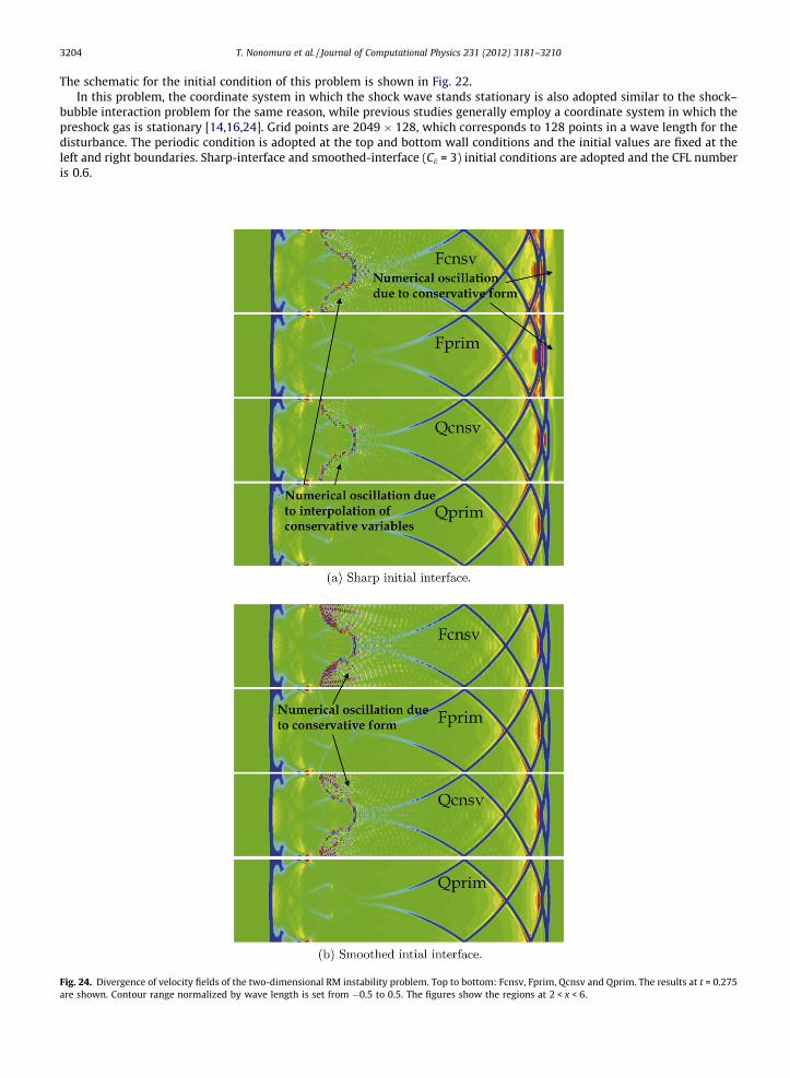
The schematic for the initial condition of this problem is shown in Fig. 22.In this problem, the coordinate system in which the shock wave stands stationary is also adopted similar to the shock–

bubble interaction problem for the same reason, while previous studies generally employ a coordinate system in which thepreshock gas is stationary [14,16,24]. Grid points are 2049 � 128, which corresponds to 128 points in a wave length for thedisturbance. The periodic condition is adopted at the top and bottom wall conditions and the initial values are fixed at theleft and right boundaries. Sharp-interface and smoothed-interface (Ce = 3) initial conditions are adopted and the CFL numberis 0.6.

Fig. 24. Divergence of velocity fields of the two-dimensional RM instability problem. Top to bottom: Fcnsv, Fprim, Qcnsv and Qprim. The results at t = 0.275are shown. Contour range normalized by wave length is set from �0.5 to 0.5. The figures show the regions at 2 < x < 6.


The results of Qprim with sharp-interface initial condition are shown in Fig. 23. Generation of spike due to the RM insta-bility is clearly observed. This shape deformation corresponds to those of previous computational studies.

Also in this problem, the characteristics of generated numerical oscillations are discussed. The distributions of velocitydivergence at t = 0.275 are presented in Fig. 24. The numerical oscillation can be clearly observed using velocity divergence,similar to the previous example. Fig. 24 illustrates that the characteristics of both numerical oscillations due to the conser-vative variable interpolation and fully conservative form are almost the same as those observed in the previous problem.

The density distributions at t = 0.825 are shown in Fig. 25. Fig. 25 shows that Fcnsv and Qcnsv induce additional spuriousinterface instabilities as well as the shock–bubble interaction. This trend does not change even with the smoothed-interface

Fig. 25. Density fields of the two-dimensional RM instability problem. Top to bottom: Fcnsv, Fprim, Qcnsv and Qprim. The results at t = 0.825 are shown.Contour range is set from 1.5 to 8.5. The figures show the regions at 2 < x < 6.


initial conditions. On the other hand, interface shape of Fprim is almost the same as that of Qprim. The numerical oscillationof Fprim, i.e. one caused by the fully conservative form, is only the spurious acoustic wave generated at the very early stageof computation, and Fprim keeps good accuracy through the computation except for this spurious acoustic waves.

The results above are almost the same as the summary of the previous test problem in Table 5.The insights obtained through the two-dimensional problems are as follows:

� The numerical oscillations caused by fully conservative form is spurious acoustic waves generated at the very early stageof computation and they can be suppressed by adopting the smoothed-interface initial condition.� The numerical oscillations caused by the interpolation of primitive variables are generated throughout the computation

and not preferred because they affect the shape of interface. Therefore, the interpolation of primitive variables should beused.

5. Conclusion

The four implementations for WCNS are applied to simulations of compressible multicomponent flows; the choices offully conservative or quasi-conservative forms by the choice of interpolations of primitive variables or conservative vari-ables, are examined and discussed. The numerical oscillations are generated by fully conservative form or by interpolationof conservative forms, which are similar to those reported in the previous studies of low-order scheme [20] and finite volumeWENO [22].

The numerical oscillations caused by fully conservative form are clearly observed for the solutions with the sharp-inter-face initial condition while it is sufficiently suppressed by adopting smoothed interface condition. On the other hand, thenumerical oscillations caused by interpolations of conservative variables are generated throughout the computation withno relation to the smoothness of interface, and they have harmful effects on the accuracy of computation; e.g. the shapeof the interface is strongly affected by this oscillation.

Similar to Johnsen and Colonius’s finite volume WENO, these errors can be eliminated by employing the quasi-conserva-tive form and the interpolation of primitive variables even if the sharp interface initial condition is adopted. Here, WCNS is afinite difference scheme, and its computational cost is 3–20 times cheaper for multi-dimensional problems than finite vol-ume WENO, as discussed in Refs. [26,27] and Appendix B. However, this implementation has at most 10% errors in mass con-servation due to its quasi-conservative form in the present problems. When the mass conservation is critical (i.e., forcombustion), the fully conservative form with interpolation of primitive variable should be considered with smoothed inter-face initial condition.

Acknowledgments

The authors are grateful to Mr. Ryoji Kojima for help in code implementation. The authors also acknowledge Dr. KeiichiIshiko for useful comments. The computations were partially conducted in JAXA’s supercomputing system. This work waspartially supported by KAKENHI (23760773).

Appendix A. Comparison of resolution of WCNS with those of existing schemes

We conduct the comparison of resolution between WCNS, the finite volume WENO by Johnsen and Colonius [22], andconventional upwind scheme by Abgrall [20] using one-dimensional material convection problem with a sharp interface.The quasi-conservative formulation with primitive variable interpolation is used for all the schemes. Five schemes are exam-ined: third order monotonically-upwind-scheme-for-conservation-law (MUSCL) scheme, fifth-order finite volume WENO,seventh-order finite volume WENO, fifth order WCNS and seventh-order WCNS. The initial condition and other computa-tional settings are same as those used in Section 3.2. The density and pressure profiles and the thicknesses of the interfacesare shown in Figs. 26 and 27, respectively. Here, the thickness of the interface nthickness is defined as follows:

nthickness ¼jdqjumpj

maxjðjqj � qjþ1jÞ; ð34Þ

where dqjump denotes the density jump across the interface.Fig. 26 shows that the all the scheme presented here can preserve the pressure equilibrium. With regard to the interface

sharpness in Figs. 26 and 27, the seventh-order WCNS and finite volume WENO have the sharpest interface, followed by thefifth-order WCNS and finite volume WENO. The interface of the MUSCL scheme is the most diffused as shown in Figs. 26 and27. This shows that the effectiveness of higher-order formulation compared with a conventional upwind scheme, and WCNSand finite volume WENO has almost the same resolution. Focusing on the slight difference in the same-order WCNS and fi-nite volume WENO, WCNS has a slightly sharper interface than WENO. This may be because WCNS has higher resolution inthe Fourier analysis [5,10,6].

Fig. 26. Comparison of WCNS with the existing schemes using the one-dimensional material convection problem with a sharp interface (t = 2.0). All theschemes are inplemented as ‘‘Qprim.’’ Here, FV denotes ‘‘finite volume.’’


Appendix B. Comparison of efficiency of WCNS and finite volume WENO

In the previous appendix, the efficiency of WCNS and finite volume WENO is discussed. As discussed in the previousappendix, the resolutions of WCNS and finite volume WENO are almost the same and WCNS has slightly higher resolution.Therefore, we can estimate the computational efficiency by measure/estimate the computational time. The computationalcost for one-dimensional problem is measured and that for multi-dimensional problem is estimated. The computational costshown here may be considered as a reference because the computational cost depends on the computational settings. For theone-dimensional problem, the computational time normalized by total of computational time of seventh-order WCNS isshown in Table 6, where computational cost of WCNS and finite volume WENO are divided into three components: nonlinearinterpolation, flux evaluation, and difference/integration. Here, these three components are used once for each for the eval-uation of spatial differencing/integration in one-dimensional problem. Table 6 shows that the computational costs of WCNSand finite volume WENO are also almost the same. It shows that nonlinear interpolation and flux evaluation are dominant in

Fig. 27. Time histories of the interface thickness of various schemes.All the schemes are inplemented as ‘‘Qprim.’’ Here, FV denotes ‘‘finite volume.’’

Table 6Componentwise computational time of one-dimensional problems for various schemes per a grid point. Here, the time is normalized by total time of seventh-order WCNS. The term FV in the table denotes ‘‘finite volume.’’

Scheme Nonlinear interpolation Flux evaluation Differencing/integration Total

Fifth-order WCNS 0.532 0.174 0.015 0.721Fifth-order FV WENO 0.528 0.174 0.003 0.705Seventh-order WCNS 0.808 0.174 0.018 1.000Seventh-order FV WENO 0.856 0.174 0.003 1.033


the computational costs of both WCNS and finite volume WENO, and hereafter we only discuss using the costs of nonlinearinterpolation and flux evaluation. Computations cost of difference/integration is ignored. Interestingly, the nonlinear inter-polation of seventh order WCNS has lower computational cost than seventh order finite volume WENO. This is because thenonlinear weight is efficiently computed by using the high-order derivatives constructed once, as discussed in Section 2.2.1,while this effect is not so clear for the fifth-order schemes and computational times for them are almost the same.

Then, we count the required number of operations of each component for the estimation of the computational cost of amulti-dimensional problem. Since dimension by dimension procedure is applicable for a finite difference scheme, twice andthree times of operation of each procedure are required in WCNS for two- and three-dimensional problems, respectively. Onthe other hand, multi-dimensional reconstruction is required in finite volume WENO. Hereafter, the uniform Cartesian grid isconsidered for instance. The fifth-order finite volume WENO requires flux values at three Gaussian points in the cell surfacein two-dimensional problems. For this, three nonlinear interpolations and three flux evaluations are required. The fifth-orderfinite volume WENO requires flux value at nine Gaussian points in the cell surface in three-dimensional problems. For this,nine nonlinear interpolations and nine flux evaluations are required. The seventh-order finite volume WENO requires fluxvalues at four Gaussian points in the cell surface in two-dimensional problems. For this, five nonlinear interpolations andfour flux evaluations are required. The seventh-order finite volume WENO requires flux values at sixteen Gaussian points

Table 7Number of required operations for multi-dimensional problems per a grid point. Here, FV in the tabledenotes ‘‘finite volume,’’ and the one operation of nonlinear interpolation includes the computationof both QL and QR. For the FV scheme, operation is counted as m � n, where m denotes the operationnumber for one surface and n does the number of surface surrounding the cell.

Scheme Nonlinear interpolation Flux evaluation

For a two-dimensional problemFifth-order WCNS 2 2Fifth-order FV WENO 6 (=3 � 2) 6 (=3 � 2)Seventh-order WCNS 2 2Seventh-order FV WENO 10 (=5 � 2) 8 (=4 � 2)

For a three-dimensional problemFifth-order WCNS 3 3Fifth-order FV WENO 27 (=9 � 3) 27 (=9 � 3)Seventh-order WCNS 3 3Seventh-order FV WENO 63 (=21 � 3) 48 (=16 � 3)

Table 8Estimated componentwise computational time of multi-dimensional problems for various schemes per a grid point.Here, the time is normalized by total time of seventh-order WCNS for one-dimensional problem. The estimation isconducted by simply multiplying the one-dimensional cost by the number of required operation for multi-dimensionalproblems, ignoring the difference/integration time. Here, FV in the table denotes ‘‘finite volume.’’

Scheme Nonlinear interpolation Flux evaluation Total

For a two-dimensional problemFifth-order WCNS 1.064 0.348 1.412Fifth-order FV WENO 3.168 1.004 4.212Seventh-order WCNS 1.616 0.348 1.964Seventh-order FV WENO 8.560 1.392 9.952

For a three-dimensional problemFifth-order WCNS 1.596 0.522 2.118Fifth-order FV WENO 14.256 4.698 18.954Seventh-order WCNS 2.424 0.522 2.946Seventh-order FV WENO 53.928 8.352 62.28


in the cell surface in three-dimensional problems. For this, twenty-one nonlinear interpolations and sixteen flux evaluationsare required. These are summarized in Table 7.

Finally, the computational cost for a multi-dimensional problem is estimated based on the number of operation and nor-malized computational cost obtained by one-dimensional code. The estimated computational cost is shown in Table 8. Theresult shows that WCNS is approximately 3–20 times computationally cheaper for multi-dimensional problems, which issimilar to the estimation in Refs. [26,27]. This presents that the efficiency of WCNS is 3–20 times higher than finite volumeWENO for the same dimensional problem and for maintaining the same order of accuracy, while considering that the reso-lution of WCNS and finite volume WENO are almost the same.

References

[1] K. Fujii, T. Nonomura, S. Tsutsumi, Toward accurate simulation and analysis of strong acoustic wave phenomena: a review from the experience of ourstudy on rocket problems, International Journal for Numerical Methods in Fluids 64 (2010) 1412–1432.

[2] T. Nonomura, K. Fujii, Recent efforts for rocket plume acoustics, in: Computational Fluid Dynamics Review 2010, World Scientific Publishing Company,2010, pp. 421–446.

[3] X. Liu, S. Osher, T. Chan, Weighted essentially non-oscillatory schemes, Journal of Computational Physics 115 (1994) 200–212.[4] G.-S. Jiang, C.-W. Shu, Efficient implementation of weighted ENO schemes, Journal of Computational Physics 126 (1) (1996) 202–228.[5] X.G. Deng, H. Zhang, Developing high-order weighted compact nonlinear schemes, Journal of Computational Physics 165 (1) (2000) 22–44.[6] S. Zhang, S. Jiang, C.-W. Shu, Development of nonlinear weighted compact schemes with increasingly higher order accuracy, Journal of Computational

Physics 227 (2008) 7294–7321.[7] P.L. Roe, Approximate Riemann solvers, parameter vectors, and difference scheme, Journal of Computational Physics 43 (2) (1981) 357–372.[8] T. Nonomura, N. Iizuka, K. Fujii, Freestream and vortex preservation properties of high-order WENO and WCNS on curvilinear grids, Computers and

Fluids 39 (2) (2010) 197–214.[9] X. Deng, M. Mao, G. Tu, H. Liu, H. Zhang, Geometric conservation law and applications to high-order finite difference schemes with stationary grids,

Journal of Computational Physics 230 (4) (2011) 1100–1115.[10] T. Nonomura, N. Iizuka, K. Fujii, Increasing order of accuracy of weighted compact nonlinear scheme, in: AIAA 2007-893, 2007.[11] C. Hirt, B. Nichols, Volume of fluid (VOF) method for the dynamics of free boundaries⁄ 1, Tech. Rep. 1, 1981.[12] S. Osher, J. Serthian, Fronts propagating with curvature-dependent speed: algorithms based on Hamilton–Jacobi formulations, Journal of

Computational Physics 79 (1988) 12–49.[13] S. Karni, Multicomponent flow calculation a consistent primitive algorithm, Journal of Computational Physics 112 (1994) 31–43.[14] R.R. Nourgaliev, T.N. Dinh, T.G. Theofanous, Adaptive characteristics-based matching for compressible multifluid dynamics, Journal of Computational

Physics 213 (2006) 500–529.[15] G. Tryggvason, B. Bunner, A. Esmaeeli, D. Juric, N. Al-Rawahi, W. Tauber, J. Han, S. Nas, Y.-J. Jan, A front tracking methods for the computations of

multiphase flow, Journal of Computational Physics 169 (2001) 708–759.[16] H. Terashima, G. Tryggvason, A front-tracking/ghost-fluid method for fluid interfaces in compressible flows, Journal of Computational Physics 228

(2009) 4012–4037.[17] H. Terashima, G. Tryggvason, A front-tracking method with projected interface conditions for compressible multi-fluid flows, Computers and Fluids 39

(2010) 1804–1814.[18] R.P. Fedkiw, T. Aslam, B. Merriman, S. Osher, A non-oscillatory Eulerian approach to interfaces in multimaterial flows (the ghost fluid method), Journal

of Computational Physics 152 (1999) 457–494.[19] X.Y. Hu, B.C. Khoo, An interface interaction method for compressible multifluids, Journal of Computational Physics 198 (2004) 35–64.[20] R.-B.M. Abgrall, How to prevent pressure oscillations in multicomponent flow calculations: a quasi conservative approach, Journal of Computational

Physics 125 (1996) 150–160.[21] R.-B. Abgrall, S. Karni, Computations of compressible multifluids, Journal of Computational Physics 169 (2001) 594–623.[22] E. Johnsen, T. Colonius, Implementation of WENO schemes in compressible multicomponent flow problems, Journal of Computational Physics 219

(2006) 715–732.[23] C.H. Chang, M.S. Liou, A robust and accurate approach to computing compressible multiphase flow: stratified flow model and AUSM+up scheme,

Journal of Computational Physics 225 (2007) 840–873.[24] S. Kawai, H. Terashima, A high-resolution scheme for compressible multicomponent flows with shock waves, International Journal for Numerical

Methods in Fluids 66 (2011) 1207–1225.[25] E. Johnsen, Spurious oscillations and conservation errors in interface-capturing schemes, Annual Research Briefs 2008, Stanford University, Center for

Turbulence Research, 2008.[26] C.-W. Shu, High-order finite difference and finite volume WENO schemes and discontinuous Galerkin methods for CFD, International Journal of

Computational Fluid Dynamics 17 (2) (2003) 107–118.


[27] V. Titarev, E. Toro, Finite-volume WENO schemes for three-dimensional conservation laws, Journal of Computational Physics 201 (1) (2004) 238–260.[28] E. Johnsen, J. Larsson, Numerical errors generated by WENO-based interface-capturing schemes in multifluid computations, in: AIAA Paper 2011-3684,

Journal of Computational Physics, submitted for publication.[29] R. Shukla, C. Pantano, J. Freund, An interface capturing method for the simulation of multi-phase compressible flows, Journal of Computational Physics

229 (2010) 7411–7439.[30] E. Toro, M. Spruce, W. Speares, Restoration of the contact surface in the HLL-Riemann solver, Shock Waves 4 (1994) 25–34.[31] T. Nonomura, K. Fujii, Effects of difference scheme type in high-order weighted compact nonlinear schemes, Journal of Computational Physics 228

(2009) 3533–3539.[32] S. Gottlieb, C.-W. Shu, Total variation diminishing Runge–Kutta schemes, Mathematics of Computation 67 (221) (1998) 73–85.[33] A.K. Henrick, T.D. Aslam, J.M. Powers, Mapped weighted essentially non-oscillatory schemes: achieving optimal order near critical points, Journal of

Computational Physics 207 (2005) 542–567.