Supercharging Crowd Dynamics Estimation inDisasters via Spatio-Temporal Deep Neural Network

Fang-Zhou Jiang∗, Lei Zhong†, Kanchana Thilakarathna∗, Aruna Seneviratne∗,Kiyoshi Takano‡, Shigeki Yamada† and Yusheng Ji†

∗Data61, CSIRO & University of New South Wales, Australia, {firstname.lastname}@data61.csiro.au†National Institute of Informatics, Japan, {zhong, shigeki, kei}@nii.ac.jp

‡University of Tokyo, Japan, eri.u-tokyo.ac.jp

Abstract—Accurate estimation of crowd dynamics is difficult,especially when it comes to fine-grained spatial and temporalpredictions. A deep understanding of these fine-grained dynamicsis crucial during a major disaster, as it guides efficient disastermanagements. However, it is particularly challenging as thesefine-grained dynamics are mainly caused by high-dimensionalindividual movement and evacuation. Furthermore, abnormaluser behavior during disasters makes the problem of accurateprediction even more acute. Traditional models have difficultiesin dealing with these high dimensional patterns caused by dis-ruptive events. For example, the 2016 Kumamoto earthquakesdisrupted normal crowd dynamics patterns significantly in theaffected regions. We first perform a thorough analysis of a crowdpopulation distribution dataset during Kumamoto earthquakescollected by a major mobile network operator in Japan, whichshows strong fine-grained temporal autocorrelation and spatialcorrelation among geographically neighboring grids. It is alsodemonstrated that temporal autocorrelation during disasters ismore than simple diurnal patterns. Moreover, there are manyfactors that could potentially influence spatial correlations andaffect the dynamics patterns. Then, we illustrate how a spatial-temporal Long-Short-Term-Memory (LSTM) deep neural networkcould be applied to boost the prediction power. It is shown that theerror in terms of Mean Square Error (MSE) is reduced by as muchas 55.1-69.4% compared to regressive models such as AR, ARIMAand SVR. Furthermore, LSTM outperforms the aforementionedmodels significantly even when little training data is available rightafter the mainshock. Finally, we also show a Region-aware LSTMdoes not necessarily outperform a regular LSTM.

Index Terms—Data Mining; Data-Driven Modeling; DisasterManagement; Spatio-Temporal Dynamics; Deep Neural Network.

I. INTRODUCTION

Since the 2011 Great East Japan Earthquake, achievingbetter understanding of urban crowd dynamics during disas-ters has received significant attentions from both governmentsand research communities. Crowd evacuation behaviors heav-ily influence disaster management and relief, where carefulprior-disaster planning and effective post-disaster evacuationguidance are key to reducing casualties and chaos. Thesebehaviors are reflected in the high dynamics of crowd popu-lation distribution observed, while our current understanding isextremely limited. For example, it is shown that many reportedevacuation spots in 2016 Kumamoto earthquake, i.e. parkingareas and shopping malls, were not officially planned andrecognized by the administrative organizations as evacuationshelters, which hampers the ability in providing food andsupplies efficiently [1].

Similar to other phenomenas caused by human behaviorssuch as video consumption patterns [2], crowd dynamics ex-hibits spatial and temporal patterns (i.e. diurnal/weekly pat-tern) [3], [4], [5], [6]. Thus, prediction of future crowd dy-namics could be achieved with relatively high accuracy innormal times. However, it becomes much more difficult whenabnormal events take place, especially during major disasters.The abnormality along with high-dimensional individual move-ment caused by large-scale evacuation makes the task highlychallenging.

A lot has been done to improve our current understandingof crowd dynamics during major disasters. For example, Songet al. [7] developed a probabilistic model to simulate andpredict human evacuations over complex geographic areas inTokyo. However, it focuses on modeling and estimation ofindividual mobility patterns and does not accurately reflectthe crowd distribution dynamics both spatially and temporally.In addition, similar to most of the existing works (i,e [1],[8]), population densities are calculated via GPS data samplescollected from users’ mobile phones, which do not accuratelyreflect the behavior of majority crowd. Sekimoto [9] proposed areal-time population movement estimation system during large-scale disasters from mobile phone data using data integrationtechniques. Again, the accuracy of system suffers as both thesample size is small and the adopted framework is simplistic.

In this paper, we first perform a thorough analysis ofa population distribution dataset collected during Kumamotoearthquakes, and show that there exists a strong spatio-temporalcorrelation of crowd population dynamics among co-locatedgrids. After that, we study and analyze factors that influencespatial grid correlations (i.e. physical distance and land us-age), which could potentially aid our understanding of crowdpopulation dynamics. Deep learning has been successfullyapplied to many fields such as image/speech/textual recognition,medical diagnostics etc [10], [11]. Therefore, to overcomethe challenges associated with abnormal human behaviors, weadopt deep neural network in an attempt to discover thosehigh dimensional patterns both spatially and temporally. Wepropose to treat crowd population density in each grid as pixelsin an image and use deep learning techniques to understandthe complex high dimensional patterns. Specifically, we applyLong-Short-Term-Memory model (LSTM) [12] to accuratelypredict crowd population distributions. The performance of

LSTM is evaluated and compared with several baseline regres-sive models, namely AR, ARIMA and SVR. To the best ofour knowledge, our paper is the first that applies deep neuralnetworks to improve urban crowd dynamic estimation, anddemonstrated with a large-scale real-world dataset collected inperiods that are highly dynamic and disruptive. Specifically, thispaper makes the following contributions;• We analyze an unique large-scale real-world crowd dy-

namics dataset during a natural disaster collected by oneof the largest mobile operators in Japan, and illustrate thehigh dimensional patterns of crowd population dynamicsboth spatially and temporally.

• We propose to treat crowd dynamics map as a series ofimages, and leverage LSTM based deep neural networkmodel for predicting the crowd dynamics in both shortand long term.

• We demonstrate and compare the performance of LSTMwith multiple popular regressive models, and show animprovement of estimation error by up to 69.4%.

• Lastly, we illustrate that LSTM outperforms in highlydynamics scenarios (i.e. disasters) even with very littletraining data, while attempts of adding intelligence to deepneural network do not necessarily work better comparedto a regular deep neural network.

The rest of the paper is organized as follows; We intro-duce the dataset in Section II and explore spatio-temporalcorrelations and patterns of crowd dynamics in Section III.Section IV describes spatial-temporal regressive models and aspatial-temporal LSTM based deep neural network. We evaluatethe performance of these models in Section V. Section VIdiscusses the work and provides the direction of future work.Finally, Section VII concludes the paper.

II. DATASET DESCRIPTION

We use a population distribution dataset derived from usermobility data collected by NTT DoCoMo1, a major mobilenetwork operator in Japan. The crowd population distributiondata is collected continuously from the operational mobilenetwork. There are three main steps of the collecting process.i) The operator aggregates the number of mobile users in eachof the base station areas (or cells). ii) The population withineach cell is estimated according to the information such asmarket share etc. Finally, the population is re-aggregate fromthe per-cell populations obtained from the previous processinto each geographical grid. iii) To preserve user’s privacy,if the population in a grid is too small, the grid will not becollected in the final dataset. Due to the high penetration ofmobile devices in Japan, it is considered that the estimatedpopulation distribution is much more accurate than any othertraditional methods of population survey [13]. The downtownarea of Kumamoto city (Chou and Higashi wards), where thedata was collected, is split into approximately 350 geographicalgrids in 500× 500m and no grid is dropped due to the privacyissue. The data covers hourly snapshot of 6 days before and

1www.nttdocomo.co.jp/english/

0 24 48 72 96 120 144Hours

260000

280000

300000

320000

340000

360000

380000

Popu

lati

on

foreshock mainshock

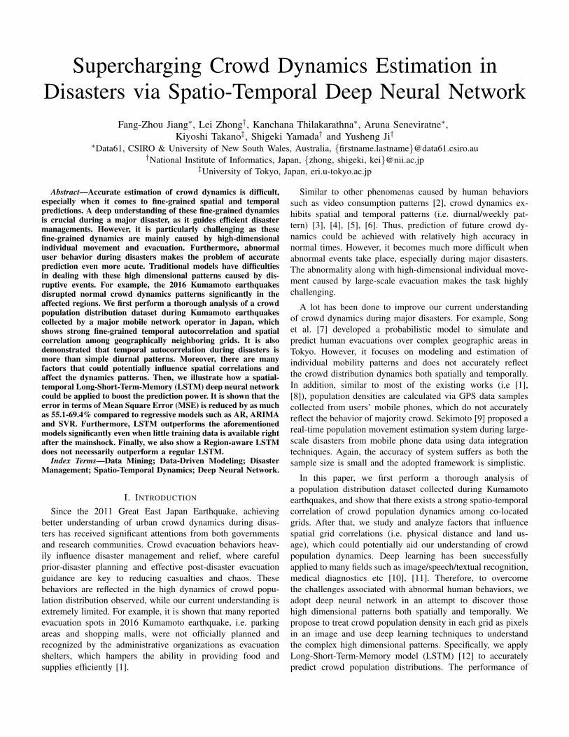
Fig. 1. Aggregated Population

after the Kumamoto earthquake from 14th of April to 19th of2016.

Land usage information of each grid is tagged using datafrom the website of national land numerical information, whichis provided by the Ministry of Land, Infrastructure, Transportand Tourism of Japan2. The data is mapped in a 100 × 100mmesh grid, which has a finer granularity than the populationdata. Land usage is categorized into 17 types such as field, for-est, river, and low/high residential buildings etc. We annotatedeach geographical grid with multiple land usages tags since theland usage data is in a finer-granularity.

III. DATA ANALYSIS

A. Aggregated Dynamics

The Kumamoto earthquakes consist of a 6.2 magnitudeforeshock at 21:26 on 14th of April and a 7.0 magnitudemainshock at 01:25 on 16th of April 2016. Fig. 1 demonstratesthe hourly change in overall population from 14th to 19th ofApril in the downtown region of Kumamoto city with the timeof foreshock and mainshock annotated. As expected, the diurnalpopulation dynamics pattern is disrupted after the foreshock,and both the peak and average population in the followingday drop slightly by approximately 5-10%. In contrast, afterthe mainshock there is a significant population drop of at least20%. Moreover, this trend of population outflow continued fortwo days following the mainshock, which could be caused byboth disaster evacuations and weekend effect. As the workdaysbegan from the 96th hour, the diurnal pattern begins recoveringto a certain extent.

B. Disruption of “Normal” Pattern

Coordinate (i, j) is used to uniquely identify each grid. Wedenote P = {pti,j}∀i, j, t, which is the population of grid (i, j)at time slot t. In addition, pi,j = pti,j ,∀t, where pi,j representsall temporal dynamics of grid (i, j).

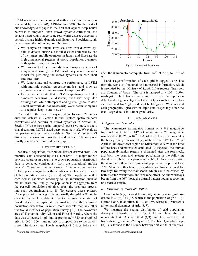
We illustrate the spatial distribution of grid populationdensity in a hourly basis in Fig. 2. At each hour, the boxrepresents first (Q1) and third (Q3) quartiles, with the redline indicating median (2nd quartile). The Inter-Quartile Range(IQR) is defined as the distance between first and third quartiles.

2http://www.mlit.go.jp/en/index.html

0 24 48 72 96 120 144Hours

0

1000

2000

3000

4000

5000

6000

7000Po

pula

tion

foreshock mainshock

Fig. 2. Distribution of Population by Hour

0 20 40 60 80 100 120 140

Hours

0

5

10

15

20

25

30

Per.(

%)o

fAno

mal

y foreshockmainshock3 > |K| ≥ 2

|K| ≥ 3

Fig. 3. Distribution of anomaly value K

Points that are outside of Q3+1.5IQR or Q1-1.5IQR are markedas ”+”. A sparse distribution with diurnal pattern is observedbefore the foreshock, while outliers drop dramatically beforethe mainshock and are almost non-existence days after themainshock due to the effects of upcoming weekend and disasterevacuation in the following two days. Diurnal pattern andsparsity start recovering past the 100th hour as both the returnof weekdays and the end of disruptive events.

Similar to [1], we define the anomaly value Kti,j using

the grid’s average population across the period and standarddeviation pi,j and σpi,j

. |K| ≥ 2 represents (≥ µ±2σ, outside95% confidence as K is normal distribution), and |K| ≥ 3indicates the case when the value is outside interval (µ ± 3σ)(99.7% confidence).

Kti,j =

(pti,j − pi,j)

σpi,j

(1)

It can be seen in Fig. 3 that the percentage of anomaly(95% confidence) reaches approximately 30% in the first 20hours. This could be explained by the fact that majority ofour data (∼85%) is recorded post disaster, therefore, “normal”time data behaves differently and is regarded as “abnormal”.Furthermore, percentage of anomaly also displays a periodicpattern that motivates us to look into finer-granularity spatio-temporal dynamics.

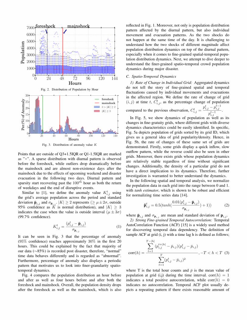
Fig. 4 compares the population distribution an hour beforeand after as well as four hours before and after both theforeshock and mainshock. Overall, the population density dropsafter the foreshock as well as the mainshock, which is also

reflected in Fig. 1. Moreover, not only is population distributionpattern affected by the diurnal pattern, but also individualmovement and evacuation patterns. As the two shocks donot happen at the same time of the day. It is challenging tounderstand how the two shocks of different magnitude affectpopulation distribution dynamics on top of the diurnal pattern,especially when it comes to fine-grained spatial-temporal popu-lation distribution dynamics. Next, we attempt to dive deeper tounderstand the finer-grained spatio-temporal crowd populationdynamics during major disaster.

C. Spatio-Temporal Dynamics

1) Rate of Change in Individual Grid: Aggregated dynamicsdo not tell the story of fine-grained spatial and temporalfluctuations caused by individual movements and evacuationsin the affected region. We define the rate of change of grid(i, j) at time t, Ct

i,j , as the percentage change of population

compared to the previous observation, Cti,j =

pti,j − pt−1i,j

pt−1i,j

.

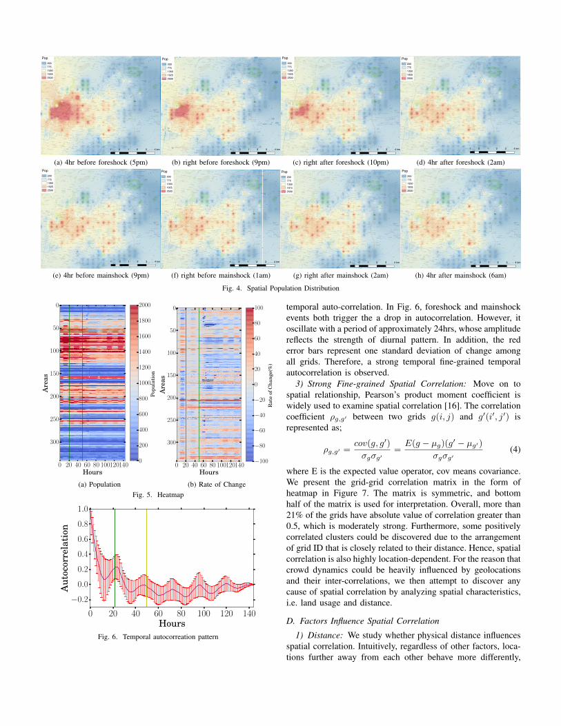
In Fig. 5, we show dynamics of population as well as itschanges in fine-gratuity grids, where different grids with diversedynamics characteristics could be easily identified. In specific,Fig. 5a depicts population of grids sorted by its grid ID, whichgives us a general idea of grid popularity/density. Hence, inFig. 5b, the rate of changes of these same set of grids aredemonstrated. Firstly, some grids display a quick inflow, slowoutflow pattern, while the reverse could also be seen in othergrids. Moreover, there exists grids whose population dynamicsare relatively stable regardless of time without significantchanges. Additionally, the density of a particular grid do nothave a direct implication to its dynamics. Therefore, furtherinvestigation is warranted to better understand the dynamics.

In the following spatial and temporal analysis, we normalizethe population data in each grid into the range between 0 and 1.with tanh estimator, which is shown to be robust and efficientfor normalizing time series data [14].

pti,j = 0.5(tanh(

0.01(pti,j − pi,j)

σpi,j

) + 1)) (2)

where pi,j and σpi,jare mean and standard deviation of pi,j .

2) Strong Fine-grained Temporal Autocorrelation: TemporalAutoCorrelation Function (ACF) [15] is a widely used methodfor discovering temporal data dependency. The definition ofsample ACF at grid (i, j) with a time lag h is defined as follows;

corr(h) =

T−|h|∑t=1

(pt+|h|i,j − pi,j)(pti,j − pi,j)

T∑t=1

(pti,j − pi,j)2,−T < h < T (3)

where T is the total hour counts and p is the mean value ofpopulation at grid (i,j) during the time interval. corr(h) = 1indicates a total positive autocorrelation, while corr(h) = 0indicates no autocorrelation. Temporal ACF plot usually de-picts a repeating pattern if there exists reasonable amount of

(a) 4hr before foreshock (5pm) (b) right before foreshock (9pm) (c) right after foreshock (10pm) (d) 4hr after foreshock (2am)

(e) 4hr before mainshock (9pm) (f) right before mainshock (1am) (g) right after mainshock (2am) (h) 4hr after mainshock (6am)

Fig. 4. Spatial Population Distribution

0 20 40 60 80 100120140Hours

0

50

100

150

200

250

300

Are

as

0

200

400

600

800

1000

1200

1400

1600

1800

2000

Popu

lati

on

(a) Population

0 20 40 60 80 100120140Hours

0

50

100

150

200

250

300

Are

as

−100

−80

−60

−40

−20

0

20

40

60

80

100

Rat

eof

Cha

nge(

%)

(b) Rate of ChangeFig. 5. Heatmap

0 20 40 60 80 100 120 140Hours

−0.2

0.0

0.2

0.4

0.6

0.8

1.0

Aut

ocor

rela

tion

Fig. 6. Temporal autocorreation pattern

temporal auto-correlation. In Fig. 6, foreshock and mainshockevents both trigger the a drop in autocorrelation. However, itoscillate with a period of approximately 24hrs, whose amplitudereflects the strength of diurnal pattern. In addition, the rederror bars represent one standard deviation of change amongall grids. Therefore, a strong temporal fine-grained temporalautocorrelation is observed.

3) Strong Fine-grained Spatial Correlation: Move on tospatial relationship, Pearson’s product moment coefficient iswidely used to examine spatial correlation [16]. The correlationcoefficient ρg,g′ between two grids g(i, j) and g′(i′, j′) isrepresented as;

ρg,g′ =cov(g, g′)

σgσg′=E(g − µg)(g′ − µg′)

σgσg′(4)

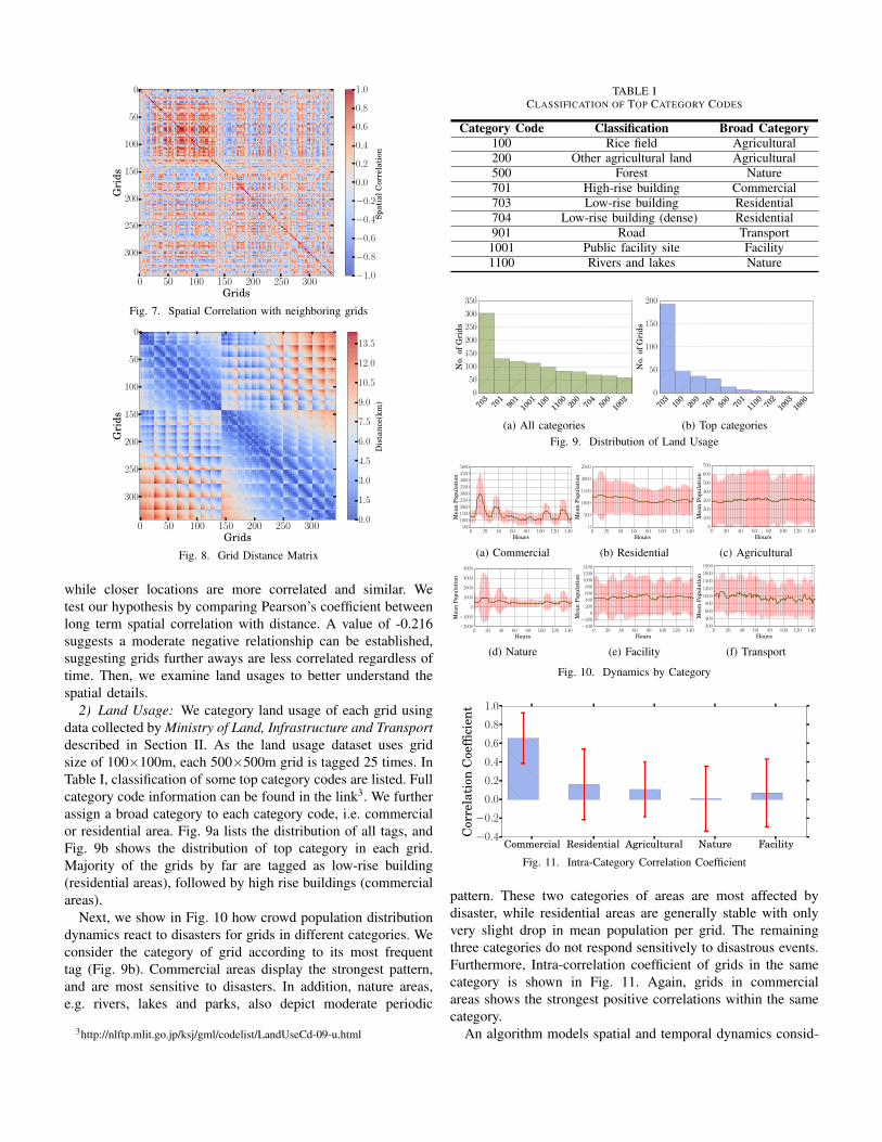
where E is the expected value operator, cov means covariance.We present the grid-grid correlation matrix in the form ofheatmap in Figure 7. The matrix is symmetric, and bottomhalf of the matrix is used for interpretation. Overall, more than21% of the grids have absolute value of correlation greater than0.5, which is moderately strong. Furthermore, some positivelycorrelated clusters could be discovered due to the arrangementof grid ID that is closely related to their distance. Hence, spatialcorrelation is also highly location-dependent. For the reason thatcrowd dynamics could be heavily influenced by geolocationsand their inter-correlations, we then attempt to discover anycause of spatial correlation by analyzing spatial characteristics,i.e. land usage and distance.

D. Factors Influence Spatial Correlation

1) Distance: We study whether physical distance influencesspatial correlation. Intuitively, regardless of other factors, loca-tions further away from each other behave more differently,

0 50 100 150 200 250 300Grids

0

50

100

150

200

250

300

Gri

ds

−1.0

−0.8

−0.6

−0.4

−0.2

0.0

0.2

0.4

0.6

0.8

1.0

Spat

ialC

orre

lati

on

Fig. 7. Spatial Correlation with neighboring grids

0 50 100 150 200 250 300Grids

0

50

100

150

200

250

300

Gri

ds

0.0

1.5

3.0

4.5

6.0

7.5

9.0

10.5

12.0

13.5

Dis

tanc

e(km

)

Fig. 8. Grid Distance Matrix

while closer locations are more correlated and similar. Wetest our hypothesis by comparing Pearson’s coefficient betweenlong term spatial correlation with distance. A value of -0.216suggests a moderate negative relationship can be established,suggesting grids further aways are less correlated regardless oftime. Then, we examine land usages to better understand thespatial details.

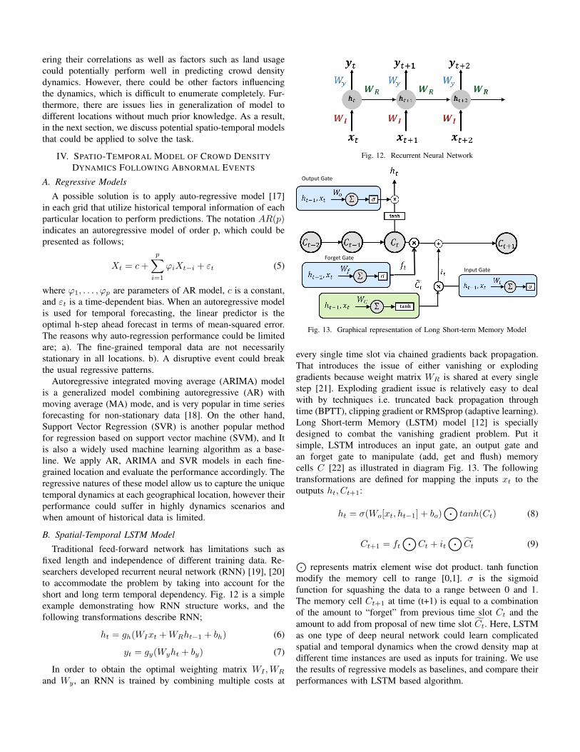
2) Land Usage: We category land usage of each grid usingdata collected by Ministry of Land, Infrastructure and Transportdescribed in Section II. As the land usage dataset uses gridsize of 100×100m, each 500×500m grid is tagged 25 times. InTable I, classification of some top category codes are listed. Fullcategory code information can be found in the link3. We furtherassign a broad category to each category code, i.e. commercialor residential area. Fig. 9a lists the distribution of all tags, andFig. 9b shows the distribution of top category in each grid.Majority of the grids by far are tagged as low-rise building(residential areas), followed by high rise buildings (commercialareas).

Next, we show in Fig. 10 how crowd population distributiondynamics react to disasters for grids in different categories. Weconsider the category of grid according to its most frequenttag (Fig. 9b). Commercial areas display the strongest pattern,and are most sensitive to disasters. In addition, nature areas,e.g. rivers, lakes and parks, also depict moderate periodic

3http://nlftp.mlit.go.jp/ksj/gml/codelist/LandUseCd-09-u.html

TABLE ICLASSIFICATION OF TOP CATEGORY CODES

Category Code Classification Broad Category100 Rice field Agricultural200 Other agricultural land Agricultural500 Forest Nature701 High-rise building Commercial703 Low-rise building Residential704 Low-rise building (dense) Residential901 Road Transport1001 Public facility site Facility1100 Rivers and lakes Nature

703

701

901

1001 10

011

00 200

704

500

1002

0

50

100

150

200

250

300

350

No.

ofG

rids

(a) All categories

703

100

200

704

500

701

1100 70

210

0316

000

50

100

150

200

No.

ofG

rids

(b) Top categoriesFig. 9. Distribution of Land Usage

0 20 40 60 80 100 120 140Hours

500100015002000250030003500400045005000

Mea

nPo

pula

tion

(a) Commercial

0 20 40 60 80 100 120 140Hours

0

500

1000

1500

2000

2500

Mea

nPo

pula

tion

(b) Residential

0 20 40 60 80 100 120 140Hours

0

100

200

300

400

500

600

700

Mea

nPo

pula

tion

(c) Agricultural

0 20 40 60 80 100 120 140Hours

−2000

−1000

0

1000

2000

3000

4000

Mea

nPo

pula

tion

(d) Nature

0 20 40 60 80 100 120 140Hours

−400−200

0200400600800

100012001400

Mea

nPo

pula

tion

(e) Facility

0 20 40 60 80 100 120 140Hours

200

400

600

800

1000

1200

1400

1600

1800

Mea

nPo

pula

tion

(f) Transport

Fig. 10. Dynamics by Category

Commercial Residential Agricultural Nature Facility−0.4

−0.2

0.0

0.2

0.4

0.6

0.8

1.0

Cor

rela

tion

Coe

ffici

ent

Fig. 11. Intra-Category Correlation Coefficient

pattern. These two categories of areas are most affected bydisaster, while residential areas are generally stable with onlyvery slight drop in mean population per grid. The remainingthree categories do not respond sensitively to disastrous events.Furthermore, Intra-correlation coefficient of grids in the samecategory is shown in Fig. 11. Again, grids in commercialareas shows the strongest positive correlations within the samecategory.

An algorithm models spatial and temporal dynamics consid-

ering their correlations as well as factors such as land usagecould potentially perform well in predicting crowd densitydynamics. However, there could be other factors influencingthe dynamics, which is difficult to enumerate completely. Fur-thermore, there are issues lies in generalization of model todifferent locations without much prior knowledge. As a result,in the next section, we discuss potential spatio-temporal modelsthat could be applied to solve the task.

IV. SPATIO-TEMPORAL MODEL OF CROWD DENSITYDYNAMICS FOLLOWING ABNORMAL EVENTS

A. Regressive Models

A possible solution is to apply auto-regressive model [17]in each grid that utilize historical temporal information of eachparticular location to perform predictions. The notation AR(p)indicates an autoregressive model of order p, which could bepresented as follows;

Xt = c+

p∑i=1

ϕiXt−i + εt (5)

where ϕ1, . . . , ϕp are parameters of AR model, c is a constant,and εt is a time-dependent bias. When an autoregressive modelis used for temporal forecasting, the linear predictor is theoptimal h-step ahead forecast in terms of mean-squared error.The reasons why auto-regression performance could be limitedare; a). The fine-grained temporal data are not necessarilystationary in all locations. b). A disruptive event could breakthe usual regressive patterns.

Autoregressive integrated moving average (ARIMA) modelis a generalized model combining autoregressive (AR) withmoving average (MA) mode, and is very popular in time seriesforecasting for non-stationary data [18]. On the other hand,Support Vector Regression (SVR) is another popular methodfor regression based on support vector machine (SVM), and Itis also a widely used machine learning algorithm as a base-line. We apply AR, ARIMA and SVR models in each fine-grained location and evaluate the performance accordingly. Theregressive natures of these model allow us to capture the uniquetemporal dynamics at each geographical location, however theirperformance could suffer in highly dynamics scenarios andwhen amount of historical data is limited.

B. Spatial-Temporal LSTM Model

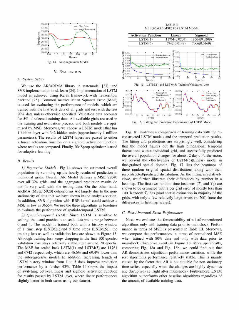
Traditional feed-forward network has limitations such asfixed length and independence of different training data. Re-searchers developed recurrent neural network (RNN) [19], [20]to accommodate the problem by taking into account for theshort and long term temporal dependency. Fig. 12 is a simpleexample demonstrating how RNN structure works, and thefollowing transformations describe RNN;

ht = gh(WIxt +WRht−1 + bh) (6)

yt = gy(Wyht + by) (7)

In order to obtain the optimal weighting matrix WI ,WR

and Wy , an RNN is trained by combining multiple costs at

Fig. 12. Recurrent Neural Network

OutputGate

ForgetGate

InputGate

Fig. 13. Graphical representation of Long Short-term Memory Model

every single time slot via chained gradients back propagation.That introduces the issue of either vanishing or explodinggradients because weight matrix WR is shared at every singlestep [21]. Exploding gradient issue is relatively easy to dealwith by techniques i.e. truncated back propagation throughtime (BPTT), clipping gradient or RMSprop (adaptive learning).Long Short-term Memory (LSTM) model [12] is speciallydesigned to combat the vanishing gradient problem. Put itsimple, LSTM introduces an input gate, an output gate andan forget gate to manipulate (add, get and flush) memorycells C [22] as illustrated in diagram Fig. 13. The followingtransformations are defined for mapping the inputs xt to theoutputs ht, Ct+1:

ht = σ(Wo[xt, ht−1] + bo)⊙

tanh(Ct) (8)

Ct+1 = ft⊙

Ct + it⊙

Ct (9)⊙represents matrix element wise dot product. tanh function

modify the memory cell to range [0,1]. σ is the sigmoidfunction for squashing the data to a range between 0 and 1.The memory cell Ct+1 at time (t+1) is equal to a combinationof the amount to “forget” from previous time slot Ct and theamount to add from proposal of new time slot Ct. Here, LSTMas one type of deep neural network could learn complicatedspatial and temporal dynamics when the crowd density map atdifferent time instances are used as inputs for training. We usethe results of regressive models as baselines, and compare theirperformances with LSTM based algorithm.

110 115 120 125 130 135 140Hours

280000

285000

290000

295000

300000

305000

310000

315000

320000

Popu

lati

on

Test DataAuto-Regression

Fig. 14. Auto-regression Model

V. EVALUATION

A. System Setup

We use the AR/ARIMA library in statemodel [23], andSVR implementation in sk-learn [24]. Implementation of LSTMmodel is achieved using Keras framework with TensorFlowbackend [25]. Common metrics Mean Squared Error (MSE)is used for evaluating the performance of models, which aretrained with the first 80% data of all grids and test with the rest20% data unless otherwise specified. Validation data accountsfor 5% of selected training data. All available girds are used inthe training and evaluation process, and both models are opti-mized by MSE. Moreover, we choose a LSTM model that has1 hidden layer with 342 hidden units (approximately 1 millionparameters). The results of LSTM layers are passed to eithera linear activation function or a sigmoid activation function,where results are compared. Finally, RMSprop optimizer is usedfor adaptive learning.

B. Results

1) Regressive Models: Fig 14 shows the estimated overallpopulation by summing up the hourly results of prediction inindividual grids. Overall, AR Model delivers a MSE 22040over all 324 grids, and the aggregated prediction results donot fit very well with the testing data. On the other hand,ARIMA (MSE:15020) outperforms AR largely due to the non-stationarity of data that we have shown in the analysis section.In addition, SVR algorithm with RBF kernel could achieve aMSE as low as 36554. We use the three algorithms as baselinesto evaluate the performance of spatial-temporal LSTM.

2) Spatial-Temporal LSTM: Since LSTM is sensitive toscaling, the usual practice is to scale data into a range between0 and 1. The model is trained both with a history windowof 1 time step (LSTM(1))and 5 time steps (LSTM(5)), thetraining loss as well as validation loss are shown in Figure 15.Although training loss keeps dropping in the first 100 epochs,validation loss stays relatively stable after around 20 epochs.The MSE for scaled back LSTM(1) and LSTM(5) are 11761and 6742 respectively, which are 46.6% and 69.4% lower thanthe autoregressive model. In addition, Increasing length ofLSTM history window from 1 to 5 does improve predictionperformance by a further 43%. Table II shows the impactof switching between linear and sigmoid activation functionfor results passed by LSTM layer, where linear performancesslightly better in both cases using our dataset.

TABLE IIMSE(SCALED MSE) FOR LSTM MODEL

Activation Function Linear SigmoidLSTM(1) 11761(0.0203) 18604(0.0209)LSTM(5) 6742(0.0149) 7006(0.0169)

0 20 40 60 80 100Epochs

0.0000.0050.0100.0150.0200.0250.0300.0350.0400.045

Mea

nSq

uare

dE

rror

(MSE

)

Training LossValidation Loss

0 20 40 60 80 100Epochs

0.00

0.01

0.02

0.03

0.04

0.05

Mea

nSq

uare

dE

rror

(MSE

)

Training LossValidation Loss

Fig. 15. LSTM(1) and LSTM(5) Training/Validation Loss

0 20 40 60 80 100 120 140Hours

260000

280000

300000

320000

340000

360000

380000

Popu

lati

on

Training DataModel Fitting(1)Test DataPrediction(1)

0 20 40 60 80 100 120 140Hours

260000

280000

300000

320000

340000

360000

380000

Popu

lati

on

Training DataModel Fitting(5)Test DataPrediction(5)

Fig. 16. Fitting and Prediction Performance of LSTM Model

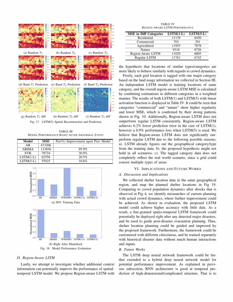
Fig. 16 illustrates a comparison of training data with the re-constructed LSTM models and the temporal prediction results.The fitting and predictions are surprisingly well, consideringthat the model figures out the high dimensional temporalfluctuations within individual grid, and successfully predictedthe overall population changes for almost 2 days. Furthermore,we present the effectiveness of LSTM(5)(Linear) model infine-grained spatial domain. Fig. 17 lists the heatmaps ofthree random original spatial distributions along with theirreconstructed/predicted distribution. As the fitting is relativelyclose, we further illustrate their differences by number in aheatmap. The first two random time instances (T1 and T2) areshown to be estimated with a per grid error of mostly less than100. Random T3 has good spatial estimation in majority of thegrids, with only a few relatively large errors (∼ 700) (note thedifferences in heatmap scales).

C. Post-Abnormal Event Performance

Next, we evaluate the forecastability of all aforementionedalgorithms only with training data prior to mainshock. Perfor-mance in terms of MSE is presented in Table III. Moreover,we compare the performances in terms of normalized MSEwhen trained with 80% data and only with data prior tomainshock (disruptive event) in Figure 18. More specifically,comparing Fig. 18a and Fig. 18b, we could find out thatAR demonstrates significant performance variation, while therest algorithms performance relatively stable. This is mainlycaused by the factor that AR is not suitable for non-stationarytime series, especially when the changes are highly dynamicsand disruptive (i.e. right after mainshock). Furthermore, LSTMalgorithm outperforms other baseline algorithms regardless ofthe amount of available training data.

0 5 10 15

0

5

10

15400

800

1200

1600

2000

2400

2800

3200

3600

(a) Random T1

0 5 10 15

0

5

10

15300

600

900

1200

1500

1800

2100

2400

2700

(b) Random T2

0 5 10 15

0

5

10

15 800

1600

2400

3200

4000

4800

5600

(c) Random T3

0 5 10 15

0

5

10

15400

800

1200

1600

2000

2400

2800

3200

3600

(d) Rand T1 Prediction0 5 10 15

0

5

10

15300

600

900

1200

1500

1800

2100

2400

2700

(e) Rand T2 Prediction0 5 10 15

0

5

10

15600

1200

1800

2400

3000

3600

4200

4800

(f) Rand T3 Prediction

0 5 10 15

0

5

10

15−160

−120

−80

−40

0

40

80

120

160

(g) Random T1 diff0 5 10 15

0

5

10

15

−160

−120

−80

−40

0

40

80

120

(h) Random T2 diff0 5 10 15

0

5

10

15

−700

−600

−500

−400

−300

−200

−100

0

(i) Random T3 diff

Fig. 17. LSTM(5) Spatial Reconstruction and Prediction

TABLE IIIMODEL PERFORMANCE RIGHT AFTER ABNORMAL EVENT

Model MSE Per(%) Improvement upon Prev ModelAR 473206 -

ARIMA 113856 95.9%SVR 78724 30.9%

LSTM(1-L) 62556 20.5%LSTM(5-L) 55925 10.6%

AR ARIMA SVR(RBF) LSTM(1-L) LSTM(5-L)0.0

0.2

0.4

0.6

0.8

1.0

Nor

mal

ized

MSE

(a) 80% Training Data

AR ARIMA SVR(RBF) LSTM(1-L) LSTM(5-L)0.0

0.2

0.4

0.6

0.8

1.0

Nor

mal

ized

MSE

(b) Right After MainshockFig. 18. Model Performance Evaluation

D. Region-Aware LSTM

Lastly, we attempt to investigate whether additional contextinformation can potentially improve the performance of spatial-temporal LSTM model. We propose Region-aware LSTM with

TABLE IVREGION-AWARE LSTM PERFORMANCE

MSE in Diff Categories LSTM(1-L) LSTM(5-L)Residential 11139 6450Commercial 703 291Agricultural 11955 7878

Nature 9318 8726Region-Aware LSTM 11029 6805

Regular LSTM 11761 6742

the hypothesis that locations of similar types/categories aremore likely to behave similarly with regards to crowd dynamics.

Firstly, each grid location is tagged with one major categorybased on the land usage information we collected in Section III.An independent LSTM model is training locations of samecategory, and the overall region-aware LSTM MSE is calculatedby combining estimations in different categories in a weightedmanner. The results of both LSTM(1) and LSTM(5) with linearactivation function is displayed in Table IV. It could be seen thatcategories “commercial” and “nature” show higher regularityand lower MSE, which is confirmed by their strong patternsshown in Fig. 10. Additionally, Region-aware LSTM does notoutperform regular LSTM consistently. Region-aware LSTMachieves 6.2% lower prediction error in the case of LSTM(1),however a 0.9% performance loss when LSTM(5) is used. Webelieve that Region-aware LSTM does not significantly out-perform regular LSTM due to the following possible reasons;a). LSTM already figures out the geographical category/typefrom the training data. b). the proposed hypothesis might nothold in all scenarios. c). The tagged category data does notcompletely reflect the real world scenario, since a grid couldconsist multiple types of areas.

VI. IMPLICATIONS AND FUTURE WORKS

A. Discussion and ImplicationsWe collected shelter location data in the same geographical

region, and map the planned shelter locations in Fig 19.Comparing to crowd population dynamics after shocks that isobserved in Fig 4, we identify mismatches of current planningwith actual crowd dynamics, where further improvement couldbe achieved. As shown in evaluation, the proposed LSTMmodel could achieve higher accuracy with little data. As aresult, a fine-grained spatio-temporal LSTM framework couldpotentially be deployed right after any detected major disasters,and be used to guide post-disaster evacuation planning. Thus,shelter location planning could be guided and improved bythe proposed framework. Furthermore, the framework could becustomized with different cities/areas, and be trained separatelywith historical disaster data without much human interactionsand inputs.B. Future Works

The LSTM deep neural network framework could be fur-ther extended to a hybrid deep neural network model forpotential performance improvement. As explained in previ-ous subsection, RNN architecture is good at temporal pre-diction of high-dimensional/complicated structure. That is to

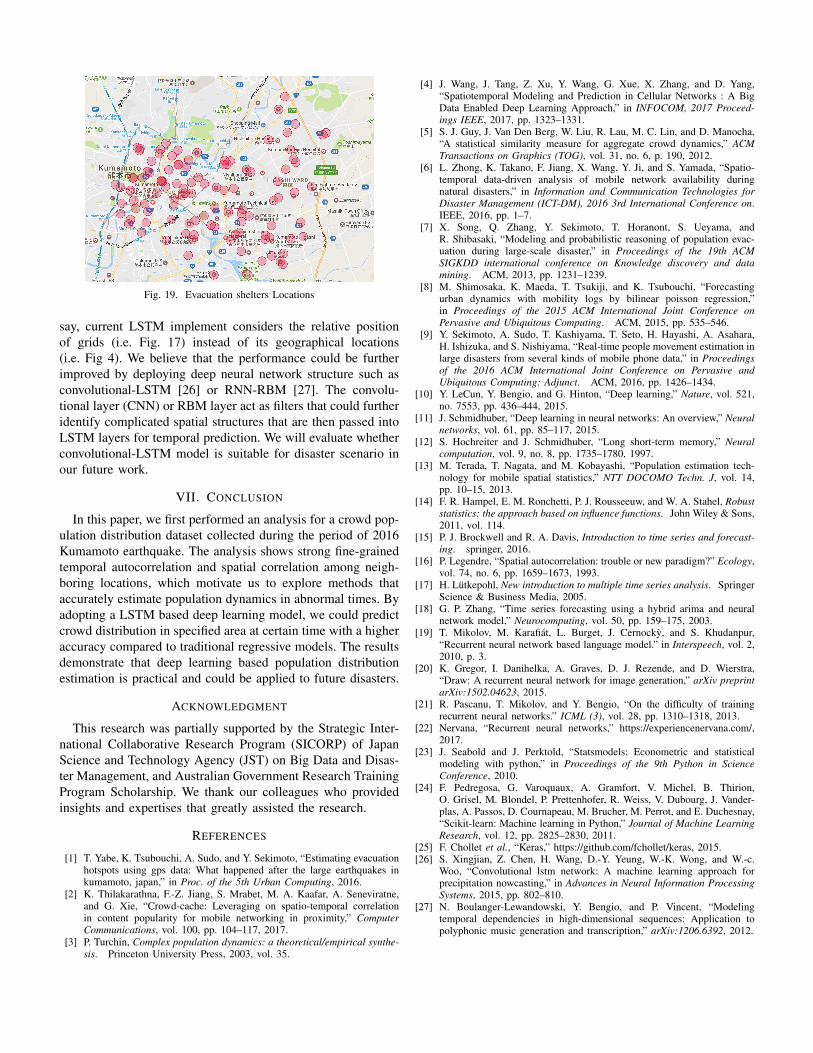
Fig. 19. Evacuation shelters Locations

say, current LSTM implement considers the relative positionof grids (i.e. Fig. 17) instead of its geographical locations(i.e. Fig 4). We believe that the performance could be furtherimproved by deploying deep neural network structure such asconvolutional-LSTM [26] or RNN-RBM [27]. The convolu-tional layer (CNN) or RBM layer act as filters that could furtheridentify complicated spatial structures that are then passed intoLSTM layers for temporal prediction. We will evaluate whetherconvolutional-LSTM model is suitable for disaster scenario inour future work.

VII. CONCLUSION

In this paper, we first performed an analysis for a crowd pop-ulation distribution dataset collected during the period of 2016Kumamoto earthquake. The analysis shows strong fine-grainedtemporal autocorrelation and spatial correlation among neigh-boring locations, which motivate us to explore methods thataccurately estimate population dynamics in abnormal times. Byadopting a LSTM based deep learning model, we could predictcrowd distribution in specified area at certain time with a higheraccuracy compared to traditional regressive models. The resultsdemonstrate that deep learning based population distributionestimation is practical and could be applied to future disasters.

ACKNOWLEDGMENT

This research was partially supported by the Strategic Inter-national Collaborative Research Program (SICORP) of JapanScience and Technology Agency (JST) on Big Data and Disas-ter Management, and Australian Government Research TrainingProgram Scholarship. We thank our colleagues who providedinsights and expertises that greatly assisted the research.

REFERENCES

[1] T. Yabe, K. Tsubouchi, A. Sudo, and Y. Sekimoto, “Estimating evacuationhotspots using gps data: What happened after the large earthquakes inkumamoto, japan,” in Proc. of the 5th Urban Computing, 2016.

[2] K. Thilakarathna, F.-Z. Jiang, S. Mrabet, M. A. Kaafar, A. Seneviratne,and G. Xie, “Crowd-cache: Leveraging on spatio-temporal correlationin content popularity for mobile networking in proximity,” ComputerCommunications, vol. 100, pp. 104–117, 2017.

[3] P. Turchin, Complex population dynamics: a theoretical/empirical synthe-sis. Princeton University Press, 2003, vol. 35.

[4] J. Wang, J. Tang, Z. Xu, Y. Wang, G. Xue, X. Zhang, and D. Yang,“Spatiotemporal Modeling and Prediction in Cellular Networks : A BigData Enabled Deep Learning Approach,” in INFOCOM, 2017 Proceed-ings IEEE, 2017, pp. 1323–1331.

[5] S. J. Guy, J. Van Den Berg, W. Liu, R. Lau, M. C. Lin, and D. Manocha,“A statistical similarity measure for aggregate crowd dynamics,” ACMTransactions on Graphics (TOG), vol. 31, no. 6, p. 190, 2012.

[6] L. Zhong, K. Takano, F. Jiang, X. Wang, Y. Ji, and S. Yamada, “Spatio-temporal data-driven analysis of mobile network availability duringnatural disasters,” in Information and Communication Technologies forDisaster Management (ICT-DM), 2016 3rd International Conference on.IEEE, 2016, pp. 1–7.

[7] X. Song, Q. Zhang, Y. Sekimoto, T. Horanont, S. Ueyama, andR. Shibasaki, “Modeling and probabilistic reasoning of population evac-uation during large-scale disaster,” in Proceedings of the 19th ACMSIGKDD international conference on Knowledge discovery and datamining. ACM, 2013, pp. 1231–1239.

[8] M. Shimosaka, K. Maeda, T. Tsukiji, and K. Tsubouchi, “Forecastingurban dynamics with mobility logs by bilinear poisson regression,”in Proceedings of the 2015 ACM International Joint Conference onPervasive and Ubiquitous Computing. ACM, 2015, pp. 535–546.

[9] Y. Sekimoto, A. Sudo, T. Kashiyama, T. Seto, H. Hayashi, A. Asahara,H. Ishizuka, and S. Nishiyama, “Real-time people movement estimation inlarge disasters from several kinds of mobile phone data,” in Proceedingsof the 2016 ACM International Joint Conference on Pervasive andUbiquitous Computing: Adjunct. ACM, 2016, pp. 1426–1434.

[10] Y. LeCun, Y. Bengio, and G. Hinton, “Deep learning,” Nature, vol. 521,no. 7553, pp. 436–444, 2015.

[11] J. Schmidhuber, “Deep learning in neural networks: An overview,” Neuralnetworks, vol. 61, pp. 85–117, 2015.

[12] S. Hochreiter and J. Schmidhuber, “Long short-term memory,” Neuralcomputation, vol. 9, no. 8, pp. 1735–1780, 1997.

[13] M. Terada, T. Nagata, and M. Kobayashi, “Population estimation tech-nology for mobile spatial statistics,” NTT DOCOMO Techn. J, vol. 14,pp. 10–15, 2013.

[14] F. R. Hampel, E. M. Ronchetti, P. J. Rousseeuw, and W. A. Stahel, Robuststatistics: the approach based on influence functions. John Wiley & Sons,2011, vol. 114.

[15] P. J. Brockwell and R. A. Davis, Introduction to time series and forecast-ing. springer, 2016.

[16] P. Legendre, “Spatial autocorrelation: trouble or new paradigm?” Ecology,vol. 74, no. 6, pp. 1659–1673, 1993.

[17] H. Lutkepohl, New introduction to multiple time series analysis. SpringerScience & Business Media, 2005.

[18] G. P. Zhang, “Time series forecasting using a hybrid arima and neuralnetwork model,” Neurocomputing, vol. 50, pp. 159–175, 2003.

[19] T. Mikolov, M. Karafiat, L. Burget, J. Cernocky, and S. Khudanpur,“Recurrent neural network based language model.” in Interspeech, vol. 2,2010, p. 3.

[20] K. Gregor, I. Danihelka, A. Graves, D. J. Rezende, and D. Wierstra,“Draw: A recurrent neural network for image generation,” arXiv preprintarXiv:1502.04623, 2015.

[21] R. Pascanu, T. Mikolov, and Y. Bengio, “On the difficulty of trainingrecurrent neural networks.” ICML (3), vol. 28, pp. 1310–1318, 2013.

[22] Nervana, “Recurrent neural networks,” https://experiencenervana.com/,2017.

[23] J. Seabold and J. Perktold, “Statsmodels: Econometric and statisticalmodeling with python,” in Proceedings of the 9th Python in ScienceConference, 2010.

[24] F. Pedregosa, G. Varoquaux, A. Gramfort, V. Michel, B. Thirion,O. Grisel, M. Blondel, P. Prettenhofer, R. Weiss, V. Dubourg, J. Vander-plas, A. Passos, D. Cournapeau, M. Brucher, M. Perrot, and E. Duchesnay,“Scikit-learn: Machine learning in Python,” Journal of Machine LearningResearch, vol. 12, pp. 2825–2830, 2011.

[25] F. Chollet et al., “Keras,” https://github.com/fchollet/keras, 2015.[26] S. Xingjian, Z. Chen, H. Wang, D.-Y. Yeung, W.-K. Wong, and W.-c.

Woo, “Convolutional lstm network: A machine learning approach forprecipitation nowcasting,” in Advances in Neural Information ProcessingSystems, 2015, pp. 802–810.

[27] N. Boulanger-Lewandowski, Y. Bengio, and P. Vincent, “Modelingtemporal dependencies in high-dimensional sequences: Application topolyphonic music generation and transcription,” arXiv:1206.6392, 2012.