A volume flattening methodology for geostatistical ... · A volume flattening methodology for geostatistical properties ... modeling of the reservoir. ... methodology for geostatistical

A volume flattening methodology for geostatistical properties estimation

Mathieu Poudret, Chakib Bennis, Jean-François Rainaud and Houman Bo-rouchaki

IFP Energies nouvelles, 1-4 avenue de Bois-Préau, 92852 Rueil-Malmaison, France {mathieu.poudret, chakib.bennis, j-francois.rainaud}@ifpen.fr Charles Delaunay Institute, FRE CNRS 2848, 10010 Troyes, France [email protected]

Abstract

In the domain of oil exploration, geostatistical methods aim at simulating petrophysical properties in a 3D grid model of reservoir. Generally, only a small amount of cells are populated with properties. Roughly speaking, the question is: which properties to give to cell c, knowing the properties of n cells at a given distance from c? Obviously, the popula-tion of the whole reservoir must be computed while respecting the spatial correlation dis-tances of properties. Thus, computing of these correlation distances is a key feature of the geostatistical simulations.

In the classical geostatistical simulation workflow, the evaluation of the correlation dis-tance is imprecise. Indeed, they are computed in a Cartesian simulation space which is not representative of the geometry of the reservoir. This induces major deformations in the final generated petrophysical properties.

We propose a new methodology based on isometric flattening of sub-surface models. Thanks to the flattening, we accurately reposition the initial populated cells in the simula-tion space, before computing the correlation distances. In this paper, we introduce our dif-ferent flattening algorithms depending on the deposit mode of the sub-surface model and present some results.

1. Introduction

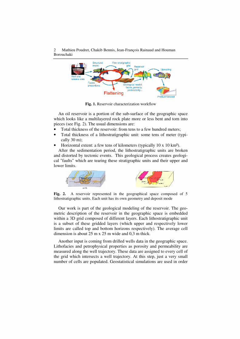
The method presented in this article is concerned with the domain of oil exploration. More particularly, we focus on an important phase of oil res-ervoir characterization: populating lithostratigraphic units represented by a fine stratigraphic grid (see Fig. 1) with rock properties, for instance litho-facies (types of rock), porosity or permeability. Properties are assigned to the center of the cells.

2 Mathieu Poudret, Chakib Bennis, Jean-François Rainaud and Houman Borouchaki

Fig. 1. Reservoir characterization workflow

An oil reservoir is a portion of the sub-surface of the geographic space which looks like a multilayered rock plate more or less bent and torn into pieces (see Fig. 2). The usual dimensions are: • Total thickness of the reservoir: from tens to a few hundred meters; • Total thickness of a lithostratigraphic unit: some tens of meter (typi-

cally 30 m); • Horizontal extent: a few tens of kilometers (typically 10 x 10 km²).

After the sedimentation period, the lithostratigraphic units are broken and distorted by tectonic events. This geological process creates geologi-cal "faults" which are tearing these stratigraphic units and their upper and lower limits.

Fig. 2. A reservoir represented in the geographical space composed of 5 lithostratigraphic units. Each unit has its own geometry and deposit mode

Our work is part of the geological modeling of the reservoir. The geo-metric description of the reservoir in the geographic space is embedded within a 3D grid composed of different layers. Each lithostratigraphic unit is a subset of these gridded layers (which upper and respectively lower limits are called top and bottom horizons respectively). The average cell dimension is about 25 m x 25 m wide and 0,3 m thick.

Another input is coming from drilled wells data in the geographic space. Lithofacies and petrophysical properties as porosity and permeability are measured along the well trajectory. These data are assigned to every cell of the grid which intersects a well trajectory. At this step, just a very small number of cells are populated. Geostatistical simulations are used in order

A volume flattening methodology for geostatistical properties estimation 3

to populate all remaining cells (representing the major part of the grid) with respect to the geological constraints.

(a) (b)

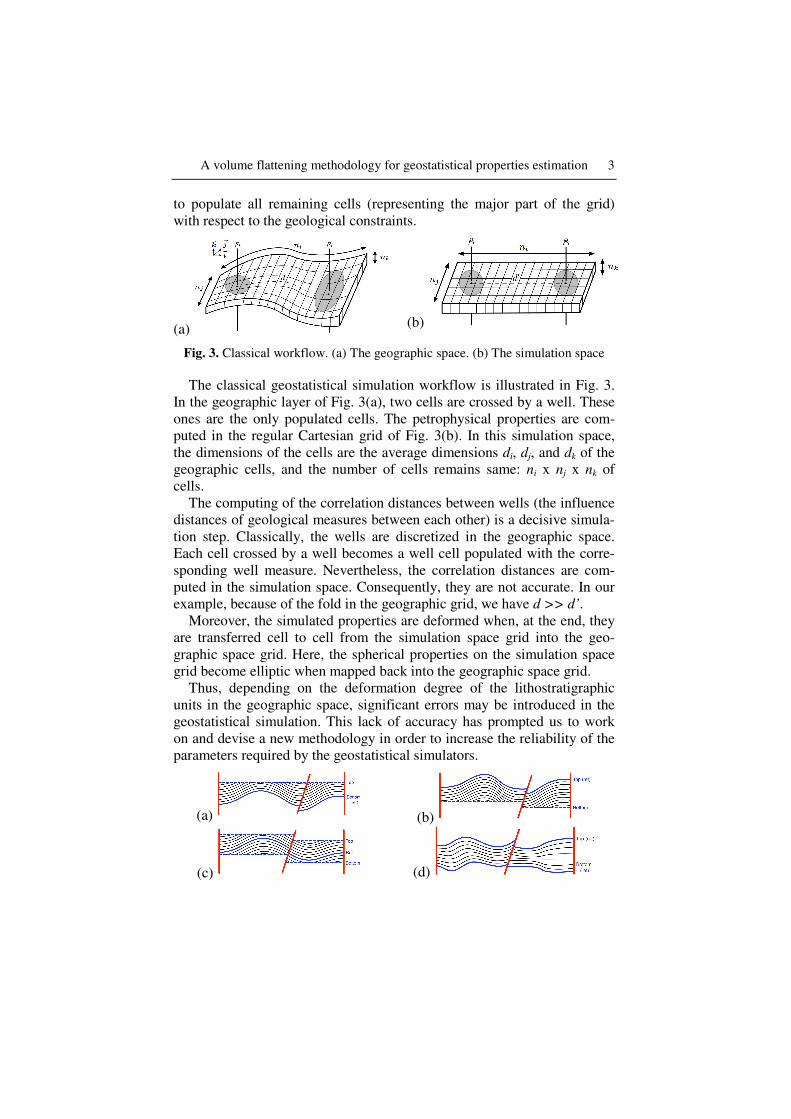
Fig. 3. Classical workflow. (a) The geographic space. (b) The simulation space

The classical geostatistical simulation workflow is illustrated in Fig. 3. In the geographic layer of Fig. 3(a), two cells are crossed by a well. These ones are the only populated cells. The petrophysical properties are com-puted in the regular Cartesian grid of Fig. 3(b). In this simulation space, the dimensions of the cells are the average dimensions di, dj, and dk of the geographic cells, and the number of cells remains same: ni x nj x nk of cells.

The computing of the correlation distances between wells (the influence distances of geological measures between each other) is a decisive simula-tion step. Classically, the wells are discretized in the geographic space. Each cell crossed by a well becomes a well cell populated with the corre-sponding well measure. Nevertheless, the correlation distances are com-puted in the simulation space. Consequently, they are not accurate. In our example, because of the fold in the geographic grid, we have d >> d’.

Moreover, the simulated properties are deformed when, at the end, they are transferred cell to cell from the simulation space grid into the geo-graphic space grid. Here, the spherical properties on the simulation space grid become elliptic when mapped back into the geographic space grid.

Thus, depending on the deformation degree of the lithostratigraphic units in the geographic space, significant errors may be introduced in the geostatistical simulation. This lack of accuracy has prompted us to work on and devise a new methodology in order to increase the reliability of the parameters required by the geostatistical simulators.

(a) (b)

(c) (d)


Fig. 4. Deposit modes. (a) Parallel to bottom. (b) Parallel to top. (c) Parallel to one inner limit. (d) Proportional

Our methodology is based on an “isometric” flattening of the studied lithostratigraphic units in order to have a better estimation of the correla-tion distances between wells. Our flattening process is optimal in the rea-sonable assumption of thin lithostratigraphic units. Thanks to this flatten-ing process, the well trajectories are accurately repositioned in the simulation space. In other respects, it is commonly known that there is not a unique way to flatten a non developable layer isometrically. We propose in this paper two flattening methods driven by the deposit modes of sedi-mentation: the parallel deposit mode and the proportional deposit mode (see Fig. 4).

Our paper is organized as follows. Our whole flattening methodology is presented in section 2. In section 3 and 4, we respectively detail the flatten-ing process in the case of the parallel and proportional deposit modes. Be-fore concluding, to illustrate our flattening-based methodology, we present in section 5 some results of actual lithostratigraphic unit populating.

2. Our flattening methodology

Our flattening methodology improves the precision of the geostatistical methods. Indeed, the simulation of petrophysical properties is computed in a flat simulation space where the well trajectories are repositioned. Thus, accurate correlation distances between wells are easily computed.


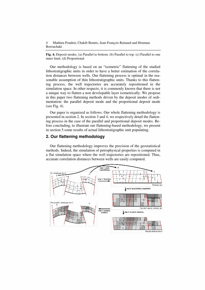
Fig. 5. The flattening methodology

Our flattening methodology is illustrated in Fig. 5. The inputs consist of one thin lithostratigraphic unit in the geographic space (represented with a grid) equipped with some well trajectories. Five steps are required to popu-late this unit with some geological properties: • step 1: isometric flattening of the lithostratigraphic unit; • step 2: repositioning of the well trajectory in the simulation space; • step 3: constitution of a bounding regular Cartesian grid and geostatisti-

cal simulation of petrophysical properties; • step 4: mapping of the simulated properties on the flattened unit; • step 5: transfer of the properties in the geographic space.

The steps are detailed in the followings. In Fig. 5, we supposed that the layers are parallel to the bottom of the unit (see Fig. 4(a)). The methodol-ogy is identical in the case of a proportional deposit mode.

a) Step 1: flattening of the lithostratigraphic unit

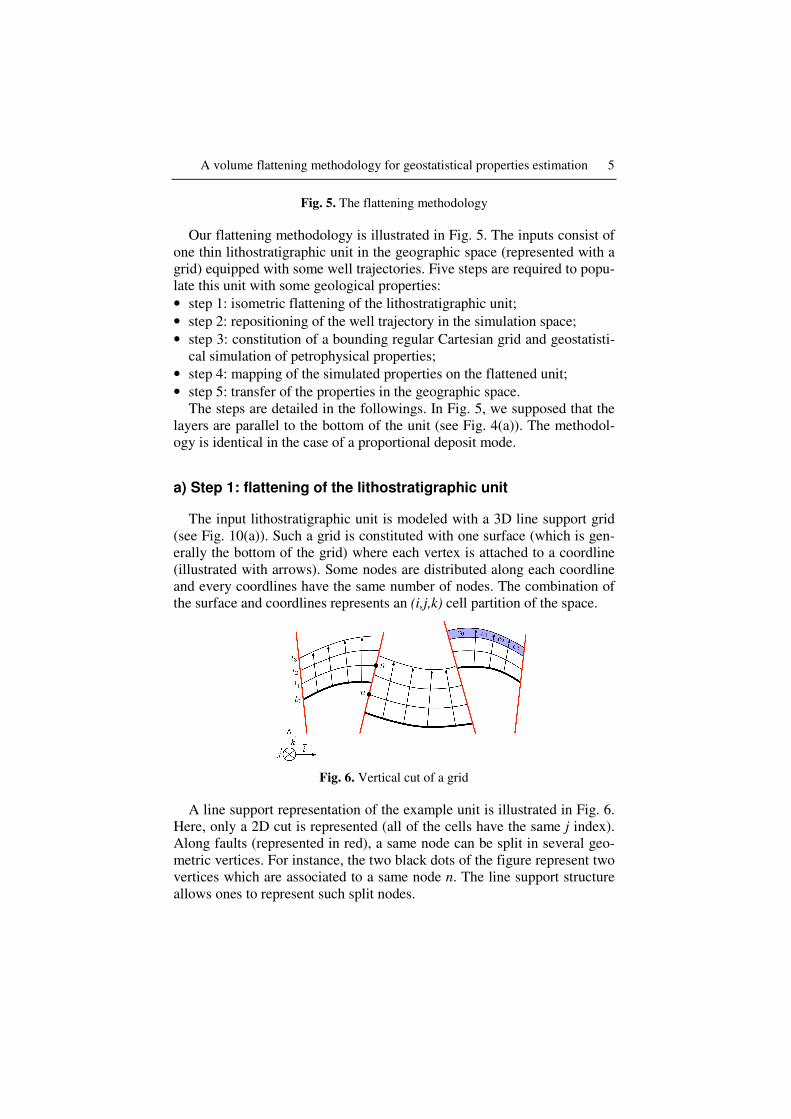
The input lithostratigraphic unit is modeled with a 3D line support grid (see Fig. 10(a)). Such a grid is constituted with one surface (which is gen-erally the bottom of the grid) where each vertex is attached to a coordline (illustrated with arrows). Some nodes are distributed along each coordline and every coordlines have the same number of nodes. The combination of the surface and coordlines represents an (i,j,k) cell partition of the space.

Fig. 6. Vertical cut of a grid

A line support representation of the example unit is illustrated in Fig. 6. Here, only a 2D cut is represented (all of the cells have the same j index). Along faults (represented in red), a same node can be split in several geo-metric vertices. For instance, the two black dots of the figure represent two vertices which are associated to a same node n. The line support structure allows ones to represent such split nodes.


In our 3D grids, each layer has the same number of cells. Some of them are not related to any geological data, for instance in an eroded layer. In order to preserve the regularity, a so-called Actnum property is associated to each grid cell. This property indicates whether a cell is active. For ex-ample, as cells c0, c1, c2 and c3 are not related to geological data, they are inactive.

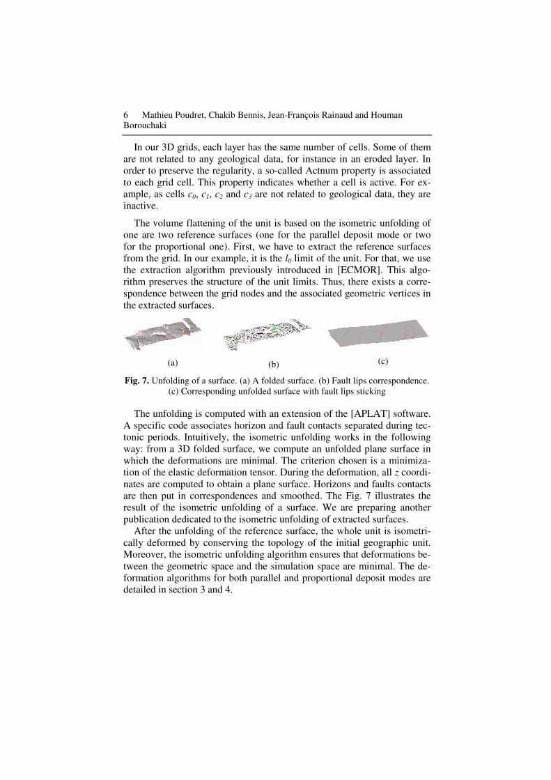
The volume flattening of the unit is based on the isometric unfolding of one are two reference surfaces (one for the parallel deposit mode or two for the proportional one). First, we have to extract the reference surfaces from the grid. In our example, it is the l0 limit of the unit. For that, we use the extraction algorithm previously introduced in [ECMOR]. This algo-rithm preserves the structure of the unit limits. Thus, there exists a corre-spondence between the grid nodes and the associated geometric vertices in the extracted surfaces.

(a)

(b)

(c)

Fig. 7. Unfolding of a surface. (a) A folded surface. (b) Fault lips correspondence. (c) Corresponding unfolded surface with fault lips sticking

The unfolding is computed with an extension of the [APLAT] software. A specific code associates horizon and fault contacts separated during tec-tonic periods. Intuitively, the isometric unfolding works in the following way: from a 3D folded surface, we compute an unfolded plane surface in which the deformations are minimal. The criterion chosen is a minimiza-tion of the elastic deformation tensor. During the deformation, all z coordi-nates are computed to obtain a plane surface. Horizons and faults contacts are then put in correspondences and smoothed. The Fig. 7 illustrates the result of the isometric unfolding of a surface. We are preparing another publication dedicated to the isometric unfolding of extracted surfaces.

After the unfolding of the reference surface, the whole unit is isometri-cally deformed by conserving the topology of the initial geographic unit. Moreover, the isometric unfolding algorithm ensures that deformations be-tween the geometric space and the simulation space are minimal. The de-formation algorithms for both parallel and proportional deposit modes are detailed in section 3 and 4.


b) Step 2: wells trajectory repositioning

There exists a complete correspondence between the structure of the ini-tial lithostratigraphic grid and the structure of the flattened grid. Indeed, our flattening process preserves the topology. Starting from the trajectory of the well, we can calculate the barycentric coordinates of the well meas-urements in each crossed cell of the original lithostratigraphic grid. Then, thanks to the correspondence, we replace these well measurements in each corresponding cell of the flattened grid and thus obtain there coordinates in the simulation space.

c) Step 3: geostatistical population of the regular Cartesian grid

Thanks to the repositioning of wells in the simulation space, the correla-tion distances between wells are easily computed. They allow ones to con-stitute the variogram models required by the geostatistical simulation. We then create a regular Cartesian grid which bound the flattened grid. The pe-trophysical properties are simulated in this new grid. Here, the discretiza-tions along the i, j and k axes are regular. The number of cells along the axes is not necessary the same than in the geographic lithostratigraphic unit. The result of the geostatistical simulation is illustrated with the grey tone attributed to each cell of the regular Cartesian grid.

d) Step 4 and 5: mapping and transfer of properties

In the last two steps, we plug back the simulated petrophysical proper-ties in the geographic space. In step 4, we map the properties from the reg-ular Cartesian grid to the flattened grid. For each cell of the flattened grid, we compute its center and then compute in which cell of the Cartesian grid it is located. Then, the value of the regular Cartesian grid cell is copied in the flattened cell. Let us notice that when several Cartesian grid cells cor-respond to a unique flattened cell, an interpolation of these Cartesian cell values may be use to obtain a more accurate results.

The step 5 consists in copying the properties of the flattened grid in the lithostratigraphic unit. A simple cell by cell copy is sufficient as the flat-tened and geographic grids have the same topology.


3. Parallel volume flattening method

In this section, we present our parallel volume flattening method (a more detailed presentation is proposed in [ECMOR]). This case corre-sponds to the parallel deposit mode of Fig. 4: every limits of the consid-ered unit are parallel to one reference surface. This reference surface may be the bottom one, the top one or an inner limit of the unit.

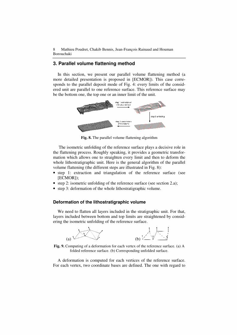
Fig. 8. The parallel volume flattening algorithm

The isometric unfolding of the reference surface plays a decisive role in the flattening process. Roughly speaking, it provides a geometric transfor-mation which allows one to straighten every limit and then to deform the whole lithostratigraphic unit. Here is the general algorithm of the parallel volume flattening (the different steps are illustrated in Fig. 8): • step 1: extraction and triangulation of the reference surface (see

[ECMOR]); • step 2: isometric unfolding of the reference surface (see section 2.a); • step 3: deformation of the whole lithostratigraphic volume.

Deformation of the lithostratigraphic volume

We need to flatten all layers included in the stratigraphic unit. For that, layers included between bottom and top limits are straightened by consid-ering the isometric unfolding of the reference surface.

(a) (b)

Fig. 9. Computing of a deformation for each vertex of the reference surface. (a) A folded reference surface. (b) Corresponding unfolded surface.

A deformation is computed for each vertices of the reference surface. For each vertex, two coordinate bases are defined. The one with regard to


the folded surface (represented with plain arrows in Fig. 9(a)) and the other one with regard to the unfolded surface (see the doted arrows). A defor-mation is the operation which transforms a base from the geographic space to the simulation space.

(a) (b)

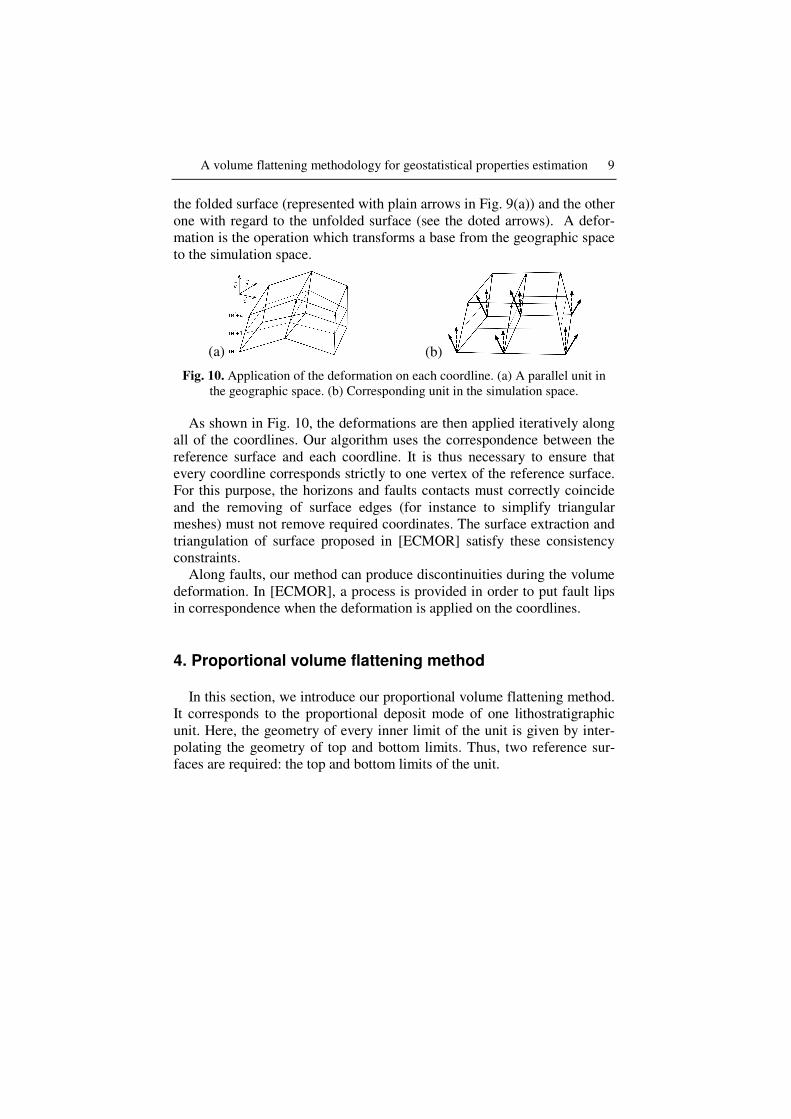
Fig. 10. Application of the deformation on each coordline. (a) A parallel unit in the geographic space. (b) Corresponding unit in the simulation space.

As shown in Fig. 10, the deformations are then applied iteratively along all of the coordlines. Our algorithm uses the correspondence between the reference surface and each coordline. It is thus necessary to ensure that every coordline corresponds strictly to one vertex of the reference surface. For this purpose, the horizons and faults contacts must correctly coincide and the removing of surface edges (for instance to simplify triangular meshes) must not remove required coordinates. The surface extraction and triangulation of surface proposed in [ECMOR] satisfy these consistency constraints.

Along faults, our method can produce discontinuities during the volume deformation. In [ECMOR], a process is provided in order to put fault lips in correspondence when the deformation is applied on the coordlines.

4. Proportional volume flattening method

In this section, we introduce our proportional volume flattening method. It corresponds to the proportional deposit mode of one lithostratigraphic unit. Here, the geometry of every inner limit of the unit is given by inter-polating the geometry of top and bottom limits. Thus, two reference sur-faces are required: the top and bottom limits of the unit.


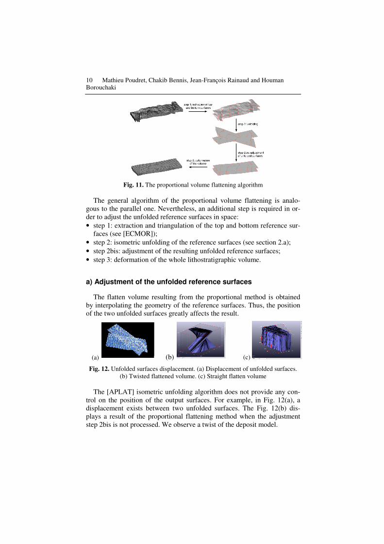
Fig. 11. The proportional volume flattening algorithm

The general algorithm of the proportional volume flattening is analo-gous to the parallel one. Nevertheless, an additional step is required in or-der to adjust the unfolded reference surfaces in space: • step 1: extraction and triangulation of the top and bottom reference sur-

faces (see [ECMOR]); • step 2: isometric unfolding of the reference surfaces (see section 2.a); • step 2bis: adjustment of the resulting unfolded reference surfaces; • step 3: deformation of the whole lithostratigraphic volume.

a) Adjustment of the unfolded reference surfaces

The flatten volume resulting from the proportional method is obtained by interpolating the geometry of the reference surfaces. Thus, the position of the two unfolded surfaces greatly affects the result.

(a) (b) (c)

Fig. 12. Unfolded surfaces displacement. (a) Displacement of unfolded surfaces. (b) Twisted flattened volume. (c) Straight flatten volume

The [APLAT] isometric unfolding algorithm does not provide any con-trol on the position of the output surfaces. For example, in Fig. 12(a), a displacement exists between two unfolded surfaces. The Fig. 12(b) dis-plays a result of the proportional flattening method when the adjustment step 2bis is not processed. We observe a twist of the deposit model.


We propose an algorithm to avoid this symptomatic behaviour. For that, we compute the translation and rotation making the two unfolded surfaces superposable. Intuitively, we obtain these transformations by minimizing the distance between each pair of unfolded surfaces.

Choosing minimization support nodes

First, we choose two sets of support nodes: one in the bottom and an-other one in the top. These sets are such that for each node of a given set, there exists a corresponding node in the other set, a node of the opposite limit which comes from the same coordline. The choice of these support nodes is decisive for the robustness of our algorithm. A support node must satisfy the following conditions: • condition 1: neither itself nor its corresponding node is adjacent to an

inactivated cell (see section 2.a); • condition 2: it is not located on fault.

These two conditions ensure that each support node has exactly one geometric position. Indeed, only the fault nodes and nodes adjacent to an inactivated cell may be associated to several geometric positions. In prac-tice, it is not mandatory to take into account every node satisfying the pre-vious conditions and sets of about ten support nodes are sufficient.

(a) (b)

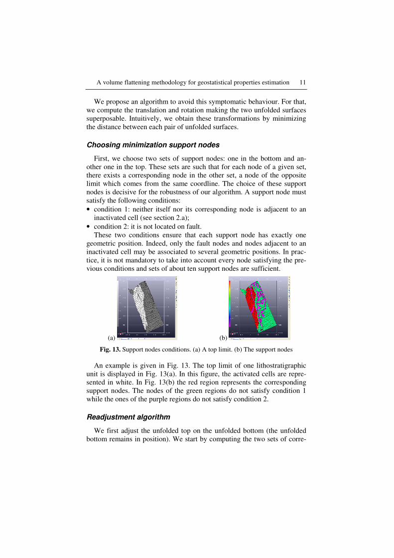
Fig. 13. Support nodes conditions. (a) A top limit. (b) The support nodes

An example is given in Fig. 13. The top limit of one lithostratigraphic unit is displayed in Fig. 13(a). In this figure, the activated cells are repre-sented in white. In Fig. 13(b) the red region represents the corresponding support nodes. The nodes of the green regions do not satisfy condition 1 while the ones of the purple regions do not satisfy condition 2.

Readjustment algorithm

We first adjust the unfolded top on the unfolded bottom (the unfolded bottom remains in position). We start by computing the two sets of corre-


sponding support nodes. By using these nodes, we then minimize the dis-tances between the two unfolded surfaces.

For that, we use the parallel flattening method to make sure that the an-gles between the bottom limit and the coordlines are well repositioned in the simulation space. By not considering these angles, the result of a pro-portional flattening is a vertical straight volume where the initial orienta-tion of the grid is completely forgotten (see Fig. 12(c)).

Finally, to minimize the error, we repeat the adjustment by considering that the top remains in position (with the same sets of support nodes).

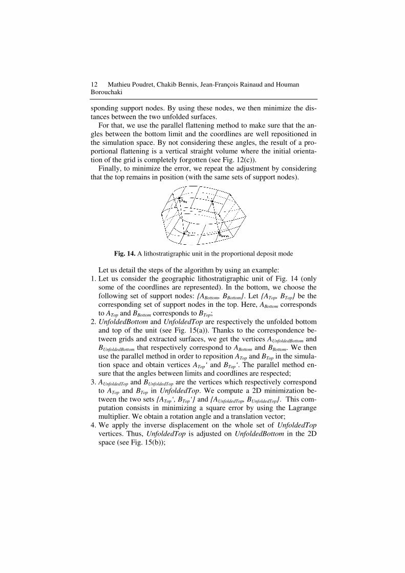
Fig. 14. A lithostratigraphic unit in the proportional deposit mode

Let us detail the steps of the algorithm by using an example: 1. Let us consider the geographic lithostratigraphic unit of Fig. 14 (only

some of the coordlines are represented). In the bottom, we choose the following set of support nodes: {ABottom, BBottom}. Let {ATop, BTop} be the corresponding set of support nodes in the top. Here, ABottom corresponds to ATop and BBottom corresponds to BTop;

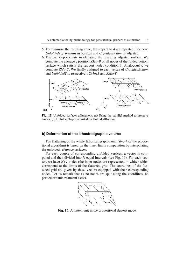
2. UnfoldedBottom and UnfoldedTop are respectively the unfolded bottom and top of the unit (see Fig. 15(a)). Thanks to the correspondence be-tween grids and extracted surfaces, we get the vertices AUnfoldedBottom and BUnfoldedBottom that respectively correspond to ABottom and BBottom. We then use the parallel method in order to reposition ATop and BTop in the simula-tion space and obtain vertices ATop‘ and BTop‘. The parallel method en-sure that the angles between limits and coordlines are respected;

3. AUnfoldedTop and BUnfoldedTop are the vertices which respectively correspond to ATop and BTop in UnfoldedTop. We compute a 2D minimization be-tween the two sets {ATop‘, BTop‘} and {AUnfoldedTop, BUnfoldedTop}. This com-putation consists in minimizing a square error by using the Lagrange multiplier. We obtain a rotation angle and a translation vector;

4. We apply the inverse displacement on the whole set of UnfoldedTop vertices. Thus, UnfoldedTop is adjusted on UnfoldedBottom in the 2D space (see Fig. 15(b));


5. To minimize the resulting error, the steps 2 to 4 are repeated. For now, UnfoldedTop remains in position and UnfoldedBottom is adjusted;

6. The last step consists in elevating the resulting adjusted surface. We compute the average z position ZMoyB of all nodes of the folded bottom surface which satisfy the support nodes condition 1. Analogously, we compute ZMoyT. We finally assigned to each vertex of UnfoldedBottom and UnfoldedTop respectively ZMoyB and ZMoyT.

(a) (b)

Fig. 15. Unfolded surfaces adjustment. (a) Using the parallel method to preserve angles. (b) UnfoldedTop is adjusted on UnfoldedBottom

b) Deformation of the lithostratigraphic volume

The flattening of the whole lithostratigraphic unit (step 4 of the propor-tional algorithm) is based on the inner limits computation by interpolating the unfolded reference surfaces.

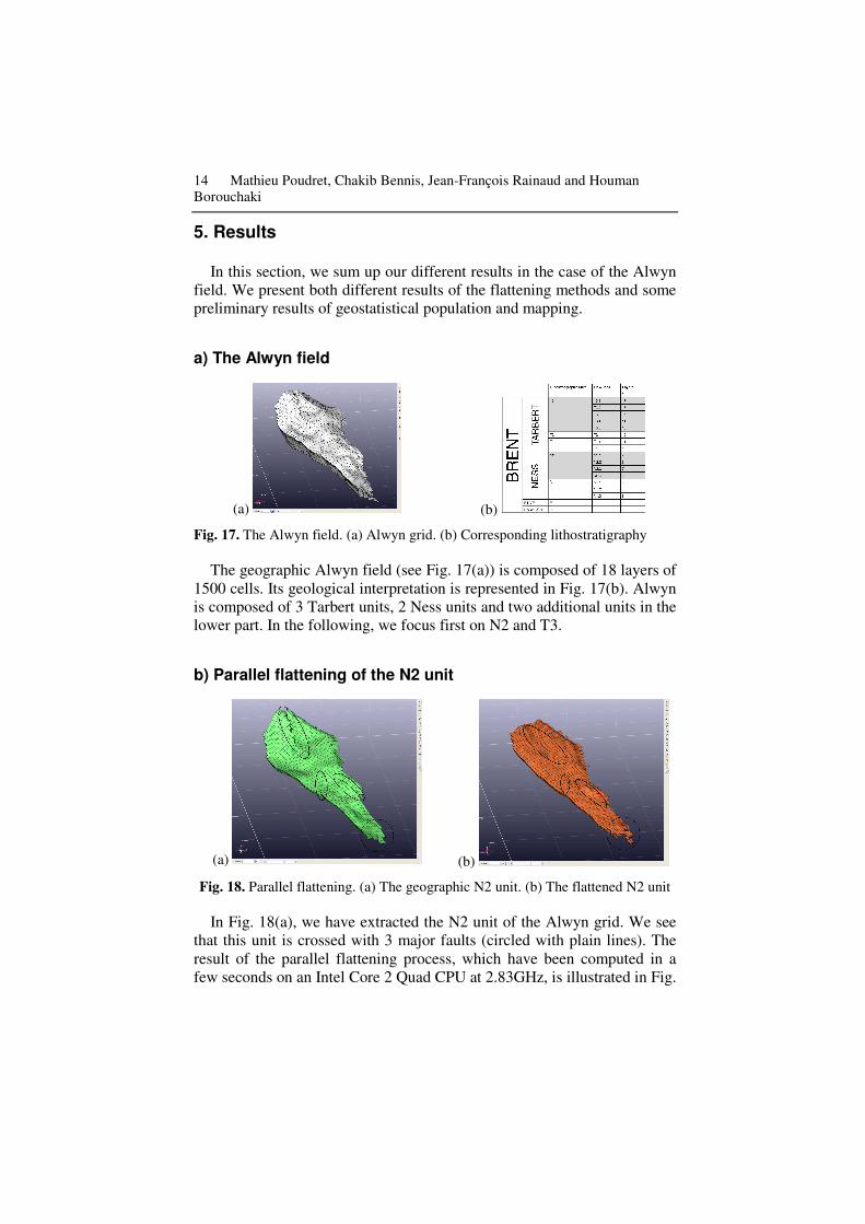
For each couple of corresponding unfolded vertices, a vector is com-puted and then divided into N equal intervals (see Fig. 16). For each vec-tor, we have N+1 nodes (the inner nodes are represented in white) which correspond to the limits of the flattened grid. The coordlines of the flat-tened grid are given by these vectors equipped with their corresponding nodes. Let us remark that as no nodes are split along the coordlines, no particular fault treatment exists.

Fig. 16. A flatten unit in the proportional deposit mode


5. Results

In this section, we sum up our different results in the case of the Alwyn field. We present both different results of the flattening methods and some preliminary results of geostatistical population and mapping.

a) The Alwyn field

(a) (b)

Fig. 17. The Alwyn field. (a) Alwyn grid. (b) Corresponding lithostratigraphy

The geographic Alwyn field (see Fig. 17(a)) is composed of 18 layers of 1500 cells. Its geological interpretation is represented in Fig. 17(b). Alwyn is composed of 3 Tarbert units, 2 Ness units and two additional units in the lower part. In the following, we focus first on N2 and T3.

b) Parallel flattening of the N2 unit

(a) (b)

Fig. 18. Parallel flattening. (a) The geographic N2 unit. (b) The flattened N2 unit

In Fig. 18(a), we have extracted the N2 unit of the Alwyn grid. We see that this unit is crossed with 3 major faults (circled with plain lines). The result of the parallel flattening process, which have been computed in a few seconds on an Intel Core 2 Quad CPU at 2.83GHz, is illustrated in Fig.


18(b). The chosen reference limit was the bottom one. We remark that the 3 fault have been correctly closed.

Two observations deserve to be pointed out. First, in the result, the top

limit is not completely flat. This comes from the behavior of the parallel algorithm. Indeed, only the reference limit is explicitly unfolded. This fea-ture is insignificant in the case of thin lithostratigraphic unit. Secondly, some differences exist between the shape of the unit in the geographic space and corresponding flattened unit (see doted circle in the bottom re-gion). The footprint of the reference surface is often different from the footprint of other limits. Here, some cells of these limits do not have corre-sponding cells in the reference surface. For now, we choose to deactivate these "orphan cells".

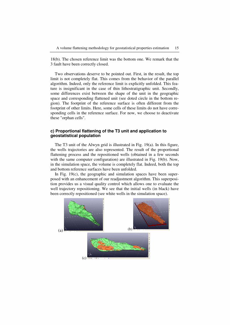
c) Proportional flattening of the T3 unit and application to geostatistical population

The T3 unit of the Alwyn grid is illustrated in Fig. 19(a). In this figure, the wells trajectories are also represented. The result of the proportional flattening process and the repositioned wells (obtained in a few seconds with the same computer configuration) are illustrated in Fig. 19(b). Now, in the simulation space, the volume is completely flat. Indeed, both the top and bottom reference surfaces have been unfolded.

In Fig. 19(c), the geographic and simulation spaces have been super-posed with an enhancement of our readjustment algorithm. This superposi-tion provides us a visual quality control which allows one to evaluate the well trajectory repositioning. We see that the initial wells (in black) have been correctly repositioned (see white wells in the simulation space).

(a) (b)

(c)


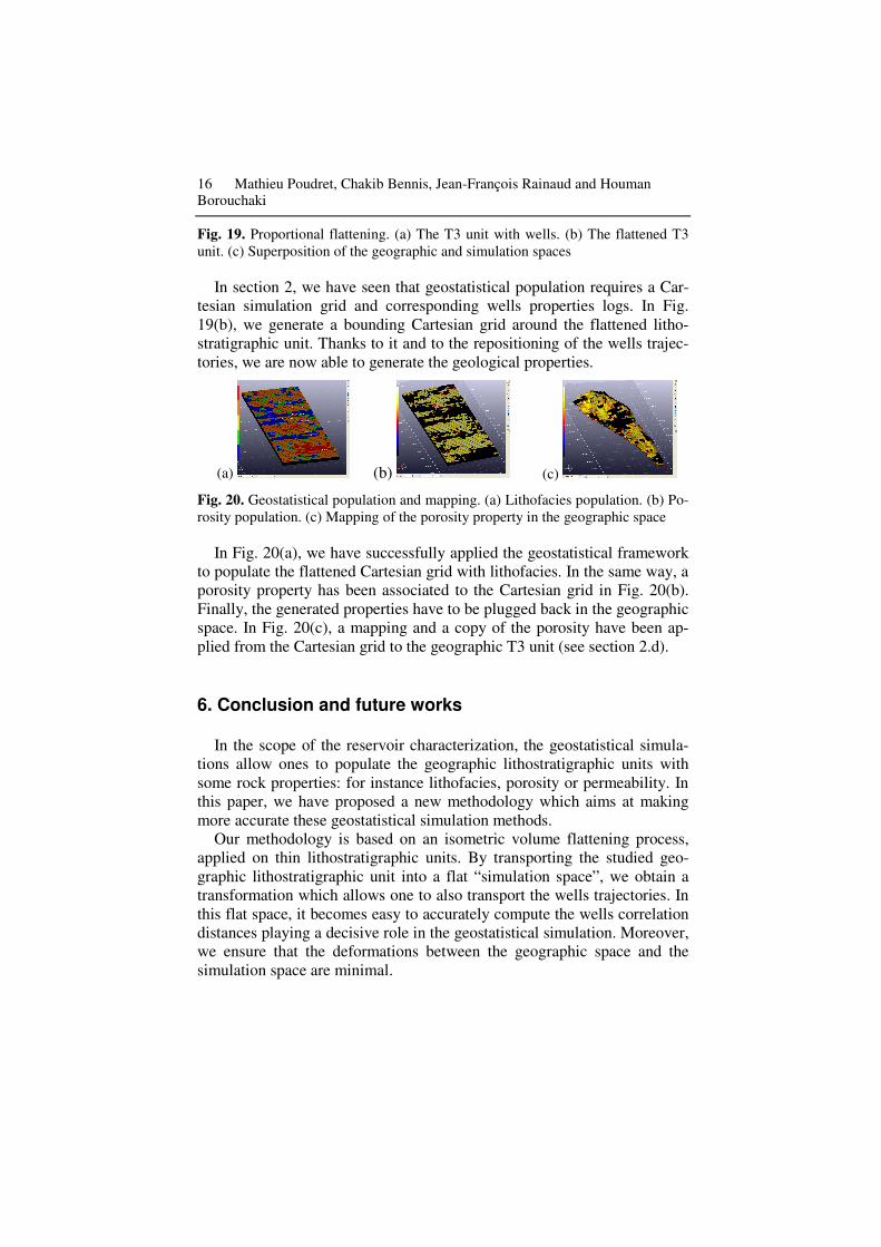
Fig. 19. Proportional flattening. (a) The T3 unit with wells. (b) The flattened T3 unit. (c) Superposition of the geographic and simulation spaces

In section 2, we have seen that geostatistical population requires a Car-tesian simulation grid and corresponding wells properties logs. In Fig. 19(b), we generate a bounding Cartesian grid around the flattened litho-stratigraphic unit. Thanks to it and to the repositioning of the wells trajec-tories, we are now able to generate the geological properties.

(a) (b) (c)

Fig. 20. Geostatistical population and mapping. (a) Lithofacies population. (b) Po-rosity population. (c) Mapping of the porosity property in the geographic space

In Fig. 20(a), we have successfully applied the geostatistical framework to populate the flattened Cartesian grid with lithofacies. In the same way, a porosity property has been associated to the Cartesian grid in Fig. 20(b). Finally, the generated properties have to be plugged back in the geographic space. In Fig. 20(c), a mapping and a copy of the porosity have been ap-plied from the Cartesian grid to the geographic T3 unit (see section 2.d).

6. Conclusion and future works

In the scope of the reservoir characterization, the geostatistical simula-tions allow ones to populate the geographic lithostratigraphic units with some rock properties: for instance lithofacies, porosity or permeability. In this paper, we have proposed a new methodology which aims at making more accurate these geostatistical simulation methods.

Our methodology is based on an isometric volume flattening process, applied on thin lithostratigraphic units. By transporting the studied geo-graphic lithostratigraphic unit into a flat “simulation space”, we obtain a transformation which allows one to also transport the wells trajectories. In this flat space, it becomes easy to accurately compute the wells correlation distances playing a decisive role in the geostatistical simulation. Moreover, we ensure that the deformations between the geographic space and the simulation space are minimal.


In this paper, we have proposed two isometric flattening methods that depend on the deposit mode of the considered lithostratigraphic unit: the parallel one and the proportional one. Finally, we have illustrated our flat-tening-based methodology by populating an actual lithostratigraphic unit.

Surface extension and hole filling

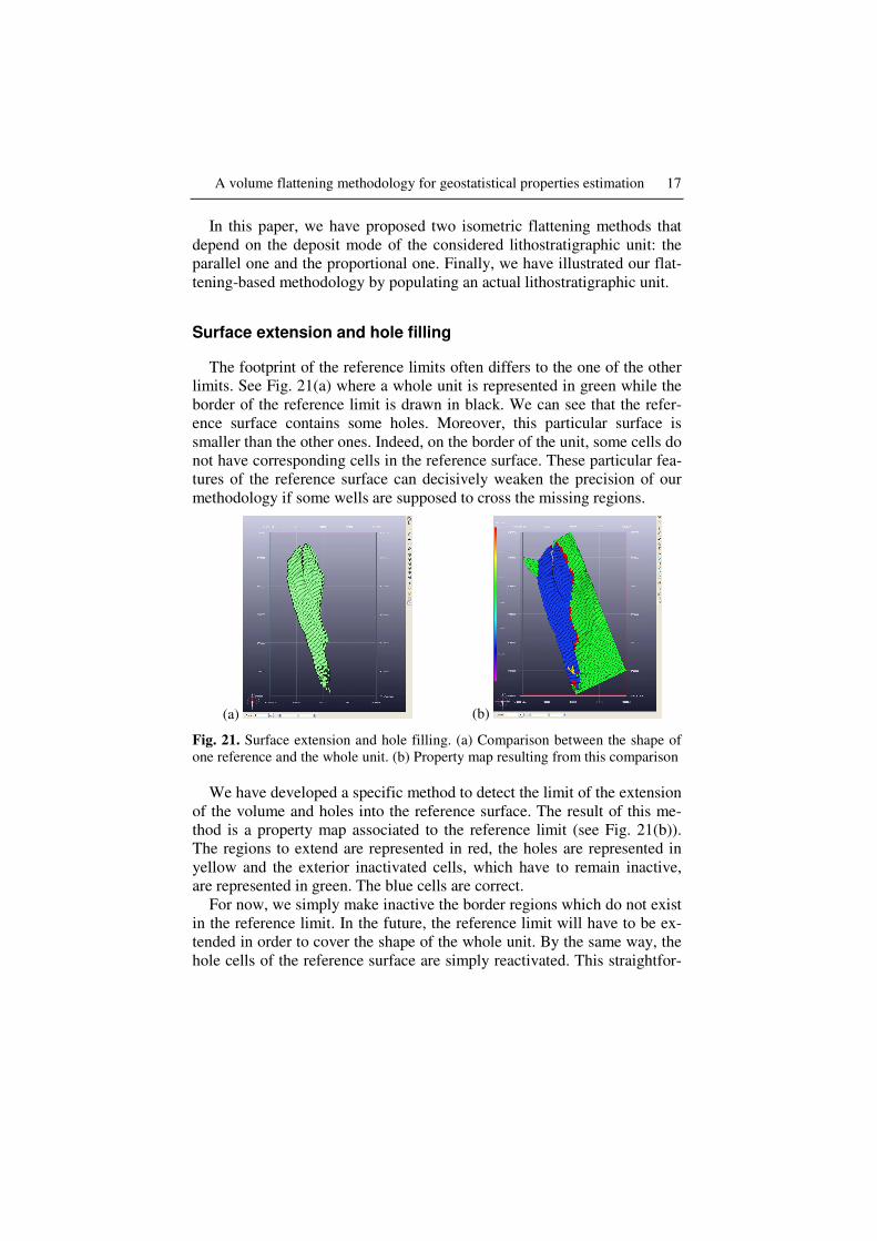
The footprint of the reference limits often differs to the one of the other limits. See Fig. 21(a) where a whole unit is represented in green while the border of the reference limit is drawn in black. We can see that the refer-ence surface contains some holes. Moreover, this particular surface is smaller than the other ones. Indeed, on the border of the unit, some cells do not have corresponding cells in the reference surface. These particular fea-tures of the reference surface can decisively weaken the precision of our methodology if some wells are supposed to cross the missing regions.

(a) (b)

Fig. 21. Surface extension and hole filling. (a) Comparison between the shape of one reference and the whole unit. (b) Property map resulting from this comparison

We have developed a specific method to detect the limit of the extension of the volume and holes into the reference surface. The result of this me-thod is a property map associated to the reference limit (see Fig. 21(b)). The regions to extend are represented in red, the holes are represented in yellow and the exterior inactivated cells, which have to remain inactive, are represented in green. The blue cells are correct.

For now, we simply make inactive the border regions which do not exist in the reference limit. In the future, the reference limit will have to be ex-tended in order to cover the shape of the whole unit. By the same way, the hole cells of the reference surface are simply reactivated. This straightfor-


ward filling solution supposes that the geometry of the inactivated cells is correct. In the future, we will have to develop a true geometric hole filling.

External reference surface

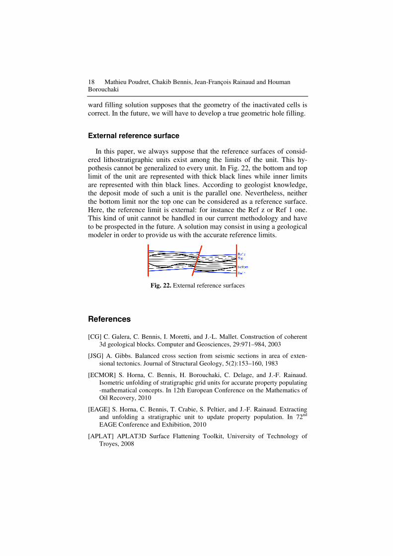
In this paper, we always suppose that the reference surfaces of consid-ered lithostratigraphic units exist among the limits of the unit. This hy-pothesis cannot be generalized to every unit. In Fig. 22, the bottom and top limit of the unit are represented with thick black lines while inner limits are represented with thin black lines. According to geologist knowledge, the deposit mode of such a unit is the parallel one. Nevertheless, neither the bottom limit nor the top one can be considered as a reference surface. Here, the reference limit is external: for instance the Ref z or Ref 1 one. This kind of unit cannot be handled in our current methodology and have to be prospected in the future. A solution may consist in using a geological modeler in order to provide us with the accurate reference limits.

Fig. 22. External reference surfaces

References

[CG] C. Galera, C. Bennis, I. Moretti, and J.-L. Mallet. Construction of coherent 3d geological blocks. Computer and Geosciences, 29:971–984, 2003

[JSG] A. Gibbs. Balanced cross section from seismic sections in area of exten-sional tectonics. Journal of Structural Geology, 5(2):153–160, 1983

[ECMOR] S. Horna, C. Bennis, H. Borouchaki, C. Delage, and J.-F. Rainaud. Isometric unfolding of stratigraphic grid units for accurate property populating -mathematical concepts. In 12th European Conference on the Mathematics of Oil Recovery, 2010

[EAGE] S. Horna, C. Bennis, T. Crabie, S. Peltier, and J.-F. Rainaud. Extracting and unfolding a stratigraphic unit to update property population. In 72nd EAGE Conference and Exhibition, 2010

[APLAT] APLAT3D Surface Flattening Toolkit, University of Technology of Troyes, 2008

Documents

A volume flattening methodology for geostatistical ... · A volume flattening methodology for geostatistical properties ... modeling of the reservoir. ... methodology for geostatistical