Embed Size (px)
Citation preview

Applied Flow Technology

AFT Mercury™ Quick Start Guide
AFT Mercury version 7 .O
lncompressible Flow Pipe System Modeling and Optimization
App/ied Flow Technology
Dynamic solutions for a fluid world ™
CAUTIONI
AFT Mercury is a sophbttcatcd pipe flo\\ anal~ -· program dcsigoed for qualified engineers with cxpenence m pipe 110\\ atW)515 and should not be uscd by untrained individuals. AFT Men.ury i:- intcndcd solcly as an aidc for pipe now analysis engineers and notas a rcplaccmcot for othcr dcsigo and analysis mclbods, including band calculatJons aod sound enginccringjudgment. AU dala gencratcd by AFT Mercury sbould be indepcndcntly verified with olher engioccring mcthods.
AFT Mercury is dcsigned to be uscd only by pcrsons who possess a leve! o[ knowledge consistcnt with that obtaincd in an undcrgraduatc cngineenng coursc in tbe analysis of pipe system fluid mcchanics and is familiar wi1 h standard iodustry practicc in pipe flow anaJysis.
Fonnal training on thc use and application of AFT Mercury is highly recommcndcd, and providcd by Applied Flow Tcchnology.
AfT Mercury is intcnded to be uscd only within thc boundarie~ of its cngineering assumptions. Thc uscr should consult the Uscr's Guide for a discussion ofall cngincering assumptions made by AFT Mcrcury.
lnformauon m 1h1s document i~ subjcct to change without nollce. No part ofth1~ Qu1ck Start GUidC mny be rcproduced nr transmitted in any fom1 ur by any mean~, elcctronic or mcchonical, for uny purpose, without thc cxpress wnllen pcrmiss1on of Aprlicd Flow Tcchnology.
10 2012 Arplied Flow Tcchnology Corporation. All right!> rcscrved.
Printed in thc Unned S tates of ~\menea
"AFT Mcrcury". "AFT Falhom", "Applied Flow Tcchnology", '·Dynamic solutions for a nuid world", ond the AfT logo ore trademarks ol' /\pphcd Flow Tcchnology Corporation.
Lntelhqu•p is a tradcmark of lntclliqulp, LLC.
Chcmpak IS a rrademark of Madison Technical Software. lnc.
Wmdows 1s u rc¡pstcrcd trademnrk ofMicrosoft Corporallon.
Contents
r 1. lntroducing AFT Mercury ............................................... 1
How AFf Mercury works ........................................................................ 1
Analysis vs. design ................................................................................... 2
Analysis ..... ......................................................................................... 2
Design ....... ..................................................... .................................... 3
1 Cost-based opümization vs. co!!.t estimali ng ............................................. 3
AFT Merc ury design capabilitics ............................................................. 3
Typcs of systcms Lhat can be optimizcd ............................................ 3
Opümization parameters available ..................................................... 4
Engineering assumptio ns in AFT Mercury ........................................... ... 4
AFT Mercury pri mary windows ............................................ ................ ... 4
Lnput windows ................................................................................. ... 5
O utput window~ ................................................................................. S
Opt imization terminology ......................................................................... 6
Design variables ................................................................................. 6 De sigo constraints .............................................................................. 6
Acli ve and inactive constrai nts .................................................... 6
Objective function .............................................................................. 6
Continuous vs. discrctc optimization ................................................. 7
Design variable linking ...................................................................... 7
Feasible and infea!\ible designs .......................................................... 7
2. Weight Optimization Example ....................................... 9
Tapies coverecl .............. ......................................................... ................... 9
Required knowledge ................................................................................. 9
Stcp l . Create the model ......................................................................... LO
Summary .. ........................................................................................ 10
A. Layout model ............................................................................... 1 O
B. Select fl uid ................................................................................... Ll
C. En ter data for rcscrvoirs .............................................................. 12
iv AFT Mercury 7.0 Quick Start Guide
D. Enter control \W\"e d:n:J. --------······························· 13 E. Enter pipe data ................ • ............................. J4
Step 2. Setup the optimization data·······--·---·-····························· 15 A. Crea te pipe size range set.. ....... ................................................... 15
B. Creale a control val ve consu-aim sel ····-·-·······- ························ 17 Step 3. AppJy optimization data .......................... ................... ....... 0 ........ 18
A. Apply optimization data to Pl ......................... 0 ........ 0 . ..... . ........... 18
B. Apply optimization data to P2 ..... ................................................ 19
C. Apply optimization data Lo J2 (FCV) ....... ... ....... ......................... 20
Step 4. Specify Optimizalion ConLrol... ............. ..................................... 2 1
Step 5. Run the OpLimiL.ation ....................... .................... 0 . . ................... 22
Step 6. Review optimization results ............................ .. ............ ........... .. 23
Conclusions ................................. ................................ ......... ... ............... 25
3. lnitial and Lite Cycle Cost Optimization Example ..... 27
Tapies covered ........... .......... o • • •• • • 0 ....... . ...... .. . . ........ . ............ . .. . .... . ...... . .... 27
Requircd knowlcdgc ........................................................ 0 ...................... 27
Model files .... 0. 0 . . .. o. o ............................................... o .. o ............................ o 28
Oplimization goaJs ................. ..... o·······-0·················································· 28
Getting started ............. o.o·o···oooo•···o···········o···················o·······o···o····o·········· 28 Review Opti mization Control .... 0 .... o ••• 0 ... 0 .. 0 ................ o ..... .......... 0 .. 0 ....... 0 29
Review databas es .............. ....... ................... o ••••• • o • • • • •• • •••••••••• 0 ••••• • •• 0 ••• • ••• • • 31
Review pipe oplimizatiun setup ................... o ............................ . 0 ..... ..... o 32
Pipe size range sets .................... 0 ....... 0 .................... 0 ....... 0 ................ 33
Pipe constraint sets ........ o .. o ........ o ................ o ............... o ....... o ....... o ... o. 34
Pipe link.ing .. 0 .. 0···0············································································ 35 Creating pipe size range sets and constraint sets ............................. 36
Review junction optimization setup ............. ............................. 0 ............ 37
Optimizing systcms with pumps ... ................ ......... .......................... 38
Modeling a pump as a fixed t1ow .............................................. 40
J unction costs ................................................................................ ... 41
J unction constraint sets .o .. o ........ 0 •••• 0 .......... o ...................................... 41
Crcating junction constrainl sets ................ 0 ....... 0······0············ .. ··0 ..... 41
Table of Contents v
Unc.Jcrstanding the modc1 ........................................................................ 42
Running tbe sccnarios and interpreúng rcsuhs ....................................... 4-+
Scenario to minimjze tirst co•a ......................................................... 4-+
Optimized pipe si7.cs .................................................................. 46
Cbeck.ing so urce of cost data ..................................................... 46
Scenario Lo minimize life cycle col>t for 20 year<. ............................ 47
Optimizing with pump curve data .......................................................... 51
Conclusion~ ............................................................................................ 51
4. Multíple Design Case Example ................................... 53
Topics covered ............... ............... .......................................................... 53
Rcquircd knowlcdgc ...... .................... ..................................................... 53
Model files .............. ....... ......................................................................... 54
Optirni7alion goals .................................................................................. 54
Gctting startcd ......................................................................................... 54
Review model ......................................................................................... 55
How the dependent design c<u;e wa~ crcatcd ................................... 57
Run the optin1ization .............................................................................. 63
Considcr the resuhs ................................................................................ 65
OptimiLe for three pipe siL.el> .................................................................. 66
Run the optimization .............................................................................. 67
Other po~~ibilities ................................................................................... 68
5. Other AFT Mercury Capabilities .................................. 69
Optimite with operating costl> spread over multiple cal>el> ..................... ó9
Yary rccurring costs over tin1e ............................................................... 69
Time vaJuc of tnoncy .............................................................................. 70
OptimiLe life cycle costs wiLh constrarncd initial cost ........................... 70
Determine cost effectiveness of replacing exil>tmg pipe ........................ 70
Working with different currcncics .......................................................... 70
Col>t!-. Vl>. si .le ........................................................................................... 70
OptimiLing rectangular duct sy~tem~ ...................................................... 71
Compare YFD vs. FCV optimi7ed systems ............................................ 71

vi AFT Mercury 7 .O Quick Start Guide
Maximum cost groups ········--------····· .......................... 71 (
Nerwork database~. ·············--··· - ···················· ............ 71
1
1

71
71 C HAPTER
lntroducing AFT Mercury
Welcome to AFT Mcrcury™ 7.0, Applied Flow Technology's powerful pipe and duct syMem optlmization tool. With AFT Mercury you can automaticaUy siLe all pipes or ducts in your c;ystcm tu mi nimi.te monetary cost. weight. volurne. or surface arca. ln addirion, you can concurrently siL.e the pumps and pipes to obtain the absoiUlc lowcst cost system that satisfies your design requirements. Finally. by accounling for non-recurring amJ recurring cosL~ . ynu can optimile pipe and duct systems to rninimi ze lifc cycle cost~ over sorne spec1fied durauon.
How AFT Mercury works
AFf Mercury cons ists uf three basic cJement~: the Graph1cal Interface, Úle Hydraulic Solver. and the Optimizalion Engi ne (i.e., the Optill'l.Uer). Figure 1.1 shows the relationship bctwcen the three.
Figure 1.1 AFT Mercury main component flow chart

2 AFT Mercury 7.0 Quick Start Guide
The Hydmulic Sol\er obuún' a balanced h)draulic solution for a spccific pipe or duct -}s1em. The Optimizer then modifies Lhe design, and the Hydraulic Solver C\alua~.., the modifioo design. The Optimi t.er continues Lh.lli process umil 11 ts l-atistied that no funher design improvements are posstble. AL thts poinL the Optir:nUer has converged on a design. and lhe re~ulting op1imiLed de!>ign is then sent back to the Grapbical Interface where it is displayed 10 the uSt.~.
The Hydraulic Solver, which functions as the pnme mover in perforrning an engineering analysis (e.g., AFf Fathom™). becomes a subroutine calied by the Optirnizer. The Optimit.er i ~ the prime mover in AFf Mercury.
The Hydraulic Solver in AFJ' Mercury was derived from AFf Fathom. a leading commercial ptpe flow analysi~ product with many years of industrial use to its credit.
The optir:nUation engine employcd by AFT Mercury uses state-of-the-art opt.imization lechnology liccnscd from Vanderplaats Research and Development, lhe lead ing company in op1imit.ation technology. VR&D's Lechnology has been used for many ycars in engincering design. with cxtcnsive use in strucwml tinitc c lcmcnt analysis.
Analysis vs. design
Analysis
Traditional piping system engineering has employed pipe fiow analysis. Engineering analysis is Lhe process of using acccptcd calculation methods to predict the behavior of a given system. These calculation methods may be manual or automated in a computcr program.
The weakne!.l. of analytical mcthods is that they require the specification of the sysLem befare lhe methods are applied. Specifically. the pipe or ducts siL.es, pump, val ve and other equipment must be specified in arder to perform the calcu lation.
However. whcn a new pipe sy~tem is bcing designed, these parameters are not known. To use Lhe analytical methods, the engineer must guess at lhe pipe sizes and required equipment, pcrform thc analysis, Lhen motlify his or her original selections a.~> necessary.
The analytical metho<h are used íteratível} to arrive ata final design.
a
1
S
Chapter 1 lntroducing AFT Mercury 3
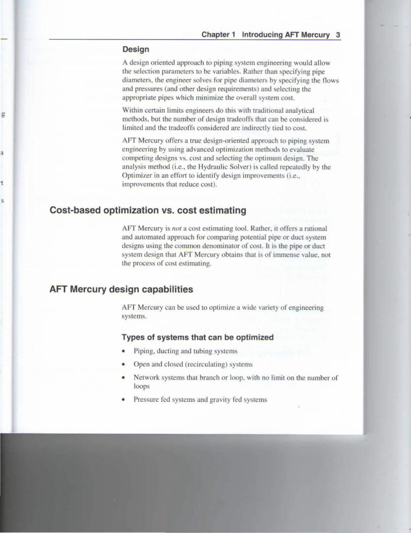
Design
A desi!,rn oriented approach to piping system engmt:ering would allow the selection parameters to be variables. Rather than <,pecifying pipe diameten,. Lhe engineer sol ves for pipe diameten. by specifying thc flows and pressures (and other design requ1remems) and 'ielecting the appropriate pipes which minimize the overall '-Y"tem cost.
Within certain limits engineers do this with traditionaJ analytical mclhods, but the number of design tradcoffl> that can be considered is Jimitcd and lhc tradeoffs considcrcd are ind1rcctly ued to cosL.
AFf Mercury offero; a true design-orienteu approach to piping systcm engineering by using advanced optimiLation methods to evaluate competing designs vs. cost and selecting the optimum design. Thc ;malysis melhod (i.e., thc Hydrau lic Solver) i~o. called repeatedly by thc Optimizer in w1 effort Lo idcntify design improvemt:nb (i.e .. improvements that reduce cost).
Cost-based optimization vs. cost estimating
AFf Mercury is nora cost estimaling too!. Rathcr. it offer'\ a rationaJ and automated approach for comparing potential pipe or ductl>ystem design~ using Lhe common denominator of cost lt b, lhe pipe or duct sy'item design Lhat AFf Mercury obtains that 1s of unmense "aJue, not the process of cost eslimating.
AFT Mercury design capabilities
AFf Mercury can be u sed to opti mize u wide variet) of engineering systcrns.
Types of systems that can be optimized
• Piping. ducting and tubing systems
• Open and cJosed (recirculating) systems
• Network systcms lhat branch or loop. ~ith no limit on the number of loops
• Pressure fcd systems and gravity fed S}Stcms
4 AFT Mercury 7.0 Quick Start Guide
• Pumped systems. mcludmg - - in parallel or in series
• Pumps wilh variable speed. controUedpres.;;;ure. conrrolled flow, and viscosity corrections
• Systems with pressure and/or OO\\ control vah-es
• Systems with vaJves closed and pump~ turned off
• Systems with heat transfer and encrgy balance
• Systems with variable density and viscosity
• Systems wiLb non-Newtonian lluid behavior
Optimization parameters available
• Pipe size
• Pipe velocily, pressure gradient, pressure. and l1ow
• Pump head rise, NPSH margin, proximity to BEP (Best Efficiency Point), power, ami others
• Control vaJve pressure drop an<.l open percentage
Engineering assumptions in AFT Mercury
AFf Mercury is based on lhe following fundamental Quid mechanics assumplions:
• lncomprcssible flow
• Steady-state conditions
• One-dimensionaJ flow
• No chemical reactions
AFT Mercury primary windows
AFT Mercury has live subordinate windows lhat work in an integr'dted fashion. You work exclusively from one of these windows at aJl times. For lhis reason they are referred to as Primary Window:;.
and
y
J
Chapter 1 lntroducing AFT Mercury 5
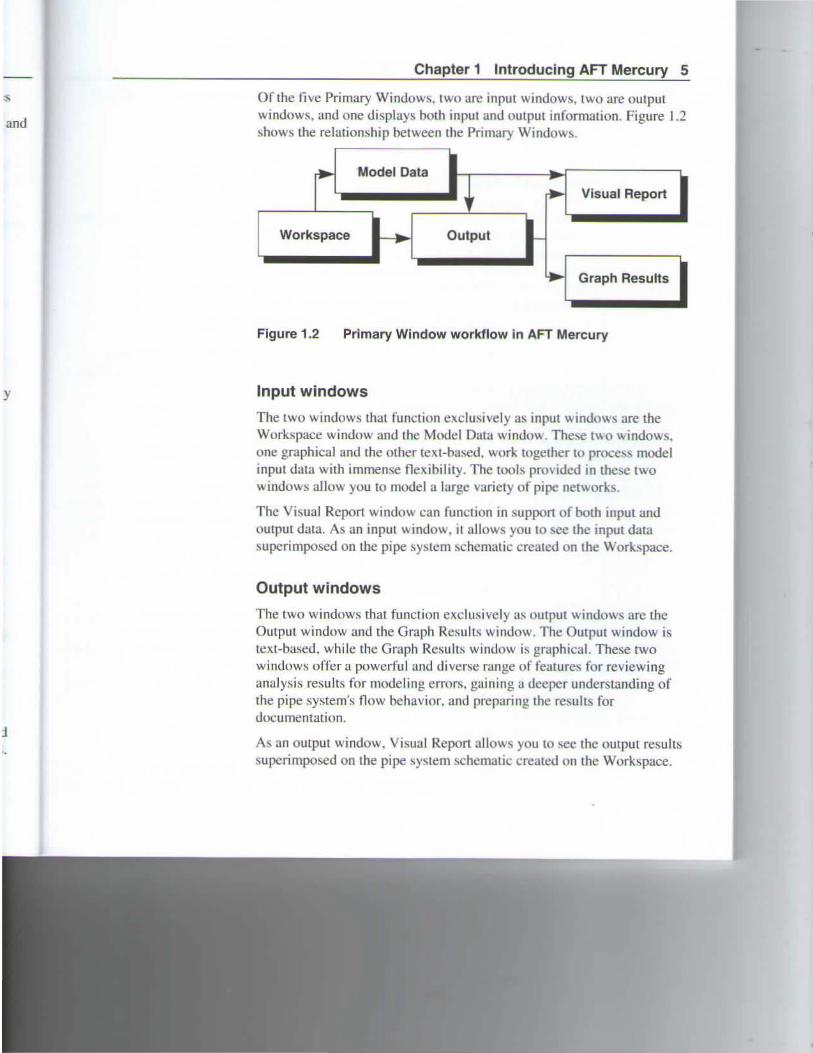
Of Lhe five Primary Windows, two are input windows, two are output windows. and one displays both input and oulput infonnation. Figure J .2 shows lhe relationship betwcen the Pnmary Window1..
r Model Data -,¡, ~ Visual Report
Workspace .. Output ,....... ~
~ Graph Results
Figure 1.2 Prlmary Window workflow in AFT Mercury
Input windows
The two windows Lhat funclion exclusively as input windows are che Workspace window and the Motlel Data window. These mo windows. one graphicaJ and lhe other text-based. work together to proce model input data wilh immense tlex ibility. The tools provttled in Lhe~e rwo windows allow you to model a large variety of pipe nerworks.
The Visual Rcport window can functjon in suppon of both input and output data. Asan input window. 11 allows you 10 sce Lhe mput data supcrirnposed on Lhe pipe system schcmatic created on the Wor~space.
Output windows
The two windows that function cxclusively a." o utput windows are che Output window and the Graph Results window. The Output window is text-based. whi le the Graph Results wintlow is gr..tphical. These two windows offer a powerful and di verse runge of features for reviewing analysis results for modeling errors, gaining a deeper understanding of the pipe system's flow bchavior, and preparing the results for documentmion.
Asan output window. Visual Report a llows you to \ee the ourput results supcrimposed on Lhe pipe system schcmatic created on the Workspace.

6 AFT Mercury 7.0 Quick Start Guide
The five Primary WtndO\\' fo~ a ughíl) ~ highly efficient system for cntering. proce-.!\ing. a.nalyzin;. md cb..-umenting incomprcssible now analy~e:. of pipe netwod::: ....
Opti mization terminology
General optimizalion terminology applicd to ptpe S} !>Lem ... is as follows:
Design variables
Thc dcsign variables in AfT Mercury are thc pipe sizes.
Design constraints
There are numcrous design constraints in AFT Mercury. Common constraints are pipe velocity, control val ve pressure drop and proximity to pump NPSH and BEP (Best Efficiency Point).
Active and inactive constraints One constraint type is pipe velocily. One may setlhe maximum to 1 O feellsec, and the mínimum to 2 feetlsec. lf the final pipe velocity were 9.9 feet/sec, the maximum velocity constraint would be aclive bccause tbe fmal value of the velocity is at or near lhe maximum velocily. On the other hand. the 9.9 feet/sec pipe velocity is far away from lhe 2 fcct/scc mínimum. lf we remove the mínimum velocity constraint, the result will still be an actual pipe velocily of 9.9 feet/sec. Thus the minimum velocity constraint is inactive and does nol influence the pipe size selectcd by the optimizer.
On the other hand, if one removed thc 10 feetlsec maximum velocity constraint. the actual vclocity would probably increase above 10 feet/sec, thus rcsulting in a differcnt pipe size. The maximum velocity is acti ve in thal if we change or remove the constraint the selected optimum would change. Changing or removing inactive constraint<. have no effect on the selected optimum.
Objective function
This is thc cost of the system. The cosl can be monetary or can be based on wcight. volume or sorne other parameter. As AFr Mercury varíes rhe
.vs:
tty
e !he ec .vi 11
ds
1ve
ed the
Chapter 1 lntroducing AFT Mercury 7
pipe !otiLes, the cost of thc pipes and associatcd cquipmcm varíes. The optirni.wtion enginc scarches for combinations of pipe sizes lhat minimi:res the objcctivc function (i.c .. cost).
Continuous vs. discrete optimization
Most commercial pipe comes in discrcte sizes (e.g., 1 inch. 2 inch, 3 inch, etc.). Whcn dea ling with discrete data. AFT Mercury evaluates tJ1c best combination of discrete pipe sizcs. lf. on the other hand. it is possible Lo obtain thc pipe in any sizc. the pipe siLes are continuous. AFT Mercury can find continuous optimums in add ition to discrete optimums. Tbc continuous opúmum should provide a better design tban the discrete. and is used usa basis for the discrete optimi~llion whicb is normally thc goal.
Design variable llnking
Thc optimization procells takcs longer al> thc number of p1pe~ of potcntially different size increases. FrequenLI) there are group!-. of pipes in your sysrem which either you want to be of !he same 'i7e for design purposcs. or mullt be the same size by virtue of their location in Lhe systcm. To do this one can Link pipes. Whcn one links pipell. one is saying that the linked group of pipes all must bave !he -.ame p1pe size, and be the same material and schedule. class. or type. A hnketl group thus collapses the i ndi viduul pipes that are pan of that group tn a 1>ingle design variable for thal group. There can be multiple linked groups in a modcl.
Feasible and infeasible designs
A feasible design is one which sat.isfics all constrainb, while an infeasible design docs not satisfy onc or more con. traints. There are many ways you can crcate a model that has no fe~ible solution. Here is any ea!> y way: Conncct a pipe toan assigned pressure Junction sct to 200 p~ig. Then place a constraint on lhe pipe that it cannot have a prcssure greater than 100 psig. Since the pipe is connected toan assigned pressure j unct.ion at 200 psig, therc is no \\a} for it to '>atisfy thc J 00 p:..ig constraint. Thus. no reasible solutton exists.

8 AFT Mercury 7.0 Quick Start Guide
e
V
CHAPTER 2
Weight Optimization Example
Topics covered
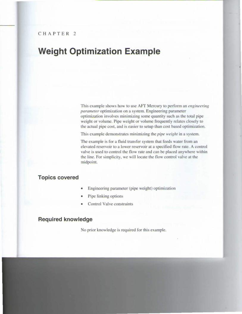
This cxample shows bow to use AFT Mercury to perfonn an engineerin~ parameter optimüation on a system. Engineering parameter optimizatjon involves minimi¿mg sorne quantity ::.uch a~ the total pipe weight or volumc. Pipe weight or \IOiume frequently relate<> clo. el y to the actual pipe cost, and is casier to setup lhan cost based optimization.
Tlús example demom.trates minimizing the pipe weiglu in a -.ystem.
Thc example is for a fluid transfer system lhat fceds water from an elevated rcl-Jervoir toa Jower reservoir ata specified tlO\\ rate. A comrol val ve is used to contro l the flow ratc and can be placcd anywhere within the Jine. For ~implicity. we wi ll locate thc tlow comrol valve <ll the midpoint.
• Engincering parameter (pipe wcight) optimizallon
• Pipe linking options
• Control Val ve constmims
Required knowledge
No prior knowledge is rcquircd for this example.
10 AFT Mercury 7.0 Quick Start Guide
Step 1. Create the model
Summary
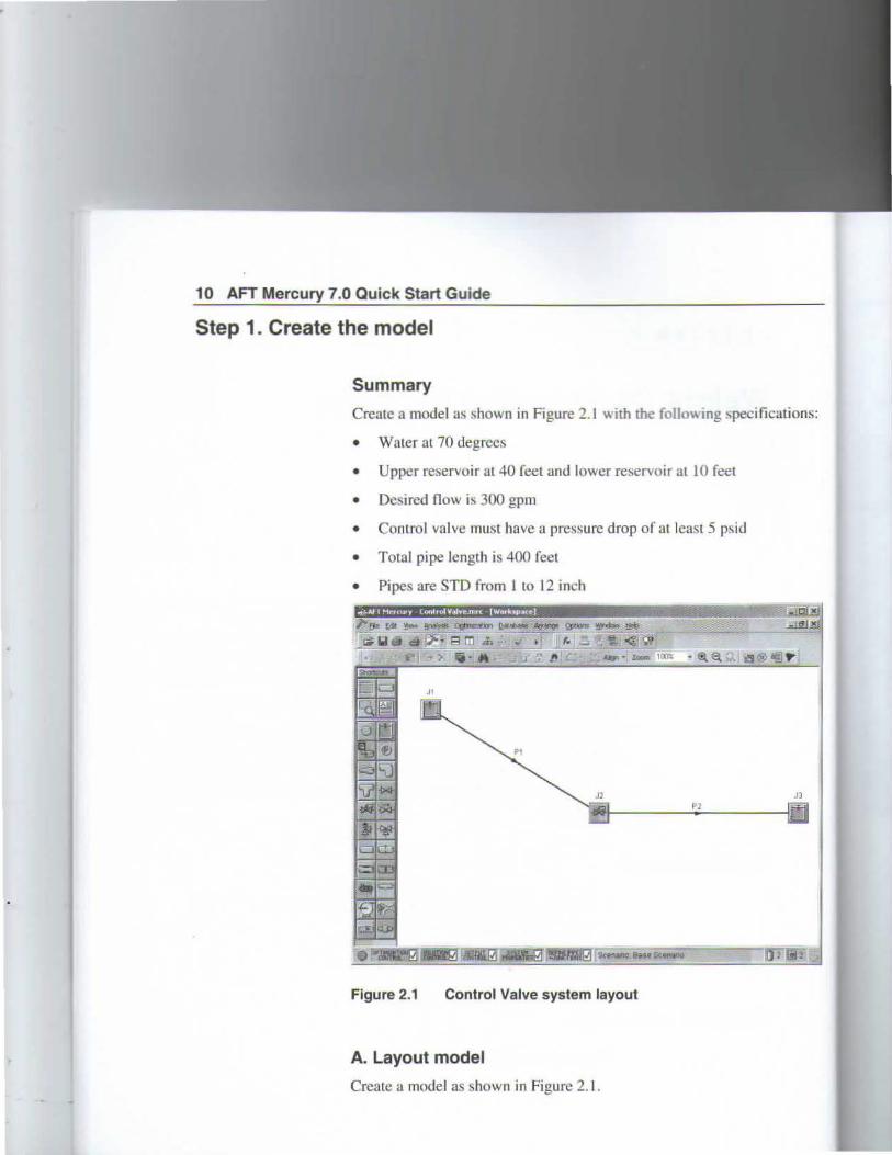
Create a modelas shown in Figure 2. 1 with the fo llowing !>peci fications:
• Water aL 70 degrccs
• Upper reservoir at 40 feet and lower reservoir at 10 feet
• Dcsired flow is 300 gpm
• Contro l val ve must ha ve a pressurc drop of at lcasL 5 psid
• Total pipe length is 400 feet
• Pipes are STO from 1 Lo 12 inch
Figure 2.1 Control Valve system layout
A. Layout model
Creale a modelas shown in Figure 2. 1.
ions:
!lm!1
!...___
:0
ti
Chapter 2 Weight Optimization Example 11
l. The threc juncLions, J 1, J2 and 13. can be dr<~gged from the Toolbox at the left and dropped on Lhe Workspace.
2. The two pipes, P l and P2. can be drawn on lbe Workspace by clicking the Pipe Drawing Tool at the uppcr right of thc Toolbox and then drawing lincs on Lhc Workspace. Makc sure Lhe dirccLional arrows poinl from J 1 Lo J2 antl Lhen J2 Lo J3. (The tlow dircction can be reversed by use of the Reverse Direction too! on Lhe Arrange menu.)
B. Select fluid
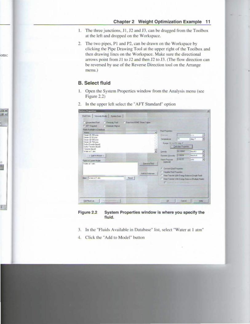
l . Open the Syslem Propcnics window from the Analysi!. menu (scc Figure 2.2)
2. In the uppcr lcft select the "AFf Standard" option
{1 .. (• .. 1 \ioc,,..,.,,.¡J s.-!i.u 1
u-twfUol ~FW o...-,..M[-IP,
~ "'"-· ~.N-
-·-,.o.- fUd-1!!& ·1 a !•n • ]50 DN t ,_@!>il-
, __ il S...@!>.O-
s.,...,@ 1'1l¡:..a ~ ~ .. o...,.¡.llqudJ
Syj'u1 lur~ !lk:Jidl I...._Jloo.-ll ;j YhJkif.l!) 41'ITI J.!""''Y
• ~IO .. odtl • i f>-. ;:] 'JmnC•..,...~oott V-"-l- a r-.. ~ ~
. cr ..... (Lo!,..._
l'
----~ ~ !
r. u..,¡- t._.....,. .. 1\odi
r H..,l_ -~.....,.,._r._
r
Figure 2.2 System Properties window is where you specify the fluid .
3. In thc "Fluid'i Availablc in Databasc" üst. select "Water at 1 mm"
4. Cl ick the "Add lO Model" button
"
12 AFT Mercury 7.0 Quick Start Guide
5. In tbc Tcmperature field type 70 a.eg F
6. Click the "Calculate Propenjes buuon (Lhi.s obtains the density, viscosily ami vapor pressure)
7. Cl ick the OK button to el ose the \\indo\\ and accept the fluid data for the model
~ 11"'1!.'&111! JSUC>OIJil•oi<
U~Uót~~ • Jí-----..:......=-~
, ~mt.,i\o..,.J¡t.. J
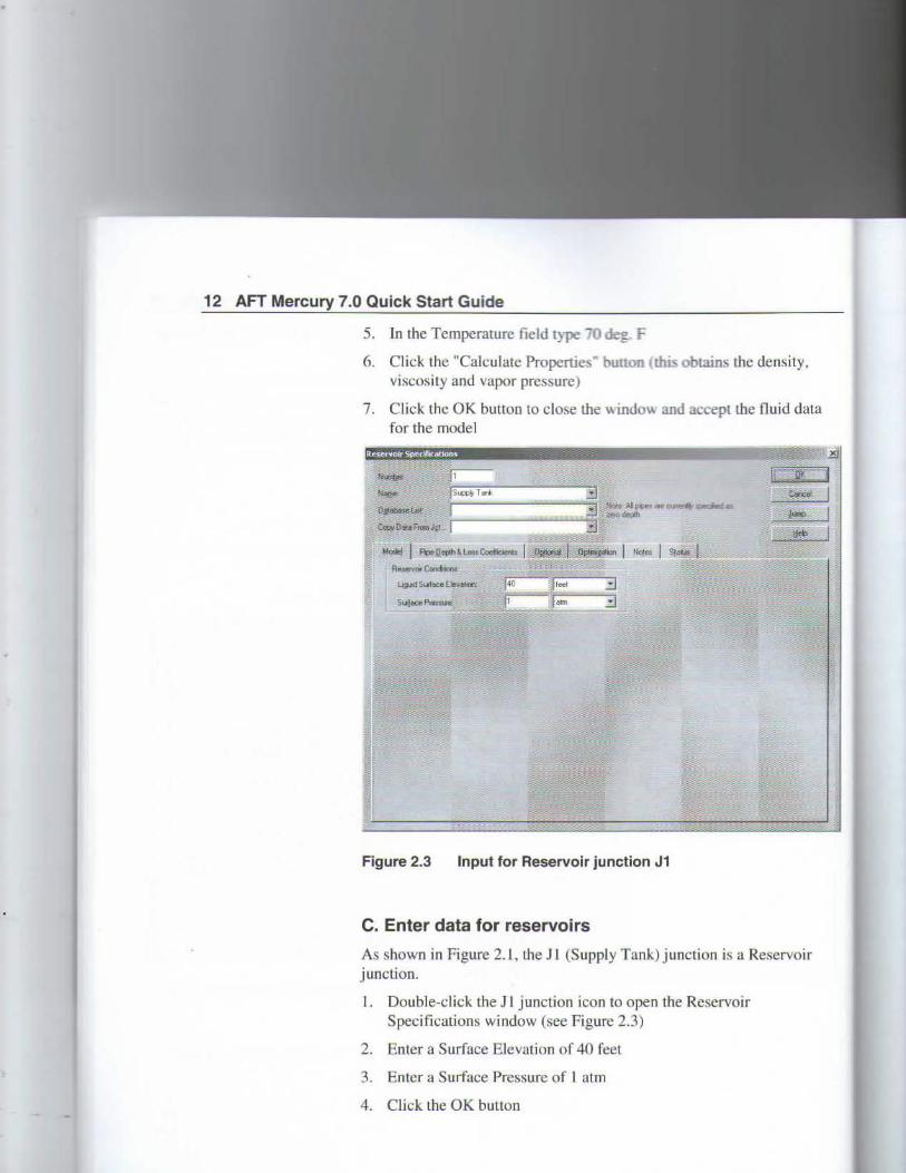
Figure 2.3 Input for Reservoir junction J1
C. Enter data for reservoirs
As shown in Figure 2. 1, the J 1 (Supply Tank) junction is a Reservoir junclion.
l. Double-click the Jl junction icon to open the Reservoir Specifications window (see Figure 2.3)
2. Entera Surface Elevation of 40 feet
3. Entera Surface Pressure of 1 atm
4. Click the OK button
ty.
data
ttr
Chapter 2 Weight Optimization Example 13
Repeat thls process for junction J3 (Discharge Tank). but use a Surface Elevation of 1 O feel.
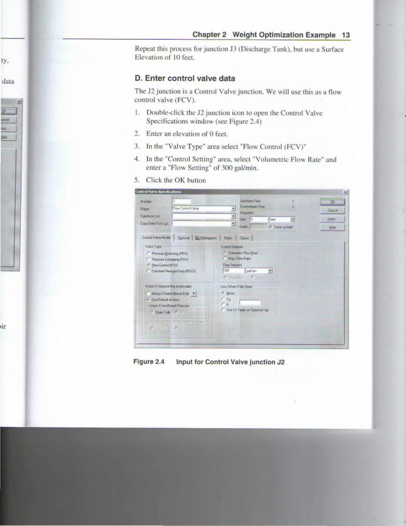
D. Enter control valve data
The J2 junction is a Control Val ve junction. Wc will use Lhis as a tlow control valve (FCV).
l. Double-click thc J2 junction icon lO open Lhe Control VaJvc Specifications window (see Figure 2.4)
2. Emcr an elevation of O feet.
J. rn the "VaJve Type" arca sclcct "Fiow Control (FCV)"
4. ln Lbe "Control Selting" area, selccl ''Volurnctric Flow Rate" and enter a "Fiow Setting" of 300 gallmin .
5. C lick the OK bullon
"""*' u_..rw 1 ti• 1 a a---~ l 11-
V.-,.,l.ilt
Cl.l;oyl) .. f.,..JJ;t 1
VIM':P>
,.. -...¡¡f!6nooii'RVJ r "'"- ;...w.r.o IPSYI • fboC.,..,,JtVl Ccr.:lri~(hop!POCV¡
-R~lll.at~
r .. _ra.,.,¡¡;¡.....,r .. 2J 1 w u .• l.ld...f A<:iooow
E~oyot .... a lniol ro:---1 .... a cl IMK r-- ;;; . ...,..,,..,
r. ·~f"'tllt
r Cx ,.. ~
3
(" llwC• lollitonOptQnillilo
Figure 2.4 Input for Control Valve j unct ion J2
c..:.! 1 ~ 1 t-4 1
14 AFT Mercury 7.0 Quick Start Guide
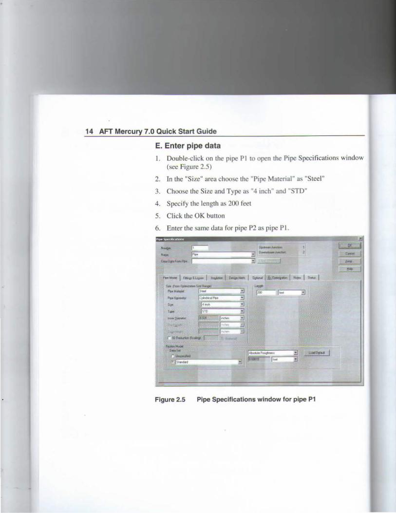
E. Enter pipe data
l. Double-cJick on the pipe PI to open lhe Pipe Specifications window (see Figure 2.5)
2. Tn the "Siz.e" area choose thc "P1pe Material" as "Steel"
3. Choose thc Sizc and Type as "4 inch' and STD"
4. Specify the length al. 200 feet
5. Click thc OK button
6. Enter the sarne data for pipe P2 as pipe Pl.
r..-.~
..... "" 'l" U....:.W
u.-...~~~---------3~9 ~~
---~~-_¿] 1
r-(s~M>~Wrd :.c..:..._ _______ _
Figure 2.5 Pipe Specifications window for pipe P1
1S window
;.;;Í: .. . TU! t= ~r. =j
r..-.:.,¡1
*""' ~m 1
Chapter 2 Weight Optimization Example 15
Step 2. Setup the optimization data
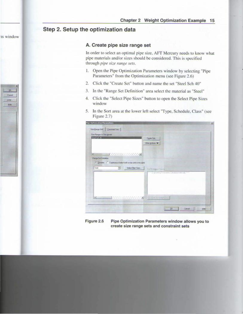
A. Create pipe size range set
In order lo select an optimal pipe site. AFf Mercury needs to know what pipe materials and/or si1cs sho uld be considered. This is ">pecified through pipe si:e range sel.\.
l. Open the Pipe OptimiL.ation Parameters window by sclecting "Pipe Parameters" from the Optimiattion menu (see Figure 2.6)
2. Click the "CrcaLc Sct" button and name the set "Sted Sch 40"
3. ln U1e "Range Set Definilion" area select thc material as "Steel"
4. Click the "Sclect Pipe Siz.cs" bulton lo open the Select Pipe Sizes window
5. In the Sort area at the lower left select "Type, Schedule, Class" (see Figure 2.7)
~-I:!M'9o~•l e-~ 1 s ... R._"''""""""'
..:J
Figure 2.6 Pipe Optimizatlon Parameters window allows you to create size range sets and constraint sets
"
16 AFT Mercury 7.0 Quick Start Guide
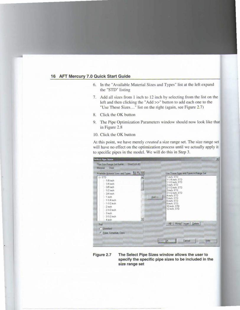
6. (n the "Available Material Sizes and Types" List at lhe Jeft expand the "STO" Jistmg
7. Add all sizes from 1 inch Lo 12 inch by selccting from the list on the left and then clicking the "Add >>" button Lo add each one Lo lhe "Use These Sires ... " list on lhe right (again, sce Figure 2.7)
8. Click lhe OK button
9. Thc Pipe Optimizution Paramclers window should now look like tbat in Figure 2.8
10. Click thc OK buuon
At this point, wc havc mcrely creared a si.le range set. Thc size rangc sct will have no effect on thc optimization process until wc actually apply it to specific pipes in the modcl. We will do lhis in Step 3.
Selet t Pipe Slles · ·~~1 ,
l"p: Saofl4<9!'SetNIII'It'- StcetS •40 ~
Figure 2.7
1 rclt STO 1114 111eh. S lO 11/2ncl1. STO 2 1nCh. STO 2·112...:11 STO 3 •nch. STO 3-1/2nc11. STO 4 1nch. STO S n:h. STO &inch. STO 8n:h. STO 10inch STO 12n:h. STO
The Select Pipe Slzes wlndow aJiows the user to specify the specific pipe sizes to be included In the size range set
j
'iel
it
:X
Chapter 2 Weight Optimization Example 17
s.s-s"' 1 ~""""' 1 ~ ... nW'!ID4"' ,,.~
hd\~Tt 1 11~ ..cl SID IVZ•• I $Tll l<• l sm ? l/11rk-h sm )IO,h STD l lfltn<h STD •-sw ~"""' SH> s.....,sw iMHO 1 IIY'k ,,r, .
ll;p.s.t . J IJ!iWtfl'•••" • 1
.!.J
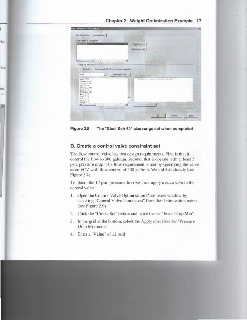
Figure 2.8 The "Steel Sch 40" size range set when completed
B. Create a control valve constraint set
Thc tlow control valve has two dcsign requirements. First is thattl control thc flow to 300 gal/min. Sccond, Lhat it operatc with atleast 5 psid prcssure drop. The flow rcquirement is met by specifying the valve asan FCV with flow control of 300 gaJ/min. We did thic; alrcady {c;ee Figure 2.4).
To ohtain the 12 psid pressure drop we must apply a constramt to the control valve.
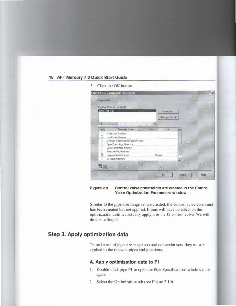
l. Open lhe Control Valvc OptimiL.aLion Parumeterl> windO\\ by sclccling "Control Yalvc Paramctcrs" from Lhe Optimt7ation menu (scc Figure 2.9)
2. Click the "Create Set" hutton and name the sct "Pres~ Drop Min"
3. In thc grid at the bottom, sclcct the Apply checkhox for 'Pressure Drop Mínimum"
4. Entera "Valuc" of 12 psid
18 AFT Mercury 7.0 Quick Start Guide
5. Click the OK buuon
Control Vt~IVt! 01Jtlllltznt.ion r .nllHUele.rs -
lie<'Jdl.ouM...-un
He<'Jdlon MI'lll1liAn Mi11mum M111g1nAboveVapo. P,......-. Oper> Percentage Ma¡num
Open Percerlage M ..........
Pruu~Dr!!>M-.un
~ PreuureDropM......,
Cv V .m. Ma1C111Un
Other~ • f
12 psir:l
Figure 2.9 Control valve constraints are created in the Control Valve Optlmizatlon Parameters wlndow
Similar 10 Lhe pipe sizc range set we created, lhc control valvc constmint has been creaLed but nol applied.ltthus will havc no effect on the optimization unti l wc actua lly apply il LO the J2 control valve. We will do this in Step 3.
Step 3. Apply optimization data
To make use of pipe size range sets and constraint sets, tbey must be applied Lo the relevant pipes and junctions.
A. Apply optimization data to P1
l. Double-click pipe Pl to opeo the Pipe Specifications window once again
2. Select the Oplimiz.ation tab (see Figure 2.10)
ol
raint
ill
ce
Chapter 2 Weight Optimization Example 19
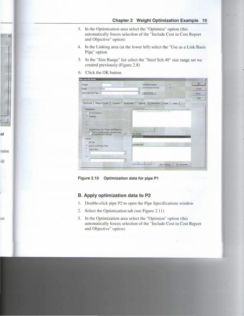
3. In the Oplimiz.atíon area sclcct thc "Optimizc" option (this a utomatically forces selection of thc "lncludc Cost in Cost Repon and Objective" option)
-L Tn the Linking arca (atthe lower left) select the "Use as a Link Basis Pipe" option
5. fn the "Size Rangc" list elcct the "Stccl Sch 40" sizc range sct we created previously (Figure 2.8)
6. Click the OK bunon
Figure 2.10 Optimization data for pipe P1
B. Apply optimization data to P2
l . Double-click pipe P2 to open the Pipe Specilicallons "inclow
2. Selcct the OplimiL.ation tab (scc Figure 2.1 1 )
3. lo the Optimization area select the "Opuma.Le" optaon (this automatically forces selection of the "lnclutle Cost in Co L Report and Objective" option)
20 AFT Mercury 7.0 Quick Start Guide
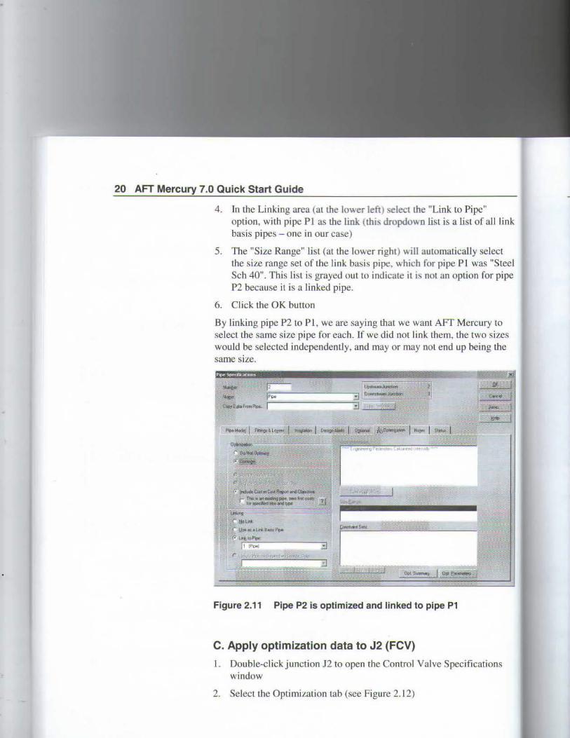
4. ln thc Linking arca (at the lower left) select tbe "Link ro Pipe" option, with pipe Pl as lhe Link (Lhis dropdown list is a list of aJIIink basis pipes - one in our case)
5. The "Süe Range" List (at the lower right) will automaticaUy select the size range set of the link basis pipe, which for pipe P J was "Steel Sch 40". This List is grayed out to indicate it is notan option for pipe P2 because it is a Jinked pipe.
6. Click the OK button
By ünking pipe P2 Lo Pl, we are saying that we want AFT Mercury lo select the same size pipe for each. lf we did not link them, tbe two sizcs would be selectcd indcpendently, and mayor rnay not end up being the same size.
Figure 2.11 Pipe P2 is optlmized and linked to pipe P1
C. Apply optimization data to J2 (FCV)
1. Double-cl ickjunction J2 to open d1e Control VaJve Specifications window
2 . Select the Optimization tab (see Figure 2.12)
Pipe" st of alll ink
illy select 1 was "Steel ion for pipe
ercury to : two sizes being the
icalions
Chapter 2 Weight Optimization Example 21
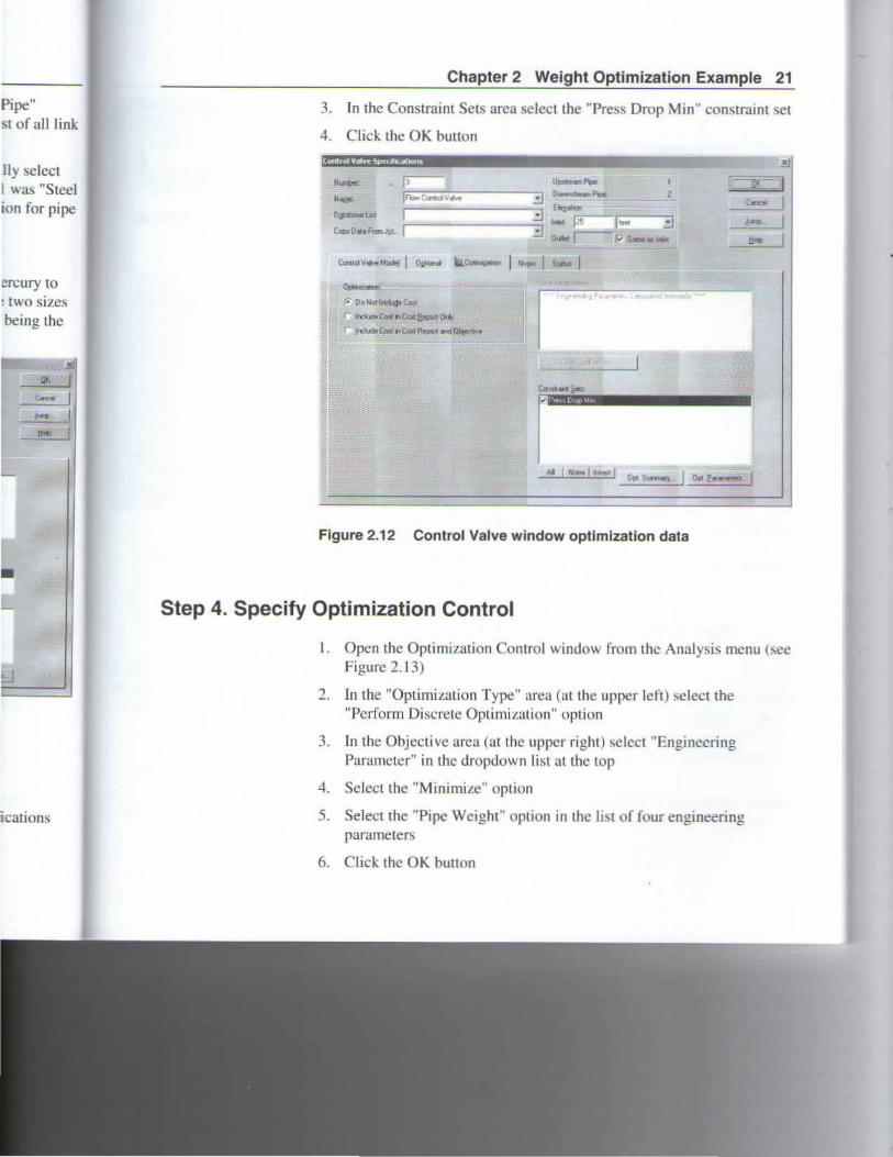
3. ln the Constraint Sccs arca select the "Press Drop Min" cono;trai m set
4. Click the OK button
~ re=¡ U-PiDe 1
N- 111ow Ccn>dV- 3 o--"'"' 2
1 l"':<IIM
fl~lclt 3...,. ~¡ ... 3 ~ ((ll\l[•oto FIOI:I~ 1
d ()""' r ~ ---ws
J lrel·'W~I'~!i!IW• o.¡. lncll.dtt Coot n eo.l f1opoo• orcl~•
Figure 2.12 Control Valve window optimization data
Step 4. Specify Optimization Control
l. Open the Optimintion Control window [rom lhe Analysis menu (sec Figure 2. 13)
2. In the "OpLimiLalion Type" area (ut the upper left) ::.elect the "Pcrform Discrete Optimit.ation" option
3. In the Objectivc arca (at thc uppcr right) sclcct "Engineering Parameter" in thc dropdown list at thc top
4. Selcct the ''Minimit.e" option
5. Select rhe ''Pipe Weight" oplion in thc list of four engrneering parameters
6. Click the OK button

22 AFT Mercury 7.0 Quick Start Guide
Opt&nuzatiDn Control - · - <:1: 'i! q,Ov .,. ~
1 Mod1fíed Method ol f ead~le Di!ecbom
Figure 2.13 Optimization Control window accepts criteria specification for how to optimize the pipe system
Step 5. Run the Optimization
We are now in a position to run the optimization. Befare doing so, take a moment to consider what this model is trying to accomplish. The pipe Pl am.l P2 sizes will be selected from the "Steel Sch 40" size range setas the same size, such that their weight is minimized while obtaining a mínimum 12 psid pressure drop across the contro l valve.
l. To run the optimizalion, select Run from the AnaJysis menu. This will start the Solulion Progress window (sce Figure 2.14). The optimum for Lhis smalJ system is qukkJy found. lt is 11.422 lbm. lL requircd 18 calls to the Hydraulic Solver to flnd the optimum.
2. Click the "View Output" hurton
n
takc a ripe PJ t as a
bis
11. It
Chapter 2 Weight Optimization Example 23
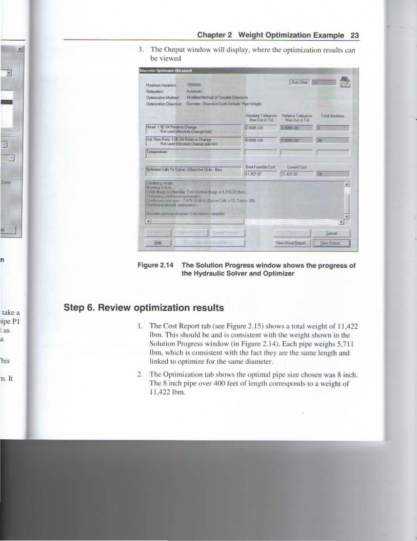
3. The Output window will display. whcrc Lhe oplimiL.ation result~ can be viewed
01screte Opbmwn Obtant!d .~
M._..lte<danl 100llll Rela.abon />JrJntdc
0-Mllhod Modiled Methld Cll f eMtJie OreeliOmo
Oplniz4bon0~ D.:atá ~Cos!J 1~ Pcle'W~
~r-.,..,. Tcx.llle<aoon1 M•DIIGI TCII
..,..,..,._"""='"'=""""~4:::-».:.;.¡;.......,...,_,....,..--...... , !Jet( fe.<1bie Cosl Culeo# Cosl
ft~t21 B7 j1H!181 [l=e __ ______,
®~ ,,. )16 20 llbm
nc,¡ <'ft.ob•l J,.... O'll
Figure 2.14 The SoluUon Progress window shows the progress of the Hydraulic Solver and Optimizer
Step 6. Review optimization results
l. The Cost Report tab (see Figure 2. 15) show'\ a total weaght of JI ,422 lbm. This should be and is consistenl wiLh the weight shown in the Solution Progress window (in Figure 2.14). Each pipe weighs 5,711 lbm. which is consisten! wilh the factthey are the same Jength and linked lo optimizc for Lhe S<lme diameter.
2. Tbe OptirniL.ation Lab ),how!. the optimal pipe .,¡Le chosen was 8 inch. The 8 inch pipe over -lOO fecl of leng:th corre.,ponds to a weight of 11,422 lbm.

24 AFT Mercury 7.0 Quick Start Guide
3. The CV ConstrainLS tab shows thar the 12 psid minimum pressure drop is satisfied in Lhat Lhe pressure drop for 8 incb pipe was 12.70 psi d.
Figure 2.15 The Output window shows the hydraulíc results of the optimized system, plus the optimal system size results

ssurc 12.70
of the
Conclusions
Chapter 2 Weight Optimization Example 25
This cxample demonstrale!-. AFf Mercury's oplimi.Gation capabilities for a simple system wilb u ~i ng le constraint. Enginccring parameter optimization for wcight is fast and easy to implcmcnl.

26 AFT Mercury 7.0 Quick Start Guide
1 1

C IIAPTER 3
lnitial and Life Cycle Cost Optimization Example
Topics covered
This cxamplc dcmonsLratcs somc key features in usi ng AFf Mcrcury Lo optimize a cooling water systcm for cost.
Thi~ example wi ll cover Lhe following Lopic!.:
• Engineering and Cost Databases - 1 Jow to connect ami use
• Linking Pipes- How to limit the numbcr of independem variable..'
• SiLe range sets and constraint scls - How Lo set requiremento; on the system
• Optimization Control - How LO optimizc for initial or life cycle cost
• Optimization outpul - How to undcrstand the optimiLation results
Required knowledge
This example assume1> that the u::.er hall !lOme familiarity wilh AFf Mercury sucb as placingjunctionll, connecting pipes. cntering pipe and junction spccification1>, and creating and using pipe \ÍZC range seLc; am.l constraints. Refer to Lhe Weight Optimimtion Example in Chapter 2 for more information on these tapies.
28 AFT 7 .O Quick Start Guide
Model files
This example uses Lhe foJiowing files, which are inslalled in the Examples folder as part of the AFf Mercury installation:
• Cooling System.mrc - AFT Mcrcury model file
• Cooling Sysrem.dat - junction cnginecring database
• Cooling System.cst - cost database associatcd with Cool ing System.dat
• pipe-sreel-sch40-galv-threaded.cst - cost dalabasc for galvanized steel
Optimization goals
Getting started
This example uses an existing modelto investigate two optimizalion cases:
1. Optimize system for initial cost with a 20-year operating period
2. Opt.imize system for lije cycle cost wilh a 20-year operating period.
To begin, start AFf Mercury and load Lhe model file Cooling System.tnrc. This modeJ has a number of dlfferent scenarios. If you are not familiar with sccnarios, you can rcvicw the Scenario Manager discussion in the Help system or Chaptcr 5 of Lhe AFT Mercury U ser Guide.
Open lhe Scenario Manager from the View menu to see the existing scenarios. Select and load the scenario "20 Year Design/Design for lnltial Cost". The model should be ready lo run, but first lets understand what the model is doing. See Figure 3.1.

ÚLed
tion
iod
period.
ou are r Jser
mg or ~rstand
Chapter 3 lnitial and Life Cycle Cost Optimization Example 29
ffl'i' 411121 Fhftté,1i*'d·l:p ''~n:.. ""~ c.- - ....- -- - ......... ~ líl'- t!ot ~liiiEi ~ ¡ .1'· 3 :1 ~
e, Q·A ·
Figure 3.1 Cooling System example model
Review Optimization Control
Open the Optimization Control wi ndow from the Analysis menu (Figure 3.2). The Optimization Control offcrs a number of features to control thc optimization process. In Lhe Optimi.wtion Type area, the first selection is "Do Not Optimize". This is equivalcnt to running AFf Mercury as onc runs AFf Fathom.
The second selection is "Calculate Costs, Do Not Optimize". This is identical to thc first sc lcction. with the exception that costs are calculated for thc systcm and displuyed in thc Output windo~ ...
Thc tJ1ird selection is "Perform Continuous Optimization". wbich selccts pipes sizes assuming the diamctcr~ are continuous. ln olher words, it ignores the fact that commercial pipe is avai lable only in discrete sizes. and instead assumes that any diamcrcr is acceptable.
The fourth selection is more realistic Lhan Lhe lhird bccausc it recognize" the fact lhat commercial pipes are avaalable Onl)' m dJc;crete sizes, and chooses the optimal combination of discrete sit.cs.
30 AFT Mercury 7.0 Quick Start Guide
Melntxil-~oiPOJ.,_,......,~::===::::¡¡
e; G1!1diert lk!t.el:llolelllod
íG-~MIIIhod
i_eareh Methocf
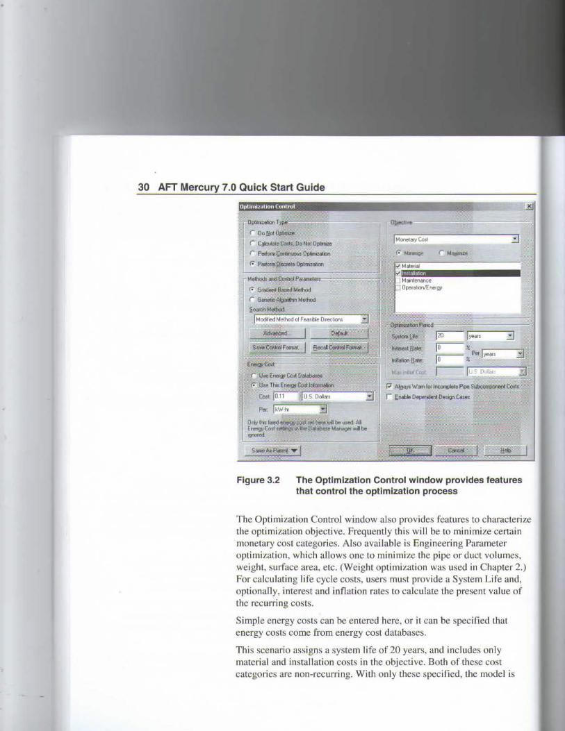
Figure 3.2 The Optimization Control window provides features that control the optlmization process
X
The Optimization Control window aJso provides features to characterize the optimizalion obj ective. Frequently Lhis will be to mi nimize certain monetary cost categories. Also available is Engineering Parameter optimization, which allows one to minimize the pipe or duct volumes, weight, surface area, etc. (Weight optimization was used in Chapte r 2.) For calculating life cycle costs, users must provide a System Life and. optionally, imerest and infiation rales ro calculare the present value of the recurring costs.
Simple energy cosls can be entered here, or it can be specified thal energy costs come from energy cost databascs.
This scenario assigns a system life of 20 years, and inc ludes only material and insta llation costs in the objecli ve. Both of these cost categories are non-recu.rring. With only these specified, the model is
1tures
-acterize ertain er 1mes, ner 2.) : and. _ue of
.ar
:1 is
Chapter 3 lnitial and Life Cycle Cost Optimization Example 31
attempting to find an optimum based on non-recurring (i.c., first or tniliaJ) COSL
Review databases
The actual materiaJ and instaUation costs Lhat Lhe Optimizarion Control window specifics are containcd in cost databases. The cost databases necdcd for this cooling water cxample alread} exíst, and just need to be accessed.
The Database Manager (opened from the Databa~e menu) shows all of Lhe available and connected tlataba&es. Databases can eithcr be engineering databases or cost datahases. Cost databases are aJways associated with an engineering database. and are thus displayed ~ubordinate to an engineering database in the dntabasc lists.
Hcrc we will summariLe sorne kcy ospects of databa.,es:
• Cost information for a pipe systcm component is accessed from a cost databasc. Cost databasc Hcms are based on corresponding items in an cngineering databasc. (The engineering database~ al!.o include cngineering information <;uch as pipe diameters. hydrauhc loss factors, etc.)
• To access a cost for a particular pipe or junction in a model. that pipe or junction must be based on items in an engineermg darabase. Morcover. that databa.~;e must be cmmected.
• There can be mulliple coM databases associated with an<l connected to an engineering database. This makes it easier to manage costs of items.
The Database Manager should appcar as shown in Figure 3.3. With thc "Junction Costs ... ", thc single data base scction is chccked. The scction should be ·'Junction/Componcnt Costs". Thc "STD Stccl Pipe 1"-36''" database only has thc Pipe Material cost cction selccted.
The engineering dawba~es associated with these two cost tlatabases are tJ1e AFf DEFAULT INTERNAL databuse. andan extemal database caUed "Junct..ions for Cooling System". For the cost data in the rwo cost databases lo be accessed by pipes antl junctions in the model, the pipe and junctions must use these two engineering databa-;es.

32 AFT Mercu 7.0 Quick Start Guide
Figure 3.3 Oatabase Manager shows avallable and connected data bases
Review pipe optimization setup
Open pipe PI on the Workspace by double-clicking it. Figure 3.4 shows the Pipe Specifications window wilh Lhe Pipe Modeltab selected, and Figure 3.5 shows it with the Optimi.t.ation tab selected.
The Optimization data offcrs Lhe ability lo optimlze or not optimize a pipe. [f Optimize is i>elected. AFT Mercury will treat Lhe pipe diameter as a variable and vary it according to cenain criteria that will be discussed shortly. Why would one choose to not optimize a pipe'! There could be a number of reasons. but onc good reason is that the pipe reprcsenL'i a pipe in an existing system and lhe dcsign does not aJJow the replacement ofthat pipe with a new one. Thereforc its diametcr is fixed, and optimi.t.ing Lhe pipe would serve no purpose. AJJ pipes in Lhis model are to be optimized. because it is a ncw system and it makes sense to select Lhe optimaJ diameters for all pipes.
!Cted
t shows 1, and
ilea lffieter
, There e low Lhe ) fi xcd . model
! lO
r;
'
Chapter 3 lnitial and life Cycle Cost Optimization Example 33
'· c.e- ¡¡----- """--"-· r::,,~=-='-------il~· o---....... COQIIP""' F"""ru. j ::!) ......,... ,.:..._j
f'v>oMMI! 1 r~&-- 1 '"""""" 1 0-AIW 1 ll~ ~-0~•"'< ... •1 >1 0V> 1 "- 1 .. ITo ... O,.-T.SiooR>oyj ~
,.,. .. _ ¡;...~ 3 t~m n.... iiJ ""- ::::J .~_ ..
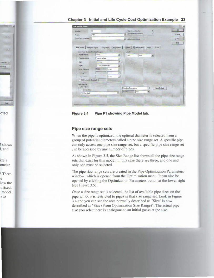
Figure 3.4 Pipe P1 showing Pipe Model tab.
Pipe size range sets
Whcn the pipe is optimized, the optimaJ diamcter is sclected from a group o f potcntial diamete rs caJled a pipe si7.-e range <;CL A specific pipe can only acccss onc pipe si1.e range set, but a speci fi c pipe size range set can be accessed by any number of pipes.
As shown in Figure 3.5. Lhe S ize Range list shows allthe pipe size range sets that ex i ~o.t for thi s modcl. In this case thcre are three. and one and only one must be selected.
The pipe size range scL<; are crcated in Lhe Pipe Optimization Pammeters window, which is opcned from the Optim.i.Lation menu. Tt can al o be ope ncd by c licking thc Optimization Parameters bmton at thc lowcr nght (scc Figure 3.5).
Once a sile range set is sclected, thc list of available pipe 'IZC on thc pipe window is rcstricted 10 pipes in that s izc range í.Cl. Look in Figure 3.4 and you can sce the arca normally describcd a.' "Sue" '" nO\\
de~crihed as "Sizc (From Optimi ~.ation Size Range)". Tbe actual pipe si .~:e you sclect hcre is ana logous to un ini tia l guess aL l)le sizc.

34 AFT Mercu 7.0 Quick Start Guide
r.o-
r r; !.....,..,...,, .. p..,.. oml~-
r: !.'-~.::'..'!'~·"" ... !1 la ..
ttolft
Figure 3.5 Pipe P1 showing Optlmlzation tab.
Pipe constraint sets
Constraints can be applicd to bolh optirnized and unoptirnized pipes. ConsLraints are dcsign limitations on certain pararneters. For example. there muy be a design rcqujremcnt that the velocity cannot excccd 10 fcelfsecond. As the optimizer cvaluates different pipe sizes. if a particular SUe resuiL-; in a velocity greatcr lhan 1 O feelfsecond. that pi pe size is rejected because it causes a constraint vioJation.
When a pipe that is not optirn.Ued has a constraint. it means thatlhe optimized pipe sizes cannot be such that it violates the constrainl for the unoptirniL.ed pipe. Thcrc can be multiple consLraints in a conslrainl set.. and multiple constraint sets applied Lo a pipe. For instance, in addition to a maximum velocity limit. a maximum pressurc limit may exist.
Constmints are contained in constraint sets, which are crcated in the Pipe Oplimilation Parameters window. This window is opencd from the Optimit.ation menu or by clicking the Opti..mization Parameters bunon at the lower right (sce Figure 3.5).

o .:.
•
•
:~ipes.
.ample. :ed 10 1
that pipe
l the 1lL for the :ünt set, ddition to
:1 the Pipe the
button at
Chapter 3 lnitial and Life Cycle Cost Optimization Example 35
As shown in Figure 3.5, pi pe P 1 has 1 wo constraint sets applied. lf yo u open !he Pipe Optimintion Paramctcrs window, you wi ll ~ee the "Max Velocity" constraint is 12 feetlsec. and the "Min Pre¡.¡." constraint is 15 psia. Olher pipes in this model can havc different consrraints appüed according to the design requircmcnts. You can view the constraint seLs for each pipe in the Model Data window. In addition, you can' iew Lhe pipes using each consLraint in thc Optimilation Summary window.
Pipe linking
Pipe Linking is the process whereby certain groups o f pipes are specified to have thc same pipe s iL.e. As pipes are linkcd it reduces the number of design variables ami allows the optimizer to run (aster. lt also has lhe effect of simplifying the design.
An unlinked pipe is o ne lhat has no link::. lo any other pipe, a.nd no othcr p ipes linked to ir. A "link bas is" pipe is one that is not linked to other pipes, but allows othcr pipes to link Lo it. A linked pipe is one linked to another pipe that is a link basis pipe.
There is a fourlh type of linking. which is related to dcpendent design cases. Tbis is discussed in the next chapter.
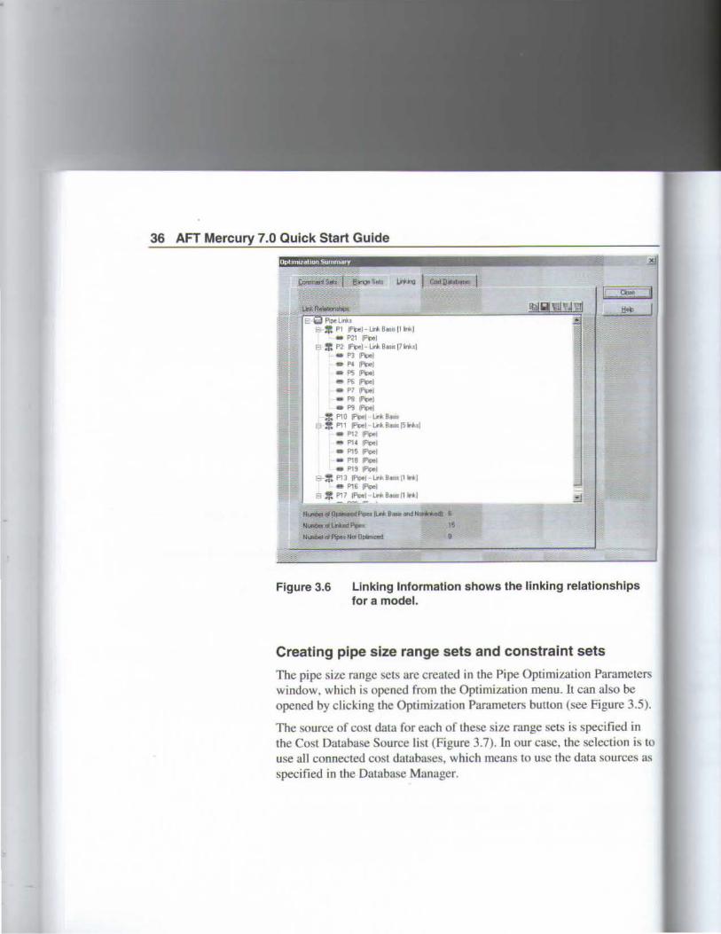
ln this model. pipe PI is a link basis pipe. To lind out how the pipe linking is speci fi cd, opcn thc Optimiattion Summary wi ndow from the Optimization menu and select the LiniJng tab. lf you select the Expand Tree button, the w indow should look likc Figure 3.6. This rree graphically shows the number of dcsign variables that AFf Mercury will !-.Oive. This particular model has twenty-one pipes that are be ing optimized. but because of lin king it has only six link basis pipes. and thus six design variables. You can also view the pipe link.ing by ~lecting the Color Linkcd Pipes feature on the OptimizaLion menu.
36 AFT Mercury 7.0 Quick Start Guide
Optmn1ahot1 Sumnwv -r.~_
~~ - 1
~~~----------------------~~==Q=v=q=e4=;~ H~ J & 0PIPOlirb
e ~ PI JPipoj-l.W<B&tls(IWJ w P21 IPopol
F : P2 JP¡pel - Lri a ... f7 inhl
- P3 !P~~~e l • P• ll'loel • f'S lf'll>eJ - F{, ~~ • f'111"4>eJ e PB ~1 • P9 ~~
: PIO ,_, l.ri a-"' % P11 ,_,.1 - l.riB-~W..I
e P1 2 ~!
• PI ' Ploel • P15 JP.>ol • P18 Pc>ol e P19 ~
F = P13 ~) ·tri B••tt(IW)
- P16 lí'lpej
s : ~7"~~-~a .... n '"'-' ·~~~~""'~~-----r::J H.-OIQ-..sP-ilñ 8-n!ll......., 6
~llnlbw llll.irNd.,.. 15 ll-a1P.-NOIODI11111:!111
Figure 3.6 Linking lnformation shows the linking relationshlps for a model.
Creating pipe size range sets and constraint sets
Tbc pipe size range sets are created in the Pipe OptimiL.ation Parameters window, which is opencd from the Optimization menu.lt can also be opened by clicking the Optimization Parameters button (see Figure 3.5).
The source of cost data for each of these size range sets i specified in the Cost Database Source list (Figure 3.7). In our case. the selection il> lO
use all cunnected cost databases, which mcans to use the data sources as specified in the Database Manager.

":!]
........ ~::::~ H ...
nships
rameters so be urc 3.5).
fied in tion is to turccs as
1
r
!!
Chapter 3 lnitial and Life Cycle Cost Optimization Example 37
Figure 3.7 Pipe slze range sets are created and modified in the Pipe Optlmlzation Parameters window.
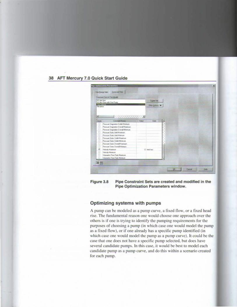
The Pipe Optimization Paramctcrs window. Constramt Sets tab. 1s
shown in Figure 3.8. Hcrc constraint scts for pipe!. are created. These constraint sets can be applicd to thc pipes of your choosing. For example, if all pipes havc a maximum vclocity of 12 feelfsec. then that constraim set should be applicd to all pipes in tbe model. Th1 i done on each pipe window, in thc Constrajnrs Scts area ~ shown in Figure 3.5.
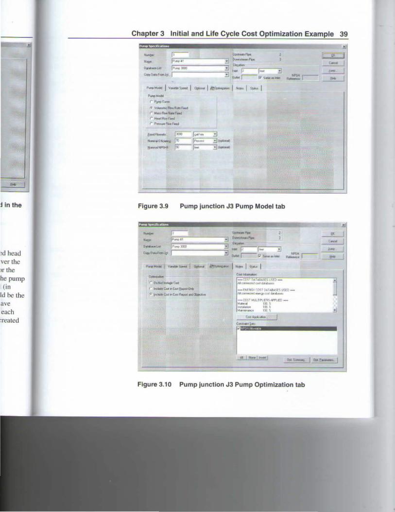
Review junction optimization setup
Opcn pump junction J3 on the WorJ..space by double-clicking iL Figure 3.9 shows Lhe Pump Specifications wimlow wllh the Pump Modeltab sclecled. and Figure 3. 1 O shows it with the Optimiz.ation tab selected.
38 AFT Mercury 7.0 Quick Start Guide
Pie!!..,. :¡,IJI.I,.,.I-tonm•n F'\.,...... . ... taueOutleltrr;~ PtHtUtt SIMio OIJbtt Mlnmum P•attull SllCIC O~tttlil Mtlllml.lfl\ P!anne SIAIII" 0vfll1i! Mñn1111 1
ll'""'-
Figure 3.8 Pipe Constraint Sets are created and modified in the Pipe Optimization Parameters wlndow.
Optimizing systems with pumps
A pump can be modeled as a pump curve. a fixed flow, ora fixcd bead rLc;e. The fundamental reason one would choose one approach ovcr Lhe olhef'b i~ if one is trying Lo identify thc pumping requirements for thc purposes of choosing a pump (in which case one would modelthc pump as a fixed flow). or if one already has a specific pump identified (in which case one would model the pump as a pump curve). l t could be the case that one docs not ha ve a specific pump selected, but does ha ve severdl candidatc pumps. In Lhis case. it would be best to modcJ cach candidate pump as a pump curve, and do this within a scenario crcated for each pump.
[1,¡, 1
1 in the
!d head ver !he Jr lhe be pump (in
Id be tbe ave ea eh :reatcd
11'
~l
Chapter 3 lnitial and Life Cycle Cost Optimization Example 39
,_.,..;,¡ l v..,.~os-o~ 1 Opi,nor 1 ~ 1 'i~ul ~1- 1 ,__ r- ~CI·-
r. ..........,FiowR·F(" ,..... fboi R.. r .,.¡ ,.. f!,o:dRaol'.al
r A.,....af\a.r .. "
Figure 3.9 Pump junctlon J3 Pump Model tab
¡,._ ~1 • ._ ~,"->=11 ........ ~~----.
0-•l.S :,:.1"-~:ml~=====..::::: ("''tl!:ut..,J,:' ''---------
~
,.. Do""' 1»"4- tnd
r ·-c.., c.. a-•ll'l\l r. lo<~~<:• C..tlt:.lllil'<t.ZO•""'illlii< 'w
-rnst OA1'AJLA.SE:S 4.1o;~DAIIO,..,..... .... IOO"fdd~•
-FIIFAr.• C.OST D•TA!IA.'iE) U>roI\ICf\'TitiiiCI~ I'I!'I ..... .Wc:oafddl!~
-cos· HUlnPI.IEAI¡!ffllf[-""*"ttl 100 \ ln:tJJ.M.t:>n 100.'
" •'"""""'"" 100 "-'~---------------' c... ~.-~~·fl
r··~ ,.. ,,_,.......,,
Figure 3.10 Pump junction J3 Pump Optimization tab
40 AFT Mercury 7 .O Quick Start Guide
Modeling a pump as a flxed flow
Thc pumps in our cooling water case are both modeled as fixed nows of 3000 gpm. ln conjunclion, the control val ves al J4 and J7 are modeled as a fixed pressure drop of 5 psid. This modcl thus reprcsents a frrst cut model wbere. based on Lhe fina cut results, the rwo pumps will become actual purnps wilb pump curves. and thc J4 and J7 control val ves will become flow control valves controlling ro 3000 gpm.
As already state<l whcn a pump is modeled as a fixed tlow, it is not a specific pump from a spccific manufacturer. Thus, the costs for the pump can only be approximated. Toa first approximation. it !lhould be possible to estimate the non-rccurring cost (i.e., material and installation cost) for the pump a~ a function of power requirements. For instance, a typical one horsepower pump (of spccific conliguration and materials of construclion) may cost $2000, and a ten horsepower may cost $4000. Olher typicaJ costs for diffcrcnt power requiremenL-; can be approximated. The actual cost for the pump will. of course, highly depend on the application. Thesc cosLs are emered into a cost database, and are accessed by the optimizer. As AFI' Mercury evaluates different combinalions of pipe sizcs. cach combination wiU require a certain power fTom the pump. With a cost assigned Lo this power, AFT Mercury can obtain a cost to cmer into the objcctive funclion which it opti mi zes. Later in this chapter, we willlook atthe cosL~ for the pumps in our example cooling water ncLwork.
[n addilion Lo non-recurring costs, rccurring costs can also be estimated. SpecificaJJy, the cost of the power uscd by tbc pump over a period of time (which AFT Mercury calls thc "systcm lifc") can be determined. All AFT Mercury needs b an overall pump efficiency lo determine the actual powcr from the ideal power. Again, sincc we do nol ha ve a specific pump selected yet. the efficiency can only be approxirnated. AFT Mercury calls thh the "nominal efficiency" (see Figure 3.9). ln adclilion, uscrs can provide a "nominal NPSHR".
A step-by-step method of pump selection proceeds in two phascs. The steps are outlines in the Hclp System and in Chapter 12 ofthe AFT Mercury U ser Guide.
l cut eco me • \\ill
nota he uld be aJiatJor .nce. a ·rials ot 000.
y lbac;e, l'erem n [ercUf) mizes. r
nated. 1 of aed. e the
:d. In
The
Chapter 3 lnitial and Life Cycle Cost Optimization Example 41
Junction costs
There are thrcc choices in specifying the co¡,t of a junction. The. e choices are provided on lhe Optimi1ation tab in the junction'l> Specificalioru. window (see Figure 3. 1 0).
l. Do Not lnclude in Cost - As il say~. the cost of the junction is enlirely neglected.
2. fncludc in Cost Repon Only- This repons aU costs for the junction. but does nol include the cost in the objecti ve function. The costs thus do not impact the overall optimization process.
3. lnclude in Cost Report and Objective- This reports aU cosLc; for the junction, and includcs the cost an the objective funclion. Tbe junctioo costs are lbus allowed lo influence the optimization procesl..
Junction constraint sets
Juncüons do not have size range scts as do pipes. but many have constraints. Junction constraints funclion similarly to pipe constraints. Sorne examples ofjunction constraints are pump NPSH and control vaJve pressure drop. Junction constraint sets are specilied similarly lo pipes. by selecting the constrainr sets from the provided li¡,L
Creating junction constraint sets
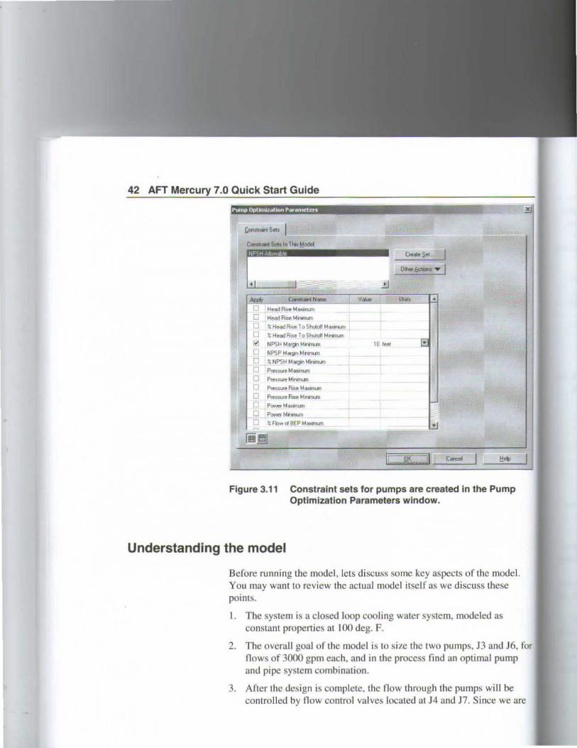
Junction constraint sets are crcated in a similar way to pipe constraint seL'i. Constraint scts for purnps, control val ves, and other lypes of j unctions are crcated on three differenl wimlows opened from tbe Optimization mcnu. Figure 3.11 show!-. a pump constraint set uscd in the cooli ng water examplc we are rcvicwing. Figure 3. 1 O shows this constraint applied Lo pump J3. lt is also applied to pump J6.
42 AFT Mercury 7.0 Quick Start Guide
tomlla¡nt !.'11• 1 CanoiiM ~In Tta Mlldel
%HeadR~ ToShAc11 M"""!"' ~ Head Rmt To Snutoll Mnnun NPSH M~!11n M1n1mum 1 O lee! NPSP Margon Mu,,...m % NPSH M111g¡n Mrwnum I'IM1Ue M_,.., f'l....._.eM........,
f'lem.re Re M a•.,.... Presoute Ar:e Mnmum PowerMllltlllliJI11
PowerMn....m :¡: Fb.o o1 BEP M~
Figure 3.11 Constralnt sets for pumps are created in the Pump Optlmizatlon Parameters window.
Understanding the model
Before runníng Lbe mo<.lel, lets dí scuss sorne kcy aspects of thc model. You may want to revíew Lhc actual model ítsclf as we díscuss Lhese points.
l. The system ís a closed loop cooli ng water system, modeled as constant propertícs at 100 deg. F.
2. The overdJI goal of the model ís Lo size thc two pumps, J3 and J6, for flows of 3000 gpm each, and in the process find an optimal pump an<.l pipe system combination.
3. Aftcr the design is complete, thc now through the pumps will be controlle<.l by llow control val ves located at J4 and J7. Since we are
•Pump
e modcl. Lb ese
:das
i
and J6. for :d pump
will be tce we are
Chapter 3 lnitial and Ufe Cycle Cost Optimization Example 43
sizing the pump!>, we set the J4 and J7 control val ves toa pressure drop of 5 psid. The choice of 5 psid is not arbitrary. but comes from a design requirement for this systcm that the now control val ve shall, ata mínimum. have a 5 psid pressure drop.
4. There are no individual now control valvcs for the three heat exchangers. J 11 , J 13 and J 15. but therc is a rcquirement that each receive at lcast 1900 gpm. We thereforc nccd Lo size the pipes such that this mínimum now is achieved. To accomplish lhis. a pipe constraint set called "Hx min tlow" cxlsts. You can review thls in the Pipe Optimi¿ation Parameter'i window opened from the Optimizalion window. This constraint is applied to pipes Pll-20. Since thc fiow through pipes P1 7-20 are the same, we really only need to apply the mínimum l'low constraint lo one of these, since they will aH have the same llow. Applying itto all four is somcwbat redundant, but no harm wi ll result and lhcrc should be no noticeable impact on lhe model run time. The same redundancy also exists for pipes connecting Lhe other two hea.t cxchanger:o..
5. A!> shown in Figure 3.6. the pipes are linked such that there are six independent pipe si7es (i.c .• dcsign variables) that will be included. The linking is such that pipes that should have the samc size are linked togethcr. For instancc. it makes sense that the suction and discharge pipes for thc pumps ha ve the same size, and Lhat each of the two pumps has thc samc si.le pipe U!> the other. Thercfore. all eight pipes in thc pumping scction are linked togcthcr (i.c .. pipes 2-9). with pipe 2 being thc link basis (any uf the eight pipes could be chosen as the link basis. and yield identical results).
6. A design requirement exists such that thc maximum velocity in any pipe is 12 feet/sec. The pipe constraint "Max velocity" includes this, and it is applied to all pipes in the modcl. (You can see which pipes use thls constra int in Lhe Optimit.ation Summary window).
7. All pipes have thc mínimum pressure constraint applied of 15 psia (the "Min prcss" constraint).
8. Tbcrc are NPSH constraints applied to each pump sucb that the NSPHA must be at least 1 O feet above the NPSHR (see Figure 3.11 ). The nominal NPSHR is set to 50 feet (scc figure 3.9).
9. Each pump has a nominal cfficicncy of 70%.
10. Tbe two pump!t and four elbows are spccificd to "fnclude in Cost Rcport and Objective" (see Figure 3.10 for pumps).

44 AFT Mercury 7.0 Quick Start Guide
1 l . Thc two cost databascs, shown in Figure 3.3, have cost data for the pipes, pumps and elbows. You can use the Cost Databasc window opcned from the Database menu to rcvicw the cost data for thcse databases. 1n summary, there is cost data for the pumps as a funclion ofpower.
12. There is an energy cost for power of a fixed 0.11 U.S. dollars per kW-hr (Figure 3.2). The cost is fi.xed in that is assumed lo be constant over the system life. l t is possible to increasc or decrease the cost ovcr time using energy cost databases.
Running the scenarios and interpreting results
For each of lhe scenarios we wiiJ evaluate. thc only change will be in the Optimization Control window. The firsl case is the one we have bcen reviewing.
Scenario to minimize first cost
As shown in Figure 3.2. the system life is set Lo 20 ycars for this sccnario, and thc objective only includcs costs for ma[erial and instaJlation.
Choose Run from the Analysis menu. When the model is run. AFT Mercury cvaluates a range of pipe si .le combinalions, and finds the one that minirnizes Lhe sum of material and installalion costs (i.c., initial cosr).
The Cost Report is shown in the General Seclion of Lhe Oulput windo\\ (sce Figure 3 .12). AFT Mercury shows aU costs in the Cost Report, e ver those thal were not used in the oplimilalion. The total cost for Lhis system is $5,738,800. (The Output Control has been setup to show coSb in Lhousands of U.S. Dollars, and to show one decimal.) This includcs al costs over 20 years. The first cost, which was the basis for the optimizalion, was tJ1e total of the rnaterinl and installalion ($6 16,000). This total is also thc cost shown as Lhc "ltems in Objective". Again, AFr Mcrcury minimizcs Lhe objecti ve. and Lhu¡, Lhe cost that was minimized was Lhe $6 16,000 cost shown in the Cost Report as "Items in Objecti ve Individual items whose cost contributed to Lhe objeclive are shown with a green background in Lhe cell.
data for the ~e window for thcse as a funcúon
ollars per lO be r decrease
~ iJl be in Lhe mve beco
I. AFf 1ds the one .. inilial
tul window ~eport, cven Jr Lhis show costs
. incl udcs aJI e 516.000). Again, AFf minimized Objective". ;hown wi th
Chapter 3 lnitial and Life Cycle Cost Optimization Example 45
• ..cJ~
Tibie U"' r,. ,~ ..... TOHII. Mateoal U>tl(lloo:(T-liiiJ T
616 6 0.0 5.122.3 GIGG 00 0.0
dJYO 5.122.3 00 0.0 5.122.3 5Jl 6 531 .6 o. o o. o
p~ P¡pt 799 7'!9 DO 00 o ~· r~po 330 1l0 00 00 00
~ ~ 82 ·~ DO 00 00 P• ...,. ,..,. 330 JJO 00 00 00 P5 ...,. ,..,. 4S 00 a o 00 P6 p.,. ,..,. po 00 no 00 P7 p.,. ,..,. 82 00 no 00 P8 p.,. ,..,. no 00 00 00 1'2 p.,. ~ le 00 00 00
!>10 Por>o p~ 'J'.Ie 00 00 OD P11 Fop. p.,. ~o 00 00 00 P12 Fopo ~ ~o 00 a o DO P1J Plpo p~ 6.7 00 00 OU P14 Pipe p~ ~o OO. 00 DO P15 Pooe p~ 50 00 00 00 PIS Popo POPe 61 00 OO. 00 P17 p,¡Je Popo ~o 00 00 00 P18 p.,. Popo. ~o 00 00 00 P19 P!IJO p.. 50 00 00 00 P2ll P.,. f\,o 1¡ 00 no no PZI p p.,. 11'1 00 DO o
Bend Sublolal 2.1 n.o n.o DO
[: 5 Bond Send 08 00 DO DO 3 Bend ..., 08 00 DO 00
J 4 B...J hui o~ Ov 00 lO J16 e..,.¡ '""" (1) o~ QQ ~o
Sublolal Gl' BZ.J n.o 51173 51223 ;J "'"" !)1,.1~11 m ~·j 00 "1i71 ~·21
J6 """" p ll .!.6115 3119 Al~ DO 2 57n1 51'11
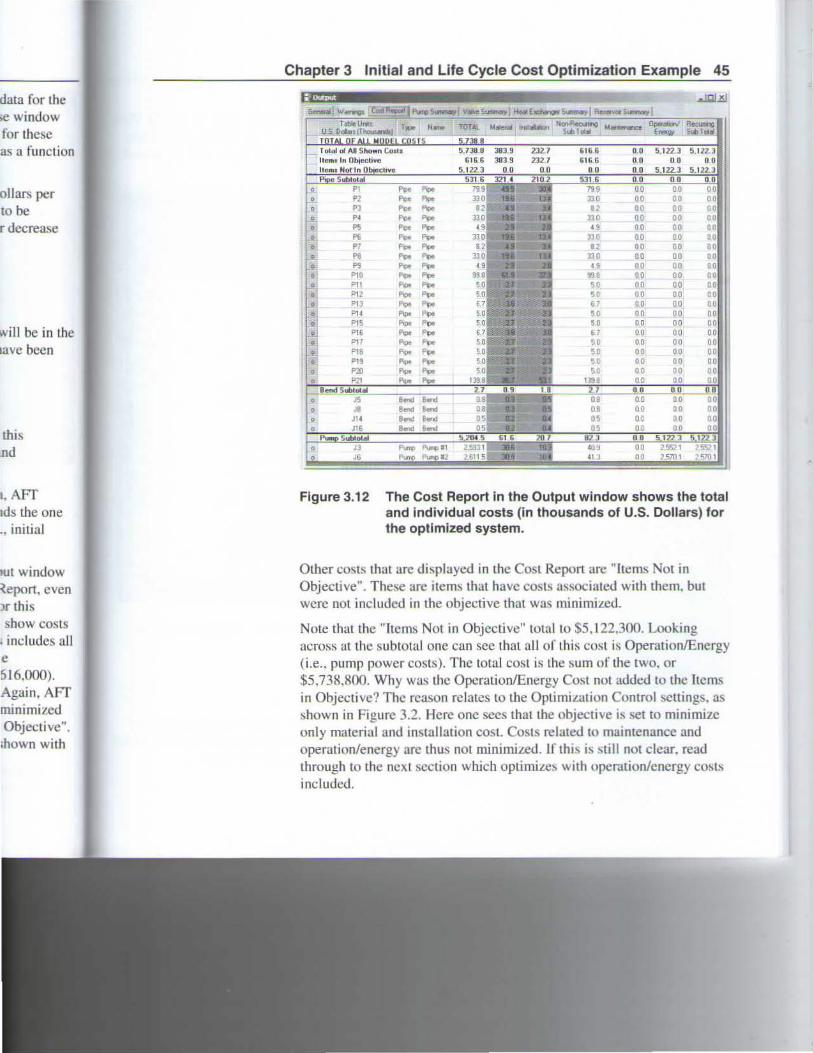
Figure 3.12 The Cost Report in the Output window shows the total and individual costs (in thousands of U.S. Dollars) for the optlmized system .
Other cosL'\ that are displayed in the CosL Repon are "ltems Not in Objeclive". These are items thal ha ve costs associated with them. but wcre not included in the objective that was minimizetl.
Note that the "[tcms Not in Objective" total lo $5.122.300. Looking across al the subtotal one can sec Lhat aiJ of this cosl is Operation!Energy (i.e., pump powcr costs). Thc total cost is the sum of the two. or $5,738,800. Why was thc Opcration/Energy Cost not added to thc ltcms in Objectivc? Thc rcason relates to lhe Oplimt¿ation Control settings, as shown in Figure 3.2. Hcrc onc sces that the objective is set ro rn.inimilc only material and installarion cost. CosL'\ related to mainrenance and operation/energy are thus not minimüed. u· thts is still not clcar. read through to the ncxt scction which optirni.Les with operationlenergy costs inclutled.
46 AFT Mercury 7.0 Quick Start Guide
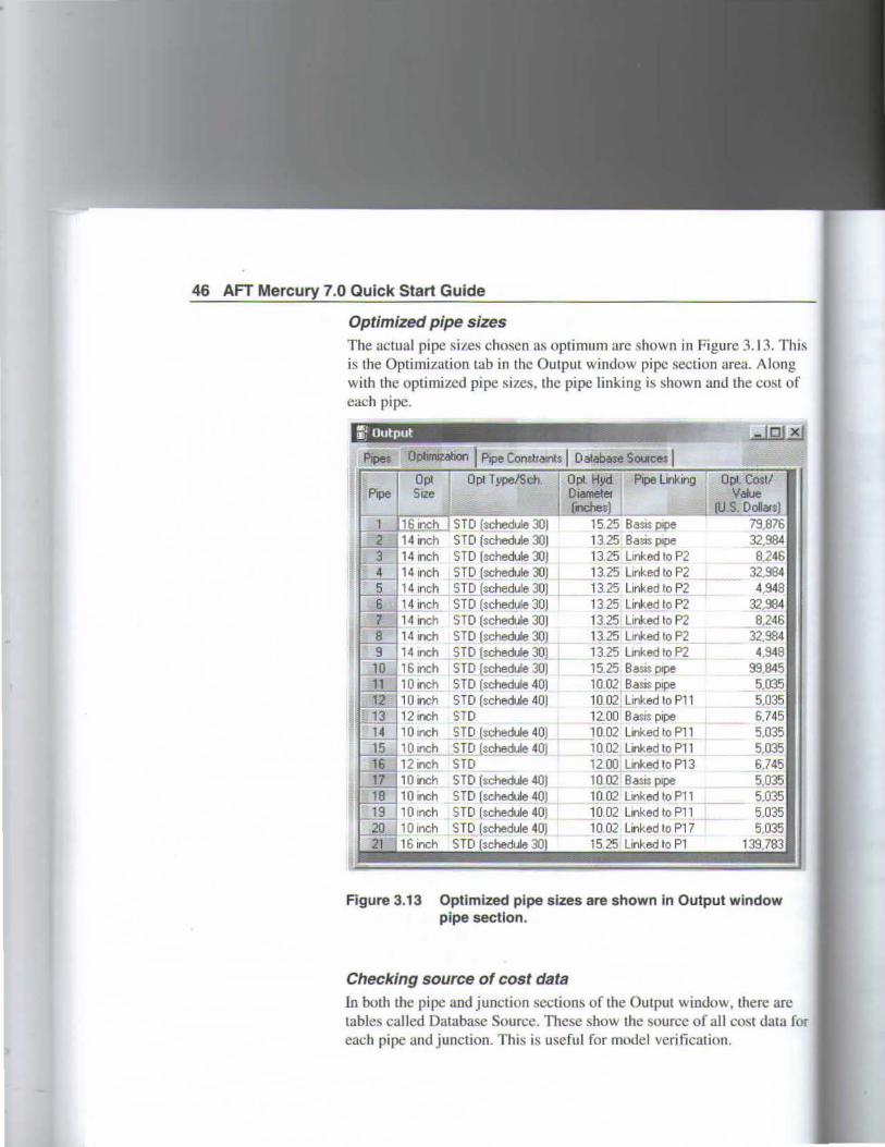
Optimized pipe sizes The actual pipe siz.es chosen as optimum are shown in Figure 3. 13. T his is the Optimization lab in thc Output window pipe section area. Along with the optimized pipe sizes. thc pipe Linking il> shown and the cost of each pipe.
1;! Output ·· 1\- -4
Opbnuzation 1 Ptpe Corulratntt 1 Oatab.lse SOUicet 1 Opt Opt Type/Sch Opl FI,Yd. Ptpe linking Size O!amete1
_ 1_ (l§.•~ILÍ STO (schedule 30)
11......_-=2~ 14 tnch STO (schedule 30) 3 14 rnch STO (schedule 30)
14 rnch STO (schedule 30) 14 1nch SJ.Q_ [schedule 30) 14 rnch i STO ~chedule 30) 14 tnch STO (schedule 30)
11.....,.,_;:;...,¡14tnch STO (schedule 30) 14 1nch STO (schedule 30) 16tnch STO Lschedule 30) 10 inch STO (schedule 40) 10 inch STO (schedule 40)
.,11._-=-1 121nch STO 1 O 1nch STO (schedule 40) 10 1nch STO (schedule 40)
STO STO (schedule 40) STO (schedule 40) STD [schedule 40) STD (schedule 40) STO (schedule 30
inches) 15.25 BasiS ptpe 13.25 Bas1s pipe 13.25 Linked lo P2 13.25 Ltnked to P2 13.25 Linked to P2 13.25 Linked to P2 13.25 Linked lo P2 13.25 Linked to P2 13.25 LJnked to P2 15.25 Basts p¡pe 10.02 Basis pipe 1 O. 02 Linked to Pll 12.00 B asis pipe 10.02 Unked to P11 10.02 Linked to P1 1 12.00 Linked lo P13 10_02 Basts pipe 10.02 Ltnked to Pll 1 O. 02 Ltnked to P11 10.02 Linked to P17 15 25 Linked to Pl
Opt Co$t) V aloe
tU.S Oolla~s) 79.876 32.984 8.246
32.984 4.948
32.984 8.246
32.984 4.948
99.845 5.035 5,035 6.745 5.035 5.035 6.745 5,035 5.035 5.035 5.035
139.783
Figure 3.13 Optimized pipe sizes are shown in Output window pipe sectlon.
Checking source of cost data In both the pipe and junction sections of the Output window. there are lables called Database Source. These show Lhe source of all co~t data for each pipe and junction. This is useflJl for model vcrification.
3. Thi~ Uong OSl Of
.876
.984 246 .984 .948 .984 246 .984 948 845 035 035 745 035 035 745 035 035 )35
J35 783
lW
· are ata for
Chapter 3 lnitial and Lite Cycle Cost Optímízation Example 47
Scenario to minimize lite cycle cost for 20 years
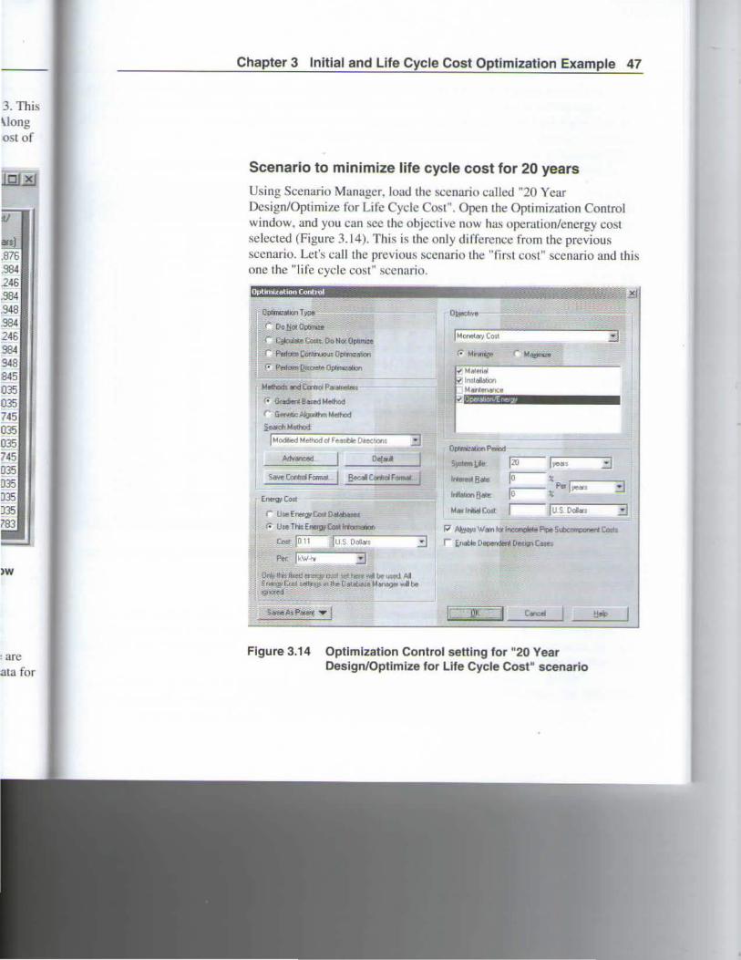
Using Scenario Manager, load thc sccnario called "20 Year Design/Oplimit.e for Life Cyclc Cost". Open the Optimization Control window. and you can scc thc objcctive now has operation!cncrgy cost selected (Figure 3. 14). This is thc only difference from the prcvjous scenario. Let's call thc previous sccnario Lhe "firsl cost" sccnario and this one the "life cycle cost" sccnario .
~~lit& Ú>Ut. "Do tfot Opbmc:e
f"'P~ottro~Oplrrl¡ziJilon
(: Poffonn {t~tat<"Opllrrlrzalm
r. Gr~Ba:..sMelhod f"' GenellcAigoályn Melhod
~llolildl M~'>od
1 Modlied M~ ol F~ DrecllOn: :a Advetad ~... 1
5.-ControlfOIIMI 1 f!dC«trooF'- 1 tnefll!ICost---
,. U"' E"""l"' Coot Delabatet
1 Dbtect1ve
IMonetary C~t
r- ~u,,.., r. M-
P ~ Vll!fn lor ~~~~ ~ S<b:xinClO et C.XU
3 r E:ntbio o~~ to«.., Castt
!F :ar
Figure 3.14 Optlmization Control setting for "20 Year Design/Optimize for Life Cycle Cost" scenario
48 AFT Mercury 7 .O Quick Start Guide
By including operaliun/energy cusL'i in lhe objective, we are now lrying to rninimize the sum of the material , installalion and operatiun/energy cost. This may cause the material and in!>tallatiun costs LO increase. Lel's see wbal happens.
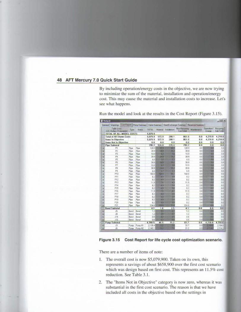
Ruo lhe model and look at lhe resulls in the Cosl Report (Figure 3.15).
11:outpul ., , ' 't :~ -.IJ;3~
Figure 3.15 Cost Report for llfe cycle cost optímizatíon scenario.
There are a number of itcms of note:
l. The overall cost is now $5.079,900. Taken on its own, this represents a savings of about $658,900 over tbe first cost scenario wbich was design based on Cirst cost. Tbis represents an 11.5% CO!)L
reduclion. See Table 3.1.
2. The "Jtems Not in Objcctivc" category is now zero, whereas it was substantial in the firsl cost scenario. The reason is that we have included all costs in the objective based on the settings in
IW trying 'energy :ase. Let's
e 3.15).
11.1 4.218 8 IU 4.218 8 0..0 0.0
0.0 DO 0.0 ~Q
00 no DO DO DO 00 00 DO 00 00 00 DO 00 DO D. O 00
~~ 1 0 0 1 00 DO o o DO
:m ario.
!nario 5% cost
ü was ave
Chapter 3 lnitial and Life Cycle Cost Optimization Example 49
Optimi1ation Control. To be complete, the Optimi7..ation Control did not include maintenancc costs. but there were no maintenance costs in any of thc cost databascs. You can see this by lookjng at thc Cost Repon column for Maintcnance. lf there were maintenance cosLc; in these cost databru;e~. there would be values in this column and the "Items Not in Objective" would not be 7ero unless Optimization Control was modified to include maintenance cost.
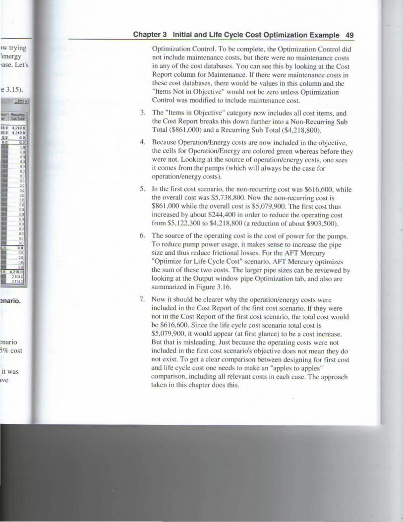
3. The "Jtems in Objective" category now include!'l all cost items. and the Cost Report brcals this down further into a Non-Recuning Sub Total ($86 1 ,000) and a Rccurring Sub Total ($4,2 18.800).
4. Bccausc Opcration/Encrgy costs are now included in the objec tive, the cells for Operation/Encrgy are colored greco whereas be fore they were nol. Looking atthe !>Ource of operation/encrgy costs. one sees it comes from the pumps (which will ulways be the case for operalion/energy cost~).
5. In the first cost sccnario, the non-rccurring cosl wus $616,600. while the overall cost was $5.738,800. Now thc non-recuning cost is $861.000 while thc overall cost is $5,079.900. The lirst costthus increased by about $244.400 in arder to reduce the operating cost from $5, 122.300 to $4.2 18.800 (a rcduclion of about $903,500).
6. The source of the operating coM is the cost of power for thc pumps. To reduce pump power usage, ll make~ sense to increase Lhe pipe sia and thus reduce frictional losse!'l. For the AFf Mercury "Optimize for Life Cycle Cost" scenario, AFf Mercury optimizes Lhe su m of these two cost!>. The larger pipe si7es can be reviewed by looking at the Output window pipe Optimi7ation tab. and also are summarit.ed in Figure 3. 16.
7. Now it o;hould be clcarer why thc operation/energy coste; were included in the Cost Repon of lhe lirst cost scenario. If they were noL in the Cost Rcport of the tirst cost sccnario, the totaJ cost would be $6 16,600. S incc the lifc cycle cost sccnario total cost is $5,079.900, it would appcar (atlirst g lancc) to be a co~>l increa~>e. But that is mislcading. Just becausc thc opcrating cost~ were not inc luded in Lhc first cost scenario' objecuve doe~ not mean they do not exjst. To gel a clear comparison between design ing for fi rst cost and life cycle cost one nceds ro makc an "apples to apples" comparison, including all rclcvant costs in each case. The approach taken in this chaptcr docs this.

50 AFT Mercury 7 .o Quick Start Guide
8. If, after having pcrformed the optimizalion, one still wants to design the system for first cost, the firsl cosl scenario results provides the optimal system desjgn Lo minimize ftrst costs. lmportantly. the designer has quantitative data on the impact of first cosl design on operation/energy costs of lhe system.
Table 3.1 Cost Summary of Optlmlzatlon Runs for Cooling System
Opti.mi.zcd for: Maú!rial lnstallation Total Operaüng Total (systcm + Rcduction j
lnitiaJ CusL 1 O yr 383.900 232.700
Life cycle cost 1 O yr 509.900 272.200
fnitial CO!il 20 yr 383.900 232.700
U fe cycle cost 20 yr 572,900 288, 100
J1 Prcnurrza1
~:
P21 16tntn 20 onch 22uodJ
Opttmtzed for ínlttal cost Optlmlzed for 10 year üfe cyclo; Optlmized for 20 year life cycJe
System operntion)
6 16,600 2.561.100 3.177,700
782.000 2.169.100 2.951.200
6 16.600 5.122.300 5.738,800
86 1 ,O(K) 4,2 18,800 5,079,900
226,5001
658,900
Jlij
Pl& 12 nch 18 neh 18 neh J17
I':ZU 10 tnch 1:0: tncn 14 111Gh
Figure 3.16 Pipe sizes selected by AFT Mercury for first cost and lite cycle cost over 20 years.
sto dcsign lides lhe , !.he esign on
19 System
Reduction
m~~ o
JU
PI~
2 ncr 18 nch 18inch J1 7
r.~
tO tnc~ . ,,nctl t 4nch
IJie
)St and
Chapter 3 lnitial and life Cycle Cost Optimization Example 51
Optimizing with pump curve data
Conclusions
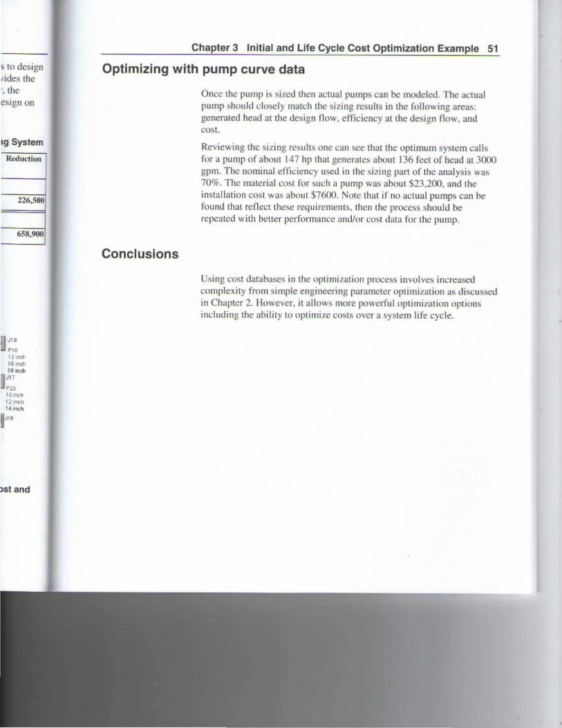
Once lhe pump is si7ed then actual pumps can be modeled. The actual pump should closely match the sizing rcsults in the following areas: generated head at rhe design tlow. efficicncy at Lhe design tlow. and COSL
Reviewi ng lhe sit.ing results one can see that the optirnum system calls for a pump of about 14 7 hp thut generate1> about 136 fcct of head at 3000 gpm. Thc nominal erficiency used in the si7i ng part of the analysis was 70%. The material cost for such u pump was about $23.200. and the installation cost was about $7600. Note that if no actual pumps can be found that renectthese requirements, then the process should be repeated with better performance nnc.l/or cost data for thc pump.
Using cost databases in thc optimization proccss in vol ves increased complexity from simple engineering parameter optimization as d iscussed in Chapter 2. Howevcr. it allow~ more powerful oplimization options including the ability to optimize costs ovcr a system life cycle.

52 AFT Mercury 7.0 Quick Start Guide

CHAPTER 4
Multiple Design Case Example
Topics covered
This example wiH optimi:tc thc pipe si.tes for a water supply system toa housing developmcnl wherc thcrc are two <.lesign cases. Tbis example uses monet.ary cost optimiL.ation.
Thjs example will cover the following ta pies:
• How dependem dcsign cases are uscd to s:uisf} two different operating modes for a system
• Pipe linling and it~ effect on how well AFT Mercury can optimize a sy!>tem
Required knowledge
This examplc assumes that thc uscr has sorne familiurity with AFr Mercury such as placing junction!>, connecting pipes, entcring pipe and junction specifications. and crealing amlul>ing pipe size range sets and constr:únt-;. Rcfcr to the Weight Optiminllion Examplc in Chapter 2 for more information on Lhese lopics.
54 AFT Mercury 7.0 Quick Start Guide
Model files
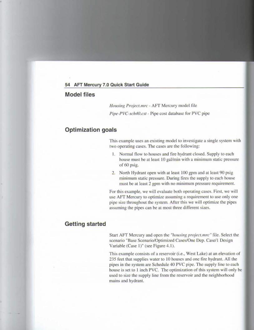
Housing Project.mrc- AFT Mercury model file
Pipe-PVC-sch40.cst- Pipe cost database for PVC pipe
Optimization goals
Getting started
This example uses an existing mo<.lelto invesligatc a single system wilh two opcrating cases. Tbe cases are the following:
l. Normal flow Lo houses and fire hydrant closed. Supply lo eacb house must be atleast 10 gaJ/min with a mínimum stalic pressure of 60 psig.
2. North Hydrant open with at leastlOO gpm and atleast 90 psig mínimum static pressure. During fires the supply to each house must be at least 2 gpm wilh no mínimum prcssurc requirement.
For this example, we will evaluate both operating cac.;es. First, we will use AFf Mercury to oplimiz.e assuming a requirement to use oruy one pipe size tlrrougbout tbe system. After this we will optimize lhe pipes assurning the pipes can be al most three different sizes.
Stan AFT Mercury and open the "lwusing projecr.mrc" file. Select the scenario "Base Scenario/Optimize<.l Cases/One Dep. Case/1 Design Variable (Case 1 )" (see Figure 4. 1 ).
This example consists of a reservoir (i.e., West Lake) atan elevation of 235 feetlhat suppüet. water to 10 houses and one tire hydranl. AIJ Lhe pipes in the system are Schedule 40 PVC pipe. The supply line to each house is set to l incb PYC. The optimization of this system will only be used to siz.e lhe supply Une from the reservoir and the neighborhood mains and h ydrant.

tem witb
each )TeSSllfC
psig 10use me m.
'Ve will lly one pipes
ect the .ign
aúon of tU the oeach only be
ood
Review model
Chapter 4 Multiple Design Case Example 55
8o:t' Sn:na10 - u-t ....
. r...ts_,¡, r-ao ... c....t - OrwOs C..:t
Q@ldb. $ E§ i 30r.avnV.ftlltila~~Aae-
Figure 4.1 Scenarlo Manager for Houslng Projec1 example
The supply lo each hou~e under normal cond ition~ i~ LO gpm with a minimum of 60 psig static pressure. The primary design case. " onnaJ Water Supply", is shown in Figure 4.2. Thi~ ca~e was built in the Base Scenario. which is not the scenario we are currentl y revie\\ ing.
X
For the supply lines Lo cach house (pipes 40-54). Lhe pipe siLe is Jixed to one inch and wiJI nol be optimizcd. Wc wam Lo flnd the single ptpe sue lhat will serve for Lhc supply from Lhc rcscrvoir. the "neigbborhood mains'', and thc hydranL (pipes 1-25, and 80). To do this. we have to establish one pipe as the "link basis p1pe" and thcn link alllhe other pipes (exccpt thc pipes Lo thc houscs) to thü, pipe. For tJlli. example. Pipe 1 was choscn as the link basis pipe. 1f wc look at the Oplimization Summary window. wc can scc lhat all Lhc p1pes are linked together. Figure 4.3 shows the Optimization Summary Window for th il> scenario.

56 AFT Mercury 7.0 Quick Start Guide
Figure 4.2. Primary Design Case layout of Housing Project, whlch is In the Base Scenario.
You can aJso in vestigute thc sizc range sets and pipe consLrainL sels for this model in lhe Pipe Optimization Parameters window opened from thc: Optimization menu. The s i1c range set incJudes aJJ PVC Schedule 40 pipe from 1 inch to 1 O inchcs. T wo pipe constraint sets ha ve been set up for a mínimum outlet ~tatic prcssure of 60 psig for supply to the houses anda mínimum outlet static prcssurc of 90 psig for thc fire hydrant.
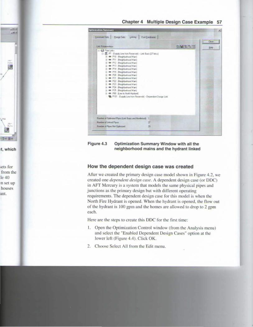
"/ 1
:t, which
>eL'I for from the le40 ~n set up bouses ant.
Chapter 4 Multiple Design Case Example 57
foclrh - : f>1 ls.m.IJ\oh<IIIR-1- lri S..nfl71riaJ
• a PtO (N~M•I 2 • P11 IH~M""I ~ e f'\2 IN"\ttu ...... M.,¡ • • P1l (N~M.,¡
¡¡; e PU (Neogtbcohood M""J "' • P1 5 (N~Manl E: a P20 (N"\tot...t...,.¡ M••l ¡;e • P21 (I'I~M,..I ffi 6 P22 tNIII!)hbcltoood M..,l 1•1 • fr.n [llo91bomood M""'I :;¡ w P24 (NIW;lhbomood Mlllli W W p;>!o [Nooghtv.IOM<I M_,J R !!!!' P80 (Lne lo No1th Hyd.>nt) .. P101 IS~pi)lllne~om Aet"'"'o"J · OOI>Ond..-.1 Oo"'l" l ri
ll..,.t;~d[lc¡t~"- ll ri ~ -..,.¡ IIOI'.Ir~>Od) 1
~~~al Lriod ~ '17
Figure 4.3 Optlmlzatlon Summary Wlndow with all the nelghborhood mains and the hydrant linked
How the dependent design case was created
Añcr we creatcd the primary design ca~o.e model shown in Figure 4.2, we crcatcd onc dependen/ desixn ("0.\e. A dependenL design case (or DDC) in AFf Mercury is a sy~-.Lem Lhat models the l>ame physical pi pes and junctions as thc prirnary dcsign but with tlifferent operating requiremenls. The dependcnt dcsign case for this model is when Lhe North Fire HydranL is opcncd. When the hydram is opened, the llow out of thc hydram is 100 gpm and thc homes are aUowed lo drop to 2 gpm cach.
Here are the steps to create this DDC for the fi r.,t time:
l. Opcn thc Optimit.ation Control wi ndow (from the Analysis menu ) and select the "Enabled Dcpcndem Del>ign ca. ... es" option at tbe lowcr lcft (Figure 4.4). ClicJ... OK.
2. Choose Sclcct AJI from the Edil menu.

58 AFT Mercury 7.0 Quick Start Guide
3. Open Duplicate Special (from the Edil menu), enteran incremenl of 100 and selecl "Make Dependent Design Case", and "Clear Constraims" (Figure 4.5). Click OK.
4. Move Lhe duplkated pipes and junctiom. to distinguish them from tbc original ones from Lhe Primary Design Case (Figure 4.6).
5. Open the J 180 hydranr to flow in thc DDC by selecting it and toggling off the Spccial CondiLion sctting on Lbe EdiL menu.
6. Opcn Lhc pipe connected to the hydnmt DDC by double-clicking pipe P180. Apply the "Fire Supply" con~traint by checking the adjaccnt box (Figure 4.7).
7. Use Global Junction Edit (from the Edit menu) to cbange all ofthe as-;igned now junctions at Lhe DDC homcs (junctioru. 140-154) from 10 gpm Lo 2 gpm (scc Figure 4.8).
Oplrnuzatron [onttol ;:!$:
r:: ~Cofto, O o N.~ Optlll<ll!
r' !'Wiínm1 ~A Opt~m~taiiOrl
r, Péda~rn Qloclole Opt11n11at10rt
Ol!ie<llvo-=o-·
Oependent design --=---=~---...... case modeling
enabled here
Figure 4.4
lcr J
Dependent Deslgn Cases modeling is enabled in the Optimization Control window

rernent
nfrom
'. nd
cking lhe
U ofthe 54) frorr
n the
Chapter 4 Multiple Design Case Example 59 -
Duplicate Special . ,~
P !nctemeti All P~ and Jt.rJChon Numbets By. 1100
r ueate §loup
r H.ge tn Output
P Make Oependent Oesagn Case
r t.eep; Ba 1
P" !;lear Constr ~nts
Figure 4.5 Duplicate Special ls the easiet way to create a dependent deslgn case

60 AFT Mercury 7.0 Quick Start Guide
\ 1"
... ...
. .. m
@]
t-.1ILM
\ "101
.... , J ! ID ,
@)
1 .... r "" ..
...
...
Jlll
l9l '1?
JIJt
@]- '~
(~IWoter ~ply
,.,. -IUI ~HJ
" ' c•.:.mt• • ª' ~
\ '111
' ~~· ca.
il
'16J
.,. .....
.llV" , ...
, .... ....... al
. ..
,"'"
.. , ... ...... ~
\ Jt't •
'"" ~
Figure 4.6 Workspace with Primary Design Case (at top) and one Dependent Deslgn Case (at bottom)
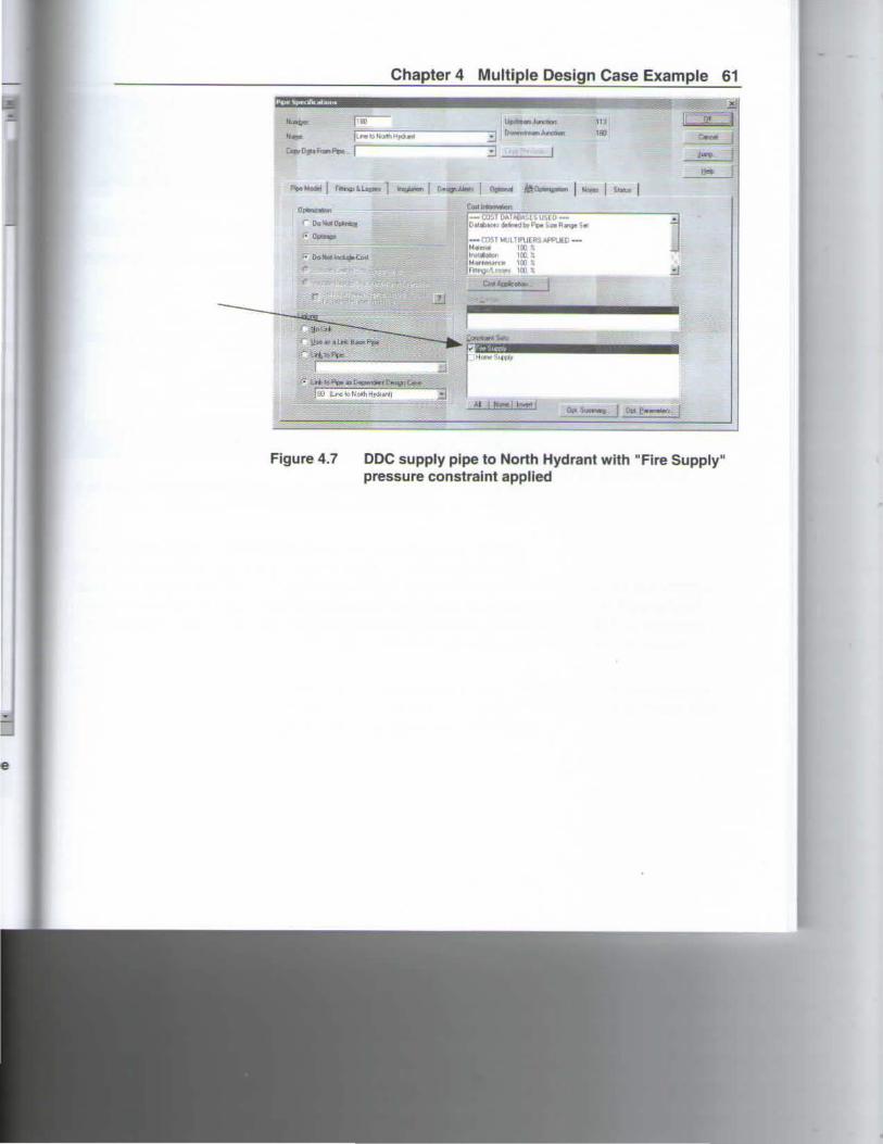
e
Chapter 4 Multíple Desígn Case Example 61
,, 1111
·: l•>Í .. ~ ... 1:'__.!\I'Q)I>C....
lm ¡u..~oNOithH""•"'I ... 8 r·-~~
Figure 4.7
~· ,,.,...¡,_¡
DDC supply pipe to North Hydrant with "Fire Supply" pressure constralnt applied

62 AFT Mercury 7 .O Quick Start Guide
@ .-Dato~
~; '!(". t..n-.o..,. ~ ~~o;M-.. A"''J'ed~w
Ket11 N<>th• S t....., Calot
Alltl•• a .. .,. IICfti•H)dl..,¡ 8mv.rw: Pelen Ownbm Fotdo 11.<1~· Nooh· Stew•tf Colot Alom
~~~:!.;~· JunG'IICI'IIcon
Jt~CIOO S ~:e Spectlll Corótt.., lour~
OptmiZahOO l~~
EJ COil Dotobo:< Mate1181 Cml MLiJiplec
l.,.talloiiOI'ICoii MtAIPiiet
~~...-
u .. pe::iled ~ Sclactod ]....,,..,loor rJ,.,~j•
Nor.e o
Horló AIIC~neetod
1011\' 101):(
Figure 4.8 Global Junction Edit is used to change the flows to 2 gpm in the homes for the fire flow DOC.
When Dupücate SpedaJ was performed with Dependent Design Case selected, each of the duplicated pipes was created with a special type of linking reJalionship. For exmnple, pipe JO] is linked to pipe 1 as "Link to Pipe as Dependent Design Case" (see Figure 4.9). This type of link functions similarly toa regular link, except the cost is not counted for Lhe pipe.
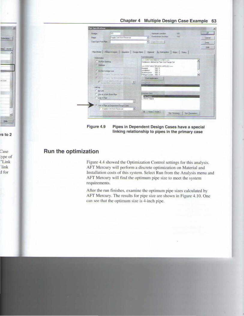
ts to 2
2ase :ype of "Link link
d for
Chapter 4 Multiple Design Case Example 63
2!J
''"""' ~~ u-.. ~o- ¡,- nr:-¡ .._ flllf:.....,""""'~..re~ .... -n ... - .... -----.3 --'4Yfíiúf-~ 1 ::;:¡ _j
''"''~~ r II<>L'"' r ll•u•tliii!<_h,. f' l.rjor.~
)l.. 1 . =::JEJ ---,..,-- r. ••• .,~ .. ~_..0..9 c....
¡, ~"'"'~''!'""""n........ 3
- COS I ... Llii'UlH>AfflJfO-'-'•- IUJ ~ In•....., roo a M.-1"'1\.1~• 10: % Flf"Q"'l- l ll :,::1~.~~·c·•~••
[011 """"...,
no
Figure 4.9 Pipes in Oependent Deslgn Cases have a specíal llnklng relatlonshlp to pipes in the primary case
Aun the optimization
c:.n~ l ._ , ~ 1
Figure 4.4 showed the Optimi.wtion Control scuings for Lhis analylli!>. AFT Mercury will perform a discrete optirnizaúon on Material and lnstallation COl.L'i of this system. Select Run rrom tbe Analysi~ menu and AFT Mercury will find the optimum pipe sizc to meet Lhe system requiremems.
After the run finishcs, examine thc opümum pipe sizell calculated by AFf Mercury. The results ror pipe size are !.hown in Figure 4. 10. Onc c:m see that thc optimum sizc is 4-inch pipe.

64 AFT Mercury 7.0 Quick Start Guide
Opt. CoW ~ Valué U.S Doler.Jl
P¡pe L¡ri(f1111
Suppjy Une from Rese~voir PVC 4 inch 4.02S 25,110.0 B~m~ prpe Ne~ghbofhood Main PVb 4rnch 4.026 4.195.0 J:i!'lkedtoP1 N e~ghboihood M atn PVC 4tnch 4.02G V~. o LrnkedtoP1 Netghboihood Matn PVC 4tnoh 4.026 2.790.0 Ltnkedlo P1 ~eighbolhood Main PVC 4 inc:h 4.026 2..790.0 Llnkedto P1 Nerghborhood Mam PVC 4tnch 4.026 2.7SO.O lrnkedto P1 Ne~ghborhood Mam PVC 4tnch; 4.026 2.790.0 LnkedloP1 Neighborhood Main PVC 4tnch! 4.026 4.185.0 l.lnked lo Pl Ne~ghbolhood Main PVC 4 inch: 4 026 2.790.0 UnkedtoP1 Netghborhood Matn PVC 4tnch' 4.026 2.790.0 Lrnkedto P1 Net¡;¡hbofhoód Main ' PVC ¡(tnch· 4 026 2.790.0 Lrnkedto P1 Neighbor~ Main PVC 4 inch 4.026 2.790.0 Llnkedto Pl
. Ne¡¡;¡hbochood Main PVC 4 inch 4 026 2.790.0 Lrnkedto P1 Lrno to Noctk Hydran_t _ PVÍ: 4tnoh 4.026 139.5 Lrnkedto P1
Supply Une ftom RMB~V()II PVC 4 inch 4.026 0.0 Dependen! Lrnked lo P1 Neigh~ochocl,d ~~-t--PVC A inch 4 026 0.0 Dependent Un~ed to P10 Nerghbochood M arn PVC 4111ch 4.026 0.0 Oependent_l,!nked_to P1 N e¡ghborhood M a~n. PVC 4mch 4.026 0.0 Depondenl Lrnked lo P12 N eighbothood M 11in PVC 41nch 4.026 0.0 DependenU,rnked to P13 N eighborhood M ain• PVC 4 inch 4.026 ___ Q,_Q _ _Q_e_p_e_r¡d~l Llnl\_ed_!o P14 Nerghborhood Marn PVC 4 rnch 4 026 0.0 Dependenl Llnked to ~15 Ncighborhood Mllln PVC 4 inch 4.02s 0.0 O ependentl.Jnked to P20 Nci¡;¡hborl:!!lod Main PVC 4 rnch J_Qfl>~ 00 Dependen! Ljnked to P21 N eishborhood Main PVC 4 inch 4.026• o. o () ependent Linked to P22 Nei~hbor hood Matn PVC 4rnch< 4.026 0.0 Dependent Ltnked to P23 N~gh!:lorhood Main PVC 4 rnch' 4.026 a. o Dependen! Unked to P24
. .N~hbothood Main PVC .!.!..rE!. 4Qf!i 0.0 D ependent Linked lt?. P25 Line to N orlh H drant p;;ié 4rnchr 4 026 a. o De endent Ltnked to P80
Figure 4.10 Optlmum pipe size In Output window
Thc cost for all optimized pipes is $61,520 (see Cost Report in Figure 4. 11 ). This is the cost for "Itcms in Objcctive". Since we did not optimize the pipe sizes to tbe homes (because these were nxed aL 1-inch). there is an additionaJ cost of $7.288 for "items not in objecti ve". The pipes that were optirnized are distinguished in the Cost Repot1 by having a green background color. The tota l cost is merely tbe sum of lhe two ($68,807).
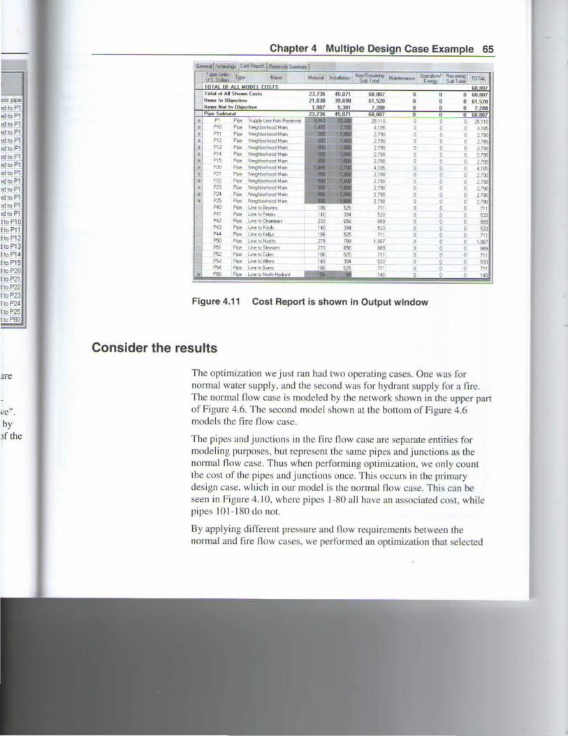
-~ !dloPl !dloPl !dloPl !d toPl !dloPl !dloPl !dloPl JdtoPl !dtx>Pl !dtx> Pl JdtoPl !dto Pl !dto P1 !dto P1 1 to PlO lto Pl1 1 lo P12 lto P13 l to Pl4 l tx> P1S l to P20 l to P2l l tx>P22 IIDP23 l to P24 l lo P25 l loPBO
ve". by Jf the
Chapter 4 Multiple Design Case Example 65
............... Nonfle<U!I1Q lo!- O"""""" IIOCI.III'V 'i<b ~ ,.. · ..,. f•"'V ¡,m T Cllol TOlÁI.
GIIIKII bll 007 o o o 6UJ107 61.520 o o o 61 .!170
7.211 o o o 7.288 68807 o o o 68.11117
o Su¡d¡o ll1l ham fiereMII ~ L ~110 Poe 'l~l'<lcEM.., 4 1&!5 u 'J '1115
Pll ~ >le9"b>fhood ....... 273:1 o o o : 7'll PIZ p~ 'le9"b>fhood ...... ~1~ i) o o ! 73:1 Pll PCIC 'l~hoodM..., ZMO o o Q ~"SO P14 Poo ~~~~ ~m o o o !790 P l5
""'" "~"""' 21~ ¡¡ o o 2.nll P:lJ r'lf"" ~~~""'" ., o o o 41115 PZ1
"""" ''~"'""' H:J(J o o D ?i'll l"ll
""'" · ·~""" ~11 o o ü ~J!IJ PZ3 """ ~legt-óc;hood ....... 27;~J o o Q 2.1'90 P24 F<>< 11"'\tWhood ....... 2m o o 2.790 P25 p.,. lh•11twhood ""'" 2.MO o o 2.790 pto F1pe Llf'l I0 9 ro'N!'It 111 a o ' 11 Pl1 F1pe L"'" toPolo11 ~ ü Q 533 P•2 f'loo LW. toc:Nnten 885 o o eas P•J ~ l'"" tO FO!~' 5Jl o o 533 P•4 Poe llr>otoK<n~. 71 1 o o '11 P50 Poe Linoto iiQflho 1 ~7 D 1.1167 PSl Lin.!: ro St..wNfs 889 o tWl9 ~ 111 o o m f';>J m a n 533 P54 ,,, ú o m
o ?80 ! .U: o n I.W
Figure 4.11 Cost Report ls shown in Output window
Consider the results
The optimizatlon we just ran had two operat ing cases. One was for normal water suppl y, and the !\econd was for hydrant supply for a fJ.Ie . T hc normal now case is modeled hy the nctwork shown tn the upper part of Figure 4.6. The second model !\hown at thc bottom of Figure 4.6 modcls the frre t1ow case.
The pipe.s and junctions in the firc flow case are separate entities for mode ling purposes, bul rcprcsent thc samc prpes and junctions as the normal llow case. Thus whcn pcrforrning optimiLation. we only count the cost of the pipes and junclions once. This occurs in the primary design case, which in our modcl is the normal flow case. This can be seen in Figure 4. 10, whcrc pipe~ 1-80 all have an a!\M>ciated cost, whilc pipes JO 1- 1 80 do no t.
By applying different pressure and tlow rcquircmcnts between the normal and fue flow case!\. we performed an optimiLation that selected
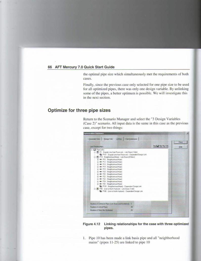
66 AFT Mercury 7.0 Quick Start Guide
the optimal pipe size which simultaneously met lhe requirements of both cases.
FinaJi y, since the previous case only selected for one pipe sL~e to be used for aH optimizecl pipes, lhere was onJy one design variable. By unlink.ing sorne of lhe pipes, a better optimum is possible. We will investigate this in the next section.
Optimize for three pipe sizes
Return to the Scenario Manager and selectlhe "3 Design Variables (Case 2)" scenario. AJI input data is the samc in this case as the previous case, except for two things:
l'lpellnb 1:1 . P1 IS~LnohnmRot••-l · lllkBaolsjlllniJ
,. P1 01 IS'4'1'1Y l.rle hom R,_.,;,l - Oeper¡don( Oecogn lnk El-= P10 fNeoghbofhoodM..,I-t...l. Bmitj2311nksl 'tl • P1 1 fNefli>b<>hood M..,l ±1 o F'12 INel\#lanoodMarol :ti • P13 j~l~dMoitol ;¡ o P14 (~lei¡11bahoodMoito)
ti • P16 INI!!Ijoboohood MoO>l ífl • P20 (Ne¡t1balwJod ManJ ltl • P2l !Nooghboohooa M.,) IIl o P22 (Nooghbomooo M...,J tfl M F'23 (Neoghb0111ood M..,J
'" • P24 (N"''!hbootoood Man) 13 a P25 (NeoghbOihood Man)
"& P110 l'loighboohoodM""') Ocl"""loriDa>gnlnk e·:~ llnetoNooii! H~I-Lri a .. [ltw l
,. P180 ILW1eloN01111H)ICifaroll O~O .. Ignlinl.
20
Figure 4.12 Llnking relationships for the case with three optlmlzed pipes.
1. Pipe 10 has been made a link basis pipe and a JI "neighborhood mains" (pipes 11-25) are linkcd to pipe 10
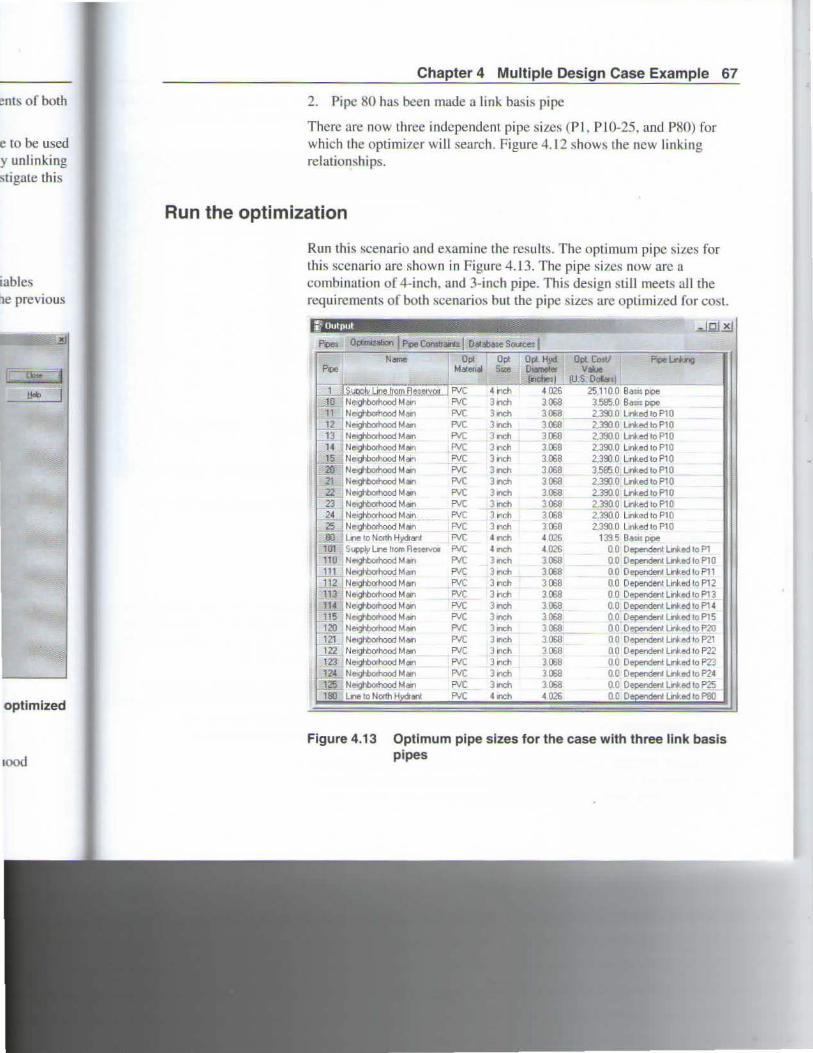
~ents of both
~e to be uscd &y unlinking · tigate this
iables be previous
optimized
lood
Chapter 4 Multiple Design Case Example 67
2. Pipe 80 has been made a link basis pipe
There are now three independent pipe sitos (P 1, P J 0-25, and PHO) for which the optimi7cr will search. Figure 4. 12 show~o. the new linking relationships.
Aun the optimization
Run this scenario and examine lhe results. The optimum pipe siLes for lhis scenario are shown io Figure 4.13. The pipe si1.es now are a combin:uion of 4-inch. and 3-inch pipe. Thi s design slill meets all the requircments of both scenarios but Lhe pipe siLes are optimized for cost.
~Oulpul '
Opt Opt Hjd OPl Cost/ ~W...,g S!Ze O~ameie~ Vakle
..J ~~ (U.S Dü
~!,JQ.O!Y.J.i~lf.Qm.flt~~~J PvC ~ 11'1Ch 4 026 25.110 O Bam p¡pe tleighbo!hood Melrl PVC 3 ti1Ch 3068 3.585.0 Bt!lm p¡pe NeiQI'b:whood Mlll'l P\1( 3111Ch 3!GI 2.390 O Lri ed lo Pl O NeiQI'b:whood M.., PVt 3111Ch 3008 2.3900 Lri-.dloP10 Neq-barhood Mm PJC Jnch 31)58 2.3910 L.ri ed to P10 " e91bo!hoo;Mi Me1n PVC 3111Ch 3068 2,390.0 Li11f.ed lo P10 N elghbcwhood M e1n PV( 3•nch 3.068 2..390 O L~rlked lo Pl O N e1ghbothood Ma111 Pvt: 310Ch 3068 3.585. O l.Jriked to Pl O tleiQI'b:whood Mall'l PJC Jnch 3068 2.390.0 Lri ed lo PlO tleqtlorhood Mlll'l PV( 3111Ch 3!GI 2. 390. O Lri,ed lo P1 O N~M4111 PV( 311'1Ch 3068 2.3900 l.lnfed to P10 Neoghborhood Ma1n PVC 3 ~nch 3068 2.390.0 L1nl<ed to Pl O Neighborhood Meon PVC J 1nch 3 068 2,390 O Llnf ed la Pl O lone to NCifth HydrMI PVC 4 rc:h 4 0.."'6 1395 Bem~
101 S~ L.roe ltom A~VOI PIIC 4111Ch 4 026 0 0 Oependenll.ri ed lO P1 110 NeqbxhoodMM"~ f'll( 3111Ch 3068 O O Oependenllri ed lo P1 O 111 1 Neq.bothood Mc>YI f'll( l onch 3068 o o Oependenlurbd lo Pll 11? Nt!!ltoborhood Ma1n PVC 3 onch 3068 0.0 Oependenllinked lo P12
..lil Ne¡ghborhood Ma1n PVC :l1noh 3068 O O Dependen~ lriced lo Pl3 JlC tlellj1bolhood Mm PVC 3mh 3068 O O Dependen( Lft· ed lo P1 4 115 Ne'!11bothoodMt!lll'l PVC 3n:h 3068 0 0 Dependent lried lo P15 120 Ne'!7ixwhood M .m PJC 3n:h 3068 - O O Oependenllri-ed lo P20 1 Z1 J Ne•ghborhood MMI PI/C ) oneh 3068 O O Dependenllrll ed to P21
_1_22 Netghborhood Mm PVC J onch 3068 ll O Dependen! I.Jnl· ed lo P22 123 Nt!!¡;lborhood Malrl PVC 3onch 3.068 O O O ependenU.Jnl ed to PZ3 l?-' NeoghborhoodMilln PVC 31rlCh 3068 0.0 Dependenii.JN ed to P24
Neq1bo!hood Matn PVC 3nch 3008 O O Dependeri Ln<ed lo P25 lJne lo NCiflh H llnl PVC 4 nch 4 026 00 o LriedtoPOO
Figure 4.13 Optlmum pipe slzes for the case wlth three link basis pipes

68 AFT Mercury 7.0 Quick Start Guide
The cost of tbe design is sbown in Figure 4. 14. The cost of Lhe optirnized pipes (i.e., llerns ln Objecüve) has changed from $61,520 Lo $56,320, a reduction of over 8% in cosl.
'Re~lf
N~.9:~i.'!O'IM"" ' P¡pe ~hoociMII!1 Popo li•VI>cohood M.n D o ¡;,., ~lei¡¡H>cwhood t.lain 2.:BJ o o o PiDe Noig!Mhood M,;, 2.:Bl o o o l'lpo N~ M.., 2~ o o o
. PipO lleVw.haod M~ 3.56!i o o o Pipo N"''lt.t>cwhood Main 2.l00 o o o Pipo ll~hoodMain 2~ o o Pipe tl""'tto<hood t.lain 2:BJ p¡pe tlo9't>ahood Moin 2.:Bl Pope ltet;~hbarhood Mllln ?~ Pipo Lino to Br....,.. n ; Pipo Lir>ol1l Pot"'• !>33 Pipo lino 111 Chon*'er ' 999 Pipo lino"' ro:wm s¡3 Pipe l ino"' kojlyt n1 Pope lJnerollotlht 11167 P¡pe llfle •o Slewarla !199 Pipe l'""loCdes m Pope lJne ro AIIMI 'jJ3
Pope
Figure 4.14 Cost Report for the case with three link basls pipes
Other possibilities
To obtain the best possible optimal systern, une can un1ink a1J the pipes in the neighborhood and aUow each pipe to be optimized independentJy. Wbilc not shown here, it is possible to reduce the cost for Lhis system to less than $49,000 (a furthcr reduclion in cosl of 13%).
This final optirnization lakes much longer to run (a few minutes vs. a few seconds previously). Since alllbe pipes are sized independently, Lhe practica! result i.s that ordering and installing tbe pipe is more complicaLed because there are so many more sizes involved.
plimized ,320, a
WOJ~l 1; '""TAl
~507 o 53,607 o $,320 o 7.288 o 63,607 D 25.' 10 u 3.595 o 2..300 o 2~ o ~.~ o 2.390 n 2.290 o 3.595 o UIO o 2~ o 2.390 o ,!.JSQ 10 UJ.J 1! m o 533 o 8119 o 533 o m o 1JlS7 Q 889 o m o 5l3 o nt ~ 140
fpes
pipes dently. tem to
s. a jy, the
C HAPTER 5
Other AFT Mercury Capabilities
This Quick Start Guidc ncccssarily omilted coverage uf a number of AFT Mercury capabilitics. This chaptcr briefly describes sorne of thc importam capabilitics not covcrcd.
Optimize with operating costs spread over multiple cases
For systcms with multiple <.lesign case~. Lhe system may operate a significant port.iun uf the time in each de~ign case mode. AFT Mercury allows one Lo assign a percenlage of the operating cost to each relevant dcsign.
For example. assumc you are dcsigning a two-pump cooling system which uses bolh pumps in thc summer but only one in the winter (because of reduccd dcmand for cooling water). The winter operating cost is thus much lcss Lhan in thc summer. Yuu can account for this by assigning the pcrccntagc of thc time lhc purnp opemtes in each design case. This allows a proper accounting of annual operating costs, anda proper life cyclc optimization to be pcrformed.
Vary recurring costs over time
Tbrougb "scale tables" AFT Mercury alluws you Lo input recurring data for pipes or junctiuns Lhat vary over time. For instance, perhaps the maintenance cost uf a piece uf equipment is low at first bul requi res incrcased maimenance nver sorne time pcriod. Thc cost for maintenancc can be varied uver time LO match the anticipatcd m~ntenance schedule.

70 AFT Mercury 7.0 Quick Start Guide
Time value of money
An important consideration in evaluating recurring cost items is the cost of money for future expenses. AFT Mercury allows you to enter an interest rate and intlation rate to account for actual value of future expenses based on today's currency vaJue. This data is entered in the Optimization Control window.
Optimize life cycle costs with constrained initial cost
Optimizing to minimize iniLiaJ cosl or life cycle cost docs not need to be an exclusive decision. One can include both criteria in the same optimization run. Thls feature is found on thc Optimization Control window. By optimizing for life cycle cost while constraining the allowed inHiaJ cost, AFf Mercury can Cind the lowcst life cyclc cost design which mccts thc initiaJ cost budget.
Determine cost effectiveness of replacing existing pipe
AFT Mercury can detennine the cost effectiveness of leaving exisling pipe in place or replacing it with new pipe. Thi~ feature is enabled in the Pipe Specifications window, Optimization tab.
Worldng with different currencies
Costs vs. size
Cost data can be emered in any currency you wisb. Different currencies can be defined in the Parameter and Unll Preferences window, and lhen uscd as a basis for cost databases.
Scale lables can be used Lo model how equjpment costs vary with pipe diameter. For instance, a 4-inch val ve will cost more than a comparable 2-inch val ve. This can be accounted for in the cost database by use of scale tables.
is Lhe COSI
eran ture in Lhe
1eed to be ¡e
mtrol he allowed :sign
!xisting )led in the
urrencics and then
ilh pipe nparable use of
Chapter 5 Other AFT Mercury Capabilities 71
Generic pump costs can be modeled a,., a function of power, and generic control vaJve cost~ can he modeled as a function of max imum Cv.
Optimizing rectangular duct systems
AFT Mercury can optímíze systems wilh only rectangular ducts ora combination of rectangular and cylindricaJ ducts. Rectangular ducts ha ve two space dimcnsions. and thus two dcsign variables are required for each independcnt duct !'..iLe.
Compare VFD vs. FCV optimizad systems
Variable Frequt:ncy Orive (VFD) control methods are frequently comparcd tu Flow Control VaJ ve (FCY) methods. However. th is is typically only evaluated in the context of a givcn pipe system. AFf Mercury allows one to optimizc the system for each of these methods. This allows a more meani ngful comparison.
Maximum cost groups
When evaluating mu ltiple operating cases, onc of Lhe pump operating modes will dri vc lhe pump selecti on for all cases. This is hy virtuc of the fact that the cost will be based on thc modc rcquiring Lhe most powcr andlor largest hcad. This can be modelcd in AFT Mercury with Maximum Cost Groups. A Max imum Cost Group allows one to couple costs togethcr for all pumps that wi ll evcmually be of Lhe same de ign (and thus cost Lhc same). This allows thc propcr cost inforrnation to be used for each dcsign case.
Maximum cost group~ can also be uscd for control valves.
Network databases
Engineering and cost databases can be locatcd on local PC's or dcployed across local or widc arca networks. The Database Manager allows users to conoect to rclcvant databases for their specific pipe system dcsign.

72 AFT Mercury 7.0 Quick Start Guide

lndex
A
AFT DEFAULT lNTERNAL DATABASE J l
AFT Mercury
e
engineenng assumptions 4
Overview 4
summary of capabi li ties 3
Constraim 6. 34
Active antllnactive 6
General juncúon 41
Pipes 34
Pump NPSH 43
ConMr.tint Set
Crcating for pipe 36
Junctions 41
Pipes 34
Control valve 9
Control Valve conslrainl set 17
Control Valve junction 13
Control Ya lve OpLimiL.alion Paramelcrs window 17
Cost Report 23, 4-t, 64
Currency units 70
D
Datahase Manager 3 1, 71
Databases 71
Cost 31
DDC See Dependent Design Case
Dependent Design Case 57
Enabling in Optirnimtion Control 57
Linking See
Dcsign variable 6. 35. 43. 66. 71
linking 7
Duct optimization 71
Duplicatc Special 58
E
Energy cost'> 48
F
Flow Control Valve 17. 7 1. See Control valve
Maximum Cost Groups 71
G Global Junclion Edil 58
Graph Resu lls window 5
lnfea.<,ible dcsign 7
lnstallation costs 44
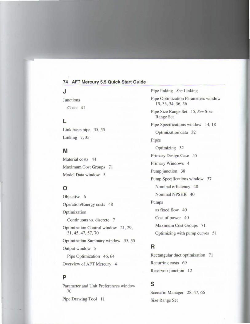
74 AFT Mercury 5.5 Quick Start Guide
J Junclions
Costs 41
L Link basis pipe 35. 55
Linking 7, 35
M Malerial COSLS 44
Maximum Cost Groups 71
Model Data window 5
o Objective ó
Operation!Encrgy costs 48
Optimization
Continuous vs. discrcte 7
Optimization Control window 2J, 29, 31' 45, 47' 57. 70
Optirniz.alion Summary window 35. 55
Output window 5
Pipe Optimt¿alion 46, 64
Overview of AFT Mercury 4
p
Paramerer and Unit Preferences window 70
Pipe Drawing Too! Ll
Pipe linking See Linking
Pipe Optimization Parameters window 15. 33,34,36,56
Pipe Size Range Set 15, See Si7c Range Sct
Pipe Specifications window 14, 18
Optimization data 32
Pipes
Opti miL.ing 32
Primary De~igo Case 55
Primary Windows 4
Pump junction 38
Pump Spccificaüons window 37
Nominal efficicncy 40
Nominal NPSHR 40
Pumps
R
as fixcd now 40
Cost or power 40
Maximum Cost Groups 71
Optimi¿ing wilh pump curves 51
Rectangular duct optirnit.ation 71
Recurring costs 69
Reservoir junclion 12
S Sccnario Manager 28, 47, 66
Size Rangc Set
Creming for pipes 36
Pipes 33
Solu1ion Progress window 22
System Lifc JO
System Pruperties window 11
T Time value of money 70
V Variable Frequency Ori ve 71
Visual Rcpo11 wi ndow 5
w Workspacc wmdow 5, 11
lndex 75

ArT Applled Flow Tedlnology
2955 Professional Place, Sulte 301 Colorado SprinQs, CO 80904 USA (719) 686 1000 sales(Jlaft.com www.aft.com