AGE Challenge: Angle Closure Glaucoma Evaluation in Anterior Segment OpticalCoherence Tomography

Huazhu Fub,1,∗, Fei Lia,1,∗, Xu Sunc,1, Xingxing Caoc,1, Jingan Liaod,1, Jose Ignacio Orlandoe,f,1, Xing Taog, Yuexiang Lih,Shihao Zhangi, Mingkui Tani, Chenglang Yuanj, Cheng Bianh, Ruitao Xiek, Jiongcheng Lik, Xiaomeng Lil, Jing Wangl,

Le Gengm, Panming Lim, Huaying Haon,o, Jiang Liup,o, Yan Kongq, Yongyong Renq, Hrvoje Bogunovicr,1, Xiulan Zhanga,1,∗∗,Yanwu Xuc,1,∗∗, for iChallenge-PACG study group2

aState Key Laboratory, Zhongshan Ophthalmic Center, Sun Yat-sen University, Guangzhou 510060, China.bInception Institute of Artificial Intelligence, Abu Dhabi, UAE.

cIntelligent Healthcare Unit, Baidu, Beijing, China.dSchool of Computer Science and Engineering, South China University of Technology, Guangzhou, Guangdong, China.

eNational Scientific and Technical Research Council, CONICET, Argentina.fYatiris Group, PLADEMA Institute, Universidad Nacional del Centro de la Provincia de Buenos Aires (UNICEN), Tandil, Argentina.

gSchool of Computer Science and Technology, Hangzhou Dianzi University, Hangzhou, China.hTencent Jarvis Lab, Shenzhen, China.

iSchool of Software Engineering, South China University of Technology, Guangzhou, China.jSchool of Biomedical Engineering, Health Science Center, Shenzhen University, Shenzhen, China.

kSchool of Electronic and Information Engineering, Shenzhen University, Shenzhen, China.lDepartment of Computer Science and Engineering, The Chinese University of Hong Kong, China.

mSchool of Electronic and Information Engineering, Soochow University, Suzhou, China.nNingbo University, Zhejiang, China

oNingbo Institute of Industrial Technology, Chinese Academy of Sciences, Zhejiang, ChinapSouthern University of Science and Technology, Shenzhen, China

qShanghai Jiaotong University, Shanghai, China.rLaboratory for Ophthalmic Image Analysis, Department of Ophthalmology, Medical University of Vienna, Vienna, Austria.

Abstract

Angle closure glaucoma (ACG) is a more aggressive disease than open-angle glaucoma, where the abnormal anatomical struc-tures of the anterior chamber angle (ACA) may cause an elevated intraocular pressure and gradually lead to glaucomatous opticneuropathy and eventually to visual impairment and blindness. Anterior Segment Optical Coherence Tomography (AS-OCT)imaging provides a fast and contactless way to discriminate angle closure from open angle. Although many medical image analysisalgorithms have been developed for glaucoma diagnosis, only a few studies have focused on AS-OCT imaging. In particular, there isno public AS-OCT dataset available for evaluating the existing methods in a uniform way, which limits progress in the developmentof automated techniques for angle closure detection and assessment. To address this, we organized the Angle closure GlaucomaEvaluation challenge (AGE), held in conjunction with MICCAI 2019. The AGE challenge consisted of two tasks: scleral spur lo-calization and angle closure classification. For this challenge, we released a large dataset of 4800 annotated AS-OCT images from199 patients, and also proposed an evaluation framework to benchmark and compare different models. During the AGE challenge,over 200 teams registered online, and more than 1100 results were submitted for online evaluation. Finally, eight teams participatedin the onsite challenge. In this paper, we summarize these eight onsite challenge methods and analyze their corresponding resultsin the two tasks. We further discuss limitations and future directions. In the AGE challenge, the top-performing approach had anaverage Euclidean Distance of 10 pixels (10µm) in scleral spur localization, while in the task of angle closure classification, allthe algorithms achieved satisfactory performances, with two best obtaining an accuracy rate of 100%. These artificial intelligencetechniques have the potential to promote new developments in AS-OCT image analysis and image-based angle closure glaucomaassessment in particular.

∗These authors contributed equally to the work.∗∗Corresponding authors: Yanwu Xu (ywxu@ieee.org), and Xiulan Zhang

(zhangxl2@mail.sysu.edu.cn).1These authors co-organized the AGE challenge. All others contributed re-

sults of their algorithms presented in the paper.2iChallenge-PACG study group includes: Yichi Zhang (Department of

Ophthalmology, Sun Yat-sen Memorial Hospital, SunYat-sen University,Guangzhou, China), Nuhui Li (Guangzhou aier eye hospital, Guangzhou,

China), Chunman Yang (Department of Ophthalmology, The Second AffiliatedHospital of GuiZhou Medical University, Kaili, China), Huang Luo (Depart-ment of Ophthalmology, The Affiliated Tranditional Chinese Medicine Hospitalof Guangzhou Medical University, Guangzhou, China), Xingyi Li (ZhongshanOphthalmic Center, Sun Yat-sen University, Guangzhou, China), Feiyan Deng(Department of Ophthalmology, The Tranditional Chinese Medicine HospitalOf Guangdong Province, Guangzhou, China), Yi Sun (Zhongshan OphthalmicCenter, Sun Yat-sen University, Guangzhou, China), Rouxi Zhou (ZhongshanOphthalmic Center, Sun Yat-sen University, Guangzhou, China).

Preprint submitted to Medical Image Analysis June 23, 2020

arX

iv:2

005.

0225

8v2

[cs

.CV

] 2

0 Ju

n 20

20

1. Introduction

As one of the world’s main ocular diseases causing irre-versible blindness, glaucoma involves both anterior and pos-terior segments of the eye. Primary angle closure glaucoma(PACG) is the major type of glaucoma in Asia (Quigley andBroman, 2006; Foster, 2001; Chansangpetch et al., 2018),where the abnormal anatomical structure of the anterior cham-ber angle (ACA) may cause elevated intraocular pressure andgradually lead to glaucomatous optic neuropathy. PACG pa-tients have a characteristic structural difference from open-angle subjects in chamber angle and ocular biometric param-eters (Nongpiur et al., 2013, 2017), including narrow cham-ber angles, short axial length, thick lens, greater iris thickness,etc. There are several ways to assess the angle structures forclinical diagnosis, e.g., gonioscopy, or anterior segment opticalcoherence tomography (AS-OCT). Gonioscopy is the currentgold standard for the assessment and diagnosis of angle clo-sure. Ophthalmologists grade the angle width into differentlevels according to the ACA structures seen under gonioscopy.However, being a contact examination, it may be uncomfort-able for the patient, and it is also technically challenging, rely-ing on the experience of the ophthalmologist in using this tech-nique. By contrast, AS-OCT examination is a fast and contact-less method for capturing the morphology of the ACA (Sharmaet al., 2014; Ang et al., 2018), which is easily used to identifyopen and narrow/closed angles. Moreover, AS-OCT imagingcan obtain measurements of various angle parameters to assessthe anterior chamber angle in clinic (Sakata et al., 2008; Nong-piur et al., 2017), including angle open distance (AOD), anteriorchamber width (ACW), trabecular iris space area (TISA), etc.Quantification of these parameters relies on the localization ofa specific mark, i.e., the scleral spur (SS), which appears as awedge projecting from the inner aspect of the anterior sclerain cross-sectional images (Sakata, 2008), as shown in Fig. 1.Thus, SS localization is also a key task for identifying openand narrow/closed angles in AS-OCT imaging. However, onelimitation of AS-OCT imaging is that ACA assessment is time-consuming and subjective. For instance, the ophthalmologistshave to manually identify specific anatomical structures, e.g.,SS points, for detecting angle closure.

Recently, automated medical image analysis algorithms haveachieved promising performances in medicine and particularlyophthalmology (Schmidt-Erfurth et al., 2018; Ting et al., 2019;Rajkomar et al., 2019; Bi et al., 2019). The availability ofdeep learning techniques has sparked tremendous global in-terest in major ophthalmic disease screening, including dia-betic retinopathy (DR) (Gulshan et al., 2016; Ting et al., 2017;Gargeya and Leng, 2017; Krause et al., 2018; Abramoff et al.,2018), glaucoma (Asaoka et al., 2016; Li et al., 2018; Fu et al.,2018a,b; Orlando et al., 2020), and age-related macular degen-eration (AMD) (Grassmann et al., 2018; Kermany et al., 2018;De Fauw et al., 2018; Liu et al., 2019; Peng et al., 2019).However, most works focus on retinal fundus photographs,with only a few dealing with AS-OCT images (Niwas et al.,2016; Fu et al., 2019a; Xu et al., 2019; Hao et al., 2020a,b).Zhongshan Ophthalmic Center has provided a semi-automated

Scleral spur localization

Open Open Closure Closure

Angle closure classification

Figure 1: AGE challenge tasks: scleral spur localization and angle closure clas-sification from AS-OCT images.

angle assessment program to calculate various ACA parame-ters, but users are required to input the SS positions (Consoleet al., 2008). For fully automated systems, Tian et al. (Tianet al., 2011) provided a parameter calculation method for high-definition OCT (HD-OCT) based on the Schwalbe’s line detec-tion. In (Fu et al., 2016, 2017), a label transfer system was pro-posed to combine segmentation, measurement and detection ofAS-OCT structures. The major ACA parameters are recoveredbased on the segmented structure and serve as features for de-tecting anterior angle closure. Besides clinical parameter calcu-lation, the visual features directly extracted from AS-OCT im-ages using computer vision techniques are also utilized to clas-sify angle-closure glaucoma. For instance, Xu et al. (Xu et al.,2012, 2013) localized the ACA region and then extracted visualfeatures to detect the glaucoma subtype. With the developmentof deep learning, Convolutional Neural Networks (CNNs) havebeen introduced to improve the performance of angle-closuredetection in AS-OCT images (Fu et al., 2019a; Xu et al., 2019;Hao et al., 2019). In (Fu et al., 2018c, 2019b), a multi-pathdeep network was designed to extract multi-scale AS-OCT rep-resentations for both the global image and clinically relevantlocal regions. Nevertheless, these approaches cannot currentlybe properly compared due to the lack of a unified evaluationdataset. Moreover, the absence of a large-scale AS-OCT datasetalso limits the rapid development and eventual deployment ofdeep learning techniques for angle closure detection.

To address these limitations, we introduced the Angle clo-sure Glaucoma Evaluation Challenge (AGE), a competition thatwas held as part of the Ophthalmic Medical Image Analysis(OMIA) workshop at the International Conference on Med-ical Image Computing and Computer Assisted Intervention(MICCAI) 2019. Our challenge follows on the success ofthe REFUGE challenge (Orlando et al., 2020), which was in-troduced for glaucoma detection in fundus image as part ofiChallenge. The challenge proposal was compliant with thegood MICCAI practices for biomedical challenges (Maier-Hein

2

et al., 2018).The key contributions of the AGE challenge were: (1) The

release of a large database of 4200 AS-OCT images with reli-able reference standard annotations for SS localization and an-gle closure identification. To the best of our knowledge, AGEwas the first challenge to provide a public AS-OCT datasetfor angle closure glaucoma. (2) The construction of a unifiedevaluation framework that enables a standardized, fair compar-ison of different algorithms on scleral spur localization andangle closure classification, as shown in Fig. 1. During theAGE challenge, more than 200 teams registered online, andmore than 1100 results were submitted for online evaluation.Eight teams participated in the final onsite challenge that tookplace in Shenzhen, China, during MICCAI 2019. In this pa-per, we analyze the outcomes and methodological contributionsmade as part of the AGE Challenge. We present and describethe competition and the released dataset, report the performanceof the algorithms that participated in the onsite competition, andidentify successful common practices for solving the tasks ofthe challenge. Finally, we take advantage of all this empiricalevidence to discuss the clinical implications of the results andto propose further improvements to this evaluation framework.To encourage further developments and to ensure a proper andfair comparison of new proposals, AGE data and its associatedevaluation platform remain open through the Grand Challengeswebsite at https://age.grand-challenge.org.

2. AGE Challenge Data

The AS-OCT images used in the AGE Challenge were ac-quired with CASIA SS-1000 OCT (Tomey, Nagoya, Japan)from the Zhongshan Ophthalmic Center, Sun Yat-sen Univer-sity, China. The examinations were performed in a standardizeddarkroom with a light intensity lower than 0.4 lux. Both left andright eyes of each patient were included if the images were eli-gible. Each AS-OCT volume contained 128 two-dimensionalcross-sectional AS-OCT images (B-scan), which divided theanterior chamber into 128 meridians. We extracted 16 imagesfrom each volume equidistantly. Eye with corrupt images orimages with significant eyelid artifacts precluding visualizationof the ACA were excluded from the analysis. Angle structureswere classified into open and closure. Gonioscopy was usedas the gold standard. It was performed by a glaucoma expert(Zhang XL) with a four-mirror Sussman gonioscope (OcularInstruments, Inc., Bellevue, WA) under standard dark illumi-nation. The angle was graded in each quadrant (inferior, su-perior, nasal, and temporal) according to the modified Scheieclassification system (Scheie, 1957) based on the identificationof anatomical landmarks: grade 0, no structures visible; grade1, non-pigmented trabecular meshwork (TM) visible; grade 2,pigmented TM visible; grade 3, SS visible; grade 4, ciliary bodyvisible. A closed angle was diagnosed if the posterior trabecu-lar meshwork was not seen for at least 180 degrees during staticgonioscopy.

Each AS-OCT image was divided in two chamber angle im-ages along the vertical middle-line. No adjustments were madeto image brightness or contrast. For each chamber angle image,

the SS was marked by four ophthalmologists (average expe-rience: 8 years, range: 5-10 years) independently. The finalstandard reference SS localization was determined by the meanof these four independent annotations, followed by a fine ad-justment by a senior glaucoma specialist (F. Li). The study in-cluded 300 eyes from 199 subjects (female: 38.7%, mean age:47.2 ± 15.4). Each volume was composed of 128 radial im-ages (B-scan). Adjacent images were similar to each other inchamber angle morphology. Therefore, we extracted only 16images from each volume to avoid the influence of this simi-larity. Thus, a total of 4800 images were extracted. Each im-age was composed of two chamber angle images, e.g., left andright. Finally, the dataset was split into a training set (1600 im-ages with 640 angle closure and 2560 open angle), a validationset (1600 images with 640 angle closures and 2560 open an-gles), and a testing set (1600 images with 640 angle closuresand 2560 open angles). Images from the same patient were as-signed to the same set. The training set was used to learn thealgorithm parameters (offline training), the validation set wasused to choose a model (online evaluation), and the testing setwas used to evaluate the model performance (onsite evaluation).

3. Challenge Evaluation

The performance of each proposed algorithm for each of thechallenge tasks was assessed using different standard evaluationmetrics. Each of them is described as follows.

3.1. Task 1: Scleral Spur LocalizationParticipants were asked to provide the estimated (x, y) coor-

dinates of the SS point. Submitted results were compared tothe reference standard by means of two metrics. The first onewas the Euclidean Distance (ED), which measures the distancebetween the estimated and ground truth SS locations, as shownin Fig. 2 (A). The second criterion was the difference in theangle opening distance (AOD) (∆AOD). AOD is defined as thedistance between the cornea and iris along a line perpendicularto the cornea at a specified distance (in AGE, we use 500 µm)from the SS point (Chansangpetch et al., 2018), as shown inFig. 2 (B). As an important indicator for angle closure assess-ment, we compared the AODs calculated using the predictionand ground truth. In general, the AOD of an open angle case islarger than that of angle closure. Thus, for an open angle im-age, we set a higher penalty for small calculated AODs, whilefor an angle closure image, we set a higher penalty for largercalculated AODs, as shown below:

• For open angle images:

∆AOD =

0.2 × |z − z∗|, if z > z∗,

0.8 × |z − z∗|, otherwise,(1)

where z and z∗ denote the AODs calculated using the esti-mated SS point and ground truth, respectively.

• For angle closure images:

∆AOD =

0.8 × |z − z∗|, if z > z∗,

0.2 × |z − z∗|, otherwise.(2)

3

ED

Scleral spur

Estimated point

Scleral spur

500 𝜇m

AOD (500)

Cornea

Iris

(A) (B)

Figure 2: (A) Euclidean Distance (ED) measures the distance between the es-timated point and ground truth of the scleral spur. (B) Angle Opening Distance(AOD) is the distance between the cornea and iris along a line perpendicular tothe cornea at a specified distance (e.g., 500 µm).

Based on the mean ED and ∆AOD values, each team receivedtwo ranks RED and RAOD (1=best). The final ranking score forthe scleral spur localization task was calculated as:

S loc = 0.4 × RED + 0.6 × RAOD, (3)

which was then used to determine the ranking of the SS local-ization leaderboard. We set a higher weight for RAOD becauseit could be used as an indicator for angle closure identificationdirectly. Teams with lower ranking scores were ranked higher.

3.2. Task 2: Angle Closure ClassificationSubmissions for the classification challenge had to pro-

vide the corresponding estimated angle closure results (posi-tive value for angle closure and non-positive value otherwise).Sensitivity and Specificity were utilized as the criteria of thechallenge:

Sensitivity =T P

T P + FN, Specificity =

T NT N + FP

, (4)

where T P and T N denote the number of true positives and truenegatives, respectively, and FP and FN denote the number offalse positives and false negatives, respectively. In addition,we also reported the area under receiver operating characteris-tic curve (AUC). Based on the Sensitivity, Specificity and AUCvalues, each team received three ranks Rsen, Rspe and RAUC

(1=best). The final ranking score for the SS localization taskwas calculated as:

S cls = 0.5 × RAUC + 0.25 × Rsen + 0.25 × Rspe. (5)

3.3. Final RankingThe overall score of the onsite challenge was calculated as:

S onsite = 0.7 × Rloc + 0.3 × Rcls. (6)

where Rloc and Rcls denote the ranking scores of the SS localiza-tion and angle closure classification tasks, respectively. A largerweight was set for the ranking of SS localization because theclinical measurements, e.g., AOD, derived from SS localizationcan be used as a primary score for angle closure classification.

Eight teams finally attended the final onsite challenge, whichwas held in Shenzhen, China, during MICCAI 2019. The testset (only the images) was released during the workshop, andthe eight teams had to submit their results within a time limit(3 hours). The final submission of each team was taken intoaccount for evaluation. Both online and onsite ranks were as-signed to each team. The final rank of the challenge was basedon a score S f inal, calculated as the weighted average of the on-line and onsite rank positions:

S f inal = 0.3 × S online + 0.7 × S onsite. (7)

Note that a higher weight was assigned to the onsite results. Inthis paper we only analyze the results from the onsite challenge,as it better reflects the generalization ability of the proposedsolutions.

4. Summary of Challenge Solutions

In the AGE challenge, we provided a unified evaluationframework for the standardized and fair comparison of differentalgorithms on two clinically relevant tasks: scleral spur local-ization and angle closure classification, as shown in Fig. 1.

Scleral spur localization task. The aim is to estimate the posi-tion of the SS point from an AS-OCT image, as shown in Fig. 3(A), which requires the algorithm to output the (x, y) coordi-nates of the SS point in image coordinates. Participants in thechallenge proposed localization algorithms based on supervisedlearning, following one of three different approaches. The firstone was to directly predict the coordinates of the SS point, asa value regression problem. The second one was to extend thesingle pixel label to a small region, as shown in Fig. 3 (B). Inthis way, the SS localization task was transferred to a binarysegmentation problem, where the segmented mask center wasused as the SS position. The third approach was to generatea two-dimensional heat map based on the SS position, e.g., aGaussian map, and then employ a regression method to esti-mate the SS point. With a heat map, the peak value was used asthe SS position. Given the coordinates (u0, v0) of the SS point,the heat map G(u, v) could be calculated as:

G(u, v) = exp{(u − u0)2 + (v − v0)2

δ2 }, (8)

where δ denotes the variance, a hyperparameter which controlsthe heat map radius. Fig. 3 (C, D) shows two generated Gaus-sian maps obtained with different values of δ. Compared withthe coordinate regression and binary segmentation approaches,the heat map solution reduces the complexity of the task, fa-cilitating convergence during training. In addition, the methodbased on heat map regression can make use of a fully convolu-tional network for training and prediction.

4

Table 1: A brief summary of the challenge methods on angle closure classification. CE = cross-entropy

Team Member Architecture ROI Ensemble Loss

Cerostar Yan Kong, Yongyong Ren ResNet34 No Single model CE lossCUEye Xiaomeng Li, Jing Wang SE-Net Yes Three-scale ROIs CE lossDream Sun Chenglang Yuan, Cheng Bian ResNet152 No Three trained model Focal loss, F-beta lossEFFUNET Xing Tao, Yuexiang Li EfficientNet No EfficientNet B3, and B5 CE lossiMed Huaying Hao, Jiang Liu ResNet50 Yes Three-scale ROIs CE lossMIPAV Le Geng, Panming Li SE-ResNet18 Yes Single model Focal lossRedscarf Shihao Zhang, Mingkui Tan Res2Net Yes Global and ROIs CE lossVistaLab Ruitao Xie, Jiongcheng Li ResNet18 Yes Four-fold models CE loss

Table 2: A brief summary of the challenge methods on scleral spur localization. MSE = mean squared error, CE = cross-entropy, ED = Euclidean Distance

Team Architecture ROI Output Ensemble Loss

Cerostar U-Net with ResNeXt34 No Binary mask Four-scale CE lossCUEye Zoom-in SE-Net Yes Value regression Three-scale ROIs MSE lossDream Sun U-Net with EfficientNet Yes Heat map EfficientNet B2, B3, B5, and B6 MSE loss, Dice lossEFFUNET U-Net with EfficientNet B5 Yes Heat map Single model MSE lossiMed GlobalNet, ResNet34 Yes Value regression Single model MSE lossMIPAV LinkNet with ResNet18 No Heat map Single model MSE lossRedscarf YOLO-V3, AG-Net Yes Heat map Single model MSE lossVistaLab U-Net, VGG19 Yes Value regression Single model ED loss

(A) (B)

(C) (D)

Figure 3: (A) Scleral spur localization aims to estimate the position of the scle-ral spur point from an AS-OCT image. (B) The binary mask based on thescleral spur region. (C, D) The heat maps generated based on scleral spur withdifferent radii.

Angle closure classification task. The aim is to predict theprobability of a given AS-OCT image having a closed angle.Hence, the majority of participating teams built binary classifi-cation frameworks that would be suitable for the identificationof angle closure.

In this section, we summarize these methods and analyzetheir corresponding results for the angle closure classificationand scleral spur localization tasks. A brief summary of themethods are provided in Tables 1 and 2, respectively.

4.1. Cerostar TeamScleral spur localization task. The Cerostar team utilized amulti-scale Res-UNet with an attention network as the back-bone. As shown in Fig. 4, their proposed Res-UNet was basedon a modified deep network ResNeXt34 (Xie et al., 2017) toextract semantic information from the input image. The Res-UNet contained a series of convolutional blocks composed of aconvolutional layer, batch normalization layer, and ReLU acti-vation. The last down-sampling layer in Res-UNet represented

AGM1x

1 co

nv, 6

4

3x3

conv

, 64

3x3

conv

, 64

3x3

conv

, 64

3x3

conv

, 64

3x3

conv

, 64

3x3

conv

, 64

3x3

conv

, 64

ReL

U

+ +

Attention generation module

1.25

x1.

0x

0.75

x0.

5x

Figure 4: The framework of the Cerostar team for scleral spur localization,where an attention generation module was added into the backbone network.

the semantic features of the image. The Cerostar team used fourparallel Res-UNet with different sized images as inputs (i.e.,1.25 x, 1.0 x, 0.75 x, 0.5 x). Then, four semantic feature mapsof the different sized Res-UNets were extracted and fed into theattention generation module, which contained eight CNN layersbelonging to the first two blocks of ResNet34 (He et al., 2016)together with one ReLU layer. Finally, a weight matrix for eachpixel was returned and used to combine the predictions of eachRes-UNet and improve results.

Angle closure classification task. The Cerostar team used astandard ResNet34 model (He et al., 2016) pre-trained on Ima-geNet and fine-tuned using AGE training data to predict angle-closure glaucoma on the whole images.

4.2. CUEye TeamScleral spur localization task. The CUEye team employed aZoom-in Squeeze-and-Excitation Network (SE-Net) (Hu et al.,

5

Initial PredictionModel A

500 x 500

400 x 400

300 x 300

224 x 224

AverageResult

Model B1

Model B2

Model B3

224 x 224

224 x 224

Figure 5: The network of the CUEye team for scleral spur localization, wherea multi-scale pipeline was utilized to combine different ROIs. The SE-Net wasused to predict the coordinates of the SS point.

2018). Each AS-OCT image from the given dataset was splitinto two different parts according to the centerline, which sim-plified the problem to finding only one SS location in each giveninput. The AS-OCT images were captured whole standardizedposition and direction (Fu et al., 2019a), so the CUEye teamonly used random shifting with 0.2 scale, random rotation with15 degrees, and random zooming with 0.2 scale for image aug-mentation. Fig. 5 shows the framework of the CUEye team.An initial model A was trained to make an initial prediction ofthe input based on SE-Net. Then, local regions of interest wererandomly cropped from the original image into three regionsof different sizes that covered approximately one-third to one-quarter of the original one around the initial prediction. Threeparallel models B1, B2, and B3 with different input sizes weretrained to make precise predictions based on a simple SE-Netmodule. Finally, the three parallel results were averaged to-gether with the initial prediction to give the final results.

Angle closure classification task. The CUEye team employeda similar architecture as used for SS localization. An initialmodel A was introduced to make the initial prediction of thescleral localization. Then, local regions of interest were ran-domly cropped around the initial prediction into three regionsof different sizes, and fed into three parallel SE-Net models topredict the classification results. Finally, their correspondingresults were averaged to provide the final classification predic-tions.

4.3. Dream Sun Team

Scleral spur localization task. The Dream Sun team intro-duced a coarse-to-fine strategy with progressive tuning, wherethe coarse and refined localization networks share the samemodel structure, as shown in Fig. 6 (A). The point annotation ofeach SS was converted to a 2D Gaussian distribution map cen-tered at the annotation position. EfficientNet (Tan and Le, 2019)was chosen as the network encoder to learn and extract hierar-chical features. After that, a skip connection module and a pyra-mid pooling module were utilized to capture the global and lo-

cal semantic features from multiple dimensions and scales. Fi-nally, the corresponding features were merged together to inferthe final response regions. Considering the intensity and shapeof SS regions, a combination of mean squared error (MSE) lossand Dice loss were used to reduce the error between predictionand ground truth. Particularly, the split images were resized to499×499 pixels for the coarse localization stage. Then, the can-didate regions from the coarse stage were cropped to 360×360pixels for the precise localization stage. Considering efficiencyand accuracy, the team selected EfficientNet-B2, B3, B5 and B6to construct multiple models and then averaged these results toobtain the final prediction.

Angle closure classification task. The Dream Sun team uti-lized ResNet152 (He et al., 2016) as the backbone architectureto perform accurate identification of angle closure. Two ResNettweaks (He et al., 2019) were tailored to enhance the classifica-tion accuracy. To reduce the contextual information loss due todown-sampling in the first convolution with a stride of 2, theyswitched the strides of the first two convolutions, as shown inFig. 6 (C). Similarly, the residual connection mechanism in thedown-sampling module also ignored 3/4 of the input featuremaps. Empirically, a 3×3 average pooling layer with a strideof 2 was inserted before the convolutional layer. To tacklethe class imbalance problem between angle closure and non-closure samples, a hybrid loss combining the Focal loss (Linet al., 2017) and F-beta loss (Eban et al., 2017) was adopted.Each OCT image was symmetrically split into two sub-images(left and right) and resized to 256×256 pixels for identifying theangle status. In addition, the training dataset was further aug-mented with random rescalings, flippings and rotations. TheAdam optimizer and cosine learning rate decay strategy wereadopted to update the network weights. The final result wasdecided by the majority vote of three models established withdifferent training iterations.

4.4. EFFUNET TeamScleral spur localization task. The EFFUNET team proposeda coarse-to-fine localization framework (Wang et al., 2019),which consisted of two networks with the same architecture,as shown in Fig. 7. These models were trained using heatmap regression, where each network was first regressed againstthe ground truth heat map at a pixel level and then the pre-dicted heat maps were used to infer landmark locations. Thecoarse network was trained to delineate the coarse localizationheat maps and to generate the ROI of the key-points, whilethe fine network was trained for accurate localization usingthe cropped ROI from the whole OCT slices. A U-Net struc-ture (Falk et al., 2019) was adopted as the backbone architecturefor each of these two components. Their encoders were basedon EfficientNet-B5 (Tan and Le, 2019), as its scaling methodallows networks to focus on more relevant regions with objectdetails. The MSE loss was used to supervise the regression ofthe heat maps.

Angle closure classification task. The EFFUNET team em-ployed EfficientNet (Tan and Le, 2019) as their backbone. Us-ing a simple and highly effective compound scaling method,

6

(A)

(B) (C)

Figure 6: (A) The framework of the Dream Sun team for the scleral spur localization task, where the coarse and refined localization networks share the same modelstructure. (B) The framework of the Dream Sun team for angle closure classification. (C) The Revised ResNet structure.

Figure 7: The framework of the EFFUNET team for the two tasks.

EfficientNet achieved state-of-the-art accuracy on the ImageNetdataset. As the resolution of the original images is 2030×998,each image was cropped into left and right images (998×998)along the corresponding vertical center line. The cropped im-ages were resized to 384×384 for the classification network.The final classification result was assigned by averaging theoutputs of EfficientNet-b3 and EfficientNet-b5.

4.5. iMed Team

Scleral spur localization task. The iMed team also employeda coarse-to-fine framework, as shown in Fig. 8 (A). In or-der to improve the performance, an image denoising method,BM4D (Maggioni et al., 2012), was first employed to suppressthe background noise. GlobalNet, with a cascaded pyramid net-work (Chen et al., 2018), was used for coarse position local-ization. Next, a random cropping processing was applied, inwhich the team randomly chose a point in a square region with

sides of 30 pixels and then, keeping its relative position, cutout a 224×224 patch from the image. These ROIs were theninput to the CNN regression network to obtain the SS localiza-tion results. The pre-trained ResNet-34 (He et al., 2016) wasemployed as the backbone architecture. First, ACA regions of224×224 were fed into the network to extract a finer featurerepresentation. Then, since the ground truth of the localizationwas normalized between 0 and 1, a Sigmoid activation func-tion was appended to the fully connected layer to normalize thecoordinate values of the output. The MSE loss was chosen tosupervise the training process.

Angle closure classification task. The iMed team used amulti-scale network with ResNet-50 (He et al., 2016) as thebackbone, with three-scale inputs in addition to the originalscale, and cropped ROIs of sizes 448×448 and 224×224, asshown in Fig. 8 (B). In clinical practice, the ACA region is themost important sign for diagnosis of glaucoma type. The globalimage (S cale1) with complete AS-OCT structure could offerthe network more global information. Meanwhile, the localimages, S cale2 and S cale3, preserve local details with higherresolutions and were thus used to learn a fine representation.Three regions with different sizes were scaled to 224×224 andused to learn different feature representations output from thelast convolutional layers in ResNet-50 (He et al., 2016). The7×7 feature maps from the parallel network modules were fedinto a global max pooling layer. A set of different descrip-tors from each stream was obtained, where each 2×1 descriptorwas generated by the fully-connected layers in the classificationnetwork. To obtain the best prediction result, the descriptorswere concatenated to create a new descriptor with size 2×3.A convolution operation with 32 kernels of size 1×3 was ap-plied to the new descriptor, and then the results were fed to thefully-connected layer for final classification. The 1×3 kernelsweighted the predictions of the three models and output them to

7

(A) (B)

dx

dy

CNN Regression(ResNet-34)

BM4D

Refinement

Random cropScleral spur localization

Scale1

Scale2

Scale3

CNN

EncoderCN

NEncoder

CNN

Encoder

224 x 224

224 x 224

224 x 224

Scale1

Scale2

Scale3

FC1

FC2

FC3

FC4Weightedensemble

Figure 8: (A) The framework of the iMed team for scleral spur localization, where GlobalNet was adopted as the backbone. (B) The framework of the iMed teamfor angle closure classification, where a multi-scale network was employed to fuse multi-scale ROIs.

Figure 9: Schematic representation of the MIPAV team’s method for scleralspur localization and angle closure classification. LinkNet was first trained togenerate the heat map to localize the scleral spur. The information containedin the heat map was extracted through a method developed from maximumlikelihood estimation (MLE) to obtain the scleral spur coordinates. Then, theACA patches were cropped with the scleral spur centered, and fed into theclassification model (i.e., SE-ResNet) to classify angle closure.

the next layer. This feature ensemble strategy enabled the mod-els to automatically learn the importance of different basic pre-dictions. Finally an objective function following a multi-scaleloss Lm was used, as given by:

Lm =

3∑s=1

{Lcls

(y(s), y∗

)}+ Lcls(y f , y∗), (9)

where s denotes each scale, and y(s) and y∗ denote the predictedlabel vector from a specific scale and the ground truth label vec-tor, respectively. y f denotes the final predicted vector from thethree-scale feature ensemble. Lcls represents the classificationloss, e.g., CE loss, which predominantly optimizes the parame-ters from the convolutional and classification layers.

4.6. MIPAV TeamScleral spur localization task. The MIPAV team employedLinkNet (Chaurasia and Culurciello, 2017), a typical light U-shaped architecture, to learn the transformation from an AS-OCT image to a probability map, as shown in Fig. 9. The en-coder part was based on a pre-trained model of ResNet18 (He

et al., 2016), which retained the first four extraction blockswithout the average pooling layer or fully connected layers.Compared with U-Net (Falk et al., 2019), LinkNet uses an ad-dition operation rather than a concatenation for the skip con-nection, which can reduce the computational cost and acceler-ate the training process. To learn the pixel-wise regression net-work, the MSE loss was utilized to calculate the difference be-tween the ground truth and predictions. Random data augmen-tation was applied before training, including adjusting bright-ness, contrast and sharpness. All enhancement factors followeda log-normal distribution. Moreover, the MIPAV team consid-ered the pixel value of the generated heat map as an ideal 2DGaussian probability density. A method based on maximumlikelihood estimation (MLE) theory was developed to obtainthe coordinates from this output heat map, which is defined asfollows:

uc =

∑i∈C ui pi∑

i∈C pi, vc =

∑i∈C vi pi∑i∈C pi

, (10)

where C indicates the set containing pixels whose values arehigher than half of the maximum in the heat map. (ui, vi) arethe corresponding coordinates, and pi is the value of the pixelin the set. Basing the results on the weighted average operationproduces less error than finding the peak directly.

Angle closure classification task. The MIPAV team used amodified SE-ResNet18 (Hu et al., 2018) as the backbone. TheSS coordinates were utilized to localize the ACA region. A128×128 patch with the SS centered was cropped as the inputof the classification network. To reduce the localization error,noise following a Gaussian distribution was added to the realcoordinates when cropping patches. The operation also servedas a form of data augmentation to make the model more gen-eralizable. A SE-ResNet18 (Hu et al., 2018) was modified asthe backbone. Experiments in (Hu et al., 2018) showed thatintegrating the SE block in different positions of the residualblocks achieves similar results. As shown in Fig. 9, the SEblock was inserted between each residual layer of a pre-trainedResNet18 (He et al., 2016), without destroying the originalresidual architecture. Data imbalance was another difficulty forachieving accurate classification. To overcome this problem,

8

the Focal loss (Lin et al., 2017) was employed as the cost func-tion during training, given by:

L f ocal = −α(1 − y)γ log(y) − (1 − y∗)yγ log(1 − y), (11)

where y and y∗ denote the predicted label and ground truth, re-spectively. α and γ are weighted parameters (α = 6 and γ = 2).After analyzing the labels, the MIPAV team found that the clo-sure status of both the left and right angle in the same AS-OCTimage were directly correlated. As such, a voting mechanismwas introduced in the final test, which efficiently increased theaccuracy of classification.

4.7. RedScarf TeamScleral spur localization task. The Redscarf team proposed atwo-stream framework combining ROI detection and heat mapregression, as shown in Fig. 10 (A). The ROI detection wassensitive to the ACA structure, but the localization accuracywas not adequate. In contrast, the heat map regression had ahigh localization accuracy, but it was easily affected by noise,misdetecting noisy points located far away from the true scleralspur pixel. As such, the team first exploited YOLO-V3 (Red-mon and Farhadi, 2018) as the detection network to identifythe ROI region. Then, AG-Net (Zhang et al., 2019) was usedas a regression network to produce accurate coordinate values.Compared with U-Net (Falk et al., 2019), AG-Net replaces theconcatenation with an attention guided filter to enhance the skipconnection, which can reduce the influence of noise and accel-erate the testing process. The detection network may identifyseveral ACA candidates, so the team proposed to average themto produce the final prediction of the true ACA structure cen-ter. Centered on the ACA structure center, a 64×64 patch wascropped as the ROI region. To train the heat map regressionnetwork, the MSE loss was utilized to calculate the differencebetween ground truth and prediction. In order to improve thegeneralization capabilities of the model, a random rotation with[−10, 10] degrees was applied before training. To convert theoutput heat map to the final scleral spur localization result, theyaveraged the position of values greater than a threshold in themap.

Angle closure classification task. The RedScarf team em-ployed a three-branch network based on Res2Net (Gao et al.,2020) as the backbone, as shown in Fig. 10 (B). Compared withResNet (He et al., 2016), Res2Net further constructs hierar-chical residual-like connections within a single residual block,which enables multi-scale features to be better captured. First,the image was cropped into two pieces, which were fed toan auxiliary model to obtain an early prediction. The auxil-iary model contained four bottlenecks with three extra auxiliarylosses. Since the auxiliary losses were not equally important,they imposed different confidences over them (0.2, 0.3, 0.5).Training models with the auxiliary loss has three advantages:1) It encourages features in the lower level to be more discrim-inative. 2) It alleviates gradient vanishing problem in the lowerlevel of the model. 3) It provides additional regularization. Inorder to model the relationship between two angles, the classifi-cation of the whole image was also treated as a multi-label task

using Res2Net. Finally, the classification result was obtainedby combining the three outputs above.

4.8. VistaLab Team

Scleral spur localization task. The VistaLab team employed acoarse-to-fine framework, as shown in Fig. 11 (A). The local-ization network was based on a pre-trained VGG19 (Simonyanand Zisserman, 2014). In deep neural networks, in general,large-scale feature maps often contain more details and con-tour information, which may be helpful for position detection.Therefore, they extracted more feature maps from the fourthblock of VGG19, which were twice as large as those from thefifth block. The outputs of both blocks were fused to obtainmore effective features. Based on a 1×1 convolutional layer, thedimensions of the fused features were reduced for more com-pactness with less parameters. Then the feature maps of thefourth block were down-sampled and combined with the featuremaps of the fifth block. At the same time, they also up-sampledthe feature maps of the fifth block for combination with thefeature maps of the fourth block. Based on this, the featuremaps of the fourth block contained more semantic information,while the fused feature maps of the fifth block contained moredetails and contour information. Finally, the feature maps ofthese two blocks were passed through the fully connected layerin sequence to produce two sets of coordinates. The coarselypositioned coordinates (Output1) were obtained by averagingthese two sets of coordinates, as shown in Fig. 11 (B). Output1was then used to crop the feature maps of the first block and thesecond block of VGG19, with ROIs of 16×16 and 8×8, respec-tively. The cropped feature maps were then further fused by asub-network, which consisted of three convolutional blocks anda fully connected layer, generating another position result (Out-put2). Finally, Output1 and Output2 were averaged to get thefinal coarse position result (Output3). Based on the coarse po-sitioning network, the random 224×224 ROIs with a Gaussiandistribution were cropped. These ROIs and labels were used totrain the fine positioning network, which had the same architec-ture as the coarse positioning network. The Euclidean Distance(ED) loss was chosen to train the coarse-to-fine framework.

Angle closure classification task. The VistaLab team utilizedResNet18 (He et al., 2016) as the backbone, and changed theoutput of the last linear layer to 2. The model was trained us-ing the Adam optimizer and CE loss function. Considering thatthe classified data is not balanced, four-fold training was usedto objectively evaluate the model. The dataset was proportion-ally divided into four parts, one of which was used as test data,while the remaining data was used for training. According todifferent divisions, four different models were trained respec-tively. Then, the four models that performed best on both thetraining set and test set, in terms of highest accuracy and lowestloss, were selected. Finally, the four results were averaged toget the final classification result.

9

RegressionNetwork

ACA DetectionNetwork

StreamEnsemble

Input AS-OCT image

ROI crop

Res2Net Ensemble

Auxiliary ModelCrop

(A) (B)

Bottleneck

1

Bottleneck

2

Bottleneck

3

Bottleneck

4

FC1

Auxiliary Model

FC2

FC3

Loss Loss

Loss

Loss

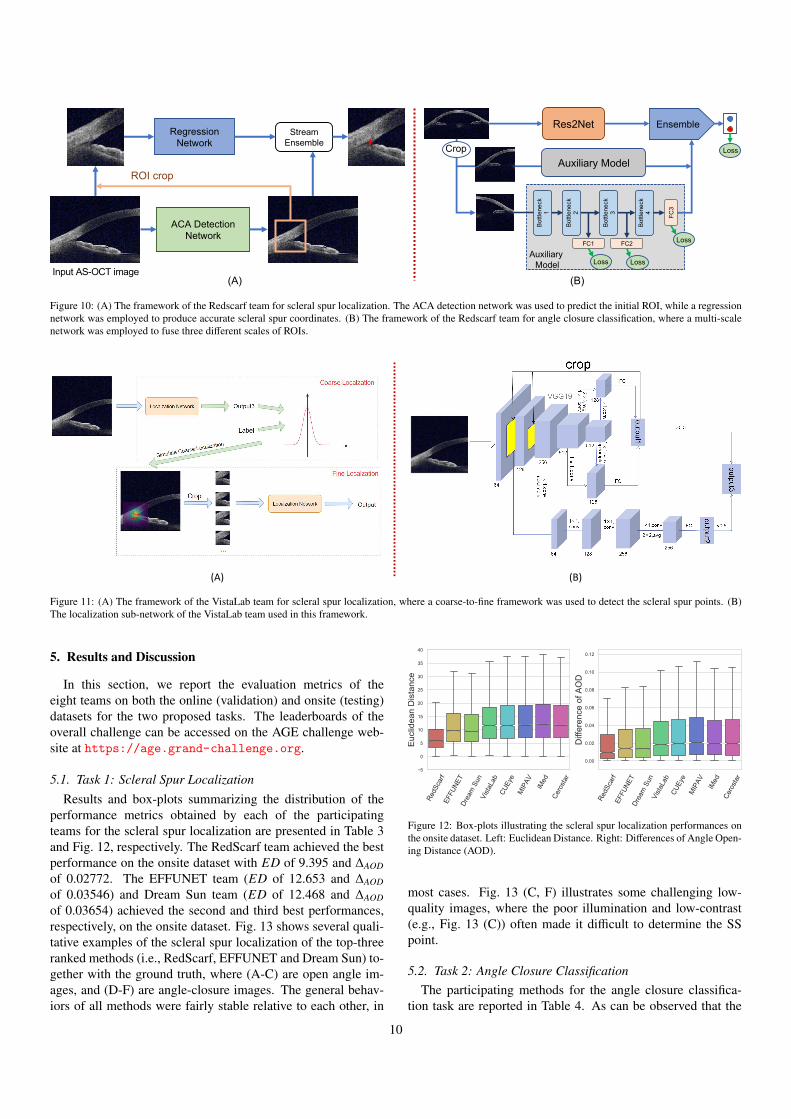
Figure 10: (A) The framework of the Redscarf team for scleral spur localization. The ACA detection network was used to predict the initial ROI, while a regressionnetwork was employed to produce accurate scleral spur coordinates. (B) The framework of the Redscarf team for angle closure classification, where a multi-scalenetwork was employed to fuse three different scales of ROIs.

(A) (B)

Figure 11: (A) The framework of the VistaLab team for scleral spur localization, where a coarse-to-fine framework was used to detect the scleral spur points. (B)The localization sub-network of the VistaLab team used in this framework.

5. Results and Discussion

In this section, we report the evaluation metrics of theeight teams on both the online (validation) and onsite (testing)datasets for the two proposed tasks. The leaderboards of theoverall challenge can be accessed on the AGE challenge web-site at https://age.grand-challenge.org.

5.1. Task 1: Scleral Spur LocalizationResults and box-plots summarizing the distribution of the

performance metrics obtained by each of the participatingteams for the scleral spur localization are presented in Table 3and Fig. 12, respectively. The RedScarf team achieved the bestperformance on the onsite dataset with ED of 9.395 and ∆AOD

of 0.02772. The EFFUNET team (ED of 12.653 and ∆AOD

of 0.03546) and Dream Sun team (ED of 12.468 and ∆AOD

of 0.03654) achieved the second and third best performances,respectively, on the onsite dataset. Fig. 13 shows several quali-tative examples of the scleral spur localization of the top-threeranked methods (i.e., RedScarf, EFFUNET and Dream Sun) to-gether with the ground truth, where (A-C) are open angle im-ages, and (D-F) are angle-closure images. The general behav-iors of all methods were fairly stable relative to each other, in

RedS

carf

EFFU

NET

Drea

m S

unVi

staL

abCU

Eye

MIP

AViM

edCe

rost

ar

5

0

5

10

15

20

25

30

35

40

Euc

lidea

n D

ista

nce

RedS

carf

EFFU

NET

Drea

m S

unVi

staL

abCU

Eye

MIP

AViM

edCe

rost

ar

0.00

0.02

0.04

0.06

0.08

0.10

0.12

Diff

eren

ce o

f AO

D

Figure 12: Box-plots illustrating the scleral spur localization performances onthe onsite dataset. Left: Euclidean Distance. Right: Differences of Angle Open-ing Distance (AOD).

most cases. Fig. 13 (C, F) illustrates some challenging low-quality images, where the poor illumination and low-contrast(e.g., Fig. 13 (C)) often made it difficult to determine the SSpoint.

5.2. Task 2: Angle Closure ClassificationThe participating methods for the angle closure classifica-

tion task are reported in Table 4. As can be observed that the

10

Figure 13: Zoomed-in scleral spur localization results of ground truth and top-three teams (i.e., RedScarf, EFFUNET and Dream Sun). Top raw images are openangle cases, while bottom raw images are angle-closure cases.

Table 3: Results of the scleral spur localization task.

Team Online (validation) data Onsite (testing) data Final RankingED ∆AOD Rank ED ∆AOD Rank S f inal Rank

EFFUNET 12.95 0.0456 4 12.65 0.0355 2 2.4 1RedScarf 16.55 0.1200 8 9.40 0.0277 1 2.4 1Dream Sun 12.90 0.0424 1 12.47 0.0365 3 2.6 3VistaLab 15.18 0.0470 6 14.00 0.0430 4 4.4 4CUEye 13.43 0.0450 3 14.39 0.0430 5 4.6 5MIPAV 13.76 0.0390 2 14.35 0.0469 6 5.2 6iMed 16.32 0.0547 7 14.87 0.0483 7 7.0 7Cerostar 13.53 0.0472 5 14.41 0.0486 8 7.4 8

Table 4: Results of the angle closure classification task.

Team Online (validation) data Onsite (testing) data Final RankingAUC Sensitivity Specificity Rank AUC Sensitivity Specificity Rank S f inal Rank

EFFUNET 1.00000 1.00000 1.00000 1 1.00000 1.00000 1.00000 1 1.0 1RedScarf 0.99976 0.99375 0.99531 8 1.00000 1.00000 1.00000 1 2.4 2VistaLab 1.00000 0.99688 1.00000 4 0.99998 1.00000 0.99375 3 3.2 3Dream Sun 1.00000 1.00000 1.00000 1 0.99992 1.00000 0.98750 4 3.4 4MIPAV 1.00000 1.00000 1.00000 1 0.99992 0.99688 0.99844 6 5.0 5iMed 0.99983 0.98750 0.99844 7 0.99959 1.00000 0.99375 5 5.4 6Cerostar 0.99999 0.99959 1.00000 5 0.99491 1.00000 0.97422 7 6.6 7CUEye 0.99297 1.00000 0.98594 6 0.98203 1.00000 0.96406 8 7.6 8

RedScarf and EFFUNET teams obtained perfect scores on theonsite dataset. Further, almost all the methods achieved a Sen-sitivity of 100%, while the major differences in performancebetween the methods is seen in the Specificity scores, rangingfrom 96.4% to 100%. However, there were still two teams,i.e., RedScarf and EFFUNET, that also obtained a Specificityof 100% on the onsite dataset. There are several possible rea-sons for this high-performance: 1) The angle closure cases inthe AGE challenge were at moderate or advanced stage, withan obvious closed anterior chamber angle making them easyto discriminate from open angle cases. 2) In contrast to theclinical quantitative measurements (e.g. anterior chamber area,ACW, AOD, and angle recess area), the visual representations

extracted by deep networks can present more information be-yond what clinicians recognize as relevant. This point was alsoobserved in other angle closure studies (Fu et al., 2019a; Xuet al., 2019; Fu et al., 2019b).

5.3. Discussion

From the AGE challenge results, the top-performing ap-proach had an average ED of 10 pixel (10µm) in scleral spurlocalization, while in the task of angle closure classification, allthe algorithms achieved satisfactory performances,with the top-two obtaining accuracy rate of 100% on the onsite dataset. Inthis section, we provide more analysis and discussion about thecomparisons between different solutions.

11

5.3.1. Scleral Spur Localization TaskThe original resolution of AS-OCT images was 2130×998,

which is too large for training deep models directly due to limi-tations in GPU memory. As such, most teams chose a coarse-to-fine strategy. For example, the solutions of the top-three teamswere all based on an ROI cropped flowchart. In fact, six out ofthe eight teams employed this strategy (see Table 2) to ensurea more precise localization. This was perhaps motivated by thefact that the scleral spur labels were provided as single pixels.Therefore, identifying a first approximation of the area and pre-dicting the final value in a second iteration allows more detailedfeatures of the ACA structure to be preserved and prevents in-formation loss caused, for example, by down-sampling. Thestandard U-Net was utilized by most methods for identifyingthe initial ROI, which could provide a satisfactory result.

As mentioned in Section 4, there are three main solutionsfor SS localization from ROI and global images, e.g., valueregression, binary mask segmentation, and heat map predic-tion. Value regression directly predicts the coordinates of theSS point by using a deep regression network (e.g., SE-Net (Huet al., 2018), ResNet (He et al., 2016), or VGG (Simonyanand Zisserman, 2014)). However, CNN regression networkshave more parameters than the segmentation networks, due tothe fully connected layers, which require more training data toavoid overfitting. Moreover, for a high-resolution image (i.e.,2130×998), it is challenging to predict a accurate coordinateswithin a small pixel-level range. By contrast, the binary masksegmentation and heat map prediction are based on segmenta-tion networks (e.g., U-Net (Falk et al., 2019) or AG-Net (Zhanget al., 2019)), which can be optimized well with limited data.Moreover, heat maps can extend the scleral spur position froma single pixel to a small area that can easily be approximated.From the online challenge evaluation results, it can be deductedthat modeling the SS localization task as a heat map predictionproblem is appropriate, with the top-three teams being based onthis.

For the network architecture, the Cerostar and CUEye teamsutilized a multi-scale ensemble framework to integrate the dif-ferent input ROIs. The Dream Sun team employed a multi-model fusion strategy to combine the results of EfficientNet B2,B3, B5, and B6. Other teams based their methods on a singlemodel to predict the SS localization. From the challenge eval-uation results, the ensemble strategy does not gain a significantimprovement over the single models. One possible reason isthat, as a one-pixel position prediction, semantic information ina larger view does not provide more representations than thatin a small ROI for SS point localization. Overall, the singlesegmentation models based on ROIs can achieve satisfactoryresults for the scleral spur localization task.

5.3.2. Angle Closure Classification TaskSimilar to the scleral spur localization task, coarse-to-fine

strategies were also widely used for angle closure classification(five out of eight teams in Table 1). The general flowchart wasfirst identify the SS point and then crop a smaller ROI, fed toa classification network to predict the angle closure. One ma-jor reason for doing this is that the main representations used

to describe features of the anterior chamber angle fall into theACA region, which is consistent with previous clinical stud-ies (Chansangpetch et al., 2018; Ang et al., 2018; Fu et al.,2019a).

From Table 1, we found that most teams built their networksbased on ResNet (He et al., 2016) or SE-Net (Hu et al., 2018).This demonstrates that basic deep networks have adequate abil-ity to distinguish the angle closure. The top-two teams utilizedadvanced deep networks, e.g., Res2Net (Gao et al., 2020) andEfficientNet (Tan and Le, 2019), and got better performances.However, due to the limited amount of training data, the deepnetworks tended to suffer from overfitting. Combining of mul-tiple models or multi-scale features is a way to prevent this. Ta-ble 1 shows that six out of the eight teams utilized ensemblingto improve the generalization performance.

5.3.3. Clinical DiscussionIn clinical practice, the localization of the SS is the basic

step to quantitatively evaluate the ACA. Therefore, we set upan independent task to automatically annotate the SS, and thencalculate the AOD according to the annotated SS. Compared tothe ground truth, the deep learning algorithms had an averagedeviation of SS localization of around 10µm. Further improve-ments are needed before they can be used in clinics. In the taskof angle closure classification, all the algorithms achieved idealperformances, with nearly 100% accuracy rate. This is under-standable since the cases included in the AGE challenge mostlyhave common ACA morphology but not special structures suchas plateau iris. Although our AGE challenge is currently thelargest public dataset composed of 4800 images, we are stillunable to predict if the algorithms would maintain good per-formance in a real-world setting, as the ACA morphologies areeven more complex in the general population. This is a verypromising start but still distant from the destination. Anotherpotential limitation of our study is that the AS-OCT imageswere only taken using a Casia SS-1000 OCT device. This couldpossibly have a negative effect on the quality and performancewhen the algorithms are applied to images from other AS-OCTacquisition devices. In a future challenge, it would be of valueto add more AS-OCT modalities from different-stage angle clo-sure patients and train the algorithms for diagnosis.

6. Conclusion

In this paper, we summarized the methods and results of theAGE challenge. We compared the performances of eight teamsthat participated in the onsite challenge at MICCAI 2019. Arti-ficial intelligence techniques were shown to be promising forhelping clinicians to reliably and rapidly identify SS points.Further, using deep learning methods to discriminate moderateor advanced angle closure from open angle also demonstratedencouraging results.

In summary, the AGE challenge is the first open AS-OCTdataset focused on scleral spur localization and angle closureclassification. The data and evaluation framework are publiclyaccessible through the Grand Challenges website at https:

12

//age.grand-challenge.org. Future participants are wel-come to submit their results on the challenge website and use itfor benchmarking their methods. The website will remain per-manently available for submissions, to encourage future devel-opments in the field. We expect that the unique AGE challengewill be beneficial to both early-stage and senior researchers inrelated fields.

References

Abramoff, M.D., Lavin, P.T., Birch, M., Shah, N., Folk, J.C., 2018. Pivotaltrial of an autonomous AI-based diagnostic system for detection of diabeticretinopathy in primary care offices. npj Digital Medicine 1, Article number:39.

Ang, M., Baskaran, M., et al., 2018. Anterior segment optical coherence to-mography. Progress in Retinal and Eye Research 66, 132–156.

Asaoka, R., Murata, H., Iwase, A., Araie, M., 2016. Detecting Preperimet-ric Glaucoma with Standard Automated Perimetry Using a Deep LearningClassifier. Ophthalmology 123, 1974–1980.

Bi, W.L., Hosny, A., et al., 2019. Artificial intelligence in cancer imaging:Clinical challenges and applications. CA: A Cancer Journal for Clinicians69, caac.21552.

Chansangpetch, S., Rojanapongpun, P., Lin, S.C., 2018. Anterior SegmentImaging for Angle Closure. American Journal of Ophthalmology 188, xvi–xxix.

Chaurasia, A., Culurciello, E., 2017. Linknet: Exploiting encoder representa-tions for efficient semantic segmentation, in: IEEE Visual Communicationsand Image Processing, pp. 1–4.

Chen, Y., Wang, Z., Peng, Y., Zhang, Z., Yu, G., Sun, J., 2018. Cascadedpyramid network for multi-person pose estimation, in: CVPR, pp. 7103–7112.

Console, J.W., Sakata, L.M., Aung, T., Friedman, D.S., He, M., 2008. Quantita-tive analysis of anterior segment optical coherence tomography images: theZhongshan Angle Assessment Program. British Journal of Ophthalmology92, 1612–1616.

De Fauw, J., Ledsam, J.R., et al., 2018. Clinically applicable deep learning fordiagnosis and referral in retinal disease. Nature Medicine 24, 1342–1350.

Eban, E., Schain, M., Mackey, A., Gordon, A., Rifkin, R., Elidan, G., 2017.Scalable Learning of Non-Decomposable Objectives, in: Proceedings of the20th International Conference on Artificial Intelligence and Statistics, pp.832–840.

Falk, T., Mai, D., et al., 2019. U-Net: deep learning for cell counting, detection,and morphometry. Nature Methods 16, 67–70.

Foster, P.J., 2001. Glaucoma in China: how big is the problem? British Journalof Ophthalmology 85, 1277–1282.

Fu, H., Baskaran, M., et al., 2019a. A Deep Learning System for AutomatedAngle-Closure Detection in Anterior Segment Optical Coherence Tomogra-phy Images. American Journal of Ophthalmology 203, 37–45.

Fu, H., Cheng, J., Xu, Y., Wong, D.W.K., Liu, J., Cao, X., 2018a. Joint OpticDisc and Cup Segmentation Based on Multi-Label Deep Network and PolarTransformation. IEEE Transactions on Medical Imaging 37, 1597–1605.

Fu, H., Cheng, J., Xu, Y., Zhang, C., Wong, D.W.K., Liu, J., Cao, X., 2018b.Disc-Aware Ensemble Network for Glaucoma Screening From Fundus Im-age. IEEE Transactions on Medical Imaging 37, 2493–2501.

Fu, H., Xu, Y., Wong, D., Liu, J., Baskaran, M., Perera, S., Aung, T., 2016. Au-tomatic Anterior Chamber Angle Structure Segmentation in AS-OCT Imagebased on Label Transfer, in: EMBC, pp. 1288–1291.

Fu, H., Xu, Y., et al., 2017. Segmentation and Quantification for Angle-ClosureGlaucoma Assessment in Anterior Segment OCT. IEEE Transactions onMedical Imaging 36, 1930–1938.

Fu, H., Xu, Y., et al., 2018c. Multi-Context Deep Network for Angle-ClosureGlaucoma Screening in Anterior Segment OCT, in: MICCAI, pp. 356–363.

Fu, H., Xu, Y., et al., 2019b. Angle-Closure Detection in Anterior SegmentOCT Based on Multilevel Deep Network. IEEE Transactions on Cybernetics, 1–9.

Gao, S., Cheng, M., Zhao, K., Zhang, X., Yang, M., Torr, P.H.S., 2020.Res2net: A new multi-scale backbone architecture. IEEE Transactions onPattern Analysis and Machine Intelligence .

Gargeya, R., Leng, T., 2017. Automated Identification of Diabetic RetinopathyUsing Deep Learning. Ophthalmology , 1–8.

Grassmann, F., Mengelkamp, J., et al., 2018. A Deep Learning Algorithmfor Prediction of Age-Related Eye Disease Study Severity Scale for Age-Related Macular Degeneration from Color Fundus Photography. Ophthal-mology 125, 1410–1420.

Gulshan, V., Peng, L., et al., 2016. Development and Validation of a DeepLearning Algorithm for Detection of Diabetic Retinopathy in Retinal Fun-dus Photographs. JAMA 316, 2402.

Hao, H., Fu, H., Xu, Y., Yang, J., Li, F., Zhang, X., Liu, J., Zhao, Y.,2020a. Open-Narrow-Synechiae Anterior Chamber Angle Classification inAS-OCT Sequences, in: MICCAI.

Hao, H., Zhao, Y., Fu, H., Shang, Q., Li, F., Zhang, X., Liu, J., 2019. Anteriorchamber angles classification in anterior segment oct images via multi-scaleregions convolutional neural networks, in: EMBC, pp. 849–852.

Hao, J., Fu, H., Xu, Y., Hu, Y., Li, F., Zhang, X., Liu, J., Zhao, Y., 2020b. Re-construction and Quantification of 3D Iris Surface for Angle-Closure Glau-coma Detection in Anterior Segment OCT, in: MICCAI.

He, K., Zhang, X., Ren, S., Sun, J., 2016. Deep Residual Learning for ImageRecognition, in: CVPR, IEEE. pp. 770–778.

He, T., Zhang, Z., Zhang, H., Zhang, Z., Xie, J., Li, M., 2019. Bag of tricksfor image classification with convolutional neural networks, in: CVPR, pp.558–567.

Hu, J., Shen, L., Sun, G., 2018. Squeeze-and-Excitation Networks, in: CVPR,pp. 7132–7141.

Kermany, D.S., Goldbaum, M., et al., 2018. Identifying Medical Diagnosesand Treatable Diseases by Image-Based Deep Learning. Cell 172, 1122–1131.e9.

Krause, J., Gulshan, V., et al., 2018. Grader Variability and the Importance ofReference Standards for Evaluating Machine Learning Models for DiabeticRetinopathy. Ophthalmology 125, 1264–1272.

Li, Z., He, Y., Keel, S., Meng, W., Chang, R.T., He, M., 2018. Efficacy ofa Deep Learning System for Detecting Glaucomatous Optic NeuropathyBased on Color Fundus Photographs. Ophthalmology 125, 1199–1206.

Lin, T.Y., Goyal, P., Girshick, R., He, K., Dollar, P., 2017. Focal loss for denseobject detection, in: ICCV, pp. 2980–2988.

Liu, H., Wong, D.W.K., Fu, H., Xu, Y., Liu, J., 2019. DeepAMD: DetectEarly Age-Related Macular Degeneration by Applying Deep Learning in aMultiple Instance Learning Framework, in: Asian Conference on ComputerVision, pp. 625–640.

Maggioni, M., Katkovnik, V., Egiazarian, K., Foi, A., 2012. Nonlocaltransform-domain filter for volumetric data denoising and reconstruction.IEEE transactions on image processing 22, 119–133.

Maier-Hein, L., Eisenmann, M., et al., 2018. Why rankings of biomedicalimage analysis competitions should be interpreted with care. Nature Com-munications 9, 5217.

Niwas, S.I., Lin, W., et al., 2016. Automated anterior segment OCT imageanalysis for Angle Closure Glaucoma mechanisms classification. ComputerMethods and Programs in Biomedicine 130, 65–75.

Nongpiur, M.E., Aboobakar, I.F., et al., 2017. Association of Baseline AnteriorSegment Parameters With the Development of Incident Gonioscopic AngleClosure. JAMA Ophthalmology 135, 252.

Nongpiur, M.E., Haaland, B.A., et al., 2013. Classification Algorithms Basedon Anterior Segment Optical Coherence Tomography Measurements for De-tection of Angle Closure. Ophthalmology 120, 48–54.

Orlando, J.I., Fu, H., et al., 2020. REFUGE Challenge: A unified framework forevaluating automated methods for glaucoma assessment from fundus pho-tographs. Medical Image Analysis 59, 101570.

Peng, Y., Dharssi, S., et al., 2019. DeepSeeNet: A Deep Learning Model forAutomated Classification of Patient-based Age-related Macular Degenera-tion Severity from Color Fundus Photographs. Ophthalmology 126, 565–575.

Quigley, H.A., Broman, A., 2006. The number of people with glaucoma world-wide in 2010 and 2020. British Journal of Ophthalmology 90, 262–267.

Rajkomar, A., Dean, J., Kohane, I., 2019. Machine Learning in Medicine. NewEngland Journal of Medicine 380, 1347–1358.

Redmon, J., Farhadi, A., 2018. YOLOv3: An Incremental Improvement. arXiv.

Sakata, L.M., 2008. Assessment of the Scleral Spur in Anterior Segment Op-tical Coherence Tomography Images. Archives of Ophthalmology 126, 181.

Sakata, L.M., Lavanya, R., et al., 2008. Comparison of Gonioscopy and Ante-

13

rior Segment Ocular Coherence Tomography in Detecting Angle Closure inDifferent Quadrants of the Anterior Chamber Angle. Ophthalmology 115,769–774.

Scheie, H.G., 1957. Width and Pigmentation of the Angle of the AnteriorChamber: A System of Grading by Gonioscopy. JAMA Ophthalmology58, 510–512.

Schmidt-Erfurth, U., Sadeghipour, A., et al., 2018. Artificial intelligence inretina. Progress in Retinal and Eye Research 67, 1–29.

Sharma, R., Sharma, A., et al., 2014. Application of anterior segment opticalcoherence tomography in glaucoma. Survey of Ophthalmology 59, 311–327.

Simonyan, K., Zisserman, A., 2014. Very Deep Convolutional Networks forLarge-Scale Image Recognition. arXiv .

Tan, M., Le, Q., 2019. EfficientNet: Rethinking model scaling for convolutionalneural networks, in: International Conference on Machine Learning, pp.6105–6114.

Tian, J., Marziliano, P., Baskaran, M., Wong, H.T., Aung, T., 2011. AutomaticAnterior Chamber Angle Assessment for HD-OCT Images. IEEE Transac-tions on Biomedical Engineering 58, 3242–3249.

Ting, D., Cheung, C., et al., 2017. Development and Validation of a DeepLearning System for Diabetic Retinopathy and Related Eye Diseases UsingRetinal Images From Multiethnic Populations With Diabetes. JAMA 318,2211.

Ting, D.S., Peng, L., et al., 2019. Deep learning in ophthalmology: The tech-nical and clinical considerations. Progress in Retinal and Eye Research 72,100759.

Wang, S., Yu, L., Yang, X., Fu, C.W., Heng, P.A., 2019. Patch-Based OutputSpace Adversarial Learning for Joint Optic Disc and Cup Segmentation.IEEE Transactions on Medical Imaging 38, 2485–2495.

Xie, S., Girshick, R., Dollar, P., Tu, Z., He, K., 2017. Aggregated ResidualTransformations for Deep Neural Networks, in: CVPR, pp. 5987–5995.

Xu, B.Y., Chiang, M., et al., 2019. Deep Learning Classifiers for AutomatedDetection of Gonioscopic Angle Closure Based on Anterior Segment OCTImages. American Journal of Ophthalmology 208, 273–280.

Xu, Y., Liu, J., et al., 2012. Anterior chamber angle classification using multi-scale histograms of oriented gradients for glaucoma subtype identification,in: EMBC, pp. 3167–3170.

Xu, Y., Liu, J., et al., 2013. Automated anterior chamber angle localization andglaucoma type classification in OCT images, in: EMBC, pp. 7380–7383.

Zhang, S., Fu, H., Yan, Y., Zhang, Y., Wu, Q., Yang, M., Tan, M., Xu, Y.,2019. Attention guided network for retinal image segmentation, in: MIC-CAI, Springer. pp. 797–805.

14