Bohdalova

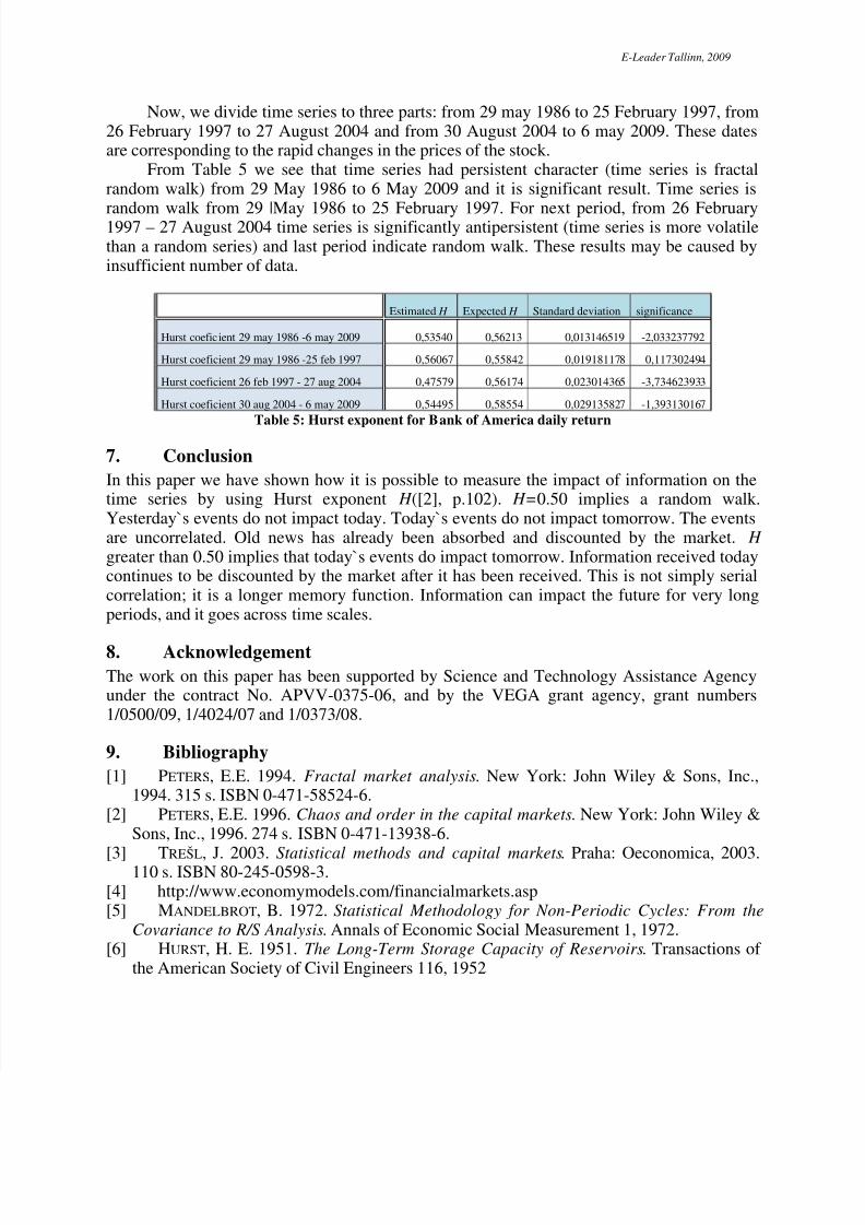
7/31/2019 Bohdalova

http://slidepdf.com/reader/full/bohdalova 1/9

E-Leader Tallinn, 2009

FINANCIAL MARKETS DURING ECONOMIC CRISIS

Mária Bohdalová and Michal Greguš

Comenius University, Faculty of ManagementBratislava, Slovak Republic

Abstract

Contemporary financial depression of the financial markets proves high fluctuations of theprices of the stocks. These fluctuations have considerable impact on the values of thefinancial portfolios. Classical approaches to modeling of the behavior of the prices of thestocks may produce wrong predictions of their future values. That is the reason why weintroduce in this paper the fractal market analysis. Fractal structure accepts globaldeterminism and local randomness of the behavior of the financial time series. We will useR/S analysis in this paper. R/S analysis can distinguish fractals from other types of timeseries, revealing the self-similar statistical structure.

Key words: financial time series modeling, fractal, R/S analysis, Hurst exponent

1. Introduction

The financial markets are an important part of any economy. For that reason, financialmarkets are also an important aspect of every model of the economy1. Markets are “efficient”if prices reflect all current information that could anticipate future events. Therefore, only thespeculative, stochastic component could be modeled, the change in prices due to changes invalue could not. If markets do not follow a random walk, it is possible that we may be over-orunderstanding our risk and return potential from investing versus speculating.

2. Introduction to Fractals and the Fractal dimensions

The development of fractal geometry has been one of the 20-th century’s most usefuland fascinating discoveries in mathematics ([2], p.45). Fractals give structure to complexity,and beauty to chaos. Most natural shapes, and time series, are best described by fractals.Fractals are self–referential, or self–similar. Fractal shapes show self–similarity with respect

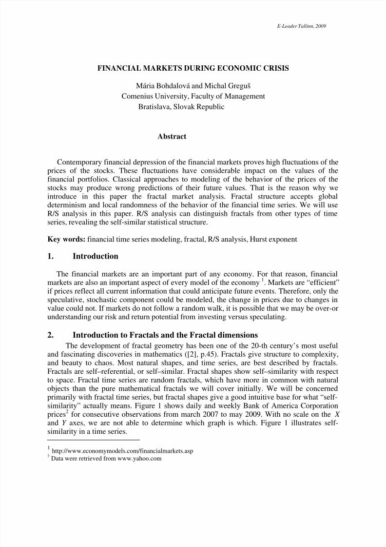
to space. Fractal time series are random fractals, which have more in common with naturalobjects than the pure mathematical fractals we will cover initially. We will be concernedprimarily with fractal time series, but fractal shapes give a good intuitive base for what “self-similarity” actually means. Figure 1 shows daily and weekly Bank of America Corporationprices2 for consecutive observations from march 2007 to may 2009. With no scale on the X and Y axes, we are not able to determine which graph is which. Figure 1 illustrates self-similarity in a time series.

1 http://www.economymodels.com/financialmarkets.asp 2 Data were retrieved from www.yahoo.com

7/31/2019 Bohdalova



Close

0

10

20

30

40

50

60

Date

2006 2007 2008 2009 2010

Close

0

10

20

30

40

50

60

Date

2006 2007 2008 2009 2010

Figure 1: Daily and weekly prices of stock Bank of America Corp.

Fractal shapes can be generated in many ways. The simplest way is to take a generatingrule and iterate it over and over again. Random fractals are combination of generating ruleschosen at random for different scales. Combination of randomness coupled with deterministicgeneration rules, or “causality”, can make fractals useful in capital market analysis. Randomfractals ([2], p.51) do not necessarily have pieces that look like pieces of the whole. Instead,they may be qualitatively related. In the case of time series, we will find that fractal timeseries are qualitatively self similar in that, at different scales, the series have similar statisticalcharacteristics. If we would like to understand the underlying causality of the structure of timeseries, then classical geometry offers little help. May be, time series is a random walk – asystem so complex that the prediction becomes impossible. In statistical term, the number of degrees of freedom or factors influencing the system is very large. These systems are notwell-described by standard Gaussian statistics. Standard statistical analysis begins byassuming that the system under study is primarily random; that is, the causal process thatcreated the time series has many component parts, or degree of freedom, and the interactionof those components is so complex that deterministic explanation is not possible ([1], p.53).Only probabilities can help us to understand and take advantage of the process. Theunderlying philosophy implies that randomness and determinism cannot coexist. In order tostudy the statistics of these systems and create a more general analytical framework, we needa probability theory that is nonparametric. In this paper we introduce nonparametricmethodology that was discovered by H.E. Hurst3.

In advance, we introduce the term fractal dimension. The fractal dimension describeshow a time series fills its space, is the product of all factors influencing the system thatproduces time series ([2], p.57). Fractal time series can have fractional dimensions. Thefractal dimension of a time series measures how jagged the time series is ([1], p.16). Aswould be expected, a straight line has a fractal dimension of 1. Time series is only randomwhen it is influenced by a large number of events that are equally likely to occur. In statisticalterm, it has a high number of degree of freedom. A random series would have no correlation

with previous points. Nothing would keep the points in the same vicinity, to preserve theirdimensionality. Instead, they will fill up whatever space they are placed in. A nonrandomtime series will reflect the nonrandom nature of its influences. The data will clump together,to reflect the correlations inherent in its influences. In other words, the time series will befractal. To determine the fractal dimension, we must measure how the object clumps togetherin its space. However, a random walk has 50–50 chance of rising or falling, hence, its fractaldimension is 1.50. The fractal dimension of a time series is important because it recognizesthat process can be somewhere between deterministic (a line with fractal dimension of 1) andrandom (a fractal dimension of 1.50). In fact, the fractal dimension of a line can range from 1

3 Hurst, H.E. 1951. The Long-Term Storage Capacity of Reservoirs. In: Transaction of the American Society of

Civil Engineers 116.

7/31/2019 Bohdalova



to 2. The normal distribution has an integer dimension of 2, which many of characteristics of the time series. At values 1.50<d <2, a time series is more jagged than a random series.

They are many ways of calculating fractal dimensions. We introduce methodology of the Hurst exponent H, and we convert it into the fractal dimension d in this paper.

3.

R/S analysis and Hurst exponentHurst was aware of Einstein`s4 work of Brownian motion. Brownian motion became theprimary model for a random walk process. Einstein found that the distance that a randomparticle covers increases with the square root of time used to measure it, or:

R=T 0.50, (1)

where R is the distance covered and T is a time index.Equation (1) is called the T to the one–half rule, and it is commonly used in statistics.Financial economists use it to annualize volatility or standard deviation. To standardize themeasure over time, Hurst decided to create a dimensionless ratio by dividing the range by thestandard deviation of the observations. Hence, the analysis is called rescaled range analysis(R/S analysis). Hurst found that most natural phenomena follow a “biased random walk” – a

trend with noise. The strength of the trend and the level of noise could be measured by howthe rescaled range scales with time, that is, by how high H is above 0.50. Peters ([1] p.56)reformulated Hurst`s work for a general time series as follows.

We begin with a time series, X={ x1, x2, …, xn}, to represent n consecutive values. Formarkets, it can be the daily changes in price of a stock index. The rescaled range wascalculated by first rescaling or “normalizing” the data by subtracting the sample mean xm:

Z r =( xr – xm), r =1,2,…,n (2)The resulting series, Z , now has a mean of zero. The next step creates a cumulative time seriesY:

Y 1=( Z 1+ Z r ), r =2,3,…,n (3)Note that, by definition, the last value of Y (Y n) will always be zero because Z has a mean of zero. The adjusted range, R

n, is the maximum minus minimum value of the Y

r :

Rn=max(Y 1, Y 2,…, Y n)–min(Y 1, Y 2,…, Y n). (4)The subscript, n, for Rn now signifies that this is the adjusted range for x1, x2, …, xn. BecauseY has been adjusted to a mean of zero, the maximum value of Y will always be greater than orequal to zero, and the minimum will always be less than or equal to zero. Hence, the adjustedrange, Rn, will always be nonnegative. This adjusted range, Rn, is the distance that the systemtravels for time index n. If we set n=T , we can apply equation (1), provided that the timeseries, X , is independent for increasing values of n. However, equation (1) applies only totime series that are in Brownian motion (they have zero mean, and variance is equal to one).To apply this concept to time series that are not in Brownian motion, we need to generalizedequation (1) and take into account systems that are not independent. Hurst found that thefollowing was a more general form of equation (1):

( R/S)n=c.n H (5)The subscript, n, for ( R/S)n refers to the R/S value for x1, x2, …, xn and c is a constant.

The R/S value of equation (5) is referred to as the rescaled range because it has zeromean and is expressed in terms of local standard deviation. In general, the R/S value scaled aswe increase the time increment, n, by a power–law value equal to H , generally called the

Hurst exponent .Rescaling allows us to compare periods of time that may be many apart. In comparing

stock returns of the 1920s with those of the 1980, prices present a problem because of inflationary growth. Rescaling minimize this problem, by rescaling the data to zero mean andstandard deviation of one, to allow diverse phenomena and time periods to be compared.

4 Einstein, A. 1908. Uber die von der molekularkinetischen Theorie der Warme geforderte Bewegung von inruhenden Flüssigkeiten suspendierten Teilchen. Annals of Physics 322.

7/31/2019 Bohdalova



Rescaled range analysis can also describe time series that have no characteristic scale. This isa characteristic of fractals.

The Hurst exponent can be approximated by plotting the log( R / Sn) versus the log(n) andsolving for the slope through an ordinary least squares regression:

log( R / Sn)=log(c)+ H .log(n) (6)

If a system is independently distributed, then H =0.50. When H differed from 0.50, theobservations are not independent. Each observation carried a „memory“ of all the events thatpreceded it. What happens today influences the future. Where we are now is a result of wherewe have been in the past. Time is important. The impact of the present on the future can beexpressed as a correlation:

C =2(2 H -1)–1, (7)where C is correlation measure and H is Hurst exponent.It is important to remember that this correlation measure is not related to the Auto CorrelationFunction (ACF) of Gaussian random variables ([2], p.70). The ACF assumes Gaussian, ornear-Gaussian, properties in the underlying distribution. The ACF works well in determiningshort-run dependence, but tends to understate long-run correlation for non-Gaussian series(full mathematical explanation we find in [5].There are three distinct classifications for the Hurst exponent ([2], p.64):

1. H =0.50: time series is random, events are random and uncorrelated. Equation (7)equals zero. The present does not influence the future. Its probability densityfunction can be normal curve, but it does not have to be. R/S analysis can classifyan independent series, no mater what the shape of the underlying distribution.

2. 0≤ H <0.50: time series is antipersistent, or ergodic. If the time series has been upin the previous period, it is more likely to be down in the next period. Conversely,if it was down before, it is more likely to be up in the next period. The strength of this antipersistent behavior depends on how close H is to zero. The closer it is tozero, the closer C in equation (7) moves toward –0.50, or negative correlation.This time series is more volatile than a random series.

3. 0.50≤ H <1.00: time series have a persistent or trend-reinforcing character. If theseries has been up (down) in the last period, then the chances are that it willcontinue to be positive (negative) in the next period. Trend is apparent. Thestrength of the trend-reinforcing behavior, or persistence, increases as H approaches 1.0. The closes H is to 0.5, the noisier it will be, and the less definedits trends will be. Persistent series are fractional Brownian motion, or biasedrandom walk5. The strength of the bias depends on how far H is above 0.50. Ahigh H value shows less noise, more persistence and clearer trends than do lowervalue. A high H means less risk.

4. Testing R/S analysis

To evaluate the significance of R/S analysis, we calculate expected value of the R/Sstatistics and the Hurst exponent. We compare the behavior of our process, described by R/Sanalysis with an independent and random system and gauge its significance.

We will test this null hypothesis: “The process is independent, identically distributedand is characterized by a random walk”6.

To verify this hypothesis, we calculate expected value of the adjusted range7 E ( R / Sn)and its variance8 Var ( E ( R / Sn)).

5 Biased random walks were extensively studied by Hurst in the 1940s and again by Mandelbrot in the 1960s and1970s. Mandelbrot called them fractional brownian motions.([2], p.61)6 This process has Gaussian structure (see [1], p.66).7 This formula was derrived by Anis and Lloyd ([1], p.71)8 Variance was calculated by Feller ([1], p.66)

7/31/2019 Bohdalova



∑−

=

−

−

⋅⋅

−

=

1

1

5.0)(

2

5.0)(

n

r

nr

r nn

n

n R/S E

π (8)

nS R E Var n ⋅

−=

26)) / ((

2π π

. (9)

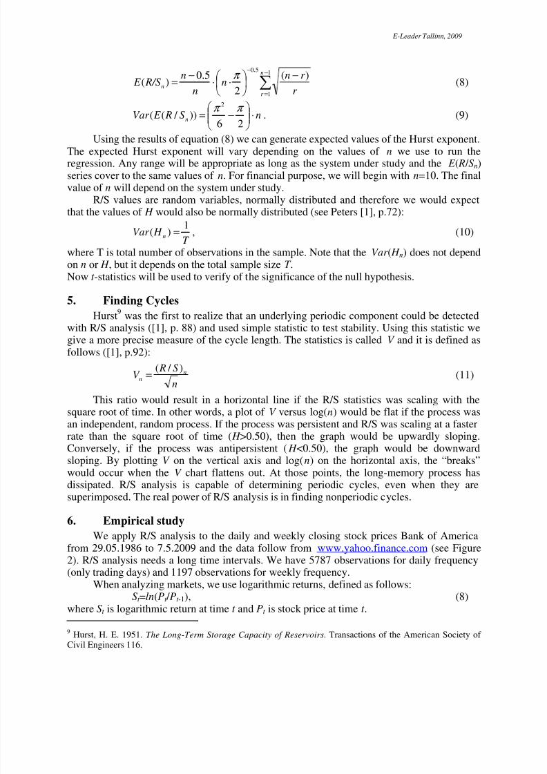
Using the results of equation (8) we can generate expected values of the Hurst exponent.The expected Hurst exponent will vary depending on the values of n we use to run theregression. Any range will be appropriate as long as the system under study and the E ( R / Sn)series cover to the same values of n. For financial purpose, we will begin with n=10. The finalvalue of n will depend on the system under study.

R/S values are random variables, normally distributed and therefore we would expectthat the values of H would also be normally distributed (see Peters [1], p.72):

T H Var

n

1)( = , (10)

where T is total number of observations in the sample. Note that the Var ( H n) does not dependon n or H , but it depends on the total sample size T .Now t -statistics will be used to verify of the significance of the null hypothesis.

5. Finding Cycles

Hurst9 was the first to realize that an underlying periodic component could be detectedwith R/S analysis ([1], p. 88) and used simple statistic to test stability. Using this statistic wegive a more precise measure of the cycle length. The statistics is called V and it is defined asfollows ([1], p.92):

n

S RV n

n

) / (= (11)

This ratio would result in a horizontal line if the R/S statistics was scaling with thesquare root of time. In other words, a plot of V versus log(n) would be flat if the process wasan independent, random process. If the process was persistent and R/S was scaling at a fasterrate than the square root of time ( H >0.50), then the graph would be upwardly sloping.Conversely, if the process was antipersistent ( H <0.50), the graph would be downwardsloping. By plotting V on the vertical axis and log(n) on the horizontal axis, the “breaks”would occur when the V chart flattens out. At those points, the long-memory process hasdissipated. R/S analysis is capable of determining periodic cycles, even when they aresuperimposed. The real power of R/S analysis is in finding nonperiodic cycles.

6. Empirical study

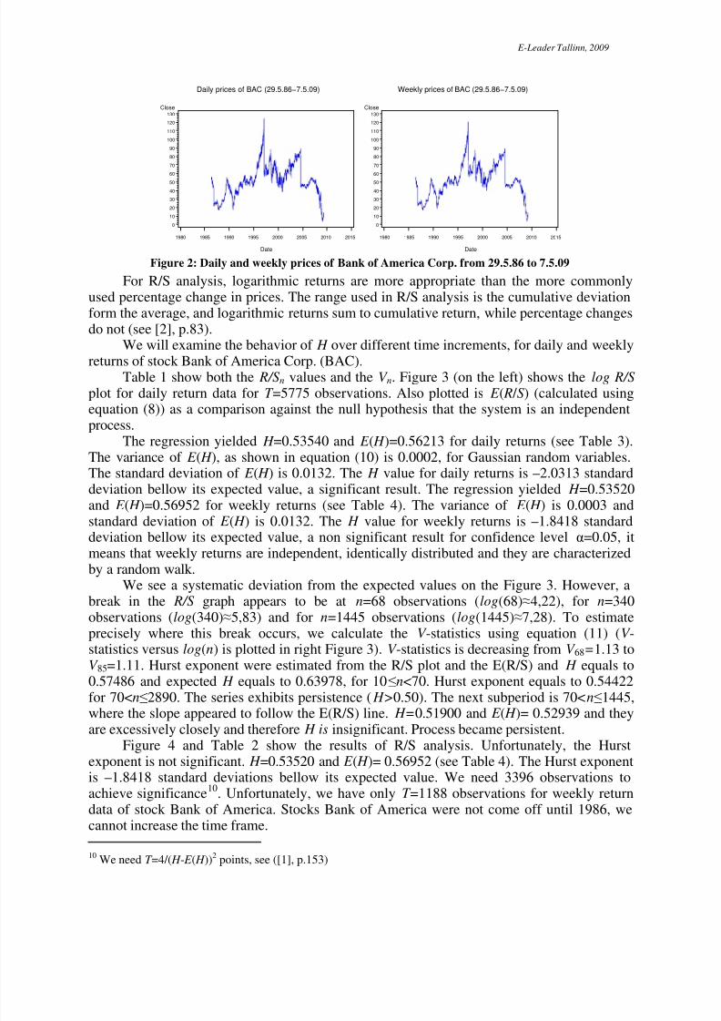
We apply R/S analysis to the daily and weekly closing stock prices Bank of Americafrom 29.05.1986 to 7.5.2009 and the data follow from www.yahoo.finance.com (see Figure2). R/S analysis needs a long time intervals. We have 5787 observations for daily frequency(only trading days) and 1197 observations for weekly frequency.

When analyzing markets, we use logarithmic returns, defined as follows:St =ln(Pt / Pt-1), (8)

where St is logarithmic return at time t and Pt is stock price at time t .

9 Hurst, H. E. 1951. The Long-Term Storage Capacity of Reservoirs. Transactions of the American Society of Civil Engineers 116.

7/31/2019 Bohdalova



Daily prices of BAC (29.5.86−7.5.09)

Close

0

10

20

30

40

50

60

70

80

90

100

110

120

130

Date

1980 1985 1990 1995 2000 2005 2010 2015

Weekly prices of BAC (29.5.86−7.5.09)

Close

0

10

20

30

40

50

60

70

80

90

100

110

120

130

Date

1980 1985 1990 1995 2000 2005 2010 2015

Figure 2: Daily and weekly prices of Bank of America Corp. from 29.5.86 to 7.5.09

For R/S analysis, logarithmic returns are more appropriate than the more commonlyused percentage change in prices. The range used in R/S analysis is the cumulative deviationform the average, and logarithmic returns sum to cumulative return, while percentage changesdo not (see [2], p.83).

We will examine the behavior of H over different time increments, for daily and weekly

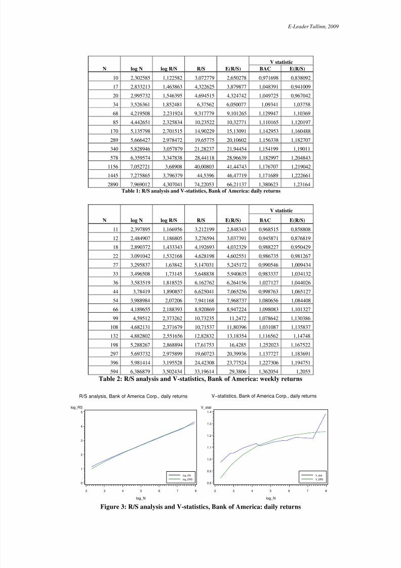
returns of stock Bank of America Corp. (BAC).Table 1 show both the R/Sn values and the V n. Figure 3 (on the left) shows the log R/S

plot for daily return data for T =5775 observations. Also plotted is E ( R / S) (calculated usingequation (8)) as a comparison against the null hypothesis that the system is an independentprocess.

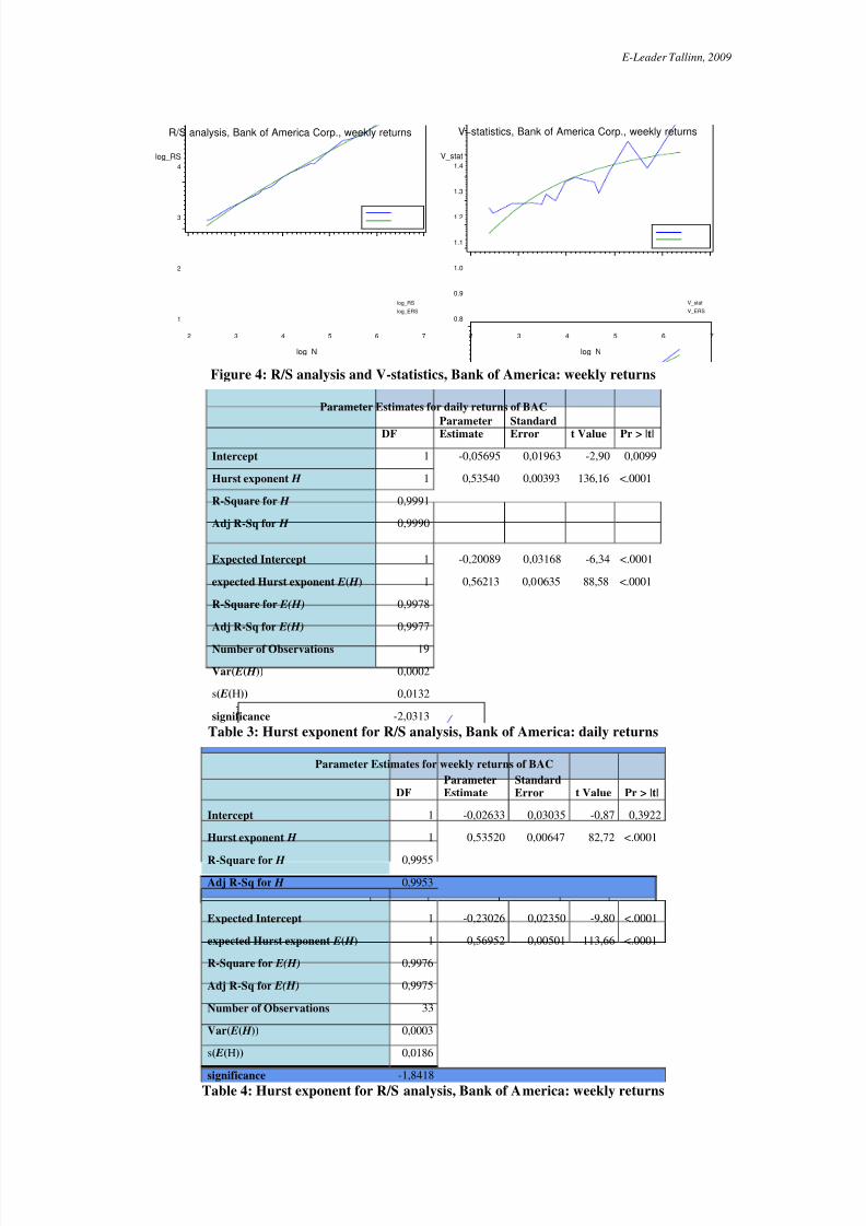
The regression yielded H =0.53540 and E ( H )=0.56213 for daily returns (see Table 3).The variance of E ( H ), as shown in equation (10) is 0.0002, for Gaussian random variables.The standard deviation of E ( H ) is 0.0132. The H value for daily returns is –2.0313 standarddeviation bellow its expected value, a significant result. The regression yielded H =0.53520and E ( H )=0.56952 for weekly returns (see Table 4). The variance of E ( H ) is 0.0003 andstandard deviation of E ( H ) is 0.0132. The H value for weekly returns is –1.8418 standard

deviation bellow its expected value, a non significant result for confidence level α=0.05, itmeans that weekly returns are independent, identically distributed and they are characterizedby a random walk.

We see a systematic deviation from the expected values on the Figure 3. However, abreak in the R/S graph appears to be at n=68 observations (log(68)≈4,22), for n=340observations (log(340)≈5,83) and for n=1445 observations (log(1445)≈7,28). To estimateprecisely where this break occurs, we calculate the V -statistics using equation (11) (V -statistics versus log(n) is plotted in right Figure 3). V -statistics is decreasing from V 68=1.13 toV 85=1.11. Hurst exponent were estimated from the R/S plot and the E(R/S) and H equals to0.57486 and expected H equals to 0.63978, for 10≤n<70. Hurst exponent equals to 0.54422 for 70<n≤2890. The series exhibits persistence ( H>0.50). The next subperiod is 70<n≤1445,

where the slope appeared to follow the E(R/S) line. H=0.51900 and E ( H )= 0.52939 and theyare excessively closely and therefore H is insignificant. Process became persistent. Figure 4 and Table 2 show the results of R/S analysis. Unfortunately, the Hurst

exponent is not significant. H =0.53520 and E ( H )= 0.56952 (see Table 4). The Hurst exponentis –1.8418 standard deviations bellow its expected value. We need 3396 observations toachieve significance10. Unfortunately, we have only T =1188 observations for weekly returndata of stock Bank of America. Stocks Bank of America were not come off until 1986, wecannot increase the time frame.

10 We need T =4/( H - E ( H ))2 points, see ([1], p.153)

7/31/2019 Bohdalova



N log N log R/S R/S E(R/S)

V statistic

BAC E(R/S)

10 2,302585 1,122582 3,072779 2,650278 0,971698 0,838092

17 2,833213 1,463863 4,322625 3,879877 1,048391 0,941009

20 2,995732 1,546395 4,694515 4,324742 1,049725 0,967042

34 3,526361 1,852481 6,37562 6,050077 1,09341 1,03758

68 4,219508 2,231924 9,317779 9,101265 1,129947 1,10369

85 4,442651 2,325834 10,23522 10,32771 1,110165 1,120197

170 5,135798 2,701515 14,90229 15,13091 1,142953 1,160488

289 5,666427 2,978472 19,65775 20,10602 1,156338 1,182707

340 5,828946 3,057879 21,28237 21,94454 1,154199 1,19011

578 6,359574 3,347838 28,44118 28,96639 1,182997 1,204843

1156 7,052721 3,68908 40,00803 41,44743 1,176707 1,219042

1445 7,275865 3,796379 44,5396 46,47719 1,171689 1,222661

2890 7,969012 4,307041 74,22053 66,21137 1,380623 1,23164Table 1: R/S analysis and V-statistics, Bank of America: daily returns

N log N log R/S R/S E(R/S)

V statistic

BAC E(R/S)

11 2,397895 1,166956 3,212199 2,848343 0,968515 0,858808

12 2,484907 1,186805 3,276594 3,037391 0,945871 0,876819

18 2,890372 1,433343 4,192693 4,032329 0,988227 0,950429

22 3,091042 1,532168 4,628198 4,602551 0,986735 0,981267

27 3,295837 1,63842 5,147031 5,245172 0,990546 1,009434

33 3,496508 1,73145 5,648838 5,940635 0,983337 1,034132

36 3,583519 1,818525 6,162762 6,264156 1,027127 1,044026

44 3,78419 1,890857 6,625041 7,065256 0,998763 1,065127

54 3,988984 2,07206 7,941168 7,968737 1,080656 1,084408

66 4,189655 2,188393 8,920869 8,947224 1,098083 1,101327

99 4,59512 2,373262 10,73235 11,2472 1,078642 1,130386

108 4,682131 2,371679 10,71537 11,80396 1,031087 1,135837

132 4,882802 2,551656 12,82832 13,18354 1,116562 1,14748

198 5,288267 2,868894 17,61753 16,4285 1,252023 1,167522

297 5,693732 2,975899 19,60723 20,39936 1,137727 1,183691

396 5,981414 3,195528 24,42308 23,77524 1,227306 1,194751

594 6,386879 3,502434 33,19614 29,3806 1,362054 1,2055

Table 2: R/S analysis and V-statistics, Bank of America: weekly returns

R/S analysis, Bank of America Corp., daily returns

log_RS

log_ERS

log_RS

0

1

2

3

4

5

log_N

2 3 4 5 6 7 8

V−statistics, Bank of America Corp., daily returns

V_stat

V_ERS

V_stat

0.8

0.9

1.0

1.1

1.2

1.3

1.4

log_N

2 3 4 5 6 7 8

Figure 3: R/S analysis and V-statistics, Bank of America: daily returns

7/31/2019 Bohdalova



R/S analysis, Bank of America Corp., weekly returns

log_RS

log_ERS

log_RS

1

2

3

4

log_N

2 3 4 5 6 7

V−statistics, Bank of America Corp., weekly returns

V_stat

V_ERS

V_stat

0.8

0.9

1.0

1.1

1.2

1.3

1.4

log_N

2 3 4 5 6 7

Figure 4: R/S analysis and V-statistics, Bank of America: weekly returns

Parameter Estimates for daily returns of BAC

DFParameterEstimate

StandardError t Value Pr > |t|

Intercept 1 -0,05695 0,01963 -2,90 0,0099

Hurst exponent H 1 0,53540 0,00393 136,16 <.0001

R-Square for H 0,9991

Adj R-Sq for H 0,9990

Expected Intercept 1 -0,20089 0,03168 -6,34 <.0001

expected Hurst exponent E( H ) 1 0,56213 0,00635 88,58 <.0001

R-Square for E(H) 0,9978

Adj R-Sq for E(H) 0,9977

Number of Observations 19

Var( E( H )) 0,0002

s( E(H)) 0,0132

significance -2,0313

Table 3: Hurst exponent for R/S analysis, Bank of America: daily returns

Parameter Estimates for weekly returns of BAC

DFParameterEstimate

StandardError t Value Pr > |t|

Intercept 1 -0,02633 0,03035 -0,87 0,3922

Hurst exponent H 1 0,53520 0,00647 82,72 <.0001

R-Square for H 0,9955

Adj R-Sq for H 0,9953

Expected Intercept 1 -0,23026 0,02350 -9,80 <.0001

expected Hurst exponent E( H ) 1 0,56952 0,00501 113,66 <.0001

R-Square for E(H) 0,9976

Adj R-Sq for E(H) 0,9975

Number of Observations 33

Var( E( H )) 0,0003

s( E(H)) 0,0186

significance -1,8418Table 4: Hurst exponent for R/S analysis, Bank of America: weekly returns

7/31/2019 Bohdalova


Documents

Bohdalova