This article was downloaded by: [National Chiao Tung University 國立交通大學]On: 28 April 2014, At: 15:15Publisher: Taylor & FrancisInforma Ltd Registered in England and Wales Registered Number: 1072954 Registered office: Mortimer House,37-41 Mortimer Street, London W1T 3JH, UK

International Journal of Production ResearchPublication details, including instructions for authors and subscription information:http://www.tandfonline.com/loi/tprs20

Cycle time estimation for semiconductor final testingprocesses with Weibull-distributed waiting timeY.T. Tai a , W.L. Pearn b & J.H. Lee ba Department of Information Management , Kai Nan University , No.1 Kainan Road, LuzhuShiang, Taoyuan 33857 , Taiwan , ROCb Department of Industrial Engineering and Management , National Chiao Tung University ,1001 University Road, Hsinchu 30010 , Taiwan , ROCPublished online: 17 Jun 2011.

To cite this article: Y.T. Tai , W.L. Pearn & J.H. Lee (2012) Cycle time estimation for semiconductor final testingprocesses with Weibull-distributed waiting time, International Journal of Production Research, 50:2, 581-592, DOI:10.1080/00207543.2010.543938

To link to this article: http://dx.doi.org/10.1080/00207543.2010.543938

PLEASE SCROLL DOWN FOR ARTICLE

Taylor & Francis makes every effort to ensure the accuracy of all the information (the “Content”) containedin the publications on our platform. However, Taylor & Francis, our agents, and our licensors make norepresentations or warranties whatsoever as to the accuracy, completeness, or suitability for any purpose of theContent. Any opinions and views expressed in this publication are the opinions and views of the authors, andare not the views of or endorsed by Taylor & Francis. The accuracy of the Content should not be relied upon andshould be independently verified with primary sources of information. Taylor and Francis shall not be liable forany losses, actions, claims, proceedings, demands, costs, expenses, damages, and other liabilities whatsoeveror howsoever caused arising directly or indirectly in connection with, in relation to or arising out of the use ofthe Content.

This article may be used for research, teaching, and private study purposes. Any substantial or systematicreproduction, redistribution, reselling, loan, sub-licensing, systematic supply, or distribution in anyform to anyone is expressly forbidden. Terms & Conditions of access and use can be found at http://www.tandfonline.com/page/terms-and-conditions

International Journal of Production ResearchVol. 50, No. 2, 15 January 2012, 581–592

Cycle time estimation for semiconductor final testing processes with

Weibull-distributed waiting time

Y.T. Taia*, W.L. Pearnb and J.H. Leeb

aDepartment of Information Management, Kai Nan University, No.1 Kainan Road, Luzhu Shiang, Taoyuan 33857,Taiwan, ROC; bDepartment of Industrial Engineering and Management, National Chiao Tung University,

1001 University Road, Hsinchu 30010, Taiwan, ROC

(Received 7 May 2010; final version received 19 October 2010)

Accurate cycle time is an essential planning basis required for many production applications, especially ondue date commitments, performance metrics analysing, capacity planning, and scheduling. The re-entrantfinal testing process is the final stage of the complicated semiconductor manufacturing process. To enhancethe ability of quick responses and to achieve better on-time delivery in final testing factories, it is essential todevelop an accurate cycle time estimation method. In this paper, we provide a statistical approach to calculatethe cycle time for multi-layer semiconductor final testing involving the sum of multiple Weibull-distributedwaiting times. In addition, percentiles of the cycle time are obtained which are useful to industrial practitionersfor due date commitments satisfying the targeted on-time delivery rate. To demonstrate the applicability of theproposed cycle time estimation model, a real example in a semiconductor final testing factory which is locatedon the Science-based Industrial Park in Hsinchu, Taiwan, is presented.

Keywords: cycle time estimation; semiconductor final testing; Weibull distribution

1. Introduction

Semiconductor final testing process is the final stage of the complicated semiconductor manufacturing process.The main purposes of the final testing process are to verify the actual performance of IC (integrated circuit) chipsand determine whether they can be accepted by customers or not. Recently, enhancing the ability of quick responsein final testing factories has become more and more important due to fierce competition in the semiconductorindustry. It is noted that cycle time estimation is an essential planning basis and tool on the due date commitmentsand the performance metrics analyses. An accurate cycle time calculation can achieve better on-time delivery. In thispaper, we present a statistical cycle time estimation model for a re-entrant semiconductor final testing process flow.The model is useful to the due date commitments and can be used to enhance the ability of quick responses in thesemiconductor final testing process flow.

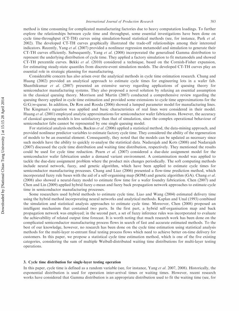
In semiconductor final testing factories, there are two major types of products, namely logic and memory IC.The logic IC has to integrate multiple functions, thus the complex system-on-chip (SoC) has wide applications suchas LAN, AUDIO, and VEDIO. In addition, there have been a number of applications of the memory IC involvingFLASH, SRAM, and DRAM. Due to the large increasing demand in memory IC products, some semiconductorfinal testing factories allocate machine capacities to the memory IC products. Therefore, we concentrate on the cycletime estimation of memory products in the paper. Generally, the memory IC final testing process involvesnine operations: (1) FT-1 (final test 1), (2) Cycling, (3) FT-2, (4) Burn-in, (5) FT-3 (6) Laser mark, (7) VM (virtualmeasurement)/scan, (8) Bake/package, and (9) Shipping, as shown in Figure 1. It should be noted that jobs re-enterthe same critical work centre multiple times (FT-1, FT-2, and FT-3), and jobs of different product types share witheach other for critical resources (the testers). Consequently, the re-entrance is an essential characteristic of thesemiconductor final testing process flow.

The FT-1 (final test 1) is the first operation of the whole final testing process flow and its process equipmentinvolves testers, handlers, and assorted handling accessories. Since a tester is the most expensive equipment, it is atypical bottleneck in an IC final testing facility (Freed et al. 2007, Chien and Wu 2003, Liow and Lendermann 2008).In the FT-1 operation, the tester is the main processing engine to test the basic functions, speed, and conductivity of

*Corresponding author. Email: yttai@mail.knu.edu.tw

ISSN 0020–7543 print/ISSN 1366–588X online

� 2012 Taylor & Francis

http://dx.doi.org/10.1080/00207543.2010.543938

http://www.tandfonline.com

Dow

nloa

ded

by [

Nat

iona

l Chi

ao T

ung

Uni

vers

ity ]

at 1

5:15

28

Apr

il 20

14

IC chips at room temperature, 25� 3�C. Through specific handler and handling accessories, the IC chips are pickedand placed in the tester to test their functions. Comparing to the process temperature of FT-1 operation, the testingtemperature of FT-2 is set to a high temperature (100� 3�C) and that of FT-3 goes down to a low temperature(0� 3�C). Through the three re-entrant FT processing steps, the IC reliability can be enhanced. For other detailedsemiconductor final testing process steps, we refer the interested readers to Pearn et al. (2004) and Chien and Wu(2003). In the semiconductor final testing process, the bottleneck machine (tester) should be utilised efficiently.Consequently, FT-1, FT-2, and FT-3 are critical operations where jobs compete with each other and wait in thequeue before they are processed. It is noted that the waiting time of the three FT operations are significantly longerthan other operations in the flow.

In semiconductor final testing shop floors, there is a great proliferation of product types. Due to various sizesand shapes of IC chips, the job processing times may vary in the FT operations, depending on the product typeof the job processed on. To prevent the critical resources from starvation (idle), the CONWIP (constant work inprocess) control policy (Spearman et al. 1990) is applied. Nadarajah and Kotz (2008) defined total cycle time as thesum of processing time and waiting time. In this paper, we consider a probabilistic model of waiting time andassume that the job processing time is predetermined, depending on its product type. In some final testing factories,waiting time data collected from shop floor can be better described by Weibull than by normal distribution. Weibulldistribution, which is a generalisation of exponential distribution, is a very flexible distribution and can easily befit to many data sets. Consequently, in the paper, we provide a cycle time estimation model consideringWeibull-distributed waiting times. The statistical cycle time estimation model can be used to obtain the cycle timeefficiently and to quickly respond to customers for various on-time delivery rates.

This paper is organised as follows. Section 2 presents a comprehensive review of existing cycle time estimationliterature. Section 3 presents the cycle time estimation model for single operation and single-layer processflow. Subsequently, Section 4 shows the combined distribution for multi-layer process flow. The combineddistribution adopting the sum of multiple Weibull distributions for multi-layer final testing process flow is shown.To demonstrate the applicability of the cycle time estimation model with the combined distribution, Section 5 givesa real-world example which is taken from a semiconductor final testing factory located on the Science-basedIndustrial Park in Hsinchu, Taiwan. Finally, Section 6 provides the conclusions.

2. Existing methods for cycle time estimation

Recent years have seen increased attention being given to cycle time estimation in the literature since the issue isan essential planning basis and an interesting research field for industrial practitioners and academic researchers.Chung and Huang (2002) classified the existing methods for cycle time estimation into four categories, includingsimulation, analytical, statistical analysis, and hybrid methods. In addition, the soft computing methods have beenwidely applied to the cycle time estimation recently and can be considered as the fifth category.

For the simulation methods, Vig and Dooley (1991) presented two methods for flow-time estimation. Therelationships between several shop factors and effects on the due-date performance using a simulation tool wereevaluated in their investigation. Raghu and Rajendran (1995) showed a simulation method to select the best rule forshop floor dispatching and developed a due-date assignment policy for a job shop. Sivakumar and Chong (2001)investigated the relationships between the selected input and output variables using a data driven discrete eventsimulation model. However, Backus et al. (2006) and De Ron and Rooda (2006) indicated that the simulation

CyclingFT-1

Burn in

Laser mark VM/Scan Bake/package Shipping

FT-2

FT-3

Figure 1. The IC final testing process with re-entry.

582 Y.T. Tai et al.

Dow

nloa

ded

by [

Nat

iona

l Chi

ao T

ung

Uni

vers

ity ]

at 1

5:15

28

Apr

il 20

14

method is time consuming for complicated manufacturing factories due to heavy computation loadings. To furtherexplore the relationships between cycle time and throughput, some essential investigations have been done oncycle time-throughput (CT-TH) curves using simulation-based statistical methods (see, for instance, Park et al.2002). The developed CT-TH curves graphically illustrated the trade-off relationships among their interestedindicators. Recently, Yang et al. (2007) provided a nonlinear regression metamodel and simulation to generate theirCT-TH curves efficiently. Subsequently, Yang et al. (2008) incorporated the generalised Gamma distribution torepresent the underlying distribution of cycle time. They applied a factory simulation to fit metamodels and showedCT-TH percentile curves. Bekki et al. (2010) considered a technique, based on the Cornish-Fisher expansion,for estimating steady-state quantiles from discrete-event simulation models. The developed CT-TH curves play anessential role in strategic planning for manufacturing.

Considerable concern has also arisen over the analytical methods in cycle time estimation research. Chung andHuang (2002) provided an analytical approach to estimate cycle times for engineering lots in a wafer fab.Shanthikumar et al. (2007) presented an extensive survey regarding applications of queuing theory forsemiconductor manufacturing systems. They also proposed a novel solution by relaxing an essential assumptionin the classical queuing theory. Morrison and Martin (2007) conducted a comprehensive review regarding thequeuing theory applied in cycle time estimation and provided some extensions to cycle time approximations for theG/G/m-queue. In addition, De Ron and Rooda (2006) showed a lumped parameter model for manufacturing lines.The Kingman’s equation was applied and basic characteristics of real lines were considered in their model.Huang et al. (2001) employed analytic approximations for semiconductor wafer fabrications. However, the accuracyof classical queuing models is less satisfactory than that of simulation, since the complex operational behaviour ofsemiconductor fabs cannot be represented by one single queuing model.

For statistical analysis methods, Backus et al. (2006) applied a statistical method, the data-mining approach, andprovided nonlinear predictor variables to estimate factory cycle time. They considered the ability of the regenerationof models to be an essential element. Consequently, they noted that the models can be updated as necessary sincesuch models have the ability to quickly re-analyse the statistical data. Nadarajah and Kots (2008) and Nadarajah(2007) discussed the cycle time distribution and waiting time distribution, respectively. They mentioned the resultscould be used for cycle time reduction. Pearn et al. (2007) considered a due-date assignment model for thesemiconductor wafer fabrication under a demand variant environment. A contamination model was applied totackle the due-date assignment problem where the product mix changes periodically. The soft computing methodsinclude neural network, fuzzy, and genetic algorithm, which have been applied to estimate cycle times forsemiconductor manufacturing processes. Chang and Liao (2006) presented a flow-time prediction method, whichincorporated fuzzy rule bases with the aid of a self-organising map (SOM) and genetic algorithm (GA). Chang et al.(2008) also showed a neural-fuzzy model to estimate flow time for a wafer foundry fabrication. Chen (2007) andChen and Lin (2009) applied hybrid fuzzy c-mean and fuzzy back propagation network approaches to estimate cycletime in semiconductor manufacturing processes.

Some researchers used hybrid methods to estimate cycle time. Liao and Wang (2004) estimated delivery timeusing the hybrid method incorporating neural networks and analytical methods. Kaplan and Unal (1993) combinedthe simulation and statistical analysis approaches to estimate cycle time. Moreover, Chen (2008) proposed anintelligent mechanism that contained two parts. In the first part, a hybrid self-organisation map and backpropagation network was employed; in the second part, a set of fuzzy inference rules was incorporated to evaluatethe achievability of related output time forecast. It is worth noting that much research work has been done on thecomplicated semiconductor manufacturing process flows in search of fast and accurate estimated methods. To thebest of our knowledge, however, no research has been done on the cycle time estimation using statistical analysismethods for the multi-layer re-entrant final testing process flows which need to achieve better on-time delivery forcustomers. In this paper, we propose a statistical cycle time estimation method, which is one of the five existingcategories, considering the sum of multiple Weibull-distributed waiting time distributions for multi-layer testingoperations.

3. Cycle time distribution for single-layer testing operation

In this paper, cycle time is defined as a random variable (see, for instance, Yang et al. 2007, 2008). Historically, theexponential distribution is used for operation inter-arrival times or waiting times. However, recent researchworks have considered that Gamma distribution is an appropriate distribution used to fit the waiting time (see, for

International Journal of Production Research 583

Dow

nloa

ded

by [

Nat

iona

l Chi

ao T

ung

Uni

vers

ity ]

at 1

5:15

28

Apr

il 20

14

instance, Nadarajah 2007, Nadarajah and Kots 2008) since Gamma distribution is a more general distributionincluding the exponential distribution as a special case. In fact, in many real situations, the waiting timedata collected from some semiconductor final testing shop floors are Weibull-distributed. It should be notedthat Weibull distribution is a very flexible distribution and can easily be fitted to many data sets. Rinne (2009)mentioned that Weibull distribution, together with the normal, exponential, �2, t, and F distributions, is one of themost popular models used in the industry. The exponential distribution is equivalent to a Weibull (1, �) distributionas a special case. Therefore, Weibull distribution would be appropriate for the modelling of waiting times. We note,particularly, that some data (for instance, life time with a variable hazard rate) are more appropriately fittedas Weibull distribution than fitted as Gamma distribution. Consequently, in this section, we present a cycletime estimation model considering Weibull-distributed waiting time for a single-layer testing operation. In thesubsequent section, a cycle time estimation model involving the sum of multiple Weibull-distributed waitingtime distributions is developed for multi-layer testing operations in the re-entrant semiconductor final testingfactories.

3.1 Weibull distribution

Weibull distribution is non-negative distribution (Johnson et al. 1994) and can be denoted as Weibull (c,�) withshape parameter c and scale parameter �. Weibull distribution is often used to model the time until failure of manydifferent physical systems. The probability density function (p.d.f.) is defined as

f ðxÞ ¼c

�cxc�1e�ðx=�Þ

c

, x4 0, c4 0, �4 0, ð1Þ

and the mean and variance are given as follows:

EðXÞ ¼ �½�ð1þ c�1Þ� and VðXÞ ¼ �2 �ð1þ 2c�1Þ � �ð1þ c�1Þ� �2h i

: ð2Þ

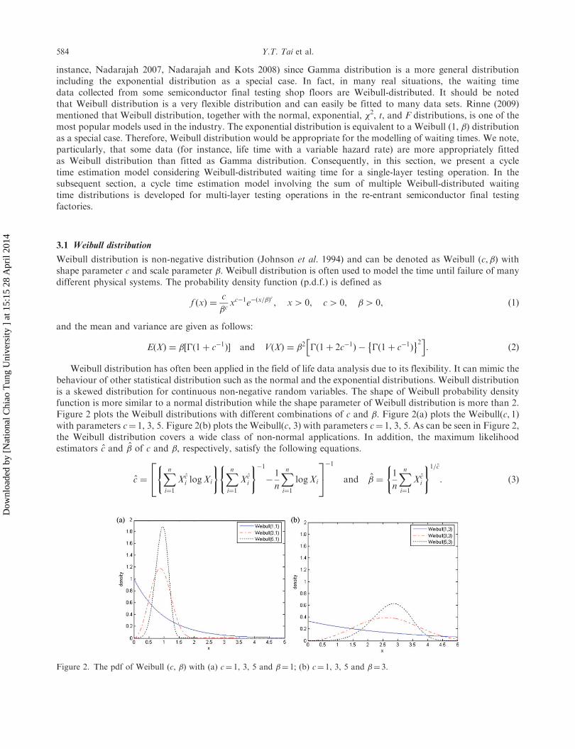
Weibull distribution has often been applied in the field of life data analysis due to its flexibility. It can mimic thebehaviour of other statistical distribution such as the normal and the exponential distributions. Weibull distributionis a skewed distribution for continuous non-negative random variables. The shape of Weibull probability densityfunction is more similar to a normal distribution while the shape parameter of Weibull distribution is more than 2.Figure 2 plots the Weibull distributions with different combinations of c and �. Figure 2(a) plots the Weibull(c, 1)with parameters c¼ 1, 3, 5. Figure 2(b) plots the Weibull(c, 3) with parameters c¼ 1, 3, 5. As can be seen in Figure 2,the Weibull distribution covers a wide class of non-normal applications. In addition, the maximum likelihoodestimators c and � of c and �, respectively, satisfy the following equations.

c ¼Xni¼1

Xci logXi

( ) Xni¼1

Xci

( )�1�1

n

Xni¼1

logXi

24

35�1

and � ¼1

n

Xni¼1

Xci

( )1=c

: ð3Þ

Figure 2. The pdf of Weibull (c, �) with (a) c¼ 1, 3, 5 and �¼ 1; (b) c¼ 1, 3, 5 and �¼ 3.

584 Y.T. Tai et al.

Dow

nloa

ded

by [

Nat

iona

l Chi

ao T

ung

Uni

vers

ity ]

at 1

5:15

28

Apr

il 20

14

3.2 Cycle time estimation for a single operation

The FT operations are the most critical operations in the re-entrant semiconductor final testing process flow.

Since the tester is the most expensive equipment and must be utilised efficiently, the waiting times of the FT

operations are significantly longer than the other miscellaneous operations. The calculation of the cycle time for oneFT operation is equal to the processing time plus the waiting time at various percentiles. The cycle time calculation

formula can be expressed as follows:

CTið�Þ ¼ PTi þWTið�Þ, ð4Þ

where CTi(�) denotes single FT operation cycle time of product type i at �-percentile, PTi denotes the processing

time of product type i, and WTi(�) is the fitted Weibull-distributed waiting time of product type i at �-percentile.We consider a small-scaled example for cycle time estimation in the FT-1 operation in which the waiting times

collected from the shop floor are Weibull-distributed. The example involves three identical parallel testing machinesand three different product types (namely, A, B, and C). The various processing times of FT-1 for product types A,

B, and C are 68, 59, and 42 minutes, respectively. The processing time is not affected by the machine processing it,

but it depends on the product type of the job processed. The ‘minute’ is used as the unit for processing time and

waiting time.The estimated values of the shape parameter of Weibull-distributed waiting times for product types A, B, and C

are 5, 3.9, and 10, respectively. The estimated values of the scale parameter of the Weibull-distributed waiting times

for product types A, B, and C are 39.7, 62.6, and 47.7, respectively. Since the waiting time of product type A in the

single FT-1 operation is fitted with parameters (5, 39.7), the 95-percentile of the waiting time is 49.44 minutes.Therefore, the estimated cycle time of product type A is equal to 117.44 minutes at 95-percentile using Equation (4).

Applying this method, the 95-percentile of the cycle times of the FT-1 operation of product types B and C are 141.94

and 95.23 minutes, respectively.

3.3 Cycle time estimation for single-layer

For the clarity and convenience to present our new development, the concept of ‘layer’ is incorporated into the cycle

time estimation model due to the essential characteristic of re-entry. Since the testers are the most critical bottleneckin final testing factories, the FT operations can be considered as the first operation of each layer. In general, there

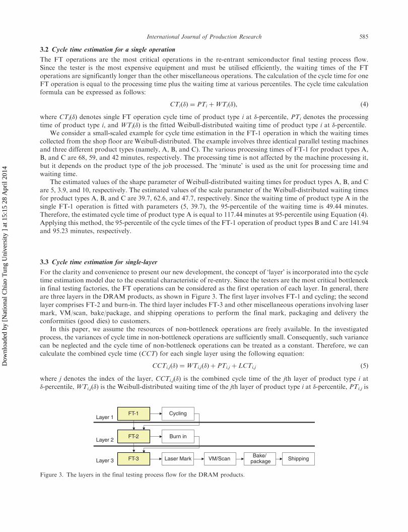
are three layers in the DRAM products, as shown in Figure 3. The first layer involves FT-1 and cycling; the second

layer comprises FT-2 and burn-in. The third layer includes FT-3 and other miscellaneous operations involving laser

mark, VM/scan, bake/package, and shipping operations to perform the final mark, packaging and delivery theconformities (good dies) to customers.

In this paper, we assume the resources of non-bottleneck operations are freely available. In the investigated

process, the variances of cycle time in non-bottleneck operations are sufficiently small. Consequently, such variance

can be neglected and the cycle time of non-bottleneck operations can be treated as a constant. Therefore, we can

calculate the combined cycle time (CCT) for each single layer using the following equation:

CCTi,jð�Þ ¼WTi,jð�Þ þ PTi,j þ LCTi,j ð5Þ

where j denotes the index of the layer, CCTi,j(�) is the combined cycle time of the jth layer of product type i at�-percentile, WTi,j(�) is the Weibull-distributed waiting time of the jth layer of product type i at �-percentile, PTi,j is

CyclingFT-1

Burn in

Laser Mark VM/Scan Bake/package Shipping

FT-2

FT-3

Layer 1

Layer 2

Layer 3

Figure 3. The layers in the final testing process flow for the DRAM products.

International Journal of Production Research 585

Dow

nloa

ded

by [

Nat

iona

l Chi

ao T

ung

Uni

vers

ity ]

at 1

5:15

28

Apr

il 20

14

the processing time for the jth layer of product type i, and LCTi,j is the sum of cycle times for those non-bottleneckoperations in the jth layer of product type i.

4. Combined distribution for multi-layer testing operations

To obtain the accurate cycle time of the whole final testing process, a combined cycle time model withconsiderations of multi-layer final testing process flow is developed. Since the final testing process is the final stageof the semiconductor manufacturing process, how to achieve better on-time delivery has become an essential issue(Lin et al. 2004). In the final testing factories, it is better to provide percentiles of cycle time instead of a constantcycle time value since the percentiles of cycle time can be used as convenient reference points for due datecommitments and other planning bases. In the final testing factory investigated, the waiting times of the FToperations in the multi-layer testing flow are Weibull-distributed. In Section 3.3, calculation of the cycle time forsingle layer is presented, which involves only one single Weibull distribution. Calculating the cycle time for themulti-layer final testing process, however, involves the sum of multiple Weibull distributions. The resulting Weibullsum becomes rather complicated. Therefore, a polynomial approximation method for the combined distributionbased on the sum of multiple Weibull distributions is adopted; then, the multi-layer cycle time calculation model canbe shown.

4.1 The polynomial approximation method for Weibull distribution

As described in the previous section, the multi-layer final testing process is a re-entrant flow and FT operation is thebottleneck of the flow. Therefore, the sum of waiting times of the three FT operations is significantly longer than theother non-critical operations and should be considered. However, it is rather difficult to achieve the exactcumulative distribution function (c.d.f.) of the sum of multiple Weibull distributions. There are no existing statisticalresults which can be applied to obtain the desired probability value directly. Hence, to effectively obtain the cycletime estimation model and to obtain the sum of Weibull-distributed waiting times of the three FT operations,we apply a cubic polynomial approximation method provided by Lu (2003) and show the method as follows.

Assume X1,X2, . . . ,Xn be independent random variables each having a Weibull distribution with parameters(c,�) of form

f ðxÞ ¼c

�cxc�1e�ðx=�Þ

c

, x4 0, c4 0, �4 0: ð6Þ

Then, the probability value of PðSn � tÞ, where Sn ¼ X1 þ � � � þ Xn, is the desired value that we are interested in.The essential idea of the cubic polynomial approximation method is to use the three quantiles to approximate thesum of multiple Weibull distributions. Suppose Xi is a random variable from Weibull distribution with parameters(c, 1). Through the transform of variable Yi ¼ Xc

i , we can obtain that Yi is a random variable from Exponential (1)distribution, where i ¼ 1, . . . , n. Therefore, the distribution function of Y1 þ � � � þ Yn is applied to approximate thedistribution function of X1 þ � � � þ Xn. Since the two distribution functions are continuously differentiablefunctions, we can find some continuously differentiable functions w(t) for each t � 0, such that

PðX1 þ � � � þ Xn � tÞ ¼ P Y1 þ � � � þ Yn � wðtÞð Þ, ð7Þ

where w(0)¼ 0. The form of w(t) can be expressed as third degree polynomial �t3c þ �t2c þ �tc. To determine thethree unknown parameters, ð�, �, �Þ, we use three quantiles of X1 þ � � � þ Xn and Y1 þ � � � þ Yn. First, we let tp satisfyPðX1 þ � � � þ Xn � tpÞ ¼ p and �p satisfy P Y1 þ � � � þ Yn � �p

� �¼ p; therefore, tp and �p are the pth quantile of

X1 þ � � � þ Xn and Y1 þ � � � þ Yn, respectively. When p ¼ 0:1, 0:5, and 0:9, we can obtain three linear functionsusing �t3cp þ �t

2cp þ �t

cp ¼ �p.

In the cubic polynomial approximation method, �p can be obtained using the Newton method. However, the tpcan not be obtained analytically, but it can be obtained using Monte Carlo simulation method. The value of adesired probability can be obtained in the following procedure.

Step 1: Solve the 1�Pn�1

i¼0 e��p�ip=i! ¼ p using the Newton method to obtain �p, where p ¼ 0:1, 0:5, and 0:9.

Step 2: Let the sample size of the simulation be N ¼ 106. Let T1,T2, . . . ,TN be a random sample fromFnðxÞ ¼ PðX1 þ � � � þ Xn � xÞ.

586 Y.T. Tai et al.

Dow

nloa

ded

by [

Nat

iona

l Chi

ao T

ung

Uni

vers

ity ]

at 1

5:15

28

Apr

il 20

14

Take n ¼ 2, for example, the desired simulation data is Ti ¼ Xi1 þ Xi

2, i ¼ 1, . . . , 106. Here, Xi1,X

i2 are the random

variables each having an identical and independent Weibull (c, 1). After sorting the order, t0:1 ¼ Tð0:1106Þ,t0:5 ¼ Tð0:5106Þ, and t0:9 ¼ Tð0:9106Þ are the approximations of the true quantiles t0.1, t0.5, and t0.9, respectively.

Step 3: The three unknown parameters �, �, and � can be obtained by the following linear equations.

�t3c0:1 þ � t2c0:1 þ �t

c0:1 ¼ �0:1, ð8Þ

�t3c0:5 þ � t2c0:5 þ �t

c0:5 ¼ �0:5, ð9Þ

�t3c0:9 þ � t2c0:9 þ �t

c0:9 ¼ �0:9: ð10Þ

Step 4: Under fixed n and shape parameter c, the estimated form of w(t) is wðtÞ ¼ �t3c þ �t2c þ �tc.

Step 5: The approximation of the distribution function of interest can be obtained as follows:

P X1 þ � � � þ Xn � tð Þ ffi P Y1 þ � � � þ Yn � w tð Þð Þ ¼ 1�Xn�1i¼0

e�w tð Þw tð Þi=i!: ð11Þ

In the simulation procedure, we set N ¼ 106; Np is a positive integer when p ¼ 0:1, 0:5, and 0:9 and TðNpÞ is pthsample quantile. In addition, we can find that the distribution of TðNpÞ approximates Nðtp, pð1� pÞ=f2nðtpÞNÞ and itserror is proportional to 1=

ffiffiffiffiNp¼ 10�ð7=2Þ (Serfling 1980). Therefore, we consider that the TðNpÞ would approach the

true pth quantile.

4.2 The accuracy of the polynomial approximation

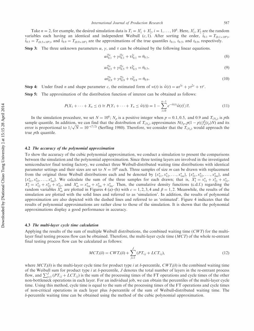
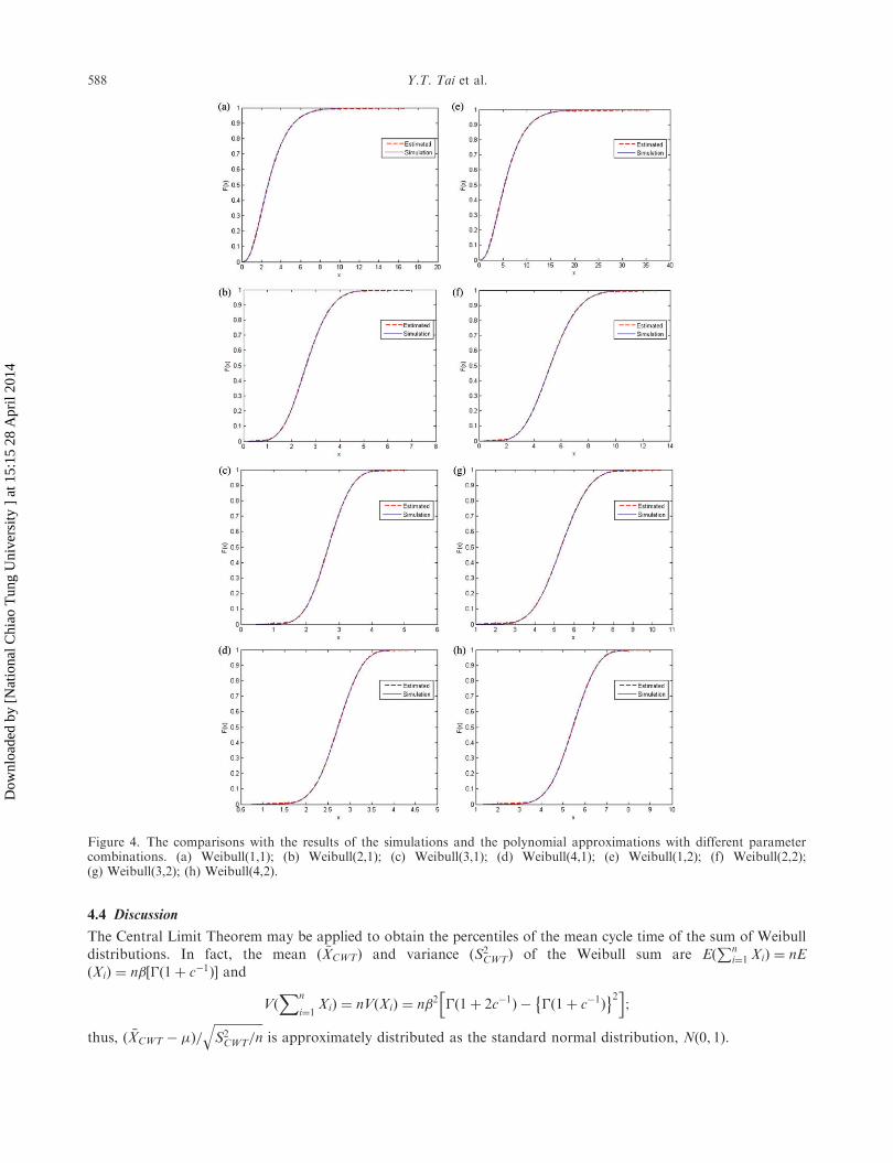
To show the accuracy of the cubic polynomial approximation, we conduct a simulation to present the comparisonsbetween the simulation and the polynomial approximation. Since three testing layers are involved in the investigatedsemiconductor final testing factory, we conduct three Weibull-distributed waiting time distributions with identicalparameter settings and their sizes are set to N ¼ 106 each. Three samples of size m can be drawn with replacementfrom the original three Weibull distributions each and be denoted by fx�11, x

�12, . . . , x�1mg, fx

�21, x

�22, . . . , x�2mg, and

fx�31, x�32, . . . , x�3mg. We calculate the sum of the three samples for each drawn; that is, X�1 ¼ x�11 þ x�21 þ x�31,

X�2 ¼ x�12 þ x�22 þ x�32, and X�m ¼ x�1m þ x�2m þ x�3m. Then, the cumulative density functions (c.d.f.) regarding therandom variables X�m are plotted in Figures 4 (a)–(h) with c ¼ 1, 2, 3, 4 and � ¼ 1, 2. Meanwhile, the results of thesimulation are plotted with the solid lines and referred to as ‘simulation’. In addition, the results of polynomialapproximation are also depicted with the dashed lines and referred to as ‘estimated’. Figure 4 indicates that theresults of polynomial approximations are rather close to those of the simulation. It is shown that the polynomialapproximations display a good performance in accuracy.

4.3 The multi-layer cycle time calculation

Applying the results of the sum of multiple Weibull distributions, the combined waiting time (CWT) for the multi-layer final testing process flow can be obtained. Therefore, the multi-layer cycle time (MCT) of the whole re-entrantfinal testing process flow can be calculated as follows:

MCTið�Þ ¼ CWTið�Þ þXJj¼1

ðPTi,j þ LCTi,jÞ, ð12Þ

where MCTi(�) is the multi-layer cycle time for product type i at �-percentile, CWTi(�) is the combined waiting timeof the Weibull sum for product type i at �-percentile, J denotes the total number of layers in the re-entrant processflow, and

PJj¼1 ðPTi,j þ LCTi,jÞ is the sum of the processing times of the FT operations and cycle times of the other

non-bottleneck operations in each layer. For an individual job, we can obtain the percentiles of the multi-layer cycletime. Using this method, cycle time is equal to the sum of the processing times of the FT operations and cycle timesof non-critical operations in each layer plus �-percentile of the sum of Weibull-distributed waiting time. The�-percentile waiting time can be obtained using the method of the cubic polynomial approximation.

International Journal of Production Research 587

Dow

nloa

ded

by [

Nat

iona

l Chi

ao T

ung

Uni

vers

ity ]

at 1

5:15

28

Apr

il 20

14

4.4 Discussion

The Central Limit Theorem may be applied to obtain the percentiles of the mean cycle time of the sum of Weibulldistributions. In fact, the mean ( �XCWT) and variance (S2

CWT) of the Weibull sum are EðPn

i¼1 XiÞ ¼ nEðXiÞ ¼ n�½�ð1þ c�1Þ� and

VðXn

i¼1XiÞ ¼ nVðXiÞ ¼ n�2 �ð1þ 2c�1Þ � �ð1þ c�1Þ

� �2h i;

thus, ð �XCWT � Þ=ffiffiffiffiffiffiffiffiffiffiffiffiffiffiffiffiS2CWT=n

qis approximately distributed as the standard normal distribution, Nð0, 1Þ.

Figure 4. The comparisons with the results of the simulations and the polynomial approximations with different parametercombinations. (a) Weibull(1,1); (b) Weibull(2,1); (c) Weibull(3,1); (d) Weibull(4,1); (e) Weibull(1,2); (f) Weibull(2,2);(g) Weibull(3,2); (h) Weibull(4,2).

588 Y.T. Tai et al.

Dow

nloa

ded

by [

Nat

iona

l Chi

ao T

ung

Uni

vers

ity ]

at 1

5:15

28

Apr

il 20

14

5. Cycle time calculation for semiconductor final testing process

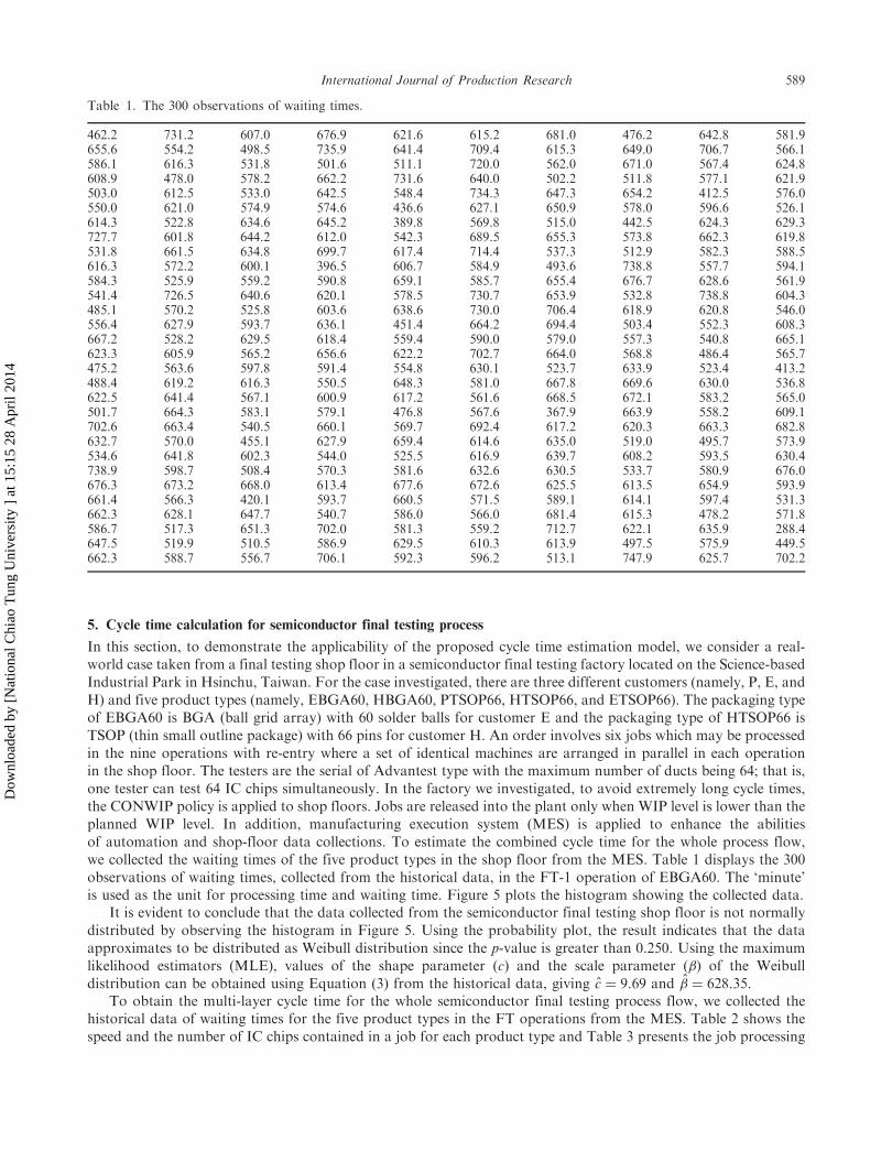
In this section, to demonstrate the applicability of the proposed cycle time estimation model, we consider a real-world case taken from a final testing shop floor in a semiconductor final testing factory located on the Science-basedIndustrial Park in Hsinchu, Taiwan. For the case investigated, there are three different customers (namely, P, E, andH) and five product types (namely, EBGA60, HBGA60, PTSOP66, HTSOP66, and ETSOP66). The packaging typeof EBGA60 is BGA (ball grid array) with 60 solder balls for customer E and the packaging type of HTSOP66 isTSOP (thin small outline package) with 66 pins for customer H. An order involves six jobs which may be processedin the nine operations with re-entry where a set of identical machines are arranged in parallel in each operationin the shop floor. The testers are the serial of Advantest type with the maximum number of ducts being 64; that is,one tester can test 64 IC chips simultaneously. In the factory we investigated, to avoid extremely long cycle times,the CONWIP policy is applied to shop floors. Jobs are released into the plant only when WIP level is lower than theplanned WIP level. In addition, manufacturing execution system (MES) is applied to enhance the abilitiesof automation and shop-floor data collections. To estimate the combined cycle time for the whole process flow,we collected the waiting times of the five product types in the shop floor from the MES. Table 1 displays the 300observations of waiting times, collected from the historical data, in the FT-1 operation of EBGA60. The ‘minute’is used as the unit for processing time and waiting time. Figure 5 plots the histogram showing the collected data.

It is evident to conclude that the data collected from the semiconductor final testing shop floor is not normallydistributed by observing the histogram in Figure 5. Using the probability plot, the result indicates that the dataapproximates to be distributed as Weibull distribution since the p-value is greater than 0.250. Using the maximumlikelihood estimators (MLE), values of the shape parameter (c) and the scale parameter (�) of the Weibulldistribution can be obtained using Equation (3) from the historical data, giving c ¼ 9:69 and � ¼ 628:35.

To obtain the multi-layer cycle time for the whole semiconductor final testing process flow, we collected thehistorical data of waiting times for the five product types in the FT operations from the MES. Table 2 shows thespeed and the number of IC chips contained in a job for each product type and Table 3 presents the job processing

Table 1. The 300 observations of waiting times.

462.2 731.2 607.0 676.9 621.6 615.2 681.0 476.2 642.8 581.9655.6 554.2 498.5 735.9 641.4 709.4 615.3 649.0 706.7 566.1586.1 616.3 531.8 501.6 511.1 720.0 562.0 671.0 567.4 624.8608.9 478.0 578.2 662.2 731.6 640.0 502.2 511.8 577.1 621.9503.0 612.5 533.0 642.5 548.4 734.3 647.3 654.2 412.5 576.0550.0 621.0 574.9 574.6 436.6 627.1 650.9 578.0 596.6 526.1614.3 522.8 634.6 645.2 389.8 569.8 515.0 442.5 624.3 629.3727.7 601.8 644.2 612.0 542.3 689.5 655.3 573.8 662.3 619.8531.8 661.5 634.8 699.7 617.4 714.4 537.3 512.9 582.3 588.5616.3 572.2 600.1 396.5 606.7 584.9 493.6 738.8 557.7 594.1584.3 525.9 559.2 590.8 659.1 585.7 655.4 676.7 628.6 561.9541.4 726.5 640.6 620.1 578.5 730.7 653.9 532.8 738.8 604.3485.1 570.2 525.8 603.6 638.6 730.0 706.4 618.9 620.8 546.0556.4 627.9 593.7 636.1 451.4 664.2 694.4 503.4 552.3 608.3667.2 528.2 629.5 618.4 559.4 590.0 579.0 557.3 540.8 665.1623.3 605.9 565.2 656.6 622.2 702.7 664.0 568.8 486.4 565.7475.2 563.6 597.8 591.4 554.8 630.1 523.7 633.9 523.4 413.2488.4 619.2 616.3 550.5 648.3 581.0 667.8 669.6 630.0 536.8622.5 641.4 567.1 600.9 617.2 561.6 668.5 672.1 583.2 565.0501.7 664.3 583.1 579.1 476.8 567.6 367.9 663.9 558.2 609.1702.6 663.4 540.5 660.1 569.7 692.4 617.2 620.3 663.3 682.8632.7 570.0 455.1 627.9 659.4 614.6 635.0 519.0 495.7 573.9534.6 641.8 602.3 544.0 525.5 616.9 639.7 608.2 593.5 630.4738.9 598.7 508.4 570.3 581.6 632.6 630.5 533.7 580.9 676.0676.3 673.2 668.0 613.4 677.6 672.6 625.5 613.5 654.9 593.9661.4 566.3 420.1 593.7 660.5 571.5 589.1 614.1 597.4 531.3662.3 628.1 647.7 540.7 586.0 566.0 681.4 615.3 478.2 571.8586.7 517.3 651.3 702.0 581.3 559.2 712.7 622.1 635.9 288.4647.5 519.9 510.5 586.9 629.5 610.3 613.9 497.5 575.9 449.5662.3 588.7 556.7 706.1 592.3 596.2 513.1 747.9 625.7 702.2

International Journal of Production Research 589

Dow

nloa

ded

by [

Nat

iona

l Chi

ao T

ung

Uni

vers

ity ]

at 1

5:15

28

Apr

il 20

14

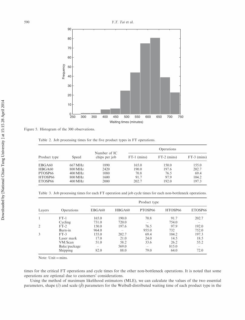
times for the critical FT operations and cycle times for the other non-bottleneck operations. It is noted that someoperations are optional due to customers’ considerations.

Using the method of maximum likelihood estimators (MLE), we can calculate the values of the two essentialparameters, shape (c) and scale (�) parameters for the Weibull-distributed waiting time of each product type in the

250 300 350 400 450 500 550 600 650 700 7500

10

20

30

40

50

60

70

80

90

Waiting times (minutes)

Freq

uenc

y

Figure 5. Histogram of the 300 observations.

Table 3. Job processing times for each FT operation and job cycle times for each non-bottleneck operations.

Layers Operations

Product type

EBGA60 HBGA60 PTOSP66 HTOSP66 ETOSP66

1 FT-1 165.0 190.0 70.8 91.7 202.7Cycling 731.0 720.0 – 754.0 –

2 FT-2 150.0 197.6 76.5 97.9 192.0Burn-in 964.0 – 955.0 732 752.0

3 FT-3 155.0 202.7 69.4 104.2 197.3Laser mark 17.0 21.0 24.0 14.5 18.5VM/Scan 51.0 58.2 33.6 26.2 55.2Bake/package – 569.0 – 815.0 –Shipping 82.0 88.0 79.0 64.0 72.0

Note: Unit¼mins.

Table 2. Job processing times for the five product types in FT operations.

Product type SpeedNumber of ICchips per job

Operations

FT-1 (mins) FT-2 (mins) FT-3 (mins)

EBGA60 667MHz 1890 165.0 150.0 155.0HBGA60 800MHz 2420 190.0 197.6 202.7PTOSP66 400MHz 1080 70.8 76.5 69.4HTOSP66 800MHz 1600 91.7 97.9 104.2ETOSP66 400MHz 2000 202.7 192.0 197.3

590 Y.T. Tai et al.

Dow

nloa

ded

by [

Nat

iona

l Chi

ao T

ung

Uni

vers

ity ]

at 1

5:15

28

Apr

il 20

14

semiconductor final testing process flow. Since the re-entrant characteristic exists in the semiconductor final testingprocess flow and jobs re-enter the same toolset of the testers, the two parameters of the Weibull distribution in eachlayer are identical for one product type. We collect the data from the MES in the shop floor and calculate the valuesof the two essential parameters, shape (c) and scale (�) of the Weibull distributions for the five product types.The values of the shape parameters (c) can be computed as 9.69, 7.42, 4.36, 6.6, and 8.59 and the values of the scaleparameter (�) can be calculated as 628.35, 766.69, 576.83, 497.65, and 533.99 for the five product types EBGA60,HBGA60, PTSOP66, HTSOP66, and ETSOP66, respectively. In addition, an alternative approach which is referredto as the method of moments estimator can also be employed to obtain the values of the parameters.

Using the sum of multiple Weibull distributions, the three-layer combined waiting time of EBGA60 can becalculated as 2000.19 minutes at 95-percentile. Therefore, based on Equation (12), the 95-percentile of the multi-layer cycle time can be computed as 4315.19 minutes for EBGA60 in the factory. Similarly, the 95-percentile of thecycle times for HBGA60, PTSOP66, HTSOP66, and ETSOP66 can be calculated as 4536.99, 3309.17, 4334.14,and 3203.79 minutes, respectively. It should be noted that the percentiles of cycle time can be used as convenientreference points for due date commitments and other planning bases. They are very useful to industrial practitionersfor achieving an accuracy basis of factory performance analysis.

6. Conclusion

Cycle time is an essential basis for due date assignment, production planning, and scheduling. In this paper,we proposed a statistical approach for cycle time estimation in the re-entrant semiconductor final testing processflow. The cycle time estimation models for single operation and single layer were first provided. Since the waitingtimes collected from the shop floor were Weibull-distributed, the multi-layer cycle time estimation model involvingthe sum of multiple Weibull distributions was presented. In addition, to quickly respond to the customers’ inquiriesof due dates and shipping schedules, percentiles of cycle time were also provided. To demonstrate the applicabilityof the proposed cycle time estimation model, we considered a real-world case taken from a shop floor in asemiconductor final testing factory located on the Science-based Industrial Park in Hsinchu, Taiwan. The results ofthe investigation indicated that the cycle time estimation model provided satisfactory calculation of the cycle time.The model considering the various percentiles of cycle time could be very useful to industrial practitioners involvedin semiconductor final testing shop floor to provide accuracy bases for due date commitments, production planning,and factory performance analysis.

References

Backus, P., Janakiram, M., Mowzoon, S., Runger, G.C., and Bhargava, A., 2006. Factory cycle-time prediction with a

data-mining approach. IEEE Transactions on Semiconductor Manufacturing, 19 (2), 252–258.Bekki, J.M., Fowler, J.W., Mackulak, G.T., and Nelson, B.L., 2010. Indirect cycle-time quantile estimation using the

Cornish-Fisher expansion. IIE Transactions, 42 (1), 31–44.Chang, P.C. and Liao, T.W., 2006. Combining SOM and fuzzy rule base for flow time prediction in semiconductor

manufacturing factory. Applied Soft Computing, 6 (2), 198–206.Chang, P.C., Wang, Y.W., and Ting, C.J., 2008. A fuzzy neural network for the flow time estimation in a semiconductor

manufacturing factory. International Journal of Production Research, 46 (4), 1017–1029.Chen, T., 2007. Predicting wafer-lot output time with a hybrid FCM-FBPN approach. IEEE Transactions on System, Man, and

Cybernetics. Part B – Cybernetics, 37 (4), 784–792.

Chen, T., 2008. An intelligent mechanism for lot output time prediction and achievability evaluation in a wafer fab. Computers &

Industrial Engineering, 54 (1), 77–94.

Chen, T. and Lin, Y.C., 2009. A fuzzy back propagation network ensemble with example classification for lot output time

prediction in a wafer fab. Applied Soft Computing, 9 (2), 658–666.

Chien, C.F. and Wu, J.Z., 2003. Analyzing repair decisions in the site imbalance problem of semiconductor test machines.

IEEE Transactions on Semiconductor Manufacturing, 16 (4), 704–711.Chung, S.H. and Huang, H.W., 2002. Cycle time estimation for wafer fab with engineering lots. IIE Transactions, 34 (2),

105–118.De Ron, A.J. and Rooda, J.E., 2006. A lumped parameter model for product flow times in manufacturing lines.

IEEE Transactions on Semiconductor Manufacturing, 19 (4), 502–509.

International Journal of Production Research 591

Dow

nloa

ded

by [

Nat

iona

l Chi

ao T

ung

Uni

vers

ity ]

at 1

5:15

28

Apr

il 20

14

Freed, T., Doerr, K.H., and Chang, T., 2007. In-house development of scheduling decision support systems: Case study forscheduling semiconductor device test operations. International Journal of Production Research, 45 (21), 5075–5093.

Haberle, K.R. and Graves, R.J., 2001. Cycle time estimation for printed circuit board assembilies. IEEE Transactions onElectronics Packaging Manufacturing, 24 (3), 188–194.

Huang, M.G., Chang, P.L., and Chou, Y.C., 2001. Analytic approximations for multiserver batch- service workstationswith multiple process recipes in semiconductor wafer fabrication. IEEE Transactions on Semiconductor Manufacturing,

14 (4), 395–405.Johnson, N.L., Kotz, S., and Balakrishnan, N., 1994. Continuous univariate distributions. 2nd ed. New York, NY: John Wiley

& Sons.

Kaplan, A.C. and Unal, A.T., 1993. A probabilistic cost-based due date assignment model for job shops. International Journalof Production Research, 31 (12), 2817–2834.

Liao, D.Y. and Wang, C.N., 2004. Neural-network-based delivery time estimates for prioritised 300-mm automatic material

handling operations. IEEE Transactions on Semiconductor Manufacturing, 17 (3), 324–332.Lin, J.T., Wang, F.K., and Lee, W.T., 2004. Capacity-constrained scheduling for a logic IC final test facility. International

Journal of Production Research, 42 (11), 79–99.Liow, L.F. and Lendermann, P., 2008. Analysis of semiconductor backend manufacturing with cycle time constrained capacity.

SIM Technical Reports, 9 (1), 44–49.Lu, H.M., 2003. The approximation of the distribution function of sum of independent and identical Weibull distribution. Thesis.

Institute of Statistics in National Chiao Tung University, Taiwan.

Morrison, J.R. and Martin, D.P., 2007. Practical extensions to cycle time approximations for the G/G/m-queue withapplications. IEEE Transactions on Automation Science and Engineering, 4 (4), 523–532.

Nadarajah, S. and Kots, S., 2008. The cycle time distribution. International Journal of Production Research, 46 (11), 3133–3141.

Nadarajah, S., 2007. The waiting time distribution. Computers & Industrial Engineering, 53 (4), 693–699.Park, S., Fowler, J.W., Mackulak, G.T., Keats, J.B., and Carlyle, W.M., 2002. D-optimal sequential experiments for generating

a simulation-based cycle time-throughput curve. Operations Research, 50 (6), 981–990.

Pearn, W.L., Chung, S.H., Chen, A.Y., and Yang, M.H., 2004. A case study on the multistage IC final testing schedulingproblem with re-entry. International Journal of Production Economics, 88 (3), 257–267.

Pearn, W.L., Chung, S.H., and Lai, C.M., 2007. Due-date assignment for wafer fabrication under demand variate environment.IEEE Transactions on Semiconductor Manufacturing, 20 (2), 165–175.

Raghu, T.S. and Rajendran, C., 1995. Due-date setting methodologies based on simulated annealing – an experimental study ina real-life job shop. International Journal of Production Research, 33 (9), 2535–2554.

Rinne, H., 2009. The Weibull distribution: A handbook. 1st ed. Boca Raton, FL: Taylor & Francis Group/Chapman & Hall.

Serfling, R.J., 1980. Approximation theorems of mathematical statistics. 2nd ed. New York, NY: John Wiley & Sons.Shanthikumar, J.G., Ding, S., and Zhang, M.T., 2007. Queueing theory for semiconductor manufacturing systems: A survey and

open problems. IEEE Transactions on Automation Science and Engineering, 4 (4), 513–521.

Sivakumar, A.I. and Chong, C.S., 2001. A simulation based analysis of cycle time distribution, and throughput in semiconductorbackend manufacturing. Computers in Industry, 45 (1), 59–78.

Shanthikumar, J.G., Ding, S., and Zhang, M.T., 2007. Queueing theory for semiconductor manufacturing systems: A survey and

open problems. IEEE Transactions on Automation Science and Engineering, 4 (4), 513–521.Spearman, M.L., Woodruff, D.L., and Hopp, W.J., 1990. CONWIP: A pull alternative to Kanban. International Journal of

Production Research, 28 (5), 879–894.Vig, M.M. and Dooley, K.J., 1991. Dynamic rules for due-date assignment. International Journal of Production Research, 29 (7),

1361–1377.Yang, F., Ankenman, B., and Nelson, B.L., 2007. Efficient generation of cycle time throughput curves through simulation and

metamodeling. Naval Research Logistics, 54 (1), 78–93.

Yang, F., Ankenman, B.E., and Nelson, B.L., 2008. Cycle time percentile curves for manufacturing systems. INFORMS Journalon Computing, 20 (4), 628–643.

592 Y.T. Tai et al.

Dow

nloa

ded

by [

Nat

iona

l Chi

ao T

ung

Uni

vers

ity ]

at 1

5:15

28

Apr

il 20

14