Embed Size (px)
Citation preview

Ricardo Jorge Sousa da Silva
Mestre em Engenharia Quımica e Bioquımica
Compact simulated countercurrentchromatography for downstream
processing of (bio)pharmaceuticals
Dissertacao para obtencao do Grau de Doutor emEngenharia Quımica e Bioquımica
Orientador:Prof. Doutor Jose Paulo Barbosa Mota, Prof. Catedratico
Faculdade Ciencias e Tecnologia
Setembro de 2013


O Autor e a Faculdade de Ciencias e Tecnologia e a Universidade Nova de Lisboa
tem o direito, perpetuo e sem limites geograficos, de arquivar e publicar esta
dissertacao atraves de exemplares impressos reproduzidos em papel ou de forma
digital, ou por qualquer outro meio conhecido ou que venha a ser inventado, e de
a divulgar atraves de repositorios cientıficos e de admitir a sua copia e distribuicao
com objectivos educacionais ou de investigacao, nao comerciais, desde que seja
dado credito ao autor e editor.


to Angela, who always believed in me, even more than Iever did, and kept me moving forward


essentially, all models are wrong, but some are usefulGeorge P. Box (1987)


Acknowledgements
Completing my PhD was one of the most challenging things I ever done. The
best part of this journey is to look back and remember all the friends made, the
(un)finished work, and all the good and bad experiences. This journey wouldn’t be
possible to accomplish without the support and encouragement of a great number
of people over the past four years.
My first debt of gratitude must go to my advisor, Prof. Jose Paulo Mota, for the
challenges and opportunities presented. His insight, encouragement, friendship
and hard questions provided me the vision necessary to complete my PhD.
I would like to acknowledge Fundacao para a Ciencia e Tecnologia (FCT/MCTES)
for the financial aid in the form of a PhD grant.
To my friends and colleagues at FCT/UNL, to Isabel Esteves for all your help,
insight, friendship along these years and support in the tough times; to Prof. Mario
Eusebio, Andriy Lyubchik, Fernando Cruz; to my recent colleagues Rui Ribeiro,
Eliana, Barbara, and Joao; and specially to Rui Rodrigues, who in the first years of
my PhD provide me with the experimental knowledge needed to accomplish this
challenge. I would also like to acknowledge Dr. Cristina Peixoto and Piergiuseppe
Nestola from IBET.
I am deeply grateful to my parents, for all the support and sacrifices that you’ve
made for me. I can only hope that one day match the example you have set. To my
sister, who was never short of words, and patience.
To Angela, who I can’t thank enough for encouraging me through this journey and
for all the time lost that I will try to make up.
vii


Table of Contents
1 Introduction 1
1.1 Relevance and Motivation . . . . . . . . . . . . . . . . . . . . . . . 1
1.2 Objectives and Outline . . . . . . . . . . . . . . . . . . . . . . . . . 3
2 Simulated Moving Bed technology: a brief review 5
2.1 Introduction . . . . . . . . . . . . . . . . . . . . . . . . . . . . . . . 5
2.2 Principle of SMB Technology: the concept of True Moving Bed . . . 6
2.3 SMB process . . . . . . . . . . . . . . . . . . . . . . . . . . . . . . . 8
2.4 SMB operation with variable parameters . . . . . . . . . . . . . . . 8
2.4.1 Varicol . . . . . . . . . . . . . . . . . . . . . . . . . . . . . . 9
2.4.2 PowerFeed . . . . . . . . . . . . . . . . . . . . . . . . . . . 10
2.4.3 ModiCon . . . . . . . . . . . . . . . . . . . . . . . . . . . . 10
2.4.4 Improved-SMB or Intermittent-SMB . . . . . . . . . . . . . 11
2.4.5 Partial-Feed, Partial-Withdrawal/Discard and Outlet-Swing
Stream SMB . . . . . . . . . . . . . . . . . . . . . . . . . . . 12
2.4.6 Other examples of non-standard SMB operation . . . . . . . 13
2.4.7 Gradient elution in SMB processes . . . . . . . . . . . . . . 14
3 Two-column open-loop system for nonlinear chiral separation 19
3.1 Introduction . . . . . . . . . . . . . . . . . . . . . . . . . . . . . . . 19
3.2 Experimental Setup . . . . . . . . . . . . . . . . . . . . . . . . . . . 22
3.3 Model based cycle design . . . . . . . . . . . . . . . . . . . . . . . 23
3.4 Chromatographic column model . . . . . . . . . . . . . . . . . . . 28
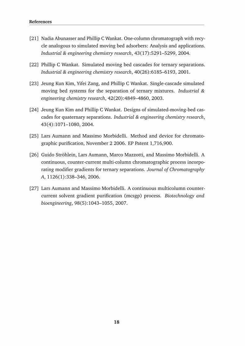
3.5 Materials and methods . . . . . . . . . . . . . . . . . . . . . . . . . 29
ix

3.5.1 System characterization . . . . . . . . . . . . . . . . . . . . 30
3.5.2 Adsorption isotherms . . . . . . . . . . . . . . . . . . . . . . 31
3.6 Results and discussion . . . . . . . . . . . . . . . . . . . . . . . . . 34
3.6.1 Batch chromatography . . . . . . . . . . . . . . . . . . . . . 34
3.6.2 Two-column open-loop SMB: continuous and discontinuous
elution . . . . . . . . . . . . . . . . . . . . . . . . . . . . . . 39
3.6.3 Two-column open-loop SMB with continuous elution . . . . 39
3.6.4 Optimal Pareto curves for the cases reported . . . . . . . . . 44
3.7 Concluding Remarks . . . . . . . . . . . . . . . . . . . . . . . . . . 46
4 Relay simulated moving bed: concept and design criteria 53
4.1 Introduction . . . . . . . . . . . . . . . . . . . . . . . . . . . . . . . 53
4.2 Process description . . . . . . . . . . . . . . . . . . . . . . . . . . . 58
4.3 Analysis under conditions of finite column efficiency . . . . . . . . 68
4.4 Conclusions . . . . . . . . . . . . . . . . . . . . . . . . . . . . . . . 79
5 Relay simulated moving bed: experimental validation 87
5.1 Introduction . . . . . . . . . . . . . . . . . . . . . . . . . . . . . . . 87
5.2 Chromatographic Column Model . . . . . . . . . . . . . . . . . . . 88
5.3 Experimental . . . . . . . . . . . . . . . . . . . . . . . . . . . . . . 89
5.4 Results and discussion . . . . . . . . . . . . . . . . . . . . . . . . . 91
5.5 Concluding Remarks . . . . . . . . . . . . . . . . . . . . . . . . . . 94
6 Gradient with Steady State Recycle process: rationalization and pilot
unit validation 97
6.1 Introduction . . . . . . . . . . . . . . . . . . . . . . . . . . . . . . . 97
6.2 Process description . . . . . . . . . . . . . . . . . . . . . . . . . . . 100
6.3 Pilot unit . . . . . . . . . . . . . . . . . . . . . . . . . . . . . . . . 104
6.3.1 Inlet flow rates . . . . . . . . . . . . . . . . . . . . . . . . . 105
6.3.2 Monitoring and fraction collection . . . . . . . . . . . . . . 107
x

6.3.3 Process automation . . . . . . . . . . . . . . . . . . . . . . . 107
6.4 Validation of moving solvent-gradient in the pilot unit . . . . . . . 108
7 Gradient with Steady State Recycle process: Model-based analysis and
experimental run 117
7.1 Materials and Methods . . . . . . . . . . . . . . . . . . . . . . . . . 117
7.2 Adsorption Equilibria . . . . . . . . . . . . . . . . . . . . . . . . . . 118
7.3 Model-based analysis tools . . . . . . . . . . . . . . . . . . . . . . . 122
7.3.1 Chromatographic column model . . . . . . . . . . . . . . . 123
7.3.2 Dynamic process model . . . . . . . . . . . . . . . . . . . . 124
7.3.3 Numerical solution . . . . . . . . . . . . . . . . . . . . . . . 126
7.3.4 GSSR cycle for purification of the peptide mixture . . . . . . 126
7.3.5 Step sequencing . . . . . . . . . . . . . . . . . . . . . . . . 128
7.3.6 Simulated cycle . . . . . . . . . . . . . . . . . . . . . . . . . 129
7.3.7 Choice of manipulated variable for tuning the process . . . 130
7.4 Experimental GSSR run . . . . . . . . . . . . . . . . . . . . . . . . 131
7.4.1 Comparison with single-column batch chromatography . . . 136
7.5 Conclusions . . . . . . . . . . . . . . . . . . . . . . . . . . . . . . . 137
8 Adenovirus purification by two-column, size-exclusion, simulated coun-
tercurrent chromatography 141
8.1 Introduction . . . . . . . . . . . . . . . . . . . . . . . . . . . . . . . 141
8.2 Material and Methods . . . . . . . . . . . . . . . . . . . . . . . . . 145
8.2.1 Cell line and medium . . . . . . . . . . . . . . . . . . . . . 145
8.2.2 Virus production . . . . . . . . . . . . . . . . . . . . . . . . 145
8.2.3 Clarification and concentration . . . . . . . . . . . . . . . . 146
8.2.4 Analytics . . . . . . . . . . . . . . . . . . . . . . . . . . . . 146
8.2.5 Chromatography . . . . . . . . . . . . . . . . . . . . . . . . 147
8.3 Mathematical Model . . . . . . . . . . . . . . . . . . . . . . . . . . 149
xi

8.4 Cycle Design . . . . . . . . . . . . . . . . . . . . . . . . . . . . . . 151
8.5 Results and Discussion . . . . . . . . . . . . . . . . . . . . . . . . . 155
8.6 Conclusions . . . . . . . . . . . . . . . . . . . . . . . . . . . . . . . 157
9 Conclusions and Future Work 163
9.1 Conclusions . . . . . . . . . . . . . . . . . . . . . . . . . . . . . . . 163
9.2 Suggestions for future work . . . . . . . . . . . . . . . . . . . . . . 164
xii

List of Figures
2.1 Schematic of a four-section TMB . . . . . . . . . . . . . . . . . . . 6
2.2 Schematic diagram of a four-section SMB unit for two consecutive
switching intervals . . . . . . . . . . . . . . . . . . . . . . . . . . . 9
2.3 Simplified scheme of the Varicol process. . . . . . . . . . . . . . . . 10
2.4 Simplified scheme of the PowerFeed process . . . . . . . . . . . . . 11
2.5 Temporal profiles of the Feed concentration in the standard SMB
and Modicon over two consecutive switching intervals . . . . . . . 12
2.6 Port configuration of an I-SMB scheme for two consecutive switching
intervals . . . . . . . . . . . . . . . . . . . . . . . . . . . . . . . . . 13
2.7 Feed and Raffinate flow-rates of a Partial-Feed operation for two
consecutive switching intervals. . . . . . . . . . . . . . . . . . . . . 14
2.8 Schematic diagram of the MultiColumn Solvent Gradient Process . 15
3.1 Possible port configuration between two consecutive columns, or
group of columns . . . . . . . . . . . . . . . . . . . . . . . . . . . . 21
3.2 Schematic diagram of semi-continuous, two-column, open-loop chro-
matograph for chiral separation. . . . . . . . . . . . . . . . . . . . 22
3.3 Details of the inlets present in the unit described and portrayed in
Fig.3.2 . . . . . . . . . . . . . . . . . . . . . . . . . . . . . . . . . . 23
3.4 Schematic diagram of the single-column SMB analog chromatograph 32
3.5 Rectangular injections (5 ml) of the racemic mixture at 5.0, 10.0,
and 15.0 g/l and flow rate of 1 ml/min . . . . . . . . . . . . . . . . 32
3.6 Breakthrough experiments of the racemic mixture at 10.0, 12.0, and
15.0 g/l for an injection volume of 15 ml at a flow rate of 1 ml/min 33
xiii

3.7 Elution profiles of the individual enantiomers from frontal analysis
experiments with a racemic mixture of Troger’s base, at total feed
concentrations of 10.0, 12.0, and 15.0 g/l, injection volume of 15 ml,
and flow rate of 1 ml/min . . . . . . . . . . . . . . . . . . . . . . . 33
3.8 Cut strategies possible in batch operation . . . . . . . . . . . . . . . 35
3.9 Schematic of the operating cycle for the batch process . . . . . . . 37
3.10 Solute concentration profile at the outlet of the system, for the
batch-wise operation defined in Table 3.2 . . . . . . . . . . . . . . 37
3.11 Schematic of the operating cycle for the SSR process. . . . . . . . . 38
3.12 Axial composition profiles in the fluid phase at four intervals of the
cycle. . . . . . . . . . . . . . . . . . . . . . . . . . . . . . . . . . . 38
3.13 Optimal (Pareto) curves of eluent consumption (Eav/Fav) versus
average feed flow rate (Fav), for solution of the separation prob-
lem defined in Table 3.1 with the batch and SSR configurations of
Figs. 3.9 and 3.11 . . . . . . . . . . . . . . . . . . . . . . . . . . . 39
3.14 Schematic of the operating cycle (2τ) for the two-column, open-loop
process with continuous elution . . . . . . . . . . . . . . . . . . . . 40
3.15 Solute concentration profile at the outlet of the system, for the two-
column, open-loop operation with continuous elution defined in
Table 3.3 . . . . . . . . . . . . . . . . . . . . . . . . . . . . . . . . . 41
3.16 Steady periodic solution of the axial composition profile for the first
switching interval for the two-column, open-loop operation with
continuous elution defined in Table 3.3 . . . . . . . . . . . . . . . . 42
3.17 Schematic of the operating cycle (2τ) for the two-column, open-loop
process with discontinuous elution . . . . . . . . . . . . . . . . . . 43
3.18 Solute concentration profile at the outlet of the system, for the two-
column, open-loop operation with continuous elution defined in
Table 3.4 . . . . . . . . . . . . . . . . . . . . . . . . . . . . . . . . . 44
3.19 Steady periodic solution of the axial composition profile for the first
switching interval for the two-column, open-loop operation with
discontinuous elution defined in Table 3.3 . . . . . . . . . . . . . . 45
xiv

3.20 Optimal (Pareto) curves of eluent consumption (Eav/Fav) versus
average feed flow rate (Fav), for solution of the separation problem
defined in Table 3.1 with the configurations of Figs. 3.9, 3.11, 3.14
and 3.17 . . . . . . . . . . . . . . . . . . . . . . . . . . . . . . . . 46
4.1 Schematic of a four-zone SMB . . . . . . . . . . . . . . . . . . . . . 54
4.2 Schematic of basic idea behind the relay SMB . . . . . . . . . . . . 57
4.3 Schematic of the R-SMB’s operating cycle for α ≤ (3 +√
5)/2 . . . 59
4.4 Equilibrium solution for complete separation of a linear adsorption
system, for which α < (3 +√
5)/2, by the R-SMB− process under
optimal operating conditions (E ′/F = 1 . . . . . . . . . . . . . . . 62
4.5 Schematic of the operating cycle for the R-SMB+ process, which is
applicable when α ≥ (3 +√
5)/2 . . . . . . . . . . . . . . . . . . . 64
4.6 Equilibrium solution for complete separation of a linear adsorption
system, for which α > (3 +√
5)/2, by the R-SMB+ process under
optimal operating conditions (E ′/F = 1 . . . . . . . . . . . . . . . 66
4.7 Desorbent consumption (E ′/F ) and specific productivity (F/V ′1) as a
function of Peclet number per column (Pe) for complete separation
(PR = PX = 0.99) of a linear adsorption system (α = 1.4) with
different four-column configurations . . . . . . . . . . . . . . . . . 74
4.9 Desorbent consumption (E ′/F ) and specific productivity (F/V ′1) as a
function of Peclet number per column (Pe) for complete separation
(PR = PX = 0.99) of a linear adsorption system (α = 3.0) with
different four-column configurations . . . . . . . . . . . . . . . . . 76
4.10 Specific productivity (F/V ′1) and desorbent consumption (E ′/F ) as
a function of selectivity (α) for complete separation (PR = PX =
0.99) of a linear adsorption system at a Peclet number per column
Pe = 200 with different four-column configurations . . . . . . . . . 77
4.11 Specific productivity (F/V ′1) and desorbent consumption (E ′/F ) as
a function of selectivity (α) for complete separation (PR = PX =
0.99) of a linear adsorption system at a Peclet number per column
Pe = 1000 with different four-column configurations: closed-loop
SMB, open-loop SMB, and the two R-SMB schemes . . . . . . . . . 78
xv

5.1 Schematic of the four-column SMB unit used in the experimental runs. 90
5.2 Schematic of the R-SMB process for the two selectivity regions . . . 92
5.3 Solute concentration profiles at the outlet of column 1 for the chro-
matographic parameters given in Table 5.2 for the R-SMB process
with α < αC . . . . . . . . . . . . . . . . . . . . . . . . . . . . . . . 92
5.4 Solute concentration profiles at the outlet of column 1 for the chro-
matographic parameters given in Table 5.2 for the R-SMB process
with α > αC . . . . . . . . . . . . . . . . . . . . . . . . . . . . . . . 93
5.5 Shematic of the open-loop smb with recycle process . . . . . . . . . 93
5.6 Pareto Plots for α < αC and α > αC . . . . . . . . . . . . . . . . . . 94
6.2 Flow diagrams of the feed and production steps for the case when
they occur at the beginning of the third switching interval and when
the product withdrawal takes longer than the injection of feed. . . 103
6.3 Schematic flowsheet of the GSSR pilot unit. . . . . . . . . . . . . . . 104
6.4 Cycle sequence chosen in the moving solvent-gradient implementation.109
6.5 Accumulated mass from the product (top) and waste (bottom) out-
lets as function of elapsed time (t/τ) for one complete cycle of the
GSSR process, with operating parameters defined in Table 6.1 . . . 110
6.6 Temporal profile of blue dextran concentration at the outlet of col-
umn 3 for 5 cycles of a GSSR process . . . . . . . . . . . . . . . . . 111
7.1 Peak deconvolution for an analytical chromatogram of the crude
peptide mixture . . . . . . . . . . . . . . . . . . . . . . . . . . . . . 119
7.2 Henry constants, Ki = (1 − εb)Hi, for the key components of the
peptide mixture, as a function of EtOH concentration . . . . . . . . 121
7.3 Henry constants, Ki = (1− εb)Hi, for the target peptide (i = 2) and
its two closest impurities (i = 2 and i = 3), as a function of EtOH
concentration . . . . . . . . . . . . . . . . . . . . . . . . . . . . . . 122
7.4 GSSR cycle for purification of the peptide mixture and snapshots of
the simulated axial concentration profiles taken at selected instants
of the cycle . . . . . . . . . . . . . . . . . . . . . . . . . . . . . . . 131
xvi

7.5 Effect of the switching interval, τ , on the elution time of the main
product peak at the outlet of the column where the product fraction
is collected. . . . . . . . . . . . . . . . . . . . . . . . . . . . . . . . 132
7.6 Temporal profile of the UV signal measured at the outlet of column 3
for the 30-cycle GSSR experiment. . . . . . . . . . . . . . . . . . . . 133
7.7 Temporal profile of the UV signal measured at the outlet of column 3
for the last four cycles of the 30-cycle GSSR experiment. . . . . . . 134
7.8 HPLC analysis of the product fraction collected during the last cycle
of the 30-cycle GSSR experiment of Fig. 7.6 . . . . . . . . . . . . . . 135
7.9 Simulated curve of optimal product recovery (recp) versus purity
(purp) for single-column batch chromatography (SCBC) subject to
the same amount of stationary phase and amount of feed injected
per cycle as in the 30-cycle GSSR experiment. . . . . . . . . . . . . 137
8.1 Standard batch downstream train for virus purification. . . . . . . . 143
8.2 Pulse experiments in isolated and connected columns. . . . . . . . 151
8.3 Set of suitable flow-path configurations for the design of a two-
column, open-loop SEC process without partial splitting of exit
streams. . . . . . . . . . . . . . . . . . . . . . . . . . . . . . . . . . 152
8.4 Schematic representation of operating cycle for the two-column,
semi-continuous open loop process. . . . . . . . . . . . . . . . . . . 154
8.5 Steady state profile at the inlet/outlet of the first switching interval. 155
8.6 Modeled profile of the two-column during the semi-continuous cycle.156
8.7 Experimental chromatogram representing the automatic column
cycling during the continuous SEC purification. . . . . . . . . . . . 156
8.8 Protein profile analyzed by SDS-PAGE. . . . . . . . . . . . . . . . . 158
xvii

List of Tables
3.1 Column characterization and adsorption parameters for the nonlin-
ear separation of Troger’s base enantiomers on Chiralpak AD and
ethanol at 25◦C . . . . . . . . . . . . . . . . . . . . . . . . . . . . . 34
3.2 Optimal operating cycle for the solution of the separation problem
defined in Table 3.1 with a batch configuration (Fig. 3.9) . . . . . . 36
3.3 Optimal operating cycle for the solution of the separation problem
defined in Table 3.1 with a two-column, open-loop configuration
with continuous elution (Fig. 3.14) . . . . . . . . . . . . . . . . . . 40
3.4 Optimal operating cycle for the solution of the separation problem
defined in Table 3.1 with a two-column, open-loop configuration
with discontinuous elution (Fig. 3.17) . . . . . . . . . . . . . . . . 43
4.1 Summary of the design equations, derived from the equilibrium
theory, for the optimum operation of the two R-SMB cycles that give
complete separation under linear adsorption conditions . . . . . . . 68
4.2 Linear adsorption column model. . . . . . . . . . . . . . . . . . . . 68
5.1 Column characterization and adsorption parameters for the linear
separation of uridine/guanosine and uridine/adenosine on Source
30 RPC (reversed phase) and 5% (v/v) ethanol in water at 30◦C . . 91
5.2 Optimal cycle parameters for the R-SMB processes . . . . . . . . . 91
5.3 Purities of the experimental runs for the R-SMB processes . . . . . 91
6.1 Operating parameters of the GSSR cycle . . . . . . . . . . . . . . . 109
7.1 Values of ε+Ki for the key components of the peptide mixture, as a
function EtOH concentration . . . . . . . . . . . . . . . . . . . . . 120
7.2 Operating parameters of the GSSR cycle . . . . . . . . . . . . . . . 128
xviii

8.1 Characterization of the two columns packed with Sepharose 4FF. . 148
8.2 Model parameters derived from analysis of pulse experiments per-
formed on the two columns placed in series. . . . . . . . . . . . . . 152
8.3 Process performance for the two-column system compared to a batch
process. . . . . . . . . . . . . . . . . . . . . . . . . . . . . . . . . . 157
xix


Resumo
A recente reducao de escala da tecnologia de Leito Movel Simulado (LMS) possibili-
tou o aparecimento de novas aplicacoes, como a purificacao de produtos de quımica
fina, acidos organicos, produtos de ındole farmaceutica, anticorpos monoclonais
e proteınas recombinantes. O nosso grupo desenvolveu recentemente uma nova
classe de processos LMS semi-contınuos que utilizam duas colunas cromatograficas
em anel aberto. Estes processos exploram os benefıcios do processo LMS mas,
utilizando uma configuracao de nodos flexıvel, uma operacao robusta das bombas
e modulacao cıclica dos caudais. A grande vantagem do processo sugerido e a sua
simplicidade de operacao pois, independentemente do numero de colunas, sao
apenas necessarias duas bombas – uma para a adicao de alimentacao e outra para
a adicao de dessorvente – bem como valvulas simples com uma operacao on-off,
por forma a controlar os caudais de fluidos retirados do sistema. A performance do
nosso processo foi testada com sucesso numa separacao enantiomerica nao linear,
usando duas estrategias de eluicao.
O princıpio de operacao do processo de duas colunas mencionado anteriormente,
descarta a divisao do fluxo de caudal em duas ou mais correntes num determinado
porto de colecta: a fraccao de produto, resıduo, ou passıveis de reciclo sao sempre
obtidas pelo direccionamento do efluente, durante um determinado perıodo do
ciclo produtivo, para um destino apropriado. Esta estrategia de gestao dos portos
de colecta e tambem explorada no processo Relay-SMB (R-SMB). Neste processo a
analogia com o LMS padrao em termos de volumes eluıdos e mantida, evitando
contudo o uso de controladores de caudal ou bombas adicionais. Neste processo o
efluente de uma zona (ou coluna) encontra-se sempre num dos seguintes estados:
(i) estagnado, (ii) direccionado completamente para a zona (ou coluna) seguinte,
ou (iii) direccionado completamente para uma linha de colecta de produto. Para
esta classe de processos foi desenvolvido um processo analogo ao LMS – o processo
R-SMB e demonstrado de acordo com a teoria do equilıbrio que este ultimo tem
a mesma regiao separativa que o processo de LMS padrao para um sistema de
adsorcao linear. De acordo com a teoria do equilıbrio, os resultados demonstram
que o R-SMB e composto por dois ciclos distintos que apenas diferem num passo
intermedio, que e dependente da selectividade da separacao a considerar.
xxi

Em muitos dos problemas de purificacao de produtos biologicos, o composto
desejado encontra-se numa posicao intermedia entre dois grupos de impurezas
- menos ou mais adsorvidas. Um corte central e, entao, uma alternativa viavel
para a recuperacao do produto de interesse. O processo de reciclo em estado
estacionario com gradientes (GSSR) e composto com um sistema multi-coluna em
anel aberto com um gradiente de solventes e uma operacao em estado estacionario
cıclico. E especialmente indicado para separacoes ternarias, visto que possibilita
a existencia de tres fraccoes ou produtos, sendo o produto de interesse contido
na fraccao intermedia. Uma descricao detalhada do processo GSSR e fornecida,
realcando a sua versatilidade, flexibilidade e simplicidade de operacao. A validacao
experimental numa unidade piloto e tambem fornecida, usando para este fim a
separacao de uma mistura de proteınas em fase reversa como referencia e caso de
estudo.
Embora a operacao em estado contınuo de sistemas cromatograficos seja signi-
ficativa, a industria biofarmaceutica encontra-se ainda cetica quanto a adocao de
processos cromatograficos multi-coluna. Isto e, em parte, devido a complexidade
acrescida da validacao do processo. Contudo, a implementacao de tecnologias
de utilizacao unica e descartavel estao neste momento a mitigar este ceticismo,
havendo assim espaco para o desenvolvimento de um processo cromatografico
semi-contınuo, compacto e eficiente. Neste sentido, foi estudada a possibilidade de
utilizacao de um sistema cromatografico em contra-corrente, composto por duas
colunas em anel aberto. A separacao de um adenovırus, utilizando cromatografia
de exclusao em condicoes isocraticas foi conseguida com sucesso e e tambem
reportada.
xxii

Abstract
The recent scale-down of the Simulated Moving Bed (SMB) technology led to new
applications, including the purification of fine chemicals, organic acids, pharmaceu-
tics, monoclonal antibodies, and recombinant proteins. We developed a novel class
of semi-continuous, two-column, open-loop SMB systems. These processes exploit
the benefits of the SMB but with a flexible node design, robust pump configuration,
and cyclic flow-rate modulation. The major advantage of our design is the simplic-
ity of its physical realization: regardless of the number of columns, it uses only
two pumps — one to supply feed and another to supply desorbent — and simple
two-way valves to control the flow rates of liquid withdrawn from the system. The
performance of our process was successfully tested on a nonlinear enantiomeric
separation, using two types of elution strategies.
The operating principle of our two-column SMB systems discards the splitting of the
flow into two or more streams at an active outlet: the product, waste, or recycled
fractions are always obtained by completely directing the effluent over a certain
period of the cycle to the appropriate destination. This strategy of handling the
product outlets was also explored in the Relay SMB. In this process, the analogy
with the standard SMB in terms of displaced volumes of fluid per switch interval is
maintained, whilst avoiding the use of flow controllers or an extra pumps. In this
process the flow through a zone (or column) is always in one of the three states:
(i) frozen, (ii) completely directed to the next zone (or column), or (iii) entirely
diverted to a product line. For this class of processes we derive a SMB analog
— the R-SMB process and demonstrate, under the framework of the equilibrium
theory, that this process has the same separation region as the classical SMB for
linear adsorption systems. In addition, the results from the equilibrium theory
show that the R-SMB process consists of two distinct cycles that differ only in their
intermediate sub-step depending on the selectivity of a given separation.
For many biopurification problems, the desired product is intermediate between
weakly and strongly adsorbing impurities, and a central cut is thus required to get
the desired product. The Gradient Steady State Recycling (GSSR) process comprises
a multi-column, open-loop system with a solvent gradient and cyclic steady-state
xxiii

operation. It is particularly suited for ternary separations: it provides three main
fractions or products, with a target product contained in the intermediate fraction. A
comprehensive description of the GSSR process is given, highlighting the versatility,
flexibility, and ease of operation of the process. The experimental validation in a
pilot unit is provided, using the purification of a crude peptide mixture by reversed
phase as a benchmark and case study.
Despite the advantages of a continuous chromatography, biopharmaceutical indus-
try is somehow skeptical about moving to multi-column chromatography. This is,
in part due to the increase in complexity in terms of process validation. However,
the implementation of single use and ready to process technologies are mitigating
these issues, therefore there is room for exploring a single compact and efficient
multi-column chromatographic process. In this sense, the use of a simple semi-
continuous, open-loop, two-column, countercurrent chromatographic process was
studied. The separation of adenovirus serotype 5 (Ad5) was successfully accom-
plished by size-exclusion chromatography under isocratic elution conditions.
xxiv

1Introduction
1.1 Relevance and Motivation
Chromatography is one of the simplest, yet effective, separation methods, able
to separate any soluble or volatile component if the right column configuration,
operating conditions, mobile phase, and stationary phase are employed. Batch
chromatography, because of its ease of operation and low capital investment, is a
well-established process used in many large-scale industries, like sugar processing,
and to some extent in the hydrocarbon industry; also chromatography proven to be
very useful, as both an analytical and preparative or process-scale purification, in
small-scale applications such as the pharmaceutical, biotechnology, fine chemistry,
and food processing industries. Although batch chromatography can be very
flexible, allowing the recovery of several fractions from a feed mixture in a single
operation, it suffers from the drawbacks of batch operation, the products are
recovered at a high dilution rate, the stationary phase is not efficiently used, and
the purity of the recovered fractions is extremely dependent on the selectivity of
the chromatographic system.
One way to overcome the above mentioned problems and to improve the separation
efficiency is to operate the process in countercurrent mode, with the mobile phase
circulating in opposite direction relative to the stationary phase. This is the operat-
ing principle of a moving-bed system, with the True Moving Bed’s being the best
idealization of the concept of continuous countercurrent adsorption chromatogra-
1

1.1. Relevance and Motivation
phy (not to be confused with liquid-liquid countercurrent chromatography). In a
binary separation, the moving bed achieves of high purity, even if the resolution of
the system is not excellent, because only the purity at the two tails of the concentra-
tion profiles, where the withdrawal ports are located, is of interest. This is contrary
to batch chromatography where the purity of the products is dependent of the
system resolution. It is also clear that the loading of the stationary phase is higher
in a moving bed than in a fixed bed system, which leads to a higher productivity
per unit mass of stationary phase. However, the advantages of the TMB process are
rapidly overcome by the difficulty of its physical realization; therefore, in practice
the continuous movement of the stationary phase is simulated in a discrete way by
replacing the moving bed by a circular train of fixed beds packed with the stationary
phase and periodically moving the inlet and outlet ports in the same direction as
the fluid flow—this is the Simulated Moving Bed (SMB) process.
The first large-scale commercial application of continuous simulated countercurrent
adsorption was developed by UOP (Universal Oil Products, Des Plaines, Illinois,
USA) in the early 1960s, under the generalized name of Sorbex.
In the last decades, the scaling-down of the SMB technology led to a new set of
applications, especially in the purification of fine chemicals, organo acids, phar-
maceutics, monoclonal antibodies, or recombinant proteins. A new trend in SMB
processes emerged from the demands of these new type of applications. Smaller
and more versatile configurations are preferred, no longer making use of the initial
process configuration where several columns with large dimensions were employed.
The moving trend is supported by an increase in complexity, which in most cases
requires highly versatile equipment and advanced optimization tools.
Although the SMB process increases throughput, purity, and yield relative to batch
chromatography, the batch process still presents the obvious advantages of being
easy to operate, requiring a low capital investment, and being easily prone to the
application of solvent gradients or center-cut separations.
The development of new chromatographic processes that attempt to combine the
”best of both worlds” of batch and SMB operation poses a challenge, whose solution
can bring economical advantages to the industry and lead to new applications in
the field of chromatographic separations.
2
1.2. Objectives and Outline
1.2 Objectives and Outline
This thesis is organized into nine chapters. The present chapter describes the
relevance and motivation of the work as well as the structure of the thesis.
Chapter 2 introduces the principles of TMB and SMB chromatography. Moreover,
a brief review of the state of the art on the SMB processes and applications is
included. This chapter finalizes with an introduction to chromatographic separation
techniques used for the separation of biological products.
Chapter 3 presents a proof of concept of the application of a streamlined, two-
column SMB system, developed by our group, to a nonlinear chiral separation
problem. In this chapter we also present two different elution strategies that
can be implemented in the two-column system. These strategies are analyzed
numerically and compared to the reference cases of batch chromatography and
steady-state recycling. This chapter is based on the submitted paper to Journal of
Chromatography A:
• R.J.S. Silva, R.C.R. Rodrigues, J.P.B Mota, Two-column streamlined simulated
moving bed applied to a nonlinear chiral separation.
Chapter 4 deals with the concept and design criteria for a new class of multicolumn
chromatographic processes that change the classical way of handling the product
outlets of simulated moving-bed (SMB) chromatography to avoid the use of flow
controllers or an extra pump. Despite the simplified manipulation of the zone flow
rates, the R-SMB process maintains the analogy with the SMB in terms of displaced
volumes of fluid per switch interval. This chapter is based on work published in
• Ricardo J.S. Silva, Rui C.R. Rodrigues, Jose P.B. Mota, Relay simulated moving
bed chromatography: Concept and design criteria, Journal of Chromatogra-
phy A, 1260 (2012),132-142.
Chapter 5 presents the experimental validation of the Relay simulated moving bed
concept, presented in the previous chapter. This chapter is an extension of the
previous work done in this field
Chapter 6 reports the process rationalization and pilot unit validation used for the
proof of concept of the Gradient with Steady State Recycling (GSSR) process for
center-cut separation of multicomponent mixtures. This chapter is based on the
work published in
3

1.2. Objectives and Outline
• Ricardo J.S. Silva, Rui C.R. Rodrigues, Hector Osuna-Sanchez, Michel Bailly,
Eric Valery, Jose P.B. Mota, A new multicolumn, open-loop process for center-
cut separation by solvent-gradient chromatography, Journal of Chromatogra-
phy A, 1217 (2010), 8257-8269.
Chapter 7 deals with the model-based analysis of the process and the optimal cycle
design. We also report on the experimental validation of this process. The work
described in the previous chapter and in the present one is summarized and some
conclusions are drawn.
Chapter 8 describes the application of the two column simulated moving bed
system, using size exclusion chromatography, in the purification of adenovirus. This
chapter is based on the paper submited to Journal of Chromatography A:
• Piergiuseppe Nestola, Ricardo J.S. Silva, Jose P.B. Mota, Adenovirus purifica-
tion by two-column, size-exclusion, simulated countercurrent chromatogra-
phy.
In Chapter 9, a few remarks and ideas for future work are presented, before
summarizing the work and drawing final conclusions.
4

2Simulated Moving Bed technology: a
brief review
2.1 Introduction
The Simulated Moving Bed (SMB) is a multicolumn, continuous, countercurrent
adsorption separation process that, generally speaking, increases throughput, purity,
and yield. The first large-scale commercial application of continuous simulated
counter-current adsorption was developed by UOP (Universal Oil Products) in
the early 1960s, since then, the SMB technology has been widely used in the
petrochemical (xylene isomer separation) and food industries (glucose-fructose
separation) on a multi-ton scale. In the last two decades, with the advent of stable
bulk stationary phases for chromatographic enantioseparation, the SMB principle
has been successfully transferred to the pharmaceutical industry.
The most recent applications of SMB technology, such as the purification of fine
chemicals, organic acids, pharmaceuticals, monoclonal antibodies, or recombinant
proteins, no longer make use of the original configuration, where several columns
with large dimension are employed. Today it is possible to build SMB systems
with column sizes ranging from 4 to 1000 mm inner diameter and to produce
pharmaceuticals on a small scale as well as on a 100-ton scale. This has opened the
opportunity for smaller and more versatile configurations, which are however more
complex to operate, thus making an empirical design quite difficult and requiring
5

2.2. Principle of SMB Technology: the concept of True Moving Bed
modeling and simulation for reliable process design and optimization.
2.2 Principle of SMB Technology: the concept of True
Moving Bed
The operation of a SMB unit can be best understood by means of the ideal concept
of the TMB, which involves the actual circulation of the solid at a constant flow rate
in opposite direction to the fluid phase. Furthermore, liquid and adsorbent streams
are continuously recycled as shown in figure 2.1. The feed is continuously injected
into the middle of the system and two product lines are collected: the extract, rich
in the more retained components, and preferentially carried with the solid phase,
and the raffinate, rich in the less retained components that move with the liquid
phase. Also, pure solvent is continuously injected at the beginning of section I and
admixed with the liquid recycled from the downstream end of section IV.
Feed RaffinateExtractDesorbent
Section I Section II Section III Section IV
B A
co
nce
ntr
atio
n
axial coordinate
Solid phase
Liquid phase
Figure 2.1: Schematic of a four-section TMB. The separation A and B is carried out insections II and III. The collection of products A and B is performed in the extract andraffinate streams, respectively.
Because of the addition and withdrawal of the four streams, the TMB unit can be
divided into four sections or zones with different flow rates of the liquid phase,
where each section plays a specific task in the separation. The separation of
components A and B is performed in sections II and III, where the more retained
component B has to be adsorbed and carried towards the extract port through the
movement of the solid, while the less retained component A has to be desorbed
6

2.2. Principle of SMB Technology: the concept of True Moving Bed
and carried by the mobile phase in the direction of the raffinate port. In section I
the solid is regenerated by desorption of the strongly adsorbed component with
fresh eluent stream. Finally, in section IV the liquid is regenerated by adsorption
of the less retained component that was not collected in the raffinate. With this
arrangement it is possible to recycle back both the solid and liquid phase to sections
IV and I, respectively. With a proper choice of the internal flow rates and solid phase
velocity, the feed mixture can be completely separated into two pure products, even
if the resolution of the system is not excellent because only the purity at the tails of
the concentration profiles, where the withdrawal ports are located, is of interest.
This is contrary to batch chromatography, where high resolution is vital in order to
achieve high purity. It is also evident that a larger portion of the stationary phase is
loaded in the moving-bed system than in a fixed-bed system. This will ultimately
lead to a higher productivity per unit mass of stationary phase.
However, the movement of the adsorbent particles, which are in most cases within
the micrometer range, is technically unfeasible as a result of particle attrition and
backmixing. Therefore, in practice the movement of the solid phase is simulated by
using fixed beds of adsorbent (chromatographic columns) and periodically moving
the inlet and outlet ports in the same direction as the fluid flow. The simulated
countercurrent behavior of the process becomes obvious when the relative move-
ment of the packed beds with respect to the inlet and outlet streams is followed
over several switching intervals (a switching interval is the time interval between
consecutive switches of the positions of the inlet and outlet ports). After a number
of switching intervals equal to the number of columns in the system, one cycle is
completed and the initial positions of all external streams are reestablished.
Due to the continuous nature of countercurrent operation, after the initial transient
start-up a TMB unit attains a steady state. On the contrary, the steady regime
attained by the discrete movement of the solid in a SMB unit is periodic, that is, it
exhibits the same time-dependent behavior over every switching interval.
The equivalence between the concepts of TMB and SMB becomes stronger as the
number of SMB columns increases and their size decreases accordingly so as to
maintain the same amount of adsorbent. Thus, if the number of SMB columns
is not too small, say more than 5 columns, the simpler model of the TMB unit
can be employed to predict the separation performance of the equivalent SMB
unit, provided that some geometric constraints and conversion rules are fulfilled.
The equivalence rules between the TMB and SMB are given by the following
7

2.3. SMB process
relationships:
Vj = NjV (2.1)
V
τ=
QS
1− ε(2.2)
QSMBj = QTMB
j +QS
1− ε(2.3)
Here V is the volume of a SMB column whereas Vj is volume of the jth section of
the TMB unit; Nj is the number of subsections in the jth section of the SMB unit, τ
is the length of the switching interval of the SMB unit, ε is the void fraction of the
adsorbent bed, QS, is the volumetric solid flow rate in the TMB unit, and QSMBj
and QTMBj are, respectively, the volumetric fluid flow rates in the equivalent SMB
and TMB units.
2.3 SMB process
Classical SMB systems are characterized by the synchronous and downstream
shifting by one column of all inlet and outlet lines after a defined switching interval
τ . As mentioned above, in a classical SMB it is possible do distinguish four different
sections defined by different liquid flow rates (figure 2.2). The number of columns
may be evenly distributed or not over the four sections; however, by definition each
section has an integer number of columns, NI/NII/NIII/NIV , and the sum of the
number of columns over the four sections is equal to the total number of columns.
Fig. 2.2 shows an example of a SMB system with a 1/2/2/1 column configuration.
2.4 SMB operation with variable parameters
The scale-down of the original SMB process into smaller SMB units has been gaining
an increasing interest over the last two decades. The recent rapid growth of these
newly emerging SMB applications has been accompanied by the development of
novel SMB schemes that are based on the conventional SMB process, but function
with time-variable operating parameters. The following modes of SMB operation
presented in this chapter aim to extend the potential of the standard SMB process.
It is worth noting that, for sake of brevity, only the operation in liquid phase is
8

2.4. SMB operation with variable parameters
E X F R
t
E X F R
t+τ
Figure 2.2: Schematic diagram of a four-section SMB unit for two consecutive switchingintervals, where the upper diagram depicts the instant t, and the bottom diagram depictsthe instant t+ τ where the input and withdrawl ports are moved one column ahead. Theposition of eluent (E), feed (F), extract (X), and raffinate (R) ports are identified by arrows.
considered.
2.4.1 Varicol
The Varicol process [1, 2] generically consists of performing a predetermined
sequence of asynchronous port switchings over every switching interval, resulting
in a time-periodic modulation of the zone lengths. When the process dynamics is
averaged over a complete cycle the Varicol scheme is equivalent to a non-integer
allocation of the number of columns per section. The possibilities for asynchronous
port switching are endless; for example, in principle it is possible that a port
may shift more than once during the switching interval, either forward or even
backwards. As a result, Varicol schemes can have an infinite number of column
configurations though only a small subset of them will give rise to high-performance
processes.
In Fig. 2.3 we show the example of a standard SMB operation, where the topmost
configuration (1/2/2/1) is kept constant during the whole switching interval t ≤ τ ;
when t = τ all ports are switched forward by one column in the direction of fluid
flow. In the Varicol process the ports are switched asynchronously. For example,
after a fraction α < 1 of the switching interval the position of the feed port is
moved forward by one column, giving rise to the middle configuration, which has
increased zone II by one column (1/3/1/1); at the end of the switching interval all
ports have moved forward by one column like in the standard SMB scheme, and
the process returns to the original zone configuration (1/2/2/1).
9
2.4. SMB operation with variable parameters
E X F R
t
E X F R
t +τ
t +ατ (α< 1 )
E X F R
SMB
VARI
COL
Figure 2.3: Simplified scheme of the Varicol process. The position of eluent (E), feed (F),extract (X), and raffinate (R) ports are identified by arrows.
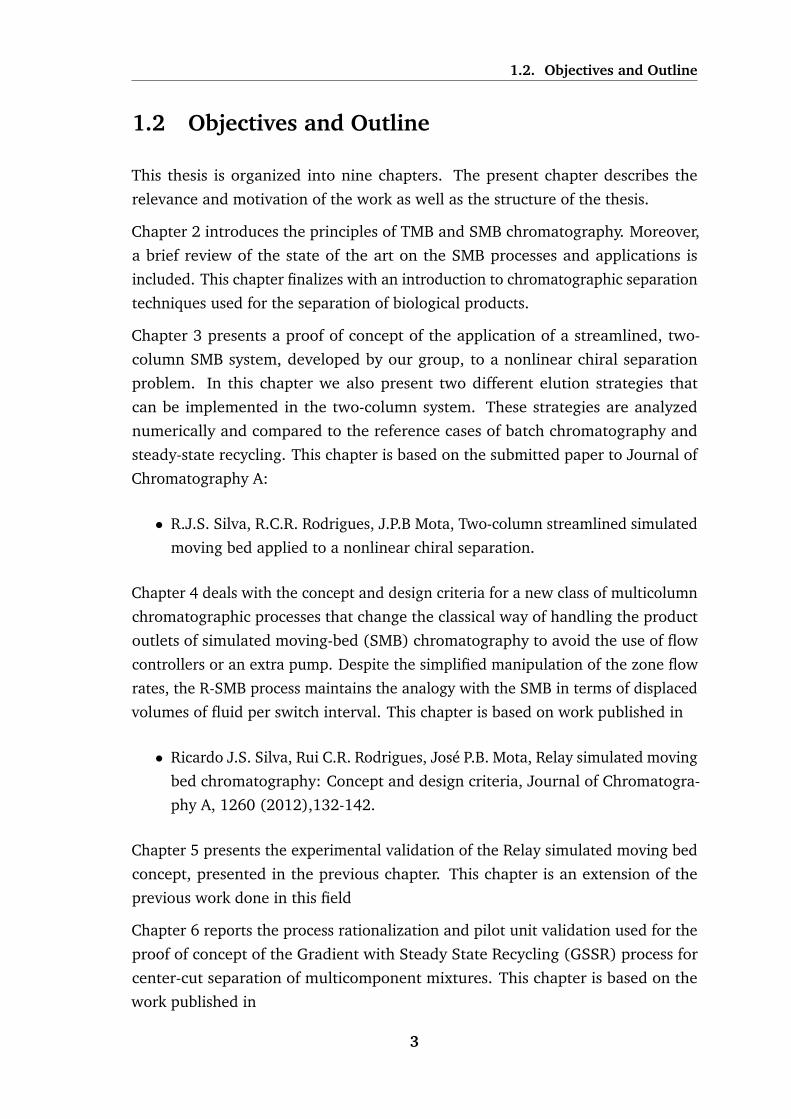
2.4.2 PowerFeed
This concept was originally introduced by Kearny and Hieb [3], and studied in more
detail by other authors [4–6]. Like the conventional SMB process, the switching
of the external ports are kept constant, in contrast to the Varicol process. The
additional performance improvement is created by the modulation of some or
all flow rates during each switching interval. Consequently, the internal flow
rates also change within a switching period. Fig. 2.4 shows an example of the
Powerfeed process, where the shaded areas are proportional to the flow rate in the
corresponding section.
2.4.3 ModiCon
Another variant of the classical SMB process is the ModiCon process [7, 8]. Like
in the standard SMB operation, the Modicon process is synchronous and also
characterized by a constant flow rate in each section; the performance improvement
is achieved by time modulation of the feed concentration over the switching interval.
One drawback of this scheme is that it only works for nonlinear separations and is
only effective for separations where the feed concentration is limited by technical
reasons and not by the solubility of the components in the used solvent.
10

2.4. SMB operation with variable parameters
SMB
POW
ERFE
ED
E X F R
t
E X F R
t +τ
t +ατ (α< 1 )
E X F R
Figure 2.4: Simplified scheme of the PowerFeed process. The position of eluent (E), feed(F), extract (X), and raffinate (R) ports are identified by arrows. The height of each shadedarea is proportional to the flow-rate through the corresponding section. The standard SMBscheme keeps the topmost configuration constant over the whole switching interval τ ; allports are then switched forward by one column in the direction of fluid flow. In PowerFeedoperation, which is illustrated by the intermediate step, the flow-rates are varied over afraction of the switching interval but the ports are only moved forward by one column atthe end of the step like in the standard SMB process.
2.4.4 Improved-SMB or Intermittent-SMB
The main application area of the ISMB [9, 10] (Improved-SMB or Intermittent-
SMB) concept is the sugar industry [11]. In this process the switching interval is
partitioned as follows: in the first part of the period, all external lines (desorbent
and feed inlets as well as extract and raffinate outlets) are distributed as in a
standard SMB scheme. However, in contrast to a classical SMB unit, the outlet of
section IV is not recycled during this part of the switching interval and, consequently,
the flow rate in section IV is zero. During the second part of the switching interval
all external ports are closed and recirculation is performed with a constant flow
rate in all sections of the plant. This SMB scheme allows a separation to be carried
out with a rather small number of columns, which of course has a positive impact
on investment costs.
11
2.4. SMB operation with variable parameters
t t +τ time
Feed
Con
cent
ratio
n
t + 2τ
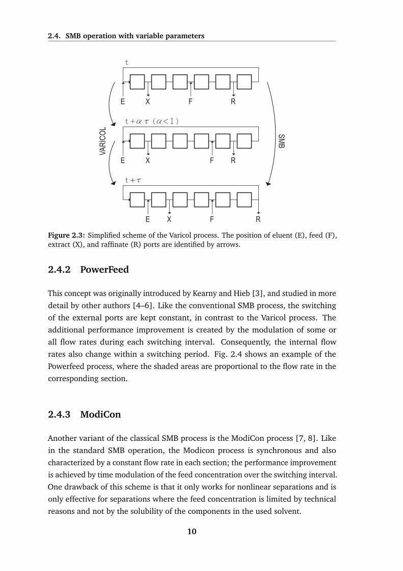
Figure 2.5: Temporal profiles of the Feed concentration in the standard SMB (in red) andModicon (in blue) over two consecutive switching intervals. Both processes are character-ized for a fixed section configuration over the switching intervals. In the exemplified case aperiod of the switching interval is characterized by a pure eluent feed (cF = 0), followedby a step wave where cF is two times the feed concentration of the equivalent SMB process.
2.4.5 Partial-Feed, Partial-Withdrawal/Discard and Outlet-Swing
Stream SMB
In the classical SMB process the composition and flow rate of the feed is constant
over the whole switching interval. The approach in the Partial-Feed [12] process
introduces two more degrees of freedom, the feed duration and feed time. Fig.
2.7 depicts the flow-rate of the feed and raffinate ports in a Partial-Feed operation.
As one can easily understand, in order to fulfill the mass balance constraints the
raffinate flow rate changes according to the variation of the feed flow. In the case
of the Partial-Feed operation the duration of the feed is shorter, but the introduced
flow rate is higher. By this procedure the total amount of feed is kept constant,
while productivity and eluent consumption may increase.
The concept of partial withdrawal [13], which is based on the variation of the
raffinate flow rate in a three-zone SMB, can be used to withdraw the more con-
centrated part of the profile or to leave inside the system the most diluted part,
respectively. As a consequence, the eluent consumption can be decreased for a
given purity requirement. An analogous operation is the so-called partial-discard.
In this case, although the recovery of the two product outlets is complete, only a
part of the outlet is kept in order to improve the overall purity and the remaining is
discarded [14] or recirculated back to the feed [15, 16].
The outlet swing stream-SMB (OSS-SMB) [17] is somewhat similar to the partial-
withdrawal techniques. With this type of operation it is possible to expand or
12

2.4. SMB operation with variable parameters
t + ατ (α< 1 )
E X F R
t
E X F R
t +τ
Figure 2.6: Port configuration of an I-SMB scheme for two consecutive switching intervals.In this process, the inlet and outlet ports are only active in a certain period of the switchinginterval, this is followed by a step of internal recycling at a discrete flow-rate.
contract the product fronts near the withdrawal points, by manipulating the outlet
flow rates, thus allowing the variation of flow rates in sections I and IV while
keeping the flow rates in sections II and III constant by modulating the eluent flow
rate.
2.4.6 Other examples of non-standard SMB operation
The 3-zone SMB scheme is probably one of the simplest schemes that deviates from
the classical 4-zone SMB [18]. This configuration relies on the removal of zone IV,
letting all fluid coming from zone III to be collected as raffinate, which prevents
any contamination of the extract coming from the recirculation line.
More recently, Jin and Wankat [19] theoretically derived a 2-zone SMB for binary
separation in which they incorporate a storage tank to temporarily hold the solvent
for later use. One-column processes that reproduce the cyclic behavior of the
multicolumn SMB chromatography by means of a recycle lag have also been
proposed [20, 21]. This setup exploits the cyclic behavior of the SMB where all
columns are subjected to the same inlet/outlet concentration waveform every Nτ
time units.
The original SMB process is only suitable for binary separations: the partitioning
of one or more less retained components (raffinate) from one or more retained
components (extract). However, in most separation cases the mixture is composed
13

2.4. SMB operation with variable parameters
time
Feed
flow
-rate
t t + τ t + 2τ
time
Raf
finat
e flo
w-ra
te
t t + τ t + 2τ
Figure 2.7: Feed and Raffinate flow-rates of a Partial-Feed operation for two consecutiveswitching intervals.
of more than two components and the goal is, in many cases, to isolate one
component that is intermediately retained in the columns. The first logical step to
achieve a “center-cut” separation is to implement a cascade of two [22, 23] or even
more [24] SMB units, making a series of partitions to isolate the desired product.
Although this is a very straightforward solution, it has an economical drawback
since the need of several SMB units implies the use of much more equipment.
2.4.7 Gradient elution in SMB processes
One characteristic of the SMB processes described so far is that they are all operated
under isocratic, isothermal conditions with nearly-incompressible liquid phases
where the thermodynamic effect of pressure changes is negligible. During the
selection of both stationary and fluid phase, one of the main goals is to find a sepa-
ration method where the first component is fairly well adsorbed on the stationary
phase while the second one can still be easily eluted under those conditions. The
elution strength can be controlled by changing the composition of the solvent or
desorbent. A solvent gradient can improve the SMB separation if the selectivity of
the components is small or if the separation under isocratic conditions is impossible.
The multicolumn counter-current solvent gradient purification (MCSGP) process is
14

2.4. SMB operation with variable parameters
a (semi-)continuous, countercurrent, multicolumn chromatography process capable
of performing three-fraction separations by changing the solvent composition along
the system [25, 26]. This process can be used either for the purification of a
single species from a multicomponent mixture or to separate a three-component
mixture in a single operation. As shown in the scheme of Figure 2.8, the continuous
6-column MCSGP process consists of a group of 3 columns that are interconnected
and another 3 columns that operate in batch mode; the interconnected columns
implement the separation gradient like in batch chromatography; the disconnected
columns perform the loading, the elution of the target product, and the elution of
strongly adsorbed species plus washing, cleaning-in-place, and re-equilibration. In
between the interconnected columns additional inlet streams are used to adjust the
required solvent composition in order to reproduce the desired solvent gradient.
This process can be operated discontinuously with only three columns [27].
IWFS P
Figure 2.8: A schematic diagram of the MultiColumn Solvent Gradient Process (MCSGP). Itis a fully continuous system comprising 6 chromatographic columns using solvent gradientfor a three-fraction separation/purifications. Like in the SMB process, the system movesone column ahead every switching interval. S are the strongly adsorbing impurities, Pis the target product, W are the weakly adsorbing impurities, I the inerts or very weaklyadsorbing impurities and F the feed mixture.
The Gradient with Steady-State Recycle (GSSR) process is particularly suited for
ternary separation of bioproducts: it provides three main fractions or cuts, with
a target product contained in the intermediate fraction. The process comprises a
multicolumn, open-loop system, with cyclic steady-state operation, that simulates a
solvent gradient moving countercurrently with respect to the solid phase. However,
the feed is always injected into the same column and the product is always collected
from the same column as in a batch process; moreover, both steps occur only once
per cycle. This process is more extensively discussed in chapters 6 and 7.
15

References
[1] Philippe Adam, Roger Narc Nicoud, Michel Bailly, and Olivier Ludemann-
Hombourger. Process and device for separation with variable-length, Octo-
ber 24 2000. US Patent 6,136,198.
[2] O Ludemann-Hombourger, RM Nicoud, and M Bailly. The varicol process: a
new multicolumn continuous chromatographic process. Separation Scienceand Technology, 35(12):1829–1862, 2000.
[3] Michael M Kearney and Kathleen L Hieb. Time variable simulated moving
bed process, April 7 1992. US Patent 5,102,553.
[4] E Kloppenburg and ED Gilles. A new concept for operating simulated moving-
bed processes. Chemical engineering & technology, 22(10):813–817, 1999.
[5] Ziyang Zhang, Marco Mazzotti, and Massimo Morbidelli. Powerfeed operation
of simulated moving bed units: changing flow-rates during the switching
interval. Journal of Chromatography A, 1006(1):87–99, 2003.
[6] Ziyang Zhang, Massimo Morbidelli, and Marco Mazzotti. Experimental assess-
ment of powerfeed chromatography. AIChE journal, 50(3):625–632, 2004.
[7] Henning Schramm, Malte Kaspereit, Achim Kienle, and Andreas Seidel-
Morgenstern. Improving simulated moving bed processes by cyclic mod-
ulation of the feed concentration. Chemical engineering & technology, 25(12):
1151–1155, 2002.
[8] H Schramm, A Kienle, M Kaspereit, and A Seidel-Morgenstern. Improved
operation of simulated moving bed processes through cyclic modulation
of feed flow and feed concentration. Chemical engineering science, 58(23):
5217–5227, 2003.
[9] Masatake Tanimura, Masao Tamura, and Takashi Teshima. Method of chro-
matographic separation, November 12 1991. US Patent 5,064,539.
16

References
[10] Kenzaburo Yoritomi, Teruo Kezuka, and Mitsumasa Moriya. Method for the
chromatographic separation of soluble components in feed solution, May 12
1981. US Patent 4,267,054.
[11] Florence Lutin, Mathieu Bailly, and Daniel Bar. Process improvements with
innovative technologies in the starch and sugar industries. Desalination, 148
(1):121–124, 2002.
[12] Yifei Zang and Phillip C Wankat. Smb operation strategy-partial feed. Indus-trial & engineering chemistry research, 41(10):2504–2511, 2002.
[13] Yifei Zang and Phillip C Wankat. Three-zone simulated moving bed with
partial feed and selective withdrawal. Industrial & engineering chemistryresearch, 41(21):5283–5289, 2002.
[14] Youn-Sang Bae and Chang-Ha Lee. Partial-discard strategy for obtaining high
purity products using simulated moving bed chromatography. Journal ofChromatography A, 1122(1):161–173, 2006.
[15] Andreas Seidel-Morgenstern, Lars Christian Keßler, and Malte Kaspereit. New
developments in simulated moving bed chromatography. Chemical engineering& technology, 31(6):826–837, 2008.
[16] Lars Christian and Seidel-Morgenstern. Method and device for chromato-
graphic separation of components with partial recovery of mixed fractions,
August 25 2010. EP Patent 1,982,752.
[17] Pedro Sa Gomes and Alırio E Rodrigues. Outlet streams swing (oss) and mul-
tifeed operation of simulated moving beds. Separation Science and Technology,
42(2):223–252, 2007.
[18] Douglas M Ruthven and CB Ching. Counter-current and simulated counter-
current adsorption separation processes. Chemical Engineering Science, 44(5):
1011–1038, 1989.
[19] Weihua Jin and Phillip C Wankat. Two-zone smb process for binary separation.
Industrial & engineering chemistry research, 44(5):1565–1575, 2005.
[20] Jose PB Mota and Joao MM Araujo. Single-column simulated-moving-bed
process with recycle lag. AIChE journal, 51(6):1641–1653, 2005.
17
References
[21] Nadia Abunasser and Phillip C Wankat. One-column chromatograph with recy-
cle analogous to simulated moving bed adsorbers: Analysis and applications.
Industrial & engineering chemistry research, 43(17):5291–5299, 2004.
[22] Phillip C Wankat. Simulated moving bed cascades for ternary separations.
Industrial & engineering chemistry research, 40(26):6185–6193, 2001.
[23] Jeung Kun Kim, Yifei Zang, and Phillip C Wankat. Single-cascade simulated
moving bed systems for the separation of ternary mixtures. Industrial &engineering chemistry research, 42(20):4849–4860, 2003.
[24] Jeung Kun Kim and Phillip C Wankat. Designs of simulated-moving-bed cas-
cades for quaternary separations. Industrial & engineering chemistry research,
43(4):1071–1080, 2004.
[25] Lars Aumann and Massimo Morbidelli. Method and device for chromato-
graphic purification, November 2 2006. EP Patent 1,716,900.
[26] Guido Strohlein, Lars Aumann, Marco Mazzotti, and Massimo Morbidelli. A
continuous, counter-current multi-column chromatographic process incorpo-
rating modifier gradients for ternary separations. Journal of ChromatographyA, 1126(1):338–346, 2006.
[27] Lars Aumann and Massimo Morbidelli. A continuous multicolumn counter-
current solvent gradient purification (mcsgp) process. Biotechnology andbioengineering, 98(5):1043–1055, 2007.
18

3Two-column open-loop system for
nonlinear chiral separation
3.1 Introduction
The simulated moving bed (SMB) is a continuous adsorption separation process
with numerous applications, many of which are difficult or even impossible to
handle using other separation techniques. The SMB process was originally devised
as a practical implementation of the true moving bed (TMB) process, where the
adsorbent and the fluid phase move counter-currently [1–3].
A binary feed (A/B) may be separated by SMB into two products: an extract product
containing mainly solute A (the more strongly adsorbed species, or group of species
with similarly strong adsorption properties) and a raffinate containing mainly solute
B (the less strongly adsorbed species or group of species). SMB chromatography
increases throughput, purity, and yield relative to batch chromatography [4–7].
This technology has been increasingly applied for the separation of pure substances
in the pharmaceutical, fine chemistry, and biotechnology industries, at all produc-
tion scales, from laboratory to pilot to production scale. This led to the development
of novel cyclic operating schemes, some of which are substantially different from
the conventional process. Broadly speaking, the new operating schemes intro-
duce periodic modulations of selected control parameters into the operating cycle.
19

3.1. Introduction
Concepts such as asynchronous port switching [8–10], cyclic modulation of feed
concentration [11, 12], time-variable manipulation of the flow rates [13–17], and
solvent-gradient operation [18–21], have been thoroughly analyzed. The extra
degrees of freedom available with these schemes improve the separation efficiency,
thus allowing for the use of units with less columns than traditionally used. The
advantages are apparent: less stationary phase is used, the set-up is more economic,
and the overall pressure drop can be reduced. Furthermore, switching from one
mixture to another is easier and takes less time than with more columns.
The classical implementation of the SMB process comprises four zones, with an
integer number of columns per zone. Alternatives to this standard operation
scheme, with less zones, have also been studied. For example, the three-zone
SMB configuration [3, 22, 23] takes the four-zone, open-loop SMB and removes
zone IV. If the amount of adsorbent allocated to each zone is properly optimized by
means of asynchronous port switching, then a three-zone asynchronous SMB can
perform better than a standard (i.e., synchronous) four-zone SMB [24–26]. The
advantages and drawbacks of the three-zone SMB have been discussed by Chin
and Wang [27]. Another example of a system that uses less zones was proposed by
Lee [28], where a two-zone SMB with continuous feeding and partial withdrawal
was used for glucose-fructose separation; this process appears to be more suitable
for enriching products than for high-purity separations [27]. Another example of a
two-zone SMB scheme uses intermittent feeding and withdrawal to achieve ternary
separations [29].
Jin and Wankat [30, 31] developed more recently other examples of two-zone
SMBs for binary separation, which incorporate a storage tank to temporarily hold
desorbent for later use. Their results show that good separation can be achieved
but with more desorbent than required by a four-zone SMB. However, partial
feed was shown to improve the product purities and recoveries considerably. The
system was subsequently extended to ternary separations [32], and a different
two-zone SMB system, which does not use a storage tank, was developed for center-
cut separation from ternary mixtures [33]. Other processes particulary suitable
for ternary separations are the MCSGP [34] and the GSSR [21] processes; these
systems incorporate the principle of counter-current operation and the possibility of
using solvent gradients. One-column processes that reproduce the cyclic behavior
of multicolumn SMB chromatography, by means of a recycle lag, have also been
proposed [35–37].
We have recently developed a semi-continuous, two-column chromatograph with a
20

3.1. Introduction
flexible node design, robust pump configuration, and cyclic flow-rate modulation
to exploit the benefits of both batch and simulated counter-current modes [38].
We emphasize the use of two columns rather than two zones, because with three
or more columns it is always possible to implement a better SMB scheme which
uses more zones with roughly the same ancillary equipment. In fact, running a
two-zone configuration with three columns can be detrimental to the separation
because the zone lengths become highly asymmetrical [39].
One advantage of our streamlined design is the simplicity of its physical realization:
the simplest configuration, with no recirculation step, requires only two pumps to
supply feed and desorbent into the system, while the flow rates of liquid withdrawn
from the system are controlled by material balance using simple two-way valves.
This type of operation implicitly discards the possibility of splitting into two or
more streams the flow exiting one column; in this sense, the product, waste, or
recycling fractions are always obtained by completely directing the effluent over
a certain period of the cycle to the appropriate destination. The different port
configurations that can be implemented with our simplest streamlined design are
depicted in Fig. 3.1. In the present work a series of two-column open-loop processes
(a)
(b) (c)
(d)
(g)(f )
(e)
Figure 3.1: Possible port configuration between two consecutive columns, or group ofcolumns: (a) complete direction of flow to the next column; (b) downstream frozen bed;(c) upstream frozen bed; (d) flow addition to circulating stream; (e) complete withdrawaland flow injection at the same node; (f) partial withdrawal, and (g) partial withdrawaland flow addition at the same node. Configurations (f) and (g) are not considered, as theyimply partial withdrawal of the exit stream from a column.
for semi-continuous enantiomeric separation are assessed both numerically and
experimentally. These schemes are compared against batch chromatography and
batch chromatography with recycle for a case of nonlinear adsorption. We explore
two cases of elution strategy: continuous elution and discontinuous elution; in the
latter case the upstream column is frozen (the flow is halted) while fresh feed is
injected into the downstream column.
21

3.2. Experimental Setup
This chapter is organized as follows. We start by describing the experimental setup
where the proofs of concept were realized, discuss the procedure for optimal cycle
design, and then the numerical approach used to solve the resulting nonlinear
programming problem. We then report on the experimental verification of the
performances of the two-column processes, using the nonlinear separation of
Troger’s base in Chiralpak AD as a convenient model separation problem. The
experiments not only support the discussion of the results but also validate the
modeling tools employed in a comparison study of the processes assessed. Finally,
the work is summarized before drawing final conclusions.
3.2 Experimental Setup
Fig. 3.2 shows a schematic of the node configuration employed in our prototype
apparatus. As stated above, the flow rate of liquid that is withdrawn at each node
is controlled by material balance. The versatility of the valves used, allows the easy
implementation of the port configurations (a)-(e) depicted in Fig. 3.1. Two-way
Col
umn
1
Col
umn
2
UV cell
X
R
F
E
E
F
R
X
UV cell
FC
Figure 3.2: Schematic diagram of semi-continuous, two-column, open-loop chromatographfor chiral separation.
valves allow the flow either to go through or not to go through. Each valve is
attached to the transfer line between columns by a tee. A two-way valve is placed
immediately downstream of the two outlet ports of each column, but preceding the
two inlet ports, to control the flow rate of liquid from the column that is circulated
22

3.3. Model based cycle design
to the other column. This valve is normally open and is only closed when the
effluent from the upstream column is totally withdrawn as product or the fluid in
the column needs to be temporarily frozen. Overall, each set-up employs 10 two-
way valves to control the port switching. The two-way valves are model SFVO
from Valco International (Schenkon, Switzerland) with pneumatic actuation. Each
valve is automated by means of a single computer-controlled three-way solenoid:
application of 50 psi opens the valve; venting the air allows the spring to return
the valve to the closed position.
The inlets of the chromatographic unit are represented in detail in Fig.3.3. This
valve scheme allows the recycling of the desorbent or feed stream back to the
original source tanks by means of a closed loop. This brings also another advantage
which is the steady operation of both pumps, thus eliminating the uncertainty in
the flow rates.
From E/Fpump
column inlet node E/F
To E/Fpump vase
(a)
(b)
Figure 3.3: Details of the inlets present in the unit described and portrayed in Fig.3.2. Thepainted valves (a) are the same of Fig.3.2.
3.3 Model based cycle design
The periodic forward movement of the active inlet/outlet ports by one column in
the direction of the fluid flow—characteristic of a SMB at the end of a switching
interval—is also implemented in our process. Because the two columns are assumed
to be identical, the cycle of a two-column system can be divided into two intervals
of identical length τ . At the end of each switching interval, i.e. every τ time
units, the inlet/outlet ports are switched, and the columns reverse roles. The port
configurations (a) to (e) shown in Fig. 3.1 are the building blocks for establishing
the cyclic operation of the two-column SMB process assessed in this work.
As described next, the feed and eluent flow rates are initially modulated in time as a
convenient means of solving the design problem. This has the fortunate side effect
23

3.3. Model based cycle design
of providing an optimal cycle with slightly better performance than one operated
with constant flow rates. For convenience, the τ -periodic modulations implemented
here are piecewise-constant, i.e., the flow rates are kept constant over each step
before jumping discretely to different values over the next step. In practice, the
switching interval is divided into a given number nQ of steps, which may have
nonuniform lengths, τn > 0,nQ∑n=1
τn = τ. (3.1)
The adopted formulation does not explicitly track the port switching over the cycle;
instead, the state of each two-way valve is inferred from the piecewise-constant
flow-rate profiles. If in Fig. 3.2, for example, Ej = 0 over a given step of the
switching interval, then the two-way valve that connects the eluent pump to the
inlet of column j is closed, otherwise it is open. Similarly, if Qj = 0 or Xj +Rj = Qj
then the two-way valve located between the inlet/outlet ports downstream of
column j is closed, otherwise it is open. This formulation is highly flexible and has
the advantage of eliminating the integer nature of the design problem, since the
only remaining degrees of freedom are the switching interval and the time-variable
flow rates.
A rigorous model-based optimization approach is employed to determine the
optimal operating parameters. The purpose of the nonlinear programming problem
(NLP) is to guarantee the fulfillment of product and process specifications, such
as minimal purities and maximal operating flow rates, while optimizing process
performance in terms of productivity and eluent consumption. At each step of the
flow-rate modulation, the following basic restrictions must be satisfied:
0 ≤ Ej ≤ Qmax, Xj ≥ 0, (3.2)
0 ≤ Fj ≤ Qmax, Rj ≥ 0, (3.3)
Qj ≤ Q′
max, (3.4)
0 ≤ (Xj +Rj) ⊥ (Qj −Xj −Rj) ≥ 0, (3.5)
0 ≤ E1 ⊥ E2 ≥ 0. (3.6)
Here, j is the column index; Qmax is the capacity of the installed pumps; Q′max is
the maximum flow rate through the column imposed by an hypothetical pressure
drop constraint; E, F , X, and R stand for the flow rates of eluent, feed, extract,
24

3.3. Model based cycle design
and raffinate, respectively; and ⊥ is the complementarity operator enforcing at
least one of the bounds to be active. The complementarity constraint 0 ≤ x ⊥ y ≥0
implies the following [40]:
x = 0 or y = 0, (3.7)
x ≥ 0, y ≥ 0. (3.8)
Here the ‘or’ operator is inclusive as both variables x and y may be zero.
The constraints defined by Eqs. 3.2–3.6 guarantee that the solution is physically
realizable with our experimental set-up. Eq. 3.5 ensures that product withdrawal
can be implemented with on-off valves: either nothing is withdrawn as product
from column j (clause Xj +Rj = 0 is active) and the flow is totally circulated to
the other column, or the exit stream from column j is totally withdrawn as product
(clause Qj − Xj − Rj = 0 is active). Note that the complementarity constraint
implicitly enforces the condition:
Qj ≥ Xj +Rj. (3.9)
This constraint is of utmost importance, as it prevents the withdrawal of product
at a flow rate larger than that provided by the column—otherwise the packed bed
would dry out and no longer be saturated with fluid. Eq. 3.6 enforces the use of a
single pump for supplying desorbent to the system.
Open-loop configurations can be generated by imposing one of the constraints:
E1 + E2 + F1 + F2 ≥ Qmin or X1 +X2 +R1 +R2 ≥ Qmin, (3.10)
as they enforce at least Qmin amount of fluid to be supplied into (or removed from)
the system at every step; Qmin should be a small, positive constant. Note that
Eq. 3.10 is not, by itself, a sufficient condition for open-loop operation; however,
when Eqs. 3.5 and 3.10 are applied together, the desired effect is achieved. Our
experience with the type of problems under consideration here has shown that
Eq. 3.10 offers an efficient method of defining the open-loop condition in a NLP
formulation.
25

3.3. Model based cycle design
Product purity and recovery are enforced through the following constraints:
PurR ≥ PurminR , PurX ≥ PurminX , (3.11)
RecR ≥ RecminR , RecX ≥ RecminX , (3.12)
where Pur and Rec denote product purity and recovery, respectively (the ’min’
superscripts represent their minimum admissible values), and the subscripts ’R’
and ’X ’ denote the extract and raffinate streams; these performance parameters
are defined as follows:
PurR =
∫ t+τt
cout1,jRjdt∫ t+τt
(cout1,j + cout2,j
)Rjdt
, PurX =
∫ t+τt
cout2,jXjdt∫ t+τt
(cout1,j + cout2,j
)Xjdt
, (3.13)
RecR =
∫ t+τt
cout1,jRjdt
cF1∫ t+τt
Fjdt, RecX =
∫ t+τt
cout2,jXjdt
cF1∫ t+τt
Fjdt, (3.14)
Eqs. 3.13 and 3.14 have been written under the assumption that component 1 is
the least retained species and component 2 the more retained one.
In practice, processes with constant flow rates are easier to implement and to
control. Because our schemes are semi-continuous, the schematics in Fig. 3.2
must be slightly changed in order to work with fixed-velocity pumps. Instead of
allowing a flow rate, say Q, to have a flexible piecewise-constant profile, i.e., taking
a different value at each sub-step of the switching interval, say Q1, ..., Qn, it is
constrained to two values only: 0 or Qmax. This way, the pump driving the flow is
always operated at Qmax but when Q must be zero the flow is directed back to the
source tank by means of one three-way valve, or two two-way valves, placed at
the pump outlet. This has the added advantage of producing a near-perfect step
change in the flow rate.
In general, the optimization of a chromatographic process is a multi-objective opti-
mization problem with conflicting interests, because one usually seeks to maximize
the productivity or feed throughput while minimizing the solvent consumption [38].
This issue is addressed here by means of Pareto curves, which are curves represent-
ing optimal points nondominant with respect to the others in terms of maximization
of the feed throughput and minimization of the solvent consumption.
For the sake of brevity, the Pareto curves presented here will be restricted to curves
on the (feed throughput)×(eluent consumption) plane, each curve representing a
set of optimal solutions for a given column configuration (or operating scheme)
26

3.3. Model based cycle design
and a fixed set of product specifications (e.g., purity and yield). Special care is
taken to subject all the Pareto curves to the same product constraints and same
amount of stationary phase so that curves for different column configurations can
be directly compared.
In the present work, the objective function, fobj, is chosen to be the maximization
of productivity, or feed throughput:
Fav =1
τ
∫ t+τ
t
(F1 + F2) dt =2
τ
∫ t+τ
t
Fjdt (3.15)
where Fav is the average feed flow rate per cycle. Given that the solvent con-
sumption is (Fav + Eav) /Fav = 1 + Eav/Fav, minimizing the solvent consumption
is the same as minimizing Eav/Fav; for a matter of simplicity we will work on the
(Fav)× (Eav/Fav) plane.
To construct a Pareto curve on this plane, we replace the constraints ’0 ≤ Ej ≤ Qmax’
and ‘’0 ≤ Fj ≤ Qmax’ by a new constraint ’0 ≤ Eav ≤ Qmax’, drop out the pressure
drop constraint given by Eq. 3.4 (this is done only for a matter of simplicity),
and carry out a series of single-objective optimizations that maximize Fav for
progressively larger values of Qmax. Hence we solve:
fobj = max Fav, s.t. Eav ≤ Qmax. (3.16)
for increasing values of the parameter Qmax. The set of points thus generated gives
the desired Pareto curve. Alternatively, we could have solved:
fobj = min Eav, s.t. Fav ≥ Qmin. (3.17)
for increasing values of Qmin. This procedure would have produced exactly the
same Pareto curve.
Each NLP problem defined by Eq. 3.16 is solved directly for steady periodic opera-
tion of the process, i.e., for cyclic steady state (CSS) conditions. To this end, the
NLP problem is formulated with a single-column analog model that reproduces the
CSS of the two-column unit [41, 42], together with a full-discretization approach
for steady period dynamics. The method is described in detail elsewhere [25, 43].
Discretization is handled via collocation, using 25 cubic Hermite elements [44] for
the spatial domain and 10–15 Radau elements (with two interior points) per sub-
step of the switching interval. The latter type of collocation elements is especially
suitable for handling process dynamics with frequent discontinuities in time [45].
27

3.4. Chromatographic column model
The flow rates remain constant over the Radau elements of a step, but are allowed
to change discretely to different values across steps.
The complementarity conditions-—Eqs. 3.5 and 3.6—are reformulated as NLP
constraints using a relaxed formulation [46]. The nonlinear programming problem
obtained after discretization and relaxation of the complementarity conditions is
formulated in AMPL [47] and solved with IPOPT 3.10 [48]. This solution strategy
has been previously employed with success by our group on a broad class of SMB
problems [36], [25] and [26]. IPOPT implements a primal-dual interior-point
method, and uses line searches based on filter methods; it directly exploits the first
and second derivative (Hessians) information provided by AMPL via automatic
differentiation.
3.4 Chromatographic column model
The complexity of the model required to simulate a particular system depends on
the nature of that system and on the accuracy required. The dispersed plug-flow
model with linear driving-force approximation for mass transfer is a sufficiently
general model to provide a realistic representation of the isothermal operation of
most liquid-phase chromatographic columns [49].
In general, the LDF model can be reasonably well approximated by an equilibrium-
dispersed model. The equilibrium-dispersive model assumes that all contributions
resulting from a lack of equilibrium can be lumped into an apparent axial disper-
sion term. The model provides a very good approximation of the dynamics of a
chromatographic column if the adsorption isotherms are linear (Henry’s law) and
mass transfer is controlled by molecular diffusion. However, the model can also be
applied with reasonable accuracy to nonlinear adsorption is the Henry’s constant
is replaced by the local slope of the adsorption isotherm in the calculation of the
local plate height.
The mass balance for a chromatographic column is:
∂ci∂θ
+ β∂qi∂θ
=τQ
εVC
(1
Pei
∂2ci∂x2− ∂ci∂x
)for 0 < x < 1 (3.18)
where subscript i is the solute index, θ = t/τ and x = z/L, the dimensionless tem-
poral and axial coordinates, respectively; ci and qi, the liquid phase and adsorbed
phase concentrations, respectively; β = (1− ε)/ε the phase ratio; VC , the geometri-
28

3.5. Materials and methods
cal column volume; Q, the flow-rate of the fluid phase; and Pei the apparent Peclet
number.
The concentrations of solute i in the liquid and in the solid phases, ci and qi,
respectively, are related through the adsorption isotherms:
qi = f (c1, c2, ..., cn) i = 1, ..., nsolutes (3.19)
If the adsorption isotherms are linear, the time derivatives ∂qi/∂θ are given by the
corresponding Henry constants; if the adsorption isotherms are nonlinear, the time
derivatives must be replaced by the total derivatives resulting from the chain rule:
∂qi∂θ
=∑k=1
(∂q?i∂ck
)(∂ck∂θ
)(3.20)
Eq.3.18 is subjected to the usual boundary conditions:
ci −1
Pei
∂ci∂x
= cini for x = 0, (3.21)
∂ci∂x
= 0 for x = 1. (3.22)
where cini , the solute concentration in the inlet effluent.
3.5 Materials and methods
To experimentally evaluate and demonstrate the feasibility of the proposed two-
column process, the separation of Troger’s base enantiomers, using ethanol as
pure mobile phase and Chiralpak AD as chiral stationary phase is proposed. The
maximum liquid concentration of the racemate used was about 80% of the solubility
value described elsewhere [50] and experimentally validated.
The pure enantiomers were purchased from Fluka (Germany), with a purity of
99%, and the racemate was purchased from Sigma-Aldrich (Germany), with a
purity of 98% and was recrystallized from ethanol (Panreac, Spain) before use.
The stationary phase (Daicel Chemical Industries Ltd, Chiral Technologies, Europe
Illkirch, France) was slurry-packed into a thermojacketed Superformance with 10
mm i.d. glass column (Gotec Labortechnik, Germany) to a bed height of 120 mm.
The system was operated isothermally at 25◦C.
29

3.5. Materials and methods
A multi-wavelenght UV detector (USB2000, Ocean Optics, USA) with a light source
(Micropack, Ostfildern, Germany), and attenuator, was used to monitor the outlet
stream of the chromatographic columns.
The HPLC pumps employed in the experiments are model K-501 from Knauer
(Berlin, Germany) with 10 ml and 50 ml pump heads, controlled by RS232 com-
munication protocol. The whole setup is fully automated and driven by our
Labview-based software system (BioCTR) for process monitoring and control of
chromatographic processes [51].
3.5.1 System characterization
The total bed porosity (ε) was determined from the retention time of 1,3,5-tri-
tert-butylbenzene (TTBB) (Sigma–Aldrich, Germany); this solute is not retained
by the stationary phase but can access its internal porosity. The packing repro-
ducibility was assessed by comparing the peak shapes and retention times of the
chromatograms obtained with the two preparative columns; both columns were
found to be identically and reasonably well packed. Extra-column volumes in the
experimental set-up were estimated from TTBB pulse experiments with and without
the two chromatographic columns.
The dimensionless plate height, hi, governing band broadening for the ith compo-
nent, can be expressed as [49]
hi2
=1
Pei+ αi
Q
εVC(3.23)
which is known as the linearized van Deemter plot. In principle, under normal
preparative flow conditions the Peclet number, Pei = vL/DiL, where DiL is the
axial dispersion coefficient for component i, should be independent of the solute
index, because DiL ≈ γvdp, where dp is the particle diameter and γ ≈ 0.5–0.7 is a
constant dependent only on the characteristics of the packing (Pei ≈ L/γdp). On
the other hand, the slope of the linearized van Deemter plot is given by
αi =1
ki
βH2i
(1 + βHi)2, (3.24)
where Hi is the local slope of the adsorption isotherm and ki is the LDF coefficient
for component i. The intercept and slope of the linearized van Deemter plot for
each enantiomer were determined by fitting the experimental dependence of hi on
30

3.5. Materials and methods
Q for diluted pulses of the solutes eluted at different flow rates.
3.5.2 Adsorption isotherms
The experimental determination of adsorption isotherms is of utmost importance
for the design and operation of any cyclic adsorption process. This statement holds
true for the two-column chromatographic process under consideration, since its
operating conditions cannot be properly determined without knowledge of the
competitive isotherms of the two enantiomers.
In the present work, the competitive isotherms were estimated with good accuracy
by applying a hybrid inverse method [52]. Briefly, a prescribed adsorption isotherm
model—in the present case, a bi-Langmuir adsorption model—is plugged into the
chromatographic column model described above and then fitted to experimental
band profiles from overloaded injections of the racemic mixture and breakthrough
data. The numerical constants of the isotherm model are tuned so that the calcu-
lated and measured band profiles match as much as possible. The bi-Langmuir
adsorption isotherm model can be written as
q?i =ai,1ci
1 +∑
j bj,1cj+
ai,2ci1 +
∑j bj,2cj
i = A,B (3.25)
where the ai and bi are the fitting parameters.
For the system characterization two different equipment configurations were used.
The first setup, used for parameter scouting, is shown in Fig. 3.4; it uses an
injection loop coupled to the six-port valve for pulse injections, using one of the
HPLC pumps to fill the loop and the other HPLC pump to elute the column. For
longer injections, such as well-defined rectangular pulses, the loop is removed and
the flow scheme is altered as described in more detail in Fig. 3.4. This change has
three major advantages: the length of the injections can be controlled without any
additional change to the experimental setup; the experimental uncertainty due to
flow disturbances is reduced because the HPLC pumps are continuously operated
in closed loop at prescribed flow rates; and, as the commutation of the six-port
valve is almost instantaneous, it is expected to provide a good approximation to
the sharp front and rear edges of a rectangular pulse. The data collected from
the pulse experiments, used in the calculation of the dimensionless plate height,
were grouped with other experiments, namely step injections of 5 ml and 15 ml of
racemic mixture at different concentrations.
31
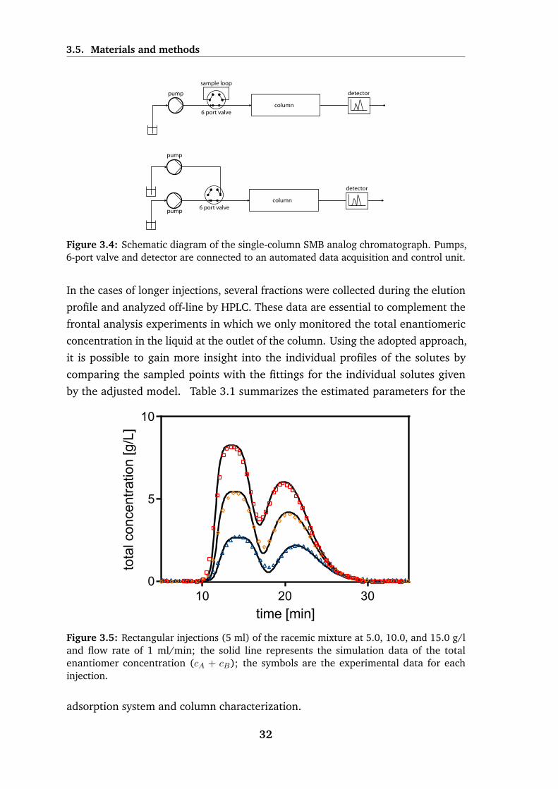
3.5. Materials and methods
detector
column
sample loop
6 port valve
pump
detector
column6 port valvepump
pump
Figure 3.4: Schematic diagram of the single-column SMB analog chromatograph. Pumps,6-port valve and detector are connected to an automated data acquisition and control unit.
In the cases of longer injections, several fractions were collected during the elution
profile and analyzed off-line by HPLC. These data are essential to complement the
frontal analysis experiments in which we only monitored the total enantiomeric
concentration in the liquid at the outlet of the column. Using the adopted approach,
it is possible to gain more insight into the individual profiles of the solutes by
comparing the sampled points with the fittings for the individual solutes given
by the adjusted model. Table 3.1 summarizes the estimated parameters for the
time [min]
tota
lcon
cent
ratio
n[g
/L]
10 20 300
5
10
Figure 3.5: Rectangular injections (5 ml) of the racemic mixture at 5.0, 10.0, and 15.0 g/land flow rate of 1 ml/min; the solid line represents the simulation data of the totalenantiomer concentration (cA + cB); the symbols are the experimental data for eachinjection.
adsorption system and column characterization.
32

3.5. Materials and methods
time [min]
tota
lcon
cent
ratio
n[g
/L]
10 20 30 400
6
12
18
Figure 3.6: Breakthrough experiments of the racemic mixture at 10.0, 12.0, and 15.0 g/lfor an injection volume of 15 ml at a flow rate of 1 ml/min; the solid line represents thesimulation data for the total enantiomer concentration (cA + cB); the symbols are theexperimental data for each injection(triangles, 10.0 g/l; squares, 12.0 g/l; circles, 15.0 g/l.
time [min]
conc
entra
tion
[g/L
]
10 20 30 400
2
4
6
8
10
Figure 3.7: Elution profiles of the individual enantiomers from frontal analysis experimentswith a racemic mixture of Troger’s base, at total feed concentrations of 10.0, 12.0, and15.0 g/l, injection volume of 15 ml, and flow rate of 1 ml/min; The solid and dashedlines represent the simulation data for the less (A) and more (B) retained enantiomers,respectively, using the equilibrium-dispersive model with bi-Langmuir isotherms and modelparameters given in Table 3.1; triangle square symbols denote the experimental indi-vidual enantiomer concentrations determined from the collected fractions of the frontalexperiments.
33

3.6. Results and discussion
Table 3.1: Column characterization and adsorption parameters for the nonlinear separationof Troger’s base enantiomers on Chiralpak AD and ethanol at 25◦C (A and B denote theless and the more retained enantiomers, respectively).
ε = 0.685 A BPei 754 665
αL [s] 0.517 0.790ai,1 1.673 3.954ai,2 0.304 0.982
bj,1 [l/g] 0.013 0.011bj,2 [l/g] 0.136 0.602
3.6 Results and discussion
Using the parameters given in Table 3.1, the methodology presented in Section 3.3
was applied to the optimal design of chromatographic cycles that are realizable
with the schematic of Fig. 3.2. The parameter values for the geometrical and
physical constraints are Qmin = 0.1 ml/min and Qmax = Q′max = 10.0 ml/min.
In order to compare fairly the performance of the processes discussed in this
section, the amount of stationary phase was kept invariant; it is also important
to note that for simplicity of operation of the experimental set-up we were only
interested in schemes that work exclusively in open loop. For the purpose of
experimental validation, the two processes studied in this work as well as the
classical batch process were operated with the same average eluent consumption
(Eav/Fav). Therefore, the value Eav/Fav was fixed at 2.9 and the corresponding
optimal operating point, where the feed flow rate is maximized while still satisfying
the constraint given by Eq. 3.4, was determined for each process.
3.6.1 Batch chromatography
Let us first consider the simplest process: batch chromatography without recycle.
In order to design this process, the two columns of the experimental set-up are
modeled as a single column with a bed height equal to the sum of the heights
of the two columns. Moreover, the parameter Pei has to be scaled because the
batch process uses a single column with twice the bed height; from the definition
of the Peclet number, it is easy to scale it according to its dependence on the
column length. Although the slope of the linearized van Deemter plot must also be
scaled, its scaling factor is already explicitly given in Eq. 3.24 as 1/(εVC) since αi is
independent of the geometrical dimensions of the column.
34

3.6. Results and discussion
fract
ion
A
fract
ion
B
fract
ion
A
fract
ion
B
fract
ion
C
I) II)
Figure 3.8: Cut strategies in batch operation. In the first case only two fractions, A and B,are generated at each cycle; in the second case three fractions are collected separately ineach cycle: two product fractions ( A and B) and an intermediate fraction (C) that can beeither recycled (as s the case in steady-state recycling) or directed to waste.
In batch chromatography there are two approaches that are generally considered
for the cut strategy (Fig. 3.8). In cut strategy I we collect two consecutive fractions,
which are both taken as products. In this case, purity and yield are coupled
together and cannot be varied independently. When high purity is demanded,
which is usually the case in pharmaceutical and fine chemical applications, this cut
strategy requires almost baseline separation of the two target components, which
in many cases can only be achieved by increasing the column volume and reducing
the feed throughput.
Cut strategy II generates an intermediate fraction between the two product fractions,
which can be either discarded or processed further. Due to the introduction of this
fraction, additional degrees of freedom are available. A high purity demand can be
satisfied with this cut strategy by increasing the size of the intermediate fraction
but at the expense of reducing the yield of separation.
The choice between the two different strategies depends not only on the column
resolution, but also on the costs associated with the extra processing of the inter-
mediate fraction (strategy II). In the present case, we are interested on the first
strategy for fractionating the products because the target yield is high and, as stated
above, the system is supposed to operate in an open-loop configuration. The design
of the cycle for the batch process must take the following points into consideration:
(i) the two products are collected alternately at the downstream end of the column,
while feed or desorbent are injected into the upstream end of the column; (ii) the
positions and lengths of the feed, elution, and the two product collection steps
must be correctly sized to optimally satisfy the purity and recovery constraints.
35

3.6. Results and discussion
Table 3.2: Optimal operating cycle for the solution of the separation problem defined inTable 3.1 with a batch configuration (Fig. 3.9). The parameter values for the NLP designproblem Qmax = Q′max=10 mL/min,(fobj = maxf) are: nQ=3, Qmin=0.1 PurminR =PurminX =0.99. The step durations, τn, are expressed in minutes; the eluent (E), feed (F),extract (X), and raffinate (R) flow rates are given in mL/min. The first value on the bottomrow is the switching interval, τ =
∑n τn.
Step, n τn E F X R1 3.265 0.000 2.572 2.572 0.0002 7.600 1.719 0.000 1.719 0.0003 6.567 1.719 0.000 0.000 1.719Average 17.432 1.385 0.478 1.221 0.642
To enforce the collection of the fractions alternately the following constraint is
added to the model: Let’s say that the cycle is divided into nQ steps that do not
necessarily have the same length. For step n let Q(n) ≥ 0 be the column flow rate;
E(n) ge0 and F (n) ≥ 0 the flow rates of eluent and feed injected at the upstream
end of the column, respectively; and X(n) ≥ 0 and R(n) ≥ 0 the flow rates of extract
and raffinate fractions collected at the downstream end of the column. Obviously,
Q(n) = E(n) + F (n) = X(n) +R(n), n = 1, ..., nQ. (3.26)
X iRi = 0, i = 1, ..., nQ. (3.27)
Also we are interested in a steady operation of both the desorbent and feed pump.
This can be traduced in the following:
E1 = ... = EnQ = E, E ≤ Qmax (3.28)
F 1 = ... = F nQ = F, F ≤ Qmax (3.29)
The optimal solution of the NLP problem defined in Table 3.1 resulted in nQ = 3,
i.e., three subdivision of the cycle. The optimal solution is reported in Table 3.2.
Analyzing the cycle one can see that we start by eluting the extract from the
injection performed on a previous cycle, also, the duration of the feed step is
shorter than the collection of extract. Because of this, a second step of elution is
necessary to recover the remaining of the extract band, after that, in the next step
we recover the raffinate fraction.
The cycle was implemented on the unit shown in Fig.3.2, using only the first
column node. Both columns were coupled together, using a zero-volume coupling.
36

3.6. Results and discussion
FX
EX
ER
Figure 3.9: Schematic of the operating cycle for the batch process. E denotes de eluentinlet, F the feed inlet, X the extract outlet and R the raffinate outlet.
The cyclic operation was performed for five cycles. In Fig. 3.10 is represented the
experimental data and the dynamic model simulation. The concordance between
experimental and simulated profiles is fairly good.
switch interval, τ
tota
lcon
cent
ratio
n[g/
L]
0 1 2 3 40
2
4
6
8
10
5
X R
Figure 3.10: Solute concentration profile at the outlet of the system, for the batch-wiseoperation defined in Table 3.2. Symbols denote the experimental data (c1 + c2), whereasthe solid line represent the dynamic process model.
Previously we discussed the importance of adding an extra fraction to a batch
elution, and the option to further process it or not. The recycling step is normally
used to recycle an impure fraction back to the system, but it can also be used
to replace the role of the desorbent, in terms of the progression of the band
in the interior of the column. Fig. 3.11 shows an optimized cycle for a steady
state recycling process, and Fig. 3.12 depicts the axial composition profiles of the
fluid phase at four different periods of the cycle. As stated before, the recycling
37

3.6. Results and discussion
EX
FX
ER
Figure 3.11: Schematic of the operating cycle for the SSR process. E denotes de eluentinlet, F the feed inlet, X the extract outlet and R the raffinate outlet.
EX
FX
ER
Figure 3.12: Axial composition profiles in the fluid phase at four intervals of the cycle.The green and blue lines represent solute 1 and 2 respectively.
step is being used for reducing the desorbent consumption, fact that is supported
by analyzing Fig. 3.13 - Pareto optimal curves for batch and SSR processes. In
this figure is possible to see that the range of productivity, represented by Fav
is slightly increased, and the desorbent consumption is decreased for the SSR
process. Generally speaking the performance of single column batch process can
be enhanced by adding a recycle step. However, the biggest leap in productivity
is obtained when the stationary phase is split into two columns, and we take
advantage on the simulated counter-current movement of the solid phase, as we
38

3.6. Results and discussion
discuss next.
FAV
E AV/
F AV
0.0 0.3 0.6 0.91
2
3
4
5
EX
FX
ER
FX
EX
ER
Figure 3.13: Optimal (Pareto) curves of eluent consumption (Eav/Fav) versus averagefeed flow rate (Fav), for solution of the separation problem defined in Table 3.1 with thebatch and SSR configuration of Figs. 3.9 and 3.11. The blue solid line represents thesolutions obtained for the batch configuration, whereas the orange line represent a caseof SSR operation. The parameter values of the NLP design problem (fobj = maxf) are:nQ=3, Qmax = Q′max=10 mL/min, Qmin=0.1 mL/min PurminR = PurminX =0.99.
3.6.2 Two-column open-loop SMB: continuous and discontinu-
ous elution
Considering the possibilities for port configuration between two consecutive columns,
given by Fig. 3.1 from (a) to (f), and that we want now to exploit the simulated
counter-current movement of the solid phase, the cycles reported next follow the
same approach that we see in a standard SMB process. The sequence of operations
that applied to a specific column, is repeated to the next column, following the
direction of the fluid phase. A complete cycle is finished when all the columns
suffer the same sequence of operations.
3.6.3 Two-column open-loop SMB with continuous elution
Let us consider a cycle that can be implemented with the schematic of Fig. 3.2:
a two-column, open-loop configuration. In order to design such cycle, the first
39

3.6. Results and discussion
condition in Eq. 3.10 is enforced at each sub-step, of the switching interval for
generating an open-loop configuration. Also, we are interested in keeping the
system as simple as possible, namely to keep the desorbent and feed pumps in a
steady operation. This can be obtained by the following constraint:
E(1)1 = E
(2)1 = E
(3)1 = E, E ≤ Qmax. (3.30)
The optimal solution for nQ = 3, i.e., for three sub-division of the switching interval
is given in Table 3.3 and a schematic of the cycle is depicted in Fig. 3.14.
Table 3.3: Optimal operating cycle for the solution of the separation problem defined inTable 3.1 with a two-column, open-loop configuration with continuous elution (Fig. 3.14).The parameter values for the NLP design problem (fobj = maxf) are: nQ=3, Qmin=0.1mL/min, Qmax = Q′max=10 mL/min, PurminR = PurminX =0.99. The step durations, τn, areexpressed in minutes; the eluent (E), feed (F), extract (X), and raffinate (R) flow rates aregiven in mL/min. The first value on the bottom row is the switching interval, τ =
∑n τn.
Step, n τn E F X R1 4.144 2.615 0.000 2.615 0.0002 0.603 2.615 7.385 0.000 10.0003 0.195 2.615 0.000 0.000 2.615Average 4.942 2.615 0.901 2.193 1.323
EX
E
X
ER
F E
R
ER
E
R
one full cycle = 2 τ
1st switching interval, τ 2nd switching interval, τ
Figure 3.14: Schematic of the operating cycle (2τ) for the two-column, open-loop processwith continuous elution. E denotes de eluent inlet, F the feed inlet, X the extract outlet andR the raffinate outlet.
The cycle was implemented on the unit shown in Fig.3.2. Upon completion of the
fourth cycle, a cyclic steady state was visible, after which a few more cycles were
carried out. In the last cyclic operation the fraction collector was used to recover
100 µL samples, which were analyzed by HPLC, and are represented in Fig. 3.15.
The agreement between experimental and simulated profiles is reasonably good.
40

3.6. Results and discussion
switch interval, τ
tota
lcon
cent
ratio
n[g
/L]
8 10 12 140
4
8
12
14 15 16
X R
Figure 3.15: Solute concentration profile at the outlet of the system, for the two-column,open-loop operation with continuous elution defined in Table 3.3. The solid line representsthe dynamic process model (c1 + c2) and the blue triangles denotes the experimentaldata; the traced green and orange lines represent the model solution for solutes 1 and 2respectively whereas the green and orange triangles are the analyzed fractions collected inthe last operating cycle.
Fig. 3.16 shows the cyclic steady state of the axial composition profiles in the liquid
phase for the first switching interval of the cycle. Over the second switching interval
the columns undergo the same steps, but their positions are reversed.
The cycle is defined by two characteristics: (i) because of the open-loop nature of
the process, both products, extract and raffinate are collected alternately recovered
at the downstream of the column end of the unit, while desorbent is supplied
into the upstream of the system; (ii) like in any counter-current process, the feed
injection is done in the point of the system where the composition of the fluid is
closest to that on the feedstock.
The position and timing of the feed injection in the system is an intrinsic component
of the design procedure, and depends on the selectivity of the separation. Because
we are operating the desorbent pump in a steady operation, we need to consider
the possibilities for superimpose the feed injection over the fractionation steps.
Depending on the volume of the feed injection compared to the fractions of the
products, three scenarios can occur while the feed injection is performed: (i) we
are recovering the extract; (ii) we are collecting the final part of the extract band,
after what we start to recover the raffinate or (iii) we are collecting the raffinate. In
the present case the Feed is injected during the raffinate collection. In Fig. 3.16 is
41

3.6. Results and discussion
ER
ER
F
EX
EX
0.1τ
0.5τ
0.9τ
τ
Figure 3.16: Steady periodic solution of the axial composition profile for the first switchinginterval for the two-column, open-loop operation with continuous elution defined inTable 3.3. The green and blue lines represent solutes 1 and 2 respectively.
possible to see that at the last instants of the switching interval, the first column is
occupied primarily by the extract band. The process discussed next takes advantage
of this fact, and keeps this band ’parked’ in the first column while we use the feed
pulse to elute the first part of the raffinate band.
Two-column open-loop SMB with discontinuous elution
This variant of the two-column open-loop presented before has a discontinuous
elution, i.e. there is a step of the switching interval, where E = 0; as a consequence,
the internal axial profiles of the fluid phase are ’frozen’. Experimentally this may be
accomplished by two different ways: (i) by switching the eluent pump flow-rate in
the determinate step to zero, or (ii) by closing the column valves at both upstream
and downstream, and recirculate the desorbent back to the vase, keeping the steady
operation of the eluent pump. The second option has the advantage of not only
eliminating the uncertainty in the flow-rates, but also the prevent the inertial flow
of the band in the interior of the column. To enforce the discontinuous flow in this
process, Eq. 3.30 has to be modified,
42

3.6. Results and discussion
E(1)1 = E
(3)1 = E, E ≤ Qmax. (3.31)
E(2)1 = 0 (3.32)
It is worth noting that this constraint serves only to fulfill the node balance for
each of the three sub-divisions of the switching interval, in practice E(2)1 is not set
to zero, instead is redirected back to the desorbent vase, by the afore mentioned
circuit of valves, that are present in each inlet node.
The optimal solution for nQ = 3, i.e., for three sub-divisions of the switching
interval is given in Table 3.4 and a schematic of the cycle is depicted in Fig. 3.17.
Table 3.4: Optimal operating cycle for the solution of the separation problem defined in Ta-ble 3.1 with a two-column, open-loop configuration with discontinuous elution (Fig. 3.17).The parameter values for the NLP design problem (fobj = maxf) are: nQ=3, Qmin = 0.1mL/min, Qmax = Q′max = 10 mL/min, PurminR = PurminX = 0.99. The step durations,τn, are expressed in minutes; the eluent (E), feed (F), extract (X), and raffinate (R) flowrates are given in mL/min. The first value on the bottom row is the switching interval,τ =
∑n τn.
Step, n τn E F X R1 4.069 2.669 0.000 2.669 0.0002 0.444 0.000 10.000 0.000 10.0003 0.758 2.669 0.000 0.000 2.669Average 5.271 2.444 0.843 2.060 1.227
EX
E
X
RR
F
ER
E
R
one full cycle = 2 τ
1st switching interval, τ 2nd switching interval, τ
E
Figure 3.17: Schematic of the operating cycle (2τ) for the two-column, open-loop processwith discontinuous elution. E denotes de eluent inlet, F the feed inlet, X the extract outletand R the raffinate outlet.
The cycle was implemented on the unit shown in Fig.3.2. Upon completion of the
43

3.6. Results and discussion
fifth cycle, a cyclic steady state was visible, after which a few more cycles were
carried out. In the last cyclic operation the fraction collector was used to recover
100 µL samples, which were analyzed by HPLC, and are represented in Fig. 3.18.
switch interval, τ
tota
lcon
cent
ratio
n[g
/L]
8 10 12 140
5
10
15
15 16
X R
Figure 3.18: Solute concentration profile at the outlet of the system, for the two-column,open-loop operation with continuous elution defined in Table 3.4. The solid line representthe dynamic process model (c1 + c2) and the blue triangles denotes the experimentaldata; the traced green and orange lines represents the model solution for solutes 1 and 2respectively whereas the green and orange triangles are the analyzed fractions collected inthe last operating cycle.
3.6.4 Optimal Pareto curves for the cases reported
Fig. 3.20 compares the optimal curves of productivity against eluent consumption,
Fav × Eav/Fav plane for the different processes presented, batch, SSR and both of
the two-column open-loop schemes. Note that any point above the Pareto curve has
worse performance than the points on the Pareto curve, because there is always one
element of the Pareto set that has a lower solvent consumption for the same feed
throughput. The points located below the Pareto curve are not feasible because the
purity constraints are not fulfilled. When moving along the Pareto curve, each point
is non-dominant with respect to the others, because it is either less productive, but
consumes less solvent, or more productive, but requires more solvent. The choice
of the optimal operating point depends also on other factors, such as the economics
of the process that are not contemplated in this analysis.
The Pareto curves of Figs. 3.13 and 3.20 were created on the assumption that
44

3.6. Results and discussion
ER
FR
EX
EX
0.1τ
0.5τ
0.9τ
τ
Figure 3.19: Steady periodic solution of the axial composition profile for the first switchinginterval for the two-column, open-loop operation with discontinuous elution defined inTable 3.3. The green and blue lines represents solutes 1 and 2 respectively.
the respective processes are constrained by the combined effects of dispersion and
mass-transfer resistances on band broadening and not by the pressure drop.
The analysis of Fig. 3.20 reveals that the two-column, open-loop processes should
perform better in terms of productivity and solvent consumption when compared to
the simpler single column processes, in fact if we look to Fig. 3.16 and comparing
it against the equivalents on the batch and SSR processes, we can clearly see why
the counter-current movement of the solid is so beneficial for the separation. In all
processes the amount of stationary phase used was kept constant, however if we
look to the internal axial composition profiles we can see that in the case of both
two-column open-loop processes the stationary phase is much more loaded with
solutes.
Looking closer to the two-open-loop processes, we can see that the discontinuous
elution slightly decreases the eluent consumption in the mid-range productivity
zone. Also, we can see that the extension in the productivity range, that the
continuous elution process offers comes at a cost, a higher eluent consumption.
45

3.7. Concluding Remarks
FAV
E AV/
F AV
0.0 0.3 0.6 0.91
2
3
4
5
FX
EX
ER
EX
FX
ER
EX
RF
ER
EX
ER
F
ER
Figure 3.20: Optimal (Pareto) curves of eluent consumption (Eav/Fav) versus averagefeed flow rate (Fav), for solution of the separation problem defined in Table 3.1 withthe configurations of Figs. 3.9, 3.11, 3.14 and 3.17. The blue, orange lines representthe solutions obtained for the batch and steady state recycling respectively, whereas thegreen and red lines represents the two-column open-loop configuration with continuousand discontinuous elution, respectively. The parameter values of the NLP design problem(fobj = maxf) are: nQ=3, Qmax = Q′max=10 mL/min, Qmin=0.1 mL/min PurminR =PurminX =0.99
3.7 Concluding Remarks
In the present work, two-column, semi-continuous chromatographic processes for
binary separation, with continuous and discontinuous elution strategies have been
presented and were experimentally validated on a nonlinear separation . These
compact systems combine a flexible node design with pulsed feeding to imple-
ment hybrid schemes between batch and simulated counter-current chromatogra-
phy modes. The semi-continuous, two-column open-loop processes combine the
simplicity and flexibility of the batch process and the increased productivity of
multi-column chromatography.
The two-column processes reported here proved to be more efficient than single-
column processes studied in this work - batch chromatography and SSR. For high-
value purifications, of which many examples are found in the pharmaceutical, fine
chemistry, and biotechnology industries, these processes appear to be promising
alternatives to single-column batch chromatography, because of their increased
performance, simplicity of implementation and operation, and easiness of scale-up.
46

References
[1] Giuseppe Storti, Marco Mazzotti, Massimo Morbidelli, and Sergio Carra. Ro-
bust design of binary countercurrent adsorption separation processes. AIChEJournal, 39(3):471–492, 1993.
[2] Marco Mazzotti, Giuseppe Storti, and Massimo Morbidelli. Optimal operation
of simulated moving bed units for nonlinear chromatographic separations.
Journal of Chromatography A, 769(1):3–24, 1997.
[3] Douglas M Ruthven and CB Ching. Counter-current and simulated counter-
current adsorption separation processes. Chemical Engineering Science, 44(5):
1011–1038, 1989.
[4] Jochen Strube, Sonja Haumreisser, Henner Schmidt-Traub, Michael Schulte,
and Reinhard Ditz. Comparison of batch elution and continuous simulated
moving bed chromatography. Organic Process Research & Development, 2(5):
305–319, 1998.
[5] Andreas Jupke, Achim Epping, and Henner Schmidt-Traub. Optimal design
of batch and simulated moving bed chromatographic separation processes.
Journal of Chromatography A, 944(1):93–117, 2002.
[6] Larry Miller, Charles Grill, Tony Yan, Olivier Dapremont, Elke Huthmann, and
Markus Juza. Batch and simulated moving bed chromatographic resolution of
a pharmaceutical racemate. Journal of Chromatography A, 1006(1):267–280,
2003.
[7] Charles M Grill, Larry Miller, and Tony Q Yan. Resolution of a racemic
pharmaceutical intermediate: A comparison of preparative hplc, steady state
recycling, and simulated moving bed. Journal of Chromatography A, 1026(1):
101–108, 2004.
[8] Philippe Adam, Roger Narc Nicoud, Michel Bailly, and Olivier Ludemann-
Hombourger. Process and device for separation with variable-length, Octo-
ber 24 2000. US Patent 6,136,198.
47

References
[9] O Ludemann-Hombourger, RM Nicoud, and M Bailly. The “varicol” process: a
new multicolumn continuous chromatographic process. Separation Scienceand Technology, 35(12):1829–1862, 2000.
[10] Abdelaziz Toumi, Felix Hanisch, and Sebastian Engell. Optimal operation of
continuous chromatographic processes: Mathematical optimization of the
varicol process. Industrial & engineering chemistry research, 41(17):4328–
4337, 2002.
[11] Henning Schramm, Malte Kaspereit, Achim Kienle, and Andreas Seidel-
Morgenstern. Improving simulated moving bed processes by cyclic mod-
ulation of the feed concentration. Chemical engineering & technology, 25(12):
1151–1155, 2002.
[12] H Schramm, A Kienle, M Kaspereit, and A Seidel-Morgenstern. Improved
operation of simulated moving bed processes through cyclic modulation
of feed flow and feed concentration. Chemical engineering science, 58(23):
5217–5227, 2003.
[13] Michael M Kearney and Kathleen L Hieb. Time variable simulated moving
bed process, April 7 1992. US Patent 5,102,553.
[14] E Kloppenburg and ED Gilles. A new concept for operating simulated moving-
bed processes. Chemical engineering & technology, 22(10):813–817, 1999.
[15] Ziyang Zhang, Marco Mazzotti, and Massimo Morbidelli. Powerfeed operation
of simulated moving bed units: changing flow-rates during the switching
interval. Journal of Chromatography A, 1006(1):87–99, 2003.
[16] Ziyang Zhang, Massimo Morbidelli, and Marco Mazzotti. Experimental assess-
ment of powerfeed chromatography. AIChE journal, 50(3):625–632, 2004.
[17] Yifei Zang and Phillip C Wankat. Smb operation strategy-partial feed. Indus-trial & engineering chemistry research, 41(10):2504–2511, 2002.
[18] Thomas B Jensen, Tiem GP Reijns, Hugo AH Billiet, and Luuk AM van der Wie-
len. Novel simulated moving-bed method for reduced solvent consumption.
Journal of Chromatography A, 873(2):149–162, 2000.
[19] Dorota Antos and Andreas Seidel-Morgenstern. Two-step solvent gradients in
simulated moving bed chromatography: Numerical study for linear equilibria.
Journal of Chromatography A, 944(1):77–91, 2002.
48

References
[20] Stefanie Abel, Marco Mazzotti, and Massimo Morbidelli. Solvent gradient
operation of simulated moving beds: 2. langmuir isotherms. Journal ofChromatography A, 1026(1):47–55, 2004.
[21] Ricardo JS Silva, Rui CR Rodrigues, Hector Osuna-Sanchez, Michel Bailly,
Eric Valery, and Jose PB Mota. A new multicolumn, open-loop process
for center-cut separation by solvent-gradient chromatography. Journal ofChromatography A, 1217(52):8257–8269, 2010.
[22] Jonathan P Meissner and Giorgio Carta. Continuous regioselective enzymatic
esterification in a simulated moving bed reactor. Industrial & engineeringchemistry research, 41(19):4722–4732, 2002.
[23] Yifei Zang and Phillip C Wankat. Three-zone simulated moving bed with
partial feed and selective withdrawal. Industrial & engineering chemistryresearch, 41(21):5283–5289, 2002.
[24] Yoshiaki Kawajiri and Lorenz T Biegler. Nonlinear programming superstruc-
ture for optimal dynamic operations of simulated moving bed processes.
Industrial & engineering chemistry research, 45(25):8503–8513, 2006.
[25] Rui CR Rodrigues, Joao MM Araujo, and Jose PB Mota. Optimal design and
experimental validation of synchronous, asynchronous and flow-modulated,
simulated moving-bed processes using a single-column setup. Journal ofChromatography A, 1162(1):14–23, 2007.
[26] Jose PB Mota, Isabel AAC Esteves, and Mario FJ Eusebio. Synchronous
and asynchronous smb processes for gas separation. AIChE journal, 53(5):
1192–1203, 2007.
[27] Chim Yong Chin and Nien-Hwa Linda Wang. Simulated moving bed equipment
designs. Separation & Purification Reviews, 33(2):77–155, 2004.
[28] Kwangnam Lee. Two-section simulated moving-bed process. SeparationScience and Technology, 35(4):519–534, 2000.
[29] Masao Ando, Masatake Tanimura, and Masao Tamura. Method of chromato-
graphic separation, November 13 1990. US Patent 4,970,002.
[30] Weihua Jin and Phillip C Wankat. Two-zone smb process for binary separation.
Industrial & engineering chemistry research, 44(5):1565–1575, 2005.
49

References
[31] Weihua Jin and Phillip C Wankat. Scaling rules and increasing feed rates
in two-zone and four-zone simulated moving bed systems. Industrial &engineering chemistry research, 45(8):2793–2807, 2006.
[32] Jin Seok Hur and Phillip C Wankat. New design of simulated moving bed
(smb) for ternary separations. Industrial & engineering chemistry research, 44
(6):1906–1913, 2005.
[33] Jin Seok Hur and Phillip C Wankat. Two-zone smb/chromatography for center-
cut separation from ternary mixtures: Linear isotherm systems. Industrial &engineering chemistry research, 45(4):1426–1433, 2006.
[34] Guido Strohlein, Lars Aumann, Thomas Muller-Spath, Abhijit Tarafder, and
Massimo Morbidelli. Continuous processing: The multicolumn countercurrent
solvent gradient purification process. 2007.
[35] Nadia Abunasser and Phillip C Wankat. One-column chromatograph with recy-
cle analogous to simulated moving bed adsorbers: Analysis and applications.
Industrial & engineering chemistry research, 43(17):5291–5299, 2004.
[36] Rui CR Rodrigues, Joao MM Araujo, Mario FJ Eusebio, and Jose PB Mota.
Experimental assessment of simulated moving bed and varicol processes using
a single-column setup. Journal of Chromatography A, 1142(1):69–80, 2007.
[37] Joao MM Araujo, Rui CR Rodrigues, Ricardo JS Silva, and Jose PB Mota.
Single-column simulated moving-bed process with recycle lag: Analysis and
applications. Adsorption Science & Technology, 25(9):647–659, 2007.
[38] Rui CR Rodrigues, Tiago JSB Canhoto, Joao MM Araujo, and Jose PB Mota.
Two-column simulated moving-bed process for binary separation. Journal ofChromatography A, 1180(1):42–52, 2008.
[39] Phillip C Wankat. Simulated moving bed cascades for ternary separations.
Industrial & engineering chemistry research, 40(26):6185–6193, 2001.
[40] M.C. Ferris and J.S. Pang. Complementarity and Variational Problems: Stateof the Art. SIAM Proceedings Series. Society for Industrial and Applied
Mathematics, 1997. ISBN 9780898713916. URL http://books.google.pt/
books?id=vQXA3oqLcnUC.
[41] Jose PB Mota and Joao MM Araujo. Single-column simulated-moving-bed
process with recycle lag. AIChE journal, 51(6):1641–1653, 2005.
50

References
[42] Joao MM Araujo, Rui CR Rodrigues, and Jose PB Mota. Use of single-column
models for efficient computation of the periodic state of a simulated moving-
bed process. Industrial & engineering chemistry research, 45(15):5314–5325,
2006.
[43] Joao MM Araujo, Rui CR Rodrigues, and Jose PB Mota. Optimal design and
operation of a certain class of asynchronous simulated moving bed processes.
Journal of Chromatography A, 1132(1):76–89, 2006.
[44] JP Barbosa Mota, E Saatdjian, D Tondeur, and AE Rodrigues. On the numerical
solution of partial differential equations with two spatial scales. Computers &chemical engineering, 21(4):387–397, 1997.
[45] Yoshiaki Kawajiri and Lorenz T Biegler. Optimization strategies for simulated
moving bed and powerfeed processes. AIChE Journal, 52(4):1343–1350,
2006.
[46] BT Baumrucker, JG Renfro, and Lorenz T Biegler. Mpec problem formulations
and solution strategies with chemical engineering applications. Computers &Chemical Engineering, 32(12):2903–2913, 2008.
[47] Robert Fourer, David M Gay, and Brian W Kernighan. AMPL: A mathematicalprogramming language. AT&T Bell Laboratories Murray Hill, NJ 07974, 1987.
[48] Andreas Wachter and Lorenz T Biegler. On the implementation of an interior-
point filter line-search algorithm for large-scale nonlinear programming.
Mathematical programming, 106(1):25–57, 2006.
[49] Douglas Morris Ruthven. Principles of adsorption and adsorption processes.
1984.
[50] Jorg Worlitschek, Marcello Bosco, Markus Huber, Volker Gramlich, and Marco
Mazzotti. Solid-liquid equilibrium of troger’s base enantiomers in ethanol:
Experiments and modelling. Helvetica chimica acta, 87(2):279–291, 2004.
[51] Mario FJ Eusebio. Development of an universal interface for monitoring and
control of chemical and biochemical processes, 2006.
[52] Joao MM Araujo, Rui CR Rodrigues, and Jose PB Mota. Determination of
competitive isotherms of enantiomers by a hybrid inverse method using
overloaded band profiles and the periodic state of the simulated moving-bed
process. Journal of Chromatography A, 1189(1):302–313, 2008.
51


4Relay simulated moving bed: concept
and design criteria
4.1 Introduction
Simulated moving-bed (SMB) chromatography, as a practical implementation of
the true moving-bed (TMB) concept, realizes continuous and effective separa-
tion of unresolved mixtures, while achieving high throughput and low desorbent
consumption [1–4].
Typically, a SMB unit consists of a train of identical chromatographic columns, as
shown in the top schematic of Fig. 4.1, divided into four sections by two inlets
and two outlets, in such a way that feed is continuously injected between sections
2 and 3, fresh desorbent is introduced between sections 4 and 1, the extract—
enriched in the more retained solute—is withdrawn between sections 1 and 2, and
the raffinate, which contains the less retained component, is collected between
sections 3 and 4. In the case of the common closed-loop configuration, the outlet
of section 4 is recycled to section 1, otherwise it is collected and possibly recycled
off-line in the case of the open-loop configuration. The countercurrent movement
of the fluid phase and of the adsorbent is simulated by periodically switching the
positions of the inlet and outlet ports by one column in the same direction of the
fluid flow; alternatively, the columns can be moved periodically by one position
against the direction of the fluid flow. The time interval between two consecutive
53

4.1. Introduction
switches is the switch interval, τ . Although the four-section SMB, with one or more
0
0.2
0.4
0.6
0.8
0 0.2 0.4 0.6 0.8
X
432
F
1
E
RD
1 0 0.2 0.4 0.6 0.8 1
c1
X
c2
X c1
R
c2
R
ci
/c
iFo
ut
t / τ t / τ
Figure 4.1: (Top) Schematic of a four-zone SMB; every τ time units, the port positionsare moved one column ahead in the direction of the fluid flow or the columns move byone position against the direction of the fluid flow. The outlet D of section 4 is recycledto section 1 in the case of the closed-loop configuration (dashed line), otherwise it iscollected and possibly recycled off-line in the case of the open-loop configuration. (Bottom)Steady periodic solution of the composition profiles in the extract (left) and raffinate (right)streams, during a switch interval, in a 4-column (1/1/1/1) SMB for a linear separationdefined by α = 1.4 and Pe = 200.
columns per section, is the most studied configuration, units with more than four
sections have been developed to improve the process performance or to achieve
multi-fraction separation [5, 6]. Moreover, SMB units with less than four sections,
namely two [7–12] and three [1, 13, 14] sections, and even one-column SMB
analogs [15–18], have also been proposed.
The increasing use of the SMB as a multipurpose unit in the pharmaceutical industry,
where it can be potentially applied to different separations at all stages of the drug-
development cycle, has led to the development of novel column configurations and
operating schemes, some of which are substantially different from the classical four-
section process. Broadly speaking, most of the new operating schemes introduce
temporal modulations of selected control parameters into the operating cycle [3].
Concepts such as asynchronous port switching (alias Varicolr) [19–21], cyclic
modulation of the feed concentration [22, 23], time-variable manipulation of the
flow rates [24–28], and modulation of solvent strength during process operation
[29–31], have been thoroughly analyzed. The extra degrees of freedom available
54

4.1. Introduction
with the non-classical schemes improve the separation efficiency, thus allowing the
units to have fewer columns. Of the recently suggested process modifications that
have shown potential for improved performance, we shall briefly discuss next only
those whose concepts are more closely related to the present work.
One of these modifications, termed outlet streams swing (OSS) [32, 33], varies the
extract and raffinate flow rates over time, while keeping the average section flow
rates over a switch interval the same as in a classic SMB. Therefore, a reduction
of the extract or raffinate flow rate over an initial fraction of the switch interval is
compensated by an increase of the same flow rate over the remaining part of the
switch interval, or vice-versa. In one variant of the OSS technique, the extract and
raffinate flow rates are both varied at the same time, with high extract and low
raffinate flow rates during an initial fraction of the switch interval, followed by low
extract and high raffinate flow rates, or vice-versa. In several test cases, including
chiral separation, the OSS scheme was shown to improve the product purities over
the classical SMB process.
Another operating concept combines non-permanent product withdrawal at one
or both outlet ports with an internal recycle and re-feeding of the impure fraction
in alternation to the original feed mixture [34]. Simulation studies for linear and
non-linear isotherms showed [35] that this fractionation and feed-back approach
(FF-SMB) is superior, in terms of process performance and product recovery, to
both the conventional SMB process as well as to a previously suggested ”partial
discard”-SMB strategy [36].
Yet another SMB modification is the improved or intermittent SMB (I-SMB) process
developed by Nippon Rensui Corp. (Tokyo, Japan) [37], which is claimed to achieve
higher productivity. In the I-SMB process the switch interval is divided in two sub-
intervals, and only during the first sub-interval the product streams are collected.
The potential of the I-SMB technology was demonstrated experimentally and by
detailed simulations in the cases of separation of binary mixtures subject to linear
and nonlinear isotherms [38–40].
For the purposes of the present discussion we are particularly interested in the
open-loop configuration of a standard SMB; this is the configuration depicted in
the top schematic of Fig. 4.1 but without the dashed line. We shall discuss later
how to change from the open-loop to the closed-loop configuration.
The temporal profiles plotted in the two graphs of Fig. 4.1 are the composition
profiles in the extract and raffinate streams, over the duration τ of a switch inter-
val, for cyclic steady-state operation of a 4-column, SMB with linear adsorption
55
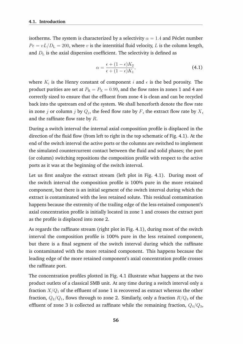
4.1. Introduction
isotherms. The system is characterized by a selectivity α = 1.4 and Peclet number
Pe = vL/DL = 200, where v is the interstitial fluid velocity, L is the column length,
and DL is the axial dispersion coefficient. The selectivity is defined as
α =ε+ (1− ε)K2
ε+ (1− ε)K1
, (4.1)
where Ki is the Henry constant of component i and ε is the bed porosity. The
product purities are set at PR = PX = 0.99, and the flow rates in zones 1 and 4 are
correctly sized to ensure that the effluent from zone 4 is clean and can be recycled
back into the upstream end of the system. We shall henceforth denote the flow rate
in zone j or column j by Qj, the feed flow rate by F , the extract flow rate by X,
and the raffinate flow rate by R.
During a switch interval the internal axial composition profile is displaced in the
direction of the fluid flow (from left to right in the top schematic of Fig. 4.1). At the
end of the switch interval the active ports or the columns are switched to implement
the simulated countercurrent contact between the fluid and solid phases; the port
(or column) switching repositions the composition profile with respect to the active
ports as it was at the beginning of the switch interval.
Let us first analyze the extract stream (left plot in Fig. 4.1). During most of
the switch interval the composition profile is 100% pure in the more retained
component, but there is an initial segment of the switch interval during which the
extract is contaminated with the less retained solute. This residual contamination
happens because the extremity of the trailing edge of the less-retained component’s
axial concentration profile is initially located in zone 1 and crosses the extract port
as the profile is displaced into zone 2.
As regards the raffinate stream (right plot in Fig. 4.1), during most of the switch
interval the composition profile is 100% pure in the less retained component,
but there is a final segment of the switch interval during which the raffinate
is contaminated with the more retained component. This happens because the
leading edge of the more retained component’s axial concentration profile crosses
the raffinate port.
The concentration profiles plotted in Fig. 4.1 illustrate what happens at the two
product outlets of a classical SMB unit. At any time during a switch interval only a
fraction X/Q1 of the effluent of zone 1 is recovered as extract whereas the other
fraction, Q2/Q1, flows through to zone 2. Similarly, only a fraction R/Q3 of the
effluent of zone 3 is collected as raffinate while the remaining fraction, Q4/Q3,
56
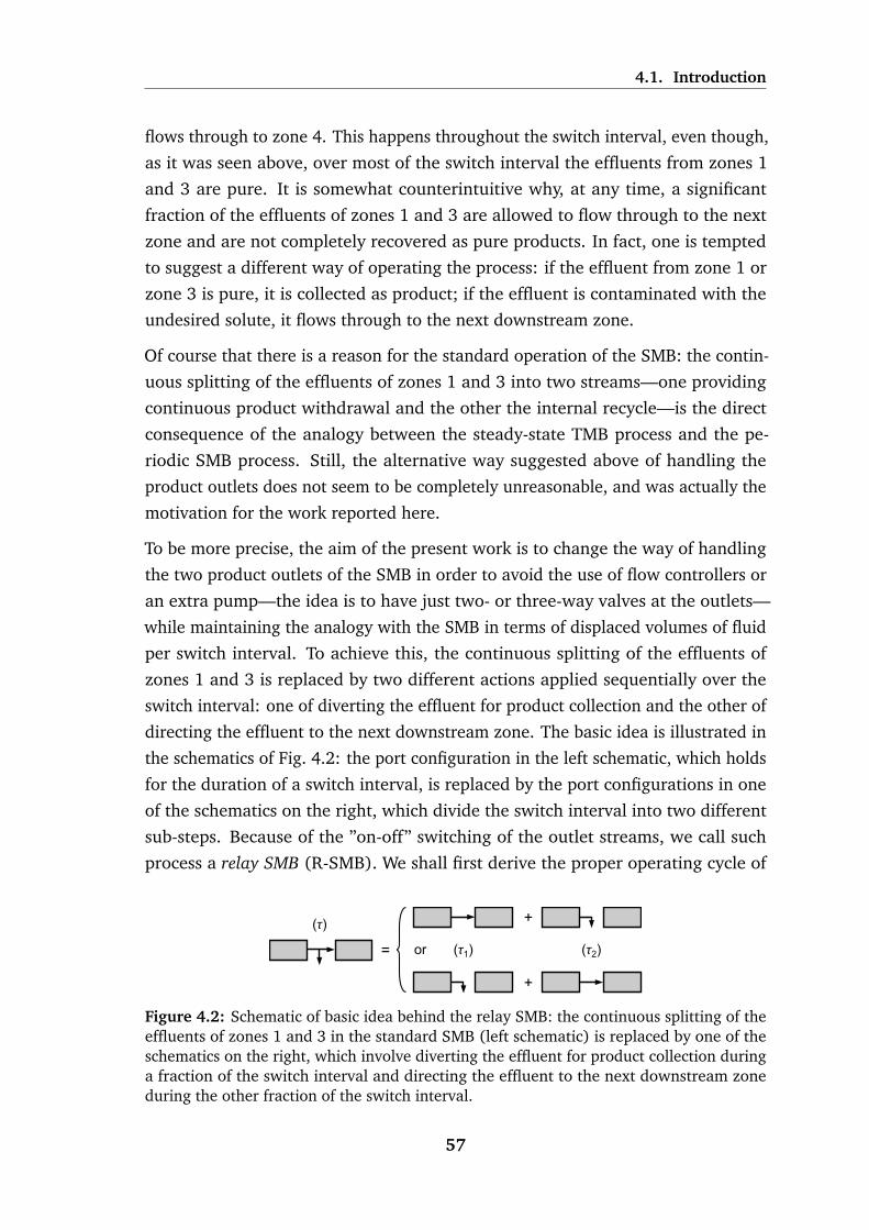
4.1. Introduction
flows through to zone 4. This happens throughout the switch interval, even though,
as it was seen above, over most of the switch interval the effluents from zones 1
and 3 are pure. It is somewhat counterintuitive why, at any time, a significant
fraction of the effluents of zones 1 and 3 are allowed to flow through to the next
zone and are not completely recovered as pure products. In fact, one is tempted
to suggest a different way of operating the process: if the effluent from zone 1 or
zone 3 is pure, it is collected as product; if the effluent is contaminated with the
undesired solute, it flows through to the next downstream zone.
Of course that there is a reason for the standard operation of the SMB: the contin-
uous splitting of the effluents of zones 1 and 3 into two streams—one providing
continuous product withdrawal and the other the internal recycle—is the direct
consequence of the analogy between the steady-state TMB process and the pe-
riodic SMB process. Still, the alternative way suggested above of handling the
product outlets does not seem to be completely unreasonable, and was actually the
motivation for the work reported here.
To be more precise, the aim of the present work is to change the way of handling
the two product outlets of the SMB in order to avoid the use of flow controllers or
an extra pump—the idea is to have just two- or three-way valves at the outlets—
while maintaining the analogy with the SMB in terms of displaced volumes of fluid
per switch interval. To achieve this, the continuous splitting of the effluents of
zones 1 and 3 is replaced by two different actions applied sequentially over the
switch interval: one of diverting the effluent for product collection and the other of
directing the effluent to the next downstream zone. The basic idea is illustrated in
the schematics of Fig. 4.2: the port configuration in the left schematic, which holds
for the duration of a switch interval, is replaced by the port configurations in one
of the schematics on the right, which divide the switch interval into two different
sub-steps. Because of the ”on-off” switching of the outlet streams, we call such
process a relay SMB (R-SMB). We shall first derive the proper operating cycle of
(τ1) (τ2)
(τ) +
+
or=
Figure 4.2: Schematic of basic idea behind the relay SMB: the continuous splitting of theeffluents of zones 1 and 3 in the standard SMB (left schematic) is replaced by one of theschematics on the right, which involve diverting the effluent for product collection duringa fraction of the switch interval and directing the effluent to the next downstream zoneduring the other fraction of the switch interval.
57

4.2. Process description
the R-SMB process and then demonstrate, under the framework of the equilibrium
theory, that the R-SMB process has the same separation region as the classical SMB
for linear adsorption systems. In addition, the results from the equilibrium theory
show that the R-SMB process consists of two distinct cycles: one for selectivities
smaller than a critical value and another cycle for larger values of α. Moreover,
it is shown that in both instances of the R-SMB concept the flow through a zone
(or column) is always in one of three states: (i) frozen, (ii) completely directed
to the next zone (or column), or (iii) entirely diverted to a product line. This
restricted ensemble of port configurations has been exploited before by our group
to derive various classes of two- and three-column SMB processes [10–12, 41].
We then examine the R-SMB process under conditions of finite column efficiency
and compare its performance to those of the classical open- and closed-loop SMBs.
Finally, the work is summarized before drawing final conclusions.
4.2 Process description
Remembering the discussion of Fig. 4.1, it is apparent that the extract is con-
taminated during an initial stage of the switch interval, whereas the raffinate is
contaminated during a final fraction of the switch interval. Thus, in the R-SMB
process the raffinate should be collected first, during an initial stage of the switch
interval, by means of the port configuration shown in the bottom-right schematic
of Fig. 4.2, and the extract should be withdrawn last, during a final stage of the
switch interval, by means of the top-right schematic of Fig. 4.2.
Let us follow this line of thought in order to complete the operating cycle of the
R-SMB and to derive one way of determining the duration of its sub-steps. In a
classical SMB, the amount of fluid that leaves zone 1 during a switch interval is τQ1,
the amount of collected extract is τX = τ(Q1 −Q2), and the amount of fluid that
is directed to section 2 is τQ2 = τ(Q1 −X); the amount of fluid that leaves zone 3
during a switch interval is τQ3, the amount of collected raffinate is τR = τ(Q3−Q4),
and the amount of fluid that is directed to section 4 is τQ4 = τ(Q3 −R).
To collect the same amount of raffinate per switch interval as in the SMB, the
effluent of zone 3 in the R-SMB is diverted for raffinate collection during the first
τ1 = τR/Q3 time units of the switch interval; during the rest of the switch interval
the outlet is directed to zone 4. To collect the same amount of extract per switch
interval as in the SMB, the effluent of zone 1 in the R-SMB is diverted for extract
withdrawal during the last τ3 = τX/Q1 units of the switch interval; during the rest
58

4.2. Process description
of the switch interval the outlet is directed to zone 2. Using the equilibrium theory,
we shall demonstrate that between these two sub-steps of the switch interval, that
is, for τ1 < t < τ − τ3, the internal axial concentration profile in the R-SMB should
be displaced in the direction of fluid flow without any product withdrawal.
Figure 4.3 shows a schematic of the proposed three-step operating cycle, which
we shall henceforward refer to as R-SMB−. In the figure caption it is stated that
the cycle is valid for α ≤ (3 +√
5)/2; it will shortly become clear why this is so.
Notice that the operating cycle of the R-SMB− has a few nonstandard features.
Fresh feed and desorbent are continuously injected into the process by means of
two constant-speed pumps, as in the classical SMB, but the two product streams
are collected discontinuously and alternately in time (pulsed outlets). Finally, the
intermediate sub-step during which there is no product withdrawal is identical to
one of the sub-steps implemented in the I-SMB process [38–40]. Note that from
an operational point of view, the use of constant-speed inlet pumps is desirable
since it leads to the easiest-to-control and most robust configuration. We shall now
432
F
1
E
432
F
1
E
432
F
1
E
X3
R1
(τ1)
D2
D3
(τ2)
(τ3)
Figure 4.3: Schematic of the R-SMB’s operating cycle for α ≤ (3 +√
5)/2; this schemeis denoted R-SMB−. As in the classical SMB, each rectangle represents a R-SMB section,with one or more columns. At the end of every switch interval the columns move by oneposition against the direction of the fluid flow or the port positions are moved one columnahead in the direction of the fluid flow.
demonstrate that for linear adsorption systems the R-SMB− scheme has the same
performance metrics and the same separation region as the classical SMB for a
specific range of selectivity values.
Using the equilibrium theory [42–44], it is possible to calculate a set of sectional
elution volumes, τQj, that give a theoretical purity of 100% for both extract and
raffinate on an SMB with ideal zones (no mass transfer and no hydrodynamic
59

4.2. Process description
resistances). The conditions that must be fulfilled for complete separation are
m1 ≥ K2, K1 ≤ m2 < m3 ≤ K2, m4 ≤ K1, (4.2)
where
mj =τQj − εV(1− ε)V
(4.3)
and V is the column volume (the N columns of the SMB are all assumed to be
identical).
Note that the conditions given by Eq. (4.2) can also be expressed as
τQ1 ≥ V ′2 , V ′1 ≤ τQ2 < τQ3 ≤ V ′2 , τQ4 ≤ V ′1 , (4.4)
where V ′i = [ε + (1 − ε)Ki]V and τQj is the volume of fluid eluted through one
column of zone j during a switch interval.
Alternatively, the constraints can be converted into equalities with safety margins
[13], say
τQ1 = γ2V′2 , τQ2 = γ1V
′1 , τQ3 = V ′2/β2, τQ4 = V ′1/β1, (4.5)
where β1, β2, γ1, and γ2 are constants ≥ 1. Note, in addition, that the selectivity, α,
defined by Eq. (4.1), can also be expressed in terms of V ′1 and V ′2 ; it is simply
α = V ′2/V′1 . (4.6)
If the inequalities in Eq. (4.4) are converted into equalities [or the safety margins
in Eq. (4.5) are all set to 1], they define the optimum operating point of the SMB
process: this operating point minimizes E ′ and maximizes F , where E ′ = E −D is
the flow rate of fresh desorbent introduced into the system and D is the flow rate
of desorbent recycled from zone 4 back into the upstream end of the system (for
the standard SMB, E = Q1 and D = Q4, but we shall use E and D for the R-SMB).
The metrics for the optimum operating point are
τE ′ = τX = τF = τR = V ′2 − V ′1 , τD = V ′1 (4.7)
60

4.2. Process description
and, hence,
F/E ′ = 1, X/E ′ = 1, R/E ′ = 1. (4.8)
It is not difficult to derive for the R-SMB− scheme the constraints, analogous
to those of Eq. (4.4), which define the operating space where there is complete
separation of the binary mixture. The constraints are:
(less retained component does not contaminate D)
τ2(E + F ) + τ3F ≤ V ′1 , (4.9)
(more retained component does not contaminate D)
(τ1 + τ2 + τ3)E ≥ V ′2 , (4.10)
(less retained component does not contaminate X)
(τ1 + τ2)E ≥ V ′1 , (4.11)
(more retained component does not contaminate R)
(τ1 + τ2)(E + F ) + τ3F ≤ V ′2 . (4.12)
As was done above for the standard SMB, the inequalities defined by Eqs. (4.9)–
(4.12) are converted into equalities to determine the optimal operating conditions
of the R-SMB− process, i.e., those that give a theoretical purity of 100% for both
extract and raffinate while minimizing E ′ and maximizing F . From these set of
equalities, the following expressions for F , τ1, τ2, and τ3, as a function of E, are
obtained:
F =V ′2 − V ′1V ′2
E, (4.13)
τ1 =V ′2 (V ′2 − V ′1)
(2V ′2 − V ′1)E, τ2 =
V ′1V′2 − (V ′2 − V ′1)2
(2V ′2 − V ′1)E, τ3 =
V ′2 − V ′1E
, (4.14)
τ = τ1 + τ2 + τ3 = V ′2/E. (4.15)
Figure 4.4 shows the equilibrium solution for the optimum operating point of the
R-SMB− process. For this operating point the amounts of fresh desorbent and
61
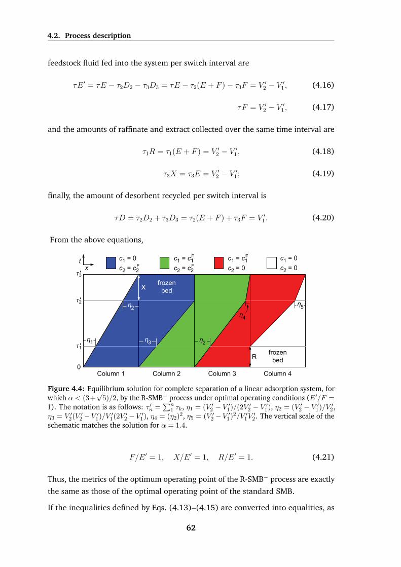
4.2. Process description
feedstock fluid fed into the system per switch interval are
τE ′ = τE − τ2D2 − τ3D3 = τE − τ2(E + F )− τ3F = V ′2 − V ′1 , (4.16)
τF = V ′2 − V ′1 , (4.17)
and the amounts of raffinate and extract collected over the same time interval are
τ1R = τ1(E + F ) = V ′2 − V ′1 , (4.18)
τ3X = τ3E = V ′2 − V ′1 ; (4.19)
finally, the amount of desorbent recycled per switch interval is
τD = τ2D2 + τ3D3 = τ2(E + F ) + τ3F = V ′1 . (4.20)
From the above equations,
0
τ1
τ2
τ3
t
x
Column 1 Column 2 Column 3 Column 4
c1 = 0
c2 = c
2F
c1 = c
1
c2 = c
2
F
F
c1 = 0
c2 = 0
c1 = c
1
c2 = 0
F
R
X
frozen
bed
frozen
bed
5
1
2
3 2
4
Figure 4.4: Equilibrium solution for complete separation of a linear adsorption system, forwhich α < (3+
√5)/2, by the R-SMB− process under optimal operating conditions (E′/F =
1). The notation is as follows: τ ′n =∑n
1 τk, η1 = (V ′2 − V ′1)/(2V ′2 − V ′1), η2 = (V ′2 − V ′1)/V ′2 ,η3 = V ′2(V ′2 −V ′1)/V ′1(2V ′2 −V ′1), η4 = (η2)
2, η5 = (V ′2 −V ′1)2/V ′1V′2 . The vertical scale of the
schematic matches the solution for α = 1.4.
F/E ′ = 1, X/E ′ = 1, R/E ′ = 1. (4.21)
Thus, the metrics of the optimum operating point of the R-SMB− process are exactly
the same as those of the optimal operating point of the standard SMB.
If the inequalities defined by Eqs. (4.13)–(4.15) are converted into equalities, as
62

4.2. Process description
was done above, but this time with safety margins, say,
τ2(E + F ) + τ3F = V ′1/β1, (4.22)
(τ1 + τ2 + τ3)E = γ2V′2 , (4.23)
(τ1 + τ2)E = γ1V′1 , (4.24)
(τ1 + τ2)(E + F ) + τ3F = V ′2/β2, (4.25)
where β1, β2, γ1, and γ2 are constants ≥ 1, then it is possible to probe the operating
space of the R-SMB− process that provides complete separation by changing the
magnitude of the safety margins.
The solution of Eqs. (4.22)–(4.25) is
F =V ′2/β2 − γ1V ′1
γ2V ′2E, (4.26)
τ1 =γ2V
′2 (V ′2/β2 − V ′1/β1)
[(γ2 + 1/β2)V ′2 − γ1V ′1 ]E, (4.27)
τ2 =(γ1γ2 + γ1/β2 + γ2/β1)V
′1V′2 − (γ1V
′1)2 − (γ2/β2)(V
′2)2
[(γ2 + 1/β2)V ′2 − γ1V ′1 ]E, (4.28)
τ3 =γ2V
′2 − γ1V ′1E
, (4.29)
τ =γ2V
′2
E. (4.30)
From the schematic of Fig. 4.3 and from Eqs. (4.22)–(4.25) it is possible to calculate
the volumes of fluid displaced per switch interval in each section of the equivalent
SMB process; the result is
τQ1 = τE = γ2V′2 , (4.31)
τQ2 = (τ1 + τ2)E = γ1V′1 , (4.32)
τQ3 = (τ1 + τ2)(E + F ) + τ3F = V ′2/β2, (4.33)
τQ4 = τ2(E + F ) + τ3F = V ′1/β1. (4.34)
63

4.2. Process description
But eqs. (4.31)–(4.34) are exactly the same as the equalities expressed in Eq. (4.5),
which proves that the R-SMB− process has the same operating region for complete
separation as the classical SMB.
There is, however, a tricky condition with the operating cycle of the R-SMB−
process. Given that the three τ ’s must be nonnegative, Eq. (4.14) is valid for
V ′1V′2 − (V ′2 − V ′1)2 ≥ 0, which is the same as α ≤ αc, where αc = (3 +
√5)/2 is the
upper limit of α for optimum operation of the R-SMB− cycle. Thus, the R-SMB−
process should be applied to ”difficult separations” characterized by selectivity
values smaller than αc. It is worth noting that the cycle can be employed to
a certain extent above αc by adjusting the safety margins in Eqs. (4.26–4.30).
However, such operating conditions will not give the same performance metrics as
the optimum operating point of the standard SMB.
For easier separations, those for which α ≥ αc, the second sub-step of the R-SMB−
cycle is unnecessary—in fact it is detrimental for the separation performance—and
must be replaced by the result of merging sub-steps 1 and 3. The complete cycle
for α ≥ αc is depicted in the schematic of Fig. 4.5. We shall henceforward refer to
this process as R-SMB+. Again, it is not difficult to derive for the R-SMB+ scheme
432
F
1
E
432
F
1
E
X3
R1
43
F
R2
(τ1)
D3
(τ2)
(τ3)
21
E
X2
Figure 4.5: Schematic of the operating cycle for the R-SMB+ process, which is applicablewhen α ≥ (3 +
√5)/2. At the end of every switching interval the columns move by one
position against the direction of the fluid flow or the port positions are moved one columnahead in the direction of the fluid flow.
the constraints that define the operating space where there is complete separation
of the binary mixture. The constraints are:
(less retained component does not contaminate D)
τ3F ≤ V ′1 , (4.35)
64

4.2. Process description
(more retained component does not contaminate D)
(τ1 + τ2 + τ3)E ≥ V ′2 , (4.36)
(less retained component does not contaminate X)
τ1E ≥ V ′1 , (4.37)
(more retained component does not contaminate R)
τ1(E + F ) + (τ2 + τ3)F ≤ V ′2 . (4.38)
If these inequalities are converted into equalities, the following expressions for F ,
τ1, τ2, and τ3, as a function of E, are obtained:
F =V ′2 − V ′1V ′2
E, (4.39)
τ1 =V ′1E, τ2 =
(V ′2 − V ′1)2 − V ′1V ′2(V ′2 − V ′1)E
, τ3 =V ′1V
′2
(V ′2 − V ′1)E, (4.40)
τ = τ1 + τ2 + τ3 = V ′2/E. (4.41)
As expected, these equations are valid for (V ′2 − V ′1)2 − V ′1V ′2 ≥ 0 or α ≥ (3 +√
5)/2.
Figure 4.6 shows the equilibrium solution for the optimum operating point of the
R-SMB+ process. For this point the amounts of fresh eluent and feedstock fluid fed
into the system per switch interval are
τE ′ = τE − τ3D3 = τE − τ3F = V ′2 − V ′1 , τF = V ′2 − V ′1 , (4.42)
and the amounts of raffinate and extract collected over the same time interval are
τ1R1 + τ2R2 = τ1(E + F ) + τ2F = V ′2 − V ′1 , (4.43)
τ2X2 + τ3X3 = (τ2 + τ3)E = V ′2 − V ′1 ; (4.44)
finally, the amount of eluent recycle per switch interval is
τD = τ3D3 = τ3F = V ′1 . (4.45)
65
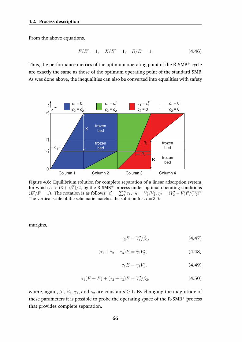
4.2. Process description
From the above equations,
F/E ′ = 1, X/E ′ = 1, R/E ′ = 1. (4.46)
Thus, the performance metrics of the optimum operating point of the R-SMB+ cycle
are exactly the same as those of the optimum operating point of the standard SMB.
As was done above, the inequalities can also be converted into equalities with safety
0
τ1
τ2
τ3
t
x
Column 1 Column 2 Column 3 Column 4
c1 = 0
c2 = c
2F
c1 = c
1
c2 = c
2
F
F
c1 = 0
c2 = 0
c1 = c
1
c2 = 0
F
R
X
frozen
bed
frozen
bed
frozen
bed
frozen
bed1
2
1
Figure 4.6: Equilibrium solution for complete separation of a linear adsorption system,for which α > (3 +
√5)/2, by the R-SMB+ process under optimal operating conditions
(E′/F = 1). The notation is as follows: τ ′n =∑n
1 τk, η1 = V ′1/V′2 , η2 = (V ′2 − V ′1)2/(V ′2)2.
The vertical scale of the schematic matches the solution for α = 3.0.
margins,
τ3F = V ′1/β1, (4.47)
(τ1 + τ2 + τ3)E = γ2V′2 , (4.48)
τ1E = γ1V′1 , (4.49)
τ1(E + F ) + (τ2 + τ3)F = V ′2/β2, (4.50)
where, again, β1, β2, γ1, and γ2 are constants ≥ 1. By changing the magnitude of
these parameters it is possible to probe the operating space of the R-SMB+ process
that provides complete separation.
66

4.2. Process description
The solution of eqs. (4.47)–(4.50) is
F =V ′2/β2 − γ1V ′1
γ2V ′2E, (4.51)
τ1 =γ1V
′1
E, (4.52)
τ2 =(γ1V
′1)2 + (γ2/β2)(V
′2)2 − (γ1γ2 + γ1/β2 + γ2/β1)V
′1V′2
(V ′2/β2 − γ1V ′1)E, (4.53)
τ3 =(γ2/β1)V
′1V′2
(V ′2/β2 − γ1V ′1)E, (4.54)
τ =γ2V
′2
E. (4.55)
From Fig. 4.5 and eqs. (4.51)–(4.55) it is possible to calculate the volume of fluid
displaced per switch interval in each section of the equivalent SMB process; the
result is
τQ1 = τE = γ2V′2 , (4.56)
τQ2 = τ1E = γ1V′1 , (4.57)
τQ3 = τ1E + τF = V ′2/β2, (4.58)
τQ4 = τ3D3 = τ3F = V ′1/β1 (4.59)
Again, these equations are exactly the same equalities expressed in Eq. (4.5), and
this proves that for α > αc the R-SMB+ cycle has the same operating region for
complete separation as the classical SMB.
Before concluding this section, we summarize in Table 4.1 the design equations for
optimum operation of the two R-SMB cycles under linear adsorption conditions.
Note that the design equations for F and τ are the same for both cycles. Note also
that if the selectivity is small, no product stream is collected during the intermediate
sub-step of the switch interval (R-SMB− cycle, Fig. 4.3); but, if the selectivity is
large, both product streams are collected during the intermediate sub-step (R-SMB+
cycle, Fig. 4.5) because less internal recycling of the fluid is necessary.
67

4.3. Analysis under conditions of finite column efficiency
Table 4.1: Summary of the design equations, derived from the equilibrium theory, for theoptimum operation of the two R-SMB cycles that give complete separation under linearadsorption conditions; ’eq. sol.’ stands for ’equilibrium solution.’
α ≤ αc α ≥ αc
Cycle R-SMB− (Fig. 4.3) R-SMB+ (Fig. 4.5)
F/E (V ′2 − V ′1)/V ′2 (V ′2 − V ′1)/V ′2
τ1E V ′2 (V ′2 − V ′1)/(2V ′2 − V ′1) V ′1
τ2E [V ′1V′2 − (V ′2 − V ′1)2]/(2V ′2 − V ′1) [(V ′2 − V ′1)2 − V ′1V ′2 ]/(V ′2 − V ′1)
τ3E V ′2 − V ′1 V ′1V′2/(V
′2 − V ′1)
τE V ′2 V ′2
Eq. sol. Fig. 4.4 Fig. 4.6
4.3 Analysis under conditions of finite column effi-
ciency
The discussion above was based on the equilibrium theory, a convenient idealization
that assumes that the column efficiency is infinite. In practice this is never true
because there is always some band broadening in the system. Thus, a more realistic
design must take into account the limitations imposed by a finite column efficiency.
We shall adopt the simple chromatographic column model given in Table 4.2 to
design the processes in the presence of band broadening. In this simple model the
column efficiency is measured by the value of the Peclet number, Pe = vL/DL. If
each column has an efficiency equivalent to NTP theoretical plates, then the Peclet
number is Pe = 2NTP [45]. To determine the optimal SMB operating parameters
Table 4.2: Linear adsorption column model.
∂ci∂θ
=τQ
V ′i
(1
Pe
∂2ci∂x2− ∂ci∂x
), ∀x ∈ ]0, 1[
ci −1
Pe
∂ci∂x
= cini for x = 0,∂ci∂x
= 0 for x = 1
θ = t/τ, x = z/L, couti ≡ (ci)x=1
for a finite column efficiency (i.e., for a given finite value of Pe), we can restrict the
flow rate in zone 1 to a maximum operating value, say Q1 ≤ Qmax, because zone 1
is where the flow rate is highest, and then calculate by mathematical programming
68

4.3. Analysis under conditions of finite column efficiency
the optimal values of the four Qj ’s and of τ that maximize the feed flow rate, F ,
under cyclic steady state (CSS) conditions.
To do this, we solve the following optimization problem:
maximize F (τ,Qj)
s.t. SMB model under CSS conditions
Q1 ≤ Qmax, PR ≥ PminR , PX ≥ Pmin
X ,
(4.60)
where PminR and Pmin
X are the target raffinate and extract purities, respectively. The
product purities are defined as follows:
PR = 〈cR1 〉/〈cR1 + cR2 〉, PX = 〈cX2 〉/〈cX1 + cX2 〉, (4.61)
where csi is the concentration of solute i in product stream ‘s’ (‘R’ stands for raffinate,
‘X’ for extract) and 〈y〉 denotes the average of y(t) over a switch interval: it is the
value of y in the volume of liquid collected into a perfectly mixed cup during a
switching interval. For example, the average concentration of solute i in the extract
collected over a switch interval is
〈cXi 〉 = 〈couti 〉1 =
∫τ
(couti )1X dt
/∫τ
X dt (4.62)
= τ−1∫τ
(couti )1 dt (X = const). (4.63)
(Hereafter we shall employ the superscripts ‘in’ and ‘out’ to denote, respectively,
the inlet and outlet conditions for a zone or column.) For a standard SMB the flow
rate can be taken out of the integrals in Eq. (4.62) and give Eq. (4.63), because the
process is operated with constant-speed pumps. Note that under CSS conditions,
〈y〉 is independent of the number of elapsed switch intervals or cycles (one cycle is
equal to N switch intervals, where N is the number of columns).
The design problem can also include the raffinate and/or extract recoveries, RR
and RX, as constraints; these are defined as
RR = 〈cR1 〉R/(cF1F ), PX = 〈cX2 〉X/(cF2F ), (4.64)
where cFi represents the concentration of component i in the feed.
Consider, for example, a 4-column SMB unit where each column has an efficiency
equivalent to 100 theoretical plates; the Peclet number in this case is Pe = 2×100 =
69

4.3. Analysis under conditions of finite column efficiency
200. Also, consider the case where α = 1.4. If we choose PminR = Pmin
X = 0.99,
which are realistic values close to a theoretical 100% purity, and set Qmax/V′1 =
1 min−1, then the optimal SMB operating parameters are τ = 1.514 min, Q1/V′1 =
1 min−1, Q2/V′1 = 0.701 min−1, Q3/V
′1 = 0.860 min−1, and Q4 = 0.607 min−1; this
gives, E/V ′1 = 0.393 min−1, X/V ′1 = 0.299 min−1, F/V ′1 = 0.159 min−1, R/V ′1 =
0.253 min−1, and E/F = 2.47. The corresponding volumes of fluid eluted through
each zone during a switch interval are τQ1/V′1 = 1.514 = (1 + 8.1%)×α, τQ2/V
′1 =
1.061 = (1 + 6.1%) × 1, τQ3/V′1 = 1.302 = (1 − 7.0%) × α, and τQ4/V
′1 = 0.919 =
(1 − 8.1%) × 1 [cf. Eq. (4.4) with all terms divided by V ′1]. Actually, this set of
operating parameters gave rise to the composition profiles plotted in Fig. 4.1.
Because of the finite number of theoretical plates, the system is operated with
conservative mj (or τQj/V′1) values that deviate from the theoretical ones by
roughly 7.3%.
These operating parameters are for a closed-loop SMB. In this configuration the
effluent from zone 4 is recycled back to the inlet of zone 1. For a closed-loop SMB
the material balance at the inlet of zone 1, that is, the equation that governs the
desorbent recycle strategy, is
(Qcini )1 = (Qcouti )4 or (cini )1 = (Q4/Q1)(couti )4. (4.65)
For the example considered above the average solute concentrations in the effluent
from zone 4 (which is recycled desorbent) over a switch interval are 〈cout1 〉4 =
1.66×10⁻³cF1 and 〈cout2 〉4 = 3.69×10⁻³cF2 . This effluent is continuously mixed with
fresh desorbent before being introduced into the upstream end of zone 1; at that
point the average residual solute concentrations drop to 〈cin1 〉1 = 1.01×10⁻³cF1 and
〈cin2 〉1 = 2.24×10⁻³cF2 because of the dilution with fresh desorbent.
Because of the way the R-SMB was designed (Figs. 4.3 and 4.5), we are more
interested in employing an open-loop configuration to mimic the in-line desorbent
recycling of the closed-loop SMB. There are two straightforward ways of doing
this. As long as the exit stream of zone 4 is sufficiently clean, it can be sent
back to the desorbent storage tank or to an auxiliary storage tank. In the former
case the process does not require a separate recycle pump, but the inlet pump
for the desorbent must deliver a flow rate equal to Q1 = Q4 + E ′; in the latter
case, the recycle pump is fed from the auxiliary tank instead of being fed from the
downstream end of zone 4.
To ensure that the exit stream of zone 4 is clean, we can impose explicit limits on
the maximum values of (cout1 )4 and (cout2 )4; the former concentration (that of the
70

4.3. Analysis under conditions of finite column efficiency
less retained component) reaches a maximum at the end of the switch interval,
whereas the latter (that of the more retained component) attains a maximum at
the beginning of the switch interval. Alternatively, limits on the averages 〈cout1 〉4and 〈cout2 〉4 can be imposed. The specification of maximum limits for (cout1 )4 and
(cout2 )4 is equivalent to manipulating the safety margins β1 and γ2 in Eq. (4.5),
Eqs. (4.26–4.30), or Eqs. (4.51–4.55), derived from the equilibrium theory.
We are, however, more interested in solving the design problem using a formulation
similar to that given by Eq. (4.60). In this case, we must formulate mathematically
how clean the exit stream of zone 4 should be to make sure it can be recycled by the
process. The exact answer depends on how the recycled desorbent is reintroduced
into the system, namely whether the exit stream of zone 4 is sent to the main
desorbent tank or to a smaller, auxiliary storage tank.
We shall tackle this issue in a generic way that hides the specific details of the
desorbent recycle strategy; this issue is of secondary importance here given that
the focus of the present work is the presentation of the R-SMB concept.
Firstly, note that under CSS conditions the inlets and outlets of a closed-loop SMB
are related by the following global solute material balances:
〈cXi 〉X + 〈cRi 〉R = cFi F (i = 1, 2; CSS conditions). (4.66)
This means that, under CSS conditions, the amount of each solute injected into the
system over a switch interval comes out in the ensemble of the two product streams
collected over the same amount of time. Because of this, Eq. (4.60), which defines
the design problem of a closed-loop SMB, does not include any specification about
the cleanliness level of the exit stream of zone 4; this is implicitly determined by
the design procedure.
It would be convenient if Eq. (4.66) was also valid for the open-loop SMB config-
uration, since this would facilitate the design procedure. Let us determine under
which circumstances this is true. Consider again the material balance at the inlet of
zone 1 (the desorbent recycle equation), as expressed by Eq. (4.65), and integrate
it over a switch interval; the result is
〈Qcini 〉1 = 〈Qcouti 〉4 (i = 1, 2). (4.67)
Note that Eq. (4.66) is valid under CSS conditions because Eq. (4.67) holds true;
that is, Eq. (4.66) is valid under CSS conditions as along as the amount of solute
that leaves the system through zone 4 over a switch interval is put back into the
71

4.3. Analysis under conditions of finite column efficiency
system over the same time interval.
But this means that any SMB configuration that satisfies Eq. (4.67) also satisfies
Eq. (4.66) under CSS conditions. For example, an SMB process whose material
balance at the inlet of zone 1 is given by
(Qcini )1 = 〈Qcouti 〉4 (i = 1, 2), (4.68)
(notice the notation: round brackets on the l.h.s. and angle brackets on the r.h.s.)
satisfies Eq. (4.67), because the average of a constant is the constant itself, and thus
also satisfies Eq. (4.66) under CSS conditions. It is important to understand the
practical meaning of Eq. (4.68): zone I is continuously fed with the admixture of
fresh eluent and the average over a switch interval of the effluent from zone 4. In
our opinion this is the easiest way to tackle the problem of recycling the exit stream
of zone 4 in an open-loop configuration since it avoids addressing technical details
such as the size of the auxiliary storage tank, or the time-dependent variation of the
desorbent composition if the recycled eluent is sent back to the original desorbent
storage tank.
We thus replace Eq. (4.65) by Eq. (4.68) in the SMB model to convert the closed-
loop SMB into a pseudo closed-loop SMB that uses recycled desorbent with solute
concentrations equal to the time-average concentrations in the exit stream of
zone 4 under CSS conditions. If this process is operated with the parameters
determined above for the classical closed-loop SMB, the obtained product purities
are PR = 98.75% and PX = 98.84%. These values are nearly as good, but not the
same, as those of the classical closed-loop SMB.
To get exactly the same product purities and recoveries we solve the optimization
problem given by Eq. (4.60) for the pseudo closed-loop SMB. The optimal operating
parameters are τ = 1.549 min, Q1/V′1 = 1 min−1, Q2/V
′1 = 0.686 min−1, Q3/V
′1 =
0.838 min−1, and Q4/V′1 = 0.577 min−1; this gives, E/V ′1 = 0.423 min−1, X/V ′1 =
0.314 min−1, F/V ′1 = 0.152 min−1, R/V ′1 = 0.262 min−1, and E/F = 2.78. The
corresponding volumes of fluid eluted through each zone during a switch interval
are τQ1/V′1 = 1.549 = (1 + 10.6%)α, τQ2/V
′1 = 1.062 = (1 + 6.2%) × 1, τQ3/V
′1 =
1.299 = (1 − 7.2%)α, and τQ4/V′1 = 0.893 = (1 − 10.7%) × 1. The values of
τQ1/V′1 and τQ4/V
′1 changed (and τ), but those of τQ2/V
′1 and τQ3/V
′1 remained
equal to those of the closed-loop SMB. The point to note is that this desorbent
recycle strategy incurs a small penalty in performance with respect to that of the
standard closed-loop SMB: the productivity is reduced by 4.2% and the desorbent
consumption is increased by 7.7%.
72
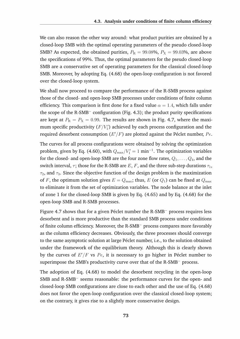
4.3. Analysis under conditions of finite column efficiency
We can also reason the other way around: what product purities are obtained by a
closed-loop SMB with the optimal operating parameters of the pseudo closed-loop
SMB? As expected, the obtained purities, PR = 99.08%, PX = 99.03%, are above
the specifications of 99%. Thus, the optimal parameters for the pseudo closed-loop
SMB are a conservative set of operating parameters for the classical closed-loop
SMB. Moreover, by adopting Eq. (4.68) the open-loop configuration is not favored
over the closed-loop system.
We shall now proceed to compare the performance of the R-SMB process against
those of the closed- and open-loop SMB processes under conditions of finite column
efficiency. This comparison is first done for a fixed value α = 1.4, which falls under
the scope of the R-SMB− configuration (Fig. 4.3); the product purity specifications
are kept at PR = PX = 0.99. The results are shown in Fig. 4.7, where the maxi-
mum specific productivity (F/V ′1) achieved by each process configuration and the
required desorbent consumption (E ′/F ) are plotted against the Peclet number, Pe.
The curves for all process configurations were obtained by solving the optimization
problem, given by Eq. (4.60), with Qmax/V′1 = 1 min−1. The optimization variables
for the closed- and open-loop SMB are the four zone flow rates, Q1, . . . , Q4, and the
switch interval, τ ; those for the R-SMB are E, F , and the three sub-step durations τ1,
τ2, and τ3. Since the objective function of the design problem is the maximization
of F , the optimum solution gives E = Qmax; thus, E (or Q1) can be fixed at Qmax
to eliminate it from the set of optimization variables. The node balance at the inlet
of zone 1 for the closed-loop SMB is given by Eq. (4.65) and by Eq. (4.68) for the
open-loop SMB and R-SMB processes.
Figure 4.7 shows that for a given Peclet number the R-SMB− process requires less
desorbent and is more productive than the standard SMB process under conditions
of finite column efficiency. Moreover, the R-SMB− process compares more favorably
as the column efficiency decreases. Obviously, the three processes should converge
to the same asymptotic solution at large Peclet number, i.e., to the solution obtained
under the framework of the equilibrium theory. Although this is clearly shown
by the curves of E ′/F vs Pe, it is necessary to go higher in Peclet number to
superimpose the SMB’s productivity curve over that of the R-SMB− process.
The adoption of Eq. (4.68) to model the desorbent recycling in the open-loop
SMB and R-SMB− seems reasonable: the performance curves for the open- and
closed-loop SMB configurations are close to each other and the use of Eq. (4.68)
does not favor the open-loop configuration over the classical closed-loop system;
on the contrary, it gives rise to a slightly more conservative design.
73

4.3. Analysis under conditions of finite column efficiency
1
2
3
4
5
6
7
100 200 300 400 500
Pe
open-loop SMB
closed-loop SMB
R-SMB-
E F/
0.05
0.1
0.15
0.2
0.25
0.3
200 400 600 800 103
R-SMB-
closed-loop SMB
open-loop SMB
Pe
F V
1/
Figure 4.7: Desorbent consumption (E′/F ) and specific productivity (F/V ′1) as a functionof Peclet number per column (Pe) for complete separation (PR = PX = 0.99) of a linearadsorption system (α = 1.4) with different four-column configurations: closed-loop SMB(top schematic in Fig. 4.1 including the dashed line), open-loop SMB (top schematic inFig. 4.1 without the dashed line), and R-SMB− (Fig. 4.3); in the latter two cases, thedesorbent recycling is given by Eq. (4.68)
Fig. 4.8 gives some insight into why the productivity of the R-SMB− is much higher
than that of the classical SMB process under conditions of small column efficiency.
This figure shows a snapshot of the axial concentration profile along the train of
columns, taken at the middle of the switch interval, for the R-SMB− (solid lines)
and closed-loop SMB (dashed lines) for Pe = 200; the profiles for the closed-loop
SMB at Pe = 1000 are also included for comparison. Because the R-SMB− system
can withstand a much higher feed flow rate than the SMB for Pe = 200, the R-SMB−
74

4.3. Analysis under conditions of finite column efficiency
is loaded with substantially more solute than the SMB system. More interesting,
however, is that the concentration profile of the more retained solute, c2, in sections
1 and 2 of the R-SMB− system for Pe = 200 is close to that of the SMB process
in the same two zones but for Pe = 1000. The same observation applies to the
concentration profile of the less retained solute, c1, but in sections 3 and 4. Hence,
for small Peclet numbers, such as Pe = 200, the concentration profiles in the
R-SMB− process are much closer to those given by the equilibrium solution (infinite
column efficiency) than the concentration profiles in the closed-loop SMB. Thus,
the influence of column efficiency on process performance is much less detrimental
on the R-SMB− than on the classical SMB.
0
0.2
0.4
0.6
0.8
1
0 0.5 1 1.5 2 2.5 3 3.5 4
column 1 column 2 column 3 column 4X FE R D
z /L
ci /
ciF
c2 c
1
c1
c2
R-SMB- (Pe = 200) SMB (Pe = 200) SMB (Pe = 103)
Figure 4.8: Axial concentration profiles, taken at the middle of the switch interval (τ/2)under CSS conditions, for the 4-column R-SMB− (solid lines) and 4-column closed-loopSMB (dashed lines). The operating parameters are: α = 1.4, Pe = 200, and PR = PX =0.99. The concentration profiles for the closed-loop SMB at Pe = 1000 are included forcomparison.
Figure 4.9 shows graphs of F/V ′1 and E ′/F plotted against Pe for a fixed value
α = 3.0, which falls under the scope of the R-SMB+ configuration (Fig. 4.5); the
design problem and purity constraints are the same as before. Again, it is observed
that for a given Peclet number the R-SMB+ process is more productive and requires
less desorbent than the standard SMB process under conditions of small column
75

4.3. Analysis under conditions of finite column efficiency
efficiency, and that the comparison increasingly favors the R-SMB+ configuration
as the column efficiency decreases. Although for α = 1.4 the superimposition of the
E ′/F -vs-Pe curves of the three processes is observed for ca. Pe > 300, for α = 3.0
the superimposition is shifted to higher Pe values, well above Pe = 500.
1
1.1
1.2
1.3
1.4
1.5
1.6
1.7
1.8
1.9
100 200 300 400 500
Pe
E F/
open-loop SMB
closed-loop SMB
R-SMB+
0.4
0.45
0.5
0.55
0.6
0.65
200 400 600 800 103
R-SMB+
closed-loop SMB
open-loop SMB
Pe
F V
1/
Figure 4.9: Desorbent consumption (E′/F ) and specific productivity (F/V ′1) as a functionof Peclet number per column (Pe) for complete separation (PR = PX = 0.99) of a linearadsorption system (α = 3.0) with different four-column configurations: closed-loop SMB(top schematic in Fig. 4.1 including dashed line), open-loop SMB (top schematic in Fig. 4.1without dashed line), and R-SMB+ (Fig. 4.5); in the latter two cases, the desorbent recyclingis governed by Eq. (4.68).
In Figs. 4.7 and 4.9 we examined the performance of the various process configu-
rations for a fixed value of α and variable Peclet number. It is also instructive to
examine how the R-SMB process compares against the classical SMB configurations
76

4.3. Analysis under conditions of finite column efficiency
as a function of α at a fixed value of Pe. This is shown in Fig. 4.10 for Pe = 200
and in Fig. 4.11 for Pe = 1000. As in Figs. 4.7 and 4.9, the performance indicators
are the specific productivity (F/V ′1) and the desorbent consumption (E ′/F ).
0.1
0.2
0.3
0.4
0.5
0.6
0.7
1 1.5 2 2.5 3 3.5 4
α = V2 /V1
α c
open-loop SMB
closed-loop SMB
R-SMB-
R-SMB+
F V
1/
τ 2 > 0
τ 2 = 0
τ 2 > 0
τ 2 = 0
1
1.5
2
2.5
3
1 1.5 2 2.5 3 3.5 4
E F/
open-loop SMB
closed-loop SMB
R-SMB-
R-SMB+
α = V2 /V1
α c
τ 2 = 0
τ 2 =
0
τ 2 > 0
τ 2 > 0
Figure 4.10: Specific productivity (F/V ′1) and desorbent consumption (E′/F ) as a functionof selectivity (α) for complete separation (PR = PX = 0.99) of a linear adsorption systemat a Peclet number per column Pe = 200 with different four-column configurations: closed-loop SMB, open-loop SMB, and the two R-SMB schemes; Eq. (4.68) governs the desorbentrecycling policy of all open-loop schemes. αc = (3+
√5)/2; the two small straight lines split
each R-SMB curve into a segment over which τ2 (second sub-step of the switch interval) iszero and another segment over which τ2 > 0.
In each graph of Figs. 4.10 and 4.11 there are two curves for the R-SMB process:
one curve for the R-SMB− configuration (solid blue line) and another curve for
the R-SMB+ configuration (dashed blue line). Consider what happens when one
77

4.3. Analysis under conditions of finite column efficiency
moves along the x-axis of the graphs, that is, from small towards large values
of α or vice versa, and take Fig. 4.10 as an example. As expected, for values
of α < αc = (3 +√
5)/2, the R-SMB− configuration is better than the R-SMB+
configuration: the specific productivity is higher and the desorbent consumption is
lower; but the reverse trend is observed for α > αc. This is because the R-SMB−
was designed for α < αc, whereas the R-SMB+ is well suited for α > αc.
0.1
0.2
0.3
0.4
0.5
0.6
0.7
0.8
1 1.5 2 2.5 3 3.5 4
α c
τ 2 > 0
τ 2 = 0
τ 2 > 0
τ 2 = 0
α = V2 /V1
F V
1/
1
1.1
1.2
1.3
1.4
1.5
1.6
1 1.5 2 2.5 3 3.5 4
α c
τ 2 =
0
τ 2 =
0
τ 2 > 0
τ 2 >
0
E F/
α = V2 /V1
open-loop SMB
closed-loop SMB
R-SMB-
R-SMB+
open-loop SMB
closed-loop SMB
R-SMB-
R-SMB+
Figure 4.11: Specific productivity (F/V ′1) and desorbent consumption (E′/F ) as a functionof selectivity (α) for complete separation (PR = PX = 0.99) of a linear adsorption systemat a Peclet number per column Pe = 1000 with different four-column configurations:closed-loop SMB, open-loop SMB, and the two R-SMB schemes; Eq. (4.68) governs thedesorbent recycling policy of all open-loop configurations. αc = (3 +
√5)/2; the two small
straight lines split each R-SMB curve into a segment over which τ2 (second sub-step of theswitch interval) is zero and another segment over which τ2 > 0.
78
4.4. Conclusions
The optimum duration τ2 of the intermediate sub-step of the R-SMB− process, the
one during which the axial concentration profile is displaced in the direction of
fluid flow without any product withdrawal, decreases as the value of α increases
from a small value below αc until it shrinks to zero at a value of α slightly smaller
than αc. For larger values of α and if we stick to the R-SMB− configuration, it is best
to operate the process with only sub-steps 1 and 3, because τ2 = 0 will always give
better results than τ2 > 0, but at the cost of a high penalty in performance: a sharp
decrease in productivity and increase in desorbent consumption are observed.
Now consider the behavior of the R-SMB+ process as α decreases from values well
above αc down to a small value. The optimum duration τ2 of the intermediate sub-
step of the R-SMB+ process, the one during which there is simultaneous extract and
raffinate withdrawals, decreases as the value of α decreases until it shrinks to zero
at a value of α slightly smaller than αc. Below that value it is preferable to operate
the R-SMB+ process without the intermediate sub-step, but at the cost of a large
performance penalty, especially a significant increase in desorbent consumption.
Notice that if the intermediate step is removed from both the R-SMB− and R-SMB+
processes, we end up with the same two-step process configuration (cf. Figs. 4.3
and Fig. 4.5 without step 2). Actually, there is a small region around αc where the
optimum value of τ2 is impracticably small; over this region it is best to operate the
R-SMB process using the 2-step cycle with negligible loss in performance.
An interesting observation drawn from the graphs in Figs. 4.10 and 4.11 is that
when the line segment of the R-SMB− for which τ2 > 0 is connected to the line
segment of the R-SMB+ for which τ2 > 0, a smooth curve is obtained without
any discontinuous transition in the slope around αc. This observation strengths
our belief that the R-SMB− and R-SMB+ are indeed the correct SMB analogs for
intermittent operation of the product outlets. Lastly, it is shown that for Pe = 200
the R-SMB process performs significantly better than the classical SMB process
over the whole range of α values studied, but less so for Pe = 1000 because both
processes should have the same performance under conditions of infinite column
efficiency.
4.4 Conclusions
The present work gives the first account of the R-SMB concept and its realization
under the form of the analog of the classical four-section SMB process. R-SMB
79
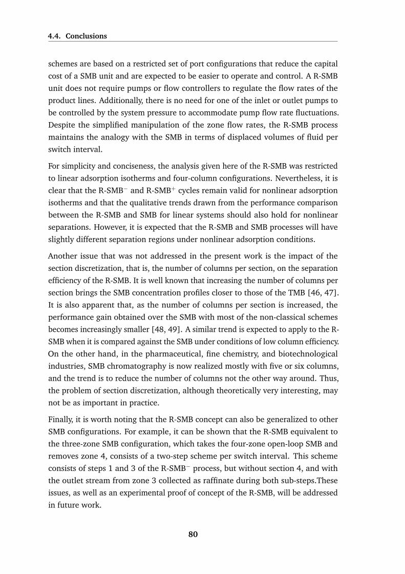
4.4. Conclusions
schemes are based on a restricted set of port configurations that reduce the capital
cost of a SMB unit and are expected to be easier to operate and control. A R-SMB
unit does not require pumps or flow controllers to regulate the flow rates of the
product lines. Additionally, there is no need for one of the inlet or outlet pumps to
be controlled by the system pressure to accommodate pump flow rate fluctuations.
Despite the simplified manipulation of the zone flow rates, the R-SMB process
maintains the analogy with the SMB in terms of displaced volumes of fluid per
switch interval.
For simplicity and conciseness, the analysis given here of the R-SMB was restricted
to linear adsorption isotherms and four-column configurations. Nevertheless, it is
clear that the R-SMB− and R-SMB+ cycles remain valid for nonlinear adsorption
isotherms and that the qualitative trends drawn from the performance comparison
between the R-SMB and SMB for linear systems should also hold for nonlinear
separations. However, it is expected that the R-SMB and SMB processes will have
slightly different separation regions under nonlinear adsorption conditions.
Another issue that was not addressed in the present work is the impact of the
section discretization, that is, the number of columns per section, on the separation
efficiency of the R-SMB. It is well known that increasing the number of columns per
section brings the SMB concentration profiles closer to those of the TMB [46, 47].
It is also apparent that, as the number of columns per section is increased, the
performance gain obtained over the SMB with most of the non-classical schemes
becomes increasingly smaller [48, 49]. A similar trend is expected to apply to the R-
SMB when it is compared against the SMB under conditions of low column efficiency.
On the other hand, in the pharmaceutical, fine chemistry, and biotechnological
industries, SMB chromatography is now realized mostly with five or six columns,
and the trend is to reduce the number of columns not the other way around. Thus,
the problem of section discretization, although theoretically very interesting, may
not be as important in practice.
Finally, it is worth noting that the R-SMB concept can also be generalized to other
SMB configurations. For example, it can be shown that the R-SMB equivalent to
the three-zone SMB configuration, which takes the four-zone open-loop SMB and
removes zone 4, consists of a two-step scheme per switch interval. This scheme
consists of steps 1 and 3 of the R-SMB− process, but without section 4, and with
the outlet stream from zone 3 collected as raffinate during both sub-steps.These
issues, as well as an experimental proof of concept of the R-SMB, will be addressed
in future work.
80

References
[1] Chim Yong Chin and Nien-Hwa Linda Wang. Simulated moving bed equipment
designs. Separation & Purification Reviews, 33(2):77–155, 2004.
[2] Pedro Sa Gomes, Mirjana Minceva, and Alırio E. Rodrigues. Simulated moving
bed technology: old and new. Adsorption, 12(5-6):375–392, 2006.
[3] A. Seidel-Morgenstern, L. C. Keßler, and M. Kaspereit. New developments in
simulated moving bed chromatography. Chemical Engineering & Technology,
31(6):826–837, 2008.
[4] Arvind Rajendran, Galatea Paredes, and Marco Mazzotti. Simulated moving
bed chromatography for the separation of enantiomers. Journal of Chromatog-raphy A, 1216(4):709 – 738, 2009.
[5] Alexandre Nicolaos, Laurence Muhr, Patrice Gotteland, Roger-Marc Nicoud,
and Michel Bailly. Application of equilibrium theory to ternary moving bed
configurations (four+ four, five+ four, eight and nine zones): I. linear case.
Journal of Chromatography A, 908(1):71–86, 2001.
[6] Alexandre Nicolaos, Laurence Muhr, Patrice Gotteland, Roger-Marc Nicoud,
and Michel Bailly. Application of the equilibrium theory to ternary moving
bed configurations (4+ 4, 5+ 4, 8 and 9 zones): Ii. langmuir case. Journal ofChromatography A, 908(1):87–109, 2001.
[7] Kwangnam Lee. Two-section simulated moving-bed process. SeparationScience and Technology, 35(4):519–534, 2000.
[8] Weihua Jin and Phillip C. Wankat. Two-zone smb process for binary separation.
Industrial & Engineering Chemistry Research, 44(5):1565–1575, 2005.
[9] Weihua Jin and Phillip C. Wankat. Scaling rules and increasing feed rates
in two-zone and four-zone simulated moving bed systems. Industrial &Engineering Chemistry Research, 45(8):2793–2807, 2006.
81

References
[10] Rui C.R. Rodrigues, Tiago J.S.B. Canhoto, Joao M.M. Araujo, and Jose P.B.
Mota. Two-column simulated moving-bed process for binary separation.
Journal of Chromatography A, 1180(1–2):42 – 52, 2008.
[11] Rui CR Rodrigues, Ricardo JS Silva, and Jose PB Mota. Streamlined, two-
column, simulated countercurrent chromatography for binary separation.
Journal of Chromatography A, 1217(20):3382–3391, 2010.
[12] Joao M.M. Araujo, Rui C.R. Rodrigues, Mario F.J. Eusebio, and Jose P.B.
Mota. Chiral separation by two-column, semi-continuous, open-loop simu-
lated moving-bed chromatography. Journal of Chromatography A, 1217(33):
5407 – 5419, 2010.
[13] Douglas M. Ruthven and C.B. Ching. Counter-current and simulated counter-
current adsorption separation processes. Chemical Engineering Science, 44(5):
1011 – 1038, 1989.
[14] Yifei Zang and Phillip C. Wankat. Three-zone simulated moving bed with
partial feed and selective withdrawal. Industrial & Engineering ChemistryResearch, 41(21):5283–5289, 2002.
[15] Nadia Abunasser, Phillip C. Wankat, Y.-S. Kim, and Yoon Mo Koo. One-column
chromatograph with recycle analogous to a four-zone simulated moving bed.
Industrial & Engineering Chemistry Research, 42(21):5268–5279, 2003.
[16] Nadia Abunasser and Phillip C. Wankat. One-column chromatograph with
recycle analogous to simulated moving bed adsorbers: Analysis and appli-
cations. Industrial & Engineering Chemistry Research, 43(17):5291–5299,
2004.
[17] Jose PB Mota and Joao MM Araujo. Single-column simulated-moving-bed
process with recycle lag. AIChE journal, 51(6):1641–1653, 2005.
[18] Joao M. M. Araujo, Rui C. R. Rodrigues, Ricardo J. S. Silva, and Jose P. B.
Mota. Single-column simulated moving-bed process with recycle lag: Analysis
and applications. Adsorption Science & Technology, 25(9):647 – 660, 2007.
[19] Philippe Adam, Roger Narc Nicoud, Michel Bailly, and Olivier Ludemann-
Hombourger. Process and device for separation with variable-length, Octo-
ber 24 2000. US Patent 6,136,198.
82

References
[20] O. Ludemann-Hombourger, R. M. Nicoud, and M. Bailly. The varicol process:
A new multicolumn continuous chromatographic process. Separation Scienceand Technology, 35(12):1829–1862, 2000.
[21] Abdelaziz Toumi, Felix Hanisch, and Sebastian Engell. Optimal operation
of continuous chromatographic processes: Mathematical optimization of
the varicol process. Industrial & Engineering Chemistry Research, 41(17):
4328–4337, 2002.
[22] H. Schramm, M. Kaspereit, A. Kienle, and A. Seidel-Morgenstern. Improving
simulated moving bed processes by cyclic modulation of the feed concentra-
tion. Chemical Engineering & Technology, 25(12):1151–1155, 2002. ISSN
1521-4125.
[23] H Schramm, A Kienle, M Kaspereit, and A Seidel-Morgenstern. Improved
operation of simulated moving bed processes through cyclic modulation
of feed flow and feed concentration. Chemical engineering science, 58(23):
5217–5227, 2003.
[24] Michael M Kearney and Kathleen L Hieb. Time variable simulated moving
bed process, April 7 1992. US Patent 5,102,553.
[25] E. Kloppenburg and E. D. Gilles. A new concept for operating simulated
moving-bed processes. Chemical Engineering & Technology, 22(10):813–817,
1999. ISSN 1521-4125.
[26] Ziyang Zhang, Marco Mazzotti, and Massimo Morbidelli. Powerfeed operation
of simulated moving bed units: changing flow-rates during the switching
interval. Journal of Chromatography A, 1006(1):87–99, 2003.
[27] Ziyang Zhang, Marco Mazzotti, and Massimo Morbidelli. Multiobjective
optimization of simulated moving bed and varicol processes using a genetic
algorithm. Journal of Chromatography A, 989(1):95–108, 2003.
[28] Yifei Zang and Phillip C. Wankat. Smb operation strategyaˆ’partial feed.
Industrial & Engineering Chemistry Research, 41(10):2504–2511, 2002.
[29] Thomas B. Jensen, Tiem G.P. Reijns, Hugo A.H. Billiet, and Luuk A.M. van der
Wielen. Novel simulated moving-bed method for reduced solvent consump-
tion. Journal of Chromatography A, 873(2):149 – 162, 2000.
83

References
[30] Dorota Antos and Andreas Seidel-Morgenstern. Two-step solvent gradients in
simulated moving bed chromatography: Numerical study for linear equilibria.
Journal of Chromatography A, 944(1):77–91, 2002.
[31] Stefanie Abel, Marco Mazzotti, and Massimo Morbidelli. Solvent gradient
operation of simulated moving beds: I. linear isotherms. Journal of chro-matography A, 944(1):23–39, 2002.
[32] Pedro Sa Gomes and Alırio E Rodrigues. Outlet streams swing (oss) and mul-
tifeed operation of simulated moving beds. Separation Science and Technology,
42(2):223–252, 2007.
[33] Pedro Sa Gomes and Alırio E Rodrigues. Outlet stream swing simulated
moving bed: Separation and regeneration regions analysis. Separation Scienceand Technology, 45(16):2259–2272, 2010.
[34] Lars Christian Keßler and Andreas Seidel-Morgenstern. Improving perfor-
mance of simulated moving bed chromatography by fractionation and feed-
back of outlet streams. Journal of Chromatography A, 1207(1–2):55 – 71,
2008.
[35] Suzhou Li, Yoshiaki Kawajiri, Jorg Raisch, and Andreas Seidel-Morgenstern.
Optimization of simulated moving bed chromatography with fractionation
and feedback: Part ii. fractionation of both outlets. Journal of ChromatographyA, 1217(33):5349–5357, 2010.
[36] Youn-Sang Bae and Chang-Ha Lee. Partial-discard strategy for obtaining high
purity products using simulated moving bed chromatography. Journal ofChromatography A, 1122(1):161–173, 2006.
[37] T. Teshima M. Tanimura, M. Tamura, 1995. Japanese Patent JP-B-H07-
046097.
[38] Shigeharu Katsuo and Marco Mazzotti. Intermittent simulated moving bed
chromatography: 1. design criteria and cyclic steady-state. Journal of Chro-matography A, 1217(8):1354–1361, 2010.
[39] Shigeharu Katsuo and Marco Mazzotti. Intermittent simulated moving bed
chromatography: 2. separation of troger’s base enantiomers. Journal ofChromatography A, 1217(18):3067–3075, 2010.
84

References
[40] Shigeharu Katsuo, Christian Langel, Anne-Laure Sandre, and Marco Mazzotti.
Intermittent simulated moving bed chromatography: 3. separation of troger’s
base enantiomers under nonlinear conditions. Journal of Chromatography A,
1218(52):9345–9352, 2011.
[41] Ricardo JS Silva, Rui CR Rodrigues, Hector Osuna-Sanchez, Michel Bailly,
Eric Valery, and Jose PB Mota. A new multicolumn, open-loop process
for center-cut separation by solvent-gradient chromatography. Journal ofChromatography A, 1217(52):8257–8269, 2010.
[42] Giuseppe Storti, Marco Mazzotti, Massimo Morbidelli, and Sergio Carra. Ro-
bust design of binary countercurrent adsorption separation processes. AIChEJournal, 39(3):471–492, 1993.
[43] Marco Mazzotti, Giuseppe Storti, and Massimo Morbidelli. Optimal operation
of simulated moving bed units for nonlinear chromatographic separations.
Journal of Chromatography A, 769(1):3 – 24, 1997.
[44] Marco Mazzotti. Equilibrium theory based design of simulated moving bed
processes for a generalized langmuir isotherm. Journal of Chromatography A,
1126(1):311–322, 2006.
[45] Georges Guiochon, Dean G Shirazi, Attila Felinger, and Anita M Katti. Fun-damentals of preparative and nonlinear chromatography. Academic Press,
2006.
[46] Luıs S. Pais, Jose M. Loureiro, and Alırio E. Rodrigues. Modeling strategies
for enantiomers separation by smb chromatography. AIChE Journal, 44(3):
561–569, 1998.
[47] Joao MM Araujo, Rui CR Rodrigues, and Jose PB Mota. Use of single-column
models for efficient computation of the periodic state of a simulated moving-
bed process. Industrial & engineering chemistry research, 45(15):5314–5325,
2006.
[48] Rui CR Rodrigues, Joao MM Araujo, Mario FJ Eusebio, and Jose PB Mota.
Experimental assessment of simulated moving bed and varicol processes using
a single-column setup. Journal of Chromatography A, 1142(1):69–80, 2007.
[49] Rui CR Rodrigues, Joao MM Araujo, and Jose PB Mota. Optimal design and
experimental validation of synchronous, asynchronous and flow-modulated,
85

References
simulated moving-bed processes using a single-column setup. Journal ofChromatography A, 1162(1):14–23, 2007.
86

5Relay simulated moving bed:
experimental validation
5.1 Introduction
In chapter 2, we have already discussed the standard operation of a SMB unit,
and the variations to this operation that extend the application and enhance this
process. Also, in chapter 3 we have introduced a new type of node operation
that can be used as an alternative to the implicitly discarding the flow splitting
at an active outlet, i.e., by obtaining the product, waste or recycling fractions by
completely directing the effluent over a certain period of the cycle to the appropriate
destination. In this sense, the previous chapter (Ch. 4), aims to apply the same
technique of outlet handling to the two product outlets of the SMB in order to
avoid the use of flow controllers or an extra pump. As before, the idea is to have
just two- or three-way valves at the outlets—while maintaining the analogy with
the SMB in terms of displaced volumes of fluid per switch interval. To achieve
this, the continuous splitting of the effluents of zones I and III is replaced by two
different actions applied sequentially over the switch interval: one of diverting the
effluent for product collection and the other of directing the effluent to the next
downstream zone.
In the present chapter, we intend to validate experimentally the concept devel-
oped before. In order to do it, we need two different separation systems with
87

5.2. Chromatographic Column Model
selectivities (α) that fall in the two regions defined in the previous chapter, i.e.,
αC ≤ (3+√
5)/2 and αC ≥ (3+√
5)/2. The separation of some pairs of nucleosides,
uridine/guanosine and uridine/adenosine, in Source 30 RPC with a desorbent
composed of 5%(v/v) ethanol/water, provides the separation problem needed for
these experiments.
We defined the selectivity of a separation in the previous chapter as:
α =ε+ (1− ε)K2
ε+ (1− ε)K1
(5.1)
The selectivity of the pairs uridine/guanosine (U/G) and uridine/adenosine (U/A)
is distributed with the order: αU/G < αC < αU/A. In this chapter, we will assess the
performance of the two variants of the R-SMB process, comparing it to a open-loop
SMB process with recycle for each separation problem.
5.2 Chromatographic Column Model
The operation of a chromatographic column in isothermal conditions is adequately
described by a dispersed-plug-flow model, with linear driving-force (LDF) approxi-
mation for mass transfer under the form of a lumped solid-diffusion model. These
assumptions are standard practice in preparative chromatography and SMB mod-
eling [1], and can be reasonably well approximated by an equilibrium-dispersed
model with dispersion coefficients dependent on the local slopes of the adsorption
isotherms [2].
For a linear adsorption system the equilibrium-dispersed model is given by the
following equations:
∂ci∂θ
=τQj
(1 + βKi)VC
(1
Pe
∂2ci∂x2− ∂ci∂x
)for 0 < x < 1 (5.2)
with boundary conditions
ci −1
Pe
∂ci∂x
= cini for x = 0, (5.3)
∂ci∂x
= 0 for x = 1. (5.4)
where subscript i is the solute index, θ = t/τ and x = z/L, the dimensionless
temporal and axial coordinates, respectively; ci, the liquid phase concentration;
88

5.3. Experimental
Ki, the Henry constant for component i, i.e., q∗i = Kici where q∗i is the equilibrium
concentration in the adsorbed phase; β = (1 − ε)/ε the phase ratio; VC , the
geometrical column volume; Qj, the flow-rate of the fluid phase; τ , a reference
time; Pe, the Peclet number Pe = vL/DL; cini , the solute concentration in the inlet
effluent.
The dimensionless plate height, hi, governing band broadening for the ith compo-
nent, can be expressed as follows in eq.5.5, [2], where ki is the LDF coefficient
for lumped solid-diffusion mass transfer. The variation of hi with the volumetric
flow-rate calculated from a simplified van Deemter plot [1]
hi2
=1
Pe+ αi
Q
VC, αi =
βKi
ki(1 + βKi)2(5.5)
5.3 Experimental
The performances of the chromatographic processes reported in the present work
have been verified with preparative-scale experiments on the nucleosides linear
binary separation of uridine/guanosine and uridine/adenosine, on reversed-phase
Source 30 RPC (GE Healthcare Amersham Biosciences, Uppsala, Sweden). The
mobile phase was fixed at 5% (v/v) ethanol in water, which was previously found
to give adequate retention and separation factors [3, 4]. All experiments were
performed isothermally at 30◦C, and the feed concentration was fixed at 0.05 g/L
for each solute. Uridine (99%), guanosine (98%) and adenosine (98%) were
purchased from Sigma–Aldrich (Steinheim, Germany), and HPLC-grade ethanol
from Panreac (Spain). The solvents were mixed in the appropriate volumetric
proportions after filtration. The chromatographic columns are Superformance
26 mm i.d. thermojacketed glass columns (Gotec Labortechnik, Germany). The
stationary phase was slurry packed into each column to a bed height L = 6.0 cm,
with mobile phase at 25 ml/min, back-pressure of 30 bar, and 30 min packing
time. The experimental set-ups follow the schematics depicted in Fig. 5.1. The
distributed valve design is based on normally closed two-way valves, since they
allow independent port switching and are quite versatile. Two-way valves can let
the flow pass when actuated or stop the flow in its default position. The two-way
valves are model SFVO from Valco International (Schenkon, Switzerland) with
pneumatic actuation. Each valve is automated by means of a single computer-
controlled three-way solenoid: application of 50 psi opens the valve; venting the
air allows the spring to return the valve to the default position.
89

5.3. Experimental
UV
Colum
n 1
Colum
n 2
Colum
n 3
Colum
n 4
EluentFeed
ExtractRaffinate
Figure 5.1: Schematic of the four-column SMB unit used in the experimental runs.
The HPLC pumps are model K-501 from Knauer (Berlin, Germany) with 10 mL
heads, controlled via RS232 communication protocol. The experimental set-up is
fully automated and driven by an in-house developed automation system using
LabView [5] software (National Instruments).
A multi-wavelength UV detector (USB2000 from Ocean Optics, USA) equipped with
a DH-2000-S-DUV light source (Micropack, Ostfildern, Germany), and attenuator,
was employed to continuously monitor the composition of the outlet effluent.
The porosity of each column (interparticle void fraction, ε) was determined from
the retention times of diluted pulses of blue dextran. Packing reproducibility was
assessed by comparing the peak shapes and retention times of the chromatograms;
both columns were found to be identically, and reasonably well, packed. The
extra volume per column, Ve, in each experimental set-up was estimated from
blue-dextran pulse experiments with and without the chromatographic columns.
The experimentally obtained value for Ve in each node is less than 0.3% of the
column volume and therefore included in the Henry constant [4].
The intercept and slope of the linearized van Deemter plot (given by equation 5.5)
for each nucleoside were determined by fitting the experimental dependence of the
plate height on flow rate for diluted pulses of the solutes; the Henry constants were
determined from the retention times of the same chromatograms, and averaged
based on all column results. Table 5.1 summarizes the obtained parameters.
90

5.4. Results and discussion
Table 5.1: Column characterization and adsorption parameters for the linear separation ofuridine/guanosine and uridine/adenosine on Source 30 RPC (reversed phase) and 5% (v/v)ethanol in water at 30◦C; ε is the packing porosity, all values are averages of measurementsbased on all columns used.
ε = 0.325 K Pe αL(s) k(s−1)Uridine (i = 1) 1.240 744 0.108 1.851Guanosine (i = 2) 1.893 640 0.163 0.930Adenosine (i = 3) 5.593 460 0.316 0.231
5.4 Results and discussion
The optimal cycle was determined by solving the NLP design problem with the
chromatographic parameters listed in Table 5.1, subject to a minimal product purity
PurXmin = PurRmin = 99% and to a maximum flow rate, corresponding to the highest
flow rate attainable by the pumps used in the experimental unit (10.00 mL/min).
Fig. 5.2 depict the operating cycles for the R-SMB process for selectivity region of
α < αC and α > αC respectively. The optimal cycle parameters for each process
are represented in Table 5.2. The cycles for the R-SMB processes were reproduced
Table 5.2: Optimal cycle parameters for the R-SMB processes. The time of each step isgiven in minutes and the flow rates in mL/min. E, F, X, R and D represent the desorbent,feed, extract, raffinate and desorbent flow rates, respectively.
ti E F X R D
R− SMB−1.405 10.000 2.249 0.000 12.249 0.0002.322 10.000 2.249 0.000 0.000 12.2492.066 10.000 2.249 10.000 0.000 2.249
R− SMB+
3.665 10.000 6.298 0.000 16.298 0.0004.915 10.000 6.298 10.000 6.298 0.0005.648 10.000 6.298 10.000 0.000 6.298
experimentally in a prototype apparatus with a schematic identical to that shown
in Fig. 5.1. The temporal concentration profiles, measured at the outlet of column
1 in the cyclic steady state, are shown and compared with the simulated profiles in
Figs. 5.3 and 5.4. The purity of the products for each process is presented in Table
5.3
Table 5.3: Purities of the experimental runs for the R-SMB processes
10th cycle 11th cycle 12th cycle average purityR-SMB- (X/R) 98.99/99.19 99.12/99.12 99.09/99.15 99.1/99.2R-SMB+ (X/R) 99.19/90.09 99.17/99.07 99.18/99.28 99.2/99.2
The performance of the R-SMB process was compared against the open-loop SMB
91
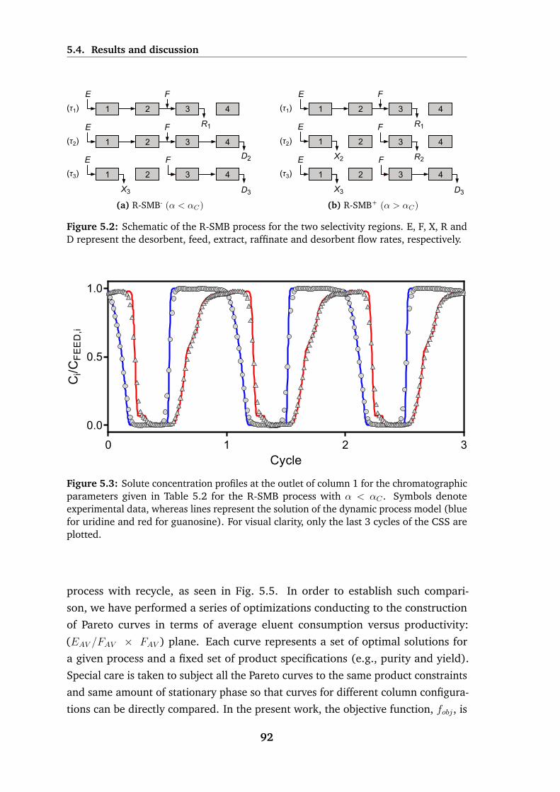
5.4. Results and discussion
432
F
1
E
432
F
1
E
432
F
1
E
X3
R1
(τ1)
D2
D3
(τ2)
(τ3)
(a) R-SMB- (α < αC)
432
F
1
E
432
F
1
E
X3
R1
43
F
R2
(τ1)
D3
(τ2)
(τ3)
21
E
X2
(b) R-SMB+ (α > αC)
Figure 5.2: Schematic of the R-SMB process for the two selectivity regions. E, F, X, R andD represent the desorbent, feed, extract, raffinate and desorbent flow rates, respectively.
Cycle
Ci/C
FEE
D,i
0 1 2 3
0.0
0.5
1.0
Figure 5.3: Solute concentration profiles at the outlet of column 1 for the chromatographicparameters given in Table 5.2 for the R-SMB process with α < αC . Symbols denoteexperimental data, whereas lines represent the solution of the dynamic process model (bluefor uridine and red for guanosine). For visual clarity, only the last 3 cycles of the CSS areplotted.
process with recycle, as seen in Fig. 5.5. In order to establish such compari-
son, we have performed a series of optimizations conducting to the construction
of Pareto curves in terms of average eluent consumption versus productivity:
(EAV /FAV × FAV ) plane. Each curve represents a set of optimal solutions for
a given process and a fixed set of product specifications (e.g., purity and yield).
Special care is taken to subject all the Pareto curves to the same product constraints
and same amount of stationary phase so that curves for different column configura-
tions can be directly compared. In the present work, the objective function, fobj, is
92

5.4. Results and discussion
Cycle
Ci/C
FEE
D,i
0 1 2 3
0.0
0.5
1.0
Figure 5.4: Solute concentration profiles at the outlet of column 1 for the chromatographicparameters given in Table 5.2 for the R-SMB process with α > αC . Symbols denoteexperimental data, whereas lines represent the solution of the dynamic process model (bluefor uridine and green for adenosine). For visual clarity, only the last 3 cycles of the CSS areplotted.
432
F
1
E
X R DD’
Figure 5.5: Shematic of the open-loop smb with recycle process. E, X, F and R denotethe desorbent, extract, feed and raffinate flow rates respectively. D and D’ denote theregenerated and recycled desorbent flow rates.
chosen to be the maximization of productivity, or feed throughput:
FAV =1
τ
∫ t+τ
t
Fdt (5.6)
In the open-loop process, the recycled desorbent D’, should be interpreted as an
off-line recycle of D, which was for simplicity was set as D′ = D. In the R-SMB
process the regenerated solvent D is not recycled as before, in order to define
a comparison on the same basis in terms of desorbent consumption we need to
account for this fact. We define EAV for the R-SMB process as:
EAV =1
τ
∫ t+τ
t
(E −D) dt (5.7)
93

5.5. Concluding Remarks
and for the open-loop process:
Eav =1
τ
∫ t+τ
t
Edt (5.8)
To construct a Pareto curve on this plane, we constraint the average desorbent
consumption to a constant value of desorbent flow rate, Emax, and carry out a
series of single-objective optimizations that maximize Fav for progressively larger
values of Emax. Hence we solve:
fobj = max Fav, s.t. E ≤ Emax. (5.9)
for increasing values of the parameter Emax. The set of points thus generated
gives the desired Pareto curve. Each NLP problem defined by Eq. 5.9 is solved
directly for steady periodic operation of the process, i.e., for cyclic steady state
(CSS) conditions.
Figure 5.6: The full and traced curves correspond to the R-SMB and open-loop SMBprocesses, respectively. The dotted curve in b) corresponds to the extension in productivityin the R-SMB process, when the constrain due to the maximum flow rate of the pumps isdropped.
(a) Pareto Plots for α < αC
FAV
E AV/
F AV
0.0 0.5 1.0 1.5 2.01.0
1.5
2.0
(b) Pareto Plots for α > αC
FAV
E AV/
F AV
0.0 2.0 4.0 6.01.00
1.15
1.30
5.5 Concluding Remarks
In the present work, we have validated experimentally the concept of the R-SMB
process, using a linear separation problem for each region of selectivity described
in chapter 4, using the separations of nucleosides pairs uridine/guanosine and
uridine/adenosine in a reversed phase system.
94

5.5. Concluding Remarks
The R-SMB, when compared to a open-loop SMB with recycle process performed
reasonably well, this demonstrates that the R-SMB process is an attractive alterna-
tive to the open and closed-loop versions of the SMB process.
Due to the simplification of the product lines, the R-SMB process permits to reduce
the capital costs of a SMB unit, maintaining the analogy with standard process in
terms of yield, and product quality specifications with the additional benefits of
simplicity of implementation and operation.
95

References
[1] Georges Guiochon, Dean G Shirazi, Attila Felinger, and Anita M Katti. Funda-mentals of preparative and nonlinear chromatography. Academic Press, 2006.
[2] Douglas Morris Ruthven. Principles of adsorption and adsorption processes.
1984.
[3] Stefanie Abel, Gultekin Erdem, Mohammad Amanullah, Manfred Morari,
Marco Mazzotti, and Massimo Morbidelli. Optimizing control of simulated
moving beds - experimental implementation. Journal of Chromatography A,
1092(1):2–16, 2005.
[4] Rui CR Rodrigues, Ricardo JS Silva, and Jose PB Mota. Streamlined, two-
column, simulated countercurrent chromatography for binary separation. Jour-nal of Chromatography A, 1217(20):3382–3391, 2010.
[5] Mario FJ Eusebio. Development of an universal interface for monitoring and
control of chemical and biochemical processes, Ph.D. Thesis, Universidade
Nova de Lisboa, 2006.
96
6Gradient with Steady State Recycle
process: rationalization and pilot unitvalidation
6.1 Introduction
The advances in biotechnology and developments in genetic engineering have
resulted in the scale up and manufacturing of biopharmaceutical products [1].
Today, downstream processing is facing the challenge of manufacturing products
with the highest degrees of purity and integrity, and overall process economy,
while keeping pace with the rapidly increasing upstream yields in biotechnology.
The fulfillment of the strict requirements by downstream purification is the major
cost factor in biotechnological production with 50-80% of the total manufacturing
cost [2].
A major part of the purification costs is related to chromatographic processes, which,
at present, are still largely operated in batch mode. This is not because chromatog-
raphy is inherently expensive, but because it is heavily used: chromatography plays
a central role in fast and efficient separation of biochemical and pharmaceutical
compounds; in fact, it still remains the work horse method in biopurification.
For most biopurification problems, the desired product is intermediate between
97
6.1. Introduction
weakly and strongly adsorbing impurities, and a central cut is thus required to
get the desired product. Conventionally, the generic three-fraction biopurification
problem is solved using batch column chromatography, often incorporating solvent
gradients. Typically, the target product is separated from process-related impurities
through a series of steps wherein a selected cut or fraction of the effluent from
the previous step is selectively adsorbed and desorbed onto a given stationary
phase using time and elution conditions as manipulated variables, until, ultimately,
yielding the product purified to the desired level. Solvent gradients are easy to apply
in sequential batch chromatography, but this operating mode suffers from high
product dilution, low efficiency and productivity, and high solvent consumption.
As a general rule, multicolumn processes combining freely adjustable, smooth
gradients and simulated countercurrent (SCC) adsorption can achieve better per-
formance than sequential batch chromatography. Early studies [3–6] on ternary
separation by isocratic SCC chromatography were focused on continuous pro-
cesses (i.e., with continuous feeding and product withdrawal) and showed that this
restrictive design criterium can only be achieved with column configurations com-
prising several fluid zones (here, a zone refers to the columns between two active
ports). The most commonly explored column configurations have been simulated
moving-bed (SMB) cascades [4, 7] and five-zone systems with side streams [8–11].
Bioseparation, on the other hand, does not require that the separation scheme be
continuous; this allows several possibilities and a multitude of operating modes
to be considered in the design of the process, which otherwise would have to be
excluded. In principle, a semi-continuous, multicolumn process can make use of
various techniques to achieve the desired separation; for example, some columns
can be dynamically interconnected, so that non-pure product cuts are internally and
countercurrently recycled, while other columns can be short circuited to operate in
pure batch mode, and others frozen to introduce time lags between the positions
of the various concentration fronts. This way some fractions can be separated
by a SCC approach (the mass-transfer zone is kept inside the system by means
of the port switching and the remixing with the feed), whereas the separation of
other fractions can be chromatographic (the mass-transfer zone is taken out of the
system). By freezing one or more columns (i.e., stopping the flow through them)
for some steps of the cycle, it is possible to decouple the migrating velocities of the
various solutes.
The schemes developed by Jin and Wankat [12, 13] and by our group [14–16] are
examples of existing processes for isocratic binary separation that combine some
98

6.1. Introduction
of the techniques above into a single hybrid scheme. The case of isocratic ternary
separation is clearly more complicated. The idea of operating only partially in a
countercurrent fashion was exploited by Masuda et al. [17] in a single cascade
process for fractional separation that is commercialized by Organo Corp., Tokyo,
Japan; the performance of this process has been analyzed by other authors [18–20].
Hur and Wankat [21] developed a two-zone SMB/chromatography hybrid system
for ternary separations, and compared its performance to those of cascades of
two-zone and four-zone SMBs. Subsequently, the same authors [22] designed a
semi-continuous, center-cut, two-zone SMB/chromatography system and a recycled
cascade with two four-zone SMBs to separate the intermediate component from
ternary mixtures.
Recently, Morbidelli and co-workers [23–28] developed a chromatographic pro-
cess for ternary separation (MCSGP-process) that exploits the power of gradient
chromatography and hybrid SMB/chromatography modes. In this process some
columns operate in counter-current mode during a fraction of the cycle while others
are short-circuited and operate in batch mode. Continuous operation of the MCSGP
requires six columns [24, 26], but the process can be reduced to a fully equivalent
semi-continuous configuration with only three chromatographic columns and three
gradient pump modules [27, 28]. Using a series of working examples, these authors
have demonstrated the superiority of MCSGP over batch chromatography.
In the present work, we describe a new multicolumn, open-loop process for center-
cut separation by solvent-gradient chromatography. The key idea is to extend
solvent-gradient batch chromatography to a train of columns and to exploit the
fractionation of the stationary phase. In single-column batch chromatography
the product and waste cuts are obtained at the same point in the system—at the
downstream end of the column—but at different times. Therefore, time (or elution
volume) is the only variable for defining the fractional cuts. If a solvent gradient is
used, it is introduced into the system at a single point—the upstream end of the
column. This, of course, does not give much freedom for dynamically adjusting the
solvent composition profile inside the column.
Although packing the stationary phase into a single column works fine for many
binary separations, this seems to be overly restrictive for center-cut separations.
The introduction of space as an additional variable (although being a discrete one),
by dividing the stationary phase into a train of columns, adds more flexibility for
manipulating the cuts and for generating the solvent gradient; furthermore, with
such a column arrangement it is possible to recycle some of the cuts from the
99

6.2. Process description
downstream end of the system to its upstream end.
In this work we show that this can be done while working in a simple, open-
loop system that resembles the batch system. Although our process implements a
solvent-gradient moving around a ring of columns, it is similar to a batch process
in terms of feeding and product collecting. We provide experimental validation in a
pilot unit, using the purification of a crude peptide mixture by reversed phase as a
working example; this proof of concept serves to highlight the versatility, flexibility,
and ease of operation of the process.
6.2 Process description
The new process, nicknamed GSSR (gradient with steady state recycle), comprises a
multi-column, open-loop system, with cyclic steady-state operation, that simulates
a solvent gradient moving countercurrently with respect to the solid phase. It
is particularly suited for ternary separations: it provides three main fractions or
products, with a target product contained in the intermediate fraction. The process
can be pictured as the superposition of three steady periodic events applied to a
ring of columns with an open-loop configuration: a moving solvent gradient, a
feeding step, and a step of product collection. A comprehensive description of the
GSSR process is provided next.
First, consider how a moving solvent gradient is implemented by means of a
plurality of solvent lines. For this purpose, consider the schematic of Fig. 6.1,
which is an example of the simplest GSSR sequence applied to a three-column train.
Note, however, that the process can operate with more columns. The three-column
train of Fig. 6.1 is supplied with three different solvents: solvent A, which has
a linear-gradient composition, and two isocratic solvents, B and C, with elution
strengths different from A.
The inlet positions and flow rates of the solvent lines are defined for a single
switching interval as a set of steps over that period of time. The sequence is then
repeated a number of times equal to the number of columns, the only difference
between a switching interval and the next being the shift of the solvent inlets by
one column in the direction of the fluid flow. A complete cycle is defined by the
sequence of steps for the set of switching intervals.
From this description, it follows that the inlet positions and flow rates of the solvent
lines are periodic in time, with period τ , where τ is the duration of a switching
100

6.2. Process description
interval. There is always an open outlet, which is taken as a waste fraction, in
order to keep the system in open loop. The net effect of this cyclic scheme is
the simulation of the counter-current movement of the solid phase relative to an
open-loop solvent gradient that is τ -periodic in time.
If the system is operated for a large number of cycles, the solvent will develop a
steady, τ -periodic, axial composition profile extending over the columns. Note that
the solvent composition profile will not be spatially periodic (i.e., it will not be
periodic along a coordinate extending from the upstream end of the first column to
the downstream end of the last column), but only time periodic; for the profile to
be spatially periodic, all columns would have to the supplied with the same solvent
gradient.
1st τ
2nd τ
3rd τ
321
A B
321
C BA
321
B C A
C(a) (b)
(c) (d)
(e) (f)
321
A B
321
D BAA
D
D
321
B A
Figure 6.1: Basic sequencing of the solvent lines for a three-column GSSR process. Therighthand sequence—steps b, d, and f—is for operation without on-line regeneration orcleaning in place. A sequence with desorption zone consists of performing the lefthandstep for an initial fraction, say α, of the corresponding switching interval, followed by itsrighthand counterpart for the remaining (1− α). All active outlets are diverted to waste.
In biochromatography a suitable regeneration method is essential for maximizing
column performance and obtaining reproducible results. The regeneration usually
entails the use of a strong solvent to remove highly adsorbed impurities, and may
require post-equilibration of the column with regular buffer. For this purpose, the
GSSR process provides the possibility for in-line regeneration or cleaning in place
(CIP) by dividing the switching interval into two sub-steps and replacing solvent C
by a stronger solvent D over the first sub-step. Thus, during an initial fraction,
say α, of each switching interval, the column whose upstream end is attached to the
active inlet line of solvent C is partially or totally flushed with solvent D; during this
time, the addition of solvent C is halted. Moreover, while the column is desorbed
with solvent D, the outlet effluent of the upstream column is diverted to waste.
Once the initial sub-step of the switching interval is completed, the two columns
101

6.2. Process description
resume their normal operation. It is worth noting that nothing has yet been said
about feeding and product collecting; thus, for the moment all active outlets (e.g.,
those depicted in Fig. 6.1) should be interpreted as waste outlets.
In order to establish a GSSR cycle, two additional steps must be defined: (i) the
time interval during which fresh feed is supplied into the system; and (ii) the
time interval during which the target product is collected. These two steps are
cyclic, but take place only once per cycle, i.e., they are both Nτ -periodic, where
N is the number of columns. Moreover, they can be applied anywhere within
the cycle and can cross or extend over consecutive switching intervals; depending
on the difficulty of separation, the feed injection and product withdrawal can be
performed over different intervals of the cycle, or they can take place at the same
time, or they can partially overlap. However, the feed is always injected into the
same column as a rectangular pulse and the product is always collected from the
same column.
In order to explain how the feed and production steps work in a GSSR process,
let us consider again a three-column ring, such as the one shown in Fig. 6.1. For
difficult separations—those in which the target product is surrounded by closely
eluting impurities—the feeding and product collecting should occur at opposite
ends of the ring to establish the longest path between the feed inlet and the product
outlet, and thus help to separate the impurities nearest to the target component.
Without loss of generality, it will be assumed that the feed line is connected to the
inlet of column 1 and the product line connected to the outlet of column 3.
Since in many cases the target solute will not be completely separated from its
two nearest neighbor impurities when it reaches the collection point at the down-
stream end of the ring, the two impure cuts surrounding the purified product—one
containing the leading edge of the target component and the other the trailing
edge—must be recycled to the feed point at the upstream end of the system in
order to maximize the recovery rate. For optimal performance, the two mixed cuts
must be recycled in a such a way as to surround the feed pulse loaded into the feed
column. Therefore, for difficult separations that require this recycling strategy the
feed and product withdrawal steps must necessarily overlap. Moreover, to get the
most efficient separation the feed pulse should be moved through the system by the
moving solvent gradient (A) and not eluted isocratically with either solvent B or C.
From this discussion it is now clear when to carry out the feed and production steps
within the sequencing of the solvent lines shown in Fig. 6.1 for the case where the
feed line is connected to inlet of column 1 and the product line connected to the
102

6.2. Process description
outlet of column 3: the two steps must take place somewhere in the time interval
of the cycle spanned by steps d, e, and f of Fig. 6.1, because during these steps the
effluent from column 3 is recycled to the upstream end of column 1. Given that
steps d and f have the same duration, combining the collection of the target peak
with step e is a simple and pragmatic solution that places the product collection in
the middle of the recycling sequence. Moreover, by feeding in step e the mixture is
injected into the correct column, which is the one that is afterwards eluted with
the solvent gradient.
There is one last detail to take into account regarding the feed and production
steps. If the feed step is shorter than the production step, column 1 should be
frozen after the feed step while the product is still being withdrawn from column 3,
so that when the mixed cut containing the trailing edge of the product is recycled
to the upstream end of column 1 it is placed next to the feed cut.
Prod
D
321
AFeed
Prod
D
321
A
321
A
321
Feed C A
Prod
Prod(a)
(b)
Figure 6.2: Flow diagrams of the feed and production steps for the case when they occur atthe beginning of the third switching interval and when the product withdrawal takes longerthan the injection of feed. Schematics (a) and (b) are for operations with and withouton-line regeneration or cleaning in place, respectively. When the production step is finishedthe normal operation of the train of solvents is resumed.
Figure 6.2 shows the flow diagrams of the feed and production steps for the case
when they occur at the beginning of the third switching interval, as discussed
above, and when the product withdrawal takes longer than the injection of feed;
the two sub-cases of operation with and without CIP must be handled separately
103

6.3. Pilot unit
and require different flow diagrams. When the production step is finished the
normal operation of the train of solvents is resumed. Other cases of placement of
the feed and production steps in the GSSR cycle are discussed elsewhere [29].
Before concluding this section, it is worth noting that, in practice, the solvent gradi-
ent does not strictly follow the rules for simulating its counter-current movement
around the ring of columns, but only approximately, due to the interference of
the feeding and product collecting. The precise simulation of the counter-current
movement of the solid is given up in favor of the extra flexibility provided by our
cycle. Also, because the points of feeding and product collecting are fixed, each
column can play a unique role in the separation. For the same reason, the N
switching intervals that comprise a full GSSR cycle will not necessarily have the
same length. This is different from multi-column systems adhering strictly to the
simulated counter-current concept, where all columns undergo the same sequence
of steps but phase out in time by multiples of the same switching interval, and
opens up opportunities for a whole new range of cycles.
6.3 Pilot unit
Colu
mn 1
Colu
mn 2
Colu
mn 3
UVFC
Waste
Product
FeedvFn
vDn
vCn
vBn
vF
Solvent D
Solvent B
Solvent C
Solvent A1
Solvent A2
vW3
vW
2v
W1
vCO3
vCO
2vCO
1
vP
vA2
3
vA1
3
vC
3
vB3
vD3
vA2
2
vA1
2
vC
2
vB2
vD
2
vA21
vC1
vA1
1
vB
1
vD1
Figure 6.3: Schematic flowsheet of the GSSR pilot unit. vαj , two-way valve; UV, UV detector;FC, fraction collector.
Figure 6.3 shows a schematic flowsheet of the GSSR pilot unit. We use a distributed
valve design based on two-way valves, since they are quite versatile and make it
104

6.3. Pilot unit
possible to implement independent port switching. Two-way valves allow the flow
either to go through or not to go through. The two-way valves are model SFVO
from Valco International (Schenkon, Switzerland) with pneumatic actuation. Each
valve is automated by means of a single computer-controlled, three-way solenoid:
application of 50 psi opens the valve; venting the air allows the spring to return
the valve to the closed position. Overall, the pilot unit employs 28 two-way valves.
Each set of six valves, {vCO, vA1, vA2, vB, vC, vD}j (j = 1, 2, 3), is connected to a
special tee with six inlets and one outlet; a check valve is placed in front of valve
vCO to prevent the occurrence of flow reversal. The other valves are attached to
the transfers lines between columns by regular tees.
By simultaneously closing valve vCOj (= 0) and opening valve vWj (= 1), the
effluent from column j is directed to the corresponding waste line; similarly, by
simultaneously closing valve vCO3 (= 0) and opening valve vP (= 1), the effluent
from column 3 is directed to the product line.
6.3.1 Inlet flow rates
The GSSR process employs three isocratic solvent streams—B, C, and D—with
different solvent compositions, and one solvent-gradient stream, A. The composition
of the solvent-gradient stream is τ -periodic in time and is continuously supplied
into the process at constant flow rate QA. Solvents B and C are fed to the process
at constant flow rates QB and QC, respectively; their flows, however, may have to
be temporarily stopped while feeding or collecting product. Solvent D replaces
solvent C during the desorption step of every switching interval; its flow rate, D,
is constant. Finally, the feedstock fluid is injected once per cycle as a rectangular
pulse with flow rate F . Overall, the inlet flow rates of the GSSR process are either
constant or on/off; in the latter case, the flow rate is kept constant, at 0 or Q, over
a given time interval before jumping discretely to the other value, Q or 0, over the
next interval.
The HPLC pumps for the solvent lines B, C, and D, as well as that for the feed line,
F, are operated under steady conditions at their prescribed flow rates to minimize
disturbances in their operation. To interrupt the feed flow or the flow of one of
the isocratic solvent streams, say stream B, the control software closes valve vBjand opens valve vBn to redirect the flow back to the solvent storage tank. Since
for all purposes the valve switching is instantaneous, the net effect is a very good
approximation of the sharp edge of the step change in the flow rate. To redirect the
105

6.3. Pilot unit
flow of solvent B to column j, valve vBn is closed and valve vBj is open; the sharp
edge of the step change in the flow rate is well reproduced again. The valves which
are employed for redirecting the flow of an inlet line back to its source tank are
vFn, vBn, vCn, and vDn.
Over each switching interval, the composition of solvent A changes linearly with
time from c(0)A to c(τ)A ,
cA(t) = c(0)A +
c(τ)A − c
(0)A
τ(t mod τ), (6.1)
where (· mod ·) is the modulo operator, i.e., (t mod τ) ≡ t − int (t/τ). In the
pilot unit, the solvent-gradient line is mimicked by the admixture of two isocratic
solvent streams, A1 and A2, driven by two variable-velocity isocratic pumps, with
two different solvent compositions, respectively, cA1 and cA2, that satisfy cA1 ≤min{c(0)A , c
(τ)A } and cA2 ≥ max{c(0)A , c
(τ)A }. To reproduce the solvent gradient by
the admixture of streams A1 and A2, the flow rates of the two HPLC pumps,
QA1 and QA2, are determined from the following material balances:
QA1 +QA2 = QA, (6.2)
QA1cA1 +QA2cA2 = QAcA. (6.3)
It is easily shown that QA1(t) and QA2(t) are τ -periodic, linear functions of time:
QA1(t) = Q(0)A1 +
Q(τ)A1 −Q
(0)A1
τ( t mod τ), (6.4)
QA2(t) = Q(0)A2 +
Q(τ)A2 −Q
(0)A2
τ( t mod τ), (6.5)
where
Q(0)A1 = QA
c(0)A − cA2
cA1 − cA2
, Q(τ)A1 = QA
c(τ)A − cA2
cA1 − cA2
, (6.6)
Q(0)A2 = QA
c(0)A − cA1
cA2 − cA1
, Q(τ)A2 = QA
c(τ)A − cA1
cA2 − cA1
. (6.7)
The six HPLC pumps employed in the pilot plant are model K-501 from Knauer
(Berlin, Germany) with 10 mL and 50 mL pump heads, commanded by RS232
communication protocol.
106

6.3. Pilot unit
6.3.2 Monitoring and fraction collection
A multi-wavelength UV detector (USB2000 from Ocean Optics, USA) with attenua-
tor, connected to a DH-2000-S-DUV light source (Micropack, Ostfildern, Germany),
is attached to the outlet of column 3. The communication between the UV detector
and the control software is handled via a USB connection.
A fraction collector is also installed at the outlet of column 3, after the UV detector,
for the periodic collection of internal samples that can be later analyzed by off-line
HLPC. Each fraction is collected into a vial using an electrically driven, six-port,
two-position valve, model K6 from Knauer (Berlin, Germany), commanded by
RS232 communication protocol.
Most of the time, the effluent from column 3 flows through the UV measuring cell
and through the injection loop of the six-port valve and is (i) directed to column 1,
or (ii) collected as product, or (iii) removed as waste. At selected times the six-port
valve is switched to inject position and valve vFC is open, to place the injection
loop within the flow path of mobile phase from a pressurized tank. The sample in
the injection loop is thus pushed onto the vial for off-line HPLC analysis and the
injection loop is washed with mobile phase. This occurs during a small, specified
time interval at given instants of the cycle defined by the operator. During this time
the effluent from column 3 bypasses the injection loop and is directly diverted into
column 1. When the six-port valve is switched back to ‘load’ position and valve vFC
is closed, the mobile phase in the loop is pushed to the downstream column while
the loop is being filled. Thus, the circulating flow in the pilot unit is not interrupted.
The extra volumes in the pilot unit due to ancillary equipment, tubbing, detectors,
and fraction collector were estimated to be 4.5 mL.
6.3.3 Process automation
The whole set-up, including pumps, two-way valves, UV detector, and fraction col-
lector, is fully automated and driven by BioCTR [30]—our Labview-based software
for process monitoring and control of multicolumn chromatographic processes.
A GSSR cycle is defined by a set of parameters, which are specified by the operator
and can be changed while the pilot is running. Besides the number of columns, N ,
switching interval, τ , and the various flow rates, the set of operating parameters
for a GSSR cycle includes other parameters that are described next. The start of the
feed injection, tF, is defined relative to the cycle time, τcyc = Nτ , as tF/τcyc, but the
107
6.4. Validation of moving solvent-gradient in the pilot unit
duration of the injection, ∆tF, is defined in absolute time units. Product collection
is defined similarly; hence, tP/τcyc is the relative position of the start of collection
and ∆tP specifies its duration.
The GSSR process can operate with a desorption zone where solvent C is replaced
by a stronger solvent D. This step is applied once per switching interval and,
therefore, is best defined with respect to that time interval. During the initial
interval 0 ≤ t/τ < ∆tD/τ of every switching interval the system is operated with
solvent D, whereas during the rest of the period, ∆tD/τ ≤ t/τ < 1, solvent D is
replaced by normal solvent C. The solvent-gradient parameters QA, c(0)A , and c(τ)A
are automatically converted by the control software into the flow rate parameters
Q(0)A1, Q
(τ)A1 , Q(0)
A2, and Q(τ)A2 , using Eqs. (6.6) and (6.7).
6.4 Validation of moving solvent-gradient in the pi-
lot unit
Before applying the GSSR process to the purification of the crude peptide mixture,
the pilot unit underwent extensive testing in order to validate the automation of
the valve sequencing, pump actuation, solvent-gradient implementation by the
admixture of two isocratic pumps, pulsed feeding, and waste and product collecting.
For example, some preliminary tests to validate the automation of the pumps and
valves was carried out on the pilot unit using pure water and without the three
chromatographic columns, which were simply replaced by capillary tee connections.
The rate of accumulated mass from the waste and product lines was monitored in
real time using a precision balance, model TE3102S from Sartorius (Goettingen,
Germany). The rate of accumulated mass, dm/dt (g/min), is proportional to the
flow rate, Q (cm3/min), the scaling factor being the density ρ (g/cm3) of the fluid:
ρ−1(dm/dt) = Q. The balance reading gives the mass accumulated over a given
period of time, m = ρ∫Qdt.
In Fig. 6.4 a possible cycle configuration for the GSSR process is depicted. The
proposed sequence was used to test the moving solvent-gradient implementation.
The operating parameters for this scheme are shown in Table 6.1.
Although these tests were very successful (Fig. 6.5), they gave only a partial, and
necessarily limited, validation of the practical implementation of the GSSR cycle on
the pilot unit.
108

6.4. Validation of moving solvent-gradient in the pilot unit
Collect
Collect
ADF
AC
t fee
d
tcolle
ct
A
A
CB
t = 0
t = tperiod
t = 3.tperiod
B D
C
D
B
A B
A
t = 2.tperiod
ADB
ACB
t de
s =
α.t
pe
riod
(1
-α).
t pe
riod
t d
es
= α
. tp
erio
d
(1
-α).
t pe
riod
t de
s =
α.t
pe
riod
(1
-α).
t pe
riod
t feed
t co
lect
Figure 6.4: Cycle sequence chosen in the moving solvent-gradient implementation. Thecycle depicted includes a desorption zone and injection in the 3rd period. The operatingparameters are shown in Table 6.1.
Table 6.1: Operating parameters of the GSSR cycle. Second and third columns give,respectively, the blue dextran concentration, cFeed, and the flow rate of the solvent line;solvent-gradient A increases cA linearly from 0.24 g/L to 0.44g/L over every switchinginterval. Notation: NC , number of columns; τ , switching interval; τcyc = NC .τ , cycle time;tF and ∆tF, position and duration of feed injection; tP and ∆tP, position and duration ofproduct collection; ∆tD, duration of desorption step.
(Ci − g/L) (mL/min) (min)Feed 0.00 0.5 τ 5.0Solvent A 0.24−−0.44 5.0 ∆tD 0.25τSolvent B 0.25 1.0 ∆tF 0.10τSolvent C 0.25 1.25 ∆tP 0.20τSolvent D 0.57 5.0 tF, tP 2τ/τcyc
More realistic tests on the implementation of the moving solvent-gradient were
performed on the pilot unit with three columns and a nonadsorbed tracer. The
three chromatographic columns employed in these tests are Superformance 26-
mm ID thermo-jacketed glass columns (Gotec Labortechnik, Muhltal, Germany).
Reversed-phase Source 30 RPC (30 µm particle size; GE Healthcare Amersham
Biosciences, Uppsala, Sweden) was slurry packed into each column to a bed height
of L = 6 cm with 5%-v/v ethanol/water at 25 ml/min, back-pressure of 30 bar, and
30 min packing time.
In these tests, changes in the solvent composition (say, changes in the water/ethanol
ratio) were replaced by equivalent changes in the concentration of blue dextran
109

6.4. Validation of moving solvent-gradient in the pilot unit
6
5
4
3
2
1
0
0 0.5 1 1.5 2 2.5 3
120
100
80
60
40
20
0
Dimensionless time, t/tperiod
Acum
ula
ted o
utlet m
ass (
g/m
in)
Collect
Waste
Figure 6.5: Accumulated mass from the product (top) and waste (bottom) outlets asfunction of elapsed time (t/τ) for one complete cycle of the GSSR process, with operat-ing parameters defined in Table 6.1. Lines are the theoretical profiles and symbols theexperimental data.
(BD) in an isocratic solvent. BD is a dextran polymer with an average molecule
weight of 2×10⁶. Its large molecular size prevents it from penetrating into the pore
volume of the adsorbent particles; in practice, this tracer probes the interparticle
void volume in the columns and extra-column dead volumes.
Figure 6.6 compares the BD’s concentration profile measured by UV at the outlet
of column 3 with the profile predicted by process simulation. In this tested GSSR
cycle, feed is introduced into column 1 and product collected from column 3. The
switching interval is τ = 5 min and the feed (pure water) flow rate, F = 0.5 mL/min.
The duration of the desorption zone is ∆tD/τ = 0.25; the instants, scaled by the
cycle time, when feed is injected an the product is collected are the same and
equal to tF/τcyc = tP/τcyc = 0.667 (beginning of the third switching interval); the
duration of the feed pulse is ∆tF = 30 s and the duration of the product withdrawal
is ∆tP = 60 s. The compositions and flow rates of the solvent lines are: solvent A1,
0.24 g/L, solvent A2, 0.44 g/L; QA1 + QA2 = 5 mL/min; solvent B, 0.25 g/L,
110

6.4. Validation of moving solvent-gradient in the pilot unit
QB = 1 mL/min; solvent C, 0.25 g/L, QC = 1.25 gL/min; and solvent D, 0.57 g/L,
D = 5 mL/min.
0 2 4 6 8 10 12 14
0.4
0.3
0.2
0.1
0
Co
nce
ntr
atio
n in
Liq
uid
ph
ase
(g
/L) 0.5
0.6
12 13 14 15
0.6
0.5
0.4
0.3
Dimensionless time, t / τ
Figure 6.6: Temporal profile of blue dextran concentration at the outlet of column 3for 5 cycles of a GSSR process. Lines are the theoretical predictions and symbols are theexperimental UV data. The inset at lower-right zooms the profile for the 5th cycle.
The theoretical profile shown in Fig.6.6 was predicted by the GSSR model with
interparticle porosity ε = 0.39, intraparticle porosity εp = 0, and Peclet number
Pe = vL/DL = 700, where v is the linear velocity of the fluid and DL is the
dispersion coefficient. The GSSR model was solved for nc = 0, since the solvent
(i = 0) is the only component in the system (The default values H ′0 = 0 and
n0 = 0 guarantee that it does not adsorb). The effect of dead volumes in the
pilot unit was lumped into the value of ε; extra-column volumes represent roughly
100×(0.39− 0.32) = 7% of the volume of the packed beds. Figure 6.6 shows that
there is good agreement between the experimental profile and the theoretical one.
We can now tackle more confidently the difficult center-cut purification problem of
the crude peptide mixture.
111
References
[1] Gary Walsh. Biopharmaceuticals: recent approvals and likely directions.
Trends in biotechnology, 23(11):553–558, 2005.
[2] A Cecılia A Roque, Christopher R Lowe, and M Angela Taipa. Antibodies
and genetically engineered related molecules: production and purification.
Biotechnology progress, 20(3):639–654, 2004.
[3] R. Wooley, Z. Ma, and N.-H. L. Wang. A nine-zone simulating moving bed
for the recovery of glucose and xylose from biomass hydrolyzate. Industrial& Engineering Chemistry Research, 37(9):3699–3709, 1998. doi: 10.1021/
ie9800896.
[4] Phillip C. Wankat. Simulated moving bed cascades for ternary separations.
Industrial & Engineering Chemistry Research, 40(26):6185–6193, 2001. doi:
10.1021/ie010075r.
[5] Alexandre Nicolaos, Laurence Muhr, Patrice Gotteland, Roger-Marc Nicoud,
and Michel Bailly. Application of equilibrium theory to ternary moving bed
configurations (four+ four, five+ four, eight and nine zones): I. linear case.
Journal of Chromatography A, 908(1):71–86, 2001.
[6] Alexandre Nicolaos, Laurence Muhr, Patrice Gotteland, Roger-Marc Nicoud,
and Michel Bailly. Application of the equilibrium theory to ternary moving
bed configurations (4+ 4, 5+ 4, 8 and 9 zones): Ii. langmuir case. Journal ofChromatography A, 908(1):87–109, 2001.
[7] Anthony S. T. Chiang. Continuous chromatographic process based on smb
technology. AIChE Journal, 44(8):1930–1932, 1998.
[8] Y. A. Beste and W. Arlt. Side-stream simulated moving-bed chromatography
for multicomponent separation. Chemical Engineering & Technology, 25(10):
956–962, 2002.
[9] Jeung Kun Kim, Yifei Zang, and Phillip C Wankat. Single-cascade simulated
112

References
moving bed systems for the separation of ternary mixtures. Industrial &engineering chemistry research, 42(20):4849–4860, 2003.
[10] Stefanie Abel, Matthaus U Babler, Cordin Arpagaus, Marco Mazzotti, and
Joachim Stadler. Two-fraction and three-fraction continuous simulated mov-
ing bed separation of nucleosides. Journal of Chromatography A, 1043(2):
201–210, 2004.
[11] Galatea Paredes, Stefanie Abel, Marco Mazzotti, Massimo Morbidelli, and
Joachim Stadler. Analysis of a simulated moving bed operation for three-
fraction separations (3f-smb). Industrial & engineering chemistry research, 43
(19):6157–6167, 2004.
[12] Weihua Jin and Phillip C Wankat. Two-zone smb process for binary separation.
Industrial & engineering chemistry research, 44(5):1565–1575, 2005.
[13] Weihua Jin and Phillip C Wankat. Scaling rules and increasing feed rates
in two-zone and four-zone simulated moving bed systems. Industrial &engineering chemistry research, 45(8):2793–2807, 2006.
[14] Rui CR Rodrigues, Tiago JSB Canhoto, Joao MM Araujo, and Jose PB Mota.
Two-column simulated moving-bed process for binary separation. Journal ofChromatography A, 1180(1):42–52, 2008.
[15] Rui CR Rodrigues, Ricardo JS Silva, and Jose PB Mota. Streamlined, two-
column, simulated countercurrent chromatography for binary separation.
Journal of Chromatography A, 1217(20):3382–3391, 2010.
[16] Joao MM Araujo, Rui CR Rodrigues, Mario FJ Eusebio, and Jose PB Mota. Chi-
ral separation by two-column, semi-continuous, open-loop simulated moving-
bed chromatography. Journal of Chromatography A, 1217(33):5407–5419,
2010.
[17] Takayuki Masuda, Tohru Sonobe, Fumihiko Matsuda, and Masaharu Horie.
Process for fractional separation of multi-component fluid mixture, March 30
1993. US Patent 5,198,120.
[18] Vera G Mata and Alırio E Rodrigues. Separation of ternary mixtures by
pseudo-simulated moving bed chromatography. Journal of ChromatographyA, 939(1):23–40, 2001.
113
References
[19] Eduardo A Borges da Silva and Alırio E Rodrigues. Design of chromatographic
multicomponent separation by a pseudo-simulated moving bed. AIChE journal,52(11):3794–3812, 2006.
[20] EA Borges da Silva and AE Rodrigues. Design methodology and performance
analysis of a pseudo-simulated moving bed for ternary separation. SeparationScience and Technology, 43(3):533–566, 2008.
[21] Jin Seok Hur and Phillip C Wankat. New design of simulated moving bed
(smb) for ternary separations. Industrial & engineering chemistry research, 44
(6):1906–1913, 2005.
[22] Jin Seok Hur and Phillip C Wankat. Two-zone smb/chromatography for center-
cut separation from ternary mixtures: Linear isotherm systems. Industrial &engineering chemistry research, 45(4):1426–1433, 2006.
[23] Lars Aumann, Michael Bavand, Thomas Muller-Spath, and Guido Strohlein.
Method for identification and purification of multi-specific polypeptides,
March 15 2012. WO Patent App. PCT/EP2012/054,507.
[24] Guido Strohlein, Lars Aumann, Marco Mazzotti, and Massimo Morbidelli. A
continuous, counter-current multi-column chromatographic process incorpo-
rating modifier gradients for ternary separations. Journal of ChromatographyA, 1126(1):338–346, 2006.
[25] Lars Aumann and Massimo Morbidelli. A continuous multicolumn counter-
current solvent gradient purification (mcsgp) process. Biotechnology andbioengineering, 98(5):1043–1055, 2007.
[26] Lars Aumann, Guido Stroehlein, and Massimo Morbidelli. Parametric study
of a 6-column countercurrent solvent gradient purification (mcsgp) unit.
Biotechnology and bioengineering, 98(5):1029–1042, 2007.
[27] Lars Aumann and Massimo Morbidelli. A semicontinuous 3-column coun-
tercurrent solvent gradient purification (mcsgp) process. Biotechnology andbioengineering, 99(3):728–733, 2008.
[28] Thomas Muller-Spath, Lars Aumann, Lena Melter, Guido Strohlein, and Mas-
simo Morbidelli. Chromatographic separation of three monoclonal antibody
variants using multicolumn countercurrent solvent gradient purification (mc-
sgp). Biotechnology and bioengineering, 100(6):1166–1177, 2008.
114

References
[29] Eric Valery, Hector Osuna Sanchez, and Michel Bailly. Gradient-elution multi-
column separation method, October 9 2009. WO Patent 2,009,122,281.
[30] Mario FJ Eusebio. Development of an universal interface for monitoring and
control of chemical and biochemical processes, Ph.D. Thesis, Universidade
Nova de Lisboa, 2006.
115


7Gradient with Steady State Recycleprocess: Model-based analysis and
experimental run
Proteins and peptides represent a growing sector in the pharmaceutical industry.
Reversed-phase, high-performance liquid chromatography (RP-HPLC) has found
wide use in the production of peptides for pharmaceutical formulations, due to
its ability to provide high-resolution separation combined with good reproducibil-
ity. However, peptide mixtures can be complex, with significantly heterogeneous
physico-chemical properties (including hydrophobic and highly hydrophilic com-
pounds), thus rendering their efficient separation by RP-HPLC challenging [1].
Here, we demonstrate that the GSSR process is well suited for this task at prepara-
tive scale.
7.1 Materials and Methods
The selected packing material is Kromasil C18 (Eka Chemicals AB, Sweden), an
octadecyl-bonded, reversed-phase silica, with high hydrophobicity, narrow pore
size distribution (∼ 100 A), and very low content of metal impurities. Detrimental
ionic interactions between basic peptides and residual ionized silanol groups in
C18 phases often produce peak tailing [2, 3], which is undesirable when high
117

7.2. Adsorption Equilibria
product purity is required; the Kromasil C18 phase has a high graft density and
end-capping, and is therefore expected to exhibit a low silanol activity under the
selected experimental conditions. The analytical experiments were performed
with 5 µm Kromasil C18 purchased prepacked into a 0.46 × 15 cm column; the
preparative experiments were performed with 25 µm Kromasil C18, packed into
three 1 × 10 cm stainless steel columns by NOVASEP. The system was operated
isothermally at 30◦C.
The mobile phases used in this study are aqueous solutions of ethanol (EtOH) with a
fixed residual amount of 0.1%-v/v terephthalic acid (TFA); the EtOH concentrations
varied from 20% up to 50%-v/v. HPLC-grade EtOH and TFA were purchased from
Panreac (Barcelona, Spain). The EtOH buffers were first prepared by diluting
EtOH in deionized water, filtering through a 0.22-µm membrane, and adding TFA
thereafter to prepare the final mobile phases. All solvents were degassed prior to
use.
Figure 7.1 shows a chromatogram of the crude mixture for a 250 µL injection at
1 g/L into the Kromasil analytical column, eluted with water/ethanol/TFA (75/
25/0.1, %-v/v) at 0.5 mL/min. The crude mixture is characterized by three main
cuts: a weakly adsorbing (early eluting) cut containing three major impurities, an
intermediate cut with the target product and at least four neighboring impurities,
and a strongly adsorbing (late eluting) cut containing three impurities; the target
product corresponds to the largest peak of the chromatogram, with roughly 50%
of the total peak area. From the analysis of the chromatogram in Fig. 7.1, it is
clear that the desired product is intermediate between nearby, weaker and stronger
adsorbing impurities; a central cut is thus required to get the desired pure product.
7.2 Adsorption Equilibria
When dealing with the purification of a complex, multicomponent mixture, like the
crude peptide mixture, it is convenient to minimize the number of solutes taken
into consideration in the design procedure to make it numerically tractable. This is
similar to the method often used in dealing with the design of distillation columns
for the separation of petroleum fractions, where only a few selected key components
are considered in the calculations. In the present case, five key components were
selected: the most weakly adsorbed (earliest eluting) impurity (i = 1), the target
product (i = 3) and its two closest impurities (i = 2 and i = 4), and the most
strongly adsorbed (latest eluting) impurity (i = 5). The key components are
118
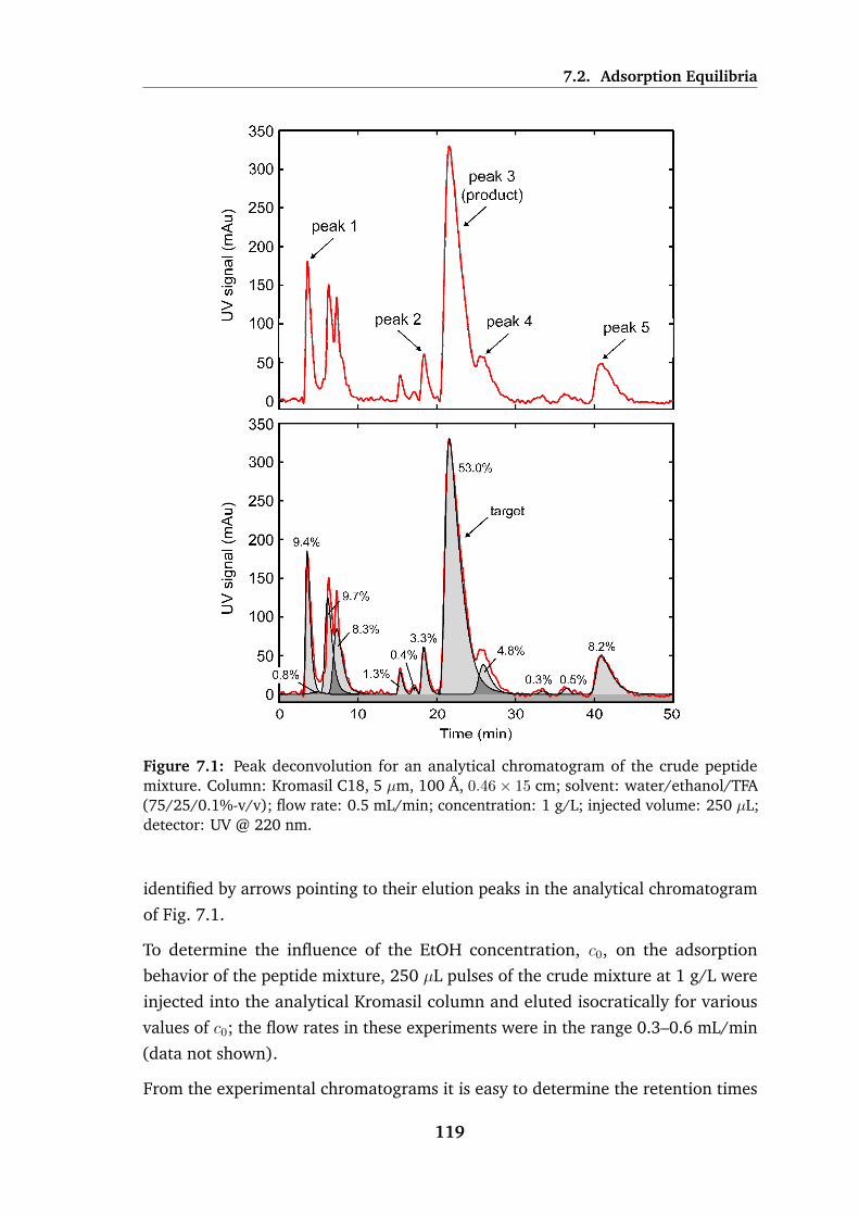
7.2. Adsorption Equilibria
Figure 7.1: Peak deconvolution for an analytical chromatogram of the crude peptidemixture. Column: Kromasil C18, 5 µm, 100 A, 0.46× 15 cm; solvent: water/ethanol/TFA(75/25/0.1%-v/v); flow rate: 0.5 mL/min; concentration: 1 g/L; injected volume: 250 µL;detector: UV @ 220 nm.
identified by arrows pointing to their elution peaks in the analytical chromatogram
of Fig. 7.1.
To determine the influence of the EtOH concentration, c0, on the adsorption
behavior of the peptide mixture, 250 µL pulses of the crude mixture at 1 g/L were
injected into the analytical Kromasil column and eluted isocratically for various
values of c0; the flow rates in these experiments were in the range 0.3–0.6 mL/min
(data not shown).
From the experimental chromatograms it is easy to determine the retention times
119

7.2. Adsorption Equilibria
of the key components for each value of c0. The retention time, ti, for solute i, is
related to the thermodynamic and elution parameters by
ti =ε+Ki
Q/V. (7.1)
From the known value of ti it is straightforward to determine the Henry’s constant,
Ki, or, more conveniently, the value of ε+Ki:
ε+Ki =tiQ
V. (7.2)
The calculated values of ε+Ki are listed in Table 7.1, where it is shown that for
the least retained component, ε+K1 stabilizes at ≈ 0.61 as c0 is increased.
Table 7.1: Values of ε+Ki for the key components of the peptide mixture, as a functionEtOH concentration, c0 (%-v/v), and their fitting to an expression of the form Ki =K ′i/(c0/100)ni; data calculated from the retention times using Eq. 7.2.
ε+Ki
c0 Key component(%-v/v) 1 2 3 4 5
20 1.25 8.02 10.47 12.47 21.6325 0.61 3.85 4.87 5.79 9.1330 0.62 2.35 2.72 3.14 4.5440 0.61 1.20 1.29 1.42 1.7350 0.59 0.82 0.85 0.89 0.95K ′i 8×10⁻⁷ 0.016 0.016 0.018 0.017ni 8.36 3.83 4.02 4.08 4.47
Since the value of ε [= εb + (1− εb)εp] for a well-packed column chromatographic
column is usually in the range 0.60–0.70, we take ε = 0.61 and assume that for
practical purposes the least retained solute does not adsorb for large values of c0;
this allows us to calculate the values of Ki [= (1−εb)Hi] for all the key components.
The dependence of each Ki on c0 was fitted to a function of the type Ki = K ′i/cni0 ,
which is identical to the one used in the development of Eq. (7.5); the fitted values
of K ′i and ni are listed in the two bottom lines of Table 7.1.
The fitted curves are directly compared with the experimental data in Fig. 7.2,
which shows that the dependence of Ki on c0 is well described by an equation of
the form Ki = K ′i/cni0 .
120

7.2. Adsorption Equilibria
0
0.5
1
0.1 0.2 0.3 0.4 0.5 0.6
0
2
4
6
8
0
4
8
12
2
6
10
14
0.1 0.2 0.3 0.4 0.5 0.6
5
15
25
0.1 0.2 0.3 0.4 0.5 0.6
EtOH concentration, c0 (v/v)
Component 1
Component 2 Component 3
Component 4 Component 5
e(1
b
)K
e(1
b
)Ke
(1 b
)K
Figure 7.2: Henry constants, Ki = (1 − εb)Hi, for the key components of the peptidemixture, as a function of EtOH concentration, c0 (%-v/v). Symbols are experimental dataand lines are plots of K ′i/c
ni0 with parameters taken from Table 7.1
To stress the difficulty of the peptide separation problem, the Henry constant of
the target peptide (i = 3) and those of its two closest impurities (i = 2 and i = 4)
are plotted against c0 in Fig. 7.3 for comparison. When the K-curves are plotted
together and compared, it is seen that the retention factors of the two impurities
are very close to that of the target peptide. This makes the purification of the
target peptide a difficult separation problem and, thus, a good case study for the
GSSR process. Note also that the selectivities, αij = Kj/Ki = (Hj/Hi)cni−nj
0 , for the
pair combinations (i, j) of the three solutes are weakly dependent on c0 because
ni − nj ≈ 0. Thus, the solvent gradient must be properly placed along the three
columns to effectively help at accomplishing the separation.
121

7.3. Model-based analysis tools
0
2
4
6
8
10
12
14
0.1 0.2 0.3 0.4 0.5 0.6
Solute 2
Solute 3
Solute 4
K
c0 (v/v)
Figure 7.3: Henry constants, Ki = (1− εb)Hi, for the target peptide (i = 2) and its twoclosest impurities (i = 2 and i = 3), as a function of EtOH concentration, c0 (%-v/v).Symbols are experimental data and lines are plots of K ′i/c
ni0 with parameters taken from
Table 7.1.
7.3 Model-based analysis tools
For the sake of simplicity, we shall employ a linear adsorption model to help
explain the operation of the GSSR process for the purification of the peptide crude
mixture. A comprehensive, numerical study of the GSSR process, based on a more
realistic multicomponent adsorption model of the peptide mixture, will be reported
elsewhere.
The adsorption equilibrium of the competing solutes is the basis for the design or
optimization of any chromatographic process governed by the thermodynamics of
adsorption; this is the case of the peptide mixture on the 25 µm Kromasil C18 phase
for the working range of linear velocities used in the preparative experiments. Mass
transfer and axial dispersion certainly influence the composition fronts, by smearing
the concentration profiles, but do not change their stoichiometric positions when
the process is not limited by the adsorption kinetics. If the adsorption isotherms are
known, suitable operating conditions can be determined through the application
of design rules, such as those developed for the SMB process [4], or by computer-
aided optimization. A short-cut method for designing the GSSR cycle is presented
below.
122

7.3. Model-based analysis tools
7.3.1 Chromatographic column model
Under linear adsorption conditions, the equilibrium adsorbed concentrations can
be expressed as
qi = (εp +Hi)ci, (7.3)
where i is the solute index; c, the concentration in the liquid phase; q, the adsorbed
concentration per unit volume of stationary phase; εp, the intraparticle porosity;
and H, the Henry’s constant. Henceforth index i = 0 shall denote the solvent
modifier (EtOH) and i = 1, . . . , nc, the nc components of the peptide mixture.
The Henry’s constant is strongly affected by the solvent composition; examples of
expressions often used in the literature to model the dependence of Hi on c0 are
[5–7]
Hi = H ′i/cni0 and Hi = H ′i/e
nic0 , (7.4)
where H ′i and ni are adjustable parameters.
For simplicity, we use the equilibrium-dispersed model for describing the dynamics
of each chromatographic column [8]. If the dependence of Hi on c0 is given by
Hi = H ′i/cni0 , the equilibrium-dispersed model can be written as(
ε+VeV
)∂ci∂t
+Ki
(∂ci∂t− nici
c0
∂c0∂t
)=Q
V
(hi2
∂2ci∂x2− ∂ci∂x
), ∀x ∈ ]0, 1[, (7.5)
with boundary conditions
ci −hi2
∂ci∂x
= cini for x = 0, (7.6)
∂ci∂x
= 0 for x = 1. (7.7)
In these equations, ε = εb +(1− εb)εp is the total bed porosity (εb is the interparticle
void fraction); Ki = (1− εb)Hi, the Henry’s constant expressed per unit volume of
column; t, the time coordinate; x = z/L, the dimensionless axial coordinate along
the column; L and V , the length and volume of the column; Ve is the extra dead
volume per column; Q, the flow rate through the column; h, the dimensionless
plate height; and cin, the solute concentration in the inlet effluent. The left-hand
side of Eq. (7.5) is the expansion of εb(∂ci/∂t) + (1 − εb)(∂qi/∂t). Note that for
i = 0 (EtOH in the solvent), we have set H ′0 = 0 and n0 = 0.
123

7.3. Model-based analysis tools
The dimensionless plate height, hi, governing band broadening for the ith compo-
nent, can be expressed as [9]
hi2
=1
Pe+ αi
Q
V+ γi
V
Q, (7.8)
where
αi =ε− εb +Ki
ki(ε+Ki)2, γi =
εbDim
αbL2. (7.9)
Here, Pe = vL/DL is the hydrodynamic Peclet number (DL ∝ dpv is the hy-
drodynamic dispersion coefficient and dp the particle diameter); k ∝ d−2p , the
linear-driving-force coefficient for lumped solid-diffusion mass transfer (including
film diffusion); Dm, the molecular diffusion coefficient; and αb ≈ 3, the tortuos-
ity factor of the packed bed. Note that γ measures the effect of bulk molecular
diffusion on band broadening.
The 1+Q+Q−1 dependence of h in Eq. (7.8) gives the well-known van Deemter plot
[8]. In the working range of linear velocity used in our preparative experiments,
the γ’s are negligible and Eq. (7.8) can be simplified to a linear relation between h
and Q, because Pe is roughly constant and the α’s are only weakly dependent on Q.
For computational convenience, however, the γ’s are assigned a small, but realistic
value, in order to keep the boundary condition in Eq. (7.6) valid when Q = 0, i.e.,
when the flow through a column is halted.
7.3.2 Dynamic process model
The GSSR process’s model is obtained by assembling N instances of the chromato-
graphic column model, one for each of the N columns, and linking them through
appropriate material balances written for the inlet nodes of the columns.
The node balances at each column inlet are written in a way that mimics our
experimental implementation of the GSSR process. Binary variables (i.e., variables
that can only take the values 0 or 1) are introduced to define the state of the
two-way valves installed in the pilot unit (Fig. 6.3); if the variable is equal to 0, the
valve is closed; if it is equal to 1, the valve is open.
124

7.3. Model-based analysis tools
The material balances on the flow rates at the N column inlets are
Q1 = (1− vWN − vP)QN +∑s∈S
vs1Qs + vFF, (7.10)
Qj = (1− vWj−1)Qj−1 +∑s∈S
vsjQs (j = 2, . . . , N), (7.11)
where S = {A, . . . ,D} represents the train of solvents; the v’s, the states of the
corresponding two-way valves depicted in Fig. 6.3; Qj, the volumetric flow rate
through column j; Qs, the flow rate of solvent s; and F , the feed flow rate. We
recall that for our pilot unit, N = 3.
The balance for column 1 is different from the other two balances, because its inlet
is connected to the feed line, and because the outlet of its upstream neighboring
column (i.e., column 3) is connected to the product line. Note also that Eq. (7.10)
is written under the assumption that vWN and vP are never both set to 1 at the same
time, because it is physically impossible to simultaneously collect waste and product
from the same column outlet. To obtain a more robust mathematical balance, it
suffices to replace (1− vWN − vP) by (1−max{vWN , vP}).
The component material balances at the column inlets can be written a
(Qcini )1 = (1− vWN − vP)(Qcouti )N +∑s∈S
vs1Qscsi + vFFcFi , (7.12)
(Qcini )j = (1− vWj−1)(Qcouti )j−1 +∑s∈S
vsjQscsi (j = 2, 3), (7.13)
where cinij and coutij are the concentrations of component i at the upstream and
downstream ends of column j, respectively; csi , the concentration in solvent s; and
cFi , the concentration in the feed.
Note that in Eqs. (7.12) and (7.13), i runs over the set of solutes and the solvent
modifier (i = 0). Obviously, csi = 0 for i > 0 and s ∈ {A, . . . ,D} because the peptide
mixture is not injected into the system via the train of solvents. The cFi , on the
other hand, are different from zero for i > 0, because they define the feedstock
composition; moreover, cF0 defines the modifier concentration in the feed. The
concentrations cs0 for s ∈ {B, . . . ,D} are constant (i.e., time independent), because
they define the modifier concentrations in the isocratic solvents; but the modifier
concentration, cA0 , in the solvent-gradient line, A, is time variable according to
piecewise-linear periodic profile given by Eq. (6.1).
125
7.3. Model-based analysis tools
7.3.3 Numerical solution
The GSSR’s dynamic process model was solved using two different numerical
solution strategies. In one case the model equations were solved directly for cyclic
steady state (CSS) conditions to get the GSSR’s steady periodic solution. To this end,
each instance of the chromatographic column model—one for each column—was
discretized both in time, t ∈ [0, Nτ ], and in the spatial coordinate, z ∈ [0, 1], and
the GSSR’s CSS condition
cij(t+Nτ, z) = cij(t, z) ∀ z ∈ [0, 1] (7.14)
was directly applied at t = 0 [this gives cij(Nτ, z) = cij(0, z)]. This full-discretization
approach gives rise to a large sparse system of nonlinear equations that can be
solved using a suitable solver.
Note that the GSSR’s CSS condition is different from the CSS condition for multi-
column, simulated counter-current adsorption processes [10–13]:
ci,j+1(t+ τ, z) = cij(t, z). (7.15)
This is because the GSSR’s feed inlet and product outlet lines are attached to fixed
columns and, therefore, do not advance their position by one column at the end of
every switching interval as all other lines do.
The method above provides the steady periodic solution, but not the initial transient
cycles until the CSS is attained, starting, e.g., from a clean system, nor the path
followed by the process between two steady periodic states because of a change
in an operating parameter. To determine the GSSR’s cycle-to-cycle dynamics we
employed a standard method-of-lines approach: the model was discretized in the
spatial coordinate, z ∈ [0, 1], to obtain a sparse system of differential-algebraic
equations (DAE) for which robust and computationally efficient software is widely
available to generate a numerical solution along the time coordinate.
7.3.4 GSSR cycle for purification of the peptide mixture
The GSSR cycle for the purification of the crude peptide mixture consists of a
standard cycle with a desorption step (∆tD > 0), in which the feed and production
steps start at the beginning of the third switching interval (tF = tP = 2τ); this cycle
is quite similar to the one tested with the blue dextran tracer.
126

7.3. Model-based analysis tools
Shortcut design procedure
The design procedure for a chromatographic process should not be too complicated
or tedious, nor should it be time consuming, otherwise the process will be of limited
use in industrial practice. Here, we briefly describe a simple shortcut procedure
for designing a GSSR cycle, which is based only on the retention times of the key
components.
The EtOH concentration in the solvents is restricted to the range 25–50% v/v; over
this working range, the values of ε+K for the target peptide and its two closest
impurities decrease by roughly 80%, thus giving a good extent of variation of the
retention times. For simplicity, the EtOH concentrations in solvents B and C are
fixed at 25% v/v and that in the stronger solvent D at 50% v/v. The gradient is
applied somewhere in between these two values. The train of solvents are handled
with only two solvent storage tanks: one with 25% v/v EtOH and the other with
50%. The solvent gradient (solvent line A) is built from the admixture of different
amounts of solvent drawn from the two tanks.
Given that the HPLC pumps have 10 mL heads, we design the system with external
flow rates of roughly 1–5 mL/min and a maximum internal flow rate around
8 mL/min, which for the GSSR cycle is given by QA + QB + QC. Solvent A is
responsible for doing most the separation, whereas the purpose of solvents B and C
is to restrain the width of the central cut by adding a little more retention to the
side parts of the target peak that are recycled. The mixed cut with the leading edge
of the target peptide is diluted with solvent C during recycling (step d of Fig. 6.1),
whereas the mixed cut with the trailing edge is diluted with solvent B (step f of
Fig. 6.1). Thus solvent C should have a somewhat higher flow rate than solvent B,
because the leading mixed cut is less retentive than the trailing one. If the flow rates
of the isocratic solvents are fixed at QB = 1 mL/min and QC = 1.25 mL/min, the
flow rate of the solvent gradient should be QA ≈ 5.7 mL/min to give a maximum
internal flow rate of 8 mL/min.
The cycle time is fixed at ca. 10 min; this gives τ = 3 + 1/3 min, which we round up
to 3.5 min. We want the central cut to move from one column to the next over the
duration of a switching interval by the injection of the solvent gradient. To achieve
this, the retention time of the target solute in one column should be equal to the
switching interval, i.e.,
[ε+K3(c0)]V + Ve = QAτ. (7.16)
Here, V is the column volume; Ve, the extra dead volume per column; K3, the
127
7.3. Model-based analysis tools
Henry constant of the target peak; and c0, the EtOH concentration at which the
gradient is centered around. Solving for c0 gives 34.0% v/v. Thus, working with
34%-v/v EtOH in the solvent will induce a retention time of the target peptide per
column equal to the switching interval. By applying the same procedure to the
two closest impurities, gives 32.4% v/v for the less retained one and 35.4% for the
more retained. So as a first approximation, a total gradient from 32.4% to 35.4%
v/v is to be expected.
Complete elution of the most retained impurity at 5 mL/min with solvent D (50%-
v/v EtOH) gives ∆tD ≈ 1.5 min. The feedstock is diluted in 25%-v/v EtOH solvent
at cF = 0.53 g/L, and 1 mL of feed solution is injected per cycle, which gives a feed
pulse of ∆tF = 0.5 min at F = 2 mL/min. This feed concentration is in the linear
response range of the UV detector, well below its saturation limit. The width of
the central cut, as measured by the positions of the two closest impurities, is about
1/3 of a column length; using an expression similar to Eq. 7.16, but with its l.-h.-s.
multiplied by 0.33 and τ replaced by ∆tP, gives a collection time of about 1.1 min
that we round down to ∆tP = 1 min in order to introduce a small safety margin.
The set of operating parameters are summarized in Table 7.2 and were found to be
adequate for exploratory experiments with the GSSR pilot unit.
Table 7.2: Operating parameters of the GSSR cycle. Second and third columns give,respectively, the EtOH concentration, c0, and the flow rate of the solvent line; solvent-gradient A increases c0 linearly from 32.4% to 35.4% v/v over every switching interval.Notation: τ , switching interval; tF and ∆tF, position and duration of feed injection; tP and∆tP, position and duration of product collection; ∆tD, duration of desorption step.
(%-v/v) (mL/min) (min)Feed 0.25 2.0 τ 3.5Solvent A 0.324–0.354 5.7 ∆tD 1.5Solvent B 0.25 1.0 ∆tF 0.5Solvent C 0.25 1.25 ∆tP 1.0Solvent D 0.50 5.0 tF, tP 7.0
7.3.5 Step sequencing
To determine the sequencing of the inlet/outlet lines for the selected GSSR cycle,
we resort to the schematics in Figs. 6.1 and 6.2. During the first two switching
intervals of the cycle the train of solvents is unaffected by the feed and production
steps, because these steps occur during the third switching interval. Thus, the
128

7.3. Model-based analysis tools
chronograms of port switching for the first two switching intervals of the cycle are
taken directly from steps a–d in Fig. 6.1.
The feed and production steps start at the beginning of the third switching interval,
but it must be noted that the production step is longer than the feed step (∆tP >
∆tF); moreover, both steps occur while the desorption step is performed on the
third column, because ∆tD > max(∆tF,∆tP). Thus, the third switching interval
starts with the two bottom steps of Fig. 6.2; the duration of the first step is ∆tF and
that of the second is ∆tP −∆tF. Finally, the cycle ends with the sequencing of the
solvent lines given by steps e and f of Fig. 6.1; but note that step e takes ∆tD −∆tP
and is followed by step f for the remaining τ −∆tD of the switching interval.
7.3.6 Simulated cycle
The full GSSR cycle is shown in Fig. 7.4, along with snapshots of the simulated
axial concentration profiles in the three columns taken at selected instants of the
cycle when switching between some of the steps. For a better visualization, the
concentration profiles have been scaled by the corresponding concentrations in the
feed; this has the effect of magnifying the profiles for the impurities, which would,
otherwise, be difficult to discern for some steps of the cycle. The axial solvent
composition profile is represented by the dashed lines on a secondary y-axis with a
linear scale ranging from 25% to 50%-v/v EtOH. The duration of each step of the
cycle is given at the left of the corresponding flow diagram; thus the first step takes
∆tD time units, the second step takes τ −∆tD time units, and so forth.
Fresh feedstock fluid is injected into the upstream end of column 1 at the start of
the third switching interval, while at the same time the target peptide contained
in the feed pulse injected in the previous cycle is obtained in purified form at the
downstream end of column 3. This way, each pulse of feed injected per cycle is
forced to travel over the entire length of the system to get maximum separation
between neighbor peaks.
Product withdrawal starts after the recycle of solute 2 and of the cut in which it is
mixed with the leading edge of the product. The product collecting step continues
until breakthrough of the target peptide’s slower neighbor impurity. After product
collection, the impure cut containing the trailing edge of the target peptide mixed
with its slower neighbor impurity is recycled to the upstream end of column 1.
Ideally, this cut should be injected into the upstream end of column 1 right after
the injection of feed. To achieve this, and since the product collecting step is
129

7.3. Model-based analysis tools
longer than the feed step, the feed column (i.e., column 1) is frozen during the last
∆tP −∆tF time units of product collection to wait for the recycled cut.
The more weakly adsorbed impurity is pushed into column 2 during the third
switching interval and then purged out of the system during the first switching
interval of the following cycle. The most weakly adsorbed impurity is taken out
of the system through column 2 during the last step of the cycle and the first step
of the following cycle (these two steps are contiguous in time). The most strongly
adsorbed impurity, which is the slowest traveling species in the system, is purged
out of the system mostly during the strong desorption step applied to column 2,
but with a delay of one cycle. The product’s slower neighbor impurity is discarded
from the system in three waste cuts taken from the three columns; the product’s
faster neighbor impurity is taken out of the system through columns 2 and 3.
7.3.7 Choice of manipulated variable for tuning the process
Whatever procedure is employed for process design, even a computer-aided one
based on a detailed process model, it is always necessary to dynamically adjust
some of the operating parameters during process operation to compensate for
deviations from the target purity arising from imperfect design and experimental
variability.
The switching interval, τ , was selected as manipulated variable for dynamically
adjusting the GSSR process. The efficacy of this choice was verified by a parametric
and sensitivity analysis of the process using the model-based tools described above,
and is in line with methods proposed by some authors for controlling the SMB
process [14].
Figure 7.5 shows an experimental study of the effect of τ on the UV signal at the
outlet of column 3—the one from which product is collected—over a full GSSR
cycle. The purified product cut is clearly identified by a broad peak in the UV
signal. For τ = 2.61 min the purified product exits column 3 after the collection has
taken place, whereas for τ = 4.21 min the purified cut exits column 3 before being
diverted for product collection; for τ = 3.5 min, the product peak seems to be well
positioned with respect to the collecting interval, as can be seen by the simulated
composition profiles which have been superposed on the experimental graphic.
130

7.4. Experimental GSSR run
31F A P2D
31 A P2D
0.1 0.3 0.5 0.7 0.9 0.1 0.3 0.5 0.7 0.9 0.1 0.3 0.5 0.7 0.9
x = z / L
Column 1 Column 2 Column 30.25
0
ciF
__ci
321AB C
321AB
D
321C A
321D AB
B
321B A
D 321B A
C
1
2
3
4
5
Target
Faster
neighbourTarget
ΔtD
− ΔtDτ
ΔtD
− ΔtDτ
− ΔtDτ
ΔtP − ΔtF
ΔtD − ΔtP
ΔtF
Slower
neighbour
50% EtOH
25% EtOH
Figure 7.4: GSSR cycle for purification of the peptide mixture and snapshots of thesimulated axial concentration profiles taken at selected instants of the cycle. The dashedlines represent the EtOH axial concentration profiles (%-v/v). The operating parametersare listed in Table 7.2.
7.4 Experimental GSSR run
As an experimental proof of concept of the GSSR process, the pilot unit was operated
over a long period of time—30 full cycles—in order to attain the cyclic steady state
conditions and to assess the reproducibility and stability of the pilot unit over a
long period of operation.
131

7.4. Experimental GSSR run
0 0.5 1 1.5 2 32.5
τ = 2.61 min
0
0.1
0.2
0.3
0.4
0.5
0
0.1
0.2
0.3
0.4
0.5
0
0.1
0.2
0.3
0.4
0.5
UV
sig
na
l (A
u)
Dimensionless time, t /τ
τ = 3.5 min
τ = 4.21 min
total
peak 2
product
peak 4
Figure 7.5: Effect of the switching interval, τ , on the elution time of the main productpeak at the outlet of the column where the product fraction is collected. The experimentstarted with τ = 3 min and then its value was changed every three cycles to one of thevalues shown in the graphics; the sequence was from top to bottom. Each graph shows theexperimental UV profile at the column outlet before changing the value of τ . The gray areashows the time interval for product collection. The lines for τ = 3.5 min are the simulatedconcentration profiles of the central key components of the peptide mixture (the productand its two nearest impurities); the black line is the simulated total concentration profile.
Figure 7.6 shows the temporal UV profile at the outlet of the third column for the
30-cycle GSSR experiment; in this figure the time scale is made dimensionless by
dividing the process time by the value of the switching interval, τ ; with this time
132

7.4. Experimental GSSR run
UV
sig
na
l (A
u)
0
0
0.1
0.2
0.3
0.4
0.5
6 12 18 24
τ = 3.5 min 3.45 min
30 36 42 48 54
3.4 min 3.2 min 3.1 min 3.0 min
0
0.1
0.2
0.3
0.4
0.5
54 60 66 72 78
3.0 min
82 84 86 88 90
τ = 3.3 min
Dimensionless time, t /τ
Figure 7.6: Temporal profile of the UV signal measured at the outlet of column 3 for the30-cycle GSSR experiment.
scaling, a complete GSSR cycle takes three dimensionless time units, and the cycles
start at t/τ = 0, 3, 6, 9, and so forth.
As discussed above, τ was employed as a manipulated variable to adjust the relative
position of the moving composition profile in the GSSR loop with respect to the
outlet ports. The switching interval was initially set at τ = 3.5 min. However,
while monitoring the UV signal at the outlet of the third column, and using as a
guide the position of the product peak with respect to the time frame for product
collecting, the value of τ was ultimately decreased to 3.3 min; this action corrected
the relative position of the moving composition profile in the GSSR loop.
The value of τ for each cycle is shown at the top of Fig. 7.6. The value of τ was
initially set to 3.5 min over the first 4 cycles, but was then adjusted to 3.45 min
over the following 4 cycles in an attempt to move the collected product fraction to
the correct position. Based on the elution time of the product peak at the outlet
133

7.4. Experimental GSSR run
78 80 82 84 86 87 87.5 88 88.5 89 89.5 90
0
0.1
0.2
0.3
0.4
UV
sig
na
l (A
u)
0.5
Dimensionless time, t /τ
Figure 7.7: Temporal profile of the UV signal measured at the outlet of column 3 forthe last four cycles of the 30-cycle GSSR experiment. The time scale for the 30th cycle isexpanded to improve visual clarity. The grayed area shows the time interval during whichproduct was collected in the 30th cycle.
of column 3, the initial reduction of τ to 3.45 min was found to be insufficient, so
its value was further reduced to 3.4 min over the following 3 cycles, then changed
to 3.2 min over another 3 cycles, further reduced to 3.1 min for another 3 cycles,
and finally settled at 3.0 min for another 4 cycles. The elution times of the main
product peak at the outlet of column 3 for values of τ equal to 3.0, 3.1, 3.2 and
3.4 min were fitted to a third-order polynomial, from which the optimum value
of τ was determined to be ≈ 3.3 min. This value of τ was kept fixed over the last
16 cycles of operation.
Figure 7.7 shows the temporal UV profile at the outlet of column 3 for the last four
cycles of the 30-cycle GSSR run, i.e., cycles 27 through 30. The time coordinate is
scaled by the value of the switching interval and expanded for the 30th cycle for
better visualization. The grayed rectangle shows the interval during which product
is collected in the last cycle of the run; the peak in the UV signal appears to be well
positioned by reference to Fig. 7.5.
Figure 7.8 shows the HPLC analysis of the product fraction collected over the
30th cycle; the analytical chromatogram of the product cut demonstrates that the
product purity obtained experimentally meets the value originally aimed at, i.e.,
purp ≥ 98%. Actually, it is visually difficult to discern the existence of any trace of
the faster neighbor impurity in the chromatogram of Fig. 7.8; however, our peak
fitting procedure detects a small amount of impurity within the scatter of the UV
signal’s baseline, which is why we do not report 100% purity for the collected
product fraction.
134

7.4. Experimental GSSR run
20 30 4010
Elution time (min)
0.025
0.00
0.05
0.075
0.00
0.025
0.05
0.075UV
sig
na
l (A
u)
17.213
21.093
area ≈ 98%
Figure 7.8: HPLC analysis of the product fraction collected during the last cycle of the30-cycle GSSR experiment of Fig. 7.6.
Purity is not the only determining performance variable for the chromatographic
separation of a high value-added bioproduct; recovery is also another important
performance variable. The product recovery for the experimental GSSR run was
determined by the following procedure. The concentration of the target peptide
in the product fraction, cPp , can be determined by comparing the peak areas for
the target peptide in two analytical chromatograms: one for the feed (top graph
of Fig. 7.1) and the other for the collected product fraction (Fig. 7.8). Since the
volumes of injected sample were the same in both chromatograms,
cPp =APp
AFp
QF
QPcFp , (7.17)
where cFp is the solute concentration in the feed mixture, AFp is the peak area of
the target solute in the analytical chromatogram of the feed mixture (Fig. 7.1),
and QF is the flow rate at which the chromatogram was obtained; APp is the peak
area of the target peptide in the chromatogram of the product fraction from the
135

7.4. Experimental GSSR run
GSSR process (Fig. 7.8) and QP is the flow rate at which the corresponding chro-
matogram was obtained. In the present case, the values are QF = 0.558 mL/min,
QP = 0.631 mL/min, AFp = 0.769 mAU×min, AP
p = 0.1145 mAU×min, and
cF = 0.5295 g/L. From Eq. (7.17), we get cP = 0.089 g/L. The amount of target so-
lute injected per GSSR cycle is fp = cFpF∆tF = (0.5295 g/L)(2 mL/min)(0.5 min) =
0.529 g and the amount of target solute collected per cycle in the purified cut
is mp = cPpQP∆tP = (0.089 g/L)(5.7 mL/min)(1 min) = 0.505 g (note that for
the GSSR cycle under analysis, QP = QA); therefore, the product recovery is
recp = mp/fp = 0.505/0.529 = 95.3%.
7.4.1 Comparison with single-column batch chromatography
We have determined by simulation the optimal operation of single-column batch
chromatography with linear solvent gradient, and compared its performance with
that of the 30-cycle GSSR experiment for the same amount of stationary phase
and same amount of feed injected per cycle. The best solvent-gradient policy for
the batch process that maximizes the recovery of the target peptide for purity
specifications above 90% turns out to be isocratic elution. To see why this is so,
first notice that the Henry constants given in Table 7.1 decrease monotonically with
the EtOH concentration (c0) in the solvent. But more importantly, however, is that
the selectivities between the target peptide and its two neighbor impurities, α21
and α32, where
αij =1 + βKi
1 + βKj
(7.18)
and β = (1− ε)/ε is the phase ratio, also follow the same trend with respect to c0.
Since the batch process does not achieve baseline separation of the target product
from its two neighbor impurities at the lowest EtOH concentration considered in
the GSSR experiments (c0,min = 0.25 v/v), the three peaks will elute even closer
to each other if the value of c0 is increased. Thus, the optimal solvent-gradient
policy for the batch process that maximizes the recovery is isocratic elution with
c0 = c0,min.
Figure 7.9 shows the numerical results of maximizing the recovery, recp, achieved
by the batch process for purity specifications purp ≥ (purp)min in the range 0.9 ≤(purp)min ≤ 0.98. The amounts of stationary phase and feed injected per cycle are
the same as those for the 30-cycle GSSR experiment. Figure 7.9 shows that the GSSR
process performs considerably better than the batch process: in the experimental
GSSR run 95.3% of the target product was recovered with 98% purity, whereas only
136

7.5. Conclusions
52% of the product would be recovered at the same purity with the batch process.
Since there is a single outlet in a one-column system, it is not possible to reject
waste fractions—e.g., one containing the most weakly retained impurities—early
in the cycle through intermediate waste outlets as in a multicolumn system. This
imposes a constraint on the minimum length of the cycle for the batch process,
which has a direct impact on its productivity. The GSSR process, on the other
hand, is not limited by this constraint. As a result, the productivity achieved in the
30-cycle GSSR experiment is 4.2 times higher than the productivity that would be
achieved with the batch process for the same purity specification of 98%.
0.5
0.6
0.7
0.8
0.9
1
0.9 0.92 0.94 0.96 0.98
Purity, purp
Re
co
ve
ry, re
cp
GSSR (exp)
SCBC (sim)
Figure 7.9: Simulated curve of optimal product recovery (recp) versus purity (purp) forsingle-column batch chromatography (SCBC) subject to the same amount of stationaryphase and amount of feed injected per cycle as in the 30-cycle GSSR experiment. The opencircles are the optimal numerical solutions of the maximization of recp for the batch processsubject to the purity constraint purp ≥ (purp)min, for various values of (purp)min; the closedcircle gives the performance of the experimental GSSR run.
7.5 Conclusions
A new multicolumn, open-loop process for center-cut separation by solvent-gradient
chromatography has been introduced. The process combines the simulated counter-
current operation of a moving solvent gradient with steps of pulsed feed injection
and product withdrawal at fixed positions in a train of columns. With the use of
multiple columns, better solvent gradients can be implemented and the cuts can be
137

7.5. Conclusions
manipulated more flexibly. Moreover, by means of the port switching it is possible
to recycle some of the mixed cuts from the downstream end of the system to its
upstream end, thereby increasing product recovery. We have shown that this can be
done while working in a simple, open-loop system that resembles the batch system.
The experimental results presented here show that the GSSR process can separate
an intermediate retained component from complex mixtures of biomolecules with
nearby-eluting impurities, with high purity without sacrificing the product recov-
ery. The GSSR experiments reported here were performed under diluted, linear
conditions, which necessarily limits the assessment of the process performance to
purity and recovery. For example, it is difficult to report on specific productivity
and solvent consumption for a linear system; under those conditions, one cannot
discuss about absolute values and the best we can do is to compare productivity
and solvent consumption between processes for the same amount of stationary
phase. For example, if the value of F∆tFrecp/τcyc is higher for process x than for
process y, then the productivity of process x is higher than that of process y, and a
similar reasoning can be applied to the solvent consumption; we have followed this
procedure above to compare the performance of the GSSR process and that of the
batch process.
The GSSR process also appears to be easy to control, as we have demonstrated by
dynamically adjusting the value of the switching interval to correct the position of
the moving composition profile in the GSSR loop with respect to the outlet ports.
Upcoming research will provide further demonstrations that the GSSR process can
perform difficult separations better and more efficiently than the current batch
gradient process, and will compare its performance against those of other competing
processes under conditions not limited by the feed concentration.
138

References
[1] A Abbood, C Smadja, C Herrenknecht, Y Alahmad, A Tchapla, and M Taverna.
Retention mechanism of peptides on a stationary phase embedded with a
quaternary ammonium group: A liquid chromatography study. Journal ofChromatography A, 1216(15):3244–3251, 2009.
[2] Fabrice Gritti and Georges Guiochon. Influence of a buffered solution on the
adsorption isotherm and overloaded band profiles of an ionizable compound.
Journal of Chromatography A, 1028(2):197–210, 2004.
[3] Fabrice Gritti and Georges Guiochon. Role of the buffer in retention and
adsorption mechanism of ionic species in reversed-phase liquid chromatogra-
phy: I. analytical and overloaded band profiles on kromasil-c18. Journal ofChromatography A, 1038(1):53–66, 2004.
[4] Marco Mazzotti, Giuseppe Storti, and Massimo Morbidelli. Optimal operation
of simulated moving bed units for nonlinear chromatographic separations.
Journal of Chromatography A, 769(1):3–24, 1997.
[5] Niklas Jakobsson, Marcus Degerman, and Bernt Nilsson. Optimisation and ro-
bustness analysis of a hydrophobic interaction chromatography step. Journalof Chromatography A, 1099(1):157–166, 2005.
[6] Marcus Degerman, Niklas Jakobsson, and Bernt Nilsson. Constrained opti-
mization of a preparative ion-exchange step for antibody purification. Journalof Chromatography A, 1113(1):92–100, 2006.
[7] Marcus Degerman, Niklas Jakobsson, and Bernt Nilsson. Modeling and
optimization of preparative reversed-phase liquid chromatography for insulin
purification. Journal of Chromatography A, 1162(1):41–49, 2007.
[8] Georges Guiochon, Sadroddin Golshan Shirazi, and Anita M Katti. Funda-
mentals of preparative and nonlinear chromatography. 1994.
[9] Douglas Morris Ruthven. Principles of adsorption and adsorption processes.
1984.
139

References
[10] Jose PB Mota and Joao MM Araujo. Single-column simulated-moving-bed
process with recycle lag. AIChE journal, 51(6):1641–1653, 2005.
[11] Joao MM Araujo, Rui CR Rodrigues, and Jose PB Mota. Use of single-column
models for efficient computation of the periodic state of a simulated moving-
bed process. Industrial & engineering chemistry research, 45(15):5314–5325,
2006.
[12] Joao MM Araujo, Rui CR Rodrigues, and Jose PB Mota. Optimal design and
operation of a certain class of asynchronous simulated moving bed processes.
Journal of Chromatography A, 1132(1):76–89, 2006.
[13] Rui CR Rodrigues, Joao MM Araujo, Mario FJ Eusebio, and Jose PB Mota.
Experimental assessment of simulated moving bed and varicol processes using
a single-column setup. Journal of Chromatography A, 1142(1):69–80, 2007.
[14] Eric Valery and Olivier Ludemann-Hombourger. Method and device for
separating fractions of a mixture, February 2 2007. WO Patent 2,007,012,750.
140

8Adenovirus purification by two-column,
size-exclusion, simulatedcountercurrent chromatography
8.1 Introduction
Viral vectors are playing an increasingly important role in the vaccine and gene
therapy fields. Adenoviruses (Ads), in particular, are considered one of the most
suitable platforms for production of viral vaccines and gene therapy vectors; they
are medium-sized (90–100 nm), nonenveloped, icosahedral viruses composed of a
nucleocapsid and linear, non-segmented double stranded (ds) DNA genome that is
about 36 kb long. Their broad tissue tropism and large transgene packing capacity
make them attractive candidates for innovative virotherapies [1]. Adenoviruses can
be produced in a complementary cell line in both adherent and suspension culture
systems, such as HEK-293 or PER-C6 cells, or A549 for oncolytic therapies [2, 3].
The use of recombinant adenoviruses for vaccination and gene therapy requires fast
and highly efficient purification protocols that yield high recoveries of infectious
particles, maintain viral infectivity, and effectively remove contaminating DNA and
host cell proteins, while also concentrating the viral samples for final delivery. The
concentration of adenoviruses is critical not only to obtain high titer vector stocks,
but also to reduce the handled volume; the latter accelerates the downstream
141

8.1. Introduction
processing and keeps the scalability of the purification train at a manageable level.
The downstream processing of complex biopharmaceuticals, such as recombinant
proteins, antibodies or vaccines, is gaining increasing importance in order to
fulfil the requirements for a reliable production process with high purity and
yield, and, also importantly, cost efficiency [4]. The downstream purification
train of biopharmaceuticals has been extensively developed in the past years by
combining different chromatography steps, namely ion-exchange and size-exclusion
chromatography (and less frequently affinity chromatography), intermingled with
concentration and ultra/diafiltration steps [1, 5–9].
Currently, the most frequently adopted approach is sequential, discontinuous pro-
cessing of the clarified bioreaction bulk. Typically, the target product is separated
from process-related impurities through a series of steps wherein a selected cut or
fraction of the effluent from the previous step is selectively adsorbed and desorbed
onto a given stationary phase using time and elution conditions as manipulated
variables, until, ultimately, yielding the product purified to the desired level. Unlike
other industries, biotechnology is late to embrace continuous processing, mainly
due to the fact that innovation in this industry has traditionally been more prod-
uct than process oriented [10]. However, the increasing interest in vaccines and
gene therapy, together with the need to decrease the cost per dose, has led to the
development of new chromatographic tools [11–14].
The classical approach for adenovirus purification consists of three major steps —
clarification, concentration/purification, and polishing — applied sequentially: (i) clar-
ification of the harvested bioreaction bulk to remove cell and cell debris; (ii) ultra/
diafiltration; (iii) anion exchange; (iv) ultra/diafiltration step to concentrate the
product; and (v) size-exclusion chromatography as a final polishing step. The
size-exclusion chromatography step is carried out last mainly because of its low pro-
ductivity and high product dilution. Usually in this final step the amount processed
is reduced by 50 to 100 fold.
The purpose of the clarification is to efficiently remove cell debris and large aggre-
gates (product- or process-related), while maintaining and protecting the product
quality in the flow-through stream. The concentration step reduces the volume of
clarified bulk by effectively removing low molecular weight HCP, fragmented HC
DNA, and possibly fragmented, product-related impurities, e.g., viral proteins. This
step is a key factor for decreasing the upfront investment in downstream equipment
and materials. If detergent was used to disrupt the cells, the diafiltration removes
the detergent and associated lipids from the cells.
142

8.1. Introduction
Bioreactor Bulk
Clari cation
#1 Ultra ltration/Dia ltration
AEX Chromatography
#2 Ultra ltration/Dia ltration
SEC Chromatography
Figure 8.1: Standard batch downstream train for virus purification. The bioreactor bulk istreated with triton and benzonase and subsequently clarified. Two Ultra/diafiltration stepsare required before of the chromatography unit operation.
Polishing is a critical step for the purification of biopharmaceuticals; purity is
mandatory and product quality/potency must be as high as possible, or as defined
in the corresponding requirements, so that its final clinical application is effective
and safe. Therefore, this step is typically quite challenging as it should resolve
impurities — either process- or product-related — very closely related to the product
of interest.
It is often the case that IEX chromatography is used vertically within the DSP
strategy, as it easily fits from early capture to final purification steps. IEX is typically
operated in positive (bind-elute) mode: most of the impurities are collected in the
flow-through pool, while the virus particles and some of the impurities are retained
in the matrix. Due to the differences in charge of the different components, it is
possible to use this process with high resolution elution gradients, separating the
adsorbed materials into fractionated cuts, even though they are closely related.
Size-exclusion chromatography (SEC) and ultra/diafiltration (usually by TFF) are
two other widely used processes at the very latest stage for formulating the product.
Both rely on molecule size, making them suitable for buffer exchange, the former
permitting milder conditions. It is often argued that TFF scales more easily (by
143

8.1. Introduction
increasing the membrane area) because in the latter case the load should not
normally exceed 10% of the column bed volume.
Unlike the rather expensive affinity chromatography, which achieves good recovery
yields based on immobilized metal affinity, heparin, or others, IEX chromatography
is generally much more affordable at large scales and offers a broad spectrum of
stationary phases for the capture of virus particles.
One process-based way to reduce the overall cost of the downstream chromato-
graphic steps cost of goods (CoG) can be obtained by using continuous chromatogra-
phy permitting higher throughput, lower buffer consume, higher capacity utilization
and reducing column volume, hence increased productivity. Simulating moving
bed is a practical implementation of the concept of the true moving-bed (TMB),
where instead of one column with a moving solid phase, a series of several columns
with fixed beds are used[15, 16]; its use is widely applied for small molecules and
binary separations, in particular with chiral compounds under isocratic elution
conditions[17–19].
Studies concerning continuous processing have been performed mostly with pro-
teins and monoclonal antibody (mAb)[10, 20–22]; this is primarily because bio-
pharmaceutical industry is dominate by those bioproducts. To date the purification
of large biomolecules such as virus, has rarely been explored[23]. Despite the
advantages of a continuous chromatography, biopharmaceutical industry is some-
how sceptical in moving toward a multi-column chromatography. This is, in part,
due to the increase in complexity in terms of process validation. However, the
implementation of single use and ready-to-process technologies are mitigating
these issues, therefore there is room for exploring a single compact and efficient
multi-column chromatographic process.
In the present work the use of a simple semi-continuous, open-loop, two-column
countercurrent chromatographic process was studied. The separation of aden-
ovirus serotype 5 (Ad5) was established by using a size-exclusion resin under
isocratic elution. Size-exclusion chromatography (SEC) is a well-known technique,
widely used in biochromatography to separate smaller contaminants from large
biomolecules while a gentle process without adsorption phenomena occurring
between the stationary phase and the target product. SEC has been used for both
polishing and intermediate purification of adenoviruses[1, 24–26]. However, it is
often claimed that the main drawbacks of SEC are its low productivity and scale-up
difficulties, thus a costly unit operation. Nevertheless, moving from a batch towards
a semi-continuous process the earlier mentioned problems can be easily overcame.
144

8.2. Material and Methods
In the present work the size-exclusion chromatography step is applied after the
first ultra/diafiltration step. The reason is to challenge the size-exclusion unit
operation in order to prove that, once productivity is no longer an issue, the classic
scheme can be changed to meet specific needs in terms of reduction of cost of
goods or purity requirements. Eglon et al. [1] showed that advantages of placing
the size-exclusion chromatographic step earlier in the process, followed by anionic
exchange, with the elimination of the intermediated concentration/buffer exchange
step. It worth pointing out that the purity level required by the authorities is
usually expressed as amount of DNA and HCP per dose; this implies that several
purification steps may be required for applications whose therapeutic dose is very
high (i.e., gene therapy), whereas for VLP or mucosa vaccine few steps may be
sufficient to reach the desired purity level. For this reason, the performance of our
process is always reported in terms of percentage of impurity clearance.
In Clearance of the contaminants, namely DNA and host cell protein (HCP) were
assessed. The process performance were also evaluated concerning the productivity
and buffer consumption compared to a standard batch process.
8.2 Material and Methods
8.2.1 Cell line and medium
Two hundred and ninety-three (293) cells purchased from ATCC (ATCC-CRL-1573)
were adapted to suspension and grown in a commercial serum-free medium,
Ex-Cell 293 (SAFC Biosciences, USA), supplemented with 4 mM of glutamine
(Invitrogen, UK), in a humidified atmosphere of 8% CO2 in air at 37◦C using shake
flasks (Corning, USA). The cells were routinely propagated twice a week using an
inoculum of 0.5× 10⁶ cells/mL. Cell concentration and viability were determined
by counting cells on a Fuchs-Rosenthal haemocytometer (Brand, Germany) using
the trypan blue (Invitrogen, UK) dye exclusion method.
8.2.2 Virus production
We used a replication-defective adenovirus derived from serotype 5 adenovirus
(Ad5) expressing GFP protein. The viruses were produced in a 2 L bioreactor
with 1 L working volume (Sartorius-Stedim Biotech, Germany). The agitation rate
145

8.2. Material and Methods
was set at 70 rpm and the dissolved oxygen was controlled at 50% air saturation
by gas mixing and stirred cascade control with an airflow of 0.01 L/min; the pH
was controlled at 7.2 by aeration with a gaseous CO2 mixture and 1 M NaHCO3;
all infections were done at a cell concentration (CCI) of 106 cells/mL using a
multiplicity of infection (MOI) of 5; the adenoviruses were harvested at 48 hpi
(hours post-infection). The amount of infections particples (IP) in the bulk (before
purification) was in the range 109–1010 IP/mL.
8.2.3 Clarification and concentration
Upon harvesting, the bioreaction bulk was supplemented with 0.1% Triton X100
(Sigma Aldrich, MO, USA) and incubated for 2 hours at 37◦C with 50 U/ml of
Benzonase (Merck Millipore, Germany) to digest the DNA and to release the
adenoviral vectors from the intracellular material by cell lysis.
Subsequently, the bulk was microfiltrated using a Sartopore 2 membrane capsule
(Sartorius Stedim Biotech, Germany) comprising a 0.8 µm prefilter and a 0.45 µm
filter, and concentrated up to 10 times and diafiltered up to 5 times with 20 mM
Tris & 150 mM NaCl at pH 8 on a Sartorius Stedim Biotech cassette prototype with
an average cut-off of 750 kDa. Before use, the capsules were washed with one
capsule volume of Milli Q water and two capsule volumes of buffer. The bulk was
stored in aliquots at −80◦C until further use.
8.2.4 Analytics
The protocol for the quantification of total viral particles was a two-step procedure:
DNA extraction according to the instructions on the “High Pure Viral Nucleic
Acid Kit” (Roche) manual and real-time PCR. The number of viral DNA copies
was determined by real-time PCR and LightCycler system (Roche Diagnostics)
using a Fast Start DNA master SYBR Green I kit to track a specific Ad5 sequence
(Roche Diagnostics). Internal plasmid of 4.15× 10⁹/2µl was chosen as reference
standard. The total particle concentrations were confirmed using Nanosight NS500
(NanoSight Ltd, UK), and the size distribution was determined. The average of
the two measures was the value chosen for assessing the virus recovery yield.
Protein profile analysis was performed in 4–12% NuPage gradient pre-cast gels
(Invitrogen). The gels were stained by Coomassie Instant Blue (Expedeon Ltd, UK)
and the protein concentration was determined using BCA kits (Pierce, Rockford,
146

8.2. Material and Methods
USA) and bovine serum albumin (BSA) as the standard protein. The protein were
precipitated using 99% ethanol and incubated overnight at −20◦.C
The amount of host cell protein (HCP) was determined using a commercial available
ELISA kit for HEK293 cell line (Cygnus Technologies, Inc.). The sample was
diluted in PBS and the assay was performed according to the manufacture protocol,
the 96 well plate was read by an absorbance microplate reader at 450/650 nm
(SpectraMax 340). DNA was quantified by QuanT-iT Picogreen kit (Invitrogen).
After 5 minutes of incubation, the fluorescence was measured by Luminometery
(Turner BioSystems). Purified DNA was used as standard.
8.2.5 Chromatography
Size exclusion chromatography (SEC) is based on the well-established ability of size
exclusion (SE) media — also referred to as gel filtration (GF) media — to separate
molecules according to differences in molecular size as they pass through a GF
medium packed in a column. The selected size-exclusion medium was Sepharose
4 Fast Flow (S4FF, GE Healthcare), which is supplied by the manufacturer with
an average particle size of 90 µm (range of 45–165 µm). S4FF is based on a
highly cross-linked 4% agarose matrix, which gives good physical stability and
chromatographic qualities; its exclusion limit for globular proteins is ca. 3× 10⁷.
The S4FF matrix enables processing of large volumes, making it suitable for use at
process scale.
The very first data employed to design the process was the chromatogram for a small
injection of the clarified bioreaction bulk on a XK 26/40 column (GE Healthcare;
i.d. of 2.6 cm, maximum bed height of 40 cm) at a flow rate of 3 mL/min (data
not shown). By noting that the resolution in SEC varies with the square root of
bed height, we estimated that the total bed height could be reduced to around
20–25 cm while keeping a reasonable separation between the virus peak and its
closest impurity. We thus aimed at packing two columns with a bed height of
ca. 10–12 cm.
Two XK 26/20 chromatographic columns (i.d. of 2.6 cm, maximum bed height of
20 cm) were slurry packed with S4FF according to the manufacturer’s specifications.
The excess ethanol supplied with SF44 was decanted and replaced with working
buffer (20 mM Tris, 150 mM NaCl, pH 8) before packing into the columns. The
columns were initially filled with 70% slurry of S4FF and allowed to settle by
gravity overnight. The flow rate was then increased in stepwise fashion up to
147

8.2. Material and Methods
4 ml/min. The final, stabilized column lengths were 10.4 cm and 10.8 cm. No
measures were taken to improve the balancing of the bed heights.
The UV absorbance of the effluent from each column was automatically monitored
in real-time at 12 distinct wavelengths ranging from 230 nm to 300 nm using
two USB4000 multiwavelength UV detectors (Ocean Optics, USA) with attenuator,
sharing the same DH-2000-S-DUV light source (Micropack, Ostfildern, Germany)
by means of a bifurcated optical fiber assembly. For each experiment, samples at
every switches were collected and analyzed for virus and impurity contents.
After packing the columns, their efficiency was tested to check the quality of
packing. The internal porosity was assessed using a high molecular weight (HMW)
gel filtration calibration kit (GE Healthcare, Buckinghamshire, UK) containing
5 globular proteins with molecular weights in the range 44,000 to 669,000 and
Blue Dextran (BD) 2000.
One should expect BD 2000 to be completely excluded from the S4FF’s intraparticle
porosity and the elution volume for BD 2000 should thus be equal to the column
void volume, Vo = εoVc, where Vc is the geometric column volume and εo is the
interparticle porosity of the S4FF packing. We observed, however, that the elution
volume for a short pulse of CsCl-purified Ad5 gave a smaller Vo than for BD.
Therefore, the smaller of the two Vo values was taken as the better estimate of the
true column void volume.
Table 8.1: Characterization of the two columns packed with Sepharose 4FF.
Column 1 Column 2Vc (cm3) 55.2 57.3L (cm) 10.4 10.8Vo (cm3) 16.8 15.2N (–) 281 220
The total porosity, ε = εo + (1 − εo)εp, where εp is the intraparticle porosity, was
estimated from the elution peak for a small injection of 2% acetone as tracer; for
completeness, the number of theoretical plates (N) measured with this tracer was
also calculated (Table 8.1). For a well-packed column of gel-filtration media the
void volume Vo should be equivalent to approximately 30% of the total column
volume Vc. Table 8.1 shows that this is indeed the case for our two columns.
Before each experiment the columns were sanitized with 1 M NaOH, washed with
Milli Q water, and equilibrated with 5 bed volumes of running buffer (20 mM Tris,
150 mM NaCl, pH 8).
148

8.3. Mathematical Model
8.3 Mathematical Model
The perception of many practitioners is that (semi-)continuous multicolumn chro-
matography, such as the SEC process presented here, requires a lot of process data
and modeling work to determine the design space, and, in many cases, careful
fine tunning to make get the process working correctly. This has precluded the
use of this technique in routine separation problems. While this may be true for
the most challenging separation problems, say, those with complex solvent gradi-
ents operated under high loading conditions, it is certainly not the case for a SEC
process.
We shall adopt a simple equilibrium-dispersive adsorption column breakthrough
model for computer-aided design of the SEC step. The model can be written as
εi∂ci∂t
+Q
Vc
(∂ci∂x− hi
2
∂2ci∂x2
)= 0, (8.1)
where t is the time coordinate, x = z/L is the dimensionless axial coordinate along
the packed bed, L and Vc are the length and volume of the column, i is the solute
index, c is the solute concentration in the mobile phase, and Q is the volumetric
flow rate of mobile phase.
The symbol εi denotes the volumetric fraction of the chromatographic column that
is accessible to component i (i.e., the overall porosity of the packed bed that is
probed by component i); εi can be expressed as
εi = εo + (1− εo)Hi, Hi = εp
∫ ∞dm,i
ψ(σ) dσ, (8.2)
where εo is the interparticle porosity, εp is the intraparticle porosity, and ψ(·) is the
pore size distribution of the size exclusion medium,1 i.e., ψ(σ) dσ is the fraction of
the porous volume of a Sepharex 4FF particle with pore diameters between σ and
σ + dσ; dm,i is the size of the biomolecule (including any existing hydration layer).
Equation 8.1 is subject to the following boundary conditions:
ci −hi2
∂ci∂x
= cini for x = 0, (8.3)
∂ci∂x
= 0 for x = 1, (8.4)
1The function ψ(·) is normalized distribution,∫∞0ψ(σ) dσ = 1, and Ψ(dm,i) ≡
∫∞dm,i
ψ(σ) dσ canbe regarded as the exclusion factor for a biomolecule of size dm,i.
149

8.3. Mathematical Model
where cini (t) is the inlet concentration of component i.
In our simple model the column efficiency is measured by the dimensionless plate
height, hi = L/Ni, where Ni is the number of theoretical plates for component i.
The approximate additivity of the effects of axial dispersion, external mass transfer
resistance, and diffusion for linear systems was demonstrated long ago by various
authors (e.g., by Haynes and Sarma [] using moments analysis). This means that
in the modeling of chromatographic columns under inert or linear equilibrium
conditions it is seldom worth modeling the band broadening using a more complex
descriptor than an overall effective dispersion coefficient (or, alternatively, and
overall effective rate coefficient) incorporating both effects of axial dispersion and
the various mass transfer resistances. Using the additivity of linear resistances, the
dimensionless plate height for a SEC column can be expressed as
hi2
=1
Peo+
(vdp4L
)1
β
(1− εo
εi
)2(2
3kf,i+
dp15Dp,i
), (8.5)
where β = (1−εo)/εo is the phase ratio, kf,i is the external film resistance coefficient,
dp is the particle diameter, and Dp,i is the intraparticle diffusion coefficient; Peo =
vL/DL is the hydrodynamic Peclet number, which under typical preparative flow
rate conditions is inversely proportional to the particle diameter and independent
of the fluid velocity, i.e., Peo ≈ L/γdp, where γ is a constant with a value of
about 0.5. If the biomolecule is completely excluded from the gel then εi = εo and
hi/2 = 1/Peo.
To design the SEC process it is necessary to measure the retention volume of each
component, to determine the value of εi, and the extent of band broadening at
the working flow rate, to determine the value of hi. We used PeakFit to quickly
estimate the location, area, and broadening of the peaks. These data were then
used as initial guess in a more accurate deconvolution procedure, which fits the
superposition of multiple solutions of eq. 8.1 (one for each component) without
neglecting the non-infinitesimal size of the injected sample.
The results of this approach are given in Fig. 8.2 which shows the chromatograms
for injections of a small volume of the clarified bioreaction bulk into columns
1 and 2 separately and into the two columns coupled in series. Pulse experiments
A and B refer to injections into column 2 and column 1, respectively. The black line
is the experimental chromatogram (UV signal) whereas the colored lines are the
deconvolution of the peaks. The blue line depicts the virus peak. Figures C and
D show the experiments performed on the two columns arranged in series. The
150

8.4. Cycle Design
Time (min)
UV
sign
al@
234
nm(m
AU
)
0 20 40 60 80 1000
250
500
750
1000
Time (min)
UV
sign
al@
234
nm(m
AU
)
0 20 40 60 80 1000
250
500
750
1000
Time (min)
@langisV
Un
432)
UA
m(m
0 50 100 1500
200
400
600
Time (min)
)U
Am(
mn
432
@langisV
U0 50 100 150 200
0
200
400
600
(A) (B)
(C) (D)
Figure 8.2: Pulse experiments A and B represent columns 2 and 1 respectively. Theblack line correspond to the experimental chromatogram while the color line indicate thedeconvolution of the peaks. The blue line depicts the virus peak. Figure C and D showsthe two columns in series, impurity were gathered into three main groups and modeledaccording. The red line represent the modeled chromatogram, whereas the black line isthe experimental one.
complex multicomponent mixture in the bioreaction bulk impurity is modeled as a
simpler mixture of fours key components: (1) the virus, which is the largest species
and, hence, the earliest eluting species; (2) a large impurity that elutes close to the
virus; (3) an intermediate impurity that elutes after the larger impurity; (4) and a
small impurity that is the last eluting species. The red line represent the modeled
chromatogram, obtained by superposing the individual chromatograms for the four
key components.
Table 8.2 lists the model parameters derived from analysis of pulse experiments
performed on the two columns placed in series.
8.4 Cycle Design
Fig. 8.3 shows a schematic of the set of feasible flow diagrams for designing the
operating cycle for the class of two-column, open-loop SEC processes considered
in the present work; they represent the alternative configurations that can be
151

8.4. Cycle Design
Table 8.2: Model parameters derived from analysis of pulse experiments performed on thetwo columns placed in series. i is the component index, cF is the feed concentration, whichis assumed to be proportional to the area under the UV absorbance peak (arbitrary unitss.t.
∑i c
Fi = 1), ε is the accessible porosity, and N is the number of theoretical plates per
column.
i 1 2 3 4cFi 0.140 0.165 0.154 0.541εi 0.306 0.564 0.750 0.945Ni 61 18 51 69
considered for the implementation of any given step of the cycle. The set includes
the following configurations: (a) directing the flow to the next column; (b) adding
an external stream to the circulating flow; (c) freezing one column (temporarily
stopping the flow through the column); and (d) withdrawing the effluent from
one column while injecting an external stream into the other column. In this class
of two-column, open-loop SEC processes the flow through a column is always in
one of three states: (i) frozen, (ii) completely directed to the next column, or (iii)
entirely diverted to either the product line or the waste line.
(a)
(c)
(b)
(d)
(e) (f)
Figure 8.3: Set of suitable flow-path configurations for the design of a two-column, open-loop SEC process without partial splitting of exit streams: (a) complete direction of flowto the next column; (b) flow addition to circulating stream; (c) frozen bed; (d) completewithdrawal and flow injection at the same node. Partial splitting of an exit stream andclosed-loop recirculation are given by configurations e and f, respectively.
We have purposively excluded from the set of feasible configurations those in
which the flow exiting one column is split into two or more streams — schematic eillustrates what is meant by split flow — or in which the flow is recirculated in
closed loop (schematic f). The reason for discarding these configurations is to
avoid the use of flow controllers or an extra pump; our objective is to design a SEC
process that is physically realizable with simple two- or three-way valves to control
the flow paths in the system and requires a minimum number of pumps — one for
injecting the feed and another for injecting the mobile phase.
152

8.4. Cycle Design
In a two-column SEC process the cycle is divided into two equal-length time
intervals, which we shall henceforth refer to as switch intervals. To design the cycle
it suffices to define the sequence of flow-line configurations for one of the switch
intervals; the sequence for the other twin switch interval is similar, but the positions
of the two columns are exchanged. The sequence for a switch interval is defined
as a serial arrangement of flow-line configurations taken from the set shown in
Fig. 8.3. To each flow-path configuration one has to assign (i) the positions of
columns 1 and 2, (ii) the nature of each inlet (feed or eluent), and (iii) the nature
of each outlet (product or waste). Although this picture may sound too theoretical
to the downstream processing engineer, we advocate that this process-systems-
engineering view of the downstream process, and of the SEC step in particular, is
very helpful, as it very clearly establishes the
In practice, it is easier to keep the columns fixed in space and to move the positions
of the inlet and outlet lines by means of an automated arrangement of two- or
three-way valves.
A rigorous model-based optimization approach was employed to determine the
optimal operating parameters. The purpose of the nonlinear programming problem
(NLP) is to guarantee the fulfillment of product and process specifications, such
as minimal purities and maximal operating flow rates, while optimizing process
performance in terms of productivity and eluent consumption. Using the parameters
in Tables 1 and 2 we designed the cycle depicted in Fig. 8.4. Each switching interval
is divided into four sub-steps:
Step 1. The upstream column is eluted while the effluent of the downstream
column is diverted to the waste line.
Step 2. The upstream column is eluted but its effluent is diverted to the waste
line instead of being directed to the downstream column. The downstream
column is fed with the clarified bioreaction bulk while is effluent is collected
as purified product.
Step 3. The system is operated as in step 1 but the effluent of the downstream
column is collected as product.
Step 4. The upstream column is eluted but its effluent is again diverted to
the waste line instead of being directed to the downstream column. The
downstream column is kept frozen, that is, the flow through the column is
temporarily halted.
153
8.4. Cycle Design
1 nmulo
C
UV
nmulo
C2
UV
P
W
F
E
E
F
W
P
E
W
PE
W
F
WE
PE
W
EP
E
E
W
F
P
W
E
1 switchst 2 switchnd
Figure 8.4: Top figure, show a schematic representation of operating cycle for the two-column, semi-continuous open loop process. E denotes the eluent inlet; F,the feed inlet,Pand W present the product and waste outlet respectively. On the bottom the scheme ofthe two-column unit is shown. For each column 5 switching valves are associated with.UVdetectors are present at the outlet of the columns.
Figure 8.5 shows the simulated axial concentration profiles of the key components
in the two columns at the start of each sub-step of the switching interval.
Figure 8.6 shows the simulated temporal profiles of the key components at the
outlet of each column during the first switching interval of the cycle.
154
8.5. Results and Discussion
E
E
E
E
F
E
P
P
W
W
W
W
1st s
witch
ing in
terva
l2n
d swi
tching
inter
val
Figure 8.5: Steady state profile at the inlet/outlet of the first switching interval of thetwo columns operating according to the scheme in figure 2. Over the second interval thecolumns undergo the same steps but their positions is exchanged.Blue lines denotes thevirus as less retain product. Yellow line represent the most retained product, most likelyDNA fragments.
8.5 Results and Discussion
The cycle was implemented experimentally in laboratory prototype unit. The unit
was operated for five cycles, which was more than enough to attain the cyclic
steady state. Fig. 8.7 compares the temporal profile of the UV signal measured
experimentally at the outlet of column 2 and the simulated profile. The agreement
between the experimental and simulated profiles is fairly good.
Table 8.1 shows the evaluated process performance for the two-column system
compared to the standard single-column batch process for the same amount of
gel permeation medium. The virus recovery yield was determined by RT-PCR and
Nanosight quantification. The protein profile analyzed by SDS-PAGE. The products
(P1 and P2) from the operational point for the cycle 4 and 5 were analyzed. For
155

8.5. Results and Discussion
t/tswitch
UVsignal@234nm(mAU)
0.00 0.25 0.50 0.75 1.000
250
500W W
t/tswitch
UVsignal@234nm(mAU)
0.00 0.25 0.50 0.75 1.000
250
500W P
F
Figure 8.6: Modeled profile of the two-column during the semi-continuous cycle. Thefigure on the left displays the profile at the outlet of the second column, whereas the profileof the outlet of the fist column is displayed on the right. The waste fractions are indicatedin gray while product is evidenced by the strips pattern.The blue and red lines denote thevirus and the overall predicted UV signal, respectively.
t / tswitch
UVsig
nal@
234n
m(m
AU)
0 70
200
400
600
8 9 10 11
Figure 8.7: Experimental chromatogram representing the automatic column cycling duringthe continuous SEC purification. The window in gray displays the virus fraction.
each line 15µg of protein were loaded. The protein related to the adenovirus
capside, namely hexon, penton and core are marked within the red boxes.
It is seen that DNA clearance and HCP clearance achieved with our two-column
process are identical to those obtained with the traditional process. However, the
virus recovery yield is increased from 57% to 86% and the productivity is boosted
by 6-fold. This is a clear demonstration that with this increased productivity, size
exclusion can do much more than just final polishing and buffer exchange in the
downstream train of a biopurification. It worth to point out that the purity level
required by the authorities is usually expressed as amount of DNA and host cell
protein per dose, this implies that for application where the theraputic dose is very
156

8.5. Results and Discussion
Table 8.3: Process performance for the two-column system compared to a batch process.Virus recovery yield was determined by RT-PCR and Nanosight quantification.
Productivity Virus Recovery Yield DNA Clearance HCP ClearanceL min−1 [%] [%] [%]
2-columns process0.67 86.3 90 89
Batch process0.11 57.4 94 94
high (i.e gene therapy) several steps can be required, whereas for VLP or mucose
vaccine few steps can be enough to reach the desired purity level. For this reason
in the work presented the performance of the 2-column simulated chromatography
is always indicated in terms of % clearance.
188
98
62
49
38
28
1714
6
3
MWMP1-4-1
P2-4-1P1-4-2
P2-4-2P1-5-1
P2-5-1P1-5-2
P2-5-2Feed
CsCl
Figure 8.8: Protein profile analyzed by SDS-PAGE. The products (P1 and P2) from theoperational point for the cycle 4 and 5 were analyzed. For each line 15µg of protein wereloaded.The protein related to the adenovirus capside, namely hexon, penton and core aremarked within the red boxes.
157

8.6. Conclusions
8.6 Conclusions
In the present work, we report on the successful separation of adenovirus serotype 5
(Ad5) by size exclusion chromatography using a simple, yet efficient, two-column,
semi-continuous, simulated moving-bed process operated in an open-loop con-
figuration. Clearance of impurities, namely DNA and host cell protein (HCP),
were experimentally assessed. Our results showed a virus recovery yield of 86%,
and a clearance of 90% and 89% for DNA and HCP, respectively. These figures
compare very favorably against single-column batch chromatography for the same
volume of size-exclusion resin. In conclusion, the main drawbacks of size-exclusion
chromatography, namely lower productivity and product dilution, and scale up
difficulties, were easily overcome by an innovative two-column configuration that
keeps the mixed fractions inside the system at all times.
158

References
[1] Marc N. Eglon, Aoife M. Duffy, Timothy O’Brien, and Padraig M. Strappe. Pu-
rification of adenoviral vectors by combined anion exchange and gel filtration
chromatography. J.Gene Med., 11(11):978–989, 2009.
[2] Maria M Segura, Raul Alba, Assumpcio Bosch, and Miguel Chillon. Advances
in helper-dependent adenoviral vector research. Curr. Gene Ther., 8(4):222–
235, 2008.
[3] Amine Kamen and Olivier Henry. Development and optimization of an
adenovirus production process. J.Gene Med., 6(S1):S184–S192, 2004.
[4] Jun Wang, Rene Faber, and Mathias Ulbricht. Influence of pore structure and
architecture of photo-grafted functional layers on separation performance of
cellulose-based macroporous membrane adsorbers. J. Chromatogr. A, 1216
(37):6490–6501, 2009.
[5] John O. Konz, Ann L. Lee, John A. Lewis, and Sangeetha L. Sagar. Develop-
ment of a purification process for adenovirus: controlling virus aggregation
to improve the clearance of host cell dna. Biotechnol. Prog., 21(2):466–472,
2005.
[6] John O. Konz, Rebecca C. Livingood, Andrew J. Bett, Aaron R. Goerke,
Michael E. Laska, and Sangeetha L. Sagar. Serotype specificity of aden-
ovirus purification using anion-exchange chromatography. Hum. Gene Ther.,16(11):1346–1353, Nov 2005.
[7] E. Burova and E. Ioffe. Chromatographic purification of recombinant aden-
oviral and adeno-associated viral vectors: methods and implications. GeneTher., 12 Suppl 1:S5–17, Oct 2005.
[8] C. Peixoto, T. B. Ferreira, M J T. Carrondo, P. E. Cruz, and P. M. Alves.
Purification of adenoviral vectors using expanded bed chromatography. J.Virol. Methods, 132(1-2):121–126, Mar 2006.
159

References
[9] Aaron R. Goerke, Brian C S. To, Ann L. Lee, Sangeetha L. Sagar, and John O.
Konz. Development of a novel adenovirus purification process utilizing
selective precipitation of cellular dna. Biotechnol. Bioeng., 91(1):12–21, Jul
2005.
[10] Rahul Godawat, Kevin Brower, Sujit Jain, Konstantin Konstantinov, Frank
Riske, and Veena Warikoo. Periodic counter-current chromatography – design
and operational considerations for integrated and continuous purification of
proteins. Biotechnol. Journal, 7(12):1496–1508, Dec 2012.
[11] Milos Barut, Ales Podgornik, Peter Brne, and Ales Strancar. Convective inter-
action media short monolithic columns: enabling chromatographic supports
for the separation and purification of large biomolecules. J. Sep. Sci., 28(15):
1876–1892, Oct 2005.
[12] William Riordan, Steve Heilmann, Kurt Brorson, Kannan Seshadri, Yi He, and
Mark Etzel. Design of salt-tolerant membrane adsorbers for viral clearance.
Biotechnol. Bioeng., 103(5):920–929, Aug 2009.
[13] Tiago Vicente, Rene Faber, Paula M Alves, Manuel JT Carrondo, and Jose PB
Mota. Impact of ligand density on the optimization of ion-exchange membrane
chromatography for viral vector purification. Biotechnology and bioengineering,
108(6):1347–1359, 2011.
[14] Dong-Sop Lee, Byong-Moon Kim, and Dai-Wu Seol. Improved purification of
recombinant adenoviral vector by metal affinity membrane chromatography.
Biochem. Biophys. Res. Commun., 378(3):640–644, Jan 2009.
[15] Ricardo JS Silva, Rui CR Rodrigues, and Jose PB Mota. Relay simulated
moving bed chromatography: Concept and design criteria. J. Chromatogr. A,
1260:132–142, 2012.
[16] Andreas Seidel-Morgenstern, LC Keßler, and Malte Kaspereit. New develop-
ments in simulated moving bed chromatography. Chem. Eng. Tech., 31(6):
826–837, 2008.
[17] Arvind Rajendran, Galatea Paredes, and Marco Mazzotti. Simulated moving
bed chromatography for the separation of enantiomers. J. Chromatogr. A,
1216(4):709–738, 2009.
160

References
[18] Eric R Francotte and Paul Richert. Applications of simulated moving-bed
chromatography to the separation of the enantiomers of chiral drugs. J.Chromatogr. A, 769(1):101–107, 1997.
[19] Pedro Sa Gomes, Mirjana Minceva, and Alırio E Rodrigues. Simulated moving
bed technology: old and new. Adsorption, 12(5-6):375–392, 2006.
[20] Martin Kratli, Thomas Muller-Spath, and Massimo Morbidelli. Multifraction
separation in countercurrent chromatography (mcsgp). Biotechnol. Bioeng.,10.1002/bit.24901, 2013.
[21] Veena Warikoo, Rahul Godawat, Kevin Brower, Sujit Jain, Daniel Cummings,
Elizabeth Simons, Timothy Johnson, Jason Walther, Marcella Yu, Benjamin
Wright, Jean McLarty, Kenneth P. Karey, Chris Hwang, Weichang Zhou, Frank
Riske, and Konstantin Konstantinov. Integrated continuous production of
recombinant therapeutic proteins. Biotechnol. Bioeng., 109(12):3018–3029,
Dec 2012.
[22] Lars Aumann and Massimo Morbidelli. A continuous multicolumn counter-
current solvent gradient purification (mcsgp) process. Biotechnol. Bioeng., 98
(5):1043–1055, Dec 2007.
[23] D. A. Homeman, M. Ottens, L. A. M. Van der Wielen, D. Van Roosmalen,
L. J. P. Van der Broeke, and J. T. F. Keurentjes, EP1461246 (2004).
[24] E Burova and E Ioffe. Chromatographic purification of recombinant adenoviral
and adeno-associated viral vectors: methods and implications. Gene Ther., 12:
S5–S17, 2005.
[25] Bernd Kalbfuss, Michael Wolff, Robert Morenweiser, and Udo Reichl. Purifi-
cation of cell culture-derived human influenza a virus by size-exclusion and
anion-exchange chromatography. Biotechnol. Bioeng., 96(5):932–944, 2007.
[26] Vladimir Slepushkin, Nancy Chang, Reuben Cohen, YUXIANG Gan, BING
Jiang, E Deausen, D Berlinger, G Binder, K Andre, L Humeau, et al. Large-
scale purification of a lentiviral vector by size exclusion chromatography or
mustang q ion exchange capsule. Bioprocess J., 2:89–95, 2003.
161


9Conclusions and Future Work
9.1 Conclusions
In the present thesis we have exploited several simulated counter-current adsorption
based processes both experimentally and theoretically.
A two-column open-loop system previously proposed by our group was assessed
experimentally and numerically with a nonlinear enantiomeric separation while
exploring two different elution strategies. The results have proven the effectiveness
of the presented scheme for the chosen binary separation. The two-column SMB
process demonstrated to be a real alternative to single-column batch chromatogra-
phy with recycling. This new unit couples the simplicity of the batch system with
the high performance of the continuous process. It has a minimum equipment
requirement, since it uses only two pumps to supply feed and desorbent into the
system, while the flow rates of liquid withdrawn from the system are controlled
by material balance using simple two-way valves. This type of operation implicitly
discards the flow splitting at an active outlet, in this sense, the product, waste or
recycling fractions are always obtained by completely directing the effluent over a
certain period of the cycle to the appropriate destination.
This strategy of handling the product outlets was also explored in the Relay SMB.
For this class of processes we derive a SMB analog — the R-SMB process and
demonstrate, under the framework of the equilibrium theory, that this process
163

9.2. Suggestions for future work
has the same separation region as the classical SMB for linear adsorption systems.
In the framework of equilibrium theory is was possible to show that the R-SMB
process consists of two distinct cycles that differ only in their intermediate sub-step
depending on the selectivity of a given separation. The analogy with the standard
SMB in terms of displaced volumes of fluid per switch interval could be maintained
in the R-SMB process while using simple two-way valves to control the flow-rates
of liquid withdrawn from the system by material balance.
Despite the advantages of a continuous chromatography, biopharmaceutical indus-
try is somehow skeptical about moving to multi-column chromatography. This is, in
part due to the increase in complexity in terms of process validation. In this sense
the current thesis shows two different approaches possible to the biopurification
challenges. The GSSR process, particularly suited for ternary separations, exploits
the advantages of a countercurrent adsorption process combined with a cyclic sol-
vent gradient operation. This process was experimentally validated in a pilot unit,
using a test-case of a crude mixture of peptides. The two-column open-loop system
presented in the last chapter of this thesis aimed at the purification of adenovirus.
The designed process was successfully applied in a size exclusion system under
isocratic elution conditions. The simplicity of the design cycle and ease of operation
are comparable to common batch chromatographic operation, with the additional
advantage of incorporating the benefits of coutercurrent operation.
9.2 Suggestions for future work
In the last decade the paradigm for chromatographic separation has substantially
changed, mostly due to an emerging area of opportunity for continuous chromatog-
raphy in the field of biotechnological downstream processing. Here, the productions
demands represents the kilogram to low ton range at best, for compounds with
high added value, such as recombinant proteins or monoclonal antibodies. The de-
veloped tools and schemes have proved to be powerful instruments at the research
level and seem suitable for this low level of production scale. Following this line of
opportunity, further developments should be investigated.
The application of gradient elution profiles in the developed two-column schemes
is a possibility not yet exploited and could lead to an important process in the
biotechnology world as well the evolution of the process from binary separation to
a center-cut behavior can also be an important path for further developments.
164

9.2. Suggestions for future work
Another subject that could be of interest is the operation with different types
of packed beds. This could lead to a process intensification of the downstream
separation processes, where usually it is necessary to perform several steps of
purification, each one with a characteristic yield.
Regenerative medicine based on stem cells has been changing the way medicine
is practiced today and hopefully will revolutionize healthcare over the next years.
Although there has been significant research focused on the optimization of current
cell culture systems, much less has been targeted at the development of efficient
and scalable downstream processes in order to obtain a significant number of
these cells for cell therapy in a cost-effective approach, while maintaining their
bioactivity.
The separation of cells by phenotype from heterogeneous mixtures (e.g. whole
blood) has applications in a wide range of fields in medicine and biology. One of
the major challenges for tissue engineering will be the separation of stem cells in
large scale. On this subject there is a huge need for novel cost-effective scalable
separation processes with high resolution. Among the many stem cell separation
methods, affinity-based approaches are the most efficient and reliable due to the
high specificity of antibodies that recognize stem cell surface markers. For positive
cell isolation, cells of interest are labeled and bind to the column while unlabeled
cells pass through. For negative cell isolation, unwanted cells are labeled for
depletion and bind to the column while cells of interest pass through and are
untouched.
As we have seen, although nowadays the chromatographic processes are available
for different fields and scales, there is still room for the application and improve-
ment of this technology, either by the creation of new markets, like in the case of
the growing interest in biotechnological products, or by the appearance of new
technologies that can change the spectrum of the possible compounds obtained by
chromatography.
165