arX

iv:1

301.

2141

v1 [

cond

-mat

.sta

t-m

ech]

10

Jan

2013

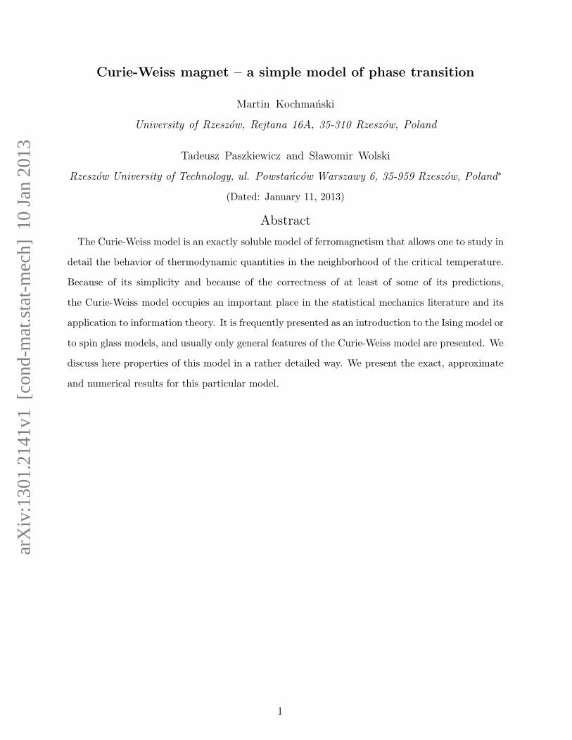
Curie-Weiss magnet – a simple model of phase transition

Martin Kochmanski

University of Rzeszow, Rejtana 16A, 35-310 Rzeszow, Poland

Tadeusz Paszkiewicz and S lawomir Wolski

Rzeszow University of Technology, ul. Powstancow Warszawy 6, 35-959 Rzeszow, Poland∗

(Dated: January 11, 2013)

Abstract

The Curie-Weiss model is an exactly soluble model of ferromagnetism that allows one to study in

detail the behavior of thermodynamic quantities in the neighborhood of the critical temperature.

Because of its simplicity and because of the correctness of at least of some of its predictions,

the Curie-Weiss model occupies an important place in the statistical mechanics literature and its

application to information theory. It is frequently presented as an introduction to the Ising model or

to spin glass models, and usually only general features of the Curie-Weiss model are presented. We

discuss here properties of this model in a rather detailed way. We present the exact, approximate

and numerical results for this particular model.

1

I. INTRODUCTION

A phase transition is the transformation of a thermodynamic system from one phase or

state to another. During a phase transition of a given medium certain properties change,

often discontinuously, as a result of some external conditions, such as temperature, pressure

or the magnetic field. For example, a liquid may become gas upon heating to the boiling

point, resulting in an abrupt change in volume.

In the case of a ferromagnet one should predict the dependence of such quantities as the

free and internal energy, heat capacity and magnetic susceptibility on temperature T and

magnetic induction B. Generally, this is very complicated task. Ma1 stressed the distinction

between the direct approach to the problem of phase transitions and the approach exploiting

symmetries of the problem. Here we shall illustrate the former approach. This means

calculations of physical properties of interest in terms of parameters given in a particular

model, i.e. solving a model. The calculations may be done analytically or numerically;

exactly or approximately.

The approach exploiting symmetries does not attempt to solve the model. From various

symmetry properties one deduces some important physical properties.

We shall focus on a particular model – the Curie-Weiss model of a magnet. This model

is also called the infinite range Ising model. The Curie Weiss model is an exactly soluble

model of ferromagnetism that allows one to study in detail the behavior of thermodynamic

quantities in the neighborhood of the critical temperature. Since not all predictions of this

model agree with experiment, other models must be considered. However, because of its

simplicity and because of the correctness of at least some of its predictions, the classical

Curie-Weiss model occupies a central place in the statistical mechanics literature. It is

frequently presented as an introduction to the Ising model or to spin glass models2−10. In

these references only general features of the Curie-Weiss model are discussed. This is why

we shall discuss here properties of this model in a rather detailed way. We present the exact,

approximate and numerical results for this particular model.

2

II. THE CURIE-WEISS MODEL

One of simplest classical systems exhibiting phase transition – the Curie-Weiss model has

been introduced by Pierre Curie and then by Pierre Weiss in their development of simplified

theory of ferromagnetism6,9. We shall call it the C-W magnet. Let us call the set of integers

from 1 to N a lattice, and its element i a site. We assign a variable si (the Ising spin) to

each site. The Ising spin is characterized by the binary value: +1 if microscopic magnetic

moment is pointing up or −1 if it is pointed down. Particles with the Ising spins interact

via Hamiltonian

Hint = − J

N

∑

1≤i<j≤N

sisj. (1)

The constant J is positive. The interaction energy of all pairs of spins of the Curie-Weiss

magnet is the same and their interaction depends on N . The normalization by 1/N makes

HN a quantity of the order N. The underlying assumption of an infinite-range interaction is

clearly unphysical. The Hamiltonian (1) does not depend on dimension of the space which

Curie-Weiss magnet is occupying.

The magnetic moment of a particle is proportional to the spin µi = µsi, where µ is

the magnetic moment. In an applied magnetic field with the magnetic induction vector B

particles with magnetic moments being parallel or antiparallel to B, acquire the energy

Hf = −µBN∑

i=1

si . (2)

The complete Hamiltonian consists of two terms

H = − J

N

∑

1≤i<j≤N

sisj − µBN∑

i=1

si . (3)

The Hamiltonian (3) does not change if we reverse signs of all spins si → −si (i =

1, 2, . . . , N) and the direction of the induction vector B → −B

H (s1, . . . , sn;B) = H (−s1, . . . ,−sn;−B) . (4)

Denote a particular configuration (s1, s2, . . . , sN) by {s}. To each configuration {s} there

corresponds an energy E ({s}) = H ({s}).

The nature of phase transitions of magnetic systems is well understood. At temperature

0K magnetic systems, in particular the M-W magnet, are in a lowest energy state with all

3

spins being parallel. Thus, their magnetization M is finite and our magnet is ferromagnetic.

As temperature is increased from zero the thermal noise randomizes spins. A fraction of

them become antiparallel. This disorder grows with raising temperature and a diminishing

fraction of them points at the initial direction. At temperature Tc – the critical temperature,

and beyond, magnetization vanishes and the material becomes paramagnetic. For T above

Tc, there must be macroscopically large regions in which a net fraction of spins are aligned

up. However, their magnetization mutually compensates – they cannot make a finite fraction

of all regions agree. For T just below Tc the compensation is not complete and the small,

but finite, fraction points in the same direction.

For left-hand vicinity of Tc thermodynamic functions depend on the dimensionless pa-

rameter t = (T − Tc) /Tc and consists of terms regular in t and singular in it. The singular

terms depend on powers of |t|−1. These powers are called the critical indexes (or critical

exponents) and are defined for B = 0 and t → 0. The specific heat c per one particle and

the magnetic susceptibility χT for the paramagnetic phase are characterized respectively by

critical indexes α and γ, whereas in the ferromagnetic phase they are characterized by α′

and γ′. For example in the paramagnetic phase

c ∼ |t|−α , χT ∼ |t|−γ . (5)

We shall calculate these sets of critical indexes, as well as the dependence of the internal

energy and entropy on |t|, for ferromagnetic and paramagnetic phases of the Curie-Weiss

magnet.

In the presence of the magnetic field the dependence of magnetization on the magnetic

field at |t| = 0 is characterized by the critical index δ

m ∼ B1/δ . (6)

In the following, in place of temperature we will use θ = kBT , kB being the Boltzmann

constant.

4

III. CALCULATION OF FREE ENERGY

Note that due to the particular structure of the Hamiltonian of C-W magnet, the Hamil-

tonian (1) can be written as

Hint = − J

2N

(

N∑

i=1

si

)2

+J

2. (7)

This form of Hamiltonian can be considered as a defining feature of mean field models.

The partition function is defined as usual as11

ZN =∑

{s}e−E({s})/θ . (8)

The summation is performed over all 2N configurations {s}. Note that a different method

calculating spin configurations can be used3−5.

Introduce two dimensionless quantities K = J/θ and h = µB/θ. Then, the partition

function (8) can be written as

ZN (θ) =∑

{s}exp

K

2N

(

N∑

i=1

si

)2

− K

2+ h

N∑

i=1

si

=

= e−K2

∑

{s}exp

(

√

K

2N

N∑

i=1

si

)2

+ h

N∑

i=1

si

.

(9)

Thermodynamic functions can be obtained via the Helmholtz free energy FN (θ, B)11

FN (θ, B) = −θ lnZN (θ, B) . (10)

Free energy is minimized when a system reaches equilibrium10,11. The derivative of FN (θ, B)

with respect to B gives

∂FN (θ, B)

∂B= −µ

⟨

N∑

i=1

si

⟩

= −µ

N∑

i=1

〈si〉, (11)

where 〈si〉 means the mean value of si calculated with the canonical distribution function11.

The minus derivative (11) defines magnetization M of C-W magnet, thus

M = µN∑

i=1

〈si〉. (12)

5

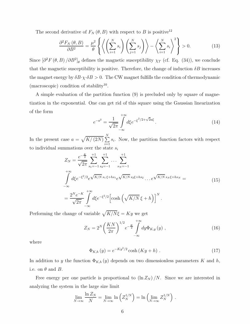
The second derivative of FN (θ, B) with respect to B is positive12

∂2FN (θ, B)

∂B2=

µ2

θ

⟨(

N∑

i=1

si

)(

N∑

j=1

sj

)⟩

−⟨

N∑

i=1

si

⟩2

> 0. (13)

Since [∂2F (θ, B) /∂B2]θ defines the magnetic susceptibility χT (cf. Eq. (34)), we conclude

that the magnetic susceptibility is positive. Therefore, the change of induction δB increases

the magnet energy by δB·χ·δB > 0. The CW magnet fulfills the condition of thermodynamic

(macroscopic) condition of stability10.

A simple evaluation of the partition function (9) is precluded only by square of magne-

tization in the exponential. One can get rid of this square using the Gaussian linearization

of the form

e−a2 =1√2π

+∞∫

−∞

dξe−ξ2/2+

√2aξ

. (14)

In the present case a =√

K/ (2N)N∑

i=1

si. Now, the partition function factors with respect

to individual summations over the state si

ZN =e−

K2

√2π

+1∑

s1=−1

+1∑

s2=−1

. . .+1∑

sN=−1

+∞∫

−∞

dξe−ξ2/2e√

K/N s1 ξ+hs1e√

K/N s2ξ+hs2 . . . e√

K/N sN ξ+hsN =

=2Ne−K

√2π

+∞∫

−∞

dξe−ξ2/2[

cosh(

√

K/N ξ + h)]N

.

(15)

Performing the change of variable√

K/Nξ = Ky we get

ZN = 2N

(

KN

2π

)1/2

e−K2

+∞∫

−∞

dyΦK,y (y) , (16)

where

ΦK,h (y) = e−Ky2/2 cosh (Ky + h) . (17)

In addition to y the function ΦK,h (y) depends on two dimensionless parameters K and h,

i.e. on θ and B.

Free energy per one particle is proportional to (lnZN) /N . Since we are interested in

analyzing the system in the large size limit

limN→∞

lnZN

N= lim

N→∞ln(

Z1/NN

)

= ln(

limN→∞

Z1/NN

)

.

6

For ZN (15) we obtain

−f (θ, B)

θ= lim

N→∞

1

Nln(

e−K2

√

KN/2π)

+ ln 2+

+ ln limN→∞

+∞∫

−∞

dy [ΦK,h (y)] N

1/N

.

(18)

In order to obtain the explicit form of the function f (θ, B) we use the Laplace theorem13.

The result is

− f (θ, B)

θ= ln max

−∞≤y≤∞ΦK,h (y) + ln 2 . (19)

Let us introduce a function of y related to free energy

fθ,h (y) = −θ [ln 2 + ln Φθ,h (y)] . (20)

To find the dependence of free energy on thermodynamic variables θ and B one should find

extreme points of fK,h (y). For these points (dfK,y (y) /dy)θ,B = 0. Since

(

∂f

∂y

)

θ,B

= − θK

ΦK,h (y)[tanh (Ky + h) − y] ΦK,h (y) = −θc [tanh (Ky + h) − y] ,

the state of minimum of free energy occurs for y obeying the equation

y = tanh (Ky + h) . (21)

For various values of θ (K) and B (h) solutions of this equation provide the function y =

y (θ, B) of state variables. Therefore, the function Φ (θ, B) = max−∞≤y≤∞

ΦK,h (y) is a composite

function of θ and B, namely ΦK,y (y (θ, B)) and also depends implicitly on these two state

variables. Now Eq. (19) can be rewritten in the form

f (θ, B) = −θ ln 2 − θ ln Φ (θ, B) ,

or

f (θ, B) = −θ ln 2 − θ ln{

e−Ky2(θ,B)/2 cosh [Ky (θ, B) + h]}

. (22)

Using two familiar identities15 d tanhx/dx = cosh−2 x and

cosh2 x =(

1 − tanh2 x)−1

=(

1 − y2)−1

, (23)

we calculate the second partial derivative of f with respect to y

(

∂2f

∂y2

)

θ,h

∣

∣

∣

∣

∣

y=y(θ,B)

= −θK{

K[

1 − y2 (θ, B)]

− 1}

. (24)

7

In the Appendix we show that there exist solutions of Eq. (21) for which this derivative is

positive, hence for them free energy is minimal.

For the reversed magnetic field the solution of Eq. (21) is −y

− y = tanh [K (−y − h)] . (25)

Therefore, free energy f (θ, B) (19) is an even function of B (and h)

− f (θ,−B)

θ= ln 2 + ln

{

e−K(−y(θ,B))2/2 cosh [−K (−y (θ, B)) − h]}

= −f (θ, B)

θ. (26)

These properties of free energy and solutions of Eq. (21) are the reason why in the following

we will always have in mind the positive value of B.

The product of (∂y/∂h)θ and (∂2fK,h (y) /∂y2)θ,h is positive because

(

∂y

∂h

)

θ

(

∂2fK,h (y)

∂y2

)

θ,h

=θK

cosh2 (Ky + h). (27)

Introduce here Kc = 1 – the critical value of the parameter K. From the definition of K

it is seen that the critical value of θ is θc = J .

In the mean field approximation (cf. for example14) the Hamiltonian (3) is approximated

by

Hmf = −N∑

i=1

(Jy + µB) si.

For this Hamiltonian the statistical sum is

Zmf (θ, B) = [2 cosh (Ky + h)]N

and the corresponding free energy is

Fmf (θ, B) = −θN [ln 2 + ln cosh (Ky + h)] .

Using the thermodynamic identity (11) we obtain Eq. (21).

IV. FREE ENERGY OF C-W MAGNET IN THE ABSENCE OF THE MAGNETIC

FIELD

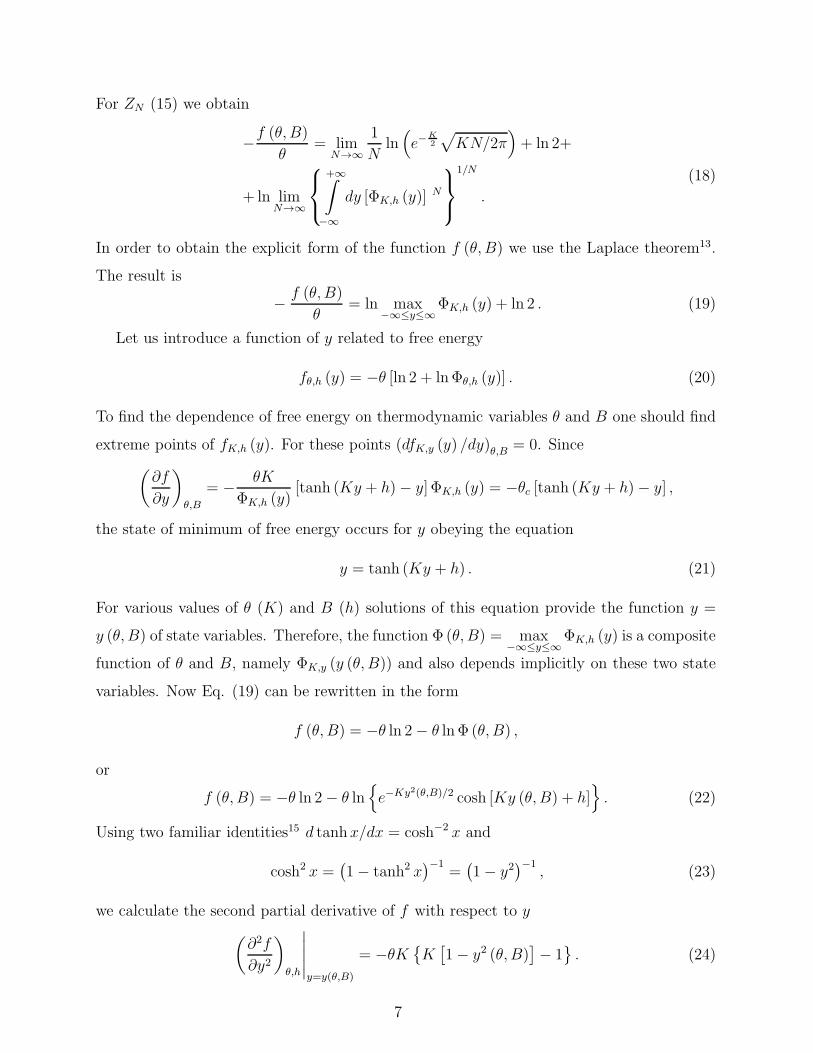
Suppose that B = 0 (h = 0). If we plot g (y) = y and q (y) = tanh (Ky) as functions of y,

the points of intersection determine solutions of Eq. (21). Referring to Fig. 1 (left panel),

8

we have to make distinction between cases. If θ > θc (θ > J) the slope of of the function

q (y) at the origin K = J/θ = θc/θ < 1 is smaller than the slope of linear function g (y) = y,

which is 1, thus these graphs intersect only at the origin. It is easy to check that for this

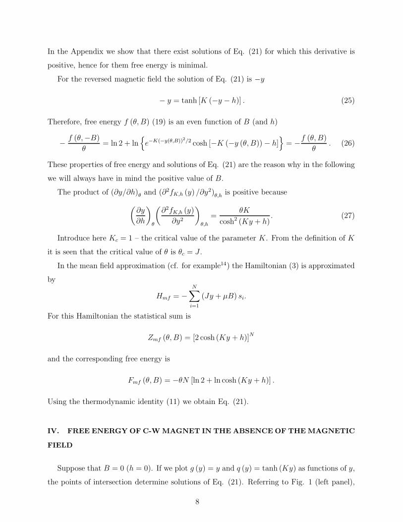
solution the second derivative of free energy (19) is positive (cf. Appendix). Therefore, the

extreme indeed is a minimum (cf. Fig. 2).

On the other hand when θ < θc (θ < J), the initial slope of tanh(Ky) is larger than that

of linear function, but since values of tanh function cannot take values outside the interval

(−1,+1), the two functions have to intersect in two additional, symmetric nonzero points

±y (θ) (Fig. 1). In this case in the Appendix we show that the second derivative of free

energy is negative at the origin y = 0, which means that there is a maximum at y = 0 (cf.

Fig. 2). This derivative is positive at y = ±y (θ). Free energy f (θ) attains minimal value

at y = ±y (θ), hence these solutions correspond to the thermodynamically stable states.

-1

-0.5

0

0.5

1

-2 -1.5 -1 -0.5 0 0.5 1 1.5 2g(y)

, q(y

)

y

g(y)=yQ(y)=tgh(Ky) θ > θcQ(y)=tgh(Ky) θ < θc

-1

-0.5

0

0.5

1

-2 -1.5 -1 -0.5 0 0.5 1 1.5 2g(y)

, q(y

)

y

g(y)=yQ(y)=tgh(Ky+h) θ > θcQ(y)=tgh(Ky+h) θ < θc

FIG. 1. Graphical solution of Eq. (21). The full line represents the function g(y) = y. The dotted

lines: θ < θc, the dashed lines: θ ≥ θc. Left panel: h = 0 (B = 0). Right panel: h > 0 (B > 0).

The parameter K and temperature θ can be expressed in terms of t = (θ/θc − 1), namely

K =θcθ

=1

1 + t,

θ = (1 + t) θc .

(28)

9

V. MAGNETIZATION AND MAGNETIC SUSCEPTIBILITY OF CURIE-WEISS

MAGNET

Consider the C-W magnet when the magnetic field B is brought back. Magnetization

per particle, m, is a partial derivative of free energy f (θ, B) after B

m (θ, h) = −[

∂f (θ, h)

∂B

]

θ

= µ

[

∂ ln Φ (θ, h)

∂h

]

θ

=

= µ∂ ln ΦK,h (y)

∂h

∣

∣

∣

∣

y=y(θ,B)

+ µ∂ ln ΦK,h (y)

∂y

∣

∣

∣

∣

y=y(θ,B)

∂y (θ, B)

∂h.

(29)

Since ΦK,h (y) attains an extremum at y (θ, B), the second term on right hand side of (29)

vanishes. The contribution of the first term yields the equation of state

m = µ tanh

(

K

µm + h

)

, (30)

which has a closed analytic form. Therefore, according to Eq. (21), the study of y is

equivalent to the study of of magnetization m.

Consider the solutions of Eq. (21) for B > 0. When θ < θc the plots of functions

g (y) = y and Q (y) = tanh (Ky + h) intersect in three non symmetric and nonzero points

(cf. right panel of Fig. 1). Only for positive value of y = y (θ, B) free energy f attains

the global minimum. To one of negative values there corresponds a local minimum, to the

remaining a maximum (cf. Fig. 2). The negative values of y (θ, B) (as well as m (θ, B))

do not correspond to stable states and should be omitted. One should notice that negative

values of y for positive h are not compatible with the symmetry (25) of the state equation.

When θ ≥ θc the graphs of g (y) and Q (y) intersect at one point y (θ, B) > 0. For this value

of y (θ, B) free energy has global minimum (cf. Fig. 2).

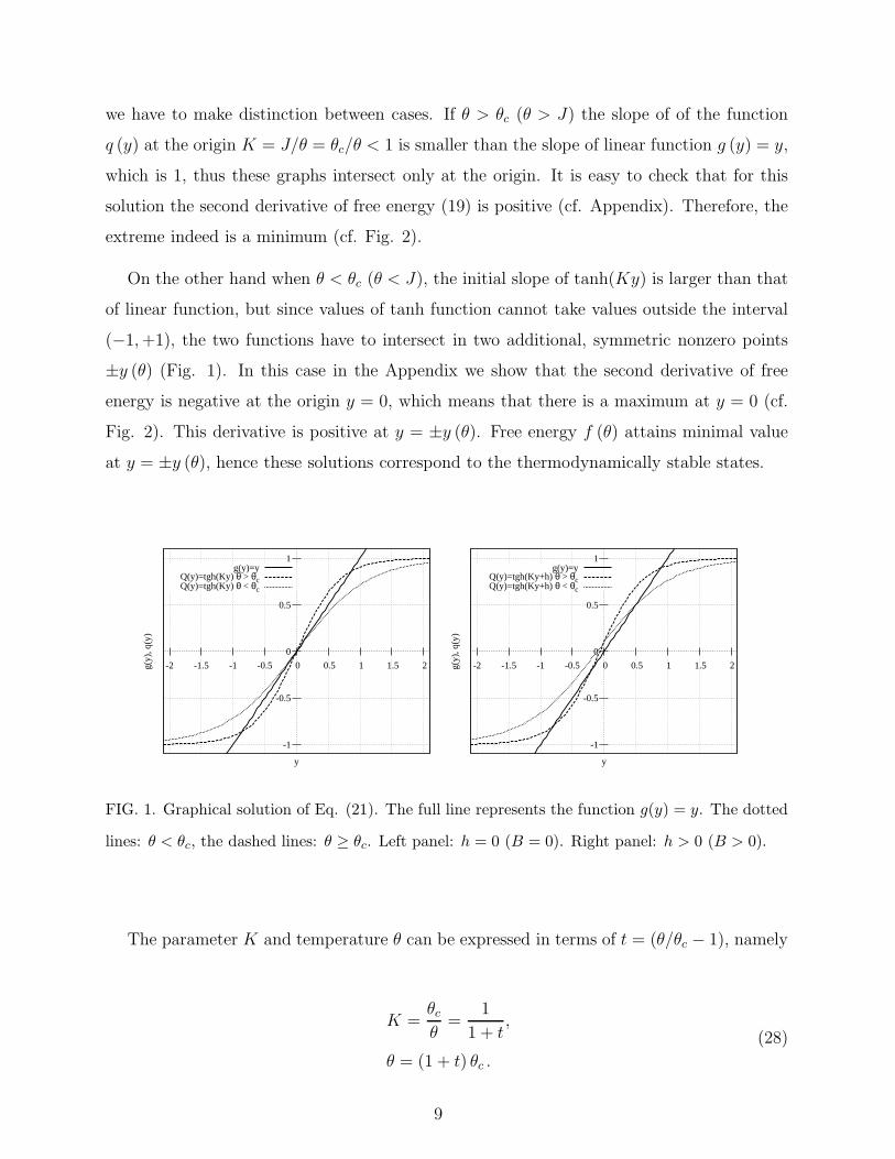
Consider Eq. (21) for small values of |t| and h = 0. We can expand tanh (Ky) into

Taylor’s series. Using Eq. (28) we obtain

y ≃√

3(K − 1)1/2

K3/2∼ |t|1/2. (31)

Hence, in agreement with Fig. 3, we conclude that

m ∼ |t|1/2 . (32)

When positive B → 0 then y (θ, h) → y (θ) of Fig 3. Thus, we note the existence of

10

-0.7

-0.6

-0.5

-0.4

-0.3

-0.2

-0.1

0

-2 -1.5 -1 -0.5 0 0.5 1 1.5 2

f K,h

(y)

y

θ>θc, h=0

-0.8-0.7-0.6-0.5-0.4-0.3-0.2-0.1

0 0.1 0.2

-2 -1.5 -1 -0.5 0 0.5 1 1.5 2

f K,h

(y)

y

θ>θc, h=0.2

-1.4

-1.2

-1

-0.8

-0.6

-0.4

-0.2

0

-2 -1.5 -1 -0.5 0 0.5 1 1.5 2

f K,h

(y)

y

θ<θc, h=0

-1.6

-1.4

-1.2

-1

-0.8

-0.6

-0.4

-0.2

0

0.2

-2 -1.5 -1 -0.5 0 0.5 1 1.5 2

f K,h

(y)

y

θ<θc, h=0.2

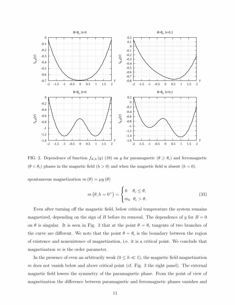
FIG. 2. Dependence of function fK,h (y) (19) on y for paramagnetic (θ ≥ θc) and ferromagnetic

(θ < θc) phases in the magnetic field (h > 0) and when the magnetic field is absent (h = 0).

spontaneous magnetization m (θ) = µy (θ)

m(

θ, h = 0+)

=

0 θc ≤ θ,

m0 θc > θ.(33)

Even after turning off the magnetic field, below critical temperature the system remains

magnetized, depending on the sign of B before its removal. The dependence of y for B = 0

on θ is singular. It is seen in Fig. 3 that at the point θ = θc tangents of two branches of

the curve are different. We note that the point θ = θc is the boundary between the region

of existence and nonexistence of magnetization, i.e. it is a critical point. We conclude that

magnetization m is the order parameter.

In the presence of even an arbitrarily weak (0 ≤ h ≪ 1), the magnetic field magnetization

m does not vanish below and above critical point (cf. Fig. 3 the right panel). The external

magnetic field lowers the symmetry of the paramagnetic phase. From the point of view of

magnetization the difference between paramagnetic and ferromagnetic phases vanishes and

11

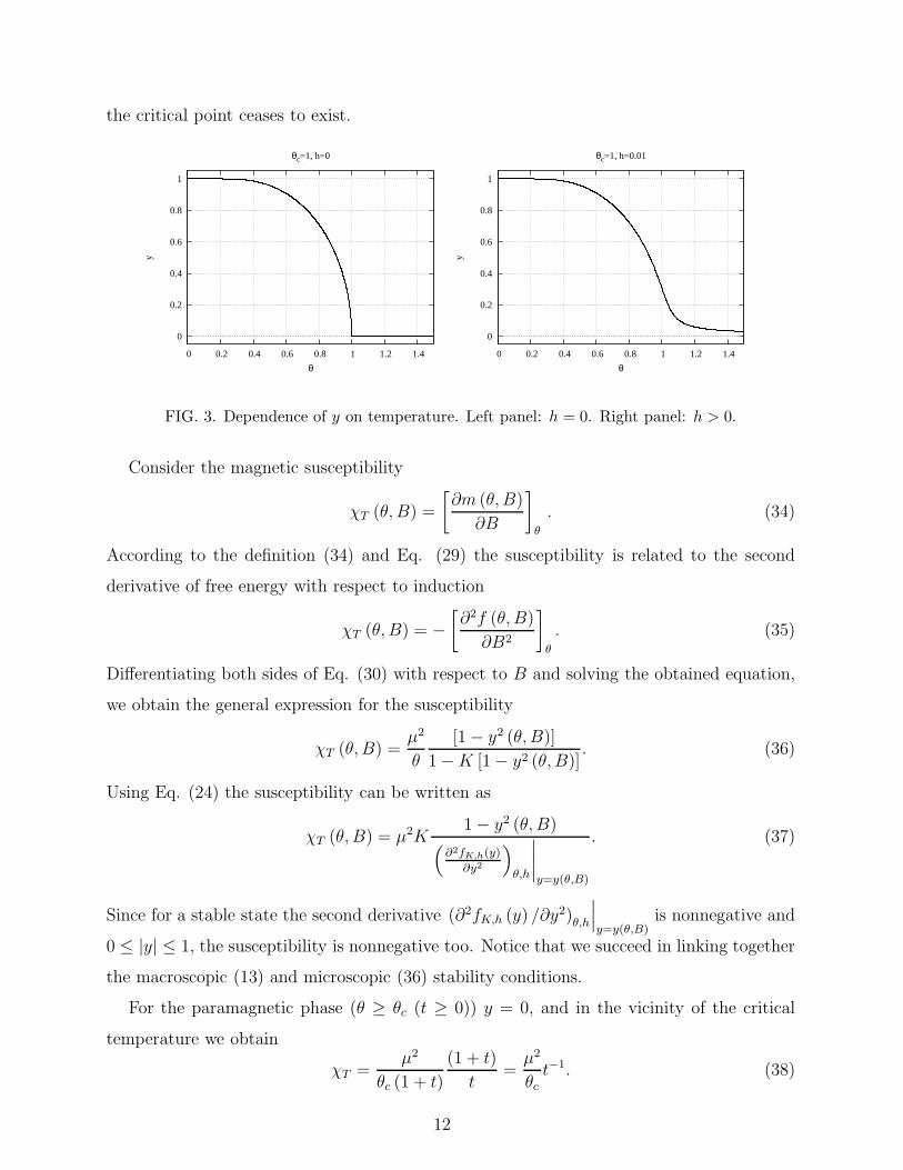
the critical point ceases to exist.

0

0.2

0.4

0.6

0.8

1

0 0.2 0.4 0.6 0.8 1 1.2 1.4

y

θ

θc=1, h=0

0

0.2

0.4

0.6

0.8

1

0 0.2 0.4 0.6 0.8 1 1.2 1.4

y

θ

θc=1, h=0.01

FIG. 3. Dependence of y on temperature. Left panel: h = 0. Right panel: h > 0.

Consider the magnetic susceptibility

χT (θ, B) =

[

∂m (θ, B)

∂B

]

θ

. (34)

According to the definition (34) and Eq. (29) the susceptibility is related to the second

derivative of free energy with respect to induction

χT (θ, B) = −[

∂2f (θ, B)

∂B2

]

θ

. (35)

Differentiating both sides of Eq. (30) with respect to B and solving the obtained equation,

we obtain the general expression for the susceptibility

χT (θ, B) =µ2

θ

[1 − y2 (θ, B)]

1 −K [1 − y2 (θ, B)]. (36)

Using Eq. (24) the susceptibility can be written as

χT (θ, B) = µ2K1 − y2 (θ, B)

(

∂2fK,h(y)

∂y2

)

θ,h

∣

∣

∣

∣

y=y(θ,B)

. (37)

Since for a stable state the second derivative (∂2fK,h (y) /∂y2)θ,h

∣

∣

∣

y=y(θ,B)is nonnegative and

0 ≤ |y| ≤ 1, the susceptibility is nonnegative too. Notice that we succeed in linking together

the macroscopic (13) and microscopic (36) stability conditions.

For the paramagnetic phase (θ ≥ θc (t ≥ 0)) y = 0, and in the vicinity of the critical

temperature we obtain

χT =µ2

θc (1 + t)

(1 + t)

t=

µ2

θct−1. (38)

12

This means that the critical index γ = 1.

The function arctanhy obeys the equation

arctanhy = Ky + h . (39)

We shall study solutions of Eq. (39) in vicinity of the critical temperature. For small y one

can expand arctanhy into Taylor’s series15. For θ < θc (t < 0) Eq. (39) reduces to

y3 − 3|t|

1 − |t|y − 3h = 0. (40)

In the ferromagnetic phase and in the absence of the magnetic field, the order parameter

does not vanish

y2 =3 |t|

1 − |t| (t < 0) . (41)

When B = 0 from Eq. (41) it follows that for ferromagnetic phase in vicinity of critical

temperature m ∼√

3 |t|. Thus the critical index of magnetization is β ′ = 1/2.

Consider the susceptibility (36) in ferromagnetic phase in the vicinity of the critical

temperature. Using the expressions (28) and (41) for the ferromagnetic phase we obtain

limB→0

χT (θ, B) ∼ µ2

θc|t|−1 , (42)

and according to the definition (5) for both phases the critical indexes of magnetization are

equal: γ = γ′ = 1. We shall note that in the case of ferromagnetic phase one should use the

relation (40). We conclude that for both phases the magnetic susceptibility of Curie-Weiss

magnet is divergent at the critical temperature. This singular behavior is shown in Fig. 4.

0

0.2

0.4

0.6

0.8

1

1.2

1.4

0 0.2 0.4 0.6 0.8 1 1.2 1.4

y

θ

θc=1, h=0, µ=0.1

0

0.02

0.04

0.06

0.08

0.1

0.12

0.14

0 0.2 0.4 0.6 0.8 1 1.2 1.4

y

θ

θc=1, h=0.01, µ=0.1

FIG. 4. Dependence of the susceptibility on temperature. Left panel: h = 0. Right panel h > 0.

13

At the critical point t = 0, hence y = 3√

3 h1/3. Therefore, according the definition (6),

the critical index for the critical isotherm δ = 3.

Continuous phase transitions occur when a new state of reduced symmetry develops con-

tinuously from the disordered (high temperature) phase. The ordered phase of M-C magnet

has lower symmetry than the symmetry (4) of the Hamiltonian, thus the symmetry is spon-

taneously broken. There exist two equivalent symmetry related states of C-W magnet with

magnetization +m i −m respectively, with equal free energies. These states are macroscopi-

cally different, so thermal fluctuations will not bring them into contact in the thermodynamic

limit. To describe the ordered state we introduced magnetization – the macroscopic order

parameter that describes the character and strength of the broken symmetry.

VI. APPROXIMATE THEORY – THE ANALYSIS OF ROOTS OF THE CUBIC

EQUATION FOR MAGNETIZATION

Now we shall study the roots of the cubic equation (40) for the ferromagnetic phase.

Since free energy is an even function of B we assume that h > 0. We shall study the so

called the incomplete cubic equation

y3 + 3 (−p) y + 2q = 0 , (43)

where p = |t| / (1 − |t|) , q = −3h/2.

It is worthwhile to recall that assumptions proposed by Landau for an incompressible

magnet result in free energy depending only on even powers of magnetization10,16,17

f (m, T ) = f0 (T ) + α (T )m2 +1

2β (T )m4.

This form of free energy leads to a cubic equation for magnetization.

Introduce a characteristic value of the parameter ht

ht =2

3

( |t|1 − |t|

)32

. (44)

Roots of Eq. (43) depend on the sign of the discriminant15 D = (q2 − p3)

D =

(

3

2h

)2

−( |t|

1 + |t|

)3

=

(

3

2

)2(

h2 − h2t

)

. (45)

If D < 0 inequalities −ht < h < ht hold. If D > 0, then h > ht or h < −ht.

14

If D < 0 all tree roots are real

y(<)1 (t, h) = u< (t, h) + v< (t, h) ,

y(<)2 (t, h) = ε2u< (t, h) + ε1v< (t, h) ,

y(<)3 (t, h) = ε1u< (t, h) + ε2v< (t, h) ,

(46)

where

u< (t, h) =3

√

−q + i√

|D|, v< (t, h) = [u< (t, h)]∗ ,

ε1 =(

−1 + i√

3)

/2, ε2 = ε∗1 .(47)

Using relations (47) we can show that

y(<)1 (t, h) = 2 Reu< (t, h) ,(

y(<)σ

)∗(t, h) = y(<)

σ (t, h) (σ = 2, 3) .

If D > 0 (i.e. h2 > h2t ) only one root is real

y> (t, h) = u> (t, h) + v> (t, h) , (48)

where

u> (t, h) =3

√

3h

2+√D, v> (t, h) =

3

√

3h

2−√D. (49)

The two remaining two roots are complex.

If we combine Eqs. (44)-(49) we obtain the functions u< (t, u), v< (t, u) and u> (t, u),

v> (t, u) in the useful form

u> (t, h) = (3/2)1/33

√

h +√

h2 − h2t , v> (t, h) = (3/2)1/3

3

√

h−√

h2 − h2t ,

u< (t, h) = (3/2)1/33

√

h + i√

h2t − h2, v< (t, h) = (3/2)1/3

3

√

h− i√

h2t − h2 .

(50)

Consider functions u> (t, h) and v> (t, h) for negative h

u> (t,−h) = 3√−1

3

√

h−√

h2 − h2t = 3

√−1 v> (t, h) ,

v> (t,−h) = 3√−1

3

√

h +√

h2 − h2t = 3

√−1 u> (t, h) .

(51)

Similar relations hold also for u< and v<. Among three root of unity ε1, ε2 and ε3 = −1

only the latter root yields proper symmetry relation (25)

y(σ)j (t,−h) = −y

(σ)j (t, h) (σ = >,<; j = 1, 2, 3) . (52)

15

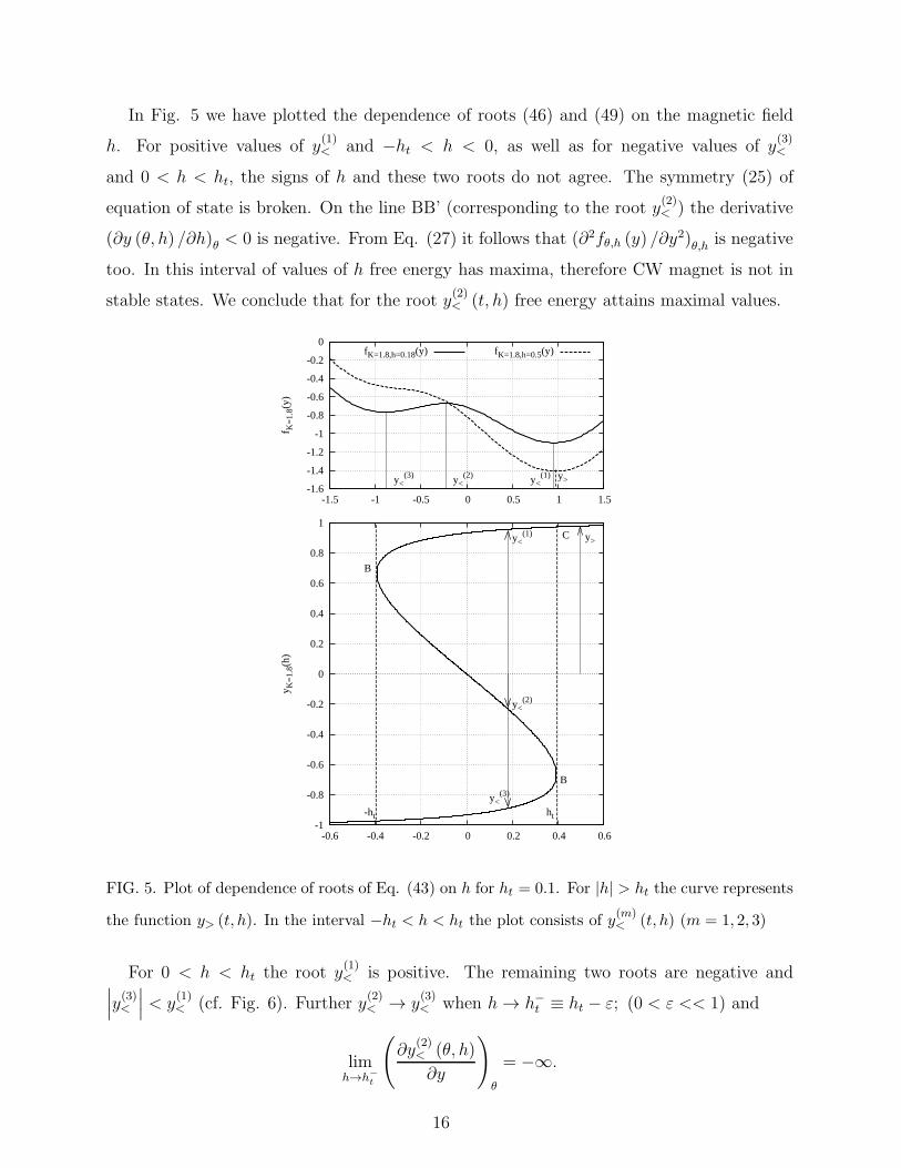
In Fig. 5 we have plotted the dependence of roots (46) and (49) on the magnetic field

h. For positive values of y(1)< and −ht < h < 0, as well as for negative values of y

(3)<

and 0 < h < ht, the signs of h and these two roots do not agree. The symmetry (25) of

equation of state is broken. On the line BB’ (corresponding to the root y(2)< ) the derivative

(∂y (θ, h) /∂h)θ < 0 is negative. From Eq. (27) it follows that (∂2fθ,h (y) /∂y2)θ,h is negative

too. In this interval of values of h free energy has maxima, therefore CW magnet is not in

stable states. We conclude that for the root y(2)< (t, h) free energy attains maximal values.

-1.6

-1.4

-1.2

-1

-0.8

-0.6

-0.4

-0.2

0

-1.5 -1 -0.5 0 0.5 1 1.5

f K=

1.8(

y)

y<(1)y<

(2)y<(3) y>

fK=1.8,h=0.18(y) fK=1.8,h=0.5(y)

-1

-0.8

-0.6

-0.4

-0.2

0

0.2

0.4

0.6

0.8

1

-0.6 -0.4 -0.2 0 0.2 0.4 0.6

y K=

1.8(

h)

ht-ht

y<(1)

y<(2)

y<(3)

C

B

B

y>

FIG. 5. Plot of dependence of roots of Eq. (43) on h for ht = 0.1. For |h| > ht the curve represents

the function y> (t, h). In the interval −ht < h < ht the plot consists of y(m)< (t, h) (m = 1, 2, 3)

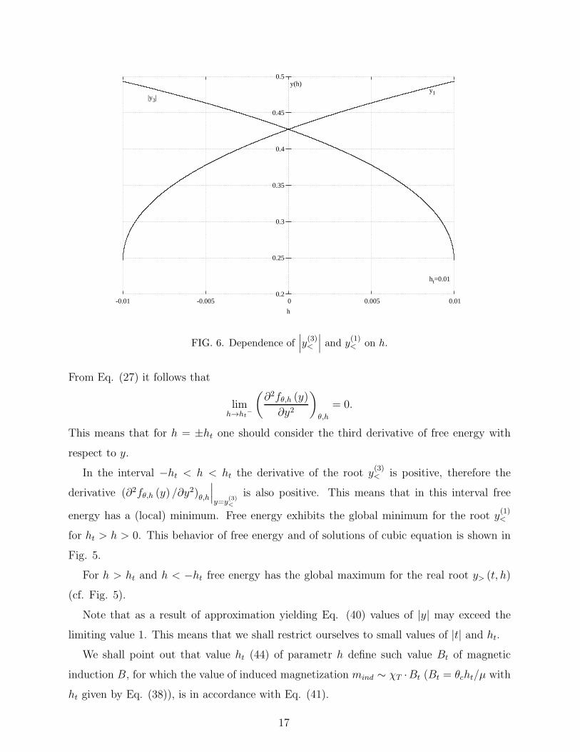
For 0 < h < ht the root y(1)< is positive. The remaining two roots are negative and

∣

∣

∣y(3)<

∣

∣

∣< y

(1)< (cf. Fig. 6). Further y

(2)< → y

(3)< when h → h−

t ≡ ht − ε; (0 < ε << 1) and

limh→h−

t

(

∂y(2)< (θ, h)

∂y

)

θ

= −∞.

16

0.2

0.25

0.3

0.35

0.4

0.45

0.5

-0.01 -0.005 0 0.005 0.01

h

|y3|y1

ht=0.01

y(h)

FIG. 6. Dependence of∣

∣

∣y(3)<

∣

∣

∣and y

(1)< on h.

From Eq. (27) it follows that

limh→ht

−

(

∂2fθ,h (y)

∂y2

)

θ,h

= 0.

This means that for h = ±ht one should consider the third derivative of free energy with

respect to y.

In the interval −ht < h < ht the derivative of the root y(3)< is positive, therefore the

derivative (∂2fθ,h (y) /∂y2)θ,h

∣

∣

∣

y=y(3)<

is also positive. This means that in this interval free

energy has a (local) minimum. Free energy exhibits the global minimum for the root y(1)<

for ht > h > 0. This behavior of free energy and of solutions of cubic equation is shown in

Fig. 5.

For h > ht and h < −ht free energy has the global maximum for the real root y> (t, h)

(cf. Fig. 5).

Note that as a result of approximation yielding Eq. (40) values of |y| may exceed the

limiting value 1. This means that we shall restrict ourselves to small values of |t| and ht.

We shall point out that value ht (44) of parametr h define such value Bt of magnetic

induction B, for which the value of induced magnetization mind ∼ χT ·Bt (Bt = θcht/µ with

ht given by Eq. (38)), is in accordance with Eq. (41).

17

If h ≪ ht (|t| 6= 0) the magnetic field B is week and does not influence the thermodynamic

quantities characterizing the system. If h ≫ ht the field B is strong. If t = 0 (T = Tc) all

magnetic fields are strong. As we have shown, if t ∼ 0 and field is strong, m ∼ h1/3.

VII. PROPERTIES OF THE INTERNAL ENERGY, ENTROPY AND SPECIFIC

HEAT OF THE CURIE-WEISS MAGNET

To find the internal energy U we shall use the familiar thermodynamic identity11

U = −θ2∂

∂θ

(

F

θ

)

= Nθ2∂

∂θ

(

−f

θ

)

B

.

For the internal energy per one spin this formula gives

u = −θ2∂

∂θ

[

−Ky2/2 + ln cosh (Ky + h)]

.

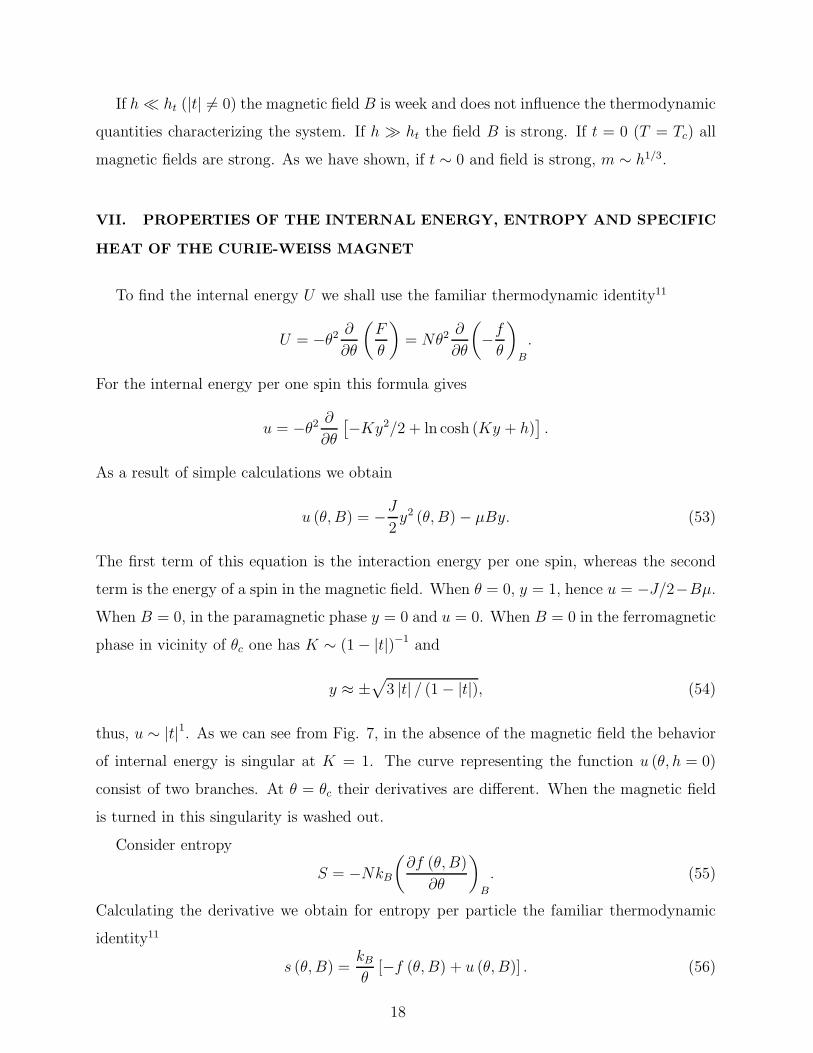
As a result of simple calculations we obtain

u (θ, B) = −J

2y2 (θ, B) − µBy. (53)

The first term of this equation is the interaction energy per one spin, whereas the second

term is the energy of a spin in the magnetic field. When θ = 0, y = 1, hence u = −J/2−Bµ.

When B = 0, in the paramagnetic phase y = 0 and u = 0. When B = 0 in the ferromagnetic

phase in vicinity of θc one has K ∼ (1 − |t|)−1 and

y ≈ ±√

3 |t| / (1 − |t|), (54)

thus, u ∼ |t|1. As we can see from Fig. 7, in the absence of the magnetic field the behavior

of internal energy is singular at K = 1. The curve representing the function u (θ, h = 0)

consist of two branches. At θ = θc their derivatives are different. When the magnetic field

is turned in this singularity is washed out.

Consider entropy

S = −NkB

(

∂f (θ, B)

∂θ

)

B

. (55)

Calculating the derivative we obtain for entropy per particle the familiar thermodynamic

identity11

s (θ, B) =kBθ

[−f (θ, B) + u (θ, B)] . (56)

18

-0.5

-0.4

-0.3

-0.2

-0.1

0

0 0.2 0.4 0.6 0.8 1 1.2 1.4

u(θ,

h)

θ

θc=1, h=0

-0.5

-0.4

-0.3

-0.2

-0.1

0

0 0.2 0.4 0.6 0.8 1 1.2 1.4

u(θ,

h)

θ

θc=1, h=0.05

FIG. 7. Dependence of the internal energy on temperature. Left panel: h = 0. Right panel h > 0.

For low temperatures

f (θ, B) ∼ u (θ, B)

θ.

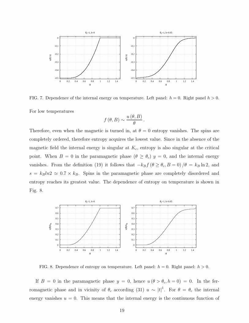
Therefore, even when the magnetic is turned in, at θ = 0 entropy vanishes. The spins are

completely ordered, therefore entropy acquires the lowest value. Since in the absence of the

magnetic field the internal energy is singular at Kc, entropy is also singular at the critical

point. When B = 0 in the paramagnetic phase (θ ≥ θc) y = 0, and the internal energy

vanishes. From the definition (19) it follows that −kBf (θ ≥ θc, B = 0) /θ = kB ln 2, and

s = kBln2 ≃ 0.7 × kB. Spins in the paramagnetic phase are completely disordered and

entropy reaches its greatest value. The dependence of entropy on temperature is shown in

Fig. 8.

0

0.1

0.2

0.3

0.4

0.5

0.6

0.7

0 0.2 0.4 0.6 0.8 1 1.2 1.4

s(θ)

/kB

θ

θc=1, h=0

0

0.1

0.2

0.3

0.4

0.5

0.6

0.7

0 0.2 0.4 0.6 0.8 1 1.2 1.4

s(θ)

/kB

θ

θc=1, h=0.05

FIG. 8. Dependence of entropy on temperature. Left panel: h = 0. Right panel: h > 0.

If B = 0 in the paramagnetic phase y = 0, hence u (θ > θc, h = 0) = 0. In the fer-

romagnetic phase and in vicinity of θc according (31) u ∼ |t|1. For θ = θc the internal

energy vanishes u = 0. This means that the internal energy is the continuous function of

19

temperature u(θ−c ) = u(θ+c ) = 0.

Entropy s also is a continuous function of temperature. To show this property in the case

of ferromagnetic phase and vicinity of θc we use Eqs. (22) and (31) and Tylor’s series for

ln [tanh (Ky)] we get

s ≈ kB (ln 2 − 3 |t| /2) .

We see that, as one may expect, that entropy of the ferromagnetic phase is smaller than

entropy of paramagnetic phase and for |t| = 0 attains its maximal value.

The behavior of heat capacity in vicinity of the critical temperature is more complex. To

calculate heat capacity per one particle one can use one of two thermodynamic relations,

namely11

c (θ, B) = kB

(

∂u (θ, B)

∂θ

)

B

, (57)

or

c (θ, B) = θ

(

∂s (θ, B)

∂θ

)

B

. (58)

It is an easy task to show that these identities yield the same result. We shall consider Eq.

(57). From Eq (53) it follows that heat capacity c (θ, B) depends on derivative (∂y/∂θ)B

c = −kBθ (Ky + h)

(

∂y

∂θ

)

B

.

Differentiating both sides of Eq. (21) with respect to y, solving the obtained equation for

(∂y (θ, B) /∂θ)B and applying the identity (23), we obtain an analytic expression for this

derivative(

∂y

∂θ

)

B

= −1

θ

(Ky + h)

cosh2 (Ky + h) −K.

With the help of the above relation we obtain the final form of expression for heat capacity

per one particle

c = kB(1 − y2) (Ky + h)2

(1 −K) + Ky2. (59)

When B = 0 in the paramagnetic phase (θ ≥ θc) magnetization m vanishes, i.e. y = 0.

Hence, c = 0. Since limθ→0

y = 1 in this limit c also vanishes.

Consider heat capacity in ferromagnetic phase in the vicinity of the critical temperature.

Using expressions (28) and (54) we obtain

c

kB≈ 3

2(1 − |t|) . (60)

20

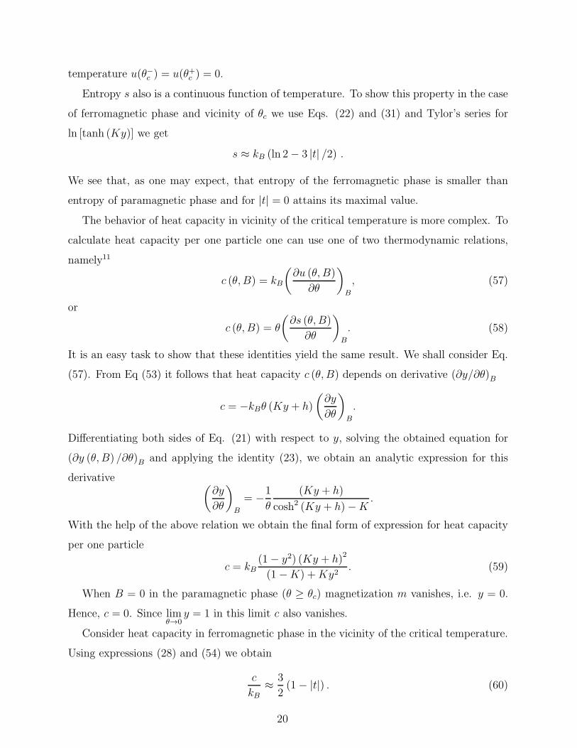
Heat capacity is discontinuous at θc

c(

θ−c , B = 0)

− c(

θ+c , B = 0)

= 3kB/2, (61)

with θ±c = θc ± ǫ, and 0 < ǫ ≪ 1. The zero field heat capacity is singular at the critical

temperature, whereas in the magnetic field it exhibits a peak at the transition point (cf.

Fig. 9).

0

0.2

0.4

0.6

0.8

1

1.2

1.4

1.6

0 0.2 0.4 0.6 0.8 1 1.2 1.4

c/k B

θ

θc=1, h=0

0

0.2

0.4

0.6

0.8

1

1.2

0 0.2 0.4 0.6 0.8 1 1.2 1.4

c/k B

θ

θc=1, h=0.01

FIG. 9. Dependence of heat capacity per one particle on temperature. Left panel: h = 0. Right

panel: h > 0.

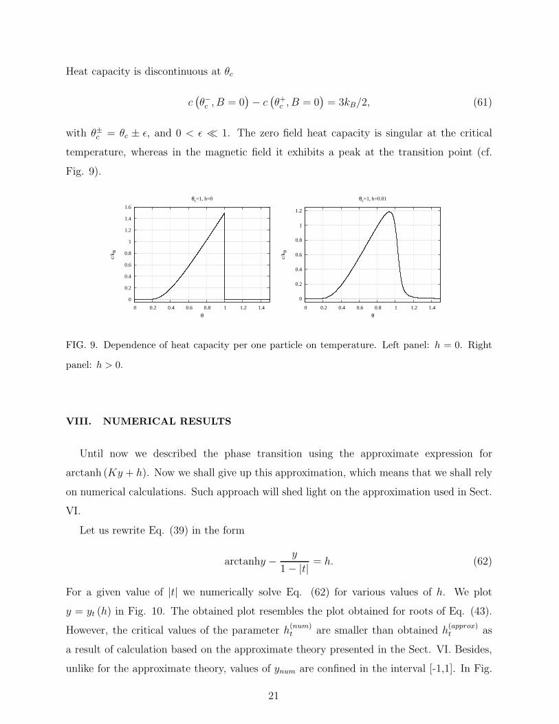
VIII. NUMERICAL RESULTS

Until now we described the phase transition using the approximate expression for

arctanh (Ky + h). Now we shall give up this approximation, which means that we shall rely

on numerical calculations. Such approach will shed light on the approximation used in Sect.

VI.

Let us rewrite Eq. (39) in the form

arctanhy − y

1 − |t| = h. (62)

For a given value of |t| we numerically solve Eq. (62) for various values of h. We plot

y = yt (h) in Fig. 10. The obtained plot resembles the plot obtained for roots of Eq. (43).

However, the critical values of the parameter h(num)t are smaller than obtained h

(approx)t as

a result of calculation based on the approximate theory presented in the Sect. VI. Besides,

unlike for the approximate theory, values of ynum are confined in the interval [-1,1]. In Fig.

21

-1

-0.5

0

0.5

1

-0.8 -0.6 -0.4 -0.2 0 0.2 0.4 0.6 0.8

y

h

-ht(app)

-ht ht

ht(app)

y(h) y(h)(app)

FIG. 10. Dependence of yt (h) on the magnetic field h. Dashed line represents the dependence of

roots of Eq. (43) on the magnetic field. The full line is plot of the function (62).

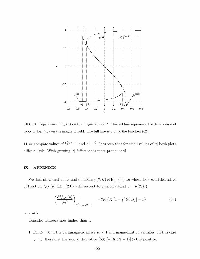
11 we compare values of h(approx)t and h

(num)t . It is seen that for small values of |t| both plots

differ a little. With growing |t| difference is more pronounced.

IX. APPENDIX

We shall show that there exist solutions y (θ, B) of Eq. (39) for which the second derivative

of function fK,h (y) (Eq. (20)) with respect to y calculated at y = y (θ, B)

(

∂2fθ,h (y)

∂y2

)

θ,h

∣

∣

∣

∣

∣

y=y(θ,B)

= −θK{

K[

1 − y2 (θ, B)]

− 1}

(63)

is positive.

Consider temperatures higher than θc.

1. For B = 0 in the paramagnetic phase K ≤ 1 and magnetization vanishes. In this case

y = 0, therefore, the second derivative (63) [−θK (K − 1)] > 0 is positive.

22

0

2

4

6

8

10

0 0.1 0.2 0.3 0.4 0.5 0.6 0.7 0.8 0.9 1

h t

t

ht ht(app)

FIG. 11. Plot of dependence of critical value of the magnetic field ht on the parameter t. The full

line – result numerical calculation, the dashed line represents the dependence resulting from the

cubic equation (43).

2. If B > 0 magnetization is positive, hence 1 > y > 0. The double inequality 0 <

K [1 − y2 (θ, B)] < 1 holds. Therefore, K [1 − y2 (θ, B)] − 1 < 0. Hence, the the

second derivative (63) is positive. The same arguments are valid for the negative

value of induction (B < 0 and y < 0).

In the case of θ < θc the parameter K is greater than unity. As we know (cf. Sect. IV),

if B = 0, Eq. (21) has three solutions, namely y = 0 and y = ±y (θ) ≡ ±y0.

1. For y = 0 the derivative (63) is negative

(

∂2fθ,h (y)

∂y2

)

θ,h

∣

∣

∣

∣

∣

y=0

= θK (1 −K) < 0. (64)

This means that in the ferromagnetic phase the solution y = 0 corresponds to a max-

imum of free energy.

2. In the case of two remaining solutions the second derivative reads

(

∂2fK,h (y)

∂y2

)

θ,h

∣

∣

∣

∣

∣

y=±y0

= −θK[

K(

1 − y20)

− 1]

. (65)

23

We shall express the parameter K by y0. Using Eq. (39) we can write

K =arctanhy0

y0.

With the help of this relation we find

(

∂2fK,h (y)

∂y2

)

θ,h

∣

∣

∣

∣

∣

y=±y0

= −θK

[

arctanhy0y0

(

1 − y20)

− 1

]

. (66)

For small y0 we can use the approximate expression arctanhy0 ≈ y0+y30/3. This yields

the inequality

(1 − y20) arctanhy0y0

≈(

1 + y20/3) (

1 − y20)

<(

1 − y40)

< 1,

and the second derivative of free energy is positive. In the ferromagnetic phase, in

vicinity of critical temperature, for solutions ±y0 free energy reaches a minimum.

The function

ϕ (y0) =arctanhy0

y0

(

1 − y20)

is monotonically decreasing in the interval (0, 1] and 0 ≤ ϕ (y0) < 1.

Using the logarithmic representation18 arctanhy0 = 12

ln(

y0+1y0−1

)

and the limiting

value18 limx→0

x ln x = 0 we can show that

limy0→1−

arctanhy0y0

(

1 − y20)

= 0,

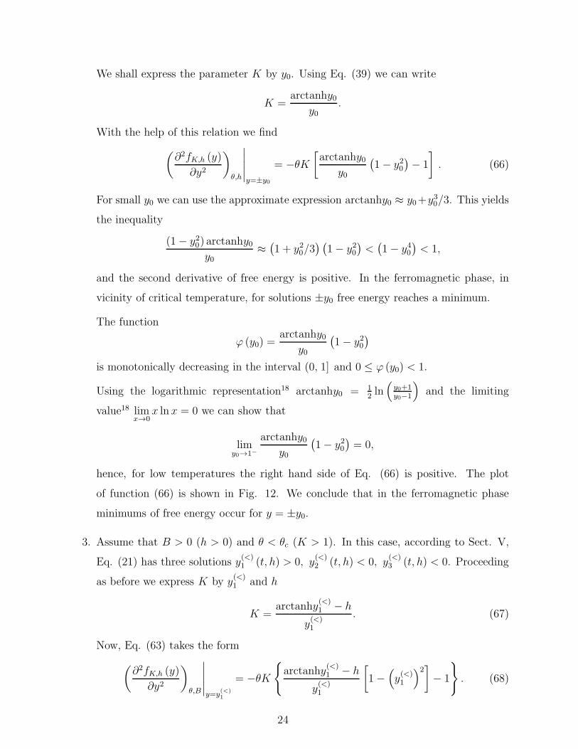
hence, for low temperatures the right hand side of Eq. (66) is positive. The plot

of function (66) is shown in Fig. 12. We conclude that in the ferromagnetic phase

minimums of free energy occur for y = ±y0.

3. Assume that B > 0 (h > 0) and θ < θc (K > 1). In this case, according to Sect. V,

Eq. (21) has three solutions y(<)1 (t, h) > 0, y

(<)2 (t, h) < 0, y

(<)3 (t, h) < 0. Proceeding

as before we express K by y(<)1 and h

K =arctanhy

(<)1 − h

y(<)1

. (67)

Now, Eq. (63) takes the form

(

∂2fK,h (y)

∂y2

)

θ,B

∣

∣

∣

∣

∣

y=y(<)1

= −θK

{

arctanhy(<)1 − h

y(<)1

[

1 −(

y(<)1

)2]

− 1

}

. (68)

24

-2

-1.5

-1

-0.5

0

0.5

1

-2 -1 0 1 2

f K,h

(y)

t

fK,h(y)dfK,h(y)/dy

d2fK,h(y)/dy2

FIG. 12. Plot of fK,h (y) (solid line), dfK,h (y) /dy (broken line) and d2fK,h (y) /dy2 (dotted line).

To zeros of dfK,h (y) /dy there correspond extremums of fK,h (y). Two of them are minimums

becaused2fK,h(y)

dy2> 0.

Since 0 < y(<)1 ≤ 1, the inequality

[

1 −(

y(<)1

)2]

< 1 holds. Thus, the additional term

of Eq. (68) is non-positive

− h

y(<)1

[

1 −(

y(<)1

)2]

≤ 0,

and, even in this case, the second derivative of free energy is positive.

∗ tapasz@prz.edu.pl

25

1 S-K Ma, Modern Theory of Critical Phenomena (Benjamin, Reading, MA, 1976).

2 S. Adams, Lectures on on Mathematical Statistical Mechanics, Dublin Institute for Advanced

Studies, 2006.

3 A. Bovier and I. Kurkova, A Short Course on Mean Field spin glasses.

4 R. Kuhn, Equilibrium Analysis of Complex Systems, Lecture Notes of 7CCMCS03, King’s Col-

lege, London 2010.

5 N. Macris, Statistical Physics for Communication and Computer Science, Lecture Notes 3: Ising

Model, Ecole Polytechniqe Federale de Lausanne, 2011.

6 M. Kac, “Mathematical Mechanisms of Phase Transitions” in: Statistical Mechanics of Phase

Transitions and Superfluidity, edited by M. Chretilin, E.P. Gross, S. Dresser (Gordon and

Breach Science Publishers, New York, 1968).

7 N. Merhav, Statistical Physics and Information Theory, Foundations and Trends in Communi-

cations and Information Theory, 6, 1212 (2009).

8 A. Montanari, Stat 316, Stochastic Processes on Graphs, Introduction and the Curie-Weiss

model Stanford University, 2007.

9 H. Nishimori, Statistical Physics of Spin Glasses and Information Processing. An Introduction

(Clarendon Press, Oxford, 2001).

10 L.E. Reichl, A Modern Course in Statistical Physics, Chapter 4, (University of Texas Press,

Austin, 1980).

11 K. Huang, Statistical Mechanics (Wiley, Hoboken NJ, 1987).

12 F. Reif, Statistical Physics, Berkeley Physics Course, Vol. 5 (McGrawHill, New York, 1967).

13 G. Polya, G. Szego, Problems and Theorems in Analysis I: Series, Integral Calculus, Theory of

Functions, Chapter 5 (Springer, Heidelberg, 1976).

14 P. Palffy-Muhoray, Am. J. Phys. 70, 433, 2002.

15 I.N. Bronshtein, K.A. Semendyaev, G. Musiol, H. Muehling, Handbook of Mathematics

(Springer, 4th edition 2004).

16 J. Als-Nielsen, R.J. Birgenau, Am. J. Phys. 45, 554, 1977.

17 J.J. Binney, N.J. Dowrick, A.J. Fisher, M.E.J. Newman, The Theory of Critical Phenomena.

An Introduction to Renormalization Group (Clarendon Press, Oxford 1992).

18 Handbook of Mathematical functions edited by Milton Abramowitz and Irene A. Stegun (Dover

Publications, New York, 1964).

26