Embed Size (px)
Citation preview

409
7How to Measure
Uncertainty withProbability
*Optional sections
O U T L I N E
■ Introduce the idea of randomness.
■ Learn how to obtain a sample space of a random experiment.
■ Distinguish between a simulation and the actual probability of an event.
■ Learn how to compute an approximate probability by simulation.
■ Understand how to apply the basic rules in probability.
■ Learn how to read and use a Venn diagram.
■ Understand when to use the partition rule and when to use Bayes’s rule
■ Learn how to differentiate between a discrete and a continuous random variable.
■ Understand the difference between a Binomial random variable and a geometric random variable.
■ Learn how to calculate the expected value and the standard deviation of a random variable in thediscrete case and sometimes in the continuous case.
O B J E C T I V E S
7.1 Introduction
7.2 What Is Probability?
7.3 Simulating Probabilities
7.4 The Language of Probability
7.4.1 Sample Space and Events7.4.2 Rules of Probabilities7.4.3 Partitioning and Bayes’s Rule*
7.5 Random Variables
7.5.1 Discrete Random Variables7.5.2 Binomial Random Variables7.5.3 Geometric Random Variables*7.5.4 Continuous Random Variables*
ALIAMC07_0131497561.QXD 03/28/2005 05:55 PM Page 409
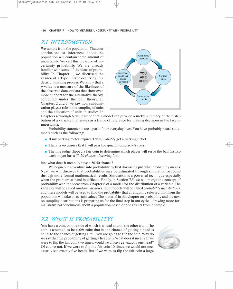
7.1 INTRODUCTIONWe sample from the population.Thus, ourconclusions or inferences about thepopulation will contain some amount ofuncertainty. We call this measure of un-certainty probability. We are alreadyfamiliar with some of the ideas of proba-bility. In Chapter 1, we discussed thechance of a Type I error occurring in adecision-making process.We know that ap-value is a measure of the likeliness ofthe observed data, or data that show evenmore support for the alternative theory,computed under the null theory. InChapters 2 and 3, we saw how randomi-zation plays a role in the sampling of unitsand the allocation of units in studies. InChapters 4 through 6, we learned that a model can provide a useful summary of the distri-bution of a variable that serves as a frame of reference for making decisions in the face ofuncertainty.
Probability statements are a part of our everyday lives.You have probably heard state-ments such as the following:
■ If my parking meter expires, I will probably get a parking ticket.
■ There is no chance that I will pass the quiz in tomorrow’s class.
■ The line judge flipped a fair coin to determine which player will serve the ball first, soeach player has a 50-50 chance of serving first.
Just what does it mean to have a 50-50 chance?We begin our adventure into probability by first discussing just what probability means.
Next, we will discover that probabilities may be estimated through simulation or foundthrough more formal mathematical results. Simulation is a powerful technique especiallywhen the problem at hand is difficult. Finally, in Section 7.5, we will merge the concept ofprobability with the ideas from Chapter 6 of a model for the distribution of a variable. Thevariables will be called random variables, their models will be called probability distributions,and these models will be used to find the probability that a randomly selected unit from thepopulation will take on certain values.The material in this chapter on probability and the nexton sampling distributions is preparing us for the final step in our cycle—drawing more for-mal statistical conclusions about a population based on the results from a sample.
7.2 WHAT IS PROBABILITY?You have a coin, on one side of which is a head and on the other a tail.Thecoin is assumed to be a fair coin; that is, the chance of getting a head isequal to the chance of getting a tail.You are going to flip the coin.Why dowe say that the probability of getting a head is What does it mean? If wewere to flip the fair coin two times, would we always get exactly one head?Of course not. If we were to flip the fair coin 10 times, we would not nec-essarily see exactly five heads. But if we were to flip the fair coin a large
12?
410 CHAPTER 7 HOW TO MEASURE UNCERTAINTY WITH PROBABILITY
Summarizeresults
Interpretresults &
makedecision
Collectdata
Formulatetheories
YOUARE
HERE
ALIAMC07_0131497561.QXD 03/28/2005 05:55 PM Page 410
7.2 WHAT IS PROBABILITY? 411
Think About It
number of times, we would expect about half of the flips to result in a head. This use ofthe word probability is based on the relative-frequency interpretation, which applies tosituations in which the conditions are exactly repeatable. The probability of an outcome isdefined as the proportion of times the event would occur if the process were repeated overand over many times under the same conditions. This is also called the long-term relativefrequency of the outcome.
DEFINITION: The probability that an outcome will occur is the proportion of time it oc-curs over the long run—that is, the relative frequency with which that outcome occurs.
The emphasis on long term or in the long run is very important. The probability of a headbeing equal to does not mean that we will get one head in every two flips of the coin. Flip-ping the coin four times and observing the sequence THTT would not be strong evidencethat the probability of a head is However, if, out of 1000 coin flips, approximately 25% ofthe outcomes were heads, then it would be more reasonable to conclude that the coin wasbiased and the probability of getting a head is closer to 0.25, rather than the fair value of As we increase the total number of flips, we would expect the proportion of heads to beginto settle down to a constant value. This value is what we assign as the probability of gettinga head.
12.
14.
12
Pennies on EdgePeople often flip a coin to make a random selection between two options, based on theassumption that the coin is fair (that is, the probability of getting a head is ). Suppose thatyou stand a penny on its edge and then make it fall over by using your hand with a downwardstroke (palm side down) and striking the table. Would the probability of getting a head stillbe
How would you determine this probability of a head?
Would you use one penny or different pennies? How many repetitions would you do?
Try it and see what happens!
12?
12
The relative-frequency approach to defining probabilities applies to situations thatcan be thought of as being repeatable under similar conditions. Some situations are notlikely to be repeated under the same conditions. You are planning an outdoor party for theupcoming Saturday afternoon from 2 p.m. to 4 p.m. What is the probability that it will rainduring the party? Two softball teams, the Jaguars and the Panthers, have made it to the finalgame of the tournament.What is the probability that the Jaguars will beat the Panthers? Insuch situations, a person would use his or her own experiences, background, and knowl-edge to assign a probability to the outcome. Such probabilities are called personal or subj-ective probabilities, which represent a person’s degree of belief that the outcome willhappen. Different people may arrive at different personal probabilities, all of which wouldbe considered correct. Any probability, however, must be between 0 and 1 (or 0% and100%). There are certain rules that should be met. We will learn about some of these rulesin Section 7.4.
ALIAMC07_0131497561.QXD 03/28/2005 05:55 PM Page 411
412 CHAPTER 7 HOW TO MEASURE UNCERTAINTY WITH PROBABILITY
Probabilities help us make decisions. On the Friday night before the party, the weatherforecast stated that on Saturday there would be periods of rain and a high temperature of68 degrees. Even though it may not rain, based on this information, you decide to set up andhold the party indoors instead of outdoors. You need to fly to Chicago to attend a boardmeeting for Tuesday afternoon and wish to book a flight leaving Tuesday morning.There aretwo airlines that each offer a flight which, if on time, would allow you to make your meeting.One airline has a record that boasts that 88% of such flights to Chicago are on time. For theother airline, the probability of being on time is reported to be only 73%. These probabili-ties, along with other information, such as price or safety records, would help you decidewhich flight to reserve. However, no matter which airline is selected, your particular flight willeither be on time, or it will not be on time. Probabilities cannot determine whether the out-come will occur for any individual case.
We will focus on the relative-frequency approach to defining probability. In the coinflipping example, there are two methods for determining the probability of getting a head thatboth fit the relative-frequency interpretation. We might assume that coins are made suchthat the two possible outcomes are equally likely, thus assigning the probability of to eachoutcome. We might actually observe the relative frequency of getting a head by repeatedlyflipping the coin a large number of times and using the relative frequency as an estimate ofthe probability of getting a head.This process of estimating probabilities through simulationis our next topic.
7.3 SIMULATING PROBABILITIESOne of the basic components in the study of probability is a random process. A randomprocess is one that can be repeated under similar conditions. Although the set of possibleoutcomes is known, the exact outcome for an individual repetition cannot be predicted withcertainty. However, there is a predictable long-term pattern such that the relative frequencyfor a given outcome to occur settles down to a constant value. Flipping a fair coin is an ex-ample of a random process.We have worked with other random processes—selecting vouch-ers out of a bag, assigning subjects to receive one of two treatments, or selecting a registeredvoter at random from a population of registered voters.
12
DEFINITION: A random process is a repeatable process whose set of possible outcomesis known, but the exact outcome cannot be predicted with certainty. However, there is apredictable long-term pattern of outcomes such that the relative frequency for a givenoutcome to occur settles down to a constant value.
Some probabilities can be very difficult or time consuming to calculate.We may be ableto estimate the probability through simulation. To simulate means to imitate—to generateconditions that approximate the actual conditions. To simulate a random process, we coulduse any one of a number of different devices: a calculator, a computer program, or a table ofrandom numbers.We would first need to specify the conditions of the underlying random cir-cumstance (that is, provide a model that lists the possible individual outcomes and corre-sponding probabilities). Next, we need to outline how to simulate an individual outcome andhow to represent a single repetition of the random process. Finally, you simulate many rep-etitions, say n repetitions are simulated, and determine the number of times that the eventof interest occurred, say x times. The corresponding relative frequency, , would be usedto estimate the probability of that event.
x>n
ALIAMC07_0131497561.QXD 03/28/2005 05:55 PM Page 412
7.3 SIMULATING PROBABILITIES 413
Let’s apply these basic steps to estimate some probabilities.
DEFINITION: A simulation is the imitation of random or chance behavior using randomdevices such as random number generators or a table of random numbers.The basic steps for finding a probability by simulation are as follows:
Step 1: Specify a model for the individual outcomes of the underlying randomphenomenon.
Step 2: Outline how to simulate an individual outcome and how to represent a singlerepetition of the random process.
Step 3: Simulate many repetitions, say, n times, determine the number of times x thatthe event occurred in the n repetitions, and estimate the probability of the eventby its relative frequency, .x>n
Example 7.1 ◆ How Many Heads?ProblemConsider the random process of flipping a fair coin 10 times. One possible resultingsequence is HHTHHHTHHH. This sequence has a total of eight heads.(a) Specify the model for an individual outcome of tossing a fair coin.(b) What is the probability of getting a total of eight heads in 10 flips of a fair coin? First
estimate the probability with a simulation.Then try to determine the actual probabilitybased on the fair coin model.
(c) Would a total of eight heads be considered unusual if the coin were actually fair?
Solution(a) The individual outcomes are a head and a tail, and for a fair coin, the probability of each
would be (b) To get the approximate probability value we will simulate individual outcomes and rep-
etitions of the experiment of flipping a coin 10 times.A computer or calculator could beused to generate a random sequence of the integers 1 and 2 where a 1 could representa head and a 2 could represent a tail. We would need to simulate 10 flips of a fair cointo represent a single repetition.
For the TI graphing calculator, setting the seed value to 18 and using therandInt(1, 2) function, the first 10 generated integers would be 1, 1, 1, 1, 1, 2, 1, 1, 1, 2.This sequence would represent the coin flip sequence of HHHHHTHHHT, which doeshave a total of eight heads.
To represent the flipping of a fair coin using a random number table with digits0, 1, 2, through 9, you might designate that the five odd digits will correspond to a headand the five even digits to a tail. Using Table I, starting at Row 10, Column 1, readingleft to right, the first 10 digits are 8, 5, 4, 7, 5, 3, 6, 8, 5, 7. This sequence would representthe coin flip sequence of THTHHHTTHH, which has a total of six heads, not eight.
Next we need to repeat this process many times. The following data provide theresults of 50 repetitions using the TI calculator with a seed value of 18 (the outcomesresulting in eight heads (or 1’s) are highlighted in bold). There are two sequences
12.
ALIAMC07_0131497561.QXD 03/28/2005 05:55 PM Page 413
414 CHAPTER 7 HOW TO MEASURE UNCERTAINTY WITH PROBABILITY
Let's Do It!
7.17.1
among the fifty with eight heads, they are the first and the third sequences in the firstcolumn.
1111121112 1222222212 1122122111 2211112212 12222221221111122122 1121121211 1122121212 1221221221 12111111221212111111 1222111211 2111111222 1211122121 12122211212211222111 1121221211 2111212121 1221212221 11212212112122221222 1121121211 2212121121 2112111121 22221222212111211122 2112221222 1222122221 2221122222 21222111222212121111 2112211221 1222112212 1221112121 22111221211221122222 1112212112 2112221121 2212221221 11212212222211112221 2111211221 1212122211 1212121121 12112222211112212211 1121221212 1121121122 2121212122 2122121211
Since we have just 2 out of 50 repetitions resulting in a total of eight heads, our estimatedprobability is or 0.04. In this simulation, we did pretty well. As it turns out, thereare 45 ways to obtain a total of eight heads out of 10 flips of a fair coin and a total of1024 equally likely possible sequences of 10 flips. So the actual probability of getting eightheads is
(c) A total of eight heads is considered pretty unusual if the coin were actually fair sincethe probability of this to occur is just 0.044.
What We’ve Learned: Simulation, if feasible, is a powerful way to approximate probabilities.
45>1024 = 0.043945.
2>50
A Family PlanA couple plans to have children. They would like to have a boy to beable to pass on the family name.After some discussion, they decide tocontinue to have children until they have a boy or until they havethree children, whichever comes first.What is the probability that theywill have a boy among their children? Let’s simulate this couple’sfamily plan and estimate this probability.
Step 1: Specify a model for the individual outcomes.The random process is to continue to have children until a boy is born or untilthere are a total of three children, whichever comes first. The individual randomphenomenon is to “have a child” and the response of interest is its “gender.” Weneed to start with some basic assumptions about these individual outcomes of“girl” and “boy.” It seems fairly reasonable to assume that■ each child has probability of being a boy and of being a girl, and■ the gender of successive children is independent (that is, knowing the gender of
a child does not influence the gender of any of the successive children).
Step 2: Simulate individual outcomes and a repetition.We will need to simulate the gender of a single child. We can use a calculator orcomputer with a built-in random number generator to simulate an individual out-come. There are only two possible outcomes, boy and girl, so we need to generate
12
12
ALIAMC07_0131497561.QXD 03/28/2005 05:55 PM Page 414

7.3 SIMULATING PROBABILITIES 415
a random sequence of two values (for example, 1 and 2). We need to decide whichvalue will represent a boy and which will represent a girl:
To simulate one repetition of the family plan, we will use successive random val-ues until either a boy (a “1”) or three children (three girls, “222”) are obtained.
Using the TI graphing calculator with a seed value of 102 and we canwrite down the first few values and,below each, write either a “B” or a“G” to represent a boy or a girl out-come and then add a line to separatesuccessive repetitions. The followingis an example of a total of five repeti-tions of the family plan:(a) In the first repetition, how many children did the couple have? One
Did the couple have a boy? Yes
(b) In the second repetition, how many children did the couple have? Did the couple have a boy?
(c) In the third repetition, how many children did the couple have? Did the couple have a boy?
Note: If you do not have a random number generator, you can use a table of ran-dom numbers. If we use a table of random numbers, we have 10 digits, 0 through 9.A single random digit can simulate the gender of a single child. We need to decidewhich five numbers will represent, for example, a boy:
let the child is a boy,
then the child is a girl.
To simulate one repetition of the familyplan, we will use successive random digits untileither a boy or three children are obtained. Starting at Row 14, Column 1 ofTable I, reading left to right, the first few digits are recorded with either a “B” or a“G” below each to represent a boy or a girl outcome and a line to separate suc-cessive repetitions.
Step 3: Simulate many repetitions and estimate the probability.Working with a partner or in small groups, simulate many repetitions of the familyplan and use the relative frequency of the event “the couple has a boy” to estimateits probability. Using your calculator with your group’s choice of a seed or therandom-number table with your group’s choice of a starting point, simulate a totalof 10 repetitions. Start by writing out a list of a number of generated values. Beloweach value, write either a “B” or a “G” to represent a boy or a girl outcome, thenadd a line to separate successive repetitions.You will generally need more than just10 values. You need to generate enough values to be able to have 10 lines, repre-senting 10 completed repetitions.
=
=0 2 4 6 8
N = 2,
Let 1 = the child is a boy, then let = the child is a girl.
End of thefirst repetition
End of thefifth repetition
1B
1B1B
2G
1B
2G
2G
1B
1B
End of thefirst repetition
2B
1G
1G
6B
5G
6B
3G
0B
1G
ALIAMC07_0131497561.QXD 03/28/2005 05:55 PM Page 415
416 CHAPTER 7 HOW TO MEASURE UNCERTAINTY WITH PROBABILITY
(a) Out of the first 10 repetitions, how many times did the couple have a boy?
(b) Your group’s estimate of the probability that this strategy will produce aboy is .
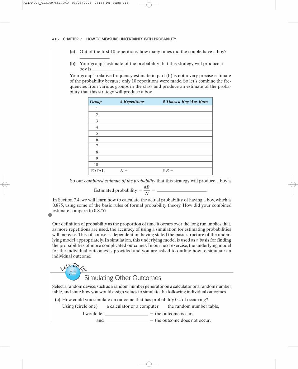
Your group’s relative frequency estimate in part (b) is not a very precise estimateof the probability because only 10 repetitions were made. So let’s combine the fre-quencies from various groups in the class and produce an estimate of the proba-bility that this strategy will produce a boy.
Group # Repetitions # Times a Boy Was Born
1
2
3
4
5
6
7
8
9
10
TOTAL N � # B �
So our combined estimate of the probability that this strategy will produce a boy is
.
In Section 7.4, we will learn how to calculate the actual probability of having a boy, which is0.875, using some of the basic rules of formal probability theory. How did your combinedestimate compare to 0.875?
Estimated probability =
#BN
=
Our definition of probability as the proportion of time it occurs over the long run implies that,as more repetitions are used, the accuracy of using a simulation for estimating probabilitieswill increase. This, of course, is dependent on having stated the basic structure of the under-lying model appropriately. In simulation, this underlying model is used as a basis for findingthe probabilities of more complicated outcomes. In our next exercise, the underlying modelfor the individual outcomes is provided and you are asked to outline how to simulate anindividual outcome.
Let's Do It!
7.27.2Simulating Other Outcomes
Select a random device,such as a random number generator on a calculator or a random numbertable, and state how you would assign values to simulate the following individual outcomes.
(a) How could you simulate an outcome that has probability 0.4 of occurring?Using (circle one) a calculator or a computer the random number table,
and = the outcome does not occur.
I would let = the outcome occurs
ALIAMC07_0131497561.QXD 03/28/2005 05:55 PM Page 416
7.3 SIMULATING PROBABILITIES 417
(b) How could you simulate a random process having four possible outcomes,represented by A, B, C, and D, with respective probabilities 0.1, 0.2, 0.3, and 0.4 ofoccurring?
Using (circle one) a calculator or a computer the random number table,
(c) How could you simulate an outcome that has probability 0.45 of occurring?
Using (circle one) a calculator or a computer the random number table.
and = the outcome does not occur.
I would let = the outcome occurs
let = Outcome C occurs, and
= Outcome D occurs.
I would let = Outcome A occurs,
= Outcome B occurs,Let
's Do It!
7.37.3The Three Doors
There are three doors. Behind one door is a car. Behind each of the other two doors is a goat.As a contestant, you are asked to select a door, with the idea that you will receive the prizethat is behind that door. The game host knows what is behind each door. After you select adoor, the host opens one of the remaining doors that has a goat behind it. Note that, nomatter which door you select, at least one of the remaining doors for the host to open has agoat behind it. The host then gives you the following two options:
1. Stay with the door you originally selected and receive the prize behind it.2. Switch to the other remaining closed door and receive the prize behind it.
What is the probability of winning the car if you stay with your original choice? What is theprobability of winning the car if you switch? Will switching increase your chance of winningthe car? Does your neighbor agree with you?
If the answer is not clear, you could carry out a simulation to estimate the probabilityof winning if you stay and the probability of winning if you switch.
Here is one way to simulate the game show: Working with a partner, designate oneperson to be the game host and the other the contestant (you can switch roles halfway throughthe simulation). The game host controls the three doors, represented by three index cards.These three cards are identical except that on the back of one of the cards there is a car andthe back of the other two cards is a goat. (Note: Three cards from a standard deck will alsowork, a black-suited card as the car, and two red-suited cards as the goats.) The host will layout the three cards blank side up, making sure he or she knows which has the car on theother side. You begin to take turns playing the game and, as you do, keep a record sheet,listing your strategy as either stay or switch, and the outcome as either win a car or win a goat.Once you have performed many repetitions, you can use the relative frequencies to estimatethe corresponding probabilities.
ALIAMC07_0131497561.QXD 03/28/2005 05:55 PM Page 417
418 CHAPTER 7 HOW TO MEASURE UNCERTAINTY WITH PROBABILITY
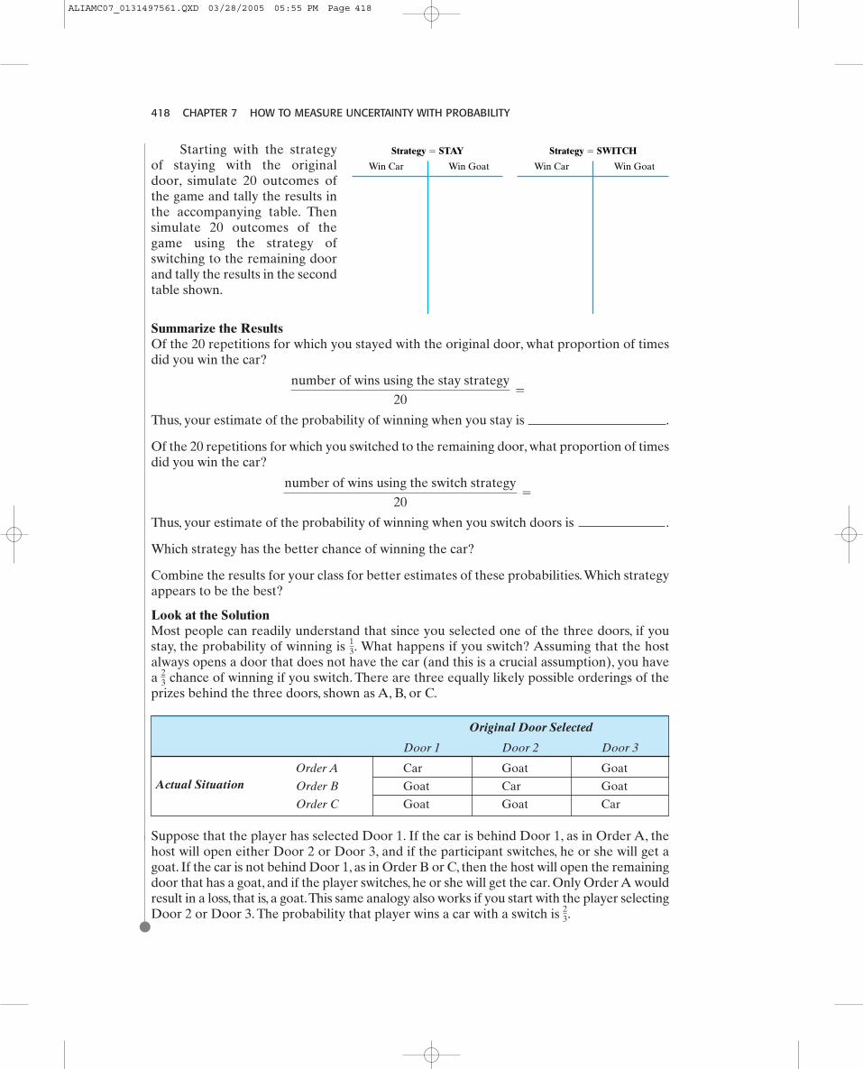
Original Door Selected
Door 1 Door 2 Door 3
Order A Car Goat Goat
Order B Goat Car Goat
Order C Goat Goat Car
Actual Situation
Suppose that the player has selected Door 1. If the car is behind Door 1, as in Order A, thehost will open either Door 2 or Door 3, and if the participant switches, he or she will get agoat. If the car is not behind Door 1, as in Order B or C, then the host will open the remainingdoor that has a goat, and if the player switches, he or she will get the car. Only Order A wouldresult in a loss, that is, a goat.This same analogy also works if you start with the player selectingDoor 2 or Door 3. The probability that player wins a car with a switch is 23.
Starting with the strategyof staying with the originaldoor, simulate 20 outcomes ofthe game and tally the results inthe accompanying table. Thensimulate 20 outcomes of thegame using the strategy ofswitching to the remaining doorand tally the results in the secondtable shown.
Summarize the ResultsOf the 20 repetitions for which you stayed with the original door, what proportion of timesdid you win the car?
Thus, your estimate of the probability of winning when you stay is .
Of the 20 repetitions for which you switched to the remaining door, what proportion of timesdid you win the car?
Thus, your estimate of the probability of winning when you switch doors is .
Which strategy has the better chance of winning the car?
Combine the results for your class for better estimates of these probabilities.Which strategyappears to be the best?
Look at the SolutionMost people can readily understand that since you selected one of the three doors, if youstay, the probability of winning is What happens if you switch? Assuming that the hostalways opens a door that does not have the car (and this is a crucial assumption), you havea chance of winning if you switch. There are three equally likely possible orderings of theprizes behind the three doors, shown as A, B, or C.
23
13.
number of wins using the switch strategy20
=
number of wins using the stay strategy20
=
Strategy � STAY Strategy � SWITCH
Win Car Win Goat Win Car Win Goat
ALIAMC07_0131497561.QXD 03/28/2005 05:55 PM Page 418
7.3 SIMULATING PROBABILITIES 419
7.3 EXERCISES7.1 For each of the following probabilities, state whether the relative-frequency approach or
personal probability would be most appropriate for determining the probability:(a) Tom, the manager of a small apartment complex, recently installed new doorbells for
each apartment. According to Tom, about of the doorbells will not be working in6 months and will need replacing.
(b) The manufacturer of the doorbells used by Tom in his apartment complex reports thatthe probability a doorbell will become defective within the 6-month warranty periodis 0.03.
7.2 For each of the following probabilities, state whether the relative-frequency approach orpersonal probability would be most appropriate for determining the probability:(a) The probability of getting 10 true or false questions correct on a quiz, if for each ques-
tion you were simply guessing the answer.(b) The probability that you will be living in a different state within the next two years.
7.3 In Section 7.2, two interpretations of probability were discussed, the long-run relative-frequency approach and personal probability. For some probabilities the long-run relative-frequency approach may not be appropriate. Provide an example and explain your answer.
7.4 Refer to Example 7.1 and use the results in the table of 50 repetitions to estimate the fol-lowing probabilities:(a) Estimate the probability of getting exactly five heads in 10 flips of a fair coin.(b) Estimate the probability of getting fewer than three heads in 10 flips of a fair coin.(c) Estimate the probability of getting more than three heads in 10 flips of a fair coin.(d) Estimate the probability of getting a run of at least six consecutive heads in row in 10 flips
of a fair coin.
7.5 Is Your Coin Fair?(a) Take a coin, flip it 10 times, and record the number of times that resulted in a head.(b) Repeat part (a) an additional 9 times for a total of 100 flips, keeping track of the number
of heads for each set of 10 flips and the cumulative proportion after each additional setof 10 flips.
(c) Make a series plot of the cumulative proportion of heads after each set of 10 flips.(d) Did the proportion of heads start to settle down around a constant value? What is that
approximate value? Do you think your coin is fair?
7.6 A Family Plan Revisited Recall the couple who plans to continue to have children until theyhave a boy or until they have three children, whichever comes first. We estimated the prob-ability that they will have a boy among their children. We compared our combined estimateto the actual probability of 0.875.(a) Generate an additional 100 repetitions of this family plan (using a seed value of 102, or
Row 25, Column 1 of the random number table). Report the total number of repetitionsresulting in having a boy.
(b) Combine the results from “Let’s do it! 7.1” with those in part (a) and report an updatedcombined estimate of the probability that this strategy will produce a boy. How does thisestimate compare to 0.875?
(c) Suppose that the family plan is to continue to have children until they have a boy oruntil they have four children, whichever comes first. Do you think the probability of hav-ing a boy with this strategy will be larger than, smaller than, or equal to 0.875? Performa simulation and estimate this probability.
7.7 Planning a Family The Smiths are planning their family and both want an equal numberof boys and girls. Mrs. Smith says that their chances are best if they plan on having two
14
ALIAMC07_0131497561.QXD 03/28/2005 05:55 PM Page 419
420 CHAPTER 7 HOW TO MEASURE UNCERTAINTY WITH PROBABILITY
children. Mr. Smith says that they have a better chance of having an equal number of boysand girls if they plan on having four children.(a) Assuming that boy and girl babies are equally likely, who do you think is correct?
Mrs. Smith, Mr. Smith, or are they both correct?(b) Check your answer to part (a) by performing a simulation.To have comparable precision
in your probability estimates, use the same number of repetitions for both Mrs. Smith’sstrategy and Mr. Smith’s strategy. Provide all relevant details and a summary of yourresults.
7.8 ESP? A classic experiment to detect ESP uses a shuffled deck of five cards—one witha wave, one with a star, one with a circle, one with a square, and one with a cross. A total of10 cards will be drawn, one by one, with replacement, from this deck. The subject is asked toguess the symbol on each card drawn.(a) If a subject actually lacks ESP, what is the probability that he or she will correctly guess
the symbol on a card?(b) If a subject actually has ESP, should the probability that he or she will correctly guess the
symbol on a card be smaller than, larger than, or the same as the probability in part (a)?(c) Julie thinks she has ESP. She wishes to test the following hypotheses:
Julie does not have ESP, so the probability of a correct answer is just 0.20.Julie does have ESP, so the probability of a correct answer is greater than 0.20.
Julie participates in the experiment and is right in 6 of 10 tries. You are asked to test, ata 1% significance level, the hypothesis that Julie has ESP. Design and carry out a simu-lation to estimate the p-value, that is, the chance of getting 6 or more correct answers outof 10, if indeed Julie was just guessing and does not have ESP. Based on your estimatedp-value, what is your conclusion?
7.9 Consider the process of playing a game in which the probability of winning is 0.20 and theprobability of losing is 0.80.(a) If you were to use your calculator or a random number table to simulate playing this
game, what numbers would you generate and how would you assign values to simulatewinning and losing?
(b) With your calculator (using a seed value of 72) or the random number table (Row 36,Column 1), simulate playing this game 50 times. Show the numbers generated and indi-cate which ones correspond to wins and which ones correspond to losses.
(c) From the simulated results, calculate an estimate of the probability of winning. How doesit compare to the actual probability of winning of 0.20?
7.4 THE LANGUAGE OF PROBABILITYIn this section, we turn to some of the basic ideas of probability and introduce some notationand rules. These rules will allow us to compute the probabilities of simple events andsome more complex events. We begin by listing some of the key components in the study ofprobability.
7.4.1 Sample Spaces and EventsFirst, we have a random process. This could be tossing a fair coin three times, rolling a pairof fair dice, or picking a registered voter at random. Next, we have the sample space oroutcome set for the random process.The sample space, denoted by S, is the set of all possible
H1:H0:
ALIAMC07_0131497561.QXD 03/28/2005 05:55 PM Page 420

7.4 THE LANGUAGE OF PROBABILITY 421
There are eight possible individual outcomes in this sample space. Since the coin is assumedto be fair, the eight outcomes can be assumed to be equally likely (that is, the probability as-signed to each individual outcome is ).
If the random process were tossing a fair coin three times and the outcome is definedas the number of heads, the sample space is given by There are four possibleoutcomes in this latest sample space. However, these four outcomes are not equally likely.Getting exactly one head is more likely to occur than getting zero heads, since three of theindividual outcomes correspond to the outcome of exactly one head andonly one individual outcome corresponds to zero heads
From these two examples we can see that
■ the sample space does not necessarily need to be a set of numbers, although a codingscheme could be established if the outcome is not numeric.
■ the definition of what constitutes an individual outcome is key in representing the samplespace correctly.
■ the individual outcomes in a sample space are not necessarily equally likely.
5TTT6.5HTT, THT, TTH6
S = 50, 1, 2, 36.18
Thirdtoss
Secondtoss
Firsttoss T
H
T
H
T
H
T
H
H
T
T
H
T
H
HHH
HHT
HTH
HTT
THH
THT
TTH
TTT
S � or S � {HHH, HHT, HTH, HTT THH, THT, TTH, TTT}.
Note: A comma is used to sep-arate each outcome in the list.
DEFINITION: A sample space or outcome set is the set of all possible individual out-comes of a random process. The sample space is typically denoted by S and may berepresented as a list, a tree diagram, an interval of values, a grid of possible values, andso on.
outcomes of the random process. If the random process were tossing a fair coin three times,then the outcomes that make up the sample space can be found in an orderly way using the“tree” method, as shown here.
ALIAMC07_0131497561.QXD 03/28/2005 05:55 PM Page 421

422 CHAPTER 7 HOW TO MEASURE UNCERTAINTY WITH PROBABILITY
Let's Do It!
7.57.5Voting Preference
Consider the process of randomly selecting two adults from Washtenaw County and recordingthe voting preference for each adult as Republican, Democrat, Independent, or Other. Thetwo adults randomly chosen (in the order selected) are Ryan and Caitlyn. Which of thefollowing gives the correct sample space for the set of possible outcomes of this experiment?Circle your answer.
(a)(b)(c)(d) None of the above.
S = 5Republican, Independent6.S = 5Republican, Democrat, Independent, Other6.S = 5Ryan, Caitlyn6.
Let's Do It!
7.47.4Sample Spaces
Give the sample space S for each of the following descriptions. Some are provided for youas examples.
(a) Toss a fair coin once:(b) Roll two fair dice:
(c) Roll two fair dice and record the sum of the values on the two dice:
(d) Take a random sample of size 10 from a lot of parts and record the number of defectivesin the sample:
(e) Select a student at random and record the time spent studying statistics in the last24-hour period:
(f) Select a bus commuter at random and record the waiting time between his or her arrivalat a bus stop and the arrival of the next bus to that stop:
S = 5
S = 5any time t between 0 hours and 24 hours 1inclusive26 or S = [0, 24].
S = 5
S = 5
S = 5
11, 12 11, 22 11, 32 11, 42 11, 52 11, 6212, 12 12, 22 12, 32 12, 42 12, 52 12, 6213, 12 13, 22 13, 32 13, 42 13, 52 13, 6214, 12 14, 22 14, 32 14, 42 14, 52 14, 6215, 12 15, 22 15, 32 15, 42 15, 52 15, 6216, 12 16, 22 16, 32 16, 42 16, 52 16, 62 6 .
S = 5H, T6.
ALIAMC07_0131497561.QXD 03/28/2005 05:55 PM Page 422
7.4 THE LANGUAGE OF PROBABILITY 423
Did you select (b) in the preceding “Let’s do it!” exercise? If so, you selected the correctsample space if the random process had been to randomly select exactly one adult fromWashtenaw County and record his or her voting preference.
Did you select (c)? If so, you selected a set that represents just one of the possible in-dividual outcomes, (R, I), which represents “Ryan is Republican and Caitlyn is Indepen-dent.”The correct answer is (d), since the actual sample space contains a total of 16 possibleindividual outcomes. We should also note that the outcome (R, I) is different from theoutcome (I, R), which represents “Ryan is Independent and Caitlyn is Republican.” In otherwords, the order of the responses does matter. If we actually surveyed a larger number ofadults and we were interested in learning about the proportion of adults for each of thepolitical preference categories, we might not be concerned about the order of the responses.
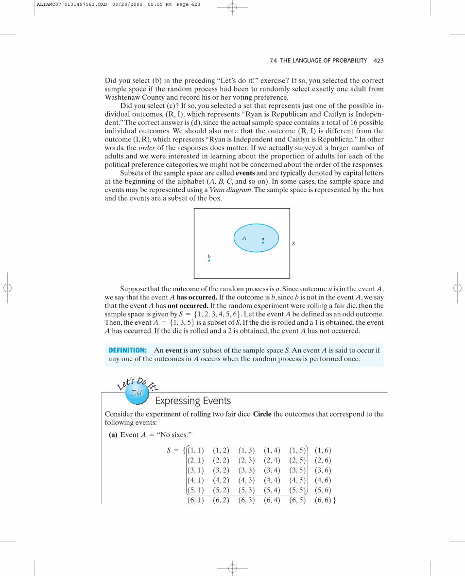
Subsets of the sample space are called events and are typically denoted by capital lettersat the beginning of the alphabet (A, B, C, and so on). In some cases, the sample space andevents may be represented using a Venn diagram.The sample space is represented by the boxand the events are a subset of the box.
SA a
b
DEFINITION: An event is any subset of the sample space S.An event A is said to occur ifany one of the outcomes in A occurs when the random process is performed once.
Let's Do It!
7.67.6Expressing Events
Consider the experiment of rolling two fair dice. Circle the outcomes that correspond to thefollowing events:
(a) Event
S = 5
11, 12 11, 22 11, 32 11, 42 11, 52 11, 6212, 12 12, 22 12, 32 12, 42 12, 52 12, 6213, 12 13, 22 13, 32 13, 42 13, 52 13, 6214, 12 14, 22 14, 32 14, 42 14, 52 14, 6215, 12 15, 22 15, 32 15, 42 15, 52 15, 6216, 12 16, 22 16, 32 16, 42 16, 52 16, 62 6
A = “No sixes.”
Suppose that the outcome of the random process is a. Since outcome a is in the event A,we say that the event A has occurred. If the outcome is b, since b is not in the event A, we saythat the event A has not occurred. If the random experiment were rolling a fair die, then thesample space is given by Let the event A be defined as an odd outcome.Then, the event is a subset of S. If the die is rolled and a 1 is obtained, the eventA has occurred. If the die is rolled and a 2 is obtained, the event A has not occurred.
A = 51, 3, 56S = 51, 2, 3, 4, 5, 66.
ALIAMC07_0131497561.QXD 03/28/2005 05:55 PM Page 423
424 CHAPTER 7 HOW TO MEASURE UNCERTAINTY WITH PROBABILITY
Let's Do It!
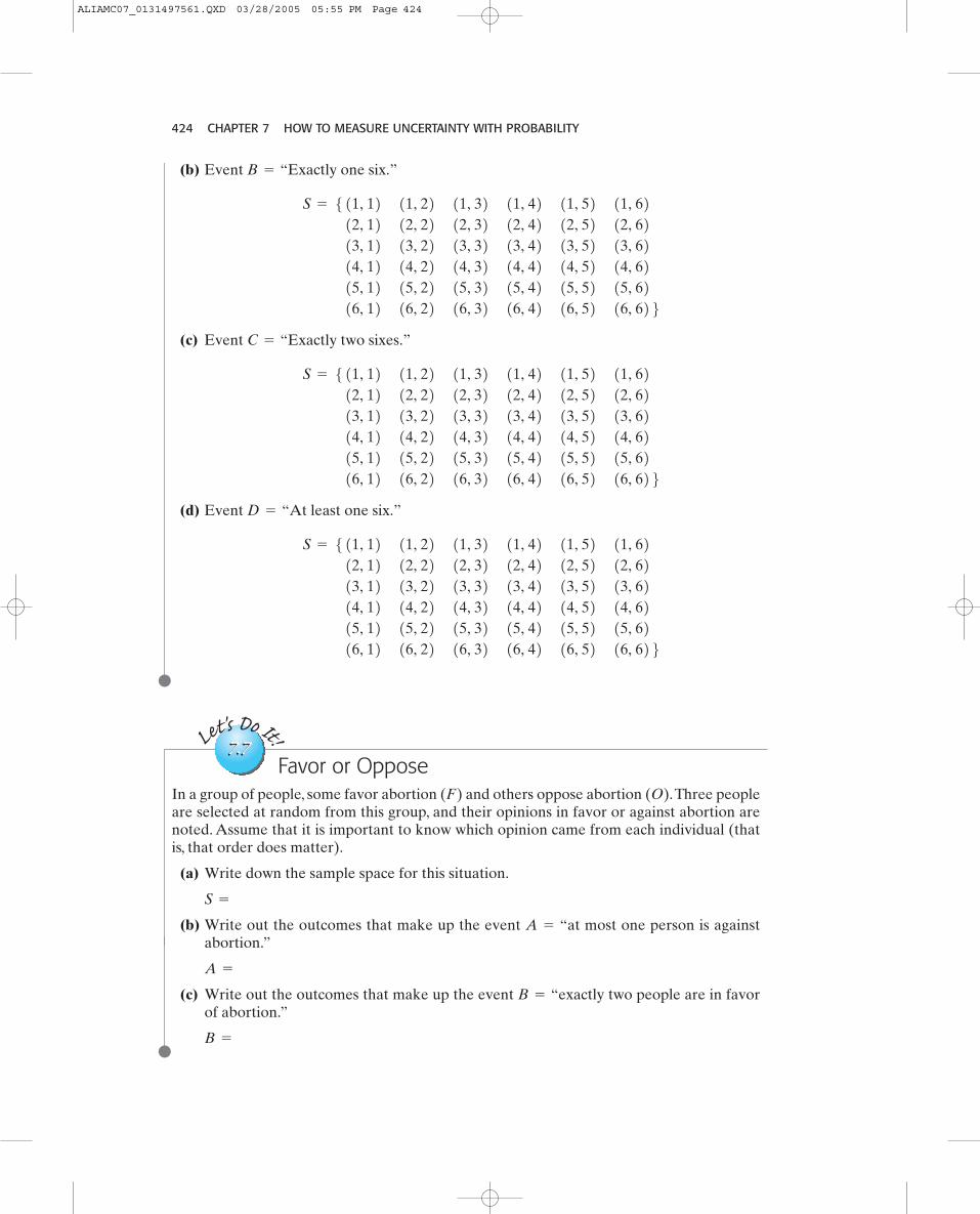
7.77.7Favor or Oppose
In a group of people, some favor abortion (F) and others oppose abortion (O).Three peopleare selected at random from this group, and their opinions in favor or against abortion arenoted. Assume that it is important to know which opinion came from each individual (thatis, that order does matter).
(a) Write down the sample space for this situation.
(b) Write out the outcomes that make up the event “at most one person is againstabortion.”
(c) Write out the outcomes that make up the event “exactly two people are in favorof abortion.”
B =
B =
A =
A =
S =
(b) Event
(c) Event
(d) Event
S = 5
11, 12 11, 22 11, 32 11, 42 11, 52 11, 6212, 12 12, 22 12, 32 12, 42 12, 52 12, 6213, 12 13, 22 13, 32 13, 42 13, 52 13, 6214, 12 14, 22 14, 32 14, 42 14, 52 14, 6215, 12 15, 22 15, 32 15, 42 15, 52 15, 6216, 12 16, 22 16, 32 16, 42 16, 52 16, 62 6
D = “At least one six.”
S = 5
11, 12 11, 22 11, 32 11, 42 11, 52 11, 6212, 12 12, 22 12, 32 12, 42 12, 52 12, 6213, 12 13, 22 13, 32 13, 42 13, 52 13, 6214, 12 14, 22 14, 32 14, 42 14, 52 14, 6215, 12 15, 22 15, 32 15, 42 15, 52 15, 6216, 12 16, 22 16, 32 16, 42 16, 52 16, 62 6
C = “Exactly two sixes.”
S = 5
11, 12 11, 22 11, 32 11, 42 11, 52 11, 6212, 12 12, 22 12, 32 12, 42 12, 52 12, 6213, 12 13, 22 13, 32 13, 42 13, 52 13, 6214, 12 14, 22 14, 32 14, 42 14, 52 14, 6215, 12 15, 22 15, 32 15, 42 15, 52 15, 6216, 12 16, 22 16, 32 16, 42 16, 52 16, 62 6
B = “Exactly one six.”
ALIAMC07_0131497561.QXD 03/28/2005 05:55 PM Page 424
7.4 THE LANGUAGE OF PROBABILITY 425
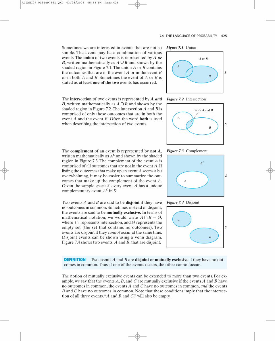
Sometimes we are interested in events that are not sosimple. The event may be a combination of variousevents. The union of two events is represented by A orB, written mathematically as and shown by theshaded region in Figure 7.1. The union A or B containsthe outcomes that are in the event A or in the event Bor in both A and B. Sometimes the event of A or B isstated as at least one of the two events has occurred.
The intersection of two events is represented by A andB, written mathematically as and shown by theshaded region in Figure 7.2. The intersection A and B iscomprised of only those outcomes that are in both theevent A and the event B. Often the word both is usedwhen describing the intersection of two events.
The complement of an event is represented by not A,written mathematically as and shown by the shadedregion in Figure 7.3. The complement of the event A iscomprised of all outcomes that are not in the event A. Iflisting the outcomes that make up an event A seems a bitoverwhelming, it may be easier to summarize the out-comes that make up the complement of the event A.Given the sample space S, every event A has a uniquecomplementary event in S.
Two events A and B are said to be disjoint if they haveno outcomes in common. Sometimes, instead of disjoint,the events are said to be mutually exclusive. In terms ofmathematical notation, we would write where represents intersection, and represents theempty set (the set that contains no outcomes). Twoevents are disjoint if they cannot occur at the same time.Disjoint events can be shown using a Venn diagram.Figure 7.4 shows two events, A and B, that are disjoint.
¤¨
A ¨ B = ¤,
AC
AC
A º B
A ª B
S
A
B
A or B
Figure 7.1 Union
S
A
B
Both A and B
Figure 7.2 Intersection
S
AC
A
Figure 7.3 Complement
S
A
B
Figure 7.4 Disjoint
DEFINITION: Two events A and B are disjoint or mutually exclusive if they have no out-comes in common. Thus, if one of the events occurs, the other cannot occur.
The notion of mutually exclusive events can be extended to more than two events. For ex-ample, we say that the events A, B, and C are mutually exclusive if the events A and B haveno outcomes in common, the events A and C have no outcomes in common, and the eventsB and C have no outcomes in common. Note that these conditions imply that the intersec-tion of all three events, “A and B and C,” will also be empty.
ALIAMC07_0131497561.QXD 03/28/2005 05:55 PM Page 425
426 CHAPTER 7 HOW TO MEASURE UNCERTAINTY WITH PROBABILITY
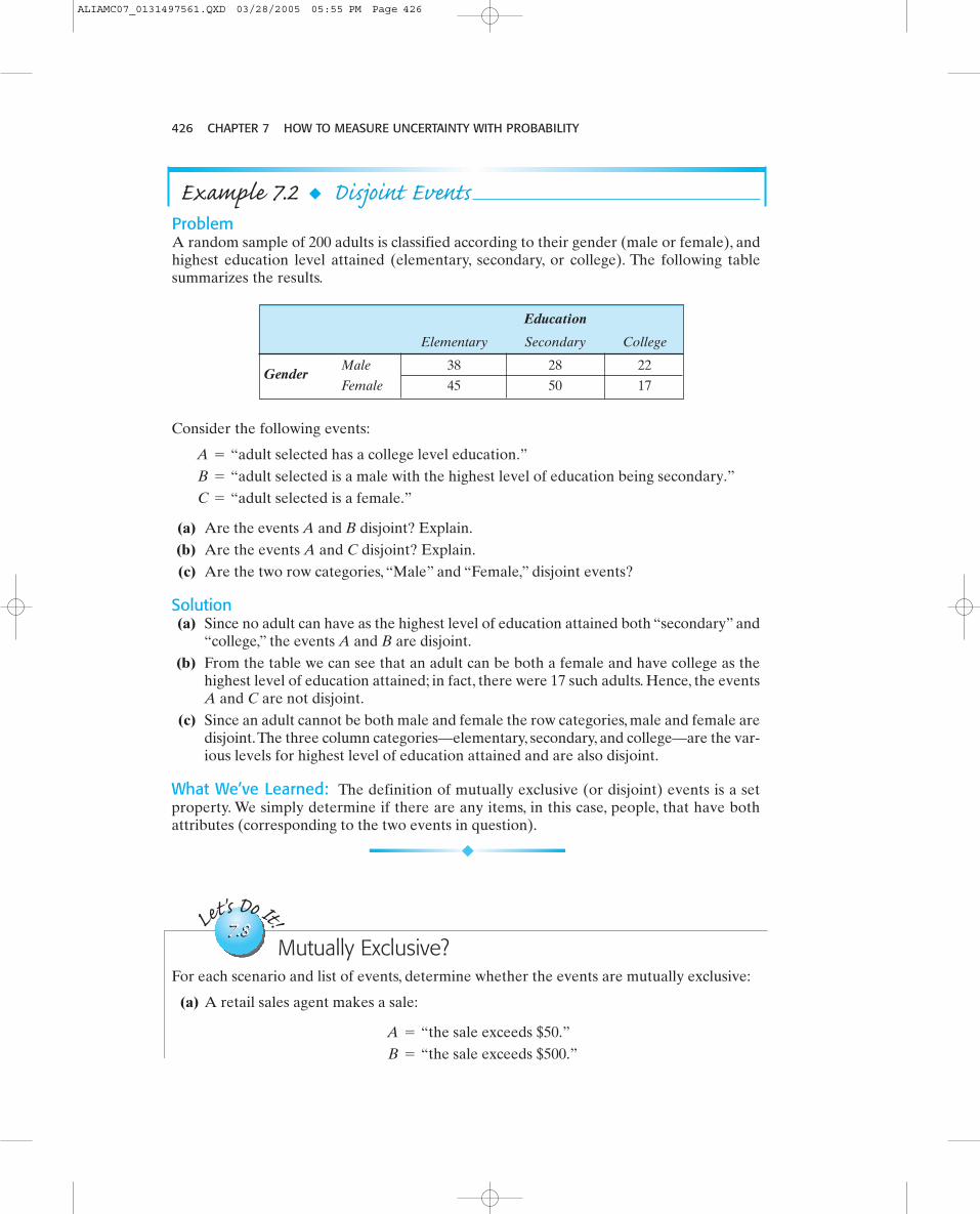
Example 7.2 ◆ Disjoint EventsProblemA random sample of 200 adults is classified according to their gender (male or female), andhighest education level attained (elementary, secondary, or college). The following tablesummarizes the results.
Education
Elementary Secondary College
Male 38 28 22
Female 45 50 17Gender
Consider the following events:
(a) Are the events A and B disjoint? Explain.(b) Are the events A and C disjoint? Explain.(c) Are the two row categories, “Male” and “Female,” disjoint events?
Solution(a) Since no adult can have as the highest level of education attained both “secondary” and
“college,” the events A and B are disjoint.(b) From the table we can see that an adult can be both a female and have college as the
highest level of education attained; in fact, there were 17 such adults. Hence, the eventsA and C are not disjoint.
(c) Since an adult cannot be both male and female the row categories, male and female aredisjoint.The three column categories—elementary, secondary, and college—are the var-ious levels for highest level of education attained and are also disjoint.
What We’ve Learned: The definition of mutually exclusive (or disjoint) events is a setproperty. We simply determine if there are any items, in this case, people, that have bothattributes (corresponding to the two events in question).
C = “adult selected is a female.” B = “adult selected is a male with the highest level of education being secondary.” A = “adult selected has a college level education.”
Let's Do It!
7.87.8Mutually Exclusive?
For each scenario and list of events, determine whether the events are mutually exclusive:
(a) A retail sales agent makes a sale:
B = “the sale exceeds $500.” A = “the sale exceeds $50.”
ALIAMC07_0131497561.QXD 03/28/2005 05:55 PM Page 426

7.4 THE LANGUAGE OF PROBABILITY 427
7.4 EXERCISES7.10 Each day a bus travels from City A to City D by way of Cities B and C (as shown). André is
a traveler who can get on the bus at any one of the cities and can get off at any other cityalong the route (except not the same city in which he got on the bus).
City A City B City C City D
(a) Give the sample space (all possible outcome pairs) for representing the starting and end-ing points of André’s journey.
(b) Let E be the event that André gets off at a city that comes after City B on the route ofthe bus. List the outcomes from the sample space in part (a) that make up the event E.
7.11 Two chess players, Gabe and Ellie, decide to play several games of chess.They will stop play-ing if Gabe wins two matches or if they have played a total of three games in all. Each gamecan be won by either Gabe or Ellie, and there can be no ties.(a) Give the sample space (all possible outcomes) for the series of games played by Gabe
and Ellie.(b) Let A be the event that no player wins two consecutive games. List the outcomes from
the sample space in part (a) that make up the event A.
7.12 Replacement and Order A basket contains three balls, one green, one yellow, and one white.Two balls will be selected from the basket. For example, the outcome “G,Y” represents thatthe green ball was selected, followed by the yellow ball.
Write out the corresponding sample space if(a) the sampling procedure was with replacement and order matters.(b) the sampling procedure was with replacement and order doesn’t matter.(c) the sampling procedure was without replacement and order matters.(d) the sampling procedure was without replacement and order doesn’t matter.
7.13 A simple random sample of students will be selected from a student body, and college status,classified as either full time or part time, will be recorded.(a) Give the sample space if just one student will be selected at random.(b) Give the sample space if four students will be selected at random.(c) Give the sample space if 20 students will be selected at random and the outcome of
interest is the number of full-time students.
7.14 At a formal conference a meeting takes place where one faculty member from each of thenine different colleges attends. Upon all faculty members arriving, each shakes hands with
(b) A retail sales agent makes a sale:
(c) Ten students are selected at random:
C = “at most five are female.” B = “at least seven are female.” A = “no more than three are female.”
C = “the sale exceeds $1000.” B = “the sale is between $100 and $500.” A = “the sale is less than $50.”
ALIAMC07_0131497561.QXD 03/28/2005 05:55 PM Page 427
428 CHAPTER 7 HOW TO MEASURE UNCERTAINTY WITH PROBABILITY
each other. How many handshakes are there? How can you express the answer in general ifthe meeting consists of one faculty from each of N colleges?
7.15 Disjoint? Consider the experiment of drawing a card from a standard deck. Letand
(a) Are the events A and B disjoint? Explain.(b) Are the events A and C disjoint? Explain.(c) Are the events B and C disjoint? Explain.
7.16 A travel agency offers ten different brochures, arranged in piles for customers to select from.One of the employees told a customer to take any selection of brochures they wish but notto take more than one of each kind.Assuming that the customer takes at least one brochure,how many different selections are possible?
7.4.2 Rules of ProbabilitiesWe return to the idea of probability and relate it to events and the outcomes of a samplespace. To any event A, we assign a number P(A) called the probability of the event A. Re-call that the probability of an event was defined as the relative frequency with which that eventwould occur in the long run. When the sample space contains a finite number of possibleoutcomes, we have another technique for assigning the probability of an event:
■ Assign a probability to each individual outcome, each being a number between 0 and1, such that the sum of these individual probabilities is equal to 1.
■ The probability of any event is the sum of the probabilities of the outcomes that makeup that event.
If the outcomes in the sample space are equally likely to occur, the probability of an event Ais simply the proportion of outcomes in the sample space that make up the event A. Do notautomatically assume that the outcomes in the sample space are equally likely—it will dependon the random process and the definition of the outcome that is being recorded. Our first ex-ercise does involve equally likely outcomes. Soon we will learn some probability rules thatwill help us determine the probabilities of outcomes that are not equally likely.
C = “spade.”A = “heart,” B = “king,”
Let's Do It!
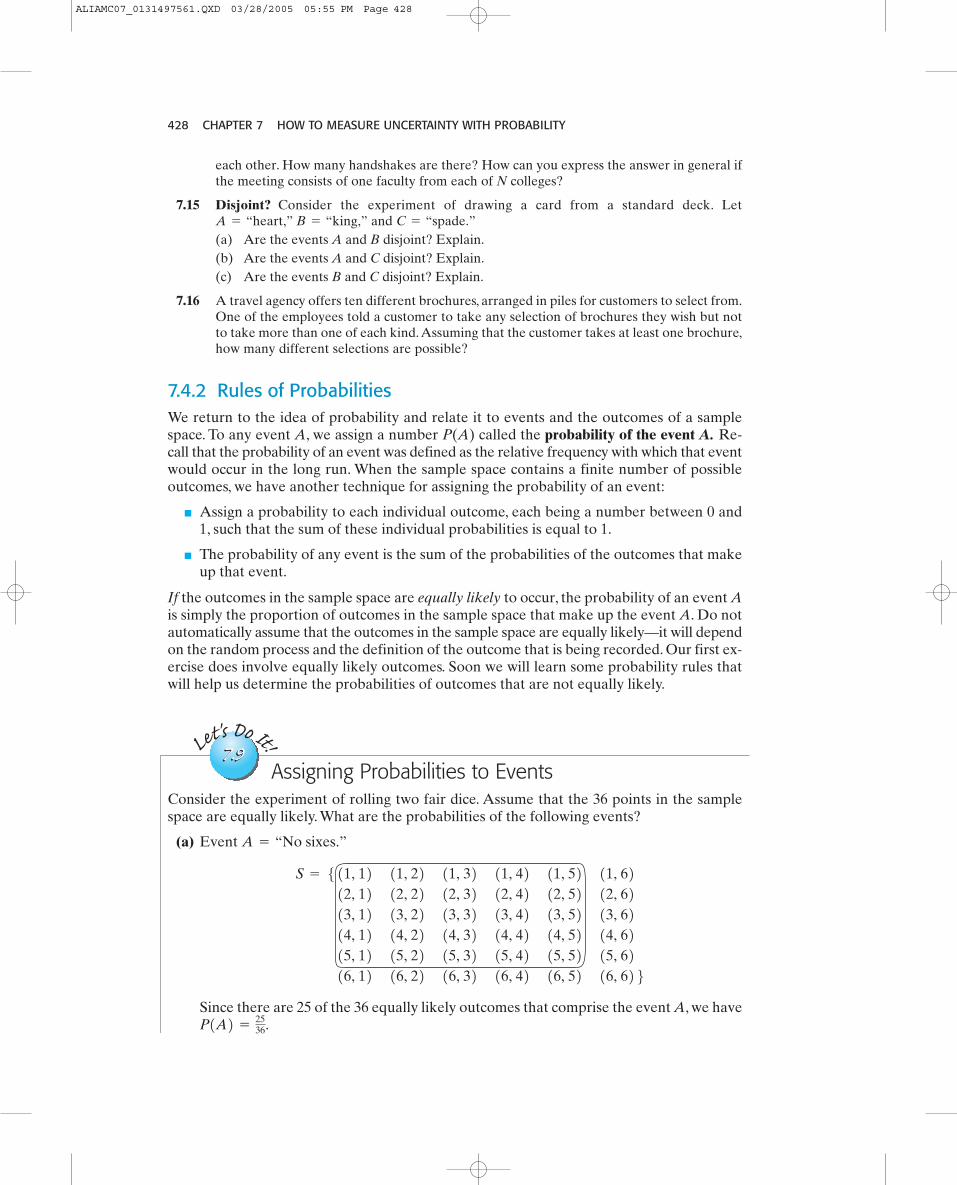
7.97.9Assigning Probabilities to Events
Consider the experiment of rolling two fair dice. Assume that the 36 points in the samplespace are equally likely. What are the probabilities of the following events?
(a) Event
Since there are 25 of the 36 equally likely outcomes that comprise the event A, we haveP1A2 =
2536.
S = 5
11, 12 11, 22 11, 32 11, 42 11, 52 11, 6212, 12 12, 22 12, 32 12, 42 12, 52 12, 6213, 12 13, 22 13, 32 13, 42 13, 52 13, 6214, 12 14, 22 14, 32 14, 42 14, 52 14, 6215, 12 15, 22 15, 32 15, 42 15, 52 15, 6216, 12 16, 22 16, 32 16, 42 16, 52 16, 62 6
A = “No sixes.”
ALIAMC07_0131497561.QXD 03/28/2005 05:55 PM Page 428
7.4 THE LANGUAGE OF PROBABILITY 429
The third rule is called the complement rule. Any event and its corresponding comple-ment are disjoint sets, which when brought back together give us the whole sample space S.The probability of the sample space S is 1, so the probabilities of the event and its comple-ment must add up to 1.This rule can be very useful. If finding the probability of an event seemstoo difficult, see if finding the probability of the complement of the event is easier.
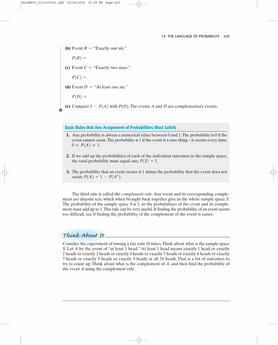
(b) Event
(c) Event
(d) Event
(e) Compare with P(D). The events A and D are complementary events.1 - P1A2P1D2 =
D = “At least one six.”
P1C2 =
C = “Exactly two sixes.”
P1B2 =
B = “Exactly one six.”
Think About ItConsider the experiment of tossing a fair coin 10 times.Think about what is the sample spaceS. Let A be the event of “at least 1 head.” At least 1 head means exactly 1 head or exactly2 heads or exactly 3 heads or exactly 4 heads or exactly 5 heads or exactly 6 heads or exactly7 heads or exactly 8 heads or exactly 9 heads or all 10 heads. That is a lot of outcomes totry to count up. Think about what is the complement of A, and then find the probability ofthe event A using the complement rule.
Basic Rules that Any Assignment of Probabilities Must Satisfy
1. Any probability is always a numerical value between 0 and 1.The probability is 0 if theevent cannot occur.The probability is 1 if the event is a sure thing—it occurs every time;
2. If we add up the probabilities of each of the individual outcomes in the sample space,the total probability must equal one;
3. The probability that an event occurs is 1 minus the probability that the event does notoccur; P1A2 = 1 - P1AC2.
P1S2 = 1.
0 … P1A2 … 1.
ALIAMC07_0131497561.QXD 03/28/2005 05:55 PM Page 429
430 CHAPTER 7 HOW TO MEASURE UNCERTAINTY WITH PROBABILITY
Let's Do It!
7.107.10A Fair Die?
A die, with faces 1, 2, 3, 4, 5, 6, is suspected to be unfair in the sense of having a tendencytoward showing the larger faces. We wish to test the following hypotheses:
The die is fair (that is, it has an equal chance for all six faces).The die has a tendency toward showing larger faces.
For the data, you will roll the die two times. Recall the 36 possible pairs of faces if you roll adie two times:
The sum of the two rolls will be the response used to make the decision between the twohypotheses.
(a) Consider the possible sum of 11. Circle the outcomes in the accompanying sample spacethat correspond to having a sum of 11.What is the probability of getting a sum of 11 onthe next two rolls?
The suggested format for the decision rule is to reject if the sum of the two rolls is too large.(b) The direction of extreme is (circle one)
one-sided to the right. one-sided to the left. two-sided.
(c) What is the p-value if the observed sum actually equals 11? (Hint: Think about thedefinition of a p-value.)
(d) Would an observed sum of 11 be statistically significant at the 5% significance level? atthe 10% level? Explain.
H0
S = 5
11, 12 11, 22 11, 32 11, 42 11, 52 11, 6212, 12 12, 22 12, 32 12, 42 12, 52 12, 6213, 12 13, 22 13, 32 13, 42 13, 52 13, 6214, 12 14, 22 14, 32 14, 42 14, 52 14, 6215, 12 15, 22 15, 32 15, 42 15, 52 15, 6216, 12 16, 22 16, 32 16, 42 16, 52 16, 62 6 .
H1:H0:
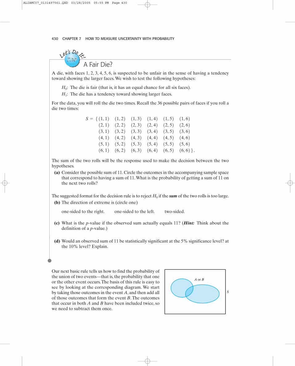
Our next basic rule tells us how to find the probability ofthe union of two events—that is, the probability that oneor the other event occurs.The basis of this rule is easy tosee by looking at the corresponding diagram. We startby taking those outcomes in the event A, and then add allof those outcomes that form the event B. The outcomesthat occur in both A and B have been included twice, sowe need to subtract them once.
S
A
B
A or B
ALIAMC07_0131497561.QXD 03/28/2005 05:55 PM Page 430
7.4 THE LANGUAGE OF PROBABILITY 431
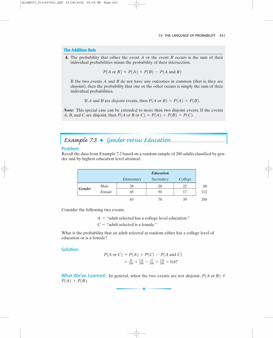
Example 7.3 ◆ Gender versus EducationProblemRecall the data from Example 7.2 based on a random sample of 200 adults classified by gen-der and by highest education level attained.
Education
Elementary Secondary College
Male 38 28 22 88
Female 45 50 17 112
83 78 39 200
Consider the following two events:
What is the probability that an adult selected at random either has a college level ofeducation or is a female?
Solution
What We’ve Learned: In general, when the two events are not disjoint,P1A2 + P1B2. P1A or B2 Z
=39
200 +112200 -
17200 =
134200 = 0.67
P1A or C2 = P1A2 + P1C2 - P1A and C2
C = “adult selected is a female.”
A = “adult selected has a college-level education.”
Gender
The Addition Rule
4. The probability that either the event A or the event B occurs is the sum of theirindividual probabilities minus the probability of their intersection.
If the two events A and B do not have any outcomes in common (that is, they aredisjoint), then the probability that one or the other occurs is simply the sum of theirindividual probabilities.
Note: This special case can be extended to more than two disjoint events. If the eventsA, B, and C are disjoint, then P1A or B or C2 = P1A2 + P1B2 + P1C2.
If A and B are disjoint events, then P1A or B2 = P1A2 + P1B2.
P1A or B2 = P1A2 + P1B2 - P1A and B2
ALIAMC07_0131497561.QXD 03/28/2005 05:55 PM Page 431
432 CHAPTER 7 HOW TO MEASURE UNCERTAINTY WITH PROBABILITY
Sometimes, we will have some given information about the outcome of the randomprocess. We may wish to update the probability of a certain event occurring taking into ac-count this given information. Consider rolling a single fair die one time.The sample space is
and each of the six outcomes is equally likely.The probability of gettingthe value of 1 is then But suppose that we know the outcome was an odd value: Now, whatis the probability that the value is a 1? Since we know the outcome was an odd value, we nolonger consider the original sample space as the set of possible outcomes. There are onlythree possible outcomes in the updated sample space—namely, Each of these threeoutcomes is now equally likely.Thus, the updated probability is What we have just computedis a conditional probability, the probability of the event given the event
has occurred, represented by the general expression In other words,conditioning on the fact that the event B has occurred, we wish to find the updated proba-bility that the event A will occur.
Our next rule tells us how to find suchconditional probabilities. The basis of thisrule is easy to see by looking at the corre-sponding diagram. Since we know that theevent B has occurred, we start by taking onlythose outcomes in the event B. This set ofoutcomes is our updated sample space andwill form the base of our probability expres-sion. We wish to find the probability of the
P1A ƒB2.B = 5ODD6 A = 516,13.51, 3, 56.
16.
S = 51, 2, 3, 4, 5, 66,
A
B
B � updated sample space
A given B Original samplespace S
Let's Do It!
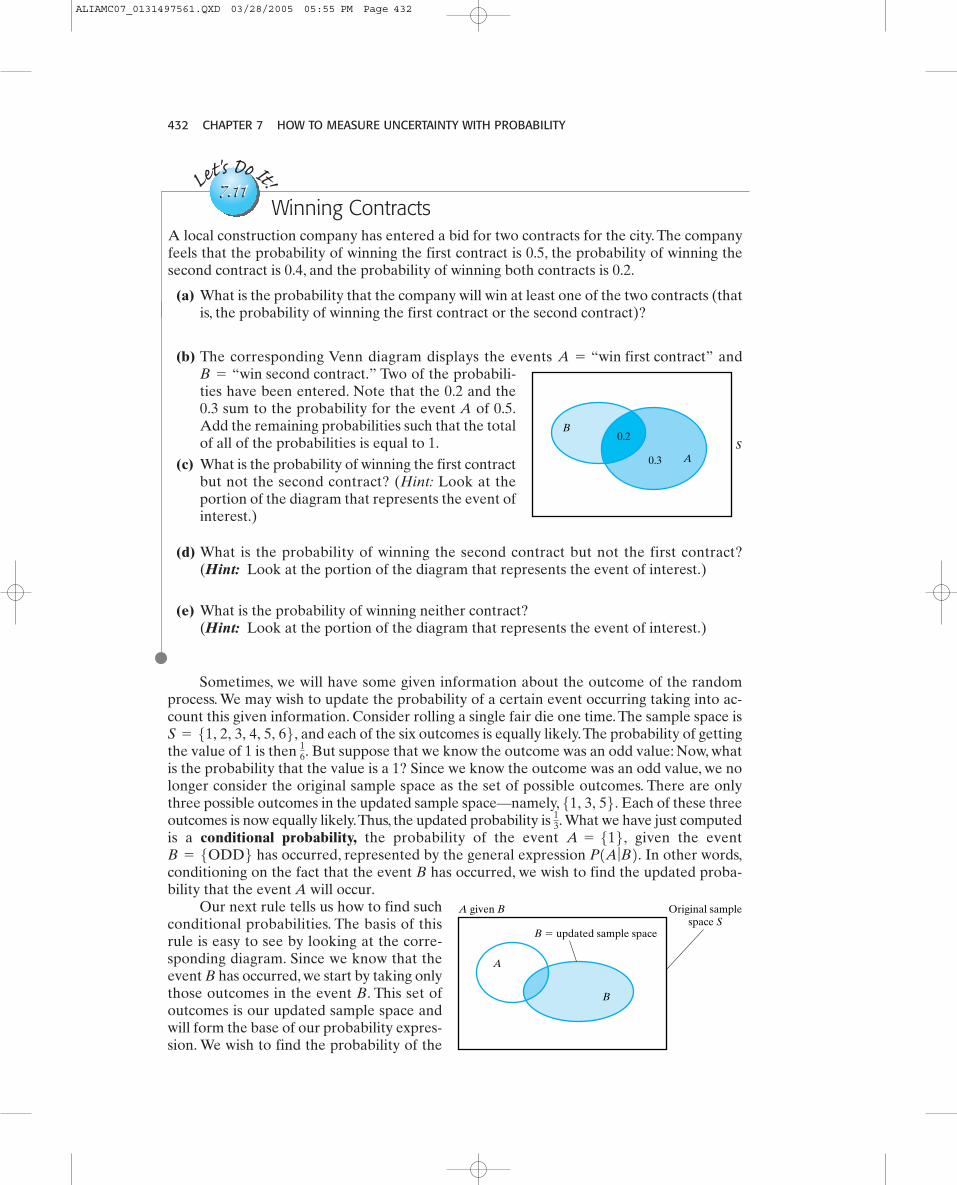
7.117.11Winning Contracts
A local construction company has entered a bid for two contracts for the city. The companyfeels that the probability of winning the first contract is 0.5, the probability of winning thesecond contract is 0.4, and the probability of winning both contracts is 0.2.
(a) What is the probability that the company will win at least one of the two contracts (thatis, the probability of winning the first contract or the second contract)?
(b) The corresponding Venn diagram displays the events andTwo of the probabili-
ties have been entered. Note that the 0.2 and the0.3 sum to the probability for the event A of 0.5.Add the remaining probabilities such that the totalof all of the probabilities is equal to 1.
(c) What is the probability of winning the first contractbut not the second contract? (Hint: Look at theportion of the diagram that represents the event ofinterest.)
(d) What is the probability of winning the second contract but not the first contract? (Hint: Look at the portion of the diagram that represents the event of interest.)
(e) What is the probability of winning neither contract?(Hint: Look at the portion of the diagram that represents the event of interest.)
B = “win second contract.”A = “win first contract”
A
B0.2
0.3S
ALIAMC07_0131497561.QXD 03/28/2005 05:55 PM Page 432

7.4 THE LANGUAGE OF PROBABILITY 433
event A occurring on this updated sample space. The only outcomes in the event A includ-ed in this updated sample space are those belonging to both the event A and the event B (thatis, the outcomes that comprise the intersection between A and B).
Example 7.4 ◆ Gender versus EducationProblemRecall the data from Example 7.2 based on a random sample of 200 adults classified by gen-der and by highest education level attained.
Education
Elementary Secondary College
Male 38 28 22 88
Female 45 50 17 112
83 78 39 200
Consider the following two events:
What is the probability that an adult selected at random has a college level of educationgiven that the adult is a female? That is, find
SolutionSince we are given that the selected adult is a female, we only need to consider the 112females as our updated sample space. Among the 112 females, there were 17 females whohad a college level education.
If we use the more formal rule, we have:
P1A ƒC2 =
P1A and C2P1C2 =
17200112200
=
17112
= 0.152.
P1A ƒC2 = P1college level education ƒfemale2 =
17112
= 0.152
P1A ƒC2. C = “adult selected is a female.” A = “adult selected has a college-level education.”
Gender
Conditional Probability
5. The conditional probability of the event A occurring, given that event B has occurred,is given by
Note: We could rewrite this rule and have an expression for calculating an intersection,called the multiplication rule.
P1both events will occur at the same time2 = P1A and B2 = P1B2P1A ƒB2 = P1A2P1B ƒA2
P1A ƒB2 =
P1A and B2P1B2 , if P1B2 7 0.
The basis of this rule is as follows: For both events to occur, first we must have one occur (forexample, the event B), and then given that B has occurred, the event A must also occur.Of course, the events A and B could be switched around, which gives us the last part of thepreceding result.
ALIAMC07_0131497561.QXD 03/28/2005 05:55 PM Page 433
434 CHAPTER 7 HOW TO MEASURE UNCERTAINTY WITH PROBABILITY
What We’ve Learned: If the information about the events is presented in a two-way fre-quency table of counts, finding conditional probabilities is straightforward. In this example,the given event was “female,” so we focused only on the female row of counts and expressedthe number with a college-level education as a fraction of the total number of females.
Let's Do It!
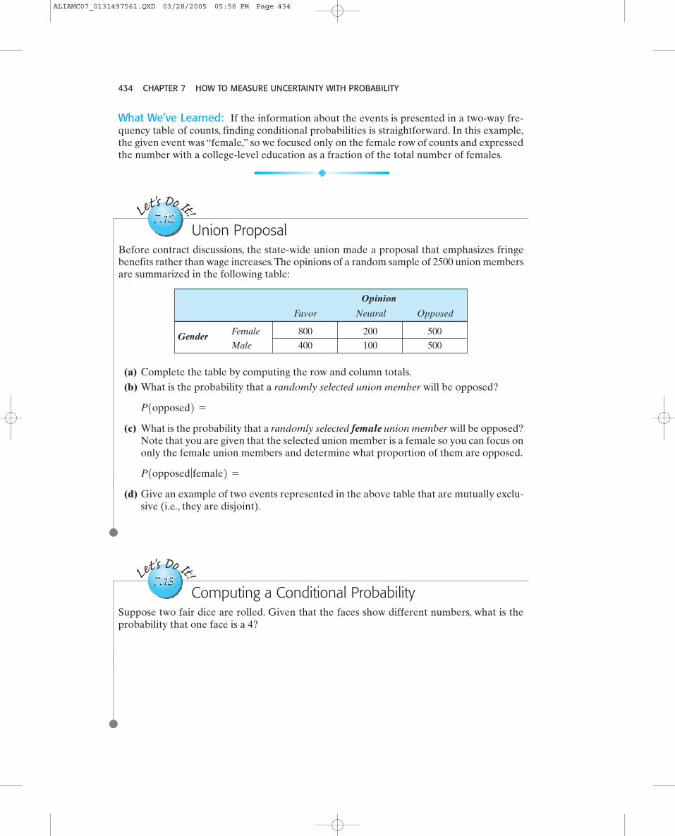
7.127.12Union Proposal
Before contract discussions, the state-wide union made a proposal that emphasizes fringebenefits rather than wage increases.The opinions of a random sample of 2500 union membersare summarized in the following table:
Opinion
Favor Neutral Opposed
Female 800 200 500
Male 400 100 500Gender
(a) Complete the table by computing the row and column totals.(b) What is the probability that a randomly selected union member will be opposed?
(c) What is the probability that a randomly selected female union member will be opposed?Note that you are given that the selected union member is a female so you can focus ononly the female union members and determine what proportion of them are opposed.
(d) Give an example of two events represented in the above table that are mutually exclu-sive (i.e., they are disjoint).
P1opposed ƒfemale2 =
P1opposed2 =
Let's Do It!
7.137.13Computing a Conditional Probability
Suppose two fair dice are rolled. Given that the faces show different numbers, what is theprobability that one face is a 4?
ALIAMC07_0131497561.QXD 03/28/2005 05:56 PM Page 434

7.4 THE LANGUAGE OF PROBABILITY 435
Suppose that for events A and B we have and What does this tellus about the two events A and B? This is what happened in Scenario II of the previous ex-ercise. If knowing that event B occurred does not change the probability of the event Aoccurring—that is, —we say the two events are independent.P1A ƒB2 = P1A2
P1A2 = 0.3.P1A ƒB2 = 0.3
Think About It
DEFINITION: Two events A and B are independent if or, equivalently, if
If two events do not influence each other (that is, if knowing one has occurred does notchange the probability of the other occurring), the events are independent. If two eventsare independent, the multiplication rule tells us that the probability of them both occur-ring together is found by multiplying their individual probabilities:If two events A and B are independent (only in this case), then P1A and B2 = P1A2P1B2.
P1B ƒA2 = P1B2. P1A ƒB2 = P1A2
Let's Do It!
7.147.14More Conditional Probabilities
Scenario I The random process is rolling a fair die one time.The sample space is
(a) What is the probability of getting a 2?(b) Suppose that we know that the outcome was
an even value; now, what is the probability of getting a 2?
Scenario II The random process is tossing a fair coin two times.The sample space is
(a) What is the probability of getting a head on the second toss?
(b) What is the probability of getting a head on the second toss, given it was a head on the first toss?
P1H on 2nd ƒH on 1st2 =
P1H on 2nd2 =
S = 5HH, HT, TH, TT6.
P12 ƒEven2 =
P122 =
S = 51, 2, 3, 4, 5, 66.
In Scenario I of the preceding exercise, how do your answers to parts (a) and (b) compare?
In Scenario II, how do your answers to parts (a) and (b) compare?
What makes these two scenarios different?
ALIAMC07_0131497561.QXD 03/28/2005 05:56 PM Page 435
436 CHAPTER 7 HOW TO MEASURE UNCERTAINTY WITH PROBABILITY
Example 7.6ProblemGerald Kushel, Ed.D., is the author of several books, including Effective Thinking forUncommon Success. In a 1991 interview for Bottom Line Personal newsletter, Dr. Kushelreported the results of a survey conducted to study success. A total of 1200 people were
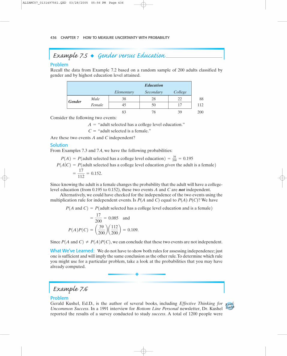
Example 7.5 ◆ Gender versus EducationProblemRecall the data from Example 7.2 based on a random sample of 200 adults classified bygender and by highest education level attained.
Education
Elementary Secondary College
Male 38 28 22 88
Female 45 50 17 112
83 78 39 200Consider the following two events:
Are these two events A and C independent?
SolutionFrom Examples 7.3 and 7.4, we have the following probabilities:
Since knowing the adult is a female changes the probability that the adult will have a college-level education (from 0.195 to 0.152), these two events A and C are not independent.
Alternatively, we could have checked for the independence of the two events using themultiplication rule for independent events. Is P(A and C) equal to P(A) P(C)? We have
Since we can conclude that these two events are not independent.
What We’ve Learned: We do not have to show both rules for assessing independence; justone is sufficient and will imply the same conclusion as the other rule.To determine which ruleyou might use for a particular problem, take a look at the probabilities that you may havealready computed.
P1A and C2 Z P1A2P1C2, P1A2P1C2 = a 39
200b a112
200b = 0.109.
=
17200
= 0.085 and
P1A and C2 = P1adult selected has a college level education and is a female2
=
17112
= 0.152.
P1A ƒC2 = P1adult selected has a college level education given the adult is a female2 P1A2 = P1adult selected has a college level education2 =
39200 = 0.195
C = “adult selected is a female.” A = “adult selected has a college level education.”
Gender
ALIAMC07_0131497561.QXD 03/28/2005 05:56 PM Page 436
7.4 THE LANGUAGE OF PROBABILITY 437
(b) How many people interviewed said they enjoy their personal lives but not their jobs?(c) Given a person enjoys their job, what is the probability they enjoy their personal life?(d) Are the events enjoy their job and enjoy their personal life mutually exclusive?
Explain.(e) Are the events enjoy their job and enjoy their personal life independent? Explain.
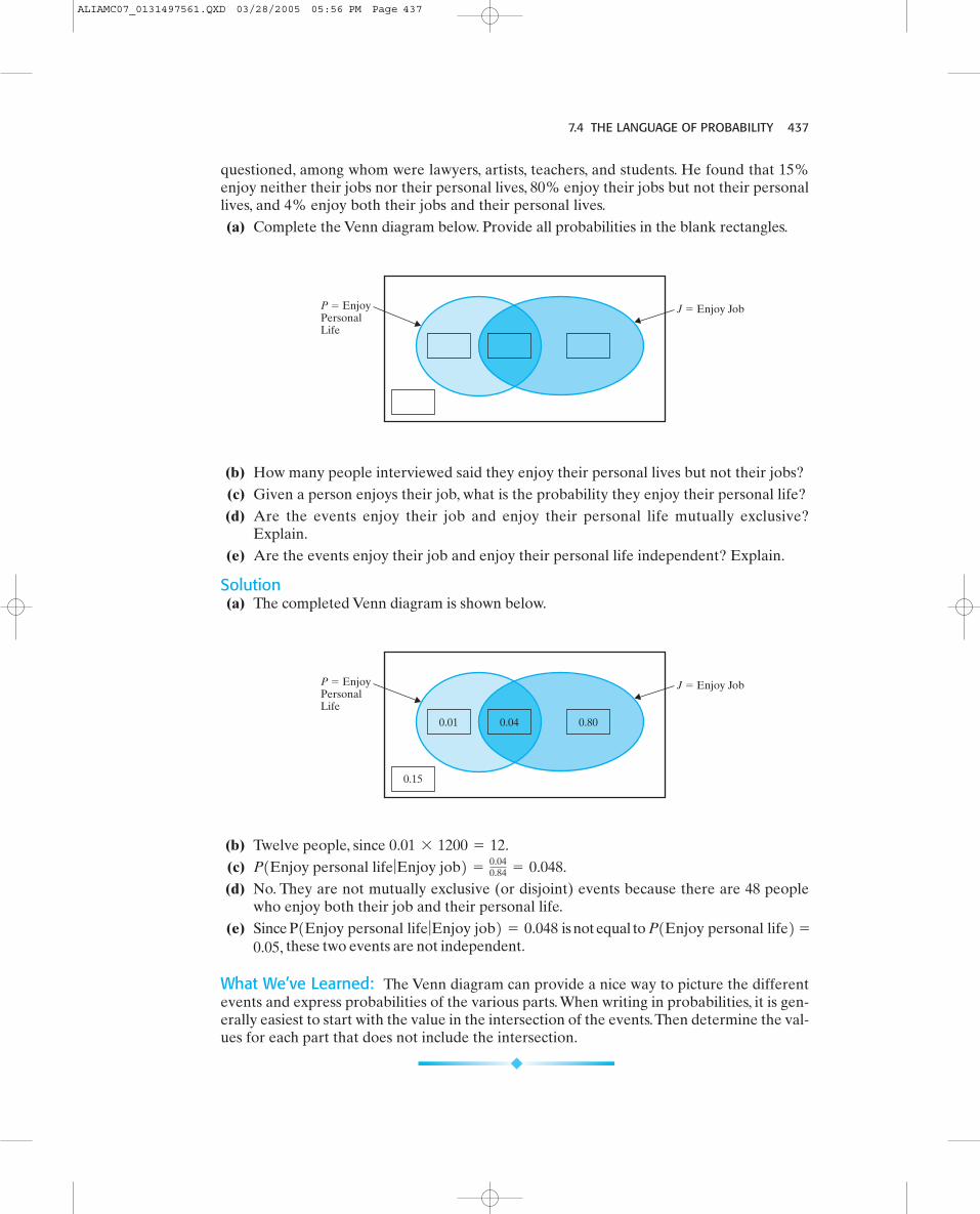
Solution(a) The completed Venn diagram is shown below.
J � Enjoy JobP � EnjoyPersonalLife
J � Enjoy JobP � EnjoyPersonalLife
0.800.040.01
0.15
(b) Twelve people, since (c)(d) No. They are not mutually exclusive (or disjoint) events because there are 48 people
who enjoy both their job and their personal life.(e) Since is not equal to
these two events are not independent.
What We’ve Learned: The Venn diagram can provide a nice way to picture the differentevents and express probabilities of the various parts.When writing in probabilities, it is gen-erally easiest to start with the value in the intersection of the events.Then determine the val-ues for each part that does not include the intersection.
0.05,P1Enjoy personal life2 =P1Enjoy personal life ƒEnjoy job2 = 0.048
P1Enjoy personal life ƒEnjoy job2 =0.040.84 = 0.048.
0.01 * 1200 = 12.
questioned, among whom were lawyers, artists, teachers, and students. He found that 15%enjoy neither their jobs nor their personal lives, 80% enjoy their jobs but not their personallives, and 4% enjoy both their jobs and their personal lives.(a) Complete the Venn diagram below. Provide all probabilities in the blank rectangles.
ALIAMC07_0131497561.QXD 03/28/2005 05:56 PM Page 437
438 CHAPTER 7 HOW TO MEASURE UNCERTAINTY WITH PROBABILITY
Let's Do It!
7.157.15A Family Plan Revisited
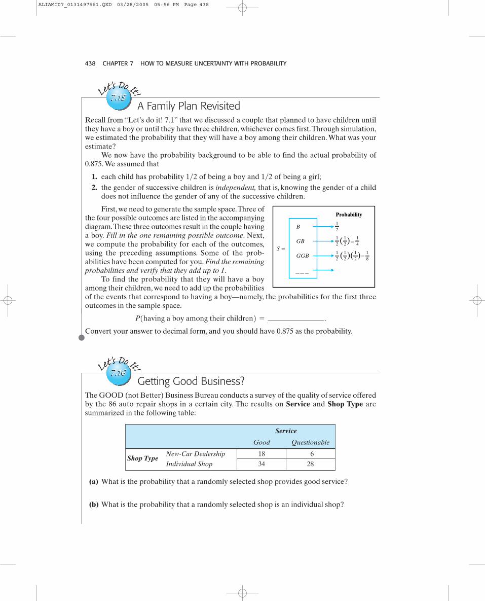
Recall from “Let’s do it! 7.1” that we discussed a couple that planned to have children untilthey have a boy or until they have three children, whichever comes first.Through simulation,we estimated the probability that they will have a boy among their children. What was yourestimate?
We now have the probability background to be able to find the actual probability of0.875. We assumed that
1. each child has probability 1�2 of being a boy and 1�2 of being a girl;2. the gender of successive children is independent, that is, knowing the gender of a child
does not influence the gender of any of the successive children.
First, we need to generate the sample space.Three ofthe four possible outcomes are listed in the accompanyingdiagram.These three outcomes result in the couple havinga boy. Fill in the one remaining possible outcome. Next,we compute the probability for each of the outcomes,using the preceding assumptions. Some of the prob-abilities have been computed for you. Find the remainingprobabilities and verify that they add up to 1.
To find the probability that they will have a boyamong their children, we need to add up the probabilitiesof the events that correspond to having a boy—namely, the probabilities for the first threeoutcomes in the sample space.
.
Convert your answer to decimal form, and you should have 0.875 as the probability.
P1having a boy among their children2 =
Probability
B
GB
GGB
— — —
S �
12
12
14( )�
12
12
12
12
18( )( )�
Let's Do It!
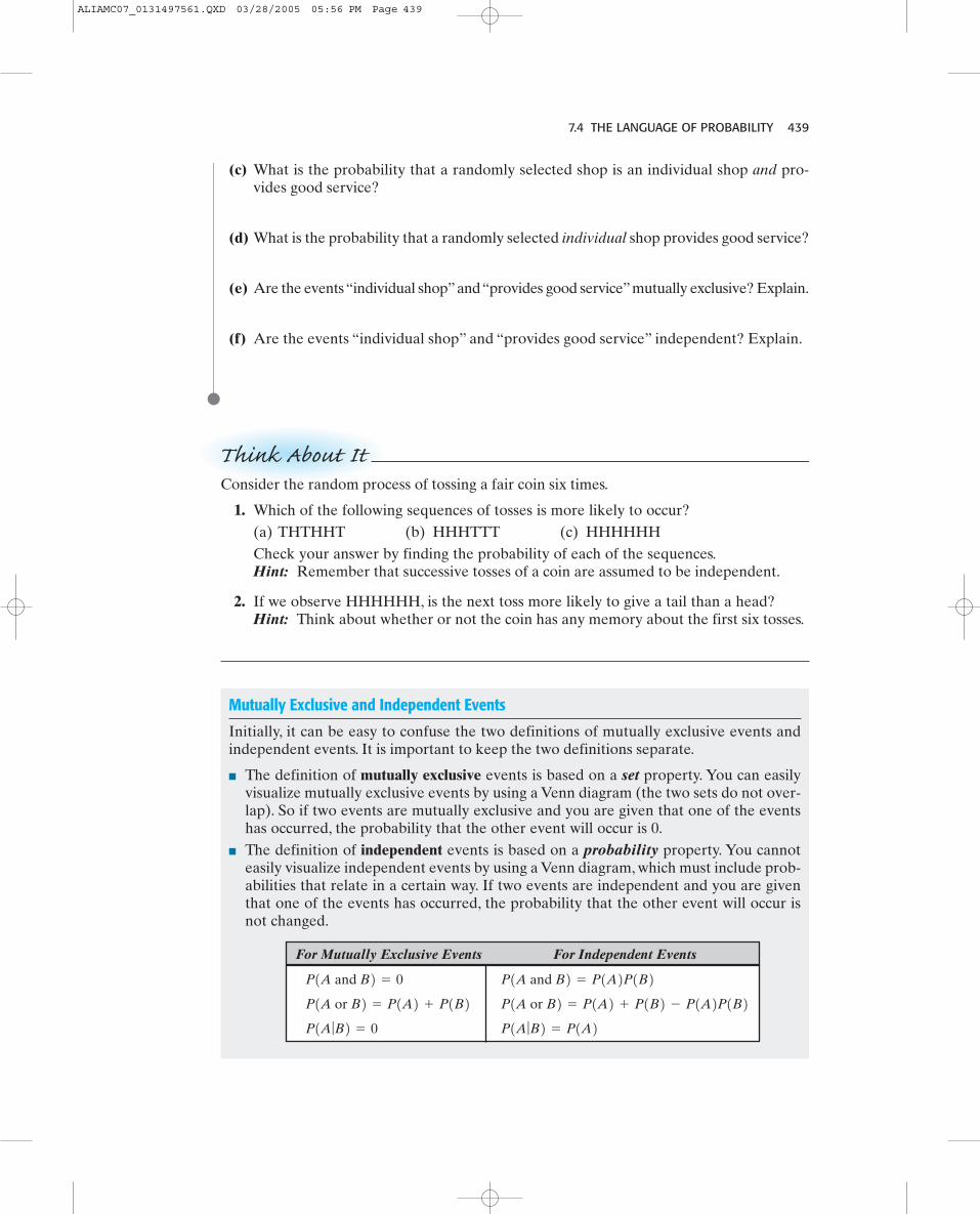
7.167.16Getting Good Business?
The GOOD (not Better) Business Bureau conducts a survey of the quality of service offeredby the 86 auto repair shops in a certain city. The results on Service and Shop Type aresummarized in the following table:
Service
Good Questionable
New-Car Dealership 18 6
Individual Shop 34 28Shop Type
(a) What is the probability that a randomly selected shop provides good service?
(b) What is the probability that a randomly selected shop is an individual shop?
ALIAMC07_0131497561.QXD 03/28/2005 05:56 PM Page 438
7.4 THE LANGUAGE OF PROBABILITY 439
(c) What is the probability that a randomly selected shop is an individual shop and pro-vides good service?
(d) What is the probability that a randomly selected individual shop provides good service?
(e) Are the events“individual shop”and“provides good service”mutually exclusive? Explain.
(f) Are the events “individual shop” and “provides good service” independent? Explain.
Think About ItConsider the random process of tossing a fair coin six times.
1. Which of the following sequences of tosses is more likely to occur?(a) THTHHT (b) HHHTTT (c) HHHHHHCheck your answer by finding the probability of each of the sequences.Hint: Remember that successive tosses of a coin are assumed to be independent.
2. If we observe HHHHHH, is the next toss more likely to give a tail than a head?Hint: Think about whether or not the coin has any memory about the first six tosses.
Mutually Exclusive and Independent Events
Initially, it can be easy to confuse the two definitions of mutually exclusive events andindependent events. It is important to keep the two definitions separate.
■ The definition of mutually exclusive events is based on a set property. You can easilyvisualize mutually exclusive events by using a Venn diagram (the two sets do not over-lap). So if two events are mutually exclusive and you are given that one of the eventshas occurred, the probability that the other event will occur is 0.
■ The definition of independent events is based on a probability property. You cannoteasily visualize independent events by using a Venn diagram, which must include prob-abilities that relate in a certain way. If two events are independent and you are giventhat one of the events has occurred, the probability that the other event will occur isnot changed.
For Mutually Exclusive Events For Independent Events
P1A ƒB2 = P1A2P1A ƒB2 = 0
P1A or B2 = P1A2 + P1B2 - P1A2P1B2P1A or B2 = P1A2 + P1B2P1A and B2 = P1A2P1B2P1A and B2 = 0
ALIAMC07_0131497561.QXD 03/28/2005 05:56 PM Page 439
440 CHAPTER 7 HOW TO MEASURE UNCERTAINTY WITH PROBABILITY
7.4 EXERCISES7.17 What Is the Error? Identify the error, if any, in each statement. If no error, write “no error.”
(a) The probabilities that an automobile salesperson will sell 0, 1, 2, or at least 3 cars on agiven day in February are 0.19, 0.38, 0.29, and 0.15, respectively.
(b) The probability that it will rain tomorrow is 0.40 and the probability that it will not raintomorrow is 0.52.
(c) The probabilities that the printer will make 0, 1, 2, 3, or at least 4 mistakes in printing adocument are 0.19, 0.34, 0.43, and 0.29, respectively.
(d) On a single draw from a deck of playing cards, the probability of selecting a heart is theprobability of selecting a black card (i.e., spade or club) is and the probability ofselecting both a heart and a black card is
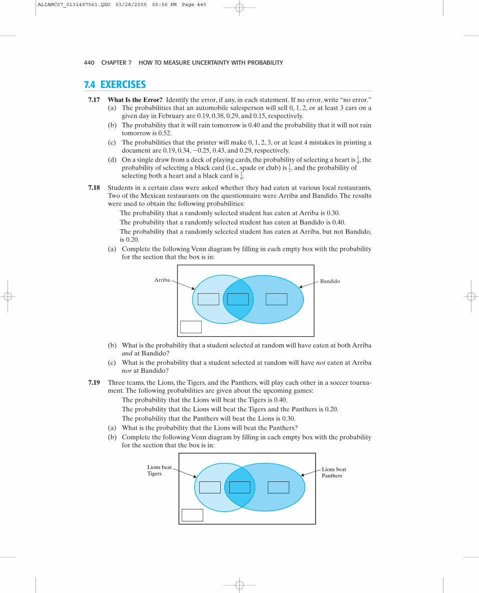
7.18 Students in a certain class were asked whether they had eaten at various local restaurants.Two of the Mexican restaurants on the questionnaire were Arriba and Bandido. The resultswere used to obtain the following probabilities:
The probability that a randomly selected student has eaten at Arriba is 0.30.The probability that a randomly selected student has eaten at Bandido is 0.40.The probability that a randomly selected student has eaten at Arriba, but not Bandido,is 0.20.
(a) Complete the following Venn diagram by filling in each empty box with the probabilityfor the section that the box is in:
18.
12,
14,
-0.25,
BandidoArriba
Lions beatPanthers
Lions beatTigers
(b) What is the probability that a student selected at random will have eaten at both Arribaand at Bandido?
(c) What is the probability that a student selected at random will have not eaten at Arribanor at Bandido?
7.19 Three teams, the Lions, the Tigers, and the Panthers, will play each other in a soccer tourna-ment. The following probabilities are given about the upcoming games:
The probability that the Lions will beat the Tigers is 0.40.The probability that the Lions will beat the Tigers and the Panthers is 0.20.The probability that the Panthers will beat the Lions is 0.30.
(a) What is the probability that the Lions will beat the Panthers?(b) Complete the following Venn diagram by filling in each empty box with the probability
for the section that the box is in:
ALIAMC07_0131497561.QXD 03/28/2005 05:56 PM Page 440

7.4 THE LANGUAGE OF PROBABILITY 441
(c) What is the probability that the Lions will win at least one of the matches against theTigers and the Panthers?
(d) Given that the Lions beat the Tigers, what is the probability that the Lions will beat thePanthers?
7.20 A study was conducted to assess the effectiveness of a new medication for seasickness ascompared to a standard medication. A group of 160 seasick patients were randomly dividedinto two groups, with the first 80 selected at random assigned to receive the new medicationand the other 80 assigned to the receive the standard medication. The results are presentedin the following table:
Physical Attractiveness
Attractive (A) Unattractive (NA)
Helped (H) 34 26
Did not Help (NH) 46 54HelpingBehavior
Medication
New Standard
Improved 60 48
Did Not Improve 20 32Response
(a) What is the probability that a randomly selected patient will improve?(b) Given that the patient received the standard medication, what is the probability that the
patient will improve?(c) Given that the patient received the new medication, what is the probability that the
patient will improve?(d) The first 80 randomly selected patients were assigned to the new medication. Using your
calculator (with a seed value of 58) or the random number table (Row 24, Column 1), givethe labels for the first five patients to receive the new medication.
7.21 Consider the following set of short probability questions. Use the rules and results from thischapter to answer each question.(a) If the probability of buying a pair of shoes is 0.52 and the probability of buying a dress
is 0.67, and these two events are independent, find the probability of buying an outfit; thatis, a pair of shoes and a dress.
(b) You bought two turtledoves not knowing their sex.If the probability of getting a female tur-tledove is 0.59, find the probability of getting at least one female turtledove in the pair youbought.Assume the sex of one turtledove is independent of the sex of the other turtledove.
(c) Three foreign students are applying to medical school. If the probability that one studenthas a French citizenship is 0.78, find the probability that exactly two of these students willhave French citizenship. Assume that the citizenship of a student is independent of thatfor another student.
(d) Suppose you have four friends.You would like to call and invite the first one, who acceptsyour invitation to go to the movies with you. If the probability that a friend actuallyaccepts the invitation is 0.75, find the probability that the first friend to accept theinvitation occurs on your third attempt.
(e) You found five golden earrings on a beach. If the probability of finding a real goldenearring on a beach is 0.43, find the probability of getting three or fewer real goldenearrings among the five.
(f) In an amusement park you decide to play a game where if you shoot inside a circle youwin a prize. If the probability of getting a prize is 0.38, find the probability of getting aprize on or before the fourth trial. Assume that the trials are independent.
7.22 The results of a study relating physical attractiveness to helping behavior are shown here:
ALIAMC07_0131497561.QXD 03/28/2005 05:56 PM Page 441
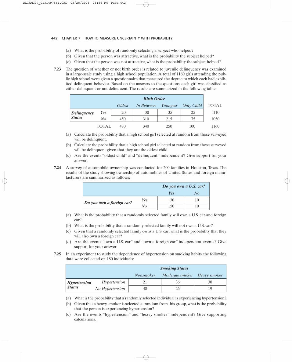
442 CHAPTER 7 HOW TO MEASURE UNCERTAINTY WITH PROBABILITY
(a) What is the probability of randomly selecting a subject who helped?(b) Given that the person was attractive, what is the probability the subject helped?(c) Given that the person was not attractive, what is the probability the subject helped?
7.23 The question of whether or not birth order is related to juvenile delinquency was examinedin a large-scale study using a high school population. A total of 1160 girls attending the pub-lic high school were given a questionnaire that measured the degree to which each had exhib-ited delinquent behavior. Based on the answers to the questions, each girl was classified aseither delinquent or not delinquent. The results are summarized in the following table:
Birth Order
Oldest In Between Youngest Only Child TOTAL
Yes 20 30 35 25 110
No 450 310 215 75 1050
TOTAL 470 340 250 100 1160
(a) Calculate the probability that a high school girl selected at random from those surveyedwill be delinquent.
(b) Calculate the probability that a high school girl selected at random from those surveyedwill be delinquent given that they are the oldest child.
(c) Are the events “oldest child” and “delinquent” independent? Give support for youranswer.
7.24 A survey of automobile ownership was conducted for 200 families in Houston, Texas. Theresults of the study showing ownership of automobiles of United States and foreign manu-facturers are summarized as follows:
Do you own a U.S. car?
Yes No
Yes 30 10
No 150 10Do you own a foreign car?
(a) What is the probability that a randomly selected family will own a U.S. car and foreigncar?
(b) What is the probability that a randomly selected family will not own a U.S. car?(c) Given that a randomly selected family owns a U.S. car, what is the probability that they
will also own a foreign car?(d) Are the events “own a U.S. car” and “own a foreign car” independent events? Give
support for your answer.
7.25 In an experiment to study the dependence of hypertension on smoking habits, the followingdata were collected on 180 individuals:
Smoking Status
Nonsmoker Moderate smoker Heavy smoker
Hypertension 21 36 30
No Hypertension 48 26 19HypertensionStatus
(a) What is the probability that a randomly selected individual is experiencing hypertension?(b) Given that a heavy smoker is selected at random from this group, what is the probability
that the person is experiencing hypertension?(c) Are the events “hypertension” and “heavy smoker” independent? Give supporting
calculations.
DelinquencyStatus
ALIAMC07_0131497561.QXD 03/28/2005 05:56 PM Page 442
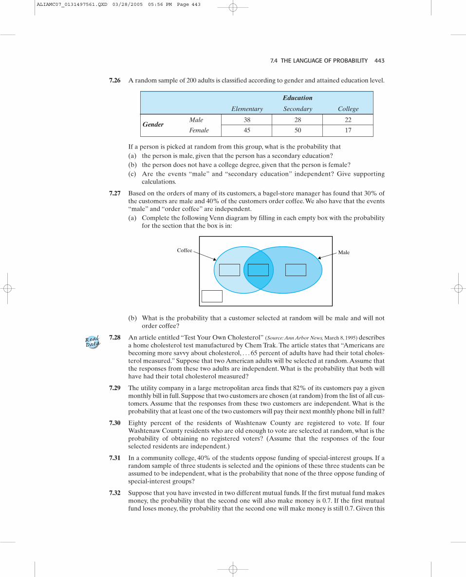
7.4 THE LANGUAGE OF PROBABILITY 443
7.26 A random sample of 200 adults is classified according to gender and attained education level.
Education
Elementary Secondary College
Male 38 28 22
Female 45 50 17Gender
If a person is picked at random from this group, what is the probability that(a) the person is male, given that the person has a secondary education?(b) the person does not have a college degree, given that the person is female?(c) Are the events “male” and “secondary education” independent? Give supporting
calculations.
7.27 Based on the orders of many of its customers, a bagel-store manager has found that 30% ofthe customers are male and 40% of the customers order coffee. We also have that the events“male” and “order coffee” are independent.(a) Complete the following Venn diagram by filling in each empty box with the probability
for the section that the box is in:
MaleCoffee
(b) What is the probability that a customer selected at random will be male and will notorder coffee?
7.28 An article entitled “Test Your Own Cholesterol” (Source: Ann Arbor News, March 8, 1995) describesa home cholesterol test manufactured by Chem Trak. The article states that “Americans arebecoming more savvy about cholesterol, 65 percent of adults have had their total choles-terol measured.” Suppose that two American adults will be selected at random. Assume thatthe responses from these two adults are independent. What is the probability that both willhave had their total cholesterol measured?
7.29 The utility company in a large metropolitan area finds that 82% of its customers pay a givenmonthly bill in full. Suppose that two customers are chosen (at random) from the list of all cus-tomers. Assume that the responses from these two customers are independent. What is theprobability that at least one of the two customers will pay their next monthly phone bill in full?
7.30 Eighty percent of the residents of Washtenaw County are registered to vote. If fourWashtenaw County residents who are old enough to vote are selected at random, what is theprobability of obtaining no registered voters? (Assume that the responses of the fourselected residents are independent.)
7.31 In a community college, 40% of the students oppose funding of special-interest groups. If arandom sample of three students is selected and the opinions of these three students can beassumed to be independent, what is the probability that none of the three oppose funding ofspecial-interest groups?
7.32 Suppose that you have invested in two different mutual funds. If the first mutual fund makesmoney, the probability that the second one will also make money is 0.7. If the first mutualfund loses money, the probability that the second one will make money is still 0.7. Given this
Á
ALIAMC07_0131497561.QXD 03/28/2005 05:56 PM Page 443
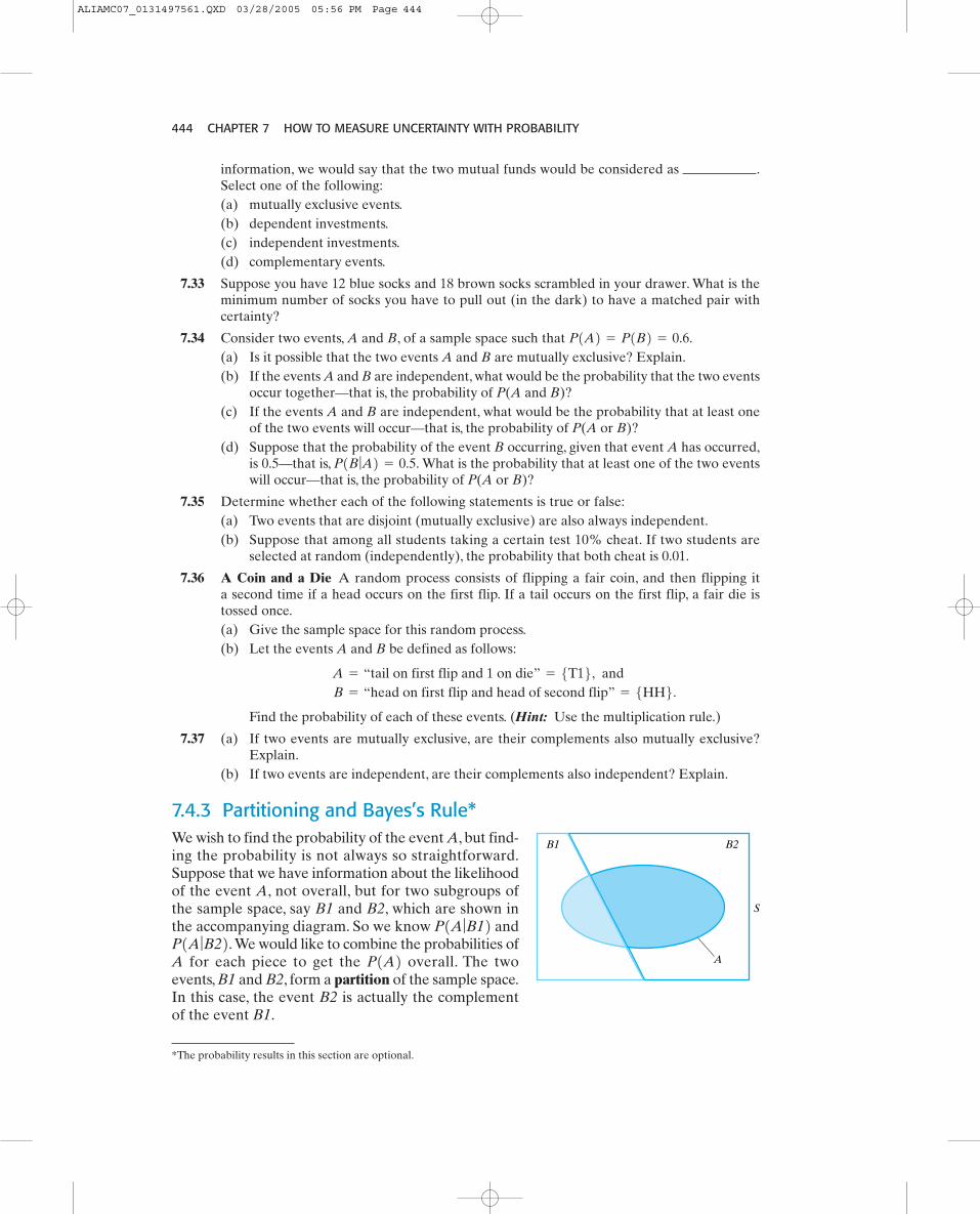
444 CHAPTER 7 HOW TO MEASURE UNCERTAINTY WITH PROBABILITY
information, we would say that the two mutual funds would be considered as .Select one of the following:(a) mutually exclusive events.(b) dependent investments.(c) independent investments.(d) complementary events.
7.33 Suppose you have 12 blue socks and 18 brown socks scrambled in your drawer. What is theminimum number of socks you have to pull out (in the dark) to have a matched pair withcertainty?
7.34 Consider two events, A and B, of a sample space such that (a) Is it possible that the two events A and B are mutually exclusive? Explain.(b) If the events A and B are independent, what would be the probability that the two events
occur together—that is, the probability of P(A and B)?(c) If the events A and B are independent, what would be the probability that at least one
of the two events will occur—that is, the probability of P(A or B)?(d) Suppose that the probability of the event B occurring, given that event A has occurred,
is 0.5—that is, What is the probability that at least one of the two eventswill occur—that is, the probability of P(A or B)?
7.35 Determine whether each of the following statements is true or false:(a) Two events that are disjoint (mutually exclusive) are also always independent.(b) Suppose that among all students taking a certain test 10% cheat. If two students are
selected at random (independently), the probability that both cheat is 0.01.
7.36 A Coin and a Die A random process consists of flipping a fair coin, and then flipping ita second time if a head occurs on the first flip. If a tail occurs on the first flip, a fair die istossed once.(a) Give the sample space for this random process.(b) Let the events A and B be defined as follows:
Find the probability of each of these events. (Hint: Use the multiplication rule.)
7.37 (a) If two events are mutually exclusive, are their complements also mutually exclusive?Explain.
(b) If two events are independent, are their complements also independent? Explain.
7.4.3 Partitioning and Bayes’s Rule*We wish to find the probability of the event A, but find-ing the probability is not always so straightforward.Suppose that we have information about the likelihoodof the event A, not overall, but for two subgroups ofthe sample space, say B1 and B2, which are shown inthe accompanying diagram. So we know and
We would like to combine the probabilities ofA for each piece to get the overall. The twoevents, B1 and B2, form a partition of the sample space.In this case, the event B2 is actually the complementof the event B1.
P1A2P1A ƒB22. P1A ƒB12
B = “head on first flip and head of second flip” = 5HH6. A = “tail on first flip and 1 on die” = 5T16, and
P1B ƒA2 = 0.5.
P1A2 = P1B2 = 0.6.
B1 B2
A
S
*The probability results in this section are optional.
ALIAMC07_0131497561.QXD 03/28/2005 05:56 PM Page 444
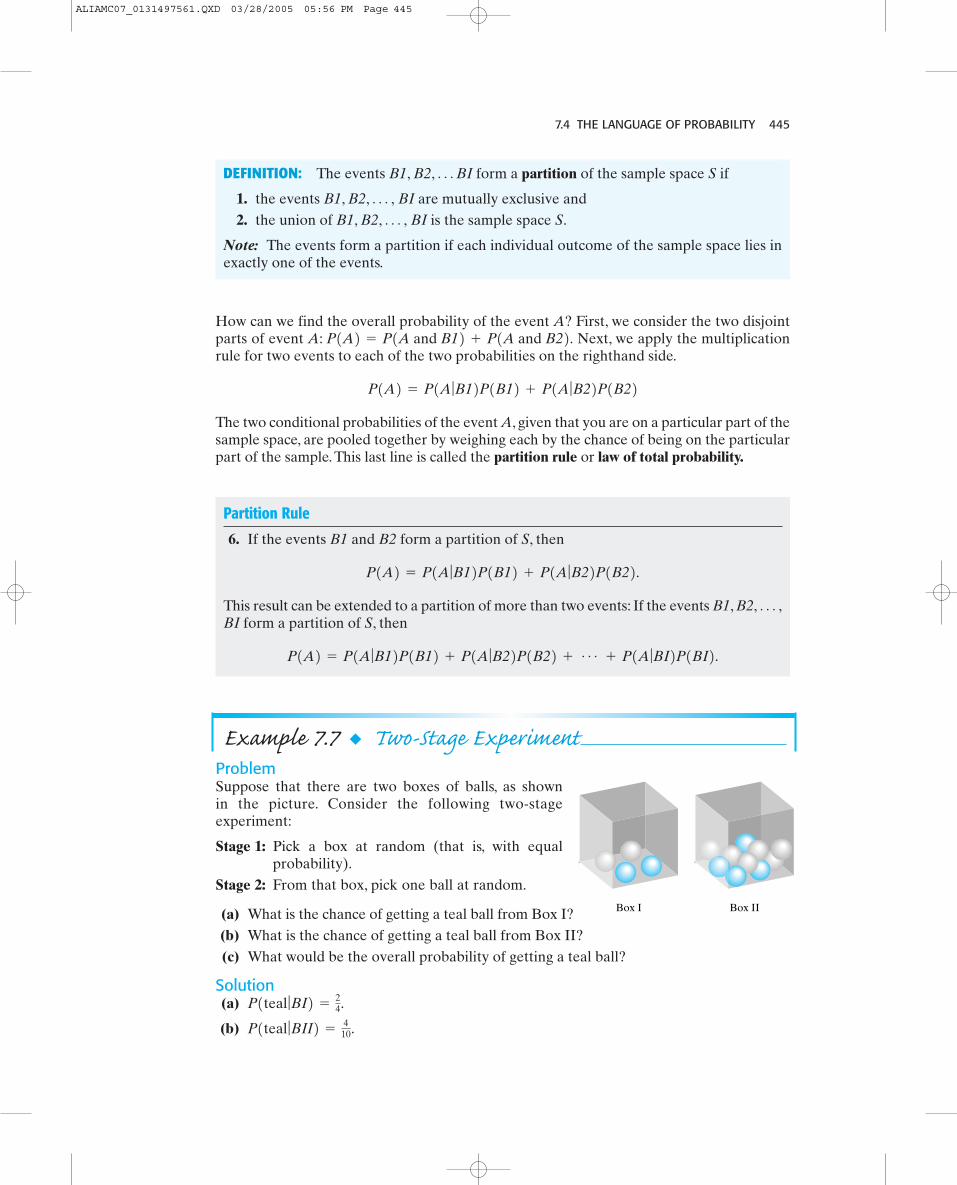
7.4 THE LANGUAGE OF PROBABILITY 445
How can we find the overall probability of the event A? First, we consider the two disjointparts of event A: Next, we apply the multiplicationrule for two events to each of the two probabilities on the righthand side.
The two conditional probabilities of the event A, given that you are on a particular part of thesample space, are pooled together by weighing each by the chance of being on the particularpart of the sample. This last line is called the partition rule or law of total probability.
P1A2 = P1A ƒB12P1B12 + P1A ƒB22P1B22
P1A2 = P1A and B12 + P1A and B22.
DEFINITION: The events B1, B2, BI form a partition of the sample space S if
1. the events B1, B2, BI are mutually exclusive and2. the union of B1, B2, BI is the sample space S.
Note: The events form a partition if each individual outcome of the sample space lies inexactly one of the events.
Á ,Á ,
Á
Example 7.7 ◆ Two-Stage ExperimentProblemSuppose that there are two boxes of balls, as shownin the picture. Consider the following two-stageexperiment:
Stage 1: Pick a box at random (that is, with equalprobability).
Stage 2: From that box, pick one ball at random.
(a) What is the chance of getting a teal ball from Box I?(b) What is the chance of getting a teal ball from Box II?(c) What would be the overall probability of getting a teal ball?
Solution(a)
(b) P1teal ƒBII2 =410.
P1teal ƒBI2 =24.
Box I Box II
Partition Rule
6. If the events B1 and B2 form a partition of S, then
This result can be extended to a partition of more than two events: If the events B1, B2,BI form a partition of S, then
P1A2 = P1A ƒB12P1B12 + P1A ƒB22P1B22 +Á
+ P1A ƒBI2P1BI2.
Á ,
P1A2 = P1A ƒB12P1B12 + P1A ƒB22P1B22.
ALIAMC07_0131497561.QXD 03/28/2005 05:56 PM Page 445

446 CHAPTER 7 HOW TO MEASURE UNCERTAINTY WITH PROBABILITY
(c)
What We’ve Learned: In this example, the calculation of the probability of getting a tealball obviously depends on which box is selected—the two boxes form what is called a parti-tion. Since in Stage 1 of the experiment a box is selected at random, the probability that weselect any given box is Finally, in part (c) we used the partition rule, a form of weightedaverage, to combine the two probabilities from parts (a) and (b).
12.
= 0.45.
= 12421122 + 1 41021122
P1teal2 = P1teal ƒBI2P1BI2 + P1teal ƒBII2P1BII2Let
's Do It!
7.177.17Defective Razors
A store sells three different types of disposable razors.The probability that the type A razorswill be defective is 0.3, and the probability that Type B and C razors will be defective are 0.2and 0.1, respectively. Suppose that 20% of the razors are of Type A, 30% are of Type B, andthe rest are of Type C.
What is the probability that a randomly selected razor will not be defective?
One interesting application of the partition rule is called the Warner’s randomized responsemodel, which is discussed in the next example. Suppose that we want to estimate the pro-portion of high school students in a school district who have engaged in illicit drug use.Askingthis question directly would probably yield little useful information. How can we get accu-rate answers to a sensitive question that respondents might be reluctant to answer truthfully?
Example 7.8 ◆ Getting Answers to Sensitive QuestionsProblemSet up a survey with two questions. Let Q1 be the sensitive question.Then, the second ques-tion, Q2, is any other question for which you know what proportion of “yes” responses youshould expect to get. For example,
Survey
Q1: “Have you ever shoplifted?” YES NO
Q2: “Is the second flip of your fair coin a head?” YES NO
ALIAMC07_0131497561.QXD 03/28/2005 05:56 PM Page 446

7.4 THE LANGUAGE OF PROBABILITY 447
The respondent determines which question he or she answers using some probabilitydevice under his or her control. For example, we could have the respondent flip a fair cointwo times. If the first flip results in a the respondent is to answer question Q1 truth-fully, and if the flip results in a the respondent is to answer question Q2 truthfully.Since only the respondent knows which question he or she is answering, there should be nostigma attached to a “yes” or “no” response.Although everyone flips the fair coin two times,the result of the second flip would only be needed if the first flip was a But can we stillfind out the proportion who respond “yes” to the sensitive question?
We wish to learn about the proportion in the population for which the true responseto question Q1 is “yes”—that is, the probability of a yes response, given question Q1.Applying the partition rule to the event “yes,” with the partition being Q1 or Q2, we have
We would know, by the probability device used to determine which question is answered, thevalues of P(Q1) and P(Q2). We would also know the value of For the secondflip of a fair coin question, it would be 0.50. We would use the proportion of “yes” responsesto estimate the P(YES). All that remains is the probability of interest, whichwe can solve for.
If 41% of those surveyed responded with a “yes.” Calculate and interpretwhat it means.
Solution
So we would estimate that about 32% of the population represented by this sample haveshoplifted.
What We’ve Learned: Probability can help us find answers to questions that would bedifficult to ask directly and get good answers. This particular method works better if thenumber of those surveyed is large.
P1YES ƒQ12 = 0.32
P1YES ƒQ12 =
0.41 - 10.5210.520.5
0.41 = P1YES ƒQ1210.52 + 10.5210.52 P1YES2 = P1YES ƒQ12P1Q12 + P1YES ƒQ22P1Q22
P1YES ƒQ12P1YES ƒQ12,
P1YES ƒQ22.
P1YES2 = P1YES ƒQ12P1Q12 + P1YES ƒQ22P1Q22.
5T6.
5T6,5H6,Let
's Do It!
7.187.18Getting Answers to Sensitive Questions
Perform the Warner’s randomized response model with the students in your class.
■ Determine the sensitive question of interest and enter it in the survey below as Q1.■ Select two random mechanisms for the model—one for determining which of the
two questions will be answered, and the other for developing a second question, Q2in the survey, for which you know the proportion of time you expect someone toanswer “yes” to it.
Since most students will have some type of coin, you could have everyone flip their coin twotimes, keeping the results of the two flips to themselves.The first flip of the coin can be usedto determine which of the two questions is to be answered. For example, if the first flip is a
ALIAMC07_0131497561.QXD 03/28/2005 05:56 PM Page 447

448 CHAPTER 7 HOW TO MEASURE UNCERTAINTY WITH PROBABILITY
head, answer Q1; otherwise, answer Q2. The second question will involve the result of thesecond flip of the coin, for example, “Was the second flip of the coin a head?”
ProcedureDistribute slips of paper (small squares, all the same size work well), one to each student, forrecording their response. Each student will answer one and only one question, either Q1 orQ2, based on the outcome of their first flip of the coin. So only one word should be writtenon each slip of paper. No names should be written on the paper, and certainly no indicationas to which question was answered. For example, do not write
Collect the results:
Plug all the values into the following expression and compute your estimate of
We would estimate that
P1YES2 = P1YES ƒQ12P1Q12 + P1YES ƒQ22P1Q22P1YES ƒQ12.
Proportion of yes responses =
= estimate of P1YES2.Number of yes responses =
.Number of responses =
.
“Q1 = No.”
Think About ItSuppose that it is estimated that about 1 in 1000 people in the United States have a certainrare disease. A diagnostic test is available for this disease that is 98% accurate (i.e., returnsa positive result) for people who have the disease and 95% accurate (i.e., returns a negativeresult) for people who do not have the disease. Given that a person has tested positively forthe disease, what do you think is the probability that the person actually has the disease? Doyou think the probability is higher or lower than 50%? Higher Lower
As we shall see in our next example, the partition rule also plays an important part indetermining the false positive rate for a diagnostic test, that is, the proportion of people whodo not have the disease even though the test came back positive.
Survey
Q1: Sensitive question YES NO
Q2: On the second flip of the coin, did you get a head? YES NO
ALIAMC07_0131497561.QXD 03/28/2005 05:56 PM Page 448
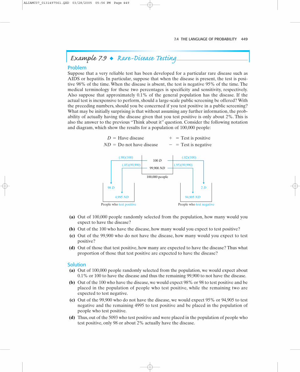
7.4 THE LANGUAGE OF PROBABILITY 449
(a) Out of 100,000 people randomly selected from the population, how many would youexpect to have the disease?
(b) Out of the 100 who have the disease, how many would you expect to test positive?(c) Out of the 99,900 who do not have the disease, how many would you expect to test
positive?(d) Out of those that test positive, how many are expected to have the disease? Thus what
proportion of those that test positive are expected to have the disease?
Solution(a) Out of 100,000 people randomly selected from the population, we would expect about
0.1% or 100 to have the disease and thus the remaining 99,900 to not have the disease.(b) Out of the 100 who have the disease, we would expect 98% or 98 to test positive and be
placed in the population of people who test positive, while the remaining two areexpected to test negative.
(c) Out of the 99,900 who do not have the disease, we would expect 95% or 94,905 to testnegative and the remaining 4995 to test positive and be placed in the population ofpeople who test positive.
(d) Thus, out of the 5093 who test positive and were placed in the population of people whotest positive, only 98 or about 2% actually have the disease.
Example 7.9 ◆ Rare-Disease TestingProblemSuppose that a very reliable test has been developed for a particular rare disease such asAIDS or hepatitis. In particular, suppose that when the disease is present, the test is posi-tive 98% of the time. When the disease is absent, the test is negative 95% of the time. Themedical terminology for these two percentages is specificity and sensitivity, respectively.Also suppose that approximately 0.1% of the general population has the disease. If theactual test is inexpensive to perform, should a large-scale public screening be offered? Withthe preceding numbers, should you be concerned if you test positive in a public screening?What may be initially surprising is that without assuming any further information, the prob-ability of actually having the disease given that you test positive is only about 2%. This isalso the answer to the previous “Think about it” question. Consider the following notationand diagram, which show the results for a population of 100,000 people:
ND = Do not have disease - = Test is negative D = Have disease + = Test is positive
People who test positive People who test negative
94,905 ND4,995 ND
2 D98 D
100,000 people
99,900 ND
100 D(.95)(99,990)
(.02)(100)
(.05)(99,990)
(.98)(100)
ALIAMC07_0131497561.QXD 03/28/2005 05:56 PM Page 449
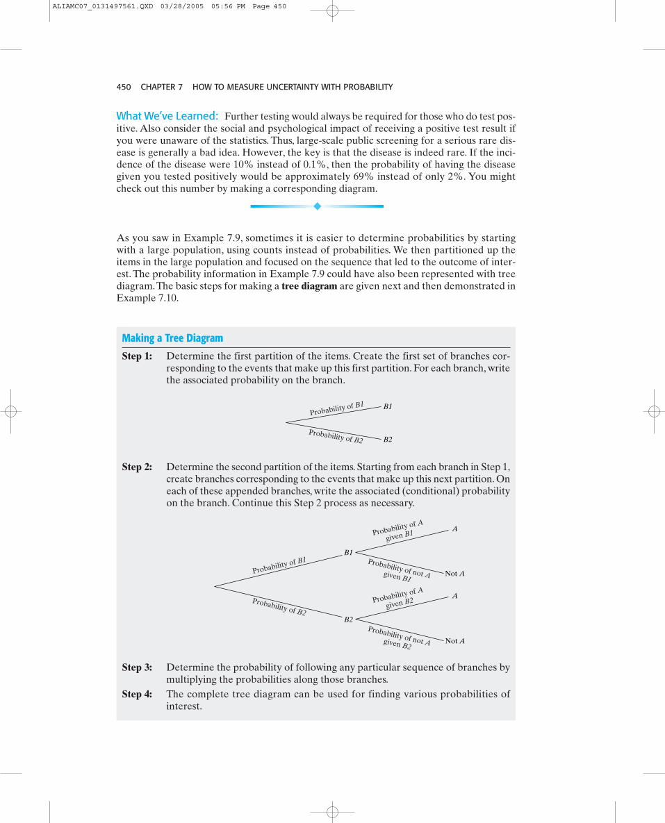
450 CHAPTER 7 HOW TO MEASURE UNCERTAINTY WITH PROBABILITY
What We’ve Learned: Further testing would always be required for those who do test pos-itive. Also consider the social and psychological impact of receiving a positive test result ifyou were unaware of the statistics. Thus, large-scale public screening for a serious rare dis-ease is generally a bad idea. However, the key is that the disease is indeed rare. If the inci-dence of the disease were 10% instead of 0.1%, then the probability of having the diseasegiven you tested positively would be approximately 69% instead of only 2%. You mightcheck out this number by making a corresponding diagram.
As you saw in Example 7.9, sometimes it is easier to determine probabilities by startingwith a large population, using counts instead of probabilities. We then partitioned up theitems in the large population and focused on the sequence that led to the outcome of inter-est. The probability information in Example 7.9 could have also been represented with treediagram.The basic steps for making a tree diagram are given next and then demonstrated inExample 7.10.
Making a Tree Diagram
Step 1: Determine the first partition of the items. Create the first set of branches cor-responding to the events that make up this first partition. For each branch, writethe associated probability on the branch.
Step 2: Determine the second partition of the items. Starting from each branch in Step 1,create branches corresponding to the events that make up this next partition. Oneach of these appended branches, write the associated (conditional) probabilityon the branch. Continue this Step 2 process as necessary.
Step 3: Determine the probability of following any particular sequence of branches bymultiplying the probabilities along those branches.
Step 4: The complete tree diagram can be used for finding various probabilities ofinterest.
Probability of B1
Probability of B2
B1
B2
B1
B2
Not A
A
Not A
A
Probability of B1
Probability of B2
Probability of A
given B1
Probability of A
given B2
Probability of not Agiven B1
Probability of not Agiven B2
ALIAMC07_0131497561.QXD 03/28/2005 05:56 PM Page 450
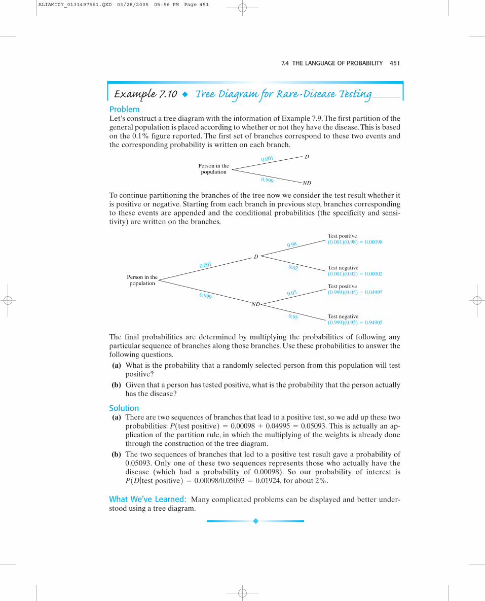
7.4 THE LANGUAGE OF PROBABILITY 451
To continue partitioning the branches of the tree now we consider the test result whether itis positive or negative. Starting from each branch in previous step, branches correspondingto these events are appended and the conditional probabilities (the specificity and sensi-tivity) are written on the branches.
Example 7.10 ◆ Tree Diagram for Rare-Disease TestingProblemLet’s construct a tree diagram with the information of Example 7.9.The first partition of thegeneral population is placed according to whether or not they have the disease.This is basedon the 0.1% figure reported. The first set of branches correspond to these two events andthe corresponding probability is written on each branch.
D
ND
Person in thepopulation
0.001
0.999
Test positive(0.001)(0.98) � 0.00098
Test negative(0.001)(0.02) � 0.00002
Test positive(0.999)(0.05) � 0.04995
Test negative(0.999)(0.95) � 0.94905
Person in thepopulation
D
ND
0.001
0.999
0.98
0.05
0.02
0.95
The final probabilities are determined by multiplying the probabilities of following anyparticular sequence of branches along those branches. Use these probabilities to answer thefollowing questions.(a) What is the probability that a randomly selected person from this population will test
positive?(b) Given that a person has tested positive, what is the probability that the person actually
has the disease?
Solution(a) There are two sequences of branches that lead to a positive test, so we add up these two
probabilities: This is actually an ap-plication of the partition rule, in which the multiplying of the weights is already donethrough the construction of the tree diagram.
(b) The two sequences of branches that led to a positive test result gave a probability of0.05093. Only one of these two sequences represents those who actually have thedisease (which had a probability of 0.00098). So our probability of interest is
for about 2%.
What We’ve Learned: Many complicated problems can be displayed and better under-stood using a tree diagram.
P1D ƒtest positive2 = 0.00098/0.05093 = 0.01924,
P1test positive2 = 0.00098 + 0.04995 = 0.05093.
ALIAMC07_0131497561.QXD 03/28/2005 05:56 PM Page 451
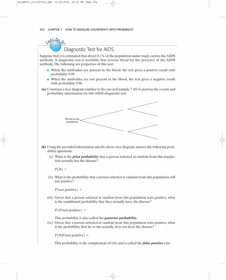
452 CHAPTER 7 HOW TO MEASURE UNCERTAINTY WITH PROBABILITY
Let's Do It!
7.197.19Diagnostic Test for AIDS
Suppose that it is estimated that about 0.1% of the population under study carries the AIDSantibody. A diagnostic test is available that screens blood for the presence of the AIDSantibody. The following are properties of this test:
■ When the antibodies are present in the blood, the test gives a positive result withprobability 0.99.
■ When the antibodies are not present in the blood, the test gives a negative resultwith probability 0.96.
(a) Construct a tree diagram (similar to the one in Example 7.10) to portray the events andprobability information for this AIDS-diagnostic test.
Person in thepopulation
(b) Using the provided information and the above tree diagram, answer the following prob-ability questions:
(i) What is the prior probability that a person selected at random from this popula-tion actually has the disease?
(ii) What is the probability that a person selected at random from this population willtest positive?
(iii) Given that a person selected at random from this population tests positive, whatis the conditional probability that they actually have the disease?
This probability is also called the posterior probability.(iv) Given that a person selected at random from this population tests positive, what
is the probability that he or she actually does not have the disease?
This probability is the complement of (iii) and is called the false-positive rate.
P1ND ƒ test positive2 =
P1D ƒ test positive2 =
P1test positive2 =
P1D2 =
ALIAMC07_0131497561.QXD 03/28/2005 05:56 PM Page 452
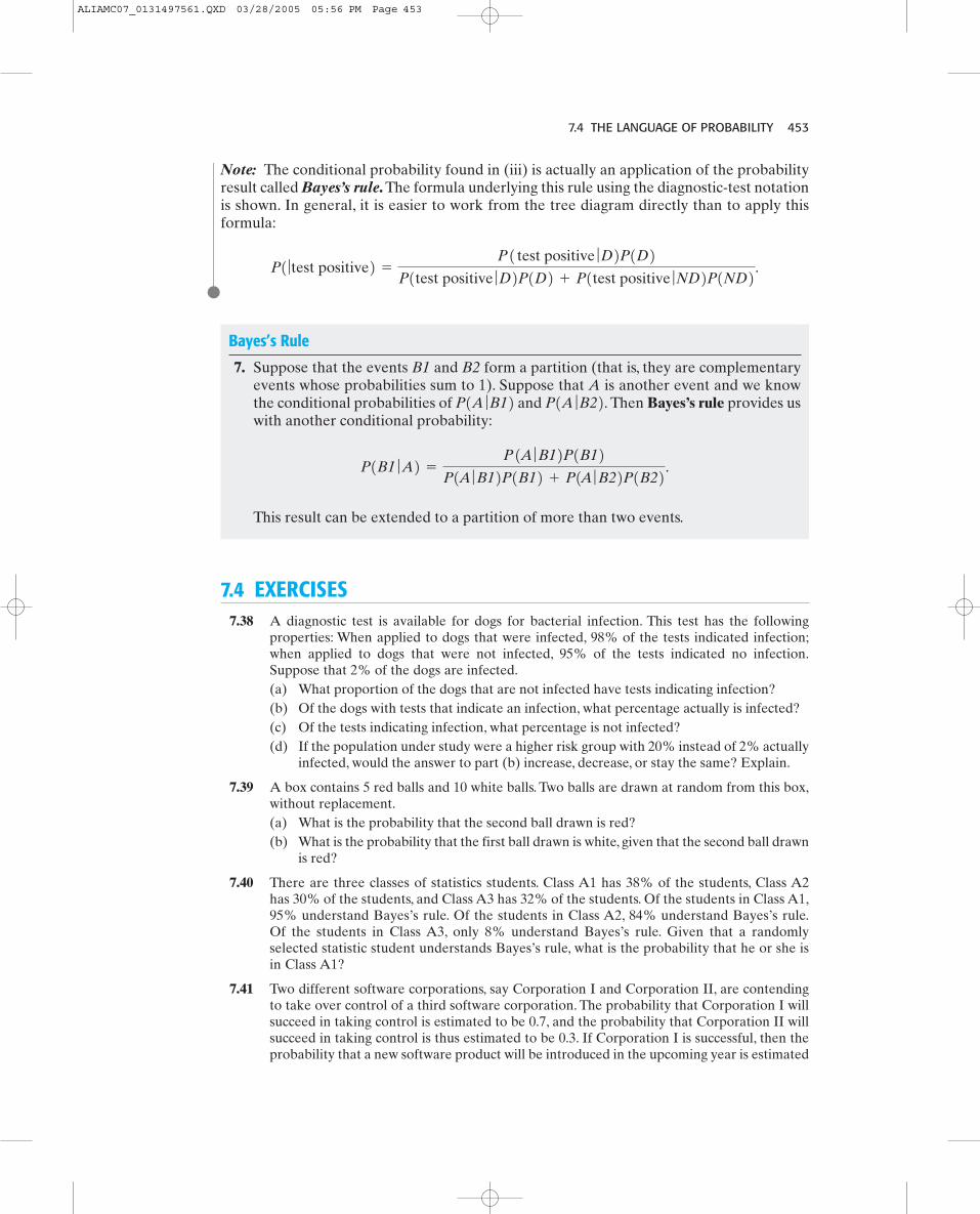
7.4 THE LANGUAGE OF PROBABILITY 453
Note: The conditional probability found in (iii) is actually an application of the probabilityresult called Bayes’s rule. The formula underlying this rule using the diagnostic-test notationis shown. In general, it is easier to work from the tree diagram directly than to apply thisformula:
P1 ƒtest positive2 =
P1test positive ƒ D2P1D2P1test positive ƒ D2P1D2 + P1test positive ƒ ND2P1ND2.
Bayes’s Rule
7. Suppose that the events B1 and B2 form a partition (that is, they are complementaryevents whose probabilities sum to 1). Suppose that A is another event and we knowthe conditional probabilities of and Then Bayes’s rule provides uswith another conditional probability:
This result can be extended to a partition of more than two events.
P1B1 ƒ A2 =
P1A ƒ B12P1B12P1A ƒ B12P1B12 + P1A ƒ B22P1B22.
P1A ƒ B22.P1A ƒ B12
7.4 EXERCISES7.38 A diagnostic test is available for dogs for bacterial infection. This test has the following
properties: When applied to dogs that were infected, 98% of the tests indicated infection;when applied to dogs that were not infected, 95% of the tests indicated no infection.Suppose that 2% of the dogs are infected.(a) What proportion of the dogs that are not infected have tests indicating infection?(b) Of the dogs with tests that indicate an infection, what percentage actually is infected?(c) Of the tests indicating infection, what percentage is not infected?(d) If the population under study were a higher risk group with 20% instead of 2% actually
infected, would the answer to part (b) increase, decrease, or stay the same? Explain.
7.39 A box contains 5 red balls and 10 white balls. Two balls are drawn at random from this box,without replacement.(a) What is the probability that the second ball drawn is red?(b) What is the probability that the first ball drawn is white, given that the second ball drawn
is red?
7.40 There are three classes of statistics students. Class A1 has 38% of the students, Class A2has 30% of the students, and Class A3 has 32% of the students. Of the students in Class A1,95% understand Bayes’s rule. Of the students in Class A2, 84% understand Bayes’s rule.Of the students in Class A3, only 8% understand Bayes’s rule. Given that a randomlyselected statistic student understands Bayes’s rule, what is the probability that he or she isin Class A1?
7.41 Two different software corporations, say Corporation I and Corporation II, are contendingto take over control of a third software corporation. The probability that Corporation I willsucceed in taking control is estimated to be 0.7, and the probability that Corporation II willsucceed in taking control is thus estimated to be 0.3. If Corporation I is successful, then theprobability that a new software product will be introduced in the upcoming year is estimated
ALIAMC07_0131497561.QXD 03/28/2005 05:56 PM Page 453
454 CHAPTER 7 HOW TO MEASURE UNCERTAINTY WITH PROBABILITY
at 0.8. If Corporation II is successful, then the probability that a new software product willbe introduced in the upcoming year is estimated at only 0.4.(a) What is the probability that a new software product will be introduced in the upcoming
year?(b) Given that a new software product is introduced in the upcoming year, what is the prob-
ability that Corporation I was successful in taking over control?
7.42 The membership for a small college is composed of 80% students and 20% faculty.The pres-ident of the college has introduced a proposal requiring all students to take an introductorystatistical-reasoning course. Among faculty, 60% favor the proposal, 15% oppose the pro-posal, and 25% are neutral on the proposal. Among students, 40% are in favor, 50% oppose,and the rest are neutral. A letter (from a member of the college) was sent to the presidentregarding this proposal. Show all work for the following questions:(a) What is the probability the writer of this letter favors the new proposal?(b) Given that the writer of the letter states he/she is in favor of the new proposal, what is
the probability the letter was sent by a faculty member?
7.43 A paint store sells three types of high-volume paint sprayers used by professional painters:Type I, Type II, and Type III. Based on records, 70% of the sprayer sales are of Type I, and20% are of Type II. About 3% of the Type I sprayers need repair during warranty period,while the figure for Type II is 4% and the figure for Type III is 5%.(a) Find the probability that a randomly selected sprayer purchased from this store will need
repair under warranty.(b) Find the probability that two randomly selected sprayers purchased from this store will
both need repair under warranty.(c) Find the probability that a sprayer is a Type III sprayer, given that it needed repair dur-
ing warranty period.
7.44 A diagnostic test for drug use among Olympic athletes based on a blood sample was thoughtto be excellent. Among drug users, 98% had a positive test. Among nondrug users, 95% hada negative test. Suppose that 1% of the athletes are, indeed, drug users.(a) What proportion of the athletes tested would have a positive test?(b) Of those athletes whose test is positive, what proportion are really drug users?
7.45 Suppose that only two factories make Playstation machines. Factory 1 produces 70% of themachines and Factory 2 produces the remaining 30%. Of the machines produced at Factory1, 2% are defective. Of the machines produced at Factory 2, 5% are defective.(a) What proportion of Playstation machines produced by these two factories are defective?(b) Suppose that you purchase a Playstation machine and it is defective. What is the proba-
bility that it was produced by Factory 1?
7.46 Suppose that it is known that, among students taking a certain entrance exam, 10% cheat onthe exam and 90% do not cheat on the exam. Also, about 70% of the cheaters get a perfectscore, while only 20% of the noncheaters get a perfect score.(a) Create a tree diagram for this situation.(b) What is the probability that a randomly selected student taking the exam will get a perfect
score?(c) Given that a student has a perfect score on the exam, what is the conditional probability
that it was obtained by cheating?
7.5 RANDOM VARIABLESMany gambling games use dice in which the number of dots rolled for a single die is equallylikely to be 1, 2, 3, 4, 5, or 6. Consider the random experiment of rolling two fair dice. Thecorresponding sample space is shown.Assuming that all of these 36 points are equally likely,
ALIAMC07_0131497561.QXD 03/28/2005 05:56 PM Page 454
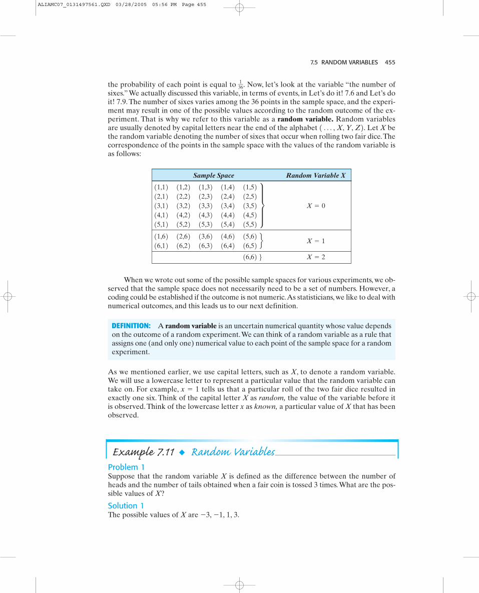
7.5 RANDOM VARIABLES 455
the probability of each point is equal to Now, let’s look at the variable “the number ofsixes.” We actually discussed this variable, in terms of events, in Let’s do it! 7.6 and Let’s doit! 7.9. The number of sixes varies among the 36 points in the sample space, and the experi-ment may result in one of the possible values according to the random outcome of the ex-periment. That is why we refer to this variable as a random variable. Random variablesare usually denoted by capital letters near the end of the alphabet Let X bethe random variable denoting the number of sixes that occur when rolling two fair dice.Thecorrespondence of the points in the sample space with the values of the random variable isas follows:
1Á , X, Y, Z2.
136.
Sample Space Random Variable X
X = 216,62 6X = 1
11,62 12,62 13,62 14,62 15,6216,12 16,22 16,32 16,42 16,52 f
X = 0
11,12 11,22 11,32 11,42 11,5212,12 12,22 12,32 12,42 12,5213,12 13,22 13,32 13,42 13,5214,12 14,22 14,32 14,42 14,5215,12 15,22 15,32 15,42 15,52
u
When we wrote out some of the possible sample spaces for various experiments, we ob-served that the sample space does not necessarily need to be a set of numbers. However, acoding could be established if the outcome is not numeric.As statisticians, we like to deal withnumerical outcomes, and this leads us to our next definition.
DEFINITION: A random variable is an uncertain numerical quantity whose value dependson the outcome of a random experiment.We can think of a random variable as a rule thatassigns one (and only one) numerical value to each point of the sample space for a randomexperiment.
As we mentioned earlier, we use capital letters, such as X, to denote a random variable.We will use a lowercase letter to represent a particular value that the random variable cantake on. For example, tells us that a particular roll of the two fair dice resulted inexactly one six. Think of the capital letter X as random, the value of the variable before itis observed. Think of the lowercase letter x as known, a particular value of X that has beenobserved.
x = 1
Example 7.11 ◆ Random VariablesProblem 1Suppose that the random variable X is defined as the difference between the number ofheads and the number of tails obtained when a fair coin is tossed 3 times. What are the pos-sible values of X?
Solution 1The possible values of X are -3, -1, 1, 3.
ALIAMC07_0131497561.QXD 03/28/2005 05:56 PM Page 455
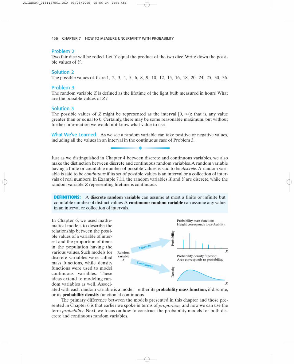
456 CHAPTER 7 HOW TO MEASURE UNCERTAINTY WITH PROBABILITY
Problem 2Two fair dice will be rolled. Let Y equal the product of the two dice. Write down the possi-ble values of Y.
Solution 2The possible values of Y are 1, 2, 3, 4, 5, 6, 8, 9, 10, 12, 15, 16, 18, 20, 24, 25, 30, 36.
Problem 3The random variable Z is defined as the lifetime of the light bulb measured in hours. Whatare the possible values of Z?
Solution 3The possible values of Z might be represented as the interval that is, any valuegreater than or equal to 0. Certainly, there may be some reasonable maximum, but withoutfurther information we would not know what value to use.
What We’ve Learned: As we see a random variable can take positive or negative values,including all the values in an interval in the continuous case of Problem 3.
[0, q2;
Just as we distinguished in Chapter 4 between discrete and continuous variables, we alsomake the distinction between discrete and continuous random variables.A random variablehaving a finite or countable number of possible values is said to be discrete. A random vari-able is said to be continuous if its set of possible values is an interval or a collection of inter-vals of real numbers. In Example 7.11, the random variables X and Y are discrete, while therandom variable Z representing lifetime is continuous.
DEFINITIONS: A discrete random variable can assume at most a finite or infinite butcountable number of distinct values.A continuous random variable can assume any valuein an interval or collection of intervals.
In Chapter 6, we used mathe-matical models to describe therelationship between the possi-ble values of a variable of inter-est and the proportion of itemsin the population having thevarious values. Such models fordiscrete variables were calledmass functions, while densityfunctions were used to modelcontinuous variables. Theseideas extend to modeling ran-dom variables as well. Associ-ated with each random variable is a model—either its probability mass function, if discrete,or its probability density function, if continuous.
The primary difference between the models presented in this chapter and those pre-sented in Chapter 6 is that earlier we spoke in terms of proportion, and now we can use theterm probability. Next, we focus on how to construct the probability models for both dis-crete and continuous random variables.
Probability density function:Area corresponds to probability.
Probability mass function:Height corresponds to probability.
Continuous
Discrete
Den
sity
Pro
babi
lity
Randomvariable
X
X
X
ALIAMC07_0131497561.QXD 03/28/2005 05:56 PM Page 456

7.5 RANDOM VARIABLES 457
7.5.1 Discrete Random VariablesA random variable X having a finite or countable number, k, of possible values is said to bediscrete. A probability is assigned to each of the k possible values, where each probabilitymust be between 0 and 1 and the sum of all of the probabilities must equal 1. The set of val-ues along with their probabilities is called the probability distribution of X or probabilitymass function for X. If X is a discrete random variable taking on the values withprobabilities the probability distribution of X is given by
We can also represent this function as
p1, p2, Á pk,x1, x2, Á xk,
Value of X
ProbabilitypkÁp2p1P1X � x2xkÁx2x1X � x
p1x2 = d p1 if x = x1
p2 if x = x2
o o
pk if x = xk
DEFINITION: The probability distribution of a discrete random variable X is a table or rulethat assigns a probability to each of the possible values of the random variable X. Thevalues of a discrete probability distribution (the assigned probabilities) must be between0 and 1 and must add up to 1, that is, ©pi = 1.
Recall the random experiment of rolling two fair dice and the random variable X defined tobe “the number of sixes.”The possible values for the random variable X are 0, 1, and 2. Sinceonly one of the 36 equally likely outcomes corresponds to having exactly two sixes, the prob-ability that the random variable takes on the value of 2 is equal to The probability that
is equal to since 25 of the outcomes correspond to obtaining no sixes. Likewise, theprobability that is equal to The probability distribution for X is given in the followingtable. Notice that the probabilities do sum up to one.
A picture of the probability distribution of a discreterandom variable X can be displayed using a stick graph or aprobability bar graph, as shown in the next example.
1036.X = 1
2536,X = 0
136.
P(X � x)
X � x
2536
0
136
2
1036
1
Probability
Example 7.12 ◆ People in a Household ProblemLet X be the number of people in ahousehold for a certain community.Consider the following probabilitydistribution for X, which assumesthat there are no more than sevenpeople in a household.
Value of X 1 2 3 4 5 6 7
Probability0.20 0.32 0.18 0.15 0.07 0.03P1X � x2
X � x
(a) What must be the probability of seven people in a household for this to be a legitimatediscrete distribution?
(b) Display this probability distribution graphically—use either a stick graph or a probabilitybar graph.
ALIAMC07_0131497561.QXD 03/28/2005 05:56 PM Page 457

458 CHAPTER 7 HOW TO MEASURE UNCERTAINTY WITH PROBABILITY
(c) What is the probability that a randomly chosen household contains more than fivepeople?
(d) What is the probability that a randomly chosen household contains no more than twopeople?
(e) What is the probability that a randomly selected household has more than two but atmost four people?
Solution(a) .(b)
1 - 10.20 + 0.32 + 0.18 + 0.15 + 0.07 + 0.032 = 0.05
0 1 2 3 4 5 6 7
X � number of people
Stick graph Probability bar graph
X � number of people
0.2
0.3
0.4
00 1 2 3 4 5 6 7
0.2
0.3
0.4
0
Pro
babi
lity
Pro
babi
lity
Let's Do It!
7.207.20Sum of Pips
In a game called craps, two dice are rolled and the sum of the faces on the two dice determineswhether the player wins, loses, or continues rolling the dice. Let X be the sum of the valueson the two dice. Recall the 36 possible pairs of faces of the two dice.
S = 5
11, 12 11, 22 11, 32 11, 42 11, 52 11, 6212, 12 12, 22 12, 32 12, 42 12, 52 12, 6213, 12 13, 22 13, 32 13, 42 13, 52 13, 6214, 12 14, 22 14, 32 14, 42 14, 52 14, 6215, 12 15, 22 15, 32 15, 42 15, 52 15, 6216, 12 16, 22 16, 32 16, 42 16, 52 16, 62 6 .
(c)(d)(e)
What We’ve Learned: For a discrete probability model, we need to read the probabilityquestion carefully. In part (b) we found the probability of more than five people. If the ques-tion had asked for the probability of five or more, the answer would not have been 0.08, butrather Since probabilities are assigned to the finite (or countable)outcomes, whether or not an endpoint outcome is included can change the probability of theevent.
0.07 + 0.03 + 0.05 = 0.15.
P12 6 X … 42 = 0.18 + 0.15 = 0.33.P1X … 22 = 0.32 + 0.20 = 0.52.P1X 7 52 = 0.03 + 0.05 = 0.08.
ALIAMC07_0131497561.QXD 03/28/2005 05:56 PM Page 458
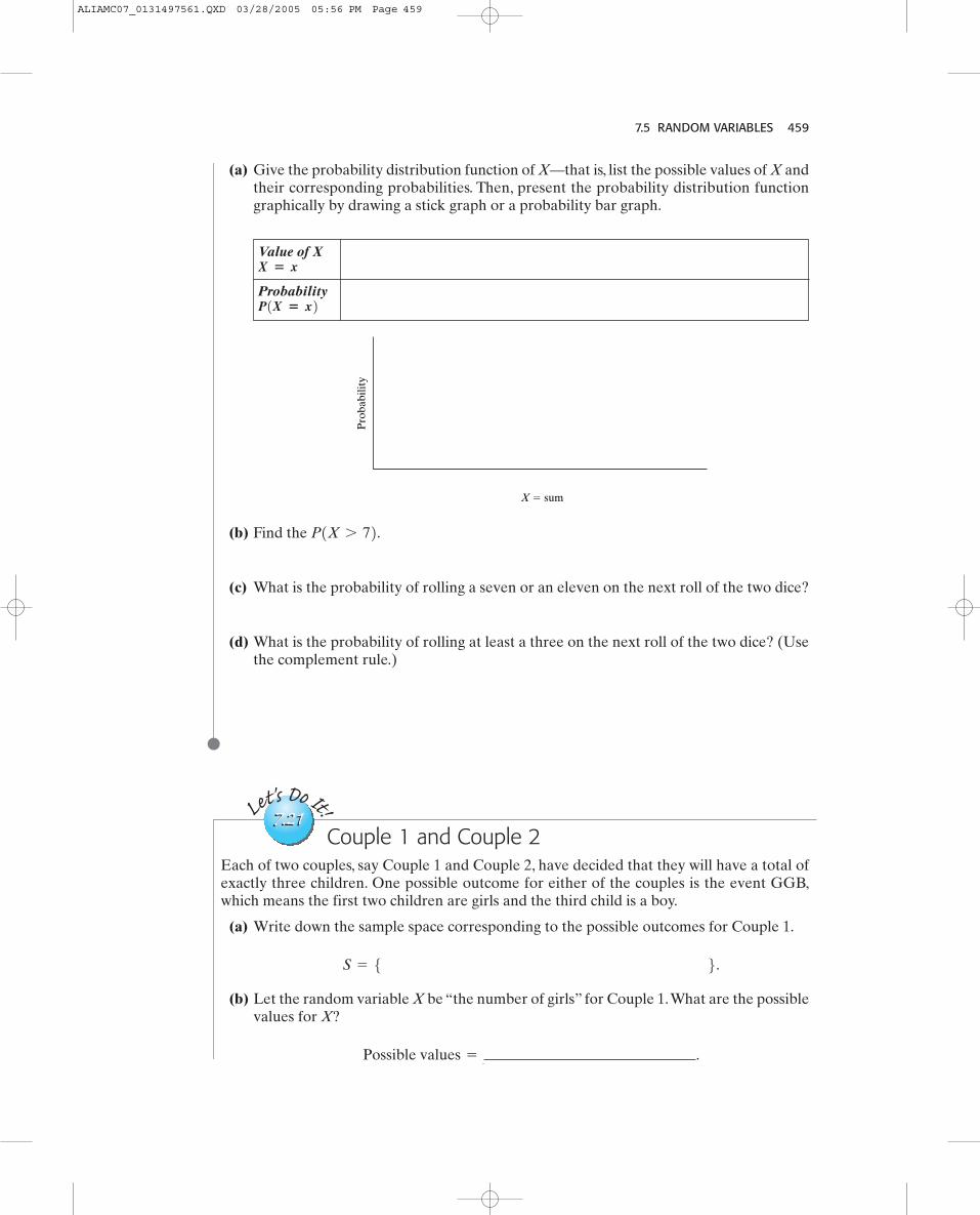
7.5 RANDOM VARIABLES 459
Value of X
ProbabilityP1X � x2X � x
(a) Give the probability distribution function of X—that is, list the possible values of X andtheir corresponding probabilities. Then, present the probability distribution functiongraphically by drawing a stick graph or a probability bar graph.
X � sum
Pro
babi
lity
(b) Find the
(c) What is the probability of rolling a seven or an eleven on the next roll of the two dice?
(d) What is the probability of rolling at least a three on the next roll of the two dice? (Usethe complement rule.)
P1X 7 72.
Let's Do It!
7.217.21Couple 1 and Couple 2
Each of two couples, say Couple 1 and Couple 2, have decided that they will have a total ofexactly three children. One possible outcome for either of the couples is the event GGB,which means the first two children are girls and the third child is a boy.
(a) Write down the sample space corresponding to the possible outcomes for Couple 1.
(b) Let the random variable X be “the number of girls” for Couple 1.What are the possiblevalues for X?
.Possible values =
S = 5 6.
ALIAMC07_0131497561.QXD 03/28/2005 05:56 PM Page 459

460 CHAPTER 7 HOW TO MEASURE UNCERTAINTY WITH PROBABILITY
1 2 3 4 5 6 1 2 3 4 5 6 1 2 3 4 5 6
In Chapter 5, we discussed how to summarize a set of data using numerical summaries ofthe center and spread of the data. So before we turn to continuous random variables, we willlearn how to summarize a discrete probability distribution by using the mean and the stan-dard deviation.The mean of a discrete random variable X is the point at which the probabilitystick graph or bar graph would balance.
Value of X
ProbabilityP(X � x)
X � x
(c) Assume that each child has probability of being a girl and of being a boy and that thegender of successive children is independent. Give the probability distribution for therandom variable “number of girls” for Couple 1.X =
12
12
(d) Assuming that the outcome for Couple 1 is independent of the outcome for Couple 2,what is the probability that the two couples will have the same number of girls?
The mean of X is also referred to as the expected value of X and is calculated as follows:
DEFINITION: If X is a discrete random variable taking on the values withprobabilities then the mean or expected value of X is given by
E1X2 = m = x1p1 + x2p2 +Á
+ xkpk = axipi.
p1, p2, Á pk,x1, x2, Á xk,
A note of caution regarding the term expected: The expected value of a random variabledoes not necessarily have to equal one of the values that are possible for the random vari-able.The mean is the value that you would expect, on average—that is, the mean of observedvalues X in a very large number of repetitions of the random experiment.
ALIAMC07_0131497561.QXD 03/28/2005 05:56 PM Page 460
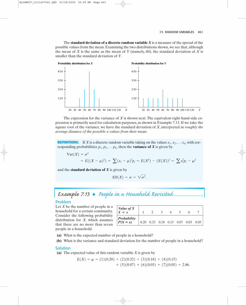
7.5 RANDOM VARIABLES 461
X20 30 40 50 60 70 80 90 100 110 120
Probability distribution for X Probability distribution for Y
4/10
3/10
2/10
1/10
Y20 30 40 50 60 70 80 90 100 110 120
4/10
3/10
2/10
1/10
The expression for the variance of X is shown next. The equivalent right-hand-side ex-pression is primarily used for calculation purposes, as shown in Example 7.13. If we take thesquare root of the variance, we have the standard deviation of X, interpreted as roughly theaverage distance of the possible x-values from their mean.
DEFINITIONS: If X is a discrete random variable taking on the values with cor-responding probabilities then the variance of X is given by
and the standard deviation of X is given by
SD1X2 = s = 2s2.
= E11X - m222 = a 1xi - m22pi = E1X22 - 1E1X222 = axi2pi - m2
Var1X2 = s2
p1, p2, Á pk,x1, x2, Á xk,
Example 7.13 ◆ People in a Household RevisitedProblemLet X be the number of people in ahousehold for a certain community.Consider the following probabilitydistribution for X, which assumesthat there are no more than sevenpeople in a household.
Value of X1 2 3 4 5 6 7
ProbabilityP(X � x) 0.20 0.32 0.18 0.15 0.07 0.03 0.05
X � x
(a) What is the expected number of people in a household?(b) What is the variance and standard deviation for the number of people in a household?
Solution(a) The expected value of this random variable X is given by
+ 15210.072 + 16210.032 + 17210.052 = 2.86. E1X2 = m = 11210.202 + 12210.322 + 13210.182 + 14210.152
The standard deviation of a discrete random variable X is a measure of the spread of thepossible values from the mean. Examining the two distributions shown, we see that, althoughthe mean of X is the same as the mean of Y (namely, 60), the standard deviation of X issmaller than the standard deviation of Y.
ALIAMC07_0131497561.QXD 03/28/2005 05:56 PM Page 461
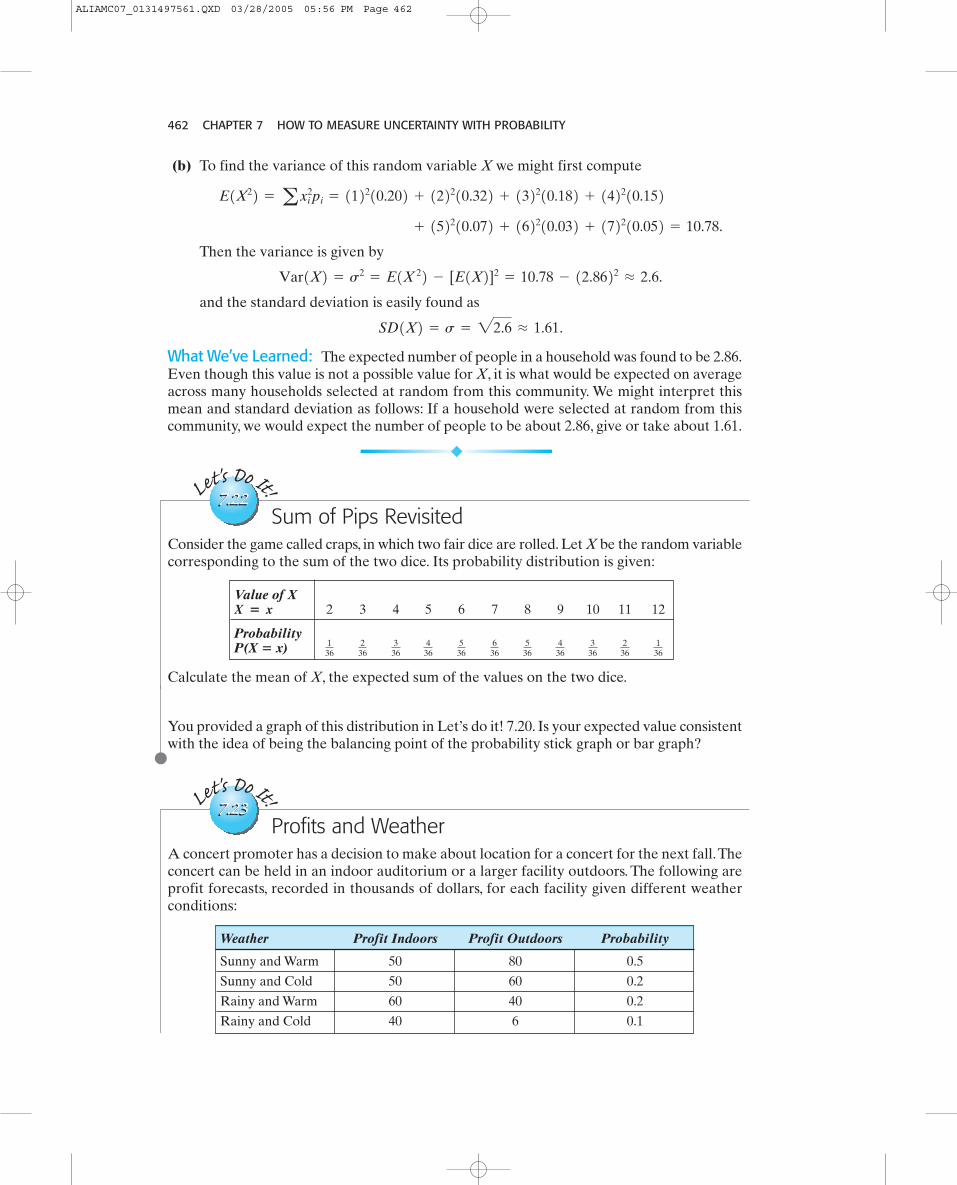
462 CHAPTER 7 HOW TO MEASURE UNCERTAINTY WITH PROBABILITY
Let's Do It!
7.227.22Sum of Pips Revisited
Consider the game called craps, in which two fair dice are rolled. Let X be the random variablecorresponding to the sum of the two dice. Its probability distribution is given:
(b) To find the variance of this random variable X we might first compute
Then the variance is given by
and the standard deviation is easily found as
What We’ve Learned: The expected number of people in a household was found to be 2.86.Even though this value is not a possible value for X, it is what would be expected on averageacross many households selected at random from this community. We might interpret thismean and standard deviation as follows: If a household were selected at random from thiscommunity, we would expect the number of people to be about 2.86, give or take about 1.61.
SD1X2 = s = 22.6 L 1.61.
Var1X2 = s2= E1X 22 - [E1X2]2
= 10.78 - 12.8622 L 2.6.
+ 152210.072 + 162210.032 + 172210.052 = 10.78.
E1X22 = axi2pi = 112210.202 + 122210.322 + 132210.182 + 142210.152
Let's Do It!
7.237.23
Value of X2 3 4 5 6 7 8 9 10 11 12
Probability P(X � x) 1
36236
336
436
536
636
536
436
336
236
136
X � x
Calculate the mean of X, the expected sum of the values on the two dice.
You provided a graph of this distribution in Let’s do it! 7.20. Is your expected value consistentwith the idea of being the balancing point of the probability stick graph or bar graph?
Weather Profit Indoors Profit Outdoors Probability
Sunny and Warm 50 80 0.5
Sunny and Cold 50 60 0.2
Rainy and Warm 60 40 0.2
Rainy and Cold 40 6 0.1
Profits and WeatherA concert promoter has a decision to make about location for a concert for the next fall.Theconcert can be held in an indoor auditorium or a larger facility outdoors. The following areprofit forecasts, recorded in thousands of dollars, for each facility given different weatherconditions:
ALIAMC07_0131497561.QXD 03/28/2005 05:56 PM Page 462

7.5 RANDOM VARIABLES 463
7.5.2 Binomial Random VariablesAt the start of Section 7.5, we learned that there are two broad types, of random variables,namely, discrete and continuous. Within each of these broad types, there are families of ran-dom variables that are common and have a special name. In this section, we will focus on aparticular family of discrete random variables called binomial random variables. To under-stand the probability mass function for a binomial random variable, we must first reviewsome basic counting problems that involve computing combinations. Then, we discuss an ex-periment in which there are only two possible outcomes, one referred to as a success and theother as a failure, with the probability of a success represented by p.This experiment is calleda Bernoulli trial and forms the basis of the distribution of a binomial random variable.
CombinationsSuppose that you have exactly two friends, Emily and Caitlyn. You are going to considerinviting them to dinner. If you decide to invite two friends to dinner you have just onechoice—invite them both. If you decide to invite exactly one friend to dinner, you have twochoices—invite just Emily or invite just Caitlyn. If you decide to invite no friends to dinneryou again have just one choice—invite no one.With this dinner invitation example, you haveperformed some basic counting problems called combinations. Let’s look at this countingproblem a little more formally.
Suppose that you have a set that contains just two distinguishable values,How many subsets are there that would contain exactly two values? The answer is just onesubset—namely, the set How many subsets are there that would contain exactlyone value? There are two possible subsets—namely, and How many subsets arethere that contain exactly zero values (no values)? There is just one subset, called theempty set, represented by The following table summarizes these counting questions:¤.
526.51651, 26.S = 51, 26.
(a) The expected profit for the indoor facility is $51,000. Compute the expected profitassociated with the outdoor facility.
Outdoor facility expected (include your units).
(b) Which location is preferred if the objective is maximizing the expected profit?
(c) Which location is preferred if the promoter must clear a profit of at least $40,000?
(d) Which location has the least variability in the profits? Explain. No calculations arenecessary—just picture the two distributions graphically.
profit =
ALIAMC07_0131497561.QXD 03/28/2005 05:56 PM Page 463

464 CHAPTER 7 HOW TO MEASURE UNCERTAINTY WITH PROBABILITY
Combinations
“n choose x” represents the number of ways of selecting x items (without replacement)from a set of n distinguishable items when the order of the selection is not important andis given by
Note: By definition, we have and Anx B = 0 if x 6 0 or n 6 x.0! = 1
anxb =
n!x!1n - x2!, where n! = n1n - 121n - 22Á 122112.
How many subsets of S � {1, 2}are there that contain Answer The subsets are Combination
exactly zero values (no values)? 1
exactly one value? 2
exactly two values? 1 a22b = 151, 26Á
a21b = 2516, 526Á
a20b = 1¤Á
Á
If we add up the “answer” column, we have a total of four possible subsets of the setIn general, the total number of possible subsets is computed as where n is the
number of elements in the original set.The last column presents the mathematical expressionfor determining the number of ways of selecting a certain number of items (without replace-ment) from a set of distinguishable items when the order of the selection is not important. Forexample, is the number of combinations of two items taking one at a time (that is, the num-ber of ways you can select one item from two distinguishable items, which is equal to two).
In general, is the number of combinations of n distinguishable items taking x itemsat a time and is read “n choose x.” The general formula for finding the number of combina-tions is as follows:
Anx BA 21 B
2n,S = 51, 26.
The TI graphing calculators have an operation called nCr for finding the number of combi-nations.This operation is found under the MATH PRB menu.The steps for finding the num-ber of combinations of 20 items taking two at a time are as follows:
Your output screen should look like
the total # items, n � 20
for the operation nCr
the # items you wish to select, r � 2
0 32 2 ENTERMATH
The answer is
a202b =
20!2!18!
= 190.
ALIAMC07_0131497561.QXD 03/28/2005 05:56 PM Page 464
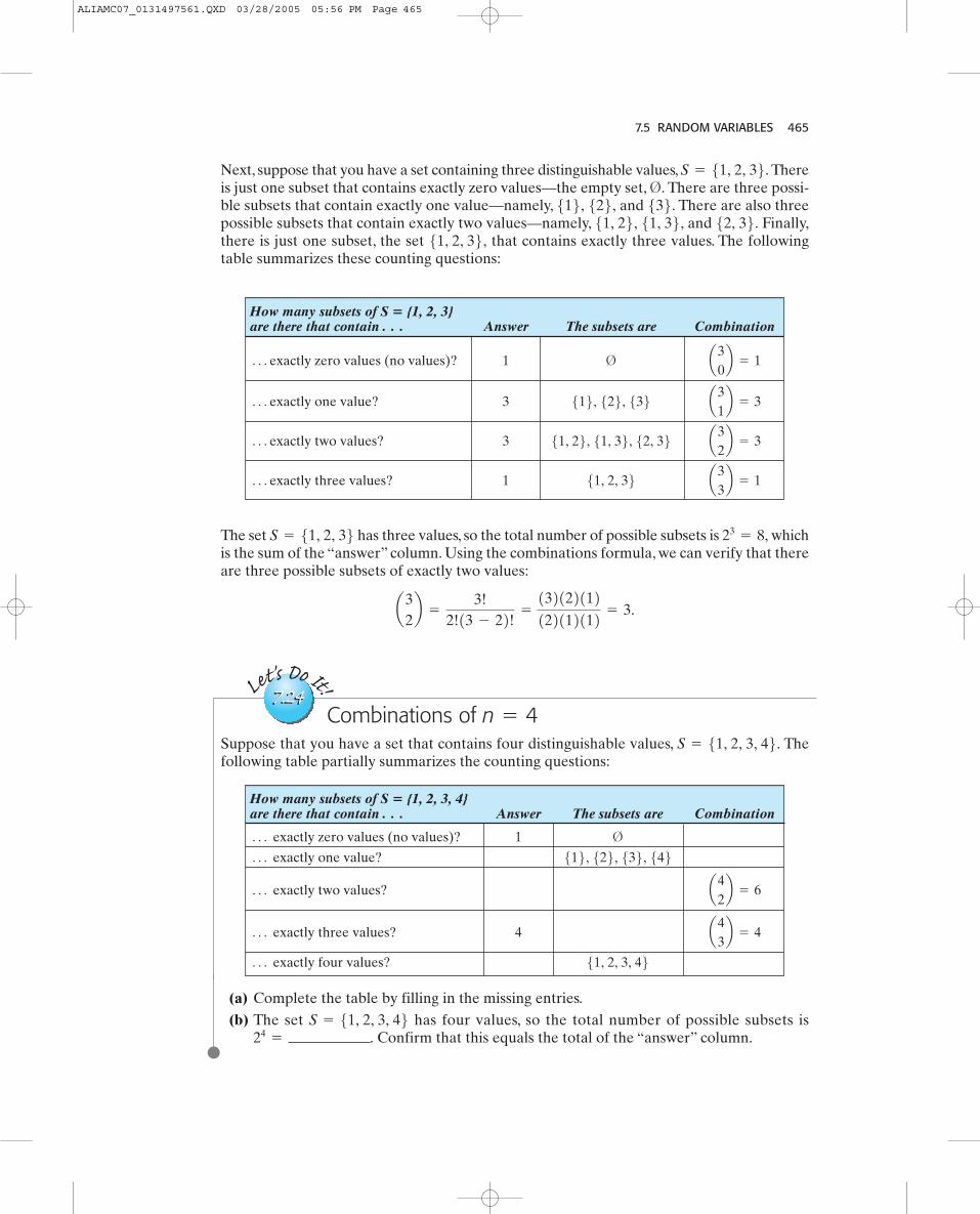
7.5 RANDOM VARIABLES 465
Next, suppose that you have a set containing three distinguishable values, Thereis just one subset that contains exactly zero values—the empty set, There are three possi-ble subsets that contain exactly one value—namely, and There are also threepossible subsets that contain exactly two values—namely, and Finally,there is just one subset, the set that contains exactly three values. The followingtable summarizes these counting questions:
51, 2, 36, 52, 36.51, 26, 51, 36,536.516, 526, ¤.S = 51, 2, 36.
How many subsets of S � {1, 2, 3}are there that contain Answer The subsets are Combination
exactly zero values (no values)? 1
exactly one value? 3
exactly two values? 3
exactly three values? 1 a33b = 151, 2, 36Á
a32b = 351, 26, 51, 36, 52, 36Á
a31b = 3516, 526, 536Á
a30b = 1¤Á
Á
The set has three values, so the total number of possible subsets is whichis the sum of the “answer” column. Using the combinations formula, we can verify that thereare three possible subsets of exactly two values:
a32b =
3!2!13 - 22! =
132122112122112112 = 3.
23= 8,S = 51, 2, 36
Let's Do It!
7.247.24Combinations of n � 4
Suppose that you have a set that contains four distinguishable values, Thefollowing table partially summarizes the counting questions:
S = 51, 2, 3, 46.
How many subsets of S � {1, 2, 3, 4}are there that contain Answer The subsets are Combination
exactly zero values (no values)? 1
exactly one value?
exactly two values?
exactly three values? 4
exactly four values? 51, 2, 3, 46Á
a43b = 4Á
a42b = 6Á
516, 526, 536, 546Á
¤Á
Á
(a) Complete the table by filling in the missing entries.(b) The set has four values, so the total number of possible subsets is
. Confirm that this equals the total of the “answer” column.24=
S = 51, 2, 3, 46
ALIAMC07_0131497561.QXD 03/28/2005 05:56 PM Page 465
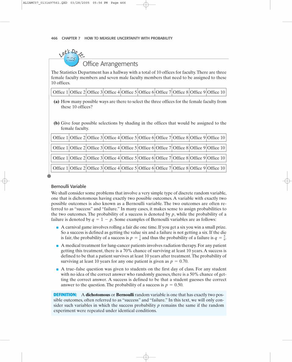
466 CHAPTER 7 HOW TO MEASURE UNCERTAINTY WITH PROBABILITY
Let's Do It!
7.257.25
Bernoulli VariableWe shall consider some problems that involve a very simple type of discrete random variable,one that is dichotomous having exactly two possible outcomes. A variable with exactly twopossible outcomes is also known as a Bernoulli variable. The two outcomes are often re-ferred to as “success” and “failure.” In many cases, it makes sense to assign probabilities tothe two outcomes. The probability of a success is denoted by p, while the probability of afailure is denoted by Some examples of Bernoulli variables are as follows:
■ A carnival game involves rolling a fair die one time. If you get a six you win a small prize.So a success is defined as getting the value six and a failure is not getting a six. If the dieis fair, the probability of a success is and thus the probability of a failure is
■ A medical treatment for lung-cancer patients involves radiation therapy. For any patientgetting this treatment, there is a 70% chance of surviving at least 10 years. A success isdefined to be that a patient survives at least 10 years after treatment.The probability ofsurviving at least 10 years for any one patient is given as
■ A true–false question was given to students on the first day of class. For any studentwith no idea of the correct answer who randomly guesses, there is a 50% chance of get-ting the correct answer. A success is defined to be that a student guesses the correctanswer to the question. The probability of a success is p = 0.50.
p = 0.70.
q =56.p =
16
q = 1 - p.
Office ArrangementsThe Statistics Department has a hallway with a total of 10 offices for faculty.There are threefemale faculty members and seven male faculty members that need to be assigned to these10 offices.
Office 1 Office 2 Office 3 Office 4 Office 5 Office 6 Office 7 Office 8 Office 9 Office 10
(a) How many possible ways are there to select the three offices for the female faculty fromthese 10 offices?
(b) Give four possible selections by shading in the offices that would be assigned to thefemale faculty.
Office 1 Office 2 Office 3 Office 4 Office 5 Office 6 Office 7 Office 8 Office 9 Office 10
Office 1 Office 2 Office 3 Office 4 Office 5 Office 6 Office 7 Office 8 Office 9 Office 10
Office 1 Office 2 Office 3 Office 4 Office 5 Office 6 Office 7 Office 8 Office 9 Office 10
Office 1 Office 2 Office 3 Office 4 Office 5 Office 6 Office 7 Office 8 Office 9 Office 10
DEFINITION: A dichotomous or Bernoulli random variable is one that has exactly two pos-sible outcomes, often referred to as “success” and “failure.” In this text, we will only con-sider such variables in which the success probability p remains the same if the randomexperiment were repeated under identical conditions.
ALIAMC07_0131497561.QXD 03/28/2005 05:56 PM Page 466
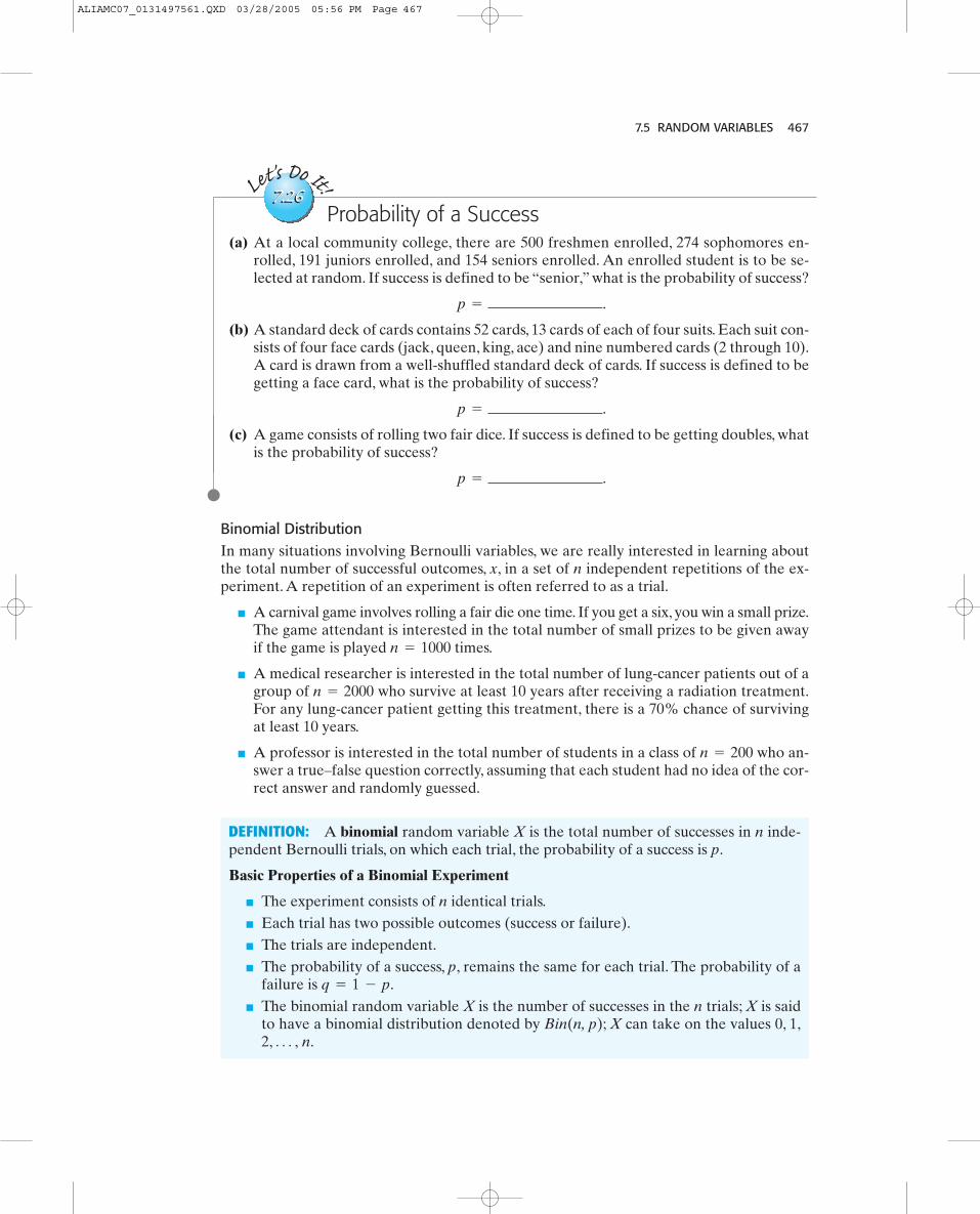
7.5 RANDOM VARIABLES 467
Binomial DistributionIn many situations involving Bernoulli variables, we are really interested in learning aboutthe total number of successful outcomes, x, in a set of n independent repetitions of the ex-periment. A repetition of an experiment is often referred to as a trial.
■ A carnival game involves rolling a fair die one time. If you get a six, you win a small prize.The game attendant is interested in the total number of small prizes to be given awayif the game is played times.
■ A medical researcher is interested in the total number of lung-cancer patients out of agroup of who survive at least 10 years after receiving a radiation treatment.For any lung-cancer patient getting this treatment, there is a 70% chance of survivingat least 10 years.
■ A professor is interested in the total number of students in a class of who an-swer a true–false question correctly, assuming that each student had no idea of the cor-rect answer and randomly guessed.
n = 200
n = 2000
n = 1000
Let's Do It!
7.267.26Probability of a Success
(a) At a local community college, there are 500 freshmen enrolled, 274 sophomores en-rolled, 191 juniors enrolled, and 154 seniors enrolled. An enrolled student is to be se-lected at random. If success is defined to be “senior,” what is the probability of success?
.
(b) A standard deck of cards contains 52 cards, 13 cards of each of four suits. Each suit con-sists of four face cards (jack, queen, king, ace) and nine numbered cards (2 through 10).A card is drawn from a well-shuffled standard deck of cards. If success is defined to begetting a face card, what is the probability of success?
.
(c) A game consists of rolling two fair dice. If success is defined to be getting doubles, whatis the probability of success?
.p =
p =
p =
DEFINITION: A binomial random variable X is the total number of successes in n inde-pendent Bernoulli trials, on which each trial, the probability of a success is p.
Basic Properties of a Binomial Experiment
■ The experiment consists of n identical trials.■ Each trial has two possible outcomes (success or failure).■ The trials are independent.■ The probability of a success, p, remains the same for each trial. The probability of a
failure is ■ The binomial random variable X is the number of successes in the n trials; X is said
to have a binomial distribution denoted by Bin(n, p); X can take on the values 0, 1,2, Á , n.
q = 1 - p.
ALIAMC07_0131497561.QXD 03/28/2005 05:56 PM Page 467

468 CHAPTER 7 HOW TO MEASURE UNCERTAINTY WITH PROBABILITY
a
b
c
a
b
c
a
b
c
a
b
c
Q1 Q2 Q3 Q4
Each question is worth one point for a total possible score of four points. Suppose that astudent will just be guessing the answer for each question independently. The probability ofgetting Question 1 correct would be just The probability of getting Question 2 correct isalso In fact, the probability of getting any one question correct would be If we let the ran-dom variable X be the number of correct answers, then a model for X would be a binomialdistribution with and —that is, X has a distribution. Let’s work out thisbinomial probability distribution.
First, we consider the outcome (that is, that the student gets all four questions in-correct for a score of 0). Since the student is assumed to be guessing the answer for eachquestion independently, we can find the probability of getting all four questions incorrect bymultiplying the individual probabilities for each question.
Similarly, we would find the probability of getting all four questions correct by multiplyingthe individual probabilities for each question.
How would we find the probability that the student will get a score of 1? The outcome would occur for each of the following four possible situations:
Q1 correct, Q2 incorrect, Q3 incorrect, Q4 incorrect;Q1 incorrect, Q2 correct, Q3 incorrect, Q4 incorrect;Q1 incorrect, Q2 incorrect, Q3 correct, Q4 incorrect;Q1 incorrect, Q2 incorrect, Q3 incorrect, Q4 correct.
Using our combinations formula, is the number of ways to select exactly one question tobe answered correctly out of four possible questions, which is equal to four. Each of these fourpossible situations has probability where corresponds to the one questionanswered correctly and corresponds to the three questions answered incorrectly. Sum-ming up the probabilities for these four possible situations, we get
Using our combinations formula and the independence of the questions, we also have
P1X = 32 = a43b A 13 B 3 A 23 B 1 = 4 A 13 B 3 A 23 B 1 = 0.0988.
P1X = 22 = a42b A 13 B 2 A 23 B 2 = 6 A 13 B 2 A 23 B 2 = 0.2963:
P1X = 12 = a41b A 13 B 1 A 23 B 3 = 4 A 13 B 1 A 23 B 3 = 0.3951.
12323113211132112323,
1412
X = 1
= A 13 B A 13 B A 13 B A 13 B = A 13 B 4 = 0.0123
= P1Q1 correct2 P1Q2 correct2 P1Q3 correct2 P1Q4 correct2 P1X = 42 = P1all 4 questions correct2
= A 23 B A 23 B A 23 B A 23 B = A 23 B 4 = 0.1975
= P1Q1 incorrect2 P1Q2 incorrect2 P1Q3 incorrect2 P1Q4 incorrect2 P1X = 02 = P1all 4 questions incorrect2
X = 0
Bin14, 132p =13n = 4
13.
13.
13.
Suppose that your next statistics quiz consists of four multiple-choice questions. Each of thefour questions will have three possible answers to select from.
ALIAMC07_0131497561.QXD 03/28/2005 05:56 PM Page 468
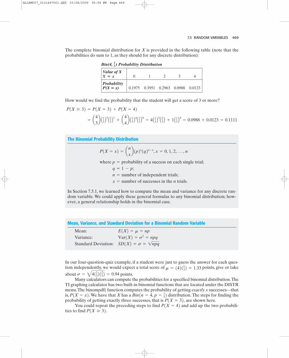
7.5 RANDOM VARIABLES 469
The complete binomial distribution for X is provided in the following table (note that theprobabilities do sum to 1, as they should for any discrete distribution):
Value of X0 1 2 3 4
Probability P(X � x) 0.1975 0.3951 0.2963 0.0988 0.0123
X � x
Bin( ) Probability Distribution4, 13
How would we find the probability that the student will get a score of 3 or more?
= a43b A 13 B 3 A 23 B 1 + a4
4b A 13 B 4 A 23 B 0 = 4 A 13 B 3 A 23 B + 1 A 13 B 4 = 0.0988 + 0.0123 = 0.1111
P1X Ú 32 = P1X = 32 + P1X = 42
The Binomial Probability Distribution
In Section 7.5.1, we learned how to compute the mean and variance for any discrete ran-dom variable. We could apply these general formulas to any binomial distribution; how-ever, a general relationship holds in the binomial case.
x = number of successes in the n trials. n = number of independent trials; q = 1 - p;
where p = probability of a success on each single trial;
P1X = x2 = anxb1p2x1q2n - x, x = 0, 1, 2, Á , n
Mean, Variance, and Standard Deviation for a Binomial Random Variable
Mean:Variance:Standard Deviation: SD1X2 = s = 1npq
Var1X2 = s2= npq
E1X2 = m = np
In our four-question-quiz example, if a student were just to guess the answer for each ques-tion independently, we would expect a total score of points, give or take
about points.Many calculators can compute the probabilities for a specified binomial distribution.The
TI graphing calculator has two built-in binomial functions that are located under the DISTRmenu.The binompdf( function computes the probability of getting exactly x successes—thatis, We have that X has a distribution. The steps for finding theprobability of getting exactly three successes, that is are shown here.
You could repeat the preceding steps to find and add up the two probabili-ties to find P1X Ú 32. P1X = 42P1X = 32,Bin1n = 4, p =
132P1X = x2.
s = 2411321232 = 0.94m = 1421132 = 1.33
ALIAMC07_0131497561.QXD 03/28/2005 05:56 PM Page 469
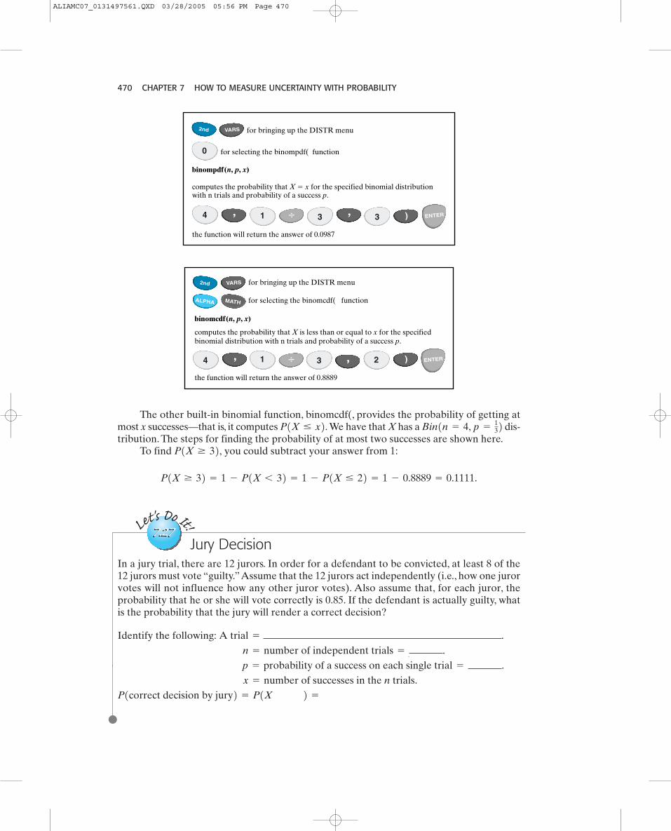
470 CHAPTER 7 HOW TO MEASURE UNCERTAINTY WITH PROBABILITY
The other built-in binomial function, binomcdf(, provides the probability of getting atmost x successes—that is, it computes We have that X has a dis-tribution. The steps for finding the probability of at most two successes are shown here.
To find you could subtract your answer from 1:
P1X Ú 32 = 1 - P1X 6 32 = 1 - P1X … 22 = 1 - 0.8889 = 0.1111.
P1X Ú 32,Bin1n = 4, p =
132P1X … x2.
for bringing up the DISTR menu
for selecting the binompdf( function
binompdf(n, p, x)
the function will return the answer of 0.0987
computes the probability that X � x for the specified binomial distribution with n trials and probability of a success p.
0
1 3 3 ENTER�
2nd VARS
,, )4
for bringing up the DISTR menu
for selecting the binomcdf( function
binomcdf(n, p, x)
the function will return the answer of 0.8889
computes the probability that X is less than or equal to x for the specified binomial distribution with n trials and probability of a success p.
1 3 24 ENTER
MATH
�
ALPHA
2nd VARS
, , )
Let's Do It!
7.277.27Jury Decision
In a jury trial, there are 12 jurors. In order for a defendant to be convicted, at least 8 of the12 jurors must vote “guilty.”Assume that the 12 jurors act independently (i.e., how one jurorvotes will not influence how any other juror votes). Also assume that, for each juror, theprobability that he or she will vote correctly is 0.85. If the defendant is actually guilty, whatis the probability that the jury will render a correct decision?
..
.
P1correct decision by jury2 = P1X 2 =
x = number of successes in the n trials.p = probability of a success on each single trial =
n = number of independent trials =
Identify the following: A trial =
ALIAMC07_0131497561.QXD 03/28/2005 05:56 PM Page 470
7.5 RANDOM VARIABLES 471
Think About It
Maximum of 13Suppose that in a particular country couples are permitted to have exactly one child.We willrefer to this as the original ruling. Assume that all couples can have children and each childhas probability 0.5 of being a boy and of being a girl. Would you expect the number of boysto be more than, less than, or about the same as the number of girls under this original ruling?What would the average number of children per family be under this original ruling?
Consider a new ruling that allows couples to have children until they get a boy or until theyhave 13 children, whichever comes first. Would you expect the number of boys to be morethan, less than, or about the same as the number of girls under this new ruling? What doyou think the average number of children per family would be under this new ruling?
7.5.3 Geometric Random VariablesMany actions in life are repeated until a success (or until a failure) occurs.The number of timesa student might take their driving test before receiving a pass, or the number of calls a sales-person must make before their first sale is made. Situations like these can be represented bya geometric distribution.
Problems like the new ruling are called waiting-time problems because you count how manytrials you have to perform (or wait for) until you see a success (a boy in this case). Thedistribution described here is called the geometric distribution. However, in the maximumof 13 new ruling, we planned to stop if we have 13 children. So we actually have a truncatedgeometric distribution. To get a better understanding about this type of distribution, we willsimulate the maximum of 13 ruling in the next Let’s Do It! exercise.
Let's Do It!
7.287.28Simulating the Maximum of 13 Ruling
Divide your class into four groups of students. Have each group of students perform asimulation of the maximum of 13 ruling using a different probability p of having a boy.
Group 1: Simulate the maximum of 13 ruling assuming that the probability of having a boyis
Group 2: Simulate the maximum of 13 ruling assuming that the probability of having a boyis
Group 3: Simulate the maximum of 13 ruling assuming that the probability of having a boyis
Group 4: Simulate the maximum of 13 ruling assuming that the probability of having a boyis
Details for how to perform the simulation and record the results are provided next for eachgroup. Each person in a group should start with a different seed value. Combine the resultsfor all students within each group (if possible each group should obtain about 100 repetitions).Then compare the results between the groups. Comment on the shape of the distributions andthe resulting averages.
p = 0.8.
p = 0.5.
p = 0.3.
p = 0.1.
ALIAMC07_0131497561.QXD 03/28/2005 05:56 PM Page 471

472 CHAPTER 7 HOW TO MEASURE UNCERTAINTY WITH PROBABILITY
1 2 4 63 5 7 8 9 10 11 12 13 13 girlsX � number of children until a boy is born (or 13 girls)
1 2 4 63 5 7 8 9 10 11 12 13 13 girlsX � number of children until a boy is born (or 13 girls)
Group 1: Your simulation can be based on using and 1, 2, 3, 4, 5, 6, 7, 8 or If you use a seed value of 60935, your first repetition (of having children until a boy or 13children) would be 7 2 3 4 4 8 6 9 8 5 0, resulting in having 11 children in total, 10 girls firstand ending with a boy. You would then add your result to the frequency plot by placing anX above the value of 11. The next repetition (of having children until a boy or 13 children)would result in 8 3 7 7 0 for a family with 5 children, the last one a boy, and you would placean X above the value of 5 on the frequency plot.
(a) Perform many simulations and record the results on a frequency plot.
9 = girl.0 = boy,
(b) Use the results of your simulation and compute the average (expected) number ofchildren per family.
Expected number of children per family
Group 2: Your simulation can be based on using 0, 1, and 3, 4, 5, 6, 7, 8 or If you use a seed value of 7593, your first repetition (of having children until a boy or 13children) would be just the 0, resulting in just one child—a boy. You would add your resultto the frequency plot by placing an X above the value of 1. The next repetition would resultin 8 1 8 0, for a family with 4 children, the last one being a boy, and you would place an X abovethe value of 4.
(a) Perform many simulations and record the results on a frequency plot.
9 = girl.2 = boy,
1p = 0.12:
(b) Use the results of your simulation and compute the average (expected) number of chil-dren per family.
Expected number of children per family
Group 3: Your simulation is like that of flipping a four coin. In this case and and you keep having children until you see a 1. Then you count the total number of children
1 = boy0 = girl
1p = 0.32:
ALIAMC07_0131497561.QXD 03/28/2005 05:56 PM Page 472

7.5 RANDOM VARIABLES 473
1 2 4 63 5 7 8 9 10 11 12 13 13 girlsX � number of children until a boy is born (or 13 girls)
1 2 4 63 5 7 8 9 10 11 12 13 13 girlsX � number of children until a boy is born (or 13 girls)
including the last one who is a boy. If you use a seed value of 3599, you would observe 0 0 0 1and thus have 4 children. You would add your result to the frequency plot by placing an Xabove the value of 4.The next repetition would result in a family with 2 children, the last onea boy, and you would place an X above the value of 2.
(a) Perform many simulations and record the results on a frequency plot.
(b) Use the results of your simulation and compute the average (expected) number ofchildren per family.
Expected number of children per family
Overall Comments:
1p = 0.82:
(b) Use the results of your simulation and compute the average (expected) number ofchildren per family.
Expected number of children per family
Group 4: Your simulation can be based on using 0, 1, 2, 3, 4, 5, 6, and 8 or If you use a seed value of 97, you would observe a 3 and thus have 1 child—a boy.You wouldadd your result to the frequency plot by placing an X above the value of 1.The next repetitionwould result in 0 for a family with 1 child, and you would again place an X on top of the firstX that is above the value of 1.
(a) Perform many simulations and record the results on a frequency plot.
9 = girl.7 = boy,
1p = 0.52:
ALIAMC07_0131497561.QXD 03/28/2005 05:56 PM Page 473
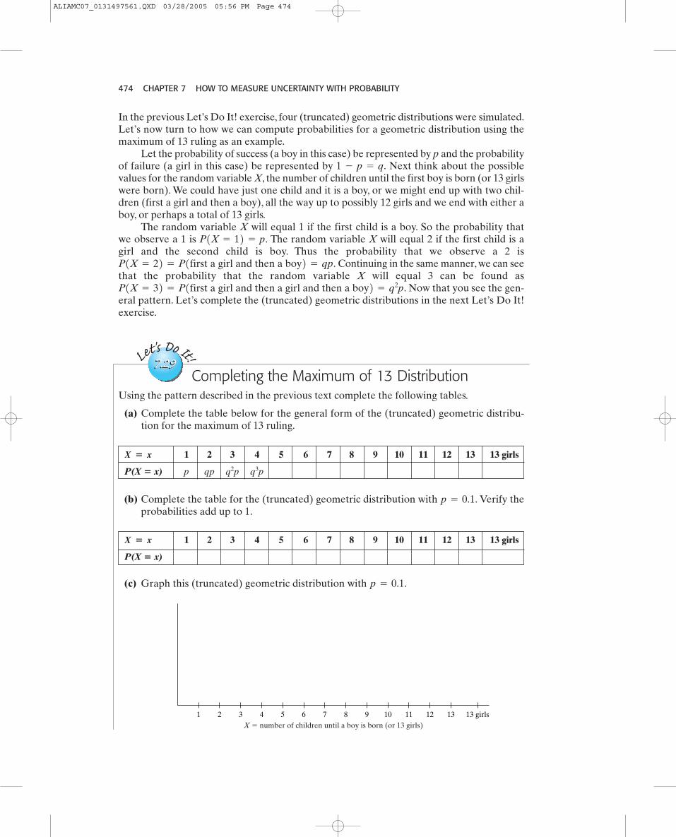
474 CHAPTER 7 HOW TO MEASURE UNCERTAINTY WITH PROBABILITY
Let's Do It!
7.297.29
1 2 4 63 5 7 8 9 10 11 12 13 13 girlsX � number of children until a boy is born (or 13 girls)
In the previous Let’s Do It! exercise, four (truncated) geometric distributions were simulated.Let’s now turn to how we can compute probabilities for a geometric distribution using themaximum of 13 ruling as an example.
Let the probability of success (a boy in this case) be represented by p and the probabilityof failure (a girl in this case) be represented by Next think about the possiblevalues for the random variable X, the number of children until the first boy is born (or 13 girlswere born). We could have just one child and it is a boy, or we might end up with two chil-dren (first a girl and then a boy), all the way up to possibly 12 girls and we end with either aboy, or perhaps a total of 13 girls.
The random variable X will equal 1 if the first child is a boy. So the probability thatwe observe a 1 is The random variable X will equal 2 if the first child is agirl and the second child is boy. Thus the probability that we observe a 2 is
Continuing in the same manner, we can seethat the probability that the random variable X will equal 3 can be found as
Now that you see the gen-eral pattern. Let’s complete the (truncated) geometric distributions in the next Let’s Do It!exercise.
P1X = 32 = P1first a girl and then a girl and then a boy2 = q2p.
P1X = 22 = P1first a girl and then a boy2 = qp.
P1X = 12 = p.
1 - p = q.
1 2 3 4 5 6 7 8 9 10 11 12 13 13 girls
P(X � x) p qp q3pq2p
X � x
Completing the Maximum of 13 DistributionUsing the pattern described in the previous text complete the following tables.
(a) Complete the table below for the general form of the (truncated) geometric distribu-tion for the maximum of 13 ruling.
1 2 3 4 5 6 7 8 9 10 11 12 13 13 girls
P(X � x)
X � x
(b) Complete the table for the (truncated) geometric distribution with Verify theprobabilities add up to 1.
p = 0.1.
(c) Graph this (truncated) geometric distribution with p = 0.1.
ALIAMC07_0131497561.QXD 03/28/2005 05:56 PM Page 474
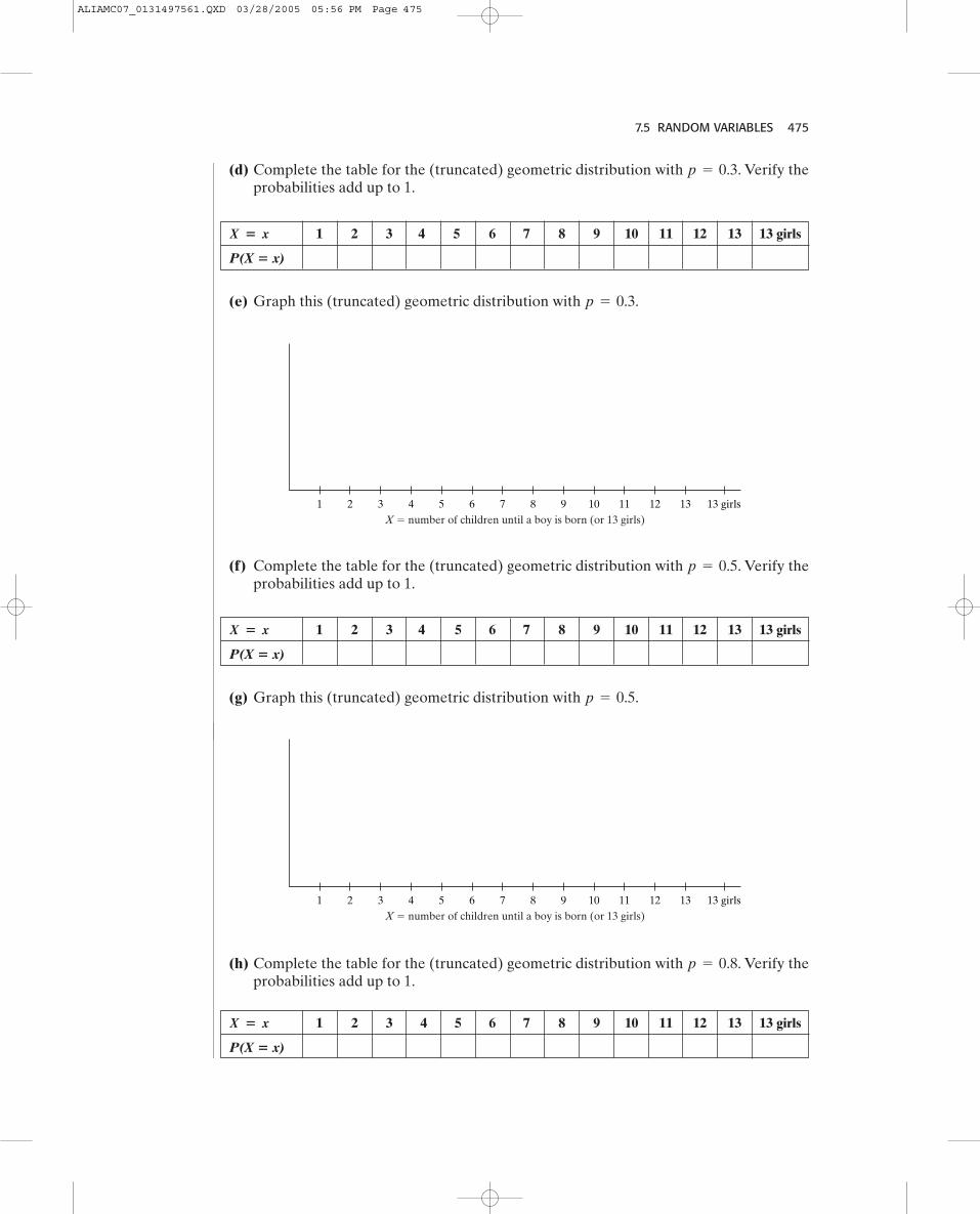
7.5 RANDOM VARIABLES 475
1 2 4 63 5 7 8 9 10 11 12 13 13 girlsX � number of children until a boy is born (or 13 girls)
1 2 4 63 5 7 8 9 10 11 12 13 13 girlsX � number of children until a boy is born (or 13 girls)
1 2 3 4 5 6 7 8 9 10 11 12 13 13 girls
P(X � x)
X � x
1 2 3 4 5 6 7 8 9 10 11 12 13 13 girls
P(X � x)
X � x
1 2 3 4 5 6 7 8 9 10 11 12 13 13 girls
P(X � x)
X � x
(g) Graph this (truncated) geometric distribution with p = 0.5.
(f) Complete the table for the (truncated) geometric distribution with Verify theprobabilities add up to 1.
p = 0.5.
(e) Graph this (truncated) geometric distribution with p = 0.3.
(d) Complete the table for the (truncated) geometric distribution with Verify theprobabilities add up to 1.
p = 0.3.
(h) Complete the table for the (truncated) geometric distribution with Verify theprobabilities add up to 1.
p = 0.8.
ALIAMC07_0131497561.QXD 03/28/2005 05:56 PM Page 475
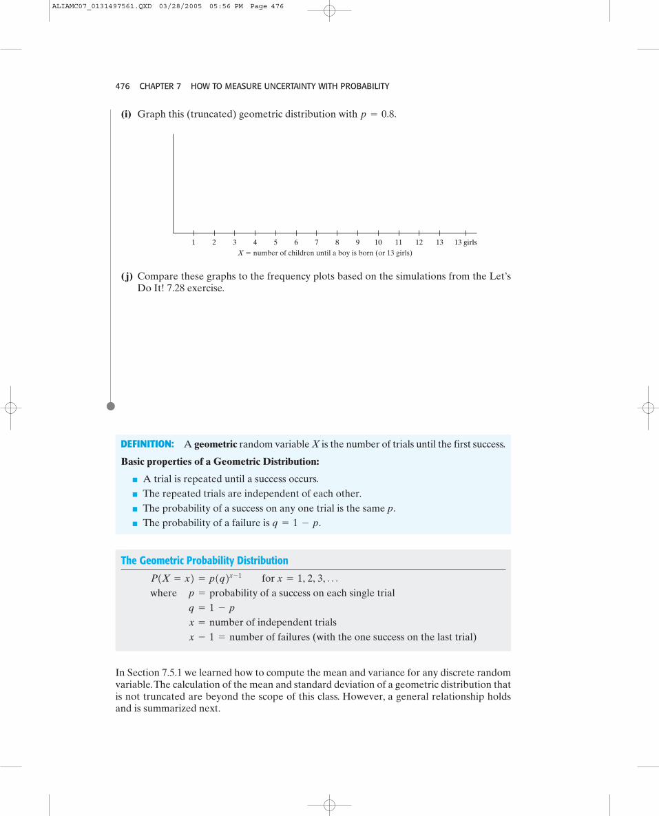
476 CHAPTER 7 HOW TO MEASURE UNCERTAINTY WITH PROBABILITY
(j) Compare these graphs to the frequency plots based on the simulations from the Let’sDo It! 7.28 exercise.
(i) Graph this (truncated) geometric distribution with p = 0.8.
DEFINITION: A geometric random variable X is the number of trials until the first success.
Basic properties of a Geometric Distribution:
■ A trial is repeated until a success occurs.■ The repeated trials are independent of each other.■ The probability of a success on any one trial is the same p.■ The probability of a failure is q = 1 - p.
The Geometric Probability Distribution
forwhere of a success on each single trial
of independent trialsof failures (with the one success on the last trial) x - 1 = number
x = number q = 1 - p
p = probabilityx = 1, 2, 3, Á P1X = x2 = p1q2x - 1
In Section 7.5.1 we learned how to compute the mean and variance for any discrete randomvariable.The calculation of the mean and standard deviation of a geometric distribution thatis not truncated are beyond the scope of this class. However, a general relationship holdsand is summarized next.
1 2 4 63 5 7 8 9 10 11 12 13 13 girlsX � number of children until a boy is born (or 13 girls)
ALIAMC07_0131497561.QXD 03/28/2005 05:56 PM Page 476
7.5 RANDOM VARIABLES 477
Let's Do It!
7.307.30The Expected Number of Children
Let’s see how close the simulated expected values found in the Let’s Do It! 7.28 exercise areto the actual expected values.
(a) For group 1:The simulated
(b) For group 2:The simulated
(c) For group 3:The simulated
(d) For group 4:The simulated mean = The true mean = p = 0.80
mean = The true mean = p = 0.50mean = The true mean = p = 0.30mean = The true mean = p = 0.10
Mean, Variance, and Standard Deviation for a Geometric Random Variable
Mean:
Variance:
Standard Deviation: SD1X2 = s =
1qp
Var1X2 = s2=
q
p2
E1X2 = m =
1p
Example 7.14 ◆ Carpet CleaningProblemJeff’s part-time job is to make phone calls trying to set up appointments for a free demon-stration of a new carpet cleaning machine. From past experience, the probability that Jeffwill secure an appointment on any given call is 0.30.(a) What is the probability that Jeff’s first secured appointment will occur on the fourth call?(b) On average, how many calls need to be made to secure an appointment?
Solution(a)(b) The mean number of calls required is
What We’ve Learned: If we are interested in counting the number of trials until the firstsuccess, then we have a geometric random variable. Even though theoretically a success maynever occur, the geometric distribution is a discrete probability distribution between thevalues of X can be listed— Notice that as x becomes larger, gets closerto zero.The sum of all the probabilities in a geometric distribution can be shown to be equalto one.
P1X = x21, 2, 3, Á .
10.30 = 3.33.
P1X = 42 = 0.3010.7024 - 1= 0.1029.
ALIAMC07_0131497561.QXD 03/28/2005 05:56 PM Page 477

478 CHAPTER 7 HOW TO MEASURE UNCERTAINTY WITH PROBABILITY
7.5.4 Continuous Random VariablesA random variable X that takes its values in some interval, or union of intervals, is said to becontinuous. A probability cannot be assigned to each of the possible values since the num-ber of possible values in an interval cannot be counted. So we must assign a probability of 0to each individual value; otherwise, the sum of the probabilities would eventually be greaterthan 1.The idea is to assign probabilities to intervals of outcomes, not single values, and rep-resent these probabilities as areas under a curve, called a probability density curve.
Den
sity
X X
Den
sity
0 3210 321
DEFINITION: The probability distribution function (or density) of a continuous randomvariable X is a non-negative function such that the area under the function over an inter-val is equal to the probability that the random variable X is in the interval.The values of acontinuous probability distribution must be at least 0 and the total area under the curve mustbe 1.
We have looked at density curves in the past. Now, instead of referring to our area calcula-tions as finding a proportion, we may state that we are finding a probability.
Suppose that the probability density function forthe income of a randomly selected American adult isas given in the graph. How would you find the proba-bility of selecting a person at random from this popu-lation with an income between $30,000 and $40,000?
We would use the probability density function to findthe area under it between 30 and 40.
The calculation of the mean and standard deviation when a probability density functionis available is similar to the expressions for the discrete case, except that we need to use abranch of calculus called integration in place of summation. However, the location of thecenter of gravity or mean of the density may be evident when looking at the function.
P[30 6 X 6 40] = ?0 10 20 30 40
area � P(30 � X � 40)
50 60 70 80 90
X � income (in $1000’s)
Den
sity
DEFINITION: The mean or expected value of a continuous random variable X is the pointat which the probability density function would balance.
Example 7.15 ◆ A Long Pregnancy ProblemLet X be the length of a pregnancy in days. Thus, X is a continuous random variable.Suppose that it has approximately a normal distribution with a mean of 266 days and a stan-dard deviation of 16 days—that is, X is N(266, 16).
ALIAMC07_0131497561.QXD 03/28/2005 05:56 PM Page 478

7.5 RANDOM VARIABLES 479
X � length of pregnancy218 314310
298282266250234
N(266, 16)
What is the probability that a pregnancy lasts at least 310 days?
SolutionWe want to compute We will do roughly the same calculations as we havedone in the previous chapter for normal distributions, but using the language of probabilityinstead of proportion.
Using the TI:Using Table II, we would first compute the standard score for 310, namely,
We use Table II to find the area to the right of 2.75. Recall that TableII provides areas to the left of various values of Z. So
What We’ve Learned: If a population of responses follows a normal distribution, and if Xrepresents the response for a randomly selected unit from the population, then X is said tobe a normal random variable—that is, the random variable X is said to have a normal dis-tribution. Finding probabilities about a normally distributed random variables still involvefinding a corresponding area under the normal density that serves as the model for thatrandom variable.
1 - 0.9970 = 0.0030.P1X 7 3102 = P1Z 7 2.752 =z =
310 - 26616 = 2.75.
P1X 7 3102 = normalcdf1310, 266, 162 = 0.00298.
P1X 7 3122.
Normal random variables are the most common class of continuous random variables.Thereare many characteristics whose distribution follow a bell-shaped normal curve.The family ofnormal distributions plays a prominent role in statistics. Normal distributions can also beused to approximate probabilities for some other types of random variables. In the next ex-ample, binomial probabilities will be approximated using a normal distribution. In the nextchapter, we will learn that a normal distribution can be the approximate model for varioussample statistics.
Example 7.16 ◆ Approximating Probabilities with a NormalDistribution
ProblemThe CEO of a very large company is convinced that a majority of his employees are happyand expect to stay with his company over the next five years. However, a recent randomsample of 400 employees resulted in only 192 saying they were happy and planned to stay.
ALIAMC07_0131497561.QXD 03/28/2005 05:56 PM Page 479

480 CHAPTER 7 HOW TO MEASURE UNCERTAINTY WITH PROBABILITY
If indeed 50% of the employees are happy and plan to stay, how likely would it be to find192 or fewer saying so in a random sample of 400 employees?(a) Let number of employees in the sample who are happy and plan to stay. Sup-
pose indeed that 50% of all employees are happy and plan to stay.What is the exact dis-tribution of the random variable X?
(b) If indeed 50% of the employees are happy and plan to stay, how likely would it be tofind 192 or fewer saying so in a random sample of 400 employees? Compute this prob-ability first using the exact distribution from part (a) if you have a calculator or com-puter that can do the work. Then compute this probability using the following usefulresult:
X = the
The family of normal distributions is not the only class of models for continuous randomvariables. Our final Let’s do it! exercise returns us to the uniform density curve as the prob-ability distribution for the continuous random variable to process a loanapplication.
X = time
Solution(a) The random variable X has a binomial distribution with and (b) We would like to find Using the TI graphing calculator we could com-
pute:Since both and are both 200 and
well above the ‘at least 5’ requirement, we can use the normal approximation to a bi-nomial model. We have a mean of and a standard deviation of
So we will do roughly the same calculations as we have done in the previous chapter fornormal distributions to find our approximate probability.
Using the TI,Using Table II, we would first compute the standard score for 192, namely,
We use Table II to find the area to the left of Recall thatTable II provides areas to the left of various values of Z.
What We’ve Learned: Models allow us to compute probabilities of various events. In thiscase, we were able to use a large sample normal model as an approximation for modeling thenumber of employees who are happy and expect to stay.We found that it is not very unusualto observe only 192 out of 400 employees who are happy and plan to stay, even if 50% of theemployees are happy and plan to stay.
P1X … 1922 L P1Z … -0.82 = 0.2119.
-0.80.z =192 - 200
10 = -0.8.
P1X … 1922 L normalcdf1-E99, 192, 200, 102 = 0.2119.
2np11 - p2 = 240010.50211 - 0.502 = 2100 = 10.
np = 1400210.52 = 200
n11 - p2 = 1400211 - 0.52np = 1400210.052P1X … 1922 = binomialcdf1400, 0.5, 1922 = 0.23.P1X … 1922.
p = 0.50.n = 400
Normal Approximation to the Binomial
If X is a binomial random variable based on n trials and success probability p, and thenumber of trials n is large, then the distribution of X can be approximated by a normaldistribution with and standard
Note: This approximation works best when both np and are at least 5.n11 - p2deviation = 2np11 - p2.mean = np
ALIAMC07_0131497561.QXD 03/28/2005 05:56 PM Page 480
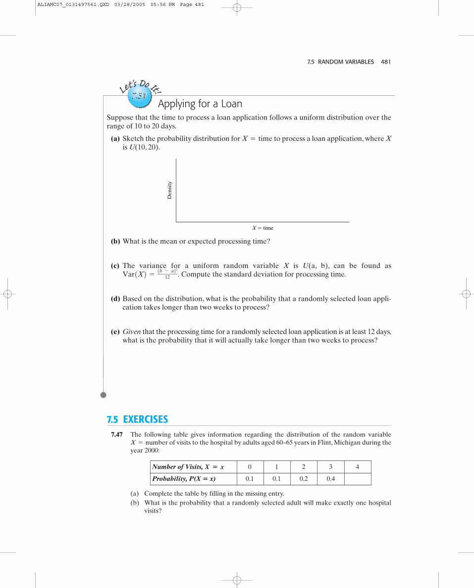
7.5 RANDOM VARIABLES 481
7.5 EXERCISES7.47 The following table gives information regarding the distribution of the random variable
of visits to the hospital by adults aged 60–65 years in Flint, Michigan during theyear 2000:X = number
Let's Do It!
7.317.31Applying for a Loan
Suppose that the time to process a loan application follows a uniform distribution over therange of 10 to 20 days.
(a) Sketch the probability distribution for to process a loan application, where Xis U(10, 20).
X = time
X � time
Den
sity
(b) What is the mean or expected processing time?
(c) The variance for a uniform random variable X is U(a, b), can be found asCompute the standard deviation for processing time.
(d) Based on the distribution, what is the probability that a randomly selected loan appli-cation takes longer than two weeks to process?
(e) Given that the processing time for a randomly selected loan application is at least 12 days,what is the probability that it will actually take longer than two weeks to process?
Var1X2 =
1b - a2212 .
Number of Visits, 0 1 2 3 4
Probability, P(X � x) 0.1 0.1 0.2 0.4
X � x
(a) Complete the table by filling in the missing entry.(b) What is the probability that a randomly selected adult will make exactly one hospital
visits?
ALIAMC07_0131497561.QXD 03/28/2005 05:56 PM Page 481

482 CHAPTER 7 HOW TO MEASURE UNCERTAINTY WITH PROBABILITY
(c) What is the probability that a randomly selected adult will make fewer than three hos-pital visits?
(d) Given that an adult has fewer than three hospital visits, what is the probability that heor she will have only one hospital visit?
7.48 A travel agency conducted a survey of its customer travelers. One of the responses measuredwas number of distinct hotels occupied by travelers in a particular year. The resultsare presented in the following table:
X = the
Number of Distinct Hotels, 1 2 3 4 5
Probability, P(X � x) 0.10 0.40 0.25 0.15
X � x
(a) Complete the table by filling in the missing entry, and sketch the stick graph for thisprobability distribution. Be sure to label all important features.
(b) What is the probability that a randomly selected traveler will use exactly five distincthotels?
(c) What is the probability that a randomly selected traveler will use fewer than three distincthotels?
(d) Given that a traveler uses fewer than three distinct hotels, what is the probability that heor she will use only one hotel?
7.49 With versus without ReplacementAn urn contains three balls, of which one is teal and twoare white.The experiment consists of selecting one ball ata time without replacement until the teal ball is chosen,at which point no further selections are made.(a) Write down the sample space for this experiment.(b) Let the random variable X be the number of the draw
on which the teal ball is selected—that is,total number of balls selected.What are the possible values for this random variable X?
(c) Repeat parts (a) and (b) assuming that the ball is selected with replacement.
7.50 Let X denote the random variable that takes any of the values 0, 1 with probabilities 0.2,0.5, and 0.3, respectively. Calculate the mean and the standard deviation of the randomvariable X.
7.51 Let X be the number of televisionsin a randomly selected Zone Cityhousehold. The mass function of Xis given in the corresponding table.(a) Complete the mass function of
X and sketch the stick graph ofthe mass function of X. Be sure to label all important features.
(b) What is the probability that a randomly selected household has at least one TV?(c) What is the expected number of televisions per household?
-1,
X = the
Select balls untilyou get the blue ball
Value of X0 1 2 3 4
ProbabilityP(X � x) 0.05 0.30 0.40 0.20
X � x
7.52 An automobile agency located inBeverly Hills, California, specializesin the rental of luxury automobiles.The distribution of daily demand(number of automobiles rented) atthis agency is summarized. What isthe expected value of daily demand (i.e., the expected number of automobiles rented)?
Value of X0 1 2 3 4
ProbabilityP(X � x) 0.15 0.30 0.40 0.10 0.05
X � x
ALIAMC07_0131497561.QXD 03/28/2005 05:56 PM Page 482
7.5 RANDOM VARIABLES 483
7.53 Consider the following game: You flip a fair coin until a tail appears for the first time. If thetail appears on the nth flip, you win dollars. Let X represent the amount won. Show thatyour expected winnings is equal to plus infinity, This problem is called theSt. Petersburg paradox. Would you be willing to pay $1,000,000 to play this game once?Would you be willing to pay $1,000,000 for each game if you could play for as long as youlike and only have to settle up when you stopped playing?
7.54 Alfredo, a visitor to a casino, wishes to participate at a game of chance. He has twooptions.
Option 1 A fair coin is tossed once. The player gets $4 if it falls heads and nothing other-wise. The entry fee for this option is $2.
E1X2 = + q .2n
Outcome H T
Net Return $2
Probability 0.5 0.5
-$2
Option 2 A fair coin is tossed twice. The player gets $8 if it falls heads on both tosses andnothing otherwise. The entry fee for this option is $3.
Using the expected net return as a criterion, which of the two options will be more attrac-tive to Alfredo? Show all supporting details.
7.55 An Interesting CaseA random variable X takes on the values 1 and with probability and respectively.Let(a) What is the expected value for Y?(b) What is the standard deviation for Y?
7.56 A total of four school buses are carrying a total of 148 students from the same school to theconcert hall. The buses are carrying 40, 33, 25, and 50 students, respectively. One of the stu-dents is randomly selected. Let X be the number of students that were on the bus carryingthis randomly selected student. One of the four bus drivers is also randomly selected. Let Ybe the number of students on this driver’s bus.(a) Which one do you think is larger, E(X) or E(Y)? Why?(b) Compute E(X) and E(Y) to check your answer to part (a).
7.57 Suppose that the number of cars, X, that pass through a car wash between 4:00 P.M. and5:00 P.M. on any sunny Friday has the following probability distribution:
Y = X2.
13,
23-1
Expected Net Return = 0.
Value of X4 5 6 7 8 9
Probability P(X � x) 1
614
14
112
112
X � x
(a) Complete the distribution.(b) What is the probability that at least six cars will pass through the car wash between
4:00 P.M. and 5:00 P.M. on any sunny Friday?(c) What is E(X), the expected number of cars that pass through a car wash between 4:00 P.M.
and 5:00 P.M. on any sunny Friday?(d) In Chapter 5, we discussed linear transformations. We saw that the mean of a new vari-
able Y, which is a linear transformation of the variable X, is found by plugging the meanof X directly into the linear transformation. So, if represents the amount ofmoney, in dollars, paid to the attendant by the manager for each car, what is the atten-dant’s expected earnings for this particular period?
Y = 2X - 1
ALIAMC07_0131497561.QXD 03/28/2005 05:56 PM Page 483
484 CHAPTER 7 HOW TO MEASURE UNCERTAINTY WITH PROBABILITY
7.58 It is known that micro-ovens produced by a certain company will be defective with proba-bility 0.01 independently of each other. The company sells the micro-ovens in groups of 10and offers a money-back guarantee that at most one of the 10 micro-ovens is defective.(a) If X is the number of defective micro-ovens in a group of ten, how is the random vari-
able X is distributed?(b) What is the expected number of micro-ovens in a group of ten that are defective and
thus would have to be replaced?
7.59 Combinations of Suppose that you have a set that contains five distinguishable val-ues, The following table partially summarizes the counting questions:S = 51, 2, 3, 4, 56.n � 5.
How many subsets of S � {1, 2, 3, 4, 5}are there that contain Answer The subsets are Combination
exactly zero values (no values)? 1
exactly one value?
exactly two values?
exactly three values? 10
exactly four values?
exactly five values? 51, 2, 3, 4, 56Á
Á
Á
a52b = 10Á
516, 526, 536, 546, 556Á
Á
Á
(a) Complete the table by filling in the missing entries.(b) The set has five values, so the total number of possible subsets is
. Confirm that this value equals the sum in the “answer” column.
7.60 Suppose that the random variable X has a binomial distribution with and Find each of the following quantities:(a)(b)(c)(d)(e)(f)
7.61 In each given case, a random variable, X, is defined. You are to decide whether or not X hasa binomial distribution. Justify your answer by referring to specific assumptions that are orare not satisfied.(a) Six days a week for a year, you play the three-digit (“Pick Three”) Michigan lottery.You
win on a given day if your three-digit number matches the one selected at random by theState of Michigan. For the first six months, you select the number 123 each day; for thelast six months, you select the number 234 each day. Let X be the number of days inthe year that your choice is a winner.
(b) Studies have found that 80% of dorm residents get along with their roommates. Eachroom in a certain dorm has two occupants.A survey was conducted by selecting 10 roomsat random and asking each occupant “Do you get along with your roommate?” Let X bethe number of “yes’s” among the 20 responses obtained.
7.62 An experiment is designed to test whether a subject has ESP, extrasensory perception. Atotal of 96 cards is drawn, one by one, with replacement, from a well-shuffled ordinary deckof cards. The subject is asked to guess the suit of each card drawn. There are four possiblechoices for each card—namely, spades, hearts, diamonds, and clubs. We wish to test the null
Var1X2 = s2.E1X2 = m.P1X = 1.52.P1X … 72.P1X 7 82.P1X = 22.
p = 0.4.n = 10
25=
S = 51, 2, 3, 4, 56
ALIAMC07_0131497561.QXD 03/28/2005 05:56 PM Page 484
7.5 RANDOM VARIABLES 485
hypothesis that the subject is only guessing and does not have ESP against the one-sidedalternative hypothesis that the subject has ESP.(a) State the appropriate hypotheses in terms of probability of getting a correct
response.(b) The subject gets 35 correct out of the 96 cards. Give the p-value for this test.Think about
the direction of extreme, based on your alternative hypothesis. Use your TI and thebinomcdf(function to find the p-value.
(c) Give your decision using a significance level of (d) State your conclusion using a well-written sentence.
Note: In Chapter 9, you will revisit this ESP scenario in a Let’s do it! exercise.You will applyanother test to assess the significance of the results.
7.63 A tax attorney claims that more than 1% of all tax returns filed in the previous year wereaudited.To test this claim, a researcher took a random sample of 18 taxpayers and found thatonly one return was audited.(a) Give the appropriate null and alternative hypotheses about the value of p, the propor-
tion of audited tax returns.(b) Find the p-value of the test, based on the researcher’s sample results. Think about the
direction of extreme, based on your alternative hypothesis.(c) Carefully explain, in words, what the p-value means in this case, in terms of repeated
samples.(d) If you were to set a significance level 1%, would you reject or accept the null hypothe-
sis? Explain.
7.64 In a computer lab, students must wait to get a computer terminal. It is assumed that the wait-ing time for the next available terminal is uniformly distributed between 0 and 15 minutes.(a) Sketch the distribution of X (the waiting time, in minutes). Be sure to provide all im-
portant features.(b) On average a student will have to wait minutes for the next available terminal.(c) What is the probability that a student will have to wait more than 10 minutes for the
next available terminal?(d) Students have been complaining that the waiting time is too long. So a test will be con-
ducted to assess if the mean waiting time is greater than the average computed in (b).(i) What is the direction of extreme?
(ii) Suppose that a randomly selected student was observed to wait 13 minutes for thenext available terminal. Give the corresponding p-value for this observation.
(iii) Using a 10% significance level, what is your decision? Explain.
7.65 No one likes to wait at a bus stop for very long. A city bus line states that the length of timea bus is late is uniformly distributed between 0 and 10 minutes.(a) Sketch the distribution for the variable late (in minutes). Be sure to provide
all important features.(b) For the distribution in part (a), what is the mean or expected time a bus will be late—that
is, what is E(X)?(c) For the distribution in part (a), what is the probability that a bus will arrive no more than
three minutes late?(d) The director has been receiving a number of complaints from its riders regarding how late
buses have been running. He obtains the help of a statistician to test the alternativetheory that the mean time a bus will be late is greater than that given in part (b).
(i) What is the direction of extreme?(ii) Suppose that, at a randomly selected bus stop, the bus arrives nine minutes late.
What is the corresponding p-value for this observation?(iii) Using a 15% significance level, what is your decision?
X = time
a = 0.05.
p = the
ALIAMC07_0131497561.QXD 03/28/2005 05:56 PM Page 485

486 CHAPTER 7 HOW TO MEASURE UNCERTAINTY WITH PROBABILITY
7.66 Even drugstore managers have their own headaches, due to chronic late and incompletepayments from insurers and other medical personnel. As reported in the March 25, 1995New York Times, “Pharmacy Fund, a new company based in New York, thinks it has a cure.It buys bills from the previous day’s prescription sales at a slight discount, paying the phar-macist immediately and eliminating weeks of cash flow delays for drugstores. The PharmacyFund then collects from the health plans.” The article also reports that drugstores typicallyhad to wait between 30 to 45 days to collect payments from insurers. Suppose that the wait-ing time, in days, to collect payment for non–Pharmacy Fund drugstores is uniformly dis-tributed between 30 and 45 days.(a) Sketch the distribution for the random variable time in days to collect pay-
ment for non–Pharmacy Fund drugstores. Be sure to label and give appropriate valueson the axes.
(b) What is the expected waiting time to collect payment for non–Pharmacy Fund drugstores?(c) What is the probability that a non–Pharmacy Fund drugstore will have to wait at least
six weeks?(d) What is the probability that a non–Pharmacy Fund drugstore will have to wait at least
six weeks, given that it has had to wait at least five weeks for payment?(e) Based on your results to parts (c) and (d), are the events “wait at least six weeks” and
“wait at least five weeks” independent events? Explain.
7.67 In a certain island in the Pacific the probability that a thunderstorm will occur on a givenday during the summer (starting July 1) is equal to 0.3. Assuming independence from day today, answer the following questions.(a) Let X be defined as the number of days until the first thunderstorm occurs. How is X
distributed?(b) What is the expected value of X?(c) What is the probability that the first thunderstorm of the summer occurs on August 6?
7.68 Suppose that the time for an operator to place a long-distance call is normally distributedwith a mean of 20 seconds and a standard deviation of 5 seconds.(a) What is the probability that a long-distance call will go through in less than 10 seconds?(b) What is the probability that it will take longer than 32 seconds for a long-distance call to
go through?
7.69 The SAT scores of applicants to a certain university are normally distributed with a meanof 1170 and a standard deviation of 80. Let X represent the score of a randomly selectedapplicant.(a) Explain in words what means and compute this probability.(b) Applicants whose SAT scores are in the upper 2.5% qualify for a scholarship.
(i) What percentile must an applicant’s SAT score attain in order to qualify for ascholarship?
(ii) What SAT score must an applicant attain in order to qualify for a scholarship?
SUMMARY
■ We sample from the population.Thus, our conclusions or inferences about the populationwill contain some amount of uncertainty and the evaluation of probabilities.
■ We focused on the relative frequency interpretation of probability, namely, probability asthe proportion of times an outcome would occur over the long run.
■ Probabilities can be found through simulation or through more formal mathematicalresults.
P11050 6 X 6 12502
X = waiting
ALIAMC07_0131497561.QXD 03/28/2005 05:56 PM Page 486

KEY FORMULAS 487
■ Probability is an important tool in the decision-making process. Probability helps us quan-titatively evaluate competing theories, to be able to assess whether the observed data areunlikely or probable under a given hypothesis (that is, to compute the p-value).
■ To make a decision, we will use the sample data to compute sample statistics, such asthe sample mean or sample proportion. The value for a sample statistic will vary in arandom manner from sample to sample. Thus a sample statistic is a random variable thathas a distribution.
■ There are two types of random variables—discrete and continuous. We characterize thepattern of the distribution of values of a random variable via a probability distribution.Probability distributions are used to find various probabilities and expectations. Withinthe two broad types of random variables, there are families of random variables that arecommon and have a special name.
■ A binomial random variable is basically a count of how many times an outcome occurs ina certain number of trials of a random experiment where the probability of a success onany one outcome is p.
■ If independent trials are performed until a success occurs (each trial having the same prob-ability of success p), the number of trials needed until the first success occurs is said to bea geometric random variable.
■ We revisited two families of continuous probability distributions—the normal distribu-tions and the uniform distributions and saw that even a binomial distribution can beapproximated with a normal model if the sample size n is large enough.
■ Looking ahead: We will see the important role of the normal distributions in our studyof the probability distributions of various sample statistics. Chapter 8, on sampling distri-butions, is our final topic to prepare us for the more formal statistical decision-makingprocedures presented in Chapters 9 through 15.
KEY FORMULAS
Basic Probability Rules
1. The probability that the event A occurs is denoted by P(A). For any event A,
2. The sum of the probabilities of each of the individual outcomes (for finite or infinitelycountable S) in the sample space must equal one.
3. Complement rule. The probability that an event occurs is 1 minus the probabilitythat the event does not occur.
4. Addition rule. The probability that either the event A or the event B occurs is thesum of their individual probabilities minus the probability of their intersection.
If A and B are mutually exclusive (ordisjoint) events, then
5. The conditional probability of the event A occurring, given the event B has occurred,is given by
P1A ƒ B2 =
P1A and B2P1B2 , if P1B2 7 0.
P1A or B2 = P1A2 + P1B2.P1A or B2 = P1A2 + P1B2 - P1A and B2.
P1A2 = 1 - P1AC2.P1S2 = 1.
0 … P1A2 … 1.
ALIAMC07_0131497561.QXD 03/28/2005 05:56 PM Page 487

488 CHAPTER 7 HOW TO MEASURE UNCERTAINTY WITH PROBABILITY
This leads to the following multiplication rule:
If two events do not influence each other—that is, if knowing that one has occurreddoes not change the probability of the other occurring—the events are independent.Two events A and B are independent if or, equivalently,
or, equivalently,6. Partition rule. If the events form a partition, then
7. Bayes’s rule. Let the events form a partition. Suppose that A is anoth-er event and we know the conditional probabilities Then the conditional probability of say B1 given that event A has occurred is given by
Note: A tree diagram is often useful for computing partition rule or Bayes’s ruleprobabilities.
=
P1A ƒB12P1B12P1A ƒB12P1B12 + P1A ƒB22P1B22 +
Á+ P1A ƒBI2P1BI2.
P1B1 ƒA2 =
P1A ƒB12P1B12P1A2
P1A ƒB12, P1A ƒB22, Á P1A ƒBI2.B1, B2, Á , BI
P1A2 = P1A ƒB12P1B12 + P1A ƒB22P1B22 +Á
+ P1A ƒBI2P1BI2.B1, B2, Á , BI
P1A and B2 = P1A2P1B2.P1B ƒA2 = P1B2 P1A ƒB2 = P1A2
= P1B2P1A ƒB2 = P1A2P1B ƒA2.P1both events will occur at the same time2 = P1A and B2
Binomial Random Variable
Var1X2 = npq
E1X2 = np
P1X = x2 = anxb1p2x1q2n - x, x = 0, 1, 2, Á , n
Discrete Random Variable
Let X be a discrete random variable taking on the values ,with probabilities
= E11X - m222 = a 1xi - m22pi = E1X22 - 1E1X222 = axi2pi - m2
Var1X2 = s2
E1X2 = m = x1p1 + x2p2 +Á
+ xkpk = axipi.
p1, p2, Á pk.x1, x2, Á xk,
Geometric Random Variable
Var1X2 =
q
p2
E1X2 =
1p
P1X = x2 = p1q2x - 1
ALIAMC07_0131497561.QXD 03/28/2005 05:56 PM Page 488
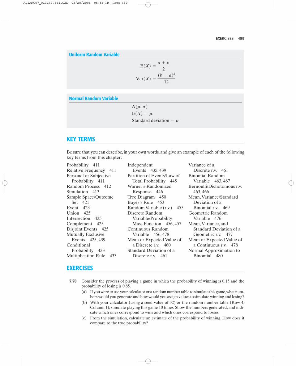
EXERCISES 489
Uniform Random Variable
Var1X2 =
1b - a2212
E1X2 =
a + b2
Normal Random Variable
Standard deviation = s
E1X2 = m
N1m, s2
KEY TERMS
Be sure that you can describe, in your own words, and give an example of each of the followingkey terms from this chapter:
Probability 411Relative Frequency 411Personal or Subjective
Probability 411Random Process 412Simulation 413Sample Space/Outcome
Set 421Event 423Union 425Intersection 425Complement 425Disjoint Events 425Mutually Exclusive
Events 425, 439Conditional
Probability 433Multiplication Rule 433
Independent Events 435, 439
Partition of Events/Law ofTotal Probability 445
Warner’s RandomizedResponse 446
Tree Diagram 450Bayes’s Rule 453Random Variable (r.v.) 455Discrete Random
Variable/Probability Mass Function 456, 457
Continuous RandomVariable 456, 478
Mean or Expected Value ofa Discrete r.v. 460
Standard Deviation of aDiscrete r.v. 461
Variance of a Discrete r.v. 461
Binomial Random Variable 463, 467
Bernoulli/Dichotomous r.v.463, 466
Mean, Variance/StandardDeviation of a Binomial r.v. 469
Geometric RandomVariable 476
Mean, Variance, andStandard Deviation of aGeometric r.v. 477
Mean or Expected Value ofa Continuous r.v. 478
Normal Approximation toBinomial 480
EXERCISES
7.70 Consider the process of playing a game in which the probability of winning is 0.15 and theprobability of losing is 0.85.(a) If you were to use your calculator or a random number table to simulate this game,what num-
bers would you generate and how would you assign values to simulate winning and losing?(b) With your calculator (using a seed value of 32) or the random number table (Row 4,
Column 1), simulate playing this game 10 times. Show the numbers generated, and indi-cate which ones correspond to wins and which ones correspond to losses.
(c) From the simulation, calculate an estimate of the probability of winning. How does itcompare to the true probability?
ALIAMC07_0131497561.QXD 03/28/2005 05:56 PM Page 489
490 CHAPTER 7 HOW TO MEASURE UNCERTAINTY WITH PROBABILITY
7.71 It is known that 70% of all students at a certain university have brown eyes, 20% of allbrown-eyed students have red hair, and 15% of all brown-eyed, red-haired students are left-handed. It is also known that 40% of the non-brown-eyed students have red hair.(a) What percentage of students in that university have brown eyes and red hair?(b) What percentage of students are brown-eyed,red-haired,and left-handed at that university?(c) What percentage of all students at that university have red hair?
7.72 The ELISA test is used to screen blood samples for antibodies to the HIV virus. It measures an“absorbency ratio.”Blood samples from HIV-infected donors usually,but not always,give highratios, while those from uninfected donors usually, but not always, give low ratios. Considerusing this test on a sample of blood.The null and alternative hypotheses are defined as
The blood sample is not infected with HIV.The blood sample is infected with HIV.
Suppose that the decision rule is as follows: If the observed absorbency ratio is greater thanthree, the blood sample is judged to be infected with the HIV virus (that is, the test is positive);otherwise, it is judged to be free of the HIV virus (that is, the test is negative). For this rule, itis known that 98% of HIV patients will test positive and 2% will test negative, while 7% ofuninfected donors will test positive and 93% will test negative.(a) What do Type I and Type II errors represent in this situation?(b) What are the values of and for this procedure?(c) Suppose that the decision rule was changed so that a higher absorbency ratio is required
to judge a blood sample as testing positive.(i) The value of would increase. decrease. remain the same.
(ii) The value of would increase. decrease. remain the same.
7.73 In a certain community, 12% of the families own an Alsatian dog, a type of German shepherd,10% of the families own a Siamese cat, and 17% of the families own either an Alsatian dogor a Siamese cat. A family is to be randomly chosen. A Venn diagram may help in answeringthe following questions:(a) What is the probability that the family owns both an Alsatian dog and a Siamese cat?(b) Given that the family does not own a Siamese cat, what is the probability that it owns an
Alsatian dog?
7.74 Consider the following game: Players select two digits from 0 through 9, inclusive and thensum the values of the two digits.A winning sum is determined by randomly selecting two dig-its and computing the sum. For example, if the two randomly selected digits are 3 and 5, thena winning ticket is any ticket in which the two digits sum to 8. Note that there are 100 choicesfor selecting two digits Assume that each of the 100 choices is equallylikely to be selected for determining the winning sum.(a) How many possible sums are there? Give the values for all possible sums.(b) Find the probability of winning if the winning sum is 2.(c) Find the probability of winning if the winning sum is 5.(d) Which possible sum would result in the largest probability of winning?
7.75 Matching Numbers.(a) Consider Game 1.The game host selects a number from 1 to 10 (1, 2, 3, 4, 5, 6, 7, 8, 9, 10).
You must also select a number from this same list of 1 to 10.You win if and only if you select the same number as the game host. What is the proba-bility that you win?
(b) Consider Game 2.The game host selects a number from 1 to 10 (1,2,3,4,5,6,7,8,9,10). Youand four of your friends must each select a number from this same list (with replacement).You win if and only if at least one among the five selects the same number as the gamehost. What is the probability that you win?
100, 01, Á , 98, 992.
b
a
ba
H1:H0:
ALIAMC07_0131497561.QXD 03/28/2005 05:56 PM Page 490
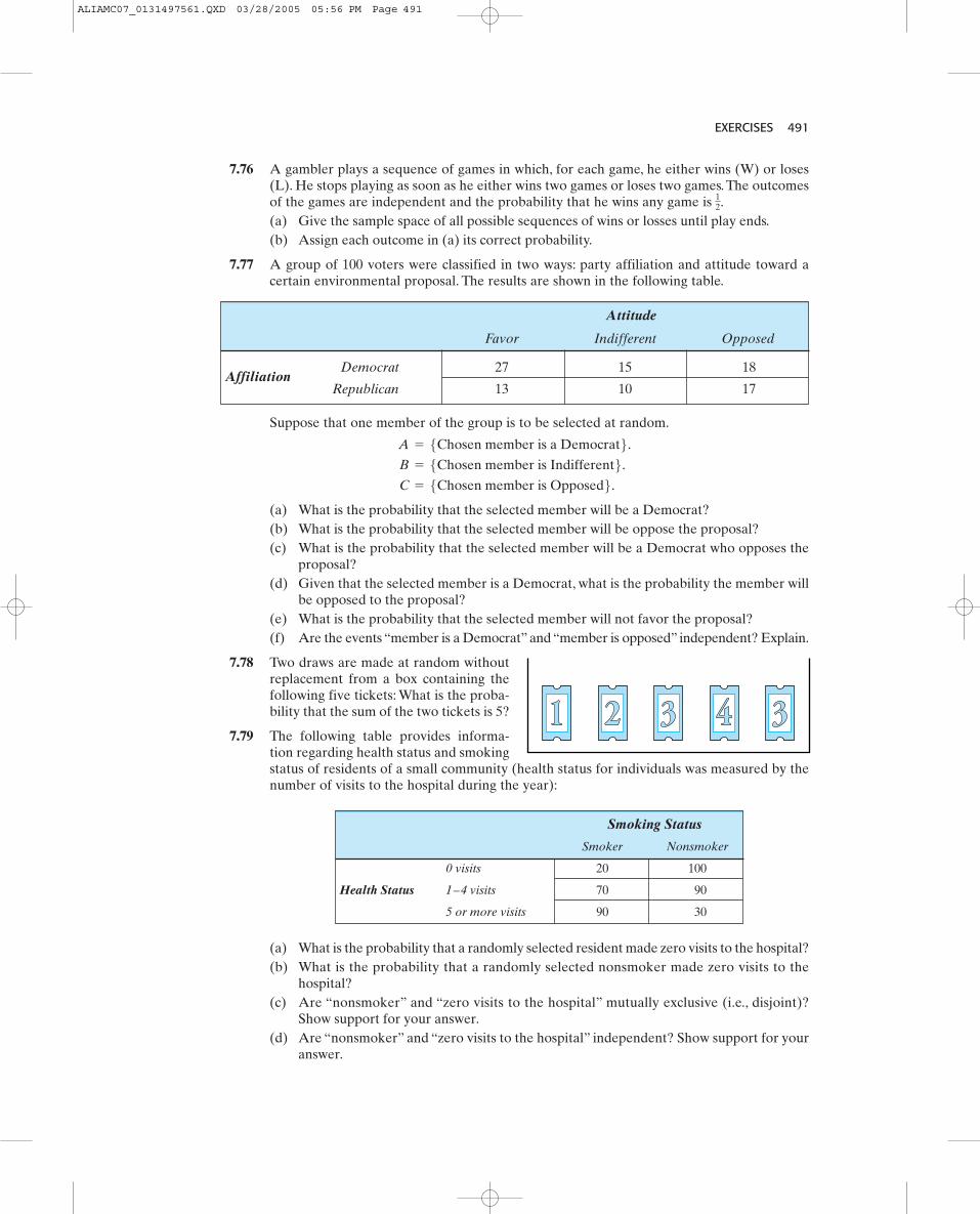
EXERCISES 491
7.76 A gambler plays a sequence of games in which, for each game, he either wins (W) or loses(L). He stops playing as soon as he either wins two games or loses two games. The outcomesof the games are independent and the probability that he wins any game is (a) Give the sample space of all possible sequences of wins or losses until play ends.(b) Assign each outcome in (a) its correct probability.
7.77 A group of 100 voters were classified in two ways: party affiliation and attitude toward acertain environmental proposal. The results are shown in the following table.
12.
Attitude
Favor Indifferent Opposed
AffiliationDemocrat 27 15 18
Republican 13 10 17
Suppose that one member of the group is to be selected at random.
(a) What is the probability that the selected member will be a Democrat?(b) What is the probability that the selected member will be oppose the proposal?(c) What is the probability that the selected member will be a Democrat who opposes the
proposal?(d) Given that the selected member is a Democrat, what is the probability the member will
be opposed to the proposal?(e) What is the probability that the selected member will not favor the proposal?(f) Are the events “member is a Democrat” and “member is opposed” independent? Explain.
7.78 Two draws are made at random withoutreplacement from a box containing thefollowing five tickets: What is the proba-bility that the sum of the two tickets is 5?
7.79 The following table provides informa-tion regarding health status and smokingstatus of residents of a small community (health status for individuals was measured by thenumber of visits to the hospital during the year):
C = 5Chosen member is Opposed6. B = 5Chosen member is Indifferent6. A = 5Chosen member is a Democrat6.
Smoking Status
20 100
Health Status 70 90
90 305 or more visits
1–4 visits
0 visits
NonsmokerSmoker
(a) What is the probability that a randomly selected resident made zero visits to the hospital?(b) What is the probability that a randomly selected nonsmoker made zero visits to the
hospital?(c) Are “nonsmoker” and “zero visits to the hospital” mutually exclusive (i.e., disjoint)?
Show support for your answer.(d) Are “nonsmoker” and “zero visits to the hospital” independent? Show support for your
answer.
ALIAMC07_0131497561.QXD 03/28/2005 05:56 PM Page 491
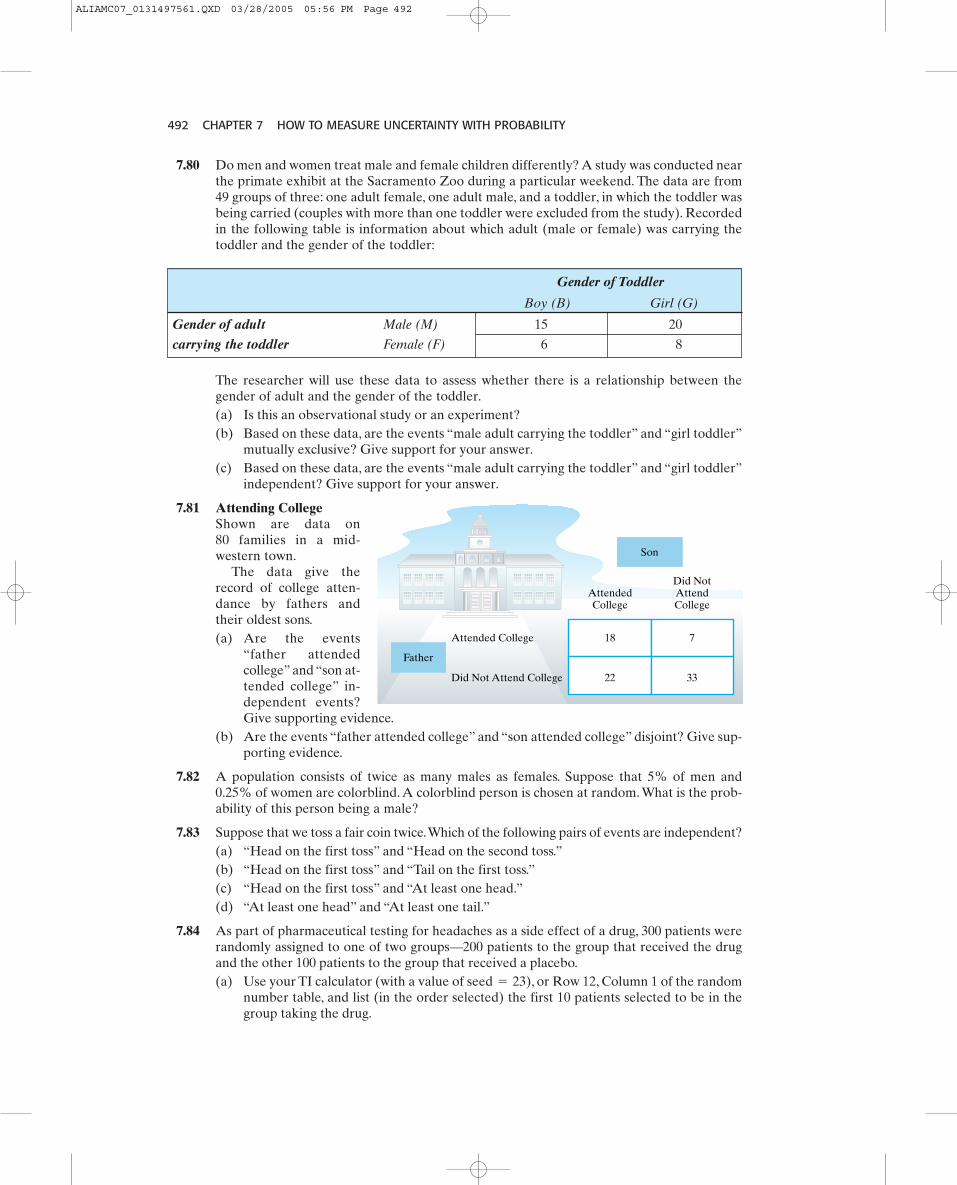
492 CHAPTER 7 HOW TO MEASURE UNCERTAINTY WITH PROBABILITY
7.80 Do men and women treat male and female children differently? A study was conducted nearthe primate exhibit at the Sacramento Zoo during a particular weekend. The data are from49 groups of three: one adult female, one adult male, and a toddler, in which the toddler wasbeing carried (couples with more than one toddler were excluded from the study). Recordedin the following table is information about which adult (male or female) was carrying thetoddler and the gender of the toddler:
Gender of Toddler
Boy (B) Girl (G)
Gender of adult Male (M) 15 20
carrying the toddler Female (F) 6 8
The researcher will use these data to assess whether there is a relationship between thegender of adult and the gender of the toddler.(a) Is this an observational study or an experiment?(b) Based on these data, are the events “male adult carrying the toddler” and “girl toddler”
mutually exclusive? Give support for your answer.(c) Based on these data, are the events “male adult carrying the toddler” and “girl toddler”
independent? Give support for your answer.
7.81 Attending CollegeShown are data on80 families in a mid-western town.
The data give therecord of college atten-dance by fathers andtheir oldest sons.(a) Are the events
“father attendedcollege” and “son at-tended college” in-dependent events?Give supporting evidence.
(b) Are the events “father attended college” and “son attended college” disjoint? Give sup-porting evidence.
7.82 A population consists of twice as many males as females. Suppose that 5% of men and0.25% of women are colorblind. A colorblind person is chosen at random. What is the prob-ability of this person being a male?
7.83 Suppose that we toss a fair coin twice.Which of the following pairs of events are independent?(a) “Head on the first toss” and “Head on the second toss.”(b) “Head on the first toss” and “Tail on the first toss.”(c) “Head on the first toss” and “At least one head.”(d) “At least one head” and “At least one tail.”
7.84 As part of pharmaceutical testing for headaches as a side effect of a drug, 300 patients wererandomly assigned to one of two groups—200 patients to the group that received the drugand the other 100 patients to the group that received a placebo.(a) Use your TI calculator (with a value of ), or Row 12, Column 1 of the random
number table, and list (in the order selected) the first 10 patients selected to be in thegroup taking the drug.
seed = 23
Attended College
AttendedCollege
Did Not Attend College
Did NotAttendCollege
18
22
7
33
Father
Son
ALIAMC07_0131497561.QXD 03/28/2005 05:56 PM Page 492

EXERCISES 493
The number of patients in each group who had a headache within the first hour after receiv-ing the treatment was recorded. Results are recorded here:
Treatment Group
Drug Placebo
Headache Headache 44 12
Status No Headache 156 88
(b) Suppose that a patient is selected at random.What is the probability that the patient didhave a headache in the first hour after treatment?
(c) Suppose that a patient is selected at random. Given that the patient was given the drug,what is the probability that the patient did have a headache in the first hour aftertreatment?
(d) Are the events “drug” and “headache” mutually exclusive? Explain your answer.(e) Are the events “drug” and “headache” independent events? Explain your answer.
7.85 Viviana applies to graduate school at two universities. Assuming that the probability ofacceptance at University A is 0.4, the probability of acceptance at University B is 0.3, and theprobability of acceptance at both universities is 0.1, answer the following questions:(a) Is the event of acceptance at University A independent of the event of acceptance at
University B? Explain.(b) Is the event of acceptance at University A mutually exclusive of the event of acceptance
at University B? Explain.(c) What is the probability that Viviana is not accepted to either university?
7.86 Varivax, a vaccine for chicken pox, was approved by the FDA. One injection of the vaccineis recommended for children 12 months to 12 years old. Two injections, given four to eightweeks apart, are recommended for those 13 or older who have not had chicken pox. It wasreported that 2.8% of all vaccinated children still develop chicken pox. However, such casesare generally mild, with an average of 50 lesions compared to an average of 300 lesions thatdevelop from a natural chicken-pox infection.(a) Suppose that we take a simple random sample of two children who have not yet had
chicken pox, but have been vaccinated. What is the probability that both children stilldevelop chicken pox?
(b) The McCoy family has two children, 2 and 4 years of age, both of whom received thevaccine since they had not yet had chicken pox. Does the probability calculated in (a)apply to these two children? Explain why or why not.
7.87 If the probability of a certain test to yield a “positive” reaction is equal to 0.85, what is theprobability that fewer than four “negative” reactions occur before the first positive reaction?The test results are assumed to be independent to each other.
7.88 Suppose that, in a certain country, 10% of the elderly people have diabetes. It is also knownthat 30% of the elderly people are living below poverty level, 35% of the elderly populationfall into at least one of these categories, and 5% of the elderly population fall into both ofthese categories.(a) Given that a randomly selected elderly person is living below the poverty level, what is
the probability that she or he has diabetes?(b) Are the events “has diabetes” and “living below the poverty level” mutually exclusive
events in this elderly population? Explain.(c) Are the events “has diabetes” and “living below the poverty level” independent events
in this elderly population? Explain.
ALIAMC07_0131497561.QXD 03/28/2005 05:56 PM Page 493
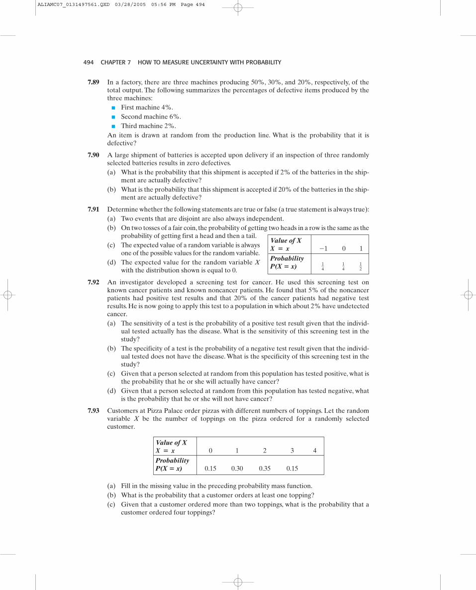
494 CHAPTER 7 HOW TO MEASURE UNCERTAINTY WITH PROBABILITY
7.89 In a factory, there are three machines producing 50%, 30%, and 20%, respectively, of thetotal output. The following summarizes the percentages of defective items produced by thethree machines:
■ First machine 4%.■ Second machine 6%.■ Third machine 2%.
An item is drawn at random from the production line. What is the probability that it isdefective?
7.90 A large shipment of batteries is accepted upon delivery if an inspection of three randomlyselected batteries results in zero defectives.(a) What is the probability that this shipment is accepted if 2% of the batteries in the ship-
ment are actually defective?(b) What is the probability that this shipment is accepted if 20% of the batteries in the ship-
ment are actually defective?
7.91 Determine whether the following statements are true or false (a true statement is always true):(a) Two events that are disjoint are also always independent.(b) On two tosses of a fair coin, the probability of getting two heads in a row is the same as the
probability of getting first a head and then a tail.(c) The expected value of a random variable is always
one of the possible values for the random variable.(d) The expected value for the random variable X
with the distribution shown is equal to 0.
Value of X0 1 2 3 4
Probability P(X � x) 0.15 0.30 0.35 0.15
X � x
Value of X0 1
Probability P(X � x) 1
214
14
-1X � x
(a) Fill in the missing value in the preceding probability mass function.(b) What is the probability that a customer orders at least one topping?(c) Given that a customer ordered more than two toppings, what is the probability that a
customer ordered four toppings?
7.92 An investigator developed a screening test for cancer. He used this screening test onknown cancer patients and known noncancer patients. He found that 5% of the noncancerpatients had positive test results and that 20% of the cancer patients had negative testresults. He is now going to apply this test to a population in which about 2% have undetectedcancer.(a) The sensitivity of a test is the probability of a positive test result given that the individ-
ual tested actually has the disease. What is the sensitivity of this screening test in thestudy?
(b) The specificity of a test is the probability of a negative test result given that the individ-ual tested does not have the disease. What is the specificity of this screening test in thestudy?
(c) Given that a person selected at random from this population has tested positive, what isthe probability that he or she will actually have cancer?
(d) Given that a person selected at random from this population has tested negative, whatis the probability that he or she will not have cancer?
7.93 Customers at Pizza Palace order pizzas with different numbers of toppings. Let the randomvariable X be the number of toppings on the pizza ordered for a randomly selectedcustomer.
ALIAMC07_0131497561.QXD 03/28/2005 05:56 PM Page 494
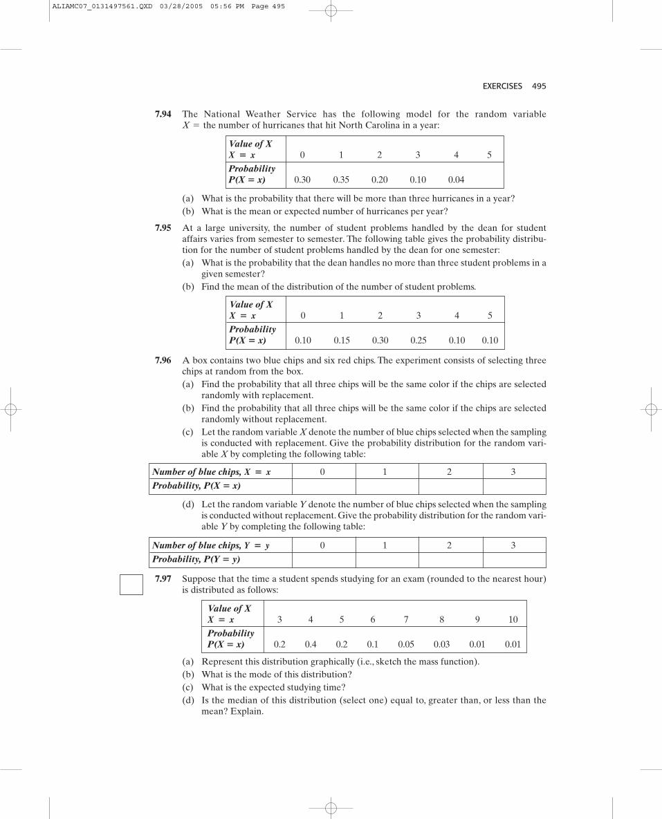
EXERCISES 495
Value of X0 1 2 3 4 5
ProbabilityP(X � x) 0.10 0.15 0.30 0.25 0.10 0.10
X � x
Value of X0 1 2 3 4 5
Probability P(X � x) 0.30 0.35 0.20 0.10 0.04
X � x
(a) What is the probability that there will be more than three hurricanes in a year?(b) What is the mean or expected number of hurricanes per year?
7.95 At a large university, the number of student problems handled by the dean for studentaffairs varies from semester to semester. The following table gives the probability distribu-tion for the number of student problems handled by the dean for one semester:(a) What is the probability that the dean handles no more than three student problems in a
given semester?(b) Find the mean of the distribution of the number of student problems.
7.96 A box contains two blue chips and six red chips. The experiment consists of selecting threechips at random from the box.(a) Find the probability that all three chips will be the same color if the chips are selected
randomly with replacement.(b) Find the probability that all three chips will be the same color if the chips are selected
randomly without replacement.(c) Let the random variable X denote the number of blue chips selected when the sampling
is conducted with replacement. Give the probability distribution for the random vari-able X by completing the following table:
Number of blue chips, 0 1 2 3
Probability, P(Y � y)
Y � y
Number of blue chips, 0 1 2 3
Probability, P(X � x)
X � x
(d) Let the random variable Y denote the number of blue chips selected when the samplingis conducted without replacement. Give the probability distribution for the random vari-able Y by completing the following table:
7.94 The National Weather Service has the following model for the random variableof hurricanes that hit North Carolina in a year:X = the number
7.97 Suppose that the time a student spends studying for an exam (rounded to the nearest hour)is distributed as follows:
Value of X3 4 5 6 7 8 9 10
ProbabilityP(X � x) 0.2 0.4 0.2 0.1 0.05 0.03 0.01 0.01
X � x
(a) Represent this distribution graphically (i.e., sketch the mass function).(b) What is the mode of this distribution?(c) What is the expected studying time?(d) Is the median of this distribution (select one) equal to, greater than, or less than the
mean? Explain.
ALIAMC07_0131497561.QXD 03/28/2005 05:56 PM Page 495
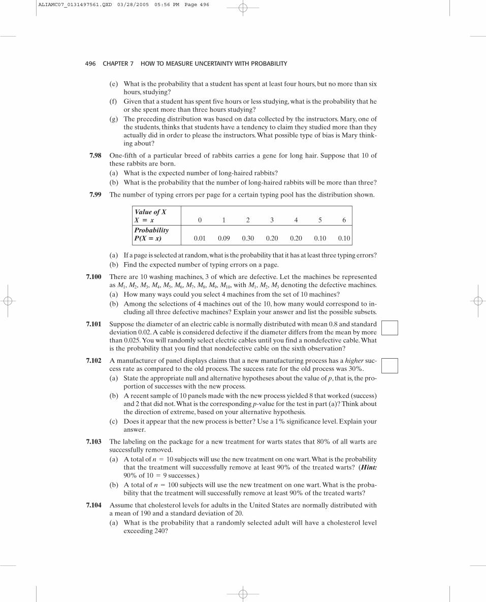
496 CHAPTER 7 HOW TO MEASURE UNCERTAINTY WITH PROBABILITY
(a) If a page is selected at random,what is the probability that it has at least three typing errors?(b) Find the expected number of typing errors on a page.
7.100 There are 10 washing machines, 3 of which are defective. Let the machines be representedas with denoting the defective machines.(a) How many ways could you select 4 machines from the set of 10 machines?(b) Among the selections of 4 machines out of the 10, how many would correspond to in-
cluding all three defective machines? Explain your answer and list the possible subsets.
7.101 Suppose the diameter of an electric cable is normally distributed with mean 0.8 and standarddeviation 0.02.A cable is considered defective if the diameter differs from the mean by morethan 0.025.You will randomly select electric cables until you find a nondefective cable.Whatis the probability that you find that nondefective cable on the sixth observation?
7.102 A manufacturer of panel displays claims that a new manufacturing process has a higher suc-cess rate as compared to the old process. The success rate for the old process was 30%.(a) State the appropriate null and alternative hypotheses about the value of p, that is, the pro-
portion of successes with the new process.(b) A recent sample of 10 panels made with the new process yielded 8 that worked (success)
and 2 that did not.What is the corresponding p-value for the test in part (a)? Think aboutthe direction of extreme, based on your alternative hypothesis.
(c) Does it appear that the new process is better? Use a 1% significance level. Explain youranswer.
7.103 The labeling on the package for a new treatment for warts states that 80% of all warts aresuccessfully removed.(a) A total of subjects will use the new treatment on one wart.What is the probability
that the treatment will successfully remove at least 90% of the treated warts? (Hint:90% of successes.)
(b) A total of subjects will use the new treatment on one wart. What is the proba-bility that the treatment will successfully remove at least 90% of the treated warts?
7.104 Assume that cholesterol levels for adults in the United States are normally distributed witha mean of 190 and a standard deviation of 20.(a) What is the probability that a randomly selected adult will have a cholesterol level
exceeding 240?
n = 10010 = 9
n = 10
M1, M2, M3M1, M2, M3, M4, M5, M6, M7, M8, M9, M10,
Value of X0 1 2 3 4 5 6
ProbabilityP(X � x) 0.01 0.09 0.30 0.20 0.20 0.10 0.10
X � x
(e) What is the probability that a student has spent at least four hours, but no more than sixhours, studying?
(f) Given that a student has spent five hours or less studying, what is the probability that heor she spent more than three hours studying?
(g) The preceding distribution was based on data collected by the instructors. Mary, one ofthe students, thinks that students have a tendency to claim they studied more than theyactually did in order to please the instructors. What possible type of bias is Mary think-ing about?
7.98 One-fifth of a particular breed of rabbits carries a gene for long hair. Suppose that 10 ofthese rabbits are born.(a) What is the expected number of long-haired rabbits?(b) What is the probability that the number of long-haired rabbits will be more than three?
7.99 The number of typing errors per page for a certain typing pool has the distribution shown.
ALIAMC07_0131497561.QXD 03/28/2005 05:56 PM Page 496
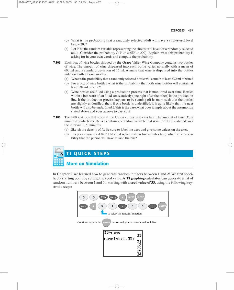
EXERCISES 497
(b) What is the probability that a randomly selected adult will have a cholesterol levelbelow 200?
(c) Let Y be the random variable representing the cholesterol level for a randomly selectedadult. Consider the probability Explain what this probability isasking for in your own words and compute the probability.
7.105 Each box of wine bottles shipped by the Grape Valley Wine Company contains two bottlesof wine. The amount of wine dispensed into each bottle varies normally with a mean of600 ml and a standard deviation of 16 ml. Assume that wine is dispensed into the bottlesindependently of one another.(a) What is the probability that a randomly selected bottle will contain at least 592 ml of wine?(b) For a box of wine bottles, what is the probability that both wine bottles will contain at
least 592 ml of wine?(c) Wine bottles are filled using a production process that is monitored over time. Bottles
within a box were often filled consecutively (one right after the other) in the productionline. If the production process happens to be running off its mark such that the bottlesare slightly underfilled, then, if one bottle is underfilled, it is quite likely that the nextbottle will also be underfilled. If this is the case, what does it imply about the assumptionstated above and your answer to part (b)?
7.106 The 8:00 A.M. bus that stops at the Union corner is always late. The amount of time, X, inminutes by which it’s late is a continuous random variable that is uniformly distributed overthe interval [0, 5] minutes.(a) Sketch the density of X. Be sure to label the axes and give some values on the axes.(b) If a person arrives at 8:02 A.M. (that is, he or she is two minutes late), what is the proba-
bility that the person will have missed the bus?
P1Y 7 240 ƒY 7 2002.
T I Q U I C K S T E P S
More on Simulation
In Chapter 2, we learned how to generate random integers between 1 and N. We first speci-fied a starting point by setting the seed value.A TI graphing calculator can generate a list ofrandom numbers between 1 and 50, starting with a seed value of 33, using the following key-stroke steps:
01
3 3
5 5
ENTERENTER
ENTER
Continue to push the button and your screen should look likeENTER
MATH
MATH
, )
STO
to select the randInt( function
ALIAMC07_0131497561.QXD 03/28/2005 05:56 PM Page 497
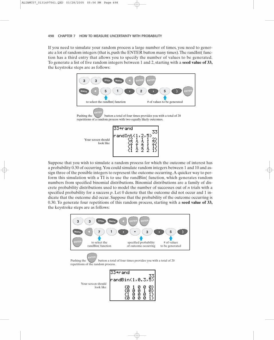
498 CHAPTER 7 HOW TO MEASURE UNCERTAINTY WITH PROBABILITY
Your screen should look like
Pushing the button a total of four times provides you with a total of 20repetitions of a random process with two equally likely outcomes.
to select the randInt( function # of values to be generated
1
3 3
5 5
ENTERENTER
ENTER
ENTER
MATH
MATH
, , )
STO
2
Suppose that you wish to simulate a random process for which the outcome of interest hasa probability 0.30 of occurring.You could simulate random integers between 1 and 10 and as-sign three of the possible integers to represent the outcome occurring.A quicker way to per-form this simulation with a TI is to use the randBin( function, which generates randomnumbers from specified binomial distributions. Binomial distributions are a family of dis-crete probability distributions used to model the number of successes out of n trials with aspecified probability for a success p. Let 0 denote that the outcome did not occur and 1 in-dicate that the outcome did occur. Suppose that the probability of the outcome occurring is0.30. To generate four repetitions of this random process, starting with a seed value of 33,the keystroke steps are as follows:
Your screen should look like
• 57
Pushing the button a total of four times provides you with a total of 20repetitions of the random process.
to select therandBin( function
# of valuesto be generated
specified probabilityof outcome occurring
1
3
3
3 ENTERENTER
ENTER
ENTER
MATH
MATH
, , )
STO
If you need to simulate your random process a large number of times, you need to gener-ate a lot of random integers (that is, push the ENTER button many times).The randInt( func-tion has a third entry that allows you to specify the number of values to be generated.To generate a list of five random integers between 1 and 2, starting with a seed value of 33,the keystroke steps are as follows:
ALIAMC07_0131497561.QXD 03/28/2005 05:56 PM Page 498