ICTP93Gibiansky

Leonid V. GIBIANSKY

Princeton UniversityNJ 08544 PRINCETON (U.S.A.)

Bounds on the Effective Moduliof Composite Materials

School on Homogenization

ICTP, Trieste, September 6–17, 1993

CONTENTS

1. Composite materials and their effective properties2. Bounds on the effective properties of composite materials3. The translation method to bound effective moduli of composites4. Implementation of the translation method to the plane elasticity problem

169

170 L.V. Gibiansky

1 Composite materials and their effective properties

1.1 Introduction

The course is devoted to studying the properties of composite materials. Composite-like materials are very common in nature as well as in engineering because they allowto combine the properties of component materials in an optimal way, allow to createmedia with such unusual and contradictory combination of properties as stiffness anddissipativeness, stiffness in one direction and softness in the other one, high stiffness andlow weight etc.

The pore structure of the bonds, trunks of the wood, leafs of the trees provide anexamples when mixture of stiff and soft tissues can be treated as a composite and leadsto the desired properties. Steel is the other example of the composite. The fine structureof the steel is grain-like mixture of monocrystals.

Engineers use composites for a long time. The well-known examples are given byreinforced concrete, plywood or fiber reinforced carbon composites. Composite materialsare important for the optimal design problems because use of composite constructions isoften the only way to achieve the desirable combination of properties with the availablecomponent materials. For examples, the honeycomb-like structures are light and possessa high bending stiffness due to the special structure that can be treated as a compositeof stiff aluminum matrix and air (pores).

The common feature of all these examples is that locally unhomogeneous materialbehaves as a homogeneous medium when the characteristic size of the inclusions is muchsmaller then the size of the whole sample and the characteristic wavelength of externalfields. In such a situation the properties of the composite can be described by theeffective moduli that is some special kind of averaging of the properties of the components.The branch of mathematics that study the behaviour of such materials is called thehomogenization theory. In this lecture we

1. formulate mathematical statement of the homogenization problem;2. give two equivalent definitions of the effective properties of composite material;

3. study the direct problem of homogenization theory, i.e. the problem of calculationof the effective properties for a composite of given structure;

4. find the effective properties of laminate composites and Hashin-Shtrikman assem-blages of coated spheres.

The second lecture of the course devoted to the statement of the problem of boundson the effective properties, in the third one we describe the translation method for de-riving such bounds and illustrate this method on the simplest example of the bounds onconducting composite. The fourth lecture devoted to implementation of the translationmethod to the two-dimensional isotropic elastic composite. We also touch some openquestions in this field. The main goal of the course is not only to give an introduction tothe problem of bounds on the effective moduli, but also to give rigorous, powerful andsimple method to attack the problems of such type.

Remark The actual course slightly differed from this lecture notes. It also includedthe description of variational principles for the media with complex moduli with an ap-plications to the problem of bounds on the complex effective conductivity of a composite.

Bounds on Effective Moduli 171

Last lecture of the course that is not reflected here was devoted to some bounds on conduc-tivity of multiphase materials, description of optimal microstructures (namely, of matrixlaminate composite of high rank) that realize some of the bounds. We also discussed thestatement of optimal design problem and use of homogenization theory in optimal design.Most of these results can be found in the mentioned at the references original papers. Thereferences on the original papers that are used in the course are given at the end of eachsection.

1.2 Notations

Let introduce some notations that are used in the course. First, let us denote all vectorsand tensors as a bold characters, unit tensor as I

I = δiδj =

1 0 00 1 00 0 1

, (1.1)

symbol (·) denotes the convolution of the tensors over one index, namely

a · b = aibi, A · b = Aijbjli, A · B = AijBjklilk, b · D · b = Dijbibj , (1.2)

etc., where ai, bi, Aij , and Bij are the elements of the vectors a, b and tensors A, andB respectively in the Cartesian basis, li is the ort of the axis xi. We use summationagreement that sum is taken over the repeating indices from 1 to N, where N is thedimension of the space, N = 2 or N = 3. Two dots are used in the elasticity theorynotations as follows

ε · ·σ = εijσji, ε · ·C · ·ε = Cijklεjiεlk. (1.3)

We also denote as ∇ the Hamiltonian operator

∇ = liδ

δx1. (1.4)

1.3 Composite materials and their effective properties.

We begin with formulation of the homogenization problem for two isotropic conductingmaterials. To study the effective properties of a mixture it is sufficient to deal with spaceperiodic structures. The case of random composite has some specific features but most ofthe results are simplier to prove and describe for the periodic structures, generalizationon random case is a technical problem. A composite which is not periodic, but saystatistically homogeneous, can be replaced by a periodic one with negligible change inits effective properties: one can take a sufficiently large cubic representative sample ofthe statistically homogeneous composite and extend it periodically. For simplicity westart with a description of a two-dimensional two-phase composite combined from twoconducting materials.

172 L.V. Gibiansky

We assume that each element of periodicity S is divided into the parts S1 and S2 withthe prescribed volume fractions m1 and m2 respectively, see Figure 1.

S1 ∪ S2 = S,(volS1)/(volS) = m1,(volS2)/(volS) = m2,

m1 + m2 = 1

(1.5)

We can assume that volS = 1 without loss of generality.

Figure 1: two-phase composite material.

Suppose that these two parts are occupied by two isotropic materials with differentconductivities Σ1 = σ1I and Σ2 = σ2I respectively. The state of the media is describedby the linear elliptic system of differential equations of electrostatic

∇ · j = 0, j = Σ · e, e = −∇φ, (1.6)

where φ is the electrical potential, j is a current and e is an electrical field. The conduc-tivity tensor Σ has the form

Σ(x) = (σ1χ1(x) + σ2χ2(x)) I, (1.7)

where χi(x), i = 1, 2 are the characteristic functions of the subdomains S1, S2

χi(x) ={

1, if x ∈ Si

0, otherwise.(1.8)

We denote also Σi = σi I, i = 1, 2

Remark: The conductivity equations (1.6) describe also heat conductance, diffusionof particles or liquid in a porous medium, magnetic permeability etc. as it is summarizedin the following table, but we use the notations of electrical conductivity problem.


Problem j e φ Σ

Thermal

Conduction

Heat current Temperature

gradient

Temperature Thermal

conductivity

Electrical

Conduction

Electrical

current

Electrical field Electrical

potential

Conductivity

Dielectrics Displacement

field

Electric field Potential Permittivity

Diffusion Particle

current

Gradient of

concentration

Concentration Diffusivity

Magnetism Magnetic

induction

Magnetic field

intensity

Potential Permeability

Stoke’s flow Current Pressure

gradient

Pressure Viscosity

Homogenized

flow in porous

media

Fluid current Pressure

gradient

Pressure Permeability

Described periodical structure acts in a smooth external field as a homogeneousanisotropic conductor, that can be described by the effective properties tensor Σ0. Thereexist two equivalent definitions of the effective properties tensor.

Let put the composite into the homogeneous external fields. The local fields in thecell of periodicity are S-periodic. Let compute the average values of the current andelectrical fields over the cell of periodicity S

< j >=∫

Sj(x)dS, < e >=

∫

Se(x)dS, (1.9)

One can prove that these values are connected by linear relationship

< j >= Σ0· < e >, (1.10)

Here and below the symbol < · > denotes the average value of (·), i.e.

< (·) >=∫

S(·)dS/ volS, (1.11)

Definition 1. Symmetric, positive definite (2 × 2) tensor Σ0 defined by the aboveprocedure is called the tensor of effective conductivity of the composite.

Due to the linearity of the state law (1.6), the tensor Σ0 is independent of externalfields, that make this definition meaningful. Effective properties tensor Σ0 depends onthe properties of the components, on their volume fractions, and also strongly dependson geometrical structure of the composite.

This derivation can be done rigorously using the technic of multiscale decomposition,but we omit these details. Interested reader can find the details in the book by Sanchez-Palencia.

Basing on this definition one can calculate the effective properties tensor for any givenmicrogeometry. Indeed, let study the following boundary value problem combining theequations (1.6) with boundary conditions

φ = −e01x1, if x = {x1, x2} ∈ Γ. (1.12)

174 L.V. Gibiansky

Here e01 is some constant and Γ is the boundary of the periodic cell. Let assume that wesolve this problem either analytically or numerically and denote as j0 = j(x), e0 = e(x),where j(x) and e(x) is the solution of (1.6), (1.12). One can check that e0 = {e01, 0}.Indeed

e0 = −∫

S∇φdS =

∫

Γn e01dΓ = e01l1. (1.13)

Here l1 is the ort of the axis x1 and n is the external normal to the Γ. Now let us rewritethe effective state law (1.10) in a component form

j01 = σ011e01 + σ0

12e02, j02 = σ021e01 + σ0

22e02, (1.14)

where σ0ij are the elements of the effective conductivity tensor Σ0, and substitute the

value e02 = 0 in it. We immediately arrive at the relations

σ011 = j01/e01, σ0

21 = j02/e01. (1.15)

Similarly, by solving the equations (1.6) in conjunction with the boundary conditions

φ = −e02x2 if x = {x1, x2} ∈ Γ (1.16)

we arrive at the relations

σ022 = j02/e02, σ0

12 = j01/e02 (1.17)

where j01, and j02 are the averaged over the periodic cell current fields for the problemwith boundary conditions (1.16)

In general, for more complicated problems, we need to solve as many boundary valueproblems as the dimension of the space of phase variables. Namely, this number is equalto N for N -dimensional conductivity problem, equal to 3 for two-dimensional elasticityand equal to 6 for the three-dimensional elasticity.

There exists the other definition of the effective properties tensor based on the energyarguments.

Definition 2. Tensor of the effective properties of a composite is defined as a tensorof properties of the medium that in the homogeneous external filed e0 stores exactly thesame amount of energy as a composite medium subject to the same homogeneous field

e0 · Σ0 · e0 =< e(x) · Σ(x) · e(x) > . (1.18)

Here e(x) is the solution of the problem (1.6) with periodic boundary conditions andwith an additional condition e0 =< e(x) >. Using Dirichlet variational principle onecan write

e0 · Σ0 · e0 = infe : e = ∇φ< e >= e0

< e(x) · Σ(x) · e(x) >, (1.19)

Similarly, by using Thompson variational principle, one can write

j0 · Σ−10 · j0 = inf

j : ∇ · j = 0,< j >= j0

< j(x) · Σ−1(x) · j(x) >, (1.20)


The definitions (1.10) and (1.19)-(1.20) are equivalent. The first one is useful tocompute the effective properties for given structures, the second one is a key that pro-vides an opportunity to use variational methods to construct the bounds on the effectiveproperties. To prove the equivalence we mention first that

< e(x) · Σ(x) · e(x) >=< e(x) · j(x) >= e0 · j0 +∑

k 6=0

e(k) · j(k), (1.21)

where we used the Fourier transformation and the Plancherel’s equality to justify thesecond equality. Here k is a wave vector of the Fourier transformation, e(k) and j(k)are the Fourier coefficients of the electrical and current fields respectively. Electrical fieldis a potential one

e = −∇φ. (1.22)

Current field is divergence free (∇ · j = 0); therefore one can introduce vector potentialA such that

j = ∇× A, (1.23)

where (×) is a sign of vector product. Conditions (1.22) and (1.23) can be presented interms of the Fourier images of these fields as

ˆe(k) = −k ˆφ(k), ˆj(k) = k × A(k). (1.24)

Therefore

ˆe(k) · ˆj(k) = φ(k)k · k × A(k) = 0. (1.25)

Let define the effective properties tensor via energy relationship (1.19). Substituting(1.19), (1.25) into (1.21) we arrive at the relation

e0 · Σ0 · e0 = e0 · j0 (1.26)

that is valid for any field e0. Therefore j0 = Σ0 · e0 as it is stated by (1.10); thus weproved the equivalence of two definitions.

1.4 Examples of calculations of the effective moduli of some

particular structures

For the most of the structures the effective properties can be calculated only numericallybecause the boundary value problems (that are needed to be solved to find these moduli)can be solved only numerically. But there exist a limited number of special classes ofcomposites that allow the analytical calculation of the properties, these composites areof special interest and we study them in more details.

176 L.V. Gibiansky

1.4.1 Laminate composite.

Let us assume that the component materials are laminated in a proportions m1 and m2

and let denote the ort in the direction of lamination as n, and the ort along the laminateas t, see Figure 2.

Figure 2: laminate composite of two phases.

To calculate the effective properties let put this composite into the homogeneousexternal field e0. The local fields in the materials are peace-wise constant in this case,namely

e(x) = e1χ1(x) + e2χ2(x), j(x) = j1χ1(x) + j2χ2(x) (1.27)

Now the average fields are calculated as

e0 = m1e1 + m2e2, j0 = m1j1 + m2j2. (1.28)

Due to the differential restriction on the electrical and current fields the following jumpconditions should be satisfied on the boundary of the layers

(e1 − e2) · t = 0, (j1 − j2) · n = 0. (1.29)

Therefore, by taking into account the jump conditions (1.29) for the electrical field weget

e1 = e0 + e′n, e2 = e0 −m1

m2

e′n, (1.30)

where e′ is some scalar constant. Note also that

j1 = Σ1 · e1, j2 = Σ2 · e2. (1.31)

Let assume now that the field e0 is given and let calculate j0. The following equalitiesare obvious consequences of (1.30)-(1.31)

j0 = m1j1+m2j2 = m1Σ1 ·e1+m2Σ2 ·e2 = (m1Σ1+m2Σ2)e0+m1e′(Σ1−Σ2)·n (1.32)

The constant e′ can be found from jump conditions (1.29) for the current field. Namely,from the equations (1.30) -(1.31) we get

j1 − j2 = (Σ1 − Σ2) · e0 +e′

m2(m2Σ1 + m1Σ2) · n (1.33)


Projecting (1.33) on the direction n we obtain

e′ = −m2[n · (m2Σ1 + m1Σ2) · n]−1n · (Σ1 −Σ2) · e0 (1.34)

Combining (1.32) and (1.34) we get the result

j0 = Σ0 · e0, (1.35)

where

Σ0 = (m1Σ1 +m2Σ2)−m1m2(Σ1−Σ2) ·n[n ·(m2Σ1 +m1Σ2) ·n]−1n ·(Σ1−Σ2) (1.36)

In a more general setting for the state law

J = D · E (1.37)

with the jump conditions on the boundary with the normal n

P (n) · (E1 − E2) = 0, P⊥(n) · (J1 − J2) = 0 (1.38)

we obtainD0 = m1D1 + m2D2− (1.39)

−m1m2(D1−D2)·P⊥(n)[P⊥(n)·(m2D1+m1D2)·P⊥(n)]−1P⊥(n)·(D1−D2). (1.40)

Here P⊥(n) is a projector operator on the subspace of the discontinuous components ofthe vector E on the boundary with the normal n.

The derivation is literally the same. We just need to use more general projectionoperator and more general definition of the convolution (·).

1.4.2 Hashin structures

The other example of the structures whose effective moduli can be computed analyticallywas suggested by Hashin and used by Hashin and Shtrikman in order to prove the attain-ability of the bound on the effective properties of a composite. They study the followingprocess. Let put into the space filled by the conducting material with the properties σ0

an inclusions consisting of a core of the material σ1 and surrounded by the sphere of thematerial σ2, see Figure 3.

Figure 3: Hashin-Shtrikman construction.

178 L.V. Gibiansky

Let put this construction into the homogeneous on infinity electrical field e0. In thepolar coordinates we look for the solution of the conductivity problem in a form

φ1 = a1r cos α, in the core, (1.41)

φ2 = (a2r + b2/r2) cos α, in the coating, (1.42)

φ0 = a0r cos α, in the medium, (1.43)

where r is a radial coordinate r =√

x · x, α is an angle between the direction of theapplied field v and radius vector x. The electrical and current fields in this case expressedas

e1 = −∇φ1 = −a1v = −a1[cos αvr − sin αvα], (1.44)

j1 = σ1e1 = −σ1a1[cos αvr − sin αvα], (1.45)

e2 = −∇φ2 = −[a2 − 2b2/r3] cos αvr + [a2 + b2/r

3] sin αvα], (1.46)

j2 = σ2e2 = −σ2[a2 − 2b2/r3] cos αvr + σ2[a2 + b2/r

3] sin αvα], (1.47)

e0 = −∇φ0 = −a0v = −a0[cos αvr − sin αvα], (1.48)

j0 = σ0e0 = −σ0a0[cos αvr − sin αvα], (1.49)

where vr and vα are the unit radial and tangential vectors in terms of which v = cos αvr−sin αvα. These potentials satisfy the conductivity equations in each of the regions. Weonly need to find the constant to satisfy the jump conditions on the interface of theseregions. Continuity of the potential leads to the conditions

a1 = a2 + b2/r31, a0 = a2 + b2/r

32 (1.50)

Jump conditions on the current field give

σ1a1 = σ2[a2 − b2/r31], σ0a0 = σ2[a2 − 2b2/r

32]. (1.51)

By substituting (1.50) into (1.51) we arrive at the system of equations

a2 = −b2[σ1 + 2σ2]/[r31(σ1 − σ2)] = −b2[1 + 3σ2/(σ1 − σ2)]/r

31 (1.52)

a2 = −b2[σ0 + 2σ2]/[r32(σ0 − σ2)] = −b2[1 + 3σ2/(σ0 − σ2)]/r

32. (1.53)

From these equations we deduce that

1

σ0 − σ2=

1

m1

1

σ1 − σ2+

m2

3m1σ2, (1.54)

wherem1 = 1 − m2 = r3

1/r32, (1.55)

m1 and m2 are the volume fractions of the materials in the inclusion. If the constantσ0 satisfies the relation (1.54) the solution of the conductivity problem for the describedgeometry is given by (1.41)-(1.43). As we see, the field outside the inclusion is exactlythe same as it would be without it. It means that we can put the other inclusions inthe space without changing the average electrical field. Let fill all the space by such


inclusions (we need infinitely many scales of the inclusion’s sizes to do it). Resultingmedium possesses the effective conductivity constant σ0. It consists of the materials σ1

and σ2 taken in the proportions m1 and m2.We can do the same for the two-dimensional conductivity, the result is given be the

relation1

σ0 − σ2

=1

m1

1

σ1 − σ2

+m2

2m1σ2

. (1.56)

Let denote the conductivity of such a medium as σ2HS = σ0 Changing the order of the

materials in a structure (i.e. studying the composite with inclusions consisting of thecore of the second material surrounded by the first material) we obtain the other mediawith conductivity (in two dimensions)

1

σ1HS − σ1

=1

m2

1

σ2 − σ1+

m1

2m2σ1(1.57)

As we will see later, conductivity σ0 of any isotropic composite lies between these values

σ0 ∈ [σ1HS, σ2

HS] (1.58)

1.5 Conclusions

As we see, the effective properties of the composite depend on the properties of componentmaterials, their volume fractions in the composite, but also depend very strongly on themicrostructure. When the microstructure is known the properties of the composite canbe computed. We face absolutely different situation when we know a little or nothingabout the microstructure of the material but are interested in their effective moduli. Suchproblems often arise in optimal design of composite materials when we want to createthe composite that is the best according to some optimality criteria In this situation themicrostructure is unknown, it needs to be determined. But some a-priory informationthat does not depend on the structure would be helpful and desirable. We address thiskind of problems in the next lecture.

1.6 References

R.M. Christensen, Mechanics of Composite Materials (Wiley-Interscience, New-York,1979).

Z. Hashin and S. Shtrikman, A variational approach to the theory of the elasticbehavior of multiphase materials, J. Mech. Phys. Solid, 11, (1963), 127 - 140.

E. Sanchez - Palencia, Nonhomogeneous Media and Vibration Theory (Lecture Notesin Physics 127, Springer - Verlag, 1980).

2 Bounds on the effective properties of composite

materials

As we saw, the effective moduli of the composite strongly depend on their microstruc-ture. To illustrate it let study the example of the two-dimensional conductivity prob-

180 L.V. Gibiansky

lem. For such a case the tensor of effective properties is a second order tensor that canbe completely characterized by two rotationally invariant parameters, namely, by theireigenvalues λ1 and λ2, and by the orientation φ. The space of invariant characteristic istwo-dimensional and can be easily illustrated, see Figure 4.

Figure 4. Plane of invariants of conductivity matrices in two dimensions.

Let us put on this plane the effective properties of the structures that we calculatedat the last lecture. Let rewrite the formula for the effective conductivity of laminatematerial in the basis that is connected with the normal n to the laminates. We get

λ1 = σh = (m1/σ1 + m2/σ2)−1, λ2 = σa = m1σ1 + m2σ2 (2.1)

Points A and B on the Figure 3 correspond to the laminate composites with the normalto layers n oriented along and perpendicular to the direction of the x1 axis, respectively.Note, that the diagonal of the first sector (see Figure 4) is the axis of symmetry for thepicture, because we always may rotate composite possessing the eigenvalues (λ1, λ2) andget the material with the pair of eigenvalues (λ2, λ1). Points C and D correspond to theHashin-Shtrikman assemblages of coated circles. They differ by the order of the materials:for the more conducting one (with the higher conductivity) the inclusion consists ofthe core of the less conducting material surrounded by the circle of more conductingmaterial and vise-versa for the other point. All these media were composed from the sameamounts of the same component materials, but the effective properties of these media areabsolutely different. The only reason is the difference in the microstructure. Arbitrarycomposite corresponds to some point G in the plane (λ1, λ2). The question arises how farcan we change the properties by changing the microstructure of a composite, how largeis the region in the space of invariants of the effective properties tensors that correspondsto some composite materials. Let me give two definitions that are essential:

Definitions:

1. Gm -closure: Let assume that we have in our disposal the set {U} of the com-ponent materials. The set of the effective properties tensors of the composites combinedfrom the given amounts of the component materials is called the Gm-closure of the set U


and is denoted as GmU -set.

GmU = ∪χi(x):<χi(x)>=miD0(χi(x)) (2.2)

The union of all such GmU sets over the volume fractions mi is called G-closure ofthe set U and is denoted as GU

GU = ∪miGmU, (2.3)

see Figure 4 for the conductivity example.In the other words, G-closure or GU -set is the set of the effective properties of all

the composites that can be prepared from arbitrary amounts of the component materials.Knowledge of these sets is important for many reasons. They provide a benchmark

for testing experimental results and approximation theories, and can provide an indicatoras to whether the average response of a given composite is extreme in the sense of beingclose to the edge of these sets. There exists a simple way (2.3) to find G-closure if weknow the Gm-closure set. Therefore we concentrate our attention on the problem offinding Gm-closure.

There is no direct and straightforward way (at least it is not known) to find GmUset. The way how people do it is the following:

1. First one need to construct the bounds on the effective properties of compositesthat do not depend on microstructure. They depend on the properties of componentmaterials, their volume fractions, but do not depend on the details of the microstructure.They are valid for a composite material of any structure with fixed volume fractions ofthe components. In the space of invariants of the effective properties tensors they definethe set PmU such that

GmU ⊂ PmU. (2.4)

2. Then one can look for the set of the effective properties tensors of a particu-lar structures combined from given component materials (laminate composite, laminatecomposite of laminate composite, Hashin-Shtrikman - type structures etc.) to define theset LmU such that

LmU ⊂ GmU. (2.5)

It gives the bound of the GmU -set from inside. If both bounds coincide it allows us todefine GmU itself;

If LmU = PmU, then LmU = GmU = PmU. (2.6)

The goal of our course is to describe the method for constructing geometrically inde-pendent bounds on the effective properties of a composite, i.e. the method to find thePmU -set. We also describe the microgeometries that are candidates to be optimal, i.e.that are extremal in the sense that they correspond to the bounds of the G-sets. It is nowrecognized that optimal bounds are important in the context of structural optimization:the microstructures that achieve the bounds are often the best candidates for use in thedesign of a structure.

There exist just few examples where the whole G or Gm sets are known. Theyinclude the bounds on the conductivity tensor of two- and three-dimensional two-phase

182 L.V. Gibiansky

composite, bounds on effective complex conductivity for two-phase two-dimensional com-posite, coupled problem of two second order diffusion equations for two-dimensional two-component composite. There are much more problems for which some bounds on theproperties are known, there exist the composites that correspond to some parts of bounds,but there are no such structures for some other parts of the boundary. Among such exam-ples are three-dimensional two-phase complex-conducting composites, elastic composite,bounds on the effective properties for three-phase composites, etc. Now we are goingto discuss the method of constructing geometrically independent bounds on the effectiveproperties of composite materials.

2.1 Bounds on the effective properties tensor

For a long time people tried to suggest different approximations for the effective moduliof the mixtures. Voigt suggested the arithmetic mean

D0 =< D(x) >=∑

i

miDi (2.7)

as a good approximation for the effective properties. The other approximation wassuggested by Reuss who proposed the harmonic mean expression for the effective moduliof a composite

D0 =< D−1(x) >−1= [∑

i

miD−1i ]−1 (2.8)

Wiener proved that (2.7) and (2.8) are actually the upper and low bounds on the effectivemoduli of the mixture. These bounds are now known as Reuss-Voigt bounds or, in thecontext of elasticity, as Hill’s bounds

< D−1(x) >−1 ≤ D0 ≤ < D(x) > (2.9)

Remark: We say that A ≥ B if the difference of these two tensors C = A − B ispositive semidefinite tensor , i.e. all the eigenvalues of this tensor C are greater or equalto zero.

Note that for the conductivity case these bounds are exact in a sense that there existsa composite (namely, laminate composite) that has one eigenvalue (across the laminate)equal to the harmonic mean of the component conductivities whereas the other ones areequal to the arithmetic mean of phases conductivities. So, in the Figure 4 these boundsform the square that contains GmU set and this square is the minimal one because twocorner points of it correspond to the laminate composites.

Now I’d like to show how to prove these bounds, because it is the key point of thefollowing discussion.

2.2 Proof of the Reuss-Voigt-Wiener bounds.

To prove the bounds one can start with the variational definition of the effective proper-ties. Namely, we have

e0 · D0 · e0 = infe=∇φ,<e>=e0

< e · D · e > . (2.10)


By substituting the constant field e(x) = e0 into the right hand side of the equation(2.10) we get

e0 · D0 · e0 ≤ < e0 · D · e0 > = e0· < D > ·e0. (2.11)

These arguments are valid for any value of the average field e0. Therefore we can deducethe inequality for the matrices

D0 ≤ < D > (2.12)

from the inequality (2.11) for the quadratic forms. Similarly,

j0 ·D−10 ·j0 = inf

j :∇·j=0,<j>=j0

< j ·D−1 ·j > ≤ < j0 ·D−1 ·j0 > = j0· < D−1 > ·j0,

(2.13)and therefore

D−10 ≤ < D−1 > . (2.14)

Reuss bound follows immediately from this statement.As we see the procedure is based on the assumption that either electrical or current

field is constant throughout the composite. It may be true for some structures and somefields, as we will see. In that situations the bounds are exact in a sense that there existsa composite that has the effective properties tensor that corresponds to the equality inthe expressions (2.9) .

2. Variational proof.The other proof (that is not so elementary but more useful for us because it can be

improved in order to receive more restrictive bounds) is the following. As earlier we startwith the variational definition of the effective properties tensor but now we construct thebound by omitting the differential restrictions e = −∇φ on the fields. Namely,

e0 · D0 · e0 = infe:e=∇φ,<e>=e0

< e · D · e > ≥ infe:<e>=e0

< e · D · e > . (2.15)

Note, that when we drop off the differential restriction we decrease the value of thefunctional. The last problem is the standard problem of calculus of variations and canbe easily solved. The main idea is that we drop of the local (i.e. point-wise) restrictionsthat we can not investigate, but save the integral restrictions that are easy to handle.Let take into account the remaining restriction by vector Lagrange multiplier γ

infe:<e>=e0

< e · D · e >= supγ

infe

< e · D · e + 2γ · (e − e0) > (2.16)

Stationary conditions lead to the equations

2D · e + 2γ = 0, (2.17)

ore = −D−1 · γ. (2.18)

Note that the equation (2.17) requires the current field j = D ·e to be constant through-out the composite. Here the constant vector parameter γ can be found from the restric-tion < e >= e0, namely

γ = − < D−1 >−1 ·e0 (2.19)

184 L.V. Gibiansky

By substituting (2.18), (2.19) into (2.15) we get

< e · D · e > = < e0· < D−1 >−1 ·D−1 · D · D−1· < D−1 >−1 ·e0 >

= e0· < D−1 >−1 ·e0 (2.20)

that proves the Reuss bound. Note that the condition

D(x) ≥ 0, (2.21)

is required in order for the stationary solution of the problem to be a minimum of thefunctional. This condition for the two-phase composite can be rewritten as

D1 ≥ 0, D2 ≥ 0. (2.22)

It will be essential in a future for the procedure of improving of Reuss-Voigt bounds.Similarly, one can get Voigt bounds starting from the variational principle in terms

of the current fields.As we see, any information about the microstructure of the composite disappears from

the problem when we drop off the differential restrictions on the fields like e = −∇φ. So,the key idea to improve the bound is to take these differential restrictions into accountby some way. We concentrate our attention on so called translation method that use theintegral corollaries of the differential restriction to improve the Reuss-Voigt bounds, butbefore I’d like to mention very briefly the other methods that can be used to obtain thebounds on the effective properties.

1. Hashin-Shtrikman method was suggested by the authors in 1962 when they as-sumed the isotropy of the composite and found the bounds on the effective conductivityand on the bulk and shear moduli of elastic composites. This method was reformulatedfor the anisotropic materials later by Avellaneda, Kohn, Lipton, and Milton and thebounds that can be obtained by this method are proved to be equivalent to the trans-lation bounds for some special choice of the parameters. Whereas Reuss-Voigt boundsrequire one of the fields to be constant throughout the composite, this method requiresthe constant field only in one of the phases and allows fluctuations of the fields in theothers components.

2. Analytical method (see Bergman, Milton) is based on the analytic properties of theeffective conductivity as a function σ0 = σ0(σ1, σ2) of the two component conductivities.In fact, because this is a homogeneous function it suffices to set one of the componentconductivities equal to 1 and to study the effective conductivity as a function of theremaining component conductivity σ0 = σ1σ0(1, σ2/σ1). The resulting function of onecomplex variable is essentially a so called Stieltjes function and many of the bounds onthe complex effective conductivity correspond to bounds on this Stieltjes function. Thismethod has an advantage of being able to handle complex moduli case, but it is difficult togeneralize it to more general problems because it requires studying of analytic functionsof several variables. This theory is not too developed to be used for the construction ofthe bounds.

3. Translation method was suggested in different but close forms by Murat & Tartarand Lurie & Cherkaev around ten years ago. The main idea of the translation method


is to bound the functional (2.10) (and therefore the effective tensor D0) by taking intoaccount the differential restrictions

e = −∇φ (2.23)

through their integral corollaries

〈e · T e〉 ≥ 〈e〉 · T 〈e〉, (2.24)

which are hold for every field e satisfying (2.23) for some special choices of the matrixT . Here T is the so called translation matrix which may possess several free parameters.The choice of this matrix is dictated by the differential properties (2.23) of the field e.Functions that possess properties similar to (2.24) under averaging are called quasiconvexfunctions. For a general discussion of quasiconvexity and methods for finding quadraticquasiconvex function see, for example, Tartar, Ball, and Dacorogna.

We discuss this method in details in the next lecture.

2.3 References

Avellaneda, M. Optimal bounds and microgeometries for elastic composites, SIAM J.Appl. Math.,47,1987, p.1216.

Ball, J.M., Currie, J.C., and Oliver , P.J. 1981 Null Lagrangians, weak continuity andvariational problems of arbitrary order, J. Funct. Anal., 41, 135-174.

Baker, G.A. 1969 Best error bounds for Pade approximants to convergent series ofStieltjes, J. Appl. Phys., 10, 814-820.

Bergman, D.J. 1982 Rigorous bounds for the complex dielectric constant of a twocomponent composite, Ann. Phys., 138, 78-114.


B. Dacorogna, Weak continuity and weak lower semicontinuity of non-linear func-tionals ( Lecture Notes in Math. 922, Springer-Verlag, 1982).

Golden, K. and Papanicolaou, G. 1985 Bounds for effective parameters of multicom-ponent media by analytic continuation, J. Stat. Phys., 40, 655-667.

Z. Hashin and S. Shtrikman, A variational approach to the theory of the elasticbehavior of multiphase materials, J. Mech. Phys. Solid, 11, (1963), 127 - 140.

Lurie, K.A. and Cherkaev, A.V. 1986 The effective characteristics of composite ma-terials and optimal design of constructions, Advances’ in Mechanics (Poland), 9, 3 -81.

Milton, G.W. 1981 Bounds on the complex permittivity of a two-component compos-ite material, J. Appl. Phys., 52, 5286-5293.

G.W. Milton, On characterizing the set of possible effective tensors of composites:The variational method and the translation method, Comm. of Pure and Appl. Math.,vol.XLIII, (1990), 63-125.

G.W. Milton, A brief review of the translation method for bounding effective elastictensors of composites, Continuum Models and Discrete Systems, ed. by G. A. Maugin,vol. 1, (1990), 60-74.

186 L.V. Gibiansky

F. Murat and L. Tartar, Calcul des variations et homogeneisation, Les Methodes del’Homogeneisation: Theorie et Applications en Physique, Coll. de la Dir. des Etudes etRecherches de Electr. de France, Eyrolles, Paris, (1985), 319 - 370.

L. Tartar, Estimations fines des coefficients homogeneises, Ennio de Giorgi Collo-quium, P.Kree,ed., Pitman Research Notes in Math. 125, (1985), 168 - 187.

L. Tartar, Compensated compactness and applications to partial differential equa-tions, Nonlinear Analysis and Mechanics, Heriott-Watt Symp. VI, R.J. Knops ed., Pit-man Press, (1979).

3 The translation method to bound the effective

moduli of composites.

The translation method is based on the variational definition of the effective propertiesand on bounds on some energy type functionals. It consists of several well-formulatedsteps, namely

1. choosing appropriate functionals to study;2. studying the differential properties of the phase variables in order to define

quadratic quasiconvex functions.3. finding the lower bounds for these functionals by using existence of the quasiconvex

quadratic forms; finding the bounds on effective properties tensor by using the boundsfor the functionals;

4. checking the attainability of the bounds by examining particular microstructures.We discuss first three steps in this and in the next lecture, last lecture of the course

is devoted to the description of optimal structures.

3.1 Choosing appropriate functionals.

Let start with figure similar to the Figure 4 that was discussed during the previouslecture.

Figure 5: Construction of the functionals that give the bound for the GmU set forthe conductivity problem.

It shows approximate form of the GmU set for the conductivity problem. Let studywhat kind of functionals we need to estimate in order to obtain the desired bound for the


GmU set. Let minimize (over all microstructures, i.e. over all characteristic functions χi)the energy stored by the composite in the homogeneous external field e01

W01 = infχi:<χi(x)>=mi

e01 · D0(χi) · e01. (3.1)

We find out first, that it is optimal to rotate composite so that the minimal conductivitydirection be oriented along the vector e01. In fact, the structure tries to minimize thelowest eigenvalue because


λmin(χi)e01 · e01 (3.2)

It means that the optimal composite corresponds to the corner point of the set GmU , seeFigure 5, say to the point A if the direction e01 coincides with the axis λ1. As we see,this functional reflects only properties of the medium in the direction of the applied fielde01 and can not ”feel” the properties in the orthogonal direction. Let now minimize theenergy stored by the composite placed into the external field e02 that is orthogonal toe01


e02 · D0(χi) · e02 (3.3)

The optimal composite (that gives a solution to the problem (3.3)) corresponds to thepoints B on the Figure 5 and possesses the minimal conductivity direction λ2 orientedalong the vector e02. As we see, by bounding the functionals W01 and W02 we can onlybound the minimal eigenvalue of the conductivity matrix that corresponds to the Reussbounds. We can bound the eigenvalues of the conductivity matrix only independently.It happens because the functional of the type (3.2)-(3.3) reflects the properties of themedium only in one particular direction. In order to take into account the propertiesof the composite in the other direction we may combine the above two functionals andstudy the quadratic form

We = W01 + W02 = infχi:<χi(x)>=mi

[e01 · D0(χi) · e01 + e02 · D0(χi) · e02]

= infχi:<χi(x)>=mi

[λ1(χi)e01 · e01 + λ2(χi)e02 · e02] (3.4)

This functional is a weighted sum of the eigenvalues. In order to minimize such functionalthe composite has to minimize the sum of its eigenvalues. Bound for this functionalshows how far can we move the point that corresponds to the effective properties of thecomposite in the direction of arrow on the Figure 5. They define the position of thestraight line that is tangential to the set PmU : GmU ∈ PmU . Changing the ”weights”of each eigenvalue (by changing an amplitude of the vectors e01 and e02) we change thisdirection within the third sector as it is shown in the Figure 5. As we see, one canconstruct the lower bound of the set GmU for the two-dimensional conducting compositeby bounding the functional (3.4). In the three dimensional space we need to study alsothe functional that is the sum of three terms. Each of these terms is an energy stored bythe composite in the homogeneous external field. These three fields should be orthogonalto each other in order for the functional to reflect the properties of the medium in threeorthogonal directions. In order to find the upper bound we need to construct an energy

188 L.V. Gibiansky

type functional that “move” the composite in the direction toward the upper bound,namely

Wj = W01 + W02 = infχi:<χi(x)>=mi

[j01 · D−10 (χi) · j01 + j02 · D−1

0 (χi) · j02]

= infχi:<χi(x)>=mi

[λ−11 (χi)j01 · j01 + λ−1

2 (χi)j02 · j02] (3.5)

By using similar arguments one can define the functionals to be minimized for anyspecific problem under study. The key idea is the following: to find the bound one needto find the energy type functional that achieves its minimum on the boundary that oneis looking for.

3.2 Formulation of the variational problem and specific features

of this problem.

Now we want to transform the functional under study into some standard form and tostudy the properties of the resulting variational problem. Let us do it on the example ofthe functional We. By using the variational definition of the effective properties tensorwe can rewrite (3.4) as

We = infχi: χi=mi

infe1 : e1 = ∇φ1,< e1 >= e01

infe2 : e2 = ∇φ2,< e2 >= e02

< e1 ·D(χi) ·e1+e2 ·D(χi) ·e2 > .

(3.6)It is a quadratic form that can be rewritten as

We = W = infχi: χi(x)=mi

infE:<E>=E0,E∈EK

< E · D(χi) · E >, (3.7)

where E is a vector of phase variables, E = (e1, e2) in this example, EK is the set ofadmissible vector fields E

EK = {E : E(x) is S − periodic and satisfy some differential restrictions}, (3.8)

and D is the block-diagonal matrix of properties

D =(

D 00 D

)

(3.9)

in this example. The definition of the set EK includes the differential restrictions thatdepend on the particular problem. For the problem under study, the differential restric-tions require for the first and the last two elements of the vector E to be gradients ofsome potentials, i.e.

EKe = {E : E(x), E = (E1, E2, E3, E4) = (e1, e2), e1 = −∇φ1, e2 = −∇φ2}.(3.10)

Remark: The other functional Wj also can be presented in the same form where

E = j1, j2, D =(

D−1 00 D−1

)

, (3.11)


and

EKj = {E : E = (j1, j2), ∇ · j1 = 0, ∇ · j2 = 0}. (3.12)

We arrive at the variational problem with quadratic integrand. Note, that this prob-lem is not a classical problem of calculus of variations because it contains differentialrestrictions that are local for the phase variable E. The other specific feature is that theintegrand of this problem is not a convex function. To see it we note that the set of thevalues of the tensor D has only two values:

D(x) = D1χ1(x) + D1χ2(x) (3.13)

We can also check that the function F (E, D) = E · D · E is not convex as a functionof several variables E and D. Let try to solve this problem in order to understand thedifficulties that arise here. First, let us interchange the order of the infimums and takeinto account the restrictions on the functions χi by Lagrange multipliers γi.

W = infχi: <χi(x)>=mi

infE :< E >= E0,

E ∈ EK

< E · D(χi) · E >=

infE :< E >= E0,

E ∈ EK

maxγi

{ < infχi

[E · D(χi) · E + γi(χi(x) − mi)] >= (3.14)

infE :< E >= E0,

E ∈ EK

maxγi

{< mini

[E · Di · E + γi] > −γimi}

The internal maximum over the Lagrange multiplies γi is not essential, because γi arejust the parameters, one can handle this problem by using the standard arguments. Themost difficult part is the solution of the minimization problem

infE :< E >= E0,

E ∈ EK

< W ′ >, W ′ = mini

[E · Di · E + γi] (3.15)

Figure 6 illustrates the integrand of this variational problem for the two-phase compositeby a schematic picture. Each of the functions Wi = E · Di · E + γi is represented by aparabola that crosses the vertical axis at the point γi.

190 L.V. Gibiansky

The result of the minimum over i is the nonconvex function W ′ that is highlighted inthe Figure 6.

Figure 6: Energy minimization problem for two-phase composite material (a) and theschematic picture of the solution to this problem (b).

Let study the variational problem (3.15). First, drop off the differential restrictionEK and find the function

CW (E0) = infE:<E>=E0

< W ′(E) > (3.16)

We have already solved the similar problem while were proving the the Reuss-Voigt-Wiener bounds. The solution of the problem oscillates from the parabola representingthe energy of the first material to the other parabola that corresponds to the second onein order to preserve the average value of the phase variable E and minimize the functionalCW (E0). The cell of periodicity is divided into two parts S1 and S2 in the proportionsm1 and m2 (see Figure 6b), and E = E1 when x ∈ S1, E = E2 when x ∈ S2. Theaverage values of the fields and the energy are given by

E0 = m1E1 + m2E2, CW (E0) = m1W1(E1) + m2W2(E2), (3.17)

The value CW (E0) is clearly less than the value W ′(E0). It is clear from the picturethat the value CW (E0) is given by the convex envelope of the function W ′, straight linein the Figure 6 is tangential to the both parabolas W1 and W2. The volume fractions aredefined by the values E1 and E2. For the one dimensional example where E is a scalarwe have

m1 =E0 − E1

E2 − E1, m2 =

E2 − E0

E2 − E1, (3.18)

The Lagrange multipliers γi are chosen to modify the function W ′ in order to satisfy therestrictions < χi >= m1.

The situation changes when we take into account the differential restrictions on thefield E ∈ EK. In this case the field E is no more arbitrary, there exist jump conditions


on the boundary of the sets S1 and S2. For example, if the field E is a gradient of somepotential then (E1 −E2) · t = 0, where t is the tangential vector to the boundary of theregions S1 and S2. If E is a current field, then (E1 −E2) ·n = 0, where n is the normalvector to the boundary of S1 and S2, etc. In such a situation the values E1 and E2 areno more arbitrary. They satisfy the jump conditions and therefore depend on the formof the boundary, i.e. on functions χi. Therefore, the function QW (E0)

QW (E0) = infE :<E>=E0, E∈EK

< W ′ > (3.19)

lies above the function CW (E0), but below the function W ′. This function is called aquasiconvex envelope of the function W ′(E0); it is a largest quasiconvex function that isless or equal to W ′(E0). We need to find the bounds on the function QW (E0) in orderto find the bound on the effective properties. The main problem is that there existsno general procedure like convexification to find such kind of function, i.e. to solve thevariational problems like (3.19). We construct the bounds on the functional (3.19) bytaking into account not the differential restrictions e ∈ EK themselves, but their integralcorollaries.

3.3 Quasiconvex functions.

Let me introduce briefly some definitions and notations of so called quasiconvexity theorythat is closely related to our problem under study.

1.Definition of quasiconvexity.We start with the definition of convexity: The function F (v) is called convex if

F (v0) ≤< F (v0 + ξ) > for all ξ : ξ ∈ Lp, < ξ >= 0, (3.20)

Here v0 is a constant vector that in our examples represents the average value of thephase variable v over the periodic cell and ξ = v − v0 is a fluctuatiing part of it. Letus add to this inequality the requirement that the “trial fields” ξ satisfies the differentialrestrictions EK. We come to the definition of so called A-quasiconvexity, which is dueto Morrey (1953): The function F (v) is called A-quasiconvex in the point v0, if

F (v0) ≤ < F (v0 + ξ) >, for all ξ ∈ Ξ, (3.21)

where

Ξ = {ξ : < ξ >= 0, (3.22)

A(ξ) =∑

aijk

∂ξj

∂x= 0, (3.23)

ξj ∈ Lp, j = 1, ..m, ξj are S periodic}, (3.24)

and S is an arbitrary unit hypercube in Rn.We observe that the difference between convexity and quasiconvexity is in the require-

ment (3.23). One can see that any convex function is also quasiconvex, because the set

192 L.V. Gibiansky

of the trial functions ξ is larger in the case of convexity than in case of quasiconvexity.The inverse statement is not true. Differential restrictions E ∈ EK enlarge the set ofthe functions that satisfy the convexity inequality (3.20). We can use these functionsas follows. Let assume that we found some quasiconvex functions. Then we can addthe conditions (3.21) as integral restriction on the phase variables that follows from thedifferential one. Now if we drop off the differential restriction (3.23) from the problem(3.19) but add their integral corollaries (3.21) we end up with the new problem thatpossesses some good properties. First, it can be solved, because it contains only integralrestrictions. Then, it takes into account some of the properties of the fields in the form(3.21). We may hope, that the obtained function is a good low bound for the functionQW (E0).

3.4 Examples of quasiconvex but not convex function.

Consider the functionF (v) = det v, (3.25)

where v is given by

v = [e1, e2] =

(

δφ1

δx1

δφ2

δx1

δφ1

δx2

δφ2

δx2

)

. (3.26)

Obviously, F (v) is not convex. Let us prove, however, that it is quasiconvex. Thesimplest and the most visible way to prove quasiconvexity of the quadratic functions isto use the Fourier transformation. Indeed, one can check that the function F (v) can bepresented as a quadratic form of the vector E that we have introduced earlier

< F (v) >=< E · T · E >, (3.27)

where

E = (e1, e2) =

−δφ1

δx1

−δφ1

δx2

−δφ2

δx1

−δφ2

δx2

, T =

0 0 0 10 0 −1 00 −1 0 01 0 0 0

(3.28)

By using the Plancherel’s equality we rewrite (3.27) as

< F (v) >=∑

k

E · T · E = E0 · T · E0 +∑

k 6=0

E(k) · T · E(k), (3.29)

where k is a Fourier wave vector, E0 =< E > is the average field and E(k) are theFourier coefficients of the field E(x) that have the following representation, see (3.28)

E = −

k1φ1

k2φ1

k1φ2

k2φ2

. (3.30)

Here k1 and k2 are the coordinates of the wave vector k and φ1 and φ2 are the Fourierimages of the potentials. By substituting (3.30) into (3.29) we immediately arrive at


(3.20) with the equality sign in it. Such functions F (v) that satisfy the quasiconvexitycondition with an equality sign are called quasiaffine functions.

For any set of the differential restrictions EK one can find the quasiconvex quadraticforms using this approach of Fourier analyses. We mention that such functions candepend on several parameters. For example, the function

F (E) = tE · T · E, (3.31)

where E and T are given by (3.28) is quasiconvex for any t. Using similar analysis in aFourier space one can check that the same function (3.31) is quasiconvex for any valueof the parameter t if

E = (j1, j2), ∇ · j1 = 0, ∇ · j2 = 0. (3.32)

3.5 Bound on the functional and on the effective properties by

using the quasiconvex functions.

Having in mind the existence of quasiconvex quadratic functions for any set of differentialrestrictions EK we continue studying the minimization problem (3.7). We can drop offthe differential restrictions, take into account the existence of the quasiconvex functionssuch that

< E · T · E >≥ E0 · T · E0 (3.33)

by Lagrange multipliers and solve the problem similar to how we did it before for thecase without differential restrictions. I’d like to show the other way to do it. Namely,let me add and subtract the quasiaffine combination from the original functional and usethe condition (3.33). We get

E0 · D0 · E0 =

infE :< E >= E0,

E ∈ EK

< E · (D − tT ) · E + tE · T · E >

≥ infE :< E >= E0,

E ∈ EK

< E(D − tT ) · E > +tE0 · T · E0 (3.34)

Now let bound the first term from below by Reuss bound

E0 · D0 · E0 ≥ infE:<E>=E0

< E · (D − tT ) · E > +tE0 · T · E0 =

E0· < (D − tT )−1 >−1 ·E0 + tE0 · T · E0. (3.35)

(Remember that in order to obtain Reuss bound we need to drop of the differentialrestriction and solve remaining variational problem). Note, that we need to insure (bychoosing an appropriate value of the parameter t) that (D − tT ) ≥ 0 , i.e. that thismatrix is positive semidefinite throughout the composite. This bound is valid for anyaverage field E0. Therefore we arrive at the inequality for the matrices

D0 ≥ < (D − tT )−1 >−1 +tT (3.36)

194 L.V. Gibiansky

that bounds the effective properties tensor D0. This bound contains one free parametert that should be chosen in order to make this bound the most restrictive, but keeping inmind that (D − tT ) is positive in any of the phases:

D0 ≥ < (D − tT )−1 >−1 +t T for any t : D1 − tT ≥ 0, D1 − tT ≥ 0, (3.37)

In fact, we found the required bound. The only problem remains that matrices Di andT can be of a large dimension. But we need to manipulate with them in order to find theanswer in an appropriate form. The matrix T may depend on several free parametersand we need to find their suitable values that optimize the bounds (3.37). Note, that thebound (3.37) is valid for a composite of an arbitrary number of phases. For the two-phasematerials there exists a fraction linear transformation (so called Y-transformation) thatgreatly simplifies the expressions. Namely, let denote

Y(D0) = m2D1 +m1D2−m1m2(D1−D2) ·(D0−m1D1−m2D2)−1 ·(D1−D2). (3.38)

In terms of the tensor Y the effective properties tensor D0 is expressed as

D0 = m1D1 + m2D2 − m1m2(D1 − D2) · (m2D1 + m1D2 + Y )−1 · (D1 − D2). (3.39)

If the matrix (D1 − D2) does not degenerate, then the bounds (3.37) can be repre-sented in a surprisingly simple form

Y(D0) + T ≥ 0, (3.40)

as follows from (3.37) and the definition of the tensor Y . Here we omit the parameter t,it can be inserted in the definition of the matrix T . The scalar inequality

det [Y(D0) + T] ≥ 0. (3.41)

that follows from (3.40) gives us a simple form of the bound of the GmU set. It is validfor any matrix T of the quasiconvex quadratic form such that

D1 − T ≥ 0, D2 − T ≥ 0, (3.42)

One should choose the matrix T in order to make the bounds (3.41) as restrictive aspossible. One can argue that it is optimal to choose matrix T in order to minimize thesum of the ranks of the matrices

rank[D1 − T ] + rank[D2 − T ] (3.43)

(a lot of examples and arguments suggest this rule although the rigorous proof for thegeneral case is not found yet). Note some useful property of the bound in the form(3.41): it does not depend on the volume fractions of the materials in the composite. Allinformation about the volume fraction is “hidden” in the definition of the Y-tensor. Letalso mention some helpful properties of the Y-transformation, namely

Y (Di) = −D1, Y (D−10 ) = Y −1(D0) (3.44)


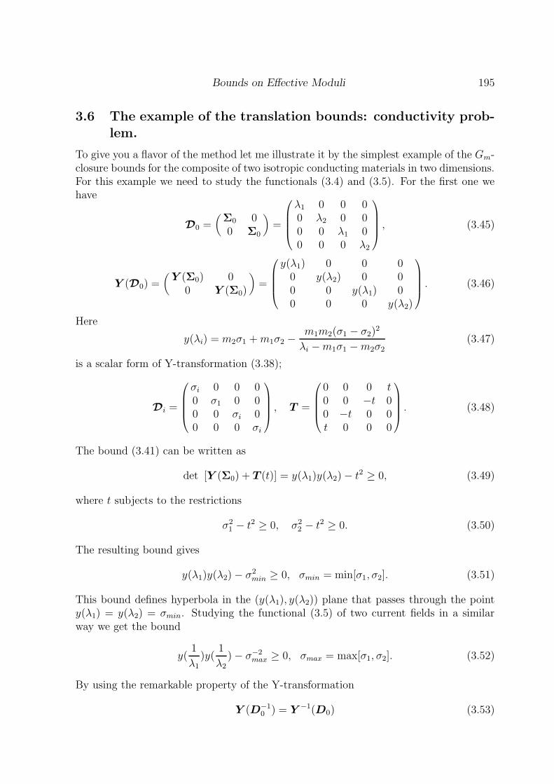
3.6 The example of the translation bounds: conductivity prob-

lem.

To give you a flavor of the method let me illustrate it by the simplest example of the Gm-closure bounds for the composite of two isotropic conducting materials in two dimensions.For this example we need to study the functionals (3.4) and (3.5). For the first one wehave

D0 =(

Σ0 00 Σ0

)

=

λ1 0 0 00 λ2 0 00 0 λ1 00 0 0 λ2

, (3.45)

Y (D0) =(

Y (Σ0) 00 Y (Σ0)

)

=

y(λ1) 0 0 00 y(λ2) 0 00 0 y(λ1) 00 0 0 y(λ2)

. (3.46)

Here

y(λi) = m2σ1 + m1σ2 −m1m2(σ1 − σ2)

2

λi − m1σ1 − m2σ2(3.47)

is a scalar form of Y-transformation (3.38);

Di =

σi 0 0 00 σ1 0 00 0 σi 00 0 0 σi

, T =

0 0 0 t0 0 −t 00 −t 0 0t 0 0 0

. (3.48)

The bound (3.41) can be written as

det [Y (Σ0) + T (t)] = y(λ1)y(λ2) − t2 ≥ 0, (3.49)

where t subjects to the restrictions

σ21 − t2 ≥ 0, σ2

2 − t2 ≥ 0. (3.50)

The resulting bound gives

y(λ1)y(λ2) − σ2min ≥ 0, σmin = min[σ1, σ2]. (3.51)

This bound defines hyperbola in the (y(λ1), y(λ2)) plane that passes through the pointy(λ1) = y(λ2) = σmin. Studying the functional (3.5) of two current fields in a similarway we get the bound

y(1

λ1

)y(1

λ2

) − σ−2max ≥ 0, σmax = max[σ1, σ2]. (3.52)

By using the remarkable property of the Y-transformation

Y (D−10 ) = Y −1(D0) (3.53)

196 L.V. Gibiansky

we end up with the upper bound

y(λ1)y(λ2) − σ2max ≤ 0. (3.54)

It is the other hyperbola that passes through the point y(λ1) = y(λ2) = σmax.Now we need to map these bounds into the plane of invariants of the tensor Σ0 instead

of the plane Y (Σ0). In order to do it we mention that

λi = m1σ1 + m2σ2 −m1m2(σ1 − σ2)

2

m2σ1 + m1σ2 + y(λi), i = 1, 2, (3.55)

is a fraction linear transformation, it maps hyperbola in the Y -plane into the hyperbolain the Σ-plane. Any hyperbola can be defined by three points that it comes through.Hyperbola (3.51) passes through the points

A = (0,∞), B = (∞, 0), C = (σ1, σ1). (3.56)

Therefore corresponding hyperbola in Σ plane passes through the points

A = (σh, σa), B = (σa, σh), C = (σ1HS, σ1

HS), (3.57)

whereσh = [m1/σ1 + m2/σ2]

−1, σh = m1σ1 + m2σ2, (3.58)

and the expression σ1HS is defined by the formula (1.53). Similarly, the upper boundary

hyperbola (3.54) passes (in the Σ plane) through the points

A = (σh, σa), B = (σa, σh), C = (σ2HS, σ2

HS), (3.59)

see (1.52). Obviously, the points A and B correspond to the laminate structures andpoints σ2

HS and σ2HS correspond to the Hashin-Shtrikman constructions. At last, let me

give you the expressions that define boundary hyperbolas

1

λ1 − σ1+

1

λ2 − σ1=

1

m2

1

λ2 − σ1+

m1

m2

1

2σ1(3.60)

(lower bound) and

1

λ1 − σ2

+1

λ1 − σ2

=1

m1

1

λ1 − σ2

+m2

m1

1

2σ2

(3.61)

( upper bound).

3.7 References


B. Dacorogna, Week continuity and week lower semicontinuity of non-linear function-als ( Lecture Notes in Math. 922, Springer-Verlag, 1982).


Z. Hashin and S. Shtrikman , A variational approach to the theory of the effectivemagnetic permeability of multiphase materials, J. Appl. Physics, 35, (1962), 3125 -3131.

14. Z. Hashin and S. Shtrikman, A variational approach to the theory of the elasticbehavior of multiphase materials, J. Mech. Phys. Solid, 11, (1963), 127 - 140.

15. R.V. Kohn and G.W. Milton, Variational bounds on the effective moduli ofanisotropic composites, J. Mech. Phys. Solids, vol. 36, 6, (1988), 597-629. R.V. Kohnand G.W. Milton, On bounding the effective conductivity of anisotropic composites,Homogenization and Effective Moduli of Materials and Media, J.Ericksen et al. eds.,Springer-Verlag, (1986), 97-125.

K.A. Lurie and A.V. Cherkaev, G-closure of a set of anisotropically conducting mediain the two-dimensional case, J.Opt.Th. Appl., 42, (1984), 283 - 304 and errata, 53, (1987),317.

K.A. Lurie and A.V. Cherkaev, G-closure of some particular sets of admissible ma-terial characteristics for the problem of bending of thin plates, J. Opt. Th. Appl. 42,(1984), 305 - 316.

K.A. Lurie and A.V. Cherkaev, Exact estimates of conductivity of composites formedby two isotropically conducting media taken in prescribed proportion, Proc. Roy. Soc.Edinburgh , 99 A, (1984), 71-87 (first version preprint 783, Ioffe Physicotechnical Insti-tute, Leningrad,1982).

K.A. Lurie and A.V. Cherkaev, Exact estimates of the conductivity of a binary mix-ture of isotropic materials,” Proc. Roy. Soc. Edinburgh, 104 A, (1986), 21 - 38 (firstversion preprint 894, Ioffe Physicotechnical Institute, Leningrad,1984).

K.A. Lurie and A.V. Cherkaev, The effective characteristics of composite materialsand optimal design of constructions, Advances’ in Mechanics (Poland), 9(2), (1986), 3 -81.

G.W. Milton, On characterizing the set of possible effective tensors of composites:The variational method and the translation method, Comm. of Pure and Appl. Math.,vol.XLIII, (1990), 63-125.

F. Murat and L. Tartar, Calcul des variations et homogeneisation, Les Methodes del’Homogeneisation: Theorie et Applications en Physique, Coll. de la Dir. des Etudes etRecherches de Electr. de France, Eyrolles, Paris, (1985), 319

E. Sanchez - Palencia, Nonhomogeneous Media and Vibration Theory (Lecture Notesin Physics 127, Springer - Verlag, 1980).

L. Tartar, Estimations fines des coefficients homogeneises, Ennio de Giorgi Collo-quium, P.Kree,ed., Pitman Research Notes in Math. 125, (1985), 168 - 187.

4 Implementation of the translation method to the

plane elasticity problem

In this lecture we prove the bounds on the effective properties of an isotropic compositemade from two isotropic elastic materials with known properties. The materials aresupposed to be mixed in an arbitrary way but with fixed volume fractions. First weadopt the translation method for the planar elasticity. Then we give an elementary proof

198 L.V. Gibiansky

of the known Hashin–Shtrikman and Walpole bounds and show how to apply the samemethod to prove the coupled bounds for the shear and bulk moduli of an isotropic elasticcomposite. The results are also valid for the effective moduli of a transversally isotropicthree-dimensional composite with arbitrary cylindrical inclusions.

First we describe the equations of the plane elasticity, introduce the notations, andgive the statement of the problem.

4.1 Basic equations and notations.

We deal with the plane problem of the elasticity. Let x = (x1, x2) be the Cartesiancoordinates, u = (u1, u2) be the displacement vector, ε be the strain tensor, σ be thestress tensor. The state of an isotropic body is characterized by the following system:

ε = 12(∇u + (∇u)T ),

∇ · σ = 0, σ = σT ,

σ = C(K, µ) · ·ε,

(4.1)

where ∇ is the two-dimensional Hamilton operator, C(K(x), µ(x)) is the tensor of rigid-ity of an isotropic material - the fourth order symmetric positively defined tensor, and(··) are the convolutions with regard to two indices.

It is convenient to introduce the following orthonormal basis in the space of thesymmetric second order tensors :

a1 = (ii + jj)/√

2, a2 = (ii − jj)/√

2,a3 = (ij + ji)/

√2, ai · ·aj = δij ,

(4.2)

where i and j are the unit vectors of the Cartesian axis x1 and x2, δij is the Kroneckersymbol. In this basis the isotropic tensor C(K, µ) of rigidity is represented by the diagonalmatrix

C(K, µ) =

2K 0 00 2µ 00 0 2µ

. (4.3)

The elastic energy density can be represented either as a quadratic form of strains

Wε = ε · ·C · ·ε (4.4)

or as a quadratic form of stresses

Wσ = σ · ·S · ·σ, (4.5)

where

S = C−1 =

12K

0 00 1

2µ0

0 0 12µ

(4.6)

is the compliance tensor.


The energy density W stored in the composite is known to be equal

Wε =< ε > · · C0 · · < ε > (4.7)

or

Wσ =< σ > · · S0 · · < σ >, (4.8)

where the effective compliance tensor S0 is determined as S0 = C−10 .

The problem of bounds for the elastic moduli has a long history. Hashin and Shtrik-man suggested the variational method which allows them to take into account differentialrestrictions on stress and strain fields; they found new bounds of the elastic moduli of anisotropic mixture made from isotropic materials.

Originally, the Hashin–Shtrikman bounds were formulated for isotropic three dimen-sional mixtures; however, later they were formulated for the transversal isotropic com-posites with cylindrical inclusions as well. The above problem is just the case we studyhere.

The original materials were supposed to be “well ordered”. This means that bothbulk and shear moduli of the first material are bigger than those of the second one

µ1 ≥ µ2, K1 ≥ K2. (4.9)

The obtained bounds have the form

K lHS ≤ K0 ≤ Ku

HS, µlHS ≤ µ0 ≤ µu

HS, (4.10)

where

K lHS = K2 +

m11

K1−K2

+ m2

K2+µ2

, (4.11)

KuHS = K1 +

m21

K2−K1

+ m1

K1+µ1

, (4.12)

µlHS = µ2 +

m1

1µ1−µ2

+ m2 (K2+2µ2)2µ2 (K2+µ2)

, (4.13)

µuHS = µ1 +

m2

1µ2−µ1

+ m1 (K1+2µ1)2µ1 (K1+µ1)

. (4.14)

200 L.V. Gibiansky

These expressions bound the bulk and shear moduli of a composite independently,see Figure 7.

Figure 7: bounds on bulk and shear moduli of an isotropic two-phase elastic compos-ite.

By using the introduced “Y-transformation” the above values K lHS, Ku

HS and µlHS, µu

HS

can be defined as the unique solutions of the equations

y(K lHS) = µ2, y(Ku

HS) = µ1,

y(µlHS) = K2µ2

K2+2µ2

, y(µuHS) = K1µ1

K1+2µ1

.(4.15)

Walpole [9, 10] considered the opposite case of “badly ordered” original materialswhen

µ1 ≥ µ2, K1 ≤ K2. (4.16)

He obtained the bounds for the effective moduli of an isotropic mixture by using similarvariational method. The two-dimensional Walpole’s bounds we are dealing with alsohave a simple representation in terms of the “Y-transformation”:

K lW ≤ K0 ≤ Ku

W , µlW ≤ µ0 ≤ µu

W , (4.17)

where the parameters K lW , Ku

W and µlW , µu

W satisfy the equations:

y(K lW ) = µ2, y(Ku

W ) = µ1,

y(µlW ) = K1µ2

K1+2µ2

, y(µuW ) = K2µ1

K2+2µ1

.(4.18)

Remark 2.3: Note that the cases (4.9) and (4.16) cover all possible relations betweenthe elastic moduli of two original materials because one can order the materials so that

µ1 ≥ µ2. (4.19)


Recently we applied the translation method to this problem, reproved all the knownbounds, and found new, more restrictive bounds on the elastic moduli of a composite. Letus restrict our attention to the case of well-ordered component materials. The oppositecase can be treated similarly. In Figure 7 the Hashin-Shtrikman bounds are presented asa rectangular whereas the new bounds cut the corners of this rectangular.

As we have learned in the previous lectures, the method is based on the lower boundof the functional I

I =N∑

i=1

Wi. (4.20)

This functional is equal to the sum of the values of elastic energy Wi stored in the elementof periodicity of a composite which is exposed to N linearly independent external stressor strain fields with fixed mean values. The energy functional is used because its value isequal to the energy stored by an equivalent homogeneous medium in the uniform field.The equivalent medium is characterized by the tensor of the effective properties, and theuniform external field coincides with the mean value of the field in the composite.

Clearly, the lower bound of the functional (4.20) provides also the bounds of theeffective tensor we are interest in. Below we get the bounds of the functional (4.20)independent of the microstructure of a mixture and extract the geometrically independentbounds for the effective moduli from them.

4.2 Functionals

Now we specify the functional of the type (4.20) which attains minimal values at theboundary of the set of pairs (K0, µ0). We discuss here functionals providing bounds forvarious components of the boundary.

To obtain the lower bound for the bulk modulus one can expose composite to anexternal hydrostatic strain εh = ε1a1 because the energy of an isotropic composite underthe action of this field is proportional to the effective bulk modulus K0.

Iε =< ε(x) · ·C(x) · ·ε(x) >= (2K0)ε21,

ε(x) ∈ (4.1), < ε(x) >= ε1 a1.(4.21)

It is clear that the lower bound of the functional (4.21) gives the lower bound of theeffective bulk modulus K0, because the amplitude ε1 of the hydrostatic strain field isassumed to be fixed.

To get the upper bound of this modulus, we need to expose the composite to thehydrostatic stress σh = σ1 a1; this makes the stored energy proportional to 1/K0. Thelower bound of the corresponding functional gives us the upper bound of K0. So, thistime we minimize the functional

Iσ =< σ(x) · ·S(x) · ·σ(x) >= (2K0)−1σ2

1,

σ(x) ∈ (4.1), < σ(x) >= σ1 a1,(4.22)

where σ1 is a given constant.

202 L.V. Gibiansky

We will see that the exact bounds of these functionals provide the Hashin - Shtrikmanbounds for the bulk modulus.

Similarly, to obtain the lower bound for the shear modulus of a mixture one canexamine the energy stored in a composite exposed to the shear-type trial strain. This waywe obtain an bound on any of the two shear moduli of the mixture which is anisotropicin general. However, the other shear modulus can have arbitrary value and the energyfunctionals of the types (4.21), (4.22) are not sensitive to its value. To provide theisotropy of the mixture we should also care about the reaction of the composite on theorthogonal shear field. So, to bound the shear modulus of an isotropic composite weshould minimize the functional equal to the sum of two values of energy stored by themedium under the action of two trial orthogonal shear fields ε = ε2 a2 and ε′ = ε3 a3.

Iεε =< ε(x) · ·C(x) · ·ε(x) + ε′(x) · ·C(x) · ·ε(x) >

= 2µ0(ε22 + ε2

3),

if ε(x), ε′(x) ∈ (4.1),

< ε(x) >= ε2a2, < ε′(x) >= ε3a3,

(4.23)

where ε2 and ε3 are fixed constants. To find the upper bound of the shear modulus weuse the functional equal to the sum of two energies stored in a composite exposed to twoorthogonal shear stresses σ = σ2 a2 and σ′ = σ3 a3

Iσσ =< σ(x) · ·S(x) · ·σ(x) + σ′(x) · ·S(x) · ·σ′(x) >

= 12µ0

(σ22 + σ2

3),

if σ, σ′ ∈ (4.1), < σ >= σ2 a2, < σ′ >= σ3 a3.

(4.24)

Here σ2 and σ3 are given constants. We show below that the lower bounds of thesefunctionals lead to the Hashin - Shtrikman and Walpole bounds for the shear modulus.

In order to get coupled shear-bulk bounds one can expose a composite to three differ-ent fields: a hydrostatic field and two orthogonal shear fields. We have a choice betweenstress and strain trial fields (two shear fields are supposed to be of the same nature toprovide isotropy of the mixture). Therefore the following functionals should be consid-ered:

Iεεε = Iε + Iεε, (4.25)

Iσσσ = Iσ + Iσσ, (4.26)

Iσεε = Iσ + Iεε, (4.27)

Iεσσ = Iε + Iσσ. (4.28)

The lower bounds on the last two of these functionals give us a required component ofthe boundary for the well-ordered case.

Indeed, the lower bounds of the functionals Iεεε and Iσσσ provide the lower andupper bounds of the convex combination of the effective bulk and shear moduli because


these functionals linearly depend on these moduli (the functional Iεεε) or on their inversevalues (the functional Iσσσ ).

In the well ordered case (4.9), however, the points of maximal and minimal values ofboth moduli (the Hashin - Shtrikman points A and C on Fig.7 ) are attainable by specialmicrostructures (see [5], for example); and it is clear that the bounds of these functionalscannot improve the classical inequalities (4.10), (4.15).

On the other hand, minimization of the functionals Iσεε or Iεσσ demands to mini-mize one of the moduli and maximize the other one. We show below that for well orderedmaterials it leads to coupled bounds of the moduli which are more restrictive then theHashin - Shtrikman ones.

In the badly ordered case (4.16) we face the opposite situation: the bounds of thefunctionals Iεεε and Iσσσ improve the Walpole bounds, and the bounds of the func-tionals Iσεε and Iεσσ leads to known ones.

The situation is illustrated by the Figure 7 where arrows show the directions in theplane (K, µ) that correspond to minimization of the discussed functionals.

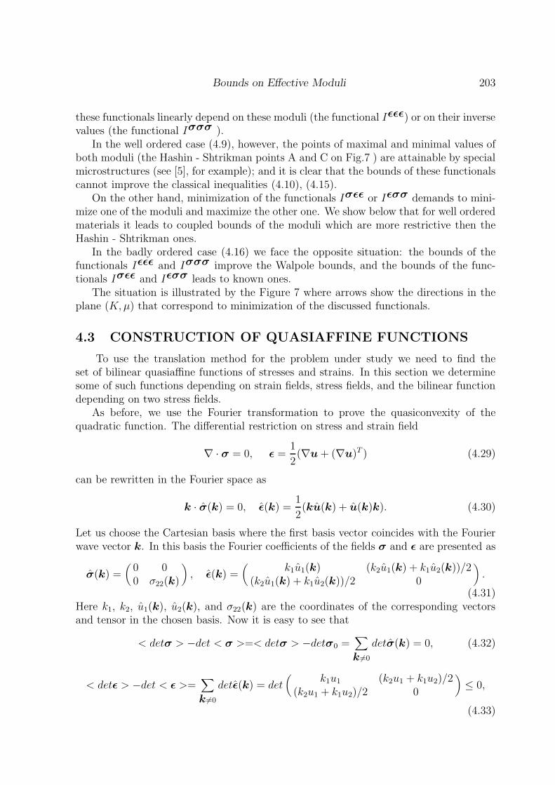
4.3 CONSTRUCTION OF QUASIAFFINE FUNCTIONS

To use the translation method for the problem under study we need to find theset of bilinear quasiaffine functions of stresses and strains. In this section we determinesome of such functions depending on strain fields, stress fields, and the bilinear functiondepending on two stress fields.

As before, we use the Fourier transformation to prove the quasiconvexity of thequadratic function. The differential restriction on stress and strain field

∇ · σ = 0, ε =1

2(∇u + (∇u)T ) (4.29)

can be rewritten in the Fourier space as

k · σ(k) = 0, ε(k) =1

2(ku(k) + u(k)k). (4.30)

Let us choose the Cartesian basis where the first basis vector coincides with the Fourierwave vector k. In this basis the Fourier coefficients of the fields σ and ε are presented as

σ(k) =(

0 00 σ22(k)

)

, ε(k) =(

k1u1(k) (k2u1(k) + k1u2(k))/2(k2u1(k) + k1u2(k))/2 0

)

.

(4.31)Here k1, k2, u1(k), u2(k), and σ22(k) are the coordinates of the corresponding vectorsand tensor in the chosen basis. Now it is easy to see that

< detσ > −det < σ >=< detσ > −detσ0 =∑

k 6=0

detσ(k) = 0, (4.32)

< detε > −det < ε >=∑

k 6=0

detε(k) = det(

k1u1 (k2u1 + k1u2)/2(k2u1 + k1u2)/2 0

)

≤ 0,

(4.33)

204 L.V. Gibiansky

< σ · R · σ′ · RT > − < σ > ·R· < σ′ > ·RT

=∑

k 6=0

(

0 00 σ22

)(

0 1−1 0

)(

0 00 σ′

22

)(

0 111 0

)

= 0. (4.34)

It completes the prove of the quasiconvexity of the following functions (where we use thetensor basis a1, a2, a3 to present translation matrices):

t det σ = σ · T σ · σ, T σ(t) =

t 0 00 −t 00 0 −t

, for all t, (4.35)

t det ε = ε · T ε · ε, T ε(t) =

t 0 00 −t 00 0 −t

, for all t ≤ 0, (4.36)

σ · R · σ′ · RT = σ · T σ · σ, T σσ =

0 0 00 0 t0 −t 0

, for all t. (4.37)

Using these functions we show the proof of the Hashin-Shtrikman bounds on the bulkmodulus of a composite and Hashin-Shtrikman and Walpole upper bounds on the shearmodulus. Quasiconvexity of the other functions that are necessary to use in the prove ofthe other bounds can be constructed in a similar way.

4.4 Prove of the Hashin-Shtrikman and Walpole bounds

In this section we get some of the Hashin - Shtrikman and Walpole bounds by usinga regular procedure of the translation method. We prove it here for the demonstrationof a regular procedure on simple examples.

4.5 Bounds for the bulk modulus

4.5.1 The lower bound.

To bound the functional Iε we need the symmetric translation strain-strain matrixTε (see (4.36)).

To get the result we use the bounds of the third lecture

Y (D0) + T ≥ 0, (4.38)

where we should substitute the following matrices

Di = C i, i = 1, 2,

T = Tε(t).(4.39)


The conditions of the positivity of the matrices C1 − Tε(t) and C2 − Tε(t) have theform

2Ki − t 0 00 2µi + t 00 0 2µi + t

≥ 0, i = 1, 2 (4.40)

and lead to the scalar inequalities

t ≤ 0, t ≥ −min{µ1, µ2} = −µmin. (4.41)

The bound for the isotropic matrix Dε0 = C ′

0 associated with the functional Iε has theform

y(2K0) + t 0 00 y(2µ0) − t 00 0 y(2µ0) − t

≥ 0 (4.42)

and leads to the inequality for the bulk modulus K0

y(2K0) ≥ −t, t ∈ (4.41). (4.43)

The most restrictive bound corresponds to the critical value

t = t∗ = −µmin (4.44)

of the parameter t. This bound coincides with the Hashin - Shtrikman and Walpole lowerbound for the bulk modulus (see (4.10)–(4.15), (4.17)– (4.18)).

4.5.2 The upper bound.

The upper bound for the bulk modulus can be obtained analogously using the functionalIσ instead of Iε and the quasiaffine function associated with the translation matrixTσ(t). For this functional, the matrices Di, i = 0, 1, 2 are equal

Di = Si , i = 0, 1, 2. (4.45)

Now the restrictions on matrix T have the form

12Ki

− t1 0 0

0 12µi

+ t1 0

0 0 12µi

+ t1

≥ 0 (4.46)

or scalar form

− 1

2µ1= −min{ 1

2µ1,

1

2µ2} ≤ t ≤ min{ 1

2K1,

1

2K2}. (4.47)

The bound for an isotropic effective tensor S0 becomes

y( 12K0

) + t1 0 0

0 y( 12µ0

) − t1 0

0 0 y( 12µ0

) − t1

≥ 0. (4.48)

206 L.V. Gibiansky

The corresponding scalar inequality for a bulk modulus K0

y(1

2K0) + t1 ≥ 0 (4.49)

becomes the most restrictive when the parameter t1 is chosen as t1 = t∗1 = − 12µ1

. Byusing the properties of the Y-transformation it can be represented in the form

y(K0) ≤ µmax. (4.50)

This bound coincides with the Hashin-Shtrikman and Walpole upper bounds for the bulkmodulus (see (4.10)–(4.15), (4.17)– (4.18)).

4.6 Upper bounds for the shear modulus

To obtain the upper bound for the shear modulus of the mixture we use the sameprocedure for estimating the functional Iσσ. In this case

E = {σ1, σ2, σ3, σ′1, σ′

2, σ′3} (4.51)

is a six-dimensional vector consisting of the components of two stress tensors σ and σ′;the (6 × 6) matrices

Di =(

Si 00 Si

)

, i = 0, 1, 2 (4.52)

are block-diagonal. We construct the matrix Tσσ of a quasiafine quadratic function ofthe vector E using the bilinear quasiaffine forms (4.35) - (4.37)

Tσσ(t1, t2) =

−t1 0 0 0 0 00 t1 0 0 0 t20 0 t1 0 −t2 00 0 0 −t1 0 00 0 −t2 0 t1 00 t2 0 0 0 t1

. (4.53)

The restrictions on T now have the matrix form

Dσσi − Tσσ(t1, t2) =

12Ki

+ t1 0 0 0 0 0

0 12µi

− t1 0 0 0 −t2

0 0 12µi

− t1 0 t2 0

0 0 0 12Ki

+ t1 0 0

0 0 t2 0 12µi

− t1 0

0 −t2 0 0 0 12µi

− t1

≥ 0,

i = 1, 2,

(4.54)


or the scalar form

t1 ≥ − 1

2Kmax

, (4.55)

(1

2µmax

− t1)2 − t22 ≥ 0, (4.56)

whereKmax = max{K1, K2},

µmax = max{µ1, µ2} = µmax.(4.57)

The critical values t∗1, t∗2 of the parameters t1, t2 are equal

t∗1 = − 1

2Kmax

, t∗2 =1

2µmax

+1

2Kmax

. (4.58)

The bound becomes

Y (Dσσ0 ) + Tσσ(t∗1, t∗2) =

y( 12K0

) − t∗1 0 0 0 0 0

0 y( 12µ0

) + t∗1 0 0 0 t∗2

0 0 y( 12µ0

) + t∗1 0 −t∗2 0

0 0 0 y( 12K0

) − t∗1 0 0

0 0 −t∗2 0 y( 12µ0

) + t∗1 0

0 t∗2 0 0 0 y( 12µ0

) + t∗1

≥ 0.(4.59)

It leads to the scalar inequality

y(1

2µ0) + t∗1 − t∗2 = y(

1

2µ0) − 2

Kmax

− 1

µmax

≥ 0 (4.60)

or

y(µ0) ≤Kmaxµmax

Kmax + 2µmax

. (4.61)

It coincides with the Hashin – Shtrikman bound (see (4.10)–(4.15)) in the well orderedcase (4.9) and with the Walpole bound (see (4.17)–(4.18)) in the badly ordered case(4.16).

The other bounds can be obtained in a similar way, they are presented by the Figure7.

References

[1] A.V. Cherkaev and L.V. Gibiansky, The exact coupled bounds for effective tensorsof electrical and magnetic properties of two-component two-dimensional composites,to appear in the Proceedings of Royal Society Edinbourgh.

[2] A.V. Cherkaev and L.V. Gibiansky, Coupled estimates for the bulk and shear moduliof a two-dimensional isotropic elastic composite, J. Mech. Phys. Solids, V 41 N 5,937-980, 1993,

208 L.V. Gibiansky

[3] R.M. Christensen, Mechanics of Composite Materials (Wiley-Interscience, New-York, 1979).

[4] B. Dacorogna, Weak continuity and weak lower semicontinuity of non-linear func-tionals ( Lecture Notes in Math. 922, Springer-Verlag, 1982).

[5] G. Francfort and F. Murat, Homogenization and optimal bounds in linear elasticity,Arch. Rational Mech. Anal., 94, (1986), 307 - 334.

[6] Z. Hashin and S. Shtrikman, A variational approach to the theory of the elasticbehavior of multiphase materials, J. Mech. Phys. Solid, 11, (1963), 127 - 140.

[7] G.W. Milton, On characterizing the set of possible effective tensors of composites:The variational method and the translation method, Comm. of Pure and Appl.Math., vol.XLIII, (1990), 63-125.

[8] G.W. Milton, A brief review of the translation method for bounding effective elas-tic tensors of composites, Continuum Models and Discrete Systems, ed. by G. A.Maugin, vol. 1, (1990), 60-74.

[9] L.J. Walpole, On bounds for the overall elastic moduli of inhomogeneous systems -I, J.Mech. Phys. Solids, 14, (1966), 151-162.

[10] L.J. Walpole, On the overall elastic moduli of composite materials, J.Mech. Phys.Solids, 17, (1969), 235-251.

Documents

ICTP93Gibiansky