Embed Size (px)
Citation preview

IN THIS LECTURE, YOU WILL LEARN:
Am simple perfect competition production
medium-run model view of what determines the
economy’s total output/income
how the prices of the factors of production are
determined according to this model
how total income is distributed
what determines the demand for goods and
services
how equilibrium in the goods market is achieved
2 theories of consumption0

1CHAPTER 3 National Income
Outline of model
A closed economy, market-clearing model
Supply side
factor markets (supply, demand, price)
determination of output/income
Demand side
determinants of C, I, and G
Equilibrium
goods market
loanable funds market
2CHAPTER 3 National Income
Production Model
Vast oversimplifications of the real world in a
model can still allow it to provide important
insights.
Consider the following model
Single, closed economy
One consumption good

3CHAPTER 3 National Income
Factors of production
K = capital:
tools, machines, and structures used in
production
L = labor:
the physical and mental efforts of
workers

4CHAPTER 3 National Income
The production function: Y = F(K,L)
shows how much output (Y )
the economy can produce from
K units of capital and L units of labor
reflects the economy’s level of technology
We assume that the production function for the
economy as a whole exhibits constant returns to
scale

5CHAPTER 3 National Income
Returns to scale: a review
Initially Y1 = F (K1 ,L1 )
Scale all inputs by the same factor z:
K2 = zK1 and L2 = zL1
(e.g., if z = 1.2, then all inputs are increased by 20%)
What happens to output, Y2 = F (K2,L2 )?
If constant returns to scale, Y2 = zY1
If increasing returns to scale, Y2 > zY1
If decreasing returns to scale, Y2 < zY1
6CHAPTER 3 National Income
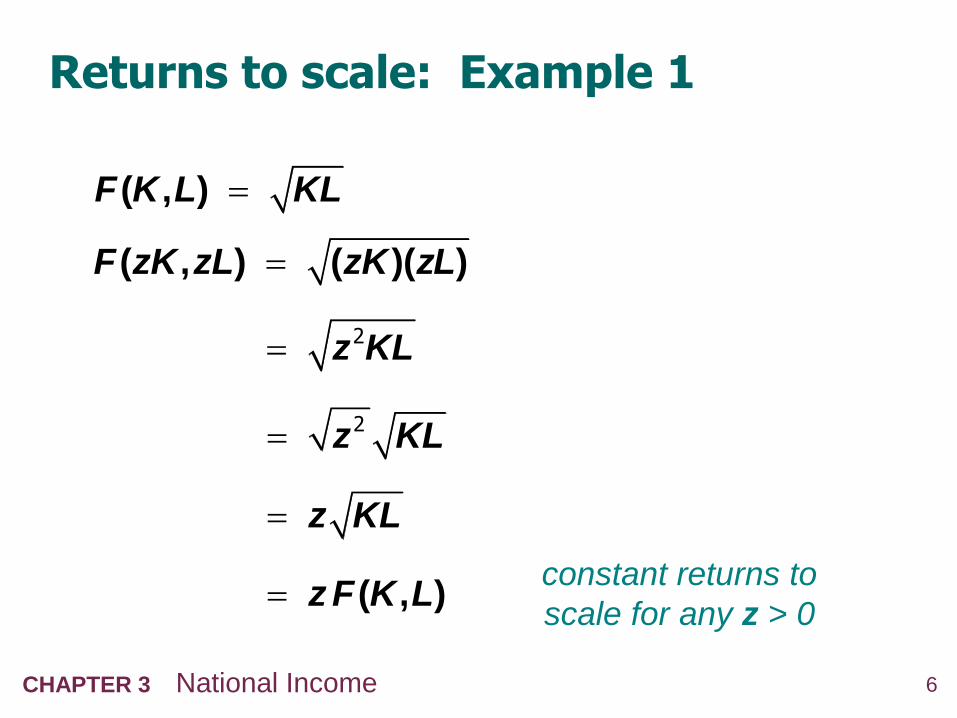
Returns to scale: Example 1
( , )F K L KL
( , ) ( )( )F zK zL zK zL
z KL 2
z KL 2
z KL
( , )z F K Lconstant returns to
scale for any z > 0
7CHAPTER 3 National Income
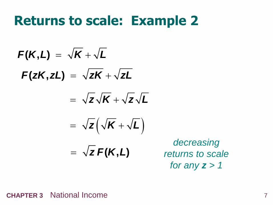
Returns to scale: Example 2
( , )F K L K L
( , )F zK zL zK zL
z K z L
( , )z F K Ldecreasing
returns to scale
for any z > 1
z K L

8CHAPTER 3 National Income
Returns to scale: Example 3
( , )F K L K L 2 2
( , ) ( ) ( )F zK zL zK zL 2 2
( , )z F K L 2 increasing returns
to scale for any
z > 1
z K L 2 2 2
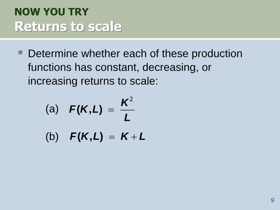
NOW YOU TRY
Returns to scale
Determine whether each of these production
functions has constant, decreasing, or
increasing returns to scale:
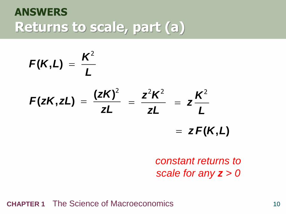
(a)
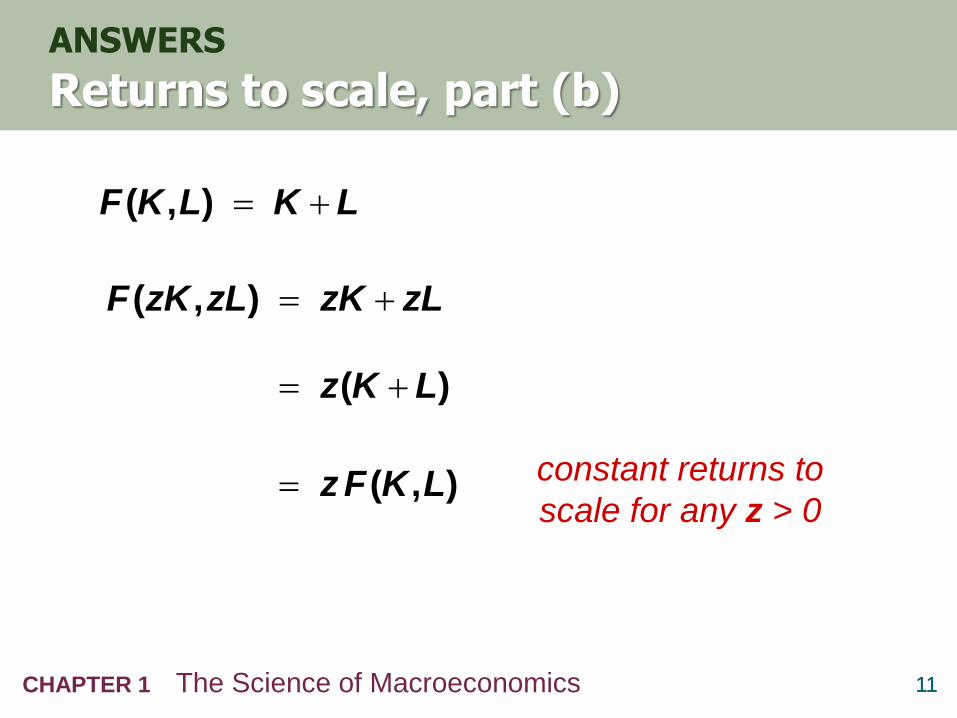
(b)
9
( , )K
F K LL
2
( , )F K L K L
10CHAPTER 1 The Science of Macroeconomics
ANSWERS
Returns to scale, part (a)
10
( , )K
F K LL
2
( )( , )
zKF zK zL
zL
2z K
zL
2 2K
zL
2
( , )z F K L
constant returns to
scale for any z > 0
11CHAPTER 1 The Science of Macroeconomics
ANSWERS
Returns to scale, part (b)
11
( , )F K L K L
( , )F zK zL zK zL
( )z K L
( , )z F K L constant returns to
scale for any z > 0

12CHAPTER 3 National Income
Assumptions
1. Technology is fixed.
2. The economy’s supplies of capital and labor
are fixed at
and K K L L

13CHAPTER 3 National Income
Determining GDP
Output is determined by the fixed factor supplies
and the fixed state of technology:
, ( )Y F K L

14CHAPTER 3 National Income
The distribution of national income
determined by factor prices,
the prices per unit firms pay for the factors of
production
wage = price of L
rental rate = price of K
15CHAPTER 3 National Income
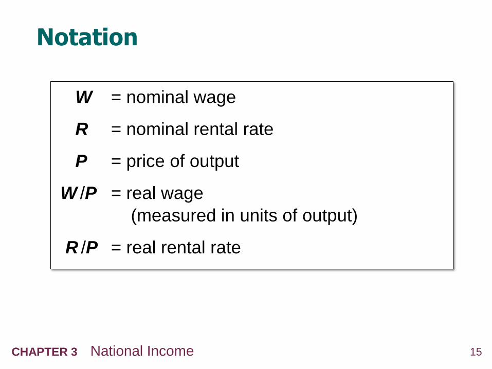
Notation
W = nominal wage
R = nominal rental rate
P = price of output
W /P = real wage
(measured in units of output)
R /P = real rental rate

16CHAPTER 3 National Income
How factor prices are determined
Factor prices determined by supply and demand
in factor markets.
Recall: Supply of each factor is fixed.
What about demand?

17CHAPTER 3 National Income
Demand for labor
Assume markets are competitive:
each firm takes W, R, and P as given.
Basic idea:
A firm hires each unit of labor
if the cost does not exceed the benefit.
cost = real wage
benefit = marginal product of labor

18CHAPTER 3 National Income
Marginal product of labor (MPL)
definition:
The extra output the firm can produce
using an additional unit of labor
(holding other inputs fixed):
MPL = F (K,L+1) – F (K,L)
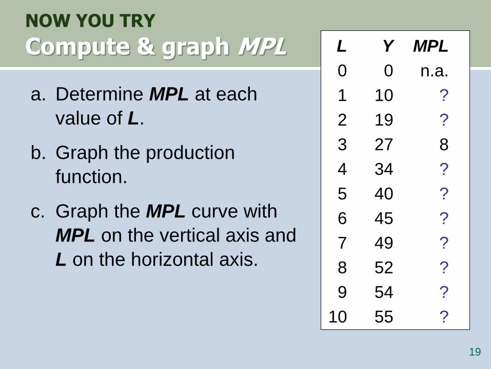
NOW YOU TRY
Compute & graph MPL
a. Determine MPL at each
value of L.
b. Graph the production
function.
c. Graph the MPL curve with
MPL on the vertical axis and
L on the horizontal axis.
19
L Y MPL
0 0 n.a.
1 10 ?
2 19 ?
3 27 8
4 34 ?
5 40 ?
6 45 ?
7 49 ?
8 52 ?
9 54 ?
10 55 ?
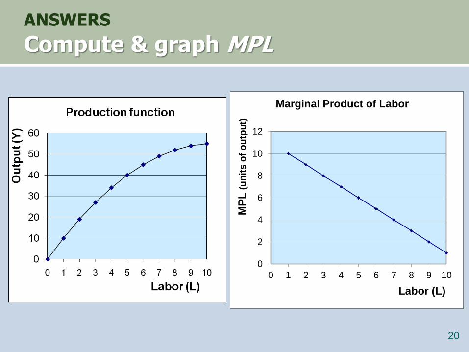
ANSWERS
Compute & graph MPL
20
0
2
4
6
8
10
12
0 1 2 3 4 5 6 7 8 9 10
MP
L(u
nit
s o
f o
utp
ut)
Labor (L)
Marginal Product of Labor

21CHAPTER 3 National Income
Y
output
MPL and the production function
Llabor
F K L( , )
1
MPL
1
MPL
1MPL
As more labor is
added, MPL
Slope of the production
function equals MPL

22CHAPTER 3 National Income
Diminishing marginal returns
As an input is increased,
its marginal product falls (other things equal).
Intuition:
Suppose L while holding K fixed
fewer machines per worker
lower worker productivity

NOW YOU TRY
Identifying Diminishing Returns
Which of these production functions have
diminishing marginal returns to labor?
23
a) 2 15F K L K L ( , )
F K L KL( , )b)
c) 2 15F K L K L ( , )

24CHAPTER 1 The Science of Macroeconomics
ANSWERS
Identifying Diminishing Returns
24
a) 2 15F K L K L ( , )
F K L KL( , )b)
c) 2 15F K L K L ( , )
No, MPL = 15 for all L
Yes, MPL falls as L rises
Yes, MPL falls as L rises

25CHAPTER 1 The Science of Macroeconomics
NOW YOU TRY
MPL and labor demand
Suppose W/P = 6.
If L = 3, should firm hire
more or less labor? Why?
If L = 7, should firm hire
more or less labor? Why?
25
L Y MPL
0 0 n.a.
1 10 10
2 19 9
3 27 8
4 34 7
5 40 6
6 45 5
7 49 4
8 52 3
9 54 2
10 55 1

26CHAPTER 1 The Science of Macroeconomics
ANSWERS
MPL and labor demand
If L = 3, should firm hire more or less
labor?
Answer: YES, because the benefit
of the 4th worker (MPL = 7) exceeds
its cost (W/P = 6)
If L = 7, should firm hire more or less
labor?
Answer: NO, the firm should reduce
labor. The 7th worker adds
MPL = 4 units of output but costs the
firm W/P = 6. 26
L Y MPL
0 0 n.a.
1 10 10
2 19 9
3 27 8
4 34 7
5 40 6
6 45 5
7 49 4
8 52 3
9 54 2
10 55 1
27CHAPTER 3 National Income
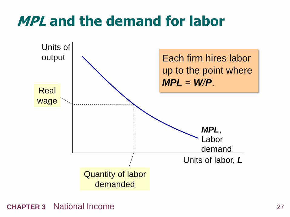
MPL and the demand for labor
Each firm hires labor
up to the point where
MPL = W/P.
Units of
output
Units of labor, L
MPL, Labor demand
Real
wage
Quantity of labor
demanded

28CHAPTER 3 National Income
The equilibrium real wage
The real wage
adjusts to equate
labor demand
with supply.
Units of
output
Units of labor, L
MPL, Labor demand
equilibrium
real wage
Labor
supply
L
29CHAPTER 3 National Income
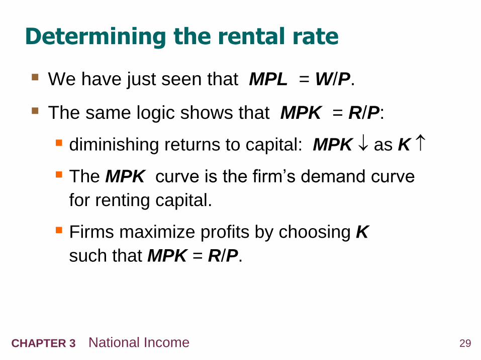
Determining the rental rate
We have just seen that MPL = W/P.
The same logic shows that MPK = R/P:
diminishing returns to capital: MPK as K
The MPK curve is the firm’s demand curve
for renting capital.
Firms maximize profits by choosing K
such that MPK = R/P.

30CHAPTER 3 National Income
The equilibrium real rental rate
The real rental rate
adjusts to equate
demand for capital
with supply.
Units of
output
Units of capital, K
MPK, demand for capital
equilibrium
R/P
Supply of
capital
K

31CHAPTER 3 National Income
The Neoclassical Theory of Distribution
states that each factor input is paid its marginal
product
a good starting point for thinking about income
distribution
32CHAPTER 3 National Income
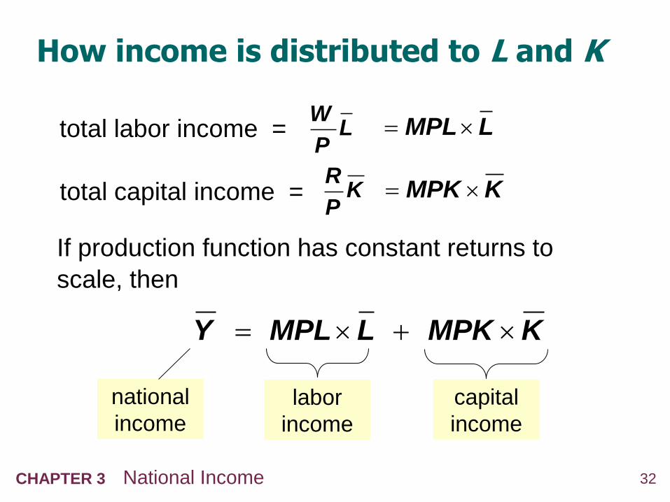
How income is distributed to L and K
total labor income =
If production function has constant returns to
scale, then
total capital income =
WL
PMPL L
RK
PMPK K
Y MPL L MPK K
labor
income
capital
income
national
income
0
0.1
0.2
0.3
0.4
0.5
0.6
0.7
0.8
0.9
1
1960 1965 1970 1975 1980 1985 1990 1995 2000 2005 2010
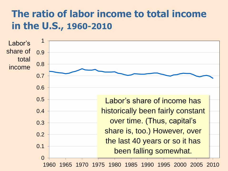
The ratio of labor income to total income
in the U.S., 1960-2010
Labor’s
share of
total
income
Labor’s share of income has
historically been fairly constant
over time. (Thus, capital’s
share is, too.) However, over
the last 40 years or so it has
been falling somewhat.

34CHAPTER 3 National Income
Share of Labor Income by Sector

35CHAPTER 3 National Income
The Cobb-Douglas Production Function
The Cobb-Douglas production function has
constant factor shares:
= capital’s share of total income:
capital income = MPK × K = Y
labor income = MPL × L = (1 – )Y
The Cobb-Douglas production function is:
where A represents the level of technology.
1Y AK L

36CHAPTER 3 National Income
The Cobb-Douglas Production Function
Each factor’s marginal product is proportional to
its average product:
1 1 YMPK AK L
K
(1 )(1 )
YMPL AK L
L
37CHAPTER 3 National Income
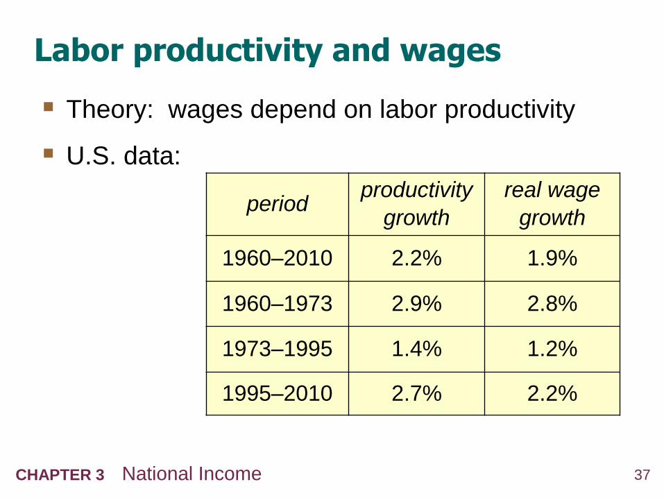
Labor productivity and wages
Theory: wages depend on labor productivity
U.S. data:
periodproductivity
growth
real wage
growth
1960–2010 2.2% 1.9%
1960–1973 2.9% 2.8%
1973–1995 1.4% 1.2%
1995–2010 2.7% 2.2%
38CHAPTER 3 National Income
Analyzing the Production Model
Per capita = per person
Per worker = per member of the labor force.
In this model, the two are equal.
We can perform a change of variables to define
output per capita (y) and capital per person (k).
39CHAPTER 3 National Income
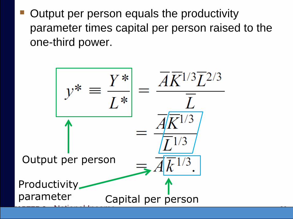
Output per person equals the productivity
parameter times capital per person raised to the
one-third power.
Output per person
Capital per person
Productivity parameter

40CHAPTER 3 National Income
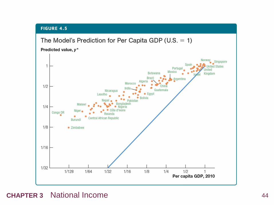
What makes a country rich or poor?
Output per person is higher if the productivity
parameter is higher or if the amount of capital
per person is higher.
What can you infer about the value of the
productivity parameter or the amount of capital
in poor countries?
41CHAPTER 3 National Income
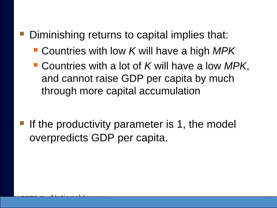
Diminishing returns to capital implies that:
Countries with low K will have a high MPK
Countries with a lot of K will have a low MPK,
and cannot raise GDP per capita by much
through more capital accumulation
If the productivity parameter is 1, the model
overpredicts GDP per capita.

42CHAPTER 3 National Income

43CHAPTER 3 National Income
44CHAPTER 3 National Income

45CHAPTER 3 National Income
Case Study: Why Doesn’t Capital Flow
from Rich to Poor Countries?
If MPK is higher in poor countries with low K,
why doesn’t capital flow to those countries?
Short Answer: Simple production model with
no difference in productivity across countries is
misguided.
We must also consider the productivity
parameter.

46CHAPTER 3 National Income
Productivity Differences:
Improving the Fit of the Model
The productivity parameter measures how
efficiently countries are using their factor
inputs.
Often called total factor productivity (TFP)
If TFP is no longer equal to 1, we can obtain
a better fit of the model.

47CHAPTER 3 National Income
However, data on TFP is not collected.
It can be calculated because we have data on
output and capital per person.
TFP is referred to as the “residual.”
A lower level of TFP
Implies that workers produce less output for any
given level of capital per person

48CHAPTER 3 National Income

49CHAPTER 3 National Income

50CHAPTER 3 National Income

51CHAPTER 3 National Income
Output differences between the richest and
poorest countries?
Differences in capital per person explain about
one-quarter of the difference.
TFP explains the remaining three-quarters.
Thus, rich countries are rich because:
They have more capital per person.
More importantly, they use labor and capital
more efficiently.

52CHAPTER 3 National Income
Outline of model
A closed economy, market-clearing model
Supply side
factor markets (supply, demand, price)
determination of output/income
Demand side
determinants of C, I, and G
Equilibrium
goods market
loanable funds market
DONE
DONE
Next

53CHAPTER 3 National Income
Demand for goods and services
Components of aggregate demand:
C = consumer demand for g & s
I = demand for investment goods
G = government demand for g & s
(closed economy: no NX )

54CHAPTER 3 National Income
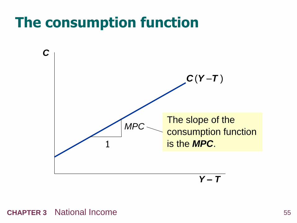
Consumption, C
def: Disposable income is total income minus
total taxes: Y – T.
Consumption function: C = C (Y – T )
Shows that (Y – T ) C
def: Marginal propensity to consume (MPC)
is the change in C when disposable income
increases by one dollar.
55CHAPTER 3 National Income
The consumption function
C
Y – T
C (Y –T )
1
MPCThe slope of the
consumption function
is the MPC.

56CHAPTER 3 National Income
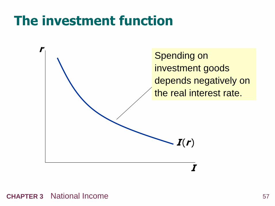
Investment, I
The investment function is I = I (r )
where r denotes the real interest rate,
the nominal interest rate corrected for inflation.
The real interest rate is
the cost of borrowing
the opportunity cost of using one’s own
funds to finance investment spending
So, r I
57CHAPTER 3 National Income
The investment function
r
I
I (r )
Spending on
investment goods
depends negatively on
the real interest rate.

58CHAPTER 3 National Income
Government spending, G
G = govt spending on goods and services
G excludes transfer payments
(e.g., Social Security benefits,
unemployment insurance benefits)
Assume government spending and total taxes
are exogenous:
and G G T T
59CHAPTER 3 National Income
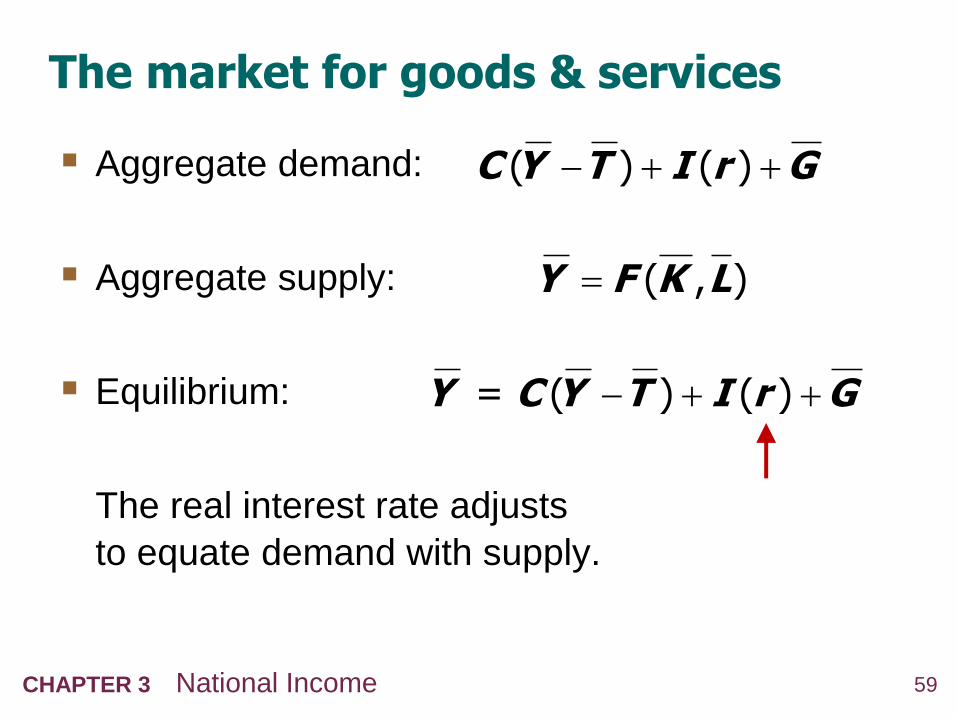
The market for goods & services
Aggregate demand:
Aggregate supply:
Equilibrium:
The real interest rate adjusts
to equate demand with supply.
( ) ( )C Y T I r G
( , )Y F K L
= ( ) ( )Y C Y T I r G

60CHAPTER 3 National Income
The loanable funds market
A simple supply–demand model of the financial
system.
One asset: “loanable funds”
demand for funds: investment
supply of funds: saving
“price” of funds: real interest rate

61CHAPTER 3 National Income
Demand for funds: Investment
The demand for loanable funds…
comes from investment:
Firms borrow to finance spending on plant &
equipment, new office buildings, etc.
Consumers borrow to buy new houses.
depends negatively on r,
the “price” of loanable funds
(cost of borrowing).
62CHAPTER 3 National Income
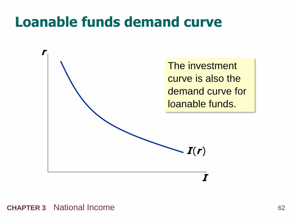
Loanable funds demand curve
r
I
I (r )
The investment
curve is also the
demand curve for
loanable funds.

63CHAPTER 3 National Income
Supply of funds: Saving
The supply of loanable funds comes from
saving:
Households use their saving to make bank
deposits, purchase bonds and other assets.
These funds become available to firms to
borrow to finance investment spending.
The government may also contribute to saving
if it does not spend all the tax revenue it
receives.

64CHAPTER 3 National Income
Types of saving
private saving = (Y – T ) – C
public saving = T – G
national saving, S
= private saving + public saving
= (Y –T ) – C + T – G
= Y – C – G
65CHAPTER 3 National Income
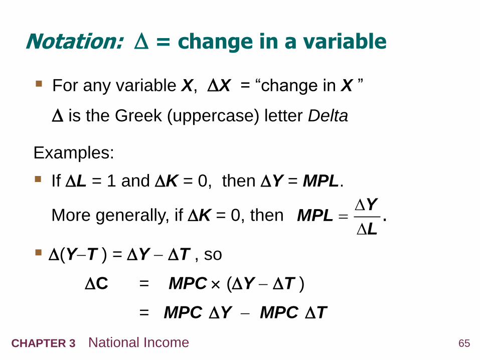
Notation: = change in a variable
For any variable X, X = “change in X ”
is the Greek (uppercase) letter Delta
Examples:
If L = 1 and K = 0, then Y = MPL.
More generally, if K = 0, thenY
MPLL
.
(YT ) = Y T , so
C = MPC (Y T )
= MPC Y MPC T
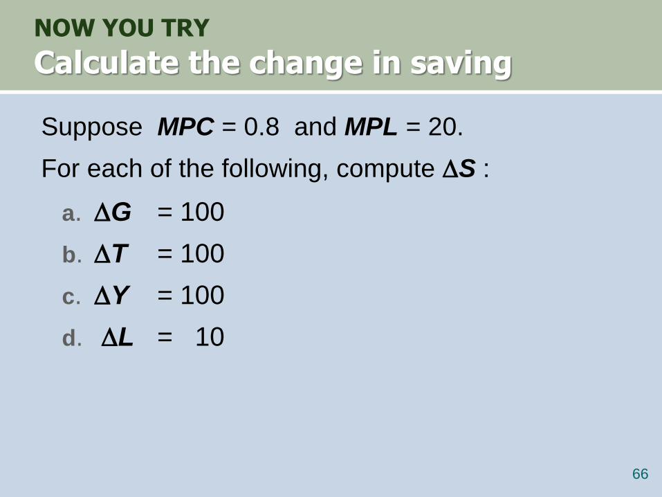
NOW YOU TRY
Calculate the change in saving
Suppose MPC = 0.8 and MPL = 20.
For each of the following, compute S :
a. G = 100
b. T = 100
c. Y = 100
d. L = 10
66

67CHAPTER 1 The Science of Macroeconomics
NOW YOU TRY
Answers
67
S Y C G 0.8( )Y Y T G
0.2 0.8Y T G
1. 0a 0S
0.8 0 0b. 10 8S
0.2 0 0c. 10 2S
MPL 20 10 20 ,d. 0Y L
0.2 0.2 200 40.S Y

68CHAPTER 3 National Income
Budget surpluses and deficits
If T > G, budget surplus = (T – G)
= public saving.
If T < G, budget deficit = (G – T)
and public saving is negative.
If T = G , balanced budget, public saving = 0.
The U.S. government finances its deficit by
issuing Treasury bonds–i.e., borrowing.

U.S. Federal Government Surplus/Deficit, 1940–2016
pe
rce
nt
of
GD
P
-35
-30
-25
-20
-15
-10
-5
0
5
10
1940 1950 1960 1970 1980 1990 2000 2010

U.S. Federal Government Debt, 1940–2016
pe
rce
nt
of
GD
P
0
20
40
60
80
100
120
140
1940 1950 1960 1970 1980 1990 2000 2010
71CHAPTER 3 National Income
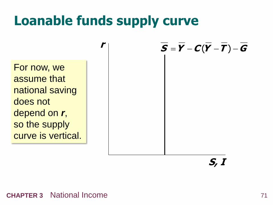
Loanable funds supply curve
r
S, I
( )S Y C Y T G
For now, we
assume that
national saving
does not
depend on r,
so the supply
curve is vertical.
72CHAPTER 3 National Income
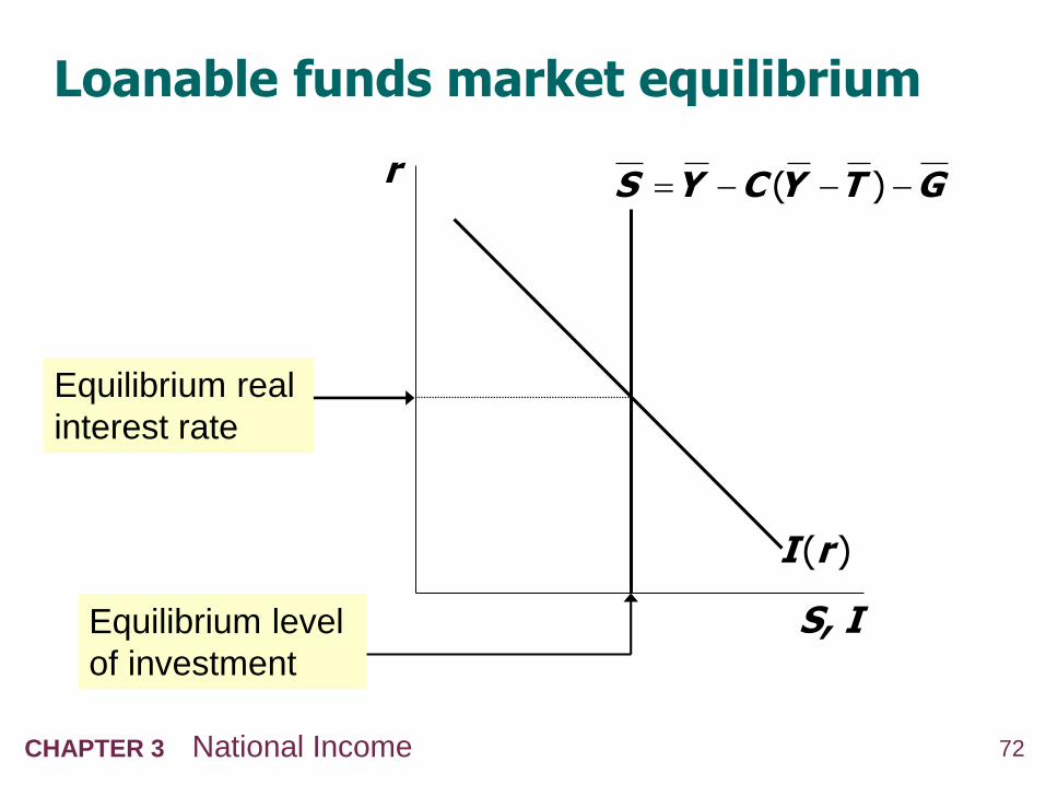
Loanable funds market equilibrium
r
S, I
I (r )
( )S Y C Y T G
Equilibrium real
interest rate
Equilibrium level
of investment

73CHAPTER 3 National Income
The special role of r
r adjusts to equilibrate the goods market and the
loanable funds market simultaneously:
If L.F. market in equilibrium, then
Y – C – G = I
Add (C +G ) to both sides to get
Y = C + I + G (goods market eq’m)
Thus, Eq’m in L.F.
market
Eq’m in goods
market

74CHAPTER 3 National Income
Digression: Mastering models
To master a model, be sure to know:
1. Which of its variables are endogenous and
which are exogenous.
2. For each curve in the diagram, know:
a. definition
b. intuition for slope
c. all the things that can shift the curve

75CHAPTER 3 National Income
Mastering the loanable funds model
Things that shift the saving curve
public saving
fiscal policy: changes in G or T
private saving
preferences
tax laws that affect saving
–401(k)
– IRA
– replace income tax with consumption tax

76CHAPTER 3 National Income
CASE STUDY:
The Reagan deficits
Reagan policies during early 1980s:
increases in defense spending: G > 0
big tax cuts: T < 0
Both policies reduce national saving:
( )S Y C Y T G
G S T C S

77CHAPTER 3 National Income
CASE STUDY:
The Reagan deficits
r
S, I
1S
I (r )
r1
I1
r22. …which causes
the real interest
rate to rise…
I2
3. …which reduces
the level of
investment.
1. The increase in
the deficit
reduces saving…
2S
78CHAPTER 3 National Income
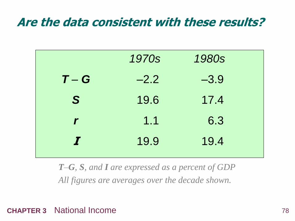
Are the data consistent with these results?
1970s 1980s
T – G –2.2 –3.9
S 19.6 17.4
r 1.1 6.3
I 19.9 19.4
T–G, S, and I are expressed as a percent of GDP
All figures are averages over the decade shown.

79CHAPTER 3 National Income
Mastering the loanable funds model, continued
Things that shift the investment curve:
some technological innovations
to take advantage some innovations,
firms must buy new investment goods
tax laws that affect investment
e.g., investment tax credit

80CHAPTER 3 National Income
An increase in investment demand
An increase in desired investment…
r
S, I
I1
S
I2
r1
r2
…raises the
interest rate.
But the equilibrium
level of investment
cannot increase
because the
supply of loanable
funds is fixed.
81CHAPTER 3 National Income
Another look at Consumption, Saving
and the interest rate Why might saving depend on r ?
How would the results of an increase in
investment demand be different?
Would r rise as much?
Would the equilibrium value of I change?

82CHAPTER 3 National Income
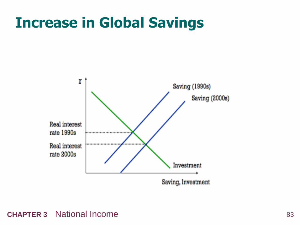
An increase in investment demand when
saving depends on r
r
S, I
I(r)
( )S r
I(r)2
r1
r2
An increase in
investment demand
raises r,
which induces an
increase in the
quantity of saving,
which allows Ito increase.
I1 I2
83CHAPTER 3 National Income
Increase in Global Savings

84CHAPTER 3 National Income
Effect on Global Balances
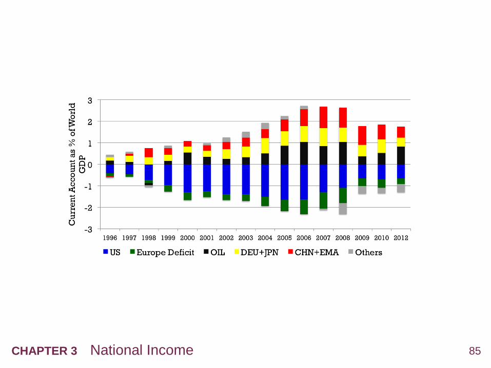
85CHAPTER 3 National Income
86CHAPTER 3 National Income
87CHAPTER 3 National Income

88CHAPTER 3 National Income
Consumption
How do you decide how much to spend on
consumption?

89CHAPTER 3 National Income
Consumption
2 competing views of consumption
1. Consumption depends primarily on current
income (Keynesian consumption function).
2. People prefer a smooth path for consumption
compared to a path that involves large
movements (Permanent Income/Life Cycle
Hypothesis).

90CHAPTER 3 National Income
The Keynesian consumption function
C
Y
C C cY
slope = APC
As income rises, consumers save a bigger
fraction of their income, so APC falls.
C Cc
Y Y APC

91CHAPTER 3 National Income
Early empirical successes: Results from early studies Households with higher incomes:
consume more, MPC > 0
save more, MPC < 1
save a larger fraction of their income,
APC as Y
Very strong correlation between income and
consumption:
income seemed to be the main
determinant of consumption
92CHAPTER 3 National Income
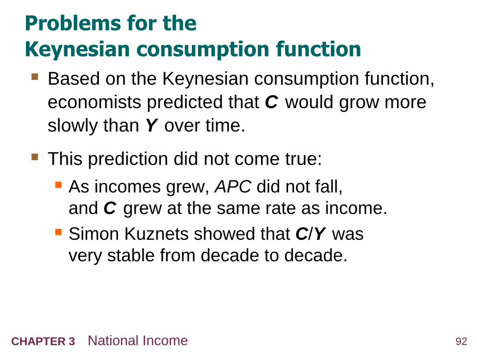
Problems for the
Keynesian consumption function
Based on the Keynesian consumption function,
economists predicted that C would grow more
slowly than Y over time.
This prediction did not come true:
As incomes grew, APC did not fall,
and C grew at the same rate as income.
Simon Kuznets showed that C/Y was
very stable from decade to decade.
93CHAPTER 3 National Income
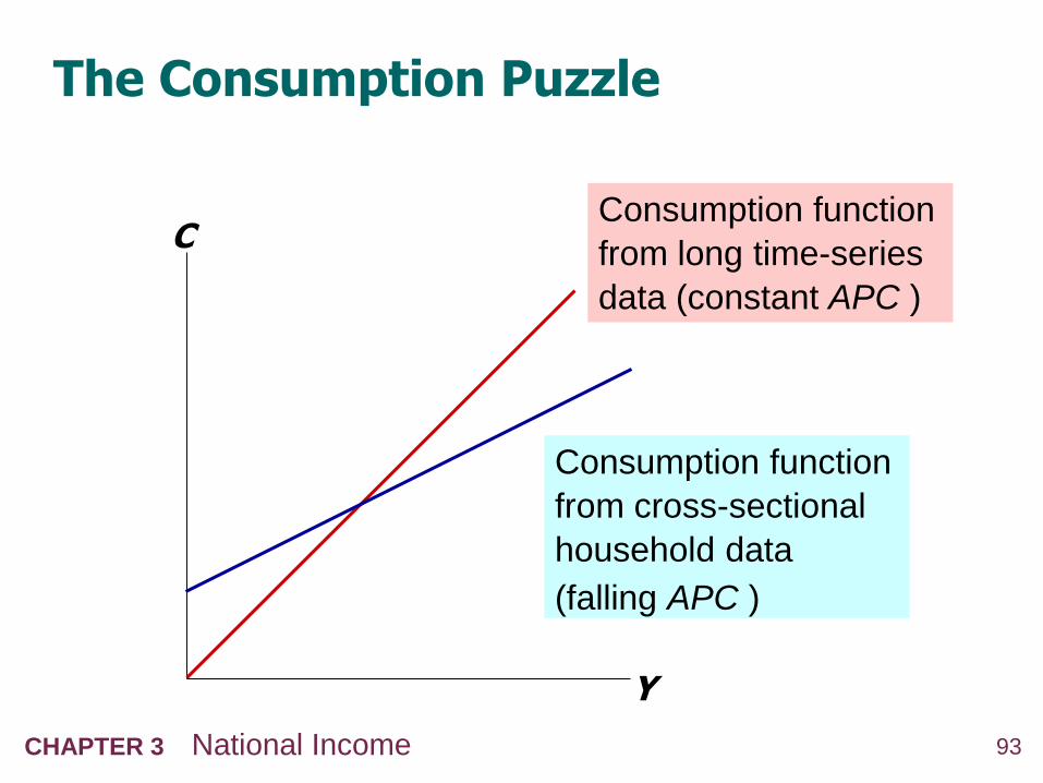
The Consumption Puzzle
C
Y
Consumption function
from long time-series
data (constant APC )
Consumption function
from cross-sectional
household data
(falling APC )

94CHAPTER 3 National Income
Irving Fisher and Intertemporal Choice
The basis for much subsequent work on
consumption.
Assumes consumer is forward-looking and
chooses consumption for the present and future
to maximize lifetime satisfaction.
Consumer’s choices are subject to an
intertemporal budget constraint,
a measure of the total resources available for
present and future consumption.

95CHAPTER 3 National Income
The basic two-period model
Period 1: the present
Period 2: the future
Notation
Y1, Y2 = income in period 1, 2
C1, C2 = consumption in period 1, 2
S = Y1 C1 = saving in period 1
(S < 0 if the consumer borrows in period 1)

96CHAPTER 3 National Income
Deriving the intertemporal
budget constraint
Period 2 budget constraint:
2 2 (1 )C Y r S
2 1 1(1 )( )Y r Y C
Rearrange terms:
1 2 2 1(1 ) (1 )r C C Y r Y
Divide through by (1+r ) to get…

97CHAPTER 3 National Income
The intertemporal budget constraint
2 21 1
1 1
C YC Y
r r
present value of
lifetime consumption
present value of
lifetime income

98CHAPTER 3 National Income
The intertemporal budget constraint
The budget
constraint shows
all combinations
of C1 and C2 that
just exhaust the
consumer’s
resources.C1
C2
1 2 (1 )Y Y r
1 2(1 )r Y Y
Y1
Y2
Borrowing
SavingConsump =
income in
both periods
2 21 1
1 1
C YC Y
r r

99CHAPTER 3 National Income
The intertemporal budget constraint
The slope of
the budget
line equals
(1+r )
C1
C2
Y1
Y2
1
(1+r )
2 21 1
1 1
C YC Y
r r

100CHAPTER 3 National Income
Consumer preferences
An indifference
curve shows
all combinations
of C1 and C2
that make the
consumer
equally happy.
C1
C2
IC1
IC2
Higher
indifference
curves
represent
higher levels
of happiness.
101CHAPTER 3 National Income
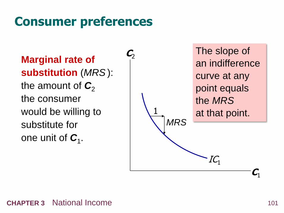
Consumer preferences
Marginal rate of
substitution (MRS ):
the amount of C2
the consumer
would be willing to
substitute for
one unit of C1.
C1
C2
IC1
The slope of
an indifference
curve at any
point equals
the MRS
at that point.1
MRS
102CHAPTER 3 National Income
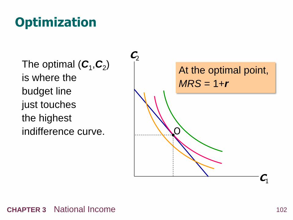
Optimization
The optimal (C1,C2)
is where the
budget line
just touches
the highest
indifference curve.
C1
C2
O
At the optimal point,
MRS = 1+r

103CHAPTER 3 National Income
How C responds to changes in Y
An increase
in Y1 or Y2
shifts the
budget line
outward.
C1
C2Results:
Provided they are
both normal goods,
C1 and C2 both
increase,
…whether the
income increase
occurs in period 1
or period 2.

104CHAPTER 3 National Income
Keynes vs. Fisher
Keynes:
Current consumption depends only on
current income.
Fisher:
Current consumption depends only on
the present value of lifetime income.
The timing of income is irrelevant
because the consumer can borrow or lend
between periods.

105CHAPTER 3 National Income
A
How C responds to changes in r
An increase in r
pivots the budget
line around the
point (Y1,Y2 ).
C1
C2
Y1
Y2
A
B
As depicted here,
C1 falls and C2 rises.
However, it could
turn out differently…
106CHAPTER 3 National Income
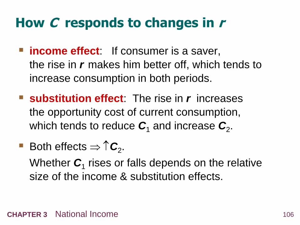
How C responds to changes in r
income effect: If consumer is a saver,
the rise in r makes him better off, which tends to
increase consumption in both periods.
substitution effect: The rise in r increases
the opportunity cost of current consumption,
which tends to reduce C1 and increase C2.
Both effects C2.
Whether C1 rises or falls depends on the relative
size of the income & substitution effects.
107CHAPTER 3 National Income
Constraints on borrowing
In Fisher’s theory, the timing of income is irrelevant:
Consumer can borrow and lend across periods.
Example: If consumer learns that her future income
will increase, she can spread the extra consumption
over both periods by borrowing in the current period.
However, if consumer faces borrowing constraints
(a.k.a. liquidity constraints), then she may not be
able to increase current consumption
…and her consumption may behave as in the
Keynesian theory even though she is rational &
forward-looking.
108CHAPTER 3 National Income
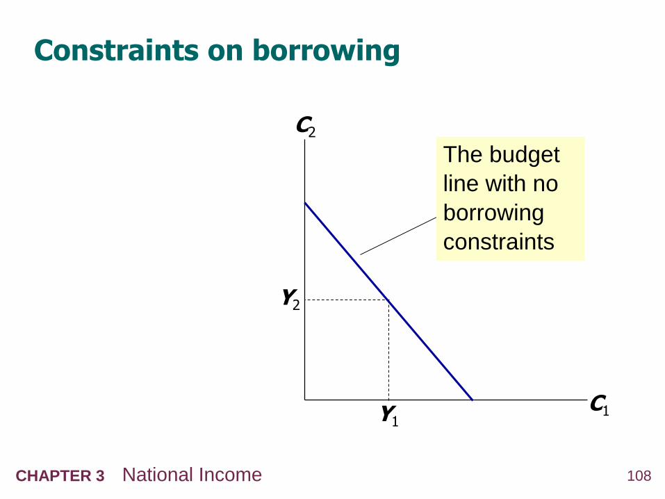
Constraints on borrowing
The budget
line with no
borrowing
constraints
C1
C2
Y1
Y2

109CHAPTER 3 National Income
Constraints on borrowing
The borrowing
constraint takes
the form:
C1 Y1
C1
C2
Y1
Y2
The budget
line with a
borrowing
constraint

110CHAPTER 3 National Income
Consumer optimization when the
borrowing constraint is not binding
The borrowing
constraint is not
binding if the
consumer’s
optimal C1
is less than Y1.
C1
C2
Y1
111CHAPTER 3 National Income
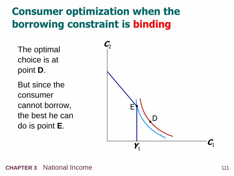
Consumer optimization when the
borrowing constraint is binding
The optimal
choice is at
point D.
But since the
consumer
cannot borrow,
the best he can
do is point E.
C1
C2
Y1
D
E

L E C T U R E S U M M A R Y
Total output is determined by:
the economy’s quantities of capital and labor
the level of technology
Competitive firms hire each factor until its marginal
product equals its price.
If the production function has constant returns to
scale, then labor income plus capital income
equals total income (output).
112

L E C T U R E S U M M A R Y
A closed economy’s output is used for
consumption, investment, and government
spending.
The real interest rate adjusts to equate
the demand for and supply of:
goods and services.
loanable funds.
113

L E C T U R E S U M M A R Y
A decrease in national saving causes the interest
rate to rise and investment to fall.
An increase in investment demand causes the
interest rate to rise but does not affect the
equilibrium level of investment if the supply of
loanable funds is fixed.
114

115CHAPTER 1 The Science of Macroeconomics
L E C T U R E S U M M A R Y
Alternative Views of Consumption
1. Keynesian consumption theory
Keynes’s conjectures
MPC is between 0 and 1
APC falls as income rises
current income is the main determinant of
current consumption
Empirical studies
in household data & short time series:
confirmation of Keynes’s conjectures
in long-time series data:
APC does not fall as income rises115
116CHAPTER 1 The Science of Macroeconomics
L E C T U R E S U M M A R Y
2. Fisher’s theory of intertemporal choice
Consumer chooses current & future
consumption to maximize lifetime satisfaction of
subject to an intertemporal budget constraint.
Current consumption depends on lifetime
income, not current income, provided consumer
can borrow & save.
116