Latent variable models: a review of estimation methods · 9-10 September Latent variable models: a review of estimation methods Irini Moustaki London School of Economics Conference

9-10 September

Latent variable models: a review of estimationmethods

Irini MoustakiLondon School of Economics

Conference to honor the scientific contributions of Professor Michael Browne

Ohio State University

9-10 September

Outline

• Modeling approaches for ordinal variables

• Review methods of estimation for latent variable models

• Look at a special case: longitudinal data

• Goodness-of-fit tests and Model selection criteria

• Applications


9-10 September

Notation and general aim

Manifest variables are denoted by: x1, x2, . . . , xp.

Latent variables are denoted by: z1, z2, . . . , zq.

One wants to find a set of latent variables z1, . . . , zq, fewer in number than theobserved variables (q < p), that contain essentially the same information


9-10 September

Estimation Methods

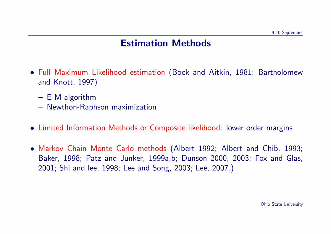
• Full Maximum Likelihood estimation (Bock and Aitkin, 1981; Bartholomewand Knott, 1997)

– E-M algorithm– Newthon-Raphson maximization

• Limited Information Methods or Composite likelihood: lower order margins

• Markov Chain Monte Carlo methods (Albert 1992; Albert and Chib, 1993;Baker, 1998; Patz and Junker, 1999a,b; Dunson 2000, 2003; Fox and Glas,2001; Shi and lee, 1998; Lee and Song, 2003; Lee, 2007.)


9-10 September

Full Maximum Likelihood

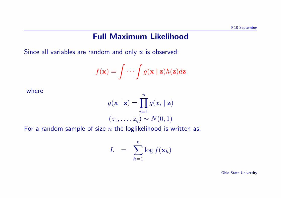
Since all variables are random and only x is observed:

f(x) =∫· · ·

∫g(x | z)h(z)dz

where

g(x | z) =p∏i=1

g(xi | z)

(z1, . . . , zq) ∼ N(0, 1)For a random sample of size n the loglikelihood is written as:

L =n∑h=1

log f(xh)


9-10 September

Notes

• q-dimension integration (Laplace, quadrature points, adaptive, Monte Carlo)

• Maximization (E-M, Newthon-Raphson)


9-10 September

Composite likelihoods a categorization based on Varin andVidoni, 2005

• Omission methods: remove terms that make the evaluation of the fulllikelihood complicated. (Besag, 1974; Azzalini, 1983)

• Subsetting methods: likelihoods composed of univariate, bivariate, trivariate,... margins (Cox and Reid 2004).

• They all fall within the context of pseudo likelihood methods (Godambe, 1960)or misspecified models (White, 1982)


9-10 September

Composite likelihoods based on marginal densities

• Key idea: The model still holds marginally for a specific set of variables.

• Use only information from the univariate or/and bivariate margins.

• e.g.: maximize the sum of all the log bivariate likelihoods.

• The estimator obtained for large n is consistent and asymptotically normal.

• Aim: decrease the number of integrals required without loosing too muchprecision.


9-10 September

Bayesian framework estimation

Let us denote by v′ = (z′,α′) the vector with all the unknown parameters

The joint posterior distribution of the parameter vector v:

h(v | x) =g(x | v)ψ(v)∫

. . .∫g(x | v)ψ(v)dv

∝ g(x | v)ψ(v), (1)

which is the likelihood of the data multiplied by the prior distribution (ψ(v)) of all model

parameters including the latent variables and divided by a normalizing constant.

Calculating the normalizing constant requires multi-dimensional integration that can be very heavy

computationally if not infeasible.


9-10 September

The main steps of the Bayesian approach are:

1. Inference is based on: h(v | x).

2. The mean, mode or any other percentile vector and the standard deviation of h(v | x) can

be used as an estimator of v and its corresponding standard error.

3. Analytic evaluation of the above expectation is impossible. Alternatives include numerical

evaluation, analytic approximations and Monte Carlo integration.

4. MCMC methods are used for sampling from the posterior distribution (Metropolis Hastings

algorithm, Gibbs sampling)


9-10 September

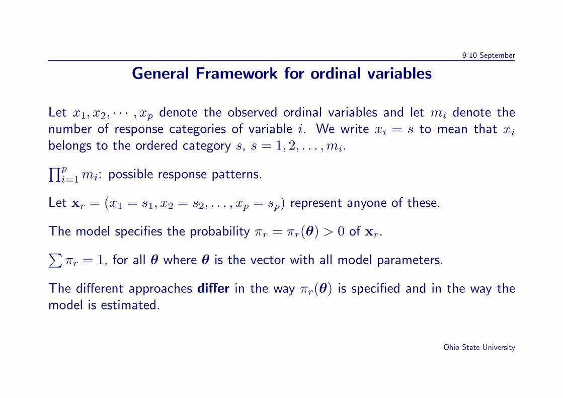
General Framework for ordinal variables

Let x1, x2, · · · , xp denote the observed ordinal variables and let mi denote thenumber of response categories of variable i. We write xi = s to mean that xibelongs to the ordered category s, s = 1, 2, . . . ,mi.∏pi=1mi: possible response patterns.

Let xr = (x1 = s1, x2 = s2, . . . , xp = sp) represent anyone of these.

The model specifies the probability πr = πr(θ) > 0 of xr.∑πr = 1, for all θ where θ is the vector with all model parameters.

The different approaches differ in the way πr(θ) is specified and in the way themodel is estimated.


9-10 September

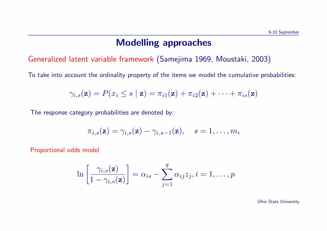
Modelling approaches

Generalized latent variable framework (Samejima 1969, Moustaki, 2003)

To take into account the ordinality property of the items we model the cumulative probabilities:

γi,s(z) = P (xi ≤ s | z) = πi1(z) + πi2(z) + · · ·+ πis(z)

The response category probabilities are denoted by:

πi,s(z) = γi,s(z)− γi,s−1(z), s = 1, . . . ,mi

Proportional odds model

ln[

γi,s(z)1− γi,s(z)

]= αis −

q∑j=1

αijzj, i = 1, . . . , p


9-10 September

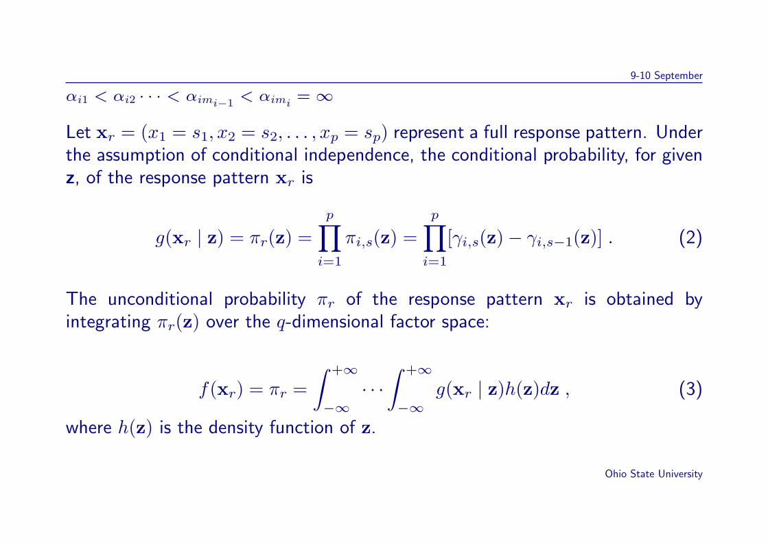
αi1 < αi2 · · · < αimi−1< αimi = ∞

Let xr = (x1 = s1, x2 = s2, . . . , xp = sp) represent a full response pattern. Underthe assumption of conditional independence, the conditional probability, for givenz, of the response pattern xr is

g(xr | z) = πr(z) =p∏i=1

πi,s(z) =p∏i=1

[γi,s(z)− γi,s−1(z)] . (2)

The unconditional probability πr of the response pattern xr is obtained byintegrating πr(z) over the q-dimensional factor space:

f(xr) = πr =∫ +∞

−∞· · ·

∫ +∞

−∞g(xr | z)h(z)dz , (3)

where h(z) is the density function of z.


9-10 September

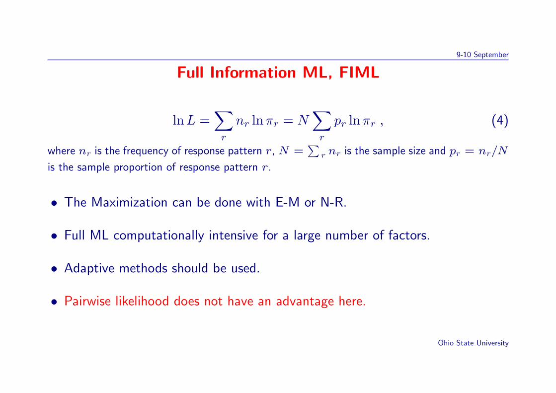
Full Information ML, FIML

lnL =∑r

nr lnπr = N∑r

pr lnπr , (4)

where nr is the frequency of response pattern r, N =∑

r nr is the sample size and pr = nr/N

is the sample proportion of response pattern r.

• The Maximization can be done with E-M or N-R.

• Full ML computationally intensive for a large number of factors.

• Adaptive methods should be used.

• Pairwise likelihood does not have an advantage here.


9-10 September

MCMC estimation

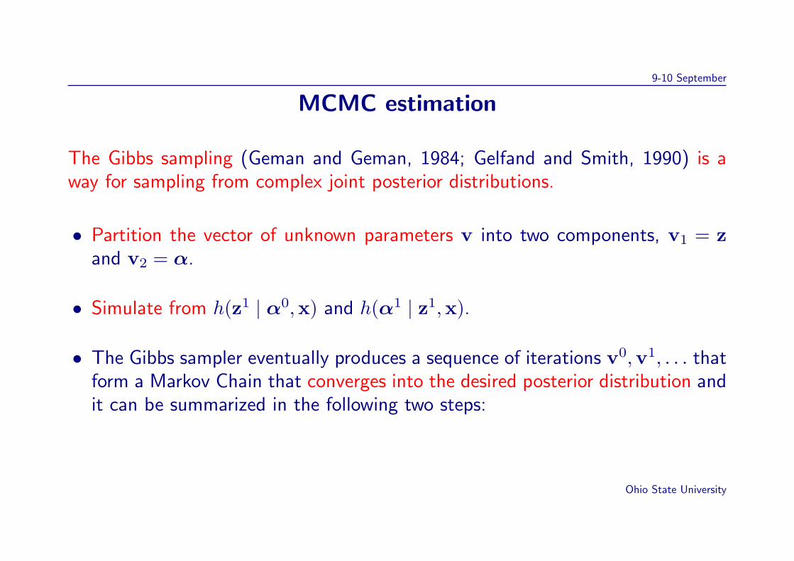
The Gibbs sampling (Geman and Geman, 1984; Gelfand and Smith, 1990) is away for sampling from complex joint posterior distributions.

• Partition the vector of unknown parameters v into two components, v1 = zand v2 = α.

• Simulate from h(z1 | α0,x) and h(α1 | z1,x).

• The Gibbs sampler eventually produces a sequence of iterations v0,v1, . . . thatform a Markov Chain that converges into the desired posterior distribution andit can be summarized in the following two steps:


9-10 September

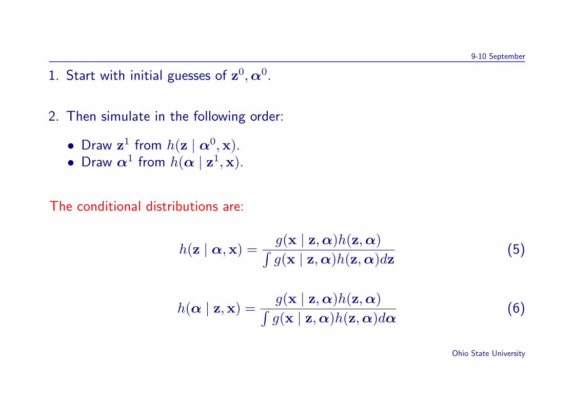
1. Start with initial guesses of z0,α0.

2. Then simulate in the following order:

• Draw z1 from h(z | α0,x).• Draw α1 from h(α | z1,x).

The conditional distributions are:

h(z | α,x) =g(x | z,α)h(z,α)∫g(x | z,α)h(z,α)dz

(5)

h(α | z,x) =g(x | z,α)h(z,α)∫g(x | z,α)h(z,α)dα

(6)


9-10 September

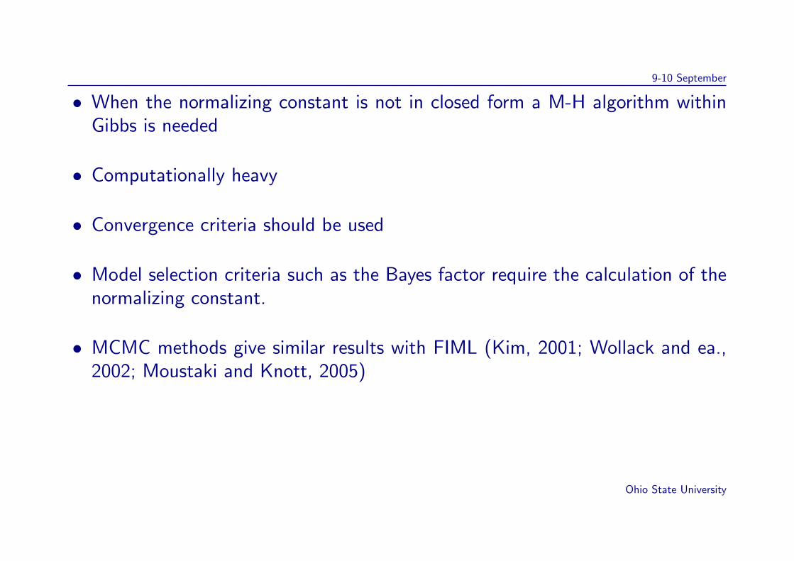
• When the normalizing constant is not in closed form a M-H algorithm withinGibbs is needed

• Computationally heavy

• Convergence criteria should be used

• Model selection criteria such as the Bayes factor require the calculation of thenormalizing constant.

• MCMC methods give similar results with FIML (Kim, 2001; Wollack and ea.,2002; Moustaki and Knott, 2005)


9-10 September

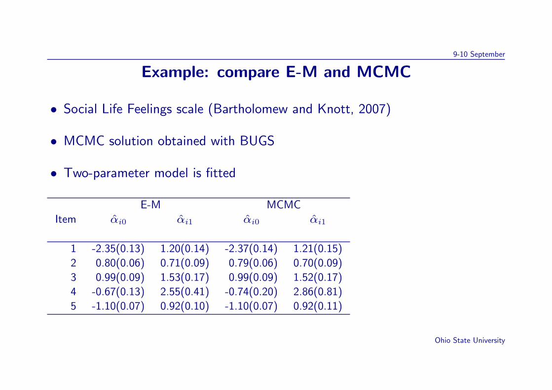
Example: compare E-M and MCMC

• Social Life Feelings scale (Bartholomew and Knott, 2007)

• MCMC solution obtained with BUGS

• Two-parameter model is fitted

E-M MCMC

Item αi0 αi1 αi0 αi1

1 -2.35(0.13) 1.20(0.14) -2.37(0.14) 1.21(0.15)

2 0.80(0.06) 0.71(0.09) 0.79(0.06) 0.70(0.09)

3 0.99(0.09) 1.53(0.17) 0.99(0.09) 1.52(0.17)

4 -0.67(0.13) 2.55(0.41) -0.74(0.20) 2.86(0.81)

5 -1.10(0.07) 0.92(0.10) -1.10(0.07) 0.92(0.11)


9-10 September

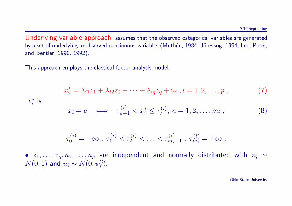
Underlying variable approach assumes that the observed categorical variables are generated

by a set of underlying unobserved continuous variables (Muthen, 1984; Joreskog, 1994; Lee, Poon,

and Bentler, 1990, 1992).

This approach employs the classical factor analysis model:

x∗i = λi1z1 + λi2z2 + · · ·+ λiqzq + ui , i = 1, 2, . . . , p , (7)

x∗i is

xi = a ⇐⇒ τ(i)a−1 < x∗i ≤ τ (i)

a , a = 1, 2, . . . ,mi , (8)

τ(i)0 = −∞ , τ

(i)1 < τ

(i)2 < . . . < τ

(i)mi−1 , τ

(i)mi

= +∞ ,

• z1, . . . , zq, u1, . . . , up are independent and normally distributed with zj ∼N(0, 1) and ui ∼ N(0, ψ2

i ).


9-10 September

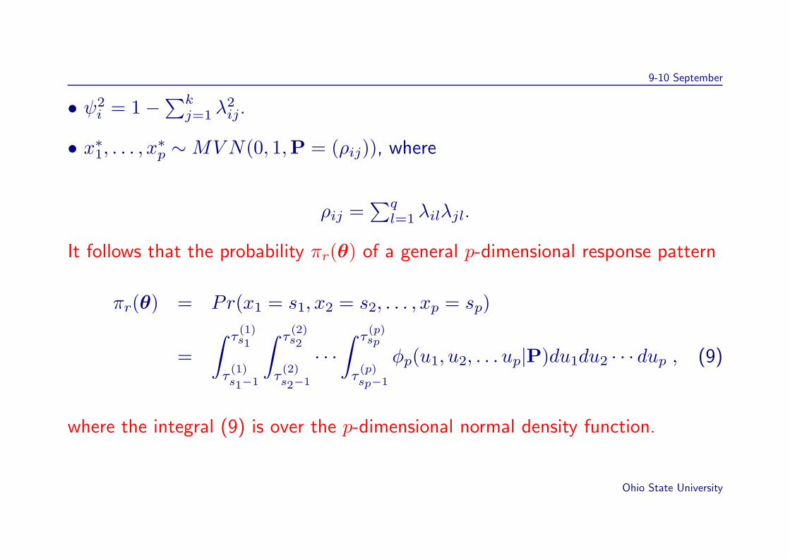
• ψ2i = 1−

∑kj=1 λ

2ij.

• x∗1, . . . , x∗p ∼MVN(0, 1,P = (ρij)), where

ρij =∑ql=1 λilλjl.

It follows that the probability πr(θ) of a general p-dimensional response pattern

πr(θ) = Pr(x1 = s1, x2 = s2, . . . , xp = sp)

=∫ τ

(1)s1

τ(1)s1−1

∫ τ(2)s2

τ(2)s2−1

· · ·∫ τ

(p)sp

τ(p)sp−1

φp(u1, u2, . . . up|P)du1du2 · · · dup , (9)

where the integral (9) is over the p-dimensional normal density function.


9-10 September

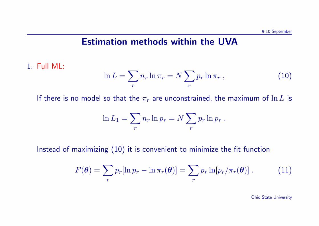
Estimation methods within the UVA

1. Full ML:lnL =

∑r

nr lnπr = N∑r

pr lnπr , (10)

If there is no model so that the πr are unconstrained, the maximum of lnL is

lnL1 =∑r

nr ln pr = N∑r

pr ln pr .

Instead of maximizing (10) it is convenient to minimize the fit function

F (θ) =∑r

pr[ln pr − lnπr(θ)] =∑r

pr ln[pr/πr(θ)] . (11)


9-10 September

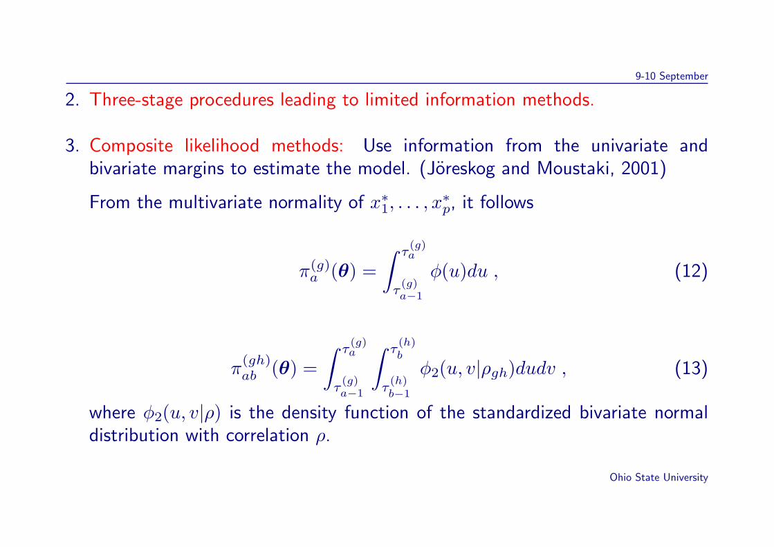
2. Three-stage procedures leading to limited information methods.

3. Composite likelihood methods: Use information from the univariate andbivariate margins to estimate the model. (Joreskog and Moustaki, 2001)

From the multivariate normality of x∗1, . . . , x∗p, it follows

π(g)a (θ) =

∫ τ(g)a

τ(g)a−1

φ(u)du , (12)

π(gh)ab (θ) =

∫ τ(g)a

τ(g)a−1

∫ τ(h)b

τ(h)b−1

φ2(u, v|ρgh)dudv , (13)

where φ2(u, v|ρ) is the density function of the standardized bivariate normaldistribution with correlation ρ.


9-10 September

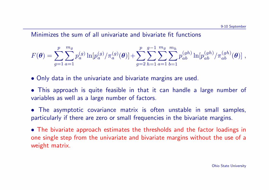
Minimizes the sum of all univariate and bivariate fit functions

F (θ) =p∑g=1

mg∑a=1

p(g)a ln[p(g)

a /π(g)a (θ)]+

p∑g=2

g−1∑h=1

mg∑a=1

mh∑b=1

p(gh)ab ln[p(gh)

ab /π(gh)ab (θ)] ,

• Only data in the univariate and bivariate margins are used.

• This approach is quite feasible in that it can handle a large number ofvariables as well as a large number of factors.

• The asymptotic covariance matrix is often unstable in small samples,particularly if there are zero or small frequencies in the bivariate margins.

• The bivariate approach estimates the thresholds and the factor loadings inone single step from the univariate and bivariate margins without the use of aweight matrix.


9-10 September

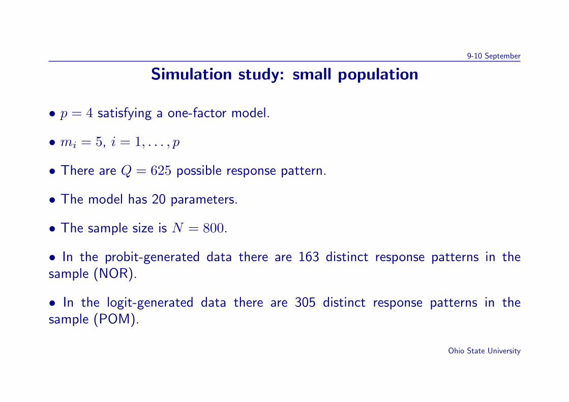
Simulation study: small population

• p = 4 satisfying a one-factor model.

• mi = 5, i = 1, . . . , p

• There are Q = 625 possible response pattern.

• The model has 20 parameters.

• The sample size is N = 800.

• In the probit-generated data there are 163 distinct response patterns in thesample (NOR).

• In the logit-generated data there are 305 distinct response patterns in thesample (POM).


9-10 September

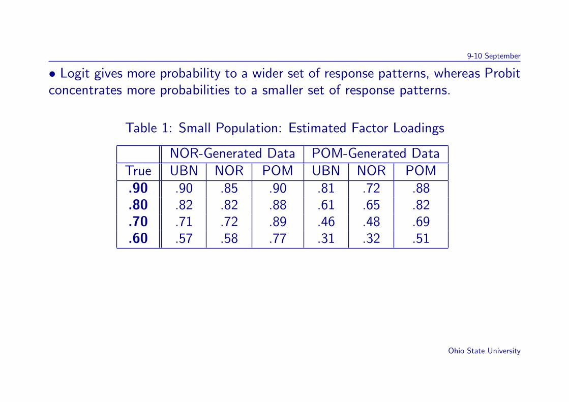
• Logit gives more probability to a wider set of response patterns, whereas Probitconcentrates more probabilities to a smaller set of response patterns.

Table 1: Small Population: Estimated Factor Loadings

NOR-Generated Data POM-Generated DataTrue UBN NOR POM UBN NOR POM.90 .90 .85 .90 .81 .72 .88.80 .82 .82 .88 .61 .65 .82.70 .71 .72 .89 .46 .48 .69.60 .57 .58 .77 .31 .32 .51


9-10 September

Multivariate longitudinal ordinal data

• Study the evolvement in time of traits, attitudes, ability, etc.

• Characteristics of longitudinal data:

– Extra dependencies to account for (within time/ between time).– Factor changes over time are modelled through a multivariate normal

distribution. The covariance matrix imposed on the time-related latentvariables accounts for the dependence of the item responses across time.

– A GLLVM that accounts for dependencies within time and across timeusing time specific factors and a heteroscedastic item-dependent randomeffect term (Dunson 2003, JASA and Cagnone, Moustaki, Vasdekis, 2009,BJMSP).

– An autoregressive model is used to model the structural part of the model.


9-10 September

• Within Structural Equation Modelling (SEM) framework longitudinal data aretreated in different ways:

– Individual response curves over time by means of latent variable growthmodels. The main feature of this class of models is that the parametersof the curve, random intercept and random slope, can be viewed as latentvariables.

– Allow for correlated errors.


9-10 September

Notation for longitudinal data

Let x1t, x2t, . . . , xpt be the ordinal observed variables measured at time t, (t =1, . . . , T ).

The mi ordered categories of the ith item measured at time t have responsecategory probabilities πit(1)(zt, ui), πit(2)(zt, ui), · · · , πit(mi)(zt, ui)

• The time-dependent latent variable zt account for the dependencies amongthe p items measured at time t

• The random effect ui accounts for the dependencies among the item imeasuredat different time points.


9-10 September

Model specification and assumptions

The systematic component:

ηit(s) = τit(s) − αitzt + ui , i = 1, . . . , p; s = 1, . . . ,mi; t = 1, . . . , T. (14)

The link between the systematic component and the conditional means of therandom component distributions is

ηit(s) = vit(s)(γit(s))

where γit(s) = P (xit ≤ s | zt, ui) and vit(s)(.) is the link function.


9-10 September

• The associations among the items measured at time t are explained by thelatent variable zt.

Cov(ηit, ηi′t) = αitαi′tV ar(zt), i 6= i′ (15)

with V ar(zt) = φ2(t−1)σ21 + I(t ≥ 2)

∑t−1k=1 φ

2(k−1)

• The associations among the same item measured across time (xi1, . . . , xiT )are explained by the item-specific random effect ui.

Cov(ηit, ηit′) = αitαit′Cov(zt, zt′) + σ2ui, t < t′ (16)

Cov(zt, zt′) = φt+t′−2σ2

1 + I(t ≥ 2)∑t−2k=0 φ

t′−t+2k, where I(.) is the indicatorfunction.


9-10 September

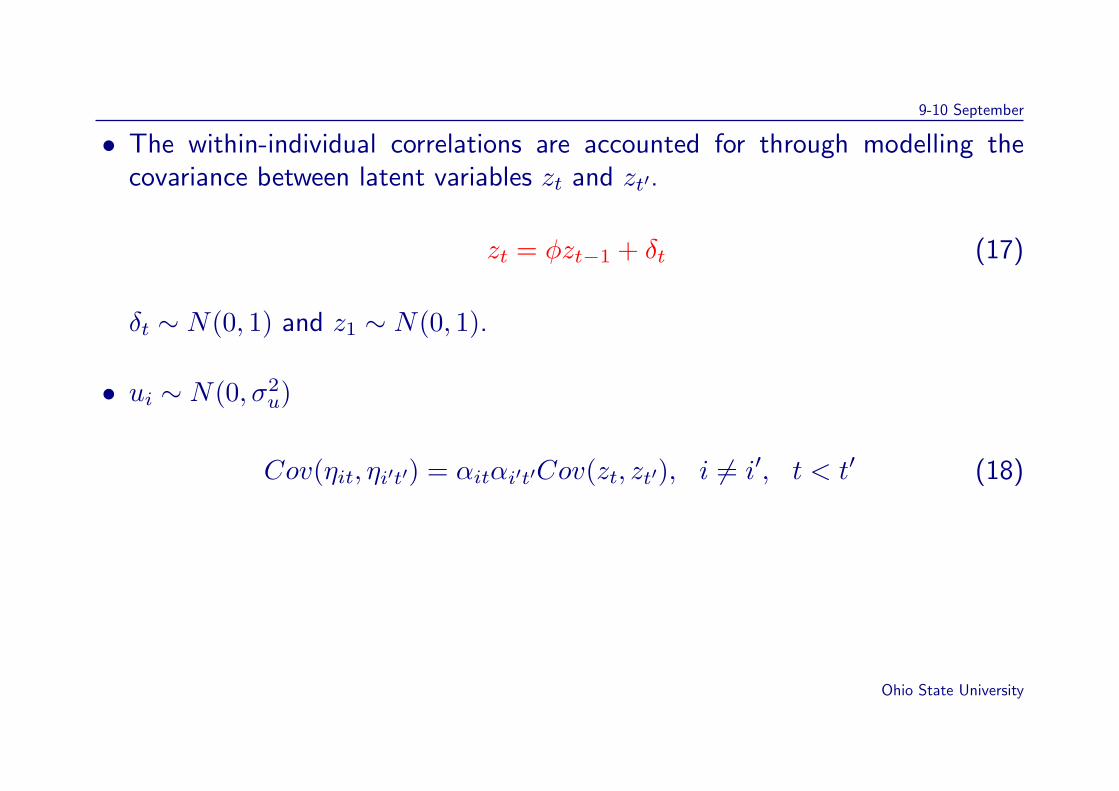
• The within-individual correlations are accounted for through modelling thecovariance between latent variables zt and zt′.

zt = φzt−1 + δt (17)

δt ∼ N(0, 1) and z1 ∼ N(0, 1).

• ui ∼ N(0, σ2u)

Cov(ηit, ηi′t′) = αitαi′t′Cov(zt, zt′), i 6= i′, t < t′ (18)


9-10 September

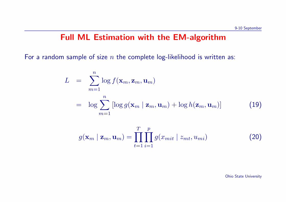
Full ML Estimation with the EM-algorithm

For a random sample of size n the complete log-likelihood is written as:

L =n∑

m=1

log f(xm, zm,um)

= logn∑

m=1

[log g(xm | zm,um) + log h(zm,um)] (19)

g(xm | zm,um) =T∏t=1

p∏i=1

g(xmit | zmt, umi) (20)


9-10 September

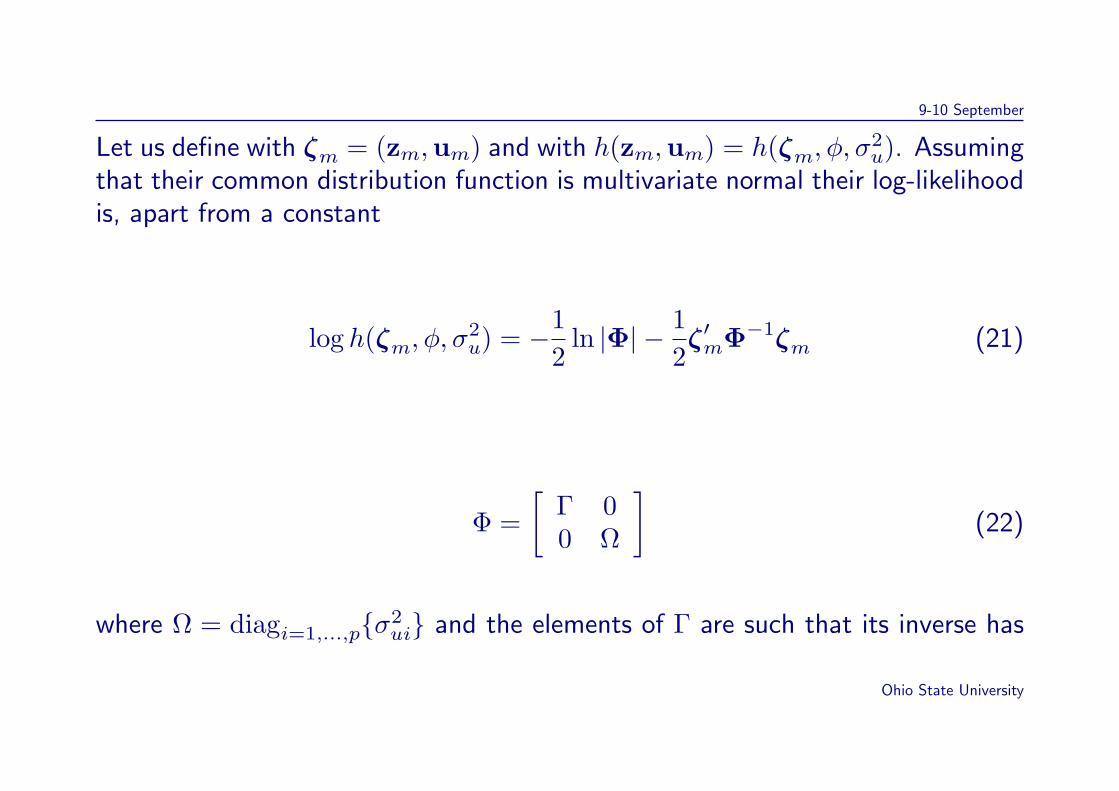
Let us define with ζm = (zm,um) and with h(zm,um) = h(ζm, φ, σ2u). Assuming

that their common distribution function is multivariate normal their log-likelihoodis, apart from a constant

log h(ζm, φ, σ2u) = −1

2ln |Φ| − 1

2ζ′mΦ−1ζm (21)

Φ =[

Γ 00 Ω

](22)

where Ω = diagi=1,...,pσ2ui and the elements of Γ are such that its inverse has


9-10 September

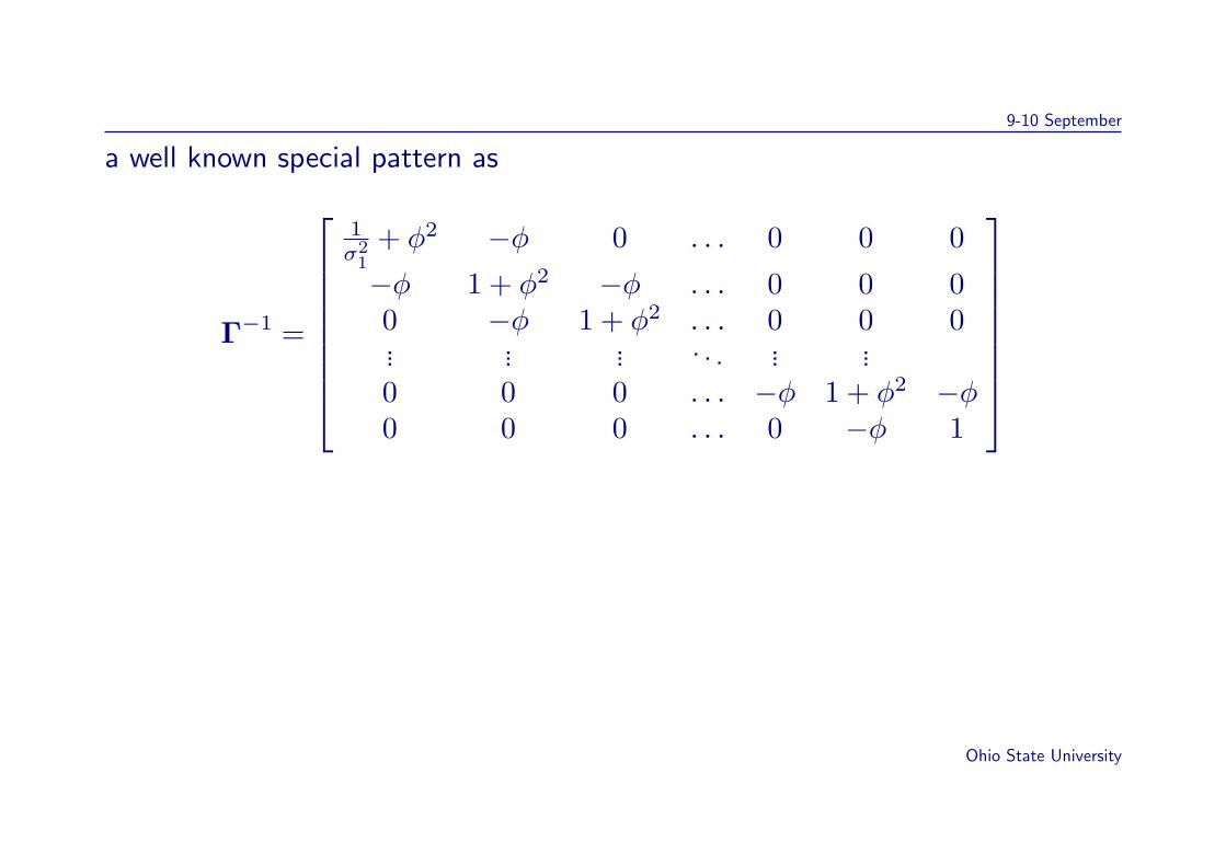
a well known special pattern as

Γ−1 =

1σ2

1+ φ2 −φ 0 . . . 0 0 0

−φ 1 + φ2 −φ . . . 0 0 00 −φ 1 + φ2 . . . 0 0 0... ... ... . . . ... ...0 0 0 . . . −φ 1 + φ2 −φ0 0 0 . . . 0 −φ 1


9-10 September

EM-algorithm

• E-step: the expected score function of the model parameters is computed.The expectation is with respect to the posterior distribution of (zm,um) giventhe observations (h(zm,um | xm)) for each individual.

• M-step: updated parameter estimates are obtained.

• The full ML is very computationally intensive as the number of items andfactors increase.


9-10 September

Composite likelihood estimation

Vasdekis, Cagnone, Moustaki (working paper)

• The model specification remains the same.

• S1 = (i, j, t); 1 ≤ i < j ≤ p; t = 1, . . . , T

• S2 = (i, i′, t, t′); 1 ≤ i ≤ p; 1 ≤ i′ ≤ p; 1 ≤ t < t′ ≤ T


9-10 September

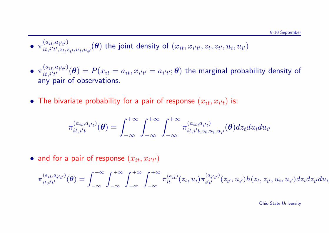
• π(ait,ai′t′)it,i′t′,zt,zt′,ui,ui′

(θ) the joint density of (xit, xi′t′, zt, zt′, ui, ui′)

• π(ait,ai′t′)it,i′t′ (θ) = P (xit = ait, xi′t′ = ai′t′;θ) the marginal probability density of

any pair of observations.

• The bivariate probability for a pair of response (xit, xi′t) is:

π(ait,ai′t)it,i′t (θ) =

∫ +∞

−∞

∫ +∞

−∞

∫ +∞

−∞π

(ait,ai′t)it,i′t,zt,ui,ui′

(θ)dztduidui′

• and for a pair of response (xit, xi′t′)

π(ait,ai′t′)it,i′t′ (θ) =

∫ +∞

−∞

∫ +∞

−∞

∫ +∞

−∞

∫ +∞

−∞π

(ait)

it (zt, ui)π(ai′t′)i′t′ (zt′, ui′)h(zt, zt′, ui, ui′)dztdzt′duidui′


9-10 September

• The latter can be three dimensional if it happens that i = i′. In any case, themaximum number of integrations we have to deal with, is four.

The contribution of any given individual to the log pairwise likelihood is therefore:

pl(θ;y) =

∑S1

log π(ait,ai′t)it,i′t (θ) +

∑S2

log π(ait,ai′t′)it,i′t′ (θ)

(23)

Since each component of equation (23) is a likelihood object we can claimthat ∇pl(θ) = 0 is unbiased under the usual regularity conditions. Themaximum pairwise likelihood estimator θPL is consistent and asymptoticallynormally distributed (Arnold and Strauss, 1991) under regularity conditions foundin Lehman (1983), Crowder (1986) or Geys et. al. (1997).

The maximization of the likelihood in (23) is done with the E-M algorithm.


9-10 September

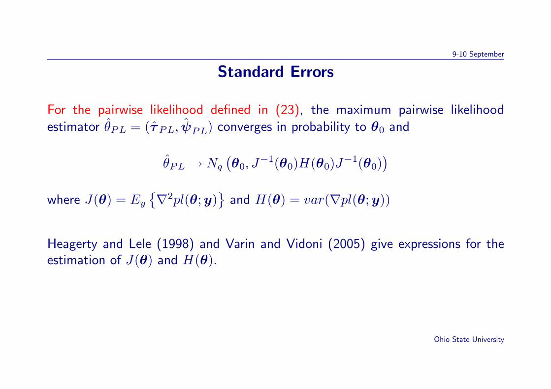
Standard Errors

For the pairwise likelihood defined in (23), the maximum pairwise likelihoodestimator θPL = (τPL, ψPL) converges in probability to θ0 and

θPL → Nq(θ0, J

−1(θ0)H(θ0)J−1(θ0))

where J(θ) = Ey∇2pl(θ;y)

and H(θ) = var(∇pl(θ;y))

Heagerty and Lele (1998) and Varin and Vidoni (2005) give expressions for theestimation of J(θ) and H(θ).


9-10 September

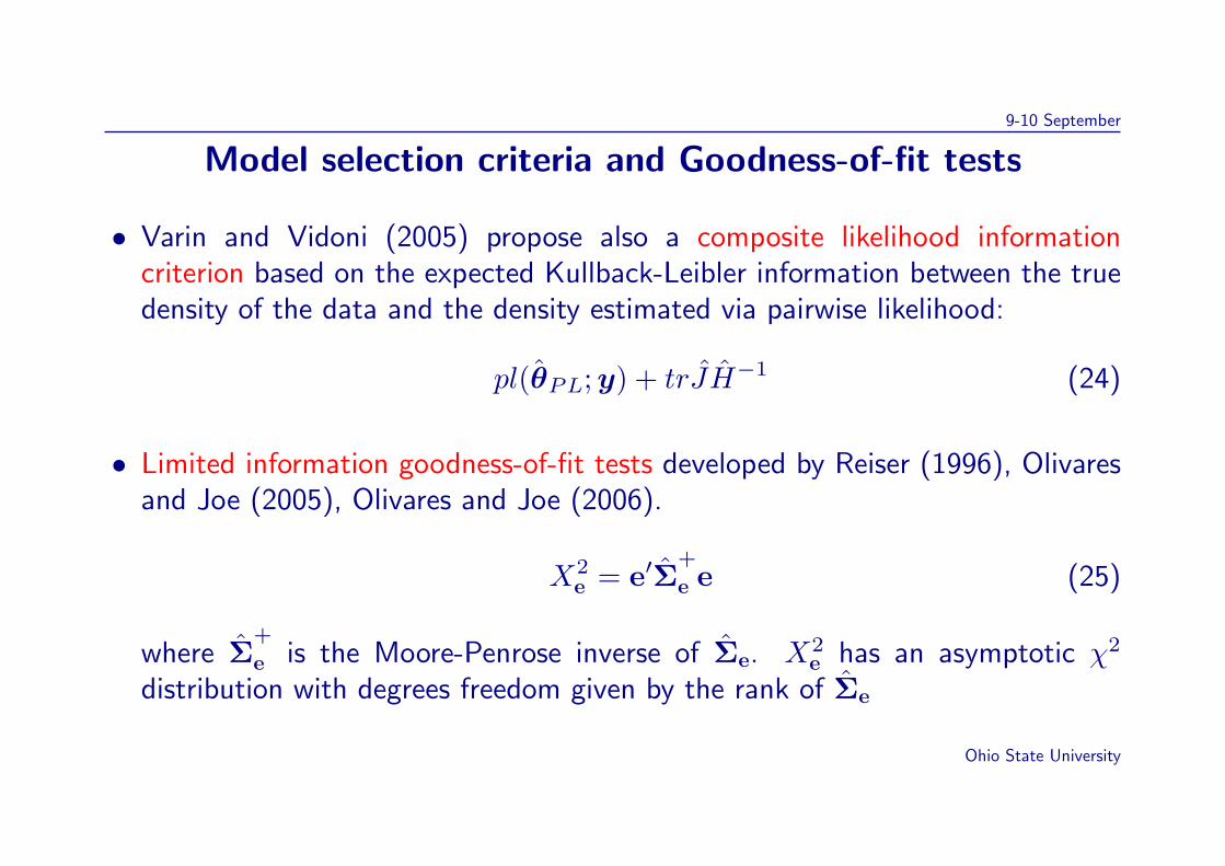
Model selection criteria and Goodness-of-fit tests

• Varin and Vidoni (2005) propose also a composite likelihood informationcriterion based on the expected Kullback-Leibler information between the truedensity of the data and the density estimated via pairwise likelihood:

pl(θPL;y) + trJH−1 (24)

• Limited information goodness-of-fit tests developed by Reiser (1996), Olivaresand Joe (2005), Olivares and Joe (2006).

X2e = e′Σ

+

e e (25)

where Σ+

e is the Moore-Penrose inverse of Σe. X2e has an asymptotic χ2

distribution with degrees freedom given by the rank of Σe


9-10 September

Application: British Household Panel Survey

BHPS: study social and economic change at the individual and household level inBritain.

The original data set consists of 6 ordinal items on social and political attitudesmeasured at 5 different waves (1992, 1994, 1996, 1998, 2000). The sample sizewas 3784. A random sample of 500 is considered.

The following three items for three waves (1994=1,1996=2, 1998=3) are used:

• Private enterprise solves economic problems [Enterp]

• Govt. has obligation to provide jobs [Gov]

• Strong trade unions protect employees [Trunion]


9-10 September

• The response alternatives are: Strongly agree, Agree, Not agree/disagree,disagree, strongly disagree.

• We collapsed the first two categories and the last two categories.

• A full ML and pairwise method are used to estimate the model.

• Five quadrature points are used


9-10 September

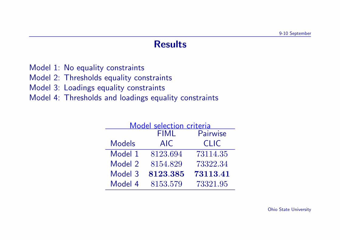
Results

Model 1: No equality constraintsModel 2: Thresholds equality constraintsModel 3: Loadings equality constraintsModel 4: Thresholds and loadings equality constraints

Model selection criteriaFIML Pairwise

Models AIC CLICModel 1 8123.694 73114.35Model 2 8154.829 73322.34Model 3 8123.385 73113.41Model 4 8153.579 73321.95


9-10 September

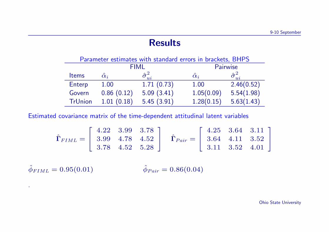
Results

Parameter estimates with standard errors in brackets, BHPSFIML Pairwise

Items αi σ2ui αi σ2

ui

Enterp 1.00 1.71 (0.73) 1.00 2.46(0.52)

Govern 0.86 (0.12) 5.09 (3.41) 1.05(0.09) 5.54(1.98)

TrUnion 1.01 (0.18) 5.45 (3.91) 1.28(0.15) 5.63(1.43)

Estimated covariance matrix of the time-dependent attitudinal latent variables

ΓFIML =

4.22 3.99 3.78

3.99 4.78 4.52

3.78 4.52 5.28

ΓPair =

4.25 3.64 3.11

3.64 4.11 3.52

3.11 3.52 4.01

φFIML = 0.95(0.01) φPair = 0.86(0.04)

.


9-10 September

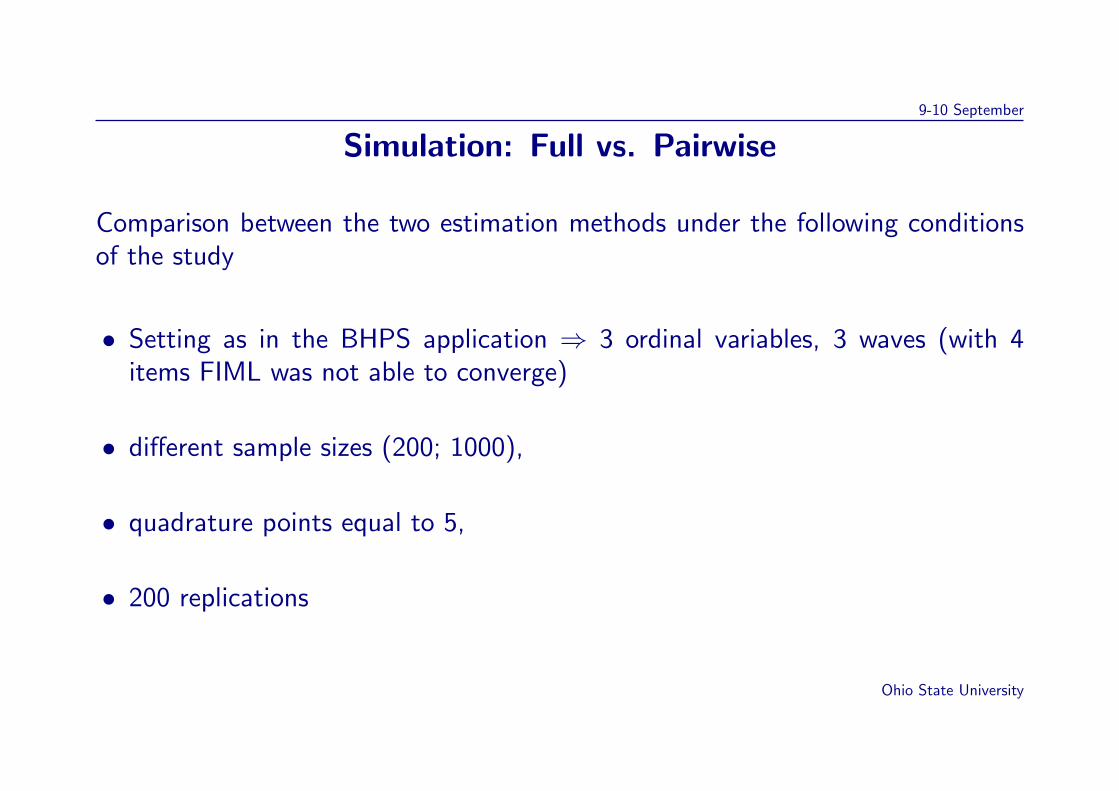
Simulation: Full vs. Pairwise

Comparison between the two estimation methods under the following conditionsof the study

• Setting as in the BHPS application ⇒ 3 ordinal variables, 3 waves (with 4items FIML was not able to converge)

• different sample sizes (200; 1000),

• quadrature points equal to 5,

• 200 replications


9-10 September

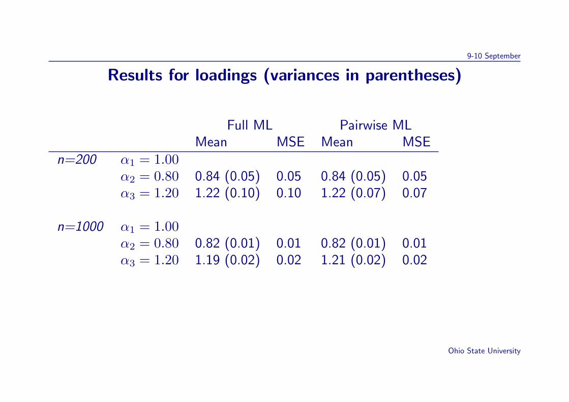
Results for loadings (variances in parentheses)

Full ML Pairwise MLMean MSE Mean MSE

n=200 α1 = 1.00α2 = 0.80 0.84 (0.05) 0.05 0.84 (0.05) 0.05α3 = 1.20 1.22 (0.10) 0.10 1.22 (0.07) 0.07

n=1000 α1 = 1.00α2 = 0.80 0.82 (0.01) 0.01 0.82 (0.01) 0.01α3 = 1.20 1.19 (0.02) 0.02 1.21 (0.02) 0.02


9-10 September

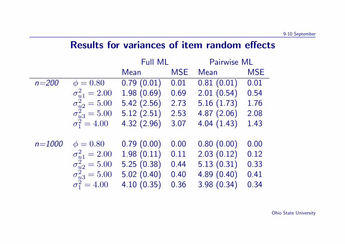
Results for variances of item random effects

Full ML Pairwise MLMean MSE Mean MSE

n=200 φ = 0.80 0.79 (0.01) 0.01 0.81 (0.01) 0.01σ2u1 = 2.00 1.98 (0.69) 0.69 2.01 (0.54) 0.54σ2u2 = 5.00 5.42 (2.56) 2.73 5.16 (1.73) 1.76σ2u3 = 5.00 5.12 (2.51) 2.53 4.87 (2.06) 2.08σ2

1 = 4.00 4.32 (2.96) 3.07 4.04 (1.43) 1.43

n=1000 φ = 0.80 0.79 (0.00) 0.00 0.80 (0.00) 0.00σ2u1 = 2.00 1.98 (0.11) 0.11 2.03 (0.12) 0.12σ2u2 = 5.00 5.25 (0.38) 0.44 5.13 (0.31) 0.33σ2u3 = 5.00 5.02 (0.40) 0.40 4.89 (0.40) 0.41σ2

1 = 4.00 4.10 (0.35) 0.36 3.98 (0.34) 0.34


9-10 September

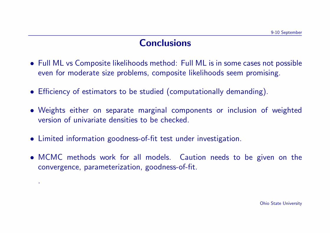
Conclusions

• Full ML vs Composite likelihoods method: Full ML is in some cases not possibleeven for moderate size problems, composite likelihoods seem promising.

• Efficiency of estimators to be studied (computationally demanding).

• Weights either on separate marginal components or inclusion of weightedversion of univariate densities to be checked.

• Limited information goodness-of-fit test under investigation.

• MCMC methods work for all models. Caution needs to be given on theconvergence, parameterization, goodness-of-fit.

.


Documents

Latent variable models: a review of estimation methods · 9-10 September Latent variable models: a review of estimation methods Irini Moustaki London School of Economics Conference