1

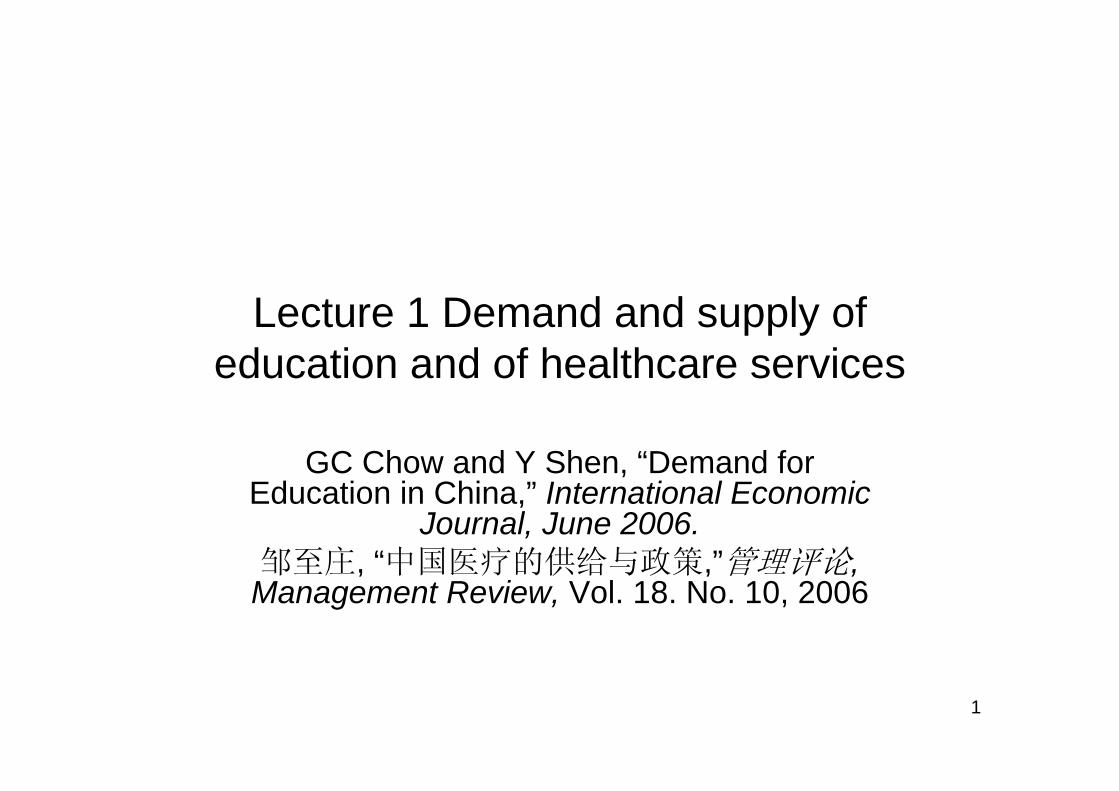
Lecture 1 Demand and supply of education and of healthcare services

GC Chow and Y Shen, “Demand for Education in China,” International Economic

Journal, June 2006. 邹至庄, “中国医疗的供给与政策,”管理评论,

Management Review, Vol. 18. No. 10, 2006

2

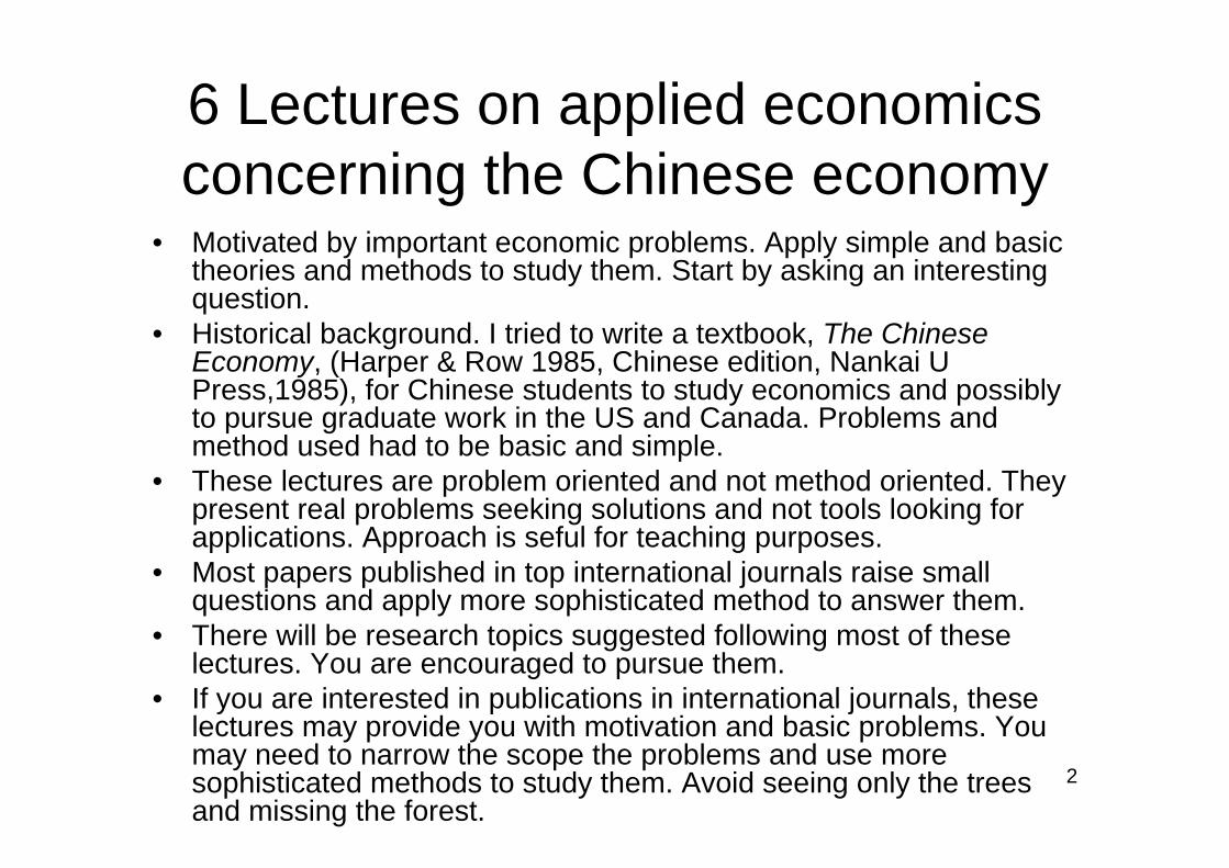
6 Lectures on applied economics concerning the Chinese economy

• Motivated by important economic problems. Apply simple and basictheories and methods to study them. Start by asking an interesting question.

• Historical background. I tried to write a textbook, The Chinese Economy, (Harper & Row 1985, Chinese edition, Nankai U Press,1985), for Chinese students to study economics and possibly to pursue graduate work in the US and Canada. Problems and method used had to be basic and simple.

• These lectures are problem oriented and not method oriented. They present real problems seeking solutions and not tools looking for applications. Approach is seful for teaching purposes.

• Most papers published in top international journals raise small questions and apply more sophisticated method to answer them.

• There will be research topics suggested following most of these lectures. You are encouraged to pursue them.

• If you are interested in publications in international journals, these lectures may provide you with motivation and basic problems. Youmay need to narrow the scope the problems and use more sophisticated methods to study them. Avoid seeing only the treesand missing the forest.

3

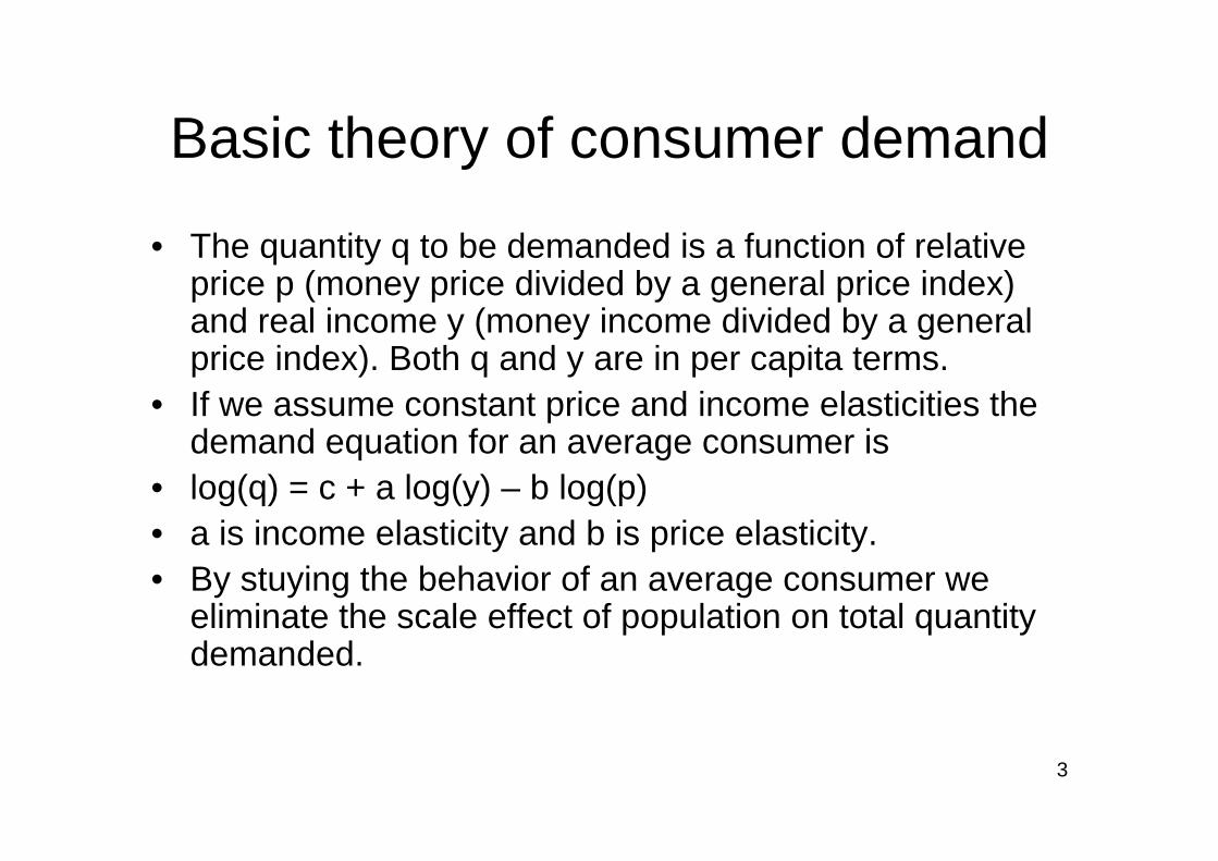
Basic theory of consumer demand

• The quantity q to be demanded is a function of relative price p (money price divided by a general price index) and real income y (money income divided by a general price index). Both q and y are in per capita terms.

• If we assume constant price and income elasticities the demand equation for an average consumer is

• log(q) = c + a log(y) – b log(p)• a is income elasticity and b is price elasticity.• By stuying the behavior of an average consumer we

eliminate the scale effect of population on total quantity demanded.

4

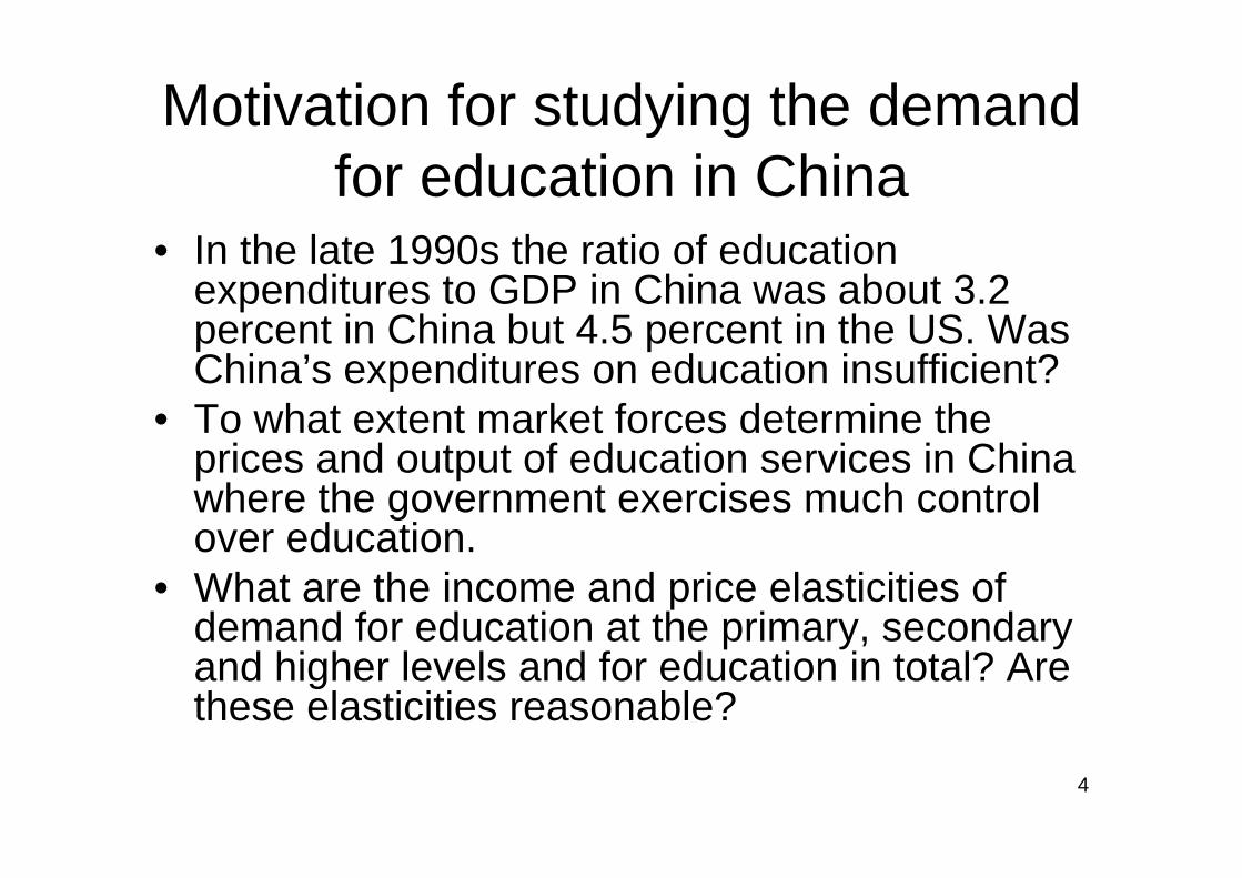
Motivation for studying the demand for education in China

• In the late 1990s the ratio of education expenditures to GDP in China was about 3.2 percent in China but 4.5 percent in the US. Was China’s expenditures on education insufficient?

• To what extent market forces determine the prices and output of education services in China where the government exercises much control over education.

• What are the income and price elasticities of demand for education at the primary, secondary and higher levels and for education in total? Are these elasticities reasonable?

5

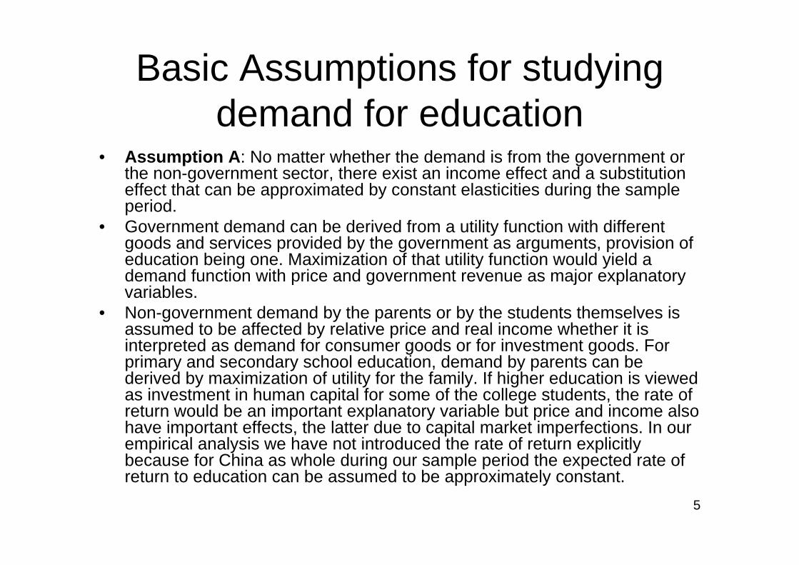
Basic Assumptions for studying demand for education

• Assumption A: No matter whether the demand is from the government or the non-government sector, there exist an income effect and a substitution effect that can be approximated by constant elasticities during the sample period.

• Government demand can be derived from a utility function with different goods and services provided by the government as arguments, provision of education being one. Maximization of that utility function would yield a demand function with price and government revenue as major explanatory variables.

• Non-government demand by the parents or by the students themselves is assumed to be affected by relative price and real income whether it is interpreted as demand for consumer goods or for investment goods. For primary and secondary school education, demand by parents can bederived by maximization of utility for the family. If higher education is viewed as investment in human capital for some of the college students, the rate of return would be an important explanatory variable but price and income also have important effects, the latter due to capital market imperfections. In our empirical analysis we have not introduced the rate of return explicitly because for China as whole during our sample period the expected rate of return to education can be assumed to be approximately constant.

6

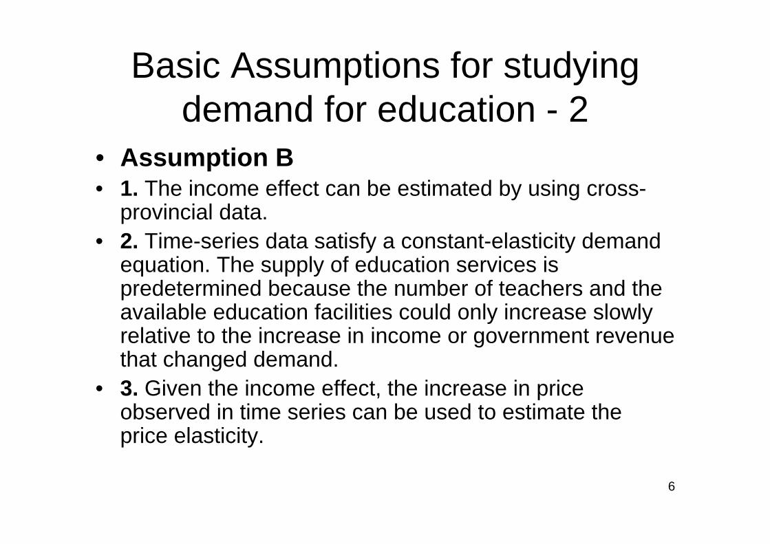
Basic Assumptions for studying demand for education - 2

• Assumption B• 1. The income effect can be estimated by using cross-

provincial data.• 2. Time-series data satisfy a constant-elasticity demand

equation. The supply of education services is predetermined because the number of teachers and the available education facilities could only increase slowly relative to the increase in income or government revenue that changed demand.

• 3. Given the income effect, the increase in price observed in time series can be used to estimate the price elasticity.

7

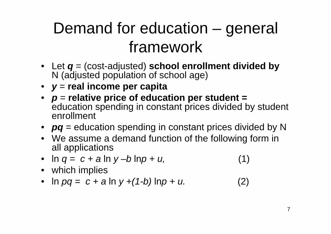
Demand for education – general framework

• Let q = (cost-adjusted) school enrollment divided byN (adjusted population of school age)

• y = real income per capita • p = relative price of education per student =

education spending in constant prices divided by student enrollment

• pq = education spending in constant prices divided by N • We assume a demand function of the following form in

all applications• ln q = c + a ln y –b lnp + u, (1)• which implies• ln pq = c + a ln y +(1-b) lnp + u. (2)

8

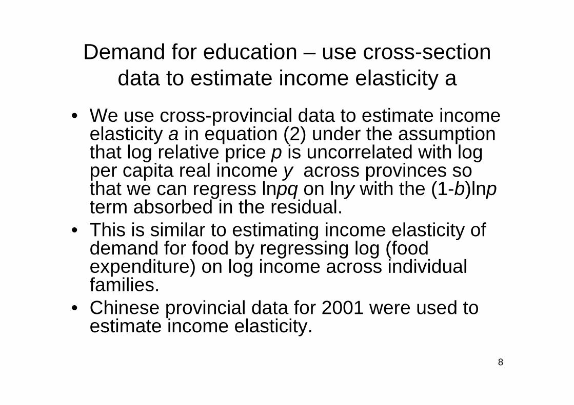
Demand for education – use cross-section data to estimate income elasticity a

• We use cross-provincial data to estimate income elasticity a in equation (2) under the assumption that log relative price p is uncorrelated with log per capita real income y across provinces so that we can regress lnpq on lny with the (1-b)lnpterm absorbed in the residual.

• This is similar to estimating income elasticity of demand for food by regressing log (food expenditure) on log income across individual families.

• Chinese provincial data for 2001 were used to estimate income elasticity.

9

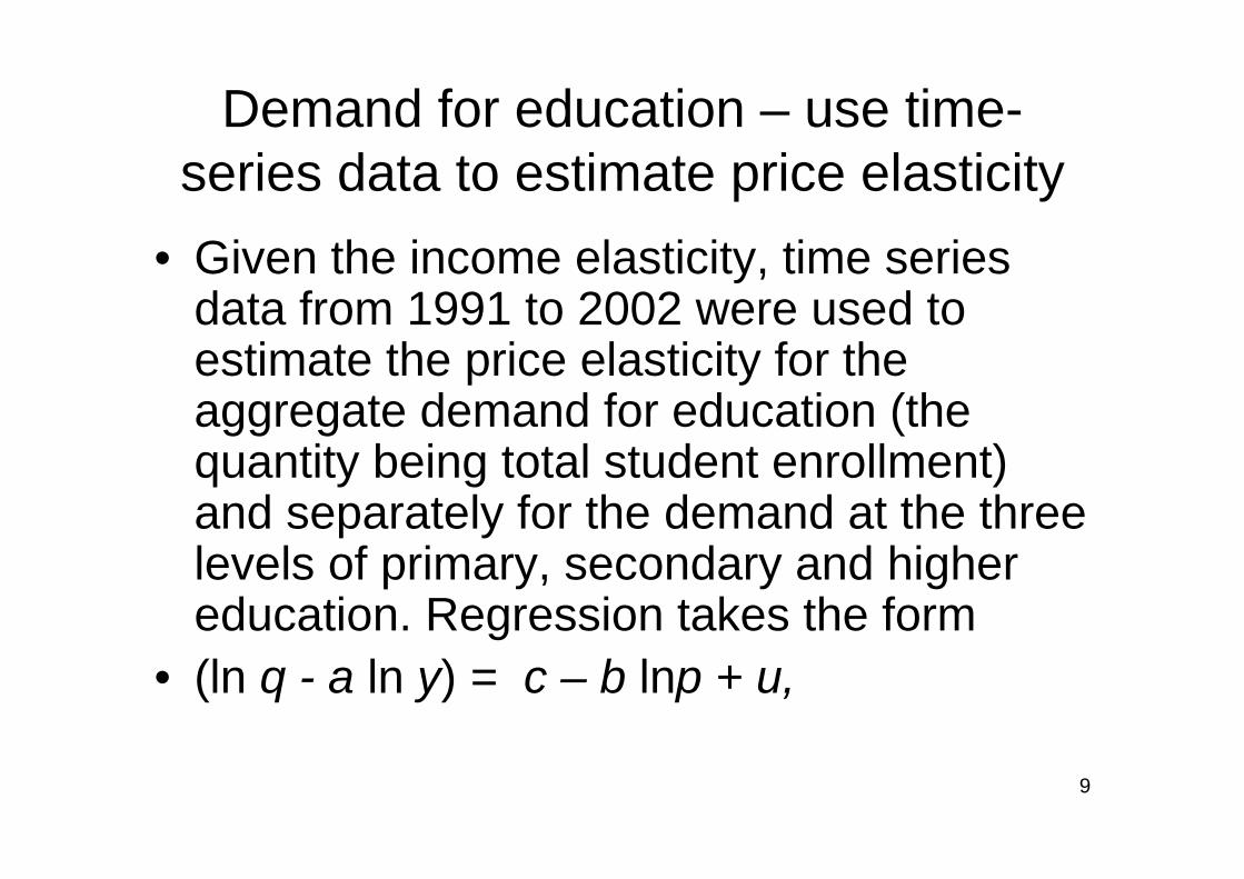
Demand for education – use time-series data to estimate price elasticity

• Given the income elasticity, time series data from 1991 to 2002 were used to estimate the price elasticity for the aggregate demand for education (the quantity being total student enrollment) and separately for the demand at the three levels of primary, secondary and higher education. Regression takes the form

• (ln q - a ln y) = c – b lnp + u,

10

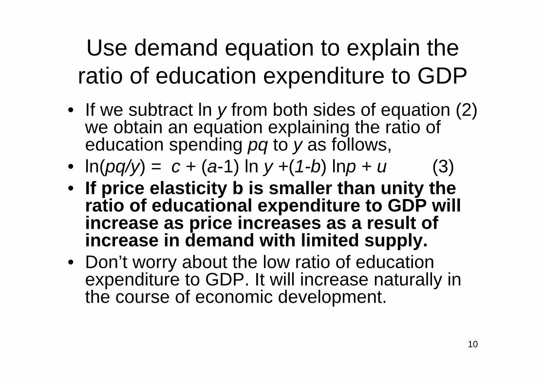
Use demand equation to explain the ratio of education expenditure to GDP

• If we subtract ln y from both sides of equation (2) we obtain an equation explaining the ratio of education spending pq to y as follows,

• ln(pq/y) = c + (a-1) ln y +(1-b) lnp + u (3) • If price elasticity b is smaller than unity the

ratio of educational expenditure to GDP will increase as price increases as a result of increase in demand with limited supply.

• Don’t worry about the low ratio of education expenditure to GDP. It will increase naturally in the course of economic development.

11

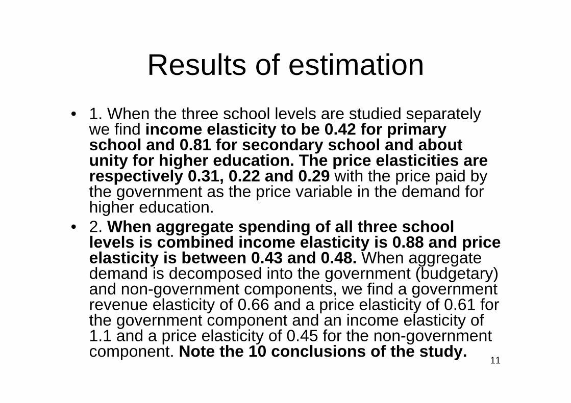
Results of estimation• 1. When the three school levels are studied separately

we find income elasticity to be 0.42 for primary school and 0.81 for secondary school and about unity for higher education. The price elasticities are respectively 0.31, 0.22 and 0.29 with the price paid by the government as the price variable in the demand for higher education.

• 2. When aggregate spending of all three school levels is combined income elasticity is 0.88 and price elasticity is between 0.43 and 0.48. When aggregate demand is decomposed into the government (budgetary) and non-government components, we find a government revenue elasticity of 0.66 and a price elasticity of 0.61 for the government component and an income elasticity of 1.1 and a price elasticity of 0.45 for the non-government component. Note the 10 conclusions of the study.

12

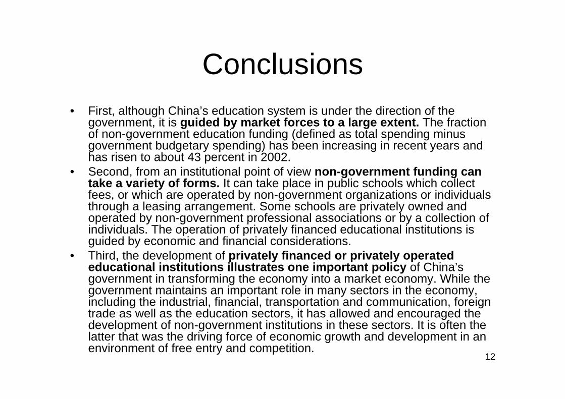
Conclusions• First, although China’s education system is under the direction of the

government, it is guided by market forces to a large extent. The fraction of non-government education funding (defined as total spending minus government budgetary spending) has been increasing in recent years and has risen to about 43 percent in 2002.

• Second, from an institutional point of view non-government funding can take a variety of forms. It can take place in public schools which collect fees, or which are operated by non-government organizations or individuals through a leasing arrangement. Some schools are privately owned and operated by non-government professional associations or by a collection of individuals. The operation of privately financed educational institutions is guided by economic and financial considerations.

• Third, the development of privately financed or privately operated educational institutions illustrates one important policy of China’s government in transforming the economy into a market economy. While the government maintains an important role in many sectors in the economy, including the industrial, financial, transportation and communication, foreign trade as well as the education sectors, it has allowed and encouraged the development of non-government institutions in these sectors. It is often the latter that was the driving force of economic growth and development in an environment of free entry and competition.

13

Conclusions - 2• Fourth, as compared with the parents in the United States the Chinese

parents have more choices of schools for their children. They are not subject to paying a real estate tax to finance the usually only local public school available to their children. The Chinese schools are financed partly by general tax revenue and partly by tuition. There are several public and private schools available to most urban families. The schools are not obliged to accept any student below the standard they set, and thus have different academic standards. Parents have choice of primary andsecondary schools and schools, public and private, can choose their students.

• Fifth, the framework of demand analysis is applicable to explain the spending on education, with real income and relative price as the major explanatory variables.

• Seventh, when aggregate spending of all three school levels is studied income elasticity is 0.88 and price elasticity is between 0.43 and 0.48.When aggregate demand is decomposed into the government (budgetary) and non-government components, we find a government revenue elasticity of 0.66 and a price elasticity of 0.61 for the government component and an income elasticity of 1.1 and a price elasticity of 0.45 for the non-government component. (Note the possible overestimation of price elasticity due to over estimation of the increase in price as a result of proportionally more students enrolled in universities in later years.)

14

Conclusions - 3• Eighth, our framework can explain the ratio of education expenditures to GDP very

well. The increase in this ratio from 3.38 in 1991 to 5.21 in 2002 can be explained by the increase in real GDP and government revenue which raised demand. Given an inelastic supply of education services, this resulted in a large increase in price. Since demand is price inelastic, total spending increased as price increased. This mechanism, explicitly given in equation (5), can explain the increase in the ratio of education spending to GDP in other rapidly developing countries as well..

• Ninth, on the relation between income inequality and education inequality (respectively measured by the standard deviation of log (per capita income) and log (per capita education spending) across provinces), to the extent that the demand for education is affected by income, income inequality will be reflected in education inequality. For primary school and secondary school education, the degree of education inequality is less than the degree of income inequality, indicating that education opportunities tend to be more nearly equal among families of different incomes. However, since other factors than income affect education expenditures as well, inequality in education spending can be larger than income inequality. This is the case for higher education, and to a lesser extent for aggregate education and for its government and non-government components.

• Tenth, the Chinese government places a strong emphasis on developing world class universities and has spent a large amount on higher education. In the mean time it has a policy of compulsory education for nine years but many children aged fifteen or below do not receive the required education because the central government has given the responsibility for providing it to provincial and local governments which may have limited financial resources and resort to collecting tuitions and fees from the students.

15

Demand and supply of healthcare -motivation

• Economic conditions of the Chinese people have improved a great deal since economic reform started in 1978 but healthcare provision has become worse for many people.

• To what extent is this true? Need to find evidence. For a long time many economists in China liked to make remarks beginning with “我认为.” Economics is not an expression of opinion but a scientific explanation of facts.

• If true how do we explain it?• How can we improve it? What is a good policy to

improve healthcare?

16

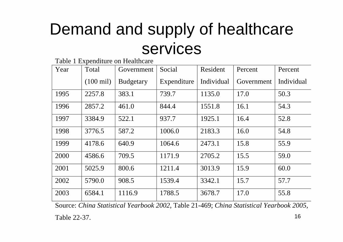
Demand and supply of healthcare services

Table 1 Expenditure on Healthcare Year Total

(100 mil)

Government

Budgetary

Social

Expenditure

Resident

Individual

Percent

Government

Percent

Individual

1995 2257.8 383.1 739.7 1135.0 17.0 50.3

1996 2857.2 461.0 844.4 1551.8 16.1 54.3

1997 3384.9 522.1 937.7 1925.1 16.4 52.8

1998 3776.5 587.2 1006.0 2183.3 16.0 54.8

1999 4178.6 640.9 1064.6 2473.1 15.8 55.9

2000 4586.6 709.5 1171.9 2705.2 15.5 59.0

2001 5025.9 800.6 1211.4 3013.9 15.9 60.0

2002 5790.0 908.5 1539.4 3342.1 15.7 57.7

2003 6584.1 1116.9 1788.5 3678.7 17.0 55.8

Source: China Statistical Yearbook 2002, Table 21-469; China Statistical Yearbook 2005,

Table 22-37.

17

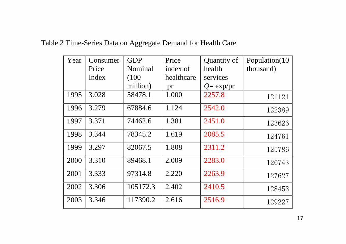
Table 2 Time-Series Data on Aggregate Demand for Health Care

Year ConsumerPrice Index

GDP Nominal (100 million)

Price index of healthcare pr

Quantity of health services Q= exp/pr

Population(10 thousand)

1995 3.028 58478.1 1.000 2257.8 121121

1996 3.279 67884.6 1.124 2542.0 122389

1997 3.371 74462.6 1.381 2451.0 123626

1998 3.344 78345.2 1.619 2085.5 124761

1999 3.297 82067.5 1.808 2311.2 125786

2000 3.310 89468.1 2.009 2283.0 126743

2001 3.333 97314.8 2.220 2263.9 127627

2002 3.306 105172.3 2.402 2410.5 128453

2003 3.346 117390.2 2.616 2516.9 129227

18

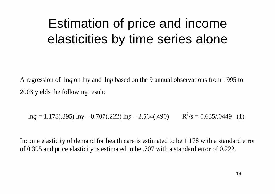
Estimation of price and income elasticities by time series alone

A regression of lnq on lny and lnp based on the 9 annual observations from 1995 to

2003 yields the following result:

lnq = 1.178(.395) lny – 0.707(.222) lnp – 2.564(.490) R2/s = 0.635/.0449 (1)

Income elasticity of demand for health care is estimated to be 1.178 with a standard error of 0.395 and price elasticity is estimated to be .707 with a standard error of 0.222.

19

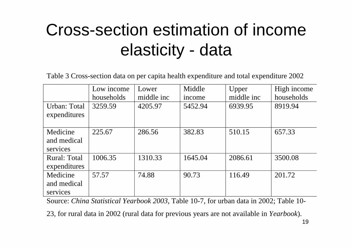
Cross-section estimation of income elasticity - data

Table 3 Cross-section data on per capita health expenditure and total expenditure 2002

Low income households

Lower middle inc

Middle income

Upper middle inc

High income households

Urban: Total expenditures

3259.59 4205.97 5452.94 6939.95 8919.94

Medicine and medical services

225.67 286.56 382.83 510.15 657.33

Rural: Total expenditures

1006.35 1310.33 1645.04 2086.61 3500.08

Medicine and medical services

57.57 74.88 90.73 116.49 201.72

Source: China Statistical Yearbook 2003, Table 10-7, for urban data in 2002; Table 10-

23, for rural data in 2002 (rural data for previous years are not available in Yearbook).

20

Cross-section estimation of income elasticity - results

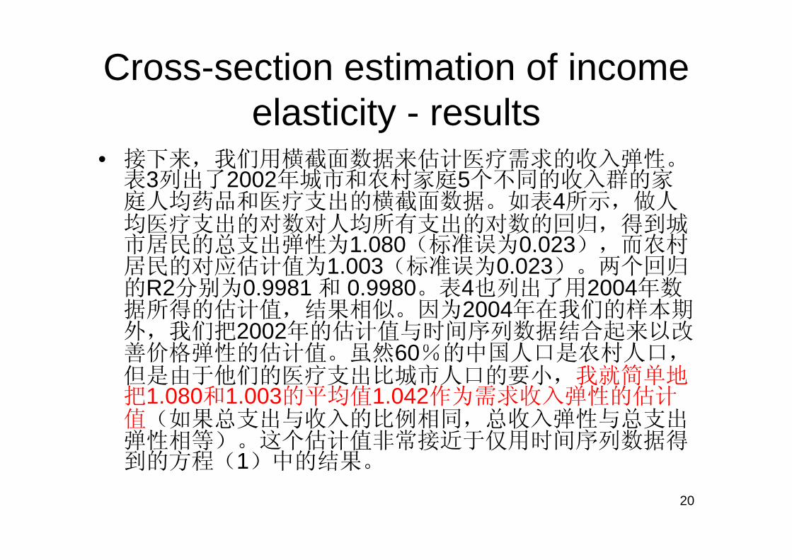
• 接下来，我们用横截面数据来估计医疗需求的收入弹性。表3列出了2002年城市和农村家庭5个不同的收入群的家庭人均药品和医疗支出的横截面数据。如表4所示，做人均医疗支出的对数对人均所有支出的对数的回归，得到城市居民的总支出弹性为1.080（标准误为0.023），而农村居民的对应估计值为1.003（标准误为0.023）。两个回归的R2分别为0.9981 和 0.9980。表4也列出了用2004年数据所得的估计值，结果相似。因为2004年在我们的样本期外，我们把2002年的估计值与时间序列数据结合起来以改善价格弹性的估计值。虽然60％的中国人口是农村人口，但是由于他们的医疗支出比城市人口的要小，我就简单地把1.080和1.003的平均值1.042作为需求收入弹性的估计值（如果总支出与收入的比例相同，总收入弹性与总支出弹性相等）。这个估计值非常接近于仅用时间序列数据得到的方程（1）中的结果。

21

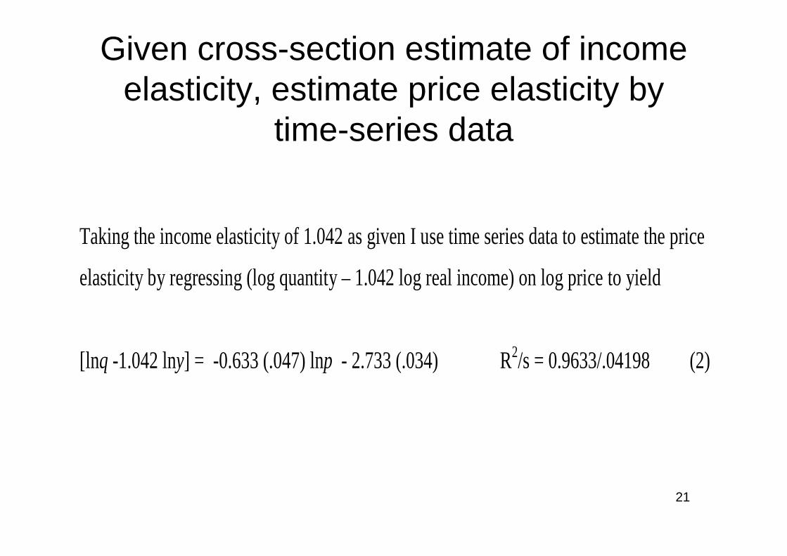
Given cross-section estimate of income elasticity, estimate price elasticity by

time-series data

Taking the income elasticity of 1.042 as given I use time series data to estimate the price

elasticity by regressing (log quantity – 1.042 log real income) on log price to yield

[lnq -1.042 lny] = -0.633 (.047) lnp - 2.733 (.034) R2/s = 0.9633/.04198 (2)

22

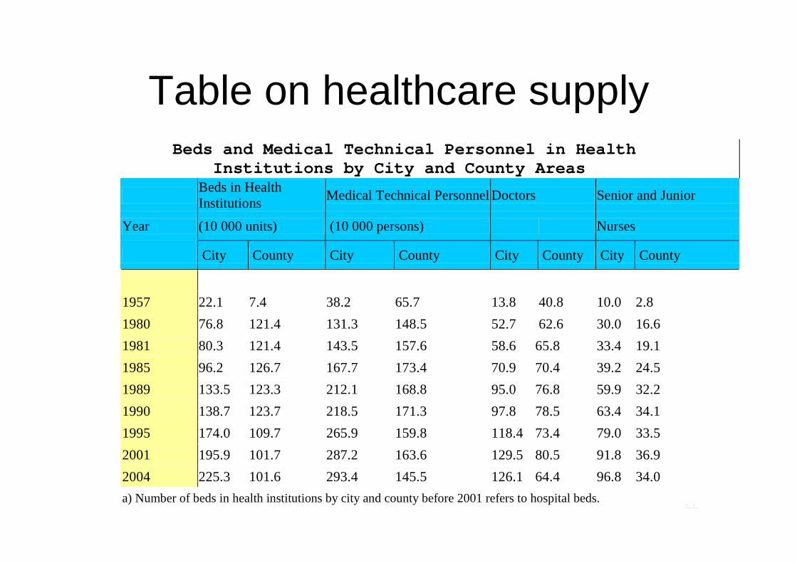
Table on healthcare supply Beds and Medical Technical Personnel in Health Institutions by City and County Areas

Beds in Health Institutions Medical Technical Personnel Doctors Senior and Junior

Year (10 000 units) (10 000 persons) Nurses

City County City County City County City County

1957 22.1 7.4 38.2 65.7 13.8 40.8 10.0 2.8 1980 76.8 121.4 131.3 148.5 52.7 62.6 30.0 16.6 1981 80.3 121.4 143.5 157.6 58.6 65.8 33.4 19.1 1985 96.2 126.7 167.7 173.4 70.9 70.4 39.2 24.5 1989 133.5 123.3 212.1 168.8 95.0 76.8 59.9 32.2 1990 138.7 123.7 218.5 171.3 97.8 78.5 63.4 34.1 1995 174.0 109.7 265.9 159.8 118.4 73.4 79.0 33.5 2001 195.9 101.7 287.2 163.6 129.5 80.5 91.8 36.9 2004 225.3 101.6 293.4 145.5 126.1 64.4 96.8 34.0 a) Number of beds in health institutions by city and county before 2001 refers to hospital beds.

23

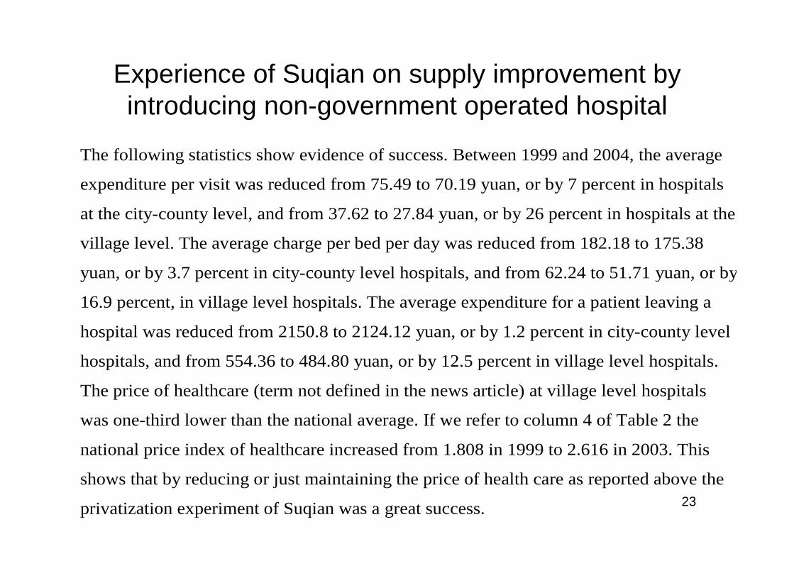
Experience of Suqian on supply improvement by introducing non-government operated hospital

The following statistics show evidence of success. Between 1999 and 2004, the average

expenditure per visit was reduced from 75.49 to 70.19 yuan, or by 7 percent in hospitals

at the city-county level, and from 37.62 to 27.84 yuan, or by 26 percent in hospitals at the

village level. The average charge per bed per day was reduced from 182.18 to 175.38

yuan, or by 3.7 percent in city-county level hospitals, and from 62.24 to 51.71 yuan, or by

16.9 percent, in village level hospitals. The average expenditure for a patient leaving a

hospital was reduced from 2150.8 to 2124.12 yuan, or by 1.2 percent in city-county level

hospitals, and from 554.36 to 484.80 yuan, or by 12.5 percent in village level hospitals.

The price of healthcare (term not defined in the news article) at village level hospitals

was one-third lower than the national average. If we refer to column 4 of Table 2 the

national price index of healthcare increased from 1.808 in 1999 to 2.616 in 2003. This

shows that by reducing or just maintaining the price of health care as reported above the

privatization experiment of Suqian was a great success.

24

Demand theory applies to healthcare in spite of asymmetric information

While I agree that asymmetric information, monopoly power and profit seeking at the

expense of the consumers exist, evidence in Suqian and elsewhere has demonstrated that

these are not sufficient to undermine the advantage of private supply of healthcare as

compared with public supply. A public hospital in lack of funds provided by the

government and doctors working in such a hospital can also use monopoly power to raise

more funds or to increase income at the expense of the consumers. Evidence of this will

be provided in section 6 where asymmetric information will be further discussed. A

private system allows for competition among many hospitals and reduces the monopoly

power of government hospitals. Given the available hospitals and doctors, most

consumers in Suqian and elsewhere are able to choose the better ones even some may be

misled. Doctors and hospitals misleading patients for short-term profits will be

discovered by the intelligent ones and words will spread. They will lose out in the long-

run and most of them understand this.

2525

Improvement in supply is an important aspect of healthcare reform

• This analysis does not deal with the problem of how to pay for healthcare or the healthcare insurance system. It deals with the supply side and not the demand side of the healthcare problem.

• On the demand side, if the government wants to help pay for the cost of healthcare it should subsidize the consumers and not the public hospitals because the consumers can decide which hospitals provide good services and only good hospitals get the money through providing good services to consumers.

26

Exchange rate of RMB – another application of demand and supply

• In 2007, the exchange rate of RMB against the US dollar was considered under valued, or the US dollar was overpriced again the RMB.

• Consider the market for exchange of dollars with the RMB. Define the price of $ as number of RMB per dollar. The equilibrium price of $ decreased because the supply of dollar had increased as a result of China’s trade surplus and of the Chinese having earned a lot of $ to be exchanged for the RMB.

27

Exercises• To improve your proficiency in applied economics one

simple way is to replicate the empirical results of published studies. Get the data and reestimate some or all of the equations.

• Try to improve the equations by changing some variables, either conceptually different variables (as in the case of permanent income of Milton Friedman replacing current income for explaining aggregate consumption), different measures of the same variables, or new variables.

• Use more up-to-date data, data for a different country or region, quarterly v. annual data, family v. provincial data.