The Islamic University Gaza

Higher Education Deanship

Faculty of Engineering

Electrical Engineering

Communication Systems

غزة – اإلسالمية الجامعة

العليا الدراسات عمادة

الهندسة كلية

الهندسة الكهربائية

أنظمة االتصاالت

LTE Antenna’s Parameter Enhancement for Mobile

Communication Applications

Submitted by:

Eng. Ahmed Hamdi Abo absa

Supervised by:

Dr. Mohamed Ouda

Dr. Ammar Abu Hudrouss

A Thesis Submitted in Partial Fulfillment of Requirements for the Degree of Master in Electrical

Engineering-Communication Systems.

م 1031-هـ 3411

i

THESIS ABSTRACT

Long Term Evolution (LTE) is a fourth generation standard for wireless communications of

high data speed at the user terminal. This evolved technology needs a cutting edge system

component to be designed for the node B (Base station) and the user mobile device.

In any wireless device, the performance of radio communications depends on the design of an

efficient antenna. The objective of this research work is to design printed antennas suitable for

use within LTE mobile terminals. To satisfy the antenna size of LTE devices, meander line

technology is used to reduce the resonant length of the antenna. Professional design software

(HFSS) is used to design and optimize a 0.78 and 2.5 GHz single element Meander Line

Antenna and E-shape MLA as anew shape to give an enhancement the bandwidth and the

small gain.

We used in this thesis two techniques: the first technique is parametric study where study each

variable in the antenna then study the effect each of them on the antenna, after that go to other

type and make the work until finish all the variables. The second technique is optimization

technique using Genetic Algorithms. This technique can be effectively used in the design of

various complex antenna and millimeter dimension circuits, where the performance of this

technique to design the antenna is a good precision design of antenna elements for low and

high frequency applications. MATLAB codes were written to determine the resonant

frequency and the bandwidth for each study in this thesis.

ii

Dedicated to

My Parents

Their prayers and perseverance led to this accomplishment

iii

ACKNOWLEDGEMENTS

In the name of Allah, the Most Gracious and the Most Merciful All praises and glory is to

Allah (SWT) for blessing me with opportunities abound and showering upon me his mercy

and guidance all through the life. I pray that He continues the same the rest of my life. And

may peace and blessings of Allah be upon Prophet Muhammad, a guidance and inspiration to

our lives.

I would like to thank my supervisors, Dr. Mohammed Ouda and Dr. Ammar Abu Hudrouss

for their guidance and expertise throughout this thesis. There were always there when I

needed them, and even with their tight schedule, they have always found time for me. I am

extremely grateful to them for their prompt replies and their numerous proofreads. I am also

very grateful to my thesis committee members, Dr. Mostafa Abu Al Naser and Dr. Tala Skaik

for their care, cooperation and constructive advices.

Special thanks to my colleagues and friends especially Eng. Abdelsalam Al Astal, Eng.

Ammar Al Tatar and Eng. Ahmed Al Farra for their encouragements and various help that

they provided throughout my graduate studies at Islamic University. I would like to give my

special thanks to my parents, brothers, sisters and my wife for their support, patience and love.

Without their encouragement, motivation and understanding it would have been impossible

for me to complete this work.

iv

Table of Contents

THESIS ABSTRACT .................................................................................................................................... i

ACKNOWLEDGEMENTS ......................................................................................................................... iii

LIST OF TABLES ....................................................................................................................................... vi

LIST OF FIGURES .................................................................................................................................... vii

CHAPTER 1 ................................................................................................................................................. 1

INTRODUCTION ........................................................................................................................................ 1

1.1 INTRODUCTION ........................................................................................................................ 1

1.2 REVIEW OF MOBILE COMMUNICATION STANDARDS .................................................... 1

1.2.1 INTRODUCTION ................................................................................................................ 2

1.2.2 THE FIRST MOBILE GENERATIONS (1G TO 2.5G) ...................................................... 2

1.2.3 THIRD MOBILE GENERATION NETWORKS (3G) ........................................................ 2

1.2.4 FUTURE MOBILE GENERATION NETWORKS (4G) .................................................... 3

1.3 LONG TERM EVOLUTION (LTE) ............................................................................................ 5

1.3.1 WHAT IS LTE? .................................................................................................................... 5

1.3.2 LTE BANDS ......................................................................................................................... 6

1.3.3 PERFORMANCE GOALS FOR LTE .................................................................................. 7

1.4 High Frequency Structure Simulator HFSS V. 12 ........................................................................ 8

1.5 THESIS MOTIVATION............................................................................................................... 9

1.6 THESIS OBJECTIVES................................................................................................................. 9

1.7 THESIS OVERVIEW ................................................................................................................. 10

REFERENCES ........................................................................................................................................... 10

CHAPTER 2 ............................................................................................................................................... 12

LITERATURE REVIEW ........................................................................................................................... 12

2.1 INTRODUCTION ...................................................................................................................... 12

2.2 PRINTED ANTENNA FOR MOBILE DEVICES ..................................................................... 12

2.2.1 ANTENNA BASICS .......................................................................................................... 13

2.3 ELECTRICALLY SMALL ANTENNA .................................................................................... 20

2.3.1 FUNDAMENTAL LIMITATIONS.................................................................................... 20

2.3.2 LIMIT ON RADIATION EFFICIENCY............................................................................ 21

v

REFERENCES ........................................................................................................................................... 22

CHAPTER 3 ............................................................................................................................................... 25

ANALYSIS AND DESIGN OF MEANDER LINE ANTENNA FOR LTE MOBILE

COMMUNICATIONS IN 0.78 GHZ ......................................................................................................... 25

3.1 INTRODUCTION ...................................................................................................................... 25

3.2 PARAMETRIC STUDY............................................................................................................. 26

3.3 THE OPTIMIZATION OF MLA WITH GENETIC ALGORITHM ......................................... 36

3.4 THE MLA DESIGN AND SIMULATION RESULTS USING GENETIC ALGORITHMS ... 39

3.5 COMPARISON BETWEEN OUR MLA FOR LTE AND MLA FOR LTE IN [8] ................... 42

3.6 CONCLUSIONS ......................................................................................................................... 45

REFERENCES ........................................................................................................................................... 45

CHAPTER 4 ............................................................................................................................................... 47

ANALYSIS AND DESIGN E-SHAPE MEANDER LINE ANTENNA FOR LTE MOBILE

COMMUNICATION IN 2.5 GHZ ............................................................................................................. 47

4.1 INTRODUCTION ...................................................................................................................... 47

4.2 E- SHAPE MLA ANALYSIS..................................................................................................... 48

4.3 PARAMETRIC STUDY............................................................................................................. 51

4.4 THE OPTIMIZATION OF E-SHAPE MLA WITH GENETIC ALGORITHM ....................... 61

4.5 THE E-SHAPE MLA DESIGN AND SIMULATION RESULTS USING GENETIC ALGORITHMS. 63

4.6 THE OPTIMIZATION OF E-SHAPE MLA WITH GENETIC ALGORITHM ON DIFFERENT SUBSTRATES . 66

4.7 CONCLUSIONS ......................................................................................................................... 67

REFERENCES ........................................................................................................................................... 67

CHAPTER 5 ............................................................................................................................................... 69

CONCLUSION ........................................................................................................................................... 69

5.1 CONCLUSION ........................................................................................................................... 69

5.2 FUTURE WORK ........................................................................................................................ 70

vi

LIST OF TABLES

Table 1.1: Transport Technologies [5], [6] .................................................................................... 3

Table 1.2: Lte Fdd Frequency Bands And Channel Numbers [6] ................................................. 6

Table 1.3: Lte Performance Requirements [10] ............................................................................. 7

Table 3.1: Specifications Of The Ga ............................................................................................ 38

Table 3.2: The Parameters Were Optimized By Using Ga In Hfss (All Parameters Are Given

In Mm) ........................................................................................................................ 39

Table 3.3: The Difference Between The Final Design Using Parametric And Optimization

Method ........................................................................................................................ 42

Table 3.4: Mla For Lte In [8] Specifications ............................................................................... 43

Table 3.5: Differences Between Our Mla And Mla In [8] ........................................................... 45

Table 4.1: The Ground Height Effect On The E-Shape Mla ....................................................... 52

Table 4.2: The Width W3 Affecting On The E-Shape Mla ......................................................... 53

Table 4.3: The Width W1, W5 And W6 Effect On The E-Shape Of The Mla ............................ 55

Table 4.4: The Width W2 Affecting On The E-Shape Mla ......................................................... 57

Table 4.5: The Width W2 Affecting On The E-Shape Mla ......................................................... 59

Table 4.6: Specification Of The Ga ............................................................................................. 62

Table 4.7: The Parameters Were Optimized By Using Ga In Hfss ............................................. 63

Table 4.8: The Difference Between The Final Design Using Parametric And Optimization

Method ........................................................................................................................ 66

Table 4.9: The Difference Between The Different Substrate Materials ...................................... 66

Table 4.10: The Antenna Parameters For The Different Substrate Materials ............................. 67

vii

LIST OF FIGURES

Figure 1.1: The Evolution of Wireless Communication Standards [8] ......................................... 5

Figure 2.1: Basic rectangular microstip patch antenna construction ........................................... 18

Figure 2.2: Microstrip Antenna Feeding Methods...................................................................... 18

Figure 2.3: Planar Inverted F Antenna......................................................................................... 19

Figure 2.4: The Fundamental Section of the Meander Line Antenna ......................................... 20

Figure 2.5: Equivalent Circuits of a Magnetic and Electric Dipole............................................. 22

Figure 3.1: MLA Antenna in [3] .................................................................................................. 26

Figure 3.2:MLA antenna for LTE in 0.78 GHZ .......................................................................... 26

Figure 3.3: Parameters in MLA ................................................................................................... 26

Figure 3.4: Return loss for the different height of the ground ..................................................... 27

Figure 3.5: Return loss for the different values for the width w1 ................................................ 28

Figure 3.6: Max gain for the resonant frequency at the phi from -1800 to 1800 for different

values of w1 ............................................................................................................... 28

Figure 3.7: Max gain for the resonant frequency at the theta from 00 to 1800 for different

values of w1 ............................................................................................................... 29

Figure 3.8: Return loss for varying the width w2 ........................................................................ 30

Figure 3.9: Max gain for the resonant frequency at the phi from -1800 to 1800 for different

values of w2 ............................................................................................................... 30

Figure 3.10: Max gain for the resonant frequency at the theta from 00 to 1800 for different

values of w2 ............................................................................................................... 31

Figure 3.11: Return loss for the different width of w3 ................................................................ 32

Figure 3.12: Max gain for the resonant frequency at the phi from -1800 to 1800 for different

values of w3 ............................................................................................................... 32

Figure 3.13: Max gain for the resonant frequency at the theta from 00 to 1800 for different

values of w3 ............................................................................................................... 33

Figure 3.14: Return loss for the different width w4 .................................................................... 34

Figure 3.15: Max gain for the resonant frequency at the phi from -1800 to 1800 for different

values of w4 ............................................................................................................... 34

Figure 3.16: Max gain for the resonant frequency at the theta from 00 to 1800 for different

values of w4 ............................................................................................................... 35

Figure 3.17: The final design for the MLA using parametric study ............................................ 35

Figure 3.18: The return loss for the final design for the MLA using parametric study ............... 36

Figure 3.19: The radiation pattern for the final design for the MLA using parametric study ..... 36

Figure 3.20: The gain for the final design for the MLA using parametric study......................... 36

Figure 3.21: The optimization flowchart of GA technique ......................................................... 37

Figure 3.22: Using GA technique in HFSS ................................................................................. 38

Figure 3.23: The final design of the MLA using GA. ................................................................. 39

Figure 3.24: The return loss for the final design of MLA using GA. .......................................... 40

viii

Figure 3.25: The radiation pattern for the final design of MLA using GA ................................. 40

Figure 3.26: The gain for the final design of the MLA using GA. .............................................. 40

Figure 3.27: The maximum gain for each frequency at phi=0. ................................................... 41

Figure 3.28: Max gain for the resonant frequency at the phi from -1800 to 1800 ...................... 41

Figure 3.29: Max gain for the resonant frequency at the theta from 00 to 1800 ......................... 42

Figure 3.30: HFSS Model for the MLA Antenna in [8] .............................................................. 43

Figure 3.31: Reflection Coefficient for the Designed MLA ........................................................ 44

Figure 3.32: 3D Radiation Pattern ............................................................................................... 44

Figure 4.1: MLA Antenna shape in [10]...................................................................................... 48

Figure 4.2: The E-shape MLA antenna ....................................................................................... 48

Figure 4.3: E-shape MLA ............................................................................................................ 49

Figure 4.4: Equivalent circuits of (a) rectangular patch and (b) E-shape antenna [14] ............... 50

Figure 4.5: Return loss for the different height of the ground ..................................................... 51

Figure 4.6: Max gain for each frequency input at phi = 0 ........................................................... 52

Figure 4.7: Return loss for the different values for the width w3 ................................................ 53

Figure 4.8: Max gain for each frequency at phi=0 ...................................................................... 54

Figure 4.9: Return loss for varying the width w1, w5 and w6 .................................................... 55

Figure 4.10: Max gain for each frequency at phi=0 when varying the width w1, w5 and w6 .... 56

Figure 4.11: Return loss for the different width w2 .................................................................... 57

Figure 4.12: Max gain for each frequency at phi=0 .................................................................... 58

Figure 4.13: Return loss for the different width w4 .................................................................... 59

Figure 4.14: Max gain at each frequency at phi=0 ...................................................................... 60

Figure 4.15: The final design for the E-shape MLA using Parametric study .............................. 60

Figure 4.16: The return loss for the final design for the E-shape MLA using Parametric study. 61

Figure 4.17: The radiation pattern for the final design for the E-shape MLA using Parametric

study .......................................................................................................................... 61

Figure 4.18: The gain for the final design for the E-shape MLA using Parametric study .......... 61

Figure 4.19: Using GA technique in HFSS ................................................................................. 62

Figure 4.20: The final design of the E-shape MLA using GA. ................................................... 64

Figure 4.21: The return loss for the final design of the E-shape MLA using GA. ...................... 64

Figure 4.22: The radiation pattern for the final design of the E-shape MLA using GA.............. 65

Figure 4.23: The gain for the final design of the E-shape MLA using GA. ................................ 65

Figure 4.24: The maximum gain for each frequency at pi=0. ..................................................... 65

1

CHAPTER 1

INTRODUCTION

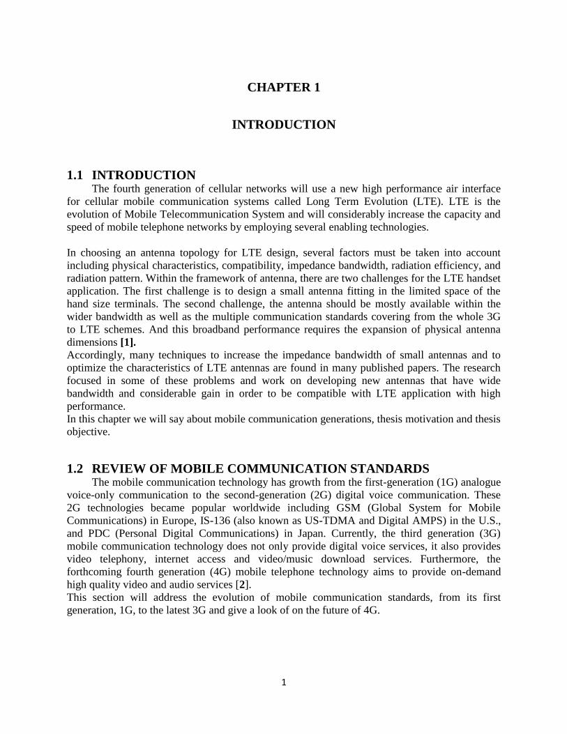
1.1 INTRODUCTION The fourth generation of cellular networks will use a new high performance air interface

for cellular mobile communication systems called Long Term Evolution (LTE). LTE is the

evolution of Mobile Telecommunication System and will considerably increase the capacity and

speed of mobile telephone networks by employing several enabling technologies.

In choosing an antenna topology for LTE design, several factors must be taken into account

including physical characteristics, compatibility, impedance bandwidth, radiation efficiency, and

radiation pattern. Within the framework of antenna, there are two challenges for the LTE handset

application. The first challenge is to design a small antenna fitting in the limited space of the

hand size terminals. The second challenge, the antenna should be mostly available within the

wider bandwidth as well as the multiple communication standards covering from the whole 3G

to LTE schemes. And this broadband performance requires the expansion of physical antenna

dimensions [1].

Accordingly, many techniques to increase the impedance bandwidth of small antennas and to

optimize the characteristics of LTE antennas are found in many published papers. The research

focused in some of these problems and work on developing new antennas that have wide

bandwidth and considerable gain in order to be compatible with LTE application with high

performance.

In this chapter we will say about mobile communication generations, thesis motivation and thesis

objective.

1.2 REVIEW OF MOBILE COMMUNICATION STANDARDS The mobile communication technology has growth from the first-generation (1G) analogue

voice-only communication to the second-generation (2G) digital voice communication. These

2G technologies became popular worldwide including GSM (Global System for Mobile

Communications) in Europe, IS-136 (also known as US-TDMA and Digital AMPS) in the U.S.,

and PDC (Personal Digital Communications) in Japan. Currently, the third generation (3G)

mobile communication technology does not only provide digital voice services, it also provides

video telephony, internet access and video/music download services. Furthermore, the

forthcoming fourth generation (4G) mobile telephone technology aims to provide on-demand

high quality video and audio services [2].

This section will address the evolution of mobile communication standards, from its first

generation, 1G, to the latest 3G and give a look of on the future of 4G.

2

1.2.1 INTRODUCTION

New mobile generations do not pretend to improve the voice communication experience

but try to give the user access to a new global communication reality. The aim is to reach

communication every time and everywhere and to provide users with a new set of services. The

growth of the number of mobile subscribers over the last years led to a saturation of voice-

oriented wireless telephony. From 214 million subscribers in 1997 to 1162 million in 2002 [3], it

is predicted that by 2016 there will be 1.43 billion subscribers worldwide [4]. It is now time to

explore new demands and to find new ways to extend the mobile concept. The first steps have

already been taken by the 2.5G, which gave users access to data networks (e.g. Internet access

and MMS - Multimedia Message Service). However, users and applications demanded more

communication data rates. In response to this demand a new generation with new standards has

been developed - 3G.

In the last years, benefiting from 3G constant delays, many new mobile technologies were

deployed with great success e.g. Wi-Fi (Wireless Fidelity). Now, all this new technologies (e.g.

UMTS, Wi-Fi, and Bluetooth) can only be achieved by a new mobile generation. This new

mobile generation to be deployed must work with many mobile technologies while being

transparent to the final user.

1.2.2 THE FIRST MOBILE GENERATIONS (1G TO 2.5G)

In 1G, a narrow band analogue wireless network is used, with this we can have the voice

calls and can send text messages. These services are provided with circuit switching. The 2G

narrow band wireless network also uses the circuit switching model but provides more voice

clarity as compared to 1G.

Both 1G and 2G deal with voice calls and sending messages i.e. SMS (Short Message Service).

The latest technologies such as GPRS (General Packet Radio Service), is not available in these

generations. But the greatest disadvantage to 1G is that it can be used only within a particular

nation, where in the case of 2G, the roaming facility is a semi-global one.

In between 2G and 3G there is another generation called 2.5G. Initially, this mid generation was

introduced mainly for involving latest bandwidth technology with addition to the existing 2G

generation.

1.2.3 THIRD MOBILE GENERATION NETWORKS (3G)

To overcome the limitations of 2G and 2.5G, 3G was introduced. In 3G a Wide Band

Wireless Network is utilized with which the clarity increases and gives the perfection as like that

of a real conversation. The data are sent through a technology called Packet Switching .Voice

calls are interpreted through Circuit Switching.

With the help of 3G, we can access many new services too. One such service is global roaming.

In 3G we can also have several entertainments services such as Fast Communication, Internet,

Mobile T.V, Video Conferencing, Video Calls, Multi Media Messaging Service (MMS), 3D

gaming, Multi-Gaming etc.

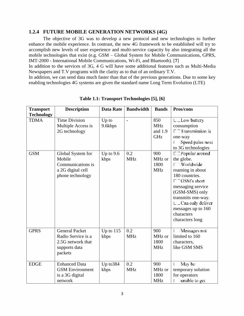
Table 1 shows some specifications for some of the standards used in the first three generations

such as data rate, bandwidth and bands.

3

1.2.4 FUTURE MOBILE GENERATION NETWORKS (4G)

The objective of 3G was to develop a new protocol and new technologies to further

enhance the mobile experience. In contrast, the new 4G framework to be established will try to

accomplish new levels of user experience and multi-service capacity by also integrating all the

mobile technologies that exist (e.g. GSM – Global System for Mobile Communications, GPRS,

IMT-2000 - International Mobile Communications, Wi-Fi, and Bluetooth). [7]

In addition to the services of 3G, 4 G will have some additional features such as Multi-Media

Newspapers and T.V programs with the clarity as to that of an ordinary T.V.

In addition, we can send data much faster than that of the previous generations. Due to some key

enabling technologies 4G systems are given the standard name Long Term Evolution (LTE)

Table 1.1: Transport Technologies [5], [6]

Transport

Technology

Description Data Rate Bandwidth Bands Pros/cons

TDMA Time Division

Multiple Access is

2G technology

Up to

9.6kbps

-

850

MHz

and 1.9

GHz

consumption

one-way

to 3G technologies

GSM

Global System for

Mobile

Communications is

a 2G digital cell

phone technology

Up to 9.6

kbps

0.2

MHz

900

MHz or

1800

MHz

the globe.

roaming in about

180 countries.

messaging service

(GSM-SMS) only

transmits one-way.

messages up to 160

characters

characters long

GPRS

General Packet

Radio Service is a

2.5G network that

supports data

packets

Up to 115

kbps

0.2

MHz

900

MHz or

1800

MHz

limited to 160

characters,

like GSM SMS

EDGE

Enhanced Data

GSM Environment

is a 3G digital

network

Up to384

kbps

0.2

MHz

900

MHz or

1800

MHz

temporary solution

for operators

4

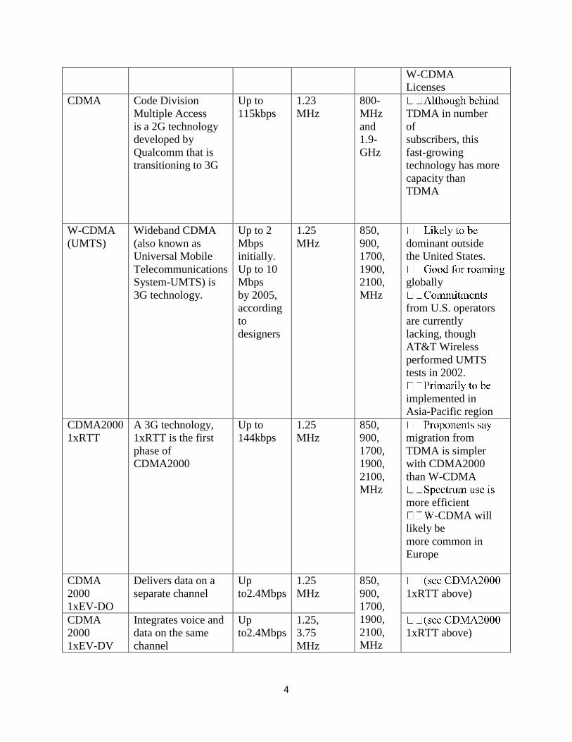
W-CDMA

Licenses

CDMA

Code Division

Multiple Access

is a 2G technology

developed by

Qualcomm that is

transitioning to 3G

Up to

115kbps

1.23

MHz

800-

MHz

and

1.9-

GHz

TDMA in number

of

subscribers, this

fast-growing

technology has more

capacity than

TDMA

W-CDMA

(UMTS)

Wideband CDMA

(also known as

Universal Mobile

Telecommunications

System-UMTS) is

3G technology.

Up to 2

Mbps

initially.

Up to 10

Mbps

by 2005,

according

to

designers

1.25

MHz

850,

900,

1700,

1900,

2100,

MHz

dominant outside

the United States.

globally

from U.S. operators

are currently

lacking, though

AT&T Wireless

performed UMTS

tests in 2002.

implemented in

Asia-Pacific region

CDMA2000

1xRTT

A 3G technology,

1xRTT is the first

phase of

CDMA2000

Up to

144kbps

1.25

MHz

850,

900,

1700,

1900,

2100,

MHz

migration from

TDMA is simpler

with CDMA2000

than W-CDMA

more efficient

-CDMA will

likely be

more common in

Europe

CDMA

2000

1xEV-DO

Delivers data on a

separate channel

Up

to2.4Mbps

1.25

MHz

850,

900,

1700,

1900,

2100,

MHz

1xRTT above)

CDMA

2000

1xEV-DV

Integrates voice and

data on the same

channel

Up

to2.4Mbps

1.25,

3.75

MHz

1xRTT above)

5

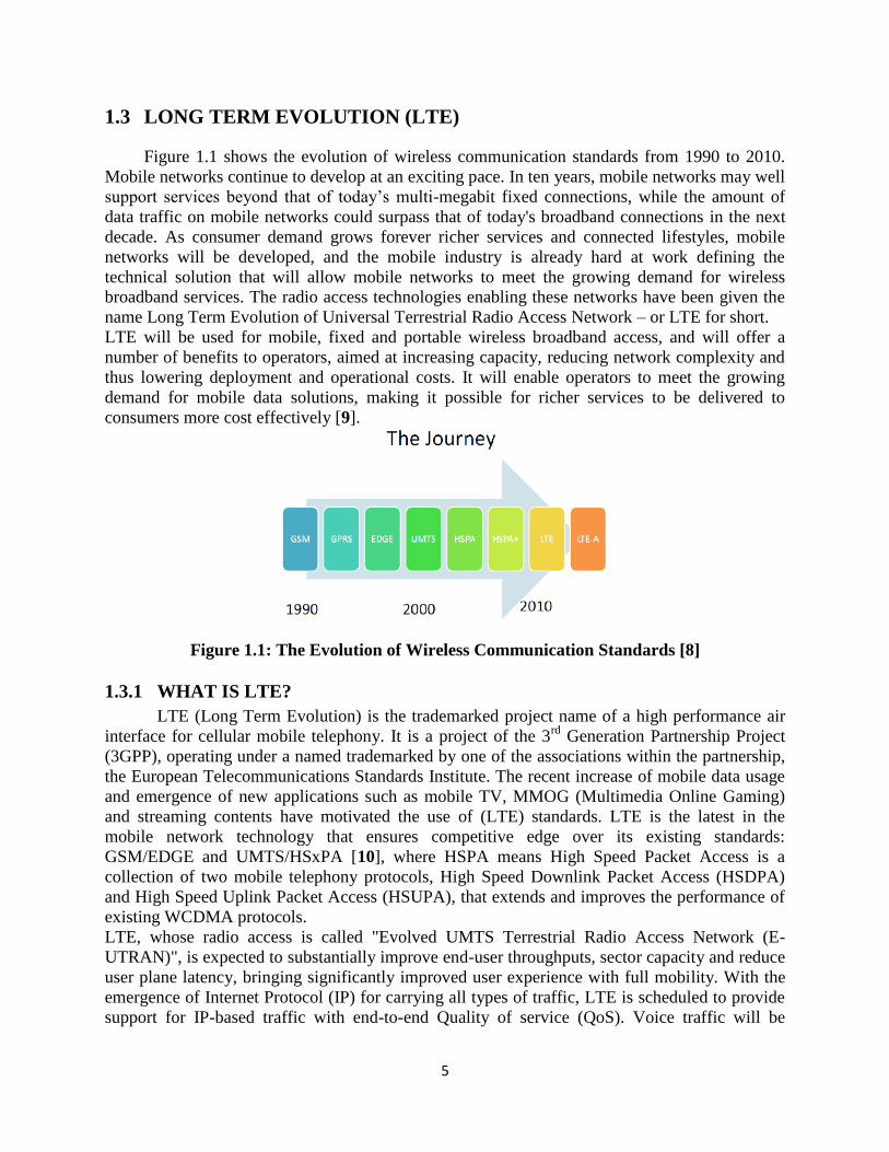
1.3 LONG TERM EVOLUTION (LTE)

Figure 1.1 shows the evolution of wireless communication standards from 1990 to 2010.

Mobile networks continue to develop at an exciting pace. In ten years, mobile networks may well

support services beyond that of today’s multi-megabit fixed connections, while the amount of

data traffic on mobile networks could surpass that of today's broadband connections in the next

decade. As consumer demand grows forever richer services and connected lifestyles, mobile

networks will be developed, and the mobile industry is already hard at work defining the

technical solution that will allow mobile networks to meet the growing demand for wireless

broadband services. The radio access technologies enabling these networks have been given the

name Long Term Evolution of Universal Terrestrial Radio Access Network – or LTE for short.

LTE will be used for mobile, fixed and portable wireless broadband access, and will offer a

number of benefits to operators, aimed at increasing capacity, reducing network complexity and

thus lowering deployment and operational costs. It will enable operators to meet the growing

demand for mobile data solutions, making it possible for richer services to be delivered to

consumers more cost effectively [9].

Figure 1.1: The Evolution of Wireless Communication Standards [8]

1.3.1 WHAT IS LTE?

LTE (Long Term Evolution) is the trademarked project name of a high performance air

interface for cellular mobile telephony. It is a project of the 3rd

Generation Partnership Project

(3GPP), operating under a named trademarked by one of the associations within the partnership,

the European Telecommunications Standards Institute. The recent increase of mobile data usage

and emergence of new applications such as mobile TV, MMOG (Multimedia Online Gaming)

and streaming contents have motivated the use of (LTE) standards. LTE is the latest in the

mobile network technology that ensures competitive edge over its existing standards:

GSM/EDGE and UMTS/HSxPA [10], where HSPA means High Speed Packet Access is a

collection of two mobile telephony protocols, High Speed Downlink Packet Access (HSDPA)

and High Speed Uplink Packet Access (HSUPA), that extends and improves the performance of

existing WCDMA protocols.

LTE, whose radio access is called "Evolved UMTS Terrestrial Radio Access Network (E-

UTRAN)", is expected to substantially improve end-user throughputs, sector capacity and reduce

user plane latency, bringing significantly improved user experience with full mobility. With the

emergence of Internet Protocol (IP) for carrying all types of traffic, LTE is scheduled to provide

support for IP-based traffic with end-to-end Quality of service (QoS). Voice traffic will be

6

supported mainly as Voice over IP (VoIP) enabling better integration with other multimedia

services. [10].

LTE uses Evolved Packet Core (EPC) network architecture to support the EUTRAN which

reduces the number of network elements, simplifies functionality, improves redundancy, but

most importantly allows for connections and hand-over to other fixed line and wireless access

technologies in a flawless manner. The aggressive performance of LTE rely on physical layer

technologies, such as, Orthogonal Frequency Division Multiplexing (OFDM), Multiple-Input

Multiple-Output (MIMO) systems and Smart Antennas to achieve these targets. The main

objective of LTE is to minimize the system and user-equipment complexities for high data

throughput and reduced latency.

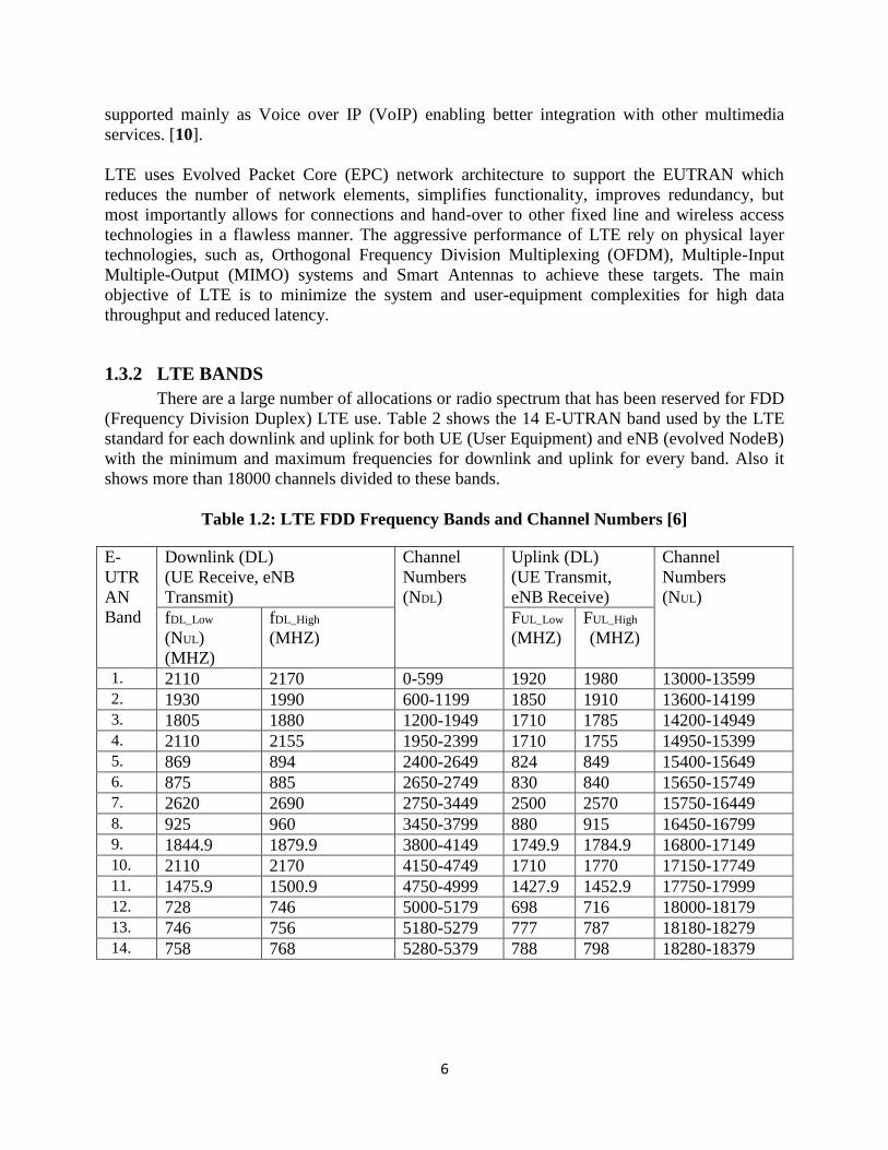
1.3.2 LTE BANDS

There are a large number of allocations or radio spectrum that has been reserved for FDD

(Frequency Division Duplex) LTE use. Table 2 shows the 14 E-UTRAN band used by the LTE

standard for each downlink and uplink for both UE (User Equipment) and eNB (evolved NodeB)

with the minimum and maximum frequencies for downlink and uplink for every band. Also it

shows more than 18000 channels divided to these bands.

Table 1.2: LTE FDD Frequency Bands and Channel Numbers [6]

E-

UTR

AN

Band

Downlink (DL)

(UE Receive, eNB

Transmit)

Channel

Numbers

(NDL)

Uplink (DL)

(UE Transmit,

eNB Receive)

Channel

Numbers

(NUL)

fDL_Low

(NUL)

(MHZ)

fDL_High

(MHZ)

FUL_Low

(MHZ)

FUL_High

(MHZ)

1. 2110 2170 0-599 1920 1980 13000-13599 2. 1930 1990 600-1199 1850 1910 13600-14199 3. 1805 1880 1200-1949 1710 1785 14200-14949 4. 2110 2155 1950-2399 1710 1755 14950-15399 5. 869 894 2400-2649 824 849 15400-15649 6. 875 885 2650-2749 830 840 15650-15749 7. 2620 2690 2750-3449 2500 2570 15750-16449 8. 925 960 3450-3799 880 915 16450-16799 9. 1844.9 1879.9 3800-4149 1749.9 1784.9 16800-17149 10. 2110 2170 4150-4749 1710 1770 17150-17749 11. 1475.9 1500.9 4750-4999 1427.9 1452.9 17750-17999 12. 728 746 5000-5179 698 716 18000-18179 13. 746 756 5180-5279 777 787 18180-18279 14. 758 768 5280-5379 788 798 18280-18379

7

1.3.3 PERFORMANCE GOALS FOR LTE

E-UTRA is expected to support different types of services including web browsing, FTP

(File Transfer Protocol), video streaming, VoIP (Voice over Internet Protocol), online gaming,

real time video, push-to-talk and push-to-view. Therefore, LTE is being designed to be a high

data rate and low latency system as indicated by the key performance criteria shown in Table 3.

The bandwidth capability of a UE is expected to be up to 20 MHz for both transmission and

reception. The service provider can however deploy cells with any of the bandwidths listed in

Table 3. This gives flexibility to service providers to tailor their offering dependent on the

amount of available spectrum or the ability to start with limited spectrum for lower upfront cost

and grow the spectrum for extra capacity.

TABLE 1.3: LTE PERFORMANCE REQUIREMENTS [10]

Metric Requirements

Peak Data Rate DL: 100Mbps

UL: 50Mbps

(For 20MHz Spectrum)

Mobility Support Up to 500Kmph but optimized for low

speeds from 0-15kmph

Control Plane Latency (Transition Time to

Active State)

<100ms (For Idle to Active)

User Plane Latency <5ms

Control Plane Capacity >200 users per cell (For 5MHz spectrum)

Coverage (Cell Size) 5-100Km with slight degradation after

30Km

Spectrum Flexibility 1.25, 2.5, 5, 10, 15 and 20 MHz

LTE has an instantaneous downlink peak data rate (DL) of 100 Mbps within a 20 MHz downlink

spectrum allocation (5 bps/Hz) and an instantaneous uplink peak data rate (UL) of 50 Mb/s (2.5

bps/Hz) within a 20 MHz uplink spectrum allocation. The Control plane latency has a transition

time of less than 100 ms from a camped state to an active state and less than 50 ms from a

dormant state and an active state. The control plane capacity is at least 200 users per cell and is

supported in the active state for spectrum allocations up to 5 MHz. The user plane latency is of

less than 5ms in unloading condition (i.e. single user with single data stream) for small IP packet.

The downlink average user throughput per MHz for 4G networks is 3 to 4 times larger and the

uplink average user throughput per MHz is 2 to 3 times larger as compared to 3G networks. The

target for spectrum efficiency of downlink in a loaded network is 3 to 4 times larger and for

uplink it is 2 to 3 times larger. E-UTRAN should be optimized for low mobile speed from 0 to 15

km/h. The higher mobile speed between 15 and 120 km/h should be supported with high

performance and mobility across the cellular network shall be maintained at speeds from 120

km/h to 350 km/h (or even up to 500 km/h depending on the frequency band).Throughput,

spectrum efficiency and mobility targets above should be met for 5 km cells, and with a slight

degradation for 30 km cells and the cells in a range up to 100 km should not be precluded.

Co-existence in the same geographical area and co-location with GERAN/UTRAN on adjacent

channels is also accounted for. GERAN is an abbreviation for GSMEDGE Radio Access

Network. The standards for GERAN are maintained by the 3GPP (Third Generation Partnership

8

Project). GERAN is a key part of GSM, and also of combined UMTS/GSM networks. GERAN

is the radio part of GSM/EDGE together with the network that joins the base stations and the

base station controllers. The network represents the core of a GSM network, through which

phone calls and packet data are routed from and to the PSTN and Internet to and from subscriber

handsets. A mobile phone operator's network comprises one or more GERANs, coupled with

UTRANs in the case of a UMTS/GSM network.

A GERAN network without EDGE is a GRAN, but is otherwise identical in concept. A GERAN

network without GSM is an ERAN

1.4 High Frequency Structure Simulator HFSS V. 12 HFSS is the industry-standard simulation tool for 3D full-wave electromagnetic field

simulation. HFSS provides E- and H-fields, currents, S-parameters and near and far radiated field

results. Intrinsic to the success of HFSS as an engineering design tool is its automated solution

process where users are only required to specify geometry, material properties and the desired

output. From here HFSS will automatically generate an appropriate, efficient and accurate mesh

for solving the problem using the proven finite element method.

The core of the program HFSS is based on the finite element method (FEM) (its practical

application often known as finite element analysis (FEA)) where it is a numerical technique for

finding approximate solutions to partial differential equations (PDE) and their systems, as well as

(less often) integral equations. FEM is a special case of the more general Galerkin method with

polynomial approximation functions. The solution approach is based on eliminating the spatial

derivatives from the PDE. This approximates the PDE with

a system of algebraic equations for steady state problems,

a system of ordinary differential equations for transient problems.

These equation systems are linear if the underlying PDE is linear, and vice versa. Algebraic

equation systems are then solved using numerical linear algebra methods. Ordinary differential

equations that arise in transient problems then numerically integrated using standard techniques

such as Euler's method, Runge Kutta, etc.

There is a large number of open source and commercial finite element softwares. More recently,

first web browser-based FEA applications became available such as in NC Lab.

In solving partial differential equations, the primary challenge is to create an equation that

approximates the equation to be studied, but is numerically stable, meaning that errors in the

input and intermediate calculations do not accumulate and cause the resulting output to be

meaningless. There are many ways of doing this, all with advantages and disadvantages. The

finite element method is a good choice for solving partial differential equations over complicated

domains (like cars and oil pipelines), when the domain changes (as during a solid state reaction

with a moving boundary), when the desired precision varies over the entire domain, or when the

solution lacks smoothness. For instance, in a frontal crash simulation it is possible to increase

prediction accuracy in "important" areas like the front of the car and reduce it in its rear (thus

reducing cost of the simulation). Another example would be in Numerical weather prediction,

9

where it is more important to have accurate predictions over developing highly nonlinear

phenomena (such as tropical cyclones in the atmosphere, or eddies in the ocean) rather than

relatively calm areas.

HFSS software automatically generates an appropriate, efficient and accurate mesh for solving

the problem using the proven finite element method. With HFSS, the physics define the mesh;

the mesh does not define the physics.

To solve the most demanding high-frequency simulations all of the HFSS solvers are equipped

with High-Performance Computing (HPC) options including Domain Decomposition and

Distributed Processing. These HPC options will decrease computation time and leverage existing

computer resources to solve very large simulations.

Engineers rely on the accuracy, capacity, and performance of HFSS to design high-speed

components including on-chip embedded passives, IC packages, PCB interconnects, and high-

frequency components such as antennas, RF/microwave components, and biomedical devices

[11].

1.5 THESIS MOTIVATION In the recent years, there has been rapid growth in wireless communications. With the

increasing number of users and limited bandwidth available, operators are trying hard to

optimize the network for larger capacity and improved quality coverage. This has led to the field

of antenna engineering to constantly evolve and accommodate the need for wideband, low-cost,

miniaturized and easily integrated antennas [12].

Since LTE will be the technology used for the next generation of mobile communication which

will be implemented by the end of this year and will be commercialized by the coming years,

there will be a huge demand for it. Because of these reasons, mobile phones should be

compatible with the technology mentioned above and in order to achieve this, mobile antennas

should be properly designed according to the new LTE standards.

In this thesis, we propose an enhancement for the meander line antenna for designing an antenna

within the LTE specifications in 0.78 and 2.5 GHz; where the band 0.7-0.8 GHz was used at

2010 in UEA and the band from 2.3-2.6 GHz will be used at 2015 in the Middle East [13].

1.6 THESIS OBJECTIVES The objectives for this work are the following:

A. Analyze, design and optimize a single element meander line antenna system for LTE

standards. The design should fit within a cellular phone handset size and satisfy the

following requirements.

a. Operating frequency of 0.780 and 2.5 GHz with a bandwidth greater than 40 MHz

b. Size of the antenna should be small.

B. Select the best enhancement of the antenna that deal with satisfaction of LTE.

C. Design a new modification for the LTE antenna standards.

10

1.7 THESIS OVERVIEW The thesis is organized in five chapters as follows:

Chapter 2 of this thesis starts with an introduction of the types of mobile printed antennas and

electrically small antennas and it summarizes the reviewed literature. In Chapter 3, the analysis

and design of a Meander Line Antenna (MLA) in 0.78GHz is described and compare it with the

antenna for LTE in 0.78 GHz as shown in [13]. Chapter 4 describes the analysis and design of an

E-shape Meander Line Antenna in 2.5 GHz. The simulated (HFSS) radiation characteristics

associated with the designed antenna will be discussed in this chapter also. Finally chapter 5

describes the conclusions drawn from this research work and recommendations on future work to

be carried on this subject.

REFERENCES [1] S. Lee and A. Kim, "Broadband Internal Antenna for 700MHz LTE Application with Distributed

Feeder",Advanced CAE Lab, Samsung Electronics416, Metan-3dong, 443-742, Korea,2009.

[2] K. Peter. Analysis and Comparison of 1G , 2G , 3G ,4G and 5G TelecomServices. [Online].

http://hubpages.com/hub/3G-and-4G-Mobile-Services, 27/06/2012.

[3] ITU. (2002) Mobile cellular, subscribers per 100 people. [Online].

http://www.itu.int/ITU-D/ict/statistics/at_glance/cellular02.pdf, 27/06/2012.

[4] Mobile cellular, subscribers per 100 people. [Online].

http://www.phonearena.com/news/Analysts-predict-VoLTE-growth-74-million-subscribers-by-

2016_id30208, 27/06/2012.

[5] 2G – 3G Cellular Wireless data transport terminology. [Online].

www.arcelect.com/2G-3G_Cellular_Wireless.htm, 27/06/2012.

[6] M. S. Sharawi, "RF Planning and Optimization for LTE Networks," in Evolved Cellular

Network Planning and Optimization for UMTS and LTE,” Lingyang Song Jia Shen, Ed.: CRC

Press, 2010, ch. 11, pp. 399-432.

[7] Vasco Pereira and Tiago Sousa, "Evolution of Mobile Communications: from 1G to 4G,"

Department of Informatics Engineering of the University of Coimbra.

[8] E. Dahlman, S. Parkvall and J. Sköld, "4G LTE/LTE-Advancedfor Mobile Broadband,"

Published by Elsevier Ltd, 2011.

[9] NOKIA. LTE - Delivering the optimal upgrade path for 3G networks. [Online].

http://www.nokia.com/NOKIA_COM_1/Press/Press_Events/Nokia_Technology_Media_Briefin

g/LTE_Press_Backgrounder.pdf, 27/06/2012.

[10] Motorola. TECHNICAL WHITE PAPER: Long Term Evolution (LTE): A Technical

Overview. [Online]. www.motorola.com/lte, 27/06/2012.

11

[11]ANSOFT CORPORATION, “user’s guide – High Frequency Structure Simulator",225 West

Station Square Dr. Suite 200 · Pittsburgh, PA 15219-1119,2005 Ansoft Corporation.

[12] C. A Balanis, Antenna theory-Analysis and Design, 2nd ed.: John Wiley &

Sons Ltd, 1997.

[13] Africa and Middle East to reach 18m LTE users by end of 2015. [Online].

http://www.globaltelecomsbusiness.com/Article/2948423/Africa-and-Middle-East-to-reach-18m-

LTE-users-by-end-of-2015.html, 27/06/2012.

[14] M. S. Sharawi, Yanal S. Faouri, and Sheikh S. Iqbal, “Design of an Electrically Small

Meander Antenna for LTE Mobile Terminals in the 800 MHz Band”, IEE GCC Conference and

Exhibition (GCC), February 19-22, Dubai, United Arab Emirates, 2011.

12

CHAPTER 2

LITERATURE REVIEW

2.1 INTRODUCTION The development of small integrated printed antennas plays a significant role in the

progress of rapidly expanding wireless communication applications. They are increasingly used

in wireless communication systems due to advantages of being lightweight, compact and

conformal.[1].

In mobile communications, meander line antennas are recently favored over other printed

antennas due to its simplicity and ease in integration.

A more compact design of a meander line antenna was designed to operate at 2.4-GHz for

WLAN application [2]. The researchers described two different designs of meander line antenna

with and without conductor line. The designed antennas were fabricated on a double-sided FR-4

printed circuit board using standard PCB technique and tested with a Network Analyzer. A

bandwidth of 152 MHz and return loss of -37.7dB were obtained at the operating center

frequency of 2.4 GHz. The effect on the antenna radiation and reflection properties with varying

the MLA length, width, number of turns and conductor dimensions are also discussed in this

paper.

In [3], a meander line antenna with smaller dimensions (40 x 40 cm) is presented. The designed

antenna exhibited a bandwidth of 274 MHz and return loss of -25 dB at a center frequency of

1.575 GHz.

Reference [4], discusses the design process of two electrically small printed antennas, suitable

for mobile communication handsets. In this design, the resonant frequency of the antenna is

significantly reduced by employing shorted patches, which maximizes the length of the current

path for a given area. In the literature, reductions in operating frequencies are also achieved

using different methods, such as; shorting posts [5], high dielectric constant material [6],

resistive loads [7], and deformation of the conductor shape (in addition to using a shorting post)

[8], each with their relative merits and disadvantages.

It is evident from the literature review that most of the designed antenna with reduced element

size have the trend to use higher frequency bands (i.e. 2.4 GHz and 5.5 GHz) [5][7][8][9]. But

very little references are available for designing low frequency antennas with limited size; the

best of them is shown in [10], where the authors design the antenna for LTE mobile in 800 MHz

but the antenna has a very small gain -16 dB. Similar antenna is available in [11], but it needs to

be improved in terms of antenna efficiency and cost effectiveness.

In this research work, a 0.78 GHz and 2.5 GHz antennas with limited dimensions will be

analyzed and designed for 4th

generation (LTE) of cellular.

2.2 PRINTED ANTENNA FOR MOBILE DEVICES Planner antennas are low profile, cost-effective and flat in appearance which makes them

suitable for recent communication systems, such as the Global System for Mobile (GSM; 890-

960 MHz), the Digital Communication System (DCS; 1710-1880 MHz), the Personal

Communication System (PCS; 1850-1990 MHz), the Universal Mobile Telecommunication

13

System (UMTS; 1920-2170), the Wireless Local Area Networks (WLANs) in the 2.4 GHz

(2400-2484 MHz) and 5.2 GHz (5150-5350 MHz) bands [11] and Long Term Evolution (LTE)

in the 700 MHz (758-798 MHz). LTE is a new standard for wireless communication that FCC

has recently agreed to adopt for the 4th generation cellular phones. Before LTE antennas can be

designed with confidence, basic characteristics of antennas in general needs to be understood.

2.2.1 ANTENNA BASICS

According to the IEEE Standard Definitions, the antenna or aerial is defined as "a means

of radiating or receiving radio waves" [12]. In other words, antennas act as an interface for

electromagnetic energy, propagating between free space and guided medium. Amongst the

various types of antennas that include wire antennas, aperture antennas, reflector antennas, lens

antennas etc., microstrip patches are one of the most versatile, conformal and easy to fabricate

antennas.

Good antenna design is a critical factor in obtaining good range and stable throughput in a

wireless application. This is especially true in low power and compact designs where antenna

space is less than optimal. To obtain the desired performance, it is required that users have at

least a basic knowledge about how antennas function and the design parameters involved. These

parameters include selecting the correct antenna, antenna tuning, matching, gain/loss, and

knowing the required radiation pattern.

2.2.1.1 BASIC ANTENNA PARAMETERS:

Some of the basic antenna characteristics that a designer should be familiar with before

starting the design process are briefly described below:

Antenna gain

Relates the intensity of an antenna in a given direction to the intensity that would be produced by

a hypothetical ideal antenna that radiates equally in all directions (isotropically) and has no

losses.

Gain is 4π times the ratio of an antenna’s radiation intensity in a given direction to the total

power accepted by the antenna. Peak gain, in turn, is the maximum gain over all the user-

specified directions of the far-field infinite sphere.

The following equation is used to calculate the gain

where, {U} is the radiation intensity in watts per steradian in the direction specified and {Pacc} is

the accepted power in watts entering the antenna.

Gain can be confused with directivity, since they are equivalent for lossless antennas. Gain is

related to directivity by the radiation efficiency of the antenna. If the radiation efficiency is

100%, they are equal.

Peak Realized Gain

Realized gain is 4π times the ratio of an antenna’s radiation intensity in a given direction to the

total power incident upon the antenna port(s).

14

Peak realized gain, in turn, is the maximum realized gain over all the user-specified directions of

the far-field infinite sphere.

The following equation is used to calculate realized gain [13]

where, {U} is the radiation intensity in watts per steradian in the direction specified, and

{Pincident} is the incident power in watts.

Antenna Directivity

It is defined by direction to the radiation intensity averaged over all directions.

( )

Peak Directivity

Directivity is defined as the ratio of an antenna’s radiation intensity in a given direction to the

radiation intensity averaged over all directions. Peak directivity, in turn, is the maximum

directivity over all the user-specified directions of the far-field infinite sphere. [13]

Directivity is a dimensionless quantity represented by

where, {U} is the radiation intensity in watts per steradian in the direction specified and {Prad} is

the radiated power in watts.

• For a lossless antenna, the directivity will be equal to the gain. However, if the antenna has

inherent losses, the directivity is related to the gain by the radiation efficiency of the antenna.

Antenna Bandwidth

The bandwidth of an antenna refers to the range of frequencies over which the antenna can

operate correctly. The antenna's bandwidth is the number of Hz for which the antenna will

exhibit an SWR less than 2:1. The bandwidth can also be described in terms of percentage of the

center frequency of the band. In this way, bandwidth is constant relative to frequency. If

bandwidth was expressed in absolute units of frequency, it would be different depending upon

the center frequency. Different types of antennas have different bandwidth limitations. [12].

Antenna Radiation Patterns

An antenna radiation pattern is a 3-D plot of its radiation far from the source. Antenna radiation

patterns usually take two forms, the elevation pattern and the azimuth pattern. The elevation

pattern is a graph of the energy radiated from the antenna looking at it from the side (E-Plane).

The azimuth pattern is a graph of the energy radiated from the antenna as if you were looking at

it from directly above the antenna (H-Plane).

15

Maximum intensity (Max U)

The radiation intensity {U} is the power radiated from an antenna per unit solid angle. The

maximum intensity of the radiation is measured in watts per steradian and is calculated by [13]

( ) | |

where, { ( )} is the radiation intensity in watts per steradian, {|E|} is the magnitude of the

E-field, { } is the intrinsic impedance of free space and it is equal to 376.7 ohms, {r} is the

distance from the antenna, in meters.

Radiated Power

Radiated power is the amount of time-averaged power (in watts) exiting around? a radiating

antenna structure through a radiation boundary.

For a general radiating structure, radiated power is computed as [13]

{∫

}

where, {Prad} is the radiated power in watts; {Re} is the real part of a complex number, {s}

represents the radiation boundary surfaces, {E} is the radiated electric field, {H*} is the

conjugate of H and {ds} is the local radiation boundary unit normal directed out of the 3D

model.

Accepted Power

The accepted power is the amount of time-averaged power (in watts) entering a radiating antenna

structure through one or more ports. For antennas with a single port, accepted power is a measure

of the incident power reduced by the mismatch loss at the port plane. [13]

For a general radiating structure, accepted power is computed as

{∫

}

where, {Pacc} is the accepted power in watts, {Re} is the real part of a complex number,

{A} is the union of all port boundaries in the model, {E} is the radiated electric field, {H*} is the

conjugate of H and {ds} is the local port-boundary unit normal directed into the model.

For the simple case of an antenna with one lossless port containing a single propagating mode,

the above expression reduces to [13]

| | ( | |

)

where, {a} is the complex modal excitation specified, {S11} is the reflection coefficient of the

antenna.

Incident Power

Incident power is the total amount of time-averaged power (in watts) incident upon all port

boundaries of an antenna structure.

For the simple case of an antenna with one lossless port containing a single propagating mode,

the incident power Pincident is given by [13]

16

| |

where, {a} is the complex modal excitation specified.

Radiation Efficiency

The radiation efficiency is the ratio of the radiated power to the accepted power given by [13]

where, {Prad} is the radiated power in watts, {Pacc} is the accepted power in watts.

Polarization

Polarization is defined as the orientation of the electric field of an electromagnetic wave.

Polarization is in general described by an ellipse.

Two special cases of elliptical polarization are linear polarization and circular polarization. The

initial polarization of a radio wave is determined by the antenna.

With linear polarization the electric field vector stays in the same plane all the time. Vertically

polarized radiation is somewhat less affected by reflections over the transmission path.

Omnidirectional antennas always have vertical polarization. With horizontal polarization, such

reflections cause variations in received signal strength. Horizontal antennas are less likely to pick

up man-made interference, which ordinarily is vertically polarized.

In circular polarization the electric field vector appears to be rotating with circular motion about

the direction of propagation, making one full turn for each RF cycle. This rotation may be

righthand or lefthand. Choice of polarization is one of the design choices available to the RF

system designer.

Input Impedance

For an efficient transfer of energy, the impedance of the radio, of the antenna and of the

transmission cable connecting them must be the same.

Transceivers and their transmission lines are typically designed for 50Ω impedance. If the

antenna has impedance different from 50 Ω, then there is a mismatch and an impedance

matching circuit is required.

2.2.1.2 MINIATURIZATION TRADE-OFFS

To satisfy the object of this project, an LTE printed antenna needs to be designed with

pre-specified dimensions. Since these dimensions are small, size of the existing printed antennas

needs to be reduced. But reducing the size of the antenna results is reduced performance. Some

of the parameters that suffer in this process are:

• Reduced efficiency (or gain)

• Shorter range

• Smaller useful bandwidth

• More critical tuning

• Increased sensitivity to component and PCB spread

• Increased sensitivity to external factors

17

Several performance factors deteriorate with miniaturization, but some antenna types tolerate

miniaturization better than others. How much a given antenna can be reduced in size depends on

the actual requirements for range, bandwidth, and repeatability. In general, an antenna can be

reduced to half its natural size with moderate impact on performance. However, after a 1/2

reduction, performance becomes progressively worse as the radiation resistance drops off

rapidly. As loading and antenna losses often increase with reduced size, it is clear that efficiency

drops off quite rapidly [14].

2.2.1.3 TYPES OF PRINTED ANTENNA

The leading printed antennas commonly used in embedded applications are: Microstrip

Lines/Patch, Planar Inverted 'F' (PIFA), Meander Line (MLA) etc. Microstrip lines are an

extension of the monopole. They can be easily fabricated by etching a copper strip of the radio

circuit board. While very inexpensive to make, its performance is limited by surrounding

electronics on the circuit board. Microstrip monopole is also only a single-frequency solution.

Patch antennas are a good choice for a system that requires a beam pattern focused in a certain

direction. Patches are fabricated out of square or round copper clad on the top surface of a circuit

board. Their radiation beam is normal to the surface of the board. One antenna type becoming

increasingly popular is planar inverted F antenna (PIFA). The PIFA antenna literally looks like

the letter 'F' lying on its side with the two shorter sections providing feed and ground points and

the 'tail' providing the radiating surface. PIFAs make good embedded antennas in that they

exhibit a somewhat omnidirectional pattern and can be made to radiate in more than one

frequency band.

PIFA has a low profile, and it can easily be incorporated into wireless handsets. PIFA antennas

are generally used with a ground plane, which is generally the cellular phone circuit board

ground plane. The Meander Line Antenna (MLA) is a new type of radiating element, made from

a combination of a loop antenna and frequency tuning meander lines.

The electrical length of the MLA is made up mostly by the delay characteristic of the meander

line rather than the length of the radiating structure itself. MLAs can be designed to exhibit

broadband capabilities that allow operation on several frequency bands. For the base stations

classical dipoles are very common. The common dipole has long been recognized as an efficient

radiator when cut to the appropriate frequency length. It is made from bending the end of an

open circuit two-wire transmission line into a 'T' shape, where the top of the 'T' is the radiating

section of the antenna. The length of the top is lambda, the wavelength of the signal. In some

applications also monopole antennas with λ/2 or λ/4 length mounted over ground plane are used.

There are also special antenna constructions for special applications. When you need to flood a

wide but defined area with RF energy, such as for perimeter security systems, tunnels, and

cellular- or 802.11-system interior zones, one approach is to use an RF-leaky feeder cable to

provide controlled radiation.

2.2.1.3.1 MICROSTRIP PATCH ANTENNA

In its simplest form a microstrip antenna consists of a dielectric substrate sandwiched

between two conducting surfaces: the antenna plane and the ground plane.

The simplified microstrip patch antenna is shown in Figure 2.1.

18

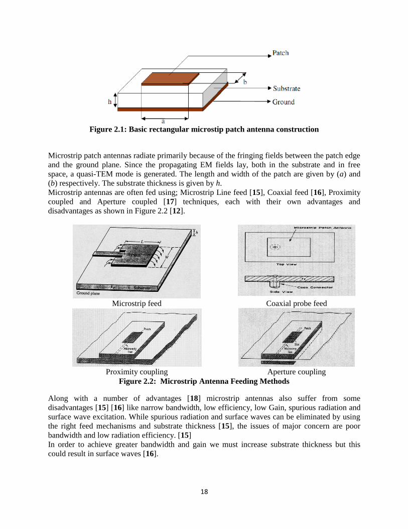
Figure 2.1: Basic rectangular microstip patch antenna construction

Microstrip patch antennas radiate primarily because of the fringing fields between the patch edge

and the ground plane. Since the propagating EM fields lay, both in the substrate and in free

space, a quasi-TEM mode is generated. The length and width of the patch are given by (a) and

(b) respectively. The substrate thickness is given by h.

Microstrip antennas are often fed using; Microstrip Line feed [15], Coaxial feed [16], Proximity

coupled and Aperture coupled [17] techniques, each with their own advantages and

disadvantages as shown in Figure 2.2 [12].

Coaxial probe feed Microstrip feed

Aperture coupling Proximity coupling

Figure 2.2: Microstrip Antenna Feeding Methods

Along with a number of advantages [18] microstrip antennas also suffer from some

disadvantages [15] [16] like narrow bandwidth, low efficiency, low Gain, spurious radiation and

surface wave excitation. While spurious radiation and surface waves can be eliminated by using

the right feed mechanisms and substrate thickness [15], the issues of major concern are poor

bandwidth and low radiation efficiency. [15]

In order to achieve greater bandwidth and gain we must increase substrate thickness but this

could result in surface waves [16].

19

2.2.1.3.2 PLANAR INVERTED F ANTENNA

The planar inverted F antenna is popular for portable wireless devices because of its low profile,

small size, and built-in structure [19]. The other major advantages are easy fabrication, low

manufacturing cost, and simple structure [20]. Conventional PIFA has limited bandwidth of 4 %

to 12 % for a -10 dB return loss [21]. Also, PIFA’s inherent bandwidth is higher than the

bandwidth of the conventional patch antenna (since a thick air substrate is used). The basic PIFA

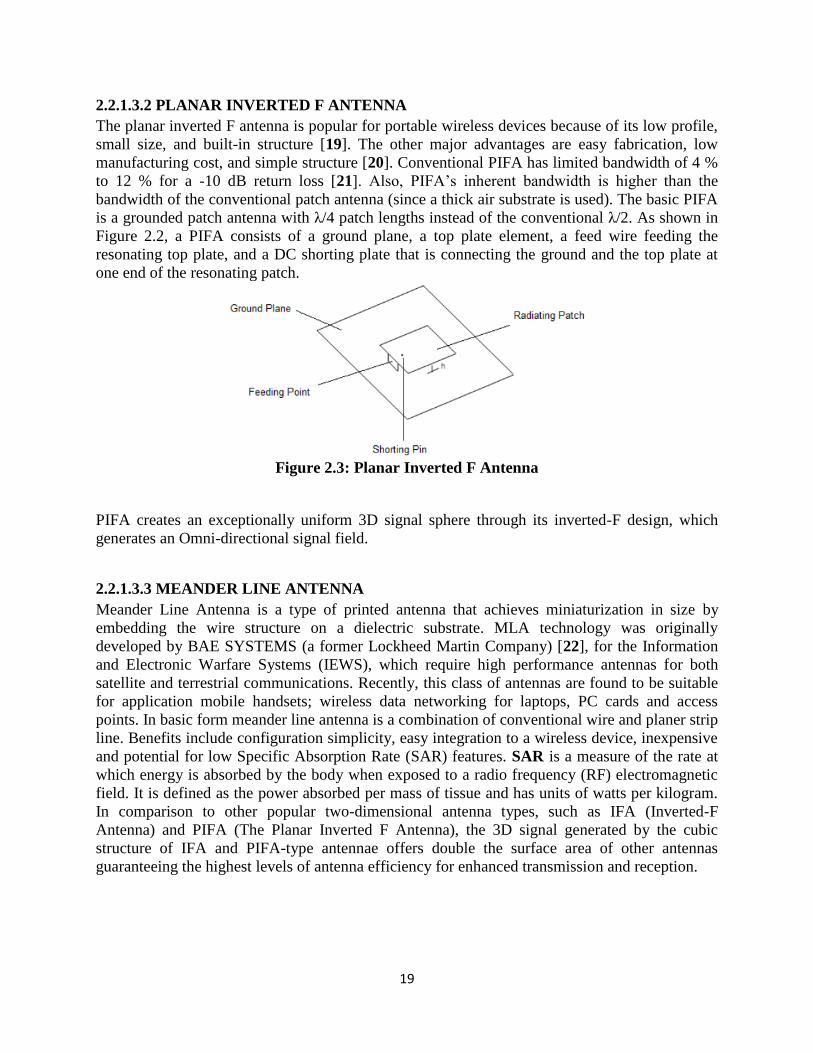
is a grounded patch antenna with λ/4 patch lengths instead of the conventional λ/2. As shown in

Figure 2.2, a PIFA consists of a ground plane, a top plate element, a feed wire feeding the

resonating top plate, and a DC shorting plate that is connecting the ground and the top plate at

one end of the resonating patch.

Figure 2.3: Planar Inverted F Antenna

PIFA creates an exceptionally uniform 3D signal sphere through its inverted-F design, which

generates an Omni-directional signal field.

2.2.1.3.3 MEANDER LINE ANTENNA

Meander Line Antenna is a type of printed antenna that achieves miniaturization in size by

embedding the wire structure on a dielectric substrate. MLA technology was originally

developed by BAE SYSTEMS (a former Lockheed Martin Company) [22], for the Information

and Electronic Warfare Systems (IEWS), which require high performance antennas for both

satellite and terrestrial communications. Recently, this class of antennas are found to be suitable

for application mobile handsets; wireless data networking for laptops, PC cards and access

points. In basic form meander line antenna is a combination of conventional wire and planer strip

line. Benefits include configuration simplicity, easy integration to a wireless device, inexpensive

and potential for low Specific Absorption Rate (SAR) features. SAR is a measure of the rate at

which energy is absorbed by the body when exposed to a radio frequency (RF) electromagnetic

field. It is defined as the power absorbed per mass of tissue and has units of watts per kilogram.

In comparison to other popular two-dimensional antenna types, such as IFA (Inverted-F

Antenna) and PIFA (The Planar Inverted F Antenna), the 3D signal generated by the cubic

structure of IFA and PIFA-type antennae offers double the surface area of other antennas

guaranteeing the highest levels of antenna efficiency for enhanced transmission and reception.

20

2.2.1.3.3.1 DESIGNING OF MEANDER LINE ANTENNA

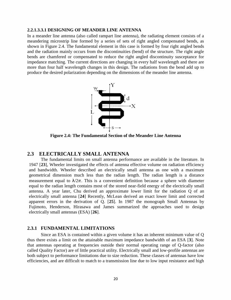
In a meander line antenna (also called rampart line antenna), the radiating element consists of a

meandering microstrip line formed by a series of sets of right angled compensated bends, as

shown in Figure 2.4. The fundamental element in this case is formed by four right angled bends

and the radiation mainly occurs from the discontinuities (bend) of the structure. The right angle

bends are chamfered or compensated to reduce the right angled discontinuity susceptance for

impedance matching. The current directions are changing in every half wavelength and there are

more than four half wavelength changes in this design. The radiations from the bend add up to

produce the desired polarization depending on the dimensions of the meander line antenna.

Figure 2.4: The Fundamental Section of the Meander Line Antenna

2.3 ELECTRICALLY SMALL ANTENNA The fundamental limits on small antenna performance are available in the literature. In

1947 [23], Wheeler investigated the effects of antenna effective volume on radiation efficiency

and bandwidth. Wheeler described an electrically small antenna as one with a maximum

geometrical dimension much less than the radian length. The radian length is a distance

measurement equal to λ/2 . This is a convenient definition because a sphere with diameter

equal to the radian length contains most of the stored near-field energy of the electrically small

antenna. A year later, Chu derived an approximate lower limit for the radiation Q of an

electrically small antenna [24] Recently, McLean derived an exact lower limit and corrected

apparent errors in the derivation of Q. [25]. In 1987 the monograph Small Antennas by

Fujimoto, Henderson, Hirasawa and James summarized the approaches used to design

electrically small antennas (ESA) [26].

2.3.1 FUNDAMENTAL LIMITATIONS

Since an ESA is contained within a given volume it has an inherent minimum value of Q

thus there exists a limit on the attainable maximum impedance bandwidth of an ESA [3]. Note

that antennas operating at frequencies outside their normal operating range of Q-factor (also

called Quality Factor) are of little practical utility. Electrically small and low-profile antennas are

both subject to performance limitations due to size reduction. These classes of antennas have low

efficiencies, and are difficult to match to a transmission line due to low input resistance and high

21

input reactance. In addition, ESAs typically exhibit narrow impedance bandwidth, which is an

important parameter in the antenna design process.

2.3.2 LIMIT ON RADIATION EFFICIENCY

Generally Q is defined in terms of the ratio of the energy stored in the resonator to the

energy being lost in one cycle:

The Q factor is commonly used to describe the ratio of the reactance to the resistance in a device.

So equation (2.11) can be written as

where X is the reactance or stored energy, and R is the ohmic resistance. Analogously, Chu

defines the radiation Q for an antenna as

where is the radian frequency, Prad is the radiated power, and W is the time-averaged, non-

propagating, stored electric or magnetic energy, whichever is greater [24]. Electrically small

antennas have high input reactance and low input resistance.

Therefore, they have high Q and low frequency bandwidth. ESAs also have low radiation

efficiency. The radiation efficiency of an antenna is defined by

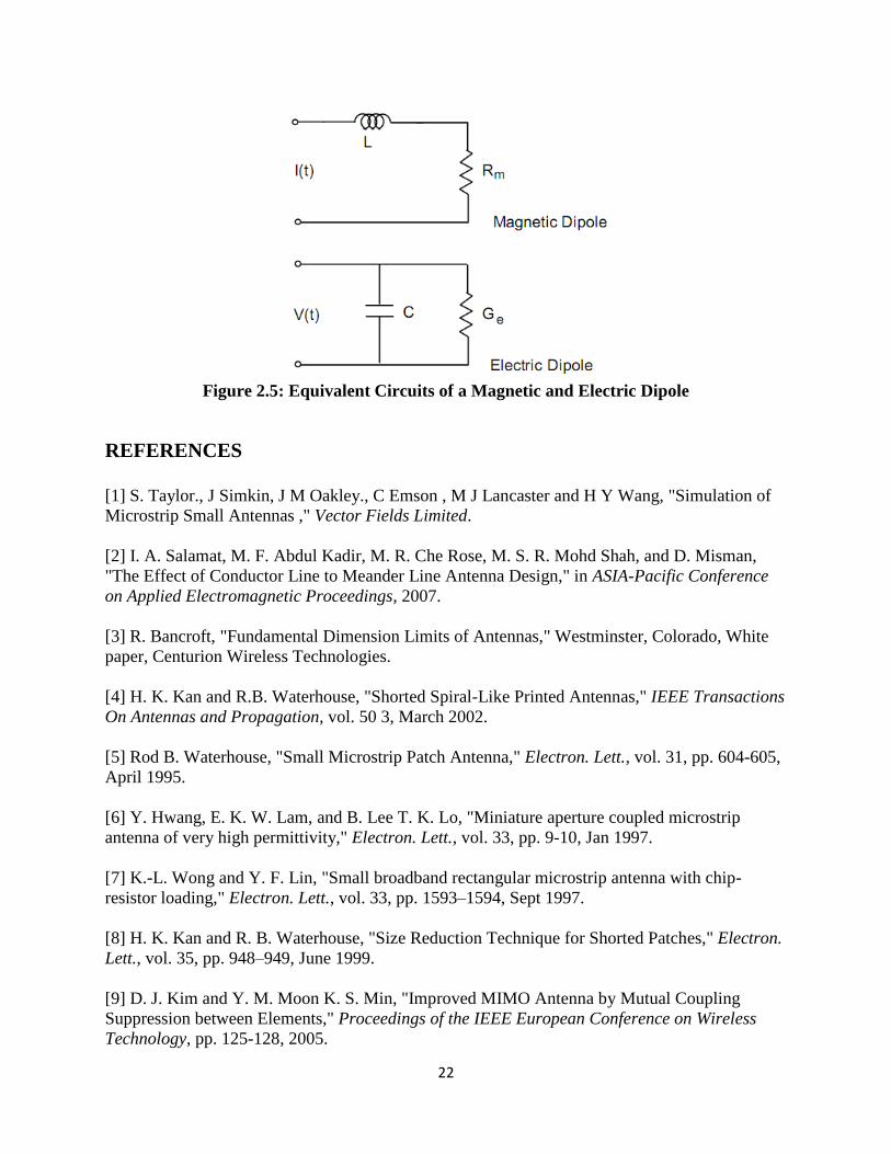
where Rr is the radiation resistance of the antenna and Rm refers to the ohmic losses in the

antenna structure and any matching device. The radiation efficiency ( ) of a receiving antenna

is the fraction of energy delivered by the antenna from free space to a load representing the

receiver [25]. Every small antenna can be made to perform like a lumped reactance, specifically,

a capacitor, inductor, or some combination of the two. An electric dipole, or dipole antenna,

behaves like a capacitor. A magnetic dipole, or loop antenna, behaves like an inductor. Either

antenna can be represented by some combination of a reactive and a resistive lumped element.

The reactance in the equivalent circuit describes the portion of the input energy that is stored in

the near-field of the antenna. The resistive element represents the radiation resistance of the

antenna. Wheeler models the magnetic dipole as a series inductance and resistance and the

electric dipole as a shunt capacitance and susceptance [25]. This representation is consistent with

circuit duality. Both equivalent circuits are illustrated in Figure 2.5.

22

Figure 2.5: Equivalent Circuits of a Magnetic and Electric Dipole

REFERENCES

[1] S. Taylor., J Simkin, J M Oakley., C Emson , M J Lancaster and H Y Wang, "Simulation of

Microstrip Small Antennas ," Vector Fields Limited.

[2] I. A. Salamat, M. F. Abdul Kadir, M. R. Che Rose, M. S. R. Mohd Shah, and D. Misman,

"The Effect of Conductor Line to Meander Line Antenna Design," in ASIA-Pacific Conference

on Applied Electromagnetic Proceedings, 2007.

[3] R. Bancroft, "Fundamental Dimension Limits of Antennas," Westminster, Colorado, White

paper, Centurion Wireless Technologies.

[4] H. K. Kan and R.B. Waterhouse, "Shorted Spiral-Like Printed Antennas," IEEE Transactions

On Antennas and Propagation, vol. 50 3, March 2002.

[5] Rod B. Waterhouse, "Small Microstrip Patch Antenna," Electron. Lett., vol. 31, pp. 604-605,

April 1995.

[6] Y. Hwang, E. K. W. Lam, and B. Lee T. K. Lo, "Miniature aperture coupled microstrip

antenna of very high permittivity," Electron. Lett., vol. 33, pp. 9-10, Jan 1997.

[7] K.-L. Wong and Y. F. Lin, "Small broadband rectangular microstrip antenna with chip-

resistor loading," Electron. Lett., vol. 33, pp. 1593–1594, Sept 1997.

[8] H. K. Kan and R. B. Waterhouse, "Size Reduction Technique for Shorted Patches," Electron.

Lett., vol. 35, pp. 948–949, June 1999.

[9] D. J. Kim and Y. M. Moon K. S. Min, "Improved MIMO Antenna by Mutual Coupling

Suppression between Elements," Proceedings of the IEEE European Conference on Wireless

Technology, pp. 125-128, 2005.

23

[10] M. S. Sharawi, Y. S. Faouri, and S.S. Iqbal, “Design of an Electrically Small Meander

Antenna for LTE Mobile Terminals in The 800 MHz Band”, IEE GCC Conference and

Exhibition (GCC), February 19-22, Dubai, United Arab Emirates, 2011.

[11] K. L. Wong, Planar Antennas for Wireless Communications: Wiley, 2003.

[12] C. A Balanis, Antenna theory-Analysis and Design, 2nd ed.: John Wiley &

Sons Ltd, 1997.

[13] Ansoft Corporation, "HFSS Online Help," V. 9.2.

[14] Freescale Semiconductor. (2006, July) Compact Integrated Antennas Application

Note.

[15] R., Bhartia, P., Bahl, I. Garg, Microstrip Antenna Design Handbook.: Artech House,

Inc, 2001.

[16] G., and Ray, K.P. Kumar, Broadband Microstrip Antennas: Artech House, Inc,

2003.

[17] B. R. Waterhouse, Microstrip Patch Antennas: A Designer’s Guide: Kluwer

Academic Publishers, 2003.

[18] P. S. Nakar, Design of a compact Microstrip Patch Antenna for use in Wireless/Cellular

Devices: Master’s Thesis report, 2004.

[19] Z. Du, Q. Wang and K. Gong F. Wang, "Enhanced-bandwidth PIFA with T-shaped ground

plane," Electronic Letters, vol. 40, no. 23, pp. 1504 – 1505, Nov 2004.

[20] J. Hoon and H. Choi B. Kim, "Small wideband PIFA for mobile phones at 1800

145 MHz," , vol. 1, pp. 27-29, May 2004.

[21] C. R. Rowell and R. D. Murch, "A compact PIFA suitable for dual-frequency 900/1800-

MHz operation," IEEE Trans. Antennas Propagation, vol. 46, pp. 596-598, April 1998.

[22] Frank M. Caimi. (2002) SkyCross, Inc.

[23] H.A. Wheeler, "Fundamental Limits of Small Antennas," Proceedings of the I.R.E.

(IEEE), pp. 1479-1484, Dec. 1947.

[24] J. McLean, "A Re-Examination of the Fundamental Limits on the Radiation Q of

Electrically Small Antennas," IEEE Transactions on Antennas and Propagation, vol. 44, no. 5,

pp. 672-675, May 1996.

24

[25] H. Wheeler, "Small Antennas," in Antenna Engineering Handbook, R. Johnson, Ed., 1993,

ch. 6.

25

CHAPTER 3

ANALYSIS AND DESIGN OF MEANDER LINE ANTENNA FOR LTE

MOBILE COMMUNICATIONS IN 0.78 GHZ

3.1 INTRODUCTION In chapter 2, we described some types of MLA that deal with LTE in the band 0.78 and

2.5 GHz. In this chapter, we will analyze and design the structure that has better gain and

bandwidth for LTE mobile communications.

A microstrip patch antenna consists of a dielectric substrate, with a ground plane on the other

side. Due to its multiple advantages such as low weight , low profile planar configuration, low

fabrication cost and capability to integrate with microwave integrated circuits technology, the

microstrip patch antenna is very well suited for applications such as wireless communications

system, cellular phones, pagers, radar systems, and satellite communications systems [1].

The development of small-integrated antennas plays a significant role in the progress of the

rapidly expanding military and commercial communication applications.

The gain, the bandwidth enhancement and its return loss improvement without increasing

antenna size and production process are important to apply this antenna to the modern mobile

communication systems and need to be carried out [2].

The MLA in [3] was designed for GSM mobile application in 0.9 GHz as shown in Figure 3.1. In

this chapter, we modify this antenna for LTE mobile communication (as shown in Figure 3.2) is

designed at resonant frequency 0.78 GHz and we will in this chapter describe how to reach this

design antenna.

A comprehensive parametric study has been carried out to understand the effects of various

dimensional parameters as shown in section 3.2. Because electromagnetic optimization

parameters can be either continuous, discrete, or both, making the design process slow and

complicated, many researchers have applied genetic algorithms to the design of broadband patch

antennas [4-5]. A Genetic algorithms optimum approach of the dimension of MLA based on the

combination of GA with the commercial electromagnetic simulation tool, the FEM based

software, HFSS by ANSOFT. The attractiveness of GA optimization is that improved bandwidth

performance doesn’t increase overall dimensions or manufacturing cost. The design process of

MLA optimization with GA is described in Section 3.3. In Section 3.4 the GA optimized antenna

designs and results are proposed. In section 3.5 we apply this antenna on other substrate

materials. Finally the conclusion is written in Section 3.6.

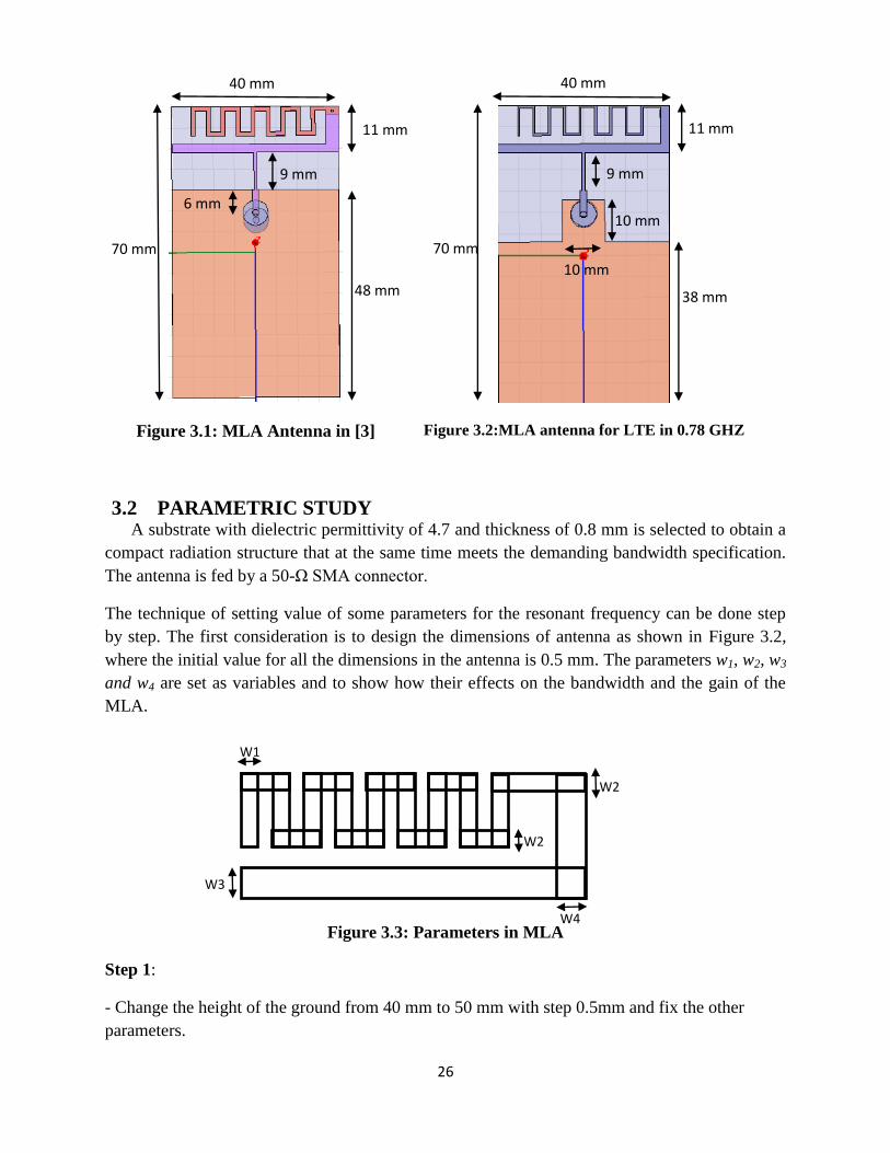
26

Figure 3.1: MLA Antenna in [3] Figure 3.2:MLA antenna for LTE in 0.78 GHZ

3.2 PARAMETRIC STUDY A substrate with dielectric permittivity of 4.7 and thickness of 0.8 mm is selected to obtain a

compact radiation structure that at the same time meets the demanding bandwidth specification.

The antenna is fed by a 50-Ω SMA connector.

The technique of setting value of some parameters for the resonant frequency can be done step

by step. The first consideration is to design the dimensions of antenna as shown in Figure 3.2,

where the initial value for all the dimensions in the antenna is 0.5 mm. The parameters w1, w2, w3

and w4 are set as variables and to show how their effects on the bandwidth and the gain of the

MLA.

Figure 3.3: Parameters in MLA

Step 1:

- Change the height of the ground from 40 mm to 50 mm with step 0.5mm and fix the other

parameters.

W2

W4

W1

W3

W2

48 mm

70 mm

40 mm

9 mm

6 mm

11 mm

40 mm

70 mm

38 mm

10 mm

10 mm

9 mm

11 mm

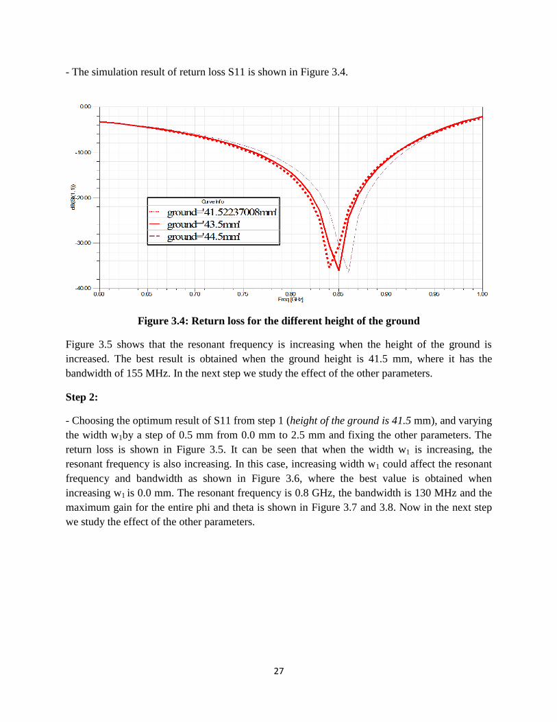
27

- The simulation result of return loss S11 is shown in Figure 3.4.

Figure 3.4: Return loss for the different height of the ground

Figure 3.5 shows that the resonant frequency is increasing when the height of the ground is

increased. The best result is obtained when the ground height is 41.5 mm, where it has the

bandwidth of 155 MHz. In the next step we study the effect of the other parameters.

Step 2:

- Choosing the optimum result of S11 from step 1 (height of the ground is 41.5 mm), and varying

the width w1by a step of 0.5 mm from 0.0 mm to 2.5 mm and fixing the other parameters. The

return loss is shown in Figure 3.5. It can be seen that when the width w1 is increasing, the

resonant frequency is also increasing. In this case, increasing width w1 could affect the resonant

frequency and bandwidth as shown in Figure 3.6, where the best value is obtained when

increasing w1 is 0.0 mm. The resonant frequency is 0.8 GHz, the bandwidth is 130 MHz and the

maximum gain for the entire phi and theta is shown in Figure 3.7 and 3.8. Now in the next step

we study the effect of the other parameters.

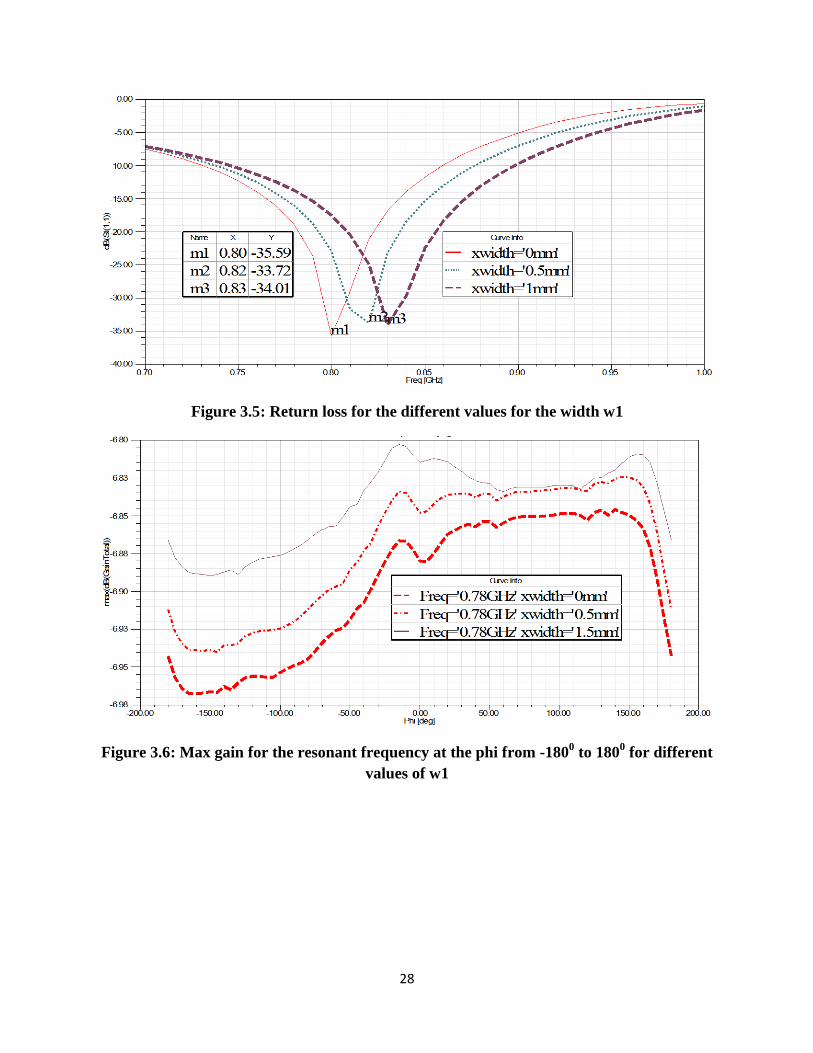
28

Figure 3.5: Return loss for the different values for the width w1

Figure 3.6: Max gain for the resonant frequency at the phi from -1800 to 180

0 for different

values of w1

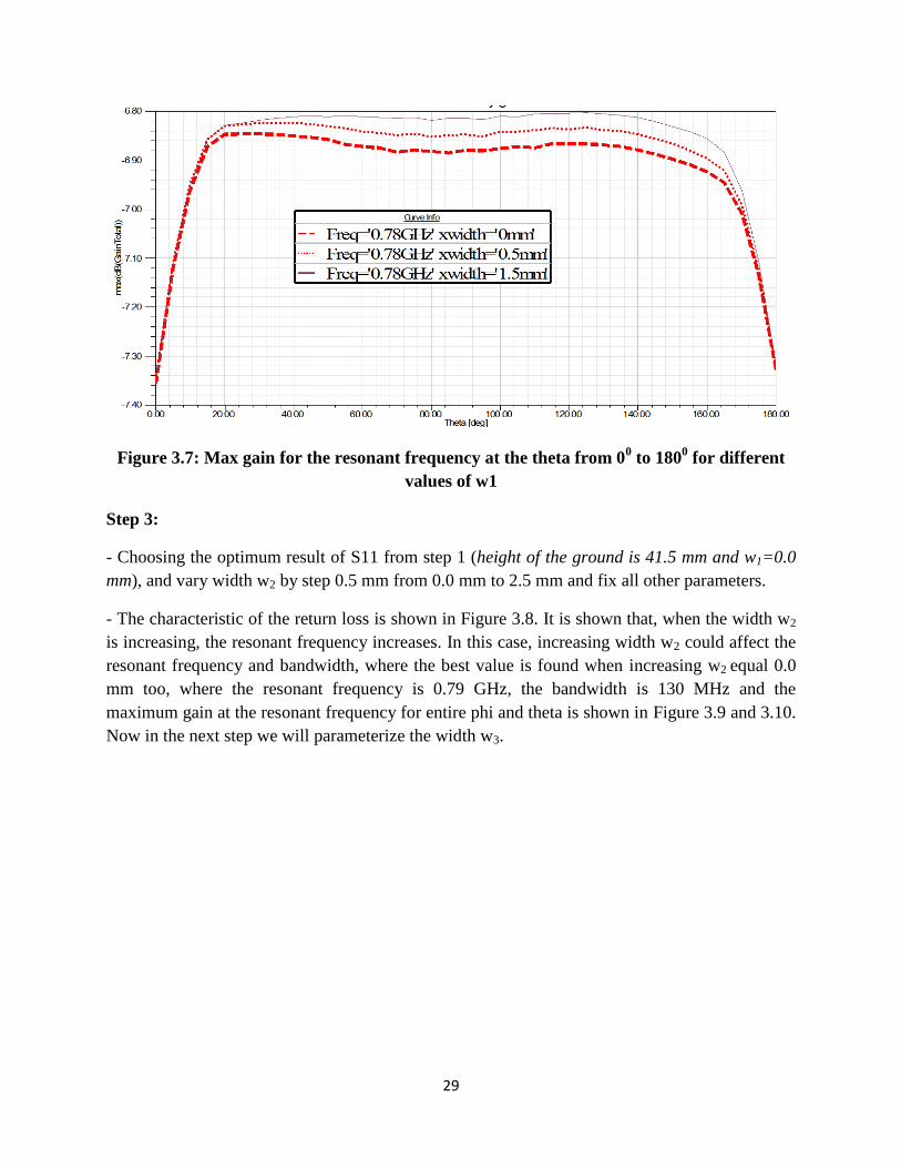
29

Figure 3.7: Max gain for the resonant frequency at the theta from 00 to 180

0 for different

values of w1

Step 3:

- Choosing the optimum result of S11 from step 1 (height of the ground is 41.5 mm and w1=0.0

mm), and vary width w2 by step 0.5 mm from 0.0 mm to 2.5 mm and fix all other parameters.

- The characteristic of the return loss is shown in Figure 3.8. It is shown that, when the width w2

is increasing, the resonant frequency increases. In this case, increasing width w2 could affect the

resonant frequency and bandwidth, where the best value is found when increasing w2 equal 0.0

mm too, where the resonant frequency is 0.79 GHz, the bandwidth is 130 MHz and the

maximum gain at the resonant frequency for entire phi and theta is shown in Figure 3.9 and 3.10.

Now in the next step we will parameterize the width w3.

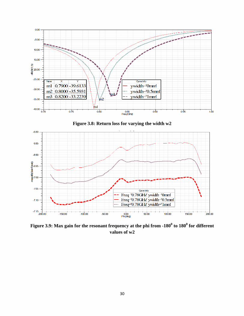
30

Figure 3.8: Return loss for varying the width w2

Figure 3.9: Max gain for the resonant frequency at the phi from -1800 to 180

0 for different

values of w2

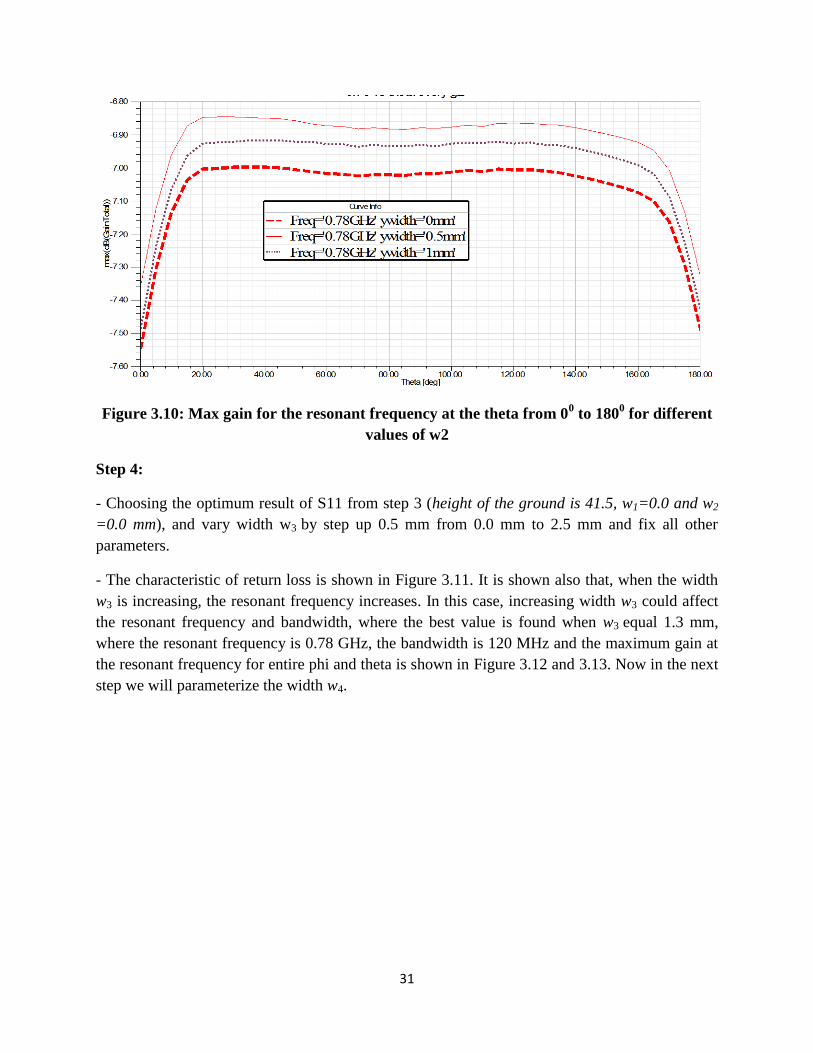
31

Figure 3.10: Max gain for the resonant frequency at the theta from 00 to 180

0 for different

values of w2

Step 4:

- Choosing the optimum result of S11 from step 3 (height of the ground is 41.5, w1=0.0 and w2

=0.0 mm), and vary width w3 by step up 0.5 mm from 0.0 mm to 2.5 mm and fix all other

parameters.

- The characteristic of return loss is shown in Figure 3.11. It is shown also that, when the width

w3 is increasing, the resonant frequency increases. In this case, increasing width w3 could affect

the resonant frequency and bandwidth, where the best value is found when w3 equal 1.3 mm,

where the resonant frequency is 0.78 GHz, the bandwidth is 120 MHz and the maximum gain at

the resonant frequency for entire phi and theta is shown in Figure 3.12 and 3.13. Now in the next

step we will parameterize the width w4.

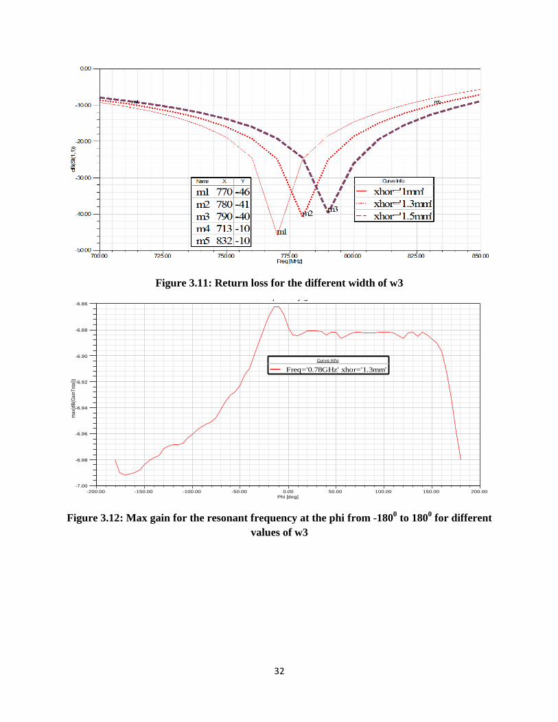
32

Figure 3.11: Return loss for the different width of w3

Figure 3.12: Max gain for the resonant frequency at the phi from -1800 to 180

0 for different

values of w3

-200.00 -150.00 -100.00 -50.00 0.00 50.00 100.00 150.00 200.00

Phi [deg]

-7.00

-6.98

-6.96

-6.94

-6.92

-6.90

-6.88

-6.86

ma

x(d

B(G

ain

To

tal)

)

Ansoft LLC Patch_Antenna_ADKv10.78 vs pi every g1

Curve Info

Freq='0.78GHz' xhor='1.3mm'

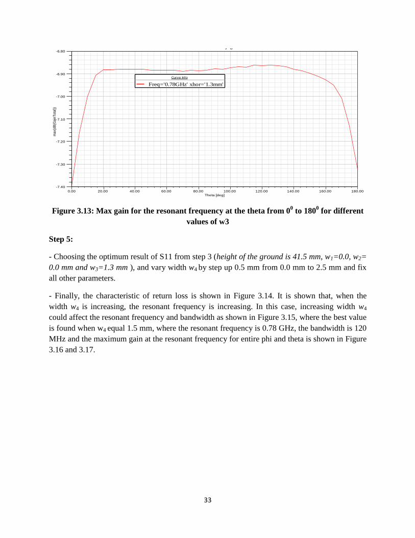
33

Figure 3.13: Max gain for the resonant frequency at the theta from 00 to 180

0 for different

values of w3

Step 5:

- Choosing the optimum result of S11 from step 3 (height of the ground is 41.5 mm, w1=0.0, w2=

0.0 mm and w3=1.3 mm ), and vary width w4 by step up 0.5 mm from 0.0 mm to 2.5 mm and fix

all other parameters.

- Finally, the characteristic of return loss is shown in Figure 3.14. It is shown that, when the

width w4 is increasing, the resonant frequency is increasing. In this case, increasing width w4

could affect the resonant frequency and bandwidth as shown in Figure 3.15, where the best value

is found when w4 equal 1.5 mm, where the resonant frequency is 0.78 GHz, the bandwidth is 120

MHz and the maximum gain at the resonant frequency for entire phi and theta is shown in Figure

3.16 and 3.17.

0.00 20.00 40.00 60.00 80.00 100.00 120.00 140.00 160.00 180.00

Theta [deg]

-7.40

-7.30

-7.20

-7.10

-7.00

-6.90

-6.80m

ax(

dB

(Ga

inT

ota

l))

Ansoft LLC Patch_Antenna_ADKv10.78 vs theta every g2

Curve Info

Freq='0.78GHz' xhor='1.3mm'

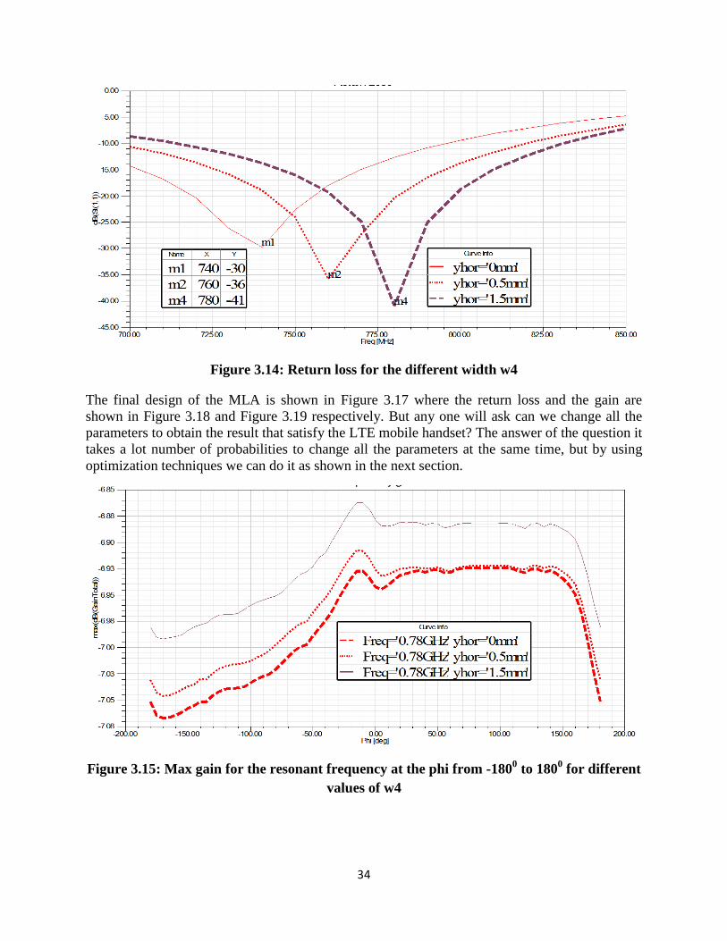
34

Figure 3.14: Return loss for the different width w4

The final design of the MLA is shown in Figure 3.17 where the return loss and the gain are

shown in Figure 3.18 and Figure 3.19 respectively. But any one will ask can we change all the

parameters to obtain the result that satisfy the LTE mobile handset? The answer of the question it

takes a lot number of probabilities to change all the parameters at the same time, but by using

optimization techniques we can do it as shown in the next section.

Figure 3.15: Max gain for the resonant frequency at the phi from -1800 to 180

0 for different

values of w4

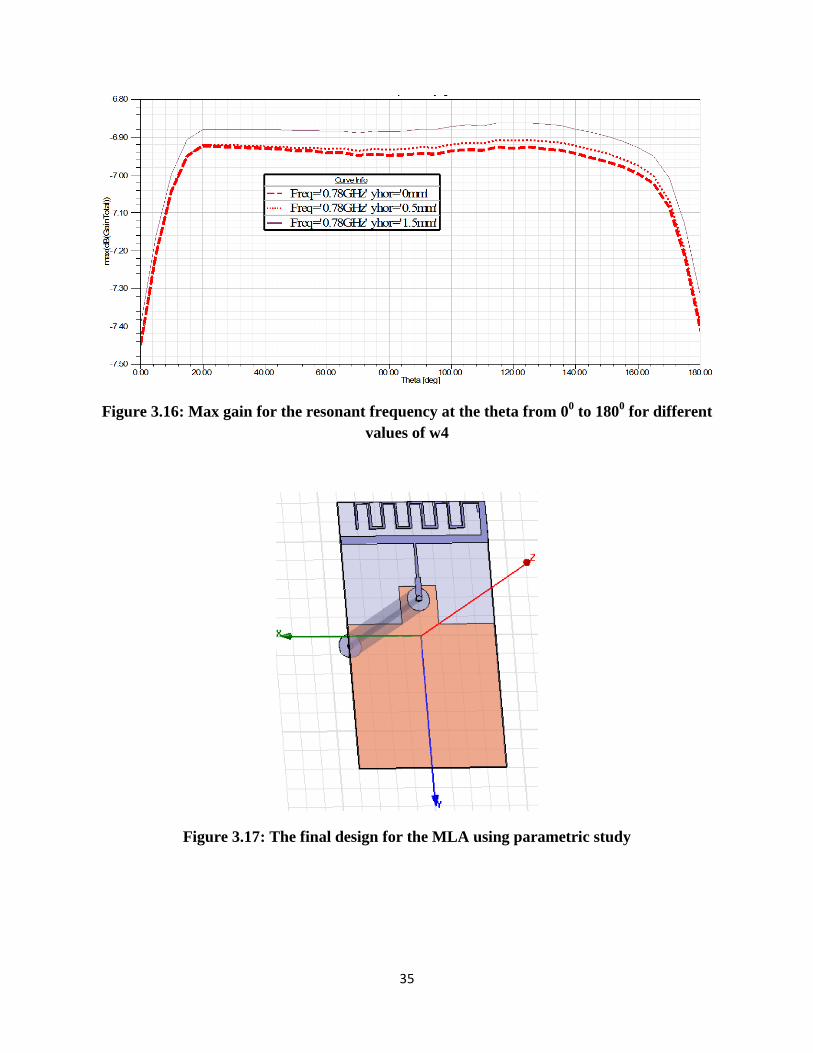
35

Figure 3.16: Max gain for the resonant frequency at the theta from 00 to 180

0 for different

values of w4

Figure 3.17: The final design for the MLA using parametric study

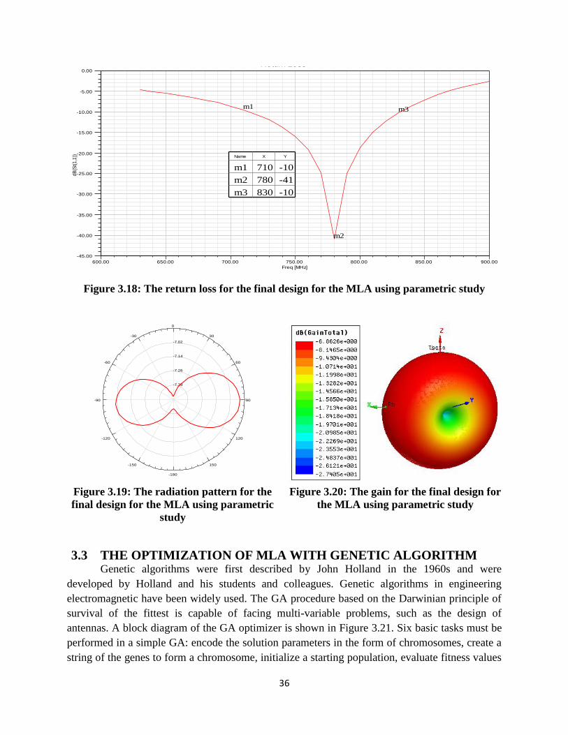
36

Figure 3.18: The return loss for the final design for the MLA using parametric study

Figure 3.19: The radiation pattern for the

final design for the MLA using parametric

study

Figure 3.20: The gain for the final design for

the MLA using parametric study

3.3 THE OPTIMIZATION OF MLA WITH GENETIC ALGORITHM Genetic algorithms were first described by John Holland in the 1960s and were

developed by Holland and his students and colleagues. Genetic algorithms in engineering

electromagnetic have been widely used. The GA procedure based on the Darwinian principle of

survival of the fittest is capable of facing multi-variable problems, such as the design of

antennas. A block diagram of the GA optimizer is shown in Figure 3.21. Six basic tasks must be

performed in a simple GA: encode the solution parameters in the form of chromosomes, create a

string of the genes to form a chromosome, initialize a starting population, evaluate fitness values

600.00 650.00 700.00 750.00 800.00 850.00 900.00

Freq [MHz]

-45.00

-40.00

-35.00

-30.00

-25.00

-20.00

-15.00

-10.00

-5.00

0.00d

B(S

t(1

,1))

Ansoft LLC Patch_Antenna_ADKv1Return Loss

m1

m2

m3

Name X Y

m1 710 -10

m2 780 -41

m3 830 -10

Setup1 : Sweep1

-7.38

-7.26

-7.14

-7.02

90

60

30

0

-30

-60

-90

-120

-150

-180

150

120

Ansoft LLC Patch_Antenna_ADKv1Radiation Pattern 1

Curve Info

dB(GainTotal)

Setup1 : LastAdaptive

Freq='0.78GHz' Phi='0deg' yground='11mm'

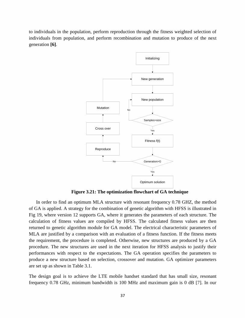
37

to individuals in the population, perform reproduction through the fitness weighted selection of

individuals from population, and perform recombination and mutation to produce of the next

generation [6].

Initializing

New generation

New population

Fitness f(t)

Optimum solution

Reproduce

Cross over

Mutation

Samples>size

Generation>G

Yes

Yes

No

No

Figure 3.21: The optimization flowchart of GA technique

In order to find an optimum MLA structure with resonant frequency 0.78 GHZ, the method

of GA is applied. A strategy for the combination of genetic algorithm with HFSS is illustrated in

Fig 19, where version 12 supports GA, where it generates the parameters of each structure. The

calculation of fitness values are compiled by HFSS. The calculated fitness values are then

returned to genetic algorithm module for GA model. The electrical characteristic parameters of

MLA are justified by a comparison with an evaluation of a fitness function. If the fitness meets

the requirement, the procedure is completed. Otherwise, new structures are produced by a GA

procedure. The new structures are used in the next iteration for HFSS analysis to justify their

performances with respect to the expectations. The GA operation specifies the parameters to

produce a new structure based on selection, crossover and mutation. GA optimizer parameters

are set up as shown in Table 3.1.

The design goal is to achieve the LTE mobile handset standard that has small size, resonant

frequency 0.78 GHz, minimum bandwidth is 100 MHz and maximum gain is 0 dB [7]. In our

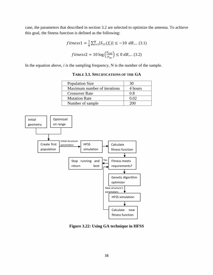
38

case, the parameters that described in section 3.2 are selected to optimize the antenna. To achieve

this goal, the fitness function is defined as the following:

∑ | ( )| ... (3.1)

(

) ... (3.2)

In the equation above, i is the sampling frequency, N is the number of the sample.

TABLE 3.1. SPECIFICATIONS OF THE GA

Population Size 30

Maximum number of iterations 4 hours

Crossover Rate 0.8

Mutation Rate 0.02

Number of sample 200

Figure 3.22: Using GA technique in HFSS

Calculate new

fitness function

HFSS simulation

Yes

HFSS

simulation

Calculate

fitness function

Stop running and

return best

solution

Genetic Algorithm

optimizer

Initial

geometry

Optimizati

on range

Create first

population

Initial structure

parameters

Fitness meets

requirements?

New structure‘s

parameters

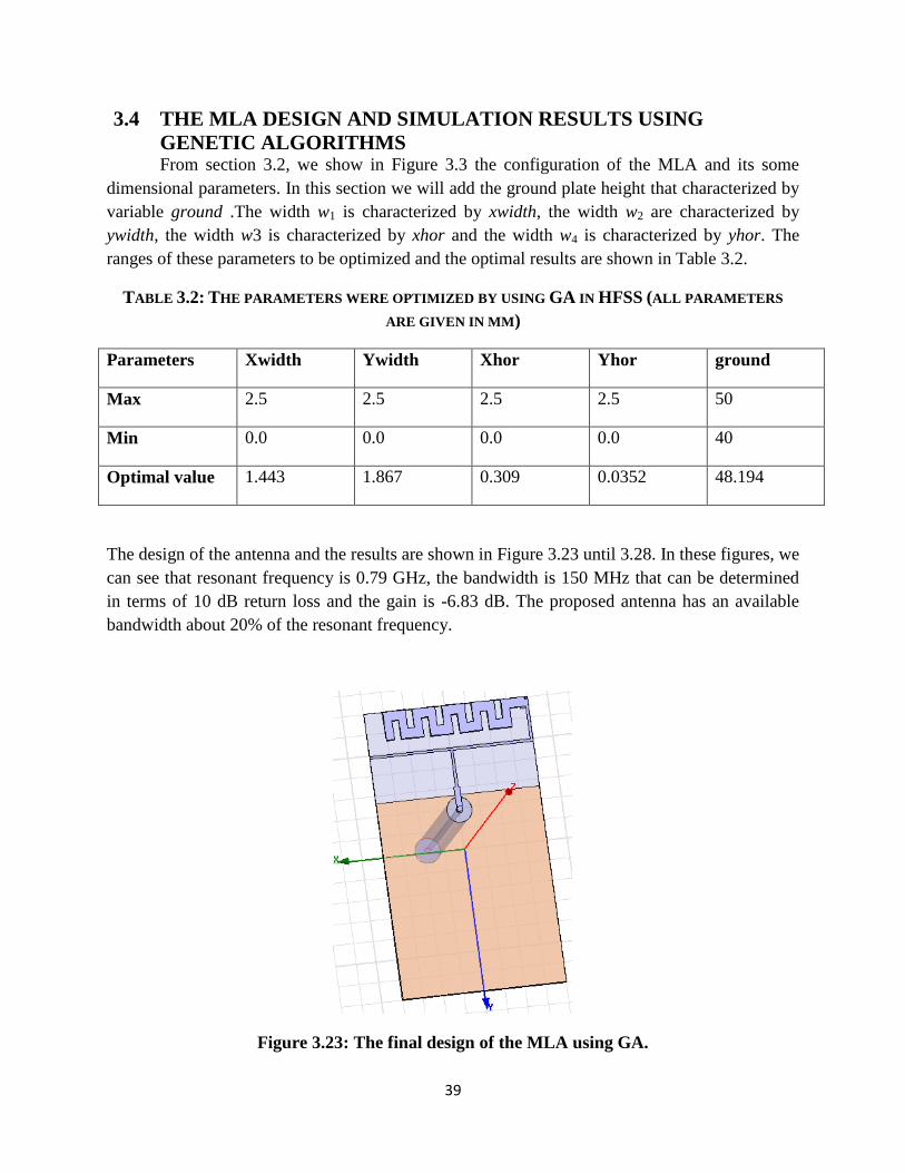
39

3.4 THE MLA DESIGN AND SIMULATION RESULTS USING

GENETIC ALGORITHMS From section 3.2, we show in Figure 3.3 the configuration of the MLA and its some

dimensional parameters. In this section we will add the ground plate height that characterized by

variable ground .The width w1 is characterized by xwidth, the width w2 are characterized by

ywidth, the width w3 is characterized by xhor and the width w4 is characterized by yhor. The

ranges of these parameters to be optimized and the optimal results are shown in Table 3.2.

TABLE 3.2: THE PARAMETERS WERE OPTIMIZED BY USING GA IN HFSS (ALL PARAMETERS

ARE GIVEN IN MM)

Parameters Xwidth Ywidth Xhor Yhor ground

Max 2.5 2.5 2.5 2.5 50

Min 0.0 0.0 0.0 0.0 40

Optimal value 1.443 1.867 0.309 0.0352 48.194

The design of the antenna and the results are shown in Figure 3.23 until 3.28. In these figures, we

can see that resonant frequency is 0.79 GHz, the bandwidth is 150 MHz that can be determined

in terms of 10 dB return loss and the gain is -6.83 dB. The proposed antenna has an available

bandwidth about 20% of the resonant frequency.

Figure 3.23: The final design of the MLA using GA.

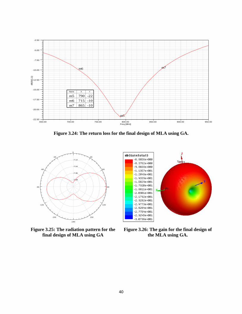
40

Figure 3.24: The return loss for the final design of MLA using GA.

Figure 3.25: The radiation pattern for the

final design of MLA using GA

Figure 3.26: The gain for the final design of

the MLA using GA.

650.00 700.00 750.00 800.00 850.00 900.00 950.00

Freq [MHz]

-22.50

-20.00

-17.50

-15.00

-12.50

-10.00

-7.50

-5.00

-2.50

dB

(St(

1,1

))

Ansoft LLC Patch_Antenna_ADKv1Return Loss

m6

m5

m7

Name X Y

m5 790 -22

m6 715 -10

m7 865 -10

-7.48

-7.36

-7.24

-7.12

90

60

30

0

-30

-60

-90

-120

-150

-180

150

120

Ansoft LLC Patch_Antenna_ADKv1Radiation Pattern 1

Curve Info

dB(GainTotal)

Setup1 : LastAdaptive

Freq='0.78GHz' Phi='0deg'

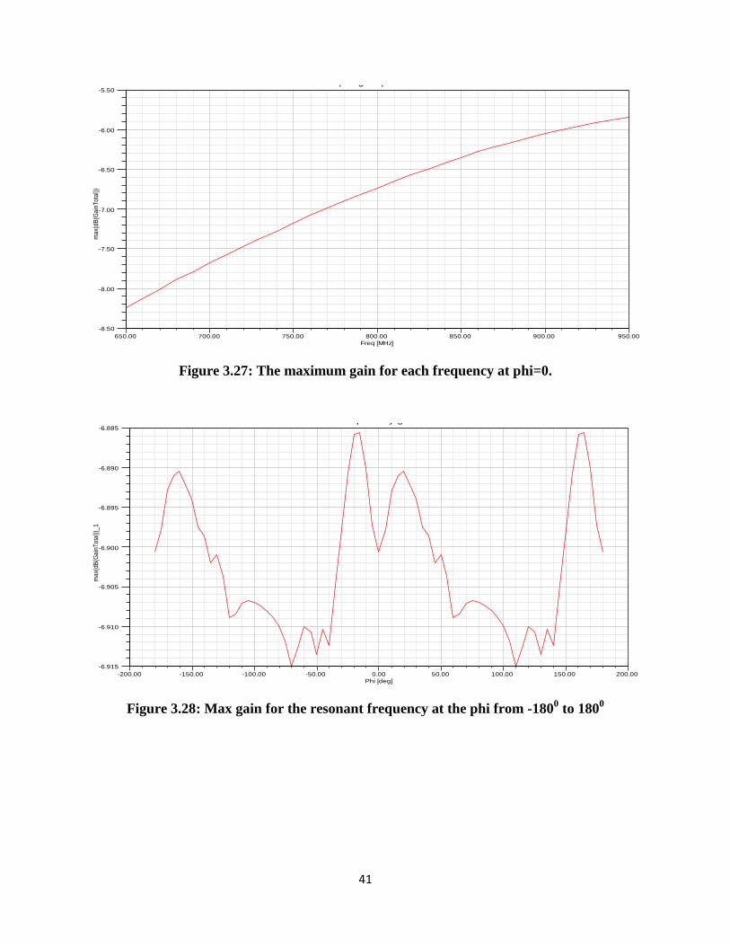
41

Figure 3.27: The maximum gain for each frequency at phi=0.

Figure 3.28: Max gain for the resonant frequency at the phi from -1800 to 180

0

650.00 700.00 750.00 800.00 850.00 900.00 950.00

Freq [MHz]

-8.50

-8.00

-7.50

-7.00

-6.50

-6.00

-5.50m

ax(

dB

(Ga

inT

ota

l))

Ansoft LLC Patch_Antenna_ADKv1Freq vs gain phi=0ground='48.1940672mm' Phi='0deg' xhor='0.3093813898mm' xw idth='1.442991424mm' yhor='...

-200.00 -150.00 -100.00 -50.00 0.00 50.00 100.00 150.00 200.00

Phi [deg]

-6.915

-6.910

-6.905

-6.900

-6.895

-6.890

-6.885

ma

x(d

B(G

ain

To

tal)

)_1

Ansoft LLC Patch_Antenna_ADKv10.78 vs pi every g1

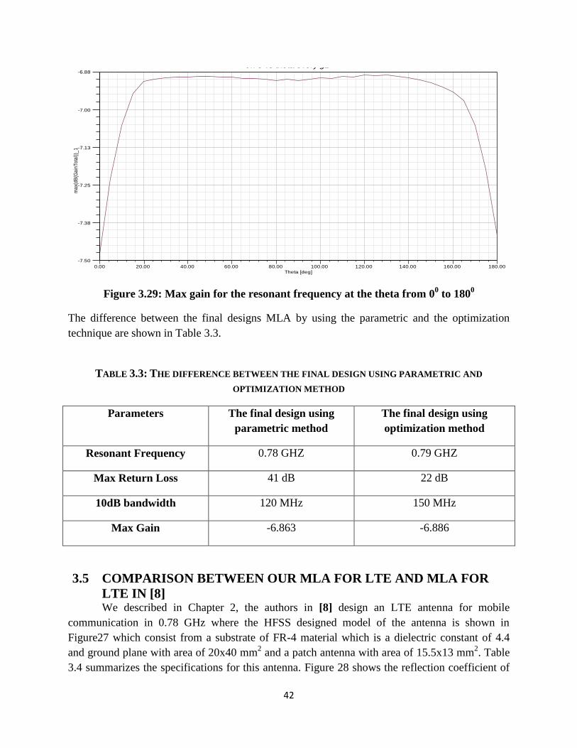
42

Figure 3.29: Max gain for the resonant frequency at the theta from 00 to 180

0

The difference between the final designs MLA by using the parametric and the optimization

technique are shown in Table 3.3.

TABLE 3.3: THE DIFFERENCE BETWEEN THE FINAL DESIGN USING PARAMETRIC AND

OPTIMIZATION METHOD

Parameters The final design using

parametric method

The final design using

optimization method

Resonant Frequency 0.78 GHZ 0.79 GHZ

Max Return Loss 41 dB 22 dB

10dB bandwidth 120 MHz 150 MHz

Max Gain -6.863 -6.886

3.5 COMPARISON BETWEEN OUR MLA FOR LTE AND MLA FOR

LTE IN [8] We described in Chapter 2, the authors in [8] design an LTE antenna for mobile

communication in 0.78 GHz where the HFSS designed model of the antenna is shown in

Figure27 which consist from a substrate of FR-4 material which is a dielectric constant of 4.4

and ground plane with area of 20x40 mm2 and a patch antenna with area of 15.5x13 mm

2. Table

3.4 summarizes the specifications for this antenna. Figure 28 shows the reflection coefficient of

0.00 20.00 40.00 60.00 80.00 100.00 120.00 140.00 160.00 180.00

Theta [deg]

-7.50

-7.38

-7.25

-7.13

-7.00

-6.88m

ax(

dB

(Ga

inT

ota

l))_

1

Ansoft LLC Patch_Antenna_ADKv10.78 vs theta every g2Freq='0.78GHz' ground='48.1940672mm' xhor='0.30938...

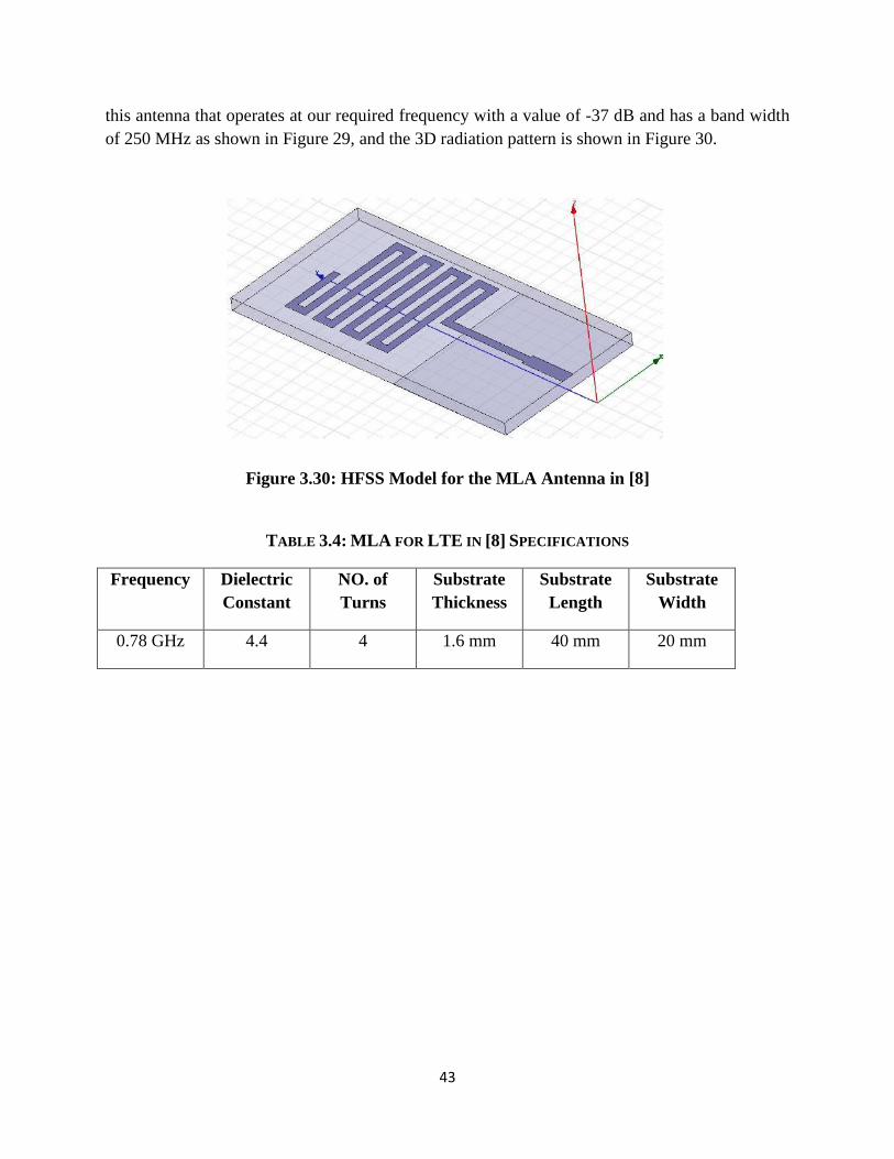
43

this antenna that operates at our required frequency with a value of -37 dB and has a band width

of 250 MHz as shown in Figure 29, and the 3D radiation pattern is shown in Figure 30.

Figure 3.30: HFSS Model for the MLA Antenna in [8]

TABLE 3.4: MLA FOR LTE IN [8] SPECIFICATIONS

Frequency Dielectric

Constant

NO. of

Turns

Substrate

Thickness

Substrate

Length

Substrate

Width

0.78 GHz 4.4 4 1.6 mm 40 mm 20 mm

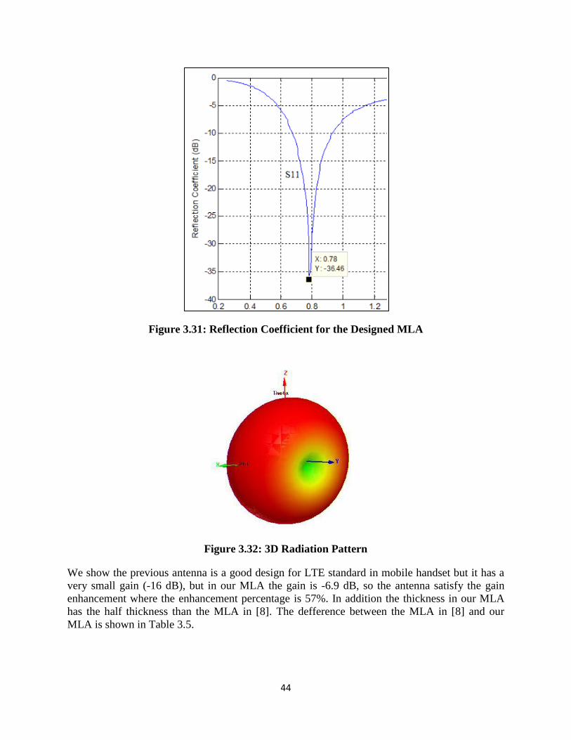
44

Figure 3.31: Reflection Coefficient for the Designed MLA

Figure 3.32: 3D Radiation Pattern

We show the previous antenna is a good design for LTE standard in mobile handset but it has a

very small gain (-16 dB), but in our MLA the gain is -6.9 dB, so the antenna satisfy the gain

enhancement where the enhancement percentage is 57%. In addition the thickness in our MLA

has the half thickness than the MLA in [8]. The defference between the MLA in [8] and our

MLA is shown in Table 3.5.

45

TABLE 3.5: DIFFERENCES BETWEEN OUR MLA AND MLA IN [8]

Our MLA MLA in [8]

Gain -6.68 dB -16 dB

Bandwidth 150 MHz 260 MHz

Length 70 mm 40 mm

Width 40 mm 20 mm

Thickness 0.8 mm 1.6 mm

3.6 CONCLUSIONS An electrically small MLA operating at the 0.78 GHz was studied in this chapter using

HFSS software package. We apply parametric and optimization technique using genetic

algorithms to achieve the antenna for the standard LTE mobile handset. The antenna provided a

significant gain enhancement. Finally we compare the MLA with the antenna in [8] where Table

3.5 summarizes the differences between the two designed antennas. It is evident that our MLA

antenna is more suitable for use due to its thickness height is much less than the antenna in [8] in

addition with the enhancement gain.

REFERENCES

[1] C. A. Balanis, Antenna Theory: Analysis and Design. New York: Wiley, Second ed., 1997.

[2] S. K. Patel, Y. P. Kosta, E-shape Microstrip Patch Antenna Design for GPS Application,

Institute of Technology, NIRMA University, December, 2011.

[3] Hai-Ming Hsiao, Jeun-Wen Wu, Jui-Han Lu and Yau-Der Wang, Multi-Band Dual-Meander-

Line Antenna for Mobile Handsets, the National Science Council (NSC), Taiwan, R.O.C., under

Grant NSC93-2213-E-022-001, 2006.

[4] H. Choo, H. Ling, “Design of broadband and dual-band microstrip antennas on highdielectric

substrate using the genetic algorithm,” IEEE Proc. Microwaves Antennas Propagat., vol. 150, no.

3, pp. 137-142, June 2003.

[5] K. Michael, A. Kucharski, “Genetic algorithm optimization for broadband patch antenna

design,” Proc. of the 16th International Conference on Microwaves, Radar and Wireless

Communications, MIKON-2006, Kraków , vol. 2, pp. 748-751, May 22-24, 2006.

46

[6] J. Michael, Johnson, Y. Rahmat-Samii, “Genetic algorithms in Engineering

Electromagnetics,” IEEE.AP.Magazine, vol. 39(4), pp.7-21, Aug. 1997.

[7] M. S. Sharawi , RF Planning and Optimization for LTE Networks, Taylor and Francis Group,

LLC , 2011.

[8] Mohammad S. Sharawi, Yanal S. Faouri, and Sheikh S. Iqbal, “Design of an Electrically

Small Meander Antenna for LTE Mobile Terminals in the 800 MHz Band”, IEE GCC Conference

and Exhibition (GCC), February 19-22, Dubai, United Arab Emirates, 2011.

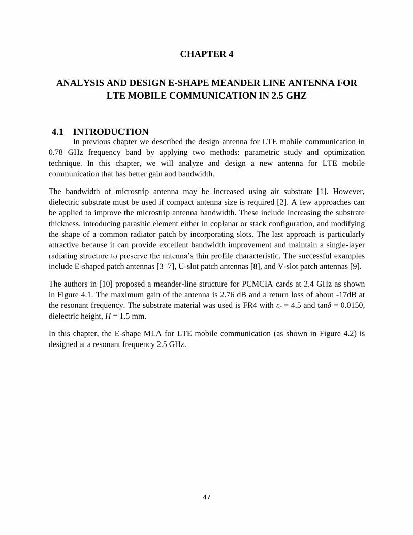
47

CHAPTER 4

ANALYSIS AND DESIGN E-SHAPE MEANDER LINE ANTENNA FOR

LTE MOBILE COMMUNICATION IN 2.5 GHZ

4.1 INTRODUCTION In previous chapter we described the design antenna for LTE mobile communication in

0.78 GHz frequency band by applying two methods: parametric study and optimization

technique. In this chapter, we will analyze and design a new antenna for LTE mobile

communication that has better gain and bandwidth.

The bandwidth of microstrip antenna may be increased using air substrate [1]. However,

dielectric substrate must be used if compact antenna size is required [2]. A few approaches can

be applied to improve the microstrip antenna bandwidth. These include increasing the substrate

thickness, introducing parasitic element either in coplanar or stack configuration, and modifying

the shape of a common radiator patch by incorporating slots. The last approach is particularly

attractive because it can provide excellent bandwidth improvement and maintain a single-layer

radiating structure to preserve the antenna’s thin profile characteristic. The successful examples

include E-shaped patch antennas [3–7], U-slot patch antennas [8], and V-slot patch antennas [9].

The authors in [10] proposed a meander-line structure for PCMCIA cards at 2.4 GHz as shown

in Figure 4.1. The maximum gain of the antenna is 2.76 dB and a return loss of about -17dB at

the resonant frequency. The substrate material was used is FR4 with εr = 4.5 and tanδ = 0.0150,

dielectric height, H = 1.5 mm.

In this chapter, the E-shape MLA for LTE mobile communication (as shown in Figure 4.2) is

designed at a resonant frequency 2.5 GHz.

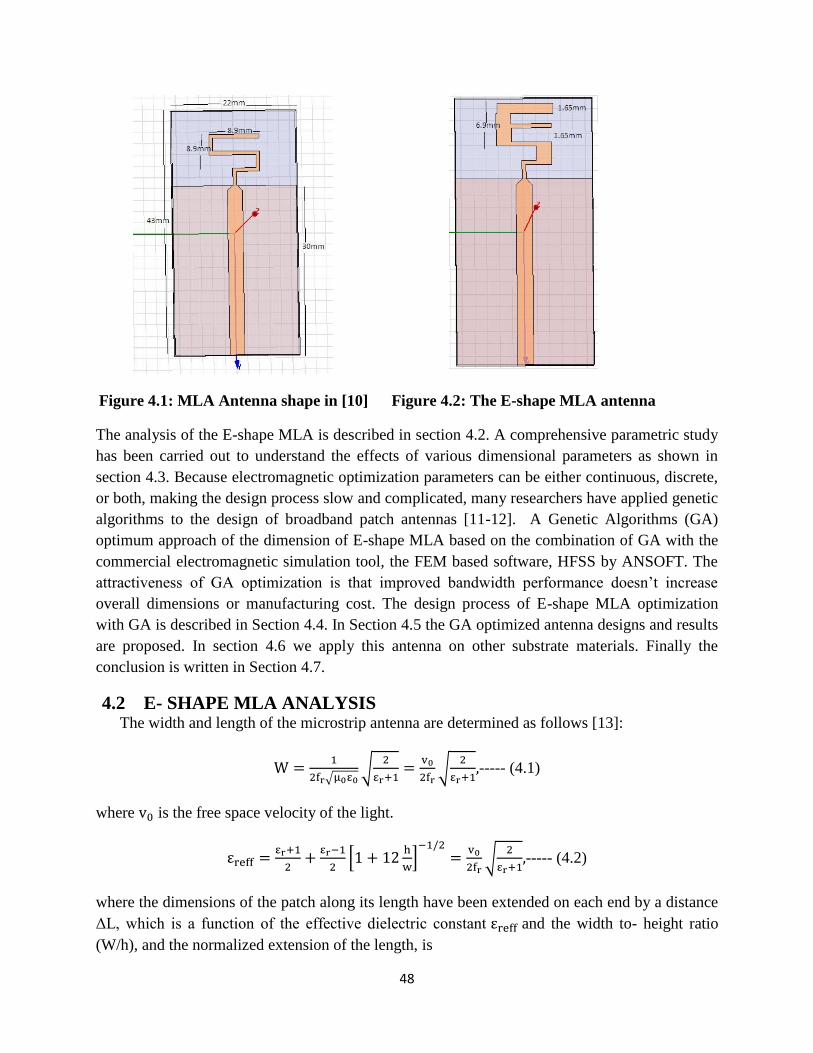
48

Figure 4.1: MLA Antenna shape in [10] Figure 4.2: The E-shape MLA antenna

The analysis of the E-shape MLA is described in section 4.2. A comprehensive parametric study

has been carried out to understand the effects of various dimensional parameters as shown in

section 4.3. Because electromagnetic optimization parameters can be either continuous, discrete,

or both, making the design process slow and complicated, many researchers have applied genetic

algorithms to the design of broadband patch antennas [11-12]. A Genetic Algorithms (GA)

optimum approach of the dimension of E-shape MLA based on the combination of GA with the

commercial electromagnetic simulation tool, the FEM based software, HFSS by ANSOFT. The

attractiveness of GA optimization is that improved bandwidth performance doesn’t increase

overall dimensions or manufacturing cost. The design process of E-shape MLA optimization

with GA is described in Section 4.4. In Section 4.5 the GA optimized antenna designs and results

are proposed. In section 4.6 we apply this antenna on other substrate materials. Finally the

conclusion is written in Section 4.7.

4.2 E- SHAPE MLA ANALYSIS The width and length of the microstrip antenna are determined as follows [13]:

√ √

√

----- (4.1)

where is the free space velocity of the light.

*

+

√

----- (4.2)

where the dimensions of the patch along its length have been extended on each end by a distance

ΔL, which is a function of the effective dielectric constant and the width to- height ratio

(W/h), and the normalized extension of the length, is

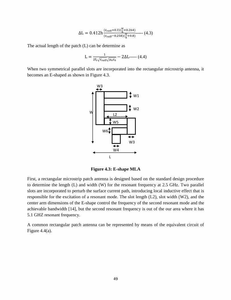
49

( )(

)

( )(

)

----- (4.3)

The actual length of the patch (L) can be determine as

√ √ ----- (4.4)

When two symmetrical parallel slots are incorporated into the rectangular microstrip antenna, it

becomes an E-shaped as shown in Figure 4.3.

Figure 4.3: E-shape MLA

First, a rectangular microstrip patch antenna is designed based on the standard design procedure

to determine the length (L) and width (W) for the resonant frequency at 2.5 GHz. Two parallel

slots are incorporated to perturb the surface current path, introducing local inductive effect that is

responsible for the excitation of a resonant mode. The slot length (L2), slot width (W2), and the

center arm dimensions of the E-shape control the frequency of the second resonant mode and the

achievable bandwidth [14], but the second resonant frequency is out of the our area where it has

5.1 GHZ resonant frequency.

A common rectangular patch antenna can be represented by means of the equivalent circuit of

Figure 4.4(a).

W5

W3

W1

W2

W3

W4

W6

L2 W

L

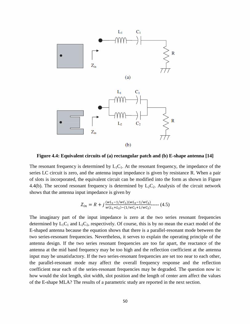
50

Figure 4.4: Equivalent circuits of (a) rectangular patch and (b) E-shape antenna [14]

The resonant frequency is determined by L1C1. At the resonant frequency, the impedance of the

series LC circuit is zero, and the antenna input impedance is given by resistance R. When a pair

of slots is incorporated, the equivalent circuit can be modified into the form as shown in Figure

4.4(b). The second resonant frequency is determined by L2C2. Analysis of the circuit network

shows that the antenna input impedance is given by

( )( )⁄⁄

( ) ( )⁄⁄----- (4.5)

The imaginary part of the input impedance is zero at the two series resonant frequencies

determined by L1C1 and L2C2, respectively. Of course, this is by no mean the exact model of the

E-shaped antenna because the equation shows that there is a parallel-resonant mode between the

two series-resonant frequencies. Nevertheless, it serves to explain the operating principle of the

antenna design. If the two series resonant frequencies are too far apart, the reactance of the

antenna at the mid band frequency may be too high and the reflection coefficient at the antenna

input may be unsatisfactory. If the two series-resonant frequencies are set too near to each other,

the parallel-resonant mode may affect the overall frequency response and the reflection

coefficient near each of the series-resonant frequencies may be degraded. The question now is:

how would the slot length, slot width, slot position and the length of center arm affect the values

of the E-shape MLA? The results of a parametric study are reported in the next section.

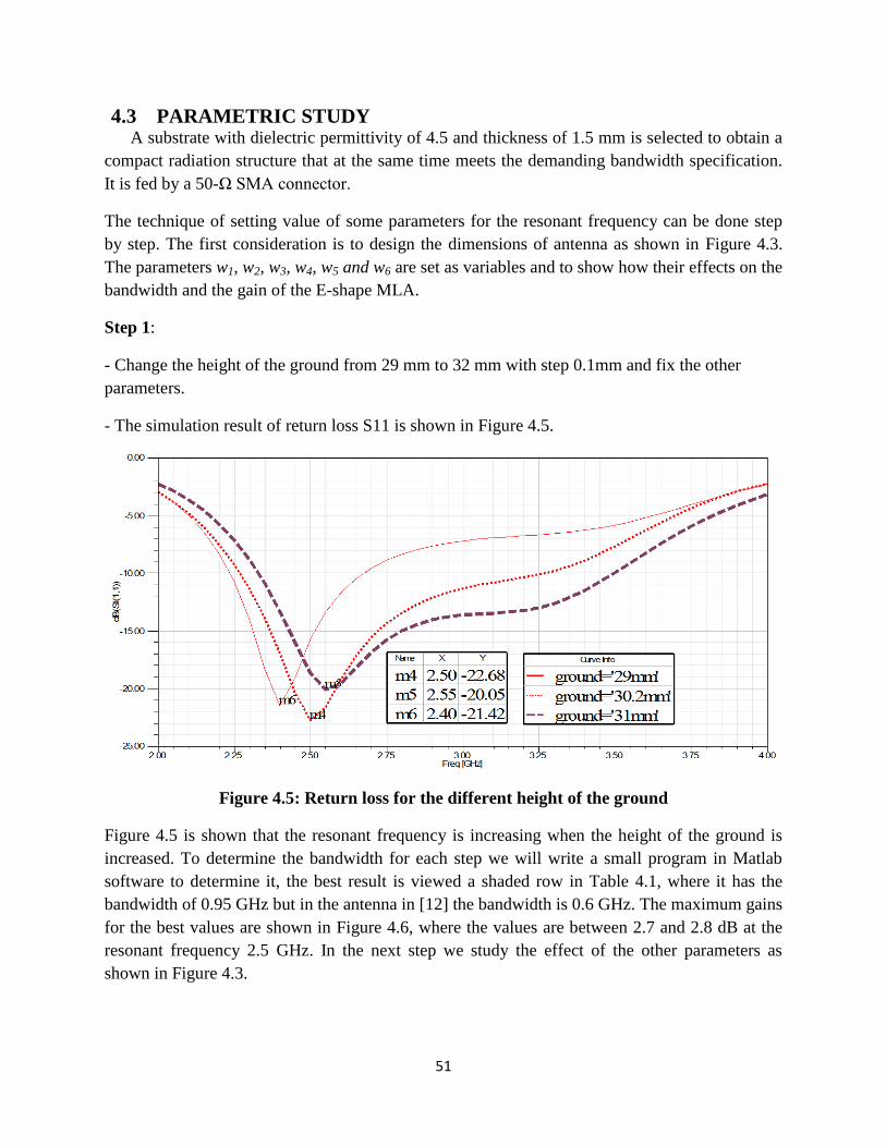
51

4.3 PARAMETRIC STUDY A substrate with dielectric permittivity of 4.5 and thickness of 1.5 mm is selected to obtain a

compact radiation structure that at the same time meets the demanding bandwidth specification.

It is fed by a 50-Ω SMA connector.

The technique of setting value of some parameters for the resonant frequency can be done step

by step. The first consideration is to design the dimensions of antenna as shown in Figure 4.3.

The parameters w1, w2, w3, w4, w5 and w6 are set as variables and to show how their effects on the

bandwidth and the gain of the E-shape MLA.

Step 1:

- Change the height of the ground from 29 mm to 32 mm with step 0.1mm and fix the other

parameters.

- The simulation result of return loss S11 is shown in Figure 4.5.

Figure 4.5: Return loss for the different height of the ground

Figure 4.5 is shown that the resonant frequency is increasing when the height of the ground is

increased. To determine the bandwidth for each step we will write a small program in Matlab

software to determine it, the best result is viewed a shaded row in Table 4.1, where it has the

bandwidth of 0.95 GHz but in the antenna in [12] the bandwidth is 0.6 GHz. The maximum gains

for the best values are shown in Figure 4.6, where the values are between 2.7 and 2.8 dB at the

resonant frequency 2.5 GHz. In the next step we study the effect of the other parameters as

shown in Figure 4.3.

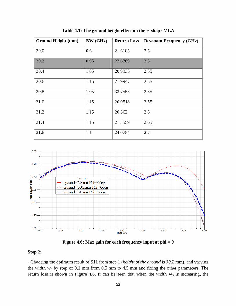
52

Table 4.1: The ground height effect on the E-shape MLA

Ground Height (mm) BW (GHz) Return Loss Resonant Frequency (GHz)

30.0 0.6 21.6185 2.5

30.2 0.95 22.6769 2.5

30.4 1.05 20.9935 2.55

30.6 1.15 21.9947 2.55

30.8 1.05 33.7555 2.55

31.0 1.15 20.0518 2.55

31.2 1.15 20.362 2.6

31.4 1.15 21.3559 2.65

31.6 1.1 24.0754 2.7

Figure 4.6: Max gain for each frequency input at phi = 0

Step 2:

- Choosing the optimum result of S11 from step 1 (height of the ground is 30.2 mm), and varying

the width w3 by step of 0.1 mm from 0.5 mm to 4.5 mm and fixing the other parameters. The

return loss is shown in Figure 4.6. It can be seen that when the width w3 is increasing, the

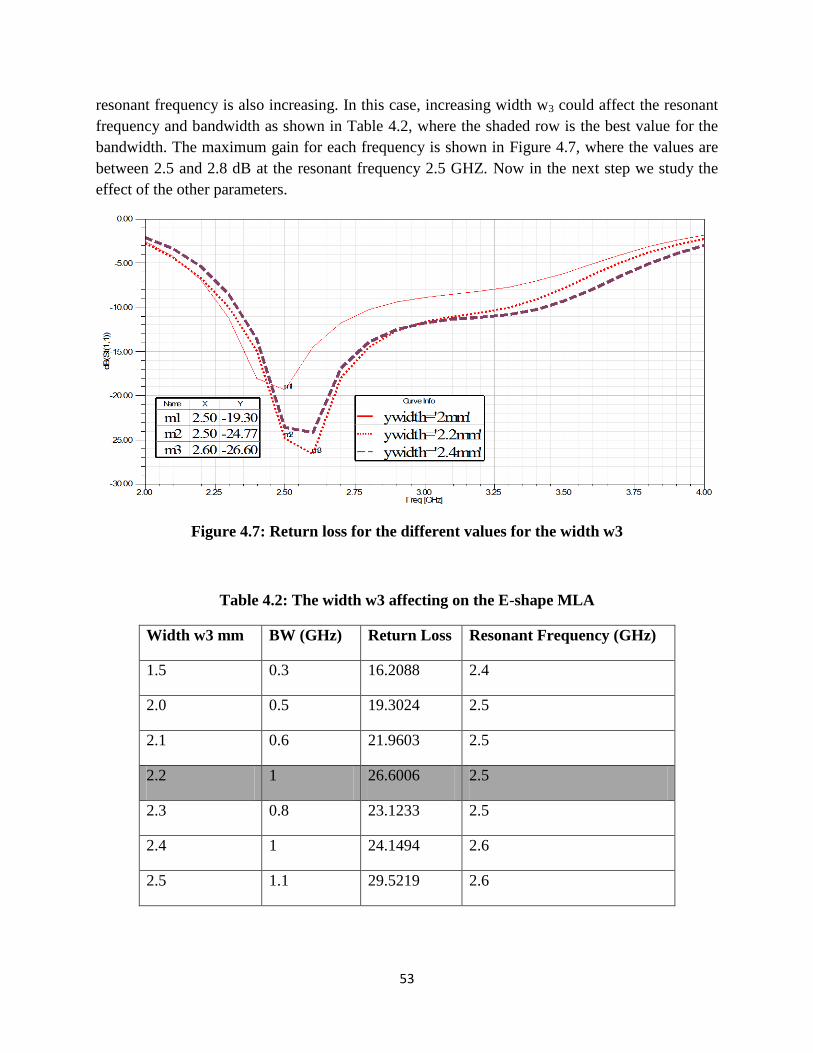
53

resonant frequency is also increasing. In this case, increasing width w3 could affect the resonant

frequency and bandwidth as shown in Table 4.2, where the shaded row is the best value for the

bandwidth. The maximum gain for each frequency is shown in Figure 4.7, where the values are

between 2.5 and 2.8 dB at the resonant frequency 2.5 GHZ. Now in the next step we study the

effect of the other parameters.

Figure 4.7: Return loss for the different values for the width w3

Table 4.2: The width w3 affecting on the E-shape MLA

Width w3 mm BW (GHz) Return Loss Resonant Frequency (GHz)

1.5 0.3 16.2088 2.4

2.0 0.5 19.3024 2.5

2.1 0.6 21.9603 2.5

2.2 1 26.6006 2.5

2.3 0.8 23.1233 2.5

2.4 1 24.1494 2.6

2.5 1.1 29.5219 2.6

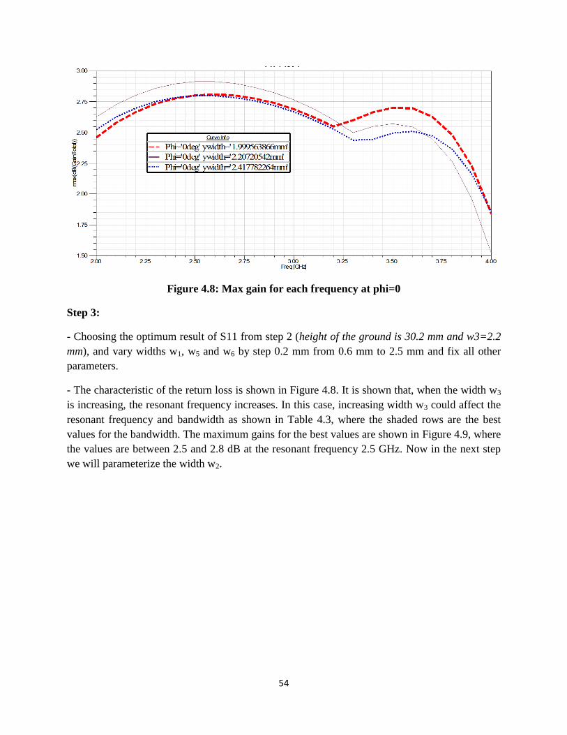
54

Figure 4.8: Max gain for each frequency at phi=0

Step 3:

- Choosing the optimum result of S11 from step 2 (height of the ground is 30.2 mm and w3=2.2

mm), and vary widths w1, w5 and w6 by step 0.2 mm from 0.6 mm to 2.5 mm and fix all other

parameters.

- The characteristic of the return loss is shown in Figure 4.8. It is shown that, when the width w3

is increasing, the resonant frequency increases. In this case, increasing width w3 could affect the

resonant frequency and bandwidth as shown in Table 4.3, where the shaded rows are the best

values for the bandwidth. The maximum gains for the best values are shown in Figure 4.9, where

the values are between 2.5 and 2.8 dB at the resonant frequency 2.5 GHz. Now in the next step

we will parameterize the width w2.

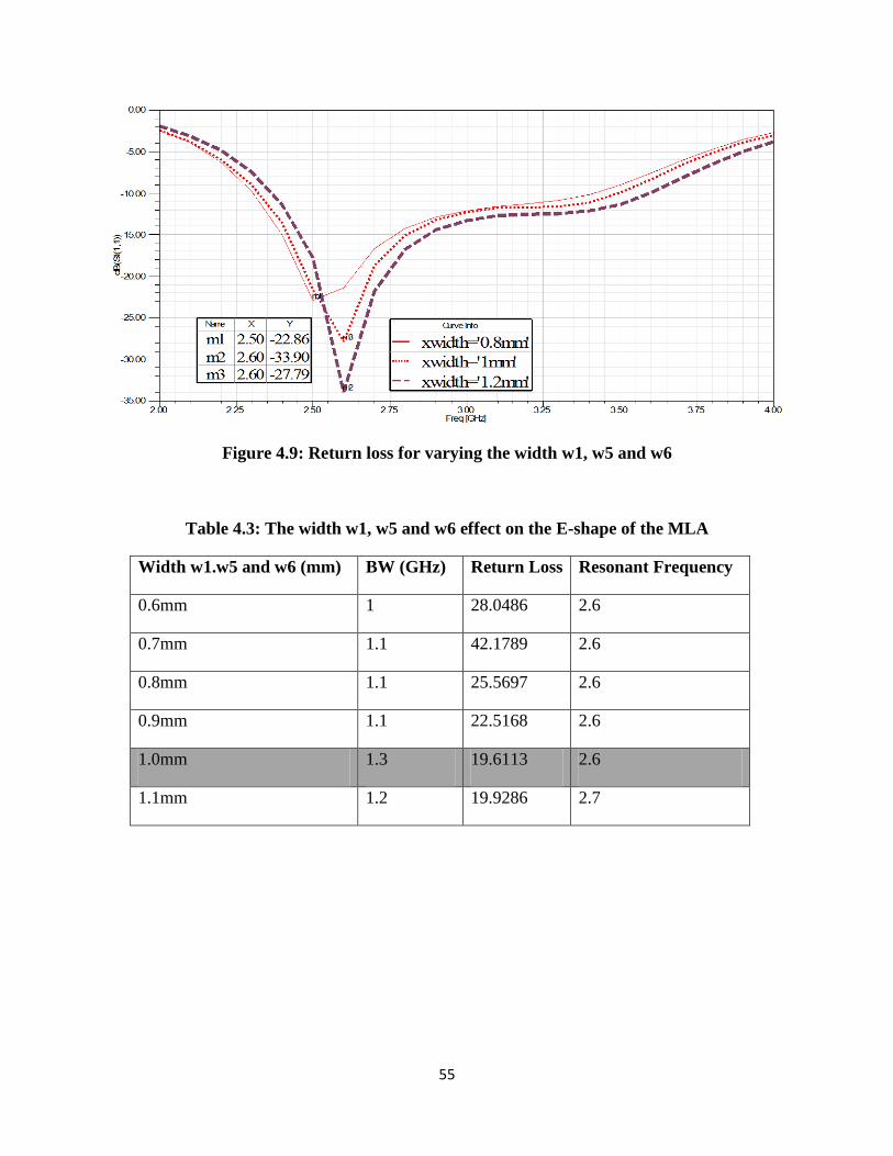
55

Figure 4.9: Return loss for varying the width w1, w5 and w6

Table 4.3: The width w1, w5 and w6 effect on the E-shape of the MLA

Width w1.w5 and w6 (mm) BW (GHz) Return Loss Resonant Frequency

0.6mm 1 28.0486 2.6

0.7mm 1.1 42.1789 2.6

0.8mm 1.1 25.5697 2.6

0.9mm 1.1 22.5168 2.6

1.0mm 1.3 19.6113 2.6

1.1mm 1.2 19.9286 2.7

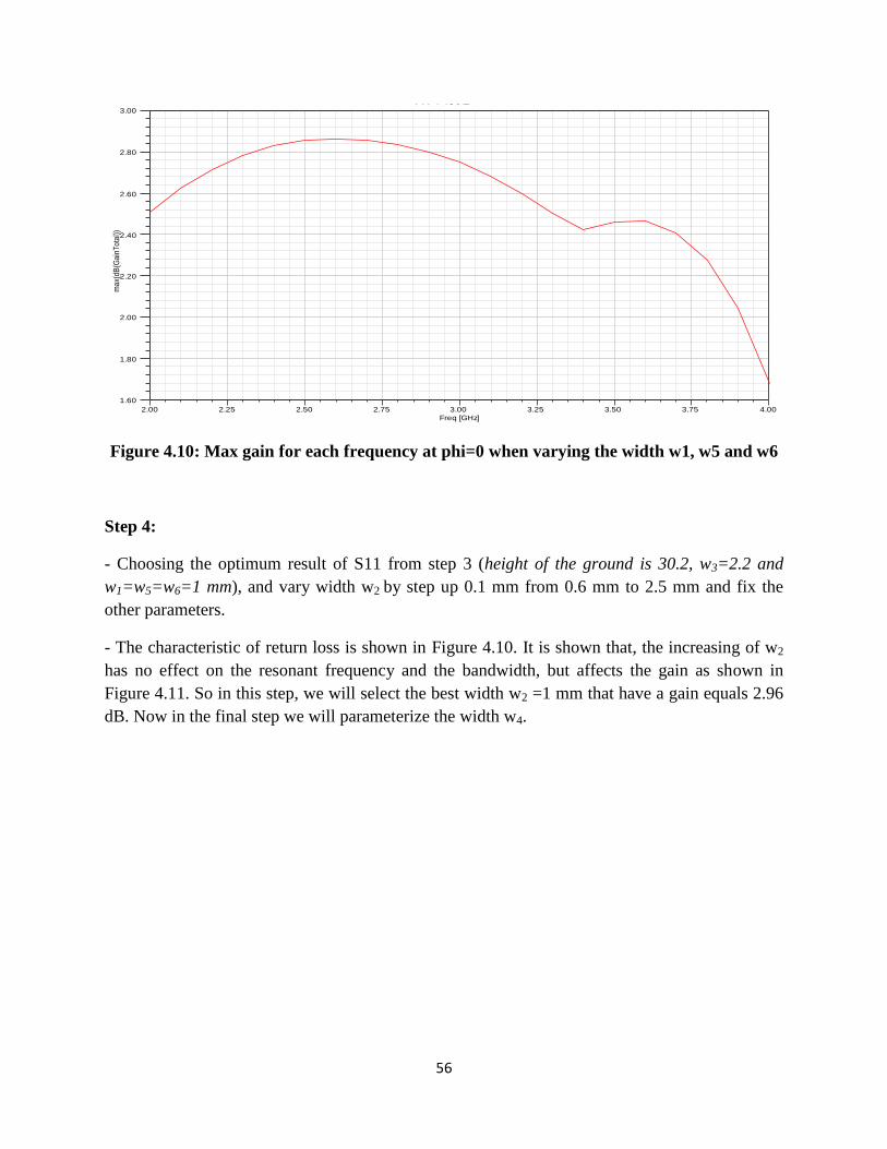
56

Figure 4.10: Max gain for each frequency at phi=0 when varying the width w1, w5 and w6

Step 4:

- Choosing the optimum result of S11 from step 3 (height of the ground is 30.2, w3=2.2 and

w1=w5=w6=1 mm), and vary width w2 by step up 0.1 mm from 0.6 mm to 2.5 mm and fix the

other parameters.

- The characteristic of return loss is shown in Figure 4.10. It is shown that, the increasing of w2

has no effect on the resonant frequency and the bandwidth, but affects the gain as shown in

Figure 4.11. So in this step, we will select the best width w2 =1 mm that have a gain equals 2.96

dB. Now in the final step we will parameterize the width w4.

2.00 2.25 2.50 2.75 3.00 3.25 3.50 3.75 4.00

Freq [GHz]

1.60

1.80

2.00

2.20

2.40

2.60

2.80

3.00m

ax(

dB

(Ga

inT

ota

l))

Ansoft LLC Patch_Antenna_ADKv1XY Plot 1

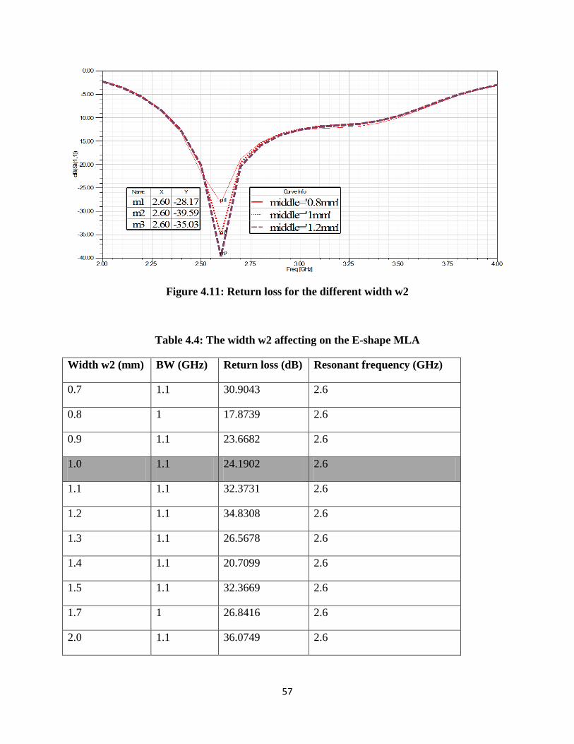
57

Figure 4.11: Return loss for the different width w2

Table 4.4: The width w2 affecting on the E-shape MLA

Width w2 (mm) BW (GHz) Return loss (dB) Resonant frequency (GHz)

0.7 1.1 30.9043 2.6

0.8 1 17.8739 2.6

0.9 1.1 23.6682 2.6

1.0 1.1 24.1902 2.6

1.1 1.1 32.3731 2.6

1.2 1.1 34.8308 2.6

1.3 1.1 26.5678 2.6

1.4 1.1 20.7099 2.6

1.5 1.1 32.3669 2.6

1.7 1 26.8416 2.6

2.0 1.1 36.0749 2.6

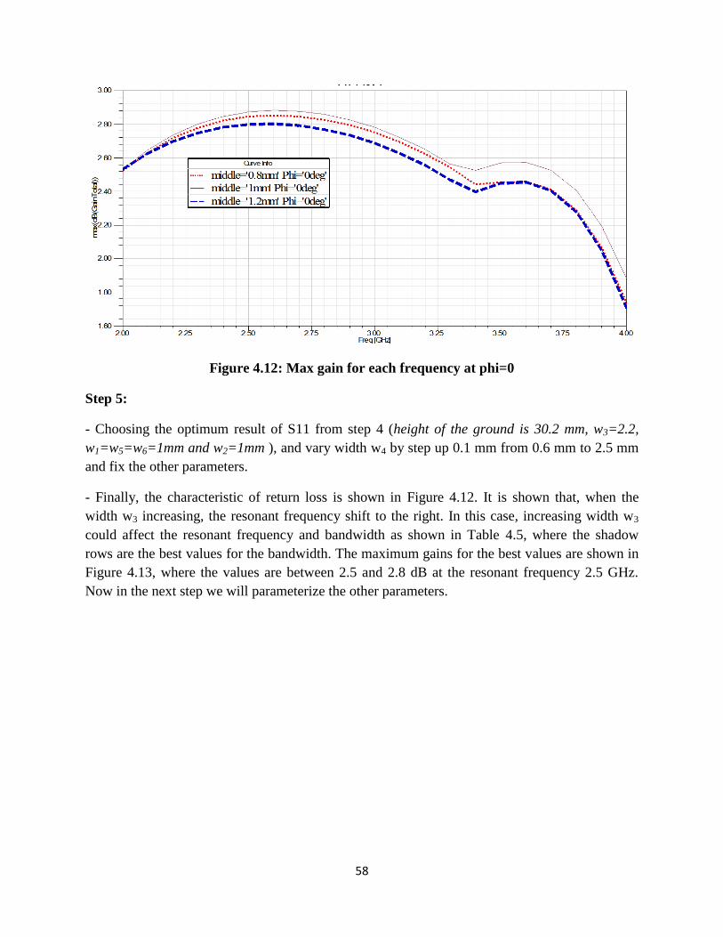
58

Figure 4.12: Max gain for each frequency at phi=0

Step 5:

- Choosing the optimum result of S11 from step 4 (height of the ground is 30.2 mm, w3=2.2,

w1=w5=w6=1mm and w2=1mm ), and vary width w4 by step up 0.1 mm from 0.6 mm to 2.5 mm

and fix the other parameters.

- Finally, the characteristic of return loss is shown in Figure 4.12. It is shown that, when the

width w3 increasing, the resonant frequency shift to the right. In this case, increasing width w3

could affect the resonant frequency and bandwidth as shown in Table 4.5, where the shadow

rows are the best values for the bandwidth. The maximum gains for the best values are shown in

Figure 4.13, where the values are between 2.5 and 2.8 dB at the resonant frequency 2.5 GHz.

Now in the next step we will parameterize the other parameters.

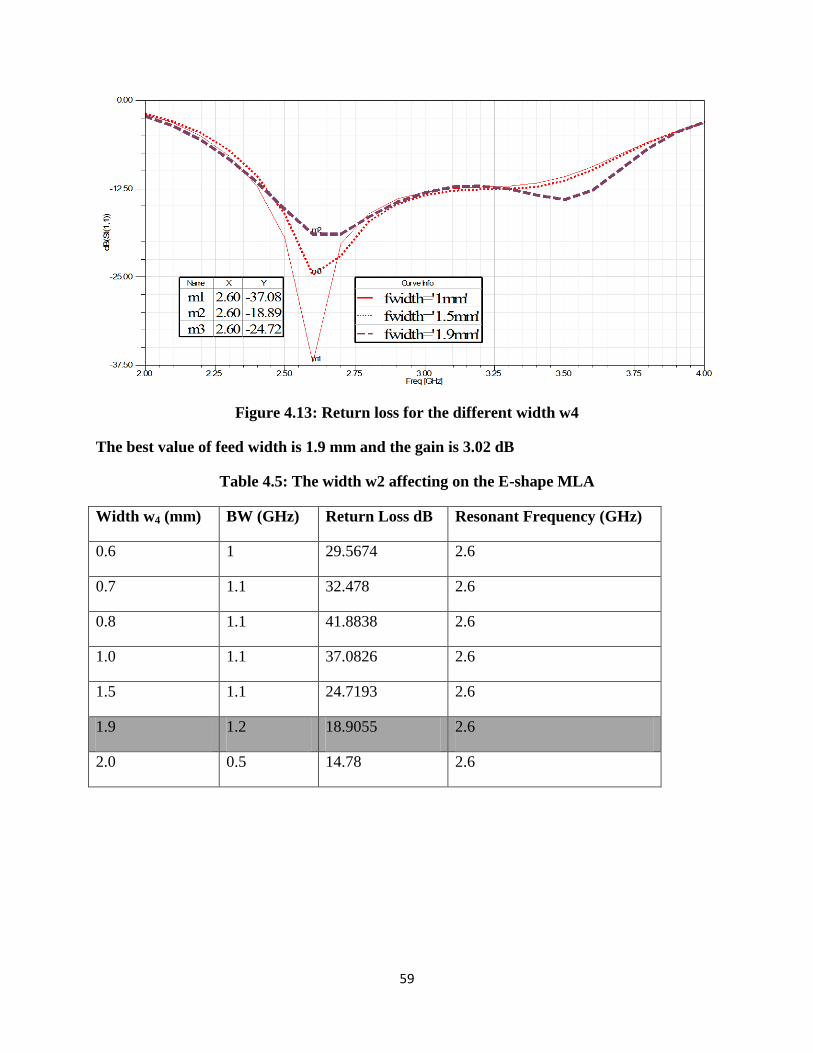
59

Figure 4.13: Return loss for the different width w4

The best value of feed width is 1.9 mm and the gain is 3.02 dB

Table 4.5: The width w2 affecting on the E-shape MLA

Width w4 (mm) BW (GHz) Return Loss dB Resonant Frequency (GHz)

0.6 1 29.5674 2.6

0.7 1.1 32.478 2.6

0.8 1.1 41.8838 2.6

1.0 1.1 37.0826 2.6

1.5 1.1 24.7193 2.6

1.9 1.2 18.9055 2.6

2.0 0.5 14.78 2.6

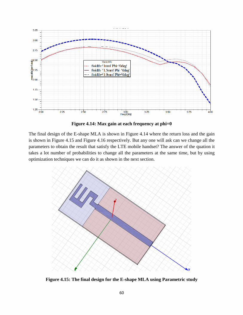
60

Figure 4.14: Max gain at each frequency at phi=0

The final design of the E-shape MLA is shown in Figure 4.14 where the return loss and the gain

is shown in Figure 4.15 and Figure 4.16 respectively. But any one will ask can we change all the

parameters to obtain the result that satisfy the LTE mobile handset? The answer of the quation it

takes a lot number of probabilities to change all the parameters at the same time, but by using

optimization techniques we can do it as shown in the next section.

Figure 4.15: The final design for the E-shape MLA using Parametric study

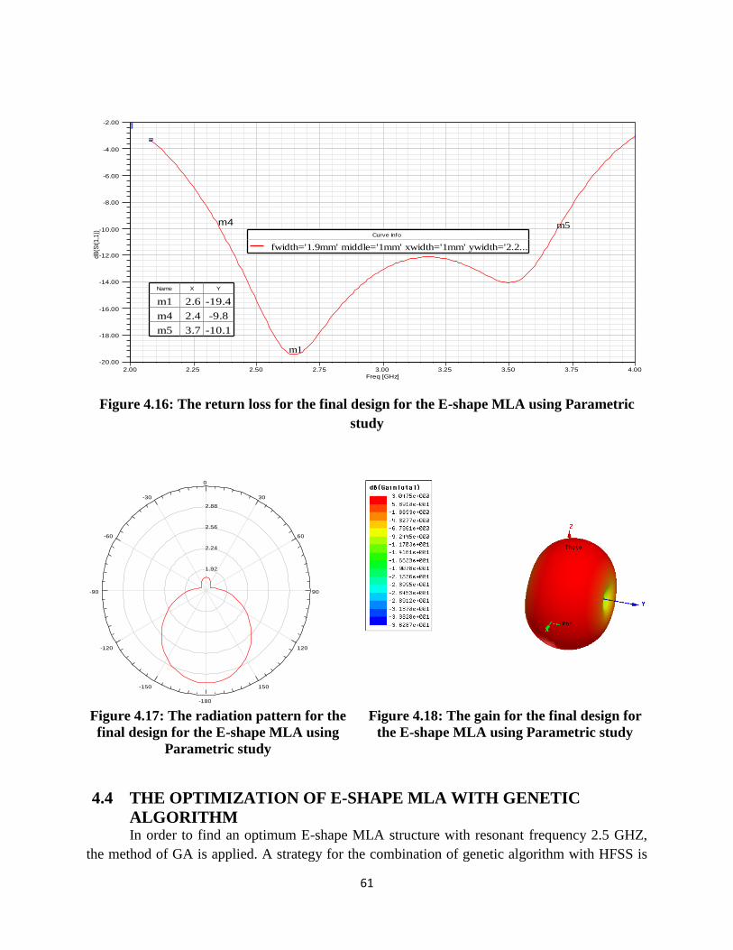
61

Figure 4.16: The return loss for the final design for the E-shape MLA using Parametric

study

Figure 4.17: The radiation pattern for the

final design for the E-shape MLA using

Parametric study

Figure 4.18: The gain for the final design for

the E-shape MLA using Parametric study

4.4 THE OPTIMIZATION OF E-SHAPE MLA WITH GENETIC

ALGORITHM In order to find an optimum E-shape MLA structure with resonant frequency 2.5 GHZ,

the method of GA is applied. A strategy for the combination of genetic algorithm with HFSS is

2.00 2.25 2.50 2.75 3.00 3.25 3.50 3.75 4.00

Freq [GHz]

-20.00

-18.00

-16.00

-14.00

-12.00

-10.00

-8.00

-6.00

-4.00

-2.00

dB

(St(

1,1

))

Ansoft LLC Patch_Antenna_ADKv1Return Loss

m4

m1

m5

Name X Y

m1 2.6 -19.4

m4 2.4 -9.8

m5 3.7 -10.1

Curve Info

fwidth='1.9mm' middle='1mm' xwidth='1mm' ywidth='2.2...

1.92

2.24

2.56

2.88

90

60

30

0

-30

-60

-90

-120

-150

-180

150

120

Ansoft LLC Patch_Antenna_ADKv1Radiation Pattern 1

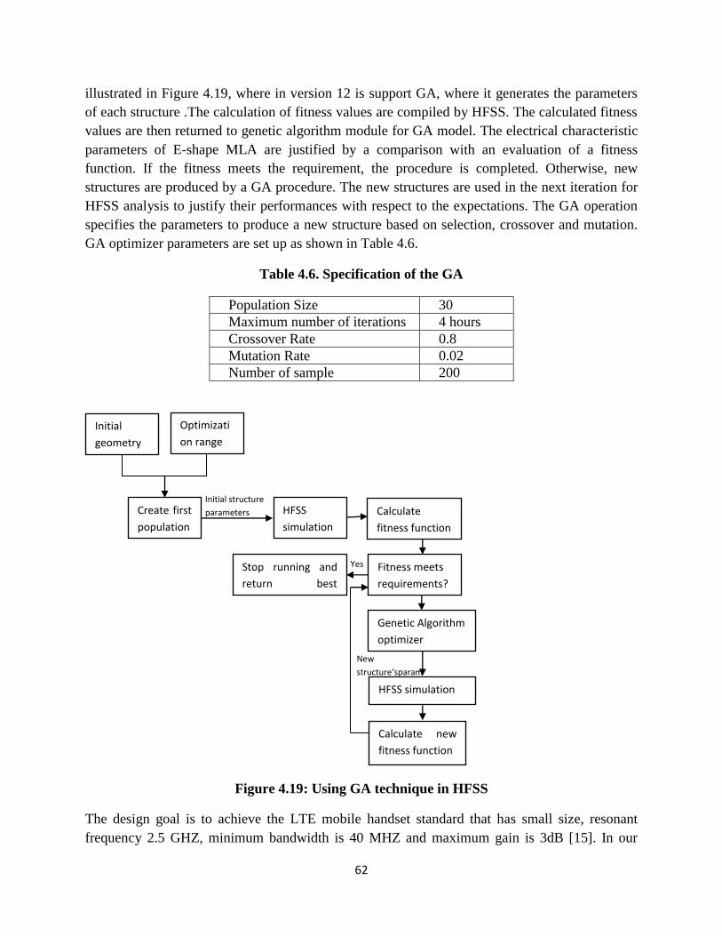
62

illustrated in Figure 4.19, where in version 12 is support GA, where it generates the parameters

of each structure .The calculation of fitness values are compiled by HFSS. The calculated fitness

values are then returned to genetic algorithm module for GA model. The electrical characteristic

parameters of E-shape MLA are justified by a comparison with an evaluation of a fitness

function. If the fitness meets the requirement, the procedure is completed. Otherwise, new

structures are produced by a GA procedure. The new structures are used in the next iteration for

HFSS analysis to justify their performances with respect to the expectations. The GA operation

specifies the parameters to produce a new structure based on selection, crossover and mutation.

GA optimizer parameters are set up as shown in Table 4.6.

Table 4.6. Specification of the GA

Population Size 30

Maximum number of iterations 4 hours

Crossover Rate 0.8

Mutation Rate 0.02

Number of sample 200

Figure 4.19: Using GA technique in HFSS

The design goal is to achieve the LTE mobile handset standard that has small size, resonant

frequency 2.5 GHZ, minimum bandwidth is 40 MHZ and maximum gain is 3dB [15]. In our

Calculate new

fitness function

HFSS simulation

Yes

HFSS

simulation

Calculate

fitness function

Stop running and

return best

solution

Genetic Algorithm

optimizer

Initial

geometry

Optimizati

on range

Create first

population

Initial structure

parameters

Fitness meets

requirements?

New

structure‘sparam

eters

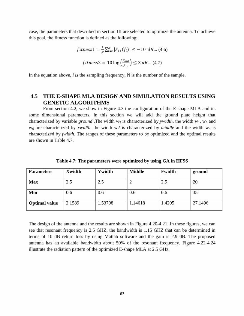
63

case, the parameters that described in section III are selected to optimize the antenna. To achieve

this goal, the fitness function is defined as the following:

∑ | ( )| ... (4.6)

(

) ... (4.7)

In the equation above, i is the sampling frequency, N is the number of the sample.

4.5 THE E-SHAPE MLA DESIGN AND SIMULATION RESULTS USING

GENETIC ALGORITHMS From section 4.2, we show in Figure 4.3 the configuration of the E-shape MLA and its

some dimensional parameters. In this section we will add the ground plate height that

characterized by variable ground .The width w3 is characterized by ywidth, the width w1, w5 and

w6 are characterized by xwidth, the width w2 is characterized by middle and the width w4 is

characterized by fwidth. The ranges of these parameters to be optimized and the optimal results

are shown in Table 4.7.

Table 4.7: The parameters were optimized by using GA in HFSS

Parameters Xwidth Ywidth Middle Fwidth ground

Max 2.5 2.5 2 2.5 20

Min 0.6 0.6 0.6 0.6 35

Optimal value 2.1589 1.53708 1.14618 1.4205 27.1496

The design of the antenna and the results are shown in Figure 4.20-4.21. In these figures, we can

see that resonant frequency is 2.5 GHZ, the bandwidth is 1.15 GHZ that can be determined in

terms of 10 dB return loss by using Matlab software and the gain is 2.9 dB. The proposed

antenna has an available bandwidth about 50% of the resonant frequency. Figure 4.22-4.24

illustrate the radiation pattern of the optimized E-shape MLA at 2.5 GHz.

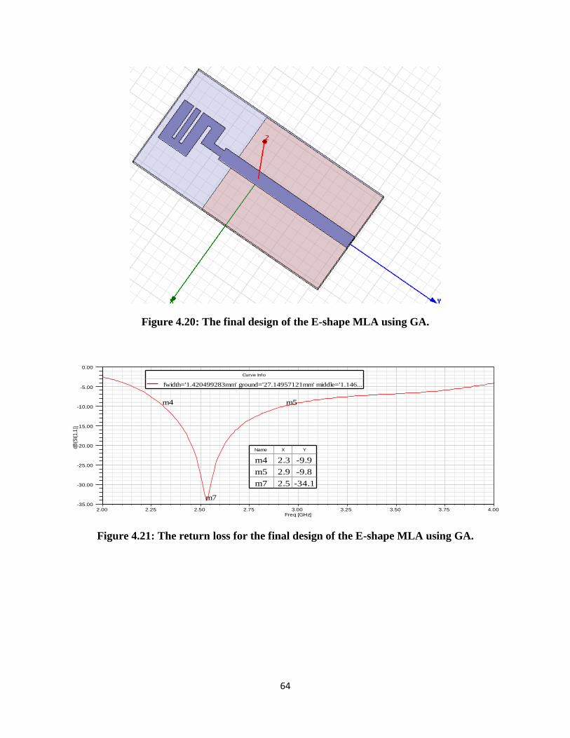
64

Figure 4.20: The final design of the E-shape MLA using GA.

Figure 4.21: The return loss for the final design of the E-shape MLA using GA.

2.00 2.25 2.50 2.75 3.00 3.25 3.50 3.75 4.00Freq [GHz]

-35.00

-30.00

-25.00

-20.00

-15.00

-10.00

-5.00

0.00

dB

(St(

1,1

))

Ansoft LLC Patch_Antenna_ADKv1Return Loss

m4

m7

m5

Name X Y

m4 2.3 -9.9

m5 2.9 -9.8

m7 2.5 -34.1

Curve Info

fwidth='1.420499283mm' ground='27.14957121mm' middle='1.146...

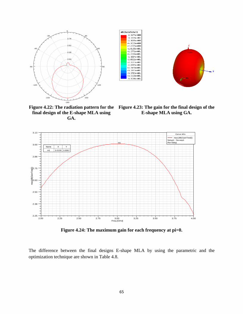
65

Figure 4.22: The radiation pattern for the

final design of the E-shape MLA using

GA.

Figure 4.23: The gain for the final design of the

E-shape MLA using GA.

Figure 4.24: The maximum gain for each frequency at pi=0.

The difference between the final designs E-shape MLA by using the parametric and the

optimization technique are shown in Table 4.8.

2.04

2.28

2.52

2.76

90

60

30

0

-30

-60

-90

-120

-150

-180

150

120

Ansoft LLC Patch_Antenna_ADKv1Radiation Pattern 1

Curve Info

dB(GainTotal)

Setup1 : LastAdaptive

Freq='2.5GHz' Phi='0deg'

2.00 2.25 2.50 2.75 3.00 3.25 3.50 3.75 4.00

Freq [GHz]

2.25

2.38

2.50

2.63

2.75

2.88

3.00

3.13

ma

x(d

B(G

ain

To

tal)

)

Ansoft LLC Patch_Antenna_ADKv1XY Plot 1

m1

Curve Info

max(dB(GainTotal))

Setup1 : Sw eep1

Phi='0deg'

Name X Y

m1 3.0100 3.0067

66

TABLE 4.8: THE DIFFERENCE BETWEEN THE FINAL DESIGN USING PARAMETRIC AND OPTIMIZATION METHOD

Parameters The final design using

parametric method

The final design using

optimization method

Resonant Frequency 2.6 GHZ 2.5 GHZ

Max Return Loss 19 dB 34 dB

10dB bandwidth 1.2 GHZ 0.65 GHZ

Max Gain 3.02 2.93

4.6 THE OPTIMIZATION OF E-SHAPE MLA WITH GENETIC

ALGORITHM ON DIFFERENT SUBSTRATES In the previous sections, we apply the parametric and optimization on the E-shape MLA that

has a substrate material FR4 with εr = 4.5 and tanδ = 0.0150, dielectric height and h = 1.5 mm. In

this section we will apply the same parameters on other substrate materials as shown in Table

4.9.

Table 4.9: The difference between the different substrate materials

Substrate material Relative Permittivity Substrate Height (mm)

FR4 4.5 1.5

RO5880 1.96 1.5

RO3003 3 1.5

The results for the different substrate materials are shown in Table 4.10.

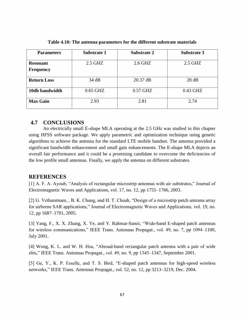
67

Table 4.10: The antenna parameters for the different substrate materials

Parameters Substrate 1 Substrate 2 Substrate 3

Resonant

Frequency

2.5 GHZ 2.6 GHZ 2.5 GHZ

Return Loss 34 dB 20.37 dB 28 dB

10db bandwidth 0.65 GHZ 0.57 GHZ 0.43 GHZ

Max Gain 2.93 2.81 2.74

4.7 CONCLUSIONS An electrically small E-shape MLA operating at the 2.5 GHz was studied in this chapter

using HFSS software package. We apply parametric and optimization technique using genetic

algorithms to achieve the antenna for the standard LTE mobile handset. The antenna provided a

significant bandwidth enhancement and small gain enhancements. The E-shape MLA depicts an

overall fair performance and it could be a promising candidate to overcome the deficiencies of

the low profile small antennas. Finally, we apply the antenna on different substrates.

REFERENCES

[1] A. F. A. Ayoub, “Analysis of rectangular microstrip antennas with air substrates,” Journal of

Electromagnetic Waves and Applications, vol. 17, no. 12, pp 1755–1766, 2003.

[2] G. Vetharatnam, , B. K. Chung, and H. T. Chuah, “Design of a microstrip patch antenna array

for airborne SAR applications,” Journal of Electromagnetic Waves and Applications, vol. 19, no.

12, pp 1687–1701, 2005.

[3] Yang, F., X. X. Zhang, X. Ye, and Y. Rahmat-Samii, “Wide-band E-shaped patch antennas

for wireless communications,” IEEE Trans. Antennas Propagat., vol. 49, no. 7, pp 1094–1100,

July 2001.

[4] Wong, K. L. and W. H. Hsu, “Abroad-band rectangular patch antenna with a pair of wide

slits,” IEEE Trans. Antennas Propagat., vol. 49, no. 9, pp 1345–1347, September 2001.

[5] Ge, Y., K. P. Esselle, and T. S. Bird, “E-shaped patch antennas for high-speed wireless

networks,” IEEE Trans. Antennas Propagat., vol. 52, no. 12, pp 3213–3219, Dec. 2004.

68

[6] Y. Ge, K. P. Esselle, and T. S. Bird, “A compact E-shaped patch antenna with corrugated

wings,” IEEE Trans. Antennas Propagat., vol. 54, no. 8,pp 2411–2413, Aug. 2006.

[7] A. Yu, and X. X. Zhang, “A method to enhance the bandwidth of microstrip antennas using a

modified E-shaped patch,” Proceedings of Radio and Wireless Conference, pp 261–264, Aug.

10–13, 2003.

[8] K. F. Lee, , et al., “Experimental and simulation studies of the coaxially fed U-slots

rectangular patch antenna,” IEE Proc. Microw. Antenna Propag., vol. 144, no. 5, pp 354–358,

October 1997.

[9] G. Rafi, and L. Shafai, “Broadband microstrip patch antenna with V-slot,” IEE Proc. Microw.

Antenna Propag., Vol. 151, No. 5, pp 435–440, October 2004.

[10] C.-C. Lin, S.-W. Kuo, and H.-R. Chuang, “A 2.4-GHz printed meander line antenna for

USB WLAN with notebook-PC housing,” IEEE Microw. Wireless Compon. Lett., vol.15, no. 9,

pp. 546-548, Sept. 2005.

[11] H. Choo, H. Ling, “Design of broadband and dual-band microstrip antennas on

highdielectric substrate using the genetic algorithm,” IEEE Proc. Microwaves Antennas

Propagat., vol. 150, no. 3 , pp. 137-142, June 2003.

[12] K. Michael, A. Kucharski, “Genetic algorithm optimization for broadband patch antenna

design,” Proc. of the 16th International Conference on Microwaves, Radar and Wireless

Communications, MIKON-2006, Kraków , vol. 2, pp. 748-751, May 22-24, 2006.

[13] M. K. Verma, Sapna Verma and D. C. Dhubkarya, “Analysis and designing of E-shape

microstrip patch antenna for the wireless communication systems”, International Conference on

Emerging Trends in Electronic and Photonic Devices & Systems, 2009.

[14] B.-K. Ang and B.-K. Chung, “A wideband E-shaped microstrip patch antenna for 5–6 GHz

wireless Communications,” Progress in Electromagnetics Research, PIER 75, pp 397–407, 2007.

[15] M. S. Sharawi , RF Planning and Optimization for LTE Networks, Taylor and Francis

Group, LLC , 2011.

69

CHAPTER 5

CONCLUSION

5.1 CONCLUSION

In this research work, a printed antenna is designed using meander line technique to

demonstrated lager impedance bandwidth for considerably small dimensions. Two types of

Meander Line antennas have been studied in this thesis. The first type is the design of MLA for

LTE mobile application in 0.78 GHz band and the second is the design of E-shape MLA for LTE

mobile application in 2.5 GHz band.

The first contribution of this research work, we analysis and design MLA for LTE mobile

application in 0.78 GHz band that has a correct selection of MLA dimensions that deal with it.

And we show that as tabulated in the conclusion section of chapter 3, The MLA in this research

has better gain comparing with MLA was used for it.

The second contribution of this research work is to analysis and design E-shape MLA for LTE

mobile handsets in 2.5 GHz band, where is the new shape antenna developed from the original

MLA. And we show the antenna has better bandwidth and gain for MLAs were used for the

same subject as described in chapter 4.

We used in this thesis two techniques: the first technique is parametric study where study each

variable in the antenna then study the effect each of them on the antenna, after that go to other

type and make the work until finish all the variables. We show the results from this technique is

a good method for enhancement the gain an the bandwidth but not the optimal solution.

The second technique is optimization technique using Genetic Algorithms at various times (4

hours, 1 day and 3 days) was found in HFSS v.12. This technique can be effectively used in the

design of various complex antenna and millimeter dimension circuits, where the performance of

this technique to design the antenna is a good precision design of antenna elements for low and

70

high frequency applications as shown the results in chapter 3 and 4. MATLAB codes were

written to determine the resonant frequency and the bandwidth for each study in this thesis.

5.2 FUTURE WORK Fabricate the two types of MLA and compare it with the simulation results.

Use Meta-material based substrates to further reduce the antenna size and introduce

enhancement the bandwidth and the gain.

Design and implement MIMO antenna systems for LTE standards of mobile phones with

reduced correlation coefficient. This is particularly challenging due to the size limitations

and usage of 0.78 and 2.5 GHz band for this system.

Design the LTE antenna in 1.8 GHz band where it will used in the Middle East at 2016.

Apply other optimization techniques such as particle swarm optimization (PSO), bacterial

foraging (BF) and compare the results with genetic algorithms.