Embed Size (px)
Citation preview

Lesson 1
Optimal Signal Processing
LTH
August 2008
Statistical Digital Signal Processing and Modeling,
Hayes, M:
John Wiley & Sons, 1996. ISBN 0471594318
Bengt Mandersson Department of Electroscience
Lund University
2
Optimal Signal Processing
The sound of ‘Signalbehandling’
‘s’ ‘i’ ‘g’ ‘n’ ‘………………………’
‘s’ ‘i’ noise harmonic signal How can this be generated as output from a linear filter? Determine the filter and the input signal. LPC model of syntetic sound production In syntetic speech production, the parameters often are updated every 5 milliseconds.
pulse train
white noise LPC-model
speech output from pulse train
)(0 zH speech output from white noise (waveform and spectra)
3
Optimal Signal Processing Chapter 2. Digital signal processing impulse response, convolution, system function, Fourier, z-transforms page 7-20 Matrix description. page 20-52 Hints. page 8-18, 21, 49. Chapter 3. Random processing, such as correlation functions, correlation matrices. Random variables page 58-74 Random Processes page 74-119 Hints. page 77, 79, 80, 85, 95, 99, 100, 101, 106 Chapter 4. Signal models, Deterministic and Stochastic approach. Padé, Prony page 133-154 Shank page 154-160 All-pole Modeling page 160,165 Linear prediction page 165-174 4.5 not included 4.6 page 178-188 4.7 Stochastic Models page 188-200 Hints. page 130, 135, 138, 147, 148,149 195, 195 Chapter 5. Levinson-Durbin recursion. page 215-225, 233-241 page 242 – 276 not included Hints. Table 5.1 – 5.4, figure 5.10 Chapter 6. Latttice FIR and IIR filters, only 6.2 and 6.4.1, 6.4.3 page 289-293, 297, 298, 304-307 6.5 page 308-324 Chapter 7. Optimal filters. Linear prediction. Wiener filters. Specially FIR filters. FIR- Wiener filter page 335-345 IIR- Wiener filter page 353-371 7.4 not included Hints. page 337-339, 354, 355, 358-363, 370 Chapter 8. Spectrum estimation. Nonparametric methods page 393-399, 408-425 8.3 (8.5 see chap 4) , 8.6 page 426-429, 451-472 Hints. page 394, 408
4
Optimal Signal Processing Digital Signal Processing Example: Echo system
Digital filter. A/D
Low pass-filter
Low pass- D/A
Sampling Reconstruction Digital circuit
Delay D
Delay 2D
D/A A/D x(t) x(n) y(t) y(n)
loadspeakermicrophone
+
+

5
Optimal Signal Processing
An application from the text book Noise cancellation (chapter 7, page 349)
A signal is disturbed by additive noise v1(n). Try to measure the noise v(n) from the source and estimate the noise v1(n) added to the signal. Then subtract the noise v1(n) from the received signal.
Signal source
H(z)
v(n)
Estimate of v1(n) Wiener filter
Noise source
s(n) s(n)+v1(n) s(n)
v1(n) v(n)
6
Optimal Signal Processing Optimal signal processing in Hay's book Chapter 2: Brief review of digital signal processing. Chapter 3: Brief review of random signals. The filters Hgen(z) and Hreceiver(z) are of type FIR IIR all-pole IIR Chapter 4, 5 and 6: Make a model Hgen(z) from the properties of s(n). Chapter 7: Determine Hreceiver(z). Chapter 8: Estimation of spectra.
received signal x(n)
white noise w(n) or impulse δ(n)
Estimate Hgen(z) from properties of s(n)
noice v(n)
hgen(n) Hgen(z)
transmitted s(n) hreceiver(n)
Hreceiver(z) y(n)
Determine Hreceiver(z)
7
Optimal Signal Processing Chapter 2 Digital Signal Processing Difference equation
y n a k y n k b k x n kk
q
k
p
( ) ( ) ( ) ( ) ( )= − − + −==∑∑
01
MATLAB: A=[1 0.5 0.5]; B=[1 1]; y=filter(B,A,x); Convolution
y n h k x n k
k( ) ( ) ( )= −
=−∞
∞
∑
impulse: ( ) [0 0 0 1 0 0 0]nδ↑
=
unit step: ( ) [0 0 0 1 111...]u n↑
= System function
)()()(
zAzBzH =
Frequency function
)()()( ω
ωω
j
jj
eAeBeH =
8
Optimal Signal Processing FIR, IIR filters FIR: Circuit with impulse response with finite length Example
( ) ( ) ( 1), ( ) ( ) ( 1)y n x n x n h n n nδ δ= + − = + − IIR: Circuit with impulse response with infinite length Example
( ) 0.5 ( 1) ( ), ( ) 0.5 ( )ny n y n x n h n u n= − + = All-pole IIR-filters IIR-filters with poles only ( all zeroes in origin, B(z)=constant) Example
15.011)( −−
=z
zH

9
Optimal Signal Processing Solvning the convolution sum.
( ) ( ) ( ) ( ) ( )
k ky n h k x n k x k h n k
∞ ∞
=−∞ =−∞
= − = −∑ ∑
( ) (0) ( ) (1) ( 1) (2) ( 2)y n h x n h x n h x n= ⋅ ⋅ ⋅ + − + − ⋅ ⋅ ⋅
Example ( ) [1 2 3 4], ( ) [4 2 2]x n h n↑ ↑
= = Method A: Vector notation
[ ] )(
)1(..
)1()(
)1()...1()0()( nxh
Nnx
nxnx
Nhhhny TT
−−=
⎥⎥⎥⎥⎥⎥
⎦
⎤
⎢⎢⎢⎢⎢⎢
⎣
⎡
+−
−−=
Method B: Graphical solution Write
( ) : 1 2 3 4
(0 ) : 2 2 4 (0) 4 1 4
(1 ) : 2 2 4 (1) 2 1 4 2 10
x k
h k y
h k y
↑
↑
↑
− = ⋅ =
− = ⋅ + ⋅ =
Gives the output ( ) [4 10 18 26 14 8]y n↑
= MATLAB: x=[1 2 3 4]; h=[4 2 2]; y=conv(x,h)
10
Optimal Signal Processing Method C: Convolution matrix Use matrix notations
( ) [1 2 3 4], ( ) [4 2 2]x n h n↑ ↑
= =
xx xx x xx x x
x xx
hhh
yyyyyy
( )( ) ( )( ) ( ) ( )( ) ( ) ( )
( ) ( )( )
( )( )( )
( )( )( )( )( )(5)
0 0 01 0 02 1 03 2 1
0 3 20 0 3
012
01234
⎡
⎣
⎢⎢⎢⎢⎢⎢⎢
⎤
⎦
⎥⎥⎥⎥⎥⎥⎥
⋅⎡
⎣
⎢⎢⎢
⎤
⎦
⎥⎥⎥
=
⎡
⎣
⎢⎢⎢⎢⎢⎢⎢
⎤
⎦
⎥⎥⎥⎥⎥⎥⎥
1 0 02 1 03 2 14 3 20 4 30 0 4
422
4101826148
⎡
⎣
⎢⎢⎢⎢⎢⎢⎢
⎤
⎦
⎥⎥⎥⎥⎥⎥⎥
⋅⎡
⎣
⎢⎢⎢
⎤
⎦
⎥⎥⎥
=
⎡
⎣
⎢⎢⎢⎢⎢⎢⎢
⎤
⎦
⎥⎥⎥⎥⎥⎥⎥
X h y=
In Matlab: x=[1 2 3 4]’; X=convmtx(x,3) h=[4 2 2]', y=X*h (In signal processing, all vectors are column vectors)
11
Optimal Signal Processing Properties of matrices
The square matrix ( )A n n× is:
symmetrical if TA A=
Hermitian if ( )T HA A A∗= =
invertable if 1AA I− =
Toeplitz if all diagonals are identical
3 4 52 3 41 2 3
A⎡ ⎤⎢ ⎥= ⎢ ⎥⎢ ⎥⎣ ⎦
Hermitian (symmetrical) Toeplitz if
3 2 12 3 21 2 3
A⎡ ⎤⎢ ⎥= ⎢ ⎥⎢ ⎥⎣ ⎦
[3,2,1]A Toep=
orthogonal if TA A I=
12
Optimal Signal Processing Linear equation (page 31-34)
[ ]A is a n m matrix∗
A x b= gives
1 , ( )x A b if n m A invertable−= =
1( )H Hx A A A b if n m−= >
(overdetermined, more equations than variables.) Described more in chapter 4
mnifbAAAx HH <= −1)( (underdetermined, less equations than variables) Eigenvalue:
A v v A I= − =λ λ, ( ) 0
,eigenvalues v eigenvectorsλ
ΛΛ= −
ofdiagonaltheinseigenvalueVofcolumnstheinrseigenvectowithVVA ,1

13
Optimal Signal Processing Optimisation ( minimizing): (page 49)
If z real: 2( )f z z=
2 2( ) 2 ; 0
0 min ;
d d df z z z zdz dz dz
gives z as imum
= = =
=
If z is complex: 2( ) | |f z z z z∗= =
( )zofconjugatetheisz∗
Derivate with respect to zorz∗ separately while
treating the other as a constant.
2
2
| |
| |
d dz z z zdz dzd dz z z z
dz dz
∗ ∗
∗∗ ∗
= =
= =
Setting this derivatives equal to zero gives the same minimum (page 49). This is used sometimes in the textbook.
14
Optimal Signal Processing Example on circuits A
)()(5.0)()1()1(5.0)(
11 zXzzYzzYnxnyny−− +=
−+−=
B C Lattice filters
FIR-lattice filter
IIR-lattice filter
y(n), Y(z) x(n), X(z)
Г1 z-1 z-1
-Г1 -Г2
Г2
Y(z) X(z)
y(n) Г1 x(n)
z-1 z-1 Г1 Г2
Г2
Y(z) X(z)y(n) x(n)
z-1
0.5
X(z)
y(n) x(n) z-1
0.5
z-1
0.5
0.5
Y(z)
15
Optimal Signal Processing Correlation functions (deterministic)
Autocorrelation function
( )( ) ( ) ( ) ( )x xxn
r l x n x n l r l∞
=−∞
= − =∑
Cross-correlation function
r l y n x n lyxn
( ) ( ) ( )= −=−∞
∞
∑
( ) ( ) ( )xr l x l x l= ∗ −
r l y l x lyx ( ) ( ) ( )= ∗ − Relation between input and output
( ) ( ) ( )yx xr l h l r l= ∗
( ) ( ) ( )y h xr l r l r l= ∗
16
Optimal Signal Processing Example on correlation, echo
x1 x2
y=x1+x2
rx1
ry
rx1y

17
Optimal Signal Processing Example of correlation, delay in mobile phones (GSM)
Input signal to the GSM phone
Output signal after GSM
Crosscorrelation
In Matlab: rxy=xcorr(input,output)
18
Optimal Signal Processing Chapter 3 Discrete-Time Random Processes
Random variables (3.2 page 58-74)
Probability density function f xX ( )
Probability distribution function: F xX ( )
Expected value (mean): m E x x f x dxX= = ∫{ } ( )
Mean-square value: E x x f x dxX{ } ( )2 2= ∫
Variance: 2 2 2[ ] {[ ] } [ ] ( )x XVar x E x m x m f x dxσ= = − = −∫
General: y g x E y E g x g x f x dxX= = = ∫( ); { } { ( )} ( ) ( )
Relation: 2 2 2[ ] {[ ] } { }Var x E x m E X m= − = −
Correlation. Dependency between random variables x and y
Correlation: { }xyr E x y=
Covariance: {[ ][ ]}xy x yc E x m y m= − −
19
Optimal Signal Processing Stochastic processes (3.3 page 74 ) (Wide-sense stationary processes, WSS) Example A: Sinusoids with random phase x n A n( ) sin( )= +ω0 Φ , Φ is a random variable and x n( ) is a random process. Example B: Noise (white noise, colored noise). Example C: Speech signals. The autocorrelation sequence and the cross-correlation sequence and their Fourier transforms are important in this course. Autocorrelation sequence:
( ) { ( ) ( )}xr m E x k x k m∗= − Cross-correlation sequence.
( ) { ( ) ( )}xyr m E x k y k m∗= − Estimation of the autocorrelation sequence (ergodic processes)
1( ) { ( ) ( )} ( ) ( )xsum overN values
r m E x k x k m x k x k mN
= − = −∑
20
Optimal Signal Processing Interpreting of autocorrelation sequence: Signal Autocorrelation sequence
Sinusoid:
White noise.
Colored noise
Speech signal: Vowel.

21
Optimal Signal Processing Properties of autocorrelation sequence (page 83) (Wide-sense stationary processes, WSS) Definition:
[ ] [ ]
[ ] [ ] ∗∗∗∗∗
∗∗∗
=+=−=
=−=−=
)()()()()(
)()()()()(
krknxnxEnxknxE
knxnxEknxnxEkr
x
x
Symmetry:
( ) ( )x xr k r k∗= − Mean-square value:
2(0) [| ( )| ] 0 ( )xr E x n positive= ≥
Maximum value:
(0) | ( ) |x xr r k≥ Non-stationary processes For signals that are not wide-sense stationary processes, (not WSS), we have to use the definitions (see chapter 4)
)}()({),(
)}()({),(*
*
lxkyElkr
lxkxElkr
yx
x
=
=
22
Optimal Signal Processing Correlation matrix (WSS)
[ (0) (1)... ( 1)]Tx x x x N= −
[ ]
(0) (1) (2) ( )
(1) (0) (1) ( 1)
(2) (1) (0) ( 2)
( ) ( 1) ( 2) (0)
Hx
x x x
x x x x
x x x x
x x x x
R E x x
r r r r p
r r r r p
r r r r p
r p r p r p r
∗ ∗ ∗
∗ ∗
∗
= =
⎡ ⎤⋅⋅⋅⎢ ⎥
⋅⋅⋅ −⎢ ⎥⎢ ⎥= ⋅⋅⋅ −⎢ ⎥⎢ ⎥⋅⎢ ⎥
− − ⋅⋅⋅⎢ ⎥⎣ ⎦
Properties of the correlation matrix Hermitian Toeplitz Toeplitz if real-valued process Eigenvalues are real and non-negative Estimate of the correlation function
1
0
1ˆ ( ) ( ) ( )N
xn
r k x n x n kN
−∗
=
= −∑ Estimate of the cross-correlation function
)()(1)(ˆ
1
0
knynxN
krN
nxy −= ∗
−
=∑
23
Optimal Signal Processing Power spectrum of random process (3.3.8 page 94): (Wide-sense stationary processes, WSS) x(n) is a wide sense stationary random process (WSS, x(n) real-valued, h(n) real) with autocorrelation r kx ( ) The Fourier transform and the z-transform are given by: The Fourier transform of r kx ( ) :
P e r k ex
jx
j k( ) ( )ω ω= −∑
The Z-transform of r kx ( ) :
P z r k zx x
k( ) ( )= −∑
Properties Symmetry (real processes)
: ( ) ( )j jx xP e P eω ω−=
Positive:
( ) 0jxP e ω ≥
Total power:
1(0) ( )2
jx xr P e d
π ωπ
ωπ −
= ∫
24
Optimal Signal Processing Filtering of random processes, (3.4 page 99, 100, 101): Input-output relation
y n x n h n x k h n kk
( ) ( ) ( ) ( ) ( )= ∗ = −= −∞
∞
∑ Autocorrelation function for the output
r k E y n y n k h l r m l k h my xml
( ) { ( ) ( )} ( ) ( ) ( )= − = − +=−∞
∞
=−∞
∞
∑∑ Cross correlation functions
r k E y n x n k h l r k lyx xl
( ) { ( ) ( )} ( ) ( )= − = −=−∞
∞
∑
∑∞
−∞=
+=−=l
xxy lkrlhknynxEkr )()(}()({)(
h(n) H(ejω)
y(n) x(n)
ry(k) rx(k)

25
Optimal Signal Processing Using convolution and power spectra
( ) ( ) ( ) ( ) ( )hDefine r k h l h l k h k h k= + = ∗ −∑ Correlation functions
r k r k h k h k r k r ky x x h( ) ( ) ( ) ( ) ( ) ( )= ∗ ∗ − = ∗ r k r k h kyx x( ) ( ) ( )= ∗
)()()( khkrkr xxy −∗= Spectra
P e P e H eyj
xj j( ) ( ) | ( )|ω ω ω= 2
P e P e H eyxj
xj j( ) ( ) ( )ω ω ω=
)()()( ωωω jjx
jxy eHePeP ∗=
P z P z H z Hzy x( ) ( ) ( ) ( )=1
26
Optimal Signal Processing Spectral factorization (3.5 page 104) x(n) is a WSS process with autocorrelation rx(k). We assume that the process are generated from white noise v(n) filtered in a filter with system function Q(z), Then, v(n) is called the innovation process of the process x(n). Can we find the filter Q(z) from x(n) and rx(k)? Is Q(z) stable and causal? Is 1/Q(z) stable and causal?
r k kP zv
v
( ) ( )( )
=
=
σ δσ
02
02
r kP z Q z Q zx
x
( )( ) ( ) ( / )= ∗ ∗σ 0
2 1
white noise v(n)
rv(k)
1/Q(z)
Q(z)
our process x(n)
white noise v(n)

27
Optimal Signal Processing
Lesson 2
Chapter 4. Signal Modeling
LTH
August 2008
Bengt Mandersson Department of Electroscience
Lund University
28
Optimal Signal Processing
Chapter 4 Signal modeling In Chapter 2, we have given a brief review of digital signal processing and some basic matrix definitions. Then, in chapter 3, the basics of random processes was given, specially autocorrelation sequence, power spectra (power spectral density) and filtering random processes. Now, we will use our knowledge of random processes to analyze signals which could be described as random processes such as speech signals. We assume that we have a random process such as speech signals and we want to describe this process in terms of the output from digital filters. We will have matrix equations and then, in chapter 5, we will describe a well-known algorithm (the Levinson-Durbin algorithm) to solve the equations.
29
Optimal Signal Processing Applications:
Speech coding in Mobile phones Synthetic speech Seismology Biomedical applications Radar Sonar Designing optimum filters for noise reduction
30
Optimal Signal Processing
Seismology
Deterministic signals. Padé chapter 4.3 page 134-138 Prony chapter 4.4 page 145-148 Shanks method chapter 4.4.2 page 154-158 All-pole model chapter4.4.3 Random signals. All-pole model chapter 4.7.2 page 194 The all-pole model is the most common method and we will concentrate us in the use of this method.

31
Optimal Signal Processing
Padés approximation (chap 4.3, page 133 - 141) Start with the difference equation and let the input be δ(n) and the output x(n). Then,
1 0( ) ( ) ( ) ( ) ( ) ( )
p q
k kx n a k x n k b k n k b nδ
= =
+ − = − =∑ ∑
This can be written in matrix forms,
(0) 0 0(0)(1) (0) 0
1 (1)(1)( ) ( 1) ( ) .(2) ( )
( 1) ( ) ( 1)
( ) 0( ) ( 1) ( ) 0
q
q
p
p q
p
xbx xb
ax q x q x q pa b q
x q x q x q p
a px q p x q p x q
⋅ ⋅ ⋅⎡ ⎤⎢ ⎥ ⎡⋅ ⋅ ⋅⎢ ⎥
⎡ ⎤⎢ ⎥⋅⎢ ⎥⎢ ⎥− ⋅ ⋅ ⋅ − ⎢ ⎥⎢ ⎥⎢ ⎥⎢ ⎥⋅⋅⋅⋅⋅⋅⋅⋅⋅⋅⋅⋅⋅⋅⋅⋅⋅⋅⋅⋅⋅⋅⋅⋅⋅⋅⋅ ⋅ =⎢ ⎥⎢ ⎥
+ ⋅ ⋅ ⋅ − + ⎢ ⎥⋅ ⋅⋅⋅⋅⎢ ⎥⎢ ⎥⎢ ⎥⋅ ⎢ ⎥⎣ ⎦⎢ ⎥
+ + − ⋅ ⋅ ⋅⎢ ⎥⎢ ⎥⋅⎣ ⎦
⎤⎢ ⎥⎢ ⎥⎢ ⎥⎢ ⎥⎢ ⎥⎢ ⎥⎢ ⎥⎢ ⎥⎢ ⎥⎢ ⎥⎣ ⎦
We divide the equation in two parts (row 1 to q and q+1 to q+p)
p qX a b= or 0
1
1
0q
pq
X baX +
⎡ ⎤ ⎡ ⎤ ⎡ ⎤=⎢ ⎥ ⎢ ⎥ ⎢ ⎥
⎣ ⎦ ⎣ ⎦⎣ ⎦
Now, we use the lower part to determine a(n). Then, we use these values of a(n) to determine b(n) from the upper part. We illustrate the method with an example.
32
Optimal Signal Processing
Example of Pade’s approximation Use Padé to determine ( )H z for 2, 2p q= = for the signal
( ) 0.5 ( ) [0 1/ 2 1/ 2 3 / 8 1/ 4 5 / 32 3 / 32 7 /128 ...]nx n n u n↑
= =
We know the system function (use table for z-transform)
1
1 2
0.5( )1 0.25
zH zz z
−
− −=− +
We now use method of Pade’ and see if we got the same solution. In matrix form, we have
(0) 0 0 (0)(1) (0) 0 (1)(2) (1) (0) (2)
1(1)
(3) (2) (1) 0(2)
(4) (3) (2) 0(5) (4) (3) 0(6) (5) (4) 0
x bx x bx x x b
ax x x
ax x xx x xx x x
⎡ ⎤ ⎡ ⎤⎢ ⎥ ⎢ ⎥⎢ ⎥ ⎢ ⎥⎢ ⎥ ⎢ ⎥
⎡ ⎤⎢ ⎥ ⎢ ⎥⋅⋅⋅⋅⋅⋅⋅⋅⋅⋅⋅⋅⋅⋅⋅⋅⋅⋅⋅⋅⋅⋅⋅⋅⋅⋅⋅ ⋅⋅⋅⋅⎢ ⎥⎢ ⎥ ⎢ ⎥⋅ =⎢ ⎥⎢ ⎥ ⎢ ⎥⎢ ⎥⎢ ⎥ ⎢ ⎥⎣ ⎦
⎢ ⎥ ⎢ ⎥⎢ ⎥ ⎢ ⎥⎢ ⎥ ⎢ ⎥⎢ ⎥ ⎢ ⎥⎣ ⎦ ⎣ ⎦
Pade’: Use the rows 4 and 5 to solve a(1),a(2), Then rows 1,2,3 to solve b(0),b(1),b(2.)
1(3) (2) (1) 0
(1)(4) (3) (2) 0
(2)
x x xa
x x xa
⎡ ⎤⎡ ⎤ ⎡ ⎤⎢ ⎥⋅ =⎢ ⎥ ⎢ ⎥⎢ ⎥⎣ ⎦ ⎣ ⎦⎢ ⎥⎣ ⎦
==>
(2) (1) (1) (3)(3) (2) (2) (4)
qX a
x x a xx x a x
⎡ ⎤ ⎡ ⎤ ⎡ ⎤⋅ = −⎢ ⎥ ⎢ ⎥ ⎢ ⎥
⎣ ⎦ ⎣ ⎦ ⎣ ⎦
This gives 1 2 1 23 8 1 2
12
3 81 4
12
11 4
/ // /
( )( )
//
( )( ) /
⎡
⎣⎢
⎤
⎦⎥⎡
⎣⎢
⎤
⎦⎥ = −
⎡
⎣⎢
⎤
⎦⎥ ⇒
⎡
⎣⎢
⎤
⎦⎥ =
−⎡
⎣⎢
⎤
⎦⎥
aa
aa
Then, use row 1,2 and 3 to determine b(n).
(0) (0) 0(1) (1) (1) (0) 0.5(2) (2) (1) (1) (2) (0) 0
b xb x a xb x a x a x
= == + == + + =
which gives the filter 1
1 2
0.5( )1 0.25
zH zz z
−
− −=− +
33
Optimal Signal Processing
Prony’s method (chap 4.4, page 144 – 149)
In Pade’s approximation, we use a square matrix to determine a(n). If we use more equations, then we got an overdetermined equation system but we know from the first session how to solve this. This method is called Prony’s method. We use the same example to illustrate this. Example of the Prony method. We restrict us to use 3 rows because we solve it manually. Then use the row 4,5,6 and solve it as an overdetermined equation system. The formula for this from chapter 2.
( )A x b n m= > ==>1( )H Hx A A A b−=
Now, we use this formula for row 4,5 and 6.
(2) (1)(3) (2)(4) (3)
q
x xX x x
x x
⎡ ⎤⎢ ⎥= ⎢ ⎥⎢ ⎥⎣ ⎦
,
(2) (1)(2) (3) (4) 0.45 0.53
(3) (2)(1) (2) (3) 0.53 0.64
(4) (3)
Tq q
x xx x x
X X x xx x x
x x
⎡ ⎤⎡ ⎤ ⎡ ⎤⎢ ⎥= =⎢ ⎥ ⎢ ⎥⎢ ⎥⎣ ⎦ ⎣ ⎦⎢ ⎥⎣ ⎦
gives ⎥⎦
⎤⎢⎣
⎡−==
⎥⎥⎥
⎦
⎤
⎢⎢⎢
⎣
⎡−=⎥
⎦
⎤⎢⎣
⎡ −
25.1
...)5()4()3(
)()2()1( 1
xxx
XXXaa T
qqTq
Then b(n) the same as in a), which gives 1
1 2
0.5( )1 0.25
zH zz z
−
− −=− + .
Comment: The z-transform of x(n) can be found in a formula table to
be just 1
1 2( )1 0.25
zH zz z
−
− −=− + and due to no noise , both methods gives
the exact solution. The disadvantage of these two methods is that the correlation matrix is not a Toeplitz matrix. Now, we restrict us now to use an all-pole model.
34
Optimal Signal Processing
All-pole model. (chap 4.4.3, page 162 – 165) This is the most common model used in practical applications (synthetic speech, speech coding in mobile phones). We assume that the signal x(n) can be modeled as output from an p-order all-pole filter.
The difference equation for the input ( )nδ is
1
( ) ( ) ( ) (0) ( )p
pk
x n a k x n k b nδ=
+ − =∑
and the system function
1 2
1
(0) (0)( )1 (1) (2) ( ) 1 ( )
p pkp p p
pk
b bH za z a z a p z a k z
− − −−
=
= =+ + + ⋅ ⋅ ⋅+ +∑
The output should be zero for all 0n ≠ . We define an error
1
( ) ( ) ( ) ( )p
pk
e n x n a k x n k=
= + −∑
and we minimize
2
0| ( ) |
np e nε
∞
=
=∑
This can be described by the following figure (b(0)=1).
1
( ) 1 ( )p
kp p
k
A z a k z−
=
= +∑ The filter Ap(z) is called the predicting error filter (PEF).
impulse ≈δ(n)
00
1( )( )
H zA z
=
our signal x(n)
impulse δ(n)
( ) ( )pHz A z=

35
Optimal Signal Processing We use a least squares solution to solve the problem. Take the derivative (for simplicity, we assume real valued signals).
2
0 0
0 1
0
( )
| ( ) | 2 ( ) ( )( ) ( ) ( )
2 ( ) [ ( ) ( ) ( ) ]( )
2 ( ) ( ) 0 1,2,..,
n np p p
p
pn lp
n
p
e n and given dataorthogonal
e n e n e na k a k a k
e n x n a l x n la k
e n x n k k p
ε ∞ ∞
= =
∞
= =
∞
=
∂ ∂ ∂= = =∂ ∂ ∂
∂= + − =∂
= − = =
∑ ∑
∑ ∑
∑1442443
Then 0 1
[ ( ) ( ) ( ) ] ( ) 0p
pn l
x n a l x n l x n k∞
= =
+ − − =∑ ∑
With
∑∞
=
−=0
)()()(n
x knxnxkr
we got the result
1 ( )
( ) ( ) ( ) 0x
p
p xl r k l
r k a l r l k= −
+ − =∑ 14243
or rewritten
1
( ) ( ) ( ) 1,...,p
p x xl
a l r k l r k k p=
− = − =∑
This equation is called the normal equation or the Yule-Walker equation.
36
Optimal Signal Processing In matrix form
(0) (1) (2) ( 1) (1)
(1) (0) (1) ( 2) (2)
(2) (1) (0) ( 3) (3)
( 1) ( 2) ( 3) (0) ( )
x x x x p
x x x x p
x x x x p
x x x x p
px aR
r r r r p a
r r r r p a
r r r r p a
r p r p r p r a p
∗ ∗ ∗
∗ ∗
∗
⎡ ⎤⋅ ⋅ ⋅ − ⎡ ⎤⎢ ⎥ ⎢ ⎥⋅ ⋅ ⋅ −⎢ ⎥ ⎢ ⎥⎢ ⎥ ⎢ ⎥⋅ ⋅ ⋅ − ⋅⎢ ⎥ ⎢ ⎥⎢ ⎥⋅ ⋅ ⋅ ⎢ ⎥⋅⎢ ⎥ ⎢ ⎥− − − ⋅ ⋅ ⋅ ⋅⎢ ⎥ ⎢ ⎥⎣ ⎦⎣ ⎦114444444444244444444443
(1)(2)(3).( )
x
x
x
x
rrr
r p
⎡ ⎤⎢ ⎥⎢ ⎥⎢ ⎥= −⎢ ⎥⎢ ⎥⎢ ⎥⎣ ⎦
4243
Orthogonality principle. We can derive the filter in a slightly different way. Writing
2
0 0 0 1
0 1 0
,min 0( )mod
| ( ) | ( ) ( ) ( )[ ( ) ( ) ( )]
( ) ( ) ( ) ( ) ( )
p
pn n n k
p
pn k n
p
p e n and given datamust be orthogonalcalled el error
e n e n e n e n x n a k x n k
e n x n a k e n x n k
ε
ε∞ ∞ ∞
= = = =
∞ ∞
= = =
=
= = = + − =
= + −
∑ ∑ ∑ ∑
∑ ∑ ∑1442443 1442443
The minimum error (model error) is now found as
0 0 1
1
,min ( ) ( ) [ ( ) ( ) ( )] ( )
(0) ( ) ( )
p
p pn n k
p
x xk
p e n x n x n a k x n k x n
r a k r k
εε∞ ∞
= = =
=
= = = + − =
= +
∑ ∑ ∑
∑
1
,min (0) ( ) ( )p
p x xk
p r a k r kεε=
= = +∑
37
Optimal Signal Processing This equation can be added to the matrix equation described above.
Then, we got (for real signals ( ) ( )x xr k r k∗ = )
(0) (1) (2) ( 1) 1(1) (0) (1) ( 2) (1)(2) (1) (0) ( 3) (2)
( 1) ( 2) ( 3) (0) ( )
x x x x
x x x x p
x x x x p
x x x x p
pxa
r r r r p
r r r r p a
r r r r p a
r p r p r p r a p
R
∗ ∗ ∗
∗ ∗
∗
⎡ ⎤⋅ ⋅ ⋅ − ⎡ ⎤⎢ ⎥ ⎢ ⎥⋅ ⋅ ⋅ −⎢ ⎥ ⎢ ⎥⎢ ⎥ ⎢ ⎥⋅ ⋅ ⋅ − ⋅⎢ ⎥ ⎢ ⎥⎢ ⎥⋅ ⋅ ⋅ ⎢ ⎥⋅⎢ ⎥ ⎢ ⎥− − − ⋅ ⋅ ⋅ ⋅⎢ ⎥ ⎢ ⎥⎣ ⎦⎣ ⎦1424314444444444244444444443 {
1
00
.0
p
p uε
ε⎡ ⎤⎢ ⎥⎢ ⎥⎢ ⎥=⎢ ⎥⎢ ⎥⎢ ⎥⎣ ⎦
1x p pR a uε= This is a symmetrical Toeplitz matrix equation system and can be solve with the method described in chapter 5. This all-pole model is often called Prediction Error Filter (PEF) or Linear Prediction Coding (LPC). Shank’s method (4.4.2, see Hayes)
38
Optimal Signal Processing
Application: FIR Least Squares Inverse Filters: Chap. 4.4.5 Exercise 3, problem 4.19 , Exercise 4 (Computer exercise 1) The following system is given The input signal is an impulse,
)(ninput δ= , and the desired output from our receiver is a delayed version of the input impulse,
)( 0nnoutputdesired −= δ .
This means that we want to have the overall impulse response )()()( 0nnnhng −≈∗ δ We define the error signal )()()()( 0 nhngnnne ∗−−= δ
Determine the receiver impulse response )(nh .which we will minimize
)(ε 20
nenA ∑∞
==
Solution: See Exercise 3 and exercise4 (Computer exercise)
v(n), white noise, 2
vσ
x(n)=g(n)
)(nh)( ng
Desired output δ(n-n0)
Input δ(n)

39
Optimal Signal Processing
Finite Data Records, all-pole modeling (4.6, see Hayes) The error is defined as
ε p
ne n=
=
∞
∑ | ( )|20
but x n( ) is known only for n in the interval [0 N], Then,
ε pC
n p
N
e n==∑ | ( )|2
Autocorrelation Method (most common used method)
Determine r kx ( ) assuming x n( ) = 0 outside the interval [0 N]. Exactly as the Prony’s all-pole method with the autocorrelation matrix a Toeplitz matrix. Covariance Method (used sometimes)
Use only values of x n( ) in the interval [0 N]. Like the Prony’s method but the autocorrelation matrix is now not a Toeplitz matrix.
40
Optimal Signal Processing
Stochastic model 4.7, All-pole model 4.7.2 page 194. An all-pole stochastic model is called an autoregressive model (AR). The equations are identical to the all-pole model we had before. The only difference is the definition of the autocorrelation sequence.
1
( ) ( ) ( ) 1,...,p
p x xl
a l r n l r k k p=
− = − =∑
( ) { ( ) ( )}xr k E x n x n l= − The minimum error (model error) is
1
,min (0) ( ) ( )p
p x xk
p r a k r kεε=
= = +∑
We now write the model as (predicting error filter, PEF)
1
( ) 1 ( )p
kp p
k
A z a k z−
=
= +∑
white noise ≈v(n)
00
1( )( )
H zA z
=
our process x(n)
white noise v(n)
( ) ( )pHz A z=
41
Optimal Signal Processing
Stochastic model with both poles and zeroes. ARMA-model (4.7 page 189. The solution with both poles and zeroes is more difficult.
Solve the problem in 2 steps like before (first a kp ( ) , then b kq ( ) )
The differential equation is ( )white input noise with vσ 2 1=
x n a l x n l b l v n lpl
p
ql
q
( ) ( ) ( ) ( ) ( )+ − = −= =∑ ∑
1 0
Multiply with x n k*( )− and take { }E .... gives ( ( ) )ap 0 1=
a l r k l b l r k lpl
p
x q v x
r k l h l kl
q
c k
vx v
q
( ) ( ) ( ) ( )( ) ( )
( )
*=
− = −=
∑ ∑− = −0 0
2σ1 24 34
1 2444 3444
42
Optimal Signal Processing
The right side is ( )l k≥
c k b l h l kql k
q
q( ) ( ) ( )*= −=∑
This gives the equations
a l r k lc k k q
k qpl
p
xq( ) ( )( )
=∑ − =
≤ ≤
>⎧⎨⎩0
00
or in matrix form
RR
aca
bp
q⎡
⎣⎢
⎤
⎦⎥ =
⎡
⎣⎢
⎤
⎦⎥0
* Determine ap from the lower part, then cq from the upper part.
* From cq back to bq we use spectral factorization.

43
Optimal Signal Processing From chapter 3, we have
P z Q z Qzx v( ) ( ) ( )*
*=σ 2 1
Take the transform of YWE:
A z P z C z B z Hzp x q q( ) ( ) ( ) ( ) ( )*
*= =1
A z P z C z B zB zA zp x q q
q
p( ) ( ) ( ) ( )
( / )( / )
* *
* *= =11
An finally
C z A z B z B zq p q q( ) ( / ) ( ) ( / )* * * *1 1= The left side is known and hopefully we can identify the factors in the right side.
44
Optimal Signal Processing
Example - ARMA model Problem: We will estimate a first order ARMA model from
r r rx x x( ) , ( ) , ( ) ,0 3 1 2 2 1= = =
Solution: We have p q= = 1 which gives the equations
3 22 31 2
1 01
01
1
1
⎡
⎣
⎢⎢⎢
⎤
⎦
⎥⎥⎥
⎡
⎣⎢
⎤
⎦⎥ =
⎡
⎣
⎢⎢⎢
⎤
⎦
⎥⎥⎥
a
cc
( )( )
Then, we found a1 1 2= − / from the lower equation and
cc
1
1
01
3 22 3
11 2
21 2
( )( ) / /
⎡
⎣⎢
⎤
⎦⎥ =
⎡
⎣⎢
⎤
⎦⎥ −⎡
⎣⎢
⎤
⎦⎥ =
⎡
⎣⎢
⎤
⎦⎥
⎟⎟⎠
⎞⎜⎜⎝
⎛<≥=
usednotkkckkc
0)(20)(
1
1
45
Optimal Signal Processing
Now, we have to identify B zq ( ) We have
C z A z z zq p
C z A z
z
q p
( ) ( / ) (... ) ( )* *
( ) ( / )
. . .
* *
1 212
112
1
1
74
12
1
= + + −−
+ −
1 244 344 124 34
1 24444 34444
But
B z B zq q( ) ( / )* *1 must be symmetrical so we can write
⎪⎩
⎪⎨⎧
++
++=
=++=
=++=
−
−
−
−
phaseminimumnotzzphaseminimumzz
zcczcc
zzzBzB qq
)26.14.0()26.14.0()4.026.1()4.026.1(
)()(21
47
21)/1()(
1
1
211
21
1**
which gives the filter (choose minimum phase)
1
1
1
1
211
31.0126.1
211
4.026.1)(−
−
−
−
−
+=−
+=z
z
z
zzH

46
Optimal Signal Processing
Lesson 3
Chapter 5. Levinson-Durbin Recursion
LTH
September 2008
Bengt Mandersson Department of Electroscience
Lund University
47
Optimal Signal Processing
Chapter 5 Levinson-Durbin recursion
In chapter 4, we derive the normal equations or Yule-walker equations for an all-pole model (chap 4.4.3, page 162 – 165).
The difference equation for the input ( )nδ is
1
( ) ( ) ( ) (0) ( )p
pk
x n a k x n k b nδ=
+ − =∑
and the system function
1 2
1
(0) (0)( )1 (1) (2) ( ) 1 ( )
p pkp p p
pk
b bH za z a z a p z a k z
− − −−
=
= =+ + + ⋅ ⋅ ⋅+ +∑
The output should be zero for all 0n ≠ . We define an error
1
( ) ( ) ( ) ( )p
pk
e n x n a k x n k=
= + −∑
and we minimize
2
0| ( ) |
np e nε
∞
=
=∑
This can be described by the following figure (b(0)=1).
1
( ) 1 ( )p
kp p
k
A z a k z−
=
= +∑
impulse ≈δ(n)
00
1( )( )
H zA z
=
our signal x(n)
impulse δ(n)
( ) ( )pHz A z=
48
The solution derived in chapter 4 is
1
( ) ( ) ( ) 1,...,p
p x xl
a l r k l r k k p=
− = − =∑
In matrix form
(0) (1) (2) ( 1) (1)
(1) (0) (1) ( 2) (2)
(2) (1) (0) ( 3) (3)
( 1) ( 2) ( 3) (0) ( )
x x x x p
x x x x p
x x x x p
x x x x p
px aR
r r r r p a
r r r r p a
r r r r p a
r p r p r p r a p
∗ ∗ ∗
∗ ∗
∗
⎡ ⎤⋅ ⋅ ⋅ − ⎡ ⎤⎢ ⎥ ⎢ ⎥⋅ ⋅ ⋅ −⎢ ⎥ ⎢ ⎥⎢ ⎥ ⎢ ⎥⋅ ⋅ ⋅ − ⋅⎢ ⎥ ⎢ ⎥⎢ ⎥⋅ ⋅ ⋅ ⎢ ⎥⋅⎢ ⎥ ⎢ ⎥− − − ⋅ ⋅ ⋅ ⋅⎢ ⎥ ⎢ ⎥⎣ ⎦⎣ ⎦114444444444244444444443
(1)(2)(3).( )
x
x
x
x
rrr
r p
⎡ ⎤⎢ ⎥⎢ ⎥⎢ ⎥= −⎢ ⎥⎢ ⎥⎢ ⎥⎣ ⎦
4243
The optimal coefficients can be found just by inverting the correlation matrix. The value of resulting minimum cost function was
1,min (0) ( ) ( )
p
p x xk
p r a k r kεε=
= = +∑
The minimum cost is decreasing if the order p increases and can be used to chose an appropriate the value of the order p. Combining the two equations into one matrix equation gives
(0) (1) (2) ( 1) 1(1) (0) (1) ( 2) (1)
(2) (1) (0) ( 3) (2)
( 1) ( 2) ( 3) (0) ( )
x x x x
x x x x p
x x x x p
x x x x p
pxa
r r r r p
r r r r p a
r r r r p a
r p r p r p r a p
R
∗ ∗ ∗
∗ ∗
∗
⎡ ⎤⋅ ⋅ ⋅ − ⎡ ⎤⎢ ⎥ ⎢ ⎥⋅ ⋅ ⋅ −⎢ ⎥ ⎢ ⎥⎢ ⎥ ⎢ ⎥⋅ ⋅ ⋅ − ⋅⎢ ⎥ ⎢ ⎥⎢ ⎥⋅ ⋅ ⋅ ⎢ ⎥⋅⎢ ⎥ ⎢ ⎥− − − ⋅ ⋅ ⋅ ⋅⎢ ⎥ ⎢ ⎥⎣ ⎦⎣ ⎦1424314444444444244444444443 {
1
00
.0
p
p uε
ε⎡ ⎤⎢ ⎥⎢ ⎥⎢ ⎥=⎢ ⎥⎢ ⎥⎢ ⎥⎣ ⎦
1x p pR a uε= We will now derive an iterative solution this equations.
49
Levinson-Durbin recursion The autocorrelation matrix for this system is Hermitian Toeplitz (symmetrical Toeplitz for real valued signals). For solving this types of matrix equation, a very well known algorithm is the Levinson-Durbin recursion. We assume here real valued signals (for complex signal, see the textbook). We start with the normal equation from chapter 4 (page 216-219)
1
( ) ( ) ( ) 0; 1, 2...p
x p kl
r k a l r l k k p=
+ − = =∑
and the error
1
(0) ( ) ( )p
p x xl
r a l r lε=
= +∑
In matrix form (index p denotes the order of the filter)
(0) (1) (2) ( ) 1(1) (0) (1) ( 1) (1) 0(2) (1) (0) ( 1) (2) 0
.0( ) ( 1) ( 2) (0) ( )
x x x x p
x x x x p
x x x x p
x x x x p
ppa
r r r r p
r r r r p a
r r r r p a
r p r p r p r a p
R
ε⎡ ⎤⋅ ⋅ ⋅ ⎡ ⎤ ⎡⎢ ⎥ ⎢ ⎥ ⎢⋅ ⋅ ⋅ −⎢ ⎥ ⎢ ⎥ ⎢⎢ ⎥ ⎢ ⎥ ⎢⋅ ⋅ ⋅ − ⋅ =⎢ ⎥ ⎢ ⎥ ⎢⎢ ⎥⋅ ⋅ ⋅ ⎢ ⎥⋅⎢ ⎥ ⎢ ⎥− − ⋅ ⋅ ⋅⎢ ⎥ ⎢ ⎥ ⎣⎣ ⎦⎣ ⎦14243144444444424444444443 {
1p uε
⎤⎥⎥⎥⎥
⎢ ⎥⎢ ⎥
⎦
1p p pR a uε=
Now we will derive an algorithm to solve this iteratively . The idea is to solve it in a recursive procedure starting a1, then a2, a3, up to ap.

50
Optimal Signal Processing Then, in step j we have
(0) (1) (2) ( ) 1(1)(1) (0) (1) ( 1) 0
(2) (1) (0) ( 2) (2) 0.
0( ) ( 1) ( 2) (0) ( )
x x x x j
jx x x x
x x x x j
x x x x j
jja
r r r r jar r r r j
r r r r j a
r j r j r j r a j
R
ε⎡ ⎤ ⎡ ⎤⋅ ⋅ ⋅ ⎡⎢ ⎥ ⎢ ⎥ ⎢⋅ ⋅ ⋅ −⎢ ⎥ ⎢ ⎥ ⎢⎢ ⎥ ⎢ ⎥ ⎢⋅ ⋅ ⋅ − ⋅ =⎢ ⎥ ⎢ ⎥ ⎢
⋅ ⋅ ⋅⎢ ⎥ ⎢ ⎥⋅⎢ ⎥ ⎢ ⎥− − ⋅ ⋅ ⋅ ⎢ ⎥⎢ ⎥ ⎣⎣ ⎦⎣ ⎦14243144444444424444444443 {
1j uε
⎤⎥⎥⎥⎥
⎢ ⎥⎢ ⎥
⎦
1j j jR a uε=
Add one row and one column including the following equation
1
( 1) ( ) ( 1 )j
j x j xi
r j a i r j iγ=
= + + + −∑
The new matrix is
1
1(0) (1) (2) ( 1)(1)(1) (0) (1) ( )(2)(2) (1) (0) ( 1)
( )( ) ( 1) ( 2) (1)0( 1) ( ) ( 1) (0)
x x x x
jx x x x
jx x x x
jx x x x
x x x x
j
r r r r jar r r r jar r r r j
a jr j r j r j rr j r j r j r
R +
⎡ ⎤ ⎡⋅ ⋅ ⋅ +⎢ ⎥ ⎢
⋅ ⋅ ⋅⎢ ⎥ ⎢⎢ ⎥ ⎢⋅ ⋅ ⋅ −⎢ ⎥ ⎢⋅
⋅⎢ ⎥⋅ ⋅ ⋅⎢ ⎥− − ⋅ ⋅ ⋅⎢ ⎥⎢ ⎥+ − ⋅ ⋅ ⋅ ⎣⎣ ⎦144444444424444444443 {
00
.0
j
j
ε
γ
⎤ ⎡ ⎤⎥ ⎢ ⎥⎥ ⎢ ⎥⎥ ⎢ ⎥⎥ = ⎢ ⎥
⎢ ⎥ ⎢ ⎥⎢ ⎥ ⎢ ⎥⎢ ⎥ ⎢ ⎥⎢ ⎥ ⎢ ⎥⎣ ⎦⎦14243
51
Optimal Signal Processing Use the symmetry to write this as
( ,Tj jR R symmetrical= )
0(0) (1) (2) ( 1)( )(1) (0) (1) ( )( 1)(2) (1) (0) ( 1)
(1)( ) ( 1) ( 2) (1)1( 1) ( ) ( 1) (0)
x x x x
jx x x x
jx x x x
jx x x x
x x x x
r r r r ja jr r r r ja jr r r r j
ar j r j r j rr j r j r j r
⎡ ⎤ ⎡⋅ ⋅ ⋅ +⎢ ⎥ ⎢
⋅ ⋅ ⋅⎢ ⎥ ⎢⎢ ⎥ ⎢ −⋅ ⋅ ⋅ −⎢ ⎥ ⎢⋅
⋅⎢ ⎥ ⎢⋅ ⋅ ⋅⎢ ⎥ ⎢− − ⋅ ⋅ ⋅⎢ ⎥⎢ ⎥+ − ⋅ ⋅ ⋅ ⎣⎣ ⎦144444444424444444443 {
00
.0
j
j
γ
ε
⎤ ⎡ ⎤⎥ ⎢ ⎥⎥ ⎢ ⎥⎥ ⎢ ⎥⎥ = ⎢ ⎥⎥ ⎢ ⎥⎥ ⎢ ⎥
⎢ ⎥ ⎢ ⎥⎢ ⎥ ⎢ ⎥⎣ ⎦⎦14243
52
Optimal Signal Processing Now, make a linear combination of these two equations
{
1 1 1
1
1 0(1) ( ) 0 0(2) ( 1) 0 0
. .0 0( ) (1)
0 1
j j
j j
j jj j j
j j
j j
jja
a a j
a a jR
a j a
ε
ε γ
γ ε
+ + +
+
⎧ ⎫⎪ ⎪⎡ ⎤ ⎡ ⎤ ⎡ ⎤ ⎡ ⎤⎪ ⎪⎢ ⎥ ⎢ ⎥ ⎢ ⎥ ⎢ ⎥⎪ ⎪⎢ ⎥ ⎢ ⎥ ⎢ ⎥ ⎢ ⎥⎪ ⎪⎢ ⎥ ⎢ ⎥ ⎢ ⎥ ⎢ ⎥−⎪ ⎪⎢ ⎥ ⎢ ⎥⋅ +Γ = + Γ⎢ ⎥ ⎢ ⎥⎨ ⎬
⋅ ⋅⎢ ⎥ ⎢ ⎥ ⎢ ⎥ ⎢ ⎥⎪ ⎪⎢ ⎥ ⎢ ⎥ ⎢ ⎥ ⎢ ⎥⎪ ⎪⎢ ⎥ ⎢ ⎥ ⎢ ⎥ ⎢ ⎥⎪ ⎪⎢ ⎥ ⎢ ⎥ ⎢ ⎥ ⎢ ⎥⎪ ⎪ ⎣ ⎦ ⎣ ⎦⎣ ⎦ ⎣ ⎦
⎪ ⎪⎩ ⎭142431444442444443
1 1u+1442443
This new matrix equation must satisfy
1 1 1 1j j jR a uε+ + += Then, the lowest element in the vector on the right side must be zero. Then we got
1
1
0j j j
jj
j
γ εγε
+
+
+ Γ =
Γ = −
and also 2
1 1 1(1 | | )j j j j j jε ε γ ε+ + += + Γ = − Γ
53
Optimal Signal Processing This results in the update equation for a
1
11
1
1
1 1 0(1) (1) ( )(2) (2) ( 1)
( ) ( ) (1)( 1) 0 1
j j j
j j jj
j j j
j
a a a ja a a j
a j a j aa j
+
++
+
+
⎡ ⎤ ⎡ ⎤ ⎡ ⎤⎢ ⎥ ⎢ ⎥ ⎢ ⎥⎢ ⎥ ⎢ ⎥ ⎢ ⎥⎢ ⎥ ⎢ ⎥ ⎢ ⎥−⎢ ⎥ ⎢ ⎥ ⎢ ⎥= +Γ
⋅⎢ ⎥ ⋅ ⋅⎢ ⎥ ⎢ ⎥⎢ ⎥ ⎢ ⎥ ⎢ ⎥⎢ ⎥ ⎢ ⎥ ⎢ ⎥⎢ ⎥ ⎢ ⎥ ⎢ ⎥+ ⎣ ⎦ ⎣ ⎦⎣ ⎦
Alternatively, we can write
1 1( ) ( ) ( 1) 1, 2,..., 1j j j ja i a i a j i i j+ += + Γ − + = + Note that
1 1
0
(0) 1
( 1) 0
( 1)
(0)
j
j
j j
x
a
a j
a j
rε+ +
=
+ =
+ = Γ
=
This algorithm is easy to implement in a computer program. This is shown in table 5.1 in the textbook. The parameters
jΓ are called the reflection parameters. For stable filters (all poles inside the unit circle), the reflection parameters are bounded by
| | 1jΓ < .

54
Optimal Signal Processing
55
Optimal Signal Processing The relation between ja and jΓ can be written as (page 234)
0
11 1
11
2
2 2 1 2 1 1 2 1 1 1 2
2 2
3
33
3
3
1(0) 11 0(1) 0 1
(0) 1 0 1 0 1(1) (1) (1)(2) 0 1 0 1
(0)(1)(2)(2)
aa
aa
aa a a a
a
aa
aaa
=
⎡ ⎤ ⎡ ⎤⎡ ⎤ ⎡ ⎤= = + Γ =⎢ ⎥ ⎢ ⎥⎢ ⎥ ⎢ ⎥ Γ⎣ ⎦ ⎣ ⎦ ⎣ ⎦⎣ ⎦⎡ ⎤ ⎡ ⎤⎡ ⎤ ⎡ ⎤ ⎡ ⎤ ⎡ ⎤⎢ ⎥ ⎢ ⎥⎢ ⎥ ⎢ ⎥ ⎢ ⎥ ⎢ ⎥= = + Γ = Γ + Γ Γ = Γ + Γ ⋅Γ⎢ ⎥ ⎢ ⎥⎢ ⎥ ⎢ ⎥ ⎢ ⎥ ⎢ ⎥⎢ ⎥ ⎢ ⎥⎢ ⎥ ⎢ ⎥ ⎢ ⎥ ⎢ ⎥ Γ⎣ ⎦ ⎣ ⎦ ⎣ ⎦ ⎣ ⎦ ⎣ ⎦⎣ ⎦⎡⎢⎢=
⎣
2 23
2 2
1 0(1) (2)(2) (1)
0 1
a aa a
⎤ ⎡ ⎤ ⎡ ⎤⎥ ⎢ ⎥ ⎢ ⎥⎥ ⎢ ⎥ ⎢ ⎥= + Γ
⎢ ⎥ ⎢ ⎥ ⎢ ⎥⎢ ⎥ ⎢ ⎥ ⎢ ⎥
⎣ ⎦ ⎣ ⎦⎦
56
Optimal Signal Processing Lattice filter
The parameters jΓ can be interpreted in a specific structure of digital filters, called the lattice filters (see page 225 and chapter 6 and also homework 1). a) Second order FIR-lattice filter 1 2
1 1 2 2( ) 1 ( )H z z z− −= + Γ + Γ Γ + Γ b) Second order IIR-lattice filter
1 21 1 2 2
1( )1 ( )
H zz z− −=
+ Γ + Γ Γ + Γ
y(n), Y(z) x(n), X(z)
Г1
z-1 z-1
-Г1 -Г2
Г2
Y(z) X(z)
y(n) Г1 x(n)
z-1 z-1 Г1 Г2
Г2
57
Optimal Signal Processing Relation between the polynomial ja and the
reflection coefficients jΓ using z-transform
We have 1 (1) (2) ( ) Tj j j ja a a a j⎡ ⎤= ⋅ ⋅⋅⎣ ⎦
Then define ( ) (2) (1) 1R Tj j j ja a j a a⎡ ⎤= ⋅ ⋅ ⋅⎣ ⎦
Then we can write the update equation (page 224, 235, 236)
1 1( ) ( ) ( 1)Rj j j ja i a i a i+ += + Γ −
Make a variable substitution 1i j i⇒ − + gives
1 1
)1 ( 1) (( )
( 1) ( 1) ( )Rj j j j
âRj
R jj i a ia i
a j i a j i a j i+ +
+ −
− + = − + + Γ −1442443 14243 14243

58
Optimal Signal Processing Taking the z-transform of these equations gives
Forwards: (from gamma to polynomial)
11 1
11 1
( ) ( ) ( )
( ) ( )
Rj j j j
R Rj j j j
A z A z z A z
A z z A A z
−+ +
−+ +
⎧ = + Γ⎪⎨
= +Γ⎪⎩
In matrix form this can be written (page 224 and page 236
11 1
11 1
( ) 1 ( )
( ) ( )j j j
R Rj j j
A z z A z
A z z A z
−+ +
−+ +
⎡ ⎤ ⎡ ⎤Γ⎡ ⎤= ⎢ ⎥ ⎢ ⎥⎢ ⎥
Γ⎢ ⎥ ⎢ ⎥⎢ ⎥⎣ ⎦ ⎣ ⎦ ⎣ ⎦
Backwards: (From polynomial to gamma)
1 111
1 21 1 1
1 1 121
( )( ) 1(1 | | ) 1 ( )( )
1( ) ( ) ( )(1 | | )
jj jRR
j j jj
Rj j j j
j
A zA z z zz A zA z
A z A z A z
− −++
−+ + +
+ + ++
⎡ ⎤ ⎡ ⎤ ⎡ ⎤− Γ=⎢ ⎥ ⎢ ⎥ ⎢ ⎥
− Γ −Γ⎢ ⎥ ⎢ ⎥ ⎢ ⎥⎣ ⎦ ⎣ ⎦⎣ ⎦
⎡ ⎤= −Γ⎣ ⎦− Γ
59
Optimal Signal Processing Backwards ireratively
If the filter is given by ( )pa n , the reflection parameters jΓ can be determined, see textbook page 235, page 236, table 5.3.
1
1 1 121
The step down recursion (see table 5.3)Identify ( )
Loop j=p-1, p-2, ... 1Then,determine from
1( ) ( ) ( 1) 1, 2,...,1
Identify ( )
p p
j j
j j j jj
j j
a p
a a
a i a i a j i i j
a j
+
+ + ++
Γ =
⎡ ⎤= − Γ − + =⎣ ⎦− Γ
Γ =
60
Optimal Signal Processing The Levinson-Durbin algorithm determine relation between autocorrelation r(x),polynomial a(k) and the reflection coefficients. This can be summarized in the figure below and in the table 5.1 –5.4.
c
(1), (2), ...., ( ),x x xr r r p
1 2, ,..., pΓ Γ Γ
(1), (2), ...., ( )p p pa a a p
Levinson-Durbin Table 5.1
Table 5.2
Table 5.4
Table 5.3
61
Optimal Signal Processing

62
Optimal Signal Processing
Lesson 4
Chapter 6. Lattice Filters
LTH
September 2008
Bengt Mandersson Department of Electroscience
Lund University
63
Optimal Signal Processing
Chapter 3 Review of filtering random processes Input-output relation (convolution)
y n x n h n x k h n kk
( ) ( ) ( ) ( ) ( )= ∗ = −= −∞
∞
∑ Autocorrelation function (deterministic)
))(()()()( krknxnxkr xx
nx =−=∑
Autocorrelation function (random processes)
))(()}()({)( krknxnxEkr xxx =−= Cross correlation function (random processes)
)}()({)( knxnyEkr xy −=
h(n) H(ejω)
y(n) x(n)
ry(k) rx(k)
64
Optimal Signal Processing
Autocorrelation function for the output
r k E y n y n k h l r m l k h my xml
( ) { ( ) ( )} ( ) ( ) ( )= − = − +=−∞
∞
=−∞
∞
∑∑ Cross correlation functions
r k E y n x n k h l r k lyx xl
( ) { ( ) ( )} ( ) ( )= − = −=−∞
∞
∑
∑∞
−∞=
+=−=l
xxy lkrlhknynxEkr )()()}()({)( Correlation functions
)()()()( khkhkrkr xy −∗∗=
)()()( khkrkr xyx ∗=
)()()( khkrkr xxy −∗= Spectra
P e P e H eyj
xj j( ) ( ) | ( )|ω ω ω= 2
P e P e H eyxj
xj j( ) ( ) ( )ω ω ω=
)()()( ωωω jjx
jxy eHePeP ∗=
)()()()( 1−= zHzHzPzP xy
)()()( zHzPzP xyx =
)()()( 1−= zHzPzP xxy
65
Optimal Signal Processing
Chapter 3 Review of the All-pole model.
The difference equation for the input ( )nδ is (deterministic)
1
( ) ( ) ( ) (0) ( )p
pk
x n a k x n k b nδ=
+ − =∑
and the system function
1 2
1
(0) (0)( )1 (1) (2) ( ) 1 ( )
p pkp p p
pk
b bH za z a z a p z a k z
− − −−
=
= =+ + + ⋅ ⋅ ⋅+ +∑
The output should be zero for all 0n ≠ . We define an error
1
( ) ( ) ( ) ( )p
pk
e n x n a k x n k=
= + −∑
and we minimize
2
0| ( ) |
np e nε
∞
=
=∑
This can be described by the following figure (b(0)=1).
1
( ) 1 ( )p
kp p
k
A z a k z−
=
= +∑ The filter Ap(z) is called the predicting error filter (PEF).
impulse ≈δ(n)
00
1( )( )
H zA z
=
our signal x(n)
impulse δ(n)
( ) ( )pHz A z=

66
Optimal Signal Processing We use a least squares solution to solve the problem. Take the derivative (for simplicity, we assume real valued signals).
2
0 0
0 1
0
( )
| ( ) | 2 ( ) ( )( ) ( ) ( )
2 ( ) [ ( ) ( ) ( ) ]( )
2 ( ) ( ) 0 1,2,..,
n np p p
p
pn lp
n
p
e n and given dataorthogonal
e n e n e na k a k a k
e n x n a l x n la k
e n x n k k p
ε ∞ ∞
= =
∞
= =
∞
=
∂ ∂ ∂= = =∂ ∂ ∂
∂= + − =∂
= − = =
∑ ∑
∑ ∑
∑1442443
Then 0 1
[ ( ) ( ) ( ) ] ( ) 0p
pn l
x n a l x n l x n k∞
= =
+ − − =∑ ∑
With
∑∞
=
−=0
)()()(n
x knxnxkr
we got the result
0)()()(
1 )(
=−+∑= −
p
l lkr
xpx
x
klrlakr43421
or rewritten
1
( ) ( ) ( ) 1,...,p
p x xl
a l r k l r k k p=
− = − =∑
This equation is called the normal equation or the Yule-Walker equation.
67
Optimal Signal Processing
In matrix form
⎥⎥⎥⎥⎥⎥
⎦
⎤
⎢⎢⎢⎢⎢⎢
⎣
⎡
−=
⎥⎥⎥⎥⎥⎥⎥
⎦
⎤
⎢⎢⎢⎢⎢⎢⎢
⎣
⎡
⋅
⎥⎥⎥⎥⎥⎥⎥⎥
⎦
⎤
⎢⎢⎢⎢⎢⎢⎢⎢
⎣
⎡
−−−
−−−
)(
)3()2()1(
)(
)3()2()1(
)0(...)3()2()1(
)3(...)0()1()2()2(...)1()0()1()1(...)2()1()0(
pr
rrr
pa
aaa
rprprpr
prrrrprrrrprrrr
x
x
x
x
p
p
p
p
xxxx
xxxx
xxxx
xxxx
Orthogonality principle. We can derive the filter in a slightly different way. Writing
2
0 0 0 1
0 1 0
,min 0( )mod
| ( ) | ( ) ( ) ( )[ ( ) ( ) ( )]
( ) ( ) ( ) ( ) ( )
p
pn n n k
p
pn k n
p
p e n and given datamust be orthogonalcalled el error
e n e n e n e n x n a k x n k
e n x n a k e n x n k
ε
ε∞ ∞ ∞
= = = =
∞ ∞
= = =
=
= = = + − =
= + −
∑ ∑ ∑ ∑
∑ ∑ ∑1442443 1442443
The minimum error (model error) is now found as
0 0 1
1
,min ( ) ( ) [ ( ) ( ) ( )] ( )
(0) ( ) ( )
p
p pn n k
p
x xk
p e n x n x n a k x n k x n
r a k r k
εε∞ ∞
= = =
=
= = = + − =
= +
∑ ∑ ∑
∑
1
,min (0) ( ) ( )p
p x xk
p r a k r kεε=
= = +∑
68
Optimal Signal Processing This equation can be added to the matrix equation described above.
Then, we got (for real signals ( ) ( )x xr k r k∗ = )
3214342144444444 344444444 21
1
0
00
)(
)2()1(
1
)0(...)2()1()(
)2(...)0()1()2()1(...)1()0()1(
)(...)2()1()0(
uppa
pa
aa
xR
rprprpr
prrrrprrrrprrrr
p
p
p
p
xxxx
xxxx
xxxx
xxxx
ε
ε
⎥⎥⎥⎥⎥⎥
⎦
⎤
⎢⎢⎢⎢⎢⎢
⎣
⎡
⋅=
⎥⎥⎥⎥⎥⎥⎥
⎦
⎤
⎢⎢⎢⎢⎢⎢⎢
⎣
⎡
⋅
⎥⎥⎥⎥⎥⎥⎥⎥
⎦
⎤
⎢⎢⎢⎢⎢⎢⎢⎢
⎣
⎡
−−
−−
1x p pR a uε= This is a symmetrical Toeplitz matrix equation system and can be solve with the Levinson-Durbin algorithm described in chapter 5. This all-pole model is often called Prediction Error Filter (PEF) or Linear Prediction Coding (LPC).
69
Optimal Signal Processing Chapter 6 Lattice Filters In chapter 4, we derive the normal equations or Yule-walker equations for an all-pole model. And in chapter 5 we derived an algorithm (Levinson-Durbin) to solve the equations. In this chapter we will interpret the signals direct in a Lattice FIR structure.
The difference equation for the input ( )nδ is
∑
=
=−+p
k ne
p nbknxkanx1 )(
)()0()()()(43421δ
and the system function
)()0(
)(1
)0()(
1
zAb
zka
bzHpk
p
p
k
=+
=−
=∑
The output should be zero for all 0n ≠ . The error was defined as
444 3444 21)(
1))()(()()(
nxofestimateorprediction
p
kp knxkanxne ∑
=
−−−=

70
Optimal Signal Processing We minimized the cost
2
0| ( ) |
np e nε
∞
=
=∑
The solution was given by the normal equation ( chapter 4, page 216-219)
1( ) ( ) ( ) 0; 1, 2...
p
x p kl
r k a l r l k k p=
+ − = =∑
and the error
1
(0) ( ) ( )p
p x xl
r a l r lε=
= +∑
71
Optimal Signal Processing In matrix form this can be written as
⎥⎥⎥⎥⎥⎥
⎦
⎤
⎢⎢⎢⎢⎢⎢
⎣
⎡
−=
⎥⎥⎥⎥⎥⎥⎥
⎦
⎤
⎢⎢⎢⎢⎢⎢⎢
⎣
⎡
⋅
⎥⎥⎥⎥⎥⎥⎥⎥
⎦
⎤
⎢⎢⎢⎢⎢⎢⎢⎢
⎣
⎡
−−−
−−−
)(
)3()2()1(
)(
)3(
)2()1(
)0(...)3()2()1(
)3(...)0()1()2()2(...)1()0()1()1(...)2()1()0(
pr
rrr
pa
pa
a
aa
rprprpr
prrrrprrrrprrrr
x
x
x
x
p
p
p
p
xxxx
xxxx
xxxx
xxxx
43421
1
,min (0) ( ) ( )p
p x xk
p r a k r kεε=
= = +∑
or as
{
1
0
00
)(
)2()1(
1
)0(...)2()1()(
)2(...)0()1()2()1(...)1()0()1(
)(...)2()1()0(
uppa
pa
aa
xR
rprprpr
prrrrprrrrprrrr
p
p
p
p
xxxx
xxxx
xxxx
xxxx
ε
ε
⎥⎥⎥⎥⎥⎥
⎦
⎤
⎢⎢⎢⎢⎢⎢
⎣
⎡
=
⎥⎥⎥⎥⎥⎥
⎦
⎤
⎢⎢⎢⎢⎢⎢
⎣
⎡
⋅
⎥⎥⎥⎥⎥⎥⎥⎥
⎦
⎤
⎢⎢⎢⎢⎢⎢⎢⎢
⎣
⎡
−−
−−
4342144444444 344444444 21
1x p pR a uε= Levinson-Durbin (chapter 5) solves the normal equations iteratively.
The solution gives )(ka j and jΓ in each step j=1,..,p
72
Optimal Signal Processing
73
Optimal Signal Processing
Example of all-pole model of vowels Example 1 Vowel ‘i’ with order p=6
Upper left: Signal , Upper right: Fourier transform (DFT) of the signal Middle: Autocorrelation sequence of the signal
Pole-zero plot Spectrum from poles
Lower left: Impulse response to HIIR(z)=1/A(z) Lower right : Output from HFIR(z)=A(z). Coefficients ap(k) for order p=6. a=[1.0000 -0.4912 0.1714 -1.0041 0.1397 -0.4127 0.7529] Reflection coefficients: Γ= [ -0.7021 -0.2154 -0.5704 -0.0168 -0.0990 0.7529]

74
Optimal Signal Processing
Example 2 Vowel ‘i’ with order p=8
Upper left: Signal , Upper right: Fourier transform (DFT) of the signal Middle: Autocorrelation sequence of the signal
Pole-zero plot Spectrum from poles
Lower left: Impulse response to HIIR(z)=1/A(z) Lower right : Output from HFIR(z)=A(z). Coefficients ap(k) for order p=8. a=[1.0000 -0.1191 0.3997 -1.1694 -0.2256 -0.9065 0.6446 0.1265 0.5622] Reflection coefficients: Γ= [ -0.7021 -0.2154 -0.5704 -0.0168 -0.0990 0.7529 0.2829 0.5622]
75
Optimal Signal Processing
LPC Speech encoding
LPC model of syntetic sound production
In syntetic speech production, the parameters often are updated every 5 milliseconds.
pulse train (waveform and spectra)
white noise (waveform and spectra
LPC-model (All-pole model)
speech output from pulse train (waveform and spectra)
speech output from white noise (waveform and spectra)
)(0 zH
76
Optimal Signal Processing The principles of the speech coding in GSM Transmitting mobile Radio channel Receiving mobile In the laboratory work 1, we listen to the signals after each block and we also plot the waveforms and the spectra after each step.
pitch and amplitude
error signal after pitch reduction and down sampling
error signal from LPC
input speach
LPC coding
High-pass filter
Coding of the error signal including down sampling
Pitch estimation
error signal reflection coefficients
output speach
LPC decoding
Low-pass filter
decoding of the error signal and restore sampling rate
Insert pitch
77
Optimal Signal Processing
FIR Lattice Filter structure Now we look at signals direct in the FIR Lattice Filter structure. We determine the coefficients direct from the signal not determining the autocorrelation function r(k). The error signal (output signal) is
)(ˆ)()()()()(
)(ˆ
1nxnxknxkanxne
nx
p
p
k−=−+=
−
=∑
444 3444 21
with )()()(ˆ
1
knxkanx p
p
k
−−= ∑=
We refer this error as the forward prediction error and use the notation
)(ˆ)()()()()(
)(ˆ
1nxnxknxkanxne
nx
p
p
k−=−+=
−
=
+ ∑444 3444 21
This signal is found as the output from the upper branch in the Lattice FIR filter. Now, we also define the signal in the lower branch as the backward prediction error.

78
Optimal Signal Processing
Forward/Backward Prediction Error From chapter 5, we have (page 224, 235, 236) (real signals)
1 1( ) ( ) ( 1)Rj j j ja i a i a i+ += + Γ −
a i a i a ijR
jR
j j+ += − +1 11( ) ( ) ( )Γ and the transforms
A z A z z A zj j j jR
+−
+= +11
1( ) ( ) ( )Γ
A z z A z A zjR
jR
j j+−
+= +11
1( ) ( ) ( )Γ
The output in each step is
E z A z X zj j+ =( ) ( ) ( )
E z A z X zj jR− =( ) ( ) ( )
The error signal is the
e n e n e nj j j j++ +
+−= + −1 1 1( ) ( ) ( )Γ
e n e n e nj j j j+− −
+= − +1 11( ) ( ) ( )Γ
79
Optimal Signal Processing
Second order Lattice-FIR-filter (real signals) We can interpret the forward prediction error in the upper branch and the backward prediction error in the lower branch in the Lattice FIR filter shown below.
FIR H(z)=A (z) We now will briefly present methods using the Lattice structure. Forward Covariance Method, page 308 Backward Covariance Method, page 313
Burgs Method, page 317
Another method is the modified covariance method (page 322) using only FIR structure. 6.4 IIR Lattice filters. Some examples in the exercises
e0+(n) e1
+(n) e2+(n)
e0-(n) e2
-(n) e1-(n)
Γ2 Γ1 x(n)
Γ2 Γ1 z-1 z-1
80
Optimal Signal Processing
Forward Covariance method, page 308 Given: The Lattice FIR structure (real signals). Task: Determine the predictor, which minimize the forward prediction error
∑=
++ =N
jnjj ne 2|)(|ε
where
)1()()( 11 −Γ+= −−
++−
+ nenene jjjj Solution:
Take the derivative of ε j+
with respect to Γ j+
[ ] 0)1()1()(2
)(2
111
)1(1
=−−Γ+=
=Γ
=Γ
−−
−−
++−
=
−
+
+
=
++
+
∑
∑−−
nenene
ene
jjjj
N
jn
ne
j
jN
jnj
j
j
j
321δδ
δδε
This gives the solution
21
11
|))1((|
))1(()(
−
−−=Γ
−−=
−−
+−=+
∑∑
ne
nene
jN
jn
jjN
jnj
81
Optimal Signal Processing Backward Covariance method (page 313-314) Given: The Lattice FIR structure (real signals). Task: Determine the predictor, which minimize the forward prediction error
∑=
−− =N
jnjj ne 2|)(|ε
with
)()1()( 11 nenene jjjj+−
−−−
− Γ+−=
Solution: Take the derivative of −
jε with respect to −Γ j
This gives the solution
21
11
|)(|
))1(()(
ne
nene
jN
jn
jjN
jnj +
−=
−−
+−=−
∑∑ −
−=Γ

82
Optimal Signal Processing Burgs method (page 317-319) Given: The Lattice FIR structure (real signals). Task: Determine the predictor, which minimize the forward prediction error
)|)(||)((| 22 nene j
N
jnjjj
Bj
−
=
+−+ +=+= ∑εεε
with
)1()()( 11 −Γ+= −−
+−
+ nenene jBjjj
)()1()( 11 nenene jBjjj
+−
−−
− Γ+−= Solution:
Take the derivative of Bjε with respect to
BjΓ
This gives the solution
)|)1(||)((|
))1(()(22
12
1
11
−+
−−=Γ
−−
+−=
−−
+−=
∑∑
nene
nene
jjN
jn
jjN
jnBj
83
Optimal Signal Processing
Burgs method step by step Step 1:
)|)1(||)((|
))1(()(222
1
11
−+
−−=Γ∑
∑=
=
nxnx
nxnxN
n
N
nB
Step 2:
Nnnxnxne B ,...,1),1()()( 11 =−Γ+=+
)()1()( 11 nxnxne BΓ+−=−
Step 3
)|)1(||)((|
))1(()(22
12
12
1122
−+
−−=Γ
−+=
−+=
∑∑
nene
neneN
n
N
nB
Step 4
Nnnenene B ,...,2),1()()( 1212 =−Γ+= −++
)()1()( 1212 nenene B +−− Γ+−= and so on
84
Optimal Signal Processing
Which method is the best? Useful for short data sequences. The forward and backward covariance methods can give reflection coefficients not always less than 1 and then, the signal model is not stable. The reflection coefficients estimated using the Burg method are always less than 1 and signal model is stable.
85
Optimal Signal Processing
Burgs method modified with a window Given: The Lattice FIR structure (real signals). Task: Determine the predictor, which minimize the forward prediction error
)|)(||)()(|( 22 nenenw j
N
jnjjjj
Bj
−
=
+−+ +=+= ∑εεε
Solution:
This gives the solution (see exercise 6.18)
)|))1(||)()(|(
))1(()()(22
12
11
111
−+
−−=Γ
−−
+−−=
−−
+−−=
∑∑
nenenw
nenenw
jjjN
jn
jjjN
jnBj

86
Optimal Signal Processing
Forward/Backward Covariance method, page 322. Gives the coefficients ap(k) direct. Given: The Lattice FIR structure (real signals). Task: Determine the predictor, which minimize the forward prediction error
)|)(||)((| 22 nene p
N
pnp
Mp
−
=
+ +=∑ε
with
)()()()(1
knxkanxne p
p
kp −+= ∑
=
+
)()()()(1
kpnxkapnxne p
p
kp +−+−= ∑
=
−
Solution:
Take the derivative of Mpε with respect to )(ka M
p
This gives the solution
)),()0,(()()),(),((1
lpprlrkalpkprklr xxpxx
p
k−+−=−−+∑
=

73
Optimal Signal Processing
Lesson 5
Chapter 7. Wiener Filters
LTH
September 2008
Bengt Mandersson Department of Electroscience
Lund University
74
Chapter 7 Wiener Filters
In this chapter we will use the model shown below. The signal into the receiver is x(n) (received signal). Normally, this signal is disturbed by additive white noise v(n). The information is in s(n). Also, we often used the approach that the information signal is modeled as white noise w(n) filtered in a filter g(n). We will minimize the output error e(n), which we describe as the difference between the desired output d(n) and the estimated output.
2 2ˆminimize [ ( )] [( ( ) ( )) ]E e n E d n d nξ = = −
Applications. Filtering s(n): The desired signal is s(n) and we will determine the optimum filter for noise reduction. Smoothing: Like filtering but we allow an extra delay in the output signal (specially image processing). Prediction: The output is a prediction of future values of s(n). One step predictor. predict next value s(n+1). Equalization: The desired signal is w(n) and we will determine the optimum filter for whitening the output spectrum (inverse filtering, deconvolution). Other applications: Echo cancellation. Noise cancellation. Pulse shaping.
received x(n) g0(n)
G0(z) w(n) h(n)
H(z)
noise v(n)
desired output d(n)
error e(n)
s(n)
estimatedoutput
)(ˆ nd
75
Prediction Error Filter PEF (second order) from chapter 4 Model of the signal x(n). Input: white noise w n( ) or impulse δ ( )n
∑
∑
=
=
−−=
−=
=−+=
2
12
2
12
)()()(ˆ
)(ˆ)(
)()()()(
l
l
lnxlanx
withnxnx
lnxlanxne
We can rewrite the figure
signalerrornxnxnesignalestimatednxnd
önskadsignaldesirednd
)(ˆ)()()(ˆ)(ˆ
)()(
−==
w(n) e(n)
δ ( )n
x n( )
r kx ( )A z( )
A z a z a z( ) ( ) ( )= + +− −1 1 221
22
1A z( )
δ ( )n
w(n) d n x n( ) ( )=
e(n) $( ) $( )d n x n=
],[)( 21 aanh −=
1A z( ) z-1
76
Optimum Filters (process the received signal x(n)) We assume uncorrelated noise v(n). d n( ) could be: s n( ) , filtering noisy signal )(nx s n n( )− 0 , smoothing (allow delay) s n n( )+ 0 , predict future values )( 0nn −δ , inverse filtering, deconvolution h(n) causal FIR filter: easy, useful (chap. 7.2) h(n) noncausal IIR filter: easy, less useful (chap. 7.3.1) h(n) causal IIR filter more difficult, useful (chap. 7.3.2) We assume that correlation functions )(krx , )(krdx and )(krd are known or could be estimated.
v(n)
x(n) s(n)
δ ( )n r kx ( )r ks ( )
w(n) d n( )
e(n) $( )d nh n( ) g n0 ( )

77
Derivation of the optimal solution (Wiener filter). Real-valued random signals. We start with
2 2ˆ[ ( )] [( ( ) ( )) ]E e n E d n d nξ = = −
with
ˆ( ) ( ) ( )l
d n h l x n l∞
=−∞= −∑ (in general noncausal filter)
and
ˆ( ) ( ) ( ) ( ) ( ) ( )
le n d n d n d n h l x n l
∞
=−∞= − = − −∑
Set the derivative of ξ with respect to h(k) equal to zero for all k.
2[ ( )] 2 [ ( ) ( )] 2 [ ( ) ( ( ))] 0( ) ( )
E e n E e n e n E e n x n kh k h k
ξ ∂ ∂= = = − − =∂ ∂
which gives [ ( ) ( )] 0E e n x n k− = (The orthogonality principle) Replace e(n) and then
[( ( ) ( ) ( )) ( )] 0l
E d n h l x n l x n k∞
=−∞− − − =∑
and we got the Wiener-Hopf equations
( ) ( ) ( )x dxl
h l r k l r k∞
=−∞
− =∑
78
Derivation of the minimum error Writing
2
min
0(n) and given dataorthogona
[ ( )] [ ( ) ( )] { ( )[ ( ) ( ) ( )]}
{ ( ) ( ) ( ) { ( ) ( )}
l
l
el
E e n E e n e n E e n d n h l x n l
E e n d n h l E e n x n l
ξ
ξ
∞
=−∞
∞
=−∞ =
= = = − − =
= + −
∑
∑14243 1442443
This gives the minimum error
min [ ( ) ( )] {[ ( ) ( ) ( )] ( )}
(0) ( ) ( ) (0) ( ) ( )
l
d xd d dxl l
E e n d n E d n h l x n l d n
r h l r l r h l r l
ξ∞
=−∞
∞ ∞
=∞ =∞
= = − − =
= − − = −
∑
∑ ∑
and
min (0) ( ) ( )d dxl
r h l r lξ∞
=−∞
= −∑
79
The Wiener filter was derive from random signals. For a deterministic approach we have to use the definition of autocorrelation and cross correlation
( ) ( ) ( )
( ) ( ) ( )
xn
dxn
r k x n x n k
r k d n x n k
∞
=−∞
∞
=−∞
= −
= −
∑
∑
Then, minimize
2 2
0 0
ˆ( ) ( ( ) ( ))n n
e n d n d nε∞ ∞
= =
= = −∑ ∑
The Wiener-Hopf equations will be the same. Now, we will look at the three types of filters H(z) FIR Wiener filter (in the textbook denoted W(z)) Noncausal IIR filter Causal Wiener filter (at the end of this chapter)
80
FIR Wiener filter (pp. 337-339, table 7.1 page 339) The Wiener-Hopf equations are now
1
0( ) ( ) ( ) 0,1,..., 1
p
x dxl
h l r k l r k k p−
=
− = = −∑
or in matrix form
(0) (1) (2) ( 1) (0)(0)(1) (0) (1) ( 2) (1(1)(2) (1) (0) ( 3) (2)
( 1)( 1) ( 2) ( 3) (0)
x x x dx
x x x x dx
x x x x
x x x x
x hR
r r r r p rhr r r r p rhr r r r p h
h pr p r p r p r
⋅ ⋅ ⋅ −⎡ ⎤ ⎡ ⎤⎢ ⎥ ⎢ ⎥⋅ ⋅ ⋅ −⎢ ⎥ ⎢ ⎥⎢ ⎥ ⎢ ⎥⋅ ⋅ ⋅ − ⋅ =⎢ ⎥ ⎢ ⎥⋅⋅ ⋅ ⋅⎢ ⎥ ⎢ ⎥⎢ ⎥ ⎢ ⎥−− − − ⋅ ⋅ ⋅ ⋅ ⎣ ⎦⎣ ⎦14243144444444424444444443
)(2)
.( 1)
dx
dx
dxr
r
r p
⎡ ⎤⎢ ⎥⎢ ⎥⎢ ⎥⎢ ⎥⎢ ⎥⎢ ⎥−⎣ ⎦14243
x dxR h r=
The solution is 1
x dxh R r−= and the minimum error
1
min0
(0) ( ) ( )p
d dxl
r h l r lξ−
=
= −∑
which also can be written
dxxT
dxdoptT
dxddx
p
ld rRrrhrrlrlhr 1
1
0min )0()0()()()0( −
−
=
−=−=−= ∑ξ

81
Noncausal IIR Wiener filter (pp. 353-356, table 7.2) The Wiener-Hopf equation are here
( ) ( ) ( )x dx
lh l r k l r k all k
∞
=−∞
− =∑
Here we have a complete convolution and it can be solved using z-transform or Fourier transform
( ) ( ) ( )( )
( ) ;( )
( )( )
( )
x dx
dx
xj
j dxj
x
H z P z P zP z
H zP z
P eH e
P e
ωω
ω
=
=
=
The minimum error is
min (0) ( ) ( )d dxl
r h l r lξ∞
=−∞
= − ∑ We can use the Parseval’s relation and also write this in the frequency domain. Then, (see properties of the Fourier transform, see page 356, Table 7.2)
[ ] ωπ
ξ ωωωπ
πdePeHeP j
dxjj
d )()()(21
min∗
−−= ∫
82
Filtering received signal for noise reduction The received signal is disturbed by additive zero mean white noise
( ) ( ) ( )x n s n v n= +
Desired signal is now s(n). Then
( ) ( ) ( )( ) [ ( ) ( )] [ ( ) ( ( ) ( ))] ( )( ) ( ) ( )( ) ( )
x s v
dx s
x s v
dx s
r k r k r kr k E d n x n k E s n s n k v n k r kP z P z P zP z P z
= += − = − + − == +=
received x(n) g0(n)
G0(z) w(n) h(n)
H(z)
noise v(n)
desired d(n)=s(n)
error e(n)
s(n)
Estimated
)(ˆ nd
83
Causal FIR-filter for noise reduction
The FIR-filter equations are
1
0
( ) ( ) ( ) 0,1,..., 1p
x dxl
h l r k l r k k p−
=
− = = −∑
Now, they will be
1
0( )( ( ) ( )) ( )
p
s v sl
h l r k l r k l r k−
=
− + − =∑
or
( )s v sR R h r+ = and
1( )opt s v sh R R r−= + The spectrum we find from the Fourier Transform
)}({)( nhFouriereH optj =ω
84
Noncausal IIR-filter for noise reduction
For non-causal IIR filter, we have
( ) ( ) ( )( )
( ) ;( )
( )( )
( )
x dx
dx
xj
j dxj
x
H z P z P zP z
H zP z
P eH e
P e
ωω
ω
=
=
=
In the filtering problem the power spectra are
( ) ( ) ( )( ) ( )
x s v
dx s
P z P z P zP z P z
= +=
which gives the Wiener filter
( )( ) ;
( ) ( )
( )( ) ;
( ) ( )
s
s vj
j sj j
s v
P zH z
P z P z
P eH e
P e P e
ωω
ω ω
=+
=+
We see that for frequencies with low noise,
1|)(| ≈ωjeH

85
Prediction
In a one-step predictor, the desired signal is s(n+1).
Desired signal is now s(n+1). Then
( ) [ ( ) ( )] [ ( 1) ( ( )] ( 1)( ) ( )
dx s
dx s
r k E d n x n k E s n s n k r kP z z P z
= − = + − = +=
This gives the Wiener-Hopf equation
1
0( ) ( ) ( 1) 0,1,..., 1
p
s sl
h l r k l r k k p−
=
− = + = −∑
error e(n)
received x(n) g0(n)
G0(z) w(n) h(n)
H(z)
noise v(n)
desired d(n)=s(n+1)
s(n)
estimated
)(ˆ nd
86
Noise cancellation (page 349)
A signal is disturbed by additive noise v1(n). Try to measure the noise v(n) from the source and estimate the noise v1(n) added to the signal. Then subtract the noise v1(n) from the received signal.
Signal source
H(z)
v(n)
Estimate of v1(n) Wiener filter
Noise source
s(n) s(n)+v1(n) s(n)
v1(n) v(n)
87
Deconvolution (equalizing, inverse filtering) Desired signal here is w(n) (or allow delay, w(n-n0)). (see also problem 4.19) This means that
0( ) ( ) ( )g n h n n nδ∗ ≈ −
received x(n) g0(n)
G0(z) h(n) H(z)
noise v(n)
desired d(n)=w(n-n0)
error e(n)
s(n) w(n)
estimated
)(ˆ nd
88
Causal IIR Wiener filter –1 (page 358-362) Derivation of the causal filter is more difficult. The Wiener solution is
)()()(0
krlkrlh dxxl
=−∑∞
= We divide the solution into two steps. In step 1, we whitening the input signal x(n). From chapter 3, we have spectral factorization
)()()( 120
−= zQzQzPx σ
If the chose )(1)(
zQzF
σ= the signal ε(n) will be white with
variance equal to 1.
Q(z) F(z) w(n) x(n) ε(n)
1/F(z) H(z)
G(z)
H(z)
Step 1 Step 2
Q(z) F(z) w(n) x(n) ε(n)
1/F(z) H(z)
G(z)
H(z)
Step 1 Step 2
89
IIR, causal filter – 2 Step 2 In step 2 we know have (Wiener-Hopf equation)
)()()(0
krlkrlg dl
εε =−∑∞
=
with )()( kkr δε = The optimal filter (the causal filter, k≥0) is then
)()()( kukrkg dε= with the z-transform
[ ]+= )()( zPzG dε The notation […]+ means the causal part of the argument.
90
IIR, causal filter – 3
Vi have to determine )(zPdε . Then
)()(
))}()()(({)}()({)(
lkrlf
lknxlfndEknndEkr
dxl
l
d
+=
=−−=
=−=
∑
∑εε
where
)}({)( 1 zFZnf −= Then
)()()()()( 1
0
1−
− ==zQzPzFzPzP dx
dxd σε
To find G(z) we take the causal part
+− ⎥⎦
⎤⎢⎣
⎡=
)()()( 1
0 zQzPzG dx
σ
Combining step 1 and step 2 gives finally
+− ⎥⎦
⎤⎢⎣
⎡==
)()(
)(1)()()( 12
0 zQzP
zQzGzFzH dx
σ
91
Relation between causal and non causal IIR Wiener filter Non causal IIR Wiener filter
)()(
)(1
)()()( 12
0−==
zQzP
zQzPzPzH dx
x
dx
σ
Causal IIR Wiener filter
+− ⎥⎦
⎤⎢⎣
⎡=
)()(
)(1)( 12
0 zQzP
zQzH dx
σ
We can see both filters as a cascade two filters there the first is a whitening filter . The minimum error is as before
min
0(0) ( ) ( )d dx
lr h l r lξ
∞
=−
= −∑
92
Adaptive filtering. Chapter 9 or the course ´Adaptive Signal Processing´. We want to minimize the error
2 2ˆ[ ( )] [( ( ) ( )) ]E e n E d n d nξ = = −
Iterative solution We can solve this iteratively using the update equation
)}()({'2)(
)(')()(1
knxneEkh
khkhkh
n
nnn
−+=
=−=+
μδ
ξδμ
there 'μ is the step size. Adaptive solution (Least Mean Square, LMS)
Use the approximation
)()()}()({ knxneknxneE −≈− which gives
)()('2)()(1 knxnekhkh nn −+=+ μ
How to chose step size 'μ ? Does the algorithm converge? How fast?
93
Optimal Signal Processing
Lesson 6
Chapter 8. Spectrum estimation
LTH
October 2008
Bengt Mandersson Department of Electroscience
Lund University
94
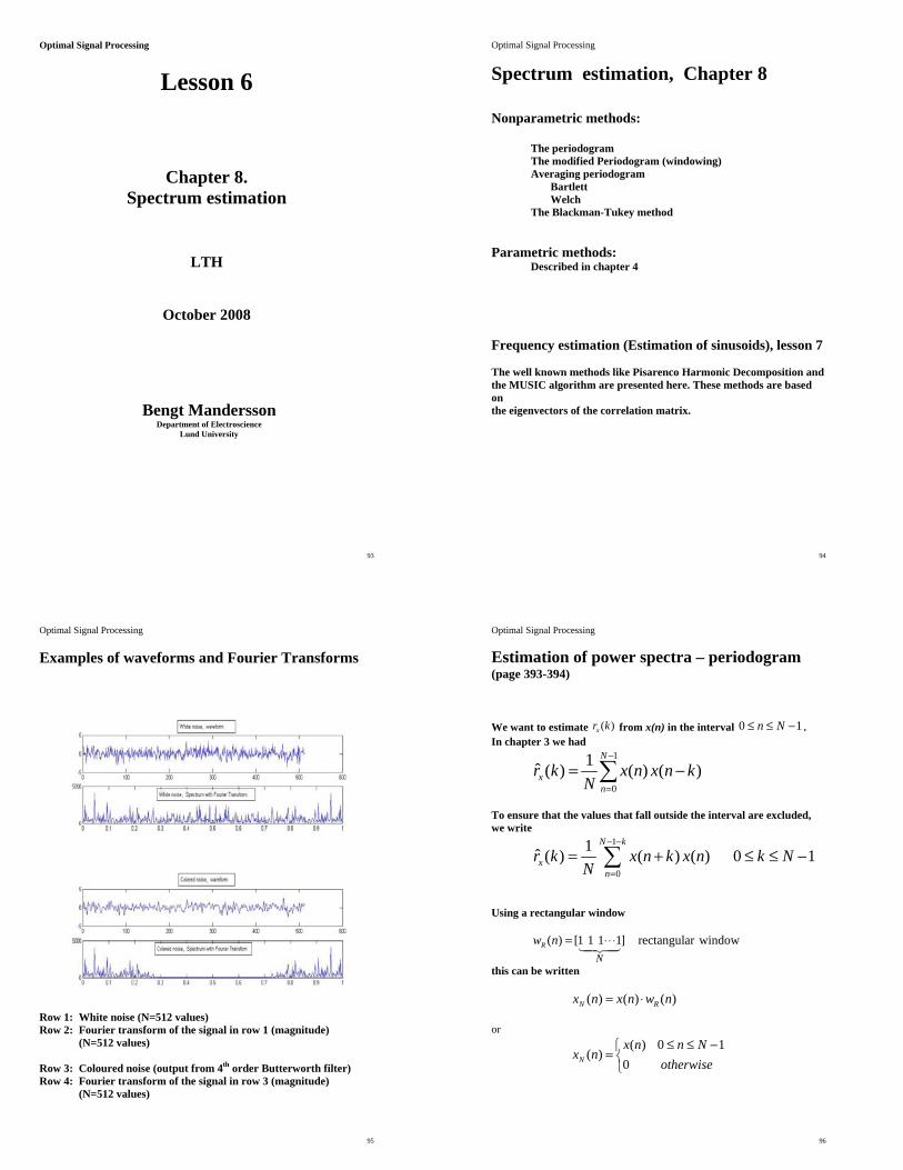
Optimal Signal Processing
Spectrum estimation, Chapter 8 Nonparametric methods: The periodogram The modified Periodogram (windowing) Averaging periodogram Bartlett Welch The Blackman-Tukey method Parametric methods:
Described in chapter 4 Frequency estimation (Estimation of sinusoids), lesson 7 The well known methods like Pisarenco Harmonic Decomposition and the MUSIC algorithm are presented here. These methods are based on the eigenvectors of the correlation matrix.
95
Optimal Signal Processing Examples of waveforms and Fourier Transforms
Row 1: White noise (N=512 values) Row 2: Fourier transform of the signal in row 1 (magnitude) (N=512 values) Row 3: Coloured noise (output from 4th order Butterworth filter) Row 4: Fourier transform of the signal in row 3 (magnitude) (N=512 values)
96
Optimal Signal Processing
Estimation of power spectra – periodogram (page 393-394)
We want to estimate ( )xr k from x(n) in the interval 0 1n N≤ ≤ − . In chapter 3 we had
1
0
1ˆ ( ) ( ) ( )N
xn
r k x n x n kN
−
=
= −∑ To ensure that the values that fall outside the interval are excluded, we write
1
0
1ˆ ( ) ( ) ( ) 0 1N k
xn
r k x n k x n k NN
− −
=
= + ≤ ≤ −∑
Using a rectangular window
( ) [1 1 1 1] rectangular windowR
N
w n = ⋅⋅⋅14243
this can be written
( ) ( ) ( )N Rx n x n w n= ⋅ or
( ) 0 1( )
0N
x n n Nx n
otherwise≤ ≤ −⎧
= ⎨⎩

97
Optimal Signal Processing The estimated autocorrelation can now be written
1ˆ ( ) ( ) ( )
1 ( ) ( ) ( ) ( )
1 ( ) ( )
x N Nn
R Rn
N N
r k x n k x nN
x n k w n k x n w nN
x k x kN
∞
=−∞
∞
=−∞
= +
= + +
= ∗ −
∑
∑
Then ˆ ( )xr k is defined for 1 1N k N− + ≤ ≤ − Now, we take the Fourier Transform of ˆ ( )xr k , and then we get
1
1
ˆ ˆ( ) ( )N
j j kper x
k NP e r k eω ω
−−
=− +
= ∑
which is called the periodogram. We see that it also can be written
21 1ˆ ( ) ( ) ( ) | ( ) |j j j jper N N NP e X e X e X e
N Nω ω ω ω∗= =
Using DFT (FFT), the periodogram will be
2 / 21 1ˆ ( ) ( ) ( ) | ( ) |j k Nper N N NP e X k X k X k
N Nπ ∗= =
98
Optimal Signal Processing
The Performance of the Periodogram (page 398-399) The estimate is unbiased if
ˆ{ ( )} ( )j jx xE P e P eω ω=
The estimate is consistent if it is (asymptotically) unbiased and if ˆlim var{ ( )} 0j
xNP e ω
→∞=
Taking the mean of ˆ ( )xr k , we got ( 0k ≥ ) (page 398-399)
{ } { }
{ } )()(1)()(1
)()(1)(ˆ
1
0
1
0
krN
kNkrN
nxknxEN
nxknxEN
krE
xx
kN
n
kN
n
NNn
−==+=
=+=
∑∑
∑−−
=
−−
=
∞
−∞=
Defining the Bartlett (triangular) window
⎪⎩
⎪⎨⎧
>
≤−=
Nk
NkN
kNkwB
||0
||||)(
we can write
ˆ{ ( )} ( ) ( )x B xE r k w k r k=
99
Optimal Signal Processing
Using this, we have (page 399)
1
11
1
ˆ ˆ{ ( )} { ( ) }
ˆ{ ( )} ( ) ( )
Nj j k
per xk N
Nj k j k
x x Bk N k
E P e E r k e
E r k e r k w k e
ω ω
ω ω
−−
=− +
− ∞− −
=− + =−∞
= =
= =
∑
∑ ∑
or
1ˆ{ ( )} ( ) ( )2
j j jper x BE P e P e W eω ω ω
π= ∗
The Bartlett (triangular) window can be seen as the convolution of two rectangular windows. The window is
21 sin( / 2)( )
sin( / 2)j
BNW e
Nω ω
ω⎡ ⎤
= ⎢ ⎥⎣ ⎦
Plot of )( ωjB eW , N=100, bandwidth 0.89*2π/N
100
Optimal Signal Processing
The estimate in asymptotically unbiased due to
ˆlim { ( )} ( )j jper xN
E P e P eω ω
→∞=
The variance is (textbook page 404, 405)
2ˆvar{ ( )} ( )j j
per xP e P eω ω≈ so the periodogram is not a consistent estimate of the power spectrum.

101
Optimal Signal Processing
The Modified Periodogram (windowing x(n)) The periodogram use a rectangular window wR(n)
2 21 1ˆ ( ) | ( ) | | ( ) ( ) ) |j j j nper N R
nP e X e x n w n e
N Nω ω ω
∞−
=−∞
= = ∑
If we use other windows, we got the modified periodogram
2
12
0
1ˆ ( ) | ( ) ( ) ) |
1 | ( ) ) |
j j nM
nN
j n
n
P e x n w n eNU
U w n eN
ω ω
ω
∞−
=−∞−
−
=
=
=
∑
∑
102
Optimal Signal Processing
Properties of the modified periodogram
103
Optimal Signal Processing
Example of the resolution
Row 1: Waveform of a vowel ‘a’, N=500 (50 ms)- Row 2: Fourier transform of the N=500 values in row 1. Row 3: Part of the waveform in row 1, N=100, (10 ms) Row 4: Fourier transform of the N=100 values in row 3.
104
Optimal Signal Processing
Spectrogram Spectrogram is a plot of spectrum as function of the time using a sliding window. The command in Matlab is specgram(x,Nfft,Fs); Nfft is the length of the time window (length of the fft). Fs is the sample frequency. Example of spectrogram of the word ‘mamma’.
Top: Waveform of the word ‘mamma’. Middle: Specgram with wide time window, N=200 (20 ms) Bottom: Specgram with narrow time window, N=50 (5 ms)

105
Optimal Signal Processing
Averaging periodogram. Bartlett’s Method (page 412.414) In order to reduce the variance we must use averaging.
We divide the input sequence x(n) of length N into K blocks of length L,
NKL
=
Then, determine the power spectra for each block and take the average. The variance will decrease but also the resolution will decrease. The variance will be
)(1)}(ˆvar{ 2 ωω jx
jB eP
KeP ≈
106
Optimal Signal Processing
107
Optimal Signal Processing Averaging periodogram. Welch’s Method (page 419) The method of Welch is similar to the Bartlett’s method but we allow overlapping of the blocks and using windows w(n). The estimated properties of Welch’s method is found in table 8.5
108
Optimal Signal Processing Blackman-Tukey Method (page 420-423)
With the Blackman-Tukey method we calculate ˆ ( )xr k from all N data. But for large k, the estimate is not so god.
Multiply ˆ ( )xr k with a window symmetric around k=0 and take the Fourier Transform. This gives
1
1
ˆ ˆ( ) ( ) ( )N
j j kBT x
k NP e r k w k eω ω
−−
=− += ∑
The spectrum of the window must be positive for all frequencies, i.e.
0)( ≥ωjeW , to guarantee that 0)( ≥ωjBT eP . This is not true for
a rectangular time window.

109
Optimal Signal Processing
110
Optimal Signal Processing
Example of the Blackman-Tukey Method
Row 1: Spectrum from FFT. Row 2: Autocorrelation Row 3: Time window Row 4: Windowed autocorrelation Row 5: Blackman-Tukey Spectrum (from windowed autocorr)
111
Optimal Signal Processing Conclusion We have always a trade-off between resolution and variance. Time windows Rectangular window has the best resolution but also highest leakage (highest side lobes) Averaging Averaging decreases the variance but for fix length of data the resolution also will decrease. Performance comparisons
Definitions see page 424-426 Resolution: ωΔ
Variability: 2})(ˆ{(}(ˆvar{
ω
ω
νj
x
jx
ePEeP=
Figure of merit: ων Δ⋅=M
Quality factor: ν1=Q
112
Optimal Signal Processing Filter bank implementation of periodogram We can interpret the periodogram as the output from of bank of band pass filters.
2
1
0|)(|1)( nj
N
n
jx enx
NeP ωω −
−
=∑=
For the frequency iω , this can be written
20
1
0
20 |)()(||)(|)( =
−
== −== ∑ ni
N
nn
jx knhnxNnyeP iω
i.e. the squared of the output from the filter at n=0; The band pass filters are then
⎪⎩
⎪⎨⎧ −−=
=otherwise
NkeNkh
kj
i
i
0
0),...,1(1)(
ω
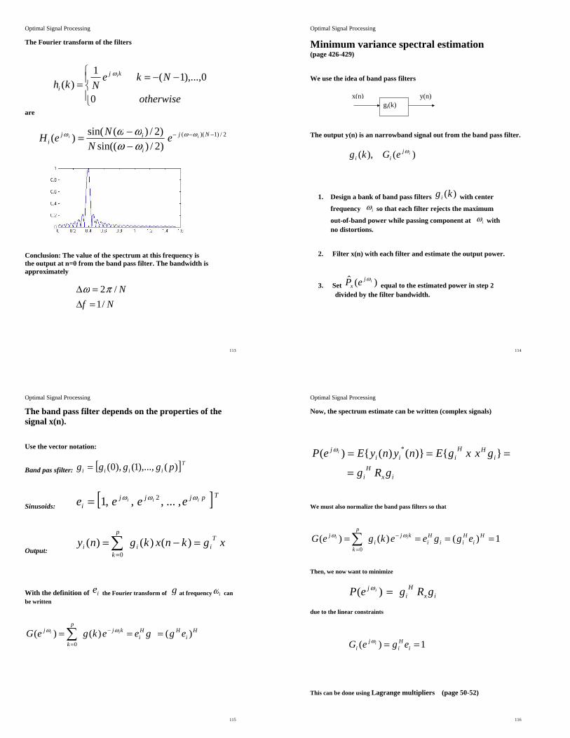
113
Optimal Signal Processing The Fourier transform of the filters
⎪⎩
⎪⎨⎧ −−=
=otherwise
NkeNkh
kj
i
i
0
0),...,1(1)(
ω
are
2/)1)((
)2/)sin(()2/)(sin()( −−−
−−= Nj
i
iji
ii eN
NeH ωωω
ωωωω
Conclusion: The value of the spectrum at this frequency is the output at n=0 from the band pass filter. The bandwidth is approximately
NfN
/1/2
=Δ=Δ πω
114
Optimal Signal Processing Minimum variance spectral estimation (page 426-429) We use the idea of band pass filters The output y(n) is an narrowband signal out from the band pass filter.
)(),( ijii eGkg ω
1. Design a bank of band pass filters )(kgi with center
frequency iω so that each filter rejects the maximum
out-of-band power while passing component at iω with no distortions.
2. Filter x(n) with each filter and estimate the output power.
3. Set )(ˆ ijx eP ω
equal to the estimated power in step 2 divided by the filter bandwidth.
gi(k) x(n) y(n)
115
Optimal Signal Processing
The band pass filter depends on the properties of the signal x(n). Use the vector notation:
Band pas sfilter: [ ]Tiiii pgggg )(),...,1(),0(=
Sinusoids: [ ]Tpjjji
iii eeee ωωω ,...,,,1 2=
Output: xgknxkgny T
ii
p
ki =−=∑
=
)()()(0
With the definition of ie the Fourier transform of g at frequency iω can be written
Hi
HHi
kjp
k
j eggeekgeG ii )()()(0
=== −
=∑ ωω
116
Optimal Signal Processing Now, the spectrum estimate can be written (complex signals)
ixH
i
iHH
iiij
gRg
gxxgEnynyEeP i
=
=== }{)}()({)( *ω
We must also normalize the band pass filters so that
1)()()(0
==== −
=∑ H
iHii
Hi
kji
p
k
j eggeekgeG ii ωω
Then, we now want to minimize
ixH
ij gRgeP i =)( ω
due to the linear constraints
1)( == iHi
ji egeG iω
This can be done using Lagrange multipliers (page 50-52)

117
Optimal Signal Processing Introduce the Lagrange multiplier
μand minimize (page 50-52)
4342143421 zerobeshould thisthisminimize
)1(21),( i
Hiix
Hii eggRggL −+= μμ
Differentiate ),( μigL
with respect to H
ig . Then
0),(* =−=∇ iixi egRgLig
μμ
and
ixi eRg 1−= μ
Differentiate ),( μigL
with respect to μ gives
01),( =−= iH
ii eggL μδμδ
118
Optimal Signal Processing Then using
ixi eRg 1−= μ
we have
ixHi eRe 1
1−=μ
This gives the filter
ixHi
ixi eRe
eRg 1
1
−
−
=
The power at frequency iω is estimated as
ixHi
ixH
ij
eRegRgeP i
1
1)( −==ω
We normalized the band pass filter but we must also normalize for the bandwidth of the band pass filter (length p+1). A correction factor (p+1) (see page 429) finally gives the minimum variance estimate for any ω
eRepeP
xH
jMV 1
1)( −+=ω

119
Optimal Signal Processing
Lesson 7
Chapter 8. Frequency estimation
LTH
October 2008
Bengt Mandersson Department of Electroscience
Lund University
120
Optimal Signal Processing
Chapter 8, Spectrum estimation Nonparametric methods: lesson 6 The periodogram The modified Periodogram (windowing) Averaging periodogram Bartlett Welch The Minimum variance method The Blackman-Tukey method Parametric methods:
Described in chapter 4 Pade Prony All-pole model Lattice structures in chapter 6 Frequency estimation (Estimation of sinusoids), lesson 7 The well known methods like Pisarenco Harmonic Decomposition and the MUSIC algorithm are presented here. These methods are based on the eigenvectors of the correlation matrix. Pisarenco Harmonic Decomposition The MUSIC algorithm The Eigenvector method (EV) (Minimum norm) Principal components Blackman-Tukey frequency estimation Minimum variance Frequency estimation
121
Optimal Signal Processing
Frequency estimation The model is that we have sinusoids in white noise.
)()(1
nweAnx nji
p
i
i +=∑=
ω
with the complex amplitude
ijii eAA φ||=
The phase is randomly distributed in the interval πφπ ≤≤− i We want to estimate
I: The amplitudes ij
iii eAAA φ||;|| =
II: The frequency ii f,ω III: Number of sinusoids p
122
Optimal Signal Processing
Frequency estimation, Examples on eigenvectors and eigenvalues of the correlation matrix. Sinusoid in white noise
)()*1.0**2sin()( nwnnx += π
Upper: Waveform of a sinusoid in white noise Middle: Spectrum from DFT Lower: The eigenvalues of the correlation matrix Rx.
The first 5 eigenvectors (left) and their spectra (right)

123
Optimal Signal Processing
Frequency estimation, Examples on eigenvectors and eigenvalues of the correlation matrix. Vowel ‘i’.
Upper: Waveform of a vowel ‘i’. Middle: Spectrum from DFT Lower: The eigenvalues of the correlation matrix Rx.
The first 5 eigenvectors (left) and their spectra (right)
124
Optimal Signal Processing
Frequency estimation, correlation matrix. We assume first that p=1,
)()( 11 nweAnx nj += ω
1,...,0 −= Nn
or
weAx += 11 with
[ ]TNxxxx )1(,...),1(),0( −=
[ ]TNjjj eeee )1(21
111 ,...,,,1 −= ωωω
[ ]TNwwww )1(,...),1(),0( −=
The correlation matrix is
IeePweAweAE
xxER
wH
H
Hx
2111
1111 }))({(
}{
σ+=
=++=
==
The power of the sinusoids is 2
11 || AP = .
125
Optimal Signal Processing Frequency estimation, eigenvalues and eigenvectors. Eigenvalues and eigenvectors for sinusoids in white noise.
Multiply xR with 1e ,
12
1
12
1111
12
1111
)(
)(
)(
eNP
eeeeP
eIeePeR
w
wH
wH
x
σσ
σ
+=
=+=
=+=
We now identify one eigenvalue and corresponding eigenvector
)1()(
)(
11
max2
11
12
11
==+=
+=
pifonlyevNP
eNPeR
w
wx
λσλ
σ
126
Optimal Signal Processing Frequency estimation, eigenvalues and eigenvectors. The other eigenvectors must be orthogonal to eigenvector 1.
)(...
,...,3,2
)(
min2
32
2
2111
λσλλλσ
σ
wN
iw
iwH
ix
Niv
vIeePvR
====
==
=+=
The noise subspace is determined by vi ,i=2,...,N
The signal subspace is determined by v1

127
Optimal Signal Processing
Frequency estimation. A: Estimate Rx and determine the eigenvalues and eigenvectors.
B: Estimate the variance of the noise as min2 λσ =w .
C: Estimate the signal power as
NP minmax
1̂λλ −=
Note that
11
211
evNP w
=+= σλ
D: Estimate the frequency from the eigenvector 1.
)}1(arg{ 11 v=ω (second index)
128
Optimal Signal Processing
Frequency estimation, Frequency estimation function The eigenvectors 2v to Nv
are orthogonal to 11 ev = .
Nive i
H ,...,2,01 ==
But
kji
N
ki
Hji ekvveeV ωω −
−
=∑== )()(
1
0
For 1ωω = we have
0)()( 11
1
01 === −
−
=∑ kj
i
N
ki
Hji ekvveeV ωω
This is valid for all eigenvectors 2v to Nv
.
129
Optimal Signal Processing We define the frequency estimation function as
2
21
0
2
||1
|)(|
1|)(
1|)(ˆ
iH
kji
N
k
kji
ji
ve
ekveVeP
=
===−
−
=∑ ω
ωω
We can also compute the Z-transform
ki
N
ki zkvzV −
−
=∑= )()(
1
0
and determine the zeroes of )(zVi
130
Optimal Signal Processing
Frequency estimation. Averaging over all noise eigenvectors yield
2
2
||
1)(ˆ
iH
i
N
i
j
veeP
α
ω
∑=
=
Example from the textbook page 455 Upper figure: Averaging over the noise eigenvectors with the
weight equal to one. Lower figure: Overlay plot over the frequency estimation function from each of the noise eigenvectors

131
Optimal Signal Processing
Frequency estimation. Several sinusoids in white noise
)()(
1nweAnx nj
i
p
i
i +=∑=
ω
and for p=2
IeePeeP
weAeAweAeAE
xxER
wHH
H
Hx
2222111
22112211 }))({(
}{
σ++=
=++++=
==
Eigenvaules
subspacesignaltheinseigenvaluethearesubspacenoise
subspacesignal
i
w
wii
υσ
συλ
⎪⎩
⎪⎨⎧ +
≈2
2
132
Optimal Signal Processing The frequency estimation function is now
2
1||
1)(ˆ
iH
i
N
pi
j
veeP
α
ω
∑+=
=
We will now look at some methods using the frequency estimation function above. The first is called the Pisarenco Decomposition method. This method is very sensitive to the noise but describe the principle for the methods. A well known method is the MUSIC algorithm. The frequency estimation function is sometimes called the pseudospectrum or eigenspectrum.
133
Optimal Signal Processing Frequency estimation: Pisarenco 1: Assume p complex sinusoids in white noise 2: Assume the dimension of Rx (p+1)*(p+1), i.e. only one noise
eigenvector. This assumptions means that only one eigenvector corresponds to the noise subspace.
Then 2
1min wp σλλ == + and the frequency estimation function (pseudospectrum) is defined
2min
2min
0
||1
|)(|
1)(ˆ
ve
ekveP
H
kjp
k
jPHD
=
==−
=∑ ω
ω
kp
kzkvzV −
=∑= )()( min
0min
134
Optimal Signal Processing
Frequency estimation: MUSIC Page 464, 465
MUSIC: MUltiple SIgnal Characterization The frequency estimation is achieved by averaging the pseudospectra over the noise eigenvectors.
2
1||
1)(ˆ
iH
M
pi
jMU
veeP
∑+=
=ω
Then estimate the position of the peaks in )(ˆ ωjMU eP

135
Optimal Signal Processing
Principal Components Spectrum Estimation. These methods use the signal subspace. (page 470-471) The Blackman-Tukey power spectrum was determined from a windowed autocorrelation sequence
1
1
ˆ ˆ( ) ( ) ( )N
j j kBT x
k NP e r k w k eω ω
−−
=− +
= ∑
If w(k) is a Bartlett window, the Blackman-Tukey estimate can be written in terms of the autocorrelation matrix
eReM
ekrkMM
eP xHkj
x
M
Mk
jBT
1)(ˆ|)|(1)(ˆ =−= ∑−=
ωω
In terms of eigenvectors (eigendecomposition) this is
2
1||1)(ˆ
iH
i
M
i
jBT ve
MeP λω ∑
=
=
136
Optimal Signal Processing Now, use only the eigenvectors corresponding to the sinusoids. Then the Blackman-Tukey principal frequency estimation is defined by
2
1
||1)(ˆi
Hi
p
i
jBTPC ve
MeP λω ∑
=− =
The minimum variance power spectrum estimate was defined by
eReMeP
xH
jMV 1)( −=ω
Rewrite this in terms of eigenvectors and only use eigenvectors corresponding to the sinusoids gives the minimum variance frequency estimation
iH
i
p
i
jMVPC
ve
MeP
λ
ω
1)(
1∑
=
− =
137
Optimal Signal Processing
138
Optimal Signal Processing Example of sinusoids in white noise Power spectrum estimation
1varaiancewithnoisewhitewith2502sin5.02002sin
=+⋅⋅+⋅⋅=
v(n)v(n)n).π(n).π(x(n)
Row 1: Waveform of input signal x(n) Row 2 FFT of x(n), N=1024 (Periodogram) Row 3 Averaging with the Welch method (10 subintervals, rectangular time window) Row 4 Blackman-Tukey estimate with M=20 (hamming window) Row 5 Minimum variance method with M=20, Row 6 All-pole model of order M=20 (Levinson Durbin algorithm). (All spectra in 1024 frequency points. y axis in dB)

139
Optimal Signal Processing Example of sinusoids in white noise Frequency estimation methods
1varaiancewithnoisewhitewith2502sin5.02002sin
=+⋅⋅+⋅⋅=
v(n)v(n)n).π(n).π(x(n)
Row 1 FFT of x(n), N=1024 (Periodogram). Row 2 Pisarenco Harmonic Decomposition p=4, M=5. Row 3 The MUSIC algorithm p=4, M=30. Row 4 The Eigenvector method (EV) p=4, M=30. Row 5 Principal components Blackman-Tukey frequency estimation (PC-BT) p=4, M=30. (All spectra in 1024 frequency points, y axis in dB)

Optimal Signal Processing 2008
A brief review
We have focused on methods used in practical applications
All-pole modeling in chapter 4 (LPC, Prediction Error Filter) Levinson Durbin Recursion using the reflection parameters Γ in chapter 5. Lattice structure in chapter 6, Burgs algorithm Wiener FIR Filters in chapter 7 Power Spectrum Estimation using the Periodogram in chapter 8 Frequency estimation (MUSIC)
Chapter 3 Filtering random processes (real signals) input: )(nx output: )(ny
)()()()()( knhkxnhnxnyk
−=∗= ∑
)()()()( khkhkrkr xy −∗∗=
)()()( krkhkr xyx ∗=
)()()( krkhkr xxy ∗−=
)()()()( ωωωω jjjx
jy eHeHePeP ∗=
)()()( ωωω jjx
jyx eHePeP =
)()()( ωωω jjx
jxy eHePeP ∗=
)()()()( 1−= zHzHzPzP xy
)()()( zHzPzP xyx =
)()()( 1−= zHzPzP xxy
Chapter 4 System modeling
All-pole modeling This can be described by the following figure.
1
( ) 1 ( )p
kp p
k
A z a k z−
=
= +∑
0
1
1( )1 ( )
pk
pk
H za k z−
=
=+∑
Minimize 2
0| ( ) |
np e nε
∞
=
=∑ with 1
( ) ( ) ( ) ( )p
pk
e n x n a k x n k=
= + −∑
gives the normal equations
1
( ) ( ) ( ) 1,...,p
p x xl
a l r k l r k k p=
− = − =∑
(0) (1) (2) ( 1) (1)
(1) (0) (1) ( 2) (2)
(2) (1) (0) ( 3) (3)
( 1) ( 2) ( 3) (0) ( )
x x x x p
x x x x p
x x x x p
x x x x p
px aR
r r r r p a
r r r r p a
r r r r p a
r p r p r p r a p
∗ ∗ ∗
∗ ∗
∗
⎡ ⎤⋅ ⋅ ⋅ − ⎡ ⎤⎢ ⎥ ⎢ ⎥⋅ ⋅ ⋅ −⎢ ⎥ ⎢ ⎥⎢ ⎥ ⎢ ⎥⋅ ⋅ ⋅ − ⋅⎢ ⎥ ⎢ ⎥⎢ ⎥⋅ ⋅ ⋅ ⎢ ⎥⋅⎢ ⎥ ⎢ ⎥− − − ⋅ ⋅ ⋅ ⋅⎢ ⎥ ⎢ ⎥⎣ ⎦⎣ ⎦114444444444244444444443
(1)(2)(3).( )
x
x
x
x
rrr
r p
⎡ ⎤⎢ ⎥⎢ ⎥⎢ ⎥= −⎢ ⎥⎢ ⎥⎢ ⎥⎣ ⎦
4243
1
,min (0) ( ) ( )p
p x xk
p r a k r kεε=
= = +∑
impulse ≈δ(n)
00
1( )( )
H zA z
=
our signal x(n)
impulse δ(n)
( ) ( )pHz A z=
Chapter 5 Levinson-Durbin recursion
The Levinson-Durbin algorithm determine relation between autocorrelation r(x),polynomial a(k) and the reflection coefficients. The matrix equation can be written
(0) (1) (2) ( 1) 1(1) (0) (1) ( 2) (1)
(2) (1) (0) ( 3) (2)
( 1) ( 2) ( 3) (0) ( )
x x x x
x x x x p
x x x x p
x x x x p
pxa
r r r r p
r r r r p a
r r r r p a
r p r p r p r a p
R
∗ ∗ ∗
∗ ∗
∗
⎡ ⎤⋅ ⋅ ⋅ − ⎡ ⎤⎢ ⎥ ⎢ ⎥⋅ ⋅ ⋅ −⎢ ⎥ ⎢ ⎥⎢ ⎥ ⎢ ⎥⋅ ⋅ ⋅ − ⋅⎢ ⎥ ⎢ ⎥⎢ ⎥⋅ ⋅ ⋅ ⎢ ⎥⋅⎢ ⎥ ⎢ ⎥− − − ⋅ ⋅ ⋅ ⋅⎢ ⎥ ⎢ ⎥⎣ ⎦⎣ ⎦1424314444444444244444444443 {
1
00
.0
p
p uε
ε⎡ ⎤⎢ ⎥⎢ ⎥⎢ ⎥=⎢ ⎥⎢ ⎥⎢ ⎥⎣ ⎦
1x p pR a uε= This can be summarized in the figure below and in the table 5.1 –5.4.
c
(1), (2), ...., ( ),x x xr r r p
1 2, ,..., pΓ Γ Γ
(1), (2), ...., ( )p p pa a a p
Levinson-Durbin Table 5 1
Table
Table
Table

Chapter 6 Lattice Structure
FIR H(z)=A (z)
Burgs algorithm Lattice FIR Lattice IIR
e0+(n) e1
+(n) e2+(n)
e0-(n) e2
-(n) e1-(n)
Γ2 Γ1 x(n)
Γ2 Γ1 z-1 z-1
Chapter 7. Wiener filters We will minimize the output error e(n), which we describe as the difference between the desired output d(n) and the estimated output. Applications. Filtering s(n): The desired signal is s(n) and we will determine the optimum filter for noise reduction. Smoothing: Like filtering but we allow an extra delay in the output signal (specially image processing). Prediction: The output is a prediction of future values of s(n). One step predictor. predict next value s(n+1). Equalization: The desired signal is w(n) and we will determine the optimum filter for whitening the output spectrum (inverse filtering, deconvolution). Other applications: Echo cancellation. Noise cancellation. Pulse shaping. Minimizing
2 2ˆ[ ( )] [( ( ) ( )) ]E e n E d n d nξ = = − gives the wiener-Hopf equations
( ) ( ) ( )x dxl
h l r k l r k∞
=−∞
− =∑
min (0) ( ) ( )d dxl
r h l r lξ∞
=−∞
= −∑
received x(n) g(n)
G(z) w(n) h(n)
H(z)
noise v(n)
desired d(n)
error e(n)
s(n)
Estimatedˆ() dn
FIR Wiener filter
1
0( ) ( ) ( ) 0,1,..., 1
p
x dxl
h l r k l r k k p−
=
− = = −∑
Non-causal IIR Wiener filter
( )( )
( )
jj dx
jx
P eH e
P e
ωω
ω=
Causal IIR Wiener filter
2 1
( )1( )( ) ( )
dx
Take the causalpart of this
P zH zQ z Q zσ −
+
⎡ ⎤= ⎢ ⎥
⎣ ⎦14243
FIR-filter for noise reduction
1( )opt s v sh R R r−= +
Non-causal IIR-filter for noise reduction
( )( ) ;
( ) ( )
jj s
j js v
P eH e
P e P e
ωω
ω ω=+
Chapter 8 Power Spectrum Estimation
The Fourier Transform of ˆ ( )xr k is called the periodogram 1
1
ˆ ˆ( ) ( )N
j j kper x
k NP e r k eω ω
−−
=− +
= ∑
We see that it also can be written
21 1ˆ ( ) ( ) ( ) | ( ) |j j j j
per N N NP e X e X e X eN N
ω ω ω ω∗= =
Using DFT (FFT), the periodogram will be
2 / 21 1ˆ ( ) ( ) ( ) | ( ) |j k N
per N N NP e X k X k X kN N
π ∗= =
Averaging periodogram. Bartlett’s Method Welch’s method Blackman-Tukey method
Minimum variance method Frequency estimation (Estimation of sinusoids) Pisarenco Harmonic Decomposition The MUSIC algorithm The Eigenvector method (EV) Principal components Blackman-Tukey frequency estimation