MATEMATIČNO MODELIRANJE DVODIMENZIONALNIH …

© Acta hydrotechnica 18/28 (2000), LjubljanaISSN 1581-0267

3

UDK: 519.61/64:532.5 UDC: 519.61/64:532.5Izvirni znanstveni članek Scientific paper

MATEMATIČNO MODELIRANJE DVODIMENZIONALNIHTURBULENTNIH TOKOV V KRIVOČRTNIH KOORDINATNIH SISTEMIHMATHEMATICAL MODELLING OF TWO-DIMENSIONAL TURBULENT

FLOW IN CURVILINEAR COORDINATE SYSTEMS

Slavko GERČER

V prvem delu naloge je obravnavana matematična izpeljava dinamične in kontinuitetne enačbe vkrivočrtnem koordinatnem sistemu. Namen razvoja teh enačb je priprava temeljnih izhodišč za t. i.prvi pristop k reševanju enačb, ki jih uporabimo v transformirani obliki za krivočrtni koordinatnisistem. V drugem delu naloge pa je izveden t.i. drugi pristop, enačbe so rešene v netransformiraniobliki.Razložena je numerična diskretizacija dinamične in kontinuitetne enačbe na pravokotnimreži. Razvita je teoretična izpeljava numerične diskretizacije po metodi končnih volumnov zapoljubno obliko celic (trapezi), ki sestavljajo numerično mrežo.Na tej podlagi je bil razvitračunalniški model (PCFLOW2D-CURVE), ki omogoča modeliranje tokov za poljubno oblikostrukturirane numerične mreže. Narejen je računalniški program v CADD okolju (GEO-CURVE),ki generira numerično mrežo za poljubno obliko rečnega korita. Naloga podaja pregled in temeljepristopa k reševanju enačb v krivočrtnem koordinatnem sistemu. Zato je dobra matematičnapodlaga za vse, ki bodo nadaljevali z razvojem modelov v krivočrtnih koordinatah.Ključne besede: matematični modeli, dvodimenzionalno modeliranje, numerične metode, metodakončnih volumnov, krivočrtni koordinatni sistem

In the first part of the thesis, a mathematical derivation of the dynamic and the mass conservationequation in curvilinear coordinate system is presented. The mean purpose of the derivation ofequations is to establish the basics of the first approach for the solving of the equations which, intheir transformed form, are later used in a curvilinear coordinate system. In the second part, the so-called second approach is derived, where the equations are solved in a non-transformed form.Thenumerical discretisation of the dynamic and mass conservation equations in the orthogonal grid isinterpreted. The theoretical derivation of the numerical discretisation of equations for trapezoidalcells is described using a finite volume method. Afterwards, a new mathematical model(PCFLOW2D-CURVE) which enables the modelling of flow for any optional structure of numericalgrid was developed. A new software (GEO-CURVE) in the CADD environment was developed togenerate a numerical grid for any optional form of the riverbed. The thesis gives a review and basicprinciples of solving the equations in a curvilinear coordinate system. Therefore, it can be used as agood mathematical basis for the further development of curvilinear models.Key words: mathematical models, two-dimensional modelling, numerical methods, finite volumemethod, curvilinear coordinate system

Gerčer, S.: Matematično modeliranje dvodimenzionalnih turbulentnih tokov v krivočrtnih koordinatnih sistemih -Mathematical Modelling of Two-Dimensional Turbulent Flow in Curvilinear Coordinate Systems

© Acta hydrotechnica 18/28 (2000), 3-40, Ljubljana

4

1. UVOD

Gibanje vode v naravnih vodotokih je vsplošnem tridimenzionalno. Transportenergije, toplote in polutantov poteka v vsehsmereh. Tok v vodotokih, kjer širina za redvelikosti presega globino, lahkopoenostavljeno obravnavamo kotdvodimenzionalnega.

V matematičnem modelu lahko uporabimoosnovne enačbe, ki so povprečene po globinitoka. Kontinuitetno, dinamično enačbo inenačbe modela turbulence (dodatno pa lahkoše konvekcijsko difuzijsko enačbo za širjenjepolutantov ali toploto) običajno zapišemo vobliki parcialnih diferencialnih enačb. Te solahko izražene v Kartezijevem koordinatnemsistemu (slika 1), ki je primeren za v naraviredke ravne kanale. Za ukrivljene struge znepravokotno obliko je primernejša uporabakrivočrtnega koordinatnega sistema, ki seprilagaja nepravilnim robovom računskegapodročja (slika 2).

Ker omenjene enačbe običajno analitičnoniso rešljive, jih poskušamo reševati spomočjo numerične diskretizacije. Metod zareševanje splošnih parcialno-diferencialnihenačb je več, v glavnem pa jih delimo na:- metode končnih elementov,- metode robnih elementov,- metode končnih razlik.

Metoda končnih razlik oziroma njenavariantna metoda končnih volumnov ima prireševanju problemov mehanike tekočinnajdaljšo tradicijo. Zanjo je značilnapreprostost in jasna fizikalna interpretacija.Tudi na Katedri na mehaniko tekočin FGG seje ta metoda najbolj uveljavila kot primerna zareševanje tovrstnih enačb.

Izvirna metoda končnih volumnov temeljina pravokotnem koordinatnem sistemu, karpomeni, da imajo celice v tlorisu vedno oblikopravokotnikov ali kvadratov (slika1). Topredstavlja določeno omejitev, saj npr. primodeliranju toka s prosto gladino v naravnihrečnih koritih nastopijo težave zaradi slabeprilagoditve numerične mreže nepravilnimrobovom računskega področja. Običajnotovrstne težave rešujemo z zgostitvijo mreže,kar pa posledično vpliva na veliko poraboračunalniških zmogljivosti, tako spomina kotpredvsem časa računanja.

1. INTRODUCTION

In natural waters, there is generally a three-dimensional flow. The transport of energy,heat and pollutants is performed in alldirections. The flow in waters where the widthand length are, by an order of magnitude,greater than the depth, can be considered to betwo-dimensional, and, therefore, simplifiedinto a two-dimensional flow.

In the mathematical model, we can use thebasic equations averaged along the depth. Themass conservation equation, dynamic equationand the turbulence closure scheme equations,as well as the advection-dispersion equationfor the transport of heat or pollutants, areusually written as partial differential equations.These can be written in the Cartesiancoordinate system (Figure 1), suitable forstraight channels, which are very rare innature. For non-orthogonally shaped and bendriverbeds, the use of a curvilinear coordinatesystem is more convenient. In this way, thenon-regular borders of the computationaldomain are better described (Figure 2).

The equations mentioned above are usuallyanalytically insolvable; therefore, numericaldiscretisation is used to solve these equations.There are several methods for solving generalpartial differential equations, which can bemostly divided into- finite element methods,- border element methods and- finite difference methods.

The finite difference method (respectively,a derivative known as the finite volumemethod) has the longest tradition in the solvingof fluid mechanics problems. This method ischaracterised by its simplicity and clearphysical interpretation. At the Chair of FluidMechanics at the University of Ljubljana, thismethod is mostly used as the most convenientfor solving the equations mentioned above.

The fundamental finite volume method isbased on an orthogonal coordinate system. Inthe horizontal plane, all the cells are rectanglesor squares (Figure 1). This represents a certainlimitation, as the boundary of thecomputational domain with the natural riverbeds is very difficult to describe. Refining thegrid at the boundaries, which is the methodusually used to solve the problem, results in ahigher consumption of computationalcapacities (memory, and, in particular,computational time).



5

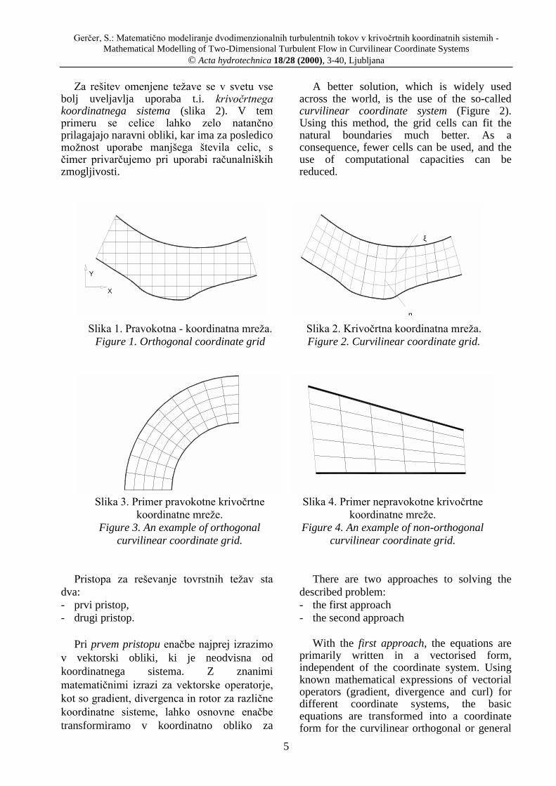
Za rešitev omenjene težave se v svetu vsebolj uveljavlja uporaba t.i. krivočrtnegakoordinatnega sistema (slika 2). V temprimeru se celice lahko zelo natančnoprilagajajo naravni obliki, kar ima za posledicomožnost uporabe manjšega števila celic, sčimer privarčujemo pri uporabi računalniškihzmogljivosti.

A better solution, which is widely usedacross the world, is the use of the so-calledcurvilinear coordinate system (Figure 2).Using this method, the grid cells can fit thenatural boundaries much better. As aconsequence, fewer cells can be used, and theuse of computational capacities can bereduced.

X

Y

η

ξ

Slika 1. Pravokotna - koordinatna mreža.Figure 1. Orthogonal coordinate grid

Slika 2. Krivočrtna koordinatna mreža.Figure 2. Curvilinear coordinate grid.

Slika 3. Primer pravokotne krivočrtnekoordinatne mreže.

Figure 3. An example of orthogonalcurvilinear coordinate grid.

Slika 4. Primer nepravokotne krivočrtnekoordinatne mreže.

Figure 4. An example of non-orthogonalcurvilinear coordinate grid.

Pristopa za reševanje tovrstnih težav stadva:- prvi pristop,- drugi pristop.

Pri prvem pristopu enačbe najprej izrazimov vektorski obliki, ki je neodvisna odkoordinatnega sistema. Z znanimimatematičnimi izrazi za vektorske operatorje,kot so gradient, divergenca in rotor za različnekoordinatne sisteme, lahko osnovne enačbetransformiramo v koordinatno obliko za

There are two approaches to solving thedescribed problem:- the first approach- the second approach

With the first approach, the equations areprimarily written in a vectorised form,independent of the coordinate system. Usingknown mathematical expressions of vectorialoperators (gradient, divergence and curl) fordifferent coordinate systems, the basicequations are transformed into a coordinateform for the curvilinear orthogonal or general



6

krivočrtni pravokotni ali splošni nepravokotnisistem (realno območje Φ z robom Γ v ravniniX-Y na –sliki 5) . Tega potem preslikamo vpravokotno mrežo (območje Φ’ z robom Γ’ vravnini ξ-η), na kateri izvedemo numeričnodiskretizacijo enačb. Končne rezultate natopreslikamo nazaj v krivočrtni sistem.

Lastnost območja Φ’ je ta, da jekonstruirano samo iz horizontalnih invertikalnih črt (slika 5).

non-orthogonal system (real area Φ with theboundary Γ in the plane X-Y – see Figure 5).The equations are further transformed into anorthogonal grid (real area Φ’ with theboundary Γ’ in the plane ξ-η), where thenumerical discretisation of the equations isapplied. The results are finally transformedback into the curvilinear system.

By definition, the boundaries of the area Φ’consist only of horizontal and vertical lines(Figure 5).

Y

X

ΓΦ

ξ

ΦΓ

Slika 5. Transformacija območja krivočrtne koordinatne mreže v pravokotno.Figure 5. Transformation of an area with a curvilinear coordinate grid into an orthogonal grid.

Tako vsaki diskretizirani točki P znotrajobmočja Φ pripada transformirana točka P’znotraj območja Φ’. V splošnem opisanipostopek pomeni, da enačbe, ki so izražene sspremenljivkama X-Y transformiramo tako, dajih lahko izrazimo s spremenljivkama ξ-η. Poizvedeni transformaciji koordinat in enačblahko za njihovo rešitev uporabimo numeričnemetode, ki veljajo za pravokotna območja.

Pri drugem pristopu uporabimo osnovneenačbe v običajnem Kartezijevemkoordinatnem sistemu, vpliv nepravokotnihcelic krivočrtne mreže pa nato upoštevamo prinumerični diskretizaciji (slika 6).

In this way, a single transformed point P’within the area Φ’ belongs to each discretepoint P within the area Φ. Generally, thedescribed procedure shows how to transformequations expressed with the X-Y variablesinto equations expressed with the ξ-ηvariables. After the transformation of thecoordinates and the equations, the samenumerical methods as used for the rectangularcomputational domains may be used.

With the second approach, the basicequations in the Cartesian coordinate systemare used, and the influence of non-rectangularcells is taken into account later, during thenumerical discretisation (Figure 6).

Y

X

U

V

U

VU

V

U

V

Slika 6. Diskretizacija osnovnih enačb v X-Y sistemu v krivočrtni koordinatni mreži.Figure 6. Discretisation of the basic equations in X-Y system in a curvilinear coordinate grid.



7

V primeru prvega pristopa se srečamo zzahtevno matematično transformacijo enačb innato podobno numerično diskretizacijo, kot jože uporabljamo v naših obstoječihmatematičnih modelih.

V drugem primeru pa poznamo enačbe vpravokotnem koordinatnem sistemu, vendarnumerična diskretizacija po metodi končnihvolumnov za poljubne oblike kontrolnihpovršin v naših matematičnih modelih še nibila razvita.

2. PRVI PRISTOP

2.1 ENAČBEDVODIMENZIONALNEGA TOKA VKARTEZIJEVEM KOORDINATNEM

SISTEMU

Kontinuitetno in dinamično enačbo vkonzervativni obliki lahko za primerdvodimenzionalnega toka uporabimo vKartezijevem koordinatnem sistemu. Priizpeljavi enačb so upoštevane naslednjepredpostavke (Četina, 1988):- stalni tok,- tok je dvodimenzionalen, hitrosti u in v so

povprečene po globini,- napetosti zaradi trenja ob dno izrazimo z

Manningovo empirično enačbo,- ni upoštevana “rigid lid” aproksimacija,

tako da so spremembe globine v primerjaviz osnovno globino lahko velike.

- upoštevan je model konstantne efektivneviskoznosti νef.

Kontinuitetna enačba:

The first approach demands a complicatedmathematical transformation of the equationsand numerical discretisation, similar to thediscretisation which is already known from ourexisting mathematical models.

With the second approach, we use the well-known equations in the orthogonal coordinatesystem, while the numerical discretisationusing the finite volume method for anyoptional shape of the control volumes has notyet been developed and used in ourmathematical models.

2. THE FIRST APPROACH

2.1 EQUATIONS OF TWO-DIMENSIONAL FLOW IN THE

CARTESIAN COORDINATESYSTEM

The mass conservation equation and thedynamic equation can be used in theirconservative form for describing two-dimensional flow in the Cartesian coordinatesystem. With the derivation of equations, thefollowing assumptions were taken into account(Četina, 1988):- steady flow,- two-dimensional flow, velocities u and v

are averaged along the depth,- shear stress at the bottom is taken into

account by using Manning’s empiricalequation,

- the “rigid lid” approximation is not takeninto account; thus, the surface elevationsmay vary significantly in comparison to theinitial surface,

- the constant effective viscosity model νef istaken into account.

Mass conservation equation:

0)()( =+

y

hv

x

hu

∂∂

∂∂

(1)

Dinamična enačba: Dynamic equation:

)

(

)

(

)(

)( 3

4

222

2

y

uh

yx

uh

xh

vuughn

x

zgh

x

hgh

y

huv

x

huefef

d

∂∂υ

∂∂

∂∂υ

∂∂

∂∂

∂∂

∂∂

∂∂ +++−−−=+

)

(

)

(

)(

)( 3

4

222

2

y

vh

yx

vh

xh

vuvghn

y

zgh

y

hgh

y

hv

x

huvefef

d

∂∂υ

∂∂

∂∂υ

∂∂

∂∂

∂∂

∂∂

∂∂ +++−−−=+ (2)



8

2.2 ENAČBEDVODIMENZIONALNEGA TOKA V

NEPRAVOKOTNEMKRIVOČRTNEM KOORDINATNEM

SISTEMU

Za izpeljavo enačb potrebujemomatematične osnove, ki so sorazmerno obširnein v literaturi zelo težko dosegljive. Ravnorazlaga matematične izpeljave v tej nalogi najbi bila temeljno izhodišče pri prihodnjemrazvoju matematičnih modelov, ki bi temeljilina krivočrtnih koordinatnih sistemih.

2.2.1 Fizikalna interpretacija zvezekrivočrtnega in Katerzijevega

koordinatnega sistema

Krivočrtni koordinatni sistem predstavljaosi ξ-η, ki v splošnem med seboj nistapravokotni. Poljuben vektor F

! lahko

razstavimo na komponenti Fξ in Fη vkrivočrtnem koordinatnem sistemu oziroma Fx

in Fy v Kartezijevem koordinatnem sistemu(slika 7).

2.2 THE EQUATIONS OF TWO-DIMENSIONAL FLOW IN THE

NON-ORTHOGONALCURVILINEAR COORDINATE

SYSTEM

To derive the equations, a relativelyextensive mathematical background is needed,and this is very difficult to find in literature.The explanation of the mathematicalderivation in the thesis should be used as thefundamental starting point in the futuredevelopment of the mathematical models,based on curvilinear coordinates.

2.2.1 Physical interpretation of theconnection between the curvilinear and

Cartesian coordinate system

The curvilinear coordinate system isdescribed by axes ξ-η, which, in general, arenot orthogonal. Any optional vector F

! can be

partitioned into components Fξ in Fη in acurvilinear coordinate system and intocomponents Fx in Fy in the Cartesiancoordinate system (Figure 7).

X

φ

η FY

α

ξF

Y

F

F

F

η

ξ

X

γex

ey

e eξη

cos(xF

α )

sin(F

α )y

cos(Fη

γ)

γ

Slika 7. Vektor F v krivočrtnem in Katerzijevem koordinatnem sistemu.Figure 7. Vector F in a curvilinear and in the Cartesian coordinate system.

F! = Fx xe

! + Fy ye!

= Fξ ξe!

+ Fη ηe!

(3)



9

Zanima nas zveza med komponentamivektorja F

! v Kartezijevem in krivočrtnem

kordinatnem sistemu. Zvezo lahko zapišemo vobliki:

We would like to express the connectionbetween the vectorial components in bothcoordinate systems. This connection can bewritten as:

Fx=C1 Fξ+C2 Fη (4)Fy=C3 Fξ+C4 Fη (5)

in še obratno: and in the opposite way:

Fξ=C5 Fx+C6 Fy (6)Fη=C7 Fx+C8 Fy (7)

Člene po krajši izpeljavi lahko zapišemo vobliki preglednice (preglednica 1):

After a short derivation, all the coefficientscan be written in a form of table (Table 1):

Preglednica 1. Koeficienti zveze Katerzijevih in krivočrtnih komponent poljubnega vektorja.Table 1. Transformation coefficients between the Cartesian

and the curvilinear components of an optional vector.

Ci Ci =f(Cj) Ci =f(α,Φ) Ci =f(α,Φ=90°)C1

7685

8

CC-CC

C cos(α) cos(α)

C2

7685

6

CC-CC

C- cos(α+Φ) -sin(α)

C3

7685

7

CC-CC

C- sin(α) sin(α)

C4

7685

5

CC-CC

C sin(α+Φ) cos(α)

C5

3241

4

CC-CC

C cos(α)

+

Φ

Φ)(sin

))cos(sin(αcos(α)

C6

3241

2

CC-CC

C- sin(α) -

Φ

Φ)(sin

))cos(cos(αsin(α)

C7

3241

3

CC-CC

C-

Φ)sin(

)sin(- α -sin(α)

C8

3241

1

CC-CC

C

Φ)sin(

)cos(α cos(α)



10

2.2.2 Uporaba matematične interpretacijeza potrebe 2D-matematičnega modela

Matematično interpretacijo smo uporabili znamenom izpeljave matematičnih operatorjev,kot so gradient in divergenca v krivočrtnemkoordinatnem sistemu. Le te smo vnadaljevanju uporabili za transformacijodinamične in kontinuitetne enačbe.

Gradient skalarnega polja:

2.2.2 The use of the mathematicalinterpretation in a 2D mathematical model

The mathematical interpretation was usedto derive the mathematical operators, such asgradient and divergence, in curvilinearcoordinate system. These operators werefurther used for transformation of the massconservation and the dynamic equation.

Gradient of a scalar field:

grad(u)=∇ (u)= yx ey

ue

x

uu !!

∂∂+

∂∂=

Χ∂∂

= ηξ αα ee!!

2211 HH +=

= ηξ ξηηξe e 1211

*

221222

*

11 !!

∂∂−

∂∂+

∂∂−

∂∂ u

qu

qq

quq

uq

q

q(8)

Za poseben primer pravokotnegakrivočrtnega koordinatnega sistema velja:

In a special case – orthogonal curvilinearcoordinate system – the equation can bewritten as:

grad(u)=∇ (u)= yx ey

ue

x

uu !!

∂∂+

∂∂=

Χ∂∂

= ηξ αα ee!!

2211 HH + = ηξ ηξe

1 e

1

21

!!

∂∂+

∂∂ u

H

u

H(9)

Definicija prvega odvoda. Zanimala nas jezveza:

Definition of the first derivative. Theexpression

)(Qfu =Χ∂

∂

oziroma v razviti obliki: or, in its developed form

),( ηξfx

u =∂∂

, ),( ηξfy

u =∂∂

Rezultat izpeljave lahko predstavimo vobliki:

can be derived into

∂∂

∂∂−

∂∂

∂∂=

∂∂

ηξξηuyuy

Jx

u 1 (10)

kjer je where

∂∂

∂∂−

∂∂

∂∂=−==

ξηηξyxyx

qqqqJ 122211* (11)



11

V posebnem primeru pravokotne krivočrtnebaze se izrazi poenostavijo in enačba dobinaslednjo obliko:

The expressions are simplified in thespecial case of the orthogonal curvilinear base.The equation can be written in the followingform:

∂∂

∂∂−

∂∂

∂∂=

∂∂

ηξξηuyuy

HHxu

21

1 (12)

Definicija drugega odvoda: Definition of the second derivative:

)(Χ=Χ∂

Χ∂∂∂

f

u

(13)

ali še v razviti obliki: or in its developed form:

),( ηξfx

x

u

=∂

∂∂∂

, ),( ηξfy

y

u

=∂

∂∂∂

(14)

Do zveze lahko pridemo preko enačbprvega odvoda

The connection can be found using theequations of the first derivative:

=∂

∂∂∂

x

x

u

xx

u

∂∂∂ 2

=

+

∂∂∂

∂∂+

∂∂∂

∂∂

∂∂−

∂∂∂

∂∂

ηηξηξηξξξηuyuyyuy

J

22222

22

1

+

∂∂

∂∂−

∂∂

∂∂

∂∂∂

∂∂+

∂∂∂

∂∂

∂∂−

∂∂∂

∂∂

ηξξηηηξηξηξξξηuxuxyyyyyyy

J

22222

32

1

∂∂

∂∂−

∂∂

∂∂

∂∂∂

∂∂+

∂∂∂

∂∂

∂∂−

∂∂∂

∂∂

ξηηξηηξηξηξξξηuyuyxyxyyxy 22222

2



12

2.2.3 Zveza med koeficienti fizikalne inmatematične interpretacije

Primerjavo koeficientov matematične infizikalne interpretacije podajamo vpreglednici 2:

2.2.3 The connection between thecoefficients of the physical and the

mathematical interpretation

The comparison between the coefficients ofthe mathematical and the physicalinterpretation is given in Table 2:

Preglednica 2. Fizikalni koeficienti, izraženi v krivočrtnem koordinatnem sistemu.Table 2. Coefficients of the physical interpretation in a curvilinear coordinate system.

Ci Ci =f(Cj) Ci =f(α,Φ)C1

7685

8

CC-CC

C

η∂∂y

J

H 1

C2

7685

6

CC-CC

C-

ξ∂∂− y

J

H 2

C3

7685

7

CC-CC

C-

η∂∂− x

J

H 1

C4

7685

5

CC-CC

C

ξ∂∂x

J

H 2

C5

3241

4

CC-CC

Cξ∂

∂x

1H

1

C6

3241

2

CC-CC

C-

ξ∂∂y

1H

1

C7

3241

3

CC-CC

C-

η∂∂x

2H

1

C8

3241

1

CC-CC

C

η∂∂y

2H

1

kjer veljajo še naslednje zveze: where the following equations are valid:

∂∂

∂∂−

∂∂

∂∂=−==

ξηηξyxyxqqqqJ 122211*

22

1H

∂∂+

∂∂=

ξξyx

22

2H

∂∂+

∂∂=

ηηyx



13

2.2.4 Kontinuitetna enačba v krivočrtnemkoordinatnem sistemu

Kontinuitetna enačba 2D modela vKaterzijevem koordinatnem sistemu se glasi(Četina, 1988):

2.2.4 Mass conservation equation in thecurvilinear coordinate system

The mass conservation equation of the 2Dmodel in the Cartesian coordinate system isgiven as (Četina, 1988):

0)v( =!hdiv ⇒ 0

)()( =+y

hv

x

hu

∂∂

∂∂

(15)

kjer je vektor hitrosti v!

enak: where the velocity vector is equal to

ηξξ eveueveuv yyxx!!!!! +=+= (16)

ux = C1 uξ + C2 vη (17)vy = C3 uξ + C4 vη (18)

Da lahko zapišemo kontinuitetno enačbo vkrivočrtnem koordinatnem sistemu ξ-η,moramo upoštevati enačbo transformacijeprvega odvoda:

To transform the mass conservationequation into the curvilinear coordinate systemξ-η, the equation of transformation of the firstderivative must be accounted for:

0)()(1)()(1 =

∂

∂∂∂+

∂∂

∂∂−+

∂

∂∂∂−

∂∂

∂∂

ηξξηηξξηvhxvhx

J

uhyuhy

J (19)

Končna oblika kontinuitetne enačbe dobinaslednjo obliko:

Finally, the mass conservation equation iswritten as:

( )( ) ( )( )

( )( ) ( )( ) 0C 1

1

4343

2121

=

+

∂∂

∂∂++

∂∂

∂∂−

+

+

∂∂

∂∂−+

∂∂

∂∂

ηξηξ

ηξηξ

ηξξη

ηξξη

vCuhxvCuChxJ

vCuChyvCuChyJ

(20)

2.2.5 Kontinuitetna enačba v pravokonemkrivočrtnem koordinatnem sistemu

Ob upoštevanju poenostavitev dobi splošnakontinuitetna enačba v pravokotnemkrivočrtnem koordinanem sistemu naslednjoobliko:

2.2.5 The mass conservation equation in anorthogonal curvilinear coordinate system

Taking into account the simplifications, thegeneral mass conservation equation in theorthogonal curvilinear coordinate system getsthe following form:

( ) ( ) 0112 =

∂∂+

∂∂

ηξ ηξhvHhuH

J

Ta enačba je dobro poznana iz literature(Četina, 1983). Zato lahko sklepamo, da je bilaizpeljava kontinuitetne enačbe (20) vnepravokotnem krivočrtnem koordinatnemsistemu enačba pravilna.

This equation is well known from literature(Četina, 1983). Therefore, the derivation of themass conservation equation (20) in the non-orthogonal curvilinear coordinate system maybe considered as correct.



14

2.2.5 Dinamična enačba v krivočrtnemkoordinatnem sistemu

Osnovna dinamična enačba v vektorskiobliki se za primer stacionarnega stanja innestisljive tekočine in ob upoštevanjuturbulentnega modela konstantne efektivneviskoznosti νef poenostavi v:

2.2.5 Dynamic equation in a curvilinearcoordinate system

In the case of steady flow, non-compressible fluid and taking into account theconstant effective viscosity turbulence modelνef, the basic dynamic equation in vectorialform is simplified into:

v)p(grad1-Fv))v(( !!!! ∆+= efgrad νρ

(21)

Prvi člen na levi strani dinamične enačbepredstavlja konvekcijski pospešek ( K

!), prvi

člen na desni strani vpliv masnih in tlačnih sil( M!

), zadnji člen na desni strani pa vpliv silefektivne viskoznosti (C

!)

Za zapis dinamične enačbe vnepravokotnem krivočrtnem koordinatnemsistemu ξ-η smo vsak člen enačbe posebejtransformirali na podlagi pripravljenih izrazov,opisanih in izpeljanih v predhodnih poglavjih.

Konvekcijski člen K!

The first term on the left side of theequation represents the advective acceleration( K!

); the first term on the right side representsthe influence of mass and pressure force ( M

!);

and the last term expresses the influence ofeffective viscosity ( C

!).

To write the dynamic equation in the non-orthogonal curvilinear coordinate system ξ-η,each term of the equation was transformedseparately, on the basis of the previouslywritten equations.

Advective term K!

y

vhu

x

huK yxx

x ∂∂

+∂

∂=

)()( 2

, y

hv

x

vhuK yyx

y ∂∂

+∂

∂=

)()( 2

se transformira v: is transformed into:

( )( ) ( )( )( )

−+

∂∂

∂∂−+

∂∂

∂∂= ηξηξηξξ ηξξη

vCuCvCuChyvCuChyJ

CK 43212

2151

+

( )( )( ) ( )( )

−

∂∂

∂∂+++

∂∂

∂∂−

24343216

1C ηξηξηξ ηξξηvCuChxvCuCvCuChx

J (22)

( )( ) ( )( )( )

−+

∂∂

∂∂−+

∂∂

∂∂= ηξηξηξη ηξξη

vCuCvCuChyvCuChyJ

CK 43212

2171

+

( )( )( ) ( )( )

−

∂∂

∂∂+++

∂∂

∂∂−

24343218

1C ηξηξηξ ηξξηvCuChxvCuCvCuChx

J (23)

Člen masnih in tlačnih sil M!

Mass and pressure force term M!

3

4

22

2)(

h

vuughnzh

xghM

yxx

dx

+−+

∂∂−= ,

3

4

22

2)(

h

vuvghnzh

yghM

yxy

dy

+−+

∂∂−=



15

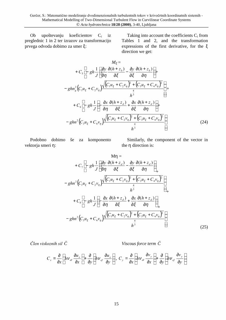
Ob upoštevanju koeficientov Ci izpreglednic 1 in 2 ter izrazov za transformacijoprvega odvoda dobimo za smer ξ:

Taking into account the coefficients Ci fromTables 1 and 2, and the transformationexpressions of the first derivative, for the ξdirection we get:

Mξ =

∂+∂

∂∂−

∂+∂

∂∂−+

ηξξη)()(1

5bb zhyzhy

JghC +

( ) ( ) ( )

+++

+−34

243

221

212

h

vCuCvCuCvCuCghng

ηξηξηξ +

∂+∂

∂∂+

∂+∂

∂∂−−+

ηξξη)()(1

6dd zhxzhx

JghC +

( ) ( ) ( )

+++

+−34

243

221

432

h

vCuCvCuCvCuCghn ηξηξ

ηξ (24)

Podobno dobimo še za komponentovektorja smeri η:

Similarly, the component of the vector inthe η direction is:

Mη =

∂+∂

∂∂−

∂+∂

∂∂−+

ηξξη)()(1

7dd zhyzhy

JghC

+

( ) ( ) ( )

+++

+−34

243

221

212

h


ηξ

+

∂+∂

∂∂+

∂+∂

∂∂−−+

ηξξη)()(1

8dd zhxzhx

JghC

+

( ) ( ) ( )

+++

+−34

243

221

432

h


ηξ

(25)

Člen viskoznih sil C!

Viscous force term C!

∂

∂∂∂+

∂∂

∂∂=

yuh

yxuh

xC x

efx

x νν ef ,

∂∂

∂∂+

∂∂

∂∂=

yv

hyx

vh

xC y

efy

y νν ef



16

se transformira v: is transformed to:

∂

+∂∂∂

−∂

+∂∂∂

∂∂∂

∂∂+

∂∂∂

∂∂

∂∂−

∂∂∂

∂∂

+

∂

+∂∂∂−

∂+∂

∂∂

∂∂∂

∂∂

+∂∂

∂∂∂

∂∂

−∂∂

∂

∂∂

+

∂∂+∂

∂∂+

∂∂+∂

∂∂

∂∂−

∂∂+∂

∂∂

+

∂

+∂∂∂+

∂+∂

∂∂−

∂∂+

+

∂

+∂∂∂

−∂

+∂∂∂

∂∂∂

∂∂

+∂∂

∂∂∂

∂∂

−∂∂

∂

∂∂

+

∂

+∂∂∂−

∂+∂

∂∂

∂∂∂

∂∂

+∂∂

∂∂∂

∂∂

−∂∂

∂

∂∂

+

∂∂+∂

∂∂

+∂∂

∂∂∂

∂∂

−∂∂+∂

∂∂

+

∂

+∂∂∂

−∂

+∂∂∂

∂∂

=

ξηηξηηξηξηξξξη

ηξξηηηξηξηξξξη

ηηξηξξηξξη

ηξξη



ηηξηξηξξξη

ηξξη

ν

ηξηξ

ηξηξ

ηξηξηξ

ηξηξ

ηξηξ

ηξηξ

ηξηξ

ηξηξ

ξ

)()(2

)()(21

)()(2

)(1

)()(1

)()(2

)()(21

)(2

)(1

)()(1

212122222

212122222

3

2122

212

2122

2

2121

212122222

212122222

3

21222

2122

2

2121

vCuCyvCuCyxxxxxxx

vCuCxvCuCxyyyyyyyJ

vCuCxvCuCxxvCuCxJ

h

vCuCxvCuCxJy

h

vCuCyvCuCyxyxyyxy

vCuCxvCuCxyyyyyyyJ

vCuCyuyyvCuCyJ

h

vCuCyvCuCyJx

h

C ef

(26)

in and

∂

+∂∂∂−

∂+∂

∂∂

∂∂∂

∂∂+

∂∂∂

∂∂

∂∂−

∂∂∂

∂∂

+

∂

+∂∂∂−

∂+∂

∂∂

∂∂∂

∂∂+

∂∂∂

∂∂

∂∂−

∂∂∂

∂∂

+

∂∂+∂

∂∂+

∂∂+∂

∂∂

∂∂−

∂∂+∂

∂∂

+

∂

+∂∂∂+

∂+∂

∂∂−

∂∂+

+

∂+∂

∂∂−

∂

+∂

∂∂

∂∂∂

∂∂+

∂∂∂

∂∂

∂∂−

∂∂∂

∂∂

+

∂

+∂∂∂−

∂+∂

∂∂

∂∂∂

∂∂+

∂∂∂

∂∂

∂∂−

∂∂∂

∂∂

+

∂∂+∂

∂∂+

∂∂∂

∂∂

∂∂−

∂∂+∂

∂∂

+

∂

+∂∂∂−

∂+∂

∂∂

∂∂

=



ηηξηξξηξξη

ηξξη



ηηξηξηξξξη

ηξξη

ν

ηξηξ

ηξηξ

ηξηξηξ

ηξηξ

ηξηηξ

ηξηξ

ηξηξ

ηξηξ

η

)()(2

)()(21

)()(2

)(1

)()(1

)()(2

)()(21

)2

)(1

)()(1

434322222

434322222

3

4322

432

4322

2

4343

434322222

434322222

3

43222

4322

2

4343

vCuCyvCuCyxxxxxxx

vCuCxvCuCxyyyyyyyJ

vCuCxvCuCxxvCuCxJ

h

vCuCxvCuCxJy

h

vCuCyvCuCyxyxyyxy

vCuCxvCuCxyyyyyyyJ

vCuCyuyyvCuCyJ

h

vCuCyvCuCyJx

h

C ef

(27)



17

Končno obliko dimamiče enačbe lahkozapišemo v obliki:

Finally, the dynamic equation can be givenas:

0=−− ξξξ CMK0=−− ηηη CMK

2.2.6 Dinamična enačba v pravokotnemkrivočrtnem koordinatnem sistemu

Ker je izpeljava dinamične enačbe zaprimer pravokotne krivočrtne koordinatnemreže iz splošne enačbe precej obsežna, je bilav Gerčer (2000) predstavljena samo izpeljavanjenih členov, ki jih lahko primerjamo zrezultati iz literature (Tan, 1998).

3. DRUGI PRISTOP

3.1 METODA KONČNIHVOLUMNOV

3.1.1 Splošno o metodi

Vsaka numerična rešitev diferencialnihenačb je v bistvu niz števil v diskretnih točkahračunskega področja, iz katerih lahkougotovimo razporeditev odvisne spremenljivkeΦ. Računsko področje diskretiziramo inizrazimo diferencialne enačbe z vrednostmiodvisne spremenljivke Φ v diskretnih točkah.Tako dobimo sistem algebrajskih enačb(diskretizirane enačbe).

Pri diskretizaciji lahko uporabimopravokotni ali splošni krivočrtni koordinatnisistem. Glavna pomanjkljivost prvega je vslabem prilagajanju nepravilnimgeometrijskim robovom računskega območja.Zato je treba uporabiti zgoščevanje mrežekončnih volumnov. Posledica tega pa je velikaporaba računalniških zmogljivosti, predvsemčasa računanja.

Uporaba metode tudi na krivočrtni mreži, jeeden glavnih ciljev te naloge. Zmožnostprilagajanja “naravnim oblikam”, ki nastopajov inženirski praksi, pripomore k znatnemuzmanjšanju potrebnega časa računanja.

Podrobnosti diskretizacijskega postopka innačina reševanja sistema algebrajskih enačbnajdemo v (Patankar, 1980) za primerpravokotnega Katerzijevega koordinatnegasistema.

2.2.6 Dynamic equation in an orthogonalcurvilinear coordinate system

Derivation of the dynamic equation in thecase of the orthogonal curvilinear coordinatesystem from the general equation is relativelyextensive. Therefore, only derivation of theindividual terms which can be compared to theresults found in the literature (Tan, 1998) isgiven in Gerčer (2000).

3. THE SECOND APPROACH

3.1 FINITE VOLUME METHOD

3.1.1 General description of the method

Any numerical solution of differentialequations is represented as a series of numbersin discrete points of the computational area,from which the distribution of the dependentvariable Φ is evident. Thus we get a system ofalgebraic equations (discretised equations).

An orthogonal or a general curvilinearcoordinate system can be used for thediscretisation. The main deficiency of the firstone is in the less precise fitting of thenumerical grid to natural boundaries of thecomputational domain. Therefore, the grid ofcontrol volumes must be refined, and, as aconsequence, the consumption ofcomputational capacities (in particular thecomputational time) is much higher.

One of the main goals of the research wasalso to use the method in a curvilinear grid.The possibility of the precise fitting to naturalboundaries which are common in anengineering praxis, helps to decrease thecomputational time significantly.

Details about the discretisation procedureand the methods of solving of the algebraicequations system for the case of the orthogonalCartesian system can be found in (Patankar,1980).



18

Ker je postopek za pravokotno mrežo hkratitudi podlaga za nepravokotno mrežo, so vnadaljevanju najprej podane podrobnostipostopka za Kartezijev, nato pa še za splošnikrivočrtni koordinatni sistem. Namen obehizpeljav je naslednji :1. Natančno spoznati metodo za primer

pravokotne mreže. Temelji metode končnihvolumnov so sicer zelo jasno razloženi vliteraturi (Četina, 1983; Patankar, 1980)vendar ne dovolj natančno, da bi namneposredno lahko to koristilo pri izpeljavimetode za primer krivočrtne koordinatnemreže. Za primere pravokotne mreže je bilrazvit matematični model TEACH(Gosman, 1976), ki je bil kasneje šedopolnjen na KMTe FGG z naslednjimiizpopolnitvami:- mogoča je uporaba poljubne geometrije,

ki jo prekriva pravokotna numeričnamreža

- vgrajen je globinsko povprečni model- mogoča je simulacija nestalnega toka.

Na podlagi dopolnjene verzije modela je bilna KMTe FGG razvit računalniški programPCFLOW2D, ki se uporablja za reševanjedvodimenzionalnih turbulentnih tokov.Vendar pa, razen v izvornih kodahračunalniških programov TEACH oziromaPCFLOW2D, v literaturi ni mogoče najtivseh podrobnosti postopka diskretizacije, kijih potrebujemo za izpeljavo te metode tudina nepravokotni krivočrtni mreži.Zato je najprej podrobno opisan postopekza pravokotno mrežo.

2. Izvirnost izpeljave v krivočrtnemkoordinatnem sistemu. Izpeljava metodekončnih volumnov za primer krivočrtnemreže ni prevzeta iz literature, temveč jeizpeljana v okviru te naloge. Postopki soprikazani zelo podrobno, zato da bi bililahko kasneje podlaga za morebitnespremembe in dopolnitve.

The procedure for the orthogonal grid, atthe same time, represents the basics for thenon-orthogonal grid. Therefore, in thecontinuation, the details about the procedurefor the Cartesian coordinate system are givenfirst, followed by the procedure for a generalcurvilinear coordinate system. The mainpurpose of both derivations is:1. To perceive the method for the case of the

orthogonal grid as well as possible. Thebasics of the finite volume method areexplained clearly in literature (Četina, 1983;Patankar, 1980). However, the explanationis not exact enough to use directly in thederivation of the method for the situation ofthe curvilinear coordinate grid. For differentcases of the orthogonal grid, themathematical model TEACH (Gosman,1976) was developed, and later upgraded, atthe Chair of Fluid Mechanics, with thefollowing improvements:− any optional geometry data which can be

covered by an orthogonal numerical gridmay be used,

− a depth averaged model is included,− simulation of unsteady flow is possible.

On the basis of the upgraded version of theTEACH model a new mathematical modelPCFLOW2D was developed at the Chair ofFluid Mechanics at the University ofLjubljana. The model is used for thecomputation of two-dimensional turbulentflows.Unfortunately, it was not possible to find, inthe literature, all the necessary details of thediscretisation procedure which were neededto derive the method in the non-orthogonalcurvilinear grid, except for the source codeof both computer programmes. Thus, theprocedure in the orthogonal grid isdescribed first.

2. Originality of the derivation in curvilinearcoordinate system. The derivation of thefinite volume method in a curvilinear gridwas not adopted from literature; acompletely new derivation has beenperformed within the framework of thethesis. Therefore, all procedures are givenin detail, to represent a quality foundationfor further changes and upgrades of themethod.



19

3. Kontrola izpeljave. Temeljna kontrolaizpeljave na krivočrtni koordinatni mreži bouporaba primera, ko je krivočrtna mrežaenaka pravokotni. V tem primeru se morajoenačbe poenostaviti v znano obliko enačbza pravokotne mreže.

Glavni koraki postopka diskretizacije sonaslednji:A. Priprava računske mreže: računsko

področje razdelimo na določeno številocelic t.i. končnih volumnov, ki imajo vsredišču diskretno točko (P).

B. Integracija enačb: integriramodiferencialne enačbe znotraj končnihvolumnov. Rezultat so diskretiziranealgebrajske enačbe za vsak kontrolnivolumen posebej. Te predstavljajo istefizikalne zakonitosti na območjukontrolnega volumna kot diferencialneenačbe v kontinuumu.

C. Reševanje diskretiziranih enačb: z rešitvijodiskretiziranih enačb dobimo končnevrednosti odvisne spremenljivke Φ.

3. Verification of the derivation. The casewhere a curvilinear and orthogonal gridwere equal was used as a generalverification of the model. In this case, theequations must be simplified into theknown forms that are used with theorthogonal grid.

The main steps in the discretisationprocedure were the following:A. Arrangement of the computation grid: the

computational domain is divided into anumber of cells, the so-called finitevolumes. Each control volume has adiscrete point P in its centre.

B. Integration of the equations: differentialequations are integrated within the finitevolume. As a result, we get discretisedalgebraic equations for each finite volume.These equations represent the samephysical phenomena within the controlvolume, as they are represented by thedifferential equations for the wholecontinuum.

C. Solving of the discretised equations: thefinal results of solved discretised equationsare values of the dependent variable Φ.

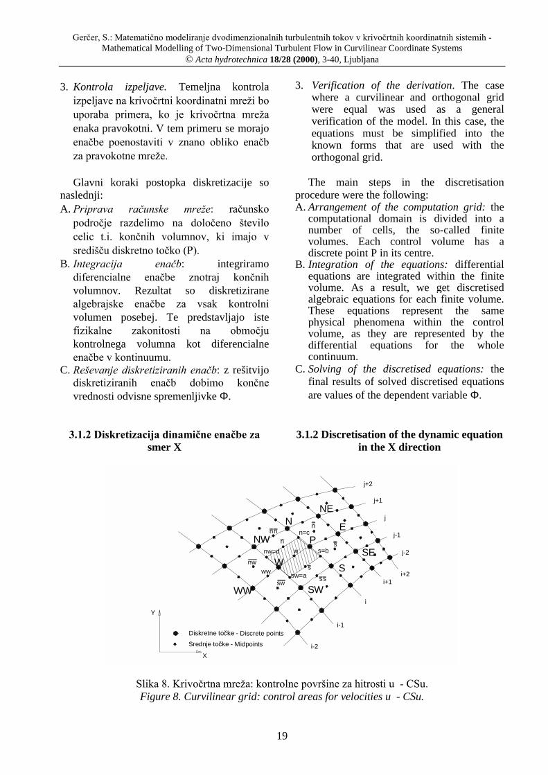
3.1.2 Diskretizacija dinamične enačbe zasmer X

3.1.2 Discretisation of the dynamic equationin the X direction

Srednje točke - Midpoints

Diskretne točke - Discrete points

Y

X

P

N

W

ENW

SW

NE

S

SE

WW

n=c

nw=d s=b

sw=a

w

n

nw

n

s

sw

ww

nn

s

ss

i

i+1i+2

i-1

i-2

j+2

j+1

j

j-1

j-2

Slika 8. Krivočrtna mreža: kontrolne površine za hitrosti u - CSu.Figure 8. Curvilinear grid: control areas for velocities u - CSu.



20

Želimo diskretizirati enačbo: We would like to discretise the followingequation:

34

222

2

)

(

)

(

)(

)(

hvuughn

xz

ghxhgh

yuh

yxuh

xyhuv

xhu b

efef+−−−=−−+

∂∂

∂∂

∂∂υ

∂∂

∂∂υ

∂∂

∂∂

∂∂

(28)

Integrirajmo dinamično enačbo po kontrolnipovršini Csu (slika 8) in uporabimo Greenovteorem o pretvorbi ploskovnega integrala nakrivuljnega. Rezultat je algebrajska enačba vobliki:

If we integrate the dynamic equation alongthe control area Csu (Figure 8) and useGreene’s theorem to transform the surfaceintegral to the linear one, we get the followingalgebraic equation as a result:

uwsssnnnwwWePww Suauauauaau ++++= - D (29)

Kjer posamezne člene enačbe izrazimo vobliki preglednice (za člene ai upoštevamohibridno shemo, preglednica 3):

Individual terms of equation 29 aredescribed in Table 3 for the hybrid numericalscheme:

Preglednica 3. Koeficienti diskretizirane dinamične enačbe za smer X na krivočrtni mreži.Table 3. Coefficients of the discretised dynamic equation for the X direction in curvilinear grid.

členi / terms a konvekcijski členi / convective terms F

2,

2 2P

PP

P

FD

FMAXa −

=

( )( )( )( )

−+−−+

=SNwwee

SNwweeP xxvhvh

yyuhuhF

4

1

2,

2 4W

WW

W

FD

FMAXa +

=

( )( )( )( )

−+−−+−=

nwswwwwwww

nwswwwwwwwW xxvhvh

yyuhuhF

4

1

2,

2 3n

nn

n

FD

FMAXa −

=

( )( )( )( )

−−++−−−++

=PNWNWnwnwnn

PNWNWnwnwnnn xxxxvhvh

yyyyuhuhF

41

2,

2 1s

ss

s

FD

FMAXa +

=

( )( )( )( )

−−++−−−++−=

WswPsswswss

WswPsswswsss xxxxvhvh

yyyyuhuhF

41

PsnWPw Saaaaa −+++=nwnssw

w

srsrgwwP S

h

vunghS ,,,

3

4

222 +−=

Suw= { })()()()( nwswWnnwnsnPswssw yyhyyhyyhyyhgh −+−+−+−−

{ })()()()( nwswbWnnwnbsnbPswssbw yyzyyzyyzyyzgh −+−+−+−−

(se nadaljuje na naslednji strani) (continued on the next page)



21

difuzijski členi / diffusive terms D

nwnnnnPsPswsssnwWswW uDuDuDuDuDuDuDuDD 42314231 +++++++=

( )( ) ( )( )

−−+−−= ssSNssSN

P

PP xxxxyyyy

S

KD

21

21

1

( )( ) ( )( )

−−+−−= snSNsnSN

P

PP xxxxyyyy

S

KD

21

21

2

( )( ) ( )( )

−−+−−= snSNnnSN

P

PP xxxxyyyy

S

KD

21

21

3

( )( ) ( )( )

−−+−−= nsSNnsSN

P

PP xxxxyyyy

S

KD

21

21

4

( )( ) ( )( )

−−+−−= wssnwswwssnwsw

W

WW xxxxyyyy

S

KD

2

1

2

11

( )( ) ( )( )

−−+−−= snnwswsnnwsw

W

WW xxxxyyyy

S

KD

21

21

2

( )( ) ( )( )

−−+−−= nwnnwswnwnnwsw

W

WW xxxxyyyy

S

KD

21

21

3

( )( ) ( )( )

−−+−−= wnnsnwswwnwsnwsw

W

WW xxxxyyyy

S

KD

21

21

4

( )( ) ( )( )

−−−++−−−+= SWSWSWPSSWSWSWPS

s

ss xxxxxxyyyyyy

S

KD

2

1

2

11

( )( ) ( )( )

−−−++−−−+= SPWSWPSSPWSWPS

s

ss xxxxxxyyyyyy

S

KD

2

1

2

12

( )( ) ( )( )

−−−++−−−+= PWWSWPSPWWSWPS

s

ss xxxxxxyyyyyy

S

KD

2

1

2

13

( )( ) ( )( )

−−−++−−−+= WSWWSWPSWSWWSWPS

s

ss xxxxxxyyyyyy

S

KD

2

1

2

14

( )( ) ( )( )

−−−++−−−+= WPPNWNWWPPNWNW

n

nn xxxxxxyyyyyy

S

KD

2

1

2

11

( )( ) ( )( )

−−−++−−−+= PNPNWNWPNPNWNW

n

nn xxxxxxyyyyyy

S

KD

2

1

2

12

( )( ) ( )( )

−−−++−−−+= NNWPNWNWNNWPNWNW

n

nn xxxxxxyyyyyy

S

KD

2

1

2

13

( )( ) ( )( )

−−−++−−−+= NWWPNWNWNWWPNWNW

n

nn xxxxxxyyyyyy

S

KD

2

1

2

14



22

3.1.3 Diskretizacija dinamične enačbe zasmer Y

3.1.3 Discretisation of the dynamic equationin the Y direction

Nnn

Y

WW


X


ww

NW

nw

nw=d

W

sw

nn=c j-1

i-1

S

i-2

SW

P

sw=a

w

s

s=b

ss

s

SE

i

i+1

j-2

i+2

En

NE

j+2

j+1

j

ss

ss

SS

SSW

SSE

e

nn

ssw

sse

Slika 9. Krivočrtna mreža: kontrolna površina za hitrosti v - CSv.Figure 9. Curvilinear grid: control areas for velocities v - CSv.

Podobno kot za smer x določimo še za smery (slika 9). Rezultat diskretizacije na kontrolnipovršini CSv je algebrajska enačba:

The procedure for the Y direction is verysimilar to that described for the X direction(Figure 9). The result of the discretisation forthe control area CSv is, again, an algebraicequation:

uswsnPsesssSss Svavavavaav ++++= - D (30)

3.1.4 Diskretizacija kontinuitetne enačbe 3.1.5 Discretisation of the mass conservationequation

Nnn

Y



NW

nwW

n=dn j-1

i-1

S

i-2

SW

P

sw

w

s=a

s

ss

s=bSE

i

i+1

j-2

i+2

En=c

NE

j+2

j+1

j

Slika 10. Krivočrtna mreža: kontrolni volumen za globine h - CVh.Figure 10. Curvilinear grid: control volume for depth h - CSh.



23

Integriramo kontinuitetno enačbo: The mass conservation equation isintegrated:

∫∫ +CSh

dSyhv

xhu

∂∂

∂∂ )()(

Ponovimo tudi dinamično enačbo za smerX v točki »w » kontrolnega volumna CVu:

Let us write the dynamic equation in the Xdirection for the point ‘w’ of the controlvolume CVu again:

uwsssnnnwwWePww Suauauauaau ++++= - D (31)

Če bi v kontinuitetni enačbi poznali točneglobine h, bi jo lahko na osnovi Greenovegateorema o pretvorbi ploskovnega integrala nakrivuljni integral zapisali v naslednji obliki:

If we knew the exact depth h in the massconservation equation, we would be able towrite it in the following form (on the basis ofGreene’s theorem about the transformation ofthe surface to the linear integral):

( ) ( ) ( ) ( ){ }( ) ( ) ( ) ( ){ } 0=+++

−+++

dawcdnbceabs

dawcdnbceabs

dXhudXhudXhudXhu

dYhudYhudYhudYhu (32)

Ker točnih globin ne poznamo, najprejpredpostavimo približne globine nadračunskim območjem (h*). S pripadajočimipredpostavljenimi globinami iz dinamičneenačbe izračunamo približne hitrosti u* in v*.Točne vrednosti pa lahko zapišemo v obliki žeznanih relacij:

As the exact depth is not known, theapproximate depth above the computationalarea (h*) is assumed. Next, the approximatevelocities u* and v* are calculated from thedynamic equation using the approximate depthvalues h*. Exact values can be written in theform of known relations:

u= u* + u'v= v* + v'h= h* + h'

kjer so:u*,v*,h* približne vrednostiu’,v’,h’ popravek do točne vrednostiu, v, h točne vrednosti.

Diskretizirana oblika kontinuitetne enačbena kontrolni površini CSh po izpeljavizapišemo kot:

where:u*, v*, h* are the approximate values;u’, v’, h’ represent the corrigendum andu, v, h are the exact values.

The mass conservation equation in itsdiscretised form for the control area CSh is,after derivation, written as:

Mpahahahahahahahahah hNWNWhNENEhSWSwhSESEhWWhNNhEEhSShPP ++++++++= ''''''''' (33)



24

kjer veljajo še naslednje zveze : where the following relations are valid:

2,

21

11

1S

SS

hS

CD

CMAXa +

=

2,

22

22

2S

SS

hS

CD

CMAXa +

= (34)

2,

21

11

1E

EE

hE

CD

CMAXa +

=

2,

22

22

2E

EE

hE

CD

CMAXa +

= (35)

2,

21

11

1N

NN

hN

CD

CMAXa +

=

2,

22

22

2N

NN

hN

CD

CMAXa +

= (36)

2,

21

11

1W

WW

hW

CD

CMAXa +

=

2,

22

22

2W

WW

hW

CD

CMAXa +

= (37)

WESNP aaaaa +++= (38)

( )

−

+−

+−

+−

−=

dawwdaww

cdnncdnn

bceebcee

abssabss

p

dXvhdYuh

dXvhdYuh

dXvhdYuh

dXvhdYuh

M

****

****

****

****

1 (39)

Reševanje sistema algebrajskih enačb (33)v vseh točkah računske mreže nam dapopravljene vrednosti h' v diskretnih točkahmreže. To potem omogoči račun popravkovhitrosti u' in v' (enačbe (40) do (47)). Spopravljenimi hitrostmi ponovimo izračundinamične enačbe za smeri X in Y. Toponavljamo, dokler niso izpolnjene vseenačbe, tako obe dinamični kot tudikontinuitetna enačba. Vrednosti popravkovhitrosti in globin so pod neko vnaprejpredpisano dopustno relativno vrednostjo, ki jopredpišemo kot kriterij konvergence (npr.0.1%).

The solution of the algebraic equationssystem (33) in all points of numerical gridgives a series of rectified values h' in thediscrete points of the grid. With these values,the velocity corrigendas u' and v' arecalculated using (40) to (47). With the rectifiedvelocities, the dynamic equation in both the Xand Y directions are calculated again. Theprocedure is repeated until all equations, bothdynamic and the mass conservation equation,are completed. At that time, the values ofdepth and velocity corrigenda must be lessthan the allowed relative error, which is givenin advance as the convergence criterion (e.g.0.1%).

'4

'3

'2

'1

'WuwnuwPuwsuww hDhDhDhDu +++= (40)'

4'

3'

2'

1'

WvwnvwPvwsvww hDhDhDhDv +++= (41)'

4'

3'

2'

1'

PuenueEuesuee hDhDhDhDu +++= (42)'

4'

3'

2'

1'

PvenveEvesvee hDhDhDhDv +++= (43)'

4'

3'

2'

1'

susPussusSuss hDhDhDhDu +++= (44)'

4'

3'

2'

1'

svsPvssvsSvss hDhDhDhDv +++= (45)'

4'

3'

2'

1'

sunPunnunPunn hDhDhDhDu +++= (46)'

4'

3'

2'

1'

svnPvnnvnPvnn hDhDhDhDv +++= (47)



25

4. ZAPIS RAČUNALNIŠKIHPROGRAMOV

4.1 PROGRAM GEO-CURVE –PROGRAM ZA KONSTRUIRANJENEPRAVOKOTNE KRIVOČRTNE

MREŽE

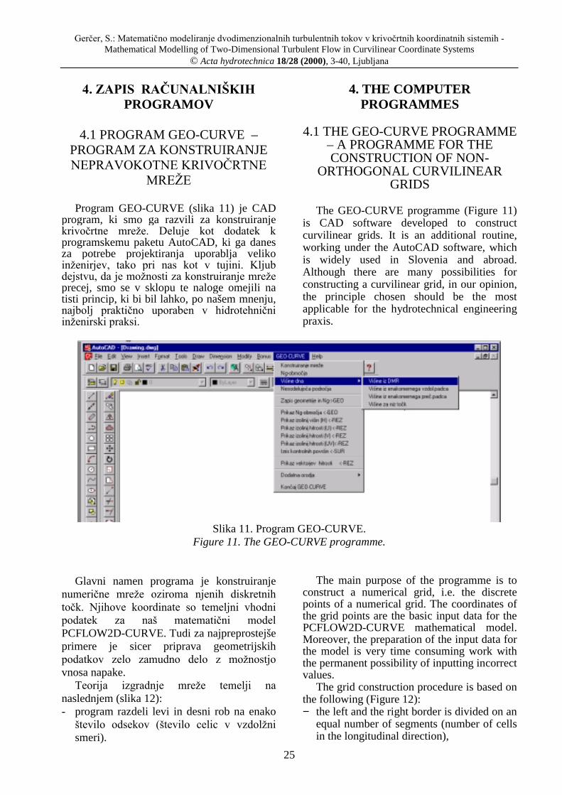
Program GEO-CURVE (slika 11) je CADprogram, ki smo ga razvili za konstruiranjekrivočrtne mreže. Deluje kot dodatek kprogramskemu paketu AutoCAD, ki ga danesza potrebe projektiranja uporablja velikoinženirjev, tako pri nas kot v tujini. Kljubdejstvu, da je možnosti za konstruiranje mrežeprecej, smo se v sklopu te naloge omejili natisti princip, ki bi bil lahko, po našem mnenju,najbolj praktično uporaben v hidrotehničniinženirski praksi.

4. THE COMPUTERPROGRAMMES

4.1 THE GEO-CURVE PROGRAMME– A PROGRAMME FOR THECONSTRUCTION OF NON-

ORTHOGONAL CURVILINEARGRIDS

The GEO-CURVE programme (Figure 11)is CAD software developed to constructcurvilinear grids. It is an additional routine,working under the AutoCAD software, whichis widely used in Slovenia and abroad.Although there are many possibilities forconstructing a curvilinear grid, in our opinion,the principle chosen should be the mostapplicable for the hydrotechnical engineeringpraxis.

Slika 11. Program GEO-CURVE.Figure 11. The GEO-CURVE programme.

Glavni namen programa je konstruiranjenumerične mreže oziroma njenih diskretnihtočk. Njihove koordinate so temeljni vhodnipodatek za naš matematični modelPCFLOW2D-CURVE. Tudi za najpreprostejšeprimere je sicer priprava geometrijskihpodatkov zelo zamudno delo z možnostjovnosa napake.

Teorija izgradnje mreže temelji nanaslednjem (slika 12):- program razdeli levi in desni rob na enako

število odsekov (število celic v vzdolžnismeri).

The main purpose of the programme is toconstruct a numerical grid, i.e. the discretepoints of a numerical grid. The coordinates ofthe grid points are the basic input data for thePCFLOW2D-CURVE mathematical model.Moreover, the preparation of the input data forthe model is very time consuming work withthe permanent possibility of inputting incorrectvalues.

The grid construction procedure is based onthe following (Figure 12):− the left and the right border is divided on an

equal number of segments (number of cellsin the longitudinal direction),



26

- točke levega in desnega roba poveže s črto(prečni profil).

- črto prečnega profila razdeli na enakoštevilo odsekov (število lamel).

- med odsekoma sosednjih profilov poiščegeometrijsko sredino (diskretna točka).

Kot rezultat program kreira mrežodiskretnih točk in izriše kontrolne površine zaglobine CSh.

− points at the left and the right side areconnected by a line (cross-section),

− all cross-section lines are divided into anequal number of segments (number of cellsin the transverse direction),

− between two adjacent profiles, a discretepoint in the geometric mean of the profilesis found.

As a result, a grid of discrete points and thecontrol areas for the depth CSh are created.

Diskretne točke mrežeDiscrete points of the grid

Levi rob - Left border

Desni rob - Right borderZačetna smer toka

Initial flowdirection

j2j1j3 j4 j5 j6 j..n

i1

i2

i3

i4

i5

i6

i7

i8

i9

Slika 12. Konstruiranje numerične mreže.Figure12. The construction of the numerical grid.

dLdL

dLdL dL

Dd dDDd dD

dL

dD

Slika 13. Teoretična osnova za konstruiranje mreže.Figure13. Theoretical basis for the grid construction.



27

4.2 PROGRAM PCFLOW2D–MATEMATIČNI MODEL ZA

RAČUN GLADIN PRI PRAVOKOTNIMREŽI

Program temelji na teoretičnih podlagahmodela TEACH (Gosman, 1976), ki je bilkasneje dopolnjen na KMTe FGG (Četina,1980). Model je bil večkrat verificiran kot tudiuporabljen na praktičnih primerih, zato lahkonjegove rešitve upoštevamo kot ustrezne.

4.3 PROGRAM PCFLOW2D - CURVE– MATEMATIČNI MODEL ZA

RAČUN GLADIN PRINEPRAVOKOTNI KRIVOČRTNI

MREŽI

Program PCFLOW2D-CURVE temelji napodanih teoretičnih podlagah drugega pristopareševanja enačb v krivočrtnem koordinatnemsistemu. Odločili smo se namreč za konceptuporabe netransformiranih enačb vKartezijevih koordinatah X-Y, vplivkrivočrtne mreže pa nato upoštevamo pripostopkih diskretizacije.

5. VERIFIKACIJAMATEMATIČNEGA MODELA

Za verifikacijo modela smo izbrali primere,ki nam lahko potrdijo, da je teoretičnaizpeljava enačb za primer krivočrtnenumerične mreže pravilna. Podobno kot smoposamezne člene diskretiziranih enačb prikrivočrtni mreži kontrolirali z ustreznimi členipri pravokotni mreži, smo sedaj tudi za celotenmodel PCFLOW2D-CURVE najprej uporabiliprimerjavo rezultatov s poenostavljenimprimerom toka v pravokotnem kanalu v oblikičrke Z.

Kot bomo videli v nadaljevanju, so rezultatizelo podobni tistim, ki jih dobimo z žepreverjenim modelom PCFLOW2D.

Drugi primer verifikacije pa je tok v kanaluz dvojno krivino, kjer smo izračunanonadvišanje gladin primerjali z ustreznimipoenostavljenimi analitičnimi izrazi.

4.2 THE PCFLOW2D PROGRAMME– A MATHEMATICAL MODEL FORTHE CALCULATION OF SURFACE

ELEVATIONS USING ANORTHOGONAL GRID

The programme is based on the TEACHmodel (Gosman, 1976). It was additionallyupgraded at the Chair of Fluid Mechanics atthe University of Ljubljana (Četina, 1980).The PCFLOW2D model has been verifiedseveral times and used in many practicalproblems; therefore, the results of the modelmay be considered as the reference results.

4.3 THE PCFLOW2D-CURVESOFTWARE – A MATHEMATICALMODEL FOR THE CALCULATIONOF SURFACE ELEVATIONS USING

A NON-ORTHOGONALCURVILINEAR GRID

The PCFLOW2D-CURVE programme isbased on the theory of the second approach ofsolving the equations in a non-orthogonalcurvilinear coordinate system. The concept ofusing non-transformed equations in CartesianX-Y coordinates was adopted, and the impactof the non-orthogonal grid is taken intoaccount later in the discretisation procedure.

5. VERIFICATION OF THEMATHEMATICAL MODEL

The cases which confirmed the correctnessof the theoretical derivation of the equations ina non-orthogonal curvilinear coordinatesystem were chosen to verify the model.Similarly, as the individual terms of theequations were compared to the adequateterms of the equations for the orthogonal grid,the results of the complete PCFLOW2D-CURVE model were compared to a simplifiedflow case in a rectangular ‘Z’ shaped channel(Fig. 14).

As can be seen, the results are very close tothe results of the already verified PCFLOW2Dmodel.

The second case chosen was flow in adouble curved channel, where the calculatedsurface elevations were compared to theresults of adequate simplified analyticalequations.



28

5.1 TOK V PRAVOKOTNEMKANALU V OBLIKI ČRKE Z

5.1.1 Uporaba modela PCFLOW2D pripravokotni mreži

Primer predstavlja tipičendvodimenzionalni tok, kjer nastane vspodnjem levem kotu izrazit vrtinec. Ker je bilta primer že testiran s pravokotno mrežo in jebila izvedena tudi primerjava z rezultatimodela FLOW3D, lahko z gotovostjoizhajamo iz dejstva, da so rezultati modelaPCFLOW2D na pravokotni mreži pravilni.

V izbranem primeru imajo stene kanala vtlorisu pravokotno obliko, kar je v praksi sicerredko. Robni pogoji so definirani tako, da jedolvodno konstantna globina H = konst,gorvodno pa je podan pretok Q - glej sliko 14.

5.1 FLOW IN A RECTANGULAR ‘Z’SHAPED CHANNEL

5.1.1 The use of the PCFLOW2D modelwithin an orthogonal grid

The case represents a typical two-dimensional flow, where a well-defined vortexoccurs in the lower left corner. As the case hasalready been tested using an orthogonal grid,and also a comparison with the 3D modelFLOW3D results has been done, we maysurely consider the results of the PCFLOW2Dmodel correct.

The channel walls represent a rectangle inthe horizontal plan, which is rather rare in thetechnical praxis. The downward boundarycondition is defined as constant depth(H = const), and at the upward boundary, thedischarge (Q) is given (see Figure 14).

Slika 14. Aksonometričen prikaz pravokotnega kanala v obliki črke »Z«.Figure 14. Axonometric view of the rectangular ‘Z’ shaped channel.

Področje kanala diskretiziramo spravokotno mrežo s 14 x 22 celicami. Zaradilažjega računanja na robovih modelPCFLOW2D zahteva še definiranje dvehvrstic oziroma stolpcev kontrolnih površin(celic) na zunanjih straneh robov kanala. Takoima naša numerična mreža skupno velikost 18x 22 kontrolnih površin (CSh).

Velikost posamične celice je dX = 2m(širina) in dY = 2m (dolžina). Dno jevodoravno, zato je aktivnim celicam pripisanakota dna 0, neaktivnim celicam pa 10 m

The channel is discretised by an orthogonalgrid with 14 x 22 cells. For the sake ofsimplifying the calculation, two more rows(columns) of control areas need to be definedat the outer borders of the channel. Thus, thedimension of the final numerical grid is 18 x22 control areas (CSh).

The width of each cell is dX = 2m, and thelength dY = 2m. The channel has a horizontalbed; therefore, the bed elevation of active cellsis equal to 0, while that of the non-active cellsis set to 10 m (to avoid pouring over the



29

(velika vrednost prepreči preliv iz kanala).Drugi pomembnejši vhodni podatki so še :

- Q=konst.=0.5 m3/s (gorvodni robni pogoj)- H = 0.1 m (predpisana gladina na

dolvodnem robu)- Ng v vseh celicah = 0.01 3/1sm- Predpostavljene globine (H) na začetku

računa v celicah = 0.08m- Predpostavljene hitrosti na začetku računa

za smer Y (v) = 0.05 ms-1

- Predpostavljene hitrosti na začetku računaza smer X (u) = 0.00 ms-1

- Faktorji podrelaksacije za hitrosti u, v inglobine H : URFU = URFV = URFH = 1.0.

Rezultat izračuna: kot rezultat izračunadobimo porazdelitev hitrosti u in v ter globin hv vseh točkah numerične mreže (sliki 15 in16).

channel walls).Other important input data are:

− Q=const.=0.5 m3/s (upward boundarycondition)

− H = 0.1 m (downward boundary condition)− Ng in all cells = 0.01 3/1sm− Initial water depth (H) in all cells = 0.08 m− Initial velocities in the Y direction (v) =

0.05 ms-1

− Initial velocities in the X direction (u) =0.00 ms-1

− Under-relaxation factors for velocities u, vand depth H: URFU = URFV = URFH =1.0

The result of the computation: thedistribution of velocities (u and v) and depth(h) in all discrete points of the grid are theresult of the computation (Figures 15 and 16).

Slika 15. Razporeditev vektorjev hitrosti v diskretnih točkah (model PCFLOW).Figure 15. Velocity vector distribution in discrete points (the PCFLOW model).



30

Slika 16. Primerjava izračunanih vektorjev hitrosti med modeloma PCFLOW2Din PCFLOW2D-CURVE pri pravokotni mreži.

Figure 16. Comparison of the velocity vectors between the PCFLOW2Dand PCFLOW2D-CURVE models using the orthogonal grid.

5.1.2 Uporaba modela PCFLOW2D-CURVE pri pravokotni mreži

Novi model PCFLOW2D-CURVE smonajprej uporabili za enake vhodne podatke, kotsmo jih upoštevali pri modelu PCFLOW2D.Pravokotna Kartezijeva mreža je namreč leposeben primer splošne krivočrtne mreže in vprimeru pravilnega delovanja modelaPCFLOW2D – CURVE bi se rezultati moraliujemati s tistimi na sliki 15. Primerjavaizračunanih vektorjev hitrosti je prikazana nasliki 16.

Kot je razvidno iz prikaza vektorjev hitrosti(slika 15), dobimo v kotu izrazit vrtinecoziroma recirkulirajoče področje.

Koristen podatek za kasnejšo primerjavo

5.1.2 The use of the PCFLOW2D-CURVEmodel within an orthogonal grid

The new PCFLOW2D-CURVE model wasfirst used with the same input data as was usedwith the PCFLOW2D model. The orthogonalCartesian grid is, finally, only a special case ofthe general curvilinear grid, and if thePCFLOW2D – CURVE model workedproperly, the results should be in agreementwith the results in Figure 15. The comparisonof velocity vectors is in Figure 16.

As it can be seen from Figure 15, arecirculation area (a well-defined vortex) ispresent in the corner.

Other useful information for the later



31

učinkovitosti modelov je tudi število iteracij,ki so potrebne, da vse enačbe (kontinuitetna indinamični) konvergirajo h končni vrednosti.Za dosego rezultata na sliki 15 je bilopotrebnih 1004 iteracij pri zahtevaninatančnosti SORMAX=0.001.

Poudarimo še enkrat, da je bil ta primerračuna podrobno preverjen na podlagiprimerjave med modeloma PCFLOW2D infrancoskim modelom FLOW3D. Rezultatimed modeloma so se popolnoma ujemali, zatosmo jih upoštevali kot merodajne za nadaljnjoprimerjavo z rezultati modela PCFLOW2D -CURVE.

optimisation of the model is the number ofiterations used to get the equation convergence(the mass conservation and the dynamicequation). 1004 iterations were needed to getthe results shown in Fig. 15 with the requiredaccuracy SORMAX=0.001.

To emphasise once again: this particularcase was verified in detail on the basis ofcomparison between the PCFLOW2D resultsand the results of the French model FLOW3D.The results were in complete agreement; thus,they were used as a reference for furthercomparison with the PCFLOW2D-CURVEmodel.

5.1.3 Uporaba modela PCFLOW2D-CURVE pri krivočrtni mreži

Naslednja stopnja verifikacije modela jebila uporaba krivočrtne mreže, ki smo jokreirali s pomočjo programa za konstruiranjekrivočrtne mreže GEO-CURVE. Za osnovosmo vzeli približno enako število sodelujočihcelic kot pri pravokotni mreži, torej 18 x 22krivočrtnih kontrolnih površin (slika 17).

5.1.3 The use of the PCFLOW2D-CURVEmodel within a non-orthogonal grid

The next step in the verification of themodel was to use a curvilinear grid generatedby the GEO-CURVE programme.Approximately the same number of controlvolumes as with the orthogonal grid was used:18 x 22 curvilinear control areas (Figure 17).

Slika 17. Krivočrtna mreža na »Z kanalu«.Figure 17. Curvilinear grid in the ‘Z’ shaped channel.



32

Kot smo že omenili, je ta primer za uporabokrivočrtne mreže zelo neugoden, je pa koristenza testiranje modela. Pravokotni robovinamreč onemogočajo izvedbo »gladkih«prehodov celic, zato je konstrukcija mreže zelozahtevna. »Gladki« prehodi so pomembnizaradi interpolacij, ki so potrebne za določitevvrednosti u,v in h na robovih celic.

As already mentioned, this particular case isvery inconvenient for use with the curvilinearcoordinates; however, it is useful for thepurpose of testing. The orthogonally shapedborders exclude the possibility of having»smooth« passages between the cells;therefore, the construction of the grid is verydemanding. The »smooth« passages are ofgreat importance due to interpolations, whichare needed to calculate the values of u, v and hat the borders of the cells.

Slika 18. Primerjava vektorjev hitrosti med modeloma PCFLOW2Din PCFLOW2D-CURVE pri krivočrtni mreži.

Figure 18. A comparison of the velocity vector fields between the PCFLOW2D modeland the PCFLOW2D-CURVE model using the curvilinear grid.



33

Analiza rezultatov. Iz primerjave rezultatovmodelov v primeru uporabe pravokotne mreže(PCFLOW2D) in krivočrtne mreže(PCFLOW2D-CURVE) lahko za slednjegaugotovimo naslednje (slika 18):A. Model PCFLOW2D-CURVE se obnaša

enako kot model PCFLOW2D v primeru,da ga uporabimo za pravokotno mrežo. Stem je deloma že potrjena pravilnadiskretizacija osnovnih enačb, saj jepravokotna Kartezijeva mreža le posebenprimer splošne krivočrtne mreže.

B. Tudi pri uporabi krivočrtne mreže sovektorji hitrosti izračunani pravilno tako posmeri kot velikosti, manjša odstopanja sozaradi številnih iteracij na robovih.

C. Globine in skupni pretok konvergirajo kpravilnemu končnemu stanju.

D. Krivočrtna mreža zahteva pri enakemštevilu celic, zaradi povečanja številainterpolacij, več računalniškega časa (oz.iteracij). Vendar je prednost krivočrtnemreže očitna v primerih, ko lahko zaradilažjega prilagajanja robovom število celicbistveno zmanjšamo.

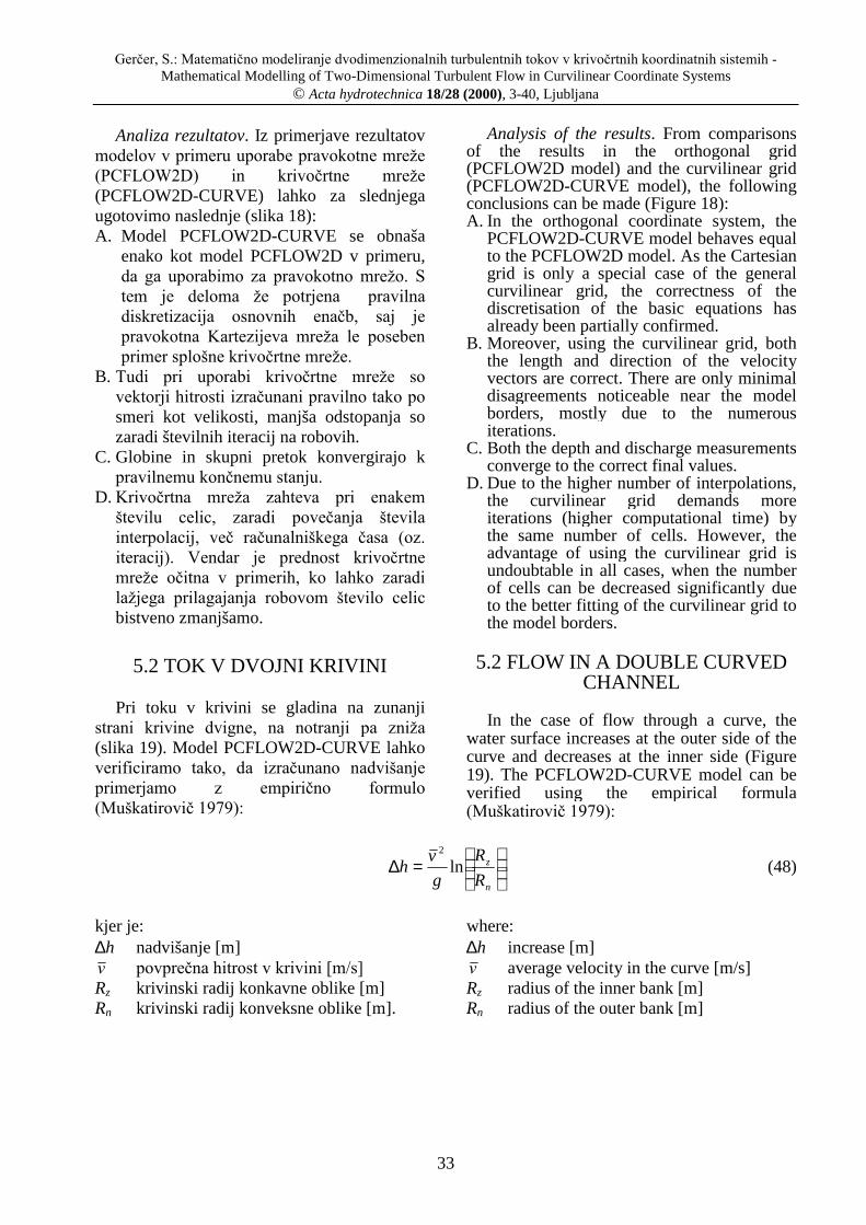
5.2 TOK V DVOJNI KRIVINI

Pri toku v krivini se gladina na zunanjistrani krivine dvigne, na notranji pa zniža(slika 19). Model PCFLOW2D-CURVE lahkoverificiramo tako, da izračunano nadvišanjeprimerjamo z empirično formulo(Muškatirovič 1979):

Analysis of the results. From comparisonsof the results in the orthogonal grid(PCFLOW2D model) and the curvilinear grid(PCFLOW2D-CURVE model), the followingconclusions can be made (Figure 18):A. In the orthogonal coordinate system, the

PCFLOW2D-CURVE model behaves equalto the PCFLOW2D model. As the Cartesiangrid is only a special case of the generalcurvilinear grid, the correctness of thediscretisation of the basic equations hasalready been partially confirmed.

B. Moreover, using the curvilinear grid, boththe length and direction of the velocityvectors are correct. There are only minimaldisagreements noticeable near the modelborders, mostly due to the numerousiterations.

C. Both the depth and discharge measurementsconverge to the correct final values.

D. Due to the higher number of interpolations,the curvilinear grid demands moreiterations (higher computational time) bythe same number of cells. However, theadvantage of using the curvilinear grid isundoubtable in all cases, when the numberof cells can be decreased significantly dueto the better fitting of the curvilinear grid tothe model borders.

5.2 FLOW IN A DOUBLE CURVEDCHANNEL

In the case of flow through a curve, thewater surface increases at the outer side of thecurve and decreases at the inner side (Figure19). The PCFLOW2D-CURVE model can beverified using the empirical formula(Muškatirovič 1979):

=∆

n

z

R

R

g

vh ln

2

(48)

kjer je:∆h nadvišanje [m]v povprečna hitrost v krivini [m/s]Rz krivinski radij konkavne oblike [m]Rn krivinski radij konveksne oblike [m].

where:∆h increase [m]v average velocity in the curve [m/s]Rz radius of the inner bank [m]Rn radius of the outer bank [m]



34

Slika 19. Nadvišanje gladine v krivini.Figure 19. Increase of the water surface in a curve.

Krivočrtno mrežo na sliki 20 smooblikovali s pomočjo programa GEO-CURVE.Čeprav bi v tem primeru lahko uporabili tudipravokotno krivočrtno mrežo, smo ostali primreži, kjer robovi kontrolnih površin medseboj ne tvorijo pravih kotov. Tako v računusodelujejo tudi členi, ki izražajonepravokotnost in lahko dodatno preverimopravilnost diskretizacije enačb v krivočrtnemsistemu. Opozoriti moramo še, da kontrolnepovršine zunaj osnovnega korita (rdeče barve)pri računu ne sodelujejo, zato njihova oblika inlega tako rakoč ni pomembna. Kot smo žeomenili, jih uporabljamo zgolj zaradi lažjegadefiniranja robnih pogojev na premaknjenimreži (CSu, CSh).

Kot vhodne podatke smo upoštevalinaslednje vrednosti:- stalni tok, pravokotno obliko prečnega

preseka kanala z vtočno in iztočno širinoB=14m,

- koto dna aktivnih celic 0 (torej primervodoravnega dna, izključen vpliv padcadna) ter koto dna neaktivnih celic 10m.

- Q=konst.=0.5m3/s (gorvodni robni pogoj)- H=1 m (predpisana globina na dolvodnem

robu modela)- v vseh celicah je Ng = 0.01 3/1sm- predpostavljene globine (H) na začetku

računa v celicah = 0.8m- predpostavljene hitrosti na začetku računa

za smer Y: v = 0.05 ms-1

- predpostavljene hitrosti na začetku računaza smer X: u = 0.00 ms-1

- faktorji podrelaksacije za hitrosti u,v inglobine h : URFU = URFV = URFH = 1.0.

The curvilinear grid shown in Figure 20was generated by the GEO-CURVEprogramme. Although in this case anorthogonal curvilinear grid might be used, wedecided for the general (non-orthogonal)curvilinear grid. In this way, the terms, whichexpress the non-orthogonality are alsoinvolved, and the case can be treated as anadditional verification of the discretisation ofequations in a curvilinear coordinate system.The control areas which are not part of thechannel (in red colour) are not a part of thecomputation; therefore, their shape andposition is not of any importance. As alreadymentioned, these are used only for achieving abetter definition of the boundary conditions forthe shifted grid (CSu and CSh).

The following data were used as input:− Steady flow, rectangular channel, width

B=14 m along the channel.− Horizontal bed (bed slope impact was

excluded); the bed elevation of active cellsis equal to 0, while of the non-active cells isset to 10 m.

− Q=const.=0.5m3/s (upwards boundarycondition)

− H=1 m (downwards boundary condition)− In all cells, Manning’s coefficient is equal

to Ng = 0.01 3/1sm− Initial water depth (H) in all cells = 0.8m− Initial velocities in the Y direction (v) =

0.05 ms-1

− Initial velocities in the X direction (u) =0.00 ms-1

− Under-relaxation factors for velocities u, vand depth H: URFU = URFV = URFH =1.0



35

H(3,16)

H(7,10)

Rn

Rz

H=konst.

Q=konst.

Slika 20. Izračunani vektorji hitrosti v dvojni krivini.Figure 20. Calculated velocity vectors in the double curve.

Analiza rezultatov. Kot je razvidno iz slike20, se vektorji hitrosti pravilno obračajo vsmeri glavnega toka. Tako globine kot pretokpravilno konvergirajo h končni vrednosti, zapredpisano natančnostjo 1.6 odstotka pa je bilopotrebnih 495 iteracij.

Nadvišanje gladine lahko ovrednotimo nadva načina: iz rezultatov računa in s pomočjopribližne analitične enačbe. Iz rezultatovmodela PCFLOW2D-CURVE imamo (slika20):dH = H(3,16) - H(7,10) == 1.000092424 - 1.00001828 = 0.00007414 m.

Analysis of the results. As seen from Figure20, the velocity vector directions are correct,turning towards the main flow direction. Bothdepth and discharge converge towards thecorrect final value. For the required accuracy1.6 %, 495 iterations were needed.

Increase of the surface was calculated fromboth results of the computation and from theapproximate analytical formula. From thePCFLOW2D-CURVE model we obtained(Fig. 20):dH = H(3,16) - H(7,10) = 1.000092424 -1.00001828 = 0.00007414 m

Po analitični enačbi (48) pa dobimo: For the analytical equation (Eq. 48) we get:

=∆

n

z

R

R

g

vh ln

2

=0.000078339 m,

kjer smo upoštevali (slika 20):Rz = 30.64mRn = 16.64mv = 0.03548m/s.

where the following data were taken intoaccount (Fig. 20):

Rz = 30.64mRn = 16.64mv = 0.03548m/s.

Razlika med analitično iz izračunanovrednostjo je 5 odstotkov, kar kaže na pravilnodelovanje računalniškega programaPCFLOW2D-CURVE.

The difference between the analytical andthe computed value is about 5 %; therefore,the working of the PCFLOW2D-CURVEmodel may be treated as correct.



36

6. ZAKLJUČEK

Krivočrtna mreža ima v inženirski praksizelo veliko uporabnost, saj ponuja možnostboljšega prilagajanja nepravilnim robovomračunskega področja. Reševanje enačb jematematično kompleksno, zato smo v tejnalogi podali in opisali dva temeljna pristopareševanja, pri čemer smo v računalniškiprogram PCFLOW2D-CURVE potem vgradilit.i. »drugi pristop«.

6.1 PRVI PRISTOP

Enačbe, s katerimi opisujemo gibanjeturbulentnih tokov, izrazimo v vektorskiobliki, ki je neodvisna od koordinatnegasistema. Z znanimi matematičnimi izrazi zavektorske operatorje, kot so gradient,divergenca in rotor za različne koordinatnesisteme lahko nato osnovne enačbetransformiramo v koordinatno obliko zakrivočrtni pravokotni ali splošni nepravokotnikrivočrtni sistem. Tega potem preslikamo vpravokotno mrežo, na kateri izvedemonumerično diskretizacijo enačb, nato pakončne rezultate preslikamo nazaj v krivočrtnisistem.

Poseben primer splošnega krivočrtnegasistema je pravokotni krivočrtni sistem.Enačbe za ta poseben primer so v literaturidostopne, zato smo jih lahko uporabili kottemeljno kontrolo izpeljave enačb v splošnemkrivočrtnem sistemu. Kot lahko vidimo izdrugega poglavja, se razvite enačbe splošnegakrivočrtnega sistema ob ustreznihpoenostavitvah resnično transformirajo v tistev pravokotnem sistemu, tako da lahkozaključimo, da so splošne enačbe pravilnoizpeljane.

Pri nadaljnjem razmišljanju obpregledovanju izpeljanih enačb prvegapristopa pridemo do sklepa, da bi bilanumerična diskretizacija teh enačb izjemnokompleksna, predvsem pa zelo dolga.Posameznih korakov diskretizacije tudi ne bimogli fizikalno preveriti, zato bi bila možnostnapak večja. Zaradi teh razlogov smo seodločili za uporabo drugega pristopa.

6. CONCLUSIONS

The curvilinear grid is very applicable inan engineering praxis, as it better fits thenatural borders of the computational domain.Solving the equations is mathematicallycomplex; thus, in the thesis, two differentbasic approaches are given. The “secondapproach” was included in the PCFLOW2D-CURVE model.

6.1 THE FIRST APPROACH:

Equations used for the description ofmovement of the turbulent flow are written ina vectorised form, independent of thecoordinate system. With the knownmathematical expressions of vectorisedoperators such as gradient, divergence andcurl, in different coordinate systems, the basicequations are transformed into a coordinateform for the curvilinear orthogonal or generalnon-orthogonal system. This system is latertransformed into an orthogonal grid wherenumerical discretisation of the equations isperformed. Finally, the results are transformedback to the curvilinear system.

A special case of a general curvilinearsystem is an orthogonal curvilinear system.Equations for this special case are available inliterature; therefore, they were used as thebasic verification of the derivation of theequations in the general curvilinear system. Ascan be seen from the second chapter, in thespecial case (orthogonal curvilinear system),and using the appropriate simplifications, thederived equations are really transformed intothe equations used in an orthogonal system.Thus, the derivation may be consideredcorrect.

After taking into consideration thecomplexity and time used for the derivation ofthe equations of the first approach, it wasconcluded that the second approach offersbetter possibilities for the physical verificationof the individual steps of the derivation andfewer possibilities for mistakes. Therefore, wedecided to use the second approach.



37

6.2 DRUGI PRISTOP

Pri tem pristopu uporabimo osnovne enačbev običajnem Katerzijevem koordinatnemsistemu, vpliv nepravokotnih celic krivočrtnemreže pa nato upoštevamo pri numeričnidiskretizaciji.

Numerično diskretizacijo smo izvršili pometodi končnih volumnov oz. površin, ki se vsvetu veliko uporablja za reševanje gibanjaturbulentnih tokov. Tudi lastnih izkušenj zuporabo metode za primer pravokotnih mrežsmo imeli dovolj, da smo lahko v okvirunaloge izvedli še podrobno izpeljavo za primernepravokotne krivočrtne mreže. Ustrezni členiv dobljenih diskretiziranih enačbah se zaprimer pravokotne mreže kot posebnegaprimera splošne krivočrtne mreže (poglavje 3)pravilno poenostavijo, kar nam potrjuje, da jebila izpeljava uspešno izvedena.

Poudarimo lahko, da podrobne izpeljavediskretizacije za primer splošnih krivočrtnihkoordinat in hkrati premaknjene mreže nismozasledili v dosegljivi literaturi. Običajno se vtakšnih primerih uporablja nepremaknjenamreža, zato naš pristop predstavlja v svetu doneke mere novost.

Pri obeh pristopih smo za zdaj izpeljali innato diskretizirali kontinuitetno in dinamičnienačbi za primer dvodimenzionalnegaglobinsko povprečenega toka s prosto gladino.Enak postopek in pridobljene izkušnje lahkouporabimo tudi pri diskretizaciji dodatnihtransportnih enačb za skalarje (npr.temperaturo »T«, slanost »s«, koncentracijo»C« ipd.) ali količine, ki nastopajo v ustreznihmodelih turbulence (npr. tubulentna kinetičnaenergija na enoto mase »k« in stopnjo njenedisipacije »ε« pri zelo razširjenem k-ε modeluturbulence).

6.2 THE SECOND APPROACH:

Here the basic equations in the Cartesiancoordinate system are used, and the impact ofthe non-orthogonality of the cells is taken intoaccount during the discretisation of theequations.

The control volume method (control areamethod, respectively) was used for thenumerical discretisation. This method iswidely used throughout the world to solve themotion of turbulent flows. Moreover, we wereexperienced enough with the same method inorthogonal grids to perform a detailedderivation in the non-orthogonal curvilineargrid. Adequate terms in the deriveddiscretised equations are (in the case of theorthogonal grid as a special case of the generalnon-orthogonal grid – see chapter 3) simplifiedcorrectly, which confirms the success of thederivation performed.

Again, it must be emphasised that a detailedderivation of discretisation for generalcurvilinear coordinates and shifted grids cannot be found in any available literature.Usually, a non-shifted grid is used with suchcases; therefore, the approach describedrepresents, to a certain extent, an innovation,in the field.

So far, with both approaches, the massconservation and the dynamic equation werefirst derived and then discretised for the two-dimensional depth averaged free surface flow.The same procedure and the acquiredexperience may also be used for thediscretisation of additional equations, foreither the scalar transport (temperature »T«,salinity »s«, concentration »C« etc.), or anyquantity that is used in adequate turbulenceclosure schemes (the turbulent kinetic energyper mass unit »k« and the dissipation of theturbulent kinetic energy »ε« in the expandedk-ε model).



38

6.3 IZDELAVA IN VERIFIKACIJARAČUNALNIŠKEGA PROGRAMAPO DRUGI METODI:(PCFLOW2D-

CURVE)

V okviru te naloge smo se odločili zauporabo drugega pristopa, na podlagi kateregasmo pripravili matematični model in razviliračunalniški program PCFLOW2D-CURVE.Program temelji na programu PCFLOW2D, kise uporablja na Katedri za mehaniko tekočin zlaboratorijem (KMTe) za primeredvodimenzionalnih tokov pri pravokotninumerični mreži. Ker je bila že izpeljavapostopka diskretizacije in nato izdelavaračunalniškega programa zelo obsežna inzahtevna naloga, smo za potrditev pravilnegadelovanja programa izvedli le nekaj osnovnihverifikacij.

Kot prvo verifikacijo smo izvedliprimerjavo med že preverjenim modelomPCFLOW2D in modelom PCFLOW2D-CURVE pri uporabi pravokotne mreže za tokv pravokotnem kanalu v obliki črke »Z«.Rezultati so pokazali tako rekoč popolnoujemanje. To je bila prva potrditev pravilnostiizpeljave diskretizacije in delovanja razvitegaprograma PCFLOW2D-CURVE.

Pri drugi verifikaciji smo za isti primer tokav kanalu »Z« oblike izvedli primerjavo medrezultati, dobljenimi pri pravokotni mreži(program PCFLOW2D) in rezultati prikrivočrtni mreži (program PCFLOW2D-CURVE). Tudi tu se rezultati dobro ujemajo into tudi na območju izrazitega vrtinca, kinastane v spodnjem levem kotu in kaže naizrazito dvodimenzionalni tok. Do manjšihrazlik prihaja na robovih krivočrtne mreže, karje po naši oceni posledica številnih interpolacijvrednosti na robovih. Težava je povezana tudis splošnostjo podajanja robnih pogojev, kar jeposebej omenjeno tudi pri usmeritvah zanadaljnje delo.

Kot tretjo verifikacijo smo izvedliprimerjavo rezultatov modela z analitičnoformulo nadvišanja gladine v krivini. Tuditukaj lahko ugotavljamo, da so rezultatimodela dobri.

Na podlagi dosedaj opravljenih verifikacijlahko sklepamo, da je model PCFLOW2D-CURVE zasnovan pravilno in da je primernapodlaga za nadaljnji razvoj in dopolnitve.

6.3 ELABORATION ANDVERIFICATION OF THE

COMPUTER PROGRAMME BY THESECOND APPROACH: (THE

PCFLOW2D-CURVE PROGRAMME)

Within the framework of the project, it wasdecided to use the second approach as thebasis. The mathematical model and thecomputer programme PCFLOW2D-CURVEwere built. The programme itself is based onthe PCFLOW2D programme, which is used atthe Chair of Fluid Mechanics to calculate two-dimensional turbulent flows using anorthogonal grid. As the derivation of thediscretisation procedure and the creation of theprogramme were very extensive and difficult,only a few basic verifications were performedto confirm the accuracy of the modelsimulations.

First, a comparison between the alreadyverified model PCFLOW2D and the newmodel PCFLOW2D-CURVE was performed.An orthogonal grid in a ‘Z’ shaped channelwas used. The results showed practicallycomplete agreement. Thus, the correctness ofthe discretisation and the new PCFLOW2D-CURVE programme was confirmed for thefirst time.

As the second verification, for the sameflow case in the ‘Z’ shaped channel, acomparison between the results of thePCFLOW2D model (using orthogonalcoordinates) and the PCFLOW2D-CURVEmodel (using curvilinear coordinates) wasperformed. Again, the agreement of the resultsis good, even in the lower left corner, wherethe well-defined vortex occurs. At the borders,there is some disagreement, which, in ouropinion, is mostly due to the numerousinterpolations near the borders. The problem isalso connected to the generality of thedefinition of boundary conditions, which isalso emphasised in the guidelines for furtherresearch.

As the third verification, a comparison ofthe model results and an analytical formula forthe increase of the water surface in a curvewas performed. Here again, the model resultswere found to be very accurate.

Taking into account the verificationsperformed, the PCFLOW2D-CURVE modelcan be considered as correctly conceived, andmay be treated as an appropriate foundationfor further research and development.



39

6.4 PROGRAM ZAKONSTRUIRANJE KRIVOČRTNE

MREŽE (GEO-CURVE)

Za potrebe matematičnih modelov, kitemeljijo na krivočrtnih mrežah, je trebazagotoviti zmogljiva orodja za pripravonumeričnih mrež. Že za najpreprostejšeprimere je namreč ročna priprava mreže inpotrebnih geometrijskih podatkov zelozamudno opravilo s precejšnjo možnostjo, dapri vnosu pride do napake. Zato smo v okvirute naloge razvili tudi pomožni program GEO-CURVE. Kot predprocesorski program jerazvit do stopnje, da ga lahko uporabimo privečini primerov, ki nastopajo v inženirskihidrotehnični praksi modeliranjadvodimenzionalnih tokov v odprtih vodotokih.

K razvoju posebnega pomožnega programaGEO-CURVE nas je spodbudilo tudi dejstvo,da je treba pripravi podatkov(predprocesiranje) in končnemu prikazurezultatov (postprocesiranje) posvetiti večjopozornost. V svetu so v okolju Windowstakšni prijazni uporabniški vmesniki že zelouveljavljeni in za komercialno trženjeprogramov že skorajda nujni. Prve korake v tejsmeri smo naredili tudi na KMTe zvmesnikom na program PCFLOW3D inomenjenim programom GEO-CURVE.Ustrezna in kakovostno pripravljena krivočrtnamreža se lahko tako veliko bolje prilagodirobovom računskega področja, zmanjša številocelic ali pa z možnostjo uporabe gostejšihmrež zmanjša t.im. »numerično difuzijo«.

Splošne krivočrtne mreže je mogočeuporabiti pri številnih primerih simulacijetokov, ki nastopajo v hidrotehnični praksi: pritoku v strmih ukrivljenih strugah, v rekah spoplavnimi območji ter cestnimi in zželezniškimi nasipi ali npr. pri tokovih vkrožnih aeracijskih bazenih čistilnih naprav.

6.4 THE PROGRAMME FOR THECONSTRUCTION OF THE

CURVILINEAR GRID (GEO-CURVE)

Powerful tools are needed to preparenumerical grids for the mathematical modelsbased on curvilinear coordinates. Even for thesimplest cases, manual preparation of the gridand appropriate geometric data is very timeconsuming; besides, there is always theconsiderable possibility of making a mistake.Therefore, the subsidiary programme GEO-CURVE was developed within the frameworkof research. As a pre-processing tool, theprogramme has been developed up to thephase, that it can be used with most of thecases that occur in the engineering praxis ofthe modelling of two-dimensional free surfaceflows.

Development of the GEO-CURVEprogramme was also stimulated by the factthat more attention must be devoted to thepreparation of input data (pre-processing) andthe presentation of the final results (post-processing). Throughout the world, and also inthe Windows environment, such user-friendlyinterfaces are a common praxis; moreover,they are more or less obligatory for thesuccessful trading of software. The first step inthat direction has already been done at theChair of Fluid Mechanics by the developmentof the interface for the PCFLOW3D modeland with the present GEO-CURVEprogramme. In that manner, an appropriatelyand qualitatively prepared curvilinear grid canfit much better to the natural borders of thecomputational area; it can either decrease thetotal number of cells (and the computationaltime) or it can, using denser grids, decrease thefalse diffusion.

General curvilinear grids are applicable tonumerous different flow simulations: flow insteep curved channels, rivers with inundationand road or railway dykes, or e.g. with theflow in the circular aeration basins ofwastewater treatment plants.



40

VIRI - REFERENCES

Autodesk (1997). AutoCAD R14 – developers guide.Četina, M. (1983). Dvodimenzionalni račun gladin v strmih ukrivljenih strugah (Two-dimensional

computation of flow in steep curved channels). Unpublished diploma thesis, University ofLjubljana, FAGG, 103 p. (in Slovenian).

Četina, M. (1988). Matematično modeliranje dvodimenzionalnih turbulentnih tokov (Mathematicalmodelling of two-dimensional turbulent flows). Unpublished master's thesis, University ofLjubljana, FAGG, 128 p. (in Slovenian).

Četina, M. (1992). Tridimezionalni matematični baroklini model za izračun tokov v jezerih in morju(Three-dimensional mathematical baroclinic model for flow computation in lakes and sea).Unpublished doctoral thesis, University of Ljubljana, FAGG, 128 p. (in Slovenian).

Gerčer, S. (2000). Matematično modeliranje dvodimenzionalnih turbulentnih tokov v krivočrtnihkoordinatnih sistemih (Mathematical Modelling of Two-Dimensional Turbulent Flow inCurvilinear Coordinate Systems). Unpublished master's thesis, FGG, University of Ljubljana,125 p.

Gosman, A.D., Ideriah, F.J.K. (1976). TEACH-T: A general computer program for two-dimensional, turbulent, recirculating flows. Technical report, Dept. of Mechanical Engineering,Imperial College, London.

Muškatirovič (1997). Regulacija reka (River regulation), II ed., Građevinski fakultet, Beograd, 430p. (in Serbian).

Patankar, S., (1980). Numerical heat transfer and fluid flow. McGraw-Hill Book Company, 197 p.Rajar, R. (1980). Hidravlika nestalnega toka (Unsteady flow hydraulics), University textbook,

FAGG, Ljubljana (in Slovenian), 279 p.Rajar, R., Četina M. (1984), Numerical and experimental simulation of two-dimensional turbulent

flow, Proceeding of the International Conference, Portorož, Chapter 2, 29-41.Rajar, R. (1986). Hidromehanika (Fluid mechanics), University textbook, FAGG, Ljubljana, 236 p.

(in Slovenian).Rajar, R. (1992). Hidromehanika, predavanja na podiplomskem študiju (Fluid mechanics for post-

graduate students), FAGG, University of Ljubljana (in Slovenian).Rajar, R. (1993). Modeli turbulence, predavanja na podiplomskem študiju (Turbulence modelling),

FAGG, University of Ljubljana (in Slovenian).Tan Welyan (1998). Shallow water hydrodynamics. Elsevier, Amsterdam, 435 p.Tannehill, J., Anderson, D., Pletcher, R. (1997). Computational Fluid Mechanics and Heat

Transfer.

Naslov avtorja - Author's Address

mag. Slavko GERČERCGS

Lava 7, SI - 3000 Celje

Documents

MATEMATIČNO MODELIRANJE DVODIMENZIONALNIH …