Mean Vector Inferences - Jonathan Templin's Website · Additional Topics Wrapping Up Lecture #5 - 9/21/2005 Slide 2 of 34 Today’s Lecture Inferences about a Mean Vector (Chapter

Lecture #5 - 9/21/2005 Slide 1 of 34

Mean Vector Inferences

Lecture 5September 21, 2005Multivariate Analysis

Overview

Today’s Lecture

Introduction

Univariate Review

Multivariate Inferences

Likelihood Ratios

Confidence Regions

Simultaneous CIs

Additional Topics

Wrapping Up

Lecture #5 - 9/21/2005 Slide 2 of 34

Today’s Lecture

■ Inferences about a Mean Vector (Chapter 5).

◆ Univariate versions of mean vector inferences.

■ Hypothesis tests.

■ Confidence intervals.

◆ Inferences about multivariate means (mean vector).

■ Multivariate hypothesis tests.

■ Confidence ellipsoids.

■ Note: Homework # 3 due in my mailbox on Thursday (by5pm).

Overview

Introduction

Data Collection

Univariate Review


Likelihood Ratios

Confidence Regions

Simultaneous CIs

Additional Topics

Wrapping Up

Lecture #5 - 9/21/2005 Slide 3 of 34

Introduction/Recurring Themes

■ Inference - reaching valid conclusions concerning apopulation on the basis of information obtained from asample.

■ Univariate statistics perform inferences for a single variableat a time.

■ Multivariate statistics perform inferences for a set ofvariables simultaneously.

■ A recurring theme of multivariate statistics is thatcorrelated variables (for instance, p of them) should beanalyzed jointly.

■ You will discover why as today’s lecture progresses.

Overview

Introduction

Data Collection

Univariate Review


Likelihood Ratios

Confidence Regions

Simultaneous CIs

Additional Topics

Wrapping Up

Lecture #5 - 9/21/2005 Slide 4 of 34

Data Collection

■ Please pull out a piece of paper and write down:

◆ Your height in inches.

◆ An estimate of the number of inches from your elbow toyour wrist.

■ Please omit any identifying remarks.

■ I am compelled to mention that you can choose to notparticipate and yet still get credit for this course.

■ I am also compelled to mention that this example may endup being very bad...

Overview

Introduction

Univariate Review

Hypothesis Testing

Hypothesis Evaluation

H0 Not Rejected

Confidence Intervals


Likelihood Ratios

Confidence Regions

Simultaneous CIs

Additional Topics

Wrapping Up

Lecture #5 - 9/21/2005 Slide 5 of 34

A Wager

■ For whatever reason, you believe the average height ofgraduate students at KU is 68 inches.

■ Your friend, the contrarian, thinks otherwise and makesyou a bet that the average height of graduate students isnot 68 inches.

■ You collect data on a single variable: a person’s height.

■ How can you tell who wins the bet?

Overview

Introduction

Univariate Review

Hypothesis Testing


H0 Not Rejected



Likelihood Ratios

Confidence Regions

Simultaneous CIs

Additional Topics

Wrapping Up

Lecture #5 - 9/21/2005 Slide 6 of 34

Univariate Hypothesis Testing

■ Imagine that you recall hypothesis testing and formulateyour wager so as to gain statistical evidence either insupport for or against your conjecture that graduatestudents at KU are, on average, 68 inches tall.

■ The statistical null hypothesis would look a little somethinglike:

H0 : µ = 68 inches

■ And, because your friend said that, on average, KU gradstudents were not 68 inches (as opposed to saying theywere taller than 68 inches or shorter than 68 inches), thestatistical null hypothesis test would look like:

H1 : µ 6= 68 inches

Overview

Introduction

Univariate Review

Hypothesis Testing


H0 Not Rejected



Likelihood Ratios

Confidence Regions

Simultaneous CIs

Additional Topics

Wrapping Up

Lecture #5 - 9/21/2005 Slide 7 of 34

Univariate Hypothesis Testing

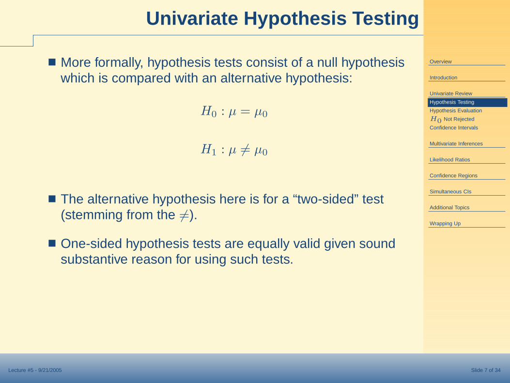
■ More formally, hypothesis tests consist of a null hypothesiswhich is compared with an alternative hypothesis:

H0 : µ = µ0

H1 : µ 6= µ0

■ The alternative hypothesis here is for a “two-sided” test(stemming from the 6=).

■ One-sided hypothesis tests are equally valid given soundsubstantive reason for using such tests.

Overview

Introduction

Univariate Review

Hypothesis Testing


H0 Not Rejected



Likelihood Ratios

Confidence Regions

Simultaneous CIs

Additional Topics

Wrapping Up

Lecture #5 - 9/21/2005 Slide 8 of 34


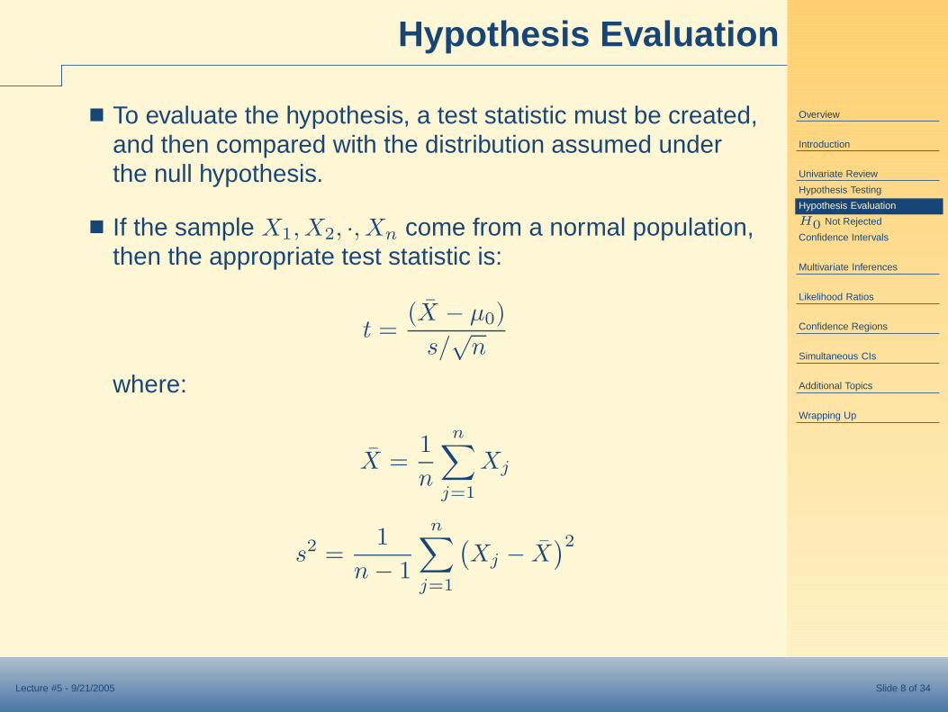
■ To evaluate the hypothesis, a test statistic must be created,and then compared with the distribution assumed underthe null hypothesis.

■ If the sample X1, X2, ·, Xn come from a normal population,then the appropriate test statistic is:

t =(X̄ − µ0)

s/√

n

where:

X̄ =1

n

n∑

j=1

Xj

s2 =1

n − 1

n∑

j=1

(

Xj − X̄)2

Overview

Introduction

Univariate Review

Hypothesis Testing


H0 Not Rejected



Likelihood Ratios

Confidence Regions

Simultaneous CIs

Additional Topics

Wrapping Up

Lecture #5 - 9/21/2005 Slide 9 of 34


■ The t statistic has a t-distribution with n − 1 degrees offreedom (df).

■ H0 is rejected if |t| is greater than a specified percentagepoint of a t-distribution with n − 1 df.

■ For instance, lets look at the values for the means of ourdata.

■ SAS Example #1...

Overview

Introduction

Univariate Review

Hypothesis Testing


H0 Not Rejected



Likelihood Ratios

Confidence Regions

Simultaneous CIs

Additional Topics

Wrapping Up

Lecture #5 - 9/21/2005 Slide 10 of 34


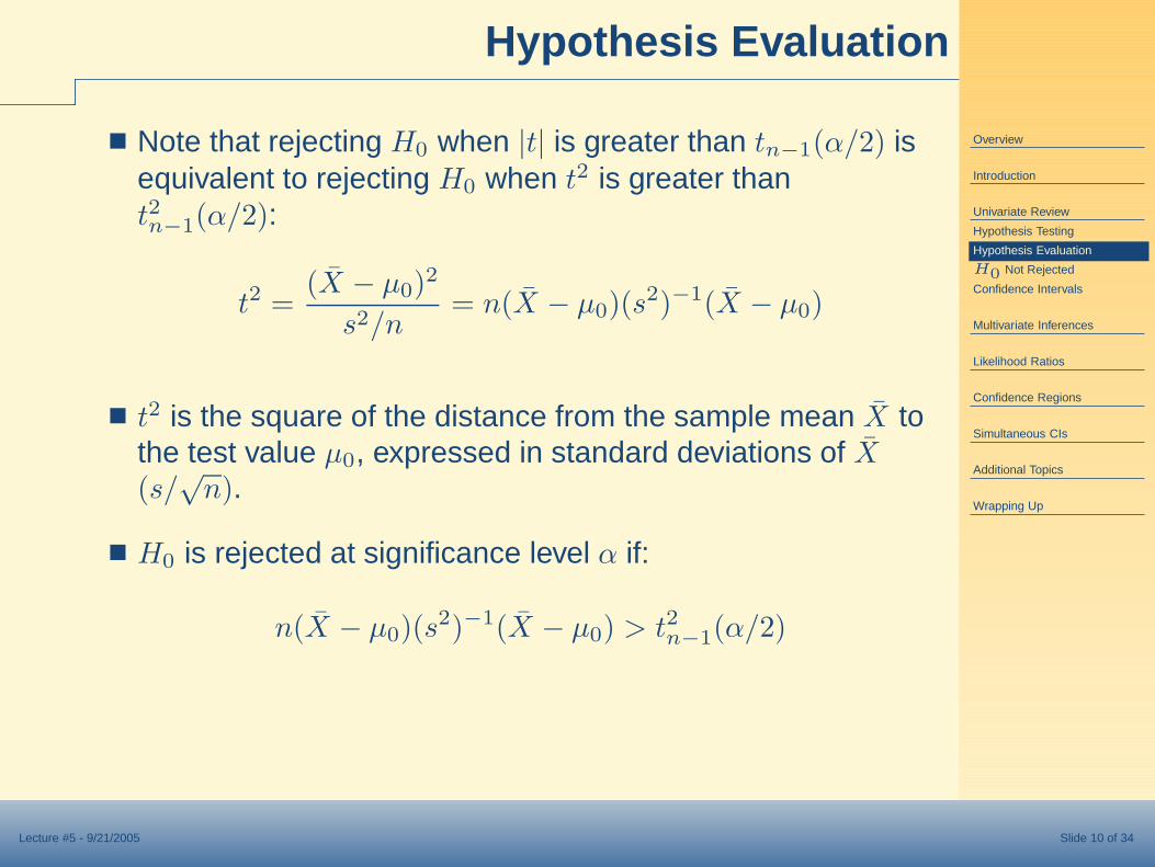
■ Note that rejecting H0 when |t| is greater than tn−1(α/2) isequivalent to rejecting H0 when t2 is greater thant2n−1(α/2):

t2 =(X̄ − µ0)

2

s2/n= n(X̄ − µ0)(s

2)−1(X̄ − µ0)

■ t2 is the square of the distance from the sample mean X̄ tothe test value µ0, expressed in standard deviations of X̄(s/

√n).

■ H0 is rejected at significance level α if:

n(X̄ − µ0)(s2)−1(X̄ − µ0) > t2n−1(α/2)

Overview

Introduction

Univariate Review

Hypothesis Testing


H0 Not Rejected



Likelihood Ratios

Confidence Regions

Simultaneous CIs

Additional Topics

Wrapping Up

Lecture #5 - 9/21/2005 Slide 11 of 34

H0 Not Rejected

■ Imagine, for instance, that for your wager you conclude thatH0 is not rejected, or that there is not enough statisticalevidence to conclude that the average height of KU gradstudents is 68 inches.

■ Does this mean that you were correct, that 68 inches is theaverage height of KU grad students?

■ Are there other values of µ that would be also beconsistent with the data?

■ Could you pick another µ0 such that you would fail to rejectH0?

Overview

Introduction

Univariate Review

Hypothesis Testing


H0 Not Rejected



Likelihood Ratios

Confidence Regions

Simultaneous CIs

Additional Topics

Wrapping Up

Lecture #5 - 9/21/2005 Slide 12 of 34


■ For the hypothesis test you just constructed, the reality isthat there could be a range of values µ where you couldnot detect differences from your sample mean.

■ This region is at the heart of the concept of confidenceintervals.

■ Recall that a confidence interval gives us a range aroundthe sample mean (X̄) where the population mean (µ) lieswith a given probability 1 − α.

■ Specifically, we say that with 100 × (1 − α)% confidencethat µ0 lies within:

x̄ ± tn−1(α/2)s√n

Overview

Introduction

Univariate Review

Hypothesis Testing


H0 Not Rejected



Likelihood Ratios

Confidence Regions

Simultaneous CIs

Additional Topics

Wrapping Up

Lecture #5 - 9/21/2005 Slide 13 of 34

Confidence Interval Example

■ In reality, what does statistical confidence translate into?

■ The statistical confidence level relays the probability thatthe mean µ falls within a specified interval.

■ This is akin to having α% of confidence intervals notcontain the true population mean.

■ Imagine you set α = 0.05, then take a set of 100 randomsamples from a population.

■ About 5 of those 100 samples would have confidenceintervals where µ is not contained in the interval.

■ In class example...

Overview

Introduction

Univariate Review


Multivariate Hypotheses

Why Multivariate?

Hotelling’s T2

MV Hypothesis Evaluation

T2 Information

Likelihood Ratios

Confidence Regions

Simultaneous CIs

Additional Topics

Wrapping Up

Lecture #5 - 9/21/2005 Slide 14 of 34


■ In univariate statistics we were concerned...

◆ ...with making hypotheses based on a single mean µ0.

◆ ...determining the location of the mean on a singleinterval.

■ Multivariate statistics, however, shift the focus from a singlemean (or single interval) to making inferences aboutmultiple means (a mean vector).

■ The problem is phrased as determining the whether a p× 1vector µ0 is a plausible value for the true mean of amultivariate distribution.

Overview

Introduction

Univariate Review



Why Multivariate?

Hotelling’s T2


T2 Information

Likelihood Ratios

Confidence Regions

Simultaneous CIs

Additional Topics

Wrapping Up

Lecture #5 - 9/21/2005 Slide 15 of 34

A Wager, Part II

■ Imagine, for instance, that you had a feeling that:

◆ The average height of KU grad students was 68 inches.

-and-

◆ The average distance from the elbow to the wrist for KUgrad students was 10 inches.

■ Your other friend, another contrarian, thinks otherwise andmakes you a bet that the average height of graduatestudents is not 68 inches and that the average forearmdistance is not 10 inches.

■ You collect data on a both variables.

■ How can you tell who wins the bet?

Overview

Introduction

Univariate Review



Why Multivariate?

Hotelling’s T2


T2 Information

Likelihood Ratios

Confidence Regions

Simultaneous CIs

Additional Topics

Wrapping Up

Lecture #5 - 9/21/2005 Slide 16 of 34


■ As with the univariate analog of the wager, a multivariatehypothesis test can be constructed.

■ In multivariate, however, each hypothesis would bephrased in terms of mean vectors rather than a singlemean value (scalar) as was done with univariate statistics:

H0 : µ = µ0

H1 : µ 6= µ0

■ Or, phrased in terms of your wager:

H0 : µ =

[

68

10

]

H1 : µ 6=[

68

10

]

Overview

Introduction

Univariate Review



Why Multivariate?

Hotelling’s T2


T2 Information

Likelihood Ratios

Confidence Regions

Simultaneous CIs

Additional Topics

Wrapping Up

Lecture #5 - 9/21/2005 Slide 17 of 34

Why Use Multivariate?

But why would we want to do use a multivariate test for amean when we already know how to test each variableindividually

■ Controls for Type I error

■ Univariate tests ignore associations between the variables(i.e., ignore the multivariate structure).

■ Multivariate tests can be more powerful (i.e. there may becases where each univariate test would not be significant,BUT the multivariate test is).

■ Multivariate tests can reveal more about the variables (i.e.,provide insight about why we rejected H0).

Overview

Introduction

Univariate Review



Why Multivariate?

Hotelling’s T2


T2 Information

Likelihood Ratios

Confidence Regions

Simultaneous CIs

Additional Topics

Wrapping Up

Lecture #5 - 9/21/2005 Slide 18 of 34

Hotelling’s T2

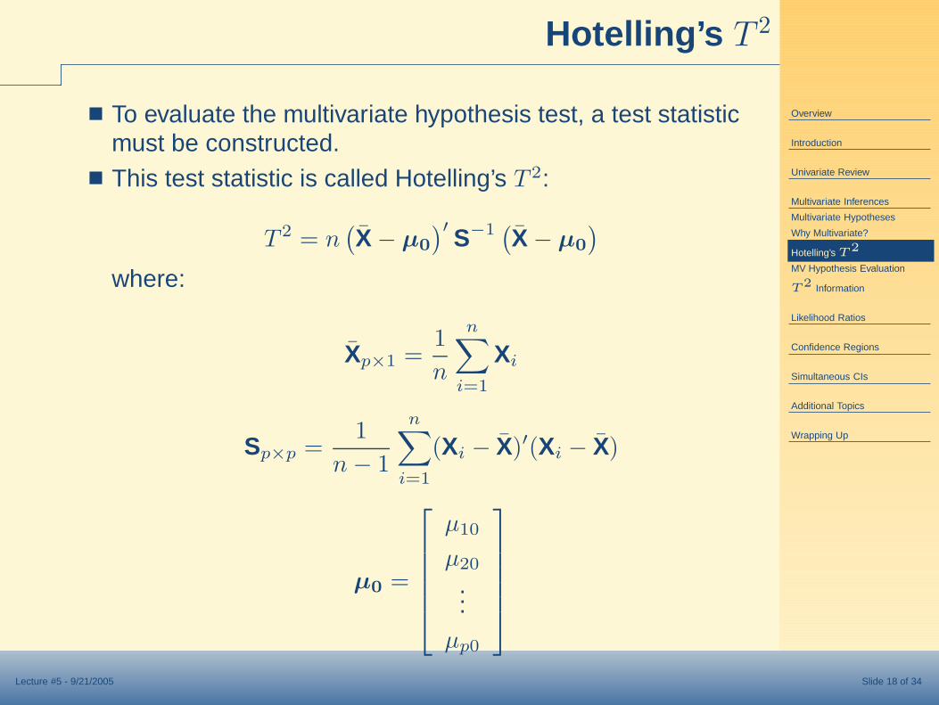
■ To evaluate the multivariate hypothesis test, a test statisticmust be constructed.

■ This test statistic is called Hotelling’s T 2:

T 2 = n(

X̄ − µ0

)′S−1 (X̄ − µ0

)

where:

X̄p×1 =1

n

n∑

i=1

Xi

Sp×p =1

n − 1

n∑

i=1

(Xi − X̄)′(Xi − X̄)

µ0 =

µ10

µ20

...µp0

Overview

Introduction

Univariate Review



Why Multivariate?

Hotelling’s T2


T2 Information

Likelihood Ratios

Confidence Regions

Simultaneous CIs

Additional Topics

Wrapping Up

Lecture #5 - 9/21/2005 Slide 19 of 34

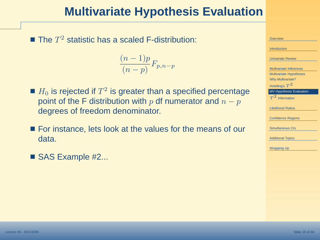
Multivariate Hypothesis Evaluation

■ The T 2 statistic has a scaled F-distribution:

(n − 1)p

(n − p)Fp,n−p

■ H0 is rejected if T 2 is greater than a specified percentagepoint of the F distribution with p df numerator and n − pdegrees of freedom denominator.

■ For instance, lets look at the values for the means of ourdata.


Overview

Introduction

Univariate Review



Why Multivariate?

Hotelling’s T2


T2 Information

Likelihood Ratios

Confidence Regions

Simultaneous CIs

Additional Topics

Wrapping Up

Lecture #5 - 9/21/2005 Slide 20 of 34

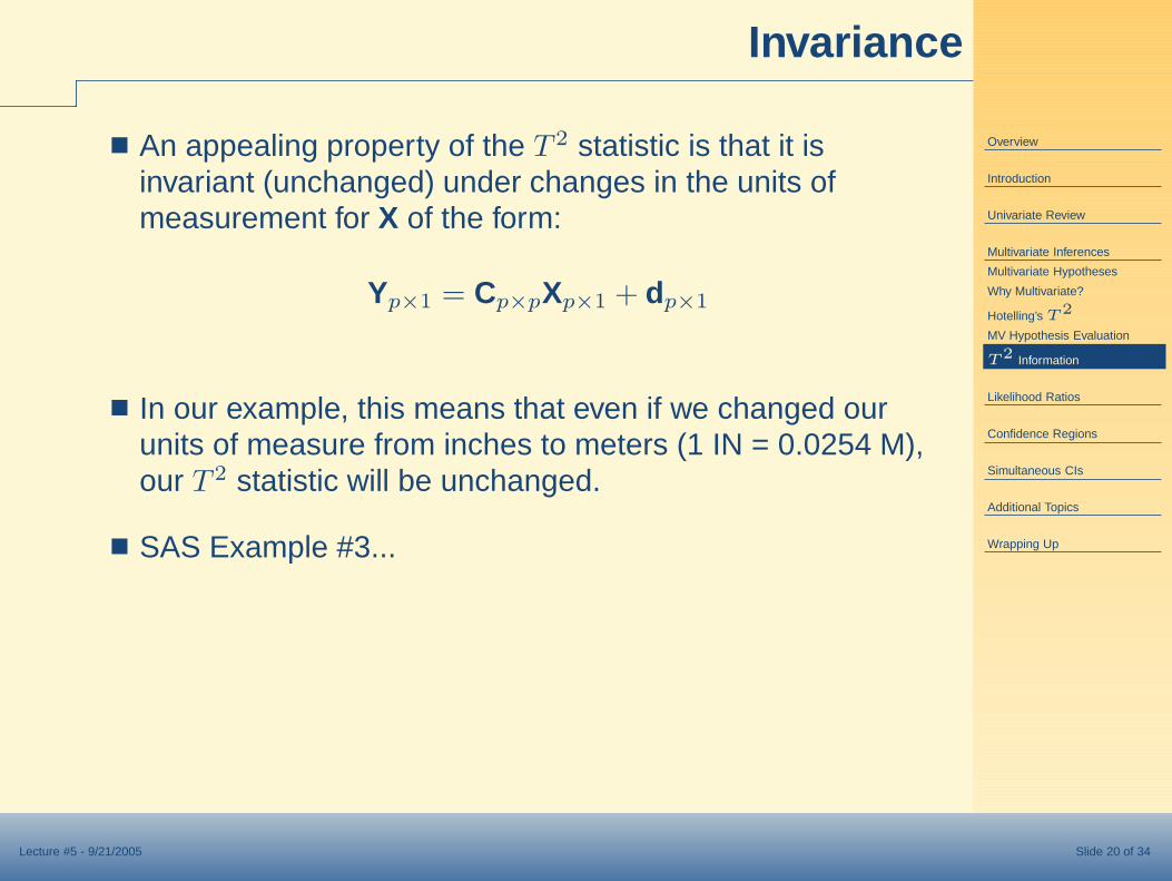
Invariance

■ An appealing property of the T 2 statistic is that it isinvariant (unchanged) under changes in the units ofmeasurement for X of the form:

Yp×1 = Cp×pXp×1 + dp×1

■ In our example, this means that even if we changed ourunits of measure from inches to meters (1 IN = 0.0254 M),our T 2 statistic will be unchanged.


Overview

Introduction

Univariate Review


Likelihood Ratios

T2 LR

Confidence Regions

Simultaneous CIs

Additional Topics

Wrapping Up

Lecture #5 - 9/21/2005 Slide 21 of 34

Likelihood Ratios

Note: This section is developed only for purposes of introducing new statistical terminology.

■ A common method for conducting hypothesis tests inmultivariate statistics is by use of likelihood ratios.

■ A likelihood ratio is formed by comparing the likelihood ofthe data under the the null hypothesis with the likelihood ofthe data overall.

■ For large samples (with frequently used distributions), LRtests have some very appealing statistical properties(known distributions, most powerful tests).

■ The hypothesis test for the multivariate mean vector can beexpressed in terms of a likelihood ratio.

■ As we generalize from a mean vector to multiple meanvectors (think going from t-tests to ANOVA), LR tests willbecome our predominant way of evaluating multivariatehypotheses.

Overview

Introduction

Univariate Review


Likelihood Ratios

T2 LR

Confidence Regions

Simultaneous CIs

Additional Topics

Wrapping Up

Lecture #5 - 9/21/2005 Slide 22 of 34

Likelihood Ratios

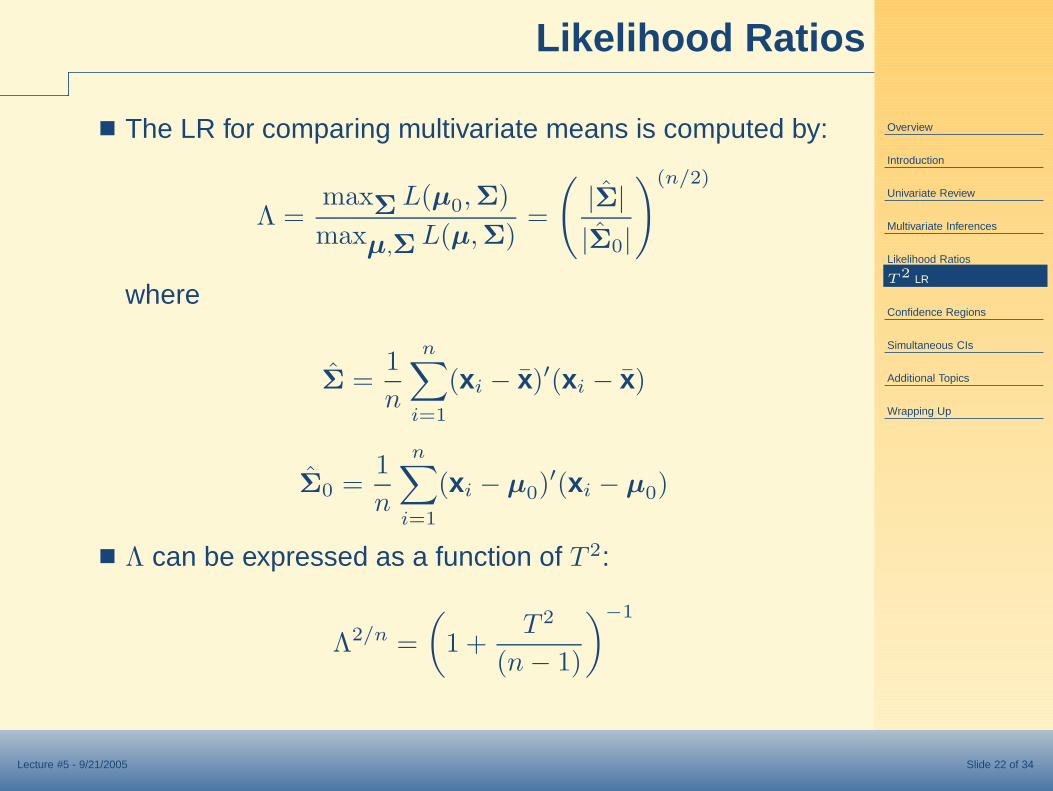
■ The LR for comparing multivariate means is computed by:

Λ =maxΣ L(µ0,Σ)

maxµ,Σ L(µ,Σ)

=

(

|Σ̂||Σ̂0|

)(n/2)

where

Σ̂ =1

n

n∑

i=1

(xi − x̄)′(xi − x̄)

Σ̂0 =1

n

n∑

i=1

(xi − µ0)′(xi − µ0)

■ Λ can be expressed as a function of T 2:

Λ2/n =

(

1 +T 2

(n − 1)

)−1

Overview

Introduction

Univariate Review


Likelihood Ratios

T2 LR

Confidence Regions

Simultaneous CIs

Additional Topics

Wrapping Up

Lecture #5 - 9/21/2005 Slide 23 of 34

Likelihood Ratios

■ Typically, when the sample size is large, the distribution ofa function Λ (−2 lnΛ) under the null hypothesis isapproximately χ2 where the degrees of freedom arereflected by the dimensionality of the hypotheses understudy.

■ −2 lnΛ is something you may get used to seeing whenusing multivariate statistics.

Overview

Introduction

Univariate Review


Likelihood Ratios

Confidence Regions

Building CRs

Simultaneous CIs

Additional Topics

Wrapping Up

Lecture #5 - 9/21/2005 Slide 24 of 34

Confidence Regions

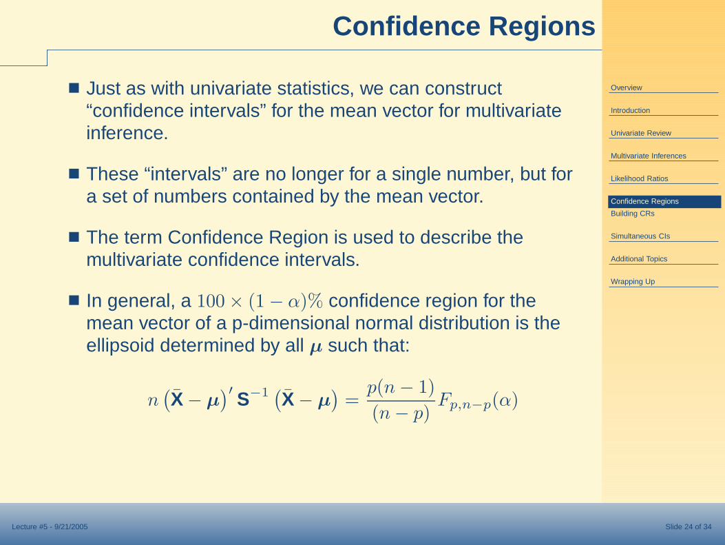
■ Just as with univariate statistics, we can construct“confidence intervals” for the mean vector for multivariateinference.

■ These “intervals” are no longer for a single number, but fora set of numbers contained by the mean vector.

■ The term Confidence Region is used to describe themultivariate confidence intervals.

■ In general, a 100 × (1 − α)% confidence region for themean vector of a p-dimensional normal distribution is theellipsoid determined by all µ such that:

n(

X̄ − µ)′

S−1 (X̄ − µ)

=p(n − 1)

(n − p)Fp,n−p(α)

Overview

Introduction

Univariate Review


Likelihood Ratios

Confidence Regions

Building CRs

Simultaneous CIs

Additional Topics

Wrapping Up

Lecture #5 - 9/21/2005 Slide 25 of 34

Building CRs - Population

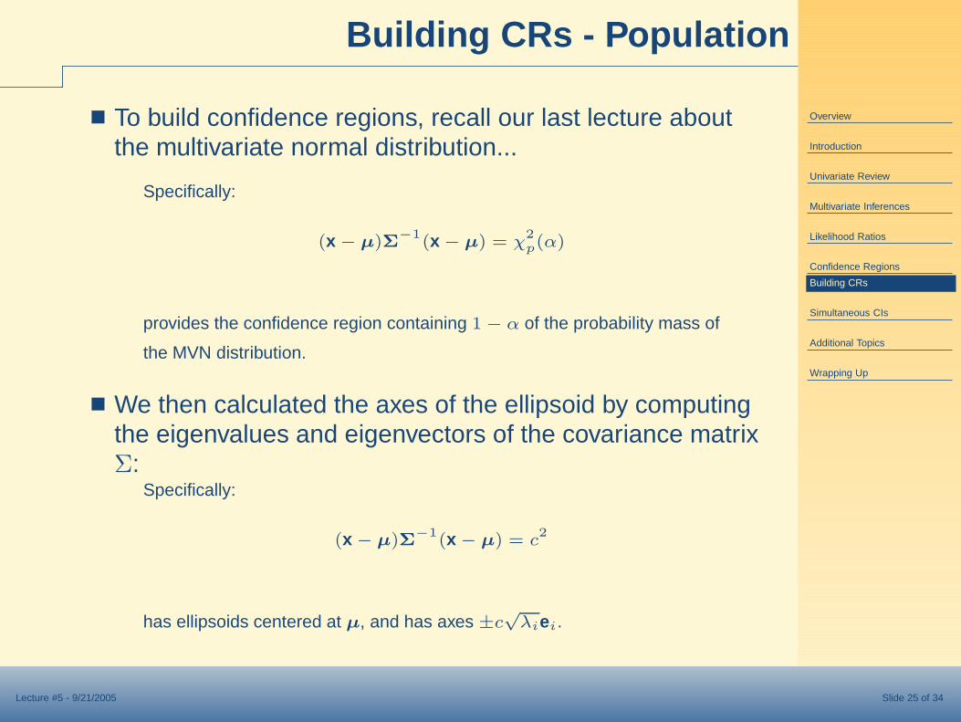
■ To build confidence regions, recall our last lecture aboutthe multivariate normal distribution...

Specifically:

(x − µ)Σ−1

(x − µ) = χ2

p(α)

provides the confidence region containing 1 − α of the probability mass of

the MVN distribution.

■ We then calculated the axes of the ellipsoid by computingthe eigenvalues and eigenvectors of the covariance matrixΣ:

Specifically:

(x − µ)Σ−1(x − µ) = c2

has ellipsoids centered at µ, and has axes ±c√

λiei.

Overview

Introduction

Univariate Review


Likelihood Ratios

Confidence Regions

Building CRs

Simultaneous CIs

Additional Topics

Wrapping Up

Lecture #5 - 9/21/2005 Slide 26 of 34

Building CRs - Sample

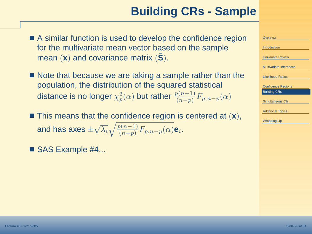
■ A similar function is used to develop the confidence regionfor the multivariate mean vector based on the samplemean (x̄) and covariance matrix (S̄).

■ Note that because we are taking a sample rather than thepopulation, the distribution of the squared statisticaldistance is no longer χ2

p(α) but rather p(n−1)(n−p) Fp,n−p(α)

■ This means that the confidence region is centered at (x̄),

and has axes ±√

λi

√

p(n−1)(n−p) Fp,n−p(α)ei.


Overview

Introduction

Univariate Review


Likelihood Ratios

Confidence Regions

Simultaneous CIs

Additional Topics

Wrapping Up

Lecture #5 - 9/21/2005 Slide 27 of 34

Simultaneous CIs

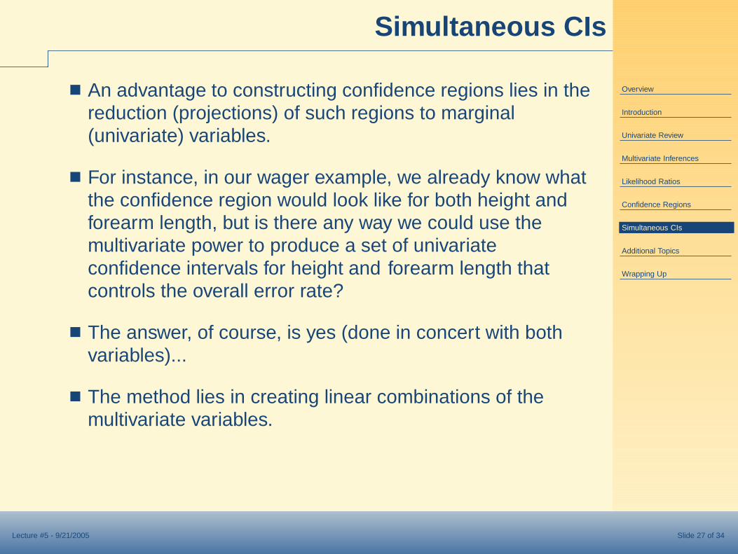
■ An advantage to constructing confidence regions lies in thereduction (projections) of such regions to marginal(univariate) variables.

■ For instance, in our wager example, we already know whatthe confidence region would look like for both height andforearm length, but is there any way we could use themultivariate power to produce a set of univariateconfidence intervals for height and forearm length thatcontrols the overall error rate?

■ The answer, of course, is yes (done in concert with bothvariables)...

■ The method lies in creating linear combinations of themultivariate variables.

Overview

Introduction

Univariate Review


Likelihood Ratios

Confidence Regions

Simultaneous CIs

Additional Topics

Wrapping Up

Lecture #5 - 9/21/2005 Slide 28 of 34

Simultaneous CIs

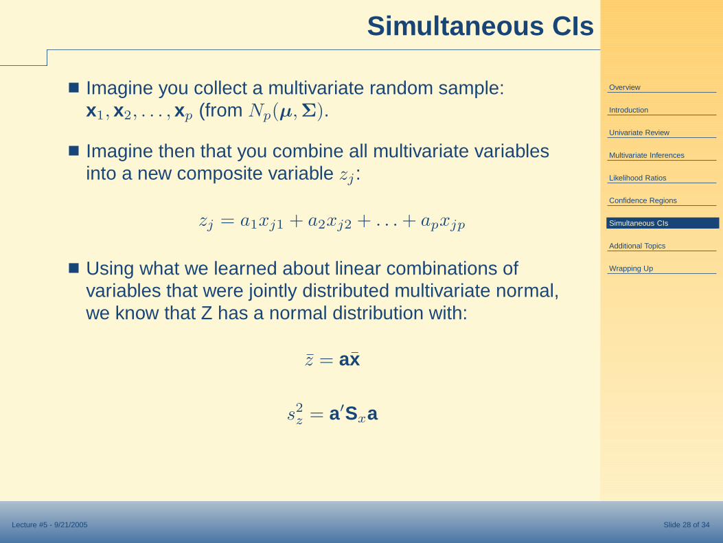
■ Imagine you collect a multivariate random sample:x1, x2, . . . , xp (from Np(µ,Σ).

■ Imagine then that you combine all multivariate variablesinto a new composite variable zj :

zj = a1xj1 + a2xj2 + . . . + apxjp

■ Using what we learned about linear combinations ofvariables that were jointly distributed multivariate normal,we know that Z has a normal distribution with:

z̄ = ax̄

s2z = a′Sxa

Overview

Introduction

Univariate Review


Likelihood Ratios

Confidence Regions

Simultaneous CIs

Additional Topics

Wrapping Up

Lecture #5 - 9/21/2005 Slide 29 of 34

Simultaneous CIs

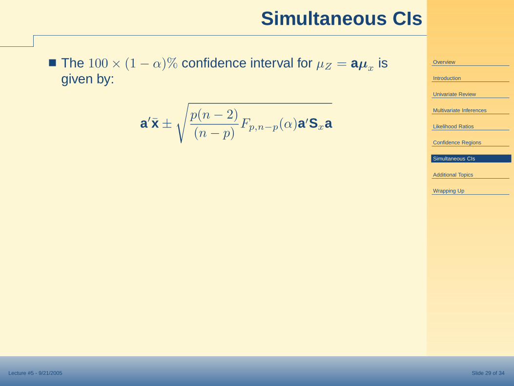
■ The 100 × (1 − α)% confidence interval for µZ = aµx isgiven by:

a′x̄ ±√

p(n − 2)

(n − p)Fp,n−p(α)a′Sxa

Overview

Introduction

Univariate Review


Likelihood Ratios

Confidence Regions

Simultaneous CIs

Additional Topics

Wrapping Up

Lecture #5 - 9/21/2005 Slide 30 of 34

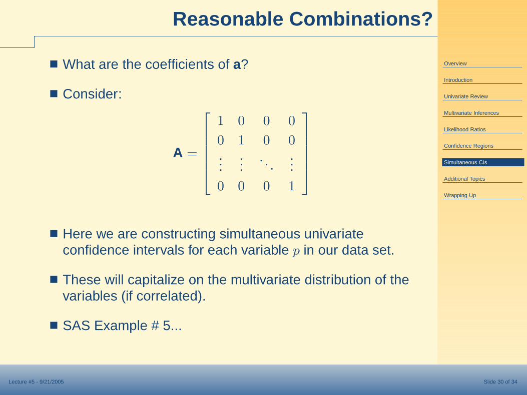
Reasonable Combinations?

■ What are the coefficients of a?

■ Consider:

A =

1 0 0 0

0 1 0 0...

.... . .

...0 0 0 1

■ Here we are constructing simultaneous univariateconfidence intervals for each variable p in our data set.

■ These will capitalize on the multivariate distribution of thevariables (if correlated).

■ SAS Example # 5...

Overview

Introduction

Univariate Review


Likelihood Ratios

Confidence Regions

Simultaneous CIs

Additional Topics

Large Samples

Additional Topics

Wrapping Up

Lecture #5 - 9/21/2005 Slide 31 of 34

Large Sample Inferences

■ Recall that the t statistic approaches normality as n getslarge.

■ Similarly, as n gets large, the distribution of T 2

approximates the χ2 formulated by the exponent of themultivariate normal distribution.

■ Practically speaking, the formula for the value of F willapproximate the χ2 distribution value, although you canchange the critical value if you feel the need to.

■ For more information see Section 5.5.

Overview

Introduction

Univariate Review


Likelihood Ratios

Confidence Regions

Simultaneous CIs

Additional Topics

Large Samples

Additional Topics

Wrapping Up

Lecture #5 - 9/21/2005 Slide 32 of 34

Additional Topics

■ Multivariate quality control charts are discussed in Section5.6.

◆ The methods used to inspect such charts are based onT 2 and linear combinations of data.

■ Inferences about the mean vector when someobservations are missing are discussed in Section 5.7.

◆ This discussion quickly moves past the scope of thiscourse, and for purposes of practicality, I am omitting itfrom lecture.

■ Corrections for serially correlated observations arediscussed in Section 5.8.

Overview

Introduction

Univariate Review


Likelihood Ratios

Confidence Regions

Simultaneous CIs

Additional Topics

Wrapping Up

Final Thought

Next Class

Lecture #5 - 9/21/2005 Slide 33 of 34

Final Thought

■ We have begun ourdiscussion of multivariateinferential statistics withmethods analogous to theunivariate t-test.

■ Today we only discussedtesting the mean vectorversus some stablequantity.

■ As we move forward, recall how your univariate coursesmoved from t-tests to ANOVA.

■ Such transitions will become apparent in the next twoweeks.

Overview

Introduction

Univariate Review


Likelihood Ratios

Confidence Regions

Simultaneous CIs

Additional Topics

Wrapping Up

Final Thought

Next Class

Lecture #5 - 9/21/2005 Slide 34 of 34

Next Time

■ Inferences for Multiple Mean Vectors.

◆ Paired comparisons.

◆ MANOVA.

◆ Profile analysis.

◆ Growth Curves.

■ More simultaneous confidence intervals.

Documents

Mean Vector Inferences - Jonathan Templin's Website · Additional Topics Wrapping Up Lecture #5 - 9/21/2005 Slide 2 of 34 Today’s Lecture Inferences about a Mean Vector (Chapter