Embed Size (px)
Citation preview
1
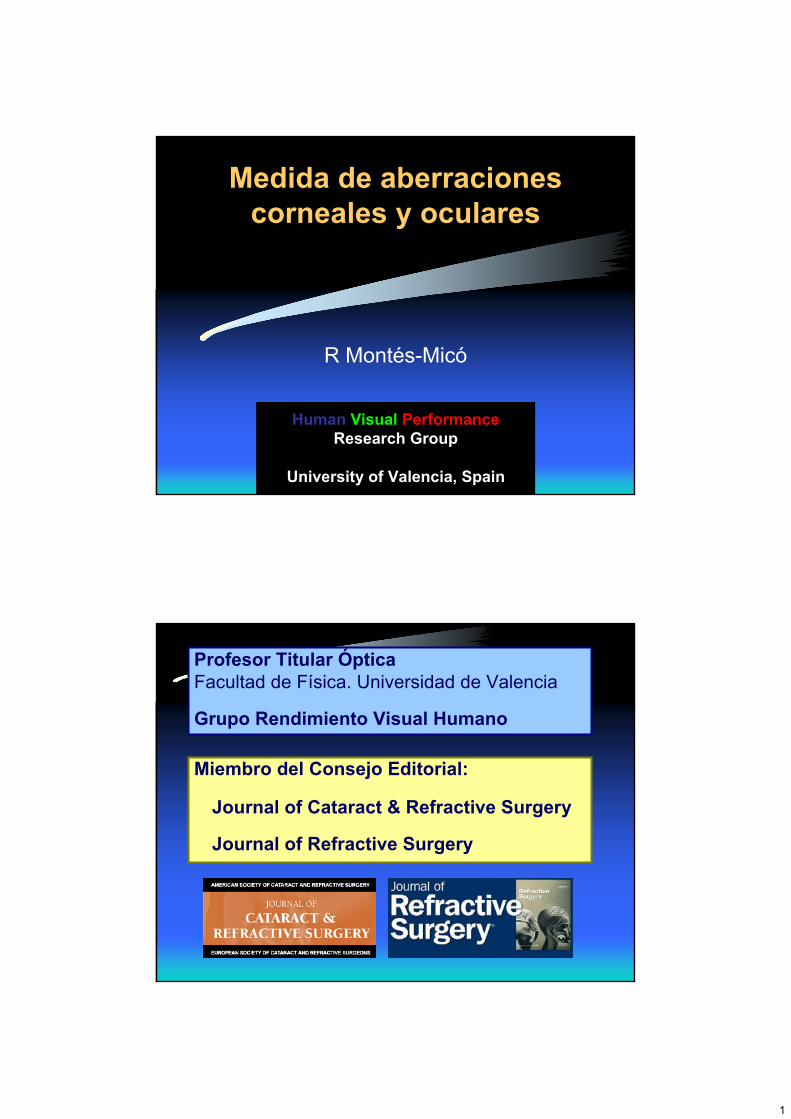
Medida de aberracionescorneales y oculares
R Montés-Micó
Human Visual PerformanceResearch Group
University of Valencia, Spain
Profesor Titular ÓpticaFacultad de Física. Universidad de Valencia
Grupo Rendimiento Visual Humano
Miembro del Consejo Editorial:
Journal of Cataract & Refractive Surgery
Journal of Refractive Surgery
2
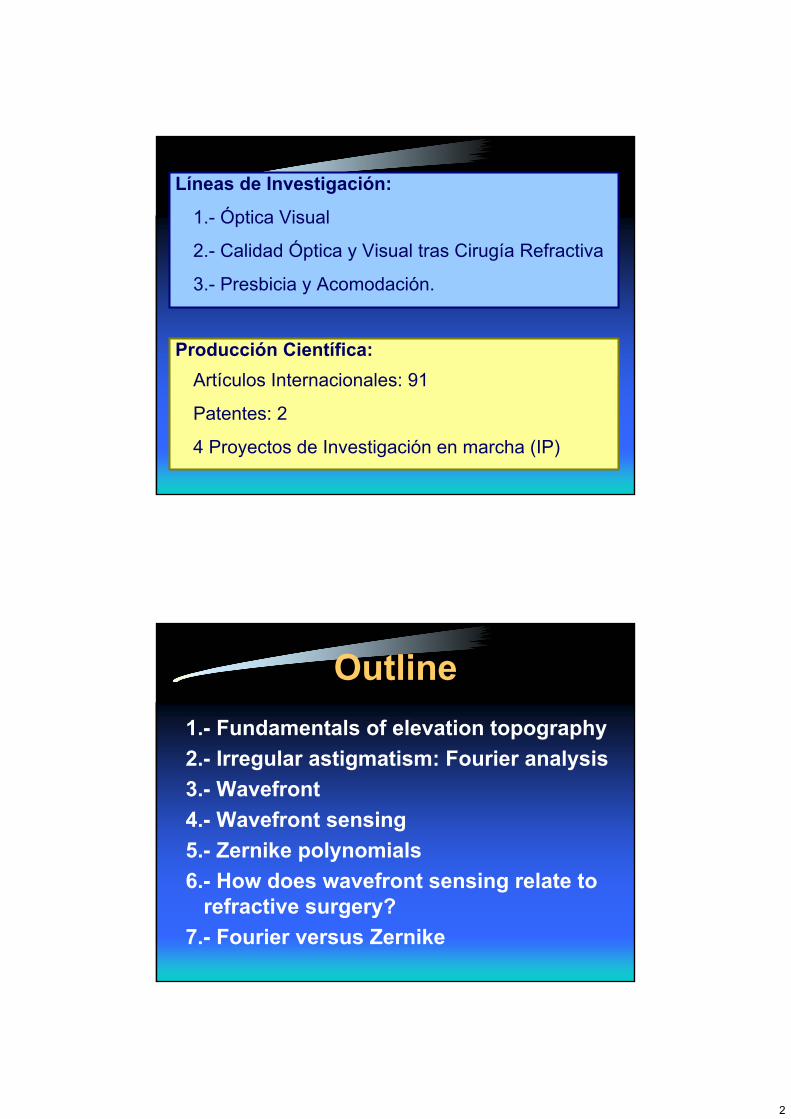
Líneas de Investigación:
1.- Óptica Visual
2.- Calidad Óptica y Visual tras Cirugía Refractiva
3.- Presbicia y Acomodación.
Producción Científica:Artículos Internacionales: 91
Patentes: 2
4 Proyectos de Investigación en marcha (IP)
Outline1.- Fundamentals of elevation topography2.- Irregular astigmatism: Fourier analysis3.- Wavefront4.- Wavefront sensing5.- Zernike polynomials6.- How does wavefront sensing relate to
refractive surgery?7.- Fourier versus Zernike
3
1.- FUNDAMENTALS OF ELEVATION MAP
TOPOGRAPHY
Two Types
• General: Placido Disc
• Orbscan/Pentacam
4
ORBSCAN: MAIN FEATURES
• Accurate elevation andcurvature information
• Anterior and posterior cornea surface’s
• Full cornea thickness
OPTICAL ADQUISITION HEAD
• Scans the eye using light slits that are projected at a 45-degree angle.
• 40 slits in total.• Processing and construction of
elevation maps of the anterior & posterior cornea.
• Pachimetry: Diferences in elevationbetween the anterior and posterior surface
5
HOW THE INFORMATION DIFFERS TO PLACIDO
BASED SYSTEMS?
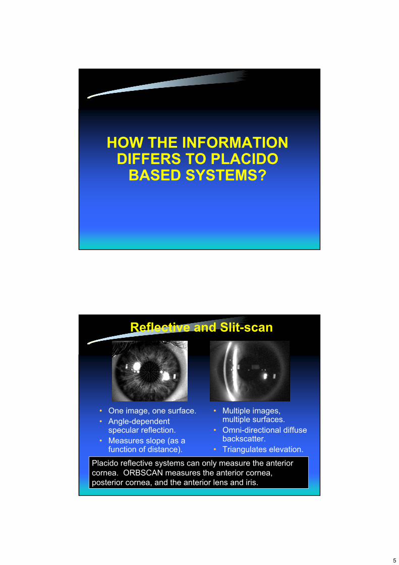
Reflective and Slit-scan
• One image, one surface.• Angle-dependent
specular reflection.• Measures slope (as a
function of distance).
• Multiple images, multiple surfaces.
• Omni-directional diffuse backscatter.
• Triangulates elevation.
Placido reflective systems can only measure the anterior cornea. ORBSCAN measures the anterior cornea, posterior cornea, and the anterior lens and iris.
6
Hybrid Technology of ORBSCAN
3. Unify triangulated and reflective data to obtain accurate surfaces in elevation, slope, and curvature.
1. Measure surface elevation directly by triangulation of backscatteredslit-beam.
2. Measure surface slope directly using specular reflection, supplemented with triangulated elevation.
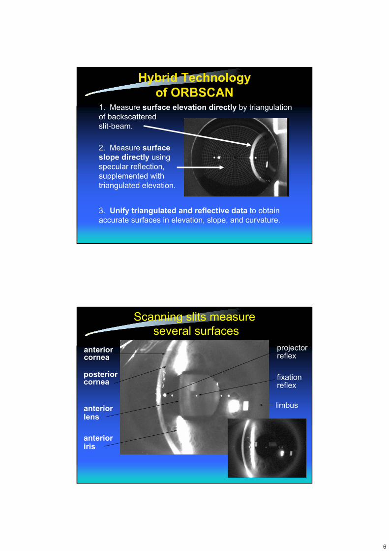
anteriorcornea
anteriorlens
limbus
anterioriris
posteriorcornea fixation
reflex
projectorreflex
Scanning slits measureseveral surfaces
7
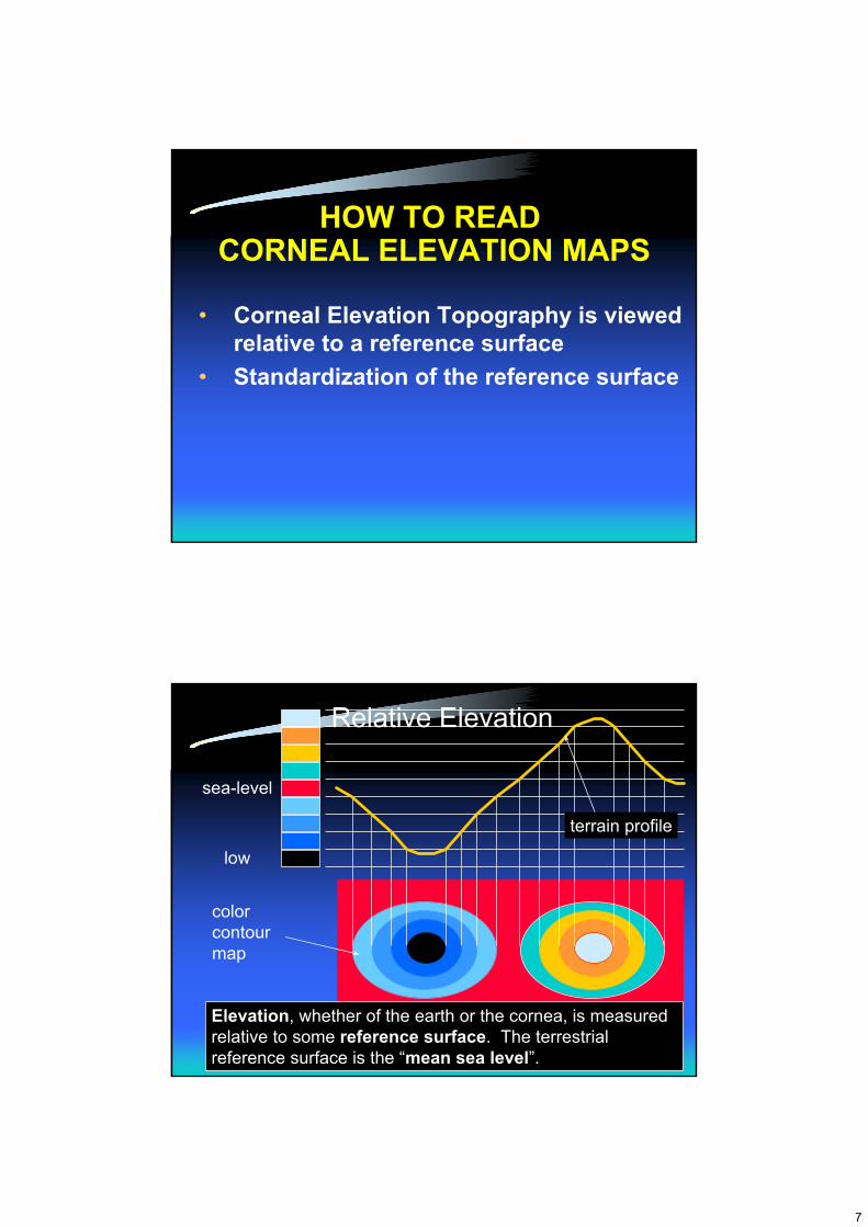
HOW TO READCORNEAL ELEVATION MAPS
• Corneal Elevation Topography is viewed relative to a reference surface
• Standardization of the reference surface
high
sea-level
low
color contour map
terrain profile
Elevation, whether of the earth or the cornea, is measured relative to some reference surface. The terrestrial reference surface is the “mean sea level”.
Relative Elevation
8
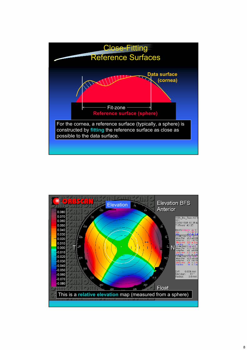
Close-Fitting Reference Surfaces
For the cornea, a reference surface (typically, a sphere) is constructed by fitting the reference surface as close as possible to the data surface.
Fit-zoneReference surface (sphere)
Data surface(cornea)
Astigmatism: Elevation (sphere) Map
This is a relative elevation map (measured from a sphere)
Elevation
9
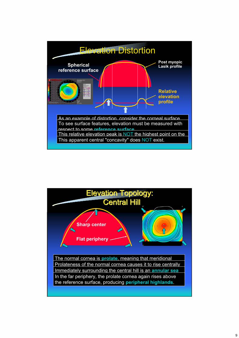
Elevation DistortionSpherical
reference surface
Post myopic Lasik profile
As an example of distortion, consider the corneal surface following myopic lasik correction. It is centrally flattened bythe surgery.To see surface features, elevation must be measured with respect to some reference surface.This relative elevation peak is NOT the highest point on the cornea.This apparent central "concavity" does NOT exist.
Relative elevation profile
Elevation Topology:Elevation Topology:Central HillCentral Hill
The normal cornea is prolate, meaning that meridionalcurvature decreases from center to periphery.Prolateness of the normal cornea causes it to rise centrally above the reference sphere. The result is a central hill.
Sharp center
Flat periphery
Immediately surrounding the central hill is an annular seawhere the cornea dips below the reference surface.In the far periphery, the prolate cornea again rises above the reference surface, producing peripheral highlands.
10
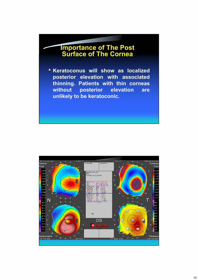
Importance of The Post Surface of The Cornea
• Keratoconus will show as localized posterior elevation with associated thinning. Patients with thin corneas without posterior elevation are unlikely to be keratoconic.
11
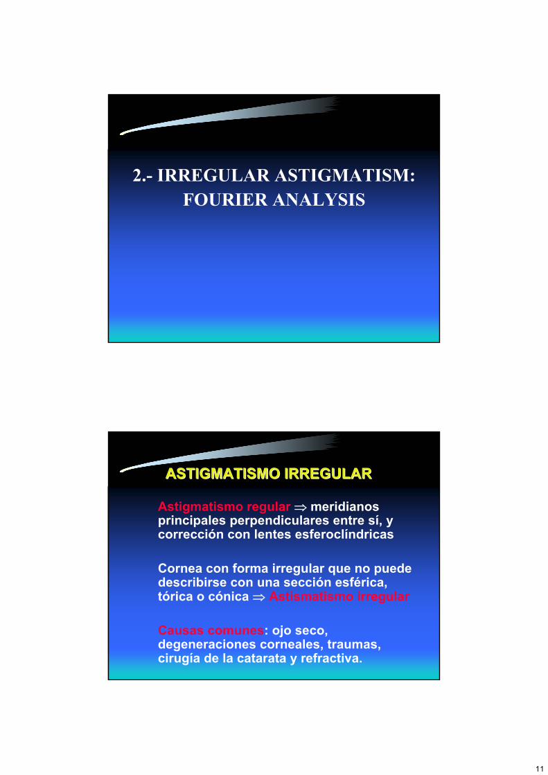
2.- IRREGULAR ASTIGMATISM: FOURIER ANALYSIS
Astigmatismo regular ⇒ meridianosprincipales perpendiculares entre sí, y corrección con lentes esferoclíndricas
Cornea con forma irregular que no puededescribirse con una sección esférica, tórica o cónica ⇒ Astismatismo irregular
Causas comunes: ojo seco, degeneraciones corneales, traumas, cirugía de la catarata y refractiva.
ASTIGMATISMO IRREGULARASTIGMATISMO IRREGULAR
12
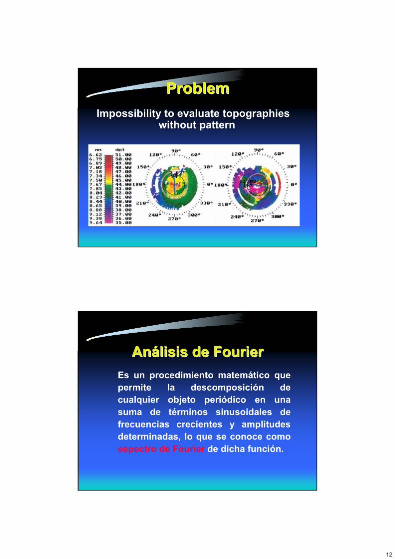
Impossibility to evaluate topographieswithout pattern
ProblemProblem
Es un procedimiento matemático que permite la descomposición de cualquier objeto periódico en una suma de términos sinusoidales de frecuencias crecientes y amplitudes determinadas, lo que se conoce como espectro de Fourier de dicha función.
AnAnáálisis de lisis de FourierFourier
13
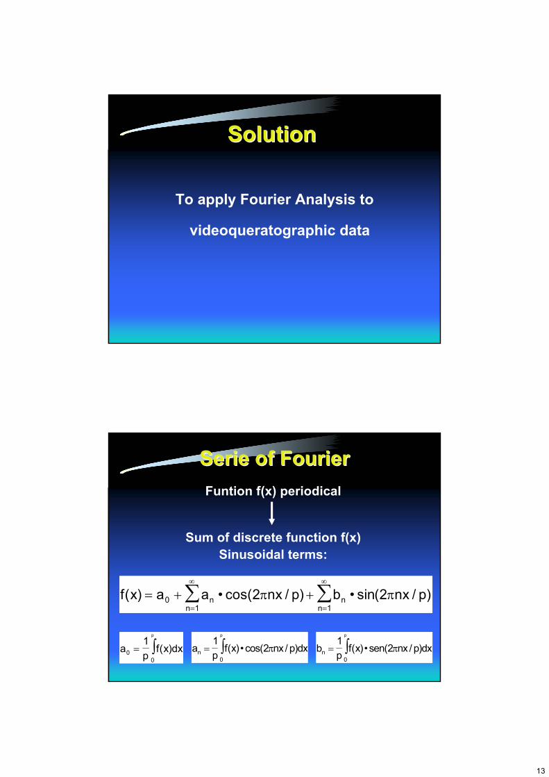
To apply Fourier Analysis to
videoqueratographic data
SolutionSolution
Funtion f(x) periodical
Sum of discrete function f(x) Sinusoidal terms:
Serie Serie ofof FourierFourier
f x a a nx p b sin nx pnn
nn
( ) • cos( / ) • ( / )= + +=
∞
=
∞
∑ ∑01 1
2 2π π
ap
f x dxp
00
1= ∫ ( ) a
pf x nx p dxn
p
= ∫12
0( )• cos( / )π b
pf x nx p dxn
p
= ∫12
0( )• sen( / )π
14
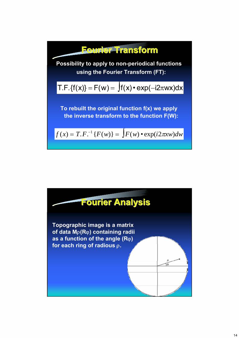
Possibility to apply to non-periodical functionsusing the Fourier Transform (FT):
To rebuilt the original function f(x) we applythe inverse transform to the function F(W):
FourierFourier TransformTransform
T F f x F w f x i wx dx. .{ ( )} ( ) ( ) • exp( )= = −∫ 2π
f x T F F w F w i xw dw( ) . . { ( )} ( ) • exp( )= =− ∫1 2π
FourierFourier AnalysisAnalysis
Topographic image is a matrixof data Mρ(Rϕ) containing radiias a function of the angle (Rϕ)for each ring of radious ρ.
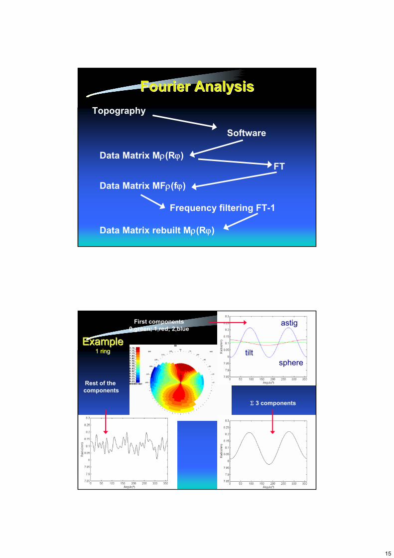
15
Topography
Software
Data Matrix Mρ(Rϕ)FT
Data Matrix MFρ(fϕ)
Frequency filtering FT-1
Data Matrix rebuilt Mρ(Rϕ)
FourierFourier AnalysisAnalysis
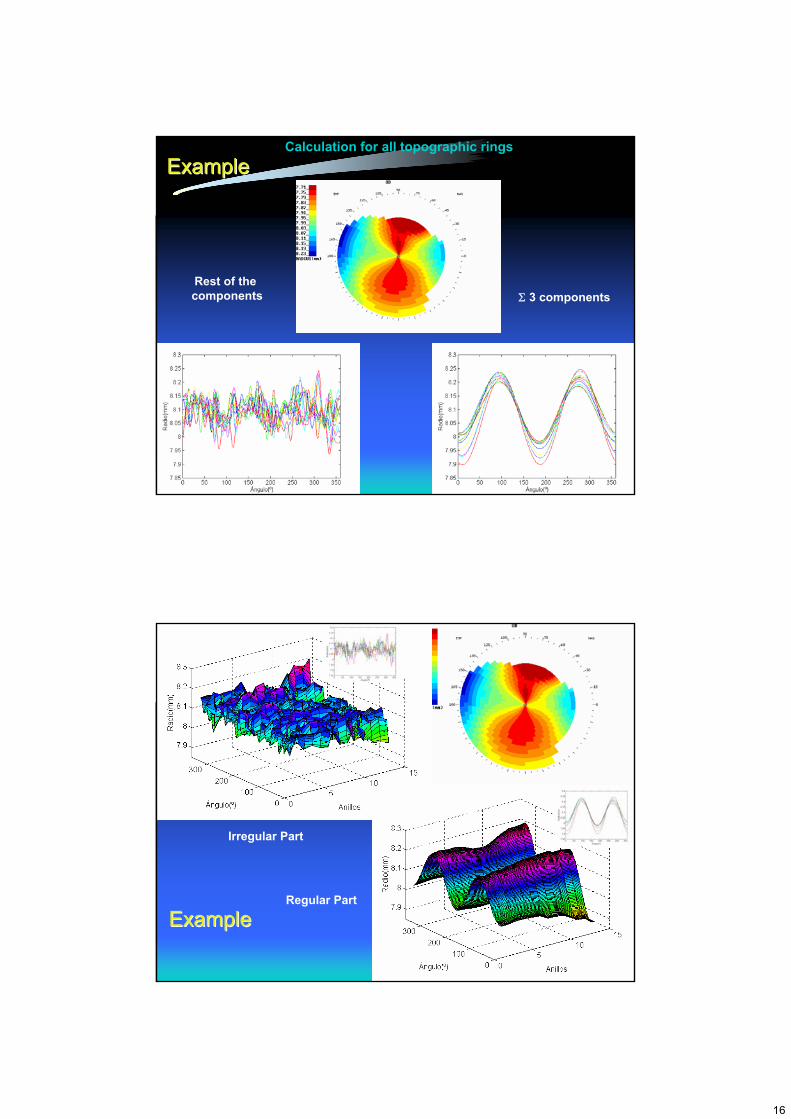
ExampleExample1 1 ringring
First components0,green; 1,red; 2,blue
Σ 3 components
Rest of thecomponents
spheretilt
astig
16
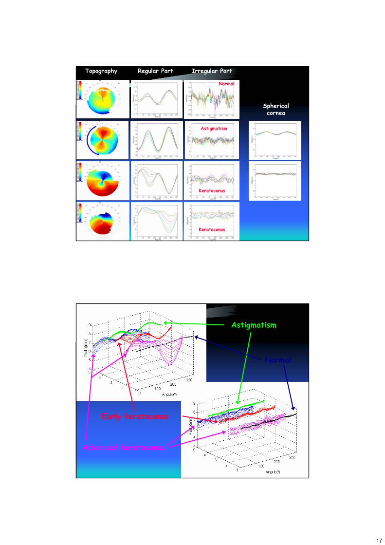
ExampleExampleCalculation for all topographic rings
Σ 3 componentsRest of thecomponents
ExampleExampleRegular Part
Irregular Part
17
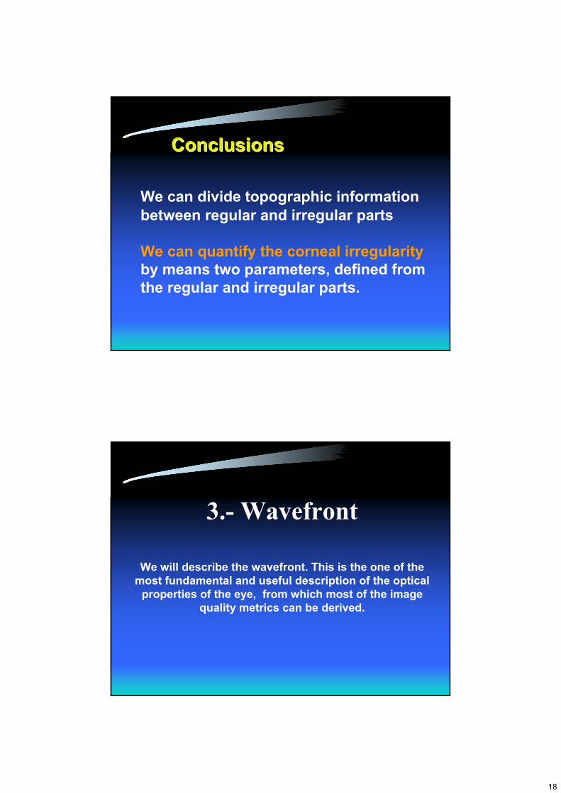
Irregular PartRegular PartTopography
Sphericalcornea
Keratoconus
Keratoconus
Normal
Astigmatism
Normal
Advanced keratoconus
Early keratoconus
Astigmatism
18
We can divide topographic informationbetween regular and irregular parts
We can quantify the corneal irregularityby means two parameters, defined fromthe regular and irregular parts.
ConclusionsConclusions
3.- Wavefront
We will describe the wavefront. This is the one of the most fundamental and useful description of the optical
properties of the eye, from which most of the image quality metrics can be derived.
19
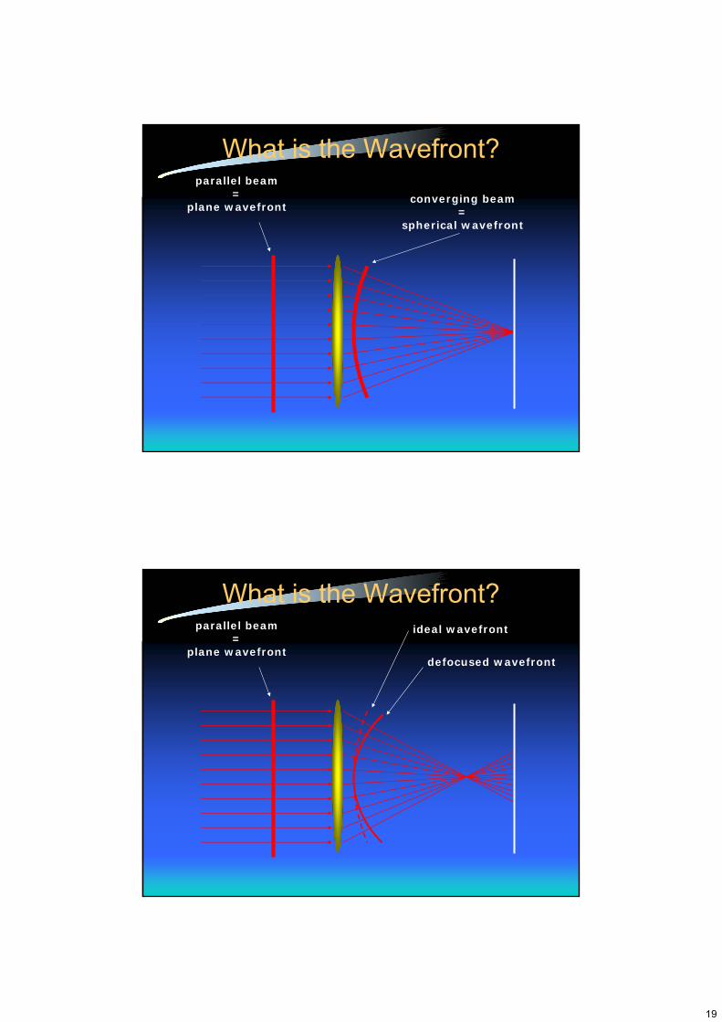
What is the Wavefront?
converging beam=
spherical wavefront
parallel beam=
plane wavefront
What is the Wavefront?ideal wavefrontparallel beam
=plane wavefront
defocused wavefront
20
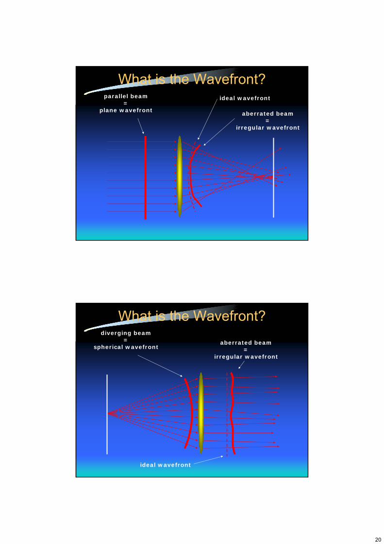
What is the Wavefront?parallel beam
=plane wavefront aberrated beam
=irregular wavefront
ideal wavefront
What is the Wavefront?
aberrated beam=
irregular wavefront
diverging beam=
spherical wavefront
ideal wavefront
21
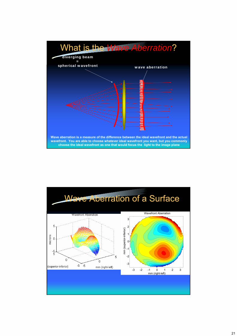
What is the Wave Aberration?diverging beam
=spherical wavefront wave aberration
Wave aberration is a measure of the difference between the ideal wavefront and the actual wavefront. You are able to choose whatever ideal wavefront you want, but you commonly
choose the ideal wavefront as one that would focus the light to the image plane
-3 -2 -1 0 1 2 3
-3
-2
-1
0
1
2
3
Wavefront Aberration
mm (right-left)
mm
(sup
erio
r-inf
erio
r)
Wave Aberration of a Surface
22
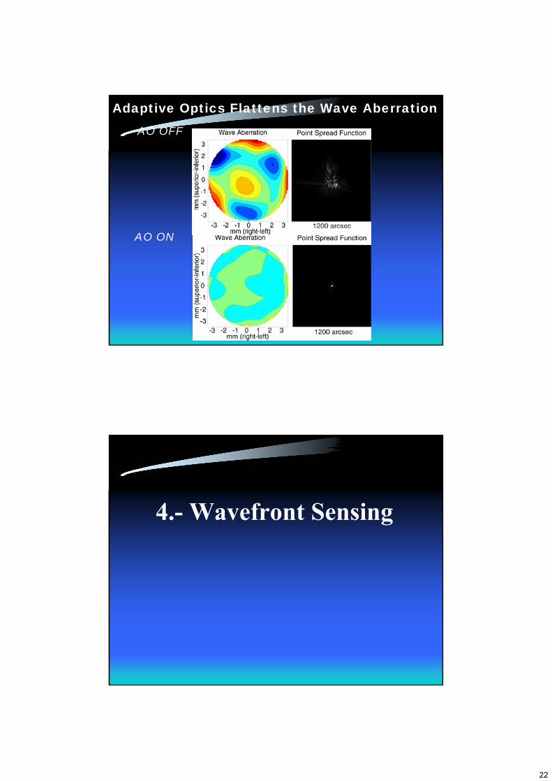
Adaptive Optics Flattens the Wave Aberration
AO ON
AO OFF
4.- Wavefront Sensing
23
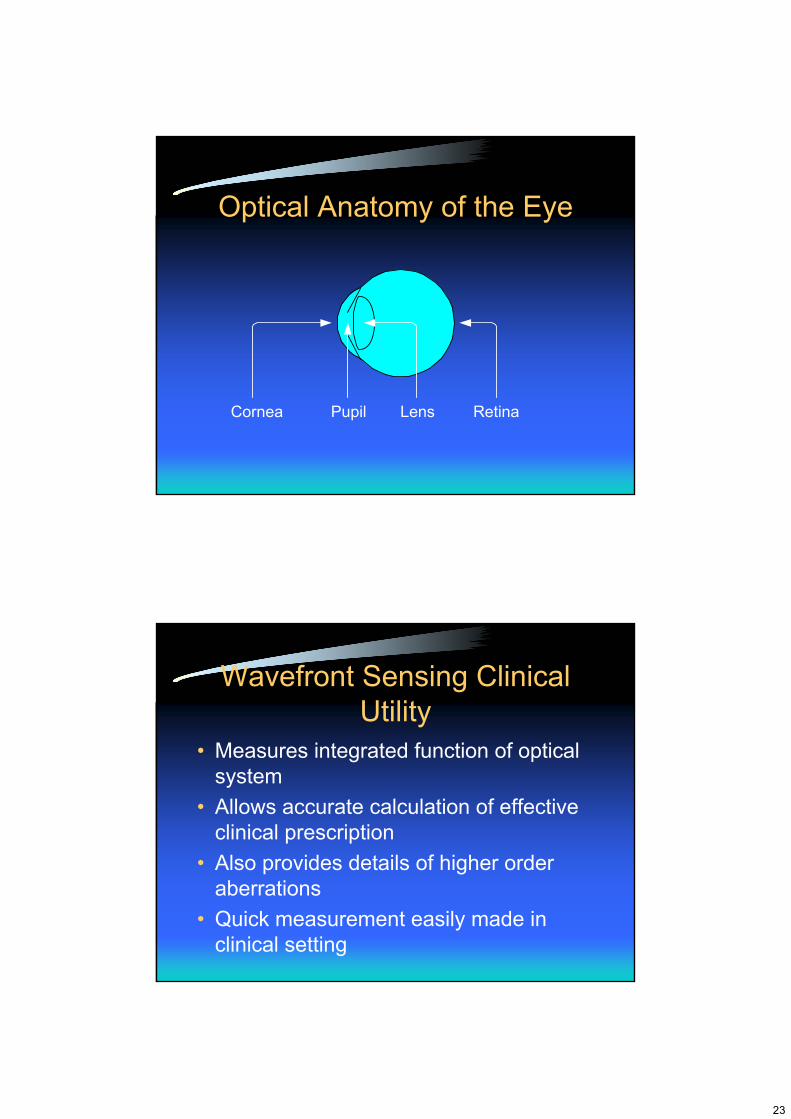
Optical Anatomy of the Eye
Cornea Pupil RetinaLens
Wavefront Sensing Clinical Utility
• Measures integrated function of optical system
• Allows accurate calculation of effective clinical prescription
• Also provides details of higher order aberrations
• Quick measurement easily made in clinical setting

24
Ideal Vision
Parallel Light Rays
Sharp Focuson Retina
Ideal Vision
Plane Wavefront
25
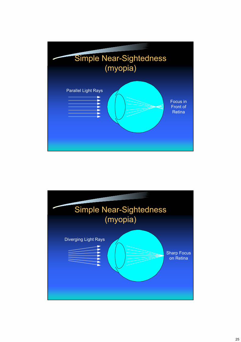
Simple Near-Sightedness(myopia)
Parallel Light Rays
Focus inFront ofRetina
Simple Near-Sightedness(myopia)
Diverging Light Rays
Sharp Focuson Retina
26
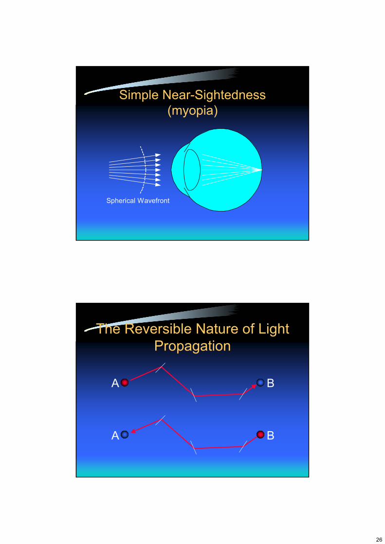
Simple Near-Sightedness(myopia)
Spherical Wavefront
The Reversible Nature of Light Propagation
A B
A B
27
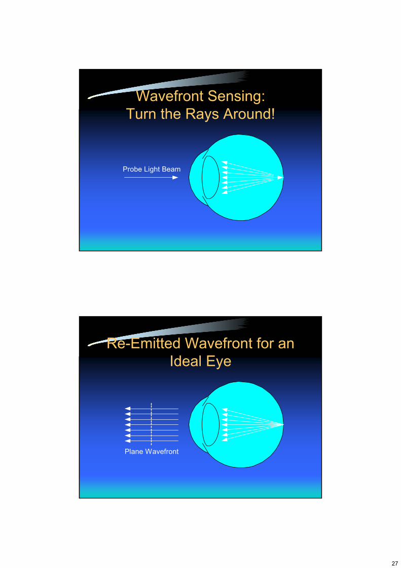
Wavefront Sensing:Turn the Rays Around!
Probe Light Beam
Re-Emitted Wavefront for an Ideal Eye
Plane Wavefront
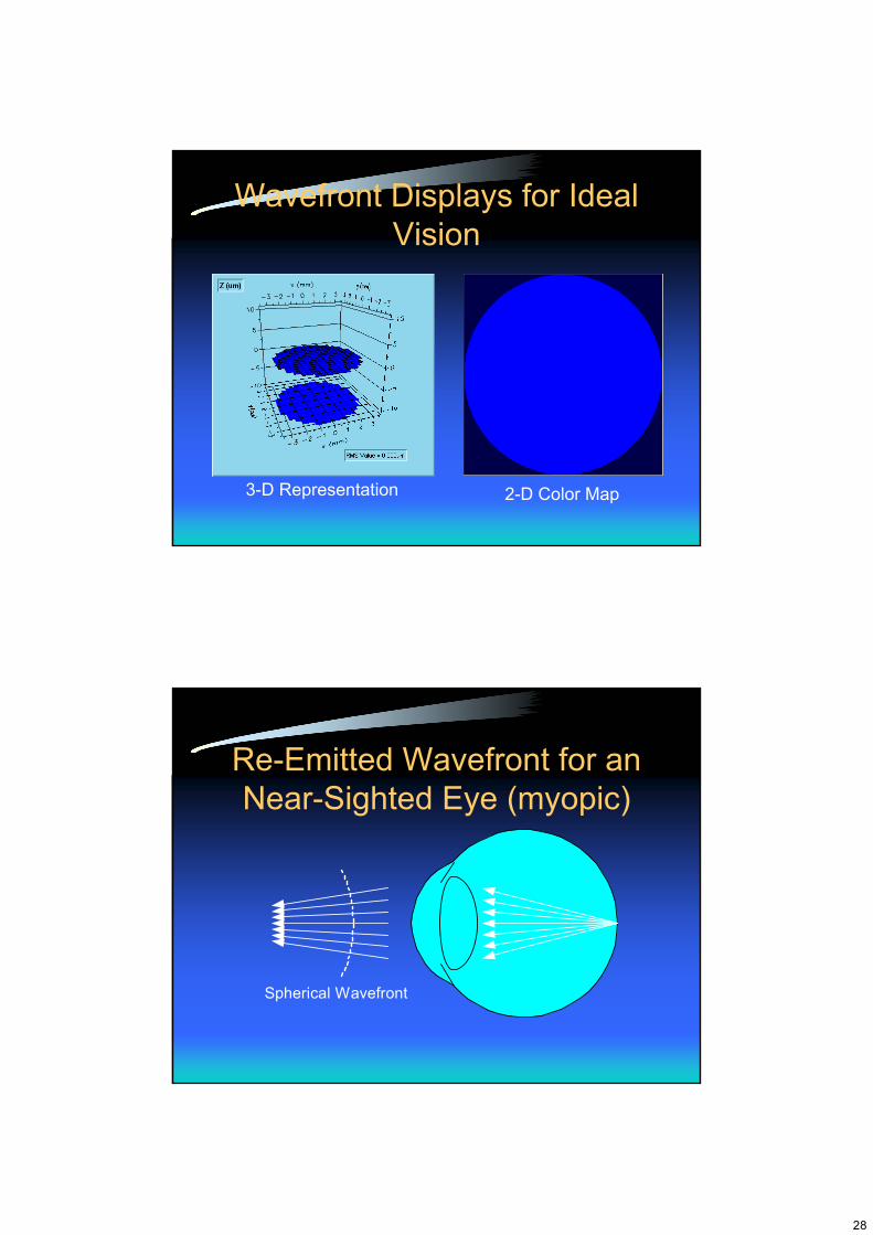
28
Wavefront Displays for Ideal Vision
3-D Representation 2-D Color Map
Re-Emitted Wavefront for an Near-Sighted Eye (myopic)
Spherical Wavefront
29
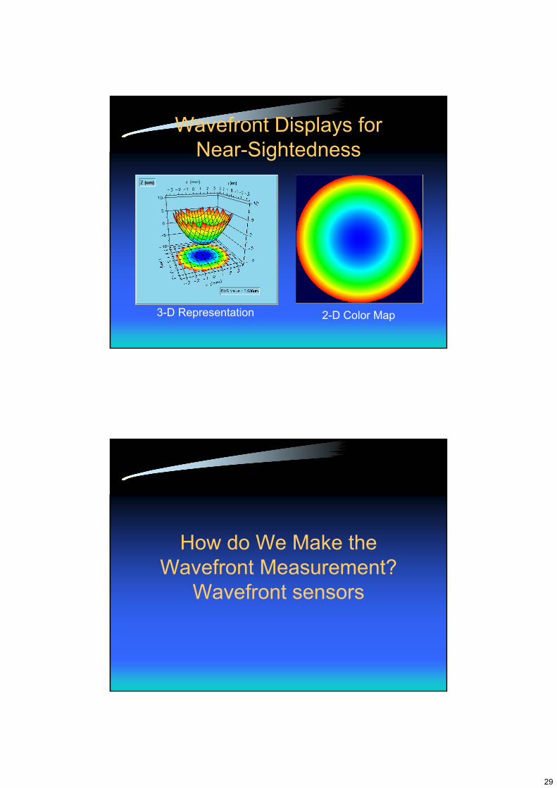
Wavefront Displays forNear-Sightedness
3-D Representation 2-D Color Map
How do We Make the Wavefront Measurement?
Wavefront sensors
30
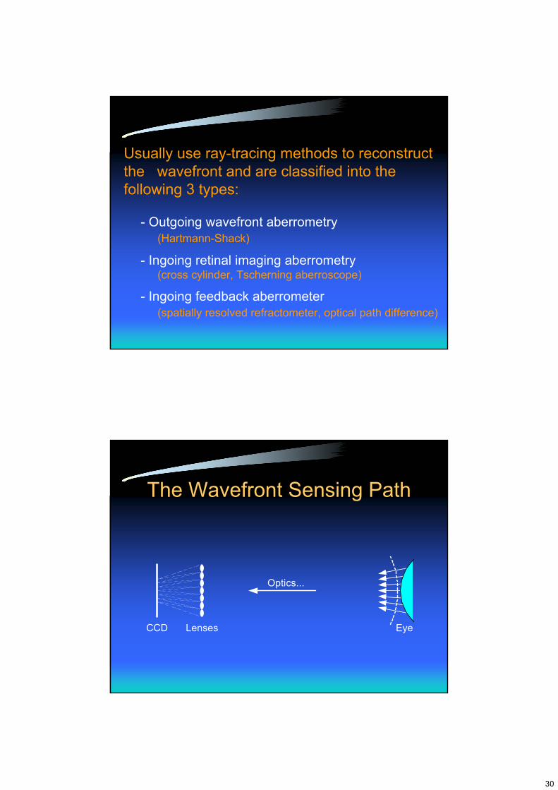
Usually use ray-tracing methods to reconstructthe wavefront and are classified into thefollowing 3 types:
- Outgoing wavefront aberrometry(Hartmann-Shack)
- Ingoing retinal imaging aberrometry(cross cylinder, Tscherning aberroscope)
- Ingoing feedback aberrometer(spatially resolved refractometer, optical path difference)
The Wavefront Sensing Path
Optics...
LensesCCD Eye
31
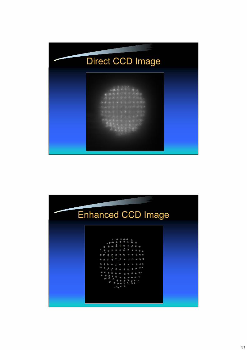
Direct CCD Image
Enhanced CCD Image
32
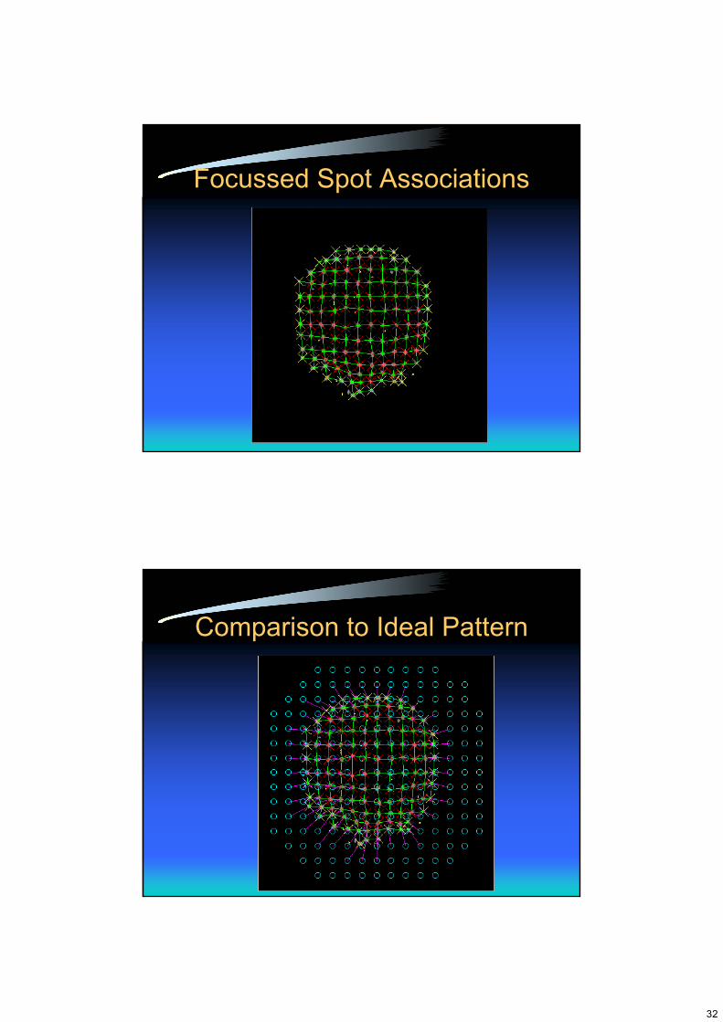
Focussed Spot Associations
Comparison to Ideal Pattern
33
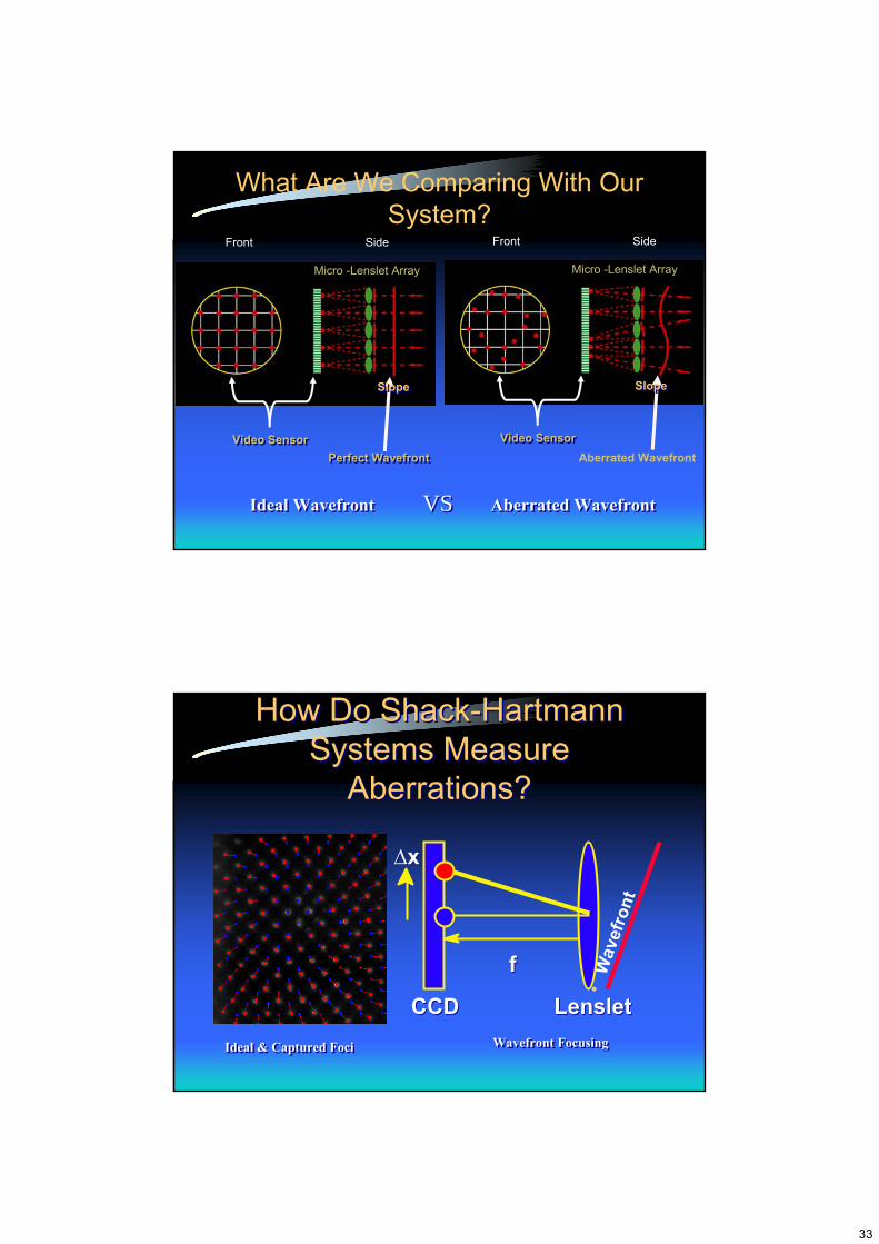
What Are We Comparing With Our System?
Perfect WavefrontPerfect Wavefront
Micro -Lenslet Array
Video SensorVideo Sensor
Ideal WavefrontIdeal Wavefront
Front Side
SlopeSlope
Front Side
Micro -Lenslet Array
Video SensorVideo SensorAberrated Wavefront
SlopeSlope
Aberrated WavefrontAberrated WavefrontVSVS
Ideal & Captured FociIdeal & Captured Foci Wavefront FocusingWavefront Focusing
•W
avef
ront
ff
CCDCCD LensletLenslet
∆∆xx
How Do Shack-Hartmann Systems Measure
Aberrations?
How Do Shack-Hartmann Systems Measure
Aberrations?
34
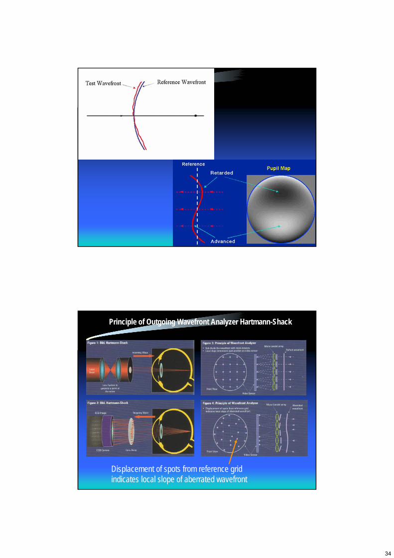
Principle of Outgoing Wavefront Analyzer Hartmann-Shack
Displacement of spots from reference gridindicates local slope of aberrated wavefront
35
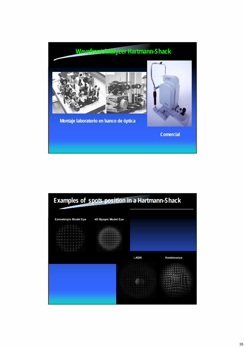
Wavefront Analyzer Hartmann-Shack
Montaje laboratorio en banco de óptica
Comercial
Examples of spots position in a Hartmann-Shack
36
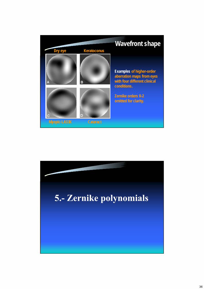
Wavefront shape
Examples of higher-order aberration maps from eyes with four different clinical conditions.
Zernike orders 0-2omitted for clarity.
Dry eye Keratoconus
Myopic-LASIK Cataract
5.- Zernike polynomials
37
► La aproximación más familiar para cuantificar las aberraciones ópticas es la de Seidel, definida para sistemas rotacionalmente simétricos
► Cuando describimos las aberraciones oculares, Seidel no se utiliza ya que la óptica del ojo no es totalmente simétrica
► Los polinomios de Taylor tambien han sido utilizados para describir las aberraciones del ojo
► Recientemente se han utilizado los polinomios de Zernike debido a sus propiedades matemáticas adecuadas para pupilas circulares
Introducción
► Polinomios de Zernike: consisten en un conjunto ortogonal de polinómios que presentan las aberraciones y además están relacionados con las aberraciones ópticas clásicas
► Parecen el método más deseable para estimaciones precisas del error de frente de onda, debido a sus propiedades de ortogonalidad (independencia de los términos entre sí) y pueden ajustarse por el método de mínimos cuadrados, que es lineal en parámetros
Introducción
38
► Los topógrafos miden la elevación corneal sólo en un número discreto de puntos y los polinómios de Zernike no son ortogonales sobre un conjunto discreto de puntos
► La técnica de ortogonalización de Gram-Smith permite expandir el conjunto discreto de datos de elevación corneal, en términos de polinómios de Zernike y conseguir las ventajas de una expansión ortogonal.Una vez completada la expansión, las funciones ortogonales se transforman en términos de polinomios de Zernike, resultando un conjunto único de coeficientes de Zernike
Introducción: Topografía
Definición y notaciones
Los polinomios de Zernike son un conjunto infinito de funciones polinómicas, ortogonales en el circulo de radio unidad.
Son muy útiles para representar la forma del frente de onda en sistemas ópticos. Su uso está muy extendido y son muy comunes distintas notaciones, normalizaciones y criterios en la asignación de signos.
39
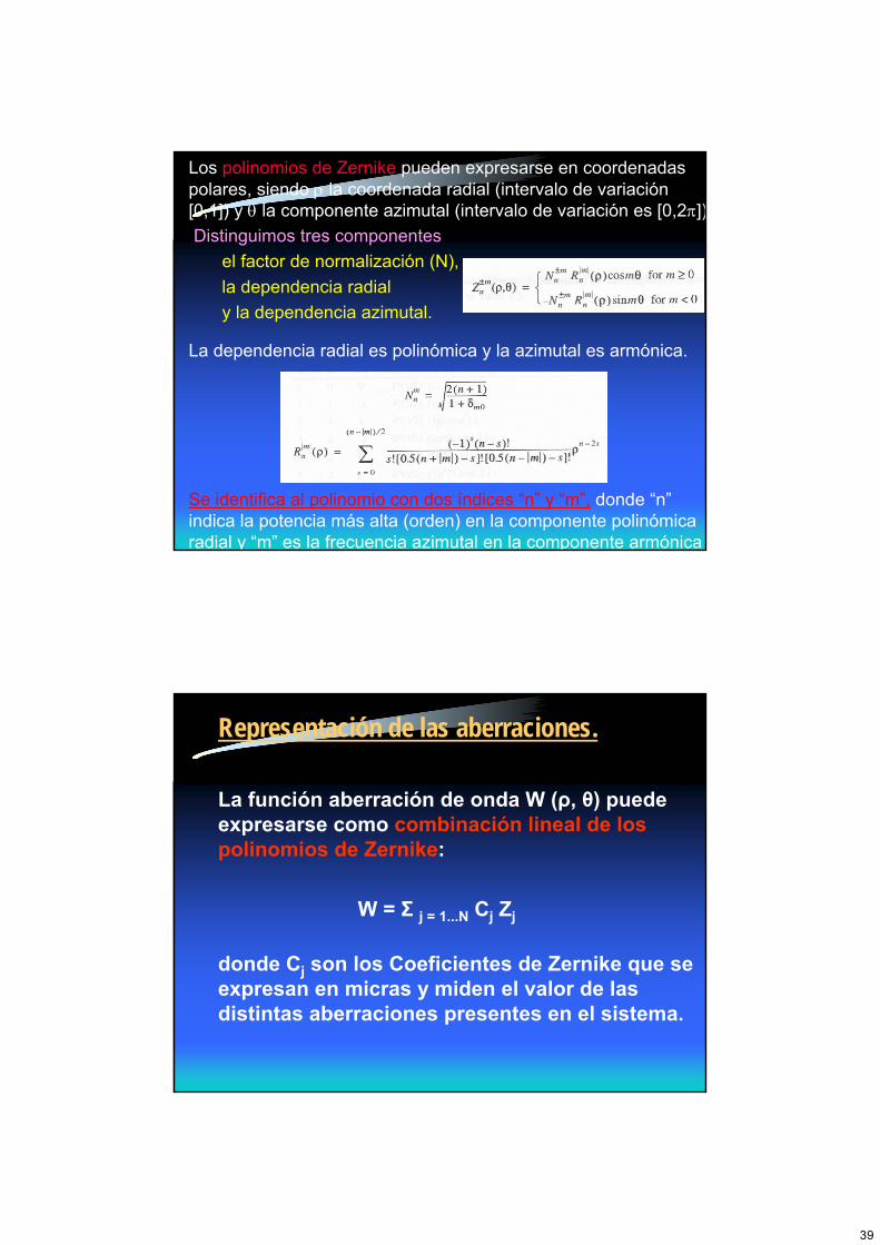
Los polinomios de Zernike pueden expresarse en coordenadas polares, siendo ρ la coordenada radial (intervalo de variación [0,1]) y θ la componente azimutal (intervalo de variación es [0,2π])Distinguimos tres componentes:
el factor de normalización (N), la dependencia radialy la dependencia azimutal.
La dependencia radial es polinómica y la azimutal es armónica.
Se identifica al polinomio con dos índices “n” y “m”, donde “n” indica la potencia más alta (orden) en la componente polinómica radial y “m” es la frecuencia azimutal en la componente armónica
Representación de las aberraciones.
La función aberración de onda W (ρ, θ) puede expresarse como combinación lineal de los polinomios de Zernike:
W = Σ j = 1...N Cj Zj
donde Cj son los Coeficientes de Zernike que se expresan en micras y miden el valor de las distintas aberraciones presentes en el sistema.
40
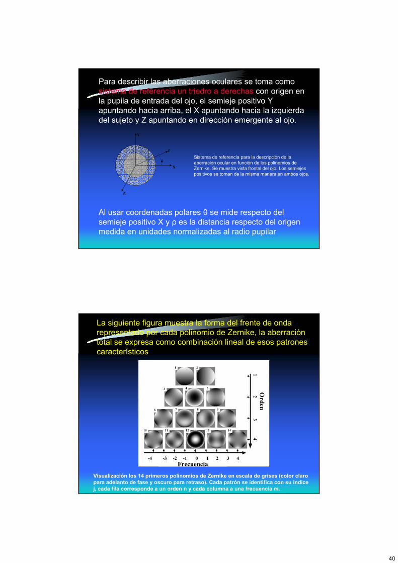
Para describir las aberraciones oculares se toma como sistema de referencia un triedro a derechas con origen en la pupila de entrada del ojo, el semieje positivo Y apuntando hacia arriba, el X apuntando hacia la izquierda del sujeto y Z apuntando en dirección emergente al ojo.
Al usar coordenadas polares θ se mide respecto del semieje positivo X y ρ es la distancia respecto del origen medida en unidades normalizadas al radio pupilar
X
Y
Z
ρ
θSistema de referencia para la descripción de la aberración ocular en función de los polinomios de Zernike. Se muestra vista frontal del ojo. Los semiejes positivos se toman de la misma manera en ambos ojos.
Ord en
Frecuencia
1 2
3 4 5
6 7 8 9
10 11 12 13 14
12
3 4
-4 -3 -2 -1 0 1 2 3 4
La siguiente figura muestra la forma del frente de onda representado por cada polinomio de Zernike, la aberración total se expresa como combinación lineal de esos patrones característicos
Visualización los 14 primeros polinomios de Zernike en escala de grises (color claro para adelanto de fase y oscuro para retraso). Cada patrón se identifica con su índice j, cada fila corresponde a un orden n y cada columna a una frecuencia m.
41
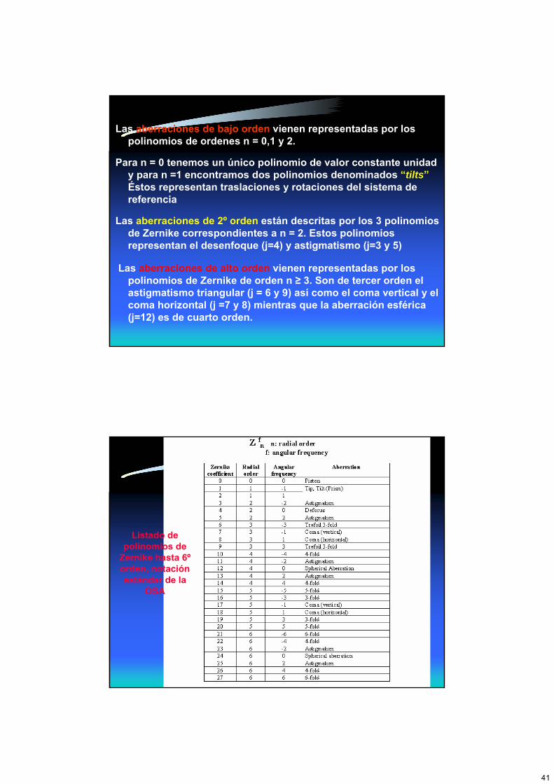
Las aberraciones de bajo orden vienen representadas por los polinomios de ordenes n = 0,1 y 2.
Para n = 0 tenemos un único polinomio de valor constante unidad y para n =1 encontramos dos polinomios denominados “tilts”Éstos representan traslaciones y rotaciones del sistema de referencia
Las aberraciones de 2º orden están descritas por los 3 polinomios de Zernike correspondientes a n = 2. Estos polinomios representan el desenfoque (j=4) y astigmatismo (j=3 y 5)
Las aberraciones de alto orden vienen representadas por los polinomios de Zernike de orden n ≥ 3. Son de tercer orden el astigmatismo triangular (j = 6 y 9) así como el coma vertical y el coma horizontal (j =7 y 8) mientras que la aberración esférica (j=12) es de cuarto orden.
Listado de polinomios de
Zernike hasta 6ºorden, notación estándar de la
OSA
42
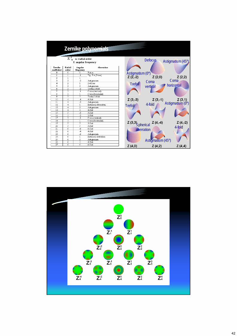
Zernike polynomials
Defocus
Astigmatism (0º)
Coma horizontal
Astigmatism (45º)
Coma vertical
Trefoil
Trefoil
Sphericalaberration
Astigmatism (0º)
Astigmatism (45º)
4-fold
4-fold
43
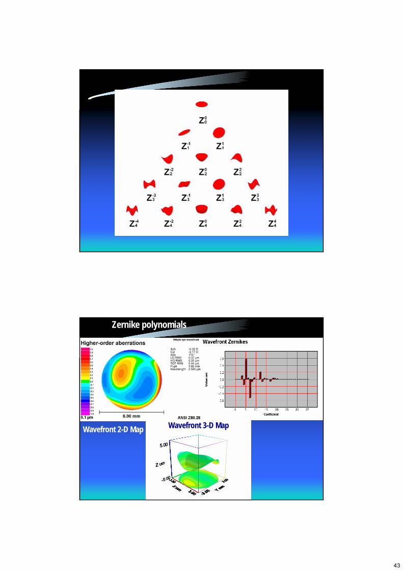
Zernike polynomials
Wavefront 3-D MapWavefront 2-D Map
44
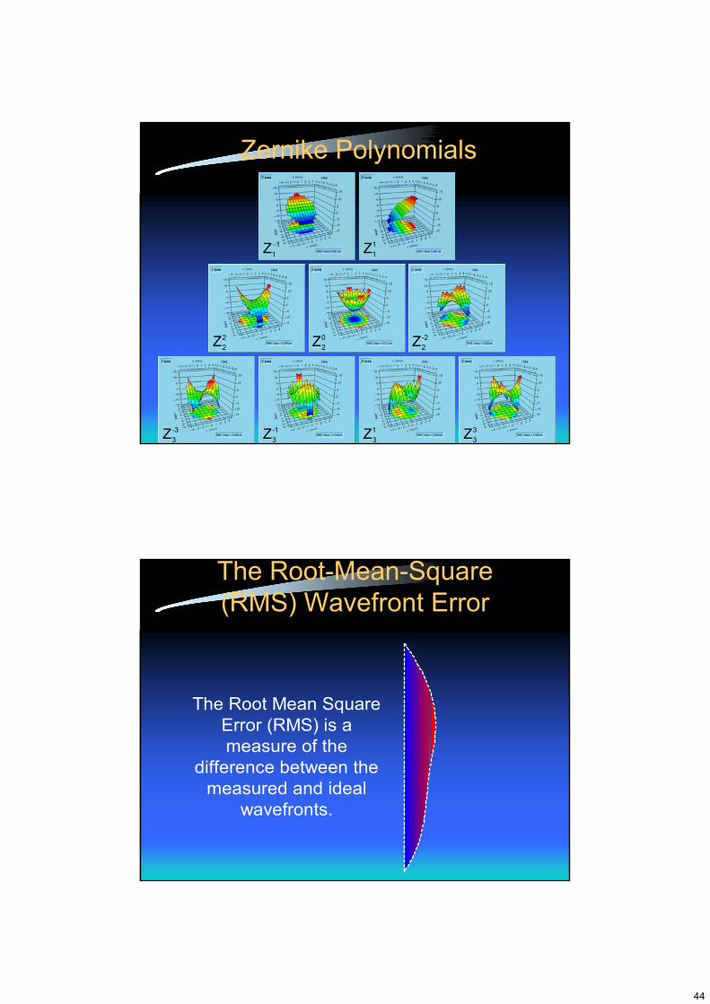
Zernike Polynomials
11Z− 1
1Z
02Z 2-
2Z22Z
3-3Z 1-
3Z 13Z 3
3Z
The Root-Mean-Square (RMS) Wavefront Error
The Root Mean SquareError (RMS) is ameasure of the
difference between themeasured and ideal
wavefronts.
45
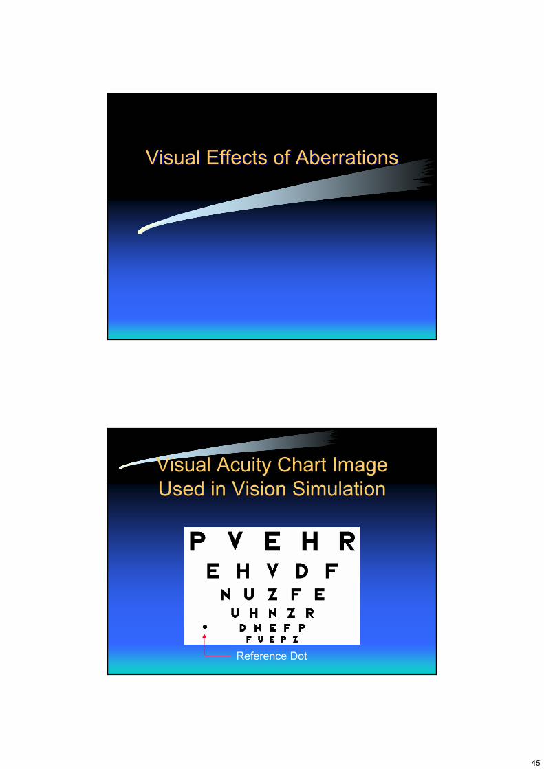
Visual Effects of AberrationsVisual Effects of Aberrations
Visual Acuity Chart Image Used in Vision Simulation
Reference Dot
46
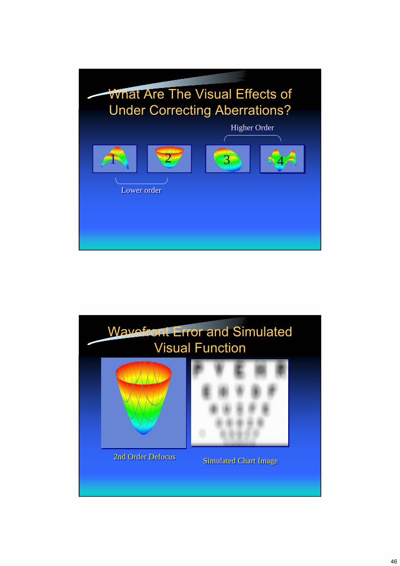
What Are The Visual Effects of Under Correcting Aberrations?
1 2
Lower orderLower order
43
Higher OrderHigher Order
Wavefront Error and Simulated Visual Function
Simulated Chart ImageSimulated Chart Image2nd Order Defocus2nd Order Defocus
47
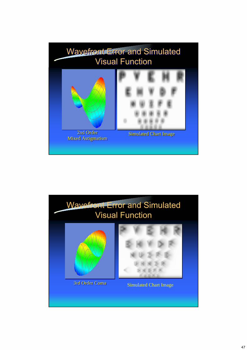
2nd Order Mixed Astigmatism
2nd Order Mixed Astigmatism
Simulated Chart ImageSimulated Chart Image
Wavefront Error and Simulated Visual Function
Wavefront Error and Simulated Visual Function
3rd Order Coma3rd Order Coma Simulated Chart Image
Wavefront Error and Simulated Visual Function
48
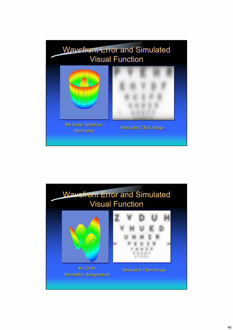
Simulated Chart ImageSimulated Chart Image4th Order SphericalAberration
4th Order SphericalAberration
Wavefront Error and Simulated Visual Function
Wavefront Error and Simulated Visual Function
4th Order Secondary Astigmatism
4th Order Secondary Astigmatism
Simulated Chart ImageSimulated Chart Image
Wavefront Error and Simulated Visual Function
49
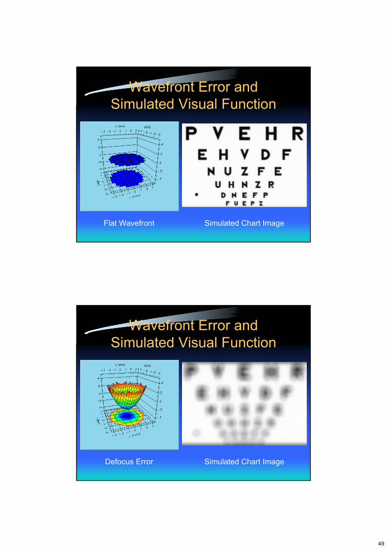
Wavefront Error and Simulated Visual Function
Flat Wavefront Simulated Chart Image
Wavefront Error and Simulated Visual Function
Defocus Error Simulated Chart Image
50
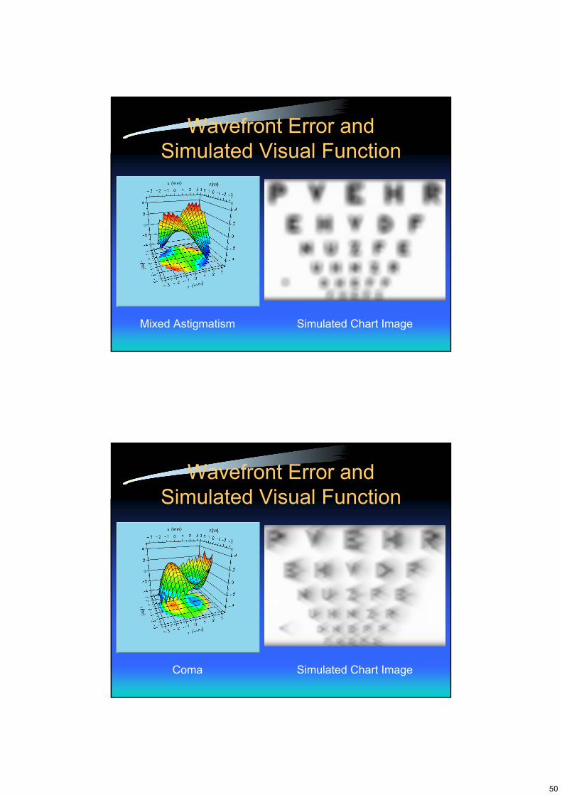
Wavefront Error and Simulated Visual Function
Mixed Astigmatism Simulated Chart Image
Wavefront Error and Simulated Visual Function
Coma Simulated Chart Image
51
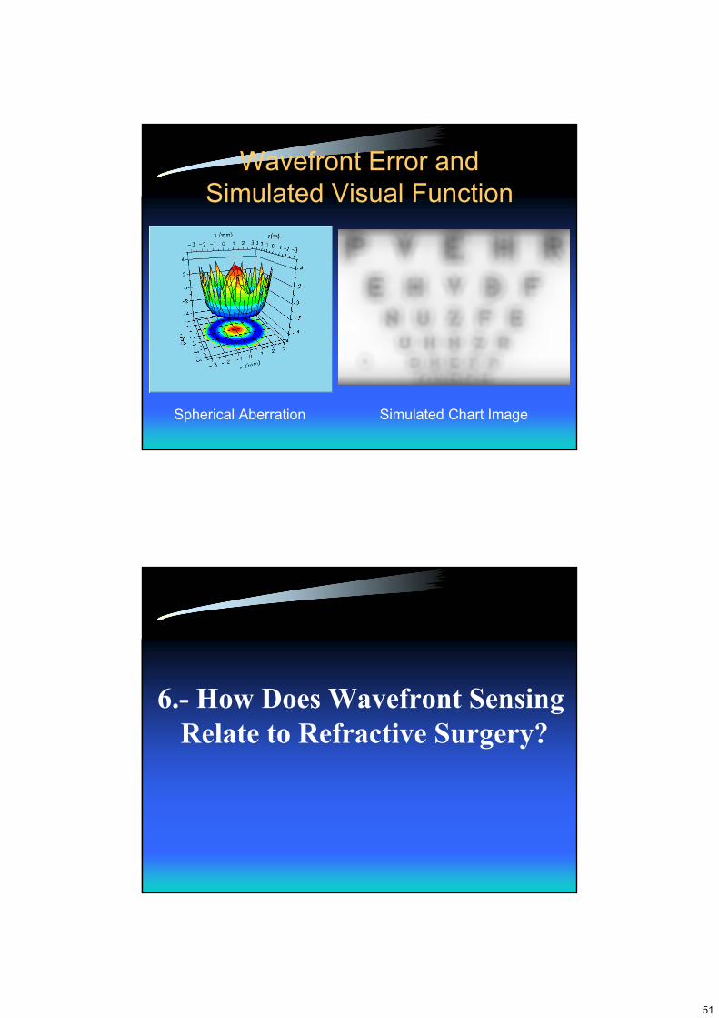
Wavefront Error and Simulated Visual Function
Spherical Aberration Simulated Chart Image
6.- How Does Wavefront SensingRelate to Refractive Surgery?
52
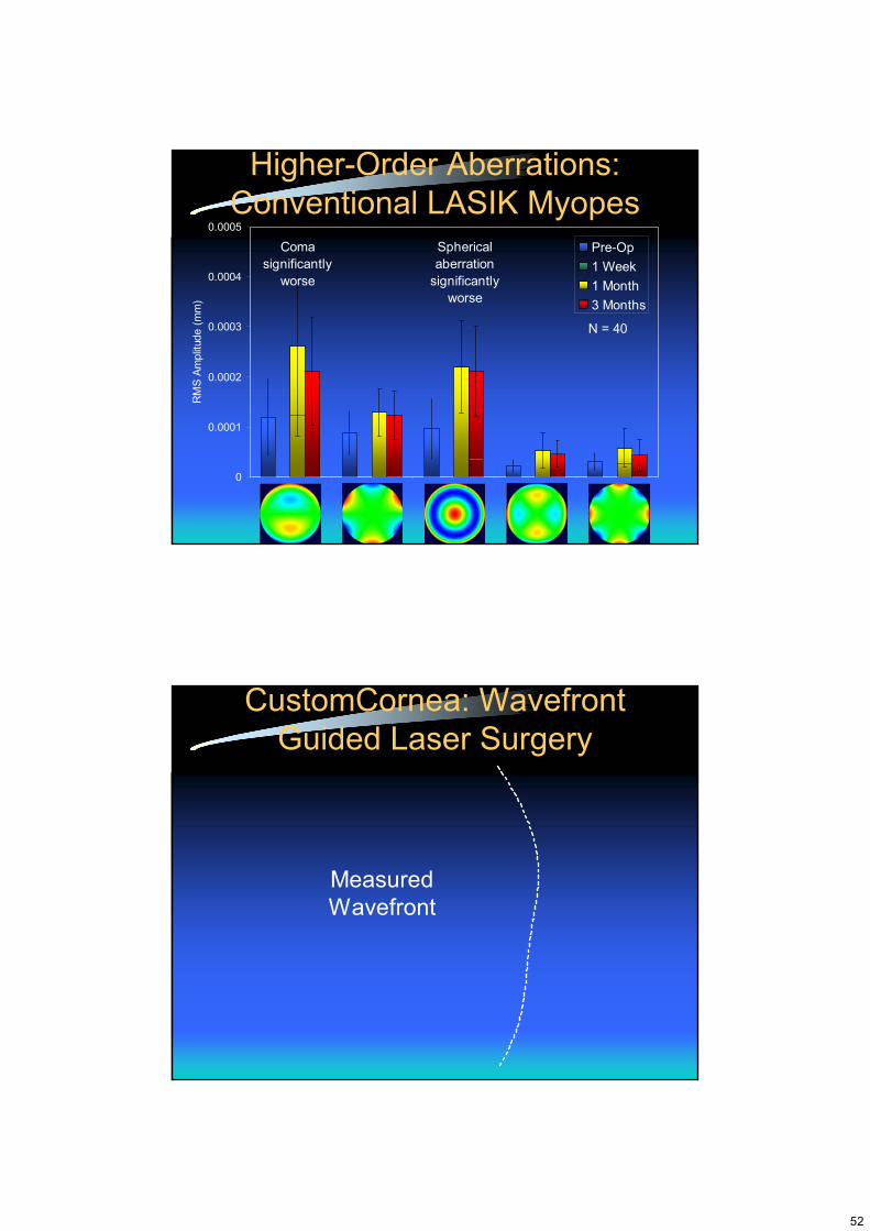
0
0.0001
0.0002
0.0003
0.0004
0.0005
c6/c7 c8/c9 c10 c11/c12 c13/c14
RM
S Am
plitu
de (m
m)
Pre-Op1 Week1 Month3 Months
Coma significantly
worse
Spherical aberration
significantly worse
N = 40
Higher-Order Aberrations: Conventional LASIK Myopes
CustomCornea: Wavefront Guided Laser Surgery
MeasuredWavefront
53
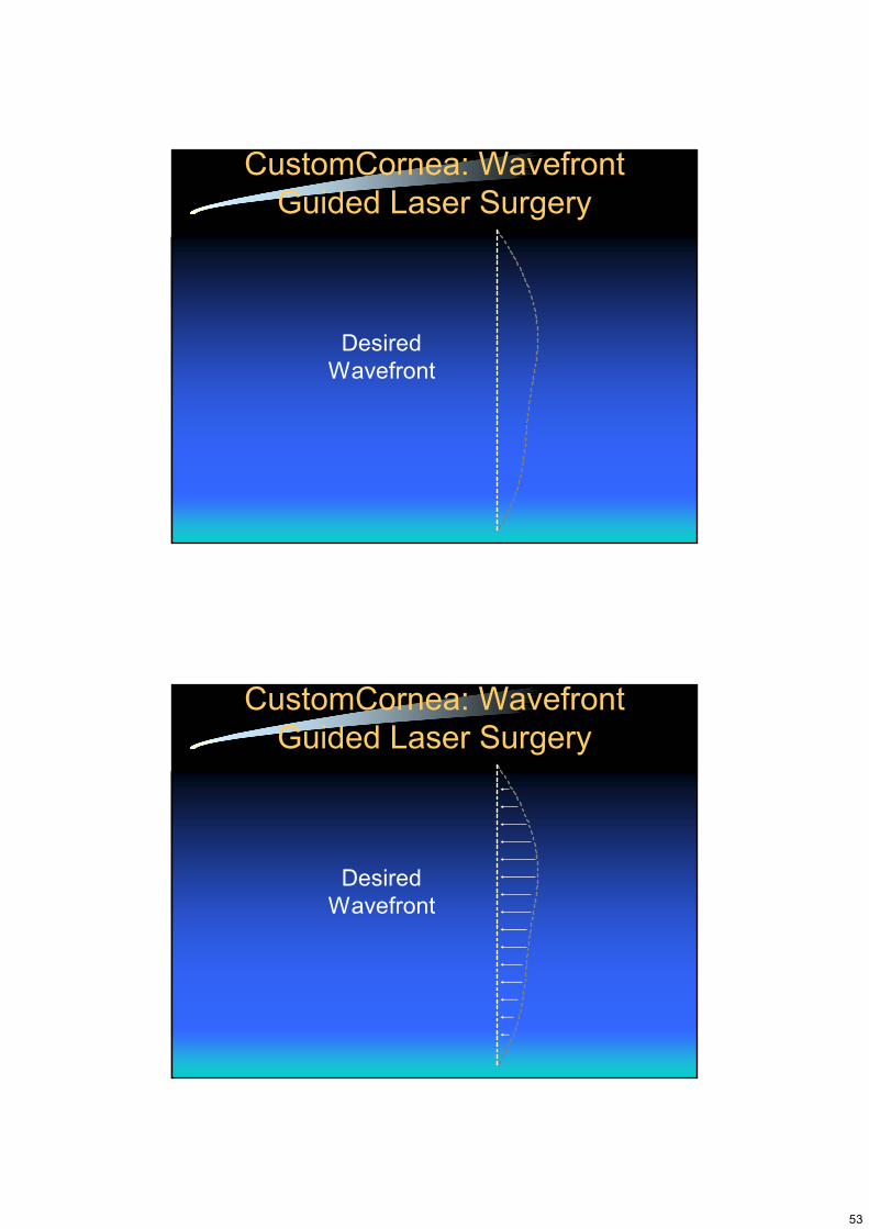
CustomCornea: Wavefront Guided Laser Surgery
DesiredWavefront
CustomCornea: Wavefront Guided Laser Surgery
DesiredWavefront
54
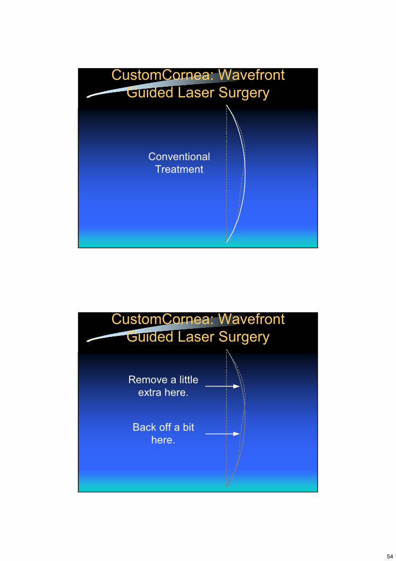
CustomCornea: Wavefront Guided Laser Surgery
ConventionalTreatment
CustomCornea: Wavefront Guided Laser Surgery
Remove a littleextra here.
Back off a bithere.
55
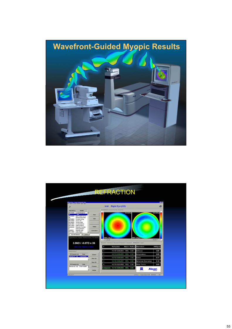
Wavefront-Guided Myopic Results
REFRACTION
56
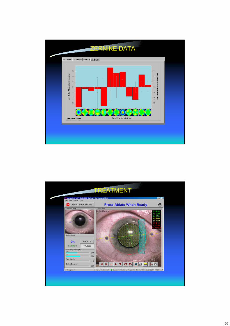
ZERNIKE DATA
TREATMENT
57
VIDEO
-2D
0D
-2D
0D
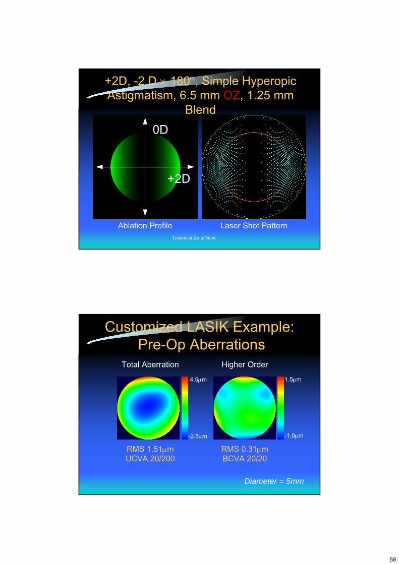
-2 D × 180° Simple Myopic Astigmatism6 mm OZ, 1.0 mm Blend
-2 D × 180° Simple Myopic Astigmatism6 mm OZ, 1.0 mm Blend
Ablation ProfileAblation Profile Laser Shot PatternLaser Shot PatternTreatment Zone 6 x 8mmTreatment Zone 6 x 8mm
58
0D
+2D
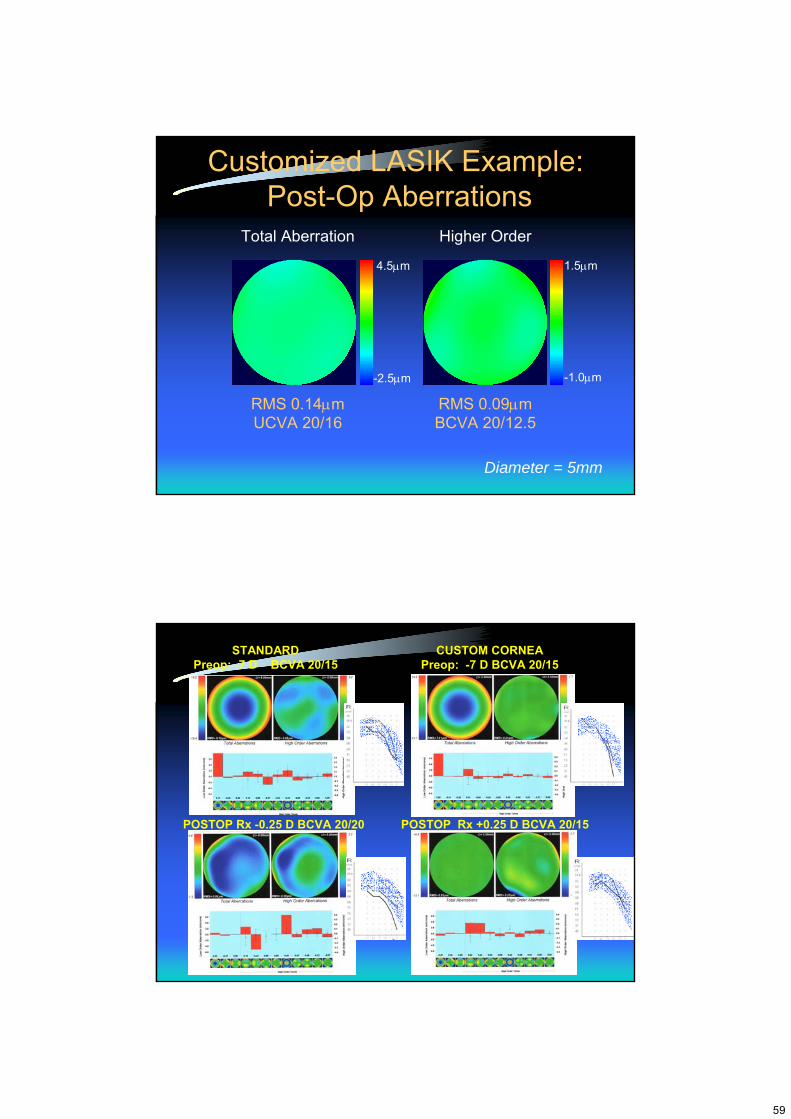
+2D, -2 D × 180°, Simple Hyperopic Astigmatism, 6.5 mm OZ, 1.25 mm
Blend
Ablation Profile Laser Shot PatternTreatment Zone 9mm
Customized LASIK Example:Pre-Op Aberrations
Total Aberration Higher Order
RMS 1.51μm UCVA 20/200
RMS 0.31μm BCVA 20/20
4.5μm
-2.5μm
1.5μm
-1.0μm
Diameter = 5mm
59
Total Aberration Higher Order
4.5μm
-2.5μm
1.5μm
-1.0μm
Diameter = 5mm
RMS 0.14μm UCVA 20/16
RMS 0.09μm BCVA 20/12.5
Customized LASIK Example:Post-Op Aberrations
STANDARDPreop: -7 D BCVA 20/15
CUSTOM CORNEAPreop: -7 D BCVA 20/15
POSTOP Rx -0.25 D BCVA 20/20 POSTOP Rx +0.25 D BCVA 20/15
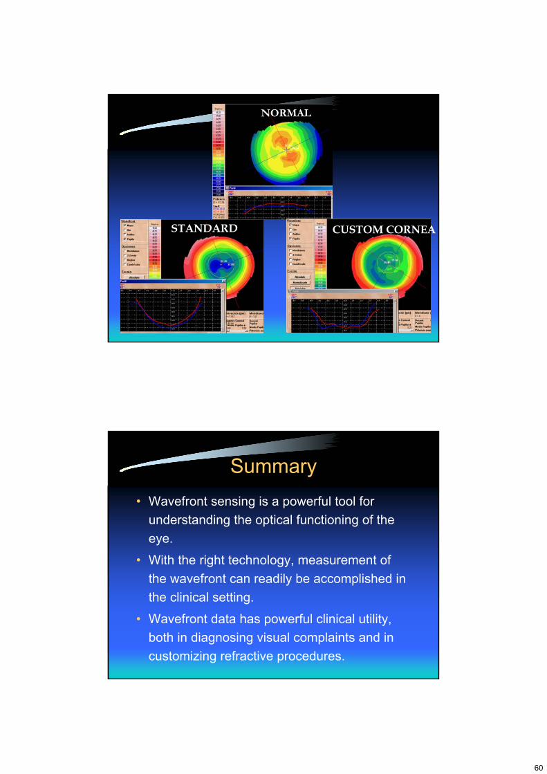
60
STANDARD CUSTOM CORNEA
NORMAL
Summary• Wavefront sensing is a powerful tool for
understanding the optical functioning of the eye.
• With the right technology, measurement of the wavefront can readily be accomplished in the clinical setting.
• Wavefront data has powerful clinical utility, both in diagnosing visual complaints and in customizing refractive procedures.
61
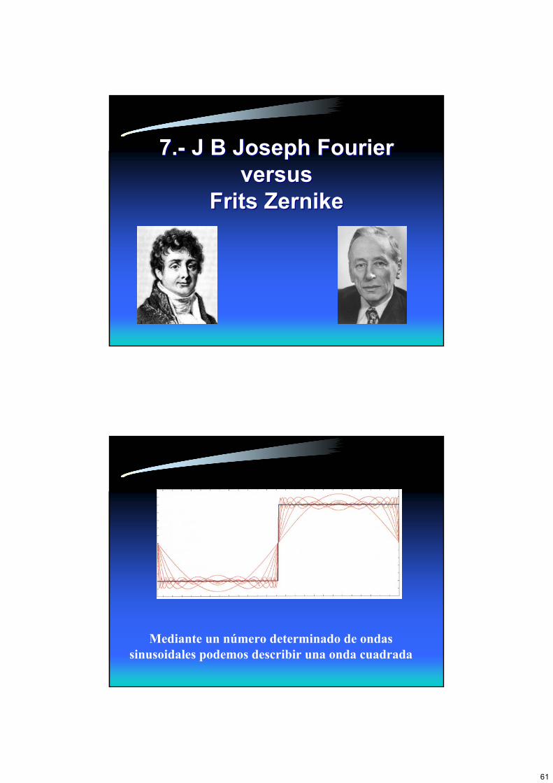
7.7.-- J B Joseph J B Joseph FourierFourierversusversus
FritsFrits ZernikeZernike
Mediante un número determinado de ondas sinusoidales podemos describir una onda cuadrada
62
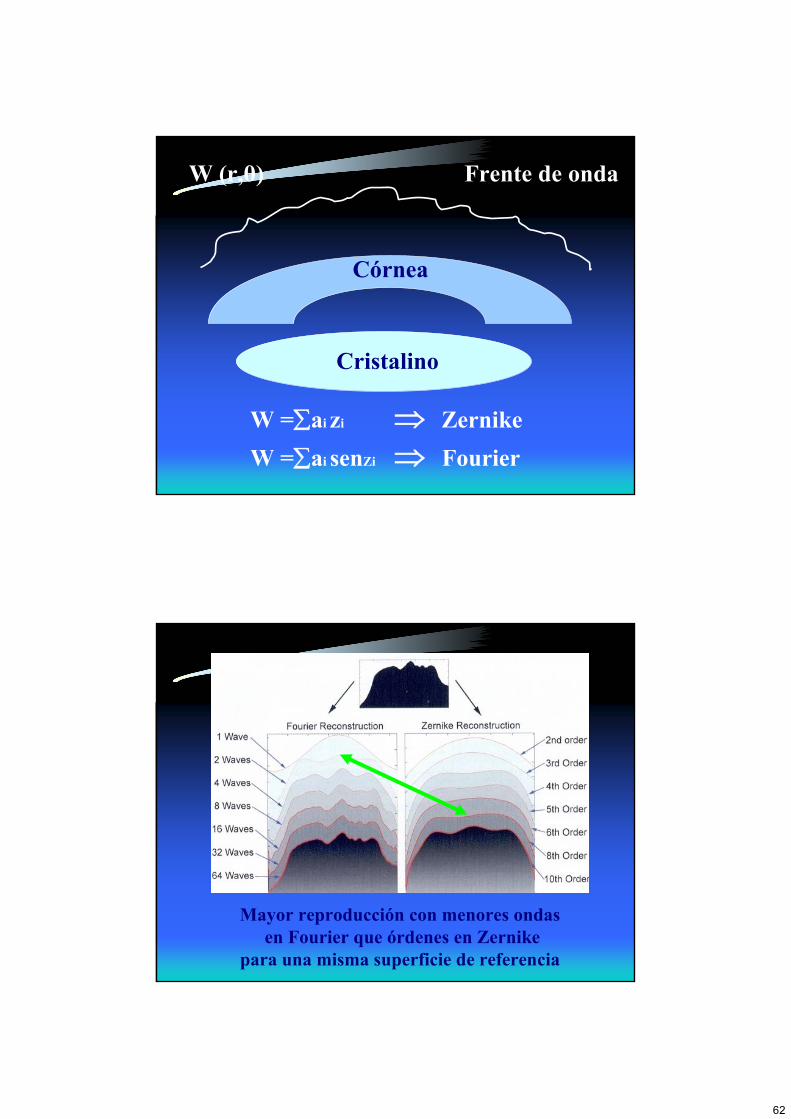
Córnea
W (r,θ) Frente de onda
W =∑ai zi ⇒ ZernikeW =∑ai senZi ⇒ Fourier
Cristalino
Mayor reproducción con menores ondasen Fourier que órdenes en Zernike
para una misma superficie de referencia
63
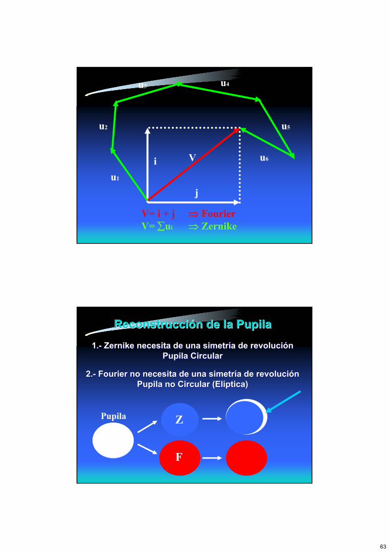
V= i + j ⇒ FourierV= ∑ui ⇒ Zernike
Vi
ju1
u2
u3 u4
u5
u6
ReconstrucciReconstruccióón de la Pupilan de la Pupila
1.1.-- Zernike necesita de una simetrZernike necesita de una simetríía de revolucia de revolucióón n Pupila CircularPupila Circular
2.2.-- FourierFourier no necesita de una simetrno necesita de una simetríía de revolucia de revolucióónnPupila no Circular (ElPupila no Circular (Elííptica)ptica)
F
ZPupila
64
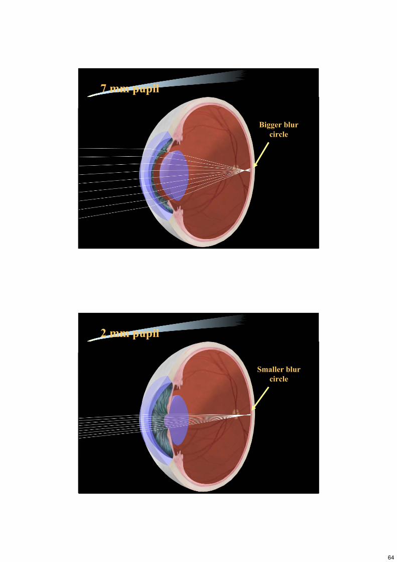
7 mm pupil
Bigger blurcircle
Smaller blurcircle
2 mm pupil
65
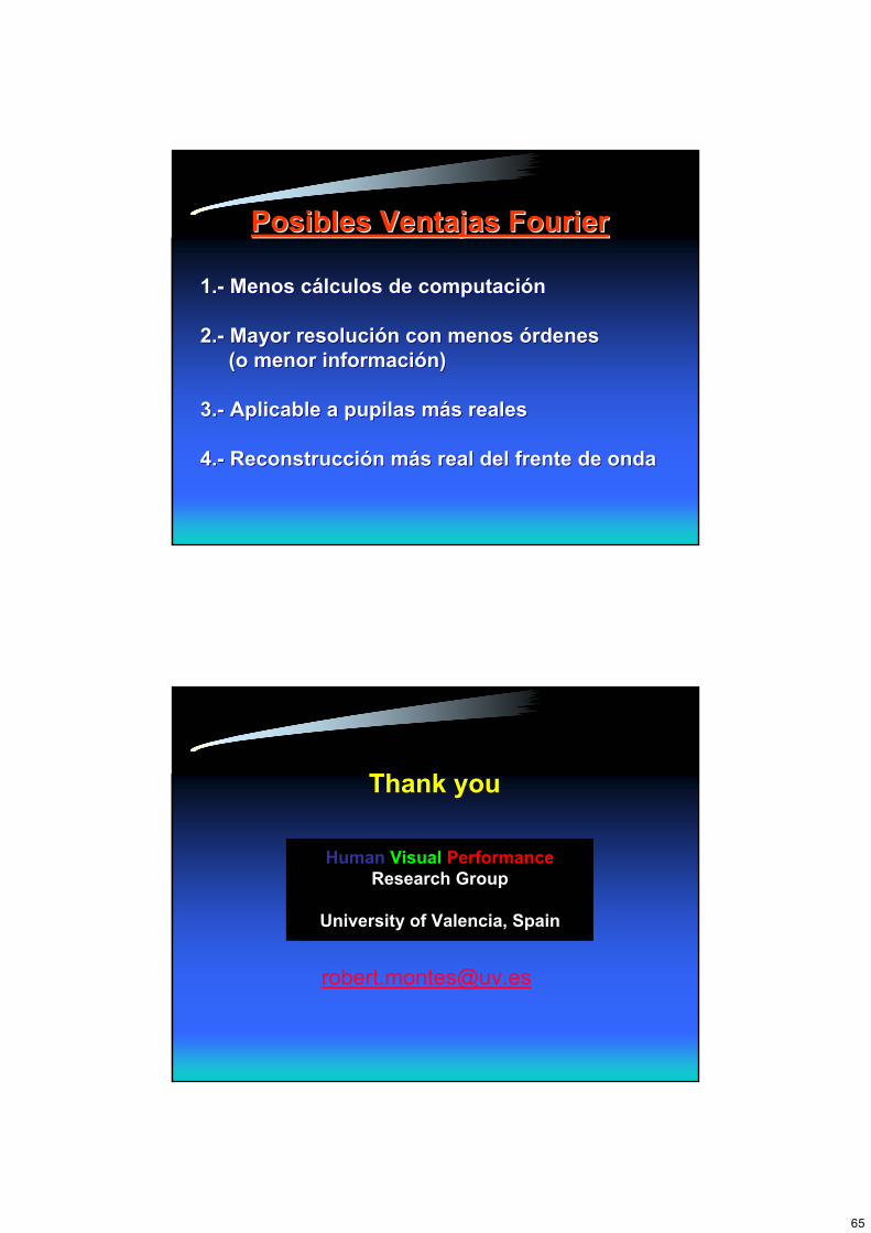
Posibles Ventajas Posibles Ventajas FourierFourier
1.1.-- Menos cMenos cáálculos de computacilculos de computacióónn
2.2.-- Mayor resoluciMayor resolucióón con menos n con menos óórdenesrdenes(o menor informaci(o menor informacióón)n)
3.3.-- Aplicable a pupilas mAplicable a pupilas máás realess reales
4.4.-- ReconstrucciReconstruccióón mn máás real del frente de ondas real del frente de onda
Thank you
Human Visual PerformanceResearch Group
University of Valencia, Spain