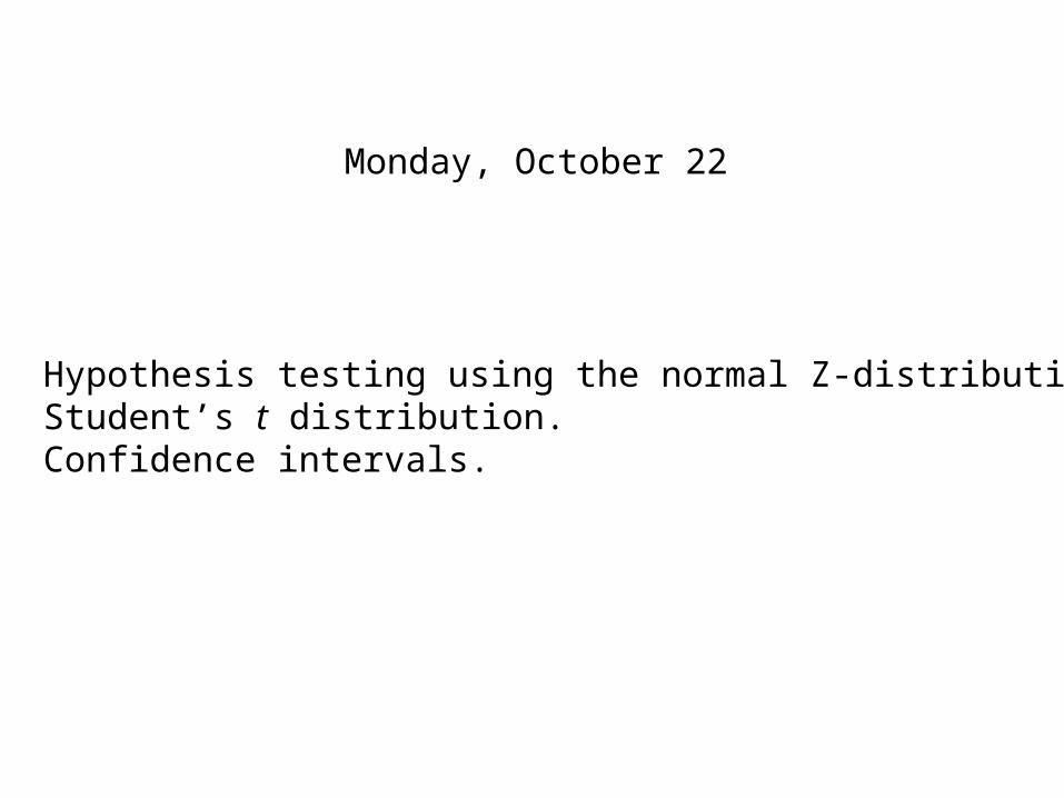
Monday, October 22

Hypothesis testing using the normal Z-distribution.Student’s t distribution.Confidence intervals.

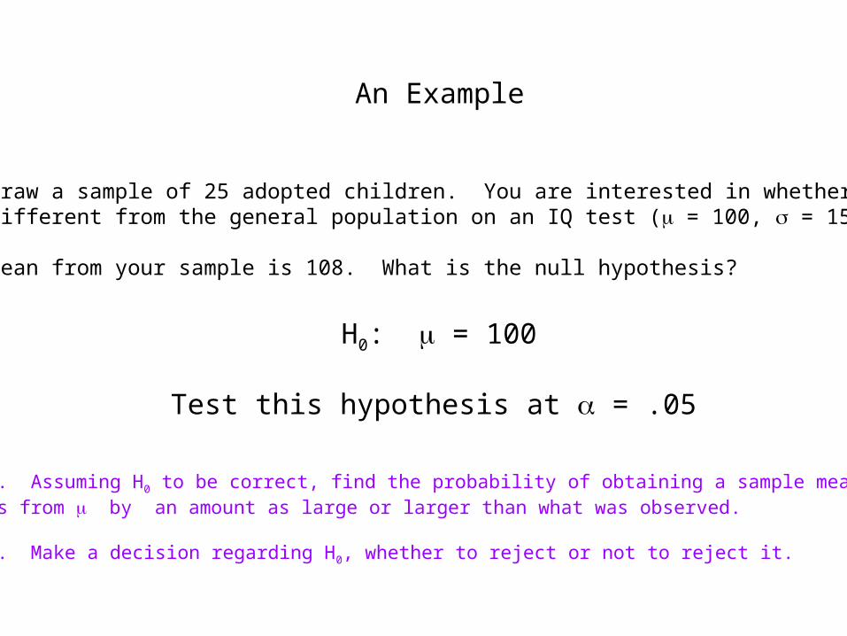
An Example

You draw a sample of 25 adopted children. You are interested in whether theyare different from the general population on an IQ test ( = 100, = 15).

The mean from your sample is 108. What is the null hypothesis?

H0: = 100

Test this hypothesis at = .05

Step 3. Assuming H0 to be correct, find the probability of obtaining a sample mean thatdiffers from by an amount as large or larger than what was observed.

Step 4. Make a decision regarding H0, whether to reject or not to reject it.

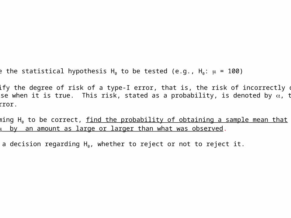
Step 1. State the statistical hypothesis H0 to be tested (e.g., H0: = 100)

Step 2. Specify the degree of risk of a type-I error, that is, the risk of incorrectly concluding that H0 is false when it is true. This risk, stated as a probability, is denoted by , the probabilityof a Type I error.

Step 3. Assuming H0 to be correct, find the probability of obtaining a sample mean thatdiffers from by an amount as large or larger than what was observed.

Step 4. Make a decision regarding H0, whether to reject or not to reject it.

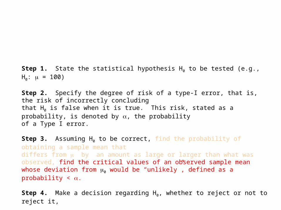
Step 1. State the statistical hypothesis H0 to be tested (e.g., H0: = 100)

Step 2. Specify the degree of risk of a type-I error, that is, the risk of incorrectly concluding that H0 is false when it is true. This risk, stated as a probability, is denoted by , the probabilityof a Type I error.

Step 3. Assuming H0 to be correct, find the probability of obtaining a sample mean thatdiffers from by an amount as large or larger than what was observed, find the critical values of an observed sample mean whose deviation from 0 would be “unlikely”, defined as a probability < .

Step 4. Make a decision regarding H0, whether to reject or not to reject it,

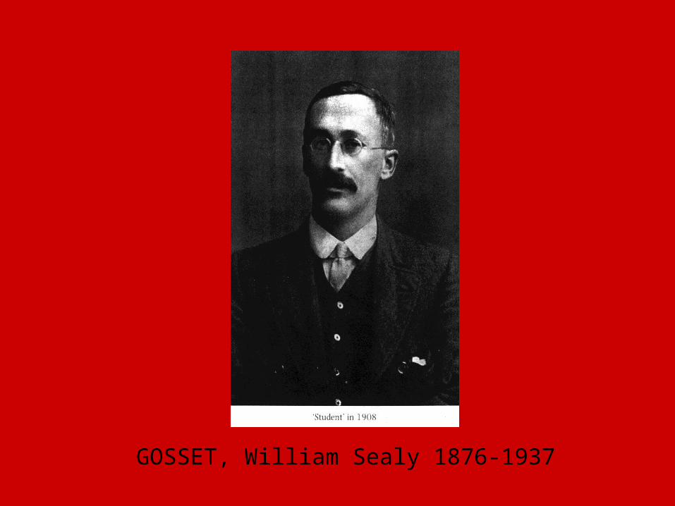
GOSSET, William Sealy 1876-1937

_

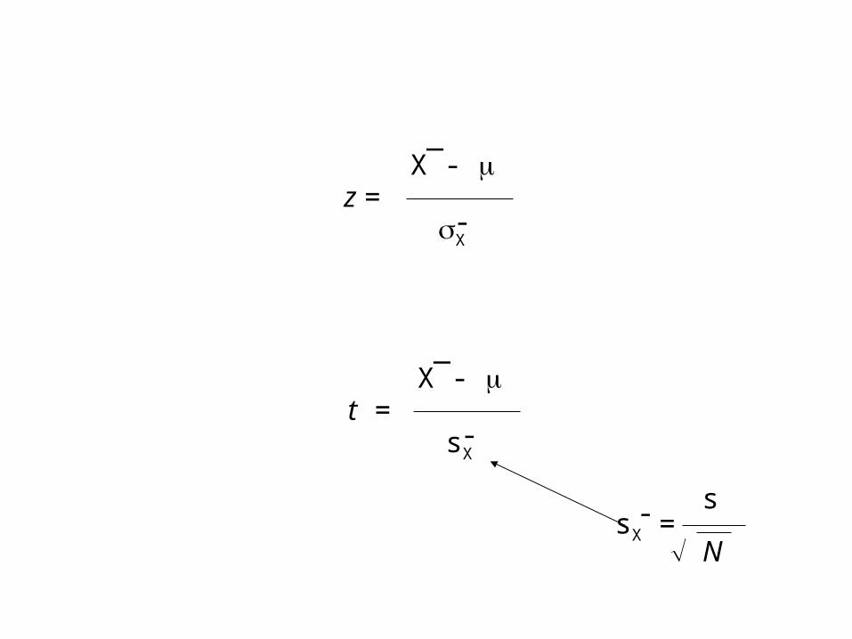
z = X -

X-

_

t = X -

sX-

sX = s

N-

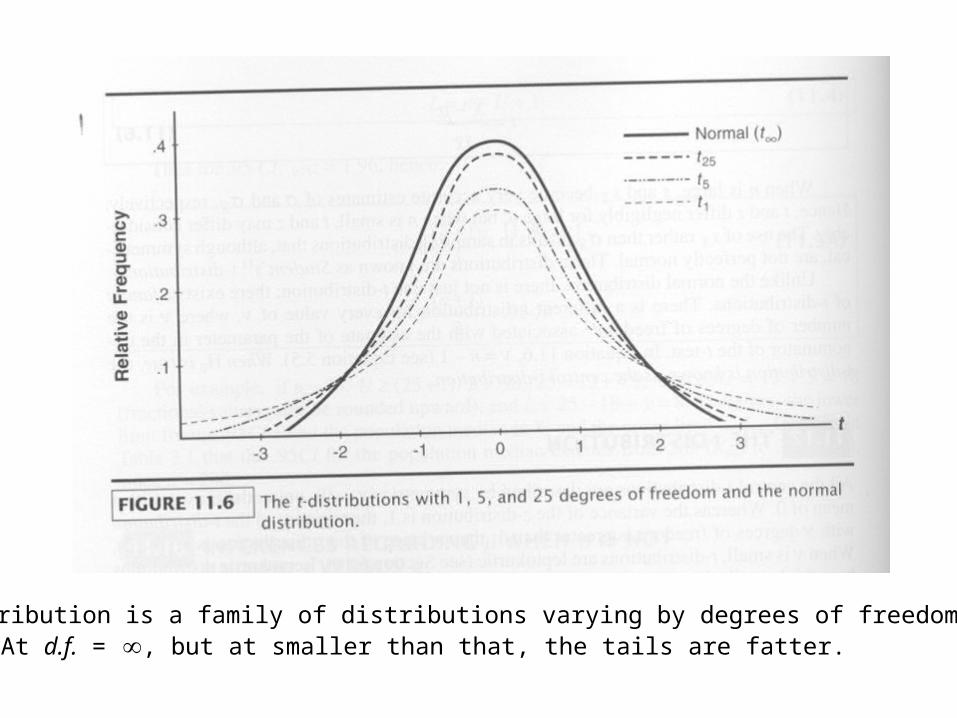
The t-distribution is a family of distributions varying by degrees of freedom (d.f., whered.f.=n-1). At d.f. = , but at smaller than that, the tails are fatter.

df = N - 1

Degrees of Freedom

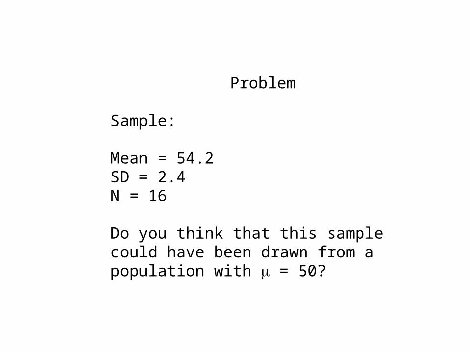
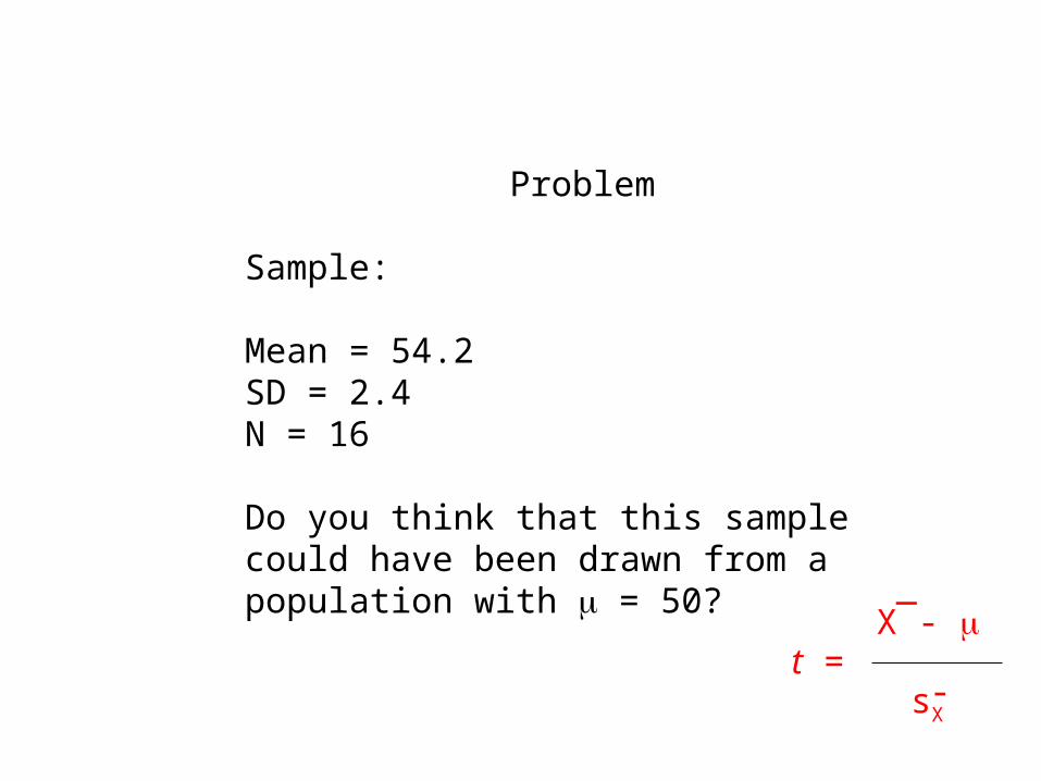
Problem

Sample:

Mean = 54.2SD = 2.4N = 16

Do you think that this sample could have been drawn from a population with = 50?

Problem

Sample:

Mean = 54.2SD = 2.4N = 16

Do you think that this sample could have been drawn from a population with = 50?

_

t = X -

sX-

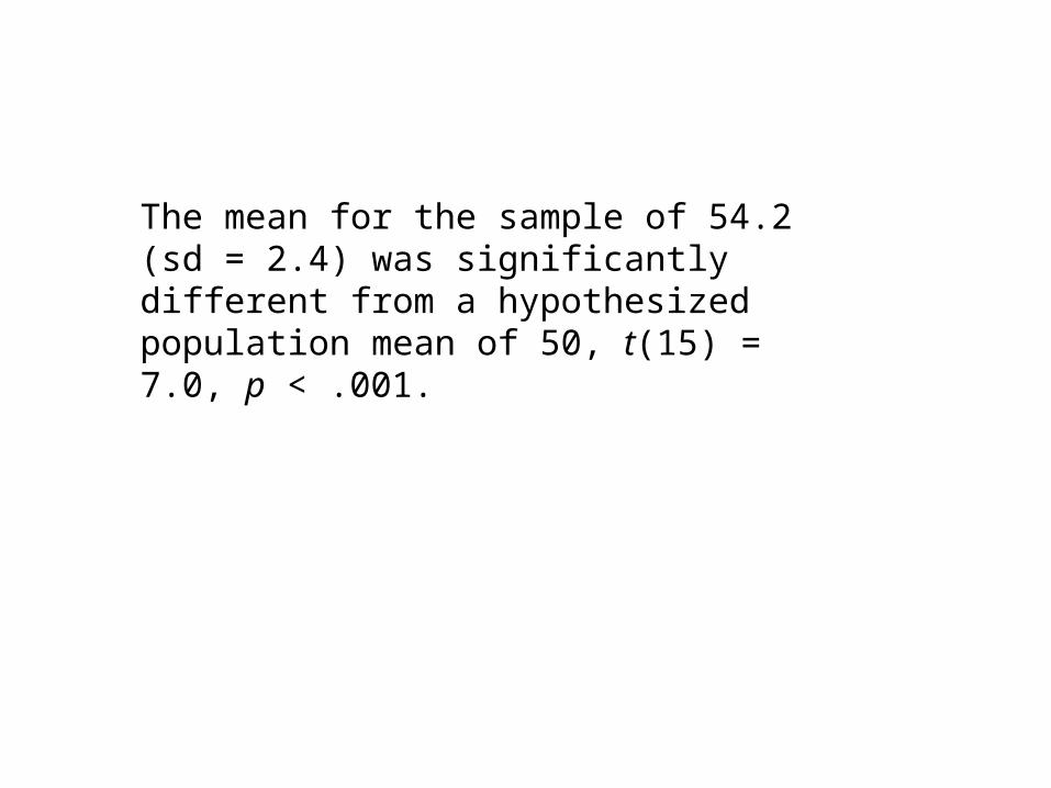
The mean for the sample of 54.2 (sd = 2.4) was significantly different from a hypothesized population mean of 50, t(15) = 7.0, p < .001.

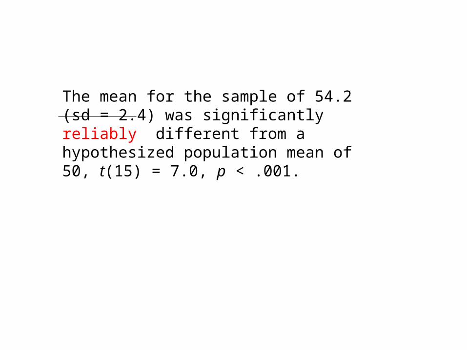
The mean for the sample of 54.2 (sd = 2.4) was significantly reliably different from a hypothesized population mean of 50, t(15) = 7.0, p < .001.

Interval Estimation (a.k.a. confidence interval)

Is there a range of possible values for that you can specify, onto which you can attach a statistical probability?

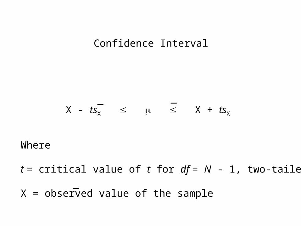
Confidence Interval

X - tsX X + tsX _ _

Where

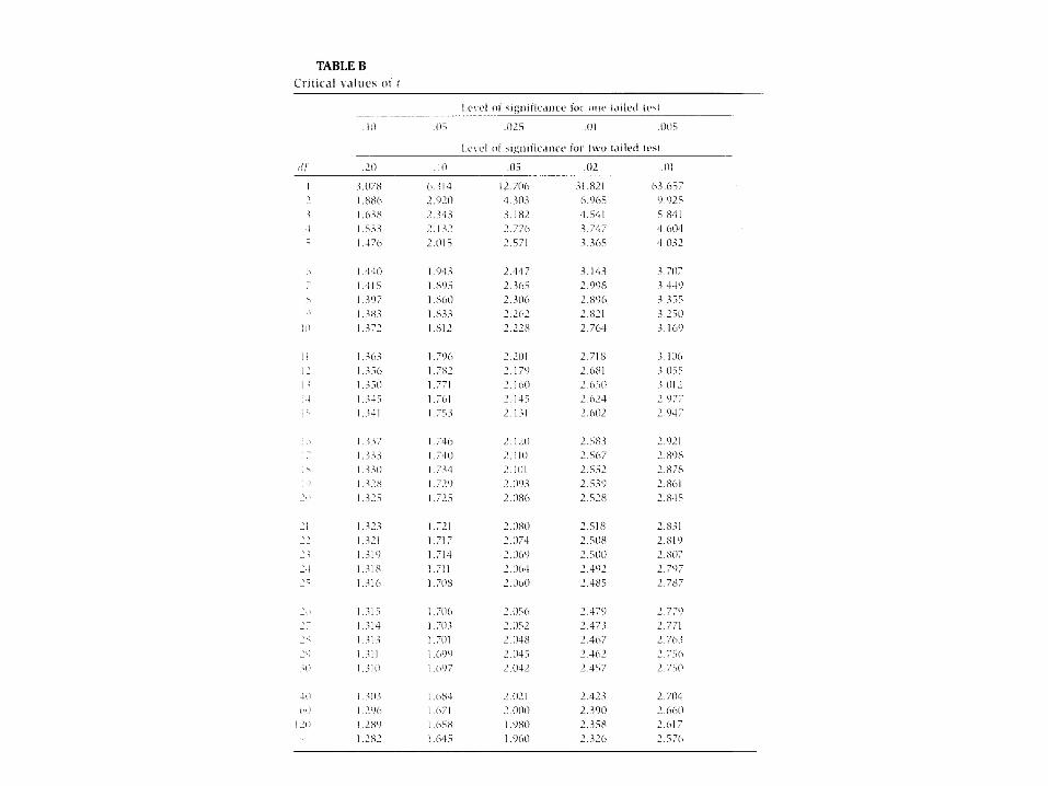
t = critical value of t for df = N - 1, two-tailed

X = observed value of the sample _

Oh no! Not again!!!