Money Illusion and Housing Frenzies�

Markus K. Brunnermeiery

Department of EconomicsPrinceton University

Christian Julliardz

Department of EconomicsLondon School of Economics

this version: February 21, 2006

AbstractA reduction in in�ation can fuel run-ups in housing prices if people su¤er

from money illusion. For example, investors who base their decision on whetherto rent or buy a house simply on monthly rent relative to current monthly mort-gage payments do not properly take into account that in�ation lowers futurereal mortgage payments. Therefore, they systematically misevaluate real estate.After empirically decomposing the price-rent ratio in a rational component andan implied mispricing, we �nd that (i) in�ation and the nominal interest rate ex-plain a large share of the time-series variation of the mispricing, (ii) the run-upsin housing prices starting in the late 1990s is reconcilable with the contempora-neous reduction in in�ation and nominal interest rates, and (iii) the tilt e¤ectalone is unlikely to rationalize these �ndings.

Keywords: Housing, Real Estate, Bubbles, In�ation, In�ation Illusion, MoneyIllusion, Mortgage Financing, Behavioral Finance

JEL classi�cation: G12, R2.

�We bene�ted from comments from Patrick Bolton, Smita Brunnermeier, James Choi, AlbinaDanilova, Emir Emiray, Will Goetzmann, Kevin Lansing, Chris Mayer, Alex Michaelides, StefanNagel, Filippos Papakonstantinou, Lasse Pedersen, Adriano Rampini, Bob Shiller, Matt Spiegel,Demosthenes Tambakis, and Haibin Zhu and seminar and conference participants at the Bank ofEngland, Cambridge-Princeton conference, CSEF, Duke-UNC Asset Pricing Conference, 2006 Econo-metric Society Winter Meetings in Boston, Federal Reserve Bank of Philadelphia, Harvard University,London School of Economics, NBER Behavioral Meetings, RFS Bubble Conference in Indiana, Whar-ton School at the University of Pennsylvania, University of Wisconsin-Madison Real Estate Researchconference, Yale Conference on Behavioral Economics. We also thank the BIS for providing part of thehousing data used in this analysis. Brunnermeier acknowledges �nancial support from the NationalScience Foundation and the Alfred P. Sloan Foundation.

yPrinceton University, Department of Economics, Bendheim Center for Finance, Princeton, NJ08544-1021 and CEPR, e-mail: markus@princeton.edu, http://www.princeton.edu/�markus

zDepartment of Economics, London School of Economics, Houghton Street, London WC2A 2AE,United Kingdom, e-mail: C.Julliard@lse.ac.uk, http://personal.lse.ac.uk/julliard/

1

1 Introduction

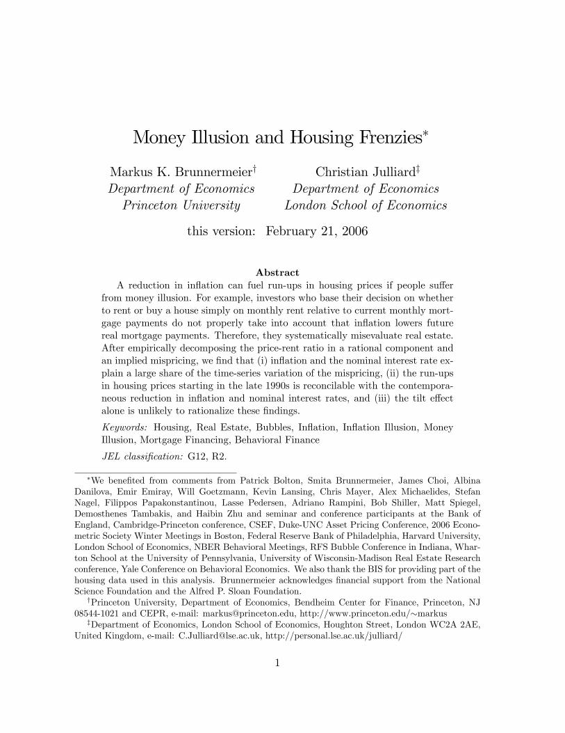
Housing prices have reached unprecedented heights in recent years. Sharp run-upsfollowed by busts are a common feature of the time-series of housing prices. Figure 1illustrates di¤erent real house price indexes and shows that this phenomenon has beenobserved in several OECD countries.

US UK CA AU

Panel A

1970 1974 1978 1982 1986 1990 1994 1998 200250

75

100

125

150

175

200

225

250

275

NLSE

DKCH

NO

Panel B

1970 1974 1978 1982 1986 1990 1994 1998 200250

75

100

125

150

175

200

225

250

275

Figure 1: Residential property (real) price indices for a group of Anglo-Saxon countries(left panel) and for Scandinavian countries and other European countries (right panel). Baseperiod is 1976, �rst quarter.

All the countries for which we have data show periods of sharp increases oftenfollowed by sharp downturns in real housing prices. Shiller (2005) documents similarpatterns for other countries and cities over shorter samples. Moreover, Case and Shiller(1989, 1990) document that house price changes are predictable and suggest that thismight be due to ine¢ ciency in the housing market. There are several potential reasonsfor this market ine¢ ciency �one of them being money illusion. The housing marketis particularly well suited to study money illusion, since frictions make it di¢ cult forprofessional investors to arbitrage possible mispricing away.In this paper we identify an empirical proxy for the mispricing in the housing market

and show that it is largely explained by movements in in�ation. In�ation matters andit matters in a particular way. Our analysis shows that a reduction in in�ation cangenerate substantial increases in housing prices in a setting in which agents are proneto money illusion. For example, people who base their decisions whether to rent or

2

buy a house simply on monthly rent relative to the current monthly payment of a �xednominal interest rate mortgage su¤er from money illusion. They mistakenly assumethat real and nominal interest rates move in lockstep. Hence, they wrongly attribute adecrease in in�ation to a decline in the real interest rate and consequently underestimatethe real cost of future mortgage payments. Therefore, they cause an upward pressureon housing prices when in�ation declines.To identify whether the link between house price movements and in�ation is due

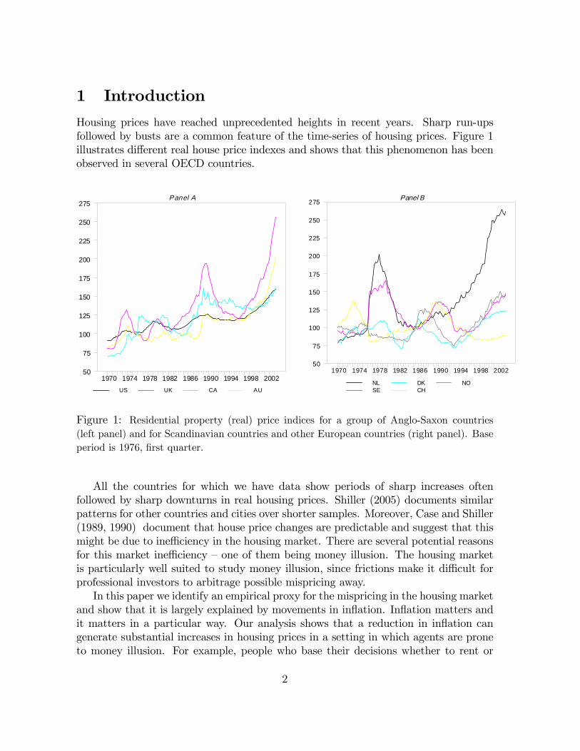
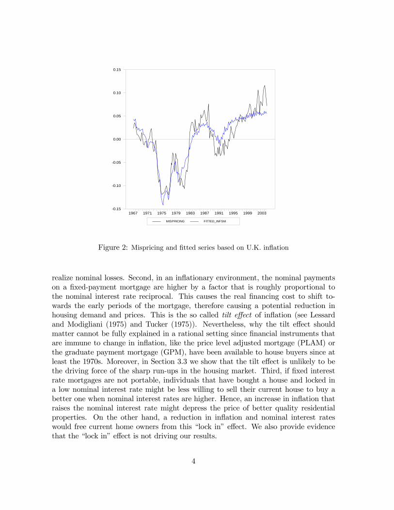
to money illusion, we �rst have to isolate the rational components of price changesthat are due to movements in fundamentals like land and construction costs, housingquality, property taxes, demographics (Mankiw and Weil (1989)) and time-varyingrisk premia.1 We do so in two stages. First, by focussing on the price-rent ratio weinsulate our analysis from fundamental movements that a¤ect housing prices and rentssymmetrically. Even though renting and buying a house are not perfect substitutes,the price-rent ratio implicitly controls for movements in the underlying service �ow.Second, we try to identify rational channels through which in�ation could in�uence theprice-rent ratio. For this purpose, using a Campbell and Shiller (1988) decomposition,we decompose the price-rent ratio into rational components (expected future returnson housing investment and rent growth rates)2 and a mispricing component. Aftercontrolling for rational channels, we �nd that in�ation has a substantial explanatorypower for the sharp run-ups and downturns of the housing market.Figure 2 depicts the time series of the (estimated) mispricing of the price-rent ratio

in the U.K. housing market and the �tted value of it using in�ation. The �rst thingto notice is that the mispricing shows sharp and persistent run-ups during the sampleperiod. Moreover, the �tted series closely tracks the momentum of the mispricing.

The close link between in�ation and housing prices could be due to the followingdeparture from rationality and/or �nancing frictions. First, as argued by Modiglianiand Cohn (1979), if agents su¤er from money illusion their evaluation of an asset willbe inversely related to the overall level of in�ation in the economy. This explanationof house price run-ups would also be in line with the �nding of McCarthy and Peach(2004) that the sharp run-up in the U.S. housing market since the late 1990s can belargely explained by taking into account the contemporaneous reduction of nominalmortgage costs. A special form of money illusion arises if home owners are averse to

1These variables alone are generally not able to capture the sharp run-ups in housing prices. It hasbecome common in the empirical literature to add cubic �frenzy�terms in the housing price regressions(see Hendry (1984) and Muellbauer and Murphy (1997)) and the rational expectations hypothesis hasbeen rejected by the data (Clayton (1996)).

2First, in�ation could be disruptive for the economy as a whole. This would lower agents�expec-tations of future real rent growth rates, thus reducing today�s price-rent ratio. Second, an increase inin�ation could make the economy riskier (or the agents more risk averse), thereby increasing the equi-librium risk-premium, which in turn reduces the price-rent ratio. Third, increase in in�ation reducesthe after-tax user cost of housing, potentially driving up housing demand (Poterba (1984)).

3

MISPRICING FITTED_INFSM

1967 1971 1975 1979 1983 1987 1991 1995 1999 2003­0.15

­0.10

­0.05

0.00

0.05

0.10

0.15

Figure 2: Mispricing and �tted series based on U.K. in�ation

realize nominal losses. Second, in an in�ationary environment, the nominal paymentson a �xed-payment mortgage are higher by a factor that is roughly proportional tothe nominal interest rate reciprocal. This causes the real �nancing cost to shift to-wards the early periods of the mortgage, therefore causing a potential reduction inhousing demand and prices. This is the so called tilt e¤ect of in�ation (see Lessardand Modigliani (1975) and Tucker (1975)). Nevertheless, why the tilt e¤ect shouldmatter cannot be fully explained in a rational setting since �nancial instruments thatare immune to change in in�ation, like the price level adjusted mortgage (PLAM) orthe graduate payment mortgage (GPM), have been available to house buyers since atleast the 1970s. Moreover, in Section 3.3 we show that the tilt e¤ect is unlikely to bethe driving force of the sharp run-ups in the housing market. Third, if �xed interestrate mortgages are not portable, individuals that have bought a house and locked ina low nominal interest rate might be less willing to sell their current house to buy abetter one when nominal interest rates are higher. Hence, an increase in in�ation thatraises the nominal interest rate might depress the price of better quality residentialproperties. On the other hand, a reduction in in�ation and nominal interest rateswould free current home owners from this �lock in�e¤ect. We also provide evidencethat the �lock in�e¤ect is not driving our results.

4

The balance of the paper is organized as follows. The next section reviews the re-lated literature on money illusion, borrowing constraint and speculative trading. Sec-tion 3 formally analyzes the link between in�ation and housing prices using the U.K.housing market as a case study.3 In particular: Section 3.1 derives a proxy for the valu-ation of the price-rent ratio of an agent that is a¤ected by money illusion and providesa �rst assessment of the empirical link between housing prices and in�ation; Section3.2 provides a method, based on the di¤erence between the objective and subjectivemeasure of the market, to identify the mispricing in the price-rent ratio, and showsthat the estimated mispricing is largely explained by changes in the rate of in�ation;Section 3.3 shows that it is unlikely that the tilt e¤ect is the driving force of the linkbetween in�ation and mispricing on the housing market. In Section 4 we extend ourempirical analysis to a cross-country setting and show that the strong link betweenhousing price mispricing and in�ation holds across countries. A �nal section concludesand a full description of the data sources is provided in the appendix.

2 Related Literature

2.1 Money Illusion

�An economic theorist can, of course, commit no greater crime than toassume money illusion.�Tobin (1972)

�In fact, I am persuadable �indeed, pretty much persuaded �that moneyillusion is a fact of life.�Blinder (2000)

In this section we sketch the links to the existing literature. In particular, wereview previous de�nitions of money illusion, relate it to the psychology literature andsummarize the empirical evidence on the e¤ect of money illusion on the stock market.

De�nition of Money Illusion. Fisher (1928, p. 4) de�nes money illusion as �thefailure to perceive that the dollar, or any other unit of money, expands or shrinks invalue.�4 Patinkin (1965, p. 22) refers to money illusion as any deviation from decisionmaking in purely real terms: �An individual will be said to be su¤ering from such anillusion if his excess-demand functions for commodities do not depend [...] solely onrelative prices and real wealth...�Leontief (1936) is more formal in his de�nition byarguing that there is no money illusion if demand and supply functions are homogenousof degree zero in all nominal prices.

3We �rst focus on the U.K. market since the longer sample period (1966:Q2�2004:Q4), the betterquality of the data, the availability of PLAMmortgage schemes, and the fact that most U.K. mortgagesare portable, allow for sharper and more robust inference.

4Most authors use the terms �money illusion�and �in�ation illusion�interchangeably. Sometimesthe latter is also used to refer to a situation where households ignore changes in in�ation.

5

Related Psychological Biases. Money illusion is also very closely related to otherpsychological judgement and decision biases. In a perfect world money is a veil andonly real prices matter. Individuals face the same situation after doubling all nominalprices and wages. The framing e¤ect states that alternative representations (framing)of the same decision problem can lead to substantially di¤erent behavior (Tverskyand Kahneman (1981)). Sha�r, Diamond, and Tversky (1997) document that agents�preferences depend to a large degree on whether the problem is phrased in real termsor nominal terms. This framing e¤ect has implications on (i) time preferences as wellas on (ii) risk attitudes. For example, if the problem is phrased in nominal terms,agents prefer the nominally less risky option to the alternative which is less risky inreal terms. That is, they avoid nominal risk rather than real risk. If on the other handthe problem is stated in real terms, their preference ranking reverses. The degree towhich individuals ignore real terms depends on the relative saliency of the nominalversus real frame.Anchoring is a special form of framing e¤ect. It refers to the phenomenon that

people tend to be unduly in�uenced by some arbitrary quantities when presented witha decision problem. This is the case even when the quantity is clearly uninformative.For example, the nominal purchasing price of a house can serve as an anchor for areference price even when the real price can be easily derived.5 Genesove and Mayer(2001) document that investors are reluctant to realize nominal losses.While individuals understand well that in�ation increases the prices of goods they

buy, they often overlook in�ation e¤ects which work through indirect channels, e.g.general equilibrium e¤ects. For example, Shiller (1997a) documents survey evidencethat the public does not think that nominal wages and in�ation comove over the long-run. Shiller (1997b) provides evidence that less than a third of the respondents in hissurvey study would have expected their nominal income to be higher if the U.S. hadexperienced higher in�ation over the last �ve years. The impact of in�ation on wagesis more indirect. In�ation increases the nominal pro�ts of the �rm, therefore it willincrease nominal wages. Similarly, the reduction in mortgage rates due to a decline inexpected future in�ation expectations is direct, while the fact that it will also lowerfuture nominal income is indirect. This inattention to indirect e¤ects can be relatedto two well known psychological judgement biases: mental accounting and cognitivedissonance. Mental accounting (Thaler (1980)) is a close cousin of narrow framing andrefers to the phenomenon that people keep track of gains and losses in di¤erent mentalaccounts. By doing so, they overlook the links between them. In our case, they ignorethe fact that higher in�ation a¤ects the interest rate of the mortgage and the laborincome growth rate in a symmetric way. Cognitive dissonance might be another reason

5Fisher (1928) provides several interesting examples of in�ation illusion due to anchoring. Forexample on pages 6-7 he writes about a conversation he had with a German shop woman during theGerman hyperin�ation period in the 1920s: �That shirt I sold you will cost me just as much to replaceas I am charging you [...] But I have made a pro�t on that shirt because I bought it for less.�

6

why individuals do not see that in�ation increases future nominal income. They havea tendency to attribute increases in nominal income to their own achievements thansimply to higher in�ation.6

In�ation Illusion and the Stock Market. To the best of our knowledge, we arethe �rst who empirically assess the link between money illusion and house prices.However, there are a list of papers that empirically document the impact of moneyillusion on stock market prices, often referred to as the �Modigliani-Cohn�hypothesis.Modigliani and Cohn (1979) argue convincingly that prices signi�cantly depart fromfundamentals since investors make two in�ation-induced judgement errors: (i) theytend to capitalize equity earnings at the nominal rate rather than the real rate and (ii)they fail to realize that �rms�corporate liabilities depreciate in real terms. Hence, stockprices are too low during high in�ation periods. Ritter and Warr (2002) document thatthe value-price ratio is positively correlated with in�ation and that this e¤ect is morepronounced for leveraged �rms. Moreover, they show that the in�ation and the value-price ratios are negatively correlated with future market returns. Using the Campbelland Shiller�s (1988) dynamic log-linear evaluation method and a subjective proxy forthe equity risk premium, Campbell and Vuolteenaho (2004) show in the time-seriesthat a large part of the mispricing in the dividend-price ratio can be explained byin�ation illusion.7 Our methodology builds on their approach with the advantage thatwe do not have to arbitrarily specify a proxy for the risk premium on the housinginvestment. In contrast, Cohen, Polk, and Vuolteenaho (2005) focus on the cross-sectional implications of money illusion on asset returns and �nd supportive evidencefor the �Modigliani-Cohn�hypothesis.Basak and Yan (2005) show, within a dynamic asset pricing model, that even though

the utility cost of money illusion (and hence the incentive to monitor real values) issmall, its e¤ect on equilibrium asset prices can be substantial. In the same spirit, Fehrand Tyran (2001) show that (under strategic complementarity) even if only a smallfraction of individuals su¤er from money illusion, the aggregate e¤ect can be large.

2.2 Borrowing Constraint and Speculation

Tilt e¤ect. Lessard and Modigliani (1975) and Tucker (1975) show that under nom-inal �xed payment and �xed interest rate mortgages, in�ation shifts the real burdenof mortgage payments towards the earlier years of the �nancing contract. This limitsthe size of the mortgages agents can obtain. This tilt e¤ect could lead to a reduction

6Shiller (1997a) also noted that �Not a single respondent volunteered anywhere on the questionnairethat he or she bene�ted from in�ation. [...] There was little mention of the fact that in�ationredistributes income from creditors to debtors.�

7Additional evidence on the time-series link between market returns and in�ation can be found inAsness (2000, 2003) and Sharpe (2002).

7

in housing demand. Kearl (1979) and Follain (1982) �nd an empirical link betweenin�ation and housing prices and argue that liquidity constraints could rationalize their�nding. Wheaton (1985) questions this simple argument in a life-cycle model andshows that several restrictive assumptions are needed for this to be the case.

Speculative Trading and Short-Sale Constraints. Borrowing constraints mightalso limit the amount of speculation. Harrison and Kreps (1978) show that speculativebehavior can arise if agents have di¤erent opinions, i.e. non-common priors. Said dif-ferently, even if they could share all the available information, they would still disagreeabout the likelihood of outcomes. Scheinkman and Xiong (2003) put this model in acontinuous-time setting and show that transaction costs dampen the speculative com-ponent of trading, but only have limited impact on the size of the bubble. Models ofthis type rely on the presence of short-sale constraints �which is a natural constraintin the housing market �to preempt the ability of rational agents to correct the mis-pricing. Other factors that limit arbitrage include noise-trader risk (DeLong, Shleifer,Summers, and Waldmann (1990)) and synchronization risk (Abreu and Brunnermeier(2003)).

3 Housing Prices and In�ation

We focus on the link between in�ation and the price-rent ratio. In principle, an agentcould either buy or rent a house to receive the same service �ow. However, rentingand buying a house are not perfect substitutes since households might derive extrautility from owning a house (e.g. ability to customize the interior, pride of ownership).Moreover, properties for rent might on average be di¤erent from properties for sale.8

Nevertheless, long-run movement in the rent level should capture long-run movementsin the service �ow. Furthermore, changes in construction cost, demographic changes,and changes in housing quality should at least in the long-run a¤ect house pricesand rent symmetrically. As a consequence, in studying mispricing on the housingmarket, we focus on the price-rent ratio. Gallin (2004) �nds that house prices andrents are cointegrated and that the price-rent ratio is a good predictor of future priceand rent changes. Compared to the price-income ratio, the price-rent ratio has theadvantage of being less likely to increase dramatically due to changes in fundamentals(e.g. in demography or property taxes). Moreover, Gallin (2003) empirically rejectsthe hypothesis of cointegration between prices and income using panel-data tests for

8The house price index re�ects all types of dwellings while rents tend to overweight smaller andlower quality dwellings. Given that high quality houses �uctuate more over the business cycle, thedata might show a spurious link between in�ation, nominal interests rate and the price-rent ratio ifin�ation and/or nominal interest rates had a clear business cycle pattern. We address this concernformally in Section 3.2.2 and show that this does not a¤ect our main �ndings.

8

cointegration, that have been shown to be more powerful than the time-series analog.This implies that the commonly used error correction representation of prices andincome would lead to erroneous frequentist inference. Finally, studying the price-rentratio is analogous to the commonly used price-dividend ratio to analyze the mispricingin the stock market.In this section we show �rst that a simple non-linear function of the nominal interest

rate is a proxy for the valuation of the price-rent ratio by an agent prone to moneyillusion. Empirically, we �rst document the correlation between nominal values andfuture price-rent ratios. To gain further understanding of this empirical link, we thendecompose the price-rent ratio into a rational component and an implied mispricing andstudy its comovements with in�ation. In this section we conduct our empirical analysisfocusing on U.K. data because the longer sample period (1966:Q2�2004:Q4) and thebetter quality of the data allow us to obtain a sharper and more robust inference. Thesubsequent Section 4 expands the analysis to a cross-country setting, con�rming theresults of the U.K. data.

3.1 Housing Prices and Money Illusion - A First-Cut 9

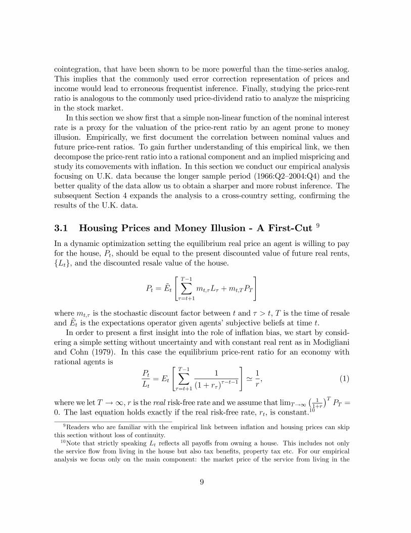
In a dynamic optimization setting the equilibrium real price an agent is willing to payfor the house, Pt, should be equal to the present discounted value of future real rents,fLtg, and the discounted resale value of the house.

Pt = ~Et

"T�1X�=t+1

mt;�L� +mt;TPT

#

where mt;� is the stochastic discount factor between t and � > t, T is the time of resaleand ~Et is the expectations operator given agents�subjective beliefs at time t.In order to present a �rst insight into the role of in�ation bias, we start by consid-

ering a simple setting without uncertainty and with constant real rent as in Modiglianiand Cohn (1979). In this case the equilibrium price-rent ratio for an economy withrational agents is

PtLt= Et

"T�1X�=t+1

1

(1 + r� )��t�1

#' 1

r, (1)

where we let T !1, r is the real risk-free rate and we assume that limT!1�

11+r

�TPT =

0. The last equation holds exactly if the real risk-free rate, rt, is constant.10

9Readers who are familiar with the empirical link between in�ation and housing prices can skipthis section without loss of continuity.10Note that strictly speaking Lt re�ects all payo¤s from owning a house. This includes not only

the service �ow from living in the house but also tax bene�ts, property tax etc. For our empiricalanalysis we focus only on the main component: the market price of the service from living in the

9

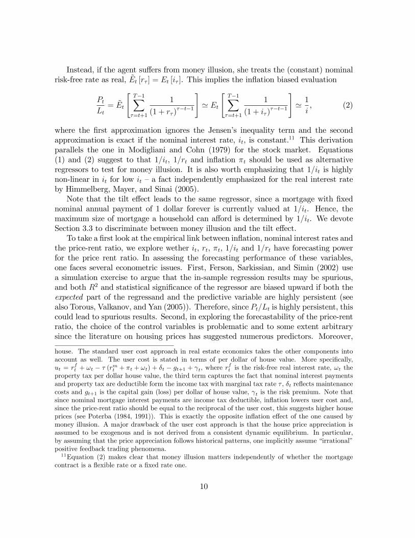
Instead, if the agent su¤ers from money illusion, she treats the (constant) nominalrisk-free rate as real, ~Et [r� ] = Et [i� ]. This implies the in�ation biased evaluation

PtLt= ~Et

"T�1X�=t+1

1

(1 + r� )��t�1

#' Et

"T�1X�=t+1

1

(1 + i� )��t�1

#' 1

i, (2)

where the �rst approximation ignores the Jensen�s inequality term and the secondapproximation is exact if the nominal interest rate, it, is constant.11 This derivationparallels the one in Modigliani and Cohn (1979) for the stock market. Equations(1) and (2) suggest to that 1=it, 1=rt and in�ation �t should be used as alternativeregressors to test for money illusion. It is also worth emphasizing that 1=it is highlynon-linear in it for low it �a fact independently emphasized for the real interest rateby Himmelberg, Mayer, and Sinai (2005).Note that the tilt e¤ect leads to the same regressor, since a mortgage with �xed

nominal annual payment of 1 dollar forever is currently valued at 1=it. Hence, themaximum size of mortgage a household can a¤ord is determined by 1=it. We devoteSection 3.3 to discriminate between money illusion and the tilt e¤ect.To take a �rst look at the empirical link between in�ation, nominal interest rates and

the price-rent ratio, we explore wether it, rt, �t, 1=it and 1=rt have forecasting powerfor the price rent ratio. In assessing the forecasting performance of these variables,one faces several econometric issues. First, Ferson, Sarkissian, and Simin (2002) usea simulation exercise to argue that the in-sample regression results may be spurious,and both R2 and statistical signi�cance of the regressor are biased upward if both theexpected part of the regressand and the predictive variable are highly persistent (seealso Torous, Valkanov, and Yan (2005)). Therefore, since Pt=Lt is highly persistent, thiscould lead to spurious results. Second, in exploring the forecastability of the price-rentratio, the choice of the control variables is problematic and to some extent arbitrarysince the literature on housing prices has suggested numerous predictors. Moreover,

house. The standard user cost approach in real estate economics takes the other components intoaccount as well. The user cost is stated in terms of per dollar of house value. More speci�cally,ut = rft + !t � � (rmt + �t + !t) + �t � gt+1 + t, where r

ft is the risk-free real interest rate, !t the

property tax per dollar house value, the third term captures the fact that nominal interest paymentsand property tax are deductible form the income tax with marginal tax rate � , �t re�ects maintenancecosts and gt+1 is the capital gain (loss) per dollar of house value, t is the risk premium. Note thatsince nominal mortgage interest payments are income tax deductible, in�ation lowers user cost and,since the price-rent ratio should be equal to the reciprocal of the user cost, this suggests higher houseprices (see Poterba (1984, 1991)). This is exactly the opposite in�ation e¤ect of the one caused bymoney illusion. A major drawback of the user cost approach is that the house price appreciation isassumed to be exogenous and is not derived from a consistent dynamic equilibrium. In particular,by assuming that the price appreciation follows historical patterns, one implicitly assume �irrational�positive feedback trading phenomena.11Equation (2) makes clear that money illusion matters independently of whether the mortgage

contract is a �exible rate or a �xed rate one.

10

Poterba (1991) outlines that the relation between house prices and forecasting variablesoften used in the literature has not been stable across sub-samples.We address both issues jointly. For the �rst problem, we remove the persistent

component of the price-rent ratio by constructing the forecasting errors

�t+1;t+1�� =

�Pt+1=Lt+1 � Et�� [Pt+1=Lt+1] for � > 0

Pt+1=Lt+1 for � = 0(3)

where � is the forecasting horizon and Et�� [Pt=Lt] is the (estimated) persistent compo-nent of the price-rent ratio and we introduce the convention that for � = 0, �t+1;t+1 =Pt+1=Lt+1. Second, we estimate Et�� [Pt=Lt] by �tting a reduced form vector auto re-gressive model (VAR) for Pt=Lt, the log gross return on housing, rh;t, the rent growthrate �lt and the log real return on the twenty-year Government Bonds, rt (constructedas the nominal rate, it, minus quarterly in�ation).12

Following Campbell and Shiller (1988), for small perturbations around the steadystate, the variables included in the VAR should capture most of the relevant informationfor the price-rent ratio. Indeed, the R2 of the VAR equation for Pt=Lt is about 99percent, which is consistent with previous studies that have outlined the high degreeof predictability of housing prices (see, among others, Kearl (1979), Follain (1982)and Muellbauer and Murphy (1997)). This approach for constructing forecast errors,�t+1;t+1�� , is parsimonious since it allows us to remove persistency from the dependentvariable without assuming a structural model. It is also conservative since the reducedform VAR is likely to over-�t the price-rent ratio. We use quarterly data over thesample period 1966 third quarter to 2004 fourth quarter.13

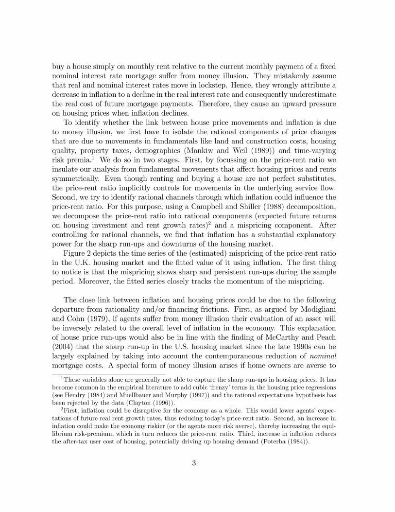
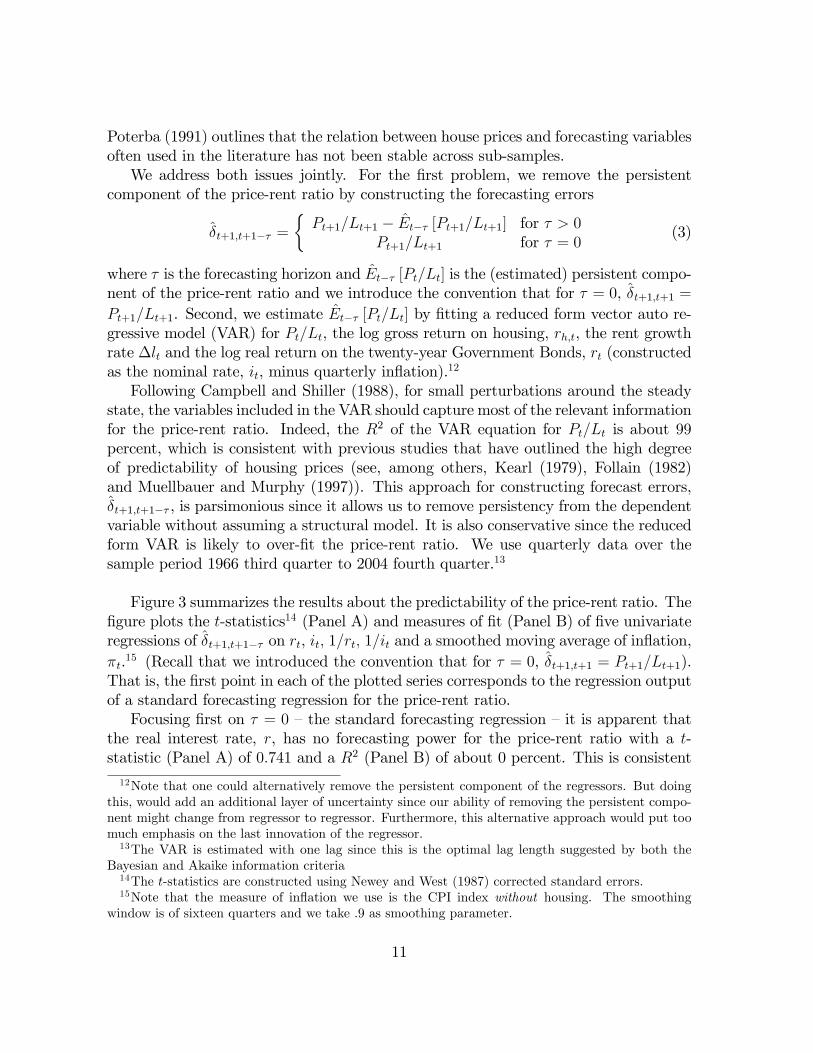
Figure 3 summarizes the results about the predictability of the price-rent ratio. The�gure plots the t-statistics14 (Panel A) and measures of �t (Panel B) of �ve univariateregressions of �t+1;t+1�� on rt, it; 1=rt; 1=it and a smoothed moving average of in�ation,�t.15 (Recall that we introduced the convention that for � = 0, �t+1;t+1 = Pt+1=Lt+1).That is, the �rst point in each of the plotted series corresponds to the regression outputof a standard forecasting regression for the price-rent ratio.Focusing �rst on � = 0 �the standard forecasting regression �it is apparent that

the real interest rate, r, has no forecasting power for the price-rent ratio with a t-statistic (Panel A) of 0:741 and a R2 (Panel B) of about 0 percent. This is consistent12Note that one could alternatively remove the persistent component of the regressors. But doing

this, would add an additional layer of uncertainty since our ability of removing the persistent compo-nent might change from regressor to regressor. Furthermore, this alternative approach would put toomuch emphasis on the last innovation of the regressor.13The VAR is estimated with one lag since this is the optimal lag length suggested by both the

Bayesian and Akaike information criteria14The t-statistics are constructed using Newey and West (1987) corrected standard errors.15Note that the measure of in�ation we use is the CPI index without housing. The smoothing

window is of sixteen quarters and we take :9 as smoothing parameter.

11

1/i inf lat ion i r 1/r

Panel A: t­statistics

s

0 1 2 3 4 5 6 7 8 9 10 11 12 13 14 15 16­4

­3

­2

­1

0

1

2

3

4

1/i inf lat ion i r 1/r

Panel B: R^2

s

0 1 2 3 4 5 6 7 8 9 10 11 12 13 14 15 160.000

0.025

0.050

0.075

0.100

0.125

0.150

Figure 3: t-statistics and R2 of univariate regressions of the forecast error �t+1;t+1�� oninterest rates and interest rate reciprocals (both nominal and real) as well as in�ation.

with the �nding of Muellbauer and Murphy (1997) that the real interest rate has noexplanatory power for movements in the real price of residential housing. The signof the slope coe¢ cient of the nominal interest rate, i, is negative suggesting that anincrease in the nominal interest rate reduces the price-rent ratio. The regressor isstatistically signi�cant only at the 10 percent level and explains about 5 percent ofthe variation in the price-rent ratio. The �gure also shows that lagged in�ation is asigni�cant predictor of the price-rent ratio and that the estimated slope coe¢ cient hasa negative sign, which is consistent with the Modigliani and Cohn (1979) argumentthat in�ation causes a negative mispricing in assets. This is also consistent with the�ndings of Kearl (1979) and Follain (1982) that housing demand is reduced by greaterin�ation. The regressor explains about 7 percent of the time variation in Pt=Lt. Fromthe predictive regression of the price-rent ratio on 1=rt �as suggested by equation (1) �we learn that this variable is not signi�cant nor has any forecasting power for the futureprice-rent ratio, reinforcing the conjecture that house prices do not tend to respondto changes in the real interest rate. However, the reciprocal of the nominal interestrate, 1=it, is highly statistically signi�cant and has a positive sign implying that theprice-rent ratio tends to comove with the valuation of agents prone to money illusion.Moreover, this regressor is able to explain about 9 percent of the time variation inthe price-rent ratio. Consistently with money illusion, in�ation �t shows a signi�cantnegative correlation with housing prices.Focusing on � > 0, we can assess whether the regressors considered have forecasting

power for the unexpected component of price-rent changes. It is clear from Figure 3 that

12

the real interest rate (both in terms of r and 1=r) generally has no explanatory powerfor the unexpected movements in the price-rent ratio. To the contrary, the nominalinterest rate, in�ation and the reciprocal of the nominal interest rate are statisticallysigni�cant forecasting variables of unexpected movements in the price-rent ratio, andexplain a substantial share of the time series variation of this variable.For robustness we check our results using the real interest rate implied by the

in�ation protected 10 years government securities, instead of using nominal interestrate minus in�ation, and using the implied in�ation instead of our smoothed in�ation.Unfortunately, this data is available only since 1982:Q1. Consistently with the previousresults, we �nd that this measure of the real interest rate also has no explanatory powerfor the price rent ratio: the regressor is not statistically signi�cant for any horizon � andits point estimates changes sign at some horizons. Moreover, using implied in�ationinstead of smoothed in�ation we obtain similar patterns as in Figure 3. The onlydi¤erence is that implied in�ation is not statistically signi�cant at two horizon levels,� = 1 and 2; this is likely to be due to the fact that we lose 16 years of quarterly datausing implied in�ation.Case and Shiller (1989, 1990) �nd that house price changes are predictable and argue

that this might be at odds with market e¢ ciency. To check whether this potentialdeparture from market e¢ ciency is connected with money illusion, we test whetherlagged in�ation and the reciprocal of the nominal interest rate and of the real interestrate help to predict the �rst di¤erence of the price-rent ratio. We �nd that (i) laggedin�ation and nominal interest rates explain 6 to 10 percent of the time series variationof the changes in the price-rent ratio, (ii) these regressors are statistically signi�cant atlevels between one and �ve percent, (iii) the estimated signs are consistent with moneyillusion, and (iv) the real interest rate does not have any predictive power for changesin the price-rent ratio.Collateral and downpayment constraints �as analyzed in Stein (1995), Bernanke

and Gertler (1989), Bernanke, Gertler, and Gilchrist (1996), Kiyotaki and Moore (1997)�combined with money illusion lead to an ampli�cation of the negative e¤ect of in�a-tion on housing prices.Of course, our results only show that the implicit stochastic discount factor is

related to in�ation. That is, the forecastability of the price-rent ratio could also bedue to preditable changes in the required risk-premium. However, this could also berational, hence it doesn�t need to be caused by money illusion.

These results suggest the presence of a strong empirical link between nominal valuesand the price-rent ratio but do not clarify whether this link is the consequence ofrational behavior or money illusion. We disentangle the role of money illusion in thenext subsection.

13

3.2 Decomposing the In�ation E¤ect

In�ation can a¤ect the price-rent ratio for rational reasons. In this subsection wedi¤erentiate the rational e¤ects of in�ation on the price-rent ratio �through expectedfuture rent growth rates and expected future returns on housing � from the e¤ectof in�ation on the mispricing. Note also that in�ation can in�uence expected futurereturns directly or through the taxation e¤ect mentioned earlier.

3.2.1 Methodology

We follow the Campbell and Shiller (1988) methodology, but also allow agents to havesubjective beliefs. Letting P be the price of housing and L be the rental payment, thegross return on housing, Rh, is given by the following accounting identity:

Rh;t+1 =Pt+1 + Lt+1

Pt:

Following Campbell and Shiller (1988), we log-linearize this relation around the steadystate but, given our focus on mispricing, we allow traders to have a probability measurefor the underlying stochastic process that is di¤erent from the objective one. As aconsequence, the steady state depends on the underlying measure of the traders. Underthe assumption that the price-rent ratio is stationary, we can log-linearize the lastequation as

rh;t+1 = (1� �) k + � (pt+1 � lt+1)� (pt � lt) + �lt+1,

where rh;t := logRh;t, pt := logPt, lt := logLt, �lt := lt� lt�1, � := 1=�1 + exp(l � p)

�,

l � p is the long run average rent-price ratio, and k is a constant. The log price-rentratio can be therefore rewritten (disregarding a constant term) as a linear combinationof future rent growth, future returns on housing and a terminal value

pt � lt = limT!1

"T�1X�=1

���1 (�lt+� � rh;t+� ) + �T (pt+T � lt+T )

#. (4)

Moving to excess rent growth rates, �let+� = �lt� rt, and excess returns (risk premia)on housing, reh;t = rh;t � rt, where rt is the real return on the long-term governmentbond (with maturity of 10 or 20 years), the price-rent ratio can be expressed as

pt � lt =

1X�=1

���1��let+� � reh;t+�

�+ lim

T!1�T (pt+T � lt+T ) . (5)

This equality also has to hold for any realization and hence, holds in expectation forany measure.

14

�Mispricing Measure. Note that if agents are not fully rational, the observedprice will deviate from the true �fundamental value� and hence the realized excessreturns reh;t+� are also distorted. Taking expectations and assuming that the transver-sality conditions hold, yields

pt � lt =

1X�=1

���1Et��let+�

��

1X�=1

���1Et�reh;t+�

�=

1X�=1

���1 ~Et��let+�

��

1X�=1

���1 ~Et�reh;t+�

�where Et is the objective expectation operator conditional on the information availableat time t and ~Et denotes investors�subjective (and potentially distorted) expectation.Adding and substracting

P1�=1 �

��1E��let+�

�from the second equation yields

pt � lt =1X�=1

���1E��let+�

��

1X�=1

���1 ~Et�reh;t+�

�+

1X�=1

���1�~Et � Et

� ��let+�

�| {z }

=: t

, (6)

where we use the convention�~Et � Et

�[x] := ~Et [x] � Et [x] and where t represents

the mispricing due to a distortion of beliefs about the future rent growth rate. Ifsubjective and objective expectation were to coincide, t would be zero. Note also

that t = �P1

�=1 ���1

�~Et � Et

� �reh;t+�

�.

So far our analysis applies to any form of belief distortion and is not speci�c tomoney illusion. In order to see how our de�nition of mispricing can capture moneyillusion, let�s consider the following example: as in Modigliani and Cohn (1979) indi-viduals fail to distinguish between nominal and real rates of returns. They mistakenlyattribute a decrease (increase) in in�ation �t to a decline (increase) in real returns, rh;t�or equivalently ignore that a decrease in in�ation also lowers nominal rent growthrate (�lt + �t), i.e. ~Et [�lt+� ] = Et [�lt+� � �t+� ]. Therefore, our mispricing measurereduces to

t = �1X�=1

���1Et [�t+� ] . (7)

That is, the mispricing and hence the price-rent ratio are increasing as expected in�a-tion declines. Note that in this particular case money illusion always causes a negativemispricing error. However, if individuals have a reference level of in�ation, say ��, thisis not necessarily true. In this case the last equation becomes

t = �1X�=1

���1Et [�t+� � ��] . (8)

15

Even though the level of mispricing is di¤erent with a reference level of in�ation, itscorrelation with in�ation is unchanged.To construct the empirical counterpart of t we follow Campbell (1991) and com-

pute the objective expectations of rent growth rates using a reduced form VAR. Thevariables included in the VAR are the log excess return on housing, reh;t, the log price-rent ratio, pt � lt, the excess rent growth rate, �let , and the exponentially smoothedmoving average of in�ation, �t. The VAR is estimated using quarterly data and thechosen lag length is one (both the Bayesian and the Akaike information criteria pre-fer this lag length for the estimated model). We obtain the empirical counterpart ofP1

�=1 ���1Et

�reh;t+�

�by substracting estimated expected rent growth terms from the

log price-rent ratio.The problem is that we do not observe ~Et

�reh;t+�

�. We follow Campbell and

Vuolteenaho (2004) and assume that ~Et�reh;t+�

�is governed by a set of risk-factors

�t. Hence, we can writeP1

�=1 ���1 ~Et

�reh;t+�

�= a + b1�t + �t. In order to determineP1

�=1 ���1 ~Et

�reh;t+�

��P1

�=1 ���1Et

�reh;t+�

�, we run an OLS of

P1�=1 �

��1Et�reh;t+�

�on

the risk-factor �t.

1X�=1

���1Et�reh;t+�

�= a+ b1�t + �t| {z }

=P1�=1 �

��1 ~Et[reh;t+� ]

+ t. (9)

We use di¤erent potential risk-factors. As suggested in Campbell and Vuolteenaho(2004) we use as �rst risk proxy the conditional volatility of an investment that is longon housing market and short on the 10 years government bonds. That is, we construct t as the OLS residual of the following linear regression

1X�=1

���1 \Et�reh;t+�

�= �+

8X�=0

b� ht�� + t. (10)

where the regressors ht�� includes seven lagged GARCH-estimates of the conditionalvolatility16 and a lagged VAR forecast of the left hand side variable. The latter actsas a control in the attempt of removing �t from the residual t. By doing so, we takea conservative approach in order not to overestimate the mispricing. We also reportresults using only seven lagged GARCH-estimates of the conditional volatility, denotedby

0t. As alternative risk factors we also used the canonical Fama-French risk factors.Some note of caution is appropriate about this decomposition. First, the measure

of mispricing t can depend crucially on the chosen subjective risk factor �t �which isarbitrary. Second, for the OLS construction in Equation (10) to be correct, �t should

16The �tted model is a GARCH(2,2) with an AR(1) component for the mean to take into accountthe persistence in housing returns.

16

be orthogonal to t. Third, in deriving our -mispricing we also assume that irrationalinvestors understand the iterated accounting identity in equation (4).In order to determine the link between the mispricing and in�ation we regress the

empirical counterpart of t on a set of variables ment to capture the impact of moneyillusion on the mispricing: �t, it, log (1=it).

"�Mispricing Measure. To derive the -mispricing we assumed that the transver-sality condition holds under both the objective and the subjective measure. We nowrelax this assumption and allow for explosive paths. Moreover, we avoid having tospecify exogenous risk factors, �, to indentify the implied mispricing due to explosivepaths.We de�ne a new measure of mispricing, "t, that under the null hypothesis of ratio-

nal pricing should be zero or at least orthogonal to proxies for money illusion. Thismispricing captures the di¤erence in expectations about future excess rent growth ratesand housing investment risk premia plus ~Et

�limT!1 �

T (pt+T � lt+T )�:

"t :=1X�=1

���1�~Et � Et

� ��let+� � reh;t+�

�+ ~Et

hlimT!1

�T (pt+T � lt+T )i. (11)

That is, "t is the di¤erence between observed log price-rent ratio and the log price-rentratio that would prevail if (i) all agents were computing expections under the objectivemeasure and (ii) the transversality condition under the objective measure holds, i.e.Et�limT!1 �

T (pt+T � lt+T )�= 0.

The "-mispricing can be expressed as a violation of the transversality conditionunder the objective measure

pt � lt =1X�=1

���1Et��let+� � reh;t+�

�+ Et

hlimT!1

�T (pt+T � lt+T )i

| {z }="t

.

To see this, take subjective expectation of equation (5) and subtract the above equationfrom it. Therefore, the "-mispricing captures bubbles which are due to potentiallyexploding paths, including the intrinsic bubbles analyzed in Froot and Obstfeld (1991).The price patterns depicted in Figure 1 make it di¢ cult to rule out a priori explosivepaths over certain subsamples. That is, imposing the objective transversality conditionmight be too strong an assumption. Explosive path might occur if for example agentsfail to understand that all the future realizations of returns and rent growth rates mustmap into the current price-rent ratio as Equation (4) implies. Note that we assume thatall traders have the same subjective measure. If traders have heterogeneous measuresand face short-sale constraints (as for example in Harrison and Kreps (1978)), "t couldalso be a¤ected by a speculative component.

17

To see how the "-mispricing relates to money illusion consider, as we did for the -mispricing, the Modigliani and Cohn (1979) benchmark. In this case we obtain thesame result as in Equation (7) and (8) with t replaced by "t. That is, money illusionimplies a negative correlation between the "-mispricing and �t, it, and � log (1=it).To estimate this mispricing we decompose the observed log price-rent ratio into

three components: the implied pricing error, "t, the discounted expected future rentgrowth, and the discounted expected future returns

pt � lt =1X�=1

���1Et�let+� �

1X�=1

���1Etreh;t+� + "t, (12)

where Et denotes conditional expectations computed using the estimated VAR.

3.2.2 Empirical Evidence

In this subsection we focus on the empirical links between mispricing measures andin�ation. Our �rst-cut analysis in Section 3.1 showed that nominal terms covary withprice-rent ratio rather than real terms. But this link might be due to rational chan-nels, frictions or money illusion. There are several rational channels through whichin�ation could a¤ect housing prices. First, if in�ation damages the real economy,P1

�=1 ���1Et

��let+�

�should be negatively related with in�ation. For example, this

could be the case of stag�ation caused by a cost-push shock. Second,P1

�=1 ���1Et [rh;t+� ]

could tend to rise if in�ation makes the economy riskier (or investors more risk averse),therefore driving up the required excess return on housing investment. If any of thesewere the case, the negative correlation between price-rent ratio and in�ation could sim-ply be the outcome of negative real e¤ects of in�ation or of time varying risk premiaon the housing investment. Most importantly, if there were no in�ation illusion, wewould expect our mispricing measures to be uncorrelated with �t, log (1=it), and it.Instead, the Modigliani and Cohn (1979) hypothesis of money illusion would predict anegative correlation between our mispricing measures and in�ation (and the nominalinterest rate), and a positive correlation between the mispricing and log (1=it).Table 1 Panel A reports the regression output of the three components of the log

price-rent ratio in Equation (6), on the exponentially smoothed moving average ofin�ation, �t, the nominal interest rate, it, and the log of its reciprocal, log (1=it).

18

Dependent Variables: Regressors:�t it log (1=it)

Slope coe¤. R2 Slope coe¤. R2 Slope coe¤. R2

Panel A: t �4:09

(13:479):83 �6:80

(11:765):74 :136

(8:020):69

1P�=1

���1Et�let+� �2:58

(2:390):12 �3:96

(1:938):09 :093

(2:083):12

�1P�=1

���1 ~Etreh;t+� 1:92

(1:066):03 3:60

(:931):03 �:050

(:595):02

Panel B:

0t �6:15

(2:483):17 �10:9

(2:668):17 :241

(2:823):19

"t �3:90(7:946)

:65 �6:30(6:927)

:55 :129(5:991)

:52

Table 1: Univariate Regressions on in�ation, nominal interest rate and illusion proxy.Newey and West (1987) corrected t-statistics in brackets.

The �rst row of Table 1 Panel A reports the univariate regression output of re-gressing the pricing errors on the proxies that are meant to capture in�ation illusion.All the regressors are highly statistically signi�cant and the estimated signs are theone we would expect under money illusion: the mispricing of the price-rent ratio tendsto rise as in�ation and nominal interest rates decrease and log (1=it) rises. Moreover,our proxies for in�ation bias are able to explain between one half and two thirds ofthe time series variation of the mispricing of the price-rent ratio. Ideally, we wouldlike to regress t on the objective expectation of future in�ation. One way to capturevariations in expected in�ation is to use the series of implied in�ation from the in�ationprotected 10 years government securities. Using this measure as explanator of t weobtain an R2 of :51 percent and a point estimate for the slope coe¢ cent of �5:06 witha t�statistics of 4:864.17The second row shows that expected future real rent growth rates seem to be nega-

tively correlated with in�ation and nominal interest rate (this last variable is signi�cantonly at the 10 percent level), and positively correlated with log (1=it). Nevertheless,only a small share (between 9 percent and 12 percent) of the time variation in expectedrent growth are explained by the regressors considered. These results are consistentwith a view in which in�ation in�uences the rent to price ratio partially due to the factthat an increase in in�ation damages the real economy. On the other hand, this couldsimply be the outcome of housing rents being more sticky than the general price level.The third row outlines that there is no signi�cant link between in�ation and (sub-

jectively expected) risk premia on the housing investment. The regressors considered

17Note that in this case, due to data availability problems, we use a sample starting in 1982:Q1.

19

are not statistically signi�cant and explain only between 2 percent and 4 percent of thetime series variation in expected future returns on housing. Moreover, the estimatedsigns of the regressors imply that in�ation is associated with a lower risk premium onhousing investment, i.e. in times of high in�ation the housing investment is consideredto be relatively less risky than investing in long-horizon government bonds. Since weuse a before-tax measure of returns on housing, this result could also be due to thefact that an increase in in�ation increases the after-tax return on housing (see Poterba(1984)), therefore requiring a lower before-tax risk premium.The sum of the slope coe¢ cients associated with each of the regressors in Table

1 Panel A is an estimate of the elasticity of the price-rent ratio with respect to thatregressor. Our results therefore imply that, on average, a one percent increase inin�ation (nominal interest rate) maps into a 4:75 (7:16) percent decrease in the priceof housing relative to rent, and that the largest contribution to this negative elasticityis given by the e¤ect of in�ation (nominal interest rate) on the mispricingPanel B of Table 1 reports the regression coe¢ cients for altnerative measures of

mispricings. Recall that 0t is the mispricing constructed without adding controls inEquation (10)18 and that "t is the mispricing constructed without specifying exogenousrisk factors and measures the mispricing that maps into a violation of the transversalitycondition under the objective measure.The �rst thing of interest is to compare the sizes of the mispricing of and 0.

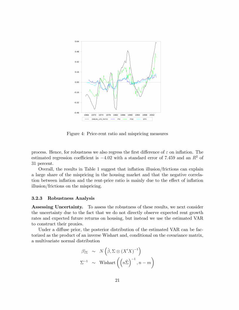
Figure 4 plots the price-rent ratio, and both -mispricing measures over our sampleperiod.First, notice that the measures of mispricing have generally the right pattern of

correlation with the price-rent ratio. Second, the -mispricing and "-mispricing capturea non-negligible fraction of the variation in the price-rent ratio. Third, as argued inthe methodological section, the 0-mispricing measure seems to attribute too large afraction of the movements in the price-rent ratio to the mispricing.Next, we analyze the explanatory power of the in�ation illusion proxies for the

0-mispricing and the "-mispricing. The �rst row of Panel B of Table 1 shows that 0t � as in�ation illusion would imply � covaries negatively (and signi�cantly) within�ation �t. Similarly, the univariate regressions with nominal interest rate it andlog (1=it) also deliver signi�cant results consistent with money illusion. Overall, theexplanatory power of the in�ation illusion proxies is reduced for the -mispricing.This is not surprising, since

0t in Figure 4 seems to overstate the time-variation of the

mispricing. The second row of Panel B of Table 1 reports the regression coe¢ cientof the "-mispricing on proxies of money illusion. Once again, the signs are consistentwith money illusion. Moreover, the estimated elasticities are fairly close to the onesobtained using t. Note that theoretically the "-mispricing could follow a martingale

18We also tried as alternative risk factors the canonical Fama-French risk factors and obtainedsimilar results as for the covariance of

0t and the money illusing proxies.

20

DMEAN_LPD_RATIO PSI PSI2 EPS

1966 1970 1974 1978 1982 1986 1990 1994 1998 2002­0.48

­0.32

­0.16

0.00

0.16

0.32

0.48

0.64

Figure 4: Price-rent ratio and mispricing measures

process. Hence, for robustness we also regress the �rst di¤erence of " on in�ation. Theestimated regression coe¢ cient is �4:02 with a standard error of 7:459 and an R2 of31 percent.Overall, the results in Table 1 suggest that in�ation illusion/frictions can explain

a large share of the mispricing in the housing market and that the negative correla-tion between in�ation and the rent-price ratio is mainly due to the e¤ect of in�ationillusion/frictions on the mispricing.

3.2.3 Robustness Analysis

Assessing Uncertainty. To assess the robustness of these results, we next considerthe uncertainty due to the fact that we do not directly observe expected rent growthrates and expected future returns on housing, but instead we use the estimated VARto construct their proxies.Under a di¤use prior, the posterior distribution of the estimated VAR can be fac-

torized as the product of an inverse Wishart and, conditional on the covariance matrix,a multivariate normal distribution

�j� � N��;� (X 0X)

�1�

��1 � Wishart��

n���1

; n�m

�

21

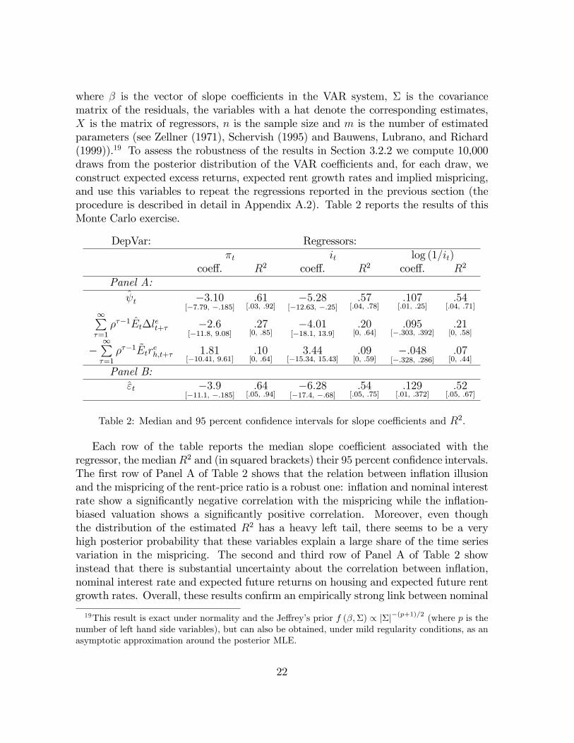
where � is the vector of slope coe¢ cients in the VAR system, � is the covariancematrix of the residuals, the variables with a hat denote the corresponding estimates,X is the matrix of regressors, n is the sample size and m is the number of estimatedparameters (see Zellner (1971), Schervish (1995) and Bauwens, Lubrano, and Richard(1999)).19 To assess the robustness of the results in Section 3.2.2 we compute 10,000draws from the posterior distribution of the VAR coe¢ cients and, for each draw, weconstruct expected excess returns, expected rent growth rates and implied mispricing,and use this variables to repeat the regressions reported in the previous section (theprocedure is described in detail in Appendix A.2). Table 2 reports the results of thisMonte Carlo exercise.

DepVar: Regressors:�t it log (1=it)

coe¤. R2 coe¤. R2 coe¤. R2

Panel A: t �3:10

[�7:79, �:185]:61

[:03, :92]�5:28

[�12:63, �:25]:57

[:04; :78]:107[:01, :25]

:54[:04, :71]

1P�=1

���1Et�let+� �2:6

[�11:8, 9:08]:27[0, :85]

�4:01[�18:1, 13:9]

:20[0, :64]

:095[�:303, :392]

:21[0, :58]

�1P�=1

���1 ~Etreh;t+� 1:81

[�10:41, 9:61]:10[0, :64]

3:44[�15:34, 15:43]

:09[0, :59]

�:048[�:328, :286]

:07[0, :44]

Panel B:"t �3:9

[�11:1, �:185]:64

[:05, :94]�6:28

[�17:4, �:68]:54

[:05; :75]:129

[:01, :372]:52

[:05, :67]

Table 2: Median and 95 percent con�dence intervals for slope coe¢ cients and R2.

Each row of the table reports the median slope coe¢ cient associated with theregressor, the medianR2 and (in squared brackets) their 95 percent con�dence intervals.The �rst row of Panel A of Table 2 shows that the relation between in�ation illusionand the mispricing of the rent-price ratio is a robust one: in�ation and nominal interestrate show a signi�cantly negative correlation with the mispricing while the in�ation-biased valuation shows a signi�cantly positive correlation. Moreover, even thoughthe distribution of the estimated R2 has a heavy left tail, there seems to be a veryhigh posterior probability that these variables explain a large share of the time seriesvariation in the mispricing. The second and third row of Panel A of Table 2 showinstead that there is substantial uncertainty about the correlation between in�ation,nominal interest rate and expected future returns on housing and expected future rentgrowth rates. Overall, these results con�rm an empirically strong link between nominal

19This result is exact under normality and the Je¤rey�s prior f (�;�) / j�j�(p+1)=2 (where p is thenumber of left hand side variables), but can also be obtained, under mild regularity conditions, as anasymptotic approximation around the posterior MLE.

22

values and the mispricing of the housing market, and suggest that this mechanism isthe main source of the negative correlation between the price-rent ratio and in�ationand the nominal interest rate.Note that these results are conditional on the estimated risk-factor �t. The reason

being that the uncertainty about �t hinges more upon what the risk-factor should bethan upon how it is estimated. To address we perfrom a similar robustness exerciseusing the "-mispricing �that does not depend on exogenous risk-factor. These resultsare reported in Panel B of Table 2 and �as in Panel A �are very similar to the onesin Table 1.

Assessing the Role of the Business Cycle. Unlike the price-dividend ratio in thestock market, the observed price-rent ratio is a less precise measure since the houseprice index re�ects all types of dwellings while the rent index tends to overweightsmaller and lower quality dwellings.The prices of high quality houses appreciate at a higher rate during booms, and

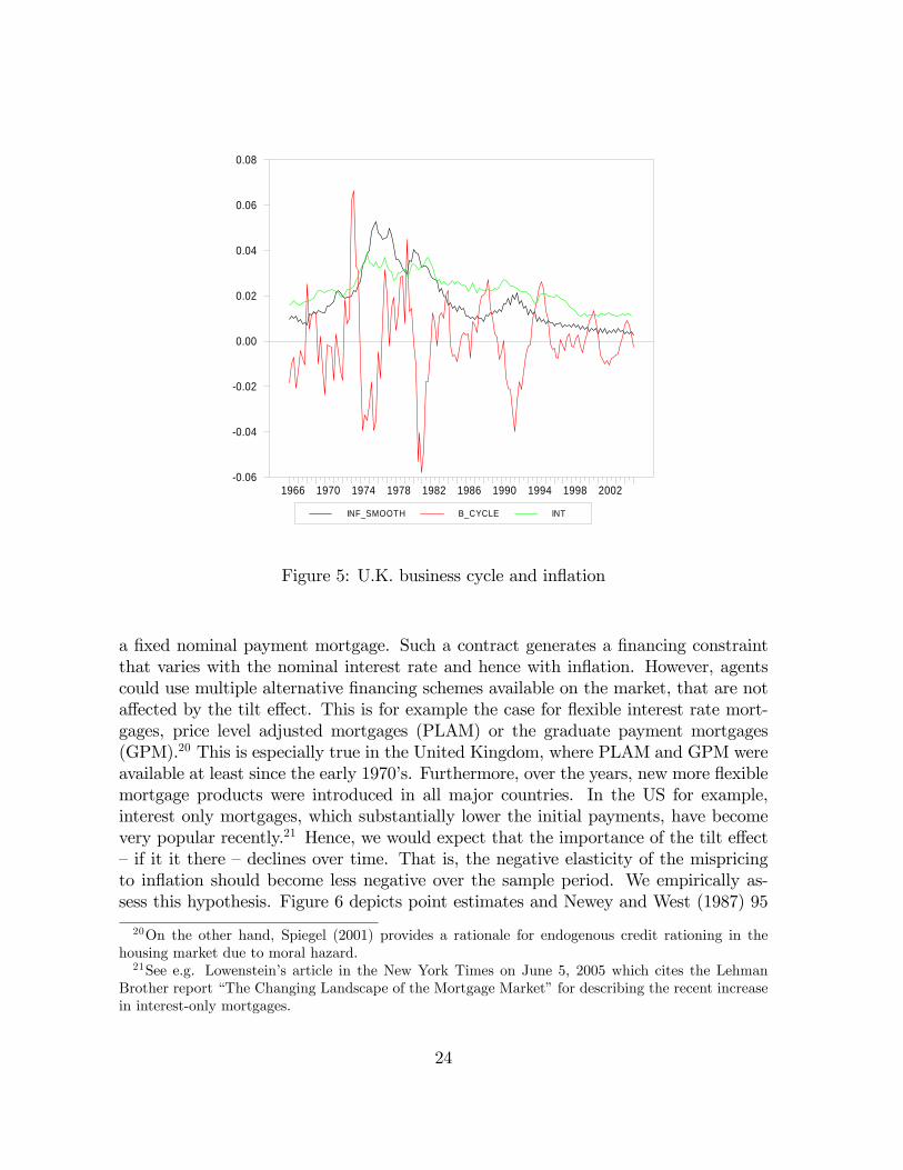
depreciate more during recessions, than cheaper houses do (see, among others, Poterba(1991) and Earley (1996)). This might cause the measured price-rent ratio to comovewith the business cycle. Hence, if in�ation and the nominal interest rate had a clearbusiness cycle pattern, our estimated mispricing measures could show a spurious cor-relation with these variables.Figure 5 plots the time series of the U.K. exponentially smoothed quarterly in�ation,

the return on the twenty-year Government Bonds, and the Hodrick and Prescott (1997)�ltered estimate of the GDP business cycle. Clearly, there does not seem to be a strongcontemporaneous correlation of in�ation and nominal interest rates with the businesscycle (the correlation coe¢ cients are �:16 and �:15 respectively). This suggests thatthe high degree of explanatory power that in�ation and the nominal interest rate havefor the housing market mispricing is unlikely to be due to the comovement of thesevariables with the business cycle. In Appendix A.3 we address this issue formally, andwe �nd that the inclusion of the business cycle in the OLS regressions for the mispricingmeasures (i) does not drive out the statistical signi�cance of �t, it and log (1=it), (ii)does not signi�cantly change the point estimates of the elasticities of the mispricingreported in Table 1, (iii) does not increase signi�cantly our ability to explain the timevariation in the mispricing, (iv) and that the business cycle alone has very little (inthe case of t and "t) or no (in the case of

0t) explanatory power for the mispricing

measures.

3.3 Tilt E¤ect

Our empirical results are consistent with money illusion. Nevertheless, we could alsobe capturing the tilt e¤ect of in�ation. Recall from Section 3.1 that the reciprocal ofthe nominal interest rate, 1=i, is proportional to the amount agents can borrow under

23

INF_SMOOTH B_CYCLE INT

1966 1970 1974 1978 1982 1986 1990 1994 1998 2002­0.06

­0.04

­0.02

0.00

0.02

0.04

0.06

0.08

Figure 5: U.K. business cycle and in�ation

a �xed nominal payment mortgage. Such a contract generates a �nancing constraintthat varies with the nominal interest rate and hence with in�ation. However, agentscould use multiple alternative �nancing schemes available on the market, that are nota¤ected by the tilt e¤ect. This is for example the case for �exible interest rate mort-gages, price level adjusted mortgages (PLAM) or the graduate payment mortgages(GPM).20 This is especially true in the United Kingdom, where PLAM and GPM wereavailable at least since the early 1970�s. Furthermore, over the years, new more �exiblemortgage products were introduced in all major countries. In the US for example,interest only mortgages, which substantially lower the initial payments, have becomevery popular recently.21 Hence, we would expect that the importance of the tilt e¤ect�if it it there �declines over time. That is, the negative elasticity of the mispricingto in�ation should become less negative over the sample period. We empirically as-sess this hypothesis. Figure 6 depicts point estimates and Newey and West (1987) 95

20On the other hand, Spiegel (2001) provides a rationale for endogenous credit rationing in thehousing market due to moral hazard.21See e.g. Lowenstein�s article in the New York Times on June 5, 2005 which cites the Lehman

Brother report �The Changing Landscape of the Mortgage Market�for describing the recent increasein interest-only mortgages.

24

percent con�dence intervals of the univariate regressions of the estimated mispricingon �t, it, and 1=it over a time-varying sample. We use the �rst ten years of data toobtain an initial estimate of the slope coe¢ cient associated with each regressor, and wethen add one data point at a time and update our estimates. For example, the pointcorresponding to 1992 �rst quarter is the estimated slope coe¢ cient over the sample1966 second quarter to 1992 �rst quarter.

Panel A: inflation

1977 1980 1983 1986 1989 1992 1995 1998 2001 2004­4.6

­4.4

­4.2

­4.0

­3.8

­3.6

­3.4

­3.2

­3.0Panel B: i

1977 1980 1983 1986 1989 1992 1995 1998 2001 2004­10.0

­9.5

­9.0

­8.5

­8.0

­7.5

­7.0

­6.5

­6.0

­5.5Panel C: log(1/i)

1977 1980 1983 1986 1989 1992 1995 1998 2001 20040.10

0.12

0.14

0.16

0.18

0.20

0.22

0.24

0.26

Figure 6: Point estimates and 95 percent Newey and West (1987) corrected con�dencebounds of slope coe¢ cients as sample size increases.

Figure 6 Panel A clearly reveals that the trend goes in the opposite direction of whatwe would expect if the tilt e¤ect were the driving mechanism behind the empiricallink between housing prices and in�ation. Over time, the negative relation betweenmispricing and in�ation becomes, if anything, more negative. The elasticity with re-spect to the interest rate is essentially �at. Only the elasticity with respect to the logof the nominal interest rate reciprocal seems to decline at the end of the sample, butthis reduction is not statistically signi�cant. Overall, these �ndings suggest that it isunlikely that the tilt e¤ect is the driving force of the empirical link between housingmispricing and in�ation.How does this �nding square with money illusion? Money illusion does not have a

clear implication whether the elasticity of mispricing to in�ation should vary over time.Nevertheless, the estimated increase (decrease in the slope coe¢ cient) is consistent witha setting in which households attention to in�ation depends on the recent history ofin�ation: after and during a period of high in�ation money illusion is very costly, hencehouseholds are more attentive to in�ation and less prone to money illusion; after andduring a period of low in�ation �as in the last part of our sample �the cost of moneyillusion is perceived to be low and hence money illusion is more wide-spread increasing

25

the elasticity of the mispricing to in�ation.

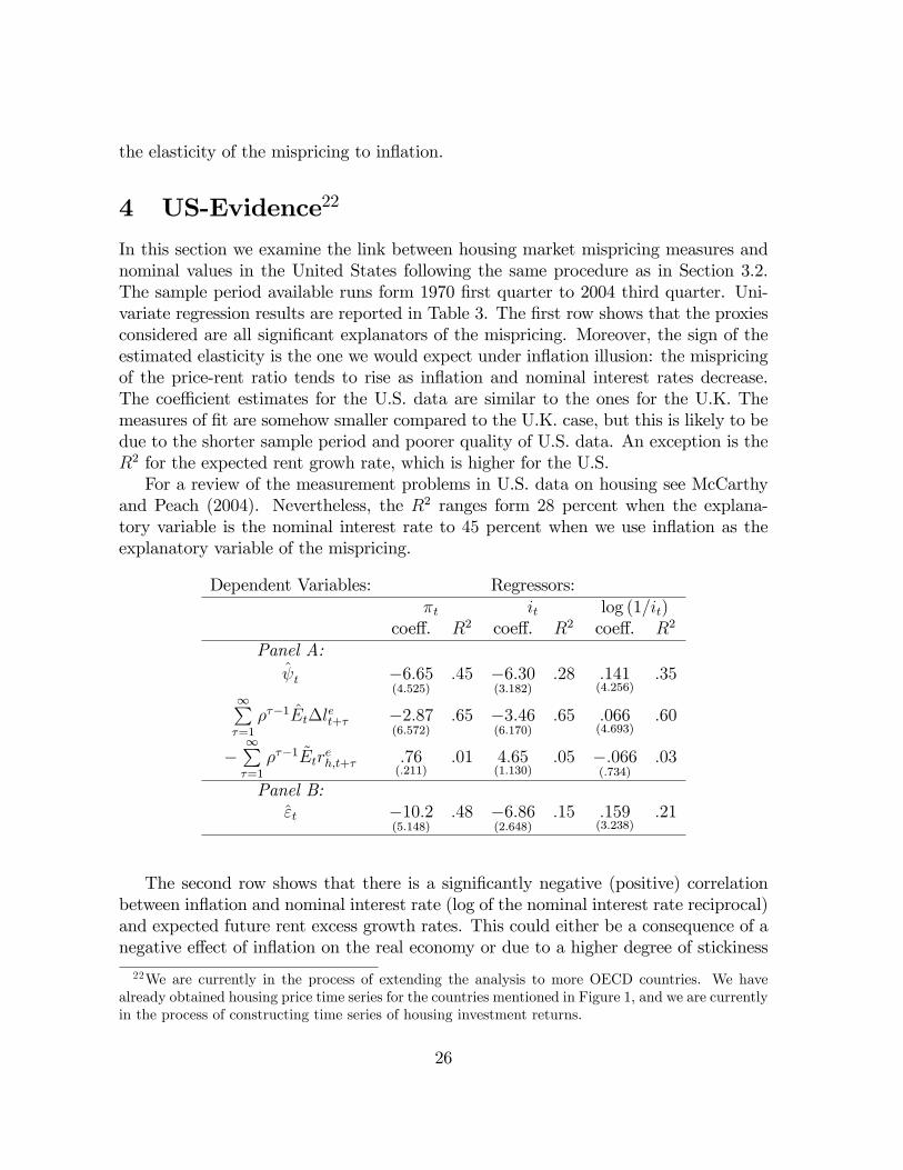
4 US-Evidence22

In this section we examine the link between housing market mispricing measures andnominal values in the United States following the same procedure as in Section 3.2.The sample period available runs form 1970 �rst quarter to 2004 third quarter. Uni-variate regression results are reported in Table 3. The �rst row shows that the proxiesconsidered are all signi�cant explanators of the mispricing. Moreover, the sign of theestimated elasticity is the one we would expect under in�ation illusion: the mispricingof the price-rent ratio tends to rise as in�ation and nominal interest rates decrease.The coe¢ cient estimates for the U.S. data are similar to the ones for the U.K. Themeasures of �t are somehow smaller compared to the U.K. case, but this is likely to bedue to the shorter sample period and poorer quality of U.S. data. An exception is theR2 for the expected rent growh rate, which is higher for the U.S.For a review of the measurement problems in U.S. data on housing see McCarthy

and Peach (2004). Nevertheless, the R2 ranges form 28 percent when the explana-tory variable is the nominal interest rate to 45 percent when we use in�ation as theexplanatory variable of the mispricing.

Dependent Variables: Regressors:�t it log (1=it)

coe¤. R2 coe¤. R2 coe¤. R2

Panel A: t �6:65

(4:525):45 �6:30

(3:182):28 :141

(4:256):35

1P�=1

���1Et�let+� �2:87

(6:572):65 �3:46

(6:170):65 :066

(4:693):60

�1P�=1

���1 ~Etreh;t+� :76

(:211):01 4:65

(1:130):05 �:066

(:734):03

Panel B:"t �10:2

(5:148):48 �6:86

(2:648):15 :159

(3:238):21

The second row shows that there is a signi�cantly negative (positive) correlationbetween in�ation and nominal interest rate (log of the nominal interest rate reciprocal)and expected future rent excess growth rates. This could either be a consequence of anegative e¤ect of in�ation on the real economy or due to a higher degree of stickiness

22We are currently in the process of extending the analysis to more OECD countries. We havealready obtained housing price time series for the countries mentioned in Figure 1, and we are currentlyin the process of constructing time series of housing investment returns.

26

in housing rents than in the general price level. The regressors considered are ableto explain between 60 percent and 65 percent of the time series variation in expectedfuture growth rates. The last row shows that there is a no statistically signi�cant linkbetween in�ation/nominal interest rate and future risk premia on housing investment.The coe¢ cients for the US are slightly lower compared to the UK coe¢ cient, whichis consistent with the di¤erent tax treatment of mortgage interest payments in bothcountries. These results imply a negative elasticity of the price-rent ratio to in�ation(nominal interest rates) of about 8:7 (5:1) and that the largest contribution to thiscomes from the e¤ect of in�ation (nominal interest rate) on the mispricing.Table 4 reports the results of a Monte Carlo exercise (described in Section A.2 of

the Appendix) analogous to the one presented in Section 3.2 and which, as in the caseof U.K. data, con�rms the soundness of the empirical link between mispricing in thehousing market and in�ation, nominal interest rate and the log of the nominal interestrate reciprocal. On the other hand, it shows that there is substantial uncertainty aboutthe rational links between in�ation (nominal interest rate) and the price-rent ratio, eventhough both variables show a signi�cantly negative correlation with the risk premiumon the housing investment.

DepVar: Regressors:�t it log (1=it)

coe¤. R2 coe¤. R2 coe¤. R2

Panel A: t �6:06

[�7:32, �2:76]:44

[:06, :66]�5:84

[�7:12, �2:14]:27

[:03; :66]:130

[:070, :155]:35

[:06, :60]1P�=1

���1Et�let+� �2:86

[�8:17, 1:53]:59

[:01, :96]�3:45

[�7:27, �0:53]:52

[:02, :71]:066

[:003, :149]:51

[:01, :70]

�1P�=1

���1t~Ereh;t+� :44

[�4:84, 3:21]:01[0, :09]

4:23[1:12, 5:82]

:04[:01, :12]

�:023[�:097, 0]

:07[0, :15]

Panel B:"t �10:2

[�16:2, �7:25]:48

[:36, :62]�6:83

[�10, �4:79]:15

[:11; :21]:159

[:115, :25]:21

[:16, :26]

Table 4: Median and 95 percent con�dence intervals for slope coe¢ cients and R2. U.S. data.

5 Conclusion

This paper studies the close link between in�ation and housing prices. It providessupportive evidence that agents are prone to money illusion since movements in themispricing in the housing market are largely explained by changes in in�ation, thenominal interest rate and a variable meant to capture money illusion. We also showthat the tilt e¤ect cannot fully explain our �ndings. These results hold for both theU.K. and the U.S. housing markets.

27

References

Abreu, D., and M. K. Brunnermeier (2003): �Bubbles and Crashes,�Economet-rica, 71(1), 173�204.

Asness, C. S. (2000): �Stocks versus Bonds: Explaining the Equity Risk Premium,�Financial Analysts Journal, 56(2), 96�113.

(2003): �Fight the Fed Model,� Journal of Portfolio Management, 30(1),11�24.

Ayuso, J., and F. Restoy (2003): �House Prices and Rents: An Equilibrium AssetPricing Approach,�working paper, Bank of Spain.

Basak, S., and H. Yan (2005): �Equilibrium Asset Prices and Investor Behavior inthe Presence of Money Illusion,�working paper, London Business School.

Bauwens, L., M. Lubrano, and J.-F. Richard (1999): Bayesian Inference inDynamic Econometric Models. Oxofrd University Press, Oxford.

Bernanke, B., and M. Gertler (1989): �Agency Costs, Net Worth, and BusinessFluctuations,�American Economic Review, 79(1), 14�31.

Bernanke, B., M. Gertler, and S. Gilchrist (1996): �The Financial Acceleratorand the Flight to Quality,�Review of Economics and Statistics, 48, 1�15.

Blinder, A. (2000): �Comment on �Near-Rational Wage and Price Setting and theLong-Run Phillips Curve�,�Brookings Papers on Economic Activity, 2000(1), 50�55.

Campbell, J. Y. (1991): �A Variance Decomposition for Stock Returns,�EconomicJournal, 101, 157�79.

Campbell, J. Y., and R. J. Shiller (1988): �The Dividend-Price Ratio and Ex-pectations of Future Dividends and Discount Factors,�Review of Financial Studies,1(3), 195�228.

Campbell, J. Y., and T. Vuolteenaho (2004): �In�ation Illusion and StockPrices,�American Economic Review Papers and Proceedings, 94, 19�23.

Case, K. E., and R. J. Shiller (1989): �The E¢ ciency of the Market for Single-Family Homes,�American Economic Review, 79, 125�137.

(1990): �Forecasting Prices and Excess Returns in the Housing Market,�AREUEA Journal, 18, 253�273.

28

Clayton, J. (1996): �Rational Expectations, Market Fundamentals and HousingPrice Volatility,�Real Estate Economics, 24(4), 441�470.

Cohen, R. B., C. Polk, and T. Vuolteenaho (2005): �Money Illusion in theStock Market: The Modigliani-Cohn Hypothesis,�Quarterly Journal of Economics,120(2), 639�668.

DeLong, J. B., A. Shleifer, L. H. Summers, and R. J. Waldmann (1990):�Noise Trader Risk in Financial Markets,� Journal of Political Economy, 98(4),703�738.

Earley, F. (1996): �Leap-Frogging in the UK Housing Market,�Housing Finance,32, 7�15.

Fehr, E., and J.-R. Tyran (2001): �Does Money Illusion Matter?,�American Eco-nomic Review, 91(5), 1239�1262.

Ferson, W. E., S. Sarkissian, and T. Simin (2002): �Spurious Regressions inFinancial Economics?,�NBER Working Paper 9143.

Fisher, I. (1928): Money Illusion. Adelphi, New York.

Follain, J. (1982): �Does In�ation A¤ect Real Behaviour? The Case of Housing,�Southern Economic Journal, 48, 570�582.

Froot, K. A., and M. Obstfeld (1991): �Intrinsic Bubbles: The Case of StockPrices,�American Economic Review, 81(5), 1189�1214.

Gallin, J. (2003): �The Long-Run Relationship between House Prices and Income:Evidence from Local Housing Markets,�Board of Governors of the Federal ReserveDiscussion Paper 2003-17.

(2004): �The Long-Run Relationship between House Prices and Rents,�Boardof Governors of the Federal Reserve Discussion Paper 2004-50.

Genesove, D., and C. Mayer (2001): �Loss Aversion and Seller Behavior: Evidencefrom the Housing Market,�Quarterly Journal of Economics, 116(4), 1233�1260.

Harrison, J. M., and D. Kreps (1978): �Speculative Investor Behavior in a StockMarket with Heterogeneous Expectations,� Quarterly Journal of Economics, 89,323�336.

Hendry, D. F. (1984): �Econometric Modelling of House Prices in the United King-dom,�in Econometrics and Quantitative Economics, ed. by D. F. Hendry, and K. F.Wallis. Basil Balckwell, Oxford.

29

Himmelberg, C., C. Mayer, and T. Sinai (2005): �Assessing High House Prices:Bubbles, Fundamentals, and Misperceptions,� Journal of Economic Perspectives,forthcoming.

Hodrick, R. J., and E. C. Prescott (1997): �Postwar U.S. Business Cycles: AnEmpirical Investigation,�Journal of Money, Credit, and Banking, 29(1), 1�16.

Kearl, J. (1979): �In�ation, Mortgage, and Housing,�Journal of Political Economy,85(5), 1115�1138.

Kiyotaki, N., and J. Moore (1997): �Credit Cycles,�Journal of Political Economy,105(2), 211�248.

Leontief, W. (1936): �The Fundametnal Assumptions of Mr. Keynes�MonetaryTheory of Unemployment,�Quarterly Journal of Economics, 5(4), 192�197.

Lessard, D., and F. Modigliani (1975): �In�ation and the Housing Market: Prob-lems and Potential Solutions,�Sloan Management Review, pp. 19�35.

Mankiw, G., and D. Weil (1989): �The Baby Boom, the Baby Bust, and theHousing Market,�Regional Science and Urban Economics, 19(2), 235�258.

McCarthy, J., and R. W. Peach (2004): �Are Home Prices the Next �Bubble�?,�FRBNY Economic Policy Review, 10(3), 1�17.

Modigliani, F., and R. Cohn (1979): �In�ation, Rational Valuation and the Mar-ket,�Financial Analysts Journal, 37(3), 24�44.

Muellbauer, J., and A. Murphy (1997): �Booms and Busts in the UK HousingMarket,�The Economic Journal, 107, 1701�1727.

Newey, W. K., and K. D. West (1987): �A Simple, Positive Semide�nite, Het-eroskedasticity and Autocorrelation Consistent Covariance Matrix,�Econometrica,55, 703�708.

Patinkin, D. (1965): Money, Interest, and Prices. Harper and Row, New York.

Piazzesi, M., and M. Schneider (2006): �In�ation and the Price of Real Assets,�.

Poterba, J. M. (1984): �Tax Subsidies to Owner-Occupied Housing: An Asset-Market Approach,�Quarterly Journal of Economics, 99(4), 729�752.

(1991): �House Price Dynamics: The Role of Tax Policy and Demography,�Brookings Papers on Economic Activity, 1991(2), 143�203.

30

Ritter, J. R., and R. S. Warr (2002): �The Decline of In�ation and the Bull Marketof 1982-1999,�Journal of Financial and Quantitative Analysis, 37(1), 29�61.

Scheinkman, J., andW. Xiong (2003): �Overcon�dence and Speculative Bubbles,�Journal of Political Economy, 111(6), 1183�1219.

Schervish, M. J. (1995): Theory of Statistics. Springer, New York.

Shafir, E., P. Diamond, and A. Tversky (1997): �Money Illusion,�QuarterlyJournal of Economics, 112(2), 341�374.

Sharpe, S. A. (2002): �Reexamining Stock Valuation and In�ation: The Implicationsof Analysts�Earning Forecasts,�Review of Economics and Statistics, 84(4), 632�648.

Shiller, R. J. (1997a): �Public Resistance to Indexation: A Puzzle,� BrookingsPapers on Economic Activity, 1997(1), 159�228.

(1997b): �Why Do People Dislike In�ation?,�in Reducing In�ation: Motiva-tion and Strategy, ed. by C. Romer, and D. H. Romer. University of Chicago Press,Chicago.

(2005): Irrational Exuberance. Princeton University Press, Princeton andOxford, 2nd edn.

Spiegel, M. (2001): �Housing Return and Construction Cycles,�Real Estate Eco-nomics, 29(4), 521�551.

Stein, J. C. (1995): �Prices and Trading Volume in the Housing Market: A Modelwith Downpayment E¤ects,�Quarterly Journal of Economics, 110(2), 379�406.

Thaler, R. (1980): �Toward a Positive Theory of Consumer Choice,� Journal ofEconomic Behavior and Organization, 1.

Tobin, J. (1972): �In�ation and Unemployment,�American Economic Review, 62(1),1�18.

Torous, W., R. Valkanov, and S. Yan (2005): �On Predicting Stock Returns withNearly Integrated Explanatory Variables,�Journal of Business, 78(1), forthcoming.

Tsatsaronis, K., and H. Zhu (2004): �What Drives Housing Price Dynamics:Corss-country Evidence,�BIS Quarterly Review, pp. 65�78.

Tucker, D. P. (1975): �The Variable-Rate Graduated-Payment Mortgage,� RealEstate Review, pp. 71�80.

31

Tversky, A., and D. Kahneman (1981): �The Framing of Decisions and the Psy-chology of Choice,�Science, 211, 453�458.

Wheaton, W. C. (1985): �Life-Cycle Theory, In�ation, and the Demand for Hous-ing,�Journal of Urban Economics, 18, 161�179.

Zellner, A. (1971): An Introduction to Bayesian Inference in Econometrics. Wiley,New York.

A Appendix

A.1 Data Description

A.1.1 U.K. Data

The house price series is from the Nationwide Building Society, and covers the sampleperiod 1966:Q2�2005:Q1. Over the period 1966:Q2�2005:Q5 the index is constructedas a weighted average using �oor area, therefore allowing to control for the in�uenceof house size. Over the periods 1974:Q1�1982:Q4, and 1983:Q1�1992:Q1 additionalcontrols (for region, property type, etc.) have been added in the construction of theindex. Since 1993 the index also takes into account changes in the neighborhoodclassi�cation. The rent series is constructed combining several sources available throughthe O¢ ce of National Statistics. Over the period 1966:01�1987:01 we use the CTMKLA:HRA series of rents on dwellings paid by tenants in the UK and we combine itwith the data on the stock of housing available trough the O¢ ce of the Deputy PrimeMinister. Over the period 1987:02�1987:12 we use the RPI-SGPE rent series of monthlypercent changes over one month. Over the period 1988:01�2005:02 we use the CZCQ -RPI series of percent changes in rent over one year. The rent-free tenancies are excludedfrom the calculation of average rents. To obtain a series in levels for the price-rent ratiowe scale the index series to match the level of the average price-rent ratio in 1990. Asinterest rate we use the 20-year par yield on British Government Securities availableover the sample 1963:Q4�2004:Q4. All the results presented in the paper are based onthe longest possible sample given the data at hand (1966:Q2�2004:Q4).The implied in�ation series, available over the period 1982:Q1-2005:Q1, is from the

Bank of England and is constructed using the in�ation protected 10 years governmentsecurities.The real GDP measure is the seasonally adjusted, chained volume measures with

constant 2002 prices and is available over the period 1955:Q1-2005:Q1 from the O¢ ceof National Statistics

32

A.1.2 U.S. Data

To construct the house price index series we use (i) the weighted repeat-sale housingprice index form the O¢ ce of Federal Housing Enterprise Oversight over the sub-sample1976:01�2004:03 and the (ii) Census Bureau housing price index (obtained through theBank of International Settlements) over the period 1970:01�1975:04. To construct therent index we use the CPI-Rent from the Bureau of Labor Statistics. We re-scale theindexes to levels to match the historical average of the U.S. price-rent ratio over thesame sample (as reported in Ayuso and Restoy (2003)). As long-run interest rate weuse the return on the 10-year Treasury bill. As measure of in�ation we use the CPIindex without housing.

A.1.3 Australian Data

The residential property price index is obtained from the Bank of International Set-tlements and available over the sample 1970:01�2005:01. The rental price index isobtained through Datastream for the period 1972:03�1980:01 and from the Bank ofInternational Settlements for the period 1980:02�2005:01. The CPI series is obtainedfrom Datastream. To construct the price-rent ratio and housing return series we rescalethe rental and property indexes so that their ratio matches the ratio of median price tomedian rent over the period 2000-2001available in the �2005 year book of Australia�from the Australian bureau of statistics (Tables 8.7 and 8.17).The estimation reportedare performed using the longest available sample given the data at hand: 1972:03-2005:01.

A.2 Assessing Uncertainty

To assess uncertainty in the regression results in Table 2, we report 95 percent con�-dence intervals for the estimated slope coe¢ cients and R2constructed via Monte Carlointegration by drawing form the posterior distribution of the estimated VAR coe¢ -cients. We proceed as follows:

1. We draw covariance matrices �� from the inverseWishart with parameters�n���1

and n�m.

2. Conditional on �� we draw a vector of coe¢ cients for the VAR, ��, from

�� � N��; �� (X 0X)

�1�:

3. Using the draws of the VAR slope coe¢ cients, ��, we construct expected dis-counted sums of rent excess growth rates (

P1�=1 �

��1 �Et�let+� ) and obtain the

33

excess housing returns (P1

�=1 ���1 �Etr

eh;t+i) in order to compute pricing errors �

and �".

4. We then regress � t, �",P1

�=1 ���1 �Et�l

et+� and

P1�=1 �

��1t

�Etreh;t+� on �t, it and

the log of the in�ation-biased evaluation 1=it; and we store the estimated slopecoe¢ cients and measures of �t.

5. We repeat this procedure 10,000 times and compute con�dence intervals for theOLS slope coe¢ cients associated with �t, it and the log of 1=it; and for thecorresponding measures of �t, from the corresponding percentiles of the MonteCarlo iterations.

A.3 Assessing the Role of the Business Cycle

To construct a business cycle proxy for the U.K. we follow Hodrick and Prescott (1997),that is we estimated the following state-space model

�yt = gt + ct (13)

gt = 2gt�1 � gt�2 + vt

where �yt is GDP growth from quarter t � 5 to quarter t, gt is the unobserved statevariable meant to capture the smooth time varying trend, and ct is the cyclical compo-nent. The variance of vt is normalized to be 1=1600 times the variance of the cyclicalcomponent, ct, as it is customary with quarterly data. This state-space representationis estimated via Kalman �lter and Kalman smoother.Table A1 reports OLS regressions of our mispricing measures ("t and t) on the

variables meant to capture money illusion (�t, it and log (1=i)) and the business cyclecomponent of GDP identi�ed by the H-P �lter (ct).

34

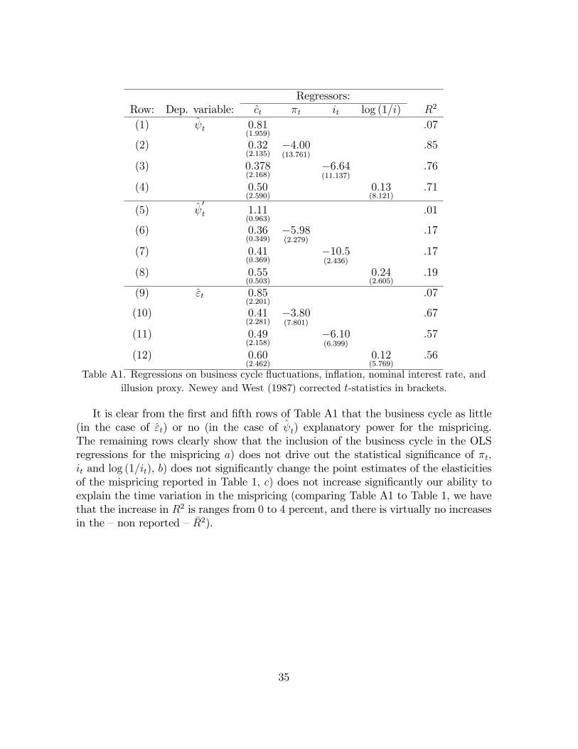
Regressors:Row: Dep. variable: ct �t it log (1=i) R2

(1) t 0:81(1:959)

:07

(2) 0:32(2:135)

�4:00(13:761)

:85

(3) 0:378(2:168)

�6:64(11:137)

:76

(4) 0:50(2:590)

0:13(8:121)

:71

(5) 0t 1:11

(0:963):01

(6) 0:36(0:349)

�5:98(2:279)

:17

(7) 0:41(0:369)

�10:5(2:436)

:17

(8) 0:55(0:503)

0:24(2:605)

:19

(9) "t 0:85(2:201)

:07

(10) 0:41(2:281)

�3:80(7:801)

:67

(11) 0:49(2:158)

�6:10(6:399)

:57

(12) 0:60(2:462)

0:12(5:769)

:56

Table A1. Regressions on business cycle �uctuations, in�ation, nominal interest rate, andillusion proxy. Newey and West (1987) corrected t-statistics in brackets.

It is clear from the �rst and �fth rows of Table A1 that the business cycle as little(in the case of "t) or no (in the case of t) explanatory power for the mispricing.The remaining rows clearly show that the inclusion of the business cycle in the OLSregressions for the mispricing a) does not drive out the statistical signi�cance of �t;it and log (1=it), b) does not signi�cantly change the point estimates of the elasticitiesof the mispricing reported in Table 1, c) does not increase signi�cantly our ability toexplain the time variation in the mispricing (comparing Table A1 to Table 1, we havethat the increase in R2 is ranges from 0 to 4 percent, and there is virtually no increasesin the �non reported � �R2).

35

B Things to remember

We run horse-races by NLLS with

"t = �+ �1 log (1=it) + �2 log (1= (k + rt))

"t = �+ �1 log �t + �2 log (1= (k + rt))

"t = �+ � log (1= (k + rt))

with k as free parameter, and even in this cases the real interest rate turned out to bestatistically irrelevant (�le: nonlinear_estimates.out).

36