OCEANENGGPAPER01D3Cd01

Ocean Engineering 43 (2012) 32–42

Contents lists available at SciVerse ScienceDirect

Ocean Engineering

0029-80

doi:10.1

n Corr

fax: þ9

E-m

prahlad

journal homepage: www.elsevier.com/locate/oceaneng

Discrete wavelet neural network approach in significant wave heightforecasting for multistep lead time

Paresh Chandra Deka n, R. Prahlada

Department of Applied Mechanics & Hydraulics, National Institute of Technology Karnataka, Surathkal, Karnataka 575025, India

a r t i c l e i n f o

Article history:

Received 10 March 2011

Accepted 2 January 2012

Editor-in-Chief: A.I. IncecikWavelet transform was hybridised with ANN naming Wavelet Neural Network (WLNN) for significant

wave height forecasting near Mangalore, west coast of India, upto 48 h lead time. The main time series

Keywords:

Artificial neural network

Wavelet transform

Multiresolution

Time series forecasting

Significant wave height

Hybridisation

18/$ - see front matter & 2012 Elsevier Ltd. A

016/j.oceaneng.2012.01.017

esponding author. Tel.: þ91 0824 2474000x3

1 0824 2474033.

ail addresses: [email protected] (P.C. Dek

[email protected] (R. Prahlada).

a b s t r a c t

Recently Artificial Neural network (ANN) was extensively used as non-linear inter-extrapolator for

ocean wave forecasting as well as other application in ocean engineering. In this current study, the

of significant wave height data were decomposed to multiresolution time series using discrete wavelet

transformations. Then, the multiresolution time series data were used as input of the ANN to forecast

the significant wave height at different multistep lead time. It was shown how the proposed model,

WLNN, that makes use of multiresolution time series as input, allows for more accurate and consistent

predictions with respect to classical ANN models. The proposed wavelet model (WLNN) results

revealed that it was better forecasted and consistent than single ANN model because of using

multiresolution time series data as inputs.

& 2012 Elsevier Ltd. All rights reserved.

1. Introduction

Real time forecast of ocean waves generated by wind over atime step of a few hours or days at a specific location is requiredfor planning and maintenance of any marine activities. The timeseries of significant wave height (Hs) can be modelled as arandom process. But Hs is not random, it has some correlationthat can be exploited to extrapolate the future from its pastvalues. In order to analyse such processes, recently soft comput-ing approach such as artificial neural networks, fuzzy logic andgenetic algorithms has been gaining popularity since last decadedue to its versatility in handling non linearity and somewhatextent to handle non stationarity. Classical time series modelssuch as ARMA (Auto regressive moving average), ARIMA (Autoregressive integrated moving average) are basically linear modelsassuming that data are stationary, and have a limited ability tocapture non-stationarities and non-linearity in data series. On theother hand, soft computing normally utilises tolerance to uncer-tainties, imprecision, and partial truth associated with inputinformation in order to come up with robust solution handlingnon-linearities and non-stationarities effectively.

Forecasting of ocean wave parameters using Artificial NeuralNetworks (ANN) was carried out by different authors since last

ll rights reserved.

315;

a),

decade. Deo and Naidu (1999), Rao et al. (2001) used ANN toforecast significant wave height for lead time up to 24 h. Agarwaland Deo (2002) compared ANN with ARMA and ARIMA using a3hourly significant wave height series and found that ANN wasmore accurate than latter for 3 and 6 h lead time. Makarynskyyet al. (2005) used ANN to forecast significant wave height andzero-up-crossing wave period for a leadtime up to 24 h.

ANN is suitable for handling large amounts of dynamic, noisyand non-linear data, specially for partially understood underlyingphysical processes. This makes them effective to time seriesmodelling problems of data-driven nature (Nourani et al., 2009).In spite of suitable flexibility of ANN, it may not be able to copewith non-stationary data if pre-processing of the input andoutput data is not performed (Cannas et al., 2006). As nonstationary signals are frequently encountered in a variety ofengineering fields such as ocean and earthquake, hybridisationof ANN with other techniques may provide effective modelling.

In the last decade, wavelet transform has become a usefultechnique for analysing variations, periodicities, and trends intime series (Lu, 2002; Xingang et al., 2003; Coulibaly and Burn,2004; Partal and Kucuk, 2006).

Wavelet analysis is multiresolution analysis in time andfrequency domain and is the important derivative of the Fouriertransform. Here, the original signal is represented by differentresolution intervals using discrete wavelet transform (DWT). Inother words, the complex significant wave height time series maybe decomposed into several simple time series using a DWT. Thus,some features of the subseries can be seen more clearly than the

www.elsevier.com/locate/oceaneng

www.elsevier.com/locate/oceaneng

dx.doi.org/10.1016/j.oceaneng.2012.01.017

mailto:[email protected]

mailto:[email protected]

dx.doi.org/10.1016/j.oceaneng.2012.01.017

Fig. 1. Multiresolution decomposition tree.

P.C. Deka, R. Prahlada / Ocean Engineering 43 (2012) 32–42 33

original signal series. These decomposed time series may be givenas inputs to ANN which can handle non-linearity efficiently;higher forecasting accuracy may be obtained. Forecasts are moreaccurate than that obtained by original signals due to the fact thatthe features of the subseries are obvious. This is why thehybridisation of wavelet transformation and neural network canperforms better than single ANN model.

In practice, analysing non-stationary and non linear timeseries is difficult because this series is affected by complexfactors. Using only one resolution component to model thesignificant wave height time series does not easily clarify theinternal mechanism of the phenomenon (Chou and Wang, 2004).Therefore, the hybrid wavelet transform and neural network thatuses several resolution components could be applied to modelsignificant wave height time series. The proposed Hybrid modelwhich uses multiscale signals as input data may present moreprobable forecasting rather than a single pattern input.

A hybrid wavelet predictor-corrector model was developed byZhou et al. (2008) for prediction of monthly discharge time seriesand showed that the model has higher prediction accuracy thanARIMA and seasonal ARIMA. Recently hybridisation of waveletand fuzzy has been applied by Ozger (2010) to forecast significantwave height and average wave period for a lead time up to 48 hand the results obtained was satisfactory and better than auto-regressive, ANN, and Fuzzy logic model.

In this study, it is aimed to illustrate a new approach tosignificant wave height forecasting based on combination ofdiscrete wavelet transform and artificial neural network techni-ques. This approach can improve the low level model accuraciesin long range (424 h) significant wave height forecasting. Forthis purpose, wavelet neural network (WLNN) algorithm has beenintroduced and employed to develop a significant wave heightforecasting model which has an ability to make forecasts up to48 h using 3hourly wave height observed data. The results ofWLNN model are compared with the results obtained from singleANN model. Also, the proposed WLNN model performance areevaluated to assess the model efficiency in the higher lead timesalongwith different decomposition levels.

2. Wavelet theory

A Wavelet transformation is a signal processing tool likeFourier transformation with the ability of analysing both station-ary as well as non stationary data, and to produce both time andfrequency information with a higher (more than one) resolution,which is not available from the traditional transformation (Four-ier and Short Term Fourier Transform).

The wavelet transform breaks the signal into its wavelets(small wave) which are scaled and shifted versions of the originalwavelet (mother wavelet).

The wavelet transformation is of two kinds:

�
Continuous wavelet transformation (CWT) and � Discrete wavelet transformation (DWT).
2.1. Continuous wavelet transformation (CWT)

The continuous wavelet transform (CWT) is defined in terms ofdilations and translations of a mother wavelet function C(t)

CWTcx ¼cc

x ðt,sÞ ¼1ffiffi

sp

Z 1�1

xðtÞcn t�ts

� �dt ð1Þ

Where s is the scale parameter, t is the translation parameter and the* denotes the complex conjugate, C(t) is the transforming function,and it is called the mother wavelet, and x(t) is the input signal.

As from above equation the analysis of a signal starts withkeeping a mother wavelet C(t) at the beginning of the signal x(t)and it is shifted forward over entire length of the signal. Aftercovering the full length of signal, a set of wavelet coefficients aregenerated at each step which are the measure of correlationbetween wavelet and the signal.

2.2. Discrete wavelet transformation (DWT)

Like continuous wavelet transformation the discrete wavelettransformation calculates the wavelet coefficients at discrete inter-vals of time and scale. In the DWT, filters of different cut-offfrequencies are used to analyse the signal at different scales. Thesignal x(t) is passed through a series of high pass filters and low passfilters and down sampled (i.e. throwing away every second datapoint) to analyse the high frequencies and low frequencies, respec-tively, as shown in the Fig. 1. The output from the high pass and lowpass filters are the approximation coefficients (A1, A2y An) anddetail coefficients (D1, D2yDn), respectively. The process of decom-posing a signal in to its sub bands or sub signals as represented inthe Fig. 1 is also termed as multiresolution signal decomposition.

The Discretized continuous wavelet transform produces N2

coefficients from a data set of length N; hence additional, orredundant information is locked up within the coefficients (Katulet al., 1994), which may or may not be a desired property. Thecontinuous wavelet transform and its discretization are redundant;that is the signal, which for real applications will be specified asdiscrete data set, is over specified by the transform coefficients.

The choice of wavelet transformation is in fact an important partof wavelet analysis and depends very much upon both the proper-ties of the signal under investigation and what the investigator islooking for. The continuous and discrete transform each have theirown favourable properties. Due to its redundancy, or over specifica-tion of the signal, the continuous wavelet transform is computa-tionally expansive and does not lend itself well to statistical analysis,whereas the zero redundancy of the discrete transformation lendsitself to the statistical analysis of the signal (Addison et al., 2001).

Logarithmic uniform spacing (Mallat, 1998) can be used for the s

scale discretization with correspondingly coarser resolution of thelocations, which allows a complete orthogonal wavelet basis to beconstructed. It allows for N transform coefficients to completelydescribe a signal of length N, i.e. with zero redundancy. These discretewavelets are not specified continuously, but rather at discretelocations on the time axis. The resulting discrete wavelet transform(DWT) can only be translated and dilated in discrete jumps.

For the signal x(t), the discrete wavelets have the form:

cm,n

t�ts

� �¼

1ffiffiffiffiffiffism

0

p ct�ntosm

o

smo

� �ð2Þ

where m and n are integers that control the wavelet dilation andtranslation, respectively, so is a fixed dilation step greater than 1;s is the scale and t is the location parameter and must be greaterthan zero. From the Eq. (2), it can be seen that the translation

P.C. Deka, R. Prahlada / Ocean Engineering 43 (2012) 32–4234

steps ntosmo depend upon the dilation, sm

o . Hence, discrete wavelettransform using Mallat algorithm was selected for decompositionand reconstruction of time series.

3. Methodology

Here, considering the dominance of persistence in the waveheight time series future significant wave heights to be forecastedfrom the past/previous wave heights. Significant wave heightupto previous four time steps (3hourly data�4¼12 h) weretaken as predictor variables. The input scenarios formed byvarious predictor configurations are;

[1]
Hs(t) [2] Hs(t), Hs(t�1) [3] Hs(t), Hs(t�1), Hs(t�2) [4] Hs(t), Hs(t�1), Hs(t�2), Hs(t�3).
Where Hs(t) is the current significant wave height.Also Hs(t�1), Hs(t�2), Hs(t�3) are onetime step, two time

step and three time step past wave height, respectively. Thepredictand is Hs(tþn) where n is the lead time. These input andoutput scenarios are same for both ANN and WLNN model. Forboth the models, testing data were selected from the sameportion of entire data which is the last 25% of the year.

Here, wavelet and ANN techniques are used together as acombined method. While wavelet transform is employed todecompose significant wave height time series into their spectralbands, ANN is used as a predictive tool that relates predictand(output) and predictors (inputs).

The real world observed time series are discrete, such as stream-flow, waveheight, etc. So discrete wavelet transform were selectedfor decomposition and reconstruction of significant waveheight timeseries. The original non-stationary time series were decomposedinto a certain number of stationary time series through discretewavelet transform such as, periodic properties, non-linearity anddependence relationship of the original time series were separated,so each wavelet transform series has obvious regularities. Then the

Fig. 2. Basic ANN model structure.

Fig. 3. Schematic diagram of th

ANN model was used to simulate the wavelet transform series in theform of approximations and details coefficients and gives recon-structed predicted significant wave heights in the output. Therefore,the prediction accuracy was expected to improve.

4. Artificial neural network

ANN is a flexible mathematical structure having an interconnectedassembly of simple processing elements or nodes, which emulatesthe function of neurons in the human brain. It possesses thecapability of representing the arbitrary complex non-linear relation-ship between the input and output of any system. Mathematically, anANN can be treated as universal approximators having an ability tolearn from examples without the need of explicit physics.

In this study, a single layer feed forward network with a backpropagation learning algorithm was been selected for the ANNmodel as shown in Fig. 2. Here, TRAIN LM (Levenberg–Marquardt)learning function, Tangent Sigmoid as transfer function waschosen and the analysis was carried out for different inputscenarios of previous time steps significant wave height data.The optimal structure of the ANN was selected based on meansquare error during training. The ANN model implementation wascarried out using MATLAB routines.

Here, the ANN was trained using Levenberg–Marquardt (LM)technique because it is more powerful and faster than theconventional gradient descent technique (Hagen and Menhaj,1994; Kisi, 2007). The application of LM to neural networktraining is described in Hagen and Menhaj (1994).

5. Wavelet neural network (WLNN)

Combination of wavelet transformation with other models wasreported since few years in different fields. Wang et al. (2003) usedWavelet-ANN combination in hydrology to predict hydrologicaltime series. Chen et al. (2007) used the same combination toforecast tides around Taiwan and South China Sea, and concludedthat the proposed model can prominently improve the predictionquality. Nourani et al. (2009) applied wavelet-ANN to rain fallrunoff modelling to forecast both long term and short term runoffdischarges for one day ahead. Deka et al. (2010) used hybridWavelet-ANN model to forecast significant wave height of stationnear marmugao port, Arabian Sea, and the results obtained for twotime steps ahead prediction was found satisfactory.

In the proposed (WLNN) model, the Discrete Wavelet Trans-formation discretized the input data (Hs) in to number of subsignals in the form of approximations and details and henceforth,these sub signals were used as input to ANN. The schematicdiagram of proposed WLNN model is shown in Fig. 3.

The objectives of WLNN model is to forecast t-hours aheadsignificant wave height from previous wave heights. Here, futurewave heights were taken as predictand and past wave heights aspredictor. After decomposing the time series into several

e proposed WLNN model.


resolution levels, each level subseries predictand data wereestimated from its corresponding separated predictor level.

Here, ANN part was constructed with appropriate sub-seriesbelongs to different scales as generated by DWT. These new seriesconsists of details and approximations were used as input to ANN.The sensitivity analysis for subseries variables with correspondingoutput variables was not performed for determining effective inputvariables as it was focussed only on decomposed subseries inputs.

In the proposed WLNN model, only input signals were decom-posed into wavelet coefficients so that ANN was exposed to largenumber of weights attached with higher input nodes duringtraining. Hence, the higher adaptability was achieved for input–output mapping. The output signals were kept as original serieswithout decomposition where reconstruction was not required.

Fig. 4. Location of the study area.

Table 1Statistical properties of the data.

Min Max Mean Skewness Kurtosis Std. deviation

0.25 3.09 1.025 0.78 0.4867 0.6289

6. Performance indices

The conventional performance evaluation such as correlationcoefficient is seems to be unsuitable for model evaluation(Legates and McCabe, 1999). Correlation coefficient has been usedin several data analysis. But as discussed by Kim and Park (OceanEng., 2005), it is not the best error statistics and may bemisleading compared to other error statistics such as Root MeanSquared Error (RMSE). Also, Keren and Kisi (J. Hydrology, 2006)also had a good discussion showing that a correlation coefficientvalue of close to one does not necessarily means a good predic-tion. The correlation coefficient shows the degree to which twovariables are linearly related. Here, coefficient of efficiency is usedto test the performance of model better than average or not.However, mean relative error, mean absolute error and Rootmean square error can be used for better evaluation of modelperformance. In this study, following performance indices basedon goodness of fit are used.

1.
Coefficient of efficiency,
CE¼ 1�

PðX�YÞ2P

x2

2.
Mean absolute error,
MAE¼

P9X�Y9N

3.
Root mean square error,
RMSE¼

ffiffiffiffiffiffiffiffiffiffiffiffiffiffiffiffiffiffiffiffiffiffiffiffiffiffiffiffiffiffiPNi ¼ 1 ðX�YÞ2

N

s

4.
Mean relative error, (%)
MRE¼1

N

XN

i ¼ 1

9X�Y9X� 100

where, X¼observed values, Y¼predicted values, N¼totalnumber of values, and x¼X�Xmean.

7. Study area

The data used in the current study are processed significantwave height (Hs) of the station SW4 (Latitude 1215603100 andlongitude 7414305800) located near west coast of India as shown inFig. 4, which was collected from New Mangalore Port Trust(NMPT) for the year 2004–2005.

From the statistical properties of the wave data presented inTable 1, it revealed that the data used in this study is not havingmuch significant variation. The value of standard deviation andkurtosis is also small means the most of the data are closelyspaced. Out of one year total data points of 2920 with threehourly (3 hr) time resolution, initial 75% of the data was used fortraining and remaining 25% of the data was used for testing themodel as shown in the Fig. 5.

8. Analysis and results

The data sets from one station located in Indian Ocean (westcoast) were used for model applications. The proposed WLNNmodel results were compared with classical ANN model results.Models were tested for various lead-times of 3, 6, 12, 24 and 48 h.Different input combinations as mentioned earlier were tried forsignificant wave height variables.

At the first stage, a multilayer perceptron (MLP) feed forwardANN model without data pre-processing was used to forecastsignificant waveheight. Each MLP was trained with 1–10 hiddenneurons in the hidden layer with Levenberg–Marquardt backpropagation as the training algorithm with sigmoidal activationfunction to optimise the parameters which were sufficient toproduce results for all lead-times.

In this study, a number of ANN models has been developedand the best model (optimised structure) out of various inputcombinations were selected. The best ANN model testing resultsobtained for input three (3rd scenarios) with seven (7) neurons inthe hidden layer based on various performances indices werepresented in Table 2.

It can be seen from the Table 2 that C.E (Coefficient ofefficiency) values changes with respect to lead-time forecast.For significant wave height, the C. E values were found rangesfrom 0.888 for 3 h lead-time to �0.071for 48 h lead-time. Forshort time forecasting, it seems to be quite satisfactory. But forlongtime forecasting, it is beyond acceptable accuracy.

The model efficiency is decreasing drastically as lead-timeprogresses beyond 6 h lead-time. The Root mean squared error

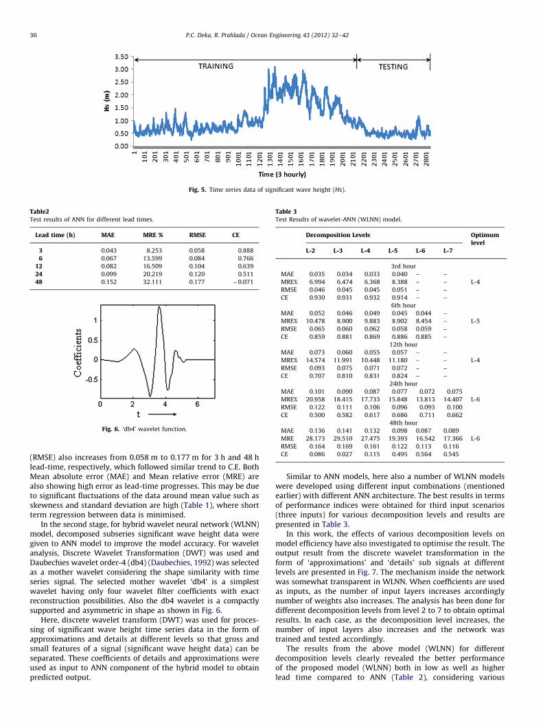
Fig. 5. Time series data of significant wave height (Hs).

Table2Test results of ANN for different lead times.

Lead time (h) MAE MRE % RMSE CE

3 0.043 8.253 0.058 0.888

6 0.067 13.599 0.084 0.766

12 0.082 16.509 0.104 0.639

24 0.099 20.219 0.120 0.511

48 0.152 32.111 0.177 �0.071

Fig. 6. ‘db4’ wavelet function.

Table 3Test Results of wavelet-ANN (WLNN) model.

Decomposition Levels Optimumlevel

L-2 L-3 L-4 L-5 L-6 L-7

3rd hour

MAE 0.035 0.034 0.033 0.040 – –

MRE% 6.994 6.474 6.368 8.388 – – L-4

RMSE 0.046 0.045 0.045 0.051 – –

CE 0.930 0.931 0.932 0.914 – –

6th hour

MAE 0.052 0.046 0.049 0.045 0.044 –

MRE% 10.478 8.900 9.883 8.902 8.454 – L-5

RMSE 0.065 0.060 0.062 0.058 0.059 –

CE 0.859 0.881 0.869 0.886 0.885 –

12th hour

MAE 0.073 0.060 0.055 0.057 – –

MRE% 14.574 11.991 10.448 11.180 – – L-4

RMSE 0.093 0.075 0.071 0.072 – –

CE 0.707 0.810 0.831 0.824 – –

24th hour

MAE 0.101 0.090 0.087 0.077 0.072 0.075

MRE% 20.958 18.415 17.733 15.848 13.813 14.407 L-6

RMSE 0.122 0.111 0.106 0.096 0.093 0.100

CE 0.500 0.582 0.617 0.686 0.711 0.662

48th hour

MAE 0.136 0.141 0.132 0.098 0.087 0.089

MRE 28.173 29.510 27.475 19.393 16.542 17.366 L-6

RMSE 0.164 0.169 0.161 0.122 0.113 0.116

CE 0.086 0.027 0.115 0.495 0.564 0.545


(RMSE) also increases from 0.058 m to 0.177 m for 3 h and 48 hlead-time, respectively, which followed similar trend to C.E. BothMean absolute error (MAE) and Mean relative error (MRE) arealso showing high error as lead-time progresses. This may be dueto significant fluctuations of the data around mean value such asskewness and standard deviation are high (Table 1), where shortterm regression between data is minimised.

In the second stage, for hybrid wavelet neural network (WLNN)model, decomposed subseries significant wave height data weregiven to ANN model to improve the model accuracy. For waveletanalysis, Discrete Wavelet Transformation (DWT) was used andDaubechies wavelet order-4 (db4) (Daubechies, 1992) was selectedas a mother wavelet considering the shape similarity with timeseries signal. The selected mother wavelet ‘db4’ is a simplestwavelet having only four wavelet filter coefficients with exactreconstruction possibilities. Also the db4 wavelet is a compactlysupported and asymmetric in shape as shown in Fig. 6.

Here, discrete wavelet transform (DWT) was used for proces-sing of significant wave height time series data in the form ofapproximations and details at different levels so that gross andsmall features of a signal (significant wave height data) can beseparated. These coefficients of details and approximations wereused as input to ANN component of the hybrid model to obtainpredicted output.

Similar to ANN models, here also a number of WLNN modelswere developed using different input combinations (mentionedearlier) with different ANN architecture. The best results in termsof performance indices were obtained for third input scenarios(three inputs) for various decomposition levels and results arepresented in Table 3.

In this work, the effects of various decomposition levels onmodel efficiency have also investigated to optimise the result. Theoutput result from the discrete wavelet transformation in theform of ‘approximations’ and ‘details’ sub signals at differentlevels are presented in Fig. 7. The mechanism inside the networkwas somewhat transparent in WLNN. When coefficients are usedas inputs, as the number of input layers increases accordinglynumber of weights also increases. The analysis has been done fordifferent decomposition levels from level 2 to 7 to obtain optimalresults. In each case, as the decomposition level increases, thenumber of input layers also increases and the network wastrained and tested accordingly.

The results from the above model (WLNN) for differentdecomposition levels clearly revealed the better performanceof the proposed model (WLNN) both in low as well as higherlead time compared to ANN (Table 2), considering various

Fig. 7. Sub signals after data decomposition through DWT at level-7.

Fig. 8. Observed and predicted time series for 3rd hour prediction.

Fig. 9. Observed and predicted time series for 6th hour prediction.



performance indices. The basic WLNN model of decompositionlevel 2 (L-2) was performing better than best ANN modelconsidering coefficient of efficiency and least error criteria. Also,other WLNN improved models based on different decompositionlevels (L-3, L-4, L-5, L-6, and L-7) performed better thanANN model.

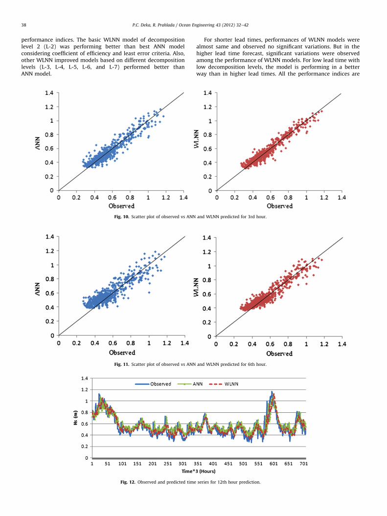
Fig. 10. Scatter plot of observed vs ANN


Fig. 12. Observed and predicted time

For shorter lead times, performances of WLNN models werealmost same and observed no significant variations. But in thehigher lead time forecast, significant variations were observedamong the performance of WLNN models. For low lead time withlow decomposition levels, the model is performing in a betterway than in higher lead times. All the performance indices are

and WLNN predicted for 3rd hour.

and WLNN predicted for 6th hour.

series for 12th hour prediction.


showing similar trend to rank a model based on low variation ofmaximum and minimum data value.

Again from the time series plot in Fig. 8 for three hoursprediction, it was observed that the ANN and WLNN modelresults were closely following the observed data. But in lowervalues, ANN was deviating far from WLNN and observed points




in sixth hour prediction (Fig. 9). The scatter plot ANN vsobserved and WLNN vs observed also reveals the same conclu-sion mentioned already as shown in Fig. 10 and Fig. 11. It wasclearly observed that the correlation was stronger betweenWLNN and observed points compared to ANN and observedpoints.




Fig. 18. Variation of RMSE over a lead time.


As lead time increases, the performances of ANN decreasesdrastically but, WLNN performance decreases gradually as shownin Figs. 12 and 13 in the time series plot and also in the scatterplots shown in Figs. 14 and 15. For lead time 48 h, the perfor-mance of both the models was highlighted in Figs. 16 and 17. Itwas observed from the Figs. 16 and 17 that the proposed WLNNmodel was almost following the trend of observed plot ascompared to ANN. Also, the variation of RMSE for different leadtime forecasting was presented for ANN and WLNN in Fig. 18. Agradual decline change was observed for WLNN where as suddendecline change was appeared for ANN after 24 h prediction.

In the WLNN, the results obtained for different lead times hadundergone different decomposition levels starting from 2 to 7. Ineach lead time analysis, there was an increasing trend in theperformance from low decomposition levels towards higherdecomposition levels. At the stage where the optimum value(higher C.E or lower Errors) is reached, the performance started todecline, and the analysis for the further decomposition levels wasstopped. The result corresponding to an optimum value wasconsidered to be the optimum decomposition level as illustratedin Fig. 19 and it was considered as the best model among theWLNN models.

Based on the results, it was noticed that the number ofdecomposition levels had some impact on the results. Since therandom parts of original time series were mainly in the firstresolution level, obviously the prediction errors were also mainlyin the first resolution level. Thus, the errors were not increased



proportionately with the resolution number. Usually, multilevel/multiresolution decomposition was performed to explore thefiner details of the signal. Higher level approximation showedsmoother version of the signal, while the lower level decomposi-tion was less smooth and had similar smoothness to the originalsignal (Fig. 7). Multilevel decomposition in the details indicatesdifferent natures of the signal.

Again for higher lead time forecast, higher model efficiencywas obtained at higher or optimum decomposition levels. Thesemay be due to the effect of correlation of more smoothenedsignals with flattened variability between the inputs and output.The generalisation capability of ANN seems to be very high with



Fig. 19. Depiction of optimum decomposition level for 3rd and 48th hour.


more wavelet transformed sub signals as inputs with optimalhidden neurons upto certain lead-time or optimal lead-time.

However, in wavelet transformation, higher decompositionlevels provide details and coefficients similar to persistence uptocertain level which can be assumed as optimum level. Althoughincreasing of decomposition level can progress the model ability,an optimum level was selected by trial and error in the study.

The main reason for WLNN performance improvement is thatWLNN model can extract the characteristics of wave heightvariation processes through decomposing the non-stationary timeseries of significant wave height into several stationary timeseries. In significant height time series, approximation coefficientsdenotes the deterministic components, such as tendency/trend,period and approximate period, etc. whereas details coefficientsdenotes the stochastic components and the noise. These station-ary time series can exhibit the fine structures of the wave heighttime series, reduce the interference between the deterministiccomponents and the stochastic components, and increase thestability of the data variation. Therefore, the prediction accuracyis improved.

9. Conclusions

In this study, a hybrid model of wavelet and ANN (WLNN) hasbeen developed to forecast significant wave height for higher leadtimes up to 48 h at west coast of India. The accuracy of WLNNmodel has been investigated for forecasting significant waveheight in the present study. The WLNN models were developedby combining two techniques such as ANN and DWT. The WLNNmodel results were also compared with single ANN model in thestudy. The WLNN and ANN model performance were tested byapplying to different input scenarios of past significant waveheight data near west coast station of India. The accuracy ofWLNN models was found to be much better than ANN model inmodelling significant wave height.

For the present study, the decomposition levels 4 and 5 werethe optimum levels for lower lead times (3 h–12 h). For the higherlead times (24 h–48 h), the decomposition level 6 was appearedto be the optimal level as per analysis. From the results, it isconfirmed that for lower lead times, lesser decomposition levelsare enough to achieve optimal performance. In higher lead time,the uncertainty demands more decomposition levels.

In this study, only one buoy station data of 3hourly timeresolution for one year was used and further studies using moredata from various stations may require reinforcing the conclu-sions. Also, Mallat algorithm with db4 type wavelet was used for

DWT for the time series data. Other type of wavelet with differentalgorithm could be used for construction of WLNN models.

The proposed wavelet model (WLNN) results shows that it isbetter forecasted and consistent than single ANN model due tothe use of multiresolution time series sub signals as inputs.

Acknowledgement

The authors acknowledged the New Mangalore Port Trust(NMPT), Mangalore for providing necessary data for the analysisand the Department of Applied Mechanics & Hydraulics, NationalInstitute of Technology Karnataka for the necessary infrastruc-tural support. The authors are also grateful to the reviewers fortheir valuable comments for improving the quality of the paper.

References

Addison, P.S., Murry, K.B., Watson, J.N., 2001. Wavelet transform analysis of openchannel wake flows. ASCE J. Eng. Mech. 127 (1), 58–70.

Agarwal, J.D., Deo, M.C., 2002. On-line wave prediction. Marine Structures 15,57–74.

Coulibaly, P., Burn, H.D., 2004. Wavelet analysis of variability in annual Canadianstreamflows. Water Resour. Res. 40 (3), 1–14.

Chou, C.M., Wang, R.Y., 2004. Application of wavelet based multi-model Kalmanfilters to real-time flood forecasting. Hydrol. Processes 18, 987–1008.

Cannas, B., Fanni, A., See, L., Sias, G., 2006. Data preprocessing for river flowforecasting using neural networks, wavelet transforms and data partitioning.Phys. Chem. Earth 31 (18), 1164–1171.

Chen, B.F., Wang, H.D., Chu, C.C., 2007. Wavelet and artificial neural networkanalyses of tide forecasting and supplement of tides around Taiwan and SouthChina Sea. Ocean Eng. 34, 2161–2175.

Deka, P.C., Mandal, S., Prahlada, R., 2010.Multiresulution wavelet-ANN model forsignificantwave height forecasting. Proceedings of national conference onhydraulics and water resources, HYDRO-2010, Dec-16–18th, pp. 230–235.

Deo, M.C., Naidu, C.S., 1999. Real time wave forecasting using neural network.Ocean Eng. 26 (3), 191–203.

Daubechies, I., 1992. Ten lectures on wavelets. Society for Industrial and AppliedMathematics, Philadelphia, PA.

Hagen, M., Menhaj, M., 1994. Training multilayer networks with the Marquardtalgorithm. IEEE Trans. Neural Networks 5 (6), 989–993.

Kisi, O., 2007. Streamflow forecasting using different artificial neural networkalgorithms. J. Hydrol. Eng., ASCE 12 (5), 532–539.

Katul, G.G., Parlange, M.B., Chu, C.R., 1994. Intermittency, local isotropy, and non-Gaussian statistics of atmospheric turbulence. Phys. Fluids 6 (7), 2480–2491.

Lu, R.Y., 2002. Decomposition of interdecadal and interannual components fornorth China rainfall in rainy season. Chin. J. Atmos. 26, 611–624.

Legates, D.R., McCabeJr., D.R., 1999. Evaluating the use of goodness-of-fit measuresin hydrologic and hydroclimatic model validation. Water Resour. Res. 35 (1),233–241.

Makarynskyy, O., Pires-Silva, A.A., Makarynskyy, D., Ventura-Soares, C., 2005.Artificial neural networks in wave predictions at the west coast of Portugal.Comput. Geosci. 31, 415–424.

Mallat, S.G., 1998. A wavelet tour of signal processing. Academic, San Diego.Nourani, V., Komasi, M., Mano, A., 2009. A multivariate ANN-wavelet approach for

rainfall–runoff modeling. Water Resour. Manag. 23, 2877–2894. doi:10.1007/s11269-009-9414.

dx.doi.org/10.1007/s11269-009-9414

dx.doi.org/10.1007/s11269-009-9414


Ozger, M., 2010. Significant wave height forecasting using wavelet fuzzy logicapproach. Ocean Eng. 37, 1443–1451.

Partal, T., Kucuk, M., 2006. Flow forecasting for a Hawaii stream using ratingcurves and neural networks. J Hydrol. 317, 63–80.

Rao, S., Mandal, S., Prabhaharan, N., 2001.Wave forecasting in near real time basisusing neural networks. In: Proceedings of International Conference in OceanEng., ICOE-2001. Ocean Engineering Centre, IIT Madras, 103–108.

Xingang, D., Ping, W., Jifan, C., 2003. Multiscale characteristics of the rainy seasonrainfall and interdecadal decaying of summer monsoon in North China. Chin.Sci. Bull. 48, 2730–2734.

Zhou, H.C., Peng, Y., Liang, G.H., 2008. The research of monthly dischargepredictor-corrector model based on wavelet decomposition. Water Resources

Manag. 22, 217–227.

Documents

OCEANENGGPAPER01D3Cd01