박사 학위논문

Ph. D. Dissertation

초광대역 테라헤르츠 전자기파를 이용한 퓨리에

광학현상 및응용 연구

Fourier optical phenomena and applications using ultra broadband

terahertz waves

이 강 희 (李 剛 熙 Lee, Kanghee)

물리학과

Department of Physics

KAIST

2013

초광대역 테라헤르츠 전자기파를 이용한 퓨리에

광학현상 및응용 연구

Fourier optical phenomena and applications using ultra broadband

terahertz waves

Fourier optical phenomena and applications using

ultra broadband terahertz waves

Advisor : Professor Ahn, Jaewook

by

Lee, Kanghee

Department of Physics

KAIST

A thesis submitted to the faculty of KAIST in partial fulfillment of

the requirements for the degree of Doctor of Philosophy in the Department

of Physics . The study was conducted in accordance with Code of Research

Ethics1.

2013. 5. 23.

Approved by

Professor Ahn, Jaewook

[Advisor]

1Declaration of Ethical Conduct in Research: I, as a graduate student of KAIST, hereby declare that

I have not committed any acts that may damage the credibility of my research. These include, but are

not limited to: falsification, thesis written by someone else, distortion of research findings or plagiarism.

I affirm that my thesis contains honest conclusions based on my own careful research under the guidance

of my thesis advisor.

초광대역 테라헤르츠 전자기파를 이용한 퓨리에

광학현상 및응용 연구

이 강희

위 논문은 한국과학기술원 박사학위논문으로

학위논문심사위원회에서심사 통과하였음.

2013년 5월 23일

심사위원장 안 재 욱 (인)

심사위원 김 병 윤 (인)

심사위원 민 범 기 (인)

심사위원 박 용 근 (인)

심사위원 조 영 달 (인)

DPH

20097058

이 강 희. Lee, Kanghee. Fourier optical phenomena and applications using ultra broad-

band terahertz waves. 초광대역 테라헤르츠 전자기파를 이용한 퓨리에 광학 현상 및

응용 연구. Department of Physics . 2013. 71p. Advisor Prof. Ahn, Jaewook. Text in

English.

ABSTRACT

Pulsed terahertz (THz) waves which are generated from femtosecond laser pulses have ultra-broad

bandwidth compared to other frequency electromagnetic waves. In addition, phase measurement of

pulsed THz waves is very convenient because we can directly measure the field of them. In this disserta-

tion, we study Fourier optical phenomena and their applications with these ultra broadband pulsed THz

waves.

Diffraction pattern can be achieved by spectral analysis of ultra broadband THz waves instead

of scan detection. With this principle, we demonstrate three different single-pixel diffraction imaging

systems which need only one dimensional data acquisition processes for two dimensional imaging. In the

first experiment, we set a coherent optical computer and show that complex 2D images are reconstructed

with only 30 waveform measurements by rotating a hole mask placed in the spatial frequency domain.

In the second, we also demonstrate one waveform diffraction imaging with the time separating hole mask

in the coherent optical computer. In the last experiment, we use a wedge prism, or a slanted phase

retarder, instead of the coherent optical computer and achieve much higher signal-to-noise-rate imaging.

Polarization of ultra broadband THz waves is not easily represented by polarization theories of

monochromatic waves. To show this, we shape unconventional polarization states of few-cycle THz pulse

by illuminating spatiotemporal controlled ultrafast laser pulses on a circularly metal-patterned InAs thin

film surface. For this polarization shaping, a set of wedges having various directions and thicknesses are

arranged to achieve proper spatiotemporal controlling of ultrafast laser pulses. By them, we generate

THz waves of various uncommon polarization states, such as polarization alternation between right and

left circular polarization states. We also define a time domain representation of polarization to analyze

these types of polarization.

We also study sub-wavelength diffraction and, especially, focus to study of phase shift anomalies

caused by sub-wavelength diffraction. From scalar diffraction theories, it is generally known that −π/2

phase shift, or Gouy phase shift, happens in normal diffraction cases. By direct field measurement in

THz time domain spectroscopy, we demonstrate that the phase shift can vary between 0 to −π, instead

of the constant, −π/2, in sub-wavelength diffraction. Nearly π/2 phase retardation with respect to

the Gouy phase shift happens in transmission through a small slit perpendicular to the electric field,

while nearly π/2 phase advance happens in transmission through a small slit parallel to the electric field

or a small circular hole. The physical reason of these disagreements is plasmon coupling or magnetic

dipole radiation. Due to these phase shift anomalies, diffraction pattern is also modulated from the

expectation of the scalar diffraction theory, and we study sub-wavelength Young’s double-slit experiment

to demonstrate it.

i

Contents

Abstract . . . . . . . . . . . . . . . . . . . . . . . . . . . . . . . . . . . . . . i

Contents . . . . . . . . . . . . . . . . . . . . . . . . . . . . . . . . . . . . . . ii

List of Tables . . . . . . . . . . . . . . . . . . . . . . . . . . . . . . . . . . . v

List of Figures . . . . . . . . . . . . . . . . . . . . . . . . . . . . . . . . . . vi

Chapter 1. Introduction 1

Chapter 2. Terahertz waves in terahertz time domain spectroscopy 3

2.1 Introduction . . . . . . . . . . . . . . . . . . . . . . . . . . . . . . . 3

2.2 Terahertz spectrum . . . . . . . . . . . . . . . . . . . . . . . . . . 3

2.3 Generation of terahertz waves in THz-TDS . . . . . . . . . . . . 4

2.3.1 Photoconductive antenna . . . . . . . . . . . . . . . . . . 4

2.3.2 Photo-Dember currents from low bandgap semiconductor 5

2.4 Detection of terahertz waves in THz-TDS . . . . . . . . . . . . . 7

2.4.1 Electro-optical sampling . . . . . . . . . . . . . . . . . . . 7

2.4.2 Photoconductive antenna . . . . . . . . . . . . . . . . . . 8

2.5 Refractive index calculation in THz-TDS . . . . . . . . . . . . . 8

Chapter 3. Single-pixel broadband diffraction imaging 12

3.1 Main concept . . . . . . . . . . . . . . . . . . . . . . . . . . . . . . 12

3.1.1 Advantage from direct phase measurement . . . . . . . . 12

3.1.2 Advantage from ultra-broad bandwidth . . . . . . . . . . 13

3.2 Single-pixel diffraction imaging with coherent optical computer 15

3.2.1 Introduction . . . . . . . . . . . . . . . . . . . . . . . . . . 15

3.2.2 Theory . . . . . . . . . . . . . . . . . . . . . . . . . . . . . 15

3.2.3 Experimental description . . . . . . . . . . . . . . . . . . . 16

3.2.4 Results . . . . . . . . . . . . . . . . . . . . . . . . . . . . . 16

3.2.5 Discussion . . . . . . . . . . . . . . . . . . . . . . . . . . . 19

3.2.6 Summary . . . . . . . . . . . . . . . . . . . . . . . . . . . . 20

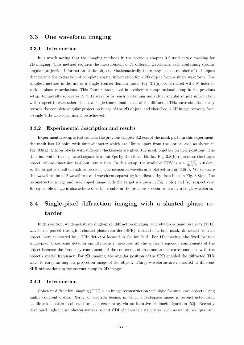
3.3 One waveform imaging . . . . . . . . . . . . . . . . . . . . . . . . 22

3.3.1 Introduction . . . . . . . . . . . . . . . . . . . . . . . . . . 22

3.3.2 Experimental description and results . . . . . . . . . . . 22

3.4 Single-pixel diffraction imaging with a slanted phase retarder . 22

3.4.1 Introduction . . . . . . . . . . . . . . . . . . . . . . . . . . 22

ii

3.4.2 Theory . . . . . . . . . . . . . . . . . . . . . . . . . . . . . 24

3.4.3 Experimental description and results . . . . . . . . . . . 25

3.4.4 Image resolution . . . . . . . . . . . . . . . . . . . . . . . . 27

3.4.5 Discussion . . . . . . . . . . . . . . . . . . . . . . . . . . . 27

3.4.6 Summary . . . . . . . . . . . . . . . . . . . . . . . . . . . . 27

Chapter 4. Polarization shaping of few-cycle terahertz wave 31

4.1 Introduction . . . . . . . . . . . . . . . . . . . . . . . . . . . . . . . 31

4.2 Polarization representation for few-cycle THz waves . . . . . . . 32

4.3 Experimental description . . . . . . . . . . . . . . . . . . . . . . . 33

4.4 Results . . . . . . . . . . . . . . . . . . . . . . . . . . . . . . . . . . 35

4.5 Discussion . . . . . . . . . . . . . . . . . . . . . . . . . . . . . . . . 38

4.6 Summary . . . . . . . . . . . . . . . . . . . . . . . . . . . . . . . . 38

Chapter 5. Sub-wavelength diffraction and phase shift anomalies caused by

it 40

5.1 Introduction . . . . . . . . . . . . . . . . . . . . . . . . . . . . . . . 40

5.2 General theory of phase shift anomaly in sub-wavelength diffrac-

tion . . . . . . . . . . . . . . . . . . . . . . . . . . . . . . . . . . . . 41

5.3 Experimental description . . . . . . . . . . . . . . . . . . . . . . . 42

5.4 Sub-wavelength single slit diffraction . . . . . . . . . . . . . . . . 44

5.4.1 Perpendicular polarized electric field . . . . . . . . . . . . 44

5.4.2 Parallel polarized electric field . . . . . . . . . . . . . . . 48

5.4.3 Comparison between θ = π/2 and θ = 0 . . . . . . . . . . 49

5.4.4 Arbitrary polarizations . . . . . . . . . . . . . . . . . . . . 49

5.5 Sub-wavelength circular hole diffraction . . . . . . . . . . . . . . 53

5.6 Diffraction pattern modulation in sub-wavelength Young’s double-

slit experiment . . . . . . . . . . . . . . . . . . . . . . . . . . . . . 55

5.6.1 Theory . . . . . . . . . . . . . . . . . . . . . . . . . . . . . 55

5.6.2 Experimental description . . . . . . . . . . . . . . . . . . . 56

5.6.3 Results . . . . . . . . . . . . . . . . . . . . . . . . . . . . . 56

5.7 Discussion . . . . . . . . . . . . . . . . . . . . . . . . . . . . . . . . 59

5.7.1 Comparison with sub-wavelength Gouy phase shift based

on the scalar diffraction theory . . . . . . . . . . . . . . . 59

5.7.2 A wire-grid polarizer with high extinction ratio . . . . . 59

5.8 Summary . . . . . . . . . . . . . . . . . . . . . . . . . . . . . . . . 59

Chapter 6. Conclusion 62

– iii –

References 64

Summary (in Korean) 72

– iv –

List of Tables

5.1 Summary of amplitude and phase behavior of sub-wavelength-scale diffraction . . . . . . 60

v

List of Figures

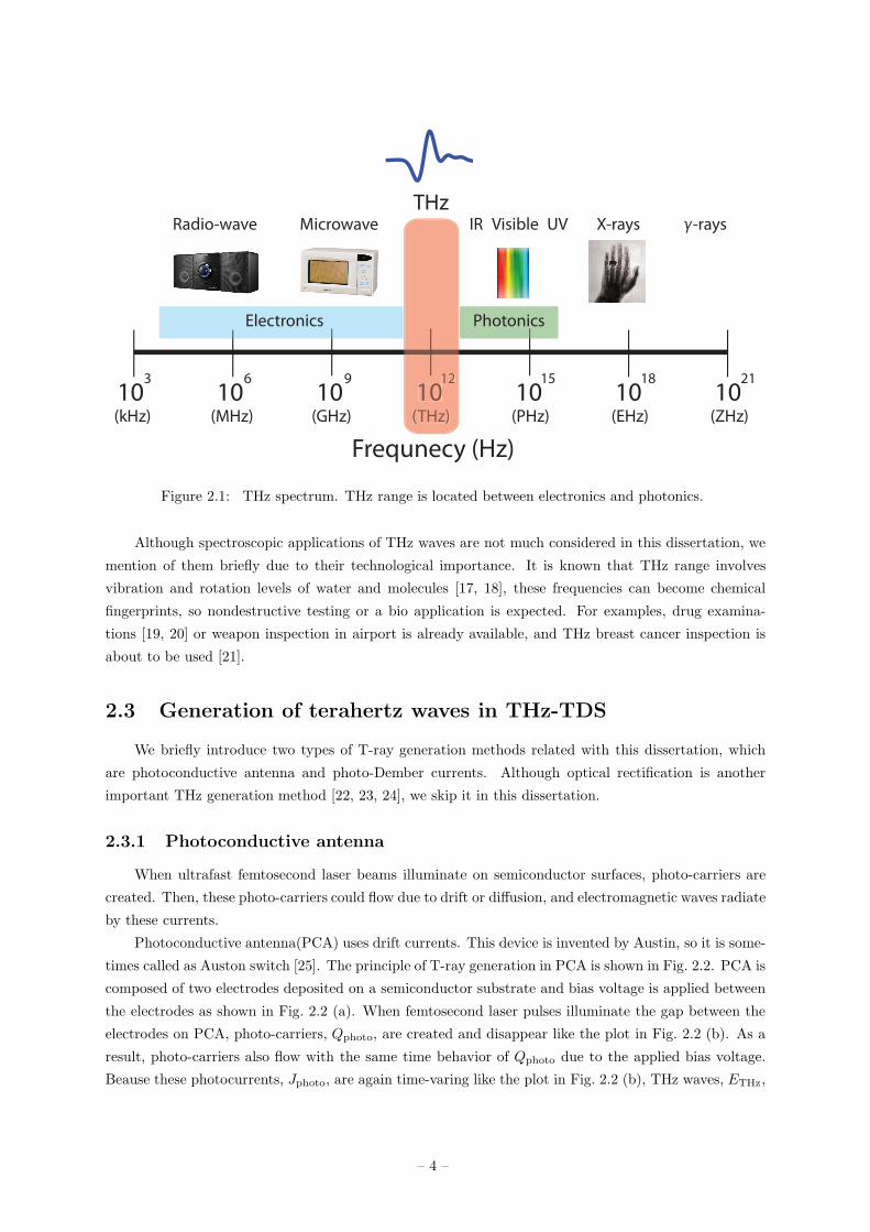
2.1 THz spectrum. THz range is located between electronics and photonics. . . . . . . . . . 4

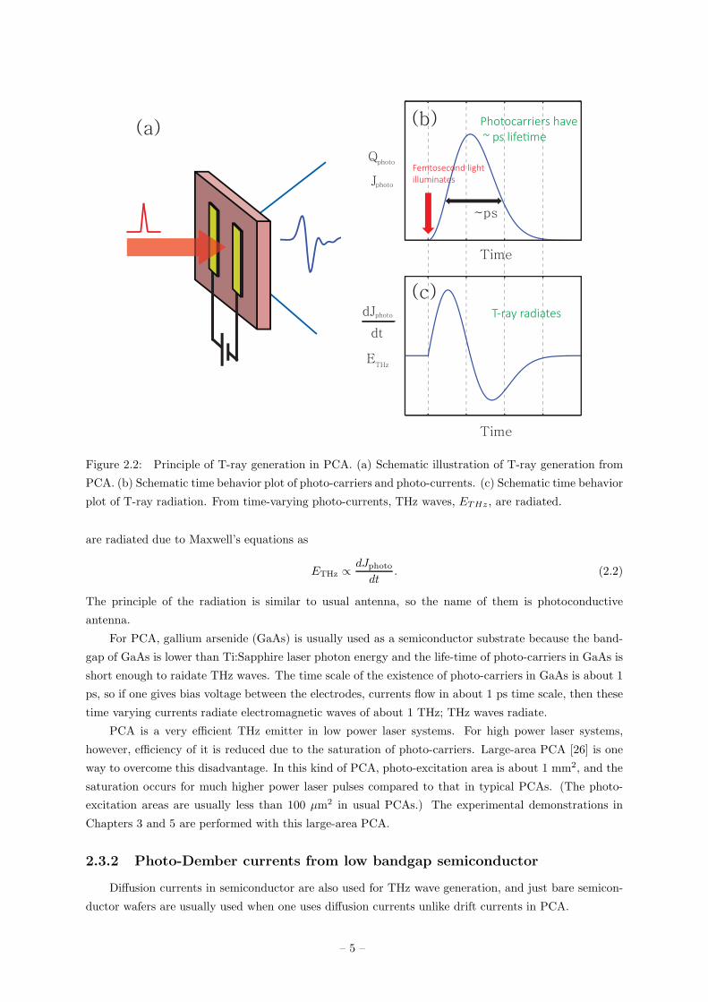
2.2 Principle of T-ray generation in PCA. (a) Schematic illustration of T-ray generation

from PCA. (b) Schematic time behavior plot of photo-carriers and photo-currents. (c)

Schematic time behavior plot of T-ray radiation. From time-varying photo-currents, THz

waves, ETHz , are radiated. . . . . . . . . . . . . . . . . . . . . . . . . . . . . . . . . . . . 5

2.3 Schematic diagram of photo-Dember currents near the surface of the semiconductor. Due

to the mobility difference, net currents are built up. . . . . . . . . . . . . . . . . . . . . . 6

2.4 Schematic setup of THz detection with electro-optical sampling. (a) Balance detection

setup. (b) One photo-detector setup. . . . . . . . . . . . . . . . . . . . . . . . . . . . . . 8

2.5 Schematical drawing of a typical THz-TDS setup. For generation and detection, femtosec-

ond laser pulses are used. We note that the emitter part and the detector part can be

replaceable for proper purposes. . . . . . . . . . . . . . . . . . . . . . . . . . . . . . . . . 9

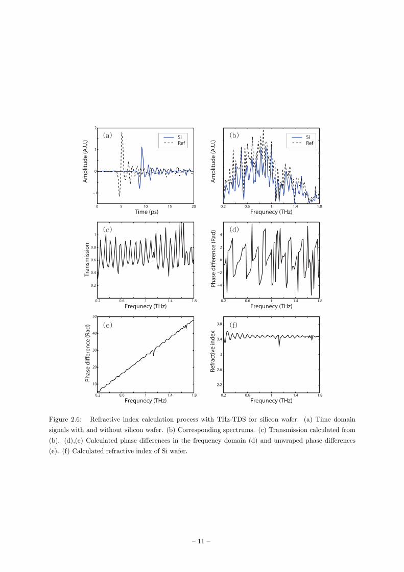
2.6 Refractive index calculation process with THz-TDS for silicon wafer. (a) Time domain

signals with and without silicon wafer. (b) Corresponding spectrums. (c) Transmission

calculated from (b). (d),(e) Calculated phase differences in the frequency domain (d) and

unwraped phase differences (e). (f) Calculated refractive index of Si wafer. . . . . . . . . 11

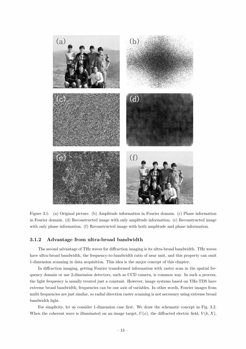
3.1 (a) Original picture. (b) Amplitude information in Fourier domain. (c) Phase informa-

tion in Fourier domain. (d) Reconstructed image with only amplitude information. (e)

Reconstructed image with only phase information. (f) Reconstructed image with both

amplitude and phase information. . . . . . . . . . . . . . . . . . . . . . . . . . . . . . . . 13

3.2 Concepts of (a) conventional diffraction imaging with monochromatic waves and (b) single-

pixel diffraction imaging with extreme broadband waves . . . . . . . . . . . . . . . . . . . 14

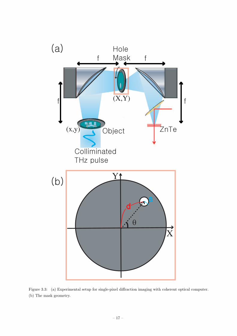
3.3 (a) Experimental setup for single-pixel diffraction imaging with coherent optical computer.

(b) The mask geometry. . . . . . . . . . . . . . . . . . . . . . . . . . . . . . . . . . . . . 17

3.4 Experimental results. (a) Imaging target. (b) Measured time signals. (c-f) Reconstructed

image with 6 waveforms (c), 10 waveforms (d), 15 waveforms (e), and 30 waveforms (f). . 18

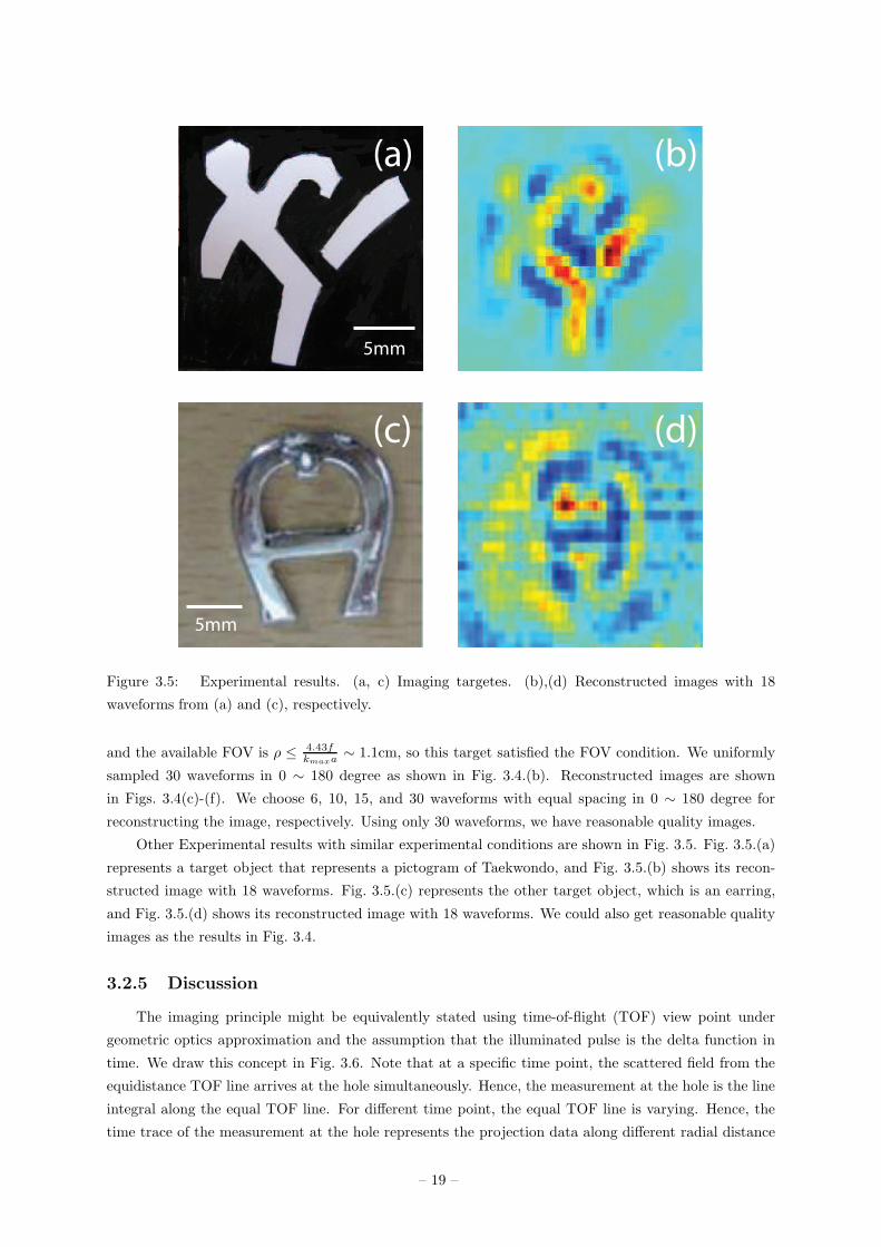
3.5 Experimental results. (a, c) Imaging targetes. (b),(d) Reconstructed images with 18

waveforms from (a) and (c), respectively. . . . . . . . . . . . . . . . . . . . . . . . . . . . 19

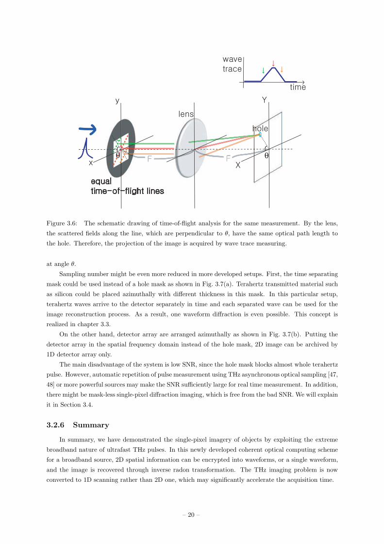
3.6 The schematic drawing of time-of-flight analysis for the same measurement. By the lens,

the scattered fields along the line, which are perpendicular to θ, have the same optical

path length to the hole. Therefore, the projection of the image is acquired by wave trace

measuring. . . . . . . . . . . . . . . . . . . . . . . . . . . . . . . . . . . . . . . . . . . . . 20

3.7 More developed schemes of single-pixel diffraction imaging with coherent optical computer.

(a) One waveform diffraction imaging from time seperation. (b) Detection array concept. 21

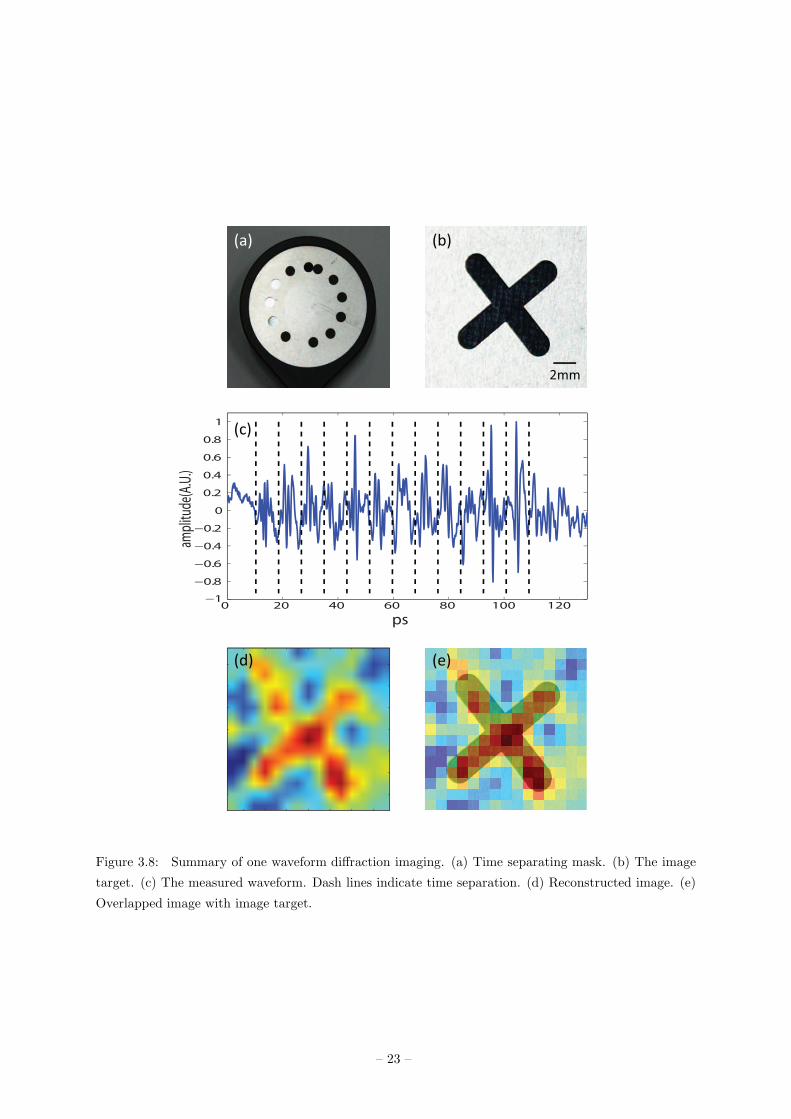
3.8 Summary of one waveform diffraction imaging. (a) Time separating mask. (b) The image

target. (c) The measured waveform. Dash lines indicate time separation. (d) Recon-

structed image. (e) Overlapped image with image target. . . . . . . . . . . . . . . . . . . 23

vi

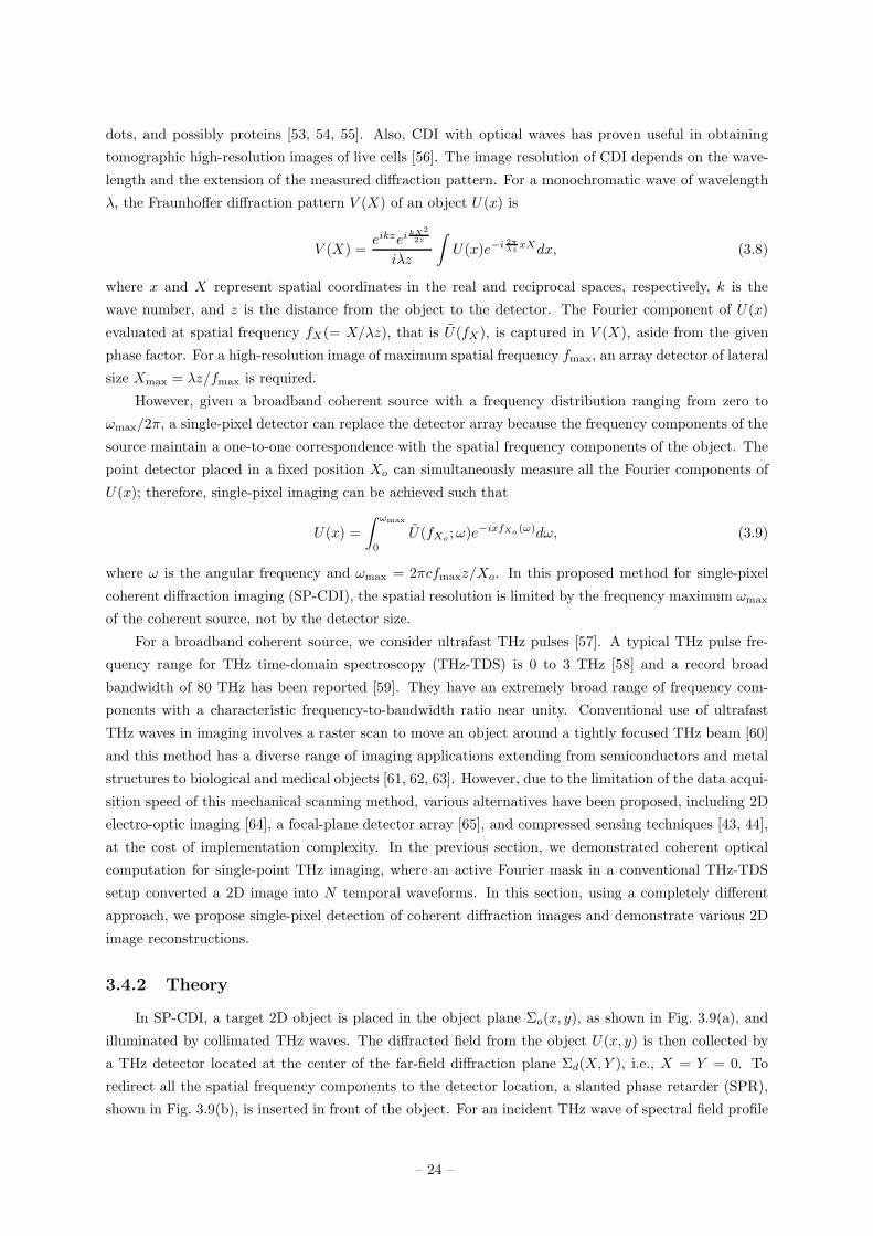
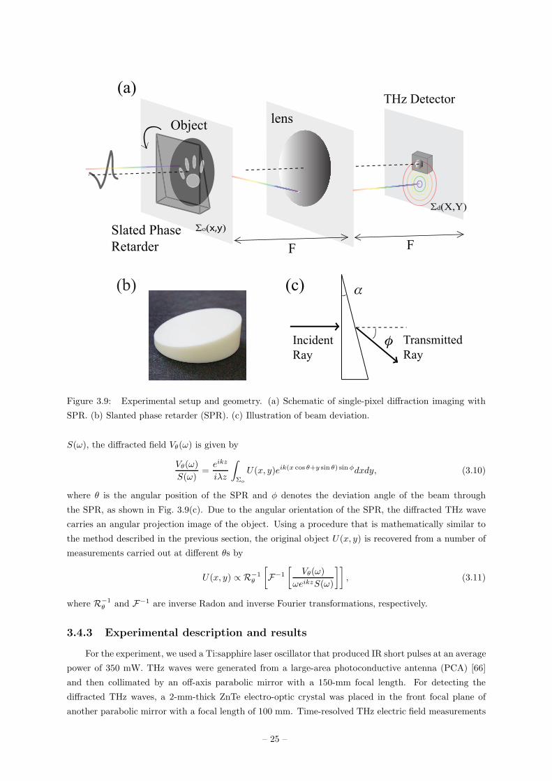
3.9 Experimental setup and geometry. (a) Schematic of single-pixel diffraction imaging with

SPR. (b) Slanted phase retarder (SPR). (c) Illustration of beam deviation. . . . . . . . . 25

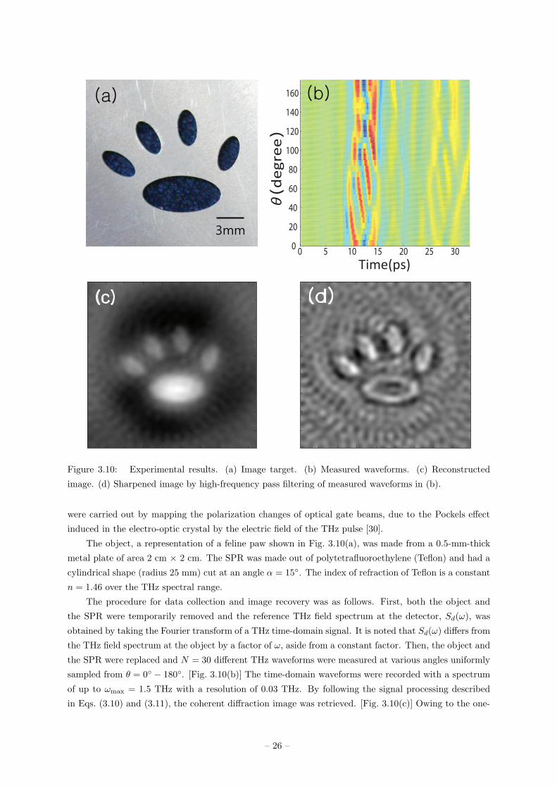
3.10 Experimental results. (a) Image target. (b) Measured waveforms. (c) Reconstructed

image. (d) Sharpened image by high-frequency pass filtering of measured waveforms in (b). 26

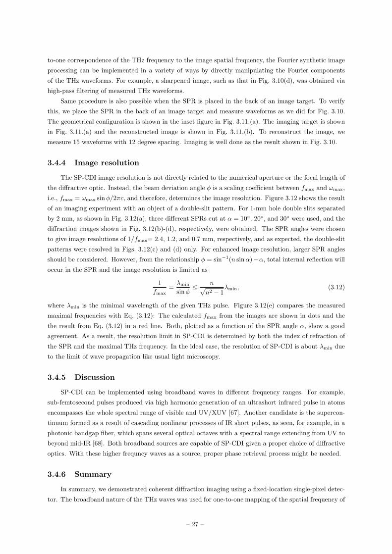
3.11 Imaging results with the SPR which is placed behind the image target. (a) Imaging target.

(b) Reconstructed image with 15 waveforms. . . . . . . . . . . . . . . . . . . . . . . . . . 28

3.12 (a) Image resolution target. (b)-(d) Reconstructed images with SPRs at α = 10◦ (b), 20◦

(c), and 30◦ (d). (e) Maximum spatial frequency fmax (in λmin unit) plotted as a function

of SPR angle α. The blue line denotes silicon SPR while the red line denotes Teflon SPR

in (e). . . . . . . . . . . . . . . . . . . . . . . . . . . . . . . . . . . . . . . . . . . . . . . . 29

4.1 (a) The temporal profile of the combined pulse (blue) represented in a three-dimensional

coordinate space of Ex, and Ey ; and its projections to each plane, respectively. (b) The

temporal profiles of the right (blue) and the left (red) circular polarization amplitudes.

(c) Calculated time-varying polarization ellipticity. (For the definition, see the text.) The

arrows in (b) and (c) represent the peak positions of the individual half-cycle pulses. . . 33

4.2 Experimental setup for the generation of polarization-shaped THz waves. (Inset) Laser

beam is refracted from a single glass wedge to the edge of an InAs disk pattern, where

the azimuthal angle θ and the thickness l of the glass wedge determine the polarization

and timing of the generated THz pulse, respectively. When a set of glass wedges of

different azimuthal angles and thicknesses is used at the same time, as-many THz pulses

are generated simultaneously from the various locations in the InAs disk and the combined

THz wave is made with non-linear polarization. . . . . . . . . . . . . . . . . . . . . . . . 34

4.3 Electric filed ~E(t) of a linearly-polarized THz pulse measured by a polarization-sensitive

detector as a function of the azimuthal angle θ of a glass wedge: (a) The measured x-

polarized component, x · ~E(t); (b) The measured y-polarization component, y · ~E(t); (c)

The the THz peak amplitudes of (b) and (c) plotted as a function of θ, where the dotted

lines are cos θ (red) and sin θ (blue); (d) The polarization angle tan−1(x · ~E(t)/y · ~E(t))

calculated from (c). . . . . . . . . . . . . . . . . . . . . . . . . . . . . . . . . . . . . . . . 36

4.4 (a) THz pulse shaping with four glass wedges. The inset shows the orientation of the

glass wedges. (For the detail, see the text.) Four THz pulses which are linearly polarized

are weaved to make circularly polarized THz wave. (b) Calculated right-circular polariza-

tion amplitude∣

∣

∣ER(t)

∣

∣

∣(blue) and left-circular polarization amplitude

∣

∣

∣EL(t)

∣

∣

∣(Red). (c)

Calculated polarization elipticity ε(t). The dots represent the experimental data and the

solid line the numerical simulation. The dashed lines along ε(t) = ±π/2 indicate perfect

circular polarization. . . . . . . . . . . . . . . . . . . . . . . . . . . . . . . . . . . . . . . 37

– vii –

4.5 Examples of THz pulse shaping with six glass wedges. (a-c) THz pulse shaping for polar-

ization rotation: (a) The electric field ~E(t) is plotted in a three-dimensional space defined

by Ex, Ey, and time. The dots represent the experimental data while the solid line the sim-

ulation. The inset shows the glass wedge arrangement, where the arrows indicate the glass

wedge orientation, and the ordering number indicates the glass thickness. (b) Amplitude

absolutes of the calculated right- and left-circular polarization components,∣

∣

∣ER(t)

∣

∣

∣(blue)

and∣

∣

∣EL(t)

∣

∣

∣(red), respectively. (c) Polarization ellipticity ε(t), which shows that polar-

ization changes from linear, right-circular, and back to linear in one-cycle time duration.

The dashed line at ε(t) = π/2 (-π/2) indicates perfect left (right) circular polarization

state. (d-f) THz pulse shaping for polarization alternation: (d) Electric field vector, (e)

Circular polarization amplitude absolutes, (f) polarization ellipticity. Polarization state

changes from right circular to left circular. . . . . . . . . . . . . . . . . . . . . . . . . . . 39

5.1 (a) Experimental setup. (b) Knife-edge experiment for THz beam spot and (c) recon-

structed THz beam spot sizes. Blue, red, and black lines represent 0.3 THz, 0.4 THz, 0.5

THz, respectively. . . . . . . . . . . . . . . . . . . . . . . . . . . . . . . . . . . . . . . . . 43

5.2 Geometry of sub-wavelength single slit diffraction. . . . . . . . . . . . . . . . . . . . . . . 45

5.3 Transmitted THz waves through sub-wavelength-scale slits for θ = π/2 case. (a) Measured

time signals and (b) their amplitude transmission plotted with d/λ. Black line in (b)

represents a fitting line based on eq. 5.8. . . . . . . . . . . . . . . . . . . . . . . . . . . . . 46

5.4 Measured phase shifts of diffracted THz waves from sub-wavelength-scale slits: (a) Optical

microscopic image of a slit and the directions of E and B fields and momentum. (b)

Normalized THz waveforms diffracted from slits of d = 100, 300, 500, and 700 µm (from

the top to the bottom). (c) Phase shifts, φslit − φG, for 0.3, 0.35, 0.4, and 0.45 THz are

plotted as a function of d/λ. Black dashed line represents a fitting based on Eq. 5.9. The

inset figure in (c) is the log-log plot of − tan(φslit − φG) and d/λ. . . . . . . . . . . . . . 47

5.5 Transmitted THz waves through sub-wavelength-scale slits for θ = 0 case. (a) Measured

time signals and (b) their amplitude transmission plotted with d/λ. Black line in (b)

represents a fitting line based on eq. 5.15. . . . . . . . . . . . . . . . . . . . . . . . . . . . 50

5.6 Measured electric fields through slits having their width of (a) d = 30 µm, (b) d = 40 µm,

(c) d = 50 µm, (d) d = 100 µm, (e) d = 150 µm, and (f) d = 200 µm. All signals are

normalized. Red lines represent θ = 0 cases while blue lines represent θ = π/2 cases. Dot

lines mean reference fields which are measured without slits. . . . . . . . . . . . . . . . . 51

5.7 The amplitude spectra of transmitted THz pulses from various slits of (a) d=30, (b) 40,

(c) 50, (d) 100, (e) 150, and (f) 200 µm, respectively, are plotted as functions of wave

direction θ and frequency. (g) Transmission amplitudes retrieved at 0.5 THz depicted with

white dashes in (a-e). Dashed lines in (g) represents theoretical expectations in Eq. 5.16.

All the amplitudes are normalized by their own maximum transmission amplitudes. . . . 52

5.8 Measured data of sub-wavelength circular hole diffraction. Phase shifts, φhole − φG, mea-

sured at 0.3, 0.35, 0.4, and 0.45 THz are, respectively, plotted with a/λ. Black dashed

line represents the theoretical guide line from Eq. 5.20. The inset figure is an optical

microscopic image of a typical circular hole. . . . . . . . . . . . . . . . . . . . . . . . . . 54

5.9 (a) Ordinary Young’s double-slit diffraction pattern. (b) Sub-wavelength Young’s double-

slit diffraction pattern. . . . . . . . . . . . . . . . . . . . . . . . . . . . . . . . . . . . . . 55

– viii –

5.10 Photograph of the experimental setup to measure diffraction pattern of double-slit diffrac-

tion. The inset drawing shows the scheme. . . . . . . . . . . . . . . . . . . . . . . . . . . . 57

5.11 Measured time signals and diffraction patterns from aperture 1 (a-d) and aperture 2 (e-h).

All time signals and patterns are normalized. (a,e) Measured time signals with perpen-

dicular polarization. (b,f) Diffraction pattern at 0.6 THz from (a) and (e), respectively.

(c,g) Measured time signals with parallel polarization. (d,h) Diffraction pattern at 0.6

THz from (c) and (g), respectively. Red crosses in (b,f) and blue circles in (d,h) represent

experimental data. Black dash lines in (b,d,f,h) represent theoretical expectation base on

scalar diffraction theory. Red dash line in (b) and blue dash line in (d) are fitting lines

based on Eq. 5.24. . . . . . . . . . . . . . . . . . . . . . . . . . . . . . . . . . . . . . . . . 58

5.12 Summary of phase shift anomalies in sub-wavelength-scale diffraction . . . . . . . . . . . 61

– ix –

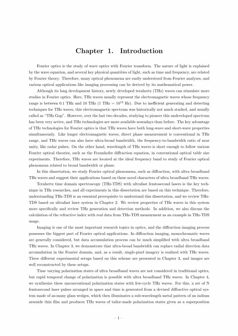
Chapter 1. Introduction

Fourier optics is the study of wave optics with Fourier transform. The nature of light is explained

by the wave equation, and several key physical quantities of light, such as time and frequency, are related

by Fourier theory. Therefore, many optical phenomena are easily understood from Fourier analyses, and

various optical applications like imaging processing can be derived by its mathematical power.

Although its long development history, newly developed terahertz (THz) waves can stimulate more

studies in Fourier optics. Here, THz waves usually represent the electromagnetic waves whose frequency

range is between 0.1 THz and 10 THz (1 THz = 1012 Hz). Due to inefficient generating and detecting

techniques for THz waves, this electromagnetic spectrum was historically not much studied, and usually

called as “THz Gap”. However, over the last two decades, studying to pioneer this undeveloped spectrum

has been very active, and THz technologies are more available nowadays than before. The key advantage

of THz technologies for Fourier optics is that THz waves have both long-wave and short-wave properties

simultaneously. Like longer electromagnetic waves, direct phase measurement is conventional in THz

range, and THz waves can also have ultra-broad bandwidth, the frequency-to-bandwidth ratio of near

unity, like radar pulses. On the other hand, wavelength of THz waves is short enough to follow various

Fourier optical theories, such as the Fraunhofer diffraction equation, in conventional optical table size

experiments. Therefore, THz waves are located at the ideal frequency band to study of Fourier optical

phenomena related to broad bandwidth or phase.

In this dissertation, we study Fourier optical phenomena, such as diffraction, with ultra broadband

THz waves and suggest their applications based on these novel characters of ultra broadband THz waves.

Terahertz time domain spectroscopy (THz-TDS) with ultrafast femtosecond lasers is the key tech-

nique in THz researches, and all experiments in this dissertation are based on this technique. Therefore,

understanding THz-TDS is an essential prerequisite to understand this dissertation, and we review THz-

TDS based on ultrafast laser system in Chapter 2. We review properties of THz waves in this system

more specifically and review THz generation and detection methods. In addition, we also discuss the

calculation of the refractive index with real data from THz-TDS measurment as an example in THz-TDS

usage.

Imaging is one of the most important research topics in optics, and the diffraction imaging process

possesses the biggest part of Fourier optical applications. In diffraction imaging, monochromatic waves

are generally considered, but data accumulation process can be much simplified with ultra broadband

THz waves. In Chapter 3, we demonstrate that ultra-broad bandwidth can replace radial direction data

accumulation in the Fourier domain, and, as a result, single-pixel imagery is realized with THz waves.

Three different experimental setups based on this scheme are presented in Chapter 3, and images are

well reconstructed by these setups.

Time varying polarization states of ultra broadband waves are not considered in traditional optics,

but rapid temporal change of polarization is possible with ultra broadband THz waves. In Chapter 4,

we synthesize these unconventional polarization states with few-cycle THz waves. For this, a set of N

femtosecond laser pulses arranged in space and time is generated from a devised diffractive optical sys-

tem made of as-many glass wedges, which then illuminates a sub-wavelength metal pattern of an indium

arsenide thin film and produces THz waves of tailor-made polarization states given as a superposition

– 1 –

of N linearly-polarized THz pulses. By properly superposing temporally-shifted linear polarization com-

ponents, we successfully generate THz waves of various polarization states, such as polarization rotation

and alternation between circular polarization states. We also analyze these polarization states with our

own representation which one not fully described by monochromatic analysis.

It is known that scalar diffraction theories can not be applied in sub-wavelength diffraction, but phase

studies are not much considered since phase measurement of light is not straightforward in other frequency

ranges. In Chapter 5, we investigate phase shift anomalies that are caused by wave diffraction from a

slit or a circular aperture of sub-wavelength scale. Nearly π/2-phase delay from a small perpendicular

slit and π/2-phase advance from a small parallel slit, and also from a small circular aperture, have been

directly measured. These results demonstrate that the common π/2 phase advance of diffraction waves

in the far-field region, known as Gouy phase shift, is not valid in sub-wavelength diffraction, and, instead

of that, phase shifts can vary from 0 to π with respect to the propagating factor, eikR. Physical origin of

these phase shift anomalies is plasmon coupling or magnetic dipole radiation, and theoretical predictions

based on these models are in good agreement with the experimental results. Due to these phase shift

anomalies, diffraction pattern is also modulated from the expectation of scalar diffraction theories, and

we verify this modulation by studying sub-wavelength Young’s double-slit experiment.

– 2 –

Chapter 2. Terahertz waves in terahertz time

domain spectroscopy

2.1 Introduction

In photonics community, ultrashort or ultrafast femtosecond pulses denote electromagnetic pulses

whose time durations are the order of the femtosecond (1 fs=10−15 s). These pulses have a broadband

optical spectrum due to the uncertainty principle, and can be created by mode-locked laser technologies

such as a passive mode-locked 800 nm-centered Ti:Sapphire laser. With these laser technologies, numer-

ous applications, such as ultrafast time-resolved spectroscopy [1, 2, 3], micro-machining [4, 5], coherent

control [6, 7, 8, 9, 10], precision measurement [11, 12], and bio imaging [13, 14], are convenient nowadays.

Terahertz time domain spectroscopy (THz-TDS) is one of the important applications in these fem-

tosecond laser technologies. In THz-TDS, one generates THz pulses and measures their fields directly in

time domain with femtosecond laser pulses. Because of its convenience compare to other THz techniques,

THz-TDS is placed on the center of THz applications including THz spectroscopy and THz imaging.

There are two characters which distinguish THz-TDS from other THz techniques. Firstly, generated

THz waves in THz-TDS are few-cycles or sub-cycle pulses, so they have ultra-broad bandwidth. Here,

we define ultra-broad bandwidth as bandwidth having the frequency-to-bandwidth ratio of near unity

in this dissertation. The second one is direct phase measuring capability of THz waves. In THz-TDS,

one detects the field of THz waves in time domain directly, so phase information of THz waves can be

obtained by conventional Fourier transform process.

All THz researches in this dissertation are based on THz-TDS, and these researches are strongly

related with the above two characters. Due to the significance of them, we review the THz-TDS technique

in this chapter. After then, we briefly discuss the calculation of refractive index in transmission geometry

of THz-TDS in order to demonstrate these special advantages of THz-TDS.

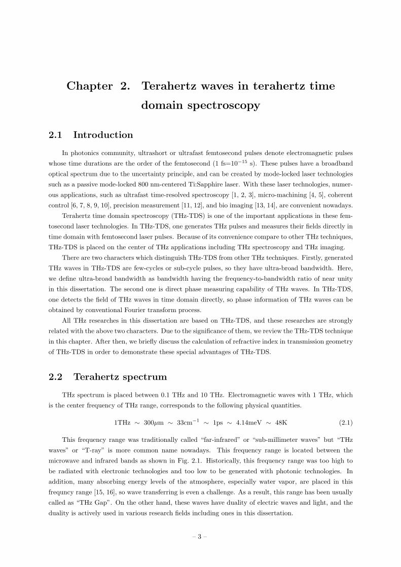
2.2 Terahertz spectrum

THz spectrum is placed between 0.1 THz and 10 THz. Electromagnetic waves with 1 THz, which

is the center frequency of THz range, corresponds to the following physical quantities.

1THz ∼ 300µm ∼ 33cm−1 ∼ 1ps ∼ 4.14meV ∼ 48K (2.1)

This frequency range was traditionally called “far-infrared” or “sub-millimeter waves” but “THz

waves” or “T-ray” is more common name nowadays. This frequency range is located between the

microwave and infrared bands as shown in Fig. 2.1. Historically, this frequency range was too high to

be radiated with electronic technologies and too low to be generated with photonic technologies. In

addition, many absorbing energy levels of the atmosphere, especially water vapor, are placed in this

frequncy range [15, 16], so wave transferring is even a challenge. As a result, this range has been usually

called as “THz Gap”. On the other hand, these waves have duality of electric waves and light, and the

duality is actively used in various research fields including ones in this dissertation.

– 3 –

10 10 10 10 10 103 18151296

1021

Frequnecy (Hz)

(THz)(GHz)(MHz)(kHz) (PHz) (EHz) (ZHz)

1012

(THz)

Electronics Photonics

THzRadio-wave Microwave Visible X-raysIR UV γ-rays

Figure 2.1: THz spectrum. THz range is located between electronics and photonics.

Although spectroscopic applications of THz waves are not much considered in this dissertation, we

mention of them briefly due to their technological importance. It is known that THz range involves

vibration and rotation levels of water and molecules [17, 18], these frequencies can become chemical

fingerprints, so nondestructive testing or a bio application is expected. For examples, drug examina-

tions [19, 20] or weapon inspection in airport is already available, and THz breast cancer inspection is

about to be used [21].

2.3 Generation of terahertz waves in THz-TDS

We briefly introduce two types of T-ray generation methods related with this dissertation, which

are photoconductive antenna and photo-Dember currents. Although optical rectification is another

important THz generation method [22, 23, 24], we skip it in this dissertation.

2.3.1 Photoconductive antenna

When ultrafast femtosecond laser beams illuminate on semiconductor surfaces, photo-carriers are

created. Then, these photo-carriers could flow due to drift or diffusion, and electromagnetic waves radiate

by these currents.

Photoconductive antenna(PCA) uses drift currents. This device is invented by Austin, so it is some-

times called as Auston switch [25]. The principle of T-ray generation in PCA is shown in Fig. 2.2. PCA is

composed of two electrodes deposited on a semiconductor substrate and bias voltage is applied between

the electrodes as shown in Fig. 2.2 (a). When femtosecond laser pulses illuminate the gap between the

electrodes on PCA, photo-carriers, Qphoto, are created and disappear like the plot in Fig. 2.2 (b). As a

result, photo-carriers also flow with the same time behavior of Qphoto due to the applied bias voltage.

Beause these photocurrents, Jphoto, are again time-varing like the plot in Fig. 2.2 (b), THz waves, ETHz,

– 4 –

Time

Time

~ps

Q

J

photo

photo

dJphoto

dt

ETHz

Photocarriers have

~ ps life�me

T-ray radiates

Femtosecond light

illuminates

(a) (b)

(c)

Figure 2.2: Principle of T-ray generation in PCA. (a) Schematic illustration of T-ray generation from

PCA. (b) Schematic time behavior plot of photo-carriers and photo-currents. (c) Schematic time behavior

plot of T-ray radiation. From time-varying photo-currents, THz waves, ETHz , are radiated.

are radiated due to Maxwell’s equations as

ETHz ∝dJphoto

dt. (2.2)

The principle of the radiation is similar to usual antenna, so the name of them is photoconductive

antenna.

For PCA, gallium arsenide (GaAs) is usually used as a semiconductor substrate because the band-

gap of GaAs is lower than Ti:Sapphire laser photon energy and the life-time of photo-carriers in GaAs is

short enough to raidate THz waves. The time scale of the existence of photo-carriers in GaAs is about 1

ps, so if one gives bias voltage between the electrodes, currents flow in about 1 ps time scale, then these

time varying currents radiate electromagnetic waves of about 1 THz; THz waves radiate.

PCA is a very efficient THz emitter in low power laser systems. For high power laser systems,

however, efficiency of it is reduced due to the saturation of photo-carriers. Large-area PCA [26] is one

way to overcome this disadvantage. In this kind of PCA, photo-excitation area is about 1 mm2, and the

saturation occurs for much higher power laser pulses compared to that in typical PCAs. (The photo-

excitation areas are usually less than 100 µm2 in usual PCAs.) The experimental demonstrations in

Chapters 3 and 5 are performed with this large-area PCA.

2.3.2 Photo-Dember currents from low bandgap semiconductor

Diffusion currents in semiconductor are also used for THz wave generation, and just bare semicon-

ductor wafers are usually used when one uses diffusion currents unlike drift currents in PCA.

– 5 –

Hole

Electron

Semiconductor

Semiconductor

Hole

Electron

Laser illuminates

on semiconductor

Carriers

are created

Electons

di!use

more

di!usion direction

current direction

after ~ps

Figure 2.3: Schematic diagram of photo-Dember currents near the surface of the semiconductor. Due

to the mobility difference, net currents are built up.

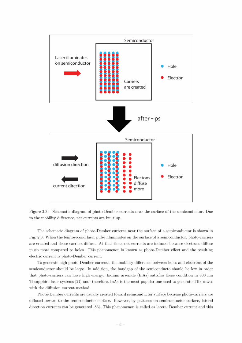
The schematic diagram of photo-Dember currents near the surface of a semiconductor is shown in

Fig. 2.3. When the femtosecond laser pulse illuminates on the surface of a semiconductor, photo-carriers

are created and those carriers diffuse. At that time, net currents are induced because electrons diffuse

much more compared to holes. This phenomenon is known as photo-Dember effect and the resulting

electric current is photo-Dember current.

To generate high photo-Dember currents, the mobility difference between holes and electrons of the

semiconductor should be large. In addition, the bandgap of the semiconducto should be low in order

that photo-carriers can have high energy. Indium arsenide (InAs) satisfies these condition in 800 nm

Ti:sapphire laser systems [27] and, therefore, InAs is the most popular one used to generate THz waves

with the diffusion current method.

Photo-Dember currents are usually created toward semiconductor surface because photo-carriers are

diffused inward to the semiconductor surface. However, by patterns on semiconductor surface, lateral

direction currents can be generated [85]. This phenomenon is called as lateral Dember current and this

– 6 –

phenomenon is used to generate polarization shaped THz waves in Chapter 4.

2.4 Detection of terahertz waves in THz-TDS

There are several ways to detect THz waves in THz-TDS, and coherent sampling in time domain

with electro-optical crystal and PCA are common ways. We used electro-optical crystal in Chapters 3

and 5 while PCA is used in Chapter 4 in this dissertation, so we review these two ways in this section.

2.4.1 Electro-optical sampling

One way to detect THz waves is using the Pockels effect in non-linear crystals. The Pockels effect

produces birefringence of non-linear crystals by an applied electric field on the crystal, and is distinguished

from Kerr effect by the fact that the birefringence is proportional to the applied electric voltage. From

this birefringence, the polarization of the transmitting light is rotated. As a result, because of the

linearity between the field strength and the polarization rotation, one can maesure the amount of the

field strength by maesuring the amount of polarization rotating. Because one uses the birefringence for

polarization rotation, the non-linear crystal should be aligned in a proper angle to get more polarization

rotation [28].

When THz waves and femtosecond laser pulses are propagating together in non-linear electro-optic

crystals, femtosecond laser pulses feel THz pulses as DC electric voltage because the duration of fem-

tosecond laser pulses is usually much shorter than the temporal field change of THz waves. As a result,

by controlling the time interval between THz waves and femtosecond laser pulses, one can get THz time

domain field shapes directly.

The most common non-linear crystal for electro-optical sampling is <110>-oriented zinc telluride

(ZnTe) because of the phase matching condition in 800 nm Ti:sapphire laser systems [29, 30, 31]. Because

the refractive indexes of ZnTe in THz frequency and in 800 nm are similar, THz waves and laser pulses

are move together in quite longer distance than in other semiconductors. Therefore, the amount of

polarization change is much bigger than that by other semiconductors. The disadvantage of ZnTe is its

phonon-mode which is located in the frequency range between 3 THz and 7 THz [32]. As a result, higher

frequency of THz waves is difficult to mearsure with ZnTe. To get higher frequency range measurement,

gallium phosphide (GaP) is usually used instead of ZnTe.

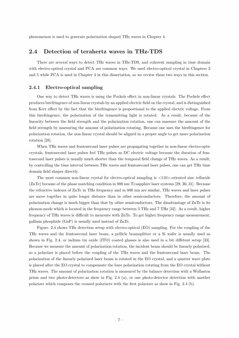
Figure. 2.4 shows THz detection setup with electro-optical (EO) sampling. For the coupling of the

THz waves and the femtosecond laser beam, a pellicle beamsplitter or a Si wafer is usually used as

shown in Fig. 2.4, or indium tin oxide (ITO) coated glasses is also used in a bit diffetent setup [33].

Because we measure the amount of polarization rotation, the incident beam should be linearly polarized,

so a polarizer is placed before the coupling of the THz waves and the femtosecond laser beam. The

polarization of the linearly polarized laser beam is rotated in the EO crystal, and a quarter wave plate

is placed after the EO crystal to compensate the bare polarization rotating from the EO crystal without

THz waves. The amount of polarization rotation is measured by the balance detection with a Wollaston

prism and two photo-detectors as show in Fig. 2.4 (a), or one photo-detector detection with another

polarizer which composes the crossed polarizers with the first polarizer as show in Fig. 2.4 (b).

– 7 –

(a) (b)

PDPD

Wollaston prism

QWP

EO crystal

Polarizer Polarizer

EO crystal

Polarizer

QWP

PD

Pellicle BS Pellicle BS

Figure 2.4: Schematic setup of THz detection with electro-optical sampling. (a) Balance detection

setup. (b) One photo-detector setup.

2.4.2 Photoconductive antenna

One can also use PCA to detect THz waves as well as THz generation. When the femtosecond laser

pulse illuminates on PCA, photo-carriers are created similarly as in the generation case. In the detection

scheme, on the other hand, the bias voltage is not necessary. Instead of the bias voltage, THz waves

themselves accelerate photo-carriers, then currents which are proportional to the THz field strength are

made. From the measurement of these currents by controlling the time interval between THz waves and

femtosecond laser pulses, THz field shapes can be detected.

Unlike PCA for THz generation, the photo-carrier life time in the semiconductor must be very

short to get high resolution sampling because the sum of the photo-carrier lifetime and the duration

of femtosecond laser pulses determine the time resolution. Therefore, low-temperature grown GaAs, of

which the photo-carrier life time is less than 200 fs, is usually used for it.

2.5 Refractive index calculation in THz-TDS

To show an example of THz-TDS usages, we review the refractive index calculation from real data

measured by THz-TDS in this section.

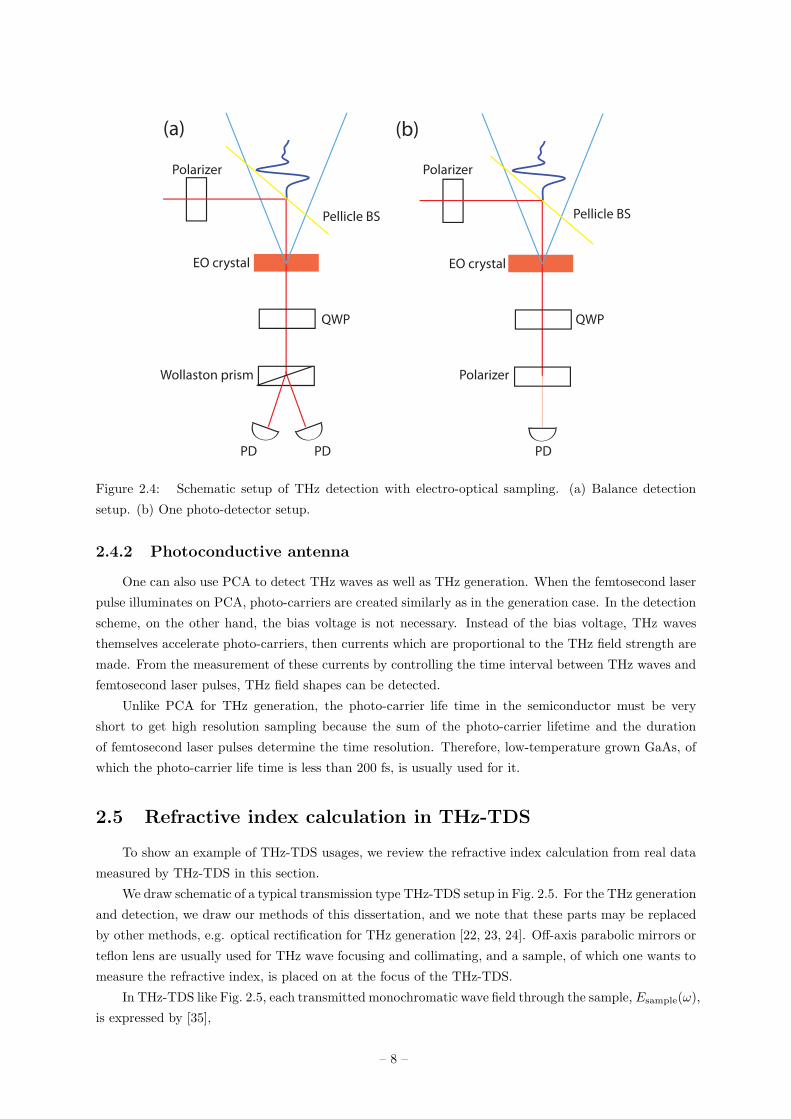
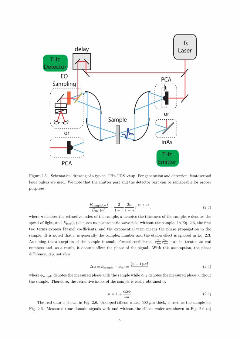
We draw schematic of a typical transmission type THz-TDS setup in Fig. 2.5. For the THz generation

and detection, we draw our methods of this dissertation, and we note that these parts may be replaced

by other methods, e.g. optical rectification for THz generation [22, 23, 24]. Off-axis parabolic mirrors or

teflon lens are usually used for THz wave focusing and collimating, and a sample, of which one wants to

measure the refractive index, is placed on at the focus of the THz-TDS.

In THz-TDS like Fig. 2.5, each transmitted monochromatic wave field through the sample, Esample(ω),

is expressed by [35],

– 8 –

THz

Emitter

THz

Detector

Sample

Laserfs

delay

PCA

InAs

or

PCA

or

EO

Sampling

Figure 2.5: Schematical drawing of a typical THz-TDS setup. For generation and detection, femtosecond

laser pulses are used. We note that the emitter part and the detector part can be replaceable for proper

purposes.

Esample(ω)

ERef(ω)=

2

1 + n

2n

1 + nei

(n−1)ωd

c , (2.3)

where n denotes the refractive index of the sample, d denotes the thickness of the sample, c denotes the

speed of light, and ERef(ω) denotes monochromatic wave field without the sample. In Eq. 2.3, the first

two terms express Fresnel coefficients, and the exponential term means the phase propagation in the

sample. It is noted that n is generally the complex number and the etalon effect is ignored in Eq. 2.3.

Assuming the absorption of the sample is small, Fresnel coefficients, 21+n

2n1+n , can be treated as real

numbers and, as a result, it doesn’t affect the phase of the signal. With this assumption, the phase

difference, ∆φ, satisfies

∆φ = φsample − φref =(n− 1)ωd

c, (2.4)

where φsample denotes the measured phase with the sample while φref denotes the measured phase without

the sample. Therefore, the refractive index of the sample is easily obtained by

n = 1 +c∆φ

ωd. (2.5)

The real data is shown in Fig. 2.6. Undoped silicon wafer, 500 µm thick, is used as the sample for

Fig. 2.6. Measured time domain signals with and without the silicon wafer are shown in Fig. 2.6 (a)

– 9 –

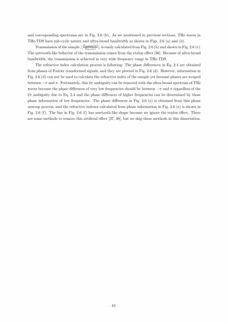
and corresponding spectrums are in Fig. 2.6 (b). As we mentioned in previous sections, THz waves in

THz-TDS have sub-cycle nature and ultra-broad bandwidth as shown in Figs. 2.6 (a) and (b).

Transmission of the sample, |Esample(ω)ERef (ω) |, is easily calculated from Fig. 2.6 (b) and shown in Fig. 2.6 (c).

The sawtooth-like behavior of the transmission comes from the etalon effect [36]. Because of ultra-broad

bandwidth, the transmission is achieved in very wide frequency range in THz-TDS.

The refractive index calculation process is following: The phase differences in Eq. 2.4 are obtained

from phases of Fourier transformed signals, and they are plotted in Fig. 2.6 (d). However, information in

Fig. 2.6 (d) can not be used to calculate the refractive index of the sample yet because phases are wraped

between −π and π. Fortunately, this 2π ambiguity can be removed with the ultra-broad spectrum of THz

waves because the phase diffrences of very low frequencies should be between −π and π regardless of the

2π ambiguity due to Eq. 2.4 and the phase diffrences of higher frequencies can be determined by these

phase information of low frequencies. The phase diffrences in Fig. 2.6 (e) is obtained from this phase

unwrap process, and the refractive indexes calculated from phase information in Fig. 2.6 (e) is shown in

Fig. 2.6 (f). The line in Fig. 2.6 (f) has sawtooth-like shape because we ignore the etalon effect. There

are some methods to remove this artificial effect [37, 38], but we skip these methods in this dissertation.

– 10 –

SiRef

0.2 0.6 1 1.4 1.8

Frequnecy (THz)A

mp

litu

de

(A

.U.)

0.2 0.6 1 1.4 1.8

0.2

0.4

0.6

0.8

1

Frequnecy (THz)

Tra

nsm

issi

on

0.2 0.6 1 1.4 1.8

−4

−2

0

2

4

Frequnecy (THz)

Ph

ase

di"

ere

nce

(R

ad

)

0.2 0.6 1 1.4 1.8

10

20

30

40

50

Frequnecy (THz)

Ph

ase

di"

ere

nce

(R

ad

)

0.2 0.6 1 1.4 1.8

2.2

2.6

3

3.4

3.8

Frequnecy (THz)

Re

fra

ctiv

e in

de

x0 5 10 15 20

−1

0

1

2

Time (ps)

Am

plit

ud

e (

A.U

.)

SiRef

(a) (b)

(c)

(e) (f)

(d)

Figure 2.6: Refractive index calculation process with THz-TDS for silicon wafer. (a) Time domain

signals with and without silicon wafer. (b) Corresponding spectrums. (c) Transmission calculated from

(b). (d),(e) Calculated phase differences in the frequency domain (d) and unwraped phase differences

(e). (f) Calculated refractive index of Si wafer.

– 11 –

Chapter 3. Single-pixel broadband diffraction

imaging

Imaging is one of the most important research topics in optics and diffraction imaging is also an

important research topic in Fourier optical application. In diffraction imaging, coherent light illuminates

an image target and is diffracted by the image target. In far field condition, the diffracted light has

the amplitude and phase profile just as Fourier transform of the image target. Therefore, if one gets

this Fourier transformed information in far field, original image information of the image target can be

obtained by Fourier transform: this is the basic principle of diffraction imaging.

If one perform a diffraction imagery with THz-TDS system, direct phase measurement and ultra-

broad bandwidth, which we emphasize in Chapter 2, give great advantages. With direct phase measure-

ment, phase retrieval processes are not necessary as against visible light diffraction imaging. Ultra-broad

bandwidth gives even better advantage; Raster scanning or 2 dimensional detectors usually seems to be

essential to get 2 dimensional information, but it doesn’t with ultra-broad bandwidth THz waves. In the

following sections, we show these advantages in more detail and demonstrate three different single-pixel

imagery which use the ultra-broad bandwidth nature of THz waves.

Research results including both experiments and theories in this chapter are published in Optics

Letter Vol. 35 pp. 508-510 (2010) and Applied Physics Letters Vol. 97 pp. 241101 (2010), entitled

“Coherent Optical Computing for T-ray Imaging” and “Single pixel coherent diffraction imaging,” re-

spectively.

3.1 Main concept

3.1.1 Advantage from direct phase measurement

In diffraction imaging, both Fourier transformed spectral phase and amplitude information are natu-

rally essential. However, relatively, the spectral phase information is more important than the amplitude

information. To see it, we show an example in Fig. 3.1. The original picture, which denotes peoples who

mostly help this dissertation, is in Fig. 3.1(a), and the Fourier transformed amplitude and phase infor-

mation of the picture are shown in Figs. 3.1(b), (c). Figs. 3.1(d),(e),(f) represent reconstructed images

with only amplitude information, only phase information, and both amplitude and phase information,

respectively. As show in Fig. 3.1, the image in Fig. 3.1(e) shows the shape of the original image in

Fig. 3.1(a) while the image in Fig. 3.1(d) shows nothing.

Nevertheless, acquisition of phase information is not straightforward in usual diffraction imaging. If

one uses visible light as the light source in diffraction imaging, the Fourier transformed phase information

is usually not able to be obtained because there is not direct phase detector in visible light frequency.

Therefore, phase information of diffractive waves must be retrieved by phase retrieval algorithms, such

as Gerchberg–Saxton algorithm [39].

On the other hand, in THz diffraction imaging, one can obtain both amplitude and phase information

simultaneously as shown in Chapter. 2. As a result, phase retrieval algorithms are not necessary in THz

diffraction imaging. This is the first advantage of diffraction imagery with THz-TDS system.

– 12 –

(a) (b)

(c) (d)

(e) (f)

Figure 3.1: (a) Original picture. (b) Amplitude information in Fourier domain. (c) Phase information

in Fourier domain. (d) Reconstructed image with only amplitude information. (e) Reconstructed image

with only phase information. (f) Reconstructed image with both amplitude and phase information.

3.1.2 Advantage from ultra-broad bandwidth

The second advantage of THz waves for diffraction imaging is its ultra-broad bandwidth. THz waves

have ultra-broad bandwidth, the frequency-to-bandwidth ratio of near unit, and this property can omit

1-dimension scanning in data acquisition. This idea is the major concept of this chapter.

In diffraction imaging, getting Fourier transformed information with raster scan in the spatial fre-

quency domain or use 2-dimension detectors, such as CCD camera, is common way. In such a process,

the light frequency is usually treated just a constant. However, image systems based on THz-TDS have

extreme broad bandwidth, frequencies can be one axis of variables. In other words, Fourier images from

multi frequencies are just similar, so radial direction raster scanning is not necessary using extreme broad

bandwidth light.

For simplicity, let us consider 1-dimension case first. We draw the schematic concept in Fig. 3.2.

When the coherent wave is illuminated on an image target, U(x), the diffracted electric field, V (k,X),

– 13 –

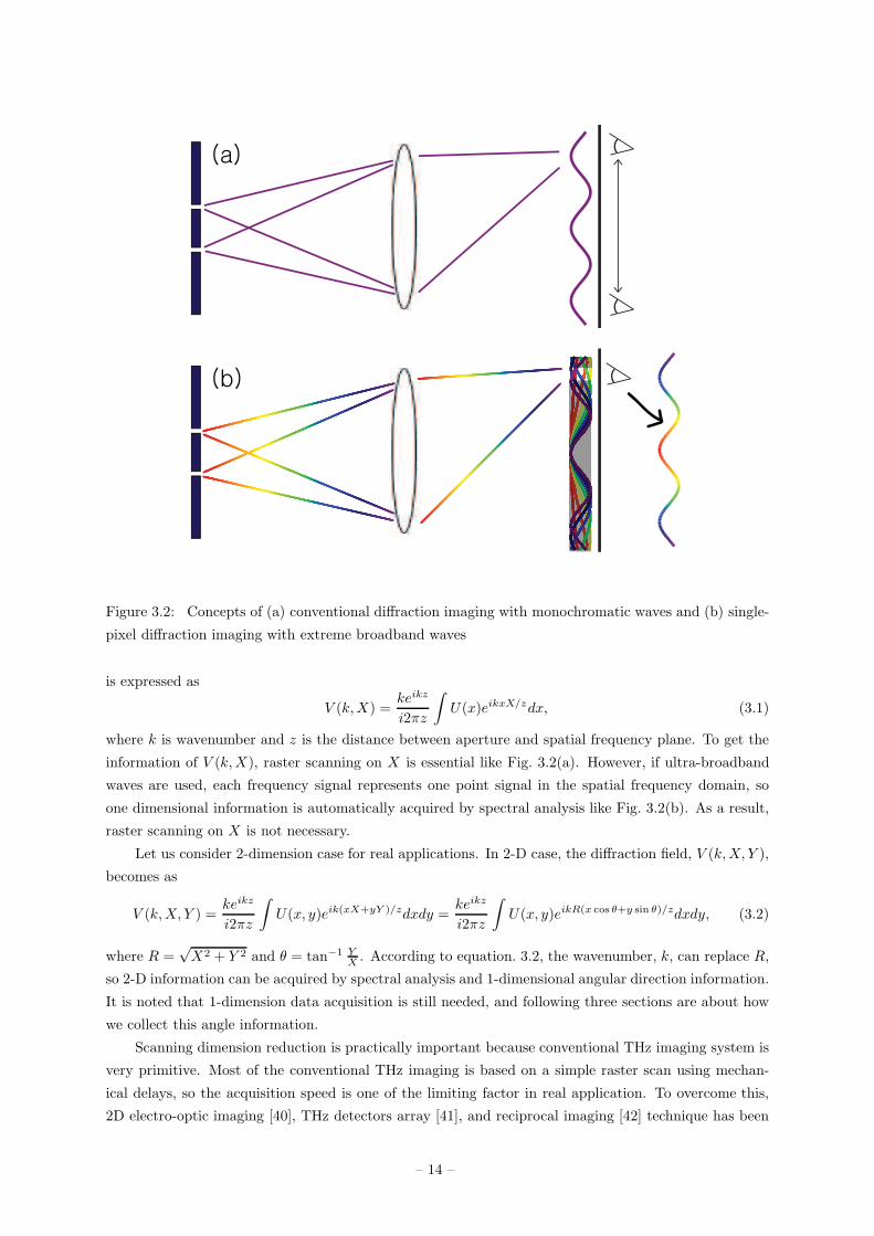
Figure 3.2: Concepts of (a) conventional diffraction imaging with monochromatic waves and (b) single-

pixel diffraction imaging with extreme broadband waves

is expressed as

V (k,X) =keikz

i2πz

∫

U(x)eikxX/zdx, (3.1)

where k is wavenumber and z is the distance between aperture and spatial frequency plane. To get the

information of V (k,X), raster scanning on X is essential like Fig. 3.2(a). However, if ultra-broadband

waves are used, each frequency signal represents one point signal in the spatial frequency domain, so

one dimensional information is automatically acquired by spectral analysis like Fig. 3.2(b). As a result,

raster scanning on X is not necessary.

Let us consider 2-dimension case for real applications. In 2-D case, the diffraction field, V (k,X, Y ),

becomes as

V (k,X, Y ) =keikz

i2πz

∫

U(x, y)eik(xX+yY )/zdxdy =keikz

i2πz

∫

U(x, y)eikR(x cos θ+y sin θ)/zdxdy, (3.2)

where R =√X2 + Y 2 and θ = tan−1 Y

X . According to equation. 3.2, the wavenumber, k, can replace R,

so 2-D information can be acquired by spectral analysis and 1-dimensional angular direction information.

It is noted that 1-dimension data acquisition is still needed, and following three sections are about how

we collect this angle information.

Scanning dimension reduction is practically important because conventional THz imaging system is

very primitive. Most of the conventional THz imaging is based on a simple raster scan using mechan-

ical delays, so the acquisition speed is one of the limiting factor in real application. To overcome this,

2D electro-optic imaging [40], THz detectors array [41], and reciprocal imaging [42] technique has been

– 14 –

proposed at the cost of high implementation complexity. Recently, Chan et. al. [43, 44] has employed a

compressed sensing (CS) [45] technique in signal processing community for THz-imaging. In their works,

using only a single detection and intelligent choices of spatial modulation, they reduced the image acqui-

sition time significantly. However, those works were mainly based on THz-intensity measurement rather

than exploiting the extremely broad band nature of THz-spectrum. It is now well known that the broad

band THz signal can be reliably measured using THz-TDS. Furthermore, fast waveform measurement is

under investigation by many groups [46], for which mechanical scanning is now being replaced by electro-

optical scanning skill as phase locked THz-asynchronous optical sampling(AOS) [47, 48]. Therefore, the

application goal of the broadband diffraction imaging is to exploit the extremely broad bandwidth of

THz signal to drastically reduce the number of samples; hence, to accelerate the acquisition time.

3.2 Single-pixel diffraction imaging with coherent optical com-

puter

3.2.1 Introduction

Coherent optical computer, or 4F-correlator, deals with acquisition of information carried by elec-

tromagnetic waves and has found many applications in image and signal processing [36, 49]. The basic

operation is setting the double-Fourier transform optical systems with transform optics, such as lens,

and Fourier filters, M(X,Y ) to set the relation of an object, U(x, y) and an image v(x′, y′) as

V (x′, y′) = F [M(X,Y )× F [U(x, y)]], (3.3)

where F represent the Fourier transform. This well-known relation between the object and image is

usually defined for a monochromatic wave.

In this section, a single pixel THz imaging system is proposed by exploiting ultra-broad bandwidth

of THz-TDS pulses. In the proposed system, a collimated THz beam is illuminated on a targets and

the scatted fields are measured through a hole at the Fourier plane using a coherent optical computer.

This setup allows conversion of temporal spectrum of THz-pulse to a radial spatial frequency spoke in

Fourier domain. Hence, 2-D image can be readily obtained by rotating a hole around an optical axis.

Experimental results confirm that a complicated object can be reliably obtained using only 30 waveform

measurements.

3.2.2 Theory

This idea can be explained using Fourier optics theory [50]. The target object is placed at an image

(x, y) plane, and illuminated by collimated terahertz pulses as shown in Fig. 3.3. The scattered field from

the object is then collected by transform optic and is propagated to the spatial frequency plan (X,Y ).

In the spatial frequency domain, a hole mask is placed such that it samples a specific spatial frequency,

which is then measured by a detector, electro-optic sampling using ZnTe thin film in this case.

As the mask M(X,Y ) is located at the far field, the detector measurement through the mask on

the Fourier plan can be represented by y(k):

V (k) = S(k)(k

i2πf)2∫

M(X,Y )[

∫

U(x, y)e−ik(xX+yY )

f dxdy]dXdY (3.4)

– 15 –

where S(k) is the spectrum of the emitter, U(x, y)is the object, f is the focal length, and k = 2πλ is

the wavenumber, respectively. Furthermore, the spectrum of the emitter, S(k), can be readily measured

using the same setup without the object and the mask.

If the mask is composed of an infinitesimal hole at distance d with angle θ; i.e. M(X,Y ) = δ(X −d cos θ, Y − d sin θ), the equation (3.4) can be simplified as

V (k, θ) = S(k)(k

i2πf)2∫

U(x, y)e−ikd

f(x cos θ+y sin θ)dxdy. (3.5)

Using the Fourier slice theorem [51], the inverse Fourier transforms of V (k,θ)S(k) ( i2πfk )2 provides as

P (u, θ) =

∫

U(x, y)δ(x cos θ + y sin θ − fu

d)dxdy (3.6)

which corresponds to the projection of the image on the θ direction, or sinogram. Therefore, one can

recover original image U(x, y) using inverse Radon transformation, if one can collect measurement for

sufficient number of θ′s by rotating the hole.

In the real experiment situation, the hole has nonzero radius a as shown in Fig. 3.3, so the equation

(3.6) can be replaced by,

P (k, θ) =πa2

4

∫

U(x, y)2J1(kaρ/2f)

kaρ/2fe

−ikdf

(x cos θ+y sin θ)dxdy (3.7)

where ρ =√

x2 + y2, and J1 represents the first order bessel function of the first kind, respectively. This

Bessel term correction results in distortion to the reconstructed image and determines the imaging field-

of-view(FOV). For example, the imaging FOV is limited as ρ < 4.43fkmaxa

, which satisfies 2J1(kaρ/2f)kaρ/2f > 1

2

where kmax denotes the maximum wavenumber in the imaging process. This implies that the FOV

is inversely proportional to kmax. Furthermore, the image resolution of our system is determined by

the maximum spatial frequency, which is proportional to the distance to the hole, d. With a simple

calculation, it can be shown that the image resolution is given by kmaxdF . Hence, the larger d and the

smaller a provide better image reconstruction at the expense of SNR loss. On the other hand, the longer

focal length F is good for FOV although bad for image resolution.

3.2.3 Experimental description

In the experimental setup, we used 100 MHz, 350 mW, 50 fs Ti:sappire oscillator system. Large

area PCA [26] and < 110 >-oriented 1 mm ZnTe are used as an emitter and a detector. The mask has

a 5 mm diameter hole, which is 15 mm apart from the optical axis. Parabolic mirrors with f = 150mm

are used for collimating emitted terahertz pulse and propagating to the mask, and a parabolic mirror

with f = 100mm is used for focusing to the detector. Shorter focal length focusing mirrors are usually

preferred due to the tight focusing and a large NA. Although we use two different focal length parabolic

mirrors, the principle is the same and our analysis still holds. Spectrums up to 1.5 THz frequency signals

use for imaging process. The frequency interval is given by about 0.01 THz.

3.2.4 Results

Experimental results are shown in Fig. 3.4. Fig. 3.4.(a) represents the target object that represents

“light” in Korean, whose dimension is about 2cm× 2cm. The hole mask has 5mm diameter hole and is

apart 15mm from the center of the mask. Entire target was illuminated, using a collimated THz pulses,

– 16 –

θ

Figure 3.3: (a) Experimental setup for single-pixel diffraction imaging with coherent optical computer.

(b) The mask geometry.

– 17 –

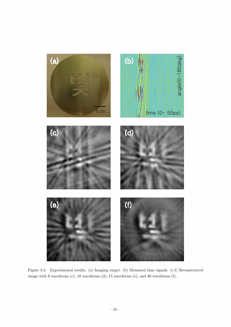
Figure 3.4: Experimental results. (a) Imaging target. (b) Measured time signals. (c-f) Reconstructed

image with 6 waveforms (c), 10 waveforms (d), 15 waveforms (e), and 30 waveforms (f).

– 18 –

5mm

(a) (b)

(c) (d)

5mm

Figure 3.5: Experimental results. (a, c) Imaging targetes. (b),(d) Reconstructed images with 18

waveforms from (a) and (c), respectively.

and the available FOV is ρ ≤ 4.43fkmaxa

∼ 1.1cm, so this target satisfied the FOV condition. We uniformly

sampled 30 waveforms in 0 ∼ 180 degree as shown in Fig. 3.4.(b). Reconstructed images are shown

in Figs. 3.4(c)-(f). We choose 6, 10, 15, and 30 waveforms with equal spacing in 0 ∼ 180 degree for

reconstructing the image, respectively. Using only 30 waveforms, we have reasonable quality images.

Other Experimental results with similar experimental conditions are shown in Fig. 3.5. Fig. 3.5.(a)

represents a target object that represents a pictogram of Taekwondo, and Fig. 3.5.(b) shows its recon-

structed image with 18 waveforms. Fig. 3.5.(c) represents the other target object, which is an earring,

and Fig. 3.5.(d) shows its reconstructed image with 18 waveforms. We could also get reasonable quality

images as the results in Fig. 3.4.

3.2.5 Discussion

The imaging principle might be equivalently stated using time-of-flight (TOF) view point under

geometric optics approximation and the assumption that the illuminated pulse is the delta function in

time. We draw this concept in Fig. 3.6. Note that at a specific time point, the scattered field from the

equidistance TOF line arrives at the hole simultaneously. Hence, the measurement at the hole is the line

integral along the equal TOF line. For different time point, the equal TOF line is varying. Hence, the

time trace of the measurement at the hole represents the projection data along different radial distance

– 19 –

θθ

Figure 3.6: The schematic drawing of time-of-flight analysis for the same measurement. By the lens,

the scattered fields along the line, which are perpendicular to θ, have the same optical path length to

the hole. Therefore, the projection of the image is acquired by wave trace measuring.

at angle θ.

Sampling number might be even more reduced in more developed setups. First, the time separating

mask could be used instead of a hole mask as shown in Fig. 3.7(a). Terahertz transmitted material such

as silicon could be placed azimuthally with different thickness in this mask. In this particular setup,

terahertz waves arrive to the detector separately in time and each separated wave can be used for the

image reconstruction process. As a result, one waveform diffraction is even possible. This concept is

realized in chapter 3.3.

On the other hand, detector array are arranged azimuthally as shown in Fig. 3.7(b). Putting the

detector array in the spatial frequency domain instead of the hole mask, 2D image can be archived by

1D detector array only.

The main disadvantage of the system is low SNR, since the hole mask blocks almost whole terahertz

pulse. However, automatic repetition of pulse measurement using THz asynchronous optical sampling [47,

48] or more powerful sources may make the SNR sufficiently large for real time measurement. In addition,

there might be mask-less single-pixel diffraction imaging, which is free from the bad SNR. We will explain

it in Section 3.4.

3.2.6 Summary

In summary, we have demonstrated the single-pixel imagery of objects by exploiting the extreme

broadband nature of ultrafast THz pulses. In this newly developed coherent optical computing scheme

for a broadband source, 2D spatial information can be encrypted into waveforms, or a single waveform,

and the image is recovered through inverse radon transformation. The THz imaging problem is now

converted to 1D scanning rather than 2D one, which may significantly accelerate the acquisition time.

– 20 –

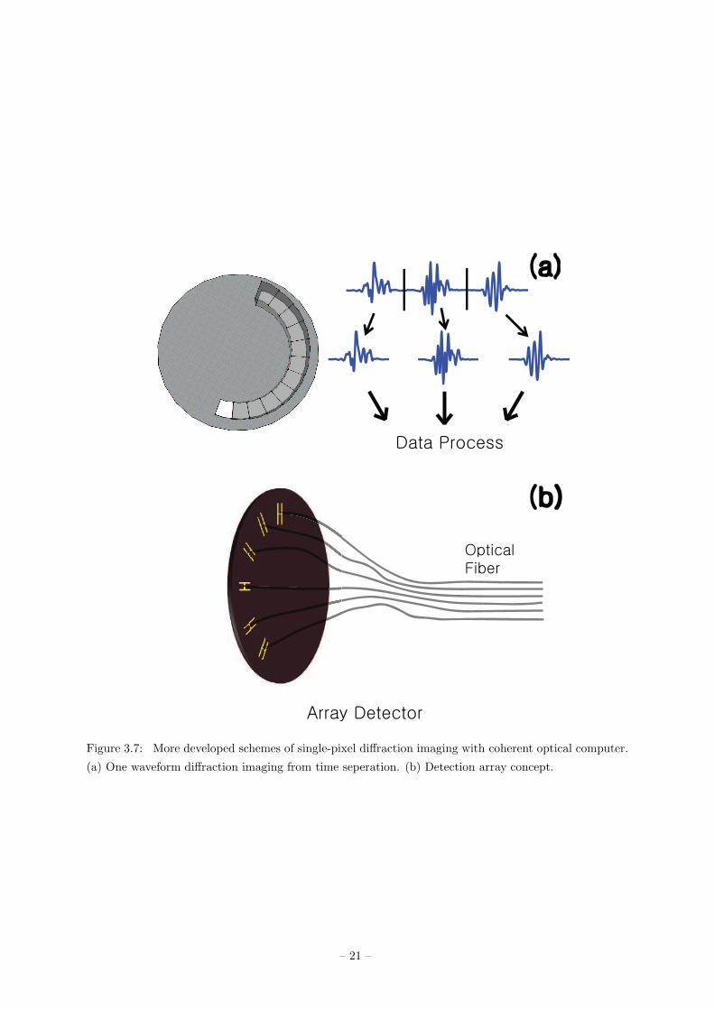
Figure 3.7: More developed schemes of single-pixel diffraction imaging with coherent optical computer.

(a) One waveform diffraction imaging from time seperation. (b) Detection array concept.

– 21 –

3.3 One waveform imaging

3.3.1 Introduction

It is worth noting that the imaging methods in the previous chapter 3.2 used active masking for

2D imaging. This method requires the measurement of N different waveforms, each containing specific

angular projection information of the object. Mathematically there may exist a number of techniques

that permit the extraction of complete spatial information for a 2D object from a single waveform. The

simplest method is the use of a single Fourier-domain mask [Fig. 3.7(a)] constructed with N holes of

various phase retardations. This Fourier mask, used in a coherent computational setup in the previous

setup, temporally separates N THz waveforms, each containing individual angular object information

with respect to each other. Then, a single time-domain scan of the diffracted THz wave simultaneously

records the complete angular projection image of the 2D object, and therefore, a 2D image recovery from

a single THz waveform might be achieved.

3.3.2 Experimental description and results

Experimental setup is just same as the previous chapter 3.2 except the mask part. In this experiment,

the mask has 12 holes with 6mm-diameter which are 15mm apart from the optical axis as shown in

Fig. 3.8(a). Silicon blocks with different thicknesses are glued the mask together on hole positions. The

time interval of the separated signals is about 8ps by the silicon blocks. Fig. 3.8(b) represents the target

object, whose dimension is about 1cm × 1cm. In this setup, the available FOV is ρ ≤ 4.43fkmaxa

∼ 0.8cm,

so the target is small enough to be seen. The measured waveform is plotted in Fig. 3.8(c). We separate

this waveform into 12 waveforms and waveform separating is indicated by dash lines in Fig. 3.8(c). The

reconstructed image and overlapped image with the target is shown in Fig. 3.8(d) and (e), respectively.

Recognizable image is also achieved as the results in the previous section from only a single waveform.

3.4 Single-pixel diffraction imaging with a slanted phase re-

tarder

In this section, we demonstrate single-pixel diffraction imaging, whereby broadband terahertz (THz)

waveforms passed through a slanted phase retarder (SPR), instead of a hole mask, diffracted from an

object, were measured by a THz detector located in the far field. For 1D imaging, the fixed-location

single-pixel broadband detector simultaneously measured all the spatial frequency components of the

object because the frequency components of the source maintain a one-to-one correspondence with the

object’s spatial frequency. For 2D imaging, the angular position of the SPR enabled the diffracted THz

wave to carry an angular projection image of the object. Thirty waveforms are measured at different

SPR orientations to reconstruct complex 2D images.

3.4.1 Introduction

Coherent diffraction imaging (CDI) is an image reconstruction technique for small-size objects using

highly coherent optical, X-ray, or electron beams, in which a real-space image is reconstructed from

a diffraction pattern collected by a detector array via an iterative feedback algorithm [52]. Recently

developed high-energy photon sources permit CDI of nanoscale structures, such as nanotubes, quantum

– 22 –

2mm

(a) (b)

(d) (e)

0 20 40 60 80 100 120−1

−0.8

−0.6

−0.4

−0.2

0

0.2

0.4

0.6

0.8

1

ps

ampl

itude

(A.U

.)

(c)

Figure 3.8: Summary of one waveform diffraction imaging. (a) Time separating mask. (b) The image

target. (c) The measured waveform. Dash lines indicate time separation. (d) Reconstructed image. (e)

Overlapped image with image target.

– 23 –

dots, and possibly proteins [53, 54, 55]. Also, CDI with optical waves has proven useful in obtaining

tomographic high-resolution images of live cells [56]. The image resolution of CDI depends on the wave-

length and the extension of the measured diffraction pattern. For a monochromatic wave of wavelength

λ, the Fraunhoffer diffraction pattern V (X) of an object U(x) is

V (X) =eikzei

kX2

2z

iλz

∫

U(x)e−i 2πλz

xXdx, (3.8)

where x and X represent spatial coordinates in the real and reciprocal spaces, respectively, k is the

wave number, and z is the distance from the object to the detector. The Fourier component of U(x)

evaluated at spatial frequency fX(= X/λz), that is U(fX), is captured in V (X), aside from the given

phase factor. For a high-resolution image of maximum spatial frequency fmax, an array detector of lateral

size Xmax = λz/fmax is required.

However, given a broadband coherent source with a frequency distribution ranging from zero to

ωmax/2π, a single-pixel detector can replace the detector array because the frequency components of the

source maintain a one-to-one correspondence with the spatial frequency components of the object. The

point detector placed in a fixed position Xo can simultaneously measure all the Fourier components of

U(x); therefore, single-pixel imaging can be achieved such that

U(x) =

∫ ωmax

0

U(fXo;ω)e−ixfXo (ω)dω, (3.9)

where ω is the angular frequency and ωmax = 2πcfmaxz/Xo. In this proposed method for single-pixel

coherent diffraction imaging (SP-CDI), the spatial resolution is limited by the frequency maximum ωmax

of the coherent source, not by the detector size.

For a broadband coherent source, we consider ultrafast THz pulses [57]. A typical THz pulse fre-

quency range for THz time-domain spectroscopy (THz-TDS) is 0 to 3 THz [58] and a record broad

bandwidth of 80 THz has been reported [59]. They have an extremely broad range of frequency com-

ponents with a characteristic frequency-to-bandwidth ratio near unity. Conventional use of ultrafast

THz waves in imaging involves a raster scan to move an object around a tightly focused THz beam [60]

and this method has a diverse range of imaging applications extending from semiconductors and metal

structures to biological and medical objects [61, 62, 63]. However, due to the limitation of the data acqui-

sition speed of this mechanical scanning method, various alternatives have been proposed, including 2D

electro-optic imaging [64], a focal-plane detector array [65], and compressed sensing techniques [43, 44],

at the cost of implementation complexity. In the previous section, we demonstrated coherent optical

computation for single-point THz imaging, where an active Fourier mask in a conventional THz-TDS

setup converted a 2D image into N temporal waveforms. In this section, using a completely different

approach, we propose single-pixel detection of coherent diffraction images and demonstrate various 2D

image reconstructions.

3.4.2 Theory

In SP-CDI, a target 2D object is placed in the object plane Σo(x, y), as shown in Fig. 3.9(a), and

illuminated by collimated THz waves. The diffracted field from the object U(x, y) is then collected by

a THz detector located at the center of the far-field diffraction plane Σd(X,Y ), i.e., X = Y = 0. To

redirect all the spatial frequency components to the detector location, a slanted phase retarder (SPR),

shown in Fig. 3.9(b), is inserted in front of the object. For an incident THz wave of spectral field profile

– 24 –

Slated Phase

Retarder

Object

α

φIncident

Ray

Transmitted

Ray

FF

(a)

(b) (c)

Σο(x,y)

Σd(X,Y)

lens

THz Detector

Figure 3.9: Experimental setup and geometry. (a) Schematic of single-pixel diffraction imaging with

SPR. (b) Slanted phase retarder (SPR). (c) Illustration of beam deviation.

S(ω), the diffracted field Vθ(ω) is given by

Vθ(ω)

S(ω)=

eikz

iλz

∫

Σo

U(x, y)eik(x cos θ+y sin θ) sinφdxdy, (3.10)

where θ is the angular position of the SPR and φ denotes the deviation angle of the beam through

the SPR, as shown in Fig. 3.9(c). Due to the angular orientation of the SPR, the diffracted THz wave

carries an angular projection image of the object. Using a procedure that is mathematically similar to

the method described in the previous section, the original object U(x, y) is recovered from a number of

measurements carried out at different θs by

U(x, y) ∝ R−1θ

[

F−1

[

Vθ(ω)

ωeikzS(ω)

]]

, (3.11)

where R−1θ and F−1 are inverse Radon and inverse Fourier transformations, respectively.

3.4.3 Experimental description and results

For the experiment, we used a Ti:sapphire laser oscillator that produced IR short pulses at an average

power of 350 mW. THz waves were generated from a large-area photoconductive antenna (PCA) [66]

and then collimated by an off-axis parabolic mirror with a 150-mm focal length. For detecting the

diffracted THz waves, a 2-mm-thick ZnTe electro-optic crystal was placed in the front focal plane of

another parabolic mirror with a focal length of 100 mm. Time-resolved THz electric field measurements

– 25 –

0

20

40

60

80

100

120

140

160

0 5 10 15 20 25 30

Time(ps)θ(

de

gre

e)

Figure 3.10: Experimental results. (a) Image target. (b) Measured waveforms. (c) Reconstructed

image. (d) Sharpened image by high-frequency pass filtering of measured waveforms in (b).

were carried out by mapping the polarization changes of optical gate beams, due to the Pockels effect

induced in the electro-optic crystal by the electric field of the THz pulse [30].

The object, a representation of a feline paw shown in Fig. 3.10(a), was made from a 0.5-mm-thick

metal plate of area 2 cm × 2 cm. The SPR was made out of polytetrafluoroethylene (Teflon) and had a

cylindrical shape (radius 25 mm) cut at an angle α = 15◦. The index of refraction of Teflon is a constant

n = 1.46 over the THz spectral range.

The procedure for data collection and image recovery was as follows. First, both the object and

the SPR were temporarily removed and the reference THz field spectrum at the detector, Sd(ω), was

obtained by taking the Fourier transform of a THz time-domain signal. It is noted that Sd(ω) differs from

the THz field spectrum at the object by a factor of ω, aside from a constant factor. Then, the object and

the SPR were replaced and N = 30 different THz waveforms were measured at various angles uniformly

sampled from θ = 0◦ − 180◦. [Fig. 3.10(b)] The time-domain waveforms were recorded with a spectrum

of up to ωmax = 1.5 THz with a resolution of 0.03 THz. By following the signal processing described

in Eqs. (3.10) and (3.11), the coherent diffraction image was retrieved. [Fig. 3.10(c)] Owing to the one-

– 26 –

to-one correspondence of the THz frequency to the image spatial frequency, the Fourier synthetic image

processing can be implemented in a variety of ways by directly manipulating the Fourier components

of the THz waveforms. For example, a sharpened image, such as that in Fig. 3.10(d), was obtained via

high-pass filtering of measured THz waveforms.

Same procedure is also possible when the SPR is placed in the back of an image target. To verify

this, we place the SPR in the back of an image target and measure waveforms as we did for Fig. 3.10.

The geometrical configuration is shown in the inset figure in Fig. 3.11.(a). The imaging target is shown

in Fig. 3.11.(a) and the reconstructed image is shown in Fig. 3.11.(b). To reconstruct the image, we

measure 15 waveforms with 12 degree spacing. Imaging is well done as the result shown in Fig. 3.10.

3.4.4 Image resolution

The SP-CDI image resolution is not directly related to the numerical aperture or the focal length of

the diffractive optic. Instead, the beam deviation angle φ is a scaling coefficient between fmax and ωmax,

i.e., fmax = ωmax sinφ/2πc, and therefore, determines the image resolution. Figure 3.12 shows the result

of an imaging experiment with an object of a double-slit pattern. For 1-mm hole double slits separated

by 2 mm, as shown in Fig. 3.12(a), three different SPRs cut at α = 10◦, 20◦, and 30◦ were used, and the

diffraction images shown in Fig. 3.12(b)-(d), respectively, were obtained. The SPR angles were chosen

to give image resolutions of 1/fmax= 2.4, 1.2, and 0.7 mm, respectively, and as expected, the double-slit

patterns were resolved in Figs. 3.12(c) and (d) only. For enhanced image resolution, larger SPR angles

should be considered. However, from the relationship φ = sin−1(n sinα)−α, total internal reflection will

occur in the SPR and the image resolution is limited as

1

fmax=

λmin

sinφ≤ n√

n2 − 1λmin, (3.12)

where λmin is the minimal wavelength of the given THz pulse. Figure 3.12(e) compares the measured

maximal frequencies with Eq. (3.12): The calculated fmax from the images are shown in dots and the

the result from Eq. (3.12) in a red line. Both, plotted as a function of the SPR angle α, show a good

agreement. As a result, the resolution limit in SP-CDI is determined by both the index of refraction of

the SPR and the maximal THz frequency. In the ideal case, the resolution of SP-CDI is about λmin due

to the limit of wave propagation like usual light microscopy.

3.4.5 Discussion

SP-CDI can be implemented using broadband waves in different frequency ranges. For example,

sub-femtosecond pulses produced via high harmonic generation of an ultrashort infrared pulse in atoms

encompasses the whole spectral range of visible and UV/XUV [67]. Another candidate is the supercon-

tinuum formed as a result of cascading nonlinear processes of IR short pulses, as seen, for example, in a

photonic bandgap fiber, which spans several optical octaves with a spectral range extending from UV to

beyond mid-IR [68]. Both broadband sources are capable of SP-CDI given a proper choice of diffractive

optics. With these higher frequncy waves as a source, proper phase retrieval process might be needed.

3.4.6 Summary

In summary, we demonstrated coherent diffraction imaging using a fixed-location single-pixel detec-

tor. The broadband nature of the THz waves was used for one-to-one mapping of the spatial frequency of

– 27 –

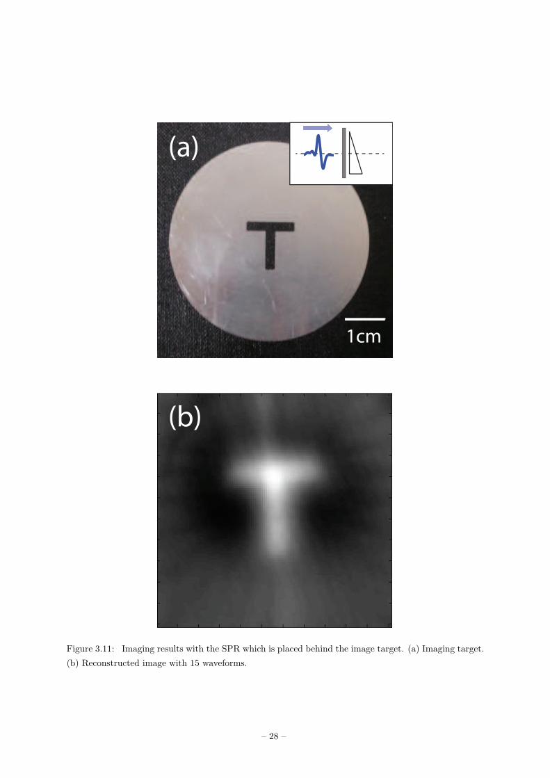
(a)

(b)

1cm

Figure 3.11: Imaging results with the SPR which is placed behind the image target. (a) Imaging target.

(b) Reconstructed image with 15 waveforms.

– 28 –

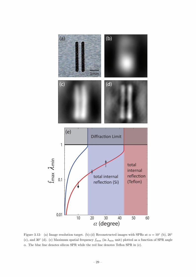
α (degree)10 20 30 40 50 60

0.1

total

internal

reflec�on

(Teflon)

total internal

reflec�on (Si)

Diffrac�on Limit

λ

(a) (b)

(c) (d)

(e)

3mm

f ma

xm

in

1

0.01

Figure 3.12: (a) Image resolution target. (b)-(d) Reconstructed images with SPRs at α = 10◦ (b), 20◦

(c), and 30◦ (d). (e) Maximum spatial frequency fmax (in λmin unit) plotted as a function of SPR angle

α. The blue line denotes silicon SPR while the red line denotes Teflon SPR in (e).

– 29 –

an object to the frequency of the diffracted waves, and by adopting a slanted phase retarder, a fixed-point

single detector collected complete 2D angular projection images of various objects, enabling single-pixel

2D coherent diffraction imaging. Our proposed idea could eliminate the need for area detection in

coherent diffraction imaging.

– 30 –

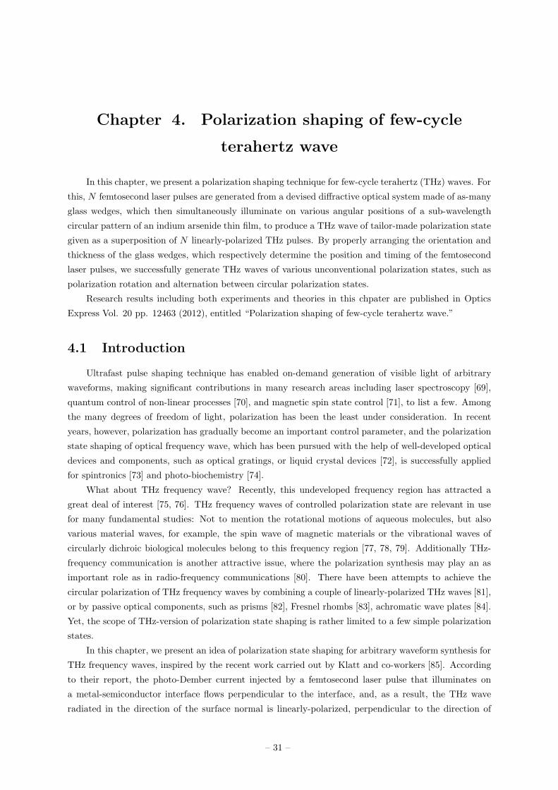
Chapter 4. Polarization shaping of few-cycle

terahertz wave

In this chapter, we present a polarization shaping technique for few-cycle terahertz (THz) waves. For

this, N femtosecond laser pulses are generated from a devised diffractive optical system made of as-many

glass wedges, which then simultaneously illuminate on various angular positions of a sub-wavelength

circular pattern of an indium arsenide thin film, to produce a THz wave of tailor-made polarization state

given as a superposition of N linearly-polarized THz pulses. By properly arranging the orientation and

thickness of the glass wedges, which respectively determine the position and timing of the femtosecond

laser pulses, we successfully generate THz waves of various unconventional polarization states, such as

polarization rotation and alternation between circular polarization states.

Research results including both experiments and theories in this chpater are published in Optics

Express Vol. 20 pp. 12463 (2012), entitled “Polarization shaping of few-cycle terahertz wave.”

4.1 Introduction

Ultrafast pulse shaping technique has enabled on-demand generation of visible light of arbitrary

waveforms, making significant contributions in many research areas including laser spectroscopy [69],

quantum control of non-linear processes [70], and magnetic spin state control [71], to list a few. Among

the many degrees of freedom of light, polarization has been the least under consideration. In recent

years, however, polarization has gradually become an important control parameter, and the polarization

state shaping of optical frequency wave, which has been pursued with the help of well-developed optical

devices and components, such as optical gratings, or liquid crystal devices [72], is successfully applied

for spintronics [73] and photo-biochemistry [74].

What about THz frequency wave? Recently, this undeveloped frequency region has attracted a

great deal of interest [75, 76]. THz frequency waves of controlled polarization state are relevant in use

for many fundamental studies: Not to mention the rotational motions of aqueous molecules, but also

various material waves, for example, the spin wave of magnetic materials or the vibrational waves of

circularly dichroic biological molecules belong to this frequency region [77, 78, 79]. Additionally THz-

frequency communication is another attractive issue, where the polarization synthesis may play an as

important role as in radio-frequency communications [80]. There have been attempts to achieve the

circular polarization of THz frequency waves by combining a couple of linearly-polarized THz waves [81],

or by passive optical components, such as prisms [82], Fresnel rhombs [83], achromatic wave plates [84].

Yet, the scope of THz-version of polarization state shaping is rather limited to a few simple polarization

states.

In this chapter, we present an idea of polarization state shaping for arbitrary waveform synthesis for

THz frequency waves, inspired by the recent work carried out by Klatt and co-workers [85]. According

to their report, the photo-Dember current injected by a femtosecond laser pulse that illuminates on

a metal-semiconductor interface flows perpendicular to the interface, and, as a result, the THz wave

radiated in the direction of the surface normal is linearly-polarized, perpendicular to the direction of

– 31 –

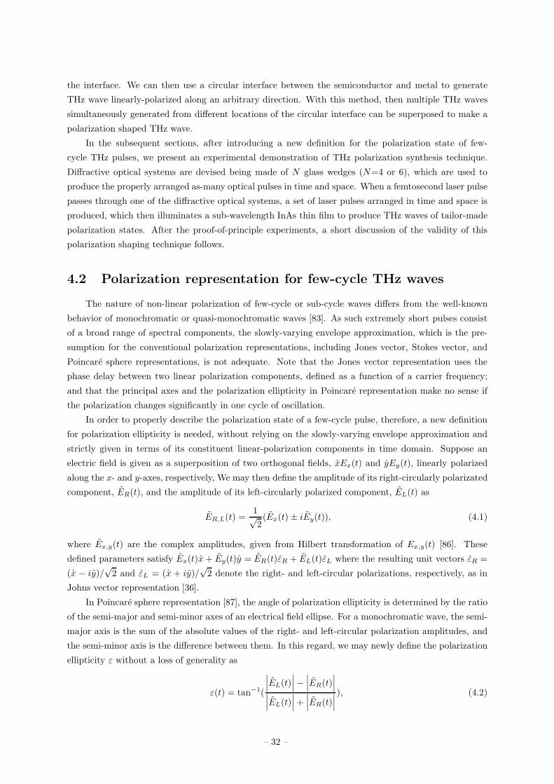
the interface. We can then use a circular interface between the semiconductor and metal to generate

THz wave linearly-polarized along an arbitrary direction. With this method, then multiple THz waves

simultaneously generated from different locations of the circular interface can be superposed to make a

polarization shaped THz wave.

In the subsequent sections, after introducing a new definition for the polarization state of few-

cycle THz pulses, we present an experimental demonstration of THz polarization synthesis technique.

Diffractive optical systems are devised being made of N glass wedges (N=4 or 6), which are used to

produce the properly arranged as-many optical pulses in time and space. When a femtosecond laser pulse

passes through one of the diffractive optical systems, a set of laser pulses arranged in time and space is

produced, which then illuminates a sub-wavelength InAs thin film to produce THz waves of tailor-made

polarization states. After the proof-of-principle experiments, a short discussion of the validity of this

polarization shaping technique follows.

4.2 Polarization representation for few-cycle THz waves

The nature of non-linear polarization of few-cycle or sub-cycle waves differs from the well-known

behavior of monochromatic or quasi-monochromatic waves [83]. As such extremely short pulses consist

of a broad range of spectral components, the slowly-varying envelope approximation, which is the pre-

sumption for the conventional polarization representations, including Jones vector, Stokes vector, and

Poincare sphere representations, is not adequate. Note that the Jones vector representation uses the

phase delay between two linear polarization components, defined as a function of a carrier frequency;

and that the principal axes and the polarization ellipticity in Poincare representation make no sense if

the polarization changes significantly in one cycle of oscillation.

In order to properly describe the polarization state of a few-cycle pulse, therefore, a new definition

for polarization ellipticity is needed, without relying on the slowly-varying envelope approximation and

strictly given in terms of its constituent linear-polarization components in time domain. Suppose an

electric field is given as a superposition of two orthogonal fields, xEx(t) and yEy(t), linearly polarized

along the x- and y-axes, respectively, We may then define the amplitude of its right-circularly polarizated

component, ER(t), and the amplitude of its left-circularly polarized component, EL(t) as

ER,L(t) =1√2(Ex(t)± iEy(t)), (4.1)

where Ex,y(t) are the complex amplitudes, given from Hilbert transformation of Ex,y(t) [86]. These

defined parameters satisfy Ex(t)x+ Ey(t)y = ER(t)εR + EL(t)εL where the resulting unit vectors εR =

(x − iy)/√2 and εL = (x + iy)/

√2 denote the right- and left-circular polarizations, respectively, as in

Johns vector representation [36].

In Poincare sphere representation [87], the angle of polarization ellipticity is determined by the ratio

of the semi-major and semi-minor axes of an electrical field ellipse. For a monochromatic wave, the semi-

major axis is the sum of the absolute values of the right- and left-circular polarization amplitudes, and

the semi-minor axis is the difference between them. In this regard, we may newly define the polarization

ellipticity ε without a loss of generality as

ε(t) = tan−1(

∣

∣

∣EL(t)

∣

∣

∣−∣

∣

∣ER(t)

∣

∣

∣

∣

∣

∣EL(t)

∣

∣

∣+∣

∣

∣ER(t)

∣

∣

∣

), (4.2)

– 32 –

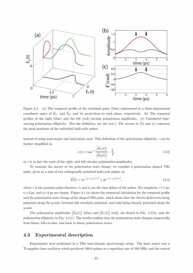
03.5

7

0

0

time (ps)

1 2 3 4 5 60

0.5

1

1.5

Am

plit

ud

e

1 2 3 4 5 6

−0.8

−0.4

0

0.4

0.8

time (ps)

time (ps)

(a)(b)

(c)

(ra

d)

ε

xE (t)

yE

(t)

Figure 4.1: (a) The temporal profile of the combined pulse (blue) represented in a three-dimensional

coordinate space of Ex, and Ey; and its projections to each plane, respectively. (b) The temporal

profiles of the right (blue) and the left (red) circular polarization amplitudes. (c) Calculated time-

varying polarization ellipticity. (For the definition, see the text.) The arrows in (b) and (c) represent

the peak positions of the individual half-cycle pulses.

instead of using semi-major and semi-minor axes. This definition of the polarization ellipticity ε can be

further simplified as,

ε(t) = tan−1

∣

∣

∣EL(t)

∣

∣

∣

∣

∣

∣ER(t)

∣

∣

∣

− π

4, (4.3)

so ε is in fact the ratio of the right- and left-circular polarization amplitudes.

To examine the nature of the polarization state change, we consider a polarization shaped THz

pulse, given as a sum of two orthogonally polarized half-cycle pulses, as

~E(t) = xe−(t−t1)2/τ2

+ ye−(t−t2)2/τ2

, (4.4)

where τ is the gaussian pulse duration, t1 and t2 are the time delays of the pulses. For simplicity, τ=1 ps,

t1=3 ps, and t2=4 ps are chosen. Figure 4.1 (a) shows the numerical calculation for the temporal profile

and the polarization state change of the shaped THz pulse, which shows that the electric field starts being

polarized along the y-axis, becomes left-circularly polarized, and ends being linearly polarized along the

y-axis.

The polarization amplitudes∣

∣

∣ER(t)

∣

∣

∣(blue) and

∣

∣

∣EL(t)

∣

∣

∣(red), are drawn in Fig. 4.1(b), and the

polarization ellipticity in Fig. 4.1(c). The results confirm that the polarization state changes sequentially

from linear, left-circular, and back to linear polarization states.

4.3 Experimental description

Experiments were performed in a THz time-domain spectroscopy setup. The laser source was a

Ti:sapphire laser oscillator which produced 100-fs pulses at a repetition rate of 100 MHz, and the central

– 33 –

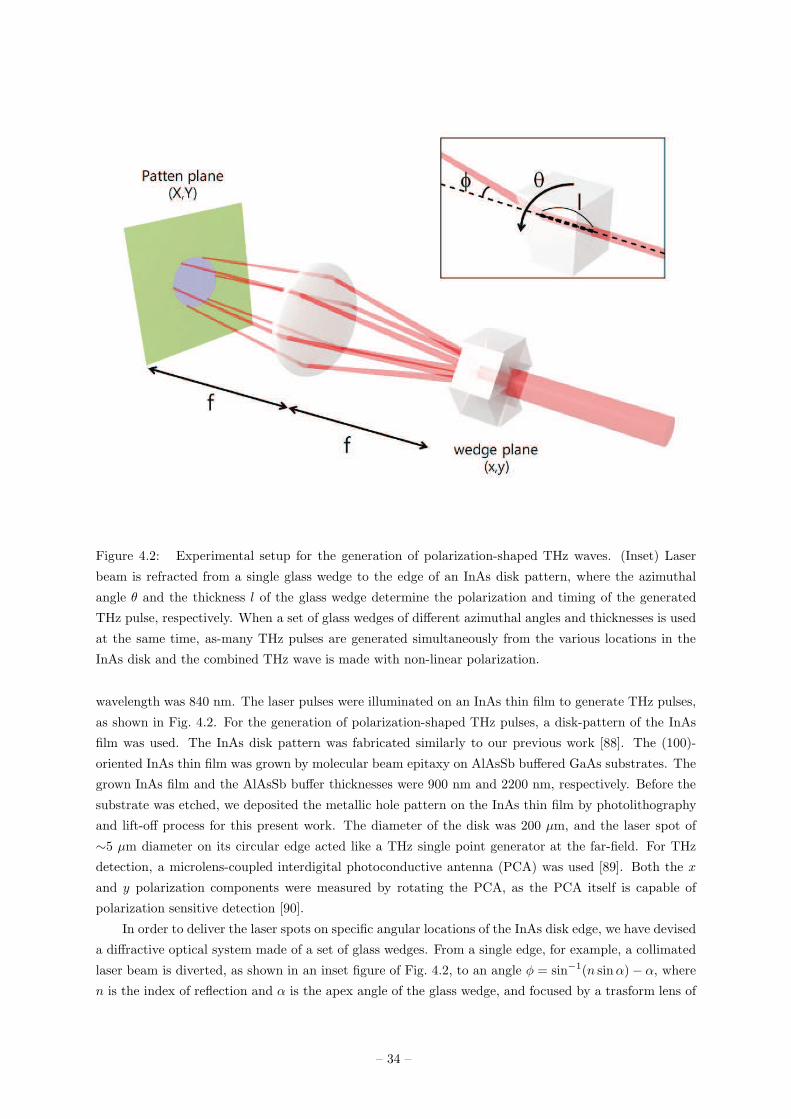
Figure 4.2: Experimental setup for the generation of polarization-shaped THz waves. (Inset) Laser

beam is refracted from a single glass wedge to the edge of an InAs disk pattern, where the azimuthal

angle θ and the thickness l of the glass wedge determine the polarization and timing of the generated

THz pulse, respectively. When a set of glass wedges of different azimuthal angles and thicknesses is used

at the same time, as-many THz pulses are generated simultaneously from the various locations in the

InAs disk and the combined THz wave is made with non-linear polarization.

wavelength was 840 nm. The laser pulses were illuminated on an InAs thin film to generate THz pulses,

as shown in Fig. 4.2. For the generation of polarization-shaped THz pulses, a disk-pattern of the InAs

film was used. The InAs disk pattern was fabricated similarly to our previous work [88]. The (100)-

oriented InAs thin film was grown by molecular beam epitaxy on AlAsSb buffered GaAs substrates. The

grown InAs film and the AlAsSb buffer thicknesses were 900 nm and 2200 nm, respectively. Before the

substrate was etched, we deposited the metallic hole pattern on the InAs thin film by photolithography

and lift-off process for this present work. The diameter of the disk was 200 µm, and the laser spot of

∼5 µm diameter on its circular edge acted like a THz single point generator at the far-field. For THz

detection, a microlens-coupled interdigital photoconductive antenna (PCA) was used [89]. Both the x

and y polarization components were measured by rotating the PCA, as the PCA itself is capable of

polarization sensitive detection [90].

In order to deliver the laser spots on specific angular locations of the InAs disk edge, we have devised

a diffractive optical system made of a set of glass wedges. From a single edge, for example, a collimated

laser beam is diverted, as shown in an inset figure of Fig. 4.2, to an angle φ = sin−1(n sinα)− α, where

n is the index of reflection and α is the apex angle of the glass wedge, and focused by a trasform lens of

– 34 –

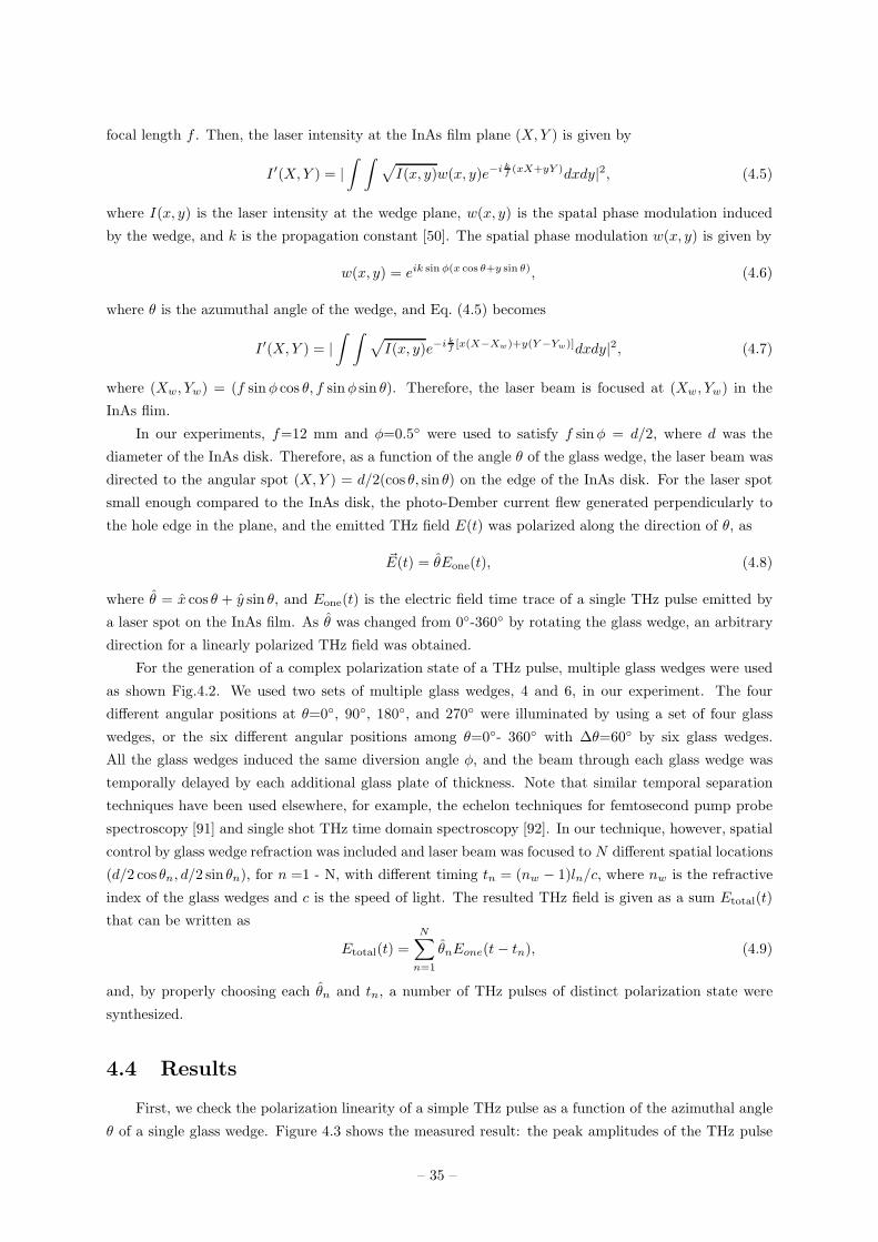
focal length f . Then, the laser intensity at the InAs film plane (X,Y ) is given by

I ′(X,Y ) = |∫ ∫

√

I(x, y)w(x, y)e−i kf(xX+yY )dxdy|2, (4.5)

where I(x, y) is the laser intensity at the wedge plane, w(x, y) is the spatal phase modulation induced

by the wedge, and k is the propagation constant [50]. The spatial phase modulation w(x, y) is given by

w(x, y) = eik sinφ(x cos θ+y sin θ), (4.6)

where θ is the azumuthal angle of the wedge, and Eq. (4.5) becomes

I ′(X,Y ) = |∫ ∫

√

I(x, y)e−i kf[x(X−Xw)+y(Y−Yw)]dxdy|2, (4.7)

where (Xw, Yw) = (f sinφ cos θ, f sinφ sin θ). Therefore, the laser beam is focused at (Xw, Yw) in the

InAs flim.

In our experiments, f=12 mm and φ=0.5◦ were used to satisfy f sinφ = d/2, where d was the

diameter of the InAs disk. Therefore, as a function of the angle θ of the glass wedge, the laser beam was

directed to the angular spot (X,Y ) = d/2(cos θ, sin θ) on the edge of the InAs disk. For the laser spot

small enough compared to the InAs disk, the photo-Dember current flew generated perpendicularly to

the hole edge in the plane, and the emitted THz field E(t) was polarized along the direction of θ, as

~E(t) = θEone(t), (4.8)

where θ = x cos θ + y sin θ, and Eone(t) is the electric field time trace of a single THz pulse emitted by

a laser spot on the InAs film. As θ was changed from 0◦-360◦ by rotating the glass wedge, an arbitrary

direction for a linearly polarized THz field was obtained.

For the generation of a complex polarization state of a THz pulse, multiple glass wedges were used

as shown Fig.4.2. We used two sets of multiple glass wedges, 4 and 6, in our experiment. The four

different angular positions at θ=0◦, 90◦, 180◦, and 270◦ were illuminated by using a set of four glass

wedges, or the six different angular positions among θ=0◦- 360◦ with ∆θ=60◦ by six glass wedges.

All the glass wedges induced the same diversion angle φ, and the beam through each glass wedge was

temporally delayed by each additional glass plate of thickness. Note that similar temporal separation

techniques have been used elsewhere, for example, the echelon techniques for femtosecond pump probe

spectroscopy [91] and single shot THz time domain spectroscopy [92]. In our technique, however, spatial

control by glass wedge refraction was included and laser beam was focused to N different spatial locations

(d/2 cos θn, d/2 sin θn), for n =1 - N, with different timing tn = (nw − 1)ln/c, where nw is the refractive

index of the glass wedges and c is the speed of light. The resulted THz field is given as a sum Etotal(t)

that can be written as

Etotal(t) =

N∑

n=1

θnEone(t− tn), (4.9)

and, by properly choosing each θn and tn, a number of THz pulses of distinct polarization state were

synthesized.

4.4 Results

First, we check the polarization linearity of a simple THz pulse as a function of the azimuthal angle

θ of a single glass wedge. Figure 4.3 shows the measured result: the peak amplitudes of the THz pulse

– 35 –

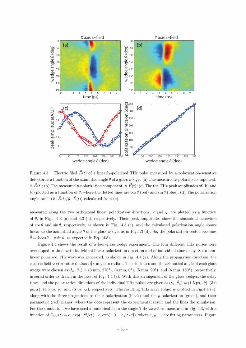
X axis E−�eld

time (ps)0 1 2 3 4 5 6 7 8 9

0

50

100

150

200

250

300

350

Y axis E−�eld

time (ps)0 1 2 3 4 5 6 7 8 9

0

50

100

150

200

250

300

350

0 50 100 150 200 250 300 350

50

100

150

200

250

300

350

0 50 100 150 200 250 300 350

−1

−0.5

0

0.5

1

wedge angle θ (deg)

pe

ak

am

pli

tud

e(A

.U.)

po

lari

zati

on

dir

ec

tio

n (

de

g)

(a) (b)

(c) (d)

wedge angle θ (deg)

we

dg

e a

ng

le θ

(de

g)

we

dg

e a

ng

le θ

(de

g)

1

Figure 4.3: Electric filed ~E(t) of a linearly-polarized THz pulse measured by a polarization-sensitive

detector as a function of the azimuthal angle θ of a glass wedge: (a) The measured x-polarized component,

x· ~E(t); (b) The measured y-polarization component, y · ~E(t); (c) The the THz peak amplitudes of (b) and

(c) plotted as a function of θ, where the dotted lines are cos θ (red) and sin θ (blue); (d) The polarization

angle tan−1(x · ~E(t)/y · ~E(t)) calculated from (c).

measured along the two orthogonal linear polarization directions, x and y, are plotted as a function

of θ, in Figs. 4.3 (a) and 4.3 (b), respectively. Their peak amplitudes show the sinusoidal behaviors

of cos θ and sin θ, respectively, as shown in Fig. 4.3 (c), and the calculated polarization angle shows

linear to the azimuthal angle θ of the glass wedge, as in Fig.4.3 (d). So, the polarization vector becomes

θ = x cos θ + y sin θ, as expected in Eq. (4.8).

Figure 4.4 shows the result of a four-glass wedge experiment. The four different THz pulses were

overlapped in time, with individual linear polarization direction and of individual time delay. So, a non-

linear polarized THz wave was generated, as shown in Fig. 4.4 (a). Along the propagation direction, the

electric field vector rotated about 32π angle in radian. The thickness and the azimuthal angle of each glass

wedge were chosen as (ln, θn) = (3 mm, 270◦), (4 mm, 0◦), (5 mm, 90◦), and (6 mm, 180◦), respectively,

in serial order as drawn in the inset of Fig. 4.4 (a). With this arrangement of the glass wedges, the delay

times and the polarization directions of the individual THz pulses are given as (tn, θn) = (1.5 ps, -y), (3.0

ps, x), (4.5 ps, y), and (6 ps, -x), respectively. The resulting THz wave (blue) is plotted in Fig.4.4 (a),

along with the three projections to the x-polarization (black) and the y-polarization (green), and their

parametric (red) planes, where the dots represent the experimental result and the lines the simulation.

For the simulation, we have used a numerical fit to the single THz waveform measured in Fig. 4.3, with a

function of Eone(t) = c1 exp(−t2/c22)−c3 exp(−(t− c4)2/c25), where c1,2,···,5 are fitting parameters. Figure

– 36 –

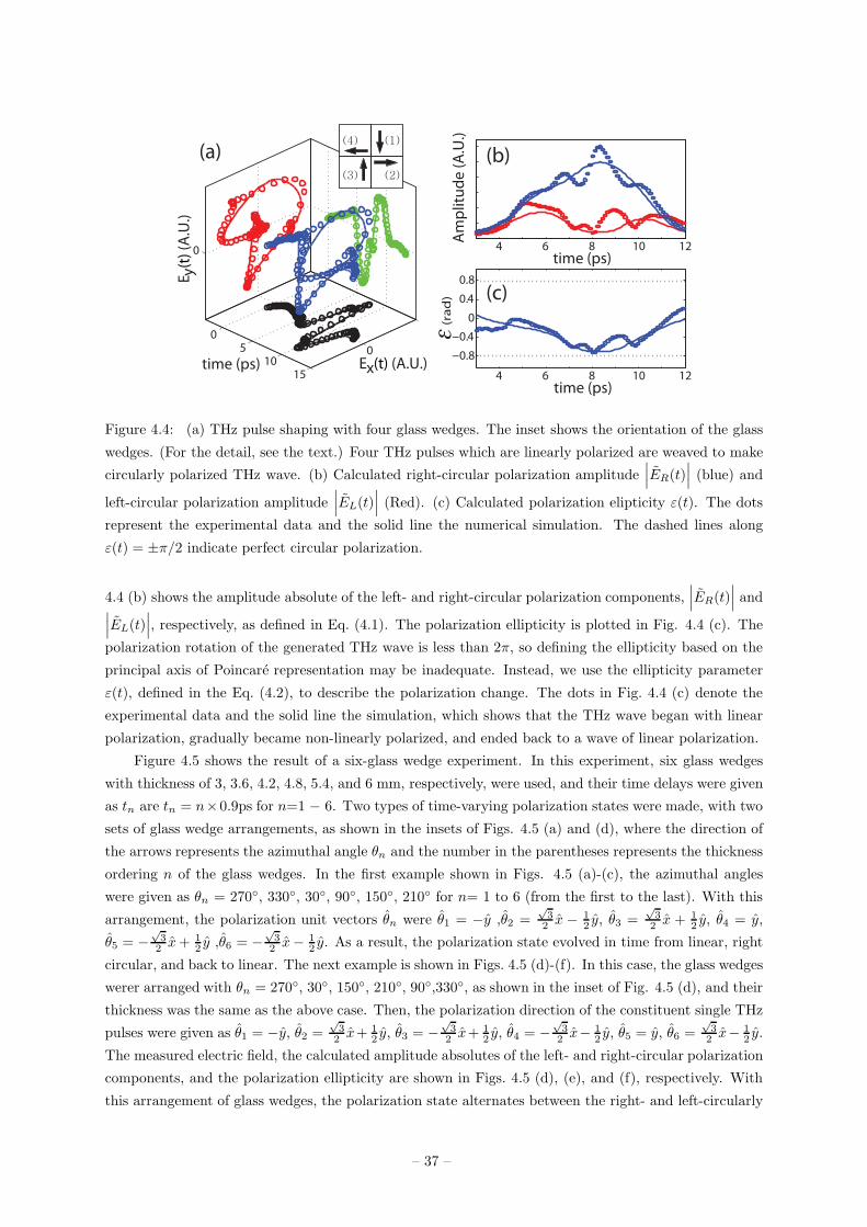
(a)

xE (t) (A.U.)

time (ps)

(ra

d)

ε

−0.8

−0.4

0

0.4

0.8

4 6 8 10 12

05

1015

0

0time (ps)

Am

pli

tud

e (

A.U

.)

4 6 8 10 12time (ps)

yE (

t) (

A.U

.)

(b)

(c)

(1)

(2)(3)

(4)

Figure 4.4: (a) THz pulse shaping with four glass wedges. The inset shows the orientation of the glass

wedges. (For the detail, see the text.) Four THz pulses which are linearly polarized are weaved to make

circularly polarized THz wave. (b) Calculated right-circular polarization amplitude∣

∣

∣ER(t)

∣

∣

∣(blue) and

left-circular polarization amplitude∣

∣

∣EL(t)

∣

∣

∣(Red). (c) Calculated polarization elipticity ε(t). The dots

represent the experimental data and the solid line the numerical simulation. The dashed lines along

ε(t) = ±π/2 indicate perfect circular polarization.

4.4 (b) shows the amplitude absolute of the left- and right-circular polarization components,∣

∣

∣ER(t)

∣

∣

∣and

∣

∣

∣EL(t)

∣

∣

∣, respectively, as defined in Eq. (4.1). The polarization ellipticity is plotted in Fig. 4.4 (c). The

polarization rotation of the generated THz wave is less than 2π, so defining the ellipticity based on the

principal axis of Poincare representation may be inadequate. Instead, we use the ellipticity parameter

ε(t), defined in the Eq. (4.2), to describe the polarization change. The dots in Fig. 4.4 (c) denote the

experimental data and the solid line the simulation, which shows that the THz wave began with linear

polarization, gradually became non-linearly polarized, and ended back to a wave of linear polarization.

Figure 4.5 shows the result of a six-glass wedge experiment. In this experiment, six glass wedges

with thickness of 3, 3.6, 4.2, 4.8, 5.4, and 6 mm, respectively, were used, and their time delays were given

as tn are tn = n×0.9ps for n=1 − 6. Two types of time-varying polarization states were made, with two

sets of glass wedge arrangements, as shown in the insets of Figs. 4.5 (a) and (d), where the direction of

the arrows represents the azimuthal angle θn and the number in the parentheses represents the thickness

ordering n of the glass wedges. In the first example shown in Figs. 4.5 (a)-(c), the azimuthal angles

were given as θn = 270◦, 330◦, 30◦, 90◦, 150◦, 210◦ for n= 1 to 6 (from the first to the last). With this

arrangement, the polarization unit vectors θn were θ1 = −y ,θ2 =√32 x − 1

2 y, θ3 =√32 x + 1

2 y, θ4 = y,

θ5 = −√32 x+ 1

2 y ,θ6 = −√32 x− 1

2 y. As a result, the polarization state evolved in time from linear, right

circular, and back to linear. The next example is shown in Figs. 4.5 (d)-(f). In this case, the glass wedges

werer arranged with θn = 270◦, 30◦, 150◦, 210◦, 90◦,330◦, as shown in the inset of Fig. 4.5 (d), and their

thickness was the same as the above case. Then, the polarization direction of the constituent single THz

pulses were given as θ1 = −y, θ2 =√32 x+ 1

2 y, θ3 = −√32 x+ 1

2 y, θ4 = −√32 x− 1

2 y, θ5 = y, θ6 =√32 x− 1

2 y.

The measured electric field, the calculated amplitude absolutes of the left- and right-circular polarization

components, and the polarization ellipticity are shown in Figs. 4.5 (d), (e), and (f), respectively. With

this arrangement of glass wedges, the polarization state alternates between the right- and left-circularly

– 37 –

polarizations.

4.5 Discussion

Now we discuss the validity of the presented THz polarization shaping technique. The arrangement of

N laser pulses on as-many angular positions of the circular edge of a small InAs disk becomes technically

valid if the laser spot size becomes significantly smaller than the the radius of the InAs disk pattern.

So, the maximum number of wedges is determined by the relation between the size of focused laser spot

and the geometrical factors of the glass wedges. Suppose that the glass wedges are of a square shape of

length L, which is the maximally allowed size for incoming laser beam. Then, the lateral size d of the

laser spot is given by,

d =2fλ

L, (4.10)

where λ is the wavelength of the femtosecond laser. In our experimental condition, d ≈ 0.02 mm2/L.

Considering the size of the InAs pattern, that is D = 200µm, and the validity condition, D ≫ d, we can

estimate that the number of allowed angular positions for the focused laser spots, given approximately

as A/L2, where A is the lens area, reaches up to a few hundreds. Therefore, a few hundreds of glass

wedges could be used in the THz pulse shaping method.

It is also worth to discuss about a proper size for the InAs pattern. If the diameter of the pattern

D is increased, the experimental condition easily follows the postulation that femtosecond laser spots

should be much smaller then the pattern size. However, at the same time, the spatial distribution of the

THz emission points gets increased, causing an amplitude loss of the resulting net THz wave. For an

estimation, we use Fourier optics theory to estimate this loss η, which is given by

η = 1− 2J1(πf#D/2λTHz)

πf#D/2λTHz(4.11)

where J1 is the first-order Bessel function of the first kind, λTHz is the wavelength of the THz wave,

and f# is the f -number of its focusing optics. In our experiment, f# =1, and the amplitude loss ratio

is estimated less then 10% for the most part of the frequency range of the generated THz waves. If we

used a circular pattern with D = 600 µm, a 30% amplitude loss at 0.5 THz is expected.

4.6 Summary

In summary, we have presented a THz pulse-shaping technique for polarization state control, by

superposing a number of THz pulses of various linear polarization vectors. For this, a number of fem-

tosecond optical pulses were arranged spatially and temporally with a set of glass wedges of various

thickness, and were used to illuminate on various angular locations of the circular edge of a InAs disk

pattern. Then, the lateral photo-Dember currents off from the edge interface generated linearly po-

larized THz pulses, whose polarization direction was determined by the direction of the currents. For

experimental demonstration, we used two systems made of four or six glass wedges to synthesize var-

ious unconventional polarization states, such as polarization rotation and alternation between circular

polarization states.

– 38 –

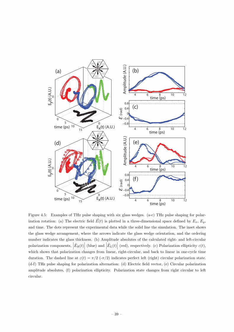
0.8

4 6 8 10 12

4 6 8 10 12

Am

pli

tud

e (

A.U

.)

time (ps)

time (ps)

time (ps)

time (ps)

(ra

d)

ε (

rad

)ε

Am

pli

tud

e (

A.U

.)4 6 8 10 12

4 6 8 10 12

−0.8

−0.4

0

0.4

0.8

−0.8

−0.4

0

0.4

05

1015

0

0

time (ps) xE (t) (A.U.)

yE (

t) (

A.U

.)

05

1015

0

0

time (ps) xE (t) (A.U.)

yE (

t) (

A.U

.)

(a) (b)

(c)

(d) (e)

(f )

(5)(4)

(3)

(6)(1)

(2)

(3)(5)

(2)

(4)(1)

(6)

Figure 4.5: Examples of THz pulse shaping with six glass wedges. (a-c) THz pulse shaping for polar-

ization rotation: (a) The electric field ~E(t) is plotted in a three-dimensional space defined by Ex, Ey ,

and time. The dots represent the experimental data while the solid line the simulation. The inset shows

the glass wedge arrangement, where the arrows indicate the glass wedge orientation, and the ordering

number indicates the glass thickness. (b) Amplitude absolutes of the calculated right- and left-circular

polarization components,∣

∣

∣ER(t)

∣

∣

∣(blue) and

∣

∣

∣EL(t)

∣

∣

∣(red), respectively. (c) Polarization ellipticity ε(t),

which shows that polarization changes from linear, right-circular, and back to linear in one-cycle time

duration. The dashed line at ε(t) = π/2 (-π/2) indicates perfect left (right) circular polarization state.

(d-f) THz pulse shaping for polarization alternation: (d) Electric field vector, (e) Circular polarization

amplitude absolutes, (f) polarization ellipticity. Polarization state changes from right circular to left

circular.

– 39 –

Chapter 5. Sub-wavelength diffraction and phase

shift anomalies caused by it

In previous chapters, we have described diffraction imaging and polarization shaping techniques

with ordinary Fourier optics theory or scalar diffraction theory. In this chapter, we study sub-wavelength

diffraction phenomena which can’t be explained by scalar diffraction theory.

Terahertz time-domain spectroscopy system has great advantages to study these phenomena. First,

with ultra-broad bandwidth THz waves, studying diffraction phenomena with many scale factors, aper-

ture scale over wavelength, is easily possible without many experiment samples. Second, we could also

study phase behaviors of sub-wavelength diffraction as well as amplitude behaviors. In addition, sub-

wavelength structures can be easily fabricated for THz experiements, and experiments with real metals

can be treated as experiments with ideal perfect conductors due to dielectic properties of real metals in

THz range [93].

Research results including both experiments and theories in this chapter are published in Optics

Letters Vol. 35 pp. 508-510 (2013), entitled “Phase-shift anomaly caused by sub-wavelength-scale metal

slit or aperture diffraction.”

5.1 Introduction

Electromagnetic wave diffraction through an aperture, such as a slit or a circular hole, has been

fully explained with the Kirchhoff’s scalar diffraction theory when the size of the aperture, d, is large

compared to the wavelength, λ, of the electromagnetic wave [35, 36]. However, as Bethe pointed out [94],

the diffraction phenomena from an aperture is not consistent with this scalar diffraction theory when

the size of the aperture becomes equivalent to, or smaller than, the wavelength, and vectorial nature of

the electric and magnetic fields needs to be considered.

After Bethe’s theoretical expectation, the subject of sub-wavelength aperture transmission has been

one of the important research topics under active investigations. Furthermore, the latest emergence of

near-field optical applications and sub-wavelength resolution imaging has even fueled the desire to better

understand the sub-wavelength diffraction phenomena in various experimental situations [95, 96, 97].

Some of the examples are the sub-wavelength transmitted power, the propagation distribution, local

field enhancement, and so on [98, 99, 100, 101, 102, 103, 104, 119, 120, 121, 122]. To list a few, the

extraordinary power transmission phenomena in sub-wavelength groove patterned slits [119, 120], more

recently, the Fabry-Perot-like behaviors in thick-slit transmission [121, 122] and strong field enhancement

in small width slits are experimentally observed and theoretically explained [103, 104].

Recently, phase studies of electromagnetic waves becomes also more important because phase prop-

erties of few-cycles or even sub-cycle electromagnetic waves are used in various research areas [105, 106,

107, 108, 109]. In optical frequency, application research such as wave plate design based on phase shift

properties [123, 124] of sub-wavelength diffraction are on-going. Since a phase measurement is easily

achieved from a time domain signal in terahertz freqeunecy region, some papers studied anomalous

phase shift in sub-wavelength near-field transmission with this frequency range experiment [110, 111].

– 40 –

In this chapter, we develop a phenomenological theory for sub-wavelength diffraction problem, and

verify its predictions by the direct field measurement of terahertz time-domain diffraction experiment. We

study three types of test geometries, a single slit, a circular aperture, and double slits of sub-wavelength

scale, and the diffraction behaviors are investigated as a function of their geometrical factors, aperture

scale over the wavelength.

We first study the diffraction phenomena from a sub-wavelength-scale metal slit. The resulting

amplitude and phase behavior of the diffracted wave and their polarization dependence exhibit substan-

tially different physics that are not explained by scalar diffraction theory. We note that the disagreement

between these phenomena and scalar diffraction theory is attributed to the failure of Kirchhoff’s as-

sumption, which is that both electric and magnetic fields in aperture are the same as the incident ones.

To remove this disagreement, we set theoretical arguments based on the induction of the electric cur-

rent [103, 104] and effective magnetic dipole radiation [94]. Our theoretical argument predicts that (1)

the transmission amplitude does not linearly scale to the slit width but surprisingly maintains a con-

stant or scales quadratically, depending on the polarization of the incident electric field, and that (2) the

transmission phase also changes dramatically from the constant Gouy phase advancement, gaining either

a positive or negative additional phase shift, depending on the polarization. Experimental verification

of the sub-wavelength slit diffraction shows an excellent agreement of such predictions.

We also study the diffraction phenomena from a sub-wavelength-scale metal circualr hole. In this

geometry, we only focus phase behavior since amplitude behavior of sub-wavelength hole diffraction is

quite well studied for a long time [94, 98]. In a small hole limit, dffraction effectively becomes the

magnetic dipole radiation [94], so π/2 more phase shift from Gouy phase happens in far field compared

from a large aperture transmission. The phase shift in the intermediate regime is also calculated and

compared with experimental results.

Finally, we study the diffraction phenomena of double slits. Because of phase shift anomalies in

a sub-wavelength slit transmission, diffraction pattern in Young’s double-slit experiment is modulated

from the expectation by scalar diffraction theory. In addition, we find these modulation depends on light

polarization because phase shift anomalies are strongly related to it.

5.2 General theory of phase shift anomaly in sub-wavelength

diffraction

Let us consider a linearly polarized electromagnetic wave of angular frequency ω and wave number

k = ω/c propagating along z-direction diffracts through an aperture located at z = 0. A time varying

phase factor e−iωt are skipped in following all equations. When the aperture is a perfect conductor and

large enough so that the aperture edge effect is ignored, the diffracted wave in the far-field region at

~R = (X,Y, Z) is given according to Kirchhoff’s scalar diffraction theory [35] by

~ET (~R) = −ikeikR

2πR

∫ ∫

Σ

~E0e−ik xX+yY

R Ødxdy, (5.1)

where ET represents the diffraction of the transmitted wave, Σ denotes the aperture plane, Ø the

obliquity factor, E0 the incident electric field amplitude, k = ω/c, and R = |~R|. The π/2 phase advance,

or −π/2 phase delay, of ET (~R) with respect to the eikR phase factor in plane-wave propagation is

caused by the transverse wave confinement through the aperture, and is generally known as Gouy phase

shift [112, 113, 114, 115]. We designate this phase shift as φG.

– 41 –

When a sub-wavelength aperture is used, however, the scalar diffraction theory based on Eq. 5.1

fails because the electric field on the sub-wavelength aperture is not same as the incident electric field

and changes as that the shape of the aperture changes. Unlike the electric field, the magnetic field on an

aperture does not have such shape dependence due to the symmetric boundary consideration [94] and,

therefore, we can classify sub-wavelength diffraction as 2 types: electric field enhanced type and electric

field reduced type.

Electric field enhanced type can be understood by induced charges and currents, or plasmon coupling.

The induced electric field can be obtained from the vector potential ~A(~R) given by

~A(~R) =µ0e

ikR

4π0R

∫

Σ

~J(x, y)e−ik xX+yYR dxdy, (5.2)

where ~J(x, y) is the current density and µ0 is the magnetic permeability. It is noted that electrostatic

potential is ignored in the lowest order perturbation calculation as the net charge accumulation is zero.

From electromagnetic theories, equation 5.2 becomes

~E(~R) = ikZeikR

4πR

∫

Σ

~J(x, y)e−ik xX+yY

R dxdy (5.3)

where Z =√

µ0

ε0. According to Gauss law, a pair of opposite charges are accumulated being in phase

with the electric field, so electric current density, ~J(x, y), is induced and its time variance is phase-shifted

from the incident electric field as

~J(x, y)/∣

∣

∣

~J(x, y)∣

∣

∣= −i ~E0/

∣

∣

∣

~E0

∣

∣

∣. (5.4)

From equations 5.3 and 5.4, we could know the phase of this induced field becomes as

~Eind(R) ∝ ~E0eikR. (5.5)

Therefore, this induced field has same phase as the phase factor, eikR. As a result, diffracted waves from

electric field enhanced type apertures have phase retardation compared from normal Gouy phase shift.

Electric field reduced type can be understood by Bethe diffraction [94]. In this type, the electric

field is negligibly small, so the diffracted field mainly results from the remain magnetic field. The most

convenient way to understand these types of diffraction is Bethe’s effective magnetic dipole model [94].

In this model, although they are nonexistent, we could imagine effective magnetic surface density and

corresponding magnetic dipole moment satisfying proper boundary conditions of the geometry, and treat

diffraction field as this effective magnetic dipole radiation. From the definition of dipole moment, the

effective magnetic dipole, ~m, should be

~m ∝ − ~H0. (5.6)

where ~H0 denotes the incident magnetic field. Therefore, the diffracted wave, ~EMD(R), becomes

~EMD(R) ∝ − ~E0eikR. (5.7)

As a result, diffracted waves from electric field reduced type apertures have phase advancement compared

to normal Gouy phase shift.

5.3 Experimental description

Experimental verification of a sub-wavelength diffraction was performed with transmission-type

terahertz (THz) frequency waves. We adopted the waveform capture technique routinely used in a con-

ventional THz time-domain spectroscopy [116, 117] as shown in Fig. 5.1 (a). THz pulses were generated

– 42 –

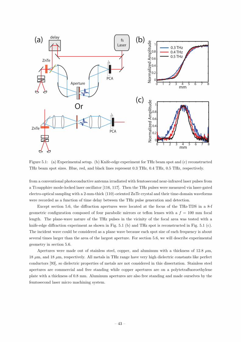
PCA

ZnTe

Aperture

Laserfs

delay

Or

PCAZnTe

0 1 2 3 4 5 6 7 8

0

0.2

0.4

0.6

0.8

1

mmN

orm

aliz

ed

Am

plit

ud

e

(a)

(c)

0 1 2 3 4 5 6 7 80

0.2

0.4

0.6

0.8

1

mm

No

rma

lize

d A

mp

litu

de(b)

0.3 THz0.4 THz0.5 THz

Figure 5.1: (a) Experimental setup. (b) Knife-edge experiment for THz beam spot and (c) reconstructed

THz beam spot sizes. Blue, red, and black lines represent 0.3 THz, 0.4 THz, 0.5 THz, respectively.

from a conventional photoconductive antenna irradiated with femtosecond near-infrared laser pulses from

a Ti:sapphire mode-locked laser oscillator [116, 117]. Then the THz pulses were measured via laser-gated

electro-optical sampling with a 2-mm-thick 〈110〉-oriented ZnTe crystal and their time-domain waveforms

were recorded as a function of time delay between the THz pulse generation and detection.

Except section 5.6, the diffraction apertures were located at the focus of the THz-TDS in a 8-f

geometric configuration composed of four parabolic mirrors or teflon lenses with a f = 100 mm focal

length. The plane-wave nature of the THz pulses in the vicinity of the focal area was tested with a

knife-edge diffraction experiment as shown in Fig. 5.1 (b) and THz spot is reconstructed in Fig. 5.1 (c).

The incident wave could be considered as a plane wave because each spot size of each frequency is about

several times larger than the area of the largest aperture. For section 5.6, we will describe experimental

geometry in section 5.6.

Apertures were made out of stainless steel, copper, and aluminum with a thickness of 12.8 µm,

18 µm, and 18 µm, respectively. All metals in THz range have very high dielectric constants like perfect

conductors [93], so dielectric properties of metals are not considered in this dissertation. Stainless steel

apertures are commercial and free standing while copper apertures are on a polytetrafluoroethylene

plate with a thickness of 0.8 mm. Aluminum apertures are also free standing and made ourselves by the

femtosecond laser micro machining system.

– 43 –

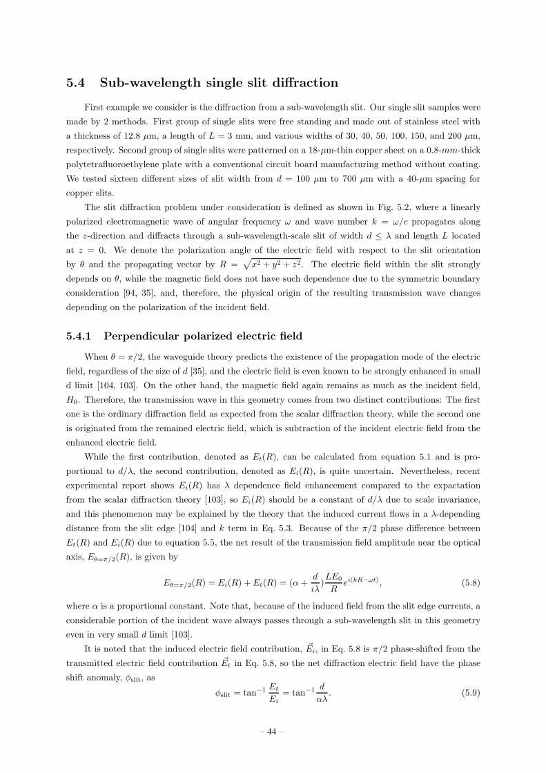
5.4 Sub-wavelength single slit diffraction

First example we consider is the diffraction from a sub-wavelength slit. Our single slit samples were

made by 2 methods. First group of single slits were free standing and made out of stainless steel with

a thickness of 12.8 µm, a length of L = 3 mm, and various widths of 30, 40, 50, 100, 150, and 200 µm,

respectively. Second group of single slits were patterned on a 18-µm-thin copper sheet on a 0.8-mm-thick

polytetrafluoroethylene plate with a conventional circuit board manufacturing method without coating.

We tested sixteen different sizes of slit width from d = 100 µm to 700 µm with a 40-µm spacing for

copper slits.

The slit diffraction problem under consideration is defined as shown in Fig. 5.2, where a linearly

polarized electromagnetic wave of angular frequency ω and wave number k = ω/c propagates along

the z-direction and diffracts through a sub-wavelength-scale slit of width d ≤ λ and length L located

at z = 0. We denote the polarization angle of the electric field with respect to the slit orientation

by θ and the propagating vector by R =√

x2 + y2 + z2. The electric field within the slit strongly

depends on θ, while the magnetic field does not have such dependence due to the symmetric boundary

consideration [94, 35], and, therefore, the physical origin of the resulting transmission wave changes

depending on the polarization of the incident field.

5.4.1 Perpendicular polarized electric field

When θ = π/2, the waveguide theory predicts the existence of the propagation mode of the electric

field, regardless of the size of d [35], and the electric field is even known to be strongly enhanced in small

d limit [104, 103]. On the other hand, the magnetic field again remains as much as the incident field,

H0. Therefore, the transmission wave in this geometry comes from two distinct contributions: The first

one is the ordinary diffraction field as expected from the scalar diffraction theory, while the second one

is originated from the remained electric field, which is subtraction of the incident electric field from the

enhanced electric field.

While the first contribution, denoted as Et(R), can be calculated from equation 5.1 and is pro-

portional to d/λ, the second contribution, denoted as Ei(R), is quite uncertain. Nevertheless, recent

experimental report shows Ei(R) has λ dependence field enhancement compared to the expactation

from the scalar diffraction theory [103], so Ei(R) should be a constant of d/λ due to scale invariance,

and this phenomenon may be explained by the theory that the induced current flows in a λ-depending

distance from the slit edge [104] and k term in Eq. 5.3. Because of the π/2 phase difference between

Et(R) and Ei(R) due to equation 5.5, the net result of the transmission field amplitude near the optical

axis, Eθ=π/2(R), is given by

Eθ=π/2(R) = Ei(R) + Et(R) = (α+d

iλ)LE0

Rei(kR−ωt), (5.8)

where α is a proportional constant. Note that, because of the induced field from the slit edge currents, a

considerable portion of the incident wave always passes through a sub-wavelength slit in this geometry

even in very small d limit [103].

It is noted that the induced electric field contribution, ~Ei, in Eq. 5.8 is π/2 phase-shifted from the

transmitted electric field contribution ~Et in Eq. 5.8, so the net diffraction electric field have the phase

shift anomaly, φslit, as

φslit = tan−1 Et

Ei= tan−1 d

αλ. (5.9)

– 44 –

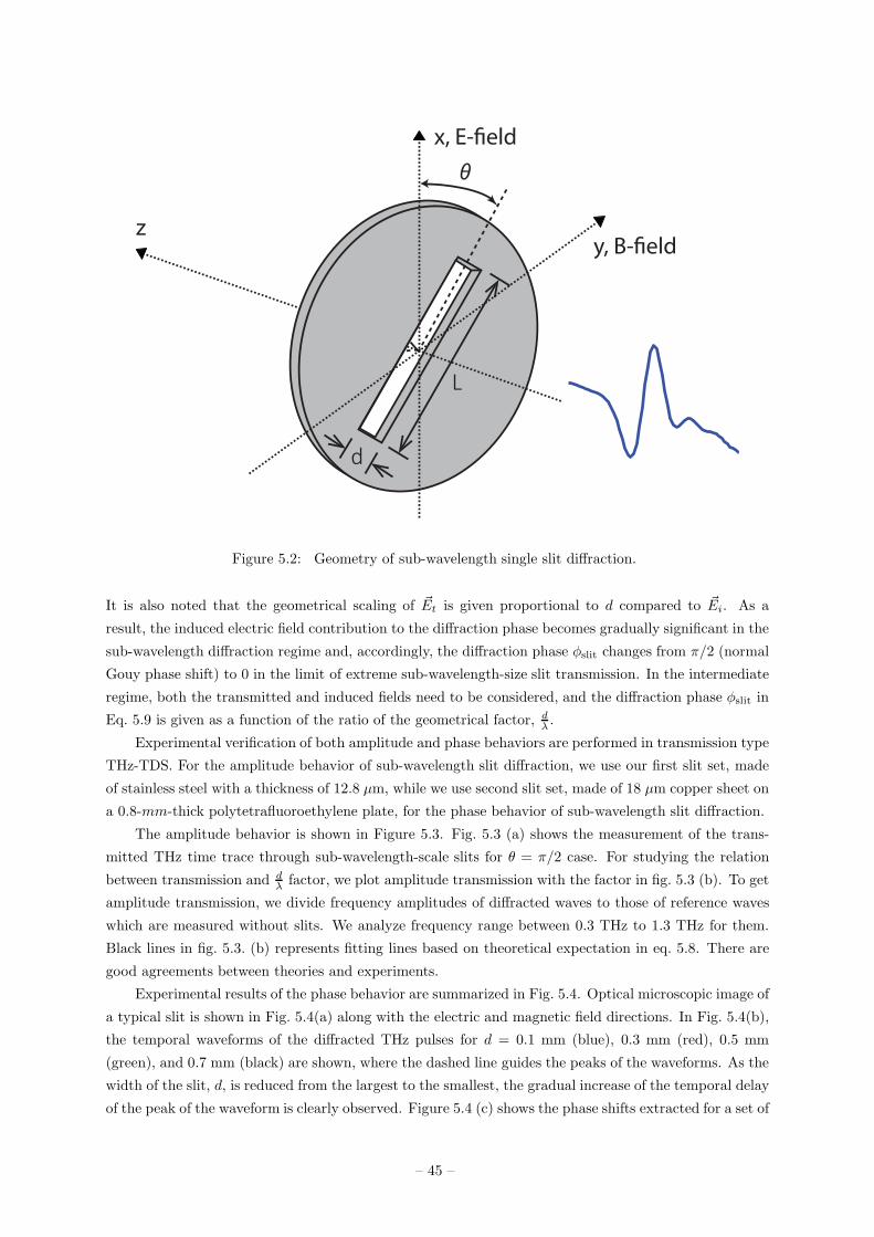
x, E-�eld

θ

y, B-�eld

d

L

z

Figure 5.2: Geometry of sub-wavelength single slit diffraction.

It is also noted that the geometrical scaling of ~Et is given proportional to d compared to ~Ei. As a

result, the induced electric field contribution to the diffraction phase becomes gradually significant in the

sub-wavelength diffraction regime and, accordingly, the diffraction phase φslit changes from π/2 (normal

Gouy phase shift) to 0 in the limit of extreme sub-wavelength-size slit transmission. In the intermediate

regime, both the transmitted and induced fields need to be considered, and the diffraction phase φslit in

Eq. 5.9 is given as a function of the ratio of the geometrical factor, dλ .

Experimental verification of both amplitude and phase behaviors are performed in transmission type

THz-TDS. For the amplitude behavior of sub-wavelength slit diffraction, we use our first slit set, made

of stainless steel with a thickness of 12.8 µm, while we use second slit set, made of 18 µm copper sheet on

a 0.8-mm-thick polytetrafluoroethylene plate, for the phase behavior of sub-wavelength slit diffraction.

The amplitude behavior is shown in Figure 5.3. Fig. 5.3 (a) shows the measurement of the trans-

mitted THz time trace through sub-wavelength-scale slits for θ = π/2 case. For studying the relation

between transmission and dλ factor, we plot amplitude transmission with the factor in fig. 5.3 (b). To get

amplitude transmission, we divide frequency amplitudes of diffracted waves to those of reference waves

which are measured without slits. We analyze frequency range between 0.3 THz to 1.3 THz for them.

Black lines in fig. 5.3. (b) represents fitting lines based on theoretical expectation in eq. 5.8. There are

good agreements between theories and experiments.

Experimental results of the phase behavior are summarized in Fig. 5.4. Optical microscopic image of

a typical slit is shown in Fig. 5.4(a) along with the electric and magnetic field directions. In Fig. 5.4(b),

the temporal waveforms of the diffracted THz pulses for d = 0.1 mm (blue), 0.3 mm (red), 0.5 mm

(green), and 0.7 mm (black) are shown, where the dashed line guides the peaks of the waveforms. As the

width of the slit, d, is reduced from the largest to the smallest, the gradual increase of the temporal delay

of the peak of the waveform is clearly observed. Figure 5.4 (c) shows the phase shifts extracted for a set of

– 45 –

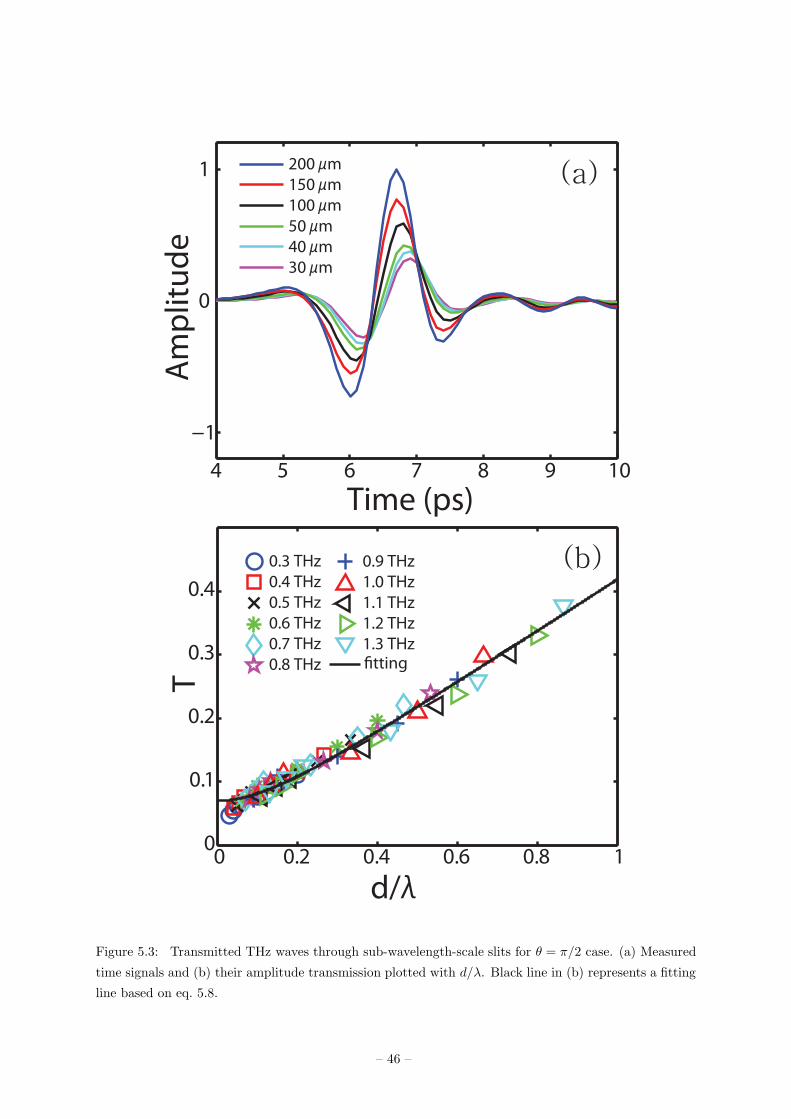
0 0.2 0.4 0.6 0.8 10

0.1

0.2

0.3

0.4

T

(b)

4 5 6 7 8 9 10

−1

0

1

200 µm

150 µm

100 µm

50 µm

40 µm

30 µm

Time (ps)

Am

pli

tud

e(a)

0.3 THz

0.4 THz

0.5 THz

0.6 THz

0.7 THz

0.8 THz

0.9 THz

1.0 THz

1.1 THz

1.2 THz

1.3 THz"tting

d/λ

Figure 5.3: Transmitted THz waves through sub-wavelength-scale slits for θ = π/2 case. (a) Measured

time signals and (b) their amplitude transmission plotted with d/λ. Black line in (b) represents a fitting

line based on eq. 5.8.

– 46 –

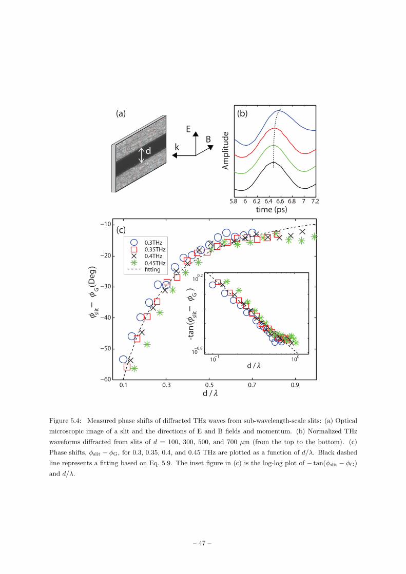
time (ps)

Am

plit

ud

e

0.1 0.3 0.5 0.7 0.9−60

−50

−40

−30

−20

−10

d / λ

φ −

φ

(D

eg

)

0.3THz0.35THz0.4THz0.45THz!tting

(b)

(c)

5.8 6 6.2 6.4 6.6 6.8 7 7.2

(a)

d

BE

k

slit

G

10−1

100

10−0.8

100.2

-ta

n

d / λ

(φ −

φ

)

slit

G

Figure 5.4: Measured phase shifts of diffracted THz waves from sub-wavelength-scale slits: (a) Optical

microscopic image of a slit and the directions of E and B fields and momentum. (b) Normalized THz

waveforms diffracted from slits of d = 100, 300, 500, and 700 µm (from the top to the bottom). (c)

Phase shifts, φslit − φG, for 0.3, 0.35, 0.4, and 0.45 THz are plotted as a function of d/λ. Black dashed

line represents a fitting based on Eq. 5.9. The inset figure in (c) is the log-log plot of − tan(φslit − φG)

and d/λ.

– 47 –

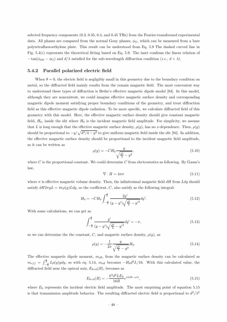
selected frequency components (0.3, 0.35, 0.4, and 0.45 THz) from the Fourier-transformed experimental

data. All phases are compared from the normal Gouy phases, φG, which can be measured from a bare

polytetrafluoroethylene plate. This result can be understood from Eq. 5.9 The dashed curved line in

Fig. 5.4(c) represents the theoretical fitting based on Eq. 5.9. The inset confirms the linear relation of

− tan(φslit − φG) and d/λ satisfied for the sub-wavelength diffraction condition (i.e., d < λ).

5.4.2 Parallel polarized electric field

When θ = 0, the electric field is negligibly small in this geometry due to the boundary condition on

metal, so the diffracted field mainly results from the remain magnetic field. The most convenient way

to understand these types of diffraction is Bethe’s effective magnetic dipole model [94]. In this model,

although they are nonexistent, we could imagine effective magnetic surface density and corresponding

magnetic dipole moment satisfying proper boundary conditions of the geometry, and treat diffraction

field as this effective magnetic dipole radiation. To be more specific, we calculate diffracted field of this

geometry with this model. Here, the effective magnetic surface density should give constant magnetic

field, H0, inside the slit where H0 is the incident magnetic field amplitude. For simplicity, we assume

that L is long enough that the effective magnetic surface density, ρ(y), has no x-dependence. Then, ρ(y)

should be proportional to −y/√

d2/4− y2 to give uniform magnetic field inside the slit [94]. In addition,

the effective magnetic surface density should be proportional to the incident magnetic field amplitude,

so it can be written as

ρ(y) = −CH0y

√

d2

4 − y2, (5.10)

where C is the proportional constant. We could determine C from electrostatics as following. By Gauss’s

law,

∇ ·H = 4πσ (5.11)

where σ is effective magnetic volume density. Then, the infinitesimal magnetic field dH from Ldy should

satisfy dH2πyL = 4πρ(y)Ldy, so the coefficient, C, also satisfy as the following integral:

H0 = −CH0

∫ d2

− d2

2y′

(y − y′)√

d2

4 − y′2dy′. (5.12)

With some calculations, we can get as

∫ d2

−d2

y′

(y − y′)√

d2

4 − y′2dy′ = −π, (5.13)

so we can determine the the constant, C, and magnetic surface density, ρ(y), as

ρ(y) = − 1

2π

y√

d2

4 − y2H0. (5.14)

The effective magnetic dipole moment, meff , from the magnetic surface density can be calculated as

meff =∫

d2

− d2

Lρ(y)ydy, so with eq. 5.14, meff becomes −H0d2L/16. With this calculated value, the

diffracted field near the optical axis, Eθ=0(R), becomes as

Eθ=0(R) = −k2d2LE0

16Rei(kR−ωt), (5.15)

where E0 represents the incident electric field amplitude. The most surprising point of equation 5.15

is that transmission amplitude behavior. The resulting diffracted electric field is proportional to d2/λ2

– 48 –

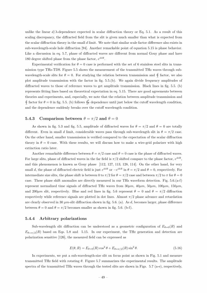
unlike the linear d/λ-dependence expected in scalar diffraction theory or Eq. 5.1. As a result of this

scaling discrepancy, the diffracted field from the slit is given much smaller than what is expected from

the scalar diffraction theory in the small d limit. We note that similar scale factor difference also exists in

sub-wavelength-scale hole diffraction [94]. Another remarkable point of equation 5.15 is phase behavior.

Like a discussion in eq. 5.7, phase of diffracted waves are different from normal Gouy phase and have

180 degree shifted phase from the phase factor, eikR.

Experimental verification for θ = 0 case is performed with the set of 6 stainless steel slits in trans-

mission type THz-TDS. Figure 5.5 shows the measurement of the transmitted THz waves through sub-

wavelength-scale slits for θ = 0. For studying the relation between transmission and dλ factor, we also

plot amplitude transmission with the factor in fig. 5.5.(b). We again divide frequency amplitudes of

diffracted waves to those of reference waves to get amplitude transmission. Black lines in fig. 5.5. (b)

represents fitting lines based on theoretical expectation in eq. 5.15. There are good agreements between

theories and experiments, and, especially, we note that the relation between amplitude transmission anddλ factor for θ = 0 in fig. 5.5. (b) follows d2

λ2 dependence until just below the cutoff wavelength condition,

and the dependence suddenly breaks over the cutoff wavelength condition.

5.4.3 Comparison between θ = π/2 and θ = 0

As shown in fig. 5.3 and fig. 5.5, amplitude of diffracted waves for θ = π/2 and θ = 0 are totally

different. Even in small d limit, considerable waves pass through sub-wavelength slit in θ = π/2 case.

On the other hand, smaller transmission is verified compared to the expectation of the scalar diffraction

theory in θ = 0 case. With these results, we will discuss how to make a wire-grid polarizer with high

extinction ratio later.

Another remarkable difference between θ = π/2 case and θ = 0 case is the phase of diffracted waves.

For large slits, phase of diffracted waves in the far field is π/2 shifted compare to the phase factor, eikR,

and this phenomenon is known as Gouy phase [112, 127, 113, 128, 114]. On the other hand, for very

small d, the phase of diffracted electric field is just eikR or −eikR in θ = π/2 and θ = 0, respectively. For

intermediate size slits, the phase shift is between 0 to π/2 for θ = π/2 case and between π/2 to π for θ = 0

case. These phase shift anomalies are directly measured in our THz waveform detection. Fig. 5.6.(a-f)

represent normalized time signals of diffracted THz waves from 30µm, 40µm, 50µm, 100µm, 150µm,

and 200µm slit, respectively. Blue and red lines in fig. 5.6 represent θ = 0 and θ = π/2 diffraction

respectively while reference signals are plotted in dot lines. Almost π/2 phase advance and retardation

are clearly observed in 30 µm-slit diffraction shown in fig. 5.6. (a). As d, becomes larger, phase difference

between θ = 0 and θ = π/2 becomes smaller as shown in fig. 5.6. (b-f).

5.4.4 Arbitrary polarizations

Sub-wavelength slit diffraction can be understood as a geometric configuration of Eθ=0(R) and

Eθ=π/2(R) based on Eqs. 5.8 and 5.15. In our experiment, the THz generation and detection are

polarization sensitive [126], the measured field can be expressed as

E(θ,R) = Eθ=0(R) cos2 θ + Eθ=π/2(R) sin2 θ. (5.16)

In experiments, we put a sub-wavelength-size slit on focus point as shown in Fig. 5.1 and measure

transmitted THz field with rotating θ. Figure 5.7 summarizes the experimental results. The amplitude

spectra of the transmitted THz waves through the tested slits are shown in Figs. 5.7 (a-e), respectively,

– 49 –

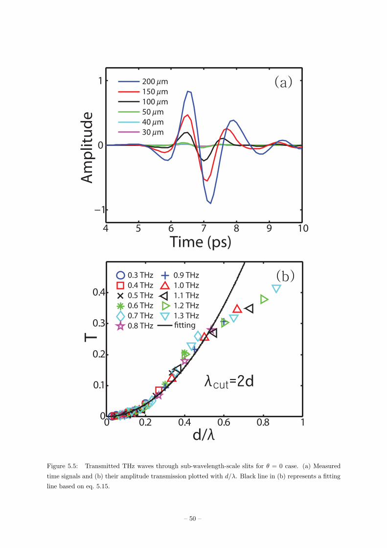
0 0.2 0.4 0.6 0.8 10

0.1

0.2

0.3

0.4

d/λ

T

(b)

4 5 6 7 8 9 10

−1

0

1

Time (ps)

Am

plit

ud

e(a)

λ =2d

200 µm150 µm100 µm50 µm40 µm30 µm

0.3 THz0.4 THz0.5 THz0.6 THz0.7 THz0.8 THz

0.9 THz1.0 THz1.1 THz1.2 THz1.3 THz"tting

Figure 5.5: Transmitted THz waves through sub-wavelength-scale slits for θ = 0 case. (a) Measured

time signals and (b) their amplitude transmission plotted with d/λ. Black line in (b) represents a fitting

line based on eq. 5.15.

– 50 –

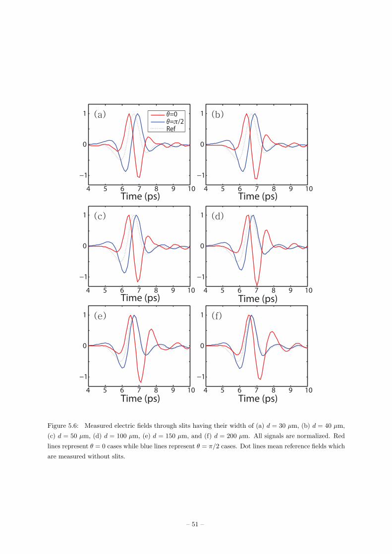
4 5 6 7 8 9 10

−1

0

1

4 5 6 7 8 9 10

−1

0

1

4 5 6 7 8 9 10

−1

0

1

4 5 6 7 8 9 10

−1

0

1

4 5 6 7 8 9 10

−1

0

1

4 5 6 7 8 9 10

−1

0

1

θ=0θ=π/2Ref

Time (ps) Time (ps)

Time (ps) Time (ps)

Time (ps) Time (ps)

(a) (b)

(c) (d)

(e) (f)

Figure 5.6: Measured electric fields through slits having their width of (a) d = 30 µm, (b) d = 40 µm,

(c) d = 50 µm, (d) d = 100 µm, (e) d = 150 µm, and (f) d = 200 µm. All signals are normalized. Red

lines represent θ = 0 cases while blue lines represent θ = π/2 cases. Dot lines mean reference fields which

are measured without slits.

– 51 –

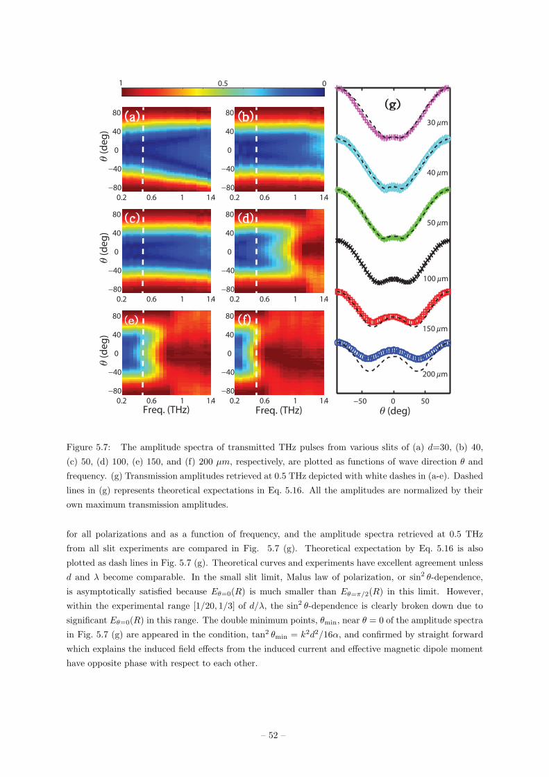
30 µm

40 µm

50 µm

100 µm

150 µm

200 µm

Freq. (THz)

0.2 0.6 1 1.4

−80

−40

0

40

80

0.2 0.6 1 1.4

−80

−40

0

40

80

0.2 0.6 1 1.4

−80

−40

0

40

80

0.2 0.6 1 1.4

−80

−40

0

40

80

0.2 0.6 1 1.4

−80

−40

0

40

80

0.2 0.6 1 1.4

−80

−40

0

40

80

θ (deg)

θ (d

eg

)

Freq. (THz)

θ (d

eg

)θ

(de

g)

−50 0 50

01

(g)

0.5

(b)

(d)

(f)

(a)

(c)

(e)

Figure 5.7: The amplitude spectra of transmitted THz pulses from various slits of (a) d=30, (b) 40,

(c) 50, (d) 100, (e) 150, and (f) 200 µm, respectively, are plotted as functions of wave direction θ and

frequency. (g) Transmission amplitudes retrieved at 0.5 THz depicted with white dashes in (a-e). Dashed

lines in (g) represents theoretical expectations in Eq. 5.16. All the amplitudes are normalized by their

own maximum transmission amplitudes.

for all polarizations and as a function of frequency, and the amplitude spectra retrieved at 0.5 THz

from all slit experiments are compared in Fig. 5.7 (g). Theoretical expectation by Eq. 5.16 is also

plotted as dash lines in Fig. 5.7 (g). Theoretical curves and experiments have excellent agreement unless

d and λ become comparable. In the small slit limit, Malus law of polarization, or sin2 θ-dependence,

is asymptotically satisfied because Eθ=0(R) is much smaller than Eθ=π/2(R) in this limit. However,

within the experimental range [1/20, 1/3] of d/λ, the sin2 θ-dependence is clearly broken down due to

significant Eθ=0(R) in this range. The double minimum points, θmin, near θ = 0 of the amplitude spectra

in Fig. 5.7 (g) are appeared in the condition, tan2 θmin = k2d2/16α, and confirmed by straight forward

which explains the induced field effects from the induced current and effective magnetic dipole moment

have opposite phase with respect to each other.

– 52 –

5.5 Sub-wavelength circular hole diffraction

In this section, we consider another example, the diffraction from a circular-hole aperture of sub-

wavelength scale. Because transmission amplitude is well studied in this geometry [94, 98], we focus

phase shift anomalies of sub-wavelength circular hole diffraction in this section.

With the same experimental procedure of the sub-wavelength slit experiment was taken now with a

series of circular-hole apertures. We tested sixteen different sizes of hole radius varied from a = 100 µm

to 475 µm with a 25 µm spacing. Those were patterned on a 18-µm-thin copper sheet on a 0.8-mm-thick

polytetrafluoroethylene plate. Experimental results of phase shift anomalies of sub-wavelength circular

hole diffraction summarized in Fig. 5.8. We observe that the peak gradually advances for the smaller

hole apertures, which direction is opposite to the slit case where the peak was retarded. First of all, the

electric fields on a sub-wavelength circular hole apertures are very week compared to incident electric

fields unlike electric field enhancement in slit case because tangential part of the electric field on metal

is zero and, therefore, sub-wavelength circular hole diffraction is classified in electric field reduced type

like sub-wavelength slit diffraction in θ = 0 as we mentioned in Section 5.4.2. On the limit of extreme

sub-wavelength-size circular aperture transmission, therefore, it is expected that the diffracted electric

field is the radiation from an effective magnetic dipole, ~m, and this effective magnetic dipole and induced

field from the dipole should satisfy equations 5.6 and 5.7. Accordingly, the diffraction phase φd changes

from π/2 (normal Gouy phase shift) to π in the limit of extreme sub-wavelength-size circular aperture

transmission. Therefore, the observed phase advancement is consistent with the expectation of −π phase

shift according to our expectation for the limiting case of the sub-wavelength circular-hole aperture

diffraction.

More quantitatively, we can calculate the phase shift of circular-hole diffraction with the help of

both Bethe’s formal work [94] and the optical theorem [35]: The optical theorem relates the total cross

section σt to the forward scattering field amplitude, or

σt =4π

kIm[f(k = k0)], (5.17)

where Im[f(k = k0)] represents the imaginary part of the forward scattering field amplitude. We indicate

it as Im[f(k = k0)] = EIm/E0. In the small aperture limit, σt = 128k4a6/27π [94], so EIm/E0 becomes

EIm

E0=

32

27π2

k5a6

R. (5.18)

Also, according to Bethe [94],EMD

E0=

4

3π

a3k2

R, (5.19)

where EMD denotes the field having −π shift from the phase factor as we discussed in section 5.2.

Therefore, the phase shift of sub-wavelength diffraction can be obtained as

φhole = φG + tan−1EMD

EIm= φG + tan−1 9λ3

64π2a3, (5.20)

for the small aperture limit a ≪ λ. It is noted that Eq. 5.20 can be also derived in a different approach

of the radiation-reaction model from Collin [118]. The dashed line in Fig. 5.8 represents the theoretical

expectation in Eq. 5.20 Within the tested range of the hole size, (i.e., 0.1 < a/λ < 0.7 ), the phase

shift changes from 90 degree to zero degree. Since this relation is satisfied in small limit approximation,

experimental results and the theoretical expectation are a mismatch. More detailed expectation of the

total cross section σt [98] may clear this mismatch.

– 53 –

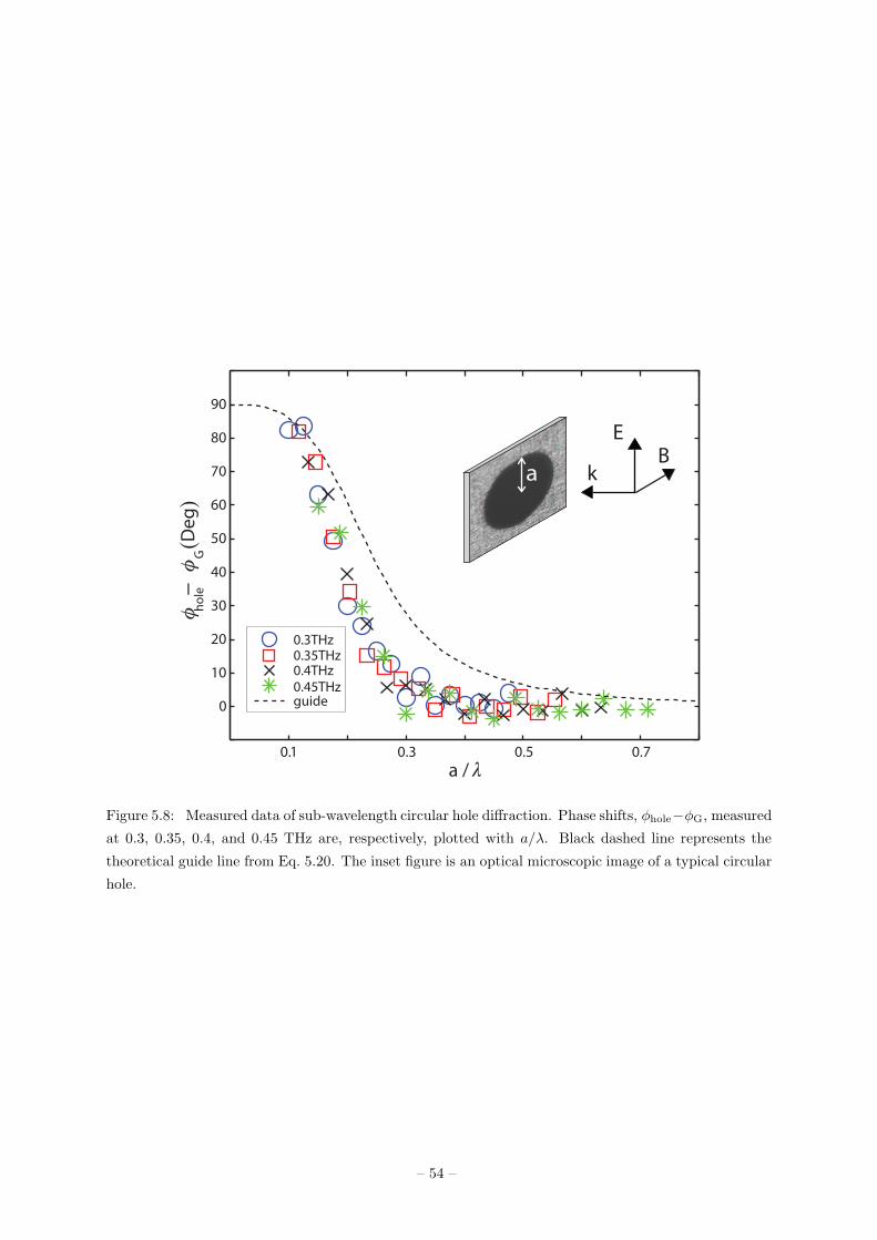
a / λ0.1 0.3 0.5 0.7

0

10

20

30

40

50

60

70

80

90

0.3THz0.35THz0.4THz0.45THzguide

aB

E

k

φ

−

φ

(De

g)

ho

leG

Figure 5.8: Measured data of sub-wavelength circular hole diffraction. Phase shifts, φhole−φG, measured

at 0.3, 0.35, 0.4, and 0.45 THz are, respectively, plotted with a/λ. Black dashed line represents the

theoretical guide line from Eq. 5.20. The inset figure is an optical microscopic image of a typical circular

hole.

– 54 –

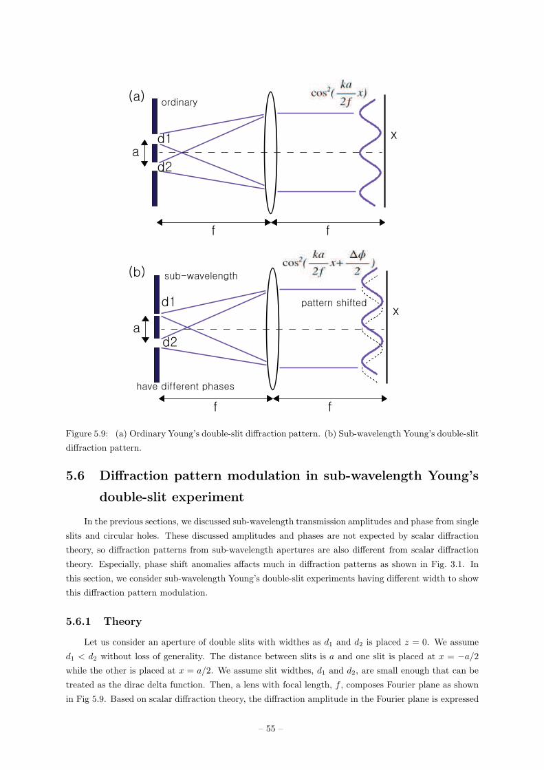
Figure 5.9: (a) Ordinary Young’s double-slit diffraction pattern. (b) Sub-wavelength Young’s double-slit

diffraction pattern.

5.6 Diffraction pattern modulation in sub-wavelength Young’s

double-slit experiment

In the previous sections, we discussed sub-wavelength transmission amplitudes and phase from single

slits and circular holes. These discussed amplitudes and phases are not expected by scalar diffraction

theory, so diffraction patterns from sub-wavelength apertures are also different from scalar diffraction

theory. Especially, phase shift anomalies affacts much in diffraction patterns as shown in Fig. 3.1. In

this section, we consider sub-wavelength Young’s double-slit experiments having different width to show

this diffraction pattern modulation.

5.6.1 Theory

Let us consider an aperture of double slits with widthes as d1 and d2 is placed z = 0. We assume

d1 < d2 without loss of generality. The distance between slits is a and one slit is placed at x = −a/2

while the other is placed at x = a/2. We assume slit widthes, d1 and d2, are small enough that can be

treated as the dirac delta function. Then, a lens with focal length, f , composes Fourier plane as shown

in Fig 5.9. Based on scalar diffraction theory, the diffraction amplitude in the Fourier plane is expressed

– 55 –

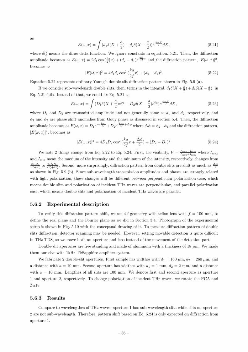
as

E(ω, x) =

∫

(d1δ(X +a

2) + d2δ(X − a

2))ei

kxXf dX, (5.21)

where δ() means the dirac delta function. We ignore constants in equation. 5.21. Then, the diffraction

amplitude becomes as E(ω, x) = 2d1 cos (ka2f x) + (d2 − d1)e

i ka2f x and the diffraction pattern, |E(ω, x)|2,

becomes as

|E(ω, x)|2 = 4d1d2 cos2 (

ka

2fx) + (d2 − d1)

2. (5.22)

Equation 5.22 represents ordinary Young’s double-slit diffraction pattern shown in Fig. 5.9 (a).

If we consider sub-wavelength double slits, then, terms in the integral, d1δ(X + a2 ) + d2δ(X − a

2 ), in

Eq. 5.21 fails. Instead of that, we could fix Eq. 5.21 as

E(ω, x) =

∫

(D1δ(X +a

2)eφ1 +D2δ(X − a

2)eφ2)ei

kxXf dX, (5.23)

where D1 and D2 are transmitted amplitude and not generally same as d1 and d2, respectively, and

φ1 and φ2 are phase shift anomalies from Gouy phase as discussed in section 5.4. Then, the diffraction

amplitude becomes as E(ω, x) = D1e−i kax

2f +D2ei kax

2f +∆φ where ∆φ = φ2−φ1 and the diffraction pattern,

|E(ω, x)|2, becomes as

|E(ω, x)|2 = 4D1D2 cos2 (

ka

2fx+

∆φ

2) + (D2 −D1)

2. (5.24)

We note 2 things change from Eq. 5.22 to Eq. 5.24. First, the visibility, V = Imax−Imin

Imax+Iminwhere Imax

and Imin mean the maxium of the intensity and the minimum of the intensity, respectively, changes from2d1d2

d21+d2

2to 2D1D2

D21+D2

2. Second, more surprisingly, diffraction pattern from double slits are shift as much as ∆φ

2

as shown in Fig. 5.9 (b). Since sub-wavelength transmission amplitudes and phases are strongly related

with light polarization, these changes will be different between perpendicular polarization case, which

means double slits and polarization of incident THz waves are perpendicular, and parallel polarization

case, which means double slits and polarization of incident THz waves are parallel.

5.6.2 Experimental description

To verify this diffraction pattern shift, we set 4-f geometry with teflon lens with f = 100 mm, to

define the real plane and the Fourier plane as we did in Section 3.4. Photograph of the experimental

setup is shown in Fig. 5.10 with the conceptual drawing of it. To measure diffraction pattern of double

slits diffraction, detector scanning may be needed. However, setting movable detection is quite difficult

in THz-TDS, so we move both an aperture and lens instead of the movement of the detection part.

Double-slit apertures are free standing and made of aluminum with a thickness of 18 µm. We made

them ourselve with 1kHz Ti:Sapphire amplifier system.

We fabricate 2 double-slit apertures. First sample has widthes with d1 = 160 µm, d2 = 260 µm, and

a distance with a = 10 mm. Second aperture has widthes with d1 = 1 mm, d2 = 2 mm, and a distance

with a = 10 mm. Lengthes of all slits are 100 mm. We denote first and second aperture as aperture

1 and aperture 2, respectively. To change polarization of incident THz waves, we rotate the PCA and

ZnTe.

5.6.3 Results

Compare to wavelengthes of THz waves, aperture 1 has sub-wavelength slits while slits on aperture

2 are not sub-wavelength. Therefore, pattern shift based on Eq. 5.24 is only expected on diffraction from

aperture 1.

– 56 –

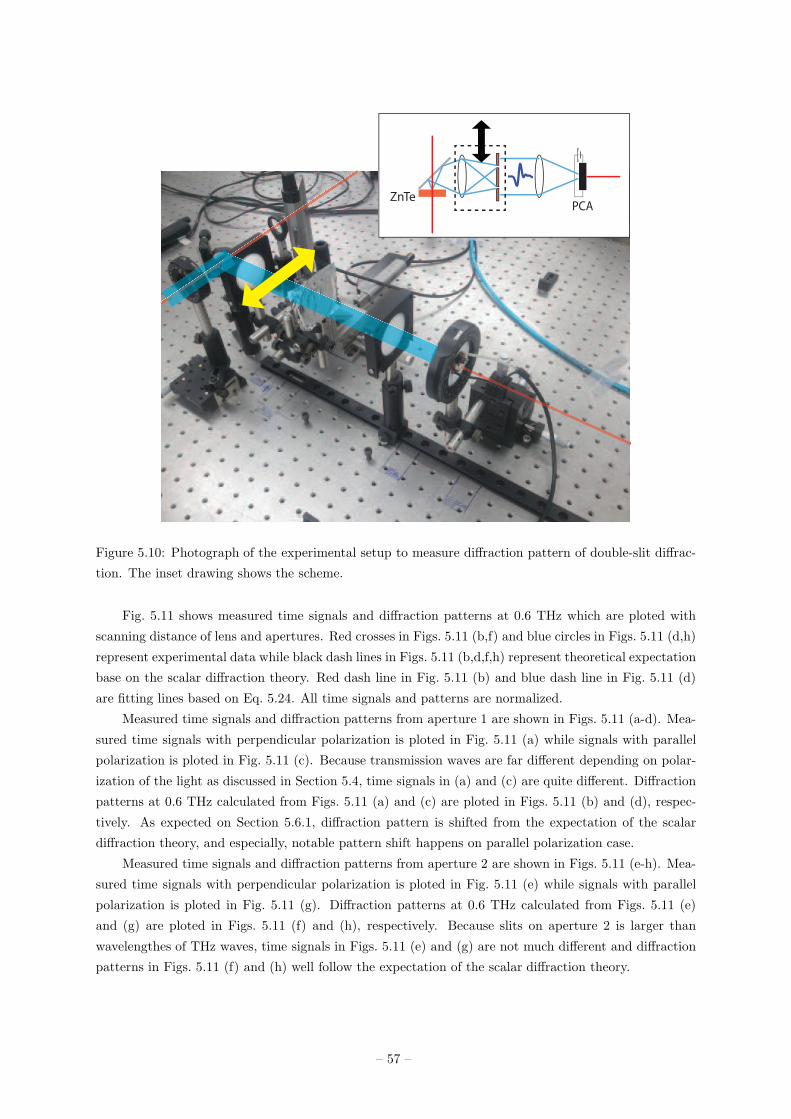
PCAZnTe

Figure 5.10: Photograph of the experimental setup to measure diffraction pattern of double-slit diffrac-

tion. The inset drawing shows the scheme.

Fig. 5.11 shows measured time signals and diffraction patterns at 0.6 THz which are ploted with

scanning distance of lens and apertures. Red crosses in Figs. 5.11 (b,f) and blue circles in Figs. 5.11 (d,h)

represent experimental data while black dash lines in Figs. 5.11 (b,d,f,h) represent theoretical expectation

base on the scalar diffraction theory. Red dash line in Fig. 5.11 (b) and blue dash line in Fig. 5.11 (d)

are fitting lines based on Eq. 5.24. All time signals and patterns are normalized.

Measured time signals and diffraction patterns from aperture 1 are shown in Figs. 5.11 (a-d). Mea-

sured time signals with perpendicular polarization is ploted in Fig. 5.11 (a) while signals with parallel

polarization is ploted in Fig. 5.11 (c). Because transmission waves are far different depending on polar-

ization of the light as discussed in Section 5.4, time signals in (a) and (c) are quite different. Diffraction

patterns at 0.6 THz calculated from Figs. 5.11 (a) and (c) are ploted in Figs. 5.11 (b) and (d), respec-

tively. As expected on Section 5.6.1, diffraction pattern is shifted from the expectation of the scalar

diffraction theory, and especially, notable pattern shift happens on parallel polarization case.

Measured time signals and diffraction patterns from aperture 2 are shown in Figs. 5.11 (e-h). Mea-

sured time signals with perpendicular polarization is ploted in Fig. 5.11 (e) while signals with parallel

polarization is ploted in Fig. 5.11 (g). Diffraction patterns at 0.6 THz calculated from Figs. 5.11 (e)

and (g) are ploted in Figs. 5.11 (f) and (h), respectively. Because slits on aperture 2 is larger than

wavelengthes of THz waves, time signals in Figs. 5.11 (e) and (g) are not much different and diffraction

patterns in Figs. 5.11 (f) and (h) well follow the expectation of the scalar diffraction theory.

– 57 –

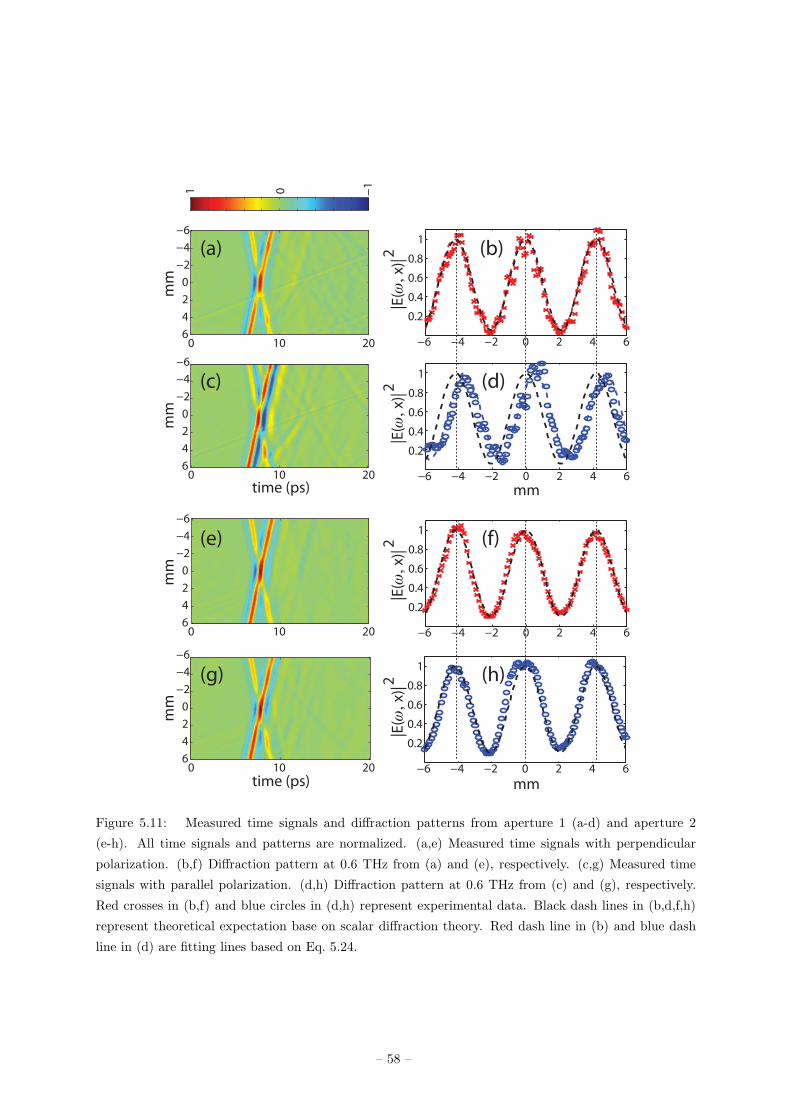
0 10 20

−6

−4

−2

0

2

4

6

mm

time (ps)

−101

−6 −4 −2 0 2 4 6

0.2

0.4

0.6

0.8

1

0 10 20

−6

−4

−2

0

2

4

6

mm

0 10 20

−6

−4

−2

0

2

4

6

mm

0 10 20

−6

−4

−2

0

2

4

6

mm

time (ps) mm−6 −4 −2 0 2 4 6

0.2

0.4

0.6

0.8

1

−6 −4 −2 0 2 4 6

0.2

0.4

0.6

0.8

1

−6 −4 −2 0 2 4 6

0.2

0.4

0.6

0.8

1

mm

|E(ω

, x)

|2(a) (b)

(c)

(e)

(g)

(d)

(f)

(h)

|E(ω

, x)

|2|E

(ω,

x)|2

|E(ω

, x)

|2

Figure 5.11: Measured time signals and diffraction patterns from aperture 1 (a-d) and aperture 2

(e-h). All time signals and patterns are normalized. (a,e) Measured time signals with perpendicular

polarization. (b,f) Diffraction pattern at 0.6 THz from (a) and (e), respectively. (c,g) Measured time

signals with parallel polarization. (d,h) Diffraction pattern at 0.6 THz from (c) and (g), respectively.

Red crosses in (b,f) and blue circles in (d,h) represent experimental data. Black dash lines in (b,d,f,h)

represent theoretical expectation base on scalar diffraction theory. Red dash line in (b) and blue dash

line in (d) are fitting lines based on Eq. 5.24.

– 58 –

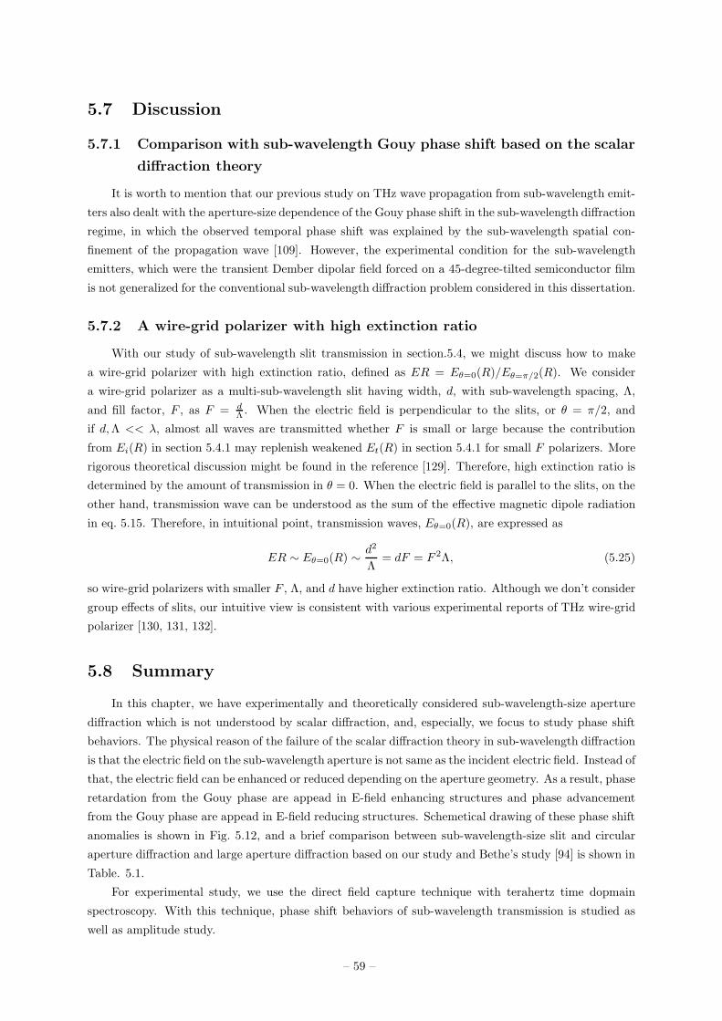
5.7 Discussion

5.7.1 Comparison with sub-wavelength Gouy phase shift based on the scalar

diffraction theory

It is worth to mention that our previous study on THz wave propagation from sub-wavelength emit-

ters also dealt with the aperture-size dependence of the Gouy phase shift in the sub-wavelength diffraction

regime, in which the observed temporal phase shift was explained by the sub-wavelength spatial con-

finement of the propagation wave [109]. However, the experimental condition for the sub-wavelength

emitters, which were the transient Dember dipolar field forced on a 45-degree-tilted semiconductor film

is not generalized for the conventional sub-wavelength diffraction problem considered in this dissertation.

5.7.2 A wire-grid polarizer with high extinction ratio

With our study of sub-wavelength slit transmission in section.5.4, we might discuss how to make

a wire-grid polarizer with high extinction ratio, defined as ER = Eθ=0(R)/Eθ=π/2(R). We consider

a wire-grid polarizer as a multi-sub-wavelength slit having width, d, with sub-wavelength spacing, Λ,

and fill factor, F , as F = dΛ . When the electric field is perpendicular to the slits, or θ = π/2, and

if d,Λ << λ, almost all waves are transmitted whether F is small or large because the contribution

from Ei(R) in section 5.4.1 may replenish weakened Et(R) in section 5.4.1 for small F polarizers. More

rigorous theoretical discussion might be found in the reference [129]. Therefore, high extinction ratio is

determined by the amount of transmission in θ = 0. When the electric field is parallel to the slits, on the

other hand, transmission wave can be understood as the sum of the effective magnetic dipole radiation

in eq. 5.15. Therefore, in intuitional point, transmission waves, Eθ=0(R), are expressed as

ER ∼ Eθ=0(R) ∼ d2

Λ= dF = F 2Λ, (5.25)

so wire-grid polarizers with smaller F , Λ, and d have higher extinction ratio. Although we don’t consider

group effects of slits, our intuitive view is consistent with various experimental reports of THz wire-grid

polarizer [130, 131, 132].

5.8 Summary

In this chapter, we have experimentally and theoretically considered sub-wavelength-size aperture

diffraction which is not understood by scalar diffraction, and, especially, we focus to study phase shift

behaviors. The physical reason of the failure of the scalar diffraction theory in sub-wavelength diffraction

is that the electric field on the sub-wavelength aperture is not same as the incident electric field. Instead of

that, the electric field can be enhanced or reduced depending on the aperture geometry. As a result, phase

retardation from the Gouy phase are appead in E-field enhancing structures and phase advancement

from the Gouy phase are appead in E-field reducing structures. Schemetical drawing of these phase shift

anomalies is shown in Fig. 5.12, and a brief comparison between sub-wavelength-size slit and circular

aperture diffraction and large aperture diffraction based on our study and Bethe’s study [94] is shown in

Table. 5.1.

For experimental study, we use the direct field capture technique with terahertz time dopmain

spectroscopy. With this technique, phase shift behaviors of sub-wavelength transmission is studied as

well as amplitude study.

– 59 –

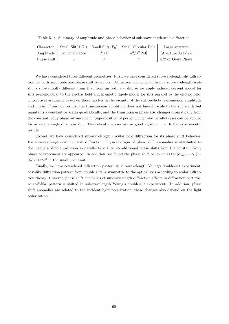
Table 5.1: Summary of amplitude and phase behavior of sub-wavelength-scale diffraction

Charactor Small Slit(⊥E0) Small Slit(‖E0) Small Circular Hole Large aperture

Amplitude no dependence d2/λ2 a3/λ2 [94] (Aperture Area)/λ

Phase shift 0 π π π/2 or Gouy Phase

We have considered three different geometries. First, we have considered sub-wavelength slit diffrac-

tion for both amplitude and phase shift behaviors. Diffraction phenomenon from a sub-wavelength-scale

slit is substantially different from that from an ordinary slit, so we apply induced current model for

slits perpendicular to the electric field and magnetic dipole model for slits parallel to the electric field.

Theoretical argument based on these models in the vicinity of the slit predicts transmission amplitude

and phase. From our results, the transmission amplitude does not linearly scale to the slit width but

maintains a constant or scales quadratically, and the transmission phase also changes dramatically from

the constant Gouy phase advancement. Superposition of perpendicular and parallel cases can be applied

for arbitrary angle direction slit. Theoretical analyses are in good agreement with the experimental

results.

Second, we have considered sub-wavelength circular hole diffraction for its phase shift behavior.

For sub-wavelength circular hole diffraction, physical origin of phase shift anomalies is attributed to

the magnetic dipole radiation as parallel type slits, so additional phase shifts from the constant Gouy

phase advancement are appeared. In addition, we found the phase shift behavior as tan(φhole − φG) =

9λ3/64π2a3 in the small hole limit.

Finally, we have considered diffraction pattern in sub-wavelength Young’s double-slit experiment.

cos2-like diffraction pattern from double slits is symmetric to the optical axis according to scalar diffrac-

tion theory. However, phase shift anomalies of sub-wavelength diffraction affacts in diffraction patterns,

so cos2-like pattern is shifted in sub-wavelength Young’s double-slit experiment. In addition, phase

shift anomalies are related to the incident light polarization, these changes also depend on the light

polarization.

– 60 –

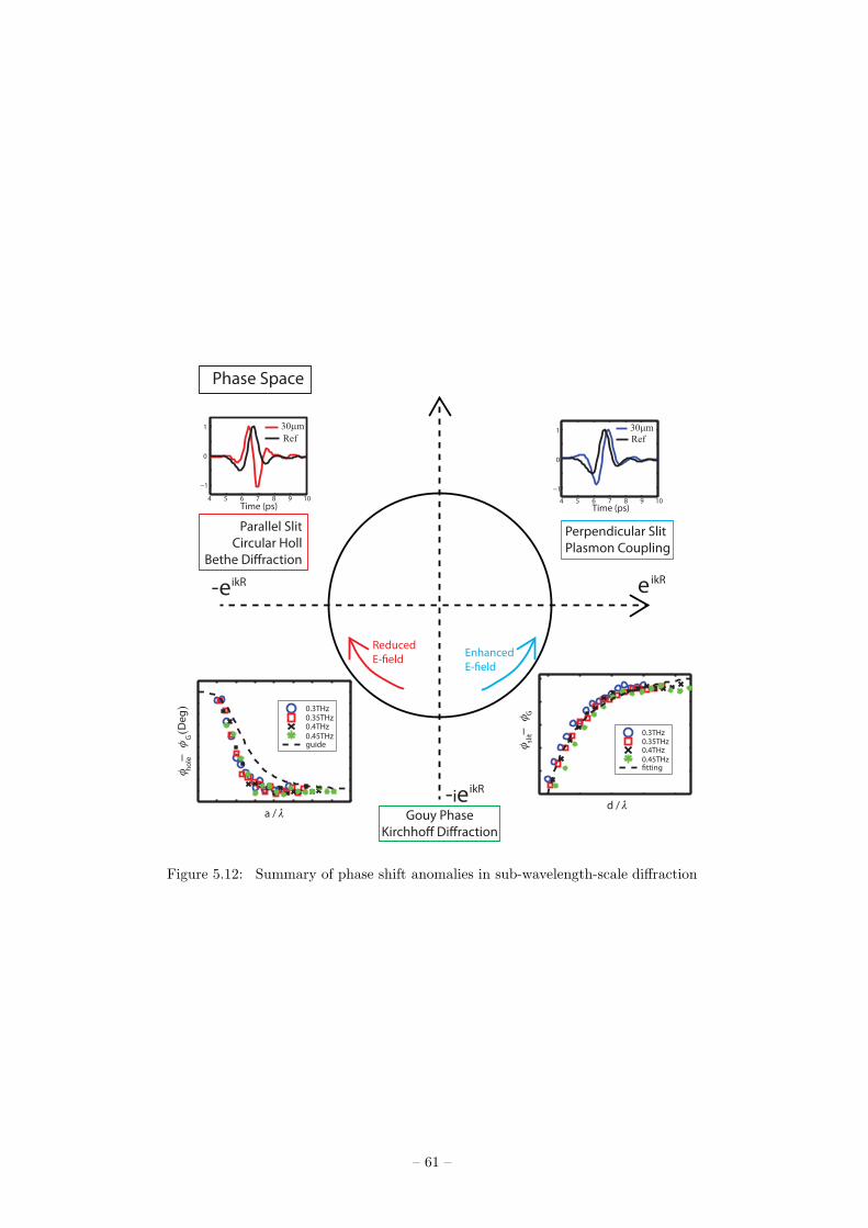
Phase Space

ikReikR-e

ikR-ie

4 5 6 7 8 9 10

−1

0

1

Time (ps)

30µm

Ref

4 5 6 7 8 9 10

−1

0

1

Time (ps)

30µm

Ref

Parallel Slit

Circular Holl

Bethe Di!raction

Perpendicular Slit

Plasmon Coupling

Gouy Phase

Kirchho! Di!raction

Enhanced

E-"eld

Reduced

E-"eld

d / λ

φ

−

φ

0.3THz0.35THz0.4THz0.45THz!tting

slit

G

a / λ

0.3THz0.35THz0.4THz0.45THzguide

φ

−

φ

(De

g)

ho

leG

Figure 5.12: Summary of phase shift anomalies in sub-wavelength-scale diffraction

– 61 –

Chapter 6. Conclusion

Terahertz technologies had been undeveloped for a long time, but they are actively used in many

research areas nowadays. One of the core THz technologies is terahertz time domain spectroscopy based

on femtosecond laser systems. T-ray in THz-TDS has 2 great advantages compared to T-ray in other

THz technologies or other optical sources. First, it has ultra-broad bandwidth or, in other words, it has

the frequency-to-bandwidth ratio of near unity. Second, phase measurement by direct field detection

with optical gating is convenient. With these unique properties, researches to expand optical physics

and applications are in progress.

In this dissertation, we study Fourier optical phenomena using ultra broadband terahertz waves

and developed Fourier optical applications such as diffraction imaging and pulse shaping. We also study

sub-wavelength diffraction and phase shift anomalies of it. Firstly, we learn that radial information

of diffracted pattern can be achieved by spectral analysis of ultra broadband waves, so we propose

three different diffraction imaging systems which reduce sampling number drastically. In these three

systems, a single pixel detector is only needed to get two dimensional image information. At first, we

demonstrate that complex images are reconstructed by only 30 waveform measurements in the coherent

optical computer geometry with a hole mask. We also demonstrate even one waveform diffraction imaging

is possible with the time separating hole mask. We demonstrate similar scheme with a slanted phase

retarder in much higher signal to noise ratio. Our proposed imaging systems can instantly be applied in

many THz imaging system for security search or biomedical imaging.

Secondly, we produce polarization shaped few-cycle THz pulse by the illumination of the spatiotem-

poral controlled femtosecond laser pulses on the circularly metal patterned InAs surface. A set of wedges

with various orientations and thicknesses are arranged to get proper spatiotemporal controlling in this

technique. As a result, we successfully generate THz waves of various unconventional polarization states,

such as polarization rotation and alternation between circular polarization states. Since these kinds

of polarizations are very uncommon in traditional optics, we also propose time domain representation

of polarization. This polarization shaping technique might be used for spectroscopic studies of circular

dichroism in chiral molecules or THz coherent control related with spiral spin state. Because polarization

can bring more information, it can also be used in THz communication.

Finally, we study sub-wavelength diffraction and, especially, phase shift anomalies caused by it. It is

generally known that −π/2 phase shift from the propagating phase is exist in usual diffraction and this

phase shift is called as the Gouy phase shift. With direct phase measurement in terahertz time domain

spectroscopy, we demonstrate that shifting phase can be between 0 to −π in sub-wavelength diffraction

instead of Gouy phase shift. With comparing Gouy phase shift, nearly π/2 phase retardation is observed

in transmitted waves from a sub-wavelength slit which is perpendicular to the electric field. On the other

hand, π/2 phase advance is observed in transmitted waves from a sub-wavelength slit which is parallel

to the electric field or a sub-wavelength circular aperture. We propose the physical origin of these phase

shift anomalies as plasmon coupling or magnetic dipole radiation, and theories are in good agreement

with the experimental results. From these phase shift anomalies, diffraction patterns are also modulated,

and we verify this in sub-wavelength Young’s double-slit experiment. For future work, it will be worth

checking that diffraction from other sub-wavelength structures follow our physical models. Based on our

– 62 –

research results, plasmonic devices such as phase retarders or plasmonic lens could also be developed.

Various other researches with ultra broadband terahertz waves could also be possible. One example

is THz-version spectral encoding imaging with ultra broadband terahertz waves instead of a broadband

visible light source [133, 134]. The principle of this imaging system is similar to our single-pixel imaging

systems in Chapter. 3 except that time frequencies encode real space information instead of spatial

frequency information. Developing THz diffractive optics, such as a grating or a prism, is a challenge for

it, but plasmonic devices [135] can be used to overcome it.

– 63 –

References

[1] A. Stolow, A. E. Bragg and D. M. Neumark, “Femtosecond time-resolved photoelectron spec-

troscopy,” Chem. Rev. 104, 1719 (2004).

[2] V. Blanchet, M. Z. Zgierski, T. Seideman, and A. Stolow, “Discerning vibronic molecular dynamics

using time-resolved photoelectron spectroscopy,” Nature 401, 52 (1999).

[3] K. Jang, J. Lim, J. Ahn, J. Kim, K. Yee, J. S. Ahn, and S. Cheong, “Ultrafast IR spectroscopic study

of coherent phonons and dynamic spin–lattice coupling in multiferroic LuMnO3,” New Journal of

Physics 12, 023017 (2010).

[4] P.P Pronko, S.K Dutta, J Squier, J.V Rudd, D Du, G Mourou, “Machining of sub-micron holes

using a femtosecondlaser at 800 nm,” Opt. Comm. 114, 106 (1995).

[5] G Della Valle, R Osellame and P Laporta, “Micromachining of photonic devices by femtosecond

laser pulses,” J. Opt. A: Pure Appl. Opt 11, 013001 (2009).

[6] M. Shapiro and P. Brumer, Principles of the Quantum Control of Molecular Processes, (Wiley, New

York, 2003).

[7] R. S. Judson, and H. Rabitz, “Teaching lasers to control molecules,” Phys. Rev. Lett. 68, 1500

(1992).

[8] J. Lim, H. Lee, S. Lee, and J. Ahn, “Quantum control in two-dimensional Fourier transform spec-

troscopy,” Phys. Rev. A 84, 013425 (2011).

[9] S. Lee, J. Lim, J. Ahn, V. Hakobyan, and S. Guerin, “Strong-field two-level two-photon transition

by phase shaping,” Phys. Rev. A 82, 023408 (2010).

[10] J. Lim, H. Lee, J. Kim, S. Lee, and J. Ahn, “Coherent transients mimicked by two-photon coherent

control of three-level system,” Phys. Rev. A 83, 053429 (2011).

[11] Th. Udem, R. Holzwarth, and T. W. Hansch, “Optical frequency metrology,” Nature 416, 233

(2002).

[12] Th. Udem, J. Reichert, R. Holzwarth, and T. W. Hansch, “Absolute optical frequency measurement

of the cesium D1 line with a mode-locked laser,” Phys. Rev. Lett. 82, 3568 (1999).

[13] W Denk, JH Strickler, WW Webb, “Two-photon laser scanning fluorescence microscopy,” Science

248, 73 (1990).

[14] J. M. Schmitt, “Optical coherence tomography (OCT): a review,” IEEE Selected Topics in Quantum

Electronics 5, 1205 (1999).

[15] M. van Exter, Ch. Fattinger, and D. Grischkowsky, “Terahertz time-domain spectroscopy of water

vapor,” Opt. Lett. 14, 1128 (1989).

– 64 –

[16] G. Klatt, R. Gebs, H. Schafer, M. Nagel, C., A. Bartels, and T. Dekorsy, “High-resolution terahertz

spectrometer,” IEEE Selected Topics in Quantum Electronics 17, 159 (2011).

[17] B. Ferguson, and X.-C. Zhang, “Materials for terahertz science and technology,” Nature Materials

1, 26 (2002).

[18] E. Pickwell and V. P. Wallace, “Biomedical applications of terahertz technology,” J. Phys. D: Appl.

Phys. 39, R301 (2006).

[19] K. Kawase, O. Yuichi, W. Yuuki, and I. Hiroyuki, “Non-destructive terahertz imaging of illicit drugs

using spectral fingerprints,” Opt. Express 11, 2549 (2003).

[20] J. Lu, L. Chen, T. Kao, H. Chang, H. Chen, A. Liu, Y. Chen, R. Wu, W. Liu, J. Chyi, and C.

Sun, “Terahertz Microchip for Illicit Drug Detection,” IEEE Photonics Technology Letters 18, 2254

(2006).

[21] P. C. Ashworth, E. Pickwell-MacPherson, E. Provenzano, S. E. Pinder, A. D. Purushotham, M.

Pepper, and V. P. Wallace, “Terahertz pulsed spectroscopy of freshly excised human breast cancer,”

Opt. Express 17, 12444 (2009).

[22] A. Rice, Y. Jin, X. F. Ma, X.-C. Zhang, D. Bliss, J. Larkin, and M. Alexander, “Terahertz optical

rectification from <110> zinc-blende crystals,” Appl. Phys. Lett 64, 1324 (1994).

[23] L. Xu, X.-C. Zhang, and D.H. Auston, “Terehertz beam generation by femtosecond optical pulses

in electro-optics materials,” Appl. Phys. Lett 61, 1784 (1992).

[24] K.-L. Yeh, M. C. Hoffmann, J. Hebling, and K. A. Nelson, “Generation of 10µJ ultrashort terahertz

pulses by optical rectification,” Appl. Phys. Lett 90, 171121 (2007).

[25] D. H. Auston, K. P. Cheung, and P. R. Smith, “Picosecond photoconducting Hertzian dipoles,”

Appl. Phys. Lett. 45, 284 (1984).

[26] A. Dreyhaupt, S. Winnerl, T. Dekorsy, and M. Helm, “High-intensity terahertz radiation from a

microstructured large-area photoconductor,” Appl. Phys. Lett 86, 121114 (2005).

[27] K. Liu, J. Xu, T. Yuan, and X.-C. Zhang, “Terahertz radiation from InAs induced by carrier diffusion

and drift,” Phys. Rev. B 73, 155330 (2006).

[28] Paul C. M. Planken, Han-Kwang Nienhuys, Huib J. Bakker, and Tom Wenckebach, “Measurement

and calculation of the orientation dependence of terahertz pulse detection in ZnTe,” J. Opt. Soc.

Am. B 18, 313 (2001).

[29] M. Nagai, K. Tanaka, H. Ohtake, T. Bessho, T. Sugiura, T. Hirosumi, and M. Yoshida, “Generation

and detection of terahertz radiation by electro-optical process in GaAs using 1.56 µm fiber laser

pulses,” Appl. Phys. Lett 85, 3974 (2004).

[30] A. Nahata, A. S. Weling, and T. F. Heinz, ”A wideband, “coherent terahertz spectroscopy system

using optical rectification and electro-optic sampling,” Appl. Phys. Lett. 69, 2321 (1996).

[31] J. Ahn, A. V. Efimov, R. D. Averitt, and A. J. Taylor, “Terahertz waveform synthesis via optical

rectification of shaped optical pulses,” Opt. Express 11, 2486 (2003).

– 65 –

[32] G. Gallot, J. Zhang, R. W. McGowan, T. Jeon, and D. Grischkowsky, “Measurements of the THz ab-

sorption and dispersion of ZnTe and their relevance to the electro-optic detection of THz radiation,”

Appl. Phys. Lett 74, 3450 (1999).

[33] T. Bauer, J. S. Kolb, T. Loffler, E. Mohler, H. G. Roskos, and U. C. Pernisz, “Indium–tin–oxide-

coated glass as dichroic mirror for far-infrared electromagnetic radiation,” J. Appl. Phys. 92, 2210

(2002).

[34] Z. Jiang, F. G. Sun, Q. Chen, and X.-C. Zhang, “Electro-optic sampling near zero optical transmis-

sion point,” Appl. Phys. Lett 74, 1191 (1999).

[35] J. D. Jackson, Classical Electrodynamics, 3rd ed. (Wiley, 1999).

[36] E. Hecht, Optics, 4th ed. (Addison Wesley, 2002).

[37] M. Naftaly, and R.E. Miles, “A method for removing etalon oscillations from THz time-domain

spectra,” Opt. Comm. 280, 291 (2007).

[38] W. Withayachumnankul, B. Ferguson, T. Rainsford, S. Mickan, and D. Abbott, “Direct Fabry-Perot

effect removal,” Fluctuation and Noise Letters 6, L227 (2006).

[39] R. W. Gerchberg and W. O. Saxton, “A practical algorithm for the determination of the phase from

image and diffraction plane pictures,” Optik 35, 237 (1972).

[40] Q. Wu, T. D. Hewitt, and X.-C. Zhang, “Two dimensional electrooptic imaging of THz beams,”

Appl. Phys. Lett. 69, 1026 (1996).

[41] B. Pradarutti, R. Muller, W. Freese, G. Matthaus, S. Riehemann, G. Notni, S. Nolte, and A.

Tunnermann, “Terahertz line detection by a microlens array coupled photoconductive antenna ar-

ray,” Opt. Express 16, 18444 (2008).

[42] J. Xu and X.-C. Zhang, “Terahertz wave reciprocal imaging,” Appl. Phys. Lett 88, 151107 (2006).

[43] W. L. Chan, M. L. Moravec, R. G. Baraniuk, and D. M. Mittleman, “Terahertz imaging with

compressed sensing and phase retrieval,” Opt. Lett. 33, 974 (2008).

[44] W. L. Chan, K. Charan, D. Takhar, K. F. Kelly, R. G. Baraniuk, and D. M. Mittleman, “A single-

pixel terahertz imaging system based on compressed sensing,” Appl. Phys. Lett 93, 121105 (2008).

[45] D. L. Donoho, “Compressed Sensing,” IEEE Transactions on Information Theory 52, 1289 (2006).

[46] D. Zimdars, “High speed terahertz reflection imaging,” Proc. SPIE 5692, 255 (2005).

[47] T. Yasui, E. Saneyoshi, and T. Araki, “Asynchronous optical sampling terahertz time-domain spec-

troscopy for ultrahigh spectral resolution and rapid data acquisition,” Appl. Phys. Lett 87, 061101

(2005).

[48] Y. Kim, and D.-S. Yee, “High-speed terahertz time-domain spectroscopy based on electronically

controlled optical sampling,” Opt. Lett. 35, 3715 (2010).

[49] D. Casasent, “Coherent optical computing,” Computer 12, 27 (1979).

[50] J. W. Goodman, Introduction to Fourier Optics, 3rd ed. (Roberts & Company Publishers, Engle-

wood, 2005).

– 66 –

[51] Okan K. Ersoy, Diffraction, Fourier Optics and Imaging, Ch. 18. (Wiley-Interscience, 2007).

[52] J. R. Fienup, ”Reconstruction of an object from the modulus of its Fourier transoform,” Opt. Lett.

3, 27 (1976).

[53] J. M. Zuo, I. Vartanyants, M. Gao, R. Zhang, and L. A. Nagahara, ”Atomic resolution imaging of

a carbon nanotube from difraction intensities,” Science 300, 1419 (2003).

[54] I. A. Vartanyants, I. K. Robinson, J. D. Onken,M. A. Pfeifer, G. J. Williams, F. Pfeiffer, H. Metzger,

Z. Zhong, and G. Bauer, ”Coherent x-ray diffraction from quantum dots,” Phys. Rev. B 71, 245302

(2005).

[55] R. Neutze, R. Wouts, D. Spoel, E. Weckert, and J. Hajdu, Potential for biomolecular imaging with

femtosecond X-ray pulses,” Nature 406, 752 (2000).

[56] Y. Sung, W. Choi, C. Fang-Yen, K. Badizadegan, R. R. Dasari, and M. S. Feld, ”Optical diffraction

tomography for high resolution live cell imaging,” Opt. Express 17, 266 (2009).

[57] B. I. Greene, J. F. Federici, D. R. Dykaar, R. R. Jones, and P. H. Bucksbaum, “Interferometric

characterization of 160 fs far-infrared light pulses,” Appl. Phys. Lett. 59, 893 (1991).

[58] C. Fattinger and D. Grischkowsky, “Terahertz beams,” Appl. Phys. Lett. 54, 490 (1989).

[59] T. Zentgraf, R. Huber., N. C. Nielsen, D. S. Chemla, and R. A. Kaindl, “Ultrabroadband 50-130

THz pulses generated via phase-matched difference frequency mixing in LiIO3,” Opt. Express 15,

5775 (2007).

[60] B. B. Hu and M. C. Nuss, “Imaging with terahertz waves,” Opt. Lett. 20, 1716 (1995).

[61] D. M. Mittleman, M. Gupta, R. Neelamani, R. G. Baraniuk, J. V. Rudd and M. Koch, “Recent

advances in terahertz imaging,” Appl. Phys. B: Lasers and Opt. 68, 1085 (1999).

[62] M. T. Reiten, D. Grischkowsky, and R. A. Cheville, “Properties of surface waves determined via

bistatic terahertz impulse ranging,” Appl. Phys. Lett. 78, 1146 (2001).

[63] S. Wang, B. Ferguson, D. Abbott, and X. C. Zhang,“T-ray imaging and tomography,” J. Biol. Phys.,

29, 247 (2003).

[64] Q. Wu, T. D. Hewitt, and X.-C. Zhang, “Two-dimensional electro-optic imaging of THz beams,”

Appl. Phys. Lett. 69, 1026 (1996).

[65] B. Pradarutti, R. Muller, W. Freese, G. Matthaus, S. Riehemann, G. Notni, S. Nolte, and A.

Tunnermann, ‘Terahertz line detection by a microlens array coupled photoconductive antenna ar-

ray,” Opt. Express 16, 18443 (2008).

[66] F. Peter, S. Winnerl, S. Nitsche, A. Dreyhaupt, H. Schneider, and M. Helm, “Coherent terahertz

detection with a large-area photoconductive antenna,” Appl. Phys. Lett. 91, 081109 (2007).

[67] X. F. Li, A. L’Huillier, M. Ferray, L. A. Lompre, and G. Mainfray, “Multiple-harmonic generation

in rare gases at high laser intensity,” Phys. Rev. A 39, 5751 (1989).

– 67 –

[68] P. Domachuk, N. A. Wolchover, M. Cronin-Golomb, A. Wang, A. K. George, C. M. B. Cordeiro, J.

C. Knight, and F. G. Omenetto, “Over 4000 nm bandwidth of mid-IR supercontinuum generation

in sub-centimeter segments of highly nonlinear tellurite PCFs,” Opt. Express, 16, 7161 (2008).

[69] W. S. Warren, “Effects of pulse shaping in laser spectroscopy and nuclear magnetic resonance,”

Science 242, 878 (1988).

[70] D. Meshulach and Y. Silberberg, “Coherent quantum control of two-photon transitions by a fem-

tosecond laser pulse,” Nature 396, 239 (1998).

[71] A. V. Kimel, A. Kirilyuk, A. Tsvetkov, R. V. Pisarev, and Th. Rasing, “Laser-induced ultrafast

spin reorientation in the antiferromagnet TmFeO3,” Nature 429, 850 (2004).

[72] T. Brixner and G. Gerber, “Femtosecond polarization pulse shaping,” Opt. Lett. 26, 557 (2001).

[73] A. V. Kimel, A. Kirilyuk, F. Hansteen, R. V Pisarev, and Th. Rasing, “Nonthermal optical control

of magnetism and ultrafast laser- induced spin dynamics in solids,” J. Phys. Condens. Matter 19,

043201 (2007).

[74] M. Shapiro and P. Brumer, “Controlled photon induced symmetry breaking: chiral molecular prod-

ucts from achiral precursors,” J. Chem. Phys. 95, 8658 (1991).

[75] P. H. Siegel, “Terahertz technology,” IEEE Trans. Microw. Theory Tech. 50, 910 (2002).

[76] M. Tonouchi, “Cutting-edge terahertz technology,” Nature Photonics 1, 97 (2007).

[77] J. Kono, “Spintronics: Coherent terahertz control,” Nature Photonics 5, 5 (2011).

[78] T. Kampfrath, A. Sell, G. Klatt, A. Pashkin, S. Mahrlein, T. Dekorsy, M. Wolf, M. Fiebig, A.

Leitenstorfer and R. Huber, “Coherent terahertz control of antiferromagnetic spin waves,” Nature

Photonics 5, 31 (2011).

[79] L. A. Nafie, “Infrared and Raman vibrational optical activity: theoretical and experimental aspects,”

Annu. Rev. Phys. Chem. 48, 357 (1997).

[80] R. Piesiewicz, T. Kleine-Ostmann, D. Mittleman, M. Koch, J. SchoebeI, N. Krumbholz, and T.

Kurner, “Short-range ultra-broadband terahertz communications: concepts and perspectives,” IEEE

Ant. Prop. Magazine 49, 24 (2007).

[81] R. Shimano, H. Nishimura, and T. Sato, “Frequency tunable circular polarization control of terahertz

radiation,” Jpn. J. Appl. Phys. 44, 676 (2005).

[82] Y. Hirota, R. Hattori, M. Tani, and M. Hangyo, “Polarization modulation of terahertz electromag-

netic radiation by four-contact photoconductive antenna,” Opt. Express 14, 4486 (2006).

[83] J. Shan, J. I. Dadap, and T. F. Heinz, “Circularly polarized light in the single-cycle limit: the nature

of highly polychromatic radiation of defined polarization,” Opt. Express 17, 7431 (2009).

[84] J. Masson and G. Gallot, “Terahertz achromatic quarter-wave plate,” Opt. Lett. 31, 265 (2006).

[85] G. Klatt, F. Hilser, W. Qiao, M. Beck, R. Gebs, A. Bartels, K. Huska, U. Lemmer, G. Bastian,

M.B. Johnston, M. Fischer, J. Faist, and T. Dekorsy, “Terahertz emission from lateral photo-Dember

currents,” Opt. Express 18, 4939 (2010).

– 68 –

[86] R. N. Bracewell, The Fourier Transform and Its Applications, 3rd ed. (McGraw-Hill, N.Y., 2000),

Ch. 13.

[87] T. Brixner, “Poincare representation of polarization-shaped femtosecond laser pulses,” Appl. Phys.

B 76, 531 (2007).

[88] M. Yi, K. Lee, J. Lim, Y. Hong, Y.-D. Jho, and J. Ahn, “Terahertz waves emitted from an optical

Fiber,” Opt. Express 18, 13693 (2010).

[89] G. Matthaus,S. Nolte, R. Hohmuth, M. Voitsch, W. Richter, B. Pradarutti, S. Riehemann, G. Notni,

and A. Tunnermann, “Microlens coupled interdigital photoconductive switch,” Appl. Phys. Lett.

93, 091110 (2008).

[90] Y. Kim, J. Ahn, B. G. Kim, and D. Yee, “Terahertz birefringence in zinc oxide,” Jpn. J. Appl. Phys.

50, 030203 (2011).

[91] G. P. Wakeham and K. A. Nelson, “Dual-echelon single-shot femtosecond spectroscopy,” Opt. Lett.

25, 505 (2000).

[92] K. Y. Kim, B. Yellampalle, A. J. Taylor, G. Rodriguez, and J. H. Glownia, “Single-shot terahertz

pulse characterization via two-dimensional electro-optic imaging with dual echelons,” Opt. Lett. 32,

1968 (2007).

[93] H. Yasuda and I. Hosako, “Measurement of terahertz refractive index of metal with terahertz time-

domain spectroscopy,” Jpn. J. Appl. Phys. 47, 1632 (2008).

[94] H. A. Bethe, “Theory of diffraction by small holes,” Phys. Rev. 66, 163 (1944).

[95] T. W. Ebbesen, H. J. Lezec, H. F. Ghaemi, T. Thio, and P. A. Wolff, “Extraordinary optical

transmission through sub-wavelength hole arrays,” Nature 391, 667 (1998).

[96] Robert C. Dunn, “Near-Field Scanning Optical Microscopy,” Chem. Rev. 99, 2891 (1999).

[97] H.W. Kihm, S.M. Koo, Q.H. Kim, K. Bao, J.E. Kihm, W.S. Bak, S.H. Eah, C. Lienau, H. Kim,

P. Nordlander, N.J. Halas, N.K. Park, and D.-S. Kim, “Bethe-hole polarization analyser for the

magnetic vector of light,” Nature Communications 2, 451 (2011).

[98] C. J. Bouwkamp, “Diffraction theory,” Rep. Prog. Phys. 17, 35 (1954).

[99] C. Huang, R. D. Kodis, and H. Levine, “Diffraction by Apertures,” J. Appl. Phys. 26, 151 (1955).

[100] Y. Nomura, and S. Katsura, “Diffraction of electromagnetic waves by circular plate and circular

hole”, J. Phys. Soc. Jpn. 10, 285 (1955).

[101] C. Obermuller and K. Karrai, “Far field characterization of diffracting circular apertures,” Appl.

Phys. Lett. 67, 3408 (1995).

[102] D. J. Shin, A. Chavez-Pirson, S. H. Kim, S. T. Jung, and Y. H. Lee, “Diffraction by a

subwavelength-sized aperture in a metal plane,” J. Opt. Soc. Amer. A 18, 1477 (2001).

[103] M. A. Seo, H. R. Park, S. M. Koo, D. J. Park, J. H. Kang, O. K. Suwal, S. S. Choi, P. C. M.

Planken, G. S. Park, N. K. Park, Q. H. Park, and D. S. Kim, “Terahertz field enhancement by a

metallic nano slit operating beyond the skin-depth limit,” Nature Photon. 3, 152 (2009).

– 69 –

[104] J. H. Kang, D. S. Kim, and Q-H.Park, “Local Capacitor Model for Plasmonic Electric Field

Enhancement,” Phys. Rev. Lett. 102, 093906 (2009).

[105] G. G. Paulus, F. Grasbon, H. Walther, P. Villoresi, M. Nisoli, S. Stagira, E. Priori, and S. De

Silvestri, “Absolute-phase phenomena in photoionization with few-cycle laser pulses,” Nature 414,

182 (2001).

[106] D. J. Jones, S. A. Diddams, J. K. Ranka, A. Stentz, R. S. Windeler, J. L. Hall, and S. T. Cundiff,

“Carrier-envelope phase control of femtosecond mode-locked lasers and direct optical frequency

synthesis,” Science 288, 635 (2000).

[107] T. Brabec and F. Krausz, “Intense few-cycle laser field: frontiers of nonlinear optics,” Rev. Mod.

Phys. 72, 545 (2000).

[108] K. Lee and J. Ahn, “Single-pixel coherent diffraction imaging,” Appl. Phys. Lett. 97, 241101

(2010).

[109] M. Yi, K. Lee, J. D. Song, and J. Ahn, “Terahertz phase microscopy in the sub-wavelength regime,”

Appl. Phys. Lett. 100, 161110 (2012).

[110] O. Mitrofanov, M. Lee, J. W. P. Hsu, L. N. Pfeiffer, K. W. West, J. D. Wynn, and J. F. Federici,

“Terahertz pulse propagation through small apertures,” Appl. Phys. Lett. 79, 907 (2001).

[111] A. J. L. Adam, J. M. Brok, M. A. Seo, K. J. Ahn, D. S. Kim, J. H. Kang, Q-H. Park, M. Nagel, and

P. C. M. Planken, “Advanced terahertz electric near-field measurements at sub-wavelength diameter

metallic apertures,” Opt. Express 16, 7407 (2008).

[112] L. G. Gouy, “Sur une propriete nouvelle des ondes lumineuses,” C. R. Acad. Sci. Paris 110, 1251

(1890).

[113] A. E. Siegman, Lasers (University Science Books, Mill Hill, 1986).

[114] S. Feng and H. G. Winful, “Physical origin of the Gouy phase shift,” Opt. Lett. 26, 485 (2001).

[115] N. C. R. Holme, B. C. Daly, M. T. Myaing, and T. B. Norris, “Gouy phase shift of single-cycle

picosecond acoustic pulses,” Appl. Phys. Lett. 83, 392 (2003).

[116] D. Grischkowsky, S. Keiding, M. van Exter, and Ch. Fattinger, “Far-infrared time-domain spec-

troscopy with terahertz beams of dielectrics and semiconductors,” J. Opt. Soc. Am. B 7, 2006

(1990).

[117] Y.-S. Lee, Principles of Terahertz Science and Technology (Springer, USA, 2009).

[118] R. E. Collin, “Rayleigh scattering and power conservation,” IEEE Trans. Antennas Propagat. 29,

795 (1891).

[119] F. J. Garcıa-Vidal, H. J. Lezec, T. W. Ebbesen,and L. Martın-Moreno, “Multiple paths to enhance

optical transmission through a single subwavelength slit,” Phys. Rev. Lett. 90, 213901 (2003).

[120] C. Wang, C. Du, and X. Luo, “Refining the model of light diffraction from a subwavelength slit

surrounded by grooves on a metallic film,” Phys. Rev. B 74, 245403 (2006).

– 70 –

[121] Y. Takakura, “Optical resonance in a narrow slit in a thick metallic screen,” Phys. Rev. Lett. 86,

5601 (2001).

[122] F. Yang and J. R. Sambles, “Resonant transmission of microwaves through a narrow metallic slit,”

Phys. Rev. Lett. 89, 063901 (2002).

[123] E. H. Khoo, E. P. Li, and K. B. Crozier, “Plasmonic wave plate based on subwavelength nanoslits,”

Opt. lett. 36, 2498 (2011).

[124] P. F. Chimento, N. V. Kuzmin, J. Bosman, P. F. A. Alkemade, G. W. ’t Hooft, and E. R. Eliel,

“A subwavelength slit as a quarter-wave retarder,” Opt. Express 19, 24219 (2011).

[125] Kanghee Lee, Minwoo Yi, Sang Eon Park, and Jaewook Ahn, “Phase-shift anomaly caused by

subwavelength-scale metal slit or aperture diffraction,” Opt. Lett. 38, 166 (2013).

[126] Youngchan Kim, Minwoo Yi, Bog G. Kim, and Jaewook Ahn, “Investigation of THz birefringence

measurement and calculation in Al2O3 and LiNbO3,” Appl. Opt. 50, 2906 (2011).

[127] A. Rubinowicz, “On the anomalous propagation of phase in the focus,” Phys. Rev. 54, 931 (1938).

[128] A. B. Ruffin, J. V. Rudd, J. F. Whitaker, S. Feng, and H. G. Winful, “Direct observation of the

Gouy phase shift with single-cycle Terahertz pulses,” Phys. Rev. Lett. 83, 3410 (1999).

[129] J. A. Porto, F. J. Garcıa-Vidal, and J. B. Pendry, “Transmission resonances on metallic gratings

with very narrow slits,” Phys. Rev. Lett. 83, 2845 (1999).

[130] I. Yamada, K. Takano, M. Hangyo, M. Saito, and W. Watanabe, “Terahertz wire-grid polarizers

with micrometer-pitch Al gratings,” Opt. Lett. 34, 274 (2009).

[131] K. Takano, H. Yokoyama, A. Ichii, I. Morimoto, and M. Hangyo, “Wire-grid polarizer sheet in the

terahertz region fabricated by nanoimprint technology,” Opt. Lett. 36, 2665 (2011).

[132] John S. Cetnar, John R. Middendorf, and Elliott R. Brown, “Extraordinary optical transmission

and extinction in a terahertz wire-grid polarizer,” Appl. Phys. Lett. 100, 231912 (2012).

[133] D. Yelin, S. H. Yun, B. E. Bouma, and G. J. Tearney, “Three-dimensional imaging using spectral

encoding heterodyne interferometry,” Opt. Lett. 30, 1794 (2005).

[134] D. Yelin, I. Rizvi, W. M. White, J. T. Motz, T. Hasan, B. E. Bouma, and G. J. Tearney, “Three-

dimensional miniature endoscopy,” Nature 443, 765 (2006).

[135] T. Prasad, V. L. Colvin, Z. Jian, and D. M. Mittleman, “Superprism effect in a metal-clad terahertz

photonic crystal slab,” Opt. Lett. 32, 683 (2007).

– 71 –

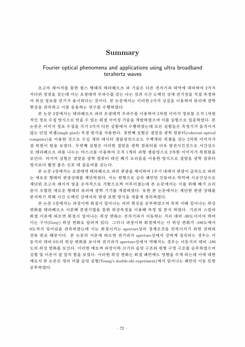
Summary

Fourier optical phenomena and applications using ultra broadbandterahertz waves

초고속 레이저를 통한 펄스 형태의 테라헤르츠 파 기술은 다른 전자기파 대역에 대비하여 2가지

커다란 장점을 갖는데 이는 초광대역 주파수를 갖는 다는 것과 시간 도메인 상에 전기장을 직접 측정하

여 위상 정보를 얻기가 용이하다는 것이다. 본 논문에서는 이러한 2가지 성질을 이용하여 퓨리에 광학

현상을 관측하고 이를 응용하는 연구를 수행하였다.

본 논문 3장에서는 테라헤르츠 파의 초광대역 주파수를 이용하여 2차원 이미지 정보를 오직 1차원

적인정보수집방식으로얻을수있는회절이미징기술을개발하였으며이를실험으로입증하였다. 본

논문은 이미지 정보 수집을 각기 3가지 다른 실험에서 수행하였는데 모든 실험들은 측정기가 움직이지

않는 단일픽셀(single pixel)측정 방식을사용한다. 첫번째 실험은결맞음 광학컴퓨터(coherent optical

computer)을 이용한 것으로 수십 개의 데이터 샘플링만으로도 수백개의 픽셀을 갖는 2차원 이미지가

잘 복원이 됨을 보였다. 두번째 실험은 이러한 결맞음 광학 컴퓨터를 더욱 발전시킨것으로 시간상으

로 테라헤르츠 파를 나누는 마스크를 이용하여 오직 1개의 파형 샘플링으로 2차원 이미지가 복원됨을

보인다. 마지막 실험은 결맞음 광학 컴퓨터 대신 쐐기 프리즘을 이용한 방식으로 결맞음 광학 컴퓨터

방식보다 훨씬 좋은 신호 대 잡음비를 갖는다.

본논문 4장에서는초광대역테라헤르츠파의편광을제어하여 1주기내에서편광이급속도로바뀌

는 새로운 형태의 편광상태를 재단하였다. 이는 원형으로 금속 패턴된 인듐비소 박막에 시공간상으로

재단된 초고속 레이저 빛을 순차적으로 가함으로써 이루어졌는데 본 논문에서는 이를 위해 쐐기 프리

즘이 조합된 새로운 형태의 퓨리에 광학 기기를 개발하였다. 또한 본 논문에서는 재단한 편광 상태를

분석하기 위해 시간 도메인 상에서의 편광 표현 방식을 새롭게 정의하였다.

본 논문 5장에서는 파장이하 회절시 일어나는 여러 현상을 공부하였으며 특히 이때 일어나는 위상

변화를 테라헤르츠 시분해 분광기법을 통한 위상측정을 이용해 측정 및 분석 하였다. 기존의 스칼라

회절 이론에 따르면 회절시 일어나는 위상 변화는 전자기파가 이동하는 거리 대비 -90도이어야 하며

이는 구이(Gouy) 위상 변화로 알려져 있다. 그러나 파장이하 회절에서는 이 위상 변화가 -180도에서

0도까지 일어남을 관측하였는데 이는 회절시키는 aperture상의 경계조건을 만족시키기 위한 전하와

전류 분포 때문이다. 본 논문의 이론에 따르면 전기파가 aperture상에서 강하게 집속되는 경우는 이

동거리 대비 0도의 위상 변화를 보이며 전기파가 aperture상에서 약해지는 경우는 이동거리 대비 -180

도의 위상 변화를 보인다. 이러한 예로써파장이하 크기의 슬릿 구조와 원형 구멍 구조를공부하였으며

실험 및 이론이 잘 일치 함을 보였다. 이러한 위상 변화는 회절 패턴에도 영향을 주게 되는데 이에 대한

예로서 본 논문은 영의 더블 슬릿 실험(Young’s double-slit experiment)에서 일어나는 패턴의 이동 또한

공부하였다.

– 72 –

감 사 의 글

이 논문을 완성하기까지 주위의 모든 분들로부터 수많은 도움을 받았습니다. 먼저 학위과정 동안

저를 지도해주신 안재욱 교수님께 진심으로 감사드립니다. 논문 지도뿐 아니라 조언과 충고를 통해 많

은 것을 배울 수 있었습니다. 또한 바쁘신 일정에도 논문 심사를 해주신 김병윤 교수님, 박용근 교수님,

민범기 교수님, 조영달 교수님께 감사드립니다.

학위 과정동안 실험과 논문 연구에 많은 도움을 준 실험실 식구들인 경진이형, 민우형, 영찬이형,

상경이형, 종석이형, 대훈이, 한결이, 효섭이에게 감사의 말을 전합니다. 연구실 사무일을 맡아준 인

영이 누나에게도 감사의 말을 전합니다. 학위과정 중 삶에 활력과 많은 조언을 준 룸메이트 재훈이,

택이, 영우 등을 비롯한 여러 친구들에게도 감사의 말을 전합니다. 특히 테라헤르츠 연구에 있어 많은

부분에서 도움을 준 민우형에게 다시 고마운 마음을 전합니다.

끝으로 오늘의 제가 있을 수 있도록 항상 저를 믿어주신 아버지와 사랑으로 보살펴주신 어머니,

힘이 되준 형에게 큰 감사를 드립니다.

– 73 –

이 력 서

이 름 : 이 강 희

생 년 월 일 : 1984년 11월 1일

E-mail 주 소 : kangheelee@kaist.ac.kr

학 력

2000. 3. – 2002. 2. 서울과학고등학교 (2년 수료)

2002. 3. – 2007. 2. KAIST 물리학과 (B.S.)

2007. 3. – 현재 KAIST 물리학과 석.박사 통합 과정

경 력

2008. 3. – 2009. 2. KAIST 물리학과 일반물리학 조교

2009. 3. – 2009. 6. KAIST 물리학과 물리학 실험 3 조교

2009. 9. – 2009. 12. KAIST 물리학과 파동광학 조교

학회활동

1. Sangkyung Lee, Kanghee Lee, Jaewook Ahn, and Chang Yong Park, Saturated Absorption Line-

shape Analysis Of Rubidium D2 Lines, KPS 2008 Spring, J-08, Daejeon, April 17-18, 2008.

2. Minwoo Yi, Kanghee Lee, Youngchan Kim, Dae-Su Yee, and Jaewook Ahn, The Multilayer

Interference Study of Terahertz Transmission Time-domain Spectroscopy, KPS 2008 Fall, IB-18,

Gwangju, October 23-24, 2008.

3. 이강희, 이민우, 진경환, 예종철, 안재욱, 의료 영상 수집용 원격 테라헤르츠 시분해 분광 모듈

개발과 테라헤르츠 영역에서의 압축 측정(compressed Sensing), KPS 2008 Fall, Ip-007, Gwangju,

October 23-24, 2008

4. Kanghee Lee, Minwoo Yi, and Jaewook Ahn, Experimental Study Of Terahertz Radiation Pattern

In Large-area Photoconductive Antenna, KPS 2009 Spring, Ip-II-014, Deajeon, April 23-24, 2009

5. Kanghee Lee, Minwoo Yi, Kyung Hwan Jin, Jong Chul Ye, and Jaewook Ahn, Terahertz Imaging

of Sub-Wavelength Objects Via Multispectral Reconstruction Algorithm, IRMMW-THz, Paradise

Hotel, Busan, Korea, September 21-25, 2009.

6. 이강희, 진경환, 예종철, 안재욱, 테라헤르츠 이미징을 위한 결맞음 광학 컴퓨터, 한국 광학회 창립

20주년 기념 특별학술발표회, W2A-l1, 광주, 김대중 컨벤션센터, 2009년 10월 20-21일

7. 이민우, 이강희, 임종석, 신상훈, 송진동, 홍영빈, 조영달, 안재욱, 광섬유를 이용한 테라헤르츠 발

생과 근접장 현미경 응용,” 2010년도 학국광학회 동계학술발표회, F4A-I2, 대전, 한국과학기술원,

2010년 1월 20-22일. (우수논문상)

– 74 –

8. 임종석, 이한결, 이상경, 이강희, 안재욱, 양자함수의 결맞음 제어를 이용한 진보된 2차원 푸리에

변환 분광학, 2010년도 한국광학회 동계학술발표회, F1E-VI6, 대전, 한국과학기술원, 2010년 1월

20-22일.

9. Minwoo Yi, Kanghee Lee, Jongseok Lim, Youngbin Hong, Young-Dahl Jho, and Jaewook Ahn,

THz waves emitted from an Optical Fiber, APLS 2010, Th-E2-4, Seogwipo KAL Hotel, Jeju Island,

Korea, May 11-15, 2010.

10. Kanghee Lee, Jong Hwan Jin, Jong Chul Ye, and Jaewook Ahn, 2D image encrypted in a single

THz waveform, APLS 2010, Th-E3-4, Seogwipo KAL Hotel, Jeju Island, Korea, May 11-15, 2010.

11. Kanghee Lee, Kyung Hwan Jin, Jong Chul Ye, and Jaewook Ahn, Coherent Optical Computing

for Terahertz Imaging, CLEO/QELS 2010, San Jose, CWO3, May 16-21, 2010.

12. Minwoo Yi, Kanghee Lee, Jongseok Lim, Jaewook Ahn, S. H. Shin, Jin-Dong Song, Youngbin

Hong, and Young-Dahl Jho, Terahertz Emission from Optical Fiber Tip and near-Field Microscope

Applications, CLEO/QELS 2010, San Jose, CWO2, May 16-21, 2010.

13. Jongseok Lim, Sangkyung Lee, Kanghee Lee, and Jaewook Ahn, Coherent Control of Wavefunc-

tions in 2-D Fourier Transform Optical Spectroscopy, CLEO/QELS 2010, San Jose, QFB6, May

16-21, 2010.

14. Kanghee Lee, Hangyeol Lee, and Jaewook Ahn, Terahertz Single-pixel Coherent Diffraction Imag-

ing, 한국물리학회 가을학술논문발표회 및 임시총회, 보광휘닉스파크, Ip-II-050, 10/20-22, 2010.

15. Kanghee Lee, and Jaewook Ahn, Single-pixel coherent diffraction imaging, 2nd THz-Bio Work-

shop, P-27, Jan 19-20, (2011)

16. Minwoo Yi, Kanghee Lee, Jongseok Lim, Youngbin Hong, Young-Dahl Jho, and Jaewook Ahn,

Terahertz Waves Emitted from an Optical Fiber, 2nd THz-Bio Workshop, P-29, Jan 19-20, (2011)

17. Kanghee Lee, and Jaewook Ahn, Single-pixel coherent diffraction imaging with THz waves, CLEO/QELS

2010, Baltimore, CThV7, May 1-6, (2011)

18. Kanghee Lee, Youngchan Kim, Jai Seok Ahn, Sang Wook Cheong, and Jaewook Ahn, Terahertz

spectroscopy of orthorhombic multiferroic YMn2o5 and TbMn2o5, ALTA 2011, KAL hotel, Jeju,

May 11-14 (2011).

19. Minwoo Yi, Kanghee Lee, Jin-Dong Song, and Jaewook Ahn, Temporal and spectral deformation

of THz pulses from sub-wavelength size InAs apertures, ALTA 2011, KAL hotel, Jeju, May 11-14

(2011).

20. Minwoo Yi, Kanghee Lee, Jin-Dong Song, and Jaewook Ahn, Sub-wavelength terahertz microscopy

using spectro-temporal phase analysis, IRMMW-THz, Hyatt Regency Downtown, Houston TX USA,

October 2-7, 2011.

21. Kanghee Lee, Minwoo Yi, Jin-Dong Song, and Jaewook Ahn, Generation of polarization shaped

terahertz waves, 한국물리학회 가을학술논문발표회 및 임시총회, 부산 벡스코, IG-13, 10/19-21,

2011. (우수발표상)

22. Kanghee Lee, Minwoo Yi, Jin Dong Song, and Jaewook Ahn, Generation of Polarization Shaped

Terahertz Waves, CLEO/QELS 2012, San Jose convention center, CM2L4, May 7 (2012).

23. 이강희, 정광용, 서민교, 박상언, 안재욱, 파장 이하 통과시 나타나는 마이크로파의 특이위상변화,

2012년도 한국광학회 하계학술발표회, M2D-I5, 제주도, 금호리조트, 2012년 8월 27-29일.

– 75 –

24. Kanghee Lee, Minwoo Yi, Sang Eon Park, and Jaewook Ahn, Phase-shift anomaly caused by

sub-wavelength-scale metal slit or aperture diffraction, 4th THz-Bio Workshop, p-22, Seoul, Seoul

National University, Feb. 14-15, 2013 (Poster Award).

25. Kanghee Lee, Minwoo Yi, Sang Eon Park, and Jaewook Ahn, Polarization effects on phase-shift

anomaly in sub-wavelength diffraction, 한국물리학회 봄학술논문발표회 및 임시총회, 대전 컨벤션

센터, IG-04, 4/24-26, 2013.

연구업적

1. Minwoo Yi, Kanghee Lee, and Jaewook Ahn, “Optimal Molar Fractions of Ternary Zinc-blende

Terahertz Emitters,” Journal of the Korean Physical Society 51(2), 475-479 (August 2007).

2. Minwoo Yi, Kanghee Lee, Inhee Maeng, Joo-Hiuk Son, R. D. Averitt, and Jaewook Ahn, “Tailoring

the Spectra of Terahertz Emission from CdTe and ZnTe Electro-Optic Crystals,” Japanese Journal

of Applied Physics 47(1), 202-204 (January 2008).

3. Kanghee Lee, Minwoo Yi, and Jaewook Ahn, “Modleing of THz Frequency Spectrum via Optical

Rectification in THz Time Domain Spectroscopy,” Journal of the Korean Society for Nondestructive

Testing 28(2), 119-124 (April 2008).

4. Sangkyung Lee, Kanghee Lee, and Jaewook Ahn, “Reversed Peaks of Saturated Absorption Spec-

tra of Atomic Rubidium,” Japanese Journal of Applied Physics 48, 032301 (March 2009).

5. Kanghee Lee, Kyung Hwan Jin, Jong Chul Ye, and Jaewook Ahn, “Coherent Optical Computing

for T-ray Imaging,” Optics Letters 35(4), 508 (February 15, 2010).

6. Kyung Hwan Jin, Kanghee Lee, Jaewook Ahn, and Jong Chul Ye, “Compressive inverse scattering

using ultrashort pulses,” Proc. SPIE, Vol. 7533, 75330D (February 2010).

7. Minwoo Yi, Kanghee Lee, Jongseok Lim, Youngbin Hong, Young-Dahl Jho, and Jaewook Ahn,

“Terahertz Waves Emitted from an Optical Fiber,” Optics Express 18, 13693–13699 (June 2010).

8. Kanghee Lee and Jaewook Ahn, “Single pixel coherent diffraction imaging,” Applied Physics

Letters 97, 241101 (Dec. 13, 2010).

9. Minwoo Yi, Kanghee Lee, Jin Dong Song, and Jaewook Ahn, “Terahertz phase microscopy in the

sub-wavelength regime,” Applied Physics Letters 100, 161110 (April 2012).

10. Kanghee Lee, Minwoo Yi, Jin Dong Song, and Jaewook Ahn, “Polarization shaping of few-cycle

terahertz wave,” Optics Express 20, 12463 (May 2012).

11. Jongseok Lim, Kanghee Lee, and Jaewook Ahn, “Ultrafast Rabi flopping in a three-level energy

ladder,” Optics Letters 37 (16), 3378 (August 2012).

12. Kanghee Lee, Minwoo Yi, Sang Eon Park, and Jaewook Ahn, “Phase-shift anomaly caused by

sub-wavelength-scale metal slit or aperture diffraction,” Optics Letters 38 (2), 166 (Jan. 2013).

13. Sang-Gil Park, Kanghee Lee, Jaewook Ahn, and Ki-Hun Jeong, “Index Tailoring Silicon for

Terahertz Photonics,” (submitted).

14. Daehoon Han, Kanghee Lee, Jongseok Lim, Sei Sun Hong, Young Kie Kim, and Jaewook Ahn,

“Terahertz lens made out of stone,” (submitted).

– 76 –

15. Kanghee Lee, and Jaewook Ahn, “Terahertz wave diffraction from a sub-wavelength-scale slit,”

(in preparation).

특 허

1. Jaewook Ahn, Kanghee Lee, and Minu Yi, Contact type terahertz time domain spectrum device,

Korea Patent, 10-1017796 (2011-02-18).

2. Jaewook Ahn, Kanghee Lee, Minu Yi, Jongseok Lim,Youngdahl Cho, Yong-bin Hong, and Jihoon

Jeong, Device for terahertz emitter using thin indium arsenic film optical fiber and manufacturing

method thereof, Korea Patent, 10-1067368 (2011-09-19).

3. Jaewook Ahn, Jong Chul Ye, Kyunghwan Jin, and Kanghee Lee, Terahertz time domain spectrum

device and image apparatus using the spectrum device, Korea Patent, 10-1074003 (2011-10-10).

4. Jaewook Ahn, Kanghee Lee, Jong Chul Ye, and Kyunghwan Jin, Terahertz time domain spectral

apparatus and image processing method for reducing sampling number, Korea Patent, 10-1077595

(2011-10-21).

5. Jaewook Ahn and Kanghee Lee, Imaging device for terahertz single-pixel diffraction image, Korea

Patent, 10-1107853 (2012-01-12)

– 77 –