PHYSICAL REVIEW D Observation results by the TAMA300

PHYSICAL REVIEW D 71, 082002 (2005)

Observation results by the TAMA300 detector on gravitational wave burstsfrom stellar-core collapses

Masaki Ando,1 Koji Arai,2 Youichi Aso,1 Peter Beyersdorf,2 Kazuhiro Hayama,3 Yukiyoshi Iida,1 Nobuyuki Kanda,4

Seiji Kawamura,2 Kazuhiro Kondo,5 Norikatsu Mio,6 Shinji Miyoki,5 Shigenori Moriwaki,6 Shigeo Nagano,7

Kenji Numata,8 Shuichi Sato,2 Kentaro Somiya,6 Hideyuki Tagoshi,9 Hirotaka Takahashi,9,10 Ryutaro Takahashi,2

Daisuke Tatsumi,2 Yoshiki Tsunesada,2 Zong-Hong Zhu,2 Tomomi Akutsu,5 Tomotada Akutsu,3 Akito Araya,11

Hideki Asada,12 Mark A. Barton,5 Youhei Fujiki,10 Masa-Katsu Fujimoto,2 Ryuichi Fujita,9 Mitsuhiro Fukushima,2

Toshifumi Futamase,13 Yusaku Hamuro,10 Tomiyoshi Haruyama,14 Hideaki Hayakawa,5 Gerhard Heinzel,15

Gen’ichi Horikoshi,14,† Hideo Iguchi,16 Kunihito Ioka,17 Hideki Ishitsuka,5 Norihiko Kamikubota,14

Takaharu Kaneyama,10 Yoshikazu Karasawa,13 Kunihiko Kasahara,5 Taketoshi Kasai,12 Mayu Katsuki,4 Keita Kawabe,18

Mari Kawamura,19 Nobuki Kawashima,20 Fumiko Kawazoe,21 Yasufumi Kojima,22 Keiko Kokeyama,21 Yoshihide Kozai,2

Hideaki Kudoh,19,23 Kazuaki Kuroda,5 Takashi Kuwabara,10 Namio Matsuda,24 Kazuyuki Miura,25 Osamu Miyakawa,26

Shoken Miyama,2 Hiromi Mizusawa,10 Mitsuru Musha,27 Yoshitaka Nagayama,4 Ken’ichi Nakagawa,27

Takashi Nakamura,19 Hiroyuki Nakano,4 Ken-ichi Nakao,4 Yuhiko Nishi,1 Yujiro Ogawa,14 Masatake Ohashi,5

Naoko Ohishi,2 Akira Okutomi,5 Ken-ichi Oohara,10 Shigemi Otsuka,1 Yoshio Saito,14 Shihori Sakata,21 Misao Sasaki,28

Kouichi Sato,29 Nobuaki Sato,14 Youhei Sato,27 Hidetsugu Seki,1 Aya Sekido,30 Naoki Seto,31 Masaru Shibata,32

Hisaaki Shinkai,33 Takakazu Shintomi,14 Kenji Soida,1 Toshikazu Suzuki,14 Akiteru Takamori,11 Shuzo Takemoto,19

Kohei Takeno,6 Takahiro Tanaka,19 Keisuke Taniguchi,34 Shinsuke Taniguchi,1 Toru Tanji,6 C. T. Taylor,5

Souichi Telada,35 Kuniharu Tochikubo,1 Masao Tokunari,5 Takayuki Tomaru,14 Kimio Tsubono,1 Nobuhiro Tsuda,29

Takashi Uchiyama,5 Akitoshi Ueda,2 Ken-ichi Ueda,27 Fumihiko Usui,36 Koichi Waseda,2 Yuko Watanabe,25

Hiromi Yakura,25 Akira Yamamoto,14 Kazuhiro Yamamoto,5 Toshitaka Yamazaki,2 Yuriko Yanagi,21 Tatsuo Yoda,1

Jun’ichi Yokoyama,9 and Tatsuru Yoshida13

1Department of Physics, The University of Tokyo, Bunkyo-ku, Tokyo 113-0033, Japan2National Astronomical Observatory, Mitaka, Tokyo 181-8588, Japan

3Department of Astronomy, The University of Tokyo, Bunkyo-ku, Tokyo 113-0033, Japan4Graduate School of Science, Osaka City University, Sumiyoshi-ku, Osaka 558-8585, Japan

5Institute for Cosmic Ray Research, The University of Tokyo, Kashiwa, Chiba 277-8582, Japan6Department of Advanced Materials Science, The University of Tokyo, Kashiwa, Chiba 277-8561, Japan

7National Institute of Information and Communications Technology, Koganei, Tokyo 184-8795, Japan8NASA Goddard Space Flight Center, Greenbelt, Maryland 20771, USA

9Graduate School of Science, Osaka University, Toyonaka, Osaka 560-0043, Japan10Faculty of Science, Niigata University, Niigata, Niigata 950-2102, Japan

11Earthquake Research Institute, The University of Tokyo, Bunkyo-ku, Tokyo 113-0032, Japan12Faculty of Science and Technology, Hirosaki University, Hirosaki, Aomori 036-8561, Japan

13Graduate School of Science, Tohoku University, Sendai, Miyagi 980-8578, Japan14High Energy Accelerator Research Organization, Tsukuba, Ibaraki 305-0801, Japan

15Max-Planck-Institut fuer Gravitationsphysik, Callinstrasse 38, D-30167 Hannover, Germany16Tokyo Institute of Technology, Meguro-ku, Tokyo 152-8551, Japan

17Physics Department, Pennsylvania State University, University Park, Pennsylvania 16802, USA18LIGO Hanford Observatory, Richland, Washington 99352, USA

19Faculty of Science, Kyoto University, Sakyo-ku, Kyoto 606-8502, Japan20Kinki University, Higashi-Osaka, Osaka 577-8502, Japan

21Ochanomizu University, Bunkyo-ku, Tokyo 112-8610, Japan22Department of Physics, Hiroshima University, Higashi-Hiroshima, Hiroshima 739-8526, Japan

23Theoretical Astrophysics Group, Department of Physics, The University of Tokyo, Bunkyo-ku, Tokyo 113-0033, Japan24Tokyo Denki University, Chiyoda-ku, Tokyo 101-8457, Japan

25Department of Physics, Miyagi University of Education, Aoba Aramaki, Sendai 980-0845, Japan26California Institute of Technology, Pasadena, California 91125, USA

27Institute for Laser Science, University of Electro-Communications, Chofugaoka, Chofu, Tokyo 182-8585, Japan28Yukawa Institute for Theoretical Physics, Kyoto University, Sakyo-ku, Kyoto 606-8502, Japan

29Precision Engineering Division, Faculty of Engineering, Tokai University, Hiratsuka, Kanagawa 259-1292, Japan30Waseda University, Shinjyuku-ku, Tokyo 169-8555, Japan

31Theoretical Astrophysics, California Institute of Technology, Pasadena, California 91125, USA32Graduate School of Arts and Sciences, The University of Tokyo, Meguro-ku, Tokyo 153-8902, Japan

33RIKEN, Wako, Saitaka 351-0198, Japan

1550-7998=2005=71(8)=082002(17)$23.00 082002-1 2005 The American Physical Society

MASAKI ANDO et al. PHYSICAL REVIEW D 71, 082002 (2005)
34Department of Physics, University of Illinois at Urbana-Champaign, Urbana, Illinois 61801-3080, USA
35National Institute of Advanced Industrial Science and Technology, Tsukuba, Ibaraki 305-8563, Japan36ISAS/JAXA, Sagamihara, Kanagawa 229-8510, Japan(Received 22 January 2005; published 27 April 2005)

*Email add†Deceased

We present data-analysis schemes and results of observations with the TAMA300 gravitational wavedetector, targeting burst signals from stellar-core collapse events. In analyses for burst gravitational waves,the detection and fake-reduction schemes are different from well-investigated ones for a chirp waveanalysis, because precise waveform templates are not available. We used an excess -power filter for theextraction of gravitational wave candidates, and developed two methods for the reduction of fake eventscaused by nonstationary noises of the detector. These analysis schemes were applied to real data from theTAMA300 interferometric gravitational wave detector. As a result, fake events were reduced by a factor ofabout 1000 in the best cases. In addition, in order to interpret the event candidates from an astronomicalviewpoint, we performed a Monte-Carlo simulation with an assumed Galactic event distribution modeland with burst waveforms obtained from numerical simulations of stellar-core collapses. We set an upperlimit of 5:0� 103 events= sec on the burst gravitational wave event rate in our Galaxy with a confidencelevel of 90%. This work shows prospects on the search for burst gravitational waves, by establishing ananalysis scheme for the observation data from an interferometric gravitational wave detector.

DOI: 10.1103/PhysRevD.71.082002 PACS numbers: 04.80.Nn, 07.05.Kf, 95.55.Ym, 95.85.Sz

I. INTRODUCTION

Direct observations of gravitational waves (GWs) willreveal new aspects of the Universe [1]. Since GWs areemitted by the bulk motion of matter, and are hardlyabsorbed or scattered, they have a potential to carry astro-physical and cosmological information different from thatby electromagnetic waves. In order to create a new field ofGW astronomy, several groups around the world are devel-oping and operating GW detectors. Among them, mucheffort is being made recently on interferometric detectors:LIGO [2] in U. S. A., VIRGO [3] and GEO [4] in Europe,and TAMA [5,6] in Japan. These detectors have widefrequency-band sensitivity between about 10 Hz and afew kHz range, and have an ability to observe the wave-form of a GW, which would contain astrophysical infor-mation. In these detectors, both high sensitivity and highstability are required because GW signals are expected tobe extremely faint and rare.

There are several kinds of target GW sources in theseinterferometric detectors [7,8], and data-analysis schemesare being developed and applied to the observation data.Since GW signals are considered to be faint, an efficientdata-analysis scheme is required to extract the signals ofGWs from noisy detector outputs. The target GWs areclassified by the signal waveforms: chirp waves, continu-ous waves, burst waves, and so on. A chirp wave is asinusoidal waveform with increasing frequency and ampli-tude in time, which is radiated from an inspiraling compactbinary just before its merger. Since this waveform is wellpredicted, an effective and sophisticated method ofmatched filtering is used in chirp wave search; correlationsbetween the data and a template (the predicted waveform)are calculated to extract a GW signal from noisy data

ress: [email protected]

082002

[9,10]. A continuous wave has a sinusoidal waveformwith a stable frequency for over many years, which isradiated from a quasistationary compact binary or a rotat-ing neutron star. A matched filtering method can also beused in the search for continuous waves from knownsources, because we can predict their waveforms preciselyby observations with electromagnetic waves [11,12].

A burst wave, which is the target of this article, is also apromising gravitational waveform class. This wave, a shortspikelike wave with a typical duration time of less than100 msec, is emitted from stellar-core collapse in a super-nova explosion or a merger of a binary system. Unlike thechirp and continuous wave cases, a matched filteringmethod cannot be used in a burst-wave analysis. This isbecause a set of precise waveform templates that cover thesource parameters is not available, while typical wave-forms are obtained by numerical simulations [13–15].Thus, several signal-extraction methods, called burst fil-ters, have been proposed for the detection of these burstgravitational waves: an excess power filter [16], a clusterfilter in the time-frequency plane [17], a slope (or a linear-fit) filter [18], and a pulse correlation filter [19]. Since wehave only a little knowledge on the waveforms, these filterslook for unusual events in the Gaussian-noise background.

For the detection of GWs, evaluation and reduction offake-event backgrounds are critical problems. In eachanalysis scheme described above, we define an evaluationfilter (such as a correlation with the template in a matchedfiltering method, and certain statistics describing any un-usual behavior of the data in burst analyses), and record thefilter output as a GW event trigger if it is above a giventhreshold. The event triggers usually contain fake events,which are caused by statistical and externally inducedexcesses in the detector noise level. Although an idealinterferometric detector would have a stationary Gaussian-noise behavior, the detector output is far from stationary inpractice, affected by external disturbances, such as seismic

-2

OBSERVATION RESULTS BY THE TAMA300 DETECTOR . . . PHYSICAL REVIEW D 71, 082002 (2005)

motion, acoustic disturbance, changes in the temperatureand pressure, and so on. As a result, it is likely that realsignals are buried in these fake events, or are dismissedwith a larger detection threshold set to reduce fakes. Thus,rejection of these fake events, or a veto in other words, isindispensable for the detection of GWs. In a chirp waveanalysis case, the output of the matched filter is lessaffected by nonstationary noises because it is only sensitiveto a waveform similar to GWs. In addition, since we knowa precise waveform of the target GW signal, we can rejectthe fake events by evaluating how well the candidatewaveform fits to the template [9,10,20]. On the otherhand, the effect of fake events are more serious and criticalin the burst analysis case. Since burst filters are designed toextract any unusual behavior of the detector output, theyare also sensitive to nonstationary noises by their nature.Moreover, it is not straightforward to distinguish thesefakes from a real signal, and to reject them, because wedo not know the precise GW waveforms.

There are several schemes to reject these fake events:coincidences by multiple detectors, veto analyses withdetector monitor signals, rejection by waveform behaviors,and so on. Among them, the most powerful and reliableway will be a coincidence analysis with multiple indepen-dent detectors [21–23]. If we detect gravitational wavecandidates with multiple detectors simultaneously (orwithin an acceptable time difference), we can declare thedetection of a real signal with high confidence. In a roughestimation, the fake rate is reduced by a power of thenumber of independent detectors. On the other hand, fakereduction with a single detector is also important, even in acoincidence analysis as the rejection of fakes with a singledetector would reduce accidental coincidences. In obser-vation runs, many auxiliary signals are recorded togetherwith the GW signal channel in order to monitor the detec-tor status. Since some of them are sensitive to detectorinstabilities, it is possible to reject nonstationary noiseswith them [24,25]. In addition, even without precise GWwaveforms, fake events are rejected by investigations ofthe signal behavior with our knowledge or assumptions onthe waveforms [26].

In this article, we present a data-analysis scheme forburst GWs, and results obtained by applying them to realobservation data. The data used in this work were over2700 hours of data obtained during the sixth, eighth, andninth data-taking runs (DT6, DT8, and DT9, respectively)of the TAMA300 detector [5,6,27]. We adopted an excesspower filter as a burst filter, which is robust for uncertain-ties of the GW waveforms [16,28]. In addition, we usedtwo fake-reduction methods. One was a veto with detectormonitor signals. Another was our new method of rejectionbased on the waveform behavior of the time scale.Although there have been several previous works on simi-lar veto methods [24–26], they were applied to a limitedsubset of observation data. We implemented these veto

082002

methods in our burst analysis code, analyzed real observa-tion data, and evaluated their effectiveness. Such a full-scale analysis is important because the effectiveness of thevetoes strongly depends on the quality of the real data.

The obtained event triggers were interpreted from anastronomical point of view; the results were used to setupper limits on Galactic events. We carried out Monte-Carlo simulations of Galactic events with waveforms ob-tained by numerical simulations of stellar-core collapses.In previous works, upper limits by real observations havebeen set with artificial waveform models of short spikes,Gaussian waves, or sine-Gaussian waves [21,29,30]. Onthe other hand, realistic waveforms by numerical simula-tions have been used to evaluate the efficiencies of burstfilters with simulated Gaussian noises [18,19]. We intendedto set upper limits in a realistic way: using a realisticdistribution of the Galactic events, targeting at realisticwaveforms obtained by numerical simulations, and analyz-ing long observation data from the detector. As a result, weexpect to obtain prospects for both current and futureresearch.

This article is organized as follows. In Section II, weoverview our burst analysis: target waves, analyzed data,and our burst filter. In Section III, we describe veto meth-ods with a monitor signal and the signal behavior. Afterthat, we present analysis results and an interpretation of theresults, setting an upper limit on the Galactic events, inSection IV. At last, we present discussions and a conclusionof our research in Section V and VI.

II. GENERATION OF EVENT TRIGGERS

In this Section, we overview the target GW signal char-acteristics, used data, and a burst filter used in this work.

A. Target gravitational waves

The target of the analysis in this work is a burst GWfrom stellar-core collapse (core-collapse supernova explo-sion). It is difficult to predict its waveform analytically,because of the complex time evolution of the mass den-sities in the explosion process. Thus, the explosion processand radiated GWs have been investigated by numericalsimulations [13–15]. Although these simulations wereperformed with differently simplified models, similarwaveforms were obtained in these simulations.

Among these simulations, Dimmelmeier et al. havepresented rather systematic surveys on GWs from stellar-core collapses [13]. They have obtained 26 waveformswith relativistic simulations of rotational supernova corecollapses, with axisymmetric models with different initialconditions in a differential rotation, an initial rotation rate,and an adiabatic index at subnuclear densities. Althoughthe simulation did not cover all of the initial parameters, weused them as reference waveforms in our analysis, assum-ing that typical characteristics and behavior of the GWs

-3

0 10 20 30 40 50-2

-1

0

1G

W A

mp

litu

de

(str

ain

)

Time [msec]

A1B1G1A3B3G1A4B1G2

[ x 10-20 ]

Waveform type:

FIG. 1 (color online). Waveform examples from the DFMgravitational waveform catalog. The amplitudes are for an eventat 10 kpc distance from the detector.


from stellar-core collapses are included in this waveformcatalog.

We processed the original waveforms of the catalog (wecall it Dimmelmeier-Font-Muller (DFM) catalog in thisarticle) with a 30 Hz second-order high-pass digital filter,and resampled them to 20 kHz in order to be compatiblewith the data from the detector (described in the next part).Figure 1 shows examples from the waveform catalog.While these waveforms have different behaviors, theyhave common characteristics: about a 1 msec-short spike,and a total duration of less than 100 msec. According to theDFM catalog, the averaged amplitude of GWs radiated bysupernovae at the Galactic center (8.5 kpc distance fromthe detector) is hhpeaki � 1:5� 10�20 in a peak strainamplitude, or hhrssi � 4� 10�22 �Hz�1=2� in root-sum-square (RSS) amplitude. Here, a RSS amplitude is definedby

102 10310-24

10-22

10-20

Det

ecto

r N

ois

e L

evel

[1

/Hz1/

2 ]

Frequency [Hz]

TAMA

LCGT design sensitivity

noise level(DT9)

GW

RS

S A

mp

litu

de

and

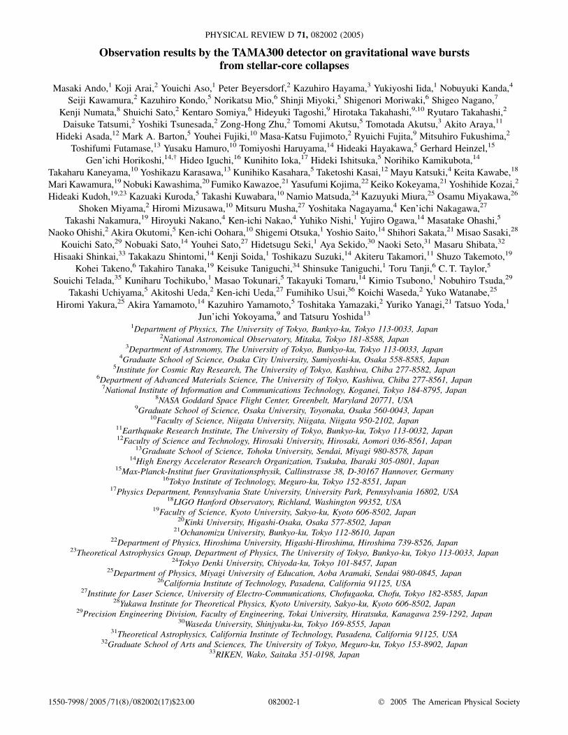
FIG. 2 (color online). RSS amplitude and central frequencycalculated from waveforms in the DFM catalog. The amplitudesare for events at the Galactic center (closed circles), and forevents at 100 pc distance from the detector (open circles). Thesource angle is assumed to be optical in this plot. Each error barindicates the frequency range within which the power spectrumvalue is above half of its peak value. The noise level of TAMA atDT9 and the design sensitivity of LCGT [39] are shown together.

082002

hrss ��Z 1

�1jht�j2dt

�1=2; (1)

where ht� is the strain amplitude of the GW [29,31]. In theaxisymmetric model used to obtain the DFM catalog, thewaves are radiated only in a plus polarization, and theradiated amplitude has an angular dependence of sin��2,where � is the angle between the symmetric axis and thepropagation axis of GW to the detector [13–15]. Theamplitudes described above are calculated with optimalsource angle (� � �=2). The central frequencies of thewaves, which are calculated from the weighting average ofthe power spectra, range from 90 Hz to 1.2 kHz (Fig. 2),which is around the observation band of interferometricdetectors. Also, it is estimated from the DFM catalog that atotal energy radiated as GWs in one event is hEtoti � 8�10�8�M�c

2�, in average [13]. Here, M� is the mass of theSun.

B. Data from a gravitational wave detector TAMA300

We applied our analysis method to observation dataobtained by TAMA300 [5,6]; TAMA300 is a Japaneselaser-interferometric gravitational wave detector, locatedat the Mitaka campus of the National AstronomicalObservatory of Japan (NAOJ) in Tokyo (35 400N,139 320E). TAMA300 has an optical configuration of aMichelson interferometer with 300 m-length Fabry-Perotarm cavities and with power recycling to enhance the laserpower in the interferometer. During the operation, themirrors of the detector are shaken by a 625 Hz sinusoidalsignal, which enables us to calibrate the detector sensitivitycontinuously with a relative error of less than 1% [32]. Themain output signal of the detector, which would containGW signals, is recorded with a 20 kHz, 16 bit data-acquisition system [33]. Besides the main output signal,over 150 monitor signals are also recorded during theobservation: signals for the laser power in and from theinterferometer, detector control-loop signals, seismic andacoustic monitor signals, signals for temperature and pres-sure monitor, and so on [27]. These monitor signals areused for diagnosing the detector condition, and for vetoanalyses (Section III). The recorded data are stored indigital linear tape (DLT) tapes on site, and are sent to

TABLE I. Summary of long data-taking runs by TAMA300.The floor noise level and total observation data amount aredescribed. The last column (D. C.) represents the duty cyclethroughout the data-taking run.

Term Noise level Total data D. C.[Hz�1=2] [hours]

DT6 Aug.–Sept., 2001 5� 10�21 1038 87%DT8 Feb.–April, 2003 3� 10�21 1157 81%DT9 Nov., 2003–Jan., 2004 2� 10�21 558 54%

-4

102 103

10-21

10-20

10-19

10-18

10-17T

ypic

al N

ois

e L

evel

[1

/Hz1/

2 ]

Frequency [Hz]

DT6

DT8DT9

C

V

VV

V

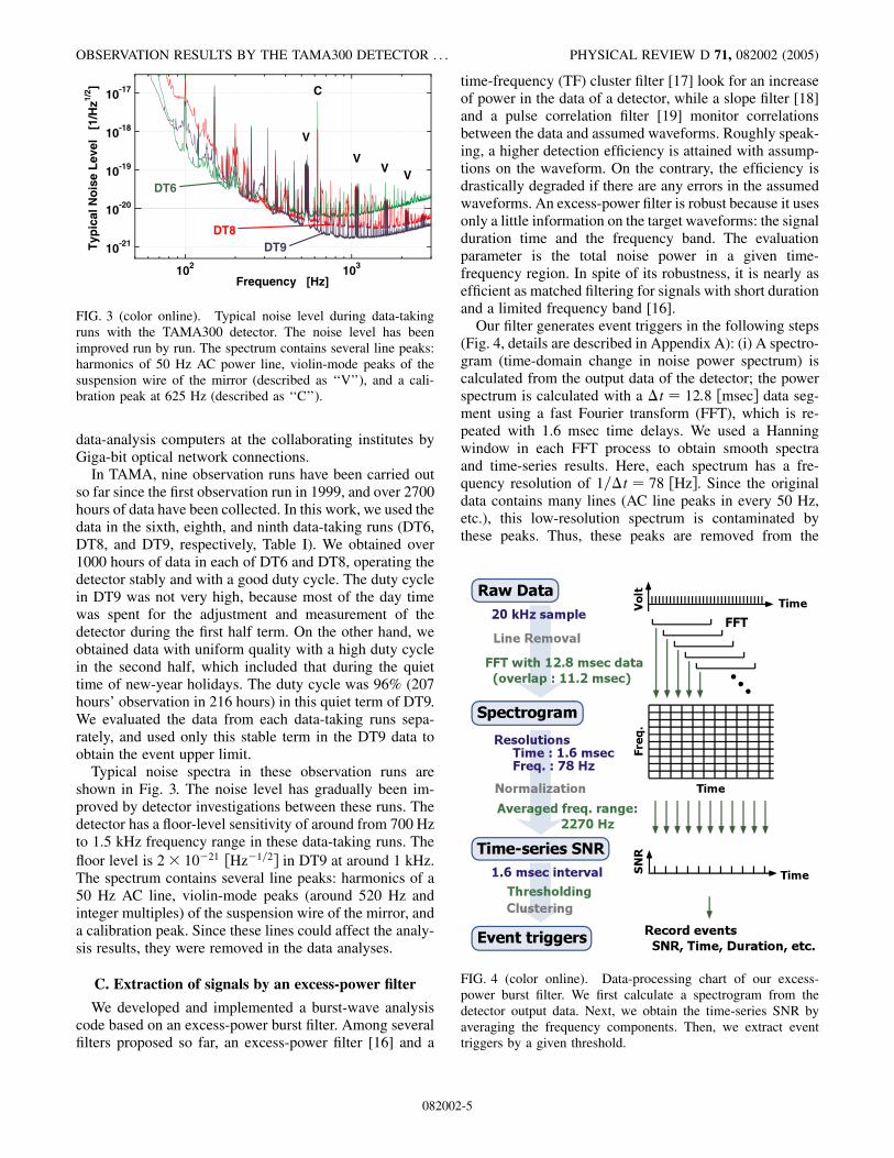
FIG. 3 (color online). Typical noise level during data-takingruns with the TAMA300 detector. The noise level has beenimproved run by run. The spectrum contains several line peaks:harmonics of 50 Hz AC power line, violin-mode peaks of thesuspension wire of the mirror (described as ‘‘V’’), and a cali-bration peak at 625 Hz (described as ‘‘C’’).

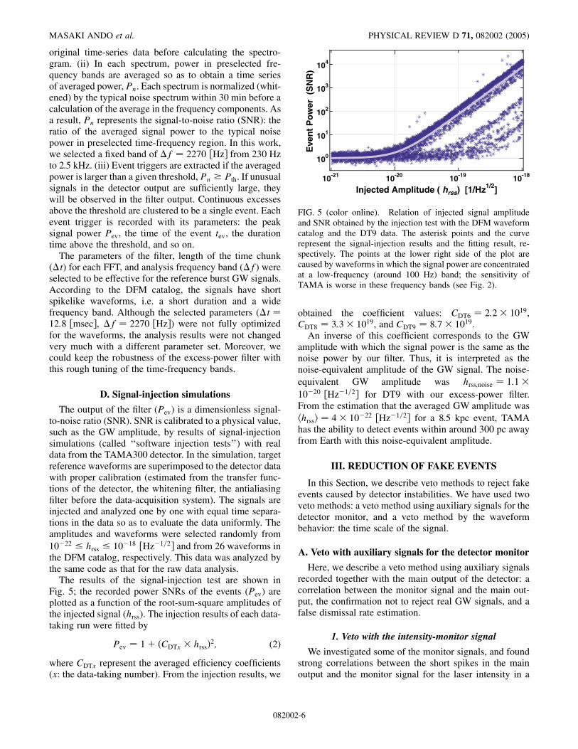
FIG. 4 (color online). Data-processing chart of our excess-power burst filter. We first calculate a spectrogram from thedetector output data. Next, we obtain the time-series SNR byaveraging the frequency components. Then, we extract eventtriggers by a given threshold.


data-analysis computers at the collaborating institutes byGiga-bit optical network connections.

In TAMA, nine observation runs have been carried outso far since the first observation run in 1999, and over 2700hours of data have been collected. In this work, we used thedata in the sixth, eighth, and ninth data-taking runs (DT6,DT8, and DT9, respectively, Table I). We obtained over1000 hours of data in each of DT6 and DT8, operating thedetector stably and with a good duty cycle. The duty cyclein DT9 was not very high, because most of the day timewas spent for the adjustment and measurement of thedetector during the first half term. On the other hand, weobtained data with uniform quality with a high duty cyclein the second half, which included that during the quiettime of new-year holidays. The duty cycle was 96% (207hours’ observation in 216 hours) in this quiet term of DT9.We evaluated the data from each data-taking runs sepa-rately, and used only this stable term in the DT9 data toobtain the event upper limit.

Typical noise spectra in these observation runs areshown in Fig. 3. The noise level has gradually been im-proved by detector investigations between these runs. Thedetector has a floor-level sensitivity of around from 700 Hzto 1.5 kHz frequency range in these data-taking runs. Thefloor level is 2� 10�21 �Hz�1=2� in DT9 at around 1 kHz.The spectrum contains several line peaks: harmonics of a50 Hz AC line, violin-mode peaks (around 520 Hz andinteger multiples) of the suspension wire of the mirror, anda calibration peak. Since these lines could affect the analy-sis results, they were removed in the data analyses.

C. Extraction of signals by an excess-power filter

We developed and implemented a burst-wave analysiscode based on an excess-power burst filter. Among severalfilters proposed so far, an excess-power filter [16] and a

082002

time-frequency (TF) cluster filter [17] look for an increaseof power in the data of a detector, while a slope filter [18]and a pulse correlation filter [19] monitor correlationsbetween the data and assumed waveforms. Roughly speak-ing, a higher detection efficiency is attained with assump-tions on the waveform. On the contrary, the efficiency isdrastically degraded if there are any errors in the assumedwaveforms. An excess-power filter is robust because it usesonly a little information on the target waveforms: the signalduration time and the frequency band. The evaluationparameter is the total noise power in a given time-frequency region. In spite of its robustness, it is nearly asefficient as matched filtering for signals with short durationand a limited frequency band [16].

Our filter generates event triggers in the following steps(Fig. 4, details are described in Appendix A): (i) A spectro-gram (time-domain change in noise power spectrum) iscalculated from the output data of the detector; the powerspectrum is calculated with a �t � 12:8 �msec� data seg-ment using a fast Fourier transform (FFT), which is re-peated with 1.6 msec time delays. We used a Hanningwindow in each FFT process to obtain smooth spectraand time-series results. Here, each spectrum has a fre-quency resolution of 1=�t � 78 �Hz�. Since the originaldata contains many lines (AC line peaks in every 50 Hz,etc.), this low-resolution spectrum is contaminated bythese peaks. Thus, these peaks are removed from the

-5

10-21 10-20 10-19 10-18

100

101

102

103

104

Injected Amplitude ( hrss) [1/Hz1/2]

Eve

nt

Po

wer

(S

NR

)

FIG. 5 (color online). Relation of injected signal amplitudeand SNR obtained by the injection test with the DFM waveformcatalog and the DT9 data. The asterisk points and the curverepresent the signal-injection results and the fitting result, re-spectively. The points at the lower right side of the plot arecaused by waveforms in which the signal power are concentratedat a low-frequency (around 100 Hz) band; the sensitivity ofTAMA is worse in these frequency bands (see Fig. 2).


original time-series data before calculating the spectro-gram. (ii) In each spectrum, power in preselected fre-quency bands are averaged so as to obtain a time seriesof averaged power, Pn. Each spectrum is normalized (whit-ened) by the typical noise spectrum within 30 min before acalculation of the average in the frequency components. Asa result, Pn represents the signal-to-noise ratio (SNR): theratio of the averaged signal power to the typical noisepower in preselected time-frequency region. In this work,we selected a fixed band of �f � 2270 �Hz� from 230 Hzto 2.5 kHz. (iii) Event triggers are extracted if the averagedpower is larger than a given threshold, Pn � Pth. If unusualsignals in the detector output are sufficiently large, theywill be observed in the filter output. Continuous excessesabove the threshold are clustered to be a single event. Eachevent trigger is recorded with its parameters: the peaksignal power Pev, the time of the event tev, the durationtime above the threshold, and so on.

The parameters of the filter, length of the time chunk(�t) for each FFT, and analysis frequency band (�f) wereselected to be effective for the reference burst GW signals.According to the DFM catalog, the signals have shortspikelike waveforms, i.e. a short duration and a widefrequency band. Although the selected parameters (�t �12:8 �msec�, �f � 2270 �Hz�) were not fully optimizedfor the waveforms, the analysis results were not changedvery much with a different parameter set. Moreover, wecould keep the robustness of the excess-power filter withthis rough tuning of the time-frequency bands.

D. Signal-injection simulations

The output of the filter (Pev) is a dimensionless signal-to-noise ratio (SNR). SNR is calibrated to a physical value,such as the GW amplitude, by results of signal-injectionsimulations (called ‘‘software injection tests’’) with realdata from the TAMA300 detector. In the simulation, targetreference waveforms are superimposed to the detector datawith proper calibration (estimated from the transfer func-tions of the detector, the whitening filter, the antialiasingfilter before the data-acquisition system). The signals areinjected and analyzed one by one with equal time separa-tions in the data so as to evaluate the data uniformly. Theamplitudes and waveforms were selected randomly from10�22 � hrss � 10�18 �Hz�1=2� and from 26 waveforms inthe DFM catalog, respectively. This data was analyzed bythe same code as that for the raw data analysis.

The results of the signal-injection test are shown inFig. 5; the recorded power SNRs of the events (Pev) areplotted as a function of the root-sum-square amplitudes ofthe injected signal (hrss). The injection results of each data-taking run were fitted by

Pev � 1� CDTx � hrss�2; (2)

where CDTx represent the averaged efficiency coefficients(x: the data-taking number). From the injection results, we

082002

obtained the coefficient values: CDT6 � 2:2� 1019,CDT8 � 3:3� 1019, and CDT9 � 8:7� 1019.

An inverse of this coefficient corresponds to the GWamplitude with which the signal power is the same as thenoise power by our filter. Thus, it is interpreted as thenoise-equivalent amplitude of the GW signal. The noise-equivalent GW amplitude was hrss;noise � 1:1�10�20 �Hz�1=2� for DT9 with our excess-power filter.From the estimation that the averaged GW amplitude washhrssi � 4� 10�22 �Hz�1=2� for a 8.5 kpc event, TAMAhas the ability to detect events within around 300 pc awayfrom Earth with this noise-equivalent amplitude.

III. REDUCTION OF FAKE EVENTS

In this Section, we describe veto methods to reject fakeevents caused by detector instabilities. We have used twoveto methods: a veto method using auxiliary signals for thedetector monitor, and a veto method by the waveformbehavior: the time scale of the signal.

A. Veto with auxiliary signals for the detector monitor

Here, we describe a veto method using auxiliary signalsrecorded together with the main output of the detector: acorrelation between the monitor signal and the main out-put, the confirmation not to reject real GW signals, and afalse dismissal rate estimation.

1. Veto with the intensity-monitor signal

We investigated some of the monitor signals, and foundstrong correlations between the short spikes in the mainoutput and the monitor signal for the laser intensity in a

-6

100 101

10-3

10-2

10-1

100

Fra

ctio

n a

bo

ve T

hre

sho

ld

Threshold Power for Veto (Pth, int)

Gaussiannoise

DT9

DT8

DT6

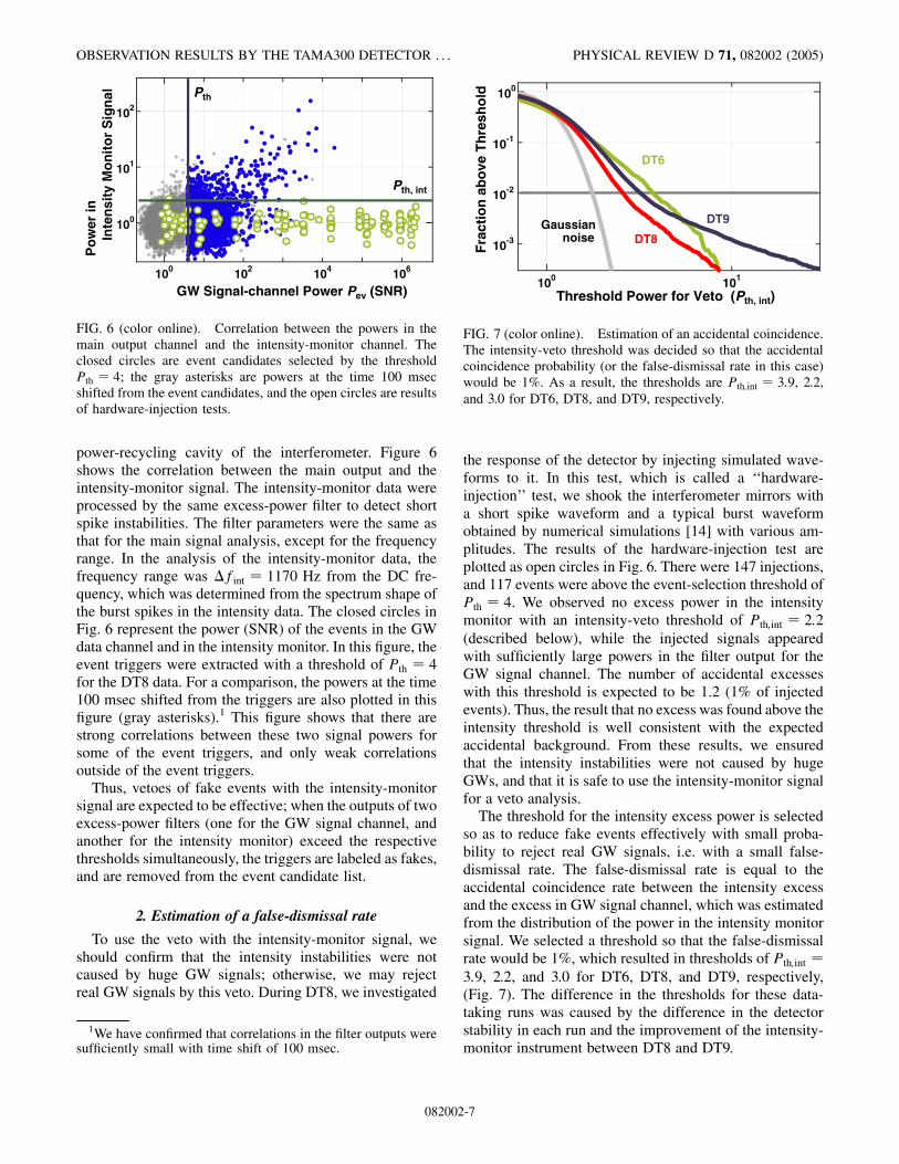
FIG. 7 (color online). Estimation of an accidental coincidence.The intensity-veto threshold was decided so that the accidentalcoincidence probability (or the false-dismissal rate in this case)would be 1%. As a result, the thresholds are Pth;int � 3:9, 2.2,and 3.0 for DT6, DT8, and DT9, respectively.

100 102 104 106

100

101

102

Po

wer

in

GW Signal-channel Power Pev (SNR)

Inte

nsi

ty M

on

ito

r S

ign

al Pth

Pth, int

FIG. 6 (color online). Correlation between the powers in themain output channel and the intensity-monitor channel. Theclosed circles are event candidates selected by the thresholdPth � 4; the gray asterisks are powers at the time 100 msecshifted from the event candidates, and the open circles are resultsof hardware-injection tests.


power-recycling cavity of the interferometer. Figure 6shows the correlation between the main output and theintensity-monitor signal. The intensity-monitor data wereprocessed by the same excess-power filter to detect shortspike instabilities. The filter parameters were the same asthat for the main signal analysis, except for the frequencyrange. In the analysis of the intensity-monitor data, thefrequency range was �fint � 1170 Hz from the DC fre-quency, which was determined from the spectrum shape ofthe burst spikes in the intensity data. The closed circles inFig. 6 represent the power (SNR) of the events in the GWdata channel and in the intensity monitor. In this figure, theevent triggers were extracted with a threshold of Pth � 4for the DT8 data. For a comparison, the powers at the time100 msec shifted from the triggers are also plotted in thisfigure (gray asterisks).1 This figure shows that there arestrong correlations between these two signal powers forsome of the event triggers, and only weak correlationsoutside of the event triggers.

Thus, vetoes of fake events with the intensity-monitorsignal are expected to be effective; when the outputs of twoexcess-power filters (one for the GW signal channel, andanother for the intensity monitor) exceed the respectivethresholds simultaneously, the triggers are labeled as fakes,and are removed from the event candidate list.

2. Estimation of a false-dismissal rate

To use the veto with the intensity-monitor signal, weshould confirm that the intensity instabilities were notcaused by huge GW signals; otherwise, we may rejectreal GW signals by this veto. During DT8, we investigated

1We have confirmed that correlations in the filter outputs weresufficiently small with time shift of 100 msec.

082002

the response of the detector by injecting simulated wave-forms to it. In this test, which is called a ‘‘hardware-injection’’ test, we shook the interferometer mirrors witha short spike waveform and a typical burst waveformobtained by numerical simulations [14] with various am-plitudes. The results of the hardware-injection test areplotted as open circles in Fig. 6. There were 147 injections,and 117 events were above the event-selection threshold ofPth � 4. We observed no excess power in the intensitymonitor with an intensity-veto threshold of Pth;int � 2:2(described below), while the injected signals appearedwith sufficiently large powers in the filter output for theGW signal channel. The number of accidental excesseswith this threshold is expected to be 1.2 (1% of injectedevents). Thus, the result that no excess was found above theintensity threshold is well consistent with the expectedaccidental background. From these results, we ensuredthat the intensity instabilities were not caused by hugeGWs, and that it is safe to use the intensity-monitor signalfor a veto analysis.

The threshold for the intensity excess power is selectedso as to reduce fake events effectively with small proba-bility to reject real GW signals, i.e. with a small false-dismissal rate. The false-dismissal rate is equal to theaccidental coincidence rate between the intensity excessand the excess in GW signal channel, which was estimatedfrom the distribution of the power in the intensity monitorsignal. We selected a threshold so that the false-dismissalrate would be 1%, which resulted in thresholds of Pth;int �

3:9, 2.2, and 3.0 for DT6, DT8, and DT9, respectively,(Fig. 7). The difference in the thresholds for these data-taking runs was caused by the difference in the detectorstability in each run and the improvement of the intensity-monitor instrument between DT8 and DT9.

-7

0 20 40 60 80 100 120100

101

102

103

c2 value

c 1 v

alu

e

for

refe

renc

e

Larger amplitu

de

Longer

Shorter

Data point

D

No signal

wav

efo

rm

a

Curve

Reference point

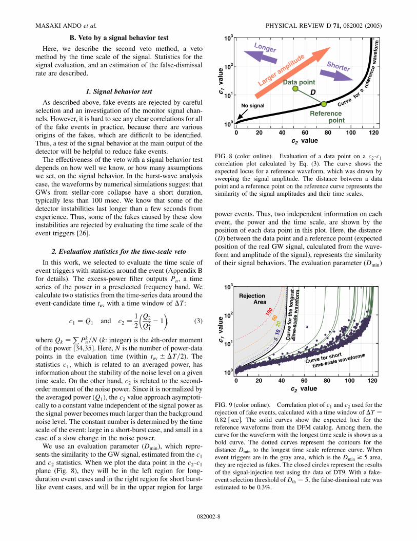
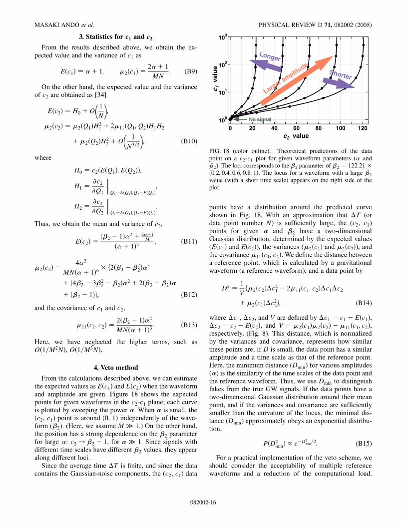
FIG. 8 (color online). Evaluation of a data point on a c2-c1correlation plot calculated by Eq. (3). The curve shows theexpected locus for a reference waveform, which was drawn bysweeping the signal amplitude. The distance between a datapoint and a reference point on the reference curve represents thesimilarity of the signal amplitudes and their time scales.

0 20 40 60 80 100 120100

101

102

103

c2 value

c 1 v

alu

e

Rejection

100

5020

105

Area

Cu

rve

for

the

lon

ges

tti

me-

scal

e w

avef

orm

Curve for short

time-scale waveforms

FIG. 9 (color online). Correlation plot of c1 and c2 used for therejection of fake events, calculated with a time window of �T �0:82 �sec�. The solid curves show the expected loci for thereference waveforms from the DFM catalog. Among them, thecurve for the waveform with the longest time scale is shown as abold curve. The dotted curves represent the contours for thedistance Dmin to the longest time scale reference curve. Whenevent triggers are in the gray area, which is the Dmin � 5 area,they are rejected as fakes. The closed circles represent the resultsof the signal-injection test using the data of DT9. With a fake-event selection threshold of Dth � 5, the false-dismissal rate wasestimated to be 0.3%.


B. Veto by a signal behavior test

Here, we describe the second veto method, a vetomethod by the time scale of the signal. Statistics for thesignal evaluation, and an estimation of the false-dismissalrate are described.

1. Signal behavior test

As described above, fake events are rejected by carefulselection and an investigation of the monitor signal chan-nels. However, it is hard to see any clear correlations for allof the fake events in practice, because there are variousorigins of the fakes, which are difficult to be identified.Thus, a test of the signal behavior at the main output of thedetector will be helpful to reduce fake events.

The effectiveness of the veto with a signal behavior testdepends on how well we know, or how many assumptionswe set, on the signal behavior. In the burst-wave analysiscase, the waveforms by numerical simulations suggest thatGWs from stellar-core collapse have a short duration,typically less than 100 msec. We know that some of thedetector instabilities last longer than a few seconds fromexperience. Thus, some of the fakes caused by these slowinstabilities are rejected by evaluating the time scale of theevent triggers [26].

2. Evaluation statistics for the time-scale veto

In this work, we selected to evaluate the time scale ofevent triggers with statistics around the event (Appendix Bfor details). The excess-power filter outputs Pn, a timeseries of the power in a preselected frequency band. Wecalculate two statistics from the time-series data around theevent-candidate time tev with a time window of �T:

c1 � Q1 and c2 �1

2

�Q2

Q21

� 1�; (3)

where Qk �PPkn=N (k: integer) is the kth-order moment

of the power [34,35]. Here, N is the number of power-datapoints in the evaluation time (within tev ��T=2). Thestatistics c1, which is related to an averaged power, hasinformation about the stability of the noise level on a giventime scale. On the other hand, c2 is related to the second-order moment of the noise power. Since it is normalized bythe averaged power (Q1), the c2 value approach asymptoti-cally to a constant value independent of the signal power asthe signal power becomes much larger than the backgroundnoise level. The constant number is determined by the timescale of the event: large in a short-burst case, and small in acase of a slow change in the noise power.

We use an evaluation parameter (Dmin), which repre-sents the similarity to the GW signal, estimated from the c1and c2 statistics. When we plot the data point in the c2-c1plane (Fig. 8), they will be in the left region for long-duration event cases and in the right region for short burst-like event cases, and will be in the upper region for large

082002

power events. Thus, two independent information on eachevent, the power and the time scale, are shown by theposition of each data point in this plot. Here, the distance(D) between the data point and a reference point (expectedposition of the real GW signal, calculated from the wave-form and amplitude of the signal), represents the similarityof their signal behaviors. The evaluation parameter (Dmin)

-8

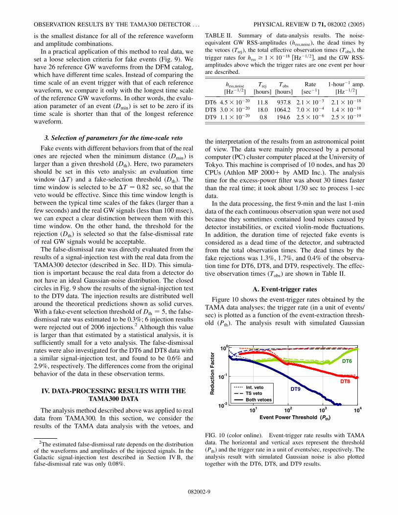
TABLE II. Summary of data-analysis results. The noise-equivalent GW RSS-amplitudes (hrss;noise), the dead times bythe vetoes (Trej), the total effective observation times (Tobs), thetrigger rates for hrss � 1� 10�18 �Hz�1=2�, and the GW RSS-amplitudes above which the trigger rates are one event per hourare described.

hrss;noise Trej Tobs Rate 1-hour�1 amp.[Hz�1=2] [hours] [hours] [sec�1] [Hz�1=2]

DT6 4:5� 10�20 11.8 937.8 2:1� 10�3 2:1� 10�18

DT8 3:0� 10�20 18.0 1064.2 7:0� 10�4 1:4� 10�18

DT9 1:1� 10�20 0.8 194.6 2:5� 10�6 2:5� 10�19

101 102 103 10410-2

10-1

100

Event Power Threshold (Pth)

rotca

F n

oitcu

deR

DT9

DT8

DT6

Int. vetoTS vetoBoth vetoes


is the smallest distance for all of the reference waveformand amplitude combinations.

In a practical application of this method to real data, weset a loose selection criteria for fake events (Fig. 9). Wehave 26 reference GW waveforms from the DFM catalog,which have different time scales. Instead of comparing thetime scale of an event trigger with that of each referencewaveform, we compare it only with the longest time scaleof the reference GW waveforms. In other words, the evalu-ation parameter of an event (Dmin) is set to be zero if itstime scale is shorter than that of the longest referencewaveform.

3. Selection of parameters for the time-scale veto

Fake events with different behaviors from that of the realones are rejected when the minimum distance (Dmin) islarger than a given threshold (Dth). Here, two parametersshould be set in this veto analysis: an evaluation timewindow (�T) and a fake-selection threshold (Dth). Thetime window is selected to be �T � 0:82 sec, so that theveto would be effective. Since this time window length isbetween the typical time scales of the fakes (larger than afew seconds) and the real GW signals (less than 100 msec),we can expect a clear distinction between them with thistime window. On the other hand, the threshold for therejection (Dth) is selected so that the false-dismissal rateof real GW signals would be acceptable.

The false-dismissal rate was directly evaluated from theresults of a signal-injection test with the real data from theTAMA300 detector (described in Sec. II D). This simula-tion is important because the real data from a detector donot have an ideal Gaussian-noise distribution. The closedcircles in Fig. 9 show the results of the signal-injection testto the DT9 data. The injection results are distributed wellaround the theoretical predictions shown as solid curves.With a fake-event selection threshold ofDth � 5, the false-dismissal rate was estimated to be 0.3%; 6 injection resultswere rejected out of 2006 injections.2 Although this valueis larger than that estimated by a statistical analysis, it issufficiently small for a veto analysis. The false-dismissalrates were also investigated for the DT6 and DT8 data witha similar signal-injection test, and found to be 0.6% and2.9%, respectively. The differences come from the originalbehavior of the data in these observation terms.

IV. DATA-PROCESSING RESULTS WITH THETAMA300 DATA

The analysis method described above was applied to realdata from TAMA300. In this section, we consider theresults of the TAMA data analysis with the vetoes, and

2The estimated false-dismissal rate depends on the distributionof the waveforms and amplitudes of the injected signals. In theGalactic signal-injection test described in Section IV B, thefalse-dismissal rate was only 0.08%.

082002

the interpretation of the results from an astronomical pointof view. The data were mainly processed by a personalcomputer (PC) cluster computer placed at the University ofTokyo. This machine is comprised of 10 nodes, and has 20CPUs (Athlon MP 2000� by AMD Inc.). The analysistime for the excess-power filter was about 30 times fasterthan the real time; it took about 1/30 sec to process 1-secdata.

In the data processing, the first 9-min and the last 1-mindata of the each continuous observation span were not usedbecause they sometimes contained loud noises caused bydetector instabilities, or excited violin-mode fluctuations.In addition, the duration time of rejected fake events isconsidered as a dead time of the detector, and subtractedfrom the total observation times. The dead times by thefake rejections was 1.3%, 1.7%, and 0.4% of the observa-tion time for DT6, DT8, and DT9, respectively. The effec-tive observation times (Tobs) are shown in Table II.

A. Event-trigger rates

Figure 10 shows the event-trigger rates obtained by theTAMA data analyses; the trigger rate (in a unit of events/sec) is plotted as a function of the event-extraction thresh-old (Pth). The analysis result with simulated Gaussian

FIG. 10 (color online). Event-trigger rate results with TAMAdata. The horizontal and vertical axes represent the threshold(Pth) and the trigger rate in a unit of events/sec, respectively. Theanalysis result with simulated Gaussian noise is also plottedtogether with the DT6, DT8, and DT9 results.

-9

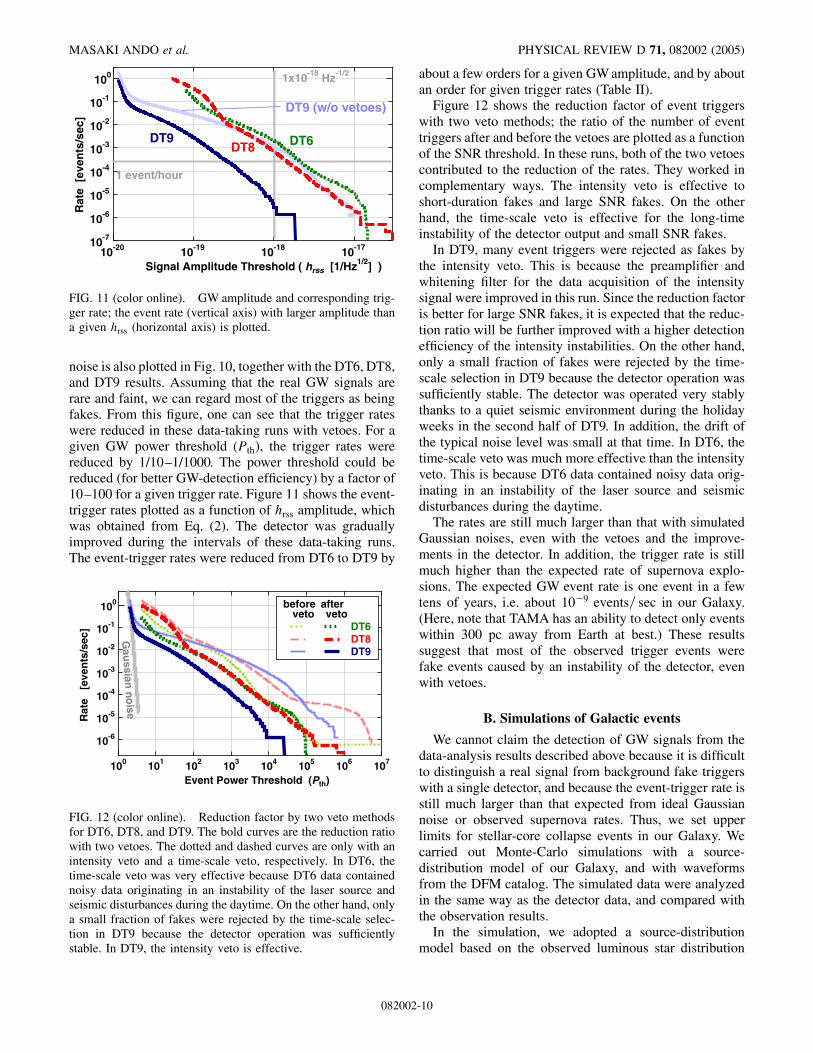
10-20 10-19 10-18 10-1710-7

10-6

10-5

10-4

10-3

10-2

10-1

100R

ate

[ev

ents

/se c

]

Signal Amplitude Threshold ( hrss [1/Hz1/2] )

DT9DT8 DT6

1 event/hour

1x10-18 Hz-1/2

DT9 (w/o vetoes)

FIG. 11 (color online). GW amplitude and corresponding trig-ger rate; the event rate (vertical axis) with larger amplitude thana given hrss (horizontal axis) is plotted.


noise is also plotted in Fig. 10, together with the DT6, DT8,and DT9 results. Assuming that the real GW signals arerare and faint, we can regard most of the triggers as beingfakes. From this figure, one can see that the trigger rateswere reduced in these data-taking runs with vetoes. For agiven GW power threshold (Pth), the trigger rates werereduced by 1/10–1/1000. The power threshold could bereduced (for better GW-detection efficiency) by a factor of10–100 for a given trigger rate. Figure 11 shows the event-trigger rates plotted as a function of hrss amplitude, whichwas obtained from Eq. (2). The detector was graduallyimproved during the intervals of these data-taking runs.The event-trigger rates were reduced from DT6 to DT9 by

100 101 102 103 104 105 106 107

10-6

10-5

10-4

10-3

10-2

10-1

100


]ces/stneve[ eta

R

esi

on

nais

sua

G

DT9

DT6DT8

afterveto

beforeveto

FIG. 12 (color online). Reduction factor by two veto methodsfor DT6, DT8, and DT9. The bold curves are the reduction ratiowith two vetoes. The dotted and dashed curves are only with anintensity veto and a time-scale veto, respectively. In DT6, thetime-scale veto was very effective because DT6 data containednoisy data originating in an instability of the laser source andseismic disturbances during the daytime. On the other hand, onlya small fraction of fakes were rejected by the time-scale selec-tion in DT9 because the detector operation was sufficientlystable. In DT9, the intensity veto is effective.

082002

about a few orders for a given GW amplitude, and by aboutan order for given trigger rates (Table II).

Figure 12 shows the reduction factor of event triggerswith two veto methods; the ratio of the number of eventtriggers after and before the vetoes are plotted as a functionof the SNR threshold. In these runs, both of the two vetoescontributed to the reduction of the rates. They worked incomplementary ways. The intensity veto is effective toshort-duration fakes and large SNR fakes. On the otherhand, the time-scale veto is effective for the long-timeinstability of the detector output and small SNR fakes.

In DT9, many event triggers were rejected as fakes bythe intensity veto. This is because the preamplifier andwhitening filter for the data acquisition of the intensitysignal were improved in this run. Since the reduction factoris better for large SNR fakes, it is expected that the reduc-tion ratio will be further improved with a higher detectionefficiency of the intensity instabilities. On the other hand,only a small fraction of fakes were rejected by the time-scale selection in DT9 because the detector operation wassufficiently stable. The detector was operated very stablythanks to a quiet seismic environment during the holidayweeks in the second half of DT9. In addition, the drift ofthe typical noise level was small at that time. In DT6, thetime-scale veto was much more effective than the intensityveto. This is because DT6 data contained noisy data orig-inating in an instability of the laser source and seismicdisturbances during the daytime.

The rates are still much larger than that with simulatedGaussian noises, even with the vetoes and the improve-ments in the detector. In addition, the trigger rate is stillmuch higher than the expected rate of supernova explo-sions. The expected GW event rate is one event in a fewtens of years, i.e. about 10�9 events= sec in our Galaxy.(Here, note that TAMA has an ability to detect only eventswithin 300 pc away from Earth at best.) These resultssuggest that most of the observed trigger events werefake events caused by an instability of the detector, evenwith vetoes.

B. Simulations of Galactic events

We cannot claim the detection of GW signals from thedata-analysis results described above because it is difficultto distinguish a real signal from background fake triggerswith a single detector, and because the event-trigger rate isstill much larger than that expected from ideal Gaussiannoise or observed supernova rates. Thus, we set upperlimits for stellar-core collapse events in our Galaxy. Wecarried out Monte-Carlo simulations with a source-distribution model of our Galaxy, and with waveformsfrom the DFM catalog. The simulated data were analyzedin the same way as the detector data, and compared withthe observation results.

In the simulation, we adopted a source-distributionmodel based on the observed luminous star distribution

-10

100 101 102 10310-8

10-7

10-6

10-5

10-4

10-4

10-3

10-2

10-1

100


Rat

e [

even

ts/s

ec]

(after vetos)

Gau

ssian n

oise

Galactic eventsEfficiency for

Det

ecti

on

eff

icie

ncy

Event rate in DT9

Threshold

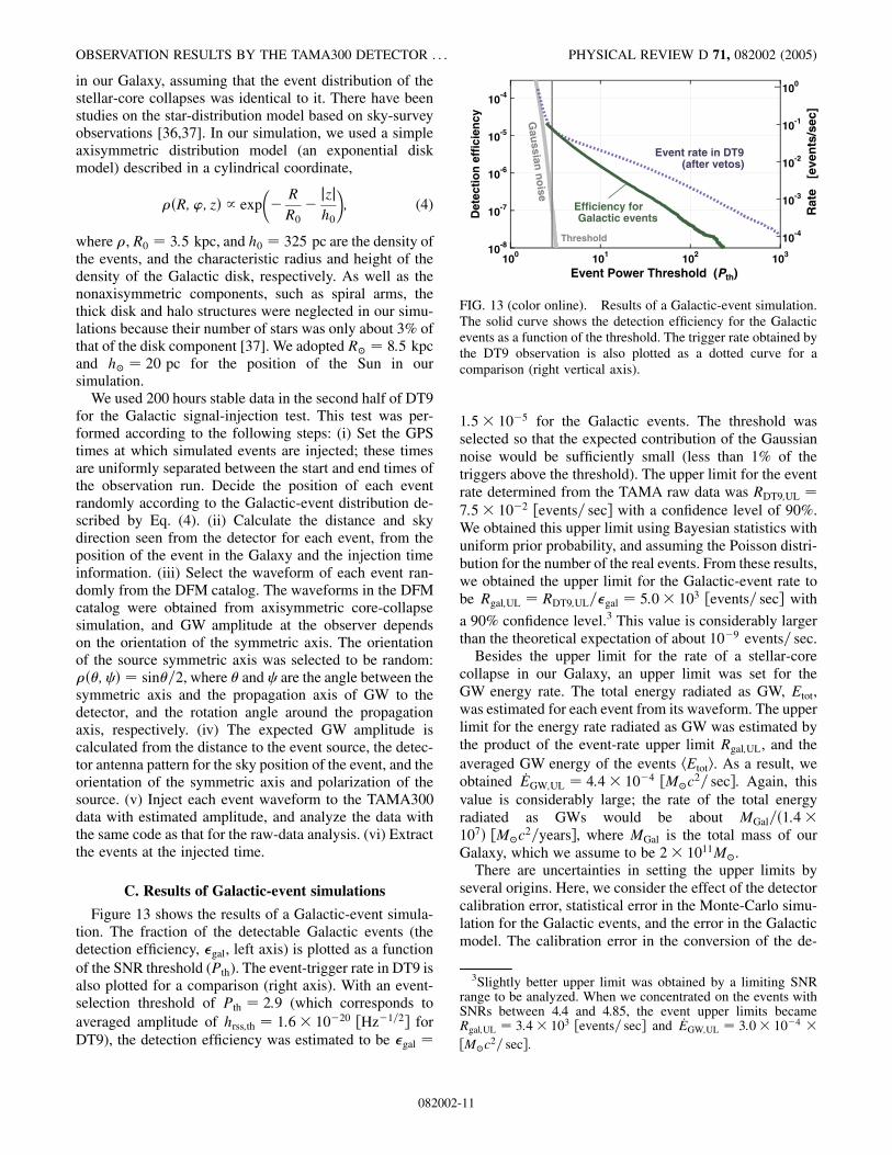
FIG. 13 (color online). Results of a Galactic-event simulation.The solid curve shows the detection efficiency for the Galacticevents as a function of the threshold. The trigger rate obtained bythe DT9 observation is also plotted as a dotted curve for acomparison (right vertical axis).

3Slightly better upper limit was obtained by a limiting SNRrange to be analyzed. When we concentrated on the events withSNRs between 4.4 and 4.85, the event upper limits becameRgal;UL � 3:4� 103 �events= sec� and _EGW;UL � 3:0� 10�4 �

�M�c2= sec�.


in our Galaxy, assuming that the event distribution of thestellar-core collapses was identical to it. There have beenstudies on the star-distribution model based on sky-surveyobservations [36,37]. In our simulation, we used a simpleaxisymmetric distribution model (an exponential diskmodel) described in a cylindrical coordinate,

�R;’; z� / exp��RR0

�jzjh0

�; (4)

where �, R0 � 3:5 kpc, and h0 � 325 pc are the density ofthe events, and the characteristic radius and height of thedensity of the Galactic disk, respectively. As well as thenonaxisymmetric components, such as spiral arms, thethick disk and halo structures were neglected in our simu-lations because their number of stars was only about 3% ofthat of the disk component [37]. We adopted R� � 8:5 kpcand h� � 20 pc for the position of the Sun in oursimulation.

We used 200 hours stable data in the second half of DT9for the Galactic signal-injection test. This test was per-formed according to the following steps: (i) Set the GPStimes at which simulated events are injected; these timesare uniformly separated between the start and end times ofthe observation run. Decide the position of each eventrandomly according to the Galactic-event distribution de-scribed by Eq. (4). (ii) Calculate the distance and skydirection seen from the detector for each event, from theposition of the event in the Galaxy and the injection timeinformation. (iii) Select the waveform of each event ran-domly from the DFM catalog. The waveforms in the DFMcatalog were obtained from axisymmetric core-collapsesimulation, and GW amplitude at the observer dependson the orientation of the symmetric axis. The orientationof the source symmetric axis was selected to be random:��; � � sin�=2, where � and are the angle between thesymmetric axis and the propagation axis of GW to thedetector, and the rotation angle around the propagationaxis, respectively. (iv) The expected GW amplitude iscalculated from the distance to the event source, the detec-tor antenna pattern for the sky position of the event, and theorientation of the symmetric axis and polarization of thesource. (v) Inject each event waveform to the TAMA300data with estimated amplitude, and analyze the data withthe same code as that for the raw-data analysis. (vi) Extractthe events at the injected time.

C. Results of Galactic-event simulations

Figure 13 shows the results of a Galactic-event simula-tion. The fraction of the detectable Galactic events (thedetection efficiency, �gal, left axis) is plotted as a functionof the SNR threshold (Pth). The event-trigger rate in DT9 isalso plotted for a comparison (right axis). With an event-selection threshold of Pth � 2:9 (which corresponds toaveraged amplitude of hrss;th � 1:6� 10�20 �Hz�1=2� forDT9), the detection efficiency was estimated to be �gal �

082002

1:5� 10�5 for the Galactic events. The threshold wasselected so that the expected contribution of the Gaussiannoise would be sufficiently small (less than 1% of thetriggers above the threshold). The upper limit for the eventrate determined from the TAMA raw data was RDT9;UL �

7:5� 10�2 �events= sec� with a confidence level of 90%.We obtained this upper limit using Bayesian statistics withuniform prior probability, and assuming the Poisson distri-bution for the number of the real events. From these results,we obtained the upper limit for the Galactic-event rate tobe Rgal;UL � RDT9;UL=�gal � 5:0� 103 �events= sec� with

a 90% confidence level.3 This value is considerably largerthan the theoretical expectation of about 10�9 events= sec.

Besides the upper limit for the rate of a stellar-corecollapse in our Galaxy, an upper limit was set for theGW energy rate. The total energy radiated as GW, Etot,was estimated for each event from its waveform. The upperlimit for the energy rate radiated as GW was estimated bythe product of the event-rate upper limit Rgal;UL, and theaveraged GW energy of the events hEtoti. As a result, weobtained _EGW;UL � 4:4� 10�4 �M�c2= sec�. Again, thisvalue is considerably large; the rate of the total energyradiated as GWs would be about MGal=1:4�107� �M�c2=years�, where MGal is the total mass of ourGalaxy, which we assume to be 2� 1011M�.

There are uncertainties in setting the upper limits byseveral origins. Here, we consider the effect of the detectorcalibration error, statistical error in the Monte-Carlo simu-lation for the Galactic events, and the error in the Galacticmodel. The calibration error in the conversion of the de-

-11

0

0.5

1

10-18 10-17 10-1610-1

100

101

102

GW Amplitude (hrss)

ycneiciff

E]ya

d/stneve[ eta

R

Gau1

SG850SG1304

SG554

Gau0.5

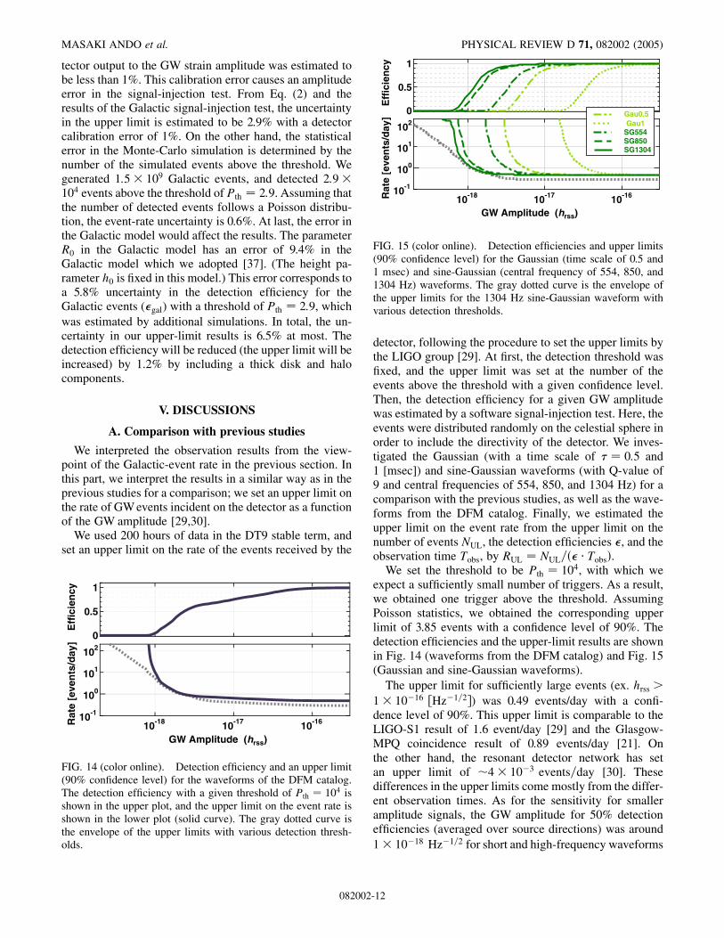
FIG. 15 (color online). Detection efficiencies and upper limits(90% confidence level) for the Gaussian (time scale of 0.5 and1 msec) and sine-Gaussian (central frequency of 554, 850, and1304 Hz) waveforms. The gray dotted curve is the envelope ofthe upper limits for the 1304 Hz sine-Gaussian waveform withvarious detection thresholds.


tector output to the GW strain amplitude was estimated tobe less than 1%. This calibration error causes an amplitudeerror in the signal-injection test. From Eq. (2) and theresults of the Galactic signal-injection test, the uncertaintyin the upper limit is estimated to be 2.9% with a detectorcalibration error of 1%. On the other hand, the statisticalerror in the Monte-Carlo simulation is determined by thenumber of the simulated events above the threshold. Wegenerated 1:5� 109 Galactic events, and detected 2:9�104 events above the threshold of Pth � 2:9. Assuming thatthe number of detected events follows a Poisson distribu-tion, the event-rate uncertainty is 0.6%. At last, the error inthe Galactic model would affect the results. The parameterR0 in the Galactic model has an error of 9.4% in theGalactic model which we adopted [37]. (The height pa-rameter h0 is fixed in this model.) This error corresponds toa 5.8% uncertainty in the detection efficiency for theGalactic events (�gal) with a threshold of Pth � 2:9, whichwas estimated by additional simulations. In total, the un-certainty in our upper-limit results is 6.5% at most. Thedetection efficiency will be reduced (the upper limit will beincreased) by 1.2% by including a thick disk and halocomponents.

V. DISCUSSIONS

A. Comparison with previous studies

We interpreted the observation results from the view-point of the Galactic-event rate in the previous section. Inthis part, we interpret the results in a similar way as in theprevious studies for a comparison; we set an upper limit onthe rate of GW events incident on the detector as a functionof the GW amplitude [29,30].

We used 200 hours of data in the DT9 stable term, andset an upper limit on the rate of the events received by the

0

0.5

1

10-18 10-17 10-1610-1

100

101

102

GW Amplitude (hrss)

Eff

icie

ncy

Rat

e [e

ven

ts/d

ay]

FIG. 14 (color online). Detection efficiency and an upper limit(90% confidence level) for the waveforms of the DFM catalog.The detection efficiency with a given threshold of Pth � 104 isshown in the upper plot, and the upper limit on the event rate isshown in the lower plot (solid curve). The gray dotted curve isthe envelope of the upper limits with various detection thresh-olds.

082002

detector, following the procedure to set the upper limits bythe LIGO group [29]. At first, the detection threshold wasfixed, and the upper limit was set at the number of theevents above the threshold with a given confidence level.Then, the detection efficiency for a given GW amplitudewas estimated by a software signal-injection test. Here, theevents were distributed randomly on the celestial sphere inorder to include the directivity of the detector. We inves-tigated the Gaussian (with a time scale of � � 0:5 and1 [msec]) and sine-Gaussian waveforms (with Q-value of9 and central frequencies of 554, 850, and 1304 Hz) for acomparison with the previous studies, as well as the wave-forms from the DFM catalog. Finally, we estimated theupper limit on the event rate from the upper limit on thenumber of events NUL, the detection efficiencies �, and theobservation time Tobs, by RUL � NUL=� � Tobs�.

We set the threshold to be Pth � 104, with which weexpect a sufficiently small number of triggers. As a result,we obtained one trigger above the threshold. AssumingPoisson statistics, we obtained the corresponding upperlimit of 3.85 events with a confidence level of 90%. Thedetection efficiencies and the upper-limit results are shownin Fig. 14 (waveforms from the DFM catalog) and Fig. 15(Gaussian and sine-Gaussian waveforms).

The upper limit for sufficiently large events (ex. hrss >1� 10�16 �Hz�1=2�) was 0.49 events/day with a confi-dence level of 90%. This upper limit is comparable to theLIGO-S1 result of 1.6 event/day [29] and the Glasgow-MPQ coincidence result of 0.89 events/day [21]. Onthe other hand, the resonant detector network has setan upper limit of �4� 10�3 events=day [30]. Thesedifferences in the upper limits come mostly from the differ-ent observation times. As for the sensitivity for smalleramplitude signals, the GW amplitude for 50% detectionefficiencies (averaged over source directions) was around1� 10�18 Hz�1=2 for short and high-frequency waveforms

-12


in our case. The upper limit curve is almost comparablewith the LIGO-S1 results for high-frequency signals, andlarger for lower frequency (< 800 Hz) ones [29].

B. Outlook for the detection of burst GWs

The large event rate and upper limit results show that thedetector output is still dominated by fake events, even afterthese vetoes. Thus, further research efforts are necessary todetect burst gravitational waves. In this part, we discuss theoutlook to better vetoes, coincidence analyses with otherobservatories, and better performance of the detector anddata-processing scheme.

In Section III A, we presented a veto analysis methodwith only one monitor signal, an intensity monitor. Similarmethods can be used with the other monitor signals alongwith careful investigations of their correlations with themain output of the detector. However, we have found noother monitor signal with a clear correlation so far: laserpower at the signal port (the dark port), monitors for theseismic fluctuations, an acoustic monitor signal. Thus, it isnecessary to investigate more deeply the monitor signals,and to introduce better monitor signals that are sensitive tothe detector instabilities.

There are other event-selection criteria than the time-scale selection method presented in Section III B. Forexample, the time scale of an event can be simply evaluatedby the duration time above the event-selection threshold. Inthis case, we should consider that the veto results will bestrongly dependent on the event amplitude.4 We will beable to reduce fake events even further by knowing thecommon characteristics of the target events, and settingthem as event-selection criteria. For this, more systematicand precise simulations of stellar-core collapses and inves-tigation on the waveform will be helpful.

Coincidence analyses with the other detectors for GWs,electromagnetic waves, and neutrinos will improve theresult significantly, though we have focused on the reduc-tion of fakes with a single detector in this article. Theobservation runs by TAMA300 (DT8 and DT9) were car-ried out at the same term as the LIGO second and thirdscientific (observation) runs (called S2 and S3), and coin-cidence analyses are underway [38]. We note that our workdiscussed in this article is also a part of the LIGO-TAMAcoincidence analysis; the list of the event triggers obtainedin our work will be used in the coincidence analysis.

In addition to a reduction of fakes, the improvements ofthe detector both in the floor noise level and in the reduc-tion of nonstationary noises are also important. The per-formance of the TAMA300 detector has gradually beenimproved from DT6 to DT9 concerning both the noise

4Veto with band-limited root-mean-square (RMS) amplitudeused in [29] corresponds to a veto only with c1. In this method,we cannot avoid huge GW events from being rejected by theveto.

082002

level and the stability, and the detector still has room forimprovement. In addition, burst filters with higher efficien-cies are under development in the TAMA group and othergroups. Since we can only observe events within about the300 pc range with the current sensitivity of TAMA, thedetection efficiency for the Galactic events is very small(�gal � 3:4� 10�5 with a threshold for a noise-equivalentGW amplitude). The sensitivity should be improved byabout two orders so as to cover our Galaxy, and to realizea sufficiently large detection efficiency. This sensitivitywill be realized by the next-generation detectors, such asLCGT (Fig. 2) [39] and advanced LIGO [40].

VI. CONCLUSION

We presented data-analysis schemes and results of ob-servation data by TAMA300, targeting at burst signalsfrom stellar-core collapses. Since precise waveforms arenot available for burst gravitational waves, the detectionschemes (the construction of a detection filter and therejection of fake events) are different from those forchirp-wave analyses. We investigated two methods forthe reduction of nonstationary noises, and applied themto real data from the TAMA300 interferometric gravita-tional wave detector. As a result, these veto methods, a vetowith a detector monitor signal and a veto by time-scaleselection, worked efficiently in a complementary way. Theformer and the latter were effective for short-spike noisesand for slow instabilities of the detector, respectively. Thefake-event rate was reduced by a factor of about 1000 in thebest case.

The obtained event-trigger rate was interpreted from theviewpoint of the burst gravitational wave events in ourGalaxy. From the observation and analysis results, we setan upper limit for the Galactic-event rate to be 5:0�103 events= sec (confidence level 90%), based on aGalactic disk model [37] and waveforms obtained bynumerical simulations of stellar-core collapses [13]. Inaddition, we determined the upper limit for the rate ofthe energy radiated as gravitational wave bursts to be 4:4�10�4 M�c2= sec (confidence level 90%). These large upperlimits show that the detector output was still dominated byfake events, even after the selection of events, and gives usprospects on both current and future research: the necessityfor further improvement of the analysis schemes, coinci-dence analyses with multiple detectors, better predictionson the waveforms, and future detectors, such as LCGT andadvanced LIGO, to cover the whole of our Galaxy. Thiswork has shown, we believe, prospects for these researchactivities.

ACKNOWLEDGMENTS

This research is supported in part by a Grant-in-Aid forScientific Research on Priority Areas (415) of the Ministryof Education, Culture, Sports, Science and Technology.

-13

0 0.5 1 1.5 2 2.5 3

-800

-400

0

400

AD

C c

ou

nt

Time [sec]

1.585 1.59 1.595 1.6

-800

-400

0

400

AD

C c

ou

nt

Time [sec]

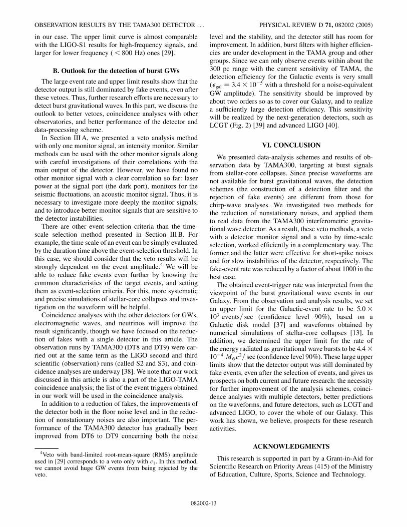
FIG. 16. Example of the line removal results for the DT9 data.Time-series data before (plotted in gray) and after (plotted inblack) the line removal are shown. The lower plot is a zoom upof the spike in the upper plot.

102 10310-21

10-20

10-19

10-18

Str

ain

no

ise

[1/

Hz1/

2 ]

Frequency [Hz]

C

V

VV

V

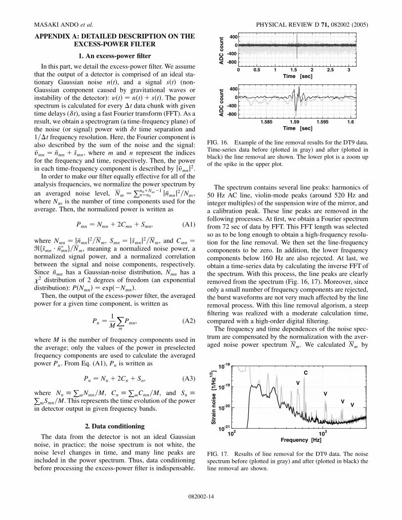
FIG. 17. Results of line removal for the DT9 data. The noisespectrum before (plotted in gray) and after (plotted in black) theline removal are shown.


APPENDIX A: DETAILED DESCRIPTION ON THEEXCESS-POWER FILTER

1. An excess-power filter

In this part, we detail the excess-power filter. We assumethat the output of a detector is comprised of an ideal sta-tionary Gaussian noise nt�, and a signal st� (non-Gaussian component caused by gravitational waves orinstability of the detector): vt� � nt� � st�. The powerspectrum is calculated for every �t data chunk with giventime delays (!t), using a fast Fourier transform (FFT). As aresult, we obtain a spectrogram (a time-frequency plane) ofthe noise (or signal) power with !t time separation and1=�t frequency resolution. Here, the Fourier component isalso described by the sum of the noise and the signal:~vmn � ~nmn � ~smn, where m and n represent the indicesfor the frequency and time, respectively. Then, the powerin each time-frequency component is described by j~vmnj2.

In order to make our filter equally effective for all of theanalysis frequencies, we normalize the power spectrum byan averaged noise level, Nm �

Pn0�Nav�1n�n0 j~nmnj2=Nav,

where Nav is the number of time components used for theaverage. Then, the normalized power is written as

Pmn � Nmn � 2Cmn � Smn; (A1)

where Nmn � j~nmnj2=Nm, Smn � j~smnj2=Nm, and Cmn �<f~smn � ~n�mng=Nm, meaning a normalized noise power, anormalized signal power, and a normalized correlationbetween the signal and noise components, respectively.Since ~nmn has a Gaussian-noise distribution, Nmn has a$2 distribution of 2 degrees of freedom (an exponentialdistribution): PNmn� � exp�Nmn�.

Then, the output of the excess-power filter, the averagedpower for a given time component, is written as

Pn �1

M

Xm

Pmn; (A2)

where M is the number of frequency components used inthe average; only the values of the power in preselectedfrequency components are used to calculate the averagedpower Pn. From Eq. (A1), Pn is written as

Pn � Nn � 2Cn � Sn; (A3)

where Nn �PmNmn=M, Cn �

PmCmn=M, and Sn �P

mSmn=M. This represents the time evolution of the powerin detector output in given frequency bands.

2. Data conditioning

The data from the detector is not an ideal Gaussiannoise, in practice; the noise spectrum is not white, thenoise level changes in time, and many line peaks areincluded in the power spectrum. Thus, data conditioningbefore processing the excess-power filter is indispensable.

082002

The spectrum contains several line peaks: harmonics of50 Hz AC line, violin-mode peaks (around 520 Hz andinteger multiples) of the suspension wire of the mirror, anda calibration peak. These line peaks are removed in thefollowing processes. At first, we obtain a Fourier spectrumfrom 72 sec of data by FFT. This FFT length was selectedso as to be long enough to obtain a high-frequency resolu-tion for the line removal. We then set the line-frequencycomponents to be zero. In addition, the lower frequencycomponents below 160 Hz are also rejected. At last, weobtain a time-series data by calculating the inverse FFT ofthe spectrum. With this process, the line peaks are clearlyremoved from the spectrum (Fig. 16, 17). Moreover, sinceonly a small number of frequency components are rejected,the burst waveforms are not very much affected by the lineremoval process. With this line removal algorism, a steepfiltering was realized with a moderate calculation time,compared with a high-order digital filtering.

The frequency and time dependences of the noise spec-trum are compensated by the normalization with the aver-aged noise power spectrum Nm. We calculated Nm by

-14


averaging the power spectra for 30 min before the dataanalyzed by the excess-power filter. In order to avoid thelarge spikes from disturbing the averaged spectrum, werejected noisy 0.7% (which corresponds to outliers largerthan about a 5-sigma level in exponential distribution)spectra from those used in each average. We found thatwe could obtain stable averaged spectra, and that eachspectrum was normalized well with this method.

APPENDIX B: TIME-SCALE EVALUATIONAND VETO

1. Evaluation in �T time chunk

In this part, we describe the details of the veto methodwith time-scale evaluation of the event triggers. In our vetomethods, each event is evaluated by the statistics in a tev ��T=2 data chunk (tev: the time of the event). Here, N datapoints of the excess-power filter output are contained in thetime window �T, i.e. �T � N!t. From the output of theexcess-power filter Pn, we define the evaluation parametersc1 and c2 as

c1 � Q1; c2 �Q2

Q21

� 1; (B1)

where Q1 and Q2 are the first- and second-order momentsof Pn for N data points, respectively, written as:

Q1 �1

N

Xn0�N�1

n�n0

Pn; Q2 �1

N

Xn0�N�1

n�n0

Pn�2: (B2)

Here, note that Q1 is an averaged power for M� N time-frequency components. On the other hand, c2 is defined bythe second-order moment normalized by the averagedpower. This value is analogous to the kurtosis (defined bythe fourth-order moment of data), which describes anynon-Gaussianity of the data [34,35].

2. Statistics of Q1 and Q2

We calculate the statistics of parameters Q1 and Q2 as apreparation for calculating the statistics of the parametersc1 and c2, defined in Eq. (B1). Although the M� Ncomponents are not independent in practice, because ofoverlapping in time and a window function, we describethe following calculations while assuming that they areindependent, for simplicity. In practical use, the statistics(the averages, the variances, and the covariance) are esti-mated by replacing the time and frequency window size, Nand M, by effective time and frequency range, Neff andMeff . The effective window sizes, Neff and Meff , are esti-mated by simulations with Gaussian noises.

From Eq. (A3), Q1 is also written by the sum of thenoise, signal, and their correlation terms. Thus, the ex-pected value is

082002

EQ1� �1

N

Xn

fSn � ENn� � 2ECn�g � %� 1; (B3)

where we define the average of the signal componentpower by

% �1

N

Xn

Sn; (B4)

and we use relations ENn� � 1 and ECn� � 0. The ex-pected value of the square of Q1 is written as

EQ21� � E

�1

N2

Xj

Xl

Sj � Nj � 2Cj�Sl � Nl � 2Cl��

�2%� 1

MN� %� 1�2;

where we use relations ENkNl� � ENk�ENl� k � l�,EN2

n� � M� 1�=M, and so on. Thus, the variance ofQ1 is written as

(2Q1� � EQ21� � EQ1�

2 �2%� 1�

MN: (B5)

On the other hand, the expected value of Q2 is

EQ2� � E�1

N

Xn

Sn � Nn � 2Cn�2

�

� )2%2 � 2%� 1�2%� 1

M; (B6)

where )2 is a constant value related to the second-ordermoment of the signal,

)2%2 �Xn

S2n=N: (B7)

Similarly, a constant value, )3, is written asPnS

3n=N �

)3%3. The constant numbers %, )2, and )3 are determined

only by the waveform and the amplitude of the signal. Thevalue % represents the normalized signal power. The value)2 depends on the time scale of the signal; )2 becomeslarge for a short signal.

With more complicated, but similar, calculations, thevariance of Q2 and the covariance between Q1 and Q2

are obtained to be

(2Q2��8

N)3%3�

20M�32

M2N)2%2

�16M2�M�3�

M3N%�

22M2�5M�3�

M3N;

(11Q1;Q2��2

MN

�2)2%2�

3M�1�

M%�

M�1

M

: (B8)

-15

0 20 40 60 80 100 120100

101

102

103

c2 value

c 1 v

alu

e

Larger amplitu

de

Longer

Shorter

No signal

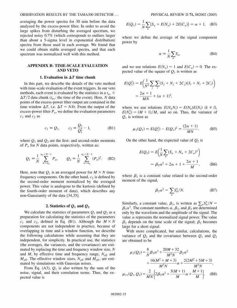
FIG. 18 (color online). Theoretical predictions of the datapoint on a c2-c1 plot for given waveform parameters (% and)2). The loci corresponds to the )2 parameter of )2 � 122:21�0:2; 0:4; 0:6; 0:8; 1�. The locus for a waveform with a large )2

value (with a short time scale) appears on the right side of theplot.


3. Statistics for c1 and c2

From the results described above, we obtain the ex-pected value and the variance of c1 as

Ec1� � %� 1; (2c1� �2%� 1

MN: (B9)

On the other hand, the expected value and the varianceof c2 are obtained as [34]

Ec2� � H0 �O�1

N

�;

(2c2� � (2Q1�H21 � 2(11Q1; Q2�H1H2

�(2Q2�H22 �O

�1

N3=2

�; (B10)

where

H0 � c2EQ1�; EQ2��;

H1 �@c2@Q1

Q1�EQ1�;Q2�EQ2�

;

H2 �@c2@Q2

Q1�EQ1�;Q2�EQ2�

:

Thus, we obtain the mean and variance of c2,

Ec2� �)2 � 1�%2 � 2%�1

M

%� 1�2; (B11)

(2c2� �4%2

MN%� 1�6� f2)3 � )2

2�%3

� 4)3 � 3)22 � )2�%2 � 2)3 � )2�%

� )2 � 1�g; (B12)

and the covariance of c1 and c2,

(11c1; c2� �2)2 � 1�%2

MN%� 1�3: (B13)

Here, we have neglected the higher terms, such asO1=M2N�, O1=M3N�.

4. Veto method

From the calculations described above, we can estimatethe expected values as Ec1� and Ec2� when the waveformand amplitude are given. Figure 18 shows the expectedpoints for given waveforms in the c2-c1 plane; each curveis plotted by sweeping the power %. When % is small, the(c2, c1) point is around (0, 1) independently of the wave-form ()2). (Here, we assume M � 1.) On the other hand,the position has a strong dependence on the )2 parameterfor large %: c2 ! )2 � 1, for %� 1. Since signals withdifferent time scales have different )2 values, they appearalong different loci.

Since the average time �T is finite, and since the datacontains the Gaussian-noise components, the (c2, c1) data

082002

points have a distribution around the predicted curveshown in Fig. 18. With an approximation that �T (ordata point number N) is sufficiently large, the (c2, c1)points for given % and )2 have a two-dimensionalGaussian distribution, determined by the expected values(Ec1� and Ec2�), the variances ((2c1� and (2c2�), andthe covariance (11c1; c2�. We define the distance betweena reference point, which is calculated by a gravitationalwaveform (a reference waveform), and a data point by

D2 �1

Vf(2c2��c

21 � 2(11c1; c2��c1�c2

�(2c1��c22g; (B14)

where �c1, �c2, and V are defined by �c1 � c1 � Ec1�,�c2 � c2 � Ec2�, and V � (2c1�(2c2� �(11c1; c2�,respectively, (Fig. 8). This distance, which is normalizedby the variances and covariance, represents how similarthese points are; if D is small, the data point has a similaramplitude and a time scale as that of the reference point.Here, the minimum distance (Dmin) for various amplitudes(%) is the similarity of the time scales of the data point andthe reference waveform. Thus, we use Dmin to distinguishfakes from the true GW signals. If the data points have atwo-dimensional Gaussian distribution around their meanpoint, and if the variances and covariance are sufficientlysmaller than the curvature of the locus, the minimal dis-tance (Dmin) approximately obeys an exponential distribu-tion,

PD2min� / e

�D2min=2: (B15)

For a practical implementation of the veto scheme, weshould consider the acceptability of multiple referencewaveforms and a reduction of the computational load.

-16


Thus, we adopted a conservative way for the veto analysis;we reject only the events with longer time scales than thelongest one in the reference waveforms (Fig. 9). We useone waveform with the smallest )2 value, i.e. with thelongest time scale, as the reference waveform, and set

082002

Dmin � 0 if the data point is on the right side of thereference locus in the c1-c2 plot. In addition, we preparea map ofDmin in the c1-c2 plane before the data analysis, soas to reduce the computational load during the dataanalysis.

[1] K. S. Thorne, in Three Hundred Years of Gravitation,edited by S. Hawking and W. Israel (CambridgeUniversity Press, Cambridge, England, 1987), p. 330.

[2] A. Abramovici et al., Science 256, 325 (1992).[3] VIRGO Collaboration, ‘‘VIRGO Final Design Report,’’

VIR-TRE-1000-13, 1997 (unpublished); C. Bradaschia,et al., Nucl. Instrum. Methods Phys. Res., Sect. A 289,518 (1990).

[4] K. Danzmann et al., ‘‘Proposal for a 600m Laser-Interferometric Gravitational Wave Antenna,’’ Max-Planck-Institut fur Quantenoptik Report No. 190, 1994(unpublished).

[5] K. Tsubono, Gravitational Wave Experiments, edited byE. Coccia, G. Pizzella, and F. Ronga (World Scientific,Singapore, 1995), p. 112; K. Kuroda et al., GravitationalWaves: Sources and Detectors, edited by I. Ciufolini andF. Fidecaro (World Scientific, Singapore, 1997), p. 100.

[6] M. Ando et al., Phys. Rev. Lett. 86, 3950 (2001).[7] K. S. Thorne, Rev. Mod. Phys. 52, 285 (1980).[8] B. F. Schutz, Classical Quantum Gravity 16, A131 (1999).[9] B. Allen et al., Phys. Rev. Lett. 83, 1498 (1999).

[10] H. Tagoshi et al., Phys. Rev. D 63, 062001 (2001).[11] T. M. Niebauer et al., Phys. Rev. D 47, 3106 (1993); K.

Soida et al., Classical Quantum Gravity 20 , S645 (2003).[12] B. Abbott et al., Phys. Rev. D 69, 082004 (2004).[13] H. Dimmelmeier , J. A. Font, and E. Muller, Astron.

Astrophys. 393, 523 (2002).[14] T. Zwerger and E. Muller, Astron. Astrophys. 320, 209

(1997); E. Muller, M. Rampp, R. Buras, H. Janka, and D.Shoemaker, Astrophys. J. 603, 221 (2004).

[15] C. D. Ott, A. Burrows, E. Livne, and R. Walder,Astrophys. J. 600, 834 (2004); T. Harada, H. Iguchi, andM. Shibata, Phys. Rev. D 68, 024002 (2003); K. Kotake, S.Yamada, and K. Sato, Phys. Rev. D 68, 044023 (2003); M.Shibata and Y. Sekiguchi, Phys. Rev. D 69, 084024 (2004).

[16] W. G. Anderson et al., Phys. Rev. D 63, 042003 (2001);W. G. Anderson et al., Phys. Rev. D 60, 102001 (1999); A.Vicere, Phys. Rev. D 66, 062002 (2002).

[17] S. D. Mohanty, Phys. Rev. D 61, 122002 (2000); J.Sylvestre, Phys. Rev. D 66, 102004 (2002).

[18] T. Pradier et al., Phys. Rev. D 63, 042002 (2001); N.Arnaud et al., Phys. Rev. D 67, 062004 (2003).

[19] N. Arnaud et al., Phys. Rev. D 59, 082002 (1999).[20] B. Allen, Phys. Rev. D 71, 062001 (2005).[21] D. Nicholson et al., Phys. Lett. A 218, 175 (1996).

[22] H. Takahashi et al., Phys. Rev. D 70, 042003 (2004); N.Arnaud et al., Phys. Rev. D 68, 102001 (2003).

[23] P. Astone et al., Phys. Rev. D 59, 122001 (1999); Z. Allenet al., Phys. Rev. Lett. 85, 5046 (2000); P. Astone et al.,Classical Quantum Gravity 11, 2093 (1994).

[24] L. Cadonati and E. Katsavounidis, Classical QuantumGravity 20, S633 (2003); K. Kotter et al., ClassicalQuantum Gravity 20, S895 (2003).

[25] S. D. Mohanty and S. Mukherjee, Classical QuantumGravity 19, 1471 (2002).

[26] M. Ando et al., Classical Quantum Gravity 20, S697(2003).

[27] R. Takahashi et al., Classical Quantum Gravity 21, S403(2004); M. Ando, Classical Quantum Gravity 19, 1409(2002).

[28] M. Ando et al., Classical Quantum Gravity 21, S735(2004).

[29] B. Abbott et al., Phys. Rev. D 69, 102001 (2004).[30] P. Astone et al., Phys. Rev. D 68, 022001 (2003).[31] L. Cadonati, Classical Quantum Gravity 21, S1695 (2004).[32] S. Telada et al., in Gravitational Wave detection II, edited

by and (Universal Academy Press, Tokyo, 2000), p. 129;TAMA Collaboration, N. Kanda, Int. J. Mod. Phys. D 9,233 (2000),

[33] D. Tatsumi et al., in Gravitational Wave detection II,edited by and (Universal Academy Press, Tokyo, 2000),p. 113.

[34] H. Cramer, Mathematical methods of statistics (PrincetonUniversity, Princeton, NJ, 1946).

[35] W. Press et al., Numerical Recipes in C (CambridgeUniversity Press, Cambridge, England, 1988).

[36] R. Wainscoat, M. Cohen, K. Volk, H. Walker, and D.Schwartz, Astrophys. J. Suppl. Ser. 83, 111 (1992) andthe references therein.

[37] J. Larsen and R. Humphreys, Astron. J. 125, 1958 (2003).[38] P. J. Sutton et al., Classical Quantum Gravity 21, S1801

(2004).[39] K. Kuroda et al., Int. J. Mod. Phys. D 8, 557 (1999); K.

Kuroda et al., Classical Quantum Gravity 20, S871 (2003).[40] P. Fritschel, Proceedings of the SPIE meeting

Gravitational-Wave Detection (4856-39), Waikoloa,Hawaii, 2002, edited by P. Saulson and M. Cruise(International Society for Optical Engineering, WA,2002), p. 282.

-17

Documents

PHYSICAL REVIEW D Observation results by the TAMA300