Embed Size (px)
Citation preview
8/15/2019 Rachu.pdf
http://slidepdf.com/reader/full/rachupdf 1/646
THESE
présentée à
L’I NSTITUT NATIONAL DES SCIENCES APPLIQUEES DE TOULOUSE
pour l’obtention du
DOCTORAT
SCIENCE DES PROCEDES
SPECIALITE : GENIE DES PROCEDES ET DE L’ENVIRONNEMENT
par
Srayut RACHU
Master of Environmental Engineering – Chulalongkorn University, Bangkok, Thaïlande
CONTRIBUTION A LA MISE AU POINT D’UN LOGICIEL DE
CALCUL DE PROCEDES ET FILIERES DE TRAITEMENT D’EAUXRESIDUAIRES HUILEUSES
Soutenance prévue le 16 Décembre 2005 devant la commission d’examen:
M. D. HADJIEV Professeur, IUT, Lorient Rapporteur
M. J. ROLS Professeur, UPS, Toulouse Rapporteur
M. Y. AURELLE Professeur, INSA, Toulouse Directeur de thèse
M. A. LINE Professeur, INSA, Toulouse Directeur de LIPE
M. R. BEN AIM Professeur Emérite, INSA, Toulouse
M. S. SAIPANICH PDG, Progress Technology Consultants Co.,Ltd., Thaïlande
M. H. ROQUE Professeur Emérite, INSA, Toulouse Invité

8/15/2019 Rachu.pdf
http://slidepdf.com/reader/full/rachupdf 2/646
Executive summary

8/15/2019 Rachu.pdf
http://slidepdf.com/reader/full/rachupdf 3/646
Sommaire
Sommaire
Le traitement des eaux résiduaires huileuses est l’un des sujets de recherche majeurs
dans le laboratoire GPI. L’hydrocarbure ou l’huile est l’un des polluants de l’eau les plus
importants. Une petite quantité de l’huile peut produire le film vastement couvrant la surface
de l’eau, lequel affecte le transfert de l’oxygène et par conséquence ruine l’écosystème. Mêmes’il est biodégradable, il contribue à la demande biologique en oxygène (DBO) importante. En
plus, étant donné ses propriétés, à la haute concentration, il cause l’effet nuisible dans le
procédé de traitement biologique. Toutefois, l’hydrocarbure ou l’huile peut avoir la valeur ou
être récupérée ou recyclée à condition où il peut être séparé de l’eau. En cet effet, les
techniques de la séparation huile/eau sont parmi des recherches principales dans le laboratoire
GPI. Il y a plusieurs études sur les techniques, les procédés et les innovations de la séparation
d’huile initiée par le laboratoire GPI. Chaque étude peut être appropriée à certaine condition
de l’opération ou certain caractéristique des eaux résiduaires.
Ainsi, les buts de cette thèse sont de réexaminer les recherches du laboratoire GPI,
réalisées dans l’Equipe du Professeur AURELLE, sur le procédé de traitement des eauxrésiduaires huileuses ; d’établir le design du procédure générale avec les précautions de tels
procédés ; et, ensuite, valoriser et maximiser l’utilisation de ces connaissances établies sous
forme du logiciel. Ainsi, les objectifs de la thèse ont été définis pour réaliser ces buts ci-
dessus :
1. Réexaminer les technologies de traitement pour les eaux résiduaires huileuses ou les
eaux résiduaires polluées par l’hydrocarbure, dans les recherches de doctorat réalisées
dans l’Equipe du Professeur Yves AURELLE, du commencement jusqu’ au présent.
2.
Généraliser et proposer le modèle de chaque procédé relatif.
3. Composer le textbook sur les eaux résiduaires hydrocarbure-polluées ou les procédés
de traitement des eaux résiduaires huileuses, basés sur le résultat des 1 er et 2ème
objectifs.
4. Développer le prototype du logiciel pour la recommandation de sélection du procédé,
le design des unités procédé et la simulation du plan de procédé de traitement des eaux
résiduaires huileuses.
Sommaire des procédés de traitement des eaux résiduaires huileuses
Les trois premiers objectifs sont accomplis dans la Partie 1 à la Partie 3 de cette thèse.Tous les filières de procédé de récupération d’huile, étudiées dans le laboratoire GPI, avaient
été réexaminées ; et ses modèles mathématiques correspondantes aussi bien que la limitation
du design et les paramètres influents avaient été établis. Ces procédés qui sont réexaminés
sous les buts et objectifs du travail de cette thèse sont ;
1. L’Écrémeur déshuileurs
Ce dispositif est développé pour récupérer sélectivement la couche d’huile de la
surface de l’eau sans entraînant de l’eau avec lui. On a trouvé que le moyen pour réaliser la
bonne sélection d’huile dépend de l’énergie de surface ou de la tension superficielle critique
du matériel écrémeur. Le matériel avec la basse tension superficielle critique convient à êtreutilisé comme matériel écrémeur.
[1]

8/15/2019 Rachu.pdf
http://slidepdf.com/reader/full/rachupdf 4/646

8/15/2019 Rachu.pdf
http://slidepdf.com/reader/full/rachupdf 5/646
Sommaire
• Pour le tambour déshuileur, la vitesse périphérique ne devrait pas être supérieure de
0.8 m/s. En fin d’éviter l’entraînement d’eau, la vitesse de 0.44 m/s ou moins est
recommandée.
• Pour le disque déshuileur, la vitesse périphérique ne devrait pas être supérieure de 1.13
m/s. En fin d’éviter l’entraînement d’eau, la vitesse de 0.5 m/s ou moins est
recommandée.• Les modèles se prouvent valides pour les écrémeurs faites de SS, PP, PVC et PTFE.
2. Le Décanteur
Sa théorie importante, à savoir la loi de STOKE, est citée. Selon cette théorie, les
gouttelettes peuvent être récupérées à condition qu’elles entrent dans le décanteur à la
distance ascensionnelle nécessaire pour atteindre la surface de décantation, comme la surface
de l’eau ou la surface de l’intercepteurs d’huile intérieurs, avant d’être entraînées hors du
réservoir par l’eau. D’après ce concept, la relation typique de la taille de gouttelette et son
efficacité de séparation par classe de goutte (ηd) est comme celles montrées dans la fig. 2-1.
V
U
Q
d = dc
d < dc
d > dc
ENTREE SORTIEL
H, D
d
ηd
d c
d < d c
Zone 1 Zone 2
d = or > d c
API
PPI (n plaques)
L
H
H
H1
La cellule “Spiraloil”
(section transversale)
Hauteures sont
differentes.
H2
Figure. 2-1 Schéma et courbe caractéristique de l’efficacitéd’un décanteur
Les modèles mathématiques générales pour les procédé de 3 variétés différentes, c’est-
à-dire le décanteur classique (API), le décanteur lamellaires (PPI), et le décanteur compacte
(Spiraloil) sont proposées et vérifiées :
Pour d ≥ diamètre coupure, dc %100=d η {2.1}
Pour d ≤ dc %100⋅=dc
d
d U
U η {2.2}
La vitesse ascensionnelle d’une
gouttelette (Ud)c
d
d gU
μ
ρ
18
2⋅⋅Δ=
{2.3}
La diamètre de coupure, c’est-à-dire la plus petite taille de gouttelette dont l’efficacité de
séparation est de 100%, est déterminée par les équations suivantes,
Le décanteur simple,
(A = aire ecoulement, Q = debitd’eau)
1/2
ΔρgLA
c18HQμ
cd
⎟⎟
⎠
⎞
⎜⎜⎝
⎛ =
{2.4}
[3]

8/15/2019 Rachu.pdf
http://slidepdf.com/reader/full/rachupdf 6/646

8/15/2019 Rachu.pdf
http://slidepdf.com/reader/full/rachupdf 7/646

8/15/2019 Rachu.pdf
http://slidepdf.com/reader/full/rachupdf 8/646
Sommaire
Les modèles sont valides dans ces hypothèses ;
• 48 < Re < 1100. Re est le terme (ρcVD/μc) dans l’équation. 1 < H/D < 10.
•
La diamètre de coalesceur (D) est environ 5.0 cm. Pour le coalesceur de diamètre
important, il y a un risque de court-circuit par entrainant despassages préférentiels le longdes parois du coalesceur.
• Le modèle est valide pour la diamètre de gouttelette (d) de 1 micron ou plus.
• Vitesse d’écoulement (V) est entre 0.5 et 2.0 cm/s (1.8 - 120 m/h).
• Le diamètre de fibre (dF) = 100 - 200 microns.
• Coefficienct de vide (ε) est 0.845 - 0.96.
• La concentration initiale de hydrocarbure < 1000 mg/l.
•
Les lits sont de type brosse et sont oleophiles.
Pour le coalesceur dynamique (ou brosse tournante),
%100)0.74V0.58
Fd0.03D
0.53 N0.35H0.35ε)(10.580.67d(d
η ⋅−= {3.3}
Les modèles sont valides dans ces hypothèses,
• 52 < Re < 1164. Re est le terme (ρcVD/4c) dans l’équation. 1 < H/D < 2.
• Vitesse de rotation (N) = 0.167 - 3.33 rps (10 to 200 rpm).
• Vitesse d’écoulement (V) = 0.1 - 1.1 cm/s (3.6 to 39.6 m/h).
•
Diamètre de fibre (dF) = 100 - 300 microns.
• Diameter de coalesceur (D) < 11.5 cm.
•
Le modèle est valide pour la diamètre de gouttelette (d) de 10 microns ou plus.• Les lits sont de type brosse et sont oleophiles.
Pout le coalesceur fibreux non-ordonnée (laine d’acier),
%100))()()()(35.3( 36.003..003.023.0 ⋅= −−
D
H
D
d
D
d VD F
c
c
d μ
ρ η
{3.4}
Les modèles sont valides dans ces hypothèses,
•
Re est entre 840 - 2470.
•
La diamètre de fibre (dF) = 40-75 microns.•
Coefficient de vide (ε) est environ 0.95.
• La diamètre de coalesceur (D) = 5 cm.
• La hauteur d’intercepteur tournant (H) = 0.07 - 0.21 m.
• Vitesse (V) = 1 - 2.5 cm/s (36 to 90 m/h).
• Le modèle est valide pour la diamètre de gouttelette (d) de 1 microns ou plus.
• La concentration initiale de hydrocarbure est environ 1000 mg/l.
•
Le lit est oleophile.
[6]

8/15/2019 Rachu.pdf
http://slidepdf.com/reader/full/rachupdf 9/646

8/15/2019 Rachu.pdf
http://slidepdf.com/reader/full/rachupdf 10/646
Sommaire
Ur = vitesse relative de decantation
Vr = vitesse relative d’ecoulement
Vr Ur
Vr
Ur
Gouttelette
Lignes de
courant
Bulle
a) Interception directe b) Sédimentation c) Diffusion
Fig. 4-2 Schéma des 3modes de transport
SIEM’s model,
%100)1())(
2
3(
,
exp
⋅−=Φ
−bd
H
AV
ref d eαη
η {4.1}5919.0
exp)(009005.0)( theoη αη =
{4.2}
diff Int sed theo η η η η ++= {4.3}
2)(2
3
b Int
d
d =η
{4.4}
r c
water oilsed
V
gd
μ
ρ η
18
2
/Δ
= {4.5}
3/2)(9.0br
Diff d dV
KT
μ η =
{4.6}
c
bwater air
br
gd U V
μ
ρ
18
2
/Δ== {4.7}
Où μc = Viscosité de phase contenue (eau) (L2/T)
K = Constante de Boltzman (1.38*10-23)T = Température absolue (Kelvin)
d b = Taille de bulle (L)
d = Diamètre de gouttelette (L)Vr = Vitesse relative enter des bulles et des gouttelettes (L/T)
Quant à l’équation de généralisation du modèle de SIEM, fondée sur le concept de
l’équilibre de population, sa forme générale est comme montrée ci-dessous. Le κ2, ref est la
constante, calculée par ηd,ref dans le modèle de SIEM. Mais, le point clé est le moyen
d’adapter la valeur de Φ et τ pour s’approprier à la condition du design et contribue à la
prédiction correcte de l’efficacité, c’est-à-dire, utiliser le Φ de SIEM avec le design τ, ou vice-
versa, dans la calcul. La logique est assez compliquée pour résumer en un paragraphe court, et
donc n’est pas citée ici. Pour de plus ample information, veuillez consulter le rapport principal
de la thèse (Chapitre 6, Partie 3). La logique est d’ailleurs disponible dans le logiciel.
[8]

8/15/2019 Rachu.pdf
http://slidepdf.com/reader/full/rachupdf 11/646
Sommaire
%100)1()( ,2 ⋅−= Φ− τ κ
η ref ed {4.8}
Les équations pour le design du pressurisateur ou du système de l’eau pressurisésont aussi proposées et vérifiées dans cette thèse ;
La concentration du gaz dissous,
')().( H gas MW P ygasConc ⋅⋅⋅= mg/l {4.9}
Le débit du gas ou d’ air dégazé,
))/(10082.0()(' 33K molmT PPQ R H y atm
⋅×⋅⋅−⋅⋅⋅⋅=Φ − m3/s {4.10}
où H’ = constante de Henry (molair /(m3
water -atm)) et y = fraction molaire du gaz
dans l’air. Pour l’air, y = 1.
La consommation énergétique de la compresseur,
pump
gauge pw
pump
atm pw PQPPQ
Power η η
)()( ⋅
=
−⋅
= Watt {4.11}
La consommation énergétique du pressurisateur au débit Q pw ,
pw
atm
air
comp
Qgas MW
gasConc
P
PT RPower ⋅⋅
⎥⎥⎥
⎦
⎤
⎢⎢⎢
⎣
⎡−⎥
⎦
⎤⎢⎣
⎡⋅⋅=
−
)(
)(1
4.0
1)
4.1
14.1(
η
Watt {4.12}
Où R air = Constante universal du gaz. T = température absolue
5. L’Hydrocyclone
L’hydrocyclone est le procédé de séparation accéléré. Son concept de travail principalest de remplacer l’accélération gravitationnelle qui dirige la vitesse de décantation au moyen
de l’accélération centrifuge supérieure. MA et AURELLE ont proposé une approche nouvelle
de prévoir l’efficacité hydrocyclone, appelée le modèle d’analyse trajectoire pour
l’hydrocyclone biphasique (liquide-liquide), fondée sur la loi de STOKE. En fait, ce modèle
peut prévoir, par l’équation théorique, l’efficacité de séparation par classe des gouttelettes
d’huile de toute taille dans les eaux résiduaires ; à la différence des autres modèles qui sont
basés sur les concepts du modèle empirique et de la similarité. Ainsi, il est très pratique de
comprendre l’effet des paramètres reliés à la performance d’hydrocyclone. Le modèle est
constitué des équations qui dirigent 3 éléments de vitesse des gouttelettes d’huile à l’intérieur
du cyclone, comme montré ci-dessous.
∫=∫L
0 W
dZdR
zvvR U
dR {5.1}
R
V 2
18μ
2Δρd
U = {5.2}
0.65)R
nD)(
2i
πD
Q(V = {5.3}
3
19.1
2
63.81233.3 ⎟⎟
⎠
⎞⎜⎜
⎝
⎛ +⎟⎟
⎠
⎞⎜⎜
⎝
⎛ −+−=
z R
R
z R
R
z R
R
zW
W {5.4}
[9]

8/15/2019 Rachu.pdf
http://slidepdf.com/reader/full/rachupdf 12/646
Sommaire
2))2/tan(Znπ(0.5D
QzW
β ⋅−= {5.5}
)2
tan(2
β ⋅−= Z
D R n
z {5.6}
)2/5.1tan(
)(25.0o
n D L = {5.7}
Pour le hydrocyclone de type THEW, quand Z = L:
)2/(186.0nVZZ
D R = {5.8}
d = dc
d > dcd < dc
Z
R
L
R d
P a r o i s
LZVV
0.5Dn
0.186Dn
d
ηd
d c
d < d c
Zone 1 Zone 2
d = or > d c
100%
Fig. 5-1 Trajectories of oil droplets and typical efficiency curve
from trajectory analysis model
L’efficacité par classes peut être calculée par les relations:
Pour d ≥ diamètre de coupure,dc %100=d η {5.9}
Pour d < dc
%100
)2
186.0()2
(
)2
186.0(
22
22
⋅−
−=
nn
nd
d D D
D R
η
{5.10}
Les modèles sont valides dans ces conditions,
• Veuillez noter que les équations sont fondées sur la géométrie d’hydrocyclone liquide-
liquide initiée par Professeur THEW, en Angleterre. Pour les utiliser avec d’autres
types d’hydrocyclone, certaines constantes numériques (par exemple 0.63, 3.33, etc.)
dans les éq. 5.3, 5.4 et 5.8 doivent être réexaminées pour s’approprier aux géométries
nouvelles.
• Le modèle est valide pour la taille des gouttelettes (d) de 20 microns et plus.
• Les équations sont valides pour l’hydroclone ayant seulement 2 entrées.
[10]

8/15/2019 Rachu.pdf
http://slidepdf.com/reader/full/rachupdf 13/646
Sommaire
• Le débit de purge huile à surverse (Qoveflow) est généralement petite, pas plus de 10%.
Son effet sur les profils de vitesse et d’efficacité est petit, et donc, négligeable. La
Qoveflow recommandée est de 1.8 à 2 fois du débit entrant de l’huile.
• Le modèle tend à prévoir l’efficacité plus basse quand d < d80%, et celle plus haute
quand d > d80%. L’erreur dans la prédiction de la diamètre de coupure est environs
10-20%, c’est-à-dire, si la diamètre de coupure prévue est 50 microns, la diamètre decoupure constatée devrait être environs 40-45 microns. Pour de plus ample
information, veuillez consulter la référence.
MA et AURELLE a également inventé une nouvelle type d’hydrocyclone pour la
séparation simultanée de l’huile, des matières en suspension (MES) et de l’eau, appelée
l’hydrocyclone triphasique. Le modèle pour cet hydrocyclone est établi nouvellement dans
cette thèse et également basé sur le concept d’analyse trajectoire.
Solid-liquid Liquid-liquid (de type Thew)
DoDDs
DiDu
Dp
L5 L3L1L3
L4
Note: Di/D=0.25 pour 1- entrée et 0.175 for 2- entrée, Do/D=0.43,Ds/D=0.28, Du/D=0.19, Dp/D=0.034,
L1/D=0.4,L2/D=5, L3/D=15, L4/D=0.3, Solid-liquid :angle =12o, liquid-liquid angle =1.5
o
Fig. 5-2 Hydrocyclone triphasique
Entree
Entree
Sortie eau
Purge MES
Purge huile
Fig. 5.-3 Trajectoires de l’huile (sphere) and MES (cube) dans le hydrocyclone triphasique
Solide-liquide
(RIETEMA)
Liquide-liquide
(THEW)
Fig. 5-4 Profils des vitesses axiales dans le hydrocyclone triphasique
[11]

8/15/2019 Rachu.pdf
http://slidepdf.com/reader/full/rachupdf 14/646
Sommaire
Généralement, les équations pour l’hydrocyclone triphasique sont similaires à celles
pour l’hydrocyclone biphasique avec un peu de modifications, c’est-à-dire ;
• Remplacer l’éq. 5.3 par l’éq. 5.11.
0.65)R
nD
(2i
D4
π
(Q/2)
0.676V⎟⎟⎟
⎟
⎠
⎞
⎜⎜⎜
⎜
⎝
⎛
= {5.11}
•
Remplacer, dans l’éq. 5.1, « Dn » par « Do » et « L » par « L5 ».
Pour l’efficacité solide-liquide, elle peut être calculée par le model de RIETEMA ou
d’autres modèles compatibles dont la partie solide-liquide de l’hydrocyclone est conforme à la
géométrie de l’hydrocyclone de RIETEMA.
Finalement, les équations de la fuite de pression ou la perte de charge pour
l’hydrocyclone biphasique ou triphasique sont établies dans cette thèse :
Pour l’hydrocyclone biphasique, la perte de charge dans l’entrée/surverse (Po) et
l’entrée/sousverse (Pu) peuvent être calculée par les équations suivantes,1611.0
4
3.2
)1(
6.216 ⎟
⎟ ⎠
⎞⎜⎜⎝
⎛
−⋅=Δ
f n
o R D
QP bar (V : m/s et D : meter) {5.12}
4
2.2
6.4
n
u D
QP =Δ bar {5.13}
Pour l’hydrocyclone triphasique, la perte de charge entre l’entrée et la sortie d’huile
(Poil), entre la sortie d’eau (Pw) et la sortie de MES (PSS) peuvent être calculée par les
équations suivantes,
4D
2.12Q49.8water ΔP = bar {5.14}
4D
2.34Q21ssΔP = bar {5.15}
4D
2.03Q55
oilΔP = bar {5.16}
6. Les procédés membranaires
Le principe de travail
Le procédé membranaire est le procédé de séparation qui est basé, principalement
mais non entièrement, sur le concept de filtration. Physiquement, la membrane est le matériel
perméable ou semi-perméable qui restreindre la motion de certaines espèces. Théoriquement,
on peut toujours séparer certains composants d’émulsion à condition que la membrane choisie
convient à la différence dimensionnelle.
[12]

8/15/2019 Rachu.pdf
http://slidepdf.com/reader/full/rachupdf 15/646

8/15/2019 Rachu.pdf
http://slidepdf.com/reader/full/rachupdf 16/646
Sommaire
• Le technique pour prévoir le débit du mélange de 2 émulsions différentes. Ce
technique est également proposé et vérifié dan cette thèse. Il est utile quand
l’émulsion mélangée peut être prévue et sa proportion tend à varier.
Permeat
Retentat
Membrane
pompe
Reservoir
d’alimentation
Alimentation
Po
Pi
Pp
Echangeur de chaleur
Fig. 6-2 Schéma de l’unité ultrafiltration tangentielle en “batch”
Quant au modèle mathématique des procédés membranaires, on met l’accent sur le
modèle de l’UF dans l’opération batch car il joue un rôle majeur dans le traitement d’eaux
résiduaires huileuses. On a adopté deux modèles largement utilisés : le modèle de la couche
de gel et le modèle des résistances en série. Les équations des deux modèles sont comme
montrées ci-dessous,
Le modèle de la couche de gel
)ln(C
C kV J
g β = l/(m2-h) {6.1}
Le modèle de résistance en série,
t m
t
PV RP J
⋅⋅+=
α φ ' l/(m2-h) {6.2}
Les valeurs de k, α ,β, φ, R ’m, et Cg varient selon les caractéristiques des eaux
résiduaires et les types de la membrane.
7. Le procédé thermique
L’intérêt principal du procédé de ce type est à la distillation hétéroazéotropique (DH).
L’application de la DH au traitement des slops de raffinerie ainsi que des retentats issus de
l’UF de l’huile de coupe est réalisée par LUCENA et AURELLE. Le procédé est accompli par
l’addition du produit chimique qui favorise la formation azéotropique (appelée extractant),
généralement les hydrocarbures, dans l’eau résiduaire. Ceci réduira la température d’ébullitiondu système, et donc économisera l’énergie. Ces applications apportent la possibilité de
revaloriser ces matériels résiduaires potentiels. Son application inverse, à savoir le stripping
(pour récupérer la substance volatile de l’eau au moyen de l’addition du vapeur), est
également réalisée.
L’hétéroazéotrope est l’un des phénomènes liés au équilibre vapeur-liquide-liquide
(VLLE). Le diagramme isobare du mélange immiscible hétéroazéotropique est démontré dans
la figure 7-1. Il est constaté que la courbe de bulle de ce diagramme est représentée par une
ligne horizontale à la température constante, appelée « la température azéotropique ». A
cette température, les deux liquides dans le mélange évaporent, quelle que soit la composition
du mélange. La composition de la vapeur est toujours yH jusqu’à ce que il reste seulement une
espèce de liquide dans la phase liquide.
[14]

8/15/2019 Rachu.pdf
http://slidepdf.com/reader/full/rachupdf 17/646
Sommaire
A
xw = 1
yw = 1
T P = const.
Huile pur Eau pur
xw = 0
yw = 0
Huile +V
xw , yw
Point d’ebullition
de B
Vapeur (V)
Eau + V
Huile+eau
xw = xH
yw = yH
Point d’ebullition
d’eau
THB C
D
xw,1
xw,2
xw,3xw,4=1
xw,5=1
xw,6=1
yw,1’ to yw,4
= yH
yw,5
yw,6
xw,1’
Azeotrope (H)
Fig. 7-1Diagramme d’équilibre isobar: température-concentration de l’eau residuaireshuileuses
Dans le cas des eaux résiduaires huileuses, spécialement celles concentrées comme le
slop ou le retentat de l’UF dérivant de l’UF de l’huile de coupe, si l’extractant est choisi
correctement, elles formeront une condition azéotropique et, pendant son évaporation, extraira
le teneur en eau des eaux résiduaires. L’eau sera extraite jusqu’à ce que le résidu devienne
l’hydrocarbure sans eau. Le vapeur condensera pour former le distillat contenant deux
couches séparées du extractant (la couche supérieure) et l’eau (la couche inférieure) de la
composition xH (= yH). Plus la valeur de yH est haute, mieux la capacité de l’extraction d’eau
est. Les données théoriques de yH, basées sur la loi de Raoult et la loi de Dalton, sont
également proposées comme montrées dans la table 7-1.
Table 7-1 Heteroazeotropic temperature and composition des certaines hydrocarbures
ExtractantMolecular
weight(g/mol)
TH
(deg. C)yH
(by molar)yH
(by volume)y H observed
(by volume)
C6H14 56 61.6 0.209 0.0351
C7H16 100 79.2 0.452 0.0922
C8H18 114 89.5 0.616 0.188
C9H20 128 94.8 0.827 0.3255
C10H22 142 97.6 0.914 0.495 0.468C11H24 156 98.9 0.959 0.6663
C12H26 170 99.5 0.98 0.7953 0.767
C13H28 184 99.8 0.991 0.890
C14H30 198 99.95 0.996 0.9542
C15H32 212 99.999 0.998 0.9702
C16H34 226 ≈ 100 0.999 0.9840
Les équations utilisées dans le calcul de l’entraîneur ou extractant, dans le cas des
eaux résiduaires huileuses et la vapeur, dans le cas du stripping, sont comme montrées ci-
dessous,
[15]

8/15/2019 Rachu.pdf
http://slidepdf.com/reader/full/rachupdf 18/646

8/15/2019 Rachu.pdf
http://slidepdf.com/reader/full/rachupdf 19/646

8/15/2019 Rachu.pdf
http://slidepdf.com/reader/full/rachupdf 20/646
Sommaire
Toutefois, il faut noter que il n’existe pas les produits chimiques et les doses
universels qui sont valides pour toute émulsion. Les types des produits chimiques efficaces,
de la concentration optimal et du niveau des polluants résiduaires doivent être évalués d’abord
d’échelle de laboratoire avant le design du procédé chimique complet.
En tout cas, à l’égard des design du réacteur, ils sont identiques, quel que soit le produit chimique appliqué. Ils sont pratiquement identiques au réacteur utilisé pour la
coagulation/floculation dans le traitement d’eau. Les équations utilisées pour l’évaluation du
réacteur et de l’agitateur, c’est-à-dire 8.1 à 8.3, sont incluses dans le logiciel.
5.0
⎟⎟ ⎠
⎞⎜⎜⎝
⎛ =
V
PG
μ {8.1}
Où G = Gradient de vitisse (t-1, normalement en sec –1)
μ = Viscosité d’eau,
P = Consommation énergétique d’agitateur(ML2s-3,e.g. watt)
V = Volume de réacteur (L3)
Pour les turbines,
ρ 53 Dn N P p= {8.2}
Pour les pales tournantes ,
μ
ρ
V
C nAvG d
2
3
= {8.3}
Où N p = Nombre de puissanceρ = Mass volumique de l’eau usée (= celle de l’eau)
n = Vitesse de rotation (rev/s) (e.q. 8.2)
n = Nombre de pales (e.q. 8.3)
D = Impeller diameter (m)
A = Surface d’une pale (m2)
v = vitesse périphérique (m2)
Cd = Coefficient de traînée des pales (normalement = 0.6)
M
M
Separateur
Bassin de floculationBassin de coagulation
Produit
chemiqueEmulsion
G = 50 s-1 G = 30 s-1 G = 20 s-1
G = 100-300 s-1
Fig. 8-3 L’example de design de coagulation-floculation
[18]

8/15/2019 Rachu.pdf
http://slidepdf.com/reader/full/rachupdf 21/646
Sommaire
9. Les procédés de finition
Bien que l’huile soit récupérée de l’eau par les procédés précédents, il y a
normalement de l’huile laissée dans l’eau traitée. En plus, les polluants d’autres formes
généralement présents dans les eaux résiduaires huileuses, surtout les agents tensioactifs/co-
tensioactifs, sont encore présents dans l’eau traitée, et contribue au haut niveau de la DOT.Ainsi l’eau traitée est normalement transmise au procédé de finition avant de se décharger au
corps d’eau recevant. Deux procédés de finition largement utilisés, c’est-à-dire le traitement
biologique et l’adsorption sur le charbon actif , sont réalisés.
Comme le procédé biologique est lui-même la science majeure, le calcul détaillé
n’est pas inclus dans les buts et objectifs du travail de cette thèse. Seulement les données
utiles sur le procédé biologique, concernant le traitement des eaux résiduaires huileuses, sont
réexaminées et incluses dans le rapport principal de cette thèse (Partie 3, Chapitre 11).
Les équations du design du filtre CAG, ainsi que la capacité d’adsorption (q) de
certains co-tensioactifs, sont réexaminées et incluses, c’est-à-dire,
Le temps d’opération totale avant le remplacement de lit (t T ):
Quand l’isotherme (q. VS.C relation) et les données du front d’adsorption (Qa et Ha
comme les fonctions de C) sont disponible ;
)( eo
abT
C C Q
Qq HAt
−−⋅⋅
= ρ {9.1}
Où tT = Temps d’opération totale avant le remplacement de lit
H = Hauteur de litA = Section de la colonne
ρ b = Mass volumique de charbon actif
q = Capacité d’adsorption
Qa = Capacité d’adsorption disponible dans la zone de
l’adsorption
Q = Débit
Co,Ce = Concentration initiale et concentration de la solution en
soluté en équilibre avec l’adsorbant
Quand les données mentionnées ci-dessus ne sont pas disponibles ;
)( eo
b
T C C Q
q HA E
t −
⋅⋅⋅
=
ρ
{9.2}
E est la saturation efficace de lit. La valeur recommandée est environs 50-95%.
[19]

8/15/2019 Rachu.pdf
http://slidepdf.com/reader/full/rachupdf 22/646
Sommaire
Ha
CCo
Ce
H
t = 0
S a t
u r e d
z o n e
Z o n e
d ’ a d s o r p t i o n
CCo
Ce
H
t = tT
Ha
Regeneration
de lit est necessaire.
Lit fixe
de
charbon
actif
HT
ENTREE
SORTIE
Vitesse =V
Fig. 9-1 Evolution du front d’adsorption
Temps de séjour (τ ):
)/( AQ
H =τ {9.3}
Perte de charge (P):
La parte de charge peut être calculée par l’équation Kozeny-Carman.
32
2)1(180
ε ρ
ε μ
⋅⋅⋅
−
= dpg
V H
Pc
m {9.4}
10. La méthodologie générale pour la sélection des procédés
En fin de achever le premier objectif, la méthodologie sur la sélection du procédé
de traitement des eaux résiduaires huileuses est proposé, comme montré dans la table 10-1.
Les filières de procédé recommandés pour le traitement d’émulsion de l’huile de coupe et
l’émulsion secondaire, fondés sur les recherches GPI, sont également proposés, comme
montrés dans les figures 10-1 et 10-2.
[20]

8/15/2019 Rachu.pdf
http://slidepdf.com/reader/full/rachupdf 23/646
Sommaire
T a b l e 1 0 - 1 L a m é t h o d o l o g i e
g é n é r a l e p o u r l a s é l e c t i o n d e s p r o c é d é s
[21]

8/15/2019 Rachu.pdf
http://slidepdf.com/reader/full/rachupdf 24/646

8/15/2019 Rachu.pdf
http://slidepdf.com/reader/full/rachupdf 25/646
Sommaire
Développement du logiciel
L’objectif final de cette thèse est de développer un logiciel de design et calcul d’une
filière de traitement adoptée à l’épuration des eaux résiduaires huileuses. Ceci vise à valoriser
et appliquer le savoir-faire ainsi que les résultats importants de la recherche, en les présentant
de façon conviviale. Pour réussir à ces objectifs, le logiciel, à savoir le logiciel GPI , est diviséen 4 modes majeurs, c’est-à-dire,
• Le mode de documentation électronique : fournit les connaissances de
fond ainsi que une base de données utile sur la pollution d’huile et les
procédés de traitement. En fait, le textbook dans la Partie 3 est transformé en
directoire « e-book » du logiciel.
• Le mode de recommandation du procédé : fournit les recommandations
pour restreindre la gamme des procédés faisables pour tout influents débits.
Le critère de sélection est comme proposé dans les méthodologies dans la
Partie 3, Chapitre 12.
• Le mode de design (calcul) : est utilisé pour évaluer l’unité procédé. Les
modèles utilisés dans le calcul sont comme résumés dans la Partie 3.
• Le mode d’analyse (simulation) : permet l’utilisateurs d’intégrer tout
procédé de séparation qui est inclus dans la base de données du logiciel, en
but d’établir leur propre filières de procédé de traitement. Et le logiciel va
simuler la filière de procédé pour prévoir l’efficacité de chaque unité.
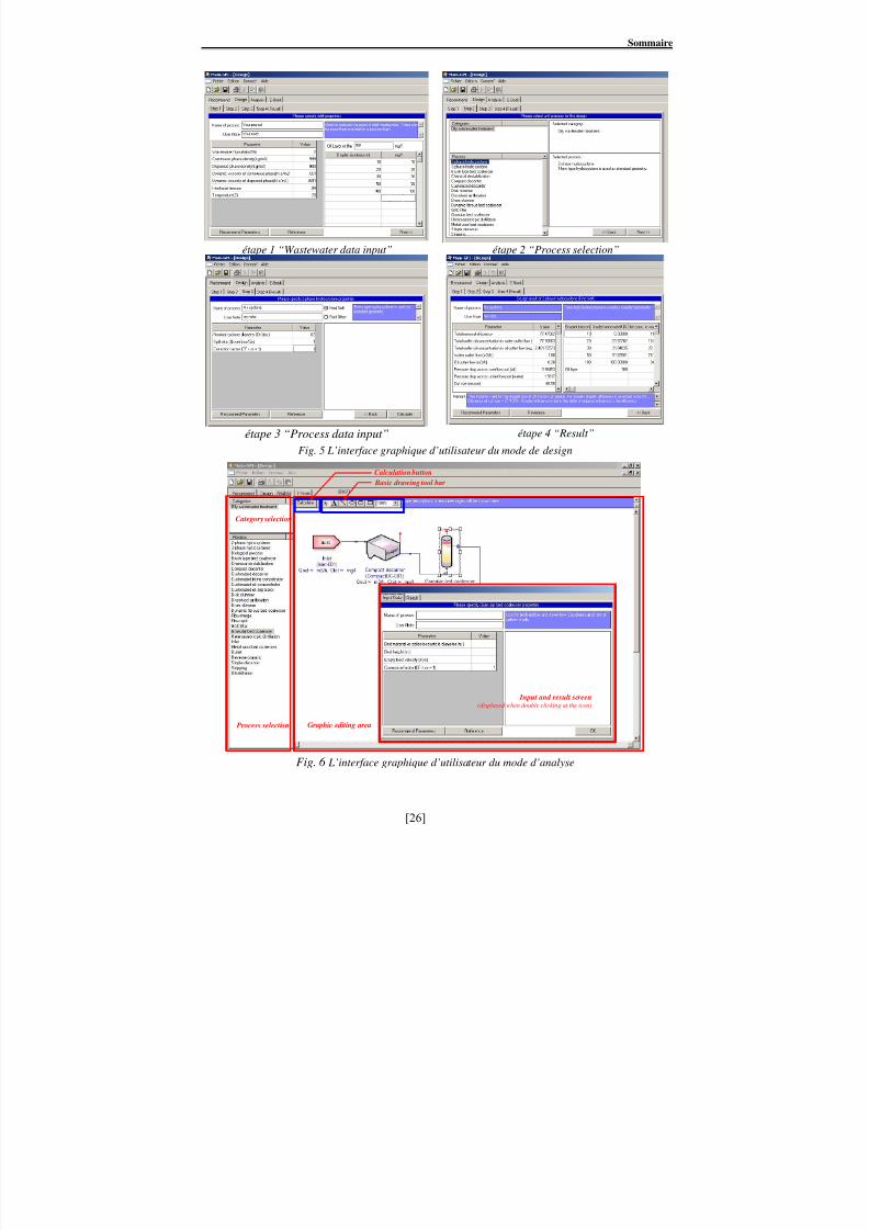
Le logiciel est développé pour être « upgradable ». Son architecture compose de la
base de données sous forme de fichier texte ordinaire et les « sub-programmes ». Pour« upgrader » le logiciel, il peut se faire facilement en ajoutant les données, comme le nom de
nouveau procédé et son paramètre de lien nécessaire pour le calcul, à la base de données. Le
logiciel liera automatiquement le nouveau procédé à l’interface graphique d’utilisateur. Quant
au calcul du « sub-programme » du nouveau procédé, il peut être développé séparément en
utilisant la langue de programmation Visual Basic. Le moyen le plus facile est de copier le
code de source d’un procédé existant et modifier l’équation pour convenir au nouveau
procédé. Après la compilation dans un fichier exécutable, il peut être copié pour remplacer
l’ancien fichier de logiciel GPI sans réinstaller le logiciel. Ainsi le logiciel pourrait se
développé davantage jusqu’à ce qu’il peut couvrir plus de recherches et procédés dans
l’avenir. Les interfaces du logiciel pour chaque mode sont comme montrées dans les figures
suivantes.
Cette thèse est accomplie par les supports considérables de Professeur AURELLE,
mon directeur de thèse, et M. Surapol SAIPANICH, PD-G de la société Progress Technology
Consultants Co.,Ltd. (Thailand). Je suis très reconnaissant pour leur conseil et
encouragement.
[23]

8/15/2019 Rachu.pdf
http://slidepdf.com/reader/full/rachupdf 26/646

8/15/2019 Rachu.pdf
http://slidepdf.com/reader/full/rachupdf 27/646
8/15/2019 Rachu.pdf
http://slidepdf.com/reader/full/rachupdf 28/646
Sommaire
étape 1 “Wastewater data input” étape 2 “Process selection”
étape 3 “Process data input” étape 4 “Result”
Fig. 5 L’interface graphique d’utilisateur du mode de design
Graphic editing area
Basic drawing tool bar
Calculation button
Input and result screen(displayed when double clicking at the icon)
Category selection
Process selection
Fig. 6 L’interface graphique d’utilisateur du mode d’analyse
[26]

8/15/2019 Rachu.pdf
http://slidepdf.com/reader/full/rachupdf 29/646
Résumé

8/15/2019 Rachu.pdf
http://slidepdf.com/reader/full/rachupdf 30/646

8/15/2019 Rachu.pdf
http://slidepdf.com/reader/full/rachupdf 31/646
Nom : RACHU Prénom : Srayut
COMPUTER PROGRAM DEVELOPMENT FOR OILY WASTEWATER
TREATMENT PROCESS SELECTION, DESIGN AND SIMULATION
562 pagesThèse de Doctorat : Science des procédés
Spécialité :Génie des Procédés et de l’Environnement
I.N.S.A. Toulouse, 2005, n°
Résumé :
The aims of this thesis is to summarize the researches of GPI lab on oily wastewater
treatment processes and establish general design procedure and consideration for such
processes, and then, value and maximize the use of these established knowledge in the form
of computer program.
The first part of the thesis contributes to reviewing the related researches in GPI lab,
directed by Prof. Y. AURELLE. Significant finding of each thesis is realized.
The second part of the thesis is generalization of models. In this part, models proposed
in the researches are cross-verified with other researches and generalised. New models are
also proposed when there is no existing model or the existing models need to be revised.
The third part of thesis contributes to composure of a textbook that includes all
significant finding from every research as well as the generalized models and their limitations
of every process found in the second part. The textbook includes these processes, i.e.
skimmer, decanter, coalescer, dissolved air flotation, hydrocyclone, membrane processes,
thermal process, chemical process, biological treatment and carbon adsorption, as well as
guideline for process selection.
The final part of the thesis is program development. The program developed in this
thesis consists of 4 main features, i.e. process recommendation for the wastewater being
considered, design of unit process, simulation of process train and provision of knowledge on
process design in the form of e-book, based on the text book in the third part.
The textbook, the program and its source code may be available upon request. For
more information, please contact Pr. Y. AURELLE or [email protected]
Mots clés : Skimmer, Decanter, Coalescer, Dissolved air flotation, Hydrocyclone, Membrane,
Distillation, Destabilization, Biological treatment, Adsorption, Program, Oily wastewater

8/15/2019 Rachu.pdf
http://slidepdf.com/reader/full/rachupdf 32/646
PRODUCTION SCIENTIFIQUE
Publications dans des actes de congrès avec comité de lecture, sur texte complet
S. Rachu, Y. Aurelle, S. Saipanich .
Simulation program on hydrocarbon polluted wastewater treatment processes
16th International Congress of Chemical and Process Engineering (CHISA 2004),
Prague, Czech Republic, 22-26 August 2004

8/15/2019 Rachu.pdf
http://slidepdf.com/reader/full/rachupdf 33/646

8/15/2019 Rachu.pdf
http://slidepdf.com/reader/full/rachupdf 34/646
Remerciements
J e r emer ci e si ncèr ement Monsi eur l e prof esseur Yves AURELLE pour
m' avoi r accuei l l i dans son équi pe, pour m' avoi r f ai t par t ager ses
connai ssances et ses i dées i nnovant es et pour son assi st ance t out au l ong
de ce t r avai l .
I woul d l i ke t o t hank Dr . Sur apol SAIPANICH f or hi s over whel mi ng
suppor t and encour agement . If not because of him, this work would never happen.
J ' adresse égal ement t ous mes r emer ci ements à :
Monsi eur Di mi t r e HADJIEV , pr of esseur à l ' USB de Lor i ent , , et
Monsi eur J ean Luc ROLS, pr of esseur à l ' UPS de Toul ouse pour avoi r accept é
de j uger ce t r avai l en f ai sant par t i e du j ur y,
Monsi eur BEN AIM , pr of esseur émér i t e à l ' I NSA et Monsi eur Al ai n
LINE, pr of esseur à l ' I NSA, pour avoi r accept é de par t i ci per au j ur y de
cet t e t hèse,
Monsi eur Henr y ROQUES prof esseur émér i t e à l ' I NSA pour sa pr ésence
au j ur y de cet t e t hèse,
I woul d l i ke t o t hank my col l eagues at Progress Technology
Consultants Co. , Lt d ( Thai l and) f or t hei r suppor t and t hei r ki ndness. Many
t hanks t o Kr i sana KHWANPAE f or hi s gr eat support on pr ogr ammi ng. Mygr at i t ude t o Bowornsak WANICHKUL, Chai yaporn PUPRASERT and Pi sut
PAINMANAKUL f or t hei r pr i cel ess advi ce. I owe you guys a boon.
Thank t o t he French Embassy in Thailand f or t hei r f i nanci al suppor t
dur i ng t he f i r st t wo years of my st udi es. Thanks t o the embassy personnel s,
par t i cul ar l y, Khun Hataiporn, Khun Wanpen f or t hei r assi st ance, Khun
Chanida f or her super b t r ansl at i on.
Mes r emerci ement s s' adr essent égal ement à t out es l es per sonnes qui
m' ont beaucoup ai dé t ant à Monsi eur Loui s LOPEZ, Monsi eur Gi l l es HEBRARD,Madame Eugéni e BADORC, Madame Dani èl e CORRADI et Madame AURELLE. J e
r emerci e égal ement mes ami s du l abo, part i cul i èr ement , Ol i ver LORAIN et
Eduar do LUCENA .
Enf i n, j e r emer ci e mes ami s Thaï l andai s de Toul ouse ( P’ Lek, P’ Tou,
P’ Aot e, A, Pond, Por , Pew, Gol f , Mon, Aey- Al exandr e, 1, Fon, Chi n, Chat ,
Pat , Vee, Choke, Si t h, J u, Bomb, et c. ) qui m' ont assur é par l eur humour ,
une ambi ance sympat hi que et per mi s d’ ef f ect uer de gr andes f êtes pendant mon
séj our en Fr ance.

8/15/2019 Rachu.pdf
http://slidepdf.com/reader/full/rachupdf 35/646
Table des matières
8/15/2019 Rachu.pdf
http://slidepdf.com/reader/full/rachupdf 36/646
Contents
- i -
Contents
Page
Part I Introduction and bibliography
Chapter 1 Introduction 2
Chapter 2 Objectives 4
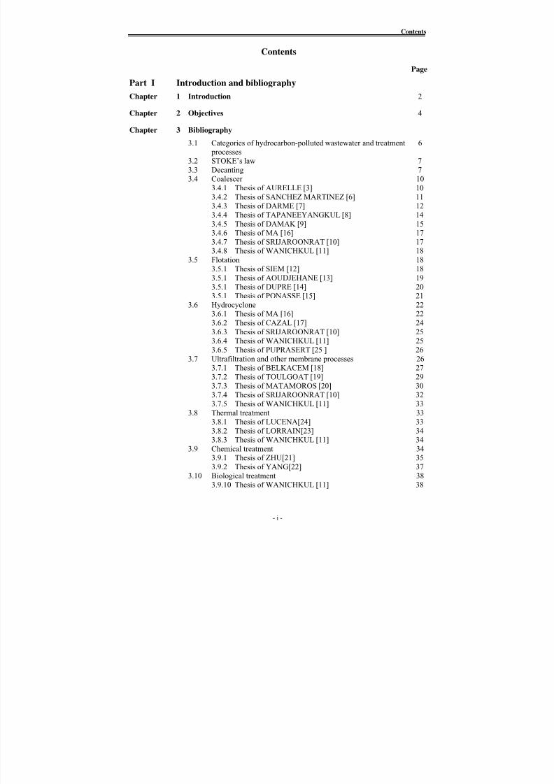
Chapter 3 Bibliography
3.1 Categories of hydrocarbon-polluted wastewater and treatment 6
processes
3.2 STOKE’s law 7
3.3 Decanting 7
3.4 Coalescer 10
3.4.1 Thesis of AURELLE [3] 10
3.4.2 Thesis of SANCHEZ MARTINEZ [6] 11
3.4.3 Thesis of DARME [7] 12
3.4.4 Thesis of TAPANEEYANGKUL [8] 14
3.4.5 Thesis of DAMAK [9] 15
3.4.6 Thesis of MA [16] 17
3.4.7 Thesis of SRIJAROONRAT [10] 17
3.4.8 Thesis of WANICHKUL [11] 18
3.5 Flotation 18
3.5.1 Thesis of SIEM [12] 18
3.5.1 Thesis of AOUDJEHANE [13] 19
3.5.1 Thesis of DUPRE [14] 203.5.1 Thesis of PONASSE [15] 21
3.6 Hydrocyclone 22
3.6.1 Thesis of MA [16] 22
3.6.2 Thesis of CAZAL [17] 24
3.6.3 Thesis of SRIJAROONRAT [10] 25
3.6.4 Thesis of WANICHKUL [11] 25
3.6.5 Thesis of PUPRASERT [25 ] 26
3.7 Ultrafiltration and other membrane processes 26
3.7.1 Thesis of BELKACEM [18] 27
3.7.2 Thesis of TOULGOAT [19] 29
3.7.3 Thesis of MATAMOROS [20] 303.7.4 Thesis of SRIJAROONRAT [10] 32
3.7.5 Thesis of WANICHKUL [11] 33
3.8 Thermal treatment 33
3.8.1 Thesis of LUCENA[24] 33
3.8.2 Thesis of LORRAIN[23] 34
3.8.3 Thesis of WANICHKUL [11] 34
3.9 Chemical treatment 34
3.9.1 Thesis of ZHU[21] 35
3.9.2 Thesis of YANG[22] 37
3.10 Biological treatment 38
3.9.10 Thesis of WANICHKUL [11] 38

8/15/2019 Rachu.pdf
http://slidepdf.com/reader/full/rachupdf 37/646
Contents
- ii -
Contents (Con’t)
Page
3.11 Skimmer 38
3.12 Application researches 39
3.12.1 Thesis of SRIJAROONRAT [10] 40
3.12.2 Thesis of WANICHKUL [11] 41
Chapter 4 Conclusion 44

8/15/2019 Rachu.pdf
http://slidepdf.com/reader/full/rachupdf 38/646

8/15/2019 Rachu.pdf
http://slidepdf.com/reader/full/rachupdf 39/646
Contents
- iv -
Contents (Con’t)
Page
5.1.4 Conclusion and generalized model of two-phase 84
hydrocyclone
5.1.5
Generalized model for pressure drop of two-phase 85hydrocyclone
5.2 Three-phase hydrocyclone 87
5.2.1 Model development and verification for liquid-liquid 87
section
5.2.2 Model development and verification for solid-liquid section89
5.2.3
Generalized Model for pressure drop of three-phase 90
hydrocyclone
Chapter 6 Membrane process
6.1
Ultrafiltration 93
6.1.1
Resistance model 94
6.1.2 Film theory based model 96
6.1.3 Model verification 97
6.1.4 Flux prediction for mixture of cutting oil microemulsion 102
and macroemulsion
6.1.5
Theoretical flux prediction for batch cross-flow UF process 104
6.1.6 UF efficiency 107
6.1.7 Minimum and maximum transmembrane pressure and 108
power required
6.1.8 Conclusion and generalized model of UF 110
6.2
Nanofiltration and Reverse osmosis 110Chapter 7 Heteroazeotropic Distillation
7.1 Theoretical model 113
7.2 Model verification 116
7.3 Conclusion and generalized model of heteroazeotropic distillation 116

8/15/2019 Rachu.pdf
http://slidepdf.com/reader/full/rachupdf 40/646
Contents
- v -
Content
Page
Part III Summary of researches: Oily wastewater treatment
Chapter 1 Oily or hydrocarbon-polluted wastewater
1.1 Introduction 119
1.2 Hydrocarbons and oils 119
1.2.1 Hydrocarbons 119
1.2.2 Fats and oils 124
1.2.3 Petroleum and petroleum products 124
1.2.4
Oils in term of oily wastewater 126
1.3 Other compositions of oily wastewater 126
1.3.1 Surfactants 126
1.3.2 Soaps 127
1.3.3
Co-surfactants 1281.3.4 Suspended solids 1281
1.3.5
Other components 128
1.4 Categories of oily wastewater 128
1.4.1
Classification by the nature of the continuous phase 128
1.4.2 Classification by the stability of oily wastewater 128
1.4.3 Classification by the degree of dispersion 129
1.5 Characteristics of certain oily wastewaters 132
1.6 Standards, Laws, and Regulations 133
Chapter 2 Overview for oily wastewater treatment process design
2.1
Decantation velocity and STOKE’s law 1382.2
Application of surface chemistry for oily wastewater treatment 139
2.2.1 Liquid-gas and liquid-liquid interfaces 139
2.2.2 Liquid-solid and liquid-liquid-solid interfaces 142
2.2.3 Capillary pressure and LAPLACE’s law 146
2.3 Important parameters in oily wastewater treatment and 147
their method of analysis
2.3.1
Oil concentration 147
2.3.2 Size distribution , spectrum or granulometry 149
2.3.3
Other parameters 155
2.4 Overview of oily wastewater treatment processes 155
2.4.1
Decanter 156
2.4.2 Coalescer 156
2.4.3 Hydrocyclone 156
2.4.4 Dissolved air flotation (DAF) 157
2.4.5
Skimmer 157
2.4.6 Membrane processes 157
2.4.7 Thermal processes 157
2.4.8 Chemical process 158
2.4.9 Finishing processes 158

8/15/2019 Rachu.pdf
http://slidepdf.com/reader/full/rachupdf 41/646
Contents
- vi -
Content (Con’t)
Page
2.5 Determination of degree of treatment 158
2.5.1
Overall degree of treatment 1582.5.2 Degree of treatment of each process 158
Chapter 3 Oil skimmer
3.1 General 162
3.2 Oil drum skimmer 164
3.2.1 Working principles 164
3.2.2 Design calculation and design consideration 169
3.3 Oil disc skimmer 171
3.3.1 Working principles 171
3.3.2 Design calculation and design consideration 173
3.4 Productivity comparison between drum and disc skimmer 1733.5 Advantage and disadvantage of drum and disc skimmer 174
Chapter 4 Decanting
4.1 General 176
4.2 Simple Decanter or API tank 177
4.2.1 Working principles 177
4.2.2 Design calculation 179
4.2.3
Design considerations 182
4.2.4 Construction of simple decanters 183
4.3 Compact decanter 186
4.3.1
Working principles 1864.3.2 Design calculation 190
4.3.3 Design considerations 192
4.3.4 Variations, advantage and disadvantage of compact 193
decanters
Chapter 5 Coalescer
5.1 General 195
5.2 Granular bed coalescer 195
5.2.1 Working principles 195
5.2.2 Design calculation 209
5.2.3 Design consideration 2115.2.4 Variations, advantage and disadvantage of granular 212
bed coalescer
5.3 Guide coalescer 213
5.3.1 Working principles 213
5.3.2 Design calculation 215
5.3.3 Design consideration 215
5.4 Fibrous Bed coalescer 216
5.4.1 Working principles 216
5.4.2 Design calculation 226
5.4.3 Design consideration 227
5.4.4 Variations, advantage and disadvantage of fibrous bed 229coalescer

8/15/2019 Rachu.pdf
http://slidepdf.com/reader/full/rachupdf 42/646
Contents
- vii -
Content (Con’t)
Page
Chapter 6 Dissolved air flotation
6.1 General 232
6.2 Working principles 233
6.2.1
Filter based model 233
6.2.2 Population balance model 238
6.2.3 Generalized model of DAF from combination of 240
filtration based model and population balance model
6.2.4 Influent parameters 241
6.3 Design calculation 244
6.4 Design consideration and construction of DAF reactor 254
6.5
Pressurized water system or saturator 262
6.5.1
Working principle and design calculation 2626.5.2 Type of saturator and injection valve 267
6.6 Variations, advantage and disadvantage of DAF 270
Chapter 7 Hydrocyclone
7.1 General 272
7.2 Two-phase hydrocyclone 273
7.2.1 Working principles 273
7.2.2
Design calculation 289
7.2.3 Design considerations 292
7.2.4 Variations, advantage and disadvantage of 295
hydrocy clone7.3 Three-phase hydrocyclone 295
7.3.1 Working principles 295
7.3.2 Design calculation and design consideration 299
7.3.3
Advantage and disadvantage of three-phase 299
hydrocyclone
Chapter 8 Membrane process
8.1 General 300
8.1.1 Classification of membrane processes 300
8.1.2 Mode of operation of membrane processes 302
8.1.3
Membrane structure 3028.1.4 Membrane material 303
8.1.5
Membrane module type 306
8.2 Ultrafiltration (UF) 311
8.2.1 Basic knowledge and working principles 311
8.2.2 UF process design for oily wastewater treatment 323
8.2.3 Design consideration and significant findings from 338
GPI’s researches
8.3 Microfiltration (MF) 349
8.3.1
Basic knowledge and working principles 349
8.3.2 Significant findings on MF for oily wastewater 350
treatment from GPI researches
8/15/2019 Rachu.pdf
http://slidepdf.com/reader/full/rachupdf 43/646

8/15/2019 Rachu.pdf
http://slidepdf.com/reader/full/rachupdf 44/646
Contents
- ix -
Chapter 11 Finishing processes
11.1 General 397
11.2 Biological treatment 397
11.2.1 Basic knowledge 397
11.2.2
Design consideration and significant finding on 404 biological treatment for oily wastewater from GPI’s
researches
11.3 Adsorption 405
11.3.1
Activated carbon (AC) 406
11.3.2 Basic knowledge 407
11.3.3 Design calculation 412
Chapter 12 Guideline for treatment process selection and examples of treatment
processes for certain oily wastewaters
12.1 Guideline for treatment process selection 414
12.1.1
Oil film 41412.1.2
Primary emulsion 416
12.1.3 Secondary emulsion 417
12.1.4 Macroemulsion and microemulsion 418
12.1.5 Concentrated oily wastewater or refinery slops 418
12.2 Examples of treatment processes for certain oily wastewaters 419
12.2.1 Treatment of cutting oil emulsion 419
12.2.2
Treatment of non-stabilized secondary emulsion 420

8/15/2019 Rachu.pdf
http://slidepdf.com/reader/full/rachupdf 45/646
Contents
- x -
Contents
Page
Part IV Computer program development
Chapter 1 Program overview
1.1 Introduction 423
1.2 Conceptual design of the program 423
1.2.1 E-book mode 424
1.2.2 Recommendation mode 426
1.2.3 Design mode 427
1.2.4
Analysis mode 428
1.3 Development tools 432
1.3.1 Main development software package 432
1.3.2 Special graphic user interface (GUI) component 433
1.3.3
The third party software 4331.4 Program architecture 434
1.4.1
Forms 434
1.4.2 Modules 437
1.4.3
Modules 437
1.4.4 Class modules 437
1.4.5 Add-in project 437
1.5 Program development 438
Chapter 2 Program reference and user manual
2.1 Overview of the program 439
2.1.1
Main program 4392.1.2
Project window 441
2.1.3 E-books worksheet 441
2.1.4 Recommend worksheet 442
2.1.5 Design worksheet 444
2.1.6 Analysis mode 445
2.1.7 Warning dialog box 447
2.2
Program capability 447
2.3 Program limitation 447
2.4
System requirement 449
2.5 User instruction 449
2.5.1
Program Installation 449
2.5.2 Starting the program 450
2.5.3 Using E-book mode 450
2.5.4 Using Recommend mode 450
2.5.5
Using Design mode 452
2.5.6 Using Analysis mode 454
2.5.7 Printing and file operation 457
2.6 Upgrading procedure and recommendation for further 458
development
2.6.1 Upgrading procedure 458
2.6.2
Recommendation for further development 460

8/15/2019 Rachu.pdf
http://slidepdf.com/reader/full/rachupdf 46/646
Contents
- xi -
Contents
Page
Chapter 3 Process references
1)
Drum skimmer 4632)
Disk skimmer 465
3) Simple decanter 467
4)
Compact decanter 470
5) Customized decanter 473
6) Granular bed coalescer 476
7) Brush type bed coalescer 480
8) Dynamic fibrous bed coalescer 484
9) Metal wool bed coalescer 488
10) Dissolved air flotation 492
11) Two-phase hydrocyclone 498
12) Three-phase hydrocyclone 502
13) Ultrafiltration 506
14) Reverse osmosis 510
15) Heteroazeotropic distillation 513
16) Stripping 515
17) Chemical destabilization, coagulation-flocculation 517
18) Biological treatment 520
19) GAC filter 522
20) Customized concentrator 526
21) Customized oil separator 528
22) Customized inline concentrator 53023) Inlet 532
24) Outlet 533
25) Flow merge 534
26) Flow split 536

8/15/2019 Rachu.pdf
http://slidepdf.com/reader/full/rachupdf 47/646
Contents
- xii -
Contents
Page
General conclusion 537
Reference 540
Annexe 546

8/15/2019 Rachu.pdf
http://slidepdf.com/reader/full/rachupdf 48/646
Nomenclatures

8/15/2019 Rachu.pdf
http://slidepdf.com/reader/full/rachupdf 49/646
Nomenclature
xiii
Nomenclature
a Constant for population balance equation
A Flow area (Cross sectional) area of decanter L2
A Cross section area of flotation column L2
A Flow area in membrane module (= HW) L
2
C Considered or required or design oil concentration ML-3
C’g The 1st (or lower or pseudo) gel concentration in film model,
used at the lower range of concentration before inflection
point in flux vs. Log (Concentration) curve (in mass/ volume
or volume/volume)
ML-3
Ca Capillary number = μo V/γo
Cg Gel concentration in film model (in mass/ volume or
volume/volume)
ML-3
Co Initial oil concentration of feed or influent wastewater ML-3
Cod Inlet concentration of the droplet diameter “d” M/L3
Cod Inlet concentration of the droplet diameter “d”, dilution effect
from addition of pressurized water is not included.
M/L3
Conc(Air) Concentration of dissolved air in pressurized water M/L3
Conc(O2) Concentration of dissolved oxygen in pressurized water M/L3
Cy50 Cyclone number of d 50%
d Diameter of dispersed phase, in our case, oil L
D Water depth or L
Diameter of the skimmer or L
Diameter of coalescer bed, such as diameter of brush or L
Nominal diameter of 3-phases hydrocyclone (the largest
diameter of the cyclone) or
L
Hydraulic diameter of flow channel in membrane module
(Channel between membrane surface and membrane module
wall)
L
d b Average diameter of air bubble L
d c Cut size of the decanter or API tank L
d F Diameter of fiber in fibrous-bed coalescer L
Di Diameter of inlet port of hydrocyclone L
Dn Nominal diameter of hydrocyclone. ( = diameter of inlet of
lower conical part for Thew type hydrocyclone)
L
d p Diameter of collector or coalescer bed material, such as resin L
d xx% , d xx Diameter of droplet corresponding to removal efficiency of
“xx”%, such as d 75%, etc. d 100% or d c stands for cut size
M
e Surface roughness of flow channel L
f Friction factor of Darcy-Weisbach’s equationg Gravitational acceleration L/T2
G Turbulent intensity
H Travelling or rising distance of oil drop, depending on
configuration of the decanter. Exp. For PPI, H = distance
between plates or
L
Height of bed, or bed depth of coalescer or L
Height of flow channel in membrane module or L
Height of contact (or effective) zone of flotation column. If
both pressurized water and wastewater are fed at the bottom
of the column, the contact zone is equal to column height.
L
Href H at reference operating condition of DAF reactor L
Hreq H at design or required operating condition of DAF reactor LI Immersion depth of the disk in liquid or L

8/15/2019 Rachu.pdf
http://slidepdf.com/reader/full/rachupdf 50/646

8/15/2019 Rachu.pdf
http://slidepdf.com/reader/full/rachupdf 51/646
Nomenclature
xv
V Empty bed velocity or L/T
Empty bed velocity of DAF (based on sum of pressurized water
and wastewater flow) or
L/T
Tangential velocity of particle or oil drop in hydrocyclone or L/T
Recirculation velocity in cross-flow membrane process L/T
Vol Volume L3
Vr Relative velocity between bubble and oil drop L/T
W Axial velocity of particle or oil drop in hydrocyclone or L/T
Width of flow channel in membrane module L
x Molar fraction in liquid (water) Mol/mol
y Molar fraction in vapor Mol/mol
Z Distance in axial axis of hydrocyclone L
ΔP Pressure drop, (in m of water, for Kozeny-Carman’s equation)
Or pressure drop in bar, for hydrocyclones
ΔPo Pressure drop across inlet and overflow port Bar
ΔPoil Pressure drop across inlet and oil outlet port Bar
ΔPSS Pressure drop across inlet and suspended solids outlet port Bar
ΔPu Pressure drop across inlet and underflow port BarΔPwater Pressure drop across inlet and water outlet port Bar
Greek Letter
Φ Air flowrate in flotation column L3/T
Π Vapor pressure (some references use “Psat”.) LT-2M-1
α Probability of collision or
Exponent of recirculation velocity in gel resistance equation
α.ηexp Corrected experimental removal efficiency factor of the tank
for the droplet diameter “d”
α, α3φ, αThew Correction factor for inlet velocity of hydrocycloneβ Conical angle of lower part of hydrocyclone or
Exponent of recirculation velocity in film model of
membrane
β0, β1, … , βi Adhesion efficiency between bubbles and oil drop/ bubble
agglomerate for population balance equation
ε Porosity or void ratio
φ Constant in gel resistance equation
γo Superficial tension of oil M/T2
γo/w Interfacial tension between oil and water M/T2
γo/w Interfacial tension between oil and water MT-2
ηoverall Overall efficiency of pumpκ Collision rate constant for population balance equation T
-1
κ2 Modified collision rate constant for population balance
equation (κ = κ2Φ)
T-2
κ2,ref Modified collision rate constant at reference condition T-2
κ2,req Modified collision rate constant at design or required
condition
T-2
μ Dynamic viscosity ML-1
T-1
μC Dynamic viscosity of continuous phase, in our case, water L2/T
μd Dynamic viscosity of dispersed phase, in our case, oil L2/T
μo Dynamic viscosity of oil M/(L.T)
νo Kinematic viscosity of oil L2/T
θo/w Contact angle between oil and water surface (180o means the
oil drop in perfectly sphere.)

8/15/2019 Rachu.pdf
http://slidepdf.com/reader/full/rachupdf 52/646
Nomenclature
xvi
ρ Density ML-3
ρair Density of air at required operating condition M/L3
ρc Density of continuous phases M/L3
ρm Density of emulsion M/L3
Δρ Difference between density of dispersed and continuous
phases
M/L3
τ Retention time T
ηd Removal efficiency of the tank for the droplet diameter “d” %
ηd,ref Removal efficiency of DAF process for the droplet diameter
“d” at the reference retention time (25 minutes)
%
ηDiff Efficiency factor from diffusion
ηInt Efficiency factor from direct interception
ηSed Efficiency factor from sedimentation
ηSed Efficiency factor from sedimentation
ηt Total Removal efficiency %
ηtheo Theoretical removal efficiency factor of the tank for the
droplet diameter “d”
?A, ?BB Subscript indicating component A and B respectively
?H Subscript indicating heteroazeotropic point
?mac Subscript indicating macroemulsion
?mic Subscript indicating microemulsion
?mix Subscript indicating mixture
?o Subscript indicating initial condition
?ref Subscript indicating reference condition
?θ b Superscript indicating boiling temperature

8/15/2019 Rachu.pdf
http://slidepdf.com/reader/full/rachupdf 53/646
Part I Introduction and bibliography

8/15/2019 Rachu.pdf
http://slidepdf.com/reader/full/rachupdf 54/646
Part I Introduction and bibliography
I-i
Contents
Page
Part I Introduction and bibliography
Chapter 1 Introduction I-2
Chapter 2 Objectives I-4
Chapter 3 Bibliography
3.1 Categories of hydrocarbon-polluted wastewater and treatment I-6
processes
3.2 STOKES law I-7
3.3 Decanting I-7
3.4 Coalescer I-10
3.4.1 Thesis of AURELLE [3] I-10
3.4.2 Thesis of SANCHEZ MARTINEZ [6] I-11
3.4.3 Thesis of DARME [7] I-12
3.4.4 Thesis of TAPANEEYANGKUL [8] I-14
3.4.5 Thesis of DAMAK [9] I-15
3.4.6 Thesis of MA [16] I-17
3.4.7 Thesis of SRIJAROONRAT [10] I-17
3.4.8 Thesis of WANICHKUL [11] I-18
3.5 Flotation I-18
3.5.1 Thesis of SIEM [12] I-18
3.5.1 Thesis of AOUDJEHANE [13] I-19
3.5.1 Thesis of DUPRE [14] I-203.5.1 Thesis of PONASSE [15] I-21
3.6 Hydrocyclone I-22
3.6.1 Thesis of MA [16] I-22
3.6.2 Thesis of CAZAL [17] I-24
3.6.3 Thesis of SRIJAROONRAT [10] I-25
3.6.4 Thesis of WANICHKUL [11] I-25
3.6.5 Thesis of PUPRASERT [25 ] I-26
3.7 Ultrafiltration and other membrane processes I-26
3.7.1 Thesis of BELKACEM [18] I-27
3.7.2 Thesis of TOULGOAT [19] I-29
3.7.3 Thesis of MATAMOROS [20] I-303.7.4 Thesis of SRIJAROONRAT [10] I-32
3.7.5 Thesis of WANICHKUL [11] I-33
3.8 Thermal treatment I-33
3.8.1 Thesis of LUCENA[24] I-33
3.8.2 Thesis of LORRAIN[23] I-34
3.8.3 Thesis of WANICHKUL [11] I-34
3.9 Chemical treatment I-34
3.9.1 Thesis of ZHU[21] I-35
3.9.2 Thesis of YANG[22] I-37
3.10 Biological treatment I-38
3.9.10 Thesis of WANICHKUL [11] I-38

8/15/2019 Rachu.pdf
http://slidepdf.com/reader/full/rachupdf 55/646

8/15/2019 Rachu.pdf
http://slidepdf.com/reader/full/rachupdf 56/646
Part I Introduction and bibliography
I-iii
Table
Page
Table 3.1 Summary of characteristics of wastewaters and sludges for “on site” I-24
experiment
Table 3.2 Summary of characteristics of synthetic wastewaters I-24
Table 3.3 Membranes test by MATAMOROS I-31
Figure
Page
Fig. 1-1 Summary of researches of Prof. AURELLE on hydrocarbon-polluted I-3
wastewater treatment
Fig. 3.1 Schematic of decante I-8
Fig. 3.2 Schematic of Phase inversion coalescer I-15
Fig. 3.3 Three- phase hydrocyclone I-23
Fig. 3.4 Hydrocyclone tested by WANICHKUL I-26
Fig. 3.5 Ultrafiltration models used by BELKACEM I-29
Fig. 3.6 Treatment processes for macro- and microemulsion, recommended I-32
by MATAMORS

8/15/2019 Rachu.pdf
http://slidepdf.com/reader/full/rachupdf 57/646

8/15/2019 Rachu.pdf
http://slidepdf.com/reader/full/rachupdf 58/646
Chapter 1 Introduction
2 I-2
Chapter 1 Introduction
Water pollution is one of the most important environmental problems. Wastewater
from agriculture and industrial processes, as well as domestic wastewater, is the main
pollutant source that causes water pollution problem. There are many substances that can
deteriorate water quality, thus classified as water pollutants, such as, organic matter fromdomestic wastewater, chemicals from industrial wastewater. Some valuable substances, such
as sugar, flour, oil, will become major pollutants when discharged into water bodies.
Among various kinds of pollutants, hydrocarbon, or simply called oil, is one of the
most severe pollutants because of its intrinsic properties. Small amount of hydrocarbon can
spread over wide area of water surface and affect the oxygen transfer, so cause adverse effect
to marine or water ecology. Furthermore, the hydrocarbon contributes to very high
biochemical oxygen demand and is relatively difficult for biodegradation, which is the major
natural self-purification process. So it can last relatively long in the water and causes long -
term effect.
Our laboratory has researched for various treatment processes that cover various types
of wastewater polluted by hydrocarbons. In the few decades of researches, many theses had
been accomplished as shown in Fig. 1.1. Among these, many innovations had been created
and some had been patented and commercialized. Some researches are the key steps to
understand or improve the treatment efficiency and process design. However, because there
are many kinds of oily wastewater, as well as, there are many kinds of treatment processes.
Moreover, treatment efficiency of each treatment process will vary with characteristic of
wastewater. Then, it may cause some difficulties in selecting or designing appropriate process
train that can deal with the wastewater considered as well as predicting effluent quality
accurately.
According to the difficulty stated above, this thesis had been initiated to provide the
solution and tool about how to select and optimize the process or processes train to treat the
specified wastewater to meet required effluent standard, as well as providing details about
hydrocarbon polluted wastewater and each treatment process. It can be, also, applied for
designing the process to recover valuable hydrocarbons from hydrocarbon/water mixtures in
some industries, such as perfume or pharmaceutical industries.

8/15/2019 Rachu.pdf
http://slidepdf.com/reader/full/rachupdf 59/646
Part I Introduction and bibliography
3 I-3
F i g .
1 - 1 S
u m m a r y o f r e s e a r c h e s o f P r o f .
A U R E L L E o n h y d r o c a r b o n - p o l l u t e d w a s t e w a t e r t r e a t m e n t
H y d r o c a r b o n -
p o l l u t e d o r o i l y
w a s t e w a t e r
t r e a t m e n t
D e c a n t e r
“ S p i r a l o i l ” d e c a n t e r
C H E R I D [ 4 ] , 1 9 8 6
S k i m
m e r
“ D r u m s k i m m e r ” &
“ d i s k s k i m m e r ”
T H A N G T O N G T A W I [ 5 ] , 1
9 8 8
C o a l e s c e r
“ G r a n u l a r b e d c o a l e s c e r ”
A U R E L L E [ 3 ] , 1 9 8 0
“ G r a n u l a r b e d c o a l e s c e r f o r
s t a b i l i z e d e m u l s i o n ”
D A R M E [ 6 ] , 1 9 8 3
“ D y n a m i c f i b r o u s b e d c o
a l e s c e r ”
T A P A N E E Y A N G K U L [ 8 ] , 1 9 8 9
“ P u l s e d g r a n u l a r b e d c o a
l e s c e r ” &
“ P h a s e i n v e r s i o n c o a l e s c
e r ”
D A M A K [ 9 ] , 1 9 9 2
F l o t a t i o n
“ F l o t a t i o n f o r o i l - w a t e r
s e p a r a t i o n ”
S I E M [ 1 2 ] , 1 9 8 3
“ A p p l i c a t i o n o f f l o t a t i o n
o n o i l y
w a s t e w a t e r t r e a t m e n t ”
A O U J E H A N E [ 1 3 ] , 1 9 8
6
“ M a t h e m a t i c s m o d e l o f
D A F ”
D U P R E [ 1 4 ] , 1 9 9 5
“ D e e p s h a f t D A F ”
P O N A S S E [ 1 5 ] , 1 9 9 7
H y d r o c y c l o n e
“ 2 & 3 - p h a s e h y d r o c y c l o n e ”
M A [ 1 6 ] , 1 9 9 3
“ 2 - p h a s e h y d r o c y c l o n e
f o r s t o r m w a t e r t r e a t m e n t ”
C A Z A L [ 1 7 ] , 1 9 9 6
“ H y d r o c y c l o n e w i t h g r i t p o t ” &
“ C o m b i n a t i o n C o a g u l a t i o n
- D A F - H y d r o c y c l o n e ” s e
p a r a t o r
P U P R A S E R T [ 2 5 ] , 2 0 0 4
U l t r a f i l t r a t i o n
& m
e m b r a n e
p r o c
e s s e s
“ U l t r a f i l t r a t i o n f o r c u t t i n g o
i l
e m u l s i o n t r e a t m e n t ”
B E L K A C E M [ 1 8 ] , 1 9 9 5
“ U l t r a f i l t r a t i o n f o r t h e r m
a l
e m u l s i o n t r e a t m e n t ”
T O U L G O A T [ 1 9 ] , 1 9 9 6
“ M e m b r a n e p r o c e s s e s f o r c u t t i n g
o i l e m u l s i o n t r e a t m e n t ”
M A T A M O R O S [ 2 0 ] , 1 9
9 7
T h e r m a l
t r e a t
m e n t
“ C r y s t a l l i z a t i o n f o r o i l - w a t e
r
s e p a r a t i o n ”
L O R R A I N [ 2 3 ] , 2 0 0 2
“ H e t e r o a z e o t r o p i c d i s t i l l a t i o n ”
L U C E N A [ 2 4 ] , 2 0 0 4
C h e m i c a l
t r e a t
m e n t
“ D e s t a b i l i s a t i o n o f e m u l s i o
n ”
Z H U [ 2 1 ] , 1 9 9 0
“ L o w - p o l l u t i o n e m u l s i o
n ”
Y A N G [ 2 2 ] , 1 9 9 3
“ G u i d e d & M i x e d b e d c o a l e s c e r ”
S A N C H E Z M A R T I N E Z [ 5 ] , 1 9 8 2
A p p l i c a t i o n
“ T r e a t m e n t o f
s t a b i l i z e d e m u l s i o n ”
W A N I C H K U L
[ 1 1 ]
, 2 0 0 0
“ T r e a t m e n t o f n o n -
s t a b i l i z e
d e m u l s i o n ”
S R I J A R O
O N R A T [ 1 0 ]
, 1 9 9 8

8/15/2019 Rachu.pdf
http://slidepdf.com/reader/full/rachupdf 60/646

8/15/2019 Rachu.pdf
http://slidepdf.com/reader/full/rachupdf 61/646
Part I Introduction and bibliography
5 I-5
treatment processes and key parameters affected their designs and operations, that can lead to
proper design and selection of treatment processes or creating their own variation of process
that suit their own situation.
4. To develop the prototype of program for the design, comparison and simulation
of hydrocarbon-polluted wastewater treatment processes.
At the present, computer comes to play major role in every field and become standard
equipment in almost every household, office and academic institute. Because of its powerful
logical and mathematical calculation, as well as its presentation and interaction capability, it is
very interesting to use computer in the field of hydrocarbon-polluted wastewater treatment.
Up till now, there are many commercial softwares on industrial and wastewater treatment
process calculation. Anyway, those programs are not specifically designed to deal with
hydrocarbon-polluted wastewater treatment. Furthermore, the commercial softwares are
normally developed for expert users, so they do not provide much basic data, thus, render it
difficult for non-expert users to use efficiently. Besides, they normally do not provide any
data for decision supporting, for example they can not compare the efficiency between various processes or recommend the feasible processes for considered wastewater.
So for our 4th objective, we intend to develop the prototype of program for design,
comparison and simulation of hydrocarbon-polluted wastewater treatment processes. The
program will feature;
• E-book: provides background knowledge and useful database about the oil
pollution and the treatment processes,
• Process recommendation part: provides recommendation or narrows the range of
feasible processes for any input influent,• Design (or calculation) part: used for sizing the process unit,
• Simulation part: allows users to integrate any separation processes, included in
the program database, to build their own treatment process train. And the program
will simulate the process train to forecast the efficiency of each unit.
The treatment processes, which can be calculated or simulated by the program built-in
database, will then be based mainly upon the researches reviewed in the 1st to 3rd objective.
However, the source code of the program will be available upon request to allow upgrading to
include more processes in the future.

8/15/2019 Rachu.pdf
http://slidepdf.com/reader/full/rachupdf 62/646
Part I Introduction and bibliography
6 I-6
Chapter 3 Bibliography
3.1 Categories of hydrocarbon-polluted wastewater and treatment
processes
As hydrocarbon or oil requires a great amount of oxygen or oxidizing agent to oxidize,moreover, the hydrocarbon is relatively difficult to biodegrade, thus, it becomes clear that the
use of the biological treatment with high-concentration oily wastewater is not the economical
alternative. Besides there are possibilities to reuse or recover the hydrocarbons in the
wastewater. Then almost all of treatment processes that have been studied in our laboratory
are based on separation, both physical and physico-chemical, techniques in order to separate
oil from water.
Thus, it is more suitable to categorize the oily wastewater by its physical properties.
Among these properties, the degree of dispersion of oil phase in water or the size of oil
droplet is the key parameter that plays an important role in separation process selection. So we
will categorize the oily wastewater into 4 groups, in accordance with its droplet size, i.e.,
• Hydrocarbon in form of film or layer on the surface of wastewater, or hydrocarbon
in form of big oil drops in the wastewater
• Emulsion without surfactants, by the word “emulsion”, it can be easily described
as the water with very fine dispersed oil drops
• Emulsion with surfactants
• Dissolved hydrocarbon
For treatment processes, each process has its own characteristic or limitation so it can
be used to separate some certain ranges of oil droplet. So each group of the oily wastewater
may require certain process or train of processes to separate the oil from the water to theaccepted degree. The treatment processes, studied by Professor AURELLE’s researchers,
covered the entire range of the oily wastewater stated above and can be summarized as
follow;
• Decanting
• Skimmer
• Coaleser
• Flotation
• Hydrocyclone
• Ultrafiltration
• Distillation• Biological treatment
Moreover, there are researches on chemical treatment, which relates to “breaking” the
emulsion to allow the micro droplet to coalesce and make it possible to separate by the
processes stated above. There, also, are some researches contributed to formulation of
environmental-friendly oil product, which can be easily treated and still have the same
essential working properties as the existing product’s.
Furthermore, some researches can be extensively used to solve the problems of some
special types of oily waste, such as slop (viscous mixture between crude oil and water) or
inverse emulsion (fine drops of water dispersed in oil)

8/15/2019 Rachu.pdf
http://slidepdf.com/reader/full/rachupdf 63/646
Chapter 3 Bibliography
7 I-7
Details of wastewater characteristics and treatment processes are thoroughly described
in Part 3. So, this part emphasizes on reviewing of related researches, categorized by process,
about their scope of work and significant finding, as described in next sections.
3.2 STOKES law
It is important to mention about STOKES law (eq. 3.1), because almost all of
separation processes considered here are based upon modification of parameters in this
equation. The STOKES equation is the relation between rising (or settling) velocity of
spherical object (in our case, droplet of dispersed phase) with very small Reynolds number
(10-4 to 1) and properties of dispersed phase and continuous phase.
c
E d gV
μ
ρ
18
2⋅⋅Δ
= {3.1}
Where V = rising or settling velocity (based on density of the 2 phases)
Δρ = Difference between density of dispersed phase and continuous
phase
dE = Diameter of dispersed phase
μC = Dynamic viscosity of continuous phase
In case of oily wastewater, the dispersed phase is hydrocarbon or oil and the
continuous phase is water. Because the density of hydrocarbons in our wastewater is normally
lower than water’s. It is prone to rise to surface of the water. Even though the STOKES
equation is valid only for certain flow regimes, the equation covers the range of flow
regime normally encountered in wastewater problem. It can be used to explain important
phenomena or applied to many types of processes, even a bit beyond its valid regime, with
satisfactory result. There are few modifications of STOKES law brought about by applyingsome correction factors into basic STOKES law. But the core equation usually remains the
same as shown in eq. 3.1.
Form eq. 3.1, one can increase the rising velocity of the oil drop by modifying 4
variables properly. The separation processes, which are based on the results of STOKES law
or modification of the variables in STOKES law, are decanting, coalescer, flotation process
and hydrocyclone or various types of centrifugal process. The researches on each process can
be summarized as follows.
3.3 Decanting
Decanting (or sedimentation) is the simplest separation process. It makes use of
gravity force and density difference between oil and water to separate them. Rising velocity of
oil or hydrocarbon drop in wastewater depends on its size, density, viscosity of water and
gravity constant, as described by STOKES equation. As shown in fig. 3.1, when the
homogeneous oil/water mixture flows uniformly pass through a control volume, some big oil
drops will rise to the water surface and can be retained, then, separated from the water by
means of proper equipment, such as overflow weir or skimmer. The small oil drop that can
not reach the water surface will be entrained with the water and exit the control volume
without separation.

8/15/2019 Rachu.pdf
http://slidepdf.com/reader/full/rachupdf 64/646
Part I Introduction and bibliography
8 I-8
V
U
Q
d = cut size
d < cut size
d > cut sizeInfluent Effluent
Fig. 3.1 Schematic of decanter
When the size of the decanter (or settling tank) and the distribution of oil droplets in
the wastewater are known, we can calculate the separation efficiency of the tank by
comparing the time required for each size of oil droplet to reach the surface of the tank within
hydraulic retention time of the tank. The time required for oil droplet to reach the surface can
be calculated from STOKES equation and vertical travelling distance of the droplet. If thedroplet can reach the surface before the wastewater will flow off the tank, we can say that the
droplet can be separated by that decanter. American Petroleum Institute had recommended the
geometry of the decanter, generally known as API tank. This type of decanter has been widely
used.
Because all variables in STOKES equation are practically unchanged during the
separation process by decanter. Then, the efficiency of decanter can be enhanced only by
reducing the vertical travelling distance of oil droplet to the decanting surface. This fact leads
to the modification of simple decanter by inserting submerged plates into the tank. These
plates will act as oil interceptor. Instead of rising up to the water surface, oil droplets that
reach the surfaces of these plates are intercepted, collected, and then separated from the tank.It can be said that these insertions reduce the vertical travelling time of oil drop without the
reduction of hydraulic retention time.
Theoretical efficiency of plate-inserted decanter, known as lamella decanter, parallel
plate interceptor (PPI), etc., can be calculated using the same equation as for API tank with a
little modification on decanting area. However, the selection of the shape and installation of
these plates are the state-of-art processes. The spacing between the plates should be as small
as possible to minimize the size of decanter. However, the flow of water and the collected oil
between the plates shall be taken into account to minimize shear force, thus minimize the
effect of surface distortion or “snap-off”.
Thesis of CHERID [4] is contributed to study on the compact lamella decanter,
known as “SPIRALOIL”, that shows far greater efficiency compared to the simple decanter of
the same size.
The research consisted of,
• Study of interaction between oil drop and surface of lamella plate, and influence of
wettability of lamella material, inclination of lamella plate and characteristic of
wastewater to decanter operation
• Model development for lamella decanter

8/15/2019 Rachu.pdf
http://slidepdf.com/reader/full/rachupdf 65/646

8/15/2019 Rachu.pdf
http://slidepdf.com/reader/full/rachupdf 66/646
Part I Introduction and bibliography
10 I-10
8. From the study, the optimum SPIRALOIL configuration is the one with
combination of corrugated hydrophilic and smooth hydrophobic plate insertion,
installed in horizontal position. This configuration will combine the advantage of
enlarging of the oil drop both at the end of the plate (drip point enlargement) and
within the plate (snowball enlargement). Furthermore, the horizontal installation
(inclination = 0) will favor coalescing step.
3.4 Coalescer
From STOKES law (eq. 3.1), rising velocity of the oil droplet is proportional with
square of droplet diameter. So increasing the droplet diameter will make rising velocity
increasing at greater rate than other parameters in the equation. To increase the diameter, we
need a process that can integrate small droplets into the big one. Coalescer is very effective
process that enables coalescing or integrating of a number of small oil droplets in the
wastewater into relatively big drops, which can be easily separated by ordinary decanter.
Because coalescer operation depends upon several parameters or mechanisms and each of
them can be optimized to obtain better efficiency or to fit some specific working conditions,then there are several theses related to coalescer, in order to cover every aspect of the process.
Some researches are dedicated to detailed study of mechanism of the process. Some are
contributed to various type of coalescer bed or modes of operation. While some are devoted to
application on some specific wastewater or working condition. All of these related theses on
coalescer can be outlined as follow.
3.4.1
Thesis of AURELLE [3]
This research contributed to the study on fundamental mechanism of granular bed
coalescer, which was used as a basis and guideline for following researches.
The research consisted of,
• Influence of essential parameters, i.e., geometry of bed, and operation parameters,
such as feed rate to efficiency of coalescer
• Fundamental mechanisms or phenomena, take place with in coalescer during its
operation
• Model development for granular bed coalescer
Experimental procedure
The experiment was carefully planned to cover every aspect of coalescer operation,i.e.,
• Wastewater characteristic : Hydrocarbons, used in the research, included gasoline,
kerosene at various concentrations, in form of both direct and inverse emulsion.
• Collector material : Alternatives of collector or bed material included;
• Type of material : glass beads, resin, sand, chamotte (porous dried clay)
• Wettability : Oleophilic or Hydrophilic
• Granulometry or size and size distribution of the collectors
• Geometry of colaescer
• Diameter or size of the coalescer tank
• Bed height• Empty bed flow velocity
8/15/2019 Rachu.pdf
http://slidepdf.com/reader/full/rachupdf 67/646
Chapter 3 Bibliography
11 I-11
Result
The result of this study indicate the important parameters which influent the efficiency
of coalescer. It also shows complex phenomena in coalescer operation by means of
visualization or photographic technique. Model for sizing the coalescer was proposed. The
study also provided significant criteria to select the material of bed and guideline foroptimization and for further development of coalescer
Significant findings
1. The main parameters, which effect the efficiency of the coalescer, consist of :
• Wettability of bed material,
• Bed height,
• Empty bed velocity,
• Granulometry of bed,
• Ratio of hydrocarbon in the wastewater
2. The phenomena or mechanism occur in the coalescer can be divided into 3
fundamental steps as follow.
• Step 1: Interception, which consists of 3 major transport phenomena, i.e.,
sedimentation, direct interception and diffusion. This step is normally the
efficiency-determining step of coalescer. The research makes it possible to
develop the model, based on model of filtration process, which governs all
phenomena in this step.
• Step 2: Adhesion-Coalescence. The efficiency of this step depends mainly on
wettability of bed material. So, this step can be optimized by using oleophilic
material as coalescer bed.
• Step 3: Salting out or enlargement of coalesced liquid. This step depends on4 parameters, i.e. wettability of bed material at the discharge surface, empty
bed flow velocity, interfacial tension and ratio of dispersed phase and
continuous phase in emulsion treated. So, for any given wastewater and bed
material, one can optimize this step only by varying feed flowrate. However,
the research shows that installation of guide, such as woven fibrous metal,
attached to discharge surface of granular bed, can eliminate influences of the
4 parameters described above and allow the coalescer to operate at much
higher velocity. This guide suppresses the limiting step 3 by channeling
coalesced oil directly into decanted oil layer at the decanter surface.
This thesis provides very important concepts and mechanisms of coalescer that leads
to further studies on various types of coalescer.
3.4.2
Thesis of SANCHEZ MARTINEZ [6]
This research contributed to extensive study on granular bed coalescer, first researched
by AURELLE [3]. The research was emphasized on granular bed coalescer with guide, and
mixed bed coalescer.

8/15/2019 Rachu.pdf
http://slidepdf.com/reader/full/rachupdf 68/646
Part I Introduction and bibliography
12 I-12
The research consisted of,
• Influence of essential parameters, i.e., geometry of guide, and operation
parameters, such as feed rate and ratio of oil in wastewater to efficiency of
classical coalescer and guided coalescer
• Study on mixed bed coalescer to treat direct and inverse emulsion simultaneously• Application on mixed bed coalescer with guide in phenol extraction
Experimental procedure
The experiment was conducted with transparent glass coalescer models. Coalescer bed
materials used during the experiment were sand and glass bead. Both materials were specially
coated to acquire oleophilic or hydrophilic property. 2 guides of different sizes of woven fiber
and different porosity were tested. The author intended to study the operation of coalescer for
liquid/liquid extraction. So he chose phenol extraction in this study. Phenol in wastewater can
be extracted by dissolving into appropriate hydrocarbon solvent. Solvent and wastewater will
be intensely agitated to maximize contact, thus, mass transfer. So, they normally becomeemulsion, both direct and inverse. Hydrocarbons used as solvent in the experiment were
L.C.O, medium-cut petroleum, and gasoline.
Significant findings
1. Installation of guide, porous material preferably wetted by dispersed phase, helps
optimizing the 3rd mechanism “salting out or enlarging of dispersed phase”, thus,
allow the granular bed coalescer to work at the flowrate of 1.5 - 6 times higher
than classical coalescer without guide. It helps preventing formation of mousse,
jet at the bed outlet. It also prevents formation of zone of non-coalesced drops
between decanted solvent and clarified water zone. The guided coalescer can beoperated at higher ratio of dispersed phase/ continuous phase than the classical
coalescer. The research confirms the advantage of guided coalescer proposed by
Prof. AURELLE.
2. When both direct and inverse emulsion are simultaneously present in the
wastewater, two-stages process of hydrophilic bed and hydrophobic bed
coalescers, connected in series, may encounter a problem of re-dispersion or re-
fragmentation, thus, lower the total efficiency.
3. Mixed bed coalescer, using combination of both hydrophilic and hydrophobic
bed material, is proven to be the effective way to treat direct and inverse
emulsion simultaneously.4. Application of mixed bed coalescer with guide shows satisfactory result and is
proven to be a good alternative in the field of liquid-liquid extraction process.
3.4.3 Thesis of DARME [7]
This research contributed to the application of coalescer on treatment of stabilized
emulsion. This work was one of successions of the research of AURELLE [3] in order to
understand profoundly about working mechanism, limitation and application of granular bed
coalescer.

8/15/2019 Rachu.pdf
http://slidepdf.com/reader/full/rachupdf 69/646
Chapter 3 Bibliography
13 I-13
The research consisted of,
• Influence of surfactant on coalescer operation
• Trials on optimization of each basic mechanisms of coalescer
• Study on mixed bed electrocoalescer
Experimental procedure
The experiment was conducted with transparent glass coalescer models. Coalescer bed
materials used during the experiment were oleophilic resin and glass bead. To study about
influence of surfactant on wettability, glass, resin and steel were tested. For the study on
mixed bed electrocoalescer, mixed material of aluminium and resin was tested. Emulsion of
kerosene and water was used throughout the experiment, with various dosages of cationic,
anionic and non-ionic surfactants.
Significant findings
1. Surfactants have important effects on emulsion and operation of coalescer as
follow;
• Decreasing average size of droplet in emulsion, then, results in limiting the
efficiency of the 1st mechanism “Interception step” of coalescer.
• Decreasing interfacial tension, increasing electric charge at the surface of the
droplets and increasing viscosity of surface of the droplets, then, result in
poor adhesion between droplets and bed, as well as, ineffective collision
(collision without coalescence) between droplets. These leads to limiting the
efficiency of the 2nd mechanism “Adhesion-coalescence step” of coalescer.
• Decreasing interfacial tension and adsorption of surfactant on enlargement
surface (or grill) results in limiting the efficiency of the 3 rd mechanism“Enlargement step”
2. Trials to optimize the 1st and 3rd mechanism were conducted by;
• Optimization of the 1st mechanism: increasing bed depth
• Optimization of the 3rd mechanism: installation of “guide”
The efficiency of the coalescer after these 2 modifications is not improved.
Hence, it shows that the 2nd mechanism “Adhesion-Coalescence” is the limiting
step in this case.
3. The 2nd mechanism can be optimized by destabilizing the emulsion, chemically
or electrically. To apply only the coalescer to treat stabilized emulsion, withoutadditional chemical process to destabilize or “break” the emulsion, the author
propose to destabilize the emulsion by electrostatic effect. To achieve the
electrostatic effect required, the author proposes to use the combination of
oleophilic resin and metal (such as aluminium) as coalescer bed. With carefully
selected bed materials, the electrostatic effect, caused by electrical potential of
the 2 materials, will be sufficient to subdue the surface charge of droplets,
caused by surfactants. Then, it will improve adhesion and coalescence within the
coalescer.
4. However, this mixed bed is effective only when the emulsion is stabilized by
ionic surfactant. In case of non-ionic surfactant, coalescence is hindered by
8/15/2019 Rachu.pdf
http://slidepdf.com/reader/full/rachupdf 70/646

8/15/2019 Rachu.pdf
http://slidepdf.com/reader/full/rachupdf 71/646
Chapter 3 Bibliography
15 I-15
This model is valid when 52<Re<1164. However, scaling-up of the model will
be limited by bed construction itself because the fiber elements of the bed tend to
compact by their own weight. Moreover, if the bed is too large, void ratio at the
tips of fibers will be very different from center’s. This may cause error in
calculation. So, it is recommended to use a number of small coalescers instead of
a single large one.3. This coalescer has several advantages as follow;
• Anti-clogging. No regeneration or backwashing required
• High void ratio, thus, head loss is very low
• Very small size of fiber, compared to granular bed material, ensures good
interception of oil droplets
• Treatment efficiency is adjustable by mean of adjusting rotating speed of bed
3.4.5 Thesis of DAMAK [9]
This research was intended to study another variation of coalescer, i.e., “Pulsedgranular bed coalescer”. This type of coalescer had been initiated to enable the granular bed
coalescer to treat oily wastewater with high suspended solids concentration without
regeneration or backwashing process. This coalescer, in fact, is a classical up-flow coalescer,
except it bottom end is equipped with rubber diaphragm, driven by pneumatic piston. The
diaphragm will be periodically driven up, then released to go back down. This action will
cause brief fluidization of bed and the trapped solids will be released from the bed.
The author also studied a new type of coalescer, called “Phase inversion coalescer”.
For its operation principle, the wasted emulsion will be forced downward through small tubes,
equipped at the top of coalscer column, to produce emulsion drops of required size. These
drops will flow through thick layer of hydrocarbon, which is of the same type as dispersed phase in the emulsion. The drops play the role of micro decanter. Theoretically, hydrocarbon
droplets in the emulsion drops will float to the top of the drops, then, coalesce with
surrounding hydrocarbon layer. With appropriate depth of hydrocarbon layer and size of
emulsion drop, the dispersed phase in emulsion drop will be totally separated and become
only the drop of water phase when it flow out off the hydrocarbon layer into water phase
underneath. The schematic of phase inversion coalescer will be as shown in Fig 3.2.
H y d r o c a r b
o n
l a y e r
Orifice plate
Water layer
Decanting of droplets in
emulsion drop
Influent
emulsion
Top of hydrocarbonlayer
Bottom of hydrocarbon
layer
Emulsion jet
from orifice
Emulsion
drop
Effluent
Hydrocarbon
droplets in emulsion
drop
Fig. 3.2 Schematic of Phase inversion coalescer

8/15/2019 Rachu.pdf
http://slidepdf.com/reader/full/rachupdf 72/646

8/15/2019 Rachu.pdf
http://slidepdf.com/reader/full/rachupdf 73/646
Chapter 3 Bibliography
17 I-17
4. This coalescer is suitable for treatment of primary emulsion (dE ≥50 μm). And
the study shows that the efficiency is better than that of the classic decanter.
5. For pulsed coalescer, the study shows that brief pulsation, which causes the bed
to fluidize, can regenerate the bed and clean up the accumulated matters.
6. In classical coalescer, coalescer bed material is usually lightweight resin, whichrequires the top grill to keep the bed in place without carrying over with the
wastewater. However, in this study, it shows the possibility of using of relatively
high density coalescer bed, e.g., stainless steel, without the top grill can replace
the use of lightweight material. When the grill is not required, it allows us to use
pulsating motion to fluidize, thus, regenerate the bed.
7. In this thesis, a mathematical model for sizing and calculating efficiency of
granular bed coalescer was proposed. Unlike the model of AURELLE, which
derived from theoretical mechanisms of coalescence, this model is based on
dimensional analysis. So physical properties of wastewater, which are not shown
in AURELLE’s model, are taken into account. Hence, it covers wider range of
wastewater.
3.4.6 Thesis of MA [16]
This thesis was the main research on hydrocyclone for hydrocarbon/water separation.
So it will be described in detail in section 3.6. However, the author had tested, for the first
time, the efficiency of the combination process of hydrocyclone and coalescer, which worth
describing here.
Significant findings
1. This study shows, for the first time, the possibility to use the combination process of hydrocyclone/coalescer and coalescer/hydrocyclone to improve the
total efficiency of oil/water separation.
3.4.7
Thesis of SRIJAROONRAT [10]
This thesis is an application research on treatment of non-stabilized oil/water
emulsion. This type of thesis provides important data that can be applied in real life situation.
So we will devote one section to review these theses. However, as one part of her thesis,
SRIJAROONRAT had studied on comparison between fibrous bed coalescer of brush type
and random, disorderly type (like a steel wool). She also studied on combination of
coalescer/hydrocyclone to treat non-stabilized emulsion. The idea is to use coalescer toincrease droplet size, permitting a good separation by the following hydroclclone. Her study
on coalescer will be briefly mentioned here to complete the entire coalescer studies.
Significant findings
1. At high empty bed velocity, the coalescer with random bed will coalesce and
enlarge the droplets into relatively large drop, while the coalescer with brush
type bed tends to produce stream of jet, containing small oil drop.
2. However, the disorderly fibrous (steel wool) bed coalescer tends to be clogged
by suspended solids, usually presence in the oily wastewater. So the author
proposed new configuration of fibrous bed in form of combination of 2 brushes.
The internal one is of ordinary brush. The external one will look like coil spring

8/15/2019 Rachu.pdf
http://slidepdf.com/reader/full/rachupdf 74/646

8/15/2019 Rachu.pdf
http://slidepdf.com/reader/full/rachupdf 75/646
Chapter 3 Bibliography
19 I-19
Experimental procedure
Visual study of interaction between oil droplets and bubble had been conducted in
special transparent model, equipped with a microscope and a VDO camera. For the study on
flotation, transparent flotation model was used. Emulsion used during the experiment was gas-
oil/water emulsion.
Significant findings
1. From visual study on interaction between oil droplet and air bubble, it shows that
the bubble will agglomerate within the inside of oil droplet or the oil will form a
thin skin, as a shell, around the air bubble.
2. In this thesis, mathematical model for sizing and calculating efficiency of
dissolved air flotation is proposed. The model is based on filtration model by
assuming that the air bubble is collector (sand or filter media in case of filter).
Prediction results of the model fit well with experimental results. Anyway, the
author did not account for the quantity of pressurized water that used to generatethe bubbles. This amount of water can cause dilution effect, thus, contribute to
reducing in wastewater concentration. So, the model proposed in this research
should be reconsidered again to clarify the efficiency of interception of air
bubble and the efficiency from dilution effect of pressurized water. The revised
model will be described in Part 2 of this thesis.
3.5.2 Thesis of AOUDJEHANE [13]
This research contributed to application of flotation on treatment of hydrocarbon-
polluted wastewater. This work was one of successions of the research of SIEM [12] in order
to understand profoundly about working mechanism, limitation and application of flotation.
The research consisted of,
• Study on structure of bubble/droplet agglomerate and influence of additional of
flotation reagent in form of the transfer compound( composé transferable)
• Influence of hardness and salinity of pressurized water on production of air bubble
• Study on probability of collision and coalesce of air bubble and oil droplet
Experimental procedure
Visual study of the interaction between oil droplets and bubble had been conducted inspecial transparent models, equipped with a microscope and a VDO camera. The models are
equipped with 2 syringes, located close to each other. These 2 syringes were used to supply
air (or gas) and oil to form immobilized bubble and oil droplet respectively. Bubble and oil
droplets were brought into contact to study the formation of the agglomerate. For study on
flotation, transparent flotation model was used. Hydrocarbon used in this study was kerosene.
For transfer compounds, ammonia gas, cationic surfactant and methanol were used as
promoter of mass transfer between phases.
Significant findings
1. From visual study on interaction between oil droplet and air bubble, it confirmsthe result of SIEM [12] that the bubble will agglomerate within the inside of oil

8/15/2019 Rachu.pdf
http://slidepdf.com/reader/full/rachupdf 76/646

8/15/2019 Rachu.pdf
http://slidepdf.com/reader/full/rachupdf 77/646
Chapter 3 Bibliography
21 I-21
various particles were added. Then, the air was pumped out to create vacuum. This apparatus
was used to observe nucleation of bubble. The 3rd one was a transparent flotation model.
Significant findings
1. The study result, which can be applied to hydrocarbon/water separation, is theone about formation of bubble at pressure reducing valve. The study shows that
efficiency of flotation can be improved if the design of pressure reducing valve is
optimized to generate microbubble in majority.
2. The use of hydrophobic venturi or pipe can cause the increase in size of the
largest bubble generated. These large bubbles, though small in the number,
consume almost all of the gas volume. So the number of generated
microbubbles, which plays an important role in flotation, is left but only in small
proportion.
3. Addition of surfactant in pressurized water can cause augmentation in population
of microbubbles. On the contrary, addition of polyelectrolyte will cause adecrease in electric charge, which is favorable for the coalescence of bubbles.
3.5.4 Thesis of PONASSE [15]
This research contributed to study and trial on improvement of flotation efficiency.
The author had tested several ways to improve formation of microbubble, such as addition of
chemicals, using ultrasound vibrator to create microbubble. She also performed a feasibility
study on “Deep shaft” flotation unit.
The research consisted of,
• Study on the influence of pressure reducing valve on formation of bubble
• Feasibility study on deep shaft flotation unit
• Feasibility study on combination of pressure reducing valve and ultrasound
vibrator.
Experimental procedure
To study the influence of pressure reducing valve on formation of bubble, the author
tested several pressure-reducing venturi tubes (convergence-divergence nozzles) of various
divergent angles. Tube materials tested consisted of stainless steel (hydrophilic) and plastic
(hydrophobic). Influence of divergent angle, wettability of tube, length of pipe after the
pressure reducing device and addition of some chemicals were studied.
For study on deep well flotation unit, a 30-m depth deep well unit was tested. The unit
consisted of 2 concentric pipes. The external pipe diameter was 0.15 m. On the top of the
pipes placed settling tank of 1.2*1.2 m, water depth 0.7 m. The wastewater was charged with
various suspended solids, both hydrophobic and hydrophilic. The air was introduced into the
system by several methods, i.e.,
• Direct injection into the wastewater at static mixer
• Via porous plate, located inside the wastewater pipe before enter the deep shaft
reactor
• Via injection chamber, air will forced through small orifice into the chamber
• Via membrane
8/15/2019 Rachu.pdf
http://slidepdf.com/reader/full/rachupdf 78/646

8/15/2019 Rachu.pdf
http://slidepdf.com/reader/full/rachupdf 79/646
Chapter 3 Bibliography
23 I-23
The research consisted of,
• Study on new approach for calculating two-phase hydrocyclone, used for
liquid/liquid separation application
• Study on three-phase hydrocyclone, used for liquid/liquid/solid separation
• Feasibility study on the combination process of three phase hydrocyclone andcoalescer
Experimental procedure
To study on a new approach for calculation on 2-phase hydrocyclone, the author based
his experiment on “THEW” type hydrocyclone, initiated by Professor Thew, UK. For 3-phase
hydrocyclone, he had initiated this hydrocyclone by integrating the liquid/liquid hydrocyclone
of “THEW” type and the solid/liquid hydrocyclone of “RIETEMA” type to one unit. For
coalescer tested, he used coalescers with various sizes of “brush” type beds. The emulsions
used in the experiment were based on petroleum from the “Sud-Ouest” french oil rig, with
various additions of very fine bentonite (3.7 μm) and calcium carbonate powder (6.2 or 16μm). Average oil droplet in the emulsion tested was 15 to 50 μm.
Significant findings
1. In this thesis, a mathematical model for sizing and calculating efficiency of
THEW type hydrocyclone was proposed. This model, based on calculation of
decanter, can be used to calculate trajectories of oil droplets in the cyclone, as
well as the separation efficiency for each size of oil droplet. Difference between
model prediction and experimental result is around 10%.
2. It is recommended that the optimum angle of conical section of THEW
hydrocyclone should be 8° to 12°. And ratio Dn/D (nominal diameter of cyclone/diameter of cylindrical part of the hydrocyclone) should be around 0.5.
3. The author had designed the 3-phase hydrocyclone by integrating THEW type
hydrocyclone with RIETEMA type hydrocyclone. To do so, the vortex finder of
RIETEMA hydrocyclone is replaced by THEW hydrocyclone, as shown in fig.
3.3. Test results show that the hydrocyclone is capable to separate, efficiently
and simultaneously, lightweight hydrocarbon and heavy suspended solids from
water.
4. The study shows that separation efficiency of hydrocyclone will drop rapidly if
the diameter of oil droplet is smaller than 20 μm.
Solid-liquid part (Rietema’s part) Liquid-liquid part (Thew’s part)
DoD
Ds
DiDu
Dp
L5 L3L1
L3
L4
Fig. 3.3 Three- phase hydrocyclone
Note: Di/D=0.25, Do/D=0.43,Ds/D=0.28, Du/D=0.19, Dp/D=0.034, L1/D=0.4,L2/D=5, L3/D=15, L4/D=0.3

8/15/2019 Rachu.pdf
http://slidepdf.com/reader/full/rachupdf 80/646
Part I Introduction and bibliography
24 I-24
3.6.2
Thesis of CAZAL [17]
This research contributed to the feasibility study of solid/liquid separation
hydrocyclone on treatment of storm water, domestic wastewater, and thickening of sludge. In
spite of the fact that this research is mainly related to solid/liquid separation process, it
provides useful details about model development and basic concepts of hydrocyclone.Furthermore, oily wastewater always contains some amount of suspended solids. So, some
parts of this thesis can fulfil the study of hydrocyclone for oily wastewater treatment charged
with suspended solids.
The research consisted of,
• Feasibility study on application of hydrocyclone for treatment of storm water,
domestic wastewater, thickening of primary sludge and biological sludge
• Model development for solid/liquid separation hydrocyclone and study on
influence of shape of suspended solids to separation efficiency
• Study and proposal on multi-hydrocyclone processes for treatment of storm water
Experimental procedure
For the feasibility study on hydrocyclone for wastewater treatment and sludge
thickening, the author had performed the experiment “on site”, using a pilot plant. The pilot
plant was equipped with storage tank, pumps and piping system that allow to test 2
hydrocyclones instantaneously, both in series and parallel. The hydrocyclones used in the
experiment were product of NEYRTEC, equipped with replaceable outlet. The sizes of
cyclones were tested, i.e., nominal diameter of 75 and 50 mm. Outlet ports of the cyclones can
be changed to study the influence of their sizes on cyclone operation. The wastewater and
sludges were provided by the wastewater treatment plant at Ginestous. Characteristics ofwastewater were as summarized in table 3.1. For study in laboratory, The same pilot plant was
used with synthetic wastewaters, summarized in table 3.2.
Table 3.1 Summary of characteristics of wastewaters and sludges for “on site”
experiment
Domestic
wastewaterStorm water Primary sludge
Biological
sludge
SS (mg/l) 150-490 41-700 22000-16000 4170-6660
Median diameter, d50
(μm)
24-37 10-28.8 160 36-96
Table 3.2 Summary of characteristics of synthetic wastewaters
Calcium
carbonateTalc Talc
Ion
exchange
resin 1
Ion
exchange
resin 2
Name CaCO3 A60 Steamas 29 IRP 69 OG 4B
Density (g/cm3) 2.7 2.7 2.7 1.57 1.57
Median diameter,(μm)
10 25 32 78 56

8/15/2019 Rachu.pdf
http://slidepdf.com/reader/full/rachupdf 81/646
Chapter 3 Bibliography
25 I-25
Significant findings
1. In this thesis, it shows that the efficiency of hydrocyclone for wastewater
treatment and sludge thickening application are relatively low, compared to
classic decanter or gravity thickener. Main reasons for poor efficiency consist of;
• Shear force from flow pattern in hydrocyclone, which causes deflocculationeffect or decreasing in size of biological floc
• Nature of the wastewater, which normally contains high contents of fiber
agglomerates. These fibers hinder separation phenomena in hydrocyclone
2. The author had tested the operation of hydrocyclones using the range of influent
SS concentrations from 10 mg/l to 20 g/l and maximum purge ratio of 2%. The
result shows that efficiency will increase if influent flowrate is increased.
3. Shape of suspended solid affects the efficiency of hydrocyclone. This influence
is the function of particle’s size. The smaller the size is, the less the influence is.
4. In this study, mathematics model of hydrocyclone is proposed and formcoefficient is introduced.
5. The author proposed the combination of 3 hydrocyclones in series as the
recommended process for storm water treatment. She also proposed installation
of grit pot (the short cylindical chamber), connected to discharge port of the
hydrocyclone, to minimize the influence of particle shape.
3.6.3 Thesis of SRIJAROONRAT [10]
This thesis is an application research on treatment of non-stabilized oil/water
emulsion. SRIJAROONRAT, as one part of her thesis, had studied on the combination of
coalescer/hydrocyclone to treat non-stabilized emulsion. The hydrocyclone used in thisresearch is the product of Dorr Oliver, model DOXIE 5, nominal diameter of 1 cm, 10 cm
long. Her study on hydrocyclone is briefly mentioned here to complete the entire
hydrocyclone studies.
Significant findings
1. Combination between coalescer/ hydrocyclone is proven to provide good
efficiency on the wider range of feed flowrate and size of oil droplet.
3.6.4 Thesis of WANICHKUL [11]
This thesis is an application research on treatment of stabilized oil/water emulsion.
Details of this thesis will be described in the section devoted to application thesis. However,
as one part of his thesis, WANICHKUL had studied on the combination of
coalescer/hydrocyclone and hydrocyclone/coalescer to treat non-stabilized emulsion. It will be
briefly mentioned here. WANICHKUL had been tested the combination of
coalescer/hydrocyclone and hydrocyclone/coalescer. In his experiment, he used Plexiglas
hydrocyclone as shown in fig. 3.4. The influent will be fed through 2 tangential inlet ports,
located at the upper cylindrical section. The oil and treated water will be discharged at each
corresponding outlet port. Because the oil and treated water outlet port locates at the same end
of hydrocyclone, so this configuration of hydrocyclone is called “co-current”.

8/15/2019 Rachu.pdf
http://slidepdf.com/reader/full/rachupdf 82/646

8/15/2019 Rachu.pdf
http://slidepdf.com/reader/full/rachupdf 83/646
Chapter 3 Bibliography
27 I-27
or emulsion to pass. The rest will be retained by the membrane. Working principle of
membrane process can be approximately compared to that of filtration.
Membrane processes can be divided into several categories according to the pore size
of membrane, i.e., microfiltration, ultrafiltration, nanofiltration and reverse osmosis. Each
category has different permeability and can retain different size of components. So it is crucialto select the most appropriate membrane process to achieve the required effluent quality. Then
several researches are contributed to membrane selection.
In membrane treatment system, wastewater will be circulated on one side of
membrane. The water and some components that can be passed through membrane pore will
flow to another side of membrane. This portion is called “filtrate” or “permeate”. The portion
that can not pass the membrane will have higher oil concentration because it losses its water
component. It is called “concentrate” or “retentate”. So, the membrane can be considered as a
concentrating process because the pollutant, in our case, oil, is not exactly separated, just
concentrated. Increasing in oil contents of concentrate will cause important phenomena called
polarization concentration. This can be described as oil rich layer that can obstruct flow of permeate. Solid content or some components in wastewater can be trapped in membrane pore
and cause clogging. Concentration polarization and clogging of membrane are the main
problems of this process. So many researches are devoted to solve this problem. All of related
theses on membrane process can be outlined as follows.
3.7.1 Thesis of BELKACEM [18]
This research is contributed to the application of ultrafiltration on treatment of cutting
oil emulsion. This type of emulsion is one of important oily wastewater. In metal industries,
especially metal forming plants and mechanical workshops, machine tools and products needs
good lubrication and cooling to ensure good quality of products and prolonged working life ofthe tools. Water, by its property, is very good cooling liquid and a cost-effective choice. As
well as oil is very good lubricant and anti-corrosion substance. So the combination of oil and
water in form of emulsion provides users with both properties required. To fulfil this purpose,
the emulsion is charged with surfactants and co-surfactants to increase its stabilization. From
user point of view, it yields satisfying result.
However, from environmental point of view, presence of these surfactants or
emulsifiers makes separation process very difficult. This is because the oil phase in the
emulsion is dispersed in form of very fine droplets, which impossible to be decanted naturally.
So it requires special treatment.
The research consisted of,
• Feasibility study on the application of ultrafiltration on treatment of cutting oil
macroemulsion
• Study on treatment methodology of the cutting oil emulsion by ultrafiltration
process
• Study on membrane washing solution
• Feasibility study on the application of ultrafiltration on treatment of cutting oil
microemulsion

8/15/2019 Rachu.pdf
http://slidepdf.com/reader/full/rachupdf 84/646
Part I Introduction and bibliography
28 I-28
Experimental procedure
The experiment was conducted with a batch model and a pilot-scale model. For batch
model, the author used AMICON membrane test module, (fig. 3.5). The batch model was
transparent container with pressure-tight cover. The membrane was placed at the bottom of
the container. Wastewater was added into the container, then the cover was locked in placeand compressed air line was connected to the inlet port at the cover. The wastewater was
forced through the membrane by mean of air pressure, then collected and examined. During
ultrafiltration process, the wastewater was continuously stirred by mean of magnetic stirrer.
For pilot-scale model, the author used commercialized cross flow ultrafiltration test
module, model PLEIADE UFP2 of Tech Sep co,.ltd. (fig. 3.5).Wastewater was circulated
through narrow gap between membrane and transparent wall of the model. In this manner,
wastewater flow was tangential, not perpendicular to, the membrane surface. Some
components would pass through the membrane and become permeate. The rest would be
returned to storage tank, then circulated pass membrane again until it reached some certain
concentration. After being circulated for many times, the concentrate would gain intemperature, so heat exchanger was provided to cool down the flow before re-entered the
UFP2 module.
He also tested the porous fiber membrane in the same way as the plain membrane,
described before. For the membranes, he used plain and porous fiber membrane of various cut
sizes, ranged from 40 to 150 Kdalton.
For the emulsions, he used commercialized cutting oil emulsion of both
microemulsion and macroemulsion types. He also used cutting oil macroemulsion from
mechanical workshops.
Significant findings
1. In this thesis, the author proposed a mathematical model for calculating
ultrafiltration flux of macroemulsion, as function of non-dimensional numbers.
2. The study indicates interesting aspect in integrating ultrafiltration with partial
destabilization, using salt. From this methodology, the membrane will play the
roles of filter and coalescer, which help reducing the influence of polarization
layer and concentration factor. This leads to increasing in ultrafiltration flux for
treatment of macroemulsion.
3. To solve the problem about clogging, the author proposed to use new formulatedmicroemulsion, which is not saturated by oil, to wash the membrane and slow
down clogging process. With a careful selection of surfactants in the
microemulsion, it can be easily treated by the combination process of
polyelectrolyte breaking and ultrafiltration. Because the author used co-
surfactant with poor water solubility, residual pollutant concentration after
ultrafiltration, mainly in dissolved form, was relative low, compared to ordinary
microemulsion.
4. From study on treatment of microemulsion by ultrafiltration, it shows that
ultrafiltration provides good separation between oil and water. However, the
filtrate is heavily polluted by dissolved pollutant, then additional treatment is
inevitably required. The author proposed to use reverse osmosis process to treat
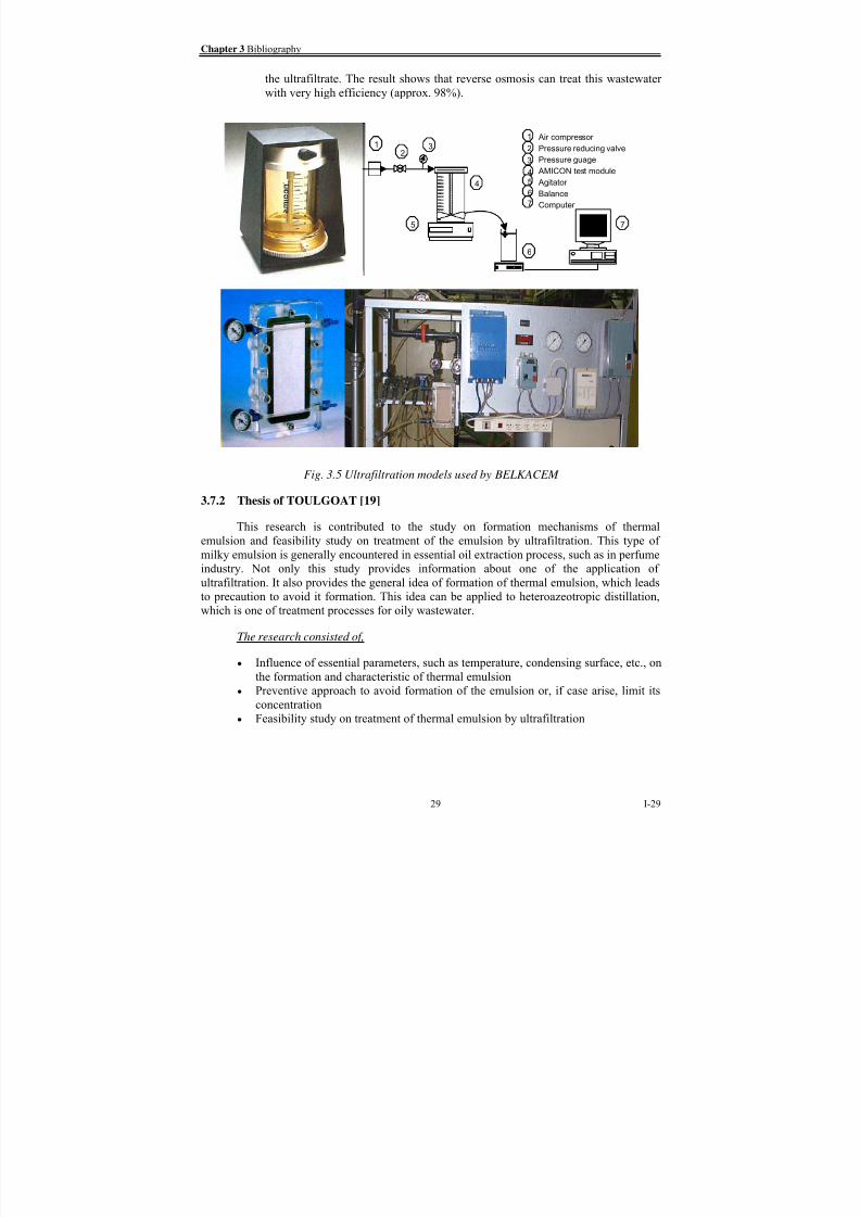
8/15/2019 Rachu.pdf
http://slidepdf.com/reader/full/rachupdf 85/646

8/15/2019 Rachu.pdf
http://slidepdf.com/reader/full/rachupdf 86/646
Part I Introduction and bibliography
30 I-30
Experimental procedure
To study on the entraining of volatile compounds with steam, the author used glass
distillation apparatus, equipped with microscope to observe the condensate. She had tested
several hydrocarbon compounds, such as alcanes with the number of C atoms from 5 to 12
(pentane to dodecane), toluene, benzaldehyde, isobutanol, series of primary alcohols, etc.
To study mechanisms of thermal emulsion formation, hydrodistillation apparatus was
used. It is, in fact, the same device as the first one, with an additional installation of a stirrer.
For the plants used for the experiment, she used several plants, i.e., cinnamon, aniseed, celery,
lavender, etc. Condensate was found in form of decanted essential oil, floating on the top, and
milky thermal emulsion.
For ultrafiltration, she used tubular ceramic membrane of 10 nm. pore size. The
experiment was conducted with membrane test module, model MEMBRALOX T1-70 of SCT
co., ltd. For the emulsion treated, she used synthetic emulsion of kerosene/water as well as
thermal emulsion from extraction of cinnamon, aniseed and celery with various doses ofsurfactants.
Significant findings
1. In this thesis, it shows that the most important parameter in thermal emulsion
formation is the variation of solubility of essential oil with changes in
temperature. She also proposed the minimum variation of solubility that can
cause the formation of thermal emulsion.
2. Condensation time is the important parameter that governs the size distribution
of the emulsion. If the condensation is relatively slow, average diameter of
droplet in the emulsion will increase.
3. The author shows that if the following compounds are present in the essential oil,
thermal emulsion will not be formed;
• Hydrocarbon of high vapor tension
• Hydrophobic hydrocarbon that solubility is not sensitive to temperature
change.
4. To avoid formation of thermal emulsion, she proposed the process called
“hydrodistillation under reduced pressure (sub-atmospheric pressure)”.
5. The study shows that “white water” or milky thermal emulsion, in fact, contains
natural surfactants. So its properties are close to that of stabilized emulsion.
6. Under carefully selected operating condition, ultrafiltration can provide good
separation efficiency between water and essential oil.
3.7.3 Thesis of MATAMOROS [20]
This research is contributed to the study on treatment of stabilized emulsion,
especially cutting oil emulsion, by various membrane processes. This research provides many
useful information and comparison data of several membrane processes.

8/15/2019 Rachu.pdf
http://slidepdf.com/reader/full/rachupdf 87/646
Chapter 3 Bibliography
31 I-31
The research consisted of,
• Feasibility study on the application of various membrane processes for treatment
of cutting oil emulsion, of both macroemulsion and microemulsion types
• Feasibility study on the application of combination processes between one of
membranes and chemical destabilizing process for treatment of cutting oilmacroemulsion and microemulsion
Experimental procedure
The experiment in laboratory scale was conducted with two batch test modules, one
was fabricated in GPI Lab, and another was AMICON test module. For pilot-scale
experiment, the author used cross flow membrane test module, model PLEIADE UFP2 from
Tech Sep co., ltd., for micro- and ultrafiltration process. For nanofiltration and reverse
osmosis, he used test module from OSMONICS.
The membranes used in the research were as tubulated in table 3.3. For emulsions, heused various commercialized cutting oil of macro- and microemulsio typesn.
Table. 3.3 Membranes test by MATAMOROS
Membrane Cut sizeInitial permeate flux
(m.s-1
.pa-1
)Material
Microfiltration 0.10 – 0.45 μm 655 - 125786 Cellulose compounds,
Polyamide and PTFE
Ultrafiltration 40-50 Kda 750*10-12
Polyacrylonitrile,
Acrylonitrile
Nanofiltration 150 – 2000 Da 1.72*10-12
- 20*10-12
Cellulose
Reverse osmosis 150 Da 2.2*10-12
Polyamide
Significant findings
1. The results from this research show that the combination between chemical
destabilization process with micro- or ultrafiltration can increase working
permeate fluxes of the membranes and still obtain good efficiency.
2. For the combination of chemical destabilization and microfiltration, the system
can operate at relatively high flux with moderate transmembrane pressure. Thisleads to development of continuous treatment process of cutting oil because, in
the past, working pressure is always the limiting factor of the process. However,
it requires high amount of salt.
3. For the combination of chemical destabilization and ultrafiltration, the result
conforms to BELKACEM’s [18] that the salt added plays important role, by
double layer compression, and/or adsorption/partial neutralization, in the
reduction of repulsive force and promotion of coagulation and coalescence of
droplets to form a free oil layer. This oil layer can be entrained by recirculation
stream, and then removed at the concentrate storage tank.

8/15/2019 Rachu.pdf
http://slidepdf.com/reader/full/rachupdf 88/646
Part I Introduction and bibliography
32 I-32
4. The permeates from the combination of two processes stated above contain high
concentration of TOD, which is the result of dissolved pollutants, especially co-
surfactants.
5. Combination between ultrafiltration and reverse osmosis shows good result both
in oil separation and dissolved pollutant elimination in permeate. However,
operating cost is relatively high.
6. The use of nanofiltration shows good efficiency result in good oil separation, as
well as dissolved pollutant elimination, at lower energy consumption than
reverse osmosis.
7. From experimental results, the author recommended 2 treatment process trains
for micro- and macroemulsion as shown in fig. 3.6
Microfiltrtion+
CaCl2
Microfiltrtion+
CaCl2
Reverse osmosisor
Nanofiltration
Reverse osmosisor
Nanofiltration
Granular activatedcarbon or
Biological treatment
Granular activatedcarbon or
Biological treatment
EffluentMacroemulsion
Decanter Decanter Decanted oil
Surfactant +
CaCl2
Recycle
Nanofiltration NanofiltrationGranular activated
carbon or
Biological treatment
Granular activated
carbon or
Biological treatment
EffluentMicroemulsion
Surfactant +
Oil
Fig. 3.6 Treatment processes for macro- and microemulsion,
recommended by MATAMOROS
3.7.4 Thesis of SRIJAROONRAT [10]
This thesis is an application research on the treatment of non-stabilized oil/water
emulsion. As one part of her thesis, SRIJAROONRAT had studied on the application of
ultrafiltration to treat non-stabilized emulsion. In her thesis, SRIJAROONRAT had tested
several types of ultrafiltration membranes, i.e., organic, inorganic and ceramic. Wastewater
used in the experiment consisted of synthetic emulsion of kerosene/water, cutting oil
emulsion, crude oil/water emulsion, and wastewater from textile plant. The result can be
summarized as follows.
Significant findings
1. Ultrafiltration process can be used to treat non-stabilized emulsion with
remarkable efficiency (approx. 100%).
2. Major problem of the ultrafiltration is the rapid decrease in permeate flux, caused
by;
• Presence of suspended solids in wastewater, these solids will deposit on the
membrane surface and/or in the pores and cause clogging.

8/15/2019 Rachu.pdf
http://slidepdf.com/reader/full/rachupdf 89/646
Chapter 3 Bibliography
33 I-33
• Presence of surfactant, the surfactant will be adsorbed or form micelles
within the membrane pores, as well as membrane surface, thus cause
changing in wettability of membrane.
3. Influence of surfactant on permeate flux also depends on material of membrane.
Inorganic (mineral) based membrane is more sensitive to surfactants than other
membranes.
3.7.5 Thesis of WANICHKUL [11]
This thesis is an application research on the treatment of stabilized oil/water emulsion.
WANICHKUL had studied on the application of ultrafiltration on cutting oil emulsion
treatment. He also studied on the treatment of ultrafiltrate by reverse osmosis.
Significant findings
1. The result on the treatment of cutting oil emulsion by ultrafiltration confirms the
result of MATAMOROS that the process is feasible and efficiency of the processis satisfying. The author recommended that operating condition should be in
permanent regime to avoid influence of concentration factor.
2. Using microemulsion with under-saturated oil concentration is an effective
method to regenerate the membrane.
3. The author had studied the efficiency of reverse osmosis on ultrafiltrate
treatment. The result shows that the process provides remarkable efficiency.
4. The result of the comparison on efficiency between ultrafiltration and distillation
on cutting oil emulsion treatment can be concluded that ultrafiltration is suitable
for macroemulsion treatment, while distillation is more efficient for
microemulsion treatment. However, from economic point of view, energyconsumption of ultrafiltration is always lower than distillation’s.
3.8 Thermal treatment
This treatment approach makes use of physical properties of hydrocarbon, water and
their mixture. Because hydrocarbon is only slightly soluble in water, we can say that the
hydrocarbon/water mixture is practically an immiscible binary system. From this fact, we can
apply the basic of phase equilibrium to develop thermal processes for hydrocarbon/water
separation. Such processes are distillation and crystallization. All related theses based on
thermal treatment can be outlined as follows.
3.8.1 Thesis of LUCENA[24]
This research is contributed to the heteroazeotropic distillation for treatment of slop,
the wasted viscous water-in-petroleum emulsion that is usually very difficult and costly to
treat. This process is very interesting innovation that allows hydrocarbon recovery by
separating from water from the slop. Certain type of hydrocarbons, considered as efficient
water extractant or entrainer, is added to the slop, then the slop undergoes distillation to
extract the water. After distillation, the distillate obtained is composed of 2 layers of clear
liquid, the entrainer in the upper layer and the water at the lower. The water can be disposed
or further treated and the entrainer can be reused for next cycle of distillation. The residue
obtained is relatively fluid, contains no water, and can be recycled to refinery unit as crudeoil.

8/15/2019 Rachu.pdf
http://slidepdf.com/reader/full/rachupdf 90/646
Part I Introduction and bibliography
34 I-34
Experimental procedure
The experiment in laboratory scale was conducted with a simple glass distillation
apparatus. The author also used the pilot-scale model for on-site treatment tests.
Significant findings
1. The result on the treatment of slop shows that the water is totally separated from
the slop. The residue consists of relatively water-free hydrocarbon. Distillate
consists of 2 separate layers of entrainer and water.
2. Observed quantity of entrainer is slightly different (5-8%) from theoretical value.
So the theoretical method for calculating entrainer quantity is accurate enough
for practical use.
3. Kerosene and gasoline are proven to be good entrainer. Their water-extracting
capacities are almost identical to that of decane and dodecane, respectively.
3.8.2
Thesis of LORRAIN[23]
This research is contributed to crystallization. However, this process has just been
studied by GPI lab for the first time. So we will not include it in this research.
3.8.3 Thesis of WANICHKUL [11]
This thesis is an application research on the treatment of stabilized oil/water emulsion.
WANICHKUL had studied on the application of distillation for the treatment of cutting oil
emulsion and permeate from ultrafiltration. He also studied the possibility to treat concentrate
from ultrafiltration of cutting oil emulsion by heteroazeotropic distillation.
Significant findings
1. Comparison on the efficiency between ultrafiltration and distillation on cutting
oil emulsion treatment, the author concluded that ultrafiltration is suitable for
macroemulsion treatment, while distillation is more efficient for microemulsion
treatment. However, from economic point of view, energy consumption of
ultrafiltration is always lower than distillation’s.
2. Heteroazeotropic distillation is proven to be an effective way to treat
“mayonnaise-like” retentate from the ultrafiltration of cutting oil emulsion. The
residue of distillation process is clear liquid, composed of oil without water. Thedistillate consists of 2 separate layers of the entrainer (in this case, decane) on the
top and the water at the bottom. However, TOD of the distillate is still high
(around 2,800 mg/l). So the additional treatment of the distillate (either by
biological treatment or RO) is required.
3.9 Chemical treatment
When we talk about chemical treatment in oil/water separation process, we normally
refer to chemical destabilization, coagulation and flocculation. The process, then, does not
“destroy” oil. Its major role is to transform the oil into the form that facilitates oil/water
separation. So, chemical treatment process usually follows by physical separation processes aswe discussed in previous sections. Normally, chemical treatment will be required when oil or

8/15/2019 Rachu.pdf
http://slidepdf.com/reader/full/rachupdf 91/646

8/15/2019 Rachu.pdf
http://slidepdf.com/reader/full/rachupdf 92/646
Part I Introduction and bibliography
36 I-36
• Mono-valence cationic electrolyte, main destabilization mechanisms are
based on Zeta potential reduction and promoting micelle formation of
surfactants.
• Bi-valence cationic electrolyte, main destabilization mechanism is based on
precipitation of surfactant to insoluble form.
• Tri-valence cationic electrolyte, main destabilization mechanisms are basedon the bridging of its cations and hydroxides and precipitation of surfactant
to insoluble form.
2. The result shows that destabilization techniques of fresh macroemulsion can also
be effective for used macroemulsion.
3. For breaking emulsion by acid, the study shows that destabilization mechanisms
for micro- and macroemulsion are different, based on type of surfactant used in
the emulsions.
• For microemulsion- surfactant used is soap. So it is sensitive to pH change.
Then, addition of acid will disturb the equilibrium of ionization of fatty acid
and make it lose its surfactant property. This type of destabilization requires
relatively small amount of acid.
• For macroemulsion- surfactant used is sulfonate type. Main destabilization
mechanisms are based on Zeta potential reduction and promoting micelle
formation of surfactants. So it requires high dosage of the acid.
4. Ferric chloride is an effective destabilization chemical for breaking
macroemulsion. However, it cannot be used to breaking microemulsion because
it will react with surfactants and form complex, which is difficult to separate.
5. High residual pollution which presents after breaking the emulsion is caused by
co-surfactant, which is fatty acid that dissolves very well in water.
6. To destabilize the emulsion stabilized by non ionic surfactant, the author
recommended to use a mixture of anionic surfactant and tri-valence electrolyte
(Alum, FeCL3) as destabilization reagent. Main breaking mechanism is based on
selective reaction between non-ionic surfactant, anionic surfactant and
electrolyte, which form insoluble complexes.
7. Breaking mechanisms of commercial adsorption reagents are based on their
components. So, their efficiencies will be known only by testing.
8. Activated carbon adsorption is proven to be an effective treatment for residual
pollution which is left after breaking the emulsion. However, investment and
operating costs of this system, esp. cost for regeneration or replacement, arerelatively high.
9. The author had proposed, for the first time, to replace fatty acid co-surfactant
with other surfactant with less water solubility to solve the problem about
residual pollutant after breaking the emulsion. In his case, he used decanol,
which is slightly soluble in water, as a co-surfactant. The new emulsion has
satisfying property. But vigorous mixing by ultrasound device is required to
disperse the oil into droplets to create the emulsion.
10. He suggested that new formula of this low pollution emulsion should be further
studied to make it soluble instantly in water, which is the way the users prefer.
8/15/2019 Rachu.pdf
http://slidepdf.com/reader/full/rachupdf 93/646
Chapter 3 Bibliography
37 I-37
3.9.2
Thesis of YANG[22]
This research is a succession of ZHU’s thesis and contributed to development of low
pollution emulsion. This thesis was a new approach in pollution control because it was one of
the first researches on pollution reduction from the source, as it is presently called “cleaner
product, CP” research, which is the branch of pollution control that is well-known and widelyacceptable now.
The research consisted of,
• Study on the formulation of low pollution cutting oil emulsion
• Study on the treatment process of that new emulsion
Experimental procedure
The author had tried to formulate low pollution cutting oil emulsion, using carefully
selected base components, i.e.,
• Base oil: commercial naphthene (cyclic aliphatic compound) based oils and
paraffin based oils,
• Surfactants: various succinic and sulfonate surfactants,
• Co-surfactants: alcohol-based, ester-based, and other co-surfactants with low water
solubility,
• Corrosion inhibitors: fatty acid alcanolamide, oleylsarcosinic acid, and fatty acid
polydiethanolamide,
• Anti-mousse reagents: polysiloxane and a commercial reagent,
• Bactericides: 4-chloro-3methylphenol, isothiazolinone, and parahydroxybenzoic
ester with phenoxyethylic alcohol,
Each emulsion formula was subjected to these 5 tests, i.e.,
• Droplet size distribution measurement: using particle analyzer (granulometer)
• Emulsification test: new products were diluted by water to observe its solubility
and stability.
• Anti-rust test: new emulsions of various concentrations were used to coat on steel
chip and rust forming was observed.
• Anti-mousse test: new emulsions were manually and intensely agitated and
characteristic and stability of mousse were observed.
• Determination of residual pollutant after chemical destabilization process or
ultrafiltration.
Significant findings
1. The author proposed new formulae of low-residual-pollutant microemulsions
and macroemulsions.
2. These new emulsions can be treated efficiently by breaking with calcium
chloride or ultrafiltration. Residual pollution after treatment is 2-57 times lower
than present commercial products.
3. Concentration of emulsion and hardness of dilution water are important
parameters, which affect stability of emulsion.

8/15/2019 Rachu.pdf
http://slidepdf.com/reader/full/rachupdf 94/646
Part I Introduction and bibliography
38 I-38
3.10 Biological treatment
Biological treatment is the most common wastewater treatment process. Because of its
versatile, efficiency and economic, biological treatment plants are widely used for both
domestic and industrial wastewater treatments. Its working principles depend mainly on
degradation and/or assimilation of pollutants by microorganisms, so called “biomass”, presentin the biological reactor. Key to obtain satisfying treatment efficiency is to optimize the
environment in the reactor to promote function of biomass. Even though oil or hydrocarbons
are biodegradable, presence of some hydrocarbons at some concentrations can cause adverse
effect on the biological treatment mechanisms by;
• Obstructing oxygen transfer: Oxygen content is an important factor in aerobic
biodegradation. Oil layer that covers water surface will obstruct transfer of oxygen
between air and water. Oil may surround biomass floc and impede oxygen transfer
of the floc in biological reactor. This leads to the decrease in treatment efficiency.
• Its high oxygen demand: Oil requires high amount of oxygen for biodegradation. It
will cause problem on insufficient aeration capability in some treatment plants that
did not account for this type of pollutant in the design procedure. It also increases
investment cost and operating cost for aeration system.
• Its toxicity: In petroleum product or industrial oil-based product, they, sometime,
contain toxic substance, such as sulfide, heavy metals, which may be added to the
oil product in form of inhibitor or additive to provide desired product properties.
When these products are discharged to water and become wastewater, these
substance will become toxicity to living water organisms, includes biomass.
There are many studies, includes some from our lab, on the effect of oil contents in
wastewater to biological treatment process and possibility or optimum condition to use biological treatment to treat oily wastewater. However, none of doctoral thesis, directed by
M.Aurelle, is fully devoted to biological treatment of oil wastewater. So we will work on this
process by reviewing the available data from our lab researches as well as outside data.
Anyway, only our lab researches will be summarized here. Synthesized result from reviewing
will be presented as a section of textbook in Part 3 of this thesis.
3.10.1
Thesis of WANICHKUL [11]
This all-purpose thesis is also contributed to biological treatment. The author had
performed biodegradability test of permeate from ultrafiltration of cutting oil emulsion.
Significant findings
1. The study shows that ultrafiltrate of cutting oil emulsion can be treated by
aerobic biological process. The result from biodegradability test shows very high
TOC reduction efficiency (82 to 90% at the retention time of 2 to 5 hours).
3.11 Skimmer
When hydrocarbon is in the form of layer on water surface. It can be simply removed
from the surface by mean of overflow weir, overflow pipe or be scooped out manually. There
is one thesis on skimmer, which is the thesis of THANGTONGTAWI [5]. This research is
8/15/2019 Rachu.pdf
http://slidepdf.com/reader/full/rachupdf 95/646
Chapter 3 Bibliography
39 I-39
contributed to study on oil drum skimmer and disk skimmer, which are very effective to
recover film or layer of oil or hydrocarbon on the surface of water.
The research consisted of,
• Influence of skimming materials, geometry of devices and characteristic ofwastewater to skimmer operation
• Model development for oil drum and disc skimmer
• Behavior of skimmers under interesting working conditions, which may affect its
efficiency
Experimental procedure
The experiment was conducted with various sizes of disc and drum skimmers to verify
effect of skimmer geometry. Various types of skimming material were tested, i.e., stainless
steel, PVC, polypropylene and fluorocarbon coated material. Kerosene and 2 types of
lubricant oil, as well as real wastewater from 4 refineries, were used in the experiment. Effecton interfacial tension was also considered by varying concentration of a commercial
surfactant.
Result
The result of this study provides models for sizing and calculating oil quantity,
recovered by the skimmers. The study, also, provides significant criteria for skimmer material
selection to obtain selective property, which allow the devices to recover only oil, not water.
Design consideration, such as limitation of model, working condition to be avoided, etc. is
included in this study.
Significant findings
1. In this thesis, mathematical models for sizing and calculating oil productivity of
the skimmer are proposed.
2. Influence of skimming material is studied and can be summarized as follow,
• Material of high surface energy, such as stainless steel, which is conditioned
by submerging in oil, will effectively recover or separate the oil from water.
However, when oil film on the surface of the tank is broken and the skimmer
is exposed to water, it will start recover the water immediately. Even after the
oil layer is present again, it will not resume its function of oil recovering.
• Material of low surface energy, such as PVC and PP, can effectively recover
oil. But it will start recovering water after the oil film is broken and the
skimmer is allowed to expose to the water surface for some times. Anyway,
it will resume its function after the presence of oil layer.
• From the study, fluorocarbon coated material, which is patented by ELF, is
the best oil-water selectivity. It always recovers only oil.
3.12 Application researches
To apply treatment processes previously described in real life situation, our lab had
performed some researches that devoted to compare the efficiency of various stand-alone
processes or combination of processes on treatment of certain type of oily wastewater. This

8/15/2019 Rachu.pdf
http://slidepdf.com/reader/full/rachupdf 96/646

8/15/2019 Rachu.pdf
http://slidepdf.com/reader/full/rachupdf 97/646
Chapter 3 Bibliography
41 I-41
3. Influence of surfactant on permeate flux, also, depends on material of membrane.
Inorganic (mineral) based membrane is more sensitive to surfactants than other
membranes.
4. Backflushing the membrane with its permeate is proven to be an effective way to
increase the limiting flux. The result shows that duration of ultrafiltrating and
backflushing cycle should be optimized to obtain best efficiency. Normally, the 2cycles is preferred to be short.
5. At high empty bed velocity, the coalescer with random bed will coalesce and
enlarge the droplets into relatively large drop, while the coalescer with brush
type bed tends to produce stream of jet, containing small oil drop.
6. However, the disorderly fibrous (steel wool) bed coalescer tends to be clogged
by suspended solids, usually presence in the oily wastewater. So the author
proposed new configuration of fibrous bed in form of the combination of 2
brushes. The internal one is of ordinary brush. The external one will look like
coil spring with its fiber elements protruding inward and toward the center. This
type of bed is believed to provide good interception, similar to the disorderly
bed, yet remain its anti-clogging properties, like brush-type bed.
7. Combination between coalescer/ hydrocyclone is proven to provide good
efficiency on the wider range of feed flowrate and size of oil droplet.
3.12.2 Thesis of WANICHKUL [11]
This thesis is an application research on the treatment of stabilized oil/water emulsion,
one of the most encountered oily wastewaters. The author also extended the research of
SRIJAROONRAT [10] on the combination of coalescer and hydrocyclone by studying the
influence of order of the 2 processes. So, WANICHKUL tested both combinations ofcoalescer/hydrocyclone and hydrocyclone/coalescer as well as the combination on
coalescer/hydrocyclone/coalescer.
The research consisted of,
• Study on treatment of stabilized emulsion by ultrafiltration and distillation
• Study on treatment of permeate from ultrafiltration by reverse osmosis, biological
treatment and distillation
• Study on treatment of retentate from ultrafiltration by heteroazotropic distillation
• Study on treatment of non-stabilized emulsion combination of coalescer/
hydrocyclone and hydrocyclone/coalescer• Study on multi stage fibrous bed coalescer
Experimental procedure
The experiment on ultrafiltration was conducted with 3 models, i.e. commercial batch
test module (effective area 37 cm2), lab scale cross flow model (effective area 100 cm2) and
pilot scale cross flow model (effective area 1 m2). For reverse osmosis, he used commercial
test module from OSMONIC co., ltd.
The stabilized emulsions tested consisted of 2 commercial cutting oil emulsions, 1
macroemulsion and 1 microemulsion. For membrane regeneration, he used the microemulsion

8/15/2019 Rachu.pdf
http://slidepdf.com/reader/full/rachupdf 98/646

8/15/2019 Rachu.pdf
http://slidepdf.com/reader/full/rachupdf 99/646

8/15/2019 Rachu.pdf
http://slidepdf.com/reader/full/rachupdf 100/646
Part I Introduction and bibliography
44 I-44
Chapter 4 Conclusion
In this part, we have reviewed all of the researches in our lab, directed by Professor
AURELLE. We can see the attempts to study many aspects of treatment processes to cope
with various type of oily wastewater. The results of each thesis make us understand working
principles and limitation of the processes in many specific cases or frameworks. In the next part, we will analyze these specific data from these theses. And then try to integrate and
generalize them to formulate design criteria or mathematical models that can be used with the
entire (or as wide as possible) range of oily wastewater.
8/15/2019 Rachu.pdf
http://slidepdf.com/reader/full/rachupdf 101/646
Part II Generalization of models for
oil-water separation process design
8/15/2019 Rachu.pdf
http://slidepdf.com/reader/full/rachupdf 102/646
Part II Generalization of models for oil-water separation process design
II-i
Contents
Page
Part II Generalization of models for oil-water separation process design
Chapter 1 Decanting
1.1 Simple decanter or API tank II-2
1.2 Lamella decanter or Parallel Plate Interceptor (PPI) II-3
1.3 Model verification II-4
1.4 Conclusion and generalized model of decanter II-7
Chapter 2 Skimmer
2.1 Drum skimmer II-9
2.2 Disk skimmer II-10
Chapter 3 Coalescer
3.1
Granular bed coalescer II-113.1.1 Filtration-based model II-11
3.1.2 Dimensional analysis-based model II-12
3.1.3 Model verification II-13
3.1.4 Conclusion and generalized model of granular bed II-14
coalescer
3.1.5 Generalized model for guide coalescer II-15
3.1.6 Generalized model for mixed bed coalescer II-16
3.1.7 Generalized model for pressure drop of granular bed II-16
coalescer and guided coalescer
3.2 Fibrous bed coalescer II-18
3.2.1
Dynamic fibrous bed coalescer model II-183.2.2
Simple fibrous bed coalescer model II-18
3.2.3 Model verification II-18
3.2.4 Conclusion and generalized model of fibrous bed coalescer II-21
3.2.5 Generalized model of random or disorderly fibrous bed II-23
coalescer
3.2.6 Generalized model for pressure drop of fibrous bed II-24
coalescer
Chapter 4 Dissolved air flotation
4.1
Dissolved Air Flotation (DAF) model for oily wastewater II-25
treatment4.2 Model verification II-26
4.2.1 Modification of filtration-based model II-26
4.2.2 Population balance method II-28
4.3 Generalized model for DAF II-30
4.4
Generalized equations for pressurized water system calculation II-35
Chapter 5 Hydrocyclone
5.1 Two-phase hydrocyclone II-37
5.1.1
Trajectory analysis-based model II-37
5.1.2 Other models II-38
5.1.3
Model verification II-39

8/15/2019 Rachu.pdf
http://slidepdf.com/reader/full/rachupdf 103/646

8/15/2019 Rachu.pdf
http://slidepdf.com/reader/full/rachupdf 104/646
Part II Generalization of models for oil-water separation process design
II-iii
Table
Page
Table 1.1 Summary of tested decanters and operating conditions II-6
Table 6.1 Summary of parameters of resistance model from UF researches on II-51
oilywastewater treatment (reference temperature = 20O C)
Table 6.2 Summary of parameters of film model from UF researches on oily II-54
wastewater treatment (reference temperature = 20O C)
Table 6.3a Summary of RO data on oily wastewater treatment II-67
Table 6.3b Summary of NF data on oily wastewater treatment II-68
Table 7.1 Heterotropic temperature and composition from various extractants II-72

8/15/2019 Rachu.pdf
http://slidepdf.com/reader/full/rachupdf 105/646
Contents
II-iv
Figure
Page
Fig. 1.1 Schematic and typical removal efficiency curve of simple decanter II-3
Fig. 1.2 Schematic of PPI decanter II-4Fig. 1.3 “Spiraloil” decanter a) Simple spiral b) Mixed spiral II-5
Fig. 1.4a Comparison between observed efficiency (1',2',3') and predicted II-6
efficiency (1,2,3) for Simple Spiral "Spiraloil" decanter
Fig. 1.4b Comparison between observed efficiency (1',2') and predicted II-6
efficiency (1,2) for Mixed Spiral "Spiraloil" decanter
Fig. 2.1 Drum and disk skimmer II-10
Fig. 3.1(a) Schematic diagram of granular bed coalescer, (b) photo of bed material II-11
with coalesced oil on their surface and (c) coalesced oil drops at the
discharge surface of bedFig. 3.2a Relation between droplet diameter VS. model's error II-14
Fig. 3.2b Comparison between observed efficiency and predicted efficiency from II-14
DAMAK's model
Fig. 3.3 Relation between observed pressure drop of granular bed coalescer and II-17
predicted upper & lower limits from Kozeny-Carman's porosity = 0.13 and 0.23
Fig. 3.4 Comparison between observed efficiency and predicted efficiency from II-19
SRIJAROONRAT's model, Verified by MA's and WANICHKUL's data
Fig. 3.5 Comparison between observed efficiency and predicted efficiency by II-
20TAPANEEYANGKUL's model for simple fibrous bed (Assume rotating speed = 450
rpm)
Fig. 3.6 Comparison between observed efficiency and predicted efficiency from II-21
modified SRIJAROONRAT's model (eq. 3.8b)
Fig. 3.7 Relation between observed efficiency and predicted efficiency from random II-23(or
disorderly) fibrous bed coalescer model and simple fibrous bed model
Fig. 4.1 Schematic diagram of DAF II-25
Fig. 4.2 Relation between theoretical efficiency factor and observed efficiency II-27
factorFig. 4.3 Relation between obseved efficiency and predicted efficiency of DAF II-27
from modified SIEM's model
Fig. 4.4 Relation between absolute pressure in pressure tank and dissolved quantity II-36
and released air volume
Fig. 5.1 Schematic diagram and trajectories of droplets in two-phase hydrocyclone II-37
Fig. 5.2 Comparison between observed efficiency and predicted efficiency from II-39
Ma's and Thew-Colman's models
Fig. 5.3a Relation between observed pressure drop (inlet/overflow) of Thew cyclone II-42
and predicted pressure drop

8/15/2019 Rachu.pdf
http://slidepdf.com/reader/full/rachupdf 106/646
8/15/2019 Rachu.pdf
http://slidepdf.com/reader/full/rachupdf 107/646
Part II Generalization of model for oil-water separation process design
II-1
Part 2 Generalization of model for oil-water separation process design
In this part, the models or researches collected and summarized in the part I are
analyzed and then generalized to obtain the model or models that governs the entire range (or
as wide as possible) of oily wastewater that we are interested in. Basic concept of each model
is briefly described here providing that it will be fully described in the next part. Then themodels and their limitations will be presented. After that, models will be tested using various
sets of data to cover the considered range of wastewater. Finally the generalized model will
then be proposed.
45

8/15/2019 Rachu.pdf
http://slidepdf.com/reader/full/rachupdf 108/646
Chapter 1 Decanting
II-2
Chapter 1 Decanting
Decanting or sedimentation is a non-accelerated process, which every input
parameters in STOKES law are not modified. According to the researches reviewed in Part I,
there are several types of decanters studied in GPI laboratory, i.e.,
1.1 Simple Decanter or API tank
Simple decanter, which is made well known and standardized by American Petroleum
Institute (API), is the simplest oil-water separation process based on classical STOKES law.
Concept of operation of the process is to provide sufficient time for droplets to float to the
surface, where it will accumulate into oil layer, before it flows out with the water at the water
outlet.
The model that governs the operation of the process is derived from comparing the
time required for the droplet to reach the surface with retention time of the tank. Fig. 1.1
shows again the diagram of decanting process. From the figure, the longest path to reach thesurface is the path starts at the bottom of the tank. The smallest droplet size that can reach the
surface is called the cut size. The droplet of cut size or bigger is always separated from
wastewater stream with 100% removal efficiency.
The smaller droplet can be also separated providing that it enters the tank near the
water surface. When uniformly distributed influent flow is valid, which is true for almost all
of properly designed tank, the removal efficiency of the droplets smaller than cut size is
proportional to its corresponding rising velocity. From these concepts, the models of
decanting process are as shown in eq. 1.1 to 1.4.
⎟ ⎠
⎞⎜⎝
⎛ = S
Q
dcU {1.1}
From STOKES law
c18μ
2dgΔρ
dU
⋅⋅= {1.2}
Then1/2
SgΔρ
c18Qμcd ⎟⎟
⎠
⎞⎜⎜⎝
⎛
⋅⋅= {1.3}
For oil droplet size, d ≥ cut size,dc
100%d
η = {1.4a}
For oil droplet size, d ≤ cut size,dc
100%
dcU
dU
dη ⋅= {1.4b}
( ) 100%maxd
mind od
Cd
η1
tη ⋅∑ ⋅=
oC
out Q
Q {1.4c}
∑−=max
min
d
d
od d
d
out C QQQ η ρ
{1.4d}
46

8/15/2019 Rachu.pdf
http://slidepdf.com/reader/full/rachupdf 109/646
Part II Generalization of model for oil-water separation process design
II-3
U
V
Q
d = cut size
d < cut size
d > cut sizeInfluent Effluent
d
ηd
d c
d < d c
Zone 1 Zone 2
d = or > d c
Fig. 1.1 Schematic and typical removal efficiency curve of simple decanter
Typical characteristic of the removal efficiency of decanter is as shown in fig. 1.1. The
equations are valid while these conditions are satisfied i.e.,
1.
Reynolds number, Re, of droplet is between 10-4 to 1, which is the range that
STOKES law is valid.
2. The oil droplets are uniformly distributed across the cross section area of the
tank.
3. The oil droplet is spherical, which is normally true.
1.2 Lamella Decanter or Parallel Plate Interceptor (PPI)
This type of decanter is the basic modification of the simple decanter. The concept is
to decrease the rising distance of droplet to intercepting surface without decreasing the
retention time. This can be achieved by inserting plates into the simple decanter to act as the
interceptors for the rising oil droplets. Rising or travelling distance (H) is the distance
between the plates, not the depth of water (D) as shown in fig. 1.2. Some times, the plates are
inclined with angle (α) as related to horizontal axis. In this case, rising distance will becomeH / cos α.
The model that governs the operation of the process is modified from the model of
simple decanter, as shown in eq. 1.5. From the equation and figure, it can be implied that the
simple tank is divided into (N+1) small decanters.
47
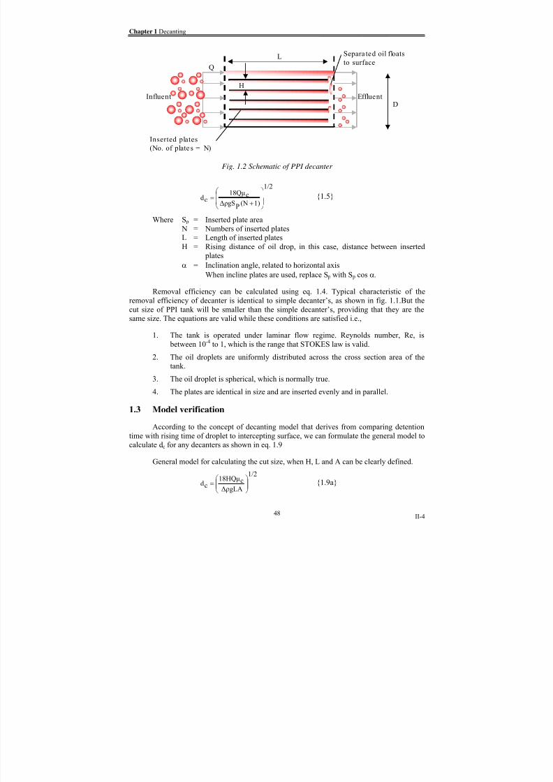
8/15/2019 Rachu.pdf
http://slidepdf.com/reader/full/rachupdf 110/646

8/15/2019 Rachu.pdf
http://slidepdf.com/reader/full/rachupdf 111/646
Part II Generalization of model for oil-water separation process design
II-5
Where Q = Wastewater flowrate
H = Rising distance of oil drop, depends on configuration of the decanter
L = Length of interceptor surface
A = Flow area (Cross sectional) area of decanter
Removal efficiency can be calculated using eq. 1.4. From the equations, we can seethat the models of simple decanters and PPI are modified forms of eq. 1.9 by simple relations
of flow velocity and tank geometry. However the models described before are derived from
basic rectangular tank and flat insertion plates.
But, in real life situation, decanters are designed or produced in various forms, such as
corrugated plate inserted tank, concentric annular insertion decanter, etc. So, sometimes, it is
very difficult to define H. Then, we propose to simplify the general model by neglecting
complicate analyzing to define H, and using concept of decanting area (Sd) instead. Sd is
calculated from the sum of every surface area within the decanter that can intercept oil
without considering whether the values H of these areas are identical or not. The other form
of general model is shown in eq. 1.9b.
1/2
dSgΔρ
c18Qμcd
⎟⎟
⎠
⎞
⎜⎜
⎝
⎛
⋅⋅= {1.9b}
To verify the theoretical model, we select the research of CHERID [4] on 2 sets of the
“SPIRALOIL” decanter, i.e.,
• “Simple Spiraloil”; fabricated from concentric annular plates as shown in fig. 1.3a
• “Mixed-spiral Spiraloil”; ”; fabricated from concentric annular plates with
corrugated plates spacer as shown in fig. 1.3b
We will use these decanters to compare the removal efficiency calculated from model
to experimental result from the research. Geometry of the decanter and operating parameters
used in the experiment are summarized in Table 1.1 and Annex A1.
Solid core,
radius = r
R
H
e
Annular plates
a) b)
Fig. 1.3 “Spiraloil” decanter a) Simple spiral b) Mixed spiral
49

8/15/2019 Rachu.pdf
http://slidepdf.com/reader/full/rachupdf 112/646
Chapter 1 Decanting
II-6
Table 1.1 Summary of tested decanters and operating conditions
Description Simple spiral “Spiraloil” Mixed spiral “Spiraloil”
Geometry
Nominal radius R (mm) 50 50
Core radius r (mm) 10 10
Length of decanter L (mm) 300 300
Total length of inserted plates (m) 3.88 N/A
Spacing between concentric annular plate (mm) 2 3
Plate thickness (mm) 0.3 0.2 for annular plates0.4 for corrugated plates
Interceptor (decanting) area (m2) 1.66 2.1
Inclination of decanter Horizontal Horizontal
Operating conditions
Flow velocity (cm/s) 0.4-1.6 0.5-1.5
(m/h) 14.4-57.6 18-54
Wastewater used Kerosene-water mixture Kerosene-water mixture
0.00%
10.00%
20.00%
30.00%
40.00%
50.00%
60.00%
70.00%
80.00%
90.00%
100.00%
0 10 20 30 40 50 6
Droplet diameter (micron)
R e m o
v a l e f f i c i e n c y ( % )
0
1'1 3'
2 2'
3
V = 1.6 cm/s (3, 3')
V = 0.8 cm/s (2, 2')
V = 0.4 cm/s (1, 1')
Fig. 1.4a Comparison between observed efficiency (1',2',3') and predicted efficiency (1,2,3) for Simple Spiral "Spiraloil" decanter
0.00%
10.00%
20.00%
30.00%
40.00%
50.00%
60.00%
70.00%
80.00%
90.00%
100.00%
0 10 20 30 40 50 6
Droplet diameter (micron)
R e m o v a l e f f i c i e n c y ( % )
0
1 (V = 0.5 cm/s)1'
2' 2 (V = 1.5 cm/s)
Fig. 1.4b Comparison between observed efficiency (1',2') and predicted efficiency (1,2) for Mixed Spiral "Spiraloil" decanter
50

8/15/2019 Rachu.pdf
http://slidepdf.com/reader/full/rachupdf 113/646
Part II Generalization of model for oil-water separation process design
II-7
Comparison graphs between observed efficiency and predicted efficiency from model
for both Spiraloil decanters are shown in fig. 1.4. These graphs show that;
1.
Predicted values for cut size are relatively accurate.
2.
Predicted efficiencies of the droplets smaller than cut size are always lower than
observed value because, in our simplified model, coalescing between rising oildrops is not accounted. Furthermore, in case that the plates are placed very close
to each other like in “Spiraloil”, oil film will accumulated at the surface of plate,
then helps reducing rising height oil droplet, thus increasing the efficiency.
3.
Correction factor for efficiency prediction of these small droplets may not be
established accurately. However, the predicted cut size can be used to design the
tank with relative high accuracy. So it is reasonable to select the cut size to cover
the majority of droplet size distribution. The predicted efficiency of smaller
droplets, which is the minority part, will cause no harm but slightly
underestimation on the total efficiency.
1.4 Conclusion and Generalized Model of decanter
From model verification result, we can conclude and propose the generalized model,
as well as, its limitation as follows,
1.
To solve oil or hydrocarbons removal efficiency of decanter, the cut size of the
decanter will be determined first. Then, graded efficiency (efficiency of each size
of droplet) and then total removal efficiency can be determined.
2. The cut size of the decanter can be determined from eq. 1.9. When configuration
of decanter is not complicate and rising distance of oil drop to interceptor can be
clearly determined, Using eq. 1.9a will give very accurate prediction. However,when configuration of the decanter is so complicate to determine the rising
distance accurately, eq.1.9b provides relatively accurate result for the cut size.
For PPI tank, the cut size can be calculated from eq. 1.5, which is the modified
form of eq. 1.9a.
1/2
ΔρgLA
c18HQμcd ⎟⎟
⎠
⎞⎜⎜⎝
⎛ = {1.9a}
1/2
dSgΔρ
c18Qμ
c
d
⎟
⎟
⎠
⎞
⎜
⎜
⎝
⎛
⋅⋅= {1.9b}
1/2
1)(NP
ΔρgS
c18Qμcd
⎟⎟
⎠
⎞
⎜⎜
⎝
⎛
+= {1.5}
3.
To determine graded and total removal efficiency, use eq. 1.4.
For oil droplet size, d ≥ cut size, dc
100%d
η = {1.4a}
51

8/15/2019 Rachu.pdf
http://slidepdf.com/reader/full/rachupdf 114/646
Chapter 1 Decanting
II-8
For oil droplet size, d ≤ cut size,dc
100%
dcU
dU
dη ⋅= {1.4b}
For total removal efficiency
( ) 100%maxd
mind od
Cd
η1
tη ⋅∑ ⋅⋅⋅=
oC
out Q
Q {1.4c}
∑−=max
min
d
d
od d
d
out C Q
QQ η ρ
{1.4d}
4. To use the models described above, the following conditions need to be satisfied
and the assumptions and limitations would be noted.
1) Reynolds number, Re, of oil droplet is between 10-4 to 1, which is the range
that STOKES law is valid.
2) The oil droplets are uniformly distributed across the cross section area of
the tank, which can be achieved by proper design of inlet chamber. And the
oil droplet is spherical, which is normally true.
3) For PPI or others forms of plate inserted decanter, the plates are identical in
size and are inserted evenly and horizontally. For PPI tank with incline
plates, S p in eq. 1.5 will be replaced by S p cos α. α is the inclination angle,
related to horizontal axis.
4) If the decanter or the inserted plates are inclined, the rising distance will be
the spacing between plates, but will be measured in vertical direction. Sothe shortest distance is obtained from the same spacing between plates,
when the plates are located horizontally.
5)
Prediction of cut size from eq.1.9b, even with its simplification, is
relatively accurate for the cut size larger than 20 microns.
6) For droplets smaller than 20 microns, they are subject to Brownian motion
and cause error in the prediction of the efficiency. So it is recommended to
avoid using the decanter for the wastewater with majority part of oil
droplets smaller than 20 microns. However, if these small droplets are the
minority part of pollutants, the models can be used to predict the efficiency
without any harm because its prediction is usually lower than observedvalue, thus make the prediction result on the safe side.
52

8/15/2019 Rachu.pdf
http://slidepdf.com/reader/full/rachupdf 115/646

8/15/2019 Rachu.pdf
http://slidepdf.com/reader/full/rachupdf 116/646

8/15/2019 Rachu.pdf
http://slidepdf.com/reader/full/rachupdf 117/646

8/15/2019 Rachu.pdf
http://slidepdf.com/reader/full/rachupdf 118/646

8/15/2019 Rachu.pdf
http://slidepdf.com/reader/full/rachupdf 119/646

8/15/2019 Rachu.pdf
http://slidepdf.com/reader/full/rachupdf 120/646
Chapter 3 Coalescer
II-14
-30%-20%-10%
0%10%20%30%40%
50%60%70%80%90%
100%
0.0E+00 5.0E-06 1.0E-05 1.5E-05 2.0E-05 2.5E-05 3.0E-05 3.5E-05 4.0E-05 4.5E-05
Droplet diameter (m)
E r r o r ( %
)
DAMAK's model AURELLE's model
Fig. 3.2a Relation between droplet diameter VS. model's error
0%
10%
20%
30%
40%
50%
60%
70%
80%
90%
100%
110%
0% 10% 20% 30% 40% 50% 60% 70% 80% 90% 100%
Observed efficiency %
P r e d
i c t e d e f f i c i e n c y %
ηd = 58 (dE/dp)0.2
(H/dp)0.12
(ρc dp V2/γo/w )
-0.08(μd/μc)
0.09(Δρ/ρc)
0.09
-10%
+10%
Fig. 3.2b Comparison between observed efficiency and predicted efficiency from DAMAK's model
3.1.4 Conclusion and generalized model of granular bed coalescer
From model verification result, we can conclude and propose the generalized model as
well as its limitation as follow,
1. To predict removal efficiency of coalescer, graded efficiency (ηd) can be
calculated by eq. 3.5. If the result from eq. 3.5 is greater than 100%, then it will
be rounded up to 100%. Total removal efficiency can be calculated by eq. 3.4.
%1000.09)
cρ
Δρ(0.09)
μc
μd(0.08)
o/wγ
dpVc
ρ(0.12)
dp
H(0.2)
dp
d58(
dη ⋅
⎟⎟⎟
⎠
⎞
⎜⎜⎜
⎝
⎛ −= {3.5}
58

8/15/2019 Rachu.pdf
http://slidepdf.com/reader/full/rachupdf 121/646

8/15/2019 Rachu.pdf
http://slidepdf.com/reader/full/rachupdf 122/646

8/15/2019 Rachu.pdf
http://slidepdf.com/reader/full/rachupdf 123/646
Part II Generalization of model for oil-water separation process design
II-17
• Lower zone or critical zone: This zone represents effective zone of coalescer bed.
The maximum height of this zone is called “critical height (Hc)”. When bed height
is greater than critical height, the efficiency will increase only slowly (From eq.
3.5: η ∝ H 0.12). In this zone, the bed will be soaked with oil so the porosity will be
low.
•
Upper zone: If the bed is higher than Hc, practically, all of oil will be trapped in
critical zone. Then in higher zone, there will be enough oil in lower zone to flow
continuously through the bed in form of “flow channeling”. So the porosity in this
zone will be lower than critical zone.
We use data from various researches [3], [26], [27] to verify the value of bed porosity.
The verification result is shown in Annex A2.2 and fig. 3.3. We can conclude that pressure
drop of granular bed can be calculated by Kozeny-Carman’s equation (eq. 3.6), using the
following recommendations, i.e.,
• When Hc is known (from literatures, etc.), pressure drop in the lower and upper
part of bed can be calculated separately, using eq. 3.6. Recommended porosity (ε)for the lower (critical) part of bed (H<Hc) is between 0.14 to 0.19. Recommended
porosity for the upper part of bed (H>Hc) is between 0.23 to 0.30.
• If it is certain that H design < Hc, use single step calculation with ε = 0.14 - 0.19.
• However, Hc is usually unknown, then it is recommended to use single step
calculation with ε = 0.13 and 0.23 to estimate minimum and maximum pressure
drop respectively (as shown in fig. 3.3).
• Because of the fact that “guide” of guided coalescer has relative high porosity (0.9
approx.), then, The pressure drop is very low, compared to granular bed, and can
be negligible. So eq. 3.6 can also be used for guided coalescer.
0
20
40
60
80
100
120
140
160
1 3 5 7 9 11 13 15 17 19 21 23 25 27 29 31
Run number
P r e s s u r e d r o p ( m )
Observed data
Upper limit (porosity = 0.13)
Lower limit (porosity = 0.23)
Fig. 3.3 Relation between observed pressure drop of granular bed coalescer and predicted upper & lower limits from Kozeny-
Carman's porosity = 0.13 and 0.23
61

8/15/2019 Rachu.pdf
http://slidepdf.com/reader/full/rachupdf 124/646
Chapter 3 Coalescer
II-18
3.2 Fibrous bed coalescer
This type of coalescer uses relatively porous fibrous material as a bed to promote
coalescing between oil droplets, as shown in fig. 3.4. Due to its high porosity, this type of bed
is hardly clogged and can handle wastewater containing suspended solids efficiently. It also
causes much less pressure drop than granular bed coalescer. However, fibrous element, whichis normally very small, can be deflected, especially in large-scale unit, and causes unpredicted
channeling, then decreasing in efficiency. Three basic steps for granular bed coalescer,
proposed by AURELLE [3], can also be used to describe phenomena taking place within the
coalescer. However, mathematical models, derived from dimensional analysis, are proven to
be more accurate.
There are 2 main categories of fibrous bed coalescers, i.e., simple fibrous bed
coalescer and dynamic (or rotating) fibrous bed coalescer. The latter is the modified form of
the former, by the installation of driving unit to drive the bed.
3.2.1
Dynamic fibrous bed coalescer model
The method is proposed by TAPANEEYANGKUL [8]. The model is based on the
classic dimensional analysis, which is an efficient tool when exact theory of the processes can
not be established. The author had conducted his research thoroughly and covered every
necessary aspect of the equipment. So his model and its limitation will be quoted here again,
as shown in eq.3.7, without the need for further verification.
%1000.74V0.58
Fd0.03D
0.53 N0.35H0.35ε)(10.580.67d
dη ⋅
⎟⎟⎟
⎠
⎞
⎜⎜⎜
⎝
⎛ −
= {3.7}
The model is verified under these conditions i.e.;
• 52 < Re < 1164.
• Rotating speed of the bed is between 10 to 200 rpm.
• Empty bed velocity is between 0.1 to 1.1 cm/s (3.6 to 39.6 m/h).
• Diameter of coalescer bed is around 11.5 cm.
• Diameter of fiber is around 100 to 300 microns.
• The beds, used in the experiment, are “bottle brush” types, made of polyamide or
polypropylene with stainless steel shaft.
3.2.2 Simple fibrous bed coalescer model
This coalescer is a predecessor of dynamic bed coalescer, described in the previous
section. However, the researches on this type of coalescer are based mainly on its application
and design consideration, rather than model development. So there is no model proposed by
GPI researchers for this equipment.
3.2.3 Model verification
After reviewing existing experimental data, it shows that each research presents onlysome parameters related to its own objectives. However we have tried to develop a model,
62

8/15/2019 Rachu.pdf
http://slidepdf.com/reader/full/rachupdf 125/646

8/15/2019 Rachu.pdf
http://slidepdf.com/reader/full/rachupdf 126/646
Chapter 3 Coalescer
II-20
For this, data from several researches [10], [11], [16] have been used to verify
TAPANNEYANGKUL’s model. The data, used to verify the model, has been limited to the
droplet size of 10 microns and greater. For smaller droplet, it is difficult to measure the
concentration of these droplets accurately. So observed data is not complete and seems
erroneous. Comparison between observed and predicted efficiency is shown in fig. 3.5.
From the graph, it shows that TAPANEEYANGKUL’s model can be adapted to
predict the efficiency of simple fibrous bed coalescer with acceptable degree of accuracy (±
20% error) when using the rotating speed = 450 rpm. This speed is too high to be reasonable.
This may be due to the fact that TAPANEEYANGKUL’s model is verified from relatively
short bed (H/D < 2) while other researches operate at H/D up to 10. So the exponent of (H/D)
from both models is quite different. In this case, we can conclude that TAPANEEYANGKUL
may not be applied to simple fiber bed coalescer.
However, it is still interesting to assume that the effect of porosity in
SRIJAROONRAT’s model should be the same as TAPANEEYANGKUL’s. So we add the
term “(1-ε)0.35
” into eq. 3.8a and solve for a new constant to replace 45.005. The modifiedmodel is shown in eq. 3.8b. Comparison between observed and predicted efficiency is shown
in fig. 3.6. The graph shows that MA’s data are better predicted, using eq. 3.8b. The model
still cannot cover WANICHKUL’s data for it is tested at very high oil inlet concentration
(7950 mg/l). However, the predicted efficiency is still on the safe side to use as a guideline.
( ) %1000.694)D
H(0.35ε10.18)
D
Fd
(0.18)D
d(0.77)
cμ
VDc
ρ104.5(
dη ⋅⎟
⎟
⎠
⎞
⎜⎜
⎝
⎛ −−−= {3.8b}
0.0%
20.0%
40.0%
60.0%
80.0%
100.0%
120.0%
0.0% 20.0% 40.0% 60.0% 80.0% 100.0% 120.0%Observed efficiency (%)
P r e d i c t e d e f f i c i e n c y ( % )
-20%
+20%
Fig 3.5 Comparison between observed efficiency and predicted efficiency by TAPANEEYANGKUL's model for simple
fibrous bed (Assume rotating speed = 450 rpm)
64

8/15/2019 Rachu.pdf
http://slidepdf.com/reader/full/rachupdf 127/646
Part II Generalization of model for oil-water separation process design
II-21
0.0%
10.0%
20.0%
30.0%
40.0%
50.0%
60.0%
70.0%
80.0%
90.0%
100.0%
0.0% 10.0% 20.0% 30.0% 40.0% 50.0% 60.0% 70.0% 80.0% 90.0% 100.0%
Observed efficiency (%)
P r e d i c t e d e f f i c i e n
c y ( % )
SRIJAROONRAT's data
MA's data
WANICHKUL's data
-20 %
+20 %
Fig. 3.6 Comparison between observed efficiency and predicted efficiency from modified SRIJAROONRAT's model (eq.
3.8b)
3.2.4 Conclusion and generalized model of fibrous bed coalescer
From model verification result, we can conclude and propose the generalized model as
well as its limitation as follows,
Dynamic fibrous bed coalescer
1. To predict removal efficiency of coalescer, graded efficiency can be calculated
by eq. 3.7. If the result from eq. 3.7 is greater than 100%, then it will be roundedup to 100%. Total removal efficiency can be calculated by eq. 3.4.
%1000.74V0.58
Fd0.03D
0.53 N0.35H0.35ε)(10.580.67d
dη ⋅
⎟⎟⎟
⎠
⎞
⎜⎜⎜
⎝
⎛ −
= {3.7}
( %maxd
mi
)n
d odC
dη
1t
η ∑ ⋅⋅⋅=o
C out
Q
Q {3.4a}
∑−=max
min
d
d
od d
d
out C Q
QQ η ρ
{3.4b}
2. The model is verified under these conditions i.e.;
• 54 < Re < 1164.
• 1 < H/D < 2. However, the maximum H/D shows in
TAPANEEYANGKUL’s research is 6. Using H/D > 2 in the model can be
also applied for comparison purpose only.
• Rotating speed of the bed is between 10 to 200 rpm. However, recommended
minimum rotating speed is 75 rpm. Using lower speed may not provide any
additional benefit over simple fibrous bed coalescer.• Empty bed velocity is between 0.1 to 1.1 cm/s (3.6 to 39.6 m/h).
65

8/15/2019 Rachu.pdf
http://slidepdf.com/reader/full/rachupdf 128/646

8/15/2019 Rachu.pdf
http://slidepdf.com/reader/full/rachupdf 129/646

8/15/2019 Rachu.pdf
http://slidepdf.com/reader/full/rachupdf 130/646
Chapter 3 Coalescer
II-24
From the graph, it shows that SRIJAROONRAT’s random fibrous bed model (eq. 3.9)
can accurately predict the efficiency of the coalescer. SRIJAROONRAT’s simple fibrous bed,
(eq. 3.8b) is used to calculate the efficiency of the coalescer for comparison. However, from
the graph, it shows that the result from eq. 3.8b tends to underestimate the efficiency from 2 to
6 times. From this, we recommend the following procedure to calculate the efficiency of
metal wool bed coalescer.
1.
Apply SRIJAROONRAT’s random fibrous bed model (eq. 3.9) if these
conditions are satisfied, i.e.,
• Velocity is between 1 to 2.5 cm/s or 36 to 90 m/h.
• Inlet concentration is around 1000 mg/l.
• The model is developed from metal wool bed coalescer, diameter = 5 cm.,
fiber diameter = 40 microns, and porosity = 0.95.
• The wool is coated with silicone, so it becomes oleophilic.
2. Even though eq. 3.9 is developed from small set of data and tortuosity can not be
established in the form of numerical factor. But, from graph 3.6, it can beestimated that the disorderly bed coalescer is 2 to 6 times more efficient that
simple bed. However, it will be clogged easily if suspended solids are present in
the wastewater.
3. Internal diameter of coalescer casing, which contains the bed, should be as close
to the diameter of the bed as possible to avoid channeling problem.
3.2.6 Generalized model for pressure drop of fibrous bed coalescer
Many researcher [8], [10], [11], [16] observed pressure drop of fibrous bed coalescers
and reported that these coalescer causes very low pressure drop due to very high porosity oftheir beds. There is no proposed model on pressure drop.
In order to calculate the pressure drop, we recommend to use any general piping loss
equations, such as Darcy’s, Colebrook-White’s or Hazen-William’s equation with the safety
factor of 2 to 5, multiplied to the actual length of the bed. However, the pressure drop of
fibrous bed coalescer is normally low (< 104 N/m2), compared to piping system pressure drop.
68

8/15/2019 Rachu.pdf
http://slidepdf.com/reader/full/rachupdf 131/646
Part II Generalization of model for oil-water separation process design
II-25
Chapter 4 Dissolved air flotation
Flotation is an accelerated separation process by increasing density difference between
continuous phase and dispersed phase. This is accomplished by mean of adding gas or air into
the wastewater to promote formation of air-solids or air-oil agglomerates. There are several
researches on flotation, its modification and applications, studied in GPI laboratory, such as
mechanical flotation, diffused air flotation, dissolved air flotation, etc. Here, we will consider
only the application of dissolved air flotation (DAF) on oily wastewater treatment.
4.1 Dissolved Air Flotation (DAF) model for oily wastewater treatment
For Dissolved Air Flotation, air bubbles are generated from pressurized (or air –
saturated) water. At GPI laboratory, the model of DAF for oily wastewater treatment is
proposed by SIEM [12]. In his study, SIEM applies filtration-based model for granular bed
coalescer, proposed by AURELLE [3], by assuming the air bubble as collector (or filter
media), as shown in eq. 4.1. However, in this case, the media is also moving. Schematic
diagram of DAF is shown in fig. 4.1.
Separated
Droplet
/bubble
agglomerate
Oil droplet
Pressurized
water system
Oily
wastewater
Air
bubble
Clarified
water
Fig. 4.1 Schematic diagram of DAF
Removal efficiency (or probability) factor of DAF is calculated from summation of
theoretical efficiency factors of 3 transport phenomena, i.e. sedimentation, direct interception,
and diffusion, as shown in eq. 4.2, and adjusted to fit with observed data, as shown in eq. 4.3.
%100
)
bd
H)
exp(α
AV
Φ
2
3(
e1d
η ⋅
⎟⎟⎟⎟⎟
⎠
⎞
⎜⎜⎜⎜⎜
⎝
⎛ −
−=
η
{4.1}
diff η
Intη
sedη
theoη ++= {4.2a}
r 18μ8
2Δρgd
sed
η = {4.2b}
69

8/15/2019 Rachu.pdf
http://slidepdf.com/reader/full/rachupdf 132/646
Chapter 4 Dissolved air flotation
II-26
2)
bd
d(
2
3Int
η = {4.2c}
2/3)
bdr μdV
KT0.9(
Diff η = {4.2d}
Vr = |V-U b| {4.2e}
0.507)theo
0.0074()exp(α η η = {4.3a}
4.2 Model verification
4.2.1 Modification of filtration-based model
From the model in section 4.1, air or gas flowrate (Φ) and the term “AV” can be
written in form of Qt as shown in eq. 4.4.
air ρ
Conc(air)
tQ
pwQ
AV
Φ⋅= {4.4a}
)x
tQ
pwQ(= {4.4b}
Normally, under certain design condition, Q pw/Qt is constant. Solubility of air in water
(Conc(air)) and air density are intrinsic (internal) property, depends on pressure, and
temperature of pressurized water, which are constant for any given pressurized water system.
Then, from eq. 4.4, it shows that the term “Φ/(AV)” is flow-independent.
From, eq. 4.2, it shows that the effciency factors vary with flowrate via relative
velocity between air bubble and oil droplet. Rising velocity of bubble (U b) is calculated by
STOKE’s law, so it does not depend on wastewater flowrate. However, if we consider eq.
4.2d, it can be implied that if we lower the flowrate until V = U b, Vr is, therefore, equal to 0.
Or when V >> U, it will seem to some one that happen to be on an oil droplet, which will be
carried along with the flow, that he run pass very slow bubble, or bubble will stay in the
reactor longer than oil drop. This cannot be true because the bubble will be carried along with
the flow as well. Furthermore, from its lower density and its bigger size, the bubble will
usually rise up faster than oil drop at the same diameter.
In fact, relative velocity (Vr ) is equal to difference between absolute velocity of bubble
(V+U b) and flow velocity of water (V) (eq. 4.2f). If we replace Vr with U b, it will cause some
changes in eq. 4.3a. We have already recalculated the eq. 4.3a (see fig. 4.1) and found that it
can be rewritten as shown in eq. 4.3b (modified SIEM’s model). Fig. 4.2 shows comparison
between observed efficiency and predicted efficiency calculated from eq. 4.1, 4.2a to 4.2d,
4.2f and 4.3b. From the graph, prediction error is about 20%.
Vr = V+U b-V = U b {4.2f}
0.5919)theo
0.009005(η)(αexp
=η {4.3b}
70

8/15/2019 Rachu.pdf
http://slidepdf.com/reader/full/rachupdf 133/646

8/15/2019 Rachu.pdf
http://slidepdf.com/reader/full/rachupdf 134/646
Chapter 4 Dissolved air flotation
II-28
Population balance method is one of popular concepts, used by many researchers, to
develop DAF model. In our lab, DUPRE [14] uses this method in her research on application
of DAF for liquid-solid separation. Concept of this method is that rate of change in the
number of oil droplets which are free or attached by 1, 2 or more air bubbles is the function of
the number of air bubble and oil droplet, as shown in eq. 4.5. Oil droplet that is attached by at
least 1 bubble, so-called oil-bubble agglomerate, will be separated. So the rate of change innumber of oil droplets represents removal efficiency.
Main assumption of population balance method is that the number of bubble is
assumed to be constant. From many researches [14], [34], It is proven that, for liquid-solid
separation, the number of bubble (N) can be safely assumed as constant without serious error,
because there are a lot more bubbles than pollutant if normal range of (Q pw/Qt) is applied.
However, in case of oily wastewater, many researches [12], [13] show that bubble-oil
agglomerates are in form of oil shell with air inside and these agglomerates are still able to
intercept more oil droplets. Those researches also show that coalescence of oil and bubble is
more effective than that of the same species. So it should be safely assumed that the number
of bubble in this case is more or less constant and the population balance method is, then,applicable.
N0
n0
k βdt
0dn
−= {4.5a}
Ni
ni
k β N1i
n1i
k βdt
idn
−−−−= {4.5b}
i = 0 to imax
3 bd6
π
Φ N = {4.5c}
no and ni represent the number of oil droplet which is free and attached by i bubbles
respectively. κ represents collision rate constant, from Saffman and Turner’s (1956)
coagulation theory, and β represents adhesion efficiency or probability that the collision
between oil drop and bubble will be successful. Removal efficiency can be written as (ni/n0),
which can be achieved by integrating eq. 4.5.
To integrate eq. 4.5, complex numerical method is required. MATSUI and LEPPINEN
[34], [37] solve the equation by Laplace transforms and suggest the solution as shown in eq.
4.6.
i
1
2 b
/d2d
κτ
eκτ)(
ei:x N
in
⎟⎟⎟⎟⎟⎟
⎠
⎞
⎜⎜⎜⎜⎜⎜
⎝
⎛
−−⋅= ⎟
⎟⎟⎟⎟
⎠
⎞
⎜⎜⎜⎜⎜
⎝
⎛
{4.6a}
i = 0 to imax –1
)1)...(2)(1i(i
1))(i1)...(xx(xi:x
−−−−
= {4.6b}
2 b
/d2dx = {4.6c}
72

8/15/2019 Rachu.pdf
http://slidepdf.com/reader/full/rachupdf 135/646

8/15/2019 Rachu.pdf
http://slidepdf.com/reader/full/rachupdf 136/646

8/15/2019 Rachu.pdf
http://slidepdf.com/reader/full/rachupdf 137/646
Part II Generalization of model for oil-water separation process design
II-31
r 18μ8
2gdoil/water
Δρ
sedη = {4.2b}
2)
bd
d(
2
3
Int
η = {4.2c}
2/3)
bdr μdV
KT0.9(
Diff η = {4.2d}
0.5919)theo
0.009005(η)exp(α =η {4.3b}
c18μ
2 b
gdair/water
Δρ
bUr V == {4.2f}
2.
To use the models described above, the following conditions need to be satisfied;
1) Inlet oil concentration should not be greater than 1,200 mg/l (before
dilution) or 435 mg/l (after dilution). Using the model with higher oil
concentration will result in underestimating the efficiency.
2) The model is tested at the following operating conditions;
• Φ/AV = 0.0516. Only this value must be used in the equations. As
long as this value is fixed, SIEM’s operating condition still holds and
the model is still valid.
• Retention time (τ), based on Qt, is around 25 minutes.
•
Droplet diameter (d) tested is between 2 to 40 microns. • Diameter of air bubbles (d b) varies from 15 to 130 microns. Tested
average diameter is 70 microns, which is used to verify the model, and
standard deviation of bubble diameters is 34.5 microns. The range of
bubble sizes is common for commercial pressurized water system or
saturator. The pressure of the test system is 4 atm (absolute).
• Tested air flowrate (Φ) is 0.42 cm3/s (4.2e-7 m3/s).
• Tested wastewater flowrate (Q) is 3.9 cm3/s (3.9e-6 m3/s)
• Tested effective water depth (H) is 0.70 m. The value of H can be
freely changed as long as (Φ/AV) is fixed. However, H between 1.8 to
2.7 is recommended by API [45].
•
Diameter of flotation column is 0.15 m Cross section area of column(A) is 0.01767 m2.
•
Ratio of pressurized water to wastewater (Q pw/Q) is 1.76.
• Air to pollutants ratio used is around 0.12 kg. air/ kg. oil.
• Ratio of number of bubble/ oil droplet tested is around 1.4 oil droplet/ 1
air bubble.
• Hydraulic loading rate or flow velocity (V), based on Qt, is 1.6 m/h
3. Because of the limitation of the pilot model, tested ratio of pressurized water to
wastewater is quite high (around 92%), compared to that of general DAF for
solid/liquid separation (less than 50%) [13]. However, API [45] recommended
air/wastewater ratio of 0.35 std. ft3
/ 100 gal of total flow for full-flow DAF process. This value is equivalent to 84% of 4-atm (abs) pressurized water/
75

8/15/2019 Rachu.pdf
http://slidepdf.com/reader/full/rachupdf 138/646

8/15/2019 Rachu.pdf
http://slidepdf.com/reader/full/rachupdf 139/646
Part II Generalization of model for oil-water separation process design
II-33
)ref τreqΦ
ref 2,κ (
e1d
η−
−= {4.15a}
Because we use τref , instead of τreq, the calculated efficiency will be
lower than the real value.
•
To decrease ( req < ref ), as well as, τ (τreq < τref ):
This will cause increasing of V, so G will increase. Then κ2 (see eq.
4.9) will be higher. Again, we do not know how much exactly. So, to
be on the safe side, we will assume that κ2 = κ2,ref . The efficiency can
be calculated by eq. 4.15b. And again, the calculated efficiency will be
lower than the real value.
)reqτreqΦref 2,
κ (e1
dη
−−= {4.15b}
• To increase ( req > ref ) and decrease τ(τreq < τref ):
This can be done by increasing pressurized water flowrate. However,
the ratio of pressurized water/ wastewater is already high (176%). Thus,
this case is unlikely to heppen. In this case, κ2(see eq. 4.9) will be
higher. Like the former case, the efficiency can be calculated by eq.
4.15b.
• To increase ( req > ref ), as well as, τ(τreq > τref ):
This case does not exist because it means that we have to decrease
wastewater flowrate. As stated above, the ratio of pressurized water/
wastewater is already high (92%). If we decrease wastewater flow,
quantity of pressurized water flow will exceed that of wastewater,which is not feasible because we have to recycle effluent at 100% plus
additional makeup water to feed the pressurized water system.
There is no obvious limit for the 4 adaptations, shown above. However
we recommend using the values within general range, shown in item 2. to
4.
7) Outlet concentration can be calculated from eq. 4.16a. If DAF effluent is
recycled to pressurized system, Cod,dil will be calculated as shown in item
8. If pressurized water comes from additional clean water, Outlet
concentration can be calculated by eq. 4.16b. In this case, effluent
quantity is equal to Qt, not Q. The subscript “dil” represents the conditionafter dilution with pressurized water.
dilod,)C
dη(1
dC −⋅=
out Q
Q {4.16a}
)
tQ
Q(
od)C
dη(1
dC −⋅=
out Q
Q {4.16b}
∑⋅−=max
min
d
d
od d
d
out C Q
QQ η ρ
{4.16c}
DAF efficiency ( DAF), which is the efficiency based on flotation effect
alone, can be calculated by the following equation.
77

8/15/2019 Rachu.pdf
http://slidepdf.com/reader/full/rachupdf 140/646

8/15/2019 Rachu.pdf
http://slidepdf.com/reader/full/rachupdf 141/646
Part II Generalization of model for oil-water separation process design
II-35
Batch experiment, such as Flota-test , will provide valuable result, if not
exact, for design propose and can be used to compare with model result.
4.4 Generalized equations for pressurized water system calculation
An important system that plays very significant role in DAF process is pressurizedwater system, since, as shown in previous section, it is the source of air bubble and ratio of
air/oil droplet is one of the key parameters in DAF process. It is still the component that
consumes almost all of the energy required in DAF process. The other required energy is
pressure drop of the process caused by hydraulic elements of the reactor, such as pipeline,
outlet weir, etc., which can be calculated by familiar pressure drop equations. This pressure
drop is substantially lower than required energy of the pressurized water system.
The power for pressurized water pump can be calculated by normal pump equation
(Power =ρgQ pwH/η pump). Head of pump (H) can be assumed to equal the absolute pressure of
the pressurized water system. For the power required for an air compressor as well as the
quantity of air released by the pressurized water will be as show below.
To calculate quantity of pressurized water that can supplied the required amount of air
bubbles, our researches show that theoretical equations based on Henry’s and Dalton’s law
give relatively accurate result. The equations can be summarized as follows,
1. To predict molar fraction of dissolved gas in the water (x), Henry’s law (eq.
4.18) will be applied. Normally, we use the molar fraction of air (y air ), which
equals to 1 , to calculate. Anyway, if we need to know the quantity of some
certain gases, i.e., oxygen or nitrogen, etc. It can also be calculated by Henry’s
law, using molar fraction of oxygen gas and nitrogen gas in air (yO2 and y N) of
0.11 and 0.89 respectively (in permanent regime). For the absolute pressure ofthe saturator or pressurized water system (P), it is recommended to use pressure
within the standard of commercial equipment range (around 4 atm(abs)). The
higher the pressure, the more the amount of bubble generated and the greater the
energy required. Henry’s constant (H) of air, oxygen, and nitrogen are 4.04 x10⁴,
8.04 x10⁴, 6.64 x10⁴ atm/mole respectively
H
yPx = {4.18}
2. When we know the molar fraction of dissolved air or gas (x) in water, we can
convert it to mg/l of dissolved air or gas or volume of air or gas per unit volumeof water by general conversion factor. The equation for calculating mg/l of
dissolved oxygen or air in pressurized water is shown in eq. 4.19a and 4.19b
respectively (using P in atm). Ratio of air flow to pressurized water flow at 20 o
C, assuming %saturation of air or gas in water is equal to 95%, are as shown in
eq. 4.20 (using P in atm).
4.5893P)2
Conc.(O = {4.19a}
22.965PConc.(air) = {4.19b}
.01910.0191P)
pwQ
Φ( −= {4.19c}
79

8/15/2019 Rachu.pdf
http://slidepdf.com/reader/full/rachupdf 142/646

8/15/2019 Rachu.pdf
http://slidepdf.com/reader/full/rachupdf 143/646
Part II Generalization of model for oil-water separation process design
II-37
Chapter 5 Hydrocyclone
Hydrocyclone is an accelerated separation process by replacing gravitational
acceleration with higher centrifugal acceleration. Hydrocyclones are widely used in many
processes, i.e., classification and separation between solid-liquid and liquid-liquid. In our
scope of work, we will consider mainly on the mathematical model of liquid-liquidhydrocyclone. There are 2 main types of hydrocyclones studied in GPI laboratory, i.e., two-
phase hydrocyclone and three-phase hydrocyclone.
5.1 Two-phase hydrocyclone
5.1.1 Trajectory analysis-based model
Every commercial hydrocyclone has its own shape and ratio between each component.
So it is difficult to develop the model to cover every type of them. In our lab, main research
on hydrocyclone is based upon MA’s study [16] on two-phase hydrocyclone for oil/water
separation. In his research, he bases his experiment on “THEW” type hydrocyclone, which isinitiated by Prof. THEW, UK. So, in our research, we will emphasize only on this type of
hydrocyclone.
MA develops hydrocyclone model, based upon trajectory analysis, which is normally
used in decanter calculation. The concept of the model is that oil droplet in the hydrocyclone
is subjected to 3 velocity components, i.e., radial velocity (U), tangential velocity (V) and
axial or vertical velocity (W), as shown in fig. 5.1. For the tangential velocity, he assumed
that the oil droplet has the same tangential velocity as the liquid, which follows the free vortex
pattern (VR n = const.). In the case of THEW’s hydrocyclone, n is equal to 0.65. The equation
of V for THEW’s hydrocyclone is a sshown in eq. 5.1c. He also assumed that vertical velocity
(W) of the droplet is similar to that of the liquid. Vertical velocity profile can be devided into2 regions. The external region, near to the wall of the hydrocyclone, has downward flow,
while the internal region has upward flow. The equation of W is in 3rd order polynomial form
as shown in eq. 5.1d and 5.1e. For the radial velocity of the droplet, he assumed that it is
governed by STOKE’s law. His assumption is that if the droplet can reach certain radial
distance where the vertical velocity starts changing from downward to upward direction (R =
R ZVV, “ZVV” means zero vertical velocity), it will be carried upward to the overflow port,
then separated from the main stream, which will flow out at the bottom (underflow) outlet.
Dn
W
V
U
Di
Do
R
Z
β
D
Ds
Z
d = dc d > dcd < dc
R
Z
R
Z
R R d
L
%100=η %100=η
a ) Schematic diagram b) Trajectory of each size of oil droplets
Note: Dn/D=0.5, Ds/D=0.25, Do/D<0.05, Di/D=0.25, β =1.5 deg
Fig. 5.1 Schematic diagram and trajectories of droplets in two-phase hydrocyclone
81

8/15/2019 Rachu.pdf
http://slidepdf.com/reader/full/rachupdf 144/646

8/15/2019 Rachu.pdf
http://slidepdf.com/reader/full/rachupdf 145/646
Part II Generalization of model for oil-water separation process design
II-39
commercial liquid-liquid hydrocyclone, such as Vertoil. So it should be applied only with that
specific hydrocyclone. Extrapolation of model is normally not guaranteed.
For THEW hydrocyclone, used by MA in his research, Prof. THEW, himself, and his
colleague, COLMAN, have proposed the model for the hydrocyclone (eq. 5.3a). However, it
is an empirical model, which seems to be obtained from curve fitting. CHEBELIN [29]quoted THEW-COLMAN’s correlation for solving d75% in his research, as shown in eq.
5.3b.
%100)e1(d
η0.19))
d
d1.8((
75% ⋅−=−−
{5.3a}
0.5
QΔρ
3)n(0.001D0.00001μ61075%
d⎥⎥⎦
⎤
⎢⎢⎣
⎡
⋅
⋅= {5.3b}
5.1.3
Model verification
To verify the models, we will compare predicted efficiency, calculated from MA’s
model, with observed data. Moreover, since MA’s model is developed from THEW
hydrocyclone. So it will be interesting to compare the MA’s model with THEW’s model. We
use the data from MA’s study, based on THEW hydrocyclone, nominal diameter 2 cm.
Operating condition used is tabulated in table 5.1. For COLMAN’s model, we used observed
value of d75% in eq. 5.3.Comparison between result from the 2 models and observed data is
shown in fig. 5.2.
0%
10%
20%
30%
40%
50%
60%
70%
80%
90%
100%110%
0.00 10.00 20.00 30.00 40.00 50.00 60.00
Droplet diameter (micron)
E f f i c i e n c
%
Colman's model
Observed data
Ma's trajectory analysis
Fig. 5.2 Comparison between observed efficiency and predicted efficiency from Ma's and Thew-Colman's models
From the graph, it shows that, at droplet size > 20 microns, MA’s and COLMAN’s
models give relatively accurate result (± 10% error). However, at d > d 80%, COLMAN’s
model seems to cause higher degree of error and predict too high value of cut size. This may
because the researchers used different assumptions or operating condition to develop their
models. In effect, it is very difficult to point out that which model is more accurate.
83
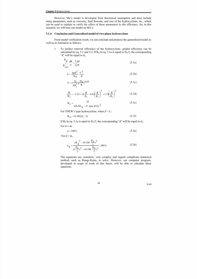
8/15/2019 Rachu.pdf
http://slidepdf.com/reader/full/rachupdf 146/646

8/15/2019 Rachu.pdf
http://slidepdf.com/reader/full/rachupdf 147/646

8/15/2019 Rachu.pdf
http://slidepdf.com/reader/full/rachupdf 148/646
Chapter 5 Hydrocyclone
II-42
0.0
1.0
2.0
3.0
4.0
5.0
6.0
0.00 0.50 1.00 1.50 2.00 2.50 3.00 3.50 4.00 4.50 5.00
Observed pressure drop (bar)
P r e d i c t e d p r e s s u r e d r o p ( b a r )
+10%
-10%
Δ po (bar) = 16 Q2.3
/Dn4
Fig. 5.3a Relation between observed pressure drop (inlet/overflow) of Thew cyclone and predicted pressure drop
0.0
1.0
2.0
3.0
4.0
5.0
6.0
7.0
0.0 1.0 2.0 3.0 4.0 5.0 6.0
Observed pressure drop (bar)
P r e d i c t e d p r e s s u r e d r o p ( b a r )
+10%
-10%
Δ pu (bar) = 4.6 Q2.2
/Dn4
Fig 5.3b Relation between observed pressure drop (inlet/underflow) of Thew cyclone and predicted pressure drop
From THEW’s research [28], Split ratio (R f ) or ratio between overflow and inlet flow
has some effect on pressure drop. However the effect of this parameter on under flow pressuredrop is very small, thus, negligible. There is more effect on overflow pressure drop. From
THEW’s and MA’s data, we can find the empirical correlation between split ratio and then
can transform eq. 5.5a to account for the split ratio. The modified equation is as follow;
0.1611
)f
R (1
2.6
4nD
2.3Q16oΔ p
⎟⎟
⎠
⎞
⎜⎜
⎝
⎛
−⋅= {5.5c}
However, the correlation is developed from relatively small set of data. Furthermore,
range of split ratio, generally used, is around 1 to 10%. Within this range, eq. 5.5a alone can
predict the efficiency with an error of only 10-20%. So we recommend using eq. 5.5a and
86
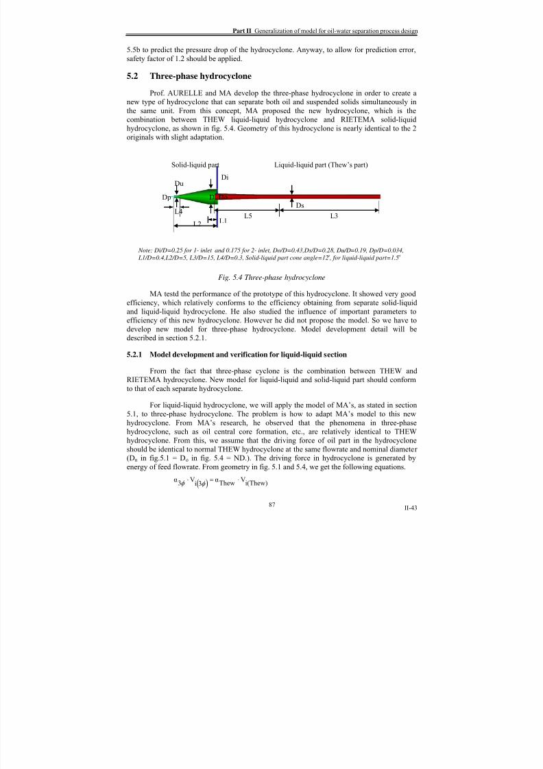
8/15/2019 Rachu.pdf
http://slidepdf.com/reader/full/rachupdf 149/646
Part II Generalization of model for oil-water separation process design
II-43
5.5b to predict the pressure drop of the hydrocyclone. Anyway, to allow for prediction error,
safety factor of 1.2 should be applied.
5.2 Three-phase hydrocyclone
Prof. AURELLE and MA develop the three-phase hydrocyclone in order to create anew type of hydrocyclone that can separate both oil and suspended solids simultaneously in
the same unit. From this concept, MA proposed the new hydrocyclone, which is the
combination between THEW liquid-liquid hydrocyclone and RIETEMA solid-liquid
hydrocyclone, as shown in fig. 5.4. Geometry of this hydrocyclone is nearly identical to the 2
originals with slight adaptation.
Solid-liquid part Liquid-liquid part (Thew’s part)
DoDDs
DiDu
Dp
L5 L3L1L2
L4
Note: Di/D=0.25 for 1- inlet and 0.175 for 2- inlet, Do/D=0.43,Ds/D=0.28, Du/D=0.19, Dp/D=0.034,
L1/D=0.4,L2/D=5, L3/D=15, L4/D=0.3, Solid-liquid part cone angle=12o , for liquid-liquid part=1.5
o
Fig. 5.4 Three-phase hydrocyclone
MA testd the performance of the prototype of this hydrocyclone. It showed very good
efficiency, which relatively conforms to the efficiency obtaining from separate solid-liquid
and liquid-liquid hydrocyclone. He also studied the influence of important parameters to
efficiency of this new hydrocyclone. However he did not propose the model. So we have to
develop new model for three-phase hydrocyclone. Model development detail will be
described in section 5.2.1.
5.2.1 Model development and verification for liquid-liquid section
From the fact that three-phase cyclone is the combination between THEW and
RIETEMA hydrocyclone. New model for liquid-liquid and solid-liquid part should conformto that of each separate hydrocyclone.
For liquid-liquid hydrocyclone, we will apply the model of MA’s, as stated in section
5.1, to three-phase hydrocyclone. The problem is how to adapt MA’s model to this new
hydrocyclone. From MA’s research, he observed that the phenomena in three-phase
hydrocyclone, such as oil central core formation, etc., are relatively identical to THEW
hydrocyclone. From this, we assume that the driving force of oil part in the hydrocyclone
should be identical to normal THEW hydrocyclone at the same flowrate and nominal diameter
(Dn in fig.5.1 = Do in fig. 5.4 = ND.). The driving force in hydrocyclone is generated by
energy of feed flowrate. From geometry in fig. 5.1 and 5.4, we get the following equations.
( ) i(Thew)V
Thewα
3iV
3α ⋅=⋅
φ φ
87

8/15/2019 Rachu.pdf
http://slidepdf.com/reader/full/rachupdf 150/646
Chapter 5 Hydrocyclone
II-44
( ) ⎟⎟⎟
⎠
⎞
⎜⎜⎜
⎝
⎛ ⋅=
⎟⎟⎟
⎠
⎞
⎜⎜⎜
⎝
⎛
⋅2)
i(Thew)π(D
4Q0.5
2)3i
π(D
4Q3
α
φ φ
⎟⎟⎟⎟
⎠
⎞
⎜⎜⎜⎜
⎝
⎛
⋅=
⎟⎟⎟⎟
⎠
⎞
⎜⎜⎜⎜
⎝
⎛
⋅2))
0.5
NDπ(0.25(
4Q0.52))
0.43
NDπ(0.25(
4Q3
αφ
676.0
2
0.43
0.50.5
3α =⎟
⎠
⎞⎜⎝
⎛ ⋅=⋅φ
{5.6}
We use α3φ in eq. 5.6 with the model in eq. 5.1 and 5.2 to predict the efficiency of the
oil part of three-phase hydrocyclone and compare the result with observed value from MA’s
data [16]. Comparison result in fig. 5.5 shows that the error from prediction is ± 20%, which
is acceptable. We have tried to select the value of α3φ arbitrarily and found that;
•
If the value of α3φ is lower, the model will predict too low efficiency.
• For higher value of α3φ, it may provide better curve fitting but we do not have any
data to support the use of it. The value of 0.676 seems more appropriate.
0.0%
20.0%
40.0%
60.0%
80.0%
100.0%
120.0%
0.0% 10.0% 20.0% 30.0% 40.0% 50.0% 60.0% 70.0% 80.0% 90.0% 100.0%
Observed efficiency (%)
P r e d i c t e d e f f i c i e n c y ( % )
+20%
-20%
Fig. 5.5 Relation between observed efficiency and predicted efficiency of liquid-liquid (Thew) part of three-phase
hydrocyclone
From model verification result, we can conclude and propose the model of liquid-
liquid part of three-phase hydrocyclone as well as its limitation as follows,
1. To predict removal efficiency of three-phase hydrocyclone, graded efficiency
can be calculated by eq. 5.7 and 5.8.Dn in this case is equal to Dc. And L in this
case is equal to L5.
∫=∫L
0 WdZ
dR
vzzR U
dR {5.7a}
88

8/15/2019 Rachu.pdf
http://slidepdf.com/reader/full/rachupdf 151/646
Part II Generalization of model for oil-water separation process design
II-45
R
V 2
18μ
2Δρd
U ⋅= {5.7b}
0.65)
R
nD(
2i
D4π
(Q/2)0.676V
⎟⎟
⎟⎟
⎠
⎞
⎜⎜
⎜⎜
⎝
⎛
= {5.7c}
3
zR
R 1.19
2
zR
R 8.63
zR
R 123.33
zW
W⎟⎟ ⎠
⎞⎜⎜⎝
⎛ +⎟⎟
⎠
⎞⎜⎜⎝
⎛ −+−= {5.7d}
2))2/tan(Znπ(0.5D
QzW
β ⋅−= {5.7e}
For d ≥ dc,
100%d
η = {5.8a}
For d < dc,
%100
)2)2
nD(0.1862)
2
nD((
)2)2
nD(0.186
2d
(R
dη ⋅
−
−= {5.8b}
2. To design the hydrocyclone by the model, it is recommended to select the cut
size that covers majority of oil droplet in the wastewater and provide a safety
factor around 10% to 25%, because the model is apt to predict too small cut size.
For example, if the desired cut size is 50 microns, it is recommended to select50(1-0.25) = 37.5 microns for eq. 5.7 and 5.8.
3. To use the models described above, the following conditions need to be satisfied
and the assumptions and limitations would be noted;
1) The model is valid for three phase hydrocyclone with geometry of the oil
part conforms to that of THEW.
2)
It is recommended to use the model only for droplet diameter of 20
microns or greater. For smaller droplet, the model can also be applied, but
for comparison purpose only.
3) Eq. 5.7c is valid for the hydrocyclone with 2 inlet ports only. If the
hydrocyclone has only 1 inlet port, replace Q/2 with Q. However, using 2inlet ports is recommended for its hydraulics stability. Please note that the
size of 2 inlet ports will be smaller than single inlet port to keep the inlet
area constant.
5.2.2 Model development and verification for solid-liquid section
From the same reason as oil-part model development, we will base our model for
solid-liquid separation on RIETEMA hydrocyclone’s model. In MA’s research, he used only
2 sizes of suspended solids. So the data is not sufficient to develop the model. However,
geometry of this part of three-phase hydrocyclone is identical to RIETEMA’s. So RITEMA’s
model should be applied without any modification.
89

8/15/2019 Rachu.pdf
http://slidepdf.com/reader/full/rachupdf 152/646

8/15/2019 Rachu.pdf
http://slidepdf.com/reader/full/rachupdf 153/646

8/15/2019 Rachu.pdf
http://slidepdf.com/reader/full/rachupdf 154/646

8/15/2019 Rachu.pdf
http://slidepdf.com/reader/full/rachupdf 155/646
Part II Generalization of model for oil-water separation process design
II-49
Chapter 6 Membrane process
Membrane process is a separation process based, mainly but not entirely, on filtration
concept. It can be said that the membrane is a very fine screen or filter. Theoretically, we can
always separate one or more components from fluid stream providing that the filter chosen is
suitable for size difference. Membranes can be categorized by their separation characteristics,i.e., microfiltration (MF), ultrafiltration (UF), nanofiltration (NF) and reverse osmosis (RO).
MF and UF have relatively large pore sizes, so they work rather like screens or sieve filters.
While separation by NF and RO, which have very tiny pore sizes, is not simply by size alone
but involves more complex factors, such as osmotic pressure. So we can group the membranes
processes into 2 categories, i.e., 1) MF and UF, 2) NF and RO.
Membrane process design depends mainly on wastewater characteristics. So, the best
way to design the membrane process is to perform feasible study in lab scale or pilot scale.
However, our lab has several researches on UF. From these researches, we have gained some
understanding of phenomena taking place in the process. Then we can use our result to set a
guideline for conceptual design or preliminary evaluation of membrane process.
6.1 Ultrafiltration
Because of their pore sizes, MF and UF are suitable for finely dispersed emulsion,
such as, secondary emulsion, macroemulsion and microemulsion. However, there is only one
research on MF of oily wastewater treatment in Prof. AURELLE’s team. Then, despite of its
feasibility on cutting oil emulsion treatment, which is one of the important applications of
membrane processes on oily wastewater treatment, we will not include MF in our thesis for
there is insufficient data. So we will emphasize on UF.
There are 2 main types of UF, as well as other, membrane processes, based on flow pattern, i.e., dead-end and cross-flow. In dead end reactor, wastewater will be fed in
perpendicular direction to membrane surface. So this mode of operation is rather like cake
filtration. Dead-end process is normally used in bench scale experiment. For cross-flow,
wastewater will be fed in tangential direction, parallel to membrane surface. It is this mode of
operation that is widely used in real life situation. So our researches are related to this process.
For wastewater treatment, our aim is to reduce the quantity of the wastewater as much
as possible while the effluent quality still meets effluent standard. So wastewater will be
recycled repeatedly until its volume reaches required limit. In this case, UF system is
normally designed as batch processes, as shown in fig. 6.1.
Permeate
Retentate
Membrane
Feed pump
Storage
tank
Fig. 6.1 Typical schematic diagram of Cross-flow membrane process
93

8/15/2019 Rachu.pdf
http://slidepdf.com/reader/full/rachupdf 156/646
Chapter 6 Membrane process
II-50
From fig. 6.1, we have to apply enough pressure to force components that can pass
through the membrane pores to the other side. The components of influent that can pass
through the membrane is called permeate. The rest that can not pass is called retentate. The
pressure difference between retentate side and permeate is called transmembrane pressure (Pt).
The retained components will accumulate at the surface of membrane and its concentration
will be increased. This accumalation and high concentratio, called concentration polarizationor gel polarization, will hinder the permeate flow. Some components may lodge in the pores.
These phenomena will make the membrane clog and rate of permeate passing through the
membrane or permeate flux will decrease. In cross-flow process, we can alter the superficial
(or recirculation) velocity at the membrane surface (V) by changing recirculation flowrate to
reduce the effect of polarization. From this brief operating principle, we can see that there are
several parameters, relates to membrane process design. So models of membrane will be
developed to describe the relation between these parameters.
There are several researches in our lab [10], [11], [18]-[22] on membrane processes.
However, they were based mainly on application. Only some of them provided models.
Furthermore those models are limited by their scopes of the experiment, then they are not ingeneral forms to apply to general case. In this thesis, we will try to develop the generalized
models, based on well-accepted theoretical models, i.e. resistance model and film model.
6.1.1 Resistance model
General form of resistance model [38], [54], [18], [11] is similar to the equation for
electrical calculation as shown in eq. 6.1.
gR f
R mR
tPJ
++= {6.1a}
Membrane resistance (R m) and fouling resistance (R f ) are property of membrane and
relatively unaffected by operating condition [38]. So it is normally be summed together and
called intrinsic membrane resistance (R’m). Eq. 6.1a , then, will become,
gR m'R
tPJ
+= {6.1b}
Gel resistance (R g) is the function of Pt and V as shown in eq. 6.2. α and φ are
numerical constants.
t Pα
VgR ⋅= φ {6.2}
This model can give the accurate evolution of flux with Pt, starting from pressure
controlled region, which the flux varies with Pt, to mass transfer controlled region, which the
flux is relatively constant, as shown in fig. 6.2.
From researches in our lab, we can summarize the value of R’m, φ and α for many
operating conditions, as tabulated in table 6.1. φ and α are dependent of wastewater inlet
concentration so it can be applied only to their corresponding concentration only.
94

8/15/2019 Rachu.pdf
http://slidepdf.com/reader/full/rachupdf 157/646
Part II Generalization of model for oil-water separation process design
II-51
T
a b l e 6 . 1
S u m m a r y o f p a r a m e t e r s o f r e s i s t a n c e m o d e l f r o m U F
r e s e a r c h e s o n o i l y w a s t e w a t e r
t r e a t m e n t ( r e f e r e n c e t e m p e r a t u r e = 2 0 O
C )
95

8/15/2019 Rachu.pdf
http://slidepdf.com/reader/full/rachupdf 158/646
Chapter 6 Membrane process
II-52
Pressure controlled
region
Mass transfer
controlled region
W a
t e r f l u x Higher recirculation flow
Higer temperature
Lower concentration
Transmembrane pressure (P )
Flux
Fig. 6.2 Typical relation between flux and various parameters
6.1.2 Film theory based model
This model is developed under the assumption that the process is in the mass transfer
controlled region. So flux is assumed to be controlled by mass transfer phenomena and
independent of Pt. Operating UF in this region will maximize the flux, thus minimize the size
of membrane. The general form of film theory based model [38], [54] is shown in eq. 6.3.
)oC
gCln(
βkVJ = {6.3}
From the equation, k is mass transfer coefficient. Cg is gel concentration, which
depends on type of wastewater. V is recirculation velocity. Two typical characteristic curves
of flux VS. retentate concentration are shown in fig. 6.3b. (Other curves also exist, but they
are very rare cases)
For the first type, the curve is flat without inflection point. This type of curve willcross the horizontal axis at C . This Cg g remains constant for the whole range of retentate
concentration.
For the second type, The curve presents an inflection point. In this case, we can say
that there are two Cg. The first one is obtained from extending the steeper part of the graph to
cross the X-axis. But it is not the real Cg and used only for flux calculation at lower range of
retentate concentration. The real Cg is obtained from the graph after inflection point. UF of
cutting oil emulsion will be in this category. In this case, the real C g normally crosses the X-
axis at approximately 100% concentration. This can imply that, theoretically, we can use UF
to filter the oily wastewater until the retentate become water-free oil. However, the flux will
become very low and the operation may become unacceptable from economic point of view.
Log (Concentration)
V1
Cg
Flux V2>V1
Fig. 6.3a Relation between flux and concentration at any recirculation velocity [38]
96

8/15/2019 Rachu.pdf
http://slidepdf.com/reader/full/rachupdf 159/646
Part II Generalization of model for oil-water separation process design
II-53
Log (Concentration)
1 2
Cg
case 1
Cg
case 2
C’g
case 2
Flux
Fig. 6.3b Typical characteristic curve of concentration VS. Flux (Log-Normal scale) [38]
From researches in our lab, we can summarize the value of k, Cg and β for various
kinds of membranes for many types and inlet concentration of wastewater, as tabulated in
table 6.2.
6.1.3
Model verification
From section 6.1.1, it shows that the resistance model can predict flux at any pressure.
However, the constants in eq. 6.2 are valid for only their own specific operating conditions,
esp. the influent oil concentration. On the other hand, eq. 6.3, even though it is supposed to be
valid only in mass transfer region, can be used to predict flux at any influent oil concentration,
providing that the Cg is known. So, it is interesting to combine eq. 6.2 and 6.3 to see if they
can be used to predict flux at any influent concentration and pressure or not. The procedures
used to combine film theory and resistance theory, which are divided into 2 cases, are as
shown below.
Case 1: Know k, and Cg
1.
Find JC,Vref
If we know the value of k and β at one known velocity (called reference velocity,
Vref ), we can calculate limiting flux at any required concentration (called C) by the film
theory.
)C
gCln(
βref
kVVref C,
J = {6.4a}
However, even the film theory is supposed to be pressure-independent, it should be noted that k and β are obtained from experimental data, which are conducted at certain
value of pressure. At that reference pressure (Pref ), the flux may not yet fully reach the mass
transfer controlled region. In fact, we frequently find that flux/concentration curve never the
reach really flat part within the recommended operating range of pressure (generally 0 to 4
bar), especially when velocity is high.
In this case, we have tried to verify if the film theory is still valid. We studied the
flux/concentration relation of cutting oil macroemulsion (Elf SeraftA) at P = 2 and 3.5 bar, V
from 0.7 to 2.8 m/s from Belkacem’s data [18]. We found that eq. 6.3 is valid at P = 3.5 bar,
where is in the mass transfer controlled region. And we also found that the form of eq.6.3 still
holds at P = 2, where flux does not yet reach fully mass transfer controlled region at low Cand/or high V. But there are some little differences in the values of k, β and Cg.
97

8/15/2019 Rachu.pdf
http://slidepdf.com/reader/full/rachupdf 160/646
Chapter 6 Membrane process
II-54
O C
)
T a b l e 6 . 2
S u m m a r y o f p a r a m e t e r s o f f i l m m o d e l f r o m U F r e s e a r c h e s o n o i l y w a s t e w a t e r t r e
a t m e n t ( r e f e r e n c e t e m p e r a t u r e
= 2 0
98

8/15/2019 Rachu.pdf
http://slidepdf.com/reader/full/rachupdf 161/646

8/15/2019 Rachu.pdf
http://slidepdf.com/reader/full/rachupdf 162/646
Chapter 6 Membrane process
II-56
Besides using the reference velocity and required velocity, other dummy velocities
can also be used to cross-check the value of αc and φc. Calculated values of the two
parameters may not be exactly the same as those calculated from Vref and V, since there is
normally some calculation error. Using average values of these αc and φc is recommended.
From αc and φc, we can calculate flux at any transmembrane pressure and at the required
concentration by the resistance theory (eq. 6.7).
tPαcVCmR
tP
PtV,C,J
φ += {6.7}
To verify the procedure from eq. 6.4 to eq. 6.6, we use data from many researches
[10], [11], [18], [20], which φ, Cg, and α of corresponding cases are available. Example of
verification data is provided in Annex A5. In this case, we use φ, Cg, and α obtained from UF
test of cutting oil macroemulsion (Elf SeraftA) at influent concentration (C ) of 4% V/V, Pref ref
= 2 bar, Vref = 1.4 m/s as a reference condition to predict flux/ pressure relation at C = 2 and 8
% V/V. Predicted relations and comparison between observed flux and predicted flux are as
in fig. 6.4 and 6.5. From the graphs, it shows that eq. 6.4 to 6.6 can be effectively used to
extend the range of eq. 6.1, 6.2 and 6.3 to cover any influent concentration.
0
20
40
60
80
100
120
140
160
180
0 0.5 1 1.5 2 2.5 3
Transmembrane Pressure (Bar)
P r e d i c t e d
F l u x ( l / ( h . m
2 ) )
Observed, C = 2% Predicted, C = 2% Observed, C = 8% Predicted, C = 8% Reference, C = 4%
Fig. 6.4 Relation between UF permeate flux and Transmembrane pressure at reference concentration (C) of = 4%, V = 1.4 m/s
and Predicted relations at C = 2 and 8%
100

8/15/2019 Rachu.pdf
http://slidepdf.com/reader/full/rachupdf 163/646
Part II Generalization of model for oil-water separation process design
II-57
0.00
20.00
40.00
60.00
80.00
100.00
120.00
140.00
160.00
180.00
0 20 40 60 80 100 120 140 160 180
Observed flux (l/ (h.m2))
P r e d i c t e d F l u x ( l / ( h . m
2 ) )
-10%
+10%
Fig. 6.5 Relation between observed and predicted flux by resistance model for ultrafiltration of macroemulsion 4% conc. and
extend to cover other conc. by film model
Case 2: Know , φ and Cg
1. Find JCref,V
From resistance theory, we can find J , when φ and αCref,V Cref Cref are known, by the
following equation.
ref PαCref V
Cref m'R
ref P
VCref,J
⋅+=
φ
{6.8}
Again, we recommend selecting the reference pressure as high as possible to
make sure that the calculated flux is in the mass transfer controlled region.
2. Find JC,V
From film theory, we can write that;
)
ref C
gCln(
)C
gCln(
VCref,J
VC,J = {6.9}
3. Find JC,Vref
In the same way as 1 and 2, we can find J , when φ and αC,Vref Cref Cref are known,
by the following equation.
101

8/15/2019 Rachu.pdf
http://slidepdf.com/reader/full/rachupdf 164/646

8/15/2019 Rachu.pdf
http://slidepdf.com/reader/full/rachupdf 165/646
Part II Generalization of model for oil-water separation process design
II-59
{6.10b}micoil,
Cmacoil,
Cmixoil,
C +=
Flux of macroemulsion and microemulsion at the total oil concentration (Jmac:Coil,mix
and Jmic:Coil, mix) can be calculated by the procedure described in the previous section.
Therefore, the flux of the mixture can be calculated by the following equation.
mixoil,C
mixCoil,mic,J
micoil,C
mixCoil,:macJ
macoil,C
mixJ
+= {6.11}
To verify this idea, we used reference data of flux of pure macroemulsion and
microemulsion, as used in section 6.1.3, to predict flux of various ratios of
micro/macroemulsion mixture. Relations between predicted values and observed data are
presented in fig. 6.6 and 6.7. Even though, the error from prediction is around 20%, this
procedure will be a useful tool for the preliminary estimation of mixture flux, especially when
UF test data on the wastewater is not available
(Module: UFP2, Membrane: IRIS 3042, T = 20o C., data from [11]. The lines show predicted value.)
0.00
20.00
40.00
60.00
80.00
100.00
120.00
140.00
160.00
180.00
0.00 0.50 1.00 1.50 2.00 2.50 3.00 3.50
Pressure (bar)
F l u
x ( l / ( s q . m . h
) )
4% Macro
1% Micro
V = 2.8 m/s
4% Macro
4% Micro
V = 2.0 m/s
4% Macro
2% Micro
V = 1.0 m/s
Fig 6.6 Comparison between predicted flux and observed flux for UF of micro/ macroemulsion mixture (Conc. shown as
% by volume of concentrate)
103

8/15/2019 Rachu.pdf
http://slidepdf.com/reader/full/rachupdf 166/646

8/15/2019 Rachu.pdf
http://slidepdf.com/reader/full/rachupdf 167/646
Part II Generalization of model for oil-water separation process design
II-61
Vol)o(Vol
oVoloCC
−= {6.14}
Eq. 6.9 can be rewritten as,
AdtoVoloC
gVol)Co(Vol
lnβ
kVdVol ⎟⎟ ⎠
⎞
⎜⎜⎝
⎛ −
⋅= {6.15a}
∫=∫
⎟⎟
⎠
⎞
⎜⎜
⎝
⎛ −
t
0Adt
βkV
lfinal
Vo
oVol
oVoloC
gVol)Co(Vol
ln
dVol {6.15b}
However, the system may not be operated in the mass transfer controlled region for the
whole time. In this case, the function J(c) in eq. 6.12 can be calculated by eq 6.7. Eq. 6.12 and
6.15b are in the form of integration of [1/ln (x)], so they can not be written in general form
since the equation will be infinity at x =1. However, a definite integration is possible, using
numerical method that can be calculated by computer.
In this thesis, we have compared the theoretical result, using reference data stated in
section 6.1.3, with observed results from UF test on used cutting oil macroemulsion (3% V of
concentrate or 2.4%V of oil, from Willamette SAS factory) from WANICHKUL’s research
[11], as shown in fig. 6.8a. The x-marked circles indicate the observed flux of fresh emulsion.
From the graph, it shows that the model can accurately predict flux of fresh (unused) emulsion
as the circles are closed to the theoretical flux curve.
Comparing with observed flux of the used emulsion, the graph shows that, at low
concentration, theoretical flux is greater than observed value. This simply because additionalfouling from foreign material in the emulsion. However, at high concentration, theoretical
flux is, somehow, lower than observed value. This can be explained by partial degradation of
the used emulsion. During its working lifetime, cutting oil emulsion will subject to many
foreign material, such as coated oil on specimen surface, small scraps of specimen, leaked
lubricant, and heat. So its quality, as well as its stability, will gradually deteriorate. This is
proven by milky appearance of used emulsion, compared with the translucent or transparent
characteristic of fresh emulsion. When partial oil is destabilized to be free oil, this means the
concentration of oil in emulsion form may be lower than its initial value. At lower
concentration, the effect of fouling overwhelms the effect of reduced concentration, so the
theoretical flux is higher than the observed value. However, at higher concentration where theconcentration effect is stronger, the theoretical flux shows lower value.
Fig. 6.8b shows evolution of permeate volume with time, the result from integration of
eq. 6.12. From the observed data, it confirms that the macroemulsion can be ultrafitrated until
the retentate is relatively pure oil. In this case, initial volume of 1643 l of 2.4%V of oil is
ultrafiltrated to the final volume of 40 l. The theoretical time required to do so is 45 hours,
compared to observed value of 34 hours. However, the theoretical volume of permeate is
higher until almost at the end of the operation. Fig.6.8c shows evolution of theoretical flux
with concentration. It must be noted that eq 6.12 to 6.15 are based on the assumption that no
additional emulsion is added to the storage tank. If the emulsion is added, eq. 6.12 must be
modified to account for it.
105

8/15/2019 Rachu.pdf
http://slidepdf.com/reader/full/rachupdf 168/646
Chapter 6 Membrane process
II-62
(Used cutting oil macroemulsion :initial volume 1643 l, final volume 40 l,
initial concentration 2.4% by volume of oil (not concentrate): Module UFP10: membrane IRIS 3042)
0.00
10.00
20.00
30.00
40.00
50.00
60.00
70.00
0 200 400 600 800 1000 1200 1400 1600 1800
Permeate volume (l)
f l u x ( l / ( s q . m . h
) )
Theoretical data at P = 1.0 Bar, v = 1.17 m/s) Observed data Theoretical data at P = 1.5 Bar, v = 1.40 m/s)
= Observed data from UF test of new
cutting oil at the same condition
P = 1.0 bar, v = 1.17 m/s P = 1.5 bar, v = 1.40 m/s
Fig. 6.8a Relation between Flux VS. theoretical and observed permeate volume
(Used cutting oil macroemulsion :initial volume 1643 l, final volume 40 l,
initial concentration 2.4% by volume as oil (not as concentrate): Module UFP10: membrane IRIS 3042)
0
200
400
600
800
1000
1200
1400
1600
1800
0.000 5.000 10.000 15.000 20.000 25.000 30.000 35.000 40.000 45.000 50.000Time (h)
P e r m e a t e v o l u m e ( l )
Theoretical data at P = 1.0 Bar, v = 1.17 m/s) Theoretical data at P = 1.5 Bar, v = 1.4 m/s) Observed data
P = 1.0 bar, v = 1.17 m/s P = 1.5 bar, v = 1.40 m/s
Fig 6.8b Relation between time VS. theoretical and observed permeate volume
106

8/15/2019 Rachu.pdf
http://slidepdf.com/reader/full/rachupdf 169/646
Part II Generalization of model for oil-water separation process design
II-63
(Elf SeralfABS cutiing oil macroemulsion: Membrane IRIS 3042, 20oC)
0.00
10.00
20.00
30.00
40.00
50.00
60.00
70.00
80.00
1 10 100
Retentate concentration (% V of oil)
P e r m e a t e f l u x ( l / m
2 . h )
P = 1 bar, V = 1.17 m/s P = 1.5 bar, V = 1.4 m/s
Fig. 6.8c Relation between theoretical flux VS. concentration of oil in retentate
6.1.6
UF efficiency
From many researches, with appropriate UF membrane pore size, it clearly shows that
oil, even in form of very tiny droplets in macroemulsion and microemulsion, cannot pass the
membrane. We can say that the removal efficiency of UF is 100%. Selection of membraneinvolves many parameters. However, AURELLE [quoted by [18]] have grouped these
parameters and proposed 3 brief criteria, i.e.,
• Pore size of membrane: To prevent oil droplets to pass through the membrane
pore, the size of the pore, firstly, must be smaller than the droplets. From
researches in our lab, we recommend that minimum pore size should be 1/4 to 1/3
of average droplet size.
• Characteristic of membrane: for oil/water separation, membrane should be
hydrophilic. Membrane material should not react with the wastewater, which can
cause pour clogging. Hydrophilic material, such as polyacrylic, cellulose acetate,
zirconium oxide, etc., is recommended. Naturally without special treatment orcoating, polysulfonate tends to be fouled by oil, resulting in low flux and frequent
washing.
• Operating condition: Operating pressure should be less than capillary pressure
required to force the oil droplets through the membrane pores. Capillary pressure
increases with the hydrophilicity of membrane and decreasing of pore size.
However, if pore size and hydrophilicity are carefully selected, the capillary
pressure is normally higher than recommended maximum pressure of the
membrane.
107

8/15/2019 Rachu.pdf
http://slidepdf.com/reader/full/rachupdf 170/646

8/15/2019 Rachu.pdf
http://slidepdf.com/reader/full/rachupdf 171/646
Part II Generalization of model for oil-water separation process design
II-65
⎥⎥⎥⎥⎥⎥⎥
⎦
⎤
⎢⎢⎢⎢⎢⎢⎢
⎣
⎡
−
⎟⎟
⎟⎟⎟⎟⎟
⎠
⎞
⎜⎜
⎜⎜⎜⎜⎜
⎝
⎛
+−+⎟
⎟
⎠
⎞
⎜
⎜
⎝
⎛
−−= 1
1/3
)o/w
θ3sino/w
sinθ(2o/w
cosθ
3
r
dr
4
2o/w
θ3coso/w
3cosθ
r
o/wcosθ
o/w2γcapP {6.17}
Normally, the value of the capillary pressure is higher than the maximum operating
pressure. For example, for UF of macroemulsion, θo/w= 135o, γo/w = 0.033 N/m, r d = 150 nm
and r = 100 nm, the capillary pressure is 11.45 bar while the maximum pressure
recommended by the manufacturer is only 4 bar.
(Elf SeralfABS cutiing oil macroemulsion, 20oC, 100% = pure cutting oil concentrate = 80% V(approx) oil )
0.00
50.00
100.00
150.00
200.00
250.00
300.00
350.00
0 10 20 30 40 50 60 70 80 90 10
Oil concentration (% V of cutting oil concentrate in water)
V i s c o s i t y ( c p )
0
Fig. 6.9 Relation between oil concentration VS. viscosity of emulsion
For the power requirement of UF system, main power consumption is the power
required to maintain transmembrane pressure at require flowrate (or recirculation velocity).
This power can be calculated straightforwardly by the basic equation
overallη
AVP
overallη
QPPower
⋅⋅=
⋅= {6.19}
Q in this case means recirculation flowrate, not the permeate flowrate. V is the
recirculation velocity and A is the flow area of liquid in UF module (the channel between the
membrane surface and the UF module wall). P in the equation is pump discharge pressure,
which is the summation of transmembrane pressure and other headloss from pipe and values
system. It should be noted that transmembrane pressure is average value of the pressure at
the inlet and outlet of UF module. Overall efficiency of pump depends on pump type. For
progressive cavity pump or progressive screw pump, the efficiency should be around 50-70%.
109

8/15/2019 Rachu.pdf
http://slidepdf.com/reader/full/rachupdf 172/646

8/15/2019 Rachu.pdf
http://slidepdf.com/reader/full/rachupdf 173/646
Part II Generalization of model for oil-water separation process design
II-67
T a b l e 6 . 3 a S u m m a r y o f R O d a t a o n o i l y w a s t e w a t e r t r e
a t m e n t
111

8/15/2019 Rachu.pdf
http://slidepdf.com/reader/full/rachupdf 174/646
Chapter 6 Membrane process
II-68
T a b l e 6 . 3
b S u m m a r y o f N F d a t a o n o i l y w a s t e w a t e r t r e a t m e n t
112

8/15/2019 Rachu.pdf
http://slidepdf.com/reader/full/rachupdf 175/646
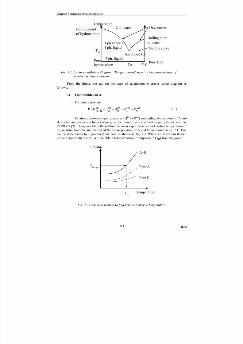
8/15/2019 Rachu.pdf
http://slidepdf.com/reader/full/rachupdf 176/646
Chapter 7 Heteroazeotropic Distillation
II-70
2 ph.vapor
Bubble curve
Pure H2O
Temperature
Azeotrope (H)
2 ph. liquid
1 ph.vapor +1 ph. liquid
Pure
hydrocarbon x,y yH
Dew curvesBoiling point
of hydrocarbonBoiling point
of water
TH
Fig. 7.1 Isobar equilibrium diagram : Temperature-Concentration characteristic of
immiscible binary mixture
From the figure, we can set the steps of calculation to create isobar diagram asfollows,
1)
Find bubble curve
For binary mixture
sat B
Psat A
P +=+=+
= θ b
BΠ
θ bA
Πθ b
BAΠP {7.1}
Relations between vapor pressures (Πθ b or Psat) and boiling temperature of A and
B, in our case, water and hydrocarbons, can be found in any standard property tables, such as
PERRY’s [2]. Then, we obtain the relation between vapor pressure and boiling temperature ofthe mixture from the summation of the vapor pressure of A and B, as shown in eq. 7.1. This
can be done easily by a graphical method, as shown in fig. 7.2. When we select our design
pressure (normally 1 atm), we can obtain heteroazeotropic temperature (TH) from the graph.
TH Temperature
Pressure
Pure A
Pure B
A+B
Pdesign
Fig. 7.2 Graphical method to find heteroazeotropic temperature
114

8/15/2019 Rachu.pdf
http://slidepdf.com/reader/full/rachupdf 177/646
Part II Generalization of model for oil-water separation process design
II-71
2)
Find dew curves
From DALTON’s law
PA
yA
p ⋅= {7.2a}
AndP
By
B p ⋅= {7.2b}
On the dew curves, partial pressure is equal to vapor pressure, then For
condensation of A
P
θdA
Π
Ayθd
AΠP
Ay
A p =→=⋅= {7.3a}
For condensation of B
P
θdBΠ
Byθd
BΠP
By
B p =→=⋅= {7.3b}
At any temperature between boiling points of pure substances and
heteroazotropic temperature (TH), we can find their corresponding vapor pressures (Π) from
fig. 7.3a. Then, from eq. 7.3, we can obtain yA and yB. This can be done easily, again, by the
graphical method as shown in fig. 7.3
T1 Temperature
Pressure
Pure A
Pure B
A+B
ΠA 1
ΠB 1
T2
ΠA 2
ΠB 2
Pure H2O
Temperature
Pure
hydrocarbon x,yyH
TH
T1
T2
yB 1
yB 2 yA 2 yA 1
Calculate yA and yB from ΠA,ΠB
by eq. 7.3, then, plot T,yA and T,yB
to obtain dew curves
Fig. 7.3 Graphical method to find dew curves
3)
Find heteroazeotropic composition
Heteroazeotropic composition (yH) can be calculated, based on eq. 7.1 and 7.3,
as shown in eq. 7.4,
P
θ bA
Π
Ay
Hy == {7.3a}
From eq. 7.1,
θ bB
Πθ bA
Π
θ bA
Π
Hy
+
= {7.4}
115

8/15/2019 Rachu.pdf
http://slidepdf.com/reader/full/rachupdf 178/646
Chapter 7 Heteroazeotropic Distillation
II-72
Vapor pressures of A and B (water and hydrocarbons) can be obtained from any
standard property tables [2]. yH indicates capability of extractant to extract water from
wastewater. For example, if yH = 0.5 mole/mole, it means 1 mole of extractant can extract 1
mole of water. The higher the yH , the better the extractant.
7.2
Model verification
From section 7.1, we can find yH of pure hydrocarbon that can be used as an
extractant, i.e., alkane with the number of carbon from 6 atoms (n-Hexane) to 16 (n-
Hexadecane). Theoretical values of yH of each alkane are tabulated in table 7.1. To compare
the theoretical value to experimental result, we use data from LUCENA’s thesis on slop
treatment, using decane and dodecane. Comparison result in table 7.1 shows that the
theoretical values are slightly higher (3.5-5.5%) than observed values.
Table 7.1 Heterotropic temperature and composition from various extractants
ExtractantMolecular
weight
(g/mol)
TH
(deg. C)
yH
(by molar)
yH
(by volume)
y H observed
(by volume)
[24]
C6H14 56 61.6 0.209 0.0351
C7H16 100 79.2 0.452 0.0922
C8H18 114 89.5 0.616 0.188
C9H20 128 94.8 0.827 0.3255
C10H22 142 97.6 0.914 0.495 0.468
C11H24 156 98.9 0.959 0.6663C12H26 170 99.5 0.98 0.7953 0.767
C13H28 184 99.8 0.991 0.890
C14H30 198 99.95 0.996 0.9542
C15H32 212 99.999 0.998 0.9702
C16H34 226 ≈ 100 0.999 0.9840
7.3 Conclusion and generalized model of heteroazeotropic distillation
From data verification result, we can conclude that the theoretical model, stated insection 7.1, provides very good prediction of heteroazotropic composition (yH). However, the
safety factor (S.F) of 1.05 or 1.1 is recommended. When we know the water volume in our
treated wastewater and determine the type of extractant, we can find quantity of extractant
required for extracting the water from the following equation. yH in eq. 7.5 will be by volume
basis, determined by the model in section 7.1. Heteroazeotropic distillation is suitable to treat
or recover valuable residue, such as slop or retentate from UF of cutting oil emulsion, which
is contaminated by relatively small amount of water.
Hy
)H
y(1
water VolumeS.FextractantVolume−
⋅= {7.5}
116

8/15/2019 Rachu.pdf
http://slidepdf.com/reader/full/rachupdf 179/646
Part II Generalization of model for oil-water separation process design
II-73
On the other hand, for stripping, we can find the theoretical quantity of steam or water
required for extracting the design volume of volatile hydrocarbons from the following
equations. Please note that the calculated volume of steam is the quantity required for
heteroazeotropic distillation only. Additional heat may be required to raise the temperature up
to the design point. Stripping is suitable to treat the waste polluted by small amount of volatile
substance. The concept is also applied to essential-oil extraction from herbs or flowers in perfume or chemical industries.
)H
y(1
Hy
nhydrocarboVolumeS.FsteamVolume
−⋅= {7.6a}
Or
)H
y(1
Hy
wastewater Volumenhydrocarbo
ionConcentratS.FsteamVolume−
⋅= {7.6b}
117

8/15/2019 Rachu.pdf
http://slidepdf.com/reader/full/rachupdf 180/646
Part III Summary of researches :
Oily wastewater treatment

8/15/2019 Rachu.pdf
http://slidepdf.com/reader/full/rachupdf 181/646
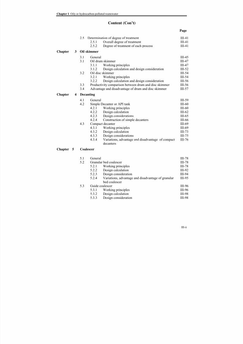
8/15/2019 Rachu.pdf
http://slidepdf.com/reader/full/rachupdf 182/646
Chapter 1 Oily or hydrocarbon-polluted wastewater
III-ii
Content (Con’t)
Page
2.5 Determination of degree of treatment III-41
2.5.1
Overall degree of treatment III-412.5.2 Degree of treatment of each process III-41
Chapter 3 Oil skimmer
3.1 General III-45
3.1 Oil drum skimmer III-47
3.1.1 Working principles III-47
3.1.2
Design calculation and design consideration III-52
3.2 Oil disc skimmer III-54
3.2.1 Working principles III-54
3.2.2 Design calculation and design consideration III-56
3.3
Productivity comparison between drum and disc skimmer III-563.4 Advantage and disadvantage of drum and disc skimmer III-57
Chapter 4 Decanting
4.1
General III-59
4.2 Simple Decanter or API tank III-60
4.2.1 Working principles III-60
4.2.2 Design calculation III-62
4.2.3 Design considerations III-65
4.2.4 Construction of simple decanters III-66
4.3 Compact decanter III-69
4.3.1
Working principles III-694.3.2
Design calculation III-73
4.3.3 Design considerations III-75
4.3.4 Variations, advantage and disadvantage of compact III-76
decanters
Chapter 5 Coalescer
5.1 General III-78
5.2 Granular bed coalescer III-78
5.2.1 Working principles III-78
5.2.2 Design calculation III-925.2.3 Design consideration III-94
5.2.4 Variations, advantage and disadvantage of granular III-95
bed coalescer
5.3 Guide coalescer III-96
5.3.1 Working principles III-96
5.3.2 Design calculation III-98
5.3.3 Design consideration III-98
8/15/2019 Rachu.pdf
http://slidepdf.com/reader/full/rachupdf 183/646
Part III Summary of researches: Oily wastewater treatment
III-iii
Content (Con’t)
Page
5.4 Fibrous Bed coalescer III-99
5.4.1
Working principles III-995.4.2 Design calculation III-109
5.4.3 Design consideration III-110
5.4.4 Variations, advantage and disadvantage of fibrous bed III-112
coalescer
Chapter 6 Dissolved air flotation
6.1
General III-115
6.2 Working principles III-116
6.2.1 Filter based model III-116
6.2.2 Population balance model III-121
6.2.3
Generalized model of DAF from combination of III-123filtration based model and population balance model
6.2.4
Influent parameters III-124
6.3
Design calculation III-127
6.4 Design consideration and construction of DAF reactor III-137
6.5 Pressurized water system or saturator III-145
6.5.1 Working principle and design calculation III-145
6.5.2 Type of saturator and injection valve III-150
6.6 Variations, advantage and disadvantage of DAF III-153
Chapter 7 Hydrocyclone
7.1
General III-1557.2
Two-phase hydrocyclone III-156
7.2.1 Working principles III-156
7.2.2 Design calculation III-172
7.2.3 Design considerations III-175
7.2.4 Variations, advantage and disadvantage of III-178
hydrocy clone
7.3
Three-phase hydrocyclone III-178
7.3.1
Working principles III-178
7.3.2 Design calculation and design consideration III-182
7.3.3 Advantage and disadvantage of three-phase III-182
hydrocyclone
Chapter 8 Membrane process
8.1 General III-183
8.1.1 Classification of membrane processes III-183
8.1.2 Mode of operation of membrane processes III-185
8.1.3
Membrane structure III-185
8.1.4 Membrane material III-186
8.1.5 Membrane module type III-189

8/15/2019 Rachu.pdf
http://slidepdf.com/reader/full/rachupdf 184/646
Chapter 1 Oily or hydrocarbon-polluted wastewater
III-iv
Content (Con’t)
Page
8.2 Ultrafiltration (UF) III-194
8.2.1
Basic knowledge and working principles III-1948.2.2 UF process design for oily wastewater treatment III-206
8.2.3 Design consideration and significant findings from III-221
GPI’s researches
8.3
Microfiltration (MF) III-232
8.3.1 Basic knowledge and working principles III-232
8.3.2 Significant findings on MF for oily wastewater III-233
treatment from GPI researches
8.4 Reverse osmosis (RO) III-235
8.4.1 Basic knowledge and working principles III-235
8.4.2 Significant findings on RO for oily wastewater III-236
treatment from GPI’s researches8.5
Nanofiltration (NF) III-239
8.5.1 Basic knowledge and working principles III-239
8.5.2 Significant findings on NF for oily wastewater III-239
treatment from GPI’s researches
8.6 Comparison of membrane processes on emulsion treatment III-242
Chapter 9 Thermal processes
9.1 General III-245
9.2
Basic knowledge on distillation III-245
9.2.1 Basic knowledge on vapor/liquid equilibrium of III-245
mixtures9.2.2 Equilibrium of various mixtures III-248
9.3 Heteroazeotropic distillation of oily wastewater III-250
9.3.1 Working principles III-250
9.3.2 Raoult’s law and Dalton’s law III-251
9.3.3 Calculation of azeotropic temperature and composition, III-252
dew curve and bubble curve.
9.3.4 Application of heteroazeotropic distillation on III-254
treatment of inverse emulsion or concentrated oily
wastewater
9.3.5 Application of heteroazeotropic distillation on III-257
treatment of the wastes polluted by trace hydrocarbons:
Steam stripping
9.3.6
Design calculation and design considerations III-257
9.4 Classical or conventional distillation of oily wastewater III-259
9.4.1 Working principles III-259
9.4.2 Significant findings on classical distillation for oily III-259
wastewater treatment from GPI’s researches

8/15/2019 Rachu.pdf
http://slidepdf.com/reader/full/rachupdf 185/646

8/15/2019 Rachu.pdf
http://slidepdf.com/reader/full/rachupdf 186/646
Chapter 1 Oily or hydrocarbon-polluted wastewater
III-vi
Table
Page
Table 1.2.1-1 Properties of some normal alkanes [1],[2] III-3
Table 1.2.1-2 Properties of some unsaturated aliphatic hydrocarbons [1],[2] III-5
Table 1.2.1-3 Properties of some benzene-series hydrocarbons [1],[2] III-6
Table 1.4.3-2 Summary of oily wastewater classification III-14
Table 1.5-1a Data of pollution from certain oils, oil products and serfactants. III-15
Table 1.6-1a Industrial effluent standard of Thailand III-17
Table 1.6-1b Industrial effluent standard of France (1998) III-18
Table 1.6-1c Industrial effluent standards of USA, categorized by pollutant sources III-19
Table 2.1-1 Summary of equations for rising velocity calculation [41] III-22
Table 2.2.1-1a Data of surface and interfacial tension (N/m) for some liquids at 20°C III-24
Table 2.2.2-1 Relation between contact angle, work adhesion, interfacial tension III-28
and spread coefficient of oil/water/solid system [42]
Table 2.3.2-1a Example of the decanting test of oil/water emulsio III-35
Table 2.3.2-1b Example of the decanting test of oil/water emulsion: sorting of the III-36
result from table 2.3.2-1a
Table 2.3.2-2 Criteria for visual observation of size distribution [22] III-37
Table 2.3.2-3 Criteria for visual observation of surface oil film [45] III-38
Table 3.2.1-1 Work adhesion and contact angles of oil, water and various materials III-48
Table 3.2.2-1 Critical surface tensions of certain materials [42] III-53
Table 5.4.1-1 Coalesced kerosene droplet size at various velocities and bed heights III-108from oleophilic “bottle brush” coalescer (d F = 100 microns,
D = 0.05 m,Co = 1 g/l, 120oC) [10]
Table 5.4.1-2 Comparison between the individual efficiency of oleophilic bottle III-108
brush coalescer, hydrocyclone, theoretical and observed efficiency of the
coupling of coalescer/hydrocyclone [10]
Table 6.3-1 General design criteria of DAF from various literatures and III-130
manufactures (hydraulic loading rate us based on total flowrate)
Table 6.4-1 Data on efficiency and coagulant concentration of various oily III-141
wastewater treatments by DAF [51]
Table 6.5-1 Constant for calculation of concentration and quantity of gas for III-148
saturator design (Operating pressure of DAF = Patm, T = 20oC)
Table 6.5-2 Air characteristic and solubility at Patm [51] III-148
Table 8.1.4-1 Advantages and disadvantages of inorganic membrane [38] III-188
Table 8.1.4-2 Summary on membrane polymeric materials [38], [54], [57] III-189
Table 8.1.5-1 General characteristic of various membrane module [38], [54], [57] III-193
Table 8.2.2-1 General design criteria of UF process from various literatures III-208
Table 8.2.2-2 Summary of parameters of film model from UF researches on oily III-209
wastewater treatment (reference temperature = 20oC)
Table 8.2.2-3 Summary of parameters of resistance model from UF researches on oily III-210wastewater treatment (ref. temperature = 20oC)

8/15/2019 Rachu.pdf
http://slidepdf.com/reader/full/rachupdf 187/646
Part III Summary of researches: Oily wastewater treatment
III-vii
Table (Con’t)
Page
Table 8.2.2-4 Procedure to predict flux/pressure relation for case 1: Know k, III-211
β, Cg and R’m
Table 8.2.2-5 Procedure to predict flux/pressure relation for case 2: Know φ, α, III-213
Cg and R’m
Table 8.2.3-1 Composition of the special cleaning microemulsion concentrate [18] III-230
Table 8.4.2-1 Summary of RO data on oily wastewater treatment III-240
Table 8.5.2-1 Summary of NF data on oily wastewater treatment III-243
Table 8.6-1 Comparison of membrane processes on cutting macroemulsion III-244
treatments (based on Elf Seraft ABS at 4% by V of oil)
Table 9.3.3-1 Heterotropic temperature and composition from various III-254
hydrocarbons [24]Table 9.3.4-1 Water extracting performance of various commercial hydrocarbons [24] III-257
Table 10.2.4-1 Results from ZHU’s research on destabilization of various emulsions III-272
Table 10.3.2-1 Recommended value of gradient and detention time III-277
Table 11-2.1-1 Rate coefficient for selected wastewaters [51] III-282
Table 11.2.1-2 Biodegradability and biotoxicity data [51] III-284
Table 11.2.1-3 Concentration of certain metals affecting biological systems [45] III-287
Table 11.2.2-1 Case studies on biological treatment of oily wastewater [66] III-287
Table 11.3.1-1 Examples of PAC and GAC properties III-289
Table 11.3.1-2 Adsorptive capacity of AC for some hydrocarbons [65] III-291Table 11.3.3-1 Adsorption isotherm and MTZ data of some co-surfactants [21] III-295
Table 12.1-1 Guideline for oily wastewater process selection (based on III-298
GPI’s researches)

8/15/2019 Rachu.pdf
http://slidepdf.com/reader/full/rachupdf 188/646
Chapter 1 Oily or hydrocarbon-polluted wastewater
III-viii
Figure
Page
Fig. 1.2.1-1 Examples of normal alkanes and derivatives with equal number of III-4
carbon atomsFig. 1.2.1-2 Examples of benzene series III-6
Fig. 1.4.3-1 Relation between droplet sizes and rising velocity of primary and III-13
secondary emulsion [11]
Fig. 1.4.3-2 Classification of oily wastewater by degree of dispersion III-14
Fig. 2.1-1 Free body diagram of oil drop in water and relation between III-21
Cd and Re [55]
Fig. 2.2.1-1 Force diagram of oil drop in water III-23
Fig. 2.2.1-2 Model for visualization of γ [40][42] III-24
Fig. 2.2.1-3 Model for visualization of adhesion work III-25Fig. 2.2.2-1 Diagram of Oil drop on solid surface in water III-25
Fig. 2.2.2-2 Model for visualization of cohesion work III-26
Fig. 2.2.2-3 Effect of surface roughness on contact angle III-27
Fig. 2.2.3-1 Section of air bubble in water III-29
Fig. 2.2.3-2 Diagram for visualizing the capillary pressure III-30
Fig. 2.3.2-1 Example of the size distribution of oil droplet in cutting oil III-32
macroemulsion (Elf Seraft 4% V of concentrate), measured by Coultronics nanosizer NDM4 [11]
Fig. 2.3.2-2 Granulometer (Source: above - Ankermid Techcross / below - CILAS) III-33
Fig. 2.3.2-3 Decanting test column III-33
Fig. 2.3.2-4 Relation between accumulated C/Co (% of C/Co when the droplet size III-36 is
equal or smaller than the given dE) and oil droplet size
Fig. 2.3.2-5 Example of estimated size distribution of oil droplets from III-37
decanting test
Fig. 2.5.2-1 Cut size determination III-43
Fig. 2.2.5-2 Economics of processes (least cost criteria) III-44
Fig. 3.1-1 Examples of oil skimming devices III-46
Fig. 3.2.1-1 Lab-scale drum skimmer: Major components are shown. III-47(Source: GPI lab)
Fig. 3.2.1-2 Surface energy or superficial tension of materials, oil and water III-48
Fig. 3.2.1-3 Influent parameters on drum skimmer performance III-52
Fig. 3.2.2-1 Occurrence of eddy currents from drum operation and no oil zone III-54
or non-productive zone that affects the productivity of the skimmer
(Source: Oil Spill Cleanup)
Fig. 3.5-1 Application of the skimmers III-58

8/15/2019 Rachu.pdf
http://slidepdf.com/reader/full/rachupdf 189/646

8/15/2019 Rachu.pdf
http://slidepdf.com/reader/full/rachupdf 190/646
Chapter 1 Oily or hydrocarbon-polluted wastewater
III-x
Fig. 5.4.3-1 Examples of fibrous bed coalescer casing III-111
Fig. 5.4.3-2 Various types of bed tested by WANICHKUL [11]: From left, a) III-112
Simple spiral, b) Double spiral, c) Solid plastic spiral, d) A module of
multi-stage bed [No. of stage can be added by increase the number of
module into the same center shaft]
Figure (Con’t)
Page
Fig. 5.4.3-3 Characteristics of oil and water drops on silicon coated (oleophilic) III-112
steel fibers and non-coated (hydrophilic) steel fibers
Fig. 6.2-1 Example of schematic diagram of DAF (Source: Aquatec Maxcon) III-115
Fig. 6.2.1-1 Diagram for considering relative velocity of bubble and oil in flotation III-117
column
Fig. 6.2.1-2 Schematic diagram of the 3 transport phenomena III-117
Fig. 6.2.1-3 Schematic of single bubble and entire height of flotation column III-118
Fig. 6.2.1-4 Relation between theoritical efficiency factor and observed efficiency III-120
factor
Fig. 6.2.4-1 Typical relation between efficiency of DAF and various parameters III-124
Fig. 6.2.4-2 Solid-bubble agglomerate and formation of oil-bubble agglomerate [14] III-126
Fig. 6.3-1 Pilot-scale DAF test and Flota-test III-135
Fig. 6.4-1 Example of necessary equipment and component details of DAF system III-
140(Source: Environ Treatment System)
Fig. 6.4-2 Necessary equipment and reactor components of DAF system III-141
Fig. 6.4-3 Examples of characteristics of scum from DAF processes III-145
Fig. 6.5-1 Example of good bubble formation from pressurized water III-146
(Source: Cornell DAF pump)
Fig. 6.5-2 Relation between power required for pump, compressor and absolute III-149
pressure of saturator for pressurized water flowrate of 10 m3/h (assume %air saturation = 95%)
Fig. 6.5-3 Schematic diagrams of saturator systems (Source: Edur pump) III-151
Fig. 6.5-4 Examples of saturator system III-152
Fig. 6.5-5 Examples of injection valve III-153
Fig. 7.1-1 Basic flow pattern and examples of hydrocyclones III-155
Fig. 7.2.1-1 General flow pattern and features of hydrocyclones III-158
Fig. 7.2.1-1 General flow pattern and features of hydrocyclones III-159
Fig. 7.2.1-2 Velocity components in hydrocyclone III-159
Fig. 7.2.1-3 Tangential velocity profile in hydrocyclone and various typed of vortex III-160
Fig. 7.2.1-4 Examples of tangential velocity profile III-161
Fig. 7.2.1-5 Example of axial or vertical velocity profile III-162
Fig. 7.2.1-6 Example of radial velocity profile [30] III-163
Fig. 7.2.1-7 Forces on oil droplets or particles in hydrocyclone III-163
Fig. 7.2.1-8 Components of velocity of oil droplets or particles in hydrocyclone III-163

8/15/2019 Rachu.pdf
http://slidepdf.com/reader/full/rachupdf 191/646

8/15/2019 Rachu.pdf
http://slidepdf.com/reader/full/rachupdf 192/646
Chapter 1 Oily or hydrocarbon-polluted wastewater
III-xii
Fig. 8.2.1-9 Diagram of polarization layer and effect of velocity on flux in film III-201
theory
Fig. 8.2.1-10 Various resistances in UF processes III-203
Fig. 8.2.2-1 Examples of flux VS. oil concentration in UF of macroemulsion III-211
Fig. 8.2.2-2 Case 1: find flux/pressure relation when k, β, Cg and R’m are known III-211Fig. 8.2.2-3 Relation between UF permeate flux and Transmembrane pressure III-212 at
Cref
= 4% by volume of oil , V = 1.4 m/s and Predicted relations at C = 2 and 8% (Oil: Elf SeraftA
cutting oil macroemulsion, Membrane: IRIS 3042 PAN )
Figure (Con’t)
Page
Fig. 8.2.2-4 Relation between Flux VS. theoretical and observed permeate volume III-216
Fig 8.2.2-5 Relation between time VS. theoretical and observed permeate volume III-217
Fig. 8.2.2-6 Calculation of required storage volume of equalization tank by III-218
graphical method
Fig. 8.2.2-7 Relation between oil concentration VS. viscosity of emulsion III-220
Fig. 8.2.3-1a Flux of non-stabilized emulsion III-222
Fig. 8.2.3-1b Photographs of non-stabilized emulsion influent, retentate and permeate III-
222(from left) [10]
Fig. 8.2.3-2 Typical relation between CaCl2 concentration and flux at low Pt III-223
Fig. 8.2.3-3a Partially destabilization by salt and coalesce of oil droplets III-224
Fig. 8.2.3-3b Magnified images (x100) of oil droplets from original (left) and III-224
partially destabilized macroemulsion (right) [11]
Fig. 8.2.3-3c Magnified images of new membrane surface (left) and the surface after III-224
UF of macroemulsion at 3 bars without salt (middle) and with salt
addition (600 mg/l CaCl2) [11]
Fig. 8.2.3-4 Relation between fluxes VS. pressure and calculated VS. observed oil III-225
concentration in retentate for partially destabilized emulsion
Fig. 8.2.3-5 Examples of feed emulsions and their corresponding UF permeates III-226
Fig. 8.2.3-6 Examples of flux enhance techniques [38] III-228
Fig. 8.2.3-7 Example of evolution of flux of macroemulsion UF with periodical III-229
cleaning with macroemulsion (membrane IRIS 3042, P = 1 bar,
V=1.5 m/s. 25oC) and schematic of interaction between membrane/
surfactants [18]
Fig. 8.2.3-8 Examples of UF test modules III-231
Fig. 8.3.1-1 Examples of MF membranes III-232
Fig. 8.3.2-1 Evolution of flux from MF (with salt addition) of macroemulsion [20] III-234
Fig. 8.4-1 Examples of RO membranes III-235
Fig. 8.4.1-1 Working principles of reverse osmosis III-235
Fig. 8.4.2-1a Typical relation between flux and pressure of RO III-237
Fig. 8.4.2-1b Typical relation between flux and log of concentration III-237

8/15/2019 Rachu.pdf
http://slidepdf.com/reader/full/rachupdf 193/646

8/15/2019 Rachu.pdf
http://slidepdf.com/reader/full/rachupdf 194/646

8/15/2019 Rachu.pdf
http://slidepdf.com/reader/full/rachupdf 195/646
Part III Summary of researches: Oily wastewater treatment
III-1
Part 3 Summary of researches: Oily or hydrocarbon-polluted wastewater
treatment
In this part, we will use the data reviewed and verified in Part 1 and Part 2 to
summarize and compose the textbook that covers every research of Prof. AURELLE. The text
will consists of;
• Types and characteristics of oily wastewater
• Related theories on oily wastewater treatment
• Oily wastewater treatment processes, based mainly on researches of Prof.
AURELLE with additional data from well-proven literatures
• Special treatment process trains for some specific oily wastewater, based on
Professor AURELLE’ s researches
118
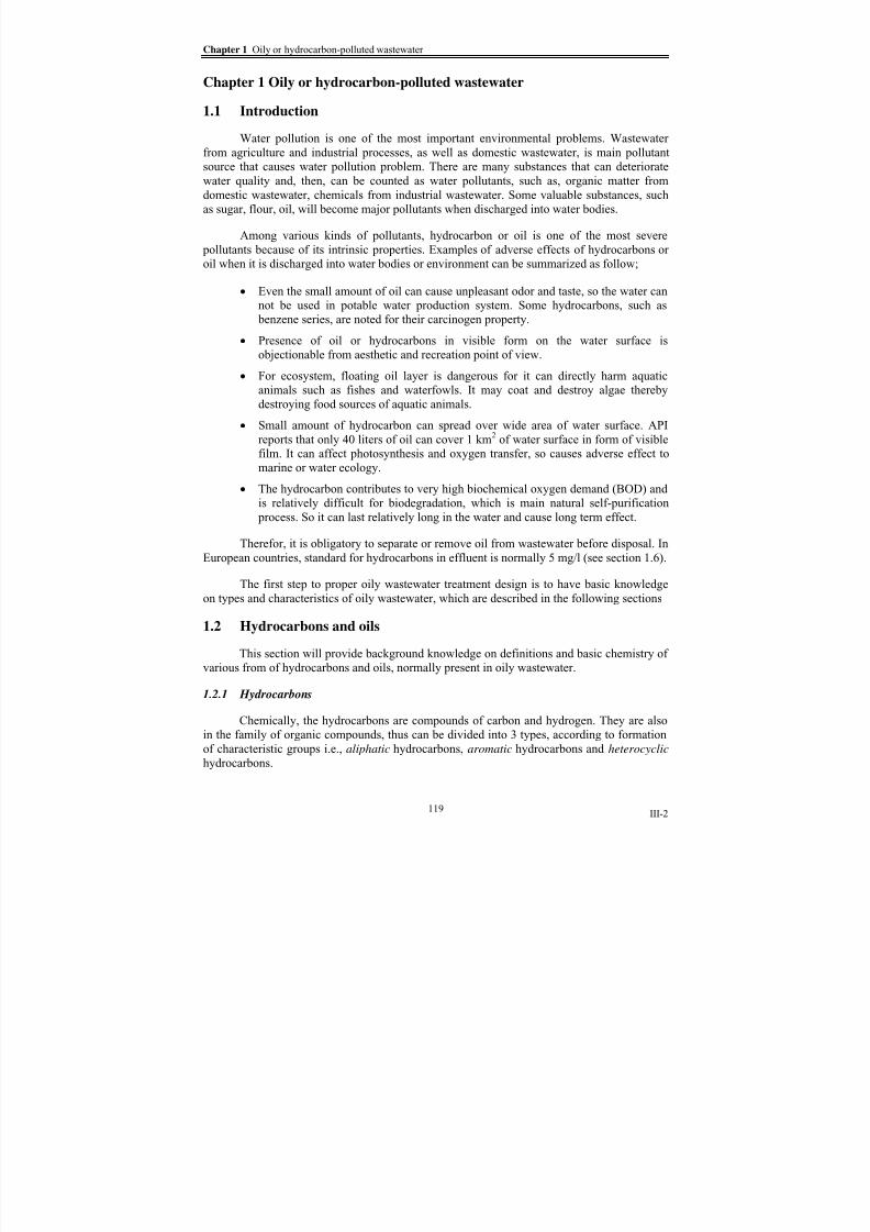
8/15/2019 Rachu.pdf
http://slidepdf.com/reader/full/rachupdf 196/646
Chapter 1 Oily or hydrocarbon-polluted wastewater
III-2
Chapter 1 Oily or hydrocarbon-polluted wastewater
1.1 Introduction
Water pollution is one of the most important environmental problems. Wastewater
from agriculture and industrial processes, as well as domestic wastewater, is main pollutantsource that causes water pollution problem. There are many substances that can deteriorate
water quality and, then, can be counted as water pollutants, such as, organic matter from
domestic wastewater, chemicals from industrial wastewater. Some valuable substances, such
as sugar, flour, oil, will become major pollutants when discharged into water bodies.
Among various kinds of pollutants, hydrocarbon or oil is one of the most severe
pollutants because of its intrinsic properties. Examples of adverse effects of hydrocarbons or
oil when it is discharged into water bodies or environment can be summarized as follow;
• Even the small amount of oil can cause unpleasant odor and taste, so the water can
not be used in potable water production system. Some hydrocarbons, such as benzene series, are noted for their carcinogen property.
• Presence of oil or hydrocarbons in visible form on the water surface is
objectionable from aesthetic and recreation point of view.
• For ecosystem, floating oil layer is dangerous for it can directly harm aquatic
animals such as fishes and waterfowls. It may coat and destroy algae thereby
destroying food sources of aquatic animals.
• Small amount of hydrocarbon can spread over wide area of water surface. API
reports that only 40 liters of oil can cover 1 km2 of water surface in form of visible
film. It can affect photosynthesis and oxygen transfer, so causes adverse effect tomarine or water ecology.
• The hydrocarbon contributes to very high biochemical oxygen demand (BOD) and
is relatively difficult for biodegradation, which is main natural self-purification
process. So it can last relatively long in the water and cause long term effect.
Therefor, it is obligatory to separate or remove oil from wastewater before disposal. In
European countries, standard for hydrocarbons in effluent is normally 5 mg/l (see section 1.6).
The first step to proper oily wastewater treatment design is to have basic knowledge
on types and characteristics of oily wastewater, which are described in the following sections
1.2 Hydrocarbons and oils
This section will provide background knowledge on definitions and basic chemistry of
various from of hydrocarbons and oils, normally present in oily wastewater.
1.2.1 Hydrocarbons
Chemically, the hydrocarbons are compounds of carbon and hydrogen. They are also
in the family of organic compounds, thus can be divided into 3 types, according to formation
of characteristic groups i.e., aliphatic hydrocarbons, aromatic hydrocarbons and heterocyclic
hydrocarbons.
119
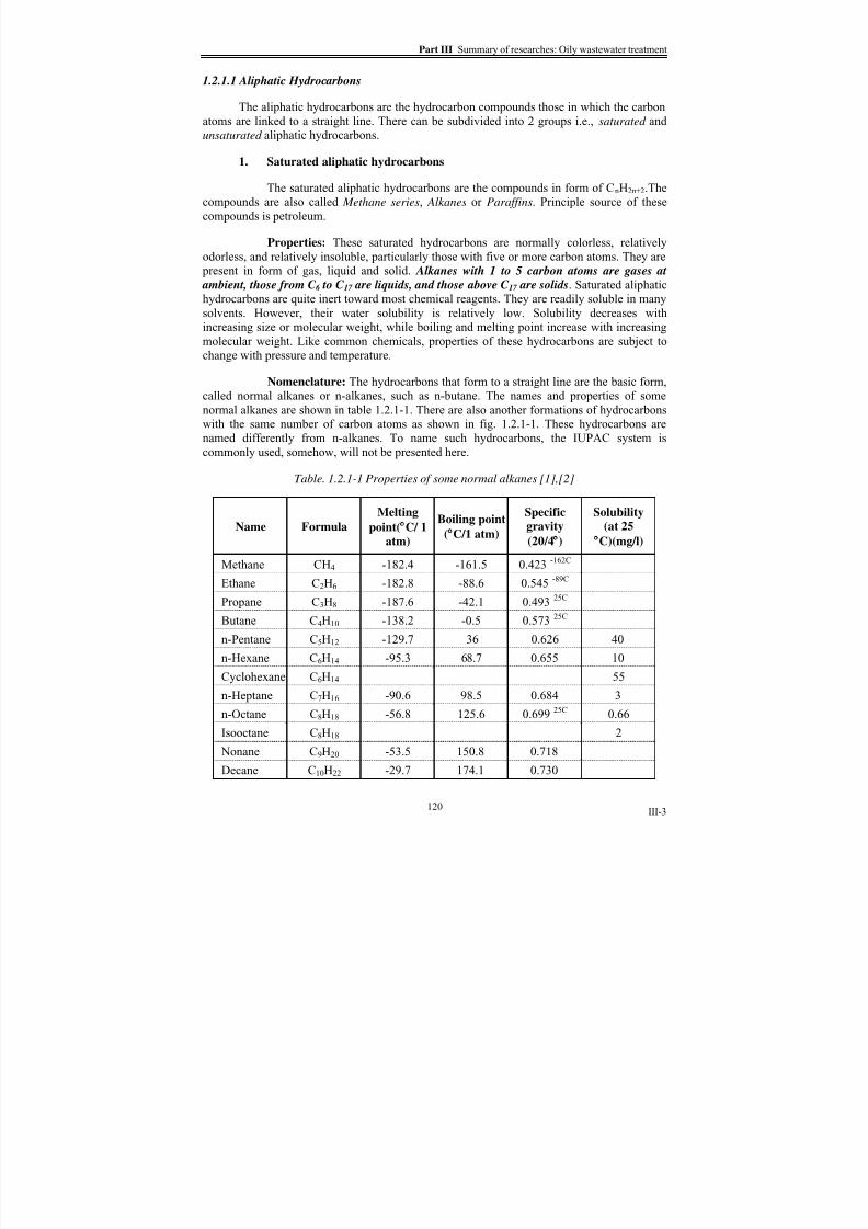
8/15/2019 Rachu.pdf
http://slidepdf.com/reader/full/rachupdf 197/646
Part III Summary of researches: Oily wastewater treatment
III-3
1.2.1.1 Aliphatic Hydrocarbons
The aliphatic hydrocarbons are the hydrocarbon compounds those in which the carbon
atoms are linked to a straight line. There can be subdivided into 2 groups i.e., saturated and
unsaturated aliphatic hydrocarbons.
1. Saturated aliphatic hydrocarbons
The saturated aliphatic hydrocarbons are the compounds in form of CnH2n+2.The
compounds are also called Methane series, Alkanes or Paraffins. Principle source of these
compounds is petroleum.
Properties: These saturated hydrocarbons are normally colorless, relatively
odorless, and relatively insoluble, particularly those with five or more carbon atoms. They are
present in form of gas, liquid and solid. Alkanes with 1 to 5 carbon atoms are gases at
ambient, those from C 6 to C 17 are liquids, and those above C 17 are solids. Saturated aliphatic
hydrocarbons are quite inert toward most chemical reagents. They are readily soluble in manysolvents. However, their water solubility is relatively low. Solubility decreases with
increasing size or molecular weight, while boiling and melting point increase with increasing
molecular weight. Like common chemicals, properties of these hydrocarbons are subject to
change with pressure and temperature.
Nomenclature: The hydrocarbons that form to a straight line are the basic form,
called normal alkanes or n-alkanes, such as n-butane. The names and properties of some
normal alkanes are shown in table 1.2.1-1. There are also another formations of hydrocarbons
with the same number of carbon atoms as shown in fig. 1.2.1-1. These hydrocarbons are
named differently from n-alkanes. To name such hydrocarbons, the IUPAC system is
commonly used, somehow, will not be presented here.
Table. 1.2.1-1 Properties of some normal alkanes [1],[2]
Name Formula
Melting
point(
C/ 1
atm)
Boiling point
(
C/1 atm)
Specific
gravity
(20/4
)
Solubility
(at 25
C)(mg/l)
Methane CH4 -182.4 -161.5 0.423 -162C
Ethane C2H6 -182.8 -88.6 0.545 -89C
Propane C3H8 -187.6 -42.1 0.493
25C
Butane C4H10 -138.2 -0.5 0.573 25C
n-Pentane C5H12 -129.7 36 0.626 40
n-Hexane C6H14 -95.3 68.7 0.655 10
Cyclohexane C6H14 55
n-Heptane C7H16 -90.6 98.5 0.684 3
n-Octane C8H18 -56.8 125.6 0.699 25C 0.66
Isooctane C8H18 2
Nonane C9H20 -53.5 150.8 0.718
Decane C10H22 -29.7 174.1 0.730
120

8/15/2019 Rachu.pdf
http://slidepdf.com/reader/full/rachupdf 198/646
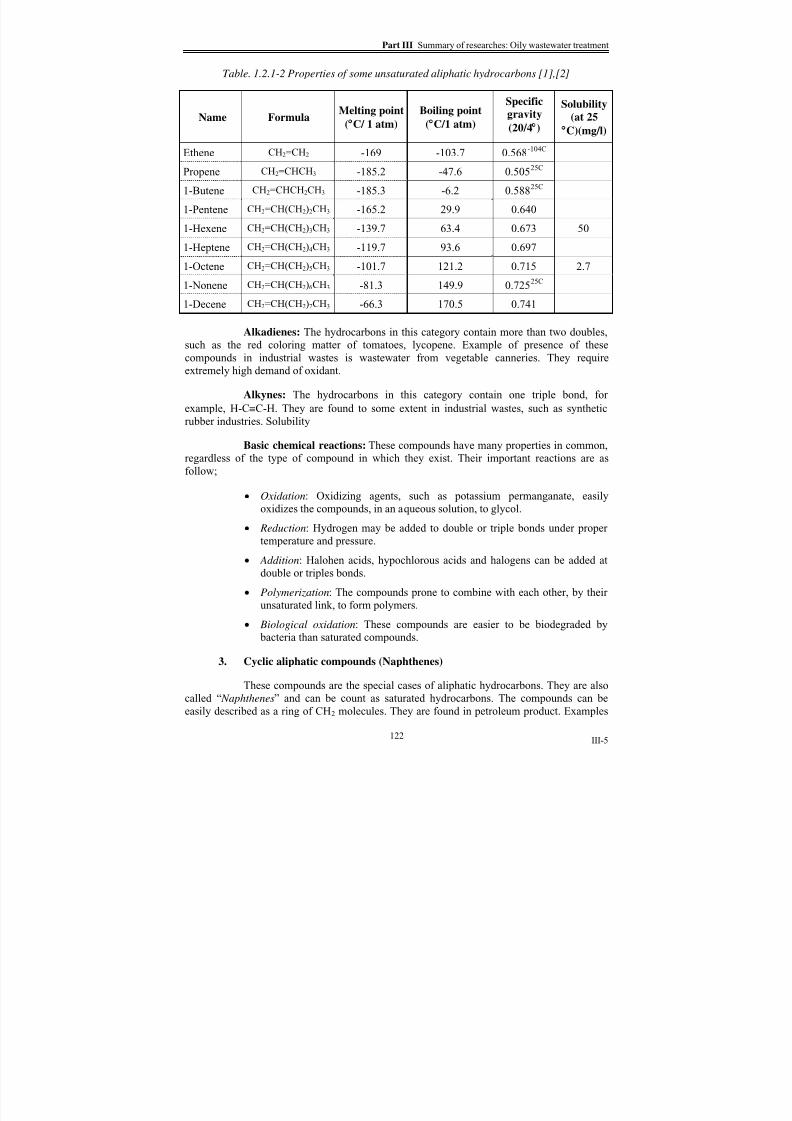
8/15/2019 Rachu.pdf
http://slidepdf.com/reader/full/rachupdf 199/646

8/15/2019 Rachu.pdf
http://slidepdf.com/reader/full/rachupdf 200/646

8/15/2019 Rachu.pdf
http://slidepdf.com/reader/full/rachupdf 201/646
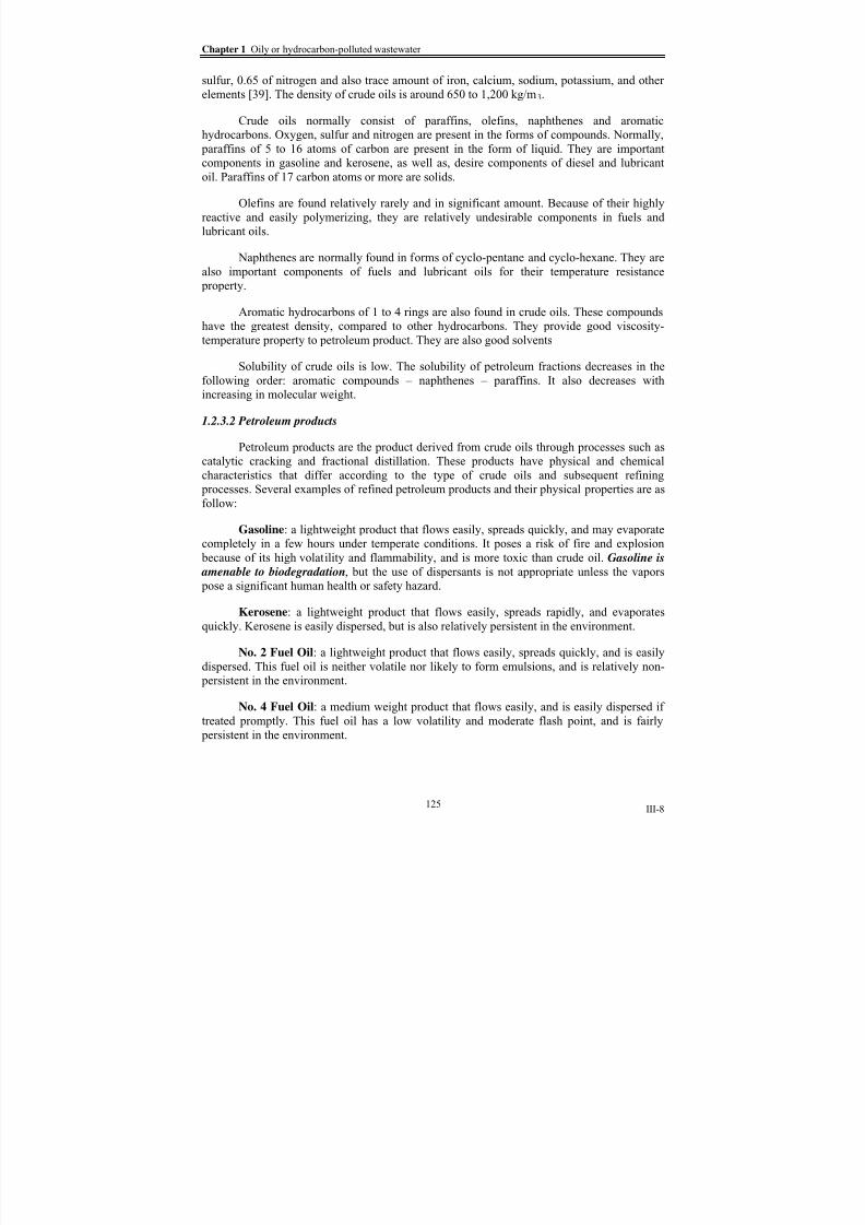
8/15/2019 Rachu.pdf
http://slidepdf.com/reader/full/rachupdf 202/646
Chapter 1 Oily or hydrocarbon-polluted wastewater
III-8
sulfur, 0.65 of nitrogen and also trace amount of iron, calcium, sodium, potassium, and other
elements [39]. The density of crude oils is around 650 to 1,200 kg/m3.
Crude oils normally consist of paraffins, olefins, naphthenes and aromatic
hydrocarbons. Oxygen, sulfur and nitrogen are present in the forms of compounds. Normally,
paraffins of 5 to 16 atoms of carbon are present in the form of liquid. They are importantcomponents in gasoline and kerosene, as well as, desire components of diesel and lubricant
oil. Paraffins of 17 carbon atoms or more are solids.
Olefins are found relatively rarely and in significant amount. Because of their highly
reactive and easily polymerizing, they are relatively undesirable components in fuels and
lubricant oils.
Naphthenes are normally found in forms of cyclo-pentane and cyclo-hexane. They are
also important components of fuels and lubricant oils for their temperature resistance
property.
Aromatic hydrocarbons of 1 to 4 rings are also found in crude oils. These compounds
have the greatest density, compared to other hydrocarbons. They provide good viscosity-
temperature property to petroleum product. They are also good solvents
Solubility of crude oils is low. The solubility of petroleum fractions decreases in the
following order: aromatic compounds – naphthenes – paraffins. It also decreases with
increasing in molecular weight.
1.2.3.2 Petroleum products
Petroleum products are the product derived from crude oils through processes such as
catalytic cracking and fractional distillation. These products have physical and chemical
characteristics that differ according to the type of crude oils and subsequent refining
processes. Several examples of refined petroleum products and their physical properties are as
follow:
Gasoline: a lightweight product that flows easily, spreads quickly, and may evaporate
completely in a few hours under temperate conditions. It poses a risk of fire and explosion
because of its high volatility and flammability, and is more toxic than crude oil. Gasoline is
amenable to biodegradation, but the use of dispersants is not appropriate unless the vapors
pose a significant human health or safety hazard.
Kerosene: a lightweight product that flows easily, spreads rapidly, and evaporates
quickly. Kerosene is easily dispersed, but is also relatively persistent in the environment.
No. 2 Fuel Oil: a lightweight product that flows easily, spreads quickly, and is easily
dispersed. This fuel oil is neither volatile nor likely to form emulsions, and is relatively non-
persistent in the environment.
No. 4 Fuel Oil: a medium weight product that flows easily, and is easily dispersed if
treated promptly. This fuel oil has a low volatility and moderate flash point, and is fairly
persistent in the environment.
125

8/15/2019 Rachu.pdf
http://slidepdf.com/reader/full/rachupdf 203/646

8/15/2019 Rachu.pdf
http://slidepdf.com/reader/full/rachupdf 204/646
Chapter 1 Oily or hydrocarbon-polluted wastewater
III-10
interfaces), it means the work required to form new surfaces. The substances that can decrease
the level of surface energy are called “ surface-active substances” or “ surfactants”. They are
also called by other names, such as, detergents (for solid/liquid interface, e.g. in washing or
cleaning process ), emulsifier, or dispersant, etc. With proper amount of surfactants, surface
energy can be substantially decreased until almost to zero. This makes it possible to create a
lot of new surface.
In our interest, surfactants can help making a lot of new surfaces of oil in the water.
This means the oils can be divided into very small droplets, which contributes to many new
surfaces, in the water, called emulsion. Theory of surface energy will be described in chapter
2. Effect and some further details of surfactants and co-surfactants will be described again
in chapter 10 “Chemical treatment processes”.
All surfactants have rather large functional groups. One end of the molecule, which
normally is organic group, is particularly soluble in oil. The other (polar group) is soluble in
waters. There are 4 main types of surfactants i.e., cationic, anionic, non-ionic and ampholytic
surfactants
1.3.1.1 Cationic surfactants
These surfactants are generally salts of quaternary ammonium hydroxide. The surface-
active properties are contained in the cations. Besides their surface-active properties, the
compounds are known for their disinfecting properties.
1.3.1.2 Anionic surfactants
These surfactants are generally sodium or potassium salts. The common ones are
sulfates and sulfonates. The surface-active properties are contained in the anions.
1.3.1.3 Non-ionic surfactants
These surfactants do not ionize and have to depend upon groups in the molecule to
render them soluble. All depend on polymers of ethylene oxide (C2H4O) to give them this
property.
1.3.1.4 Ampholytic (or amphoteric) surfactants
For these surfactants, they contain both cationic and anionic functional groups.
1.3.2
Soaps
Ordinary soaps are derived from fats and oils by saponification with sodium
hydroxide. Saponification is the special case of hydrolysis in which an alkaline agent is
present to neutralize the fatty acids as they are formed. The fats and oils are split into glycerol
and sodium soaps. The nature of the soap depends on the type of fat and oil used. Sodium and
potassium soaps are normally soluble. If the water contains hardness, calcium, magnesium
and other hardness-causing ions will precipitate soap to form metallic soap. Soap will
precipitate all hardness ions first, after that it becomes a surfactant.
127

8/15/2019 Rachu.pdf
http://slidepdf.com/reader/full/rachupdf 205/646
Part III Summary of researches: Oily wastewater treatment
III-11
1.3.3 Co-surfactants
In emulsions, especially microemulsion, they contain co-surfactants. These
compounds are normally alcohol, such as butyldiglycol, or benzylic alcohol. These
compounds are readily soluble in water thus provide good solubility to certain products, such
as cutting oil emulsion. They also increase the stability to the emulsion by promoting bothelectrical stability and mechanical stability.
1.3.4
Suspended solids
Suspended solids are commonly found in oily wastewater, especially when combined
collection systems are used. Types and concentration of suspended solids, present in oily
wastewater, depends on the sources of the wastewater. Some oil separation processes, esp. the
ones that are based on filtration concept such as granular bed coalescer and membrames, are
sensitive to the suspended solids. Suspended solids can cause adverse effect on oil separation
processes, unless it has already accounted for and mitigation measure is provided.
1.3.5 Other components
Others components found in oily wastewater depend on their source. Normally they
are the additives of the oil product, such as anti-foaming agents, anti-mousse agents,
bactericides, dyes, or anti-corrosion agents, etc. Some can present adverse effect on treatment
processes. Some may be present as residual pollutants in the effluent after oil separation
processes. So it will be very helpful if we know in advance the components of the oily
wastewater considering.
1.4 Categories of oily wastewater
Oil/water mixture systems can be categorized by many criteria. However, as stated
before that the treatment processes summarized in this book are based mainly on separation
processes, the criteria, used to categorize these oil/water mixtures, are based upon physical
properties. There are 3 main criteria, i.e., the nature of continuous phase, the stability of oily
wastewater, and the degree of dispersion.
1.4.1 Classification by the nature of the continuous phase
In binary mixture systems of oil and water, their components can be divided into 2
main phases, i.e., continuous phase, which is the majority of the two, and dispersed phase.
Direct emulsion: If continuous phase is the water, the mixture will be called “direct
emulsion”, and can be written as “o/w emulsion”, which stands for emulsion of oil in water.
Inverse emulsion: On the other hand, if the continuous phase is oil, the mixture will
be called “inverse emulsion” or “w/o emulsion”.
The treatment processes described herein this book will emphasize on oily wastewater,
which is direct emulsion. However, some processes can also be applied to inverse emulsion.
1.4.2 Classification by the stability of oily wastewater
By these criteria, oily wastewater can be divided into 2 groups:
128

8/15/2019 Rachu.pdf
http://slidepdf.com/reader/full/rachupdf 206/646

8/15/2019 Rachu.pdf
http://slidepdf.com/reader/full/rachupdf 207/646
Part III Summary of researches: Oily wastewater treatment
III-13
10-3
1 10 100 1000
Droplet diameters (microns)
R i s i n g v e l o c i t y ( m / s )
10-4
10-5
10-6
10-7
10-8
10-9
10-10
0.60 0.70 0.75
0.80 0.98 0.90
Oil
density
Secondaryemulsion
Primary
emulsion
Secondary
emulsion
Primary
emulsion
Fig. 1.4.3-1 Relation between droplet sizes and rising velocity of primaryand secondary emulsion [11]
4.
Macroemulsion
This type of emulsion contains droplet size between 0.06 to 1.0 microns. It
usually contains surfactant (and co-surfactant). This type of emulsion has a milky appearance.
A common example of this emulsion is cutting oil macroemulsion.
5. Microemulsion
This type of emulsion contains droplet size between 10 to 60 nm. It containsextensive amount of surfactants and cosurfactants. Since the droplets is very small, this type
of emulsion is usually transparent (sometimes, translucent if dyes are present or amount of o-
surfactants is low). A common example of this emulsion is cutting oil microemulsion.
Details of microemulsion amd macroemulsion will be described in details in the
chapter 10, related to “emulsion destabilization”.
From the three criteria stated above, some classes of oily wastewater from
different criteria might be overlapped. So, to summarize all of three criteria, oily wastewater
can be categorized as shown in fig. 1.4.3-1 and table 1.4.3-2.
130

8/15/2019 Rachu.pdf
http://slidepdf.com/reader/full/rachupdf 208/646

8/15/2019 Rachu.pdf
http://slidepdf.com/reader/full/rachupdf 209/646
Part III Summary of researches: Oily wastewater treatment
III-15
T a b
l e 1 . 5 - 1 a D a t a o f p o l l u t i o n f r o
m c
e r t a i n o i l s , o i l p r o d u c t s a n d s e r f a c t a n t s .
132
8/15/2019 Rachu.pdf
http://slidepdf.com/reader/full/rachupdf 210/646
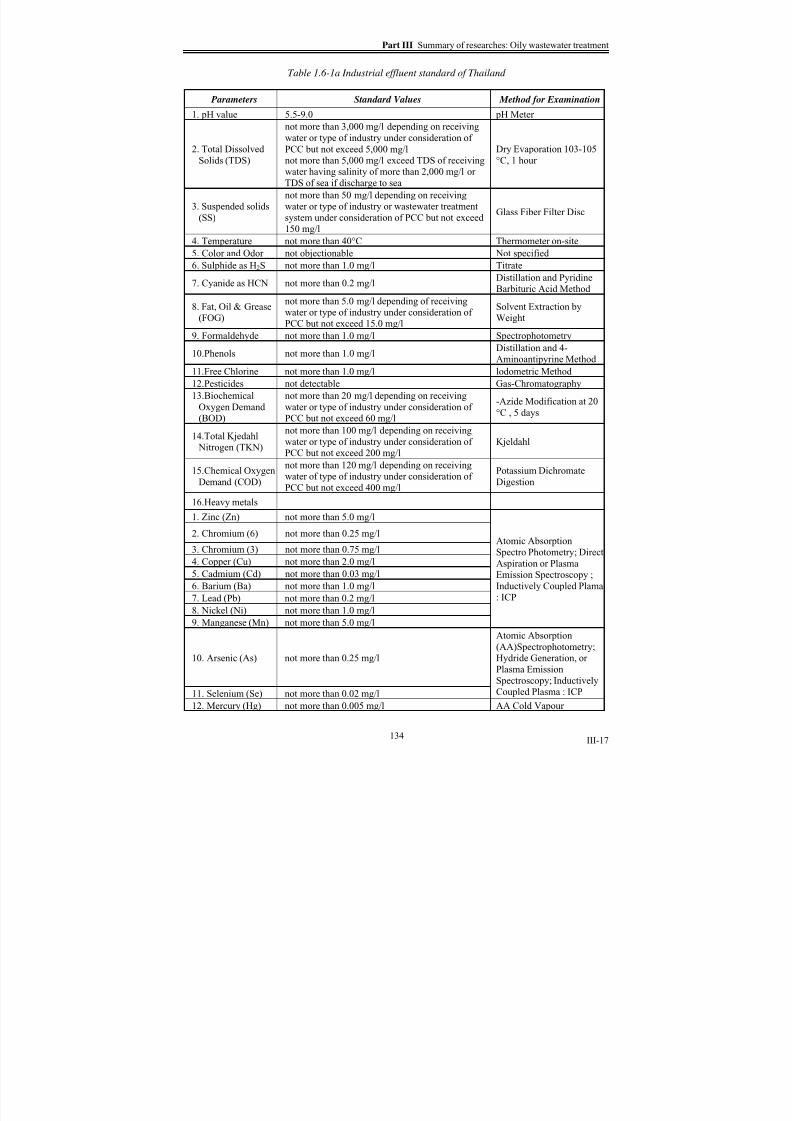
8/15/2019 Rachu.pdf
http://slidepdf.com/reader/full/rachupdf 211/646
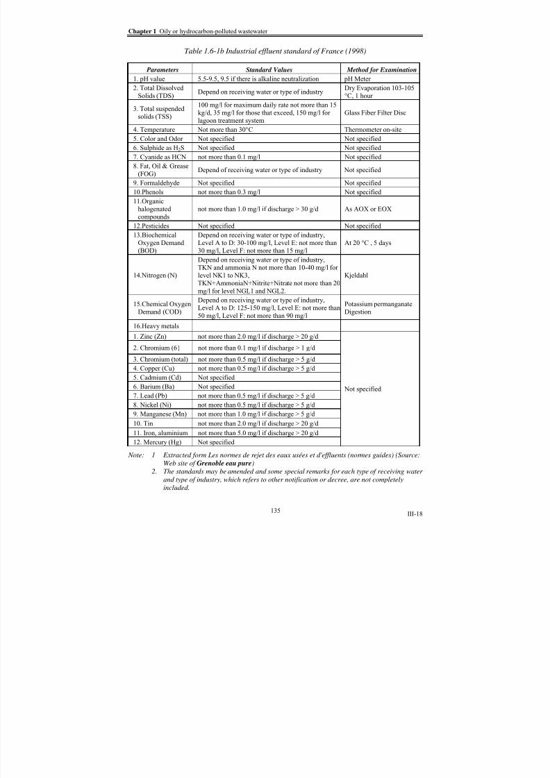
8/15/2019 Rachu.pdf
http://slidepdf.com/reader/full/rachupdf 212/646

8/15/2019 Rachu.pdf
http://slidepdf.com/reader/full/rachupdf 213/646
Part III Summary of researches: Oily wastewater treatment
III-19
Table 1.6-1c Industrial effluent standards of USA, categorized by pollutant sources
(1) CFR 40 part 419—Petroleum refining point source category
Kg / 1000 m3 of feed stock
Effluent characteristicsMaximum for any 1 day
Average of daily values for 30consecutive days shall not exceed
BOD5 34.6 18.4
COD 210.0 109.0
TSS 23.4 14.8
Oil and grease 11.1 5.9
Phenolic compound 0.25 0.120
Ammonia as N 23.4 10.6
Sulfide 0.22 0.099
Total chromium 0.52 0.30
Chromium (hexavalent) 0.046 0.020
pH 6.0-9.0 6.0-9.0
Note: 1 The limits shown in the table are to be multiplied by the process factors and size factor
to calculate the maximum for any one day and maximum average of daily values for
thirty consecutive days
(2) CFR 40 part 437—The centralized waste treatment point source category
Effluent characteristics Maximum daily (mg/l) Maximum monthly average (mg/l)
Oil and grease 127.0 38.0
pH 6.0-9.0 6.0-9.0
TSS 74.1 30.6 Metals
Arsenic 2.95 1.33
Cadmium 0.0172 0.0102
Chromium 0.746 0.323
Cobalt 56.4 18.8
Copper 0.500 0.242
Lead 0.350 0.160
Mercury 0.0172 0.00647
Tin 0.335 0.165
Zinc 8.26 4.50
Organic parameters
Bis(2-ethylhexyl) phthalate 0.215 0.101
Butylbenzyl phthalate 0.188 0.0887
Carbazole 0.598 0.276
n-Decane 0.948 0.437
Fluoranthene 0.0537 0.0268
n-Octadecane 0.589 0.302
Note: 1 The limits shown in the table arebased on best practicable control technology currently
available (BPT)
General note: The standards may be amended and some special remarks for each type of receiving
water and type of industry, which refers to other notification or decree, are notcompletely included in this chapter.
136

8/15/2019 Rachu.pdf
http://slidepdf.com/reader/full/rachupdf 214/646
Chapter 1 Oily or hydrocarbon-polluted wastewater
III-20
Table 1.6-1c Industrial effluent standards of USA, categorized by pollutant sources (Cont.)
(3) CFR 40 part 417—Soap and detergent manufacturing point source category
Kg / 1000 kg of anhydrous product
Effluent characteristics
Maximum for any 1 dayAverage of daily values for 30
consecutive days shall not exceed
BOD5 0.90 0.30
COD 4.05 1.35
TSS 0.09 0.03
Surfactants 0.90 0.30
Oil and grease 0.15 0.05
pH 6.0-9.0 6.0-9.0
(4) CFR 40 part 438—Metal products and machinery point source category
Effluent characteristics Maximum daily (mg/l)
TSS 62.0
Oil and grease (as HEM) 46.0
General note: 1 The standards may be amended and some special remarks for each type of
receiving water and type of industry, which refers to other notification or decree,
are not completely included in this chapter.
137
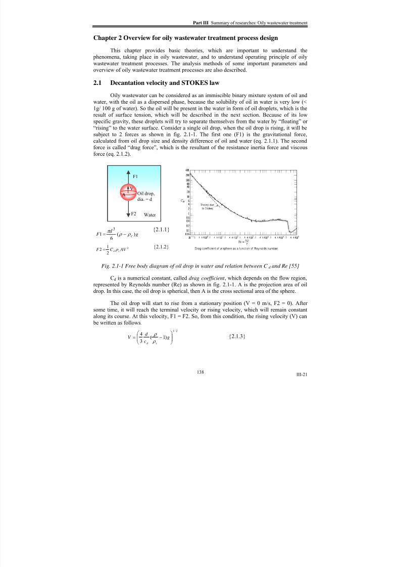
8/15/2019 Rachu.pdf
http://slidepdf.com/reader/full/rachupdf 215/646
Part III Summary of researches: Oily wastewater treatment
III-21
Chapter 2 Overview for oily wastewater treatment process design
This chapter provides basic theories, which are important to understand the
phenomena, taking place in oily wastewater, and to understand operating principle of oily
wastewater treatment processes. The analysis methods of some important parameters and
overview of oily wastewater treatment processes are also described.
2.1 Decantation velocity and STOKES law
Oily wastewater can be considered as an immiscible binary mixture system of oil and
water, with the oil as a dispersed phase, because the solubility of oil in water is very low (<
1g/ 100 g of water). So the oil will be present in the water in form of oil droplets, which is the
result of surface tension, which will be described in the next section. Because of its low
specific gravity, these droplets will try to separate themselves from the water by “floating” or
“rising” to the water surface. Consider a single oil drop, when the oil drop is rising, it will be
subject to 2 forces as shown in fig. 2.1-1. The first one (F1) is the gravitational force,
calculated from oil drop size and density difference of oil and water (eq. 2.1.1). The secondforce is called “drag force”, which is the resultant of the resistance inertia force and viscous
force (eq. 2.1.2).
F2
F1
Water
Oil drop,
dia. = d A
V
gd
F c )(6
13
ρ ρ π
−= {2.1.1}
2
2
12 AV C F cd ρ = {2.1.2}
Fig. 2.1-1 Free body diagram of oil drop in water and relation between C d and Re [55]
Cd is a numerical constant, called drag coefficient , which depends on the flow region,represented by Reynolds number (Re) as shown in fig. 2.1-1. A is the projection area of oil
drop. In this case, the oil drop is spherical, then A is the cross sectional area of the sphere.
The oil drop will start to rise from a stationary position (V = 0 m/s, F2 = 0). After
some time, it will reach the terminal velocity or rising velocity, which will remain constant
along its course. At this velocity, F1 = F2. So, from this condition, the rising velocity (V) can
be written as follows.
2/1
)1(3
4⎟⎟ ⎠
⎞⎜⎜⎝
⎛ −= g
c
d V
cd ρ
ρ {2.1.3}
138

8/15/2019 Rachu.pdf
http://slidepdf.com/reader/full/rachupdf 216/646

8/15/2019 Rachu.pdf
http://slidepdf.com/reader/full/rachupdf 217/646

8/15/2019 Rachu.pdf
http://slidepdf.com/reader/full/rachupdf 218/646
Chapter 2 Basic theory for oily wastewater treatment process design
III-24
Tip To visualize the surface tension [42], we will consider a tank that one side
wall can be moved as shown in fig. 2.2.1-2. If we try to move the wall to extend the
surface of liquid, we have to apply the force F. Then, the wall move by the distance dl.
From this, the work done or effective work can be written as:
dlF W ⋅= {2.2.2a}
When the wall is moved, we increase the surface area of the liquid, which can
be written as shown in eq. 2.2.2b.The increasing in energy of the system is as shown in
eq. 2.2.2c.
L
dl
F
F
Section
Plan
dl L A ⋅= {2.2.2b}
AG ⋅=Δ γ {2.2.2c}
We assume the process is isothermal and
reversible, so there is no heat loss. Then,
work done will be equal to energy (eq.
2.2.2d). From this, we will see that the
surface tension can be derived as shown in
eq. 2.2.2e and eq. 2.2.1
dl LdlF ⋅⋅=⋅ γ {2.2.2d}
L
F or
A
W
dl L
dlF ==
⋅⋅
=γ {2.2.2e}
Fig. 2.2.1-2 Model for Visualization of γ
Table. 2.2.1-1a Data of surface and interfacial tension (N/m) for some liquids at 20° C
[40][42]
NameSurface
tension
Interfacial
tension
(/water)
NameSurface
tension
Interfacial
tension
(/water)
Water 72.8 Ethanol 22.3
Benzene 28.9 35 n-Octanol 27.5 8.5
Acetic acid 27.6 n-Hexane 18.4 51.1
Acetone 23.7 n-Octane 21.8 5038
CCl4 26.8 45.1 Mercury 485 375
Polar organic
compounds
22-50 Aqueous
detergent
solutions
24-40
Hydrocarbon 18-30 Fluorocarbon 8-15
141

8/15/2019 Rachu.pdf
http://slidepdf.com/reader/full/rachupdf 219/646
Part III Summary of researches: Oily wastewater treatment
III-25
Adhesion work: Interfacial tension between oil and water (or any two liquids) can
relate to surface tension of each liquid by DUPRE’s equation (eq. 2.2.3a). This equation can
be also applied to solid-liquid interface, as shown in eq. 2.2.3b. γs represents surface energy of
solid.
)(owadhwoowW −+= γ γ γ {2.2.3a}
)(soadhosso W −+= γ γ γ {2.2.3b}
Tip To visualize the concept of adhesion work [42], we will consider a tank that
one side wall can be moved, filled with 2 liquids (oil and water). When we move the
wall, from eq. 2.2.2, it can be described that:
γo
γw
γo/w F
OilWater
• We increase the surface of oil and water
by γo and γw, respectively.
•
Then we attach the oil and water surfacetogether. For this, we recover an amount
of energy, called “ adhesion work”
Fig. 2.2.1-3 Model for visualization of
adhesion work
2.2.2
Liquid-solid and liquid-liquid-solid interfaces
2.2.2.1 Wetting, Contact angles, Adhesion work, and YOUNG’s equation
Wetting is the displacement from a surface of one fluid by another [40]. Therefore, it
involves three phases and, at least two phases must be fluid. To understand this, we will
consider the oil drop on a solid surface in water, as shown in fig. 2.2.2-1.
θso
γow
γsoγsw
Water
Solid
Oil droplet
Fig. 2.2.2-1 Diagram of Oil drop on solid surface in water
Contact angle: The angle between tangential line of oil drop’s surface and the surface
of solid is called “contact angle”. In case that the oil remains as a drop, it means the system is
in equilibrium. We will have definite contact angle θso. Equilibrium of force on the dropletcan be written as shown in eq. 2.2.4, known as YOUNG’s equation.
142

8/15/2019 Rachu.pdf
http://slidepdf.com/reader/full/rachupdf 220/646

8/15/2019 Rachu.pdf
http://slidepdf.com/reader/full/rachupdf 221/646

8/15/2019 Rachu.pdf
http://slidepdf.com/reader/full/rachupdf 222/646
Chapter 2 Basic theory for oily wastewater treatment process design
III-28
Table 2.2.2-1 Relation between contact angle, work adhesion, interfacial tension and spread
coefficient of oil/water/solid system [42]
Contact angle
soWadh(so)w
Relation beween
interfacial tensionCharacteristic of oil drop
= 0° > 2γow > 0 γsw > γso + γow
γso
γow
γsw
= 0° = 2γow = 0 γsw = γso + γow
γso
γow
γsw
0°<θso<90o γow <W< 2γow < 0 γsw > γso θ
γso
γow
γsw
= 90o
W = γow < 0 γsw = γso θ
γso
γow
γsw
90°<θso<180
o
0<W < γow < 0 γsw < γso θγso
γow
γsw
=180o W = 0 < 0 γso = γsw+γow
γso γsw
γow
145

8/15/2019 Rachu.pdf
http://slidepdf.com/reader/full/rachupdf 223/646
Part III Summary of researches: Oily wastewater treatment
III-29
2.2.3 Capillary pressure and LAPLACE’s law
2.2.3.1 LAPLACE’s law
LAPLACE’s law is the relation of pressure difference across the surface of liquid of
surface tension γ. If we consider the air bubble in water, at one fraction of the bubble with theradius of curvature R1, and R2 on 2 perpendicular plains (fig. 2.2.3-1), the pressure
difference, by LAPLACE’s law, will be as shown in eq. 2.2.11:
R 1 R 2Section of
surface of air
bubble in water
P (Outside pressure)
P’(Inside pressure)
Fig. 2.2.3-1 Section of air bubble in water
)11
('21 R R
PPP +=−=Δ γ {2.2.11}
From the equation, we can calculate the
pressure difference of the following
systems, i.e.,
• A soap bubble of radius R in air
RP γ 4=Δ
Because there are 2 interfaces of air/soap.
• An air bubble of radius R in water
RP
γ 2=Δ
• A cylindrical jet of water in airγ
P =Δ R
Because R 2 is infinity.
2.2.3.2
Capillary pressure
Capillary effect is an important phenomenon for oil/water separation process when we
consider flowing through porous media, such as ultrafiltration membrane. This phenomenon
will be described by fig. 2.2.3-2. When the tube with very small diameter (capillary tube) is
plunged into liquid surface. Because of surface tension of liquid, the liquid will rise into the
tube to the height h. From equilibrium, we can calculate the capillary pressure (Pc) as follow:
catmb PghPP ==− ρ {2.2.12}
From LAPLACE’s law,
r RPP atmb
θ γ γ cos22 ==− {2.2.13}
From eq. 2.2.12 and 2.2.13,
r Pc
θ γ cos2= {2.2.14a}
And
gr h
ρ
θ γ cos2= {2.2.14b}
146

8/15/2019 Rachu.pdf
http://slidepdf.com/reader/full/rachupdf 224/646
8/15/2019 Rachu.pdf
http://slidepdf.com/reader/full/rachupdf 225/646
Part III Summary of researches: Oily wastewater treatment
III-31
Method of analysis
1. Solvent extraction [1]
This method is the standard method of examination of oil and grease. They are at
least 4 variations. However, they all involve an initial extraction of oil and grease by hexaneor CFC-113. The 4 variations include,
• Partition-gravimetric method: Hexane will be used to extract the oil. Then
it will be separated from water and then evaporated. The residue will be used
as an inditator of oil and grease content.
• Partition-infrared method: CFC-113 will be used as extractant. Then it will
be measured with infrared scanning. This method is faster than gravimetric
method. The accuracy depends on selection of oil standards for calibration.
The oil used for calibration should be the same type as oil in the wastewater.
•
Soxhlet extraction: It involves the initial step of acidification and thenhexane extraction. This method tends to retain more volatile hydrocarbons.
However, it is time consuming.
• Hydrocarbon analysis: Silica gel is added to hexane to remove fatty
materials. And then the hexane will be analyzed by the first method.
2.
Turbidity measurement
Oil concentration can be measured by light loss (turbidity) or light scatter from
oil droplets in the wastewater [43]. The main advantage of this method is its simplicity and
fast response. However, it will be difficult to distinguish between oil droplets and other
particles. Some manufacturer claim that this effect can be minimized by the selection of theangle of scatter and detector. In GPI lab, some researchers use this method to measure the oil
concentration. It is suitable to use for relatively clear wastewater, such as condensate.
However, in most situations, oily wastewaters are usually contaminated by color materials and
suspended solids. This method, thus, may not provide accurate result on oil concentration.
3.
TOD measurement
If total oxygen demand (TOD) measuring instrument is available, oil
concentration can also be measured as TOD. Again, the main advantage of this method is its
fast response. However, it will be difficult to distinguish between TOD of oil and other
substances, especially surfactants and co-surfactants. So this fact should be taken intoaccount. In GPI lab, some researchers use this method to measure the oil concentration. The
data from the researches are presented in chapter 1. It must be noted that TOD includes
oxygen demand from non-organic factors, such as ammonia, sulfide. Thus its value is usually
higher than BOD.
4.
Other methods
Total organic carbon (TOC) is also widely used to measure pollutant
concentration. Its working principle bases on oxidizing of the sample, usually at high
temperature, to convert carbons to carbondioxide, which will be measured by IR, UV probe.
TOC machine can cover from ppm to ppt range. It is very useful for online control. But it doesnot account for nitrogen compounds, which have much higher oxygen demand than carbons.
148
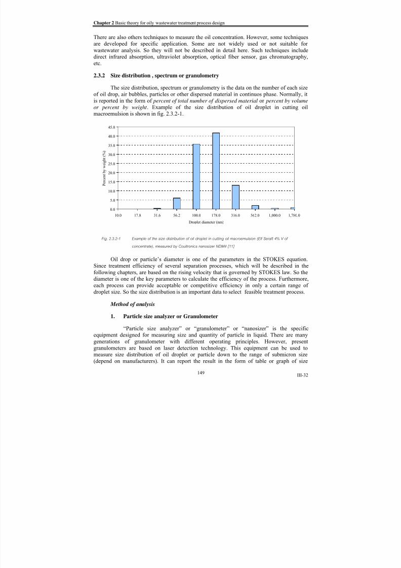
8/15/2019 Rachu.pdf
http://slidepdf.com/reader/full/rachupdf 226/646
Chapter 2 Basic theory for oily wastewater treatment process design
III-32
There are also others techniques to measure the oil concentration. However, some techniques
are developed for specific application. Some are not widely used or not suitable for
wastewater analysis. So they will not be described in detail here. Such techniques include
direct infrared absorption, ultraviolet absorption, optical fiber sensor, gas chromatography,
etc.
2.3.2 Size distribution , spectrum or granulometry
The size distribution, spectrum or granulometry is the data on the number of each size
of oil drop, air bubbles, particles or other dispersed material in continuos phase. Normally, it
is reported in the form of percent of total number of dispersed material or percent by volume
or percent by weight . Example of the size distribution of oil droplet in cutting oil
macroemulsion is shown in fig. 2.3.2-1.
0.0
5.0
10.0
15.0
20.0
25.0
30.0
35.0
40.0
45.0
10.0 17.8 31.6 56.2 100.0 178.0 316.0 562.0 1,000.0 1,780.0
Droplet diameter (nm)
P e r c e n t b y w e i g h t ( % )
Fig. 2.3.2-1 Example of the size distribution of oil droplet in cutting oil macroemulsion (Elf Seraft 4% V of
concentrate), measured by Coultronics nanosizer NDM4 [11]
Oil drop or particle’s diameter is one of the parameters in the STOKES equation.
Since treatment efficiency of several separation processes, which will be described in the
following chapters, are based on the rising velocity that is governed by STOKES law. So the
diameter is one of the key parameters to calculate the efficiency of the process. Furthermore,each process can provide acceptable or competitive efficiency in only a certain range of
droplet size. So the size distribution is an important data to select feasible treatment process.
Method of analysis
1. Particle size analyzer or Granulometer
“Particle size analyzer” or “granulometer” or “nanosizer” is the specific
equipment designed for measuring size and quantity of particle in liquid. There are many
generations of granulometer with different operating principles. However, present
granulometers are based on laser detection technology. This equipment can be used to
measure size distribution of oil droplet or particle down to the range of submicron size
(depend on manufacturers). It can report the result in the form of table or graph of size
149

8/15/2019 Rachu.pdf
http://slidepdf.com/reader/full/rachupdf 227/646
Part III Summary of researches: Oily wastewater treatment
III-33
distribution, both by number and by volume or weight. An example in fig. 2.3.2-1 was also
measured by the granulometer. Fig. 2.3.2-2 shows the picture of granulometer.
Fig. 2.3.2-2 Granulometer (Source: above - Ankermid Techcross / below - CILAS)
2. Decanting test
When the use of granulometer is not available, there is a simple method to
measure the size distribution, which is called “decanting test”. This method requires a simple
equipment as shown in fig. 2.3.2-3.
0 min 5 min 10 min …. t min
h1h2
h3
h4
Fig. 2.3.2-3 Decanting test column
150

8/15/2019 Rachu.pdf
http://slidepdf.com/reader/full/rachupdf 228/646
Chapter 2 Basic theory for oily wastewater treatment process design
III-34
Analytical procedure
1) Pour the wastewater into the decanting test column and stir. Make sure it is
homogeneous.
2) Leave the wastewater to decant, taking the water samples from various
heights of the column at preset interval.
3) Analyze the samples to find the oil concentration or other parameters that
are directly proportional to the oil concentration, such as TOD, turbidity,
etc.
4) From the collected data, we can calculate the granulometry, using this
procedure:
• At t = 0, the wastewater is homogeneous, then the oil concentration is
Co throughout the column.
• At t = t1 and height (from the bottom of the column) = h1, the
corresponding rising velocity Vh1t1 = h1/t1.
• So at this point, the oil drop that have rising velocity greater than Vh1t1
will rise past the height h1 then will not be found in the sample taken
from h1. From Vh1t1, we can calculate the corresponding droplet
diameter d h1t1 by STOKES law.
• If the oil concentration at this point is Ch1t1, and the calculated droplet
diameter is d h1t1, we can conclude that:
The fraction of d < d h1t1 = Ch1t1/Co
5) Repeat step 4), at other t and h. then, use the fraction of d < d hx tx to plot the
size distribution curve.6)
Concentration of each droplet size can be roughly represented by the
differences between value of adjacent % of accumulated C/Co. Please note
that the size and %C/Co are estimated values only. But it can provide an
idea of how the sizes of droplet are distributed.
An example of the analysis of decanting test data is shown in tab. 2.3.2-1 and fig.
2.3.2-4 and 2.3.2-5.
151

8/15/2019 Rachu.pdf
http://slidepdf.com/reader/full/rachupdf 229/646
Part III Summary of researches: Oily wastewater treatment
III-35
Table 2.3.2-1a Example of the decanting test of oil/water emulsion
Time
At sampling height
(from the bottom
of column)
Corresponding rising
velocity
Oil concentration of
the sample
% accumulated C/Co
when d <
dEht
Corresponding droplet
size (from STOKES
law)
h Vh,t
Ch,t
% Ch,t/C
odE
h,t
sec m m/s mg/l % micron
0 0.5 86 100
900 0.5 5.56E-04 57 66.28 72.8
1800 0.5 2.78E-04 25 29.07 51.4
2700 0.5 1.85E-04 8 9.30 42.0
3600 0.5 1.39E-04 3 3.49 36.4
5400 0.5 9.26E-05 1 1.16 29.7
7200 0.5 6.94E-05 0 0.00 25.7
0 1.25 86 100
900 1.25 1.39E-03 83 96.51 115.0
1800 1.25 6.94E-04 63 73.26 81.3
2700 1.25 4.63E-04 49 56.98 66.4
3600 1.25 3.47E-04 37 43.02 57.5
5400 1.25 2.31E-04 16 18.60 47.0
7200 1.25 1.74E-04 6 6.98 40.7
7200 1.25 2.06E-03 80 93.02 140.0
Note: Assume the oil is kerosene so the density (20o C) = 790 kg/m3. Water dynamic
viscosity = 1.08E-3 (N.S)/m2.
152

8/15/2019 Rachu.pdf
http://slidepdf.com/reader/full/rachupdf 230/646
Chapter 2 Basic theory for oily wastewater treatment process design
III-36
Table. 2.3.2-1b Example of the decanting test of oil/water emulsion: sorting of the result
from table 2.3.2-1a
Corresponding droplet size Corresponding rising velocity
% accumulated C/Co
when d
< dEht
Estimated C/Co for
each droplet size
dE Vh,t
% Ch,t/C
o%C/Co
micron m/s % %
25.72 6.94E-05 0
29.70 9.26E-05 1.16 1.16
36.38 1.39E-04 3.49 2.33
40.67 1.74E-04 6.98 3.49
42.00 1.85E-04 9.30 2.33
46.96 2.31E-04 18.60 9.30
51.44 2.78E-04 29.07 10.47
57.52 3.47E-04 43.02 13.95
66.41 4.63E-04 56.98 13.95
72.75 5.56E-04 66.28 9.30
81.34 6.94E-04 73.26 6.98
115.03 1.39E-03 96.51 23.26
0
10
20
30
40
50
60
70
80
90
100
0.00 20.00 40.00 60.00 80.00 100.00 120.00 140.00
Oil droplet size (dE) (micron)
% A
c c u m u l e t e d C / C o
Accumulated conc. curve h = 0.5 m h = 1.25 m
Fig. 2.3.2-4 Relation between accumulated C/Co (% of C/Co when the droplet size is equal or smaller than the
153

8/15/2019 Rachu.pdf
http://slidepdf.com/reader/full/rachupdf 231/646
Part III Summary of researches: Oily wastewater treatment
III-37
given dE) and oil droplet size
0
5
10
15
20
25
26 30 36 41 42 47 51 58 66 73 81 115
Droplet size (micron)
% b
y w e i g h t
Fig. 2.3.2-5 Example of estimated size distribution of oil droplets from decanting test
3.
Visual observation
To roughly estimate the granulometry of oily wastewater, there are simple
criteria for visual observation as shown in table 2.3.2-2. However, these criteria may be used
only when the wastewater is not polluted by suspended solids or other substances that makes
it opaque. In case of surface oil layer, API [45] recommended useful guide to evaluate oil
thickness as shown in table 2.3.2-3.
Table 2.3.2-2 Criteria for visual observation of size distribution [22]
Visual aspect Average particle size Example
Particles visible by eye 500 micron Very fine sand
Not clearly visible by eye 100 micron Starch
Opaque milky 10 micron Milk
Whitish milky 1 micron Homogenized milk
Bluish milky 0.1 micron Macroemulsion
Semitransparent 50 nm Microemulsion
Transparent 10 nm Microemulsion
Transparent 2-6 nm Micelles
Transparent 1 nm Molecules
154

8/15/2019 Rachu.pdf
http://slidepdf.com/reader/full/rachupdf 232/646
Chapter 2 Basic theory for oily wastewater treatment process design
III-38
Table 2.3.2-3 Criteria for visual observation of surface oil film [45]
Film thickness
(micron)Appearance
Approximate volume of oil
for film 1 km2 in area (l)
38.1 Barely visible under mostfavorable light conditions
37
76.2 Visible as silvery sheen on
surface of water
74
152.4 First trace of color may be
observed
148
304.8 Bright bands of color are visible 296
1016 (1 mm) Colors begin to turn dull 985
2032 (2 mm) Colors are much darker 1970
2.3.3 Other parameters
Each treatment process may require some special data for its calculation. However,
common data required by several processes include:
• Interfacial tension
• Viscosity of oil
These data can be analyzed by specialized laboratories. However, if we know the
source of the oily wastewater, we can estimate these parameters. Even when we can notspecify the exact source of oil, we still can estimate them, using the general data of oil or from
references, without too much error. These data can also be found in chapter 1 and this chapter.
2.4 Overview of oily wastewater treatment processes
As hydrocarbon or oil requires a great amount of oxygen or oxidizing agent to oxidize,
moreover, the hydrocarbon is relatively difficult to biodegrade, thus, it becomes clear that the
use of biological treatment with high-concentration oily wastewater may not be the
economical alternative. Besides there are possibilities to reuse or recover the hydrocarbons
in the wastewater. Then, if possible, it is reasonable to separate oil from the wastewater,
rather than destroy or change them into other forms.
Thus almost all of treatment processes that have been studied in GPI laboratory are
based on separation process, both physical and physico-chemical, techniques in order to
separate oil from water. From chapter 1, it shows that oily wastewaters can be divided into
several categories, mainly depending on their stability and degree of dispersion. And in the
previous sections on this chapter, it shows that physical separation of oil from water depends
on STOKES law.
Thus, to enhance separation between water and oil, it can be archived by modification
of parameters in STOKES law in the manner that make the rising velocity of oil droplets
increase. Actually, almost all of oil/water separation processes covered by Prof. AURELLE’sresearch team are STOKES law-based processes, i.e. decanter, coalescer, hydrocyclone, and
155

8/15/2019 Rachu.pdf
http://slidepdf.com/reader/full/rachupdf 233/646
Part III Summary of researches: Oily wastewater treatment
III-39
dissolved air flotation (DAF). Thus each process will has its own limitation, bound by
assumptions of STOKES law as well as its unique working characteristic.
Apart from STOKES law-based processes, there are other oil/water separation
processes that based on other physical properties between oil and water. In GPI lab, Prof.
AURELLE’s teams also studied these processes, i.e. skimmer (which is based on interfacialtension concept), membrane process (which depend on mass transfer phenomena), thermal
process (which depends on thermodynamic properties), and chemical process (which depends
on chemical reaction).
Thus, to design an efficient oily wastewater treatment process, designer should
understand working principle and limitation of each process. The following chapters will
devote to each oily wastewater treatment processes studied and perfected by Prof.
AURELLE’s team within 3 decades. However, in this section, description of each process will
be described briefly as follows,
STOKES law-based processes
2.4.1
Decanter
Decanter is an oil separation process that depends purely on STOKES law without
modification of their parameters. The oil droplets in wastewater will allow to decant (or rise)
naturally to the surface of water .It is very simple and proven to be very good process for
separation of free oil and primary emulsion. Rising velocity depends mainly on the droplet
size. In case of very small droplets, it may take too long time for the droplets to reach the
surface or it may need so large tank to become economical. However, performance of
decanter can be enhanced by reducing of rising distance of droplets, such as by lamella-plate
insertion. Actually, GPI lab had initiated a very compact decanter by this concept, called“Spiraloil”, which is commercialized by Elf Total Fina. Decanter is described in details in
chapter 4.
2.4.2 Coalescer
Coalescer is a modified or accelerated STOKES law-based separation process by
increasing the size of oil droplet. Since rising velocity is proportional to square of droplet
size, theoretically, coalescer can enhance oil separation efficiency more rapidly than other
process that work on other parameters. AURELLE is one of the pioneers on granular bed
coalescer, which was patented and, later, commercialized by Elf Total Fina. He also initiated
other type of coalescer, i.e, granular bed coalscer with guide to handle wastewater with highoil concentration, fibrouse bed coalescer that can handle wastewater with SS. Coalescer can
handle secondary emulsion effectively. However, its performance with stabilized emulsion is
not so good since the droplets are very table and unlikely to coalesce with each other.
Coalescer is described in details in chapter 5.
2.4.3 Hydrocyclone
Hydrocyclone is a modified or accelerated STOKES law-based separation process by
increasing the acceleration of the system. Hydrocyclone replaces gravity acceleration (g)
with centrifugal acceleration, which can reach several hundreds times of g. Thus it is very
compact separation process. AURELLE and MA had initiated three-phase hydrocyclone thatcan separate oil, solids and water simulteneously. Hydrocyclone use its inlet flow energy to
156

8/15/2019 Rachu.pdf
http://slidepdf.com/reader/full/rachupdf 234/646
Chapter 2 Basic theory for oily wastewater treatment process design
III-40
operate. So it is noted for its increase in efficiency with the increase of inlet flow, which is
unique advantage of the system. It can handle secondary emulsion effectively. However, its
operation has high shear characteristic. Furthermore, it driving force come only from its inlet
flow so the centrifugal force is limited. So it can not separate very small droplets (<10
microns). It must also be noted that hydrocyclone is actually a concentrator. It can not
separate water-free oil. Separated oil usually contains some water. Thus it need to be furthertreated by other process. Hydrocyclone is described in details in chapter 6.
2.4.4 Dissolved air flotation (DAF)
DAF is a modified or accelerated STOKES law-based separation process by
decreasing density difference between oil and water. It can be obtained by addition of gas
bubble or air bubble to wastewater to form agglomerates with oil droplets. Since air or gas has
low density the agglomerates, then, has lower density than oil drops, resulting in higher rising
velocity. DAF is noted for its versatility. It can separate both solids and oil. Its efficiency
depends on formation of oil-bubble agglomeration. Thus its performance is low if droplets are
very small, since collision between air bubble and oil drops is difficult. In practice, DAF will be used after coagulation-flocculation process, which can increase the droplet sizes
chemically. DAF is described in details in chapter 7.
Other processes
2.4.5 Skimmer
Skimmer is the device designed to remove oil film from the water surface. GPI lab had
studied and perfected skimmer’s oil performance so it can selectively remove only oil without
drawing the water with it. Operating principle of the oleophilic oil skimmer is based on
surface tension concepts. The skimmer studied in GPI lab was also commercialized. Detailsabout skimmer are described in chapter 3.
2.4.6 Membrane processes
Membrane processes are the promising separation processes that gain popularity in
these recent years. The key part of the processes is the membrane, which is porous material
with various ranges of pore size to suit the sizes of material to be retained or separated. Its
working principle can be compared, but not exactly identical, to that of filtration process.
With properly selected pore size, membrane processes can separate target materials with
relatively high efficiency. GPI lab had studied application of various membrane processes,
i.e., microfiltration, ultrafiltration, nanofiltration and reverse osmosis on oily wastewatertreatment. The lab also initiated studies on capacity (or flux) enhancement of membrane
process for cutting oil emulsion treatment. Membrane processes are described in details in
chapter 8.
2.4.7 Thermal processes
Thermal process is the separation process based on thermodynamic properties of
oil/water mixture. GPI lab emphasizes on heteroazeotropic distillation, which can be carried
out at the temperature that is lower than those of pure water and pure hydrocarbons. It is
achieved by addition of proper hydrocarbons, called entrainer or extractant, into the
wastewater to azeotrope point, where oil, water and vapor co-exist , during distillation. The process can be used to separate water from refinery slops and permeate from membrane
157

8/15/2019 Rachu.pdf
http://slidepdf.com/reader/full/rachupdf 235/646
Part III Summary of researches: Oily wastewater treatment
III-41
process of oily wastewater treatment. Thus it provides opportunity to recover these supposed-
to-be-wasted oil and treat the most problematic waste. Thermal processes are described in
details in chapter 9.
2.4.8 Chemical process
Chemical process for oily wastewater treatment is mainly destabilization process for
destabilizing of stable emulsion. It consists of 2 main mechanisms, i.e. destabilization of oil
droplets and coalescence or flocculation of destabilized oils. This process is necessary when
the wastewater to be treated contains stable or stabilized emulsion, otherwise it can not be
treated by STOKES law-based processes. Destabilization chemicals includes salts, acids, and
polyelectrolytes. GPI lag had studied destabilization mechanisms of each chemical which
provide understanding and knowledge on chemical selection. The detail is discussed in
chapter 10.
2.4.9 Finishing processes
To meet the effluent standards, effluent from aforementioned processes may need
further treatment before discharge to receiving water body. The most widely used processes
for finishing propose are biological treatment and adsorption (by activated carbons). These
processes are not the main interest in Prof. AURELLE’s team, which emphasize of physical
processes. However, to fulfil the whole oily wastewater treatment processes, biological
treatment and adsorption are briefly described in chapter 11.
The theories and details of each processes described in section 3 to 11 will, then, be
used to develop the software for design and simulation of oily wastewater process train,
which is the scope of work of this thesis.
2.5 Determination of degree of treatment
2.5.1 Overall degree of treatment
Before designing oily wastewater process, required overall degree of treatment or
effluent quality of the treatment system must be set. In case that the effluent is discharged to
public receiving water body, such as sewage system or natural stream, the final effluent
quality must conform to every applicable law. Examples of effluent standards are shown in
chapter 1. In case that the water is recycled or reused, required water quality for those
purposes, such as standard of recycled water quality, standard of recycled cooling water, etc.,
will determine the overall degree of treatment.
2.5.2 Degree of treatment of each process
Since the performance of every treatment process depends mainly on wastewater
characteristic, for existing facilities, wastewater must be thoroughly analyzed to obtain its
detailed characteristic. For new facilities, its characteristic must be carefully estimated. In
case of oily wastewater, performances of oil separation processes are based on degree of
dispersion and stability of the wastewater. When these data are available and limitation as
well as expected performance of each treatment process is thoroughly understand, it is
possible to select feasible process train that can treat the wastewater to meet the required
degree of treatment .
158

8/15/2019 Rachu.pdf
http://slidepdf.com/reader/full/rachupdf 236/646
Chapter 2 Basic theory for oily wastewater treatment process design
III-42
Example A: consider wastewater from in-land refinery contains 230 mg/l of non-
stabilized secondary emulsion and 10 mg/l of emulsified oil. If applicable effluent standard in
this case is 12.0 mg/l, in this case, the degree of treatment of the system is (10+230-
12)/(10+230)*100 = 95%. We can separate the secondary emulsion by compact decanter,
coalescer or DAF, which secondary emulsion removal efficiency is expected at 90%. So it
requires further treatment and the degree of treatment required in the next stage is at least 100-((100-950)/(100-80)) = 50%. In this case, It can be archieved by sending to the water to mix
with domestic wastewater and treat by biological treatment. The concentration of 12.0 mg/l
may be met by dilution effect of domestic wastewater alone. Moreover the biological process
can be reduced the oil concentration at least 50%. Thus it can be certain that the effluent
concentration of 12 mg/l is guaranteed at all times.
2.5.2.1 Graded efficiency and total removal efficiency
As stated before that efficiency of most separation process depends on the size of oil
droplets, most of researches in GPI lab had common aim to establish the relation between
the efficiency and droplet size, which will be shown in the following chapters. Ifgranulometry data (see fig. 2.3.2-5) is available, it will provide clear data on percentage of
each size of oil droplets. So it is very useful for removal efficiency calculation of each droplet
size ( graded removal efficiency) of each process. Summation of graded efficiency of each
process results in total removal efficiency of that process corresponding to that particular
wastewater , which is more accurate than the estimated value from literatures alone. In case
that the treatment system consists of several processes, overall efficiency can be determined
from summation of greaded effeciecny of ecah process, as shown in eq. 2.5.1.
100))1)....(1)(1(1( ,2.1,, ⋅−−−−= id d d overalld η η η η % {2.5.1a}
( )%100
,
,,
,
max
min ⋅⋅
=∑
io
d
d
iod id
it C
C η
η {2.5.1b}
( )%100
max
min
,
⋅
⋅
=∑
o
d
d
od overalld
overallC
C η
η {2.5.1b}
Where ηoverall = Overall efficiency of the treatment process train
ηd,overall = Graded removal efficiency of the treatment process train
ηd,i = Graded removal efficiency of the process “i”, calculated by
equation of each process shown in the following chaptersηt,i = Total removal efficiency of the process “i”
Co = Oil inlet concentration of the treatment process train
Co,i = Oil inlet concentration of the process “i”
Cod,i = Graded oil inlet concentration of the process “i”
i = the number of processes in the process train, i ≥ 1
To achieve the required effluent standard, overall efficiency of the system must be
equal of higher than the required degree of treatment, established in section 2.5.1.
159

8/15/2019 Rachu.pdf
http://slidepdf.com/reader/full/rachupdf 237/646
Part III Summary of researches: Oily wastewater treatment
III-43
2.5.2.2 Cut size determination
Since the bigger oil drops are realtively easier to remove than the smaller ones, it is
recommended to select the treatment process to handle the range of oil drops from the biggest
to the smallest size that contributes to the required degree of treatment (in case that the
granulometry data is known). This smallest size in the range described above is called cut size.
For example, if the granulometry of the wastewater is as shown in fig. 2.3.2-4, if the
required degree of treatment is 90%, from the curve, the cut size will be 90 microns.
The cut size is very useful in process design for it can be used as a representation of
the whole wastewater to calculation the required size of separation process. It can save
calculation time when many processes are to be compared. However, sizing of the process
calculated from this theoretical cut size may not be exactly equal to the degree of treatment
since the cut size is selected based on the assumption that the graded removal efficiency of
droplet equal to larger than cut size is 100% (see fig. 2.5.2-1). Thus some adjustments should be made after detailed calculation of the efficiency by eq. 2.5.1.
Droplet size
R e q u i r e d d e g r e e
o f t r e a t m e n t
Theo.
cut size
100%
Acc. %
(by weight)
Droplet diameter
ηoverall
Real eff.Theo. eff
η R = Required degree
of treatment
Theo.
cut size
Real
cut size
100%
ηR
Fig. 2.5.2-1 Cut size determination
2.5.2.3 Economics of the processes
Performance of each separation process also depends on other parameters apart from
the droplet size. Change in these parameters will also make the performance of the process
change. Thus the process train can be optimized by changing influent parameters, usually the
geometry, of each process in the process train to make the overall efficiency as close to the
required degree of treatment as possible.
Treatment capability of processes may overlap in some range of droplet sizes, which
will be summarized again in chapter 12. For example, droplet size around 20 microns can be
treated by coalescer or compact decanter. This leads to several combinations of process trains.
For example, the process train in example A may be divided into 2 alternatives, i.e. (1)
Compact decanter+activated sludge (AS), (2) Coalescer+Activated sludge. In each alternative,
the sizes of equipment and reactors can be varied within its own valid range. Thus, to select
the best alternative and process sizes, economics of each alternative should be compared.
160

8/15/2019 Rachu.pdf
http://slidepdf.com/reader/full/rachupdf 238/646

8/15/2019 Rachu.pdf
http://slidepdf.com/reader/full/rachupdf 239/646
Chapter 3 Oil skimmer
III-45
Chapter 3 Oil skimmer
3.1 General
The most basic form of oily wastewater is the presence of oil film or layer on the
water surface. The most severe case of this form of oily wastewater is the large-scale oil spill,caused by tanker or offshore platform accident. The oil will spread over wide area and cause
adverse effect on ecosystem. When the accident occurs, the oil confinement, such as booms, is
arranged to limit the spreading area. Then, the spilled oil is, sometimes, dispersed by chemical
dispersant to form tiny droplets, then left to biodegrade. Biological accelerating agents may
be added to promote biological degradation. Sometimes, specific adsorbents are added to the
oil to make it settleable or in more manageable form, such as floating agglomerate scum.
These methods may still cause adverse effect on the environment. Thus, if possible, the oil
layer is preferably removed in form of water-free oil for it can be reused.
In oily wastewater treatment process, the goal of almost all of the separation processes
is to separate the oil droplets and form an oil layer on the water surface. After that, it is alsocrucial to remove this oil layer as water-free oil, otherwise it will become new oily
wastewater. In a small container, the oil layer can be removed manually or by simple devices,
such as weir, bell mouth pipe. Anyway, in case of oil spill at sea, or upscale tank, it is difficult
to remove only oil without getting water with it even though the oil film is visibly stratified
from the water. In these cases, specific devices that have good oil selectivity are required.
There are many variations of these devices as shown in fig. 3.1-1. However, they can be
generally divided into 2 concepts i.e.,
•
Pumping or hydraulic devices: The oil will be directly pumped out or intercepted
by controlled hydraulic devices, such as adjustable-weir. Important factor that
governs the performance is the oil layer thickness. So, some mechanisms are provided to locally thicken the oil layer before removing it. Examples of the
devices include pump skimmer and weir skimmer.
• The devices based on adsorption property: This group of devices makes use of
difference between oil and water adsorption property of material to remove the oil.
The oil selectivity of material is based on the concept of interfacial tension, as
described in chapter 2. When design properly, the device can remove virtually
water-free oil from the wastewater. Examples of the devices include drum
skimmer, disc skimmer, belt skimmer, etc.
This chapter emphasizes on the drum and disk skimmer, which are thoroughlyresearched in GPI lab.
162

8/15/2019 Rachu.pdf
http://slidepdf.com/reader/full/rachupdf 240/646
Part III Summary of researches: Oily wastewater treatment
III-46
a) Disc skimmer (source: Highland tank) b) Belt skimmer (Source: Ultraspin)
c) Drum skimmer (source: ELF/GPI lab) d) Mop skimmer (source: Ultraspin)
e) Weir skimmer (Source: Skimoil) f) Pump skimmer (Source: Ro cleandesmi)
g) Dispersant spray (Source: Ro-cleandesmi) h) Absorbent (Source: Ro-cleandesmi)
Fig. 3.1-1 Examples of oil skimming devices
163

8/15/2019 Rachu.pdf
http://slidepdf.com/reader/full/rachupdf 241/646
Chapter 3 Oil skimmer
III-47
3.2 Oil drum skimmer
3.2.1
Working principles
Oil drum skimmer is the equipment that has a rotating drum which its surface acts as
an oil-skimming surface (fig. 3.2.1-1). The oil will adhere to the skimming surface, lift upfrom the surface by the skimmer’s rotating movement, and then be scraped off by a scrapper
blade into a receiving channel or container.
Drum skimmer
Scrapper
Oil receiving
trough
Oil layer
Water
Fig. 3.2.1-1 Lab-scale drum skimmer: Major components are shown. (Source: GPI lab)
The working principle of oil drum skimmer, as well as other absorption based devices,
is based on surface energies of hydrocarbon, water and skimmer material. To obtain water-
free oil, the material must have good oil selectivity. THANGTONGTAWI [5] had studied theeffect of surface energies on oil selectivity and concluded that oil selectivity of the material
depends on the difference between its critical surface tension (see chapter 2) and the
superficial (surface) tensions of hydrocarbon and water.
Water normally has higher superficial tension (around 72 dyne/cm, depending on the
temperature) than oil (25 – 40 dyne/cm). The diagram in fig. 3.2.1-2 shows surface energy of
water, oil and various materials. Adhesion of oil or water at the material surface can be
explained in term of the adhesion work (see chapter 2, eq. 5.2.5) as shown in table 3.2.1-1. If
the adhesion work of oil on solid surface in presence of water (Wadh(so)w ) is greater than that
of water on the surface in presence of oil (Wadh(sw)o), the oil film will adhere to the skimmer
surface and not be replaced by water film when the skimmer is rotated until the oil film
submerges in water. Thus, it still adheres to the surface when it is lifted from the liquid and
then removed by the scraper.
From this concept, the oil selectivity of materials can be summarized as follows,
• Material of high surface energy (or critical surface tension), such as stainless steel
(γ > 72 dyne/cm), tends to be adhered by water, rather than oil.
• Material that have the surface tension in the vicinity of oil’s, such as
polyvinylchroride (PVC), polypropylene (PP), tends to adhered by oil, rather than
water. It can be adhered by water if the oil film is not present. However, it willstart recovering oil once the oil is present again.
164

8/15/2019 Rachu.pdf
http://slidepdf.com/reader/full/rachupdf 242/646
Part III Summary of researches: Oily wastewater treatment
III-48
• Material that has very low critical surface tension (lower than surface tension of
oil), such as PTFE and fluorocarbon variations, is proven to have very good oil
selectivity since its surface energy is so low that it is hardly adhered by water.
When used as a skimmer material, it recovers only oil and hardly or does not
recover water.
2010 30 40 50 60 70
PTFE
(19)PP
(30)
PVC
(39)
Water
(72)Stainless steel
(> 72)
25 35
Material of low
surface energy
Material of high
surface energy
oil
Surface energy
(dyne/cm)
Fig. 3.2.1-2 Surface energy or superficial tension of materials, oil and water
Table 3.2.1-1 Work adhesion and contact angles of oil, water and various materials
MaterialContact angle of oil
drop in water (θ)
Wadh(so)w =
(γow(1+cos θ))
Wadh(sw)o =
(γow(1+cos 180−θ))
Stainless steel (SS) 124o 0.01543 N/m 0.05457 N/m
PVC 26
o
0.06650 N/m 0.0035 N/mPP 17o 0.0685 N/m 0.0015 N/m
PTFE 47o 0.0589 N/m 0.0111 N/m
Note: The oil used is kerosene. γ ow (at 20o C) = 35 dyne/cm.
It is interesting to note that the stainless steel, which is the most oleophilic material
(oil can spread over its surface), makes the worst oil selectivity. This, sometimes, causes
confusion since the device is, sometimes, called oleophilic oil drum skimmer . So, It should be
reminded that the device got its name from its oil selectivity, but the skimming material itself,
even though can considered as oleophilic (contact angle < 90o), is selected from its low
surface energy, rather than its oleophilicity.
3.2.1.1 Exposure history
Another important characteristic of material related to oil selectivity is the “exposure
history” or the order and duration of contact between solid and liquids. THANGTONGTAWI
study shows that,
Material of high critical surface tension
• Even the high critical surface tension material can remove oil if it is exposed to
pure oil first. Performance from SS, PVC, PP and PTFE skimmers in this case areabout identical. In case of SS, this does not seem to conform to the adhesion work
165

8/15/2019 Rachu.pdf
http://slidepdf.com/reader/full/rachupdf 243/646

8/15/2019 Rachu.pdf
http://slidepdf.com/reader/full/rachupdf 244/646
Part III Summary of researches: Oily wastewater treatment
III-50
The model will be valid when these conditions are satisfied, i.e.;
• Superficial tension of oil is in the range of 27 – 34 dynes/cm, which practically
covers all common oil.
• Capillary number (Ca = μo V/γo) is in the range of 0.2 – 1.0.
•
Oil density is around 0.79 – 0.83 kg/m3. Oil dynamic viscosity (μ) tested is
between 1.35x10⁻³ to 291x10-3 (N.s)/m2 (1.35-291 cp).
• Peripheral or tip velocity should not be greater than 0.8 m/s. To avoid water
entraining, velocity of 0.44 m/s or less is recommended.
• Recommended minimum immersion depth is 1.0-2.0 cm.
• Drum skimmer surface used for model development is polypropylene. But it is
proven to be valid for SS, PVC, and PTFE [5]. As shown in fig. 3.2.1-2.
Oil removal efficiency of the skimmer is usually 100%, if the conditions stated above
are satisfied.
100%tη = {3.2.2}
3.2.1.3 Influent parameters
Parameters that affects the performance of drum skimmer are as summarized below.
Graphical presentation of effect of various parameters on the performance of the skimmer is
shown in fig. 3.2.1-3.
1.
Diameter of drum
The oil productivity is proportional to drum diameter because it directly relates
to the skimming surface area. The larger the diameter, the bigger the area, thus the
productivity. However, the study on the oil film thickness on the surface of the drum [5]
shows that the diameter has only little effect, thus negligible, on the film thickness, which
direct relates to the skimmer performance. So the diameter of the drum could be selected to
suit the tank freeboard.
2. Length of drum
The oil productivity is proportional to drum length because, again, it directly
relates to the skimming surface area. The longer the drum, the bigger the area, thus the productivity. It does not affect the oil film thickness on the surface of the drum. So there is no
effect on the performance. However, the rotation of the drum will cause eddy current at the 2
ends of the drum. This turbulence will propel the oil film and prevent it to contact with the
parts of drum surface. If the drum is long, the area of eddy zone, compared to the entire length
of drum, will be small. So the length of drum will help improving the skimmer performance in
this sense.
3. Oil layer thickness
Oil layer thickness on the water surface will affect the oil productivity of the
skimmer when it is thinned out until it cannot supply the oil fast enough to the skimmer. Thenthere will be some part of skimmer that does not contact with the oil layer and has no
167

8/15/2019 Rachu.pdf
http://slidepdf.com/reader/full/rachupdf 245/646
Chapter 3 Oil skimmer
III-51
productivity. So the overall productivity will drop. The layer thickness of 0.4 – 0.5 cm is
considered thick enough to ensure continuous supply of oil to the skimmer.
4. Immersion depth of drum
Immersion depth means the height of the part of the drum that is lower thanwater surface, measured from the bottom of oil layer. At immersion depth of 1-2 cm.
THANGTONGTAWI reported that this parameters does not practically affect the
performance of the skimmer. The author has tested at the immersion depth around 5 - 7 cm.
The result still confirmed THANGTONGTAWI’s conclusion.
5. Immersion depth of drum
Immersion depth means the height of the part of the drum that is lower than
water surface, measured from the bottom of oil layer. At immersion depth of 1-2 cm.
THANGTONGTAWI reported that this parameters does not practically affect the
performance of the skimmer. The author has tested at the immersion depth around 5 - 7 cm.The result still confirmed THANGTONGTAWI’s conclusion.
6. Roughness of drum surface
Surface roughness affects the contact angle, thus wettability, as described in
chapter 2. However, in case oil skimmer, this change is overshadow its affect on difficulty to
remove film from the drum surface. Concavity on the surface may cause some difficulty to
scrape the oil film off the drum surface even though the oil thickness may be increased by the
roughness. So it is recommended to use relatively smooth drum surface.
7. Velocity of drum
Rotating velocity directly affects the oil productivity as shown in eq. 3.2.2. The
higher the velocity, the higher the productivity. However, the velocity also governs the
entraining of water by the dynamic force. If the velocity is too high, the rotation of the drum
will draw the water up too fast until it can reach the scrapper blade and entrain with the
skimmed oil. It is recommended to use peripheral velocity (or tip speed) of 0.44 m/s or less to
prevent water entraining.
8. Viscosity of oil
Oil productivity, as well as the oil film thickness on the surface of the drum, will
increase if the viscosity of the oil increase, as clearly shown in eq. 3.2.1.
9. Superficial tension of water and interfacial tension of oil/water
Surfactant is usually present in oily wastewater. The presence of the surfactants
lowers the superficial tension of water and interfacial tension of oil/water. Effect of surfactant
on the skimmer operation can be divided into 2 cases, i.e.,
• When oil layer is present: The efficiency of the drum skimmer is proven to
be practically independent of the presence of the surfactant [5]. So change in
superficial tension of water and the interfacial tension of oil/water does not
affect the performance of the skimmer.
168

8/15/2019 Rachu.pdf
http://slidepdf.com/reader/full/rachupdf 246/646
Part III Summary of researches: Oily wastewater treatment
III-52
• When oil layer is absent: After the oil is removed and the skimming surface
is exposed to water. The surfactant will lower superficial tension of water
until it is close to naturally interfacial tension of oil/water. So there is no
difference between oil and the water. Thus the skimmer will lose its
selectivity, even in the case of PTFE, and start recovering the water.
O i l P r o d u c t i v i t y ( P )
Tip speed
of drum
Increase D, L
Increase oil viscosity
0.8 m/s
(max of
model)
0.44 m/s
(recommended)
a) Oil productivity of various drum materials
when the oil layer is not a limiting factor [5]
b) Effect of parameters on drum skimmer
performance
Fig. 3.2.1-3 Influent parameters on drum skimmer performance
3.2.2
Design calculation and design consideration
1 Drum skimmer sizing
The size of the skimmer can be calculated by eq. 3.2.1. If oil concentration or
quantity of inlet oil is known, it could be used as required oil productivity of the skimmer.Then, the oil productivity, geometry of tank (width, length), tank freeboard and available
installation space of the skimmer and oil outlet pipe should be taken into account in order to
select a suitable size of the skimmer.
Energy requirement of the skimmer is the energy for driving the skimmer. It can
be calculated by simple product of torque and speed. The torque required depends on the
structure, weight and size of the drum.
2 Design consideration
2.1
Limitations of the equation
The mathematical model of drum skimmer (eq 3.2.1) is valid only under its
limitations shown in section 3.2.1. Application of the model beyond its limitation may cause
unpredictable error.
2.2 Practical design consideration
Besides the limitations of models shown in section 3.2.1, there are some
assumptions or operating condition that affect the performance of the skimmer but cannot be
expressed in the form of equation. To design a skimmer, these assumption and precaution, as
described below, should be taken into account to ensure good performance of the skimmer.
169

8/15/2019 Rachu.pdf
http://slidepdf.com/reader/full/rachupdf 247/646
Chapter 3 Oil skimmer
III-53
1) The model is developed under the assumption that the scrapper can
totally remove or scrape the oil film from the drum surface. So in the
real situation, scrapper should be designed properly to make sure that
it will not be a limiting factor in the operation. Scrapper should be
made of flexible material to ensure its close contact to the entire
length of the drum. However it should have good abrasive resistance.
2) The oil productivity in eq. 3.2.1 is valid under the condition that the
oil layer is not the limiting factor and the entire length of drum can
contact to the oil film. To ensure these condition, the following
precaution should be considered;
•
The drum should be properly sized to accommodate the inlet oil
quantity. So it can operate continuously without the problem
about lack of oil layer.
• Automatic control should be provided to stop the skimmer when
the oil layer in the tank is too thin to avoid the recovery of water,
esp. when high or moderate critical surface tension is used asskimming material, or when there is a risk of the presence of
surfactant in wastewater.
•
If possible, the skimming surface should be of low critical
surface tension material, such as variants of flouorocarbon, to
guarantee good oil selectivity and avoid exposure history
problem. Critical surface tensions of certain materials are listed in
table 3.2.2-1.
Table 3.2.2-1 Critical surface tensions of certain materials [42]
Materialγc (dyne/cm, 20 oC)
Poly(1,1-dihydroperfluoroctyl methacrylate) 10.6
Polyhexafluoropropylene 16.2
Polytetrafluoropropylene 18.5
Polytrifluoretylene (PTFE) 22
Poly (vinylidene fluoride) (PVDF) 25
Poly(vinyl fluoride) 28
Polyethylene ({PE) 31
Polytrifluorchloroethylene 31
Polystyrene 33
Poly (vinyl alcohol) 37Starch 39
Poly (methylmethacrylate) 39
Poly (vinyl chloride) (PVC) 39
Poly (vinylidene chloride) 40
Poly (ethylene terephthalate) 43
Cellulose 45
Poly (hexamethylene adipiamide) 46
•
Operation of the skimmer can cause eddy current around the ends
of the drum that causes the oil layer in this area vanished quicker
than other area. It results in non-productive zone of the skimmer(see fig. 3.2.2-1). To avoid this, the oil layer should be kept at
170

8/15/2019 Rachu.pdf
http://slidepdf.com/reader/full/rachupdf 248/646

8/15/2019 Rachu.pdf
http://slidepdf.com/reader/full/rachupdf 249/646
Chapter 3 Oil skimmer
III-55
3.3.1.1 Mathematical model of disc skimmer
Mathematical model of oil disc skimmer, proposed by THANGTONGTAWI, was
derived from dimensional analysis approach, using Buckingham Pi theory under a wide range
of material and wastewater properties as well as operating parameters. The model is as shown
in eq. 3.3.1
0.332g
1.17I0.452
o ν1.212 N1.2581.328D
P = {3.3.1}
Where P = Oil productivity of two sides of the skimmer (m3/s)
D = Diameter of skimmer (m)
N = Rotational speed of the skimmer (rev/s)
νo = Kinematics viscosity of oil (m2/s)
I = Immersion depth of the skimmer (m), I ≤ D/2.g = Gravitational acceleration (m/s2)
γo = Superficial tension of oil (kg/s2 or N/m = 1000 dyne/cm)
The model will be valid when these conditions are satisfied, i.e.;
•
Superficial tension of oil is in the range of 27 – 34 dynes/cm, which practically
covers all common oil.
• Capillary number (Ca = μo V/γo) is in the range of 0.04 – 3.6.
• Oil density is around 0.79 – 0.83 kg/m3. Oil dynamic viscosity (μ) tested is
between 1.35x10
-3
to 291x10
-3
(N.s)/m
2
(1.35-291 cp).• Peripheral or tip velocity should not be greater than 1.13 m/s. To avoid water
entraining, velocity of 0.5 m/s or less is recommended.
• Disc skimmer surface used for model development is PVC. But it is proven to be
valid for SS, PP, and PTFE [5].
The major difference between drum and disc model is that the disc model is the
function of immersion depth while this parameter hardly affects the drum skimmer
performance.
Oil removal efficiency of the skimmer is usually 100%, if the conditions stated above
are satisfied.
100%tη = {3.3.2}
3.3.1.2 Influent parameters
Parameters that affect the performance of disc skimmer are identical to that of the
drum skimmer, as described in section 3.2.1.2, except the immersion depth. Graphical
presentation of effect of various parameters on the performance of the skimmer is shown in
fig. 3.2.1-2.
Immersion depth of disc skimmer, in this case, represents the depth of a part of the
disc that is under the liquid free surface. From eq. 3.3.1, it shows that oil productivity incerase
172

8/15/2019 Rachu.pdf
http://slidepdf.com/reader/full/rachupdf 250/646
Part III Summary of researches: Oily wastewater treatment
III-56
with increase in the immersion depth. However the immersion depth is limited by the
diameter of the disc (I ≤ D/2)
3.3.2 Design calculation and design consideration
1
Disc skimmer sizing
The size of the skimmer can be calculated by eq. 3.3.1. If oil concentration or
quantity of inlet oil is known, it could be used as required oil productivity of the skimmer.
Then, the oil productivity, geometry of tank (width, length), tank freeboard and available
installation space of the skimmer and oil outlet pipe should be taken into account in order to
select a suitable size of the skimmer.
Like the drum skimmer, energy requirement of the skimmer is the energy for
driving the skimmer. It can be calculated by simple product of torque and speed. The torque
required depends on the structure, weight and size of the drum.
2 Design consideration
2.1 Limitations of the equation
The mathematical model of disc skimmer (eq 3.3.1) is valid only under its
limitations shown in section 3.3.1. Application of the model beyond its limitation may cause
unpredictable error.
It must be noted that the oil productivity from eq. 3.3.1 is for two sides of the disc. If scrapper is installed at only one side of the disc, the productivity can be safely
assumed to be 50 % of the value from eq. 3.3.1. Productivity of several discs are the product
of the result from eq. 3.3.1 and the number of the disc “n”.
2.2 Practical design consideration
Like the case of drum skimmer, besides the limitations of models shown in
section 3.3.1, there are some assumptions or operating condition that affect the performance
of the skimmer but cannot be expressed in the form of equation. The precaution proposed for
the drum skimmer can also be applied for the disc skimmer. Like the drum skimmer,
operation of disc skimmer also results in non-productive zone of the skimmer, starting at the
axis of the skimmer (see fig. 3.3.1-1), when the oil layer is almost totally recovered. To avoid
this, the oil layer should be kept at certain thickness to cope with this effect. The thickness of
1.0 cm is considered safe [5].
3.4 Productivity comparison between drum and disc skimmer
To compare the productivity of drum disc skimmer, THANGTONGTAWI had
proposed the alternative model of the disc skimmer (eq. 3.4.1) that has the same exponents as
the drum skimmer except for that of geometric parameters (D, L, I).
( ) ⎥⎦⎤
⎢⎣⎡ −−= 54.2)5.0(54.25.0
0.514
g
0.486o ν
1.5413.464NP I D D {3.4.1}
173

8/15/2019 Rachu.pdf
http://slidepdf.com/reader/full/rachupdf 251/646

8/15/2019 Rachu.pdf
http://slidepdf.com/reader/full/rachupdf 252/646
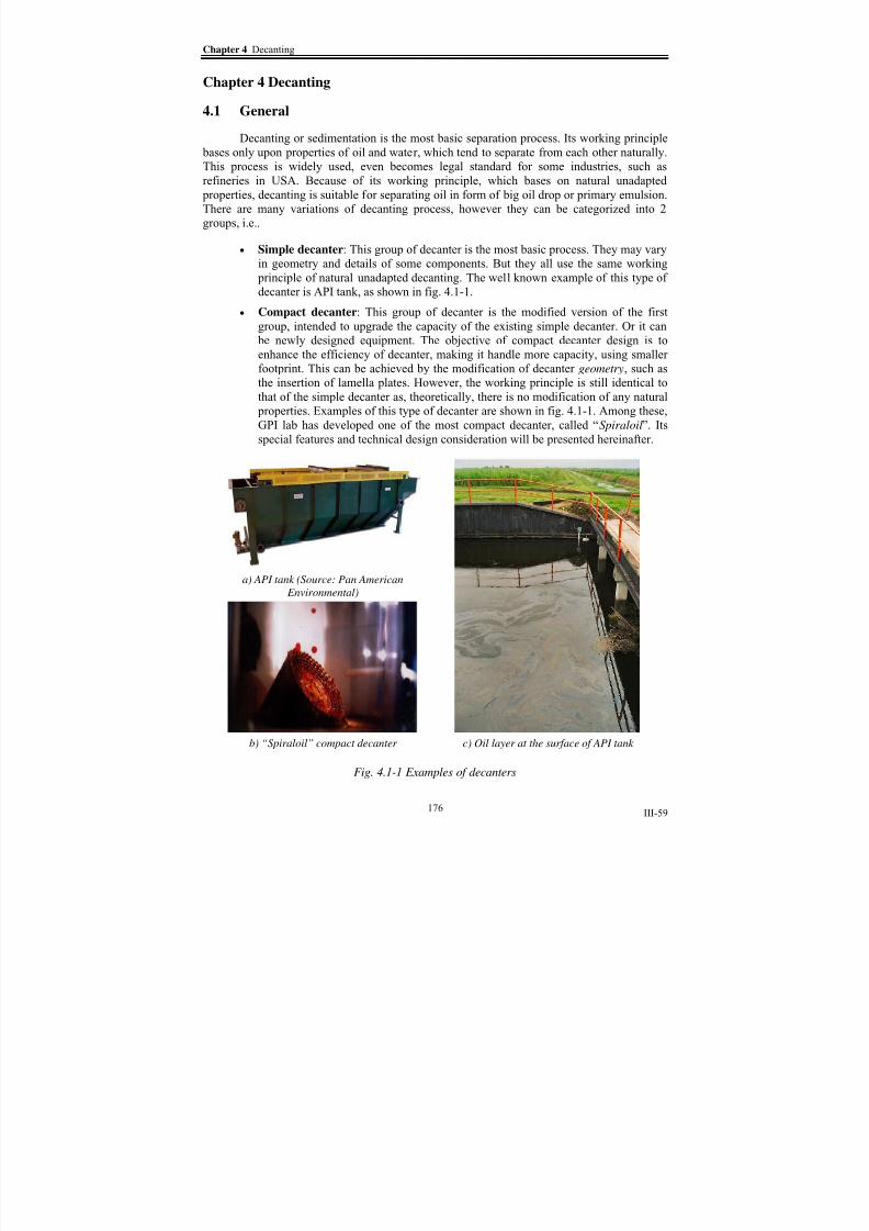
8/15/2019 Rachu.pdf
http://slidepdf.com/reader/full/rachupdf 253/646
Chapter 4 Decanting
III-59
Chapter 4 Decanting
4.1 General
Decanting or sedimentation is the most basic separation process. Its working principle
bases only upon properties of oil and water, which tend to separate from each other naturally.This process is widely used, even becomes legal standard for some industries, such as
refineries in USA. Because of its working principle, which bases on natural unadapted
properties, decanting is suitable for separating oil in form of big oil drop or primary emulsion.
There are many variations of decanting process, however they can be categorized into 2
groups, i.e.,
• Simple decanter: This group of decanter is the most basic process. They may vary
in geometry and details of some components. But they all use the same working
principle of natural unadapted decanting. The well known example of this type of
decanter is API tank, as shown in fig. 4.1-1.
• Compact decanter: This group of decanter is the modified version of the first
group, intended to upgrade the capacity of the existing simple decanter. Or it can
be newly designed equipment. The objective of compact decanter design is to
enhance the efficiency of decanter, making it handle more capacity, using smaller
footprint. This can be achieved by the modification of decanter geometry, such as
the insertion of lamella plates. However, the working principle is still identical to
that of the simple decanter as, theoretically, there is no modification of any natural
properties. Examples of this type of decanter are shown in fig. 4.1-1. Among these,
GPI lab has developed one of the most compact decanter, called “Spiraloil”. Its
special features and technical design consideration will be presented hereinafter.
a) API tank (Source: Pan American
Environmental)
b) “Spiraloil” compact decanter c) Oil layer at the surface of API tank
Fig. 4.1-1 Examples of decanters
176

8/15/2019 Rachu.pdf
http://slidepdf.com/reader/full/rachupdf 254/646
Part III Summary of researches: Oily wastewater treatment
III-60
d) Example of up-scale API tank with tank enclosure (Source: USFilter)
e) Graphical image of lamella plate decanter
(Source: USFilter)
f) Corrugated plate module of corrugated plate
decanter (Source: Dewaterworks)
Fig. 4.1-1 Examples of decanters (Con’d)
4.2 Simple Decanter or API tank
4.2.1 Working principles
Simple decanter, which is made well known and standardized by the American
Petroleum Institute (API), is the simplest oil-water separation process. Its working principle
bases on classical STOKES law (cf. Chapter 2). Concept of the operation of the process is to
provide sufficient time for oil droplets to float to the water surface and accumulate into oil
layer before they have a chance to flow out with the water at the water outlet. The equation
that governs the operation of the process is derived from comparing the time required for the
droplet to reach the surface with retention time of the tank (τ), as shown in eq. 4.2.1.
177

8/15/2019 Rachu.pdf
http://slidepdf.com/reader/full/rachupdf 255/646

8/15/2019 Rachu.pdf
http://slidepdf.com/reader/full/rachupdf 256/646

8/15/2019 Rachu.pdf
http://slidepdf.com/reader/full/rachupdf 257/646
Chapter 4 Decanting
III-63
• Theoretical limitation: Since the decanter’s working principle is based on
STOKES law, it can be applied only when the droplet behavior conforms to
the law. Thus, it can not be used with very small droplet sizes for they are
subjected to Brownian’s motion and their rising velocity are not governed by
STOKES law. Commonly, the simple decanter is used for primary emulsion
treatment (d ≥ 100 microns).
• Economic limitation: As stated before that the process is a non-accelerated
process, its required footprint or installation area may be unacceptable if too
small cut size is selected.
Thus, the suitable cut size will be considered by accounting for the 2 limitations
above. API recommends the cut size of 150 microns for API tank.
2. Decanter sizing
The size of the decanter can be determined, based on the equation in section
4.2.1, as follow:
Bottom surface area (S): The decanter size is based mainly on its bottom
surface area. In general case, it is identical to the tank surface area. Presence of some
structures or components, such as effluent trough or gutter or tank cover (at the water
surface), may affect the efficiency of the decanter. However, if these structures are present in
the ways that make the rising distance of oil droplets decrease, they will help enhancing the
efficiency. However, their effects are normally small, thus, negligible, unless they
substantially reduce the rising distance of oil drops. In latter case, the tank will become a
compact decanter, which will be described in the next section. Bottom surface area of the
simple decanter can be calculated from the rising velocity of the cut size, as shown in eq.
4.2.6. The example of relation between kerosene droplet size and its corresponding rising
velocity as shown in fig. 4.2.2-1.
⎟⎟ ⎠
⎞⎜⎜⎝
⎛ =
dcU
QS {4.2.6a}
c
c
dc
d gU
μ
ρ
18
2⋅⋅Δ= {4.2.6b}
Flow velocity (V): Flow velocity means the velocity of total wastewater along
the tank, determined from wastewater flowrate and cross sectional area of the tank. Using
high flow velocity may cause turbulent or eddy current, especially when the wastewatercollides to the far end of the tank. Turbulence in the tank may interfere the decanting of
droplets, as well as suspended solids, which are usually present in the wastewater. This may
cause carry-over of oil drop and suspended solids with the effluent of the tank.
API recommends that V should not be greater than 0.15 m/s or greater than
15V dc , whichever is smaller.
Water depth (D) and width (W): Theoretically, the efficiency of the tank does
not depend directly on these parameters. However, they have some effects on the tank
operation since they are ones of the parameters that govern the flow regime of the tank.
Furthermore, if they are not selected properly, they can cause adverse effect, such as eddy, orshort circuit.
180

8/15/2019 Rachu.pdf
http://slidepdf.com/reader/full/rachupdf 258/646
Part III Summary of researches: Oily wastewater treatment
III-64
0
20
40
60
80
100
120
140
160
180
200
0 100 200 300 400 500 600 700 800
Cut size (micron)
H y d r a u l i c l o a d i n g r a t e
( ( m 3 / h ) / m 2 )
0
0.01
0.02
0.03
0.04
0.05
R i s i n g v e l o c i t y o f d r o p l e t ( m / s )
Fig. 4.2.2-1 Relation between rising velocity, hydraulic loading rate of simple decanter and kerosene droplet size
API recommends that the ratio D/W should not be smaller than 0.3. The value of
0.5 is recommended. The depth (D) should be in the range of 0.9 to 2.5 m.
3. Removal efficiency
To determine the removal efficiency, the graded efficiency (ηd ) will be
calculated first by eq. 4.2.7a and b. Then, the total removal efficiency (ηt) can be determined
from eq. 4.2.7e.
For oil droplet size, d ≥ cut size,d c
%100=d η {4.2.7a}
For oil droplet size, d ≤ cut size,d c
%100⋅=dc
d
d U
U η {4.2.7b}
It must be noted that the graded efficiency described above is not yet accounted
for effect of flow splitting between water outlet flow and separated oil outlet flow. To
calculate graded outlet oil concentration, the effect must be taken into account, as shown ineq. 4.2.7c.
od d
out
d C Q
QC )1( η −= {4.2.7c}
Qout is outlet flow at treated water outlet port of the process. Qout is calculated
from difference between inlet flow and separated oil (in relatively pure condition) as shown
below.
d
d
d
od d
out
C Q
QQ ρ
η ∑ ⋅
−=
max
min
)(
{4.2.7d}
181

8/15/2019 Rachu.pdf
http://slidepdf.com/reader/full/rachupdf 259/646
Chapter 4 Decanting
III-65
For total removal efficiency
( )
%100
max
min ⋅
⋅
=∑
o
d
d
od d
t C
C η
η {4.2.7e}
ηt = Total Removal efficiency of the tank
ρd = Density of dispersed phase, which is oil, for oily wastewater
Cod = Inlet concentration of the droplet diameter “d”
4. Energy required
The simple decanter does not require extra energy to make it function. The
energy is required only to feed the water into the tank, then the water will flow, naturally,
through the tank by gravity. Pressure drop across the tank and piping system depend on tank
and piping design. This pressure drop can be calculated by general hydraulic equations, such
as Darcy-Weisbach’s, Manning’s, or Hazen-William’s equation, thus will not de described
here.
4.2.3 Design considerations
1.
Limitations of the equations
The equations described above are developed from the following assumptions.
Thus, it is necessary to ensure that these assumptions are valid when design your decanter.
1) Reynolds number, Re, of droplet is between 10-4 to 1, which is the range
that STOKES law is valid.
c
d c d U
μ
ρ ⋅⋅=Re {4.2.8}
2) The oil droplets are uniformly distributed across the cross section area of
the tank, which can be achieved by proper design of inlet chamber.
3) The oil droplet is spherical, which is normally true.
4) For droplets smaller than 20 microns, they are subjected to Brownian
motion and cause error in the prediction of the efficiency. So it is
recommended to avoid using the decanter for the wastewater with the
majority part of oil droplets smaller than 20 microns. However, if these
small droplets are the minority part of pollutants, the models can be used to
predict the efficiency without any harm because its prediction is usually
lower than observed value, thus make the prediction result on the safe side.
2. Safety factors
Since the design equations are simplified by many assumptions, it is
recommended to provide some safety factors to the sizing, calculated from the equations, to
cover some unexpected effects such as short circuit flow or local turbulent flow.
API recommends the safety factor for turbulent flow (Ft) as the function of
(V/U), as shown in eq. 4.2.9. U represents hydraulic loading rate or overflow rate, based ontotal flow and bottom area. For effect of short circuit, API recommends the safety factor (Fs)
182

8/15/2019 Rachu.pdf
http://slidepdf.com/reader/full/rachupdf 260/646
Part III Summary of researches: Oily wastewater treatment
III-66
of 1.2. Then the total safety factor (F), by API recommendation, is the product of Ft and Fs
(eq. 4.2.9c). Factor F will be used to multiplied the value of S, calculated from eq. 4.2.6.
9617.0)(0355.0)(0005.0 2 ++−=U
V
U
V Ft {4.2.9a}
t st F F F F ⋅=⋅= 2.1 {4.2.9b}
4.2.4
Construction of simple decanters
There are many variations of simple decanters, as shown in fig. 4.2.4-1. The most
famous one is API tank, which is the rectangular tank. However, they use the same working
principles, can be calculated by the same equations and consists of relatively the same
components.
To design the decanter, besides the sizing stated above, proper details of construction
of decanter components are also important to guarantee good efficiency. Design
considerations for important components of decanter are described hereby.
1. Inlet chamber
Inlet section, as shown in fig. 4.2.4-2, is an important of decanter for it helps
assuring that uniformly distribution of oil droplet is achieved. For this purpose, the inlet
chamber should be equipped with baffles or energy dissipation devices or structure. Widely
used structures include vertical columns, perforated wall or vertical partition. Design of inlet
section is a state of art process. So it is recommended to study the successful design from
many references and adapt to fit with the condition considering.
2. Separation section
Sizing of this section is obtained from the equations. In this section, not only the
oil will be separated, suspended solids will also settle. So sludge hopper or sludge draw-off
pipe, or other provisions for sludge removal should be provided. Geometry of this section
should be as recommended in the previous section to ensure good hydraulic condition. This
section may be covered, if necessary, to prevent accidental ignition and to prevent the loss of
volatile hydrocarbons by evaporation. Sludge hopper, sludge scrapper and surface skimmer,
should be provided, as shown in fig. 4.2.4-2.
3. Effluent and oil removal devices
Effluent and oil will be removed at the downstream end of the tank. Normally oil
retention underflow baffle is installed to prevent the oil to flow out with the effluent. API
recommends that this baffle should be installed with a maximum submergence of 55% of the
water depth and should be located as close as possible to the oil removal device. The baffle
should be extended to the top of the tank or, at least, higher than water surface.
For oil removal devices, in small unit, the weir or slotted pipe is sufficient. For
upscale tank, those simple devices may draw the water off along with the oil. So the separated
oil still contains some water, and may not be suitable for downstream reuse or recycle
process. In this case, the device with more selective property, such as rotating slotted pipe or
oil skimmer, is required. There is a chapter in this book, devoted to oil skimming process.
183

8/15/2019 Rachu.pdf
http://slidepdf.com/reader/full/rachupdf 261/646
Chapter 4 Decanting
III-67
For effluent, it is normally removed from the tank by a weir. In some small units,
bell mouth pipe is acceptable. Design consideration for effluent removal device is that it
should be of sufficient size to prevent undesired turbulence and provide good flow
distribution in the tank. Normally, the weir across the width of the tank is sufficient.
a) Example of up-scale simple decanter with inlet diffuser wall, equipped with
mechanical skimmer (Source: Monroe)
b) Example of small to medium size simple decanter with simple elbow type inlet
diffuser and weir for collecting oil (Source: Pan American)
Fig. 4.2.4-1 Variations of simple decanters
a) Graphic image shows important components of API tank (Source: US filter)
Fig. 4.2.4-2 Important components of simple decanter
184

8/15/2019 Rachu.pdf
http://slidepdf.com/reader/full/rachupdf 262/646

8/15/2019 Rachu.pdf
http://slidepdf.com/reader/full/rachupdf 263/646

8/15/2019 Rachu.pdf
http://slidepdf.com/reader/full/rachupdf 264/646

8/15/2019 Rachu.pdf
http://slidepdf.com/reader/full/rachupdf 265/646
Chapter 4 Decanting
III-71
Figure. 4.3.1-2 “Spiraloil” decanter a) Simple spiral b) Mixed spiral
0.00%
10.00%
20.00%
30.00%
40.00%
50.00%
60.00%
70.00%
80.00%
90.00%
100.00%
0 10 20 30 40 50 6
Droplet diameter (micron)
R e m o v a l e f f i c i e n c y ( % )
0
1'1 3'
2 2'
3
V = 1.6 cm/s (3, 3')
V = 0.8 cm/s (2, 2')
V = 0.4 cm/s (1, 1')
Fig. 4.3.1-3a Comparison between observed efficiency (1',2',3') and predicted efficiency (1,2,3) for Simple Spiral
"Spiraloil" decanter
0.00%
10.00%
20.00%
30.00%
40.00%
50.00%
60.00%
70.00%
80.00%
90.00%
100.00%
0 10 20 30 40 50 6
Droplet diameter (micron)
R e m o v a l e f f i c i e n
c y ( % )
0
1 (V = 0.5 cm/s)1'
2' 2 (V = 1.5 cm/s)
Fig. 4.3.1-3 Comparison between observed efficiency (1',2') and predicted efficiency (1,2) for Mixed Spiral "Spiraloil"
decanter
From the graphs, it shows that;
1.
Predicted values for cut size are relatively accurate.
2.
Predicted efficiencies of the droplets, smaller than cut size, are always lower
than observed value. This can be explained by the phenomena taking place
within the decanter, which will be described hereby.
3.
Correction factor for efficiency prediction of these small droplets may not beestablished accurately. However, the predicted cut size can be used to design the
188

8/15/2019 Rachu.pdf
http://slidepdf.com/reader/full/rachupdf 266/646

8/15/2019 Rachu.pdf
http://slidepdf.com/reader/full/rachupdf 267/646

8/15/2019 Rachu.pdf
http://slidepdf.com/reader/full/rachupdf 268/646

8/15/2019 Rachu.pdf
http://slidepdf.com/reader/full/rachupdf 269/646
Chapter 4 Decanting
III-75
such as hydraulic force, head loss, etc., in the decanter. CHERID [4] recommends the value of
0.4-1.6 cm/s or 14.4-54 m/h., 2.6 to 10.6 times higher than simple decanter.
3. Removal efficiency
To determine the removal efficiency, the graded efficiency (ηd ) will becalculated first by eq. 4.3.6a and b. For graded outlet concentration (Cd ), flow splitting effect
between treated water outlet port and separated oil outlet flow must be taken into account, as
shown in eq. 4.2.7c and 4.2.7d. Then, the total removal efficiency (ηt) can be determined fromeq. 4.3.6c.
For oil droplet size, d ≥ cut size,d c
%100=d η {4.3.6a}
For oil droplet size, d ≤ cut size,d c
%100⋅=dc
d
d U U η
{4.3.6b}
For total removal efficiency
( ) %1001 max
min
⋅⋅⋅= ∑d
d
od d
o
t C C
η η {4.3.6c}
ηt = Total Removal efficiency of the tankCod = Inlet concentration of the droplet diameter “d”
Qout = Treated water outlet flow (eq. 4.2.7d)
5.
Energy required
The compact decanter does not require extra energy to make it function. The
energy is required only to feed the water through the decanter. Pressure drop across thedecanter and piping system depends on decanter and piping design. This pressure drop can be
calculated by general hydraulic equations, such as Darcy-Weisbach’s, Manning’s, or Hazen-William’s equation, thus will not de described here. However, velocity through decanter is
relatively low, compared to velocity in pipe (0.6-2.5 m/s). So the estimated value of pressuredrop across the decanter around 0.5-1.0 m. is normally acceptable, regardless of its size and
configuration.
4.3.3
Design considerations
1.
Limitations of the equations
The equations described above are developed from the following assumptionsand limitations. Thus, it is necessary to ensure that these assumptions are valid when design
your decanter.
1) The tank is operated under laminar flow regime. Reynolds number, Re, is between 10-4 to 1, which is the range that STOKES law is valid.
2)
The oil droplets are uniformly distributed across the cross section area ofthe tank, which can be achieved by the proper design of inlet chamber.
192

8/15/2019 Rachu.pdf
http://slidepdf.com/reader/full/rachupdf 270/646

8/15/2019 Rachu.pdf
http://slidepdf.com/reader/full/rachupdf 271/646

8/15/2019 Rachu.pdf
http://slidepdf.com/reader/full/rachupdf 272/646

8/15/2019 Rachu.pdf
http://slidepdf.com/reader/full/rachupdf 273/646
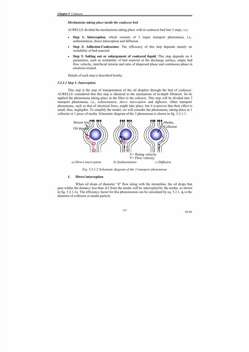
8/15/2019 Rachu.pdf
http://slidepdf.com/reader/full/rachupdf 274/646

8/15/2019 Rachu.pdf
http://slidepdf.com/reader/full/rachupdf 275/646
Part III Summary of researches: Oily wastewater treatment
III-81
2)(2
3
dp
d Int =η {5.2.1}
2. Sedimentation
Consider oil drops of diameter “d” flow along with the streamline. Because of itsdensity, the droplets will be subjected to rising velocity (U), calculated by STOKES law. When
they are far from the media, the rising velocity and flow velocity (V) will have the samedirection. When they come close to the media, the flow velocity will deviate, as shown by the
streamline, while the oil drops will be subjected to both flow velocity and their own rising
velocity. So the resultant velocity will not totally conform to streamline. And in some cases, itwill make the oil drops collide to, thus, sediment on the media. The efficiency factor for this
phenomenon can be calculated by eq. 5.2.2.
V
gd
V
U
csed
μ
ρ η
18
2Δ== {5.2.2}
3. Diffusion
For very small droplets (d < 5 microns), They will be subjected to Brownian’s
motion. These random motions can cause the droplets to collide to the media. The efficiencyfactor for this phenomenon can be calculated by eq. 5.2.3. K , in this equation, represents the
Bolzmann constant and T represents the absolute temperature.
3/2
9.0 ⎟⎟ ⎠
⎞⎜⎜⎝
⎛
⋅=
dpV d
KT
c Diff
μ η {5.2.3}
4.
Combined efficiency of step1 : Interception
From steps 1 to 3, we can calculate the efficiency factors of each transport phenomena for single collector. Theoretical efficiency factor of interception step for single
collector is the summation of the efficiency factors of those three transport phenomena, as shown
in eq. 5.2.4. From the equation, it shows that, at the same operation condition, the theoreticalefficiency factor of the single collector will vary with the droplet diameter, as shown in fig. 5.2.1-
2.
Diff Sed Int theo η η η η ++=
Thus
3/22
2
9.0)(2
3
18 ⎟⎟ ⎠
⎞⎜⎜⎝
⎛
⋅++
Δ=
dpV d
KT
dp
d
V
gd
cctheo
μ μ
ρ η {5.2.4}
198

8/15/2019 Rachu.pdf
http://slidepdf.com/reader/full/rachupdf 276/646
Chapter 5 Coalescer
III-82
1.00E-05
1.00E-04
1.00E-03
1.00E-02
1.00E-01
0.01 0.1 1 10 100
Droplet diameter (micron)
E f f c i e c n c
y f a c t o r
Diffusion efficiency factor Interception efficiency factor
Sedimentation efficiency factor Theoretical efficiency factor
Fig. 5.2.1-3 Relation between oil droplet diameter and efficiency factors of each
transportation phenomena
From the graph, the range where the theoretical efficiency factors are minimal is between 0.25 to 5 microns. So the droplets in this range is theoretically the most difficult to
separate.
To adapt the efficiency of a single collector to the entire coalescer bed, we will
consider the simplified diagram of single spherical collector, placed in laminar flow regime, as
shown in fig. 5.2.1-3a. V represents the flow velocity. The fraction of wastewater flowing pass
the single collector will be the flow that passes through the projected area of the collector (q), asshown in eq. 5.2.5a. Then, some oil drops in this fraction of the wastewater will be intercepted bythe collector. The quantity of intercepted oil drops of the single collector (c’) will be calculated
from the theoretical efficiency factor, as shown in eq. 5.2.5b.
V d q p ⋅= 2
4
π {5.2.5a}
C V d c ptheo ⋅⋅⋅= 2
4'
π η {5.2.5b}
199
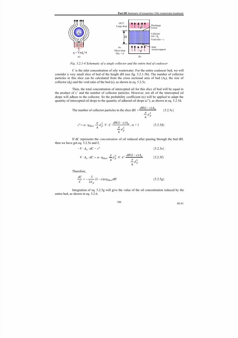
8/15/2019 Rachu.pdf
http://slidepdf.com/reader/full/rachupdf 277/646
Part III Summary of researches: Oily wastewater treatment
III-83
q = Vπd 2/4
V
d p
Collectorsize =d p,
Void ratio = ε
V
H
IN:
Micro drop
Dia. = d
OUT:
Large drop Dischargescreen
Inletscreen/support
V
a) b)
Fig. 5.2.1-4 Schematic of a single collector and the entire bed of coalescer
C is the inlet concentration of oily wastewater. For the entire coalescer bed, we will
consider a very small slice of bed of the height dH (see fig. 5.2.1-3b). The number of collector
particles in this slice can be calculated from the cross sectional area of bed (Ao), the size of
collector (d p) and the void ratio of the bed (ε), as shown in eq. 5.2.5c.
Then, the total concentration of intercepted oil for this slice of bed will be equal tothe product of c’ and the number of collector particles. However, not all of the intercepted oil
drops will adhere to the collector. So the probability coefficient (α) will be applied to adapt the
quantity of intercepted oil drops to the quantity of adhered oil drops (c”), as shown in eq. 5.2.5d.
The number of collector particles in the slice dH3
6
)1(
p
o
d
AdH
π
ε −= {5.2.5c}
3
2
6
)1(
4" p
o ptheo
d
AdH
C V d c π
ε π
η α
−
⋅⋅⋅⋅⋅= , α < 1 {5.2.5d}
If dC represents the concentration of oil reduced after passing through the bed dH,
then we have got eq. 5.2.5e and f;
"cdC AV o =⋅⋅− {5.2.5e}
3
2
6
)1(
4 p
o ptheoo
d
AdH C V d dC AV
π
ε π η α
−⋅⋅⋅⋅⋅=⋅⋅− {5.2.5f}
Therefore,
dH d C
dC theo
p
αη ε )1(2
3−−= {5.2.5g}
Integration of eq. 5.2.5g will give the value of the oil concentration reduced by theentire bed, as shown in eq. 5.2.6.
200

8/15/2019 Rachu.pdf
http://slidepdf.com/reader/full/rachupdf 278/646
Chapter 5 Coalescer
III-84
ptheo
o d
H
C
C αη ε )1(
2
3)log( −−= {5.2.6}
Thus, the theoretical removal efficiency of the coalescer, based on step 1:“Interception”, can be written as shown in eq. 5.2.7.
%1001%1001)()1(
2
3
, ⋅⎟⎟
⎠
⎞
⎜⎜
⎝
⎛ −=⋅⎟⎟
⎠
⎞⎜⎜⎝
⎛ −=
⋅−− theodp
H
o
theod eC
C η α ε
η {5.2.7}
5.2.1.2 Step 2: Adhesion and coalescence
After being intercepted from step 1, the oil droplets will be separated from the wastewater
stream if they can adhere to the surface of the collectors. After that, in good coalescers, theadhering oil drops will coalesce to each other and flow separately from the water stream, as oil
stream within the bed. Phenomena taking place in this step is shown in fig. 5.2.1-4. So themechanism in this step depends mainly on the wettability of the bed. AURELLE had tested the
effect of wettability, using hydrophilic and olephilic material as coalescer bed for secondary o/w
emulsion treatment. The result shows that:
• For Oleophilic material: The oil droplets will adhere to the collector surfaces then
form the oil film around the collectors. The oil films will accumulate in the bed until itreaches saturate level at certain height of the bed, called “ critical height” (Hc). Afterthat the oil will start to flow as a separated oil stream, called “ channeling”.
• For Hydrophilic material: The oil droplets will be trapped in the void between
collectors. These trapped oil droplets will, then, be play the role of collectors by their
own to intercept the following oil droplets. Then they will coalesce into bigger dropsand flow through the void with the wastewater stream.
Even though both materials can cause coalescence, from test result, the oleophilic material
yields good efficiency up to higher range of flow velocity. It means that oleophilic bed coalescer
can be used at higher loading rates, thus makes it more compact in size. So it is recommended touse oleophilic material as the bed for direct emulsion treatment.
5. 2.1. 3 Step 3: “Salting out” or enlargement of coalesced oil
The coalesced oil that flows through the bed in the manner of channeling will finally
reach the topmost of the bed. Then it will leave the bed for the water surface. In good coalescer,the coalesced oil will leave the bed in the form of big oil drops (diameter 2-3 mm or more).Characteristic or size of the oil drops that leave the bed depends on the phenomenon, taking place
at the top surface of the bed. AURELLE has studied this phenomenon, comparing between
oleophilic material and hydrophilic material. The result shows that:
201

8/15/2019 Rachu.pdf
http://slidepdf.com/reader/full/rachupdf 279/646

8/15/2019 Rachu.pdf
http://slidepdf.com/reader/full/rachupdf 280/646
Chapter 5 Coalescer
III-86
a) “Oil mousse” forming. Note that contact
angle < 90o.
b) Re-fragmentation of oil when the
mousse raptures
Oleophilic “salting out” surface
c) Formation of big oil drops. Note that contact
angle > 90o.
d) Oil jet and re-fragmentation of oil at high
velocity or high oil concentration
Hydrophilic “salting out” surface
Fig. 5.2.1-6 Phenomenon in step 3: “Salting out” or enlargemant of coalesced oil
• For Hydrophilic material: The drip points will appear as well. But the oil will not
form the film over the collector surface. But the film will locate between the collectors
and will grow to big oil drops and, then, be snapped off as big oil drops, withoutforming oil mousse. However , at high flow velocity or high concentration of oil,hydraulic force from water flowing out of the bed will be high. The oil will be
snapped off as a jet of oil and then, from the high hydraulic force, will be “ re-
fragmented ” to small droplets.
203

8/15/2019 Rachu.pdf
http://slidepdf.com/reader/full/rachupdf 281/646
Part III Summary of researches: Oily wastewater treatment
III-87
From the result described above, it shows that efficiency of this step depends on 4
parameters, i.e., wettability of discharge surface, flow velocity or empty bed velocity, interfacial
tension, and concentration or ratio of oil to water . To optimize the efficiency of this step,AURELLE suggestd the following methods:
• Design the coalescer at the proper velocity to avoid the re-fragmentation effect.
• Use hydrophilic material as the top layer of the bed or use top grill of hydrophilic
material, to avoid mousse formation. At the same removal efficiency, it is proven thatthe bed with hydrophilic material on the top layer can be operated at higher velocity
than that with the oleophilic top layer.
5.2.1.4 Comparison between observed efficiency and theoretical efficiency
The 3 steps mechanisms, proposed by AURELLE, can effectively describe the phenomena taking place within the coalescer bed. However, to apply it for efficiency prediction,
we have to use many assumptions to simplify them. The most important assumption is that the
efficiency mechanisms in steps 2 and 3 are optimized, so their efficiency is 100%. It means all ofoil that has been intercepted and adhered to collectors in step 1 can be separated. So the removalefficiency of coalescer can be calculated by eq. 5.2.4 and 5.2.7.
AURELLE had studies the relation between observed efficiency (α.ηexp) and thetheoretical efficiency and found that the observed values are quite different from the calculated
value in complex fashion, as shown in fig. 5.2.1-6. Relation between observed efficiency and
theoretical efficiency, suggested by AURELLE, is shown in eq. 5.2.8a. So the theoretical
efficiency in eq.5.2.7 can be modified by replacing αηtheo with α.ηexp. The efficiency of granular
bed coalescer, then, can be calculated by eq.5.2.8b.
5143.0
exp )(5484.0 theoη η α =⋅ {5.2.8a}
%1001%1001)()1(
2
3exp
⋅⎟⎟
⎠
⎞
⎜⎜
⎝
⎛ −=⋅⎟⎟
⎠
⎞⎜⎜⎝
⎛ −=
⋅−− η α ε
η dp
H
o
d eC
C {5.2.8b}
AURELLE’s model is developed under these following assumptions and conditions:
• The key assumption of this model is that mechanisms in step 2 and step 3 of thecoalescer are optimized.
•
The shape of the collector is relatively spherical. The size of the collector tested (dp)
is between 0.2 – 1 mm.
• The collector shall be wetted by dispersed phase. In case of direct (oil in water)
emulsion, the collector, then, shall be oleophilic. For inverse emulsion, oleophilic
resin is recommended.
• Range of empty bed velocity (V) shall be not greater than 0.35 cm/s (12.6 m/h)
204

8/15/2019 Rachu.pdf
http://slidepdf.com/reader/full/rachupdf 282/646

8/15/2019 Rachu.pdf
http://slidepdf.com/reader/full/rachupdf 283/646
Part III Summary of researches: Oily wastewater treatment
III-89
DAMAK [9] used HAPPEL’s theory to adapt AURELLE’s theoretical efficiency
equation, however, the accuracy is not improved. So it seems that the mechanism taking place in
the coalescer bed is so complex that it cannot be simplified to develop an accurate theoretical
model. Thus, when the exact theoretical based model can not be found. DAMAK proposed an
empirical equation for coalescer efficiency prediction, based on the dimensional analysis, as
shown in eq. 5.2.10. Typical characteristic curve between efficiency and droplet size is shown infig.5.2.1-7.
%100)()()()()(58.0 09.009.008.0
/
12.02.0 ⋅⎟⎟ ⎠
⎞⎜⎜⎝
⎛ Δ= −
cc
d
wo
c
d
dpV
dp
H
dp
d
ρ
ρ
μ
μ
γ
ρ η {5.2.10}
The model is developed under these conditions i.e.;
• The model is tested at the range of dp from 0.36 to 0.94 mm. and interfacial tension
(γow) of 11 to 42 dyne/cm. (T.I.O.A, Heptane, Anisole, Toluene and Kerosene)
•
The velocity (V) tested is in the range of 0.09 to 0.54 cm/s.
• The density difference between dispersed phase (oil) and continuous phase (water)
(Δρ) is between 83 to 314 kg/m3.
• The bed used is spherical glass bead with silicon coated to achieve oleophilicity.
• The inlet concentration of hydrocarbon tested is around 1,000 mg/l.
• If the result from eq. 5.2.10 is greater than 100%, it will be rounded up to 100%.
Verification result, using AURELLE’s experimental data, confirms that DAMAK’s model
can predict the removal efficiency with only ±10% error. It implies that the model is also valid at
the operating condition tested by AURELLE. From these test conditions, it seems that thisempirical model covers the range of the oily wastewater commonly found in real situation. Thus,
it is recommended to use this model (eq.5.2.10) for granular bed coalescer calculation.
5.2.1.6 Influent parameters
Main parameters that affect the efficiency of the granular bed coalescer include:
1. Bed height (H)
Typical relation between the bed height and the removal efficiency is as shown in
fig. 5.2.1-7. From the graph, the efficiency of coalescer will increase with increasing height, thenit will stay relatively constant. This height is called “ critical height (H c )”. The occurrence of
critical height can be described by phenomena in step 2 : adhesion- coalescence, as described
before in section 5.2.1.2. If the bed height is shorter than the critical height, it can be said thatthere is not enough accumulated oil film to trap the oil droplets and provide continuous coalesced
oil stream to form perfect “channeling”. Hc depends on wettability, roughness and size of media.
From eq. 5.2.10, it shows that the efficiency is proportional to H0.12
206

8/15/2019 Rachu.pdf
http://slidepdf.com/reader/full/rachupdf 284/646
Chapter 5 Coalescer
III-90
Droplet size (d)
Efficiency (η)
100%
Lower limit of
the model:
10 microns
Bed height (H)
Efficiency (η)
Increase V, d pMore hydrophilic
Less roughness
Hc
Fig. 5.2.1-8 Typical relation between efficiency of granular bed coalescer and various
parameters
2. Size of collector or media particle (dp)
The effect of the size of media is shown in fig. 5.2.1-7. Under the same operatingcondition, the smaller the collector size, the better the efficiency. From eq. 5.2.10, it shows that
the efficiency is proportional to d p-0.4
3. Flow velocity or empty bed velocity (V)
The effect of velocity is relatively small, compared to other parameter. From eq.
5.2.10, it shows that the efficiency is proportional to V-0.08
. However, this is true only within the
valid range of the model. At higher velocity, mousse or jet formation will occur, thus theefficiency will drop rapidly and no longer conform to eq. 5.2.10. The velocity that the mousse or
jet starts appearing is called “critical velocity”. It is recommended to use velocity not more than0.54 cm/s to avoid mousse and jet formation.
4. Wettability of bed material
The effect of wettabiblity of media is shown in fig. 5.2.1-7. It is recommended to
use oleophilic material as the coalescer bed with the thin top layer of hydrophilic material as drip
point surface.
5. Ratio of oil to water
Even though this parameter is not included in eq. 5.2.10, but it is an important
parameter that limit the working range of coalescer. In fact, the model in eq. 5.2.10 is valid for oil
concentration not greater than 1,000 mg/l. Higher oil concentration will result in mousse or jet
forming, which will greatly lower the efficiency of the coalescer. To expand the working range ofgranular bed coalescer, it is necessary to modify basic granular bed coalescer by additional
installation of oil guide, which will be described in the following section.
207

8/15/2019 Rachu.pdf
http://slidepdf.com/reader/full/rachupdf 285/646
Part III Summary of researches: Oily wastewater treatment
III-91
6. Interfacial tension and presence of surfactants
Surfactant will lower the interfacial tension, then make the oil droplets more
stabilized. This leads to poor adhesion between droplets and surface, ineffective collision
(collision without coalescence), and re-fragmentation of oil drops. So the presence of surfactantdirectly limits the efficiency of step 2 “adhesion-coalescence”. To optimize the efficiency of step
2, it is recommended to destabilize (or breaking or cracking) the emulsion before sending to thecoalescer.
7. Temperature
Properties of oil and water, such as viscosity, change with temperature. Sotemperature is inevitable an important parameter that affects coalescer efficiency. Then it is
important to design the process by taking the possible range of temperature into account. Normally, the efficiency will, more or less, increase with the temperature. The equations in this
section are developed under the temperature range between 15 to 25oC, which is the general
practical operating range.
8. Surface roughness of bed material
Surface roughness affects adhesion of oil on the surface of the solid, as shown in
chapter 2. The roughness makes the wettablity of the surface more eminent. So oleophilic
material will show more oleophilicity if its surface is rough. Contact angle of oil on the material
surface will be lower. In this case, it helps promoting direct emulsion separation.
5.2.1.7 Pressure drop
Pressure drop across coalescer bed (p), in metre, can be calculated by Kozeny-Carman’s
equation (eq. 5.2.11) (use SI unit, e.g. m, kg, second).
32
2)1(180
ε ρ
ε μ
⋅⋅⋅
−=
dpg
V H p c m {5.2.11}
All variables except porosity (ε) will be determined by designer. For the porosity of
coalescer bed, from many researches [3], [26], [27], it shows that bed porosity varies with beddepth and can be divided into 2 zones, i.e.,
• Lower zone or critical zone: This zone represents an effective zone of coalescer bed.
The maximum height of this zone is called “critical height (Hc)”. When bed height is
greater than the critical height, the efficiency will increase only slowly (from eq.5.2.10: η ∝ H
0.12). In this zone, the bed will be soaked with oil so the effective
porosity will be low.
• Upper zone: If the bed is higher than Hc, practically, all of oil will be trapped in
critical zone. Then in the higher zone, there will be enough oil in lower zone to flow
continuously through the bed in form of “channeling”. So the effective porosity in thiszone will be lower than critical zone.
208
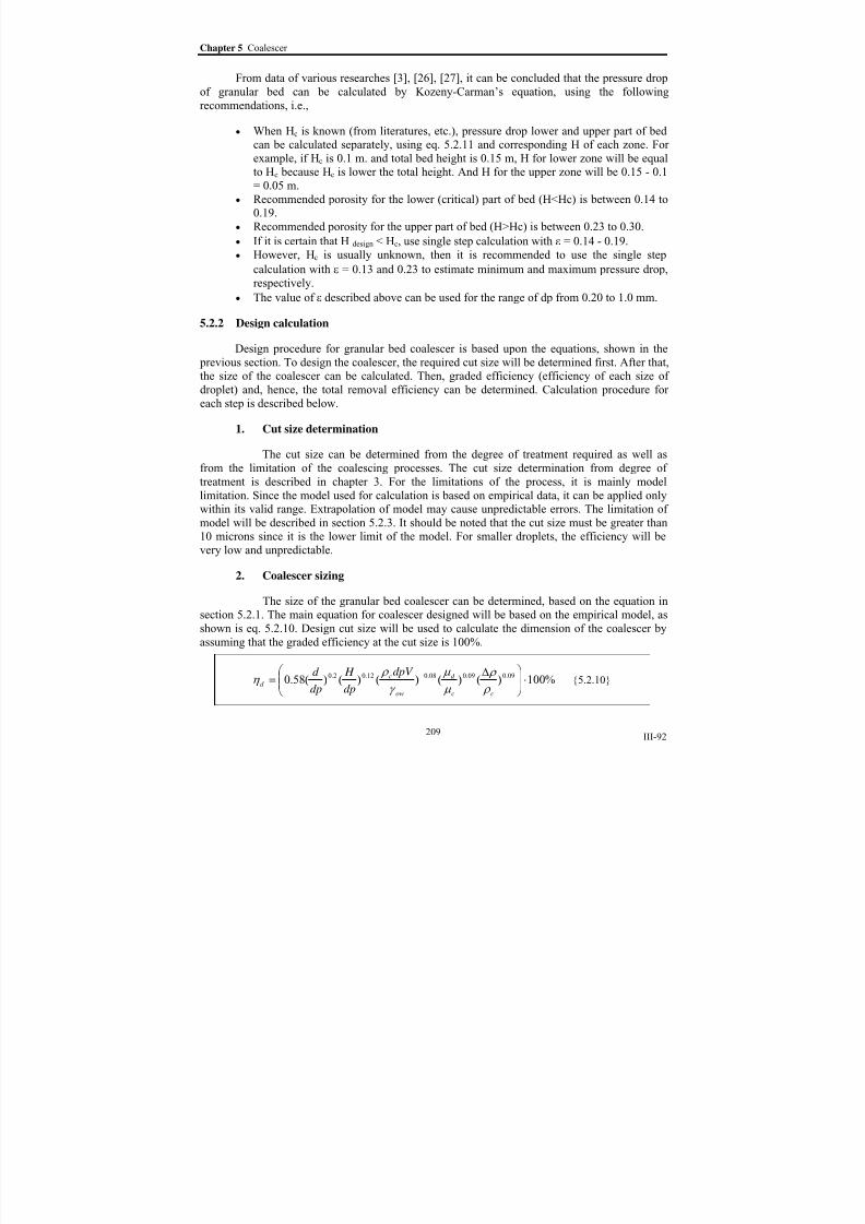
8/15/2019 Rachu.pdf
http://slidepdf.com/reader/full/rachupdf 286/646
Chapter 5 Coalescer
III-92
From data of various researches [3], [26], [27], it can be concluded that the pressure drop
of granular bed can be calculated by Kozeny-Carman’s equation, using the following
recommendations, i.e.,
• When Hc is known (from literatures, etc.), pressure drop lower and upper part of bedcan be calculated separately, using eq. 5.2.11 and corresponding H of each zone. For
example, if Hc is 0.1 m. and total bed height is 0.15 m, H for lower zone will be equalto Hc because Hc is lower the total height. And H for the upper zone will be 0.15 - 0.1
= 0.05 m.
• Recommended porosity for the lower (critical) part of bed (H<Hc) is between 0.14 to0.19.
• Recommended porosity for the upper part of bed (H>Hc) is between 0.23 to 0.30.
• If it is certain that H design < Hc, use single step calculation with ε = 0.14 - 0.19.
• However, Hc is usually unknown, then it is recommended to use the single step
calculation with ε = 0.13 and 0.23 to estimate minimum and maximum pressure drop,
respectively.
•
The value of ε described above can be used for the range of dp from 0.20 to 1.0 mm.
5.2.2 Design calculation
Design procedure for granular bed coalescer is based upon the equations, shown in the
previous section. To design the coalescer, the required cut size will be determined first. After that,the size of the coalescer can be calculated. Then, graded efficiency (efficiency of each size of
droplet) and, hence, the total removal efficiency can be determined. Calculation procedure for
each step is described below.
1. Cut size determination
The cut size can be determined from the degree of treatment required as well asfrom the limitation of the coalescing processes. The cut size determination from degree of
treatment is described in chapter 3. For the limitations of the process, it is mainly model
limitation. Since the model used for calculation is based on empirical data, it can be applied onlywithin its valid range. Extrapolation of model may cause unpredictable errors. The limitation of
model will be described in section 5.2.3. It should be noted that the cut size must be greater than10 microns since it is the lower limit of the model. For smaller droplets, the efficiency will be
very low and unpredictable.
2. Coalescer sizing
The size of the granular bed coalescer can be determined, based on the equation insection 5.2.1. The main equation for coalescer designed will be based on the empirical model, as
shown is eq. 5.2.10. Design cut size will be used to calculate the dimension of the coalescer by
assuming that the graded efficiency at the cut size is 100%.
%100)()()()()(58.0 09.009.008.012.02.0 ⋅⎟⎟ ⎠
⎞⎜⎜⎝
⎛ Δ= −
cc
d
ow
c
d
dpV
dp
H
dp
d
ρ
ρ
μ
μ
γ
ρ η {5.2.10}
209

8/15/2019 Rachu.pdf
http://slidepdf.com/reader/full/rachupdf 287/646
Part III Summary of researches: Oily wastewater treatment
III-93
Dimension of the coalescer can be arbitrarily selected under the limitations of the
model, as shown in section. 5.2.3, to make eq. 5.2.10 consistent. However, it is recommended to
select the lowest possible media diameter and highest velocity for the first trial because it willgive the most compact diameter of the coalescer. If the result is acceptable, it can be fine-adjusted
to get the most suitable dimension. If the result is unacceptable, normally too big, it may be
necessary to increase the number of units.
Fig. 5.2.2-1 shows the result of calculation from eq. 5.2.10 at various cut sizes. The
calculation is based on kerosene-water emulsion, which may be used as a guideline for coalescer
size estimation. The collector diameter, used in the graph, is 0.35 mm.
0
0.1
0.2
0.3
0.4
0.5
0.6
0.7
0.8
0.9
1
1.1
1.2
1.3
1.4
0 10 20 30 40 50 60
Cut size (micron)
B e d h e i g
h t ( m )
V = 1.94 m/h
V = 3.2 4m/h
V = 11.3 m/h
Fig 5.2.2-1 Relation between cut size and coalescer dimension
3.
Removal efficiency
To determine the removal efficiency, the graded efficiency (ηd ) will be calculated
first by eq. 5.2.10. If the result from eq. 5.2.10 is greater than 100%, then it will be rounded up to
100%.
It must be noted that the graded efficiency from the equation is not yet accounted for
effect of flow splitting between water outlet flow and separated oil outlet flow. To calculate
graded outlet oil concentration, the effect must be taken into account, as shown in eq. 5.2.12a.
od d
out
d C Q
QC )1( η −= {5.2.12a}
Qout is outlet flow at treated water outlet port of the process. Qout is calculated from
difference between inlet flow and separated oil (in relatively pure condition) as shown below.
d
d
d
od d
out
C Q
QQ ρ
η ∑ ⋅
−=
max
min
)(
{5.2.12b}
210

8/15/2019 Rachu.pdf
http://slidepdf.com/reader/full/rachupdf 288/646
Chapter 5 Coalescer
III-94
For total removal efficiency
( )
%100
max
min ⋅
⋅
=∑
o
d
d
od d
t C
C η
η {5.2.12c}
ηt = Total Removal efficiency of the tankρd = Density of dispersed phase, which is oil, for oily wastewaterCod = Inlet concentration of the droplet diameter “d”
4. Pressure drop
Pressure drop (in metre) can be calculated from Kozeny-Carman’s equation (eq.
5.2.11). Recommended value of bed porosity (ε) and other criteria are as shown in section
5.2.1.7. For diluted wastewater, the values of μ and ρ can be replaced by those of water (μc, ρc).
32
2)1(180
ε ρ
ε μ
⋅⋅⋅
−=
dpg
V H p m {5.2.11}
5.2.3 Design consideration
1. Limitations of the equations
The equations described above are developed from the following assumptions andlimitations. Thus, it is necessary to make sure that these assumptions are valid when design your
coalescer.
1) Coalescer bed shall be oleophilic and relatively spherical in shape.
2) Tested size of bed media (dp) is between 0.20 – 1.0 mm. The larger the mediasize, the lower the efficiency.
3) Tested range of bed height (H) of the model is between 1 to 10 cm. However,
bed height as low as 1 cm is not recommended. The greater the bed height, thesafer the coalescer operation. However, it also results in higher pressure drop.
4) The velocity (V) should be in the range of 0.09 to 0.54 cm/s or 3.2 to 19.4 m/h.
5) Tested interfacial tension (γow) is between 11 to 42 dyne/cm or 0.011 to 0.042 N/m. (such as, T.I.O.A, Heptane, Anisole, Toluene and Kerosene)
6) Different density between dispersed phase (oil) and continuous phase (water)
(Δρ) is between 80 to 315 kg/m3(approx.).
7)
The equation is valid for droplet size (d) of 10 microns or bigger. For smaller
droplets, result from eq. 5.2.10 may not be accurate because it is beyond thedata that has been used to verify the model.
8) The model is valid for inlet concentration between 100 to 1,000 mg/l. At
higher concentration, mousse or jet formation may occur, resulting in
unpredictable decreasing of the efficiency.
211

8/15/2019 Rachu.pdf
http://slidepdf.com/reader/full/rachupdf 289/646
Part III Summary of researches: Oily wastewater treatment
III-95
2. Construction and material selection
Granular bed coalescer consists of 2 major components, i.e., casing and bed.
1) The casing
The casing is the component that contains the bed and other importantappurtenances, such as wastewater inlet, wastewater outlet, oil outlet, clean out, etc. Researches
in GPI lab normally emphasize on working mechanisms and developing of a model so there is nodirect study on characteristic of the casing. However, because of the fact that the coalescer is
usually designed as a pressure vessel in the same manner as a pressure filter, then, casing or tank
construction criteria of the pressure filter can be readily applied to the coalescer. However, somedetails, such as oil outlet pipe, water outlet pipe and internal baffle should be adapted to ensure
good separation between oil and water. As outlined in chapter 4 “Decanting”, the internal baffleshould be installed in the manner that it can promote oil drop decanting, prevent short circuit of
oil drops to the water outlet pipe. The pipe and baffle arrangement shown in fig. 5.1-1 can be
used as a guideline for casing design.
2) The bed
From many GPI researches, it is recommended that resin is the most suitable
material for coalescer bed, because:
• It is widely used in many industries, and available in every country.
• It is produced in wide range of size and normally spherical.
• It can be coated to achieve required wettability.• Its cost is competitive.
• Its physical properties, such as hardness, etc., are also good.
Other materials that have been used as coalescer bed include glass beads, smallstainless steel balls. Material that is heavier than water, such as stainless steel, has an advantage
for it can be used without installation of top grille to prevent it from carry-over. So it can becleaned by backwash process or scouring process because the material is not retained by top
grille, then can be expanded or floated freely.
For wettability, oleophilic bed with thin layer of hydrophilic material on the
top or with hydrophilic top grille is recommended (see section 5.2.1.2). Guideline on
oleophilicity of materials is described in chapter 2. Some hydrophilic material that has goodmechanical properties can acquire oleophilic property by coating with proper substance, such as
silicone. Oleophilicity of bed may change with time from deterioration of the coating or reactionwith wastewater. It may need re-coating or replacement if decreasing in efficiency is
unacceptable.
5.2.4 Variations, advantage and disadvantage of granular bed coalescer
Variations of granular bed coalescer: There are several modifications of granular bedcolaescers, normally, on bed materials, such ad resin bed coalescer, glass bead bed coalescer.
There are 3 major modified granular bed coalescer studied at GPI lab, i.e., mixed bed coalescer ,
212

8/15/2019 Rachu.pdf
http://slidepdf.com/reader/full/rachupdf 290/646
Chapter 5 Coalescer
III-96
down-flow coalescer and guide coalescer . The latter will be fully described in the next section.
Mixed bed coalescer is another modified form of granular bed coalescer, used for mixed
direct/inverse emulsion separation, which is usually found in liquid-liquid extraction process. In
mixed bed coalescer, the bed will consist of separate layers of oleophilic and hydrophilicmaterials, placed in series in the same column. From research [6], ratio of oleophilic and
hydrophilic material and order or configuration of column (upper hydrophilic layer/loweroleophilic layer or vice versa) depends on wastewater characteristic. So it is difficult to
determine the efficiency of the coalescer by fixed equation. In this case, it is recommenced to
perform pilot test to find optimum design criteria.
Furthermore, there are also variations of coalescers, based on flow patterns i.e., up-flowcoalescer and down-flow coalescer. The researchs conducted in GPI lab are generally based on
up-flow coalescer. For down-flow coalescer, the flow pattern in this case will be identical to that
of deep-bed filter. This type of coalescer is intentionally designed to use with the oily wastewaterthat contains suspended solids. The wastewater will be fed from the top of the bed. The oil will be
coalesced in the same manner as the up-flow coalescer. However, the coalesced oil will flow up
against the wastewater stream to the inlet water surface, then be skimmed out of the reactor. Thisflow patterns can eliminate the top grille that is used for preventing carry-over of bed media in
up-flow coalescer. This allows us to clean the bed by air scouring, back washing or any propermechanism, such as pneumatic pulsation that can make the bed move up or partially fluidize to
unclog the trapped solids. Working principles of this coalescer is generally identical to that of up-flow coalescer. However, there is not enough research data to develop the math model. So it is
recommended to use the equation of up-flow coalescer for roughly estimation of efficiency.
Anyway, the exact efficiency would be obtained from pilot scale testing.
Advantage: Granular bed coalescer has a major advantage in its compactness. Testedloading rate of coalescer is 3.2 – 19.4 m/h and it can be used with the droplet size from 10
microns while, for simple decanter, the loading rate is about 0.04 m/h for 10-micron dropletseparation.
Disadvantage: The bed of this type of coalescer has relatively low porosity (0.14-0.19).
So, at high loading rate, the pressure drop may be very high. Moreover, it can make the bed clog
relatively easily. So the granular bed coalescer is sensitive to the presence of suspended solids.
5.3 Guide coalescer
5.3.1 Working principles
Guide coalescer is the modified form of simple granular bed coalescer. In guide coalescer,high-porosity oleophilic material, such as woven metal fiber or woven mesh, will be placed next
to downstream end of the granular and extended up to water surface. Coalesced oil drop will be
guided along this material until it combines with oil layer at the water surface. So, this material iscalled “ guide”. Structure of the guide shall be self-sustained or installed in perforated structure,
so the treated water can flow freely out of the guide structure, then be discharged from thecoalescer. The pictures of guide coalescer are shown in fig. 5.3.1-1.
213

8/15/2019 Rachu.pdf
http://slidepdf.com/reader/full/rachupdf 291/646

8/15/2019 Rachu.pdf
http://slidepdf.com/reader/full/rachupdf 292/646
Chapter 5 Coalescer
III-98
efficiently. To apply to higher concentration or beyond the limit stated above, bench
scale or pilot scale testing is highly recommended
This type of coalescer have been developed for 2 purposes, 1) to increase the hydraulic
loading rate of the granular bed coalescer, 2) to make it possible to use the granular bed with thewater containing very high concentration of oil, such as in liquid-liquid extraction process.
5.3.2 Design calculation
Steps of calculation, as well as cut size determination, for the guide coalescer is identical
to those of basic granular bed coalescer. However, there are some difference in details of sizing
and pressure drop calculation as described below.
1. Coalescer sizing
The size of guide coalescer can be calculated by eq. 5.2.10. For velocity less than
0.54 m/s, actual velocity will be used in the equations. However, if design velocity is greater than
0.54, the velocity of 0.54 m/s will be used, regardless of the actual velocity. The size from thecalculation can be, theoretically, used at velocity from 0.54 to 0.8 cm/s.
2. Removal efficiency
The removal efficiency can be calculated from the selected dimension, using eq.
5.2.10 and 5.2.12.
3. Pressure drop
Because of the fact that the “guide” in guided coalescer has relative high porosity
(0.9 approx.), then, The pressure drop is very low, compared to the granular part, and can be
negligible. So Kozeny-Carman’s equation (eq. 5.2.11) and recommended value of porosity fromsection 5.2.2 can also be used to predict pressure drop of guided coalescer.
5.3.3 Design consideration
1. Limitations of the equations
The limitations in this case are identical to those of granular bed coalescer (see
section 5.2.3) except for the velocity and oil concentration, which will conform to section 5.3.1.
2. Material selection
For direct emulsion treatment, granular bed in guide coalescer shall be oleophilic
material. However, instead of top layer or grill of hydrophilic media, guide will be placed on thetop of the granular bed. The guide should be made of metal or rigid material and properly coated
to obtain oleophilic property. It should have high porosity and self-sustained structure because it
is not supported by the wall of the coalescer. If the selected guide is not self-sustained, perforated
oleophilic material shall be provided to support the guide. Commercial woven wire-meshes or
metal wool, such as MuitiKnit™, Knit meshTM
, 3MTM
, etc., can be efficiently used as a guide.
215

8/15/2019 Rachu.pdf
http://slidepdf.com/reader/full/rachupdf 293/646
Part III Summary of researches: Oily wastewater treatment
III-99
5.4
Fibrous Bed coalescer
5.4.1 Working principles
This type of coalescer uses high porous fibrous material, such as fibrous bottle brush, as a
bed to promote coalescing between oil droplets. Due to its high porosity, this type of bed ishardly clogged and can handle wastewater containing suspended solids efficiently. It also causesmuch less pressure drop than granular bed coalescer. However, fibrous element, which is
normally very small, may deflect at its tip, especially in large-scale unit, and causes unpredictablechanneling of untreated wastwater, then decreasing in efficiency.
From other point of view, this coalescer can be considered as a modified form of guide
coalescer that granular bed is removed and the guide is additionally used to intercept oil, besides
its role to provide coalesced oil flow channel.
Three basic steps for granular bed coalescer, proposed by AURELLE [3], can also be
used to describe phenomena taking place within the coalescer. However, mathematics models,
derived from dimensional analysis, are proven to be more accurate.
There are 2 main categories of fibrous bed coalescers, i.e., Simple fibrous bed coalescer
and dynamic (or rotating) fibrous bed coalescer, as shown in fig. 5.4.1-1. The latter is themodified form of the former, by installation of driving unit to drive the bed.
5.4.1.1 Simple fibrous bed coalescer model
This type of coalesceruses uses fibrous material, normally, in the form of “bottle brush”
as a coalescer bed. The brush has relatively high porosity, compared to granular material. So this
coalescer causes much lower pressure drop and is hardly clogged. Furthermore, from the three-
step phenomena of coalescer, described in section 5.2.1, it shows that the efficiency of coalescerwill increase if the size of the bed media is small. For fibrous bed coalescer, the size of fiber isaround 100- 200 microns, much smaller than granular media’s. By this way, the efficiency can be
improved.
GPI lab has been studied the possibility to use this type of material as a bed for sometimes. However, the researches on this type of coalescer are based mainly on its application and
design consideration, rather than model development. So there is no model proposed for this
coalescer. Anyway, these researches, especially the study of SRIJAROONRAT [10], providesufficient raw data to formulate an empirical model. This newly formulated model, which will be
called “SRIJAROONRAT’s model”, is as shown in eq. 5.4.1. The model has been verified, usingdata from MA’s and WANICHKUL’s researches, as shown in fig. 5.4.1-2.
( ) %100)(1)()()(5.104 694.035.018.018.077.0 ⋅⎟⎟ ⎠
⎞⎜⎜⎝
⎛ −= −−
D
H
D
d
D
d VD F
c
c
d ε μ
ρ η {5.4.1}
216

8/15/2019 Rachu.pdf
http://slidepdf.com/reader/full/rachupdf 294/646
Chapter 5 Coalescer
III-100
a) Simple fibrous bed coalescer [11] b) Graphical image of dynamic fibrous bed
coalescer
c) Examples of “brush” d) Coalesced oil drops from dynamic fibrous bed
coalescer
Fig. 5.4.1-1 Fibrous bed coalescer (Source: GPI lab)
217

8/15/2019 Rachu.pdf
http://slidepdf.com/reader/full/rachupdf 295/646
Part III Summary of researches: Oily wastewater treatment
III-101
Where d F = Diameter of fiber
d = Diameter of dispersed phase, in our case, oil
D = Diameter of coalescer bed, such as diameter of brushH = Height of bed, or bed depth
V = Empty bed velocity
ε = Porosity or void ratio of the bedμC = Dynamic viscosity of continuous phase, in our case, water
ρc = Density of continuous phases
The model is developed and verified under these conditions i.e.;
• 48 < Re < 1100. Re is the term (ρcVD/μc) in the equation.
• 1 < H/D < 10.
• Diameter of coalescer bed (D) tested is around 5.0 cm. Using bigger coalescer
diameter may cause deflection at the tips of fibers because of longer overhung length,
which may cause channeling of untreated wastewater and error in efficiencycalculation.
• The model is valid for droplet size (d) of 1 microns and greater.
• Empty bed velocity (V) used in the researches [10], [11], [16] is between 0.5 to 5.0cm/s (1.8 to 180 m/h). However available raw data used to verify the model is
between 0.5 to 2.0 cm/s. Using velocity > 2.0 cm/s may cause unpredictable error oncalculated efficiency.
• Fiber size (d F) used in the researches [10], [11], [16] is between 40 to 200 microns.
However available raw data used to verify the model is between 100 to 200 microns.
Using fiber size < 100 microns may cause unpredictable error on calculated
efficiency.• Void ratio of the bed (ε) is around 0.845 to 0.96.
• The model is valid for droplet size (d) of 1 microns and greater.
• The model is verified at inlet oil concentration up to 1000 mg/l. Applying the model to
the concentration > 1000 mg/l will cause underestimation of predicted efficiency, as
shown in fig. 5.4.1-2 for WANICHKUL’s data (C = 7950 mg/l) [11].
• The beds used in these researches vary from “bottle brush” type, simple spiral typeand combination of internal bed of “simple spiral” and concentric “coil spring–like”
external bed with the tip of the fibers pointed to the centerline. However, they are alloleophilic. There is some difference in efficiency between each type, but there is too
few data to make a conclusion. However, because of its rigidity, the “simple spiral in
coil spring- like” bed tends to operate more stable without decreasing in efficiencywith time, while others tend to be deflected by weight of accumulated oil drops. In
fact, this type of bed is invented to take advantage of spiral bed for its non-cloggingand disorderly bed (section 5.4.1.3) for its rigidity and good interception efficiency.
218

8/15/2019 Rachu.pdf
http://slidepdf.com/reader/full/rachupdf 296/646

8/15/2019 Rachu.pdf
http://slidepdf.com/reader/full/rachupdf 297/646
Part III Summary of researches: Oily wastewater treatment
III-103
The equation is developed and verified under these conditions i.e.;
• 52 < Re < 1164. Re is the term (ρcVD/μc) in the equation.
• 1 < H/D < 2. However, the maximum H/D shown in TAPANEEYANGKUL’s
research [8] is 6. Using H/D > 2 in the model can be also applied for comparison
purpose only.
• Rotating speed of the bed (N) is between 0.167 to 3.33 rps (10 to 200 rpm). Pleasenote that N is in form of revolution per unit time, not radian per unit time).
Recommended minimum rotating speed is 75 rpm. Using lower speed may not
provide any additional benefit over simple fibrous bed coalescer because the effect of
rotating on interception probability may be cancelled out by the shear effect, whichcauses fragmentation of oil drops.
• Empty bed velocity (V) is between 0.1 to 1.1 cm/s (3.6 to 39.6 m/h) .
• Diameter of fiber (d F) is around 100 to 300 microns
•
Diameter of coalescer bed (D) is not greater than 11.5 cm. Using bigger diameter maycause deflection at the end of fibers from longer overhung lengths, which may cause
channeling of untreated wastewater and error in calculation.
• It is recommended to use the model only for the droplet size (d) of 10 microns or
greater. For smaller droplet, the model can also be applied, but for comparison
purpose only.
• The beds, used in the experiment, are “bottle brush” types, made of oleophilic polyamide or polypropylene with stainless steel shaft, as shown in fig. 5.4.1-1c.
5.4.1.3 Random or disorderly fibrous bed coalescer
There is another special case of simple fibrous bed coalescer that uses random ordisorderly fibrous material (such as metal wool, etc.) as coalescer bed. SRIJAROONRAT’s
research shows that removal efficiency of this coalescer is higher than that of coalescer that uses brush type bed. For this, it can be concluded that tortuosity of bed also affects the removal
efficiency. From SRIJAROONRAT’s raw data, an empirical model, based on dimensionalanalysis, can be derived as shown in eq. 5.4.3. However, this model is developed from rather
small set of data. There is an effort to verify if the simple bed model (eq. 5.4.1b) is still valid for
random fibrous bed coalescer. Comparison between efficiency from eq. 5.4.1b, eq. 5.4.3 andobserved value is shown in fig. 5.4.1-3.
%100)()()()(35.3 36.003..003.023.0 ⋅⎟⎟ ⎠ ⎞⎜⎜
⎝ ⎛ = −−
D H
Dd
Dd VD F
c
cd
μ
ρ η {5.4.3}
220

8/15/2019 Rachu.pdf
http://slidepdf.com/reader/full/rachupdf 298/646
Chapter 5 Coalescer
III-104
0.00%
10.00%
20.00%
30.00%
40.00%
50.00%
60.00%
70.00%
80.00%
90.00%
100.00%
110.00%
0% 10% 20% 30% 40% 50% 60% 70% 80% 90% 100%
Observed efficiency (%)
P r e d i c t e d E f f i c i e n c y ( % )
+10%
-10%
Fig. 5.4.1-3 Relation between observed efficiency and predicted efficiency fromrandom fibrous bed coalescer model and simple fibrous bed model
From the graph, it shows that SRIJAROONRAT’s random fibrous bed model (eq. 5.4.3)
can accurately predict the efficiency of the coalescer while the result from the simple bed model
(eq. 5.4.1b) tends to underestimate the efficiency from 2 to 6 times. This confirms that tortuosityof the bed plays very important role in efficiency of fibrous bed coalescer. However, tortousity
can not be effectively established in form of numerical value so it can not be included as a parameter in mathematics model. Eq. 5.4.3, then, can be applied only when design condition is
close to the test condition from SRIJAROONRAT’s research.
Eq. 5.4.3 is developed and verified under these conditions i.e.;
• The beds used in the experiment are highly disorderly bulk of stainless steel fiber, d F =
75 microns, and steel wool, d F = 40 microns (see fig. 5.4.1-4). However, only thelatter case, which raw experimental data is available, is used to develop the model.
The minimum size of oil droplet tested is 1 micron.
• Tested Reynolds number is between 840 to 2470.
• Porosity of the bed (ε) is around 0.95.
• Diameter of the coalescer (D)= 5 cm.
• Height of the coalescer bed (H) is between 0.07 to 0.21 m.
• Velocity (V) is between 1 to 2.5 cm/s or 36 to 90 m/h.
• Inlet concentration is around 1000 mg/l.
In case that the conditions stated above are not fully compliant, it is recommended to useeq. 5.4.1b to calculate the efficiency of the coalescer because it is proven to be valid within wider
range. In this case, predicted result from eq. 5.4.1b tends to underestimate the efficiency of thecoalescer.
221

8/15/2019 Rachu.pdf
http://slidepdf.com/reader/full/rachupdf 299/646
Part III Summary of researches: Oily wastewater treatment
III-105
a) Highly disorderly stainless steel fibers b) Steel Wool
c) Magnified picture of (a) d) Magnified picture of (b)
Fig. 5.4.1-4 Random or disorderly fibrous bed, used in the research of SRIJAROONRAT
5.4.1.4
Influent parameters
Even though each type of fibrous bed coalescer is governed by different equation, all ofthe equations is in about the same mathematics form, as shown in eq. 5.4.4. Thus, main
parameters that affect the efficiency of the fibrous bed coalescer can be commonly summarizedas shown in fig. 5.4.1-5.
))1(,,,,1
,1
,1
( ε η −= N H d d DV
f F
d {5.4.4}
222

8/15/2019 Rachu.pdf
http://slidepdf.com/reader/full/rachupdf 300/646
Chapter 5 Coalescer
III-106
Droplet size (d)
Efficiency (η)
100%
Lower limit of
the model:
1 micron
Droplet size (d)
Efficiency (η)
Increase V, D, d FDecrease H, (1-ε), NLess tortousity
100%
Fig 5.4.1-5 Typical relation between efficiency of fibrous bed coalescer and various
parameters
However, besides the parameters shown in eq. 5.4.4, there are some important parametersthat affect the efficiency of the coalescer, i.e.,
1. Tortousity
If the bed is more tortuous, the probability to intercept oil droplets will be increased.
The efficiency, then, is increased, as clearly shown in the case of wool coalescer. However, it will
tend to be clogged if suspended solids are present in wastewater.
2. Wettability of bed
From the 3 mechanisms of AURELLE [3] (section 5.4.1.1), wettability of the bed isthe key parameter that governs the step 2 “adhesion-coalescence”. In case of direct (oil in water)
emulsion treatment, he bed material shall be oleophilic to optimize the adhesion-coalescence phenomena.
3. Interfacial tension and presence of surfactants
Surfactant will lower the interfacial tension, then make the oil droplets more
stabilized. This leads to poor adhesion between droplets and surface, ineffective collision
(collision without coalescence), and re-fragmentation of oil drops. So presence of surfactantdirectly limits the efficiency of step 2 “adhesion-coalescence”. To optimize the efficiency of step
2, it is recommended to destabilize, (breaking or cracking) the emulsion before sending to thecoalescer
4. Temperature
Properties of oil and water, such as viscosity, change with temperature. Sotemperature is inevitable an important parameter that affect coalescer efficiency. Then it isimportant to design the process by taking the possible range of temperature into account.
Normally, the efficiency will, more or less, increase with the temperature. The equations in this
223

8/15/2019 Rachu.pdf
http://slidepdf.com/reader/full/rachupdf 301/646

8/15/2019 Rachu.pdf
http://slidepdf.com/reader/full/rachupdf 302/646

8/15/2019 Rachu.pdf
http://slidepdf.com/reader/full/rachupdf 303/646
Part III Summary of researches: Oily wastewater treatment
III-109
5.4.2 Design calculation
Steps of calculation, as well as cut size determination, for fibrous bed coalescer is
identical to those of basic granular bed coalescer. However, there are some difference in details of
sizing and pressure drop calculation as described below.
1.
Cut size determination
The ut size can be determined from the degree of treatment required as well as fromthe limitation of the coalescing processes. Cut size determination from degree of treatment is
described in chapter 3. For the limitations of the process, it is mainly model limitation. Since the
model used for calculation is based on empirical data, it can be applied only within its validrange. Extrapolation of model may cause unpredictable error. The limitation of each model is
described in section 5.4.1.
2. Coalescer sizing
The size of various types of fibrous bed coalescer can be calculated by eq. 5.4.1 to5.4.3. Design cut size will be used to calculate the dimension of the coalescer by assuming thatthe graded efficiency at the cut size is 100%. Dimension of the coalescer can be arbitrarily
selected under the limitations of each equation, as described in section 5.4.1.1 to 5.4.1.3.However, it is recommended to select the possible lowest fiber diameter and highest velocity for
the first trial because it will give the most compact diameter of the coalescer. If the result is
acceptable, we may try to fine-adjust the parameters to get the most suitable dimension. If theresult is unacceptable, normally too big, we may have to increase the number of units.
3. Removal efficiency
After the dimension of the coalescer is determined, graded efficiency (ηd ) can becalculated by eq. 5.4.1, 5.4.2 or 5.4.3. If the result from eq. 5.2.10 is greater than 100%, then it
will be rounded up to 100%.
It must be noted that the graded efficiency from the equation is not yet accounted for
effect of flow splitting between water outlet flow and separated oil outlet flow. To calculategraded outlet oil concentration, the effect must be taken into account, as shown in eq. 5.2.12a.
od d
out
d C Q
QC )1( η −= {5.2.12a}
Qout is outlet flow at treated water outlet port of the process. Qout is calculated from
difference between inlet flow and separated oil (in relatively pure condition) as shown below.
d
d
d
od d
out
C Q
QQ ρ
η ∑ ⋅
−=
max
min
)(
{5.2.12b}
226

8/15/2019 Rachu.pdf
http://slidepdf.com/reader/full/rachupdf 304/646
Chapter 5 Coalescer
III-110
For total removal efficiency
( )
%100
max
min ⋅
⋅
=∑
o
d
d
od d
t C
C η
η {5.2.12c}
ηt = Total Removal efficiency of the tankρd = Density of dispersed phase, which is oil, for oily wastewaterCod = Inlet concentration of the droplet diameter “d”
4. Pressure drop
As stated in section 5.4.1.5, in order to calculate the pressure drop, it is
recommended to use any general piping loss equations, such as Darcy’s, Colebrook-White’s orHazen-William’s equation (eq. 5.4.5) with the safety factor of 2 to 5, multiplied to the actual
height (H) of the bed. CHW is Hazen william’s constant, depending on surface roughness of
coalescer. Recommended value is 110-130 for steel column.
167.185.1
582.6 ⎟
⎠ ⎞⎜
⎝ ⎛
⎟⎟ ⎠ ⎞
⎜⎜⎝ ⎛ =
D
H
C
V P
HW
m {5.4.5}
5.4.3 Design consideration
1. Limitations of the equations
The equations described above are developed from the following assumptions and
limitations. Thus, it is necessary to make sure that these assumptions are valid when design thecoalescer. Limitation of each design equation (eq. 5.4.4 to 5.4.3) is described in section 5.4.1.
2.
Construction and material selection
Fibrous bed coalescer consists of 2 major components, i.e., casing and bed.
1) The casing
The casing is the component that contains the bed and other importantappurtenances, such as wastewater inlet, wastewater outlet, decanting section, oil outlet, clean
out, etc. Researches in GPI lab normally emphasize on working mechanisms and developing of amodel so there is no direct study on characteristic of the casing. However, the size of the fibrous
bed coalescer is usually small to avoid deflection at the tip of fibers, it is, then, designed as inline
unit or in the form of pipe (see fig. 5.4.1-1 and 5.4.3-1). Batteries or multi-coalescer unit is alsoavailable. Downstream decanter may be integrated or placed separately from the coalescer as
shown in fig. 5.4.3-1. As described in section 5.4.1, diameter of the decanter is normally equal tothat of coalescer or a bit bigger to facilitate placement and construction of internal baffle, water
and oil outlet pipe.Casing of coalescer can be made of any material (plastic, steel, glass, etc.) that
can withstand the operating condition. If possible, it should be oleophilic.
227

8/15/2019 Rachu.pdf
http://slidepdf.com/reader/full/rachupdf 305/646
Part III Summary of researches: Oily wastewater treatment
III-111
a) Lab scale coalescer with integrated
decanter (The bed is placed in the steel
column just below the decanter)
b) Inline-style fibrous bed coalescer [11] c) Assembly of the coalsecer and separated
decanter (Source: Elf, GPI lab)
Fig. 5.4.3-1 Examples of fibrous bed coalescer casing
2)
The bed
The bed is the most important part in the coalescer. From section 5.4.1, thereare 2 major types of fibrous beds, i.e., simple or brush type and random or disorderly type.
Difference in operating efficiency between the two is already discussed. However, one property,
which both beds have in common, is that, for direct emulsion treatment, the bed shall be
oleophilic.
Material of the bed varies from steel, stainless steel and variety of plastic, scuhas polyamide, polypropylene as shown in fig. 5.4.1-1, 5.4.1-4 and 5.4.3-2. For simple brush type,
the efficiency of the coalescer varies only slightly for various types of bed shown in the figure.
The factor that governs the efficiency for this type of bed is its oleophilicity. Guideline onwettability of material is described in chapter 2. To preliminary test olephilic property of the bed,
it can be done easily by dip or have the bed contact with oil or water. If the drop of oil or water isalmost sphere, it can be approximately concluded that the material is hydrophilic or oleophilic
respectively (see fig. 5.4.3-3)
228

8/15/2019 Rachu.pdf
http://slidepdf.com/reader/full/rachupdf 306/646

8/15/2019 Rachu.pdf
http://slidepdf.com/reader/full/rachupdf 307/646

8/15/2019 Rachu.pdf
http://slidepdf.com/reader/full/rachupdf 308/646

8/15/2019 Rachu.pdf
http://slidepdf.com/reader/full/rachupdf 309/646
Part III Summary of researches: Oily wastewater treatment
III-115
Chapter 6 Dissolved air flotation
6.1 General
Flotation is an accelerated separation process, operated by increasing density
difference between continuous phase and dispersed phase. This is accomplished by mean ofadding gas or air into the wastewater to promote formation of air-solids or air-oil
agglomerates. There are several researches on flotation, its modification and applications of
various types of flotation such as mechanical flotation, diffused air flotation, dissolved air
flotation (DAF), etc. Among these, DAF, with its finest air bubble size, is the most efficient
process. So it became the main flotation process studied in GPI lab.
6.2 Working principles
From STOKES law (eq. 6.2.1), difference density between dispersed phase and
continuos phase (Δρ) is one of the parameters that governs rising or decanting velocity of the
dispersed phase. Flotation is the separation processes of which aims to increase the densitydifference to increase the decanting velocity.
c
gd U
μ
ρ
18
2Δ= {6.2.1}
For dissolved air flotation, pressurized water which is (or almost) saturated with air or
gas will be fed to wastewater at lower, usually, atmospheric pressure. The air or gas will be
released from the pressurized water in form of tiny bubbles. These bubbles, while rise up to
the surface, will collide with dispersed phase, in case of oily wastewater oil droplets, in the
wastewater. Some will attach to the droplets and form oil-bubble agglomerates. Since the
bubble has much less density than oil and water. Density of these agglomerates will be lower
than that of oil droplets alone, thus, make the rising velocity increase. General schematic
diagram of DAF process is as shown in fig. 6.2-1.
Fig. 6.2-1 Example of schematic diagram of DAF (Source: Aquatec Maxcon)
232

8/15/2019 Rachu.pdf
http://slidepdf.com/reader/full/rachupdf 310/646

8/15/2019 Rachu.pdf
http://slidepdf.com/reader/full/rachupdf 311/646

8/15/2019 Rachu.pdf
http://slidepdf.com/reader/full/rachupdf 312/646

8/15/2019 Rachu.pdf
http://slidepdf.com/reader/full/rachupdf 313/646
Part III Summary of researches: Oily wastewater treatment
III-119
C is inlet concentration of oily wastewater. For the entire flotation column, we will
consider a very small slice of rising bubbles of the height dH (see fig. 6.2.1-3b). The number
of bubble particles in this slice can be calculated from the cross section area of bed (A), the
size of the bubble (d b) and the ratio of volume of water to total volume (ε), as shown in eq.
6.2.7c.
Then, the total concentration of intercepted oil for this slice of rising bubbles will be
equal to the product of c’ and the number of bubbles. However, not all of the intercepted oil
drops will adhere to the bubbles. So the probability coefficient (α) will be applied to adapt the
quantity of intercepted oil drops to the quantity of adhered oil drops (c”), as shown in eq.
6.2.7d.
The number of bubbles in the slice dH3
6
)1(
bd
AdH
π
ε −= {6.2.7c}
3
2
6
)1(
4"b
btheo
d
AdH
C V d c π
ε π
η α
−
⋅⋅⋅⋅⋅= , α < 1 {6.2.7d}
If dC represents the concentration of oil reduced after past through the slice of bubbles
dH, then we have got eq. 6.2.7e and f;
"cdC AV =⋅⋅− {6.2.7}
3
2
6
)1(
4b
btheo
d
AdH C V d dC AV
π
ε π η α
−⋅⋅⋅⋅⋅=⋅⋅− {6.2.7f}
Therefore,
dH d C
dC theo
b
αη ε )1(2
3−−= {6.2.7g}
Integration of eq. 6.2.7g will give the value of the oil concentration reduced by the
entire column height, as shown in eq. 6.2.8a.
b
theo
o d
H
C
C αη ε )1(
2
3)log( −−= {6.2.8a}
However, void ratio (e) of DAF system can be calculated directly from air flowratedischarged from pressurized water and total water flow as shown in eq. 6.2.8b.
AV Qt
Φ=
Φ=− ε 1 {6.2.8b}
Thus, the theoretical removal efficiency DAF, based on filtration model, can be
written as shown in eq. 6.2.8c.
%1001%1001)(
2
3
, ⋅
⎟
⎟
⎠
⎞
⎜
⎜
⎝
⎛ −=⋅⎟⎟
⎠
⎞⎜⎜
⎝
⎛ −=
⋅⋅Φ
⋅− theodp
H
AV
o
theod e
C
C η α
η {6.2.8c}
236

8/15/2019 Rachu.pdf
http://slidepdf.com/reader/full/rachupdf 314/646

8/15/2019 Rachu.pdf
http://slidepdf.com/reader/full/rachupdf 315/646
Part III Summary of researches: Oily wastewater treatment
III-121
air t
pw air Conc
Q
Q
AV ρ
)(⋅=
Φ {6.2.10a}
Or
X RQ
RQ X Q
Q
t
pw ⋅+=⋅= 1 {6.2.10b}
Normally, under certain design condition, Q pw/Qt or Q pw/Q (= R)is constant. Solubility
of air in water (X) and air density are intrinsic (internal) properties, which are constant at any
given pressure and temperature. So, from eq. 6.2.10, it shows that Φ/AV is flow-independent.
From these, it seems that predicted DAF efficiency from the filtration-based model ismathematically flow-independent. However, In fact, effect of wastewater flowrate,
sometimes, described in form of velocity or retention time, is studied by many researchers. Itis widely accepted that DAF efficiency varies with retention time. So, considering SIEM’s
research, it can be interpreted that the effect of retention time is already included in eq. 6.2.9a.Since eq. 6.2.9a is evaluated from one set of operating condition (Φ/AV = 0.0516) and
retention time (25 minutes (approx.)), it may be valid only for that condition. To expand validrange of SIEM’s model, some criteria or model that contains flowrate-dependent parameter(such as retention time, etc.) is required.
6.2.2 Population balance model
Population balance model is one of popular concepts, used by many researchers, to
develop DAF model. In GPI lab, DUPRE [14] uses this method in her research on applicationof DAF for liquid-solid separation. Concept of this method is that rate of change in the
number of pollutants which is free or attached by 1, 2 or more air bubbles is the function ofthe number of air bubble and oil droplet, as shown in eq. 6.2.11. Oil droplet that is attached by
at least 1 bubble, so-called oil-bubble agglomerate, will be separated. So rate of change innumber of oil droplets represents removal efficiency.
Main assumption of population balance method is that the number of bubble isassumed to be constant. From many researches [14], [34], It is proven that, for liquid-solidseparation, the number of bubble (N) can be safely assumed as constant without serious error,
because there are a lot more bubbles than pollutant if normal range of (Q pw/Qt) is applied.However, in case of oily wastewater, many researches [12], [13] show that bubble-oil
agglomerates are in form of oil shell with air inside and these agglomerates are still able to
intercept more oil droplets. Those researches also show that coalescence of oil and bubble ismore effective than that of the same species. So it should be safely assumed that the numberof bubble in this case is more or less constant and the population balance method is, then,
applicable.
N nk dt
dn00
0 β −= {6.2.11a}
N nk N nk dt
dniiii
i β β −−= −− 11 {6.2.11b}
i = 0 to imax
238

8/15/2019 Rachu.pdf
http://slidepdf.com/reader/full/rachupdf 316/646

8/15/2019 Rachu.pdf
http://slidepdf.com/reader/full/rachupdf 317/646
Part III Summary of researches: Oily wastewater treatment
III-123
It should be noted that eq. 6.2.13 is about the same form as eq. 6.2.9b, but the value of
κ, represented by eq. 6.2.11d, clearly represents effect of every interesting parameter,including retention time. So population balance model is flow-dependent and, then, can be
used to extend the valid range of SIEM’s model, as described in section 6.2.3.
6.2.3
Generalized model of DAF from combination of filtration based model andpopulation balance model
From section 6.2.1, it shows that SIEM’s filtration based model can be used to predict
the efficiency of DAF at any diameters of oil droplets and bubbles, as long as design retentiontime and F/AV still conforms to SIEM’s condition. And from section 6.2.2, it shows that
population balance model gives the equation that is flow-dependent. So it is possible to usethese two models to extend the valid range of SIEM’s model to another operating condition.
To do so, firstly, SIEM’s model will be used to calculate the efficiency at his operating
condition. Then, at any d and d b, eq. 6.2.11d and 6.2.13 can be rewritten in form of a function
of a parameter that we want to vary from SIEM’s condition, i.e., retention time and gasflowrate. while other parameters still conform to SIEM’s (eq. 6.2.14). When the efficiency at
SIEM’s condition is known, the efficiency at other condition can be predicted from eq. 6.2.14and relation between design value and SIEM’s value of that parameters (eq. 6.2.15 and6.2.16).
τ κ τ κτ Φ=Φ= 2.Gconst {6.2.14a})( 211
τ κ κτ η Φ−− −=−= ee {6.2.14b}
If “x” represents the variable Φ or τ that we want to vary from SIEM’s while anothervariable still conforms to SIEM’s condition, eq. 6.2.14b can be rewritten as show below.
x Ae ⋅−−=1η {6.2.14c}
Where A = constant
Ifx = B.x ref {6.2.15}
Where B = Constant
Xref = x at SIEM’s condition
Then
)(
)(
1
1
ref Ax
Ax
ref e
e−
−
−
−=η
η
{6.2.16a}
)(
)(
1
1
ref
ref
Ax
ABx
ref e
e−
−
−
−=
η
η {6.2.16b}
B
ref )1(1 η η −−= {6.2.16c}
However, changing of τ of Φ will also cause some parameter in eq. 6.2.11d change.
For example, increasing of retention time from SIEM’s condition will make V decrease. Then
G will decrease. So the constant “A” at design condition is not equal to “A” at SIEM’scondition. In this case, eq. 6.2.16 is not valid. And it is not possible to know the value of “A”
at design condition. So, the best estimation in this case is to use the value of A at some
240

8/15/2019 Rachu.pdf
http://slidepdf.com/reader/full/rachupdf 318/646
Chapter 6 Dissolved air flotation
III-124
condition that we are sure that will underestimate efficiency at design condition. Design
reactor in this case will be larger than it should be. Then it can be considered as safety factor.
Guideline to predict the efficiency from combination of SIEM’s model and population
balance model will be described again in details in section 6.3.
6.2.4 Influent parameters
From models described in section 6.2.1 and 6.2.2, main parameters that affect theefficiency of DAF can be summarized as shown in fig. 6.2.4-1.
Droplet size (d)
Efficiency (η)
100%
Lower limit of
the model:
2 micron
Droplet size (d)
Efficiency (η)
Increase d b
Decrease τ, Φ, H
100%
Fig. 6.2.4-1 Typical relation between efficiency of DAF and various parameters
From the models, it can be summarized that, efficiency of DAF can be improved by:
•
Increase the size of oil droplets. This can be done by coagulation-flocculation process.
• Decrease the size and quantities of bubbles. This can be achieved by using high
performance injection valve.
• Increase quantity of air/pollutant ratio by increasing pressurized water flowrate or
using higher saturator pressure. However, operating cost should be considered.
• Increase column height to increase retention time.
However, there are some more phenomena and parameters that also effect theefficiency of DAF, which will be described below,
1. Characteristic of bubble-pollutant agglomerate and transfer compound
Characteristic of bubble-pollutant agglomerate
Since DAF performance depends on formation of bubble-pollutant agglomerate,some researches in GPI lab [13], [14] had been conducted to study characteristics of theagglomerate. Fig. 6.2.4-2 shows characteristic of bubble-solid and bubble-oil agglomerate.
For bubble-solid agglomerate, certainly, bubbles will attach to the surface ofsolid in side-by-side manner. On the contrary, for bubble-oil agglomerate, side-by-side
characteristic is only temporary or intermediate condition. Finally, oil and bubble willintegrate in form of spherical thin film or shell of oil with air core inside. This can be
241

8/15/2019 Rachu.pdf
http://slidepdf.com/reader/full/rachupdf 319/646
Part III Summary of researches: Oily wastewater treatment
III-125
explained by the concept of spreading, described in chapter 2, section 2.2.2.2. Consider
interfacial tension between kerosene, water and air as shown below,
Oil-water: γow = 35 dynes/cm
Air-water: γw = 72 dynes/cm
Air-oil: γo = 28 dynes/cm
From chapter 2, oil will spread over the air bubble when γw > γo+ γow. From the
values of interfacial tension, it clearly shows that this condition is confirmed (72 > 28 + 35).
So the oil will spread over air bubble and form a thin film around the air.
The four ways to improve the efficiency of DAF described earlier in fig. 6.2.4-1is actually the way to improve collision probability. However, one of the most encountered
problems in DAF operation is collision between bubble and pollutant without attachment.According to the study in static transparent model [13], to form agglomerate, bubble and
pollutant must be collide or come close to each other at some certain distance for sufficient
period of time to drain water film between them and made bond to each other. To solve this problem, some chemically active agents are used to adapt properties of bubble andwastewater. The chemicals are called “transfer compound”.
Effect of transfer compound on bubble-pollutant agglomerate
Transfer compound is chemical added either as gas to bubble-forming air or as
chemical to water. Major role of the compound is to help promoting bubble-pollutantagglomerate and strengthen the bond between them. It will cause mass transfer, where it gotits name, from bubble to water or vice versa that change local interfacial or surface tension of
pollutant or bubble. This change will facilitate agglomerate formation. This effect of local
change in surface tension is known as the Marongoni effect. There are 2 major types of thecompounds, i.e., transfer gas and transfer compound for water.
• Transfer compound for water is practically a surfactant added to
pressurized water. The surfactant will reduce surface tension of water . In
case of solid separation, the effect is relatively the same as that when using
surfactant in a washing machine. Bubbles and solids will attach to each othereasier and stronger. Efficiency will be improved. This idea is actuallycommercialized by many companies, such as SAFTM (suspended air
flotation) from Enprotec.
• Transfer gas is typically a gas of highly soluble chemicals, such asammonia, which is added to bubble-forming air. The concept is that the gas
would transfer from bubble into water and make the water film raptureeasier. This will help interaction time between bubble and pollutant and
make them attach immediately after collision. In GPI lab, AOUDJEHANE[13] shows that small amount of ammonium gas added into the air actually
helps reducing coalescence time between bubble and oil droplet. However, it
also promotes coalescence between bubble and bubble. So, these effects tendto cancel out each other. The efficiency is relatively the same.
In case of oily wastewater , however, presence of surfactant in water causes the
droplet smaller and more stable. So it make the efficiency decrease. Anyway,AOUDJEHANE shows that if the surfactant is firstly added to oil and mass transfer of
242
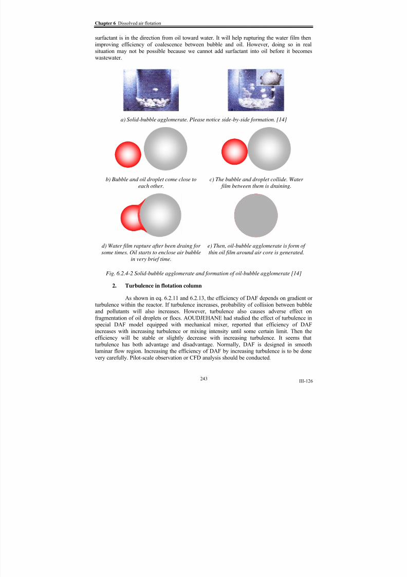
8/15/2019 Rachu.pdf
http://slidepdf.com/reader/full/rachupdf 320/646
Chapter 6 Dissolved air flotation
III-126
surfactant is in the direction from oil toward water. It will help rupturing the water film then
improving efficiency of coalescence between bubble and oil. However, doing so in real
situation may not be possible because we cannot add surfactant into oil before it becomeswastewater.
a) Solid-bubble agglomerate. Please notice side-by-side formation. [14]
b) Bubble and oil droplet come close to
each other.
c) The bubble and droplet collide. Water
film between them is draining.
d) Water film rapture after been draing for
some times. Oil starts to enclose air bubble
in very brief time.
e) Then, oil-bubble agglomerate is form of
thin oil film around air core is generated.
Fig. 6.2.4-2 Solid-bubble agglomerate and formation of oil-bubble agglomerate [14]
2.
Turbulence in flotation column
As shown in eq. 6.2.11 and 6.2.13, the efficiency of DAF depends on gradient or
turbulence within the reactor. If turbulence increases, probability of collision between bubbleand pollutants will also increases. However, turbulence also causes adverse effect on
fragmentation of oil droplets or flocs. AOUDJEHANE had studied the effect of turbulence inspecial DAF model equipped with mechanical mixer, reported that efficiency of DAF
increases with increasing turbulence or mixing intensity until some certain limit. Then theefficiency will be stable or slightly decrease with increasing turbulence. It seems that
turbulence has both advantage and disadvantage. Normally, DAF is designed in smoothlaminar flow region. Increasing the efficiency of DAF by increasing turbulence is to be done
very carefully. Pilot-scale observation or CFD analysis should be conducted.
243

8/15/2019 Rachu.pdf
http://slidepdf.com/reader/full/rachupdf 321/646
Part III Summary of researches: Oily wastewater treatment
III-127
3. Presence of surfactant
Effect of surfactant in wastewater is as discussed in “effect of transfercompound”. In presence of surfactant, oil droplets will become more stable and their sizes
will be smaller. Efficiency of DAF, then, will decrease. So it is recommended to destabilize
(or break or crack), coagulate/flocculate the wastewater before using DAF.
4. Formation of air bubbles
From, filtration-based model efficiency of DAF will increase if the size of
bubbles decreases. So pressurized water system shall be designed to make majority of verytiny droplets and avoid generating big bubbles. DUPRE [14] had studied bubble generation in
venturi-style injection vale and reported that using hydrophobic material for valveconstruction may result in bigger bubbles. She also reported that addition of surfactants in
pressurized water causes augmentation of population of microbubbles, while addition of polyelectrolyte gives the opposite result. Details of pressurized water system or saturator will
be described in section 6.5.
6.3 Design calculation
From previous sections, it shows that there are many parameters, such as wastewatercharacteristic, reactor configuration and operating condition, that effect efficiency of DAF
reactor. So, design of DAF reactor is generally based on hydraulic loading rate and some proven reactor configuration. However, to valorize the researches conducted in GPI lab,
design procedure for DAF, recommended in this section, will be based upon the models,shown in the previous sections as well as general design practices. Calculation in each step isdescribed below.
1. Cut size determination and required efficiency
The cut size can be determined from the degree of treatment required as well as
from the limitation of the DAF processes. Cut size determination from degree of treatment isdescribed in chapter 3. However, in general practice, DAF is hardly used alone but will be
combined with coagulation-floculation process (see chapter 10). After coagulation-flocculation process, granulometry of size distribution of dispersed phase in the wastewater
will be changed from that of initial wastewater. The size distribution after coagulation-flocculation may be roughly estimated, as shown in chapter 10. However, it is clear that it is
no longer possible to determine the cut size from the initial size distribution. Then the degree
of treatment (such as effluent oil concentration, etc.) will be used to calculate the requiredefficiency. This required efficiency or the required degree of treatment would be used tocompare to general recommended criteria of DAF to determine if it is feasible to use DAF for
such wastewater.
In case that there is no general design criteria or recommended efficiency for thewastewater to be treated, it is strongly recommended to perform DAF test, such as Flota-test,
to evaluate the feasibility and efficiency of DAF before designing the real unit.
2.
DAF reactor sizing
The size of the DAF can be determined based on (1) mathematics models fromsection 6.2, (2) general design criteria and (3) pilot-scale test result. Designing an efficient
244

8/15/2019 Rachu.pdf
http://slidepdf.com/reader/full/rachupdf 322/646
Chapter 6 Dissolved air flotation
III-128
DAF reactor, as well as other processes, is the state-of-art and requires experience. However,
result from the models and some useful criteria acquired from many researches, esp. GPI
researches, will be provided here to be a guideline for DAF reactor sizing.
2.1. General design criteria
Recommended design criteria from various literatures and manufacturers aresummarized in table 6.3-1. It should be noted that the values in the table are summarized fromexperiences and researches with various operating conditions and types of wastewater, then,
should be used as a guideline. It is recommended to review related researches for the type ofwastewater to be treated. If possible, DAF test, using lab-scale batch test, such as flota-test, or
pilot-scale test with the real wastewater should be performed.
2.2. DAF design by combination of filtration based model and population
balance model
From the 2 models in section 6.2, they can be used to size DAF reactor andestimate graded efficiency of DAF process at any operating condition. If direct scale-up of
SIEM’s model ( the same V and Φ/AV) is used, the cut size at H =0.70 m. is around 35microns.
If DAF is used alone without coagulation-flocculation process and cut size can
be determined, the cut size can be used to calculate surface area of DAF reactor (A) by
assuming that the efficiency at the cut size is 100%.
If cut size can not be determined, approximate size of DAF reactor can be
calculated from general criteria, described in table 6.3-1. It is recommended to use the reactor
size calculated from the general criteria as a guideline to calculate the efficiency. Then, it can be fine adjusted again to fit specific constraint of each project.
Calculation procedure and model limitation will be as described below.
2.2.1. Design DAF at SIEM’s condition ( /AV is at SIEM’s condition. H can
be varies)
1. To predict removal efficiency of DAF, reference graded efficiency
(based on Qt) can be calculated by SIEM’s model. If the result
from the equations is greater than 100%, then it will be rounded up
to 100%. The values of (Φ/AV) have to be the same as SIEM’scondition (see item 3).
%1001))(
2
3(
,
exp
⋅⎟⎟
⎠
⎞
⎜⎜
⎝
⎛ −=
Φ−
bd
H
AV
ref d eαη
η {6.2.9b}
5919.0
exp)(009005.0)( theoη αη = {6.2.9a}
diff Int sed theo η η η η ++=
2)(2
3
b Int
d
d =η {6.2.3}
245

8/15/2019 Rachu.pdf
http://slidepdf.com/reader/full/rachupdf 323/646
Part III Summary of researches: Oily wastewater treatment
III-129
r c
water oil
sed V
gd
μ
ρ η
18
2
/Δ= {6.2.4}
3/2)(9.0br
Diff d dV
KT
μ η = {6.2.5}
c
bwater air
br
gd U V
μ
ρ
18
2
/Δ== {6.2.2a}
Where μc = viscosity of continuous phase (water) (L2/T)
K = Boltzman constant (1.38*10-23
)T = Absolute temperature (Kelvin)
2. To use the equations described above, the following conditions will
be satisfied;
1) Inlet oil concentration should not be greater than 1,200 mg/l
(before dilution) or 435 mg/l (after dilution).
Using the modelwith higher oil concentration will result in underestimating ofefficiency.
• Φ/AV = 0.0516. Only this value must be used in the
equations. As long as this value is fixed, SIEM’s operating
condition still holds and the model is still valid.
• Retention time, based on total flowrate (Qt), is around 25minutes.
• Droplet diameter (d) tested is between 2 to 40 microns.
• Diameter of air bubbles (d b) varies from 15 to 130 microns.
Tested average bubble diameter is 70 microns, which is used
to verify the model, and standard deviation of bubblediameters is 34.5 microns. The range of bubble sizes iscommon for commercial pressurized water system or
saturator. The pressure of the test system is 4 atm (absolute).
• Tested air flowrate (Φ) is 0.42 cm3/s (4.2e-7 m3/s).
• Tested wastewater flowrate (Q) is 3.9 cm3/s (3.9e-6 m
3/s)
• Tested effective water depth (H) is 0.70 m. The value of H
can be freely changed as long as (Φ/AV) is fixed. However,
H between 1.8 to 2.7 is recommended by API [45].
• Diameter of flotation column is 0.15 m Cross section area of
column (A) is 0.01767 m2.
•
Ratio of pressurized water to wastewater (Q pw/Q) is 1.76.
• Air to pollutants ratio used is around 0.12 kg. air/ kg. oil.
• Ratio of number of bubble/ oil droplet tested is around 1.4
oil droplet/ 1 air bubble.
• Hydraulic loading rate or flow velocity (V), based on Q t, is
1.6 m/h
2) he model is tested at the following operating condition;
246

8/15/2019 Rachu.pdf
http://slidepdf.com/reader/full/rachupdf 324/646

8/15/2019 Rachu.pdf
http://slidepdf.com/reader/full/rachupdf 325/646
Part III Summary of researches: Oily wastewater treatment
III-131
T a
b l e 6 . 3 - 1 G e n e r a l d e s i g n c r i t e r i a o f D A F f r o m v a r i o u s l i t e r a t u r e s a n d m a n u f a c t u r e r s ( h y d r a u l i c l o a d i n g r a t e i s b a s e d o n t o
t a l f l o w r a t e )
248

8/15/2019 Rachu.pdf
http://slidepdf.com/reader/full/rachupdf 326/646
Chapter 6 Dissolved air flotation
III-132
3. To apply SIEM’s condition to other wastewater flowrate, area (Aref )
and gas flowrate (Φref ) corresponding to that flowrate can be
calculated from the following equations. The subscript of A and Φ
in this case is “ref” to indicate that SIEM’s condition (or referencecondition) still holds.
01767.0109.3 6mod
mod
⋅×
=⋅= −req
el
el
req
ref
Q A
Q
Q A m2 (Q as m3/s) {6.3.1}
01767.0
102.4 7
mod
mod
req
el
el
req
ref
A
A
A −×=Φ⋅=Φ m3/s {6.3.2}
4. If H is changed from 0.70 m. to Hreq, τ will be changed from 25
min. to τref by the following equation. The subscript of τ in this caseis “ref” to indicate that SIEM’s condition (or reference condition)
still holds.
3600
1
00046.0mod
mod
⋅=⋅= req
el
el
req
ref
H
H
H τ τ hour {6.3.3}
5. Because of limitation of the pilot model, tested ratio of pressurizedwater to wastewater is quite high (around 92%), compared to that ofgeneral DAF for solid/liquid separation (less than 50%) [13].
However, API [45] recommended air/wastewater ratio of 0.35 std.
ft3/ 100 gal of total flow for full-flow DAF process. This value is
equivalent to 84% of 4-atm (abs) pressurized water/ wastewater.
Anyway, it is interesting to adapt the model to calculate theefficiency at lower ratio of pressurized water by the procedure in
item 2.2.2.
6. Tested hydraulic loading rate or overflow rate (based on Qt) is 1.6
m/h, which is relatively low, compared to normal rate of 3-15 m/hfor domestic wastewater treatment. The value recommended by the
American Petroleum Institute (API) [45] is between 4.8-6.1 m/h. Soit is also interesting to adapt the model to calculate the efficiency at
higher overflow rate by the procedure in item 2.2.2.
2.2.2. Design DAF at other condition from SIEM’s condition
To calculate graded removal efficiency at other operating conditionthan SIEM’s model, esp. at higher overflow rate or lower ratio of pressurizedwater/wastewater, calculation procedure will start from direct scale-up of
SIEM’s condition (the same as 2.2.1). After that, adaptation by population
balance model will be applied.
Direct scale-up of SIEM’s condition (Φ/AV is at SIEM’s condition. Hcan be varied.)
1. Calculate the reference efficiency (ηd,ref ) of the model at requiredheight (Hreq), average bubble diameter (d b) and droplet sizes (d)
using eq. 6.2.2 to eq.6.2.5 and eq. 6.2.9. Use Φ/AV = 0.0516 inorder that the operating condition of SIEM still holds.
249

8/15/2019 Rachu.pdf
http://slidepdf.com/reader/full/rachupdf 327/646
Part III Summary of researches: Oily wastewater treatment
III-133
2. Scale up the area from 0.01767 m2 to required area (Areq). Other
operating condition from section 2.2.1 still holds. So efficiency
from section 2.2.1 remains the same. This required area could beapproximated from recommended hydraulic loading rate (Vreq) and
ratio of pressurized water to wastewater ((Q pw/Q)req) as shown in
table 6.3-1.
req
req pw
req
reqV
Q
A
⎟ ⎠
⎞⎜⎝
⎛ +=
)(1
{6.3.4}
3. Find Φref , corresponding to the area Areq, by following equation,
01767.0
102.4 7
mod
mod
req
el
el
req
ref
A
A
A −×=Φ⋅=Φ m3/s {6.3.2}
4. Find τref , corresponding to the height Hreq, by following equation,
60
25
70.0mod
mod
⋅=⋅= req
el
el
req
ref
H
H
H τ τ Hour {6.3.3}
Change Φ and τ from SIEM’s condition by population balance
model
5. From population balance method, calculate κ2,ref corresponding to
Areq, Hreq, τref and Φref from the reference efficiency (from item 1)
by the following equations. Please note that, at this point, SIEM’s
condition still holds. κ2,req has to be calculated separately for each
droplet diameter.
ref ref
ref d
ref τ
η κ
⋅Φ
−−=
)1ln( ,
,2 {6.3.5a}
Or
)(
,,21 ref ref ref eref d
τ κ η
Φ−−= {6.3.5b}
6. Find Φreq from required ratio of pressurized water to wastewater(see table 6.3-1 for the recommended value) by following
equations.
Q RVolume
VolumeQVolume
Volume
pw
air
pw
pw
air
req ⋅⋅=⋅=Φ {6.3.6a}
Then, from Henry’s law (section 6.5)
)10082.0()('3
3
K mol
mT PPQ R H y atmreq ⋅
⋅−⋅⋅⋅=Φ − {6.3.6b}
For air, y =1. H’ in this case in in the form of mol air /(m3 water. atm).
Henry’s constant of air at any temperature can be calculated from
an empirical equation, shown in section 6.5.
7. Choose τreq from recommended criteria (see table 6.3-1).
8.
To change Φ and τ from SIEM’s, the following procedure is
recommended and precautions should be noted.
250

8/15/2019 Rachu.pdf
http://slidepdf.com/reader/full/rachupdf 328/646
Chapter 6 Dissolved air flotation
III-134
• To decrease ( req < ref ) and increase
τ
(τreq >
τref ):
This will cause decreasing of V, so G will decrease. Then κ2
(see eq. 6.2.11, 6.2.14) will be lower. However we do not knowhow much exactly. So, to be on the safe side, we will assume
that only Φ decrease but τ = τref . In this case, κ2 will remain thesame and be equal to κ2,ref . The efficiency can be estimated by
eq. 6.3.7a.
)( ,21 ref reqref ed
τ κ η
Φ−−= {6.3.7a}
Because we use τref , instead of τreq, the calculated efficiency will
be lower than the real value.
•
To decrease ( req < ref ), as well as,
τ
(τreq <
τref ):
This will cause increasing of V, so G will increase. Then κ2 (see
eq. 6.2.11, 6.2.14) will be higher. Again, we do not know how
much exactly. So, to be on the safe side, we will assume that κ2 = κ2,ref . The efficiency can be calculated by eq. 6.3.7b. And
again, the calculated efficiency will be lower than the real value.
)( ,21 reqreqref ed
τ κ η
Φ−−= {6.3.7b}
•
To increase ( req > ref ) and decrease
τ
(τreq <
τref ):
This can be done by increasing pressurized water flowrate.However, the ratio of pressurized water/ wastewater is already
high (92%). So there is only a small gap to increase Φ (from
Q pw/Q = 92% to 100%). In this case, κ2(see eq. 6.2.11, 6.2.14)
will be higher. Like the former case, the efficiency can becalculated by eq. 6.3.7b.
• To increase ( req > ref ), as well as,
τ
(τreq >
τref ):
This case is not feasible because it means that we have to
decrease wastewater flowrate and increase pressurized water
flowrate. As stated above, the ratio of pressurized water/wastewater is already high (92%). If we decrease wastewater
flow, quantity of pressurized water flow will exceed that ofwastewater, which is not feasible because we have to recycle
effluent at 100% plus additional makeup water to feed the pressurized water system.
There is no obvious limit for the 4 adaptations, shown above.
However it is recommended to use the values of each parameter(d, d b, C, etc.) within general range, shown in item 2.2.1 andtable 6.3-1.
The procedure described in paragraph 2.2 will result in efficiency ofDAF reactor corresponding to firstly approximate size. If the calculated
efficiency dose not meet the required efficiency, the reactor size will beadjusted until it gives a satisfying efficiency.
251

8/15/2019 Rachu.pdf
http://slidepdf.com/reader/full/rachupdf 329/646
Part III Summary of researches: Oily wastewater treatment
III-135
2.3. DAF test
It must be noted that there are many other parameters that can affect efficiencyof DAF, such as presence of coagulation-flocculation process, reactor hydraulic design,
contact zone configuration, design of pressurized water system (or saturator) and injection
valve, etc. These parameters can cause some discrepancies in efficiency prediction especiallywhen coagulation-flocculation is used since the granulometry of influent will be totallychanged. In this case, pilot-scale or small batch experiment, such as Flota-test , will provide
valuable data for design propose and can be used to compare with model result to determine
the final design criteria. In fact, it is strongly recommended to perform DAF test, if possible,every time before designing DAF system. Pictures of DAF test are as shown in fig. 6.3-1
a) Pilot-scale for DAF test b) Flota-test set (Source: GPI lab)
c) Flota-test of cutting oil emulsion with
coagulant addition. Notice the float at the
surface of the reactors. (Source: GPI lab)
d) Magnified photos of non-coagulant float
(left) and flocculated float from Flota-
test(Source: GPI lab)
Fig. 6.3-1 Pilot-scale DAF test and Flota-test
3. Removal efficiency and outlet concentration
3.1. Outlet concentration
Outlet concentration and graded concentration of oil after DAF (C and Cd) can
be calculated by the following equation
dilod d out
d C Q
Q
C ,)1( η −= {6.3.8a}
252

8/15/2019 Rachu.pdf
http://slidepdf.com/reader/full/rachupdf 330/646
Chapter 6 Dissolved air flotation
III-136
∑ −=max
min
,)1(d
d
dilod d
out
C Q
QC η {6.3.8b}
∑−=max
min
,
d
d
dilod d
d
out C Q
QQ η ρ
{6.3.8c}
Co,dil and Cod,dil are the inlet concentration after dilution with pressurized water.Q/Qout represents the effect of flow splitting between treated water and oil outlet port. In labscale, where pressurized water comes from oil-free water, outlet concentration can be writtenin form of Co and Cod, which are the initial concentration of oil in wastewater before dilution
by pressurized water, as shown in eq 6.3.8d. However, in this case, effluent quantity willincrease from the initial wastewater flow (Q) to total flow (Qt), which is summation of
wastewater flow and pressurized water flow.
∑ −⋅=max
min
)()1(d
d t
od d
out Q
QC
Q
QC η {6.3.8d}
If pressurized water comes from treated effluent, remaining oil in the effluentwill effect the inlet concentration after dilution. The value of Cod,dil and Co,dil in this case can be calculated with accounting for mass balance, as shown in item 3.4.
3.2. DAF efficiency
DAF efficiency (ηDAF), which is the efficiency based on flotation effect alone,can be calculated by the following equation.
( ) %100)1(1 max
min
, ⋅⋅−⋅= ∑d
d
dilod d
o
DAF C C
η η {6.3.9a}
In lab scale, where pressurized water comes from oil-free water. DAF efficiencycan be written in form of Co and Cod, which are the initial concentration of oil in wastewater before dilution with pressurized water, as shown in eq 6.3.9b.
( )( ) %100)1(
1
)(
)()1()1(max
min
max
min
max
min
,
,
⋅⋅−=⎟⎟ ⎠
⎞⎜⎜⎝
⎛ ⋅−
=
⋅−
= ∑∑∑ d
d
od d
o
t
o
d
d t
odld
dilo
d
d
dilod d
DAF C C
Q
QC
Q
QC
C
C
η
η η
η {6.3.9b}
However, if treated water is recycled to the pressurized water system, the values
of Co,dil and Cod,dil will be affected by remaining concentration in recycled stream and will be
required more complex calculation as shown in item 3.4.
3.3. Total removal efficiency
When pressurized water comes from DAF effluent: Total removal efficiency
(ηt), which is defined as ratio between oil mass removed from water and initial oil mass, can
be calculated by the following equation.
%100⋅−
=o
o
t C
C C η {6.3.10a}
When pressurized water comes from additional clean water: Total removal
efficiency (ηt) can be calculated by the following equation. Please note that effluent quantityin this case is equal to Qt, not Q.
253

8/15/2019 Rachu.pdf
http://slidepdf.com/reader/full/rachupdf 331/646
Part III Summary of researches: Oily wastewater treatment
III-137
%100
)(
⋅−
=⋅−
=o
t
o
o
t o
t C
Q
QC C
QC
QC QC η {6.3.10b}
3.4. The value of C od,dil and C o,dil when DAF effluent is used in the pressurized
water system
If the effluent from DAF is recycled to pressurized water system, some oil left inthe effluent will be returned to the system. In this case, mass balance of oil has to be taken
into account. Thus, Cod,dil will be modified by adding this return oil repeatedly, as shown ineq. 6.3.11. Theoretically, r max in eq.6.3.11 should be infinity. The value of Cod,dil will
eventually convert to an asymptote. Anyway, using r max around 30 will practically give the
result sufficient accuracy, esp. when ηd > 20%. However, if coagulation-flocculation is used
before DAF process, the value of ηd will be so high that Cod,dil in this case is only slightly
higher than Cod.Q/Qt.
t
od
r
r
r d
t
pwdilod
Q
QC
Q
QC
x
⋅⎥⎥⎦
⎤
⎢⎢⎣
⎡−= ∑=
−
max
1
1, )1( η
{6.3.11a}
Where Q pw = R.Q. Above summation can be simplified as shown in eq. 6.3.11b.
t
od
d
r
d
dilod Q
QC
R
R
R
R
C ⋅−−
+
−−+=
−
1)1(1
)1))1(1
((1
,
max
η
η {6.3.11b}
( )∑=max
min
,,
d
d
dilod dilo C C {6.3.11c}
4.
Energy required
DAF reactor does not require extra energy to make it function. The energy is
required only to feed the water and pressurized water into the tank, then the water will flow,naturally, through the tank by gravity. Pressure drop across the tank and piping system depend
on tank and piping design. This pressure drop can be calculated by general hydraulicequations, such as Darcy-Weisbach’s, Manning’s, or Hazen-William’s equation, weir
equation, orifice head loss equation, thus will not de described here.
However, it is the pressurized water system that requires most energy in DAFsystem. Design of pressurized water system or saturator will be described separately in section
6.5
6.4 Design consideration and Construction of DAF reactor
1. Reactor material
DAF reactor can be made of concrete, steel or any material that can withstandwastewater characteristic and operating condition. Special protective coating may benecessary in case of corrosive wastewater. Otherwise normal coating is sufficient.
254

8/15/2019 Rachu.pdf
http://slidepdf.com/reader/full/rachupdf 332/646
Chapter 6 Dissolved air flotation
III-138
2. Reactor geometry and internal baffle configuration
As shown in section 6.2.4 that turbulence in reactor effects efficiency of DAF forit effects probability of collision between oil droplets and air bubbles. Theoretically,
efficiency increases with increasing turbulence or velocity gradient (G). This concept could be
applied in DAF without coagulation. However, for DAF with coagulation-flocculation, highgradient may result in re-fragmentation of flocs, which makes efficiency decrease. Besides,more turbulence may cause some undesirable eddy, which can cause carry-over of droplet
along with effluent. So geometry or configuration of internal baffle in the tank are usually
designed to minimize undesirable turbulence. However, to maximize contact or collision between bubbles and oil droplets, as well as, to ensure uniform flow distribution in the tank,DAF reactor is normally equipped with inlet baffle as shown in fig. 6.4-1. The configuration
of internal baffle is based mainly of experience. Nowadays, as computerized fluid dynamics
(CFD) tool is easier affordable, it is wildly used as a tool to design or perfect the configurationof DAF reactor
There are some attempts to design of DAF reactor to imitate the conditionwithin the flota-test, which is closest to quiescent condition. Examples of this design are
KROFTA reactor and DAF Corp. reactor, as shown in fig. 6.4-2. In KROFTA tank,
wastewater and pressurized water are fed by the rotating arm into the reactor in order thatthere is least lateral velocity.
For tank geometry, DAF reactor can be designed as rectangular or circular tank.Both shape of tank, when properly designed, can operate at about the same efficiency, eventhough some literatures [49] might claim that circular shape is superior for its better bubble
and water distribution. So other factors, such as shape of land, convenience of construction,availability and O&M cost of necessary equipment, such as scraper, skimmer, etc. should be
taken into account to determine the most suitable shape of tank.
3. DAF necessary equipment and component details
Like other treatment processes, DAF performance depends both on proper
calculation and proper equipment and component design. Nowadays, there are a lot of
packaged DAF systems and commercial products related to DAF process. Designer or ownercan contact various suppliers for more details. However, in this chapter, some details ofnecessary equipment and component details will be provided as a guideline of what is
necessary to consider in DAF process.
Fig. 6.4-1 is a good example to show necessary equipment and components ofDAF system. Brief of each equipment and component will be as described as follow.
• Inlet port or inlet channel: Inlet port or inlet channel should be designed toguarantee well bubbles and water distribution. Details of inlet port might
vary from simple branch pipes with throttling valves to big manifolds with
flow control devices (fig. 6.4-2). For circular tank, water is normally fed atthe center feed well of the tank. In this case, annular perforated pipe will be
used. Combination of good inlet port and inlet baffle, described in previousitem, will contribute to good performance of DAF system. Pressure reducing
valve or injection value or injector of pressurized water is one of the most
important component of DAF system for it plays important role in bubble
255

8/15/2019 Rachu.pdf
http://slidepdf.com/reader/full/rachupdf 333/646
Part III Summary of researches: Oily wastewater treatment
III-139
formation. The finer the bubbles, the better the efficiency. The pressure
reducing valve will be described in section 6.5.
•
Effluent outlet: Effluent outlet is normally designed as weir or bell mouth
pipe. It plays important role to control water level in the reactor so it should be designed to be adjustable. Effluent from DAF will overflow off the weirof bell month into gutter or trough, which is normally equipped with a pipe to
recycle some portion of effluent to saturator system. For rectangular channel,
outlet port normally locates at the opposite end of inlet port. However, insome designs, outlet port will locate at the same side as inlet port to
maximize agglomerate paths. Internal baffle or lateral draw-off pipe should be properly located to ensure that only clarified water will be withdrawn tothe weir or bell mouth.
• Scum or float skimmer: air-pollutant agglomerate will float and form a
layer at the surface of the tank. The float layer is normally removed by meansof skimmer. Typical skimmer for rectangular tank is chain and flight type.
For circular tank, skimmer is normally rotating skimmer blade, attached tothe same central driving unit or rotating bridge as the bottom scraper. In
some designs, skimmer for circular tank is designed as a rotating scoop (seefig. 6.4-2) to scoop off the scum and transport via its center trough that also
serves as a shaft to scum hopper. Scum hopper or scum receiving structurewill be placed a little higher than water outlet port in order to prevent water
from overflow into the structure.
• Sludge draw-off : Settleable solids are normally present in the wastewater
and will be settled within any tanks, include DAF reactor. So sludge draw-off
system should be provided. Components of the system might vary from
simple draw-off pipes to sludge hopper with sludge scrapper. For circulartank, scraper will be either peripheral driven or central driven type. For
rectangular tank, there are several types of scraper, i.e., chain and flight,auger or screw conveyor.
4. Add-on process of DAF
Coagulation-flocculation: Efficiency of DAF depends on many factors includedinfluent oil droplet sizes. Even though DAF can be used as stand alone process, its
performance is normally erratic esp. when oil droplet size is very small. To make the
performance rather steady, coagulation-flocculation process is usually included to increase the
size of pollutant to be floated. Coagulation-flocculation process consists of 2 maincomponents, i.e., rapid (or flash) mixing part for coagulant-water mixing, and flocculation (or
slow mixing) part for floc formation. There are a lot of coagulants using for wastewater
treatment, such as metal salts, polyelectrolyte. Type and dosage of coagulant vary withwastewater characteristic and can be archived by pilot testing, such as jar test or flota-test.
Details of this add-on process will be described in chapter 10. Pictures of coagulation-flocculation from flota-test of cutting oil emulsion are shown in fig. 6.3-1. Examples of casestudies on oily wastewater treatment are shown in table. 6.4-1.
256
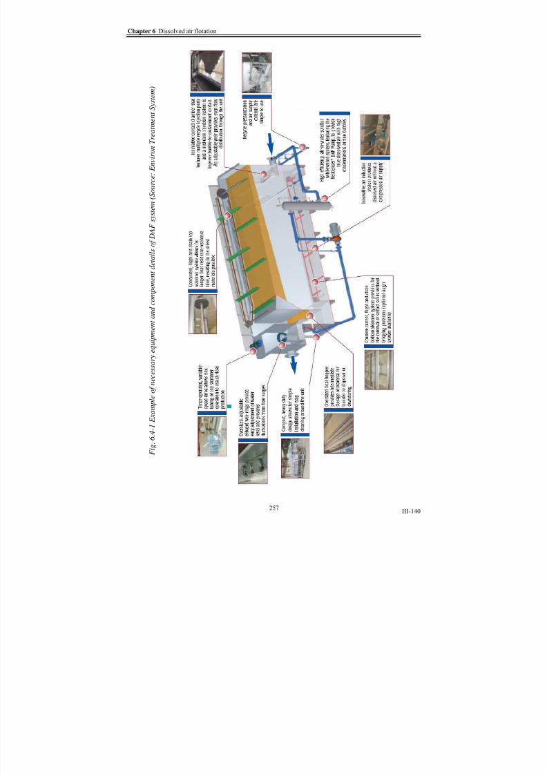
8/15/2019 Rachu.pdf
http://slidepdf.com/reader/full/rachupdf 334/646
Chapter 6 Dissolved air flotation
III-140
F i g . 6 . 4 - 1 E x a m p l e o f n e c e s s a r y e q u i p m e n t a n d c o m p o n e n t d e t a i l s o f D A F s y s t e m (
S o u r c e : E n v i r o n T r e a t m e n t S y s t e m
)
257

8/15/2019 Rachu.pdf
http://slidepdf.com/reader/full/rachupdf 335/646
Part III Summary of researches: Oily wastewater treatment
III-141
Table. 6.4-1 Data on efficiency and coagulant concentration of various oily wastewater
treatments by DAF [51]
Oil concentration
WastewaterCoagulant
(mg/l)Influent Effluent %Removal
Refinery 0 125-170 35-52 70-72
100 alum 100 10 90
130 alum 580 68 88
Oil tanker ballast water 100 alum + 1 polymer 133 15 89
Paint manufacture 150 alum + 1polymer 1900 0 100
Aircraft maintenance 30 alum + 10 activated silica 250-700 20-50 >90
Meat packing 3830 270 93
4360 170 96
Addition of transfer compound: Sometimes, efficiency of DAF is limited by
probability of air-pollutant agglomerate. In case of oily wastewater, the most frequentencountered problem is ineffective collision between bubble and oil droplets (collision
without agglomerate forming). There are some attempts to solve this problem by addingchemically active agent, called transfer compound, to change some properties of bubble or oildroplet to facilitate oil-bubble agglomerate forming. These chemicals can be added to either
wastewater or as a gas to bubbles. Examples of these chemicals are ammonium gas,
surfactants, etc. In GPI lab, DUPRE [14] had studied the effect of various transfer compoundand concluded that addition of surfactant in pressurized water can cause augmentation in population of microbubbles. On the contrary, addition of polyelectrolyte will cause decreasing
in electrical charge, then favor coalescence of bubbles.
Even though this method is used with some success for water-solid separation,
which the chemical helps forming stronger bond between bubble and solid surface, there is noclearly evidence, at least in GPI lab, that it is feasible on oily wastewater treatment (see
section 6.2.4). So it is recommended to perform DAF test with the real wastewater beforedesign this add-on system. Otherwise, coagulation-flocculation may be more suitable.
a) KROFTA’s inlet manifold with flow
control devices (Source: KROFTA)
b) Example of inlet branch pipes
(Source: Leopold)
Fig. 6.4-2 Necessary equipment and reactor components of DAF system
258

8/15/2019 Rachu.pdf
http://slidepdf.com/reader/full/rachupdf 336/646
Chapter 6 Dissolved air flotation
III-142
c) Inclined inlet baffle at the center of the
tank (Source: WR DAF)
d) Perforated pipe inlet
(Source: HUBER)
e) Bell mouth pipe outlet (Source: ETS) f) Example of weir outlet (Source: HUBER)
g) Lateral perforated pipes for effluent
draw-off (Source: Leopold)
h) Chain and flight scum skimmer
Fig. 6.4-2 Necessary equipment and reactor components of DAF system (Con’t)
259

8/15/2019 Rachu.pdf
http://slidepdf.com/reader/full/rachupdf 337/646
Part III Summary of researches: Oily wastewater treatment
III-143
i) Rotating scoop skimmer
(Source: DAF corp.)
j) Detail of rotating scoop skimmer
(Source: DAF corp.)
k) Example of CFD analysis on bubble
density in DAF reactor
(Source: InfilcoDegrémont)
l) Example of CFD analysis on velocity
distribution in DAF reactor
(Source: InfilcoDegrémont)
m) Typical flow pattern in DAF system
(Source : InfilcoDegrémont)
n) Folded flow pattern in DAF reactor
(Source: WR DAF)
o) Rectangular DAF reactor
(Source: WR DAF)
p) Circular DAF reactor
(Source: KROFTA)
Fig. 6.4-2 Necessary equipment and reactor components of DAF system (Con’t)
260

8/15/2019 Rachu.pdf
http://slidepdf.com/reader/full/rachupdf 338/646
Chapter 6 Dissolved air flotation
III-144
q) Example of shallow DAF reactor
(Source: WR DAF)
r) Graphical image of shallow DAF reactor
(Source: KROFTA)
s) Feed manifold and rotating internal baffle
in shallow DAF reactor (Source: WR DAF)
t) 4 effluent draw-off pipes in shallow DAF
reactor (Source: WR DAF)
u) Flocculation tank (Source: Aqua-
pak systems)
v) Flocculation pipe (the array of pipe
beside DAF reactor) (Source: WR DAF)
Fig. 6.4-2 Necessary equipment and reactor components of DAF system (Con’t)
5.
Characteristic of float or scum
Characteristic of float or scum of DAF depends on characteristic of wastewater.Fig. 6.4-3 shows some examples of scum from DAF. However, for refinery wastewater, petroleum or oil-related industries, which oils are components of the wastewater, scum will be
261

8/15/2019 Rachu.pdf
http://slidepdf.com/reader/full/rachupdf 339/646
Part III Summary of researches: Oily wastewater treatment
III-145
rich in oil. Some literatures [50] report that oil concentration in DAF scum is as high as 50%
by weight for DAF process with coagulation-flocculation. For oil-rich scum, it could be
possible to use oleophilic oil skimmer, which is widely used for API tank.
However, solids and other pollutants are usually present in oily wastewater, the
scum, then, contains these solids and pollutants and is in form of thick froth layer. DAFsystem can produce scum, which is normally more dense than settled sludge from settlingtank. Average concentration of 1% (solid content) could be expected. Higher concentration,
such as 3%, is reported by many sources [51].
a) Scum for petroleum industry (Source:
www.environmentalleverage.com)
b) Scum from high rate DAF reactor
(Source: InfilcoDegrémont)
c) Scum from circular DAF reactor
(Source: KROFTA)
d) Example of side window of DAF tank. Notice
float layer and bubble (Source: KROFTA)
Fig. 6.4-3 Examples of characteristics of scum from DAF processes
6.5 Pressurized water system or saturator
6.5.1 Working Principle and design calculation
Because air bubble is the heart of DAF operation, pressurized water system, then, is a
very important component of DAF for it is the source of air bubbles. Basic principle of pressurized water system or saturator is to dissolve the air into the water at high pressure.After that the pressurized water will be injected into the wastewater at operating pressure,
normally ambience. When the pressure decreases, solubility of air in water will decrease so
the excess air will become gas and cause air bubble within the water.
262

8/15/2019 Rachu.pdf
http://slidepdf.com/reader/full/rachupdf 340/646
Chapter 6 Dissolved air flotation
III-146
There are 3 major modes of pressurization in DAF process, i.e.,
• Full-flow pressurization: In this mode, whole wastewater is pressurized. It mightoperate at lower pressure since the quantity of pressurized water is high, low
dissolved concentration of air is sufficient. Reactor in this case is designed only to
handle wastewater quantity. However, pollutants, esp. suspended solids, may causesome problems to the saturator system, esp. injection valve and packed saturationtank. It can not be used if coagulation-flocculation is employed for it may cause re-
fragmentation of floc by the saturator packing.
• Partial flow pressurization: In this mode, only some portion of wastewater is pressurized and then sent to mix with the rest of wastewater to reactor. However,
pollutants in wastewater might still cause some problem to the saturator system.
• Recycled flow pressurization: This mode of operation is the most popular. Some portion of treated water is recycled to use as pressurized water. Quantity of thewater is relatively good for it has been treated. So it does not cause any problem to
the packed saturation tank. However, the reactor has to handle wastewater plusrecycled flowrate.
However, the pressurized water system for every mode of pressurization is identical.
Good saturator system has to provide a number of very tiny bubbles. Characteristic of good
pressurized water is that, when it is discharged into the reactor, it will have cloudy and milkappearance for relatively long period of time, as shown in fig. 6.5-1.
a) Example of propagation of bubbles generated by pressurized water when injected
into the top of test tank.
b) Cloudy, milky appearance of bubbles generated by pressurized water
Fig 6.5-1 Example of good bubble formation from pressurized water (Source:
Cornell DAF pump)
263

8/15/2019 Rachu.pdf
http://slidepdf.com/reader/full/rachupdf 341/646
Part III Summary of researches: Oily wastewater treatment
III-147
From GPI research [12], theoretical equations, such as Henry’s law and Dalton’s law,
can be used to calculate pressurized water system with relatively high accuracy. To size the
pressurized water system, the following procedure is proposed.
1. Quantity of air or gas in pressurized water
Solubility or concentration of air in water in saturator is practically governed byHenry’s law (eq. 6.5.1).
H
yP x = {6.5.1}
Where x = molar fraction of dissolved gas in water (mol/mol)
Y = molar fraction of gas in air (mol/mol) For air: y = 1 For oxygen:y(O2) = 0.21 (=0.11 in permanent regime) For nitrogen: y(N) =
0.79 (= 0.89 in permanent regime)P = absolute pressure of saturator (atm, or conforms to unit of H
used)H = Henry’s constant, depending on type of gas (20oC), i.e., For air:
H = 4.04x10⁴ atm/mol For oxygen: H = 8.04x10
4 atm/mol For
nitrogen: H = 6.64x10⁴ atm/mol
Eq. 6.5.1 can be used to calculate the value of “x” or molar solubility of gas in
saturator at any given pressure (P). Normally, saturator is operated at around 4 atm (abs).
Concentration of air or gas discharged within DAF reactor at ambience condition can becalculated by eq. 6.5.2.
1000)(
)().( ⋅
⋅⋅=
water MW
gas MW xgasConc water ρ mg/l {6.5.2a}
Where MW(gas) and MW(water) are molecular weight of gas and water
respectively.
Substitute x from eq. 6.5.1.
P A H water MW
gas MW P ygasConc water ⋅=⋅
⋅
⋅⋅⋅= 1000
)(
)().(
ρ {6.5.2b}
1000)(
)(⋅
⋅
⋅⋅=
H water MW
gas MW y A water
ρ {6.5.2c}
To facilitate calculation of dissolved air or gas, Henry’s constant can beexpressed in the form of molair (or gas)/(m3 water.atm), called H’. Eq. 6.5.2d can be used tocalculate the value of H’ at any temperature. Temperature is in Kelvin. From this concept, eq.
6.5.2b can be rewritten as shown in eq. 6.5.2e.
2472.1)273(02745.0)273(00039.0)273(000002.0' 23 +−−−+−−= T T T H {6.5.2d}
1000
')().(
H gas MW P ygasConc
⋅⋅= mg/l {6.5.2e}
For quantity of gas discharged in DAF reactor, it can be calculated from
difference between concentration of dissolved gas in at saturator’s pressure and that atambience pressure, 20 as shown in eq. 6.5.3.
264

8/15/2019 Rachu.pdf
http://slidepdf.com/reader/full/rachupdf 342/646

8/15/2019 Rachu.pdf
http://slidepdf.com/reader/full/rachupdf 343/646
Part III Summary of researches: Oily wastewater treatment
III-149
Energy for compressor can be practically calculated by adiabatic process
equation (PV1.4
= Constant) with satisfactory accuracy (see eq. 6.5.4). ηcomp is overallefficiency of compressor, which can be safely assumed to be around 60-70%.
pw
atmcomp
Q
gas MW
gasConc
P
P RT Power ⋅⋅
⎥⎥
⎥
⎦
⎤
⎢⎢
⎢
⎣
⎡−⎥
⎦
⎤⎢⎣
⎡⋅=
−
)(
)(1
4.0
1)
4.1
14.1(
η
{6.5.4}
Using R = 8.314 Pa.m3/(mol. K), Conc(air) in g/l and Q pw in m3/s will result in
power as Watt. Molecular weight (MW) of air is 28.95 g/mol. Fig. 6.5-2 shows relation between calculated power required for compressor and absolute pressure of saturator (P) for
10 m3/h of pressurized water.
Energy for pressurized water pump can be practically calculated by general
equation by assuming overall efficiency of the pump (η pump) around 60-70%.
pump
gauge pw
pump
atm pw PQPPQPower
η η
)()( ⋅=
−⋅= {6.5.5}
Using Q pw in m3/s and pressure (P) in Pa. will result in power as Watt. Fig. 6.5-2shows relation between calculated power required for pump and absolute pressure of saturator
(P) for 10 m3/h of pressurized water.
Energy for DAF pump The DAF pump is a special type of saturator thatintegrate the function of compressor and pressurized water pump into a single machine.Details of the pump will be described in the next section. Its energy required is theoretically
equal to summation of energy for compressor and energy for pressurized water pump.
However, single step estimation, using eq. 6.5.5 alone with η pump around 50-60% is
acceptable. The exact energy required can be obtained from manufacturer’s information.
0
20
40
60
80
100
120
140
160
180
200
0 1 2 3 4 5 6 7 8
Saturator pressure (atm. (absolute))
P o w e r
r e q u
i r e d f o r c o m p r e s s o r
( W a t t
/ 1 0 m
3 / h o
f w a t e r )
0
500
1000
1500
2000
2500
P o w
e r r e q u
i r e d f o r p u m p
( W a
t t / 1 0 m
3 / h o
f w a t e r )
Compressor
(η = 100%)
Compressor
η = 70%
Pump
(η = 100%)
Pump
η = 70%
Fig. 6.5-2 Relation between power required for pump, compressor and absolute pressure of saturator for
pressurized water flowrate of 10 m3/h (assume %air saturation = 95%)
266

8/15/2019 Rachu.pdf
http://slidepdf.com/reader/full/rachupdf 344/646
Chapter 6 Dissolved air flotation
III-150
6.5.2 Type of saturator and injection valve
1. Saturator
Saturator can be divided into 2 main categories, i.e.,
• Combination of pump and saturation tank: Schematic diagram of thissystem is generally as shown in fig. 6.5-3. Working principle of the system is
relatively the same as packaged booster pump or pump/pressure tank systemin water distribution work. However, the saturation tank has to be specially
designed to maximize air dissolution into water. For conventional system, thetank is designed as packed column, using ring packing or likewise, as shown
in fig. 6.5-4. Saturation tank in this case is classified as pressure vessel, so, insome countries, its design must conform to applicable law or regulation of
pressure vessel.
• In some designs, the pressure tank is replaced by other air-water mixing
device, which is equivalent in performance but less complex and lessexpensive. An example of this device is mixing pipe as shown in fig. 6.5-4.
• Generally, air compressor for DAF is installed. However, in case that there is
common compressed air supply, it can be readily used in DAF. In fewdesign, the pressure tank with automatic air intake system, which is widely
used in packaged pump-pressure tank system, is used.
• DAF pump: This device is combination of pump and air saturation systeminto one machine. Air will be either sucked from ambience by the pump itself
or supplied by compressor into pump suction or pump casing. The air willmix with the water within the pump. It eliminates the use of saturation tank.
Schematic diagram and examples of DAF pump are as shown in fig. 6.5-3and 6.5-4.
2. Injection valve
Injection valve or pressure reducing valve or pressure release valve is a devicethat practically generates air bubbles at the working point. The valve will reduce the pressure
of pressurized water to ambience, which cause excess dissolved gas to convert to gas bubbles.
In GPI lab, there are few researches on the value [14], [15]. From the researches, it shows thatthe gas will be firstly generated in form of large gas pocket and then will be fragmented byhydrodynamic force to form microbubbles (see fig. 6.5-5). So geometry of the valve, which
determines hydraulic condition, is the key parameter to obtain microbubbles. Many types ofvalves are shown in fig. 6.5-5. Selection of the valve is based mainly on experience. However,
it is recommended to install the value as close to mixing zone between wastewater and pressurized water as possible.
267

8/15/2019 Rachu.pdf
http://slidepdf.com/reader/full/rachupdf 345/646
Part III Summary of researches: Oily wastewater treatment
III-151
a) Conventional pressurized water system or saturator system
b) Saturator system using DAF pump
Fig. 6.5-3 Schematic diagrams of saturator systems (Source: Edur pump)
268
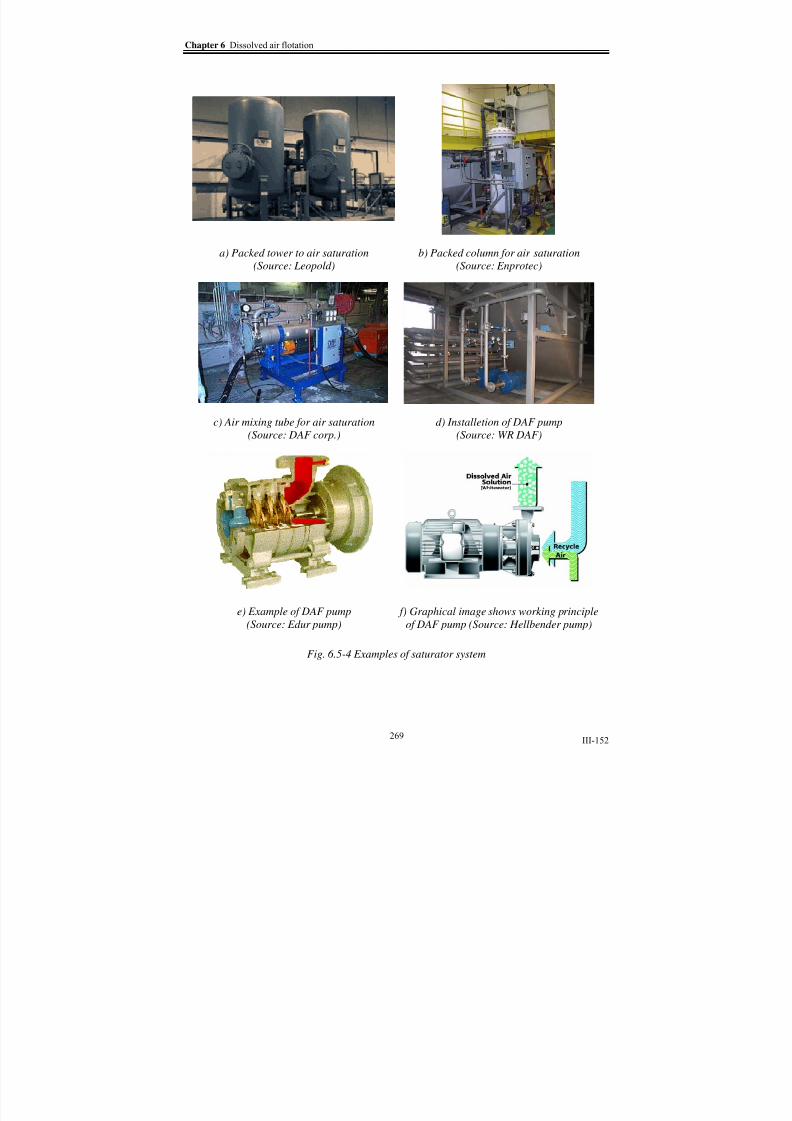
8/15/2019 Rachu.pdf
http://slidepdf.com/reader/full/rachupdf 346/646
Chapter 6 Dissolved air flotation
III-152
a) Packed tower to air saturation
(Source: Leopold)
b) Packed column for air saturation
(Source: Enprotec)
c) Air mixing tube for air saturation
(Source: DAF corp.)
d) Installetion of DAF pump
(Source: WR DAF)
e) Example of DAF pump
(Source: Edur pump)
f) Graphical image shows working principle
of DAF pump (Source: Hellbender pump)
Fig. 6.5-4 Examples of saturator system
269

8/15/2019 Rachu.pdf
http://slidepdf.com/reader/full/rachupdf 347/646
Part III Summary of researches: Oily wastewater treatment
III-153
a) Examples of injection valves [14]
b) Magnified photos of air pocket formation and fragmentation in convergence-
divergence nozzle type injection valve [14]
Fig. 6.5-5 Examples of injection valve
6.6 Variations, advantage and disadvantage of DAF
There are many variations of DAF system in many ways such as tank shape, flow
pattern, equipment, loading rate, as described before in this chapter. So selection and designof DAF is state-of-art, like many other processes, and based mainly on experience. However,data from DAF test, such as Flota-test, and studies on successful projects for the same or
related type of wastewater are useful to design DAF system.
Advantages:
1. It requires less footprint area than conventional decanter.
2. Since it is accelerated process, we have some control over many operating
parameters, such as coagulant dosage, quantity of pressurized water, etc. Then it
has more flexibility to handle variation of wastewater characteristic.3. DAF is less effected by temperature, compared to other processes.
270

8/15/2019 Rachu.pdf
http://slidepdf.com/reader/full/rachupdf 348/646
Chapter 6 Dissolved air flotation
III-154
Disadvantages:
1. Capital cost and operating is higher than conventional decanter.
2. DAF system consists of a lot of equipment, so the maintenance is higher than
conventional decanter. Moreover, it may require more skill of the operator.
3. Its efficiency depends on many parameters as described before, so it maydecrease if some parameters in not optimized.
4. Coagulation-flocculation process is normally required. This causes more expenseon chemicals.
271

8/15/2019 Rachu.pdf
http://slidepdf.com/reader/full/rachupdf 349/646
Part III Summary of researches: Oily wastewater treatment
III-155
Chapter 7 Hydrocyclone
7.1
General
Hydroyclone is an accelerated separation process. Its main working concept is to
replace the gravitational acceleration that governs decanting velocity by higher centrifugalacceleration. Hydrocyclones are widely used in many processes, i.e., classification and
separation between solid-liquid and liquid-liquid. Unlike other centrifugal machines, driving
force of hydrocyclone is generated solely from its inlet velocity. The higher the velocity (or
flowrate), the higher the efficiency. Or it can be implied that, at the same flowrate, smaller
will have higher performance that the smaller one. This is the most interesting advantage of
hydrocyclone.
Commercial hydrocyclones come in various shapes (single conical, long double
conical, etc.) and configurations (co-current or counter current, based on direction of water
and oil outlet flow). However, because it is used to make the separation between 2 phases
(such as, liquid-liquid, solid-liquid.), it will be called here as “two-phase hydrocyclone”. InGPI lab, almost all of the researches are based on this type of hydrocyclone. In this chapter,
we will consider particularly on application of hydrocyclone on oil/water separation. For
oil/water separation, the hydrocyclones usually come in the form of elongated conical
hydrocyclone, as shown in fig 7.1-1a. Vortex or spiral movement in hydrocyclone will make
oil move inward to the center where it is purged to an overflow port, as shown in fig. 7.1-1.
Treated water will flow out at an underflow port. Studies on two-phase hydrocyclone for
oil/water separation will be described in section 7.2.
However, there is another type of hydrocyclone that is initiated by AURELLE and
MA [16] in GPI lab. This special hydrocyclone is an innovation designed for simultaneous
separation of oil and suspended solids from water. Studies on this “three-phase hydrocyclone”will be summarized in section 7.3.
a) Graphical image shows vortex and oil
core in 2-phase counter current hydrocyclone
(Source: Ultraspin)
b) Graphical image of three-phase
hydrocyclone [16]
Fig. 7.1-1 Basic flow pattern and examples of hydrocyclones
272

8/15/2019 Rachu.pdf
http://slidepdf.com/reader/full/rachupdf 350/646
Chapter 7 Hydrocyclone
III-156
1 2 0
2 5 5
5 3
4 2 8
10
50
Entrée
Sortie eau
Sortie huile
Entrée
Sortie eau
Sortie huile
Tube d'aspiration
Surface intérieure
Surface extérieure
c) Industrial scale counter current 2-
phase hydrocyclone (Source: Krebs)
d) Co-current lab scale 2-phase
hydrocyclone (Source: GPI lab)
Fig. 7.1-1 Basic flow pattern and examples of hydrocyclones (Con’d)
7.2 Two-phase hydrocyclone
7.2.1
Working principles
As mentioned earlier, working principle of hydrocyclone is based on modifying an
acceleration in STOKES law (eq. 7.2.1). From the law, rising or decanting velocity (U d) of oil
droplet is proportional to acceleration (a). Generally, this acceleration means gravitational
acceleration (g). However, in centrifugal machine, liquid is forced to spin or centrifuged
around the axis of the machine. So the liquid is subjected to another acceleration, which is
centrifugal acceleration. If the liquid spins fast enough, the centrifugal acceleration (ac) will
overcome the gravity acceleration. The decanting velocity of oil droplets, as well as, removal
efficiency, will increase. The higher the centrifugal acceleration is, the better the efficiency is.
c
d
d aU
μ
ρ
18
2⋅⋅Δ= {7.2.1}
Where d = Diameter of dispersed phase, in this case, oil droplets
a = Corresponding acceleration of oil droplets
Δρ = Difference between density of dispersed phase and continuous phase
μC = Dynamic (or absolute) viscosity of continuous phase, which is water, for
oily wastewater
Ud = Rising or decanting velocity of the droplet diameter “d”
So, efficiency of hydrocyclone can be described in term of ratio between centrifugal
and gravity acceleration, called the factor of acceleration (ζ), as shown in eq. 7.2.2 .For
hydrocyclone, the driving force that makes the liquid rotate or spin comes from energy of its
own inlet flowrate. Theoretically, pressure head of feed flowrate can be converted to velocity
by energy conservation law, as shown in eq. 7.2.3.
D
V a
c
22= {7.2.2a}
gD
V
g
ac22
==ς {7.2.2a}
gH V 2= {7.2.3}
273

8/15/2019 Rachu.pdf
http://slidepdf.com/reader/full/rachupdf 351/646
Part III Summary of researches: Oily wastewater treatment
III-157
From eq. 7.2.2a and 7.2.3, ζ can be rewritten as follow,
gD
gH 2)2(2
=ς {7.2.4a}
D H 4=ς {7.2.4b}
Where ζ = Factor of acceleration
V = Tangential velocity in hydrocyclone
D = Diameter of rotation, in this case, hydrocyclone diameter
H = Head or pressure drop across hydrocyclone
Eq. 7.2.4b signifies that,
• Efficiency of hydrocyclone is direct proportional to its pressure drop.
• As stated earlier in section 7.1, efficiency of hydrocyclone will increase if the size
of hydrocyclone decreases. It can be implied that, at the same flowrate, smaller
hydrocyclone is always more efficient than the bigger one.
7.2.1.1 General flow pattern and feature of hydrocyclone
General feature
Generally, hydrocyclone consists of cylindrical section, where inlet port(s) is
tangentially placed, and conical section, which may be a smooth cone (fig. 7.1-1d and 7.2.1-
1a) or has an inflection point (fig. 7.1.1a,c and 7.2.1-b).
There may be one or two inlet ports. And it may have circular or rectangular opening.
For typical hydrocyclone, there will be an outlet port at the center of the cover of cylindrical
section. This port is always called overflow port. The port locate at the pointed end of conical
section is called underflow port. The wall of overflow port is, usually but not always,
protruded into the hydrocyclone. If it exists, this part is called vortex finder.
However, many manufacturers had separately engineered the shapes of their
hydrocyclones to fit their applications. For examples, there might be another cylindrical
section at the end of the conical section. Or there might be 2 concentric underflow without
overflow ports. Anyway, their working principal is always based on centrifugal acceleration.
Liquid-liquid hydrocyclone for oil/water seperation
Because of relatively low density difference between oil and water, compared to that
of solid and water, shape of liquid-liquid hydrocyclone for oil/water seperation has to be
adapted from typical solid-liquid hydrocyclone as shown in fig. 7.1-1 and 7.2.1-1f. The shape
of the oil/water hydrocyclone shown in the figure was researched and proposed by Prof.
THEW of University of Souththamton, UK. From the figure, another conical section with
small cone angle is added, and then followed by another cylindrical section. Overflow oil
outlet port is smaller than that of solid-liquid one. And there is no vortex finder since it is not
essential to prevent short circuit of oil to oil outlet. Moreover, THEW also shows that
presence of vortex finder resulted in lower efficiency. This hydrocyclone is widely accepted
274

8/15/2019 Rachu.pdf
http://slidepdf.com/reader/full/rachupdf 352/646
Chapter 7 Hydrocyclone
III-158
as a typical design of oil/water separation. In GPI lab, MA [16] also used THEW’s type
hydrocyclone for his model development.
General flow pattern
As mentioned earlier, general spiral flow pattern of typical hydrocyclone, which has 1overflow and 1 underflow port, is as shown in fig. 7.2.1-1a. From the figure, there are both
upward and downward flow. Upward and downward flow pattern might be difference in case
of co-current hydrocyclone, which has 2 concentric underflow ports. Nevertheless, flow
pattern will always be spiral, which causes centrifugal acceleration.
From centrifugal acceleration and density difference between oil and water, oil
droplets will tend to move toward the axis of hydrocyclone and form an oil rich zone or oil
core at the axis (fig. 7.2.1-1d) that can be purged to an oil outlet port. Water, on the other
hand, will be centrifuged outward and flow out at water outlet port, as shown in fig. 7.1-1a
and 7.2.1-1b. Oil core normally contains both oil and water (fig. 7.2.1-1e). So oil removed
from hydrocyclone still contains some amount of water. Then hydrocyclone is rather oilconcentrator than oil separator. To separate oil from this concentrated mixture, other
separation process, such as coalescer, may be required.
Sometimes, there is an air core forming at the center of oil core (fig. 7.2.1-1c). It does
not provide any separation efficiency and, sometimes, makes the operation unstable. Presence
of air core can be avoided by providing back pressure, such as valve throttling, at the outlet
port.
Oily wastewater
Concentrated oil
Treated water
Underflow port
Overflow portInlet port
a) General spiral flow
pattern in typical
hydrocyclone [30]
b) Typical trajectory of oil droplets
in liquid-liquid hydrocyclone
c) Example of
presence of air core
[30]
Fig. 7.2.1-1 General flow pattern and features of hydrocyclones
275

8/15/2019 Rachu.pdf
http://slidepdf.com/reader/full/rachupdf 353/646
Part III Summary of researches: Oily wastewater treatment
III-159
d) Oil core formation (thin red strip at
the center of the hydrocyclone) [11]
e) Magnified photo of oil core, shows tiny
oil droplets suspending in water [16]
Di
D
Dn
Ds
L1
L3
Do
θ
β
Dn/D=0.5, Ds/D=0.25, Do/D<0.05, L1/D=1, L3/D=15-20 , β =1.50
o , θ =20
o
Di/D=0.25 for 1 inlet and 0.175 for 2 inlet ports, total length/D =45 (approx.)
f) THEW’s type liquid-liquid hydrocyclone for oil/water separation
Fig. 7.2.1-1 General flow pattern and features of hydrocyclones
7.2.1.2 Velocity distribution in hydrocyclone
Flow pattern in hydorcyclone, as shown in the previous section, can be described in
the form of velocity within the hydrocyclone. Velocity at any point in the hydrocyclone can
be divided into 3 components, i.e., tangential, radial and axial velocity (fig. 7.2.1-2).
Characteristic of each velocity components will be described as follow.
VzVt
Vr
Z
R
Axial axis
H y
d r o c
y c l o n e w
a l l
Vr = Radial velocity
Vt = Tangential velocity
Vz = Axial (or vertical) velocity
Fig. 7.2.1-2 Velocity components in hydrocyclone
276
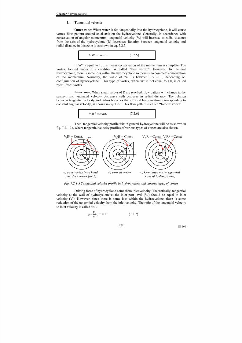
8/15/2019 Rachu.pdf
http://slidepdf.com/reader/full/rachupdf 354/646
Chapter 7 Hydrocyclone
III-160
1. Tangential velocity
Outer zone: When water is fed tangentially into the hydrocyclone, it will cause
vortex flow pattern around axial axis on the hydrocyclone. Generally, in accordance with
conservation of angular momentum, tangential velocity (Vt) will increase as radial distance
from the axis of the hydrocyclone (R) decreases. Relation between tangential velocity andradial distance in this zone is as shown in eq. 7.2.5.
.const RV n
t = {7.2.5}
If “n” is equal to 1, this means conservation of the momentum is complete. The
vortex formed under this condition is called “free vortex”. However, for general
hydrocyclone, there is some loss within the hydrocyclone so there is no complete conservation
of the momentum. Normally, the value of “n” is between 0.5 –1.0, depending on
configuration of hydrocyclone. This type of vortex, when “n” in not equal to 1.0, is called
“semi-free” vortex.
Inner zone: When small values of R are reached, flow pattern will change in the
manner that tangential velocity decreases with decrease in radial distance. The relation
between tangential velocity and radius becomes that of solid body rotation, corresponding to
constant angular velocity, as shown in eq. 7.2.6. This flow pattern is called “forced” vortex.
.1 const RV t =− {7.2.6}
Then, tangential velocity profile within general hydrocyclone will be as shown in
fig. 7.2.1-3c, where tangential velocity profiles of various types of vortex are also shown.
R
VtR n = Const. n=1
n<1
R
Vt/R = Const.
R
Ra
Vt/R = Const. VtR n = Const
a) Free vortex (n=1) and
semi-free vortex (n<1)
b) Forced vortex c) Combined vortex (general
case of hydrocyclone)
Fig. 7.2.1-3 Tangential velocity profile in hydrocyclone and various typed of vortex
Driving force of hydrocyclone come from inlet velocity. Theoretically, tangential
velocity at the wall of hydrocyclone at the inlet port level (Vc) should be equal to inlet
velocity (Vi). However, since there is some loss within the hydrocyclone, there is some
reduction of the tangential velocity from the inlet velocity. The ratio of the tangential velocity
to inlet velocity is called “α”.
i
c
V
V =α , α < 1 {7.2.7}
277

8/15/2019 Rachu.pdf
http://slidepdf.com/reader/full/rachupdf 355/646
Part III Summary of researches: Oily wastewater treatment
III-161
The value of α varies with the shape of hydrocyclone. From eq. 7.2.5 and 7.2.7,
tangential velocity at any radial distance can be written as shown below.
n
i
n
c
n
t
DV
DV RV )
2()
2( α == {7.2.8a}
n
it R
DV V )
2(α = {7.2.8b}
Where VI = Velocity in the inlet port of hydrocyclone
D = Diameter of hydrocyclone (measured at the same level as the
inlet port)
R = Radial distance
It should be noted that tangential velocity depends on “radial distance (R), and is
independent of axial distance (Z). The velocity at the same “R” will be practically identical at
any axial distance from inlet level of hydrocyclone (Z), as shown in fig. 7.2.1-4.
Vr1
Vr1
Vr1
Vr1
R= r1
a) Source: Krebs b) Data from KELSALL[30]
Fig. 7.2.1-4 Examples of tangential velocity profile
2. Axial velocity
As shown in fig. 7.1-1 and 7.2.1-1 that the outer and inner layers of liquid in
hydrocyclone move in opposite direction, axial velocity (Vz) profile will consist of both
upward and downward velocity, as shown in fig. 7.2.1-5. Axial velocity profile depends on
shape of hydrocyclone, such as angle of cone, and operating condition, such as presence of air
core. Even in the same hydrocyclone, characteristic of axial velocity profile at various zones,
such as conical zone, inlet cylindrical zone or near apex zone. etc., are not similar. However,
typical axial velocity profiles at the effective conical section of hydrocyclone can be
simplified as shown in fig. 7.2.1-5b and 7.2.1-5c. Fig. 7.2.1-5b is typical axial velocity profile
for solid-liquid separation, proposed by RIETEMA [quoted by [16]]. For fig 7.2.1-3c, it is the
278

8/15/2019 Rachu.pdf
http://slidepdf.com/reader/full/rachupdf 356/646
Chapter 7 Hydrocyclone
III-162
axial velocity profile, proposed by THEW and COLMAN [quoted by [16]] for of liquid-liquid
hydrocyclone, as well as, proposed by KASSELL [quoted by [30]] for solid-liquid separation.
There is no general relation or equation of axial velocity for hydrocyclone.
However, equations of axial velocity profile for specific shapes of hydrocyclone are available,
such as COLMAN’s equation for THEW’s type liquid-liquid hydrocyclone. The equation(shown in the next section) will be used for 2-phase hydrocyclone model development.
(Source: Krebs) (Source: [52]) (Source: Bradley [30])
a) Examples of axial velocity profiles from various sources
Locus of zero
vertical velocity
Locus of zero
vertical velocity
R
Z
L o c u
s o
f z
e r o
v e r
t i c a
l v
e l o
c i t y
H y d
r o c y
c l o n e w a l l
Axial axis
b) Axial velocity profile
with 2 downward and 1
upward flows
c) Axial velocity profile
with 1 downward and 1
upward flows
d) Axial velocity profile
predicted by COLMAN’s
equation
Fig. 7.2.1-5 Example of axial or vertical velocity profile
279

8/15/2019 Rachu.pdf
http://slidepdf.com/reader/full/rachupdf 357/646
Part III Summary of researches: Oily wastewater treatment
III-163
3. Radial velocity
Radial velocity (Vr ) normally has a maximum value near to the wall of
hydrocyclone in inward direction. Then it will decrease with decreasing of radial distance. It
might or might not reach zero value and become outward radial velocity, depending on the
shape and axial position considering. Example of radial velocity profile is shown in fig. 7.2.1-6. KELSALL [30] proposed the estimated value of radial velocity in the conical section as
shown in eq. 7.2.9.
)2
tan(θ ⋅=W U {7.2.9}
Fig. 7.2.1-6 Example of radial velocity profile [30]
7.2.1.3 Forces on particle in hydrocyclone
From the velocity fields of liquid or continuous phase decsribed above, dispersed
particles, in this case, oil droplets, suspended in hydrocyclone will subject to many
components of forces. Consider an oil droplet (or particle) in hydrocyclone as shown in fig.
7.2.1-7. The oil droplet will subject to several clearly-defined forces, such as,
F4Fr
F1
Z
R
F2
F3
F5
WV
U
Z
R
Axial axis
H y
d r o c
y c l o n e w
a l l
Resulting V
Fig. 7.2.1-7 Forces on oil droplets or particles in hydrocyclone
Fig. 7.2.1-8 Components of velocity of oildroplets or particles in hydrocyclone
280

8/15/2019 Rachu.pdf
http://slidepdf.com/reader/full/rachupdf 358/646
Chapter 7 Hydrocyclone
III-164
• Centrifugal force in radial axis (F1)
6
32
1
d
R
V F
π ρ ⋅⋅Δ= {7.2.5a}
• Drag force or hydraulic force in radial axis (F2)
421
2
22 d U Cd F c π ρ ⋅⋅= {7.2.5b}
• Gravity force (F3)
6
3
3
d gF
π ρ ⋅Δ= {7.2.5c}
• Drag force or hydraulic force in axial axis (F4)
42
1 22
4
d W Cd F c
π ρ ⋅⋅= {7.2.5d}
• Drag force or hydraulic force in tangential direction (F5)
42
1 22
5
d V Cd F c
π ρ ⋅⋅= {7.2.5e}
Where U = Radial velocity (or decanting velocity) of oil droplets
V = Tangential velocity of oil droplets
W = Axial velocity of oil droplets
Please note that three components of velocity are of oil droplets (fig 7.2.1-8), which
are not exactly the same as the three velocities (Vx, Vy, Vz) of liquid , described in the previous
sections. There are also other forces, such as lift force, etc. These forces will make the oil
droplets move in hydrocyclone and determine if those droplets can be totally, partially
separated or can not be separated by the hydrocyclone. Normally, it is not possible to exactlycalculate some components of forces or account for all forces to find the exact resultant force
that governs movement of oil droplets.
Thus, to predict if oil droplets can be separated by hydrocyclone or, on the other hand,
efficiency of hydrocyclone, there are 2 major approaches, i.e.,
• Theoretical based model, such as trajectory analysis, equilibrium orbit or
retention time based model. Well proven laws, such as STOKES law, are applied
to these models under some assumption or simplification. This type of model
might or might not be very accurate, compared to empirical model derived from
experimental data. The accuracy of the type of model depends on degree ofsimplification used by the researchers. But it is useful tool to understand the effect
of parameters to the effciency of hydrocyclone.
• Empirical based model, such as the model and reducing efficiency curve,
proposed by Yoshioka and Hotta [30], Dalstorm’s, and Plitt’s , as well as THEW-
COLMAN’s model.
7.2.1.4 Trajectory analysis model
GPI’s trajectory analysis model for oil/water separation is the work of MA [16].
Concept of MA’s model is adapted from the concept of decanter. Major assumptions thatunderlines this model are that;
281

8/15/2019 Rachu.pdf
http://slidepdf.com/reader/full/rachupdf 359/646
Part III Summary of researches: Oily wastewater treatment
III-165
• The concept of decanter that oil droplets will be separated by hydrocyclone, if the
oil droplets can reach the decanting surface before flowing out with water is
applied (see fig. 7.2.1-9). Decanting surface in this case is assumed to be the locus
of zero vertical velocity (LZVV). If the droplets can reach this line, next moment,
they will start to travel upward to oil outlet port, then, are separated from the
wastewater.
• There is equilibrium of forces in radial direction and oil droplet travels in the radial
direction at terminal velocity of immersed object in fluid stream.
• Radial velocity is governed by STOKES law.
• For tangential and axial velocity of oil droplet, it is assumed that oil droplets are
entrained by the water and have the same tangential and axial velocity as the water
at that point. So V = Vt and W = Vz.
• THEW’s type hydrocyclone is used. So tangential and axial velocity profiles are
calculated from the equations proposed by THEW, COLMAN [quoted by [16]] for
this type of hydrocyclone.
Three velocity components, used for model development, are governed by eq. 7.2.6 to
7.2.8.
Radial velocity: derived from STOKES law;
R
V d U
c
22
18⋅
Δ=
μ
ρ
{7.2.6}
Tangential velocity: derived from energy conservation law (see eq. 7.2.8) and verified by experimental data to find α and n. For THEW hydrocyclone, α = 0.50 and n = 0.65. Please
note that eq. 7.2.7b is valid only for 2-inlet ports hydrocyclone only.
65.0)2
(50.0 R
DV V i= {7.2.7a}
Or 65.0
2
4
)2
(50.0 ⎟
⎠
⎞⎜⎝
⎛
⎟⎟⎟⎟
⎠
⎞
⎜⎜⎜⎜
⎝
⎛
= R
D
D
Q
V n
i
π
{7.2.7b}
Axial velocity: COLMAN [quoted by 16]] observed axial velocity profile in lower
conical section of THEW hydrocyclone, which is the effective section, and developed axial
velocity equation in form of the 3rd order polynomial equation, as shown in eq. 7.2.8. Z-axis
starts from the bigger end of lower conical section, where R is equal to Dn/2, toward the lower
cylindrical section.
32
19.163.81233.3 ⎟⎟ ⎠
⎞⎜⎜⎝
⎛ +⎟⎟
⎠
⎞⎜⎜⎝
⎛ −+−=
z z z z R
R
R
R
R
R
W
W {7.2.8a}
2))2/tan(5.0( β π ⋅−=
Z D
QW
n
z {7.2.8b}
)2tan(2
β
⋅−= Z
D
R
n
z
{7.2.8b}
282

8/15/2019 Rachu.pdf
http://slidepdf.com/reader/full/rachupdf 360/646
Chapter 7 Hydrocyclone
III-166
Q represents wastewater inlet flowrate. Dimensions of the hydrocyclone (Di, Dn, etc.)
conform to fig. 7.2.1-1f. To find trajectory, relation between R and Z has to be found. Firstly,
consider equation of U and W as follow;
t
RU
δ
δ −= {7.2.9a}
t
Z W
δ
δ = {7.2.9b}
From above equations, we have;
W
U
Z
R=−
δ
δ {7.2.10a}
W
Z
U
R δ δ =− {7.2.10b}
Integration of eq. 7.2.10b will result in the relation between R and Z, as shown in eq.
7.2.10c.
∫∫ =− L R
RW
Z
U
R ZVV
0
δ δ {7.2.10c}
R ZVV represents any points on the locus of zero vertical velocity (LZVV), which is
normally in conical shape. However, since conical angle of the lower cone is very small
(1.5o), it can be safely assume that LZVV is cylindrical with the radius of R ZVV at the small
end on the cone (Z=L). At Z = L, from eq. 7.2.8, R ZVV is equal to 0.186(Dn/2). So relation
between R and Z or trajectory of oil droplets can be rewritten as shown in eq. 7.2.11.
Integration of the equation is transcendental and requires complex numerical method, such as
Runge-Kutta. However, it can be done by advanced calculator or computer program,including the program being developed in this research.
∫∫ =− L
RW
Z
U
R Dn
0
)2/(186.0
δ δ {7.2.11}
d = dc
d > dcd < dc
Z
R
L
R d
H y d r o c y c l o n e w a l l
LZVV
0.5Dn
0.186Dn
d
ηd
d c
d < d c
Zone 1 Zone 2
d = or > d c
100%
Fig. 7.2.1-9 Trajectories of oil droplets and typical efficiency curve
from trajectory analysis model
283

8/15/2019 Rachu.pdf
http://slidepdf.com/reader/full/rachupdf 361/646
Part III Summary of researches: Oily wastewater treatment
III-167
Efficiency determination
Fig. 7.2.1-9 shows the trajectories of oil droplets in lower conical section of
hydrocyclone. As stated before, decanting surface in this case is the locus of zero vertical
velocity (LZVV), which can be calculated from eq. 7.2.8, where W = 0. To simplify the
calculation, it is assumed that LZVV is cylindrical with R = 0.186(Dn/2).
From the figure, the longest path to reach the LZVV is the path starting at the wall of
the hydrocyclone at larger end of the cone to the zero-vertical-velocity point at the lower end
of the cone (fig. 7.2.1-9a). The smallest droplet size that can reach this point is called the cut
size (dc). The droplets of cut size or bigger are always separated from wastewater stream with
100% removal efficiency (eq. 7.2.12a).
For d ≥ dc %100=d η {7.2.12a}
The smaller droplets can be also separated providing that they enter the cone near tothe axis of the hydrocyclone. When uniformly distributed influent flow is valid, which is
practically true, the removal efficiency of the droplets smaller than cut size are proportional to
corresponding radial distance (R d) that makes the droplets reach the ZVV point at the lower
end of the cone, as shown in eq. 7.2.9b. Typical efficieny curve of the trajectory analysis
model is shown in fig. 7.2.1-12b.
For d < dc %100
)2
186.0()2
(
)2
186.0(
22
22
⋅−
−=
nn
n
d
d D D
D R
η {7.2.12b}
7.2.1.5 Other models
There are several researches that suggests the model to predict the efficiency of
hydrocyclone, both theoretical and empirical based, such as Bradley’s, Rietema’s,
Dahlstrom’s, Chebelin’s, Plitt’s, Lynch’s, etc. [16],[28]- [34]. However, most of models are
developed from solid-liquid hydrocyclone. Some models are developed for specific
commercial oil/water hydrocyclone, such as Vertoil’s. So it should be applied only with that
specific hydrocyclone. Extrapolation of model is normally not guaranteed.
For THEW’s type hydrocyclone, used by MA in his research, Prof. THEW, himself,
and his colleague, COLMAN, have proposed the model for the hydrocyclone (eq. 7.2.13a).
However, it is empirical model, which seems to be obtained from curve fitting. The equation
for estimation of d75% for THEW’s hydrocyclone, quoted by CHEBELIN [29], is as shown in
eq. 7.2.13b (use unit in kg, m, second.)
))19.0%75
(8.1(
1
−−−= d
d
d eη {7.2.13a}
5.03
%75
)(01.0⎥⎦
⎤⎢⎣
⎡
⋅Δ
⋅=
Q
Dd n
ρ
μ {7.2.13b}
284

8/15/2019 Rachu.pdf
http://slidepdf.com/reader/full/rachupdf 362/646
Chapter 7 Hydrocyclone
III-168
7.2.1.6 Comparison between observed efficiency and theoretical efficiency
MA’s model was verified by observed data obtained from crude oil/water treatment.
Fig. 7.2.1-10 shows the efficiency curve from MA’s trajectory analysis model (eq. 7.2.6 to
7.2.8, 7.2.11), THEW-COLMAN’s model (eq. 7.2.10 and 7.2.11) and observed efficiency
[16]. From the figure, it shows that, at droplet size > 20 microns, MA’s and THEW-COLMAN’s models give relatively accurate result (± 10% error). However, at d > d 80%,
THEW-COLMAN’s model seems to cause higher degree of error and predict too high value
of cut size. This may because the researchers used different assumptions or operating
condition to develop their models.
Difference between MA’s model and observed value can be explained by effect of the
assumptions used to develop the model as follow;
• Radial velocities of oil droplets are not exactly governed by STOKES law.
STOKES law is valid only in laminar flow regime (Re of droplets < 1). However,
in some cases, esp. when droplet size is large, Re might be greater than 1. And
from very short retention time, the droplets may not reach the terminal velocity,
governed by STOKES law. Furthermore, radial velocity of water, which can carry
the oil droplets along and add-up to the decanting velocity from, is not accounted.
So the value of U used in the model is, generally, lower than actual value. This is
the reason why the predicted efficiency is lower than the observed value.
• Effect of eddy current, lift forces, drag forces in vertical and tangential direction is
assumed to be negligible and cancelled. Anyway, they, in fact, can cause some
discrepancies in the prediction result.
• Effect of hinder settling, esp. near to the center of hydrocyclone
However, Ma’s model is developed from theoretical assumption and does includemany parameters, such as viscosity, feed flowrate, and size of the hydrocyclone, etc., which
can be used to explain or verify the effect of these parameters to the efficiency. So, it provides
valuable tool to designer and will be used in the computer program being developed under the
scope of work of this research. Furthermore, the trajectory analysis model is developed under
the assumptions that give underestimated result. So the predicted efficiency is on the safe side.
0%
10%
20%
30%
40%
50%
60%
70%
80%
90%
100%
110%
0.00 10.00 20.00 30.00 40.00 50.00 60.00
Droplet diameter (micron)
E f f i c i e n c y
( % )
Thew-Colman's model
Observed data
Ma's trajectory analysis
Note: Dn = 0.02 m, Q = 1.943 m3/h, Vi = 7.12 m/s: Wastewater used is crude oil/water emulsion: Δρ =
98 kg/m3, μ = 0.0011 Ns/m2, β = 15o, d = 15 to 50 microns
Fig. 7.2.1-10 Comparison between observed efficiency and predicted efficiency form MA’s model and THEW-COLMAN’s model
285

8/15/2019 Rachu.pdf
http://slidepdf.com/reader/full/rachupdf 363/646
Part III Summary of researches: Oily wastewater treatment
III-169
There is no tested evidence about the valid range of MA’s model. However, from the
assumptions used, the model should be valid for every THEW’s type hydrocyclone as long as
operating condition is in valid range of STOKES law (laminar flow region: Re < 1). Anyway,
working condition and performance of hydrocyclone are also governed or limited by other
parameters or factors. So it is more suitable to state that the model is valid in laminar flow
region when other factors also confirm to working limit of hydrocyclone, as described insection 7.2.1.7.
7.2.1.7 Influent parameters
Parameters that affect the performance of hydrocyclone are those presenting in model,
as shown in section 7.2.1.4. However there are some factors that have influent on the
efficiency of hydrocyclone that can not be expressed in form of numerical function. Influent
parameters of hydrocyclone, collected from GPI researches and many literatures, can be
summarized as follow;
1.
Droplet size (d)
Efficiency of hydrocyclone increases with increasing of droplet size, as clearly
shown in fig. 7.2.1-10. So it is recommended to avoid any action that can cause oil drops to
break-up into smeller droplets, such as using high-shear feed pump (Ex. high speed
centrifugal pump, or regenerative turbine pump). On the contrary, putting some process that
can increase the size of droplets at upstream of hydrocyclone, such as high-rate coalescer, will
help increasing hydrocyclone performance.
2. Feed flowrate (Q)
From eq. 7.2.4, efficiency of hydrocyclone will increase, if feed flowrateincreases for it will make inlet velocity, which is a driving force of hydrocyclone, increase.
However, this is true before velocity in the cyclone reaches the value that droplet re-
fragmentation occurs. There are evidences [16], [28] that the inlet velocity (V i) as high as 7
m/s is used without causing any adverse effect on efficiency. This value of Vi can be
compared to velocity of 1.7 m/s, using nominal diameter (Dn) of the cyclone. Please note that
increasing of flowrate also cause pressure drop to be increased, which effects operating cost.
Pressure drop will be described separately in section 7.2.1.8.
3. Shape of hydrocyclone
Shape of hydrocyclone substantially effects its velocity profiles and vortexformation. So it certainly effect its performance. But it can not be expressed in form of
numerical equation. Many researchers have studied effect of dimension of each component of
solid-liquid hydrocyclone (such as inlet port, overflow, underflow port, vortex finder, etc.).
For oil/water hydrocyclone, THEW has thoroughly studied the effect of geometry and
proposed the optimized shape of the cyclone, which is used in GPI researches. In fact, we
usually design hydrocyclone system from standard commercial product, which, more or less,
conform to THEW’s geometry. Anyway, MA [16] had carried out some profound studies of 2
components. The result is as shown below.
• Conical angle θ : Using lower θ (from 20o to 8o) result in decreasing of
pressure drop about 11% (from 4.5 to 4.0 bar at 1.6 m3/h, Dn = 16 mm, crudeoil/water emulsion) while the efficiency is relatively unchanged.
286

8/15/2019 Rachu.pdf
http://slidepdf.com/reader/full/rachupdf 364/646
Chapter 7 Hydrocyclone
III-170
• Ratio Dn/D: Lower Dn/D from 0.5 to 0.43 can increase efficiency (+5% for
Q = 1 to 1.6 m3/h) but pressure drop is also considerably increased (+0.5 bar
for Q = 1 to 1.6 m3/h, D = 32 mm, Dn = 16 and 14 mm).
It must be noted that the models in section 7.2.1.4 and 7.2.1.5 are valid only for
THEW’s type hydrocyclone only.
4. Inlet oil concentration (Co)
For low concentration oily wastewater (Co < 1%), the concentration has
practically no effect on efficiency. For higher concentration, theoretically, it should effect the
performance from hinder settling effect and changing of viscosity. However, THEW [28]
shows that the efficiency is little affected even at the concentration as high as 10 – 15%.
5. Purge ratio or split ratio(Rf )
For oily/water separation, oil will be purged to outlet overflow port. Purge ratio
(R f ) (or split ratio) is the ratio between oil outlet flowrate (overflow) to water feed flowrate
(Q). Theoretically, flowrate of overflow should be as close as possible to the flowrate of oil
components in the water to get relatively pure separated oil. However, in practice, it is
impossible to do so because pressure drop will be too high and some oil will entrain to
underflow port. It is recommended to use R f around 1.8 to 2.0 times of flowrate of inlet oil
[28]. For general oily wastewater, which inlet oil concentration less than 5% (by volume),
purged oil flow is relatively small compared to the whole flow. So it does not effect velocity
profile and efficiency of hydrocyclone. But it effects pressure drop, which will be described in
the next section.
6.
Wastewater characteristic and presence of surfactant
Wastewater characteristic inevitably affects efficiency of hydrocyclone. The
model in section 7.2.1.4 has included general parameters that represent characteristic of
wastewater, such as Δρ, μc, etc. So it is useful tool to understand effect of parameters on
cyclone performance. Some indirect parameters can be determined if it effects the
performance or not by considering its effect on those parameters included in the equation.
For example, presence of salinity will increase density difference, so it favors
efficiency. Presence of surfactant will lower interfacial tension, resulting in fragmentation of
droplets, so it causes adverse effect on hydrocyclone.
7.
Temperature (T)
Proporties of oil and water always change with parameter. So it is inevitable that
temperature will effect hydrocyclone efficiency. Rising in temperature make water viscosity
decrease, then favors the efficiency. However, it will decrease interfacial tension and density
difference, then has adverse effect on the efficiency. So effect of temperature on individual
waster will be accounted on these facts. Anyway, for petroleum/water emulsion at normal
working condition (<40o C), increasing of temperature, more or less, favors hydrocyclone
efficiency.
287

8/15/2019 Rachu.pdf
http://slidepdf.com/reader/full/rachupdf 365/646
Part III Summary of researches: Oily wastewater treatment
III-171
8. Presence of air core
Air core could form at the axis of hydrocyclone from presence of low-pressure
region generated by vortex, especially when it is purged directly to atmosphere. It is also
formed by changing in solubility of gas in water from decreasing of pressure. Presence of air
core might partially block the overflow port and result in instability of performance. Air coreformation can be suppressed by avoiding direct purge to atmosphere and the use of
backpressure. However, many system operating with several percent of air core (by volume)
still give satisfactory result. So throttling should be made until the efficiency is optimized
without over-emphasizing on air core formation. In fact, its formation could not be visible in
commercial opaque hydrocyclone.
7.2.1.8 Pressure drop
Pressure drop is very important parameter since it directly relates to driving force of
the hydrocyclone, as shown in eq. 7.2.4. Furthermore, purge ratio and back pressure control to
suppress the air core is normally be done by valve throttling at the two outlet ports, whichdirectly effects the pressure drop.
Pressure drop can be divided into 2 types, i.e., pressure drop across inlet and overflow
port (ΔPo) and pressure drop across inlet and underflow port (ΔPu).
Like the case of efficiency, equations of the pressure drop of hydrocyclone were
proposed, based on both theoretical and empirical approach. However, there is no pressure
drop model for THEW’s type hydrocyclone, which we knew of. Anyway, many literatures
[16], [28] – [34] show that general model of pressure drop relation is as shown in eq. 7.2.14.
)/(4.2
n
xx DQ f P =Δ {7.2.14}
From GPI researches, there are sufficient data to formulate semi-empirical models of
pressure drop from the general model, as shown below.
For pressure drop (bar) across inlet and overflow port (oil outlet);
1611.0
4
3.2
)1(
6.216 ⎟
⎟ ⎠
⎞⎜⎜⎝
⎛
−⋅=Δ
f n
o R D
QP {7.2.15a}
Flowrate and hydrocyclone diameter are in m3
/s and m, respectively. R f is lower than1.0. However, effect of purge ratio is verified from relatively small set of data, so it might
cause some error. Firthermore, for low concentration wastewater (Co<5%, Rf <10%), effect
or Rf is very small. Eq. 7.2.15a can be rewritten as eq. 7.2.15b, which can be safely used
without causing serious error.
17.1164
3.2
×=Δn
o D
QP {7.2.15b}
288

8/15/2019 Rachu.pdf
http://slidepdf.com/reader/full/rachupdf 366/646
Chapter 7 Hydrocyclone
III-172
For pressure drop (bar) across inlet and underflow port (water oultet);
4
2.2
6.4
n
u D
QP =Δ {7.2.15c}
From above equations, it should be noted that:
• Pressure drop of overflow is always higher than that of underflow. So it is used for
pump sizing. If multi-stage hydrocyclone system is used, available pressure for the
next stage is equal to (ΔPo-ΔPu). The unit of Q is in m3/s, D in meter.
• Underflow pressure drop is practically independent of split ratio. While overflow
pressure drop is slightly affected by the split ratio.
• For oily wastewater treatment, which involves low concentration of oil,
characteristic of wastewater does not affect the pressured drops.
General working pressure range of hydrocyclone is up to 6.5 bar. THEW [28]
recommended the value of 1-5 bar. Hydrocyclone selection is to be compromised between
efficiency, size (capital cost) and pressure drop (operating cost).
7.2.2 Design calculation
Design procedure for hydrocyclone is based upon the equations, shown in the previous
sections. To design two-phase hydrocyclone for oily wastewater treatment, the required cut
size will be determined first. After that, the size of the hydrocyclone can be preliminary
selected. Then, graded efficiency (efficiency of each size of droplet) and then total removal
efficiency can be determined. The procedure will be repeated until the optimum size isselected. Calculation in each step is described below.
1
Cut size determination
The cut size can be determined from the degree of treatment required as well as
from the limitation of the decanting processes. Cut size determination from degree of
treatment is described in chapter 3. For theoretical limitation, since the model is based on
STOKES law, it can be applied only when the droplet behavior conforms to the law. Thus, it
can not be used with very small droplet sizes for they are subjected to Brownian’s motion and
their rising velocity are not governs by STOKES law. There are also some limitations from
characteristic of hydrocyclon itself that governs the cut size selection. Generally,recommended smallest diameter that can be separated (but only partially) by hydrocyclone is
about 20 microns. For smaller droplets, the efficiency will be very low and erratic.
To design the hydrocyclone by MA’s model, it is recommended to select the cut
size that covers majority of oil droplet in the wastewater and provide a safety factor around
10% to 20%, because the model is apt to predict too small cut size. For example, if the desired
cut size is 50 microns, it is recommended to select 50(1-0.20) = 40 microns.
2 Hydrocyclone sizing
The size of the hydrocyclone could be roughly estimated by general designcriteria, such as maximum working pressure, hydraulic loading, etc. Fig. 7.2.1-1 shows the
289

8/15/2019 Rachu.pdf
http://slidepdf.com/reader/full/rachupdf 367/646
Part III Summary of researches: Oily wastewater treatment
III-173
relations between flowrate, inlet velocity, velocity at lower conical section (at dia. = Dn) VS.
diameter of the cylindrical part of hydrocyclone (D) at Po = 3 and 5 bars, which are generally
used as design pressure. For the exact size, the mathematical model can be used. Then the
model will be used again to find the graded efficiency of the hydrocyclone. After that, the size
may be fine adjusted again to obtain the required efficiency.
0.00
2.00
4.00
6.00
8.00
10.00
12.00
14.00
0 10 20 30 40 50 60 70 80 90 10
Diameter of cylindrical section of hydrocyclone (D) (mm)
F l o w r a
t e ( m
3 / h ) a n
d V e
l o c
i t y ( m / s )
Q at P = 5 bar
Q at P = 3 bar
Inlet V at P = 5 bar
Inlet V at P = 3 bar
V at Dn
at P = 5 bar
at P = 3 bar
0
Fig. 7.2.1-1 Corresponding flowrate and velocities of various sizes of hydrocyclones at
overflow pressure drop (Po) = 3 and 5 bars
To size the hydrocyclone and calculate greaded efficiency of the hydrocyclone,
the following procedure, based on MA’s model, is recommended.
2.1 Calculate the size of hydrocyclone (D n )
The size of the hydrocyclone can be calculated by integrating eq. 7.2.11, using
the design cut size from item 1. The corresponding R will be equal to (D n/2). The integration
can be done by the use of a scientific calculator, general mathematical software or the
computer program developed in the scope of work of this research.
∫∫ =− L
RW Z
U R
Dn
0
)2/(186.0
δ δ {7.2.11}
R
V d U
c
22
18μ
ρ Δ= {7.2.6}
65.0
2
4
)2
(50.0 ⎟
⎠
⎞⎜⎝
⎛
⎟⎟⎟⎟
⎠
⎞
⎜⎜⎜⎜
⎝
⎛
= R
D
D
Q
V n
i
π {7.2.7b}
32
19.163.81233.3 ⎟⎟
⎠
⎞⎜⎜
⎝
⎛ +⎟⎟
⎠
⎞⎜⎜
⎝
⎛ −+−=
z z z z
R
R
R
R
R
R
W
W {7.2.8a}
290

8/15/2019 Rachu.pdf
http://slidepdf.com/reader/full/rachupdf 368/646
Chapter 7 Hydrocyclone
III-174
2))2/tan(5.0( β π ⋅−=
Z D
QW
n
z
{7.2.8b}
)2
tan(2
β ⋅−= Z
D R n
z
{7.2.8b}
)2/5.1tan(
)(25.0o
n D
L =
{7.2.16}
2.2 Calculate corresponding radial entering distance (Rd)
For the droplet smaller than the cut size, it is necessary to calculate the
corresponding R d that makes the droplet reach the radial distance R = 0.186(Dn/2) at Z = L.
To calculate R d, eq. 7.2.11 need to be integrated again, using every value of “d” that is smaller
than the cut size.
3 Outlet concentration and removal efficiency
Graded efficiency
Graded efficiency (or centrifugal efficiency), in this case, represents the
efficiency calculated from the trajectory analysis method. For d ≥ dc, graded efficiency will be
equal to 100%.
For d ≥ dc %100=d η {7.2.12a}
For the droplet smaller than the cut size, the theoretical graded efficiency can be
calculated, using the R d from item 2.2, by the following equation.
For d < dc %100
)2
186.0()2
(
)2
186.0(
22
22
⋅−
−=
nn
n
d
d D D
D R
η {7.2.12b}
Outlet concentration
Outlet oil concentration at the underflow (water) and overflow (oil) outlet can be
calculated from theoretical efficiency and purged ration as shown in eq. 7.2.17a and b,
respectively. The equation is valid only when the purged flow is greater than the oil
quantity in the wastewater. Otherwise the oil that can reach the oil core will not be purged
entirely and then entrain with the underflow.
)1(
)1(
f
od d
d R
C C
−
−=
η {7.2.17a}
f
od d
overflowd R
C C
η =,
{7.2.17b}
Global efficiency and removal efficiency
Graded efficiency is not the actual efficiency of hydrocyclone because it does
not account for purged or split flow. Even though this split flow is small and hardly affects the
flow regime in the hydrocyclone, it, somehow, affects the oil concentration calculation. As
291

8/15/2019 Rachu.pdf
http://slidepdf.com/reader/full/rachupdf 369/646
Part III Summary of researches: Oily wastewater treatment
III-175
described in section 7.2.1.7, the purged flow must be greater than the oil quantity in the
wastewater. Otherwise the oil that can reach the oil core will not be purged entirely.
Total removal efficiency (ηt) of the hydrocyclone represents ratio of oil
concentration between underflow and inlet flow, which can be calculated from the following
equation.%100
1
)1(
1 max
min
⋅⋅⋅−
= ∑d
d
od d
o f
t C C R
η η {7.2.18}
Co = Inlet oil concentration of the wastewater
Cod = Inlet concentration of the droplet diameter “d”
R f = Split ratio (= Qoverflow/Q)
4 Pressure drop and energy required
The pressure drop (in bar) can be calculated from the following equations.
Generally, the overflow pressure drop is greater than that of underflow and will be used as
design pressure for feed pump selection. The unit of Q is in m3/s, D in meter.
1611.0
4
3.2
)1(
6.216 ⎟
⎟ ⎠
⎞⎜⎜⎝
⎛
−⋅=Δ
f n
o R D
QP {7.2.15a}
4
2.2
6.4
n
u D
QP =Δ {7.2.15c}
7.2.3 Design considerations
1.
Limitations of the equations
The equations described above are developed from the following assumptions
and limitations. Thus, it is necessary to ensure that these assumptions are valid when design
your hydrocyclone.
1) The model is valid only for THEW’s type hydrocyclone or other cyclones
with relative identical geometry.
2) It is recommended to use the model only for droplet diameter of 20
microns or greater. For smaller droplet, it can also be applied, but for
comparison only.
3)
Eq. 7.2.7a is valid for the hydrocyclone with 2 inlet ports only. If thehydrocyclone has only 1 inlet port, Q in the equation will be modified as
shown in eq. 7.2.7a’. However, using 2 inlet ports is recommended for its
hydraulics stability. Please note that the size of 2 inlet ports will be smaller
than a single inlet port to keep the inlet area constant.
0.65)R
nD)(
2i
πD
Q2(V = {7.2.7a’}
4) For general oily wastewater with the oil concentration of 5% or less,
overflow quantity is small, not greater than 10%. So its effect on velocity
profiles and efficiency is small, thus, negligible.
292

8/15/2019 Rachu.pdf
http://slidepdf.com/reader/full/rachupdf 370/646
Chapter 7 Hydrocyclone
III-176
5) From the assumptions used for model development, the model prediction
has some discrepancies from the actual value. However, as stated in section
7.2.1.6, it is a useful tool for understanding the effect of each parameter.
6) The hydrocyclone should be designed within the limitations shown in
section 7.2.1.7. The size of hydrocyclone should conform to commercial
standard sizes.7) From eq. 7.2.4b, it is recommended to select the smallest possible
hydrocyclone. However, the pressure drop, clogging problem from the
presence of suspended solids and cost should be taken into account.
8) From the high shear characteristic, it is reasonable to assume that there is
no coalescense taking place within the hydrocyclone. Re-fragmentation can
be avoided by following the recommended range for pressure and flowrate.
So it can imply that the overall size distribution of oil droplets is not
affected by the hydrocyclone. This assumption is useful for considering the
size distribution of each stage of multi-stage hydrocyclone system.
2.
Construction and system integration
Normally, we select the hydrocyclone from commercial products. So we cannot
do anything about its design and fabrication. However, it is necessary to study the product to
make sure if it conforms to our model limitation.
Hydrocyclone efficiency depends on the sizes of the oil droplets, so the
processes that can make the droplets smaller, such as pumping, should be avoid or kept to
minimum, at the upstream of the hydrocyclone. Or the hydrocyclone should be installed as
close to the wastewater source as possible.
Generally, oily wastewater contains some suspended solids. So the hydrocyclonesystem is designed as a coupling of soild-liquid and liquid-liquid hydrocyclone, as shown in
fig.7.2.3-1. In this case, the feed pressure of the first stage hydrocyclone should be sufficient
for the next stage hydrocyclone(s). Installation of booster pump between each stage is
possible but not recommended since it will make the oil droplets smaller.
a) schematic diagram b) An example of commercial set
Fig. 7.2.3-1 An example of the coupling between solid-liquid and liquid hydrocyclone for thetreatment of oily wastewater containing suspended solids (Source: Ultraspin)
293

8/15/2019 Rachu.pdf
http://slidepdf.com/reader/full/rachupdf 371/646
Part III Summary of researches: Oily wastewater treatment
III-177
7.2.4 Variations, advantage and disadvantage of hydrocyclone
Variation of two-phase hydrocyclone
There are some variations of liquid-liquid hydrocyclone, for example in flow pattern
(counter current, co-current), etc. (see fig. 7.1-1). In any case, the majority of the liquid-liquidhydrocyclone still conforms or relativelty close to THEW’s type. Nowadays, there are several
suppliers that commercialize these products, such as Neyrtec, Dorr Oliver, Krebs, Ultraspin,
etc. So designers can find further information from these suppliers.
However, there is another type of liquid-liquid hydrocyclone preliminary tested in GPI
lab [11] that should be mentioned here, i.e. “the co-current hydrocyclone” (fig. 7.1-1d). Main
advantage of this hydrocyclone comes from its shape which is considerable shorter (around
8.5 times of D) than THEW’s type (about 45 times of D). So it requires less installation space.
There is no study on comparison between THEW’s and the co-current cyclone efficiencies in
GPI lab. However, WANICHKUL [11] proposed useful relation between oil and water outlet
velocity of the co-current hydrocyclone. He used an oil extract pump, instead of typical outletvalves, to control oil outlet flowrate. From fig. 7.2.4-1, the effects of relation between water
outlet velocity (V1) and oil outlet velocity on oil removal efficiency are summarized below.
Oil outlet
Water outlet
V1
V2
Oil outlet
tube, dt
Case I: V 1≥ V 2 and
d t > Oil core
Case II: V 1<V 2 and
d t > Oil coreCase III: V 1≤ V 2 and
d t < Oil core
Case IV: V 1>>V 2 and
d t < Oil core
Fig. 7.2.4-1 Relation between oil and water outlet velocity in co-current hydrocyclone
• V1 ≥ V2 and the concentric oil outlet tube is greater than diameter of oil core
The oil will be largely removed. The efficiency is high.
• V1 < V2 and the oil outlet tube is greater than diameter of oil core The oil willalso be largely removed. But some oil will be entrained with the water. The
efficiency is slightly lowered.
• V1 ≤ V2 and the oil outlet tube is smaller than diameter of oil core The oil will
flow out at both oil outlet and water outlet ports. The efficiency is low.
• V1 >>V2 and the oil outlet tube is smaller than diameter of oil core The
efficiency is, somehow, relatively high from the effect of high oil outlet velocity.
These facts are useful for the co-current cyclone operation. However, the efficiency of
the co-current hydrocyclone cannot be calculated by MA’s trajectory analysis model. To
design this cyclone, designers should consult the manufacturers or find more researches on
this type of hydrocyclone.
294

8/15/2019 Rachu.pdf
http://slidepdf.com/reader/full/rachupdf 372/646
Chapter 7 Hydrocyclone
III-178
Advantages: Main advantages of the hydrocyclone include.
• Its compactness and it has no moving part.
• Its efficiency increases with flowrate (eq. 7.2.4b). This is the most distinguished
advantage of the hydrocyclone.
• No additional chemicals (such as coagulant, floccuclants) required.• The operation is not complicate.
• Its modular construction facilitates upgrading or optimization.
Disadvantages: Main disadvantages of the hydrocyclone include,
• It is a pollutant concentrator, rather than a separator. However, GPI lab has
developed the oily wastewater treatment system which is the combination of
hydrocyclone and coalescer to make it possible to obtain relatively pure separated
oil. The details will be discribed in chapter 12.
• The hydrocyclone cannot remove the oil and the suspended solids simultaneously.
So it needs at least 2 hydrocyclones of different shape. To overcome thisdisadvantage, GPI lab has initiated a special hydrocyclone that can separate both
the oil and suspended solids at the same time. The details will be described in the
following section.
7.3 Three-phase hydrocyclone
7.3.1 Working principles
As mentioned in the previous section, a limitation of general hydrocyclone is that it
cannot be used to separate solid and liquid pollutant from the wastewater simultaneously.
Coupling of standard solid-liquid and liquid-liquid hydrocyclones are normally used for this purpose (fig. 7.2.3-1). To obtain these two separations simultaneously, AURELLE and MA
[16] had initiated a new type of hydrocyclone, known as “three-phase hydrocyclone”, as
shown in fig. 7.3.1-1. The idea behind its geometry is the fusion between liquid-liquid cyclone
of THEW and solid-liquid cyclone of RIETEMA. The vortex created by inlet flow will be
used as a driving force for the 2 parts of the hydrocyclone. Three-phase hydrocyclone does
not require an inter-connecting pipe between 2 cyclones like typical 2-cyclone system (fig.
7.2.3-1). Theoretically, it means the energy loss of the system is reduced. Thus the efficiency
should be better. Installation space is also reduced.
Solid-liquid part Liquid-liquid part (Thew’s part)
DoDDs
DiDu
Dp
L5 L3L1L2
L4
Note: Di/D=0.25 for 1- inlet and 0.175 for 2- inlet, Do/D=0.43,Ds/D=0.28, Du/D=0.19, Dp/D=0.034,
L1/D=0.4,L2/D=5, L3/D=15, L4/D=0.3, Solid-liquid part cone angle=12o , for liquid-liquid part=1.5
o
Fig. 7.3.1-1 Three-phase hydrocyclone
295

8/15/2019 Rachu.pdf
http://slidepdf.com/reader/full/rachupdf 373/646
Part III Summary of researches: Oily wastewater treatment
III-179
Fig. 7.3.1-2a shows the trajectories of oil droplets and suspended solids. The solids
will be centrifuged outward to the wall of cyclone and be purged at the annular solid outlet
port at the apex of RIETEMA’s conical section. The oil droplets will move toward the axis in
the RIETEMA part and flow up into THEW part, where they will join the oil core. The oil
core will spirally flow at the axis down to the RIETEMA part again, and then be purged to oil
concentric outlet tube.
Generally, working principle of this hydrocyclone is still similar to that of two-phase
hydrocyclone. However, The result from MA’s Plexiglas model showed that the vertical
velocity in RIETMA part is slightly changed to account for the central oil core, as shown in
fig. 7.3.1-2b.
Wastewater inlet
Wastewater inlet
Water inlet
Solid annular outlet port
Concentric oil outlet tube
Fig. 7.3.1-2a Oil drop (sphere) and particle (cube) trajectories in three-phase hydrocyclone
Solid-liquid
(RIETEMA) part
Liquid-liquid
(THEW) part
Fig. 7.3.1-2b Typical vertical velocity profiles in three-phase hydrocyclone
7.3.1.1 Model for liquid-liquid part
MA reported that the flow pattern and formation of the oil core inside the THEW (oil)
part of three-phase hydrocyclone is identical to THEW’s hydrocyclone. But no mathematical
model had been proposed. However, from the identical flow pattern compared to THEW’s
cyclone, it can be safely assumed that the driving force of this hydrocyclone is identical to
THEW’s type hydrocyclone and MA’s trajectory analysis for THEW’s type hydrocyclone
should be applicable for this cyclone as well.
From the assumption that two and three-phase hydrocyclone have identical drivingforce, which is the fraction of their own inlet velocity, we have the following equation;
296

8/15/2019 Rachu.pdf
http://slidepdf.com/reader/full/rachupdf 374/646
Chapter 7 Hydrocyclone
III-180
( ) i(Thew)V
Thewα
3iV
3α ⋅=⋅
φ φ
( )
⎟⎟⎟
⎠
⎞
⎜⎜⎜
⎝
⎛ ⋅=
⎟⎟⎟
⎠
⎞
⎜⎜⎜
⎝
⎛
⋅2)
i(Thew)π(D
4Q0.5
2)3i
π(D
4Q3
α
φ φ
From the geographies of the cyclones (fig. 7.2.1-1f and 7.3.1-1),
Dn in fig.7.2.1.1f = Do in fig. 7.3.1-1 = ND.
⎟⎟⎟⎟
⎠
⎞
⎜⎜⎜⎜
⎝
⎛
⋅=
⎟⎟⎟⎟
⎠
⎞
⎜⎜⎜⎜
⎝
⎛
⋅2))
0.5
NDπ(0.25(
4Q0.5
2))0.43
NDπ(0.25(
4Q3
αφ
676.0
2
0.43
0.50.5
3α =⎟
⎠
⎞⎜⎝
⎛ ⋅=⋅φ
{7.3.1}
The subscript “3φ” and “THEW” represent that the variables belong to three-phase
hydrocyclone and THEW’s type hydrocyclone, respectively.
From above equations, MA’s model as shown in section 7.2.2 can be adapted for
three-phase hydrocyclone design by changing the value of φ in eq. 7.2.7b from 0.50 to 0.676 .
D n in the equations of 2-phase hydrocyclone is replaced by D o in case of 3-phase hydrocyclone. L in those equations is also replaced by L 5. The model was verified by the
observed data from MA’s research. The result showed that the model could predict the
theoretical oil removal efficiency of the three-phase hydrocyclone with ± 20% accuracy.
7.3.1.2
Model for solid-liquid part
MA did not propose model for solid-liquid part either. Anyway, since the geometry of
this part of three-phase hydrocyclone is similar to RIETEMA’s cyclone, the assumption that
the driving force of this cyclone is identical to standard RIETEMA hydrocyclone should be
valid. So the model derived for RIETEMA hydrocyclone, which is general form of solid-
liquid hydrocyclone, should be applicable to three-phase hydrocyclone.
RIETEMA [30] defined the performance of the hydrocyclone in the form of d50% and
the dimensionless number Cy50, as shown in eq. 5.9. To find graded efficiency besides d50%,
correlation of YOSHIOKA and HOTTA [30], for 2% < ηd <98%, may be applied (eq. 5.10).
50Cy
Qcρcη
Δ p)4
L2
)(Lcρss(ρ2
50d
=⋅−−
{7.3.2}
30.115)
50%d
d(
e1SSd,
η
−−
−= {7.3.3}
RIETEMA recommended the value of Cy50 around 3.5 for RIETEMA type
hydrocyclone, which MA used as one part of his hydrocyclone. So it is recommended to use
Cy50 =3.5 to calculate the efficiency of solid part of three-phase hydrocyclone.
297

8/15/2019 Rachu.pdf
http://slidepdf.com/reader/full/rachupdf 375/646
Part III Summary of researches: Oily wastewater treatment
III-181
7.3.1.3 Pressure drop
MA proposed the model for pressure drop calculation for his prototype hydrocyclone.
For the prototype, he used Do = 14 mm and D = 32 mm. Pressure drops across various ports of
the prototype (in bar) can be calculated from the following equations,
2.111.364Qwater ΔP = {7.3.4a}
2.340.951QssΔP = {7.3.4b}
03.2140.3 QPoil =Δ {7.3.4c}
The equations are valid only for 14/32-mm. three-phase hydrocyclone. Thus, to extend
the valid range of the equations or to develop generalized model. We consider 2 approaches.
• Similarity approach
From TRAWINSKY [33], he suggested that hydrocyclone, like other centrifugalmachines, is subject to concept of similarity or affinity law.
Δρ2
50%d
1DΔP
−−∝ {7.3.5}
So combination of eq. 7.3.4 and 7.3.5 can be used to predict the pressure drops of
any size of three-phase hydrocyclone by calculating the pressure drops of 14/32-mm.
hydrocyclone at given flowrate by eq. 7.3.4 first, then use eq. 7.3.5 to find the flowrate at
given hydrocyclone diameter and given characteristic of wastewater.
• Empirical approach
Similarity approach is theoretical based. In practice, many factors may cause some
discrepancies from theoretical value. To account for these factors, empirical approach is
introduced. We base our model on eq. 7.2.14 that we successfully applied for two-phase
hydrocyclone.
To develop and verify empirical model, we use the data from MA’s and THEW’s
research [16], [18]. The empirical models for predicting of the pressure drop across inlet and
various outlet ports are as shown in eq. 7.3.6 (ΔP in Bar, Q in m3/s, D in m.).
4D
2.12Q49.8
water ΔP = {7.3.6a}
4D
2.34Q21ssΔP = {7.3.6b}
4D
2.03Q55
oilΔP = {7.3.6c}
The equations are in the similar forms to MA’s models. However, substituting the
value of D = 32 mm in eq. 7.3.6 will not result in the exact eq. 7.3.4 because eq. 7.3.6 are
verified from wider range of data.
298

8/15/2019 Rachu.pdf
http://slidepdf.com/reader/full/rachupdf 376/646
Chapter 7 Hydrocyclone
III-182
Comparisons between the predicted pressure drops of the 2 approaches, using data
from [16], [28], are as shown in fig. 7.3.1-3. The graphs show that the two approaches give
very accurate results. However, using eq. 7.3.4 and 7.3.5 may cause some difficulty because it
requires calculation for d50% first. So using eq. 7.3.6 may be more convenient.
0.00
1.00
2.00
3.00
4.00
5.00
6.00
7.00
8.00
9.00
0.00 1.00 2.00 3.00 4.00 5.00 6.00 7.00 8.00 9.00
Observed pressure drop (bar)
P r e
d i c t e d p r e s s u r e
d r o p
( b a r )
= Pressure drop across oil outlet port
= Pressure drop across water outlet port
= Pressure drop across SS outlet port
S e m
i - e m p
i r i c a
l
S i m i l a r i t y
Fig. 7.3.1-3 Comparison between observed pressure drop and predicted valued from the 2
approaches (similarity and semi-empirical model)
7.3.2 Design calculation and design consideration
Because the mathematical models of three-phase hydrocyclone is adapted from two-
phase hydrocyclone, design procedure as well as design consideration for the three-phase
hydrocyclone will be identical to that of the two-phase, as shown in section 7.2.1 and 7.2.2.
But the efficiency and pressure drop across solid outlet port of the solid-liquid part will be
calculated additionally by eq. 7.3.2, 7.3.3 and 7.3.6b.
7.3.3 Advantage and disadvantage of three-phase hydrocyclone
Advantage: Main advantage of this hydrocyclone is that it can remove solid and oil
simultaneously. It can replace typical two-stage system. The installation space is reduced. It
also helps saving the piping work
Disadvantage: Various types of three-phase hydrocyclone are developed and patented, such as AURELLE and MA’s and few American designs. However, it is available
as custom-made equipment, rather than mass product. So it may not be cheap and may cause
some inconvenient in maintenance or part replacement. The oil and solids removal
efficiencies are also inter-related for they share the same driving force. So, in some case, to
obtain one good removal efficiency (either oil or solid), the other removal performance may
not work at the optimized condition. So the flexibility of the system is, somehow, less than
that of the coupling between 2 cyclones.
299

8/15/2019 Rachu.pdf
http://slidepdf.com/reader/full/rachupdf 377/646
Part III Summary of researches: Oily wastewater treatment
III-183
Chapter 8 Membrane process
8.1 General
Membrane process is a separation process based, mainly but not entirely, on filtration
concept. Physically, membrane is permeable or semi-permeable material, which restricts themotion of certain species [54]. Theoretically, we can always separate one or more components
from fluid stream providing that the membrane chosen is suitable for size difference.
Membrane process becomes one of the most promising separation process due to its
characteristics that fulfill modern needs, proposed by AURELLE [56], i.e.,
• Its efficient
•
Its compactness
• Its closed-system characteristic, no odor, no noise pollution
•
Its automatic control capability
Nowadays there are a lot of books, literatures and researches on membrane processes.
Membrane manufacturers can also provide useful data from their own experiences. Thus, in
this chapter, the main context will emphasize on the researches of GPI lab on the treatment
of oily wastewater by membrane processes. Only some basic principles and mathematical
model, related to the researches, will be present to provide basic understanding. UF is the
main membrane process of the GPI researches on oily wastewater treatment since its
separation characteristic practically covers the range of oil droplets found in general oily
wastewater, esp. macro- and microemulsion. Thus, majority of this chapter devotes to UF
study. For other processes, only some basic knowledge and the significant findings from the
GPI researches will be presented.
8.1.1 Classification of membrane processes
There are several types of membrane separation processes. Here will be considered
only the pressure-driven membrane processes. Other processes that use other forms of driving
forces, such as electrodialysis (electrical potential), dialysis (concentration gradient),
pervaporation (concentration and vapor pressure), will not be considered here. Pressure-driven
membrane processes can be categorized by their separation characteristics, i.e.,
microfiltration (MF), ultrafiltration (UF), nanofiltration (NF) and reverse osmosis (RO). An
example of relation between material sizes and their corresponding membrane processes is as
shown in fig. 8.1.1-1. From the relations shown in the figure, separation characteristic of eachmembrane process can be summarized as shown in fig. 8.1.1-2. Membrane are classified
either by pore size or “molecular weight cut-off” (MWCO). The latter is determined by
relation between the sizes of materials to be separated by the membranes and their molecular
weights. It should be noted that manufactures, sometimes, use different kinds of material to
determine the MWCO, i.e., proteins (globulin, albumin, etc.), saccharides (dextrans), etc.
Thus there is some difference in the relation between the pore size and molecular weight. It is
recommended to confirm with the manufacturers. The size of material, defined by MWCO,
may not be exactly equal to the pore size of the membrane. But it is the size that the
membrane can be separated with acceptable efficiency (about 90%), not absolute (100%). So
it is usually called “normal MWCO” or “NMWCO”, to distinguish from “absolute MWCO”
that which is normally not specified.
300

8/15/2019 Rachu.pdf
http://slidepdf.com/reader/full/rachupdf 378/646
Chapter 8 Membrane process
III-184
MF and UF have relatively large pore sizes, so they work rather like screens or sieve
filters. While separation by NF and RO, which have very tiny pore sizes, is not simply by size
alone but involves more complex factors, such as osmotic pressure. So we can group the
membranes processes into 2 categories, i.e., (1) MF and UF, (2) NF and RO.
Fig. 8.1.1-1 Material sizes and corresponding membrane processes (Source: Osmonics)
Fig. 8.1.1-2 Separation characteristic of membrane processes
(Source: Koch membrane system)
301

8/15/2019 Rachu.pdf
http://slidepdf.com/reader/full/rachupdf 379/646
Part III Summary of researches: Oily wastewater treatment
III-185
8.1.2 Mode of operation of membrane processes
In membrane process, wastewater or mixture that contains the objects or materials to
be separated (called “ feed ”) will be fed to membrane module. Only certain component of feed
will be able to pass through the membrane. The component that can pass through the
membrane is generally called “permeate” or “filtrate”. The rest, which is retained by themembrane, will remain in the feed side and be called “retentate” or “concentrate”.
Mode of operation, categorized by flow direction of feed, can be generally divided
into 2 modes, as shown in fig. 8.1.2-1, i.e.,
• Dead-end mode- Flow direction of feed is perpendicular to the membrane surface.
Retained component will accumulate on the membrane surface so its operation is
rather like a cake filtration. This cake could obstruct the permeate flow, resulting
in lower permeate flowrate. However, because of its simplicity, no complex piping
required, it is normally used in slab-scale for preliminary testing of membrane.
Anyway some upscale dead-end membrane, such as pleated MF, is also available.• Cross-flow or tangential flow mode- Unlike dead-end mode, the feed is pumped
over the surface of the membrane, resulting in two product streams i.e., permeate
and retentate. The later is sometimes recycled to the feed side and fed to the
membrane again until it reaches the design concentration, esp. in case that the
concentrate is the required product. General commercial membranes are
configured to be operated in this mode of operation. It is practically used in real
life situation. So, in this chapter, we emphasize only on the cross flow mode.
a) Dead end b) Cross-flow
Fig. 8.1.2-1 Mode of operation of membrane process [11]
8.1.3 Membrane structure
Application of a membrane depends on its mechanism, which, in turn, based upon its
structure. Many authors may suggest difference number of membrane structures. By some
criteria, some structures may be only sub-types of other structure. However, it can be
generally summarized into two major structures, i.e. symmetric and asymmetric membrane.
• Symmetric membranes are the membranes of uniform structure. Their separation
mechanism can be compared to in-depth filtration. Microporous membrane is
categorized in to this type of the structure. Normally, inorganic membranes, such
302

8/15/2019 Rachu.pdf
http://slidepdf.com/reader/full/rachupdf 380/646
Chapter 8 Membrane process
III-186
as ceramics, microporous glasses, metals, come under this structure. This type of
membrane may be produced by these manufacturing processes, i.e.,
•
Sintering or stretching
• Casting
•
Phase inversion and etching
•
Extrusion
• More details can be provided by membrane manufacturers or from literatures and
books. Sometimes, symmetric membranes are undergone coating process to
achieve some specific properties. In this case, it will become asymmetric
membrane with composite structure.
• Asymmetric membranes are the membranes of non-uniform structure, which
separation process takes place a thin denser “skin” layer of the membrane. Their
separation mechanism can be compared to screening or sieving. They can be
produced of a single polymer. In this case, they will be called “integrally skinned”.
Sometimes, a thin dense polymer skin is formed on the microporous support.
Then, it will be called “composite” or “non-integrally skinned” membrane.
Asymmetric membrane may be produced by these manufacturing processes, i.e.,
• Casting of skin and laminating to support film
•
Dip-coating of skin-forming polymer onto microporous support
• Phase inversion
• Gas-phase deposition of the barrier layer from a glow-discharge plasma
• Interfacial-polymerization of reactive monomers on the surface of support film
a) Symmetric structure b) Asymmetric
Fig. 8.1.3-1 Membrane structures (Source: SCT, Millipore)
8.1.4 Membrane material
Membrane material plays very important role on separation. To obtain efficient
separation, the membrane material should posses the following properties;
• Chemical resistance to feed and cleaning agents
• Mechanical and thermal stability
• High selectivity and permeability
•
Stable operation
303

8/15/2019 Rachu.pdf
http://slidepdf.com/reader/full/rachupdf 381/646
Part III Summary of researches: Oily wastewater treatment
III-187
The properties mentioned above depend on types of membrane material as well as
feed or, in our case, wastewater. Membrane materials can be divided into 2 groups, i.e.,
• Polymeric material
•
Inorganic material
Some polymeric membrane materials and their properties are briefly summarized, as
shown in table 8.1.4-2. For inorganic materials, they generally include ceramics, glasses and
metals. Almost all of inorganic membranes are in tubular form, either single-channel or multi-
channel module. For ceramic membranes, they are generally of asymmetric (composite)
structure with fine-grain skin, such as titania (TiO2) or zirconia (ZrO2), over porous support,
such as alumina (Al2O3) or zirconia. There are many variants of these composite materials,
such as zirconia/alumina, titania/alumina, carbon/zirconia, carbon/carbon, etc. For metal
membranes, stainless steel is used as support layers with sintered or coated skin, such as
zirconia. Inorganic membranes are, sometimes, coated with polymeric skin to produce the
membranes of required pore with very durable support layer, which can be re-coated when the
skin is damaged. General advantages and disadvantages of inorganic membranes are astabulated in table 8.1.4-1.
Properties and characteristic of the two types of membranes described in this section
can be used as a preliminary guideline for material selection. However, its properties may be
modified by modern coating or other process to obtain required characteristic of each
application. Furthermore, there are other materials that can be used for membrane production.
So it is recommended to consult the manufacturers and perform feasibility test before design
the system.
a) Regenerated CA, regenerated PS (above),
effect of surface thickness on void formation
b) PP(above) and Polycarbonate from
irradiation and chemical process
Fig. 8.1.4-1 Membrane materials (Structures depend on manufacturing processes.)
(Source: Millipore, Orelis, WWW.Scienceinafica.co.za)
304

8/15/2019 Rachu.pdf
http://slidepdf.com/reader/full/rachupdf 382/646
Chapter 8 Membrane process
III-188
e) Polysulfone UF d) Ceramic
Fig. 8.1.4-1 Membrane materials (Structures depend on manufacturing processes.)
(Source: Millipore, Orelis, WWW.Scienceinafica.co.za) (Con’t)
Table 8.1.4-1 Advantages and disadvantages of inorganic membrane [38]
Advantage Disadvantage
Very good chemical resistance to chlorine,
acids, alkalis, common solvents. However,
even though the membrane is very durable,
chemical resistance of other accessories, such
as seals, must be considered.
Initial cost is much more expensive than
polymeric membranes. However, lifetime and
saving in replacement cost must be taken into
account.
Wide range of pH (0.5-13, even 0-14 for
some types) and temperature (up to 125o C,
even 350o C for some types).
Ceramic membranes are naturally brittle. It
could be damaged if dropped or subjected to
severe vibration.
High pressure limit (up to 10 bar), which is
usually the limit of seals.
Require high tangential velocity (2-6 m/s). So
large pumping capacity is required.
Extended operating lifetime, more than 10
years-lifetime is reported.
Narrow range of pore size, normally available
only in MF and UF forms.
Backflushing capability allows effective
cleaning of membrane.
In general, high permeate flux.
305

8/15/2019 Rachu.pdf
http://slidepdf.com/reader/full/rachupdf 383/646
Part III Summary of researches: Oily wastewater treatment
III-189
Table 8.1.4-2 Summary on membrane polymeric materials [38], [54], [57]
MaterialType of
membraneAdvantage Disadvantage
Cellulose acetate
(CA)
MF, UF, RO Inexpensive
Wide range of pore size,
Hydrophilicity
Good fouling resistance to oil
and fat.
Narrow pH (3-6) and
temperature range (<40oC),
Moderate chlorine resistance
(<1 mg/l free Cl)
Biodegradable
Polyamide ,
aromatic (PA)
MF, UF, NF,
RO
Wide range of pH (2-12) and
temperature (to 70 o
C)
More permselectivity than
CA
Low resistance to free
chlorine, esp. in alkali solution
Biodegradable.
Polysulfone (PS) MF, UF, RO
substrate
Wide range of temperature
(up to 75oC –125
oC) and pH
(1-13)
Good chlorine resistance (to
200 ppm)
Good chemical resistance to
alcohols, acids, halogenated
hydrocarbons
Hydrophobicity,
Low range of pressure (< 7 barfor plate, <1.7 bar for hollow
fiber)
Moderate chemical resistance
to aromatic hydrocarbons,
ketones, ethers, esters
Polyacrylonitrile
(PAN)
MF, UF, RO
substrate
Hydrophilicity (modified
form)
Good chemical resistance
Narrow range of pore size
Require co-polymer to make
less brittle
Polypropylene (PP) MF, UF Inexpensive
Wide range of temperature
Good chemical resistance
Hydrophobicity
Polytetrafluoro-
ethylene (PTFE)
MF, UF Very good chemical and
thermal stability
Hydrophobicity
Expensive
Polyvinylidene
fluoride (PVDF)
MF, UF Very good chemical
resistance to chlorine, acid,
alkali, common solvents
Hydrophobicity (can be
modified to obtain
hydrophilicity), Expensive
Note: Bold letters are most usual application. [57]
8.1.5
Membrane module type
There are several types of membrane module available. However, they can be divided
into 5 types (fig. 8.1.5-1), categorized by their geometry, i.e.,
•
Tubular module
• Hollow fiber module
• Plate module
• Spiral wound module
• Other types, such as dead-end pleated module, rotating disc module, etc.
306

8/15/2019 Rachu.pdf
http://slidepdf.com/reader/full/rachupdf 384/646
Chapter 8 Membrane process
III-190
Here will be described only the first 4 types for they are normally applied on oily
wastewater treatment. General characteristic of each type of membrane module can be
summarized as shown in table 8.1.5-1. Please be noted that technologies are improved
everyday. So some data (cost, efficiency, some features, etc) need to be updated regularly.
a) Tubular (Source: Orelis, Koch) b) Hollow fiber (Source: Koch, Romicon)
c) Plate (Source: Millipore, Orelis) d) Spiral wound (Source: Orelis, ALTO japan)
Fig. 8.1.5-1 Membrane modules
307

8/15/2019 Rachu.pdf
http://slidepdf.com/reader/full/rachupdf 385/646
Part III Summary of researches: Oily wastewater treatment
III-191
e) Pleated module
(Source: Vivendi water, Sentry)
f) Rotating disk system (above) and vibrating
membrane system (Source: IGB, VSEP)
Fig. 8.1.5-1 Membrane modules (Con’t)
308

8/15/2019 Rachu.pdf
http://slidepdf.com/reader/full/rachupdf 386/646

8/15/2019 Rachu.pdf
http://slidepdf.com/reader/full/rachupdf 387/646
Part III Summary of researches: Oily wastewater treatment
III-193
8.2 Ultrafiltration (UF)
8.2.1
Basic knowledge and working principles
8.2.1.1 Pore size and molecular weight cut-off (MWCO) of UF
Ultrafiltration (UF) membrane can retain material of the size larger than 0.001-0.02
microns (1-20 nm) [38], which is the size of finely dispersed oil droplet in emulsions. So the
researches in GPI lab emphasized on the application of UF, rather than other membrane
processes. UF membranes are normally specified by the molecular weight cut-off “MWCO”.
To relate the membrane to MWCO, PORTER [59] proposed the relation based on globular
proteins as shown in fig. 8.2.1-1. Please note that if the specified MWCO is not based on the
proteins, the graph will not be valid. Hence, the exact pore size information should be
confirmed by the manufactures.
1
10
100
1.00E+00 1.00E+01 1.00E+02 1.00E+03 1.00E+04
Molecular weight cut-off (MWCO) as Kilo Daltan (kd)
P o e r s i z e ( m i c r o n s )
Fig. 8.2.1-1 Relation between pore sizes and MWCO [59]
Removal or retaining efficiency of membranes are usually described in the term of
“rejection (R)”, which is defined by eq.8.2.1.
R
P
C
C
R −=1 {8.2.1}
Where CP = Solute or pollutant concentration in permeate
CR = Solute or pollutant concentration in retentate
If the pollutants are completely rejected by the membrane, CP will become zero and R
will be equal to 1 or 100%.
Typical characteristic of rejection or removal efficiency of a membrane and molecular
weight is a shown in fig. 8.2.1-2. Existing UF membranes often posses “diffuse cut-off”,
rather than “sharp cut-off”, characteristic because of its wide distribution of pore sizes. .
NMWCO is the molecular weight at the rejection of 90%. This percentage may not be
practically exact but it is the generally accepted value. So the pore size shown in fig. 8.2.1-1 is
the effective value, corresponding to its NMWCO.
310

8/15/2019 Rachu.pdf
http://slidepdf.com/reader/full/rachupdf 388/646
Chapter 8 Membrane process
III-194
Log (molecular weight)1,000
R e j e c t i o n o r
R e m o v a l e f f i c i e n c y
Sharp
cut-off
Diffuse
cut-off
10,000 100,000
0 %
100 %
90 %
NMWCO
Ideal cut-off
Fig. 8.2.1-2 Typical characteristic curves of UF membrane
To select the appropriate membrane to separate the oil droplet or particles from the
wastewater, AURELLE summarized and proposed 3 basic considerations as follows,
• Pore size of membrane: To prevent oil droplets to pass through the membrane
pore, the size of the pore, firstly, must be smaller than the droplets. From
researches in GPI lab, it is recommended that minimum pore size should be 1/4 to
1/3 of average droplet size. Some researches [38] even proposed the ratio of 1/10.
• Characteristic of membrane: for oil/water separation, membrane should be
hydrophilic. Membrane material should not react with the wastewater, which can
cause pour clogging. Hydrophilic material, such as polyacrylic, cellulose acetate,
zirconium oxide, etc., is recommended. Naturally without special treatment orcoating, polysulfonate tends to be fouled by oil, resulting in low flux and frequent
washing.
• Operating condition: Operating pressure should be less than capillary pressure
required to force the oil droplets through the membrane pores. Capillary pressure
increases with the hydrophilicity of membrane and decreasing of pore size.
However, if pore size and hydrophilicity are carefully selected, the capillary
pressure is normally higher than recommended maximum pressure of the
membrane. The capillary pressure of oil drop can be calculated by the modified
form of the capillary equation (see chapter 2), proposed by NAZZAL (quoted by
[10], [11]) as shown in eq. 8.2.2.
⎥⎥⎥⎥⎥⎥⎥
⎦
⎤
⎢⎢⎢⎢⎢⎢⎢
⎣
⎡
−
⎟⎟⎟⎟⎟⎟⎟
⎠
⎞
⎜⎜⎜⎜⎜⎜⎜
⎝
⎛
+−+⎟⎟ ⎠
⎞⎜⎜⎝
⎛
−−= 1
1/3
)o/w
θ3sino/w
sinθ(2o/w
cosθ
3
r
dr
4
2o/w
θ3coso/w
3cosθ
r
o/wcosθ
o/w2γcapP {8.2.2}
311

8/15/2019 Rachu.pdf
http://slidepdf.com/reader/full/rachupdf 389/646
Part III Summary of researches: Oily wastewater treatment
III-195
θ
r d
2r
Membrane
Oil droplet
θ
Pore
Where r d = Radius of oil droplet (L)
r = Pore radius (L)
θ = Contact angle
γo/w = interfacial tension ofoil and water (MT
-2)
Fig. 8.2.1-3 Oil drop at membrane pore
8.2.1.2 Characteristic of cross-flow ultrafiltraton
Because almost all of the ultrafiltration processes in real life situation are in cross-flow
mode, characteristics and theories presented in this chapter, then, will be based on cross-flow
ultrafiltration. For wastewater treatment process, the aims of the process are (1) to separate
the pollutants from the water and (2) to reduce the volume of the retentate as much as
possible. So the UF processes are normally designed as a batch system, shown in fig.8.2.1-4,
which will be used to describe the characteristics of cross-flow UF in this section. In this
section, only characteristic curves are presented but the explanation and the models that
govern the characteristics will be described in the next section.
Permeate
Retentate
Membrane
Feed
pump
Storagetank
Feed
Po
Pi
Pp
Heat
exchanger
Fig. 8.2.1-4 Typical schematic of cross-flow UF for wastwater treatment
1.
Permeate flux and transmembrane pressure
From fig. 8.2.1-4, the feed will be pumped by feed pump into the cross-flow UF
module. The pressure on the feed side (P F ) will be higher than the pressure on the permeate
side (P p ), which is normally equal to atmosphere. So the solvent and the solutes that cannot be
retain will be forced through the membrane as permeate. Difference between the pressure on
feed and permeate sides (eq. 8.2.3) is called the “ transmembrane pressure” (Pt). Since the
feed inlet pressure (Pi) and outlet pressure (Po) is not identical due to losses in the membrane
module, PF is an average value of Pi and Po (eq. 8.2.4). Flowrate of permeate is usually
defined as “ permeate flux”, which is the flowrate per unit area of the membrane, such as litre
per square meter per hour (LMH).
pF t PPP −= {8.2.3}
312

8/15/2019 Rachu.pdf
http://slidepdf.com/reader/full/rachupdf 390/646

8/15/2019 Rachu.pdf
http://slidepdf.com/reader/full/rachupdf 391/646
Part III Summary of researches: Oily wastewater treatment
III-197
2. Permeate flux and feed concentration
Relations between feed concentrations and permeate fluxes in log/normal scale
are as shown in fig.8.2.1-6. The typical relation is linear, as shown in curve 1. However, in
case of oily wastewater, the curve is proven to be as shown in curve 2 [11], [18]. Other shapes
of graphs also exist but are scarcely found.
Log (Concentration)
1 2
Cg
case 1
Cg
case 2
C’g
case 2
Flux
Fig. 8.2.1-6 Characteristic curves of permeate flux and feed concentration
3.
Permeate flux and time
Constant feed concentration
Evolutions of flux with time when the feed concentration is kept constant are
shown in fig. 8.2.1-7. The flux will decrease rapidly at first, then the rate of decrease will be
slower. After that the flux will be relatively constant or steady. The fluxes shown in fig. 8.2.1-
4 are the value of flux in this steady zone. The period of time before the flux reaches steadyvalue may take few minutes or several minutes, depending on the type of wastewater, type of
membrane and operating conditions, as shown in fig 8.2.1-7. In fig. 8.2.1-7a, the relation that
the flux increases with time is scarcely observed. It occurs when the feed concentration is very
low and the cross-flow velocity is high.
Flux
Time
Higher cross-flow velocity
Lower concentration
Time
FluxHigher Pt
a) Effect of velocity and feed concentration b) Effect of transmembtane pressure
Fig. 8.2.1-7 Typical characteristics of permeate flux VS. time for constant feed conc. system
314

8/15/2019 Rachu.pdf
http://slidepdf.com/reader/full/rachupdf 392/646
Chapter 8 Membrane process
III-198
Non-constant feed concentration
Evolution of flux with in this case will be varied with wastewater characteristic,
membrane properties and operating condition. For oily wastewater treatment, the retentate is
returned to the storage tank where fresh wastewater may and may not be added, as shown in
fig. 8.2.1-4. Then it is fed repeatedly to the membrane until it reaches a requiredconcentration, or the flux is unacceptable low. In this case, the concentration of feed, as well
as flux, varies with time.
General characteristic of UF of oily wastewater in batch process described above
is as shown in fig. 8.2.1-8. At first, the flux drops relatively rapid, then rate of decrease is
lower. The flux decreases slower until it reaches a certain concentration. Then rate of decrease
in flux is higher until it become about zero.
Time
Flux
Fig. 8.2.1-8 An example of characteristic of flux VS. time for non-constant feed conc. system
8.2.1.3
Flux model in pressure controlled region
From characteristics of UF processes described above, Many researchers had tried to
explain them in term of related theories and established mathematical models to predict the
characteristics of UF. To predict flux of UF in pressure controlled region (fig.8.2.1-5b), the
widely accepted model is the one based on flow through porous channel, which is governed
by Hagen-Poiseuille law, as shown in eq. 8.2.5.
μ μ
ε t t p P
AP
x
d J ⋅=⋅⎟
⎟ ⎠
⎞⎜⎜⎝
⎛
Δ⋅
⋅=
32
2
{8.2.5}
Where J = Flux (L3L-2T-1, i.e. LMH or gallon per ft2 per day (GFD))
ε = Surface porosity of the membrane
d p = Pore diameter (L)
Pt = Transmembrane pressure (LT-2
M-1)
Δx = Length of the channel, in this case, the thickness of “skin” layer of
the membrane (L)
μ = Dynamic viscosity of feed (ML-1
T-1
)
A = Membrane permeability coefficient (L)
315

8/15/2019 Rachu.pdf
http://slidepdf.com/reader/full/rachupdf 393/646
Part III Summary of researches: Oily wastewater treatment
III-199
The model is valid the following assumptions are satisfied [38];
1. The flow is in laminar regime. Re < 2100. It is usually true under certain
conditions, such as (1) low pressure (2) low feed concentration, (3) high cross-
flow velocity.
2.
Density is constant. The liquid is incompressible.3. The flow is independent of time (steady state condition).
4. The liquid is Newtonian.
5. End effects are negligible.
This equation can also be used to calculate the water flux of the membrane. Normally,
it is difficult to determine geometry parameters in the equation, such as ε, Δx, d p. However,
these parameters are constant. So the group of parameters in the parenthesis can be
determined experimentally by UF test with a known liquid, such as water. After that, it can be
applied to other liquids by changing the viscosity.
From the equation, the flux varies linearly with the transmembrane pressure.However, when the pressure is higher, the properties of liquid, such as viscosity, etc., and the
effect of mass transfer phenomena is prevailing. Characteristic of UF will change to mass
transfer controlled region. Eq. 8.2.4 will be no longer valid.
For the water flux, it is usually governed by eq. 8.2.4. However, deviation may occur
in some cases, as shown in fig. 8.2.1-5a. This can be described by the deformation of the
membrane pores under high pressure or pore blocking due to trace material in the water. The
latter case usually occurs when tap water is used to determine the water flux.
8.2.1.4 Concentration polarization
In mass transfer controlled region, the flux is relatively constant and independent of
pressure, as shown in fig. 8.2.1-5b. To explain this, mass transfer phenomena in the UF
module should be considered. One of the important transport phenomena is the formation of
concentration polarization.
When the mixtures, solution, or wastewater is fed to the UF, particles, solutes,
macromolecules or pollutants are rejected by the membrane. These materials, then, tend to
accumulate and form a layer of high concentration of the materials at the membrane surface
(fig. 8.2.1-9). This layer is called “polarization layer”, “CP layer”, or “gel layer” [38].
However, gel layer is usaually refered to a layer of gel, which concentration is quite constant,
while polaization layer is the transition zone which concentration increase from bulkconcentration to that of gel. Characteristic of the layer depends on the type of the materials.
This layer is believed to hinder and restrict permeate flow by one of the two mechanisms, i.e.,
1.
High solute concentration increases the osmotic pressure within the polarization
layer. The osmotic pressure will oppose or counter the transmembrane pressure
and make the effective driving force of the process decrease. So the flux is
decreased.
2. High solute concentration in the polarization layer causes the solute to transport
back into the bulk liquid by concentration gradient. At certain concentration, the
transport of solute to the layer by convection and the back-transport will
counterbalance, resulting in steady flux.
316

8/15/2019 Rachu.pdf
http://slidepdf.com/reader/full/rachupdf 394/646
Chapter 8 Membrane process
III-200
Important notes on polarization layers are,
1. It is assumed to be dynamic. Changes in operating condition, such as cross-flow
velocity, pressure, will change the polarization layer. The layer will disappear if
the system does not operate. This fact makes it different from the fouling of
membrane, which will not disappear unless the membrane is cleaned.2.
It is believed to make the flux pressure-independent in mass transfer controlled
region. Change in pressure will change the polarization layer, thus, the osmotic
pressure or back-transport will be changed accordingly, resulting in
counterbalance of the system. For example, if the pressure is higher, the flux will
be briefly higher and then drop back to the previous value.
8.2.1.5 Mathematical model for mass transfer controlled region: film theory
One of the widely used model for flux prediction in mass transfer controlled region is
film theory model . It is derived by balancing the convection mass transfer and the
concentration-gradient back-transfer. The model is as shown in eq. 8.2.6a
)ln()ln(P
Pg
P
Pg
C C
C C K
C C
C C D J
−
−=
−
−=δ
{8.2.6a}
Where J = Flux (L3L-2T-1, i.e. LMH or gallon per ft2 per day (GFD))
D = Diffusion coefficient or diffusivity (L2T-1)
δ = Thickness of polarization layer (L)
K = Mass transfer coefficient (L3L-2T-1)
Cg = Gel concentration
CP = Permeate concentration, (= 0 since oil rejection is normally100%)C = Bulk concentration
Gel concentration is theoretically the concentration of gel layer at the surface of
membrane. C g is assumed to be constant for a given solution or wastewater. From fig. 8.2.1-
5b, it shows that the flux in mass transfer controlled region still varies with cross-flow
velocity. Many researchers including GPI’s [11], [18] proposed that the model could be
modified to account for the effect of cross-flow velocity (V) as shown in eq. 8.2.6b. The effect
of V on the flux is as shown in fig. 8.2.1-9. The values of k, K, and C g depend on the type
of wastewater and membrane and are usually obtained by experiment.
Membrane
Polarization layer
Permeate
Bulk concentration
CB
Cg
C p
Gel layer
Cg Log (Concentration)
V1
lux V2>V1
Fig. 8.2.1-9 Diagram of polarization layer and effect of velocity on flux in film theory
317

8/15/2019 Rachu.pdf
http://slidepdf.com/reader/full/rachupdf 395/646
Part III Summary of researches: Oily wastewater treatment
III-201
)ln(C
C kV J
g β = {8.2.6b}
The equations for determining the value of K, based on Buckingham π theory are also
widely used (eq. 8.2.6c - e) [38]. However, to use the equations, it is necessary to know the
value of Cg and D. The value of D also depends on the type of solution or wastewater.
For turbulent flow, Re>4000 33.08.0Re023.0 ScSh = {8.2.6c}
For laminar flow,
Re< 1800, Lv<L, Lc>L
33.033.033.0 )/(Re86.1 Ld ScSh h= {8.2.6d}
For laminar flow,
Lv>L, Lc>L
50.033.05.0 )/(Re664.0 Ld ScShh
=
{8.2.6e}
Where Sh = Sherwood number = kdh/D
Re = Reynolds number = ρdhV/μ
Sc = Schmidt number = μρ/D
dh = Hydraulic diameter = 4. flow area / wet perimeter (L)
Lv = Entrance length, based on velocity profile or the distance from the
entrance of membrane module flow channel that the velocity profile
becomes steady (L)
Lc = Entrance length, based on concentration profile (L)
L = Length of membrane module flow channel (L)
Eq. 8.2.6c to 8.2.6e are universal models, derived from many assumptions. So they can
provide only the approximate value of K. Eq.8.2.6a and b are also developed from
concentration-gradient assumption, described in the previous section. So it may not exactly fitreal flux/pressure curve. Some researches [54] reported that the concentration at the
membrane surface is not constant, but varies with operating condition. However the model is
accepted as an effective mathematical tool to estimate the flux in mass transfer controlled
region.
8.2.1.6 Resistance model
The porous flow model and film model cannot be used to predict the flux in both
pressure and mass transfer controlled region. So other models ware developed to govern the
whole range of flux/pressure behavior, such as resistance model and osmotic pressure model.
Here will be described resistance model for its mathematical simple that facilitates its use.
For resistance model, the concept of resistance-in-series, like in heat transfer, is
adapted. General form of the model is as shown in eq. 8.2.7.
∑=
R
P J t {8.2.7}
ΣR represents the summation of various resistances (see fig. 8.2.1-10) i.e.,
318

8/15/2019 Rachu.pdf
http://slidepdf.com/reader/full/rachupdf 396/646
Chapter 8 Membrane process
III-202
Gel /Polarization
layer
Gel resistance (R g)
Fouling resistance (R F)
(Adsorption)
Fouling resistance (R F)
(Pore Blocking)Membrane
resistance (R )
M e m b r a n e
Feed
Permeate
PF
P p
Fig. 8.2.1-10 Various resistances in UF processes
1. Membrane resistance or intrinsic membrane resistance (R m ): It is the
resistance of membrane determined using pure water as the feed. It is the inverse
of A in eq. 8.2.5. R m is theoretically constant and depends only on the type of the
membrane.
W
t
m J
P R = {8.2.8}
2. Fouling resistance (R F ): Membrane fouling, unlike concentration polarization,
is characterized by irreversible decline in flux, caused by interaction between
feed and membrane as well as deposition and accumulation of some feed
components on the membrane surface (external fouling) and/or with in the
membrane pores (internal fouling). The nature and extent of membrane fouling
as well as evolution of fouling with time are strongly influenced by nature of
membrane and characteristic of the feed. Many forms of equation to predict the
fouling are proposed, such as Hermia’s [54], Cheryan’s [38], etc. Generally, it
can be characterized by powered or exponential equation as examples shown in
eq. 8.2.9.
0: >= nt R R n
oF {8.2.9a}
Or
0: >= ne R R nt
oF {8.2.9b}
319

8/15/2019 Rachu.pdf
http://slidepdf.com/reader/full/rachupdf 397/646
Part III Summary of researches: Oily wastewater treatment
III-203
R o is initial fouling resistance. However, since fouling from feed/membrane
interaction is assumed to be because of physicochemical, it will be unaffected by
operating condition. So R F in this case can be included in R m as R m’, as shown in
eq. 8.2.9c. Many researchers [10], [11], [18] studied applications of UF on oily
wastewater treatment, using newly prepared cutting oil emulsions. They
concluded that fouling resistance of membrane, in this case, scarcely occurs, and if any, can be assumed to be constant without varying with time. So the
concept of R’m in eq. 8.2.9c is valid. However, in case of real wastewater,
fouling from foreign material deposition may be present Thus R F, in this case,
will vary with time and should be observed by pilot-scale test.
F mm R R R +=' {8.2.9c}
3. Polarization or gel resistance (R g ): This resistance is caused polarization layer.
In some literatures, it is divided into 2 separate resistances, i.e., gel resistance
and polarization resistance. However, many researches and literatures also prove
that using the resistance in a single term of R g provides sufficiently accurateresult. As described in section 8.2.1.4, the resistance is reversible and changes
with operating condition. General equation of R g is as shown in eq. 8.2.10, which
α and φ are empirical constants.
t g PV R ⋅⋅= α φ {8.2.10}
Thus, from the equations of various resistance and assumptions stated above, the
resistance model of UF on oily wastewater treatment can be rewritten as shown in eq. 8.2.11
t m
t
PV R
P J ⋅⋅+
=α φ '
{8.2.11}
Eq. 8.2.11 provides a flux/pressure curve that more or less fits the observed data both
in pressure and mass transfer controlled region. Like film model, the values of φ and
depend on type of wastewater as well as membrane and have to be obtained by experiment.
8.2.1.7 Influent parameters
Apart from feed concentration, velocity and pressure, of which effects on described in
the previous section, important parameters that affect the performance of UF process aresummarized below.
1. Viscosity
Viscosity is an important parameter that affects flow regime and shear rate. Thus
it affects the polarization layer and make the mass transfer coefficient (k) in eq. 8.2.6 change.
Generally , viscosity increases with increasing feed concentration. This can explain the
inflection point in flux/concentration curve in fig. 8.2.1-6, which is the case of general oily
wastewater. For oil/water mixture, when the concentration reaches certain value, viscosity,
thus mass transfer coefficient, changes dramatically (see fig.8.2.2-7). So the graph is shifted
from a straight line.
320

8/15/2019 Rachu.pdf
http://slidepdf.com/reader/full/rachupdf 398/646
Chapter 8 Membrane process
III-204
2. Temperature
Since many physical properties, such as viscosity, density, change with
temperature, it is inevitably one of the influent parameters on UF performance . Permeate flux
generally increases with increasing temperature. So it is beneficial to operate the UF process
at the highest possible temperature, providing that there is no unusual effect such as extrafouling due to high temperature precipitation. CHERYAN [38] proposed water flux-
temperature correlation as shown in eq. 8.2.12a. In the research on cutting oil emulsion
treatment, both fresh and used conditions, WANICHKUL [11] used permeate flux-
temperature relation as shown in eq. 8.2.12b. It was proven to be quite accurate. However, it
should be noted that higher temperature may also result in lower interfacial tension of feed
components, thus lower size of liquid dispersed phase, such as oil droplets in water.
C C C ooo J J J
155025276.1615.0 == {8.2.12a}
))(0239.0( A B
C BC Ae J J oo
−−= {8.2.12b}
3. Membrane properties
Major membrane properties that affect the performance of UF are as shown
below,
• Hydrophilicity: For UF of aqueous feed, generally, the membrane should be
hydrophilic to avoid absorption of hydrophobic or amphoteric components in
the membrane, which can cause fouling. Hydrophilicity can be roughly
determined by measurement of contact angle of oil drop on the surface of
membrane, as described in chapter 2. Membrane material can be used to
estimate membrane hydrophilicity. However, surface-coating process, whichcan modify its original properties, should be taken into account.
• Surface roughness: The membrane with smooth surface is likely to foul
less. Surface roughness of membrane also affects the contact angle
measurement and may cause error in hydrophilicity determination.
• Charge of the membrane: To separate charged particles, the membrane
should be of the same charge to take advantage of mutual repulsive force.
•
Pore sizes: As described in section 8.2.1.1, the pore sizes of membrane
should be suitable for the pollutants to be separated. GPI recommended pores
size is around 1/3 to 1/4 of the size of the pollutants (see some exception insection 8.2.3.1). Too large pore size may affect in higher initial flux but it is
clogged easily, resulting in lower flux in long term and frequent washing
process. Too small pore size also results in low flux and high energy
consumption.
•
Turbulence: As described before, flux increases with increase in turbulence.
Normally, turbulence or flow regime is controlled by cross-flow velocity.
However, there are some attempts to enhance the flux by the use of turbulent
promoters, such as inserting wire mesh or grid in membrane flow channel.
Caution is that it also promotes clogging. Some techniques choose to move
membrane, rather than liquid, to increase turbulence, such as rotating disc
membrane module.
321

8/15/2019 Rachu.pdf
http://slidepdf.com/reader/full/rachupdf 399/646
Part III Summary of researches: Oily wastewater treatment
III-205
4. Interaction between feed and membrane
Some components in feed may react or coat membrane of certain material,
resulting in adverse affects, such as fouling or decrease in rejection. For example, oils can
cause fouling to PVDF membrane for the oil structure is similar to the functional group of the
material. So it is recommended to perform UF test with real feedstream before designing the process.
8.2.2
UF process design for oily wastewater treatment
In this section, Design procedure and design consideration as well as some significant
findings about application of UF on oily wastewater treatment, based mainly on GPI
researches, are described.
8.2.2.1 Membrane selection
Pore size or MWCO: Under proper operating condition, UF membranes with MWCO
of 40 to 150 kilo-Dalton were proven to be effectively used to separate oil from secondary and
macroemulsion with rejection of 100% [10], [11], [18], [19], [20]. The oily wastewater tested
were both in fresh and used condition with the droplet sizes around 0.11-0.21 micron for
macroemulsion and 11 microns for the secondary emulsion. For microemulsion (droplet size
of 20 –100 nm or 0.02 – 0.1 μ), the membranes of MWCO of 40 – 50 kD can be used with oil
rejection of 100%. From GPI researches, it is recommended that pore size should be around
1/3 –1/4 of droplet size to be separated for stabilized emulsion. For non-stabilized emulsion,
it is recommended to use maximum pore size of 100 nm. to prevent the oil from passing
through the membrane (see section 8.2.3).
Membrane material: Apart from the pore size, membrane material and module areimportant parameters that affect membrane selection. Every research in GPI lab confirms that
hydrophilic material is the most suitable choice for oily wastewater treatment. For
polymeric materials, cellulose acetate, acrylics and polyacrylonitrile (PAN) are hydrophilic,
while PVDF and polysulfone are generally hydrophobic. In GPI lab, most experiments were
carried out by PAN membrane. For inorganic membrane, composite membranes with zirconia
(zirconium oxide) and alumina skin also provide good hydrophilicity. However, other factors,
such as limiting pressure, chemical resistance, fouling, and cost, should be taken into account
for membrane material selection. These data can be obtained from pilot scale test. It must be
noted that the membranes of the same pore sizes may give different performance it they are
made of different materials.
Membrane module: In GPI lab, all of the UFresearches were based on plate and
tubular modules. The tubular modules used in the experiments were inorganic membrane
while the plate modules were polymeric types. Thus the result can not be directly compared.
However, from many literatures, every type of module, described in section 8.1.5, is reported
to be effective for oily wastewater treatment [38]. Hence the flux obtained, fouling and cost
should be considered to select the most suitable membrane.
8.2.2.2 Prediction of permeate flux
The size of membrane is determined from the quantity of wastewater, permeate flux
and required operating cycle of the system (such as continuous 48 hours, etc.). Permeate fluxof UF membrane can be determined based on (1) mathematics models from section 8.2.1, (2)
322

8/15/2019 Rachu.pdf
http://slidepdf.com/reader/full/rachupdf 400/646
Chapter 8 Membrane process
III-206
general design criteria and (3) pilot-scale test result. The latter, if available, is the most
significant data for final decision on membrane process design since modular structure of
membrane makes it possible to scale-up the process from the test data in relatively linear
manner. However, flux result from the models and general criteria acquired from many
researches, esp. GPI researches, will be provided here to be a guideline to narrow the choices
of membranes to be test or for preliminary technical and economic analysis.
1. General design criteria
Recommended design criteria from various literatures and manufacturers are
summarized in table 8.2.2-1. It should be noted that the values in the table are summarized
from experiences and researches with various operating conditions and types of wastewater,
then, should be used as a guideline. It is recommended to review related researches for the
type of wastewater to be treated.
2. UF flux prediction by mathematical models
In case that the data required for mathematical models are available, the models
can be used for permeate flux estimation. Many literatures provide the values of important
parameters for the models, obtained from various types of wastewater and operating
conditions, which can be adapted to design the membrane process for similar wastewater.
Since almost all of GPI’s researches were interpreted using film model and
resistance models. In this section is emphasized on these 2 models. Summaries of important
parameters for film model and resistance model from GPI’s researches are tabulated in table
8.2.2-2 and 8.2.2-3. Applications of the models are summarized as follows,
(1)
Film model: The model (eq. 8.2.6a and b) can be used to predict the flux inmass transfer controlled region, where the flux is theoretically pressure-independent. It can
be used to calculate the flux at any wastewater concentration, which is very useful because
volume reduction of the wastewater, that makes the concentration change, is one of major
objectives of oily wastewater treatment process.
Flux/pressure relation graph for UF of macroemulsion contains an infection
point as shown in fig. 8.2.1-6 [11], [18]. In this case, it can be said that there are two Cg. The
first one is obtained from extending the steeper part of the graph to cross the X-axis. But it is
not the real Cg and used only for flux calculation at lower range of retentate concentration.
The real Cg is obtained from the graph after inflection point. For macroemulsion, the real C g
crosses the X-axis at approximately 100% concentration (fig. 8.2.2-1). This can imply that, theoretically, we can use UF to filter it until the retentate becomes water-free oil [18] .
However, the flux will decrease and become so low that it may become uneconomic.
323

8/15/2019 Rachu.pdf
http://slidepdf.com/reader/full/rachupdf 401/646
Part III Summary of researches: Oily wastewater treatment
III-207
R e f .
[ 3 8 ] , [ 5 9 ]
[ 5 4 ]
[ 3 8 ]
[ 3 8 ]
[ 3 8 ]
[ 3 8 ]
[ 3 8 ]
[ 3 8 ]
R e m a r k
F r e e o i l m u
s t
b e r e m o v e d
f i r s t .
K o c h ’ s d a t a
K o c h ’ s d a t a
T h e a u t h o r
r e c o m m e n d e d
G M p l a n t ,
M a x i c o
R e t e n t a t e
c o n c .
4 0 - 8 0 %
U p t o 4 0 % V
o i l 6 0 %
U p t o 1 0 0 %
3 0 - 5 0 %
5 0 % o i l , 1 0 %
S S , 9 9 .
5 %
v o l u m e
r e d u c t i o n
R e j e c t i o n
o r o u t l e t
o i l c o n c .
< 1 0 - 5 0
p p m
< 1 0
- 1 0 0
p p m
o i l
7 5 p p m
F O G
1 0
0 %
r e j e c t i o n
F l u x /
O p e r a t i n g
c o n d i t i o n
5 0 L M H ,
2 5 o C , 3 .
5 b a r
1 0 0 L M H ,
2 5 o C , 3 .
5 b a r
4 0 G F D f o r
s p i r a l , 1 6 0 -
1 2 0 G F D f o r
d i s c , n o o t h e r
d a t a
s p e c i f i e d
P o r e
s i z e o r
M W C O
5 0 - 2 0 0
k D
M e m b r a n e u s e d
C o n v e n t i o n a l U F
K o c h 2 5 2 , 1 ” t u b u l a
r ,
6 0 m
2
K o c h 2 5 2 , 1 ” t u b u l a
r ,
6 0 m
2
M e m b r e x E S P , s p i r a l
2 - s t a g e s s y s t e m o f
M e m b r e x ( s p i r a l
w o u n d + r o t a t i n g d i s c )
C a r b o s e p M 9
I n l e t o i l / d r o p l e t s
s i z e
0 . 1
- 1 0 % o i l
3
- 5 % o i l
1
- 2 % o i l
< 0 . 5 % o i l
5 - 6 % V o i l
1 , 0 0 0
p p m F O G ,
5 0 0 p p m S S
2 0 p p
m t o t a l H C ,
3 0
p p m S S
T a
b l e 8 . 2 . 2 - 1 G e n e r a l d e s i g n c r i t e r i a o f U F p r o c e s s f r o m v a r i o u
s l i t e r a t u r e s
W a s t e w a t e r
C u t t i n g o i l w a s t e w a t e r o r
s t a b i l i z e d o i l y w a s t e w a t e r
W
a s t e w a t e r c o n t a i n i n g s p e n t
c o o l a n t a n d l u b r i c a n t s
O
i l y w a s t e w a t e r c o n t a i n i n g
e m u l s i f i e d o i l
F o o d w a s t e w a t e r , w a s t e w a t e
c o n t a i n i n g s u r f a c t a n t ,
c h e m i c a l
G
e n e r a l o i l y w a s t e w a t e r
S p e n t c o o l a n t
A
u t o m o b i l e m a n u f a c t u r i n g
p l a n t w a s t e w a t e r
E f f l u e n t o f b i o l o g i c a l
t r e a t m e n t o f p e t r o l e u m o i l
r e
f i n e r y
324

8/15/2019 Rachu.pdf
http://slidepdf.com/reader/full/rachupdf 402/646
Chapter 8 Membrane process
III-208
T a b l e 8 . 2 . 2 - 2 S u m m a r y o f p a r a m e t e r s o f f i l m m o d e l f r o m U
F r e s e a r c h e s o n o i l y w a s t e w a t e r t r e a t m e n t ( r e f e r e n c e t e m p e r a t u r e = 2 0 o C )
325

8/15/2019 Rachu.pdf
http://slidepdf.com/reader/full/rachupdf 403/646
Part III Summary of researches: Oily wastewater treatment
III-209
T
a b l e 8 . 2 . 2 - 3 S u m m a r y o f p a r a m
e t e r s o f r e s i s t a n c e m o d e l f r o m
U F r e s e a r c h e s o n o i l y w a s t e w
a t e r t r e a t m e n t ( r e f . t e m p e r a t u
r e = 2 0 o C )
326

8/15/2019 Rachu.pdf
http://slidepdf.com/reader/full/rachupdf 404/646
Chapter 8 Membrane process
III-210
0.00
10.00
20.00
30.00
40.00
50.00
60.00
70.00
80.00
1 10
Retentate concentration (% V of oil)
P e r m e a t e f l u x ( l / m
2 . h )
10 0
P = 1 ba r, V = 1 .1 7 m / s P = 1 .5 ba r, V = 1.4 m /s
Fig. 8.2.2-1 Examples of flux VS. oil concentration in UF of macroemulsion
Cg Log (C)
Vref Flux V
JC,V
JC,Vref
At Pref
CPt
FluxJC,V
JC,Vref
Pref
Vref
V
a) Graph from film model a) Graph from resistance model
Fig. 8.2.2-2 Case 1: find flux/pressure relation when k, β , C g and R’m are known
Table 8.2.2-4 Procedure to predict flux/pressure relation for case 1: Know k, β , C g and R’m
Item Procedure Variables Equation
1 Find JC,V,Pref C, V)ln(Pr ,,
C
C kV J
g B
ef V C =
{8.2.13a}
2 Find JC,Vref,Pref C,Vref )ln(
Pr ,, C
C kV J
g B
ref ef Vref C
= {8.2.13b}
3 Find αC ,derived from
resistance model at one
value of C and two values
of V
R’m (or R m)
)V
ref V
ln(
ref PmR
VC,J
β)
ref V
V(ref
PmR VC,
J
ln
Cα
⎟⎟⎟⎟
⎠
⎞
⎜⎜⎜⎜
⎝
⎛
−
−
=
{8.2.13c}
4 Find φC
Pref V,C,J
ref PαcV
mR Pref V,C,
Jref
P
C
−=φ
{8.2.13d}
327

8/15/2019 Rachu.pdf
http://slidepdf.com/reader/full/rachupdf 405/646
Part III Summary of researches: Oily wastewater treatment
III-211
5 Flux/pressure relation at
conc. = CtPαcV
CmR
tP
tPV,C,
Jφ +
= {8.2.13e}
The subscript “ref” represents the parameter at reference condition that the graph
8.2.2-2a is derived from. Normally the reference condition is in mass transfer control region.Otherwise the graph will not be a straight line as shown in the figure. However the equations
are proven to provide acceptable result even when the reference pressure is in the transition
zone between pressure- and mass transfer control region. In any case, it is recommended to
select the reference pressure as high as possible and should be greater than 50% of
recommended operating range.
Eq. 8.2.13e can be used to predict flux at concentration “C” and cross-flow velocity
“V” over the entire range of working transmembrane pressure “P t”, usually recommended by
membrane manufacturers. Examples of prediction result from this concept are shown in fig.
8.2.2-3. The graphs show that the results are relatively accurate (±10%).
0
20
40
60
80
100
120
140
160
180
0 0.5 1 1.5 2 2.5 3
Transmembrane Pressure (Bar)
P r e d i c t e d F l u x ( l / ( h . m
2 ) )
Observed, C = 2% Predicted, C = 2% Observed, C = 8% Predicted, C = 8% Reference, C = 4%
Fig. 8.2.2-3 Relation between UF permeate flux and Transmembrane pressure at C ref = 4% by volume of oil , V = 1.4
m/s and Predicted relations at C = 2 and 8% (Oil: Elf SeraftA cutting oil macroemulsion, Membrane: IRIS
3042 PAN )
(3.1) Case 2: Know φ, , Cg and R’m
The procedure to find flux/pressure relation (“JC,V,Pt”) at any concentration and
pressure is as described in table 8.2.2-5.
328

8/15/2019 Rachu.pdf
http://slidepdf.com/reader/full/rachupdf 406/646

8/15/2019 Rachu.pdf
http://slidepdf.com/reader/full/rachupdf 407/646
Part III Summary of researches: Oily wastewater treatment
III-213
• Calculate total oil concentration of the mixture (Coil,mix)
micoilmacoilmixoil C C C ,.. += {8.2.15a} or
micmicmacmacmixoil RC RC C +=, {8.2.15b}
Where Coil,mix, Coil,mac, Coil,mic are oil concentration of the mixture,
macroemulsion portion and microemulsion portion, respectively. While Cmac and Cmic
represents the concentration of cutting oil concentrate of macro- and microemulsion
portions. R mac and R mic are the ratio of oil in the emulsion concentrate. For macroemulsion, the
majority part of concentrate is oil, R mac is around 80%. While R mic is around 20-30%.
For example, when macroemulsion at concentration of 4% by volume of
concentrate mixes with microemulsion of 2% by volume of concentrate, if Rmac and Rmic =
80% and 20%, total oil concentration in the mixture (Coil,mix) will be (4x0.8)+(2x0.2) =
3.6% by volume of oil.
•
Calculate permeate flexes of whole macroemulsion and wholemicroemulsion at the oil concentration of Coil,mix (Jmac:Coil,mix and
Jmic,Coil,mix) by the procedure decribed in table 8.2.2-4 and 8.2.2-5.
• Estimate the flux of the mixture by the following equation. Error of
prediction is around 20%.
mixoil,C
mixCoil,mic,J
micoil,C
mixCoil,:macJ
macoil,C
mixJ
+= {8.2.15c}
8.2.2.3
Prediction of evolution of flux, wastewater and permeate volume with time and membrane size for batch cross-flow UF system
In real situation, UF process may be designed as batch process, continuous process,
single stage process or multi stage process, depending on objectives. However, for wastewater
treatment process, UF is normally designed as batch system, as shown in fig. 8.2.1-4. In batch
process, the concentration of retentate will be increased up to required limit or as much as
possible. Then the process will be stopped and the retentate will be hauled away for final
disposal or recycling. After that the batch will start over again.
Process flux will decrease continuously with increase of the concentration. The models
and procedure described in the previous paragraph can be used to predict the permeate flux atany concentration. Thus it is possible to estimate evolution of retentate volume, permeate
volume, and flux with time. These data is important to design UF process to meet the required
operating time. However, it must be noted that predictions are based on the assumption that,
• Flux at any moment is equal to the value calculated by the model described in the
previous section.
• There is no fouling from any other foreign materials.
To find permeate volume, we consider that a small volume of permeate (dVol),
passing through a UF membrane of area “A” at a small time (dt), will be defined by the
following equation.
330

8/15/2019 Rachu.pdf
http://slidepdf.com/reader/full/rachupdf 408/646
Chapter 8 Membrane process
III-214
AdtJ(c)dVol ⋅= {8.2.16}
If the system is operated in the mass transfer controlled region, the film theory (eq.
8.2.6b) can be applied. Eq. 8.2.16, then, can be rewritten as follows,
AdtCg
ClnβkVdVol ⎟⎟
⎠
⎞⎜⎜⎝
⎛ ⋅= {8.2.17}
If we start with initial wastewater volume Volo and concentration Co and the rejection
of oil is totally completed, which is true from our every test, the concentration C will be the
function of the permeate volume at that moment V.
Vol)o(Vol
oVoloCC
−= {8.2.18}
Eq. 8.2.17 can be rewritten as,
AdtoVoloC
gVol)Co(Volln
βkVdVol
⎟⎟
⎠
⎞⎜⎜
⎝
⎛ −⋅= {8.2.19a}
∫=∫
⎟⎟
⎠
⎞
⎜⎜
⎝
⎛ −
t
0Adt
βkV
finalVol
oVol
oVoloC
gVol)Co(Vol
ln
dVol
{8.2.19b}
However, the system may not be operated in the mass transfer controlled region for
the whole time. In this case, the function J(c) in eq. 8.2.16 can be calculated by eq 8.2.11. Eq.8.2.19b is in the form of integration of [1/ln (x)], so it can not be written in general form since
the equation will be infinity at x =1. However, a definite integration is possible, using
numerical method that can be calculated by computer .
An example of flux/time prediction is shown in fig. 8.2.2-4. The flux is predicted
based on the data (Cg, k, φ, α, β, R’m ) of fresh Seraft ABS cutting oil macroemulsion and
IRIS 3042 membrane, shown in table 8.2.2-2 and 8.2.2-3. The membrane area used is 1 m2.
However, in this example, it is assumed that the system is in mass-transfer controlled region.
So eq. 8.2-19b is used.
The predicted flux/time relation is compared with the results from UF test on used cutting oil macroemulsion (Co = 3% V of concentrate or 2.4%V of oil, from Willamette SAS
factory) from WANICHKUL’s research [11], as shown in fig. 8.2.2-4. The x-marked circles
indicate the observed flux of fresh emulsion. From the graph, it shows that the model can
accurately predict flux of fresh (unused) emulsion as the circles are closed to the theoretical
flux curve.
Comparing with observed flux of the used emulsion, the graph shows that, at low
concentration, theoretical flux is greater than observed value. This is simply because of
additional fouling from foreign materials in the emulsion. From the data, the system was
undergone rinsing for 5 times, every 300-400 l of permeate volume on the average.
Furthermore, at low concentration, the system does not fully reach mass transfer controlled
region so the predicted flux from film model is higher than the actual.
331

8/15/2019 Rachu.pdf
http://slidepdf.com/reader/full/rachupdf 409/646

8/15/2019 Rachu.pdf
http://slidepdf.com/reader/full/rachupdf 410/646
Chapter 8 Membrane process
III-216
0
200
400
600
800
1000
1200
1400
1600
1800
0.000 5.000 10.000 15.000 20.000 25.000 30.000 35.000 40.000 45.000 50.000
Time (h)
P e r m e a t e v o l u m e ( l )
Theoretical data at P = 1.0 Bar, v = 1.17 m/s) Theoretical data at P = 1.5 Bar, v = 1.4 m/s) Observed data
P = 1.0 bar, v = 1.17 m/s P = 1.5 bar, v = 1.40 m/s
Fig 8.2.2-5 Relation between time VS. theoretical and observed permeate volume
Average process flux estimation: Since the equations stated in this section is very
complex and could not be solved without calculation or computer program, a rough approach
to estimate average flux has been devised and, actually, used even for real design. Average
process flux (Javg) can be calculated from the flux at the beginning (J begin) and the end of batch
(J end). In this case, the fluxes at these only 2 points are required. If the final concentration is
relatively Cg, J end can be assumed to be zero. This Javg will be preliminary used to calculate
evolution of permeate volume (eq. 8.2.20b) in stead of the integration result from eq. 8.2.19.Observed and calculated average flux from beginning to zero-flux from UF of macroemulsion
at 4% of concentrate volume, as shown in the example, are around 47 and 44 LMH,
respectively [11].
2
end begin
avg
J J J
+= {8.2.20a}
Acc. t J Vol avg permeate = {8.2.20b}
These estimated evolution data also provides the idea about the approximate size of
membrane required. If the estimated operation time is not suitable, the area of membrane can
be adjusted until it results in the required operating time. If should be noted that the predicted
result does not include the time for rinsing or cleaning the membrane, which may take as 1-2
hours per cycle, depending on method and cleaning agent.
8.2.2.4 Sizing of related facilities
General components of UF system for wastewater treatment are shown in fig. 8.2.1-4,
i.e.,
333

8/15/2019 Rachu.pdf
http://slidepdf.com/reader/full/rachupdf 411/646
Part III Summary of researches: Oily wastewater treatment
III-217
1. Equalization or storage tank
Here, only single-stage batch process is considered. Details of other types of the
processes, such as continuous process, multi-stage process, etc. can be found in many
literatures, listed in the bibliography.
For batch process without addition wastewater during UF operation, the
volume of the equalization or storage tank is simply equal to the volume of wastewater
generated during the operating cycle of the UF process. In this case, the system must have at
least 2 tanks. While one tank is being feed to the membrane, another is used to received the
incoming wastewater. Then they will be switched over when the wastewater on the first tank
is completely treated. Flux/time and wastewater volume/time relations in this case can be
directly calculated by the equations described in section 8.2.2.3. Final volume of retentate in
this case is not used for volume calculation. It is the simplest method for UF process
calculation. However, the volume of the tanks in this case will be relatively large.
For batch process with continuous or intermittent incoming wastewater into the same tank, the volume of the storage tank can be calculated by mass balance. Minimum
required storage volume is equal to the maximum difference between accumulated permeate
volume and accumulate influent wastewater volume. Graphical presentation for minimum
storage volume calculation is shown in fig. 8.2.2-6. Evolution of accumulated influent
wastewater depends on influent wastewater flow characteristic, such as constant discharge
continuously for 8 hours/ day, etc.
Time
Accumulated
volume
Permeate
Influent
wastewater Volume
required
for storage
tank
Final retentate
volume required
End of batch
End of filtration
Start cleaning
Influent stops
Fig. 8.2.2-6 Calculation of required storage volume of equalization tank by graphical method
Final retentate volume required can be estimated from recommended Cg for
similar wastewater, For evolution of accumulated permeate volume, it is more difficult to
achieve. It can be preliminary estimated by the concept described in section 8.2.2.3. However,
since the permeate flux depends on retentate concentration, which, in turn, depends on mass
balance of recycled retentate, remaining wastewater in the tank and addition influent, eq.
8.2.19b is not valid and needs to be modified. This will complicate the calculation process
even more. However, the concept of average process flux, also described in section 8.2.2.3,can be used to simplify the calculation.
334

8/15/2019 Rachu.pdf
http://slidepdf.com/reader/full/rachupdf 412/646
Chapter 8 Membrane process
III-218
2. Feed pump
Here will consider only the system with single feed pump, which is generally
used in UF process of wastewater treatment. The feed pump is an equipment that supply
wastewater to the membrane as well as maintain recirculation flowrate, thus cross-flow
velocity, in UF module.
For the flowrate, the pumping system is sized to cover the maximum
recirculation flowarate, which is normally higher than permeate flowrate and capable of
turning down to handle the minimum flowrate.
For the pressure, the pump is sized to handle the design working pressure of the
system, which may need to be varied to optimize the system performance. There are key
values of pressure that should be aware of in pumping system design, i.e.,
• Capillary pressure of the membrane: Transmembrane pressure must be
lower than the capillary pressure between oil droplets and membrane, asshown in eq. 8.2.2. So this pressure should be taken into account for pump
selection. However, for properly selected membrane, this value is normally
higher than recommend maximum operating pressure of the membrane.
• Pressure drop from membrane module friction and piping system: The
pressure drop has to be taken into account in pump design. Otherwise it may
not be able to provide the design working transmembrane pressure. For feed
and return piping system, the pressure drop can be calculated by general head
loss equations.
For membrane module, the major loss from wall friction of flow channel in
membrane module can be calculated from well-known formula, such as Darcy-Weisbach’s(eq. 8.2.21a).
2
2V
D
Lf =
major lh {8.2.21a}
For laminar flow, Re
64f = {8.2.21b}
For turbulent flow (Colebrook’s equation),
)0.5f Re
2.513.7e/Dlog(2
0.5f
1
⋅+⋅−= {8.2.21c}
“e/D” is ratio of roughness to diameter. For plate membrane, the flow channel is
usually rectangular. D of this channel can be calculated as hydraulic diameter, as shown in eq.
8.2.21d. H and W are height and width of the rectangular channel respectively.
W)2(H
4HWD
+= {8.2.21d}
The minor loss can be estimated using standard minor loss equation (h l minor (in
metre) = K minor V2
/(2g)). The latter becomes the majority of head loss when the recirculationvelocity is high.
335

8/15/2019 Rachu.pdf
http://slidepdf.com/reader/full/rachupdf 413/646
Part III Summary of researches: Oily wastewater treatment
III-219
Even though this pressure drop is not high (normally < 0.5 bar), it may become
of significant effect when the UF is operated at low transmembrane pressure, such as 0.5 to1
bar or when the concentration of retentate is high. For oily wastewater, viscosity will vary
rapidly in some range of concentration, as shown in fig. 8.2.2-7. This will cause extra pressure
drop. So, maximum viscosity expected during the operation should be accounted in pump
selection.
(Elf SeralfABS cutiing oil macroemulsion, 20oC, 100% = pure cutting oil concentrate = 80% V(approx) oil )
0.00
50.00
100.00
150.00
200.00
250.00
300.00
350.00
0 10 20 30 40 50 60 70 80 90 10
Oil concentration (% V of cutting oil concentrate in water)
V i s c o s i t y ( c p )
0
Fig. 8.2.2-7 Relation between oil concentration VS. viscosity of emulsion
For the power requirement of UF system, main power consumption is the
power required to maintain transmembrane pressure at require flowrate (or recirculation
velocity). This power can be calculated straightforwardly by the basic equation
overallη
AVP
overallη
QPPower
⋅⋅=
⋅= {8.2.21e}
Q in this case means recirculation flowrate, not the permeate flowrate. V is the
recirculation velocity and A is the flow area of liquid in UF module (the channel between the
membrane surface and the UF module wall). P in the equation is pump discharge pressure,
which is the summation of transmembrane pressure and other headloss from pipe and values
system. It should be noted that transmembrane pressure is average value of the pressure at
the inlet and outlet of UF module. Overall efficiency of pump depends on pump type. For progressive cavity pump or progressive screw pump, the efficiency should be around 50-70%.
In case that the data required for mathematical models are available, the models
can be used for permeate flux estimation. Many literatures provide the values of important
parameters for the models, obtained from various types of wastewater and operating
conditions, which can be adapted to design the membrane process for related wastewater.
3. Heat exchanger
For oily wastewater treatment, when the retentate is repeatedly pumped into
membrane process, it will accumulate heat loss from feed pumps and friction so it will gain intemperature. If the temperature is too high, it may cause adverse affect to the membrane and
336

8/15/2019 Rachu.pdf
http://slidepdf.com/reader/full/rachupdf 414/646
Chapter 8 Membrane process
III-220
seals. Thus, heat exchanger is required to maintain the temperature of feed stream within the
recommended temperature range of membrane or at the design temperature. Heat load of the
system depands on piping and components design.
To estimate the maximum heat load, it can be assumed that energy loss from
input power supply is converted solely into heat. Thus the heat load can be roughly calculatedfrom modification of eq. 8.2.21e as follows,
PQeat ⋅⎟⎟
⎠
⎞
⎜⎜
⎝
⎛ −= 1
overallη
1H {8.2.22}
Rising in temperature ( T) can be roughly calculated by basic heat capacity
equation (Heat = M.C.ΔT). C is specific heat. M is mass flowrate of feed pump. When the
heat, ΔT, and the required temperature are known. It is possible to design or select the heat
exchanger. But the design of the heat exchanger is a science into itself, which will not be
described here. It can be selected from commercial product of specially designed by heat
exchangers designers.
8.2.2.5 UF efficiency on oily wastewater treatment
From many researches in GPI lab, it clearly shows that, with appropriate UF
membrane pore size hydrocarbon or oil, even in the form of very tiny droplets in
macroemulsion and microemulsion, cannot pass the membrane. It can be said that the removal
efficiency of UF is 100%. By the way, the efficiency will be lowered after prolonged
operation, mainly from normal wear and tear problem. Characteristics of wastewater, such as
presence of free-oil or non-stablized oil may lower the oil rejection of the membrane (see
section 8.2.3-1). So oil concentration in permeate can be expected in the range of 0-100 ppm,
depending on wastewater characteristic and membrane (see table 8.2.2-1).
Even though the oil rejection is generally complete, it does not mean that there is no residual pollutant in the permeate since there may be other components of pollutants in the
wastewater that can pass through the membrane, such as surfactants and co-surfactants. Extent
of residual pollutants depends on components of the wastewater. Examples of residual
pollutants of cutting oil emulsions permeate are shown section 8.2.3 . These residual
pollutants need to be further treated, such as by RO, distillation, biological treatment,
which will be described later in the related chapters.
8.2.3
Design consideration and significant findings from GPI’s researches
In this section, design consideration and significant findings from related researches of
GPI’s lab on oily wastewater treatment by UF will be described.
8.2.3.1 Design consideration and significant finding on secondary emulsion treatment
Almost all of the researches on oily wastewater treatment by UF are based on
stabilized emulsion since it cannot be separated effectively by other single process. However,
SRIJAROONRAT [10] has researched on UF of non-stabilized secondary emulsion. Her
study provides useful information to understand the performance of UF when free-oil is
present, which is frequently found in general oily wastewater. Significant findings of the
research can be summarized as follows,
337

8/15/2019 Rachu.pdf
http://slidepdf.com/reader/full/rachupdf 415/646
Part III Summary of researches: Oily wastewater treatment
III-221
1. Flux/pressure curve of non-stabilized emulsion shows some decline at high
pressure (fig. 8.2.3-1a). For this, SRIJAROONRAT described that it causes by
pore clogging of the oil film. Since the oil is not stabilized, it can be coalesced
and coated the membrane surface. At high pressure, the oil film is pinned against
the membrane and causes the blocking more predominant. Flux was reported to
range from several hundreds to few thousands LHM [10] . However, itsfeasibility should be considered comparing to other possible processes, such as
coalescer.
2. If the pore size of membrane is selected by the same criteria as for stabilized
emulsion, i.e. 1/3 to1/4 [GPI] or 1/10 [38] of droplet size, the pore will be
relatively large, which causes lowering in capillary pressure. Thus the working
pressure may high enough to overcome the capillary pressure, resulting in
presence of oil in permeate. Permeate flux in this case will be very low.
Evidence on coalescing of oil drop in the permeate is also observed. Thus it is
recommended to select the pore size of 50-100 nm for non-stabilized emulsion
treatment. If the pore size is properly selected, oil rejection will be or almost100% (fig. 8.2.3-1b)
3. Presence of surfactant causes adverse affect on flux and oil rejection.
SRIJAROONRAT showed that, at ratio of surfactant to oil of 2% and Pt = 3 bars,
the oil can pass through the membrane and present in the permeate even when
the membrane of 100 nm is used. Operating at low-pressure (i.e. 1 bar) help
alleviating this problem. Her research can be used to explains why the rejections
of UF of real wastewaters are not equal to 100%, unlike in the lab result. This is
because free oils or tramp oils are usually present in real wastewater while they
are usually not present in synthetic wastewater used in the experiment.
4.
Residual pollutant, measured in term of TOD, varies with membrane’s efficiency
or oil rejection as well as presence of surfactants/co-surfactants or other soluble
components in the wastewater. In case that the surfactants are present, it will
tribute to main TOD in the permeate. And if their concentration are high enough,
they will make the oil pass through the membrane. The TOD in this case will be
very high from presence of oil in the permeate.
Flux of
stabilized emulsion
Pt
Flux
Flux of non-
stabilized emulsion
Fig. 8.2.3-1a Flux of non-stabilized
emulsion
Fig. 8.2.3-1b Photographs of non-stabilized emulsion
influent, retentate and permeate (from left) [10]
338

8/15/2019 Rachu.pdf
http://slidepdf.com/reader/full/rachupdf 416/646
Chapter 8 Membrane process
III-222
8.2.3.2 Design consideration and significant findings on macroemulsion treatment
Cutting oil emulsion is the major source of this type of wastewater. All of related
GPI’s researches prove that UF process is very efficient for treatment of this wastewater.
Design consideration and significant findings from GPI’s lab on macroemulsion treatment are
summarized as follows,
1. The value of Cg
Flux/pressure curve of macroemulsion follows the typical pattern as shown in
fig. 8.2.1-5b. But for the flux/concentration relation, BELKACEM [18] proven that the
relation can be approximated as being linear with an inflection point, as shown in fig.8.2.2-1.
The real Cg is about 100% of oil. It means that we can recycle the retentate to the UF module
until it is about pure oil. This result was also confirmed by WANICHKUL [11] (see example
in section 8.2.2.3). BELKACEM explained the lower values of Cg from other researches by
the assumption that they are tested within relatively short periods of time. Thus extension of
the results in log/normal scale will intersect the concentration axis at the first virtual Cg (Cg’ infig. 8.2.1-6 and 8.2.2-1) or somewhere between C’g and Cg.
2.
Flux enhancement by salt addition
Flux enhancement by salt addition was confirmed by many researches [11], [18],
[20]. The salt used in the experiments was CaCl2. Working principle of the process is that the
salt will be added to the wastewater in a certain amount to cause partial , not complete,
destabilization of the emulsion. Typical effect of salt concentration on the flux from dead-end
batch test at low Pt is as shown in fig. 8.2.3-2a. In cross-flow module, the graph is almost
identical but the difference between complete and partial destabilization is relatively smaller
and the salt requirement for partial destabilization is slightly higher from the effect of cross-flow to polarization layer formation.
Partial
destabilization
CaCl2 concentration
FluxComplete
destabilization
Lower initail
oil concentration
Partial
destabilization
CaCl2 concentration
FluxComplete
destabilization
a) From dead-end mocule b) From cross-flow module
Fig. 8.2.3-2 Typical relation between CaCl2 concentration and flux at low Pt
The effect of salt that cause changing in stability of the emulsion is reducing the
repulsive forces between droplets as well as potential barrier by modification of Zeta potential
and conductivity of the solution. This favors coalescence of oil droplets (see fig. 8.2.3-3).
339

8/15/2019 Rachu.pdf
http://slidepdf.com/reader/full/rachupdf 417/646

8/15/2019 Rachu.pdf
http://slidepdf.com/reader/full/rachupdf 418/646
Chapter 8 Membrane process
III-224
Flux of
stabilized emulsion
Pt
Flux
Flux of partially
destabilized emulsion
Theoretical
Observed
concentration
Calculated
concentration
Free-oil is not separated
from storage tank.
Free-oil is separated.
Co
Fig. 8.2.3-4 Relation between fluxes VS. pressure and calculated VS. observed oil
concentration in retentate for partially destabilized emulsion
Other significant findings and precautions on flux enhancement by salt addition
are summarized below.
•
Other types of salt can be used, such as NaCl, ferric salt or aluminium salt,
etc. The higher the valence electron of the salt, the better the destabilization
as well as the lower the salt concentration required. Thus NaCl is considered
not suitable for it required concentration is high and cause high chloride in
permeate. For Fe and Al salts, they are more expensive than CaCl2.
Furthermore, laws and regulation in many countries limit presence of high-
valence ions in effluent.
•
Presence of free-oil may cause some problem at high Pt and V, as described
in section 8.2.3.1. It can cause pore blocking, resulting in decrease in flux at
high Pt (see fig. 8.2.3-4), esp. at high value of V because it can cause high
mixing effect and turbulence, so the free-oil in the surface of tank is drawn
back with the feed stream to the UF module. This effect is also more eminent
when the membrane is hydrophobic (such as PVDF or Polysulfone). Thus, it
is recommended to separate this free-oil off the recycled stream, by
coalescer.
• Some membrane material, such as ZrO2, may interact with calcium
complexes and cause serious decrease in flux. Furthermore, membrane withlarge pore size (i.e., 150 kD) will be blocked relatively easily by free-oil, as
described in section 8.2.3.1.
3. Residual pollutant in permeate
Oil rejection or removal efficiency is about 100%. Theoretical oil concentration
in permeate is 0 ppm (see fig. 8.2.3-5). However, actual oil concentration in permeate may
greater than 0 ppm, depending on condition of equipment, wastewater characteristic and
operating condition, such as presence of free-oil or fouling materials (foulants).
Even though the oil is about completely rejected by UF. Permeate still containssurfactants/co-surfactants and some additives that, naturally, can pass through the membrane.
341

8/15/2019 Rachu.pdf
http://slidepdf.com/reader/full/rachupdf 419/646
Part III Summary of researches: Oily wastewater treatment
III-225
Some surfactants may react with other substances and form complex or integrates with its
species to form micelles that can not pass the membrane. However, it can be safely assumed
that the concentration of surfactants/co-surfactants in permeate is equal to free
surfactants/co-surfactants in inlet wastewater . For example, Elf Seraft A concentrate
contains 10% by weight of surfactant (sodiumsulfone, sodium carboxylate, triethanolamine
carboxylate), 5% of co-surfactant (benzylic alcohol), and 4% additives. Its permeate contains pollutant, measured as TOD, around 650 mg/l per 1% by volume of oil in the inlet
wastewater. Many researches [10], {11], [18] pointed that TOD removal efficiency of UF for
macroemulsion is greater than 95%.
In case that the salt is added to the wastewater, surfactants/co-surfactants will
react with the salt to form complex. However, there is not enough data to conclude its effect
on residual pollutants in permeate. So, to be on the safe side, it can be assumed that the TOD
in this case is identical to the no-salt case. And the salt will also be present in the permeate as
described in the previous paragraph.
a) Fresh macroemulsion b) Used macroemulsion c) Microemulsion
Fig. 8.2.3-5 Examples of feed emulsions and their corresponding UF permeates
8.2.3.3 Design consideration and significant findings on microemulsion treatment
Design consideration and significant findings from GPI’s lab on microemulsion
treatment are summarized as follows,
1. Flux/pressure relation and Cg
Flux/pressure relation of microemulsion is of typical pattern, like
macroemulsion. Even though the droplet size of microemulsion is always smaller that that
of macroemulsion, Its flux may be higher or lower than macroemulsion’s, depending on its
components. For example, Elf Seraft A macroemulsion (dE 150- 200 nm) has higher fluxthan Elf Emulself G3 microemulsion (dE = 50 nm.) but lower than Emulself XT (dE = 20 nm)
at the same oil concentration and operating condition. For the Cg of microemulsion, there is
no experiment that was conducted until the flux was about zero. The maximum value,
proposed by BELKACEM and based on Elf Emulself G3, (see table 8.2.2-2), is 45% by
volume of oil.
2. Oil rejection and residual pollutants in permeate
Recommended MWCO of UF membrane for microemulsion treatment is around
40-50 kD. Oil rejection, based on fresh emulsion, is 100%. For used emulsion, presence of
free-oil or foulant may cause decrease in oil rejection.
342

8/15/2019 Rachu.pdf
http://slidepdf.com/reader/full/rachupdf 420/646
Chapter 8 Membrane process
III-226
Permeate of microemulsion contains much more residual pollutants than that of
macroemulsion since it contains very high concentration of surfactants/co-surfactants and
additives (around 80% by weight). For example, Elf Emulself G3 microemulsion contains
surfactants/co-surfactants and additives around 80-85%. Its permeate contains TOD of 2,660
mg/l per 1% by volume of oil in the inlet wastewater. Many researches [10], {11], [18]
pointed that TOD removal efficiency of UF for microemulsion is around 80-90 %. Because ofhigh residual TOD, the permeate need to be further treated by RO or other feasible processes.
Flux enhancement by salt addition had never been studied in GPI’s lab.
Theoretically, the effect of salt in this case should be identical to that of macroemulsion.
However, since concentrations and types of emulsifier of the two emulsions are greatly
different. Salt requirements should be different. Thus it is recommended to perform UF test to
find salt requirement, rate of increase in flux and residual salt in the permeate before design.
8.2.3.4 Fouling and cleaning of membrane
Fouling is a major problem of membrane process. Unlike polarization, Decrease influx from fouling is irreversible. The flux will decrease with time, even when operating
condition is constant, and not recover unless proper regeneration or cleaning process is
applied. Fouling is represented in the resistance model in the form of “fouling resistance” R F(see section 8.2.1.6). Its mathematical equations are of power or exponential types. The exact
equation for each wastewater is achieved only from the experiment.
There are several references, literatures and books about fouling and cleaning of
membranes, as listed in bibliography. Here, only fouling and cleaning related to oily
wastewater will be mentioned.
1.
Typical foulants
Fouling materials, which are usually found in oily wastewater, include.
• Hydrocarbons, fats, oils and grease: These substances are usually listed as
a major foulant for UF process. Their presence should be avoided or
minimized. However, for oily wastewater treatment, its rejection becomes
the objective of the process. Free-oil cause more problems than emulsified
oil, as described in section 8.2.3-1. To reduce the fouling from oil, one
should start with the right membrane material. Hydrophilic membrane, such
as PAN, is recommended. Free oil should be removed from UF feed stream.
•
Suspended solids: For cutting oil wastewater or wastewater from mechanicalworkshops, scraps or small bits of materials from manufacturing processes
are major source of SS. Extent of clogging depends mainly on the size of the
SS. It is recommended to separate these materials from UF feed steam.
Heavy and relatively larger scraps can be settled. For smaller SS, it may be
separated by physical processes, i.e. hydrocyclone or prefilter. Generally, the
materials, which are larger than 1/10 of membrane flow channel, should be
prefiltered .
2. Flux enhancement
Many techniques are invented to slow down fouling process, resulting in longer period of high flux. Examples of these techniques, shown in fig. 8.2.3-6, include,
343

8/15/2019 Rachu.pdf
http://slidepdf.com/reader/full/rachupdf 421/646
Part III Summary of researches: Oily wastewater treatment
III-227
• Back flushing (sometimes called “backpulsing”, “backwashing”) This
method has been tested by SRIJAROONRAT [10], using “Membralox T1-
70” inorganic tubular module, active surface of 0.005 m2, equipped with
automatic backflushing equipment. After normal UF operating of 1-3
minutes, the permeate of 3 ml is automatically injected in the direction of
permeate side to feed side every 0.7 to 5 seconds. For UF of kerosene/watersecondary emulsion with backflushing, increases in flux up to 2 times were
reported. In present, this technique is commercially available, esp. for
ceramic membrane.
• Turbulence promoter: Moving of membrane, such as in rotating disc
module, or insertion of wire, mesh into the membrane flow channel can
increase turbulence, thus increase permeate flux.
• Other techniques, such as (1) co-current permeate flow, which required a
permeate pump, (2) permeate backpressure by throttling of permeate outlet
valve to optimize Pt or (3) use of pulsating feed, etc.
Fig. 8.2.3-6 Examples of flux enhance techniques [38]
3. Cleaning of membrane
When flux decreases to an unacceptable level, the membrane needs to be cleaned
to restore the flux up to or almost to the original value. Cleaning procedures always involve
combination of these means, i.e.
• Chemical, in the form of detergents, acids, alkalis, water or cleaning reagents
• Thermal, in the form of heat
•
Mechanical, in the form of hydrodynamic force.
To remove oil from the membrane, many reagents are recommended such as
alkali, alcohol, detergents or even pure water. Selection of cleaning reagent depends on type
of product (for manufacturing process), type of foulants, chemical and thermal resistance of
membrane material.
For oily wastewater treatment, rinsing with water and/or cleaning with detergents
or surfactants are generally used. Rinsing with water is proven to be efficient enough forcleaning UF membrane of used macroemulsion treatment from mechanical workshop [12],
344
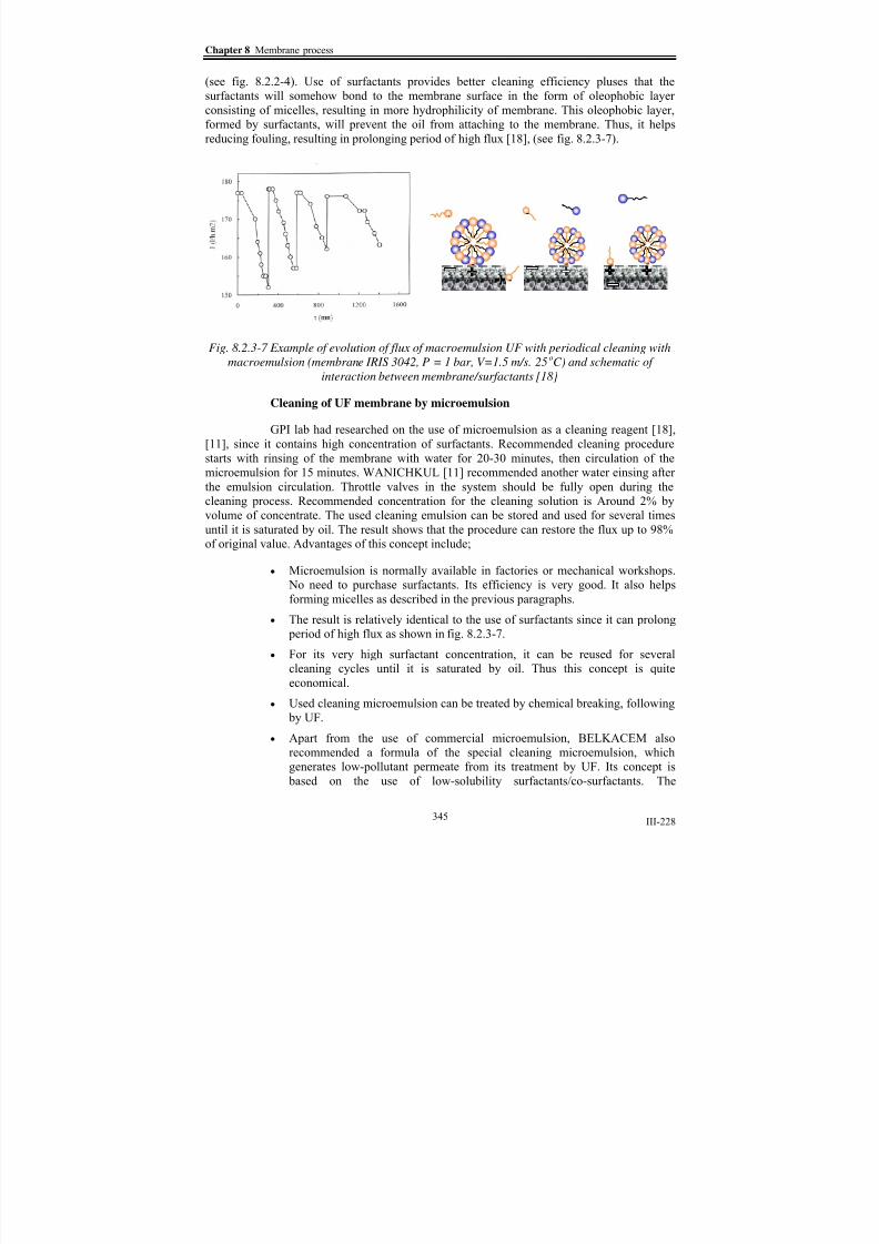
8/15/2019 Rachu.pdf
http://slidepdf.com/reader/full/rachupdf 422/646
Chapter 8 Membrane process
III-228
(see fig. 8.2.2-4). Use of surfactants provides better cleaning efficiency pluses that the
surfactants will somehow bond to the membrane surface in the form of oleophobic layer
consisting of micelles, resulting in more hydrophilicity of membrane. This oleophobic layer,
formed by surfactants, will prevent the oil from attaching to the membrane. Thus, it helps
reducing fouling, resulting in prolonging period of high flux [18], (see fig. 8.2.3-7).
-
-
- --
-
-
Fig. 8.2.3-7 Example of evolution of flux of macroemulsion UF with periodical cleaning with
macroemulsion (membrane IRIS 3042, P = 1 bar, V=1.5 m/s. 25oC) and schematic of
interaction between membrane/surfactants [18]
Cleaning of UF membrane by microemulsion
GPI lab had researched on the use of microemulsion as a cleaning reagent [18],
[11], since it contains high concentration of surfactants. Recommended cleaning procedure
starts with rinsing of the membrane with water for 20-30 minutes, then circulation of themicroemulsion for 15 minutes. WANICHKUL [11] recommended another water einsing after
the emulsion circulation. Throttle valves in the system should be fully open during the
cleaning process. Recommended concentration for the cleaning solution is Around 2% by
volume of concentrate. The used cleaning emulsion can be stored and used for several times
until it is saturated by oil. The result shows that the procedure can restore the flux up to 98%
of original value. Advantages of this concept include;
• Microemulsion is normally available in factories or mechanical workshops.
No need to purchase surfactants. Its efficiency is very good. It also helps
forming micelles as described in the previous paragraphs.
•
The result is relatively identical to the use of surfactants since it can prolong period of high flux as shown in fig. 8.2.3-7.
• For its very high surfactant concentration, it can be reused for several
cleaning cycles until it is saturated by oil. Thus this concept is quite
economical.
• Used cleaning microemulsion can be treated by chemical breaking, following
by UF.
• Apart from the use of commercial microemulsion, BELKACEM also
recommended a formula of the special cleaning microemulsion, which
generates low-pollutant permeate from its treatment by UF. Its concept is based on the use of low-solubility surfactants/co-surfactants. The
345

8/15/2019 Rachu.pdf
http://slidepdf.com/reader/full/rachupdf 423/646

8/15/2019 Rachu.pdf
http://slidepdf.com/reader/full/rachupdf 424/646
Chapter 8 Membrane process
III-230
a) Dead- end test module
(Source: Millipore)
b) Plate membrane test module (Source: Orelis, Osmonics)
c) Spiral wound test set (Source: Millipore) d) Pilot-scale test set (Source: Millipore)
Fig. 8.2.3-8 Examples of UF test modules
Almost all of the researches on oily wastewater treatment by UF are based on
stabilized emulsion since it cannot be separated effectively by other single process. However,
SRIJAROONRAT [10] has researched on UF of non-stabilized secondary emulsion. Her
study provides useful information to understand the performance of UF when free-oil is
present, which is frequently found in general oily wastewater. Significant findings of the
research can be summarized as follows,
8.2.3.6 Miscellaneous design consideration
Most of the design considerations for each category of oily wastewater are described
in the previous sections. In this section, some general remarks and common design
considerations, summarized from synthesis of literatures and GPI researches, will be
presented as follows,
• From GPI’s researches as well as other literatures, it is recommended to operate
UF system for oily wastewater around a certain flux to prolong the operating time per cycle (before cleaning) and maintain relatively steady flux. This concept
is called “critical flux”. At this flux, deposition of foulants can be counterbalanced
by shear force from cross-flow velocity. Thus the fouling resistance is relative
steady (not changing with time). This can be normally achieved by the use of
347

8/15/2019 Rachu.pdf
http://slidepdf.com/reader/full/rachupdf 425/646
Part III Summary of researches: Oily wastewater treatment
III-231
moderate pressure (1-1.5 bar). The use of higher pressure may give higher flux
but the rate of decrease in flux is higher to, resulting lower overall flux.
•
UF performance is sensitive to type of membrane, characteristic of wastewater and
operating condition. So it should be very careful to use the data from literatures or
researches to design the system. Experimental procedures of the researches should
be considered. The common mistakes on the use of researches on UF of oily
wastewater treatment are about, (1) pore size, sometimes MWCO and pore sizes
are confusing, and (2) concentration of oil, they are reported in various forms (%
by volume of oil, % by volume of concentrate in case of cutting oil emulsion, % by
weight, etc.), (3) Effect of concentration factor, some experiments carried out by
recycling the permeate to the feed stream, so the concentration of feed were
constant. The concentration effect is not included.
•
The cost of membrane system is high and the performance on secondary emulsion
treatment is not better than general separation processes. The UF, then, should be
used for some specific wastewater, separating from main stream wastewater.
8.3 Microfiltration (MF)
8.3.1
Basic knowledge and working principles
Microfiltration (MF) membrane can retain material in the range of 0.1 to about 5
microns (100-5,000 nm). It is mainly used as a clarification technique, separating suspended
solids from dissolve substance [38]. Size of MF is defined in the form of pore size, rather than
MWCO. MF membranes are available in various geometry and materials as UF. Its main
applications are separation of suspended particles in biotechnology, food and pharmaceutical
industries such as bacteria, red blood cells, latex emulsion, dairy product, etc. Examples of
MF membrane are as shown in fig. 8.3.1-1
Tubular module
(Source: Koch)
b) Plate module
(Source: Millipore)
c) MF membrane structure
(Source: Millipore)
Fig. 8.3.1-1 Examples of MF membranes
348

8/15/2019 Rachu.pdf
http://slidepdf.com/reader/full/rachupdf 426/646
Chapter 8 Membrane process
III-232
Theoretically, working principle of MF is relatively identical to that of UF. Theories,
models and characteristic curves of UF can be applied to MF. Main difference between MF
and UF is the pore size. Since the pore size of MF is relatively large. Its corresponding
capillary pressure is relatively low (around 0.1 bar). Thus, its maximum or limiting pressure is
much lower than UF. Its pore is about the same size as droplets in macroemulsion, so some oil
droplets can pass the MF membrane and be present in permeate. This is the main reason whyMF had not been studied seriously on oily wastewater treatment.
However, GPI lab had researched on the feasibility of combination between chemical
destabilization and MF for macroemulsion treatments as will be described in the following
section.
8.3.2 Significant findings on MF for oily wastewater treatment from GPI researches
As stated above that MF pore size is close to that of oil droplets in macroemulsion, to
use MF for this wastewater, the droplet size must be increased. MATAMOROS applied the
concept of flux enhancement by salt addition, like the case of UF, to MF. Significant findingsfrom the research are as described below,
1.
Recommended pore size is around 0.2 μ for MF (with salt addition) of
macroemulsion treatment. The use of too large pore results in very low or zero
oil rejection. Both oil and water can pss through the membrane. The use of
smaller pore is not possible, since its maximum pressure, calculated from pore
size, is not enough to drive the separation process. Both water and oil cannot
pass the membrane. If we increase the pressure, it can force the oil through the
membrane, resulting in very low or zero oil rejection anyway.
2. Quantity of salt required is much higher (about 3 times) than that of UF and
relatively close to the quantity required for total destabilization. Optimum dose
of CaCl 2 for macroemulsion, based on Elf Seraft ABS cutting oil macroemulsion
[20], is about 95 mg/l of Ca++
or 350 mg/l of CaCl 2 per 1% by volume of oil in
wastewater.
3. Result from dead-end test module of MF with salt addition shows very high flux,
relatively close to that of water flux. However, in case of cross-flow module, the
initial flux is about identical to the water flux at the beginning of the operation.
Then, the flux decreases rapidly within very short time (few hours), more rapid
than that of UF. The steady flux is relatively low and may not be higher than that
of UF’s flux (see fig. 8.3.2-1). Steady flux, based on Seralf ABS 4% at 0.1 bar, is
around 25 LMH.
349

8/15/2019 Rachu.pdf
http://slidepdf.com/reader/full/rachupdf 427/646
Part III Summary of researches: Oily wastewater treatment
III-233
Fig. 8.3.2-1 Evolution of flux from MF (with salt addition) of macroemulsion [20]
4.
The difference between dead-end and cross-flow model may be caused
difference in test volume since the dead-end module is much smaller than the
pilot scale cross-flow module.
5.
Rapid decrease in flux can be explained by deposition and coalesce of free-oil at
the surface as well as within the pore size of membrane since the pore size of MF
is relatively large.
6. When the membrane is properly selected, oil rejection is about 100% at low
operating pressure (about 0.05-0.1 bar). Increase in pressure beyond the capillary
pressure results in presence of oil in permeates. Since the pressure is much lower
than (about > 10 times lower) that of UF, energy consumption of MF is very
low, compared to UF.
7. Residual TOD comes from the surfactants/co-surfactants. Concentration of
residual salt and TOD are relatively identical to that of UF with salt addition,described in section 8.2.3.2.
8. To reduce fouling, MATOMAROS recommends the use of other separation
process, such as coalescer or hydrocyclone, to separate the free-oil from MF feed
stream.
9. Since quantity of salt added into the wastewater is high, the emulsion is largely
destabilized already since it is in the storage tank, indicated by presence of oil
layer on the surface. Thus, the use of MF should be compared to the combination
of destabilization and other basic process, such as decanter, coalescer.
350

8/15/2019 Rachu.pdf
http://slidepdf.com/reader/full/rachupdf 428/646
Chapter 8 Membrane process
III-234
8.4 Reverse osmosis (RO)
Reverse osmosis is the ultimate pressure driving membrane process that capable of
retaining ionic-range materials, the range of 0.1 nm. Structure of RO membrane is dense,
compared to porous structure of UF and MF’s (see fig 8.4-1). Its main application is
production of ultra pure water for many industries, such as, pharmaceutical, electronic, food,and nuclear (water for reactor). RO membranes are available in various materials and
modules, i.e. plate, etc., as described on section 8.1.
Cutaway-view of RO module
(Source: Desal)
RO pure water system
(Source: Koch)
Fig. 8.4-1 Examples of RO membranes
8.4.1 Basic knowledge and working principles
Working principles of RO is based on the concept of osmosis. Osmosis phenomenon
can be explained by considering the system of 2 compartments, separating by dense
membrane, as shown in fig. 8.4.1-1. Each compartment contains the solution at different
concentration.
Osmosis phenomenon is defined by mass transfer of the solvent through the
membrane, from the diluted solution to the concentrated one. Increase in pressure on the
concentrated side can lower or stop the mass transfer. To stop the mass transfer, the pressure
required shall be equal to “ osmotic pressure” , as shown in fig. 8.4.1-1b. If the applied
pressure is higher than the osmotic pressure, the solvent will inversely travel from concentrate
side to the diluted side (fig. 8.4.1-1c). This is the phenomenon taking place in RO and give the process its name.
DC
Posmotic
DC
P = Posmotic
DC
P = Posmotic
a) Osmosis phenomenon b) Osmotic pressure c) Reverse osmosis
Fig. 8.4.1-1 Working principles of reverse osmosis
351

8/15/2019 Rachu.pdf
http://slidepdf.com/reader/full/rachupdf 429/646
Part III Summary of researches: Oily wastewater treatment
III-235
Osmotic pressure is the function of concentration and usually defined by Van’t hoff as
shown in eq. 8.4.1.
...3
3
2
21 +++= C AC AC Aπ {8.4.1}
Where π = Osmotic pressure
C = Concentration of solutionAn = Virial coefficients of the solution
The value of A1, A2, A3, etc. depends on type of solution. The virial coeeficients of
large molecules or materials are relatively small. Thus the osmotic pressure is low and usually
negligible, as in case of MF and UF. For low molecular-weight molecules, supposed to be
separated by RO, the values of high-ordered A are high so the osmotic pressure becomes
significant.
Mathematical model for RO
Mathematical model of RO can be written in the form of resistance model, as shown ineq. 8.4.2. For RO, transmembrane pressure is countered by osmotic pressure, so the effective
driving force for the process is the difference between the two pressures. RO resistance
mainly consists of the membrane resistance. Mass transfer resistance in the boundary layer
may be accounted in some cases.
M
M t
R
P J
π −= {8.4.2}
Where J = Permeate flux
πΜ = Osmotic pressure, calculated from the concentration at themembrane surface
R M = Membrane resistance
RO may find its application in industrial water reuse process. However, due to its
minuscule pore size and very high osmotic pressure, pressure requirement, thus energy
consumption, of RO is very high. So it is scarcely used on general wastewater treatment. In
GPI lab, RO had been studied for its performance on treatment of highly polluted permeate
from UF of wasted emulsion. The studies will be summarized in the following section.
8.4.2 Significant findings on RO for oily wastewater treatment from GPI’s researches
BELKACEM [18], MATAMOROS [20] and WANICHKUL [11] had studied on
application of RO on treatment of highly polluted permeates from treatment of wasted cutting
oil emulsion. Significant findings of the researches are as summarized below,
1. RO is proven to be an efficient process for treatment of UF permeate of macro-or
microemulsion, which contains very high concentrations of surfactants/co-
surfactants that are not retained by the UF membrane. When retentate and
permeate are recycled, relation between flux and pressure from RO of
microemulsion’s permeate from UF is linear up to the maximum test pressure of
60 bars as shown in fig. 8.4.2-1a.
352

8/15/2019 Rachu.pdf
http://slidepdf.com/reader/full/rachupdf 430/646
Chapter 8 Membrane process
III-236
Pt
Flux
Lag due to
osmotic pressure
Min recommended
pressure Log (conc.)
Flux
Fig. 8.4.2-1a Typical relation between flux
and pressure of RO
Fig. 8.4.2-1b Typical relation between flux
and log of concentration
2.
Evolution of RO flux from treatment of microemulsion’s and macroemulsion’s
UF permeate, both in used and fresh condition, are relatively identical as shown
in fig. 8.4.2-2. The graph is for RO operation in batch process (see fig.8.2.1-4)without return of permeate so effect of factor of concentration is already
included.
0
20
40
60
80
100
120
140
160
180
0 2000 4000 6000 8000 10000 12000 14000
Time (sec)
F l u x ( L / ( m 2 . h ) )
Microemulsion Macroemulsion Used macroemulsion
Fig. 8.4.2-2 Examples of flux evolution from RO of the UF permeates of various emulsions (the RO permeate are not recycled) [11]
3. Flux decreases with increase in concentration factor (fig. 8.4.2-1b). There is no
clear evident if the relation between flux and factor of concentration will have
inflection point like that of UF of macroemulsion (fig. 8.2.1-6) since the
experiments were usually stopped before the zero-flux was reached. The
maximum factor of concentration (or volume reduction factor) ever tested in GPI
lab is 2.5 (at 25 bars, 30oC, V = 1.8 m/s)[18].
4. BELKACEM [18] reported that permeate’s TOD generally increases with time
or concentration factor (shown in fig. 8.4.2-3a). However, WANICHKUL
showed [11] that TOD may decrease with time or concentration factor, as shownin fig. 8.4.2-4. Decrease in permeate TOD, in this case, may be explained by
353

8/15/2019 Rachu.pdf
http://slidepdf.com/reader/full/rachupdf 431/646
Part III Summary of researches: Oily wastewater treatment
III-237
formation of micelles on the membrane surface when the concentration of feed is
continuous increased along the process time until it reaches the critical micelle
concentration (CMC) [11]. These micelles cannot pass through the membrane so
the quantity of pollutant in permeate is decreased. Formation of micelles depend
on type and concentration of surfactants/co-surfactants in the permeate, as well
as interaction between those pollutants and other material such as calcium thatmay cause formation of complexes as well as electrical charge of membranes.
Thus, exact result should be obtained from RO test.
5. Typical relation of rejection or removal efficiency with pressure, based on salt, is
as shown in fig. 8.4.2-3b [59]. But MATAMOROS [20] indicates that, for UF
permeate of microemulsion, the rejection decreases at high pressure (the dashed
line in fig. 8.4.2-5b). There is not sufficient data to evaluate the cause of this
decrease. However, it is recemmeded to use moderate transmembrane pressure
(about 20-25 bars) to obtain good rejection.
Concentration factor
Rejection and
TOD permeate
1
Rejection
TOD
Rejection
Min recommended
pressureP
t
Fig. 8.4.2-3a Relation between rejection,
TOD of permeate and concentration factor
Fig. 8.4.2-3b Relation between rejection and
transmembrane pressure
0
1
2
3
4
5
6
0 2000 4000 6000 8000 10000 12000 14000 16000
Time (sec)
T O D o f p
e r m e a t e ( m g / l )
Microemulsion Macroemulsion Used macroemulsion
Fig. 8.4.2-2 Examples of permeate TOD evolution from RO of the UF permeates of various
emulsions (the RO permeate are not recycled) [11]
354

8/15/2019 Rachu.pdf
http://slidepdf.com/reader/full/rachupdf 432/646
Chapter 8 Membrane process
III-238
6. Guidelines for RO design or evaluation, summarized from various GPI’s lab, are
as shown in table 8.4.2-1. Membrane material used is polyamide. MWCO is
around 100-150 Daltons.
8.5 Nanofiltration (NF)
Nanofiltration is an intermediate membrane process between ultrafiltration and reverse
osmosis. It is a relatively new technology, compared to others membrane processes. NF
membrane pore sizes are between those of UF and RO. It can retain the meterials of the size
around 100 – 600 nm. Thus it can be used to separate dissociated form of a compound from
the undissociated form [38]. For example, lactic, citric, and acetic acids can pass through to
NF at low pH but are rejected at high pH when in their salt forms. NF is generally used in
many industries, such as biotechnology, food, and drinking water as well as in environmental
applications. Apparently, structure and module of NF are relatively identical to those of RO.
8.5.1 Basic knowledge and working principles
Separation in NF membrane is based on both size difference, like UF, and diffusion
mechanism, like RO. Generally, NF membranes are charged so they can be used for selective
separation of charged materials. Uncharged membranes are available but very rare and not
popular. Separation mechanisms in NF membrane are not well understood. But they are
generally described in 2 approaches, i.e. ionic exclusion and, like RO, solution-diffusion.
For ionic exclusion approach, separation of charged materials by NF depends on the
charges of ions in solution to be separated and of membranes. Ions of the same charge as the
membrane will be pushed while the counter-charged ion will be attracted by the membrane
charges. For uncharged membrane, the modified form of solution-diffusion model, as shown
in eq. 8.4.2-2, was used to explain the separation mechanisms in the NF membranes by someresearchers. Applications of NF on oily wastewater treatment are known of but they are
privately designed and there are not many publications on the issue.
In GPI lab, MATAMOROS [20] performed the feasibility study on application of NF
for cutting oil emulsion treatment. The result will be summarized in the next section.
8.5.2
Significant findings on NF for oily wastewater treatment from GPI’s researches
MATAMOROS [20] had studied the performance of NF on the treatment of cutting oil
emulsions as well as permeates from UF of cutting oil emulsions, using cellulose membranes,
i.e. Desal 5 (600 Da), SV10 (100-300 Da) and SG15 (2000 Da). Significant findings of theresearch are as summarized below,
1. From the research, NF is proven to be an efficient process for treatment of UF
permeate of macro-or microemulsion, which contains very high concentrations
of surfactants/co-surfactants that are not retained by the UF membrane.
Rejection is slightly lower than that of RO. But the energy consumption is about
half of RO’s, since its pressure range is around 4 –20 bars, compared to the
range of 20 – 60 bars for RO. Evolution of flux with time and with pressure for
NF of permeate are relatively identical to that of RO (fig. 8.4.2-1 and 8.4.2-2).
355

8/15/2019 Rachu.pdf
http://slidepdf.com/reader/full/rachupdf 433/646
Part III Summary of researches: Oily wastewater treatment
III-239
T a b l e 8 . 4 . 2 - 1 S u m m a r y
o f R O d a t a o n o i l y w a s t e w a t e r
t r e a t m e n t
356

8/15/2019 Rachu.pdf
http://slidepdf.com/reader/full/rachupdf 434/646
Chapter 8 Membrane process
III-240
2. NF performances on macro- and microemulsion treatment were also studied.
The result showed that, at constant feed concentration, relation between pressure
and flux of NF for macro- and microemulsion treatment are divided into 2
regions i.e. pressure controlled and mass transfer controlled region (fig 8.5.2-1),
like that of UF.
3. Relation of flux and theoretical concentration of feed, when permeate is not
recycled, is as shown in fig. 8.5.2-2. The relation is not linear so it is not
governed by film model (section 8.2.1.5). This can be explained by
destabilization in-situ of emulsified oil during NF operation, justified from
presence of oil layer in the storage tank. Destabilization of oil, like the case of
UF with salt addition, makes the real feed concentration lower than theoretical
value.
4.
Results of MATAMOROS are as shown in table 8.5.2-1. From the table, TOD
removal efficiencies of UF are always higher than UF. This means the oil is
completely separated and the surfactants/co-surfactants are retained with higherefficiency. However, it should be noted that the results are based on fresh
emulsion. For used emulsion, result may differ and should be obtained by pilot
test.
Fig. 8.5.2-1 Relation of flux and transmembrane pressure of NF for macroemulsion
(Elf Seraft ABS) and microemulsion treatment (Elf Emulself G3 EAB), using desal5
membrane at 20oC [20]
357

8/15/2019 Rachu.pdf
http://slidepdf.com/reader/full/rachupdf 435/646
Part III Summary of researches: Oily wastewater treatment
III-241
Fig. 8.5.2-2 Relation of flux and theoretical feed concentration of NF for macro-
and microemulsion treatment [20]
8.6 Comparison of membrane processes on emulsion treatment
Major objective of GPI’s researches on oily wastewater treatment by membrane
process is the treatment of stabilized emulsion. From the previous sections, they show that
performance of each process or combinations of processes on emulsion treatment are
different. To compare the performance of processes or combinations of membrane processes,
MATAMOROS had performed pilot test of various processes using the same macroemulsion.His results are tabulated in table 8.6-1. However, It should be noted that,
1. The results are based on specific operating conditions, types of wastewater and
membrane. Since performances of membrane processes are sensitive these
parameters, the results can be used as a guideline for preliminary evaluation
only.
2.
Fresh emulsions were use so fouling due to foreign materials was not included.
3.
Evolutions of flux with time are not present. In real design, this data is important
for membrane sizing and determination of operating and cleaning cycle. For
example, NF and MF+CaCl2 may be very interesting from their relative lowenergy consumption. But they may foul easily, resulting in low flux for long-tern
operation and more frequent cleaning.
4. Even though the efficiency of each process is very high. It does not mean that the
permeate always conforms to the related standard. For example, permeate’s
TOD from RO of UF+RO of macroemulsion at 4% by volume of oil is around
1,250 mg/l, which is still high and may need further treatment or to be mixed
with relatively diluted wastewater and treat by conventional treatment system.
5. From the previous sections, it is obvious that membrane process is very versatile
and efficient process. But its performance is sensitive to many parameters. So it
is, again, strongly recommenced to perform pilot test before design the realmembrane process.
358

8/15/2019 Rachu.pdf
http://slidepdf.com/reader/full/rachupdf 436/646
Chapter 8 Membrane process
III-242
T a b l e 8 . 5 . 2 - 1 S u m m a r y o f N F d a t a o n o i l y w a s t e w a t e r t r e a t m e n t
359

8/15/2019 Rachu.pdf
http://slidepdf.com/reader/full/rachupdf 437/646
Part III Summary of researches: Oily wastewater treatment
III-243
Table 8.6-1 Comparison of membrane processes on cutting macroemulsion treatments
(based on Elf Seraft ABS at 4% by V of oil)
MF+CaCl2 UF UF+RO UF+NF NF
Membrane MS11107 Iris3042 Iris3042 +MS10 Iris3042+Desal5
Desal5
Global TOD
removal efficiency
(%)
97.2 95.8 99.1 97.9 97.4
TOD of final
permeate (g/l)
2.76 4.5 0.92 2.2 2.7
Pt (bar) 0.1 1 1+30 1+10 10
Flux (LMH) 24.9 52.92 52.92/42.12 52.92/30.96 27
Specific energy
consumption
(KWh/m3)
Not available 3.2 3.2+40.2 3.2+22.8 22.2
Remark See note 1 See note 2
Note 1 Initial flux of MF is very high, compared to that of water, but the membrane is
rapidly clogged by free-oil. The flux, thus, drops sharply. The final flux is
relatively low.
2 Evolution of time was not present in the original research. But the membrane tends
to be clogged by free-oil from destabilization in-situ.
3 No comparison data of microemulsion treatment was proposed.
360

8/15/2019 Rachu.pdf
http://slidepdf.com/reader/full/rachupdf 438/646
Chapter 8 Membrane process
III-244
[This page is intentionally left blank.]
361

8/15/2019 Rachu.pdf
http://slidepdf.com/reader/full/rachupdf 439/646
Part III Summary of researches: Oily wastewater treatment
III-245
Chapter 9 Thermal processes
9.1 General
Thermal processes are separation processes that involve changing of phases of the
materials to be separated. For distillation, it involves liquid and gas. For crystallization andzone refining, they involve liquid and solid. Since the processes involve phase changing, they
inevitably consume high energy. This is the reason why they are scarcely used for general
wastewater treatment. However, it may become economical alternative if the product from the
treatment can be recycled or relative easier for ultimate disposal.
Oily wastewater is actually binary system, containing, mainly, 2 immiscible liquids i.e.
oil and water. So it could be separated by thermal processes. In GPI lab, there are some
researches on applications of thermal processes on oily wastewater treatment. Most of all
were based on distillation. Only few were based on crystallization. So, in this chapter will be
emphasized on distillation, which can be divided into 2 major types, i.e. conventional
distillation and enhanced distillation, called “heteroazeotropic” distillation.
It must be noted that the researches are based on lab-scale experiments to study the
theoretical concepts that underline process operation. In real processes, the distillations are
usually carried out in distillation columns, which their designs are a major science into itself.
So it will not be mentioned here. However, the researches can be used as a guideline to
understand and evaluate the feasibility of the processes.
9.2 Basic knowledge on distillation
Since distillation always involves liquid and vapor phase of mixtures, it can be
described by the concept of vapor/liquid equilibrium. The mixtures may have two or morecomponents. However, to provide basic knowledge of the process, it is sufficient to simply
consider the mixture of 2 components, called “binary” mixture.
9.2.1 Basic knowledge on vapor/liquid equilibrium of mixtures
Since distillation always involve the mixture of two or more components, it is
necessary to know a certain number of variables to describe or characterize the equilibrium
stage of the system. The number of required variables, called “ degree of freedom” is
calculated by the phase rules, as shown in eq. 8.2.1.
N F +−= π 2
{9.2.1}
Where F = Degree of freedom
π = The number of phases, for vapor/ liquid system, π = 2
N = The number of species in the mixtures
For example, to describe a binary mixture system, required degrees of freedom are 2-
2+2 = 2, which are normally pressure and temperature. Generally, distillation processes
operate at constant pressure, so operating parameter that is used to control the process is
temperature.
To understand vapor/liquid equilibrium of a binary system, consider a binary mixture
of specie A and B in the container, as shown in fig. 9.2.1-1. Assume that overall pressure of
the system is constant at 1 atm. When the mixture is heated, temperature of the mixture will
362

8/15/2019 Rachu.pdf
http://slidepdf.com/reader/full/rachupdf 440/646
Chapter 9 Thermal processes
III-246
increase, as shown in fig. 9.2.1-2. When it reaches a certain temperature, called “bubble
point”, the first bubble of vapor will appear. From this point, the mixture will exist in both
vapor and liquid phases. Unlike a pure substance, temperature of the system during
evaporation period continuously changes, rather than being constant. When the temperature
reach a certain value, called “dew point”, the last drop of liquid will disappear.
Liquid phase
Vapor phase
P = constant
Heat
Specie B
Specie A
Time
T
Dew point
Liquid Liq Gas Gas
Bubble point
P = const.
Fig. 9.2.1-1 Diagram of a binary mixture
system
Fig. 9.2.1-2 Evolution of temperature of a
binary mixture at a constant P
Dew temperature and bubble temperature of a binary mixture varies with pressure. An
example of relation between pressure and temperature is shown in fig. 9.2.1-3. Characteristic
of P-T curve depends on types of components in the mixture.
Critical locus
T
P
C
C
Bubble curveDew curve
Methanol/Benzene
mixture
T
P
0% Methanol
100% Methanol
Fig. 9.2.1-3 Examples of P-T diagram
At a binary system at constant pressure, the dew- and bubble points of the system vary
with composition of the mixture. Compositions of the mixture are usually reported in the from
of molar fraction “x” and “y”. The value “x i” represents the ratio of moles of species i in
liquid phase (ni,l) to summation of moles of every species in liquid phase (nl) (eq. 9.2.2). On
the other hand, the value of “yi” is the ratio of moles of species i in vapor phase (ni,v) to
summation of moles of every species in vapor phase (nv) (eq. 9.2.3).
l
li
in
n x
,= , ∑ =
i
i x 1
{9.2.2}
v
vii
nn y ,= , ∑ =
i
i y 1 {9.2.3}
363

8/15/2019 Rachu.pdf
http://slidepdf.com/reader/full/rachupdf 441/646
Part III Summary of researches: Oily wastewater treatment
III-247
When the bubble points at various values of x1 are plotted, the curve is called the
“bubble curve” or “saturated liquid line”. On the other hand, when the dew points at various
values of yi are plotted, the curve is called the “dew curve” or “saturated vapor line”.
Generally, dew curve and bubble curves are plotted on the same coordinate. They can be
plotted both on T-x-y scale and P-x-y scale as shown in fig. 9.2.1-4a and b. Since distillation
process usually operates at a constant P, T-x-y curve is normally used. Relations between pressure, temperature, x and y can be combined into a three-dimension coordinate, resulting in
P-T-x-y diagram as shown in fig. 9.2.1-5.
xA = 1
yA = 1
T P = const.
Pure B Pure A
xA = 0
yA = 0
xA , yA
C
CC
Bubble curveDew curve
xA = 1
yA = 1
P T = const.
Pure B Pure A
xA = 0
yA = 0
xA , yA
C
C
C
Bubble curveDew curve
a) T-x-y diagram b) P-x-y diagram
Fig .9.2.1-4 Examples of T-x-y and P-x-y diagrams
To understand phase changing taking place in distillation process, we will consider a
P-x-y diagram as shown in fig. 9.2.1-6. From the figure, the points on the dew curve representsaturated vapor. the area above the dew curve (T-y i) is of superheated vapor. The points on the
bubble curve represent saturated liquid. The area below the bubble curve (T-xi) is of
subcooled liquid. The area between the 2 curves is the two-phase region. The two curves meet
at the edges of the diagram where saturated liquid and saturated vapor of the pure species
coexist.
P
T
1
0
yA
xA
Critical
P u r e
A
P u r e
B
xA = 1
yA = 1
T
P = const.
Pure B Pure A
xA = 0
yA = 0
yA = 0.4
= 0.6
Superheated vapor
= 0.8xA xA
a
b b’
c’ c
yA = 0.6
Subcooled liquid B u
b b l e
c u r v
e
D e w
c u r v
e
Fig. 9.2.1-5 An example of P-T-x-y diagram Fig. 9.2.1-6 An example of T-x-y diagram
364

8/15/2019 Rachu.pdf
http://slidepdf.com/reader/full/rachupdf 442/646
Chapter 9 Thermal processes
III-248
From fig. 9.2.1-6, if we heat the subcooled liquid of 60 mol-% of specie A and 40 mol-
% of specie B (so xA = 0.6, xB = 1-0.6 = 0.4) under a constant P from point a, the first bubble
will appear when the temperature reaches the bubble curve at point b. The molar fraction of
specie A in this very first bubble will be determined by drawing the horizontal line from point
b to meet the dew curve at point b’. If we continue heating, more vapors will appear while the
quantity of liquid will decrease. The compositions of liquid will follow the bubble curve from point b (xA = 0.6) to c (xA ≈ 0.8) and the composition of vapor will follow the dew curve from
b’ (yA ≈ 0.8) to c’ (yA = 0.6), respectively. When the temperature reaches point c, the last drop
of liquid disappears. The mixture will become entirely vapor with yA = 0.6. Continuing
heating, the vapor will have higher temperature and become superheated vapor. Cooling of
vapor can be explained by the same manner described above.
9.2.2 Equilibrium of various mixtures
Characteristics of vapor/liquid equilibrium curves depend on types of components of
the mixture, pressure and temperature. Examples of various types of vapor/liquid equilibrium
are as shown in fig. 9.2.2-1. The first 3 curves are of miscible mixtures. For some mixtures,the T-x-y diagrams present a maximum or minimum point where the boiling liquid at this
point produces a vapor of exactly the same composition. This point is called the “ azeotrope”.
At some conditions, liquid/liquid equilibrium (LLE) coexists with vapor/liquid
equilibrium (VLE), this give rise to vapor/liquid/liquid equilibrium (VLLE) [61], as shown in
fig. 9.2.1-1 d to f. The state that VLLE is present is called “ heterogeneous azeotropic” or
“ heteroazeotropic”. As stated before, VLLE varies with intensive properties (P,T) and may
become only VLE at certain conditions as shown in fig. 9.2.2-2.
xA = 1
yA = 1
T
Pure B Pure A
xA = 0
yA = 0
xA , yA
Locus ofazeotropeHigh P
Low P
Fig. 9.2.2-2 Examples of evolution of VLE and VLLE with pressure
365

8/15/2019 Rachu.pdf
http://slidepdf.com/reader/full/rachupdf 443/646
Part III Summary of researches: Oily wastewater treatment
III-249
Example
Methanol-Water
Ethanol-Water
Acetone-Chloroform
N-butanol-Water
Decane-Water
Polypropylene oxide-
Water
Azeo
Azeo
Azeo
Azeo
Azeo
Azeo
Azeo
Azeo
V
V
L+V
L
L+V
L
V
L+V
L
V
L+V
L
2 L
L
V
L+V
2 L
L+V
2 L L
L
L+V
V
T Y
XX , Y
T Y
XX , Y
T Y
XX , Y
T Y
XX , Y
T Y
XX , Y
T Y
XX , Y
Type
Without azeotrope
Minimum-temperature
azeotrope
Maximum-temperature
azeotrope
Heteroazeotrope
(Partially miscible)
Demixtion
Heteroazeotrope
(Immiscible)
Fig. 9.2.2-1 Examples of various types of vapor/liquid equilibrium
366

8/15/2019 Rachu.pdf
http://slidepdf.com/reader/full/rachupdf 444/646
Chapter 9 Thermal processes
III-250
9.3 Heteroazeotropic distillation of oily wastewater
Heteroazeotopic distillation, in this chapter, is technically referred to the distillation
process that a proper substance, called entrainer, is added to the feed to ensure the formation of heteroazeotrope. It does not include the process that the azeotrope occurs
naturally. However, their working principles are identical. Details of the heterotropicdistillation process are described below.
9.3.1 Working principles
Since hydrocarbons or oils have very low water-solubility, it is generally acceptable to
assume that oily wastewater, which is actually the oil/water mixture, is immiscible binary
mixture. Typical characteristic of T-x-y diagram at a constant pressure (called “isobar
diagram”) of oily wastewater is as shown in fig. 9.3.1-1. Generally, hydrocarbons have
higher boiling point than that of water.
A
xw = 1
yw = 1
T P = const.
Pure Oil Pure water
(W)
xw = 0
yw = 0
Oil +V
xw , yw
Boiling T
of BVapor (V)
W + V
Oil+water
xw = xH yw = yH
Boiling T
of Water
THB C
D
xw,1
xw,2
xw,3xw,4=1
xw,5=1
xw,6=1
yw,1’ to yw,4
= yH
yw,5
yw,6
xw,1’
Azeotrope (H)
Fig. 9.3.1-1 Typical isobar diagram oily wastewater
From the diagram, it shows that the wastewater can be boiled at the temperature lower
than that of pure water and pure oils. Heteroazeotropic distillation, which is the distillation
when the VLLE is present, makes use of this fact so it requires lower energy than classical
distillation.
From the figure, the bubble curve in this case will look like a figure “U” with square
legs (Line ABHCD). If the original wastewater contain 70 mol-% of water (xw,1 = 0.70), itwill boil at the temperature TH. The composition of this very first bubble can be determined
by drawing the horizontal line to meet the dew curve (Curve AHD). In this case, they will
intersect at point H. Thus the molar fraction of water (yw) in the bubble is that of azeotrope
(yH, xH). Continuing heating, the liquid volume gradually decreases and its composition
gradually change from xw,1 to x.w,2, xw,3, etc. However, by drawing the horizontal lines from
these values of xw, the compositions of yw are always equal to yH. During this period the
temperature is automatically constant at TH. When xw finally reaches 1, this means the
residue becomes pure water. All of oils are separated from water and in vapor phase.
After this, the temperature rises until it reaches the boiling point of pure water. The
value of xw is constant at 1. The value of yw increases from yH to yw,4, yw,5, etc. since the purewater continues boiling at add more steam to the overall vapor phase.
367

8/15/2019 Rachu.pdf
http://slidepdf.com/reader/full/rachupdf 445/646
Part III Summary of researches: Oily wastewater treatment
III-251
The vapor phase is usually condensed to recover oil vapor. If the vapor is condensed
while xw < 1, the composition of vapor will be constant at yH. From fig. 9.3.1-1, these vapors
will condense at the temperature T H , resulting in the distillate of oil and water at xw = y H .
From GPI’s research by TOULGOAT [19], the distillate will not be formed as an
emulsion if the hydrocarbons have high vapor tension and/or their water solubility is very lowand not sensitive to temperature change. This condition is usually satisfied for oily wastewater
treatment polluted by petroleum-base oil or for the carefully selected entrainer (described in
section 9.3.4). Thus the distillate from heteroazeotropic distillation of oily wastewater is
usually in the form of 2 separate layers of water and oil.
9.3.2 Raoult’s law and Dalton’s law
To define dew curve and bubble curve of a binary mixture, the following equations are
generally used, i.e. eq. 9.3.1 and eq. 9.3.2 ( Dalton’s law)
sat iii P x p = {9.3.1}
P y pii = {9.3.2}
Where pi = Partial pressure of specie i
PP
sat = Vapor pressure of specie i
P = Pressure of overall system, which is normally kept constant, e.g. 1 bar
From eq. 9.3.1 and 9.3.2, it gives rise to Raoult’s law (eq. 9.3.3). The equation is
valid under the assumption that the vapor phase is an ideal gas and the liquid phase is an
ideal liquid .
sat
iii P xP y = {9.3.3}
If the system is not ideal system, eq. 9.3.3 will be modified as shown in eq. 9.3.4
( modified Raoult’s law).
sat
iii
sat
ii f xP y γ φ = {9.3.4}
γi is called “ activity coefficient”, which is normally obtained from experiments. If γ =
1, this means the system is ideal. The equation will become Raoult’s law. The vapor pressureis replaced by the term “ fugacity” (f) and “ fugacity coeficienct“ (φ). Relation between Psat, f
and φ are as shown in eq. 9.3.5.
sat
i
sat
isat
iP
f =φ {9.3.5}
For application of oily wastewater treatment, the use of eq. 9.3.3 is proven to be
accurate enough [24], [11]. These equations will be used to determine the dew curve and
bubble curve, as well as azeotropic point of oily/water mixture, as described in the next
section.
368

8/15/2019 Rachu.pdf
http://slidepdf.com/reader/full/rachupdf 446/646
Chapter 9 Thermal processes
III-252
9.3.3 Calculation of azeotropic temperature and composition, dew curve and bubble
curve.
To calculate the isobar diagram of VLLE of oily wastewater or oil/water mixture, the
following procedure, based on the theories described in the previous section, is recommended.
1. Find the azeotropic temperature (TH) and bubble curve (T-x)
For immisible bunary mixture of A and B, it can be imagined that the two
liquids are separately located in the container. Each liquid exerts the corresponding vapor
pressure. Thus the vapor pressure of the system is the summation of the vapor pressures of
every species, as shown in eq. 9.3.6. On the bubble curve, the mixture will boil when the
vapor pressure of the mixture is equal to the overall pressure of the system (P) (eq. 9.3.6).
PPPP sat
B
sat
A
sat
B A =+=+ {9.3.6}
To find the temperature TH that corresponds to eq. 9.3.6. Relation between vapor pressure and temperature of both liquids must be known. For general liquids, their properties
can be found in many references, e.q. Perry’s [2]. If the relations are provided in the form of
data table, it may be more convenient to use graphical method to find T H, as shown in fig.
9.3.3-1. Curves of liquid A and B are drawn, using the data from the reference. Curve of the
mixture A+B is obtained by the sum of vapor pressure of A and B at the same temperature.
This curve is the relation between azeotropic temperature (TH) and pressure. Thus TH at any
given operating pressure of distillation process can always be found.
TH Temperature
Pressure
Pure A
Pure B
A+B
Pdesign
Fig. 9.3.3-1 Graphical method to find heteroazeotropic temperature
Sometimes, Relation between Psat and T of pure liquid is given in the form of
equation, called “ Antoine equation” (eq. 9.3.7).
C T
B AP T sat
−−=)ln( ,
{9.3.7}
T is temperature. A, B and C are numerical constants, depending on the types of
liquids. These constants can be also found in many references. From Antoine equations of the
two liquids, eq. 9.3.6 can be rewritten in the form of T. After solving the equation at a given
P, the resulting T is the azeotropic temperature TH. The bubble curve of an immiscible binary
mixture can de drawn as a straight horizontal line at the temperature T H on the T-x,y diagram.
369

8/15/2019 Rachu.pdf
http://slidepdf.com/reader/full/rachupdf 447/646
Part III Summary of researches: Oily wastewater treatment
III-253
2. Find the Dew curve (T-y)
At every point on the dew curve, the liquid A and B will condense so,
T sat
A A P p,
= {9.3.9}T sat
B B P p
,
=
{9.3.11}
From eq. 9.3.2, the values of y A at any T (yA,T) in the region A-V (fig. 9.3.1-1),
which A will condense, can be calculated from the following equation.
P
P yPP y p
T sat
AT
A
T sat
A
T
A
T
A
,, =→== {9.3.12}
In the same manner, the values of y A at any T (yA,T) in the region B-V
(fig. 9.3.1-1), which B will condense, can be calculated from the following equation
P
P y
P
P yPP y p
T sat
BT
A
T sat
BT
B
T sat
B
T
B
T
B
,,, 1−=→=→== {9.3.13}
By varying the values of T, yA at various value of T can be calculated . Plotting
the values of y A and T on T-x-y diagram result in a dew curve. The curve will be calculated
easily by graphical method as shown in fig. 9.3.3-2. Generally, specie A represents water. So
the value of x and y represent the molar fraction of water in liquid and vapor phase,
respectively.
T1 T2
Psat,T1
B
Temperature
Pressure
A (Pure water)
B (Pure oil)
Water+oil
Psat,T1
A
Psat,T2
A
Psat,T2
B
Pure
water (A)
Temperature
Pure
oil (B) x,yyH
TH
T1
T2
yB 1
yB 2 yA 2 yA 1
Calculate y A and y B by eq.
9.3.12 and 9.3.13, then, plot
T,y A and T,y B to obtain dew
curves
Fig. 9.3.3-2 Graphical method to find dew curve
3. Find heteroazeotropic composition (xH, yH)
From eq. 9.3.2, azeotropic composition (yH) in the form of molar fraction of “A”
can be calculated from the following equation,
P
p y A
H = {9.3.8}
At TH, liquid A (and B) will condense so,
H T sat
A AP p ,= {9.3.9}
370

8/15/2019 Rachu.pdf
http://slidepdf.com/reader/full/rachupdf 448/646
Chapter 9 Thermal processes
III-254
Thus,
H H
H H
T sat
B
T sat
A
T sat
A
T sat
A
H PP
P
P
P y
,,
,,
+== {9.3.10}
This means that, at azeotropic point, liquid phase will contain (100yH) mol-% of
specie A and 100(1-yH) mol-% of specie B. For the vapor phase, it will also contain (100yH)
mol-% of specie A and 100(1-yH) mol-% of specie B. Heteroazeotropic temperature (TH) and
composition (yH) of common hydrocarbons, calculated from theoretical equation described
above, are tabulated in table 9.3.3-1. Observed values of yH from LUCENA [24] are also
presented in the table. It shows that the theoretical equations can be used to predict the
characteristic of real process with high accuracy.
Table 9.3.3-1 Heterotropic temperature and composition from various hydrocarbons [24]
ExtractantMolecular
weight (g/mol)
TH
(deg. C)
yH
(by molar)
yH
(by volume)
y H observed
(by volume) [24]
C6H14 56 61.6 0.209 0.0351
C7H16 100 79.2 0.452 0.0922
C8H18 114 89.5 0.616 0.188
C9H20 128 94.8 0.827 0.3255
C10H22 142 97.6 0.914 0.495 0.468
C11H24 156 98.9 0.959 0.6663
C12H26 170 99.5 0.98 0.7953 0.767
C13H28 184 99.8 0.991 0.890C14H30 198 99.95 0.996 0.9542
C15H32 212 99.999 0.998 0.9702
C16H34 226 ≈ 100 0.999 0.9840
9.3.4 Application of heteroazeotropic distillation on treatment of inverse emulsion or
concentrated oily wastewater
In spite of its lower energy consumption than the classical distillation,
heteroazeotropic distillation still consumes relatively high energy. So it may not be
economical to treat general wastewater by this process. However, for the wastewater
containing high concentration of oil or inverse (water in oil) emulsion (e.g. slops from
refineries), the portion of water to be separated is relatively small and the residue from
distillation process, which is water-free oil, become valuable for it can be re-processed or
recycled. In these cases, heteroazeotropic distillation may become economically feasible.
GPI had studied applications of heteroazeotropic distillation on treatment of slop [24]
and retentate from UF of cutting oil emulsion [11]. Significant findings from the researches
are summarized as follows,
1. Addition of entrainer (or extractant)
Even though slop or retentate is naturally oil-water mixture, it may or may notcontain a component that forms an azeotrope. Sometimes, in self-entraining mode, obtained
371

8/15/2019 Rachu.pdf
http://slidepdf.com/reader/full/rachupdf 449/646

8/15/2019 Rachu.pdf
http://slidepdf.com/reader/full/rachupdf 450/646
Chapter 9 Thermal processes
III-256
From the figure, the temerature will rise from ambience to azeotropic
temperature (TH), and then remain constant until the water is totally separate. After that, the
temperature will rise up to the boiling point of the entrainer. From the example, the entrainer
is decane, theoretical TH (table 9.3.3-1) is 97.6oC, relatively identical to the observed value.
Then the temperature rises to 174oC, which is corresponding to the boiling point of decane.
The evolution of temperature is natural, without controlling of any kind. It indicates that the process is relative easy to operate.
3. Performance of the process
Condensation of the vapor phase results in the distillate consisting of 2
separate layers of entrainer (upper layer) and water (lower layer). The residue is dehydrated hydrocarbons, which is very fluid, compared to mayonnaise-like, viscous slop or UF
retentate. The pictures of feed, residue and distillate of the slop and UF retentate are as shown
in fig. 9.3.4-3.
a) b) c) d) e)
Slop (a), distillate and residue (b), magnified pictures of slop (c)and residue (d)
UF retentate (30% vol of oil),residue and distillate (e)
Fig. 9.3.4-3 Pictures of feed, residue and retentate of slop and UF retentate of used
macroemulsion (30% by volume of oil) [24], [11]
The entrainer can be simply decanted and then reused for the next distillation
cycle. For the water, even though its appearance is transparent and seems clean, it may
contain some soluble pollutants, such as some volatile chemicals or surfactants, depending
on characteristic of the feed. WANICHKUL [11] reported that TOD of the water from UF
retentate of cutting oil emulsion is around 1,000 – 2,800 mg/l. In this case, it needs to be
further treated.
In case of slops, the residue can be sent back to refinery process for
reproduction. For UF retentate, the residue, which is mainly base oil from cutting oil
emulsion, has high calorific value so it can be reused. Generally, mechanical workshops or
cutting oil users will send their UF retentates to central treatment facilities, where they can be
treated more economically. Heteroazeotropic distillation can be used in such treatment
facilities to treat these kinds of wastes.
4. Performance of entrainers
As stated before, the performances of entrainers depend on their capability toextract water from wastewaters, represented by their corresponding yH. The higher the yH, the
373

8/15/2019 Rachu.pdf
http://slidepdf.com/reader/full/rachupdf 451/646
Part III Summary of researches: Oily wastewater treatment
III-257
better the extracting performance. LUCENA had proven that the value of theoretical yH is
close to the observed value, as shown in table 9.3.3-1. Apart from pure hydrocarbons, he also
tested some general commercial hydrocarbons. The results are tabulated in table 9.3.4-1. From
the result, kerosene and gasoline are suitable to use as entrainers.
Table 9.3.4-1 Water extracting performance of various commercial hydrocarbons [24]
NameRatio of water in the distillate
or yH ( by volume)Remark
Kerosene 0.635
Gasoline 0.75
BTX cut (or fraction) 0.134
“Charge réformat “oil 0.15, 0.23, 0.455 See note 1
“Cœur FCC ” oil 0.08, 0.144, 0.343 See note 1
Note 1. These oils contain several fractions of hydrocarbons so they start extracting water with thelowest-yH hydrocarbon. When it is used up, the next higher-yH hydrocarbons are used.
9.3.5 Application of heteroazeotropic distillation on treatment of the wastes polluted by
trace hydrocarbons: Steam stripping
Steam stripping is another, in effect the reverse, form of heteroazeotropic distillation
that the small amount of relatively volatile materials, such as volatile hydrocarbons, hydrogen
sulfide or ammonia, are removed from large amount of less volatile material or wastewater.
In this case, water will be used as an entrainer to extract the pollutants. For wastewater, even
though it contains water and has self-entraining property, steam is normally used to heat the
wastewater and reduce the effective pressure in the distillation apparatus to save the energyrequired. Stripping with inert gas is also available.
Stripping reactor is generally a packed column to provide efficient vapor-liquid
contact. The waste is fed at the top of the column while the steam enters at the bottom. The
quantity of steam required to remove pollutants depends on the types of the pollutants. The
vapor of steam and pollutants flows out at the top of the column to further process, depending
on the type of pollutants. Condensate of oil and water is sent to oil separation process for
recovery of oil. Hydrogen sulfide or ammonia may be sent to flare of furnace or disposed off,
if possible. It should be noted that steam stripping is based on different concept from air
stripping, which is based on solubilty of gas governed by Henry’s law.
9.3.6 Design calculation and design considerations
9.3.6.1 Quantity of entrainer required
As stated before that the column design will not be discussed here, the major
calculation of the process is quantity of entrainer required to separate the pollutants. It can be
divided into 2 cases as follows,
374

8/15/2019 Rachu.pdf
http://slidepdf.com/reader/full/rachupdf 452/646
Chapter 9 Thermal processes
III-258
1. Heteroazeotropic distillation of concentrated oily wastewaters or slops
In this case, the entrainer is selected hydrocarbons and the pollutant is water.
Theoretical quantity of entrainer can be calculated from yH of the entrainer and quantity of
water to be removed by the following equation.
H
H
water entrainer y
yVolumeF S Volume
)1(.
−⋅= {9.3.11}
The yH of various entrainers are listed in table 9.3.3-1 and 9.3.4-1. If other
entrainer will be used, its yH can be determined from experiment or calculated by the
procedure shown in section 9.3.3. If the theoretical value of yH is used, S.F of 1.05 to 1.2 is
recommended [24].
2. Steam stripping
In this case, the entrainer is steam and the pollutant is volatile material in the
wastes. Theoretical quantity of steam can be calculated from quantity of pollutants to be
removed and their corresponding yH by the following equation.
)1(. tan
H
H ts pollusteam
y
yVolumeF S Volume
−⋅= {9.3.12}
Please note that the calculated quantity of steam is the quantity required for
heteroazeotropic distillation process only. Additional heat (sometimes, also in the form of
steam) may require to raise the temperature of the system up to the design point.
9.3.6.2 Design considerations
From GPI’s researches, design considerations can be summarized as follows,
1. In case of treatment of slop or concentrated wastewater, quantity of water should
be determined before addition of entrainer. Excess dosage of entrainer results in
more energy consumption. Since the temperature required to recover this excess
entrainer will be equal to the boiling point of the entrainer, not the azeotropic
temperature (see fig.9.3.4-2). Otherwise, this excess part will be wasted with the
residue and not be recycled.
2.
If possible, it is recommended to perform lab-scale tests or pilot-test to evaluate
the type of entrainer, its required quantity and the efficiency of the process, such
as TOD of distilled condensate, before design the real process. Since some
unknown factors, e.g. presence of surfactants, volatile substances, etc., may
affect the performance of the process.
3. For steam stripping, the components of pollutants, sometimes, may be unknown.
Thus it is strongly recommended to perform lab-scale tests or pilot tests. To
evaluate the feasibility of the system and the quantity of steam required.
4.
The process operates at high pressure. Thus presence of some chemicals, such as
hydrogen sulfide, may give rise to high-corrosive environment. So these precautions need to be taken into account in the distillation reactor design.
375

8/15/2019 Rachu.pdf
http://slidepdf.com/reader/full/rachupdf 453/646
Part III Summary of researches: Oily wastewater treatment
III-259
5. The distillation system is generally costly and consumes high energy. Economic
analysis of the system should be performed, compared to other competitive
processes, e.g. stripping VS. chemical treatment or solvent extraction or
adsorption.
9.4 Classical or conventional distillation of oily wastewater
9.4.1 Working principles
Classical or conventional distillation in this chapter is referred to the distillation
process that no entrainer is added to the feed to force the formation of azeotrope. Working
principle of classical conventional distillation is similar to that of the heteroazeotropic except
that there is no addition of entrainer to the feed. However it may contain azeotrope in case
that there are some components in the feed that can act as entrainer.
If the azeotrope is not naturally formed, the boiling point in this case will not be
lowered by azeotropism. So, more energy is required to rise the temperature up to operatingvalue. In case of oily wastewater, the temperature is around than 100oC, which is the boiling
point of the water at 1 atm. Since it consumes high energy, its application on wastewater
treatment is limited. Distillation under reduced pressure is reported to be used for emulsion
treatment in Germany. In GPI lab, WANICHKUL [11] had studied the application of
distillation on oily wastewater, as will be described in the next section.
9.4.2 Significant findings on classical distillation for oily wastewater treatment from
GPI’s researches
WANICHKUL [11] had divided his research into 2 parts, i.e. (1) distillation of
stabilized emulsion and (2) distillation of permeate from UF of stabilized emulsion.Significant findings from the research are as summarized below,
9.4.2.1 Distillation of stabilized emulsion
WANICHKUL [11] had studied the performance of distillation on stabilized
emulsions, using both macro- and microemulsion. The result shows that,
Distillation of cutting oil macroemulsion
1. The evolution of temperature of macroemulsion (based on Elf Seraft ABS 4% by
volume of concentrate) is as shown in fig. 9.4.2-1. From the figure, the
temperature rises from the initial value to 92oC and remains constant throughoutthe experiment. This can be explained that the process contains a self-induced
azeoptrope since the boiling point of the mixture is lower than the boiling point
of water (100oC).
376

8/15/2019 Rachu.pdf
http://slidepdf.com/reader/full/rachupdf 454/646
Chapter 9 Thermal processes
III-260
0
50
100
150
200
250
300
0 20 40 60 80 100 120 140 160
Time (minute)
T e m p e r a t u r e ( o C ) ,
D i s t i l l a t e v o l u m e ( m l ) .
0
3
6
9
12
15
18
T O D
o f d i s t i l l a t e ( g / l )
Temperature Accumulated distillate volume TOD of water part TOD of oil+water part
Fig. 9.4.2-1 Evolution of temperature, volume of distillate, TOD of mixed distillate and TOD
of water part of the distillate (Based on Elf Seraft ABS, 4% by volume of concentrate) [11]
2. Other evidence for self-induced azeotropism is that the distillate consists of two
separate layers of oil and water, as shown in fig. 9.4.2-2. These two parts are
readily separated. The oil part is mainly dehydrated hydrocarbons portion in the
cutting oil and can be reused or recycled.
Fig. 9.4.2-2 The feed, residue and distillate from distillation of the macroemulsion [11]
3.
Some pollutants are found in the water part of the distillate. Evolution of TOD in
the distillate is very complex, resulting from complicate ingredient of the
emulsion, as shown in fig. 9.4.2-1. From the experiment, TOD of the water part
is around 2,000-7,000 mg/l. TOD removal efficiency is around 96%, based on
cutting oil TOD of 120,000 mg/l.
4. The efficiency of the process is close to that of UF (98%) but the energy
consumption distillation process is much higher. UF, generally, requires energy
around 10-20 kWh.m-3 while energy requirement of distillation is around 625
kWh.m-3
[11]. Thus if the treatment of permeate is not concerned, UF seems to be more feasible than distillation for macroemulsion treatment.
377

8/15/2019 Rachu.pdf
http://slidepdf.com/reader/full/rachupdf 455/646
Part III Summary of researches: Oily wastewater treatment
III-261
5. From complexity of cutting oil formulation, x-y diagram of the mixture can not
be established. But the result can be used as a guideline to evaluate the feasibility
of distillation on this kind of application
Distillation of cutting oil microemulsion
1. The evolution of temperature of microemulsion (based on Elf G3 EAB 4% by
volume of concentrate) is as shown in fig. 9.4.2-3. From the figure, the
temperature rises from the initial value to 99oC and remains constant throughout
the experiment. So the process also contains an azeotrope.
0
20
40
60
80
100
120
0 10 20 30 40 50 60 70 80 90
Time (minute)
T e m p e r a t u r e ( o C ) ,
D i s t i l l a t
e v o l u m e ( m l ) .
0
3
6
9
12
15
18
T O D o f d i s t i l l a t e
( g / l )
Temperature Accumulated distillate volume TOD of water part TOD of oil+water part
Fig. 9.4.2-3 Evolution of temperature, volume of distillate , TOD of mixed distillate and TOD
of water part of the distillate (Based on Elf G3 EAB, 4% by volume of concentrate) [11]
2. The distillate also consists of the layers of oil and water, which are readily
separated (fig. 9.4.2-4). Evolution of TOD is complex, like the case of the
macroemulsion. TOD of the water part of the distillate varies from 1,200 to
2,200 mg/l. TOD removal efficiency is around 98%, based on cutting oil TOD of
75,000 mg/l. The efficiency is higher that that of UF (approx. 85%)
Fig. 9.4.2-4 The feed, residue and distillate from distillation of the microemulsion [11]
3. Energy consumption for microemulsion is relatively similar to that of
macroemulsion (approx. 625 kWh/m
-3
) . So it consumes much more energy thanUF ( < 20 kWh/m-3) [11].
378

8/15/2019 Rachu.pdf
http://slidepdf.com/reader/full/rachupdf 456/646

8/15/2019 Rachu.pdf
http://slidepdf.com/reader/full/rachupdf 457/646
Part III Summary of researches: Oily wastewater treatment
III-263
Chapter 10 Chemical treatment processes
10.1 General
Naturally, oils or hydrocarbons tend to separate from water. In their natural form,
separation of oil droplets is governed by their size. Large oil droplets separate from waterwithin a short time while small droplets take longer time to be decanted or separated .
Efficiency of most of physical separation processes aforementioned decreases with the
decrease of oil droplet sizes.
Furthermore, if the droplet sizes are small enough (< 5 microns), the oil droplets will
subject to Brownian motion. Thus theirs rising velocity are no longer governed by STOKE’s
law and can be negligible. These droplets will remain dispersing in the water without
decanting. (In fact, they may probably decant but take very long time, such as years.) In this
case, it can be said that the oil is stabilized. The oil/water mixture is called stabilized
emulsion or stable emulsion.
In some applications, it is necessary to disperse oil into water phase and keep it in the
stabilized form. Examples for these applications include some dairy product processing,
washing process using detergents or the use of cutting oil emulsion. In case of machanical
workshops, the stabilized mixture of oil and water, called “ cutting oil emulsion” is needed to
perform very important roles in lubrication of machine tools and specimens, cooling, washing
away the scraps and impurities away and protecting the tools from corrosion. The oil has to be
dispersed homogeneously in the water to provide consistent properties. For washing, greasy
dirt on the clothes needs to be removed and suspended in wash water without coming back to
the clothes again. To make the oil stable, apart from oil and water, the third components
called “ surface active agents” is always required.
When this stabilized emulsion is no longer suitable to use and then wasted, it will
become one of oily wastewater that is most difficult to treat. Thermal and membrane
processes are proven to be applicable for this kind of wastewater .
STOKE’s law-based physical separation processes (e.g. decanter, coalescer, DAF),
can not be directly used in this case since the wastewater contains very small and stable
droplets. To use these physical processes, the wastewater needs to be undergone necessary
chemical treatment processes.
Main objectives of chemical treatment processes for stabilized emulsion treatment are,
• To destabilize the emulsion and
• To make the oil drops ready to separate from the water, e.g. to increase the size
of the droplets.
GPI lab had studied chemical processes for oily wastewater treatment, which can be
summarized as shown in the following sections.
380

8/15/2019 Rachu.pdf
http://slidepdf.com/reader/full/rachupdf 458/646
Chapter 10 Chemical treatment processes
III-264
10.2 Basic knowledge
10.2.1
Stability of the emulsion
Stability of emulsion refers to the ability of the emulsion to maintain its properties,
esp. its dispersion. Stable or stabilized emulsion can, practically, maintain its oil dispersionwithout changing with time. So its required qualities, such as cooling or lubricating capacity,
are relatively consistent. Stability of emulsion are generally based on 2 factors,
• Droplet size: The oil droplet size must be very small. So they are not decanted
naturally or by STOKE’s law-based separation processes.
• Resistance to coalesce: The oil droplets must have good resistance to coalesce. So
their size distribution remain relatively constant.
From section 2.2.1, the droplet size is proportional to effective work and inverse of
interfacial tension (1/γo/w). Thus, to obtain stabilized emulsion, it is reasonable to decrease the
interfacial tension between oil and water and prevent the interaction between oil droplets.However, low interfacial tension is not the only factor that guarantees the stability of the
emulsion. AURELLE and ZHU [21] proposed the properties that give rise to stable emulsion,
which will be described in section 10.2.3. To achieve these properties, the third component,
called “ surface-active agents” or “ surfactants”, is required. Details on surfactants are
described in the following section.
10.2.2 Surface-active agents
Surface-active agents, or surfactants, are practically the materials that are soluble both
in oil and water. They usually localize themselves and form a layer (generally,
monomolecular layer) at the surfaces or interfaces. This phenomenon is called surfaceactivity, which give the materials their names. Chemically, they always comprise of large
polar functional groups. One end of the molecules that is soluble in oils is usually a long chain
of aliphatic or aromatic or both forms of organic groups with 8 to 18 carbon atoms. Being a
long chain, this hydrophobic part is usually called “ tail ” of the surfactants. Another end,
which is water soluble or hydrophilic, is usually called “ head ” of the surfactant. Thus the
symbol of surface-active agents is usually drawn as a circle with long tail as shown in fig.
10.1.2-1.
or
Hydrophilic
“head”
Hydrophobic
“tail”
-
+ + -
Anionic
Cationic Amphoteric
Nonionic
-
-
-
Oil
- Micelle
-
-
Fig. 10.2.2-1 Symbols of surface active agent and its localization at oil/water interfaces
381

8/15/2019 Rachu.pdf
http://slidepdf.com/reader/full/rachupdf 459/646
Part III Summary of researches: Oily wastewater treatment
III-265
Types of surface-active agents or surfactant are categorized by charge of their head as
follows,
1. Anionic surfactant is the surfactant that ionizes to yield a positive charge, free
ion and a negative charge (surface active ion) which localizes at the interface. Its
symbol contains a “minus” sign in the head. This type of surfactant is relativelycheap and widely used in industries. Common anionic surfactants are, i.e.,
• Soaps are usually sodium or potassium salt, derived from fats and oils by
saponification (hydrolysis with presence of alkaline agent) with sodium
hydroxide.
• Sulfate surfactants are salts of sulfated alcohol, such as dodecyl or lauryl
alcohol. General formula of these surfactants is in the form of R-OSO3-M+,
where M+ represent positive-charge ion, such as sodium or potassium.
• Sulfonate surfactants are sulfonated compound, mainly derived from esters,
amides and alkylbenzenes. An example of these surfactants is sodium
alkylbenzene sulfonate. General formula is R-SO3-M+.
2. Cationic surfactant is the surfactant that the surface-active part is cation. It is
usually salt of quaternary ammonium hydroxide, which its hydrogen of the
ammonium ion have been replaced with alkyl groups. Cationic surfactants are
quite expensive. But they are noted for their disinfecting (bactericidal) property
[1]. The symbol of the surfactant contains “plus” sign.
3.
Non-ionic surfactant is the surfactant that does not ionize and have to depend
on groups in the molecule to make it soluble [1]. The groups are usually
polymers of ethylene oxide (C2H4O). The symbol of the surfactant, in this case,
contains no sign. Examples of the surfactants are polyethyleneglycol mono-oleate, nonylphynol ethoxylene of ethylene oxides. The surfactants are noted for
adjustable hydrophil-lipophil properties.
4. Amphoteric surfactant is the surfactant that contains both positive and negative
surface-active part. Its symbol contains 2 circles, one with minus sign, another
with plus sign.
In production of industrial emulsions, esp. manufacturing of cutting oil , surface-
active agents are divided into 2 types, i.e.,
1.
Surfactants are the main surface-active agents used to lower the oil/waterinterfacial tension, thus, stabilize the oil droplets. They are usually of anionic
type. Thus they forms anionic stabilized emulsion. However, nonionic emulsions
are also available.
2. Co-surfactants are normally nonionic surfactants such as fatty alcohol. Their
localization at the surface of oil droplets among the main surfactants helps
reducing the repulsive force between the ionic heads of surfactants. Thus they
give rise to smaller droplet sizes and more stable emulsion.
Effect of surfactant: Surfactants lowers the oil/water interfacial tension (as well as
surface tension of water, in case of air/water interface) by the mechanism described in thenext section. Relation between interfacial tension and concentration of surfactant is as shown
382

8/15/2019 Rachu.pdf
http://slidepdf.com/reader/full/rachupdf 460/646
Chapter 10 Chemical treatment processes
III-266
in fig. 10.2.2-3. From the graph, interfacial tension decreases rapidly at the beginning. Then
the rate of decrease lowers until the concentration of surfactant reached a certain value, called
“ critical micelle concentration” (CMC). After that, the tension remains relatively constant.
This can be explained by the formation of groups of surfactant molecules called “ micelle” (fig
10.2.2-1). These surfactants will no longer localize at the surface of droplets, so they have no
effect on the tension.
Time
γow or
CMC
γw
Fig. 10.2.2-2 Diagram of the electrical double layer
10.2.3
Important properties to obtain stable emulsion
As mentioned in section 10.2.1, emulsion must have one or more of the following
properties, proposed by AURELLE and ZHU [21], to become stable emulsion.
1. Thermodynamic stability
Normally, interfacial tension of oil is positive. To increase the stability of oildroplets, the interfacial tension should be lower to increase the area, thus decrease the
diameter of the droplets. Addition of surfactant can lower the interfacial tension by its
localization at the droplet surface. The surfactant will try to stretch or increase the surface of
oil droplets as much as possible in order to locate itself at the surfaces. It results in virtual
force (p) that tries to stretch the surface, countering to the interfacial tension (γo/w) that tries to
contract the surface (see fig. 10.2.3-1). Effective interfacial tension is the difference between
these two forces, as shown in eq. 10.2.1.
p p
γowγow
Surfactants,
co-surfactants
Droplet surface
Water
Oil
γow = 0 γow = 0γow < 0
Coalesce Redistribute
Fig. 10.2.3-1 Interfacial of oil and water with
the presence of surfactants
Fig. 10.2.3-2 Coalescence and redistribution
of droplets in thermodynamiclly stabilizedemulsion
383

8/15/2019 Rachu.pdf
http://slidepdf.com/reader/full/rachupdf 461/646

8/15/2019 Rachu.pdf
http://slidepdf.com/reader/full/rachupdf 462/646

8/15/2019 Rachu.pdf
http://slidepdf.com/reader/full/rachupdf 463/646

8/15/2019 Rachu.pdf
http://slidepdf.com/reader/full/rachupdf 464/646
Chapter 10 Chemical treatment processes
III-270
their bridging properties or adsorb the oil droplets and from scum or sludge. They may
contain the salts that can destabilize the emulsion by the mechanism mention above.
Examples of these chemicals are the products of DEGUSSA and Primafloc.
10.2.4.2 Coagulants and destabilization chemicals
Chemicals or materials generally used to archive the destabilization mechanisms
described above include,
1.
Monovalent electrolytes
Examples of this type of salt are NaCl and H2SO4. Main destabilization
mechanism is reduction of diffuse layer. Thus required dosage is quite high in order to
provide sufficient concentration of positive ions in the entire emulsion to destabilize the
droplets. For certain types of surfactants, e.g. soaps, acid can cause destabilization be
neutralization of saponification process that gives rise to the soaps. In this case, required
concentration is much lower. Main disadvantage is the formation of saline or acid pollutants after destabilization. So it seems like the pollution changes from oily waste to saline or acid
wastes.
2.
Bivalent electrolytes
Examples of this type of chemicals are CaCl2, Ca(COOH)2 (Calcium formiate),
MgSO4 and MgCl2. Main destabilization mechanism is precipitation of surfactants. Free
surfactants in water will react with Ca or Mg ions and form complexes. Equilibrium between
adsorbed, ionized surfactants on the droplet surfaces and free surfactants is shifted . So ionized
surfactants will reverse into free surfactants thus, reduce the stability of droplets. This effect is
practically governed by solubility product of the surfactants. Required dosage in this case islower than that of monovalent ones. If inorganic electrolytes are used, they may also cause
high saline waste, depending on required dosage. Organic salts, such as calcium formiate
(Ca(COOH)2) may be more interesting since the residual pollutants is (COOH)2 which is
organic and biodegradable.
3. Multivalent electrolytes
Examples of this type of chemical are ferric chloride (FeCl3) and alum. They
are generally more effective in destabilization than the previous two chemicals. But it may not
be used with some surfactants, such as certain types of soaps. Main destabilization
mechanisms are combination between precipitation of surfactants as well as sweepcoagulation. So the actual dosage is lower than that calculated from solubility product alone
and usually lowest among the first three electrolytes
4. Surfactants of opposite charge
Examples of cationic surfactants that may be used for emulsion destabilization
are N-cetylpyridinium chloride and salts of quaternary ammonium hydroxide. Main
destabilization mechanism is adsorption and charge neutralization. Overdose must be avoided
to prevent charge reversal and re-stabilization.
387

8/15/2019 Rachu.pdf
http://slidepdf.com/reader/full/rachupdf 465/646
Part III Summary of researches: Oily wastewater treatment
III-271
5. Commercial adsorbents
Oil destabilization and absorbents are commercializes. Destabilization
mechanisms and efficiency vary with its components and emulsion ingredient.
10.2.4.3
Destabilization of emulsion stabilized by nonionic surfactants
The mechanisms stated above are generally based on emulsions stabilized by ionic
surfactants. In case of those stabilized by nonionic surfactants, the mechanisms that involve
reduction or elimination of electrical barrier are invalid since the droplets carry, practically,
no charge. Main destabilization mechanism in this case must base on precipitation of the
surfactants to form insoluble complexes. ZHU proposed original chemical destabilization
method of the emulsion stabilized by nonionic surfactants of fatty acid based by addition of
anionic surfactants (such as alkylsulfate of fatty alcohals) and cationic trivalent electrolytes
(such as alum, ferric chloride).
10.2.4.4
Dosage, efficiency and residual pollution
ZHU had tested various type of chemicals to destabilize many kinds of emulsion,
both macro- and microemulsion, both fresh and used conditions. Efficiency, residual pollution
and examples of optimum dosage are summarized as follows,
1. The emulsions and destabilization chemicals were tested in lab scale by simple
mixing and decanting.From ZHU’s criteria, chemicals are considered to be
effective destabilization reagents for that emulsion when the oil is separated
in the form of free oil at the surface within 1 hours. However, in effective
cases, the decanting is carried out within relatively short time, less than 20-30
min. Oil removal efficiency varies from 0 (cannot destabilized) up to 40-70% or 99%, depending on types of destabilization chemical and emulsion.
2. Residual pollutant after decanting of free oil is mainly co-surfactants, esp. in
the form of fatty alcohol , which is highly soluble. Concentration of this soluble
pollutant depends on ingredient of emulsion treated and initial concentration of
concentrate (in case of cutting oil emulsion) in the emulsion. This pollutant
contains high TOD and must be further treated, as previously discussed in
chapter 8 “Membrane processes”.
If salts, e.g. NaCl, etc. or acids are used to destabilization, they also cause
residual pollutants in form of saline and acid. If the residual TDS
concentration is high, it may not conform to effluent standard. This is the maindisadvantage of destabilization by salt. Effluents from destabilization with
acids, ferric chloride or alum have low pH and must be neutralized before
discharge.
3. There are no universal chemicals and dosages valid for every emulsion .
Types of effective chemicals, optimum dosages, and residual pollutants level
must be evaluated first in lab scale before design the full-scale chemical
process. However, test result from fresh emulsion can generally be applied for
used emulsion. [21]. Results from ZHU’s study on destabilization of certain
emulsions are shown in table 10.2.4-1.
4.
Increase of temperature, generally, helps improving destabilization efficiency by [21],
388

8/15/2019 Rachu.pdf
http://slidepdf.com/reader/full/rachupdf 466/646
Chapter 10 Chemical treatment processes
III-272
• Increase of Brownian motion that favors collisions of droplets
• Decrease of water viscosity that favors draining of water film around
droplets
• Partial dehydration that helps weaken mechanical barriers of droplets
Table. 10.2.4-1 Results from ZHU’s research on destabilization of various emulsions
A) Emulsions tested
Surfactant Co-surfactantsType/ appearance
%
OilName % Name %
%
Addi
-tive
%
Water
A Milky anioninc
macroemulsion
80 Sodium
alkylbenzene
sulfonate, sodium
carboxylate,
triethanolaminecarboxylate
11 Benzylic
alcohol, PEG
ester.
4 5
B Milky anioninc
macroemulsion
7 Soduim sulfonate,
alkylphosphate
33 Butyldiglycol 4
C Transparent
anioninc
microemulsion
25 Mixed soaps of
mono- and
diethanolamine of
fatty acids
38 Butyldiglycol 8 2 27.5
D Transparent
anioninc
microemulsion
6 Amine caboxylate
and K alcanolamine
30 Butyldiglycol 12
E Milky nonioninc
macroemulsion
80 PEG mono-oleate,
nonylphenolethoyla
te (8 moles of
C2H4O)
20
Note: PEG = Pltyethylene glycol
B) Results on destabilization of emulsion A at conc. of 2% by volume of concentrate, 20oC
Dosage
Chemicals
g/l meq/l
Oil
removal
eff. (%)
TOD
removal
eff. (%)
Effluent
TOD
(g/l)
HC in
effluent
(mg/l)
pH o/w
dyn/cm
H2SO4 18.3 355 97.1-97.5 99.5-99.9 1.21-1.38 470-543 0.5-0.9
NaCl 20 339 96.3-96.6 99.6-99.7 1.62-1.81 630-705 8.3-8.5
CaCl2 1.5 20 96.3-96.5 99.6-99.9 1.67-1.81 658-705 7.6-8.0 1.4
MgCl2 1.8 17 96.3-96.6 99.6-99.8 1.62-1.79 630-696 8.3-8.4
MgSO4 3 24 96.3-96.6 99.4-99.6 1.65-1.79 639-696 8.3-8.5 1.0
FeCl3 0.6 11 96.4-96.9 99.1-99.5 1.52-1.75 620-714 2.1-2.5 1.8
Alum 1 9 96.2-96.7 99.4-99.7 1.60-1.84 724-855 3.8-3.9 2.1
Ca(COOH)2 1.5 23 90.8-95.9 1.99-4.45 602-639 7.4-7.5
389

8/15/2019 Rachu.pdf
http://slidepdf.com/reader/full/rachupdf 467/646
Part III Summary of researches: Oily wastewater treatment
III-273
C) Results on destabilization of emulsion B at conc. of 2% by volume of concentrate, 20oC
Dosage
Chemicals
g/l meq/l
Oil
removal
eff. (%)
TOD
removal
eff. (%)
Effluent
TOD
(g/l)
HC in
effluent
(g/l)
pH o/w
dyn/cm
H2SO4 13.7 265 80.5-82.5 6.10-6.69 3.92-4.37 1.8-2.4
NaCl 20 339 75.0-76.5 8.50-9.00 5.27-5.60 8.4-5.8
CaCl2 2 27 80.5-81.0 6.70-6.90 4.26-4.67 8.0-8.2
MgCl2 2 19 77.5-80.0 7.10-8.10 4.48-5.04 8.3-8.6
MgSO4 3.5 28 78.5-79.5 7.30-7.70 4.59-4.82 7.6-8.2
FeCl3 1.25 23 80.0-81.0 6.70-7.10 4.26-4.48 2.7-3.8
Alum 3 27 80.0-81.0 6.70-7.10 4.26-4.48 4.3-4.6
Ca(COOH)2 2 30 73.5-78.0 7.90-9.60 4.59-5.72 8.3-8.4
D) Results on destabilization of emulsion C at conc. of 2% by volume of concentrate, 20oC
Dosage
Chemicals
g/l meq/l
Oil
removal
eff. (%)
TOD
removal
eff. (%)
Effluent
TOD
(g/l)
HC in
effluent
(g/l)
pH o/w
dyn/cm
H2SO4 3.7 71 76.3-87.3 3.90-7.70 2.60-4.90 0.6-2
NaCl 60 1016 10.5-71.5 9.30-9.60 5.80-6.00
CaCl2 2 27 70.0-71.0 9.40-9.80 5.92-6.12
MgCl2 2.5 24 69.5-70.3 9.70-9.90 6.07-6.22
Alum 6.2 55 71.0-71.5 9.30-9.40 5.81-5.92
Ca(COOH)2 3 46 64.0-70.0 9.80-11.8 6.12-7.34 3.9-4.2
E) Results on destabilization of emulsion D at conc. of 2% by volume of concentrate, 20oC
Dosage
Chemicals
g/l meq/l
Oil
removal
eff. (%)
TOD
removal
eff. (%)
Effluent
TOD
(g/l)
HC in
effluent
(mg/l)
pH o/w
dyn/cm
H2SO4 1.83 35 54.0-58.0 11.3-12.6 8.71-9.54 1.9-3.5
NaCl 50 947 46.5-53.0 13.0-15.1 9.75-11.1 9.2
CaCl2 2 27 50.5-52.0 13.3-13.8 9.95-10.3 8.7-8.8
MgCl2 2 19 53.5-55.5 12.2-12.8 9.23-9.64 8.7
MgSO4 2.5 20 53.5-54.5 12.5-12.8 9.44-9.64 8.7-8.8
Alum 4 36 52.5-57.0 11.6-13.2 8.92-9.85 4.2-6.2
Ca(COOH)2 1.5 23 43.0-52.0 13.3-16.3 9.95-11.8 7.7-8.8
390

8/15/2019 Rachu.pdf
http://slidepdf.com/reader/full/rachupdf 468/646
Chapter 10 Chemical treatment processes
III-274
F) Results on destabilization of emulsion E at conc. of 2% by volume of concentrate, 20oC
Anionic
surfactants
(%)Chemicals
(g/l)
Cmin Cmax
Oil
removal
eff. (%)
TOD
removal
eff. (%)
Effluent
TOD
(g/l)
HC in
effluent
(mg/l)
pH o/w
dyn/cm
Ferric chloride
0.6 0.6 0.8 87.5-89.5 4.85-5.80 1.92-2.29 3.0-3.1
1.0 0.6 1.5 87.1-97.3 1.14-1.32 0.46-0.53 2.7-3.2
1.2 0.6 2.0 96.8-97.7 1.05-1.46 0.42-0.59 1.7-3.0
1.5 0.6 3.0 92.3-97.0 1.37-3.60 0.55-1.42 2.6-3.1
2.0 0.6 3.5 95.2-97.4 1.19-2.22 0.48-0.89 2.7-2.8
Alum2 4 5 79.5-84.5 7.15-9.40 2.84-3.76 3.9
3 4 8 93.0-98.0 0.92-3.30 0.37-1.28
4 4 11 93.3-97.7 1.08-3.10 0.43-1.23 4.0-4.1
6 4 16 92.5-98.0 0.92-3.35 0.37-1.37 4.0-4.7
Note: The anionic surfactant used in the experiments was Melanol CL30 (for FeCl3) and Melanol V90
(for alum). They are products of SEPPIC, contains 30 and 90% of fatty acid alkylsulfate, respectively.
10.3 Process design
Even though there are many types of destabilization chemicals, from the point of
view of process design, the reactions require the same kind of reactors. The reactors in this
case are actually the same as those required for coagulation-flocculation process in potable
water treatment. In fact, destabilization process can be counted as coagulation–flocculation
process. Generally, the process is divided into 2 steps, i.e.,
• Mixing or rapid mixing
• Flocculation
Design of each step is described below,
M
M
To separation
process
Flocculator Rapid mixing
Destabilization
chemicals
Emulsion
Fig. 10.3-1 Schematic diagram of chemical process for emulsion destabilization
391

8/15/2019 Rachu.pdf
http://slidepdf.com/reader/full/rachupdf 469/646

8/15/2019 Rachu.pdf
http://slidepdf.com/reader/full/rachupdf 470/646
Chapter 10 Chemical treatment processes
III-276
Fig. 10.3.1-2 Relation between N p and Re [63]
Calculation procedure is as shown below,
1. Select required gradient (G) and detention time (τ).
2. Calculate required volume (V) from τ and wastewater flowrate (Q). Geometry
of the tank should be cubic.
τ /QV = {10.3.3}
3. Calculate require power (P) by eq. 10.3.1.
4. Calculate n and D for required power by eq. 10.3.2. Impeller diameter should
be around ½ of tank width. Mechanical mixers are commercially available,
thus it can be selected from manufacturer catalog to suit the required tank
volume.
10.3.2
Flocculator
Floculator is designed to provide mildly mixing to make the destabilized droplets or
flocs collide and coalesce into bigger drops of flocs. There are many variants of flocculator,
also categorized mainly by their mixing methods, e.g.. Baffle type, mechanical mixer type.
However, for industries, mechanical mixers are widely used for its flexibility (variable speed
drive can be used) and reliability. The industries always have personals that can due with
O&M of these machines. So there is no problem form maintenance point of view. So we will
emphasize on the mechanical mixing flocculation tank. Design criteria of flocculation tank
are based on velocity gradient (G) and detention time ( ). Recommended values are tabulated
in table 10.3.2-1
393

8/15/2019 Rachu.pdf
http://slidepdf.com/reader/full/rachupdf 471/646
Part III Summary of researches: Oily wastewater treatment
III-277
Table 10.3.2-1 Recommended value of gradient and detention time
Parameter Range Ref.
Velocity gradient (G) 20-80 s-1 [46]
20-75 s-1 [41]
20-150 s-1 Kawamura S.
Detention time (τ) 10-30 min [46]
20-30 min Kawamura S.
Product of G.τ 23,000-210,000 [41]
For mechanical mixing flocculation tanks, they are usually divided into 3
compartments of the same volume to avoid short circuit. The gradient will vary from the
highest value at the first compartment to the lowest at the final compartments (e.g. 75 s-1
to30-40 s-1 t0 20-30 s-1). There are 2 major types of mechanical mixers used in the flocculation
tanks, i.e. impeller type, like the rapid mixing tank, and paddle type, as shown in fig. 10.3.2-1.
Fig. 10.3.2.1 Paddle type mixers (Source: Norfolk WTP, Aqua Pak)
Design procedure of floccuclation tank is relatively identical to that of the rapid
mixing tank. For paddle type mixer, its sizing can be calculated by eq. 10.3.4 [64].
μ
ρ
V
C nAvG
d
2
3
=
{10.3.4}
Where G = Velocity gradient (t-1, normally in second –1)
n = The number of paddle blades
A = Surface area of one paddle (m2)
v = Tip speed of paddle (m/s)
Cd = Drag coefficient (normally = 0.6)
V = Tank volume (m3)
ρ = Density of wastewater, normally about that of water, (kg/m3)
μ = Dynamic viscosity of wastewater, normally about that of water
(kg/(m.s))
394

8/15/2019 Rachu.pdf
http://slidepdf.com/reader/full/rachupdf 472/646
Chapter 10 Chemical treatment processes
III-278
10.4 Design consideration
Process design of the chemical treatment is relatively simple. However, it must be
noted that,
1.
There are no universal chemicals and dosages valid for every emulsion .Types of effective chemicals, optimum dosages, removal efficiency and
residual pollutants level must be evaluated first in lab scale (e.g. jar test) before
design the full-scale chemical process.
Fig. 10.4-1 Jar test equipment (Source: ECE engineering)
2. Normally, there are residual pollutants in the form of soluble co-surfactants, as
well as residual salt or acid pollutants from destabilization chemical, whichneed to be further treated. The extents of residual pollutants depend of type of
destabilization chemical as well as ingredient and initial concentration of
emulsion.
3. In case of effective destabilization, destabilized oil drops can be decanted
within relatively shorts time (20 min to less than 1 hour). For mathematical
point of view, it is reasonable to use this decanting time to find the diameter of
destabilized droplets. The recommended value is 200 microns (see fig. 10.4-
2), which can be used for further calculation of the downstream separation
process, such as DAF. For the non-stabilized oil droplets (since oil removal
efficiency is < 100%), we can not be sure of its size distribution. To be on thesave size, it may be estimated that the size distribution or granulometry of non-
stabilized oil droplets remain the same as that before chemical treatment.
395

8/15/2019 Rachu.pdf
http://slidepdf.com/reader/full/rachupdf 473/646
Part III Summary of researches: Oily wastewater treatment
III-279
Fig. 10.4-2 Example of stabilized emulsion before (right) and after chemical treatment (left)
396

8/15/2019 Rachu.pdf
http://slidepdf.com/reader/full/rachupdf 474/646
Chapter 11 Finishing processes
III-280
Chapter 11 Finishing processes
11.1 General
From the previous section, various oily wastewater treatment processes are
described. At their best conditions, most processes can treat the wastewater at the oil removalefficiency more than 90%. However, in cases of high concentration wastewater, residual
pollutants from those processes may yet conform to related effluent standards. Furthermore,
there are some residual pollutants that are not exactly oils or hydrocarbons but come from
other components usually present in emulsion or oily wastewater. These pollutants are mainly
surfactants, co-surfactants, esp. in the form of fatty alcohol. Some treatment processes also
add residual pollutants to the effluent, such as salt, TDS, or acid from chemical destabilization
processes. Thus these effluents need to undergo finishing treatment processes to ensure that
their qualities meet the effluent standard.
There are 2 common finishing processes, generally used to treat the effluents of oily
wastewater from physico-chemical or physical treatments, i.e. biological treatment and adsorption.
These processes are extensively studied for long times. Details of the processes are
available in many sources, including books, journals, literatures, as well as references from
users or system manufacturers. For biological treatment, it is actually a science by its own
right. Moreover, the researches of GPI lab, directed by Prof. AURELLE do not emphasize on
these processes. Thus, in this chapter, they are only briefly described to fulfil the whole
content of oily wastewater treatment processes.
11.2 Biological treatment
11.2.1 Basic knowledge
Biological treatment processes are referred to the treatment processes that use
microorganisms to eliminate pollutants in wastewater. The pollutants may be utilized by the
microorganisms as substrates ( biodegradation), which is, then, transformed to new cells and
non-pollutant substances, e.g. CO2, H2O, etc. Sometimes, the pollutants are trapped ( sorption)
in flocs of microorganisms. Biological reactors are designed to provide controlled
environment to suit the microorganisms for their growth and utilization of the pollutants. The
reactors are also designed to prevent most of the microorganisms from carrying over with
effluent, since their presence in the effluent can be considered a kind of pollutants as well.
Biological treatment processes can be categorized by many criteria. According to the
types of microorganisms, they are generally divided into 2 types, i.e.,
• Aerobic processes, which microorganisms depend on aerobic respiration. In
these processes, oxygen is an important factor for it is used as the electron
acceptor in the respiratory metabolism of microorganisms
• Anaerobic processes, which microorganisms do not depend on oxygen. The
microorganisms in these cases generate energy by fermentation metabolism that
does not require oxygen as an electron acceptor. Some anaerobic
microorganisms use other substances as electron acceptors such as nitrate,sulfate, or carbondioxide.
397

8/15/2019 Rachu.pdf
http://slidepdf.com/reader/full/rachupdf 475/646
Part III Summary of researches: Oily wastewater treatment
III-281
From the point of view of reactor design, biological processes are generally divided
into 2 major types, i.e.,
• Suspended growth, which microorganisms are suspended within the water. The
major suspended growth aerobic system is the activated sludge process (AS).
General schematic diagram of AS is as shown in fig. 11.2.1-1. Themicroorganisms are controlled to form flocs that can be easily separated from the
water in sedimentation tanks.
• Attached growth, which microorganisms are mainly attached to solid surfaces in
the biological reactors. Examples of these processes are trickling filter,
biocontact reactor and anaerobic filter.
M Inlet wastewater
Q, So
X
QR , XR
Se
Effluent
QW, XR
Wasted sludgeSedimentation tank
or clarifier
Biological reactor
or aeration tank
Fig. 11.2.1-1 General schematic diagram of activated sludge
11.2.1.1
Mechanisms of pollutant removal by biological processes
Removal of pollutants in biological treatment are complex and consists of many
phenomena, such as removal of suspended solids by enmeshment in the floc, physico-chemical
adsorption of colloidal material and biosorption or biodegradation by microorganisms [51].
Many researches had studied these mechanisms and proposed many mathematical models to
predict the performance of the processes.
Generally, pollutants are measured in the form of the oxygen demand required to
oxidize them. If the oxygen demand is based on biological reaction, it is called biochemical
oxygen demand (BOD). If it is based on chemical reaction, such as oxidation with
dichromate, it is called chemical oxygen demand (COD). However, pollutant removal can bewritten in the form of general mathematical model as shown below [51],
n
o
nS
S X k
dt
dS ⎟⎟ ⎠
⎞⎜⎜⎝
⎛ −= {11.2.1}
Where S = COD (or BOD) concentration at time “t” (ML-3, normally in mg/l)
So = Initial COD (or BOD) concentration (t = 0) (ML-3, normally in
mg/l)
t = Time (T, normally, in day)
k n = Rate coefficient (T-1
, normally, in day-1
)
398

8/15/2019 Rachu.pdf
http://slidepdf.com/reader/full/rachupdf 476/646
Chapter 11 Finishing processes
III-282
X = Effective biomass concentration. In case of As, X represents
MLVSS
(Mixed Liquor (the mixture in aeration tank) Volatile Suspended
Solids)
(ML-3, normally in mg/l)
n = Function power order (e.g. n = 0 zero order, n = 1 first-order,etc.)
For completely mix reactor where BOD reduction ratedecreases with time since
readily biodegradable is gradually used up. Eckenfelder [51] proposed the simplified model as
follows,
S
S k
t X
S S eeo =⋅
−
{11.2.1}
Where Se = COD (or BOD) concentration of effluent (ML
-3
, normally in mg/l)
Biodegradability of substance is presented by its rate coefficient (k). The higher the
value of k, the better the biodegradability. Examples of rate coefficient for some types of
wastewater are listed in table 11.2.1-1
Table 11.2.1-1 Rate coefficient for selected wastewaters [51]
Wastewater k (d-1
) Temperature (oC)
Domestic wastewater (soluble) 8.0 20
Potato processing 36.0 20
High nitrogen organics 22.2 22
Organic phosphates 5.0 21
Cellulose acetate 2.6 20
Vegetable tannery 1.2 2.0
11.2.1.2 Biodegradability of oily wastewater
Hydrocarbons or oils are considered biodegradable but the degree of
biodegradability of each type of hydrocarbons are different, depending on theircharacteristics, such as molecular structure. Generally, small molecular hydrocarbons, such as
hexane, octane, are readily biodegradable while complex or large molecular hydrocarbons,
such as dodecane, are considered low- or non-biodegradable.
Examples of biodegradable organic compounds include common aliphatic alcohols,
aliphatic aldehydes, phenols, and aliphatic esters. Surfactants, such as alkyl benzene
sulfonates and glycols, are biodegradable. These surfactants/co-surfactants are main residual
pollutants in effluent from physical and physico-chemical treatment of oil wastewater. So it is
feasible to treat these effluent by biological processes.
399

8/15/2019 Rachu.pdf
http://slidepdf.com/reader/full/rachupdf 477/646
Part III Summary of researches: Oily wastewater treatment
III-283
Examples of substances generally resistant to biological degradation includes some
hydrocarbons, esp. long chain aliphatic and aromatics, ethers, tertiary aliphatic alcohols, and
tertiary aliphatic sulfonates.
However, biodegradability also depends on reactor design and cultures (or species)
of microorganisms. Moderate biodegradable substances may be treated if the reactor is properly design, e.g. the solid residence time (or sludge age) is long enough. Some special
cultivated bacteria can decompose oil effectively. For example, commercial mixture
containing certain emulsifier and microorganisms are used to treat sea oil spill.
On the other hand, hydrocarbons, mainly in the form of free oil, are considered to be
biotoxic substances for microorganisms. Free oils can cover the surfaces of floc and water,
thus disturb the oxygen transfer. Emulsified oil cause much less problem and usually
biodegradable. Presence of some hydrocarbons at some concentration can cause adverse effect
on the performance of the biological treatment process. Biodegradability and biotoxicity of
certain substance are presented in table 11.2.1-2. EC50% means effective concentration of the
corresponding substances that, if present in the wastewater, reduces the performance of the process to 50% of the maximum or nominal value. Nitorsomonas and heterotrophs represent
the species of bacteria for nitrification (nitrogen removal) and generally organic oxidation
( BOD removal), respectively.
It should be noted that biodegradability, shown in the table, is expressed in the form
of ratio of BOD/TOD. TOD means total oxygen demand. This parameter can be conveniently
measured by automatic sensor. So it is widely used in process control because it can be
measured in real-time mode. TOD value includes non-organic oxygen demand such as
ammonium. Thus it is usually higher than BOD. In laboratory, some researches, including
GPI’s, presented the oxygen demand in the form of TOD. When relation between BOD and
TOD is known (table 11.2.1-2) , it can be used to convert TOD, shown in the researches, to BOD for biological process design.
Some toxic substances, esp. heavy metals, may present in oil products. API recommended
the toxic threshold of some metals for biological system as shown in table 11.2.1-3.
400

8/15/2019 Rachu.pdf
http://slidepdf.com/reader/full/rachupdf 478/646
Chapter 11 Finishing processes
III-284
Table 11.2.1-2 Biodegradability and biotoxicity data [51]
401

8/15/2019 Rachu.pdf
http://slidepdf.com/reader/full/rachupdf 479/646
Part III Summary of researches: Oily wastewater treatment
III-285
Table 11.2.1-2 Biodegradability and biotoxicity data [51] (Cont.)
402

8/15/2019 Rachu.pdf
http://slidepdf.com/reader/full/rachupdf 480/646
Chapter 11 Finishing processes
III-286
Table 11.2.1-2 Biodegradability and biotoxicity data [51] (Cont.)
403

8/15/2019 Rachu.pdf
http://slidepdf.com/reader/full/rachupdf 481/646
Part III Summary of researches: Oily wastewater treatment
III-287
Table 11.2.1-3 Concentration of certain metals affecting biological systems [45]
Conc. (mg/l) Chromium (6) Copper Nickel Zinc
Threshold 10 1 1.0-2.5 5.0-10.0
Harmful 500 75 50-200 160
11.2.2 Design consideration and significant finding on biological treatment for oily
wastewater from GPI’s researches
GPI’s lab had also studied on feasibility of biological process for treatment of
residual pollutants from oil/water separation processes, discussed in the previous chapters
[11]. Design consideration and some significant findings on biological treatment of oily
wastewater are summarized below,
1.
Maximum inlet concentration of oil and expected effluent concentration
It may not be possible to designate the exact values of maximum inlet oil
concentration and expected effluent concentration since there are many parameters involved,
such as type of oil, reactor design, etc. Furthermore, biological process is noted for its
versatility. If the reactor is properly acclimated, the microorganisms can adapt to use the
existing pollutants as their main substrate. So even hydrocarbons may be treated. Apart from
the data in section 11.2.1.2, some case studies are summarized from many sources to provide
some ideas about the performance of biological treatment of oily waster, as shown in table.
11.2.2-1.
Table 11.2.2-1 Case studies on biological treatment of oily wastewater [66]
Process Inlet oil concentration (mg/l) Effluent oil (mg/l)
Activated sludge (AS) 5-100 5-40
Aerated lagoon 5-100 5-40
Stabilization pond 5-100 5-50
Chemical treatment + DAF +AS 5-100 2-20
Using data from several AS plants for petroleum refineries, API [45] reported
that BOD and COD removal efficiency is around 50-87% and 60-70%, respectively. MLSS
ranged from 1200 to 5000 mg/l. Retention time varied from 2.8 - 29 h. Eckenfelder [51]
showed that the biological processes were used effectively in petroleum refinery wastewater
treatments. He reported that, with BODin = 138-575 mg/l and CODin = 275-981 mg/l, effluent
COD is around 42-106 mg/l and rate coefficient are 1.11-1.7 d -1 and 2.74-7.97 d -1, based on
BOD and COD respectively. It shows that, with properly designed reactor, biological process
can be used to treat the oily wastewater to meet effluent standard.
2. Treatment of surfactants/co-surfactants
For the treatment of surfactant/co-surfactants, which is the main residual
pollutant in permeate of membrane process and other separation processes, WANICHKUL
[11] had performed the biodegradability test of the permeate from UF of cutting oil emulsion
404

8/15/2019 Rachu.pdf
http://slidepdf.com/reader/full/rachupdf 482/646
Chapter 11 Finishing processes
III-288
(TOD > 3600 mg/l). The result showed that, after 4 days acclamation period, total organic
carbon (TOC) removal from 5-hour biodegradation test is 82-90% at the fifth and the sixth
day. Thus it can be concluded that biological process is feasible to treat the surfactants-rich
effluent from oil/water separation.
3.
General design consideration
General design consideration on biological treatment design for oily
wastewater, summarized from many literatures, include.
• For industrial wastewater, since oily wastewater is usually only one portion
of the whole wastewater, it is recommended, if possible, to treat the oily
wastewater separately by physical or physico-chemical process. After that
the effluent from those process may be sent to mix with relatively
biodegradable wastewater, e.g. canteen wastewater, before sending to
biological treatment. This will prevent adverse effect on the biological
process by the presence of oil. It also helps saving the energy required foraeration system to cover high oxygen demand of oil. Furthermore, these
domestic wastes can provide nutrient (e.g. nitrogen and phosphorus)
required for biological treatment, which are usually not present in oily
wastewater from industrial processes . General ratio of BOD to nutrients
is BOD: N: P = 100: 5: 1. If nutrient quantities in the wastewater are not
sufficient, they must be added in the form of chemicals, e.g. urea,
anhydrous ammonia and phosphate.
• Since hydrocarbons or oils have very high oxygen demand. Their presence
must be taken into account for aeration or oxygenation system in aerobic
process, otherwise it may cause some shortage in oxygen level in the
reactor, resulting in low performance or, even, plant failure.
11.3 Adsorption
Adsorption process is referred to the process that uses special material that is capable
to adsorb molecules or colloids into its surface. This special material is called “ adsorbent”.
The molecules or colloids adsorbed are called “ adsorbate”. For its ability to remove dissolved
matters and molecules that somehow remain in the effluent of main treatment processes, the
adsorption process is usually used as a tertiary treatment or polishing process, which is the
last process before the effluent being discharged. It also used in recycled water treatment
system.
Adsorption phenomenon is caused by non-equilibrium of surface force field of the
adsorbent. Thus it tends to adsorb the molecules or colloids into itself in order to gain self-
equilibrium. Attractive forces between adsorbent and adsorbate are Van Der Waal force and
chemical bonds.
Major characteristic of adsorbent is its high surface area, which is the result from its
highly porous structure. This characteristic is indicated by a parameter called “ specific
surface area”, normally on m2/g. Adsorbates are actually adsorbed to the surface of the
material, both external surface and pore surfaces. When the adsorbent is saturated by
adsorbates, it loses its adsorptive capacity. Some adsorbents can be regenerated , normally by
heat, to recover its adsorptive capacity by removing of the adsorbates from its pores and
surfaces.
405

8/15/2019 Rachu.pdf
http://slidepdf.com/reader/full/rachupdf 483/646
Part III Summary of researches: Oily wastewater treatment
III-289
W a t e
r f i l m
P o r e d i f f u
s i o n
Adsorption to
surface
F i l m
d i f f u
s i o n
Fig. 11.3-1 Schematic diagram of adsorption
Adsorbents can be divided into 3 major types, i.e.,
• Natural adsorbents, such as natural clays, bone char, activated silica. Important
limitation of these adsorbents is that they can adsorb only some kinds of
molecules.
• Synthetic adsorbents, such as ion exchange resins. Thy have moderate specific
surface area (300-500 m2/g). Its main advantage is that it can be regenerated
relatively easily and less expensive, such as regeneration by NaCl.
• Activated carbon (AC). AC can be classified as synthetic adsorbents. But, from
its very high specific surface area (600-1100 m2/g), it is widely used. So it is
classified as its own class. Adsorption process, described in this chapter andmany literatures, is usually referred to activated carbon adsorption process.
11.3.1 Activated carbon (AC)
Activated carbon can be made of various materials, such as coconut shells, coals,
bones, etc. These materials will be subjected to dehydration process (at low heat) then
carbonization (heat at 400-600 oC), following by activation (heat at 750-950 oC) to eliminate
tar in its pore. AC can be divided into 2 type, i.e., powder activated carbon (PAC) and
granular activated carbon (GAC). AC is the most popular adsorbent for its adsorption
efficiency and very specific surface area. Examples of PAC and GAC properties are as shown
in table 11.3.1-1. From the table, Iodine number is the parameter that indicates performance of
AC on adsorption of small molecules. The higher the number, the better the performance.
Table 11.3.1-1 Examples of PAC and GAC properties
Property GAC PAC
Specific surface area (m2/g) 600-1100 600-1100
Particle size 0.55-1.0 mm 100 – 325 mesh (< 0.15 mm)
Apparent density 430-600 kg/m3 520-650 kg/m3
Specific gravity 1.30-1.55 1.4-1.5Iodine number 850-1050 700-900
406

8/15/2019 Rachu.pdf
http://slidepdf.com/reader/full/rachupdf 484/646
Chapter 11 Finishing processes
III-290
AC is capable to adsorb many kinds of substances, including heavy metals, phenol,
surfactants and hydrocarbons. Thus it is widely used as adsorbent material for polishing
process of industrial effluents. Absorption capacities of some hydrocarbons are listed in table
11.3.1-2. However, AC cannot absorb very small molecules (atoms of C < 3), such as small
molecular of organic acid and some alcohol. Anyway, they are readily biodegradable
substances, which can be easily eliminated by biological process.
For oily wastewater treatment polishing process, AC is usually used in the form of
GAC filter. Its hydraulic working principle is similar to that of sand filter or granular bed
coalescer, described in chapter 5. Thus, in this chapter, only this application will be described.
11.3.2 Basic knowledge
11.3.2.1 Isotherm diagram
The adsorptive capacity (q) at a specific temperature is normally presented in the
form of graph, called isotherm diagram (fig. 11.3.2-1). The graph is normally obtained byexperiment. In the experiment, the water to be treated (initial concentration = Co) and the
adsorbents are put in contact in a constant stirred reactor for a sufficient time to approach
equilibrium. Concentration will decrease from Co to equilibrium concentration (Ce).
1. Freundlich model, as shown in eq. 11.3.1
)/1( n
eC k q ⋅= {11.3.1}
Where q = Adsorptive capacity (amount of adsorbates adsorbed per
unit weight of adsorbent) (M/M)
k,n = Empirical constants
Ce = Equilibrium concentration (ML-3)
2. Langmuir model, as shown in eq. 11.3.2
e
e
bC
C abq
+
⋅=
1 {11.3.2}
Where a, b = Empirical constants
It is recommended to fit the empirical isotherm with the both models and usethe one that give more accurate correlation.
407

8/15/2019 Rachu.pdf
http://slidepdf.com/reader/full/rachupdf 485/646
Part III Summary of researches: Oily wastewater treatment
III-291
Table 11.3.1-2 Adsorptive capacity of AC for some hydrocarbons [65]
0
50
100
150
200
250
300
0 1000 2000 3000 4000 5000 6000
Equillibrium concentration (Ce), mg/l
A d s o r p t i v e c a p a c
i t y ( q ) , m g / g
Fig. 11.3.2-1 Examples of adsorption isotherm diagrams
408

8/15/2019 Rachu.pdf
http://slidepdf.com/reader/full/rachupdf 486/646
Chapter 11 Finishing processes
III-292
11.3.2.2 Process analysis for GAC filter
In GAC filter (or contactor), as wastewater passes through the bed at a design rate,
the pollutant will be adsorbed and its concentration will be reduced as shown in fig. 11.3.2-2.
The height of the bed in which adsorption occurs is called the mass transfer zone (MTZ).
After of MTZ, the pollutant is practically eliminated, so there is no adsorption in the lower bed under MTZ. Upper portion of bed is exposed to the pollutant first so this portion is the
first to be saturated. After it is saturated, it no longer has adsorptive capacity. The adsorption
will occur at the lower portion of bed instead. Thus it seems that the MTZ moves along the
depth of the bed as shown in fig. 11.3.2-1. When it move to the bottommost of the bed, it
signifies that the bed is expired. Pollutant concentration no longer meets the required value.
Thus the bed should be replaced.
Ha
CCo
Ce
H
t1
CCo
Ce
H
< t2
S a t u r e d
z o n e
Ha M
T Z
CCo
Ce
H
< t3
Ha
CCo
C = Ce
H
< t4
Bed needs to
be replaced.
Outlet C does not
meet requirement.
GAC bed.HT
Feed
Outlet
Fig. 11.3.2-2 Evolution of pollutant concentration along the bed depth
MTZ is obtained from experiment. The wastewater will be fed to a GAC bed at a
constant rate. Effluent concentration and feed quantity of wastewater is collected and plotted
as shown in fig. 11.3.2-3. Then, the bed height of MTZ (or adsorption height (H a )) can be
calculated by eq. 11.3.3, which is derived based upon the symmetry between C/V curve and
C/H curve.
Vc
C
Co
Ce
H
C
Co
Ce
Ha VaV b Ve
Qa Qa
Fig. 11.3.2-3 C/V curve and C/H curve
409

8/15/2019 Rachu.pdf
http://slidepdf.com/reader/full/rachupdf 487/646
Part III Summary of researches: Oily wastewater treatment
III-293
)( ce
ac
aV V
V H H
−= {11.3.3}
Where Hc = Bed height corresponding to the concentration “C” (L)
Vc = Accumulated feed volume corresponding to the concentration “C”(L3)
Ve = Accumulated feed volume at equilibrium (L3)
Va = Accumulated feed volume required to saturate the MTZ (L3)
From fig.11.3.2-2, when the MTZ moves to the bottommost of the bed, it does not
mean that the whole bed is saturated . Only the portion above the MTZ is saturated. The bed
is the MTZ is partially saturated otherwise the effluent concentration will not meet the design
value. This means the bed in the MTZ cannot be fully utilized up to it capacity. If the MTZ is
large, this means partially utilized zone is large too. The available capacity left form
utilization in the MTZ, represented by a toned area in fig. 11.3.2-3, can be calculated eq.
11.3.4.
∫ −=Ve
Vb
ca dV C C Q )( 0 {11.3.4a}
∫ −=Ve
Vb
c
a
a dV C C m
q )(1
0 {11.3.4b}
Where Qa = Total available (or left) capacity of absorbent in MTZ (M)
Co = Initial concentration (ML-3)
q a = Available adsorption of MTZ (M/M)ma = Mass of absorbent in MTZ (M)
C/V curve and C/H curve vary with empty bed velocity (or flowrate per unit area of
bed), as shown in fig. 11.3.2-4. It means that the value of Ha and Qa also vary with empty bed
velocity (v). If wastewater flowrate and empty bed velocity (v) are specified and the C/H or
C/V at that “v” and isotherm diagram are known from experiments, total bed height (HT)at
any given total operating period (tT) before the adsorbent needs to be replaced can be
calculated from basic mass balance equation, as shown in eq. 11.3.5.
abT eoo Qq AH C C V −=− ρ )(
{11.3.5a}
T T ot Avt QV ⋅⋅=⋅= {11.3.5b}
Where V0 = Total accumulated feed volume before the bed needs to be replaced
(L3)
tT = Total operating time before bed replacement ( or regeneration)
(ML-3)
A = Cross section area of GAC bed (L2)
HT = Total Bed depth (L)
ρ b = Bulk (or apparent) density of bed (ML-3)
v = Empty bed velocity (LT-1)
410

8/15/2019 Rachu.pdf
http://slidepdf.com/reader/full/rachupdf 488/646
Chapter 11 Finishing processes
III-294
The value of q is obtained from isotherm diagram while the value of Qa is calculated
by eq. 11.3.4 from C/V relation obtained from experiments. Empty bed velocity can be
chosen arbitrarily but it will affect the value of Qa as described on the previous paragraph.
Recommended value of v is around 2.5 m/h per every 0.30 m of bed height (e.g. v = 7.5 m/h
for bed height of 0.90 m.). Total operating time (tT) can be chosen to match main
manufacturing process plant shutdown, in case of industrial wastewater, such as 1 year, etc.Recommended retention time is not less than 5 min.
Since the bed is not totally saturated, effective saturation of bed (E) can be
calculated by eq. 11.3.6a and b. The value of E is normally between 0.5 – 0.95 (average 0.75).
))1(1(100(%) H
H e E a−−⋅=
{11.3.6a}
ao
a
V C
Qe −=1 {11.3.6b}
From the concept of E, eq. 11.3.5a can be rewritten in the form of E, as shown in eq.
11.3.6c
q EAH C C bT eoo ρ =− )( {11.3.6c}
11.3.2.3 Influent parameters
Important parameters that affect the performance in adsorption process include,
1. Types of adsorbate: Adsorptive capacities of AC for each molecule are
different. If possible, isotherm test on the pollutants to be removed should be performed.
2.
Specification of carbon: Adsorptive capacity depends mainly on surface area of
AC. The higher the surface, the better the capacity.
3.
Temperature: Since the process is exothermal, adsorptive capacity will
decrease with increase of temperature.
4. pH: pH affects ionization of molecules. Thus it may affect the ionization of the
molecule to be adsorbed.
5.
Turbulence: Adsorption also depends on mass transfer of adsorbates to the
surface. So turbulence of reactor affects the performance. In GAC filter, film
diffusion is usually rate determining step. Design parameters such as empty
bed velocity can be optimized in lab-scale test to obtain good performance.
Generally, recommended design criteria is proven to provide good result.
411

8/15/2019 Rachu.pdf
http://slidepdf.com/reader/full/rachupdf 489/646
Part III Summary of researches: Oily wastewater treatment
III-295
11.3.3 Design calculation
11.3.3.1 GAC filter sizing
To calculate the size of GAC filter, the following procedure is recommended,
1.
Find the reference about isotherm and relation between Qa and V at various
values of v. ZHU recommended these relation for some common co-
surfactants, usually found in effluent of cutting oil emulsion after physical or
physico-chemical processes, as shown in table 11.3.3-1.
2.
Select design empty bed velocity (v) and total operating time (tT)
3. From required wastewater flowrate (Q), calculate cross section area of GAC
filter (A) from
vQ A /= {11.3.7}
4.
Calculate q and Qa at the selected value of v, if the relation q VS. v and Q a VS.v are known from item 1.
Table 11.3.3-1 Adsorption isotherm and MTZ data of some co-surfactants [21]
Co-surfactants Relation
Benzylic alcohol
Adsorption isotherm [Lungmuir model], in mg/g (Ce in mg/l)
e
e
C
C q
31077.81
19.2−×+
=
Height of mass transfer zone, in cm (v in m/h) va H 112.01026.6 ×=
Available capacity of the bed in MTZ (by volume) AQ v
a ××= 078.01083.3
Butyldiglycol
Adsorption isotherm [Lungmuir model], in mg/g (Ce in mg/l)
e
e
C
C q
31016.41
39.1−×+
=
Note: q in mg/g, Ha in cm, Qa in cm3, A in cm
2, C in mg/l
5. Calculate Vo and HT from eq. 11.3.5.
6.
When relation between Qa and v or Ha and v are not available. It can be
assumed that Qa = 0, replace q in eq. 11.3.5 with q/ S.F , then use procedure in
step 2 to step 5 to calculate HT. The value of safety factor is between 1.3 to 2.
However, it is recommended to perform lab-scale to obtain the data about Qa
and Ha.
7. In case that the isotherm data is not available, it is strongly recommended to
perform lab-scale test. The data of other substances of the same kind can be
used to estimate the size of the filter, but for preliminary evaluation only.
412

8/15/2019 Rachu.pdf
http://slidepdf.com/reader/full/rachupdf 490/646
Chapter 11 Finishing processes
III-296
11.3.3.2 Headloss
Headloss of the filter can be calculated in the same manner as that of sand filter or
granular coalescer. The size of GAC is around 0.5-1.0 mm, about identical to that of coalescer
bed. Thus headloss of GAC bed should be calculated using the equation (Koseny-Carman)
and other data of the coalescer bed, e.g. porosity data, described in chapter 5.
11.3.3.3 Filter construction and accessories
GAC filter construction and accessories are relatively identical to those of sand
filter. So feed pumps, piping, underdrain and backwash system can be designed in the same
way as for sand filter. However specific gravity of GAC is around that of anthracite (1.3 –
1.5), which is lower than sand’s. Thus recommended backwash rate is around 20 – 50 m/h.
Bed expansion is about 50%. It should be noted that wet GAC is corrosive. Rubber liner or
equivalent anti-corrosion material must be used.
a) Granular activated carbon b) Powder activated carbon
c) AC plant (Source: Carbonel) d) Example of GAC filter (Source: NFS)
Fig.11.3.3-1 Examples of AC and GAC filter
413

8/15/2019 Rachu.pdf
http://slidepdf.com/reader/full/rachupdf 491/646
Chapter 12 Guideline for treatment process selection and examples
III-297
Chapter 12 Guideline for treatment process selection and examples of
treatment processes for certain oily wastewaters
12.1 Guideline for treatment process selection
From detail of each process, described before in the previous chapters, it is clearlyshown that each process has its own limitation and can be effectively used on some range of
oily wastewater. In this case, the treatment system will consist of several processes connecting
together as a process train. On the other hand, for some ranges of oily wastewater, there is
more than one process that can be applied to treat them. To design practical wastewater
treatment system, designers should understand the nature and limitation of each process, both
from technical and economic points of view.
It must be noted that treatment process selection and design is a state-of-art. It is
very difficult to decide that which one is the most suitable one. Normally, engineers base their
design on their experience. In some situation, it is still difficult to choose the best process train
because there are more than one applicable process. In this case, to select the most suitable process, advantages, disadvantages and economic constraints and theoretical comparison of
removal efficiency between each feasible process shall be taken into account. Concept of least
cost method can be used, as described previously in chapter 2.
In previous chapters, many researches, covering almost all of the possible range of
oily wastewater and their treatment processes, have been reviewed. These researches can be
summarized to formulate a guideline for process selection and to develop a computer program
for design and simulation of oily wastewater treatment process.
The guideline, categorized by the types of oily wastewater, can be summarized as
shown in table 12.1-1 and section 12.1.1 to 12.1.4.
12.1.1 Oil film
The oil film is the simplest form of oily wastewater. Technically, the oil in this case
is already separated from the water and presents in the form of 2 separate layers of oil and
water, rather than homogeneous mixture of oil and water. This type of oily wastewater might
be raw wastewater from the source or the result from other treatment processes, such as
decanted oil from decanter or destabilized oil retentate from UF process.
Oil layer can be removed or skimmed from water surface in several ways. The
simplest form of skimmer is overflow device, such as weir, bell mouth pipe. GPI lab hasdeveloped oil disk skimmer and oil drum skimmer based on surface chemistry concept, as
described in chapter 3. These types of skimmers have good selectivity for they recover
relatively water-free oil.
To select the skimmer, one should consider:
• Usage of skimmed oil: If the water-free skimmed oil is required, the skimmers
with good oil-water selectivity, such as drum skimmer or disk skimmer, may be
required to assure efficient separation.
414

8/15/2019 Rachu.pdf
http://slidepdf.com/reader/full/rachupdf 492/646
Part III Summary of researches: Oily wastewater treatment
III-298
T a b l e 1 2 . 1 - 1 G u i d e l i n e f o r o i l y w a s t e w a
t e r p r o c e s s s e l e c t i o n ( b a s e d o n
G P I ’ s r e s e a r c h e s )
415

8/15/2019 Rachu.pdf
http://slidepdf.com/reader/full/rachupdf 493/646
Chapter 12 Guideline for treatment process selection and examples
III-299
• Geometry or size of the decanter or oil retaining vessel : If the size of the tank
is not so large. Simple hydraulic device, such as bell mouth, can work
effectively. To enhance its oil-water selectivity, the thickness of oil layer can be
increased to avoid carry-over of water with the skimmed oil. In case of small
tank, this can be done because the open surface of tank is small. So loss of
volatile oil in this case is quite acceptable. However, it may not be practical forlarge tanks.
• Economic point of view: investment and operating cost of skimmer and
recovered benefit from usage of skimmed oil and other related cost and benefit
(if any) should be taken into account.
12.1.2 Primary emulsion
For primary emulsion, the oil droplets in the wastewater are relatively big and can be
separated by natural or non-accelerated process, i.e. decanter However, besides the oil droplet
size, presence of suspended solids in the wastewater is an important factor that has to be taken
into account. Guideline for treatment process selection in this case, categorized by presence of
suspended solids, will be as described below.
• Primary emulsion without presence of suspended solids: Examples of this
case are condensate and process waters from industries. In this case, both simple
decanter and lamella decanter are applicable. Without presence of suspended
solids, there is no risk of clogging. So, compact decanter or closely inserted
lamella decanter, such as Spiraloil, can be used.
• Primary emulsion containing coarse suspended solids: Example of this case is
wastewater from general washing, etc. In order to consider if the suspended
solids are classified as coarse suspended solids, the rising velocity of droplet andthe settling velocity of the solids will be compared. If the settling velocity of
solids is greater than the rising velocity, the suspended solids, then, tend to settle
within the oil separator. In this case, the suspended solids are considered as
“coarse” suspended solids. For API tank, design cut size of oil droplet is around
150 microns, then the suspended solids that can be classified as “coarse” will be
around 50 microns in diameter. For this type of wastewater, API tank, inclining
tube settler or lamella decanter with large spacing between plate are
recommended for they can serve 2 purposes, i.e., solids and oil separation.
Closely inserted decanter is not recommended for risk of clogging. Dissolved Air
Flotation is also a good choice in this case.
• Primary emulsion containing fine suspended solids: Example of this case is
stormwater. If these solids are fine, it will not settle in the oil separator. In this
case, theoretically, it can be treated in the same way as condensate’s. However,
the solid separation process should be provided . DAF is recommended in this
case because it can separate both oil and solids alike.
Among these 3 categories, the second or combination between the second and the
third categories are more common. Other accelerated processes, such as hydrocyclone, are
also applicable. But it requires further treatment process, such as coalescer, to treat the
separated oil. Thus it may not be economical choice when simple process can do the job as
well. In effect, when the land is not the restricting condition, the process with relatively lowloading rate, such as decanter or DAF, may be useful. Because they can serve as both solid
416

8/15/2019 Rachu.pdf
http://slidepdf.com/reader/full/rachupdf 494/646
Part III Summary of researches: Oily wastewater treatment
III-300
and oil separation, as stated above. Their voluminous size can be used to dampen any
transient conditions occurring. And they can always be upgraded or changed to other
processes that require smaller footprint in the future. Membrane process and thermal process
are applicable but not recommended for economic reason. After oil separation, the wastewater
may need finishing processes (e.g. biological treatment and carbon adsorption), depending on
amount of residual pollutants.
12.1.3 Secondary emulsion
For secondary emulsion, the oil droplet sizes in the wastewater are between 5 to 100
microns. However, since lower limitations of some treatment processes are around 20
microns, it is reasonable to divide the emulsion into 2 groups, i.e. (1) droplet size between 20-
100 microns and (2) droplet size from 5-20 microns. In both groups, the treatment processes
are still affected by presence of suspended solids. Guideline for treatment process selection,
categorized by presence of suspended solids, will be as described below.
12.1.3.1
Droplet size between 20-100 microns
• Emulsion without presence of suspended solids: Examples of this case are
condensate and oil-contaminated process waters from industries. In this case,
decanter alone is unable or uneconomical to completely treat this emulsion.
However, lamella decanter and spiraloil may be used as preliminary treatment
(but not necessary) since it can handle the upper range of oil droplets in the
emulsion. Lamella decanter is the better choice between the two because it is
more voluminous so it can handle some strayed solids, if any, or equalize some
shock load better than spiraloil. Every type of coalescers and hydrocyclones can
treat this group of emulsion effectively. However, for hydrocyclone, it always
requires further process to treat the separated oil. Combination of hydrocyclone/ coaleser is recommended. Hydrocyclone can reduce the amount of wastewater
to be treated. Then the concentrated wastewater is sent to a small coalescer since
it handles only small portion of wastewater.
• Emulsion containing coarse suspended solids: Example of this case is
wastewater from general washing, etc. In this case, Upflow granular bed
coalescer is not recommended since it can be clogged and its cleaning is very
difficult. Downflow granular bed coalescer, fibrous bed coalescer (only brush
type) and hydrocyclones are applicable. Solids can be separated by API tank or
lamella separator, which can be used as preliminary treatment process otherwise
specific solid separation process must be provided. DAF is recommended for its
solid and oil separation capability.
• Emulsion containing fine suspended solids: Example of this case is
stormwater. In this case, theoretically, it can be treated in the same way as
condensate’s. However, the solid separation process should be provided . DAF
is recommended in this case because it can separate both oil and solids alike.
12.1.3.2 Droplet size between 5 - 20 microns
In this range of droplet size, these two processes are not applicable. Fibrous bed
coalescer or hydrocyclone alone still cannot treat this emulsion. Recommended process is
DAF or combination of coalscer/ hydrocyclone/ coalescer. For the latter case, the firstcoalscer will partially coalesce the oil droplets to bigger sizes (around 10-20 microns), which
417

8/15/2019 Rachu.pdf
http://slidepdf.com/reader/full/rachupdf 495/646
Chapter 12 Guideline for treatment process selection and examples
III-301
are sufficient to separate by the hydrocyclone. Concentrated wastewater from the
hydrocyclone will be treated by the downstream coalescer. In case that SS is present, solids
separation process must be provided
Membrane process and thermal process are applicable but not recommended for
economic reason. After oil separation, the wastewater may need finishing processes (e.g. biological treatment and carbon adsorption), depending on amount of residual pollutants. It is
possible that surfactants may be present in this type of wastewater.
Effect of surfactants on the performance of each process is provided in the previous
chapters. When the efficiency equation includes the interfacial tension, efficiency of process
with presence of surfactants can be readily calculated. If not, its effect can be compensate by
applying some safety factors.
12.1.4 Macroemulsion and microemulsion
For macro- and microemulsion, the oil droplet sizes in the wastewater are between0.1 to 5 microns and 10 – 60 nm, respectively. At these ranges of dropets, Brownian motion is
predominant. Furthermore the droplets are stabilized by surfactants so they cannot coalesce.
STOKE’s law-based process without destabilization of emulsion are completely not
applicable. Recommended treatment processes are divided into 3 groups, i.e.,
• Chemical destabilization process and decanter or DAF: Major step of this
process train is destabilization of the emulsion. Detail of this process is described
in chapter 10. After destabilization, the droplets can coalesce or flocculate, then
be separated by decanter of DAF. The use of coalescer and hydrocyclone may
not provide further advantage since the interfacial after destabilization is still low
which is unfavorable for these two processes. Precaution for this process train isthe residual pollutants, depending on characteristic of wastewater and
destabilization chemicals. Finishing process is normally required.
• Membrane process: Membrane processes, esp. UF, are capable of treating these
emulsions. However, residual pollutant, esp. co-surfactants, concentration are
always high. Permeate from UF of emulsion treatment can be sent to RO to
remove these soluble pollutants. Anyway, RO effluent still contains relatively
high residual pollutants and needs further polishing treatment, such as biological
treatment or carbon adsorption.
• Thermal process: the emulsion can also be treated by classic distillation.
However energy cost will be high. Again, dissolved residual pollutant can befound in the distillate. So it needs polishing process.
12.1.5 Concentrated oily wastewater or refinery slops
Concentrated oily wastewater in this case refers mainly to retentate from membrane
process of stabilized emulsion treatment, such as cutting oil treatment. Refinery slops refers to
residue from refinery process in the form of viscous, concentrated oily wastewater, Slops
usually compose of 40-80% of water, 20-50% of hydrocarbon and 1-10% of suspended solids.
Because of their high concentration and viscous characteristic, they cannot be treated
effectively by normal physical processes. To treat these wastes, GPI lab recommends the use
of heteroazeotropic distillation (chapter 9). The process provide the opportunity to recycle theoil, esp. in case of slops, since the separated oil is relatively water-free and ready to be sent
418

8/15/2019 Rachu.pdf
http://slidepdf.com/reader/full/rachupdf 496/646
Part III Summary of researches: Oily wastewater treatment
III-302
back to refinery process. In case of retentate, the separated oil, also water-free, can be
disposed of as used oil or reused in fuel for incinerator.
12.2 Examples of treatment processes for certain oily wastewaters
Apart from detailed studies on each process, GPI lab also conducted feasibilitystudies on treatment process trains of certain oily wastewaters, i.e. non-stabilized emulsion
and cutting oil emulsion. Recommended processes trains for the two wastewaters, based on
GPI’s researches, are summarized as follows,
12.2.1 Treatment of cutting oil emulsion
Cutting oil emulsion is one of the most difficult-to-treat wastewater. From it
components, it contains relatively high concentration of oil and surfactants. Concentrate of
macroemulsion contains around 80 % of oil and 15 % of surfactants/co-surfactants. For
microemulsion, it contains 20-30 % of oil, 40-50 % of surfactants/co-surfactants and 5-10%
of water. Generally, the concentrates are mixed with water at 2-6 % by volume of to preparecutting oil emulsion. Oil and surfactants/co-surfactants contribute to very high concentration
of oxygen demand. Oil droplets are very small and very stable. Thus they cannot be treated by
STOKE’s law-based processes alone.
WANICHKUL [11] had compared the performance of many possible process trains,
e.g. combination of various membrane processes, thermal processes and biological processes.
The result showed that the feasible treatment process train, as shown in fig. 12.2.1-1, should
consist of the following processes, i.e.,
1. Ultrafiltration: UF is used to treat wasted cutting oil emulsions from sources.
It is recommended to perform lab-scale or pilot-scale test to find the optimumtype of membrane and operating condition before design the real system.
Operation at mid- or lower side of recommended pressure range might result in
less clogging and high average long-term flux. In case of macroemulsion,
partially destabilization by addition of salt, as shown in section 8.2.3.2, may
enhance permeate flux. But a skimmer should be provided to remove
destabilized oil otherwise it will clog the membrane, resulting in lower flux.
Outlet oil concentration of 0-10 mg/l can be expected.
2. Reverse osmosis: RO is used to remove major part of residual pollutants,
mainly dissolved co-surfactants, from UF permeate. At optimum operating
condition, which depends on types of emulsion and membrane, TOD removal
efficiency around 80-90% can be expected. However, since the inlet TOD is
very high, esp. in the case of microemulsion, RO permeate may still contain
high residual pollutants and need polishing treatment. Retentate from RO can
sent to treat together with the UF retentate.
3. Heteroazeotropic distillation: It is used to treat the retentate from UF and
RO. With proper entrainer, residue from the distilltion will contain relatively
water-free oil, which is the base oil in cutting oil concentrate. The residue can
be disposed as oil, not waste, or can be recycled or used in an incinerator. The
distillate is 2 separate layers of entrainer, which can be recyled for the next
distillation cycle, and oil which somehow still contain some dissolved
pollutants. It is recommended to send this distillate to mix with the UF permeate for treatment by RO.
419

8/15/2019 Rachu.pdf
http://slidepdf.com/reader/full/rachupdf 497/646
Chapter 12 Guideline for treatment process selection and examples
III-303
Heteroazeotropic distillation
M
X
Return sludge
Effluent
Wasted
sludge
Clarifier Aeration tank Distillate
TI
Heater
Permeate
Retentate
Membrane
Feed
pump
Storage
tank Feed
Po
Pi
Pp
Heat
exchanger R O P e r m e a t e
Retentate
Membrane
Feed
pump
Feed
Po
Pi
Pp
Heat
exchanger
Effluent
dischared
(If possible)
Inlet
wastewater
Entrainer
Heat
exchanger
Biological treatment
Ultrafiltration Reverse osmosis W a s t e d r e t e n t a t e
W a s t e d r e t e n t a t e
Fig. 12.2.1-1 Schematic diagram of cutting oil emulsion treatment system
4. Biological treatment: Distillate and RO permeate are treated by biological
treatment before discharge to receiving water. WANICHKUL showed that the biological treatment can use dissolved pollutants in RO as main substrate with
TOC removal efficiency more than 90%. So higher efficiency can be expected
if the permeate is mixed with the wastewater of more biodegradability, such as
domestic wastewater from office or canteen.
12.2.2 Treatment of non-stabilized secondary emulsion
This emulsion can be treated with very high efficiency by various methods. So the
efforts to enhance the performance are based mainly on minimization of process footprint.
Conventional oily wastewater treatment system is usually based on DAF, as shown in fig.
12.2.2-1, which is also effective when surfactant is present.
However, in case of non-stabilized wastewater, GPI lab proposes the compact
treatment process train for this emulsion (fig. 12.2.2-2), consisting of the following processes.
1. Upstream in-line fibrous bed coalescer: The coalescer can partially coalesce
oil droplets of diameter into bigger oil droplets. The fibrous bed is used since it
is hardly clogged by suspended solids. Empty bed velocity of the coalsecer is
reported to be as high as 130 m/h or more [11].
2. Hydrocyclone: The hydrocyclone will concentrate the partially coalesced oily
wastewater from the upstream coalescer. Since the oil droplets are partially
coalesced, thus bigger. The efficiency of cyclone is improved. The water can
420

8/15/2019 Rachu.pdf
http://slidepdf.com/reader/full/rachupdf 498/646
Part III Summary of researches: Oily wastewater treatment
III-304
be discharged or sent to further treatment if some SS or other pollutants are
still present. Concentrated oil will be sent to downstream coalescer.
3. Downstream fibrous bed coalescer: The coalescer receives the concentrated
or purged oily wastewater from the cyclone. Since the quantity of wastewater
is much reduced, the coalescer can be designed and operated at low loading
rate to ensure high efficiency without consuming unacceptable footprint. The
oil will be separated from the water and then reused or disposed of as oil. The
water can be discharged or sent to further treatment if SS or other pollutants
are still present.
Inlet
wastewater
M
X
Return sludge
Effluent
Clarifier Aeration tank
API tank
Biological treatmentDAF
To sludge
treatment
To sludge
treatment
To
sludge
treatment
Saturator
Primary sedimentation tank
OilOil
Oil
Skimmer
Skimmer
Wasted
sludge
GAC filter
(if required)
M M
Chemicals
Chemical
treament
Fig. 12.2.2-1 Schematic diagram of conventional oily wastewater treatment system
Inlet
wastewater
M
X
Return sludge
Effluent
Clarifier Aeration tank
Biological treatmentPrimary
sedimentation
tank or API tank
Oil
Wasted
sludge
GAC filter
(if required)Oil
Fibrous coalescer/
Hydrocyclone/
Fibrous coalescer
Fig. 12.2.2-2 Schematic diagram of compact oily wastewater treatment system for Non-stabilized secondary emulsion
421

8/15/2019 Rachu.pdf
http://slidepdf.com/reader/full/rachupdf 499/646
Part IV Computer program development

8/15/2019 Rachu.pdf
http://slidepdf.com/reader/full/rachupdf 500/646
Part IV Computer program development
IV-i
Contents
Page
Part IV Computer program development
Chapter 1 Program overview
1.1 Introduction IV-2
1.2
Conceptual design of the program IV-2
1.2.1 E-book mode IV-3
1.2.2 Recommendation mode IV-5
1.2.3 Design mode IV-6
1.2.4 Analysis mode IV-7
1.3 Development tools IV-11
1.3.1 Main development software package IV-11
1.3.2
Special graphic user interface (GUI) component IV-12
1.3.3
The third party software IV-121.4 Program architecture IV-13
1.4.1 Forms IV-13
1.4.2 Modules IV-16
1.4.3 Modules IV-16
1.4.4
Class modules IV-16
1.4.5 Add-in project IV-16
1.5
Program development IV-17
Chapter 2 Program reference and user manual
2.1 Overview of the program IV-15
2.1.1
Main program IV-182.1.2 Project window IV-20
2.1.3 E-books worksheet IV-20
2.1.4 Recommend worksheet IV-21
2.1.5
Design worksheet IV-23
2.1.6 Analysis mode IV-24
2.1.7 Warning dialog box IV-26
2.2 Program capability IV-26
2.3 Program limitation IV-26
2.4 System requirement IV-28
2.5
User instruction IV-28
2.5.1
Program Installation IV-28
2.5.2
Starting the program IV-29
2.5.3 Using E-book mode IV-29
2.5.4 Using Recommend mode IV-29
2.5.5 Using Design mode IV-31
2.5.6 Using Analysis mode IV-33
2.5.7 Printing and file operation IV-36
2.6
Upgrading procedure and recommendation for further IV-37
development
2.6.1 Upgrading procedure IV-37
2.6.2
Recommendation for further development IV-39

8/15/2019 Rachu.pdf
http://slidepdf.com/reader/full/rachupdf 501/646
Part IV Computer program development
IV-ii
Contents
Page
Chapter 3 Process references
1)
Drum skimmer IV-422) Disk skimmer IV44
3) Simple decanter IV-46
4) Compact decanter IV-49
5) Customized decanter IV-52
6) Granular bed coalescer IV-55
7) Brush type bed coalescer IV-59
8) Dynamic fibrous bed coalescer IV-63
9) Metal wool bed coalescer IV-67
10) Dissolved air flotation IV-71
11) Two-phase hydrocyclone IV-77
12) Three-phase hydrocyclone IV-81
13) Ultrafiltration IV-85
14) Reverse osmosis IV-89
15) Heteroazeotropic distillation IV-92
16) Stripping IV-94
17) Chemical destabilization, coagulation-flocculation IV-96
18) Biological treatment IV-99
19) GAC filter IV-101
20) Customized concentrator IV-105
21) Customized oil separator IV-107
22) Customized inline concentrator IV-10923) Inlet IV-111
24) Outlet IV-112
25) Flow merge IV-113
26) Flow split IV-115

8/15/2019 Rachu.pdf
http://slidepdf.com/reader/full/rachupdf 502/646
Part IV Computer program development
IV-iii
Table
Page
Table 2.2-1 The processes included in the GPI program IV-27
Table 1-1 Related parameters of drum skimmer IV-42Table 1-2 Influent parameters for drum skimmer IV-43
Table 2-1 Related parameters of disk skimmer IV-44
Table 2-2 Influent parameters for disk skimmer IV-44
Table 3-1 Related parameters of simple decanter IV-47
Table 3-2 Influent parameters for simple decanter IV-48
Table 4-1 Related parameters of compact decanter IV-50
Table 4-2 Influent parameters for compact decanter IV-51
Table 5-1 Related parameters of customized decanter IV-53
Table 5-2 Influent parameters for customized decanter IV-54Table 6-1 Related parameters of granular bed coalescer IV-56
Table 6-2 Influent parameters of granular bed coalescer IV-58
Table 7-1 Related parameters of brush type bed coalescer IV-60
Table 7-2 Influent parameters of brush type bed coalescer IV-62
Table 8-1 Related parameters of dynamic fibrous bed coalescer IV-64
Table 8-2 Influent parameters of dynamic fibrous bed coalescer IV-66
Table 9-1 Related parameters of metal wool bed coalescer IV-68
Table 9-2 Influent parameters of metal wool bed coalescer IV-70
Table 10-1 Related parameters of metal wool bed coalescer IV-74Table 10-2 Influent parameters of DAF IV-76
Table 11-1 Related parameters of two-phase hydrocyclone IV-79
Table 11-2 Influent parameters of two-phase hydrocyclone IV-80
Table 12-1 Related parameters of three-phase hydrocyclone IV-83
Table 12-2 Influent parameters of three-phase hydrocyclone IV-84
Table 13-1 Related parameters of ultrafiltration IV-87
Table 13-2 Influent parameters of three-phase hydrocyclone IV-88
Table 14-1 Related parameters of RO IV-90
Table 15-1 Related parameters of heteroazeotropic distillation IV-93Table 16-1 Related parameters of stripping IV-95
Table 17-1 Related parameters of chemical destabilization IV-97
Table 18-1 Related parameters of biological treatment IV-100
Table 19-1 Related parameters of GAC filter IV-103
Table 20-1 Related parameters of customized concentrator IV-106
Table 21-1 Related parameters of simple decanter IV-108
Table 22-1 Related parameters of chemical destabilization IV-110

8/15/2019 Rachu.pdf
http://slidepdf.com/reader/full/rachupdf 503/646
Part IV Computer program development
IV-iv
Figure
Page
Fig. 1.2-1 Flow chart of the program under the scope of work of this thesis IV-4
Fig. 1.2.1-1 Detailed flowchart of e-book mode IV-5Fig. 1.2.2-1 Detailed flowchart of recommendation mode IV-6
Fig. 1.2.3-1 Detailed flowchart of design mode IV-8
Fig. 1.2.4-1 Detailed flowchart of design mode: Data input operation IV-9
Fig. 1.2.4-2 Detailed flowchart of design mode: Analysis and result display operation IV-10
Fig. 1.2.4-3 Detailed flowchart of design mode: file management operation IV-11
Fig. 1.4-1 Structure of the program IV-13
Fig. 1.4.1-1 Main form (under construction) IV-14
Fig. 1.4.1-2 Project form IV-15
Fig. 1.4.1-3 Input data form IV-15Fig. 2.1.1-1 Graphic user interface of the main program IV-20
Fig. 2.1.3-1 Graphic user interface of the E-book worksheet IV-21
Fig. 2.1.4-1 Input screen ( a tabbed worksheet in project window) IV-22
Fig. 2.1.4-2 Result screen. The program will put tick marks in the first column. IV-22
Fig. 2.1.4-3 Flowchart of recommendation logic IV-23
Fig. 2.1.5-1 User interfaces of design worksheet IV-24
Fig. 2.1.6-1 User interface of analysis worksheet IV-25
Fig. 2.1.7-1 Example of warning dialog box IV-26
Fig. 2.5.3-1 Using E-book mode IV-29Fig. 2.5.4-1 Using recommend mode: Input data screen IV-30
Fig. 2.5.4-2 Using recommend mode: Result window IV-30
Fig. 2.5.5-1 Using Design mode: Step 1 “Wastewater data input” IV-31
Fig. 2.5.5-2 Using Design mode: Step 2 “Process selection” IV-32
Fig. 2.5.5-3 Using Design mode: Step 3 “Process data input” IV-32
Fig. 2.5.5-4 Using Design mode: Step 4 “Result” IV-33
Fig. 2.5.6-1 Using Analysis mode: Draw the schematic diagram IV-34
Fig. 2.5.6-2 Using Analysis mode: Process data input IV-35
Fig. 2.5.6-3 Using Analysis mode: Viewing result in the diagram IV-36
Fig. 2.5.6-4 Using Analysis mode: Exporting the result to excel IV-36
Fig. 2.6.1-1a Configuration of the database IV-37
Fig. 2.1.6-1b Examples of existing database IV-38
Fig. 2.1.6-2 Example on database upgrading. When new category is added in the IV-38
database (left), Related field in the program will be automatically
updated (right)
Fig. 1-2a Icon of drum skimmer IV-43
Fig. 1-2b Graphical diagram of drum skimmer IV-43
Fig. 2-1a Icon of disk skimmer IV-45Fig. 2-1b Graphical diagram of disk skimmer IV-45

8/15/2019 Rachu.pdf
http://slidepdf.com/reader/full/rachupdf 504/646
Part IV Computer program development
IV-v
Figure (Con’t)
Page
Fig. 3-1a Icon of simple decanter IV-47
Fig. 3-1b Graphical diagram of simple decanter IV-47Fig. 4-1a Icon of compact decanter IV-51
Fig. 4-1b Graphical diagram of compact decanter IV-51
Fig. 5-1a Icon of customized decanter IV-53
Fig. 5-1b Graphical diagram of customized decanter IV-53
Fig. 6-1a Icon of granular bed coalescer IV-57
Fig. 6-1b Graphical diagram of granular bed coalescer IV-57
Fig. 7-1a Icon of brush type bed coalescer IV-60
Fig. 7-1b Graphical diagram of brush type bed coalescer IV-60
Fig. 8-1a Icon of dynamic fibrous bed coalescer IV-64Fig. 8-1b Graphical diagram of dynamic fibrous bed coalescer IV-64
Fig. 9-1a Icon of metal wool bed coalescer IV-69
Fig. 9-1b Graphical diagram of metal wool bed coalescer IV-69
Fig. 10-1a Icon of DAF IV-75
Fig. 10-1b Graphical diagram of DAF IV-75
Fig. 11-1a Icon of 2-phase hydrocyclone IV-79
Fig. 11-1b Graphical diagram of 2-phase hydrocyclone IV-79
Fig. 12-1a Icon of 3-phase hydrocyclone IV-83
Fig. 12-1b Graphical diagram of 3-phase hydrocyclone IV-83Fig. 13-1a Icon of ultrafiltration IV-88
Fig. 13-1b Graphical diagram of ultrafiltration IV-88
Fig. 14-1a Icon of RO IV-91
Fig. 14-1b Graphical diagram of RO IV-91
Fig. 15-1a Icon of heteroazeotropic distillation IV-93
Fig. 15-1b Graphical diagram of heteroazeotropic distillation IV-93
Fig. 16-1a Icon of stripping IV-95
Fig. 16-1b Graphical diagram of stripping IV-95
Fig. 17-1a Icon of chemical destabilization IV-98
Fig. 17-1b Graphical diagram of chemical destabilization IV-98
Fig. 18-1a Icon of biological treatment IV-100
Fig. 18-1b Graphical diagram of biological treatment IV-100
Fig. 19-1a Icon of GAC filter IV-103
Fig. 19-1b Graphical diagram of GAC filter IV-103
Fig. 20-1a Icon of customized concentrator IV-106
Fig. 20-1b Graphical diagram of customized concentrator IV-106
Fig. 21-1a Icon of customized separator IV-108
Fig. 21-1b Graphical diagram of customized separator IV-108
8/15/2019 Rachu.pdf
http://slidepdf.com/reader/full/rachupdf 505/646
Part IV Computer program development
IV-vi
Figure (Con’t)
Page
Fig. 22-1a Icon of inline concentrator IV-110
Fig. 22-1b Graphical diagram of inline concentrator IV-110Fig. 23-1a Icon of inlet IV-111
Fig. 24-1a Icon of outlet IV-112
Fig. 25-1a Icon of flow merge IV-114
Fig. 26-1a Icon of flow split IV-115
Fig. 26-1b Graphical diagram of flow split IV-115

8/15/2019 Rachu.pdf
http://slidepdf.com/reader/full/rachupdf 506/646
Part IV Computer program development
IV-1
Part IV Computer program development
In this part, we will use the data reviewed and verified in Part 1 and Part 2 as well as
the text book composed in Part 3 as main theories to develop a computer program for design,
calculation and simulation of oily wastewater treatment processes.
422

8/15/2019 Rachu.pdf
http://slidepdf.com/reader/full/rachupdf 507/646
Chapter 1 Program overview
IV-2
Chapter 1 Program overview
1.1 Introduction
The final objective of this thesis is to develop a computer program for design,
calculation and simulation of oily wastewater treatment process or process train, whichincludes every process reviewed in the previous three parts. The program is developed based
on 4 major aims, i.e.,
• To provide background knowledge on oily wastewater treatment and working
principle, design formula and design consideration on each oily wastewater
treatment process.
• To provide preliminary guideline on oily wastewater treatment process selection to
suit the wastewater to be treated.
•
To calculate or size the oily wastewater treatment process under the designcondition given by user, based on GPI researches under direction of Prof.
AURELLE reviewed in Part 1 to 3.
• To simulate the oily wastewater treatment process train designed by user at any
operating condition.
In this chapter, development procedure and details of the program in development
stage are described. Details and user manual of the finished program will be described in
chapter 2.
To develop the software under the scope of work of this thesis, the following procedure is used, i.e.,
1. Conceptual design of the program
The outline of software is preliminary designed to fulfil the 4 aims described
above. Conceptual design of the program will be described section 1.2.
2. Review of related data
Related data can be divided into 2 parts, i.e. data on oily wastewater treatment
and data relating to program development. The former is thoroughly reviewed in the first 3
part of this report. The latter will be described in section 1.3.
3. Program development and debugging
Detail of each step is summarized as follows.
1.2 Conceptual design of the program
To fulfil the aims described above, the program is divided into 4 major modes, i.e.,
• E-book mode: provides background knowledge and useful database about the oil
pollution and the treatment processes,
423

8/15/2019 Rachu.pdf
http://slidepdf.com/reader/full/rachupdf 508/646
Part IV Computer program development
IV-3
• Process recommendation mode: provides recommendation to narrow the range
of feasible processes for any input influent,
• Design (or calculation) mode: used for sizing the process unit,
• Analysis mode: allows users to integrate any separation processes, included in the
program database, to build their own treatment process train. And the program willsimulate the process train to forecast the efficiency of each unit.
Framework of the program is as shown in the flowchart in fig. 1.2-1. The program is
developed as a Windows-based program to make use of many standard and useful features of
Windows and to facilitate link to other common Windows-based program, such as MS Office
software package. It also operates in multi-tasking mode so users can toggle freely from one
mode to another and can work on more than one project (meaningly, can open more than 1
window) at a time.
Conceptual design and features of each mode are described in the following sections.
1.2.1 E-book mode
E-book mode is one part of the program that is designed to provide knowledge and
useful database about the oil pollution and the treatment processes. The program in this mode
is designed to provide the following features,
1. Facilitate access or selection of the information. List of e-book files and their
brief description about the context of the file is provided. After access to the file,
detailed contents of each file are also provided to assure quick access to the
required information.
2.
E-book and help files are developed in general file formats, i.e. Acrobat and MS
office software package, to take advantage of useful features of these software,
such as browsing, word searching, printing, copy/paste capability, etc. Moreover,
users are usually familiar with these file formats so they can readily handle the
files.
3. Facilitate upgrading of the program to cover more processes in the future. The
program is versatilely designed so it can be upgraded. List of e-book files is not
fixedly coded but linked to a database that can be easily added or editing. Once
that user adds new e-book file names, their short description text, and their
location (path and directory), the program will automatically include them in theinterface (screen) of e-book mode, ready to use.
The detailed flowchart of e-book mode is as shown in fig. 1.2.1-1.
424

8/15/2019 Rachu.pdf
http://slidepdf.com/reader/full/rachupdf 509/646
Chapter 1 Program overview
IV-4
P r o c e s s u n i t
l i b r a r y
O p e n f i
l e
m a n a g e m
e n t
w i n d o w
I n p u t
w a s t e w a t e r
c h a r a c t e r i s t i c
S e l e c t
s a v e d
f i l e
F i g . 1 . 2 - 1 F l o w c h a r t o f t h e p r o g r a m u n d e r t h e s c o p e o f w o
r k o f t h i s t h e s i s
S t a r t
S e l e c t m o d e
O p e n E - b o o k
w
i n d o w
S e l e c t
E - b
o o k
D i s p l a y
E - b o o k
( A c r
o b a t )
E - b o o k
/ H e l p
l i b r a r y
O p e n
R e c o m m e n d a t i o n
w i n d o w
I n p u t
w a s t e w a t e r
d a t a
R e c o m m e n d
a p p l i c a b l e
p r o c e s s e s
O p e n
D e s i g n
w i n d o w
S e l e c t
t r e a t m e n t
p r o c e s s
D i s p l a y
c a l c u l a t i o n
r e s u l t
I n p u t
r e q u i r e d d a t a
O
p e n A n a l y s i s
w i n d o w
C r e a t e o r e d i t
p r o c e s s t r a i n
O p e n f i l e
O p e n n e w
o r s e l e c t e d
f i l e
I n p
u t s i z e
o f e
a c h u n i t
p r o c e s s
D i s p l a y
c a l c u l a t i o n
r e s u l t
P r o g r a m c a l c u l a t e
t h e p e r f o r m a n c e
o f p r o c e s s e s
P r i n
t o u t
A c r o b a t
O p e n M S E x c e l &
a u t o m a t i c a l l y
c r e a t e w o r k b o o k
C o n t i n u e
F i n i s h
P r i n t / E x p o r t
E x i s t i n g
N e w ( d e f a u l t )
A l l m o d e
O n l y f o r s i m u l a t i o n
N
o
N
o
Y e s
425

8/15/2019 Rachu.pdf
http://slidepdf.com/reader/full/rachupdf 510/646
Part IV Computer program development
IV-5
Start
Select mode
SelectE-book
tab
Select
E-book by
double-click
Display E-book
(Acrobat)
E-book
data in
srachu.mdb
Print out by
the software
Acrobat,Close the software
and return to
E-book worksheet
Other E-book
Finish
Print/ExitPrint
Exit
No
Yes
E-book
worksheet
activated
Open the E-book file
by suitable software,
e.g. Acrobat
User can use all fuction
of the software, e.g
search, copy, print, etc.E-book
files in
C:/../EBooks
Select other tab or
quit the program
E-book
To other
modes
Fig. 1.2.1-1 Detailed flowchart of e-book mode
1.2.2
Recommendation mode
Recommendation mode is one part of the program that is designed to provide
recommendation to narrow the range of feasible processes for any input influent. The program
in this mode is designed to provide the following features,
1. Facilitate data input. Interface of this part is designed to be interactive to
prompt user to input all necessary data required for decision.
2. Provide help to guide the user through each input step. It is usually that the
users do not know some required wastewater information, such as which
categories of oily wastewater they have. Thus the interface of recommendation
mode is provided with links to these data in e-book mode.
3. Provide recommendation about the feasible processes in user friendly form as
a table with important precautions provided.
The detailed flowchart of recommendation mode is as shown in fig. 1.2.2-1.
426

8/15/2019 Rachu.pdf
http://slidepdf.com/reader/full/rachupdf 511/646
Chapter 1 Program overview
IV-6
Start
Select mode
Select
Recommend
tab
Input required data,follow on-screen
instruction
Display resultas new window
Required
parameters
data in
srachu.mdb
Print out by
the program
Finish
Print/ExitPrint
Exit
No
Yes
Recommend
worksheet
activated
Program performs
logic calculation
E-book
files inC:/../EBooks
Select other tab or
quit the program
Recommendation
To other
modes
Click calculate
botton to start
calculation
Continue Need help on
some parameters
Click
recommend
parameter / reference
Display E-book
(acrobat, excel)Acrobat,
MS office
Open the E-book file
by suitable software,
e.g. Acrobat, excel
Print/Exit
Recommend parameter subroutine
New/Load/save file
subroutine
(fig. 1.2.4-3)
New/Load/save file
subroutine
(fig. 1.2.4-3)
Fig. 1.2.2-1 Detailed flowchart of recommendation mode
1.2.3 Design mode
Design mode is one part of the program that is designed for sizing the process unit.
The program in this mode is designed to provide the following features,
1. Calculate any required parameters of considering unit process when the rest
data are provided . For example, users can provide the program with geometry ofthe process to find the efficiency or vice versa.
427

8/15/2019 Rachu.pdf
http://slidepdf.com/reader/full/rachupdf 512/646
Part IV Computer program development
IV-7
2. Provide help to guide the user through each input step in case that some data is
not known. So the interface of this mode also provides links to related data files.
3. This mode is provided with printing capability so users can print out the data
and result as a hard copy. Moreover, the data can be saved for further use.
The detailed flowchart of design mode is as shown in fig. 1.2.3-1.
1.2.4 Analysis mode
Analysis of simulation mode is one part of the program that is designed to allow users
to integrate any separation processes, included in the program database, to build their own
treatment process train. And the program will simulate the process train to forecast the
efficiency of each unit process. The program in this mode is designed to provide the following
features,
1. Allow users to freely integrate any unit processes into a process train in the
form of graphical schematic diagram.
2. The program will provide with user-friendly graphic editing interface with all
common useful features, such as drag/drop, automatic snap-to-object connectors,
basic drawing and text tools. This kind of interface is a kind of common feature
in well-known software, such as MS PowerPoint, and other simulation software
(e.g. Superpro, etc.). So it can be readily handle by users.
3. Provide help to guide the user through each input step in case that some data is
not known. So the interface of this mode also provides links to related data files.
4.
The program can calculate graded efficiency, total efficiency and other
necessary components of every process, reviewed in Part 3, e.g. pressure drops
for hydrocyclone, or saturator power requirement for DAF.
5. This mode is provided with printing capability so users can print out the data
and result as a hard copy for further use.
6. The data and result can also be exported to MS Excel to use its efficient and
useful features, such as formatting, chart building, etc., for advance display and
printing of the data and the result. It also helps saving the time for developing
these existing features.
7. The data and result can be saved for further reviewing in the future.
The detailed flowcharts of analysis mode, categorized by groups of operations, are as
shown in fig. 1.2.4-1 to 1.2.4-3. They consist of,
• Data input operation
• Analysis and result display operation
• File management operation
428

8/15/2019 Rachu.pdf
http://slidepdf.com/reader/full/rachupdf 513/646
Chapter 1 Program overview
IV-8
Start
Select mode
SelectDesign
tab
Input wastewater
data, follow on-
screen instruction
Required
parameters
data in
srachu.mdb
Print out by
the program
Finish
Print/Exit
Print Exit
No
Yes
Design
worksheet
activated
Program perform
calculation /send result
to Step 4 /
Select other tab or
quit the program
Design
To other
modes
Click calculate
botton/ step 4 tab
Edit/
Continue
Need help on
some parameters
Select step
Recommend
paremeter
subroutine
(see fig. 1.2.2-1)
select required
process by click
at category
and process
Step 1: WW
data input screen
activated
Step 2:select
process screen
activated
Input required
data, follow on-
screen instruction
Step 3:Input
process data
screen activated
Step 4 : Result
screen
activated
Display result
parameters
for result
in
srachu.mdb
Edit
Edit
Edit
New/Load/save file
subroutine
(fig. 1.2.4-3)
Yes
Built-in
process
data in
srachu.mdb
A
A
No
Yes
NoYes
Help can be
accessed at all
time
New/Load/save file
subroutine
(fig. 1.2.4-3)
Required
parameters
data in
srachu.mdb
Fig. 1.2.3-1 Detailed flowchart of design mode
429

8/15/2019 Rachu.pdf
http://slidepdf.com/reader/full/rachupdf 514/646
Part IV Computer program development
IV-9
Start
Select mode
SelectAnalysis tab
Analysis
worksheet
activated
Analysis
To other
modes
Need help on
some parameters
Recommend
paremeter
subroutine
(see fig. 1.2.2-1)
New/Load/save file
subroutine
(fig. 1.2.4-3)
A
A
Help can be
accessed at all
time
select required
process by clickat process name
Program loads the
icon of the process
to the screen
move the mouse over
the icon until the
“hand” cursor appears at
the required position
More process
No
Yes
To connectthe icons
Click mouse, hold down,
move the mouse to another
required position
To edit connectoror icon position
Edit
Click mouse to
select the item
Click at the position
on the connector to
be edited, hold down &
move to new location
Double click
at the icon
Display input
data form
of the process
Input required
data, follow on-
screen instruction
Required
parameters
data in
srachu.mdb
Select operationTo enter/ edit data
of the process
No
Click OK to
close the form
Yes
Click at
required
drawing tool
button
Click and hold down mouseat require position to place
drawing object (line, text, circle, etc.)
To adddrawing object
To other operations
Icons in
C:/../Unitp
rocess
Fig. 1.2.4-1 Detailed flowchart of analysis mode: Data input operation
430

8/15/2019 Rachu.pdf
http://slidepdf.com/reader/full/rachupdf 515/646
Chapter 1 Program overview
IV-10
Click calculate
button
Program sends results
to result screen
No
Yes
To view result
in the program
Edit
No
Yes
To other operations
Formula in
UnitProcessLib
Program validates
the process train
Pass
Display warning
message
Program calculates
the result
Select operation
Double click at icon
on the process train
Display input
data form
of the process
Click at result tab
Display result form
of the process
Click OK to close
To print by the program
Click print button
or “Impremer”
in “Fichier” menu
Display print form
Click “Print”
Print out
Click OK to close
To export
to Excel
Click “Exporter”
in “Donnee”
Program open Excel and
export data and result
User can perform all
Excel operation, even
save the file in *.xls.
Operation does not
affect the program
Close excel or
click programwindow to return
To edit data
Double click at
the icon
To data
input
fig. 1.2.4-1
Result
parameters
from
srachu.mbd
From Input data
Fig. 1.2.4-1
Fig. 1.2.4-2 Detailed flowchart of analysis mode: Analysis and result display operation
431

8/15/2019 Rachu.pdf
http://slidepdf.com/reader/full/rachupdf 516/646
Part IV Computer program development
IV-11
Start
Select operation
Select “Ouvrir”
Display file
management
form
Program perform
requested operation
To other operations
Select “Nouveau”Select “Supprimer
de ficher”
Select
“Enregistrer”Select “Fermer”
New file Select filename
Yes
Display file
management
form
Display file
management
form
Display file
management
form
Select filenamePrompt to save
Program open
new project
Program open
the file
Click “Fichier”
menu
No
Save
Select filename
No Yes
No
Fig. 1.2.4-3 Detailed flowchart of file management operation
1.3 Development tools
Related data for program development are reviewed. Tools and programming
techniques are evaluated and carefully selected to suit the objective of program development.
Evaluation criteria include,
• Capability of development tools to fulfil program features described in section 1.2,
• Developing time of each tool. Suitable tool should provide ready-to-use features
required without extra code writing,
• Availability of the tools. The possible tools are firstly considered from the
development packages that are readily available without additional procurement.
Or they should be free-ware so it can be used without license problem.
From the criteria mentioned above, the program in this thesis is developed using the
following development tools, i.e.,
1.3.1 Main development software package
The program is developed using Microsoft Visual Basic programming language,
Version 6.0 (VB 6.0). The software is used under the permission of the software licensee,
Progress Technology Consultants Co., Ltd . (Thailand) (PTC). The software features ready-to-use tools to create Windows-based application, such as builders of windows, forms and
432

8/15/2019 Rachu.pdf
http://slidepdf.com/reader/full/rachupdf 517/646
Chapter 1 Program overview
IV-12
other user interfaces, e.g. input boxes, buttons, database link engines, etc, which fulfil every
development requirement. It has event-driven feature, such as start working by mouse click or
after enter the data, that is suitable for development of interactive graphic user interface.
1.3.2 Special graphic user interface (GUI) component
Graphic user component in analysis mode is developed on a special GUI component,
FlowChartX version 3.2, the product of MindFusion limited . The component is actually an
ActiveX component that can be used as an add-on of MS VB 6.0. It features presenting and
producing of drag/drop graphic image, connectors, basic drawing tools and useful VB 6.0
compatible methods and properties. The software used in our program is free demo edition,
which, somehow, provides sufficient features for our scope of work.
1.3.3 The third party software
Apart from its own VB program file, the program in this scope of work makes use of
the third party software for their useful features, i.e.,
1. Microsoft Excel
Microsoft Excel is one of the most famous spreadsheet software with a lot of
versatile and efficient features, e.g. calculation capability, chart builders, macro programming,
searching, editing, formatting and printing tools. Thus in our program, recommend
parameters, such as interfacial tension data, etc, are in excel file formats (*.xls) to facilitate
searching or copying the data to the program. In analysis mode, the result can be exported to
Excel to use its graph builder and formatting/printing facilities. Thus, to use the program of
this thesis, MS Excel is required otherwise some help file will not be available and some
results will not be exported . The program is compatible to MS excel 2000 or newer.
2. Adobe Acrobat reader
As described in section 1.2, e-book files are in acrobat format (*.pdf) to make
use of its efficient searching and categorizing features. Other useful features are that it can
operate in any platforms, e.g. Windows, Macintosh, etc., and it eliminates the problem about
the font so the file is always readable on every computer. Acrobat reader is free ware so
everybody can have a copy without purchasing. The e-book files are created by Adobe
Acrobat professional version 7.0, under the permission of the software licensee, Progress
Technology Consultants Co., Ltd . (Thailand) (PTC). To use the program of this thesis,
Acrobat reader is required otherwise some e-book files will not be available. It isrecommended to use Acrobat reader 6.0 or newer. The older version may be used but there
may be a problem about using index and fonts, which makes some letters unreadable.
3. Microsoft Access
MS Access is used as open data source connectivity (ODBC ). It allows the main
program to connect to MS Access database file format (*.mdb), which is used as principle
database of the program . To use the program, it requires only MS Access driver, which is
usually provided with Windows OS. The program will automatically acquire the driver from
the Windows in setup procedure of the program. However, if users want to change the
database, such as addition of more process, or e-book files, they will
need full MS Access
program. The database is compatible to MS Access 2000 or newer.
433

8/15/2019 Rachu.pdf
http://slidepdf.com/reader/full/rachupdf 518/646
Part IV Computer program development
IV-13
1.4 Program architecture
In this section, program architecture will be described to provide the idea about how
the program is developed and relation between components of the program. This information
is also helpful for further program development in the future.
Major program file is a Visual Basic program group named “prjThesis”(prjThesis.vbp). To fulfil the conceptual design described in section 1.2, program architecture
of “ prjThesis”, based on VB 6.0, is divided into following components, i.e. (see fig 1.4-1).
Fig. 1.4-1 Structure of the program
1.4.1 Forms
Forms are practically the graphic interface of the program. They will consists of many
controls (such as buttons, menu, etc.), which, in turns, consists of many source codes to
handle activity or event happening to the interface, such as button clicking. The program is
divided into 3 major forms, i.e.,
1.4.1.1 Main form
Main form ( frmain.frm) is the major form of the program that includes a workspace of
the program as well as command button and the menu that control basis operation and file
management operation. It is the first form that is open when the program is run. The interface
of the form is as shown in fig. 1.4.1-1.
434

8/15/2019 Rachu.pdf
http://slidepdf.com/reader/full/rachupdf 519/646
Chapter 1 Program overview
IV-14
Fig. 1.4.1-1 Main form (as seen in source code)
1.4.1.2 Project form
Project form ( frDesigngrid.frm) is the form that is used as a workspace for operation
of the program in every mode (recommendation, design, anlysis and e-book.) for one project.
It is divided into 4 tabbed worksheets that represent 4 modes of operation. Users can freely
toggle between sheets to work in each mode. The data keyed in one worksheet still remains
while working in other worksheets. Data in each field in this form will be saved as encrypted
data in the preset database file of the program. Each tabbed worksheet will contain controls
and corresponding source code required for operation in each mode, as shown in fig. 1.4.1-2.
The texts display in each fields are linked to a database file (srachu.mdb)
1.4.1.3 Input data form
Input data form ( frInputdata.frm) is the form that is used for data input in analysis
mode. Unlike the first two forms, it is normally not shown on the screen. The form will appear
when a new unit process is inserted to the schematic diagram in the analysis mode or by
double click at the process icon in the diagram. It is also used to display the result of each
process in the analysis mode after the calculation is finished.
However, Other miscellaneous forms are also developed to fulfil purposes other than
process calculation, such as frPrintMain.frm for “printing” task, frOpenDialog.fr m for “Open
file” task, etc.
435

8/15/2019 Rachu.pdf
http://slidepdf.com/reader/full/rachupdf 520/646
Part IV Computer program development
IV-15
Fig. 1.4.1-2 Project form
Fig. 1.4.1-3 Input data form
436

8/15/2019 Rachu.pdf
http://slidepdf.com/reader/full/rachupdf 521/646
Chapter 1 Program overview
IV-16
1.4.2 Modules
Modules are the source codes that govern the overall operation of the program, which
is not linked to events. The major module is Main module (modMain.bas). It governs basic
tasks of the program, such as starting the program, file path setting, etc.
There are also other supplementary modules, i.e. modDatefunctions.bas,
modDBManager.bas and modUtil.bas. These modules are the customized source codes that
govern basic file operations (such as open and save file, link to database) which are written by
AWS Co., Ltd. (Thailand), system service provider of PTC . These modules are used under
the permission of the company. The use of the modules allows us to save the time to develop
the codes for these fundamental tasks.
1.4.3 User controls
User controls are special or add-in components besides standard components that
come with standard VB development packages. In our case, one user control component’called “ctlGrid”, is added to use in various input and output form in our program.
1.4.4 Class modules
Class module is special module which can be developed to have its own customized
properties, e.g., in our case, “.isdroplet” (used to check if the process has its droplet data or
not), etc. It greatly facilitates program development. In our program, class modules are used to
control link of each type of data, i.e. process category name, unit process name and variables,
etc., between the database file and the corresponding fields in the forms. For examples, it will
link the file names and short descriptions of e-books file to display in grid table in the e-book
form. Lists of class modules are shown in fig.1.4-1.
1.4.5 Add-in project
To facilitate upgrading of the program and versatile operation of the program, the sub-
programs used for calculation of each unit process are separated as another Visual Basic
project, namely “UnitProcessLib” (UnitProcessLib.vbp). It consists of module and class
modules, i.e.,
1.4.5.1 Module
There is two modules in this add-in project. The first module is called
“ModUNPFunction” (modUNPFunction.bas). It is used to manage operation in the analysisworkspace, such as load the picture of selected unit process and run the tag number for each
unit process. It can handle more addition unit process without any modification, in case that
more processes are added in the future.
The second module is “ModExcelFunction”(ModExcelFunction.bas). It is used to
control excel operation, such as calculation of some processes, import & export data between
excel and our program.
1.4.5.2 Class modules
There are a lot of class modules in the add-in project. Each class module devotes toeach unit process (see fig. 1.4-1). Thus, if more processes are to be added, all that have to do
437

8/15/2019 Rachu.pdf
http://slidepdf.com/reader/full/rachupdf 522/646
Part IV Computer program development
IV-17
about coding is add the corresponding modules for those processes and add their variables
and corresponding help or e-book file data in the database file “srachu.mdb”. The rest of
the program needs no modification.
To develop new class modules for new processes, one of the old class modules can be
used as a prototype. Developers just change the equation and solving procedure (such asiteration, etc.) to suit the new process and then add them into the add-in project. Details and
equations used in calculation of each process are described in chapter 2.
1.5 Program development
After the conceptual design is set, all components and source codes of the program are
developed in accordance with the flowcharts aforementioned.
When all components described above are completely developed, the program then
undergoes debugging process to iron out any syntax errors and error from wrong coding.
After that, the Visual Basic source codes are complied to make a ready-to-use or
executable file and setup file, using VB compiler and the third party VB setup file builder,
called “Wise Installation system”. User will not see the components or source codes described
above. They will see only a group of executable files and supplementary files. Details and
user manual of the compiled program will be described in chapter 2.
The “setup” file, as well as the source code, of the program is submitted to Prof.
AURELLE, thesis director. So it may be available upon request. For more information,
please contact Prof. AURELLE or [email protected].
The copyright of the program, as well as the textbook shown in Part 3 of this thesisand as e-book files in the program, is registered with the Copyright office, Department of
Intellectual Properties, Thailand and under international agreement on copyright (TRIPs).
438

8/15/2019 Rachu.pdf
http://slidepdf.com/reader/full/rachupdf 523/646
Chapter 2 Program reference and user manual
IV-18
Chapter 2 Program reference and user manual
2.1 Overview of the program
The program developed under the scope of work of this thesis is the computer program
that can calculate the size of processes and simulate or analyze the performance of processtrain, defined by users, without limitation on the number and configurations of the process.
The program is intended to be upgradable to cover more process in the future . However, in
this scope of work, the program covers only wastewater treatment processes, based on GPI ’s
researches under the supervision of Prof. AURELLE. Thus, it is named “GPI” program.
GPI program is developed in accordance with the conceptual design described in the
previous chapter. Thus, GPI program can be divided into 4 main modes, i.e.,
• E-book mode: provides background knowledge and useful database about the oil
pollution and the treatment processes,
•
Process recommendation mode: provides recommendation to narrow the range
of feasible processes for any input influent,
• Design (or calculation) mode: used for sizing the process unit,
• Analysis mode: allows users to integrate any separation processes, included in the
program database, to build their own treatment process train. And the program will
simulate the process train to forecast the efficiency of each unit.
However, from the user point of view, it is more convenient to describe each mode of
program by the screens or graphic user interfaces (GUI). From this, the program can be
divided into 2 major parts, i.e. main program and project window. Their relations can
compare to those of the main Excel program and its workbook (which contains many
worksheets). Details of each part of completely developed program are shown in section 2.1.1
to 2.1.4. They will describe the features of each part and show that how the conceptual design
is transformed into real working program.
2.1.1 Main program
Main program is the main graphic user interface (see fig. 2.1.1-1) including main
menu and a blank area that are used as workspaces for project window(s). The main program
is developed from the common tasks of each mode, i.e.
•
File management operation (open, save, close, etc.) of every mode,
• Basic edit tool (such as cut, copy, paste) for certain components,
• Print and export operation of every mode,
• Access to E-books and help that can be commonly accessed by any modes of
program at any time.
Main components of this GUI is menu and tool bars. The menu, written in French
language, provides common basic functions for all modes, i.e.,
439

8/15/2019 Rachu.pdf
http://slidepdf.com/reader/full/rachupdf 524/646
Part IV Computer program development
IV-19
1. Fichier (File) menu: consists of the following functions or operations, i.e.,
• Nouveau (New): open new (blank) project window. User can use more than 1
project window independently at the same time. Change active project
window from one to another can be done by click at any area on the new
active window, like standard Windows-based softwares.• Ouvrir (Open): open existing project, which can be save as encrypted data in
database of the program.
• Fermer (Close): close active project.
• Enregistrer (Save): save active project as encrypted data in database of the
program.
• Supprimmer de fichier (Delete file): delete unwanted project from the
database.
• Imprimer (Print): print selected screen to printer in built-in preset format.
User cannot alter the format. However, data in analysis mode can beexported (see menu “donneé’”) to Excel for advance presentation or report
formatting.
• Quitter: exit the program.
2. Edition (Edit) menu: consists of the standard edit functions, i.e., resto (undo),
redo (redo), couper (cut), coupier (copy) and coller (paste) for some applicable
fields.
3. Donneé (Data) menu: consists of data transfer functions, i.e.,
• Exporter d’image (Export picture): export active process train diagram (only
in Analysis mode) as a bitmap file, compatible with presentation or graphic
editing software, such as PowerPoint, or PhotoShop.
• Exporter (Export): export active input data and result to MS Excel.
4. Aide (Help) menu: consists of help and information functions, i.e.,
• Utilisation du programme (help contents and index): open program help file,
which is exactly brought from the context of section 2.2 in this chapter.
• Documentation électronique (E-book): open E-book mode. Clicking at E-
book tab in a project window also gives the same operation.
• A propos de (About): open program information (names, version, etc.) dialog
box.
440

8/15/2019 Rachu.pdf
http://slidepdf.com/reader/full/rachupdf 525/646

8/15/2019 Rachu.pdf
http://slidepdf.com/reader/full/rachupdf 526/646
Part IV Computer program development
IV-21
open the selected e-book (see fig. 2.1.3-1). E-book worksheet is developed under the
conceptual design, shown in fig. 1.2.1-1.
The help or e-book file names and short descriptions are stored in a database, namely
“ srachu.mdb”. If there are more help files or e-books to be added into the program. Users can
simply input the filenames and their short description (as normal text data) into the databasefile, using MS Access, and copy the new help file or e-books into the existing “ Ebooks”
directory.
Overviewofoilywastewatertreatment
DecanterSTOKE’slaw,Interfacialtension,Capillary
API,PPI,Spiraloil,
Fig. 2.1.3-1 Graphic user interface of the E-book worksheet
2.1.4 Recommend worksheet
Recommend worksheet is one of the tabbed worksheets in project window (fig. 2.1.4-
1). It can provide recommendation about possible or potential processes (based on guideline
summarized from GPI’s researches in Part 3, chapter12), corresponding to input wastewater
data. Recommend worksheet is developed under the conceptual design shown in fig. 1.2.2-1.
Users just answer the preset questions to provide the closest description to the
wastewater to be treated. The questions start at the topmost frame, while the rest frames are
still disabled to avoid confusion. The frame corresponding to the previous answer will be
shown next. Fig. 2.1.4-2 is the retouched screen to show all frames at the same time. After
clicking calculation button, the program will display the result screen (fig. 2.1.4-2) and put
tick mark () in the first column to indicate the categories of the wastewater to be treated.
This mode of operation is designed for oily wastewater treatment process only since
decision logic is relatively complex so it needs fixed source code. The logic used to
recommend feasible processes is as shown in flowchart (fig. 2.1.4-3).
Thus, to upgrade the program to cover other process categories (such as air pollution
treatments) in the future, it can be done by addition of checklists in the form of help files or e-
books in e-book worksheet instead. It may not be interactive but it would be equally
effective.
442

8/15/2019 Rachu.pdf
http://slidepdf.com/reader/full/rachupdf 527/646
Chapter 2 Program reference and user manual
IV-22
Fig. 2.1.4-1 Input screen ( one of tabbed worksheets in project window)
Fig. 2.1.4-2 Result screen. The program will put tick marks in the first column.
443

8/15/2019 Rachu.pdf
http://slidepdf.com/reader/full/rachupdf 528/646
Part IV Computer program development
IV-23
Finish
By source/
granulometry
Categories
Start
Select
categories
Source /
granulometry
Display result
as new window
Program puts tick
mark in
corresponding cells
d>100μ
D=1-100μ
D<1μ Oil layer
WW contains
oil layer.
WW contains
primary emulsion.
WW contains
secondary emulsion.
WW contains
macro/micro emulsion.
Oil/HC, sheared by pump
Storm water/
condensate
Wash water w/
surfactants
Oily WW
w/o surfactants
Slop/ retentate/
conc. oily WW
Cutting oil/ stabilized
emulsion
Oil lyer + Primary +
secondary emulsion.
Oil lyer + Primary +
secondary emulsion.
Oil lyer + Primary +
secondary emulsion.
Primary +
secondary emulsion.
Slop/ retentate/
conc. oily WW
Macro/microemulsion
Known
categories J u s t s h o w
t h e g u i d e l i n e
By source
By granulometry
Fig. 2.1.4-3 Flowchart of recommendation logic
2.1.5 Design worksheet
Design worksheet is one of the tabbed worksheets in project window. It is used to
calculate any parameter providing that the remaining parameters are given, e.g. find efficiencyfrom the given size of process at the given wastewater data. Thus its operation can compare to
programmable calculator. Design mode, in this thesis, is developed for oily wastewater
treatment processes and can be expandable to cover other types of processes in the future (by
others). Design mode worksheet is also divided into 4 tabbed worksheets, devoting to each
design step, i.e.,
1. Step 1: input wastewater properties. (fig. 2.1.5-1a) Required data includes
influent parameters on oily wastewater treatment process, i.e, oil concentration,
physical properties, such as densities and viscosities of oil and water, as well as
size distribution data (granulometry). In case that some parameters are not
known, user can consult built-in parameter database, by clicking “recommend parameters” button. The database is in MS Excel format, to facilitate additional,
editting and cut/paste operation. The files are stored in directory “ RefFiles”.
2. Step 2: select the process to be calculated (fig. 2.1.5-1b). Oily wastewater
treatment processes included in the program are based on every process
reviewed and described in Part 3, i.e.,
• Skimmers
• Decanters
• Coalescers
•
Dissolved air flotation• Hydrocyclones
• Membrane processes
• Heteroazeotropic distillation
• Chemical process
(Destabilization)
444
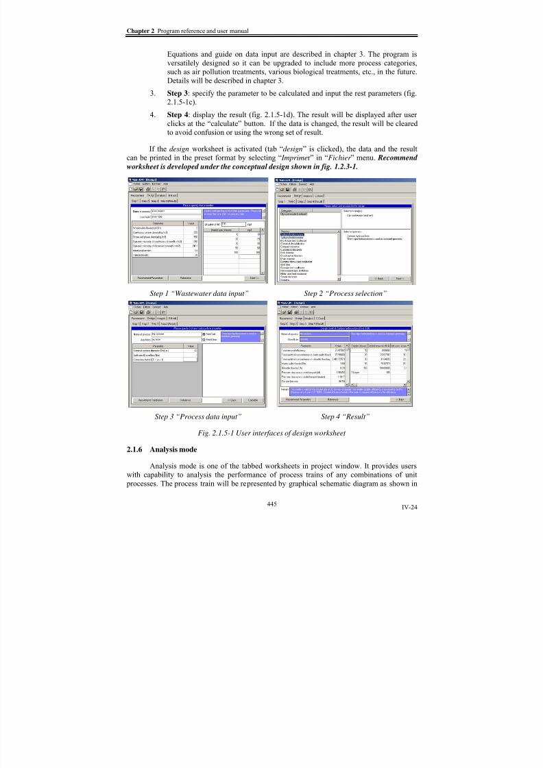
8/15/2019 Rachu.pdf
http://slidepdf.com/reader/full/rachupdf 529/646

8/15/2019 Rachu.pdf
http://slidepdf.com/reader/full/rachupdf 530/646
Part IV Computer program development
IV-25
fig. 2.1.6-1. User can select the process category in the top left list box. Then, the program
will display list of available process in that category in the lower list box. In this thesis, there
is only one category available, namely “oily wastewater treatment”.
User can insert required process by double clicking at the name of the process. Then,
the program will insert the icon (picture) of the process into the graphic-editing screen. Theicons can be move freely by normal drag/drop method. Each icon will be automatically
labeled by a code, indicating its type of process and number, such as SD-01 for simple
decanter no. 1. These tag numbers are useful for calculation of the program.
The program is equipped with automatic connector capability that can connect the
processes just by mouse clicking and dragging. Basic graphic tools, such as text box, line,
rectangular, circle, are provided. Users can add/edit these items into the diagram without
affect on calculation of the program.
Sizing of each process is specified by double clicking at the icon. Data input screen
will be displayed. After the schematic diagram and data input are ready, user can startcalculation by clicking at “calculation button” or “calcul” menu. The program will validate
the data and prompt for correction in case of error until it is cleared. Then it will analyze the
process to find efficiency of the process as well as other important parameters of each process,
such as pressure drop for hydrocyclone, etc. The details will be described in chapter 3. The
result will be displayed within the program or exported to Excel. User instructions on drawing
the diagram, calculation, etc. are described in section 2.5.
Graphic editing area
Basic drawing tool bar
Calculation button
Input and result screen(displayed when double clicking at the icon)
Category selection
Process selection
Fig. 2.1.6-1 User interface of analysis worksheet
446

8/15/2019 Rachu.pdf
http://slidepdf.com/reader/full/rachupdf 531/646
Chapter 2 Program reference and user manual
IV-26
2.1.7 Warning dialog box
Warning dialog box is the text box that is displayed when the program finds some
error, e.g. in data typing, or wants to prompt users on some events or information, e.g. SD-01:
specified droplets are beyond limit of the process. Example of warning dialog box is as shown
in fig. 2.1.7-1. It can be closed by clicking OK or close (X) button at its corner.
Fig. 2.1.7-1 Example of warning dialog box
2.2 Program capability
Capability of program, from the point of view of process calculation, can be divided
into 2 parts, in accordance with 2 main modes of the program, i.e. design and analysis mode.
The processes included in the program are mainly the treatment processes that are
reviewed in Part 3. However, there are some additional processes that are included as logical
module in the analysis mode, e.g. inlet module and outlet module, or to represent a
customized process that is not included in those of Part 3. All processes included in designand analysis mode are summarized in table 2.2-1. Equations and related parameters, as well as
guideline for data input, for each process are described in chapter 3 “Program references”.
2.3 Program limitation
Since the program is newly developed, it has some limitations, based on programming
techniques, limitation from scope of work of the thesis, as well as attempts to generalize the
program to support upgrading in the future. General limitation of the program are as
summarized below.
1)
In this scope of work, GPI program includes only oily wastewater treatment process.
2)
The unit of every parameter (e.g. kg, m. second, etc.) is fixed to lessen the
complication of the program.
3) The program includes only calculation of oil separation. Other pollutants, such as
suspended solids, are not taken into account. However, from its open
architecture, it can be upgraded to cover other treatment or other type of process
in the future.
4) The process train in the program can contain only 1 outlet since it is an important
logical module, used in program loop. In case that there is more than 1 outlet in
the real process train, user can combine those outlets, using flow merge module,
into 1 outlet. However, to do so, it does not affect calculation result.
447
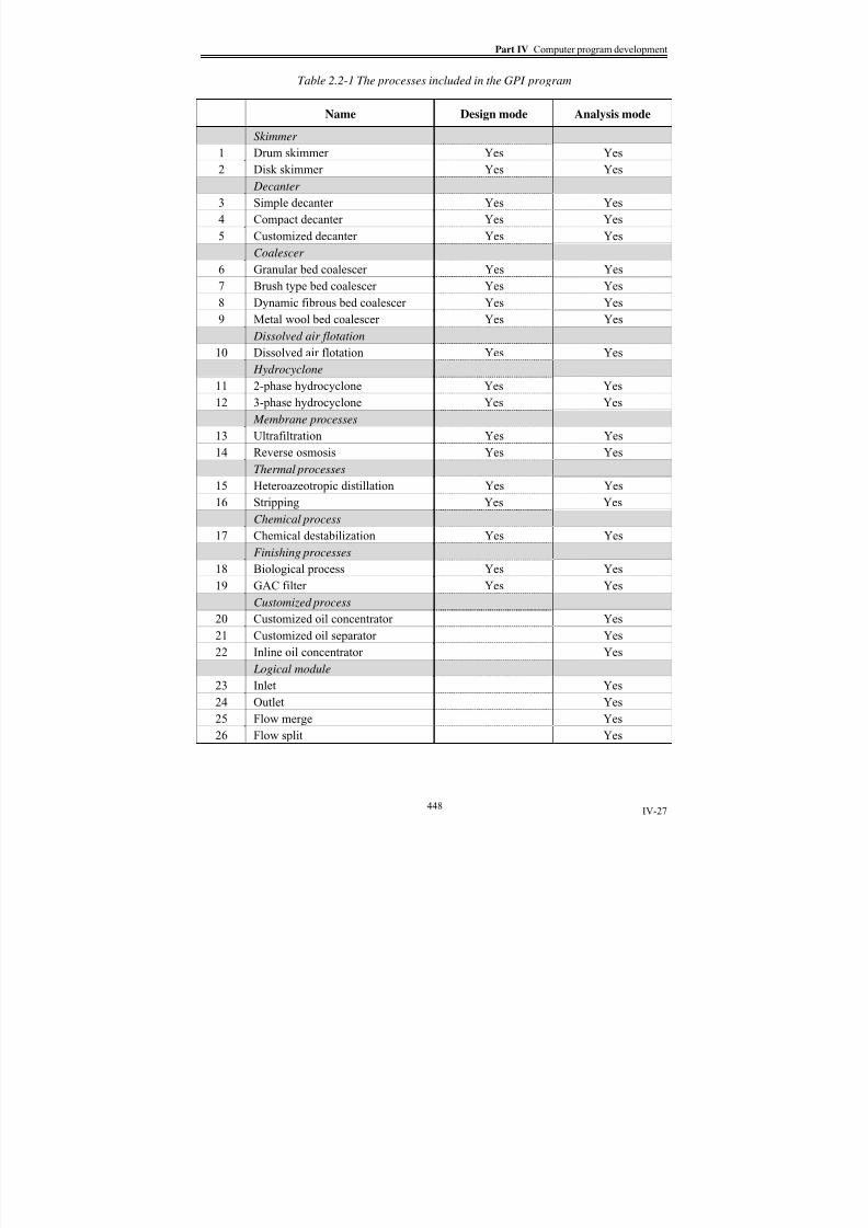
8/15/2019 Rachu.pdf
http://slidepdf.com/reader/full/rachupdf 532/646
Part IV Computer program development
IV-27
Table 2.2-1 The processes included in the GPI program
Name Design mode Analysis mode
Skimmer
1 Drum skimmer Yes Yes2 Disk skimmer Yes Yes
Decanter
3 Simple decanter Yes Yes
4 Compact decanter Yes Yes
5 Customized decanter Yes Yes
Coalescer
6 Granular bed coalescer Yes Yes
7 Brush type bed coalescer Yes Yes
8 Dynamic fibrous bed coalescer Yes Yes9 Metal wool bed coalescer Yes Yes
Dissolved air flotation
10 Dissolved air flotation Yes Yes
Hydrocyclone
11 2-phase hydrocyclone Yes Yes
12 3-phase hydrocyclone Yes Yes
Membrane processes
13 Ultrafiltration Yes Yes
14 Reverse osmosis Yes YesThermal processes
15 Heteroazeotropic distillation Yes Yes
16 Stripping Yes Yes
Chemical process
17 Chemical destabilization Yes Yes
Finishing processes
18 Biological process Yes Yes
19 GAC filter Yes Yes
Customized process20 Customized oil concentrator Yes
21 Customized oil separator Yes
22 Inline oil concentrator Yes
Logical module
23 Inlet Yes
24 Outlet Yes
25 Flow merge Yes
26 Flow split Yes
448

8/15/2019 Rachu.pdf
http://slidepdf.com/reader/full/rachupdf 533/646
Chapter 2 Program reference and user manual
IV-28
5) Some influent parameters can not be interpreted in the form of equation, such as
tortousity of bed in coalescer process, thus can not be accounted in calculation.
However, effect of these parameters can be compensated by the use of correction
factor (CF).
6)
The program requires third party program to operate, such as MS excel, Acrobat.
Some of these programs are not free-ware and may cause some expense if they
are not readily available.
7) From the limitation of VB 6.0, its control components, such as text box, menu,
table, etc., support only one font, which is Windows (English version) default
font (as seen in the windows explorer and menu of every program in the
Windows). So we cannot use symbols, Greek letters or the letters with accent ,
such as γ, τ, é, etc. in the program.
2.4 System requirement
To use the program, these hardware and software, based mainly on the requirement ofWindows, VB and Excel, are needed.
Hardware
1. Computer and processor: PC with 300 megahertz or higher processor clock
speed recommended; 233 MHz minimum required (single or dual processor
system);* Intel Pentium/Celeron family, or AMD K6/Athlon/Duron family, or
compatible processor recommended.
2.
Memory: 128 MB of RAM or greater (minimum of 256 MB is recommended.)
3. Hard disk: 50 MB of available hard-disk space
4.
Display: Super VGA (800x600) or higher resolution5. CD-ROM or DVD drive
Software
1. Windows 2000 with service pack 3 (SP3), Windows XP or higher
2. Adobe Acrobat reader 6.0 or higher
3. Microsoft Excel 2000 or higher
4. Microsoft Access 2000 or higher (Optional for database editing)
2.5 User instruction
GPI program is Windows-based program so it features familiar graphic user interface
and basic Windows function, e.g. drag/drop, etc. Thus it is quite ready to use for Windows
users. In this section, instructions for using customized features of the program are described
2.5.1 Program Installation
Setup files of the GPI program are contained in a CD. To install program;
1. Insert CD into a drive
2. The program will run setup program automatically. If auto run is not operated,
449

8/15/2019 Rachu.pdf
http://slidepdf.com/reader/full/rachupdf 534/646
Part IV Computer program development
IV-29
2.1 Use any browsing programs, such as window explorer, to browse the
contents on the CD and then <double click> at “Setup.exe”.
2.2 <Click> Windows’s “Start” button, <Click> “Run” Then type “<your CD-
ROM drive>:setup”, such as “d:setup”
3.
Follow on-screen instruction.
4. Set program will install GPI program to the computer and automatically create
an icon on the desktop and add the program into the Programs menu of the
Windows.
2.5.2 Starting the program
1. <click> Windows’s “Start” button, then <click> “Programs” and <Click> the
program name.
2. Or <double click> at the shortcut on the desktop (created by user).
3. Or <click> Windows’s “Start” button, then <click> “Programs” and <Click> the
program name.
4. The Main form and a new project window will appear on the screen. The
program is ready to use.
2.5.3 Using E-book mode
Fig 2.5.3-1 Using E-book mode
1
3
2, 4
1. <Click> “E-book” tab or “documentation électronique” in “Aide” menu.
2.
<Click> at the name of an e-book to be open3. <Click> “Open” button
4. Or <Double click> at the name
5. The program will open Acrobat and display the selected file.
2.5.4 Using Recommend mode
1. <Click> “Recommend” tab
2. <Click> a radio button to select the suitable answer for your wastewater in the
topmost frame
450

8/15/2019 Rachu.pdf
http://slidepdf.com/reader/full/rachupdf 535/646
Chapter 2 Program reference and user manual
IV-30
Fig. 2.5.4-1 Using recommend mode: Input data screen
12
5
Fig. 2.5.4-2 Using recommend mode: Result window
451

8/15/2019 Rachu.pdf
http://slidepdf.com/reader/full/rachupdf 536/646
Part IV Computer program development
IV-31
3. The frame corresponding to your first answer will be displayed. <Click> another
radio button. Other frames will be disabled to avoid confusion.
4.
<Click> suitable list box. You can select more than one box.
5.
When data input is sufficient, “Calculate” button will be enabled. <Click> the
button to start calculation and display the result.6. Result window (fig.2.5.4-2) is shown. Your wastewater is indicated by tick
marks. <Click> “X” button to close the result. To start over, go back to step 1.
2.5.5 Using Design mode
1. <Click> “Design” tab
2. <Click> “Step 1” tab. Wastewater data input screen is shown.
3. Input the data in input fields (text boxes and table) by <Click> at the selected
field, then type your data
4.
To move to next field, user arrow keys (<↓>,<↑>) or <enter> or <click> at the
next field
5. When data in step 1 is complete, <Click> “Step 2” tab or <click> “next” button.
Process selection data is shown.
Fig. 2.5.5-1 Using Design mode: Step 1 “Wastewater data input”
2
1
54
6. <Click> at required category name and process name. The text boxes on the left
hand will display short description of the selected category and process. In this
thesis, these are only 1 category, i.e. oily wastewater treatment.
452

8/15/2019 Rachu.pdf
http://slidepdf.com/reader/full/rachupdf 537/646
Chapter 2 Program reference and user manual
IV-32
Fig. 2.5.5-2 Using Design mode: Step 2 “Process selection”
1
6 6
6
Fig. 2.5.5-3 Using Design mode: Step 3 “Process data input”
7
8
9
453

8/15/2019 Rachu.pdf
http://slidepdf.com/reader/full/rachupdf 538/646
Part IV Computer program development
IV-33
7. When selection is done, <click> “Next” button or “Step 3” tab. Process data
input screen is shown.
8.
Input the data in input fields (text boxes and table) by <Click> at the selected
field, then type your data. To move to next field, user arrow keys (<↓>,<↑>) or
<enter> or <click> at the next field. The field that we want to find the answer
must be left blank. <Click> “Recommend parameters” or “Reference” for more
information on the value of each parameter and related equations and limitation
of each process.
9. When data in step 3 is complete, <Click> “Calculate” button. The program will
calculate the result and put it in the result screen “Step 4”. If the data is not
sufficient or redundant, the program will not calculate and will display a
warning.
10. After calculation, the result screen (step 4) will be automatically shown.
11. To edit some data in each step, <click> the required tab or <click> “Back” and
“Next” button. When the data is edited, the result is cleared to avoid confusion.
Fig. 2.5.5-4 Using Design mode: Step 4 “Result”
11
2.5.6 Using Analysis mode
1. <Click> “Analysis” tab
2. <Click> at require category name in the upper left box. List of processes in that
category will be shown in the lower left box. In this thesis, there is only 1
category, i.e. oily wastewater treatment.
454

8/15/2019 Rachu.pdf
http://slidepdf.com/reader/full/rachupdf 539/646
Chapter 2 Program reference and user manual
IV-34
1 5
Drag and drop to move
<Double click> to insert
3
Fig. 2.5.6-1 Using Analysis mode: Draw the schematic diagram
3.
Input your process train by drawing the schematic diagram, using the unit processes provided in the lower left box on the screen. To insert an icon or
graphic representative of the process, <Double click> at the process name. The
corresponding icon is shown in the graphic editing area.
4. To move the icon to proper location, move the cursor over the icon until it turns
into a “4-direction arrow” ( ) sign. Then <click> and hold the mouse button to
drag and release the button to drop the icon at new location.
5. Insert other processes using step 3 and 4 until all required processes are inserted.
To connect the processes together, move the cursor over the icon until it turns
into a “hand” (
) sign. Connecting points of the process will be shown as smallred squares. Move the “hand” to the required connecting point, <click> the
mouse, hold the button to a required connecting point of another process to be
connected and release the mouse. The program will draw the connecting line
automatically. Users will actually see the line while they hold and move the
mouse. User can add non-active graphic, e.g. text box, line, etc. into the diagram,
using drawing tools.
6. After connecting the processes, User must input the size of each process. To
input or edit the data of a process, <double click> at its icon. Process data input/
result screen is shown. However, the result tab will be disabled unless the
calculation is completed. The process train must contain only 1 outlet module.
But there can be several inlet modules. See chapter 3 for details and restriction ofeach module.
455

8/15/2019 Rachu.pdf
http://slidepdf.com/reader/full/rachupdf 540/646
Part IV Computer program development
IV-35
Fig. 2.5.6-2 Using Analysis mode: Process data input
7
7. After data input procedure is completed. <Click> “Calculate” button or “Calcul
Now” in “Calcul” menu to start caluculation. The program will validate the data
and display warning to prompt users to correct the errors. After the errors are
cleared, the program will calculate the result of each process. In analysis mode,
the program can calculate process performance (e.g. graded efficiency, outletconcentration of oil, etc.) only. It can not be used for sizing the process, as in the
design mode.
8. To view the result, <Double click> at required process icon. The data input/
result will be displayed. After calculation in step 8, the “Result” tab is enabled.
<Click> the tab to view the result of the process. The result tab is just the same
as that of design mode, shown in fig. 2.5.5.4.
9.
Total outlet concentration of each process will also be shown as a text box under
each icon for evaluation of the performance at-a-gaze (fig. 2.5.6-3)
10. To display result in more complex format, it must be exported to Excel. To do
so, <Click> “Exporter” in “Donneé” menu. The program will open Excel and
automatically create a workbook. Each worksheet in the workbook devotes to
result of each process (fig 2.5.6-4). User can also save this excel file. User can
formulate their own formats of result such as building graph showing graded
efficiency of every process, etc., in Excel. The diagram can also be exported to
any Windows-compatible software, such as PowerPoint, PhotoShop, etc., by
<click> at “Exporter d’image” in “Donneé” menu.
456

8/15/2019 Rachu.pdf
http://slidepdf.com/reader/full/rachupdf 541/646
Chapter 2 Program reference and user manual
IV-36
Fig. 2.5.6-3 Using Analysis mode: Viewing result in the diagram
Fig. 2.5.6-4 Using Analysis mode: Exporting the result to excel
2.5.7 Printing and file operation
1. Every screen in the program can be printed in pre-set format. To print, <click>
“Imprimer” in “Fichier” menu. Print dialog box will be shown. User can select
the mode(s) that they want to prink, then click “OK”.
2. Data and result of design and analysis can be saved in the database. To conduct
file operation (new, open, save, delete, close), <click> required operation in“Fichier” menu. File operation dialog box will be shown.
457
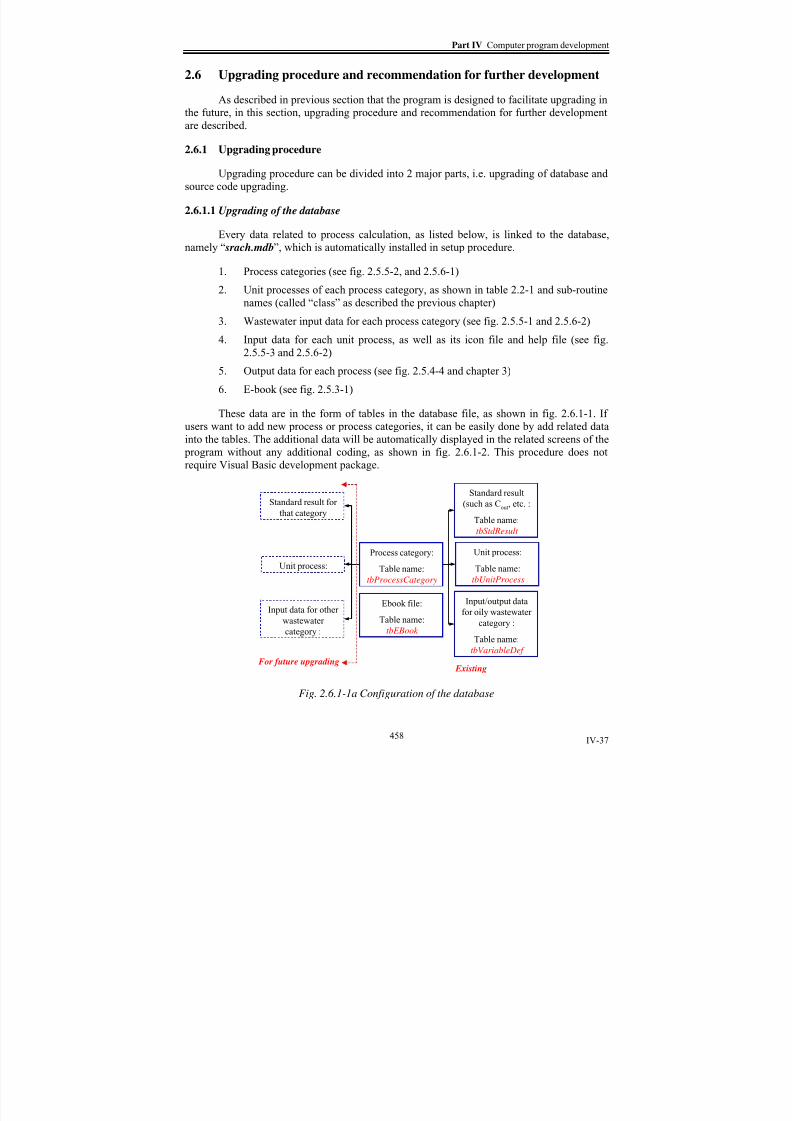
8/15/2019 Rachu.pdf
http://slidepdf.com/reader/full/rachupdf 542/646
Part IV Computer program development
IV-37
2.6 Upgrading procedure and recommendation for further development
As described in previous section that the program is designed to facilitate upgrading in
the future, in this section, upgrading procedure and recommendation for further development
are described.
2.6.1 Upgrading procedure
Upgrading procedure can be divided into 2 major parts, i.e. upgrading of database and
source code upgrading.
2.6.1.1 Upgrading of the database
Every data related to process calculation, as listed below, is linked to the database,
namely “ srach.mdb”, which is automatically installed in setup procedure.
1.
Process categories (see fig. 2.5.5-2, and 2.5.6-1)2.
Unit processes of each process category, as shown in table 2.2-1 and sub-routine
names (called “class” as described the previous chapter)
3. Wastewater input data for each process category (see fig. 2.5.5-1 and 2.5.6-2)
4. Input data for each unit process, as well as its icon file and help file (see fig.
2.5.5-3 and 2.5.6-2)
5. Output data for each process (see fig. 2.5.4-4 and chapter 3)
6. E-book (see fig. 2.5.3-1)
These data are in the form of tables in the database file, as shown in fig. 2.6.1-1. Ifusers want to add new process or process categories, it can be easily done by add related data
into the tables. The additional data will be automatically displayed in the related screens of the
program without any additional coding, as shown in fig. 2.6.1-2. This procedure does not
require Visual Basic development package.
Process category:
Table name:
tbProcessCategory
Unit process:
Table name:
tbUnitProcess
Input/output data
for oily wastewater
category :
Table name:
tbVariableDef
Standard result
(such as Cout
, etc. :
Table name:
tbStdResult
Unit process:
Input data for other
wastewater
category :
Standard result for
that category
For future upgrading Existing
Ebook file:
Table name:
tbEBook
Fig. 2.6.1-1a Configuration of the database
458

8/15/2019 Rachu.pdf
http://slidepdf.com/reader/full/rachupdf 543/646
Chapter 2 Program reference and user manual
IV-38
Fig. 2.1.6-1b Examples of existing database
CAT000001
CAT000002 Airpollutiontreatment
Airpollutiontreatment
Fig. 2.1.6-2 Example on database upgrading. When new category is added in the database
(left), Related field in the program will be automatically updated (right)
2.6.1.2 Source code updating
Even though the program’s interfaces can be easily upgraded by updating the database
file. To add sub-routines (or classes) of new processes into the program, the new classes have
to be written in Visual Basic. The simplest way to write a new class is to copy one of the old
class and change the formula or equation to suit the new process. To do so, Visual basic
development package and the original source code of any process is required. Developers can
define their own variable easily in the database file. So, in their new classes, they can use
these variables in the new equations.
459
8/15/2019 Rachu.pdf
http://slidepdf.com/reader/full/rachupdf 544/646
Part IV Computer program development
IV-39
After writing the new classes in VB, the classes need to be recompiled into executable
file. Then, the file will be copied to replace the old compiled class file without reinstallation
of the whole program.
The reason that we developed the program in the manner that it requires source code
for updating is that we can control the development of the program to proper developers. The
source code of the program is submitted to thesis director, Prof. AURELLE.
2.6.2 Recommendation for further development
Since this program in newly developed so it have some limitations as discussed in
section 2.3. However it may have prospect for further development, at least, in the following
approach.
1. To upgrade to include more process categories,
2. To add a subroutine for unit conversion (metric, US customary, etc.), which
would be very useful in case that some users may be familiar with different kindof unit.
3. To develop or include some advanced components, which may be present in the
newer version of VB, to enhance the performance of the program or make it
operate in stand-alone mode without requiring third-party software (such as
Excel). It is also useful to enhance its text display capability so it will be able to
display Greek letter, subscript, or superscript.
4. Recommend mode should be enhanced by replacing the fixed-coded source
codes with sub-program written with logical programming language, such as
Prolog.
460

8/15/2019 Rachu.pdf
http://slidepdf.com/reader/full/rachupdf 545/646
Chapter 3 Process references
IV-40
Chapter 3 Process references
Process references, which include the parameter to be calculated, equations used and
specific constraints of each process, are described in the following sections. This information
is included in the help file of the program, (<Click> “Utilisation du program” in “Aide”
menu), or (<Click> “Reference” button in any input forms or user interfaces).
Common parameters
Common parameters or variables that are used for every process module are
summarized as follows,
Parameter DescriptionVariable name in
the program
Unit used in the
program
Cod Granulometry or oil droplet size
distribution : graded concentration(concentration of oil at each droplet size)
Cind mg/l
Concentration of inlet oil in the form of
oil layer or film
Cinlayer mg/l
Co Total oil inlet concentration Co mg/l
d Granulometry or oil droplet size
distribution : droplet size
din micron
Q Wastewater flowrate Qin m3/h
T Temperature temp Celcius
ρc Dynamic (or absolute) viscosity of
continuous phase, which is water, for oily
wastewater
Denc Kg/m3
ρd Density of dispersed phase, in this case, oil Dend Kg/m3
μC Dynamic (or absolute) viscosity of
continuous phase, which is water, for oily
wastewater
Muc N.s/m2
(= 1000 cp)
μd Dynamic (Absolute) viscosity of
dispersed phase, in this case, oil
Mud N.s/m2
(= 1000 cp)
γow Interfacial tension between oil and water gow kg/s2
or N/m
(= 1000 dyne/cm)
Values of these parameters will be given by user via inlet module (See section 23).
They will be used to calculate the results, which are usually divided into 2 streams, i.e., water
outlet and oil (or concentrated oily wastewater outlet. Generally, the result will contain the
parameters mentioned above. But the values will be changed in accordance with
corresponding model or equations of each process. Then they will be sent as input data for
downstream process until the end of process train (outlet module).
General remarks and precautions of the program
General remarks and precautions of the program are as shown below,
•
The program is valid only when the oil is lighter than water.
461

8/15/2019 Rachu.pdf
http://slidepdf.com/reader/full/rachupdf 546/646
Part IV Computer program development
IV-41
• The processes available in the program generally consists of 1 inlet port and 2
outlet ports, i.e., outlet port of treated water, called “water outlet port ”, and outlet
port of separated pure oil or concentrated oily water, called “Oil outlet port ”.
• Graded concentration is specified as quantity of oil (mg) per volume of wastewater
(= volume of oil+water).
• Graded efficiency (ηd) in the program is based solely oil mass removal, regardless
of flow splitting effect. To calculate outlet concentration, flow splitting between
oil outlet port and water outlet port of each process will be taken in to account.
Thus, in some processes, outlet oil concentration is not exactly equal to (1-ηd)Cod.
• Total efficiency (ηt) in the program can be generally used to calculate total inlet
concentration. Total outlet oil concentration is equal to (1-ηt)Co in some processes.
However, there may be some exceptions in certain processes. See reference of
each process for more information.
• The pictures or icons of processes in analysis mode generally contain 3
connections or hot spots (there may be only 1 or 2 spots in some processes.) The black connection represents inlet point of the process. The red one represents oil
outlet port and the blue one represents treated water outlet port.
• In E-book mode, the e-book files are designed for a fixed directory, named
c:/SR/E-book. The directory contains an Acrobat index file
“E_book_oily_wastewater”. This index facilitates users to search for any words or
topics in all e-book files in the directory. However, it is developed by Acrobat 7.0,
it may not be run on some old versions of Acrobat reader. In this case, it is
recommend to set option of the option “ All PDF documents in” in Acrobat’s
search window to the e-book directory. It can substitute the use of the index file.
•
The program is linked to MS Excel for parameter recommendation, calculation ofsome processes and for result display. In case that, Excel security is set to “high
level”, it will happen that the program is not allowed to link to Excel. To solve or
avoid this problem, you can choose one of these options,
• Set security of Excel to medium or low. (in Menu “Tools”>Options>Security).
• If high or highest security level is needed, try setting the macro in the file
“Process_calculation.xls” as a trusted source (in Menu
“Tools”>Options>Security). Consult your corresponding Excel’s help file for
more information.
462

8/15/2019 Rachu.pdf
http://slidepdf.com/reader/full/rachupdf 547/646
Chapter 3 Process references
IV-42
1) Drum skimmer
1. Process abbreviation: DRM
2. Process description : Oleophilic oil drum skimmer
3.
Reference : Part 3, chapter 34.
List of outputs and related equations
4.1 Graded efficiency: 100% for oil film or layer and 0% for droplet.
4.2 Total efficiency: 100% for oil film or layer and 0% for droplet.
4.3 Graded outlet oil concentration in water outlet flow: This parameter is not
valid for this process.
4.4 Total outlet oil concentration in water outlet flow: This parameter is not
valid for this process.
4.5 Graded outlet oil concentration in oil outlet flow: the outlet oil in the oil
outlet flow is in pure condition (100% oil).
4.6 Total outlet oil concentration in oil outlet flow: the outlet oil in the oil
outlet flow is in pure condition (100% oil).
4.7 Inlet flow: the process is valid only for separated oil flow from upstream
process.
4.8 Water outlet flow: This process does not have this property.
4.9 Oil outlet flow: flowrate or oil productivity (m3/h) is governed by the
following equation.
0.514g
L0.486
o ν1.541 N1.5413.035D
P ⋅= CF {1.1}
5. Related parameters: Related parameters are as summarized in the following
table.
Table .1-1 Related parameters of drum skimmer
Parameter Description Variable name inthe program
Unit used in theprogram
CF Efficiency correction factor, CF ≤ 1 CF
D Diameter of skimmer D M
g Gravitational acceleration Constant = 9.81 m/s2
L Length of the skimmer L M
N Rotational speed of the skimmer N Rev/s
P Oil productivity of the skimmer Prod m3/h
γo Superficial tension of oil go kg/s2
or N/m
(= 1000 dyne/cm)
νo Kinematics viscosity of oil (used μ/ρ) m2
/s
463

8/15/2019 Rachu.pdf
http://slidepdf.com/reader/full/rachupdf 548/646
Part IV Computer program development
IV-43
6. Related graphics: Icon in analysis mode and graphic diagram for input screen for
this process are as shown below.
Drum Skimmer (DRM-??)
Scrapper
Oil layer
D
L
Fig. 1-1a Icon of drum skimmer Fig .1-1b Graphical diagram of drum skimmer
7.
Constraints and limitations
7.1
Superficial tension of oil is in the range of 27 – 34 dynes/cm, which
practically covers all common oil.
7.2
Capillary number (Ca = μo V/γo) is in the range of 0.2 – 1.0.
7.3
Oil density is around 790 – 830 kg/m3. Oil dynamic viscosity (μ) tested is
between 1.35x10⁻³ to 291x10-3 (N.s)/m2 (1.35-291 cp).
7.4 Peripheral or tip velocity should not be greater than 0.8 m/s. To avoid
water entraining, velocity of 0.44 m/s or less is recommended.
7.5
Recommended minimum immersion depth is 1.0-2.0 cm.7.6
Drum skimmer surface used for model development is polypropylene. But
it is proven to be valid for SS, PVC, and PTFE.
7.7 Skimmer can only be connected to pure oil outlet flow of upstream process.
8. Influent parameters: Effects of certain parameters, when they are increased, on
the oil removal performance of the process are summarized as follows. For more
details, see chapter 3, Part 3.
Table 1-2 Influent parameters for drum skimmer
ParameterEffect on process performance if
the parameter is increased
Length of drum + is
Diameter of skimmer + is
Oil viscosity +
Velocity ±
Present of surfactants -
Note: “+” means “increases performance”, “-“ means “decreases performance”, “± ” means
“have both positive and adverse affects”, “is” means “effect is insignificant”.
464

8/15/2019 Rachu.pdf
http://slidepdf.com/reader/full/rachupdf 549/646

8/15/2019 Rachu.pdf
http://slidepdf.com/reader/full/rachupdf 550/646
Part IV Computer program development
IV-45
6. Related graphics: Icon in analysis mode and graphic diagram for input screen for
this process are as shown below.
D i s k
Disk Skimmer (DSK-??)
I
Scrapper
D
Fig. 2-1a Icon of disk skimmer Fig. 2-1b Graphical diagram of disk skimmer
7. Constraints and limitations.
7.1 Superficial tension of oil is in the range of 27 – 34 dynes/cm, which
practically covers all common oil.7.2 Capillary number (Ca = μo V/γo) is in the range of 0.04 – 3.6.
7.3 Oil density is around 790 – 830 kg/m3. Oil dynamic viscosity (μ) tested is
between 1.35x10⁻³ to 291x10-3 (N.s)/m2 (1.35-291 cp).
7.4 Peripheral or tip velocity should not be greater than 1.13 m/s. To avoid
water entraining, velocity of 0.5 m/s or less is recommended.
7.5
Disc skimmer surface used for model development is PVC. But it is proven
to be valid for SS, PP, and PTFE.
7.6
Skimmer can only be connected to pure oil outlet flow of the upstream
process.
8.
Influent parameters: Effects of certain parameters, when they are increased, onthe oil removal performance of the process are summarized as follows. For more
details, see chapter 3, Part 3.
Table 2-2 Influent parameters for disk skimmer
ParameterEffect on process performance if
the parameter is increased
Immersion depth +
Diameter of skimmer + is
Oil viscosity +
Velocity ±
Present of surfactants -
Note: “+” means “increases performance”, “-“ means “decreases performance”, “± ” means
“have both positive and adverse affects”, “is” means “effect is insignificant”.
466

8/15/2019 Rachu.pdf
http://slidepdf.com/reader/full/rachupdf 551/646
Chapter 3 Process references
IV-46
3) Simple decanter
1. Process abbreviation: SD
2. Process description: API tank or any decanter that does not have any oil
interceptors installed in the tank so the rising distance of oil drops is equal to the
water depth.
3. Reference : Part 3, chapter 4
4. List of outputs and related equations
4.1 Graded efficiency (η d ): Graded efficiency of the process is governed by the
following equation.
For oil droplet size, d ≥ cut size,dc
%100⋅= CF d η {3.1}
For oil droplet size, d ≤ cut size,dc
%100⋅⋅=dc
d
d U
U CF η {3.2a}
For oil droplet size, d ≤ 20 microns
%0=d η {3.2b}
Rising velocity (U), m/s, of the droplet “d” or of the cut size “d c” is
calculated from the following equations.
c
d
d gU
μ
ρ
18
)10( 26−⋅⋅⋅Δ= {3.3}
⎟ ⎠
⎞⎜⎝
⎛ ⋅
=S
QU dc
3600 {3.4}
Cut size is calculated by the following equation.
6
2/1
103600.
18⋅⎟⎟
⎠
⎞⎜⎜⎝
⎛
⋅⋅Δ=
S g
Qd c
c ρ
μ micron {3.5}
4.2 Total efficiency (η t ):
( )
%100
max
min ⋅
⋅
= ∑o
d
d
od d
t C
C η
η
{3.6}
4.3 Graded outlet oil concentration in water outlet flow (C d ):
)1(d od
out
d C Q
QC η −⋅⋅=
mg/l {3.7}
4.4 Total outlet oil concentration in water outlet flow (C ):
∑=max
min
d
d
d C C mg/l {3.8}
4.5
Graded outlet oil concentration in oil outlet flow (C oild ): The outlet oil inthe oil outlet flow is in pure condition (100% oil).
467

8/15/2019 Rachu.pdf
http://slidepdf.com/reader/full/rachupdf 552/646
Part IV Computer program development
IV-47
4.6 Total outlet oil concentration in oil outlet flow (C oil): The outlet oil in the
oil outlet flow is in pure condition (100% oil).
4.7 Inlet flow (Q): Inlet flow of the process is equal to the outlet flow of the
upstream process.
4.8
Water outlet flow (Qout ):
)1000//)(1( oiloout C C QQ ρ −−=
m3/h
{3.9}
4.9 Oil outlet flow(Qoil):
out oil QQQ −=
m3/h
{3.10}
4.10 Customized output :
4.10.1 Theoretical cut size (d c): cut size is calculated by eq. 3.5.
5.
Related parameters: Related parameters are as summarized in the following table
Table 3-1 Related parameters of simple decanter
Parameter DescriptionVariable name in
the program
Unit used in the
program
dc Cut size of the decanter dc micron
S Bottom projection area of the tank S m2
Ud Rising velocity of the droplet diameter “d” Ud m/s
Udc Rising velocity of the droplet at cut size “dc” Udc m/s
Δρ Difference between density of dispersed
phase and continuous phase
Denc-Dend Kg/m3
ρc Density of continuous phase, in this case,
water
Denc Kg/m3
μC Dynamic (or absolute) viscosity of
continuous phase, which is water, for oily
wastewater
Muc N.s/m2
(= 1000 cp)
ρd Density of dispersed phase, in this case, oil Dend Kg/m3
6. Related graphics: Icon in analysis mode and graphic diagram for input screen for
this process are as shown below.
Simple decanter (SD-??)
Ud
V
Q
d = cut size
d < cut size
d > cut size
Influent
L
Oil droplets
Separated
oil layer
S
Fig. 3-1a Icon of simple decanter Fig. 3-1b Graphical diagram of simple decanter
468

8/15/2019 Rachu.pdf
http://slidepdf.com/reader/full/rachupdf 553/646
Chapter 3 Process references
IV-48
7. Constraints and limitations.
7.1 Reynolds number of droplet, Re, is between 10-4 to 1, which is the range
that STOKES law is valid.
c
d c d U
μ
ρ ⋅⋅=Re {3.11}
7.2 The oil droplets are uniformly distributed across the cross section area of
the tank, which can be achieved by proper design of inlet chamber.
7.3
ηd of oil layer is 100%.
7.4
The oil droplet is spherical, which is normally true.
7.5
For droplets smaller than 20 microns, they are subjected to Brownian
motion and cause error in the prediction of the efficiency. So it is
recommended to avoid using the decanter for the wastewater with the
majority part of oil droplets smaller than 20 microns. However, if these
small droplets are the minority part of pollutants, the models can be used to predict the efficiency without any harm because its prediction is usually
lower than observed value, thus make the prediction result on the safe side.
7.6 Oil outlet point of the process can only be connected to the skimmers only.
8. Influent parameters: Effects of certain parameters, when they are increased, on
the oil removal performance of the process are summarized as follows. For more
details, see chapter 4, Part 3.
Table 3-2 Influent parameters for simple decanter
ParameterEffect on process performance if
the parameter is increased
Hydraulic loading rate -
Droplet diameter +
Note: “+” means “increases performance”, “-“ means “decreases performance”, “± ” means
“have both positive and adverse affects”, “is” means “effect is insignificant”.
469

8/15/2019 Rachu.pdf
http://slidepdf.com/reader/full/rachupdf 554/646
Part IV Computer program development
IV-49
4) Compact decanter
1. Process abbreviation: CD
2. Process description: Parallel plate interceptor, lamella separator, or other types of
plate insertion decanter that the rising distance of the droplets is equally divided
and can be clearly specified .
3. Reference : Part 3, chapter 4
4. List of outputs and related equations
4.1 Graded efficiency (η d ): Graded efficiency of the process is governed by the
following equation.
For oil droplet size, d ≥ cut size,dc
%100⋅= CF d η {4.1}
For oil droplet size, d ≤ cut size,dc
%100⋅⋅=dc
d
d U
U CF η {4.2a}
For oil droplet size, d ≤ 20 microns
%0=d η {4.2b}
Rising velocity (U) of the droplet “d” or of the cut size “dc” is calculated
from the following equations.
c
d
d gU
μ
ρ
18
)10( 26−⋅⋅⋅Δ= m/s {4.3}
⎟⎟
⎠
⎞⎜⎜⎝
⎛
⋅+⋅=⎟⎟
⎠
⎞⎜⎜⎝
⎛
⋅=
α cos)1(36003600 N S
Q
S
QU
pd
dcm/s {4.4}
Cut size (micron) is calculated by the following equation.
6
2/1
10cos)1(3600
18⋅⎟⎟
⎠
⎞⎜⎜⎝
⎛
⋅+Δ⋅=
α ρ
μ
N gS
Qd
P
cc
micron
{4.5}
4.2 Total efficiency (η t ):
( )%100
max
min ⋅⋅
= ∑o
d
d od d
t C
C η η
{4.6}
4.3 Graded outlet oil concentration in water outlet flow (C d ):
)1(d od
out
d C Q
QC η −⋅⋅=
mg/l
{4.7}
4.4 Total outlet oil concentration in water outlet flow (C ):
∑=max
min
d
d
d C C mg/l
{4.8}
4.5 Graded outlet oil concentration in oil outlet flow (C oild ): The outlet oil in the
oil outlet flow is in pure condition (100% oil).
470

8/15/2019 Rachu.pdf
http://slidepdf.com/reader/full/rachupdf 555/646
Chapter 3 Process references
IV-50
4.6 Total outlet oil concentration in oil outlet flow (C oil): The outlet oil in the oil
outlet flow is in pure condition (100% oil).
4.7 Inlet flow (Q): Inlet flow of the process is equal to the outlet flow of the
upstream process.
4.8
Water outlet flow (Qout ):
)1000//)(1( oiloout C C QQ ρ −−= m3/h
{4.9}
4.9 Oil outlet flow(Qoil):
out oil QQQ −= m3/h
{4.10}
4.10 Customized output :
4.10.1 Theoretical cut size (d c): cut size is calculated by eq. 4.5.
4.10.2 Foot print area of the decanter (S): It is assumed to be identical to
Sp.
5.
Related parameters: Related parameters are as summarized in the following table
Table 4-1 Related parameters of compact decanter
Parameter DescriptionVariable name in
the program
Unit used in the
program
dc Cut size of the decanter dc micron
N The number of plates N
S p Area of one inserted plate (only 1 side and
measured perpendicularly to the platesurface.)
Sp m2
Ud Rising velocity of the droplet diameter “d” Ud m/s
Udc Rising velocity of the droplet at cut size “dc” Udc m/s
α Inclination of plate from horizontal axis (0-
90 degree)
incl degree
Δρ Difference between density of dispersed
phase and continuous phase
Denc-Dend Kg/m3
ρc Density of continuous phase, in this case,
water
Denc Kg/m3
μC Dynamic (or absolute) viscosity of
continuous phase, which is water, for oily
wastewater
Muc N.s/m2
(= 1000 cp)
ρd Density of dispersed phase, in this case, oil Dend Kg/m3
6. Related graphics: Icon in analysis mode and graphic diagram for input screen for
this process are as shown below.
471

8/15/2019 Rachu.pdf
http://slidepdf.com/reader/full/rachupdf 556/646
Part IV Computer program development
IV-51
C o m p a c t
Compact decanter (CD-??)
QInfluent
H
Inserted plates
(No. of plates = N)
Sp
Fig. 4-1a Icon of compact decanter Fig. 4-1b Graphical diagram of compact decanter
7. Constraints and limitations.
7.1 Reynolds number of droplet, Re, is between 10-4 to 1, which is the range
that STOKES law is valid.
c
d c d U
μ
ρ ⋅⋅=Re {4.11}
7.2 The oil droplets are uniformly distributed across the cross section area of
the tank, which can be achieved by proper design of inlet chamber.
7.3
The oil droplet is spherical, which is normally true. ηd of oil layer is 100%.
7.4
For droplets smaller than 20 microns, they are subjected to Brownian
motion and cause error in the prediction of the efficiency. So it is
recommended to avoid using the decanter for the wastewater with themajority part of oil droplets smaller than 20 microns. However, if these
small droplets are the minority part of pollutants, the models can be used to
predict the efficiency without any harm because its prediction is usually
lower than observed value, thus make the prediction result on the safe side.
7.5 Oil outlet point of the process can only be connected to the skimmers only.
8. Influent parameters: Effects of certain parameters, when they are increased, on
the oil removal performance of the process are summarized as follows. For more
details, see chapter 4, Part 3.
Table 4-2 Influent parameters for compact decanter
ParameterEffect on process performance if
the parameter is increased
Hydraulic loading rate -
Droplet diameter +
Inclination of plates (0o = horizontal axis) - but helps draining the sludge from
the plate surfaces
Note: “+” means “increases performance”, “-“ means “decreases performance”, “± ” means
“have both positive and adverse affects”, “is” means “effect is insignificant”.
472
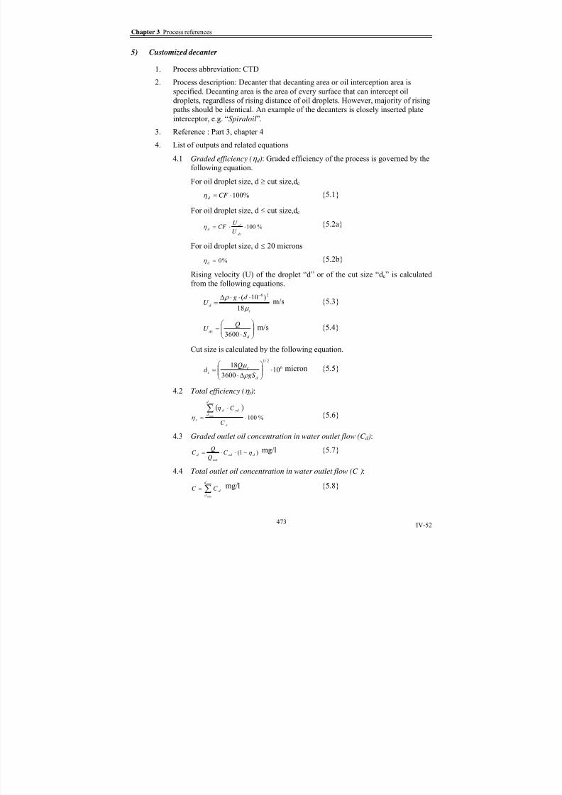
8/15/2019 Rachu.pdf
http://slidepdf.com/reader/full/rachupdf 557/646
Chapter 3 Process references
IV-52
5) Customized decanter
1. Process abbreviation: CTD
2. Process description: Decanter that decanting area or oil interception area is
specified. Decanting area is the area of every surface that can intercept oil
droplets, regardless of rising distance of oil droplets. However, majority of rising paths should be identical. An example of the decanters is closely inserted plate
interceptor, e.g. “Spiraloil”.
3. Reference : Part 3, chapter 4
4. List of outputs and related equations
4.1 Graded efficiency (η d ): Graded efficiency of the process is governed by the
following equation.
For oil droplet size, d ≥ cut size,dc
%100⋅= CF d η
{5.1}
For oil droplet size, d ≤ cut size,dc
%100⋅⋅=dc
d d
U
U CF η {5.2a}
For oil droplet size, d ≤ 20 microns
%0=d η {5.2b}
Rising velocity (U) of the droplet “d” or of the cut size “dc” is calculated
from the following equations.
c
d
d gU
μ
ρ
18
)10( 26−⋅⋅⋅Δ= m/s {5.3}
⎟⎟ ⎠
⎞⎜⎜⎝
⎛
⋅=
d
dcS
QU
3600
m/s {5.4}
Cut size is calculated by the following equation.
6
2/1
103600
18⋅⎟⎟
⎠
⎞⎜⎜⎝
⎛
Δ⋅=
d
cc
gS
Qd
ρ
μ micron {5.5}
4.2
Total efficiency (η t ):
( )
%100
max
min ⋅
⋅
=∑
o
d
d
od d
t C
C η
η
{5.6}
4.3 Graded outlet oil concentration in water outlet flow (C d ):
)1( d od
out
d C Q
QC η −⋅⋅= mg/l {5.7}
4.4 Total outlet oil concentration in water outlet flow (C ):
∑=
max
min
d
d d C C
mg/l {5.8}
473

8/15/2019 Rachu.pdf
http://slidepdf.com/reader/full/rachupdf 558/646
Part IV Computer program development
IV-53
4.5 Graded outlet oil concentration in oil outlet flow (C oild ): The outlet oil in
the oil outlet flow is in pure condition (100% oil).
4.6 Total outlet oil concentration in oil outlet flow (C oil): The outlet oil in the
oil outlet flow is in pure condition (100% oil).
4.7
Inlet flow (Q): Inlet flow of the process is equal to the outlet flow of theupstream process.
4.8 Water outlet flow (Qout ):
)1000//)(1( oiloout C C QQ ρ −−= m3/h {5.9}
4.9 Oil outlet flow(Qoil):
out oil QQQ −=
m3/h
{5.10}
4.10 Customized output :
4.10.1 Theoretical cut size (d c): cut size is calculated by eq. 5.5.
5.
Related parameters: Related parameters are as summarized in the following table
Table 5-1 Related parameters of customized decanter
Parameter DescriptionVariable name in
the program
Unit used in the
program
dc Cut size dc micron
Sd Decanting area ( the area of all surfaces in the
decanter that can intercept oil droplets)
Sd m2
Ud Rising velocity of the droplet diameter “d” Ud m/s
Udc Rising velocity of the droplet at cut size Udc m/s
Δρ Difference between density of dispersed phase
and continuous phase
Denc-Dend Kg/m3
ρc Density of continuous phase, in this case,
water
Denc Kg/m3
μC Dynamic (or absolute) viscosity of continuous
phase, which is water
Muc N.s/m2
(= 1000 cp)
ρd Density of dispersed phase, in this case, oil Dend Kg/m3
6.
Related graphics: Icon in analysis mode and graphic diagram for input screen for
this process are as shown below.
C u s t o m
Customized decanter (CTD-??)
QInfluent
Sd
Fig. 5-1a Icon of customized decanter Fig. 5-1b Graphical diagram of customized decanter
474

8/15/2019 Rachu.pdf
http://slidepdf.com/reader/full/rachupdf 559/646
Chapter 3 Process references
IV-54
7. Constraints and limitations.
7.1 Reynolds number of droplet, Re, is between 10-4 to 1, which is the range
that STOKES law is valid.
c
d c d U
μ
ρ ⋅⋅=Re {5.11}
7.2 The oil droplets are uniformly distributed across the cross section area of
the tank, which can be achieved by proper design of inlet chamber.
7.3
ηd of oil layer is 100%.
7.4
The oil droplet is spherical, which is normally true.
7.5
For droplets smaller than 20 microns, they are subjected to Brownian
motion and cause error in the prediction of the efficiency. So it is
recommended to avoid using the decanter for the wastewater with the
majority part of oil droplets smaller than 20 microns. However, if these
small droplets are the minority part of pollutants, the models can be used to predict the efficiency without any harm because its prediction is usually
lower than observed value, thus make the prediction result on the safe side.
7.6 Oil outlet point of the process can only be connected to the skimmers only.
7.7 Loading rate of the decanter can be as high as 14.1-54 m/h.
7.8 Calculated efficiencies of closely inserted plate interceptor are usually
lower than observed values. Prediction of cut size is relatively accurate so
the difference of ± 20% can be expected.
8. Influent parameters: Effects of certain parameters, when they are increased, on
the oil removal performance of the process are summarized as follows. For moredetails, see chapter 4, Part 3.
Table 5-2 Influent parameters for customized decanter
ParameterEffect on process performance if the parameter
is increased
Hydraulic loading rate -
Droplet diameter +
Inclination of plates (0o
= horizontal axis) - but helps draining the sludge from the platesurfaces
Decanting area +
Rising distance of oil - but too small distance may cause clogging.
Presence of surfactants - for closely inserted plate interceptor
Note: “+” means “increases performance”, “-“ means “decreases performance”, “± ” means
“have both positive and adverse affects”, “is” means “effect is insignificant”.
475

8/15/2019 Rachu.pdf
http://slidepdf.com/reader/full/rachupdf 560/646
Part IV Computer program development
IV-55
6) Granular bed coalescer
1. Process abbreviation: GCC
2. Process description: Granular bed coalescer in this program is based on upflow
pattern. However, it can be applied to downflow coalescer since the rising
velocity of droplet are usually small, compared to flow velocity. So relativevelocity between oil droplets and bed can be safely assumed to equal flow
velocity.
3. Reference : Part 3, chapter 5
4. List of outputs and related equations
4.1 Graded efficiency (η d ): Graded efficiency of the process is governed by the
following equation.
%100)()()()()10
(58.009.009.008.012.02.0
6
⋅Δ⋅
⋅= −
−
cc
d
ow
c
d
dpV
dp
H
dp
d CF ρ
ρ
μ
μ
γ
ρ η
{6.1}
And %100≤d η {6.2}
4.2 Total efficiency (η t ):
( )
%100
max
min ⋅
⋅
=∑
o
d
d
od d
t C
C η
η {6.3}
4.3 Graded outlet oil concentration in water outlet flow (C d ):
)1(d od
out
d C Q
QC η −⋅⋅=
mg/l
{6.4}
4.4 Total outlet oil concentration in water outlet flow (C ):
∑=max
min
d
d
d C C mg/l {6.5}
4.5 Graded outlet oil concentration in oil outlet flow (C oild ): The outlet oil in
the oil outlet flow is in pure condition (100% oil).
4.6 Total outlet oil concentration in oil outlet flow (C oil): The outlet oil in the
oil outlet flow is in pure condition (100% oil).
4.7 Inlet flow (Q): Inlet flow of the process is equal to the outlet flow of the
upstream process.
4.8 Water outlet flow (Qout ):
)1000//)(1( oiloout C C QQ ρ −−= m3/h {6.6}
4.9 Oil outlet flow(Qoil):
out oil QQQ −= m3/h {6.7}
4.10 Customized output :
4.10.1
Theoretical cut size (d c): Cut size is calculated from eq. 6.1 byassuming that the graded efficiency is 100%.
476

8/15/2019 Rachu.pdf
http://slidepdf.com/reader/full/rachupdf 561/646
Chapter 3 Process references
IV-56
4.10.2 Range of pressure drop (P): Pressure drop is calculated from
Kozeny-Carman equation, as shown in eq. 6.8. Recommended
minimum and maximum value of porosity are 0.13 and 0.23,
respectively.
32
2
)1(180ε ρ ε μ ⋅⋅⋅ −= dpg
V H Pc
c
m
{6.8}
5. Related parameters: Related parameters are as summarized in the following table
Table 6-1 Related parameters of granular bed coalescer
Parameter DescriptionVariable name in
the program
Unit used in the
program
dc Cut size dc micron
d p Diameter of collector or bed material dpc mH Bed height (height of granular bed) H m
P Pressure drop across the bed Pdropmin,
Pdropmax
m
V Flow velocity or empty bed velocity V m/s
ε Porosity or void ratio of the bed (= void
volume / total volume)
Constant 0.13 and
0.23
γow Interfacial tension between oil and water gow kg/s2
or N/m
(= 1000 dyne/cm)
Δρ Difference between density of dispersed phase and continuous phase
Denc-Dend Kg/m3
ρc Density of continuous phase, in this case,
water
Denc Kg/m3
μC Dynamic (or absolute) viscosity of
continuous phase, which is water, for oily
wastewater
Muc N.s/m2
(= 1000 cp)
μd Dynamic (or absolute) viscosity of
dispersed phase, which is oil, for oily
wastewater
Mud N.s/m2
(= 1000 cp)
ρd Density of dispersed phase, in this case,oil
Dend Kg/m3
6. Related graphics: Icon in analysis mode and graphic diagram for input screen for
this process are as shown below.
477

8/15/2019 Rachu.pdf
http://slidepdf.com/reader/full/rachupdf 562/646
Part IV Computer program development
IV-57
Granular bed
coalescer
(GCC-??)
Collector
size = d p
Void ratio = ε
Bed height
= H
Influent
Flow = Q
Effluent
Oil outlet
Velocity = V
=Q/A
Cross section area
= A
Fig. 6-1a Icon of granular bed coalescer Fig. 6-1b Graphical diagram of granular bedcoalescer
7. Constraints and limitations.
7.1 Coalescer bed shall be oleophilic and relatively spherical in shape.
7.2 Tested size of bed media (d p) is between 0.20 – 1.0 mm. The larger the
media size, the lower the efficiency.
7.3
Tested range of bed height (H) of the model is between 1 to 10 cm.
However, bed height as low as 1 cm is not recommended. The greater the
bed height, the safer the coalescer operation. However, it also results in
higher pressure drop.
7.4 The velocity (V) should be in the range of 0.09 to 0.54 cm/s or 3.2 to
19.4 m/h.
7.5 Tested interfacial tension (γow) is between 11 to 42 dyne/cm or 0.011 to
0.042 N/m. (i.e. T.I.O.A, Heptane, Anisole, Toluene and Kerosene)
7.6 Different density between dispersed phase (oil) and continuous phase
(water) (Δρ) is between 80 to 315 kg/m3 (approx.).
7.7 The equation is valid for droplet size (d) of 10 microns or bigger. For
smaller droplets, result from the equation may not be accurate because it
is beyond the data range that has been used to verify the model.
7.8 The model is valid for inlet concentration between 100 to 1,000 mg/l. At
higher concentration, mousse or jet formation may occur, resulting in
unpredictable decreasing of the efficiency.
7.9 ηd of oil layer is 100%.
7.10 Within the valid range of model, error in efficiency prediction is less than
±10%.
7.11 Oil outlet point of the process can only be connected to the skimmers
only.
478

8/15/2019 Rachu.pdf
http://slidepdf.com/reader/full/rachupdf 563/646
Chapter 3 Process references
IV-58
7.12 Recommended minimum and maximum value of porosity are 0.13 and
0.23, respectively. For pressure drop calculation, since wastewater is
rather diluted, it is assumed that density and viscosity of water is used in
the equation.
8.
Influent parameters: Effects of certain parameters, when they are increased, on
the oil removal performance of the process are summarized as follows. For more
details, see chapter 5, Part 3.
Table 6-2 Influent parameters of granular bed coalescer
ParameterEffect on process performance if
the parameter is increased
Empty bed velocity -
Droplet diameter +
Collector or bed material diameter -
Hydrophilicity of bed -
Surface roughness of bed +
Bed height +
Ratio of oil to water -
Presence of surfactants -
Temperature +
Note: “+” means “increases performance”, “-“ means “decreases performance”, “± ” means
“have both positive and adverse affects”, “is” means “effect is insignificant”.
479

8/15/2019 Rachu.pdf
http://slidepdf.com/reader/full/rachupdf 564/646
Part IV Computer program development
IV-59
7) Brush type bed coalescer
1. Process abbreviation: BCC
2. Process description: Brush type bed coalescer refers to the coalescer whose
fibrous elements are in aligned neatly in radial direction, like bottlebrush.
3. Reference : Part 3, chapter 5
4.
List of outputs and related equations
4.1 Graded efficiency (η d ): Graded efficiency of the process is governed by the
following equation.
( ) %100)(1)()10
()(5.104 694.035.018.018.06
77.0 ⋅−⋅
⋅= −−
−
D
H
D
d
D
d VDCF F
c
cd ε
μ
ρ η {7.1}
And %100≤d η
{7.2}
4.2 Total efficiency (η t ):
( )
%100
max
min ⋅
⋅
=∑
o
d
d
od d
t C
C η
η {7.3}
4.3 Graded outlet oil concentration in water outlet flow (C d ):
)1(d od
out
d C Q
QC η −⋅⋅=
mg/l
{7.4}
4.4 Total outlet oil concentration in water outlet flow (C ):
∑=max
min
d
d
d C C mg/l {7.5}
4.5 Graded outlet oil concentration in oil outlet flow (C oild ): The outlet oil in
the oil outlet flow is in pure condition (100% oil).
4.6 Total outlet oil concentration in oil outlet flow (C oil): The outlet oil in the
oil outlet flow is in pure condition (100% oil).
4.7 Inlet flow (Q): Inlet flow of the process is equal to the outlet flow of the
upstream process.
4.8 Water outlet flow (Qout
):
)1000//)(1( oiloout C C QQ ρ −−= m3/h {7.6}
4.9 Oil outlet flow(Qoil):
out oil QQQ −= m3/h {7.7}
4.10 Customized output :
4.10.1 Theoretical cut size (d c): Cut size is calculated from eq. 7.1 by
assuming that the graded efficiency is 100%.
4.10.2
Pressure drop (P): Pressure drop is calculated from Hazen –
William equation, using equivalent length of the coaleser. The
equivalent length is assumed to be 5 times of the actual length of
coalescer column.
480

8/15/2019 Rachu.pdf
http://slidepdf.com/reader/full/rachupdf 565/646
Chapter 3 Process references
IV-60
167.185.1
582.6 ⎟
⎠
⎞⎜⎝
⎛ ⎟⎟
⎠
⎞⎜⎜⎝
⎛ =
D
H
C
V P
HW
m
{7.8}
5.
Related parameters: Related parameters are as summarized in the following table
Table 7-1 Related parameters of brush type bed coalescer
Parameter DescriptionVariable name in
the program
Unit used in the
program
CHW Hazen William’s C, depanding on material. C
of 130 is recommended for steel column.
Constant = 130
dc Cut size dc micron
D Diameter of coalescer column or of brush,
which should be relatively closed.
Dcc m
dF Diameter of fiber element dF mH Bed height (height of granular bed) H m
P Pressure drop across the bed Pdrop m
V Flow velocity or empty bed velocity By calculation m/s
ε Porosity or void ratio of the bed (= void
volume / total volume) (must be < 1)
Void
ρc Density of continuous phase, in this case, water Denc Kg/m3
μC Dynamic (or absolute) viscosity of continuous
phase, which is water, for oily wastewater
Muc N.s/m2
(= 1000 cp)
ρd Density of dispersed phase, in this case, oil Dend Kg/m
3
6.
Related graphics: Icon in analysis mode and graphic diagram for input screen for
this process are as shown below.
Brush type bed
coalescer
(BCC-??)
Effluent
Oil outlet
Fiber elementsize = dF
Void ratio = ε
Bed height
= H
Influent
Flow = Q
Velocity = V
=Q/A
Cross section area
= A
Fig. 7-1a Icon of brush type bed coalescer Fig. 7-1b Graphical diagram of brush type bed
coalescer
481

8/15/2019 Rachu.pdf
http://slidepdf.com/reader/full/rachupdf 566/646
Part IV Computer program development
IV-61
7. Constraints and limitations.
7.1 48 < Re < 1100. Re is the term (ρcVD/μc) in the equation. 1 < H/D < 10.
7.2 Diameter of coalescer bed (D) tested is around 5.0 cm. Using bigger
coalescer diameter may cause deflection at the tips of fibers because of
longer overhung length, which may cause channeling of untreatedwastewater and error in efficiency calculation.
7.3 The model is valid for droplet size (d) of 1 micron and greater.
7.4 Empty bed velocity (V) is between 0.5 to 5.0 cm/s (1.8 to 180 m/h).
However available raw data used to verify the model is between 0.5 to
2.0 cm/s. Using velocity > 2.0 cm/s may cause unpredictable error on
calculated efficiency.
7.5 Fiber size (dF) is between 40 to 200 microns. However available raw data
used to verify the model is between 100 to 200 microns. Using fiber size
< 100 microns may cause unpredictable error on calculated efficiency.
7.6 Void ratio of the bed (ε) is around 0.845 to 0.96.
7.7 The model is valid for droplet size (d) of 1 microns and greater.
7.8 The model is verified at inlet oil concentration up to 1000 mg/l. Applying
the model to the concentration > 1000 mg/l will cause underestimation of
predicted efficiency.
7.9 The beds used in these researches vary from “bottle brush” type, simple
spiral type and combination of internal bed of “simple spiral” and
concentric “coil spring–like” external bed with the tip of the fibers
pointed to the centerline. However, they are all oleophilic. There is some
difference in efficiency between each type, but there is too few data to
make a conclusion. However, because of its rigidity, the “simple spiral in
coil spring- like” bed tends to operate more stable without decreasing in
efficiency with time, while others tend to be deflected by weight of
accumulated oil drops.
7.10
ηd of oil layer is 100%.
7.11
Within the valid range of model, error in efficiency prediction is less than
±20%.
7.12 Oil outlet point of the process can only be connected to the skimmers
only.
8.
Influent parameters: Effects of certain parameters, when they are increased, on
the oil removal performance of the process are summarized as follows. For more
details, see chapter 5, Part 3.
482

8/15/2019 Rachu.pdf
http://slidepdf.com/reader/full/rachupdf 567/646
Chapter 3 Process references
IV-62
Table 7-2 Influent parameters of brush type bed coalescer
ParameterEffect on process performance if
the parameter is increased
Empty bed velocity -Droplet diameter +
Diameter of fiber element -
Coalescer diameter -
Hydrophilicity of bed -
Porosity -
Bed height +
Tortousity of bed +
Presence of surfactants -Temperature +
Note: “+” means “increases performance”, “-“ means “decreases performance”, “± ” means
“have both positive and adverse affects”, “is” means “effect is insignificant”.
483

8/15/2019 Rachu.pdf
http://slidepdf.com/reader/full/rachupdf 568/646
Part IV Computer program development
IV-63
8) Dynamic fibrous bed coalescer
1. Process abbreviation: DCC
2. Process description: Dynamic fibrous bed coalescer is actually the brush type
bed coalescer whose bed is rotated by outside prime mover.
3. Reference : Part 3, chapter 5
4.
List of outputs and related equations
4.1 Graded efficiency (η d ): Graded efficiency of the process is governed by the
following equation.
( ) %100)()(1)()()(76.1 53.035.035.058.058.021.0 ⋅⋅
−⋅= −−
V
N D
D
H
D
d
D
d VDCF F
c
c
d ε μ
ρ η {8.1}
And %100≤d
η {8.2}
4.2 Total efficiency (η t ):
( )
%100
max
min ⋅
⋅
=∑
o
d
d
od d
t C
C η
η
{8.3}
4.3 Graded outlet oil concentration in water outlet flow (C d ):
)1(d od
out
d C Q
QC η −⋅⋅= mg/l {8.4}
4.4 Total outlet oil concentration in water outlet flow (C ):
∑=max
min
d
d
d C C mg/l {8.5}
4.5 Graded outlet oil concentration in oil outlet flow (C oild ): The outlet oil in
the oil outlet flow is in pure condition (100% oil).
4.6 Total outlet oil concentration in oil outlet flow (C oil): The outlet oil in the
oil outlet flow is in pure condition (100% oil).
4.7 Inlet flow (Q): Inlet flow of the process is equal to the outlet flow of the
upstream process.
4.8
Water outlet flow (Qout ):)1000//)(1( oiloout C C QQ ρ −−= m3/h
{8.6}
4.9 Oil outlet flow(Qoil):
out oil QQQ −= m3/h {8.7}
4.10 Customized output :
4.10.1 Theoretical cut size (d c): Cut size is calculated from eq. 8.1 by
assuming that the graded efficiency is 100%.
4.10.2 Pressure drop (P): Pressure drop is calculated from Hazen –
William equation, using equivalent length of the coaleser. The
484

8/15/2019 Rachu.pdf
http://slidepdf.com/reader/full/rachupdf 569/646
Chapter 3 Process references
IV-64
equivalent length is assumed to be 5 times of the actual length of
coalescer column.
167.185.1
582.6 ⎟
⎠
⎞⎜⎝
⎛ ⎟⎟
⎠
⎞⎜⎜⎝
⎛ =
D
H
C
V P
HW
m {8.8}
5. Related parameters: Related parameters are as summarized in the following table
Table 8-1 Related parameters of dynamic fibrous bed coalescer
Parameter DescriptionVariable name in
the program
Unit used in the
program
CHW Hazen William’s C, depanding on material. C
of 130 is recommended for steel column.
Constant = 130
dc Cut size dc micron
D Diameter of coalescer column or of brush,which should be relatively closed.
Dcc m
dF Diameter of fiber element dF m
H Bed height (height of granular bed) H m
N Rotating speed of bed N Rev/s
P Pressure drop across the bed Pdrop m
V Flow velocity or empty bed velocity By calculation m/s
ε Porosity or void ratio of the bed (= void
volume / total volume)
void
ρc Density of continuous phase, in this case, water Denc Kg/m3
μC Dynamic (or absolute) viscosity of continuous phase, which is water, for oily wastewater Muc N.s/m
2
(= 1000 cp)
ρd Density of dispersed phase, in this case, oil Dend Kg/m3
6. Related graphics: Icon in analysis mode and graphic diagram for input screen for
this process are as shown below.
Dynamic bed
coalescer
(DCC-??)
InfluentEffluent
Oil outlet
Fiber element
size = dF
Void ratio = ε
Bed height= H
N rev/s
Influent
Flow = Q
Velocity = V
=Q/A
Cross section area
= A
Fig. 8-1a Icon of dynamic fibrous bedcoalescer
Fig. 8-1b Graphical diagram of dynamic fibrousbed coalescer
485

8/15/2019 Rachu.pdf
http://slidepdf.com/reader/full/rachupdf 570/646
Part IV Computer program development
IV-65
7. Constraints and limitations.
7.1 52 < Re < 1164. Re is the term (ρcVD/μc) in the equation.
7.2 1 < H/D < 2. Using H/D > 2 in the model can be also applied for
comparison purpose only. However, the maximum H/D is 6.
7.3
Rotating speed of the bed (N) is between 0.167 to 3.33 rps (10 to 200 rpm).
Please note that N is in the form of revolution per unit time, not radian per
unit time). Recommended minimum rotating speed is 75 rpm. Using lower
speed may not provide any additional benefit over simple fibrous bed
coalescer because the effect of rotating on interception probability may be
cancelled out by the shear effect, which causes fragmentation of oil drops.
7.4 Empty bed velocity (V) is between 0.1 to 1.1 cm/s (3.6 to 39.6 m/h).
7.5 Diameter of fiber (dF) is around 100 to 300 microns
7.6 Diameter of coalescer bed (D) is not greater than 11.5 cm. Using bigger
diameter may cause deflection at the end of fibers from longer overhunglengths, which may cause channeling of untreated wastewater and error in
calculation.
7.7
It is recommended to use the model only for the droplet size (d) of 10
microns or greater. For smaller droplet, the model can also be applied, but
for comparison purpose only.
7.8 The beds, used in the experiment, are “bottle brush” types, made of
oleophilic polyamide or polypropylene with stainless steel shaft. The area
of shaft should not be greater than 30% of cross section area of the bed
otherwise it will affect the efficiency.
7.9
Void ratio of the bed (ε) is around 0.845 to 0.96
7.10
ηd of oil layer is 100%.
7.11
Within the valid range of model, error in efficiency prediction is less than ±
10%.
7.12 Oil outlet point of the process can only be connected to the skimmers only.
8. Influent parameters: Effects of certain parameters, when they are increased, on
the oil removal performance of the process are summarized as follows. For more
details, see chapter 5, Part 3.
486

8/15/2019 Rachu.pdf
http://slidepdf.com/reader/full/rachupdf 571/646
Chapter 3 Process references
IV-66
Table 8-2 Influent parameters of dynamic fibrous bed coalescer
ParameterEffect on process performance if
the parameter is increased
Empty bed velocity -Droplet diameter +
Diameter of fiber element -
Coalescer diameter -
Hydrophilicity of bed -
Rotating speed + within the upper limit
Porosity -
Bed height +
Tortousity of bed +Presence of surfactants -
Temperature +
Note: “+” means “increases performance”, “-“ means “decreases performance”, “± ” means
“have both positive and adverse affects”, “is” means “effect is insignificant”.
487

8/15/2019 Rachu.pdf
http://slidepdf.com/reader/full/rachupdf 572/646
Part IV Computer program development
IV-67
9) Metal wool bed coalescer
1. Process abbreviation: WCC
2. Process description: Metal wool bed coalescer is one of fibrous bed coalescer
that uses disorderly (random) or woven fiber material, like steel wool for kitchen
use, as a bed. The bed is actually not necessary to be of metal. It is just named torefer to general appearance of bed.
3.
Reference : Part 3, chapter 5
4.
List of outputs and related equations
4.1 Graded efficiency (η d ): Graded efficiency of the process is governed by the
following equation.
%100)()()()(35.3 36.003..003.023.0 ⋅⋅= −−
D
H
D
d
D
d VDCF F
c
cd
μ
ρ η
{9.1}
And %100≤d η
{9.2}
4.2 Total efficiency (η t ):
( )
%100
max
min ⋅
⋅
=∑
o
d
d
od d
t C
C η
η
{9.3}
4.3 Graded outlet oil concentration in water outlet flow (C d ):
)1( d od
out
d C
Q
QC η −⋅⋅= mg/l {9.4}
4.4 Total outlet oil concentration in water outlet flow (C ):
∑=max
min
d
d
d C C
mg/l
{9.5}
4.5 Graded outlet oil concentration in oil outlet flow (C oild ): The outlet oil in
the oil outlet flow is in pure condition (100% oil).
4.6 Total outlet oil concentration in oil outlet flow (C oil): The outlet oil in the
oil outlet flow is in pure condition (100% oil).
4.7 Inlet flow (Q): Inlet flow of the process is equal to the outlet flow of the
upstream process.
4.8 Water outlet flow (Qout ):
)1000//)(1( oiloout C C QQ ρ −−= m3/h {9.6}
4.9 Oil outlet flow(Qoil):
out oil QQQ −= m3/h {9.7}
4.10 Customized output :
4.10.1 Theoretical cut size (d c): Cut size is calculated from eq. 9.1 by
assuming that the graded efficiency is 100%.
488

8/15/2019 Rachu.pdf
http://slidepdf.com/reader/full/rachupdf 573/646
Chapter 3 Process references
IV-68
4.10.2 Pressure drop (P): Pressure drop is calculated from Hazen –
William equation, using equivalent length of the coaleser. The
equivalent length is assumed to be 5 times of the actual length of
coalescer column.
167.185.1
582.6 ⎟ ⎠ ⎞⎜
⎝ ⎛ ⎟⎟
⎠ ⎞⎜⎜
⎝ ⎛ =
D H
C V P HW
m
{9.8}
5. Related parameters: Related parameters are as summarized in the following table
Table 9-1 Related parameters of metal wool bed coalescer
Parameter DescriptionVariable name in
the program
Unit used in the
program
CHW Hazen William’s C, depanding on
material. C of 130 is recommended forsteel column.
Constant = 130
dc Cut size dc micron
D Diameter of coalescer column or of bed,
which should be relatively closed.
Dcc m
dF Diameter of fiber element dF m
H Bed height (height of granular bed) H m
P Pressure drop across the bed Pdrop m
V Flow velocity or empty bed velocity By calculation m/s
ρc Density of continuous phase, in this case,water
Denc Kg/m3
μC Dynamic (or absolute) viscosity of
continuous phase, which is water, for oily
wastewater
Muc N.s/m2
(= 1000 cp)
ρd Density of dispersed phase, in this case, oil Dend Kg/m3
6. Related graphics: Icon in analysis mode and graphic diagram for input screen for
this process are as shown below.
489

8/15/2019 Rachu.pdf
http://slidepdf.com/reader/full/rachupdf 574/646
Part IV Computer program development
IV-69
Metal wool bed
coalescer
(WCC-??)
Collector
size = d p
Void ratio = ε
Bed height
= HEffluent
Oil outlet
Influent
Flow = Q
Velocity = V
=Q/A
Cross section area
= A
Fig. 9-1a Icon of metal wool bed coalescer Fig. 9-1b Graphical diagram of metal wool bed
coalescer
7. Constraints and limitations.
7.1 The beds used in the experiment are highly disorderly bulk of stainless
steel fiber, dF = 75 microns, and steel wool, dF = 40 microns (see fig.
5.4.1-4). However, only the latter case, which raw experimental data is
available, is used to develop the model. The minimum size of oil droplet
tested is 1 micron.
7.2 Tested Reynolds number is between 840 to 2470.
7.3
Porosity of the bed (ε) is around 0.95. But there is not sufficient data toinclude it into the model.
7.4 Diameter of the coalescer (D) = 5 cm. However, according to rigidity
and, controversially, density uniformity of this type of bed, the diameter
in the model should be scaled up or down without causing serious error.
7.5 Height of the coalescer bed (H) is between 0.07 to 0.21 m.
7.6 Velocity (V) is between 1 to 2.5 cm/s or 36 to 90 m/h.
7.7
Inlet concentration is around 1000 mg/l.
7.8 ηd of oil layer is 100%.
7.9
Within the valid range of model, error in efficiency prediction is less than
± 10%.
7.10 Oil outlet point of the process can only be connected to the skimmers
only.
8.
Influent parameters: Effects of certain parameters, when they are increased, on
the oil removal performance of the process are summarized as follows. For more
details, see chapter 5, Part 3.
490

8/15/2019 Rachu.pdf
http://slidepdf.com/reader/full/rachupdf 575/646
Chapter 3 Process references
IV-70
Table 9-2 Influent parameters of metal wool bed coalescer
ParameterEffect on process performance if the parameter
is increased
Empty bed velocity -Droplet diameter +
Diameter of fiber element -
Coalescer diameter -
Hydrophilicity of bed -
Porosity not sufficient data to verify but should be -
Bed height +
Tortousity of bed + but can cause clogging
Presence of surfactants -Temperature +
Note: “+” means “increases performance”, “-“ means “decreases performance”, “± ” means
“have both positive and adverse affects”, “is” means “effect is insignificant”.
491
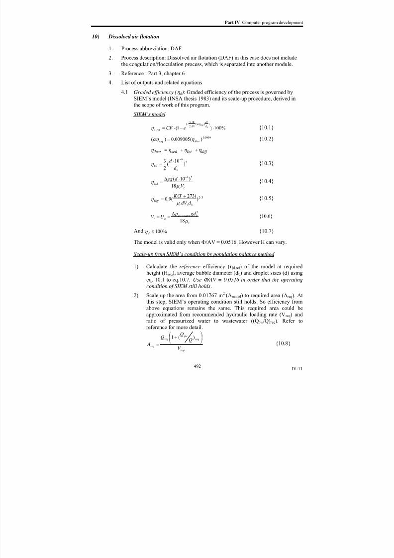
8/15/2019 Rachu.pdf
http://slidepdf.com/reader/full/rachupdf 576/646
Part IV Computer program development
IV-71
10) Dissolved air flotation
1. Process abbreviation: DAF
2. Process description: Dissolved air flotation (DAF) in this case does not include
the coagulation/flocculation process, which is separated into another module.
3. Reference : Part 3, chapter 6
4.
List of outputs and related equations
4.1 Graded efficiency (η d ): Graded efficiency of the process is governed by
SIEM’s model (INSA thesis 1983) and its scale-up procedure, derived in
the scope of work of this program.
SIEM’s model
%100)1())(
2
3(
,
exp
⋅−⋅=Φ
−bd
H
AV
ref d eCF αη
η {10.1}
5919.0exp )(009005.0)( theoη αη = {10.2}
diff Int sed theo η η η η ++=
26
)10
(2
3
b
Int d
d −⋅
=η {10.3}
r c
sed V
d g
μ
ρ η
18
)10( 26−⋅Δ= {10.4}
3/2))273(
(9.0br c
Diff d dV
T K
μ η
+= {10.5}
c
bwater air br
gd U V
μ
ρ
18
2
/Δ
== {10.6}
And %100≤d η {10.7}
The model is valid only when Φ/AV = 0.0516. However H can vary.
Scale-up from SIEM’s condition by population balance method
1) Calculate the reference efficiency (ηd,ref ) of the model at required
height (Hreq
), average bubble diameter (d b) and droplet sizes (d) using
eq. 10.1 to eq.10.7. Use Φ /AV = 0.0516 in order that the operating
condition of SIEM still holds.
2) Scale up the area from 0.01767 m2 (Amodel) to required area (Areq). At
this step, SIEM’s operating condition still holds. So efficiency from
above equations remains the same. This required area could be
approximated from recommended hydraulic loading rate (Vreq) and
ratio of pressurized water to wastewater ((Q pw/Q)req). Refer to
reference for more detail.
req
req pw
req
reqV
Q
A
⎟ ⎠
⎞⎜⎝
⎛ +
=
)(1
{10.8}
492

8/15/2019 Rachu.pdf
http://slidepdf.com/reader/full/rachupdf 577/646
Chapter 3 Process references
IV-72
3)
Find Φref , corresponding to the area Areq, by following equation,
01767.0
102.4 7
mod
mod
req
el
el
req
ref
A
A
A −×
=Φ⋅=Φ m3/s {10.9}
4)
Find τref , corresponding to the height Hreq, by following equation,
3600
1
00046.0mod
mod
⋅=⋅= req
el
el
req
ref H
H
H τ τ Hour {2.610.10}
Change Φ and τ from SIEM’s condition by population balance model
5)
From population balance method, calculate κ2,ref corresponding to
Areq, Hreq, τref and Φref from the reference efficiency (from item 1)) by
the following equations. Please note that, at this point, SIEM’s
condition still holds. κ2,req has to be calculated separately for each
droplet diameter.
ref ref
ref d
ref
τ
η κ
⋅Φ
−−=
)1ln( ,
,2 {10.11}
Or)(
,,21 ref ref ref eref d
τ κ η
Φ−−= {10.12}
6) Find Φreq from required ratio of pressurized water to wastewater (see
reference for the recommended value) by following equations.
3600
Q R
V
V Q
V
V
pw
air pw
pw
air ⋅⋅=⋅=Φ m3/s {10.13a}
Then, from Henry’s law
Q R H K molmT PP y atm ⋅⋅⋅⋅×⋅+⋅−⋅=Φ −))/(10082.0()273()( 33 {10.13b}
For air, y = 1. H is Henry’s constant as molair /(m
3
water .atm). Henry’sconstant of air can be calculated from the following equation.123 10)472.122745.00039.000002.0( −⋅+⋅−⋅+⋅−= T T T H {10.14}
7) Choose τreq from recommended criteria (see reference).
8) To change Φ and τ from SIEM’s, the following procedure is
recommended and precautions should be noted.
• To decrease ( req < ref ) and increase τ (τreq > τref ):
In this case, κ2 is assumed to remain the same and be equal to
κ2,ref . Φreq and τref are used. The efficiency can be estimated by eq.
10.15a.)( ,21 ref reqref ed
τ κ η
Φ−−= {10.15a}
The calculated efficiency will be lower than the real value.
• To decrease ( req < ref ), as well as, τ (τreq < τref ):
In this case, κ2 = κ2,ref . Φreq and τreq are used. The efficiency can
be calculated by eq. 10.15b. The calculated efficiency will be
lower than the real value.)( ,21 reqreqref ed
τ κ η
Φ−−= {10.15b}
493

8/15/2019 Rachu.pdf
http://slidepdf.com/reader/full/rachupdf 578/646
Part IV Computer program development
IV-73
• To increase ( req > ref ) and decrease
τ
(τreq <
τref ):
Like the former case, the efficiency can be calculated by eq.
10.15b.
•
To increase ( req > ref ), as well as,
τ
(τreq >
τref ):
This case is not feasible because it means that we have to
decrease wastewater flowrate and increase pressurized water
flowrate.
There is no obvious limit for the 4 adaptations, shown above.
However it is recommended to use the values of each parameter
(d, d b, C, etc.) within general range (see reference).
It must be noted that the graded efficiency in this case is independent of
source of water that is used as pressurized water.
4.2 Total efficiency (η t ): The value depends on the source of water that is used
as pressurized water. In the program, it is assumed that DAF effluent isused to prepare pressurized water.
%100)(
⋅−
=o
ot
C
C C η
{10.16a}
4.3 Graded outlet oil concentration in water outlet flow (C d ): In the program, it
is assumed that DAF effluent is used to prepare pressurized water. Thus
residual oil in the effluent is recycled. So oil of certain droplet sizes may
accumulate in the system, depending on their ηd.
dilod d
out
d C Q
QC ,)1( η −⋅= mg/l {10.17}
t
od
d
r d
dilod Q
QC
R
R R
R
C ⋅−−
+
−−+=
−
1)1(1
)1))1(1
((1max
,
η
η mg/l {10.18}
The r max is an assumed number of loop, which effluent is recycled until the
concentration reaches steady stage. Ideally, r max must approach infinity.
However, the value of r max in the program is set at 30, which is generally
sufficient to make the equation reach steady stage (esp. when ηd > 20%). If
the value of Cod,dil from r = 30 differs from Cod, dil at r = 29 more than 10%,
the program will display the warning box, showing that the oil may
accumulate in the system.
4.4 Total outlet oil concentration in water outlet flow (C ):
∑=max
min
d
d
d C C
mg/l
{10.19}
4.5 Graded outlet oil concentration in oil outlet flow (C oild ): The outlet oil in
the oil outlet flow is in pure condition (100% oil).
4.6 Total outlet oil concentration in oil outlet flow (C oil): The outlet oil in the
oil outlet flow is in pure condition (100% oil).
4.7
Inlet flow (Q): Inlet flow of the process is equal to the outlet flow of theupstream process.
494

8/15/2019 Rachu.pdf
http://slidepdf.com/reader/full/rachupdf 579/646
Chapter 3 Process references
IV-74
4.8 Water outlet flow (Qout ):
)1000//)(1( oiloout C C QQ ρ −−=
m3/h
{10.20}
4.9 Oil outlet flow(Qoil):
oiloil QQQ −= m3/h {10.21}
4.10 Customized output :
4.10.1 Ratio of air/oil (W/W)
1000
3600
0
⋅⋅
⋅Φ=
C QW
W air req
oil
air ρ
kg air / kg oil {10.22}
4.10.2 Theoretical energy (watt) required for air compressor:
pw
atmcomp
air Qair MW
air Conc
P
PT RPower ⋅⋅
⎥⎥⎥
⎦
⎤
⎢⎢⎢
⎣
⎡−⎥
⎦
⎤⎢⎣
⎡
⋅+
=
−
)1000/)((
)(1
4.0
)273()
4.1
14.1(
η
{10.23}
R air = universal gas constant (8.314)
1000
)().(
H air MW P yair Conc
⋅⋅⋅= mg/l
{10.24}
4.10.3 Theoretical energy required for pressurized water pump:
pump
atmc
pump
atm pw PPgQ RPPQPower
η
ρ
η ⋅⋅−⋅⋅⋅⋅
=⋅
−⋅=
3600
10)(
3600
)( watt {10.25}
P is measured in atm.
4.10.4 Hydraulic loading rate
A
RQ
V
)1( +
=
m/h
{10.25}
4.10.5 Retention time (based on total flow (Q+Q pressurized water ):
60⋅=V
H τ min {10.25}
5.
Related parameters: Related parameters are as summarized in the following table
Table 10-1 Related parameters of DAF
Parameter DescriptionVariable name in
the program
Unit used in the
program
A Cross section area of DAF column A m2
d b Diameter of bubble db m
H Column height DAFH m
P Absolute pressure of saturator DAFP atm
R Recycled ratio (R = Q pressurized water /Q) R
ηcomp, η pump Efficiency of air compressor and pressurized
water pump (always < 100%, 60-70% is
recommended)
Constant = 70%
Note: Other parameters are internally used. Users do not need to input. For list of others parameters, see reference.
495
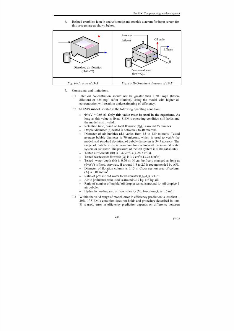
8/15/2019 Rachu.pdf
http://slidepdf.com/reader/full/rachupdf 580/646
Part IV Computer program development
IV-75
6. Related graphics: Icon in analysis mode and graphic diagram for input screen for
this process are as shown below.
Dissolved air flotation
(DAF-??)
Pressurized water
flow = Q pw
Oil outlet
Effluent
Influent
H
Area = A
Fig. 10-1a Icon of DAF Fig. 10-1b Graphical diagram of DAF
7. Constraints and limitations.
7.1 Inlet oil concentration should not be greater than 1,200 mg/l (before
dilution) or 435 mg/l (after dilution). Using the model with higher oil
concentration will result in underestimating of efficiency.
7.2 SIEM’s model is tested at the following operating condition;
• Φ/AV = 0.0516. Only this value must be used in the equations. As
long as this value is fixed, SIEM’s operating condition still holds and
the model is still valid. • Retention time, based on total flowrate (Qt), is around 25 minutes.
•
Droplet diameter (d) tested is between 2 to 40 microns.
• Diameter of air bubbles (d b) varies from 15 to 130 microns. Tested
average bubble diameter is 70 microns, which is used to verify the
model, and standard deviation of bubble diameters is 34.5 microns. The
range of bubble sizes is common for commercial pressurized water
system or saturator. The pressure of the test system is 4 atm (absolute).
• Tested air flowrate (Φ) is 0.42 cm3/s (4.2e-7 m3/s).
• Tested wastewater flowrate (Q) is 3.9 cm3/s (3.9e-6 m3/s)
•
Tested water depth (H) is 0.70 m. H can be freely changed as long as
(Φ/AV) is fixed. Anyway, H around 1.8 to 2.7 is recommended by API. • Diameter of flotation column is 0.15 m Cross section area of column
(A) is 0.01767 m2.
• Ratio of pressurized water to wastewater (Q pw/Q) is 1.76.
•
Air to pollutants ratio used is around 0.12 kg. air/ kg. oil.
• Ratio of number of bubble/ oil droplet tested is around 1.4 oil droplet/ 1
air bubble.
• Hydraulic loading rate or flow velocity (V), based on Qt, is 1.6 m/h
7.3
Within the valid range of model, error in efficiency prediction is less than ±
20%. If SIEM’s condition does not holds and procedure described in item
8) is used, error in efficiency prediction depends on difference between
496
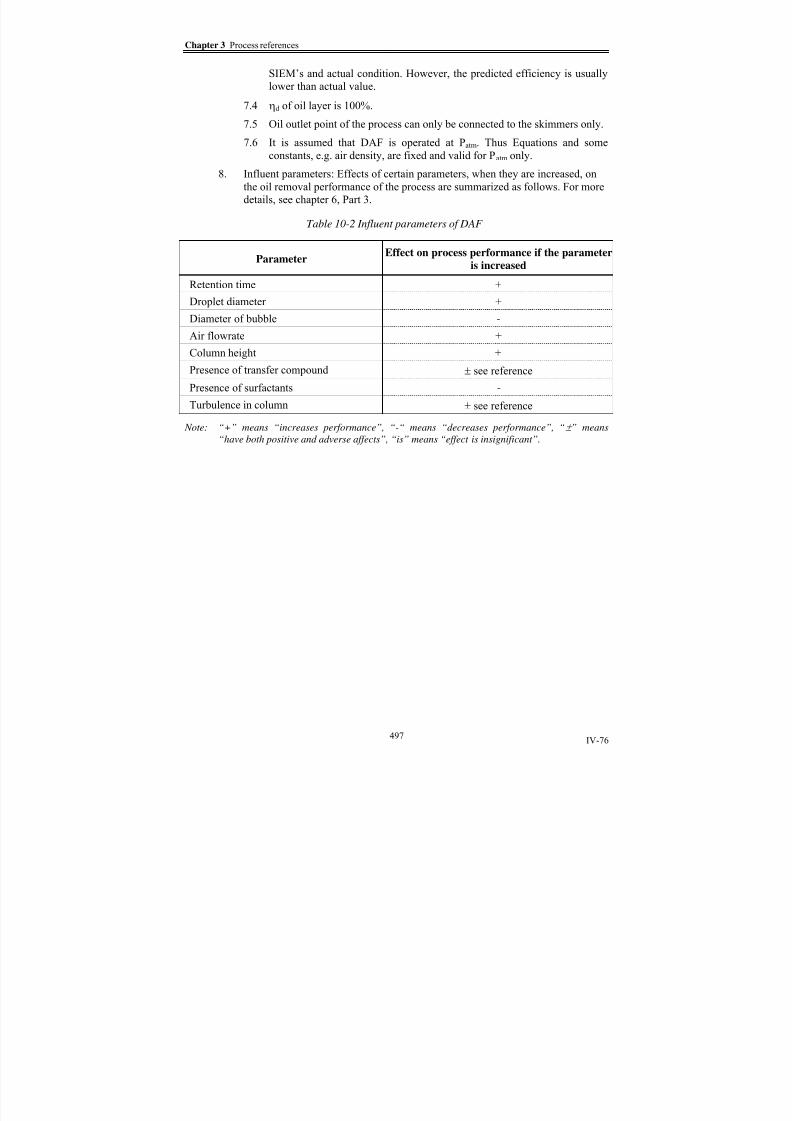
8/15/2019 Rachu.pdf
http://slidepdf.com/reader/full/rachupdf 581/646
Chapter 3 Process references
IV-76
SIEM’s and actual condition. However, the predicted efficiency is usually
lower than actual value.
7.4 ηd of oil layer is 100%.
7.5 Oil outlet point of the process can only be connected to the skimmers only.
7.6
It is assumed that DAF is operated at Patm. Thus Equations and some
constants, e.g. air density, are fixed and valid for Patm only.
8.
Influent parameters: Effects of certain parameters, when they are increased, on
the oil removal performance of the process are summarized as follows. For more
details, see chapter 6, Part 3.
Table 10-2 Influent parameters of DAF
ParameterEffect on process performance if the parameter
is increased
Retention time +
Droplet diameter +
Diameter of bubble -
Air flowrate +
Column height +
Presence of transfer compound ± see reference
Presence of surfactants -
Turbulence in column ± see reference
Note: “+” means “increases performance”, “-“ means “decreases performance”, “± ” means
“have both positive and adverse affects”, “is” means “effect is insignificant”.
497

8/15/2019 Rachu.pdf
http://slidepdf.com/reader/full/rachupdf 582/646
Part IV Computer program development
IV-77
11) Two-phase hydrocyclone
1. Process abbreviation: 2CY
2. Process description: The process is based on THEW type, liquid-liquid
hydrocyclone.
3. Reference : Part 3, chapter 7
4.
List of outputs and related equations
4.1 Graded efficiency (η d ): Graded efficiency of the process is governed by the
following equation.
For d ≥ dc, %100=η {11.1}
For d < dc,
%1002)2nD
(0.1862)2nD
((
2)2
nD(0.186
2d
(R
dη ⋅−
−
= {11.2}
R d (Radial distance from axial axis to entry position of droplet “d”
(Z=0))can be calculated from the following equations. If R d in eq. 11.3a is
equal to Dn/2, the corresponding “d” will be equal to dc.
∫=∫L
0 W
dZdR
zvvR U
dR {11.3a}
R
V 2
18μ
2)6-10Δρ(dU ⋅
⋅= m/s {11.3b}
0.65)R
nD)(
2i
πD
Q(V = m/s {11.3c}
3
19.1
2
63.81233.3 ⎟⎟ ⎠
⎞⎜⎜⎝
⎛ +⎟⎟
⎠
⎞⎜⎜⎝
⎛ −+−=
z R
R
z R
R
z R
R
zW
W {11.3d}
2))
2
tan(Znπ(0.5D
QzW
β ⋅−
= m/s {11.3e}
)2
tan(2
β ⋅−= Z
D R n
z m {11.3f}
)2/5.1tan(
)(25.0o
n D L = m {11.3g}
For THEW’s type hydrocyclone, when Z = L:
)2/(186.0 nVZZ D R = {11.3f}
4.2 Total efficiency (η t ):
∑ ⋅−
=max
min
%100)1(
1 d
d f
od d
o
t R
C
C
η η
{11.4}
498

8/15/2019 Rachu.pdf
http://slidepdf.com/reader/full/rachupdf 583/646
Chapter 3 Process references
IV-78
4.3 Graded outlet oil concentration in water outlet flow (C d ):
)1(
)1(
f
od d
d R
C C
−
−=
η
mg/l
{11.5}
4.4 Total outlet oil concentration in water outlet flow (C ):
∑=max
min
d
d
d C C mg/l
{11.6}
4.5 Graded outlet oil concentration in oil outlet flow (C oild ): Unlike other true
separation process, hydrocyclone only concentrates oil. Thus concentrated
oily wastewater, not pure oil, is obtained at oil outlet (overflow) port.
f
od d overflowd oild
R
C C C
η == ,
mg/l {11.7}
4.6 Total outlet oil concentration in oil outlet flow (C oil):
∑=
max
min
d
d
oild oil C C
mg/l
{11.8}
4.7 Inlet flow (Q): Inlet flow of the process is equal to the outlet flow of the
upstream process.
4.8 Water outlet flow (Qout ):
)1( f out RQQ −= m3/h {11.9}
4.9 Oil outlet flow(Qoil):
f oil RQQ ⋅= m3/h {11.10}
4.10
Customized output :
4.10.1 Theoretical cut size (d c): Cut size is calculated from item 4.1.
4.10.2 Pressure drop (P): Pressure drops across inlet/overflow (Po) and
inlet/underflow (Pu) ports of 2-phase hydrocyclone are governed
by the following equations.
1611.0
4
3.2
)1(
6.2)3600/(16 ⎟
⎟ ⎠
⎞⎜⎜⎝
⎛
−⋅=Δ
f n
o R D
QP bar {11.11a}
4
2.2)3600/(6.4
n
u D
QP =Δ bar {11.11b}
5. Related parameters: Related parameters are as summarized in the following table
499
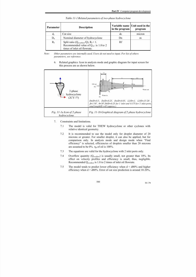
8/15/2019 Rachu.pdf
http://slidepdf.com/reader/full/rachupdf 584/646
Part IV Computer program development
IV-79
Table 11-1 Related parameters of two-phase hydrocyclone
Parameter DescriptionVariable name
in the program
Unit used in the
program
dc Cut size dc micronDn Nominal diameter of hydrocyclone Dn m
R f Split ratio (Qoverflow/Q), R f < 1.
Recommended value of Qoil is 1.8 to 2
times of inlet oil flowrate.
Rf
Note: Other parameters are internally used. Users do not need to input. For list of others
parameters, see reference.
6.
Related graphics: Icon in analysis mode and graphic diagram for input screen for
this process are as shown below.
Di
L1
D
Dn
Ds
L3
Do
θ
β
L
Oil out
Water out
Water in
2-phase
hydrocyclone
(2CY-??)
Dn/D=0.5, Ds/D=0.25, Do/D<0.05, L1/D=1, L3/D=15-20 ,
β =1.50o , θ =20o ,Di/D=0.25 for 1 inlet and 0.175 for 2 inlet ports,
total length/D =45 (approx.)
Fig. 11-1a Icon of 2-phase
hydrocyclone
Fig. 11-1b Graphical diagram of 2-phase hydrocyclone
7.
Constraints and limitations.
7.1 The model is valid for THEW hydrocyclone or other cyclones with
relative identical geometry.
7.2 It is recommended to use the model only for droplet diameter of 20
microns or greater. For smaller droplet, it can also be applied, but forcomparison only. In analysis mode and design mode when “Find
efficiency” is selected, efficiencies of droplets smaller than 20 microns
are assumed to be 0%. ηd of oil is 100%.
7.3
The equations are valid for the hydrocyclone with 2 inlet ports only.
7.4
Overflow quantity (Qoveflow) is usually small, not greater than 10%. Its
effect on velocity profiles and efficiency is small, thus, negligible.
Recommended Qoveflow is 1.8 to 2 times of inlet oil flowrate.
7.5 The model tends to predict lower efficiency when d < d80% and higher
efficiency when d > d80%. Error of cut size prediction is around 10-20%,
500

8/15/2019 Rachu.pdf
http://slidepdf.com/reader/full/rachupdf 585/646
Chapter 3 Process references
IV-80
e.g. if predicted cut size is 50 microns, observed cut size should be
around 40 – 45 microns. For more details, see reference.
7.6 Graded efficiency (ηd) in this case is based on ratio between outlet oil
quantity at water outlet port to that of inlet wastewater. Effect of split
flow is not yet taken into account.
8.
Influent parameters: Effects of certain parameters, when they are increased, on
the oil removal performance of the process are summarized as follows. For more
details, see chapter 7, Part 3.
Table 11-2 Influent parameters of two-phase hydrocyclone
ParameterEffect on process performance if
the parameter is increased
Flowrate +
Droplet diameter +
Split ratio is
Inlet oil concentration is
Pressure drop +
Presence of surfactants -
Temperature +
Note: “+” means “increases performance”, “-“ means “decreases performance”, “± ” means
“have both positive and adverse affects”, “is” means “effect is insignificant”.
501

8/15/2019 Rachu.pdf
http://slidepdf.com/reader/full/rachupdf 586/646
Part IV Computer program development
IV-81
12) Three-phase hydrocyclone
1. Process abbreviation: 3CY
2. Process description: The process is based on 3-phase hydrocyclone, initiated by
MA and AURELLE. Geometry of liquid-liquid separation of the hydrocyclone is
based on Thew type. For solid-liquid, it is based on Rietema type. It can be usedfor simultaneous separation of oil and suspended solids from wastewater.
Calculation procedure and equation are relatively identical to that of 2-phase
cyclone with only little modification. Solid removal efficiency is not included in
this program.
3. Reference : Part 3, chapter 7
4. List of outputs and related equations
4.2 Graded efficiency (η d ): Graded efficiency of the process is governed by the
following equations. Dn in this case is equal to Do and L is equal to L5 (See
graphical diagram).
For d ≥ dc, %100=η {12.1}
For d < dc,
%1002)
2
nD(0.1862)
2
nD((
2)2
nD(0.186
2d
(R
dη ⋅
−
−= {12.2}
R d (Radial distance from axial axis to entry position of droplet “d”
(Z=0))can be calculated from the following equations. If R d in eq. 12.3a is
equal to Dn/2, the corresponding “d” will be equal to dc.
∫=∫L
0 W
dZdR
zvvR U
dR {12.3a}
R
V 2
18μ
2)6-10Δρ(dU ⋅
⋅= {12.3b}
0.65)R
nD(
2
iD4
π
(Q/2)0.676V
⎟⎟⎟⎟
⎠
⎞
⎜⎜⎜⎜
⎝
⎛
= {12.3c}
3
19.1
2
63.81233.3 ⎟⎟ ⎠
⎞⎜⎜⎝
⎛ +⎟⎟
⎠
⎞⎜⎜⎝
⎛ −+−=
z R
R
z R
R
z R
R
zW
W {12.3d}
2/2))tan(Znπ(0.5D
QzW
β ⋅−= {12.3e}
)2
tan(2
β ⋅−= Z
D R n
z {12.3f}
)2/5.1tan()(25.0 o
n D L = {12.3g}
502

8/15/2019 Rachu.pdf
http://slidepdf.com/reader/full/rachupdf 587/646
Chapter 3 Process references
IV-82
For THEW’s part hydrocyclone, when Z = L:
)2/(186.0 nVZZ D R = {12.3f}
4.2 Total efficiency (η t ):
∑ ⋅−=
max
min
%100)1(
1 d
d f
od d
o
t R
C
C
η η
{12.4}
4.3 Graded outlet oil concentration in water outlet flow (C d ):
)1(
)1(
f
od d d
R
C C
−−
= η mg/l
{12.5}
4.4 Total outlet oil concentration in water outlet flow (C ):
∑=max
min
d
d
d C C mg/l 12.6}
4.5 Graded outlet oil concentration in oil outlet flow (C oild ): Unlike other true
separation process, hydrocyclone only concentrate oil. Thus concentratedoily wastewater, not pure oil, is obtained at oil outlet (overflow) port.
f
od d oild
R
C C
η = mg/l {12.7}
4.6 Total outlet oil concentration in oil outlet flow (C oil):
∑=max
min
d
d
oild oil C C mg/l {12.8}
4.7 Inlet flow (Q): Inlet flow of the process is equal to the outlet flow of the
upstream process.
4.8 Water outlet flow (Qout ):
)1(SS f out R RQQ −−= m3/h {12.9}
4.9 Oil outlet flow(Qoil):
f oil RQQ ⋅= m3/h {12.10}
4.10 Customized output :
4.10.1 Theoretical cut size (d c): Cut size is calculated from item 4.1.
4.10.2 Purged flow for SS removal:
SS ss RQQ ⋅=
{12.11}4.10.3
Pressure drop (P): Pressure drops across inlet/overflow (Po) and
inlet/underflow (Pu) ports of 2-phase hydrocyclone are governed
by the following equations.
4D
2.12(Q/3600)49.8water ΔP = bar {12.12a}
4D
2.34(Q/3600)21ssΔP = bar {12.12b}
4D
2.03(Q/3600)55
oilΔP = bar {12.12c}
503

8/15/2019 Rachu.pdf
http://slidepdf.com/reader/full/rachupdf 588/646
Part IV Computer program development
IV-83
Please not that R SS is not included in the model so the pressure drop for SS
port and water port are estimated value only. But for oil port, R f is usually
small so ΔPoil is relatively accurate and hardly affected by R f .
5. Related parameters: Related parameters are as summarized in the following table
Table 12-1 Related parameters of three-phase hydrocyclone
Parameter DescriptionVariable name
in the program
Unit used in the
program
dc Cut size dc micron
D Diameter of the biggest cylinder of
hydrocyclone (refer to related graphic)
D3cy m
R f Split ratio (Qoil /Q), Rf < 1.
Recommended value of Qoil is 1.8 to 2times of inlet oil flowrate.
R SS Split ratio (QSS/Q). Recommended value
is 0.2.
Note: 1. Other parameters are internally used. Users do not need to input. For list of others
parameters, see reference.
2. Rss is calculated by Yoshioka and Hotta relation [30]: 1-R f =0.95/((Du/Ds)4+1).
6. Related graphics: Icon in analysis mode and graphic diagram for input screen for
this process are as shown below.
Solid-liquid part Liquid-liquid part (Thew’s part)
DoDDs
DiDu
Dp
L5 L3L1L3
L4
3-phase
hydrocyclone
(3CY-??)
Note: Di/D=0.25 for 1- inlet and 0.175 for 2- inlet,
Do/D=0.43,Ds/D=0.28, Du/D=0.19, Dp/D=0.034,
L1/D=0.4,L2/D=5, L3/D=15, L4/D=0.3, Solid-liquid part cone
angle=12o , for liquid-liquid part=1.5
o
Fig. 12-1a Icon of 3-phase
hydrocyclone
Fig. 12-1b Graphical diagram of 3-phase hydrocyclone
7. Constraints and limitations.
7.1
The model is valid for THEW hydrocyclone or other cyclones with relative
identical geometry.
504

8/15/2019 Rachu.pdf
http://slidepdf.com/reader/full/rachupdf 589/646
Chapter 3 Process references
IV-84
7.2 It is recommended to use the model only for droplet diameter of 20
microns or greater. For smaller droplet, it can also be applied, but for
comparison only. In analysis mode and design mode when “Find
efficiency” is selected, efficiencies of droplets smaller than 20 microns are
assumed to be 0%. ηd of oil is 100%.
7.3
The equations are valid for the hydrocyclone with 2 inlet ports only.
7.4
Purged quantity at oil outlet port (Qoil) is usually small, not greater than
10%. Its effect on velocity profiles and efficiency is small, thus, negligible.
7.5 The model tends to predict lower efficiency when d < d80% and higher
efficiency when d > d80%. Error of cut size prediction is around 10-20%,
e.g. if predicted cut size is 50 microns, observed cut size should be around
40 – 45 microns. For more details, see reference.
7.6 SS removal coefficient is not calculated since it is not major scope of work
of this thesis so it cannot connect to other model. Only purged flow of SS
port is calculated
7.7
R SS is not included in the model so the pressure drop for SS port and water
port are estimated value only. But for oil port, R f is usually small so ΔPoil is
relatively accurate and hardly affected by R f .
7.8 Graded efficiency (ηd) in this case is based on ratio between outlet oil
quantity at water outlet port to that of inlet wastewater. Effect of split flow
is not yet taken into account.
8. Influent parameters: Effects of certain parameters, when they are increased, on
the oil removal performance of the process are summarized as follows. For more
details, see chapter 7, Part 3.
Table 12-2 Influent parameters of three-phase hydrocyclone
ParameterEffect on process performance if
the parameter is increased
Flowrate +
Droplet diameter +
Split ratio (R f ) is
Inlet oil concentration isPressure drop +
Presence of surfactants -
Temperature +
Note: “+” means “increases performance”, “-“ means “decreases performance”, “± ” means
“have both positive and adverse affects”, “is” means “effect is insignificant”.
505

8/15/2019 Rachu.pdf
http://slidepdf.com/reader/full/rachupdf 590/646
Part IV Computer program development
IV-85
13) Ultrafiltration
1. Process abbreviation: UF
2. Process description: Flux calculation of UF in the program is based on film
model and resistance model. Flux prediction is available in DESIGN mode only.
3. Reference : Part 3, chapter 8
4.
List of outputs and related equations
4.1 Graded efficiency (η d ): For stabilized emulsion wastewater, oil removal
efficiency of UF can be safely assume to be 100%. The program will use
the value of CF.100%.
%100⋅= CF d η
{13.1a}
For wastewater containing free oil or non -stabilized emulsion, the
efficiency is lower but, somehow, unpredictable. Anyway, for such
wastewater, the use of UF is not necessary. However the program will,nonetheless, assume that the efficiency is CF.100%.
4.2 Total efficiency (η t ): Total efficiency falls into the same case as that of
hydrocyclone. For UF, users normally set their final volume of filtrated
wastewater or retentate (Volretentate), which will be used for total efficiency
calculation. UF calculation in the program is based on batch system
without additional feed during operation period. So the concentration
depends on initial wastewater volume (Volo) and feed duration (tf )
∑∑ ⋅−
−=⋅
−
−=
max
min
max
min
%100
)1
1(
)1(1%100
)1(
)1(1 d
d
od d
o
d
d
o
retentate
od d
o
t
F
C
C
Vol
Vol
C
C
η η η
{13.1b}
F is factor of concentration, which is specified by user.
4.3 Graded outlet oil concentration in water outlet flow (C d ):
)1(
)1(
o
retentate
od d
d
Vol
Vol
C C
−
−=
η mg/l {13.2}
4.4 Total outlet oil concentration in water outlet flow (C ):
∑=max
min
d
d
d C C
mg/l
{13.3}
4.5 Graded outlet oil concentration in oil outlet flow (C oild ): Unlike other true
separation process, UF only concentrate oil. Thus concentrated oily
wastewater, not pure oil, is obtained as retentate. Granulometries of the
retentate were not studied. Coalescence and partial destabilization, which
leads to formation of oil film, were reported. However, to be on the safe
side, the program will assume that there is no coalesce occurring.
F C VolVol
C C od d
oretentate
od d oild η
η ==
)/( mg/l {13.4}
506

8/15/2019 Rachu.pdf
http://slidepdf.com/reader/full/rachupdf 591/646
Chapter 3 Process references
IV-86
4.6 Total outlet oil concentration in oil outlet flow (C oil):
∑=max
min
d
d
oild oil C C mg/l {13.5}
4.7 Inlet flow (Q): Inlet flow of the process is equal to the outlet flow of the
upstream process.4.8 Water outlet flow (Qout ): Actual water outlet flow from the membrane is the
product of permeate flux, which varies with time, and membrane area.
However, since the process is usually designed as batch system, outlet flow
can be chosen freely, providing that permeate storage tank is big enough.
User can freely specify permeate discharge time (td). To imitate a
continuous process, it can be assumes that default permeate discharge
duration (td) is equal to wastewater inlet duration.
)1
1()(
F t Q
t
Volt QQ f
d
retentate f
out −⋅⋅=
−⋅= m3/h
{13.6}
4.9
Oil outlet flow (Qoil): Like water outlet flow, oil outlet flow or retantateflow depends on its discharge duration (tdoil). This duration should be equal
to that of tf and td to fully imitate continuous process.
doil
f
doilretentateoilt F
t Qt VolQ
⋅
⋅== / m3/h
{13.7}
4.10 Customized output :
4.10.1 Permeate flux and volume evolution: Flux varies with time since
concentration of the feed (actually, retentate) increases from
continuous loss of its permeate. The program can calculate the
flux under the assumption that there is no fouling, which is
practically proven in case that suitable pretreament is provided.Flux will be calculated using 2 models, i.e. Film model and
Resistance model, and the related equations,
)ln(C
C kV J
g β = l/(m2-h) {13.8}
t m
t
PV R
P J
⋅⋅+=
α φ ' l/(m2-h) {13.9}
))(0239.0( A B
C BC Ae J J oo
−−= {13.10}
The values of K, Cg, etc. for certain wastewaters are provided in
help file.
If two types of wastewater with different values of k, Cg,
etc.(such as microemulsion mixes with macroemulsion.) are
encountered, the flux will be calculated using weight average
method (eq. 13.11). This calculation exists only in design mode.
mixoil,C
mixCoil,mic, J
micoil,C
mixCoil,:mac J
macoil,C
mix J +
= {13.11}
Evolution of permeate flux and volume is governed by the
following equation.
AdtJ(c)dVol ⋅= {13.12}
507

8/15/2019 Rachu.pdf
http://slidepdf.com/reader/full/rachupdf 592/646
Part IV Computer program development
IV-87
Integration of eq. 13.11 is carried out using step method by
dividing total permeate volume (eq. 3.12) into 100 parts.
4.10.2 Time required to complete one batch for a specified amount of
wastewater : It is also governed by eq. 13.12. It must be noted that
the program can calculate the flux/time evolution under the
condition that there is no additional inlet wastewater during UF
operation.
5. Related parameters: Related parameters are as summarized in the following table
Table 13-1 Related parameters of ultrafiltration
Parameter DescriptionVariable name in
the program
Unit used in the
program
A Membrane area AreaUF m2
C’g, C’
g2 Gel concentration for low range of
concentration (if any) of 1st and 2nd emulsion
Cg1low, Cg2low % oil volume/total
volume
Cg, Cg2 Real gel concentration of 1st and 2
nd emulsion
(see reference)
Cg1High,
Cg2High
% by volume of oil
Cref1, Cref2 Reference concentration of 1st and 2
ndemulsion
(conc. that is used to acquire the value of
model constants)
Cref1, Cref2 % by volume of oil
Co1/(Co1+Co2
)
Oil concentration ratio of wastewater no.1 to
total oil concentration[2], always < 1
Rofoil1 in the unit of bar,
(m/s) and l/h-m2
k’1, k’2 Constant for film model for low range of oil
concentration of 1st and 2nd emulsion
Kreflow1,
kreflow2
in the unit of bar,
(m/s) and l/h-m2
k 1, k 2 Constant for film model for high range of oil
concentration of 1st
and 2nd
emulsion
Krefhigh1,
krefhigh2
in the unit of bar,
(m/s) and l/h-m2
Pt Transmembrane pressure UFP bar
Q Flowrate of inlet wastewater Q m3/s
Rm (or R’m) Modified membrane resistance (= membrane
resistance + fouling resistance (if any))
Rm in the unit of bar,
(m/s) and l/h-m2
td Duration for discharge the permeate (after UF
operation is finished), recommended to be
equal to tf .
td h
tdoil Duration for discharge the retentate (after UF
operation is finished), recommended to be
equal to tf .
tdoil h
tf Duration to fill the storage tank by inlet
wastewater before the wastewater is stopped
and UF operation starts.
tf h
V Recirculation velocity UFV m/s
F Concentration factor (Volo /Volretentate) ConcF
α1, α2 Constant for resistance model of 1st and 2
nd
emulsion
alpharef1,
alpharef2
in the unit of bar,
(m/s) and l/h-m2
β1, β2 Constant for film model of 1st and 2
nd emulsion bref1, bref2 in the unit of bar,
(m/s) and l/h-m2
φ1,φ2 Constant for film model of 1st and 2
nd emulsion Phiref1,Phiref2 in the unit of bar,
(m/s) and l/h-m2
Note: 1. Other parameters are internally used. Users do not need to input. For list of others
parameters, see reference.
508

8/15/2019 Rachu.pdf
http://slidepdf.com/reader/full/rachupdf 593/646
Chapter 3 Process references
IV-88
6. Related graphics: Icon in analysis mode and graphic diagram for input screen for
this process are as shown below.
Ultrafiltration
(UF-??)
UF
Permeate
Retentate
Membrane
Feed
pump
Storage
tank
Feed
Po
Pi
Pp
Heat
exchanger
Pt = ((Pi+Po)/2)-P p
V
No influent added during filtration process
Fig. 13-1a Icon of ultrafiltration Fig. 13-1b Graphical diagram of ultrafiltration
7. Constraints and limitations.
7.1 Flux calculation of mixed wastewater exists only in design mode.
7.2 The process can be used for microfiltration and nanofiltration if they can be
represented by film model and resistance model.
7.3 The program can calculate only batch operation.
7.4
Accuracy of the models are governed by that of constants used, and
deviation of real operation from their assumption, thus unpredictable. If
possible, it is recommended to perform UF test, using real wastewater.
8. Influent parameters: Effects of certain parameters, when they are increased, on
the oil removal performance of the process are summarized as follows. For more
details, see chapter 8, Part 3.
Table 13-2 Influent parameters of ultrafiltration
ParameterEffect on process performance if
the parameter is increased
Viscosity of feed -
Temperature +
Membrane properties ±
Reaction between feed and membrane ±
Note: “+” means “increases performance”, “-“ means “decreases performance”, “± ” means
“have both positive and adverse affects”, “is” means “effect is insignificant”.
509

8/15/2019 Rachu.pdf
http://slidepdf.com/reader/full/rachupdf 594/646
Part IV Computer program development
IV-89
14) Reverse osmosis
1. Process abbreviation: RO
2. Process description: RO in this case is used as a finishing treatment process to
treat the effluent of UF or distillation only. Its main purpose is to remove soluble
pollutants, normally surfactants/co-surfactants, left after oil separation.Furthermore, process calculation is based mainly on specific data from
manufacturer. Thus, the module exists only in ANALYSIS mode.
3. Reference : Part 3, chapter 8
4. List of outputs and related equations
4.1 Graded efficiency (η d ): It is assumed to be 100%. CF is not allowed in this
process.
4.2 Total efficiency (η t ): It is assumed to be 100%.
4.3
Graded outlet oil concentration in water outlet flow (C d ):Cd = 0 mg/l
4.4 Total outlet oil concentration in water outlet flow (C ):
C = 0 mg/l
4.5 Graded outlet oil concentration in oil outlet flow (C oild ): Unlike other true
separation process, RO only concentrate oil. Thus concentrated oily
wastewater, not pure oil, is obtained as retentate. The program will assume
that droplet sized and numbers are not changed.
F C VolVol
C C
od d oretentate
od d
oild
η η
==)/(
mg/l {14.1}
4.6 Total outlet oil concentration in oil outlet flow (C oil):
∑=max
min
d
d
oild oil C C mg/l {14.2}
4.7 Inlet flow (Q): Inlet flow of the process is equal to the outlet flow of the
upstream process.
4.8 Water outlet flow (Qout ): Actual water oultet flow from the membrane is the
product of permeate flux, which varies with time, and membrane area.
However, since the process is usually designed as batch system, outlet flow
can be chosen freely, providing that permeate storage tank is big enough.User can freely specify permeate discharge time (td). To imitate a
continuous process, it can be assumes that default permeate discharge
duration (td) is equal to wastewater inlet duration.
)1
1()(
F t
t Q
t
Volt QQ
d
f
d
retentate f
out −⋅⋅
=−⋅
= m3/h {14.3}
4.9 Oil outlet flow (Qoil): Like water outlet flow, oil outlet flow or retantate
flow depends on its discharge duration (tdoil). This duration should be equal
to that of tf and td to fully imitate continuous process.
doil
f doilretentateoil
t F t Qt VolQ
⋅⋅== / m3/h
{14.4}
510

8/15/2019 Rachu.pdf
http://slidepdf.com/reader/full/rachupdf 595/646
Chapter 3 Process references
IV-90
4.10 Customized output :
4.10.1 TOD of water outlet flow (TODwater ): Since characteristic of inlet
wastewater for RO varies only slightly. TOD removal efficiency
(ηTOD) is within the certain range around 70-90% (see reference).
So the program will calculate the TOD from TODo and the
efficiency, using the following equation.
)/11(
1)1())((
F mg
mgC TODTOD TOD
oil
TODoowater −
⋅−⋅⋅−= η {14.5}
4.10.2 TOD of oil outlet flow (TODoil):
F F
TODTODTOD water ooil ⋅−⋅−= ))1
1(( {14.6}
5. Related parameters: Related parameters are as summarized in the following table
Table 14-1 Related parameters of RO
Parameter DescriptionVariable name
in the program
Unit used in the
program
mgTOD/
mgoil
Unit TOD of oil. For more information, see
reference
unitTOD
td Duration for discharge the permeate (after UF
operation is finished), recommended to be
equal to tf .
td h
tdoil Duration for discharge the retentate (after UF
operation is finished), recommended to beequal to tf .
tdoil h
tf Duration to fill the storage tank by inlet
wastewater before the wastewater is stopped
and UF operation starts.
tf h
TODo TOD of the inlet wastewater TODin mg/l
F Concentration factor (Volo /Volretentate) ConcF
ηTOD TOD removal efficiency. It includes only
soluble TOD. TOD from oil is not included.
effTOD %
Note: 1. Other parameters are internally used. Users do not need to input. For list of others parameters, see reference.
6. Related graphics: Icon in analysis mode and graphic diagram for input screen for
this process are as shown below.
511

8/15/2019 Rachu.pdf
http://slidepdf.com/reader/full/rachupdf 596/646
Part IV Computer program development
IV-91
RO
Reverse osmosis
(RO-??)
Permeate
Retentate
Membrane
Feed
pump
Storage
tank
Feed
Po
Pi
Pp
Heat
exchanger
Pt = ((Pi+Po)/2)-P p
V
No influent added during filtration process
Fig. 14-1a Icon of RO Fig. 14-1b Graphical diagram of RO
7. Constraints and limitations.
7.1 The process is included in the program to fulfil the entire process train of
oily wastewater treatment only. Thus, its calculation is based on data from
researches, rather than mathematical model.
7.2 The process should be connected only to the water outlet port of UF or
distillation since it can used only with oil-free water or water with only
trace of oil. If connected to other unit, the program will display warning.
7.3 The program can calculate only batch operation.
7.4
Calculated TOD is an internal result of the model. It cannot be exported to
other process because of programming limitation.
7.5 This module is available only in ANALYSIS mode.
512

8/15/2019 Rachu.pdf
http://slidepdf.com/reader/full/rachupdf 597/646
Chapter 3 Process references
IV-92
15) Heteroazeotropic distillation
1. Process abbreviation: HD
2. Process description: Heteroazeotropic distillation is an enhanced distillation
process by addition of certain chemical, usually hydrocarbons, as an entrainer to
lower the boiling point of the system and extract the water from the waste to betreated. The process can be used to treat slop or UF retentate from cutting oil
treatment or concentrated oily wastewater.
3. Reference : Part 3, chapter 9
4. List of outputs and related equations
4.1 Graded efficiency (η d ): It is assumed to be 100%. CF is not allowed in this
process.
4.2 Total efficiency (η t ): It is assumed to be 100%.
4.3 Graded outlet oil concentration in water outlet flow (C d ):
Cd = 0 mg/l4.4 Total outlet oil concentration in water outlet flow (C ):
C = 0 mg/l
4.5 Graded outlet oil concentration in oil outlet flow (C oild ): Outlet oil is in the
form of water-free oil (100% oil).
4.6 Total outlet oil concentration in oil outlet flow (C oil): Outlet oil is in the
form of water-free oil (100% oil).
4.7 Inlet flow (Q): Inlet flow of the process is equal to the outlet flow of the
upstream process.
4.8 Water outlet flow (Qout ): Water outlet flow is equal to water content of inlet
wastewater under the assumption that size of the process is sufficient tohandle inlet flowrate on real time basis.
)1000//)(1( oiloout C C QQ ρ −−= m3/h {15.1}
4.9 Oil outlet flow (Qoil): Oil outlet flow is equal to oil content of inlet
wastewater.
out oil QQQ −= m3/h {15.2}
4.10 Customized output :
4.10.1 Required quantity of entrainer: Quantity of entrainer depends on
the type of entrainer and the quantity of water to be removed,
which can be calculated by the following equation.
H
H out entrainer
y
yQQ
)1( −= m3/h {15.3}
The values of yH (azeotropic composition) of certain entrainers
are provided in the help file.
5. Related parameters: Related parameters are as summarized in the following table
513
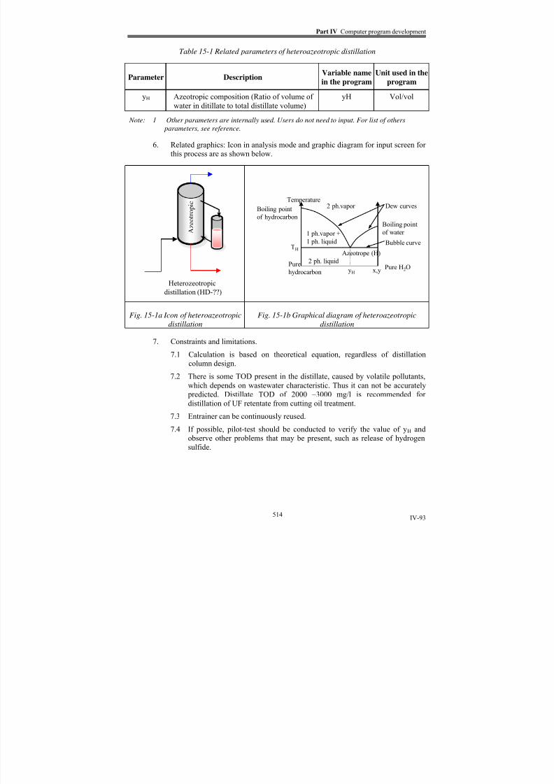
8/15/2019 Rachu.pdf
http://slidepdf.com/reader/full/rachupdf 598/646
Part IV Computer program development
IV-93
Table 15-1 Related parameters of heteroazeotropic distillation
Parameter DescriptionVariable name
in the program
Unit used in the
program
yH Azeotropic composition (Ratio of volume ofwater in ditillate to total distillate volume)
yH Vol/vol
Note: 1 Other parameters are internally used. Users do not need to input. For list of others
parameters, see reference.
6. Related graphics: Icon in analysis mode and graphic diagram for input screen for
this process are as shown below.
A z e o t r o p i c
Heterozeotropic
distillation (HD-??)
2 ph.vapor
Bubble curve
Pure H2O
Temperature
Azeotrope (H)
2 ph. liquid
1 ph.vapor +
1 ph. liquid
Pure
hydrocarbon x,y yH
Dew curvesBoiling point
of hydrocarbonBoiling point
of water
TH
Fig. 15-1a Icon of heteroazeotropic
distillation
Fig. 15-1b Graphical diagram of heteroazeotropic
distillation
7. Constraints and limitations.
7.1 Calculation is based on theoretical equation, regardless of distillation
column design.
7.2
There is some TOD present in the distillate, caused by volatile pollutants,
which depends on wastewater characteristic. Thus it can not be accurately predicted. Distillate TOD of 2000 –3000 mg/l is recommended for
distillation of UF retentate from cutting oil treatment.
7.3 Entrainer can be continuously reused.
7.4 If possible, pilot-test should be conducted to verify the value of yH and
observe other problems that may be present, such as release of hydrogen
sulfide.
514

8/15/2019 Rachu.pdf
http://slidepdf.com/reader/full/rachupdf 599/646
Chapter 3 Process references
IV-94
16) Stripping
1. Process abbreviation: ST
2. Process description: Stripping is reversed version of heteroazeotropic distillation.
It is an enhanced distillation process by addition of water, as an entrainer to
lower the boiling point of the system and extract the hydrocarbon from the wasteto be treated. The process can be used to treat water with trace volatile
hydrocarbons.
3. Reference : Part 3, chapter 9
4. List of outputs and related equations
4.1 Graded efficiency (η d ): It is assumed to be 100%. CF is not allowed in this
process.
4.2 Total efficiency (η t ): It is assumed to be 100%.
4.3 Graded outlet oil concentration in water outlet flow (C d ):
Cd = 0 mg/l4.4 Total outlet oil concentration in water outlet flow (C ):
C = 0 mg/l
4.5 Graded outlet oil concentration in oil outlet flow (C oild ): Outlet oil is in the
form of water-free oil.
4.6 Total outlet oil concentration in oil outlet flow (C oil): Outlet oil is in the
form of water-free oil.
4.7 Inlet flow (Q): Inlet flow of the process is equal to the outlet flow of the
upstream process.
4.8 Water outlet flow (Qout ): Water outlet flow is equal to water content of inlet
wastewater under the assumption that size of the process is sufficient tohandle inlet flowrate on real time basis.
)1000//)(1( oiloout C C QQ ρ −−= m3/h {16.1}
4.9 Oil outlet flow (Qoil): Oil outlet flow is equal to oil content of inlet
wastewater.
out oil QQQ −= m3/h {16.2}
4.10 Customized output :
4.10.1 Required quantity of entrainer: Quantity of entrainer, in this case,
water, depends on the type and the qauntity of hydrocarbon to be
removed, which can be calculated by the following equation.
)1( H
H oilsteam
y
yQQ−
=
m3/h
{16.3}
The values of yH (azeotropic composition) of certain
hydrocarbons are provided in the help file.
5. Related parameters: Related parameters are as summarized in the following table
515

8/15/2019 Rachu.pdf
http://slidepdf.com/reader/full/rachupdf 600/646
Part IV Computer program development
IV-95
Table 16-1 Related parameters of stripping
Parameter DescriptionVariable name
in the program
Unit used in the
program
yH Azeotropic composition (Ratio of volume ofwater in ditillate to total distillate volume).
The value for various hydrocarbons are
recommended in the help file.
yH Vol/vol
Note: 1. Other parameters are internally used. Users do not need to input. For list of others
parameters, see reference.
6. Related graphics: Icon in analysis mode and graphic diagram for input screen for
this process are as shown below.
S t r i p p i n g
Stripping (ST-??)
2 ph.vapor
Bubble curve
Pure H2O
Temperature
Azeotrope (H)
2 ph. liquid
1 ph.vapor +
1 ph. liquid
Pure
hydrocarbon x,y yH
Dew curvesBoiling point
of hydrocarbonBoiling point
of water
TH
Fig. 16-1a Icon of stripping Fig. 16-1b Graphical diagram of stripping
7.
Constraints and limitations.
7.1 Calculation is based on theoretical equation, regardless of distillation
column design.
7.2 The quantity of steam calculated by the program is not included the steam
for heating requirement.7.3 Entrainer ( water) can be continuously reused.
7.4 If possible, pilot-test should be conducted to verify the value of yH and
other problems that may be present.
516

8/15/2019 Rachu.pdf
http://slidepdf.com/reader/full/rachupdf 601/646
Chapter 3 Process references
IV-96
17) Chemical destabilization, coagulation-flocculation
1. Process abbreviation: CH
2. Process description: Calculation is based on reactor design, which can be applied
to any type of chemical or coagulant. Mixing is provided by mean of mechanical
mixers. The process is classified as inline concentrator and consists of 1 mixingtank and 3 flocculation tanks. Droplets smaller than 200 microns are assumed to
successfully coalesce to form droplets of 200 micros. For bigger oil droplets,
they are assumed to remain the same.
3. Reference : Part 3, chapter 10
4. List of outputs and related equations
4.1 Graded efficiency (η d ): This parameter is actually not valid since no oil is
removed from the wastewater. However, the term ηd in this case represents
removal efficiency due to coalesce. From this definition, the value of ηd are
as follows,
For d < 200 microns, ηd = CF.100%
For d = or > 200 microns, ηd = 0%
However, for d=200 microns, its concentration (if already existed) will
increase since coalesced droplets are assumed to be of this size.
4.2 Total efficiency (η t ): This parameter is not valid since no oil is removed.
4.3 Graded outlet oil concentration in water outlet flow (C d ): It is assumed that
all oil droplets are coalesced or flocculated to form big oil drop of 200
microns in diameter. ThusCd = Co for d > 200 microns and Cd = 0 for other values of “d”.
For d= 200 microns, its Cd is summation of its initial concentration and the
sum of concentration of droplets smaller than 200 microns.
4.4 Total outlet oil concentration in water outlet flow (C ):
C = Co mg/l
4.5 Graded outlet oil concentration in oil outlet flow (C oild ): This parameter is
not valid since no oil is removed.
4.6 Total outlet oil concentration in oil outlet flow (C oil): This parameter is not
valid since no oil is removed.
4.7 Inlet flow (Q): Inlet flow of the process is equal to the outlet flow of the
upstream process.
4.8 Water outlet flow (Qout ): Outlet flow of the process is equal to the inlet
flow.
4.9 Oil outlet flow (Qoil): This parameter is not valid since no oil is removed.
4.10 Customized output :
4.10.1 Retention time:
60⋅=QV τ
min
{17.1}
517

8/15/2019 Rachu.pdf
http://slidepdf.com/reader/full/rachupdf 602/646
Part IV Computer program development
IV-97
4.10.2 Product between G and τ
4.10.3 Power required (P) or Velocity gradient (G) of each tank: G and
P of each tank can be calculated by the following equations,
depending which value is specified by users.5.0
⎟⎟ ⎠ ⎞⎜⎜
⎝ ⎛ =
V PGμ
{17.2}
For turbine mixer,
ρ 53 Dn N P p= {17.3a}
The program features built-in Np for pitched blade turbine mixer
and propeller mixer.
For paddle mixer,3)(v A N Cd P c ⋅⋅⋅⋅= ρ {17.3b}
If turbine mixer option is selected, the program will calculate both
pitch blade and propeller type.
5.
Related parameters: Related parameters are as summarized in the following table
Table 17-1 Related parameters of chemical destabilization
Parameter DescriptionVariable name
in the program
Unit used in the
program
A Area of one paddle blade (single side) AreaPaddle m2
Cd Drag coefficient of paddle blade Constant = 0.6
D Diameter of impeller of mixer DMixer m
G Velocity gradient Grapid,
Gfloc1,2,3
Sec-1
n Rotating speed of mixer RPS1-4 Rev/s
N Number of blades NumBlade
N p Power coefficient for turbine mixer Built-in
P Power required for mixer1 of mixing tank and
mixer 2,3,4 of flocculation tanks
Prepid,
Pfloc1,2,3
Watt
v Tip speed of paddle (= 2πn (D/2)) VolRapid,
VolFloc1,2,3
m3
V Volume of mixing tank and flocculation tanks VolRapid,
VolFloc1,2,3
m3
ρc Density of continuos phase, in this case,
water
Denc Kg/m3
Note: 1 Other parameters are internally used. Users do not need to input. For list of others
parameters, see reference.
6.
Related graphics: Icon in analysis mode and graphic diagram for input screen for
this process are as shown below.
518

8/15/2019 Rachu.pdf
http://slidepdf.com/reader/full/rachupdf 603/646
Chapter 3 Process references
IV-98
Chemical
destabilizaion
(CH-??)
M
MEffluent
Flocculator Rapid mixing
Destabilization
chemicalsInfluent
G = 100-300 s-1
G = 50 s-1 G = 30 s-1 G = 20 s-1
The values of G in the figure are general values.
Fig. 17-1a Icon of chemical
destabilization
Fig. 17-1b Graphical diagram of chemical destabilization
7.
Constraints and limitations.
7.1
The program assumes that destabilization is successful and the oil droplets
coalesce to form bigger drops that can be decanted within 20 min. to 1
hour. So the final droplet size of 200 microns is proposed, Users can
change this value in the input screen.
7.2 Dosage of chemical varies with wastewater characteristic, type of
chemicals used. Thus it cannot be calculated and must be confirmed by jar
test.
7.3 For ANALYSIS mode, The configuration of the process is fixed, i.e. 1
mixing tank and 3 flocculation tanks, all with mechanical mixers.
7.4 For DESIGN mode, the program can be used for sizing 2 types of mixers,
i.e. turbine and paddle mixers. Turbine mixers are also divided into 2 cases,
i.e. pitched blade turbine and propeller. However, they will be calculated
simultaneously by the program.
519

8/15/2019 Rachu.pdf
http://slidepdf.com/reader/full/rachupdf 604/646
Part IV Computer program development
IV-99
18) Biological treatment
1. Process abbreviation: Bio
2. Process description: Biological process in this case is used as a finishing
treatment process to treat the effluent of other process. It is included in the
program to fulfil the entire process train of oily wastewater treatment. The process is not intended to refer to any specific type of biological system. Its
calculation is based on user-specified total TOD and oil removal.
3. Reference : Part 3, chapter 11
4. List of outputs and related equations
4.1 Graded efficiency (η d ): This parameter is equal to total efficiency.
4.2 Total efficiency (η t ): This parameter is specified by user.
4.3 Graded outlet oil concentration in water outlet flow (C d ):
od d d C C )1( η −=
mg/l
{18.1}
4.4 Total outlet oil concentration in water outlet flow (C ):
∑=max
min
d
d
d C C mg/l {18.2}
4.5 Graded outlet oil concentration in oil outlet flow (C oild ): This parameter is
not valid since oil is not removed but destroyed or transform into other
forms.
4.6 Total outlet oil concentration in oil outlet flow (C oil): This parameter is not
valid since oil is not removed but destroyed or transform into other forms.4.7 Inlet flow (Q): Inlet flow of the process is equal to the outlet flow of the
upstream process.
4.8 Water outlet flow (Qout ): Outlet flow of the process is equal to the inlet
flow.
4.9 Oil outlet flow (Qoil): This parameter is not valid since no oil is removed.
4.10 Customized output :
4.10.1 TOD of water outlet flow (TOD): It can be calculated by the
following equation. TODo, unit TOD and ηTOD are given by users.
)1())()1(( TOD
oil
TODot omg
mgC TODTOD η η −⋅⋅−−= mg/l {18.1}
5. Related parameters: Related parameters are as summarized in the following table
520

8/15/2019 Rachu.pdf
http://slidepdf.com/reader/full/rachupdf 605/646
Chapter 3 Process references
IV-100
Table 18-1 Related parameters of biological treatment
Parameter DescriptionVariable name
in the program
Unit used in the
program
mgTOD
/mgoil Unit TOD of oil. For more information, seereference file
unitTOD
TODo TOD of the inlet wastewater TODin mg/l
ηt Total oil removal efficiency. efft %
ηTOD TOD removal efficiency. It includes only
soluble TOD. TOD from oil is not included.
effTOD %
Note: 1 Other parameters are internally used. Users do not need to input. For list of others
parameters, see reference.
6.
Related graphics: Icon in analysis mode and graphic diagram for input screen forthis process are as shown below.
Biologicaltreatment
(Bio_??)
Influent
Effluent
Biological reactor
Clarifier
(if any)
Wasted biomass
(if any)
Fig. 18-1a Icon of biological treatment Fig. 18-1b Graphical diagram of biological treatment
7.
Constraints and limitations.
7.1
The process is included in the program to fulfil the entire process train of
oily wastewater treatment only. Thus, its calculation is based on data fromresearches, rather than mathematical model.
7.2 The module is available only in ANALYSIS mode.
7.3 Flowrate of wasted sludge is assumed to be negligible. Thus outlet flow is
equal to inlet flow.
7.4 It is assumed that there is no coalescence taking place within the process.
7.5 Calculated TOD is an internal result of the model. It cannot be exported to
other process because of programming limitation.
521

8/15/2019 Rachu.pdf
http://slidepdf.com/reader/full/rachupdf 606/646
Part IV Computer program development
IV-101
19) GAC filter
1. Process abbreviation: GAC
2. Process description: GAC filter in this case is used as a finishing treatment
process to treat the effluent of other process. It is included in the program to
fulfil the entire process train of oily wastewater treatment. Its calculation is basedon user-specified TOD removal. For oil removal, the efficiency is assumed to be
100%. Since its main objective is removal of residual pollutant, its inlet oil
concentration should be not greater than 50 mg/l. If the inlet wastewater contains
higher oil concentration, the program will display warning.
3. Reference : Part 3, chapter 11
4. List of outputs and related equations
4.1 Graded efficiency (η d ): It is assumed to be 100%.
4.2 Total efficiency (η t ): It is assumed to be 100%.
4.3 Graded outlet oil concentration in water outlet flow (C d ):
Cd = 0 mg/l
4.4 Total outlet oil concentration in water outlet flow (C ):
C = 0 mg/l
4.5 Graded outlet oil concentration in oil outlet flow (C oild ): This parameter is
not valid since oil adsorbed into the bed.
4.6 Total outlet oil concentration in oil outlet flow (C oil): This parameter is not
valid since oil is adsorbed into the bed.
4.7 Inlet flow (Q): Inlet flow of the process is equal to the outlet flow of the
upstream process.
4.8 Water outlet flow (Qout ): Outlet flow of the process is equal to the inlet
flow.
4.9 Oil outlet flow (Qoil): This parameter is not valid.
4.10 Customized output :
4.10.1 Adsorptive capacity (q): The program can predict adsorptive
capacity, using 2 well-known Isotherm models, i.e.,
• Lungmuir’s model: po
po
bC
aC q+
=1
mg/g {19.1a}
• Frendlich’s model: )/1( n
poC k q ⋅= mg/g {19.1b}
A, b, k and n are numerical constant, acquired from experiment.
User can select the model from on-screen option button.
4.10.2 Bed life span or total operation time before bed replacement (t T ):
When isotherm (q VS. C p relation) and mass transfer zone data
(Qa, Ha or E as the functions of C p) are available;
522

8/15/2019 Rachu.pdf
http://slidepdf.com/reader/full/rachupdf 607/646
Chapter 3 Process references
IV-102
)( p po
ab
T C C Q
Qq HAt
−
−⋅⋅=
ρ {19.2a}
Or,
)( p po
bT
C C Qq HA E t
− ⋅⋅⋅= ρ {19.2b}
)/(10100
11 AQd
c H
E ⋅⋅⋅
⋅−= {19.3}
E is effective saturation of bed. The recommended valued is
around 50-95% (average 75%). In the program, eq. 19.2b is used.
H and V are in m and m/h, respectively.
4.10.3
Hydraulic loading rate:
A
QV = m/h {19.4}
4.10.4 Retention time (τ ):
60)/(
⋅= AQ
H τ min {19.5}
4.10.5 Headloss (P): Head loss of the bed can be calculated from
Kozeny-Carman’s equation. Built-in minimum and maximum
void ration is 0.18 to 0.25, respectively.
32
2)1)(60/(180
ε ρ
ε μ
⋅⋅⋅
−=
dpg
V H P c
{19.3}
5. Related parameters: Related parameters are as summarized in the following table
523

8/15/2019 Rachu.pdf
http://slidepdf.com/reader/full/rachupdf 608/646
Part IV Computer program development
IV-103
Table 19-1 Related parameters of GAC filter
Parameter DescriptionVariable name in
the program
Unit used in the
program
A Cross section area of bed A m2
C p Required outlet pollutant concentration Polout mg/l
C po Inlet concentration of pollutant Polin mg/l
dp GAC particle size Dpc m
Ε Effective saturation of bed, E < 100% GACE %
H Bed height GACH m
P Pressure drop Pdropmin,
Pdropmax
m
q Isotherm data (mass of adsorbate/ mass of
adsorbent)
GACq mg/g
V Empty bed velocity or hydraulic loading rate GACV m/h
a, b Empirical constant for Lungmire’s model C po in mg/l m/h
k, n Empirical constant for Freundlich’s model C po in mg/l m/h
c, d Empirical constant for mass transfer zone data C po in mg/l m/h
ε Bed porosity or void ratio, recommended value is
0.18 – 0.25.
Void
ρc Density of continuous phase Denc kg/m3
ρ b Bulk density of bed (430 – 600 kg/m3) DenGAC kg/m
3
Note: 1. Other parameters are internally used. Users do not need to input. For list of others parameters, see reference.
6. Related graphics: Icon in analysis mode and graphic diagram for input screen for
this process are as shown below.
GAC filter
(GAC-??)
Ha
CCo
Ce
H
t = 0
S a
t u r e d
z o n e
M T Z
CCo
Ce
H
t = tT
Ha
Bed needs to
be replaced.
GAC bed.HT
Influent
Effluent
Velocity=V
Fig. 19-1a Icon of GAC filter Fig. 19-1b Graphical diagram of GAC filter
524

8/15/2019 Rachu.pdf
http://slidepdf.com/reader/full/rachupdf 609/646
Chapter 3 Process references
IV-104
7. Constraints and limitations.
7.1 Calculation is based on research data, given by users.
7.2 If possible, it is recommended to conduct is lab test, using real wastewater,
to find the exact data about isotherm adsorptive capacity (a, b, k, n), and
mass transfer zone (c and d) data of GAC bed.
525

8/15/2019 Rachu.pdf
http://slidepdf.com/reader/full/rachupdf 610/646
Part IV Computer program development
IV-105
20) Customized concentrator
1. Process abbreviation: CC
2. Process description: The process works as an oil concentrator, e.g. hydrocyclone.
But users are allowed to specify graded efficiency of the process.
3. Reference : None
4.
List of outputs and related equations
4.1 Graded efficiency (η d ): User-defined in the form of a table. Graded
efficiency of the droplet size that falls between 2 specified values will be
obtained by interpolation or extrapolation.
4.2 Total efficiency (η t ):
∑ ⋅−
−=
max
min
%100)1(
)1(1 d
d f
od d
o
t R
C
C
η η {20.1}
4.3
Graded outlet oil concentration in water outlet flow (C d ):
)1(
)1(
f
od d
d R
C C
−
−=
η mg/l
{20.2}
4.4 Total outlet oil concentration in water outlet flow (C ):
∑=max
min
d
d
d C C mg/l {20.3}
4.5 Graded outlet oil concentration in oil outlet flow (C oild ):
f
od d oild
R
C C
η = mg/l {20.4}
4.6 Total outlet oil concentration in oil outlet flow (C oil):
∑=max
min
d
d
oild oil C C {20.5}
4.7 Inlet flow (Q): Inlet flow of the process is equal to the outlet flow of the
upstream process.
4.8 Water outlet flow (Qout ):
)1( f out RQQ −= m3/h {20.6}
4.9
Oil outlet flow(Qoil):
f oil RQQ ⋅= m3/h {20.7}
4.10 Customized output : None
5.
Related parameters: Related parameters are as summarized in the following table
526

8/15/2019 Rachu.pdf
http://slidepdf.com/reader/full/rachupdf 611/646
Chapter 3 Process references
IV-106
Table 20-1 Related parameters of customized concentrator
Parameter DescriptionVariable name in
the program
Unit used in the
program
R f Split ratio (Qoil/Q) Rf
d, ηd Specified droplet size and graded efficiency
of the process
Customdin,
Customeffd
Micron, %
6. Related graphics: Icon in analysis mode and graphic diagram for input screen for
this process are as shown below.
Custom
concentrator
(CC-??)
Oil outlet
Influent
Effluent
Fig. 20-1a Icon of customized
concentrator
Fig. 20-1b Graphical diagram of customized
concentrator
527

8/15/2019 Rachu.pdf
http://slidepdf.com/reader/full/rachupdf 612/646
Part IV Computer program development
IV-107
21) Customized oil separator
1. Process abbreviation: CS
2. Process description: the process works as an oil separator, e.g. decanter. But
users are allowed to specify graded efficiency of the process.
3. Reference : None
4.
List of outputs and related equations
4.1 Graded efficiency (η d ): User-defined in the form of a table. Graded
efficiency of the droplet size that falls between 2 specified value will be
obtained by interpolation.
4.2 Total efficiency (η t ):
( )
%100
max
min ⋅
⋅
=∑
o
d
d
od d
t
C
C η
η {21.1}
4.3 Graded outlet oil concentration in water outlet flow(C d ):
)1( d od
out
d C Q
QC η −⋅⋅= mg/l {21.2}
4.4 Total outlet oil concentration in water outlet flow (C ):
∑=max
min
d
d
d C C mg/l {21.3}
4.5 Graded outlet oil concentration in oil outlet flow (C oild ): The outlet oil in
the oil outlet flow is in pure condition (100% oil).
4.6 Total outlet oil concentration in oil outlet flow (C oil): The outlet oil in the
oil outlet flow is in pure condition (100% oil).
4.7 Inlet flow (Q): Inlet flow of the process is equal to the outlet flow of the
upstream process.
4.8 Water outlet flow (Qout ):
)1000//)(1( oiloout C C QQ ρ −−= m3/h {21.4}
4.9 Oil outlet flow(Qoil):
out oil
QQQ −= m3/h {21.5}
4.10 Customized output : None
5. Related parameters: Related parameters are as summarized in the following table
528

8/15/2019 Rachu.pdf
http://slidepdf.com/reader/full/rachupdf 613/646
Chapter 3 Process references
IV-108
Table 21-1 Related parameters of customized separator
Parameter DescriptionVariable name in
the program
Unit used in the
program
d, ηd Specified droplet size and graded efficiencyof the process
Customdin,Customeffd
Micron, %
6. Related graphics: Icon in analysis mode and graphic diagram for input screen for
this process are as shown below.
Custom separator
(CS-??)
Influent
Effluent
Oil outlet
Fig. 21-1a Icon of customized separator Fig. 21-1b Graphical diagram of customized
separator
7. Constraints and limitations.
7.1
Oil outlet point of the process can only be connected to the skimmers only.
529

8/15/2019 Rachu.pdf
http://slidepdf.com/reader/full/rachupdf 614/646
Part IV Computer program development
IV-109
22) Customized inline concentrator
1. Process abbreviation: IC
2. Process description: the process work as an inline oil concentrator, e.g.
coagulation-flocculation, or inline coalescer. But users are allowed to specify
graded efficiency of the process.
3. Reference : Part 3, chapter 10
4. List of outputs and related equations
4.1 Graded efficiency (η d ): This parameter is actually not valid since no oil is
removed from the wastewater. However, the term ηd in this case represents
removal efficiency due to coalesce, defined by user in the form of a table.
Graded efficiency of the droplet size that falls between 2 specified value
will be obtained by interpolation or extrapolation. However the
concentrated oil is not separated from the wastewater but assumed to
coalesce to form bigger oil drops of a specified size (d coalesce). From thisdefinition, the value of ηd are as follows,
For d < dcoalesce, ηd is as specified by user. The rest of the droplets that are
not separated will partially coalesce to form bigger droplets at the size of
dcoalesce.
For d = or > dcoalesce, ηd is as specified by user.
However, for d = dcoalesce, its concentration (if already existed) will increase
since coalesced droplets are assumed to be of this size.
4.2 Total efficiency (η t ): This parameter is not valid since no oil is removed.
4.3
Graded outlet oil concentration in water outlet flow (C d ): It is assumed that
separated oil droplets coalesce to form big oil drop which is classified as
oil layer.
And as described above, it is assumed that there are partially coalesces of
the small oil droplets. These droplets will coalesce and form bigger oil
droplets “dcoalesce”. Or all droplets smaller than dcoalesce will coalesce to form
the droplet size “dcoalesce”.
Thus, for d < dcoalesce,
0=d C mg/l {22.1a}
For d = dcoalesce,
∑ −=coalsced
d
d d d C C min
)1( η
mg/l
{22.1b}
For d > dcoalesce,
)1( d od d C C η −⋅= mg/l {22.1c}
For oil layer,
∑+=max
min
,
d
d
d layer olayer C C C mg/l {22.1d}
530

8/15/2019 Rachu.pdf
http://slidepdf.com/reader/full/rachupdf 615/646
Chapter 3 Process references
IV-110
4.4 Total outlet oil concentration in water outlet flow (C ):
C = Co mg/l
4.5 Graded outlet oil concentration in oil outlet flow (C oild ): This parameter is
not valid since no oil is removed.
4.6
Total outlet oil concentration in oil outlet flow (C oil): This parameter is notvalid since no oil is removed.
4.7 Inlet flow (Q): Inlet flow of the process is equal to the outlet flow of the
upstream process.
4.8 Water outlet flow (Qout ): Outlet flow of the process is equal to the inlet
flow.
4.9 Oil outlet flow (Qoil): This parameter is not valid since no oil is removed.
4.10 Customized output : None
5.
Related parameters: Related parameters are as summarized in the followingtable
Table 22-1 Related parameters of customized inline concentrator
Parameter DescriptionVariable name in
the program
Unit used in the
program
dcoalesce Diameter of partially coalesced oil drop
from the process
customDcoalesce micron
d, ηd Specified droplet size and graded efficiency
of the process
Customdin,
Customeffd
Micron, %
6.
Related graphics: Icon in analysis mode and graphic diagram for input screen for
this process are as shown below.
Inline concentrator
(IC-??)
Influent
Effluent
Fig. 22-1a Icon of inline concentrator Fig. 22-1b Graphical diagram of inline concentrator
531
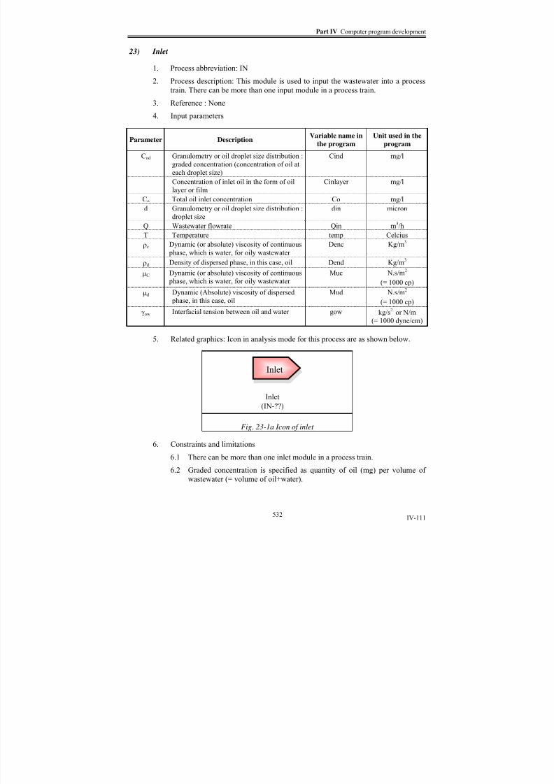
8/15/2019 Rachu.pdf
http://slidepdf.com/reader/full/rachupdf 616/646
Part IV Computer program development
IV-111
23) Inlet
1. Process abbreviation: IN
2. Process description: This module is used to input the wastewater into a process
train. There can be more than one input module in a process train.
3. Reference : None
4.
Input parameters
Parameter DescriptionVariable name in
the program
Unit used in the
program
Cod Granulometry or oil droplet size distribution :
graded concentration (concentration of oil at
each droplet size)
Cind mg/l
Concentration of inlet oil in the form of oil
layer or film
Cinlayer mg/l
Co Total oil inlet concentration Co mg/l
d Granulometry or oil droplet size distribution :
droplet size
din micron
Q Wastewater flowrate Qin m3/h
T Temperature temp Celcius
ρc Dynamic (or absolute) viscosity of continuous
phase, which is water, for oily wastewater
Denc Kg/m3
ρd Density of dispersed phase, in this case, oil Dend Kg/m3
μC Dynamic (or absolute) viscosity of continuous
phase, which is water, for oily wastewater
Muc N.s/m2
(= 1000 cp)
μd Dynamic (Absolute) viscosity of dispersed phase, in this case, oil
Mud N.s/m2
(= 1000 cp)
γow Interfacial tension between oil and water gow kg/s2
or N/m
(= 1000 dyne/cm)
5. Related graphics: Icon in analysis mode for this process are as shown below.
InletInlet
Inlet
(IN-??)
Fig. 23-1a Icon of inlet
6. Constraints and limitations
6.1 There can be more than one inlet module in a process train.
6.2 Graded concentration is specified as quantity of oil (mg) per volume of
wastewater (= volume of oil+water).
532

8/15/2019 Rachu.pdf
http://slidepdf.com/reader/full/rachupdf 617/646
Chapter 3 Process references
IV-112
24) Outlet
1. Process abbreviation: -
2. Process description: This module is used to specify the outlet point of the process
train. It is also used as a logical checkpoint of the program to perform
calculation. Thus there can be only one outlet in a process train.
3. Reference : None
4. Related graphics: Icon in analysis mode and graphic diagram for input screen for
this process are as shown below.
OutletOutlet
Outlet
Fig. 24-1a Icon of outlet
5. Constraints and limitations
5.1 There can be only one outlet in a process train.
5.2 Location of the outlet in the process train does not need to be an actual
location. However, it is recommended to place it at the end of main process
stream for faster calculation.
533

8/15/2019 Rachu.pdf
http://slidepdf.com/reader/full/rachupdf 618/646
Part IV Computer program development
IV-113
25) Flow merge
1. Process abbreviation: FM
2. Process description: This module is used to combine or merge any 2 streams of
wastewater together.
3. Reference : None
4.
Output parameters:
4.1 Wastewater flowrate (Q): It is calculated from the summation of the
flowrate of the two streams.
4.2 Granulometry or size distribution of oil droplets in the wastewater : It is
calculated from weight average value, as shown in the following equation.
21
22,11,
QC QC C
d d
d +
+=
{25.1}
4.3
Total oil concentration (C):
∑=max
min
d
d
d C C
{25.2}
4.4 Oil density (ρd): as kg/m3. It is assumed to be equal to the weight average
value, as shown in the following equation.
2211
222,111,
QC QC
QC QC d d
d +
+=
ρ ρ ρ {25.3}
4.5 Water density (ρc):
21
2211
QQQQ cc
c ++= ρ ρ
{25.4}
4.6 Oil viscosity (μd): as N.s/m2. It is assumed to be equal to the weight
average value, as shown in the following equation.
2211
222,111,
QC QC
QC QC d d
d +
+=
μ μ μ {25.5}
4.7 Water viscosity (μc):
21
2211
QQ ccc +
+=
μ μ μ
{25.6}
4.8
Temperature (T):
21
2211
QT QT T
++
= Celcius {25.7}
4.9 Interfacial tension (γow): It is assumed to be equal to the weight average
value, as shown in the following equation.
2211
222,111,
QC QC
QC QC owow
ow +
+=
γ γ γ
{25.8}
5. Related graphics: Icon in analysis mode for this process are as shown below.
534

8/15/2019 Rachu.pdf
http://slidepdf.com/reader/full/rachupdf 619/646
Chapter 3 Process references
IV-114
2
1
Flow merge(FM-??)
Fig. 25-1a Icon of flow merge
535
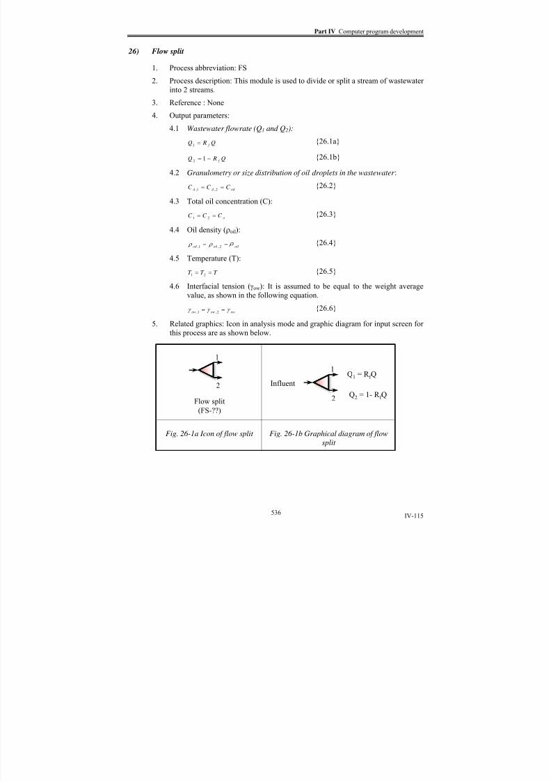
8/15/2019 Rachu.pdf
http://slidepdf.com/reader/full/rachupdf 620/646
Part IV Computer program development
IV-115
26) Flow split
1. Process abbreviation: FS
2. Process description: This module is used to divide or split a stream of wastewater
into 2 streams.
3. Reference : None
4.
Output parameters:
4.1 Wastewater flowrate (Q1 and Q2):
Q RQ f =1
{26.1a}
Q RQ f −= 12 {26.1b}
4.2 Granulometry or size distribution of oil droplets in the wastewater :
od d d C C C == 2,1, {26.2}
4.3 Total oil concentration (C):
oC C C == 21 {26.3}
4.4 Oil density (ρoil):
oiloiloil ρ ρ == 2,1, {26.4}
4.5 Temperature (T):
T T T == 21 {26.5}
4.6
Interfacial tension (γow): It is assumed to be equal to the weight averagevalue, as shown in the following equation.
owowow γ γ γ == 2,1, {26.6}
5. Related graphics: Icon in analysis mode and graphic diagram for input screen for
this process are as shown below.
2
1
Flow split
(FS-??)
2
1
Influent
Q1 = R f Q
Q2 = 1- R f Q
Fig. 26-1a Icon of flow split Fig. 26-1b Graphical diagram of flow
split
536

8/15/2019 Rachu.pdf
http://slidepdf.com/reader/full/rachupdf 621/646
Part V General conclusion

8/15/2019 Rachu.pdf
http://slidepdf.com/reader/full/rachupdf 622/646
General conclusion
V-1
General conclusion
One of the main objectives of this thesis is to review all of the researches on various
oily wastewater treatment processes, directed by Prof. AURELLE and summarize and
establish general theory or mathematical models that govern the performance and design of
such processes.
This objective is accomplished in Part 1 to Part 3 of this thesis. Every unit processes
for oil separation, studied in GPI lab, had been revised and their corresponding mathematical
models as well as design limitation and influent parameters had been found. These processes
revised under the scope of work of this thesis include,
1. Oil skimmer
This equipment is developed to selectively remove oil layer from the water
surface without carrying over the water with it. It is found that the key to achieve good oil
selectivity depends on the surface energy or critical surface tension of skimmer material. Thematerial with low critical surface tension is suitable to use as skimmer material. Mathematical
models of 2 types of skimmer, i.e. drum skimmer and disk skimmer are verified.
2.
Decanter
Its underlining theory, namely STOKE’s law, is quoted. General mathematical
models for 3 different varieties of the processes, i.e. simple decanter (e.g. API tank), parallel
plate interceptor (e.g. PPI and lamella separator), and compact decantor (e.g. Spiraloil) are
proposed and verified.
3.
Coalescer
Theoretical model, proposed by AURELLE, based on filtration model, is
reviewed. The model provides clear ideas about influent parameters on coalescer
performance. Several initiative ideas for coalescer performance enhancemen, e.g. the use of
guide to increase oil loading of the coalescer and the use of mix bed material to treat mixture
of direct/inverse emulsion simultaneously are realised. Finally, the empirical models, which
are verified by relatively wide range of data, are proposed for 4 varieties of coalescer, i.e.
granular bed coalescer , brush type bed coalescer, dynamic fibrous bed (rotating brush)
coalescer, and disorderly fibrous bed (metal wool) coalescer. Headloss equations are also
proposed in this thesis.
4.
Dissolved air flotation
Mathematical model based on filtration concept, proposed by SIEM [12] is
reviewed. The model is useful for understanding effects of influent parameters on DAF
performance. Extension equations of SIEM’s model , based on population balance theory, is
established within this thesis to extend the valid range of SIEM’s model to cover the range of
oily wastewater frequently found. Equations for saturator or pressurized water system
design are also proposed and verified within this thesis.
5. Hydrocyclone
Trajectory analysis model for 2-phase (liquid-liquid) hydrocyclone, the new
concept based on STOKE’s law, is proposed and verified. The model can actually predict
537

8/15/2019 Rachu.pdf
http://slidepdf.com/reader/full/rachupdf 623/646
General conclusion
V-2
graded oil removal efficiency of any sizes of oil droplet in the wastewater by theoretical based
equation, unlike other models which are based on curve fitting and similarity concepts. Thus
it is very useful to understand the effect of related parameters on hydrocyclone performance.
Models of three-phase hydrocyclone, GPI innovation for simultaneous removal of oil,
suspended solids amd water, are also established within the scope of work of this thesis. The
model is also based on trajectory analysis concept. Finally, headloss equations for 2- and 3- phase hydrocyclone are established in this thesis.
6.
Membrane processes
Applications of membrane processes, i.e. microfiltration (MF), ultrafiltration
(UF), nanofiltration (NF) and reverse osmosis (RO) on oily wastewater treatment in GPI lab
had been reviewed. Several useful facts from those researches are realized and calculation
techniques are established in this thesis, i.e.,
• Flux enhancement for UF on cutting oil emulsion treatment by partial
destabilization. Additional of salt, in lower amount than that for totaldestabilization, into the feed helps increasing permeate flux, thus saving on
energy consumption and membrane size. The downside of this technique,
concluded in this thesis, is that the destabilized oil can clog the membrane if
it is not properly partition or removed from recirculated feed stream.
• Cleaning of UF membrane after treatment of cutting oil by cleaning
microemulsion. It can effectively wash accumulated oil or foulants from the
membrane. It can be reused for many times until it is saturated by oil.
• Technique to extend the UF performance data at 1 condition to cover other
condition, based on combination of film model and resistance model . This
technique is proposed and verified in this thesis. It is useful when onlylimited data on the wastewater is available. It allows us to estimate evolution
of flux and permeate volume with time, which is useful for process design.
• Technique to predict flux of mixture of two different emulsion. This
technique is also proposed and verified in this thesis. It is useful when mixed
emulsion can be expected and its ratio is likely to vary.
7. Thermal process
The main interest of this type of process is heteroazeotropic distillation (HD).
Application of HD to remove water content from refinery slops and UF retentates from UF of
cutting oil emulsion is reviewed. The process is achieved by addition of certain chemical that promotes azeotropic formation (called entrainer), usually hydrocarbons, into the wastewater.
It will lower the boiling temperatur of the system, thus save the energy. These applications
provide prospects on re-value these supposed-to-be-wastes. Its reverse application, namely
stream stripping (for removing volatile substance from water by addition of stream), is also
realized. Theoretical data to calculate required amount of entrainer are also proposed.
8. Chemical process
Destabilization (or breaking or cracking) mechanism of emulsion by addition
of various chemicals, i.e. mono valence salt, bivalence salts, polyelectrolytes, acid and special
absorbates are reviewed. Equations for mixing tank and mixer designs are also reviewed andincluded in the program.
538

8/15/2019 Rachu.pdf
http://slidepdf.com/reader/full/rachupdf 624/646
General conclusion
V-3
9.
Finishing processes
Two widely used finishing processes, i.e., biological treatment and carbon
adsorption, is realized. Useful data on biological process, related to oily wastewater
treatment, and design equations of GAC filter, as well as absorptive capacity of certain
chemicals, are reviewed and included in the program.
To complete the first objective , guideline on oily wastewater treatment process
selection and recommended treatment processes for certain oily wastewater are proposed.
The final objective of the thesis is to develop the program for calculation, design and
simulation of wastewater treatment process train in order to value and make use of the know-
how and significant finding from the researches by presenting them in the form of user-
friendly program. To fulfil this objective, the program, namely GPI program, is developed. It
is divided into 4 major modes, i.e.,
•
E-book mode: provides background knowledge and useful database about theoil pollution and the treatment processes. Actually, the textbook in part 3 is
transformed into e-book files used in this mode,
• Process recommendation mode: provides recommendation to narrow the range
of feasible processes for any input influent. Selection criteria are as proposed in
the guideline in Part 3, chapter 12.
• Design (calculation) mode: used for sizing the unit process. The models used
for calculation are as summarized in Part 3.
• Analysis (simulation) mode: allows users to integrate any separation processes,
included in the program database, to build their own treatment process train. And
the program will simulate the process train to forecast the efficiency of each unit.
The program is developed to be upgradable. Its architecture consists of the database in
the form of common text database file and sub-programs. To upgrade the program, it can be
done conveniently by adding the data, such as name of new process, its related parameter
needed for calculation, into the database. The program will link the new process into the
graphic user interface automatically. For sub-program for calculation of the new process, it
can be separately developed using Visual Basic programming language. The easiest way is to
copy the source code of an existing process and change the equation to suit the new process.
After compilation in to an executable file, it can be copied to replace the old GPI program file
without re-installation of the program. So the program could be further developed to cover
more researches and processes in the future.
539

8/15/2019 Rachu.pdf
http://slidepdf.com/reader/full/rachupdf 625/646
Reference

8/15/2019 Rachu.pdf
http://slidepdf.com/reader/full/rachupdf 626/646
Reference
1 Sawyer C., Mccarty P., Parkin G.
Chemistry for environmental engineering and science
Book, 5th edition, Mcgraw-Hill, 2003
2
Perry R., Green D.Perry's chemical engineering's handbook
Book, 7th edition, Mcgraw-Hill, 1997
3 Aurelle Y.
Contribution a l'etude des mechanismes fondamentaux de la coalescence des
emulsions sur lit granulaire
Thèse de doctuer d'etat, Université Pual Sabatier,1980
4 Cherid S.
Conception et etude de nouveaux separateurs lamellaires hydrocarbon-eau de
type "SPIRALOIL"Thèse de doctorat, INSA-Toulouse, 1986
5 Thangtongtawi S.Contribution a l'etude et au dimensionnement de recuperateurs de surface du
type tambours et disques deshuileurs
Thèse de doctorat, INSA-Toulouse, 1988
6 Sanchez Martinez J.C. Application de la coalescence a l'extraction liquide-liquide
Thèse de doctorat, INSA-Toulouse, 1982
7 Darme C.
Separation par coalescence des emulsions hydrocarbure/eau stabilees par desagents tensio-actifs
Thèse de doctorat, INSA-Toulouse, 1983
8 Tapaneeyangkul P.
Etude et modilisation d'une nouvelle generation de coalesceurs liquide-
liquide: "Le coalesceur a garnissage fibreux dynamique"
Thèse de doctorat, INSA-Toulouse, 1989
9 Damak L.
Nouveaux separateurs d'emulsions huile/eua chargee en matiers en
suspension - Separateur a inversion de phase - coalesceur granulaire a lit
pulseThèse de doctorat, INSA-Toulouse, 1992
10 Srijaroonrat P.
Nouvelles techniques de traitement des emulsion hydrocarbure-eau non
stabilisee: ultrafil tration et couplage coalesceur-hydrocyclone
Thèse de doctorat, INSA-Toulouse, 1998
11 Wanichkul B. Etude des potentialities de nouveaux procedes de traitement d'emulsions
hydrocarbure-eau: ultrafiltration, distillation et couplage coalesceur-
hydrocyclone
Thèse de doctorat, INSA-Toulouse, 2000
540

8/15/2019 Rachu.pdf
http://slidepdf.com/reader/full/rachupdf 627/646
12 Siem N.Contribution a l'etude des separations hydrocarbure-eau par flottation
Thèse de doctorat, INSA-Toulouse, 1983
13 Aoudjehane M.
Traitement par flottation des effluents aqueux charges en hydrocarbures
Thèse de doctorat, INSA-Toulouse, 1986
14 Dupre V. Etude des mecanismes et de la modilisation procedes de flottation a air
dissous
Thèse de doctorat, INSA-Toulouse, 1995
15 Ponasse M. Elements theoriques et experimentaux en vue de l'amelioration des
installations de flottation a air dissous. Developpement de nouveaux
flottateurs
Thèse de doctorat, INSA-Toulouse, 1997
16 Ma B. Epuration des eaux residuraires de l'industrie petreliere Par hydrocyclonage
Thèse de doctorat, INSA-Toulouse, 1993
17 Cazal E.
Etude des potentialities des hydrocyclones dans domaine du traitement des
eaux residuaire urbains et des eaux de ruissellement
Thèse de doctorat, INSA-Toulouse, 1996
18 Belkacem M. Nouvelle methodologie dans le traitement des huiles de coupe par
ultrafiltrationThèse de doctorat, INSA-Toulouse, 1995
19 Toulgoat K.
Etude des macanismes de formation des emulsions thermiques; potentialites
de separation par ultrafiltration
Thèse de doctorat, INSA-Toulouse, 1996
20 Matamoros H.Procedes membranaires pour le traitment des emulsions stabilisees de type
fluid de coupe
Thèse de doctorat, INSA-Toulouse, 1997
21
Zhu S. Etude des traitement physico-chimiques d'epuration des emulsion d'huile de
coup; Influence de leur formulation
Thèse de doctorat, INSA-Toulouse, 1990
22 Yang C. Developpement de nouvelles formulations de fluides de coupe peu polluants,
mise au point de techniques de traitement adaptees
Thèse de doctorat, INSA-Toulouse, 1993
23 Lorain O.
Contribution a l'etude du traitement des eaux par congelation : potentialites et
applicationsThèse de doctorat, INSA-Toulouse, 2002
541

8/15/2019 Rachu.pdf
http://slidepdf.com/reader/full/rachupdf 628/646
24 Lucena E. Nouveau procede de traitement des slops de l'industrie petroliere par
distillation heteroazeotropique: comparaison avec d'autres procedes
Thèse de doctorat, INSA-Toulouse, 2004
25 Puprasert C.
Contribution a la mise au point d'application specifique des hydrocyclones en
traitement des eaux
Thèse de doctorat, INSA-Toulouse, 2004
26 Aurelle Y.
Contribution a l'etude du traitement des eaux polluees par des hydrocarbures
emulsionnes par coalescence sur resines oleophiles
Thèse de doctorat, Universite Pual Sabatier de Toulouse, 1974
27 Tan PraponTheoritical study of Coalescer and its application to treatment of wastewater
for vegetable oil industry
Master degree thesis, Chulalongkorn University, Thailand, 1984
28 Thew M.T.
Hydrocyclones for liquid-liquid separation
Lecture on the intensive short course, University of Bath, September 1984
29 Chebelin T.
Separation compacte: modilisation des hydrocyclones
Document de stade de fin d'etude, INSA-Toulouse, 1984
30 Bradley D.The hydrocyclone
Book, 196531 M.a B., Aurelle Y., Seureau J.
Three phase hydrocyclone for simultaneous separation of solids from liquid-
liquid mixtures
Publication, source unknown
32 Ma B., Aurelle Y., Wolbert D.
Efficiency estimation of liquid-liquid hydrocyclones using trajectory analysis
AIChE journal, Vol. 41, No. 6, 1995
33 Trawinski H.
Hydrocyclones
Publication, source unknown
34 Leppinen D.M., Dalziel S.B., Linden P.F. Modeling the global efficiency of dissolved air flotation
Water science and Technology, Vol. 43 No. 8, 2001
35 Yao K., Habibian M.T., O'melia C.R.Water and wastewater filtration: Concepts and application
Environmeantal sciences and Technology, No. 11, 1971
36 Henke L.Osmosis, RO and Filtration: What they have in common?
Asian Water, Vol. 19 No.5, June, 2003
542

8/15/2019 Rachu.pdf
http://slidepdf.com/reader/full/rachupdf 629/646
37 Mutsui Y., Fukushi K., Tambo, N. Modeling, simulation and operational parameters of dissolved air flotation
J. water SRT, No. 47, 1998
38 Cheryan M.
Ultrafiltration and microfiltration handbook
Book, Technomic, 1998
39 Pushkarev V.V., Yuzhaninov A.G., Men S.K.Treatment of oil containing wastewater
Book, Allerton press inc., 1983
40 Shaw D.
Introduction to colloid and surface chemistry
Book, 4th edition, Butterworth-Heinemann Ltd., 1992
41 Aurelle Y.
Physical and chemical treatment techniques Paper on short course seminar:
Faculty of engineering, Chulalonkorn university, ThailandBook, Chulalongkorn University, September 1985
42 Aurelle Y.Treatments of oil containing wastewater
Chulalongkorn University
43 Parker H.D, Pitt G.D.
Pollution control instrument for oil and effluents
Book, Graham & Trotman, 1987
44 Happel J.Viscous flow in multiparticle systems : slow motion of fluids relative to beds of
spherical particles
AIChE journal, Vol. 4 No. 2, 1985
45 American petroleum institute (API) Manual on disposal of refinery wastes: Volume on liquid wastes
Book, 1st edition, 1969
46 Metcalf & EddyWastewater engineering: Treatment, disposal, reuse
Book, 3rd edition, Mcgraw-Hill, 1991
47 Jones H.R.
Pollution control in petroleum industryBook, Noyes data corperation , 1973
48 Kiuru H.J. Development of dissolved air flotation technology from the first generation to
the newest (third) one (DAF in turbulent flow conditions)
Water science and Technology, Vol. 43 No.8, 2001
49 Degrémont
Wastewater treatment handbook
Book, 5th edition, John Wiley & son, 1979
50 Luthy R.G., Selleck R.E., Galloway T.R.
Removal of emulsified oil with organic coagulants and dissolved air flotationJ. - Water Pollut. Control Fed., Vol. 50:2, 1978
543
8/15/2019 Rachu.pdf
http://slidepdf.com/reader/full/rachupdf 630/646
51 Eckenfelder W. Jr. Industrial water pollution control
Book, 3rd edition, Mcgraw-Hill, 2000
52 Souzaa F. J., Silveira N. A.
Preliminary results of large eddy simulations of hydrocyclone
Engenharia Térmica (Thermal Engineering), Vol.3 No.2, December 2004
53 Svarovsky L., Thew M. Hydrocyclones: Analysis and applications
Book, Kluwer academics publishers, 1992
54 Scott K., Hughs R.
Industrial membrane separation technology
Book, 1st edition, Blackie academic & professional, 1996
55 Fox R.W., Mcdonald A.T.
Introduction to fluid mechanics
Book, 3rd
edition, John Wiley & son, 1985
56 Jain R.K., Aurelle Y., Cabassud C., Roustan M., Shelton S.P.
Environmeantal technologies and trends
Book, Springer, 1997
57 Judd S., Jefferson B. Membranes for wastewater recovery and re-use
Book, Elsevier , 2003
58 Murkes J., Carlsson C.G.
Crossflow filtration
Book, John Wiley & son, 1988
59 Porter M. Handbook of industrial membrane technology
Book, Noyes publications, 1990
60 Null H.Phase equilibrium in process design
Book, John Wiley & son, 1970
61 Smith J.M.,Van Ness H.C., Abbot M.M. Introduction to chemical engineering thermodynamics
Book, 6th edition, Mcgraw-Hill, 2001
62
Lucena E., Verdun P, Aurelle Y.
Nouveau procédés de valorisation des slops de raffineries et dechets huileux
par distillation heteroazeotropique
Publication, source unknown
63 US department of commerce, National technical information service Manual of practice for wastewater neutralization and precipitation
book, August 1981
64 Bellivier D., Cazes C. Dimensionnement d'une filière de traitement d'eau de gisement
Projet calcul. 5éme annee, INSA Toulouse, 2001
544

8/15/2019 Rachu.pdf
http://slidepdf.com/reader/full/rachupdf 631/646
65 Tuntulawes M.Potable water engineering
Book, 1st edition (Thai version), 1984
66 Cheng J. W., Schechter, R., Malina, J., Gloyna, E.
Separation of free oil following coalescer
Technical report CRWR-143 EHE 77-01, University of Texas at Austin,
January 1977
67 Schweitzer P. A. Handbook of separation techniques for chemical engineering
Book, McGraw-Hill, 1979
68 Rachu S.Computer program development for hydraulic design and analysis of
wastewater treatment plants
Master degree thesis, Chulalongkorn university, Thailand, 1997
69
Pakdeewatanakul K., Krue-usaha C.Visual Basic 6: Programmer edition (Thai version)
Book, D.K. book house (Thailand), 2000
70 Webb J., Jacobs R. L.Using Visual Basic for Applications: Excel edition
Book, Que Corp., 1994
545

8/15/2019 Rachu.pdf
http://slidepdf.com/reader/full/rachupdf 632/646
Annexe
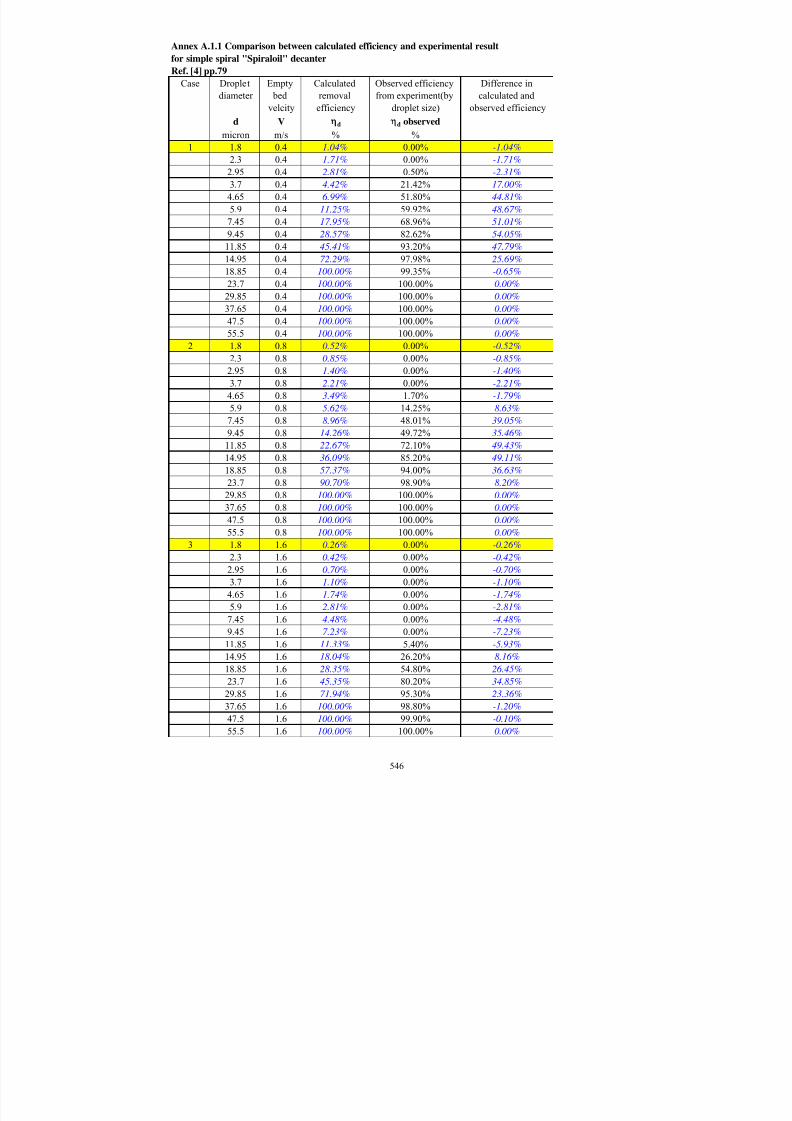
8/15/2019 Rachu.pdf
http://slidepdf.com/reader/full/rachupdf 633/646
Annex A.1.1 Comparison between calculated efficiency and experimental result
for simple spiral "Spiraloil" decanter
Ref. [4] pp.79
Case Droplet
diameter
Empty
bed
velcity
Calculated
removal
efficiency
Observed efficiency
from experiment(by
droplet size)
Difference in
calculated and
observed efficiency
d V d d observed
micron m/s % %1 1.8 0.4 1.04% 0.00% -1.04%
2.3 0.4 1.71% 0.00% -1.71%
2.95 0.4 2.81% 0.50% -2.31%
3.7 0.4 4.42% 21.42% 17.00%
4.65 0.4 6.99% 51.80% 44.81%
5.9 0.4 11.25% 59.92% 48.67%
7.45 0.4 17.95% 68.96% 51.01%
9.45 0.4 28.57% 82.62% 54.05%
11.85 0.4 45.41% 93.20% 47.79%
14.95 0.4 72.29% 97.98% 25.69%
18.85 0.4 100.00% 99.35% -0.65%
23.7 0.4 100.00% 100.00% 0.00%
29.85 0.4 100.00% 100.00% 0.00%
37.65 0.4 100.00% 100.00% 0.00%
47.5 0.4 100.00% 100.00% 0.00%
55.5 0.4 100.00% 100.00% 0.00%
2 1.8 0.8 0.52% 0.00% -0.52%
2.3 0.8 0.85% 0.00% -0.85%
2.95 0.8 1.40% 0.00% -1.40%
3.7 0.8 2.21% 0.00% -2.21%
4.65 0.8 3.49% 1.70% -1.79%
5.9 0.8 5.62% 14.25% 8.63%
7.45 0.8 8.96% 48.01% 39.05%
9.45 0.8 14.26% 49.72% 35.46%
11.85 0.8 22.67% 72.10% 49.43%
14.95 0.8 36.09% 85.20% 49.11%
18.85 0.8 57.37% 94.00% 36.63%
23.7 0.8 90.70% 98.90% 8.20%
29.85 0.8 100.00% 100.00% 0.00%
37.65 0.8 100.00% 100.00% 0.00%
47.5 0.8 100.00% 100.00% 0.00%
55.5 0.8 100.00% 100.00% 0.00%
3 1.8 1.6 0.26% 0.00% -0.26%
2.3 1.6 0.42% 0.00% -0.42%
2.95 1.6 0.70% 0.00% -0.70%
3.7 1.6 1.10% 0.00% -1.10%
4.65 1.6 1.74% 0.00% -1.74%
5.9 1.6 2.81% 0.00% -2.81%
7.45 1.6 4.48% 0.00% -4.48%
9.45 1.6 7.23% 0.00% -7.23%
11.85 1.6 11.33% 5.40% -5.93%
14.95 1.6 18.04% 26.20% 8.16%
18.85 1.6 28.35% 54.80% 26.45%
23.7 1.6 45.35% 80.20% 34.85%
29.85 1.6 71.94% 95.30% 23.36%
37.65 1.6 100.00% 98.80% -1.20%
47.5 1.6 100.00% 99.90% -0.10%
55.5 1.6 100.00% 100.00% 0.00%
546

8/15/2019 Rachu.pdf
http://slidepdf.com/reader/full/rachupdf 634/646
Annex A1.2 Comparison between calculated efficiency and experimental result
for mixed spiral "Spiraloil" decanter
Ref. [4] pp.88
Case Droplet
diameter
Empty
bed
velcity
Calculated
removal
efficiency
Observed efficiency
from experiment(by
droplet size)
Difference in
calculated and
observed efficiency
d V d d observed
micron m/s % %
1 1.80 0.5 1.88% 52.22% 50.34%
2.30 0.5 3.08% 58.83% 55.75%
2.95 0.5 5.07% 67.54% 62.47%
3.70 0.5 7.97% 72.08% 64.11%
4.65 0.5 12.60% 79.89% 67.29%
5.90 0.5 20.29% 84.97% 64.68%
7.45 0.5 32.35% 89.00% 56.65%
9.45 0.5 51.50% 94.01% 42.51%
11.85 0.5 81.85% 97.02% 15.17%
14.95 0.5 100.00% 98.22% -1.78%
18.85 0.5 100.00% 99.40% -0.60%
23.70 0.5 100.00% 100.00% 0.00%
29.85 0.5 100.00% 100.00% 0.00%
37.65 0.5 100.00% 100.00% 0.00%
47.50 0.5 100.00% 100.00% 0.00%
53.00 0.5 0.00%
2 1.80 1.5
2.30 1.5
2.95 1.5
3.70 1.5
4.65 1.5 4.20% 43.18% 38.98%
5.90 1.5 6.76% 61.82% 55.06%
7.45 1.5 10.78% 67.27% 56.49%
9.45 1.5 17.17% 71.82% 54.65%
11.85 1.5 27.28% 75.45% 48.17%
14.95 1.5 43.18% 77.27% 34.09%
18.85 1.5 70.00% 84.54% 14.54%23.70 1.5 100.00% 92.73% -7.27%
29.85 1.5 100.00% 100.00% 0.00%
37.65 1.5 100.00% 100.00% 0.00%
47.50 1.5 100.00% 100.00% 0.00%
55.50 1.5
547

8/15/2019 Rachu.pdf
http://slidepdf.com/reader/full/rachupdf 635/646
Annex A2.1 Comparison between calculated efficiency and experimental result for granular bed coalescer
Ref. [3] pp.285 & 321, [9], pp.174
Case Total
hydrocarbon
concentration
Droplet
diameter
Bed
media
diameter
Bed
height
Dispersed
phase
density
Continuous
phase
density
Density
difference
Dynamic
viscosity
of
dispersed
phase
Dynamic
viscosity of
continuous
phase
Empty
bed
velcity
Interfacial
tension
Calculated
removal
efficiency
from
DAMAK's
model
Observed
efficiency
from
experiment(by
droplet size)
Co d dp H ρd ρc ρ
μd μc V γo w ηd ηd observed
mg/l m m m kg/cu.m kg/cu.m kg/cu.m (N.s)/m2
(=1000cP
(N.s)/m2
(=0.1000cP)
m/s N/m
(=1000dyn/cm
% %
1 1000 41.00 0.37 0.01 793.4 998 204.6 1.07E-03 1.08E-03 0.00351 4.20E-02 99.79% 95.00%
1000 41.00 0.37 0.03 793.4 998 204.6 1.07E-03 1.08E-03 0.00351 4.20E-02 100.00% 98.70%
1000 41.00 0.37 0.05 793.4 998 204.6 1.07E-03 1.08E-03 0.00351 4.20E-02 100.00% 100.00%
1000 41.00 0.37 0.1 793.4 998 204.6 1.07E-03 1.08E-03 0.00351 4.20E-02 100.00% 100.00%
1000 32.65 0.37 0.03 793.4 998 204.6 1.07E-03 1.08E-03 0.00351 4.20E-02 100.00% 99.99%
1000 32.65 0.37 0.05 793.4 998 204.6 1.07E-03 1.08E-03 0.00351 4.20E-02 100.00% 100.00%
1000 32.65 0.37 0.1 793.4 998 204.6 1.07E-03 1.08E-03 0.00351 4.20E-02 100.00% 100.00%
1000 25.90 0.37 0.03 793.4 998 204.6 1.07E-03 1.08E-03 0.00351 4.20E-02 100.00% 99.00%
1000 25.90 0.37 0.05 793.4 998 204.6 1.07E-03 1.08E-03 0.00351 4.20E-02 100.00% 100.00%
1000 25.90 0.37 0.1 793.4 998 204.6 1.07E-03 1.08E-03 0.00351 4.20E-02 100.00% 100.00%
1000 20.57 0.37 0.03 793.4 998 204.6 1.07E-03 1.08E-03 0.00351 4.20E-02 99.18% 98.00%
1000 20.57 0.37 0.05 793.4 998 204.6 1.07E-03 1.08E-03 0.00351 4.20E-02 100.00% 100.00%
1000 20.57 0.37 0.1 793.4 998 204.6 1.07E-03 1.08E-03 0.00351 4.20E-02 100.00% 100.00%
1000 16.36 0.37 0.03 793.4 998 204.6 1.07E-03 1.08E-03 0.00351 4.20E-02 94.74% 96.00%
1000 16.36 0.37 0.05 793.4 998 204.6 1.07E-03 1.08E-03 0.00351 4.20E-02 100.00% 100.00%
1000 16.36 0.37 0.1 793.4 998 204.6 1.07E-03 1.08E-03 0.00351 4.20E-02 100.00% 100.00%
1000 12.99 0.37 0.03 793.4 998 204.6 1.07E-03 1.08E-03 0.00351 4.20E-02 90.47% 94.30%
1000 12.99 0.37 0.05 793.4 998 204.6 1.07E-03 1.08E-03 0.00351 4.20E-02 96.19% 99.70%
1000 12.99 0.37 0.1 793.4 998 204.6 1.07E-03 1.08E-03 0.00351 4.20E-02 100.00% 100.00%
1000 10.30 0.37 0.03 793.4 998 204.6 1.07E-03 1.08E-03 0.00351 4.20E-02 86.37% 92.00%
1000 10.30 0.37 0.05 793.4 998 204.6 1.07E-03 1.08E-03 0.00351 4.20E-02 91.83% 98.70%
1000 10.30 0.37 0.1 793.4 998 204.6 1.07E-03 1.08E-03 0.00351 4.20E-02 99.79% 100.00%
2 1000 41.00 0.37 0.03 793.4 998 204.6 1.07E-03 1.08E-03 0.00351 4.20E-02 100.00% 98.60%
1000 41.00 0.37 0.05 793.4 998 204.6 1.07E-03 1.08E-03 0.00351 4.20E-02 100.00% 100.00%
1000 41.00 0.37 0.1 793.4 998 204.6 1.07E-03 1.08E-03 0.00351 4.20E-02 100.00% 99.40%
1000 32.65 0.37 0.03 793.4 998 204.6 1.07E-03 1.08E-03 0.00351 4.20E-02 100.00% 99.00%
1000 32.65 0.37 0.05 793.4 998 204.6 1.07E-03 1.08E-03 0.00351 4.20E-02 100.00% 100.00%
1000 32.65 0.37 0.1 793.4 998 204.6 1.07E-03 1.08E-03 0.00351 4.20E-02 100.00% 99.40%
1000 25.90 0.37 0.03 793.4 998 204.6 1.07E-03 1.08E-03 0.00351 4.20E-02 100.00% 98.60%
1000 25.90 0.37 0.05 793.4 998 204.6 1.07E-03 1.08E-03 0.00351 4.20E-02 100.00% 100.00%
1000 25.90 0.37 0.1 793.4 998 204.6 1.07E-03 1.08E-03 0.00351 4.20E-02 100.00% 99.00%
1000 20.57 0.37 0.03 793.4 998 204.6
1.07E-03 1.08E-03 0.00351 4.20E-02 99.18%
97.00%1000 20.57 0.37 0.05 793.4 998 204.6 1.07E-03 1.08E-03 0.00351 4.20E-02 100.00% 100.00%
1000 20.57 0.37 0.1 793.4 998 204.6 1.07E-03 1.08E-03 0.00351 4.20E-02 100.00% 98.60%
1000 16.36 0.37 0.03 793.4 998 204.6 1.07E-03 1.08E-03 0.00351 4.20E-02 94.74% 94.60%
1000 16.36 0.37 0.05 793.4 998 204.6 1.07E-03 1.08E-03 0.00351 4.20E-02 100.00% 99.60%
1000 16.36 0.37 0.1 793.4 998 204.6 1.07E-03 1.08E-03 0.00351 4.20E-02 100.00% 98.60%
1000 12.99 0.37 0.03 793.4 998 204.6 1.07E-03 1.08E-03 0.00351 4.20E-02 90.47% 92.60%
1000 12.99 0.37 0.05 793.4 998 204.6 1.07E-03 1.08E-03 0.00351 4.20E-02 96.19% 99.20%
1000 12.99 0.37 0.1 793.4 998 204.6 1.07E-03 1.08E-03 0.00351 4.20E-02 100.00% 98.60%
1000 10.30 0.37 0.03 793.4 998 204.6 1.07E-03 1.08E-03 0.00351 4.20E-02 86.37% 88.80%
1000 10.30 0.37 0.05 793.4 998 204.6 1.07E-03 1.08E-03 0.00351 4.20E-02 91.83% 97.40%
1000 10.30 0.37 0.1 793.4 998 204.6
1.07E-03 1.08E-03 0.00351 4.20E-02 99.79%
98.20%3 1000 41.00 0.60 0.03 793.4 998 204.6 1.07E-03 1.08E-03 0.00351 4.20E-02 93.83% 97.00%
1000 41.00 0.60 0.05 793.4 998 204.6 1.07E-03 1.08E-03 0.00351 4.20E-02 99.76% 99.00%
1000 41.00 0.60 0.1 793.4 998 204.6 1.07E-03 1.08E-03 0.00351 4.20E-02 100.00% 100.00%
1000 32.65 0.60 0.03 793.4 998 204.6 1.07E-03 1.08E-03 0.00351 4.20E-02 89.66% 93.00%
1000 32.65 0.60 0.05 793.4 998 204.6 1.07E-03 1.08E-03 0.00351 4.20E-02 95.32% 97.00%
548

8/15/2019 Rachu.pdf
http://slidepdf.com/reader/full/rachupdf 636/646
Annex A2.1 Comparison between calculated efficiency and experimental result for granular bed coalescer
Ref. [3] pp.285 & 321, [9], pp.174
Case Total
hydrocarbon
concentration
Droplet
diameter
Bed
media
diameter
Bed
height
Dispersed
phase
density
Continuous
phase
density
Density
difference
Dynamic
viscosity
of
dispersed
phase
Dynamic
viscosity of
continuous
phase
Empty
bed
velcity
Interfacial
tension
Calculated
removal
efficiency
from
DAMAK's
model
Observed
efficiency
from
experiment(by
droplet size)
Co d dp H ρd ρc ρ
μd μc V γo w ηd ηd observed
mg/l m m m kg/cu.m kg/cu.m kg/cu.m (N.s)/m2
(=1000cP
(N.s)/m2
(=0.1000cP)
m/s N/m
(=1000dyn/cm
% %
1000 32.65 0.60 0.1 793.4 998 204.6 1.07E-03 1.08E-03 0.00351 4.20E-02 100.00% 100.00%
1000 25.90 0.60 0.03 793.4 998 204.6 1.07E-03 1.08E-03 0.00351 4.20E-02 85.60% 90.20%
1000 25.90 0.60 0.05 793.4 998 204.6 1.07E-03 1.08E-03 0.00351 4.20E-02 91.01% 96.40%
1000 25.90 0.60 0.1 793.4 998 204.6 1.07E-03 1.08E-03 0.00351 4.20E-02 98.90% 100.00%
1000 20.57 0.60 0.03 793.4 998 204.6 1.07E-03 1.08E-03 0.00351 4.20E-02 81.74% 83.20%
1000 20.57 0.60 0.05 793.4 998 204.6 1.07E-03 1.08E-03 0.00351 4.20E-02 86.91% 94.40%
1000 20.57 0.60 0.1 793.4 998 204.6 1.07E-03 1.08E-03 0.00351 4.20E-02 94.45% 99.40%
1000 16.36 0.60 0.03 793.4 998 204.6 1.07E-03 1.08E-03 0.00351 4.20E-02 78.08% 74.80%
1000 16.36 0.60 0.05 793.4 998 204.6 1.07E-03 1.08E-03 0.00351 4.20E-02 83.02% 91.20%
1000 16.36 0.60 0.1 793.4 998 204.6 1.07E-03 1.08E-03 0.00351 4.20E-02 90.22% 98.00%
1000 12.99 0.60 0.03 793.4 998 204.6 1.07E-03 1.08E-03 0.00351 4.20E-02 74.56% 61.00%
1000 12.99 0.60 0.05 793.4 998 204.6 1.07E-03 1.08E-03 0.00351 4.20E-02 79.28% 87.20%
1000 12.99 0.60 0.1 793.4 998 204.6 1.07E-03 1.08E-03 0.00351 4.20E-02 86.15% 96.60%
1000 10.30 0.60 0.03 793.4 998 204.6 1.07E-03 1.08E-03 0.00351 4.20E-02 71.18% 58.20%
1000 10.30 0.60 0.05 793.4 998 204.6 1.07E-03 1.08E-03 0.00351 4.20E-02 75.68% 84.00%
1000 10.30 0.60 0.1 793.4 998 204.6 1.07E-03 1.08E-03 0.00351 4.20E-02 82.25% 93.40%
4 1000 41.00 0.75 0.03 793.4 998 204.6 1.07E-03 1.08E-03 0.00351 4.20E-02 85.82% 89.60%
1000 41.00 0.75 0.05 793.4 998 204.6 1.07E-03 1.08E-03 0.00351 4.20E-02 91.25% 98.00%
1000 41.00 0.75 0.1 793.4 998 204.6 1.07E-03 1.08E-03 0.00351 4.20E-02 99.16% 100.00%
1000 32.65 0.75 0.03 793.4 998 204.6 1.07E-03 1.08E-03 0.00351 4.20E-02 82.00% 85.20%
1000 32.65 0.75 0.05 793.4 998 204.6 1.07E-03 1.08E-03 0.00351 4.20E-02 87.18% 93.20%
1000 32.65 0.75 0.1 793.4 998 204.6 1.07E-03 1.08E-03 0.00351 4.20E-02 94.75% 100.00%
1000 25.90 0.75 0.03 793.4 998 204.6 1.07E-03 1.08E-03 0.00351 4.20E-02 78.29% 75.80%
1000 25.90 0.75 0.05 793.4 998 204.6 1.07E-03 1.08E-03 0.00351 4.20E-02 83.24% 96.20%
1000 25.90 0.75 0.1 793.4 998 204.6 1.07E-03 1.08E-03 0.00351 4.20E-02 90.46% 99.60%
1000 20.57 0.75 0.03 793.4 998 204.6 1.07E-03 1.08E-03 0.00351 4.20E-02 74.76% 61.00%
1000 20.57 0.75 0.05 793.4 998 204.6 1.07E-03 1.08E-03 0.00351 4.20E-02 79.49% 95.40%
1000 20.57 0.75 0.1 793.4 998 204.6 1.07E-03 1.08E-03 0.00351 4.20E-02 86.38% 99.00%
1000 16.36 0.75 0.03 793.4 998 204.6 1.07E-03 1.08E-03 0.00351 4.20E-02 71.42% 56.00%
1000 16.36 0.75 0.05 793.4 998 204.6 1.07E-03 1.08E-03 0.00351 4.20E-02 75.93% 90.80%
1000 16.36 0.75 0.1 793.4 998 204.6 1.07E-03 1.08E-03 0.00351 4.20E-02 82.52% 96.60%
1000 12.99 0.75 0.03 793.4 998 204.6
1.07E-03 1.08E-03 0.00351 4.20E-02 68.20%
42.60%1000 12.99 0.75 0.05 793.4 998 204.6 1.07E-03 1.08E-03 0.00351 4.20E-02 72.51% 83.20%
1000 12.99 0.75 0.1 793.4 998 204.6 1.07E-03 1.08E-03 0.00351 4.20E-02 78.80% 90.80%
1000 10.30 0.75 0.03 793.4 998 204.6 1.07E-03 1.08E-03 0.00351 4.20E-02 65.10% 24.60%
1000 10.30 0.75 0.05 793.4 998 204.6 1.07E-03 1.08E-03 0.00351 4.20E-02 69.22% 78.80%
1000 10.30 0.75 0.1 793.4 998 204.6 1.07E-03 1.08E-03 0.00351 4.20E-02 75.22% 84.20%
5 1000 10.00 0.36 0.02 914.5 998 83.5 2.10E-03 1.07E-03 0.0009 1.10E-02 90.55% 95.00%
1000 14.00 0.36 0.02 914.5 998 83.5 2.10E-03 1.07E-03 0.0009 1.10E-02 96.85% 96.50%
1000 20.00 0.36 0.02 914.5 998 83.5 2.10E-03 1.07E-03 0.0009 1.10E-02 100.00% 98.00%
1000 28.00 0.36 0.02 914.5 998 83.5 2.10E-03 1.07E-03 0.0009 1.10E-02 100.00% 99.00%
1000 40.00 0.36 0.02 914.5 998 83.5 2.10E-03 1.07E-03 0.0009 1.10E-02 100.00% 100.00%
1000 10.00 0.36 0.02 914.5 998 83.5
2.10E-03 1.07E-03 0.00136 1.10E-02 84.81%
91.00%1000 14.00 0.36 0.02 914.5 998 83.5 2.10E-03 1.07E-03 0.00136 1.10E-02 90.71% 94.00%
1000 20.00 0.36 0.02 914.5 998 83.5 2.10E-03 1.07E-03 0.00136 1.10E-02 97.42% 97.00%
1000 28.00 0.36 0.02 914.5 998 83.5 2.10E-03 1.07E-03 0.00136 1.10E-02 100.00% 99.00%
1000 40.00 0.36 0.02 914.5 998 83.5 2.10E-03 1.07E-03 0.00136 1.10E-02 100.00% 100.00%
1000 10.00 0.36 0.02 914.5 998 83.5 2.10E-03 1.07E-03 0.0027 1.10E-02 75.99% 75.00%
549

8/15/2019 Rachu.pdf
http://slidepdf.com/reader/full/rachupdf 637/646
Annex A2.1 Comparison between calculated efficiency and experimental result for granular bed coalescer
Ref. [3] pp.285 & 321, [9], pp.174
Case Total
hydrocarbon
concentration
Droplet
diameter
Bed
media
diameter
Bed
height
Dispersed
phase
density
Continuous
phase
density
Density
difference
Dynamic
viscosity
of
dispersed
phase
Dynamic
viscosity of
continuous
phase
Empty
bed
velcity
Interfacial
tension
Calculated
removal
efficiency
from
DAMAK's
model
Observed
efficiency
from
experiment(by
droplet size)
Co d dp H ρd ρc ρ
μd μc V γo w ηd ηd observed
mg/l m m m kg/cu.m kg/cu.m kg/cu.m (N.s)/m2
(=1000cP
(N.s)/m2
(=0.1000cP)
m/s N/m
(=1000dyn/cm
% %
1000 14.00 0.36 0.02 914.5 998 83.5 2.10E-03 1.07E-03 0.0027 1.10E-02 81.28% 86.00%
1000 20.00 0.36 0.02 914.5 998 83.5 2.10E-03 1.07E-03 0.0027 1.10E-02 87.29% 92.00%
1000 28.00 0.36 0.02 914.5 998 83.5 2.10E-03 1.07E-03 0.0027 1.10E-02 93.37% 97.00%
1000 40.00 0.36 0.02 914.5 998 83.5 2.10E-03 1.07E-03 0.0027 1.10E-02 100.00% 99.00%
1000 10.00 0.36 0.02 914.5 998 83.5 2.10E-03 1.07E-03 0.00406 1.10E-02 71.19% 67.00%
1000 14.00 0.36 0.02 914.5 998 83.5 2.10E-03 1.07E-03 0.00406 1.10E-02 76.15% 79.00%
1000 20.00 0.36 0.02 914.5 998 83.5 2.10E-03 1.07E-03 0.00406 1.10E-02 81.78% 84.00%
1000 28.00 0.36 0.02 914.5 998 83.5 2.10E-03 1.07E-03 0.00406 1.10E-02 87.47% 92.00%
1000 40.00 0.36 0.02 914.5 998 83.5 2.10E-03 1.07E-03 0.00406 1.10E-02 93.94% 94.00%
1000 10.00 0.36 0.02 914.5 998 83.5 2.10E-03 1.07E-03 0.00541 1.10E-02 68.00% 61.00%
1000 14.00 0.36 0.02 914.5 998 83.5 2.10E-03 1.07E-03 0.00541 1.10E-02 72.73% 65.00%
1000 20.00 0.36 0.02 914.5 998 83.5 2.10E-03 1.07E-03 0.00541 1.10E-02 78.11% 71.50%
1000 28.00 0.36 0.02 914.5 998 83.5 2.10E-03 1.07E-03 0.00541 1.10E-02 83.54% 85.50%
1000 40.00 0.36 0.02 914.5 998 83.5 2.10E-03 1.07E-03 0.00541 1.10E-02 89.72% 92.00%
1000 10.00 0.36 0.03 914.5 998 83.5 2.10E-03 1.07E-03 0.0027 1.10E-02 79.78% 85.00%
1000 14.00 0.36 0.03 914.5 998 83.5 2.10E-03 1.07E-03 0.0027 1.10E-02 85.34% 90.00%
1000 20.00 0.36 0.03 914.5 998 83.5 2.10E-03 1.07E-03 0.0027 1.10E-02 91.65% 94.50%
1000 28.00 0.36 0.03 914.5 998 83.5 2.10E-03 1.07E-03 0.0027 1.10E-02 98.03% 98.00%
1000 40.00 0.36 0.03 914.5 998 83.5 2.10E-03 1.07E-03 0.0027 1.10E-02 100.00% 100.00%
1000 10.00 0.36 0.05 914.5 998 83.5 2.10E-03 1.07E-03 0.0027 1.10E-02 84.83% 89.00%
1000 14.00 0.36 0.05 914.5 998 83.5 2.10E-03 1.07E-03 0.0027 1.10E-02 90.73% 92.00%
1000 20.00 0.36 0.05 914.5 998 83.5 2.10E-03 1.07E-03 0.0027 1.10E-02 97.44% 96.00%
1000 28.00 0.36 0.05 914.5 998 83.5 2.10E-03 1.07E-03 0.0027 1.10E-02 100.00% 99.00%
1000 40.00 0.36 0.05 914.5 998 83.5 2.10E-03 1.07E-03 0.0027 1.10E-02 100.00% 100.00%
1000 10.00 0.36 0.1 914.5 998 83.5 2.10E-03 1.07E-03 0.0027 1.10E-02 92.18% 93.50%
1000 14.00 0.36 0.1 914.5 998 83.5 2.10E-03 1.07E-03 0.0027 1.10E-02 98.60% 95.00%
1000 20.00 0.36 0.1 914.5 998 83.5 2.10E-03 1.07E-03 0.0027 1.10E-02 100.00% 99.00%
1000 28.00 0.36 0.1 914.5 998 83.5 2.10E-03 1.07E-03 0.0027 1.10E-02 100.00% 100.00%
1000 40.00 0.36 0.1 914.5 998 83.5 2.10E-03 1.07E-03 0.0027 1.10E-02 100.00% 100.00%
1000 10.00 0.56 0.03 914.5 998 83.5 2.10E-03 1.07E-03 0.0027 1.10E-02 66.86% 71.00%
1000 14.00 0.56 0.03 914.5 998 83.5 2.10E-03 1.07E-03 0.0027 1.10E-02 71.51% 76.00%
1000 20.00 0.56 0.03 914.5 998 83.5
2.10E-03 1.07E-03 0.0027 1.10E-02 76.80%
80.00%1000 28.00 0.56 0.03 914.5 998 83.5 2.10E-03 1.07E-03 0.0027 1.10E-02 82.15% 85.00%
1000 40.00 0.56 0.03 914.5 998 83.5 2.10E-03 1.07E-03 0.0027 1.10E-02 88.22% 94.00%
1000 10.00 0.56 0.05 914.5 998 83.5 2.10E-03 1.07E-03 0.0027 1.10E-02 71.08% 78.00%
1000 14.00 0.56 0.05 914.5 998 83.5 2.10E-03 1.07E-03 0.0027 1.10E-02 76.03% 81.00%
1000 20.00 0.56 0.05 914.5 998 83.5 2.10E-03 1.07E-03 0.0027 1.10E-02 81.66% 85.00%
1000 28.00 0.56 0.05 914.5 998 83.5 2.10E-03 1.07E-03 0.0027 1.10E-02 87.34% 92.00%
1000 40.00 0.56 0.05 914.5 998 83.5 2.10E-03 1.07E-03 0.0027 1.10E-02 93.80% 98.00%
1000 10.00 0.56 0.1 914.5 998 83.5 2.10E-03 1.07E-03 0.0027 1.10E-02 77.25% 86.00%
1000 14.00 0.56 0.1 914.5 998 83.5 2.10E-03 1.07E-03 0.0027 1.10E-02 82.63% 90.00%
1000 20.00 0.56 0.1 914.5 998 83.5 2.10E-03 1.07E-03 0.0027 1.10E-02 88.74% 98.00%
1000 28.00 0.56 0.1 914.5 998 83.5
2.10E-03 1.07E-03 0.0027 1.10E-02 94.91%
98.00%1000 40.00 0.56 0.1 914.5 998 83.5 2.10E-03 1.07E-03 0.0027 1.10E-02 100.00% 99.00%
1000 10.00 0.73 0.03 914.5 998 83.5 2.10E-03 1.07E-03 0.0027 1.10E-02 60.13% 60.00%
1000 14.00 0.73 0.03 914.5 998 83.5 2.10E-03 1.07E-03 0.0027 1.10E-02 64.32% 65.00%
1000 20.00 0.73 0.03 914.5 998 83.5 2.10E-03 1.07E-03 0.0027 1.10E-02 69.07% 70.00%
1000 28.00 0.73 0.03 914.5 998 83.5 2.10E-03 1.07E-03 0.0027 1.10E-02 73.88% 76.00%
550

8/15/2019 Rachu.pdf
http://slidepdf.com/reader/full/rachupdf 638/646
Annex A2.1 Comparison between calculated efficiency and experimental result for granular bed coalescer
Ref. [3] pp.285 & 321, [9], pp.174
Case Total
hydrocarbon
concentration
Droplet
diameter
Bed
media
diameter
Bed
height
Dispersed
phase
density
Continuous
phase
density
Density
difference
Dynamic
viscosity
of
dispersed
phase
Dynamic
viscosity of
continuous
phase
Empty
bed
velcity
Interfacial
tension
Calculated
removal
efficiency
from
DAMAK's
model
Observed
efficiency
from
experiment(by
droplet size)
Co d dp H ρd ρc ρ
μd μc V γo w ηd ηd observed
mg/l m m m kg/cu.m kg/cu.m kg/cu.m (N.s)/m2
(=1000cP
(N.s)/m2
(=0.1000cP)
m/s N/m
(=1000dyn/cm
% %
1000 40.00 0.73 0.03 914.5 998 83.5 2.10E-03 1.07E-03 0.0027 1.10E-02 79.34% 91.00%
1000 10.00 0.73 0.05 914.5 998 83.5 2.10E-03 1.07E-03 0.0027 1.10E-02 63.93% 63.00%
1000 14.00 0.73 0.05 914.5 998 83.5 2.10E-03 1.07E-03 0.0027 1.10E-02 68.38% 69.00%
1000 20.00 0.73 0.05 914.5 998 83.5 2.10E-03 1.07E-03 0.0027 1.10E-02 73.44% 75.00%
1000 28.00 0.73 0.05 914.5 998 83.5 2.10E-03 1.07E-03 0.0027 1.10E-02 78.55% 81.00%
1000 40.00 0.73 0.05 914.5 998 83.5 2.10E-03 1.07E-03 0.0027 1.10E-02 84.36% 95.00%
1000 10.00 0.73 0.1 914.5 998 83.5 2.10E-03 1.07E-03 0.0027 1.10E-02 69.48% 71.00%
1000 14.00 0.73 0.1 914.5 998 83.5 2.10E-03 1.07E-03 0.0027 1.10E-02 74.31% 76.00%
1000 20.00 0.73 0.1 914.5 998 83.5 2.10E-03 1.07E-03 0.0027 1.10E-02 79.81% 84.00%
1000 28.00 0.73 0.1 914.5 998 83.5 2.10E-03 1.07E-03 0.0027 1.10E-02 85.36% 90.00%
1000 40.00 0.73 0.1 914.5 998 83.5 2.10E-03 1.07E-03 0.0027 1.10E-02 91.68% 98.00%
1000 10.00 0.94 0.03 914.5 998 83.5 2.10E-03 1.07E-03 0.0027 1.10E-02 54.35% 53.00%
1000 14.00 0.94 0.03 914.5 998 83.5 2.10E-03 1.07E-03 0.0027 1.10E-02 58.13% 58.00%
1000 20.00 0.94 0.03 914.5 998 83.5 2.10E-03 1.07E-03 0.0027 1.10E-02 62.43% 61.00%
1000 28.00 0.94 0.03 914.5 998 83.5 2.10E-03 1.07E-03 0.0027 1.10E-02 66.77% 66.00%
1000 40.00 0.94 0.03 914.5 998 83.5 2.10E-03 1.07E-03 0.0027 1.10E-02 71.71% 75.00%
1000 10.00 0.94 0.05 914.5 998 83.5 2.10E-03 1.07E-03 0.0027 1.10E-02 57.78% 57.00%
1000 14.00 0.94 0.05 914.5 998 83.5 2.10E-03 1.07E-03 0.0027 1.10E-02 61.81% 61.00%
1000 20.00 0.94 0.05 914.5 998 83.5 2.10E-03 1.07E-03 0.0027 1.10E-02 66.38% 65.00%
1000 28.00 0.94 0.05 914.5 998 83.5 2.10E-03 1.07E-03 0.0027 1.10E-02 71.00% 71.00%
1000 40.00 0.94 0.05 914.5 998 83.5 2.10E-03 1.07E-03 0.0027 1.10E-02 76.25% 82.00%
1000 10.00 0.94 0.1 914.5 998 83.5 2.10E-03 1.07E-03 0.0027 1.10E-02 62.79% 63.00%
1000 14.00 0.94 0.1 914.5 998 83.5 2.10E-03 1.07E-03 0.0027 1.10E-02 67.17% 67.00%
1000 20.00 0.94 0.1 914.5 998 83.5 2.10E-03 1.07E-03 0.0027 1.10E-02 72.13% 72.00%
1000 28.00 0.94 0.1 914.5 998 83.5 2.10E-03 1.07E-03 0.0027 1.10E-02 77.15% 78.00%
1000 40.00 0.94 0.1 914.5 998 83.5 2.10E-03 1.07E-03 0.0027 1.10E-02 82.86% 92.00%
1000 10.00 0.73 0.03 795 998 203 1.35E-03 1.07E-03 0.0027 4.20E-02 69.68% 68.00%
1000 14.00 0.73 0.03 795 998 203 1.35E-03 1.07E-03 0.0027 4.20E-02 74.53% 77.00%
1000 20.00 0.73 0.03 795 998 203 1.35E-03 1.07E-03 0.0027 4.20E-02 80.04% 84.50%
1000 28.00 0.73 0.03 795 998 203 1.35E-03 1.07E-03 0.0027 4.20E-02 85.61% 90.00%
1000 40.00 0.73 0.03 795 998 203 1.35E-03 1.07E-03 0.0027 4.20E-02 91.94% 92.00%
1000 10.00 0.73 0.03 994.1 998 3.9
1.09E-03 1.07E-03 0.0027 1.60E-02 44.33%
40.50%1000 14.00 0.73 0.03 994.1 998 3.9 1.09E-03 1.07E-03 0.0027 1.60E-02 47.42% 45.50%
1000 20.00 0.73 0.03 994.1 998 3.9 1.09E-03 1.07E-03 0.0027 1.60E-02 50.93% 51.00%
1000 28.00 0.73 0.03 994.1 998 3.9 1.09E-03 1.07E-03 0.0027 1.60E-02 54.47% 56.00%
1000 40.00 0.73 0.03 994.1 998 3.9 1.09E-03 1.07E-03 0.0027 1.60E-02 58.50% 73.00%
1000 10.00 0.73 0.03 684 998 314 4.20E-04 1.07E-03 0.0027 3.62E-02 64.47% 62.00%
1000 14.00 0.73 0.03 684 998 314 4.20E-04 1.07E-03 0.0027 3.62E-02 68.96% 66.00%
1000 20.00 0.73 0.03 684 998 314 4.20E-04 1.07E-03 0.0027 3.62E-02 74.06% 72.10%
1000 28.00 0.73 0.03 684 998 314 4.20E-04 1.07E-03 0.0027 3.62E-02 79.21% 89.00%
1000 40.00 0.73 0.03 684 998 314 4.20E-04 1.07E-03 0.0027 3.62E-02 85.07% 90.00%
1000 10.00 0.73 0.03 860 998 138 7.16E-04 1.07E-03 0.0027 3.03E-02 61.93% 57.50%
1000 14.00 0.73 0.03 860 998 138
7.16E-04 1.07E-03 0.0027 3.03E-02 66.24%
64.50%1000 20.00 0.73 0.03 860 998 138 7.16E-04 1.07E-03 0.0027 3.03E-02 71.14% 75.00%
1000 28.00 0.73 0.03 860 998 138 7.16E-04 1.07E-03 0.0027 3.03E-02 76.09% 83.00%
1000 40.00 0.73 0.03 860 998 138 7.16E-04 1.07E-03 0.0027 3.03E-02 81.71% 89.00%
551
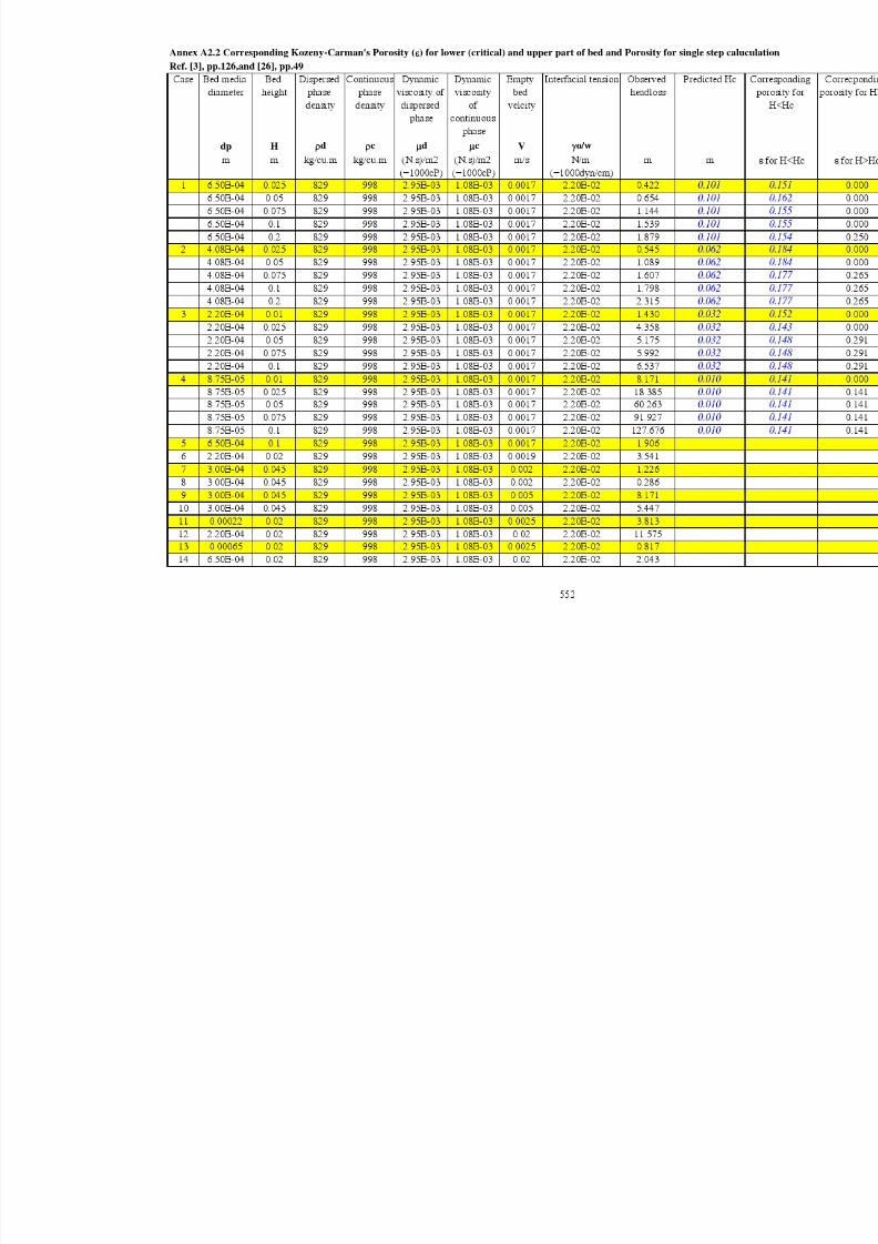
8/15/2019 Rachu.pdf
http://slidepdf.com/reader/full/rachupdf 639/646

8/15/2019 Rachu.pdf
http://slidepdf.com/reader/full/rachupdf 640/646

8/15/2019 Rachu.pdf
http://slidepdf.com/reader/full/rachupdf 641/646
Annex A.3 DAF tested by SIEM
[12] pp.130
Value
Wastewater
flowrate
Qin cu.m/s 3.9E-06
Pressurized
water flowrate
Qwater cu.m/s 4.2E-06
Qin/Qwater 0.92
Total flow Qtotal cu.m/s 8.14E-06
l/hr 29.31
Column cross
section area
Ao m2 0.0177
Velocity based
on total flow
Vo m/s 4.60E-04
Air flowrate
degassed in
DAF column
Φ cu.m/s 4.20E-07
Dissolved air
quantity in
pressurized
water
kg/cu.m 0.119
Effective
column height
H m 0.7
Bubble diameter dB m 7.00E-05
Dispersed phase density
ρd kg/cu.m 850
Continuous
phase density
ρc kg/cu.m 998
Air density kg/cu.m 1.201
Dispersed
phase viscosity
μd kg/m.s 0.0011
Continuous
phase viscosity
μc kg/m.s 0.00108
Bolzman
constant K 1.38E-23Temperature T Kelvin 293
Description
554

8/15/2019 Rachu.pdf
http://slidepdf.com/reader/full/rachupdf 642/646
Annex A.3 Comparison between observed efficiency and predicted efficiency for DAF
[12] pp.130
Item Bubble
diameter
Droplet
diameter
Rising
velocity
of dro let
Rising
velocity of
bubble
Relative
velocity
Sedimentati
on
efficienc
Interception
efficiency
Diffusio
n
efficienc
Theoritica
l totla
efficienc
Predicted
efficiencdB dE u U U-u S I D t theo exp
m m m/s m/s m/s predicted1 7.00E-05 2.10E-06 3.29E-07 2.46E-03 2.46E-03 1.34E-04 1.35E-03 4.3E-04 1.91E-03 2.21E-04
2 7.00E-05 2.60E-06 5.05E-07 2.46E-03 2.46E-03 2.05E-04 2.07E-03 3.7E-04 2.64E-03 2.68E-04
3 7.00E-05 3.30E-06 8.13E-07 2.46E-03 2.46E-03 3.30E-04 3.33E-03 3.2E-04 3.98E-03 3.42E-04
4 7.00E-05 4.10E-06 1.26E-06 2.46E-03 2.46E-03 5.10E-04 5.15E-03 2.7E-04 5.93E-03 4.33E-04
5 7.00E-05 5.10E-06 1.94E-06 2.46E-03 2.46E-03 7.89E-04 7.96E-03 2.4E-04 8.99E-03 5.54E-04
6 7.00E-05 6.50E-06 3.16E-06 2.46E-03 2.46E-03 1.28E-03 1.29E-02 2.0E-04 1.44E-02 7.32E-04
7 7.00E-05 8.20E-06 5.02E-06 2.46E-03 2.46E-03 2.04E-03 2.06E-02 1.7E-04 2.28E-02 9.61E-04
8 7.00E-05 1.03E-05 7.92E-06 2.46E-03 2.46E-03 3.23E-03 3.25E-02 1.5E-04 3.58E-02 1.26E-03
9 7.00E-05 1.30E-05 1.26E-05 2.46E-03 2.45E-03 5.15E-03 5.17E-02 1.3E-04 5.70E-02 1.65E-03
10 7.00E-05 1.64E-05 2.01E-05 2.46E-03 2.44E-03 8.22E-03 8.23E-02 1.1E-04 9.07E-02 2.17E-03
11 7.00E-05 2.06E-05 3.17E-05 2.46E-03 2.43E-03 1.30E-02 1.30E-01 9.4E-05 1.43E-01 2.85E-03 12 7.00E-05 2.59E-05 5.01E-05 2.46E-03 2.41E-03 2.07E-02 2.05E-01 8.1E-05 2.26E-01 3.74E-03
13 7.00E-05 3.27E-05 7.99E-05 2.46E-03 2.38E-03 3.35E-02 3.27E-01 7.0E-05 3.61E-01 4.93E-03
555

8/15/2019 Rachu.pdf
http://slidepdf.com/reader/full/rachupdf 643/646
Annex A3.1 Two-Phases hydrocyclone tested by MA
Ref. [26] pp.105
Description Value
Flowrate Q cu.m/s 5.40E-04Diameter of upper
c lindical ar
D m 4.00E-02
Nominal diameter of
h droc clone
Dn m 2.00E-02
Inlet diameter (2 ports) Di m 7.00E-03
Overflow diamete Dover m 2.00E-03
Underflow diamete Dunder m 1.00E-02
Angle of conical par Rad 2.62E-02
Dispersed phase densit ρd kg/cu.m 9.00E+02
Continuous phase c kg/cu.m 9.98E+02
Viscosit c Ns/m2 1.00E-03
Comparison between Observed efficiency and predicted efficiency from Ma's
and COLMAN's model for Two-Phases hydrocyclone
Ref. [26] pp.105, [16] pp.49
d75% for COLMAN model is based on [29] pp.15.
Efficienc
y
Observed
data
from
16 105
Droplet
diameter
predicted from
COLMAN 16
Droplet from
Ma's
Trajectory
methodeff% dE dE dE
% m m m
5% 8.49
10% 9.66
15% 10.89
20% 12.19 13.08
25% 13.58
30% 22 15.10 17.91
35% 16.70
40% 24 18.43 22.52
50% 25.6 22.36 26.63
60% 28.12 27.18 30.58
70% 30.75 33.39 34.12
75% 37.32
80% 34.7 42.12 37.26
90% 40 57.13 40.09
95% 72.05
99% 55.78 105.49 42.33
100% 156.93 42.54
556

8/15/2019 Rachu.pdf
http://slidepdf.com/reader/full/rachupdf 644/646
Annex A3.2 Three-Phases hydrocyclone tested by MA
Ref. [16] pp.151
Description Value
Flowrate Q cu.m/h 1.40E+00Diameter of
upper
c lindical
D m 4.00E-02
Nominal
diameter of
inlet of oil
Do m 1.40E-02
Inlet
diameter (2
Di m 5.60E-03
Underflow
diameter for
SS
Du m 6.00E-03
Underflow
diameter for
oil
Dp m 1.00E-03
Angle of
conical oil1.5
o
Angle of
conical SS
art
12o
Split ratio 2%
Comparison between Observed efficiency and predicted efficiency for
Three-Phases hydrocyclon
Ref. [16] pp.51
Efficiency
%
Droplet from
predicted
efficiency
curve micron
Droplet from
observed
efficiency
curve micron
10 5.07 8.520 9.00 9
30 12.46
40 15.81 10.5
50 18.82 12
60 21.73 14.25
80 26.83 20.5
100 31.02 42
100 50
557

8/15/2019 Rachu.pdf
http://slidepdf.com/reader/full/rachupdf 645/646
Annex A5.1 Comparison between calculated flux and experimental result from resistance model of UF (reference temparature 20oC)
Item Transmembrane
pressure
Velocity Concentratio
n (by volume
of oil, not
the
Observed flux Membrane
resistance
Gel resistance
coefficient (Rg
= Φ Vα Pt)
Alpha
(exponent of
V)
Gel
concentration
Predicted
flux (J = Pt/
(Rm + Rg))
Ref.
P or Pt V Co Jobserved Rm α Cg Jpredicted
bar m/s % l/(h.m2) % l/(h.m
2)
1 0 2.8 4 0 0.430 0.022 -1.500 16.200 0.00 see note1
2 0.1 2.8 4 14 0.430 0.022 -1.500 16.200 20.97 see note13 0.5 2.8 4 70.8 0.430 0.022 -1.500 16.200 75.21 see note1
4 1 2.8 4 114 0.430 0.022 -1.500 16.200 111.17 see note1
5 1.5 2.8 4 137.29 0.430 0.022 -1.500 16.200 132.24 see note1
6 2 2.8 4 150.8 0.430 0.022 -1.500 16.200 146.08 see note1
7 2.5 2.8 4 162.16 0.430 0.022 -1.500 16.200 155.87 see note1
8 3 2.8 4 165.4 0.430 0.022 -1.500 16.200 163.16 see note1
9 3.5 2.8 4 168.6 0.430 0.022 -1.500 16.200 168.80 see note1
10 0 2.1 4 0 0.430 0.022 -1.500 16.200 0.00 see note1
11 0.24 2.1 4 33.5 0.430 0.022 -1.500 16.200 39.77 see note1
12 0.5 2.1 4 60 0.430 0.022 -1.500 16.200 63.17 see note1
13 1 2.1 4 84.32 0.430 0.022 -1.500 16.200 86.74 see note1
14 1.5 2.1 4 97.3 0.430 0.022 -1.500 16.200 99.05 see note1
15 2 2.1 4 107.6 0.430 0.022 -1.500 16.200 106.62 see note1
16 2.5 2.1 4 110.8 0.430 0.022 -1.500 16.200 111.74 see note1
17 3 2.1 4 114 0.430 0.022 -1.500 16.200 115.44 see note1
18 0 1.4 4 0 0.430 0.022 -1.500 16.200 0.00 see note1
19 0.24 1.4 4 33.5 0.430 0.022 -1.500 16.200 32.05 see note1
20 0.5 1.4 4 45.4 0.430 0.022 -1.500 16.200 45.70 see note1
21 1 1.4 4 54 0.430 0.022 -1.500 16.200 56.88 see note1
22 1.5 1.4 4 59 0.430 0.022 -1.500 16.200 61.93 see note1
23 2 1.4 4 60 0.430 0.022 -1.500 16.200 64.80 see note1
24 2.5 1.4 4 62 0.430 0.022 -1.500 16.200 66.66 see note1
25 3 1.4 4 62.7 0.430 0.022 -1.500 16.200 67.96 see note1
26 3.5 1.4 4 63.24 0.430 0.022 -1.500 16.200 68.92 see note1
27 0 0.7 4 0 0.430 0.022 -1.500 16.200 0.00 see note1
28 0.1 0.7 4 14 0.430 0.022 -1.500 16.200 12.41 see note1
29 0.5 0.7 4 31.9 0.430 0.022 -1.500 16.200 21.66 see note1
30 1 0.7 4 33.5 0.430 0.022 -1.500 16.200 23.89 see note1
31 1.5 0.7 4 33.5 0.430 0.022 -1.500 16.200 24.73 see note132 2 0.7 4 33.5 0.430 0.022 -1.500 16.200 25.18 see note1
33 2.5 0.7 4 33.5 0.430 0.022 -1.500 16.200 25.46 see note1
34 3 0.7 4 33.5 0.430 0.022 -1.500 16.200 25.64 see note1
35 1.0 1.0 3.2 36.51 0.640 0.019 -1.401 16.200 40.07 see note2
36 1.5 1.0 3.2 48.68 0.640 0.019 -1.401 16.200 43.82 see note2
37 2.0 1.0 3.2 48.68 0.640 0.019 -1.401 16.200 45.96 see note2
38 2.5 1.0 3.2 48.68 0.640 0.019 -1.401 16.200 47.36 see note2
39 3.0 1.0 3.2 48.68 0.640 0.019 -1.401 16.200 48.33 see note2
40 1.0 2.0 3.2 60.85 0.640 0.019 -1.401 16.200 74.47 see note2
41 1.5 2.0 3.2 93.31 0.640 0.019 -1.401 16.200 88.53 see note2
42 2.0 2.0 3.2 101.42 0.640 0.019 -1.401 16.200 97.76 see note2
43 2.5 2.0 3.2 109.54 0.640 0.019 -1.401 16.200 104.29 see note2
44 3.0 2.0 3.2 117.65 0.640 0.019 -1.401 16.200 109.14 see note2
45 1.0 2.8 3.2 97.37 0.640 0.019 -1.401 16.200 92.70 see note246 1.5 2.8 3.2 109.54 0.640 0.019 -1.401 16.200 115.55 see note2
47 2.0 2.8 3.2 133.88 0.640 0.019 -1.401 16.200 131.79 see note2
48 2.5 2.8 3.2 154.16 0.640 0.019 -1.401 16.200 143.94 see note2
49 3.0 2.8 3.2 170.39 0.640 0.019 -1.401 16.200 153.35 see note2
Note 1 Ref. [18] pp.86&88, Macroemulsion: Elf Seraft A, UF membrane: IRIS3042 (polyacrylic membrane), MWCO: 50 Kdalton (15 nm.)
2 Ref. [11] , Microemulsion: Elf G3EAB, UF membrane: IRIS3042 (polyacrylic membrane), MWCO: 50 Kdalton (15 nm.)
558

8/15/2019 Rachu.pdf
http://slidepdf.com/reader/full/rachupdf 646/646
Annex A5.2 Comparison between calculated flux and experimental result from film model of UF (reference temperatur
Item Velocity Transme
mbrane
pressure
Concentration
(by volume of
oil, not the
concentrate
Observed flux Constant Constant Constant Predicted flux J =
k Vα
ln (Cg/Co)
Ref
V P or Pt Co Jobserved k Cg Jpredictedm/s bar % l/(h.m
2) % l/(h.m
2)
1 2.8 3.5 4 168.6 34.953 1.165 15.60 157.86 see no
2 2.1 3.5 4 114 34.953 1.165 15.60 112.91 see no
3 1.4 3.5 4 64 34.953 1.165 15.60 70.40 see no
4 0.7 3.5 4 33.5 34.953 1.165 15.60 31.40 see no
5 1.4 3.5 2 105.6 34.953 1.165 15.60 106.25 see no
6 1.4 3.5 8 36 34.953 1.165 15.60 34.55 see no
7 2.8 2 4 150.8 33.554 1.092 16.20 144.39 see no
8 2.1 2 4 107.6 33.554 1.092 16.20 105.48 see no
9 1.4 2 4 61.6 33.554 1.092 16.20 67.76 see no10 0.7 2 4 33.5 33.554 1.092 16.20 31.80 see no
11 1.4 2 2 101.6 33.554 1.092 16.20 101.34 see no
12 1.4 2 8 36 33.554 1.092 16.20 34.18 see no
13 1.4 2 20 28.57 12.293 1.092 100.00 28.57 see no
14 1.4 2 30 21.78 12.293 1.092 100.00 21.37 see no
15 1.4 2 40 17.14 12.293 1.092 100.00 16.27 see no
16 1.4 2 50 11.78 12.293 1.092 100.00 12.30 see no
17 1 3 0.64 42.56 15.448 1.146 14.505 48.21 see no
18 1.5 3 0.64 99.72 15.448 1.146 14.505 76.72 see no
19 2 3 0.64 113.59 15.448 1.146 14.505 106.67 see no20 2.3 3 0.64 130.72 15.448 1.146 14.505 125.19 see no
21 2.8 3 0.64 142.60 15.448 1.146 14.505 156.84 see no
22 2.8 3 1.28 110.91 15.448 1.146 14.505 122.00 see no
Note 1 Ref. [18] pp.86&88, Macroemulsion: Elf Seraft A, UF membrane: IRIS3042 (polyacrylic membrane), MWC
2 Ref. [11] , Microemulsion: Elf G3EAB, UF membrane: IRIS3042 (polyacrylic membrane), MWCO: 50 Kda
3 For item 13 to 16, Cg changes from 16.2% (of item 7-12) to 100%. So there is an inflection point in
flux vs. ln(Co) curve. In this case, the concentration at the inflection point is around 8.0%.
4 Data in tiem 1-6 and item 7 to 12 are observed from the same emulsion but at different pressure.
559


