Research Paper - et.ippt.gov.pl

Engineering Transactions, 66(3): 281–299, 2018, doi: 10.24423/EngTrans.903.20180928Polish Academy of Sciences • Institute of Fundamental Technological Research (IPPT PAN)

National Engineering School of Metz (ENIM) • Poznan University of Technology

Research Paper

Contact Between 3D Beams with Deformable CircularCross-Sections – Numerical Verification

Olga KAWA, Przemysław LITEWKA, Robert STUDZIŃSKI

Institute of Structural EngineeringPoznan University of Technology

Piotrowo 5, 60-965 Poznań, Polande-mail: {olga.kawa, przemyslaw.litewka, robert.studzinski}@put.poznan.pl

In this paper a numerical analysis of contact between three-dimensional elastic beamswith deformations at the contact zone is carried out. The authors propose a new model ofbeam-to-beam contact which is the continuation of ideas presented in [6, 7, 10]. The resultsof beam-to-beam contact analysis are compared with the ones for full 3D problem solved inthe Abaqus/enviroment. The aim of the conducted numerical simulations was to select themost appropriate 3D model and to use it as a reference to verify the accuracy of the proposedbeam-to-beam contact definition. The verifications were carried out for contact between beamswith circular cross-sections. The obtained contact forces and the displacements of beams tipsfor different beams arrangements and boundary conditions showed a satisfactory correlation.

Key words: contact; beams; finite element method; linearization; deformed cross-section;numerical analysis.

1. Introduction

The main purpose of computational contact mechanics is to provide numer-ical tools to properly describe physical behaviour of bodies coming in contact.With the development of computer methods in the mid-20th century works be-gan on using the numerical methods in contact analysis. The first papers devotedto the finite element method in the contact analysis with large strains were pub-lished by Curnier and Alart [2], Simo and Laursen [13], Wriggers andMiehe [14].

Among many other known publications the monographs by Laursen [9] andWriggers [15] deserve special attention.

The beam-to-beam contact is a special case of interaction between 3D bodies.The recent years saw a relatively wide interest in this subject. There are severalrelated contributions, e.g.: [3, 4, 8, 10, 11, 15, 17] but still there are many issues

282 O. KAWA et al.

that might be addressed. One of these, that the authors are working on is thequestion of cross-section deformations at the contact zone.

The authors assumed that the beams which are analysed undergo large dis-placement, the strains remain small and the beams cross-section are deformed.To include the deformation of the cross-sections the classical analytical resultfrom Hertzian theory of contact between two elastic cylinders is used.

In the earlier publications the authors introduced the deformations at thecontact zone by adding the value d to the penetration function [6, 7]. This valued was presented as the change of the radii of beams due to the deformation ofthe cross-section calculated from Hertzian contact [12]. In the iterative solutionprocedure in the current step d was calculated using the normal force and thenormal gap from the previous step. In this paper an interface physical law re-sulting from the Hertzian formulation was introduced in the contact definition toreplace the penalty parameter used in the approach given in [6] and [7]. Becausethe physical law for contacting bodies is introduced, the model can be calleda high-precision contact according to the nomenclature introduced in [16].

The curves representing the beams axes are defined using Hermite’s polyno-mials proposed by Litewka [10]. The appropriate kinematic variables for con-tact were discretised using the finite element method methodology. The beamswere modelled using elastic co-rotational finite elements proposed by Cris-field [1].

The results of this approach are compared to the full 3D analysis carried outin Abaqus/CAE with the elastic material assumed. The calculations were per-formed using the Newton-Raphson procedure. The choice of the appropriate FEmodel in Abaqus/CAE involved the following aspects: the beams arrangement,the mesh size and the type of finite element. For the comparison of beam-to-beam and full 3D models three verification criteria were considered – the mag-nitude of the contact forces, macroscopic displacements of beams tips and thesize of the deformations of the beams cross-section in the vicinity of the contactpoints.

2. Beam to beam contact

2.1. Kinematic relations

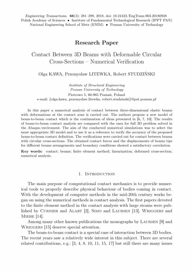
Two beams with circular cross-sections coming into contact are considered(Fig. 1). The penetration function is written as:

(2.1) gN = dn − rm − rs,

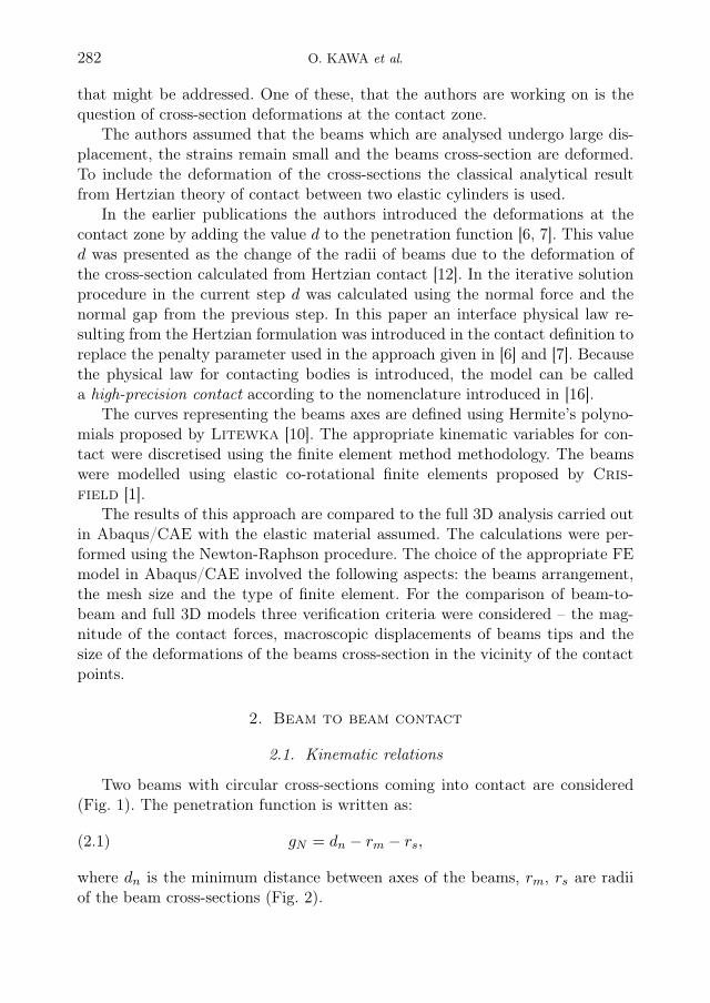
where dn is the minimum distance between axes of the beams, rm, rs are radiiof the beam cross-sections (Fig. 2).

CONTACT BETWEEN 3D BEAMS. . . 283

Fig. 1. Contacting beams.

Fig. 2. Contact criterion for beams.

The function of penetration constitutes the criterion of contact (Fig. 2). Thecontact condition is defined as in [15]:

(2.2) gN = dn − rm − rs ≤ 0.

To evaluate gN , the position vectors xmn and xsn of two closest points (Cmnand Csn) lying on two curves representing the beams axes (m and s) have to befound.

2.2. Contact points

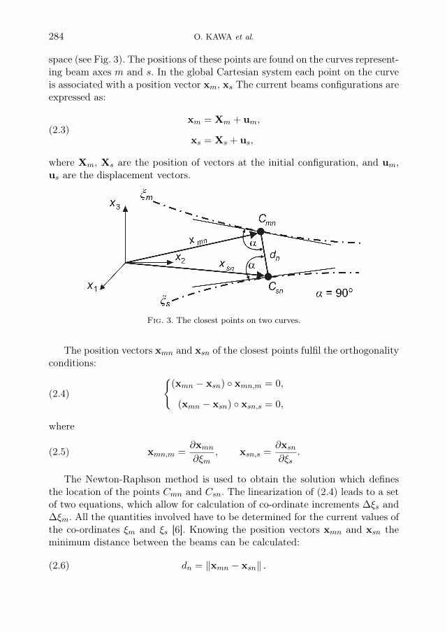
The local curvilinear co-ordinates (ξm for first beam, ξs for the second one)define the location of the closest points Cmn and Csn on the curves in the 3D

284 O. KAWA et al.

space (see Fig. 3). The positions of these points are found on the curves represent-ing beam axes m and s. In the global Cartesian system each point on the curveis associated with a position vector xm, xs The current beams configurations areexpressed as:

(2.3)xm = Xm + um,

xs = Xs + us,

where Xm, Xs are the position of vectors at the initial configuration, and um,us are the displacement vectors.

Fig. 3. The closest points on two curves.

The position vectors xmn and xsn of the closest points fulfil the orthogonalityconditions:

(2.4)

{(xmn − xsn) ◦ xmn,m = 0,

(xmn − xsn) ◦ xsn,s = 0,

where

(2.5) xmn,m =∂xmn∂ξm

, xsn,s =∂xsn∂ξs

.

The Newton-Raphson method is used to obtain the solution which definesthe location of the points Cmn and Csn. The linearization of (2.4) leads to a setof two equations, which allow for calculation of co-ordinate increments ∆ξs and∆ξm. All the quantities involved have to be determined for the current values ofthe co-ordinates ξm and ξs [6]. Knowing the position vectors xmn and xsn theminimum distance between the beams can be calculated:

(2.6) dn = ‖xmn − xsn‖ .


2.3. Hertzian contact

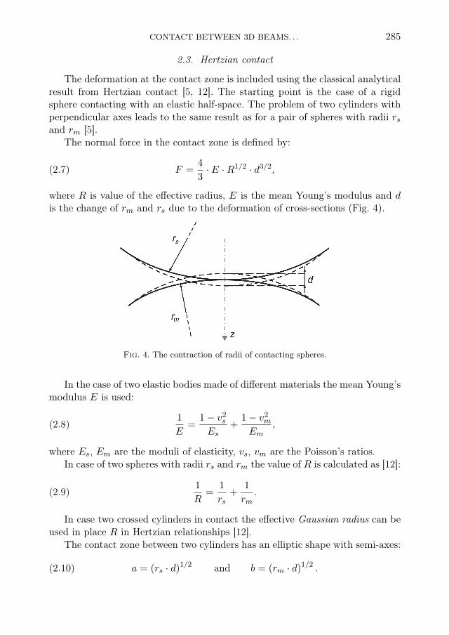
The deformation at the contact zone is included using the classical analyticalresult from Hertzian contact [5, 12]. The starting point is the case of a rigidsphere contacting with an elastic half-space. The problem of two cylinders withperpendicular axes leads to the same result as for a pair of spheres with radii rsand rm [5].

The normal force in the contact zone is defined by:

(2.7) F =4

3· E ·R1/2 · d3/2,

where R is value of the effective radius, E is the mean Young’s modulus and dis the change of rm and rs due to the deformation of cross-sections (Fig. 4).

Fig. 4. The contraction of radii of contacting spheres.

In the case of two elastic bodies made of different materials the mean Young’smodulus E is used:

(2.8)1

E=

1− v2sEs

+1− v2mEm

,

where Es, Em are the moduli of elasticity, vs, vm are the Poisson’s ratios.In case of two spheres with radii rs and rm the value of R is calculated as [12]:

(2.9)1

R=

1

rs+

1

rm.

In case two crossed cylinders in contact the effective Gaussian radius can beused in place R in Hertzian relationships [12].

The contact zone between two cylinders has an elliptic shape with semi-axes:

(2.10) a = (rs · d)1/2 and b = (rm · d)1/2 .

286 O. KAWA et al.

The contact area is calculated as:

(2.11) A = π · d · R̃,

where the effective Gaussian radius of curvature of the surface is written as:

(2.12) R̃ = (rs · rm)1/2 .

In our case of contact between beams with perpendicular axes the value ofGaussian radius has been used in all calculations.

The value of d in Eq (2.7) can be written as

(2.13) d =3

√9

16·

F2/3N

E2/3 ·R1/3.

In this approach the normal gap used to define contact is assumed as thesimple measure of cross-sections deformation, thus:

(2.14) gN = d,

so the normal force can be expressed as:

(2.15) FN =4

3· E ·R1/2 · g3/2N .

Thus, the penalty parameter which is used in the standard penalty methodto calculate the normal force:

(2.16) FN = εN · gN

is now replaced by:

(2.17) εN =4

3· E ·R1/2 · g1/2N .

Therefore, in this approach the cross-sections deformation is introduced byreplacing the penalty parameter with the Hertzian contact stiffness. It is empha-sized, that the main idea was to use such a simple approach without any complexformulations, meant to improve the beam-to-beam contact formulation, whichitself is also a simplification of the full 3D analysis.

In the iterative solution procedure in the current step the radii change d isevaluated using the normal force and the normal gap gN from the current step.


2.4. Weak form and its linearization

For two bodies the solution of contact problem involves finding a minimumof the potential energy functional Π what can be written down as:

(2.18) minΠ = min (Π1 +Π2 +Πc),

where Π1, Π2 are the components of potential energy for the first and the sec-ond body, while Πc is the part of the energy related to contact. This leads to asolution of a functional minimization with inequality constraints. Using the con-cept of an active set the inequality constraints can be replaced by the equalityconstraints [10].

The contact contribution to the corresponding weak form is [16]:

(2.19) δΠc = FNδgN .

Substituting from Eq. (2.12) gives:

(2.20) δΠc =4

3· E ·R1/2 · g3/2N δgN .

The linearization required for the Newton solution scheme for the non-linearcontact problem is written as:

(2.21) ∆δΠc =(

2 · E ·R1/2 · g1/2N

)∆gNδgN +

(4

3· E ·R1/2 · g3/2N

)∆δgN .

The variation, linearization and second variation of the penetration functiongN are obtained just like in the case without the cross-section deformation –they are presented in detail in [10].

3. Finite element model definition in Abaqus/CAE

The aim of the conducted numerical simulations in the Abaqus/CAE programwas a verification of the developed beam-to-beam contact model, which is ableto describe the contact interface between beams of circular cross-section. It iswell known that the finite element simulations are very sensitive to both the typeof the finite element and the mesh size. Therefore, the convergence analysis ofthe finite element model was performed first.

Numerical data for all the calculations here and for all the examples in Sec. 4are given without any specified physical units, though it is understood, that anyconsistent unit set might be used.

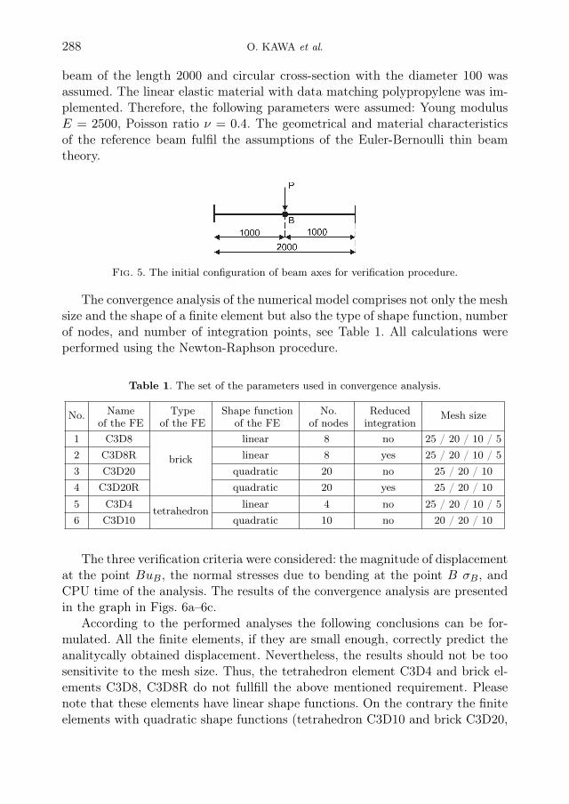
The analytical solutions of the clamped-clamped beam with concentratedforce applied at the mid-span were used as reference solutions (Fig. 5). The

288 O. KAWA et al.

beam of the length 2000 and circular cross-section with the diameter 100 wasassumed. The linear elastic material with data matching polypropylene was im-plemented. Therefore, the following parameters were assumed: Young modulusE = 2500, Poisson ratio ν = 0.4. The geometrical and material characteristicsof the reference beam fulfil the assumptions of the Euler-Bernoulli thin beamtheory.

Fig. 5. The initial configuration of beam axes for verification procedure.

The convergence analysis of the numerical model comprises not only the meshsize and the shape of a finite element but also the type of shape function, numberof nodes, and number of integration points, see Table 1. All calculations wereperformed using the Newton-Raphson procedure.

Table 1. The set of the parameters used in convergence analysis.

No. Nameof the FE

Typeof the FE

Shape functionof the FE

No.of nodes

Reducedintegration

Mesh size

1 C3D8

brick

linear 8 no 25 / 20 / 10 / 52 C3D8R linear 8 yes 25 / 20 / 10 / 53 C3D20 quadratic 20 no 25 / 20 / 104 C3D20R quadratic 20 yes 25 / 20 / 105 C3D4

tetrahedronlinear 4 no 25 / 20 / 10 / 5

6 C3D10 quadratic 10 no 20 / 20 / 10

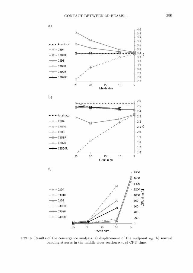
The three verification criteria were considered: the magnitude of displacementat the point BuB, the normal stresses due to bending at the point B σB, andCPU time of the analysis. The results of the convergence analysis are presentedin the graph in Figs. 6a–6c.

According to the performed analyses the following conclusions can be for-mulated. All the finite elements, if they are small enough, correctly predict theanalitycally obtained displacement. Nevertheless, the results should not be toosensitivite to the mesh size. Thus, the tetrahedron element C3D4 and brick el-ements C3D8, C3D8R do not fullfill the above mentioned requirement. Pleasenote that these elements have linear shape functions. On the contrary the finiteelements with quadratic shape functions (tetrahedron C3D10 and brick C3D20,


a)

b)

c)

Fig. 6. Results of the convergence analysis: a) displacement of the midpoint uB , b) normalbending stresses in the middle cross section σB , c) CPU time.

290 O. KAWA et al.

C3D20R) are not so much sensitive to the mesh size. A similar observation ap-plies to the normal stress criterion (stress at the point B, σB). Finally, takinginto account the third criterion – computational cost (CPU time criterion), theC3D20R finite element with 10 mesh size will be used for further analyses.

4. Numerical examples

4.1. Introduction

Three examples of beam-to-beam contact are presented in this section. It isassumed that the beams which are analysed undergo large displacements, thestrains remain small and the beams cross-sections are deformed.

In the beam-to-beam model each beam is discretized using twenty finite ele-ments proposed by Crisfield [1]. The Hermite’s polynomials used by Litewka[10] are representing the curves of the beams. The imposed displacements areapplied simultaneously in 60 or 30 equal increments.

In the 3D finite element simulations in Abaqus/CAE the 20-node quadraticbrick (C3D20R) finite elements were used, as was decided in Sec. 3.

4.2. Example 1

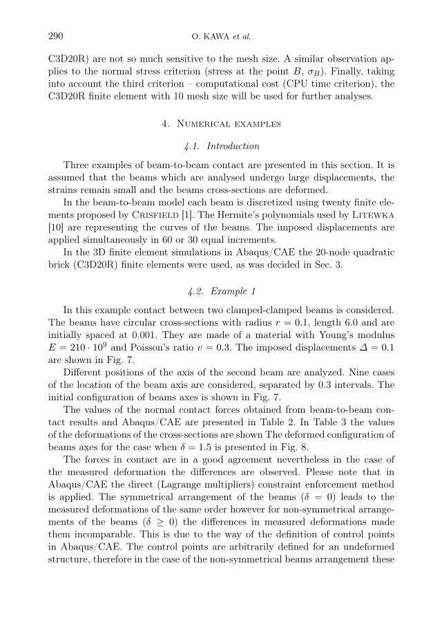
In this example contact between two clamped-clamped beams is considered.The beams have circular cross-sections with radius r = 0.1, length 6.0 and areinitially spaced at 0.001. They are made of a material with Young’s modulusE = 210 · 109 and Poisson’s ratio v = 0.3. The imposed displacements ∆ = 0.1are shown in Fig. 7.

Different positions of the axis of the second beam are analyzed. Nine casesof the location of the beam axis are considered, separated by 0.3 intervals. Theinitial configuration of beams axes is shown in Fig. 7.

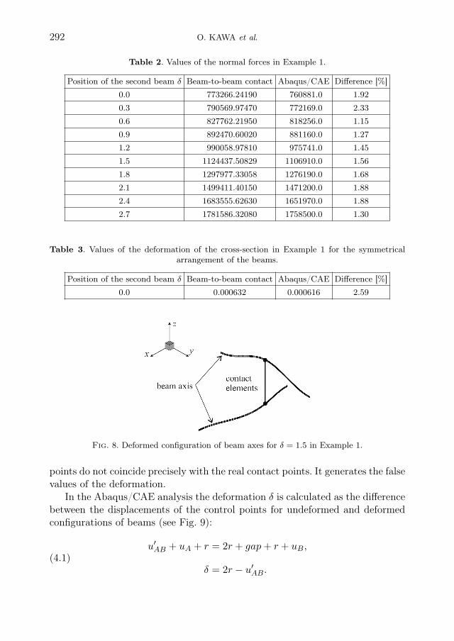
The values of the normal contact forces obtained from beam-to-beam con-tact results and Abaqus/CAE are presented in Table 2. In Table 3 the valuesof the deformations of the cross-sections are shown The deformed configuration ofbeams axes for the case when δ = 1.5 is presented in Fig. 8.

The forces in contact are in a good agreement nevertheless in the case ofthe measured deformation the differences are observed. Please note that inAbaqus/CAE the direct (Lagrange multipliers) constraint enforcement methodis applied. The symmetrical arrangement of the beams (δ = 0) leads to themeasured deformations of the same order however for non-symmetrical arrange-ments of the beams (δ ≥ 0) the differences in measured deformations madethem incomparable. This is due to the way of the definition of control pointsin Abaqus/CAE. The control points are arbitrarily defined for an undeformedstructure, therefore in the case of the non-symmetrical beams arrangement these


Fig. 7. The initial configuration of beam axes in Example 1.

292 O. KAWA et al.

Table 2. Values of the normal forces in Example 1.

Position of the second beam δ Beam-to-beam contact Abaqus/CAE Difference [%]0.0 773266.24190 760881.0 1.920.3 790569.97470 772169.0 2.330.6 827762.21950 818256.0 1.150.9 892470.60020 881160.0 1.271.2 990058.97810 975741.0 1.451.5 1124437.50829 1106910.0 1.561.8 1297977.33058 1276190.0 1.682.1 1499411.40150 1471200.0 1.882.4 1683555.62630 1651970.0 1.882.7 1781586.32080 1758500.0 1.30

Table 3. Values of the deformation of the cross-section in Example 1 for the symmetricalarrangement of the beams.

Position of the second beam δ Beam-to-beam contact Abaqus/CAE Difference [%]0.0 0.000632 0.000616 2.59

Fig. 8. Deformed configuration of beam axes for δ = 1.5 in Example 1.

points do not coincide precisely with the real contact points. It generates the falsevalues of the deformation.

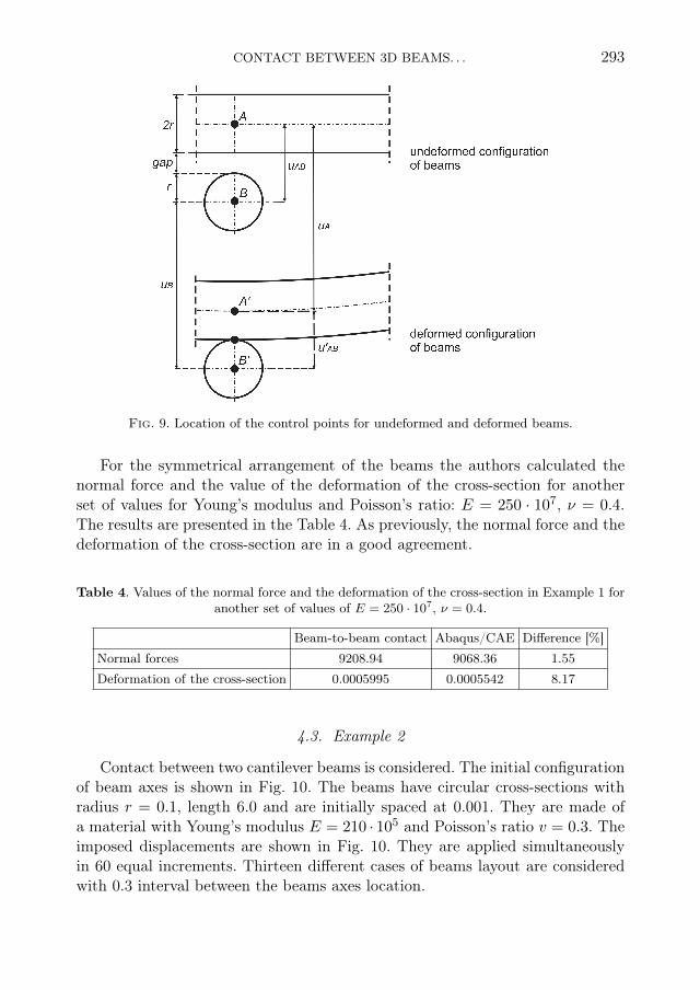
In the Abaqus/CAE analysis the deformation δ is calculated as the differencebetween the displacements of the control points for undeformed and deformedconfigurations of beams (see Fig. 9):

(4.1)u′AB + uA + r = 2r + gap+ r + uB,

δ = 2r − u′AB.


Fig. 9. Location of the control points for undeformed and deformed beams.

For the symmetrical arrangement of the beams the authors calculated thenormal force and the value of the deformation of the cross-section for anotherset of values for Young’s modulus and Poisson’s ratio: E = 250 · 107, ν = 0.4.The results are presented in the Table 4. As previously, the normal force and thedeformation of the cross-section are in a good agreement.

Table 4. Values of the normal force and the deformation of the cross-section in Example 1 foranother set of values of E = 250 · 107, ν = 0.4.

Beam-to-beam contact Abaqus/CAE Difference [%]Normal forces 9208.94 9068.36 1.55Deformation of the cross-section 0.0005995 0.0005542 8.17

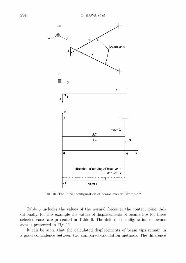
4.3. Example 2

Contact between two cantilever beams is considered. The initial configurationof beam axes is shown in Fig. 10. The beams have circular cross-sections withradius r = 0.1, length 6.0 and are initially spaced at 0.001. They are made ofa material with Young’s modulus E = 210 · 105 and Poisson’s ratio v = 0.3. Theimposed displacements are shown in Fig. 10. They are applied simultaneouslyin 60 equal increments. Thirteen different cases of beams layout are consideredwith 0.3 interval between the beams axes location.

294 O. KAWA et al.

Fig. 10. The initial configuration of beams axes in Example 2.

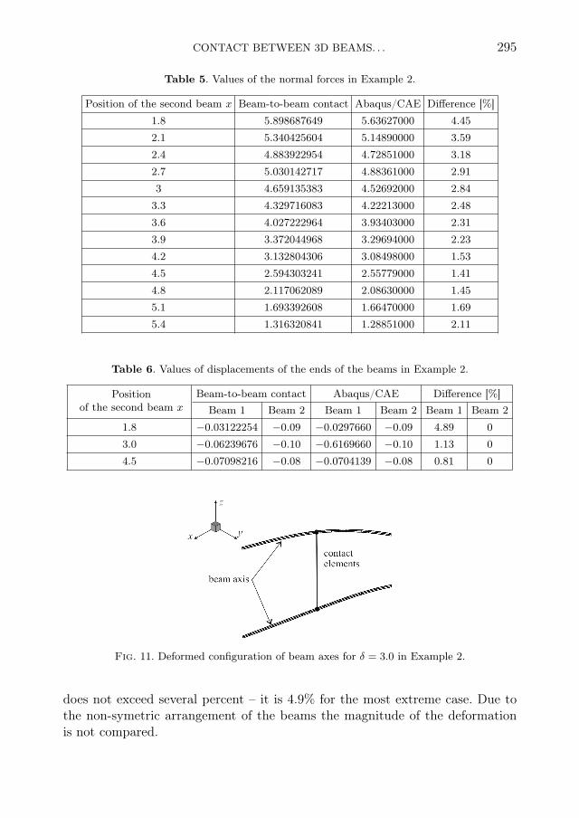
Table 5 includes the values of the normal forces at the contact zone. Ad-ditionally, for this example the values of displacements of beams tips for threeselected cases are presented in Table 6. The deformed configuration of beamsaxes is presented in Fig. 11.

It can be seen, that the calculated displacements of beam tips remain ina good coincidence between two compared calculation methods. The difference



Position of the second beam x Beam-to-beam contact Abaqus/CAE Difference [%]1.8 5.898687649 5.63627000 4.452.1 5.340425604 5.14890000 3.592.4 4.883922954 4.72851000 3.182.7 5.030142717 4.88361000 2.913 4.659135383 4.52692000 2.843.3 4.329716083 4.22213000 2.483.6 4.027222964 3.93403000 2.313.9 3.372044968 3.29694000 2.234.2 3.132804306 3.08498000 1.534.5 2.594303241 2.55779000 1.414.8 2.117062089 2.08630000 1.455.1 1.693392608 1.66470000 1.695.4 1.316320841 1.28851000 2.11

Table 6. Values of displacements of the ends of the beams in Example 2.

Positionof the second beam x

Beam-to-beam contact Abaqus/CAE Difference [%]Beam 1 Beam 2 Beam 1 Beam 2 Beam 1 Beam 2

1.8 −0.03122254 −0.09 −0.0297660 −0.09 4.89 03.0 −0.06239676 −0.10 −0.6169660 −0.10 1.13 04.5 −0.07098216 −0.08 −0.0704139 −0.08 0.81 0

Fig. 11. Deformed configuration of beam axes for δ = 3.0 in Example 2.

does not exceed several percent – it is 4.9% for the most extreme case. Due tothe non-symetric arrangement of the beams the magnitude of the deformationis not compared.

296 O. KAWA et al.

4.4. Example 3

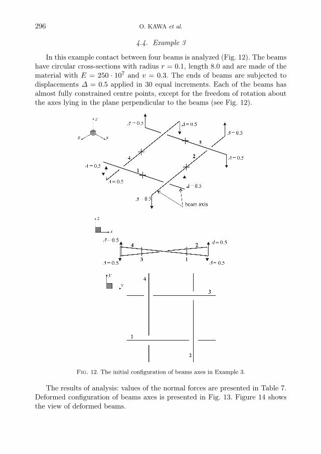
In this example contact between four beams is analyzed (Fig. 12). The beamshave circular cross-sections with radius r = 0.1, length 8.0 and are made of thematerial with E = 250 · 107 and v = 0.3. The ends of beams are subjected todisplacements ∆ = 0.5 applied in 30 equal increments. Each of the beams hasalmost fully constrained centre points, except for the freedom of rotation aboutthe axes lying in the plane perpendicular to the beams (see Fig. 12).

Fig. 12. The initial configuration of beams axes in Example 3.

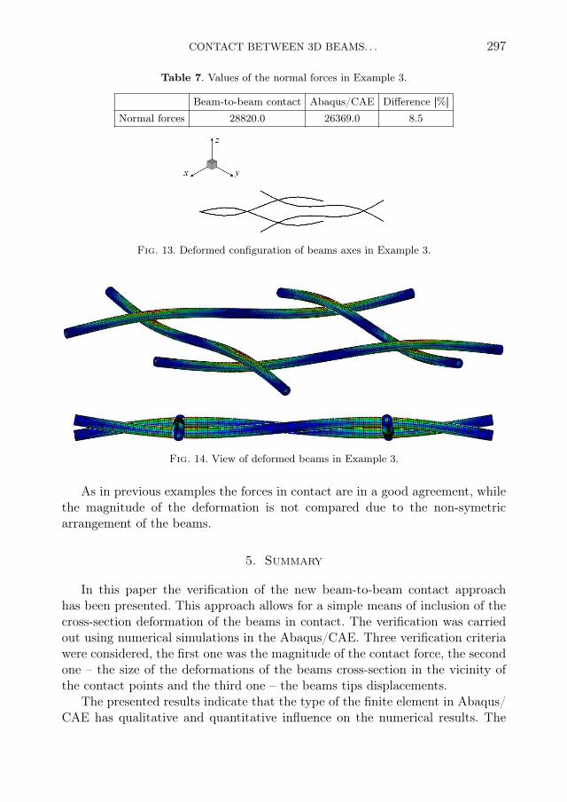
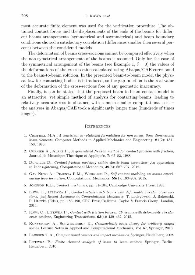
The results of analysis: values of the normal forces are presented in Table 7.Deformed configuration of beams axes is presented in Fig. 13. Figure 14 showsthe view of deformed beams.



Beam-to-beam contact Abaqus/CAE Difference [%]Normal forces 28820.0 26369.0 8.5

Fig. 13. Deformed configuration of beams axes in Example 3.

Fig. 14. View of deformed beams in Example 3.

As in previous examples the forces in contact are in a good agreement, whilethe magnitude of the deformation is not compared due to the non-symetricarrangement of the beams.

5. Summary

In this paper the verification of the new beam-to-beam contact approachhas been presented. This approach allows for a simple means of inclusion of thecross-section deformation of the beams in contact. The verification was carriedout using numerical simulations in the Abaqus/CAE. Three verification criteriawere considered, the first one was the magnitude of the contact force, the secondone – the size of the deformations of the beams cross-section in the vicinity ofthe contact points and the third one – the beams tips displacements.

The presented results indicate that the type of the finite element in Abaqus/CAE has qualitative and quantitative influence on the numerical results. The

298 O. KAWA et al.

most accurate finite element was used for the verification procedure. The ob-tained contact forces and the displacements of the ends of the beams for differ-ent beams arrangements (symmetrical and asymmetrical) and beam boundaryconditions showed a satisfactory correlation (differences smaller then several per-cent) between the considered models.

The deformation of beams cross-sections cannot be compared effectively whenthe non-symetrical arrangements of the beams is assumed. Only for the case ofthe symmetrical arrangement of the beams (see Example 1, δ = 0) the values ofthe deformations of the cross-section calculated using Abaqus/CAE correspondto the beam-to-beam solution. In the presented beam-to-beam model the physi-cal law for contacting bodies is introduced, so the gap function is the real valueof the deformation of the cross-sections free of any geometric inaccuracy.

Finally, it can be stated that the proposed beam-to-beam contact model isan attractive, yet simple method of analysis for contacting beams, leading torelatively accurate results obtained with a much smaller computational cost –the analyses in Abaqus/CAE took a significantly longer time (hundreds of timeslonger).

References

1. Crisfield M.A., A consistent co-rotational formulation for non-linear, three-dimensionalbeam-elements, Computer Methods in Applied Mechanics and Engineering, 81(2): 131–150, 1990.

2. Curnier A., Alart P., A generalized Newton method for contact problem with friction,Journal de Mécanique Théorique et Appliquée, 7: 67–82, 1988.

3. Durville D., Contact-friction modeling within elastic beam assemblies: An applicationto knot tightening, Computational Mechanics, 49(6): 687–707, 2012.

4. Gay Neto A., Pimenta P.M., Wriggers P., Self-contact modeling on beams experi-encing loop formation, Computational Mechanics, 55(1): 193–208, 2015.

5. Johnson K.L., Contact mechanics, pp. 81–104, Cambridge University Press, 1985.

6. Kawa O., Litewka P., Contact between 3-D beams with deformable circular cross sec-tions, [in:] Recent Advances in Computational Mechanics, T. Łodygowski, J. Rakowski,P. Litewka (Eds.), pp. 183–190, CRC Press/Balkema, Taylor & Francis Group, London,2014.

7. Kawa O., Litewka P., Contact with friction between 3D beams with deformable circularcross sections, Engineering Transactions, 63(4): 439–462, 2015.

8. Konyukhov A., Schweizerhof K., Geometrically exact theory for arbitrary shapedbodies, Lecture Notes in Applied and Computational Mechanics, Vol. 67, Springer, 2013.

9. Laursen T.A., Computational contact and impact mechanics, Springer, Heidelberg, 2002.

10. Litewka P., Finite element analysis of beam to beam contact, Springer, Berlin–Heidelberg, 2010.


11. Meier C., Wall W., Popp A., A unified approach for beam-to-beam contact, ComputerMethods in Applied Mechanics and Engineering, 315: 972–1010, 2017.

12. Popov V.L., Contact Mechanics and Friction, pp. 55–64, Springer, Berlin–Heidelberg,2010.

13. Simo J.C., Laursen T.A., An augmented Lagrangian treatment of contact problemsinvolving friction, Computers and Structures, 42(1): 97–116, 1992.

14. Wriggers P., Miehe C., On the treatment of contact contraints within coupled ther-momechanical analysis, [in:] Proceedings of EUROMECH, Finite Inelastic Deformations,Desdo B., Stein E. (Eds.), Springer, Berlin 1992.

15. Wriggers P., Zavarise G., On contact between three-dimensional beams undergoinglarge deflections, Communications in Numerical Method in Engineering, 13(6): 429–438,1997.

16. Wriggers P., Computational contact mechanics, 1st Ed., pp. 339–354, Wiley, 2002.

17. Zavarise G., Wriggers P., Contact with friction between beams in 3-D space, Interna-tional Journal for Numerical Methods in Engineering, 49(8): 977–1006, 2000.

Received April 10, 2018; accepted version May 28, 2018.

Documents

Research Paper - et.ippt.gov.pl