Simulation Modelling Practice and Theory - پرشینگیگcdn.persiangig.com/.../Vibration_control_of_vehicle_active_suspensio… · investigated the overall performance of a semi-active

Simulation Modelling Practice and Theory 17 (2009) 778–793

Contents lists available at ScienceDirect

Simulation Modelling Practice and Theory

journal homepage: www.elsevier .com/locate /s impat

Vibration control of vehicle active suspension system using a newrobust neural network control system_Ikbal Eski, S�ahin Yıldırım *

Erciyes University, Faculty of Engineering, Mechanical Engineering Department, Talas Cad, Kayseri 38039, Turkey

a r t i c l e i n f o

Article history:Received 25 April 2008Received in revised form 21 January 2009Accepted 23 January 2009Available online 3 February 2009

Keywords:PID controllerNeural networksWhole vehicle’s suspensionRobust controller

1569-190X/$ - see front matter � 2009 Elsevier B.Vdoi:10.1016/j.simpat.2009.01.004

* Corresponding author. Tel.: +90 352 4374901x3E-mail address: [email protected] (S�. Yıldırım

a b s t r a c t

The main problem of vehicle vibration comes from road roughness. For that reason, it isnecessary to control vibration of vehicle’s suspension by using a robust artificial neural net-work control system scheme. Neural network based robust control system is designed tocontrol vibration of vehicle’s suspensions for full suspension system. Moreover, the fullvehicle system has seven degrees of freedom on the vertical direction of vehicle’s chassis,on the angular variation around X-axis and on the angular variation around Y-axis. The pro-posed control system is consisted of a robust controller, a neural controller, a model neuralnetwork of vehicle’s suspension system. On the other hand, standard PID controller is alsoused to control whole vehicle’s suspension system for comparison.

Consequently, random road roughnesses are used as disturbance of control system. Thesimulation results are indicated that the proposed control system has superior perfor-mance at adapting random road disturbance for vehicle’s suspension.

� 2009 Elsevier B.V. All rights reserved.

1. Introduction

Over recent years, the active suspension systems have come into commercial use, especially in the passenger car industry.These modern systems offer improved comfort and road holding in varying driving and loading conditions compared to thematching properties achieved with traditional passive means. Most of the new systems are fitted in to large luxurious cars.However, these systems would be at their most advantageous in small size passenger cars and off-road vehicles.

Swevers et al. have been presented a flexible and transparent model-free control structure based on physical insights inthe car and semi-active suspension dynamics used to linearise and decouple the system, and decentralized linear feedback[1]. A load-dependent controller design approach to solve the problem of multi-objective control for vehicle active suspen-sion systems by using linear matrix inequalities have been presented [2]. Du and Zhang have been presented H1 controlproblem for active vehicle suspension systems with actuator time delay [3]. An approach to design static output feedbackand non-fragile static output feedback H1 controllers for active vehicle suspensions by using linear matrix inequalitiesand genetic algorithms have been searched [4]. Vibration control performance of a semi-active electrorheological seat sus-pension system using a robust sliding mode controller has been searched by Huang and Chen [5]. Ieluzzi et al. have beeninvestigated the overall performance of a semi-active suspension control for a heavy truck [6]. Spectral decomposition meth-ods have been applied to compute accurately the rms values for the control forces, suspension strokes and tyre deflection atfront and rear in a half-car model with preview [7]. Guclu has been presented vibration control performance of a seat sus-pension system of non-linear full vehicle model using fuzzy logic controller [8]. A multidisciplinary optimization method hasbeen applied to the design of mechatronic vehicles with active suspensions [9]. Neural network control method has been

. All rights reserved.

2053; fax: +90 352 4375784.).

mailto:[email protected]

http://www.sciencedirect.com/science/journal/1569190X

http://www.elsevier.com/locate/simpat

_I. Eski, S�. Yıldırım / Simulation Modelling Practice and Theory 17 (2009) 778–793 779

developed to control a seat suspension system of non-linear full vehicle model [10]. Yıldırım and Uzmay have been inves-tigated the variation of vertical vibrations of vehicles using a neural network [11]. An active horizontal spray-boom suspen-sion, reducing yawing and jolting, has been designed by Anthonis and Ramon [12]. A semi-active control of vehiclesuspension system with magnetorheological (MR) damper has been presented by Yao et al. [13]. Spentzas and Kanarachoshave been presented a methodology for the design of active/hybrid car suspension systems with the goal to maximize pas-senger comfort [14]. A methodology for the design of active car suspension systems has been presented [15]. Yagiz and Yük-sek have been researched sliding mode control of active suspensions for a full vehicle model [16].

In this paper, a robust neural network based robust control system for whole vehicle’s vibration control is proposed. Thepaper first describes the full vehicle suspension model under consideration. Second, the proposed control system and stan-dard PID controller are outlined in Section 3. Third, the results of proposed neural based control system and PID control sys-tem are given and discussed. Finally, the effectiveness of the proposed control method is concluded in Section 5.

2. Full vehicle model

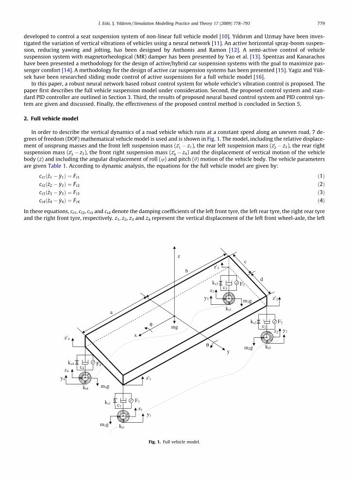
In order to describe the vertical dynamics of a road vehicle which runs at a constant speed along an uneven road, 7 de-grees of freedom (DOF) mathematical vehicle model is used and is shown in Fig. 1. The model, including the relative displace-ment of unsprung masses and the front left suspension mass (z01 � z1), the rear left suspension mass (z02 � z2), the rear rightsuspension mass (z03 � z3), the front right suspension mass (z04 � z4) and the displacement of vertical motion of the vehiclebody (z) and including the angular displacement of roll (u) and pitch (h) motion of the vehicle body. The vehicle parametersare given Table 1. According to dynamic analysis, the equations for the full vehicle model are given by:

ct1ð _z1 � _y1Þ ¼ Ft1 ð1Þct2ð _z2 � _y2Þ ¼ Ft2 ð2Þct3ð _z3 � _y3Þ ¼ Ft3 ð3Þct4ð _z4 � _y4Þ ¼ Ft4 ð4Þ

In these equations, ct1, ct2, ct3 and ct4 denote the damping coefficients of the left front tyre, the left rear tyre, the right rear tyreand the right front tyre, respectively. z1, z2, z3 and z4 represent the vertical displacement of the left front wheel-axle, the left

y4

z'4

z4

z2

z'2

mg φ

θ

z

y

a

b

c

d

ks1

ks2

ks3

c1

c2

c3

c4

m1g

z'1

m4g

m2g

x

z1

y1

kt1

ks4

kt4

kt2

z'3

y3 m3g

z3

kt3

F1

F3

F4

F2

y2

Fig. 1. Full vehicle model.

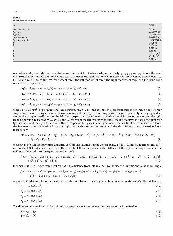
Table 1Full vehicle parameters.

m 1020 kg

m1 = m2 = m3 = m4 15 kgks1 = ks4 22,000 N/mks2 = ks3 19,000 N/mc1 = c2 = c3 = c4 800 N s/mkt1 = kt2 = kt3 = kt4 143,000 N/ma 1.025 mb 2.204 mc 0.612 md 0.85 mJx 1859 kg m2

Jy 471 kg m2

g 9.81 m/s2

780 _I. Eski, S�. Yıldırım / Simulation Modelling Practice and Theory 17 (2009) 778–793

rear wheel-axle, the right rear wheel-axle and the right front wheel-axle, respectively. y1, y2, y3 and y4 denote the roaddisturbance input for left front wheel, the left rear wheel, the right rear wheel and the right front wheel, respectively. Ft1,Ft2, Ft3 and Ft4 delineate the left front wheel force, the left rear wheel force, the right rear wheel force and the right frontwheel force, respectively

m1€z1 ¼ kt1ðy1 � z1Þ þ ks1ðz01 � z1Þ þ c1ð _z01 � _z1Þ þ F1 þm1 ð5Þ

m2€z2 ¼ kt2ðy2 � z2Þ þ ks2ðz02 � z2Þ þ c2ð _z02 � _z2Þ þ F2 þm2g ð6Þ



where g = 9.81 m/s2 is a gravitational acceleration. m1, m2, m3 and m4 are the left front suspension mass, the left rearsuspension mass, the right rear suspension mass and the right front suspension mass, respectively. c1, c2, c3 and c4

denote the damping coefficients of the left front suspension, the left rear suspension, the right rear suspension and the rightfront suspension, respectively. kt1, kt2, kt3 and kt4 represent the left front tyre stiffness, the left rear tyre stiffness, the right reartyre stiffness and the right front tyre stiffness, respectively. F1, F2, F3 and F4 delineate the left front active suspension force,the left rear active suspension force, the right rear active suspension force and the right front active suspension force,respectively

m€z ¼ ks1ðz1 � z01Þ þ ks2ðz2 � z02Þ þ ks3ðz3 � z03Þ þ ks4ðz4 � z04Þ þ c1ð _z1 � _z01Þ þ c2ð _z2 � _z02Þ þ c3ð _z3 � _z03Þ þ c4ð _z4 � _z04Þ� F1 � F2 � F3 � F4 þmg ð9Þ

where m is the vehicle body mass and z the vertical displacement of the vehicle body. ks1, ks2, ks3 and ks4 represent the stiff-ness of the left front suspension, the stiffness of the left rear suspension, the stiffness of the right rear suspension and thestiffness of the right front suspension, respectively

Jx€/ ¼ �½ks3ðz3 � z03Þ þ c3ð _z3 � _z03Þ þ ks4ðz4 � z04Þ þ c4ð _z4 � _z04Þ�c½ks1ðz1 � z01Þ þ c1ð _z1 � _z01Þ þ ks2ðz2 � z02Þ þ c2ð _z2 � _z02Þ�dþ ðF3 þ F4Þc � ðF1 þ F2Þd ð10Þ

In which, c is CG distance from right axle, d is CG distance from left axle, Jx is roll moment of inertia and u is the roll angle

Jy€h ¼ �½ks1ðz1 � z01Þ þ c1ð _z1 � _z01Þ þ ks4ðz4 � z04Þ þ c4ð _z4 � _z04Þ�a½ks2ðz2 � z02Þ þ c2ð _z2 � _z02Þ þ ks3ðz3 � z03Þþ c3ð _z3 � _z03Þ�bþ ðF1 þ F4Þa� ðF2 þ F3Þb ð11Þ

where a is CG distance from front axle, b is CG distance from rear axle, Jy is pitch moment of inertia and h is the pitch angle.

z01 ¼ z� ðah� d/Þ ð12Þ

z02 ¼ zþ ðbh� d/Þ ð13Þ

z03 ¼ zþ ðbhþ c/Þ ð14Þ

z04 ¼ z� ðahþ c/Þ ð15Þ

The differential equations can be written in state-space notation when the state vector X is defined as

_X ¼ AX þ BQ ð16ÞY ¼ CX þ DQ ð17Þ


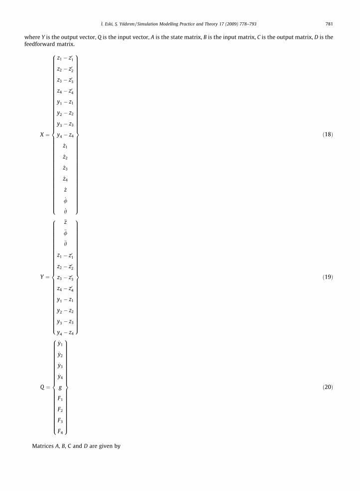
where Y is the output vector, Q is the input vector, A is the state matrix, B is the input matrix, C is the output matrix, D is thefeedforward matrix.

X ¼

z1 � z01

z2 � z02

z3 � z03

z4 � z04

y1 � z1

y2 � z2

y3 � z3

y4 � z4

_z1

_z2

_z3

_z4

_z

_/

_h

8>>>>>>>>>>>>>>>>>>>>>>>>>>>>>>>>>>>>>>>>>>><>>>>>>>>>>>>>>>>>>>>>>>>>>>>>>>>>>>>>>>>>>>:

9>>>>>>>>>>>>>>>>>>>>>>>>>>>>>>>>>>>>>>>>>>>=>>>>>>>>>>>>>>>>>>>>>>>>>>>>>>>>>>>>>>>>>>>;

ð18Þ

Y ¼

€z

€/

€h

z1 � z01

z2 � z02

z3 � z03

z4 � z04

y1 � z1

y2 � z2

y3 � z3

y4 � z4

8>>>>>>>>>>>>>>>>>>>>>>>>>>>>><>>>>>>>>>>>>>>>>>>>>>>>>>>>>>:

9>>>>>>>>>>>>>>>>>>>>>>>>>>>>>=>>>>>>>>>>>>>>>>>>>>>>>>>>>>>;

ð19Þ

Q ¼

_y1

_y2

_y3

_y4

g

F1

F2

F3

F4

8>>>>>>>>>>>>>>>>>>>>>>><>>>>>>>>>>>>>>>>>>>>>>>:

9>>>>>>>>>>>>>>>>>>>>>>>=>>>>>>>>>>>>>>>>>>>>>>>;

ð20Þ

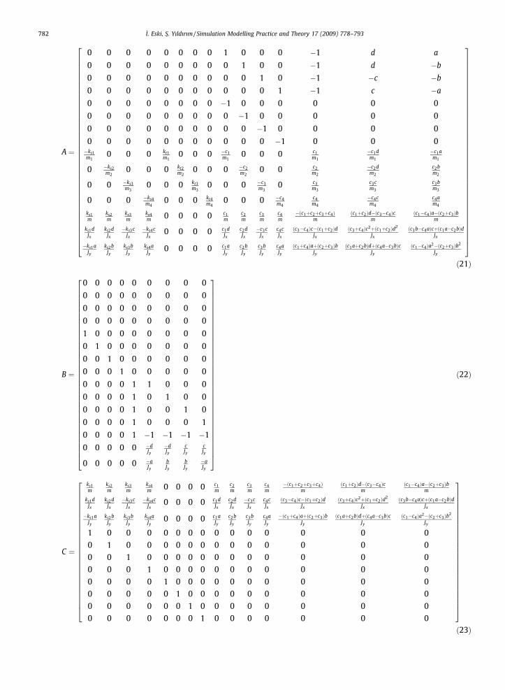
Matrices A, B, C and D are given by


A ¼

0 0 0 0 0 0 0 0 1 0 0 0 �1 d a

0 0 0 0 0 0 0 0 0 1 0 0 �1 d �b

0 0 0 0 0 0 0 0 0 0 1 0 �1 �c �b

0 0 0 0 0 0 0 0 0 0 0 1 �1 c �a

0 0 0 0 0 0 0 0 �1 0 0 0 0 0 0

0 0 0 0 0 0 0 0 0 �1 0 0 0 0 0

0 0 0 0 0 0 0 0 0 0 �1 0 0 0 0

0 0 0 0 0 0 0 0 0 0 0 �1 0 0 0�ks1m1

0 0 0 kt1m1

0 0 0 �c1m1

0 0 0 c1m1

�c1dm1

�c1am1

0 �ks2m2

0 0 0 kt2m2

0 0 0 �c2m2

0 0 c2m2

�c2dm2

c2bm2

0 0 �ks3m3

0 0 0 kt3m3

0 0 0 �c3m3

0 c3m3

c3cm3

c3bm3

0 0 0 �ks4m4

0 0 0 kt4m4

0 0 0 �c4m4

c4m4

�c4cm4

c4am4

ks1m

ks2m

ks3m

ks4m 0 0 0 0 c1

mc2m

c3m

c4m

�ðc1þc2þc3þc4Þm

ðc1þc2Þd�ðc3�c4Þcm

ðc1�c4Þa�ðc2þc3Þbm

ks1dJx

ks2dJx

�ks3cJx

�ks4cJx

0 0 0 0 c1dJx

c2dJx

�c3cJx

c4cJx

ðc3�c4Þc�ðc1þc2ÞdJx

ðc3þc4Þc2þðc1þc2Þd2

Jx

ðc3b�c4aÞcþðc1a�c2bÞdJx

�ks1aJy

ks2bJy

ks3bJy

ks4aJy

0 0 0 0 c1aJy

c2bJy

c3bJy

c4aJy

ðc1þc4Þaþðc2þc3ÞbJy

ðc1aþc2bÞdþðc4a�c3bÞcJy

ðc1�c4Þa2�ðc2þc3Þb2

Jy

26666666666666666666666666666666666666664

37777777777777777777777777777777777777775

ð21Þ

B ¼

0 0 0 0 0 0 0 0 0

0 0 0 0 0 0 0 0 0

0 0 0 0 0 0 0 0 0

0 0 0 0 0 0 0 0 0

1 0 0 0 0 0 0 0 0

0 1 0 0 0 0 0 0 0

0 0 1 0 0 0 0 0 0

0 0 0 1 0 0 0 0 0

0 0 0 0 1 1 0 0 0

0 0 0 0 1 0 1 0 0

0 0 0 0 1 0 0 1 0

0 0 0 0 1 0 0 0 1

0 0 0 0 1 �1 �1 �1 �1

0 0 0 0 0 �dJy

�dJy

cJy

cJy

0 0 0 0 0 �aJy

bJy

bJy

�aJy

2666666666666666666666666666666666664

3777777777777777777777777777777777775

ð22Þ

C ¼

ks1m

ks2m

ks3m

ks4m 0 0 0 0 c1

mc2m

c3m

c4m

�ðc1þc2þc3þc4Þm

ðc1þc2Þd�ðc3�c4Þcm

ðc1�c4Þa�ðc2þc3Þbm

ks1dJx

ks2dJx

�ks3cJx

�ks4cJx

0 0 0 0 c1dJx

c2dJx

�c3cJx

c4cJx

ðc3�c4Þc�ðc1þc2ÞdJx

ðc3þc4Þc2þðc1þc2Þd2

Jx

ðc3b�c4aÞcþðc1a�c2bÞdJx

�ks1aJy

ks2bJy

ks3bJy

ks4aJy

0 0 0 0 c1aJy

c2bJy

c3bJy

c4aJy

�ðc1þc4Þaþðc2þc3ÞbJy

ðc1aþc2bÞdþðc4a�c3bÞcJy

ðc1�c4Þa2�ðc2þc3Þb2

Jy

1 0 0 0 0 0 0 0 0 0 0 0 0 0 0

0 1 0 0 0 0 0 0 0 0 0 0 0 0 0

0 0 1 0 0 0 0 0 0 0 0 0 0 0 0

0 0 0 1 0 0 0 0 0 0 0 0 0 0 0

0 0 0 0 1 0 0 0 0 0 0 0 0 0 0

0 0 0 0 0 1 0 0 0 0 0 0 0 0 0

0 0 0 0 0 0 1 0 0 0 0 0 0 0 0

0 0 0 0 0 0 0 1 0 0 0 0 0 0 0

26666666666666666666666664

37777777777777777777777775

ð23Þ


D ¼

0 0 0 0 1 �1 �1 �1 �10 0 0 0 0 �d

Jx

�dJx

cJx

cJx

0 0 0 0 0 �aJx

bJx

bJx

�aJx

0 0 0 0 0 0 0 0 00 0 0 0 0 0 0 0 00 0 0 0 0 0 0 0 00 0 0 0 0 0 0 0 00 0 0 0 0 0 0 0 00 0 0 0 0 0 0 0 00 0 0 0 0 0 0 0 00 0 0 0 0 0 0 0 0

2666666666666666666664

3777777777777777777775

ð24Þ

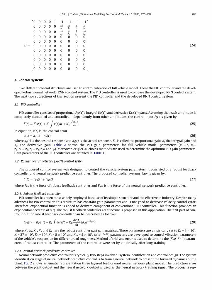
3. Control systems

Two different control structures are used to control vibration of full vehicle model. These the PID controller and the devel-oped Robust neural network (RNN) control system. The PID controller is used to compare the developed RNN control system.The next two subsections of this section present the PID controller and the developed RNN control system.

3.1. PID controller

PID controller consists of proportional P(e(t)), integral I(e(t)) and derivative D(e(t)) parts. Assuming that each amplitude iscompletely decoupled and controlled independently from other amplitudes, the control input F(t) is given by

FðtÞ ¼ KPeðtÞ þ KI

ZeðtÞdt þ KD

deðtÞdt

: ð25Þ

In equation, e(t) is the control error
eðtÞ ¼ xdðtÞ � xaðtÞ; ð26Þ
where xd(t) is the desired response and xa(t) is the actual response. KP is called the proportional gain, KI the integral gain andKD the derivative gain. Table 2 shows the PID gain parameters for full vehicle model parameters (z01 � z1; z02�z2; z03 � z3; z04 � z4; z; h and /). Moreover, Zeigler–Nicholds methods are used to determine the optimum PID gain parameters.Gain parameters of the PID controller are detailed in Table 1.

3.2. Robust neural network (RNN) control system

The proposed control system was designed to control the vehicle system parameters. It consisted of a robust feedbackcontroller and neural network predictive controller. The proposed controller systems’ law is given by:

FðtÞ ¼ FFBðtÞ þ FNNðtÞ ð27Þ

where FFB is the force of robust feedback controller and FNN is the force of the neural network predictive controller.

3.2.1. Robust feedback controllerPID controller has been most widely employed because of its simple structure and the effective in industry. Despite many

advances for PID controller, this structure has constant gain parameters and is not good to decrease velocity control error.Therefore, exponential function is added to derivate component of conventional PID controller. This function provides anexponential decrease of e(t). The robust feedback controller architecture is proposed in this application. The first part of con-trol input for robust feedback controller can be described as follows:

FFBðtÞ ¼ KPeðtÞ þ KI

ZeðtÞdt þ KD

deðtÞdtðKReð�KR1tÞÞ; ð28Þ

where KP, KI, KD, KR and KR1 are the robust controller part gain matrices. These parameters are empirically set to KP = 9 � 105,KI = 27 � 105, KD = 102, KR = 5 � 107 and KR1 = 5 � 106. ðKReð�KR1tÞÞ parameters are developed to control vibration parametersof the vehicle’s suspension for different road roughness. Method of trial and error is used to determine the ðKReð�KR1tÞÞ param-eters of robust controller. The parameters of the controller were set by empirically after long training.

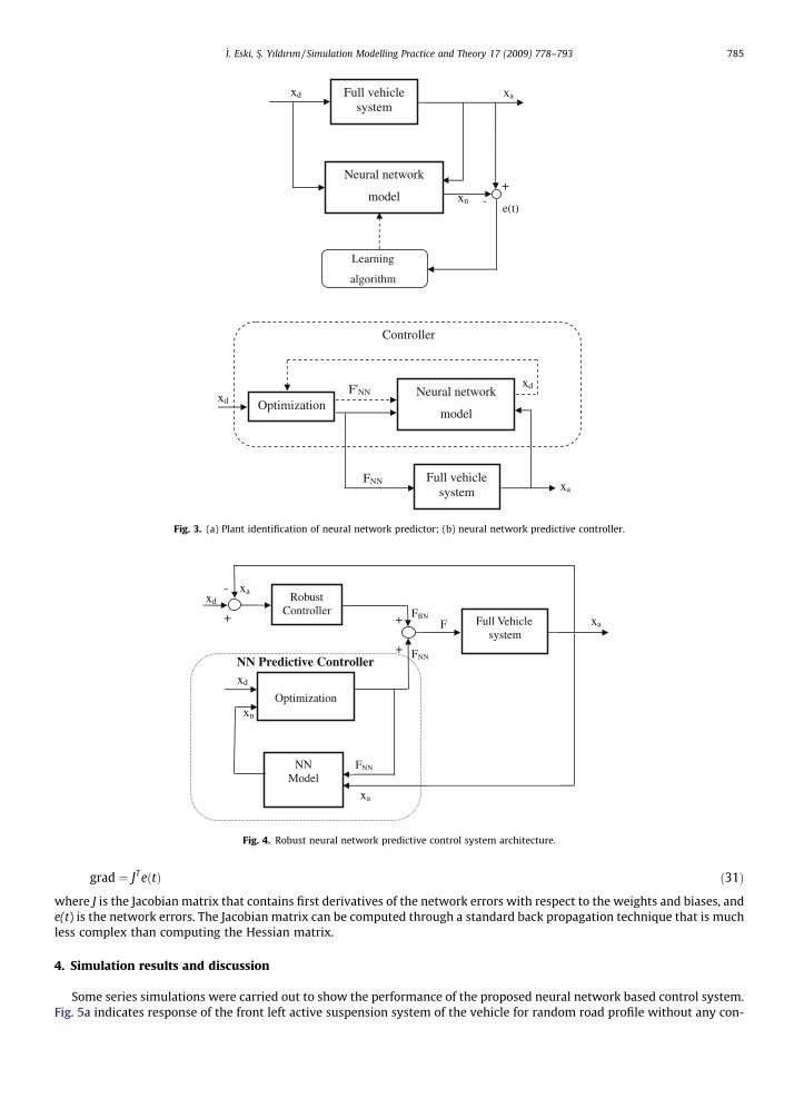
3.2.1. Neural network predictive controllerNeural network predictive controller is typically two steps involved: system identification and control design. The system

identification stage of neural network predictive control is to train a neural network to present the forward dynamics of theplant. Fig. 2 shows schematic representation three layered feedforward neural network plant model. The prediction errorbetween the plant output and the neural network output is used as the neural network training signal. The process is rep-

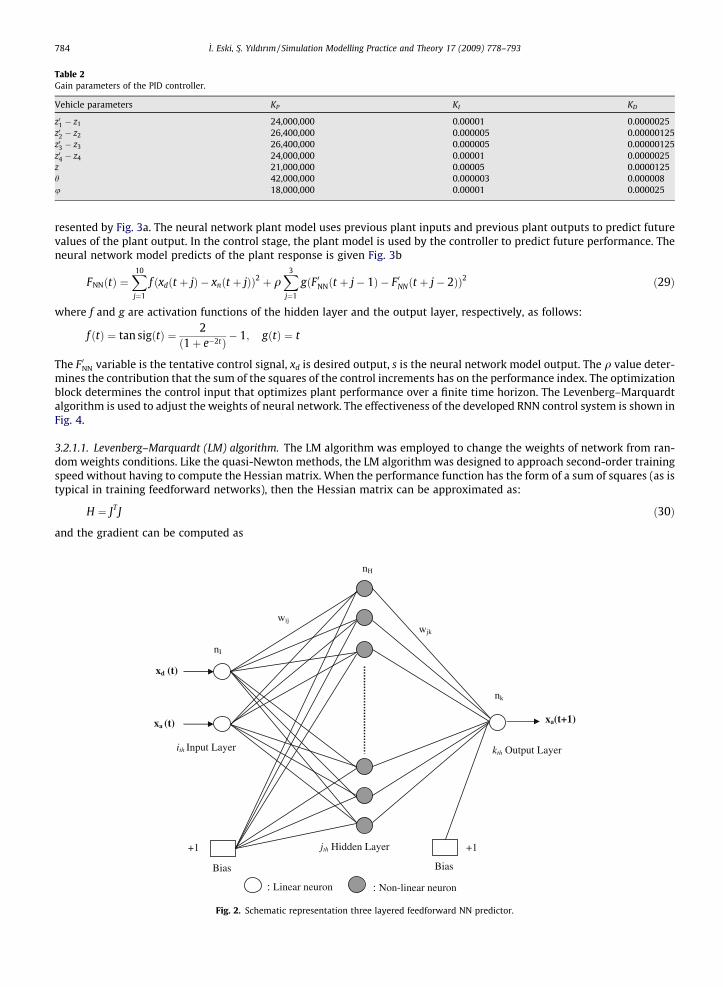
Table 2Gain parameters of the PID controller.

Vehicle parameters KP KI KD

z01 � z1 24,000,000 0.00001 0.0000025z02 � z2 26,400,000 0.000005 0.00000125z03 � z3 26,400,000 0.000005 0.00000125z04 � z4 24,000,000 0.00001 0.0000025z 21,000,000 0.00005 0.0000125h 42,000,000 0.000003 0.000008u 18,000,000 0.00001 0.000025


resented by Fig. 3a. The neural network plant model uses previous plant inputs and previous plant outputs to predict futurevalues of the plant output. In the control stage, the plant model is used by the controller to predict future performance. Theneural network model predicts of the plant response is given Fig. 3b

FNNðtÞ ¼X10

j¼1

f ðxdðt þ jÞ � xnðt þ jÞÞ2 þ qX3

j¼1

gðF 0NNðt þ j� 1Þ � F 0NNðt þ j� 2ÞÞ2 ð29Þ

where f and g are activation functions of the hidden layer and the output layer, respectively, as follows:

f ðtÞ ¼ tan sigðtÞ ¼ 2ð1þ e�2tÞ � 1; gðtÞ ¼ t

The F 0NN variable is the tentative control signal, xd is desired output, s is the neural network model output. The q value deter-mines the contribution that the sum of the squares of the control increments has on the performance index. The optimizationblock determines the control input that optimizes plant performance over a finite time horizon. The Levenberg–Marquardtalgorithm is used to adjust the weights of neural network. The effectiveness of the developed RNN control system is shown inFig. 4.

3.2.1.1. Levenberg–Marquardt (LM) algorithm. The LM algorithm was employed to change the weights of network from ran-dom weights conditions. Like the quasi-Newton methods, the LM algorithm was designed to approach second-order trainingspeed without having to compute the Hessian matrix. When the performance function has the form of a sum of squares (as istypical in training feedforward networks), then the Hessian matrix can be approximated as:

H ¼ JT J ð30Þ

and the gradient can be computed as

wij

wjk

nI

: Linear neuron : Non-linear neuron

nH

kth Output Layer

xa(t+1)

nk

xa (t)

ith Input Layer

jth Hidden Layer

xd (t)

Bias Bias

+1 +1

Fig. 2. Schematic representation three layered feedforward NN predictor.

Neural network

model

Full vehicle system

+ -

xa

xn

xd

Learning

algorithm

e(t)

Neural network

model

xa

Optimization

Full vehicle system

FNN

F'NNxd

Controller

xd

Fig. 3. (a) Plant identification of neural network predictor; (b) neural network predictive controller.

NN Model

Full Vehicle system

xd

xa

RobustController

xdxa

xa

Optimizationxn

FNN

FBN+

+

-

+ F

NN Predictive Controller

FNN

Fig. 4. Robust neural network predictive control system architecture.


grad ¼ JT eðtÞ ð31Þ

where J is the Jacobian matrix that contains first derivatives of the network errors with respect to the weights and biases, ande(t) is the network errors. The Jacobian matrix can be computed through a standard back propagation technique that is muchless complex than computing the Hessian matrix.

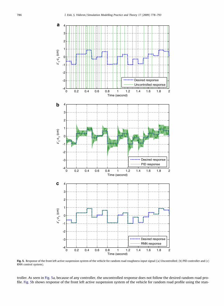
4. Simulation results and discussion

Some series simulations were carried out to show the performance of the proposed neural network based control system.Fig. 5a indicates response of the front left active suspension system of the vehicle for random road profile without any con-

0 0.2 0.4 0.6 0.8 1 1.2 1.4 1.6 1.8 2-4

-3

-2

-1

0

1

2

3

4

Time (second)

Time (second)

Time (second)

z'1-z

1(c

m)

Desired response

Uncontrolled response

0 0.2 0.4 0.6 0.8 1 1.2 1.4 1.6 1.8 2-4

-3

-2

-1

0

1

2

3

4

z'1-z

1(c

m)

Desired response

PID response

0 0.2 0.4 0.6 0.8 1 1.2 1.4 1.6 1.8 2-4

-3

-2

-1

0

1

2

3

4

z'1-z

1(c

m)

Desired response

RNN response

a

b

c

Fig. 5. Response of the front left active suspension system of the vehicle for random road roughness input signal ((a) Uncontrolled; (b) PID controller and (c)RNN control system).


troller. As seen in Fig. 5a, because of any controller, the uncontrolled response does not follow the desired random road pro-file. Fig. 5b shows response of the front left active suspension system of the vehicle for random road profile using the stan-

0 0.2 0.4 0.6 0.8 1 1.2 1.4 1.6 1.8 2-4

-3

-2

-1

0

1

2

3

4

z'2-z

2(c

m)

Desired response


0 0.2 0.4 0.6 0.8 1 1.2 1.4 1.6 1.8 2-4

-3

-2

-1

0

1

2

3

4

z'2-z

2(c

m)

Desired response

PID response

0 0.2 0.4 0.6 0.8 1 1.2 1.4 1.6 1.8 2-4

-3

-2

-1

0

1

2

3

4

Time (second)

Time (second)

Time (second)

z'2-z

2(c

m)

Desired response

RNN response

a

b

c

Fig. 6. Response of the rear left active suspension system of the vehicle for random road roughness input signal ((a) Uncontrolled; (b) PID controller and (c)RNN control system).


dard PID controller. As can be seen figure, the result of the PID controller does not follow the desired random road profilesignal. The result of the RNN control system for the front left active suspension system of the vehicle given in Fig. 5c. As de-picted from Fig. 5c, the proposed control system has good performance at adapting random road roughness.

0 0.2 0.4 0.6 0.8 1 1.2 1.4 1.6 1.8 2-4

-3

-2

-1

0

1

2

3

4

Time (second)

Time (second)

Time (second)

z'3-z

3(c

m)

Desired response


0 0.2 0.4 0.6 0.8 1 1.2 1.4 1.6 1.8 2-4

-3

-2

-1

0

1

2

3

4

z'3-z

3(cm

)

Desired response

PID response

0 0.2 0.4 0.6 0.8 1 1.2 1.4 1.6 1.8 2-4

-3

-2

-1

0

1

2

3

4

z'3-z

3(c

m)

Desired response

RNN response

a

b

c

Fig. 7. Response of the rear right active suspension system of the vehicle for random road roughness input signal ((a) Uncontrolled; (b) PID controller and(c) RNN control system).


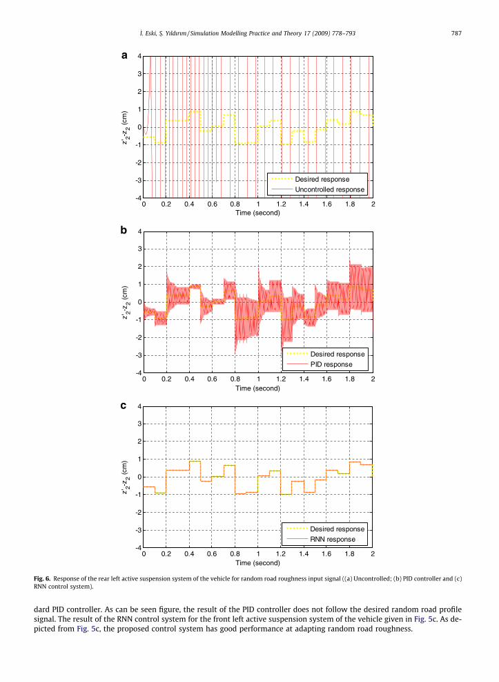
Fig. 6a–c give the result of without any controller, the PID controller and the proposed RNN control system for the rear leftactive suspension system. As shown in Fig. 6b, both the desired random road profile and the PID controller result are notfollowed.

0 0.2 0.4 0.6 0.8 1 1.2 1.4 1.6 1.8 2-4

-3

-2

-1

0

1

2

3

4

z'4-z

4(c

m)

Desired response


0 0.2 0.4 0.6 0.8 1 1.2 1.4 1.6 1.8 2-4

-3

-2

-1

0

1

2

3

4

Time (second)

Time (second)

Time (second)

z'4-z

4(c

m)

Desired response

PID response

0 0.2 0.4 0.6 0.8 1 1.2 1.4 1.6 1.8 2-4

-3

-2

-1

0

1

2

3

4

z'4-z

4(c

m)

Desired response

RNN response

a

b

c

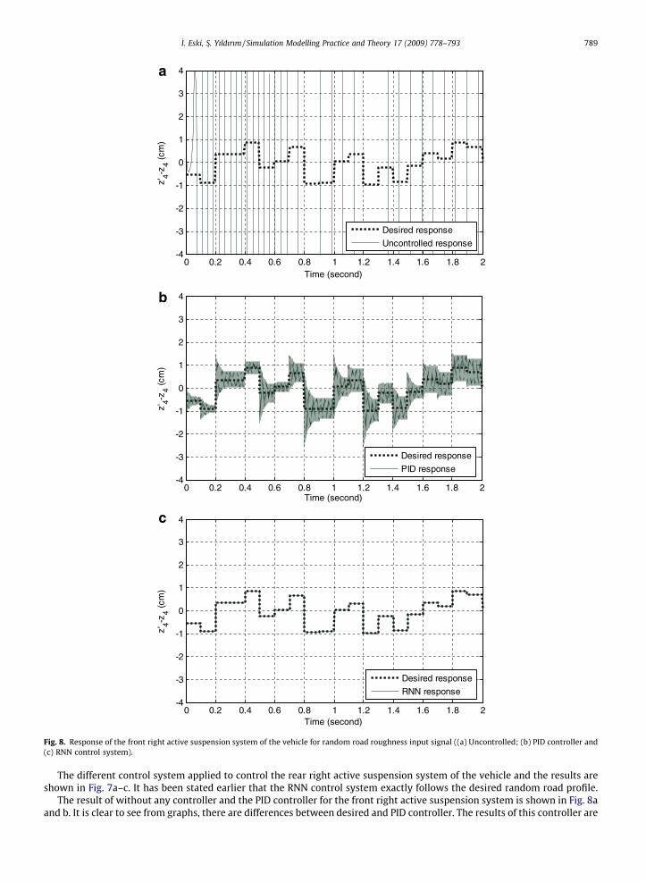
Fig. 8. Response of the front right active suspension system of the vehicle for random road roughness input signal ((a) Uncontrolled; (b) PID controller and(c) RNN control system).


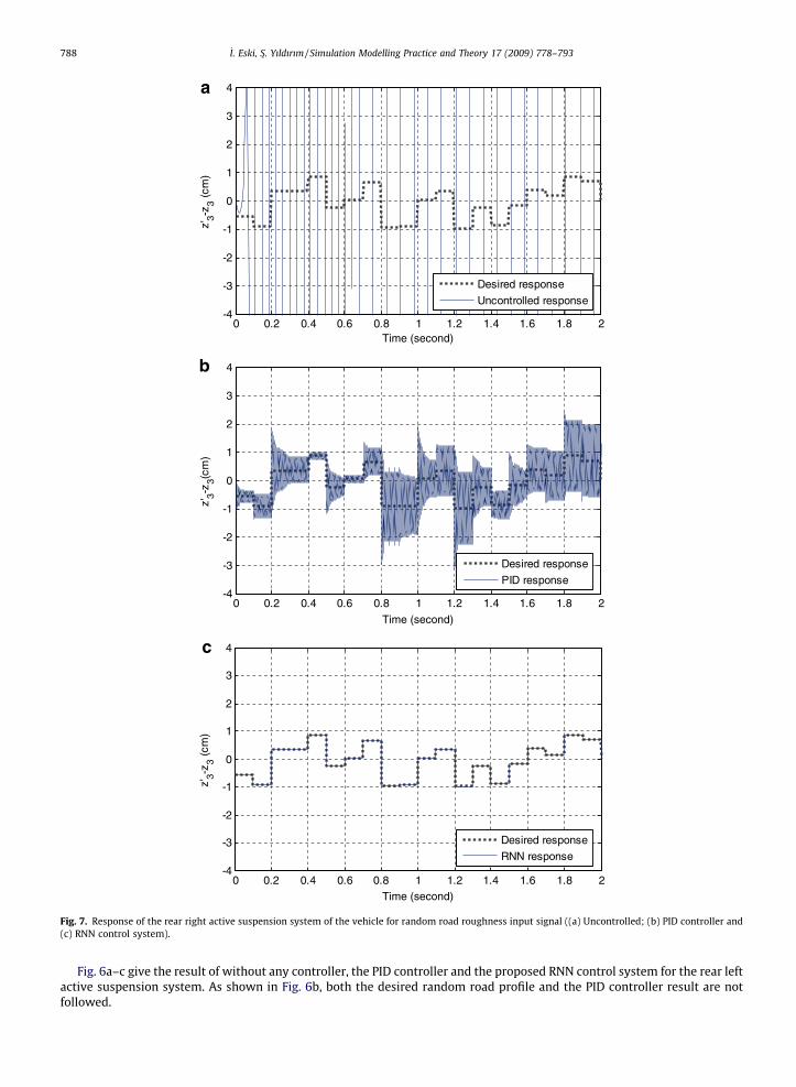
The different control system applied to control the rear right active suspension system of the vehicle and the results areshown in Fig. 7a–c. It has been stated earlier that the RNN control system exactly follows the desired random road profile.

The result of without any controller and the PID controller for the front right active suspension system is shown in Fig. 8aand b. It is clear to see from graphs, there are differences between desired and PID controller. The results of this controller are

0 0.2 0.4 0.6 0.8 1 1.2 1.4 1.6 1.8 2-1

-0.5

0

0.5

1

Time (second)

Time (second)

Time (second)

z (c

m)

Desired response


0 0.2 0.4 0.6 0.8 1 1.2 1.4 1.6 1.8 2-1

-0.5

0

0.5

1

z (c

m)

Desired response

PID response

0 0.2 0.4 0.6 0.8 1 1.2 1.4 1.6 1.8 2-1

-0.5

0

0.5

1

z (c

m)

Desired response

RNN response

a

b

c

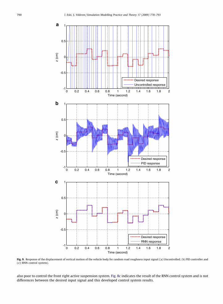
Fig. 9. Response of the displacement of vertical motion of the vehicle body for random road roughness input signal ((a) Uncontrolled; (b) PID controller and(c)) RNN control system).


also poor to control the front right active suspension system. Fig. 8c indicates the result of the RNN control system and is notdifferences between the desired input signal and this developed control system results.

0 0.2 0.4 0.6 0.8 1 1.2 1.4 1.6 1.8 2

-0.008

-0.006

-0.004

-0.002

0

0.002

0.004

0.006

0.008

Time (second)

Time (second)

Time (second)

φ(r

ad)

Desired response


0 0.2 0.4 0.6 0.8 1 1.2 1.4 1.6 1.8 2

-0.008

-0.006

-0.004

-0.002

0

0.002

0.004

0.006

0.008

φ(r

ad)

Desired response

PID response

0 0.2 0.4 0.6 0.8 1 1.2 1.4 1.6 1.8 2

-0.008

-0.006

-0.004

-0.002

0

0.002

0.004

0.006

0.008

φ(r

ad)

Desired response

RNN response

a

b

c

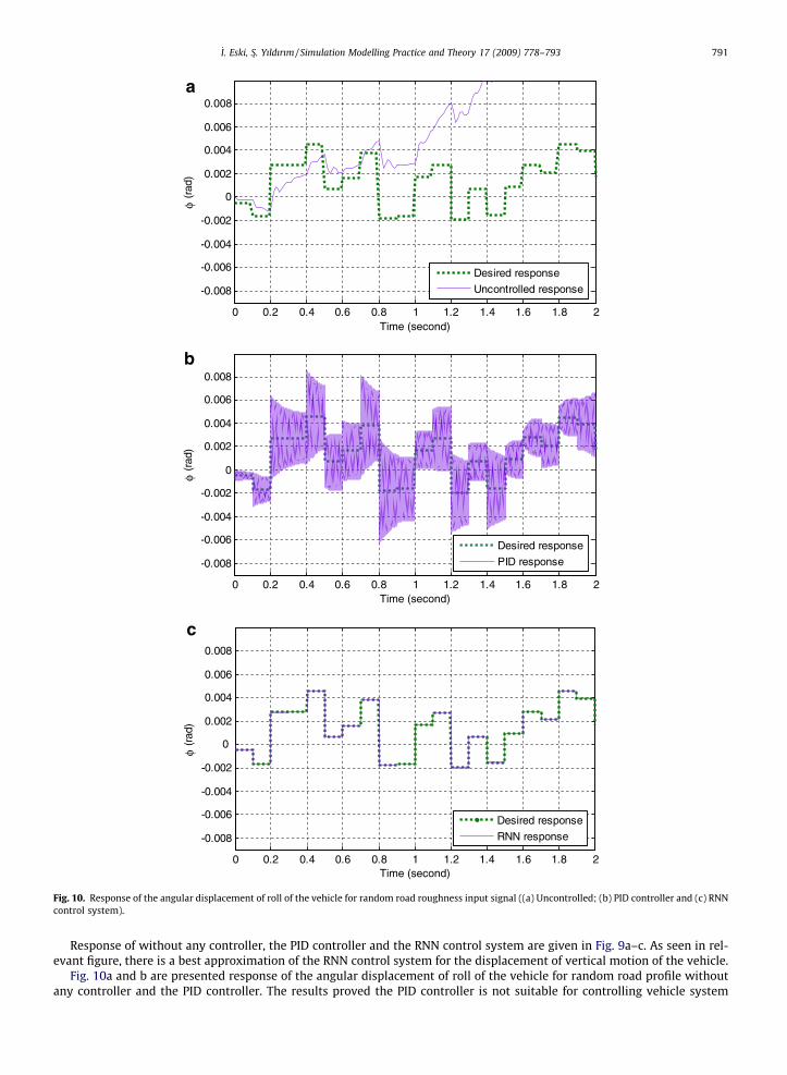
Fig. 10. Response of the angular displacement of roll of the vehicle for random road roughness input signal ((a) Uncontrolled; (b) PID controller and (c) RNNcontrol system).


Response of without any controller, the PID controller and the RNN control system are given in Fig. 9a–c. As seen in rel-evant figure, there is a best approximation of the RNN control system for the displacement of vertical motion of the vehicle.

Fig. 10a and b are presented response of the angular displacement of roll of the vehicle for random road profile withoutany controller and the PID controller. The results proved the PID controller is not suitable for controlling vehicle system

0 0.2 0.4 0.6 0.8 1 1.2 1.4 1.6 1.8 2

-0.008

-0.006

-0.004

-0.002

0

0.002

0.004

0.006

0.008

Time (second)

Time (second)

Time (second)

θ(r

ad)

Desired response

PID response

0 0.2 0.4 0.6 0.8 1 1.2 1.4 1.6 1.8 2

-0.008

-0.006

-0.004

-0.002

0

0.002

0.004

0.006

0.008

θ(r

ad)

Desired response

PID response

0 0.2 0.4 0.6 0.8 1 1.2 1.4 1.6 1.8 2

-0.008

-0.006

-0.004

-0.002

0

0.002

0.004

0.006

0.008

θ(r

ad)

Desired response

RNN response

a

b

c

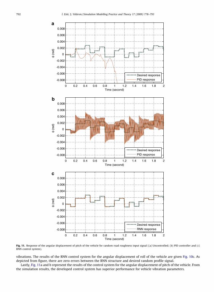
Fig. 11. Response of the angular displacement of pitch of the vehicle for random road roughness input signal ((a) Uncontrolled; (b) PID controller and (c)RNN control system).


vibrations. The results of the RNN control system for the angular displacement of roll of the vehicle are given Fig. 10c. Asdepicted from figure, there are zero errors between the RNN structure and desired random profile signal.

Lastly, Fig. 11a and b represent the results of the control system for the angular displacement of pitch of the vehicle. Fromthe simulation results, the developed control system has superior performance for vehicle vibration parameters.


5. Conclusions and discussion

In this paper, neural network based control system for whole vehicle active suspension system parameters has been de-signed. The full vehicle model is considered seven degrees of freedom system. The performance is compared to both the PIDcontroller and the proposed RNN control system for random road roughness profile. The proposed NN based control systemis consisted of a robust feedback controller and feedforward neural network predictive controller. From the simulation re-sults, it is seen that using the associated control system with robust feedback controller and neural network controller highabsolute road profile tracking performance can be achieved for random road roughness. It confirms the effectiveness androbustness of the proposed RNN control system. The reason of the best performance of the neural network based robust con-trol system could be explained in the following:

� Robust performance: Neural network based control system is the inclusion of both linear and non-linear neurons in thenetwork structure. Besides, exponential function use robust controller and this function provides an exponential decreaseof e(t).

� Adaptive learning: Neural network based control system again regulates weights of neural network controller versus var-iable road profile.

� Self-organization: Neural network can create its own organization or representation of the information it receives duringlearning time.

� Fault tolerance: Because of parallel structure of neural network based control system, fault spreads on this parallel struc-ture. Therefore, fault tolerance is considerably good.

Finally, the performance of the RNN control system is better than standard PID controller.

Acknowledgement

This research results consisted of a part of project TUBITAK-105M224 (Active Suspension Control of Vehicles using Arti-ficial Neural Network Controller). The authors wish to express their thanks to TUBITAK for supporting this project.

References

[1] J. Swevers, C. Lauwerys, B. Vandersmissen, M. Maes, K. Reybrouck, P. Sas, A model-free control structure for the on-line tuning of the semi-activesuspension of a passenger car, Mechanical Systems and Signal Processing 21 (2007) 1422–1436.

[2] H. Gao, J. Lam, C. Wang, Multi-objective control of vehicle active suspension systems via load-dependent controllers, Journal of Sound and Vibration290 (2006) 654–675.

[3] H. Du, N. Zhang, H1 control of active vehicle suspensions with actuator time delay, Journal of Sound and Vibration 301 (2007) 236–252.[4] H. Du, J. Lam, K.Y. Sze, Non-fragile output feedback H1 vehicle suspension control using genetic algorithm, Engineering Applications of Artificial

Intelligence 16 (2003) 667–680.[5] S.J. Huang, H.Y. Chen, Adaptive sliding controller with self-tuning fuzzy compensation for vehicle suspension control, Mechatronics 16 (2006) 607–622.[6] M. Ieluzzi, P. Turco, M. Montiglio, Development of a heavy truck semi-active suspension control, Control Engineering Practice 14 (2006) 305–312.[7] A.G. Thompson, B.R. Davis, Computation of the rms state variables and control forces in a half-car model with preview active suspension using spectral

decomposition methods, Journal of Sound and Vibration 285 (2005) 571–583.[8] R. Guclu, Fuzzy logic control of seat vibrations of a non-linear full vehicle model, Nonlinear Dynamics 40 (2005) 21–34.[9] Y. He, J. McPhee, Multidisciplinary design optimization of mechatronic vehicles with active suspensions, Journal of Sound and Vibration 283 (2005)

217–241.[10] R. Guclu, K. Gulez, Neural network control of seat vibrations of a non-linear full vehicle model using PMSM, Mathematical and Computer Modelling 47

(2008) 1356–1371.[11] S�. Yıldırım, _I. Uzmay, Neural network applications to vehicle’s vibration analysis, Mechanism and Machine Theory 38 (2003) 27–41.[12] J. Anthonis, H. Ramon, Design of an active suspension to suppress the horizontal vibrations of a spray boom, Journal of Sound and Vibration 266 (2003)

573–583.[13] G.Z. Yao, F.F. Yap, G. Chen, W.H. Li, S.H. Yeo, MR damper and its application for semi-active control of vehicle suspension system, Mechatronics 12

(2002) 963–973.[14] K. Spentzas, S.A. Kanarachos, Design of a non-linear hybrid car suspension system using neural networks, Mathematics and Computers in Simulation

60 (2002) 369–378.[15] F.J. D’Amato, D.E. Viassolo, Fuzzy Control for Active Suspensions, Mechatronics 10 (2000) 897–920.[16] N. Yagiz, I. Yüksek, Sliding mode control of active suspensions for a full vehicle model, International Journal of Vehicle Design 26 (2001) 264–276.

Documents

Simulation Modelling Practice and Theory - پرشینگیگcdn.persiangig.com/.../Vibration_control_of_vehicle_active_suspensio… · investigated the overall performance of a semi-active