Unit 8 SUPPLEMENT – Normal, T, Chi Square, F, and Sums …people.umass.edu/~biep540w/pdf/8. SUPPLEMENT - Normal T Chi... · SUPPLEMENT – Normal, T, Chi Square, ... Nature Population

BIOSTATS 540 – Fall 2017 8. SUPPLEMENT – Normal, T, Chi Square, F and Sums of Normals Page 1 of 22

Nature Population/ Sample

Observation/ Data

Relationships/ Modeling

Analysis/ Synthesis

Unit 8

SUPPLEMENT – Normal, T, Chi Square, F, and Sums of Normals

Topic

1. Normal Distribution ……………………………………………………..… a. Definition ……………………………………………………………….. b. Calculations Using Online Apps ………………………………………… c. Calculations Using R ……………………………………………………. d. Calculations Using Stata ………………………………………………… 2. Student T Distribution …………………………………………………… a. Definition ……………………………………………………………….. b. Calculations Using Online Apps ………………………………………… c. Calculations Using R ……………………………………………………. d. Calculations Using Stata ………………………………………………… 3. Chi Square Distribution …………………………………………….…… a. Definition ……………………………………………………………….. b. Calculations Using Online Apps ………………………………………… c. Calculations Using R ……………………………………………………. d. Calculations Using Stata ………………………………………………… 4. F Distribution ……………………………………………………………… a. Definition ……………………………………………………………….. b. Calculations Using Online Apps ………………………………………… c. Calculations Using R ……………………………………………………. d. Calculations Using Stata ………………………………………………… 5. Sums and Differences of Independent Normal Random Variables ……

2 2 4 6 6 7 7 9 11 11

12 12 14 16 16

17 17 18 20 20

21



Observation/ Data


Analysis/ Synthesis

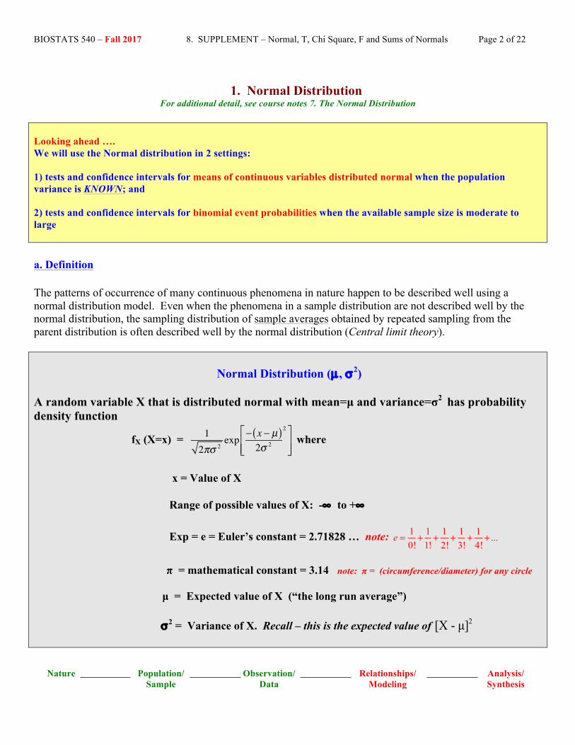
1. Normal Distribution

For additional detail, see course notes 7. The Normal Distribution Looking ahead …. We will use the Normal distribution in 2 settings: 1) tests and confidence intervals for means of continuous variables distributed normal when the population variance is KNOWN; and 2) tests and confidence intervals for binomial event probabilities when the available sample size is moderate to large a. Definition The patterns of occurrence of many continuous phenomena in nature happen to be described well using a normal distribution model. Even when the phenomena in a sample distribution are not described well by the normal distribution, the sampling distribution of sample averages obtained by repeated sampling from the parent distribution is often described well by the normal distribution (Central limit theory).

Normal Distribution (µ , σ2)

A random variable X that is distributed normal with mean=µ and variance=σ2 has probability density function

fX (X=x) = 12πσ 2

exp− x − µ( )2σ 2

2⎡

⎣⎢⎢

⎤

⎦⎥⎥

where

x = Value of X Range of possible values of X: -∞ to +∞

Exp = e = Euler’s constant = 2.71828 … note: 1 1 1 1 1 ...0! 1! 2! 3! 4!

e = + + + + +

π = mathematical constant = 3.14 note: π = (circumference/diameter) for any circle

µ = Expected value of X (“the long run average”) σ2 = Variance of X. Recall – this is the expected value of 2[X - µ]



Observation/ Data


Analysis/ Synthesis

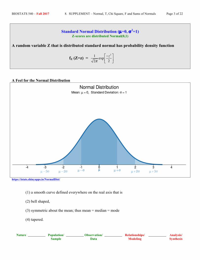
Standard Normal Distribution (µ=0, σ2=1)

Z-scores are distributed Normal(0,1) A random variable Z that is distributed standard normal has probability density function

fZ (Z=z) = 12πexp −z2

2⎡

⎣⎢

⎤

⎦⎥

A Feel for the Normal Distribution

https://istats.shinyapps.io/NormalDist/ (1) a smooth curve defined everywhere on the real axis that is (2) bell shaped, (3) symmetric about the mean; thus mean = median = mode (4) tapered.



Observation/ Data


Analysis/ Synthesis

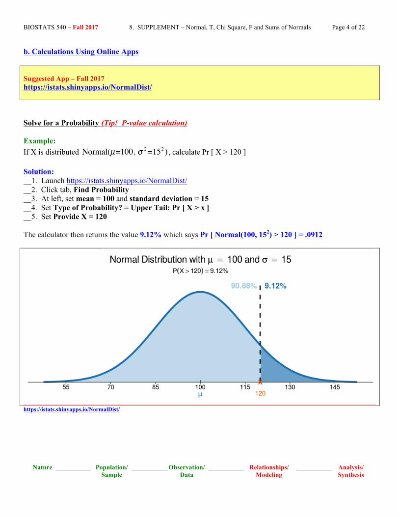
b. Calculations Using Online Apps Suggested App – Fall 2017 https://istats.shinyapps.io/NormalDist/

Solve for a Probability (Tip! P-value calculation) Example: If X is distributed Normal(µ=100, σ 2 =152 ) , calculate Pr [ X > 120 ] Solution: __1. Launch https://istats.shinyapps.io/NormalDist/ __2. Click tab, Find Probability __3. At left, set mean = 100 and standard deviation = 15 __4. Set Type of Probability? = Upper Tail: Pr [ X > x ] __5. Set Provide X = 120 The calculator then returns the value 9.12% which says Pr [ Normal(100, 152) > 120 ] = .0912

https://istats.shinyapps.io/NormalDist/



Observation/ Data


Analysis/ Synthesis

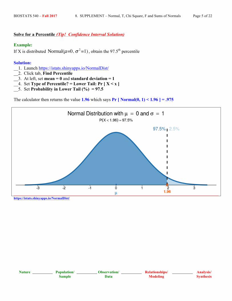
Solve for a Percentile (Tip! Confidence Interval Solution) Example: If X is distributed Normal(µ=0, σ 2 =1) , obtain the 97.5th percentile Solution: __1. Launch https://istats.shinyapps.io/NormalDist/ __2. Click tab, Find Percentile __3. At left, set mean = 0 and standard deviation = 1 __4. Set Type of Percentile? = Lower Tail: Pr [ X < x ] __5. Set Probability in Lower Tail (%) = 97.5 The calculator then returns the value 1.96 which says Pr [ Normal(0, 1) < 1.96 ] = .975

https://istats.shinyapps.io/NormalDist/



Observation/ Data


Analysis/ Synthesis

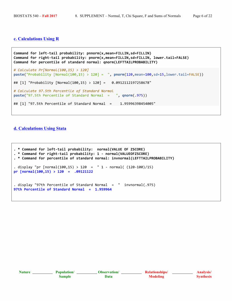
c. Calculations Using R Command for left-‐tail probability: pnnorm(x,mean=FILLIN,sd=FILLIN) Command for right-‐tail probability: pnorm(x,mean=FILLIN,sd=FILLIN, lower.tail=FALSE) Command for percentile of standard normal: qnorm(LEFTTAILPROBABILITY)

# Calculate Pr[Normal(100,15) > 120] paste("Probability [Normal(100,15) > 120] = ", pnorm(120,mean=100,sd=15,lower.tail=FALSE))

## [1] "Probability [Normal(100,15) > 120] = 0.0912112197258678"

# Calculate 97.5th Percentile of Standard Normal paste("97.5th Percentile of Standard Normal = ", qnorm(.975))

## [1] "97.5th Percentile of Standard Normal = 1.95996398454005"

d. Calculations Using Stata

. * Command for left-‐tail probability: normal(VALUE OF ZSCORE)

. * Command for right-‐tail probability: 1 -‐ normal(VALUEOFZSCORE)

. * Command for percentile of standard normal: invnormal(LEFTTAILPROBABILITY) . display "pr [normal(100,15) > 120 = " 1 -‐ normal( (120-‐100)/15) pr [normal(100,15) > 120 = .09121122 . display "97th Percentile of Standard Normal = " invnormal(.975) 97th Percentile of Standard Normal = 1.959964



Observation/ Data


Analysis/ Synthesis

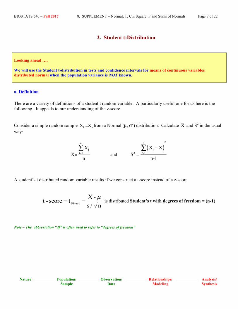
2. Student t-Distribution

Looking ahead …. We will use the Student t-distribution in tests and confidence intervals for means of continuous variables distributed normal when the population variance is NOT known. a. Definition There are a variety of definitions of a student t random variable. A particularly useful one for us here is the following. It appeals to our understanding of the z-score. Consider a simple random sample X1...Xn from a Normal (µ, σ2) distribution. Calculate X and S2 in the usual way:

X=Xi

i=1

n

∑n

and S2 =Xi − X( )

i=1

n

∑2

n-1

A student’s t distributed random variable results if we construct a t-score instead of a z-score.

t - score = t = X -s / nDF=n-1

µ is distributed Student’s t with degrees of freedom = (n-1)

Note – The abbreviation “df” is often used to refer to “degrees of freedom”



Observation/ Data


Analysis/ Synthesis

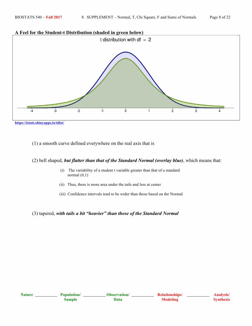
A Feel for the Student-t Distribution (shaded in green below)

https://istats.shinyapps.io/tdist/ (1) a smooth curve defined everywhere on the real axis that is (2) bell shaped, but flatter than that of the Standard Normal (overlay blue), which means that:

(i) The variability of a student t variable greater than that of a standard normal (0,1) (ii) Thus, there is more area under the tails and less at center (iii) Confidence intervals tend to be wider than those based on the Normal

(3) tapered, with tails a bit “heavier” than those of the Standard Normal



Observation/ Data


Analysis/ Synthesis

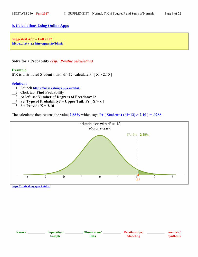
b. Calculations Using Online Apps Suggested App – Fall 2017 https://istats.shinyapps.io/tdist/

Solve for a Probability (Tip! P-value calculation) Example: If X is distributed Student-t with df=12, calculate Pr [ X > 2.10 ] Solution: __1. Launch https://istats.shinyapps.io/tdist/ __2. Click tab, Find Probability __3. At left, set Number of Degrees of Freedom=12 __4. Set Type of Probability? = Upper Tail: Pr [ X > x ] __5. Set Provide X = 2.10 The calculator then returns the value 2.88% which says Pr [ Student-t (df=12) > 2.10 ] = .0288

https://istats.shinyapps.io/tdist/



Observation/ Data


Analysis/ Synthesis

Solve for a Percentile (Tip! Confidence Interval Solution) Example: If X is distributed Student-t (df=12) obtain the 97.5th percentile Solution: __1. Launch https://istats.shinyapps.io/tdist/ __2. Click tab, Find Percentile __3. At left, set Number of Degrees of Freedom=12 __4. Set Type of Percentile? = Lower Tail: Pr [ X < x ] __5. Set Probability in Lower Tail (%) = 97.5 The calculator then returns the value 2.179 which says Pr [ Student-t (df=12) < 2.179 ] = .975

https://istats.shinyapps.io/tdist/



Observation/ Data


Analysis/ Synthesis

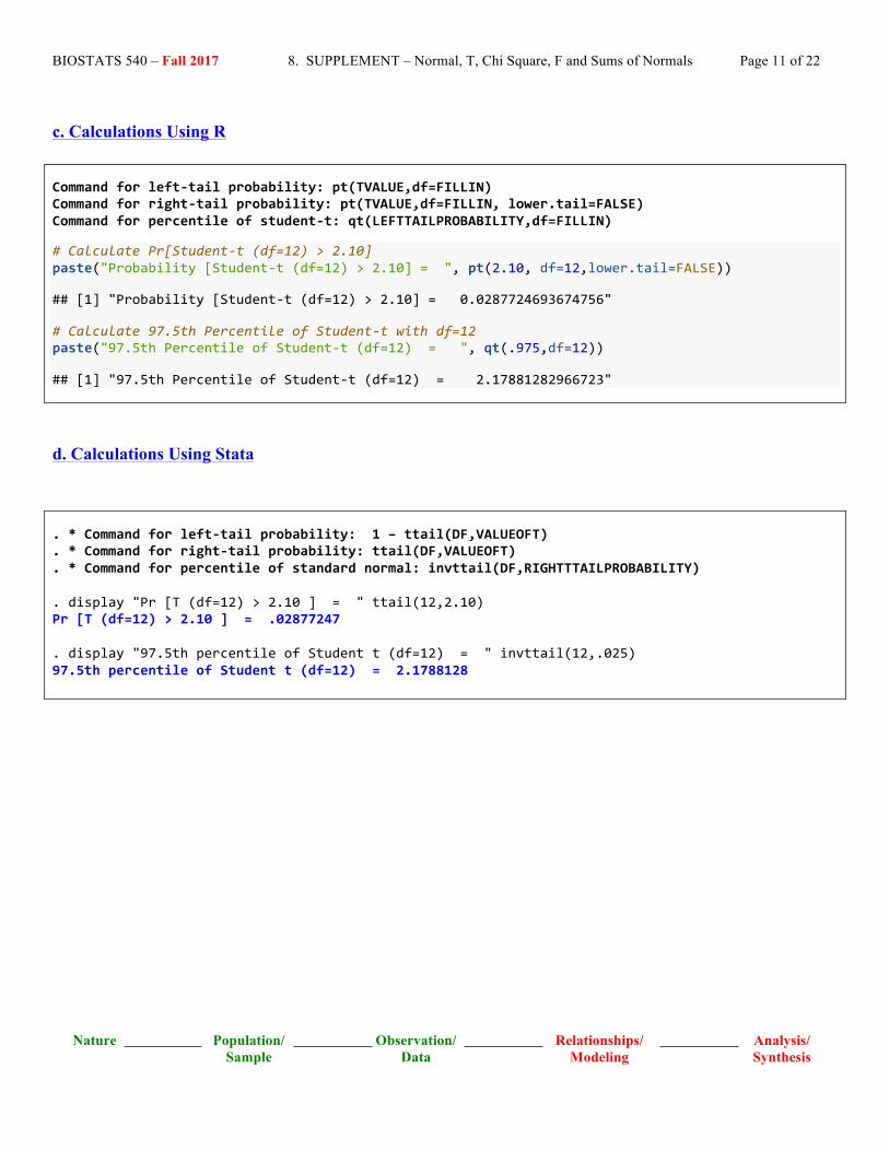
c. Calculations Using R Command for left-‐tail probability: pt(TVALUE,df=FILLIN) Command for right-‐tail probability: pt(TVALUE,df=FILLIN, lower.tail=FALSE) Command for percentile of student-‐t: qt(LEFTTAILPROBABILITY,df=FILLIN)

# Calculate Pr[Student-‐t (df=12) > 2.10] paste("Probability [Student-‐t (df=12) > 2.10] = ", pt(2.10, df=12,lower.tail=FALSE))

## [1] "Probability [Student-‐t (df=12) > 2.10] = 0.0287724693674756"

# Calculate 97.5th Percentile of Student-‐t with df=12 paste("97.5th Percentile of Student-‐t (df=12) = ", qt(.975,df=12))

## [1] "97.5th Percentile of Student-‐t (df=12) = 2.17881282966723"


. * Command for left-‐tail probability: 1 – ttail(DF,VALUEOFT)

. * Command for right-‐tail probability: ttail(DF,VALUEOFT)

. * Command for percentile of standard normal: invttail(DF,RIGHTTTAILPROBABILITY) . display "Pr [T (df=12) > 2.10 ] = " ttail(12,2.10) Pr [T (df=12) > 2.10 ] = .02877247 . display "97.5th percentile of Student t (df=12) = " invttail(12,.025) 97.5th percentile of Student t (df=12) = 2.1788128



Observation/ Data


Analysis/ Synthesis

3. Chi Square Distribution

Looking ahead …. Percentiles of the chi square distribution are used in settings of continuous outcomes that are distributed normal. Specifically, it is used in tests and confidence intervals for a single population variance or single population standard deviation. a. Definition One setting (not the only one, but the one we are considering in this course) is the setting of a simple random sample from a Normal distribution. We want to test a hypothesis or construct a confidence interval estimate of the variance parameter, σ2. To do this, we work with a new random variable Y that is defined as follows:

2

2

(n-1)SY=σ

,

In this formula, S2 is the sample variance that you learned in Unit 1. Under simple random sampling from a Normal(µ,σ2)

2

2

(n-1)SY=σ

is distributed Chi Square with degrees of freedom = (n-1)

The above can be stated more formally. (1) If the random variable X follows a normal probability distribution with mean µ and variance σ2, Then the random variable V defined:

( )2

2

X-V=

µσ

is distributed chi square distribution with degree of freedom = 1.

(2) If each of the random variables V1, ..., Vk is distributed chi square with degree of freedom = 1, and if these are independent, Then their sum, defined: V1 + ... + Vk is distributed chi square distribution with degrees of freedom = k



Observation/ Data


Analysis/ Synthesis

For the interested reader: The two definitions on the previous page are consistent because it is possible (with a

little algebra) to re-write Y= (n-1)S2

σ 2 as the sum of (n-1) independent chi square random variables V, each with

degrees of freedom = 1. NOTE: For this course, it is not necessary to know the probability density function for the chi square distribution. A Feel for the Chi Square Distribution

https://istats.shinyapps.io/ChisqDist/ (1) A chi square random variable can assume only non-negative values. Specifically, the probability density function has domain [0, ∞ ) and is not defined for outcome values less than zero. Thus, (2) Thus, the chi square distribution is NOT symmetric. Pr[Y > y] is NOT EQUAL to Pr[Y < -y] Tip – This means that, in contrast to those for the Normal or Student-t, the values of chi square distribution percentiles are NOT symmetric around zero. à For example, you have to solve for the 2.5th and 97.5th percentiles separately. (3) The chi square distribution is less skewed as the number of degrees of freedom increases. Degrees of freedom=1 Degrees of freedom=5 Degrees of freedom=10

https://istats.shinyapps.io/ChisqDist/



Observation/ Data


Analysis/ Synthesis

b. Calculations Using Online Apps Suggested App – Fall 2017 https://istats.shinyapps.io/ChisqDist/

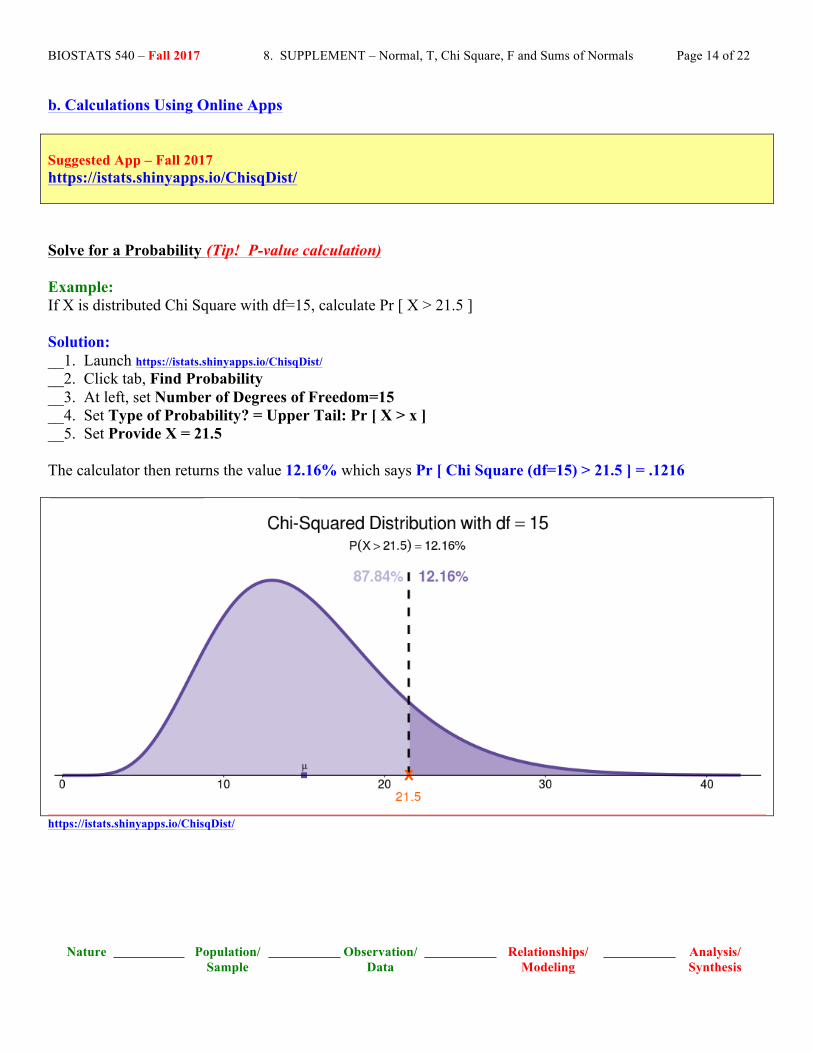
Solve for a Probability (Tip! P-value calculation) Example: If X is distributed Chi Square with df=15, calculate Pr [ X > 21.5 ] Solution: __1. Launch https://istats.shinyapps.io/ChisqDist/ __2. Click tab, Find Probability __3. At left, set Number of Degrees of Freedom=15 __4. Set Type of Probability? = Upper Tail: Pr [ X > x ] __5. Set Provide X = 21.5 The calculator then returns the value 12.16% which says Pr [ Chi Square (df=15) > 21.5 ] = .1216




Observation/ Data


Analysis/ Synthesis

Solve for a Percentile (Tip! Confidence Interval Solution) Example: If X is distributed Chi Square (df=15) obtain the 2.5th and 97.5th percentiles. Notice that they are not symmetric about zero! Solution: __1. Launch https://istats.shinyapps.io/ChisqDist/ __2. Click tab, Find Percentile __3. At left, set Number of Degrees of Freedom=15 __4. Set Type of Percentile? = Lower Tail: Pr [ X < x ] __5. Set Probability in Lower Tail (%) = 2.5 __6. Set Probability in Lower Tail (%) = 97.5 The calculator then returns the values 6.262 and 27.488, which say Pr [ Chi Square (df=15) < 6.262 ] = .025 and Pr [ Chi Square (df=15) < 27.488 ] = .975, respectively.




Observation/ Data


Analysis/ Synthesis

c. Calculations Using R Command for left-‐tail probability: pchisq(VALUE,df=FILLIN) Command for right-‐tail probability: pchisq(VALUE,df=FILLIN, lower.tail=FALSE) Command for percentile of chi square: qchisq(LEFTTAILPROBABILITY,df=FILLIN)

# Calculate Pr[Chi Square (df=15) > 21.5] paste("Probability [Chi Square (df=15) > 21.5] = ", pchisq(21.5, df=15,lower.tail=FALSE))

## [1] "Probability [Chi Square (df=15) > 21.5] = 0.121600308000176"

# Calculate 2.5th and 97.5th Percentiles of Chi Square with df=15 paste("2.5th Percentile of Chi Square (df=15) = ", qchisq(.025,df=15))

## [1] "2.5th Percentile of Chi Square (df=15) = 6.26213779504325"

paste("97.5th Percentile of Chi Square (df=15) = ", qchisq(.975,df=15))

## [1] "97.5th Percentile of Chi Square (df=15) = 27.488392863443"


. * Command for left-‐tail probability: 1 – chi2tail(DF,VALUE)

. * Command for right-‐tail probability: chi2tail(DF,VALUEOFT)

. * Command for percentile of standard normal: invchi2(DF,LEFTTAILPROBABILITY) . display "Pr [ Chi square (df=15) > 21.5 ] = "chi2tail(15,21.5) Pr [ Chi square (df=15) > 21.5 ] = .12160031

. display "2.5th Percentile of Chi Square (df=15) = " invchi2(15,.025) 2.5th Percentile of Chi Square (df=15) = 6.2621378 . display "97.5th Percentile of Chi Square (df=15) = " invchi2(15,.975) 97.5th Percentile of Chi Square (df=15) = 27.488393



Observation/ Data


Analysis/ Synthesis

4. F Distribution Looking ahead …. Percentiles of the F distribution are used in settings of samples from normal distributions and are used in tests and confidence intervals for the ratio of two independent variances. a. Definition

Unlike the approach used to compare two means in the continuous variable setting (where we will look at their difference), the comparison of two variances is accomplished by looking at their ratio. Ratio values close to one are evidence of similarity. Of interest will be a confidence interval estimate of the ratio of two variances in the setting where data are comprised of two independent samples of data, each from a separate Normal distribution. Suppose X1 , ... , Xnx is a simple random sample from a normal distribution with mean µX and variance σ X

2 . Suppose further that Y1 , ... , Yny is a simple random sample from a normal distribution with mean µY and variance σ Y

2 . If the two sample variances are calculated in the usual way

( )xn 2

i2 i=1X

x

x xS

n -1

−=∑

and

( )Yn 2

i2 i=1Y

Y

y yS

n -1

−=∑

Then

x y

2 2X x

n 1,n -1 2 2Y y

SFS

σσ− = is distributed F with two degree of freedom specifications

Numerator degrees of freedom, df1 = nx-1 Denominator degrees of freedom, df2 = ny-1



Observation/ Data


Analysis/ Synthesis

b. Calculations Using Online Apps Suggested App – Fall 2017 https://istats.shinyapps.io/FDist/

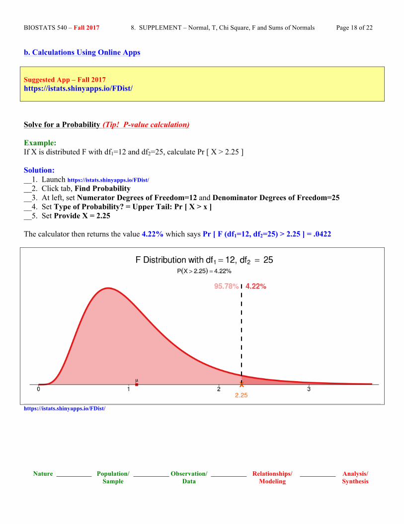
Solve for a Probability (Tip! P-value calculation) Example: If X is distributed F with df1=12 and df2=25, calculate Pr [ X > 2.25 ] Solution: __1. Launch https://istats.shinyapps.io/FDist/ __2. Click tab, Find Probability __3. At left, set Numerator Degrees of Freedom=12 and Denominator Degrees of Freedom=25 __4. Set Type of Probability? = Upper Tail: Pr [ X > x ] __5. Set Provide X = 2.25 The calculator then returns the value 4.22% which says Pr [ F (df1=12, df2=25) > 2.25 ] = .0422

https://istats.shinyapps.io/FDist/



Observation/ Data


Analysis/ Synthesis

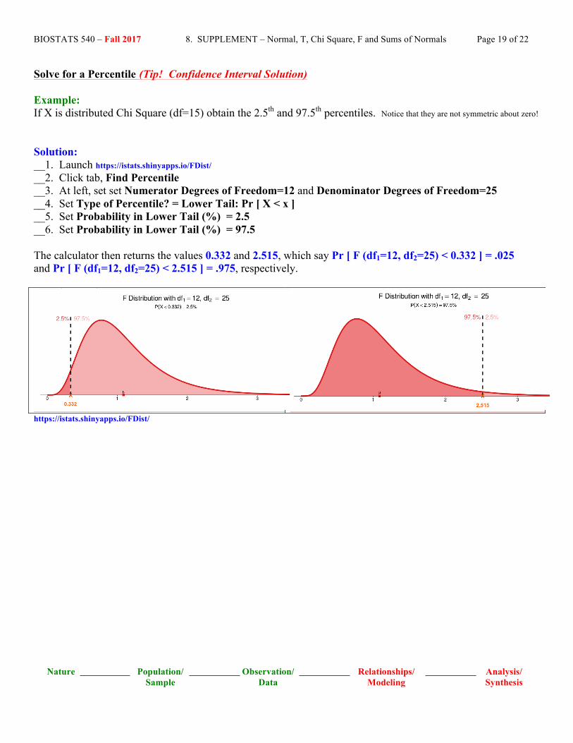
Solve for a Percentile (Tip! Confidence Interval Solution) Example: If X is distributed Chi Square (df=15) obtain the 2.5th and 97.5th percentiles. Notice that they are not symmetric about zero! Solution: __1. Launch https://istats.shinyapps.io/FDist/ __2. Click tab, Find Percentile __3. At left, set set Numerator Degrees of Freedom=12 and Denominator Degrees of Freedom=25 __4. Set Type of Percentile? = Lower Tail: Pr [ X < x ] __5. Set Probability in Lower Tail (%) = 2.5 __6. Set Probability in Lower Tail (%) = 97.5 The calculator then returns the values 0.332 and 2.515, which say Pr [ F (df1=12, df2=25) < 0.332 ] = .025 and Pr [ F (df1=12, df2=25) < 2.515 ] = .975, respectively.

https://istats.shinyapps.io/FDist/



Observation/ Data


Analysis/ Synthesis

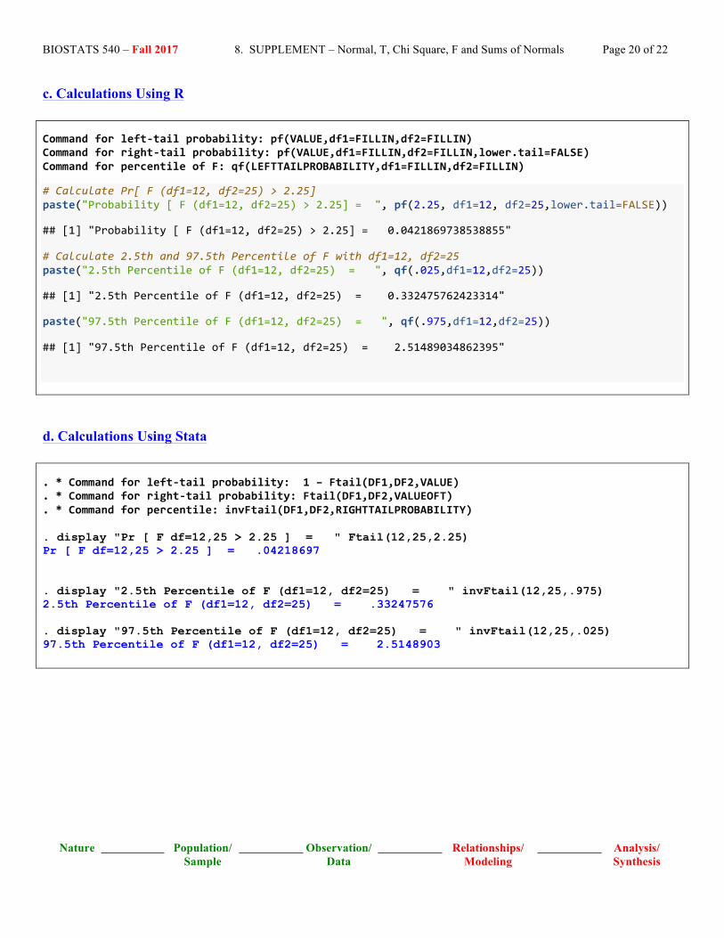
c. Calculations Using R Command for left-‐tail probability: pf(VALUE,df1=FILLIN,df2=FILLIN) Command for right-‐tail probability: pf(VALUE,df1=FILLIN,df2=FILLIN,lower.tail=FALSE) Command for percentile of F: qf(LEFTTAILPROBABILITY,df1=FILLIN,df2=FILLIN)

# Calculate Pr[ F (df1=12, df2=25) > 2.25] paste("Probability [ F (df1=12, df2=25) > 2.25] = ", pf(2.25, df1=12, df2=25,lower.tail=FALSE))

## [1] "Probability [ F (df1=12, df2=25) > 2.25] = 0.0421869738538855"

# Calculate 2.5th and 97.5th Percentile of F with df1=12, df2=25 paste("2.5th Percentile of F (df1=12, df2=25) = ", qf(.025,df1=12,df2=25))

## [1] "2.5th Percentile of F (df1=12, df2=25) = 0.332475762423314"

paste("97.5th Percentile of F (df1=12, df2=25) = ", qf(.975,df1=12,df2=25))

## [1] "97.5th Percentile of F (df1=12, df2=25) = 2.51489034862395"


. * Command for left-‐tail probability: 1 – Ftail(DF1,DF2,VALUE)

. * Command for right-‐tail probability: Ftail(DF1,DF2,VALUEOFT)

. * Command for percentile: invFtail(DF1,DF2,RIGHTTAILPROBABILITY) . display "Pr [ F df=12,25 > 2.25 ] = " Ftail(12,25,2.25) Pr [ F df=12,25 > 2.25 ] = .04218697 . display "2.5th Percentile of F (df1=12, df2=25) = " invFtail(12,25,.975) 2.5th Percentile of F (df1=12, df2=25) = .33247576 . display "97.5th Percentile of F (df1=12, df2=25) = " invFtail(12,25,.025) 97.5th Percentile of F (df1=12, df2=25) = 2.5148903



Observation/ Data


Analysis/ Synthesis

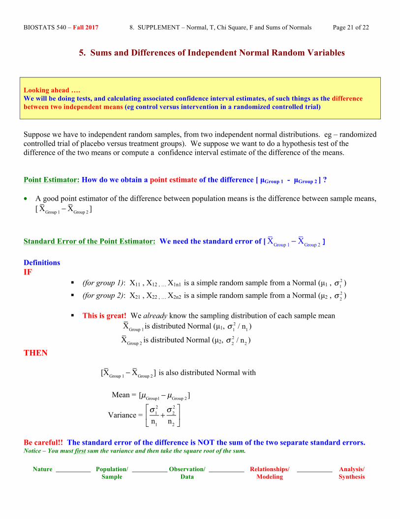
5. Sums and Differences of Independent Normal Random Variables

Looking ahead …. We will be doing tests, and calculating associated confidence interval estimates, of such things as the difference between two independent means (eg control versus intervention in a randomized controlled trial) Suppose we have to independent random samples, from two independent normal distributions. eg – randomized controlled trial of placebo versus treatment groups). We suppose we want to do a hypothesis test of the difference of the two means or compute a confidence interval estimate of the difference of the means. Point Estimator: How do we obtain a point estimate of the difference [ µGroup 1 - µGroup 2 ] ? • A good point estimator of the difference between population means is the difference between sample means,

[ XGroup 1 − XGroup 2 ]

Standard Error of the Point Estimator: We need the standard error of [ XGroup 1 − XGroup 2 ]

Definitions IF

§ (for group 1): X11 , X12 , … X1n1 is a simple random sample from a Normal (µ1 , σ 12 )

§ (for group 2): X21 , X22 , … X2n2 is a simple random sample from a Normal (µ2 , σ 22 )

§ This is great! We already know the sampling distribution of each sample mean

XGroup 1 is distributed Normal (µ1, σ 1

2 / n1 )

XGroup 2 is distributed Normal (µ2, σ 2

2 / n2 )

THEN

[XGroup 1 − XGroup 2 ] is also distributed Normal with

Mean =

[µGroup1 − µGroup 2 ]

Variance =

σ 12

n1

+σ 2

2

n2

⎡

⎣⎢

⎤

⎦⎥

Be careful!! The standard error of the difference is NOT the sum of the two separate standard errors. Notice – You must first sum the variance and then take the square root of the sum.



Observation/ Data


Analysis/ Synthesis

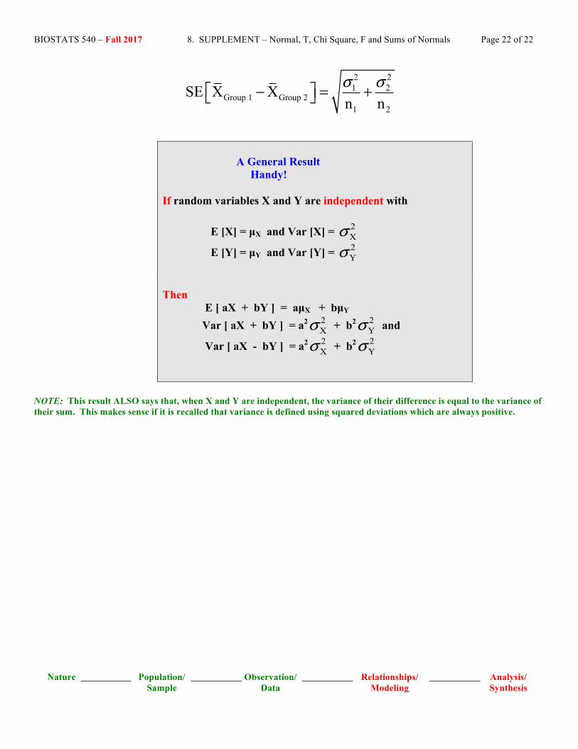
2 21 2

Group 1 Group 21 2

SE X Xn nσ σ⎡ ⎤− = +⎣ ⎦

A General Result Handy! If random variables X and Y are independent with E [X] = µX and Var [X] = 2

Xσ

E [Y] = µY and Var [Y] = 2Yσ

Then E [ aX + bY ] = aµX + bµY

Var [ aX + bY ] = a2 2Xσ + b2 2

Yσ and

Var [ aX - bY ] = a2 2Xσ + b2 2

Yσ

NOTE: This result ALSO says that, when X and Y are independent, the variance of their difference is equal to the variance of their sum. This makes sense if it is recalled that variance is defined using squared deviations which are always positive.

Documents

Unit 8 SUPPLEMENT – Normal, T, Chi Square, F, and Sums …people.umass.edu/~biep540w/pdf/8. SUPPLEMENT - Normal T Chi... · SUPPLEMENT – Normal, T, Chi Square, ... Nature Population