Embed Size (px)
Citation preview

seires noitacilbup ytisrevinU otlaASNOITATRESSID LAROTCOD 591 / 6102
rof gnissecorp yarra enohporciM seuqinhcet oidua laitaps cirtemarap
sitiloP sitnohcrA
fo rotcoD fo eerged eht rof detelpmoc noitatressid larotcod A eht fo noissimrep eht htiw ,dednefed eb ot )ygolonhceT( ecneicS
cilbup a ta ,gnireenignE lacirtcelE fo loohcS ytisrevinU otlaA rebmevoN 4 no loohcs eht fo 4S llah erutcel eht ta dleh noitanimaxe
.noon ta 6102
ytisrevinU otlaA gnireenignE lacirtcelE fo loohcS
scitsuocA dna gnissecorP langiS fo tnemtrapeD scitsuocA noitacinummoC
rosseforp gnisivrepuS dnalniF ,ytisrevinU otlaA ,ikkluP elliV rosseforP
rosivda sisehT
dnalniF ,ytisrevinU otlaA ,ikkluP elliV rosseforP
srenimaxe yranimilerP airtsuA ,zarG ,strA gnimrofreP dna cisuM fo ytisrevinU ,rettoZ znarF rotcoD
ASU ,AC ,ogeiD naS ,mmoclauQ ,sreteP sliN rotcoD
tnenoppO ASU ,YN ,yesreJ weN ,scitsuoca hm ,oklE yraG rotcoD
seires noitacilbup ytisrevinU otlaASNOITATRESSID LAROTCOD 591 / 6102
© sitiloP sitnohcrA
NBSI 4-8307-06-259-879 )detnirp( NBSI 7-7307-06-259-879 )fdp(
L-NSSI 4394-9971 NSSI 4394-9971 )detnirp( NSSI 2494-9971 )fdp(
:NBSI:NRU/if.nru//:ptth 7-7307-06-259-879
yO aifarginU iknisleH 6102
dnalniF
tcartsbA otlaA 67000-IF ,00011 xoB .O.P ,ytisrevinU otlaA if.otlaa.www
rohtuA sitiloP sitnohcrA
noitatressid larotcod eht fo emaN seuqinhcet oidua laitaps cirtemarap rof gnissecorp yarra enohporciM
rehsilbuP gnireenignE lacirtcelE fo loohcS tinU scitsuocA dna gnissecorP langiS fo tnemtrapeD
seireS seires noitacilbup ytisrevinU otlaA SNOITATRESSID LAROTCOD 591 / 6102 hcraeser fo dleiF gnissecorP langiS dna scitsuocA
dettimbus tpircsunaM 6102 yaM 91 ecnefed eht fo etaD 6102 rebmevoN 4 )etad( detnarg hsilbup ot noissimreP 6102 tsuguA 9 egaugnaL hsilgnE
hpargonoM noitatressid elcitrA noitatressid yassE
tcartsbAa sa desingocer ylgnisaercni si senecs dnuos dedrocer fo seitreporp laitaps fo noitcudorpeR
detneiro-amenic ro citsemod htiw ,snoitacilppa evisremmi gnigreme lla fo tnemele laicurc dna ,gnicnerefnocelet evisremmi dna ecneserpelet ,tnemniatretne rof noitcudorper lausivoidua
lareneg a morf tfieneb snoitacilppa hcuS .selpmaxe yek gnieb ytilaer lautriv dna detnemgua fo yteirav a morf noitamrofni laitaps tiolpxe ot elba gnieb ,krowemarf gnissecorp oidua laitaps tnerapsnart yllautpecrep a ni enecs dnuos lanigiro eht ecudorper ot redro ni stamrof gnidrocer
.yawdohtem noitcudorper dnuos laitaps cirtemarap tnecer a si )CAriD( gnidoC oiduA lanoitceriD
oidua D3 lasrevinu a no desab si tI .krowemarf a hcus fo stnemeriuqer eht fo ynam slfiluf taht rof noitcudorper lautpecrep evitceffe dna elbixefl seveihca dna tamrof-B sa nwonk tamrof
.senohpdaeh ro srekaepsduoltaht nwohs si ti ,yltsriF .ti dnetxe ot smia dna CAriD fo ledom eht no sesucof krow siht fo traP
-B eht setareneg taht yarra gnidrocer lennahc-ruof eht fo noitamrofni tnuocca otni gnikat yb.noitcudorper dna enecs dnuos eht fo sisylana htob evorpmi ot elbissop si ti ,slangis tamrof
.snoitarugfinoc gnidrocer suoirav rof desilareneg era sgnidnfi eseht ,yldnoceSlacirehps eht ,niamod mrofsnart laitaps a ni detpmetta si CAriD fo noitasilareneg rehtruf A ni ledom CAriD eht gnitalumroF .slangis tamrof-B redro-rehgih htiw ,)DHS( niamod cinomrah
fo noituloser desaercni eht htiw CAriD fo ssenevitceffe lautpecrep eht senibmoc DHS eht .CAriD lanoitidart fo snoitatimil tsom semocrevo dna tamrof-B redro-rehgih
rof detartsnomed era dnuos laitaps fo gnissecorp cirtemarap fo snoitacilppa levon emoS laitaps eht gniyfidom fo laitnetop eht swohs tsrfi ehT .gnireenigne cisum dna dnuos
swohs dnoces eht elihw ,senecs dnuos fo noitalupinam evitaerc rof gnidrocer eht ni noitamrofni .seuqinhcet gnidrocer dnuorrus dehsilbatse htiw derutpac noitcudorper cisum fo tnemevorpmi
seuc noitasilanretxe dna ecnatsid gniyevnoc ni seuqinhcet cirtemarap fo ssenevitceffe ehT a ni srekaepsduol gnisu ecnatsid deviecrep eht gnillortnoc ni hcraeser ot del ,senohpdaeh revo tcapmoc a gnisu oitar ygrene tnarebrever-ot-tcerid eht gnitalupinam yb deveihca si sihT .moor
.nrettap ytivitcerid elbairav a htiw yarra rekaepsduollaitaps eht fo noitasilarua ,senecs dnuos dedrocer fo noitcudorper morf trapa ,yltsaL
detius-llew si melborp siht taht etartsnomed eW .tseretni fo era secaps lacitsuoca fo seitreporp egral a htiw derutpac sesnopser eslupmi moor fo erutan ehT .sisylana laitaps cirtemarap ot
noitceted rof sehcaorppa hcus dna ,sehcaorppa noituloser-hgih yrev swolla yarra enohporcim dna deilppa era wodniw noitavresbo trohs elgnis a ni snoitcefler elpitlum fo noitasilacol dna
.derapmoc sdrowyeK noitcudorper dnuos ,sisylana dlefi dnuos ,syarra enohporcim ,oidua laitaps
)detnirp( NBSI 4-8307-06-259-879 )fdp( NBSI 7-7307-06-259-879 L-NSSI 4394-9971 )detnirp( NSSI 4394-9971 )fdp( NSSI 2494-9971
rehsilbup fo noitacoL iknisleH gnitnirp fo noitacoL iknisleH raeY 6102 segaP 512 nru :NBSI:NRU/fi.nru//:ptth 7-7307-06-259-879

Preface
This thesis work was carried out at the Department of Signal Process-
ing and Acoustics, School of Electrical Engineering, Aalto University in
Espoo, Finland. The research leading to these results has received fund-
ing from the European Research Council under the European Community
Seventh Framework Programme (FP7/2007-2013)/ERC grant agreement
no [240453].
First and foremost, I would like to express my gratitude to my supervi-
sor Prof. Ville Pulkki, for his insight in the research pertaining this thesis
and his endless patience with my constant diversions. His unconventional
approach to attacking research problems has been very inspiring, as were
his dance moves.
I am also thankful to the pre-examiners of the thesis manuscript, Dr.
Franz Zotter and Dr. Nils Peters, and their prompt reviews during sum-
mertime. I sincerely hope it was not an ordeal.
The Communication Acoustics research group, in which I belonged, made
our workplace a very special and stimulating environment. My gratitude
extends to all the people that passed from it during my stay. I would
like to thank especially Dr. Mikko-Ville Laitinen, Tapani Pihlajamäki,
Dr. Juha Vilkamo, Symeon Delikaris-Manias, Alessandro Altoè, Javier
Gómez Bolaños, Ilkka Huhtakallio, Dr. Olli Santala, Dr. Marko Takanen,
Dr. Jukka Ahonen, Dr. Marko Hiipakka, Dr. Catarina Hiipakka, Olli
Rummukainen, Teemu Koski, Julia Turku, Juhani Paasonen, and Henri
Pöntynen.
The audio research community at Aalto University is large and strong
and the amount of knowledge and enthusiasm on everything audio- and
acoustics-related is staggering. I have learned a lot from my friends and
collaborators Dr. Sakari Tervo, Dr. Roberto Pugliese, and Dr. Julian
Parker. Many thanks also to Dr. Hannes Gamper, Dr. Stefano D’Angelo,
1

Preface
Sofoklis Kakouros, Fabian Esqueda, Sami Oksanen, and all the rest of the
great people I met from the Audio Signal Processing, Virtual Acoustics,
and Speech Technology groups.
I would additionally like to thank my hosts, Prof. Ramani Duraiswami
and Dr. Dmitry Zotkin, for their hospitality during my research visit at
UMIACS, University of Maryland, MA, USA.
My parents and my sister supported me all these years and for that I
am very grateful to them, especially considering that they believe I am
still some kind of a student (and they are not totally wrong). And lastly,
I am most grateful to my partner Henna Tahvanainen who stood by my
side throughout this work. Her presence helped me through all the ebbs
and flows of research, and made this thesis a reality.
Helsinki, September 17, 2016,
Archontis Politis
2
Contents
Preface 1
Contents 3
List of Publications 7
Author’s Contribution 9
List of Figures 11
1. Introduction 19
2. Physical Modelling of Spatial Sound Scenes and Array Pro-
cessing 23
2.1 Physical properties of sound fields . . . . . . . . . . . . . . . 23
2.1.1 Statistical properties of sound field quantities . . . . 25
2.1.2 Diffuse sound field . . . . . . . . . . . . . . . . . . . . 26
2.1.3 Microphones and array processing . . . . . . . . . . . 28
2.1.4 DoA estimation and acoustic localisation in complex
scenes . . . . . . . . . . . . . . . . . . . . . . . . . . . . 33
2.1.5 Spherical harmonic representation of sound field quan-
tities and acoustical spherical processing . . . . . . . 36
3. Perception and Technology of Spatial Sound 43
3.1 Spatial sound perception . . . . . . . . . . . . . . . . . . . . . 43
3.1.1 Time-frequency resolution . . . . . . . . . . . . . . . . 43
3.1.2 Localisation cues . . . . . . . . . . . . . . . . . . . . . 44
3.1.3 Dynamic binaural cues . . . . . . . . . . . . . . . . . 45
3.1.4 Distance cues . . . . . . . . . . . . . . . . . . . . . . . 45
3.1.5 Precedence effect and summing localisation . . . . . . 46
3
Contents
3.1.6 Apparent source width, spaciousness and interaural
coherence . . . . . . . . . . . . . . . . . . . . . . . . . . 47
3.2 Spatial sound technologies . . . . . . . . . . . . . . . . . . . . 48
3.2.1 Binaural technology . . . . . . . . . . . . . . . . . . . 48
3.2.2 Loudspeaker-based reproduction . . . . . . . . . . . . 49
3.2.3 Spatial sound recording . . . . . . . . . . . . . . . . . 54
3.3 Evaluation of spatial sound reproduction . . . . . . . . . . . 57
3.3.1 Technical evaluation . . . . . . . . . . . . . . . . . . 57
3.3.2 Listening tests . . . . . . . . . . . . . . . . . . . . . . 58
4. Non-parametric Methods for Spatial Sound Recording and
Reproduction 61
4.1 Ambisonics . . . . . . . . . . . . . . . . . . . . . . . . . . . . . 61
4.1.1 Recording and encoding . . . . . . . . . . . . . . . . . 63
4.1.2 Sound-scene manipulation . . . . . . . . . . . . . . . 65
4.1.3 Decoding and panning . . . . . . . . . . . . . . . . . . 67
4.1.4 Binaural decoding . . . . . . . . . . . . . . . . . . . . 68
4.1.5 Discussion . . . . . . . . . . . . . . . . . . . . . . . . . 68
4.2 Other non-parametric approaches . . . . . . . . . . . . . . . 69
5. Parametric Methods for Spatial Sound Recording and Re-
production 71
5.1 Spatial audio coding and upmixing . . . . . . . . . . . . . . . 71
5.1.1 Spatial audio coding . . . . . . . . . . . . . . . . . . . 71
5.1.2 Upmixing . . . . . . . . . . . . . . . . . . . . . . . . . . 73
5.1.3 Binaural reproduction . . . . . . . . . . . . . . . . . . 74
5.1.4 Discussion . . . . . . . . . . . . . . . . . . . . . . . . . 74
5.2 Parametric reproduction of recorded sound scenes . . . . . . 74
5.2.1 Assumptions on array input and output setup prop-
erties. . . . . . . . . . . . . . . . . . . . . . . . . . . . . 75
5.2.2 Assumptions on the sound-field model and estima-
tion of parameters. . . . . . . . . . . . . . . . . . . . . 76
5.3 Directional Audio Coding . . . . . . . . . . . . . . . . . . . . . 80
5.3.1 Analysis . . . . . . . . . . . . . . . . . . . . . . . . . . 80
5.3.2 Synthesis . . . . . . . . . . . . . . . . . . . . . . . . . 82
5.3.3 Sound scene synthesis and manipulation . . . . . . . 85
5.3.4 Binauralisation, transcoding and upmixing . . . . . 85
5.3.5 Discussion . . . . . . . . . . . . . . . . . . . . . . . . . 87
5.4 Analysis and synthesis of room acoustics . . . . . . . . . . . 88
4

Contents
6. Contributions 91
6.1 Perceptual distance control . . . . . . . . . . . . . . . . . . . 91
6.2 Improving parametric reproduction of B-format recordings
using array information . . . . . . . . . . . . . . . . . . . . . 91
6.3 Extending high-frequency estimation of DoA and diffuseness 92
6.4 Parametric sound-field manipulation . . . . . . . . . . . . . . 92
6.5 Enhancement of spaced microphone array recordings . . . . 93
6.6 Higher-order DirAC . . . . . . . . . . . . . . . . . . . . . . . . 93
6.7 Analysis of spatial room impulse responses . . . . . . . . . . 94
References 95
Publications 121
5

Contents
6
List of Publications
This thesis consists of an overview and of the following publications which
are referred to in the text by their Roman numerals.
I Archontis Politis, Ville Pulkki. Broadband Analysis and Synthesis
for Directional Audio Coding using A-format Input Signals. In 131st
Convention of the Audio Engineering Society, New York, NY, USA,
October 2011.
II Archontis Politis, Tapani Pihlajamäki, Ville Pulkki. Parametric Spa-
tial Audio Effects. In 15th International Conference on Digital Audio
Effects (DAFx-12), York, UK, September 2012.
III Archontis Politis, Mikko-Ville Laitinen, Jukka Ahonen, Ville Pulkki.
Parametric Spatial Audio Processing of Spaced Microphone Array
Recordings for Multichannel Reproduction. Journal of the Audio En-
gineering Society, 63, 4, 216–227, April 2015.
IV Archontis Politis, Symeon Delikaris-Manias, Ville Pulkki. Direction-
of-Arrival and Diffuseness Estimation Above Spatial Aliasing for
Symmetrical Directional Microphone Arrays. In IEEE International
Conference on Audio, Speech and Signal Processing, Brisbane, Aus-
tralia, April 2015.
V Archontis Politis, Juha Vilkamo, Ville Pulkki. Sector-Based Para-
metric Sound Field Reproduction in the Spherical Harmonic Do-
main. IEEE Journal of Selected Topics in Signal Processing, 9, 5,
852–866, August 2015.
VI Mikko-Ville Laitinen, Archontis Politis, Ilkka Huhtakallio, Ville Pulkki.
Controlling the Perceived Distance of an Auditory Object by Manip-
7

List of Publications
ulation of Loudspeaker Directivity. JASA Express Letters, 137, 6,
EL462–EL468, June 2015.
VII Sakari Tervo, Archontis Politis. Direction of Arrival Estimation of
Reflections from Room Impulse Responses Using a Spherical Micro-
phone Array. IEEE/ACM Transactions on Audio, Speech, and Lan-
guage Processing, 23, 10, 1539–1551, October 2015.
8
Author’s Contribution
Publication I: “Broadband Analysis and Synthesis for DirectionalAudio Coding using A-format Input Signals”
The author developed the methods, conducted the measurements and
wrote the article, under the supervision of the second author.
Publication II: “Parametric Spatial Audio Effects”
The present author developed and implemented the methods related to di-
rectional and reverberance modifications of recorded sound scenes, apart
from the acoustical zooming and translation effects. The remainder of
the methods were conceived and implemented by the second author. The
present author wrote the article, except section 3.3 which was written by
the second author.
Publication III: “Parametric Spatial Audio Processing of SpacedMicrophone Array Recordings for Multichannel Reproduction”
The present author implemented the methods in the paper, conducted the
objective evaluation and wrote most of the article. The analysis formula-
tion was developed by the present author, while the synthesis formulation
was developed by the second author. Additionally, the second author de-
signed the listening test and analyzed the results.
9

Author’s Contribution
Publication IV: “Direction-of-Arrival and Diffuseness EstimationAbove Spatial Aliasing for Symmetrical Directional MicrophoneArrays”
The present author developed and implemented the methods presented in
the paper and wrote most of the article. The evaluation of the method and
presentation of results was shared between the present and the second
author.
Publication V: “Sector-Based Parametric Sound Field Reproductionin the Spherical Harmonic Domain”
The present author developed the methods of the paper with the exception
of the optimal mixing stage of the synthesis, which is based on previous
work by the second author. The acoustic analysis in a sector was originally
conceived by the third author of the paper, who also supervised the work.
The implementation, listening tests, and evaluation responsibilities were
shared between the present and second author. The present author wrote
most of the work, with the exception of section V, and III.E.
Publication VI: “Controlling the Perceived Distance of an AuditoryObject by Manipulation of Loudspeaker Directivity”
The present author designed the beamforming operations for control of
the directivity pattern and formulated the theoretical model followed through-
out the work. The writing work was shared between the first and the
present author.
Publication VII: “Direction of Arrival Estimation of Reflections fromRoom Impulse Responses Using a Spherical Microphone Array”
The author formulated the measurement-based array response interpo-
lation and transform. The measurements were shared between the first
and the present author.
10
List of Figures
2.1 Directional patterns for a) common directional microphones,
b) omnidirectional microphone mounted on a hard cylinder
of 5 cm radius, and c) omnidirectional microphone mounted
on a sphere of 5 cm radius. . . . . . . . . . . . . . . . . . . . 30
2.2 Spherical harmonic functions up to order N = 3 of (a) real
form, and (b) complex form. The surfaces correspond to the
magnitude of the SHs. Blue and red indicate positive and
negative values for real SHs, while the colour map indicates
the phase for the complex SHs. . . . . . . . . . . . . . . . . . 38
3.1 (a) Measured head-related impulse responses of the author
in the horizontal plane for the left ear, and (b) extracted
and smoothed ITD surfaces from the measured responses
as seen from above. . . . . . . . . . . . . . . . . . . . . . . . . 49
3.2 Amplitude panning patterns for a 7.0 loudspeaker setup, us-
ing a) VBAP, b) VBIP, c) MDAP with a spread of 45 degrees,
and d) ambisonic panning with naive mode-matching decod-
ing. The black dashed line indicates the energy preservation
capabilities of the panning curves as the sum of the squared
gains for each direction. . . . . . . . . . . . . . . . . . . . . . 52
3.3 WFS sound pressure rendering of a virtual point source (red
cross) using a linear array of 21 secondary sources (black cir-
cles), with an inter-source spacing of 15 cm. Two frequencies
are plotted: a) below the spatial aliasing limit and b) above
the spatial aliasing limit. . . . . . . . . . . . . . . . . . . . . 53
11

List of Figures
3.4 Main surround array designs (first row) and rear surround
array designs (second row) for surround music recording.
The dimensions are indicative and adapted from Theile (2001).
. . . . . . . . . . . . . . . . . . . . . . . . . . . . . . . . . . . . 55
3.5 Generation of the reference and rendering through room
simulation for the evaluation of perceived distance from the
reference. . . . . . . . . . . . . . . . . . . . . . . . . . . . . . 60
4.1 General non-parametric mapping of microphone array sig-
nals to the reproduction setup. The bold arrows indicate
signal flow while the dashed ones indicate other parame-
ters. . . . . . . . . . . . . . . . . . . . . . . . . . . . . . . . . . 62
4.2 Schematic of ambisonic encoding and decoding. The bold
arrows indicate signal flow, while the dashed ones indicate
other parameters. . . . . . . . . . . . . . . . . . . . . . . . . . 63
4.3 Depiction of major ambisonic transformations of a sound
scene. In (c) directional compression is shown with yellow
and expansion with light blue. In (d) the modified boundary
curve shows the directional energy modification compared
to the original sound scene. . . . . . . . . . . . . . . . . . . . 66
5.1 Block diagrams of basic signal and parameters flow in SAC
and upmixing examples. Signal flow is indicated with solid
arrows, and parameter flow with dashed arrows. The TFT/FB
blocks indicate time-frequency transform or filter bank op-
erations. In SAC, inter-channel level differences (ICLD),
phase differences (ICPD), and the inter-channel coherence
(ICC) are computed and transmitted. In upmixing these
channel dependencies are used to estimate parameters for
a primary–ambient (or direct–diffuse) decomposition. . . . . 72
12
List of Figures
5.2 Block diagrams of exemplary implementations for paramet-
ric reproduction based on a) spatial filtering/beamforming
and b) blind source separation. Signal flow is indicated with
solid arrows and parameter flow with dashed arrows. The
TFT/FB blocks indicate time-frequency transform or filter
bank operations. In (a) a number of dominant sources and
their directions are estimated and extracted by adaptive
beamforming, while in (b) independent components are de-
tected in the mixture and clustered into meaningful source
signals based on information of the array response. . . . . . 78
5.3 Block diagram of DirAC analysis. Signal flow is indicated
with solid arrows and parameter flow with dashed arrows.
The TFT/FB blocks indicate time-frequency transform or fil-
ter bank operations. The notation of signals and parameters
follows the one in the text. . . . . . . . . . . . . . . . . . . . 82
5.4 Block diagram of VM-DirAC synthesis. Signal flow is in-
dicated with solid arrows and parameter flow with dashed
arrows. The TFT/FB blocks indicate time-frequency trans-
form or filter bank operations. The notation of signals and
parameters follows the one in the text. . . . . . . . . . . . . 84
13

List of Figures
14
List of Abbreviations
ASW apparent source width
BCC Binaural Cue Coding
BSS blind source separation
CSD cross-spectral density
DDR direct-to-diffuse ratio
DirAC Directional Audio Coding
DoA direction-of-arrival
DRR direct-to-reverberant ratio
ERB equivalent rectangular bandwidth
HOA higher-order Ambisonics
HRTF head-related transfer function
IACC interaural cross correlation
IC interaural coherence
ICA independent component analysis
ICC inter-channel coherence
ICLD inter-channel level difference
ICPD inter-channel phase difference
ILD interaural level difference
ISHT inverse spherical harmonic transform
ITD interaural time difference
LEV listener envelopment
MDAP multiple direction amplitude panning
15
List of Abbreviations
ML maximum likelihood
MPEG Moving Pictures Expert Group
MUSHRA multi-stimulus with hidden reference and anchor test
NMF non-negative matrix factorization
PCA principal component analysis
PS Parametric Stereo
PSD power-spectral density
QMF quadrature mirror filter bank
S3AC Spatially Squeezed Surround Audio Coding
SAC Spatial Audio Coding
SASC Spatial Audio Scene Coding
SDM Spatial Decomposition Method
SH spherical harmonic
SHD spherical harmonic domain
SHT spherical harmonic transform
SIRR Spatial Impulse Response Rendering
SNR signal-to-noise ratio
SRP steered response power
TDoA time-difference of arrival
VBAP vector-base amplitude panning
VBIP vector-base intensity panning
WFS wave field synthesis
WNG white noise gain
16
List of Symbols
a directional wave-amplitude density
a vector of sound field coefficients in the SHD
bn modified radial sound field expansion terms due to sensor
directivity or scatterer
b pressure and pressure-gradient (B-format) signal vector
c speed of sound
d directional response of single sensor
D decorrelation matrix
f frequency
g vector of loudspeaker amplitude panning gains
h directional response of array channel at the origin
h array response (steering) vector
H matrix of array response vectors at multiple directions
i sound intensity
I identity matrix
jn radial sound field expansion terms (spherical Bessel func-
tions)
k wave number
M mixing matrix
p sound pressure
Pn Legendre polynomial of degree n
Pnm associated Legendre functions of degree n and order m
17
List of Symbols
Q directivity factor of microphone or beamformer
r coordinate vector
s vector of output signals for reproduction setup
Sxy cross-spectral density of x and y
t time
u sound particle velocity
v pressure-gradient signal vector
w beamforming weight vector
x vector of recorded signals
y vector of spherical harmonics
Ynm spherical harmonic of order n and degree m
Y matrix of SHs at multiple directions
Z0 characteristic acoustic impedance of air
α angle between two directions
β reactivity index
γ unit vector on the direction of (θ, φ)
Γ direct-to-diffuse ratio
Γdiff diffuse field coherence matrix of microphone array
Δf frequency bandwidth
θ inclination (or polar) angle
κ directivity coefficient of directional microphone capsules
λ regularization term for least-squares inversion
μ recursive smoothing coefficient
ρ ambient density of air
τμ recursive smoothing time constant
φ azimuthal angle
ψ diffuseness index
ω angular frequency
18
1. Introduction
Spatial sound technologies, the methods to capture, transmit, and repro-
duce the spatial aspects of a sound scene, were in a sense fully devel-
oped with the invention of stereophony, in 1931, by Alan Blumlein in his
famous patent. Stereophony opened up a new listening dimension and
constituted a huge leap in listening experience compared to the previous
monophonic sound transmission. Until today, such a grand leap in sound
production, in terms of the spatial qualities of sound, hasn’t occurred yet.
Stereophony impacted all aspects of sound production and added spatial
sound technologies in the field of audio engineering. More importantly,
these improvements were achieved in a highly efficient way, using the
minimum number of two channels and bringing a well-defined and effec-
tive set of tools that made the most of this pair of channels for recording,
transmission and playback of spatial sound content.
Production of content in stereophony lies traditionally somewhere be-
tween engineering and a creative craft. Music producers rarely surrender
their work on purely automated procedures; every production step goes
through a listening evaluation loop, until the result satisfies its creator.
In this sense, creating the spatial aspects of audio content is a purely
creative process; there are no restrictions on what can be done by the pro-
ducer or the tonmeister, and the result does not necessarily correspond
to the original sound scene. So far, no automated or computational pro-
cedure is able to beat the results of such creative tuning of the content.
The above process encompasses also the art of recording; good recording
engineers will do their own evaluation and they will deliver to the mix-
ing engineer, or tonmeister, subjectively well-balanced components of the
sound scene to be then mixed creatively.
On the other hand, music production is also an engineering task, some-
thing that needs to be achieved in a short time span and for which the
19

Introduction
above creative process is not always entirely possible. The produced con-
tent should ideally sound at least plausible and natural to the ears of the
listener, and a good performance should be captured preserving its good
qualities in any case. Hence, along with and in aid of the creative pro-
cess, various engineering techniques were developed for effective record-
ing, modification, and reproduction of spatial sound recordings.
The major issue of the stereophonic approach is its scalability. What is
possible with the two channels of stereophony becomes much more convo-
luted in a surround system of five or more channels. Recording the sound
scene with more than two microphones and aiming to preserve its spa-
tial properties becomes a daunting task. That became apparent during
the short life of quadraphony in the 1970s, which was a first attempt to
go one step beyond stereophony without success. However, even though
a failed attempt, quadraphony revealed the problem of handling the spa-
tial sound information effectively and in a rational manner. Going one
step further, certain researchers from that time envisioned already more
holistic methods beyond a fixed discrete number of channels that could
potentially deliver a large leap in experience from stereo.
Today’s emerging technologies pose additional challenges to spatial sound
production which the present discrete multichannel technologies hardly
meet. The experience leap from stereo to surround has failed to reach a
wide audience, mainly due to the restrictive requirements of a fixed layout
that becomes harder to align for more than two channels and that would
rarely work effectively in a domestic setup. We can envision today that in
the smart house of the future, where possibly the location of the user is
tracked, taking into account and aligning a wide range of layouts should
be possible. Furthermore, with the domination of portable music play-
ers and smart phones, headphone audio has overshadowed loudspeaker
listening in every day life, making headphone and binaural audio produc-
tion necessary. Finally, as content generation nowadays is shared between
the professionals of the past and everyday creators, due to wider access to
affordable tools, it is a matter of time before a large section of hobbyists
and creators require versatile tools that deliver high spatial fidelity with
minimal tuning.
The above processes consider primarily aesthetically critical applica-
tions, such as music production, where there are resources to involve cre-
ative tuning. There are other applications of spatial sound where this is
either not possible or not desired. In telepresence applications, for exam-
20
Introduction
ple, quality requirements are not as stringent as for music production.
However, realism, in terms of spatial properties of the transmitted sound
scene, is a desired requirement. Similarly, virtual and augmented audio
reality require a seamless and effective way to combine automatically real
recordings with interactive synthetic sound scenes. Auralisation of acous-
tic spaces, the process of making audible the acoustic characteristics of ar-
chitectural or natural spaces of interest, also demands reproduction that
is as realistic as possible.
All these recent emerging needs and applications indicate that a mod-
ern spatial audio processing pipeline should be able to a) separate the
recording process of the reproduction setup, b) use whatever spatial in-
formation exists in the recordings, with some knowledge of the record-
ing method or setup but without being bound to any, and c) distribute
the sound in the best way possible to loudspeakers or headphones, inde-
pendently of their arrangement. This introduction focuses on past and
present approaches to achieve this task. A distinction is made through-
out the thesis between non-parametric and parametric methods, with the
former considering only the properties of the recording and reproduction
setup and the latter considering additionally relationships between the
recorded signals.
The research leading to this thesis belongs to the second class, the para-
metric methods, with the aim of presenting practical strategies for achiev-
ing both high perceptual quality and realism in a single spatial sound
processing framework. More specifically, the research focuses on both
recording and reproduction rather than producing solely synthetic sound
scenes. The issues that are tackled are those of meaningful analysis of the
recordings, flexible handling of various recording and input setups, practi-
cal applications to sound engineering, and auralisation of room acoustics.
Furthermore, even though the techniques that are presented rely on cer-
tain design choices, we believe that the outcomes can be useful for most
parametric spatial audio processing methods.
The thesis is organised as follows. The second section presents briefly
the physical foundations of sound field modelling, acoustic analysis, and
recording and array processing that are relevant to the research of this
thesis. The third section outlines the most important psychoacoustical
aspects of spatial sound perception and the key technological components
of spatial sound reproduction. In the fourth and fifth sections, the princi-
ples, the strengths, and the limitations of non-parametric and parametric
21

Introduction
methods are outlined. Finally, the fifth section presents a summary of the
main contributions of this thesis.
22
2. Physical Modelling of Spatial SoundScenes and Array Processing
In this section we present the physical fundamentals of how a complex
sound scene is modelled and captured. The primary quantities of interest
are introduced, and a brief summary of the associated estimation and
processing is presented.
2.1 Physical properties of sound fields
Complex sound scenes comprise multiple physical sound sources and their
acoustic interaction with the surrounding environment that result in a
certain sound field. In spatial sound recording and reproduction problems,
we commonly aim to capture or reproduce sound fields in a source-free
region, with propagation dictated by the homogenous wave equation(∇2 − 1
c2∂2
∂2t
)p(r, t) = 0, (2.1)
where ∇2 is the Laplacian, c is the speed of sound, and p is the sound
pressure at point r and at time t. In its frequency domain counterpart,
the sound field satisfies the Helmholtz equation(∇2 + k2
)p(r, ω) = 0, (2.2)
where k = ω/c is the wave number at angular frequency ω. We can further
assume that the region of interest to capture or reproduce sound is in the
far field of sources, an assumption that is usually fulfilled in practice. In
this case, any sound field can be expressed as a continuous superposition
of plane waves coming from all directions with a plane-wave amplitude
density a(γ). The unit vector γ denotes the direction-of-arrival (DoA) of
the plane wave at inclination θ and azimuth φ, with components
γ =
⎡⎢⎢⎣
sin θ cosφ
sin θ sinφ
cos θ
⎤⎥⎥⎦ . (2.3)
23
Physical Modelling of Spatial Sound Scenes and Array Processing
The sound pressure due to a single plane wave incident from γ at point r
is the exponential function
p(r,γ, ω) = a(γ, ω)ejkγ·r, (2.4)
with j2 = −1 the imaginary unit, while the total field pressure at the same
point is
p(r, ω) =
∫γ∈S2
a(γ, ω)ejkγ·r dγ, (2.5)
integrated over the surface of the unit sphere S2
∫γ∈S2
dγ =
∫ π
0
∫ π
−πsin θdθdφ. (2.6)
The same amplitude density results in a certain acoustic particle veloc-
ity at any point r. Due the plane-wave assumption, the velocity u for a
single direction of incidence γ at point r is
u(r,γ, ω) = − 1
Z0a(γ, ω)ejkγ·rγ, (2.7)
and the total field velocity at that point is
u(r, ω) = − 1
Z0
∫a(γ, ω)ejkγ·rγ dγ, (2.8)
where Z0 = cρ0 is the characteristic acoustic impedance of air and ρ0 is
the ambient air density.
Apart from the pressure and velocity, the energetic properties of the
sound field are of interest. The energy flow per unit surface at the field
point r is given by the acoustic intensity vector, which for a single-frequency
(monochromatic) field is given by
i(r, ω) =1
2p(r, ω)u∗(r, ω). (2.9)
The real part of this complex acoustic intensity ia = �{i} is termed active
intensity, and it expresses the propagating part of the energy flow, while
the imaginary part ir = �{i} is called reactive intensity, and it expresses
the energy that locally oscillates at the field point with zero net energy
transfer (Fahy, 2002; Jacobsen, 2007). The total energy density at the
field point is
E(r, ω) =1
4cZ0
[Z20 ||u(r, ω)||2 + |p(r, ω)|2
], (2.10)
where || · || is the l2-norm of a vector and | · | the magnitude of a scalar.
It is possible to define various sound field indicators (Jacobsen, 1990)
based on the above energetic quantities, useful for various tasks such as
24

Physical Modelling of Spatial Sound Scenes and Array Processing
source power measurements, intensity measurements and noise identifi-
cation, and sound field characterisation. Sound field characterisation (Ja-
cobsen, 1990, 1989; Gauthier et al., 2014; Scharrer and Vorlander, 2013)
refers to distinguishing between different conditions that result in a cer-
tain sound field. These conditions may be, for instance, the presence of
multiple sources, standing waves or strong reactive components, and re-
verberant behaviour. A sound field indicator of special interest in this
work is the reactivity index (Jacobsen, 1990, 1989; Vigran, 1988; Schiffrer
and Stanzial, 1994)
β(r, ω) =||ia(r, ω)||cE(r, ω)
. (2.11)
In a basic propagating field, such as that of a single plane wave or a
monopole source in the far field, this quantity is unity since ||ia|| = cE.
This indicator evidently vanishes in a purely reactive field, such as in the
presence of a standing wave or a strong evanescent wave very close to a
vibrating surface, because the active intensity approaches zero.
2.1.1 Statistical properties of sound field quantities
In practice, and for spatial sound processing, steady-state pure-tone fields
are of limited interest. It is of greater practical importance to consider a
statistical description of field quantities. Such a statistical model of a
sound scene can be expressed by the sound amplitude density of (2.4),
but now seen as a random variable with certain spatial and temporal cor-
relations that depend on the acoustic components of the scene. Spatial
statistics can be defined between the signals carried by two plane waves
from directions γ and γ ′ as
Sγγ′(ω) = E[a(ω,γ)a∗(ω,γ ′)
], (2.12)
where E [·] denotes statistical expectation. The power-spectral densities
(PSDs) of pressure and velocity are then
Spp(ω) = E[|p(ω)|2
]= E
[∫a(γ, ω) dγ
∫a∗(γ ′, ω) dγ ′
]
=
∫ ∫Sγγ′(ω) dγ dγ ′ (2.13)
and
Suu(ω) = E[||u(ω)||2
]=
1
Z20
E
[∫a(γ, ω)γ dγ
∫a∗(γ ′, ω)γ ′ dγ ′
]
=1
Z20
∫ ∫Sγγ′(ω)γ · γ ′ dγ dγ ′
=1
Z20
∫ ∫Sγγ′(ω) cosα dγ dγ ′, (2.14)
25

Physical Modelling of Spatial Sound Scenes and Array Processing
where α is the angle between directions γ and γ ′. It is also useful to define
a vector cross-spectral density (CSD) between pressure and the velocity
components as
spu = E [p(ω)u∗(ω)] = − 1
Z0
∫ ∫Sγγ′(ω)γ ′ dγ dγ ′. (2.15)
Now it is possible to reformulate the active intensity, energy density,
and reactivity index of (2.9–2.11) in terms of pressure and velocity power
and cross-spectra as
ia(ω) =1
2�{spu(ω)} , (2.16)
E(ω) =1
4cZ0
[Z20Suu(ω) + Spp(ω)
], (2.17)
and
β(ω) =||ia(ω)||cE(ω)
= 2Z0||� {spu(ω)} ||
Z20Suu(ω) + Spp(ω)
, (2.18)
where the hat ( ) denotes the statistical version of the energetic quanti-
ties.
2.1.2 Diffuse sound field
Apart from indicating reactive conditions in a pure-tone field, which is of
limited practical importance for spatial sound processing, the latter in-
dex β acquires a more useful and intuitive meaning in its statistical ver-
sion. In the case of a single plane wave carrying a random signal, β will
still equal unity, although the index now will be less than one in the case
of multiple uncorrelated sounds incident from various directions. This
makes it an indicator of how closely the sound field resembles diffuse con-
ditions, where a diffuse field results from multiple plane waves incident
from any direction with equal probability and random amplitudes. When
the incident sound power for each direction is constant, the diffuse field
is termed isotropic (Jacobsen, 1979; Del Galdo et al., 2012). The isotropic
diffuse field approximates the reverberant conditions in common rooms
quite well, and hence it is an important model for various applications,
such as adaptive beamforming, dereverberation and speech enhancement
(Benesty et al., 2008; Brandstein and Ward, 2013), spatial audio coding
(Faller, 2008; Pulkki, 2007), and inference of the microphone array geom-
etry (McCowan et al., 2008), among others.
Seeing what happens to the previously defined quantities in the case
of an isotropic diffuse field is instructive. Firstly, due to the isotropy, we
have
Sγγ′(ω) = E[a(ω,γ)a∗(ω,γ ′)
]=
σ2df(ω)
4πδγ−γ′ , (2.19)
26
Physical Modelling of Spatial Sound Scenes and Array Processing
where σ2df is the total power (or variance) of the diffuse field and δγ−γ′ is
an angular delta function. The pressure and velocity PSDs are then
Spp(ω) =
∫ ∫Sγγ′(ω) dγ dγ ′ = σ2
df(ω) (2.20)
and
Suu(ω) =1
Z20
∫ ∫Sγγ′(ω) cosα dγ dγ ′ =
1
Z20
σ2df(ω), (2.21)
where cosα reduces to unity due to the delta function. On the other hand,
the CSD between pressure and velocity is
spu = − 1
4πZ0σ2df(ω)
∫γ dγ = 0, (2.22)
meaning that in a purely diffuse field the velocity and pressure at a cer-
tain point have zero correlation. Plugging these results into the energetic
quantities of interest, we have
ia(ω) =1
2�{spu(ω)} = 0, (2.23)
E(ω) =1
4cZ0
[Z20Suu(ω) + Spp(ω)
]=
1
2cZ0σ2df(ω), (2.24)
β(ω) = 2Z0||� {spu(ω)} ||
Z20Suu(ω) + Spp(ω)
= 0. (2.25)
The last relation is the basis for a diffuseness index, which is defined for
the remainder of this thesis as
ψ(ω) = 1− β(ω). (2.26)
The diffuseness of (2.26) is unity in a purely diffuse field and becomes zero
for a single plane wave. This diffuseness index has been used extensively
in a variety of spatial audio processing tasks (Merimaa and Pulkki, 2005;
Pulkki, 2007). Additionally, in a simple model of a mixture of a single
plane wave and an ideal diffuse field, diffuseness is directly related to the
direct-to-diffuse power ratio (DDR), and one can be used interchangeably
with the other. The DDR is commonly estimated in speech enhancement
applications based on adaptive filtering, as it can be used to construct
a Wiener filter to suppress diffuse reverberant sound and enhance the
signal (Simmer et al., 2001). It is simply given by
Γ(ω) =σ2pw(ω)
σ2df(ω)
, (2.27)
where σ2pw is the PSD of the plane-wave signal. Expressing the ideal dif-
fuseness for the same mixture as ψ = σ2df/(σ
2df + σ2
pw) gives the relation
ψ(ω) =1
1 + Γ(ω). (2.28)
27
Physical Modelling of Spatial Sound Scenes and Array Processing
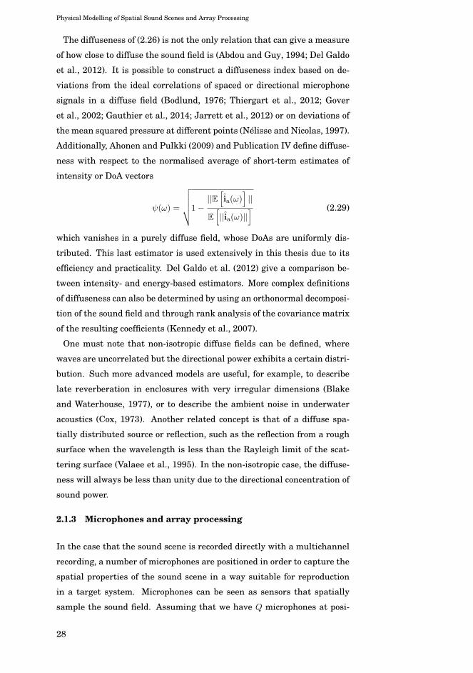
The diffuseness of (2.26) is not the only relation that can give a measure
of how close to diffuse the sound field is (Abdou and Guy, 1994; Del Galdo
et al., 2012). It is possible to construct a diffuseness index based on de-
viations from the ideal correlations of spaced or directional microphone
signals in a diffuse field (Bodlund, 1976; Thiergart et al., 2012; Gover
et al., 2002; Gauthier et al., 2014; Jarrett et al., 2012) or on deviations of
the mean squared pressure at different points (Nélisse and Nicolas, 1997).
Additionally, Ahonen and Pulkki (2009) and Publication IV define diffuse-
ness with respect to the normalised average of short-term estimates of
intensity or DoA vectors
ψ(ω) =
√√√√√1−||E
[ia(ω)
]||
E
[||ia(ω)||
] (2.29)
which vanishes in a purely diffuse field, whose DoAs are uniformly dis-
tributed. This last estimator is used extensively in this thesis due to its
efficiency and practicality. Del Galdo et al. (2012) give a comparison be-
tween intensity- and energy-based estimators. More complex definitions
of diffuseness can also be determined by using an orthonormal decomposi-
tion of the sound field and through rank analysis of the covariance matrix
of the resulting coefficients (Kennedy et al., 2007).
One must note that non-isotropic diffuse fields can be defined, where
waves are uncorrelated but the directional power exhibits a certain distri-
bution. Such more advanced models are useful, for example, to describe
late reverberation in enclosures with very irregular dimensions (Blake
and Waterhouse, 1977), or to describe the ambient noise in underwater
acoustics (Cox, 1973). Another related concept is that of a diffuse spa-
tially distributed source or reflection, such as the reflection from a rough
surface when the wavelength is less than the Rayleigh limit of the scat-
tering surface (Valaee et al., 1995). In the non-isotropic case, the diffuse-
ness will always be less than unity due to the directional concentration of
sound power.
2.1.3 Microphones and array processing
In the case that the sound scene is recorded directly with a multichannel
recording, a number of microphones are positioned in order to capture the
spatial properties of the sound scene in a way suitable for reproduction
in a target system. Microphones can be seen as sensors that spatially
sample the sound field. Assuming that we have Q microphones at posi-
28
Physical Modelling of Spatial Sound Scenes and Array Processing
tions rq, with q = 1, .., Q, let us denote the microphone signal vector as
x = [x1, ..., xQ]T . Considering the directional sensitivity that individual
sensors may exhibit, we denote the frequency-dependent directional re-
sponse of a single sensor as d(γ, ω).
The overall directional response of the array to a unit amplitude plane
wave incident from direction γ is termed the steering vector of the array,
and it is denoted here by h(γ, ω) = [h1(γ), ..., hQ(γ)]T , where
hq(γ, ω) = dq(γ, ω)ejkγ·rq (2.30)
so that, for a sound scene with amplitude density a(γ, ω), the array signals
are given by
x(ω) =
∫h(γ, ω)a(γ, ω) dγ. (2.31)
For an omnidirectional microphone, the signal is proportional to the acous-
tic pressure at that point: xq(ω) = p(rq, ω). In spatial sound recording,
directional microphones are often preferred since, due to their inherent
directionality, their arrangement can be tuned to directly provide spatial
cues during reproduction. Additionally, they are more appropriate for ad-
vanced parametric and non-parametric processing suitable for arbitrary
speaker setups. Directional microphones can be physically realised by a
combination of vents on the capsule, resulting in directionality that is a
combination of an omnidirectional and a pressure-gradient response
d(γ) = κ+ (1− κ)γ · γq, (2.32)
where γq is the orientation of the capsule and γ · γq = cosαq is the cosine
angle between the DoA and the orientation of the capsule. The coefficient
κ ∈ [0, 1] determines the portion of the omnidirectional (pressure) and the
dipole (pressure-gradient) component and depends on the construction.
Example polar plots of directional patterns for common values of κ are
shown in Fig. 2.1.
Recently, microphone arrays based on microphones mounted on some
acoustically hard baffle are gaining popularity (Meyer and Elko, 2004;
Abhayapala and Ward, 2002; Moreau et al., 2006; Rafaely, 2015; Li and
Duraiswami, 2007; Teutsch, 2007; Jin et al., 2014), mainly for the follow-
ing reasons. Firstly, the baffle enforces directivity on otherwise omnidi-
rectional capsules, which are less costly than directional ones and easier
to construct. Secondly, it provides a natural casing for the assortment of
electronic components of the array resulting in a compact portable setup.
Thirdly, basic constructions, such as spherical baffles (for 3D acoustic
29

Physical Modelling of Spatial Sound Scenes and Array Processing
0.2
0.4
0.6
0.8
1
30
210
60
240
90
270
120
300
150
330
180 0
(a)
κ = 1 (omni)κ = 1/2 (cardioid)κ = 1/4 (hypercardioid)
κ = (√3− 1)/2 (supercardioid)
κ = 0 (dipole)
0.5
1
1.5
2
30
210
60
240
90
270
120
300
150
330
180 0
(b)
100 Hz500 Hz1 kHz4 kHz12 kHz
0.5
1
1.5
2
30
210
60
240
90
270
120
300
150
330
180 0
(c)
100 Hz500 Hz1 kHz4 kHz12 kHz
Figure 2.1. Directional patterns for a) common directional microphones, b) omnidirec-tional microphone mounted on a hard cylinder of 5 cm radius, and c) omnidi-rectional microphone mounted on a sphere of 5 cm radius.
analysis and recording) or cylindrical baffles (for 2D analysis and record-
ing), have symmetry properties that enable a modal analysis of the sound
field properties, as will be detailed in the next section.
The array response of microphones on a baffle does not obey equation
(2.30) due to the presence of the scattered field. Theoretical expressions
exist for the fundamental cases of sensors on the surface of a sphere or an
infinitely long cylinder of radius R:
hcylq (γ, ω) = B0(kR) + 2∞∑n=1
jnBn(kR) cosnαq (2.33)
and
hsphq (γ, ω) =∞∑n=0
jn(2n+ 1)bn(kR)Pn(cosαq), (2.34)
where Bn and bn are combinations of normal and spherical Bessel-family
functions, respectively (Rafaely, 2015; Teutsch, 2007), expressing incom-
ing and outgoing circular or spherical waves. Computational routines that
generate steering vectors for arbitrary arrays of omnidirectional or direc-
tional microphones in free field or around a cylindrical or spherical scat-
terer are presented by the author (Politis, 2015b). Example polar plots for
a microphone on the surface of a rigid cylinder and sphere are shown in
Fig. 2.1.
A fundamental operation in array processing is beamforming, where the
array signals are combined with appropriate gain factors to achieve a de-
sired directionality at the output. These beamforming weights are de-
signed based on the application at hand, ranging from source-signal sepa-
ration and estimation to dereverberation and speech enhancement, locali-
30

Physical Modelling of Spatial Sound Scenes and Array Processing
sation of sources and tracking, and analysis of room acoustics. Beamforming-
related research is vast and ubiquitous in the field of array processing;
the interested reader is referred to the literature (Van Veen and Buckley,
1988; Johnson and Dudgeon, 1992; Van Trees, 2004; Benesty et al., 2008;
Brandstein and Ward, 2013).
In terms of spatial sound processing, beamforming is one way to dis-
tribute multichannel recordings to the speakers, by generating speaker
signals that correspond to appropriate beams that form the desired sound
scene. Beamforming is also essential for acoustic analysis and parameter
estimation of the sound field quantities. A few basic cases of interest are
highlighted below.
In its most general form beamforming is simply expressed as
y(ω) = wH(ω)x(ω) (2.35)
or by using the amplitude density formalism as
y(ω) =
∫wH(ω)h(γ, ω)a(γ, ω) dγ, (2.36)
with w = [w1, ..., wQ]T being the vector of complex weights applied to each
microphone signal for a certain frequency. The weights naturally depend
on the array geometry, or equivalently on the steering vector. The most
basic beamforming operation is phase-aligning the received signals in a
certain direction so that they sum coherently while other directions are
attenuated due to partially incoherent summation. If the microphones
are omnidirectional, the weights correspond to the well-known delay-and-
sum beamformer. For the general case, this operation corresponds to
a plane-wave decomposition operation in the beamforming direction γ0,
with weights given by
wpw(ω) =h(γ0, ω)
||h(γ0, ω)||2. (2.37)
The denominator forces unity amplitude in the look direction γ0. This de-
sign maximises the improvement of signal-to-noise ratio (SNR) compared
to a single microphone of the array, known as white noise gain (WNG)
(Brandstein and Ward, 2013).
The plane-wave decomposition beamformer of (2.37) is optimal to re-
duce microphone noise, but not to suppress diffuse sound. Such a design
requires minimisation of the power output of the array in all directions
except the steering direction. The weights of such a design correspond to
a maximum-directivity, or superdirective, beamformer and are given by
31
Physical Modelling of Spatial Sound Scenes and Array Processing
(Brandstein and Ward, 2013)
wdi(ω) =Γ−1diffh(γ0, ω)
hH(γ0, ω)Γ−1diffh(γ0, ω)
, (2.38)
where Γ is the coherence matrix of the array in the presence of the isotropic
diffuse field of (2.19), given by
[Γdiff ]ij =
∫hi(γ, ω)h
∗j (γ, ω) dγ√∫
|hi(γ, ω)|2 dγ∫|hj(γ, ω)|2 dγ
with i, j = 1, ..., Q. (2.39)
The plane-wave decomposition beamformer of (2.37) can be obtained from
(2.38) if the noise is assumed spatially white, Γdiff = IQ. It is evident
that the above designs depend only on the array properties and a basic
model of a noise field, and are thus non-adaptive. Contrarily, a large class
of beamforming methods exist that adapt the weights based on signal
statistics and are thus more effective when the interfering noise deviates
from the simple models above (Benesty et al., 2008; Brandstein and Ward,
2013).
A second beamforming example of importance to this thesis is the gen-
eral problem of approximating a target pattern with an arbitrary array
in a least-squares error sense. This is especially useful to spatial sound
processing as it provides means to directly obtain signals that deliver the
appropriate spatial cues during reproduction. The target patterns can
be, for example, amplitude panning gains for loudspeaker reproduction
(Backman, 2003) or head-related transfer functions (HRTFs) for head-
phone reproduction (Chen et al., 1992). The least-squares approach to
beamforming design has been useful in this work both for its flexibility
and for the fact that it can take into account nonidealities in the array re-
sponse that are generally not captured by simple theoretical models, such
as the ones in (2.32–2.34). The beamforming weights are obtained in the
following way. Let us assume that the target pattern is given by the direc-
tional function d(γ) and the squared error between the beamformer and
the target in a certain direction is given by
ed(γ) = ||wHh(γ)− d(γ)||2, (2.40)
so that its mean integrated in all directions is
〈ed(γ)〉 =∫||wHh(γ)− d(γ)||2 dγ. (2.41)
We are looking for the weight vector that minimise the mean squared er-
ror of (2.41). In practice, we can assume that the array response and the
32
Physical Modelling of Spatial Sound Scenes and Array Processing
target pattern is known either through an analytical formula or measure-
ments in K discrete directions. We can then formulate the solution to
(2.41) as a linear problem
w = argwmin||wHH− d||+ λ2||wHw||, (2.42)
where λ is a regularisation term, d = [d(γ1), ..., d(γK)] is the vector of
target values and H = [h(γ1), ...,h(γK)] the matrix of steering vectors
for the specified directions. The system of (2.42 ) admits the closed form
solution of
wH = dHH(HHH + λ2IQ)−1. (2.43)
The regularisation term λ ensures that the weights are constrained to
sensible values if the inversion of HHH is not well-conditioned.
A fundamental beamforming-related operation in this work is the mea-
surement of the acoustic particle velocity of (2.8). Considering that the
measurement is at the origin r = 0, the notional centre of the array, the
components of the particle velocity vector correspond to the integrated
product of the sound field density and the direction cosines of the DoA, or
equivalently, three orthogonal dipole patterns in acoustic terminology. As
a result, the acoustic velocity can be measured with the dipole patterns
produced by the specific beamforming weights
WHuh(γ) =
⎡⎢⎢⎣
sin θ cosφ
sin θ sinφ
cos θ
⎤⎥⎥⎦ = γ, (2.44)
where Wu = [wx,wy,wz] is the matrix of the weight vectors for each of
the three components of the velocity vector. The weight matrix for this ve-
locity beamforming can be derived from analytical array models (Cazzo-
lato and Ghan, 2005; Hacihabiboglu, 2014; Sondergaard and Wille, 2015)
or from the least-squares approach of (2.43). Alternatively, the measure-
ment can be performed by three equalised pressure-gradient microphones
placed proximately, with the drawback that the estimation of each com-
ponent will not be exactly coincident with each other.
2.1.4 DoA estimation and acoustic localisation in complexscenes
Parametric approaches to reproduction of recorded sound scenes extract
information on the DoA of directional sound components to be used in the
synthesis stage for spatialisation of such components. DoA estimation,
33
Physical Modelling of Spatial Sound Scenes and Array Processing
similar to beamforming, is a wide field of research. Three large families of
solutions are mentioned here. Steered-response power (SRP) approaches
generate a power map from the output of a beamformer steered towards
multiple directions, with peaks corresponding to dominant source direc-
tions. Time-difference-of-arrival (TDoA) approaches infer the DoA from
inter-sensor delays obtained through correlations and the geometry of the
array. Spectral or subspace approaches are able to infer multiple source
directions at a single frequency through subspace decomposition of the
array signal covariance matrix, such as the MUSIC (Schmidt, 1986) and
ESPRIT (Roy and Kailath, 1989) methods. For an overview of approaches,
the reader is referred to Benesty et al. (2008) and Brandstein and Ward
(2013).
For the parametric sound reproduction methods of interest in this work,
and contrary to speech enhancement applications, many of the above ap-
proaches can be either unusable in the complex acoustic scenarios of a
variety of interesting sound scenes or too complex and computationally
demanding for a perceptually motivated reproduction of spatial sound.
Alternatively, we focus on DoA information obtained through the acoustic
active intensity vector. It is trivial to see from (2.9) that the acoustic in-
tensity in the case of a single far-field source points to the opposite of the
DoA. It is also straightforward to deduce from the vanishing active inten-
sity in a reverberant field that it still provides a meaningful estimate for a
source in presence of reverberation after adequate time averaging. Tervo
(2009), Levin et al. (2010), and Günel (2013) have studied the statistics of
the intensity vector. These statistics have been exploited for DoA estima-
tion (Hickling et al., 1993; Tervo, 2009; Thiergart et al., 2009; Günel and
Hacihabiboglu, 2011; Levin et al., 2012; Jarrett et al., 2010; Moore et al.,
2015; Wu et al., 2015) and spatial audio processing (Merimaa and Pulkki,
2005; Hurtado-Huyssen and Polack, 2005; Pulkki, 2007).
Utilising the acoustic intensity exhibits some advantages in the repro-
duction task. Firstly, if the acoustic particle velocity is measured, esti-
mating the active intensity is a very efficient operation suitable for real-
time applications, and it avoids the directional scanning and peak finding
of many SRP and subspace approaches. Secondly, for multiple sources
or extended source distributions at a single frequency, correlated or un-
correlated, the intensity gives an estimate that always lies between the
directions of the sources. This property may seem a drawback from an
acoustical estimation or source localisation point of view, but it has some
34
Physical Modelling of Spatial Sound Scenes and Array Processing
perceptual relevance useful for sound reproduction, as the intensity will
essentially point towards the direction that most of the acoustic energy
propagates. There is evidence that the auditory system cannot localise
separately multiple directional components in a narrow frequency band
(Faller and Merimaa, 2004) and is instead dominated by a single direc-
tional cue related to the source distribution, with the exception of extreme
synthetic cases where the overall image does not get fused (Tahvanainen
et al., 2011). The active intensity seems to give information that is aligned
with this dominant directional perception.
Two sound field cases of interest are presented to highlight the be-
haviour of intensity for distributed sound sources. The first is a source
with a deterministic, possibly complex, spatial distribution g(γ, ω), which
can be modelled as (Valaee et al., 1995; Lee et al., 1997)
a(γ, ω) = g(γ, ω)s(ω) (2.45)
carrying the random source signal s(ω). This model includes cases in
which sound incident from some direction is a delayed and scaled copy
of the source signal. Examples include scattering from a curved surface
focusing sound towards the array or extended vibrating sound sources
with correlated point-to-point surface vibrations. The spatial correlation
of (2.45) is
Sγγ′(ω) = g(γ, ω)g∗(γ ′, ω)Sss(ω), (2.46)
with Sss being the PSD of the signal s. By inserting (2.46) into (2.15), the
active intensity vector results in
ia = −Sss(ω)
2Z0
∫ ∫�{g(γ, ω)g∗(γ ′, ω)
}γ ′ dγ dγ ′. (2.47)
The second case considers a diffusely distributed source, where the source
signal is uncorrelated between different directions. Examples include
the diffuse reflections and the non-isotropic diffuse fields mentioned in
Sec. 2.1.2. Such a distribution can be known only through its directional
power g2(γ, ω) as
Sγγ′(ω) = g2(γ, ω)δγ−γ′ . (2.48)
The resulting intensity, after inserting (2.48) in (2.15), is
ia = −1
2Z0
∫g2(γ, ω)γ dγ. (2.49)
It is obvious that (2.49) expresses an average of all directions γ, weighted
with the power distribution g2(γ, ω). Non-continuous versions of these re-
lations for a discrete number of point sources, relevant for loudspeaker re-
production systems, have been presented earlier (Merimaa, 2007; De Sena
35

Physical Modelling of Spatial Sound Scenes and Array Processing
et al., 2013). A pair of normalised vector quantities termed velocity and
energy vectors (Makita, 1962; Gerzon, 1992a), special cases of (2.47) and
(2.49), have been applied extensively for the evaluation of panning and
non-parametric multichannel sound reproduction (Gerzon, 1992c,b; Ger-
zon and Barton, 1992; Jot et al., 1999; Daniel et al., 1999; Poletti, 2000;
Lee et al., 2004; Zotter et al., 2012; Zotter and Frank, 2012; Epain et al.,
2014).
Intensity is not a suitable choice when detailed DoA estimates of mul-
tiple sources or reflections are required; detailed analysis and auralisa-
tion of spatial room impulse responses is such an application. In Publi-
cation VII, the DoAs of reflections from the early part of room impulse
responses are estimated with high-resolution subspace- and maximum-
likelihood (ML) based methods.
2.1.5 Spherical harmonic representation of sound fieldquantities and acoustical spherical processing
The previous sections defined all sound field quantities with respect to a
plane-wave amplitude density. Furthermore, the effect of the array sam-
pling on the sound field, beamforming, and measurement of the acous-
tic velocity were all defined as linear integral operators on that sound
field density, computed over the unit sphere S2. It is advantageous to
study these linear operators in terms of an orthogonal expansion. This is
accomplished by means of the Spherical Harmonic Transform (SHT), or
Spherical Fourier Transform, in which spherical functions are projected
onto harmonic functions that constitute an orthonormal basis over the
unit sphere. For a detailed analysis on the SHT and an overview of op-
erations on the spherical harmonic, or spectral, domain (SHD) the reader
is referred to Driscoll and Healy (1994). We highlight some fundamental
properties of the SHT with applications to acoustical processing.
The vector of angular spectrum coefficients f of a square integrable func-
tion f(γ) on the unit sphere S2 is given by the SHT as
f = SHT {f(γ)} =∫γ∈S2
f(Ω)y∗(γ) dγ, (2.50)
where the infinite-dimensional basis vector y(γ) has as its entries the
spherical harmonics (SHs) Ynm of integer order n ≥ 0 and degree m ∈[−n, n]:
[y(γ)]q = Ynm, with q = n2 + n+m+ 1 (2.51)
and [y∗(γ)]q = Y ∗nm(γ) denotes its complex conjugate. Conventions of
36
Physical Modelling of Spatial Sound Scenes and Array Processing
spherical harmonics vary between different scientific fields. A common
orthonormal complex form in most fields is 1
Ynm(θ, φ) = (−1)m√
(2n+ 1)
4π
(n−m)!
(n+m)!Pnm(cos θ)ejmφ, (2.52)
where Pnm are unnormalised associated Legendre functions of degree n.
Another form commonly used in audio are the real SHs defined as
Ynm(θ, φ) =
√(2− δm0)
(2n+ 1)
4π
(n− |m|)!(n+ |m|)!Pn|m|(cos θ)ym(φ), (2.53)
with
ym(φ) =
⎧⎪⎪⎪⎪⎨⎪⎪⎪⎪⎩
sin |m|φ m < 0,
1 m = 0,
cosmφ m > 0,
(2.54)
and δm0 the Kronecker delta. Using the real form, no conjugation occurs in
(2.50). One can change between the real and complex SH basis by means
of deterministic unitary matrices; example routines for this conversion
are contributed by the author (Politis, 2015d). An example of real and
complex SHs up to order N = 3 are displayed in Fig. 2.2.
The inverse SHT is given by
f(γ) = ISHT {f} = fTy(γ). (2.55)
The orthonormality of the SHs results in∫y(γ)yH(γ) dγ = I, (2.56)
where I is the identity matrix. Due to this orthonormality, Parseval’s
theorem for the SHT states that∫f(γ)g∗(γ) dγ = gH f and
∫|f(Ω)|2dΩ = ‖f‖2 . (2.57)
These last two relations show the usefulness of the SHT from a practi-
cal viewpoint, with directional integrals collapsing into vector products
between spectral coefficients.
In most practical cases, order-limited (or band-limited) functions are
considered, meaning that there is no energy in terms above some order N ,
so that |fq|2 = 0 for q > (N + 1)2. We denote the respective (N + 1)2-sized
coefficient vector as fN . For two functions f(Ω) and g(Ω) band-limited to
1Note that here it is assumed that the Condon-Shortley phase term (−1)m is notincluded in the definition of the associated Legendre functions Pnm.
37

Physical Modelling of Spatial Sound Scenes and Array Processing
(a)
(b)
Figure 2.2. Spherical harmonic functions up to order N = 3 of (a) real form, and (b)complex form. The surfaces correspond to the magnitude of the SHs. Blueand red indicate positive and negative values for real SHs, while the colourmap indicates the phase for the complex SHs.
order L and M respectively, (2.57) is limited accordingly by the smaller
order of the two.
Let us now assume that we have a finite-order representation of the
sound scene amplitude density aN = SHT {a(γ)}. It can be shown, by
solving the homogenous Helmholtz equation of (2.2) in spherical coordi-
nates (Williams, 1999; Ziomek, 1994), that the pressure around the origin
at position r due to the amplitude density a(γ) can be expressed as
p(r,γr, ω) = 4πN∑
n=0
jn(kr)n∑
m=−nanm(ω)Ynm(γr), (2.58)
where r = ||r||, γr = r/||r||, and jn are the spherical Bessel functions
of order n. Note that if the pressure is sampled around a scatterer as
in (2.34) or directional sensors are used, then jn should be replaced by
38

Physical Modelling of Spatial Sound Scenes and Array Processing
the appropriate radial functions bn. See, for example, Teutsch (2007) for
details. Taking the SHT of the pressure over a sphere of radius r and
inserting (2.58),
pnm(r, ω) =
∫p(r,γr, ω)Y
∗nm(γr) dγr
= 4πN∑
n=0
jn(kr)n∑
m=−nanm(ω)
∫Ynm(γr)Y
∗nm(γr) dγr
= 4πjn(kr)anm(ω). (2.59)
For the above equation to hold with negligible error inside a spheri-
cal region of radius R, the truncation order N depends on the maximum
wavelength of interest kmax. It is given by Kennedy et al. (2007) as
N =
⌈ekmaxR
2
⌉(2.60)
with ·� denoting the integer ceiling function. Relation (2.59) is impor-
tant for two reasons. First, it shows that we can encode any sound scene
within a distance R from the origin with a finite dimensional vector of
sound field coefficients aN . Second, it demonstrates a practical way to
capture the sound field coefficients aN through measurement of the pres-
sure over a sphere and by its subsequent SHT. These two reasons consti-
tute the basis of spherical array processing for recording, acoustic anal-
ysis and beamforming (Williams, 1999; Meyer and Elko, 2004; Teutsch,
2007; Rafaely, 2015), and spherical acoustic holophony or higher-order
Ambisonics (HOA) (Gerzon, 1973; Daniel, 2000; Poletti, 2005; Zotter, 2009a).
If the sound field coefficients are obtained, many spatial processing op-
erations simplify considerably. For example, beamforming design can be
performed directly in the spherical domain. If we define a beamforming
pattern w(γ) band-limited to order N with coefficients wN = SHT {w(γ)},Parseval’s theorem (2.57) dictates that the beamformer output is the dot
product of the beampattern’s coefficients and those of the sound field:
y(ω) =
∫w∗(γ)a(γ, ω) dγ = wH
NaN . (2.61)
Similarly to (2.37), and by substituting h(γ) = y∗(γ), the plane wave
decomposition beamformer weights in the SHD can be derived:
wpw(γ0) = wdi(γ0) =4π
(N + 1)2y∗N (γ0), (2.62)
where the relation ||yN (γ)||2 = (N + 1)2/(4π) is used in the denominator.
In the SHD, the plane-wave decomposition beamformer is also that of the
maximum-directivity of (2.38). This is due to the fact that the diffuse field
39
Physical Modelling of Spatial Sound Scenes and Array Processing
coherence Γdiff of the sound field coefficients in the diffuse field of (2.19) is
the identity matrix
Γdiff =4π
σ2df
E[aN aHN
]=
∫yN (γ)yH
N (γ) dγ = IN . (2.63)
A comprehensive set of routines for beamforming design, localisation of
sources and adaptive beamforming in the SHD is contributed by the au-
thor (Politis, 2016).
The acoustic particle velocity is also directly related to the sound field
coefficients of the first order a1. More specifically, if we define a signal
vector of pressure p(ω) and equalised pressure-gradient signals v(ω) =
−Z0u(ω) as
b =
⎡⎣ p(ω)
v(ω)
⎤⎦ =
⎡⎢⎢⎢⎢⎢⎣
p(ω)
vx(ω)
vy(ω)
vz(ω)
⎤⎥⎥⎥⎥⎥⎦ , (2.64)
we can directly relate it to the field coefficients through the transforma-
tion matrix Ma→pu as
b = Ma→pua1. (2.65)
The pressure and pressure-gradient signal vector b is known in the spa-
tial sound literature as B-format2. The transformation matrix is given for
the real and complex SH conventions presented above as
Mreala→pu =
√4π
⎡⎢⎢⎢⎢⎢⎣
1 0 0 0
0 0 0 1/√3
0 1/√3 0 0
0 0 1/√3 0
⎤⎥⎥⎥⎥⎥⎦ and
Mcomplexa→pu =
√4π
⎡⎢⎢⎢⎢⎢⎣
1 0 0 0
0 1/√6 0 −1/
√6
0 −j/√6 0 −j/
√6
0 0 1/√3 0
⎤⎥⎥⎥⎥⎥⎦ . (2.66)
The spherical spectral formulation of acoustical quantities has naturally
many applications in analysis and modelling of directional patterns of
sources or receivers, interpolation of discretely measured spherical func-
tions, such as HRTFs, spatial sound processing, and acoustic analysis and
beamforming. In terms of spatial sound capture and reproduction, the
2Traditionally, B-format has been defined with an additional scaling factor of1/√2 in the pressure signal.
40

Physical Modelling of Spatial Sound Scenes and Array Processing
spherical harmonic framework was first introduced in the 1970s, formu-
lated mostly by Gerzon (1973) under the name Ambisonics, with consid-
erable development towards a usable first-order implementation (Gerzon,
1975b; Farrar, 1979; Fellgett, 1975; Gerzon, 1975a).
In practice, severe practical limitations are imposed on acquiring the
sound field coefficient vector of (2.60) up to an order higher than the
first few for a compact microphone array and on reproducing the sound
scene on a small volume with a reasonable number of loudspeakers. Two
major issues are encountered in practice. The first has to do with dis-
crete sampling limitations of the acoustic pressure, so that spatial alias-
ing occurs above some limiting frequency and higher-order components
contaminate lower-order ones. For a discussion on spherical sampling
schemes and conditions the reader is referred to Rafaely et al. (2007b),
Zotter (2009b), and Rafaely (2015). The second is the vanishing of higher-
order coefficients at lower frequencies at some finite radius R from the
centre of the array, expressed in (2.59) through the radial term jn or bn.
The radial terms in the expansion decay rapidly for kR < N , making
their equalisation, and consequently higher-order recording, impossible at
large wavelengths (Moreau et al., 2006; Rettberg and Spors, 2014; Baum-
gartner et al., 2011; Lösler and Zotter, 2015). In summary, recording of
high-order coefficients is practical only in some frequency range having
an upper bound imposed by spatial aliasing and a lower bound by usable
equalisation of the radial functions.
41

Physical Modelling of Spatial Sound Scenes and Array Processing
42

3. Perception and Technology of SpatialSound
In this section we first highlight the major components of spatial sound
perception. This summary broadly mentions cues that play an important
role in perceptual reproduction of spatial sound scenes rather than ex-
haustively cover spatial sound psychoacoustics. For a detailed coverage of
spatial sound psychoacoustics the reader is referred to Moore (1995) and
Blauert (1996). In the latter part of this section, the major technological
components of sound spatialisation systems are presented.
3.1 Spatial sound perception
3.1.1 Time-frequency resolution
The spatial sound processing methods developed in this thesis operate in
the time-frequency domain, imposing a certain temporal and frequency
resolution to the analysis and synthesis of the recorded sound. Since the
goal is perceptual rather than physical reproduction of the sound scene,
this resolution needs to resemble somewhat the time-frequency resolution
of the auditory system. It has been shown that the frequency-resolution
of the basilar membrane can be approximated sufficiently by a bank of
overlapping band-pass filters, known as auditory filters (Fletcher, 1940;
Moore and Glasberg, 1983). Furthermore, the width of the auditory filters
can be, in turn, approximated with an equivalent rectangular bandwidth
(ERB) formula with respect to the centre frequency fc, given as (Moore
and Glasberg, 1983)
ΔfERB = 0.108fc + 24.7. (3.1)
These results can serve as guidelines for the design of time-frequency
transforms of filter banks for perceptually-motivated analysis and synthe-
43
Perception and Technology of Spatial Sound
sis of sound. Examples include gammatone filter banks (Patterson et al.,
1995; Hohmann, 2002), constant-Q transforms (Schörkhuber and Klapuri,
2010), the ERBlet transform (Necciari et al., 2013), and filter banks for
perceptual coding and spatial sound coding, such as quadrature mirror
filter (QMF) banks used by Schuijers et al. (2004), Herre et al. (2008), and
in Publication V.
3.1.2 Localisation cues
Sound localisation is dominated by two major cues. The first is the TDoA
of a wavefront at the ears incident from a certain angle, termed interau-
ral time difference (ITD). ITDs translate to interaural phase differences in
auditory processing. However, this translation is possible unambiguously
only at frequencies with a wavelength about half the interaural distance.
Above roughly 1.5 kHz (Moore, 1995), ITDs are not effective through de-
tection of phase differences, and they seem to contribute only through
time differences between the envelopes of the ear signals (Henning, 1974;
Salminen et al., 2015). The second major cue is the level difference be-
tween the two ear signals due to scattering effects of the head that at-
tenuate the signal at the contralateral ear with respect to the direction
of arrival, termed interaural level difference (ILD). Diffraction effects are
strong at low frequencies and hence ILDs are most effective above about 1
kHz. Even though it has been found that ILDs can also contribute to low
frequency localisation, this basic model of ITD dominance at low frequen-
cies and ILD dominance at mid-high frequencies, known as the duplex
theory of localisation (Rayleigh, 1907), is prevalent in technological appli-
cations of spatial sound.
ITDs and ILDs provide information on lateralisation, localisation across
the left-right direction. Due to the strong left-right symmetry of the head
and its almost ellipsoidal shape, it is possible to define cones of directions
centred at the interaural axis, at which ITDs and ILDs change weakly,
with the most extreme example being the median plane. Such a trajectory
is termed a cone of confusion. Localisation of elevated sources or of front-
back sources on a cone of confusion do not rely on ITDs and ILDs, but on
monaural spectral cues that occur mostly due to the effect of the pinna,
head shape, and shoulders (Musicant and Butler, 1984). Since the pinna
dimensions are within the range of only a few centimetres, pinna cues
are naturally high-frequency ones (Moore, 1995). Pinna-related notches
and peaks are deemed especially significant for the perception of elevation
44
Perception and Technology of Spatial Sound
(Roffler and Butler, 1968; Blauert, 1969; Macpherson and Sabin, 2013).
3.1.3 Dynamic binaural cues
Localisation of an unknown sound source in anechoic conditions, espe-
cially across cones of confusion, can be a daunting task in the absence of
other assisting cues if the listener and the source are immobilised. Free-
field localisation can improve considerably through relative motions be-
tween the listener and the source. Small head rotations especially can
jointly modify all major localisation cues and resolve front-back confu-
sions or ambiguous elevation effectively (Wallach, 1940; Thurlow et al.,
1967; Perrett and Noble, 1997; Wightman and Kistler, 1999).
3.1.4 Distance cues
Perception of a distance of a sound source relies on many factors and
is strongly dependent on the familiarity of the listener with the source
sound itself. In the range of distances encountered in regular rooms, the
inverse-distance law of sound pressure level attenuation is probably the
most prominent distance cue. However, level attenuation with distance is
a relative cue and possible only if the listener has an auditory reference
distance for the source.
In absence of a reference, the auditory system seems able to infer dis-
tance from a variety of additional cues. For close ranges below about 1 m,
ITD and ILD become distance-dependent, due to near-field effects of the
sound source that are otherwise negligible at longer ranges. Significant
ILDs occur even at low frequencies at such distances (Brungart and Rabi-
nowitz, 1999). These supplementary binaural cues seem to be utilised by
the auditory system for nearby sources (Brungart and Rabinowitz, 1999;
Brungart et al., 1999).
Otherwise, at regular distances an important factor in distance per-
ception is the direct-to-reverberant ratio (DRR) of the source power over
the reverberant sound power reflected and diffused by the room (Zahorik
et al., 2005). Reverberation in itself is not a primary cue, but it affects
jointly a number of distance cues. Recent research shows that externali-
sation and distance perception may originate from short-term statistics of
ILD (Catic et al., 2013, 2015) or ITD fluctuations (Bronkhorst, 2002) that
occur in reverberant conditions. Furthermore, there is evidence of monau-
ral cues that depend on reverberation (Lounsbury and Butler, 1979), such
45
Perception and Technology of Spatial Sound
as information due to absorption and filtering of the reflected sound with
regards to the direct sound. Phase coherence of partials over frequency
and the effect of reverberation on them has also been proposed to con-
tribute to distance perception (Laitinen et al., 2013).
Exploitation of the DRR to control distance perception was tested in
Publication VI by modifying the directionality of a loudspeaker array in
order to affect the DRR at the listener position. That study inspired fur-
ther work by Wendt et al. (2016). Distance control using multiple loud-
speakers, targeting control of either DRR or of the related binaural cues,
has been also proposed by de Bruijn et al. (2008), Jeon et al. (2015) and
Laitinen et al. (2015).
At long distances, after a few tens of metres, propagation effects become
perceptible, mainly due to the kinetic energy of the wave dissipating as
thermal energy in air, reducing high frequency content (Little et al., 1992).
Another common dynamic cue for distance perception is the Doppler ef-
fect of a moving source or listener at high speeds, with its characteristic
frequency shift (Lutfi and Wang, 1999).
3.1.5 Precedence effect and summing localisation
The precedence effect (Wallach et al., 1949; Haas, 1972), or the law of first
wavefront (Blauert, 1996), refers to the phenomenon of a leading sound
completely dominating localisation if the lagging sound, coming from a
different direction, follows in short interval ranging from about 5 ms to
40 ms (Moore, 1995). This effect occurs for onsets, transient and discon-
tinuous sounds, and it is responsible for our ability to suppress partially
the effect of echoes on localisation in rooms and enclosures. However,
even though information on the direction of an echo is lost, the listener is
still able to hear spectral differences due to the room, important for per-
ception of the source distance and the environment. A review of related
psychoacoustical research is given by Litovsky et al. (1999).
The precedence effect is important for sound reproduction because it
determines temporal limits after which panning and spatialisation opera-
tions, based on summing localisation (Blauert, 1996), are effective. Sum-
ming localisation refers to the phenomenon of two fully or partially cor-
related sounds, arriving at the listener from different directions, being
perceived as a single coherent spatial image. For amplitude and time-
delay panning techniques to be effective, the listener should be positioned
so that wavefronts from the speakers arrive with time differences smaller
46

Perception and Technology of Spatial Sound
than the precedence effect limit, otherwise the sound is completely pulled
to the closest speaker.
3.1.6 Apparent source width, spaciousness and interauralcoherence
Perception of a spatially extended source, perceived as such either due
to its physical extent or due to the contributing room acoustics, has been
termed in the literature as apparent source width (ASW). In room acous-
tics research, ASW is usually associated with early lateral reflections hav-
ing a widening effect around the direct sound (Morimoto and Maekawa,
1989; Barron, 1971; Griesinger, 1997). Another related concept is the per-
ception of spaciousness and listener envelopment (LEV), usually associ-
ated with the later reverberant diffuse sound, where no clear direction-
ality can be perceived (Bradley and Soulodre, 1995; Griesinger, 1997).
Recent psychoacoustical studies investigate additionally the effect of the
spatial distribution itself, and how it affects perception (Hirvonen and
Pulkki, 2006, 2008; Santala and Pulkki, 2011).
Both LEV and ASW are important in sound reproduction for two rea-
sons. First, the sound reproduction method should be able to recreate
them appropriately, since they are fundamental parts of a natural and
engaging listening experience. Second, understanding them is important
for the design of sound engineering tools and techniques that are able
to control these two attributes. In general such spatialisation effects are
introduced through emulation of room acoustics.
Understanding the cues that contribute to the ASW and LEV is still
under research. A commonly mentioned quantity is the interaural cross
correlation (IACC), the normalised short-term cross-correlation between
the two binaural signals (Hidaka et al., 1995). IACC is, however, a broad-
band index which can be misleading as an indicator of ASW (Mason et al.,
2005; Käsbach et al., 2013). A more appropriate index is its frequency-
domain counterpart, the interaural coherence (IC) (Blauert and Linde-
mann, 1986). Currently, the focus is moving from these signal statistics
to the short-term statistics of the binaural localisation cues themselves.
Mason et al. (2004) and Käsbach et al. (2014) study the fluctuations of
ITDs as a cue for ASW.
47
Perception and Technology of Spatial Sound
3.2 Spatial sound technologies
3.2.1 Binaural technology
ITDs, ILDs, and spectral cues for a source in the free field are encoded
into the acoustic transfer function from the source to the ears of the lis-
tener. These transfer functions can be measured in anechoic conditions
for multiple directions around the listener and stored as digital filters,
known as head-related transfer functions (HRTFs). HRTFs are crucial
for headphone-based binaural reproduction of spatial sound since source
signals can be spatialised by their filtering with the respective HRTFs
for the desired direction. Synthetic room reverberation can be generated
for headphones based on similar principles and, more specifically, on the
diffuse-field coherence of the HRTFs (Borß and Martin, 2009; Vilkamo
et al., 2012).
Properly measured HRTFs for the specific individual will contain all the
free-field listening localisation cues mentioned above except the dynamic
ones. Dynamic cues can be added by tracking the head of the listener (Al-
gazi et al., 2004) with an adequate temporal resolution (Laitinen et al.,
2012b), which resolves localisation confusion (Begault et al., 2001), and
more importantly, preserves the orientation of the sound scene with re-
spect to the listener’s movement, which is a requirement for a natural and
immersive experience. Individualisation of HRTFs is a difficult task due
to the lengthy measurement process and the demanding requirements on
anechoic conditions and on measurement apparatus, making it unsuitable
for general deployment of binaural spatial sound applications. Hence, ei-
ther HRTFs based on a generic ear model are used, or parametric HRTFs
or HRTFs from a database are individualised based on external infor-
mation, such as morphological features (Jin et al., 2000; Algazi et al.,
2001; Zotkin et al., 2003; Hu et al., 2006; Xu et al., 2009), head scans
(Guillon et al., 2008; Gamper et al., 2015; Politis et al., 2016), or active
tuning through listening tasks (Tan and Gan, 1998; Runkle et al., 2000;
Silzle, 2002; Seeber and Fastl, 2003; Iwaya, 2006; Härmä et al., 2012). All
aspects related to HRTFs have been studied extensively in the last two
decades, including rapid measurement (Enzner, 2009; Zotkin et al., 2006),
efficient storage and compression (Kistler and Wightman, 1992; Larcher
et al., 2000; Romigh et al., 2015), efficient filter modelling (Kulkarni and
Colburn, 2004; Huopaniemi et al., 1999), interpolation (Gamper, 2013;
48
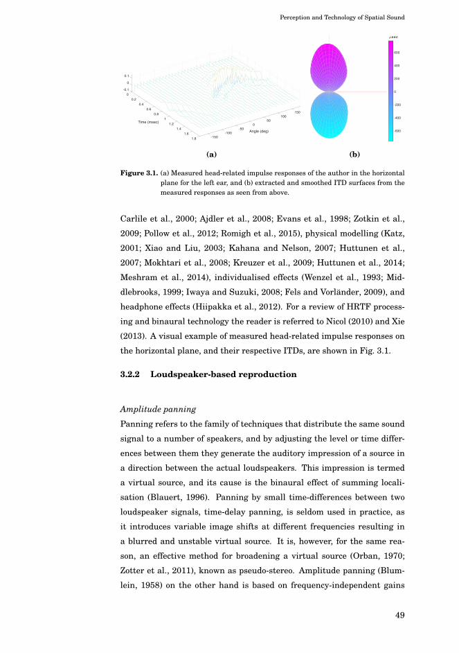
Perception and Technology of Spatial Sound
Angle (deg)
Time (msec)
-0.10
0.2
0.4
0.61500.8
1001 50
1.2 01.4 -50
-1001.6-1501.8
0
0.1
(a)
-600
-400
-200
0
200
400
600
μsec
(b)
Figure 3.1. (a) Measured head-related impulse responses of the author in the horizontalplane for the left ear, and (b) extracted and smoothed ITD surfaces from themeasured responses as seen from above.
Carlile et al., 2000; Ajdler et al., 2008; Evans et al., 1998; Zotkin et al.,
2009; Pollow et al., 2012; Romigh et al., 2015), physical modelling (Katz,
2001; Xiao and Liu, 2003; Kahana and Nelson, 2007; Huttunen et al.,
2007; Mokhtari et al., 2008; Kreuzer et al., 2009; Huttunen et al., 2014;
Meshram et al., 2014), individualised effects (Wenzel et al., 1993; Mid-
dlebrooks, 1999; Iwaya and Suzuki, 2008; Fels and Vorländer, 2009), and
headphone effects (Hiipakka et al., 2012). For a review of HRTF process-
ing and binaural technology the reader is referred to Nicol (2010) and Xie
(2013). A visual example of measured head-related impulse responses on
the horizontal plane, and their respective ITDs, are shown in Fig. 3.1.
3.2.2 Loudspeaker-based reproduction
Amplitude panning
Panning refers to the family of techniques that distribute the same sound
signal to a number of speakers, and by adjusting the level or time differ-
ences between them they generate the auditory impression of a source in
a direction between the actual loudspeakers. This impression is termed
a virtual source, and its cause is the binaural effect of summing locali-
sation (Blauert, 1996). Panning by small time-differences between two
loudspeaker signals, time-delay panning, is seldom used in practice, as
it introduces variable image shifts at different frequencies resulting in
a blurred and unstable virtual source. It is, however, for the same rea-
son, an effective method for broadening a virtual source (Orban, 1970;
Zotter et al., 2011), known as pseudo-stereo. Amplitude panning (Blum-
lein, 1958) on the other hand is based on frequency-independent gains
49
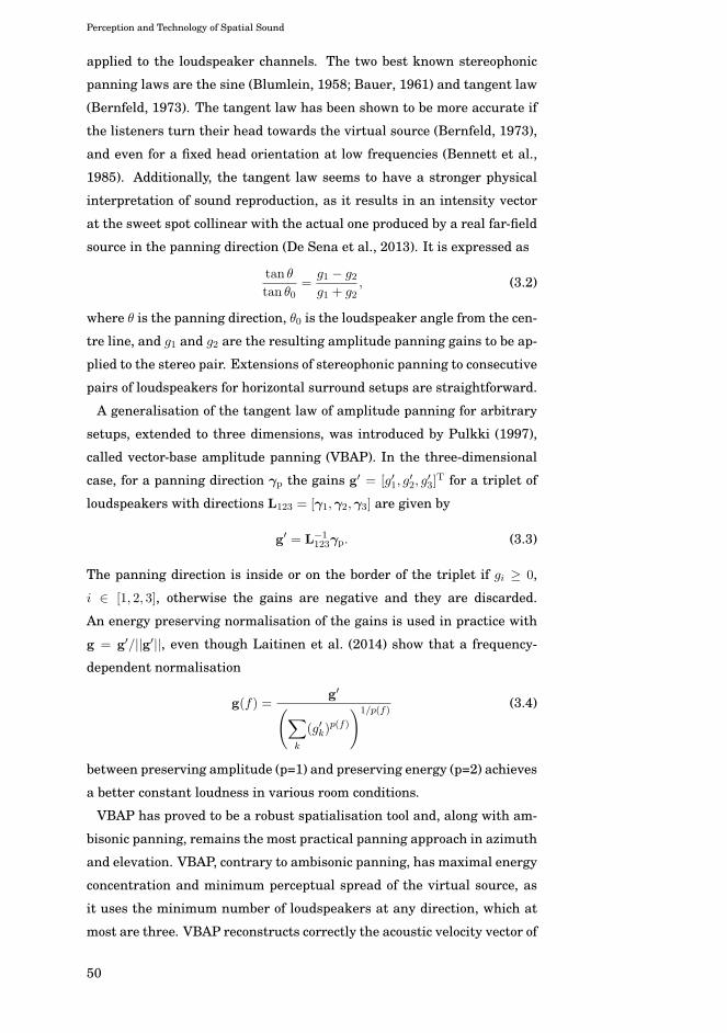
Perception and Technology of Spatial Sound
applied to the loudspeaker channels. The two best known stereophonic
panning laws are the sine (Blumlein, 1958; Bauer, 1961) and tangent law
(Bernfeld, 1973). The tangent law has been shown to be more accurate if
the listeners turn their head towards the virtual source (Bernfeld, 1973),
and even for a fixed head orientation at low frequencies (Bennett et al.,
1985). Additionally, the tangent law seems to have a stronger physical
interpretation of sound reproduction, as it results in an intensity vector
at the sweet spot collinear with the actual one produced by a real far-field
source in the panning direction (De Sena et al., 2013). It is expressed as
tan θ
tan θ0=
g1 − g2g1 + g2
, (3.2)
where θ is the panning direction, θ0 is the loudspeaker angle from the cen-
tre line, and g1 and g2 are the resulting amplitude panning gains to be ap-
plied to the stereo pair. Extensions of stereophonic panning to consecutive
pairs of loudspeakers for horizontal surround setups are straightforward.
A generalisation of the tangent law of amplitude panning for arbitrary
setups, extended to three dimensions, was introduced by Pulkki (1997),
called vector-base amplitude panning (VBAP). In the three-dimensional
case, for a panning direction γp the gains g′ = [g′1, g′2, g′3]T for a triplet of
loudspeakers with directions L123 = [γ1,γ2,γ3] are given by
g′ = L−1123γp. (3.3)
The panning direction is inside or on the border of the triplet if gi ≥ 0,
i ∈ [1, 2, 3], otherwise the gains are negative and they are discarded.
An energy preserving normalisation of the gains is used in practice with
g = g′/||g′||, even though Laitinen et al. (2014) show that a frequency-
dependent normalisation
g(f) =g′(∑
k
(g′k)p(f)
)1/p(f)(3.4)
between preserving amplitude (p=1) and preserving energy (p=2) achieves
a better constant loudness in various room conditions.
VBAP has proved to be a robust spatialisation tool and, along with am-
bisonic panning, remains the most practical panning approach in azimuth
and elevation. VBAP, contrary to ambisonic panning, has maximal energy
concentration and minimum perceptual spread of the virtual source, as
it uses the minimum number of loudspeakers at any direction, which at
most are three. VBAP reconstructs correctly the acoustic velocity vector of
50
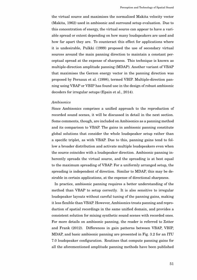
Perception and Technology of Spatial Sound
the virtual source and maximises the normalised Makita velocity vector
(Makita, 1962) used in ambisonic and surround setup evaluation. Due to
this concentration of energy, the virtual source can appear to have a vari-
able spread or extent depending on how many loudspeakers are used and
how far apart they are. To counteract this effect for applications where
it is undesirable, Pulkki (1999) proposed the use of secondary virtual
sources around the main panning direction to maintain a constant per-
ceptual spread at the expense of sharpness. This technique is known as
multiple-direction amplitude panning (MDAP). Another variant of VBAP
that maximises the Gerzon energy vector in the panning direction was
proposed by Pernaux et al. (1998), termed VBIP. Multiple-direction pan-
ning using VBAP or VBIP has found use in the design of robust ambisonic
decoders for irregular setups (Epain et al., 2014).
Ambisonics
Since Ambisonics comprises a unified approach to the reproduction of
recorded sound scenes, it will be discussed in detail in the next section.
Some comments, though, are included on Ambisonics as a panning method
and its comparison to VBAP. The gains in ambisonic panning constitute
global solutions that consider the whole loudspeaker setup rather than
a specific triplet, as with VBAP. Due to this, panning gains tend to fol-
low a broader distribution and activate multiple loudspeakers even when
the source coincides with a loudspeaker direction. Ambisonic panning in-
herently spreads the virtual source, and the spreading is at best equal
to the maximum spreading of VBAP. For a uniformly arranged setup, the
spreading is independent of direction. Similar to MDAP, this may be de-
sirable in certain applications, at the expense of directional sharpness.
In practice, ambisonic panning requires a better understanding of the
method than VBAP to setup correctly. It is also sensitive to irregular
loudspeaker layouts without careful tuning of the panning gains, making
it less flexible than VBAP. However, Ambisonics treats panning and repro-
duction of spatial recordings in the same unified domain, and provides a
consistent solution for mixing synthetic sound scenes with recorded ones.
For more details on ambisonic panning, the reader is referred to Zotter
and Frank (2012). Differences in gain patterns between VBAP, VBIP,
MDAP, and basic ambisonic panning are presented in Fig. 3.2 for an ITU
7.0 loudspeaker configuration. Routines that compute panning gains for
all the aforementioned amplitude panning methods have been published
51

Perception and Technology of Spatial Sound
0.2
0.4
0.6
0.8
1
30
210
60
240
90
270
120
300
150
330
180 0
(a) VBAP
0.2
0.4
0.6
0.8
1
30
210
60
240
90
270
120
300
150
330
180 0
(b) VBIP
0.2
0.4
0.6
0.8
1
30
210
60
240
90
270
120
300
150
330
180 0
(c) MDAP
0.2
0.4
0.6
0.8
1
30
210
60
240
90
270
120
300
150
330
180 0
(d) Ambisonic panning
Figure 3.2. Amplitude panning patterns for a 7.0 loudspeaker setup, using a) VBAP, b)VBIP, c) MDAP with a spread of 45 degrees, and d) ambisonic panning withnaive mode-matching decoding. The black dashed line indicates the energypreservation capabilities of the panning curves as the sum of the squaredgains for each direction.
by the author (Politis, 2015a).
Wave-field synthesis
Wave-field synthesis (WFS) is a spatialisation method based on the Kirchhoff-
Helmholtz integral theorem, which states that the acoustic field inside a
source-free region can be determined completely by the values of the pres-
sure and pressure-gradient on a surface that encloses it (Berkhout et al.,
1993; Boone et al., 1995; Spors et al., 2008). By reducing the problem to
two dimensions and with a few simplifying steps, WFS approximates an
acoustic field over a large area with a dense distribution of loudspeakers
on a boundary which can be either completely surrounding or covering
only partially the area. The method derives sets of digital filters for the
loudspeaker array that can recreate plane waves and point sources over
the valid region of reconstruction. WFS, like certain variants of high-
52
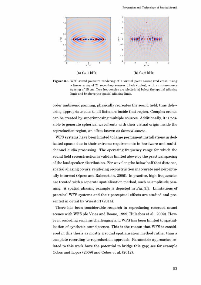
Perception and Technology of Spatial Sound
-2 -1 0 1 2x / m
-2
-1.5
-1
-0.5
0
0.5
1
1.5
2
y / m
(a) f = 1 kHz
-2 -1 0 1 2x / m
-2
-1.5
-1
-0.5
0
0.5
1
1.5
2
y / m
(b) f = 2 kHz
Figure 3.3. WFS sound pressure rendering of a virtual point source (red cross) usinga linear array of 21 secondary sources (black circles), with an inter-sourcespacing of 15 cm. Two frequencies are plotted: a) below the spatial aliasinglimit and b) above the spatial aliasing limit.
order ambisonic panning, physically recreates the sound field, thus deliv-
ering appropriate cues to all listeners inside that region. Complex scenes
can be created by superimposing multiple sources. Additionally, it is pos-
sible to generate spherical wavefronts with their virtual origin inside the
reproduction region, an effect known as focused source.
WFS systems have been limited to large permanent installations in ded-
icated spaces due to their extreme requirements in hardware and multi-
channel audio processing. The operating frequency range for which the
sound field reconstruction is valid is limited above by the practical spacing
of the loudspeaker distribution. For wavelengths below half that distance,
spatial aliasing occurs, rendering reconstruction inaccurate and perceptu-
ally incorrect (Spors and Rabenstein, 2006). In practice, high-frequencies
are treated with a separate spatialisation method, such as amplitude pan-
ning. A spatial aliasing example is depicted in Fig. 3.3. Limitations of
practical WFS systems and their perceptual effects are studied and pre-
sented in detail by Wierstorf (2014).
There has been considerable research in reproducing recorded sound
scenes with WFS (de Vries and Boone, 1999; Hulsebos et al., 2002). How-
ever, recording remains challenging and WFS has been limited to spatial-
isation of synthetic sound scenes. This is the reason that WFS is consid-
ered in this thesis as mostly a sound spatialisation method rather than a
complete recording-to-reproduction approach. Parametric approaches re-
lated to this work have the potential to bridge this gap; see for example
Cobos and Lopez (2009) and Cobos et al. (2012).
53
Perception and Technology of Spatial Sound
3.2.3 Spatial sound recording
Conventional surround recording
Spatial sound recording relies on using a small number of microphones,
and then either reproducing directly the recorded signals to the speaker
setup or mixing them in order to provide appropriate spatial cues at re-
production for a specific setup. The first approach, including the first
stereophonic recording techniques (Blumlein, 1958), is called here con-
ventional surround recording. Surround recording can be classified into
two major approaches, coincident and spaced (Lipshitz, 1986). Coincident
techniques use directional microphones placed very closely together, and
hence they introduce minimal time differences between the two channels.
Directional cues are delivered mainly by the directivity gain differences
between the two microphones oriented towards different directions. Such
an example is the XY, or Blumlein, method which employs two figure-
of-eight (pressure-gradient) microphones oriented orthogonally. Spaced
techniques, on the other hand, with omnidirectional or directional micro-
phones that can be metres apart, rely mainly on time differences between
the two microphones. The major difference between coincident and spaced
methods is the cues they rely on at reproduction. The former achieve
mostly frequency-independent inter-channel differences, resulting in sta-
ble localisation cues. However, due to the small spacing of the capsules,
the two signals can be highly correlated, which may result in lack of spa-
ciousness even for highly reverberant or diffuse sound scenes. In contrast,
spaced setups can generate ambiguous localisation cues (Lipshitz, 1986;
Pulkki, 2002) due to the frequency-dependent phase differences of the two
channels, but they may be more suitable for reproduction of ambient and
diffuse sound, which is mostly uncorrelated in the two channels (Theile,
1991). A popular example of a method that can modify inter-channel level
differences by mixing the two signals is the mid-side method (Blumlein,
1958), a coincident arrangement of a dipole microphone oriented sideways
and a cardioid looking forward (Julstrom, 1990).
With the introduction of surround systems, stereophonic recording tech-
niques were extended to multichannel ones based on similar principles
(Kassier et al., 2005). Most multichannel recording arrangements follow
the surround layout, and they try to optimise recording of the sound stage
with localisation cues only for the frontal loudspeaker triangle (Theile,
2001; Williams, 2004; Kassier et al., 2005). The recording channels for the
54
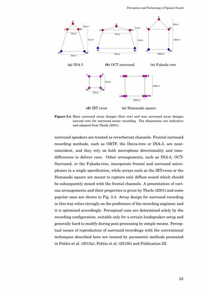
Perception and Technology of Spatial Sound
(a) INA 5 (b) OCT surround (c) Fukada tree
(d) IRT cross (e) Hamasaki square
Figure 3.4. Main surround array designs (first row) and rear surround array designs(second row) for surround music recording. The dimensions are indicativeand adapted from Theile (2001).
surround speakers are treated as reverberant channels. Frontal surround
recording methods, such as ORTF, the Decca-tree or INA-3, are near-
coincident, and they rely on both microphone directionality and time-
differences to deliver cues. Other arrangements, such as INA-5, OCT-
Surround, or the Fukada-tree, incorporate frontal and surround micro-
phones in a single specification, while arrays such as the IRT-cross or the
Hamasaki square are meant to capture only diffuse sound which should
be subsequently mixed with the frontal channels. A presentation of vari-
ous arrangements and their properties is given by Theile (2001) and some
popular ones are shown in Fig. 3.4. Array design for surround recording
in this way relies strongly on the preference of the recording engineer, and
it is optimised accordingly. Perceptual cues are determined solely by the
recording configuration, suitable only for a certain loudspeaker setup and
generally hard to modify during post-processing by simple means. Percep-
tual issues of reproduction of surround recordings with the conventional
techniques described here are treated by parametric methods presented
in Politis et al. (2013a), Politis et al. (2013b) and Publication III.
55
Perception and Technology of Spatial Sound
Advanced sound scene recording
An alternative proposal for surround recording comes in the form of B-
format recording (Gerzon, 1975b), which consists of an omnidirectional
and three dipole components oriented orthogonally in a coincident ar-
rangement. B-format can be viewed in a few different ways. From a sound
engineering perspective, B-format is an extension of the stereo coincident
methods and of Blumlein recording, and any other coincident technique
can be generated using the B-format signals. From an Ambisonics point
of view, it constitutes the first-order approximation of the spatial sound
field around the recording point (see also Sec. 2.1.5). From an acoustical
point of view, B-format captures the acoustic pressure and acoustic parti-
cle velocity at the recording point, as shown in (2.64). This information is
exploited in the parametric methods developed in this thesis.
Since it is impossible to position an omnidirectional and three dipole
capsules at the same point in space, the B-format is generated by spheri-
cal arrays of either directional or omnidirectional microphones, the best-
known example being the Soundfield microphones (Farrar, 1979). Sound-
field microphones are based on tetrahedral arrangements of directional
microphones, usually sub-cardioids or cardioids (Faller and Kolundžija,
2009). The microphone signals from a tetrahedral array used to generate
the B-format is known in ambisonic literature as A-format. Additionally,
it is possible to generate B-format signals from arbitrary arrays using the
least-squares solution of (2.43).
Recently, the concepts of higher-order microphones for acoustic analy-
sis and scene recording have been studied actively. Higher-order micro-
phones follow the principles of capturing the sound field coefficients, as de-
scribed in Sec. 2.1.5. Instead of capturing only the first-order components
of the scene, or the B-format, the processing of the microphone signals
performs the SHT and delivers the higher-order components. Arbitrary
arrays (Laborie et al., 2003; Poletti, 2005; Teutsch, 2007) can be used for
this task, but normally spherical ones are preferred due to their conve-
nient properties. Recording with higher-order microphones offers greater
flexibility and improved performance during reproduction for both non-
parametric and parametric methods. Some of the properties of higher-
order recording and their use will be mentioned in the following sec-
tions. Implementation examples and additional details can be found in
the works of Meyer (2001), Laborie et al. (2003), Meyer and Elko (2004),
Li and Ruraiswami (2005), Moreau et al. (2006), Teutsch (2007), Epain
56
Perception and Technology of Spatial Sound
and Daniel (2008), Melchior et al. (2009), Jin et al. (2014), Lecomte et al.
(2015), and Bernschütz (2016).
3.3 Evaluation of spatial sound reproduction
3.3.1 Technical evaluation
Technical and instrumental evaluation of spatial sound attributes in sound
reproduction is lacking in generality, since the target of spatial sound is
the creation of an impression to the listener. Hence, as a strictly per-
ceptual effect, it depends on various subjective factors that can only be
isolated and studied appropriately in controlled psychoacoustical tests.
However, technical descriptors of some perceptual attributes are desired
for practical purposes, so that rough estimates of the performance of a
spatial sound technology can be drawn without lengthy and costly listen-
ing tests.
The best-known technical measures for multichannel systems are lim-
ited to localisation attributes, with additional ones having potential links
to perceived source extent and localisation ambiguity. All of these mea-
sures seem to be related to the complex intensity vector (Daniel et al.,
1999; Poletti, 2000; Pulkki, 2007; De Sena et al., 2013; Franck et al.,
2015), with the active part generally taken as indicating the opposite
of perceived direction and the imaginary part contributing to localisa-
tion ambiguity, or phasiness (Gerzon, 1992a; Daniel et al., 1999; Poletti,
2000). The Makita velocity vector, a normalised acoustic velocity-related
quantity, is also proportional to the intensity vector when all loudspeaker
signals are correlated (Merimaa, 2007), as in amplitude panning. Ger-
zon (1992a), observing that source summation at the ears becomes mostly
incoherent at higher frequencies, introduced the Gerzon energy vector,
which is equivalent to the intensity vector when the source signals are
uncorrelated (Merimaa, 2007). The magnitude of the energy vector is also
believed to correspond to a perceived angular spread of a sound source
(Frank, 2013b). Both vectors are fundamental in ambisonic research, and
they constitute the guidelines for designing ambisonic decoders and pan-
ners (Gerzon, 1992b; Heller et al., 2008; Zotter et al., 2012; Zotter and
Frank, 2012; Epain et al., 2014). Parametric methods such as Directional
Audio Coding (DirAC) (Pulkki, 2007), rely on the assumption of percep-
57

Perception and Technology of Spatial Sound
tual relevance of the intensity vector and diffuseness, while others rely
on the velocity-energy vectors (Goodwin and Jot, 2008). The diffuseness
of (2.26) is connected to both phasiness and the ASW and IC. Note that,
even though these measures are used for evaluation and design of spatial
sound reproduction methods, their psychoacoustical validation is lacking
at present. An exception is the work of Frank (2014, 2013b,a) on ampli-
tude panning and source extent perception, and recent work by Stitt et al.
(2016).
An alternative to simple physical metrics such as the above is evalu-
ation through auditory modelling. Here binaural signals are generated
for the method under study, and they are subsequently fed to a computa-
tional auditory model. This approach was introduced in studies on percep-
tion of virtual sources (Macpherson, 1989; Mac Cabe and Furlong, 1994;
Pulkki et al., 1999) and has been recently extended to complex spatial
sound scenes by Takanen and Lorho (2012), Takanen et al. (2013, 2014),
and Härmä et al. (2014). Most auditory models consider only binaural
non-individualised cues, and hence they are limited to evaluation of hori-
zontal reproduction systems. A model incorporating monaural cues from
individualised HRTFs for elevation perception, with applications to eval-
uation of 3D sound systems, has been proposed by Baumgartner et al.
(2014).
3.3.2 Listening tests
When simple instrumental or computational evaluation is inadequate, lis-
tening tests should be performed. For an overview on listening test de-
sign for perceptual audio evaluation, the reader is referred to Bech and
Zacharov (2007). Usually aspects of spatial sound are tested with care-
fully designed psychoacoustical experiments in highly controlled condi-
tions and with stimuli that isolates the studied percept from other factors.
For the evaluation of the parametric reproduction methods developed
in this work, listening test design brings up two difficult issues. First,
since the reproduction of natural scenes is to be studied, the stimuli are
inherently complex with spatial, temporal, and spectral cues occurring si-
multaneously, containing also semantic and other higher-level cues that
occur in every natural listening situation. Hence, evaluating how well
one method performs compared to another is studied as an audio coding
problem; different methods are considered as codecs, and they are com-
pared by estimating how well they manage to reconstruct perceptually
58

Perception and Technology of Spatial Sound
the original sound scene, the reference. For the results presented in Pub-
lication III and Publication V, mean opinion score (MOS) listening tests
were designed, based on the multi-stimulus with hidden reference and an-
chor (MUSHRA) specification (International Telecommunications Union
(ITU), 2001).
The second difficulty rises from the fact that, contrary to audio codecs or
upmixing systems, with a recorded sound scene there is no true reference
that can be repeated. Due to the lack of established tests for reproduction
of recorded spatial sound, a new approach was followed based on gener-
ation of complex synthetic reference scenes. The motivation behind this
approach is based on the following assumptions:
a) It is adequate to use as a reference synthetically generated sound
scenes that include multiple sources and natural reverberation based
on physical modelling. The choice of the modelling method can be
based on geometrical or wave-based numerical acoustics and it is
not critical, as long as it is able to generate a perceptually natural
sounding result without audible artefacts.
b) The modelled scene should be discretised and distributed to an ar-
ray of loudspeakers, including the full reverberation with its spa-
tial distribution. The discretisation should be done in such a way
as to exclude any kind of reproduction method such as Ambisonics
or VBAP. It is not an issue if the exact acoustics of the model are
modified by the discretisation process, since the aim is to create a
physically-inspired natural sounding reference and not to auralise
the properties of the model.
c) The reference can be captured by the preferred recording system, ei-
ther through simulations or by actual recordings inside the listening
room. In the case of an actual recording, the room should be close to
anechoic to have a negligible effect on the result.
d) The recorded references can serve as input signals to the reproduc-
tion methods that are to be tested. Re-rendering them to the full
loudspeaker setup or a subset of it permits direct comparison be-
tween the reference and the renderings.
Using this approach, acoustic scenarios of arbitrary complexity can be
generated and evaluated. For the listening tests of Publication III and
Publication V artificial reverberation was introduced using the image source
59

Perception and Technology of Spatial Sound
method (Allen and Berkley, 1979; Peterson, 1986) with naturally sound-
ing simulation parameters. Direct sound components, early reflections
and late reverberation were distributed to their closest loudspeakers of
the listening room setup. The process is depicted in Fig. 3.5. The same
procedure has been used to evaluate parametric spatial sound reproduc-
tion by Vilkamo et al. (2009) and Laitinen et al. (2011).
simulated or realrecording
renderingmethod
reproductionreference
room & source simulator
comparison
Figure 3.5. Generation of the reference and rendering through room simulation for theevaluation of perceived distance from the reference.
60
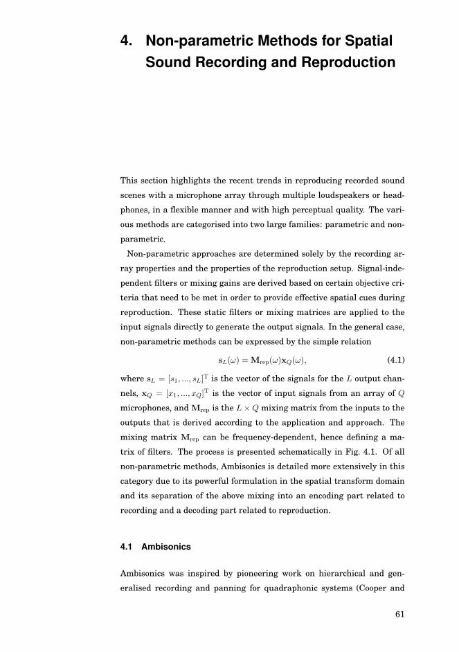
4. Non-parametric Methods for SpatialSound Recording and Reproduction
This section highlights the recent trends in reproducing recorded sound
scenes with a microphone array through multiple loudspeakers or head-
phones, in a flexible manner and with high perceptual quality. The vari-
ous methods are categorised into two large families: parametric and non-
parametric.
Non-parametric approaches are determined solely by the recording ar-
ray properties and the properties of the reproduction setup. Signal-inde-
pendent filters or mixing gains are derived based on certain objective cri-
teria that need to be met in order to provide effective spatial cues during
reproduction. These static filters or mixing matrices are applied to the
input signals directly to generate the output signals. In the general case,
non-parametric methods can be expressed by the simple relation
sL(ω) = Mrep(ω)xQ(ω), (4.1)
where sL = [s1, ..., sL]T is the vector of the signals for the L output chan-
nels, xQ = [x1, ..., xQ]T is the vector of input signals from an array of Q
microphones, and Mrep is the L×Q mixing matrix from the inputs to the
outputs that is derived according to the application and approach. The
mixing matrix Mrep can be frequency-dependent, hence defining a ma-
trix of filters. The process is presented schematically in Fig. 4.1. Of all
non-parametric methods, Ambisonics is detailed more extensively in this
category due to its powerful formulation in the spatial transform domain
and its separation of the above mixing into an encoding part related to
recording and a decoding part related to reproduction.
4.1 Ambisonics
Ambisonics was inspired by pioneering work on hierarchical and gen-
eralised recording and panning for quadraphonic systems (Cooper and
61
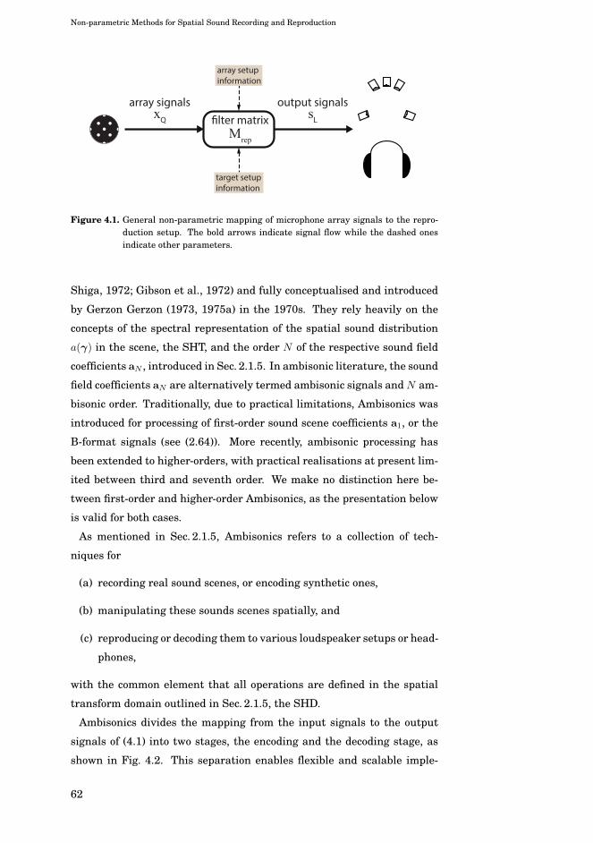
Non-parametric Methods for Spatial Sound Recording and Reproduction
array signalsxQ
output signalssLfilter matrix
Mrep
target setupinformation
array setupinformation
Figure 4.1. General non-parametric mapping of microphone array signals to the repro-duction setup. The bold arrows indicate signal flow while the dashed onesindicate other parameters.
Shiga, 1972; Gibson et al., 1972) and fully conceptualised and introduced
by Gerzon Gerzon (1973, 1975a) in the 1970s. They rely heavily on the
concepts of the spectral representation of the spatial sound distribution
a(γ) in the scene, the SHT, and the order N of the respective sound field
coefficients aN , introduced in Sec. 2.1.5. In ambisonic literature, the sound
field coefficients aN are alternatively termed ambisonic signals and N am-
bisonic order. Traditionally, due to practical limitations, Ambisonics was
introduced for processing of first-order sound scene coefficients a1, or the
B-format signals (see (2.64)). More recently, ambisonic processing has
been extended to higher-orders, with practical realisations at present lim-
ited between third and seventh order. We make no distinction here be-
tween first-order and higher-order Ambisonics, as the presentation below
is valid for both cases.
As mentioned in Sec. 2.1.5, Ambisonics refers to a collection of tech-
niques for
(a) recording real sound scenes, or encoding synthetic ones,
(b) manipulating these sounds scenes spatially, and
(c) reproducing or decoding them to various loudspeaker setups or head-
phones,
with the common element that all operations are defined in the spatial
transform domain outlined in Sec. 2.1.5, the SHD.
Ambisonics divides the mapping from the input signals to the output
signals of (4.1) into two stages, the encoding and the decoding stage, as
shown in Fig. 4.2. This separation enables flexible and scalable imple-
62

Non-parametric Methods for Spatial Sound Recording and Reproduction
mentations. For example, recordings from various microphone arrays can
be encoded into the ambisonic signals through the mathematical tools of
(2.58–2.59). Additionally, virtual sources can be encoded in a new set of
ambisonic signals of the same order through ambisonic encoding. The two
sound scenes, the recorded and synthetic, can be mixed by simple summa-
tion of the signals without regard to the recording setup. The final sound
scene can then be reproduced to a target system by means of an adequate
mixing matrix, or ambisonic decoder. This decoding matrix is designed ac-
counting for the reproduction setup properties and the order of the input
ambisonic signals.
arraysignalsxQ
ambisonicsignalsaN
ambisonicsignalsa N
outputsignalssL
decoding matrixMdec
encoding matrixMenc
target setupinformation
array setupinformation
transmissionmanipulation
Figure 4.2. Schematic of ambisonic encoding and decoding. The bold arrows indicatesignal flow, while the dashed ones indicate other parameters.
4.1.1 Recording and encoding
Ambisonic recording is no different from obtaining the sound field coeffi-
cients for general spherical acoustic processing, as detailed in Sec. 2.1.5
and Sec. 3.2.3. First-order ambisonic systems record in the B-format con-
vention, commonly employing tetrahedral microphone arrays of directional
capsules known as Soundfield microphones (Gerzon, 1975b). Higher-order
microphones, with only a few available commercially at present, follow
similar construction guidelines, replacing, however, directional capsules
for omnidirectional ones on a spherical rigid baffle. The maximum order
that the array can deliver is determined by the number of microphones
and their arrangement; for Q nearly uniformly distributed microphones
N ≤ �√Q− 1�, with �·� denoting the integer floor.
The encoding matrix Menc from the microphone signals to the ambisonic
signals
aN (ω) = Menc(ω)xQ (4.2)
can be derived in terms of the least-squares solution of (2.43) as (Moreau
63
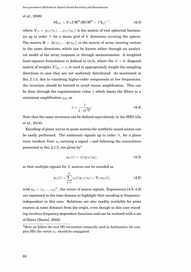
Non-parametric Methods for Spatial Sound Recording and Reproduction
et al., 2006)
Menc = YNCHH(HCHH + λ2IQ)−1, (4.3)
where YN = [yN (γ1), ...,yN (γK)] is the matrix of real spherical harmon-
ics up to order N for a dense grid of K directions covering the sphere.
The matrix H = [h(γ1), ...,h(γK)] is the matrix of array steering vectors
in the same directions, which can be known either through an analyti-
cal model of the array response or through measurements. A weighted
least-squares formulation is defined in (4.3), where the K × K diagonal
matrix of weights [C]kk = ck is used to appropriately weight the sampling
directions in case they are not uniformly distributed. As mentioned in
Sec. 2.1.5, due to vanishing higher-order components at low frequencies,
the inversion should be limited to avoid excess amplification. This can
be done through the regularisation value λ which limits the filters to a
maximum amplification gdB as
λ =1
2 · 10gdB20
. (4.4)
Note that the same inversion can be defined equivalently in the SHD (Jin
et al., 2014).
Encoding of plane waves or point sources for synthetic sound scenes can
be easily performed. The ambisonic signals up to order N , for a plane
wave incident from γ0 carrying a signal s and following the conventions
presented in Sec. 2.1.5, are given by1
aN (t) = s(t)yN (γ0), (4.5)
so that multiple signals for K sources can be encoded as
aN (t) =K∑k=1
sk(t)yN (γk) = YNsK(t), (4.6)
with sK = [s1, ..., sK ]T, the vector of source signals. Expressions (4.5–4.6)
are expressed in the time domain to highlight that encoding is frequency-
independent in this case. Relations are also readily available for point
sources at some distance from the origin, even though in this case encod-
ing involves frequency-dependent functions and can be realised with a set
of filters (Daniel, 2003).
1Here we follow the real SH convention commonly used in Ambisonics; for com-plex SHs the vector yN should be conjugated.
64
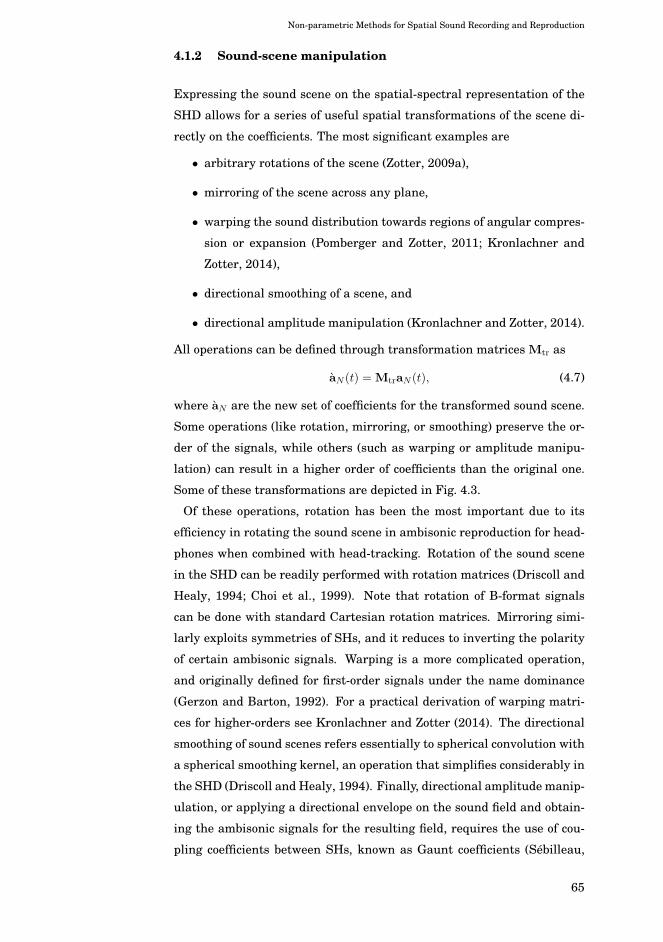
Non-parametric Methods for Spatial Sound Recording and Reproduction
4.1.2 Sound-scene manipulation
Expressing the sound scene on the spatial-spectral representation of the
SHD allows for a series of useful spatial transformations of the scene di-
rectly on the coefficients. The most significant examples are
• arbitrary rotations of the scene (Zotter, 2009a),
• mirroring of the scene across any plane,
• warping the sound distribution towards regions of angular compres-
sion or expansion (Pomberger and Zotter, 2011; Kronlachner and
Zotter, 2014),
• directional smoothing of a scene, and
• directional amplitude manipulation (Kronlachner and Zotter, 2014).
All operations can be defined through transformation matrices Mtr as
aN (t) = MtraN (t), (4.7)
where aN are the new set of coefficients for the transformed sound scene.
Some operations (like rotation, mirroring, or smoothing) preserve the or-
der of the signals, while others (such as warping or amplitude manipu-
lation) can result in a higher order of coefficients than the original one.
Some of these transformations are depicted in Fig. 4.3.
Of these operations, rotation has been the most important due to its
efficiency in rotating the sound scene in ambisonic reproduction for head-
phones when combined with head-tracking. Rotation of the sound scene
in the SHD can be readily performed with rotation matrices (Driscoll and
Healy, 1994; Choi et al., 1999). Note that rotation of B-format signals
can be done with standard Cartesian rotation matrices. Mirroring simi-
larly exploits symmetries of SHs, and it reduces to inverting the polarity
of certain ambisonic signals. Warping is a more complicated operation,
and originally defined for first-order signals under the name dominance
(Gerzon and Barton, 1992). For a practical derivation of warping matri-
ces for higher-orders see Kronlachner and Zotter (2014). The directional
smoothing of sound scenes refers essentially to spherical convolution with
a spherical smoothing kernel, an operation that simplifies considerably in
the SHD (Driscoll and Healy, 1994). Finally, directional amplitude manip-
ulation, or applying a directional envelope on the sound field and obtain-
ing the ambisonic signals for the resulting field, requires the use of cou-
pling coefficients between SHs, known as Gaunt coefficients (Sébilleau,
65
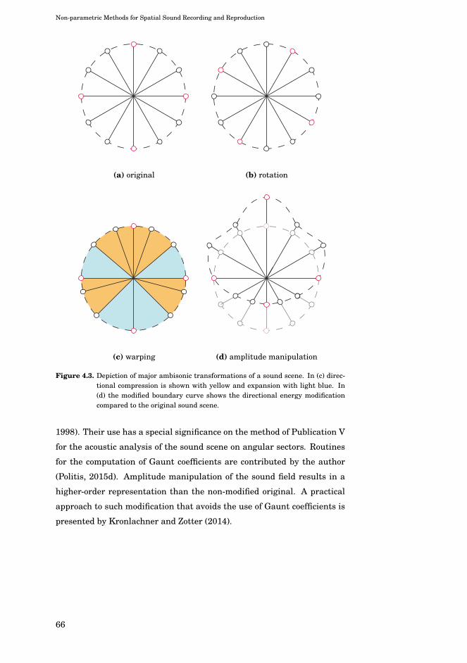
Non-parametric Methods for Spatial Sound Recording and Reproduction
(a) original (b) rotation
(c) warping (d) amplitude manipulation
Figure 4.3. Depiction of major ambisonic transformations of a sound scene. In (c) direc-tional compression is shown with yellow and expansion with light blue. In(d) the modified boundary curve shows the directional energy modificationcompared to the original sound scene.
1998). Their use has a special significance on the method of Publication V
for the acoustic analysis of the sound scene on angular sectors. Routines
for the computation of Gaunt coefficients are contributed by the author
(Politis, 2015d). Amplitude manipulation of the sound field results in a
higher-order representation than the non-modified original. A practical
approach to such modification that avoids the use of Gaunt coefficients is
presented by Kronlachner and Zotter (2014).
66

Non-parametric Methods for Spatial Sound Recording and Reproduction
4.1.3 Decoding and panning
Reproduction of ambisonic signals to a target setup is performed through
an L× (N + 1)2 decoding matrix Mdec as
sL(t) = MdecaN (t). (4.8)
Usually ambisonic decoding uses frequency-independent mixing matri-
ces. Some frequency-dependency in first-order ambisonic decoding is com-
monly introduced with either shelf-filters and a single decoding matrix or
two frequency ranges with one decoding matrix for each (Heller et al.,
2008). The aim of these designs is to preserve constant amplitude at low
frequencies and optimise the Makita velocity vector, while preserving en-
ergy at high frequencies and optimise the Gerzon energy vector. Recent
higher-order decoding designs drop the frequency-dependency and focus
primarily on optimisation of the energy vector. An overview of traditional
and recent decoder designs can be found in Zotter et al. (2012) and Zotter
and Frank (2012). Decoding to irregular speaker layouts or partial ones
can also be challenging. Recent approaches involve a combination of am-
bisonic decoding and VBAP derived gains (Batke and Keiler, 2010; Zotter
and Frank, 2012; Epain et al., 2014), modified SH basis functions (Zotter
et al., 2012), and iterative numerical optimization of the decoding gains
to achieve some target performance (Wiggins, 2007; Moore and Wakefield,
2007; Scaini and Arteaga, 2014). Example routines for the derivation of
decoding matrices with some of the above techniques are contributed by
the author (Politis, 2015c).
Ambisonic panning is essentially the combination of the decoding (4.8)
and encoding stage (4.5):
sL(t) = MdecyN (γ0)s(t). (4.9)
Panning of a virtual point source that recreates a spherical wave from its
virtual origin is also possible, similar to wave-field synthesis. Contrary
to the above plane wave formulations, its realisation treats both the vir-
tual source and the loudspeaker setup as point sources at certain radii
and expands them in the SHD. This approach has been termed near-field
compensation, and it requires careful design of the corresponding filters
due to the extreme amplification for higher-orders and low frequencies
dictated by theory (Daniel, 2003).
67
Non-parametric Methods for Spatial Sound Recording and Reproduction
4.1.4 Binaural decoding
Ambisonic reproduction for headphones can be formulated very efficiently
in the SHD through Parseval’s theorem in (2.57). Assuming that the
HRTFs of the listener are given by hbin(γ, ω) = [hl(γ, ω), hr(γ, ω)]T, and
assuming real SHs, the binaural signals sbin = [sl, sr]T are given by
sbin(ω) =
∫hbin(γ, ω)a(γ, ω) dγ = HT
bin(ω)aN (ω), (4.10)
where Hbin = [SHT {hl(γ)},SHT {hr(γ)}] = [h(l)N ,h
(r)N ] is the matrix of the
HRTFs expanded into SH coefficients. Hence the decoding matrix for am-
bisonic binaural reproduction is given directly by the expansion of the
HRTFs into SHs, and the order of the expansion is limited by the order of
the available ambisonic signals2. Binaural rendering of ambisonic signals
has been studied by Noisternig et al. (2003), Duraiswami et al. (2005),
Atkins (2011), Melchior et al. (2009), Shabtai and Rafaely (2014) and
Bernschütz (2016). Since the expanded HRTFs are truncated to the lower
order of the ambisonic signals, perceptible colouration occurs at high fre-
quencies. An approximate mean correction to this effect is proposed by
Sheaffer et al. (2014).
4.1.5 Discussion
Ambisonics is a significant leap towards many of the goals of a modern
reproduction method outlined in the introduction of this thesis. However,
it poses a number of limitations. As was mentioned before, recording of
the ambisonic signals is limited to the first few orders. A low-order rep-
resentation of a fully directional sound, such as a plane wave or a point
source, will be directionally spread and its binaural cues will deviate from
the actual ones, especially at high frequencies.
Similarly, reproduction of diffuse sound scenes can suffer from high cor-
relation between the output channels for the same reason; a low-order de-
coding is incapable of achieving the incoherent properties of a diffuse field.
Perceptual effects of these properties of ambisonic reproduction can be a
loss of brightness, increased localisation blur, loss of envelopment, in-head
localisation effects, and strong comb-filtering effects around the sweet
spot. Many of these effects were recognised in early ambisonic research
2We assume here compact recording arrays generally encountered in practice; inthis case the order of the captured sound field will be smaller than the expansionorder of the HRTFs, which is determined by the number of HRTF measurements.
68
Non-parametric Methods for Spatial Sound Recording and Reproduction
and were collectively put under the term phasiness (Gerzon, 1975c).
The task of a well-designed ambisonic decoder is to minimise these ef-
fects as much as possible. However, there are inherent limits on how much
the decoder design can alleviate the above problems, and these limits are
set by the order of the ambisonic signals. Higher-order processing natu-
rally improves on these issues as spreading of virtual sources is compacted
and correlation between output channels in complex scenes is decreased.
Perceptual effects of the order of ambisonic reproduction with virtual or
recorded sources are analysed by Braun and Frank (2011), Kearney et al.
(2012), Bertet et al. (2013), Avni et al. (2013), Stitt et al. (2014), Yang and
Xie (2014), and Bernschütz et al. (2014). Spectral effects of using more
loudspeakers than the minimum that the available ambisonic order dic-
tates are discussed by Solvang (2008) and Benjamin and Heller (2014),
while positive perceptual effects of reverberation on low-order reproduc-
tion are presented by Santala et al. (2009).
Even if direct decoding of ambisonic signals at low-orders can be inad-
equate for transparent reproduction of sound scenes, it can serve as a
very efficient and compact format for capturing and mixing them. This
is mainly due to the detachment of the format from the recording pro-
cess and the unified acoustical processing that can be performed on the
sound field coefficients described in Sec. 2.1.5. We believe that one of the
outcomes of this thesis is that low-order ambisonic reproduction can be
the basis for the more elaborate parametric methods detailed herein, and
that this approach can achieve close to transparent reproduction using the
same low-order ambisonic signals as input. The methods of Publication
I, Publication II and Publication V start from an ambisonic-like decod-
ing of B-format or higher-order signals, and they enhance their reproduc-
tion through a parametric perceptually-motivated analysis. Parametric
methods, however, have an increased price in computational complexity
compared to the simple matrixing operation of ambisonic decoding.
4.2 Other non-parametric approaches
Non-parametric methods that mix input signals to the outputs, captured
with directional patterns or with different propagation delays, correspond
invariably to some form of beamforming, one per loudspeaker, including
Ambisonics. Based on this view, beamformers that satisfy criteria other
than the decoding principles of Ambisonics can be used for multichannel
69

Non-parametric Methods for Spatial Sound Recording and Reproduction
reproduction of array recordings. One approach is to generate a set of
beamformers covering the region of interest and then to pan their sig-
nals as virtual sources from the beamforming directions at reproduction.
The method by Farina et al. (2013) does that using a set of higher-order
cardioid beamformers up to the maximum allowed order of the array, cov-
ering uniformly the sphere. A similar method is proposed in the non-
parametric part of the work by Hur et al. (2011), posed as a synthetic
array reconfiguration problem.
A second approach is to approximate the panning curves for the tar-
get setup with beamforming, obtaining directly the output signals. This
approach is conceptualised by Backman (2003) and is formulated for a
linear microphone array by Abel et al. (2010). Similarly, Ono et al. (2013)
attempts beamforming to obtain the signals for the standardised NHK
22.2 setup. For arbitrary arrays, such beam patterns can be generated
through the least squares solution (2.43).
Panning curves can be discontinuous and asymmetrical for irregular se-
tups and of very narrow directionality for dense ones, and hence they
can be poorly approximated by low-order beam patterns. The work by
Hacihabiboglu and Cvetkovic (2009) proposes a set of small differential
arrays to achieve the higher-order directivity that is required. This ap-
proach is generalised further into a framework for deriving beamformers
that reconstruct optimally the acoustic intensity in the reproduction re-
gion (De Sena et al., 2013).
Binaural reproduction using non-parametric methods is also possible
by forming a pair of beamformers that mimic the HRTFs (Chen et al.,
1992; Algazi et al., 2004; Li and Duraiswami, 2006; Sakamoto et al., 2010;
Rasumow et al., 2016). Unless hundreds of microphones are used, as
by Sakamoto et al. (2010), the high-frequency spatial variability of the
HRTFs cannot be approximated fully by small compact arrays, affecting
mostly high-frequency and individualised cues, such as ILDs and spectral
or pinna cues. These performance issues of binaural beamforming are
of the same nature as low-order effects in ambisonic reproduction over
headphones.
70
5. Parametric Methods for SpatialSound Recording and Reproduction
Parametric approaches, contrary to the non-parametric methods men-
tioned above, apart from the array properties and the properties of the
reproduction system, also take into account the statistics or dependencies
of the recorded signals themselves. By making certain assumptions on
how the sound scene is composed, they are able to overcome many of the
limitations of the non-parametric approaches. In the sections below, we
discuss the relation of parametric methods to spatial audio coding (SAC)
and upmixing methods, and then we give a summary of recent trends in
the reproduction of natural sound scenes obtained from a microphone ar-
ray. The DirAC method is presented in more detail as it constitutes the
backbone of a large part of this thesis. Finally, applications of parametric
methods to auralisation of room acoustics are discussed.
5.1 Spatial audio coding and upmixing
5.1.1 Spatial audio coding
SAC refers to the methods that aim to compress multichannel recordings
using a parametric approach in order to reduce bandwidth and process-
ing requirements. Ideally, a SAC system should be able to recreate the
multichannel content without loss of perceived quality and, ideally, with
no perceptual differences (transparency). In contrast to SAC, upmixing
refers to decomposing the audio channels of a multichannel mix in order to
redistribute them to a different target system; a classic example is stereo-
to-surround upmixing, or stereo-to-binaural conversion. Even though at
first glance the aims are different, both SAC and upmixing strive for the
same goal: process the recording in such a way that when recreated at
the target system it preserves the perceptual properties of the original.
71
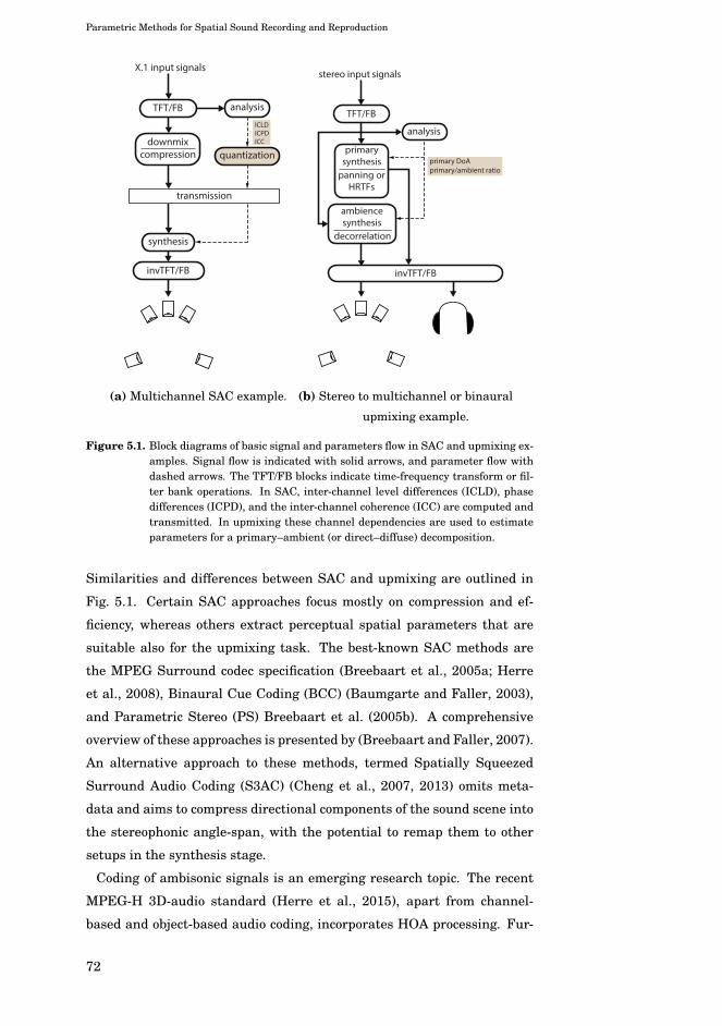
Parametric Methods for Spatial Sound Recording and Reproduction
X.1 input signals
downmixcompression
synthesis
transmission
analysis
quantization
invTFT/FB
TFT/FB
ICLDICPDICC
(a) Multichannel SAC example.
stereo input signals
primary DoAprimary/ambient ratio
primarysynthesis
panning orHRTFs
decorrelation
ambiencesynthesis
analysis
invTFT/FB
TFT/FB
(b) Stereo to multichannel or binaural
upmixing example.
Figure 5.1. Block diagrams of basic signal and parameters flow in SAC and upmixing ex-amples. Signal flow is indicated with solid arrows, and parameter flow withdashed arrows. The TFT/FB blocks indicate time-frequency transform or fil-ter bank operations. In SAC, inter-channel level differences (ICLD), phasedifferences (ICPD), and the inter-channel coherence (ICC) are computed andtransmitted. In upmixing these channel dependencies are used to estimateparameters for a primary–ambient (or direct–diffuse) decomposition.
Similarities and differences between SAC and upmixing are outlined in
Fig. 5.1. Certain SAC approaches focus mostly on compression and ef-
ficiency, whereas others extract perceptual spatial parameters that are
suitable also for the upmixing task. The best-known SAC methods are
the MPEG Surround codec specification (Breebaart et al., 2005a; Herre
et al., 2008), Binaural Cue Coding (BCC) (Baumgarte and Faller, 2003),
and Parametric Stereo (PS) Breebaart et al. (2005b). A comprehensive
overview of these approaches is presented by (Breebaart and Faller, 2007).
An alternative approach to these methods, termed Spatially Squeezed
Surround Audio Coding (S3AC) (Cheng et al., 2007, 2013) omits meta-
data and aims to compress directional components of the sound scene into
the stereophonic angle-span, with the potential to remap them to other
setups in the synthesis stage.
Coding of ambisonic signals is an emerging research topic. The recent
MPEG-H 3D-audio standard (Herre et al., 2015), apart from channel-
based and object-based audio coding, incorporates HOA processing. Fur-
72
Parametric Methods for Spatial Sound Recording and Reproduction
ther work on coding and transmission of HOA signals has been presented
by Peters et al. (2015) and Sen et al. (2016). The DirAC-based schemes of
Pulkki et al. (2013) and Publication V can be also viewed as SAC methods
for 2D and 3D HOA signals respectively.
5.1.2 Upmixing
Upmixing methods are traditionally defined for channel-based content,
with the first proposals focusing on conversion of stereo-to-surround con-
tent (Irwan and Aarts, 2002; Avendano and Jot, 2004; Faller, 2006). They
vary on how they separate the directional and diffuse components, an
approach also called direct-diffuse decomposition, or primary-ambient ex-
traction. In general, coherent signals between channels are treated as
directional, while incoherent signals are treated as ambient or diffuse.
With additional assumptions on the energies and correlations of the com-
ponents, it is possible to find estimates of their signals. A well-established
approach to direct-diffuse decomposition is the one presented by Faller
(2006) and Walther and Faller (2011), which formulates the decomposi-
tion as a multichannel Wiener filtering problem with a least-squares solu-
tion. Similar approaches solve a linear system of equations describing the
input signal and decomposed signal statistics (Avendano and Jot, 2004;
Merimaa et al., 2007; Thompson et al., 2012). A popular alternative has
been the principal component analysis (PCA) of the input signals. PCA
detects uncorrelated components and achieves effective primary-ambient
decomposition under certain conditions, as has been detailed by Irwan
and Aarts (2002), Driessen and Li (2005), Briand et al. (2006), Merimaa
et al. (2007), Baek et al. (2012), and He et al. (2014). PCA also seems
closely related to the unified-domain representation of Short et al. (2007).
No generalisation of its use has been proposed for more than stereo input.
Recent proposals either refine the direct-diffuse decomposition by com-
bining the approaches above (He et al., 2014), or apply blind source sep-
aration methods to estimate independent components in the channel sig-
nals (Nikunen et al., 2011). DirAC itself has found applications as an up-
mixing method (Pulkki, 2006; Laitinen and Pulkki, 2011; Laitinen, 2014),
with the difference that instead of inter-channel dependencies, it com-
putes global sound scene descriptors, such as the intensity vector and the
diffuseness at each subband. A method closely related to DirAC upmix-
ing is the Spatial Audio Scene Coding (SASC) based on the descriptors of
velocity and energy vectors instead of intensity and diffuseness (Goodwin
73
Parametric Methods for Spatial Sound Recording and Reproduction
and Jot, 2008, 2007).
5.1.3 Binaural reproduction
Binaural reproduction is a major application of upmixing systems, due to
the realisation that rendering a virtual loudspeaker setup through bin-
aural panning is not an effective solution, since it suffers from coloura-
tion of the material, in-head localisation, and loss of envelopment. The
directional-diffuse decomposition has been found very effective for this
task, rendering the directional component using HRTFs and decorrelat-
ing the ambient component appropriately at the two ears, fixing most of
these issues (Faller and Breebaart, 2011). This approach has been fol-
lowed by most of the major methods mentioned above, such as MPEG
Surround (Breebaart et al., 2006), BCC/PS-related reproduction (Faller
and Breebaart, 2011), S3AC (Cheng et al., 2008), SASC (Goodwin and
Jot, 2007) and DirAC (Laitinen and Pulkki, 2009).
5.1.4 Discussion
SAC and upmixing share many similarities with the reproduction meth-
ods developed in this thesis, the major difference stemming from the fact
that upmixing and SAC focus on certain channel-based formats, while
the methods studied herein focus on array recordings and reproduction of
real sound scenes. This distinction is, however, somewhat artificial, since
recording-based methods still operate with a compact finite representa-
tion of the sound scene, the array signals. Capturing the sound field still
imposes certain mixing models for directional sounds and certain correla-
tions between channels for ambient or diffuse sounds, similar to the pan-
ning and reverberation tools for mixing and creating channel-based audio
content. However, the complexity of many natural sound scenes and the
variation in recording practices and approaches makes the sound repro-
duction problem more challenging than SAC and upmixing, and justifies
many of the more complicated approaches presented in the next section.
5.2 Parametric reproduction of recorded sound scenes
This section gives an overview of parametric methods that perform an
analysis of a sound scene captured with some microphone array and its
respective reproduction. There is great variability in the approaches and
74
Parametric Methods for Spatial Sound Recording and Reproduction
their assumptions on which sound field models, source signal properties,
and array and reproduction system properties they are based on. In the
following, an attempt is made to present the various trends with respect
to these choices.
5.2.1 Assumptions on array input and output setup properties.
Even though most methods have general principles and can be applied
to arbitrary arrays, a large part of the research focuses on certain ar-
rangements dictated by the application, the target performance, cost, pro-
cessing requirements, and so on. For example, many applications con-
sider a two-dimensional model of the sound-field and hence linear, planar,
or circular arrays are adequate for its analysis. Linear arrays, popular
in array processing applications due to their simplicity in analysis and
beamforming, are suitable, for example, for two-way communication sys-
tems integrated with a flat screen, and have been used in that context
in sound scene acquisition and rendering (Beracoechea et al., 2006; Thier-
gart et al., 2011). Similarly, compact circular (Ahonen et al., 2007; Alexan-
dridis et al., 2013) and cylindrical arrays (Ahonen et al., 2012) have been
proposed for high-quality teleconferencing applications and general 2D
sound scene recording and reproduction. 2D arrays with directional mi-
crophones following the stereophonic principles of Sec. 3.2.3, popular in
music recording, have been studied for parametric recording and repro-
duction. Stereophonic arrangements were used by Ahonen et al. (2009)
and Faller (2008), and surround recording arrays have been utilised by
the author (Politis et al., 2013a,b) and Publication III. For 3D analysis
and synthesis, a minimum of four omnidirectional microphones is neces-
sary; such minimal 3D arrays are used as implementation examples by
Cobos et al. (2010) and Nikunen and Virtanen (2014). Large omnidirec-
tional arrays, on the other hand, can be useful in certain applications,
such as reproduction of sound scenes with the possibility of translation
inside the recording (Gallo et al., 2007; Niwa et al., 2008; Thiergart et al.,
2013), or auralisation of industrial environments (Verron et al., 2013).
A class of methods, instead of operating on array signals, work in their
spatial transform domain, more specifically on the SHD detailed in Sec. 2.1.5.
The advantages are apparent; it provides a standardised format for the
spatial sound scene that is independent of the array. Furthermore, it
bridges the distinction between recorded and synthetic sound scenes. Recorded
sound scenes encoded into SH or ambisonic signals suffer from the frequency-
75
Parametric Methods for Spatial Sound Recording and Reproduction
dependency issues mentioned in Sec. 2.1.5. This fact needs to be taken
into account in parametric analysis and synthesis (see Publication V),
making processing of the array signals advantageous in certain tasks,
as shown in Publication I. The most compact format for 3D analysis is
the set of first-order SH signals, or equivalently the B-format. B-format
signals can be obtained with a broadband response using practical com-
pact arrays. DirAC has been traditionally defined with B-format input,
and also the methods by Hurtado-Huyssen and Polack (2005), Berge and
Barrett (2010b), and Günel et al. (2008). Higher-order ambisonic signals
encode the sound scene with a higher spatial resolution than B-format,
when available. This increased resolution is exploited in Publication V.
Due to the decomposition of the sound scene into its spatial components,
arbitrary rendering of the recordings is possible either using suitable pan-
ning functions for loudspeaker reproduction or HRTFs for binaural repro-
duction. Many of the methods mentioned here are applied to both targets
(Pulkki, 2007; Laitinen and Pulkki, 2009; Berge and Barrett, 2010b,a; Co-
bos et al., 2012, 2010; Nikunen and Virtanen, 2014; Nikunen et al., 2015;
Verron et al., 2013, 2011; Vilkamo and Delikaris-Manias, 2015; Delikaris-
Manias et al., 2015). Targeting binaural reproduction, compared to loud-
speakers, imposes requirements on real-time processing with interactive
update rates, since modern systems consider head-tracking an essential
component for a realistic listening experience. Practical recording for ren-
dering on WFS systems also seems possible with parametric techniques
(Beracoechea et al., 2006; Cobos et al., 2012; Thiergart et al., 2013; Bai
et al., 2015).
5.2.2 Assumptions on the sound-field model and estimation ofparameters.
Direct-diffuse decomposition
In terms of the sound-field model or assumptions on the spatial properties
of the sound scene, most methods follow the dominant directional/primary
plus diffuse/ambient component found in SAC and upmixing. This decom-
position, which has been shown to be perceptually effective in the above
applications, is followed by DirAC and the methods by Hurtado-Huyssen
and Polack (2005), Gallo et al. (2007), Faller (2008), and Thiergart et al.
(2013). The active intensity vector and its statistics are exploited for this
task in DirAC and by Hurtado-Huyssen and Polack (2005) and Günel
76

Parametric Methods for Spatial Sound Recording and Reproduction
et al. (2008) due to its effectiveness and robustness. The method by Hurtado-
Huyssen and Polack (2005) attempts additionally to reproduce the energy
polarisation in the recording as a distributed sound source, while Günel
et al. (2008) uses intensity vector statistics as spatial filters to separate
the directional sounds.
Certain methods aim to extract multiple directional components per
time-frequency tile, and some drop the dependency on the diffuse/ambient
component. Cobos et al. (2010) assume just a single directional compo-
nent, while the HARPEX method (Berge and Barrett, 2010b) extracts two
plane waves from a B-format signal. This latter model is augmented with
a diffuse component by Thiergart and Habets (2012). Multiple directional
signals are extracted also by Günel et al. (2008), Hur et al. (2011), Alexan-
dridis et al. (2013), Thiergart et al. (2014), and Nikunen and Virtanen
(2014). A method that operates on SH signals and extracts multiple di-
rectional and diffuse components is presented in Publication V.
Relation to spatial filtering and enhancement
A large family of methods notices the similarity between the spatial sound
capture and reproduction problem and the more traditional array process-
ing applications of source detection, tracking and signal estimation, with
spatial filtering operations. This approach is very closely related to mul-
tichannel speech enhancement applications (see, for example, the refer-
ences in Benesty et al. (2008) and Brandstein and Ward (2013)) with the
difference that instead of trying to get a clean directional speech signal
and suppress interferers and ambient noise, all perceptual components of
interest should be estimated and preserved for transparent spatial sound
reproduction. In a sense, enhancement usually targets highly effective
suppression and quality constraints on the individual enhanced signal,
while spatial reproduction relaxes the requirements on suppression be-
tween components and targets quality constraints for their recombination
at synthesis. Both tasks have their own challenges but share many simi-
larities. An array-processing oriented approach has been applied to DirAC
by Thiergart et al. (2011). This approach has been recently generalised
by Thiergart et al. (2014) and Thiergart and Habets (2014) into a unified
framework for adaptive estimation of multiple source signals of interest
plus diffuse sound, similar to Fig. 5.2a. This work uses trade-off beam-
formers (Habets and Benesty, 2013) that can switch between maximum
suppression or low signal distortion, suitable for both enhancement and
77
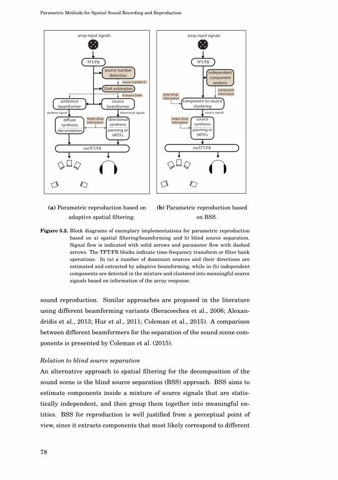
Parametric Methods for Spatial Sound Recording and Reproduction
array input signals
directionalsynthesis
panning orHRTFs
decorrelation
diffusesynthesis
source number detection
invTFT/FB
TFT/FB
DoA estimation
source beamformer
ambiencebeamformer
ambient signal directional signals
source number K
target setupinformation
K source DoAs
(a) Parametric reproduction based on
adaptive spatial filtering.
componentinformation
array input signals
sourcesynthesis
panning orHRTFs
invTFT/FB
TFT/FB
component-to-sourceclustering
independent component
analysis
source signals
target setupinformation
array setupinformation
(b) Parametric reproduction based
on BSS.
Figure 5.2. Block diagrams of exemplary implementations for parametric reproductionbased on a) spatial filtering/beamforming and b) blind source separation.Signal flow is indicated with solid arrows and parameter flow with dashedarrows. The TFT/FB blocks indicate time-frequency transform or filter bankoperations. In (a) a number of dominant sources and their directions areestimated and extracted by adaptive beamforming, while in (b) independentcomponents are detected in the mixture and clustered into meaningful sourcesignals based on information of the array response.
sound reproduction. Similar approaches are proposed in the literature
using different beamforming variants (Beracoechea et al., 2006; Alexan-
dridis et al., 2013; Hur et al., 2011; Coleman et al., 2015). A comparison
between different beamformers for the separation of the sound scene com-
ponents is presented by Coleman et al. (2015).
Relation to blind source separation
An alternative approach to spatial filtering for the decomposition of the
sound scene is the blind source separation (BSS) approach. BSS aims to
estimate components inside a mixture of source signals that are statis-
tically independent, and then group them together into meaningful en-
tities. BSS for reproduction is well justified from a perceptual point of
view, since it extracts components that most likely correspond to different
78

Parametric Methods for Spatial Sound Recording and Reproduction
sound generating objects instead of spatially filtering sounds from certain
directions. Plain BSS methods can suffer from reverberation and permu-
tation problems, which at first glance makes them unsuitable for high-
quality sound scene rendering. However, combining BSS with additional
array processing stages and a directional/diffuse separation seems to han-
dle these issues effectively; see, for example, Asano et al. (2003) and Niwa
et al. (2008). For the task of sound scene enhancement and reproduction,
the work by Niwa et al. (2008) applies independent component analysis
(ICA) on recordings of distributed arrays of omnidirectional microphones
and clusters the results into virtual sources. The work of Nikunen and
Virtanen (2014) and Nikunen et al. (2015) applies non-negative matrix
factorization (NMF) to the source separation task and estimates addi-
tionally the array spatial covariance due to each independent source sig-
nal, which determines the spatial properties of each source. An exam-
ple of BSS processing for scene analysis and reproduction is outlined in
Fig. 5.2b.
Other models
Certain recent proposals omit a sound field model and aim to utilise di-
rectly the observed spatial statistics of the sound scene for reproduction.
One such example is the spatial covariance matrix method introduced by
Hagiwara et al. (2013) which, however, requires, apart from the scene
recording, an additional reference recording at the reproduction setup
in order to match the statistics of the two adaptively. A more efficient
approach is presented by Vilkamo and Delikaris-Manias (2015), where
both scene recordings and desired spatial statistics for the target setup
are captured with non-parametric beamformers, and they are further en-
hanced by the adaptive mixing solution in (Vilkamo et al., 2013). A related
technique is used for synthesis of recordings with a sinusoidal-plus-noise
sound-field model by Verron et al. (2013).
Sparse and compressed sensing approaches to acoustic array process-
ing are highly active research areas at present. In the task of sound
scene analysis and synthesis, the work of Wabnitz et al. (2011) performs
a sparse plane wave decomposition that is used to upscale low-order am-
bisonic signals into higher-order ones. Even though not strictly a para-
metric approach, the method is signal-dependent and, combined with some
direct-diffuse decomposition (Epain and Jin, 2013), it seems suitable for
high resolution rendering of sound scenes.
79

Parametric Methods for Spatial Sound Recording and Reproduction
5.3 Directional Audio Coding
Directional Audio Coding (DirAC) is a spatial audio coding, upmixing
and reproduction method for surround audio content and recorded sound
scenes based on a perceptually-motivated analysis and synthesis frame-
work (Pulkki, 2007; Vilkamo et al., 2009). The predecessor of DirAC,
the Spatial Impulse Response Rendering (SIRR) method (Merimaa and
Pulkki, 2005; Pulkki and Merimaa, 2006), was used for spatial reproduc-
tion of room impulse responses, and many of its perceptual assumptions
and technological innovations were extended in DirAC. The perceptual
motivation comes from the fact that DirAC, instead of a physically in-
spired reproduction as in WFS or certain ambisonic decoding variants,
aims at correct and stable interaural cues and preservation of timbral and
spectral qualities in the recording. This is attempted with a direct-diffuse
decomposition of the sound scene, using the sound field parameters of the
active intensity vector and diffuseness.
5.3.1 Analysis
The original DirAC analysis operates on the B-format signal vector b =
[p, vx, vy, vz]T, as defined in (2.64)1. All operations are defined in a suitable
time-frequency transform with centre frequency index k and temporal in-
dex l. As the vector of equalised pressure-gradient components in b is
proportional to the acoustic velocity vector with v = −Z0u, we get an esti-
mate of the active intensity vector (2.16) and energy density (2.17) at the
origin of the array as
ikl = −1
2Z0�{pklv∗kl} (5.1)
Ekl =1
4cZ0
[||vkl||2 + |pkl|2
]. (5.2)
Combining (5.1) and (5.2) according to (2.18) and (2.26), we get the dif-
fuseness estimate
ψkl =2||� {pklv∗kl} ||||vkl||2 + |pkl|2
. (5.3)
Diffuseness here is defined based on the spectral densities of a single win-
dowed frame. Most publications on DirAC include an additional averag-
ing operation that extends diffuseness estimation along successive time
1We omit here the√2 scaling commonly found in the definition of the B-format
signals.
80
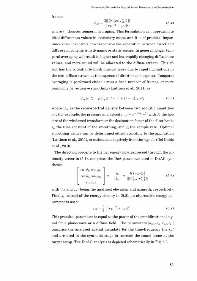
Parametric Methods for Spatial Sound Recording and Reproduction
frames
ψkl =2|| 〈� {pklv∗kl}〉 ||〈||vkl||2 + |pkl|2〉
. (5.4)
where 〈·〉 denotes temporal averaging. This formulation can approximate
ideal diffuseness values in stationary cases, and it is of practical impor-
tance since it controls how responsive the separation between direct and
diffuse components is in dynamic or static scenes. In general, longer tem-
poral averaging will result in higher and less rapidly changing diffuseness
values, and more sound will be allocated to the diffuse stream. This ef-
fect has the potential to mask musical noise due to rapid fluctuations in
the non-diffuse stream at the expense of directional sharpness. Temporal
averaging is performed either across a fixed number of frames, or more
commonly by recursive smoothing (Laitinen et al., 2011) as
Sxy(k, l) = μSxy(k, l − 1) + (1− μ)xkly∗kl, (5.5)
where Sxy is the cross-spectral density between two acoustic quantities
x, y (for example, the pressure and velocity), μ = e−K/(τμfs) with K the hop
size of the windowed transform or the decimation factor of the filter bank,
τμ the time constant of the smoothing, and fs the sample rate. Optimal
smoothing values can be determined either according to the application
(Laitinen et al., 2011), or estimated adaptively from the signals (Del Galdo
et al., 2010).
The direction opposite to the net energy flow, expressed through the in-
tensity vector in (5.1), comprises the DoA parameter used in DirAC syn-
thesis: ⎡⎢⎢⎣
cosϑkl cosϕkl
cosϑkl sinϕkl
sinϑkl
⎤⎥⎥⎦ = − ikl
||ikl||=
�{pklv∗kl}||�
{pklv
∗kl
}||, (5.6)
with ϑkl and ϕkl being the analysed elevation and azimuth, respectively.
Finally, instead of the energy density in (5.2), an alternative energy pa-
rameter is used:
εkl =1
2
[||vkl||2 + |pkl|2
]. (5.7)
This practical parameter is equal to the power of the omnidirectional sig-
nal for a plane-wave or a diffuse field. The parameters [ϑkl, ϕkl, ψkl, εkl]
comprise the analysed spatial metadata for the time-frequency tile k, l
and are used in the synthesis stage to recreate the sound scene at the
target setup. The DirAC analysis is depicted schematically in Fig. 5.3.
81

Parametric Methods for Spatial Sound Recording and Reproduction
B-format signalsb bkl
TFT/FB
intensity
energy
temporal averaging
diffuseness kl
energy kl
DoA kl kl]transmission
or decoding
Figure 5.3. Block diagram of DirAC analysis. Signal flow is indicated with solid arrowsand parameter flow with dashed arrows. The TFT/FB blocks indicate time-frequency transform or filter bank operations. The notation of signals andparameters follows the one in the text.
5.3.2 Synthesis
DirAC synthesis has been defined in two ways. The first, also termed
as low-bitrate DirAC (LB-DirAC), uses only the pressure signal from the
B-format and the metadata for the synthesis at the target setup. This
version is low in both processing and transmission requirements and is
suitable for applications where efficiency is favoured over quality or trans-
parency, such as in teleconferencing (Ahonen et al., 2007). The second
version uses all the channels of the B-format and is termed virtual micro-
phone DirAC (VM-DirAC) (Vilkamo et al., 2009). This version targets
quality-critical applications such as music recording and reproduction,
and binaural rendering and upmixing. In VM-DirAC, the processing is
done not on the pressure signal, but on the output signals of an initial am-
bisonic decoding. The virtual microphones term refers to the first-order
beamformers towards the loudspeakers that comprise the ambisonic de-
coding. Since this thesis considers high-resolution techniques, we focus
on VM-DirAC exclusively.
Assuming a preferred ambisonic decoding matrix Mdec for the target
loudspeaker setup, the output signals before enhancement zkl are given
by
zkl = Mdecbkl. (5.8)
The decoding matrix Mdec(k) can be also frequency dependent. The direct-
diffuse decomposition is performed directly on the output signal vector
z. A separation filter (or time-frequency mask) is constructed using the
diffuseness parameter for the direct and diffuse stream as
zdirkl =√1− ψklzkl (5.9)
82
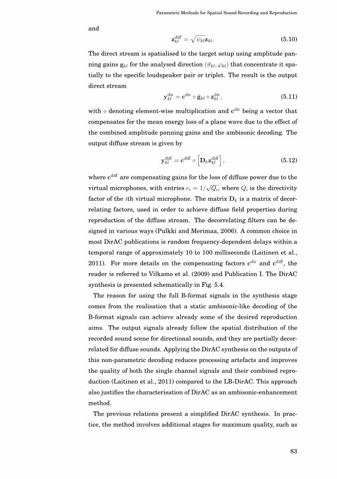
Parametric Methods for Spatial Sound Recording and Reproduction
and
zdiffkl =√ψklzkl. (5.10)
The direct stream is spatialised to the target setup using amplitude pan-
ning gains gkl for the analysed direction (ϑkl, ϕkl) that concentrate it spa-
tially to the specific loudspeaker pair or triplet. The result is the output
direct stream
ydirkl = cdir ◦ gkl ◦ zdirkl , (5.11)
with ◦ denoting element-wise multiplication and cdir being a vector that
compensates for the mean energy loss of a plane wave due to the effect of
the combined amplitude panning gains and the ambisonic decoding. The
output diffuse stream is given by
ydiffkl = cdiff ◦
[Dkz
diffkl
], (5.12)
where cdiff are compensating gains for the loss of diffuse power due to the
virtual microphones, with entries ci = 1/√Qi, where Qi is the directivity
factor of the ith virtual microphone. The matrix Dk is a matrix of decor-
relating factors, used in order to achieve diffuse field properties during
reproduction of the diffuse stream. The decorrelating filters can be de-
signed in various ways (Pulkki and Merimaa, 2006). A common choice in
most DirAC publications is random frequency-dependent delays within a
temporal range of approximately 10 to 100 milliseconds (Laitinen et al.,
2011). For more details on the compensating factors cdir and cdiff , the
reader is referred to Vilkamo et al. (2009) and Publication I. The DirAC
synthesis is presented schematically in Fig. 5.4.
The reason for using the full B-format signals in the synthesis stage
comes from the realisation that a static ambisonic-like decoding of the
B-format signals can achieve already some of the desired reproduction
aims. The output signals already follow the spatial distribution of the
recorded sound scene for directional sounds, and they are partially decor-
related for diffuse sounds. Applying the DirAC synthesis on the outputs of
this non-parametric decoding reduces processing artefacts and improves
the quality of both the single channel signals and their combined repro-
duction (Laitinen et al., 2011) compared to the LB-DirAC. This approach
also justifies the characterisation of DirAC as an ambisonic-enhancement
method.
The previous relations present a simplified DirAC synthesis. In prac-
tice, the method involves additional stages for maximum quality, such as
83

Parametric Methods for Spatial Sound Recording and Reproduction
B-format signals bkl
loudspeaker signals ykldecoding
Mdec
kl
kl kl]
directional gainsVBAP
loudspeakersetupkl
diffuse gains
decorrelationDk
invTFT/FBzkl
Figure 5.4. Block diagram of VM-DirAC synthesis. Signal flow is indicated with solidarrows and parameter flow with dashed arrows. The TFT/FB blocks indicatetime-frequency transform or filter bank operations. The notation of signalsand parameters follows the one in the text.
a multi-resolution time-frequency transform (Laitinen et al., 2011), by-
passing transients from the decorrelating filters (Laitinen et al., 2011;
Vilkamo and Pulkki, 2015), and splitting the diffuse stream into a re-
verberant and non-reverberant part (Laitinen and Pulkki, 2012). Using
these improvements the perceived quality of VM-DirAC has been found to
be high in listening tests (Vilkamo et al., 2009; Laitinen et al., 2011). The
major drawback of the VM-DirAC formulation is that it is not optimal in
achieving the energy and coherence properties that the spatial parame-
ters indicate. The reason for this is that it does not fully take into account
what is achieved already by the static decoding stage. Based on this ob-
servation, the work by Vilkamo and Pulkki (2013) proposes an alternative
formulation of DirAC synthesis which uses the optimal mixing framework
of Vilkamo et al. (2013). A mixing matrix from the B-format to the loud-
speakers is dynamically computed for each time-frequency tile that opti-
mally achieves the target energy and channel dependencies. The formu-
lation minimises additionally the amount of decorrelated energy that is
added to the output, since it exploits decorrelation that can be achieved
by mixing the inputs. The higher-order DirAC formulation of Publication
V takes full advantage of this framework.
84
Parametric Methods for Spatial Sound Recording and Reproduction
5.3.3 Sound scene synthesis and manipulation
The spatial parameters of DirAC can be used directly to create synthetic
sound scenes and spatial effects. This approach has been found to be
effective in the creation of spatial sound objects with a prescribed spa-
tial extent through panning of individual subbands of a monophonic sig-
nal over the angular region that determines that extent (Laitinen et al.,
2012a; Pihlajamäki et al., 2014). Similar approaches have been studied
earlier (Kendall, 1995; Potard and Burnett, 2004) and have been realised
recently in the methods of Verron et al. (2010) and Franck et al. (2015).
An alternative for ambisonic signals is proposed by Zotter et al. (2014).
Apart from source extent, efficient perceptual reverberation can be added
to the scene by encoding the monophonic sound into a B-format set with
added reverberation and prescribing the desired diffuseness values for the
synthesis (Laitinen et al., 2012a).
Manipulation of real recorded sound scenes is possible by modulating
the analysed parameters before the synthesis stage. This modulation of
parameters is performed based on some meaningful spatial transforma-
tion, depending on the application. Examples include a zooming effect
towards an arbitrary direction (Schultz-Amling et al., 2010) and a re-
lated transformation that projects the recorded scene onto some virtual
surfaces and allows the user to move inside the recording (Pihlajamaki
and Pulkki, 2015). Besides directional transformations, perceptual rever-
beration control can be achieved through modification of the diffuseness
parameter. Parametric scene manipulation in the time-frequency domain
allows flexible and intuitive design of spatial effects, since it involves mod-
ifying properties such as the DoA of sound and the DDR. Publication II
presents a series of such examples.
5.3.4 Binauralisation, transcoding and upmixing
Binaural reproduction with DirAC is very similar to loudspeaker render-
ing. Since head-tracking is utilised, the method should adapt the anal-
ysis and synthesis to the rotating coordinate frame of the user’s head.
Two approaches are possible for binaural rendering. The one proposed
by Laitinen and Pulkki (2009) performs the synthesis for a fixed number
of virtual loudspeakers, which are then convolved with the appropriate
HRTFs. From the potential combinations that can perform the rotation
of the recording, the most efficient is deemed to be counter-rotation of
85
Parametric Methods for Spatial Sound Recording and Reproduction
the analysed DoAs during analysis and counter-rotation of the ambisonic
decoding at synthesis. The method has been found to produce very con-
vincing results with sharp spatial images and effective externalisation
(Laitinen and Pulkki, 2009). The second approach, currently under devel-
opment, omits the virtual loudspeaker setup and replaces the amplitude
panning gains with HRTF-derived complex gains that correspond to the
time-frequency transform under use. The diffuse stream is additionally
rendered directly to binaural signals, taking into account the binaural co-
herence of diffuse sound, in a manner similar to that by Faller and Bree-
baart (2011), Borß and Martin (2009), and Vilkamo et al. (2012). The
method can additionally exploit the optimal mixing solution of Vilkamo
et al. (2013) for maximum perceived quality.
Upmixing using DirAC has been applied to stereo (Laitinen, 2014) and
surround content (Laitinen and Pulkki, 2011). It involves first encoding
the original signals into a B-format set and then processing the result
with DirAC. Some consideration should be given to the encoding process
in order to take into account the spatial non-uniformity of the input chan-
nels (Laitinen and Pulkki, 2011). An interesting application of DirAC
upmixing is re-encoding of the first-order B-format into a higher-order
ambisonic signal set, a process which has been also termed ambisonic
upscaling (Wabnitz et al., 2011). The higher-order signals can preserve
better the spatial quality and sharpness of DirAC reproduction. Further-
more, after upmixing to some reference order, material of various orders
can be mixed directly and decoded with a single optimised decoding ma-
trix for the target setup. A trivial way to perform this ambisonic upmix-
ing is to render the B-format into a uniform setup of virtual loudspeakers,
with the number and arrangement determined by the target order; see,
for example, spherical t-designs in Hardin and Sloane (1996), Gräf and
Potts (2011) and Publication V. The output signals can then be encoded
into the higher-order signals as plane waves from the virtual loudspeaker
directions using (4.6).
With reproduction for loudspeakers and headphones and upmixing for
channel-based content and recorded sound, along with spatialisation and
diffusion of synthetic spatial audio objects, DirAC shows the potential
of parametric techniques as universal spatial audio processors. Content
from various input formats can be parameterised into a common represen-
tation, and spatialised or converted to a variety of target systems or alter-
native formats. The methods have also the potential to objectify recorded
86
Parametric Methods for Spatial Sound Recording and Reproduction
sound scenes by splitting them into perceptually meaningful components
along with their estimated signals and spatial parameters (Herre et al.,
2012).
5.3.5 Discussion
DirAC resembles many of the SAC and upmixing methods mentioned in
Sec. 5.1. Using a direct-diffuse decomposition DirAC achieves its percep-
tual target better than what can be done with first-order ambisonic de-
coding (Vilkamo et al., 2009). Since DirAC was originally defined with
B-format input, it can also be seen as a method that addresses many of
the problems of first-order reproduction mentioned in Sec. 4.1.5.
DirAC can be seen differently from various points of view:
(a) From a SAC perspective: DirAC is a SAC method that is able to
transmit a monophonic downmix and metadata, which can be used
for efficient reproduction of the sound scene. This perspective is ex-
ploited mostly in the teleconferencing applications of DirAC (Ahonen
et al., 2007).
(b) From an upmixing perspective: DirAC is an upmixing method that
utilises global spatial parameters and a direct-diffuse decomposition
to upmix four channels to any loudspeaker setup or headphones with
high perceptual quality (Vilkamo et al., 2009; Laitinen et al., 2011).
(c) From an ambisonic perspective: DirAC is a first-order ambisonic de-
coder that is active, meaning that instead of a fixed decoding matrix,
a signal-dependent one is adapted that tries to decode B-format op-
timally in accordance with the analysed ambisonic measures of en-
ergy vectors and phasiness (which relate to intensity and diffuseness
as mentioned in Sec. 3.3.1). From a purist ambisonic perspective,
DirAC can be seen an ambisonic enhancement method.
(d) From an audio engineering perspective: DirAC is an audio post-
recording tool that combines the stable localisation properties of
coincident recording techniques with the envelopment qualities of
spaced microphone techniques (Pulkki, 2007), suitable also to ma-
nipulate the sound scene.
(e) From an array processing perspective: DirAC is a method that anal-
yses the DoA of the dominant source in the recording using the
acoustic intensity, estimates the DDR using the diffuseness, and
87
Parametric Methods for Spatial Sound Recording and Reproduction
constructs a Wiener filter to separate the two streams. The sep-
arate streams can then be used for enhancement or spatialisation
with appropriate sets of synthesis filters (Thiergart et al., 2009).
Even though DirAC has been originally defined for B-format input, it
has been extended to stereophonic recordings (Ahonen et al., 2009), lin-
ear arrays (Thiergart et al., 2011), circular arrays (Ahonen et al., 2012;
Vilkamo and Pulkki, 2013), and spaced surround-recording arrays ((Poli-
tis et al., 2013a,b) and Publication III). Furthermore, through the higher-
order formulation of Pulkki et al. (2013) and Publication V the resolution
of arbitrary 2D and 3D arrays can be exploited.
The analysis and synthesis model of DirAC has proved quite efficient
and effective in a variety of tasks. Beside spatial sound reproduction,
its principles have been applied to efficient perceptual synthesis for vir-
tual reality and game audio (Laitinen et al., 2012a; Pihlajamäki et al.,
2013), augmented audio reality (Pugliese et al., 2015), localisation and
tracking of sound sources (Thiergart et al., 2009), parametric spatial fil-
tering (Kallinger et al., 2009), perceptual studies on audiovisual interac-
tion (Rummukainen et al., 2014), and natural reproduction for audiologi-
cal research (Koski et al., 2013).
DirAC forms the backbone of most of the development in this thesis,
and Publication I, Publication II, Publication III and Publication V aim
to improve, extend and generalise it. However, even though a significant
part of the work operates within a DirAC context, we believe that many
of the research insights gained are useful in the more general context of
parametric spatial sound processing and reproduction.
5.4 Analysis and synthesis of room acoustics
Auralisation of measured impulse responses refers to the method of record-
ing the acoustic impulse response of an enclosure of acoustical interest,
and then listening to the result of its convolution with a test signal. This
technique is of major interest when studying auditorium acoustics and
their perceptual effects (Vorländer, 2007; Lokki et al., 2012). Aside from
the time-domain and frequency-domain effects, the complex spatial ef-
fects of the auralised space on the sound should be preserved as much as
possible. Appropriately distributing the captured room impulse response
from a set of microphones to loudspeakers or headphones is termed here
as rendering of spatial impulse responses.
88
Parametric Methods for Spatial Sound Recording and Reproduction
Even though non-parametric methods, such as Ambisonics can be used
for rendering (Gerzon, 1975d; Farina and Ayalon, 2003), this task is well
suited to a parametric analysis-synthesis framework, since the estima-
tion of reflection properties is a well-studied problem in array process-
ing. Many of the techniques that were mentioned on recording and repro-
duction can be applied without modifications to recorded room impulse
responses. However, room impulse responses exhibit a much more well-
defined structure, and better results should be expected if this knowledge
is taken into account. For example, early reflections are expected to be
broadband pulses, highly concentrated in time and temporally sparse. It
is also known that the late reverberation part exhibits a spatially diffuse
behavior with different decay rates at different frequencies.
Even though there is a wealth of literature on the analysis of room
impulse responses, mainly on DoA estimation and visualisation of early
reflections (Merimaa et al., 2001; Rafaely et al., 2007a; Donovan et al.,
2008; Tervo et al., 2011; Sun et al., 2012; Mignot et al., 2013; Morgen-
stern et al., 2015), there have been few proposals for complete analysis-
synthesis frameworks. The best-known ones are the SIRR method (Meri-
maa and Pulkki, 2005; Pulkki and Merimaa, 2006) and the recent Spatial
Decomposition method (SDM) (Tervo et al., 2013). A precursor to both
methods seem to be the work by Endoh et al. (1986) and Yamasaki and
Itow (1989) using inter-microphone correlations or the acoustic intensity
to infer the properties of early reflections, even though that work focused
solely on visualisation and not auralisation. SIRR, similarly to DirAC,
follows the principle of direct-diffuse decomposition of the captured re-
sponse in a B-format signal, with its respective spatialisation using pan-
ning and decorrelation tools. SIRR has been used both for visualisation
(Merimaa et al., 2001) and for a variety of auralisation tasks (Pätynen
and Lokki, 2011; Laird et al., 2014). SDM is a more recent proposal that
utilises cross-correlation and the array geometry to infer reflection prop-
erties. SDM drops the frequency-dependent analysis of SIRR, assuming
broadband reflections, and hence enables a higher temporal resolution
than SIRR. A single microphone signal is then spatialised to the respec-
tive DoA. SDM has been proposed as a visualisation tool of the spatial
response and its temporal development (Pätynen et al., 2013). Addition-
ally, it has been used to auralise a variety of environments for studies
on perceptual attributes of room acoustics, such as concert halls (Kuusi-
nen and Lokki, 2015; Tahvanainen et al., 2015) or music studios (Tervo
89
Parametric Methods for Spatial Sound Recording and Reproduction
et al., 2014). Generation of binaural room impulse responses using B-
format and HRTFs, and following similar principles to SIRR and SDM, is
proposed by Menzer and Faller (2008).
Alternative methods focus exclusively on rendering the diffuse portion
of the spatial response. The method by Romblom et al. (2016) presents
a comprehensive framework for diffuse response analysis and synthesis
from B-format signals, while Menzer and Faller (2010) generate diffuse
binaural room impulse responses using decaying noise sequences matched
to the binaural signal statistics of actual responses. The method by Oksa-
nen et al. (2013) spatialises diffuse reverberation in tunnel environments
using B-format recordings and efficient reverberators.
90
6. Contributions
6.1 Perceptual distance control
As mentioned in Sec. 3.1.4, perception of distance relies on a variety of
factors, with some cues being relative and others absolute and operat-
ing in different ranges. For typical enclosures and loudspeaker setups,
distance control relies mostly on manipulating the DRR in the sound ma-
terial, creating an effect of the sound source being further than the ac-
tual loudspeakers. Distances closer than the loudspeaker radius cannot
be achieved in this way, as the reverberation of the listening room itself
will determine the minimum DRR that can be achieved by playing a dry
sound from a loudspeaker. Publication VI explores the novel idea of con-
trolling the DRR of the room itself using a loudspeaker unit that com-
prises an array of multiple drivers. By applying beamforming operations
to the drivers to modify its directivity, it is possible to control the received
DRR at the listening position, reducing it or amplifying it compared to
an omnidirectional reference case. Listening test results indicate that it
is possible to perceive sources significantly closer or further than the ar-
ray radius using the above method, and with a single loudspeaker unit.
Effective control of both distance and angle can be achieved using mul-
tiple such units, and by combining the directivity control with standard
panning methods.
6.2 Improving parametric reproduction of B-format recordingsusing array information
First-order DirAC utilises the B-format signal set, which provides the ap-
propriate spatial parameters based on acoustic energy density and inten-
91
Contributions
sity, as detailed in Sec. 5.3.1. Since the B-format is generated by beam-
forming filters on a compact spherical microphone array, such as the Sound-
field microphone, there is a frequency range where the beamforming pat-
terns correspond to the ideal and frequency-independent monopole and
dipole B-format components. Around the spatial aliasing limit, the pat-
terns become corrupted by higher-order harmonic components. These
deviations affect both the analysis stage, with biased DoA estimation
and overestimation of diffuseness, and the synthesis stage, with distorted
beamformers towards the loudspeaker positions.
The aim of Publication I is to show that both of these issues can be
alleviated if there is knowledge of the array geometry that produced the
B-format signals, and access to the microphone signals before conversion.
More generally, Publication I indicates that spatial parameter estimation
for parametric reproduction is possible using array processing techniques,
even when estimation with the B-format fails.
6.3 Extending high-frequency estimation of DoA and diffuseness
Following Publication I, the work of Publication IV generalises the estima-
tion of a mean DoA direction and the DDR, or diffuseness, to more general
spherical arrays with certain symmetry properties above the spatial alias-
ing frequency. Instead of more elaborate and computationally demanding
methods that can achieve similar results, such as subspace methods, the
focus here is on a simple and light-weight energetic estimator that can
replace the intensity-based estimation of DirAC in the frequency range
where it fails. This estimator is further used in the higher-order DirAC of
Publication V.
6.4 Parametric sound-field manipulation
The work of Publication II presents the potential of parametric repro-
duction methods for creative use in an audio engineering context. This is
achieved by manipulating the analysed spatial parameters in some mean-
ingful way in order to create a certain spatial effect. A series of examples
is presented that can modify either the directional properties of the sound
scene or the balance between the directional and ambience components.
92
Contributions
6.5 Enhancement of spaced microphone array recordings
Multichannel recording of music performances commonly uses carefully
optimised spaced microphone arrays of directional microphones intended
to capture both the sound stage and the reverberant sound and deliver
recordings that can be played directly through a surround loudspeaker
setup with one-to-one channel mapping. Even though these recording
techniques provide a pleasant listening experience, they suffer from a
number of issues described in Sec. 3.2.3; mainly directional ambiguities.
Publication III shows that by applying parametric analysis and synthe-
sis on the recordings, and by considering the array properties, the overall
quality of reproduction can be improved.
6.6 Higher-order DirAC
The introduction of the thesis has presented key advantages and limita-
tions of Ambisonics and of parametric methods such as DirAC in spatial
sound reproduction. We consider that the contributions of Publication V
are multiple:
(a) it presents a way for direct-diffuse decomposition of multiple direc-
tional and diffuse components, using the effective principle of DirAC
analysis,
(b) it generalises DirAC to using input of higher-order than B-format,
and
(c) it indicates the fertile research ground of linking higher-order am-
bisonics with parametric methods, which combine the advantages of
the two.
In addition to these contributions, the sector-based analysis principle of
estimating intensity and diffuseness for an angularly-limited region has
potential applications on acoustic analysis applications other than repro-
duction. This is not, however, detailed in Publication V and is left for
future research.
93
Contributions
6.7 Analysis of spatial room impulse responses
As mentioned in Sec. 5.4, capturing and reproduction of spatial room im-
pulse responses is well suited for parametric analysis and synthesis. Cur-
rent methods rely on the assumption of a single narrowband or a single
broadband reflection component in each analysis window. This assump-
tion is easily violated when more than one reflection arrive in the same
analysis window.
The contribution of Publication VII is twofold. Firstly, it shows the possi-
bility of detection and localization of more than one reflection in the time-
frequency domain. Secondly, it shows that for room impulse responses,
where processing happens offline and computational resources are not an
issue, this task can be achieved using full ML estimation of the reflection
parameters. Additionally, a comparison between the ML estimation and
the more commonly-used subspace- and beamforming-based analysis is
presented, with the ML approach outperforming the rest.
94
References
A. Abdou and R. W. Guy. A review of objective descriptors for sound diffuseness.Canadian Acoustics, 22(3):43–44, 1994.
J. S. Abel, Y. Hur, Y.-c. Park, and D. H. Youn. A set of microphone array beam-formers implementing a constant-amplitude panning law. In 129th Conventionof the AES, San Francisco, CA, USA, 2010.
T. D. Abhayapala and D. B. Ward. Theory and design of high-order sound fieldmicrophones using spherical microphone array. In IEEE Int. Conf. on Acous-tics, Speech, and Signal Processing (ICASSP), Orlando, FL, USA, 2002.
J. Ahonen and V. Pulkki. Diffuseness estimation using temporal variation ofintensity vectors. In IEEE Workshop on Applications of Signal Processing toAudio and Acoustics (WASPAA), New Paltz, NY, USA, 2009.
J. Ahonen, V. Pulkki, and T. Lokki. Teleconference application and B-formatmicrophone array for directional audio coding. In 30th Int. Conf. of the AES:Intelligent Audio Environments, Saariselkä, Finland, 2007.
J. Ahonen, V. Pulkki, F. Kuech, G. Del Galdo, M. Kallinger, and R. Schultz-Amling. Directional audio coding with stereo microphone input. In 126thConvention of the AES. Munich, Germany, 2009.
J. Ahonen, G. Del Galdo, F. Kuech, and V. Pulkki. Directional analysis with mi-crophone array mounted on rigid cylinder for directional audio coding. Journalof the Audio Engineering Society, 60(5):311–324, 2012.
T. Ajdler, C. Faller, L. Sbaiz, and M. Vetterli. Sound field analysis along a circleand its applications to HRTF interpolation. Journal of the Audio EngineeringSociety, 56(3):156–175, 2008.
A. Alexandridis, A. Griffin, and A. Mouchtaris. Capturing and reproducing spa-tial audio based on a circular microphone array. Journal of Electrical andComputer Engineering, 2013:1–16, 2013.
V. R. Algazi, C. Avendano, and R. O. Duda. Estimation of a spherical-head modelfrom anthropometry. Journal of the Audio Engineering Society, 49(6):472–479,2001.
V. R. Algazi, R. O. Duda, and D. M. Thompson. Motion-tracked binaural sound.Journal of the Audio Engineering Society, 52(11):1142–1156, 2004.
95
References
J. B. Allen and D. A. Berkley. Image method for efficiently simulating small-roomacoustics. The Journal of the Acoustical Society of America, 65(4):943–950,1979.
F. Asano, S. Ikeda, M. Ogawa, H. Asoh, and N. Kitawaki. Combined approachof array processing and independent component analysis for blind separationof acoustic signals. IEEE Transactions on Speech and Audio Processing, 11(3):204–215, 2003.
J. Atkins. Robust beamforming and steering of arbitrary beam patterns usingspherical arrays. In IEEE Workshop on Applications of Signal Processing toAudio and Acoustics (WASPAA), New Paltz, NY, USA, 2011.
C. Avendano and J.-M. Jot. A frequency-domain approach to multichannel up-mix. Journal of the Audio Engineering Society, 52(7/8):740–749, 2004.
A. Avni, J. Ahrens, M. Geier, S. Spors, H. Wierstorf, and B. Rafaely. Spatial per-ception of sound fields recorded by spherical microphone arrays with varyingspatial resolution. The Journal of the Acoustical Society of America, 133(5):2711–2721, 2013.
J. Backman. Microphone array beam forming for multichannel recording. In114th Convention of the AES, Amsterdam, The Netherlands, 2003.
Y.-H. Baek, S.-W. Jeon, Y.-c. Park, and S. Lee. Efficient primary-ambient de-composition algorithm for audio upmix. In 133rd Convention of the AES, SanFrancisco, CA, USA, 2012.
M. R. Bai, Y.-H. Hua, C.-H. Kuo, and Y.-H. Hsieh. An integrated analysis-synthesis array system for spatial sound fields. The Journal of the AcousticalSociety of America, 137(3):1366–1376, 2015.
M. Barron. The subjective effects of first reflections in concert halls—the needfor lateral reflections. Journal of Sound and Vibration, 15(4):475–494, 1971.
J.-M. Batke and F. Keiler. Using VBAP-derived panning functions for 3D am-bisonics decoding. In 2nd Ambisonics Symposium, Paris, France, 2010.
B. B. Bauer. Phasor analysis of some stereophonic phenomena. The Journal ofthe Acoustical Society of America, 33(11):1536–1539, 1961.
F. Baumgarte and C. Faller. Binaural cue coding - part I: Psychoacoustic fun-damentals and design principles. IEEE Transactions on Speech and AudioProcessing, 11(6):509–519, 2003.
R. Baumgartner, H. Pomberger, and M. Frank. Practical implementation of ra-dial filters for ambisonic recordings. In 1st Int. Conf. on Spatial Audio (ICSA),Detmold, Germany, 2011.
R. Baumgartner, P. Majdak, and B. Laback. Modeling sound-source localizationin sagittal planes for human listeners. The Journal of the Acoustical Society ofAmerica, 136(2):791–802, 2014.
S. Bech and N. Zacharov. Perceptual Audio Evaluation – Theory, Method andApplication. John Wiley & Sons, 2007.
96
References
D. R. Begault, E. M. Wenzel, and M. R. Anderson. Direct comparison of the im-pact of head tracking, reverberation, and individualized head-related transferfunctions on the spatial perception of a virtual speech source. Journal of theAudio Engineering Society, 49(10):904–916, 2001.
J. Benesty, J. Chen, and Y. Huang. Microphone array signal processing. SpringerTopics in Signal Processing. Springer, 2008.
E. M. Benjamin and A. Heller. Assessment of ambisonic system performanceusing binaural measurements. In 137th Convention of the AES, Los Angeles,CA, USA, 2014.
J. C. Bennett, K. Barker, and F. O. Edeko. A new approach to the assessmentof stereophonic sound system performance. Journal of the Audio EngineeringSociety, 33(5):314–321, 1985.
J. A. Beracoechea, J. Casajus, L. García, L. Ortiz, and S. Torres-Guijarro. Imple-mentation of immersive audio applications using robust adaptive beamform-ing and wave field synthesis. In 120th Convention of the AES, Paris, France,2006.
S. Berge and N. Barrett. A new method for B-format to binaural transcoding. In40th Int. Conf. of the AES: Spatial Audio, Tokyo, Japan, 2010a.
S. Berge and N. Barrett. High angular resolution planewave expansion. In 2ndInt. Symposium on Ambisonics and Spherical Acoustics, Paris, France, 2010b.
A. J. Berkhout, D. de Vries, and P. Vogel. Acoustic control by wave field synthesis.The Journal of the Acoustical Society of America, 93(5):2764–2778, 1993.
B. Bernfeld. Attempts for better understanding of the directional stereophoniclistening mechanism. In 44th Convention of the AES, Rotterdam, The Nether-lands, 1973.
B. Bernschütz. Microphone arrays and sound field decomposition for dynamicbinaural recording. PhD thesis, Technische Universität Berlin, Berlin, Ger-many, 2016.
B. Bernschütz, A. V. Giner, C. Pörschmann, and J. Arend. Binaural reproductionof plane waves with reduced modal order. Acta Acustica united with Acustica,100(5):972–983, 2014.
S. Bertet, J. Daniel, E. Parizet, and O. Warusfel. Investigation on localisationaccuracy for first and higher order Ambisonics reproduced sound sources. ActaAcustica united with Acustica, 99(4):642–657, 2013.
W. K. Blake and R. V. Waterhouse. The use of cross-spectral density measure-ments in partially reverberant sound fields. Journal of Sound and Vibration,54(4):589–599, 1977.
J. Blauert. Sound localization in the median plane. Acta Acustica united withAcustica, 22(4):205–213, 1969.
J. Blauert. Spatial hearing: the psychophysics of human sound localization. MITpress, 1996.
97

References
J. Blauert and W. Lindemann. Spatial mapping of intracranial auditory eventsfor various degrees of interaural coherence. The Journal of the Acoustical So-ciety of America, 79(3):806–813, 1986.
A. D. Blumlein. British patent specification 394,325 (improvements in and relat-ing to sound-transmission, sound-recording and sound-reproducing systems).Journal of the Audio Engineering Society, 6(2):91–130, 1958.
K. Bodlund. A new quantity for comparative measurements concerning the diffu-sion of stationary sound fields. Journal of Sound and Vibration, 44(2):191–207,1976.
M. M. Boone, E. N. Verheijen, and P. F. Van Tol. Spatial sound-field reproduc-tion by wave-field synthesis. Journal of the Audio Engineering Society, 43(12):1003–1012, 1995.
C. Borß and R. Martin. An improved parametric model for perception-baseddesign of virtual acoustics. In 35th Int. Conf. of the AES: Audio for Games,London, UK, 2009.
J. S. Bradley and G. A. Soulodre. Objective measures of listener envelopment.The Journal of the Acoustical Society of America, 98(5):2590–2597, 1995.
M. Brandstein and D. Ward. Microphone arrays: Signal processing techniquesand applications. Springer, 2013.
S. Braun and M. Frank. Localization of 3D ambisonic recordings and ambisonicvirtual sources. In 1st Int. Conf. on Spatial Audio (ICSA), Detmold, Germany,2011.
J. Breebaart and C. Faller. Spatial Audio Processing: MPEG Surround and OtherApplications. Wiley, 2007.
J. Breebaart, S. Disch, C. Faller, J. Herre, G. Hotho, K. Kjörling, F. Myburg,M. Neusinger, W. Oomen, H. Purnhagen, et al. MPEG spatial audio cod-ing/MPEG surround: Overview and current status. In 119th Convention ofthe AES, New York, NY, USA, 2005a.
J. Breebaart, S. van de Par, A. Kohlrausch, and E. Schuijers. Parametric codingof stereo audio. EURASIP Journal on Applied Signal Processing, 2005:1305–1322, 2005b.
J. Breebaart, J. Herre, C. Jin, K. Kjörling, J. Koppens, J. Plogsties, and L. Ville-moes. Multi-channel goes mobile: MPEG surround binaural rendering. In 29thInt. Conf. of the AES: Audio for Mobile and Handheld Devices, Seoul, Korea,2006.
M. Briand, N. Martin, and D. Virette. Parametric representation of multichannelaudio based on principal component analysis. In 120th Convention of the AES,Paris, France, 2006.
A. W. Bronkhorst. Modeling auditory distance perception in rooms. In EAAForum Acusticum, Sevilla, Spain, 2002.
D. S. Brungart and W. M. Rabinowitz. Auditory localization of nearby sources.Head-related transfer functions. The Journal of the Acoustical Society of Amer-ica, 106(3):1465–1479, 1999.
98
References
D. S. Brungart, N. I. Durlach, and W. M. Rabinowitz. Auditory localization ofnearby sources. II. Localization of a broadband source. The Journal of theAcoustical Society of America, 106(4):1956–1968, 1999.
S. Carlile, C. Jin, and V. Van Raad. Continuous virtual auditory space usingHRTF interpolation: Acoustic and psychophysical errors. In 1st IEEE Pacific-Rim Conf. on Multimedia, Sydney, Australia, 2000.
J. Catic, S. Santurette, J. M. Buchholz, F. Gran, and T. Dau. The effect ofinteraural-level-difference fluctuations on the externalization of sound. TheJournal of the Acoustical Society of America, 134(2):1232–1241, 2013.
J. Catic, S. Santurette, and T. Dau. The role of reverberation-related binauralcues in the externalization of speech. The Journal of the Acoustical Society ofAmerica, 138(2):1154–1167, 2015.
B. S. Cazzolato and J. Ghan. Frequency domain expressions for the estimation oftime-averaged acoustic energy density. The Journal of the Acoustical Societyof America, 117(6):3750–3756, 2005.
J. Chen, B. D. Van Veen, and K. E. Hecox. External ear transfer function model-ing: A beamforming approach. The Journal of the Acoustical Society of Amer-ica, 92(4):1933–1944, 1992.
B. Cheng, C. Ritz, and I. Burnett. Principles and analysis of the squeezing ap-proach to low bit rate spatial audio coding. In IEEE Int. Conf. on Acoustics,Speech, and Signal Processing (ICASSP), Honolulu, Hawaii, 2007.
B. Cheng, C. Ritz, and I. Burnett. Binaural reproduction of spatially squeezedsurround audio. In 9th Int. Conf. on Signal Processing (ICSP), Beijing, China,2008.
B. Cheng, C. Ritz, I. Burnett, and X. Zheng. A general compression approach tomulti-channel three-dimensional audio. IEEE Transactions on Audio, Speech,and Language Processing, 21(8):1676–1688, 2013.
C. H. Choi, J. Ivanic, M. S. Gordon, and K. Ruedenberg. Rapid and stable deter-mination of rotation matrices between spherical harmonics by direct recursion.Journal of Chemical Physics, 111(19):8825–8831, 1999.
M. Cobos and J. J. Lopez. Resynthesis of sound scenes on wave-field synthesisfrom stereo mixtures using sound source separation algorithms. Journal of theAudio Engineering Society, 57(3):91–110, 2009.
M. Cobos, J. J. Lopez, and S. Spors. A sparsity-based approach to 3D binauralsound synthesis using time-frequency array processing. EURASIP Journal onAdvances in Signal Processing, 2010(1):1–13, 2010.
M. Cobos, S. Spors, J. Ahrens, and J. J. Lopez. On the use of small microphonearrays for wave field synthesis auralization. In 45th Int. Conf. of the AES:Applications of Time-Frequency Processing in Audio, Helsinki, Finland, 2012.
P. Coleman, P. Jackson, and J. Francombe. Audio object separation using micro-phone array beamforming. In 138th Convention of the AES, Warsaw, Poland,2015.
99

References
D. H. Cooper and T. Shiga. Discrete-matrix multichannel stereo. Journal of theAudio Engineering Society, 20(5):346–360, 1972.
H. Cox. Spatial correlation in arbitrary noise fields with application to ambientsea noise. The Journal of the Acoustical Society of America, 54(5):1289–1301,1973.
J. Daniel. Représentation de champs acoustiques, application à la transmissionet à la reproduction de scènes sonores complexes dans un contexte multimédia.PhD thesis, University of Paris VI, Paris, France, 2000.
J. Daniel. Spatial sound encoding including near field effect: Introducing dis-tance coding filters and a viable, new ambisonic format. In 23rd Int. Conf. ofthe AES: Signal Processing in Audio Recording and Reproduction, Helsingør,Denmark, 2003.
J. Daniel, J.-B. Rault, and J.-D. Polack. Acoustic properties and perceptive im-plications of stereophonic phenomena. In 16th Int. Conf. of the AES: SpatialSound Reproduction, Rovaniemi, Finland, 1999.
W. de Bruijn, A. Härmä, and S. van de Par. On the use of directional loudspeakersto create a sound source close to the listener. In 124th Convention of the AES,Amsterdam, The Netherlands, 2008.
E. De Sena, H. Hacihabiboglu, and Z. Cvetkovic. Analysis and design of multi-channel systems for perceptual sound field reconstruction. IEEE Transactionson Audio, Speech, and Language Processing, 21(8):1653–1665, 2013.
D. de Vries and M. M. Boone. Wave field synthesis and analysis using arraytechnology. In IEEE Workshop on Applications of Signal Processing to Audioand Acoustics (WASPAA), New Paltz, NY, USA, 1999.
G. Del Galdo, F. Kuech, M. Prus, and O. Thiergart. Three-dimensional sound fieldanalysis with Directional Audio Coding based on signal adaptive parameterestimators. In 40th Int. Conf. of the AES: Spatial Audio, Tokyo, Japan, 2010.
G. Del Galdo, M. Taseska, O. Thiergart, J. Ahonen, and V. Pulkki. The diffusesound field in energetic analysis. The Journal of the Acoustical Society of Amer-ica, 131(3):2141–2151, 2012.
S. Delikaris-Manias, J. Vilkamo, and V. Pulkki. Parametric binaural renderingutilizing compact microphone arrays. In IEEE Int. Conf. on Acoustics, Speech,and Signal Processing (ICASSP), Sydney, Australia, 2015.
A. O. Donovan, R. Duraiswami, and D. Zotkin. Imaging concert hall acousticsusing visual and audio cameras. In IEEE Int. Conf. on Acoustics, Speech, andSignal Processing (ICASSP), Las Vegas, NV, USA, 2008.
P. F. Driessen and Y. Li. An unsupervised adaptive filtering approach of 2-to-5channel upmix. In 119th Convention of the AES, New York, NY, USA, 2005.
J. R. Driscoll and D. M. Healy. Computing Fourier transforms and convolutionson the 2-sphere. Advances in Applied Mathematics, 15(2):202–250, 1994.
R. Duraiswami, D. N. Zotkin, Z. Li, E. Grassi, N. A. Gumerov, and L. S. Davis.System for capturing of high order spatial audio using spherical microphonearray and binaural head-tracked playback over headphones with head related
100

References
transfer function cue. In 119th Convention of the AES, New York, NY, USA,2005.
K. Endoh, Y. Yamasaki, and T. Itow. Grasp and development of spatial informa-tions in a room by closely located four-point microphone method. In IEEE Int.Conf. on Acoustics, Speech, and Signal Processing (ICASSP), Tokyo, Japan,1986.
G. Enzner. 3D-continuous-azimuth acquisition of head-related impulse responsesusing multi-channel adaptive filtering. In IEEE Workshop on Applications ofSignal Processing to Audio and Acoustics (WASPAA), New Paltz, NY, USA,2009.
N. Epain and J. Daniel. Improving spherical microphone arrays. In 124th Con-vention of the AES, Amsterdam, The Netherlands, 2008.
N. Epain and C. T. Jin. Super-resolution sound field imaging with sub-space pre-processing. In IEEE Int. Conf. on Acoustics, Speech, and Signal Processing(ICASSP), Vancouver, Canada, 2013.
N. Epain, C. T. Jin, and F. Zotter. Ambisonic decoding with constant angularspread. Acta Acustica united with Acustica, 100(5):928–936, 2014.
M. J. Evans, J. A. S. Angus, and A. I. Tew. Analyzing head-related transferfunction measurements using surface spherical harmonics. The Journal of theAcoustical Society of America, 104(4):2400–2411, 1998.
F. Fahy. Sound intensity. CRC Press, 2002.
C. Faller. Multiple-loudspeaker playback of stereo signals. Journal of the AudioEngineering Society, 54(11):1051–1064, 2006.
C. Faller. Microphone front-ends for spatial audio coders. In 125th Convention ofthe AES, San Francisco, CA, USA, 2008.
C. Faller and J. Breebaart. Binaural reproduction of stereo signals using upmix-ing and diffuse rendering. In 131st Convention of the AES, New York, NY,USA, 2011.
C. Faller and M. Kolundžija. Design and limitations of non-coincidence correctionfilters for soundfield microphones. In 126th Convention of the AES, Munich,Germany, 2009.
C. Faller and J. Merimaa. Source localization in complex listening situations:Selection of binaural cues based on interaural coherence. The Journal of theAcoustical Society of America, 116(5):3075–3089, 2004.
A. Farina and R. Ayalon. Recording concert hall acoustics for posterity. In 24thInt. Conf. of the AES: Multichannel Audio, The New Reality, Banff, Canada,2003.
A. Farina, A. Amendola, L. Chiesi, A. Capra, and S. Campanini. Spatial PCMsampling: A new method for sound recording and playback. In 52nd Int. Conf.of the AES: Sound Field Control, Guildford, UK, 2013.
K. Farrar. Soundfield microphone. Wireless World, 85(1526):48–50, 1979.
101

References
P. Fellgett. Ambisonics. Part one: General system description. Studio Sound, 17(8):20–22, 1975.
J. Fels and M. Vorländer. Anthropometric parameters influencing HRTFs. ActaAcustica united with Acustica, 95(2):331–342, 2009.
H. Fletcher. Auditory patterns. Reviews of Modern Physics, 12(1):47, 1940.
A. Franck, F. M. Fazi, and F. Melchior. Optimization-based reproduction of dif-fuse audio objects. In IEEE Workshop on Applications of Signal Processing toAudio and Acoustics (WASPAA), New Paltz, NY, USA, 2015.
M. Frank. Phantom sources using multiple loudspeakers in the horizontal plane.PhD thesis, Institute of Electronic Music and Acoustics (IEM), University ofMusic and Performing Arts, Graz, Austria, 2013a.
M. Frank. Source width of frontal phantom sources: Perception, measurement,and modeling. Archives of Acoustics, 38(3):311–319, 2013b.
M. Frank. Localization using different amplitude-panning methods in the frontalhorizontal plane. In EAA Joint Symposium on Auralization and Ambisonics,Berlin, Germany, 2014.
E. Gallo, N. Tsingos, and G. Lemaitre. 3D-audio matting, postediting, and reren-dering from field recordings. EURASIP Journal on Advances in Signal Pro-cessing, 2007(1):1–16, 2007.
H. Gamper. Head-related transfer function interpolation in azimuth, elevation,and distance. The Journal of the Acoustical Society of America, 134(6):EL547–EL553, 2013.
H. Gamper, M. R. P. Thomas, and I. J. Tashev. Anthropometric parameterisationof a spherical scatterer ITD model with arbitrary ear angles. In IEEE Work-shop on Applications of Signal Processing to Audio and Acoustics (WASPAA),New Paltz, NY, USA, 2015.
P.-A. Gauthier, É. Chambatte, C. Camier, Y. Pasco, and A. Berry. Beamformingregularization, scaling matrices, and inverse problems for sound field extrapo-lation and characterization: Part I — Theory. Journal of the Audio EngineeringSociety, 62(3):77–98, 2014.
M. A. Gerzon. Periphony: With-height sound reproduction. Journal of the AudioEngineering Society, 21(1):2–10, 1973.
M. A. Gerzon. Ambisonics. Part two: Studio techniques. Studio Sound, 17(8):24–26, 1975a.
M. A. Gerzon. The design of precisely coincident microphone arrays for stereoand surround sound. In 50th Convention of the AES, London, UK, 1975b.
M. A. Gerzon. A geometric model for two-channel four-speaker matrix stereosystem. Journal of the Audio Engineering Society, 23(2):98–106, 1975c.
M. A. Gerzon. Recording concert hall acoustics for posterity. Journal of the AudioEngineering Society, 23(7):569–571, 1975d.
M. A. Gerzon. General metatheory of auditory localisation. In 92nd Conventionof the AES, Vienna, Austria, 1992a.
102
References
M. A. Gerzon. Panpot laws for multispeaker stereo. In 92nd Convention of theAES’, Vienna, Austria, 1992b.
M. A. Gerzon. Psychoacoustic decoders for multispeaker stereo and surroundsound. In 93rd Convention of the AES, San Francisco, CA, USA, 1992c.
M. A. Gerzon and G. J. Barton. Ambisonic decoders for HDTV. In 92nd Conven-tion of the AES, Vienna, Austria, 1992.
J. J. Gibson, R. M. Christensen, and A. L. R. Limberg. Compatible FM broad-casting of panoramic sound. Journal of the Audio Engineering Society, 20(10):816–822, 1972.
M. Goodwin and J.-M. Jot. Spatial Audio Scene Coding. In 125th Convention ofthe AES, San Francisco, CA, USA, 2008.
M. M. Goodwin and J.-M. Jot. Binaural 3-D audio rendering based on SpatialAudio Scene Coding. In 123rd Convention of the AES, New York, NY, USA,2007.
B. N. Gover, J. G. Ryan, and M. R. Stinson. Microphone array measurementsystem for analysis of directional and spatial variations of sound fields. TheJournal of the Acoustical Society of America, 112(5):1980–1991, 2002.
M. Gräf and D. Potts. On the computation of spherical designs by a new opti-mization approach based on fast spherical Fourier transforms. NumerischeMathematik, 119(4):699–724, 2011.
D. Griesinger. The psychoacoustics of apparent source width, spaciousness andenvelopment in performance spaces. Acta Acustica united with Acustica, 83(4):721–731, 1997.
P. Guillon, T. Guignard, and R. Nicol. HRTF customization by frequency scalingand rotation shift based on a new morphological matching method. In 125thConvention of the AES, San Francisco, CA, USA, 2008.
B. Günel. On the statistical distributions of active intensity directions. Journalof Sound and Vibration, 332(20):5207–5216, 2013.
B. Günel and H. Hacihabiboglu. Sound source localization: Conventional meth-ods and intensity vector direction exploitation. In W. Wang, editor, MachineAudition: Principles, Algorithms and Systems, chapter 6, pages 126–161. IGIGlobal, 2011.
B. Günel, H. Hacihabiboglu, and A. M. Kondoz. Acoustic source separation ofconvolutive mixtures based on intensity vector statistics. IEEE Transactionson Audio, Speech, and Language Processing, 16(4):748–756, 2008.
H. Haas. The influence of a single echo on the audibility of speech. Journal ofthe Audio Engineering Society, 20(2):146–159, 1972.
E. A. Habets and J. Benesty. A two-stage beamforming approach for noise reduc-tion and dereverberation. IEEE Transactions on Audio, Speech, and LanguageProcessing, 21(5):945–958, 2013.
H. Hacihabiboglu. Theoretical analysis of open spherical microphone arrays foracoustic intensity measurements. IEEE/ACM Transactions on Audio, Speech,and Language Processing, 22(2):465–476, 2014.
103
References
H. Hacihabiboglu and Z. Cvetkovic. Panoramic recording and reproduction ofmultichannel audio using a circular microphone array. In IEEE Workshopon Applications of Signal Processing to Audio and Acoustics (WASPAA), NewPaltz, NY, USA, 2009.
H. Hagiwara, Y. Takahashi, and K. Miyoshi. Wave front reconstruction using thespatial covariance matrices method. Journal of the Audio Engineering Society,60(12):1038–1050, 2013.
R. H. Hardin and N. J. Sloane. McLaren’s improved snub cube and other newspherical designs in three dimensions. Discrete & Computational Geometry,15(4):429–441, 1996.
A. Härmä, R. Van Dinther, T. Svedström, M. Park, and J. Koppens. Personal-ization of headphone spatialization based on the relative localization error inan auditory gaming interface. In 132nd Convention of the the AES, Budapest,Hungary, 2012.
A. Härmä, M. Park, and A. Kohlrausch. Data-driven modeling of the spatialsound experience. In 136th Convention of the AES, Berlin, Germany, 2014.
J. He, E.-L. Tan, and W.-S. Gan. Linear estimation based primary-ambient ex-traction for stereo audio signals. IEEE/ACM Transactions on Audio, Speech,and Language Processing, 22(2):505–517, 2014.
A. Heller, R. Lee, and E. Benjamin. Is my decoder ambisonic? In 125th Conven-tion of the AES, San Francisco, CA, USA, 2008.
G. B. Henning. Detectability of interaural delay in high-frequency complex wave-forms. The Journal of the Acoustical Society of America, 55(1):84–90, 1974.
J. Herre, K. Kjörling, J. Breebaart, C. Faller, S. Disch, H. Purnhagen, J. Koppens,J. Hilpert, J. Rödén, W. Oomen, et al. MPEG surround - the ISO/MPEG stan-dard for efficient and compatible multichannel audio coding. Journal of theAudio Engineering Society, 56(11):932–955, 2008.
J. Herre, C. Falch, D. Mahane, G. Del Galdo, M. Kallinger, and O. Thiergart. In-teractive teleconferencing combining Spatial Audio Object Coding and DirACtechnology. Journal of the Audio Engineering Society, 59(12):924–935, 2012.
J. Herre, J. Hilpert, A. Kuntz, and J. Plogsties. MPEG-H 3D Audio—the newstandard for coding of immersive spatial audio. IEEE Journal of Selected Top-ics in Signal Processing, 9(5):770–779, 2015.
R. Hickling, W. Wei, and R. Raspet. Finding the direction of a sound sourceusing a vector sound-intensity probe. The Journal of the Acoustical Society ofAmerica, 94(4):2408–2412, 1993.
T. Hidaka, L. L. Beranek, and T. Okano. Interaural cross-correlation, lateralfraction, and low-and high-frequency sound levels as measures of acousticalquality in concert halls. The Journal of the Acoustical Society of America, 98(2):988–1007, 1995.
M. Hiipakka, M. Takanen, S. Delikaris-Manias, A. Politis, and V. Pulkki. Local-ization in binaural reproduction with insert headphones. In 132nd Conventionof the the AES, Budapest, Hungary, 2012.
104

References
T. Hirvonen and V. Pulkki. Center and spatial extent of auditory events as causedby multiple sound sources in frequency-dependent directions. Acta Acusticaunited with Acustica, 92(2):320–330, 2006.
T. Hirvonen and V. Pulkki. Perceived spatial distribution and width of horizontalensemble of independent noise signals as function of waveform and samplelength. In 124th Convention of the AES, Amsterdam, The Netherlands, 2008.
V. Hohmann. Frequency analysis and synthesis using a Gammatone filterbank.Acta Acustica united with Acustica, 88(3):433–442, 2002.
H. Hu, L. Zhou, J. Zhang, H. Ma, and Z. Wu. HRTF personalization based onmultiple regression analysis. In Int. Conf. on Computational Intelligence andSecurity (CIS), Guangzhou, China, 2006.
E. Hulsebos, D. de Vries, and E. Bourdillat. Improved microphone array configu-rations for auralization of sound fields by wave-field synthesis. Journal of theAudio Engineering Society, 50(10):779–790, 2002.
J. Huopaniemi, N. Zacharov, and M. Karjalainen. Objective and subjective eval-uation of head-related transfer function filter design. Journal of the AudioEngineering Society, 47(4):218–239, 1999.
Y. Hur, J. S. Abel, Y.-C. Park, and D. H. Youn. Techniques for synthetic reconfig-uration of microphone arrays. Journal of the Audio Engineering Society, 59(6):404–418, 2011.
A. Hurtado-Huyssen and J.-D. Polack. Acoustic intensity in multichannel ren-dering systems. In 119th Convention of the AES, New York, NY, USA, 2005.
T. Huttunen, E. Seppälä, O. Kirkeby, A. Kärkkäinen, and L. Kärkkäinen. Simula-tion of the transfer function for a head-and-torso model over the entire audiblefrequency range. Journal of Computational Acoustics, 15(4):429–448, 2007.
T. Huttunen, A. Vanne, S. Harder, R. R. Paulsen, S. King, L. Perry-Smith, andL. Kärkkäinen. Rapid generation of personalized HRTFs. In 55th Int. Conf. ofthe AES: Spatial Audio, Helsinki, Finland, 2014.
International Telecommunications Union (ITU). RECOMMENDATION ITU-RBS.1534-1: Method for the subjective assessment of intermediate quality levelof coding systems (MUSHRA), 2001.
R. Irwan and R. M. Aarts. Two-to-five channel sound processing. Journal of theAudio Engineering Society, 50(11):914–926, 2002.
Y. Iwaya. Individualization of HRTFs with tournament-style listening test: Lis-tening with other’s ears. Acoustical Science and Technology, 27(6):340–343,2006.
Y. Iwaya and Y. Suzuki. Numerical analysis of the effects of pinna shape andposition on the characteristics of head-related transfer functions. The Journalof the Acoustical Society of America, 123(5):3297–3297, 2008.
F. Jacobsen. The diffuse sound field. Technical Report 27, The Acoustics Labora-tory, Technical University of Denmark (DTU), Lyngby, Denmark, 1979.
F. Jacobsen. Active and reactive, coherent and incoherent sound fields. Journalof Sound and Vibration, 130(3):493–507, 1989.
105

References
F. Jacobsen. Sound field indicators: Useful tools. Noise Control EngineeringJournal, 35(1):37–46, 1990.
F. Jacobsen. Sound Intensity. In T. D. Rossing, editor, Springer Handbook ofAcoustics, chapter 25, pages 1053–1075. Springer, 2007.
D. P. Jarrett, E. A. Habets, and P. A. Naylor. 3D source localization in the spheri-cal harmonic domain using a pseudointensity vector. In 18th European SignalProcessing Conference (EUSIPCO), Aalborg, Denmark, 2010.
D. P. Jarrett, O. Thiergart, E. A. Habets, and P. A. Naylor. Coherence-baseddiffuseness estimation in the spherical harmonic domain. In IEEE 27th Con-vention of Electrical & Electronics Engineers in Israel (IEEEI), Eilat, Israel,2012.
S.-W. Jeon, Y.-C. Park, and D. H. Youn. Auditory distance rendering based onICPD control for stereophonic 3D audio system. IEEE Signal Processing Let-ters, 22(5):529–533, 2015.
C. Jin, P. Leong, J. Leung, A. Corderoy, and S. Carlile. Enabling individual-ized virtual auditory space using morphological measurements. In 1st IEEEPacific-Rim Conf. on Multimedia (PCM), Sydney, Australia, 2000.
C. T. Jin, N. Epain, and A. Parthy. Design, optimization and evaluation of adual-radius spherical microphone array. IEEE/ACM Transactions on Audio,Speech, and Language Processing, 22(1):193–204, 2014.
D. H. Johnson and D. E. Dudgeon. Array signal processing: Concepts and tech-niques. Simon & Schuster, 1992.
J.-M. Jot, V. Larcher, and J.-M. Pernaux. A comparative study of 3-D audio en-coding and rendering techniques. In 16th Int. Conf. of the AES: Spatial SoundReproduction, Rovaniemi, Finland, 1999.
S. Julstrom. An intuitive view of coincident stereo microphones. In 89th Conven-tion of the AES, Los Angeles, CA, USA, 1990.
Y. Kahana and P. Nelson. Boundary element simulations of the transfer functionof human heads and baffled pinnae using accurate geometric models. Journalof Sound and Vibration, 300(3):552–579, 2007.
M. Kallinger, G. Del Galdo, F. Kuech, D. Mahne, and R. Schultz-Amling. Spatialfiltering using Directional Audio Coding parameters. In IEEE Int. Conf. onAcoustics, Speech and Signal Processing (ICASSP), Taipei, Taiwan, 2009.
J. Käsbach, M. Marschall, B. Epp, and T. Dau. The relation between perceivedapparent source width and interaural cross-correlation in sound reproductionspaces with low reverberation. In 40th Italian Annual Conf. on Acoustics (AIA)and 39th German Annual Conf. on Acoustics (DAGA), Merano, Italy, 2013.
J. Käsbach, T. May, G. Oskarsdottir, C.-H. Jeong, and J. Chang. The effect ofinteraural-time-difference fluctuations on apparent source width. In ForumAcusticum, Krakow, Poland, 2014.
R. Kassier, H.-K. Lee, T. Brookes, and F. Rumsey. An informal comparison be-tween surround-sound microphone techniques. In 118th Convention of theAES, Barcelona, Spain, 2005.
106
References
B. Katz. Boundary element method calculation of individual HRTF: I. Rigidmodel calculation. The Journal of the Acoustical Society of America, 110(5):2440–2448, 2001.
G. Kearney, M. Gorzel, H. Rice, and F. Boland. Distance perception in interactivevirtual acoustic environments using first and higher order ambisonic soundfields. Acta Acustica united with Acustica, 98(1):61–71, 2012.
G. S. Kendall. The decorrelation of audio signals and its impact on spatial im-agery. Computer Music Journal, 19(4):71–87, 1995.
R. A. Kennedy, P. Sadeghi, T. D. Abhayapala, and H. M. Jones. Intrinsic limits ofdimensionality and richness in random multipath fields. IEEE Transactionson Signal Processing, 55(6):2542–2556, 2007.
D. J. Kistler and F. L. Wightman. A model of head-related transfer functionsbased on principal components analysis and minimum-phase reconstruction.The Journal of the Acoustical Society of America, 91(3):1637–1647, 1992.
T. Koski, V. Sivonen, and V. Pulkki. Measuring speech intelligibility in noisyenvironments reproduced with parametric spatial audio. In 135th Conventionof the AES, New York, NY, USA, 2013.
W. Kreuzer, P. Majdak, and Z. Chen. Fast multipole boundary element methodto calculate HRTFs for a wide frequency range. The Journal of the AcousticalSociety of America, 126(3):1280–1290, 2009.
M. Kronlachner and F. Zotter. Spatial transformations for the enhancement ofambisonic recordings. In 2nd Int. Conf. on Spatial Audio (ICSA), Erlangen,Germany, 2014.
A. Kulkarni and H. S. Colburn. Infinite-impulse-response models of the head-related transfer function. The Journal of the Acoustical Society of America,115(4):1714–1728, 2004.
A. Kuusinen and T. Lokki. Investigation of auditory distance perception andpreferences in concert halls by using virtual acoustics. The Journal of theAcoustical Society of America, 138(5):3148–3159, 2015.
A. Laborie, R. Bruno, and S. Montoya. A new comprehensive approach of sur-round sound recording. In 114th Convention of the AES, Amsterdam, TheNetherlands, 2003.
I. Laird, D. Murphy, and P. Chapman. Comparison of spatial audio techniquesfor use in stage acoustic laboratory experiments. In EAA Joint Symposium onAuralization and Ambisonics, Berlin, Germany, 2014.
M.-V. Laitinen. Converting two-channel stereo signals to B-format for DirectionalAudio Coding reproduction. In 137th Convention of the AES, Los Angeles, CA,USA, 2014.
M.-V. Laitinen and V. Pulkki. Binaural reproduction for Directional Audio Cod-ing. In IEEE Workshop on Applications of Signal Processing to Audio andAcoustics (WASPAA), New Paltz, NY, USA, 2009.
M.-V. Laitinen and V. Pulkki. Converting 5.1 audio recordings to B-format forDirectional Audio Coding reproduction. In IEEE Int. Conf. on Acoustics, Speechand Signal Processing (ICASSP), Prague, Czech Republic, 2011.
107
References
M.-V. Laitinen and V. Pulkki. Utilizing instantaneous direct-to-reverberant ra-tio in parametric spatial audio coding. In 133rd Convention of the AES, SanFrancisco, CA, USA, 2012.
M.-V. Laitinen, F. Kuech, S. Disch, and V. Pulkki. Reproducing applause-type sig-nals with Directional Audio Coding. Journal of the Audio Engineering Society,59(1/2):29–43, 2011.
M.-V. Laitinen, T. Pihlajamäki, C. Erkut, and V. Pulkki. Parametric time-frequency representation of spatial sound in virtual worlds. ACM Transactionson Applied Perception, 9(2):8: 1–20, 2012a.
M.-V. Laitinen, T. Pihlajamäki, S. Lösler, and V. Pulkki. Influence of resolution ofhead tracking in synthesis of binaural audio. In 132nd Convention of the AES,Budapest, Hungary, 2012b.
M.-V. Laitinen, S. Disch, and V. Pulkki. Sensitivity of human hearing to changesin phase spectrum. Journal of the Audio Engineering Society, 61(11):860–877,2013.
M.-V. Laitinen, J. Vilkamo, K. Jussila, A. Politis, and V. Pulkki. Gain normaliza-tion in amplitude panning as a function of frequency and room reverberance.In 55th Int. Conf. of the AES: Spatial Audio, Helsinki, Finland, 2014.
M.-V. Laitinen, A. Walther, J. Plogsties, and V. Pulkki. Auditory distance render-ing using a standard 5.1 loudspeaker layout. In 139th Convention of the AES,New York, NY, USA, 2015.
V. Larcher, O. Warusfel, J.-M. Jot, and J. Guyard. Study and comparison of ef-ficient methods for 3-D audio spatialization based on linear decomposition ofHRTF data. In 108th Convention of the AES, Paris, France, 2000.
P. Lecomte, P.-A. Gauthier, C. Langrenne, A. Garcia, and A. Berry. On the useof a Lebedev grid for Ambisonics. In 139th Convention of the AES, New York,NY, USA, 2015.
S.-L. Lee, K.-Y. Han, S.-R. Lee, and K.-M. Sung. Reduction of sound localizationerror for surround sound system using enhanced constant power panning law.IEEE Transactions on Consumer Electronics, 50(3):941–944, 2004.
Y. U. Lee, J. Choi, I. Song, and S. R. Lee. Distributed source modeling anddirection-of-arrival estimation techniques. IEEE Transactions on Signal Pro-cessing, 45(4):960–969, 1997.
D. Levin, E. A. Habets, and S. Gannot. On the angular error of intensity vectorbased direction of arrival estimation in reverberant sound fields. The Journalof the Acoustical Society of America, 128(4):1800–1811, 2010.
D. Levin, E. A. Habets, and S. Gannot. Maximum likelihood estimation of direc-tion of arrival using an acoustic vector-sensor. The Journal of the AcousticalSociety of America, 131(2):1240–1248, 2012.
Z. Li and R. Duraiswami. Headphone-based reproduction of 3D auditory scenescaptured by spherical/hemispherical microphone arrays. In IEEE Int. Conf. onAcoustics, Speech, and Signal Processing (ICASSP), Toulouse, France, 2006.
108
References
Z. Li and R. Duraiswami. Flexible and optimal design of spherical microphonearrays for beamforming. IEEE Transactions on Audio, Speech, and LanguageProcessing, 15(2):702–714, 2007.
Z. Li and R. Ruraiswami. Hemispherical microphone arrays for sound captureand beamforming. In IEEE Workshop on Applications of Signal Processing toAudio and Acoustics (WASPAA), New Paltz, NY, USA, 2005.
S. P. Lipshitz. Stereo microphone techniques: Are the purists wrong? Journal ofthe Audio Engineering Society, 34(9):716–744, 1986.
R. Y. Litovsky, H. S. Colburn, W. A. Yost, and S. J. Guzman. The precedenceeffect. The Journal of the Acoustical Society of America, 106(4):1633–1654,1999.
A. D. Little, D. H. Mershon, and P. H. Cox. Spectral content as a cue to perceivedauditory distance. Perception, 21(3):405–416, 1992.
T. Lokki, J. Pätynen, A. Kuusinen, and S. Tervo. Disentangling preference rat-ings of concert hall acoustics using subjective sensory profiles. The Journal ofthe Acoustical Society of America, 132(5):3148–3161, 2012.
S. Lösler and F. Zotter. Comprehensive radial filter design for practical higher-order ambisonic recording. In 41st German Annual Conf. on Acoustics (DAGA),Nuremberg, Germany, 2015.
B. F. Lounsbury and R. A. Butler. Estimation of distances of recorded soundspresented through headphones. Scandinavian Audiology, 8(3):145–149, 1979.
R. A. Lutfi and W. Wang. Correlational analysis of acoustic cues for the discrim-ination of auditory motion. The Journal of the Acoustical Society of America,106(2):919–928, 1999.
C. Mac Cabe and D. J. Furlong. Virtual imaging capabilities of surround soundsystems. Journal of the Audio Engineering Society, 42(1/2):38–49, 1994.
E. A. Macpherson. A computer model of binaural localization for stereo-imagingmeasurement. In 87th Convention of the AES, New York, NY, USA, 1989.
E. A. Macpherson and A. T. Sabin. Vertical-plane sound localization with dis-torted spectral cues. Hearing Research, 306:76–92, 2013.
Y. Makita. On the directional localization of sound in the stereophonic soundfield. EBU Review, 73(Part A):1536–1539, 1962.
R. Mason, T. Brookes, and F. Rumsey. Integration of measurements of interau-ral cross-correlation coefficient and interaural time difference within a singlemodel of perceived source width. In 117th Convention of the AES, San Fran-cisco, CA, USA, 2004.
R. Mason, T. Brookes, and F. Rumsey. Frequency dependency of the relationshipbetween perceived auditory source width and the interaural cross-correlationcoefficient for time-invariant stimuli. The Journal of the Acoustical Society ofAmerica, 117(3):1337–1350, 2005.
I. McCowan, M. Lincoln, and I. Himawan. Microphone array shape calibrationin diffuse noise fields. IEEE Transactions on Audio, Speech, and LanguageProcessing, 16(3):666–670, 2008.
109
References
F. Melchior, O. Thiergart, G. Del Galdo, D. de Vries, and S. Brix. Dual radiusspherical cardioid microphone arrays for binaural auralization. In 127th Con-vention of the AES, New York, NY, USA, 2009.
F. Menzer and C. Faller. Obtaining binaural room impulse responses from B-format impulse responses. In 125th Convention of the AES, San Francisco,CA, USA, 2008.
F. Menzer and C. Faller. Investigations on an early-reflection-free model forBRIRs. Journal of the Audio Engineering Society, 58(9):709–723, 2010.
J. Merimaa. Energetic sound field analysis of stereo and multichannel loud-speaker reproduction. In 123rd Convention of the AES, New York, NY, USA,2007.
J. Merimaa and V. Pulkki. Spatial impulse response rendering i: Analysis andsynthesis. Journal of the Audio Engineering Society, 53(12):1115–1127, 2005.
J. Merimaa, T. Lokki, T. Peltonen, and M. Karjalainen. Measurements, analysis,and visualization of directional room responses. In 111th Convention of theAES, New York, NY, USA, 2001.
J. Merimaa, M. M. Goodwin, and J.-M. Jot. Correlation-based ambience extrac-tion from stereo recordings. In 123rd Convention of the AES, New York, NY,USA, 2007.
A. Meshram, R. Mehra, and D. Manocha. Efficient HRTF computation usingadaptive rectangular decomposition. In 55th Int. Conf. of the AES: SpatialAudio, Helsinki, Finland, 2014.
J. Meyer. Beamforming for a circular microphone array mounted on sphericallyshaped objects. The Journal of the Acoustical Society of America, 109(1):185–193, 2001.
J. Meyer and G. W. Elko. Spherical microphone arrays for 3d sound recording. InY. Huang and J. Benesty, editors, Audio signal processing for next-generationmultimedia communication systems, chapter 3, pages 67–89. Kluwer AcademicPublishers, 2004.
J. Middlebrooks. Individual differences in external-ear transfer functions re-duced by scaling in frequency. The Journal of the Acoustical Society of America,106(3):1480–1492, 1999.
R. Mignot, L. Daudet, and F. Ollivier. Room reverberation reconstruction: In-terpolation of the early part using compressed sensing. IEEE Transactions onAudio, Speech, and Language Processing, 21(11):2301–2312, 2013.
P. Mokhtari, H. Takemoto, R. Nishimura, and H. Kato. Computer simulation ofHRTFs for personalization of 3D audio. In 2nd Int. Symposium on UniversalCommunication (ISUC), Osaka, Japan, 2008.
A. H. Moore, C. Evers, P. A. Naylor, D. L. Alon, and B. Rafaely. Direction ofarrival estimation using pseudo-intensity vectors with direct-path dominancetest. In 23rd European Signal Processing Conf. (EUSIPCO), Nice, Italy, 2015.
B. C. J. Moore. Hearing. Academic Press, 1995.
110

References
B. C. J. Moore and B. R. Glasberg. Suggested formulae for calculating auditory-filter bandwidths and excitation patterns. The Journal of the Acoustical Soci-ety of America, 74(3):750–753, 1983.
D. Moore and J. Wakefield. The design of improved first order ambisonic decodersby the application of range removal and importance in a heuristic search algo-rithm. In 31st Int. Conf. of the AES: New Directions in High Resolution Audio,London, UK, 2007.
S. Moreau, S. Bertet, and J. Daniel. 3D sound field recording with higher orderAmbisonics – objective measurements and validation of spherical microphone.In 120th Convention of the AES, Paris, France, 2006.
H. Morgenstern, B. Rafaely, and F. Zotter. Theory and investigation of acousticmultiple-input multiple-output systems based on spherical arrays in a room.The Journal of the Acoustical Society of America, 138(5):2998–3009, 2015.
M. Morimoto and Z. Maekawa. Auditory spaciousness and envelopment. In 13thInt. Congress on Acoustics (ICA), Belgrade, Serbia, 1989.
A. D. Musicant and R. A. Butler. The influence of pinnae-based spectral cueson sound localization. The Journal of the Acoustical Society of America, 75(4):1195–1200, 1984.
T. Necciari, P. Balazs, N. Holighaus, and P. L. Sondergaard. The ERBlet trans-form: An auditory-based time-frequency representation with perfect recon-struction. In IEEE Int. Conf. on Acoustics, Speech, and Signal Processing(ICASSP), Vancouver, Canada, 2013.
H. Nélisse and J. Nicolas. Characterization of a diffuse field in a reverberantroom. The Journal of the Acoustical Society of America, 101(6):3517–3524,1997.
R. Nicol. Binaural technology. Audio Engineering Society, 2010.
J. Nikunen and T. Virtanen. Direction of arrival based spatial covariance modelfor blind sound source separation. IEEE/ACM Transactions on Audio, Speech,and Language Processing, 22(3):727–739, 2014.
J. Nikunen, T. Virtanen, and M. Vilermo. Multichannel audio upmixing based onnon-negative tensor factorization representation. In IEEE Workshop on Ap-plications of Signal Processing to Audio and Acoustics (WASPAA), New Paltz,NY, USA, 2011.
J. Nikunen, A. Diment, T. Virtanen, and M. Vilermo. Binaural rendering of mi-crophone array captures based on source separation. Speech Communication,2015.
K. Niwa, T. Nishino, and K. Takeda. Encoding large array signals into a 3D soundfield representation for selective listening point audio based on blind sourceseparation. In IEEE Int. Conf. on Acoustics, Speech, and Signal Processing(ICASSP), Las Vegas, NV, USA, 2008.
M. Noisternig, T. Musil, A. Sontacchi, and R. Höldrich. 3D binaural sound repro-duction using a virtual ambisonic approach. In IEEE Int. Symposium on Vir-tual Environments, Human-Computer Interfaces and Measurement Systems(VECIMS), Lugano, Switzerland, 2003.
111

References
S. Oksanen, J. Parker, A. Politis, and V. Valimaki. A directional diffuse rever-beration model for excavated tunnels in rock. In IEEE Int. Conf. on Acoustics,Speech, and Signal Processing (ICASSP), Vancouver, Canada, 2013.
K. Ono, T. Nishiguchi, K. Matsui, and K. Hamasaki. Portable spherical micro-phone for Super Hi-Vision 22.2 multichannel audio. In 135th Convention ofthe AES, New York, NY, USA, 2013.
R. Orban. A rational technique for synthesizing pseudo-stereo from monophonicsources. Journal of the Audio Engineering Society, 18(2):157–164, 1970.
R. D. Patterson, M. H. Allerhand, and C. Giguere. Time-domain modeling of pe-ripheral auditory processing: A modular architecture and a software platform.The Journal of the Acoustical Society of America, 98(4):1890–1894, 1995.
J. Pätynen and T. Lokki. Evaluation of concert hall auralization with virtualsymphony orchestra. Building Acoustics, 18(3/4):349–366, 2011.
J. Pätynen, S. Tervo, and T. Lokki. Analysis of concert hall acoustics via visual-izations of time-frequency and spatiotemporal responsesa). The Journal of theAcoustical Society of America, 133(2):842–857, 2013.
J.-M. Pernaux, P. Boussard, and J.-M. Jot. Virtual sound source positioning andmixing in 5.1 implementation on the real-time system Genesis. In 1st Int.Conf. on Digital Audio Effects (DAFx-98), Barcelona, Spain, 1998.
S. Perrett and W. Noble. The effect of head rotations on vertical plane soundlocalization. The Journal of the Acoustical Society of America, 102(4):2325–2332, 1997.
N. Peters, D. Sen, M.-Y. Kim, O. Wuebbolt, and S. M. Weiss. Scene-based au-dio implemented with Higher Order Ambisonics (HOA). In SMPTE AnnualTechnical Conf. and Exhibition, Hollywood, CA, USA, 2015.
P. M. Peterson. Simulating the response of multiple microphones to a singleacoustic source in a reverberant room. The Journal of the Acoustical Society ofAmerica, 80(5):1527–1529, 1986.
T. Pihlajamaki and V. Pulkki. Synthesis of complex sound scenes with trans-formation of recorded spatial sound in virtual reality. Journal of the AudioEngineering Society, 63(7/8):542–551, 2015.
T. Pihlajamäki, M.-V. Laitinen, and V. Pulkki. Modular architecture for virtual-world parametric spatial audio synthesis. In 49th Int. Conf. of the AES: Audiofor Games, London, UK, 2013.
T. Pihlajamäki, O. Santala, and V. Pulkki. Synthesis of spatially extended vir-tual source with time-frequency decomposition of mono signals. Journal of theAudio Engineering Society, 62(7/8):467–484, 2014.
M. A. Poletti. A unified theory of horizontal holographic sound systems. Journalof the Audio Engineering Society, 48(12):1155–1182, 2000.
M. A. Poletti. Three-dimensional surround sound systems based on sphericalharmonics. Journal of the Audio Engineering Society, 53(11):1004–1025, 2005.
A. Politis. Vector–Base Amplitude Panning library .https://github.com/polarch/Vector-Base-Amplitude-Panning, 2015a.
112
References
A. Politis. Array Response simulator .https://github.com/polarch/Array-Response-Simulator, 2015b.
A. Politis. Higher Order Ambisonics library .https://github.com/polarch/Higher-Order-Ambisonics, 2015c.
A. Politis. Spherical Harmonic Transform library .https://github.com/polarch/Spherical-Harmonic-Transform, 2015d.
A. Politis. Spherical Array Processing library .https://github.com/polarch/Spherical-Array-Processing, 2016.
A. Politis, M.-V. Laitinen, J. Ahonen, and V. Pulkki. Parametric spatial audiocoding for spaced microphone array recordings. In 134th Convention of theAES, Rome, Italy, 2013a.
A. Politis, M.-V. Laitinen, and V. Pulkki. Spatial audio coding with spaced micro-phone arrays for music recording and reproduction. In 21st Int. Congress onAcoustics (ICA), Montreal, Canada, 2013b.
A. Politis, M. R. P. Thomas, H. Gamper, and I. J. Tashev. Applications of 3D spher-ical transforms to personalization of HRTFs. In IEEE Int. Conf. on Acoustics,Speech, and Signal Processing (ICASSP), Shanghai, China, 2016.
M. Pollow, K.-V. Nguyen, O. Warusfel, T. Carpentier, M. Müller-Trapet, M. Vor-länder, and M. Noisternig. Calculation of head-related transfer functions forarbitrary field points using spherical harmonics decomposition. Acta Acusticaunited with Acustica, 98(1):72–82, 2012.
H. Pomberger and F. Zotter. Warping of 3d ambisonic recordings. In 3rd Int. Sym-posium on Ambisonics and Spherical Acoustics, Lexington, KY, USA, 2011.
G. Potard and I. Burnett. Decorrelation techniques for the rendering of apparentsound source width in 3D audio displays. In 7th Int. Conf. on Digital AudioEffects (DAFx-04), Naples, Italy, 2004.
R. Pugliese, A. Politis, and T. Takala. ATSI: Augmented and Tangible Sonic In-teraction. In 9th Int. Conf. on Tangible, Embedded, and Embodied Interaction(TEI), Stanford, CA, USA, 2015.
V. Pulkki. Virtual sound source positioning using vector base amplitude panning.Journal of the Audio Engineering Society, 45(6):456–466, 1997.
V. Pulkki. Uniform spreading of amplitude panned virtual sources. In IEEEWorkshop on Applications of Signal Processing to Audio and Acoustics (WAS-PAA), New Paltz, NY, USA, 1999.
V. Pulkki. Microphone techniques and directional quality of sound reproduction.In 112th Convention of the AES, Munich, Germany, 2002.
V. Pulkki. Directional Audio Coding in spatial sound reproduction and stereoupmixing. In 28th Int. Conf. of the AES: The Future of Audio Technology–Surround and Beyond, Pitea, Sweden, 2006.
V. Pulkki. Spatial sound reproduction with Directional Audio Coding. Journal ofthe Audio Engineering Society, 55(6):503–516, 2007.
113
References
V. Pulkki and J. Merimaa. Spatial impulse response rendering II: Reproductionof diffuse sound and listening tests. Journal of the Audio Engineering Society,54(1/2):3–20, 2006.
V. Pulkki, M. Karjalainen, and J. Huopaniemi. Analyzing virtual sound sourceattributes using a binaural auditory model. Journal of the Audio EngineeringSociety, 47(4):203–217, 1999.
V. Pulkki, A. Politis, G. Del Galdo, and A. Kuntz. Parametric spatial audio repro-duction with higher-order B-format microphone input. In 134th Convention ofthe AES, Rome, Italy, 2013.
B. Rafaely. Fundamentals of Spherical Array Processing. Springer, 2015.
B. Rafaely, I. Balmages, and L. Eger. High-resolution plane-wave decompositionin an auditorium using a dual-radius scanning spherical microphone array.The Journal of the Acoustical Society of America, 122(5):2661–2668, 2007a.
B. Rafaely, B. Weiss, and E. Bachmat. Spatial aliasing in spherical microphonearrays. IEEE Transactions on Signal Processing, 55(3):1003–1010, 2007b.
E. Rasumow, M. Hansen, S. van de Par, D. Püschel, V. Mellert, S. Doclo, andM. Blau. Regularization approaches for synthesizing HRTF directivity pat-terns. IEEE/ACM Transactions on Audio, Speech, and Language Processing,24(2):215–225, 2016.
L. Rayleigh. On our perception of sound direction. The London, Edinburgh, andDublin Philosophical Magazine and Journal of Science, 13(74):214–232, 1907.
T. Rettberg and S. Spors. Time-domain behaviour of spherical microphone arraysat high orders. In 40th German Annual Conf. on Acoustics (DAGA), Oldenburg,Germany, 2014.
S. K. Roffler and R. A. Butler. Factors that influence the localization of soundin the vertical plane. The Journal of the Acoustical Society of America, 43(6):1255–1259, 1968.
D. Romblom, P. Depalle, C. Guastavino, and R. King. Diffuse field modelingusing physically-inspired decorrelation filters and B-format microphones: PartI Algorithm. Journal of the Audio Engineering Society, 64(4):177–193, 2016.
G. D. Romigh, D. S. Brungart, R. M. Stern, and B. D. Simpson. Efficient realspherical harmonic representation of head-related transfer functions. IEEEJournal of Selected Topics in Signal Processing, 9(5):921–930, 2015.
R. Roy and T. Kailath. ESPRIT - Estimation of signal parameters via rotationalinvariance techniques. IEEE Transactions on Acoustics, Speech, and SignalProcessing, 37(7):984–995, 1989.
O. Rummukainen, J. Radun, T. Virtanen, and V. Pulkki. Categorization of natu-ral dynamic audiovisual scenes. PloS ONE, 9(5):e95848, 2014.
P. Runkle, A. Yendiki, and G. Wakefield. Active sensory tuning for immersivespatialized audio. In Int. Conf. on Auditory Display (ICAD), Atlanta, GA, USA,2000.
114

References
S. Sakamoto, J. Kodama, S. Hongo, T. Okamoto, Y. Iwaya, and Y. Suzuki. A 3Dsound-space recording system using spherical microphone array with 252chmicrophones. In 20th Int. Congress on Acoustics (ICA), Sydney, Australia,2010.
N. H. Salminen, A. Altoe, M. Takanen, O. Santala, and V. Pulkki. Human corticalsensitivity to interaural time difference in high-frequency sounds. HearingResearch, 323:99–106, 2015.
O. Santala and V. Pulkki. Directional perception of distributed sound sources.The Journal of the Acoustical Society of America, 129(3):1522–1530, 2011.
O. Santala, H. Vertanen, J. Pekonen, J. Oksanen, and V. Pulkki. Effect of listen-ing room on audio quality in Ambisonics reproduction. In 126th Convention ofthe AES, Munich, Germany, 2009.
D. Scaini and D. Arteaga. Decoding of higher order Ambisonics to irregular pe-riphonic loudspeaker arrays. In 55th Int. Conf. of the AES: Spatial Audio,Helsinki, Finland, 2014.
R. Scharrer and M. Vorlander. Sound field classification in small microphonearrays using spatial coherences. IEEE Transactions on Audio, Speech, andLanguage Processing, 21(9):1891–1899, 2013.
G. Schiffrer and D. Stanzial. Energetic properties of acoustic fields. The Journalof the Acoustical Society of America, 96(6):3645–3653, 1994.
R. O. Schmidt. Multiple emitter location and signal parameter estimation. IEEETransactions on Antennas and Propagation, 34(3):276–280, 1986.
C. Schörkhuber and A. Klapuri. Constant-Q transform toolbox for music process-ing. In 7th Sound and Music Computing Conference (SMC), Barcelona, Spain,2010.
E. Schuijers, J. Breebaart, H. Purnhagen, and J. Engdegard. Low complexityparametric stereo coding. In 116th Convention of the AES, Berlin, Germany,2004.
R. Schultz-Amling, F. Kuech, O. Thiergart, and M. Kallinger. Acoustical zoomingbased on a parametric sound field representation. In 128th Convention of theAES, London, UK, 2010.
D. Sébilleau. On the computation of the integrated products of three sphericalharmonics. Journal of Physics A: Mathematical and General, 31(34):7157–7168, 1998.
B. Seeber and H. Fastl. Subjective selection of non-individual HRTFs. In Int.Conf. on Auditory Display (ICAD), Boston, MA, USA, 2003.
D. Sen, N. Peters, M.-Y. Kim, and M. Morrell. Efficient compression and trans-portation of scene based audio for television broadcast. In Int. Conf. of theAES: Sound Field Control, Guildford, UK, 2016.
N. R. Shabtai and B. Rafaely. Generalized spherical array beamforming for bin-aural speech reproduction. IEEE/ACM Transactions on Audio, Speech, andLanguage Processing, 22(1):238–247, 2014.
115
References
J. Sheaffer, S. Villeval, and B. Rafaely. Rendering binaural room impulse re-sponses from spherical microphone array recordings using timbre correction.In EAA Joint Symposium on Auralization and Ambisonics, Berlin, Germany,2014.
K. M. Short, R. A. Garcia, and M. L. Daniels. Multichannel audio processing us-ing a unified-domain representation. Journal of the Audio Engineering Society,55(3):156–165, 2007.
A. Silzle. Selection and tuning of HRTFs. In 112th Convention of the AES, Mu-nich, Germany, 2002.
K. U. Simmer, J. Bitzer, and C. Marro. Post-filtering techniques. In M. Brandsteinand D. Ward, editors, Microphone Arrays, chapter 2, pages 39–60. Springer,2001.
A. Solvang. Spectral impairment of two-dimensional higher order Ambisonics.Journal of the Audio Engineering Society, 56(4):267–279, 2008.
T. Sondergaard and M. Wille. Optimized vector sound intensity measurementswith a tetrahedral arrangement of microphones in a spherical shell. The Jour-nal of the Acoustical Society of America, 138(5):2820–2828, 2015.
S. Spors and R. Rabenstein. Spatial aliasing artifacts produced by linear andcircular loudspeaker arrays used for wave field synthesis. In 120th Conventionof the AES, Paris, France, 2006.
S. Spors, R. Rabenstein, and J. Ahrens. The theory of wave field synthesis revis-ited. In 124th Convention of the AES, Amsterdam, The Netherlands, 2008.
P. Stitt, S. Bertet, and M. van Walstijn. Off-centre localisation performance ofAmbisonics and HOA for large and small loudspeaker array radii. Acta Acus-tica united with Acustica, 100(5):937–944, 2014.
P. Stitt, S. Bertet, and M. van Walstijn. Extended energy vector prediction of Am-bisonically reproduced image direction at off-center listening positions. Jour-nal of the Audio Engineering Society, 64(5):299–310, 2016.
H. Sun, E. Mabande, K. Kowalczyk, and W. Kellermann. Localization of distinctreflections in rooms using spherical microphone array eigenbeam processing.The Journal of the Acoustical Society of America, 131(4):2828–2840, 2012.
H. Tahvanainen, A. Politis, T. Koski, J.-M. Koljonen, M. Takanen, and V. Pulkki.Perceived lateral distribution of anti-phasic pure tones. In Forum Acusticum,Aalborg, Denmark, 2011.
H. Tahvanainen, J. Pätynen, and T. Lokki. Studies on the perception of bass infour concert halls. Psychomusicology: Music, Mind, and Brain, 25(3):294–305,2015.
M. Takanen and G. Lorho. A binaural auditory model for the evaluation of re-produced stereophonic sound. In 45th Int. Conf. of the AES: Applications ofTime-Frequency Processing in Audio, Helsinki, Finland, 2012.
M. Takanen, O. Santala, and V. Pulkki. Binaural assessment of parametricallycoded spatial audio signals. In J. Blauert, editor, The technology of binaurallistening, chapter 13, pages 333–358. Springer, 2013.
116
References
M. Takanen, H. Wierstorf, V. Pulkki, and A. Raake. Evaluation of sound fieldsynthesis techniques with a binaural auditory model. In 55th Int. Conf. of theAES: Spatial Audio, Helsinki, Finland, 2014.
C.-J. Tan and W.-S. Gan. User-defined spectral manipulation of HRTF for im-proved localisation in 3D sound systems. Electronics Letters, 34(25):2387–2389, 1998.
S. Tervo. Direction estimation based on sound intensity vectors. In 17th Euro-pean Signal Processing Conference (EUSIPCO), pages 700–704, Glasgow, UK,2009.
S. Tervo, T. Korhonen, and T. Lokki. Estimation of reflections from impulse re-sponses. Building Acoustics, 18(1-2):159–174, 2011.
S. Tervo, J. Pätynen, A. Kuusinen, and T. Lokki. Spatial decomposition methodfor room impulse responses. Journal of the Audio Engineering Society, 61(1/2):17–28, 2013.
S. Tervo, P. Laukkanen, J. Pätynen, and T. Lokki. Preferences of critical listen-ing environments among sound engineers. Journal of the Audio EngineeringSociety, 62(5):300–314, 2014.
H. Teutsch. Modal array signal processing: Principles and applications of acous-tic wavefield decomposition. Springer, 2007.
G. Theile. On the naturalness of two-channel stereo sound. In 9th Int. Conf. ofthe AES: Television Sound Today and Tomorrow, Detroit, MI, USA, 1991.
G. Theile. Natural 5.1 music recording based on psychoacoustic principals. In19th Int. Conf. of the AES: Surround Sound-Techniques, Technology, and Per-ception, Bavaria, Germany, 2001.
O. Thiergart and E. A. P. Habets. Robust direction-of-arrival estimation of twosimultaneous plane waves from a B-format signal. In IEEE 27th Conventionof Electrical & Electronics Engineers in Israel (IEEEI), Eilat, Israel, 2012.
O. Thiergart and E. A. P. Habets. Extracting reverberant sound using a linearlyconstrained minimum variance spatial filter. IEEE Signal Processing Letters,21(5):630–634, 2014.
O. Thiergart, R. Schultz-Amling, G. Del Galdo, D. Mahne, and F. Kuech. Lo-calization of sound sources in reverberant environments based on DirectionalAudio Coding parameters. In 127th Convention of the AES, New York, NY,USA, 2009.
O. Thiergart, M. Kallinger, G. Del Galdo, and F. Kuech. Parametric spatial soundprocessing using linear microphone arrays. In A. Heuberger, G. Elst, andR. Hanke, editors, Microelectronic Systems: Circuits, Systems and Applica-tions, chapter 30, pages 321–329. Springer, 2011.
O. Thiergart, G. Del Galdo, and E. A. P. Habets. On the spatial coherence inmixed sound fields and its application to signal-to-diffuse ratio estimation. TheJournal of the Acoustical Society of America, 132(4):2337–2346, 2012.
O. Thiergart, G. Del Galdo, M. Taseska, and E. A. P. Habets. Geometry-basedspatial sound acquisition using distributed microphone arrays. IEEE Trans-actions on Audio, Speech, and Language Processing, 21(12):2583–2594, 2013.
117
References
O. Thiergart, M. Taseska, and E. A. P. Habets. An informed parametric spa-tial filter based on instantaneous direction-of-arrival estimates. IEEE/ACMTransactions on Audio, Speech, and Language Processing, 22(12):2182–2196,2014.
J. Thompson, B. Smith, A. Warner, and J.-M. Jot. Direct-diffuse decomposition ofmultichannel signals using a system of pairwise correlations. In 133rd Con-vention of the AES, San Francisco, CA, USA, 2012.
W. R. Thurlow, J. W. Mangels, and P. S. Runge. Head movements during soundlocalization. The Journal of the Acoustical society of America, 42(2):489–493,1967.
S. Valaee, B. Champagne, and P. Kabal. Parametric localization of distributedsources. IEEE Transactions on Signal Processing, 43(9):2144–2153, 1995.
H. L. Van Trees. Detection, estimation, and modulation theory. John Wiley &Sons, 2004.
B. D. Van Veen and K. M. Buckley. Beamforming: A versatile approach to spatialfiltering. IEEE ASSP magazine, 5(2):4–24, 1988.
C. Verron, M. Aramaki, R. Kronland-Martinet, and G. Pallone. A 3-D immersivesynthesizer for environmental sounds. IEEE Transactions on Audio, Speech,and Language Processing, 18(6):1550–1561, 2010.
C. Verron, P.-A. Gauthier, J. Langlois, and C. Guastavino. Binaural analy-sis/synthesis of interior aircraft sounds. In IEEE Workshop on Applicationsof Signal Processing to Audio and Acoustics (WASPAA), New Paltz, NY, USA,2011.
C. Verron, P.-A. Gauthier, J. Langlois, and C. Guastavino. Spectral and spatialmultichannel analysis/synthesis of interior aircraft sounds. IEEE Transac-tions on Audio, Speech, and Language Processing, 21(7):1317–1329, 2013.
T. E. Vigran. Acoustic intensity-energy density ratio: an index for detecting de-viations from ideal field conditions. Journal of Sound and Vibration, 127(2):343–351, 1988.
J. Vilkamo and S. Delikaris-Manias. Perceptual reproduction of spatial soundusing loudspeaker-signal-domain parametrization. IEEE/ACM Transactionson Audio, Speech, and Language Processing, 23(10):1660–1669, 2015.
J. Vilkamo and V. Pulkki. Minimization of decorrelator artifacts in DirectionalAudio Coding by covariance domain rendering. Journal of the Audio Engineer-ing Society, 61(9):637–646, 2013.
J. Vilkamo and V. Pulkki. Adaptive optimization of interchannel coherence withstereo and surround audio content. Journal of the Audio Engineering Society,62(12):861–869, 2015.
J. Vilkamo, T. Lokki, and V. Pulkki. Directional audio coding: Virtualmicrophone-based synthesis and subjective evaluation. Journal of the AudioEngineering Society, 57(9):709–724, 2009.
J. Vilkamo, B. Neugebauer, and J. Plogsties. Sparse frequency-domain reverber-ator. Journal of the Audio Engineering Society, 59(12):936–943, 2012.
118

References
J. Vilkamo, T. Bäckström, and A. Kuntz. Optimized covariance domain frame-work for time–frequency processing of spatial audio. Journal of the AudioEngineering Society, 61(6):403–411, 2013.
M. Vorländer. Auralization: Fundamentals of acoustics, modelling, simulation,algorithms and acoustic virtual reality. Springer, 2007.
A. Wabnitz, N. Epain, A. McEwan, and C. Jin. Upscaling ambisonic sound scenesusing compressed sensing techniques. In IEEE Workshop on Applications ofSignal Processing to Audio and Acoustics (WASPAA), New Paltz, NY, USA,2011.
H. Wallach. The role of head movements and vestibular and visual cues in soundlocalization. Journal of Experimental Psychology, 27(4):339, 1940.
H. Wallach, E. B. Newman, and M. R. Rosenzweig. A precedence effect in soundlocalization. The Journal of the Acoustical Society of America, 21(4):468–468,1949.
A. Walther and C. Faller. Direct-ambient decomposition and upmix of surroundsignals. In IEEE Workshop on Applications of Signal Processing to Audio andAcoustics (WASPAA), New Paltz, NY, USA, 2011.
F. Wendt, M. Frank, F. Zotter, and R. Höldrich. Influence of directivity pattern or-der on perceived distance. In 42nd German Annual Conf. on Acoustics (DAGA),Aachen, Germany, 2016.
E. M. Wenzel, M. Arruda, D. J. Kistler, and F. L. Wightman. Localization usingnonindividualized head-related transfer functions. The Journal of the Acousti-cal Society of America, 94(1):111–123, 1993.
H. Wierstorf. Perceptual assessment of sound field synthesis. PhD thesis, Tech-nische Universität Berlin, Berlin, Germany, 2014.
B. Wiggins. The generation of panning laws for irregular speaker arrays usingheuristic methods. In 31st Int. Conf. of the AES: New Directions in High Reso-lution Audio, London, UK, 2007.
F. L. Wightman and D. J. Kistler. Resolution of front–back ambiguity in spa-tial hearing by listener and source movement. The Journal of the AcousticalSociety of America, 105(5):2841–2853, 1999.
E. G. Williams. Fourier acoustics: Sound radiation and nearfield acousticalholography. Academic Press, 1999.
M. Williams. Multichannel sound recording using 3, 4 and 5 channels arrays forfront sound stage coverage. In 117th Convention of the AES, San Francisco,CA, USA, 2004.
K. Wu, V. G. Reju, and A. W. H. Khong. Multi-source direction-of-arrival esti-mation in a reverberant environment using single acoustic vector sensor. InIEEE Int. Conf. on Acoustics, Speech, and Signal Processing (ICASSP), Bris-bane, Australia, 2015.
T. Xiao and Q. H. Liu. Finite difference computation of HRTF for human hearing.The Journal of the Acoustical Society of America, 113(5):2434–2441, 2003.
119
References
B. Xie. Head-related transfer function and virtual auditory display. J. Ross Pub-lishing, 2013.
S. Xu, Z. Li, and G. Salvendy. Identification of anthropometric measurements forindividualization of HRTFs. Acta Acustica united with Acustica, 95(1):168–177, 2009.
Y. Yamasaki and T. Itow. Measurement of spatial information in sound fields byclosely located four point microphone method. Journal of the Acoustical Societyof Japan, 10(2):101–110, 1989.
L. Yang and B. Xie. Subjective evaluation on the timbre of horizontal ambison-ics reproduction. In Int. Conf. on Audio, Language and Image Processing(ICALIP), Shanghai, China, 2014.
P. Zahorik, D. S. Brungart, and A. W. Bronkhorst. Auditory distance perceptionin humans: A summary of past and present research. Acta Acustica unitedwith Acustica, 91(3):409–420, 2005.
L. Ziomek. Fundamentals of acoustic field theory and space-time signal process-ing. CRC Press, 1994.
D. Zotkin, J. Hwang, R. Duraiswaini, and L. Davis. HRTF personalization usinganthropometric measurements. In IEEE Workshop on Applications of SignalProcessing to Audio and Acoustics (WASPAA), New Paltz, NY, USA, 2003.
D. N. Zotkin, R. Duraiswami, E. Grassi, and N. A. Gumerov. Fast head-relatedtransfer function measurement via reciprocity. The Journal of the AcousticalSociety of America, 120(4):2202–2215, 2006.
D. N. Zotkin, R. Duraiswami, and N. A. Gumerov. Regularized HRTF fitting usingspherical harmonics. In IEEE Workshop on Applications of Signal Processingto Audio and Acoustics (WASPAA), New Paltz, NY, USA, 2009.
F. Zotter. Analysis and synthesis of sound-radiation with spherical arrays. PhDthesis, Institute of Electronic Music and Acoustics (IEM), University of Musicand Performing Arts, Graz, Austria, 2009a.
F. Zotter. Sampling strategies for acoustic holography/holophony on the sphere.In Int. Conf. on Acoustics (NAG/DAGA) and 35th German Annual Conf. onAcoustics (DAGA), Rotterdam, The Netherlands, 2009b.
F. Zotter and M. Frank. All-round ambisonic panning and decoding. Journal ofthe Audio Engineering Society, 60(10):807–820, 2012.
F. Zotter, M. Frank, G. Marentakis, and A. Sontacchi. Phantom source wideningwith deterministic frequency dependent time delays. In 14th Int. Conf. onDigital Audio Effects (DAFx-11), Paris, France, 2011.
F. Zotter, H. Pomberger, and M. Noisternig. Energy-preserving ambisonic decod-ing. Acta Acustica united with Acustica, 98(1):37–47, 2012.
F. Zotter, M. Frank, M. Kronlachner, and J.-W. Choi. Efficient phantom sourcewidening and diffuseness in ambisonics. In EAA Joint Symposium on Aural-ization and Ambisonics, Berlin, Germany, 2014.
120