FORSCHUNGSDATENZENTRENDES BUNDES UND DER LÄNDERSTATISTISCHE ÄMTER
FDZ-ArbeitspapierNr. 27
Künstler in den Daten der amtlichen Statistik
Carroll Haak
2008
FDZ-Arbeitspapier27.indd 1 24.07.2008 14:42:44
FDZ-ArbeitspapierNr. 25
German engeneering firms during the 1990‘s. How efficient are export champions? Alexander Schiersch
2008

FDZ-ArbeitspapierNr. 25
German engeneering firms during the 1990‘s. How efficient are export champions? Alexander Schiersch
2008
Impressum Herausgeber: Statistische Ämter des Bundes und der Länder Herstellung: Landesamt für Datenverarbeitung und Statistik Nordrhein-Westfalen Mauerstraße 51, 40476 Düsseldorf • Postfach 11 11 05, 40002 Düsseldorf Telefon 0211 9449-01 • Telefax 0211 442006 Internet: http://www.lds.nrw.de E-Mail: [email protected]
Fachliche Informationen zu dieser Veröffentlichung: Forschungsdatenzentrum der Statistischen Landesämter – Geschäftsstelle – Tel.: 0211 9449-2876 Fax.: 0211 9449-8087 [email protected]
Informationen zum Datenangebot: Statistisches Bundesamt Forschungsdatenzentrum Tel.: 0611 75-4220 Fax: 0611 72-3915 [email protected] Forschungsdatenzentrum der Statistischen Landesämter – Geschäftsstelle – Tel.: 0211 9449-2876 Fax: 0211 9449-8087 [email protected]
Erscheinungsfolge: unregelmäßig Erschienen im Juli 2008 Diese Publikation wird kostenlos als PDF-Datei zum Download unter www.forschungsdatenzentrum.de angeboten.
© Landesamt für Datenverarbeitung und Statistik Nordrhein-Westfalen, Düsseldorf, 2008 (im Auftrag der Herausgebergemeinschaft)
Vervielfältigung und Verbreitung, nur auszugsweise, mit Quellenangabe gestattet. Alle übrigen Rechte bleiben vorbehalten.
© Foto: artSILENCEcom – Fotolia.com Bei den enthaltenen statistischen Angaben handelt es sich um eigene Arbeitsergebnisse des genannten Autors im Zusammenhang mit der Nutzung der Forschungsdatenzentren. Es handelt sich hierbei ausdrücklich nicht um Ergebnisse der Statistischen Ämter des Bundes und der Länder.
Statistische Ämter des Bundes und der Länder, Forschungsdatenzentren, Arbeitspapier Nr. 25 1
German engineering firms during the 1990’s. How efficient are export
champions? *
Alexander Schiersch†
Abstract
This paper investigates the efficiency of German engineering firms and its change over time. As these firms had
been successful in the past in terms of being market-leader, it is expected that the majority of the firms works
efficiently. To analyze this question Farrell’s technical efficiency is estimated using DEA. The results contradict
these expectations. The engineering firms proved to operate quite inefficiently. Moreover, the results indicate
that the efficiency of the firms is almost normally distributed and differs with company sizes. Besides, the meas-
ured efficiency changes are not consistent with the expectation of essentially small changes over time.
JEL Classification: C14, L25, L64
Keywords: data envelopment analysis, technical efficiency, nonparametric, German engineering firms
* The Author thanks Alexander Kritikos, Andreas Stephan and Taras Bodnar for their helpful comments and their encouragement over time. Special thanks to Ramon Pohl and her colleagues at the Research Data Center in Berlin for their patience and help in data preparation.
† Dept. of Economics, Hanseatic University Rostock, Friedrich-Barnewitz-Str. 7, 18119 Rostock, Germany, Tel.: +49 (0) 381-5196-4648; E-mail: [email protected]
Statistische Ämter des Bundes und der Länder, Forschungsdatenzentren, Arbeitspapier Nr. 25 2
I. Introduction
The growth of the German economy depends to a great extent on the success of its exporting industries. Look-
ing at the workforce employed in each sector, it is the engineering industry which is most vital for the German
economy. This branch has expanded its output between 1996 and 2004 by roughly 15 percent. At the same
time its export increased by more than 50 percent reaching a value of little less than 100 billion Euros. Moreo-
ver, German engineering firms have occupied leading positions in many foreign markets and were able to hold
these positions (see e.g. Weiß, 2003, Wiechers and Schneider, 2005).
There are probably several reasons for this success. One of them is expected to be the efficiency of these
firms. Therefore, this paper examines the technical efficiency1 of Germanys engineering firms. According to the
above mentioned prosperity it is expected to find a majority of the firms operating at an efficient level, i.e. with
an efficiency score - scaled between zero and one – to be near one. This would fit with the basic economic
proposition that in a competitive environment only efficient firms are successful and able to survive. Hence, the
first hypothesis is: A majority of the German engineering firms is operating efficiently.
As there is always a minority of firms leaving the market it can also be expected to find a density of efficiency
scores that is skewed to the left with a majority of firms operating quite efficiently while a minority does not.
Moreover such skewness seems reasonable if one takes into account that the probability of survival ought to fall
with increasing inefficiency and thus with efficiency scores below the mean. Hence, the second hypothesis is:
The density of the efficiency of engineering firms is skeweed to the left. Besides efficiency, the study will also
examine its changes over time. If the first hypothesis finds support, it would also seem reasonable to expect
only small shares of changes in efficiency over time to be meaningful.
The remainder of this paper is organized as follows. Section II provides the reader with a short overview of
the methodology. The third section is devoted to the description of the data and the employed variables. The
results of the empirical analysis are presented in section IV whereas section V concludes.
II. Methodology
For the present analysis a nonparametric frontier approach was adopted to estimate Farrell’s technical efficien-
cy (Farrell, 1957). The fields of research that apply a nonparametric approach, especially the data envelopment
analysis (DEA), are enormous. DEA was used for instance to evaluate the efficiency of the Jordanian Police
Force or of regulated industries like the electricity distribution in Scandinavia. Tavares (2002) listed more than
3200 articles, working papers and books etc. that used DEA. The fundament for this success was created al-
most fifty years ago by the works of Koopmans, Debreu, Farrell and Shephard, to name the most known (Sei- 1
Efficiency in the context of this paper is defined as technical efficiency. The technical efficiency measures the ability of the firm to produce the maximum output giving a set of inputs et vice versa (Farrell, 1957).
Statistische Ämter des Bundes und der Länder, Forschungsdatenzentren, Arbeitspapier Nr. 25 3
ford, 1996). Moreover, it has to be stated that Deprins et al. (1984) invented the practical approach to measure
efficiency using a free disposal hull (FDH), while DEA became popular by the work of Charnes et al. (1978). To
make the approaches actually applicable the statistical properties of their estimators are crucial. Here Banker
(1993) and Kneip et al. (1998, 2003) as well as Simar and Wilson (2000b, 2002) have done the basic research.
There are several reasons for the popularity of nonparametric analysis in econometric research. One of them
is the fact that no assumptions regarding the functional form of the production function are necessary.2 Hence,
the usual handicap of assuming a functional form out of theoretical considerations which may correspond with
reality, but which could also be wrong, does not exist when applying nonparametric approaches. The actual
measurement utilizes a best practice frontier based on actual observations. This frontier itself is defined by the
production set
Ψ � ���, �� ��� �� ��� ������� ��, where � �� contains a set of � inputs and � � contains a set of � outputs. Since an input orientated ap-
proach will be adopted the input requirement set for all � Ψ is described as follows:
���� � �� �� ���, �� �. Thus the frontier is finally defined by
����� � ��|� ����, �� ���� ! 0 # � # 1%. This frontier can be seen as an empirical production function derived out of real input/output combinations.
The input oriented technical efficiency by Farrell for a DMU3 with an observed combination of outputs and inputs
��&, �&� based on the frontier above is given by
���&, �&� � inf��|��& ���&�% � inf��|���&, �&� Ψ%, whereas ���&, �&� is a radial measure, taking values between zero and one. Consequently, a company is consi-
dered to be efficient if it lies exactly on the frontier and hence its � takes the value of one. In contrast, if ���&, �&�
is below one (e.g. � � 0.7), the company would need to reduce the amount of assembled input by 1 , � percent
in order to operate efficiently (e.g. a reduction by 30 percent or in other words 0.7 - �& to produce �& efficiently).
Of course researchers do not know the real production set. Typically there is just a sample of observations
./ � ���0 , �0�, 1 � 1, … , �% and Ψ needs to be estimated. This can be done either by using the free disposal hull
(FDH) method or by the data envelopment analysis (DEA). The present analysis is based on DEA. Depending
on the assumed returns to scale, the production set has a convex or conical hull. The DEA estimator under vari-
able returns to scale (and therefore with a convex hull) is defined as follows:
2
The assumptions that form the basis of these nonparametric models are rather rudimental, affecting mathematic questions like a closed input/output space etc. For further information on the assumptions see for instance Simar and Wilson (2005).
3 DMU is the abbreviation for decision making unit.
Statistische Ämter des Bundes und der Länder, Forschungsdatenzentren, Arbeitspapier Nr. 25 4
34567�89� � ���, �� ��� �� : ∑ <0�0 , � = ∑ <0�0 , ∑ <0 � 1, <0 = 0!1 � 1, … , �90>?90>?90>? �, and the technical efficiency can be calculated by solving the subsequent linear program
�@567 � A1��� B 0|� : ∑ <0�0 , �� = ∑ <0�0 , ∑ <0 � 1, <0 = 0!1 � 1, … , �90>?90>?90>? %. However, a major concern in econometric analysis is the consistency of the estimator. Within this framework
under the assumption of variable returns to scale (VRS) the estimator is always consistent, although he is not
efficient if the production set exhibits constant (CRS) or non-increasing returns (NIRS) to scale (Simar and Wil-
son, 2002). On the other hand, if Ψ exhibits variable returns to scale and the model assumes constant or non-
increasing returns to scale, both �@C67 and �@/D67 are inconsistent. Therefore two tests will be performed in order
to examine the economies of scale of Ψ. Since the first one, the Kolmogorov-Smirnov test, is found to perform
rather poorly within the DEA context by Simar and Wilson (2002), the Wilcoxon rank-sum test is also utilized to
determine which assumption is appropriate.4
Another crucial point one has to look at is the potential bias of DEA – estimators. This bias traces back to the
fact that the efficiency of a firm is measured by its position within the production set compared to the frontier of
this production set. Since the latter is estimated itself based on a limited sample, Ψ4DEA is a subset of the un-
known production set HΨ4DEA I ΨJ by construction and therefore ��KLMN��� is inward – biased compared to
��LMN���. Consequently the technical efficiency of a firm is potentially upward – biased or in other words too
optimistic (Simar and Wilson, 2005). Hence, it is necessary to calculate bias-corrected estimates which can be
done by bootstrapping. Unfortunately the naive bootstrap method leads to inconsistent estimates if applied to
DEA-estimators since they are bounded (Simar and Wilson, 2005). Nevertheless, calculating bias corrected
estimates is possible and was done in the present survey (see Simar and Wilson 1998, 2000a, 2000b and Kneip
et al. 2003).
Besides the bias, nonparametric analyses are also “cursed” as some scientists put it. This “curse” is related
to the convergence of estimators and the dimensionality. Within the DEA estimators converge at a rate of
�O �� �?⁄ . Thus, as the number of inputs and outputs applied in the calculation increases the rate of convergence
decreases. A further problem appears with increasing dimensions. As shown by Wheelock and Wilson (2003)
the number of efficient firms, i.e. of DMUs that lie on the frontier, increases with a rising number of dimensions.
This is not surprising looking at the way the frontier is designed. It has to made sure therefore, that the number
of defined inputs and outputs is limited.
Besides the actual efficiency its change over time is also of interest and therefore the Malmquist Index will be
applied. In this context the essential works by Caves et al. (1982) and Färe et al. (1994) have to be mentioned.
4
Both tests are nonparametric tests. The Kolmogorov-Smirnov test compares the distribution functions of two series postulating under H&
that changes are just incidental. The reader is referred to Büning and Trenkler (1978) and Siegel and Castellan (1988) for more informa-tion. The Wilcoxon rank-sum test can be seen as a nonparametric alternative of the t-test. Here again the null hypothesis postulates iden-tical distributed series. The reader is referred to Büning and Trenkler (1978) for more information on the actual construction of the test.
Statistische Ämter des Bundes und der Länder, Forschungsdatenzentren, Arbeitspapier Nr. 25 5
The idea of decomposing the index so that the efficiency change as well as changes in the frontier could be
measured is frequently used since (Bjurek, 1996).
Now, decomposing the Malmquist Index is giving the catching – up effect (CE) as the required tool to eva-
luate efficiency changes. A CE above one reveals an improvement in efficiency between R and R S 1.The oppo-
site is true if the CE is less than one. As can be seen below, the CE also reveals the extend of change meas-
ured in percent.
�T � �U�?��U�?, �U�?��U��U , �U�
Now, the equation above leads to the question whether one should use a common frontier when calculating
�U�? and �U. Utilizing a common frontier implies a stable technology over the observed period. Without checking
this is just an assumption nothing more. However, the impact of this assumption is as critical as the assumption
concerning economies of scale. An erroneous assumption regarding the stability of technology could lead not
only to false conclusions towards the efficiency and its change over time, the measured efficiency of firms will
also be inconsistent.
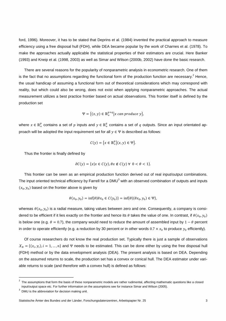
Figure 1: Efficiency and time5
Figure 1a Figure 1b
The reason for this can be found again in the construction of the frontier. Consider a simple situation as pre-
sented in Figure 1 and suppose that company A works efficient �� � 1� at each specific point in time �R, R S 1�.
So, if one presumes constant technology and therefore applies a common frontier, company A’s input/output –
combination in R will be measured as inefficient as shown in Figure 1a. On the other hand, checking for possible
changes in technology and thus calculating two frontiers based on the observations of each time, the company
5
The figure was taken from Grosskopf (1993) and adapted to the example above.
( ) ( )commonyCyC ˆˆ2 ∂=∂y
cA1cA2
2
1,
y
y
0 1x212 ,, xxx ′′ x
( )2ˆ yC∂y
( )1ˆ yC∂
2A
2
1,
y
y
1A
x
1
22 ,,
x
xx
′′′0
2
11 ,,
x
xx
′′′
Statistische Ämter des Bundes und der Länder, Forschungsdatenzentren, Arbeitspapier Nr. 25 6
is found, as assumed, to be efficient at each specific point in time as shown in Figure 1b. Moreover, in the first
case (Fig. 1a) company A seems to have enhanced its efficiency, while it actually was efficient the whole time
(Fig. 1b). Hence, simply assuming a stable technology over time and applying a common frontier would result in
inconsistent estimates. Therefore checking whether there was a change in technology or not is crucial.
A common tool to do this is the frontier shift effect (FSE), which is also a part of the malmquist index.
VWT � XY �U��U�?, �U�?��U�?��U�?, �U�?�Z Y �U��U , �U�
�U�?��U , �U�Z[? O⁄
Values larger than one indicate a positive development in technology. In this case, a company would need
fewer inputs in R S 1 producing the same output compared to the situation in R. The opposite is true if the FSE
takes values below one. Then a company would have to incorporate more inputs in R S 1 to produce the same
amount of output as in R. Consequently a FSE of one shows that the technology was stable over time.
The explanation above is based on the assumption of constant returns to scale which is a certain limitation of
the FSE. As already mentioned one has to check which assumption holds regarding the economies of scale. If
the data reveals that the frontier is characterized by variable returns to scale, it is possible that frontiers intersect
even in the two dimensional case. Moreover, intersecting frontiers are also possible under all scale assumptions
if the dimension is above two.6 In consequence the FSE can lose some of its explanatory power concerning the
direction of a measured frontier shift and its extent.7 This leads to the final question why the FSE should be
used at all? Even with the disadvantage that easily appears the FSE can still only take values above or below
one if there was a change in technology and consequently a frontier shift. Thus, it still provides the necessary
information needed to decide whether or not a common frontier should be estimated.
In order to derive consistent estimates the calculations will have to follow a strict procedure. According to the
theoretical remarks the first step is evaluating which scale assumption holds. As pointed out in this section a
correct assumption is crucial in order to avoid inconsistent estimates. Hence, the actual analysis starts by esti-
mating efficiency scores while utilizing each scale assumption and applying both the Kolmogorov-Smirnov test
and the Wilcoxon rank-sum test. Doing this, a kind of circulus vitiosus occurs. In order to estimate consistent
efficiency scores when testing the scale assumption, one should know if the technology was stable over time
and therefore if a common frontier can be utilized or not. On the other hand, knowing the correct scale assump-
tion is necessary for calculating consistent efficiency scores, which than can be used to determine the correct
frontier approach.
Here, the first calculations were conducted applying a yearly frontier and utilizing each scale assumption.
Thus, the possibility of inconsistent estimates due to a wrong assumption concerning the appropriate time frame
applied when constructing the frontier is avoided. Finally, three series of efficiency scores are available, each
one estimated under a different scale assumption. Based on these data the Kolmogorov-Smirnov test and the
6
A comprehensible example for the three dimensional case under constant returns to scale can be found in Førsund (1993). 7
See Appendix B.
Statistische Ämter des Bundes und der Länder, Forschungsdatenzentren, Arbeitspapier Nr. 25 7
Wilcoxon rank-sum test will be carried out determining the correct scale assumption. Giving this assumption the
question whether there was a change in technology and thus a frontier shift can be answered calculating the
FSE. Giving both assumptions the Hypotheses can be checked.
III. Data
This study uses data from the German Cost Structure Census of manufacturing (CSC) for the period 1995 to
2004. This sample is gathered by the German Federal Statistic office and firms are obliged to deliver the re-
quested data. All companies with more than 500 employees are constantly part of the sample. In addition small-
er companies are also included as a random subsample. The latter is held constant for four years before a new
subsample is created. Hence, within a time frame of four years the sample structure ought to be stable.
Since it is the efficiency of engineering firms that is of interest, all other companies are excluded, giving us a
sample of 23,591 observations between 1995 and 2004 with a wide range of characteristics.8 This large set of
information is generally appreciable but the chosen dimension should not be too high because of the already
mentioned “curse”. Hence, in order to avoid implausible estimates the characteristics were summed up to create
five factors. The first one is output, which is basically the gross production value, adjusted by all revenues that
have nothing to do with the core business of an engineering firm, like turnover out of ‘other activities’ or ‘trading
goods’. These revenues were excluded since they have no explanatory power in terms of a production function.
However, the model contains the input factors: ‘material’, ‘capital costs’, ‘cost of labor’ and ‘other costs’. The
characteristic ‘material’ includes all materials and preliminary products as well as energy. The factor ‘capital
costs’ contains first of all interest and amortization. Moreover, rental and leasing expenditures need to be taken
into account. Since a company could also buy a machine or a building rather than rent it, ‘capital costs’ also
include these expenses. The third input factor is also made up of several characteristics. It entails all wages
including the social insurance contributions that have to be paid by the companies. In addition all social benefits
(e.g. employee pensions) guaranteed by firms beyond legal requirements are summed up in the factor. The
remaining costs like repair, installation etc. are put into the factor ‘other cost’. After creating these new factors
their values are deflated.
Besides merging and deflating, the data were also adjusted for possible outliers and missing values. This is
crucial since nonparametric frontier models are sensitive to both, due to the fact that they do not assume any
functional form of the production function. Thus, all companies without values in one of the created input factors
have been excluded. Thereafter each input factor was divided by its corresponding output (that is the in- and
output for each firm) and all observations with a value greater than the 99.5 percentile are also excluded. Finally
all companies with just one observation over the whole period are deleted, as they are useless in terms of
changes in efficiency. Thus, the final sample contains 5,464 companies with 20,589 observations which are
8
Almost all characteristics entail information in monetary form. In this study only the monetary informations are used and summed up. The only exception is the number of employees, but these are not used as input factor in the calculation.
Statistische Ämter des Bundes und der Länder, Forschungsdatenzentren, Arbeitspapier Nr. 25 8
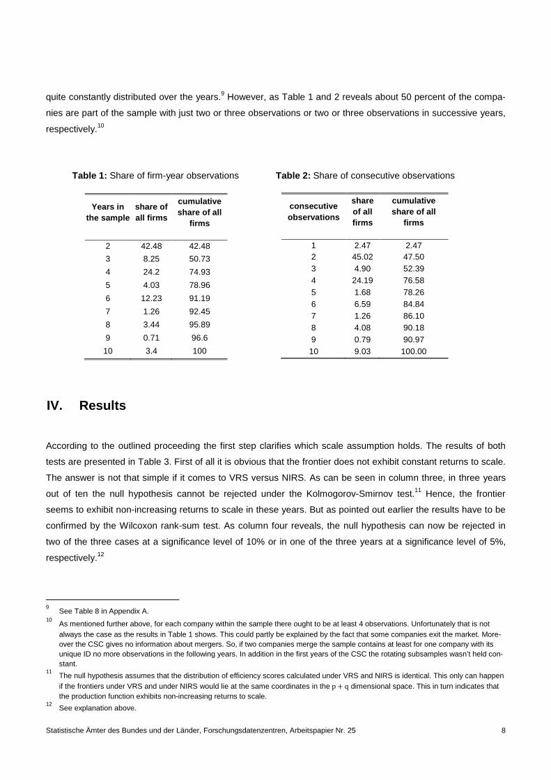
quite constantly distributed over the years.9 However, as Table 1 and 2 reveals about 50 percent of the compa-
nies are part of the sample with just two or three observations or two or three observations in successive years,
respectively.10
Table 1: Share of firm-year observations Table 2: Share of consecutive observations
IV. Results
According to the outlined proceeding the first step clarifies which scale assumption holds. The results of both
tests are presented in Table 3. First of all it is obvious that the frontier does not exhibit constant returns to scale.
The answer is not that simple if it comes to VRS versus NIRS. As can be seen in column three, in three years
out of ten the null hypothesis cannot be rejected under the Kolmogorov-Smirnov test.11 Hence, the frontier
seems to exhibit non-increasing returns to scale in these years. But as pointed out earlier the results have to be
confirmed by the Wilcoxon rank-sum test. As column four reveals, the null hypothesis can now be rejected in
two of the three cases at a significance level of 10% or in one of the three years at a significance level of 5%,
respectively.12
9 See Table 8 in Appendix A.
10 As mentioned further above, for each company within the sample there ought to be at least 4 observations. Unfortunately that is not
always the case as the results in Table 1 shows. This could partly be explained by the fact that some companies exit the market. More-over the CSC gives no information about mergers. So, if two companies merge the sample contains at least for one company with its unique ID no more observations in the following years. In addition in the first years of the CSC the rotating subsamples wasn’t held con-stant.
11 The null hypothesis assumes that the distribution of efficiency scores calculated under VRS and NIRS is identical. This only can happen
if the frontiers under VRS and under NIRS would lie at the same coordinates in the p S q dimensional space. This in turn indicates that the production function exhibits non-increasing returns to scale.
12 See explanation above.
Years in the sample
share of all firms
cumulative share of all
firms
2 42.48 42.48
3 8.25 50.73
4 24.2 74.93
5 4.03 78.96
6 12.23 91.19
7 1.26 92.45
8 3.44 95.89
9 0.71 96.6
10 3.4 100
consecutive observations
share of all firms
cumulative share of all
firms
1 2.47 2.47 2 45.02 47.50 3 4.90 52.39 4 24.19 76.58 5 1.68 78.26 6 6.59 84.84 7 1.26 86.10 8 4.08 90.18 9 0.79 90.97 10 9.03 100.00
Statistische Ämter des Bundes und der Länder, Forschungsdatenzentren, Arbeitspapier Nr. 25 9
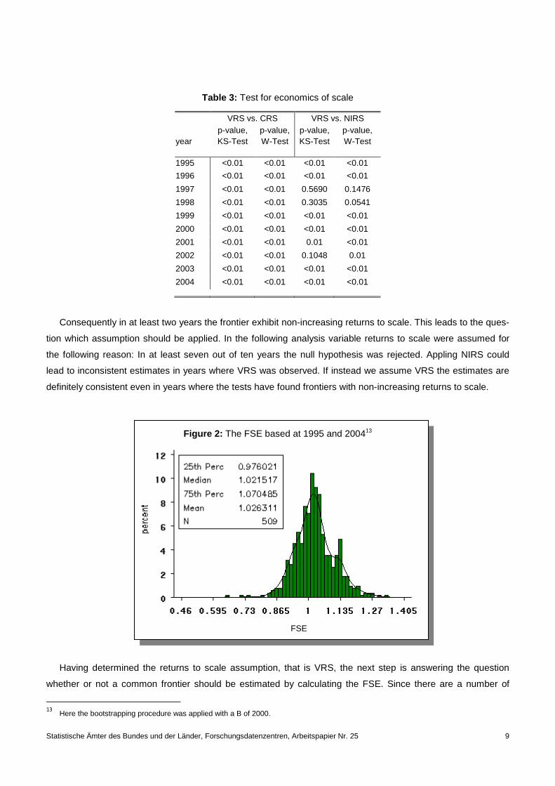
Table 3: Test for economics of scale
Consequently in at least two years the frontier exhibit non-increasing returns to scale. This leads to the ques-
tion which assumption should be applied. In the following analysis variable returns to scale were assumed for
the following reason: In at least seven out of ten years the null hypothesis was rejected. Appling NIRS could
lead to inconsistent estimates in years where VRS was observed. If instead we assume VRS the estimates are
definitely consistent even in years where the tests have found frontiers with non-increasing returns to scale.
Figure 2: The FSE based at 1995 and 200413
Having determined the returns to scale assumption, that is VRS, the next step is answering the question
whether or not a common frontier should be estimated by calculating the FSE. Since there are a number of
13
Here the bootstrapping procedure was applied with a B of 2000.
year
VRS vs. CRS VRS vs. NIRS p-value, KS-Test
p-value, W-Test
p-value, KS-Test
p-value, W-Test
1995 <0.01 <0.01 <0.01 <0.01
1996 <0.01 <0.01 <0.01 <0.01
1997 <0.01 <0.01 0.5690 0.1476
1998 <0.01 <0.01 0.3035 0.0541
1999 <0.01 <0.01 <0.01 <0.01
2000 <0.01 <0.01 <0.01 <0.01
2001 <0.01 <0.01 0.01 <0.01
2002 <0.01 <0.01 0.1048 0.01
2003 <0.01 <0.01 <0.01 <0.01
2004 <0.01 <0.01 <0.01 <0.01
FSE
Statistische Ämter des Bundes und der Länder, Forschungsdatenzentren, Arbeitspapier Nr. 25 10
possible yearly combinations it is most reasonable to use 1995 for R and 2004 for R S 1. If there was a change in
technology over time the larger the time spread the clearer should be the result. The results are presented in
Figure 2.
As the Figure reveals, there was a change in technology over time. Even with a mean of 1.027, at least 50
percent of the FSE’s take values grater 1.07 or less than 0.97. Reminding the effects that intersecting frontiers
do have on the FSE, the results above indicate that a common frontier is no option. In fact the following calcula-
tions will be based on yearly frontiers. This also accounts for the fact that the consecutive observations for
round about fifty percent of all firms within the sample lie within a timeframe of two years.
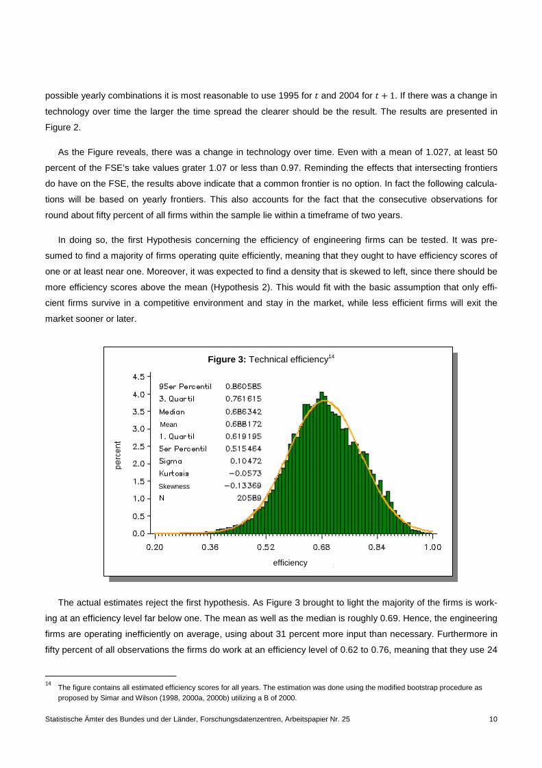
In doing so, the first Hypothesis concerning the efficiency of engineering firms can be tested. It was pre-
sumed to find a majority of firms operating quite efficiently, meaning that they ought to have efficiency scores of
one or at least near one. Moreover, it was expected to find a density that is skewed to left, since there should be
more efficiency scores above the mean (Hypothesis 2). This would fit with the basic assumption that only effi-
cient firms survive in a competitive environment and stay in the market, while less efficient firms will exit the
market sooner or later.
Figure 3: Technical efficiency14
The actual estimates reject the first hypothesis. As Figure 3 brought to light the majority of the firms is work-
ing at an efficiency level far below one. The mean as well as the median is roughly 0.69. Hence, the engineering
firms are operating inefficiently on average, using about 31 percent more input than necessary. Furthermore in
fifty percent of all observations the firms do work at an efficiency level of 0.62 to 0.76, meaning that they use 24
14
The figure contains all estimated efficiency scores for all years. The estimation was done using the modified bootstrap procedure as proposed by Simar and Wilson (1998, 2000a, 2000b) utilizing a B of 2000.
efficiency
Mean
Skewness
Statistische Ämter des Bundes und der Länder, Forschungsdatenzentren, Arbeitspapier Nr. 25 11
to 38 percent more input than necessary. Moreover, in just five percent of all cases firms have had an efficiency
score above 0.86. In contrast, 20 percent of all observed efficiencies are between 0.62 and 0.52. Hence, in
these cases firms used almost twice as much input as necessary.
Even the form of the density is surprising. The estimated efficiency scores have an almost normal distributed
density (with ^ � 06883 and b � 0,105).15 So, there are almost as many firms with efficiency scores below the
mean as there are firms with an efficiency score above the mean. Eventually the second hypothesis of a density
that is skewed to the left is not supported by the results either.
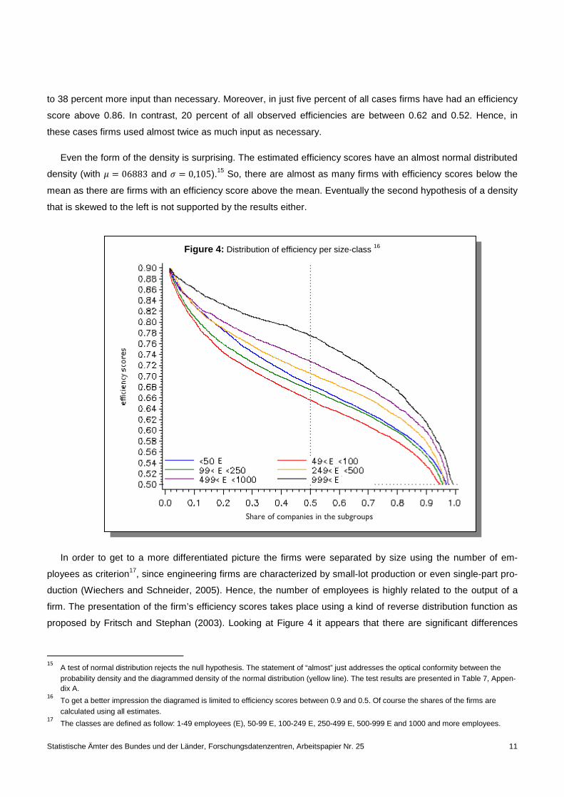
Figure 4: Distribution of efficiency per size-class 16
In order to get to a more differentiated picture the firms were separated by size using the number of em-
ployees as criterion17, since engineering firms are characterized by small-lot production or even single-part pro-
duction (Wiechers and Schneider, 2005). Hence, the number of employees is highly related to the output of a
firm. The presentation of the firm’s efficiency scores takes place using a kind of reverse distribution function as
proposed by Fritsch and Stephan (2003). Looking at Figure 4 it appears that there are significant differences
15
A test of normal distribution rejects the null hypothesis. The statement of “almost” just addresses the optical conformity between the probability density and the diagrammed density of the normal distribution (yellow line). The test results are presented in Table 7, Appen-dix A.
16 To get a better impression the diagramed is limited to efficiency scores between 0.9 and 0.5. Of course the shares of the firms are
calculated using all estimates. 17
The classes are defined as follow: 1-49 employees (E), 50-99 E, 100-249 E, 250-499 E, 500-999 E and 1000 and more employees.
Share of companies in the subgroups
E
E E
E
E E E
Statistische Ämter des Bundes und der Länder, Forschungsdatenzentren, Arbeitspapier Nr. 25 12
between the groups.18 For instance the median company in the class of 50 – 99 employees (red line) has an
efficiency of just 65.62 percent, while the median company in the class of the biggest companies (black line) has
an efficiency score of 77.52 percent. So, the latter works much more efficient than the former. A reason for this
difference could be the fact that larger companies acting globally face a higher competition. Moreover it’s ar-
gued that they better penetrate the market and have more funds to employ a better management (Badunenko,
2007).
Beyond that finding another surprising fact can be revealed by looking at the blue line. The line shows the ef-
ficiency scores of the smallest companies. As it is obvious, it lies above the lines (green and red) of the next
classes (50 – 99 E and 100 – 250 E). It becomes apparent that small companies are on average more efficient
than the next larger ones. The reasons for that are unknown, but one could speculate that there is some kind of
critical mass. That is, the growth of a company goes along with a decline in efficiency. It is reasonable to as-
sume that the price of growth is a decline in efficiency. This happens until some critical mass is achieved and
the firms are forced and have the ability to enhance their efficiency in order to survive in a global market, or to
fall back and reduce size again (or even exit the market). This would fit with the observation that the firms in
each successive class greater than the class of 100 – 249 E are on average more efficient than their predeces-
sor.
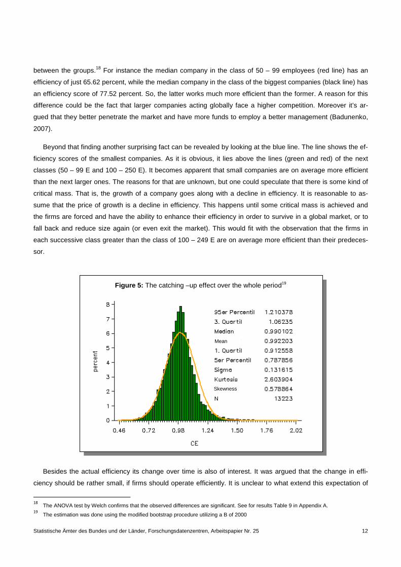
Figure 5: The catching –up effect over the whole period19
Besides the actual efficiency its change over time is also of interest. It was argued that the change in effi-
ciency should be rather small, if firms should operate efficiently. It is unclear to what extend this expectation of
18
The ANOVA test by Welch confirms that the observed differences are significant. See for results Table 9 in Appendix A. 19
The estimation was done using the modified bootstrap procedure utilizing a B of 2000
Skewness
Mean
Statistische Ämter des Bundes und der Länder, Forschungsdatenzentren, Arbeitspapier Nr. 25 13
small changes still holds, as the actual efficiency scores are found to be almost normal distributed. As defined
above the tool to measure the efficiency over time will be the catching-up effect (CE). Moreover, the applied
time frame will be the yearly change in order to use as much of the available data as possible.20 The following
Figure 5 shows all CE – values for all size-classes and all yearly intervals.
First of all it seems that the assumption of small changes still holds. The mean as well as the median is al-
most one (0.99), i.e. on average there have been no great changes in efficiency over time (on a yearly basis).
Nevertheless the figure shows a rather large standard deviation of 0.1316. Based on normal distribution 68 per-
cent of all observed changes would be in the range of 0.99 ± 0.1316. Admittedly the CE – data have no normal
distribution (with ^ � 0.99 and b � 0,1316) as it is diagrammed as yellow line in Figure 5.21
Table 4: Share of observed CE – values of different size (percent)
However, as Table 4 reveals in 35.76 percent of all observations the change was below five percent. On the
other hand, there are yearly changes in efficiency of 5 to 10 percent in 25.66 percent of all measured changes.
Moreover, there have been changes above 10 percent. Thus, a reduction in efficiency of more than 10 percent
could be observed in 21.92 percent of all changes. In contrast an increase in efficiency by more than 10 percent
took place in 16.66 percent of all cases. So, even if one has to admit that the mean as well as the median is
close to one, more than one third of all observed changes are above ten percent. The data also reveal that the
share of observations with a decrease in efficiency prevails. This is not surprising, since an increase in efficien-
cy is linked with some efforts by the company while a decrease is not.
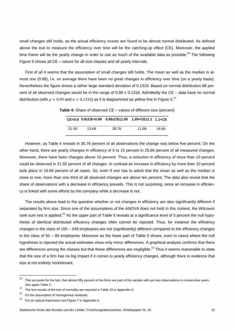
The results above lead to the question whether or not changes in efficiency are also significantly different if
separated by firm size. Since one of the assumptions of the ANOVA does not hold in this context, the Wilcoxon
rank-sum test is applied.22 As the upper part of Table 5 reveals at a significance level of 5 percent the null hypo-
thesis of identical distributed efficiency changes often cannot be rejected. Thus, for instance the efficiency
changes in the class of 100 – 249 employees are not (significantly) different compared to the efficiency changes
in the class of 50 – 99 employees. Moreover as the lower part of Table 5 shows, even in cases where the null
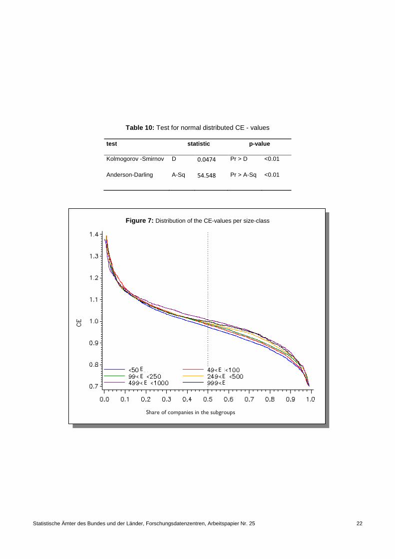
hypothesis is rejected the actual estimates show only minor differences. A graphical analysis confirms that there
are differences among the classes but that these differences are negligible.23 Thus it seems reasonable to state
that the size of a firm has no big impact if it comes to yearly efficiency changes, although there is evidence that
size is not entirely nonrelevant.
20
This accounts for the fact, that almost fifty percent of the firms are part of the sample with just two observations in consecutive years. See again Table 2.
21 The test results of the test of normality are reported in Table 10 in Appendix A.
22 It’s the assumption of homogenous residuals.
23 For an optical impression see Figure 7 in Appendix A.
CE<0.9 0.9≤≤≤≤CE<0.95 0.95≤≤≤≤CE≤≤≤≤1.05 1.05<CE≤≤≤≤1.1 1.1<CE
21.92 13.68 35.76 11.98 16.66
Statistische Ämter des Bundes und der Länder, Forschungsdatenzentren, Arbeitspapier Nr. 25 14
Table 5: Test and descriptive statistic of CE – values per size class24
We also tested whether there is a time related factor that has an influence on the change of efficiency.
Therefore, the estimates are separated by periods and the Wilcoxon rang-sum test is once again used to de-
termine whether or not the efficiency changes are significantly different in each period. In the actual analysis the
periods 96-97, 98-99 and 02-03 have been excluded due to the fact that the number of firms which had reported
their data in both years is relatively small. This traces back to the recollection of data in 1997, 1999 and 2003.
As Table 6 reveals, at a significance level of 5 percent the null hypothesis of no differences between the pe-
riods cannot be rejected in just two cases. Thus, the changes between 1995 and 1996 are not that different from
the changes in period 1997 to 1998. Furthermore, the changes in efficiency in period 95-96 are not significantly
different to the changes in period 00-01. On the other hand it is quite obvious that the change in efficiency in all
other periods is significantly different. Thus, the mean in period 99-00 shows, that the efficiency decreases by
roughly 8.5 percent on average, whereas in period 01-02 the firms enhanced their efficiency by 4 percent on
average. Comparing the results as presented in Table 5 and 6 it becomes apparent, that some time related
component is of importance in explaining the change of efficiency rather than the size of a firm.
It seems reasonable to expect this component to be the engineering business cycle. The idea is the follow-
ing: In rather recessive years (compared to the previous) the companies efforts to reduce inputs in order to ac-
count for a decreasing output could be not strong enough. Thus, in the context of the DEA model the effect
should be a reduced efficiency and accordingly a CE below one. On the other hand if there is a cyclical good
year, companies usually increase their outputs. If this goes along with an almost stable input or at least with an
24
The figures in the header denote the size classes by using the upper boundary as name, e.g. the class of 0 top 49 employees is named 49. The same applies to the row names in the upper part of the table.
size–classes
49 99 249 499 999 1000 all <0.01 0.6492 0.8050 0.0370 <0.01 <0.01 49 <0.01 <0.01 <0.01 <0.01 <0.01 99 0.5812 0.039 <0.01 <0.01 249 0.0986 <0.01 <0.01 499 <0.01 <0.01 999 1 N 2950 2622 2924 1481 975 745 99er percentil e 1.3543 1.3947 1.3715 1.3697 1.3300 1.4108 3. quartil e 1.0524 1.0646 1.0606 1.0617 1.0757 1.0607 median 0.9733 0.9846 0.9887 0.9925 1.0063 0.9989 mean 0.9781 0.9899 0.9906 0.9968 1.0049 0.9989 1. quartil e 0.8930 0.9033 0.9093 0.9262 0.9353 0.9389 1er percentil e 0.6956 0.6781 0.7053 0.7039 0.6912 0.6709 sigma 0.1345 0.1401 0.1297 0.1284 0.1199 0.1291
Statistische Ämter des Bundes und der Länder, Forschungsdatenzentren, Arbeitspapier Nr. 25 15
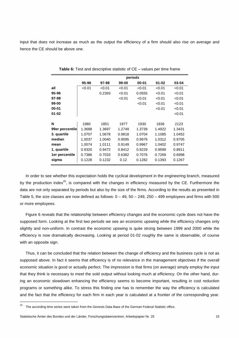
input that does not increase as much as the output the efficiency of a firm should also rise on average and
hence the CE should be above one.
Table 6: Test and descriptive statistic of CE – values per time frame
In order to see whether this expectation holds the cyclical development in the engineering branch, measured
by the production index25, is compared with the changes in efficiency measured by the CE. Furthermore the
data are not only separated by periods but also by the size of the firms. According to the results as presented in
Table 5, the size classes are now defined as follows: 0 – 49, 50 – 249, 250 – 499 employees and firms with 500
or more employees.
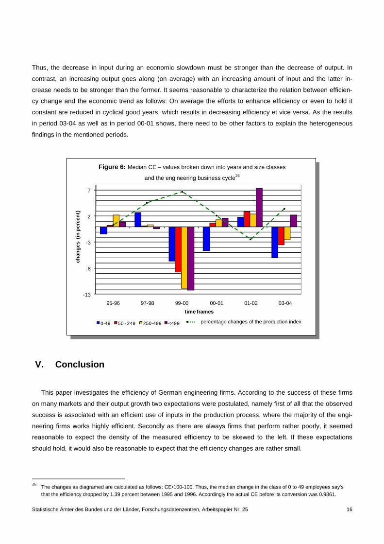
Figure 6 reveals that the relationship between efficiency changes and the economic cycle does not have the
supposed form. Looking at the first two periods we see an economic upswing while the efficiency changes only
slightly and non-uniform. In contrast the economic upswing is quite strong between 1999 and 2000 while the
efficiency is now dramatically decreasing. Looking at period 01-02 roughly the same is observable, of course
with an opposite sign.
Thus, it can be concluded that the relation between the change of efficiency and the business cycle is not as
supposed above. In fact it seems that efficiency is of no relevance in the management objectives if the overall
economic situation is good or actually perfect. The impression is that firms (on average) simply employ the input
that they think is necessary to meet the sold output without looking much at efficiency. On the other hand, dur-
ing an economic slowdown enhancing the efficiency seems to become important, resulting in cost reduction
programs or something alike. To stress this finding one has to remember the way the efficiency is calculated
and the fact that the efficiency for each firm in each year is calculated at a frontier of the corresponding year.
25
The according time series were taken from the Genesis Data Base of the German Federal Statistic office.
periods
95-96 97-98 99-00 00-01 01-02 03-04 all <0.01 <0.01 <0.01 <0.01 <0.01 <0.01 95-96 0.2393 <0.01 0.0555 <0.01 <0.01 97-98 <0.01 <0.01 <0.01 <0.01 99-00 <0.01 <0.01 <0.01 00-01 <0.01 <0.01 01-02 <0.01 N 1980 1851 1977 1930 1836 2123 99er percentil e 1.3688 1.3697 1.2749 1.3739 1.4922 1.3431 3. quartil e 1.0707 1.0678 0.9818 1.0704 1.1085 1.0452 median 1.0037 1.0040 0.9095 0.9976 1.0312 0.9705 mean 1.0074 1.0111 0.9149 0.9967 1.0402 0.9747 1. quartil e 0.9320 0.9472 0.8412 0.9229 0.9599 0.8911 1er percentil e 0.7386 0.7033 0.6382 0.7076 0.7269 0.6998 sigma 0.1228 0.1232 0.12 0.1282 0.1393 0.1267
Statistische Ämter des Bundes und der Länder, Forschungsdatenzentren, Arbeitspapier Nr. 25 16
-13
-8
-3
2
7
95-96 97-98 99-00 .00-01 .01-02 .03-04
chan
ges
(in
per
cent
)
time frames
0-49 50 - 249 250-499 <499 percentage changes of the production index
•
•
•
•
•
•
•
Thus, the decrease in input during an economic slowdown must be stronger than the decrease of output. In
contrast, an increasing output goes along (on average) with an increasing amount of input and the latter in-
crease needs to be stronger than the former. It seems reasonable to characterize the relation between efficien-
cy change and the economic trend as follows: On average the efforts to enhance efficiency or even to hold it
constant are reduced in cyclical good years, which results in decreasing efficiency et vice versa. As the results
in period 03-04 as well as in period 00-01 shows, there need to be other factors to explain the heterogeneous
findings in the mentioned periods.
Figure 6: Median CE – values broken down into years and size classes
and the engineering business cycle26
V. Conclusion
This paper investigates the efficiency of German engineering firms. According to the success of these firms
on many markets and their output growth two expectations were postulated, namely first of all that the observed
success is associated with an efficient use of inputs in the production process, where the majority of the engi-
neering firms works highly efficient. Secondly as there are always firms that perform rather poorly, it seemed
reasonable to expect the density of the measured efficiency to be skewed to the left. If these expectations
should hold, it would also be reasonable to expect that the efficiency changes are rather small.
26
The changes as diagramed are calculated as follows: CE•100-100. Thus, the median change in the class of 0 to 49 employees say’s that the efficiency dropped by 1.39 percent between 1995 and 1996. Accordingly the actual CE before its conversion was 0.9861.
Statistische Ämter des Bundes und der Länder, Forschungsdatenzentren, Arbeitspapier Nr. 25 17
The data envelopment analysis was used to test these expectations, whereas the Farrell’s efficiency scores
are estimated. The analysis was conducted based on a sample of 20,589 observations for the period 1995 to
2004. The first task was to determine which assumption concerning the economies of scale hold. Using the
Kolmogorov-Smirnov and the Wilcoxon rank-sum test it was found that the frontier is determined by variable
returns to scale. Based on this finding the next question concerning the utilization of a common frontier was
analyzed. According to the results the use of a common frontier is no option in the present analysis since the
technology has changed over time. Unfortunately the FSE, which was used to detect this change, loose some of
its explanatory power if the frontier is defined by more than two inputs. The same is true if the frontier is charac-
terized by variable returns to scale. Since both qualities are true in the present context no concrete statement
concerning the modality of the frontier shift and consequently the technological change is possible. However,
the results leave no doubt that there was a change.
After making sure that the assumptions underlying the model are correctly specified the actual analysis was
conducted going after the first expectation. The efficiency scores have been estimated using the appropriate
bootstrap and employing a yearly frontier. The results are surprising. First of all it has to be stated that the ma-
jority of the firms is operating inefficient. The mean of all estimates over the whole period is roughly 0.69.
Hence, the engineering firms could, on average, reduce their input by 31 percent while producing the same
output. The expectation that the success of the German engineering firms goes along with an efficient use of
inputs does not hold. Another interesting finding is the density of the efficiency scores. It seemed reasonable to
assume that the density would be skewed to the left. The analysis revealed that this expectation does not hold
either. The actual estimates are not normal distributed in a statistical sense, i.e. the test for normality did not
support such a predication. Nevertheless the probability density of the efficiency scores is almost normally dis-
tributed as can be seen in Figure 3.
To take a closer look at the efficiency scores the companies were also separated by size. The efficiency
scores in each of the classes differ significantly. Hence it can be pointed out that size is of importance for effi-
ciency. Of course the argument could be brought forward that it is the efficiency that is important for size, i.e.
companies will only become larger if they are efficient. First of all the results show, that there are highly efficient
companies as well as highly inefficient companies in each class. Moreover, it was shown that, in the beginning
and on average, the efficiency falls if firms become larger, so that the size influences efficiency rather than effi-
ciency influences size. The results furthermore lead to the expectation that growth usually goes along with a
decline of efficiency, or in other words that the price of growth is a decrease in efficiency. A test whether this
growth/price relation holds until some critical mass is achieved enabling the firms to enhance their efficiency
once again is left for further research.
Besides efficiency the change of efficiency over time was also of interest. It was expected that the change
will be rather small if the majority of the firms should work efficiently. This expectation was rejected as well.
Even though the mean as well as the median was found to be very close to one, roughly 38 percent of the year-
ly changes were above ten percent. Since the differences between the periods are found to be significantly in
almost all cases it seems reasonable that a factor that drives changes in efficiency would be the engineering

Statistische Ämter des Bundes und der Länder, Forschungsdatenzentren, Arbeitspapier Nr. 25 18
business cycle. The idea behind this expectation is based on the models approach to measure inefficiency. If
the output is reduced while the input is not, accordingly inefficiency should increase et vice versa. The reality
behind this expectation could be that most firms do not react quickly enough when the output goes down by
reducing the amount of employed inputs (e.g. labor input) accordingly. On the other hand if the overall economic
situation becomes better and firms are able to increase their output the additional input required (again for ex-
ample labor) is already employed and therefore the efficiency increases almost automatically. The actual find-
ings lead to doubts concerning such coherences. In fact it seems that firms neglect their efficiency, simply pro-
ducing the desired output if the overall economic situation is good, resulting in an increasing inefficiency. In con-
trast to this if the overall economic situation becomes rather difficult, compared to the previous year, the compa-
nies put more emphasize on efficiency and they reduce the input at a degree that is stronger than the decline of
output. Of course this finding needs further research in order to be more than just a first observation.
Statistische Ämter des Bundes und der Länder, Forschungsdatenzentren, Arbeitspapier Nr. 25 19
References
Badunenko, O. (2007): „Downsizing in German Chemical Manufacturing Industry during the 1990s. Why Small
is Beautiful?“, Discussion Paper 722, DIW, Berlin.
Banker, R. D. (1993): “Maximum Likelihood, Consistency and Data Envelopment Analysis: A Statistical Founda-
tion”, Management Science, 39, 1265 – 1273.
Bjurek, H. (1996): “The Malmquist Total Factor Productivity Index”, Scandinavian Journal of Economics, 98, 303
– 313.
Büning, H and G. Trenkler (1978): Nichparametrische statistische Methoden, Berlin: de Gruyter.
Caves, D. W., L. R. Christensen and W. E. Diewert (1982): “The Economic Theory of Index Numbers and the
Measurement of Input, output, and Productivity”, Econometrica, 50, 1393 – 1414.
Charnes, A., W. W. Cooper and W. Rhodes (1978): “Measuring the Inefficiency of Decision Making Units”, Eu-
ropean Journal of Operational Research 2, 429 – 444.
Deprins, D., L. Simar and H. Tulkens (1984): “Measuring Labor-Efficiency in Post Offices”, In Marchand, M., P.
Pestieau and H. Tulkens (Eds.), The Performance of Public Enterprises: Concepts and Measurements,
Amsterdam: Elsevier Science Publishers B.V.
Farrell, M. J. (1957): “The measurement of productive efficiency”, Journal of the Royal Statistical Society, Series
A, 120, 253 – 281.
Färe, R., S. Grosskopf, B. Lidgren and P. Ross (1994): “Productivity Developments in Swedish Hospitals: A
Malmquist Output Index Approach”, In Charnes A., W. Cooper, A. Y. Lewin and L. M. Seiford (Eds.), Data
Envelopment Analysis. Theory, Methodology and Applications, Dordrecht: Kluwer Academic Publishers,
253 – 272.
Fritsch, M. and A. Stephan (2003): “Die Heterogenität der technischen Effizienz innerhalb von Wirtschaftszwei-
gen“, In Pohl, R., J. Fischer, U. Rockmann and K. Semlinger (Eds.), Analysen zur regionalen Industrie-
entwicklung – Sonderauswertungen einzelbetrieblicher Daten der Amtlichen Statistik, Berlin: Statistisches
Landesamt, 143 – 156.
Grosskopf, S. (1993): „Efficiency and Productivity”, In Fried, H., C. A. K. Lovell and S. S. Schmidt (Eds.), The
Measurement of Productive Efficiency, Techniques and Application, Oxford: Oxford University Press, 160
– 194.
Kneip, A., B. U. Park and L. Simar (1998): “A Note on the Convergence of Nonparametric DEA Estimators for
Production Efficiency Scores”, Econometric Theory, 14, 783 – 793.
Statistische Ämter des Bundes und der Länder, Forschungsdatenzentren, Arbeitspapier Nr. 25 20
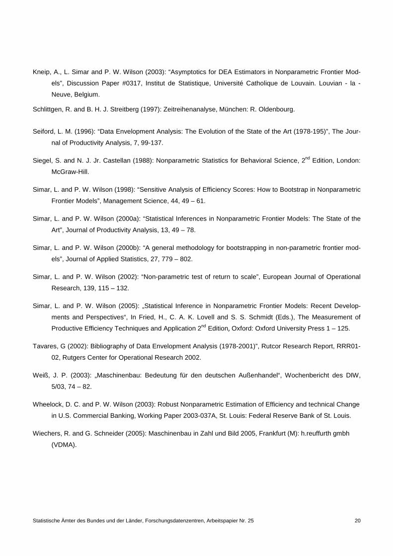
Kneip, A., L. Simar and P. W. Wilson (2003): “Asymptotics for DEA Estimators in Nonparametric Frontier Mod-
els”, Discussion Paper #0317, Institut de Statistique, Université Catholique de Louvain. Louvian - la -
Neuve, Belgium.
Schlittgen, R. and B. H. J. Streitberg (1997): Zeitreihenanalyse, München: R. Oldenbourg.
Seiford, L. M. (1996): “Data Envelopment Analysis: The Evolution of the State of the Art (1978-195)”, The Jour-
nal of Productivity Analysis, 7, 99-137.
Siegel, S. and N. J. Jr. Castellan (1988): Nonparametric Statistics for Behavioral Science, 2nd Edition, London:
McGraw-Hill.
Simar, L. and P. W. Wilson (1998): “Sensitive Analysis of Efficiency Scores: How to Bootstrap in Nonparametric
Frontier Models”, Management Science, 44, 49 – 61.
Simar, L. and P. W. Wilson (2000a): “Statistical Inferences in Nonparametric Frontier Models: The State of the
Art”, Journal of Productivity Analysis, 13, 49 – 78.
Simar, L. and P. W. Wilson (2000b): “A general methodology for bootstrapping in non-parametric frontier mod-
els”, Journal of Applied Statistics, 27, 779 – 802.
Simar, L. and P. W. Wilson (2002): “Non-parametric test of return to scale”, European Journal of Operational
Research, 139, 115 – 132.
Simar, L. and P. W. Wilson (2005): „Statistical Inference in Nonparametric Frontier Models: Recent Develop-
ments and Perspectives“, In Fried, H., C. A. K. Lovell and S. S. Schmidt (Eds.), The Measurement of
Productive Efficiency Techniques and Application 2nd Edition, Oxford: Oxford University Press 1 – 125.
Tavares, G (2002): Bibliography of Data Envelopment Analysis (1978-2001)”, Rutcor Research Report, RRR01-
02, Rutgers Center for Operational Research 2002.
Weiß, J. P. (2003): „Maschinenbau: Bedeutung für den deutschen Außenhandel“, Wochenbericht des DIW,
5/03, 74 – 82.
Wheelock, D. C. and P. W. Wilson (2003): Robust Nonparametric Estimation of Efficiency and technical Change
in U.S. Commercial Banking, Working Paper 2003-037A, St. Louis: Federal Reserve Bank of St. Louis.
Wiechers, R. and G. Schneider (2005): Maschinenbau in Zahl und Bild 2005, Frankfurt (M): h.reuffurth gmbh
(VDMA).
Statistische Ämter des Bundes und der Länder, Forschungsdatenzentren, Arbeitspapier Nr. 25 21
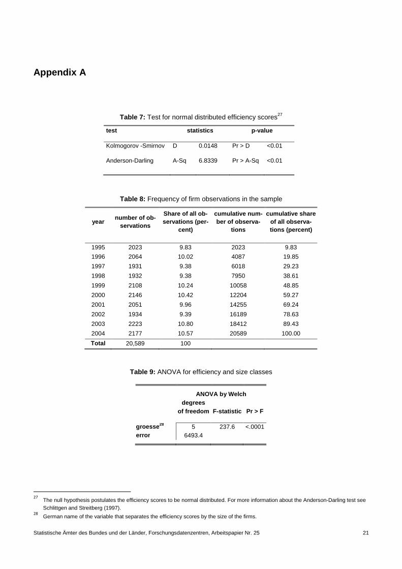
Appendix A
Table 7: Test for normal distributed efficiency scores27
test statisti cs p-value
Kolmogorov -Smirnov D 0.0148 Pr > D <0.01
Anderson-Darling A-Sq 6.8339 Pr > A-Sq <0.01
Table 8: Frequency of firm observations in the sample
year number of ob-
servations
Share of all ob-servations (per-
cent)
cumulative num-ber of observa-
tions
cumulative share of all observa-tions (percent)
1995 2023 9.83 2023 9.83
1996 2064 10.02 4087 19.85
1997 1931 9.38 6018 29.23
1998 1932 9.38 7950 38.61
1999 2108 10.24 10058 48.85
2000 2146 10.42 12204 59.27
2001 2051 9.96 14255 69.24
2002 1934 9.39 16189 78.63
2003 2223 10.80 18412 89.43
2004 2177 10.57 20589 100.00
Total 20,589 100
Table 9: ANOVA for efficiency and size classes
27
The null hypothesis postulates the efficiency scores to be normal distributed. For more information about the Anderson-Darling test see Schlittgen and Streitberg (1997).
28 German name of the variable that separates the efficiency scores by the size of the firms.
ANOVA by Welch degrees
F-statistic Pr > F of freedom
groesse 28 5 237.6 <.0001 error 6493.4
Statistische Ämter des Bundes und der Länder, Forschungsdatenzentren, Arbeitspapier Nr. 25 22
Table 10: Test for normal distributed CE - values
Figure 7: Distribution of the CE-values per size-class
test statistic p-value
Kolmogorov -Smirnov D 0.0474 Pr > D <0.01
Anderson-Darling A-Sq 54.548 Pr > A-Sq <0.01
Share of companies in the subgroups
E E
E
E E E
Statistische Ämter des Bundes und der Länder, Forschungsdatenzentren, Arbeitspapier Nr. 25 23
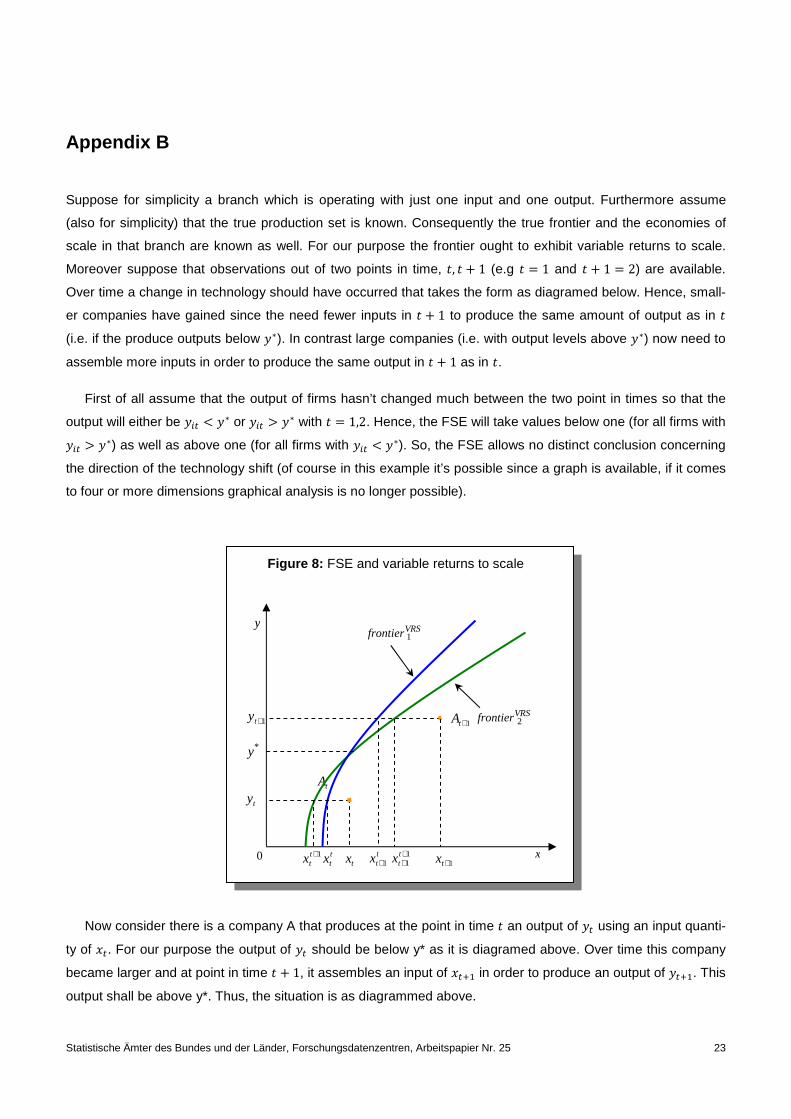
Appendix B
Suppose for simplicity a branch which is operating with just one input and one output. Furthermore assume
(also for simplicity) that the true production set is known. Consequently the true frontier and the economies of
scale in that branch are known as well. For our purpose the frontier ought to exhibit variable returns to scale.
Moreover suppose that observations out of two points in time, R, R S 1 (e.g R � 1 and R S 1 � 2) are available.
Over time a change in technology should have occurred that takes the form as diagramed below. Hence, small-
er companies have gained since the need fewer inputs in R S 1 to produce the same amount of output as in R
(i.e. if the produce outputs below �f). In contrast large companies (i.e. with output levels above �f) now need to
assemble more inputs in order to produce the same output in R S 1 as in R.
First of all assume that the output of firms hasn’t changed much between the two point in times so that the
output will either be �0U # �f or �0U B �f with R � 1,2. Hence, the FSE will take values below one (for all firms with
�0U B �f) as well as above one (for all firms with �0U # �f). So, the FSE allows no distinct conclusion concerning
the direction of the technology shift (of course in this example it’s possible since a graph is available, if it comes
to four or more dimensions graphical analysis is no longer possible).
Figure 8: FSE and variable returns to scale
Now consider there is a company A that produces at the point in time R an output of �U using an input quanti-
ty of �U. For our purpose the output of �U should be below y* as it is diagramed above. Over time this company
became larger and at point in time R S 1, it assembles an input of �U�? in order to produce an output of �U�?. This
output shall be above y*. Thus, the situation is as diagrammed above.
tA
x
y
*y
VRSfrontier 1
VRSfrontier 2
ty
1+ty
0
1+tA
1+ttx t
tx tx ttx 1+
11
++
ttx 1+tx
Statistische Ämter des Bundes und der Länder, Forschungsdatenzentren, Arbeitspapier Nr. 25 24
Firstly it became obvious that the inefficiency of firm A at each point in time has no influence regarding the
value of its FSE. This traces back to the fact that the observed output/input relation in each component in the
brackets is kept constant.29 Thus, just the location of both frontiers for each output level is of importance for the
value of the FSE. If one defines the first component in the brackets as VWT� � ��U��U�?, �U�?� �U�?��U�?, �U�?�⁄ �
and the second component as VWTg � ��U��U , �U� �U�?��U , �U�⁄ � the direction of the frontier shift as it is revealed
by the FSE depends on the successive basic constraints:
1. VWTg B 1 VWT�⁄ → VWT B 1
2. VWTg # 1 VWT�⁄ → VWT # 1
3. VWTg � 1 VWT�⁄ → VWT � 1
Hence, the FSE will only takes values greater one if the second frontier lies enough to left of the first one
(relatively) for one of the two output levels. Secondly, it is important to notice that the FSE will tend to one even
if there was a significant change in technology since either the FSEa or the FSEb will take a value greater one
while the other will be below one. In the extreme the third constraint is fulfilled and the FSE will be one. Fur-
thermore, since the product of the FSEa and the FSEb is treated with a root, the FSE must tend towards one. In
the end the FSE can take values near one even if there was a significant change in technology provided that the
frontiers intersect.
29
The first component in the brackets is θi�xi�?, yi�?� θi�?�xi�?, yi�?�⁄ . In the two dimensional example above this could be rewritten as
θi�xi�?, yi�?� � 0xi�?i /0xi�? and θi�?�xi�?, yi�?� � 0xi�?i�?/0xi�?. It follows �0xi�?i /0xi�?� �0xi�?i�?/0xi�?�⁄ and therefore 0xi�?i 0xi�?i�?⁄ . The same can be shown for the second component in the brackets. In the end the second component can be reduced to 0xii 0xii�?⁄ . As it is obvious, the outcome of the FSE depends only upon the location of the two frontiers at each point in time and for each output level.

Statistische Ämter des Bundes und der Länder,FDZ-Arbeitspapier Nr. 25, German engeneering firms during the 1990‘s. How efficient are export champions?, 2008
Recommended