BUREAU OF MINERAL RESOURCES, GEOLOGY AND GEOPHYSICS

RECORD

RECORD 1988/19

a R.V.RIG SEISHIC RESEARCH CRUISE 3,

OFFSHORE, OTWAY BASIN:

EXPLANATORY NOTES TO ACCOMPANY RELEASE OF NON-SEISMIC DATA

by

C. Lawson & M. Hazell

ion' contained in this report he. been obteined by the Bureeu of Minerel Resource., Geology end Geophysic ... ~licY of the Austrelien Governm~t, to e •• i.t in the exploretion end development of minerel resourc... It may not be eny form or ueed In e company pro.pectu. or .tatement without the perml .. ion in writing of the Director.

Bureau of Mineral Resources, Geology & Geophysics

DIVISION OF MARINE GEOSCIENCES & PETROLEUM GEOLOGY

RECORD 1988/19

R.V.RIG SEISMIC RESEARCH CRUISE 3,

OFFSHORE, OTWAY BASIN:

EXPLANATORY NOTES TO ACCOMPANY RELEASE OFNON-SEISMIC DATA

by

C.Lawson & M.Hazell

1^1 111 1111 1 1* R 8 8 0 9 0 *

CONTENTS

INTRODUCTION

GEOPHYSICAL SYSTEMS & PERFORMANCE

DATA ACQUISITION SYSTEM (DAS)

DATA PROCESSING

DATA AVAILABILITY

FIGURES

FIGURE 1: Bathymetry traces before and after processing by program SALVG.

FIGURE 2: Satellite fix assessment plot - prior to processing

Page 1

Page 1

Page 2

Page 5

Page 17

Page 13

Page 14

FIGURE 3: Satellite fix assessment plot - post processing Page 15

FIGURE 4: Tracks of Rig Seismic Survey 48 in the Bass Strait

TABLES

Page 16

TABLE 1: Field tape channel allocations. Page 3

TABLE 2: Processing channel allocations. Page 6

TABLE 3: Filter coefficients and approximate response of Page 8 filter to sine wave for magnetics filter.

TABLE 4: Sample satellite fix listing. Page 10

TABLE 5: Final channel allocations. Page 12

INTRODUCTION

The purpose of this report is to summarise the processing techniques applied to the non-seismic geophysical data on R.V.Rig Seismic Research Cruise 3 (BMR Marine Survey 48, Otway Basin of Bass Strait). The cruise was conducted between 15 June and 12 July 1985 and formed part of project 1D06 (1985/1986) and project 1C03 (1986/1987) .

GEOPHYSICAL SYSTEMS & PERFORMANCE

The following non-seismic geophysical systems were employed during Survey 48:

Navigation

Three totally independent navigation techniques were run simultaneously;

1. Magnavox Global Positioning System (GPS) T-Set, g1v1ng continous 2-D positioning to within 35 m RMS, during periods of satellite availability and good geometry.

2. Motorolla Miniranger Radio Navigation System, utilizing four shore based transponders. This system has a potential accuracy to within 5 metres.

3. A dead reckoning (DR) system, incorporating satellite navigators, gyro compasses, and sonar dopplers. The primary system, consisted of a Magnavox MXll07RS dual-channel satellite navigator, with speed input from Magnavox MX6l0D sonar doppler and headings from an Arma-Brown gyro-compass. The secondary system, consisted of a Magnavox MXl142 single channel satellite navigator, with speed input from Raytheon DSN 450 sonar doppler and headings from a Robertson gyro-compass. This system has a potential accuracy of 0.2km at fixes rising to around lkm between fixes in deep water.

Performance Comments: Both satellite navigators generally performed reliably. The MX1l07RS was interfaced to the Data Acquisition System (DAS) and latitude, longitude, course, speed (every 10 seconds) and all satellite fix details were transferred and recorded. The percentage of the total time that each system was the primary navigation system during the cruise is;

T-Set :27%

Radio Nav :12%

Dead Reckoning :61%

Both gyro-compasses performed satisfactorily for the entire survey. Both sonar dopplers performed fairly satisfactorily in low sea states but were generally erratic in high sea states.

Bathymetric Systems

Raytheon Deep-sea Bathymetric System, with a maximum power output of 2 kW at 12 kHz. This system, purchased in the early 1970's, was of very sophisticated design for its day, providing in addition to digital depths and various alarm flags, an automatic tracking facility that should theoretically provide usable bathymetric data even in marginal rec0rding conditions.

1

A new 3.5 kHz system was installed in Melbourne prior to Survey 48. This new system included an additional 8 transducers bringing the total to 16.

Performance Comments: Data quality was generally poor due to the high sea states encountered on the survey. The extensive processing required to retrieve acceptable bathymetric data is described fully later in this report.

Magnetics

Two Geometrics G801/803 proton precession magnetometers were installed in the instrument room; signals were acquired from both single and dual channel (horizontal gradient) sensors towed astern of the vessel.

Performance Comments: Performance was not as good as expected due to excessive noise. Noise level for the magnetometer was in excess of plus/minus 3 nT.

Gravity

A Bodenseewerk KSS-31 marine gravity meter has been installed on the Rig Seismic. Gravity data were recorded for the entire survey.

Performance Comments: The KSS-3l is a highly sophisticated single-axis marine gravity meter with extensive microprocessor control. The KSS-3l is designed to be interfaced to an external navigation system that can provide speed and heading input at a rate of as fast as 1 second; the speed and heading are then used by the processor to provide gyro corrections to the gravity meter to improve performance in heavy seas or during turns. For Survey 48, satisfactory gravity data have been achieved with appropriate post-survey filtering, except at sample sites where poor speed control and continuous vessel manoeuvring have produced erratic Eotvos corrections.

Due to system malfunction no data were acquired between 48,181,213200 and 48,183,055000.

DATA ACQUISITION SYSTEM (DAS)

The shipboard DAS is based on a Hewlett-Packard (HP) 1000 E-Series 16-bit minicomputer. The DAS programs run under the HP Real Time Executive (RTE-6/VM) disc-based operating system, which allows a multiprogramming environment and a large number of interactive users. Data are acquired either directly from the appropriate device through an RS-232C interface (gravity, Magnavox MXll07RS), or through a BMR-designed l6-bit digital multiplexer (magnetics, bathymetry) and attached gyro-log interface (for both sonar dopplers and gyro-compasses). After preliminary processing, plotting on strip-chart recorders, and listing on a variety of printers, the data were recorded on 9-track, 1600 bpi, phase-encoded magnetic tape in HP's 32-bit floating-point format.

Data were acquired and saved at a 10-second rate, regardless of ship speed and independently of the seismic acquisition system. The data were written to tape in 2.0 minute (12 record) blocks with 80 channels of data being recorded. The channels that were recorded are listed in Table 1.

2

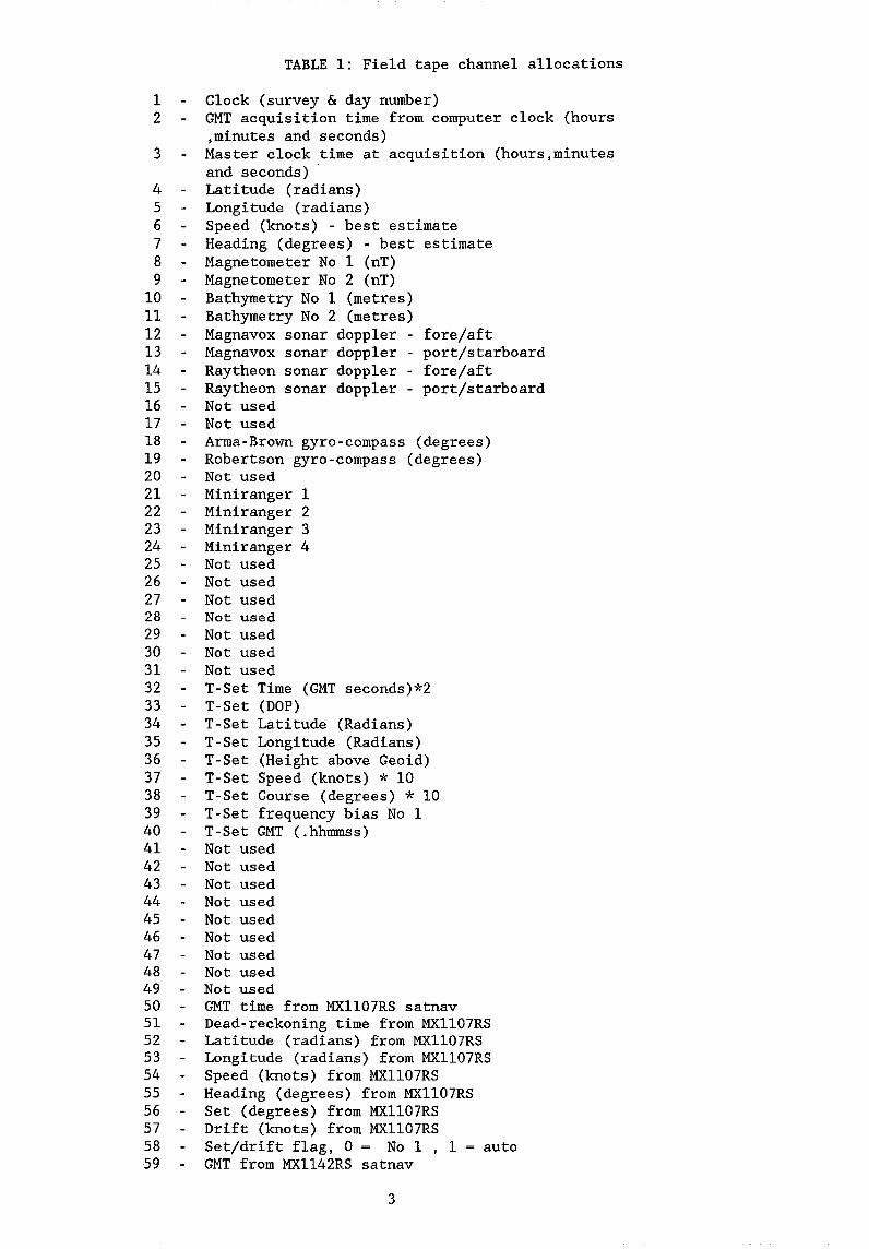
TABLE 1: Field tape channel allocations

1 Clock (survey & day number) 2 GMT acquisition time from computer clock (hours

,minutes and seconds) 3 Master clock time at acquisition (hours,minutes

and seconds) 4 Latitude (radians) 5 Longitude (radians) 6 Speed (knots) - best estimate 7 Heading (degrees) - best estimate 8 Magnetometer No 1 (nT) 9 Magnetometer No 2 (nT)

10 Bathymetry No 1 (metres) 11 Bathymetry No 2 (metres) 12 Magnavox sonar doppler - fore/aft 13 Magnavox sonar doppler - port/starboard 14 Raytheon sonar doppler - fore/aft 15 Raytheon sonar doppler - port/starboard 16 Not used 17 Not used 18 Arma-Brown gyro-compass (degrees) 19 Robertson gyro-compass (degrees) 20 Not used 21 Miniranger 1 22 Miniranger 2 23 Miniranger 3 24 Miniranger 4 25 Not used 26 Not used 27 Not used 28 Not used 29 Not used 30 Not used 31 Not used 32 T-Set Time (GMT seconds)*2 33 T-Set (DOP) 34 T-Set Latitude (Radians) 35 T-Set Longitude (Radians) 36 T-Set (Height above Geoid) 37 T-Set Speed (knots) * 10 38 T-Set Course (degrees) * 10 39 T-Set frequency bias No 1 40 T-Set GMT (.hhmmss) 41 42 43 44 45 46 47 48

Not Not Not Not Not Not Not Not

used used used used used used used used

49 Not used 50 GMT time from MX1107RS satnav 51 Dead-reckoning time from MXll07RS 52 Latitude (radians) from MXII07RS 53 Longitude (radians) from MXII07RS 54 Speed (knots) from MX1l07RS 55 Heading (degrees) from MX1107RS 56 Set (degrees) from MXll07RS 57 Drift (knots) from MXl107RS 58 Set/drift flag, 0 = No 1 1 auto 59 GMT from MXl142RS satnav

3

60 Dead-reckoning time from MXl142RS 61 Latitude (radians) from MXl142RS 62 Longitude (radians) from MXl142RS 63 Speed (knots) from MXl142RS 64 Heading (degrees) from MXl142RS 65 Set (degrees) from MXl142RS 66 Drift (knots) from MXl142RS 67 Set/drift flag from MXl142 , 0 = manual,

1 = automatic 68 Vector speed Magnavox sonar doppler 69 Vector speed Raytheon sonar doppler 70 Not used 71 Not used 72 Not used 73 Not used 74 Gravity (urns**-2 * 1000) 75 ACX (ms**2 * 1000) 76 ACY (ms**2 * 1000) 77 Sea State 78 Not used 79 Not used 80 Not used

4

DATA PROCESSING

The data were processed on an in-house Hewlett-Packard 1000 F-Series minicomputer utilising similar hardware and the same operating system as the DAS. The processing was applied in two phases, as follows:

Phase 1: transcription of field tapes; correction of time errors; production of raw data plots; bulk editing (principally deletion of bad data segments); retrieval of water depth data; assessment and retrieval of velocities; medium filter of magnetics and gravity; manual editing of problem areas; computation of incremental latitudes and longitudes; anti-alias filtering (smoothing) of magnetics, gravity, incremental latitudes and longitudes; production of final check plots; final editing.

Phase 2: tying of the dead-reckoned (DR) track to the satellite fixes using a cubic spline fitting technique to model ocean currents; assessment and deletion of poor quality satellite fixes; computation of final positions for each DR system; computation of final ship position from an appropriate mix of the available DR systems, GPS system and radio nav system; computation of final Eotvos-corrected gravity, including a correction for gravity meter drift; final data editing (particularly gravity data during turns).

A brief summary of the processing steps follows, with some detail of the techniques applied.

PHASE 1

FCOPY: All field tapes were transcribed to processing tapes with several field tapes being combined into a single processing tape. Processing tapes were separated at obvious breaks (such as recording system crashes), or after about seven days recording. Time jumps (positive or negative) were reported for processing in the next phase.

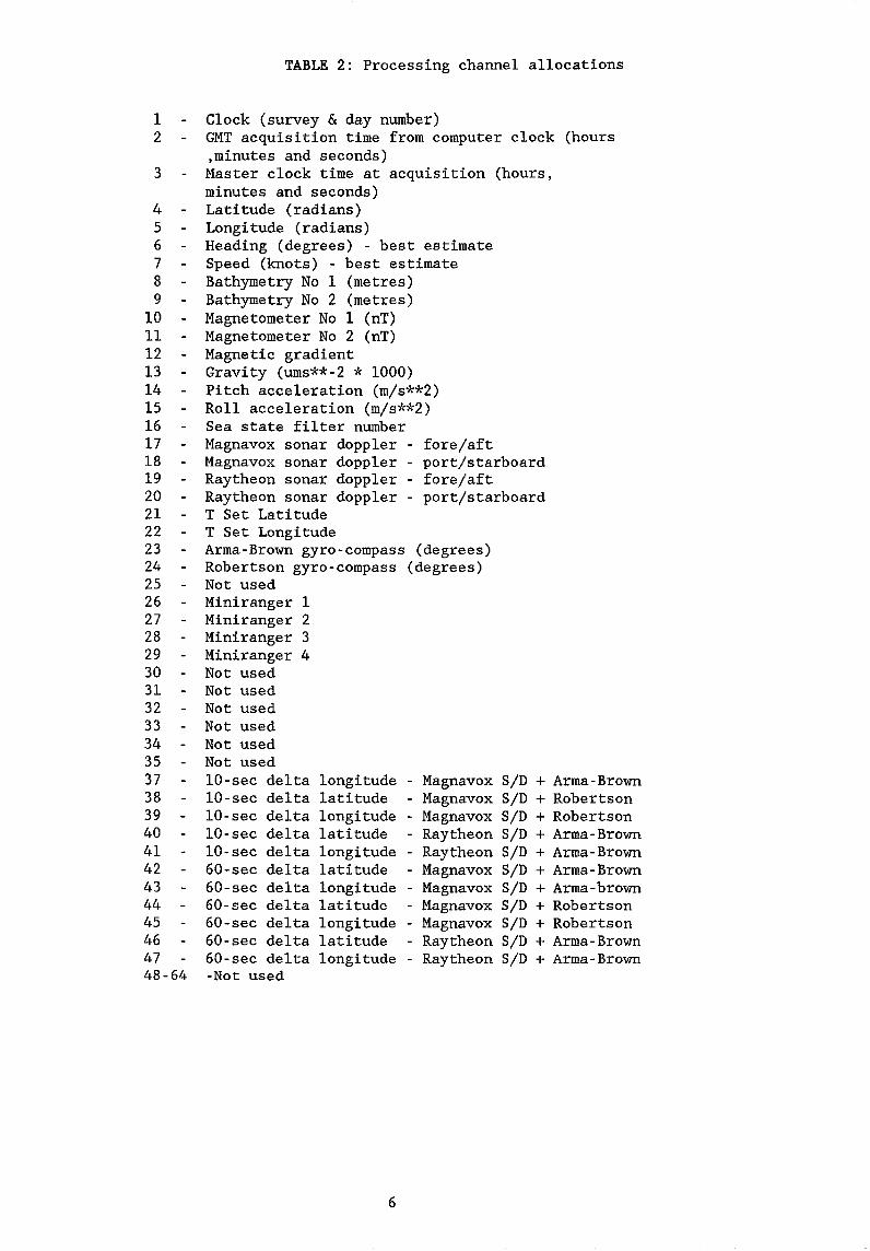
FIXTM: Time jumps reported in FCOPY were corrected, either automatically, or with a file of manual time corrections. Data channels were re-ordered (Table 2) to simplify further processing.

SALVG OVater depth recovery): Briefly stated, the problem of bathymetry recovery is to fill in all the gaps left after the Raytheon hardware/software flags were removed and to discriminate against the bad bathymetric values that still remain. To accomplish this, a file was first created of manually digitised water depths at selected points; this file was then read in conjunction with the processing data file. SALVG then performs a straight line interpolation between adjacent tie points and compares the interpolated depth with the 10-second digital depth. If the difference is less than a user-specified threshold, then the digital depth is accepted and is used to replace the previous first tie point. If the difference is greater than the threshhold, then the 10-second digital depth is replaced by the interpolated depth. In this way, the program tracks along the acceptable water depths, providing the threshold is small enough to reject bad data and large to accept good data. In the case of good digital data being totally unacceptable, as during poor sea conditions, the threshold was set to a very small number (O.Olm) and the process became one of very simple linear interpolation between adjacent tie points.

5

1 2

3

4 5 6 7 8 9

10 11 12 13 14 15 16 17 18 19 20 21 22 23 24 25 26 27 28 29 30 31 32 33 34 35 37 38 39 40 41 42 43 44 45 46 47 48-64

TABLE 2: Processing channel allocations

Clock (survey & day number) GMT acquisition time from computer clock (hours ,minutes and seconds) Master clock time at acquisition (hours, minutes and seconds) Latitude (radians) Longitude (radians) Heading (degrees) - best estimate Speed (knots) - best estimate Bathymetry No 1 (metres) Bathymetry No 2 (metres) Magnetometer No 1 (nT) Magnetometer No 2 (nT) Magnetic gradient Gravity (ums**-2 * 1000) Pitch acceleration (m/s**2) Roll acceleration (m/s**2) Sea state filter number Magnavox sonar doppler - fore/aft Magnavox sonar doppler - port/starboard Raytheon sonar doppler - fore/aft Raytheon sonar doppler - port/starboard T Set Latitude T Set Longitude Arma-Brown gyro-compass (degrees) Robertson gyro-compass (degrees) Not used Miniranger 1 Miniranger 2 Miniranger 3 Miniranger 4 Not used Not used Not used Not used Not used Not used 10-sec delta longitude - Magnavox 10-sec delta latitude - Magnavox 10-sec delta longitude - Magnavox 10-sec delta latitude - Raytheon 10-sec delta longitude - Raytheon 60-sec delta latitude - Magnavox 60-sec delta longitude - Magnavox 60-sec delta latitude - Magnavox 60-sec delta longitude - Magnavox 60-sec delta latitude - Raytheon 60-sec delta longitude - Raytheon -Not used

6

SID + Arma-Brown SID + Robertson SID + Robertson SID + Arma-Brown SID + Arma-Brown SID + Arma-Brown SID + Arma-brown SID + Robertson SID + Robertson SID + Arma-Brown SID + Arma-Brown

In practice the interval between manually digitised tie points varied from several hours in the case of good digital 10-second data, to several minutes in the case of poor 10-second data or a very rugged sea bed. The success of this process, which is routinely applied to all Rig Seismic bathymetric data, can be seen in the 'before ' and 'after' plots of Figures 1 and 2.

VARPL: All raw data channels requiring processing were plotted as strip records on a drum plotter. These plots were used to determine where editing was required and as a first guide for the setting of filter parameters.

FTAPE: This program was used for a variety of tasks as follows - (1) Removal of hardware/software flags in the bathymetric data. The Raytheon echo-sounder system provides, in addition to digital bathymetry, I flags' indicating that the echo-sounder has lost track or that the digitiser gate is searching for an echo. These flags were removed, as appropriate, and such values were replaced by the number 1.OElO (10 raised to the power 10), to indicate absent data. (2) I Bulk I deletions were done of any large blocks of irretrievable data in particular channels. (3) Automatic interpolations were done across data gaps of up to 120 seconds for selected data channels.

FDATA: The magnetic, gravity, and Magnavox and Raytheon speed log data were filtered using a sophisticated form of the medium filter, a highly successful spike deletion tool.

EDATA: This is a utility program used for the manual editing of problem areas that are not amenable to filtering or automatic editing.

MUFF: This program uses a SING function filter to smooth selected data channels. All velocity channels were smoothed to provide acceptable speeds, while gravity and magnetic data were filtered as an anti-aliasing measure prior to resampling to 60 s. The filter coefficients and the approximate responses of the filters to a sine wave are given in Table 3.

DELTA: Incremental (delta) latitude/longitudes were produced every 10 seconds by combining the ship speed with the headings from the Arma-Brown and Robertson gyro-compasses. This effectively gave two distinct dead-reckoning (DR) systems.

INTEG: The filtered incremental latitude/longitudes were re-integrated over running 60-second intervals. These 60-second incremental distances were then used in the Phase 2 processing to compute the DR vector over each satellite fix interval.

VARPL/EDATA: As the final stage of the Phase 1 processing, all processed channels were plotted again as 'strip' plots with program VARPL. Program EDATA was then used to correct any minor residual data problems.

7

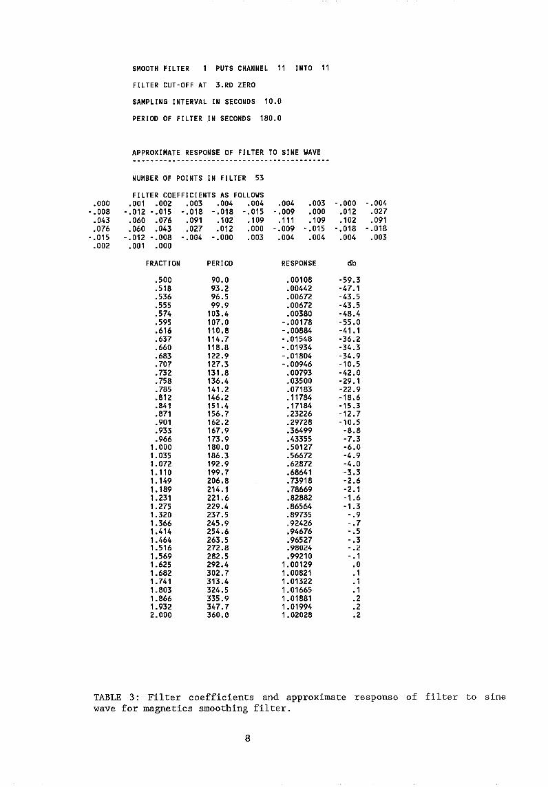
SMOOTH FILTER PUTS CHANNEL 11 INTO 11

FILTER CUT-OFF AT 3.RD ZERO

SAMPLING INTERVAL IN SECONDS 10.0

PERIOD OF FILTER IN SECONDS 180.0

APPROXIMATE RESPONSE OF FILTER TO SINE WAVE ---------------------------------------------

NUMBER OF POINTS IN FILTER 53

FILTER COEFFICIENTS AS FOLLOWS .000 .001 .002 .003 .004 .004 .004 .003 -.000 -.004

-.008 -.012 -.015 -.018 -.018 -.015 -.009 .000 .012 .027 .043 .060 .076 .091 .102 .109 .111 .109 .102 .091 .076 .060 .043 .027 .012 .000 -.009 -.015 - .018 -.018

-.015 -.012 -.008 -.004 -.000 .003 .004 .004 .004 .003 .002 .001 .000

FRACTION PERIOD RESPONSE db

.500 90.0 .00108 ·59.3

.518 93.2 .00442 -47.1

.536 96.5 .00672 -43.5

.555 99.9 .00672 -43.5

.574 103.4 .00380 -48.4

.595 107.0 -.00178 -55.0

.616 110.8 -.00884 -41.1

.637 114.7 -.01548 -36.2

.660 118.8 -.01934 -34.3

.683 122.9 -.01804 -34.9

.707 127.3 -.00946 -10.5

.732 131.8 .00793 -42.0

.758 136.4 .03500 -29.1

.785 141.2 .07183 -22.9

.812 146.2 .11784 -18.6

.841 151.4 .17184 -15.3

.871 156.7 .23226 -12.7

.901 162.2 .29728 -10.5

.933 167.9 .36499 -8.8

.966 173.9 .43355 -7.3 1.000 180.0 .50127 -6.0 1.035 186.3 .56672 -4.9 1.072 192.9 .62872 -4.0 1.110 199.7 .68641 -3.3 1.149 206.8 .73918 -2.6 1.189 214.1 .78669 -2.1 1.231 221.6 .82882 -1.6 1.275 229.4 .86564 -1.3 1.320 237.5 .89735 - .9 1.366 245.9 .92426 -.7 1.414 254.6 .94676 -.5 1.464 263.5 .96527 - .3 1.516 272.8 .98024 -.2 1.569 282.5 .99210 - .1 1.625 292.4 1.00129 .0 1.682 302.7 1.00821 .1 1.741 313.4 1.01322 .1 1.803 324.5 1.01665 .1 1.866 335.9 1.01881 .2 1.932 347.7 1.01994 .2 2.000 360.0 1.02028 .2

TABLE 3: Filter coefficients and approximate response of filter to sine wave for magnetics smoothing filter.

8

PHASE 2

Phase 2 processing encompasses the following steps -

1. Re-formatting and production of assessment listings of satellite fixes;

2. Resampling Phase 1 data;

3. Assessment of satellite fixes and deletion of those considered dubious or unacceptable;

4. Constrainment of DR track to remaining satellite fixes and computation of I-minute positions for each DR system;

5. Selection of a suitable mix of navigation systems to produce final positions;

6. Application of Eotvos and drift corrections to gravity data and conversion to absolute values;

7. Final plots and editing as necessary.

In rather more detail, the programs applied were as follows -

RESAF: Re-format the ASCII parameter file of satellite fixes and adjust each fix to the nearest whole minute of survey time using the ship speed and heading applying at that time in the Phase 1 data file.

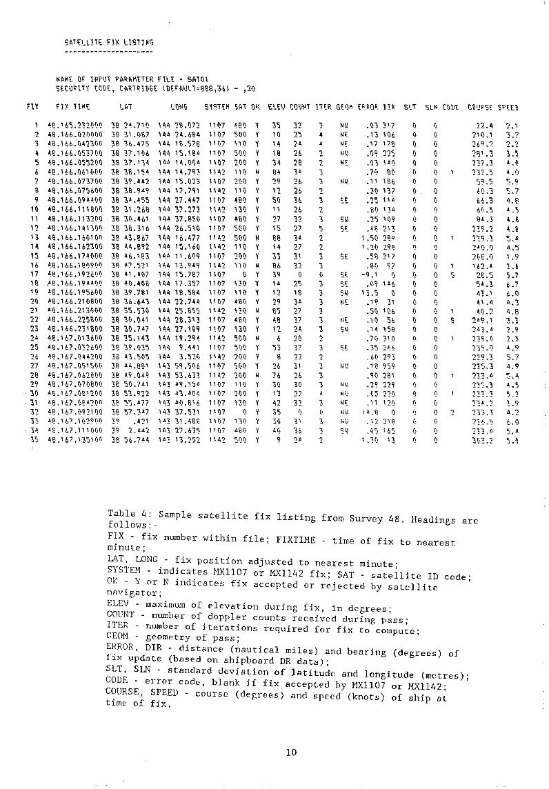
FIXES: Produce a listing of the satellite fixes for assessment purposes (Table 4).

RESAM: Concatenate the Phase 1 data files, as appropriate, and resample to produce I-minute data.

SAT12: Two passes of this program are required for each round of satellite fix assessment. During each pass, a number of options are called, as follows:

Pass 1

a. SATEL - reads in the file of satellite fixes and stores them in memory. Any fix intervals with dubious speeds (too low or too high) or any intervals that are very short «15 minutes) or very long (>120 minutes) are flagged in the output listing.

b. DRNAV - uses the incremental latitude/longitudes stored on the Phase 1 file and the satellite fix information to compute the DR path (or DR vector) for each satellite fix interval. This is saved as an ASCII parameter file.

c. CALNV - reads the DR file created by DRNAV and computes the ratio of the average DR velocity to the velocity computed from successive satellite fixes. This is done for each DR system used, and the results are listed.

d. CALPL - produces a line printer plot of the velocity ratios for each satellite fix interval.

9

S~lELLI1E FIX LIS1!~G

I'll\~t. Of Itlf'LJI f'A~f\Mt.'TtR FlU: - SAlOl SECU~lTY tODE, CA~l~lDSE tgEFAULl=8~8,36) - ,20

fE fD 1111( LONG S,(SlE~ SAl OK EtEV COgNl tiER GEn~ ERRQ~ BI. Sll SlN CODE COUPSE SPEED

48. 1 6'5. 2321)~,1) 2 48.166.020000 3 413.166.042'300 4 '5 6 7 a 9

10

"

4B.166.0';i'371)1) 018.166.0'5'5200 48.166.0611)00 018.166.07"371)0 413.166.07'5600 48.166.09 ltlt OO 48.166.1"131)1) 48.166.11'3200

;? 018.166.141300 13 413.166.160100 11: 48.166.1623(1) ''5 48.'66.174000 16 48.166.181)91)1) 17 48.166.192600 ;8 AI3,'66.;9 A400 '9 ~8.166.19'5600 20 AB.166.210800 21 AI3.166.2131)1)1) 22 413.166.22581)1) 23 413.166.231800 24 48.'67.01361)0 25 48.i67.(3261)1) 26 1:8.167.04A200 27 48.167.0'5''51)1) 28 48.167.062800 29 48.167.071)81)0 30 AI3.167.013 120'J

"13.1 67 .C'\l~2()O

~a 2~.710

38 31.0137 38 36.475 ~8 37.11)6 38 37.1'34 ~8 313 .1'54 "313 "39.442 31l 38.949 313 301.4'5'5 "38 "31.2611 "313 "3('.461 313 313.316 3B 43.867 313 44.1192 313 A6.1133 38 47. '52' "3B 41. A07 313 1:0.40B 313 "39.711\ 3B 36.6013 313 "3'5.'530 313 '31) .041 "3B "30.7 47 "313 3'5.143 "313 39.03'5 38 ·n.50'5 313 .l;lL.138' 313 49.049 '313 50.7.1;1 313 '5'3.922 313 5:'.0177 38 57.3 lt7

. 31 32 'B 4\l.167.1029QO 39 .421

- 3D, 1t13. 1 67,1111)1)1) 39 2.442 35 48.167.13'511)1) 38 56.74~

144 '21),072 '~4 2~.684 lU, 18.'5713 14~ 1'5.184 144 1~.01)"

'''4 14.793 1A4 1~.on lA417.7'11 144 27.447 144 37.273 144 37.8~0 14~ 26.'510 144 16.477 '44 15.160 14A ".609 144 13.9 49 144 15.787 144 17.3'57 144 18.'5134 144 22.7411 144 2'5.8'5'5 144 28.3;3 14~ 27.109 144 19.294 1411 9.441 144 3.52l) 143 '59.'50b 143 '33.633 1"1 A9.1'5 4

143 43. 41\4 143 40.13\6 143 37.5'31 143 31.413S! 14'3 '27.63'5 14 3 13.2~2

1107 480 '1 1107 '500 '1 , H)7 "1) '(

"07 '51)0 '1 1107 21)1) '( 1142 110 N "07 20() '1 1142 111) '1 "07 4B~' '1 1142 131) '1 11 07 480 '( 111)7 50() '1 11A2 500 N 1142 110 '1 111)7 21)1) '1 11A2 iiI) N

1'07 () '( 1107 HO '1 "07 " 0 '1 11f)7 481) '( 1142 no hi

1107 11130 'f 1107 no '( 1142 SOl) N 1 H'7 '5()() '{

1142 200 'f 1107 '500 '{ ,, 42 21)0 N

nQ? no '{ 11\07 21)1) 'I

" 1)7 1'30 '1 "()7 0 '( , H)7 1 3~' 'f 11l)7 4e r, 'f 1142 '51)l) '(

32 2'5 24 26 28 34

26 26 36 26 '32 27 '3 4

27 31 32

25 1S 34 27 37 21: 20 37 22 31 26 30 22 32

I)

31

36 24

3 0\ It

2 2 '3 '3 2 3 2 3 'S 2 2 '3 3 o 3 3 3 3 3 '3 '2 '3 2 3 '3 '3 4 '3 ()

3 3 '2

.03 '3'7

.13 11)b • i 7 i7B .09 225 .03 lAI) .70 80 ." 1136 .:10 137 .2'5 11 4

.SO nil

.2'5 , 09

.1l8 2'3

1.'50 21!<i 1 .20 29~

.513 217

.81) 97 -9.' 0

.09 146 n.'5 C'

.1 Q 31 • '51) 1 () /,

.11) '56

.14 1 ~13

.70 3'0

.3'5 2A6

.60 293

.113 9'S9

.% 28'

.29 229

.05 :121)

.11 120 i A. 8 0

· ',2 2' 13 .\):' i 6'5

1 ,3~1 1'3

I)

o I)

o o o I)

I)

I)

I)

\I (,

I)

I)

I)

Ii I)

Q

2

22.11 210.1 26<1,2 '28 1 • '3 237.1 2'3'.1. 'i 59 .. 5 6~', '3 66.'3 6L,) 84.3

1'39.1 B9.3 2 11), /)

2~'8 .1)

162.' 2L'5 ')'.".1 A3.1

~ 1.4 ~0.2

2 49.1 2A3.' n9.~

B~.0

229.3 21::·.3 23'3,4 1~·CS .1 2::'3.3 1'3'.1 21'3.3

:2'B." 3t·'3.1

Table 4: Sample satellite fix listing from Survey 48. Headings follows:- are

FIX - fix number within fl' Ie', FIXTIME . f f . - tIme 0 ix to nearest minute;

LAT, LONG - fix position adjusted to nearest minute; SYSTEM - indicates }~II07 or MXll42 fix' SAT - satellite ID code; OK - Y or N indicates fix accepted or r;jected by satellite navigator;

ELEV - maximwn of elevation during fix in degrees' COUN ' .,

T - number of.doppl~r counts received during pass; ITER - number of IteratIons required for fix to compute' GEOM - geometry of pass; ,

E~OR, DIR - distance (nautical miles) and bearing (degrees) of fIX update (based on shipboard DR data);

SLT, SLN - standard deviation of latitude and longitude (metres)' CODE - error code, blank if fix accepted by HXII07 or MX1l42 , ' C?URSE, S~EED - course (degrees) and speed (knots) of ship a~ tIme of fIX,

10

2. , '3.7 2.2 1. '5 U)

A.0 :'.9 :'.7 4,13 A • ')

4.6 ~ .8 5.4 .11.'5 1.9 2.6 '3.7 6.7 6.0 4.3 4,13 3.1 2.9 2.1 ~.9

5. 7

4.9

~.'l

5,2 3.9 4.2 6.0

Pass 2

a. CFACT - uses the DR file and a user-created file of calibration factor intervals to compute velocity calibration factors for each DR system.

b. APROX - uses the calibration factors computed in CFACT and the DR file to produce an approximately calibrated DR file.

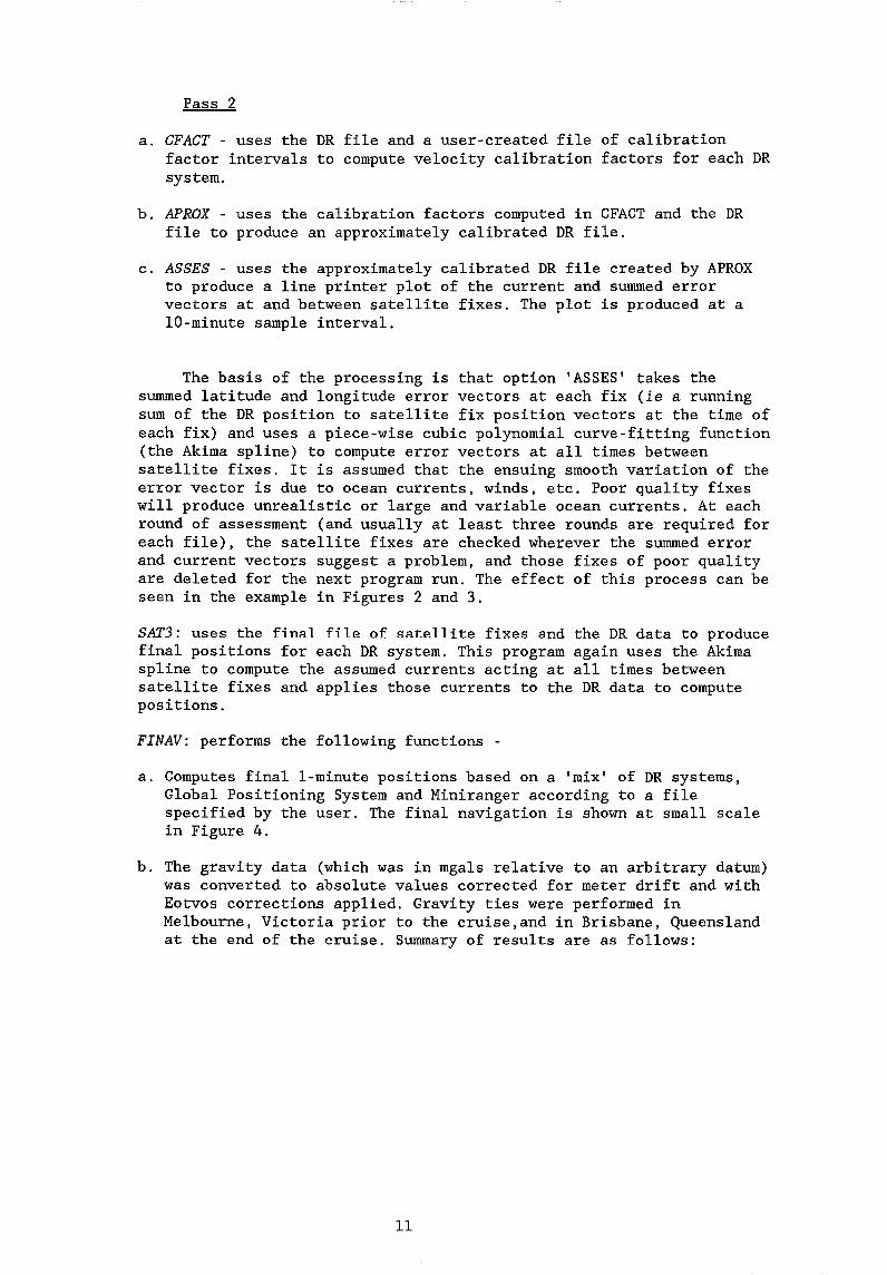
c. ASSES - uses the approximately calibrated DR file created by APROX to produce a line printer plot of the current and summed error vectors at and between satellite fixes. The plot is produced at a lO-minute sample interval.

The basis of the processing is that option 'ASSES' takes the summed latitude and longitude error vectors at each fix (ie a running sum of the DR position to satellite fix position vectors at the time of each fix) and uses a piece-wise cubic polynomial curve-fitting function (the Akima spline) to compute error vectors at all times between satellite fixes. It is assumed that the ensuing smooth variation of the error vector is due to ocean currents, winds, etc. Poor quality fixes will produce unrealistic or large and variable ocean currents. At each round of assessment (and usually at least three rounds are required for each file), the satellite fixes are checked wherever the summed error and current vectors suggest a problem, and those fixes of poor quality are deleted for the next program run. The effect of this process can be seen in the example in Figures 2 and 3.

SAT3: uses the final file of satellite fixes and the DR data to produce final positions for each DR system. This program again uses the Akima spline to compute the assumed currents acting at all times between satellite fixes and applies those currents to the DR data to compute positions.

FINAV: performs the following functions -

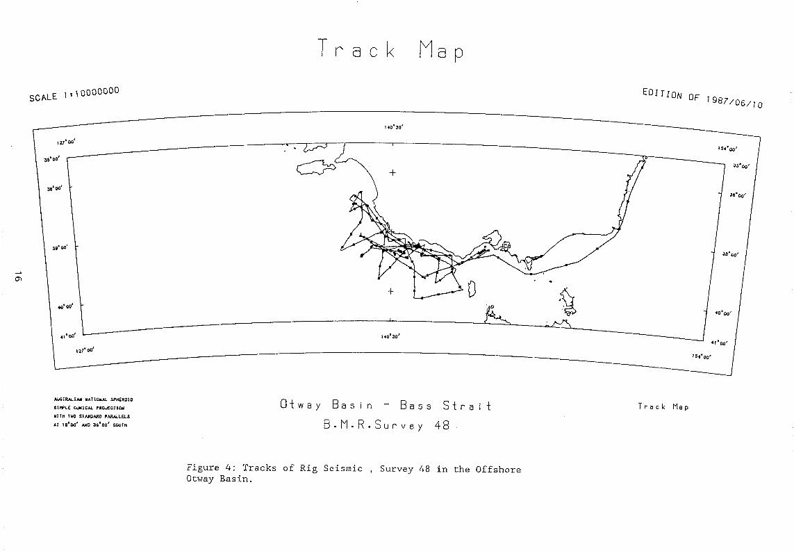
a. Computes final I-minute positions based on a 'mix' of DR systems, Global Positioning System and Miniranger according to a file specified by the user. The final navigation is shown at small scale in Figure 4.

b. The gravity data (which was in mgals relative to an arbitrary datum) was converted to absolute values corrected for meter drift and with Eotvos corrections applied. Gravity ties were performed in Melbourne, Victoria prior to the cruise,and in Brisbane, Queensland at the end of the cruise. Summary of results are as follows:

11

Ship's value (ums**-2) Corrected Value (ums**-2)

Pre-Otway -4349.75 9799884.6

Time & Date 4/6/85 1515 hrs (local)

Post Otway =-12618.75 9791675.63

Time & Date 19/7/85 1430 hrs (local)

Difference 8269.0 8209.0

Drift = 60 ums**-2.

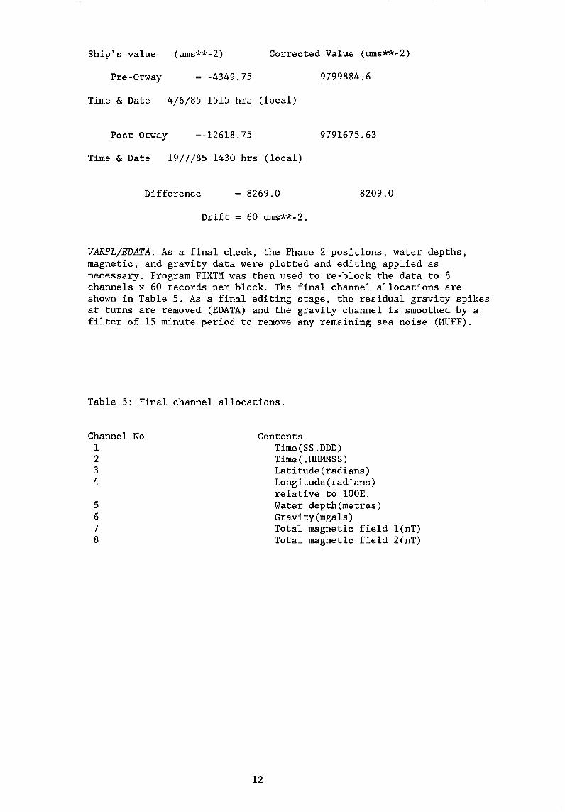
VARPL/EDATA: As a final check, the Phase 2 positions, water depths, magnetic, and gravity data were plotted and editing applied as necessary. Program FIXTM was then used to re-block the data to 8 channels x 60 records per block. The final channel allocations are shown in Table 5. As a final editing stage, the residual gravity spikes at turns are removed (EDATA) and the gravity channel is smoothed by a filter of 15 minute period to remove any remaining sea noise (MUFF).

Table 5: Final channel allocations.

Channel No 1 2 3 4

5 6 7 8

Contents

12

Time(SS.DDD) Time( .HHMMSS) Latitude (radians) Longitude (radians) relative to 100E. Water depth(metres) Gravity(mgals) Total magnetic field l(nT) Total magnetic field 2(nT)

2 7

4^4^ 4^ 4^4^4^4^ 4

"-o0^ C)

Figure 1: Bathymetry traces before (upper) and after processingby program SALVG. Vertical scale is 100 m/inch; horizontal scale

is 3 inches/hour.

13

H Hi H Hi H t....I ,, 1(7,4^H ,, H ,, Hi ^.4 ^.4^I-4 ,, H .40 Hi ,, H^H^H^H^H^I-4^1-4

44.0e."^

.0 1^ 1^1C

., .4 .4 1-4 ^1.4 .4 /.4

••

hi ,4 1-4 H H H ,,

:> Ln

un

un^ cr crIt cr^It

:Jr1^crcr cr^ cr

crcr ,r^. -^• cr •

cr

Cr^Cr.4 ,,H H H .4^.4 ,, 1-4 ,4 cr HH 1-1

crcr

cr

un^Ln^'r sr

ct1^ 454

ct cr cr

^

cr sr^cr^Lnq-

cr^ Ln

• Lfl

cr,r cr .

.7cr

t. .4

-

cr`r.

PO p,:; PI re; Vl pc; PO pr; ri re; rl

.0,01 .0^.0

C.,x

a -1a -0-a

1

1^.0

^

.10^I^•^.0^. •^.0 ,0 .0 ,0 .0 ,0 .0 ,0 .0 „Jo .0 .

.0 n :1011^ 11^ i

^

1-4^'''' .4 ..' t. '--1 .4 l'-' .4 ""i .4 ''' -4-4 .4 " .4

M tn

ro^roV-4 '1 rc,^tO

•••O'C. <1 <3 ti'D

" .4 " .4

,n ;741^ "

21 0

CD^CD^CD^CD ^^".^0 C.^!=‘^ •-•• ,r^oj^,r Ln^nj PO ,r^0.1^,r^cz „ oj^=n c, w4 4.1.j^,r^vi od PI ,J Ln

^a ,0 ,0 .0^p, P. p, N 00 M M 00 CO 0, ON 0, ON 0, ON „ *-- „ " „ „ •r, „ „

" „• .^'^•^-^•^-^ •^-^•^•^-^•^-^•^•^-^-^•^-^•^•^•^.^•^-^-

^

CJ 4^"4CJ^Cj^Oj^74^Oj " Cj^roj^Cj^C.! "• 0:1^0..j Cj 04 ".4('.4c, CJ^Cj^VJ DJ CJ 0,1^('3 CJ 0.4 04 oj Cj oj CJ 0,1 Cj 0,J 0.1 :11 C.1 Cd rQ CJ 0,NI 1.i. PO to r) po "1 n !".7^PI 1.1 r0, PO pl PI pry PO re) ro ff.; ro^ro 1,1 to^ro^ro^PI pr.^.

Ln^N.0^.0^,C144^.4^4-1

co OJ^NI

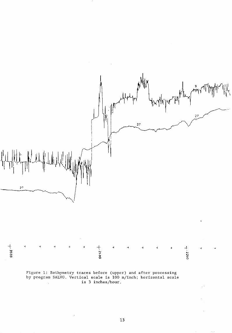
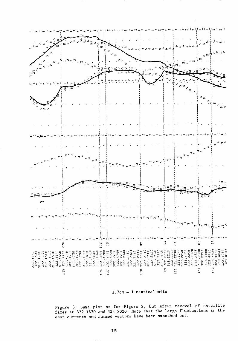
1.7cm = 1 nautical mile

Figure 2: Satellite fix assessment plot. 10-minute time (DD.HHMM) alongbottom of plot; satellite fixes indicated by row of dashes (eg. at322.1700); traces on the plot are as follows:-N & E - north & east currents for DR system 1;1 & 2 - north & east summed error vectors for DR system 1; Y & X -north & east currents for DR system 2; 3 & 4 - north & east summederror vectors for DR system 2.Note in particular the large fluctuations in the east current and theeast summed error vector on the left-hand half of the plot.

" H " " " H" "H " H"

C. C.et- cr

cr Icr

cr c,c- cr

;q•

7t-3

NI '1 NI^ '. NI N.) NI .

I^ II^ I^ I^I

!^I^ I^I^I

I^ I^I

ri^CO^ ....,^5__,l^r•^,c

c,^t>.^ co^1.6^,.,^OD^P^

NJ1-5

.-;N

N^c. -LJ

cr 'Tc-^cr

CP^CrC ^C7

,, Cr

C7

CrC4 -crCr

c!'

,, ^rq

n w.

-^Ln^1.71 Ln

.0 so^Ln.0

1

PJ :j r.1 oj rJ

Ln^PJ^.^.^:j PJ

PJ^ 0.1PJCJ

r ;

• : " ;-4 " ;.., " 1.-, I-4 r.; )44 H " H HI " H " H. " H " I-1 " I-I " HI " I-I " HI " H " H " 1-4 " 1". "I^i^I

i^I^ I^I^I

^

I^ I^I^1

^

1^..^ I^I^i

I .^La w ,0 w 43^ I^1

^

Ln1^.0^ 1^I^I so .0

^

IP 1^.0 '10 .0^ I^■ 43 .0 4:1 .0 sO .0 43NO ..0 .0 ,0 .0 ..rt .0 ,r) .0 ..1:1 4) ,..0 .0 ...0

IIIII

I-4 144^" C. "

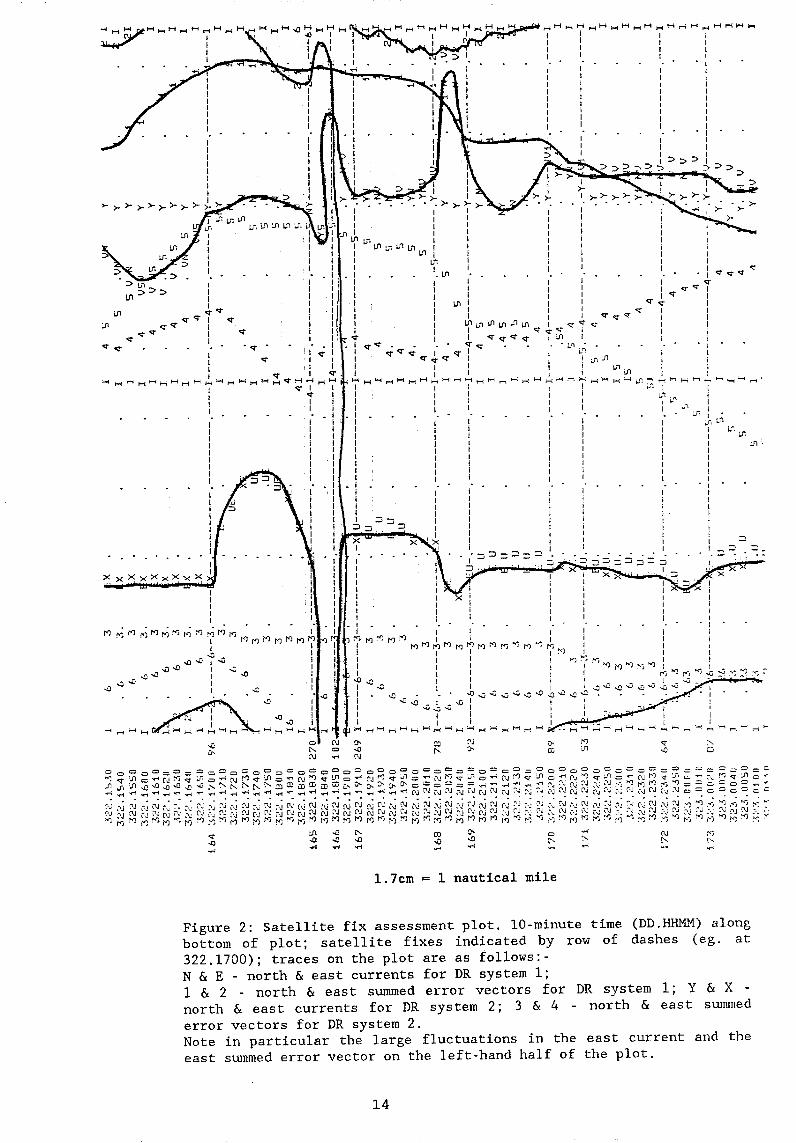
1.7cm = 1 nautical mile

Figure 3: Same plot as for Figure 2, but after removal of satellitefixes at 332.1830 and 332.2020. Note that the large fluctuations in theeast currents and summed vectors have been smoothed out.

Tr a c^V a p

SCALE 100000000

EDITION OF 1987/06/10

140 . 30'

154.00'

AUSTRALIAN WATIOMM. SPMEROIO

SIMPLE CONICAL PROJECTION

with Two STANDARD PARALLELS

AT )8'00' AND 3600' SOON

Otway Basin — Bass Stra i 1

B.M.R.Survey 48

Track Map

Figure 4: Tracks of Rig Seismic , Survey 48 in the OffshoreOtway Basin.

DATA AVAILABILITY

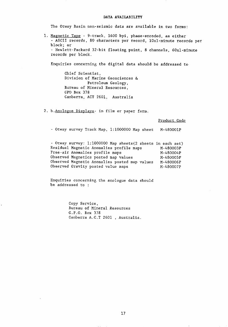
The Otway Basin non-seismic data are available in two forms:

1. Magnetic Tape - 9-track, 1600 bpi, phase-encoded, as either- ASCII records, 80 characters per record, 10xl-minute records perblock; or- Hewlett-Packard 32-bit floating point, 8 channels, 60x1-minuterecords per block.

Enquiries concerning the digital data should be addressed to

Chief Scientist,Division of Marine Geosciences &

Petroleum Geology,Bureau of Mineral Resources,GPO Box 378Canberra, ACT 2601, Australia

2. b.Anologue Displays- in film or paper form.

Product Code

- Otway survey Track Map, 1:1000000 Map sheet M-480001P

- Otway survey: 1:1000000 Map sheets(2 sheets in each set)Residual Magnetic Anomalies profile maps^M-480003PFree-air Anomalies profile maps^M-480004PObserved Magnetics posted map values^M-480005PObserved Magnetic Anomalies posted map values M-480006PObserved Gravity posted value maps^M-480007P

Enquiries concerning the anologue data shouldbe addressed to

Copy Service,Bureau of Mineral ResourcesG.P.O. Box 378Canberra A.C.T 2601 , Australia.

17