Embed Size (px)
Citation preview
Kato, Fukuda, Yamashita, Iwakura, and Yai 1
Latest Urban Rail Demand Forecast Model System in the Tokyo 1
Metropolitan Area 2
3
Hironori Kato 4
Department of Civil Engineering, The University of Tokyo 5
7-3-1, Hongo, Bunkyo-ku, Tokyo 113-8656, Japan 6
Phone: +81-3-5841-7451; Fax: +81-3-5841-7496 7
E-mail: [email protected] 8
9
Daisuke Fukuda 10
Department of Civil and Environmental Engineering, Tokyo Institute of Technology 11
2-12-1, Okayama, Meguro-ku, Tokyo 152-8552, Japan 12
Phone: +81-3-5734-2577; Fax: +81-3-5734-3578 13
E-mail: [email protected] 14
15
Yoshihisa Yamashita 16
Urban and Regional Transportation Group, Creative Research and Planning 17
1-20-22, Ebisu, Shibuya-ku, Tokyo, 150-0013, Japan 18
Phone: +81-3-5791-1133; Fax: +81-3-5791-1144 19
E-mail: [email protected] 20
21
Seiji Iwakura 22
Department of Civil Engineering, Shibaura Institute of Technology 23
3-7-5 Toyosu, Koto-ku, Tokyo 135-8548, Japan 24
Phone: +81-3-5859-8354; Fax: +81-3-5859-8401 25
E-mail: [email protected] 26
27
Tetsuo Yai 28
Department of Civil and Environmental Engineering, Tokyo Institute of Technology 29
4259, Nagatsuta-cho, Midori-ku, Yokohama, 226-8502, Japan 30
Phone: +81-45-924-5615; Fax: +81-45-924-5675 31
E-mail: [email protected] 32
33
34
Word count: 5,952 words + 5 Tables + 2 Figures = 7,702 words 35
36
Kato, Fukuda, Yamashita, Iwakura, and Yai 2
ABSTRACT 1
2
This paper reports on an urban rail travel demand forecast model system, which technically 3 supported the formulation of the Tokyo Urban Rail Development Master-plan 2016. The model 4 system was included in the forthcoming 15-year urban rail investment strategy for Tokyo. The 5 model system was utilized to quantitatively assess urban rail projects including 24 new rail 6 development projects, which had been proposed in response to expected changes in socio-7 demographic patterns, land-use market, and the government’s latest transportation policy goals. 8 The system covers the entire urban rail network within the Tokyo Metropolitan Area (TMA) of 9 approximately 50-km radius with a population of over 34 million. The system must handle over 10 80 million trips per day. Three demand models are used to predict daily rail passenger link flows: 11 the urban rail demand model, the airport rail access demand model, and the high-speed-rail rail 12 access demand model. These practical models have unique characteristics such as incorporating 13 differences in behavior between aged and non-aged travelers, reflecting expected influences of 14 urban redevelopment on trip generation and distribution, highlighting urban rail access to 15 airports or high-speed-rail stations, examining impacts of in-vehicle crowding on rail route 16 choice, and deploying urban rail-station access/egress mode choice models for rail route choice. 17 It is concluded that the model system would be well calibrated with observed data for 18 reproducing travel patterns, identifying potential problems, assessing proposed projects, 19 presenting results with high accuracy, and assisting decision-making of urban rail planners. 20 21 Keywords. Urban rail, demand forecast model system, Tokyo, Japan 22 23
Kato, Fukuda, Yamashita, Iwakura, and Yai 3
INTRODUCTION 1
2
A new long-term Tokyo Urban Rail Development Master-plan discussing the future development 3
strategies for the urban rail network in TMA was established by the Council for Transport Policy in 4
April 2016 (1). This is the latest master plan from the succession of plans that have been revised 5
approximately every 15 years since 1956. This master plan aims at providing recommendations for 6
the urban rail infrastructure development within TMA for the forthcoming 15 years by reflecting on 7
the latest socio-demographic and socio-economic conditions. See Morichi et al. (2) for the outline of 8
the previous master plan established in 2000. The latest master plan proposed the construction of 9
additional 24 new rail lines and included proposed renovation or rehabilitation of the existing major 10
rail stations. 11
For finalizing the proposals, the proposed projects were assessed separately using 46 performance 12
indexes including a cost-benefit ratio, financial feasibility, and policy impacts as proposed through 13
many discussions among the 13 committee members. The committee members are noted experts in 14
transportation planning, traffic engineering, transportation economics, urban planning, and tourism 15
research, which included three of the authors. Those indexes were quantified by using a large-scale 16
travel demand forecast model system which predicted the future urban rail passenger demand in 2030 17
for both the with and without investment cases for each proposed project. 18
This paper outlines the practical travel demand forecast model system utilized in the Tokyo Urban 19
Rail Development Master-plan in 2016. The proposed model basically follows the structure of prior 20
model that was used for the last master plan, but it adds a rail-station access/egress model while it also 21
takes accounts of rapid changes in socio-demographic patterns. It is not the intent to show the state-of-22
the-art methodologies in travel demand analysis, but to present practical applications of the travel 23
demand forecast models to assess the proposed projects for the process of urban rail transportation 24
planning in response to the latest policy goals. 25
The paper is organized as follows. The next section introduces unique characteristics of the urban 26
rail travel demand forecast model for Tokyo, followed by model development including its estimation 27
results. Then reproducibility of urban rail demand is presented. Finally, the findings are summarized 28
with further research issues. 29
30
31
CHARACTERISTICS OF URBAN RAIL TRAVEL DEMAND FORECAST MODEL IN 32
TOKYO 33
34
The model system has five distinctive characteristics by considering the unique features of the urban 35
rail services in Tokyo. First, the models incorporate the influences of rapid changes in socio-36
demographic patterns on travel demand since Tokyo is facing rapid aging and is predicted to 37
experience a further aging society in the future. The population of 65 year-olds or over accounted for 38
14.5% of the overall population in 2000, which then increased to 21.0% in 2010 and is projected to be 39
at 29% in 2030. Since senior individuals are generally expected to engage in less out-of-home activities 40
than younger individuals, peoples’ daily activity patterns may vary across the types of journeys, age 41
levels, and gender. Furthermore, destination choice patterns, mode choice patterns, and route choice 42
patterns of senior travelers could be different from those of younger travelers. Such differences are 43
taken into account in the developed model system by segmenting the travelers by age subgroup. 44
Second, the expected changes in land-use patterns are incorporated into the models. As shown in 45
Kato (3) and Suzuki et al. (4), urban redevelopment in the central district of Tokyo has grown since 46
Kato, Fukuda, Yamashita, Iwakura, and Yai 4
early 2000s. This growth was due to the Act on Special Measures Concerning Urban Regeneration 1
introduced in 2002 in which the Building Standards Law was revised to relax the maximum floor area 2
ratio constraint. This led to the sharp increase of high-rise buildings for residential, office, and mixed-3
use in the central ward areas of Tokyo. Such changes in land-use pattern in the central business district 4
(CBD) influence not only the trip generation/attraction but also the trip distribution patterns because 5
the types of trips to/from redeveloped zones may be changed. 6
Third, an airport rail access demand (ARAD) model and a high-speed-rail rail access demand 7
(HSR-RAD) model have been developed in addition to the urban rail passenger demand (URD) model. 8
The ARAD model reflects the recent government’s transportation policy that highlights the 9
improvement of accessibility to two international airports in Tokyo. The HSR-RAD model is intended 10
for predicting urban passenger demand accessing the Chuo Shinkansen that employs the 11
superconducting maglev system. A new Japanese maglev line has been planned to connect Tokyo 12
with Chukyo and ultimately with Kinki (5). The introduction of new high-speed maglev should also 13
influence the urban rail demand, particularly the one accessing to/generating from HSR stations in 14
TMA. 15
Fourth, the rail-route choice submodel in the URD model explicitly considers the in-vehicle rail 16
crowding since urban rail passengers are still suffering from serious in-vehicle congestion, particularly 17
during morning peak hours (6, 7, 8). 18
Finally, the rail route choice submodel in the URD model also incorporates an accessibility 19
measure calibrated with the rail-station access/egress mode choice submodels. The urban rail network 20
has been densely developed in TMA, where urban rail passengers have multiple options to access or 21
egress rail stations. Particularly, urban bus services are operated connecting to and from the rail stations 22
thereby affecting passenger rail route choice. 23
24
25
GOAL AND SCOPE OF MODEL DEVELOPMENT 26
27
The developed model system is intended to assess the proposed urban rail investment projects using 28
several performance indexes. To quantify these performance indexes, the link-based daily rail 29
passenger flows need to be forecasted under given future conditions. The target area covers areas in a 30
50-km radius from the CBD in Tokyo, which is generally regarded as a commutable area in TMA. 31
The area includes the five prefectures of Tokyo, Kanagawa, Saitama, Chiba, and Ibaraki and is divided 32
into 2,907 Traffic Analysis Zones (TAZs) with an average area of 1.8 km2. 33
The population-relevant numbers in the target area in 2010 were 37.24 million (nighttime 34
population), 19.13 million (nighttime worker population), 19.19 million (daytime worker population), 35
4.70 million (nighttime student population), and 4.73 million (daytime student population). In addition 36
to the urban rail network, the arterial/expressway road network is also employed from Digital Road 37
Map data while the bus network is also prepared from the information provided by bus operators. 38
Consequently, the target transport network has 18,178 links and 9,567 nodes. 39
The model system consists of the URD model, the ARAD model, and the HSR-RAD model with 40
their submodels. The model system is in line with the traditional structure of a four-step model that 41
includes trip generation/attraction, trip distribution, mode choice, and rail-route choice submodels 42
where the output of upper-level submodels constrains the total input of the lower-level submodels. 43
The daily rail passenger link flows are computed as the final output of the model system. The 44
URD model predicts the rail passenger demand for the given population while the ARAD/HSR-RAD 45
models forecasts corresponding urban rail demand for the airports and station-based HSR demands as 46
Kato, Fukuda, Yamashita, Iwakura, and Yai 5
predetermined by the National Government. Thus, trip generation/attraction submodels are not 1
included in the ARAD/HSR-RAD models. 2
3
URBAN RAIL DEMAND (URD) MODEL 4
5
Market Segmentation 6
Each submodel in the URD model forecasts travel demands by ten different trip purposes: home-to-7
workplace (H-W), home-to-school (H-S), home-to-private (H-P), out-of-home-to-private (OH-P), 8
home-to-business (H-B), workplace-to-other business (W-B), workplace-to-home (W-H), school-to-9
home (S-H), private-to-home (P-H), and business-to-home (B-H). In the trip generation/attraction 10
submodel and the trip distribution submodel, travelers are segmented by gender. Additionally, all 11
submodels segment individuals into multiple age subgroups except for the H-S trips within the mode 12
choice and the rail route choice submodels. The age subgroups are then defined into different 13
categories depending on trip purposes, gender, and submodels. 14
15
URD-Trip Generation/Attraction Submodels 16
These submodels estimate daily trip demand generated from and attracted to a zone. Simple trip rate 17
models have been applied as 18
pagi
pagG
pagi YGU (1) 19
pagj
pagA
pagj YAU (2) 20
where pagiGU is the number of daily trips with trip purpose p for age subgroup a and gender g 21
generating from zone i ; pagjAU is the number of daily trips attracted to zone j ; pag
iY represents the 22
total number of individuals; and pagG and pag
A are the constant trip rates (trips per day per 23
individual) regarding the attraction and generation, respectively. Note that pagiY and pag
jY are 24
different across trip purposes, age groups, and gender. 25
26
URD-Trip Distribution Submodel 27
This submodel predicts the daily trip distribution of the target area for the given zone-based generated 28
and attracted trips obtained from the trip generation/attraction submodels. Two modeling approaches 29
have been applied according to the classification of the Origin-Destination (O-D) pairs. First, for the 30
zones where no significant change in future land-use patterns is expected, the growth factor method 31
has been applied for predicting future trip distributions. The growth rates are adjusted with the Fratar 32
method. 33
Second, for zones where large-scale urban (re-)developments would be implemented, the gravity 34
model has been applied to estimate the trip distribution of population migrating into the (re-)developed 35
zones. The zones to which the gravity model is applied include zones in the CBD of Tokyo, the 36
Sagamihara area, along the Tsukuba Express Line, and around the Koshigaya Laketown area. By 37
incorporating zone-specific dummy variables, the gravity models are formulated as follows: 38
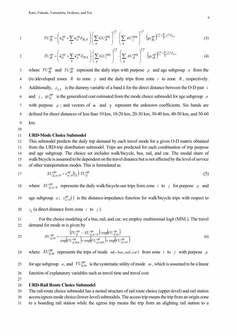
Kato, Fukuda, Yamashita, Iwakura, and Yai 6
k
kRjapk
apgc
apA
apG
apRj
g
apgj
g
apgR
kkRj
apk
apapRj gcAUGUTU
,
,0
(3) 1
k
kiRapk
apgc
apA
apG
apiR
g
apgR
g
apgi
kkiR
apk
apapiR gcAUGUTU
,
,0
(4) 2
where apRjTU and ap
iRTU represent the daily trips with purpose p and age subgroup a from the 3
(re-)developed zones R to zone j and the daily trips from zone i to zone R , respectively. 4
Additionally, kij , is the dummy variable of a band k for the direct distance between the O-D pair i5
and j , apijgc is the generalized cost estimated from the mode choice submodel for age subgroup a6
with purpose p ; and vectors of κ and γ represent the unknown coefficients. Six bands are 7
defined for direct distances of less than 10 km, 10-20 km, 20-30 km, 30-40 km, 40-50 km, and 50-60 8
km. 9
10
URD-Mode Choice Submodel 11
This submodel predicts the daily trip demand by each travel mode for a given O-D matrix obtained 12
from the URD-trip distribution submodel. Trips are predicted for each combination of trip purpose 13
and age subgroup. The choice set includes walk/bicycle, bus, rail, and car. The modal share of 14
walk/bicycle is assumed to be dependent on the travel distance but is not affected by the level of service 15
of other transportation modes. This is formulated as 16
apijij
apbw
apbwij TUlsXU //, (5) 17
where apbwijXU /, represents the daily walk/bicycle-use trips from zone i to j for purpose p and 18
age subgroup a ; apbws / is the distance-impedance function for walk/bicycle trips with respect to 19
ijl (a direct distance from zone i to j ). 20
For the choice modeling of a bus, rail, and car, we employ multinomial logit (MNL). The travel 21
demand for mode m is given by 22
ap
carijap
railijap
busij
apmij
apbwij
apijap
mijVUVUVU
VUXUTUXU
,,,
,/,,
expexpexp
exp
(6) 23
where apmijXU , represents the trips of mode carrailbusm ,, from zone i to j with purpose p 24
for age subgroup a , and apmijVU , is the systematic utility of mode m , which is assumed to be a linear 25
function of explanatory variables such as travel time and travel cost. 26
27
URD-Rail Route Choice Submodel 28
The rail-route choice submodel has a nested structure of rail route choice (upper-level) and rail station 29
access/egress mode choice (lower-level) submodels. The access trip means the trip from an origin zone 30
to a boarding rail station while the egress trip means the trip from an alighting rail station to a 31
Kato, Fukuda, Yamashita, Iwakura, and Yai 7
destination zone. The rail-station access/egress mode choice is formulated as a MNL while the rail 1
route choice is formulated as Multinomial Probit (MNP) model with structured covariance (6). It is 2
important to note that the rail route consists of an access link connecting the origin zone to a rail station, 3
rail line-haul links connecting the boarding rail station with the alighting rail station, waiting and 4
transfer links at stations, and an egress link connecting the alighting rail station to the destination zone. 5
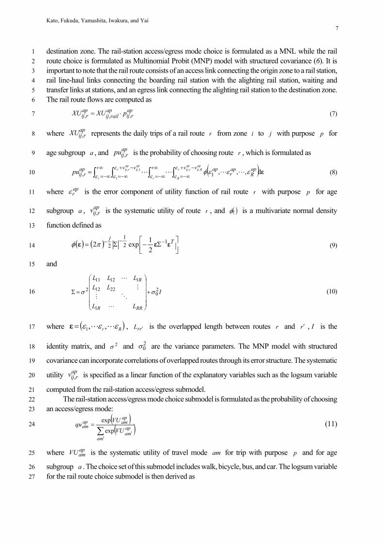
The rail route flows are computed as 6
aprij
aprailij
aprij pXUXU ,,, (7) 7
where aprijXU , represents the daily trips of a rail route r from zone i to j with purpose p for 8
age subgroup a , and aprijpu , is the probability of choosing route r , which is formulated as 9
εd,,,1,,
1
,,
1,
r
apij
aprijr
r
apRij
aprijr
R
vv vv apR
apr
apaprijpu
(8) 10
where apr is the error component of utility function of rail route r with purpose p for age 11
subgroup a , aprijv , is the systematic utility of route r , and is a multivariate normal density 12
function defined as 13
T
jεεε 1
2
1
22
1exp2 (9) 14
and 15
I
LL
LL
LLL
RRR
R
20
1
2212
11211
2
(10) 16
where Rr ,,1ε , rrL is the overlapped length between routes r and r , I is the 17
identity matrix, and 2 and 20 are the variance parameters. The MNP model with structured 18
covariance can incorporate correlations of overlapped routes through its error structure. The systematic 19
utility aprijv , is specified as a linear function of the explanatory variables such as the logsum variable 20
computed from the rail-station access/egress submodel. 21
The rail-station access/egress mode choice submodel is formulated as the probability of choosing 22
an access/egress mode: 23
ma
apma
apamap
amVU
VUqu
exp
exp (11) 24
where apamVU is the systematic utility of travel mode am for trip with purpose p and for age 25
subgroup a . The choice set of this submodel includes walk, bicycle, bus, and car. The logsum variable 26
for the rail route choice submodel is then derived as 27
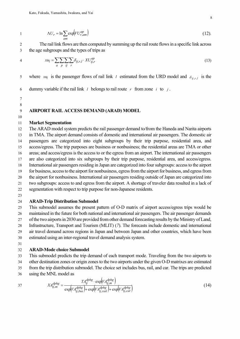
Kato, Fukuda, Yamashita, Iwakura, and Yai 8
am
apamrr VUU ,expln (12). 1
The rail link flows are then computed by summing up the rail route flows in a specific link across 2
the age subgroups and the types of trips as 3
a p ij r
aprijlrijl XUxu ,,, (13) 4
where lxu is the passenger flows of rail link l estimated from the URD model and lrij ,, is the 5
dummy variable if the rail link l belongs to rail route r from zone i to j . 6
7
8
AIRPORT RAIL ACCESS DEMAND (ARAD) MODEL 9
10
Market Segmentation 11
The ARAD model system predicts the rail passenger demand to/from the Haneda and Narita airports 12
in TMA. The airport demand consists of domestic and international air passengers. The domestic air 13
passengers are categorized into eight subgroups by their trip purpose, residential area, and 14
access/egress. The trip purposes are business or nonbusiness; the residential areas are TMA or other 15
areas; and access/egress is the access to or the egress from an airport. The international air passengers 16
are also categorized into six subgroups by their trip purpose, residential area, and access/egress. 17
International air passengers residing in Japan are categorized into four subgroups: access to the airport 18
for business, access to the airport for nonbusiness, egress from the airport for business, and egress from 19
the airport for nonbusiness. International air passengers residing outside of Japan are categorized into 20
two subgroups: access to and egress from the airport. A shortage of traveler data resulted in a lack of 21
segmentation with respect to trip purpose for non-Japanese residents. 22
23
ARAD-Trip Distribution Submodel 24
This submodel assumes the present pattern of O-D matrix of airport access/egress trips would be 25
maintained in the future for both national and international air passengers. The air passenger demands 26
of the two airports in 2030 are provided from other demand forecasting results by the Ministry of Land, 27
Infrastructure, Transport and Tourism (MLIT) (7). The forecasts include domestic and international 28
air travel demand across regions in Japan and between Japan and other countries, which have been 29
estimated using an inter-regional travel demand analysis system. 30
31
ARAD-Mode choice Submodel 32
This submodel predicts the trip demand of each transport mode. Traveling from the two airports to 33
other destination zones or origin zones to the two airports under the given O-D matrixes are estimated 34
from the trip distribution submodel. The choice set includes bus, rail, and car. The trips are predicted 35
using the MNL model as 36
dphg
carijdphg
railijdphg
busij
dphgmij
dphgijdphg
mijVAVAVA
VATAXA
,,,
,,
expexpexp
exp
(14) 37
Kato, Fukuda, Yamashita, Iwakura, and Yai 9
where dphgmijXA , represents the trips by mode carrailbusm ,, from i to j by domestic or 1
international passenger d residing at residential zone h with purpose p and for access/egress to 2
or from airport g . Additionally, dphgijTA represents the trips from i to j estimated from the trip 3
distribution submodel, and dphgmijVA , is the systematic utility, which is assumed to be a linear function 4
of explanatory variables including travel time and travel cost. It is noted that if 0g , the trip is made 5
for access to airport and the destination would be the airport whereas if 1g , the trip is made for 6
egress from airport and the origin would be the airport. 7
8
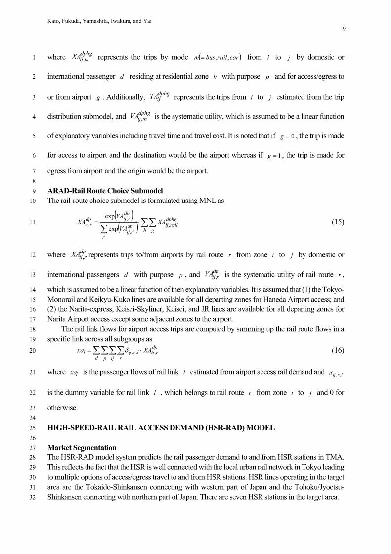
ARAD-Rail Route Choice Submodel 9
The rail-route choice submodel is formulated using MNL as 10
h g
dphgrailij
r
dprij
dprijdp
rij XAVA
VAXA ,
,
,,
exp
exp (15) 11
where dprijXA , represents trips to/from airports by rail route r from zone i to j by domestic or 12
international passengers d with purpose p , and dprijVA , is the systematic utility of rail route r , 13
which is assumed to be a linear function of then explanatory variables. It is assumed that (1) the Tokyo-14
Monorail and Keikyu-Kuko lines are available for all departing zones for Haneda Airport access; and 15
(2) the Narita-express, Keisei-Skyliner, Keisei, and JR lines are available for all departing zones for 16
Narita Airport access except some adjacent zones to the airport. 17
The rail link flows for airport access trips are computed by summing up the rail route flows in a 18
specific link across all subgroups as 19
d p ij r
dprijlrijl XAxa ,,, (16) 20
where lxa is the passenger flows of rail link l estimated from airport access rail demand and lrij ,, 21
is the dummy variable for rail link l , which belongs to rail route r from zone i to j and 0 for 22
otherwise. 23
24
HIGH-SPEED-RAIL RAIL ACCESS DEMAND (HSR-RAD) MODEL 25
26
Market Segmentation 27
The HSR-RAD model system predicts the rail passenger demand to and from HSR stations in TMA. 28
This reflects the fact that the HSR is well connected with the local urban rail network in Tokyo leading 29
to multiple options of access/egress travel to and from HSR stations. HSR lines operating in the target 30
area are the Tokaido-Shinkansen connecting with western part of Japan and the Tohoku/Jyoetsu-31
Shinkansen connecting with northern part of Japan. There are seven HSR stations in the target area. 32
Kato, Fukuda, Yamashita, Iwakura, and Yai 10
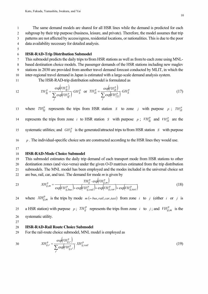
The same demand models are shared for all HSR lines while the demand is predicted for each 1
subgroup by their trip purpose (business, leisure, and private). Therefore, the model assumes that trip 2
patterns are not affected by access/egress, residential locations, or nationalities. This is due to the poor 3
data availability necessary for detailed analysis. 4
5
HSR-RAD-Trip Distribution Submodel 6
This submodel predicts the daily trips to/from HSR stations as well as from/to each zone using MNL-7
based destination choice models. The passenger demands of the HSR stations including new maglev 8
stations in 2030 are provided from another travel demand forecast conducted by MLIT, in which the 9
inter-regional travel demand in Japan is estimated with a large-scale demand analysis system. 10
The HSR-RAD-trip distribution submodel is formulated as 11
pS
j
pjS
pSjp
Sj GHVH
VHTH
exp
exp or
pS
i
pSi
piSp
iS GHVH
VHTH
exp
exp (17) 12
where pSjTH represents the trips from HSR station S to zone j with purpose p ; p
iSTH 13
represents the trips from zone i to HSR station S with purpose p ; pSjVH and p
iSVH are the 14
systematic utilities; and pSGH is the generated/attracted trips to/from HSR station S with purpose 15
p . The individual-specific choice sets are constructed according to the HSR lines they would use. 16
17
HSR-RAD-Mode Choice Submodel 18
This submodel estimates the daily trip demand of each transport mode from HSR stations to other 19
destination zones (and vice-versa) under the given O-D matrixes estimated from the trip distribution 20
submodels. The MNL model has been employed and the modes included in the universal choice set 21
are bus, rail, car, and taxi. The demand for mode m is given by 22
p
taxiijp
carijp
railijp
busij
pmij
pijp
mijVHVHVHVH
VHTHXH
,,,,
,,
expexpexpexp
exp
(18) 23
where pmijXH , is the trips by mode taxicarrailbusm ,,, from zone i to j (either i or j is 24
a HSR station) with purpose p ; pijTH represents the trips from zone i to j ; and p
mijVH , is the 25
systematic utility. 26
27
HSR-RAD-Rail Route Choice Submodel 28
For the rail-route choice submodel, MNL model is employed as 29
prailij
r
prij
prijp
rij XHVH
VHXH ,
,
,,
exp
exp
(19) 30
Kato, Fukuda, Yamashita, Iwakura, and Yai 11
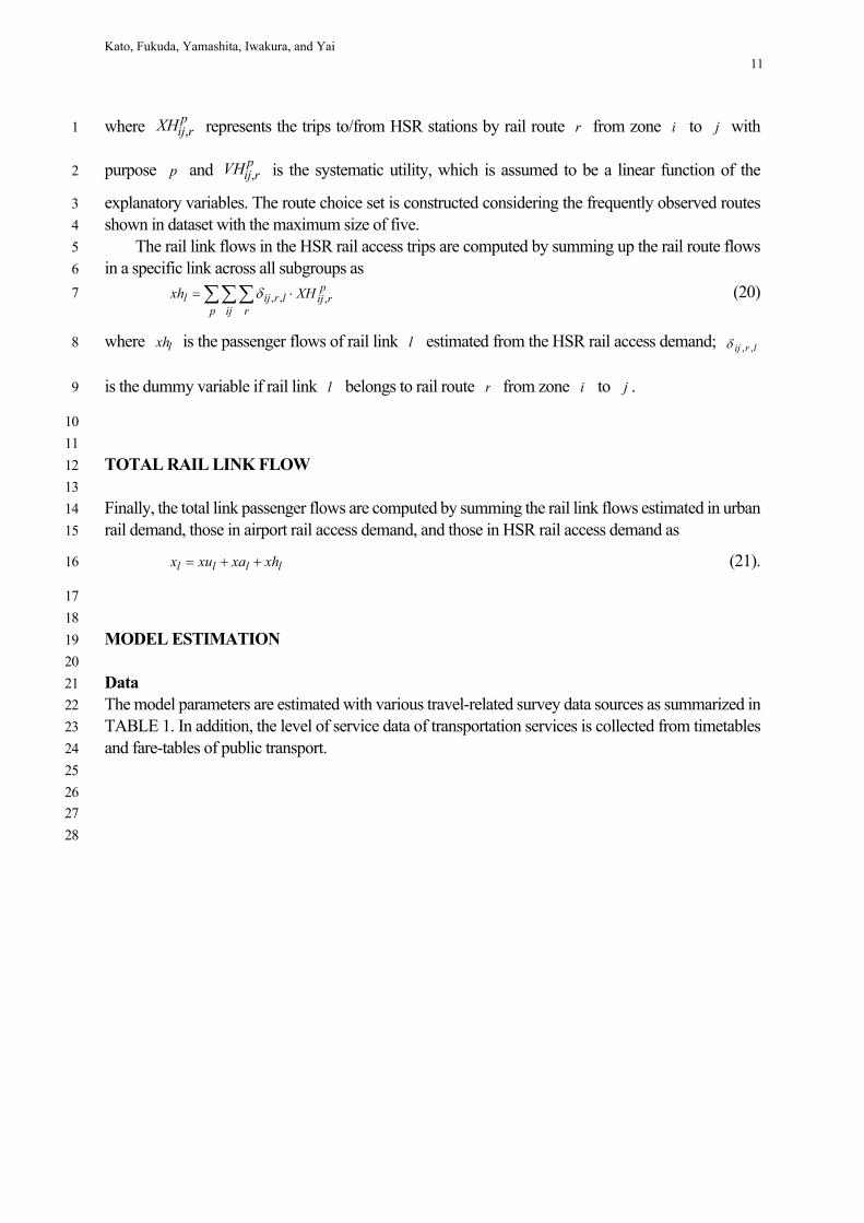
where prijXH , represents the trips to/from HSR stations by rail route r from zone i to j with 1
purpose p and prijVH , is the systematic utility, which is assumed to be a linear function of the 2
explanatory variables. The route choice set is constructed considering the frequently observed routes 3
shown in dataset with the maximum size of five. 4
The rail link flows in the HSR rail access trips are computed by summing up the rail route flows 5
in a specific link across all subgroups as 6
p ij r
prijlrijl XHxh ,,, (20) 7
where lxh is the passenger flows of rail link l estimated from the HSR rail access demand; lrij ,,8
is the dummy variable if rail link l belongs to rail route r from zone i to j . 9
10
11
TOTAL RAIL LINK FLOW 12
13
Finally, the total link passenger flows are computed by summing the rail link flows estimated in urban 14
rail demand, those in airport rail access demand, and those in HSR rail access demand as 15
llll xhxaxux (21). 16
17
18
MODEL ESTIMATION 19
20
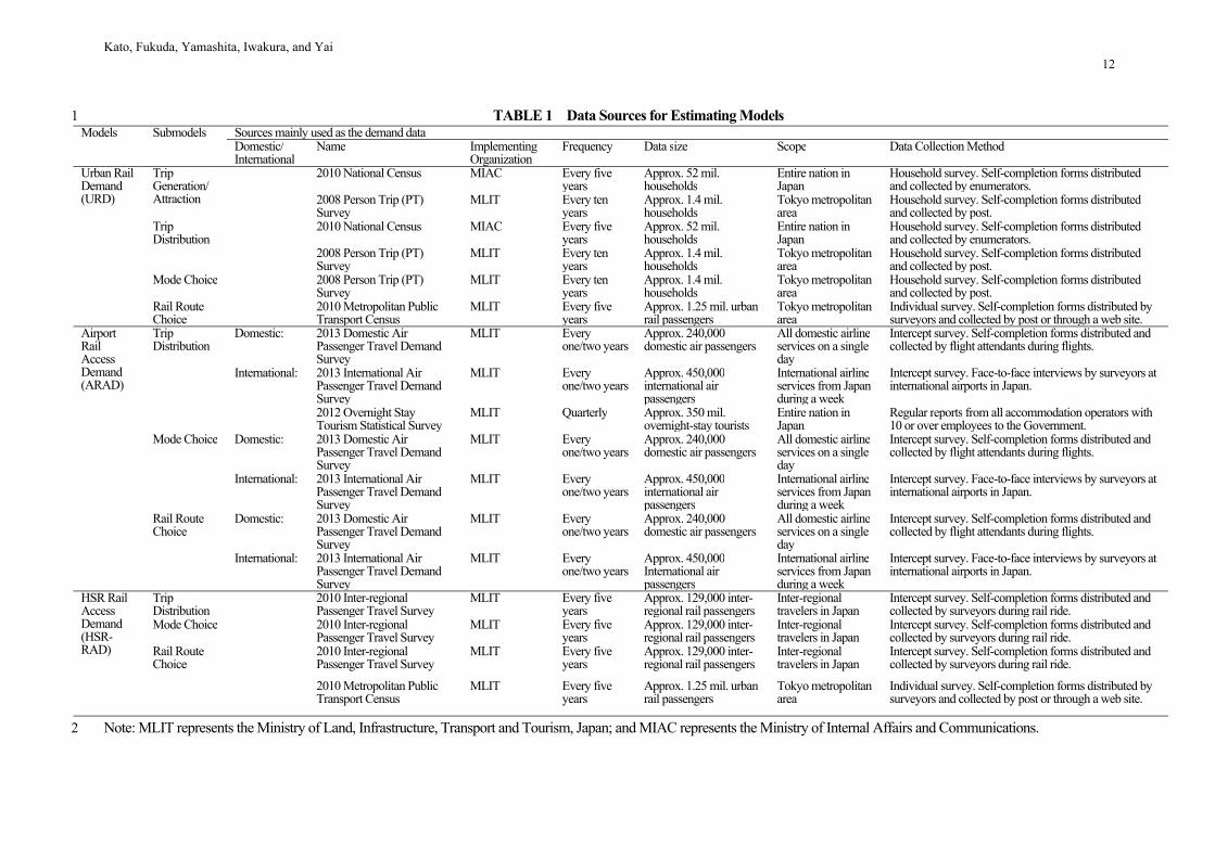
Data 21
The model parameters are estimated with various travel-related survey data sources as summarized in 22
TABLE 1. In addition, the level of service data of transportation services is collected from timetables 23
and fare-tables of public transport. 24
25
26
27
28
Kato, Fukuda, Yamashita, Iwakura, and Yai 12
TABLE 1 Data Sources for Estimating Models 1 Models Submodels Sources mainly used as the demand data
Domestic/ International
Name Implementing Organization
Frequency Data size Scope Data Collection Method
Urban Rail Demand (URD)
Trip Generation/ Attraction
2010 National Census MIAC Every five
yearsApprox. 52 mil.households
Entire nation in Japan
Household survey. Self-completion forms distributed and collected by enumerators.
2008 Person Trip (PT) Survey
MLIT Every ten years
Approx. 1.4 mil. households
Tokyo metropolitan area
Household survey. Self-completion forms distributed and collected by post.
Trip Distribution
2010 National Census MIAC Every five years
Approx. 52 mil.households
Entire nation in Japan
Household survey. Self-completion forms distributed and collected by enumerators.
2008 Person Trip (PT) Survey
MLIT Every ten years
Approx. 1.4 mil. households
Tokyo metropolitan area
Household survey. Self-completion forms distributed and collected by post.
Mode Choice 2008 Person Trip (PT) Survey
MLIT Every ten years
Approx. 1.4 mil. households
Tokyo metropolitan area
Household survey. Self-completion forms distributed and collected by post.
Rail Route Choice
2010 Metropolitan Public Transport Census
MLIT Every five years
Approx. 1.25 mil. urban rail passengers
Tokyo metropolitan area
Individual survey. Self-completion forms distributed by surveyors and collected by post or through a web site.
Airport Rail Access Demand (ARAD)
Trip Distribution
Domestic: 2013 Domestic Air Passenger Travel Demand Survey
MLIT Every one/two years
Approx. 240,000 domestic air passengers
All domestic airlineservices on a single day
Intercept survey. Self-completion forms distributed and collected by flight attendants during flights.
International: 2013 International Air Passenger Travel Demand Survey
MLIT Every one/two years
Approx. 450,000international air passengers
International airlineservices from Japan during a week
Intercept survey. Face-to-face interviews by surveyors at international airports in Japan.
2012 Overnight Stay Tourism Statistical Survey
MLIT Quarterly Approx. 350 mil. overnight-stay tourists
Entire nation in Japan
Regular reports from all accommodation operators with 10 or over employees to the Government.
Mode Choice Domestic: 2013 Domestic Air Passenger Travel Demand Survey
MLIT Every one/two years
Approx. 240,000 domestic air passengers
All domestic airlineservices on a single day
Intercept survey. Self-completion forms distributed and collected by flight attendants during flights.
International: 2013 International Air Passenger Travel Demand Survey
MLIT Every one/two years
Approx. 450,000international air passengers
International airlineservices from Japan during a week
Intercept survey. Face-to-face interviews by surveyors at international airports in Japan.
Rail Route Choice
Domestic: 2013 Domestic Air Passenger Travel Demand Survey
MLIT Every one/two years
Approx. 240,000 domestic air passengers
All domestic airlineservices on a single day
Intercept survey. Self-completion forms distributed and collected by flight attendants during flights.
International: 2013 International Air Passenger Travel Demand Survey
MLIT Every one/two years
Approx. 450,000International air passengers
International airlineservices from Japan during a week
Intercept survey. Face-to-face interviews by surveyors at international airports in Japan.
HSR Rail Access Demand (HSR-RAD)
Trip Distribution
2010 Inter-regional Passenger Travel Survey
MLIT Every five years
Approx. 129,000 inter-regional rail passengers
Inter-regional travelers in Japan
Intercept survey. Self-completion forms distributed and collected by surveyors during rail ride.
Mode Choice 2010 Inter-regional Passenger Travel Survey
MLIT Every five years
Approx. 129,000 inter-regional rail passengers
Inter-regional travelers in Japan
Intercept survey. Self-completion forms distributed and collected by surveyors during rail ride.
Rail Route Choice
2010 Inter-regional Passenger Travel Survey
MLIT Every five years
Approx. 129,000 inter-regional rail passengers
Inter-regional travelers in Japan
Intercept survey. Self-completion forms distributed and collected by surveyors during rail ride.
2010 Metropolitan Public Transport Census
MLIT Every five years
Approx. 1.25 mil. urban rail passengers
Tokyo metropolitan area
Individual survey. Self-completion forms distributed by surveyors and collected by post or through a web site.
Note: MLIT represents the Ministry of Land, Infrastructure, Transport and Tourism, Japan; and MIAC represents the Ministry of Internal Affairs and Communications.2
Kato, Fukuda, Yamashita, Iwakura, and Yai 13
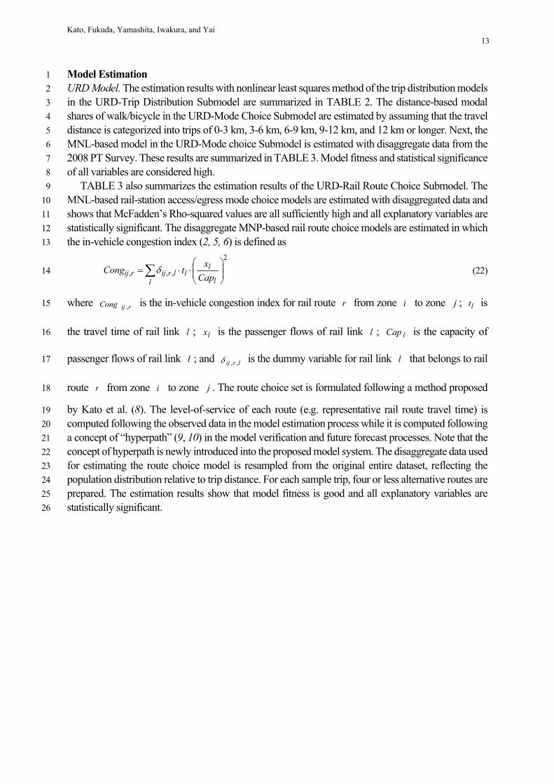
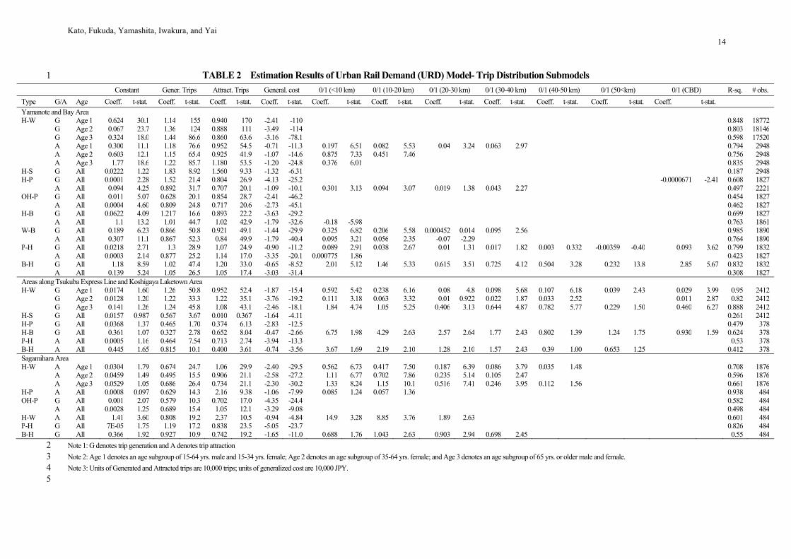
Model Estimation 1
URD Model. The estimation results with nonlinear least squares method of the trip distribution models 2
in the URD-Trip Distribution Submodel are summarized in TABLE 2. The distance-based modal 3
shares of walk/bicycle in the URD-Mode Choice Submodel are estimated by assuming that the travel 4
distance is categorized into trips of 0-3 km, 3-6 km, 6-9 km, 9-12 km, and 12 km or longer. Next, the 5
MNL-based model in the URD-Mode choice Submodel is estimated with disaggregate data from the 6
2008 PT Survey. These results are summarized in TABLE 3. Model fitness and statistical significance 7
of all variables are considered high. 8
TABLE 3 also summarizes the estimation results of the URD-Rail Route Choice Submodel. The 9
MNL-based rail-station access/egress mode choice models are estimated with disaggregated data and 10
shows that McFadden’s Rho-squared values are all sufficiently high and all explanatory variables are 11
statistically significant. The disaggregate MNP-based rail route choice models are estimated in which 12
the in-vehicle congestion index (2, 5, 6) is defined as 13
2
,,,
l l
lllrijrij Cap
xtCong (22) 14
where rijCong , is the in-vehicle congestion index for rail route r from zone i to zone j ; lt is 15
the travel time of rail link l ; lx is the passenger flows of rail link l ; lCap is the capacity of 16
passenger flows of rail link l ; and lrij ,, is the dummy variable for rail link l that belongs to rail 17
route r from zone i to zone j . The route choice set is formulated following a method proposed 18
by Kato et al. (8). The level-of-service of each route (e.g. representative rail route travel time) is 19
computed following the observed data in the model estimation process while it is computed following 20
a concept of “hyperpath” (9, 10) in the model verification and future forecast processes. Note that the 21
concept of hyperpath is newly introduced into the proposed model system. The disaggregate data used 22
for estimating the route choice model is resampled from the original entire dataset, reflecting the 23
population distribution relative to trip distance. For each sample trip, four or less alternative routes are 24
prepared. The estimation results show that model fitness is good and all explanatory variables are 25
statistically significant. 26
Kato, Fukuda, Yamashita, Iwakura, and Yai 14
TABLE 2 Estimation Results of Urban Rail Demand (URD) Model- Trip Distribution Submodels 1
Note 1: G denotes trip generation and A denotes trip attraction 2 Note 2: Age 1 denotes an age subgroup of 15-64 yrs. male and 15-34 yrs. female; Age 2 denotes an age subgroup of 35-64 yrs. female; and Age 3 denotes an age subgroup of 65 yrs. or older male and female. 3 Note 3: Units of Generated and Attracted trips are 10,000 trips; units of generalized cost are 10,000 JPY. 4 5
Constant Gener. Trips Attract. Trips General. cost 0/1 (<10 km) 0/1 (10-20 km) 0/1 (20-30 km) 0/1 (30-40 km) 0/1 (40-50 km) 0/1 (50<km) 0/1 (CBD) R-sq. # obs.
Type G/A Age Coeff. t-stat. Coeff. t-stat. Coeff. t-stat. Coeff. t-stat. Coeff. t-stat. Coeff. t-stat. Coeff. t-stat. Coeff. t-stat. Coeff. t-stat. Coeff. t-stat. Coeff. t-stat. Yamanote and Bay Area H-W G Age 1 0.624 30.1 1.14 155 0.940 170 -2.41 -110 0.848 18772 G Age 2 0.067 23.7 1.36 124 0.888 111 -3.49 -114 0.803 18146 G Age 3 0.324 18.0 1.44 86.6 0.860 63.6 -3.16 -78.1 0.598 17520 A Age 1 0.300 11.1 1.18 76.6 0.952 54.5 -0.71 -11.3 0.197 6.51 0.082 5.53 0.04 3.24 0.063 2.97 0.794 2948 A Age 2 0.603 12.1 1.15 65.4 0.925 41.9 -1.07 -14.6 0.875 7.33 0.451 7.46 0.756 2948 A Age 3 1.77 18.6 1.22 85.7 1.180 53.5 -1.20 -24.8 0.376 6.01 0.835 2948 H-S G All 0.0222 1.22 1.83 8.92 1.560 9.33 -1.32 -6.31 0.187 2948 H-P G All 0.0001 2.28 1.52 21.4 0.804 26.9 -4.13 -25.2 -0.0000671 -2.41 0.608 1827 A All 0.094 4.25 0.892 31.7 0.707 20.1 -1.09 -10.1 0.301 3.13 0.094 3.07 0.019 1.38 0.043 2.27 0.497 2221 OH-P G All 0.011 5.07 0.628 20.1 0.854 28.7 -2.41 -46.2 0.454 1827 A All 0.0004 4.60 0.809 24.8 0.717 20.6 -2.73 -45.1 0.462 1827 H-B G All 0.0622 4.09 1.217 16.6 0.893 22.2 -3.63 -29.2 0.699 1827 A All 1.1 13.2 1.01 44.7 1.02 42.9 -1.79 -32.6 -0.18 -5.98 0.763 1861 W-B G All 0.189 6.23 0.866 50.8 0.921 49.1 -1.44 -29.9 0.325 6.82 0.206 5.58 0.000452 0.014 0.095 2.56 0.985 1890 A All 0.307 11.1 0.867 52.3 0.84 49.9 -1.79 -40.4 0.095 3.21 0.056 2.35 -0.07 -2.29 0.764 1890 P-H G All 0.0218 2.71 1.3 28.9 1.07 24.9 -0.90 -11.2 0.089 2.91 0.038 2.67 0.01 1.31 0.017 1.82 0.003 0.332 -0.00359 -0.40 0.093 3.62 0.799 1832 A All 0.0003 2.14 0.877 25.2 1.14 17.0 -3.35 -20.1 0.000775 1.86 0.423 1827 B-H G All 1.18 8.59 1.02 47.4 1.20 33.0 -0.65 -8.52 2.01 5.12 1.46 5.33 0.615 3.51 0.725 4.12 0.504 3.28 0.232 13.8 2.85 5.67 0.832 1832 A All 0.139 5.24 1.05 26.5 1.05 17.4 -3.03 -31.4 0.308 1827 Areas along Tsukuba Express Line and Koshigaya Laketown Area H-W G Age 1 0.0174 1.60 1.26 50.8 0.952 52.4 -1.87 -15.4 0.592 5.42 0.238 6.16 0.08 4.8 0.098 5.68 0.107 6.18 0.039 2.43 0.029 3.99 0.95 2412 G Age 2 0.0128 1.20 1.22 33.3 1.22 35.1 -3.76 -19.2 0.111 3.18 0.063 3.32 0.01 0.922 0.022 1.87 0.033 2.52 0.011 2.87 0.82 2412 G Age 3 0.141 1.26 1.24 45.8 1.08 43.1 -2.46 -18.1 1.84 4.74 1.05 5.25 0.406 3.13 0.644 4.87 0.782 5.77 0.229 1.50 0.460 6.27 0.888 2412 H-S G All 0.0157 0.987 0.567 3.67 0.010 0.367 -1.64 -4.11 0.261 2412 H-P G All 0.0368 1.37 0.465 1.70 0.374 6.13 -2.83 -12.5 0.479 378 H-B G All 0.361 1.07 0.327 2.78 0.652 8.04 -0.47 -2.66 6.75 1.98 4.29 2.63 2.57 2.64 1.77 2.43 0.802 1.39 1.24 1.75 0.930 1.59 0.624 378 P-H A All 0.0005 1.16 0.464 7.54 0.713 2.74 -3.94 -13.3 0.53 378 B-H A All 0.445 1.65 0.815 10.1 0.400 3.61 -0.74 -3.56 3.67 1.69 2.19 2.10 1.28 2.10 1.57 2.43 0.39 1.00 0.653 1.25 0.412 378 Sagamihara Area H-W A Age 1 0.0304 1.79 0.674 24.7 1.06 29.9 -2.40 -29.5 0.562 6.73 0.417 7.50 0.187 6.39 0.086 3.79 0.035 1.48 0.708 1876 A Age 2 0.0459 1.49 0.495 15.5 0.906 21.1 -2.58 -27.2 1.11 6.77 0.702 7.86 0.235 5.14 0.105 2.47 0.596 1876 A Age 3 0.0529 1.05 0.686 26.4 0.734 21.1 -2.30 -30.2 1.33 8.24 1.15 10.1 0.516 7.41 0.246 3.95 0.112 1.56 0.661 1876 H-P A All 0.0008 0.097 0.629 14.3 2.16 9.38 -1.06 -7.99 0.085 1.24 0.057 1.36 0.938 484 OH-P G All 0.001 2.07 0.579 10.3 0.702 17.0 -4.35 -24.4 0.582 484 A All 0.0028 1.25 0.689 15.4 1.05 12.1 -3.29 -9.08 0.498 484 H-W A All 1.41 3.60 0.808 19.2 2.37 10.5 -0.94 -4.84 14.9 3.28 8.85 3.76 1.89 2.63 0.601 484 P-H G All 7E-05 1.75 1.19 17.2 0.838 23.5 -5.05 -23.7 0.826 484 B-H G All 0.366 1.92 0.927 10.9 0.742 19.2 -1.65 -11.0 0.688 1.76 1.043 2.63 0.903 2.94 0.698 2.45 0.55 484
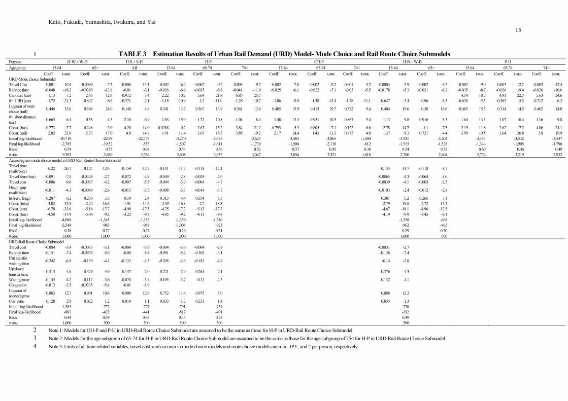
Kato, Fukuda, Yamashita, Iwakura, and Yai 15
TABLE 3 Estimation Results of Urban Rail Demand (URD) Model- Mode Choice and Rail Route Choice Submodels 1 Purpose H-W + W-H H-S + S-H H-P OH-P H-B + W-B P-H Age group 15-64 65< All 15-64 65-74 74< 15-64 65-74 74< 15-64 65< 15-64 65-74 74< Coeff. t-stat. Coeff. t-stat. Coeff. t-stat. Coeff. t-stat. Coeff. t-stat. Coeff. t-stat. Coeff. t-stat. Coeff. t-stat. Coeff. t-stat. Coeff. t-stat. Coeff. t-stat. Coeff. t-stat. Coeff. t-stat. Coeff. t-stat. URD-Mode choice Submodel Travel Cost -0.001 -10.4 -0.0009 -7.3 -0.006 -13.1 -0.002 -6.2 -0.002 -9.2 -0.003 -9.7 -0.002 -7.8 -0.002 -8.2 -0.001 -3.2 -0.0004 -2.9 -0.002 -8.2 -0.002 -9.0 -0.003 -12.2 -0.003 -12.4 Railride time -0.048 -18.2 -0.0389 -13.8 -0.01 -2.1 -0.026 -6.6 -0.035 -8.8 -0.041 -11.0 -0.025 -6.1 -0.022 -7.1 -0.03 -5.5 -0.0178 -5.3 -0.031 -8.2 -0.035 -8.7 -0.026 -9.4 -0.036 -10.6 Car own. (car) 1.13 7.2 2.45 12.9 0.972 3.4 2.22 10.2 5.64 21.8 6.85 25.7 4.14 18.7 4.91 22.3 5.63 24.6 0/1 CBD (car) -1.72 -21.3 -0.847 -8.6 -0.571 -2.1 -1.18 -10.9 -1.2 -11.0 -1.28 -10.7 -1.06 -9.9 -1.38 -15.4 -1.78 -11.1 -0.647 -5.4 -0.96 -8.3 -0.638 -5.5 -0.565 -5.5 -0.712 -6.3 Logsum of route choice (rail)
0.446 33.6 0.504 24.0 0.148 4.9 0.341 13.7 0.367 13.9 0.361 13.6 0.405 15.9 0.413 19.7 0.372 9.4 0.404 19.6 0.38 16.6 0.465 15.5 0.314 14.5 0.402 14.0
0/1 short distance (car)
0.665 6.1 0.53 4.3 2.18 6.9 1.63 15.0 1.22 10.8 1.04 8.4 1.48 13.3 0.951 10.5 0.867 5.4 1.13 9.8 0.916 8.3 1.64 13.3 1.07 10.4 1.16 9.8
Const. (bus) -0.773 -7.7 0.248 2.0 4.28 14.0 0.0288 0.2 2.67 15.2 3.84 21.2 -0.793 -5.3 -0.805 -7.1 0.122 0.6 -2.78 -14.7 -1.1 -7.5 2.15 11.8 2.62 17.2 4.06 24.1 Const. (rail) 2.82 21.8 2.73 17.0 4.8 14.8 1.91 11.4 3.67 18.3 3.85 19.2 2.17 14.4 1.43 11.3 0.875 4.0 1.37 8.3 0.721 4.4 3.99 19.5 3.64 20.8 3.8 19.9 Initial log-likelihood -10,710 -42,99 -22,773 -3,270 -3,675 -3,625 -3,483 -3,865 -1,304 -3.331 -3,204 -3,354 -3,532 -3,537 Final log-likelihood -2,785 -19,52 -553 -1,507 -1,611 -1,730 -1,508 -2,118 -812 -1.515 -1,528 -1,344 -1,905 -1.796 Rho2 0.74 0.55 0.98 0.54 0.56 0.52 0.57 0.45 0.38 0.54 0.52 0.60 0.46 0.49 # obs. 9,763 3,689 2,786 2,608 3,037 3,047 2,894 3,521 1,018 2,780 2,604 2,774 3,219 2,932 Access/egress mode choice model in URD-Rail Route Choice Submodel
Travel time (walk/bike)
-0.22 -26.7 -0.127 -12.6 -0.159 -12.7 -0.131 -11.7 -0.118 -12.1 -0.155 -13.7 -0.118 -8.7
Travel time (bus) -0.091 -7.5 -0.0449 -2.7 -0.072 -4.9 -0.049 -2.8 -0.029 -2.0 -0.0865 -4.3 -0.064 -3.0
Travel cost -0.006 -9.6 -0.0037 -4.2 -0.007 -5.3 -0.004 -3.9 -0.004 -4.7 -0.0039 -4.1 -0.003 -2.5
Height gap (walk/bike)
-0.011 -4.1 -0.0089 -2.6 -0.013 -3.5 -0.008 -3.3 -0.014 -3.7 -0.0103 -2.4 -0.012 -2.8
ln (serv. freq.) 0.287 6.2 0.236 3.5 0.19 2.4 0.313 4.4 0.354 5.5 0.381 5.2 0.265 3.1
Const. (bike) -3.02 -32.9 -2.24 -16.6 -1.91 -14.6 -2.39 -16.8 -2.7 -18.3 -2.79 -19.8 -2.72 -13.2
Const. (car) -6.78 -33.6 -5.16 -17.7 -4.98 -17.5 -4.75 -17.2 -5.12 -17.7 -4.67 -18.1 -4.96 -12.5
Const. (bus) -4.58 -17.9 -3.44 -9.2 -3.22 -9.3 -4.05 -9.2 -4.13 -9.8 -4.19 -9.9 -3.45 -6.1
Initial log-likelihood -4,086 -1,345 -1,355 -1,359 -1,340 -1,358 -668
Final log-likelihood -2,549 -983 -988 -1,008 -923 -962 -465
Rho2 0.38 0.27 0.27 0.26 0.31 0.29 0.30
# obs. 3,000 1,000 1,000 1,000 1,000 1,000 500
URD-Rail Route Choice Submodel
Travel cost -0.004 -3.9 -0.0033 -3.1 -0.004 -3.9 -0.004 -3.6 -0.004 -2.8 -0.0031 -2.7
Railride time -0.151 -7.4 -0.0974 -5.6 -0.08 -5.4 -0.091 -5.2 -0.102 -3.1 -0.136 -7.4
Flat transfer walking time
-0.242 -6.5 -0.139 -4.2 -0.133 -3.5 -0.205 -3.9 -0.183 -2.6 -0.14 -2.8
Up/down transfer time
-0.313 -4.8 -0.329 -4.9 -0.137 -2.0 -0.221 -2.9 -0.261 -2.1 -0.376 -4.3
Waiting time -0.145 -4.2 -0.112 -3.6 -0.078 -3.4 -0.105 -3.7 -0.12 -2.5 -0.132 -4.1
Congestion -0.012 -2.5 -0.0335 -5.4 -0.01 -1.9
Logsum of access/egress
0.883 12.7 0.991 10.6 0.908 12.6 0.752 11.4 0.975 5.0 0.888 12.2
Cov. ratio 0.128 2.9 0.022 1.2 0.019 1.1 0.033 1.2 0.253 1.4 0.035 1.3
Initial log-likelihood -1,585 -773 -777 -791 -734 -770
Final log-likelihood -887 -472 -441 -512 -491 -392
Rho2 0.44 0.39 0.43 0.35 0.33 0.49
# obs. 1,000 500 500 500 500 500
Note 1: Models for OH-P and P-H in URD-Rail Route Choice Submodel are assumed to be the same as those for H-P in URD-Rail Route Choice Submodel. 2 Note 2: Models for the age subgroup of 65-74 for H-P in URD-Rail Route Choice Submodel are assumed to be the same as those for the age subgroup of 75< for H-P in URD-Rail Route Choice Submodel. 3 Note 3: Units of all time related variables, travel cost, and car own in mode choice models and route choice models are min., JPY, and # per person, respectively.4
Kato, Fukuda, Yamashita, Iwakura, and Yai 16
ARAD Model. The growth factor method has been applied to estimate trip distribution of domestic air 1
passengers in the ARAD-Trip Distribution Submodel per the following the two steps. (1) Allocating 2
the trips under the assumption that the future trip distribution pattern would be the same as the current 3
distribution pattern by large-scale (L) zone level. Note the area of L zones is approximately equivalent 4
to municipal administrative area and there are 333 L zones in the target area. (2) Allocating the L-5
zone-based O-D trips into TAZ-based O-D trips in proportion to their population size. The population 6
sizes are assumed to be nighttime population for the nonbusiness trips of domestic air passengers; the 7
daytime worker population for the business trips made by domestic air passengers who reside in other 8
areas than TMA; and average of the nighttime population and daytime worker population for the 9
business trips made by domestic air passengers who reside in TMA. 10
TABLE 4 shows the estimation results of the ARAD model where the MNL-based mode choice 11
model is estimated for domestic air passengers. The results show that all models have high 12
McFadden’s Rho-squared values while all explanatory variables are statistically significant. One of 13
the unique aspects of this model is that the travel time reliability measured as the standard deviation of 14
travel times for car trips has been incorporated as one of the car-mode specific variables. The reliability 15
data were obtained from the probe database of motor vehicle companies (11). As for the routes without 16
such observed data, the following formula estimated from the route-level regression has been applied 17
to obtain the interpolated numbers (12): 18
8.313.157.95.456.32
416.34145.0130.0092.0805.28 ,,,,exp,,,,
lanetworijlanemultirijrijrijrij DDDClSD (23) 19
73.0559,1 2 RN 20
where rijSD , is the standard deviation of travel times (min.) for route r from zone i to zone j ; 21
rijCl , is the congestion index (average travel time divided by free-flow travel time); exp,,rijD is the 22
length (km) of expressway section in route r ; lanemultirijD ,, is the length (km) of non-expressway 23
section with three or more lanes in route r ; and lanetwoijD , is the length (km) of non-expressway 24
section with two lanes in route r . 25
The MNL-based rail route choice submodel is estimated for domestic air passengers in the 26
ARAD-Rail Route Choice Submodel as shown in TABLE 4. The explanatory variables are the total 27
travel time of non-express rail service; rail-ride travel time of express rail service; travel cost; and time 28
of transfers from rail to rail. Level-of-service data is computed using the hyperpath algorithm (9) for 29
each L-zone level. All models have high McFadden’s Rho-squared values and all parameters are 30
statistically significant. 31
The growth factor method is applied to the estimation of trip distribution of international air 32
passengers in the ARAD-Trip Distribution Submodel, thereby following the same process as domestic 33
air passengers. The 2013 International Air Passenger Travel Demand Survey cannot capture the origin 34
to access the airports while it can capture the L-zone-based destination. The locations of foreign 35
individuals who stayed overnight are assumed to represent their origins to access the airports using the 36
data of the 2012 Overnight Stay Tourism Statistical Survey. We note this assumption may lead to 37
biased results because they may not directly travel from their accommodation to airports or vice versa. 38
The MNL-based mode choice model is estimated for international air passengers in the ARAD-39
Mode choice Submodel in TABLE 4. The results show that the goodness-of-fit of the leisure purpose 40
model is slightly weaker than for other models. The travel time reliability is weakly significant for 41
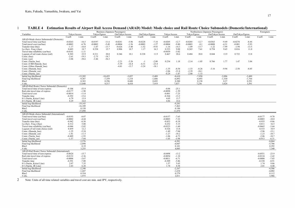
Kato, Fukuda, Yamashita, Iwakura, and Yai 17
TABLE 4 Estimation Results of Airport Rail Access Demand (ARAD) Model: Mode choice and Rail Route Choice Submodels (Domestic/International) 1 Business (Japanese Passengers) Nonbusiness (Japanese Passengers) Foreigners Variables Tokyo/Access Tokyo/Egress OutTokyo/Access OutTokyo/Egress Tokyo/Access Tokyo/Egress OutTokyo/Access OutTokyo/Egress Coeff. t-stat. Coeff. t-stat. Coeff. t-stat. Coeff. t-stat. Coeff. t-stat. Coeff. t-stat. Coeff. t-stat. Coeff. t-stat. Coeff. t-stat. ARAD-Mode choice Submmodel (Domestic)
Total travel time (car/bus) -0.0263 -16.5 -0.0197 -11.6 -0.0241 -5.96 -0.0228 -7.18 -0.0205 -12.7 -0.0205 -12.7 -0.0363 -9.49 -0.0278 -8.44
Total travel cost (car/bus) -0.0003 -6.76 -0.0003 -5.49 -0.0004 -1.56 -0.0003 -1.57 -0.0004 -9.80 -0.0003 -8.1 -0.0008 -4.31 -0.001 -5.93
Transfer time (bus) -1.17 -16.0 -1.07 -13.7 -0.626 -3.40 -1.52 -9.93 -1.16 -14.3 -1.09 -13.7 -1.22 -7.99 -1.94 -13.5
Ln (Serv. Freq.) (bus) 0.603 18.7 0.538 15.7 0.906 10.7 1.17 16.3 0.333 9.08 0.265 7.61 0.754 9.65 0.816 11.0
Travel time reliability (car/bus) -0.0141 -1.11 -0.0439 -3.02
Logsum of rail route choice (rail) 0.303 23.9 0.311 20.8 0.346 10.1 0.338 11.9 0.467 20.6 0.484 20.8 0.844 13.9 0.722 13.8
Const. (bus) -2.61 -19.5 -2.75 -18.7
Const. (car) -3.06 -38.6 -3.46 -36.3
Const. (Narita_bus) -2.21 -3.26 -1 -2.00 0.234 1.18 -2.14 -1.05 0.766 1.77 1.47 3.84
Const. (CBD-Haneda_bus) -5.39 -16.4 -6.31 -23.4
Const. (Other-Haneda_bus) -4.81 -13.7 -5.24 -18.1
Const. (Haneda_bus) -1.35 -8.54 -1.33 -8.26 -3.16 -9.94 -2.58 -8.85
Const. (Haneda_car) -2.06 -21.8 -2.39 -24.1
Const. (Narita_car) -0.29 -1.87 -2.00 -1.33
Initial log-likelihood -15,205 -10,455 -3,057 -5,489 -8,610 -7,950 -2,096 -2,489
Final log-likelihood -9,387 -7,359 -1,218 -1,686 -6,892 -6,693 -1,530 -1,764
Rho2 0.383 0.296 0.600 0.692 0.200 0.158 0.27 0.291
# obs. 13,840 9,517 4,410 7,919 7,837 7,236 3,024 3,591
ARAD-Rail Route Choice Submodel (Domestic)
Total travel time of non-express -0.106 -53.9 -0.06 -25.1
Rail-ride travel time of express -0.0177 -1.90 -0.0098 -1.59
Total travel cost -0.0014 -11.0 -0.001 -7.25
Transfer time -0.292 -13.6 -0.364 -13.2
0/1 (Narita_Keisei Line) 6.79 13.9 4.05 13.7
0/1 (Narita_JR Line) 8.29 16.0 4.86 14.6
Initial log-likelihood -19,143 -9,283
Final log-likelihood -16,109 -7,462
Rho2 0.158 0.196
# obs. 27,090 11,870
ARAD-Mode choice Submodel (International)
Total travel time (car/bus) -0.0193 -8.07 -0.0157 -7.65 -0.0177 -9.70 Total travel cost (car/bus) -0.0002 -4.44 -0.0003 -7.22 -0.0003 -10.0 Transfer time (bus) -0.942 -8.58 -0.853 -8.18 -0.935 -9.86 Ln (Serv. Freq.) (bus) 0.312 5.80 0.252 5.15 0.811 16.5 Travel time reliability (car/bus) -0.046 -2.02 -0.0323 -1.60 -0.0665 -3.64 Logsum of rail route choice (rail) 0.459 12.2 0.526 13.8 0.533 18.9 Const. (Haneda_bus) -1.25 -5.24 -1.49 -7.04 -2.96 -15.1 Const. (Haneda_car) -1.81 -11.5 -1.27 -10.2 -1.23 -10.7 Const. (Narita_bus) -0.489 -1.93 -1.06 -4.73 -2.06 -10.7 Const. (Narita_car) -1.57 -7.04 -1.05 -5.98 -0.913 -6.31 Initial log-likelihood -3,576 -4,501 -8,064 Final log-likelihood -2,898 -4,047 -5,706 Rho2 0.19 0.101 0.292 # obs. 3,255 4,085 7,340 ARAD-Rail Route Choice Submodel (International)
Total travel time of non-express -0.0624 -15.7 -0.0498 -13.2 -0.0551 -23.9 Rail-ride travel time of express -0.0132 -2.36 -0.0054 -1.10 -0.0124 -3.42 Total travel cost -0.0006 -3.67 -0.0011 -6.71 -0.0008 -7.03 Transfer time -0.391 -7.00 -0.309 -5.86 -0.338 -8.91 0/1 (Narita_Keisei Line) 2.07 7.35 1.57 5.65 1.74 9.86 0/1 (Narita_JR Line) 2.43 6.28 1.74 4.58 2.01 8.40 Initial log-likelihood -2,240 -2,267 -4,506 Final log-likelihood -1,447 -1,634 -4,002 Rho2 0.354 0.279 0.112 # obs. 1,975 2,011 3,986
Note: Units of all time related variables and travel cost are min. and JPY, respectively.2
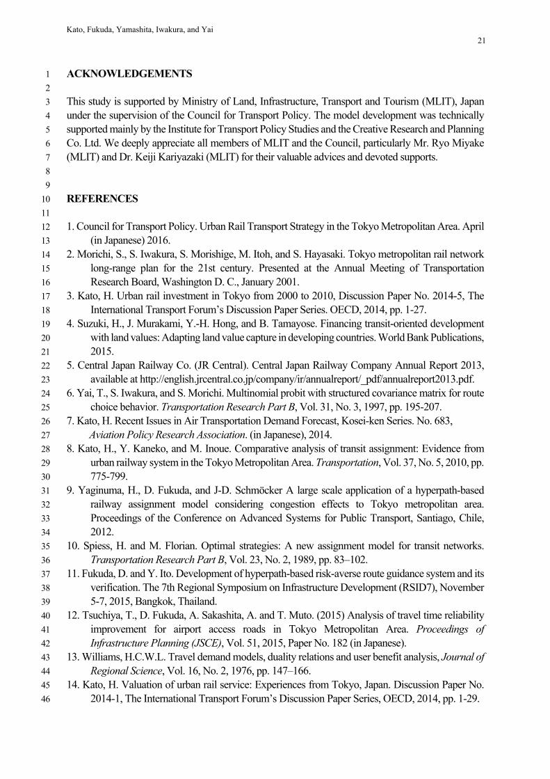
Kato, Fukuda, Yamashita, Iwakura, and Yai 18
Japanese business passengers accessing airports while it is fairly significant for non-business Japanese 1
passengers accessing airports. For international passenger accessing an airport, the opposite held true. 2
Finally, the MNL-based rail route choice model is estimated for international air passengers in 3
the ARAD-Rail Route Choice Submodel. Level-of-service data is also computed using the hyperpath 4
algorithm (9) at the L-zone level. The model fitness is high while all variables are statistically 5
significant. 6
7
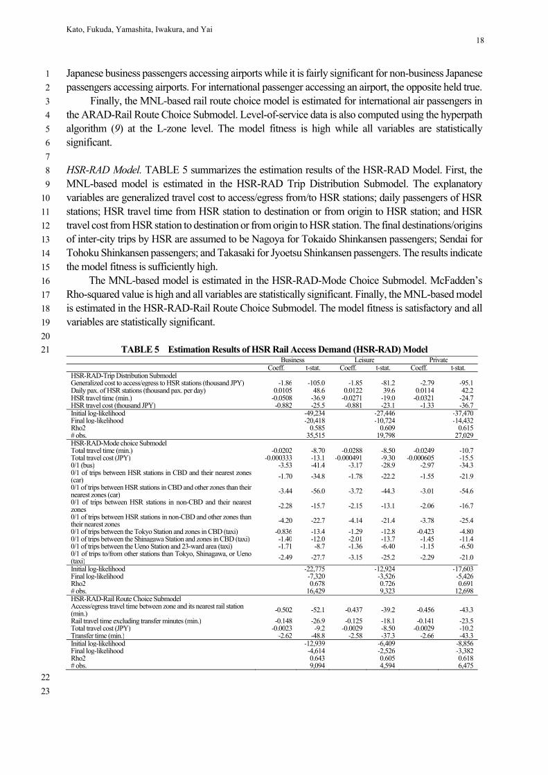
HSR-RAD Model. TABLE 5 summarizes the estimation results of the HSR-RAD Model. First, the 8
MNL-based model is estimated in the HSR-RAD Trip Distribution Submodel. The explanatory 9
variables are generalized travel cost to access/egress from/to HSR stations; daily passengers of HSR 10
stations; HSR travel time from HSR station to destination or from origin to HSR station; and HSR 11
travel cost from HSR station to destination or from origin to HSR station. The final destinations/origins 12
of inter-city trips by HSR are assumed to be Nagoya for Tokaido Shinkansen passengers; Sendai for 13
Tohoku Shinkansen passengers; and Takasaki for Jyoetsu Shinkansen passengers. The results indicate 14
the model fitness is sufficiently high. 15
The MNL-based model is estimated in the HSR-RAD-Mode Choice Submodel. McFadden’s 16
Rho-squared value is high and all variables are statistically significant. Finally, the MNL-based model 17
is estimated in the HSR-RAD-Rail Route Choice Submodel. The model fitness is satisfactory and all 18
variables are statistically significant. 19
20
TABLE 5 Estimation Results of HSR Rail Access Demand (HSR-RAD) Model 21 Business Leisure Private Coeff. t-stat. Coeff. t-stat. Coeff. t-stat.HSR-RAD-Trip Distribution Submodel Generalized cost to access/egress to HSR stations (thousand JPY) -1.86 -105.0 -1.85 -81.2 -2.79 -95.1 Daily pax. of HSR stations (thousand pax. per day) 0.0105 48.6 0.0122 39.6 0.0114 42.2 HSR travel time (min.) -0.0508 -36.9 -0.0271 -19.0 -0.0321 -24.7 HSR travel cost (thousand JPY) -0.882 -25.5 -0.881 -23.1 -1.33 -36.7 Initial log-likelihood -49,234 -27,446 -37,470Final log-likelihood -20,418 -10,724 -14,432Rho2 0.585 0.609 0.615# obs. 35,515 19,798 27,029HSR-RAD-Mode choice Submodel Total travel time (min.) -0.0202 -8.70 -0.0288 -8.50 -0.0249 -10.7 Total travel cost (JPY) -0.000333 -13.1 -0.000491 -9.30 -0.000605 -15.5 0/1 (bus) -3.53 -41.4 -3.17 -28.9 -2.97 -34.3 0/1 of trips between HSR stations in CBD and their nearest zones (car) -1.70 -34.8 -1.78 -22.2 -1.55 -21.9
0/1 of trips between HSR stations in CBD and other zones than their nearest zones (car) -3.44 -56.0 -3.72 -44.3 -3.01 -54.6
0/1 of trips between HSR stations in non-CBD and their nearest zones -2.28 -15.7 -2.15 -13.1 -2.06 -16.7
0/1 of trips between HSR stations in non-CBD and other zones than their nearest zones -4.20 -22.7 -4.14 -21.4 -3.78 -25.4
0/1 of trips between the Tokyo Station and zones in CBD (taxi) -0.836 -13.4 -1.29 -12.8 -0.423 -4.800/1 of trips between the Shinagawa Station and zones in CBD (taxi) -1.40 -12.0 -2.01 -13.7 -1.45 -11.4 0/1 of trips between the Ueno Station and 23-ward area (taxi) -1.71 -8.7 -1.36 -6.40 -1.15 -6.500/1 of trips to/from other stations than Tokyo, Shinagawa, or Ueno (taxi) -2.49 -27.7 -3.15 -25.2 -2.29 -21.0
Initial log-likelihood -22,775 -12,924 -17,603Final log-likelihood -7,320 -3,526 -5,426Rho2 0.678 0.726 0.691# obs. 16,429 9,323 12,698HSR-RAD-Rail Route Choice Submodel Access/egress travel time between zone and its nearest rail station(min.) -0.502 -52.1 -0.437 -39.2 -0.456 -43.3
Rail travel time excluding transfer minutes (min.) -0.148 -26.9 -0.125 -18.1 -0.141 -23.5 Total travel cost (JPY) -0.0023 -9.2 -0.0029 -8.50 -0.0029 -10.2 Transfer time (min.) -2.62 -48.8 -2.58 -37.3 -2.66 -43.3 Initial log-likelihood -12,939 -6,409 -8,856Final log-likelihood -4,614 -2,526 -3,382Rho2 0.643 0.605 0.618# obs. 9,094 4,594 6,475
22
23
Kato, Fukuda, Yamashita, Iwakura, and Yai 19
VALIDATION OF MODEL SYSTEM 1
2
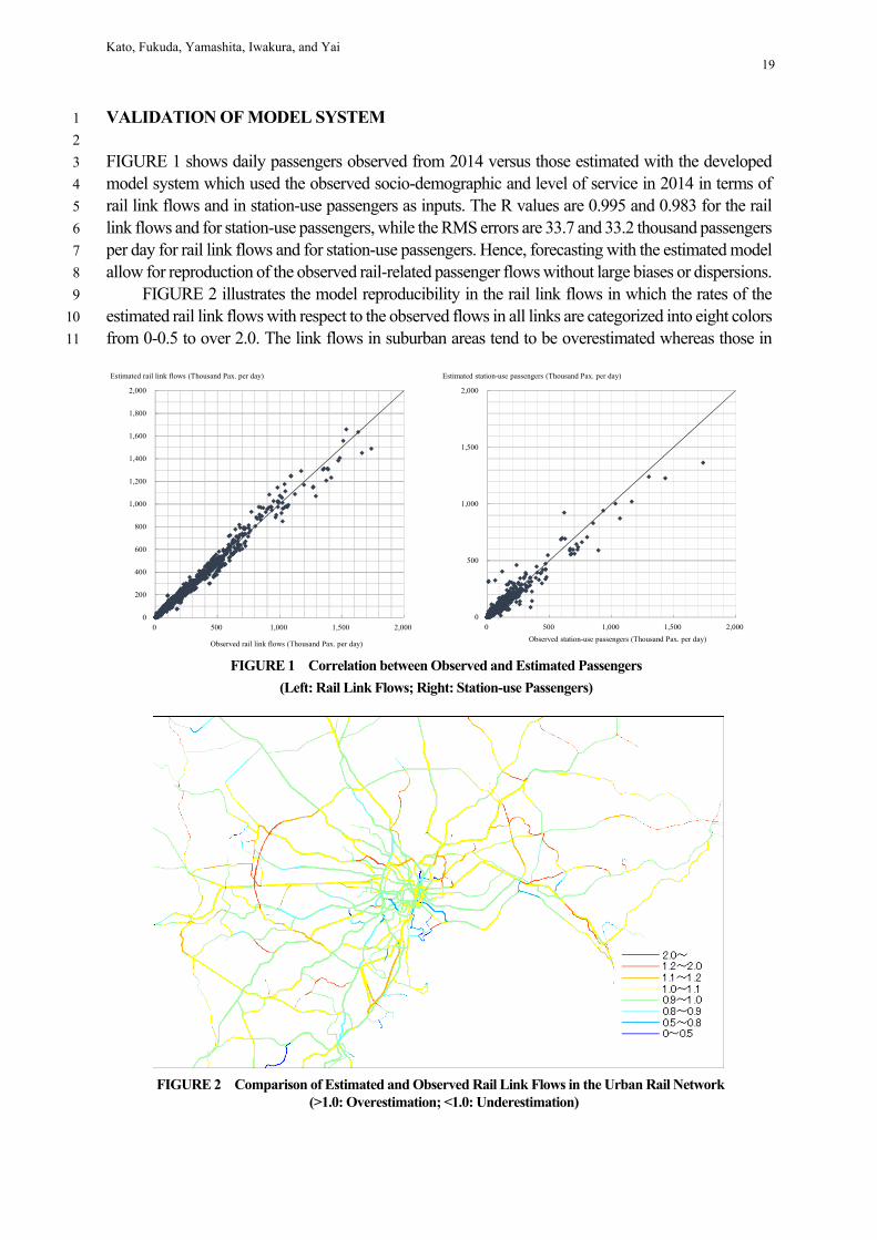
FIGURE 1 shows daily passengers observed from 2014 versus those estimated with the developed 3
model system which used the observed socio-demographic and level of service in 2014 in terms of 4
rail link flows and in station-use passengers as inputs. The R values are 0.995 and 0.983 for the rail 5
link flows and for station-use passengers, while the RMS errors are 33.7 and 33.2 thousand passengers 6
per day for rail link flows and for station-use passengers. Hence, forecasting with the estimated model 7
allow for reproduction of the observed rail-related passenger flows without large biases or dispersions. 8
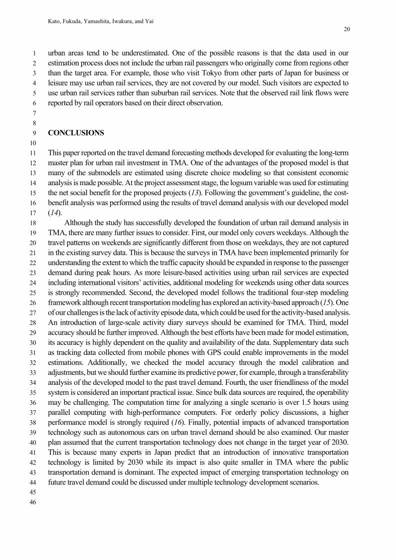
FIGURE 2 illustrates the model reproducibility in the rail link flows in which the rates of the 9
estimated rail link flows with respect to the observed flows in all links are categorized into eight colors 10
from 0-0.5 to over 2.0. The link flows in suburban areas tend to be overestimated whereas those in 11
FIGURE 1 Correlation between Observed and Estimated Passengers
(Left: Rail Link Flows; Right: Station-use Passengers)
FIGURE 2 Comparison of Estimated and Observed Rail Link Flows in the Urban Rail Network (>1.0: Overestimation; <1.0: Underestimation)
0
200
400
600
800
1,000
1,200
1,400
1,600
1,800
2,000
0 500 1,000 1,500 2,000
Observed rail link flows (Thousand Pax. per day)
Estimated rail link flows (Thousand Pax. per day)
0
500
1,000
1,500
2,000
0 500 1,000 1,500 2,000
Observed station-use passengers (Thousand Pax. per day)
Estimated station-use passengers (Thousand Pax. per day)
Kato, Fukuda, Yamashita, Iwakura, and Yai 20
urban areas tend to be underestimated. One of the possible reasons is that the data used in our 1
estimation process does not include the urban rail passengers who originally come from regions other 2
than the target area. For example, those who visit Tokyo from other parts of Japan for business or 3
leisure may use urban rail services, they are not covered by our model. Such visitors are expected to 4
use urban rail services rather than suburban rail services. Note that the observed rail link flows were 5
reported by rail operators based on their direct observation. 6
7
8
CONCLUSIONS 9
10
This paper reported on the travel demand forecasting methods developed for evaluating the long-term 11
master plan for urban rail investment in TMA. One of the advantages of the proposed model is that 12
many of the submodels are estimated using discrete choice modeling so that consistent economic 13
analysis is made possible. At the project assessment stage, the logsum variable was used for estimating 14
the net social benefit for the proposed projects (13). Following the government’s guideline, the cost-15
benefit analysis was performed using the results of travel demand analysis with our developed model 16
(14). 17
Although the study has successfully developed the foundation of urban rail demand analysis in 18
TMA, there are many further issues to consider. First, our model only covers weekdays. Although the 19
travel patterns on weekends are significantly different from those on weekdays, they are not captured 20
in the existing survey data. This is because the surveys in TMA have been implemented primarily for 21
understanding the extent to which the traffic capacity should be expanded in response to the passenger 22
demand during peak hours. As more leisure-based activities using urban rail services are expected 23
including international visitors’ activities, additional modeling for weekends using other data sources 24
is strongly recommended. Second, the developed model follows the traditional four-step modeling 25
framework although recent transportation modeling has explored an activity-based approach (15). One 26
of our challenges is the lack of activity episode data, which could be used for the activity-based analysis. 27
An introduction of large-scale activity diary surveys should be examined for TMA. Third, model 28
accuracy should be further improved. Although the best efforts have been made for model estimation, 29
its accuracy is highly dependent on the quality and availability of the data. Supplementary data such 30
as tracking data collected from mobile phones with GPS could enable improvements in the model 31
estimations. Additionally, we checked the model accuracy through the model calibration and 32
adjustments, but we should further examine its predictive power, for example, through a transferability 33
analysis of the developed model to the past travel demand. Fourth, the user friendliness of the model 34
system is considered an important practical issue. Since bulk data sources are required, the operability 35
may be challenging. The computation time for analyzing a single scenario is over 1.5 hours using 36
parallel computing with high-performance computers. For orderly policy discussions, a higher 37
performance model is strongly required (16). Finally, potential impacts of advanced transportation 38
technology such as autonomous cars on urban travel demand should be also examined. Our master 39
plan assumed that the current transportation technology does not change in the target year of 2030. 40
This is because many experts in Japan predict that an introduction of innovative transportation 41
technology is limited by 2030 while its impact is also quite smaller in TMA where the public 42
transportation demand is dominant. The expected impact of emerging transportation technology on 43
future travel demand could be discussed under multiple technology development scenarios. 44
45
46
Kato, Fukuda, Yamashita, Iwakura, and Yai 21
ACKNOWLEDGEMENTS 1
2
This study is supported by Ministry of Land, Infrastructure, Transport and Tourism (MLIT), Japan 3
under the supervision of the Council for Transport Policy. The model development was technically 4
supported mainly by the Institute for Transport Policy Studies and the Creative Research and Planning 5
Co. Ltd. We deeply appreciate all members of MLIT and the Council, particularly Mr. Ryo Miyake 6
(MLIT) and Dr. Keiji Kariyazaki (MLIT) for their valuable advices and devoted supports. 7
8
9
REFERENCES 10
11
1. Council for Transport Policy. Urban Rail Transport Strategy in the Tokyo Metropolitan Area. April 12
(in Japanese) 2016. 13
2. Morichi, S., S. Iwakura, S. Morishige, M. Itoh, and S. Hayasaki. Tokyo metropolitan rail network 14
long-range plan for the 21st century. Presented at the Annual Meeting of Transportation 15
Research Board, Washington D. C., January 2001. 16
3. Kato, H. Urban rail investment in Tokyo from 2000 to 2010, Discussion Paper No. 2014-5, The 17
International Transport Forum’s Discussion Paper Series. OECD, 2014, pp. 1-27. 18
4. Suzuki, H., J. Murakami, Y.-H. Hong, and B. Tamayose. Financing transit-oriented development 19
with land values: Adapting land value capture in developing countries. World Bank Publications, 20
2015. 21
5. Central Japan Railway Co. (JR Central). Central Japan Railway Company Annual Report 2013, 22
available at http://english.jrcentral.co.jp/company/ir/annualreport/_pdf/annualreport2013.pdf. 23
6. Yai, T., S. Iwakura, and S. Morichi. Multinomial probit with structured covariance matrix for route 24
choice behavior. Transportation Research Part B, Vol. 31, No. 3, 1997, pp. 195-207. 25
7. Kato, H. Recent Issues in Air Transportation Demand Forecast, Kosei-ken Series. No. 683, 26
Aviation Policy Research Association. (in Japanese), 2014. 27
8. Kato, H., Y. Kaneko, and M. Inoue. Comparative analysis of transit assignment: Evidence from 28
urban railway system in the Tokyo Metropolitan Area. Transportation, Vol. 37, No. 5, 2010, pp. 29
775-799. 30
9. Yaginuma, H., D. Fukuda, and J-D. Schmöcker A large scale application of a hyperpath-based 31
railway assignment model considering congestion effects to Tokyo metropolitan area. 32
Proceedings of the Conference on Advanced Systems for Public Transport, Santiago, Chile, 33
2012. 34
10. Spiess, H. and M. Florian. Optimal strategies: A new assignment model for transit networks. 35
Transportation Research Part B, Vol. 23, No. 2, 1989, pp. 83–102. 36
11. Fukuda, D. and Y. Ito. Development of hyperpath-based risk-averse route guidance system and its 37
verification. The 7th Regional Symposium on Infrastructure Development (RSID7), November 38
5-7, 2015, Bangkok, Thailand. 39
12. Tsuchiya, T., D. Fukuda, A. Sakashita, A. and T. Muto. (2015) Analysis of travel time reliability 40
improvement for airport access roads in Tokyo Metropolitan Area. Proceedings of 41
Infrastructure Planning (JSCE), Vol. 51, 2015, Paper No. 182 (in Japanese). 42
13. Williams, H.C.W.L. Travel demand models, duality relations and user benefit analysis, Journal of 43
Regional Science, Vol. 16, No. 2, 1976, pp. 147–166. 44
14. Kato, H. Valuation of urban rail service: Experiences from Tokyo, Japan. Discussion Paper No. 45
2014-1, The International Transport Forum’s Discussion Paper Series, OECD, 2014, pp. 1-29. 46
Kato, Fukuda, Yamashita, Iwakura, and Yai 22
15. Kitamura, R., A. Kikuchi, S. Fujii, and T. Yamamoto. An Overview of PCATS/DEBNetS Micro-1
Simulation System: Its Development, Extension, and Application to Demand Forecasting, 2
Kitamura, R. and Kuwahara, M. (eds.) Simulation Approaches in Transportation Analysis: 3
Recent Advances and Challenges, Springer US, Boston, MA, 2005, pp. 371-399. 4
16. Kamegai, J. and D. Fukuda. Comparison of analytical approximation methods for multinomial 5
probit model: A case study with passengers’ rail-route choice analysis in the Tokyo Metropolitan 6
Area, Presented at the 20th International Conference of Hong Kong Society for Transportation 7
Studies (HKSTS), Hong Kong, December 2015. 8