1 | P a g e   

                    Preliminary Draft                     Not for citation  

The impact of malnutrition over the life course 

 

John Hoddinott1 

John Maluccio2 

Jere Behrman3 

Reynaldo Martorell4 

Paul Melgar5 

Agnes Quisumbing1 

Manuel Ramirez‐Zea5 

Aryeh Stein4 

Kathryn Yount4 

 

July 12, 2010 

 

 

 

1 International Food Policy Research Institute, Washington DC. 2 Middlebury College 3 University of Pennsylvania 4 Emory University 5 INCAP, Guatemala City  Corresponding author: John Hoddinott, em: J.Hoddinott@cgiar.org  Acknowledgements: This research was supported by National Institutes of Health grants TW‐05598 on “Early Nutrition, Human Capital and Economic Productivity” and HD‐046125 on “Education and Health Across the Life Course in Guatemala”, National Institute of Child Health and Human Development grant 5R01HD045627‐05 on “Intergenerational Family Resource Allocation in Guatemala”, and NSF/Economics grants SES 0136616 and SES 0211404 on “Collaborative Research: Nutritional Investments in Children, Adult Human Capital and Adult Productivities.” We thank Alexis Murphy, Scott McNiven and Meng Wang for excellent research assistance in the preparation of the data for this paper. 

2 | P a g e   

 Abstract 

 

This paper examines the impact of being malnourished as measured by height for age (HAZ) at 36m over the life course. It uses data collected on individuals who participated in a nutrition supplementation trial between 1969 and 1977 in rural Guatemala and who were subsequently re‐interviewed between 2002 and 2004. We assess impacts across a wide range of domains: schooling; the marriage market; fertility; health; wages and income; and poverty and consumption in adulthood. We find that poor nutritional status at age 36m is linked to lower grade attainment and poorer cognitive skills in adulthood. Men earn lower wages and women are less likely to have independent sources of income from own business activities. Women who were stunted at age 36m have, on average, 1.9 more pregnancies and are more likely to give birth before age 17. Better nourished preschoolers are taller as adults and have more fat free mass and greater hand strength. Being stunted at age 36m increases the likelihood of living in a poor household in adulthood by 31 percentage points.  

3 | P a g e   

 

1. Introduction 

Around the world, more than 175 million preschool children are chronically malnourished or 

stunted, that is their height given their age is more than two standard deviations below that of 

international reference standards (Black et al, 2008). The physiological consequences of chronic 

malnourishment are well understood. In early life, these young children have high nutritional 

requirements, but the diets typically available to them have poor energy and nutrient 

concentrations. They are also very susceptible to infections because their immature immune 

systems fail to protect them adequately. In poor countries, foods and liquids are often 

contaminated and are thus key sources of frequent illness. Energy that should go towards 

growth is instead diverted to fighting off these infections (Martorell, 1997). Over time, 

“prolonged or severe nutrient depletion eventually leads to retardation of linear (skeletal) 

growth in children and to loss of, or failure to accumulate, muscle mass and fat” (Morris, 2001, 

p.12). This retardation of linear growth has permanent consequences as growth in stature lost 

in early life is never fully regained (Martorell, 1999).  

There are adverse neurological consequences of early ‐life chronic malnutrition.1 Early 

life malnutrition damages the hippocampus by reducing dentrite2 density (Blatt et al, 1994; 

Mazer et al, 1997; Ranade et al, 2008). It reduces element binding proteins responsible for the 

processes by which a chemical stimulus induces a cellular response. This adversely affects 

spatial navigation, memory formation (Huang et al, 2003) and memory consolidation (Valadares 

and de Sousa Almeida, 2005). In severely malnourished children, dentrites in the occipital lobe 

(responsible for the processing of visual information) and in the motor cortex are shorter, 

having fewer spines and greater numbers of abnormalities (Benítez‐Bribiesca, De la Rosa‐

Alvarez and Mansilla‐Olivares, 1999). Consistent with these findings, animal studies show that 

chronic malnutrition leads to delays in the evolution of locomotor skills (Barros et al, 2006). 

Malnutrition results in reduced myelination of axon fibers thus reducing the speed at which 

                                                            1 Scrimshaw and Gordon (1968) first posited that malnutrition might adversely affect neurological function. Levitsky and Strupp (1995) provide a review of the state of knowledge as of the mid‐1990s. The literature continues to grow ‐ a Medline search generates more than 5000 studies on the links between dimensions of malnutrition and neurological structure and function. 2 Dentrites are branch like structures, which receive signals sent along axons

4 | P a g e   

signals are transmitted (Levitsky and Strupp, 1995). Early‐life undernutrition decreases the 

number of neurons in the locus coeruleus (Pinos, Collado, Salas and Pérez‐Torrero, 2006). 

When activated by stress, the locus coeruleus increases the secretion of norepinephrine 

secretion. This stimulates cognitive function in the prefrontal cortex, while also activating the 

hypothalamic‐pituitary‐adrenal axis which release hormones that inhibit the production of 

cortisol. Thus early‐life malnutrition diminishes the ability to exhibit down regulation and 

handle stressful situations. 

Despite the large body of evidence demonstrating these adverse effects, the economic 

causes and consequences of malnutrition in early childhood have received relatively little 

attention from economists.3  There are a handful of studies that have assessed the impact on 

dimensions of schooling (see Victora et al., 2008, for a review) and a few that have adduced 

impacts on subsequent life outcomes such as lowered economic productivity in adulthood 

(Alderman, Hoddinott and Kinsey, 2006; Behrman, Alderman and Hoddinott, 2004; Horton, 

Alderman and Rivera, 2008). However, these claims are derived indirectly by stitching together 

results from a variety of sources. For example, Alderman, Hoddinott and Kinsey (2006) link their 

findings on the impact of malnutrition on schooling outcomes to separate studies that assess 

the returns to education in the Zimbabwean manufacturing sector. They make the very strong– 

and in the case of Zimbabwe clearly an incorrect – assumption that these returns are a good 

representation of what future earnings will be. The strongest evidence supporting the 

economic case for investing in nutrition comes from Hoddinott et al (2008). This showed that 

exposure to a randomized community‐level nutrition intervention from age 0‐3 years increased 

the wages of males in adulthood by more than 40 per cent but had no effect on women’s 

wages. A thought experiment taking this finding to its logical conclusion quickly finds itself in 

uncomfortable territory. Does this imply that, on economic efficiency grounds, that investments 

that improve pre‐school nutritional status should favor boys over girls, particularly in 

environments where (as is the case in rural Guatemala) there are cultural factors that limit 

                                                            3 For example, typing “economics AND education” into Google generates approximately 77 million responses. Searching “economics and malnutrition” generates about 500,000 responses and “economics AND height AND stunting” generates less than 70,000 items, a response rate of less than one‐tenth of one percent of “economics and education.”

5 | P a g e   

women’s access to the labor market? Such investments would exacerbate gender disparities, 

the reduction of which is often seen as a desirable outcome in their own right.  

 In the Sherlock Holmes story “The adventure of the Gloria Scott”, a murderer is 

discovered with a “smoking gun” in his hand (Conan Doyle, 1895). The fundamental limitation 

of existing studies on the long term economic consequences of undernutrition is their lack of a 

“smoking gun”. In this paper, we seek to rectify this weakness by demonstrating a causal link 

between early‐life malnutrition and individuals’ life course outcomes. The data demands for 

doing so are formidable. First, we need data on the anthropometry of individuals in early‐life. 

Second, we need outcome data for these same individuals across a range of life course 

characteristics such as schooling, marriage or union formation, child birth, employment, health, 

poverty status, as measured in adulthood. Third, because early life malnutrition is behaviorally 

determined, we need identifying variables that ensure our results are not “plagued by potential 

bias due to unobserved heterogeneity” (Strauss and Thomas, 2008, p. 3382).  

Four decades ago, between 1969 and 1977, two nutritional supplements (a high 

protein‐energy drink and a low‐energy drink devoid of protein, randomly assigned at the village 

level) were provided to preschool children in four villages in eastern Guatemala. Between 2002 

and 2004, we traced and interviewed individuals who were now adults and who had been 

exposed to this intervention, collecting data on a wide range of life‐course outcomes. As we 

demonstrate, these data satisfy the stringent requirements described above. Using 

Instrumental Variables estimation, we demonstrate that individuals better nourished in the first 

three years of life have dramatically better lives. They complete more schooling, have more 

success in the marriage market, and generally are in better health. As adults, they have better 

cognitive skills, earn higher wages and live in households with higher consumption levels.  

Section 2 describes the data we use. In Section 3, we discuss modelling and 

identification issues. The effects of the early childhood nutrition status on outcomes across the 

life course are presented in Section 4. Section 5 reports some checks on robustness while 

section 6 provides conclusions.  

 

 

6 | P a g e   

2. Data: The 1969–77 INCAP Nutritional Intervention and follow‐up studies 

(a) Background 

In the mid‐1960s, protein deficiency was seen as the most important nutritional problem facing 

the poor in developing countries, and there was considerable concern that this deficiency 

affected children’s ability to learn. The Institute of Nutrition of Central America and Panama 

(INCAP), based in Guatemala, was the locus of a series of studies on this subject, leading to a 

nutritional supplementation trial begun in 1969 (Habicht and Martorell, 1992; Read and 

Habicht, 1992; Martorell et al., 1995a). The principal hypothesis was that improved preschool 

nutrition would accelerate mental development. An examination of the effects on physical 

growth was included to verify that the nutritional intervention had biological potency 

(Martorell et al., 1995a). To test the principal hypothesis, 300 rural communities with 500–1000 

inhabitants in eastern Guatemala were screened in an initial study to identify villages of 

appropriate compactness (so as to facilitate access to feeding centres—see below), ethnicity 

and language, diet, access to health care facilities, demographic characteristics, child nutritional 

status, and degree of physical isolation.  

Using these criteria, two sets of village pairs (one pair of “small” villages with about 500 

residents each and another pair of “large” villages with about 900 residents each) were 

selected. Before the intervention, the village pairs were similar in terms of a variety of 

nutritional, social, and economic outcomes, though it turned out slightly less so in terms of 

educational outcomes. Child nutritional status before the intervention, as measured by length 

at three years of age, was similar across villages (Habicht et al., 1995), and indicated substantial 

undernutrition with over 50% severely stunted—height‐for‐age z‐scores less than ‐3 (Martorell, 

1992).4 Two of the villages, one from within each pair matched on population size (Conacaste 

and San Juan), were randomly assigned to receive as a dietary supplement a high protein‐

energy drink, atole. In light of concern that the social stimulation for children might also affect 

child nutritional and cognitive outcomes, thus confounding efforts to isolate the nutritional 

                                                            4 Z‐scores are used to normalize measured heights and weights against those found in well‐nourished populations. They are age‐ and sex‐ specific; for example, a Z‐score of height‐for‐age is defined as measured height minus median height of the reference population, all divided by the standard deviation of the reference population for that age/sex category. Therefore a z‐score of ‐3 means three standard deviations of the reference population below the reference median.

7 | P a g e   

effect of the atole supplement. To address this concern, in the two remaining villages, Santo 

Domingo and Espíritu Santo, an alternative supplement, fresco, was provided, under identical 

conditions. Fresco was a fruit‐flavoured drink, which was served cool. It contained no protein 

and only sufficient flavouring agents and sugar for palatability, and had about one‐third of the 

calories of atole per unit volume (Habicht and Martorell, 1992). The nutritional supplements 

were distributed in each village in centrally‐located feeding centres and were available twice 

daily, to all members of the village on a voluntary basis, for two to three hours in the mid‐

morning and two to three hours in the mid‐afternoon. All residents of all villages also were 

offered high quality curative and preventative medical care free of charge throughout the 

intervention. Preventative services, including immunization and antiparasites campaigns, were 

conducted simultaneously in all villages. To ensure that the results were not systematically 

influenced by the characteristics of the health, research, or survey teams, all personnel were 

rotated periodically throughout the four villages, each of which was separated by at least 10 

kilometres.  

From 1969 to 1977, INCAP implemented the nutritional supplementation and the 

medical care. While the supplement was freely available to all village residents, the associated 

observational data collection focused on children between zero and seven years of age at any 

point during the intervention period.5 Thus all children under seven years of age residing in the 

villages at the start of the intervention, as well as those born in the villages during the 

intervention, were included in the survey, a total of 2392 children. Data collected at the child 

level included precise measurement of actual daily supplement intakes  and periodic 

anthropometric measurements until the child reached seven years of age or until the survey 

data collection ended in 1977, whichever came first. Children in the sample, then, were all born 

between 1962 and 1977 and the type, timing, and length of exposure for particular children 

depended on their village and date of birth.6 These data were complemented by a census of  all 

                                                            5 The  intervention began  in  the  larger  villages  in  February 1969, and  in  the  smaller  villages,  in May 1969.  The nutritional supplements and medical care ended  in all  four villages at the same time,  in February 1977, and the survey data collection ended seven months later (Martorell et al., 1995a). 6 This population has been studied extensively since the original survey, with particular emphasis on the impact of the nutritional intervention. Martorell et al. (2005) gives references to many of these studies; more recent examples include Behrman et al. (2009, 2010), Hoddinott et al. (2008) and Maluccio et al. (2009). For part of the 

8 | P a g e   

individuals and households in the four  villages, conducted in 1967‐68, 1975,  1987,  1996,  and 

2002,  as well as a series of descriptive studies conducted in 1965–68 (Pirval, 1972), 1987–88 

(Bergeron, 1992) and 2002 (Estudio 1360, 2002).  

In 2002–04, a team of investigators, including the authors of this paper, undertook a 

follow‐up survey targeting all participants in the 1969–77 survey, called the Human Capital 

Study (HCS). At that time, sample members ranged from 25 to 42 years of age. Of 2392 

individuals in the original 1969–77 sample by the time of the 2002–04 HCS: 1855 (78%) were 

determined to be alive and known to be living in Guatemala: 11% had died—the majority due 

to infectious diseases in early childhood; 7% had migrated abroad; and 4% were not traceable. 

Of these 1855, 60% lived in the original villages, 8% lived in nearby villages, 23% lived in or near 

Guatemala City, and 9% lived elsewhere in Guatemala (Grajeda et al. 2005). Over a series of 

interviews, respondents provided schooling, marital and fertility histories, took tests of reading 

and non‐verbal cognitive ability, provided information on income and consumption, underwent 

physical examinations, took fitness tests and provided blood samples to measure blood glucose 

and cholesterol levels.  

  

(b) Descriptives: Pre‐school nutritional status 

During the supplementation trial between 1969 and 1977, children’s height was measured at 

ages 15 days; and 3, 6, 9, 12, 15, 18, 21, 24, 30, 36, 42, 48, 54, 60, 72 and 84 months with a 

small range around each targeted age.   Finer divisions for earlier ages were used to more 

accurately capture the more rapid growth that occurs during those ages. Not all of these 

individuals, however, were measured at the same ages or at any particular given age. The 

number of measurements greatest for children born in 1969 and 1970 (when the 

supplementation trial began) and fewest for children born in 1962 and 1963 (and who were 

therefore closer to the upper limit in terms of age at which children were measured) and for 

children born in 1976 and 1977, just before the intervention closed down.  

                                                                                                                                                                                                period covered by these surveys (particularly the 1980s and early 1990s), much of western and northern Guatemala was embroiled in civil war, though these survey villages were not directly affected. There was also a round of data collection on a subset of the population carried out in 2007–08 (Melgar et al. 2008). 

9 | P a g e   

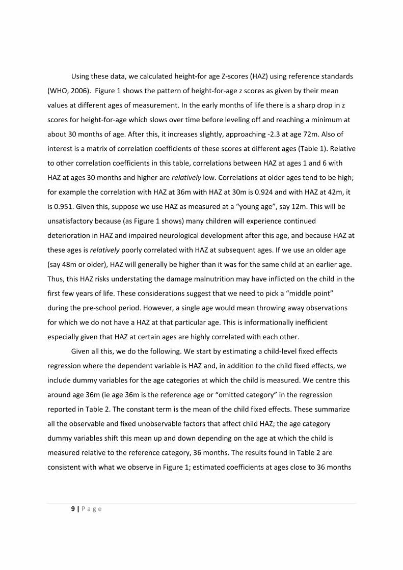
Using these data, we calculated height‐for age Z‐scores (HAZ) using reference standards 

(WHO, 2006).  Figure 1 shows the pattern of height‐for‐age z scores as given by their mean 

values at different ages of measurement. In the early months of life there is a sharp drop in z 

scores for height‐for‐age which slows over time before leveling off and reaching a minimum at 

about 30 months of age. After this, it increases slightly, approaching ‐2.3 at age 72m. Also of 

interest is a matrix of correlation coefficients of these scores at different ages (Table 1). Relative 

to other correlation coefficients in this table, correlations between HAZ at ages 1 and 6 with 

HAZ at ages 30 months and higher are relatively low. Correlations at older ages tend to be high; 

for example the correlation with HAZ at 36m with HAZ at 30m is 0.924 and with HAZ at 42m, it 

is 0.951. Given this, suppose we use HAZ as measured at a “young age”, say 12m. This will be 

unsatisfactory because (as Figure 1 shows) many children will experience continued 

deterioration in HAZ and impaired neurological development after this age, and because HAZ at 

these ages is relatively poorly correlated with HAZ at subsequent ages. If we use an older age 

(say 48m or older), HAZ will generally be higher than it was for the same child at an earlier age. 

Thus, this HAZ risks understating the damage malnutrition may have inflicted on the child in the 

first few years of life. These considerations suggest that we need to pick a “middle point” 

during the pre‐school period. However, a single age would mean throwing away observations 

for which we do not have a HAZ at that particular age. This is informationally inefficient 

especially given that HAZ at certain ages are highly correlated with each other.  

Given all this, we do the following. We start by estimating a child‐level fixed effects 

regression where the dependent variable is HAZ and, in addition to the child fixed effects, we 

include dummy variables for the age categories at which the child is measured. We centre this 

around age 36m (ie age 36m is the reference age or “omitted category” in the regression 

reported in Table 2. The constant term is the mean of the child fixed effects. These summarize 

all the observable and fixed unobservable factors that affect child HAZ; the age category 

dummy variables shift this mean up and down depending on the age at which the child is 

measured relative to the reference category, 36 months. The results found in Table 2 are 

consistent with what we observe in Figure 1; estimated coefficients at ages close to 36 months 

10 | P a g e   

have very small coefficients while those farther away (closer to 72m and closer to 1m) are 

larger.  

We then generate a synthetic measure of HAZ at 36m for all children. To do so, we start 

with 880 cases where HAZ is measured at 36m and insert these into our synthetic value. Where 

HAZ at 36m is not known, we take the closest age at which height was measured, and using the 

regression results above, we calculate a predicted value for HAZ at 36m. This has a mean value 

of ‐2.91 with standard deviation 1.03. An attractive feature of this approach is that it minimizes 

the use of observations found in the tails of our distribution of measures by age and where we 

might expect measurement error to be highest. That said, we note that the absolute value of 

mean prediction errors is likely to be higher for measures in early life (less than 18 months) 

relative to those observed late in life (at ages 60 and 72m for example) because the trend in 

mean HAZ once past 30m is linear while the trend in HAZ prior to 30m is curvilinear. Mindful of 

this concern, section 5 reports the results of robustness checks using alternative measures of 

HAZ at 36m. 

      

(c) Descriptives: Outcome variables 

We describe these thematically. The means and standard deviations of the outcomes we will 

consider, along with a brief summary of their definition, can be found in Table 3. 

 

Schooling‐related outcomes 

Individuals who had participated as children in the INCAP intervention and their spouses 

completed a schooling history. In interpreting these data, note that the formal educational 

system in Guatemala is divided into primary, secondary, and post‐secondary education. Primary 

school comprises grades one to six, and children are expected to enrol in the calendar year in 

which they turn seven years old. Secondary school consists of five to seven grades, divided into 

two parts. The first three grades of lower secondary school (to grade nine) are the “basic” 

grades, and instruction is expected to provide academic and technical skills necessary to join 

the labour force. The fourth through seventh grades of upper secondary school are the 

“diversified” grades; students can choose from among a set of academic or vocational tracks. 

11 | P a g e   

Students who plan to continue to university finish upper secondary schooling in two years; 

other tracks at the diversified level usually take three years (World Bank, 2003). Virtually all 

members of the sample had at least one grade of schooling but only a small number (less than 

3%) continued beyond secondary school. Apart from formal schooling, it was also possible to 

complete (primary and secondary school) grades via informal schooling such as adult literacy 

programs. Our overall measure of grades completed (maximum value, 12 grades) includes both 

types of schooling, though informal schooling is relatively uncommon in this population. 

  Reading comprehension was measured via a two‐part standardized test. Respondents 

who reported having passed fewer than four grades of schooling, or those who reported four to 

six grades of schooling but could not correctly read aloud the headline of a local newspaper 

article, were first given a literacy test. Individuals who passed this literacy screen, or who 

reported more than six grades of schooling then took the Inter‐American Series test vocabulary 

and reading comprehension modules (Serie Interamericana or SIA, for its acronym in Spanish): 

Level 2 for comprehension and Level 3 for vocabulary (approximately 3rd and 4th grade 

equivalents). The reading comprehension module had 40 questions and the vocabulary module 

45 questions, yielding a maximum possible score of 85 points. Questions on the test become 

progressively harder. Those who did not pass the literacy screen pre‐test were given a zero 

(18% of the sample).  

  All individuals were administered the Raven’s Progressive Matrices test (hereafter 

Raven’s test), an assessment of nonverbal cognitive ability (Raven et al., 1984). Raven’s tests 

are considered to be a measure of eductive ability—“the ability to make sense and meaning out 

of complex or confusing data; the ability to perceive new patterns and relationships” (Harcourt 

Assessment, 2008). The test consists of a series of pattern‐matching exercises with the 

respondent asked to supply a “missing piece” and with the patterns getting progressively more 

complex. We administered the first three of five scales (A, B, and C with 12 questions each for a 

maximum possible score of 36). Reading comprehension test (SIA) scores and nonverbal 

cognitive ability test (Raven’s) scores are expressed as z‐scores standardized to have mean 0 

and SD 1 within the sample.  

 

12 | P a g e   

Union formation and marriage market outcomes 

A marriage history module was administered separately to each husband and wife in the 

sample. “Marriage” refers to two individuals joining in union, usually (but not always), 

cohabitating and is not restricted to church or state‐sanctioned marriages. The module 

consisted of a series of questions on: (a) age at first marriage, duration of first marriage, age at 

subsequent marriages and at marital dissolutions; (b) information on physical and financial 

assets brought to marriage; (c) and spouse’s family background. Quisumbing et al (2005) 

provides further background and details.  

 

Fertility 

Men and women were asked about their marital history, number of live births, number of 

children who died, pregnancy intentions, and knowledge and use of a range of contraceptive 

methods. Women also were asked about their menstrual history and provided a detailed 

pregnancy history. Using these data, we construct the following outcomes: age at menarche, 

whether a woman gave birth before age 17, the interval (in months) between the first and 

second birth, the total number of pregnancies and whether a woman had experienced an infant 

or child death.  Ramakrishnan et al (2005) provide further details and extensive descriptive 

statistics. 

 

Health related outcomes 

The field study team included two physicians and four fieldworkers who collected bio‐medical 

data: measurements of anthropometry and body composition, blood pressure, tests of physical 

fitness, clinical histories and a finger‐stick whole‐blood sample from which it was possible to 

measure plasma glucose and a lipid profile.  The full set of outcomes we use are reported in 

Table 3; here we highlight three measures, in particular, are noteworthy. Based on the 

anthropometric data we collected, it is possible to construct an estimate of fat‐ free mass. Fat‐

free is a good measure of overall health human capital that affects work productivity because it 

reflects muscle and skeletal mass and thus the capacity to carry out work (McArdle, Katch and 

Katch, 1991).  We also have a measure of isometric hand strength. Using a Lafayette 

13 | P a g e   

dynamometer, subjects were asked to exert a maximal and quick handgrip twice and maximal 

values of the dominant and non‐dominant hands were recorded. Handgrip strength is highly 

correlated with total strength of 22 other muscles of the body (de Vries, 1980). Finally, another 

measure of physical work capacity was constructed: predicted maximum oxygen consumption 

(VO2max). It measures the capacity of individuals to deliver oxygen to muscle while doing 

physical work. Stein et al (2005) provides a detailed description of how these data were 

collected and how outcomes were measured. 

 

Labor Market Activities 

During HCS individuals were interviewed about all of their income‐generating activities. Topics 

covered included: a) wage labor activities for every wage job (type of occupation; wages and 

fringe benefits; description of the employer; and hours, days and months worked); b) all 

agricultural activities (amount of land cultivated; crops grown; production levels and values; use 

of inputs; and hours, days and months worked); and c) non‐agricultural own‐business activities 

(type of activities; value of goods or services provided; capital stock employed; and hours, days 

and months worked). Virtually all men (98%) and most women (69%) were engaged in some 

sort of own‐account income‐generating activity. In the year prior to the interview, 79% of men 

were working for wages (with more than half of these in unskilled occupations), 42% in own‐

account agriculture and 28% in own‐account non‐agricultural business. A third of women were 

working for wages (with the majority in unskilled occupations) and a third in own‐account non‐

agricultural business, and 20% were in own‐account agriculture. For each activity, individuals 

were asked the number of months in which they worked and how many days per month and 

hours per day they typically worked. These data are used to generate annual hours worked. In 

the case of wage labor, individuals were asked to report gross earnings, earnings nets of taxes 

and social security deductions as well as additional payments such as bonuses, transport and 

food, for the time unit (hourly, daily, weekly and so on) most relevant to their job, for each job 

they had held. These data, together with net income earned from own‐account agricultural 

activities, non‐agricultural own‐business activities and hours worked were used to construct a 

14 | P a g e   

measure of income earned per hour worked. Hoddinott, Behrman and Martorell (2005) provide 

a detailed discussion of these data. 

 

Consumption and poverty 

The Human Capital Survey include an expenditure survey which provided information on food 

and nonfood expenditures in the household in which the respondent currently resided and a 

community level food price survey. Using these data, and the method outlined in Maluccio, 

Martorell and Ramírez (2005a), we construct a measure of per capita household consumption. 

We can compare these data against a poverty line constructed for Guatemala, again see 

Maluccio, Martorell and Ramírez (2005a) for details. 

 

3. Modelling and identification 

To clarify the identification issues associated with the focus of this paper, consider a vector of 

outcomes, Y for individual i which are related to early‐life nutrition in the following way: 

Yi = β∙HAZi + γ’∙Xi + υi                    (1) 

For example, an element of Yi could be Wi, the hourly wages of person i in adulthood. HAZi is a 

measure of pre‐school nutritional status ‐ height‐for‐age z score, Xi is a vector of control 

variables with associated parameters γ and υi is a disturbance term. The parameter of primary 

interest to us is β. If E(HAZi υi) ≠ 0, β will be biased. It is not difficult to think of reasons why 

such a correlation could exist. For example, parents of these individuals who have superior 

social networks may be wealthier and may also be better placed at helping their children find 

high paying jobs. Given this, a critical issue for this paper is whether we can credibly identify the 

impact of HAZi.  

  Issues of identification have attracted considerable recent discussion and controversy in 

economics. One school of thought argues that a randomized control trial (RCT) design 

represents the most powerful and plausible way of identifying impact. In the context of this 

paper, an RCT would require malnourishing randomly selected pre‐school children and both 

following them and a control group of non‐malnourished children for the next 30‐40 years. 

Such an approach is both impractical and unethical. Lee and Lemieux (2010) argue that in 

15 | P a g e   

important ways, a Regression Discontinuity Design (RDD) can be considered as being “more 

similar” to a randomized design (Lee and Lemieux, 2010, p. 302). Lee and Lemieux note that in 

the presence of heterogenous treatment effects, RDD produces a weighted average treatment 

effect where the weights are proportional to the ex ante likelihood that an individual is close to 

the threshold. As they note, if these weights are highly varied – as is likely to be the case here – 

the RDD measure of impact will be very different from the treatment effect. With RCT and RDD 

ruled out, we adopt an Instrumental Variables approach. In doing so, we are aware of both its 

strengths and limitations, most notably that “the estimated treatment effect is applicable to 

the sub‐population whose treatment was affected by the instrument” (Lee and Lemieux, 2010, 

p. 292). In light of Deaton’s critique of local average treatment effects (LATE), we carefully 

specify and justify our choice of instruments. We take seriously Angrist and Pischke’s (2010) 

and Stock’s (2010) argument about the importance of establishing credible identification. 

Finally, following the argument laid out in Leamer (2010), we perform sensitivity analyses on 

our findings; these are found in section 5. 

To understand the logic behind our choice of instruments, consider the model outlined 

in Behrman and Hoddinott (2005).  A child’s nutritional status (HAZi) is assumed to appear as an 

argument in the welfare function of the households in which they reside (Behrman and 

Deolalikar, 1988; Strauss and Thomas, 1995). Welfare is assumed to increase as nutritional 

status improves, though possibly at a diminishing rate. Decisions that parents make about 

devoting resources to the children’s nutrition and health are constrained in several ways. There 

are resource constraints reflecting income and time available as well as prices faced by 

households. There is also a constraint arising from the production process for health outcomes, 

including nutritional status. This constraint links nutrient intakes – the physical consumption of 

macronutrients (calories and protein) and micronutrients (minerals and vitamins) – as well as 

time devoted to the production of health and nutrition, locality characteristics such as the 

presence of preventative and curative health facilities and the prevalence of infectious 

diseases, the individual’s genetic make‐up and knowledge and skill regarding the combination 

of these inputs to produce nutritional status. Maximizing the household welfare function 

16 | P a g e   

subject to these constraints generates a set of first‐order conditions that can be solved to yield 

a reduced‐form child health demand function takes the general form: 

HAZit = ht(Ci , Mt , Wt , Pt , Zit, Zi)              (2) 

where Ci is a vector of child characteristics such as sex, and genotype (for example, growth 

potential), Mt is a vector of characteristics of the principal care giver observed at time t, Wt 

captures household wealth, and Pt is a vector of all relevant prices. Z is a vector of health, 

sanitation and environmental characteristics in the locality in which the child lives that are 

assumed to influence health.  Some of these, Zi, are time invariant while others, Zit, vary over 

time.  

Given (2), our identification strategy relies on two core ideas: the existence of cohort 

and location specific transitory shocks that we assume are independent of individual 

characteristics7 – ie elements of Zit – and random variation in genotype that are found in the 

vector Ci. Our cohort and location specific transitory shocks include: exposure to the INCAP 

intervention between the ages of 0 and 36 months; exposure to the intervention between 0 

and 36 months interacted with residing in a village where atole was provided; whether the 

subject was born in 1974, 1975 or 1976 and therefore exposed in early life to the effects of an 

earthquake measuring 7.5 on the Richter scale that shook Guatemala in February 1976; and 

whether there was a government health post in the individual’s village‐of‐residence when they 

were two years of age. Our measures of variation in genotype include the logarithm of maternal 

height (Sahn, 1990) and whether the individual was a twin. 

Table 4 reports results of estimating a variant of (2). While not exactly the same as the 

“first stage regressions” that we estimate when we consider our various life‐course outcomes,8 

it provides a useful assessment of the relevance of our instruments. Specifically, we represent C 

by the individual’s sex, the inclusion of a dummy variable denoting that the individual is a twin 

and the log of mother’s height; Mt by completed grades of mother’s schooling; Wt by a wealth 

index; and Pt by a set of year‐of‐birth dummy variables that can be thought of more generally as 

                                                            7 This is analogous to the approaches described by Imbens and Angrist (1994), Card (2001) and Alderman, Hoddinott and Kinsey (2006).  8 When we specify a particular outcome, we will also specify control variables relevant to that outcome but these control variables will differ across outcomes.

17 | P a g e   

a set of variables that capture all events (including movements in all prices) common to a given 

birth cohort. Zi is denoted by a set of location‐of‐birth dummy variables while Zit captures the 

transitory shocks noted above. 

There are several attractive features of the results shown in Table 2. First, a number of 

our proposed instruments are causally related to our endogenous variable. Exposure to the 

intervention between birth and 36 months and exposed to atole and maternal height both 

increase height‐for‐age at 36 months while being a twin reduces height. These variables are all 

statistically significant. Being exposed to the 1976 earthquake in early life reduces height but 

this is not precisely measured; the p‐value for this coefficient is equal to 0.15. Exposure to the 

intervention between birth and 36 months and having a health centre in the village of birth, 

however, have no meaningful effect on height given age. An F test rejects the null hypothesis 

that these proposed instruments are jointly zero. Stock (2010) notes that, “If this F‐statistic is 

large – a common rule of thumb is F>10 – then one can treat the instruments as sufficiently 

strong that the usual two‐stage least squares output can be used” (Stock, 2010, p.87). At 16.52, 

our F statistic comfortably passes this rule of thumb.  

In addition to being correlated with height for age, an attractive feature of these 

variables is that they meet a key criterion laid out in Deaton’s (2010) critique of IV methods; 

namely that they are derived from a formal model rather than being specified ad hoc. But we 

recognize that any half‐decent economist sitting in a seminar room – or indeed a bar for that 

matter – could quibble with any of these identifying variables, viz: 

‐ Exposure to the intervention could have had an income effect that persisted after the 

supplementation trial ended in 1977;9 

                                                            9 We think this is unlikely. First, the behaviour of villagers did not suggest that the supplements were of significant monetary value. Despite the fact that supplements were freely available every day to all inhabitants of the communities, few men or school‐age children frequented the feeding centres, even on weekends when the opportunity cost of their time in terms of work or school presumably was lower. Second, the actual monetary value of the supplements was low. We estimate the cost of the ingredients for one cup of atole and one cup of fresco to have been US$ 0.018 and 0.004. Mean household incomes were approximately US$ 400 in 1975 (Bergeron, 1992). Thus one year’s worth of a daily cup of atole (US $6.60) and of fresco (US $ 1.50) was approximately 1.7% and 0.4% of average annual household income, and on average children 0–36 months of age consumed less than this. The medical care may have had a greater income effect for households, but this effect was equally present in both atole and fresco villages.

18 | P a g e   

‐ The earthquake could have had long lasting effects – for example on school availability and 

quality or on income generating opportunities;10 

‐ The establishment of a government‐run health post could reflect a process of endogenous 

program placement;11 

‐ Maternal height may reflect investments made by the mother’s own parents and 

dimensions (such as quality of child care in early life) might be correlated 

intergenerationally;  

‐ The proportion of the sample that are twins is so small (less than five percent) that the 

local average treatment effect (LATE) of this identifying instrument is not likely to be of 

interest 

In light of these legitimate concerns, we subject our instruments to a battery of tests 

described below. Further, we return to this issue in our discussion of robustness tests found in 

section 5.  

 

4. The impact of malnutrition on schooling, marriage, fertility, health, wages, labor force participation and poverty 

We now turn to the results of estimating (1) for outcomes that span the life course of these 

individuals. For each set of outcomes, we report the results of two functional form 

representations of pre‐school nutritional status; height‐for‐age z scores; and a dummy variable 

equaling one if the individual was stunted at age 36 months, zero otherwise. Note that when 

we use the z score, we have a positive parameter estimate when an improvement in nutritional 

status leads to an improvement in that outcome. When we use stunting, a negative parameter 

estimate (ie switching an individual from being stunted to not being stunted) means that an 

                                                            10 A priori, we are not convinced by such a claim. First, schools were rebuilt quite quickly after the earthquake. Second, as Bergeron (1992) and Estudio 1360 (2002) show, the livelihood and income trajectories of these villages were shaped and reshaped by many subsequent events both positive – such as the opening of new wage jobs in nearby towns ‐ and negative – such as the collapse in markets for good produced in particular villages at particular times. 11 Because we include village‐of‐birth dummy variables in all specifications, this line of criticism is restricted to claiming that there were time varying factors that lead to differences in the timing of the establishment of these health posts. We note that the three separate qualitative studies carried out in these villages, all of which discussed changes in village infrastructure, reported no such evidence (Pirval, 1972; Bergeron, 1992 and Estudio 1360, 2002). 

19 | P a g e   

improvement in nutritional status has lead to an improvement in outcomes. We first report 

these results for the full sample, then separately for females and males. Throughout we 

compare results of the Kleibergen‐Paap (KP) test statistic (Kleibergen and Paap, 2006; 

Kleibergen 2007) to the critical values presented by Stock and Yogo (2005, Table 5.1) to assess 

whether our instruments are weak. As a rule of thumb, where our test statistic has a value of 

6.3 or higher, we reject at a 5% significance level the hypothesis that the instruments are weak, 

where weak in this case means having bias in the IV results that is larger than 20% of the bias in 

the OLS results. We also report the Hansen J statistic for overidentification where the null 

hypothesis is that the overidentifying restrictions are valid (i.e., that the model is well specified 

and the instruments do not belong in the second‐stage equation). Failure to reject the null 

hypothesis for the Hansen test is evidence that if any one of the instruments is valid, so are the 

others. Since the instrument set includes the randomly allocated exposure to the intervention 

and the earthquake indicator, both of which are likely to be valid, this gives us some confidence 

in the power of this specification test. Standard errors robust to heteroscedasticity and 

clustered at maternal level. Where outcomes are expressed as 0/1 variables, we estimate linear 

probability models so as to be able to compute the IV test statistics. To save space, we do not 

report the full set of results. The footnotes to these tables report the control variables that we 

include and full results are available on request. 

 

(a) Schooling 

Table 5 reports the results of estimating the impact of pre‐school nutritional status on schooling 

outcomes. Table 5A reports these for the full sample; Tables 5B and 5C report this separately 

for women and men respectively. In the estimates of equation (1) for schooling related 

outcomes, our second stage control variables are: subject sex and birth year dummy variables; 

maternal age and education; paternal education; parental wealth index; school quality at age 7 

and 13 (whether school building is permanent structure and student teacher ratio); distance to 

feeding center; electrification of village at age 2; and village of origin. In so doing, our estimates 

control for common cohort effects, unobserved fixed effects associated with place of birth, and 

parental characteristics and time‐varying location characteristics that might be correlated with 

20 | P a g e   

these schooling outcomes. Looking across the results of the Kleibergen‐Paap (KP) test statistics, 

we see that we do well in terms of the relevance of our instruments, particularly when pre‐

school nutrition is represented by the height‐for‐age z score. In all specifications, we fail to 

reject the null hypothesis that the instruments are uncorrelated with the second stage 

schooling outcomes and in nearly all cases, the prob values of the Hansen J test are quite large. 

  These results show that there is a direct effect of poor pre‐school nutritional status on 

age at entry, the age at which an individual leaves school and the number of grades 

completed.12 When nutritional status is expressed in terms of stunting, the effect on grade 

attainment is large – a loss of nearly four grades of schooling compared to some one who was 

not stunted. The impact on grade attainment is the same for males and females; the impact on 

the age at which some one leaves school appears to be driven primarily by the female sub‐

sample.  

  The most striking results, however, are for the reading/vocabulary and Raven’s tests 

administered in adulthood. These show that poor nutritional status in early life is casually 

related to poorer outcomes on these dimensions of cognitive skill. The magnitude of these 

effects is large. They are consistent with the literature cited in the introduction to the paper on 

the neurological consequences of malnutrition. 

 

(b) Marriage market 

Table 6 reports the impact of pre‐school nutrition on success in the marriage market, doing so 

separately for women (Table 6A) and men (Table 6B). All results control for age, maternal age 

and education, paternal education, parental wealth index, electrification of village at age 2 and 

village of origin. We do well in terms of the relevance of our instruments as measured by the 

Kleibergen‐Paap (KP) test statistics, particularly when pre‐school nutrition is represented by the 

height‐for‐age z score. Out of 14 specifications, we fail to reject the null hypothesis that the 

                                                            12 Other studies include Alderman, Hoddinott and Kinsey (2006), Daniels and Adair (2004) and Mendez and Adair (1999).   

21 | P a g e   

instruments are uncorrelated with the second stage schooling outcomes and in 13 of them and 

in nearly all cases, the prob values of the Hansen J test are quite large. 

Women better nourished in early‐life marry men who are older. The parameter 

estimate reported in the bottom panel of Table 6A implies that is a woman who was not 

stunted at age 36m marries a man who is five years older than herself. Since age and 

consumption levels are correlated in this sample, this suggests that females better nourished as 

pre‐schoolers make a better match in the marriage market. A cautionary note, however, arises 

from the fact that not only do women marry older men, but they also marry men older than 

themselves; the estimated coefficient on the difference in ages between women and their 

spouses is positive. If  bargaining power within the household is correlated with age 

differentials between spouses, while women may marry into better off households they may 

also be somewhat more disadvantaged in terms of bargaining over resources within those 

households.  

  Men with better pre‐school nutritional status also do better in the marriage market, but 

along different dimensions. They marry women with more schooling and who are slightly taller; 

Behrman et al (2010) show that women with more schooling earn higher wages. 

  Finally, in preliminary work we assessed whether early‐life nutrition affected the timing 

of entry into the marriage market as measured by: age at first marriage; whether an individual 

married before 16; whether an individual married before 18; and duration of time between 

leaving school and forming first union. We did not find statistically significant impacts.13  

 

(c) Fertility 

Results are reported in Table 7. We control for birth year, maternal age and education, paternal 

education, parental wealth index, electrification of village at age 2 and village of origin. Women 

were undernourished as pre‐schoolers are more likely to give birth before age 17 and have 

more children. The latter effect is large. “Switching” a woman from being stunted to not being 

stunted would, conditional on her age, reduce the number of pregnancies she has by two. Our 

results are consistent with the finding above that better nourished females in early life 

                                                            13 These are not reported but are available on request.

22 | P a g e   

complete more grades of schooling and the extensive literature that shows that better 

educated women have fewer pregnancies. 

 

(d) Health 

Using the extensive information we have on health outcomes, we consider the impact of early 

life undernutrition on the following anthropometric outcomes in adulthood: log height, log 

Body Mass Index (BMI), whether the individual is overweight or obese (defined as having a BMI 

> 25.0), whether the individual is obese (defined as having a BMI >30.0), waist‐hip ratio, and 

head circumference. We consider three measures of physical strength: log fat free mass, hand 

strength and maximal oxygen consumption. We also examine outcomes related to risks 

associated with cardio‐vascular and other chronic diseases: Low‐density lipoprotein (LDL) 

cholesterol, the ratio of total cholesterol to High ‐density lipoprotein (HDL) cholesterol, blood 

pressure, and plasma glucose. Lastly, we consider metabolic syndrome (METS), a range of risk 

factors associated with increased risk of stroke, diabetes and coronary heart disease. 

  Results are reported in Table 8. Second stage controls are subject sex and birth year 

dummy variables, maternal age and education, paternal education, parental wealth index, 

electrification of village at age 2 and village of origin. Note that for one outcome, log height, we 

reject the null that the overidentifying conditions are valid. This is not surprising given that one 

of our instruments, maternal height, is likely to be directly correlated with height in adulthood. 

This is reassuring in that it tells us that the Hansen test has power in that it detects and rejects 

the null regarding the overidentifying conditions for the outcome where these are most likely 

to be violated. Results for the full sample are found in Table 8A with results for females (Table 

8B) and males (Table 8C) reported subsequently. 

  Individuals with better pre‐school nutritional status are taller and stronger as adults, the 

latter as measured by hand strength and fat‐free mass. While they have slightly higher body 

mass and are more likely to be overweight or obese, impacts on these outcomes are not 

precisely measured. Results on anthropometry do not differ meaningfully between men and 

women. Women are somewhat more likely to be hypertensive or pre‐hypertensive if they had 

higher HAZ scores at age 36m. Males were more likely to be diabetic or pre‐diabetic. 

23 | P a g e   

 

(e) Labor market outcomes 

We consider five labor market outcomes: log hourly earnings; log hours worked; log earned 

income; years employed doing skilled labor; whether the individual is currently employed doing 

skilled work; and whether the individual operates their own business, fulltime.14  Results are 

reported in Table 9, first for the full sample and then for females and males. Specification tests 

indicate that we can reject the null that our instruments are weak but not reject the null that 

the overidentifying restrictions are valid. 

  Better nutritional status in early life is causally linked to higher hourly earnings in 

adulthood. Being stunted at age 36m has a large adverse impact of economic productivity in 

adulthood, reducing earnings by 62.5 percent. Individuals who were better nourished as pre‐

schoolers are more likely to work in higher‐paying skilled labor or white collar work and are 

somewhat more likely to operate their own business though this latter effect is imprecisely 

measured. These results are consistent with processes by which undernutrition in early life 

leads to cognitive impairments which limited schooling attainment and the acquisition of 

cognitive skills both of which are rewarded in the Guatemalan labor market, see Behrman et al 

(2010).  

  Impacts on success in the labor market differ by sex. While there are positive effects on 

women’s economic productivity, these are imprecisely measured. Females who were better 

nourished at age 36m are more likely to work in skilled employment and were 33 percentage 

points more likely to have an independent source of income through own business activities. 

Productivity impacts on males are large and statistically significant. A one standard deviation 

increase in HAZ at age 36m increases male wages by 21.5 percent. Stunting at age 36m lowers 

hourly earnings by a massive 65.7 percent in adulthood.  

 

(f) Consumption and poverty 

In Table 10, we consider the impact of pre‐school nutritional status, expressed both as HAZ and 

as whether the individual was stunted, on the consumption levels of the household in which 

                                                            14 In preliminary work, we also considered migration status as an outcome but found no significant effects.

24 | P a g e   

the individuals who participated in the intervention reside as adults. We also consider the 

impact on the likelihood that the household has consumption levels above or below the 

poverty line. In these regressions, the second stage estimates control for sex, birth year, 

paternal education, parental wealth index, school quality at age 7 (whether school building is 

permanent structure and student teacher ratio), whether mother or father had died before 

subject turned 15, tobacco market collapse at age 15, electrification of village at age 2  and 

village of origin. We estimate these for the full sample and separately for men and women. The 

test statistics for instrument relevance are good and we do not reject the null hypothesis that 

the overidentification assumptions are valid. 

  Men and women with better nutritional status in early life live, as adults, in better‐off 

households. A one standard deviation increase in HAZ increases household per capita 

consumption by 18 percent. Since consumption is measured at the household level, all 

members, not just those of the individual who was better nourished, are better off provided 

that there are not dramatic intra‐household inequalities in consumption. Put another way, the 

benefits to improving an individual’s early‐life nutritional status are not necessarily confined to 

that individual; they spill‐over to other household members. Individuals who are stunted live in 

households with lower consumption levels and are 30.9 percent more likely to live in a 

household that is poor.  

 

5. Checks on robustness 

(a) Instrument validity 

A critical issue for this paper is whether we can credibly identify the impact of HAZi. We see the 

notion of “credibly” as having several inter‐related meanings. First, are our instruments derived 

from a credible model of our endogenous variable or are they ad hoc? This notion of credibility 

is discussed in section 3. Second, are our instruments relevant so that we can have confidence 

in the inferences that we draw from our IV estimates? As shown in Table 4 and in the results 

presented in section 4, we satisfy concerns regarding relevance. However, there are two further 

meanings that we have not considered. The first issue, raised by Lee and Lemieux (2010) and by 

Deaton (2010), that the “the estimated treatment effect is [only] applicable to the sub‐

25 | P a g e   

population whose treatment was affected by the instrument” (Lee and Lemieux, 2010, p. 292). 

A good example of why this issue is of concern here is the following. Suppose the identification 

of our results is driven by whether an individual is a twin. If this is the case, while our results are 

valid in a statistical sense (that is, they pass all the necessary specification tests), they are not 

especially meaningful given that twins make up such a small proportion of this (or indeed any 

other) population. Second, Leamer describes credible inferences in terms of the outcome of 

sensitivity analyses that “separate fragile inferences from sturdy ones” (Leamer, 2010, p. 37). 

Because we use several variables, not just one, to identify the impact of pre‐school 

nutritional status on later life outcomes, is possible to assess the sensitivity our results to the 

inclusion/exclusion of particular instruments. As described in Table 11, we consider eight 

alternative instrument sets. We report our results in Figures 2, 3 and 4 for three key findings: 

impacts on reading/vocabulary scores, hourly earnings (males) and household consumption. 

The bottom rows of Table 11 report three specification tests: the F statistic for the excluded 

instruments in the first stage regression, the Kleibergen‐Paap (KP) test statistic that the 

instruments are weak and the prob values for the Hansen J test. In each figure, the triangle 

represents the point estimate while the top and bottom ends of the bars give the end points of 

the 95 percent confidence interval.  

  The first bar in each figure is the results obtained using the full set of instruments. Note 

that alternatives 1, 2 and 3 (dropping different combinations of the twins instrument, the 

negative earthquake shock and the positive health infrastructure shock) has no meaningful 

effect on the magnitude of the parameter estimate and only slight variations in the size of the 

95 percent confidence interval. Alternatives 5 and 6, where we drop exposure to the 

intervention between 0 and 36 months, exposure to the intervention between 0 and 36 months 

and living in an atole village and, in alternative 6, whether the individual is a twin also produces 

very similar parameter estimates to those obtained with the full set of instruments and those 

found in alternatives 1, 2, and 3, but with slightly larger confidence intervals. In these five 

alternative specifications, our instrument set easily meet the relevance criteria as measured by 

the F statistic and we can reject the null hypothesis that the instruments are weak. In addition, 

we do not reject the null that the overidentifying restrictions are valid. If we drop mother’s 

26 | P a g e   

height (alternative 4) in two cases, hourly earnings (males) and household per capita 

consumption, we obtain larger estimates of impact but lose precision as seen by the wider 

confidence intervals. In the case of reading scores, the parameter estimate is similar to that 

obtained from the full set of instruments and the confidence interval is increased. Consistent 

with this, the “relevance statistics” are lower (but still reasonable) and we continue to not 

reject the null regarding the overidentifying restrictions. 

  Alternative 7 includes only exposure to the intervention between 0 and 36 months, 

exposure to the intervention between 0 and 36 months and living in an atole village as 

instruments. We get much different point estimates, much larger for reading scores and hourly 

earnings (males) and smaller for household per capita consumption. We also obtain, 

comparatively speaking, much wider confidence intervals. If we add back in exposure to the 

earthquake and being a twin (alternative 8), we reduce these intervals markedly, improve our 

relevance statistics and do not reject the null hypothesis that the overidentifying restrictions 

are valid. 

For reading outcomes, seven of the eight alternative instrument sets produce 

parameter estimates very close to that obtained by our base set. In all cases, the instrument 

sets pass tests of relevance and do not reject the test of overidentification. The minor 

difference between these lies in the size of the estimated confidence intervals. If we only use 

exposure to the intervention, and exposure interacted with atole, we get a much larger 

estimate of impact but one that is imprecisely measured.  For hourly wages (males) and 

household consumption, five of the eight alternative instrument sets produce parameter 

estimates very close to that obtained by our base set. All instrument sets pass tests of 

relevance and do not reject the test of overidentification. There are minor variations across 

these instrument sets in terms of the size of the estimated confidence intervals. Alternatives 4 

and 8, both of which exclude mother’s height, generate much higher estimates of impact but 

also wider confidence intervals. Only using exposure to the intervention, and exposure 

interacted with atole generates imprecisely measures of impact. Based on these results, we 

conclude that the estimates reported in Tables 5 to 10 are robust to concerns regarding fragile 

inferences and concerns regarding the generality of the LATE estimates. 

27 | P a g e   

 

(b) Attrition 

Despite the considerable effort and success in tracing and re‐interviewing participants from the 

original sample, attrition in this sample is substantial.15 Moreover, as shown in Grajeda et al. 

(2005), attrition in the sample is associated with a number of initial conditions, in ways that 

differ by the reason for attrition (e.g., migration versus failure to interview someone who was 

located). What is of ultimate concern in this analysis is not the level of attrition, however, but 

whether, and to what extent, the attrition invalidates the inferences we make using these data.  

We address concerns about sample attrition bias in three ways. First, in the specifications 

already shown, we include covariates, many of which, in addition to playing a role in affecting 

outcomes, are themselves associated with attrition, including being male (+),birth year (‐) and 

parental wealth (+).Conditional on the maintained assumptions about the correct functional 

form, attrition selection on right‐side variables does not lead to attrition bias (Fitzgerald et al., 

1998b).  

Second, we compare nutritional outcomes measured in the 1970s for those eventually 

re‐interviewed in HCS and those not re‐interviewed. Average height‐for‐age measured at 48 

months of age and 72 months of age are remarkably similar between those who attrited and 

those who did not. Height‐for‐age z‐scores for the two groups are all within 0.006 of one 

another (mean for 48‐month olds is ‐2.074, SD 1.03 and mean for 72‐month olds is ‐1.666, SD 

1.028) and the lowest p‐value on a t‐test with unequal variances is p=0.91. There does not 

appear to be any obvious selection between those interviewed or not based on early‐life 

nutritional status. 

                                                            15 A related problem is that of mortality selection (Pitt, 1997; Pitt and Rosenzweig, 1989). Indirect evidence that mortality selection exists in the sample is that higher risk of death is associated with younger ages (those born later) in the original sample of 2392. The older sample members represent the survivors of their respective birth cohorts, and hence they experienced a lower mortality rate (because most mortality was in infancy) compared with the later birth cohorts in the study who were followed from birth. Because data collection began in 1969 and included all children under seven years of age, it excluded all children from the villages born between 1962 and 1969 who died before the start of the survey. Another facet of mortality selection, however, has to do with the intervention itself, which may have decreased mortality rates among the younger cohort in atole versus fresco villages (Rose et al., 1992). To the extent the variables included in our models are associated with these forms of selection, our estimates partly control for mortality selection, though we do not implement any special methodology to do so. To the extent that unobservable characteristics that affect the likelihood of mortality are correlated with HAZ, our identification strategy guards biases that such a correlation might create. 

28 | P a g e   

Finally, we implement the correction procedure for attrition outlined in Fitzgerald, 

Gottschalk, and Moffitt (1998a, 1998b). We first estimate an attrition probit conditioning on all 

the exogenous variables considered in the main models, as well as an additional set of 

endogenous variables potentially associated with attrition. We include a number of variables 

that reflect family structure in previous years, since these are likely to be associated with 

migration status. They include indicators of whether the parents were alive when each sample 

member was seven years old and whether the sample members lived with both their parents in 

1975 and in 1987. During the fieldwork, locating sample members was typically facilitated by 

having access to other family members from whom the field team could gather information. 

Therefore, we also include a number of variables that capture this feature of the success of 

data collection. They include whether the parents were alive in 2002, whether they lived in the 

original village, whether a sibling of the sample member had been interviewed in the 2002–04 

follow‐up survey, and the logarithm of the number of siblings in the sample in each family. We 

emphasize that this is not a selection correction approach in which we must justify that these 

factors can be excluded from the main equations, but rather we purposively exclude them from 

those regressions since our purpose is to explore the determinants of educational outcomes 

outlined in equation (1) and not whether educational outcomes are associated with the family 

structure and interview‐related factors included in the “first‐stage” attrition regression 

(Fitzgerald, Gottschalk, and Moffitt 1998a). While we do not formally have adjustments to 

correct for selection on unobservable characteristics, by including the large number of 

endogenous observables indicated above, which are likely to be correlated with unobservables, 

we expect that we are reducing the scope for attrition bias due to unobservables, as well. 

The factors described above are highly significant in predicting attrition, above and 

beyond the conditioning variables already included in the models (results available on request.) 

They lead to weights between 0.27 and 2.34 for those individuals found in the 2002–04 sample. 

We estimate attrition weighted IV regressions for five outcomes where we perceive our results 

to be especially striking: SIA z scores, the differential (for women only) in ages between subjects 

and their spouses, number of pregnancies, log hourly earnings (for men only), and per capita 

household consumption. Table 12 shows that application of these weights generates trivial 

29 | P a g e   

changes relative to the results that do not correct for attrition, and all remain significant. We 

interpret these findings to mean that, as found in other contexts with high attrition (Fitzgerald, 

Gottschalk and Moffitt 1998b; Alderman et al. 2001a) our results do not appear to be driven by 

attrition biases. 

 

(c) Alternative measures of HAZ 

In section 2, we described how we constructed our measure of Height‐for‐Age z scores at age 

36m. We described this as a synthetic measure that used 880 actual values for HAZ (those 

available where the individual was actually measured at 36m) and estimated values where we 

took the closest age at which height was measured, and using results from a child fixed‐effects 

regression, calculated a predicted value for HAZ at 36m. We noted that this minimizes the use 

of observations found in the tails of our distribution of measures by age where we might expect 

measurement error to be highest. We also noted that prediction errors were likely to be higher 

for measures in early life (less than 18 months) relative to those observed late in life (at ages 60 

and 72m for example) because the trend in mean HAZ once past 30m is linear while the trend in 

HAZ prior to 30m is curvilinear. 

In light of this concern, we report results based on two other approaches to calculating 

HAZ. In the first alternative approach, we simply drop all children from whom these synthetic 

values are generated solely from HAZ measures when children were less than 24m. In the 

second alternative approach, we only use individuals for whom we have actual measures on 

HAZ between the ages of 30 and 42 months. We start with HAZ at age 36m for which we have 

880 observations. If we do not have HAZ at ages 36 or 42m, we use HAZ at age 30 months. This 

adds an additional 109 observations. If we do not have HAZ at ages 36 or 30m, we use HAZ at 

42m. This adds an additional 81 observations. If we do not have HAZ at age 36m, but have it for 

both 30m and 42m, we use the measure that was taken closest to 36m. (Recall that each 

targeted age, there is a small range around this when these measurements were collected). 

This adds a further 34 observations, yielding a total of 1,104 subjects with HAZ measured 

between 30 and 42 months. We estimate their impact on five outcomes: SIA z scores, the 

differential (for women only) in ages between subjects and their spouses, number of 

30 | P a g e   

pregnancies, log hourly earnings (for men only), and per capita household consumption and use 

the same specifications as those used in the results reported previously. 

Results are reported in Tables 13 and 14. For both alternatives, test statistics for 

relevance and over‐identification continue to be satisfactory. Because we have smaller sample 

sizes, not surprisingly, our parameter estimates are measured with less precision. Apart from 

the reading/vocabulary scores which are slightly lower in these alternative specifications (but 

still statistically significant), results obtained in Tables 13 and 14 are similar to those found in 

Tables 5 to 10 for these outcomes. We conclude that our results are robust to alternative 

approaches to specifying HAZ. 

 

6. Summary 

This paper examines the impact of being malnourished as measured by height for age at 36m 

over the life course of an individual. We overcome the formidable data demands this requires 

by tracing individuals who participated in a nutrition supplementation trial between 1969 and 

1977 in rural Guatemala who were subsequently re‐interviewed between 2002 and 2004. We 

assess impacts across a wide range of domains: schooling; the marriage market; fertility; health; 

wages and income; and poverty and consumption in adulthood. We account for the 

endogeneity of pre‐school nutritional status, using transitory shocks experienced as a pre‐

schooler and random variation in genotype as instruments.  

Our results indicate that higher height for age at age 36m is causally linked to the 

attainment of more schooling and on higher scores on cognitive tests in adulthood. Men earn 

higher wages and women are more likely to have independent sources of income from own 

business activities. Women stunted at age 36m have 1.9 more pregnancies and are more likely 

to give birth before age 17. Better nourished preschoolers are taller as adults and have more fat 

free mass and greater hand strength. Being stunted at age 36m increases the likelihood of living 

in a poor household in adulthood by 31 percentage points. 

Our study has potential weaknesses: the use of instrumental variables to identify 

causality, sample attrition, and the creation of a measure of anthropometric status for all 

individuals at the same point in time, 36m. We assess the validity of our instruments through 

31 | P a g e   

the use of tests of instrument weakness and overidentification and find them to be satisfactory. 

Further, we obtain comparable parameter estimates across a range of instrument sets which 

suggests that our inferences are not fragile. Alternative methods that account for sample 

attrition do not lead to differences in estimates of impact. Our results are robust to alternative 

methods of constructing the measure of HAZ. 

Individuals better nourished in the first three years of life have dramatically better lives. 

They are better schooled, have greater cognitive skills, have higher wages and live in 

households with higher levels of consumption. Given that interventions to improve nutritional 

status in early life are relatively inexpensive (Behrman, Alderman and Hoddinott, 2004; Horton, 

Alderman and Rivera, 2008), these results provide a powerful rationale for investments that 

reduce undernutrition in the developing world. 

 

32 | P a g e   

 

References 

 Alderman, H., J. Hoddinott and B. Kinsey, 2006. Long term consequences of early childhood 

malnutrition. Oxford Economic Papers 58(3): 450‐474.  Alderman, H., J. R. Behrman, H.‐P. Kohler, J. A. Maluccio, and S. Cotts Watkins. 2001a. Attrition in 

longitudinal household survey data: Some tests for three developing country samples. Demographic Research [Online] 5(4): 79–124. Available at <http://www.demographic‐research.org>. 

 Barros KM, Manhães‐De‐Castro R, Lopes‐De‐Souza S, Matos RJ, Deiró TC, Cabral‐Filho JE, Canon F., 2006. 

A regional model (Northeastern Brazil) of induced mal‐nutrition delays ontogeny of reflexes and locomotor activity in rats. Nutritional Neuroscience 9(1‐2): 99‐104. 

 Behrman, J.and A. Deolalikar, 1988. Health and nutrition. In Handbook of Development Economics vol. 1, 

H. Chenery and T.N. Srinivasan (eds.), Amsterdam: North Holland. 

Behrman, J. and J. Hoddinott, 2005. Program evaluation with unobserved heterogeneity and selective implementation: The Mexican Progresa impact on child nutrition. Oxford Bulletin of Economics and Statistics 67: 547‐569.   

 Behrman, J., H. Alderman, and J. Hoddinott, 2004. Hunger and Malnutrition, in B. Lomborg (ed.) Global 

crises, Global solutions, Cambridge University Press, Cambridge UK.   Behrman, J., J. Hoddinott, J. Maluccio and R. Martorell, 2010. Brains versus Brawn: Labor Market 

Returns to Intellectual and Physical Health Human Capital in a Developing Country. Mimeo, International Food Policy Research Institute, Washington DC. 

 Bergeron, G., 1992. Social and economic development in four ladino communities of eastern Guatemala: 

A comparative description. Food and Nutrition Bulletin 14(3): pp. 221–36.   Black, R., L.H. Allen. Z. Bhutta, L.E. Caulfield, M. de Onis, M. Ezzati, C. Mathers and J. Rivera, 2008. 

Maternal and child undernutrition: Global and regional exposures and health consequences. The Lancet 371(9609, 26 January): 1‐18. 

 Blatt, GL., CJ‐Chung, DL Rosene, L Volicer, and JR Galler, 1994. Prenatal protein malnutrition effects on 

the serotonergic system in the hippocampal formation: An immunocytochemical, ligand binding, and neurochemical study. Brain Research Bulletin 34(5); 507‐518. 

 Card, D., 2001. Estimating the return to schooling: Progress on some persistent econometric problems. 

Econometrica, 69, 1127‐60.  Conan Doyle, A., 1894. The memoirs of Sherlock Holmes. George Newnes, London.  

33 | P a g e   

Daniels M and LS Adair LS, 2004. Growth in young Filipino children predicts schooling trajectories through high school. Journal of Nutrition 134(6):1439‐46. 

 Deaton, A., 2010. Instruments, randomization and learning about development. Journal of Economic 

Literature 48(2):424‐455.  de Vries HA., 1980. Physiology of exercise in physical education and athletics. Dubuque, Iowa: Wm C 

Brown.  Estudio 1360, 2002. Changes in the socioeconomic and cultural conditions that affect the formation of 

human capital and economic productivity, Final report presented to The Institute of Nutrition of Central America and Panama (INCAP), May 13. Photocopy. 

 Fitzgerald, J., P. Gottschalk, and R. Moffitt. 1998a. An analysis of sample attrition in panel data. Journal 

of Human Resources 33 (2): 251–299.  ________. 1998b. The impact of attrition in the PSID on intergenerational analysis. Journal of Human 

Resources 33 (2): 300–344.  Giles, J., A. Park, and J. Zhang, 2003. The great proletarian Cultural Revolution, disruptions to education 

and returns to schooling in urban China. Mimeo, Michigan State University.  Grajeda, R., J. Behrman, R. Flores, J. Maluccio, R. Martorell, and A. D. Stein, 2005. The Human Capital 

study 2002–04: Tracking, data collection, coverage, and attrition Food and Nutrition Bulletin 26(2, Supplement 1): S15‐S24. 

 Habicht, J.‐P., and R. Martorell. 1992. Objectives, research design, and implementation of the INCAP 

longitudinal study. Food and Nutrition Bulletin 14 (3): 176–190.  Harcourt Assessment, 2008. Raven’s progressive matrices. <http://www.harcourt‐

uk.com/product.aspx?n=1342&s=1346&skey=3068>, accessed February 26, 2008.  Hoddinott, J., J. Behrman and R. Martorell, 2005. Labor force activities and income among young 

Guatemalan adults. Food and Nutrition Bulletin 26(2, Supplement 1): S98–S109.  Hoddinott, J., J. Maluccio, J. Behrman, R. Flores and R. Martorell, 2008. Effect of a nutrition intervention 

during early childhood on economic productivity in Guatemalan adults. The Lancet 371: 411‐416. 

 Horton, S., H. Alderman and J. Rivera, 2008. Hunger and Malnutrition.” Copenhagen Consensus 2008 

Challenge Paper. Copenhagen Consensus Center, Copenhagen, Denmark.  Huang, LT, MC Lai, CL Wang, CA Wang, CH Yang, CS Hsieh, CW Liou, and SN Yang, 2003. Long‐term 

effects of early‐life malnutrition and status epilepticus: assessment by spatial navigation and CREB(Serine‐133) phosphorylation. Brain Research: Developmental Brain Research 145(2): 213‐218. 

 

34 | P a g e   

Imbens, G. and J. Angrist, 1994. Identification and estimation of local average treatment effects. Econometrica, 62: 467‐76. 

 Kleibergen, F., 2007. Generalizing weak instrument Robust IV statistics towards multiple parameters, 

unrestricted covariance matrices and identification statistics. Journal of Econometrics 139: 181‐216. 

 Kleibergen, F., and  R. Paap, 2006. Generalized reduced rank tests using the singular value 

decomposition.  Journal of Econometrics 133: 97‐126.  Leamer, E., 2010. Tantalus on the road to asymptopia. Journal of Economic Perspectives 24(2): 31‐46.  Lee, D. and T. Lemieux, 2010. Regression discontinuity designs in economics. Journal of Economic 

Literature 48(2): 281‐355.  Levitsky, D. and B. Strupp, 1995. Malnutrition and the brain: Changing concepts, changing concerns. 

Journal of Nutrition    : 2212S‐2220S.  McArdle, William D., Frank I. Katch and Victor L. Katch, 1991. Exercise Physiology Energy, Nutrition and 

Human Performance, Lea and Febiger Publishing Co.  Maluccio, J.A., R. Martorell, R. and L.F. Ramírez, 2005a. Household expenditures and wealth among 

young Guatemalan adults. Food and Nutrition Bulletin 26(2) (Supplement 1), pp. S110–9.  Martorell, R., 1997. Undernutrition during pregnancy and early childhood and its consequences for 

cognitive and behavioural development, in M.E. Young (ed.) Early childhood development: Investing in our children’s future, Elsevier, Amsterdam. 

 Martorell, R., 1999. The nature of child malnutrition and its long‐term implications. Food and Nutrition 

Bulletin 19: 288‐92.  Martorell, R., J.P. Habicht and J.A.Rivera, 1995a. History and design of the INCAP longitudinal study 

(1969–77) and its follow up (1988–89). Journal of Nutrition 125(4S): 1027S–41S.  Mazer C, J Muneyyirci, K Taheny, N Raio, A Borella and P Whitaker‐Azmitia, 1997. Serotonin depletion 

during synaptogenesis leads to decreased synaptic density and learning deficits in the adult rat: a possible model of neurodevelopmental disorders with cognitive deficits. Brain Research 760(1&2): 68‐73. 

 Mendez M and LS Adair, 1999. Severity and timing of stunting affects performance on IQ and school 

achievement tests in late childhood. Journal of Nutrition 129(8):1555‐62.  Morris, S.,2001. Measuring nutritional dimensions of household food security, in J. Hoddinott (ed) Food 

security in practice: Methods for rural development projects, International Food Policy Research Institute, Washington DC. 

 Pitt, M. M. 1997. Estimating the determinants of child health when fertility and mortality are selective. 

Journal of Human Resources 32 (1): 127–158. 

35 | P a g e   

 Pitt, M., and M. R. Rosenzweig. 1989. The selectivity of fertility and the determinants of human capital 

investments: Parametric and semi‐parametric estimates. Department of Economics Working Paper 89–30. Providence, R.I., U.S.A.: Brown University. 

 Pelvig, P.; Pakkenberg, H.; Stark, K.; Pakkenberg, B., 2008. Neocortical glial cell numbers in human 

brains. Neurobiology of aging 29 (11): 1754–1762.   Pinos, H., P. Collado, M. Salas and E. Pérez‐Torrero, 2006. Early undernutrition decreases the number of 

neurons in the locus coeruleus of rats. Nutritional Neuroscience 9(5&6): 233‐239.  Pivaral, V.M., 1972. Características Económicas y Socioculturales de Cuatro Aldeas Ladinas de 

Guatemala. Ministerio de Educación Pública, Instituto Indigenista Nacional, Guatemala: INCAP.  Quisumbing,  A., J. Behrman, J. Maluccio, A. Murphy, and K. M. Yount, 2005. Levels, correlates, and 

differences in human, physical, and financial assets brought into marriages by young Guatemalan adults. Food and Nutrition Bulletin 26(2, Supplement 1): S55–S67. 

 Ramírez‐Zea, M., P. Melgar, R. Flores, J. Hoddinott, U. Ramakrishnan, and A. D. Stein, 2005. Physical 

fitness, body composition, blood pressure, and blood metabolic profile among young Guatemalan adults. Food and Nutrition Bulletin 26(2, Supplement 1): S88‐S97. 

 Ranade SC, A Rose, M Rao, J Gallego, P Gressens and S. Mani, 2008. Different types of nutritional 

deficiencies affect different domains of spatial memory function checked in a radial arm maze. Neuroscience 152(4): 859‐866. 

 Raven, J.C., J. H. Court, and J. Raven, 1984. Manual for Raven’s Progressive Matrices and Vocabulary 

Scales. Section 2: Coloured progressive matrices, London: H. K. Lewis.  Read, M.S. and Habicht, J.P., 1992. History of the INCAP longitudinal study on the effects of early 

nutrition supplementation in child growth and development. Food and Nutrition Bulletin 14(3): 169–75. 

 Sahn, D., 1990. The Prevalence and Determinants of Malnutrition in Côte d’Ivoire. Social Dimensions of 

Adjustment Working Paper 4. World Bank, Washington DC.  Scrimshaw, N. and J. Gordon, 1968. Malnutrition, learning and behavior MIT Press, Cambridge MA.  Stein, A., J. Behrman, A. DiGirolamo, R. Grajeda, R. Martorell, A. Quisumbing, and U. Ramakrishnan, 

2005. Schooling, Educational Achievement and Cognitive Functioning Among Young Guatemalan Adults.  Food and Nutrition Bulletin 26(2, Supplement 1): S46–S54. 

 Stock, J., 2010. The other great transformation in econometric practice: Robust tools for inference. 

Journal of Economic Perspectives 24(2): 83‐94.  Stock, J. H., and M. Yogo, 2005. Testing for Weak  Instruments  in Linear  IV Regression.  In  Identification 

and  Inference  for Econometric Models: Essays  in Honor of  Thomas Rothenberg,  eds. D. W. K. Andrews and J. H. Stock, 80–108. Cambridge: Cambridge University Press. 

36 | P a g e   

 Strauss,  J.  and  D.  Thomas,  1995.  Human  resources:  Empirical  modeling  of  household  and  family 

decisions,  in  J.R.  Behrman  and  T.N.  Srinivasan,  eds.,  Handbook  of  Development  Economics, Volume 3A, Amsterdam: North Holland Press. 

 Strauss, J. and D. Thomas, 2008. Health over the life course.  In Handbook of Development Economics, 

Volume 4, ed. T. Paul Schultz and John Strauss. New York, NY: North‐Holland (pp. 3375–3474).  Valadares CT, de Sousa Almeida S., 2005. Early protein malnutrition changes learning and memory in 

spaced but not in condensed trials in the Morris water‐maze. Nutritional Neuroscience 8(1): 39‐47. 

 Victora, C.V., Adair, L. Fall, C., Hallal, P.C., Martorell, R., Richter, L. and Sachdev, H.S., 2008. Maternal and 

child undernutrition: Consequences for adult health and human capital.  The Lancet 371(9609, 26 January): pp. 340–57.  

 WHO (World Health Organization), 2006. WHO Child Growth Standards: Length/Height‐for‐Age, Weight‐

for‐Age, Weight‐for‐Length, Weight‐for‐Height and Body Mass Index‐for‐Age: Methods and Development, World Health Organization, Geneva. 

 World Bank, 2003. Poverty in Guatemala, Report No. 24221‐GU, Washington, DC, World Bank.  

 

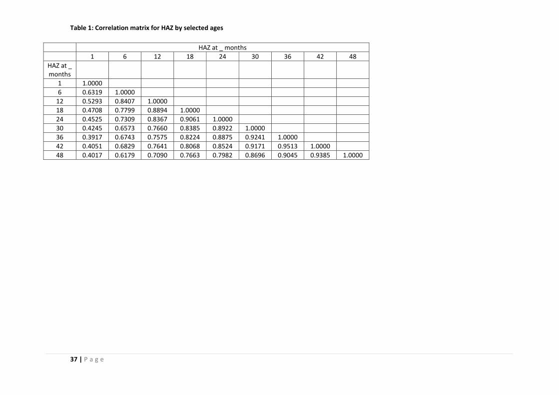
37 | P a g e   

Table 1: Correlation matrix for HAZ by selected ages 

  HAZ at _ months   1  6  12  18  24  30  36  42  48 

HAZ at _ months 

                 

1  1.0000                 6  0.6319  1.0000               12  0.5293  0.8407  1.0000             18  0.4708  0.7799  0.8894  1.0000           24  0.4525  0.7309  0.8367  0.9061  1.0000         30  0.4245  0.6573  0.7660  0.8385  0.8922  1.0000       36  0.3917  0.6743  0.7575  0.8224  0.8875  0.9241  1.0000     42  0.4051  0.6829  0.7641  0.8068  0.8524  0.9171  0.9513  1.0000   48  0.4017  0.6179  0.7090  0.7663  0.7982  0.8696  0.9045  0.9385  1.0000 

 

 

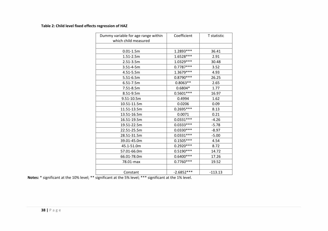
38 | P a g e   

 

Table 2: Child level fixed effects regression of HAZ 

Dummy variable for age range within which child measured 

Coefficient  T statistic 

     0.01‐1.5m  1.2893***  36.41 1.51‐2.5m  1.6528***  2.91 2.51‐3.5m  1.0329***  30.48 3.51‐4‐5m  0.7787***  3.52 4.51‐5.5m  1.3679***  4.93 5.51‐6.5m  0.8790***  26.25 6.51‐7.5m  0.8063**  2.65 7.51‐8.5m  0.6804*  1.77 8.51‐9.5m  0.5601***  16.97 9.51‐10.5m  0.4994  1.62 10.51‐11.5m  0.0206  0.09 11.51‐13.5m  0.2695***  8.13 13.51‐16.5m  0.0071  0.21 16.51‐19.5m  0.0331***  ‐4.26 19.51‐22.5m  0.0333***  ‐5.78 22.51‐25.5m  0.0330***  ‐8.97 28.51‐31.5m  0.0331***  ‐5.00 39.01‐45.0m  0.1505***  4.54 45.1‐51.0m  0.2920***  8.72 57.01‐66.0m  0.5190***  14.72 66.01‐78.0m  0.6400***  17.26 78.01‐max  0.7760***  19.52 

     Constant  ‐2.6852***  ‐113.13 

Notes: * significant at the 10% level; ** significant at the 5% level; *** significant at the 1% level.  

39 | P a g e   

 

Table 3: Outcome variables 

  Variable  Definition  Mean  Standard Deviation Schooling related outcomes  Age start school  Age (in years) when individual commenced attending 

primary school 6.80  1.09 

  Repeated primary grade  =1 if individual repeated a grade of primary school  0.48  0.50 

  Grade progression  Number of grades passed divided by the number of years between when the individual entered and terminated school, up to and including 12th grade. 

0.84  0.26 

  Age left school  Age (in years) when individual stopped attending school 

12.51  2.95 

  Highest grade attained  Highest grade of schooling attained, maximum value is 12 

4.86  3.22 

  SIA z score  Inter‐American Series test score of reading and vocabulary, standardized with mean 0 and SD 1 within the sample 

0  1 

  Raven's z score  Raven’s Progressive Matrices test score, standardized with mean 0 and SD 1 within the sample 

0  1 

Marriage market outcomes, females 

Husband's age  Age (in years) of husband at time of union formation  36.24  7.31 

  Husband's grades of schooling  Husband’s highest grade of schooling attained  4.93  3.57   Husband's Height  Husband’s height (cm)  162.46  5.72   Husband's family's land holdings  Land owned by husband’s family in manzanas (1 

manzana = 1.68 acres) 2.79  9.52 

  Age differential  Husband’s age – wife’s age  3.69  5.84   Education differential  Husband’s highest grade attained – wife’s highest 

grade attained 0.89  3.50 

  Family's land holdings differential  =1 if husband’s family has more land than wife’s family at time of union 

0.34  0.47 

Marriage market outcomes, males 

Wife's age  Age (in years) of wife at time of union formation  30.41  5.68 

  Wife's grades of schooling  Wife’s highest grade of schooling attained  4.45  3.20   Wife's Height  Wife’s height (cm)  150.52  5.19   Wife's family's land holdings  Land owned by wife’s family in manzanas (1 manzana  4.99  70.25 

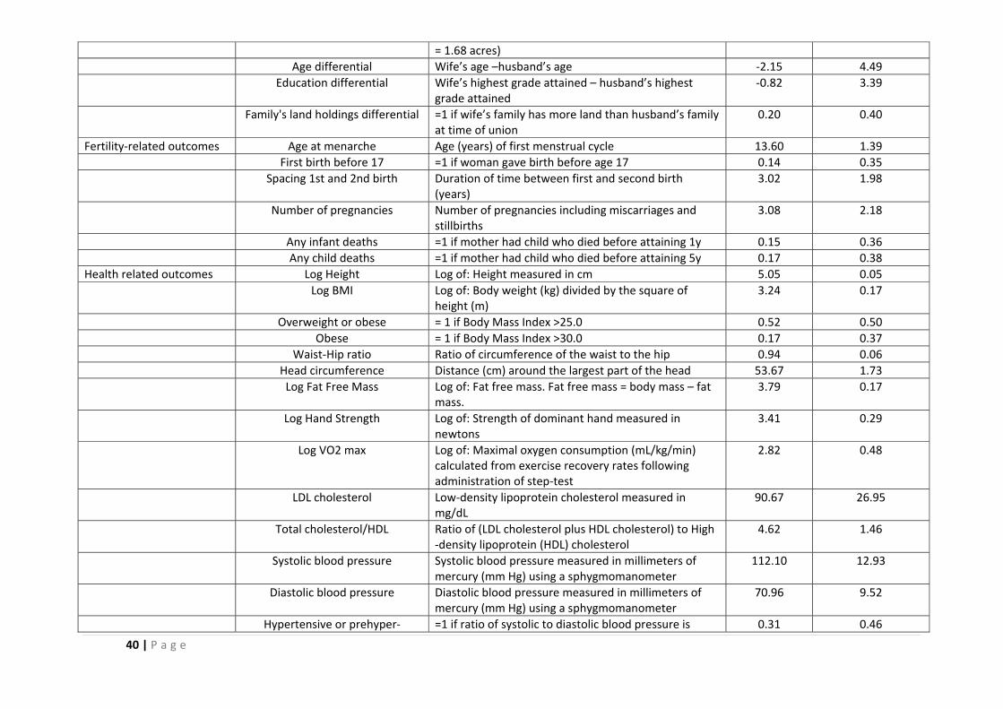
40 | P a g e   

= 1.68 acres)   Age differential  Wife’s age –husband’s age  ‐2.15  4.49   Education differential  Wife’s highest grade attained – husband’s highest 

grade attained ‐0.82  3.39 

  Family's land holdings differential  =1 if wife’s family has more land than husband’s family at time of union 

0.20  0.40 

Fertility‐related outcomes  Age at menarche  Age (years) of first menstrual cycle  13.60  1.39   First birth before 17  =1 if woman gave birth before age 17  0.14  0.35   Spacing 1st and 2nd birth  Duration of time between first and second birth 

(years) 3.02  1.98 

  Number of pregnancies  Number of pregnancies including miscarriages and stillbirths 

3.08  2.18 

  Any infant deaths  =1 if mother had child who died before attaining 1y  0.15  0.36   Any child deaths  =1 if mother had child who died before attaining 5y  0.17  0.38 Health related outcomes  Log Height  Log of: Height measured in cm  5.05  0.05 

  Log BMI  Log of: Body weight (kg) divided by the square of height (m) 

3.24  0.17 

  Overweight or obese  = 1 if Body Mass Index >25.0  0.52  0.50   Obese  = 1 if Body Mass Index >30.0  0.17  0.37   Waist‐Hip ratio  Ratio of circumference of the waist to the hip  0.94  0.06   Head circumference  Distance (cm) around the largest part of the head  53.67  1.73   Log Fat Free Mass  Log of: Fat free mass. Fat free mass = body mass – fat 

mass.  3.79  0.17 

  Log Hand Strength  Log of: Strength of dominant hand measured in newtons 

3.41  0.29 

  Log VO2 max  Log of: Maximal oxygen consumption (mL/kg/min)  calculated from exercise recovery rates following administration of step‐test 

2.82  0.48 

  LDL cholesterol  Low‐density lipoprotein cholesterol measured in mg/dL 

90.67  26.95 

  Total cholesterol/HDL  Ratio of (LDL cholesterol plus HDL cholesterol) to High ‐density lipoprotein (HDL) cholesterol 

4.62  1.46 

  Systolic blood pressure  Systolic blood pressure measured in millimeters of mercury (mm Hg) using a sphygmomanometer 

112.10  12.93 

  Diastolic blood pressure  Diastolic blood pressure measured in millimeters of mercury (mm Hg) using a sphygmomanometer 

70.96  9.52 

  Hypertensive or prehyper‐  =1 if ratio of systolic to diastolic blood pressure is  0.31  0.46 

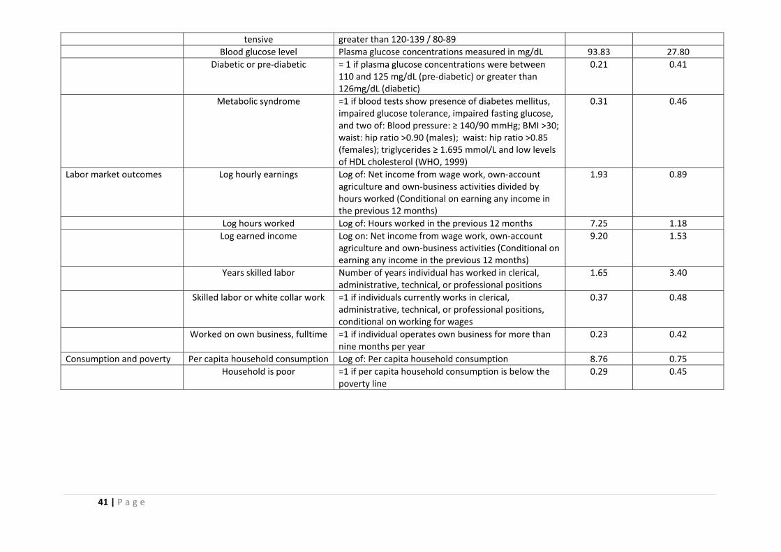
41 | P a g e   

tensive  greater than 120‐139 / 80‐89   Blood glucose level  Plasma glucose concentrations measured in mg/dL  93.83  27.80   Diabetic or pre‐diabetic  = 1 if plasma glucose concentrations were between 

110 and 125 mg/dL (pre‐diabetic) or greater than 126mg/dL (diabetic)  

0.21  0.41 

  Metabolic syndrome  =1 if blood tests show presence of diabetes mellitus, impaired glucose tolerance, impaired fasting glucose, and two of: Blood pressure: ≥ 140/90 mmHg; BMI >30; waist: hip ratio >0.90 (males);  waist: hip ratio >0.85 (females); triglycerides ≥ 1.695 mmol/L and low levels of HDL cholesterol (WHO, 1999) 

0.31  0.46 

Labor market outcomes  Log hourly earnings  Log of: Net income from wage work, own‐account agriculture and own‐business activities divided by hours worked (Conditional on earning any income in the previous 12 months) 

1.93  0.89 

  Log hours worked  Log of: Hours worked in the previous 12 months  7.25  1.18   Log earned income  Log on: Net income from wage work, own‐account 

agriculture and own‐business activities (Conditional on earning any income in the previous 12 months) 

9.20  1.53 

  Years skilled labor  Number of years individual has worked in clerical, administrative, technical, or professional positions 

1.65  3.40 

  Skilled labor or white collar work  =1 if individuals currently works in clerical, administrative, technical, or professional positions, conditional on working for wages 

0.37  0.48 

  Worked on own business, fulltime  =1 if individual operates own business for more than nine months per year 

0.23  0.42 

Consumption and poverty  Per capita household consumption Log of: Per capita household consumption  8.76  0.75   Household is poor  =1 if per capita household consumption is below the 

poverty line 0.29  0.45 

 

 

 

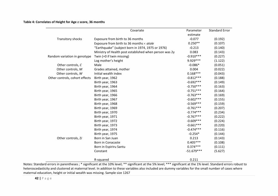
42 | P a g e   

 

Table 4: Correlates of Height for Age z score, 36 months 

  Covariate  Parameter estimate 

Standard Error 

Transitory shocks  Exposure from birth to 36 months  ‐0.077  (0.192)   Exposure from birth to 36 months × atole  0.250**  (0.107)   “Earthquake” (subject born in 1974, 1975 or 1976)  ‐0.213  (0.140)   Ministry of Health post established when person was 2y  0.083  (0.143) 

Random variation in genotype  Twin (=0 if twin missing)  ‐0.910***  (0.227)   Log mother’s height  9.929***  (1.122) 

Other controls, C  Male  ‐0.086*  (0.051) Other controls, M  Grades attained, mother  0.004  (0.022) Other controls, W  Initial wealth index  0.168***  (0.043) 

Other controls, cohort effects  Birth year, 1962  ‐0.812***  (0.188)   Birth year, 1963  ‐0.692***  (0.149)   Birth year, 1964  ‐0.750***  (0.163)   Birth year, 1965  ‐0.751***  (0.164)   Birth year, 1966  ‐0.763***  (0.169)   Birth year, 1967  ‐0.602***  (0.155)   Birth year, 1968  ‐0.569***  (0.159)   Birth year, 1969  ‐0.761***  (0.207)   Birth year, 1970  ‐0.774***  (0.234)   Birth year, 1971  ‐0.767***  (0.222)   Birth year, 1972  ‐0.609***  (0.224)   Birth year, 1973  ‐0.661***  (0.220)   Birth year, 1974  ‐0.474***  (0.116)   Birth year, 1975  ‐0.254*  (0.144) 

Other controls, Zi  Born in San Juan  0.213  (0.143)   Born in Conacaste  0.405***  (0.108)   Born in Espiriru Santu  0.374***  (0.111)   Constant  ‐51.679***  (5.627)          R‐squared  0.211   

Notes: Standard errors in parentheses ; * significant at the 10% level; ** significant at the 5% level; *** significant at the 1% level. Standard errors robust to heteroscedasticity and clustered at maternal level. In addition to these variables also included are dummy variables for the small number of cases where maternal education, height or initial wealth was missing. Sample size 1267 

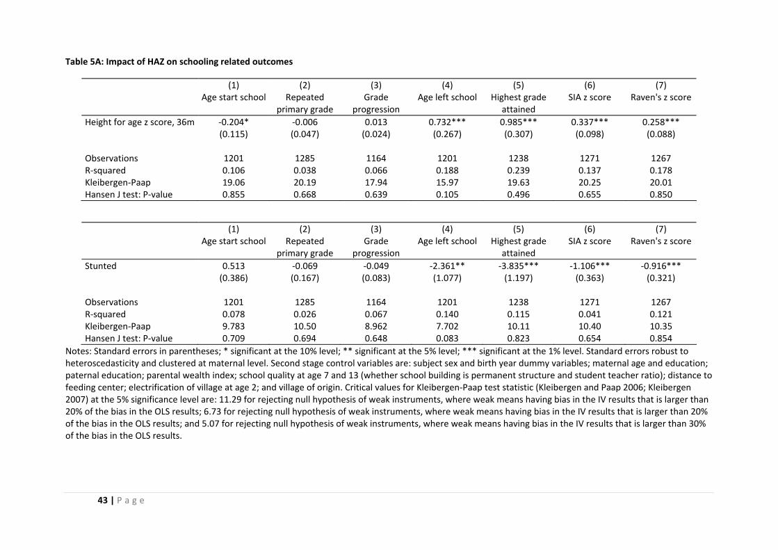
43 | P a g e   

 

Table 5A: Impact of HAZ on schooling related outcomes 

  (1)  (2)  (3)  (4)  (5)  (6)  (7)   Age start school Repeated 

primary grade Grade 

progression Age left school  Highest grade 

attained SIA z score  Raven's z score 

Height for age z score, 36m  ‐0.204*  ‐0.006  0.013  0.732***  0.985***  0.337***  0.258***   (0.115)  (0.047)  (0.024)  (0.267)  (0.307)  (0.098)  (0.088)                Observations  1201  1285  1164  1201  1238  1271  1267 R‐squared  0.106  0.038  0.066  0.188  0.239  0.137  0.178 Kleibergen‐Paap  19.06  20.19  17.94  15.97  19.63  20.25  20.01 Hansen J test: P‐value  0.855  0.668  0.639  0.105  0.496  0.655  0.850 

 

  (1)  (2)  (3)  (4)  (5)  (6)  (7)   Age start school Repeated 

primary grade Grade 

progression Age left school  Highest grade 

attained SIA z score  Raven's z score 

Stunted  0.513  ‐0.069  ‐0.049  ‐2.361**  ‐3.835***  ‐1.106***  ‐0.916***   (0.386)  (0.167)  (0.083)  (1.077)  (1.197)  (0.363)  (0.321)                Observations  1201  1285  1164  1201  1238  1271  1267 R‐squared  0.078  0.026  0.067  0.140  0.115  0.041  0.121 Kleibergen‐Paap  9.783  10.50  8.962  7.702  10.11  10.40  10.35 Hansen J test: P‐value  0.709  0.694  0.648  0.083  0.823  0.654  0.854 

Notes: Standard errors in parentheses; * significant at the 10% level; ** significant at the 5% level; *** significant at the 1% level. Standard errors robust to heteroscedasticity and clustered at maternal level. Second stage control variables are: subject sex and birth year dummy variables; maternal age and education; paternal education; parental wealth index; school quality at age 7 and 13 (whether school building is permanent structure and student teacher ratio); distance to feeding center; electrification of village at age 2; and village of origin. Critical values for Kleibergen‐Paap test statistic (Kleibergen and Paap 2006; Kleibergen 2007) at the 5% significance level are: 11.29 for rejecting null hypothesis of weak instruments, where weak means having bias in the IV results that is larger than 20% of the bias in the OLS results; 6.73 for rejecting null hypothesis of weak instruments, where weak means having bias in the IV results that is larger than 20% of the bias in the OLS results; and 5.07 for rejecting null hypothesis of weak instruments, where weak means having bias in the IV results that is larger than 30% of the bias in the OLS results. 

 

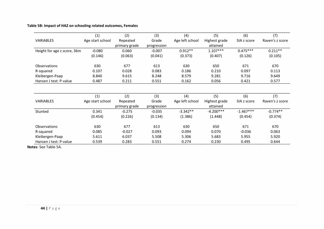
44 | P a g e   

 

Table 5B: Impact of HAZ on schooling related outcomes, Females 

  (1)  (2)  (3)  (4)  (5)  (6)  (7) VARIABLES  Age start school Repeated 

primary grade Grade 

progression Age left school  Highest grade 

attained SIA z score  Raven's z score 

Height for age z score, 36m  ‐0.080  0.060  ‐0.007  0.912**  1.107***  0.475***  0.211**   (0.146)  (0.063)  (0.041)  (0.373)  (0.407)  (0.126)  (0.105)                Observations  630  677  613  630  650  671  670 R‐squared  0.107  0.028  0.083  0.186  0.210  0.097  0.113 Kleibergen‐Paap  8.840  9.615  8.248  8.579  9.281  9.716  9.649 Hansen J test: P‐value  0.487  0.211  0.551  0.162  0.056  0.421  0.577 

 

  (1)  (2)  (3)  (4)  (5)  (6)  (7) VARIABLES  Age start school Repeated 

primary grade Grade 

progression Age left school  Highest grade 

attained SIA z score  Raven's z score 

Stunted  0.341  ‐0.275  ‐0.035  ‐3.342**  ‐4.200***  ‐1.467***  ‐0.774**   (0.454)  (0.226)  (0.134)  (1.386)  (1.448)  (0.454)  (0.374)                Observations  630  677  613  630  650  671  670 R‐squared  0.085  ‐0.027  0.093  0.094  0.070  ‐0.036  0.063 Kleibergen‐Paap  5.611  6.037  5.508  5.306  5.683  5.955  5.920 Hansen J test: P‐value  0.539  0.283  0.551  0.274  0.230  0.495  0.644 

Notes: See Table 5A.  

 

 

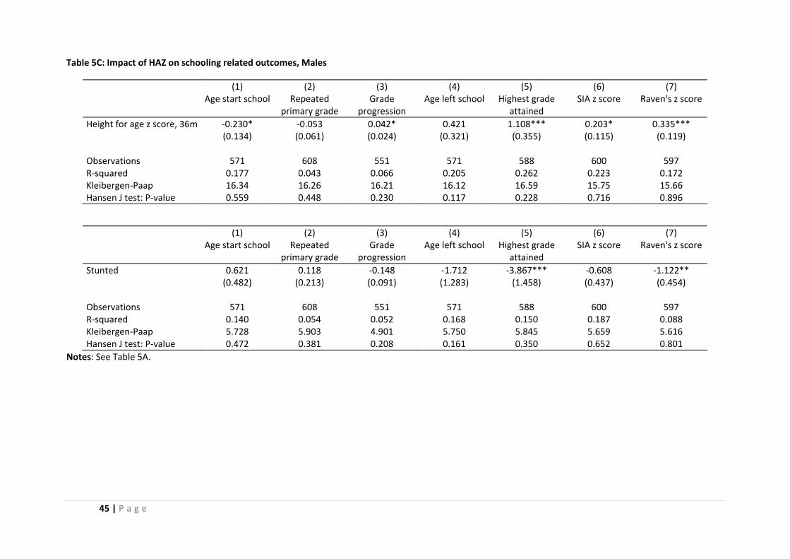
45 | P a g e   

 

Table 5C: Impact of HAZ on schooling related outcomes, Males 

  (1)  (2)  (3)  (4)  (5)  (6)  (7)   Age start school Repeated 

primary grade Grade 

progression Age left school  Highest grade 

attained SIA z score  Raven's z score 

Height for age z score, 36m  ‐0.230*  ‐0.053  0.042*  0.421  1.108***  0.203*  0.335***   (0.134)  (0.061)  (0.024)  (0.321)  (0.355)  (0.115)  (0.119)                Observations  571  608  551  571  588  600  597 R‐squared  0.177  0.043  0.066  0.205  0.262  0.223  0.172 Kleibergen‐Paap  16.34  16.26  16.21  16.12  16.59  15.75  15.66 Hansen J test: P‐value  0.559  0.448  0.230  0.117  0.228  0.716  0.896 

 

  (1)  (2)  (3)  (4)  (5)  (6)  (7)   Age start school Repeated 

primary grade Grade 

progression Age left school  Highest grade 

attained SIA z score  Raven's z score 

Stunted  0.621  0.118  ‐0.148  ‐1.712  ‐3.867***  ‐0.608  ‐1.122**   (0.482)  (0.213)  (0.091)  (1.283)  (1.458)  (0.437)  (0.454)                Observations  571  608  551  571  588  600  597 R‐squared  0.140  0.054  0.052  0.168  0.150  0.187  0.088 Kleibergen‐Paap  5.728  5.903  4.901  5.750  5.845  5.659  5.616 Hansen J test: P‐value  0.472  0.381  0.208  0.161  0.350  0.652  0.801 

Notes: See Table 5A. 

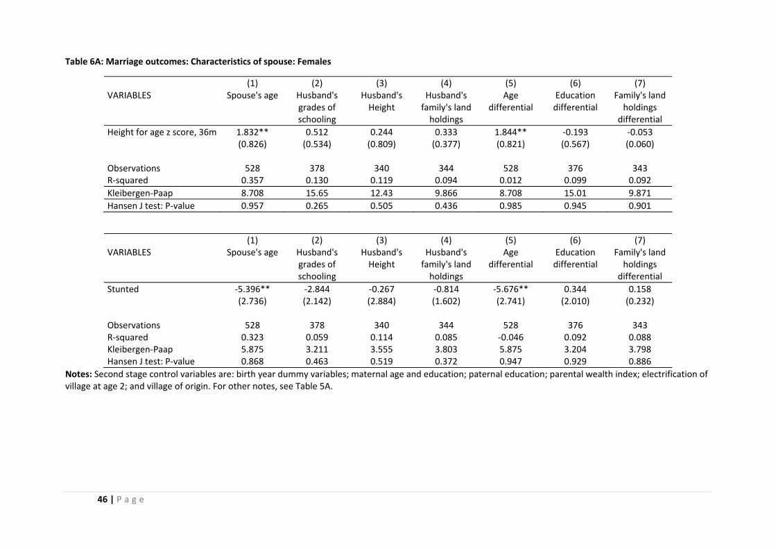
46 | P a g e   

 

Table 6A: Marriage outcomes: Characteristics of spouse: Females 

  (1)  (2)  (3)  (4)  (5)  (6)  (7) VARIABLES  Spouse's age  Husband's 

grades of schooling 

Husband's Height 

Husband's family's land holdings 

Age differential 

Education differential 

Family's land holdings 

differential Height for age z score, 36m  1.832**  0.512  0.244  0.333  1.844**  ‐0.193  ‐0.053   (0.826)  (0.534)  (0.809)  (0.377)  (0.821)  (0.567)  (0.060)                Observations  528  378  340  344  528  376  343 R‐squared  0.357  0.130  0.119  0.094  0.012  0.099  0.092 Kleibergen‐Paap  8.708  15.65  12.43  9.866  8.708  15.01  9.871 Hansen J test: P‐value  0.957  0.265  0.505  0.436  0.985  0.945  0.901 

 

  (1)  (2)  (3)  (4)  (5)  (6)  (7) VARIABLES  Spouse's age  Husband's 

grades of schooling 

Husband's Height 

Husband's family's land holdings 

Age differential 

Education differential 

Family's land holdings 

differential Stunted  ‐5.396**  ‐2.844  ‐0.267  ‐0.814  ‐5.676**  0.344  0.158   (2.736)  (2.142)  (2.884)  (1.602)  (2.741)  (2.010)  (0.232)                Observations  528  378  340  344  528  376  343 R‐squared  0.323  0.059  0.114  0.085  ‐0.046  0.092  0.088 Kleibergen‐Paap  5.875  3.211  3.555  3.803  5.875  3.204  3.798 Hansen J test: P‐value  0.868  0.463  0.519  0.372  0.947  0.929  0.886 

Notes: Second stage control variables are: birth year dummy variables; maternal age and education; paternal education; parental wealth index; electrification of village at age 2; and village of origin. For other notes, see Table 5A.  

 

 

47 | P a g e   

 

Table 6B: Marriage outcomes: Characteristics of spouse: Males 

  (1)  (2)  (3)  (4)  (5)  (6)  (7) VARIABLES  Wife's age  Wife's grades 

of schooling Wife's Height  Wife's family's 

land holdings Age differential Education 

differential Family's land holdings 

differential Height for age z score, 36m  0.672  1.058***  1.566**  ‐0.629  0.734*  ‐0.134  0.086   (0.431)  (0.343)  (0.640)  (3.625)  (0.433)  (0.385)  (0.053)                Observations  568  551  483  443  568  472  441 R‐squared  0.425  0.136  0.040  ‐0.002  0.079  0.066  0.020 Kleibergen‐Paap  18.01  17.96  14.51  14.67  18.01  17.78  14.69 Hansen J test: P‐value  0.538  0.495  0.103  0.962  0.513  0.414  0.558 

 

  (1)  (2)  (3)  (4)  (5)  (6)  (7) VARIABLES  Wife's age  Wife's grades 

of schooling Wife's Height  Wife's family's 

land holdings Age differential Education 

differential Family's land holdings 

differential Stunted  ‐1.773  ‐3.226***  ‐3.580*  1.227  ‐2.157  0.546  ‐0.249   (1.464)  (1.217)  (2.165)  (12.470)  (1.470)  (1.367)  (0.188)                Observations  568  551  483  443  568  472  441 R‐squared  0.413  0.070  0.042  ‐0.003  0.056  0.061  0.009 Kleibergen‐Paap  5.192  5.979  5.752  4.764  5.192  4.748  4.598 Hansen J test: P‐value  0.433  0.557  0.060  0.960  0.438  0.433  0.480 

Notes: See Table 6A. 

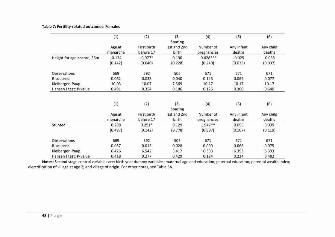
48 | P a g e   

 

Table 7: Fertility‐related outcomes: Females 

  (1)  (2)  (3)  (4)  (5)  (6)       Spacing         Age at 

menarche First birth before 17 

1st and 2nd birth 

Number of pregnancies 

Any infant deaths 

Any child deaths 

Height for age z score, 36m ‐0.134  ‐0.077*  0.190  ‐0.628***  ‐0.025  ‐0.053   (0.142)  (0.040)  (0.228)  (0.240)  (0.033)  (0.037)              Observations  669  592  505  671  671  671 R‐squared  0.062  0.038  0.040  0.143  0.069  0.077 Kleibergen‐Paap  10.03  10.07  7.569  10.17  10.17  10.17 Hansen J test: P‐value  0.491  0.354  0.186  0.126  0.300  0.640 

 

  (1)  (2)  (3)  (4)  (5)  (6)       Spacing         Age at 

menarche First birth before 17 

1st and 2nd birth 

Number of pregnancies 

Any infant deaths 

Any child deaths 

Stunted  0.298  0.251*  0.129  1.947**  0.055  0.099   (0.497)  (0.142)  (0.778)  (0.807)  (0.107)  (0.119)              Observations  669  592  505  671  671  671 R‐squared  0.057  0.013  0.028  0.099  0.066  0.075 Kleibergen‐Paap  6.426  6.542  5.417  6.393  6.393  6.393 Hansen J test: P‐value  0.418  0.277  0.429  0.124  0.224  0.482 

Notes: Second stage control variables are: birth year dummy variables; maternal age and education; paternal education; parental wealth index; electrification of village at age 2; and village of origin. For other notes, see Table 5A. 

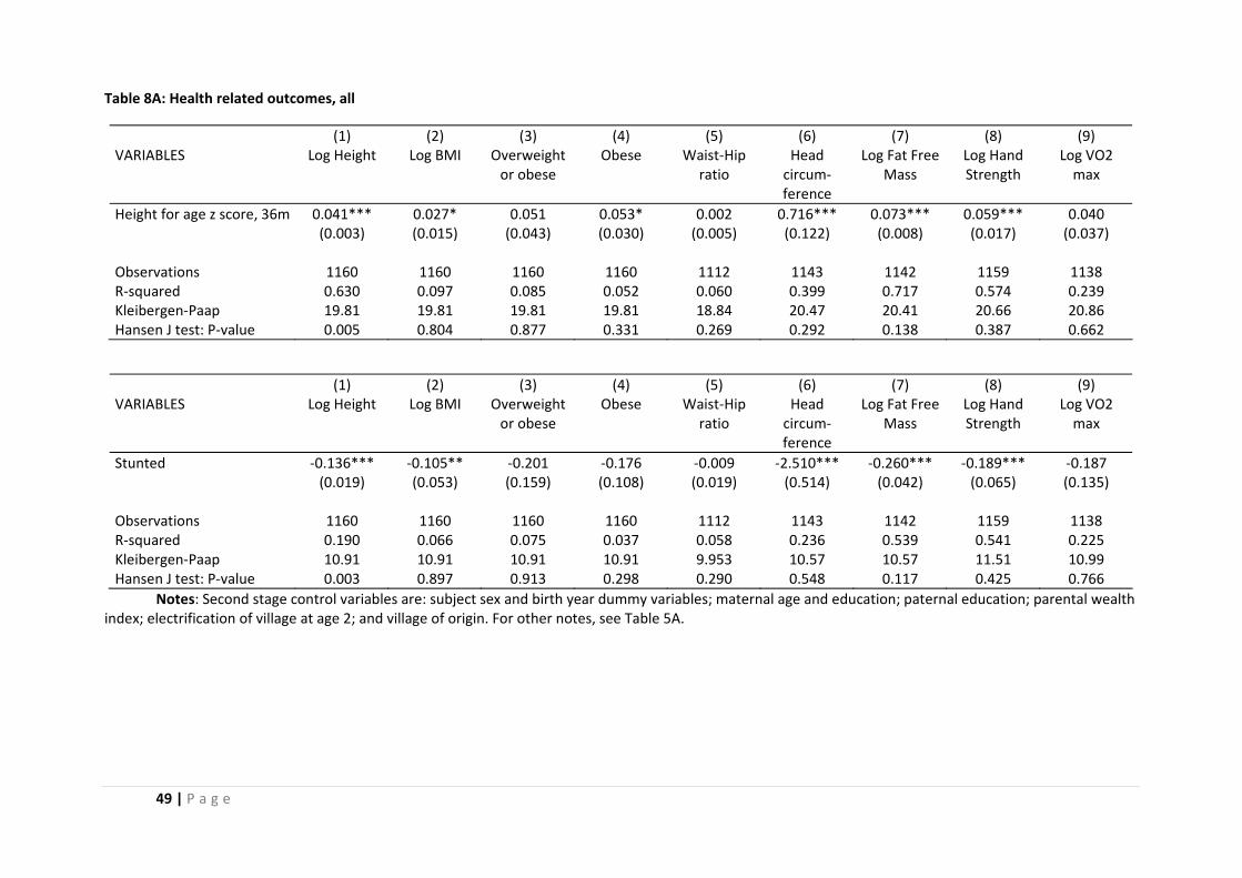
49 | P a g e   

 

Table 8A: Health related outcomes, all 

  (1)  (2)  (3)  (4)  (5)  (6)  (7)  (8)  (9) VARIABLES  Log Height  Log BMI  Overweight 

or obese Obese  Waist‐Hip 

ratio Head circum‐ ference 

Log Fat Free Mass 

Log Hand Strength 

Log VO2 max 

Height for age z score, 36m  0.041***  0.027*  0.051  0.053*  0.002  0.716***  0.073***  0.059***  0.040   (0.003)  (0.015)  (0.043)  (0.030)  (0.005)  (0.122)  (0.008)  (0.017)  (0.037)                    Observations  1160  1160  1160  1160  1112  1143  1142  1159  1138 R‐squared  0.630  0.097  0.085  0.052  0.060  0.399  0.717  0.574  0.239 Kleibergen‐Paap  19.81  19.81  19.81  19.81  18.84  20.47  20.41  20.66  20.86 Hansen J test: P‐value  0.005  0.804  0.877  0.331  0.269  0.292  0.138  0.387  0.662 

 

  (1)  (2)  (3)  (4)  (5)  (6)  (7)  (8)  (9) VARIABLES  Log Height  Log BMI  Overweight 

or obese Obese  Waist‐Hip 

ratio Head circum‐ ference 

Log Fat Free Mass 

Log Hand Strength 

Log VO2 max 

Stunted  ‐0.136***  ‐0.105**  ‐0.201  ‐0.176  ‐0.009  ‐2.510***  ‐0.260***  ‐0.189***  ‐0.187   (0.019)  (0.053)  (0.159)  (0.108)  (0.019)  (0.514)  (0.042)  (0.065)  (0.135)                    Observations  1160  1160  1160  1160  1112  1143  1142  1159  1138 R‐squared  0.190  0.066  0.075  0.037  0.058  0.236  0.539  0.541  0.225 Kleibergen‐Paap  10.91  10.91  10.91  10.91  9.953  10.57  10.57  11.51  10.99 Hansen J test: P‐value  0.003  0.897  0.913  0.298  0.290  0.548  0.117  0.425  0.766 

Notes: Second stage control variables are: subject sex and birth year dummy variables; maternal age and education; paternal education; parental wealth index; electrification of village at age 2; and village of origin. For other notes, see Table 5A. 

 

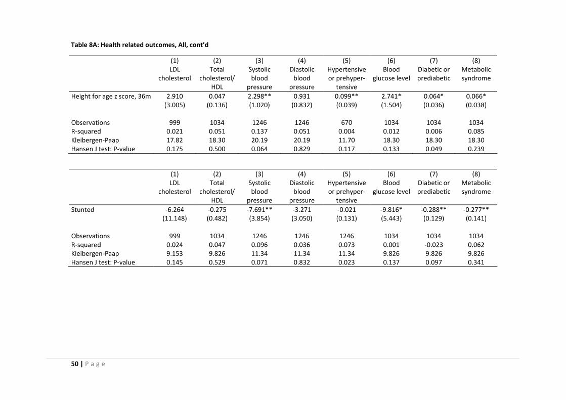
50 | P a g e   

 

Table 8A: Health related outcomes, All, cont’d 

  (1)  (2)  (3)  (4)  (5)  (6)  (7)  (8)   LDL 

cholesterol Total 

cholesterol/HDL 

Systolic blood 

pressure 

Diastolic blood 

pressure 

Hypertensive or prehyper‐ 

tensive 

Blood glucose level

Diabetic or prediabetic 

Metabolic syndrome 

Height for age z score, 36m  2.910  0.047  2.298**  0.931  0.099**  2.741*  0.064*  0.066*   (3.005)  (0.136)  (1.020)  (0.832)  (0.039)  (1.504)  (0.036)  (0.038)                  Observations  999  1034  1246  1246  670  1034  1034  1034 R‐squared  0.021  0.051  0.137  0.051  0.004  0.012  0.006  0.085 Kleibergen‐Paap  17.82  18.30  20.19  20.19  11.70  18.30  18.30  18.30 Hansen J test: P‐value  0.175  0.500  0.064  0.829  0.117  0.133  0.049  0.239  

  (1)  (2)  (3)  (4)  (5)  (6)  (7)  (8)   LDL 

cholesterol Total 

cholesterol/HDL 

Systolic blood 

pressure 

Diastolic blood 

pressure 

Hypertensive or prehyper‐ 

tensive 

Blood glucose level

Diabetic or prediabetic 

Metabolic syndrome 

Stunted  ‐6.264  ‐0.275  ‐7.691**  ‐3.271  ‐0.021  ‐9.816*  ‐0.288**  ‐0.277**   (11.148)  (0.482)  (3.854)  (3.050)  (0.131)  (5.443)  (0.129)  (0.141)                  Observations  999  1034  1246  1246  1246  1034  1034  1034 R‐squared  0.024  0.047  0.096  0.036  0.073  0.001  ‐0.023  0.062 Kleibergen‐Paap  9.153  9.826  11.34  11.34  11.34  9.826  9.826  9.826 Hansen J test: P‐value  0.145  0.529  0.071  0.832  0.023  0.137  0.097  0.341  

 

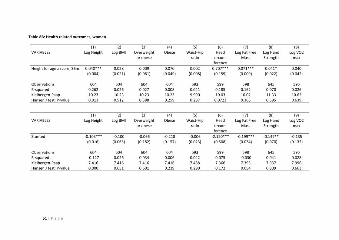
51 | P a g e   

 

 

Table 8B: Health related outcomes, women   

  (1)  (2)  (3)  (4)  (5)  (6)  (7)  (8)  (9) VARIABLES  Log Height  Log BMI  Overweight 

or obese Obese  Waist‐Hip 

ratio Head circum‐ ference 

Log Fat Free Mass 

Log Hand Strength 

Log VO2 max 

Height for age z score, 36m  0.040***  0.028  0.009  0.070  0.002  0.707***  0.071***  0.041*  0.040   (0.004)  (0.021)  (0.061)  (0.049)  (0.008)  (0.159)  (0.009)  (0.022)  (0.042)                    Observations  604  604  604  604  593  599  598  645  595 R‐squared  0.262  0.026  0.027  0.008  0.041  0.185  0.162  0.070  0.026 Kleibergen‐Paap  10.23  10.23  10.23  10.23  9.990  10.03  10.02  11.33  10.62 Hansen J test: P‐value  0.013  0.512  0.588  0.259  0.287  0.0723  0.365  0.595  0.639 

 

  (1)  (2)  (3)  (4)  (5)  (6)  (7)  (8)  (9) VARIABLES  Log Height  Log BMI  Overweight 

or obese Obese  Waist‐Hip 

ratio Head circum‐ ference 

Log Fat Free Mass 

Log Hand Strength 

Log VO2 max 

Stunted  ‐0.103***  ‐0.100  ‐0.066  ‐0.218  ‐0.006  ‐2.120***  ‐0.199***  ‐0.147**  ‐0.135   (0.016)  (0.063)  (0.182)  (0.157)  (0.023)  (0.508)  (0.034)  (0.070)  (0.132)                    Observations  604  604  604  604  593  599  598  645  595 R‐squared  ‐0.127  0.026  0.034  0.006  0.042  0.075  ‐0.030  0.041  0.028 Kleibergen‐Paap  7.416  7.416  7.416  7.416  7.488  7.366  7.393  7.937  7.996 Hansen J test: P‐value  0.000  0.651  0.601  0.239  0.290  0.172  0.054  0.809  0.663 

 

52 | P a g e   

 

Table 8B: Health related outcomes, Women , cont’d 

  (1)  (2)  (3)  (4)  (5)  (6)  (7)  (8)   LDL 

cholesterol Total 

cholesterol/HDL 

Systolic blood 

pressure 

Diastolic blood 

pressure 

Hypertensive or prehyper‐ 

tensive 

Blood glucose level

Diabetic or prediabetic 

Metabolic syndrome 

Height for age z score, 36m  2.291  ‐0.082  4.048***  3.144***  0.099**  3.370  ‐0.012  0.027   (3.379)  (0.160)  (1.364)  (1.009)  (0.039)  (2.404)  (0.051)  (0.057)                  Observations  585  600  670  670  670  600  600  600 R‐squared  0.021  0.019  0.007  ‐0.020  0.004  0.019  0.030  0.041 Kleibergen‐Paap  11.52  11.46  11.70  11.70  11.70  11.46  11.46  11.46 Hansen J test: P‐value  0.309  0.170  0.161  0.381  0.117  0.343  0.051  0.075  

  (1)  (2)  (3)  (4)  (5)  (6)  (7)  (8)   LDL 

cholesterol Total 

cholesterol/HDL 

Systolic blood 

pressure 

Diastolic blood 

pressure 

Hypertensive or prehyper‐ 

tensive 

Blood glucose level

Diabetic or prediabetic 

Metabolic syndrome 

Stunted  ‐4.337  0.091  ‐12.215***  ‐10.219***  ‐0.234*  ‐10.383  ‐0.073  ‐0.201   (11.564)  (0.547)  (4.525)  (3.589)  (0.128)  (8.465)  (0.176)  (0.193)                  Observations  585  600  670  670  670  600  600  600 R‐squared  0.027  0.022  ‐0.045  ‐0.095  ‐0.005  0.011  0.028  0.036 Kleibergen‐Paap  6.778  7.088  8.185  8.185  8.185  7.088  7.088  7.088 Hansen J test: P‐value  0.282  0.145  0.165  0.293  0.082  0.319  0.050  0.098  

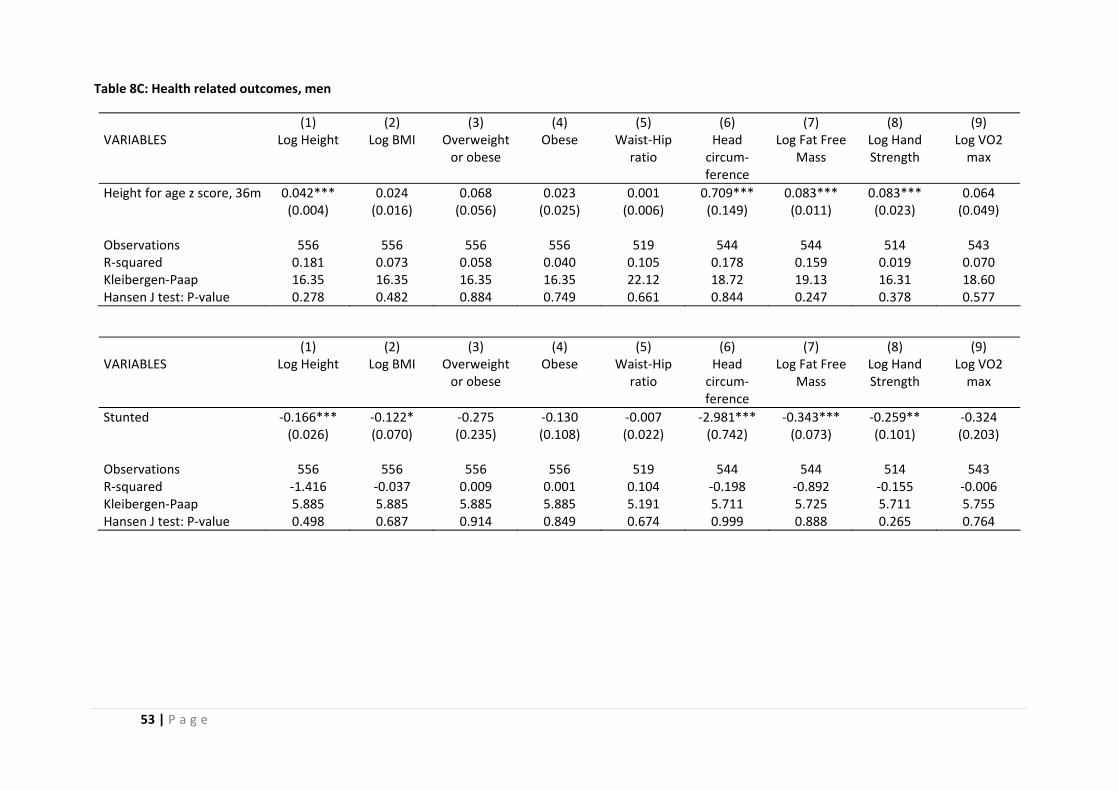
53 | P a g e   

 

Table 8C: Health related outcomes, men 

  (1)  (2)  (3)  (4)  (5)  (6)  (7)  (8)  (9) VARIABLES  Log Height  Log BMI  Overweight 

or obese Obese  Waist‐Hip 

ratio Head circum‐ ference 

Log Fat Free Mass 

Log Hand Strength 

Log VO2 max 

Height for age z score, 36m  0.042***  0.024  0.068  0.023  0.001  0.709***  0.083***  0.083***  0.064   (0.004)  (0.016)  (0.056)  (0.025)  (0.006)  (0.149)  (0.011)  (0.023)  (0.049)                    Observations  556  556  556  556  519  544  544  514  543 R‐squared  0.181  0.073  0.058  0.040  0.105  0.178  0.159  0.019  0.070 Kleibergen‐Paap  16.35  16.35  16.35  16.35  22.12  18.72  19.13  16.31  18.60 Hansen J test: P‐value  0.278  0.482  0.884  0.749  0.661  0.844  0.247  0.378  0.577 

 

  (1)  (2)  (3)  (4)  (5)  (6)  (7)  (8)  (9) VARIABLES  Log Height  Log BMI  Overweight 

or obese Obese  Waist‐Hip 

ratio Head circum‐ ference 

Log Fat Free Mass 

Log Hand Strength 

Log VO2 max 

Stunted  ‐0.166***  ‐0.122*  ‐0.275  ‐0.130  ‐0.007  ‐2.981***  ‐0.343***  ‐0.259**  ‐0.324   (0.026)  (0.070)  (0.235)  (0.108)  (0.022)  (0.742)  (0.073)  (0.101)  (0.203)                    Observations  556  556  556  556  519  544  544  514  543 R‐squared  ‐1.416  ‐0.037  0.009  0.001  0.104  ‐0.198  ‐0.892  ‐0.155  ‐0.006 Kleibergen‐Paap  5.885  5.885  5.885  5.885  5.191  5.711  5.725  5.711  5.755 Hansen J test: P‐value  0.498  0.687  0.914  0.849  0.674  0.999  0.888  0.265  0.764 

 

 

 

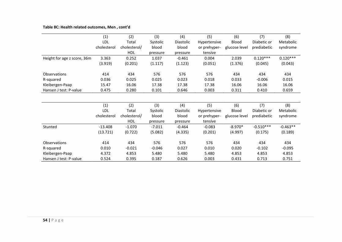
54 | P a g e   

 

Table 8C: Health related outcomes, Men , cont’d 

  (1)  (2)  (3)  (4)  (5)  (6)  (7)  (8)   LDL 

cholesterol Total 

cholesterol/HDL 

Systolic blood 

pressure 

Diastolic blood 

pressure 

Hypertensive or prehyper‐ 

tensive 

Blood glucose level

Diabetic or prediabetic 

Metabolic syndrome 

Height for age z score, 36m  3.363  0.252  1.037  ‐0.461  0.004  2.039  0.120***  0.120***   (3.919)  (0.201)  (1.117)  (1.123)  (0.051)  (1.376)  (0.045)  (0.043)                  Observations  414  434  576  576  576  434  434  434 R‐squared  0.036  0.025  0.025  0.023  0.018  0.033  ‐0.006  0.015 Kleibergen‐Paap  15.47  16.06  17.38  17.38  17.38  16.06  16.06  16.06 Hansen J test: P‐value  0.475  0.280  0.101  0.646  0.003  0.311  0.410  0.659  

  (1)  (2)  (3)  (4)  (5)  (6)  (7)  (8)   LDL 

cholesterol Total 

cholesterol/HDL 

Systolic blood 

pressure 

Diastolic blood 

pressure 

Hypertensive or prehyper‐ 

tensive 

Blood glucose level

Diabetic or prediabetic 

Metabolic syndrome 

Stunted  ‐13.408  ‐1.070  ‐7.011  ‐0.464  ‐0.083  ‐8.970*  ‐0.510***  ‐0.463**   (13.721)  (0.722)  (5.082)  (4.335)  (0.201)  (4.997)  (0.175)  (0.189)                  Observations  414  434  576  576  576  434  434  434 R‐squared  0.010  ‐0.021  ‐0.046  0.027  0.010  0.020  ‐0.102  ‐0.095 Kleibergen‐Paap  4.372  4.853  5.480  5.480  5.480  4.853  4.853  4.853 Hansen J test: P‐value  0.524  0.395  0.187  0.626  0.003  0.431  0.713  0.751  

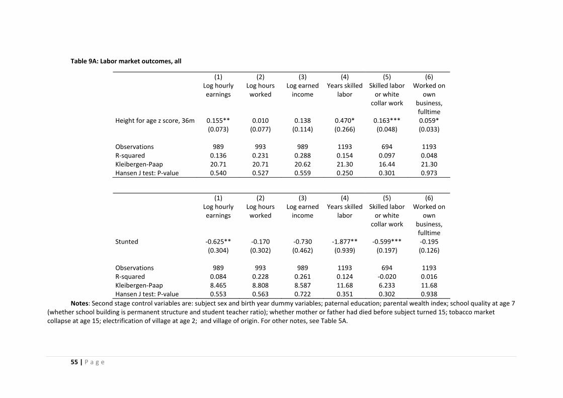
55 | P a g e   

 

 

Table 9A: Labor market outcomes, all 

  (1)  (2)  (3)  (4)  (5)  (6)   Log hourly 

earnings Log hours worked 

Log earned income 

Years skilled labor 

Skilled labor or white 

collar work 

Worked on own 

business, fulltime 

Height for age z score, 36m 0.155**  0.010  0.138  0.470*  0.163***  0.059*   (0.073)  (0.077)  (0.114)  (0.266)  (0.048)  (0.033)              Observations  989  993  989  1193  694  1193 R‐squared  0.136  0.231  0.288  0.154  0.097  0.048 Kleibergen‐Paap  20.71  20.71  20.62  21.30  16.44  21.30 Hansen J test: P‐value  0.540  0.527  0.559  0.250  0.301  0.973 

 

  (1)  (2)  (3)  (4)  (5)  (6)   Log hourly 

earnings Log hours worked 

Log earned income 

Years skilled labor 

Skilled labor or white 

collar work 

Worked on own 

business, fulltime 

Stunted  ‐0.625**  ‐0.170  ‐0.730  ‐1.877**  ‐0.599***  ‐0.195   (0.304)  (0.302)  (0.462)  (0.939)  (0.197)  (0.126)              Observations  989  993  989  1193  694  1193 R‐squared  0.084  0.228  0.261  0.124  ‐0.020  0.016 Kleibergen‐Paap  8.465  8.808  8.587  11.68  6.233  11.68 Hansen J test: P‐value  0.553  0.563  0.722  0.351  0.302  0.938 

Notes: Second stage control variables are: subject sex and birth year dummy variables; paternal education; parental wealth index; school quality at age 7 (whether school building is permanent structure and student teacher ratio); whether mother or father had died before subject turned 15; tobacco market collapse at age 15; electrification of village at age 2;  and village of origin. For other notes, see Table 5A. 

 

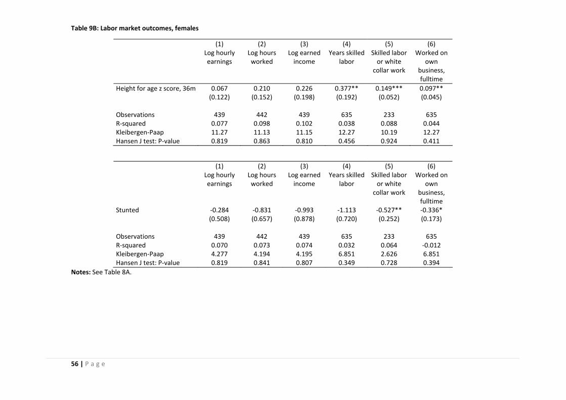
56 | P a g e   

Table 9B: Labor market outcomes, females 

  (1)  (2)  (3)  (4)  (5)  (6)   Log hourly 

earnings Log hours worked 

Log earned income 

Years skilled labor 

Skilled labor or white 

collar work 

Worked on own 

business, fulltime 

Height for age z score, 36m 0.067  0.210  0.226  0.377**  0.149***  0.097**   (0.122)  (0.152)  (0.198)  (0.192)  (0.052)  (0.045)              Observations  439  442  439  635  233  635 R‐squared  0.077  0.098  0.102  0.038  0.088  0.044 Kleibergen‐Paap  11.27  11.13  11.15  12.27  10.19  12.27 Hansen J test: P‐value  0.819  0.863  0.810  0.456  0.924  0.411 

 

  (1)  (2)  (3)  (4)  (5)  (6)   Log hourly 

earnings Log hours worked 

Log earned income 

Years skilled labor 

Skilled labor or white 

collar work 

Worked on own 

business, fulltime 

Stunted  ‐0.284  ‐0.831  ‐0.993  ‐1.113  ‐0.527**  ‐0.336*   (0.508)  (0.657)  (0.878)  (0.720)  (0.252)  (0.173)              Observations  439  442  439  635  233  635 R‐squared  0.070  0.073  0.074  0.032  0.064  ‐0.012 Kleibergen‐Paap  4.277  4.194  4.195  6.851  2.626  6.851 Hansen J test: P‐value  0.819  0.841  0.807  0.349  0.728  0.394 

Notes: See Table 8A. 

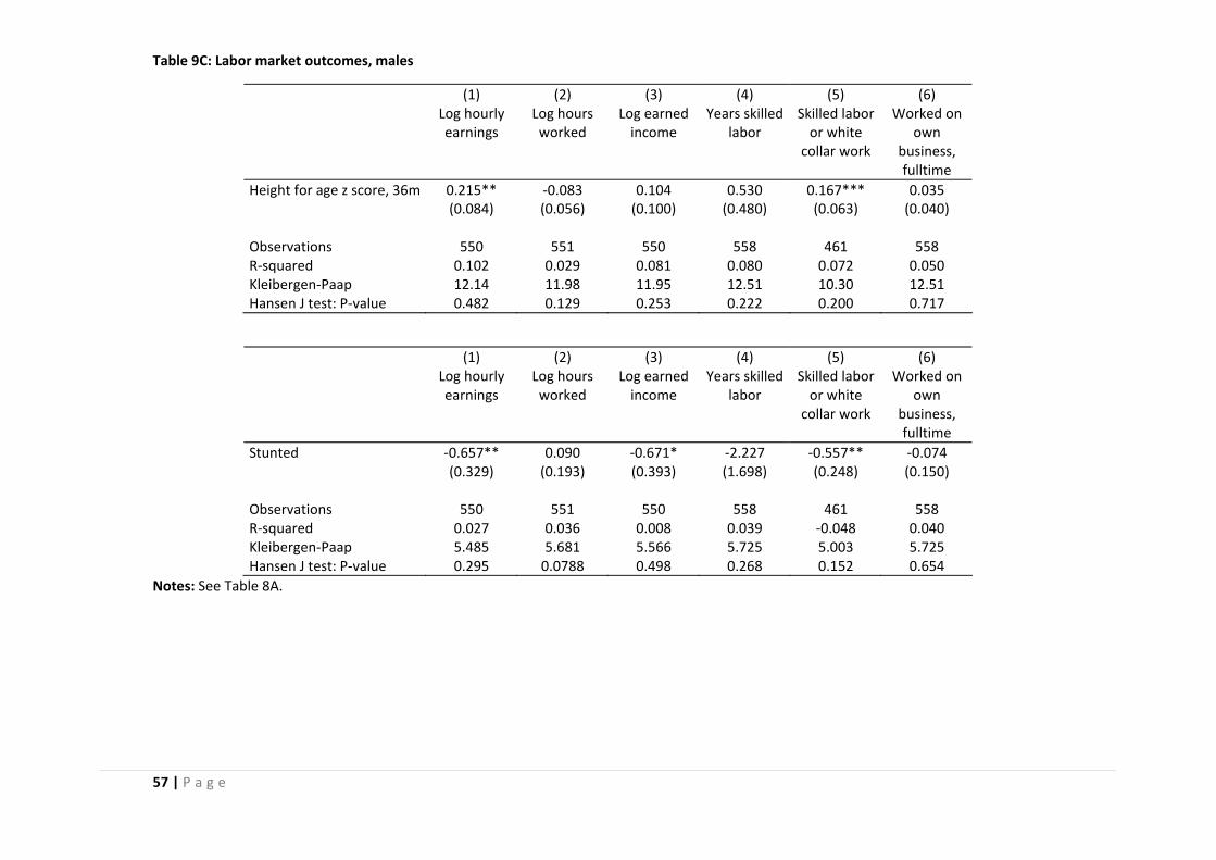
57 | P a g e   

Table 9C: Labor market outcomes, males 

  (1)  (2)  (3)  (4)  (5)  (6)   Log hourly 

earnings Log hours worked 

Log earned income 

Years skilled labor 

Skilled labor or white 

collar work 

Worked on own 

business, fulltime 

Height for age z score, 36m 0.215**  ‐0.083  0.104  0.530  0.167***  0.035   (0.084)  (0.056)  (0.100)  (0.480)  (0.063)  (0.040)              Observations  550  551  550  558  461  558 R‐squared  0.102  0.029  0.081  0.080  0.072  0.050 Kleibergen‐Paap  12.14  11.98  11.95  12.51  10.30  12.51 Hansen J test: P‐value  0.482  0.129  0.253  0.222  0.200  0.717 

 

  (1)  (2)  (3)  (4)  (5)  (6)   Log hourly 

earnings Log hours worked 

Log earned income 

Years skilled labor 

Skilled labor or white 

collar work 

Worked on own 

business, fulltime 

Stunted  ‐0.657**  0.090  ‐0.671*  ‐2.227  ‐0.557**  ‐0.074   (0.329)  (0.193)  (0.393)  (1.698)  (0.248)  (0.150)              Observations  550  551  550  558  461  558 R‐squared  0.027  0.036  0.008  0.039  ‐0.048  0.040 Kleibergen‐Paap  5.485  5.681  5.566  5.725  5.003  5.725 Hansen J test: P‐value  0.295  0.0788  0.498  0.268  0.152  0.654 

Notes: See Table 8A.

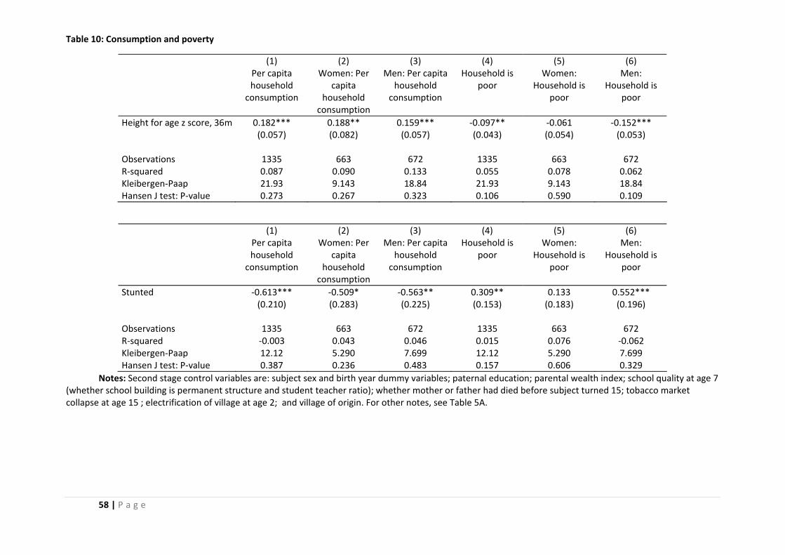
58 | P a g e   

Table 10: Consumption and poverty 

  (1)  (2)  (3)  (4)  (5)  (6)   Per capita 

household consumption 

Women: Per capita 

household consumption 

Men: Per capita household 

consumption 

Household is poor 

Women: Household is 

poor 

Men: Household is 

poor 

Height for age z score, 36m 0.182***  0.188**  0.159***  ‐0.097**  ‐0.061  ‐0.152***   (0.057)  (0.082)  (0.057)  (0.043)  (0.054)  (0.053)              Observations  1335  663  672  1335  663  672 R‐squared  0.087  0.090  0.133  0.055  0.078  0.062 Kleibergen‐Paap  21.93  9.143  18.84  21.93  9.143  18.84 Hansen J test: P‐value  0.273  0.267  0.323  0.106  0.590  0.109 

 

  (1)  (2)  (3)  (4)  (5)  (6)   Per capita 

household consumption 

Women: Per capita 

household consumption 

Men: Per capita household 

consumption 

Household is poor 

Women: Household is 

poor 

Men: Household is 

poor 

Stunted  ‐0.613***  ‐0.509*  ‐0.563**  0.309**  0.133  0.552***   (0.210)  (0.283)  (0.225)  (0.153)  (0.183)  (0.196)              Observations  1335  663  672  1335  663  672 R‐squared  ‐0.003  0.043  0.046  0.015  0.076  ‐0.062 Kleibergen‐Paap  12.12  5.290  7.699  12.12  5.290  7.699 Hansen J test: P‐value  0.387  0.236  0.483  0.157  0.606  0.329 

Notes: Second stage control variables are: subject sex and birth year dummy variables; paternal education; parental wealth index; school quality at age 7 (whether school building is permanent structure and student teacher ratio); whether mother or father had died before subject turned 15; tobacco market collapse at age 15 ; electrification of village at age 2;  and village of origin. For other notes, see Table 5A. 

 

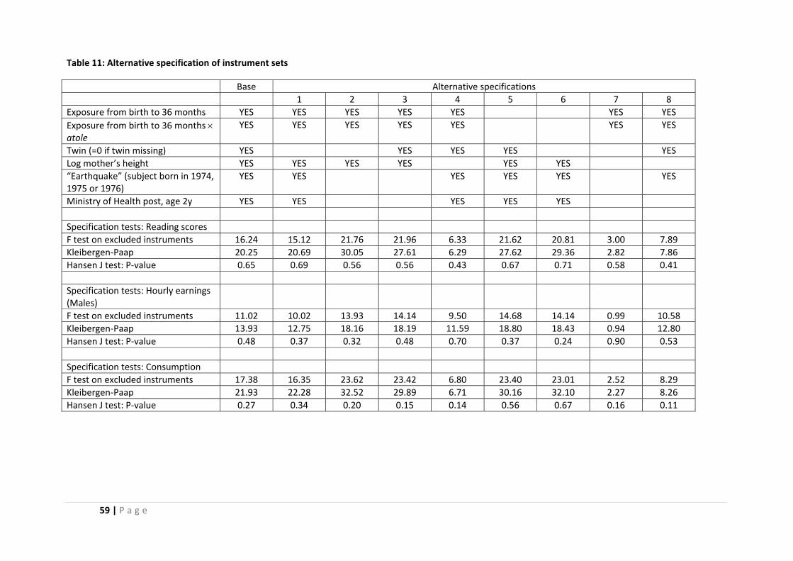
59 | P a g e   

 

Table 11: Alternative specification of instrument sets 

  Base  Alternative specifications     1  2  3  4  5  6  7  8 Exposure from birth to 36 months  YES  YES  YES  YES  YES      YES  YES Exposure from birth to 36 months × atole 

YES  YES  YES  YES  YES      YES  YES 

Twin (=0 if twin missing)  YES      YES  YES  YES      YES Log mother’s height  YES  YES  YES  YES    YES  YES     “Earthquake” (subject born in 1974, 1975 or 1976) 

YES  YES      YES  YES  YES    YES 

Ministry of Health post, age 2y  YES  YES      YES  YES  YES                        Specification tests: Reading scores                   F test on excluded instruments  16.24  15.12  21.76  21.96  6.33  21.62  20.81  3.00  7.89 Kleibergen‐Paap  20.25  20.69  30.05  27.61  6.29  27.62  29.36  2.82  7.86 Hansen J test: P‐value  0.65  0.69  0.56  0.56  0.43  0.67  0.71  0.58  0.41                    Specification tests: Hourly earnings (Males) 

                 

F test on excluded instruments  11.02  10.02  13.93  14.14  9.50  14.68  14.14  0.99  10.58 Kleibergen‐Paap  13.93  12.75  18.16  18.19  11.59  18.80  18.43  0.94  12.80 Hansen J test: P‐value  0.48  0.37  0.32  0.48  0.70  0.37  0.24  0.90  0.53                    Specification tests: Consumption                   F test on excluded instruments  17.38  16.35  23.62  23.42  6.80  23.40  23.01  2.52  8.29 Kleibergen‐Paap  21.93  22.28  32.52  29.89  6.71  30.16  32.10  2.27  8.26 Hansen J test: P‐value  0.27  0.34  0.20  0.15  0.14  0.56  0.67  0.16  0.11  

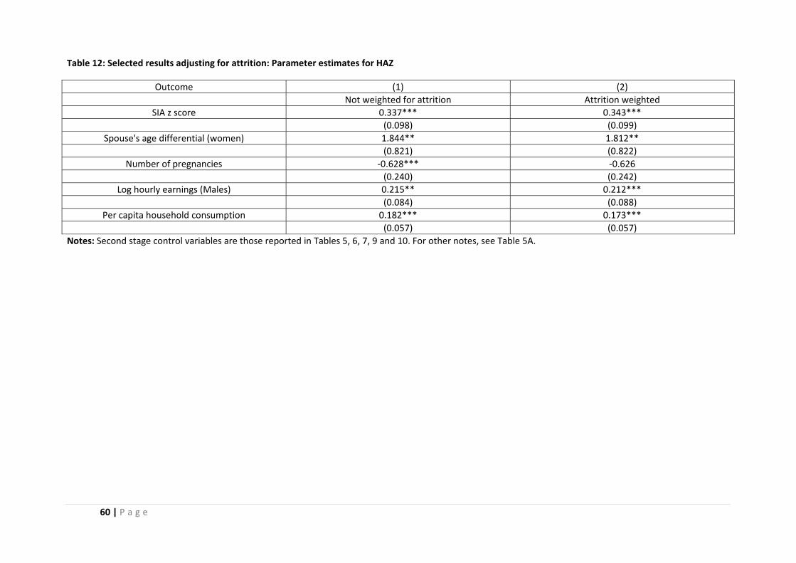
60 | P a g e   

 

Table 12: Selected results adjusting for attrition: Parameter estimates for HAZ 

Outcome  (1)  (2)   Not weighted for attrition  Attrition weighted 

SIA z score  0.337***  0.343***   (0.098)  (0.099) 

Spouse's age differential (women)  1.844**  1.812**   (0.821)  (0.822) 

Number of pregnancies  ‐0.628***  ‐0.626   (0.240)  (0.242) 

Log hourly earnings (Males)  0.215**  0.212***   (0.084)  (0.088) 

Per capita household consumption  0.182***  0.173***   (0.057)  (0.057) Notes: Second stage control variables are those reported in Tables 5, 6, 7, 9 and 10. For other notes, see Table 5A.  

 

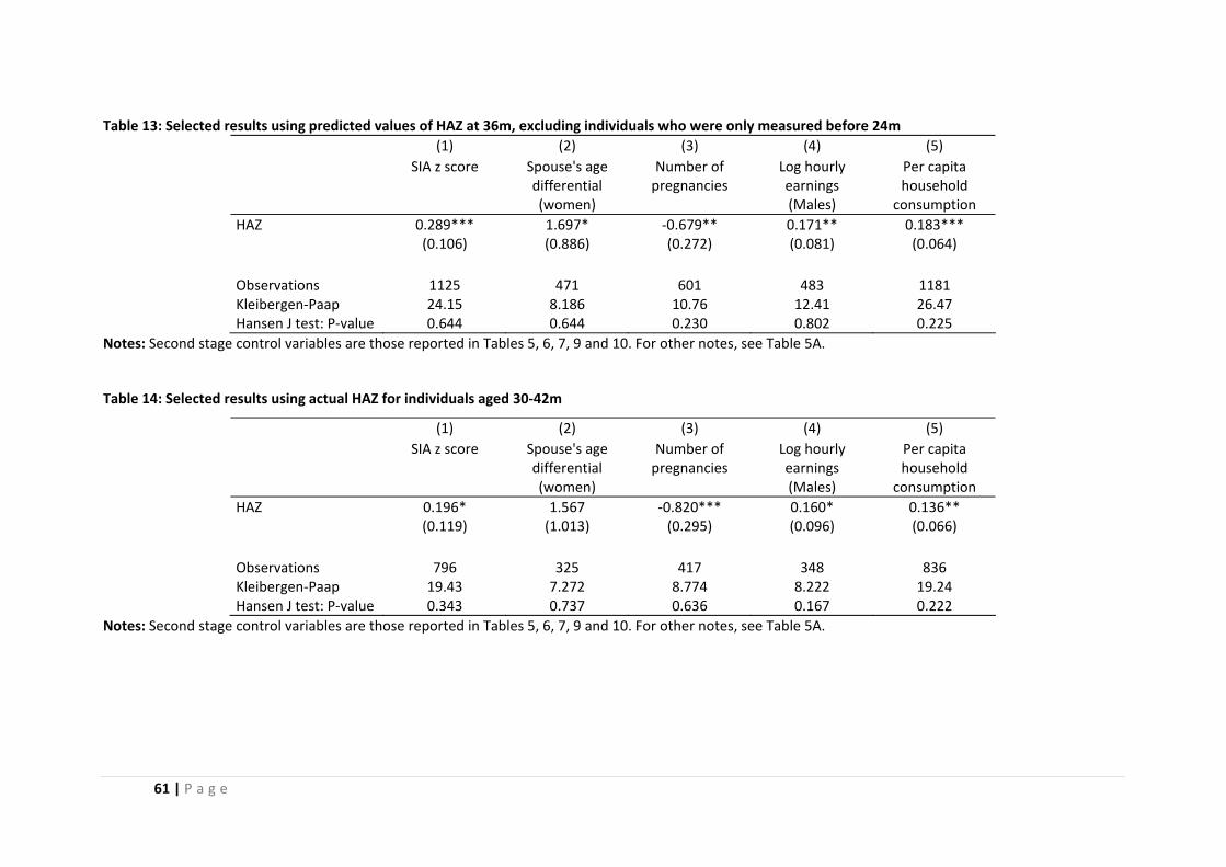
61 | P a g e   

 

 

Table 13: Selected results using predicted values of HAZ at 36m, excluding individuals who were only measured before 24m   (1)  (2)  (3)  (4)  (5)   SIA z score  Spouse's age 

differential (women) 

Number of pregnancies 

Log hourly earnings (Males) 

Per capita household 

consumption HAZ  0.289***  1.697*  ‐0.679**  0.171**  0.183***   (0.106)  (0.886)  (0.272)  (0.081)  (0.064)            Observations  1125  471  601  483  1181 Kleibergen‐Paap  24.15  8.186  10.76  12.41  26.47 Hansen J test: P‐value  0.644  0.644  0.230  0.802  0.225 

Notes: Second stage control variables are those reported in Tables 5, 6, 7, 9 and 10. For other notes, see Table 5A.  

Table 14: Selected results using actual HAZ for individuals aged 30‐42m 

  (1)  (2)  (3)  (4)  (5)   SIA z score  Spouse's age 

differential (women) 

Number of pregnancies 

Log hourly earnings (Males) 

Per capita household 

consumption HAZ  0.196*  1.567  ‐0.820***  0.160*  0.136**   (0.119)  (1.013)  (0.295)  (0.096)  (0.066)            Observations  796  325  417  348  836 Kleibergen‐Paap  19.43  7.272  8.774  8.222  19.24 Hansen J test: P‐value  0.343  0.737  0.636  0.167  0.222 

Notes: Second stage control variables are those reported in Tables 5, 6, 7, 9 and 10. For other notes, see Table 5A.  

 

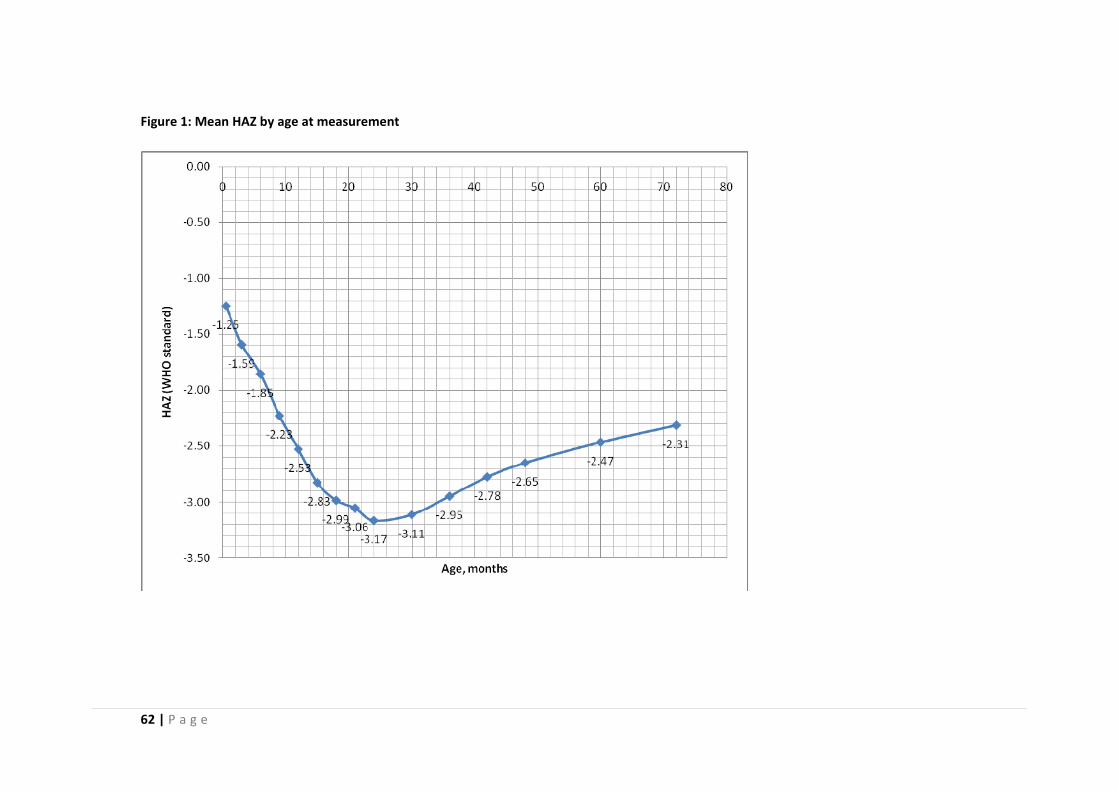
62 | P a g e   

 

 

Figure 1: Mean HAZ by age at measurement 

 

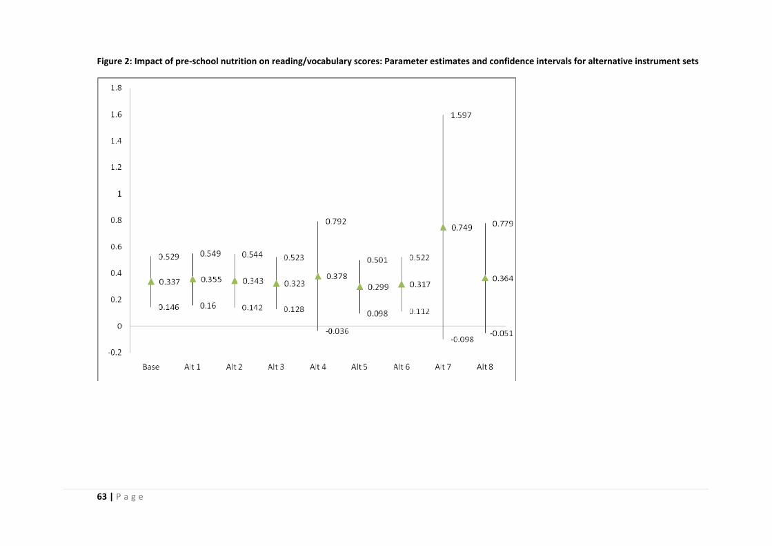
63 | P a g e   

 

Figure 2: Impact of pre‐school nutrition on reading/vocabulary scores: Parameter estimates and confidence intervals for alternative instrument sets 

 

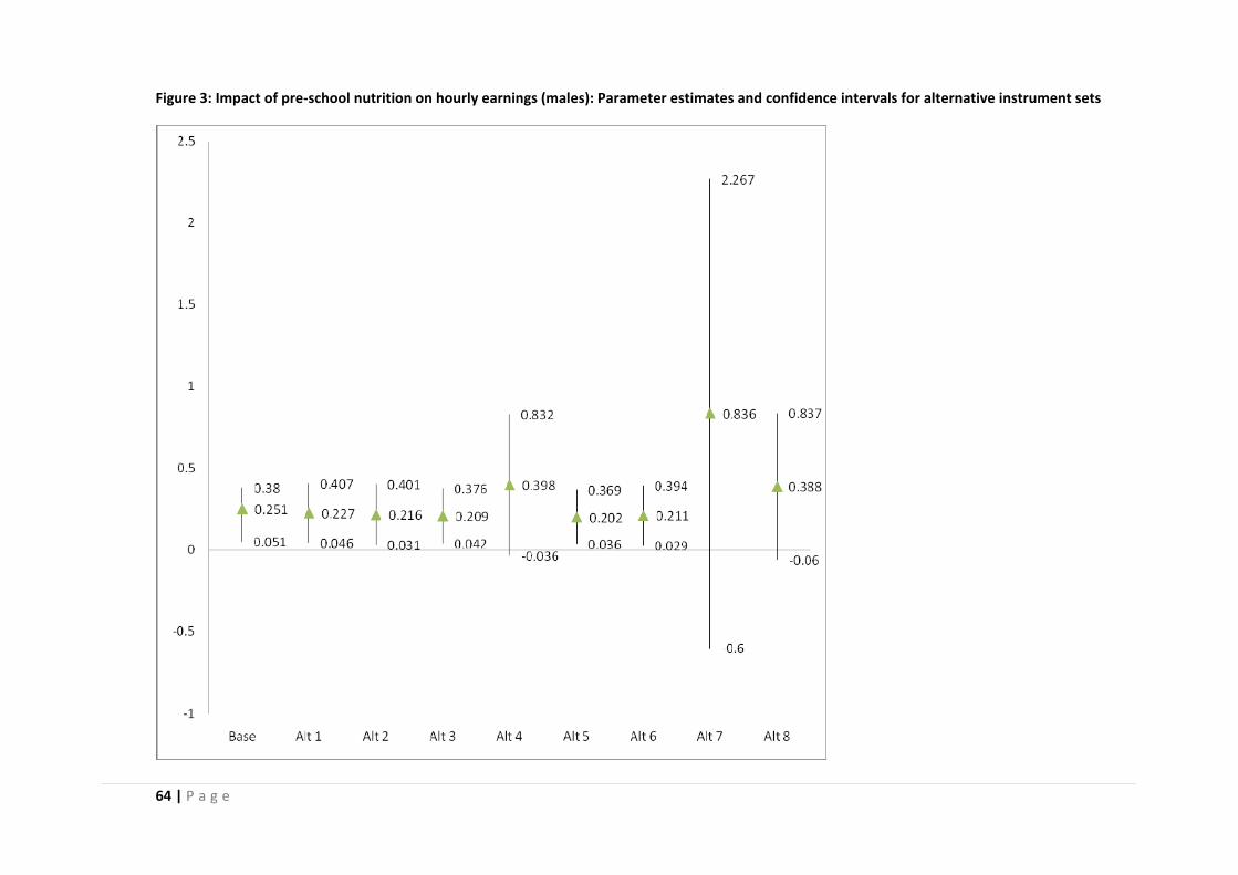
64 | P a g e   

 

Figure 3: Impact of pre‐school nutrition on hourly earnings (males): Parameter estimates and confidence intervals for alternative instrument sets 

 

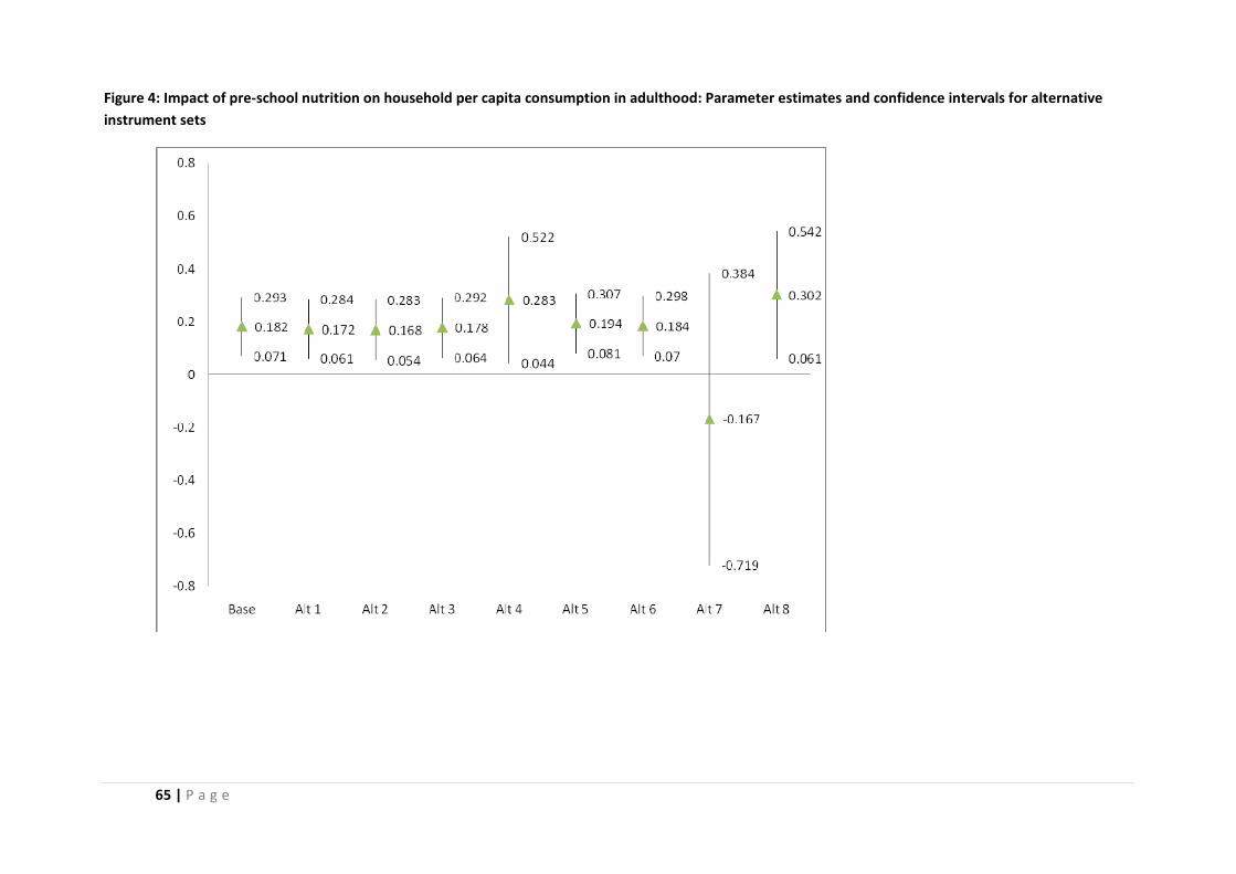
65 | P a g e   

 

Figure 4: Impact of pre‐school nutrition on household per capita consumption in adulthood: Parameter estimates and confidence intervals for alternative instrument sets