Market Dynamics and the Forward Premium Anomaly:

A Model of Interacting Agents

Phillips Hogan and Evan Myer1

Dr. Craig Burnside, Advisor

Dr. Michelle Connolly, Thesis Seminar Professor

                                                                                                               1 The authors can be reached at either evan.myer@duke.edu or phillips.hogan@duke.edu. Additionally, the authors would like to thank Prof. Craig Burnside, Prof. Michelle Connolly, Prof. Connell Fullenkamp, and Prof. David Banks for their help and advice with this project. We would also like to thank Prof. Thomas Lux of the University of Kiel for patiently answering our questions about his models over email.

Hogan  and  Myer,  i    

Abstract

This paper presents a stochastic model of exchange rates, which is used to explain the forward premium anomaly. In the model, agents switch between four trading strategies, and these changes drive the evolution of the exchange rate. This framework is meant to more realistically represent the important market dynamics of exchange rates, as we suspect these to be the cause of the forward premium anomaly. Our simulations of the model indicate two conclusions: (i) many of the statistical regularities observed in currency markets, including the forward premium anomaly, can be thought of as results derived from the actions of heterogeneous agents, and (ii) the dynamics of estimates of the beta coefficient in tests of UIP are driven by perceived relationships between changes in interest rates and agents’ aggregate views on the value of the exchange rate, which we call the fundamental value. Section I presents an introduction to the topic, and section II provides the theoretical basis of our model, then the mathematical definition of the model. Section III presents the results of a typical simulation which section IV compares to relevant stylized facts of currency markets. Sections V and VI present our results and a conclusion of what we have drawn from the model.

Hogan  and  Myer,  1    

I. Introduction

 Beginning in the early 1980s economists noticed a puzzling feature of international

currency markets: low interest rate currencies tended to depreciate relative to high interest rate

currencies. This well documented empirical regularity contradicts well-established economic

theory and has wide ranging implications not only in international finance but also throughout

macroeconomics, as exchange rate dynamics are fundamental to topics as disparate as

international trade and monetary policy. Despite the importance of the puzzle, there is still no

satisfying explanation for why it occurs.

Standard economic theory and intuition suggests that when the interest rate in a foreign

country is higher than the domestic interest rate, the foreign country’s currency should

depreciate. This is based on uncovered interest rate parity (UIP) and covered interest rate parity

(CIP). UIP is a no-arbitrage condition that states exchange rates between two currencies will

fluctuate to exactly offset interest rate differentials such that investors are indifferent between

interest incomes across currencies. Covered interest rate parity (CIP) states the price of forward

contracts will adjust to offset differences in nominal interest rates. UIP, together with CIP, are

two of the key requirements for a stable equilibrium with real interest rate parity and real

exchange rate parity.

Both conditions imply agents are indifferent between interest returns in two different

currencies because the difference in interest rates between the domestic and foreign markets is

exactly offset by changes in the exchange rate. Empirically, however, the UIP condition fails to

hold across most currencies and most times: The foreign currency tends to appreciate when the

foreign nominal interest rate exceeds the domestic interest rate. An equivalent finding is that the

forward premium – defined as the difference between the forward and spot exchange rates – is a

biased predictor of future spot exchange rates. Empirical estimates of the regression of returns in

the currency market on the magnitude of the forward premium typically yield estimates of the

slope coefficient that are less than 0 implying appreciation (depreciation) when UIP predicts

depreciation (appreciation). This finding is known as the forward premium anomaly, and is

considered one the most important puzzles in international finance.

In this paper, we will explore the relationship between trading strategies at the micro-

level and the forward premium puzzle. Specifically, we aim to show how the forward premium

Hogan  and  Myer,  2    

anomaly can arise out of agents’ decisions regarding which of four trading types to pursue in the

spot market: value trading, carry trading, optimistic noise trading, and pessimistic noise trading.

We aim to show that the interaction of agents’ choices regarding trading strategies and the

resulting positions in the market determine the exchange rate in a manner inconsistent with UIP.

This approach to the puzzle reflects a very basic insight; namely, that the exchange rate between

two currencies is a market phenomenon. It is wholly determined by the buying and selling of

speculative traders, and if traders do not trade according CIP or UIP, then the predicted

relationship should not hold.

II. Literature Review

 The forward premium anomaly has been extensively reviewed in economic literature.

The anomaly has been consistently found for most freely floating currencies, and appears robust

to changes in the numeraire currency. Froot and Thaler (1990) find that the average estimated

beta across 75 published studies is -0.88.

A number of solutions to the problem have been proposed, and most center on one of

three explanations. By far the most popular proposal is the presence of a time-variable risk

premium in currency markets. Since UIP is derived from an assumption of risk neutrality, this

seems like an intuitive and promising avenue. However, attempts to identify variable risk factors

have proven largely unsuccessful, as have attempts to effectively reproduce the observed data

patterns using models that incorporate time-variable risk premia. Engel (1996) provides a

comprehensive survey of the literature regarding risk premia and the forward anomaly.

The second, and somewhat less popular, set of explanations centers on behavioral factors.

Extensive work has been done regarding potential explanations involving peso problems,

learning, bandwagon effects, overconfidence, and irrational expectations among others. For

example, Burnside, Han, and Wang (2011) propose an explanation for the forward premium

puzzle based upon investor overconfidence. Overconfidence causes both the forward and the

spot exchange rates to overshoot their average long-run levels in the same direction. However,

the forward rate overshoots more than the spot rate, which implies that the forward premium

rises in response to a positive signal. Later, the overreaction in the spot rate is, on average,

reversed. The rise in the forward premium is a predictor of this correction, and is therefore, on

Hogan  and  Myer,  3    

average, a negative predictor of future exchange rate changes. These attempts have also proven

largely unsatisfactory. Our paper looks to build on these attempts to explain the forward

premium anomaly by directly examining the role agents’ decisions regarding trading strategies

play in producing the anomaly. Many of these behavioral effects may play a significant role in a

particular agent’s choice of strategy, but the mechanism by which those behaviors influence the

exchange rate is through the implementation of that strategy in the market. We therefore focus on

the effects of choosing a particular trading strategy on the exchange rate rather than the

motivation for choosing strategies themselves.

Most research that attempts to model the forward premium anomaly uses consumption

models based on a representative agent to predict spot and forward rates. For example, Lafuente,

Perez, and Ruiz (2009) reformulate a consumption model by allowing for the existence of

different monetary policy regimes. They simulate a model using two different consumers

differentiated by the amount of information that they extract from central bank announcements

and other news sources. They calibrate the exogenous and stochastic parameters using quarterly

data from the US and Canada for the second quarter of 1984 through 2004. Their numerical

simulations reveal that a bias can exist when the consumers are acting under incomplete

information regarding the future size of the money supply. These types of consumption models

are common in the literature, but do not provide a satisfactory answer to the anomaly. Most

often, they require unrealistic assumptions about agent’s preferences (i.e. extreme risk aversion)

in order to fully explain the anomaly. Furthermore, all of these models fail to take into account

the interaction of different traders in the market. This is an important omission considering the

interactions of traders are what drive the exchange rate. Representative agent models also seem

particularly ill-suited to explain the forward premium anomaly, given the importance of

heterogeneity in the market dynamics that also determine the exchange rate.

More recently, some authors such as Baillie and Bollerslev (2000) and Maynard and

Phillips (2001) have attempted to explain the forward premium anomaly as a largely statistical

phenomenon arising from the persistent autocorrelation of forward premiums. Again, these

attempts have achieved limited success.

Other work has attempted to model the exchange rate as a random or pseudo-random

walk. For example, Baillie and Bollerslev (2000) present a stylized model of the exchange rate as

a semi-martingale that imposes UIP and allows the daily spot exchange rate to possess very

Hogan  and  Myer,  4    

persistent volatility. This model accurately reproduces some of the observed data on the forward

premium anomaly and concludes that the spot market will converge to UIP with larger sample

sizes and longer time horizons. These models make an important contribution by allowing for

stochastic variation in the exchange rate, but remain silent on the driving force behind the

variation. Namely, they do not directly model the impact of traders’ decisions on the spot rate.

Recently, a new branch of simple stochastic models of interacting agents has been

proposed, predominately in models of the stock market. These models focus not on the direct

modeling of the determinants of agents’ market behavior such as agent preferences, but rather on

a set of rules that govern all agents’ decisions. For example, Lux and Marchesi (1999) present a

simple model of a stock market in which agents switch between optimistic or pessimistic noise

and fundamental trading strategies based on the perceived profit of each strategy in a given

period. The model accurately reproduces many of the stylized facts found in empirical studies of

the stock market from the fat tails on the distribution of returns to volatility clustering. In our

paper, we seek to build on this new style of model by adapting it to the currency markets.

III. Theoretical Framework

 

Consider three different investment strategies: buying domestic T-bills that pay interest

rate i; converting domestic currency units (DCU) into foreign currency units (FCU) at the rate St

(DCU/FCU), buy foreign T-bills that pay i*, and converting the proceeds back to DCU at time

t+1 at the exchange rate St+1; or converting DCU to FCU at the rate St, buying the foreign T-

bills, and converting the proceeds back to DCU using forward contracts priced at time t with

price Ft. The returns to the three strategies are

(1+ !)

(1)

!!!!!!

(1+ !∗)

(2)

and

!!!!(1+ !∗)

(3)

Hogan  and  Myer,  5    

where i* is the foreign interest rate, i is domestic interest rate, St+1 is the future spot price, St is

the current spot price, and Ft is the forward rate.

The first and third investment strategies both have payoffs at time t+1 that are fixed at

time t, so according to a no-arbitrage condition

1+ ! =!!!!(1+ !∗)

(4)

This equivalence is known as covered interest rate parity (CIP), and implies that the price of the

forward contract will adjust to exactly offset any differences in interest rates.

Similarly, if we assume that investors are risk-neutral with respect to nominal payoffs,

the expected excess return of the second strategy must be zero:

!! 1+ !∗!!!!!!

− 1+ ! = 0

(5)

Here, Et(·) is the expectation conditional on all relevant information at time t. Equation (5)

reduces to

1+ ! =

!! !!!!!!

(1+ !∗)

(6)

This is the typical formulation of uncovered interest rate parity (UIP), which implies that the

foreign currency is expected to appreciate by the amount the domestic interest rate exceeds the

foreign.

We can use CIP to substitute for the term (1 + i) in the equation of UIP and arrive at

!! !!!!!!

(1+ !∗) =!!!!(1+ !∗)

(7)

By simplification, we can derive the following equivalencies:

!! = !!(!!!!) (8)

Hogan  and  Myer,  6    

or

!! − !! = !! !!!! − !! (9)

Both equations imply that the forward rate is an unbiased predictor of the future spot rate.

We can test whether the forward rate is unbiased by running the regression

!!!! − !! = !! + !! !!!! − ! + !!!!,! (10)

If both CIP and UIP hold, we should be unable to reject the null hypothesis that α=0 and β=1.

Empirically, CIP holds as a virtual identity, so this regression is typically interpreted as a test of

UIP. A rejection of the null hypothesis is tantamount to a rejection of UIP. However, empirical

estimates of the regression consistently reject the null, and in some cases even find estimates of β

that are less than 0. Using the full sample of available exchange rate data, Burnside (2014) shows

that the regression in equation (10) yield both positive and negative estimates of the beta

parameter for different currencies2, meaning the forward premium is either a biased or unbiased

predictor of the future spot rate depending on the currency. Moreover, there does not seem to be

any easily identifiable relationship between the sign of the beta coefficient and any relevant

economic variable – or any easily identifiable risk premium – that can explain the sign of the

beta coefficient for a particular currency. The only observed regularity is the tendency for

systematic deviations from UIP to appear more significant in developed markets than emerging

markets. Typical explanations for why currencies deviate from UIP often rely on restrictions on

the free flow of capital or low levels of liquidity, which imply that deviations should be more

persistent in emerging markets. Burnside (2014) also showed that rolling estimates of beta from

five years’ worth of one month forwards display significant time variability, consistent with

previous findings including Baillie and Bollerslev (2000). This implies a dynamic relationship

between interest rates and exchange rates, not captured by UIP.

We believe that there is an intuitive explanation for both observed regularities. Namely,

rising interest rates signal different economic conditions in every economy, but the effects tend

to be generalized for emerging and developed markets. In emerging markets, a rise in short term

interest rates often signal the central bank’s attempt to combat inflation or influence economic

activity. Similarly, a rise in longer-term interest rates typically reflects an increase in the risk

                                                                                                               2  See  the  top  panel  of  Appendix  2.  

Hogan  and  Myer,  7    

premium investors demand to compensate for holding that nation’s debt. Regardless of the cause

of the interest rate hike, the signal of rising interest rates in an emerging market tends to indicate

economic instability, which implies a future depreciation of the currency. In contrast, an increase

in interest rates in developed markets typically indicates very little and may actually signal

strong economic activity, which could lead investors to expect an appreciation of the currency.3

Moreover, the relative importance of the interest rate signal, as well as the information it carries,

can change across time within the same currency. For example, a rising interest rate in a period

of high economic stress likely has greater relative importance as an indicator of future economic

conditions than in a period of economic stability. Because UIP cannot account for the difference

in information carried by the changing interest rate signal across economies and times, these

types of signals likely influence the activity of traders in foreign exchange markets far more than

UIP.4 Since the exchange rate is determined by the actions of traders in a market, we believe

deviations from UIP are partially driven by traders’ responses to changing interest rate signals

that do not conform to UIP.

We attempt to replicate and explain the regularities in estimates of beta by creating a

model more grounded in empirical market dynamics. In our model, a pool of traders is divided

into four groups: value traders, carry traders, optimistic noise traders, and pessimistic noise

traders. Value trading is a trading strategy that seeks to profit from expected reversions to a

fundamental exchange rate. The value strategy consists of buying (selling) the foreign currency

when the spot exchange rate is below (above) the fundamental value. Carry trading is a trading

strategy that seeks to profit from differences in nominal interest rates across currencies. That is,

an investor borrows in a low yielding currency and lends in a high yielding currency in order to

capture the interest rate differential as profit. Both optimistic and pessimistic noise traders adjust

their holdings according to measures of market sentiment and recent price changes. Instead of

focusing on fundamentals, these traders attempt to identify price trends, and also consider the

behavior of other agents as a source of information, which results in a tendency towards herding

behavior. Optimistic noise traders anticipate an increase in the exchange rate, while pessimistic

                                                                                                               3  One  notable  exception  to  this  relationship  can  be  observed  during  the  European  Sovereign  Debt  Crisis.  Rising  long  term  interest  rates  in  many  European  countries  during  this  period  reflected  rising  risk  premia  and  heightened  economic  instability.  Our  model  predicts  that  UIP  is  more  likely  to  hold  during  this  time  period.  One  interesting  avenue  for  future  research  would  be  to  empirically  investigate  that  prediction.  4  Based on a survey of market participants carried out by Cheung and Chinn (2001) we conclude that most traders do not base trading decisions on UIP or any other equilibrium condition (such as PPP) in the currency market.  

Hogan  and  Myer,  8    

noise traders anticipate a decrease in the exchange rate. Following Lux and Marchesi (1999), we

have built a stochastic, probabilistic model of when agents are more likely to switch between the

four trading strategies based on expected profit in each period. These changes in strategy drive

changes in the exchange rate.5

First, we define a set of probabilities that agents will switch between various positions in

some increment of time. For optimistic and pessimistic noise traders, the probability of switching

from an optimistic position to a pessimistic position, or vice versa, is dependent upon a measure

of market sentiment and the change in the spot exchange rate over the given time increment. As

market sentiment becomes increasingly positive (negative), traders are more likely to switch to

optimistic (pessimistic) positions. Similarly, as the change in the exchange rate over the period

becomes larger and more positive, traders are more likely to switch to optimistic positions. All

other transitions – between value and carry strategies and between noise and value or carry

positions – are determined by profit differentials. The profit of optimistic or pessimistic noise

positions is the absolute value of the percent change in the spot exchange rate over the time

interval. The profit of a carry position is the interest rate differential plus the change in the spot

exchange rate over the time interval. The profit of a value position is the magnitude of the

deviation from the fundamental exchange rate minus any cost of carry from holding the position.

The probability that an agent will switch from one position type to another increases as the

magnitude of the perceived profit differential increases.

Second, we use those transitions to determine excess demand for the foreign currency,

dependent upon the change in number of traders holding each type of position at the end of each

time interval. As defined by our model, optimistic noise traders create excess demand for the

foreign currency while pessimistic noise traders reduce excess demand for the foreign currency.

Carry traders create or reduce excess demand for the foreign currency depending on the sign of

the interest rate differential—when the foreign interest rate is greater than the domestic interest

rate, carry traders create excess demand. When the domestic interest rate is higher, carry traders

reduce excess demand. Similarly, value traders create or reduce excess demand for the foreign

currency depending on whether the fundamental value of the exchange rate is higher or lower

than the spot exchange rate. When the fundamental exchange rate is higher than the spot rate,

value traders create excess demand. When the fundamental exchange rate is lower, value traders

                                                                                                               5  The  dynamics  of  the  model  are  described  mathematically  later  in  this  section.  

Hogan  and  Myer,  9    

reduce excess demand. Therefore, the total amount of excess demand at any point in time is the

sum of the excess demand generated by all trading positions.

Finally, we define a process for determining the exchange rate given some level of excess

demand. Over a given time interval, there is the probability of the exchange rate adjusting up or

down to compensate for any given level of excess demand. That adjustment in the exchange rate

then feeds back into the model by altering profit differentials in the next period, which lead to

new expected profits and lead agents to change their positions.

Because our model is a partial equilibrium model focused on the exchange rate, we

remain agnostic on the determinants of interest rates and the fundamental value. We estimate an

autoregressive degree one (AR(1)) process for determining the foreign and domestic interest

rates given by:

!! = !!!!! + !! (11)

We then simulate the process twice: once for a complete history of the foreign interest rate and

once for a complete history of the domestic interest rate. Similarly, we estimate an AR(1)

process for the fundamental value of the exchange rate. The period-by-period innovations of all

three processes are meant to account for macroeconomic variables and news events that

influence interest rates and the fundamental value of the exchange rate but are not endogenous to

our model.

We interpret the fundamental value of the exchange rate as the conditional expectation at

time t of the exchange rate at time t+1. The expectation is conditioned on all information

available at time t including any changes in the domestic and foreign interest rates. More

generally, the fundamental value in our model can be understood as the aggregate expectation

across the differing views of fundamental traders in the market. Therefore changes in the

fundamental value are responses to changes in the information set, including changes in the

domestic and foreign interest rates. As the information carried by the interest rate signal changes

across economies or time, the change in the conditional expectation as a response to a change in

the domestic or foreign interest rate will vary. Given that both the foreign and domestic interest

rates and the fundamental value are defined by three independent AR(1) processes, our model

does not define how the fundamental value updates according to changes in the interest rates.

Even though it may well be impossible to capture the actual impact of the interest rate signal on

Hogan  and  Myer,  10    

the conditional expectation, we can attempt to replicate the observed empirical regularities of the

beta coefficient – e.g. the difference between emerging and developed markets – by imposing a

functional relationship between the fundamental value and interest rates that intuitively

reproduces how investors perceive changes in interest rates.

Mathematically, the model is defined as follows:

(i) Variables and Initial Conditions

 

We denote:

N = Total number of traders

Nc = Number of carry traders

Nv = Number of value traders

No = Number of optimistic noise traders

Np = Number of pessimistic noise traders

St = The spot value of the exchange rate

Sf = The fundamental value of the exchange rate

(ii) Profits from the four trading strategies

 

Profit from the carry strategy is the interest rate differential plus any capital appreciation

from the change in spot price:

!! = !! − !! +!!!! − !!

!!

(12)

Profit from the value strategy is the magnitude of the reversion to the fundamental value

discounted at an appropriate rate d (due to the longer time horizon associated with reversions

fundamental value) minus the cost of carry from interest rate differentials:

!! = !!! − !!!!

− !! − !!

(13)

Profits from optimistic and pessimistic noise strategies are simply the rate of capital appreciation

or depreciation measured as the percent deviation from the starting price (pt):

Hogan  and  Myer,  11    

!! =!!!! − !!

!!

(14)

and

!! = −!!!! − !!

!!

(15)

(iii) Switches between optimistic and pessimistic noise strategies

 

The probabilities of switching between an optimistic and pessimistic noise strategy and

vice versa in a time increment Δt are given by Δt·ψo,p and Δt·ψp,o, where:

!!,! = !!!!! !!!!

(16)

!!,! = !!

!!! !!!

(17)

and

!! = !!! + !!!!!! − !!

!!

(18)

Where Vn is the average interval between changes in noise trading strategies, U1 is a forcing term

for transitions between noise trading strategies, and the major influences are the price trend and

market sentiment (X) as measured by the numbers of optimistic and pessimistic chartists:

! =

!! − !!!!

(19)

αs is a parameter for an agent’s sensitivity to market sentiment and αp is a parameter for an

agent’s sensitivity to price changes.

Hogan  and  Myer,  12    

(iv) Switches between value and carry strategies

 

The probabilities of switching between value and carry strategies and vice versa in a time

increment Δt are given by Δt·ψc,v and Δt·ψv,c, where:

!!,! = !!!!! !!!

(20)

!!,! = !!!!! !!!!

(21)

and

!! = !! !! − !! (22)

Vs is the average interval between changes between value and carry strategies, U2 is a forcing

term for transitions between value and carry strategies, and αr is a parameter for an agent’s

sensitivity to profit differentials.

(v) Switches from noise to value or carry strategies

 

The probabilities of switching from noise to value or carry strategies in a time increment

Δt are given by Δt·ψo,c, Δt·ψo,v, Δt·ψp,c, and Δt·ψp,v where:

!!,! = !!!!! !!!,!

(23)

!!,! = !!

!!! !!!,!

(24)

!!,! = !!!!! !!!,!

(25)

and

!!,! = !!

!!! !!!,!

(26)

Hogan  and  Myer,  13    

The U terms are all forcing terms for transitions between noise and value or carry

strategies given by:

!!,! = !! !! − !! (27)

!!,! = !! !! − !! (28)

!!,! = !! !! − !! (29)

and

!!,! = !! !! − !! (30)

(vi) Switches from value or carry to noise strategies

 

The probabilities of switching from value or carry to noise strategies in a time increment

Δt are given by Δt·ψc,o, Δt·ψc,p, Δt·ψv,o, and Δt·ψv,p where:

!!,! = !!!!! !!!!,!

(31)

!!,! = !!!!! !!!!,!

(32)

!!,! = !!!!! !!!!,!

(33)

 

and

!!,! = !!!!! !!!!,!

(34)

Hogan  and  Myer,  14    

(vii) Excess Demand Specification

 

The total amount of excess demand (EDt) in the market at the end of each period is the

sum of excess demand from optimistic traders (EDo), excess demand from pessimistic traders

(EDp), excess demand from carry traders (EDc), and excess demand from value traders (EDv),

measured according to the number of traders switching strategy in each period and can be

expressed as:

!"! = !!,!!! − !!,! !! − !! (35)

!"! = !!,!!! − !!,!

!! − !!!!

(36)

!"! = (!!,!!! − !!,!)! (37)

and

!"! = (!!,!!! − !!,!)! (38)

Where η is the average trading volume of each agent while the level of excess demand in the two

strategy groups is based on the magnitude of the expected profit.

(viii) Price Determination

 

Price changes are modelled as endogenous responses by the market to imbalances

between demand and supply. We translate excess demand in the market into price changes

according to the equations:

! = ! !"! (39)

and

!!!! = !! ± ! > ! , !~! 0,1 (40)

Hogan  and  Myer,  15    

where ρ represents the probability of a change in the spot rate and β is a measurement of the

magnitude of the market reaction to one unit amount of excess demand in the market.

IV. Typical Simulation6

 

We begin a typical simulation by simulating the AR(1) processes for the interest rates and

the fundamental value. Next, we randomly assign traders to each of the four trading strategies as

draws from a normal distribution over an interval from 250 to 500. Finally, we define the starting

value of the exchange rate. Once the initial conditions of our model are defined, we begin

calculating profit differentials according to the equations outlined above. Those profit

differentials are then used to compute the probability that a given trader will switch from his

initial strategy to each of the three alternatives. We translate those probabilities into actual

changes in trading strategy according to a Bernoulli random draw where the number trials is the

number of traders in the strategy and the probability of success is the probability of switching

from the current strategy to an alternative. The change of the number of traders in each group

creates excess demand according to the equations above. The level of excess demand in the

market then translates to a probability that the exchange rate adjusts up or down by a given

amount. We specify two amounts by which the exchange rate can change. The smaller of the two

amounts is used in ordinary periods; the larger of the two amounts is used in periods where there

is a particularly high level of excess demand caused by high levels of switching. In the latter

case, the excess demand is always greater than one, so the probability of a change in the

exchange rate is one. Whether the exchange rate actually adjusts is determined by comparing the

probability of a change to a random number between zero and one. If the probability is greater

than the random number, the exchange rate adjusts by the specified tick size; otherwise the

exchange rate remains constant. Once the change in the exchange rate has been determined, we

calculate new profit differentials according to the updated exchange rate and the process repeats

itself.

In simulations of our model, we divide each trading day into 500 equal periods of time.

The interest rates and fundamental value update daily, and so remain constant across the 500

periods within each day. In contrast, we allow traders to switch positions during each of the 500                                                                                                                6  The  Matlab  code  for  this  simulation  is  attached  in  Appendix  3.  

Hogan  and  Myer,  16    

intraday periods, so the exchange rate can change during each smaller interval of time. We

believe this allows us to more accurately reproduce the dynamics of actual markets in which

traders can adjust their positioning intraday. The introduction of the intraday periods also allows

more flexibility in the model by allowing for a greater range of price movements in any given

day.

The interest rates and the fundamental value are updated at the beginning of each day, so

the first periods of the day typically are the most volatile. During these periods, the exchange rate

typically adjusts up or down by the larger tick size to reflect the higher excess demand caused by

traders updating their positions according to the new information. The probability that a given

trader changes his strategy in any later intraday period is relatively small because only previous

price changes influence his decisions. In any given period the number of traders changing

positions is very small and the exchange rate typically adjust by the smaller tick size. This

dynamic allows us to capture the diurnality typical of high frequency financial data. Nonetheless,

over the course of the day these small changes in each period can lead to large changes in the

exchange rate. This helps maintain stability in the model by preventing the exchange rate from

moving faster than traders can adjust.

Figure 1 shows the sample path of exchange rates and returns from a typical simulation

(the exchange rate has been artificially shifted up by one unit to better see the relationship):7  

Figure 1

                                                                                                               7  Appendix  1  shows  further  plots  of  inputs  into  the  model  and  the  resulting  outputs.    

Hogan  and  Myer,  17    

As is obvious from Figure 1, the exchange rate very closely tracks the evolution of the

fundamental value. This is derived from the constraints placed on our model. The domestic and

foreign interest rates in our model are annualized daily rates. While the difference in annualized

rates may be relatively large, the interest rate differential within any given intraday period is

typically very small. Similarly, changes in the exchange rate within each intraday period are

limited to a defined tick size, which limits the profit available to optimistic and pessimistic noise

traders. The exchange rate must adjust in same direction several times sequentially before the

profit of these strategies becomes large. In contrast, the profit from value trading is the percent

deviation of the actual exchange rate from the fundamental value. Even very small deviations

from the fundamental value produce a profit differential that is significantly larger than the other

strategies. Therefore, while carry trading and optimistic or pessimistic noise trading can produce

short-term fluctuations around the fundament value, eventually the deviations cause traders to

switch back to value positions and the exchange rate to revert back to the fundamental value.

The parameters of our model were chosen in order to reproduce the moments of the

distributions of returns typical of currency markets. Figure 2 compares the sample statistics

generated by our model to those of the Euro.8

Figure 2

Sample Statistics

Mean Median Max Min Kurtosis Skewness

Model Output 0.0000 0.0000 0.0800 -0.0621 5.1174 -0.1894

EUR/USD9 0.0071 0.0000 0.0460 -0.0350 5.5115 0.1714

Similarly, the autoregressive parameters for the AR(1) processes were set at 0.9985 to simulate a

near random walk in interest rates and the fundamental value. Given that the exchange rate

closely tracks the fundamental value, the high autoregressive parameter in the fundamental value

also imposes approximate martingale behavior in the exchange rate, consistent with empirical

findings.

                                                                                                               8  Our  model  is  not  designed  to  replicate  the  EUR/USD  exchange  rate  per  se.  Rather,  this  comparison  was  chosen  due  to  the  large  amount  of  information  available  on  that  particular  exchange  rate.    9  Insert  Source  

Hogan  and  Myer,  18    

V. Stylized Facts

 

Exchange rate returns are characterized by a number of statistical properties that prevail

with surprising uniformity across currencies and are typically known as stylized facts of currency

markets. First, the distribution of returns is non-normal, displaying excess kurtosis. For the

sample above, the kurtosis of the distribution of daily returns is 5.12. Such excess kurtosis is

consistent across trials. A Jarque-Bera test for the same returns rejects the null hypothesis of

normality at the 95% level. The t-statistic for the test is 848.08 and the p-value is 0.00.10 Again,

this rejection of the null is consistent across repeated trials.

Our model also displays similar predictability in returns and volatility as empirical

exchange rates. Andersen et al (2000) showed that there is no autocorrelation in raw returns, but

squared returns and absolute returns showed some autocorrelation up to approximately the first

20 lags. Figure 3 reports the results of Ljung-Box tests on raw, squared, and absolute returns

from the sample simulation for various lag lengths. At each lag length, we reject the null of no

autocorrelation for the squared and absolute returns, consistent with empirical findings. The

serial correlation in squared returns is a good indicator of volatility clustering or ARCH effects

in our returns. In our model, periods of high volatility tend to be driven by a high proportion of

optimistic and pessimistic noise traders in the market, consistent with the results of Lux and

Marchesi (1999).

As opposed to empirical findings, we similarly reject the null of no autocorrelation for

raw returns. However, the autocorrelation in raw returns is driven almost entirely by highly

significant autocorrelation in the first and second lag, which differs from empirical findings.11

Some amount of the observed autocorrelation in raw returns is also likely the result of using

Bartlett’s standard errors for the Ljung-Box test, which assume normally distributed residuals, as

opposed to Newey-West or White’s standard errors which are robust to heteroskedasticity in the

residuals.

                                                                                                               10  This  compares  to  a  t-­‐stat  of  740.8  for  the  EUR/USD  exchange  rate.  11Appendix  1  also  shows  a  graph  of  the  sample  ACF  for  raw,  squared,  and  absolute  returns  and  the  95%  confidence  intervals  for  the  same  series.    

Hogan  and  Myer,  19    

Figure 3

Ljung-Box Test

Lags

5 10 15 20 25

Raw t-stat 69.0635 75.5069 76.0972 78.8669 85.5336

p-value 0.00 0.00 0.00 0.00 0.00

Squared

t-stat 308.918 414.381 475.57 579.416 685.051

p-value 0.00 0.00 0.00 0.00 0.00

Absolute

t-stat 244.586 406.512 535.138 722.389 878.782

p-value 0.00 0.00 0.00 0.00 0.00

In regressions like equation (10), the R-squared values are typically very small – on the

order of (10-3) – meaning the regressions explain very little of the observed variance of returns in

currency markets. Burnside et al (2011) found that the ratio of the variance of monthly returns to

the monthly forward premium is on the order of 100:1, explaining the limited predictive power

of forward premiums. As can be seen in Figure 4, multiple simulations of our model replicate all

of these findings.12

Finally, in our model both carry and momentum trading strategies are profitable,

consistent with empirical findings from Burnside (2013). The average, annualized monthly

returns for carry and momentum trading taken from the sample simulation above are 7.45% and

2.7% respectively.

VI. Results

 

After simulating our model, we ran the regression in equation (10) on our simulated data,

and found that our model yields both positive and negative estimates of beta across different

trials. The left panel of Figure 4 reports the results of these regressions. Our model also

                                                                                                               12  The  scatter  plots  shows  in  Appendix  2  are  good  visualizations  of  these  stylized  facts.  

Hogan  and  Myer,  20    

reproduces the same time-variability in rolling estimates of beta calculated from five-years’

worth of one month forwards as is seen empirically.13

As explained in Section IV, the primary force driving price change in our model is the

fundamental value. The majority of the magnitude and sign of the change in the exchange rate

period by period consequently can be explained by changes in the fundamental value. Therefore,

estimates of the beta parameter in equation (10) ought to be highly dependent on the relationship

between the evolution of the fundamental value and interest rates. The right panel of Figure 4

reports the results of a second regression of the forward premium on returns calculated using the

fundamental value instead of the exchange rate.

This second regression is designed to capture the impact of changing interest rate

differentials on the evolution of the fundamental value. That is, this second regression is

designed to capture how changes in the information set due to changes in the interest rate affect

the conditional expectation of the exchange rate at time t+1. In every case, the sign of the beta

coefficient is the same across both regressions. This implies that the beta coefficient in the

regression test for UIP is really a proxy for the relationship between the fundamental value and

interest rate differentials. In these first simulations of our model, we did not impose a functional

relationship between interest rates and the evolution of the fundamental value. The two interest

rates and the fundamental value were defined by entirely independent AR(1) processes, so the

regressions reported in the left panel of Figure 4 capture purely spurious correlations between the

two.

Figure 4

Estimated Regression Coefficients

Trial Equation (10) Fundamental Value Returns

α β R-Squared α β R-Squared

1 0.0060 1.5961 0.0083 0.0060 1.5961 0.007

(0.0057) (1.2449)

(0.0057) (1.2449)

2 0.0000 2.1244 0.0203 0.0003 1.4852 0.0093

(0.0042) (1.0507)

(0.0044) (1.0932)

                                                                                                               13  See  Appendix  2  for  comparisons.    

Hogan  and  Myer,  21    

3 0.0016 -0.7625 0.0024 0.0019 -1.4246 0.0077

(0.0039) (1.1128)

(0.0040) (1.1546)

4 0.0019 -0.1911 0.0002 0.0014 -0.8379 0.0044

(0.0050) (0.8816) (0.0051) (0.8958)

In contrast, we can impose very simple functional relationships between the evolution of

the fundamental value and interest rates in order to test whether the interest rate signals outlined

in Section III can account for the empirical dynamics of estimates of beta. This is not meant to

represent any theoretical relationship between interest rates and exchange rates. Rather, it is

simply mean to impose the type of relationship outlined in Section III. First, we compute a three

month moving average of daily interest rates and the standard deviation of daily interest rates

over that period. We then compute the number of standard deviations away from that moving

average of the current domestic and foreign interest rate. The difference of those two measures

for the two interest rates then captures the relative movements of the foreign and domestic

interest rates away from their historical trends.14 If the measure is positive (negative) it implies

the domestic (foreign) interest rate is increasing more rapidly than what would be expected.

Using that measure, we can reproduce the interest rate signals discussed in Section III.

For example, assume that the foreign economy is an emerging market and the foreign

interest rate is higher than the domestic. The forward premium calculated under CIP will predict

an appreciation (depreciation) of the domestic (foreign) currency in each period. If the foreign

interest rate begins to increase rapidly relative to the domestic, investors should infer that the

foreign economy is in a period of relatively high stress and expect depreciation of the foreign

currency in the future. That expectation is reflected in a change in the fundamental value,

understood as the conditional expectation of the exchange rate at time t+1. Specifically the

fundamental value should rise. By subtracting our relative momentum measure, we can tie the

returns each day to the increase or decrease in the predicted appreciation (depreciation) of the

domestic (foreign) currency based on what the interest rates would predict. The value we are

subtracting – the relative deviation of the foreign interest rate – is negative, so the net effect on

the fundamental value is positive. As the fundamental value rises, the exchange rate also adjusts

                                                                                                               14  We  use  a  relative  measure  of  momentum  in  order  to  avoid  situations  where  global  interest  rates  are  rising  in  tandem,  which  could  be  a  different  signal  of  future  economic  conditions.  

Hogan  and  Myer,  22    

higher causing depreciation of the foreign currency as predicted by our signal. In this case, a

regression test of UIP should fail to reject the null because the relationship between interest rates

and exchange rates defined by UIP is the same as the relationship implied by the economic

signal. We can impose this type of signal by subtracting the scaled relative momentum measure

from our fundamental value.

If we add instead of subtract the relative difference in deviations to the fundamental

value, then we impose a negative correlation between the fundamental value and the interest rate

differential leading to a negative beta estimate. This is consistent with the interest rate signal in

developed markets, in which rising interest rates are signs of relative economic stability and

often attract capital inflows. Figure 5 shows the beta estimates for several simulations under each

imposed correlation.

Figure 5

Regression Coefficients with Imposed Correlations

Trial Subtracting Deviations Adding Deviations

α β R-Squared α β R-Squared

1 0.0525 2.3397 0.017 -0.0443 -1.9151 0.0228

(0.0276) (1.2692)

(0.0209) (0.8930)

2 0.0839 3.9806 0.0287 -0.1128 -6.1224 0.0787

(0.0345) (1.6487)

(0.0283) (1.4921)

3 0.0233 1.0003 0.0134 -0.0952 -4.8 0.0491

(0.0144) (0.6109)

(0.0309) (1.5054)

4 0.0209 1.1198 0.0061 -0.0733 -3.8737 0.0245

(0.0180) (1.0158)

(0.0345) (1.7399)

5 0.0839 3.9806 0.0287 -0.0555 -2.395 0.0263

(0.0345) (1.6487) (0.0248) (1.0375)

In the regressions reported in Figure 5, we divided the relative momentum measure by 15

prior to adding or subtracting it from the fundamental value. The maximum change in the

fundamental value due to the functional relationship with interest rates was approximately nine

cents. Nonetheless, we can still easily predict the sign of the beta coefficient based on the type of

Hogan  and  Myer,  23    

relationship we impose. Reducing the strength of that relationship by four does not change the

result, implying that even a very weak relationship between interest rates and the fundamental

value can determine whether or not UIP holds.

VII. Conclusion

 

Our model can successfully replicate the forward premium anomaly, solely by specifying

the interactions of agents. These specifications also allow us to replicate many of the stylized

facts found in currency markets including excess kurtosis, non-normality of returns, and positive

average profits for carry and momentum trading. This suggests that many of the statistical

regularities observed in currency markets can be thought of as being derived from the

interactions of heterogeneous agents in the market. The ability to account for both the dynamics

of the forward premium anomaly and other stylized facts is one of the major strengths of our

model.

Empirical evidence shows that there are both positive and negative values of the estimate

of the beta coefficient in a regression of change in spot price on the forward premium, and

failures to reject UIP are more common in emerging markets than developed. Our model

proposes an intuitive explanation for this relationship: The driving force behind the change in

spot prices is what we call the fundamental value of the exchange rate. Because the change in the

fundamental value drives the change in the spot price, the regression of change in spot price on

the forward premium is really a proxy for the relationship between the changes in the

fundamental value relative to the interest rate differential. Therefore, the time variability of

rolling beta estimates and the difference in sign found across multiple regressions can be thought

of as reflecting the changing nature of the relationship between the fundamental value and the

evolution of interest rate differentials. Our model accounts for this by allowing the same signal,

like a change in the foreign interest rate, to have a differing impact on the exchange rate

depending on the context. For any given pair of currencies, that relationship may or may not

conform to the relationship predicted by UIP. As reported in Figure 5, if we impose the

relationships outlined in Section III on the fundamental value and interest rate differentials, we

calculate beta estimates consistent with empirical findings, lending credence to our initial

Hogan  and  Myer,  24    

hypothesis that the failure of UIP to hold in certain currency pairs is related to how traders

interpret the signal of increasing interest rates.

Given the relationship between carry trading and interest rates, intuitively one might

expect carry trading to drive rejections of UIP. In order to capture the carry across two currencies

a trader has to purchase the higher yielding currency, which should cause it to appreciate.

Nonetheless, our model actually suggests that rejections of UIP are driven primarily by value

trading. Within our model, carry traders play a much more limited role. They exploit existing

conditions in the market – namely low volatility and high interest rate differentials – rather than

directly contributing to the market dynamics that drive price changes. Given that carry trading is

a relatively static buy and hold strategy designed to capture interest differentials rather than

actual price changes, this may be somewhat unsurprising within the context of our model.

However, changing the time horizons used to calculate profit differentials, the preferences of

agents, or the values of parameters governing switching behavior could lead to a more prominent

role for carry traders.

One limitation of our model is our inability to produce a general equilibrium. However,

for the purposes of our paper, that is somewhat ancillary. We are attempting to model the

forward premium anomaly based on traders’ decisions. Since those decisions are not based on a

general equilibrium, we expect these decisions to be independent of the macroeconomic forces

shaping general equilibria. In theory, the rules governing agents’ decisions and the interrelations

of model inputs could be further specified to arrive at and account for a general equilibrium, but

for the purposes of this paper the simpler model is sufficient and we believe increases the

reliability of our conclusions. There is likely some force that relates the exchange rate to the

prices of goods across different economies, but that force lies outside the explanation of why the

forward premium anomaly exists.

Hogan  and  Myer,  25    

VI. Works Cited

Andersen, Torben G., et al. Exchange rate returns standardized by realized volatility are

(nearly) Gaussian. No. w7488. National bureau of economic research, 2000.

Baillie, Richard T., and Tim Bollerslev. "The forward premium anomaly is not as bad as

you think." Journal of International Money and Finance 19.4 (2000): 471-488.

Burnside, Craig. “Estimation and Inference in Linear Factor Models.” Lecture: Duke

University Course, September 2013.

Burnside, Craig. “Uncovered Interest Parity.” Lecture: Northwestern Course, February

2014.

Burnside, Craig, et al. "Investor overconfidence and the forward premium puzzle." The

Review of Economic Studies 78.2 (2011): 523-558.

Cheung, Yin-Wong, and Menzie David Chinn. "Currency traders and exchange rate

dynamics: a survey of the US market." Journal of International Money and Finance 20.4 (2001):

439-471.

Engel, Charles. "The forward discount anomaly and the risk premium: A survey of recent

evidence." Journal of empirical finance 3.2 (1996): 123-192.

Froot, Kenneth A., and Richard H. Thaler. "Anomalies: foreign exchange." The Journal

of Economic Perspectives 4.3 (1990): 179-192.

Hens IV, Thorsten, and Klaus Reiner Schenk-Hoppé, eds. Handbook of Financial

Markets: Dynamics and Evolution: Dynamics and Evolution. Access Online via Elsevier, 2009.

Lafuente, Juan A., Rafaela Perez, and Jesús Ruiz. "Monetary policy uncertainty and the

forward bias for foreign exchange (preliminary version)." (2009).

Lux, Thomas, and Michele Marchesi. "Scaling and criticality in a stochastic multi-agent

model of a financial market." Nature 397.6719 (1999): 498-500.

Maynard, Alex, and Peter CB Phillips. "Rethinking an old empirical puzzle: Econometric

evidence on the forward discount anomaly." Journal of applied econometrics 16.6 (2001): 671-

708.

Stanley, MICHAEL HR, et al. "Can statistical physics contribute to the science of

economics?." Fractals-an Interdisciplinary Journal on the Complex Geometry 4.2 (1996): 415-

426.

Hogan  and  Myer,  26    

Appendix 1 – Input/Output of a Typical Simulation  

Hogan  and  Myer,  27    

Hogan  and  Myer,  28    

Hogan  and  Myer,  29    

Appendix 2 – Comparison to Empirical Beta Regularities  

Output from Our Model

Beta

Time

Hogan  and  Myer,  30    

Output from Our Model

Appreciation

Forward Premium

Hogan  and  Myer,  31    

Appendix 3 – Matlab Code

Model  %Set number of days for the simulation. T = 4400; %Preallocate daily variables. I = arima('Constant',0.0015,'AR',0.9985,'Variance',0.0003); I2 = arima('Constant',0.0045,'AR',0.9985,'Variance',0.0003); SF = arima('Constant',0.0015,'AR',0.9985,'Variance',0.0001); ISimD = simulate(I,T); ISimF = simulate(I2,T); IDiff = (ISimD-ISimF)*0.01; MAI = tsmovavg(ISimD,'s',60,1); MAI2 = tsmovavg(ISimF,'s',60,1); StdMAI = std(MAI(61:end)); StdMAI2 = std(MAI2(61:end)); XI = ISimD(61:end)-MAI(61:end); XI2 = ISimF(61:end)-MAI2(61:end); Zeros = zeros(1,60); Ones = ones(1,60); YI = padarray(XI/StdMAI,[60 0],1,'pre'); YI2 = padarray(XI2/StdMAI2,[60 0],1,'pre'); SFSim2 = simulate(SF,T); SFSim = SFSim2(1:end)+((YI-YI2)./15); Price = zeros(T,1); NCHist = zeros(T,1); NVHist = zeros(T,1); NPlusHist = zeros(T,1); NMinusHist = zeros(T,1); PiVHist = zeros(T,1); PiCHist = zeros(T,1); PiPlusHist = zeros(T,1); PiMinusHist = zeros(T,1); PHist = zeros(T,1); XHist = zeros(T,1); %Set number of microsteps within each day. N = 500; %Preallocate microstep variables. NV=zeros(N,1); NC=zeros(N,1); NMinus=zeros(N,1); NPlus=zeros(N,1); EDC=zeros(N,1); EDV=zeros(N,1); EDMinus=zeros(N,1); EDPlus=zeros(N,1); EDTot=zeros(N,1);

Hogan  and  Myer,  32    

P=zeros(N,1); ST=zeros(N,1); X=zeros(N,1); Y=zeros(N,1); PiC=zeros(N,1); PiV=zeros(N,1); PiMinus=zeros(N,1); PiPlus=zeros(N,1); U1=zeros(N,1); U2=zeros(N,1); U31=zeros(N,1); U32=zeros(N,1); U41=zeros(N,1); U42=zeros(N,1); Psi1=zeros(N,1); Psi2=zeros(N,1); Psi3=zeros(N,1); Psi4=zeros(N,1); Psi5=zeros(N,1); Psi6=zeros(N,1); Psi7=zeros(N,1); Psi8=zeros(N,1); Psi9=zeros(N,1); Psi10=zeros(N,1); Psi11=zeros(N,1); Psi12=zeros(N,1); AA=zeros(N,1); BB=zeros(N,1); CC=zeros(N,1); DD=zeros(N,1); EE=zeros(N,1); FF=zeros(N,1); GG=zeros(N,1); HH=zeros(N,1); II=zeros(N,1); JJ=zeros(N,1); KK=zeros(N,1); LL=zeros(N,1); %Specify initial numbers of traders, drawn from a Gaussian distribution. NV(1)=250; NC(1)=250; NPlus(1)=250; NMinus(1)=250; %NV(1)=randi([250 500],1,1); %NC(1)=randi([250 500],1,1); %NMinus(1)=randi([250 500],1,1); %NPlus(1)=randi([250 500],1,1); NTot=(NC(1)+NV(1)+NMinus(1)+NPlus(1)); NCHist(1) = NC(1); NVHist(1) = NV(1); NPlusHist(1) = NPlus(1); NMinusHist(1) = NMinus(1); XHist(1) = ((NPlus(1)-NMinus(1))/(NPlus(1)+NMinus(1)));

Hogan  and  Myer,  33    

%Specify parameter values. a=2; b=0.5; c=10; d=5/NTot; e=2; f=0.5; g=3; h=1; DR = 0.8; %Specify the initial value of the exchange rate. Price(1) = 1; %Begin the daily loop. for t = 2:T %Begin the microstep loop. for n = 1:N-1 %Set opening price for each microstep loop equal to the previous %loop's closing price. ST(1) = Price(t-1); %Set initial values of all variables equal to the value at the end of %the previous loop. NC(1) = NCHist(t-1); NV(1) = NVHist(t-1); NPlus(1) = NPlusHist(t-1); NMinus(1) = NMinusHist(t-1); X(1) = XHist(t-1); %Calculate the value of every variable at each microstep. Y(n) = ((ST(n)-Price(t-1))./Price(t-1)); if IDiff(t)>0 PiC(n) = ((abs((IDiff(t))))/a)*100; else PiC(n) = ((abs((IDiff(t))))/a)*100; end if SFSim(t)>ST(n) PiV(n) = (abs(((DR*(SFSim(t)-ST(n)))./ST(n))/a)+(IDiff(t)/a))*100; else PiV(n) = (abs(((DR*(SFSim(t)-ST(n)))./ST(n))/a)-(IDiff(t)/a))*100; end PiMinus(n) = -((Y(n))./e)*100; PiPlus(n) = ((Y(n))./e)*100; U1(n) = (f*X(n))+(b*(Y(n)/e)); U2(n) = (b*(PiC(n)-PiV(n))); U31(n) = (b*(PiC(n)-PiPlus(n))); U32(n) = (b*(PiC(n)-PiMinus(n))); U41(n) = (b*(PiV(n)-PiPlus(n))); U42(n) = (b*(PiV(n)-PiMinus(n)));

Hogan  and  Myer,  34    

Psi1(n) = (e.*(NMinus(n)/NTot).*exp(-U1(n)))/N; Psi2(n) = (e.*(NPlus(n)/NTot).*exp(U1(n)))/N; Psi3(n) = (a.*(NV(n)/NTot).*exp(U2(n)))/N; Psi4(n) = (a*(NC(n)/NTot).*exp(-U2(n)))/N; Psi5(n) = (e.*(NPlus(n)/NTot).*exp(U31(n)))/N; Psi6(n) = (e.*(NMinus(n)/NTot).*exp(U32(n)))/N; Psi7(n) = (e.*(NPlus(n)/NTot)*exp(U41(n)))/N; Psi8(n) = (e.*(NMinus(n)/NTot)*exp(U42(n)))/N; Psi9(n) = (a.*(NC(n)/NTot).*exp(-U31(n)))/N; Psi10(n) = (a.*(NC(n)/NTot).*exp(-U32(n)))/N; Psi11(n) = (a.*(NV(n)/NTot).*exp(-U41(n)))/N; Psi12(n) = (a.*(NV(n)/NTot).*exp(-U42(n)))/N; AA(n) = fastbin(NMinus(n),Psi1(n)); BB(n) = fastbin(NPlus(n),Psi2(n)); CC(n) = fastbin(NV(n),Psi3(n)); DD(n) = fastbin(NC(n),Psi4(n)); EE(n) = fastbin(NPlus(n),Psi5(n)); FF(n) = fastbin(NMinus(n),Psi6(n)); GG(n) = fastbin(NPlus(n),Psi7(n)); HH(n) = fastbin(NMinus(n),Psi8(n)); II(n) = fastbin(NC(n),Psi9(n)); JJ(n) = fastbin(NC(n),Psi10(n)); KK(n) = fastbin(NV(n),Psi11(n)); LL(n) = fastbin(NV(n),Psi12(n)); NPlus(n+1) = NPlus(n)+AA(n)+II(n)+KK(n)-BB(n)-EE(n)-GG(n); NMinus(n+1) = NMinus(n)+BB(n)+JJ(n)+LL(n)-AA(n)-FF(n)-HH(n); NV(n+1) = NV(n)+DD(n)+GG(n)+HH(n)-CC(n)-KK(n)-LL(n); NC(n+1) = NC(n)+CC(n)+EE(n)+FF(n)-DD(n)-II(n)-JJ(n); X(n+1) = ((NPlus(n)-NMinus(n))/(NPlus(n)+NMinus(n))); if IDiff(t)>0 EDC(n) = -((NC(n+1)-NC(n))*(h*(abs(IDiff(t))))); else EDC(n) = (NC(n+1)-NC(n))*(h*(abs(IDiff(t)))); end if SFSim(t)>ST(n) EDV(n) = (NV(n+1)-NV(n)).*(g*(abs(SFSim(t)-ST(n))./ST(n))); else EDV(n) = -(NV(n+1)-NV(n)).*(g*(abs(SFSim(t)-ST(n))./ST(n))); end EDMinus(n) = (-(NMinus(n+1)-NMinus(n))*d); EDPlus(n) = ((NPlus(n+1)-NPlus(n))*d); EDTot(n) = (EDC(n)+EDV(n)+EDMinus(n)+EDPlus(n)); P(n) = ((c).*EDTot(n)); if abs(P(n))<1 ST(n+1) = ST(n)+((sign(P(n)))*((abs(P(n)))>rand))/1500; else ST(n+1) = ST(n)+((sign(P(n)))*((abs(P(n)))>rand))/500; end end %Collect the daily spot price as the final value of the spot rate from %each microstep loop. Price(t) = ST(N); %Compile final numbers of traders in each strategy.

Hogan  and  Myer,  35    

NCHist(t) = NC(N); NVHist(t) = NV(N); NPlusHist(t) = NPlus(N); NMinusHist(t) = NMinus(N); %Compile profits of each strategy. PiVHist(t) = PiV(N-1); PiCHist(t) = PiC(N-1)+((Price(t)-Price(t-1))/Price(t-1)); PiPlusHist(t) = PiPlus(N-1); PiMinusHist(t) = PiMinus(N-1); PHist(t) = P(N-1); XHist(t) = X(N-1); end %Compute continuously compounded returns. Return = log(Price(2:end))-log(Price(1:end-1)); %Calculate a rolling regression to find beta estimates. H = Price(1:22:end); SFS = SFSim(1:22:end-1); Return2 = (H(2:end)-H(1:end-1))./(H(1:end-1)); Return3 = (SFS(2:end)-H(1:end-1))./(SFS(1:end-1)); Fwd = H.*((((1+(ISimD(1:22:end))*0.01).^(1/252)).^264)./(((1+(ISimF(1:22:end))*0.01).^(1/252)).^264)); FwdPts = (Fwd-H)./H; Fwd2 = SFS.*((((1+(ISimD(1:22:end))*0.01).^(1/252)).^264)./(((1+(ISimF(1:22:end))*0.01).^(1/252)).^264)); FwdPts2 = (Fwd2-SFS)./SFS; FP = ([ones((T/22)-1,1) FwdPts(1:end-1)]); FP2 = ([ones((T/22)-1,1) FwdPts2(1:end-1)]); for p = 1:(T/22)-61 B(p,1:2) = regress(Return2(p:(p+60)),FP(p:(p+60),1:2)); Coef(p) = B(p,2); end %Generate price and return plots.

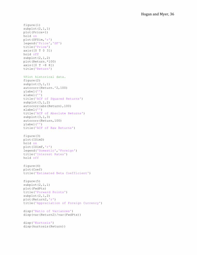
Hogan  and  Myer,  36    

figure(1) subplot(2,1,1) plot(Price+1) hold on plot(SFSim,'r') legend('Price','SF') title('Price') axis([0 T 0 3]) hold off subplot(2,1,2) plot(Return.*100) axis([0 T -8 8]) title('Return') %Plot historical data. figure(2) subplot(3,1,1) autocorr(Return.^2,100) ylabel('') xlabel('') title('ACF of Squared Returns') subplot(3,1,2) autocorr(abs(Return),100) xlabel('') title('ACF of Absolute Returns') subplot(3,1,3) autocorr(Return,100) ylabel('') title('ACF of Raw Returns') figure(3) plot(ISimD) hold on plot(ISimF,'r') legend('Domestic','Foreign') title('Interest Rates') hold off figure(4) plot(Coef) title('Estimated Beta Coefficient') figure(5) subplot(2,1,1) plot(FwdPts) title('Forward Points') subplot(2,1,2) plot(Return2,'r') title('Appreciation of Foreign Currency') disp('Ratio of Variances') disp(var(Return2)/var(FwdPts)) disp('Kurtosis') disp(kurtosis(Return))

Hogan  and  Myer,  37    

disp('Skewness') disp(skewness(Return)) disp('JBTest') disp(jbtest(Return)) disp('Parameter Estimates') [b,bint,r,rint,stats] = regress(Return2,FP); [b2,bint2,r2,rint2,stats2] = regress(Return3,FP2); stats3 = regstats(Return2, FwdPts(1:end-1)); stats4 = regstats(Return3, FwdPts2(1:end-1)); disp(b) disp(sqrt(diag(stats3.covb))) disp(b2) disp(sqrt(diag(stats4.covb))) figure(6) scatter(FwdPts(1:end-1)*100,Return2*100,'.') hold on int = b(1); slope = b(2); line = @(x) int + slope*x; ezplotline = ezplot(line, [-7 7]); set(ezplotline,'Color','r') plot(ezplotline) axis([-15 15 -15 15]) title('Equation (5) Regression') xlabel('Forward Premium') ylabel('Monthly Returns') hold off disp('R^2') disp(stats(1)) disp(stats2(1)) [P1,P2] = profits(Price(1:22:end),(((1+(ISimD(1:22:end))*0.01).^(1/252)).^264),(((1+(ISimF(1:22:end))*0.01).^(1/252)).^264)); disp('Momentum Profit') disp(P1) disp('Carry Profit') disp(P2)

Fastbin Algorithm function k = fastbin(n,p) %Step 1 q = 1-p; s = p/q; a = (n+1)*s;

Hogan  and  Myer,  38    

r = q^n; %Step 2 u = rand; k = 0; %Step 3&4 while u > r u = u - r; k = k + 1; r = ((a/k)-s)*r; end  

  Profit Calculations  function [P1, P2] = profits(X,I1,I2) for n = (2:length(X)-1) if ((X(n)-X(n-1))/X(n-1))>0 Y1(n+1) = ((X(n+1)-X(n))/X(n)); else Y1(n+1) = -((X(n+1)-X(n))/X(n)); end if (I1(n)-I2(n))>0 Y2(n) = (-((X(n)-X(n-1))/X(n-1)))+abs((I1(n)-I2(n))); else Y2(n) = (((X(n)-X(n-1))/X(n-1)))+abs((I1(n)-I2(n))); end P1 = (1+mean(Y1))^12-1; P2 = (1+mean(Y2))^12-1; end