Embed Size (px)
Citation preview
Plotly 한번에 제대로 배우기
인터랙티브 그래프 생성JSON 데이터 형식으로 저장벡터 이미지, 래스터 이미지로 Export 가능
홈페이지: https://plotly.com/python/
Plotly 특징
import numpy as np
import pandas as pd
from urllib.request import urlopen
import json
import plotly.io as pio
import plotly.express as px
import plotly.graph_objects as go
import plotly.figure_factory as ff
from plotly.subplots import make_subplots
from plotly.validators.scatter.marker import SymbolValidator
Plotly 차트
산점도(Scatter Plots)
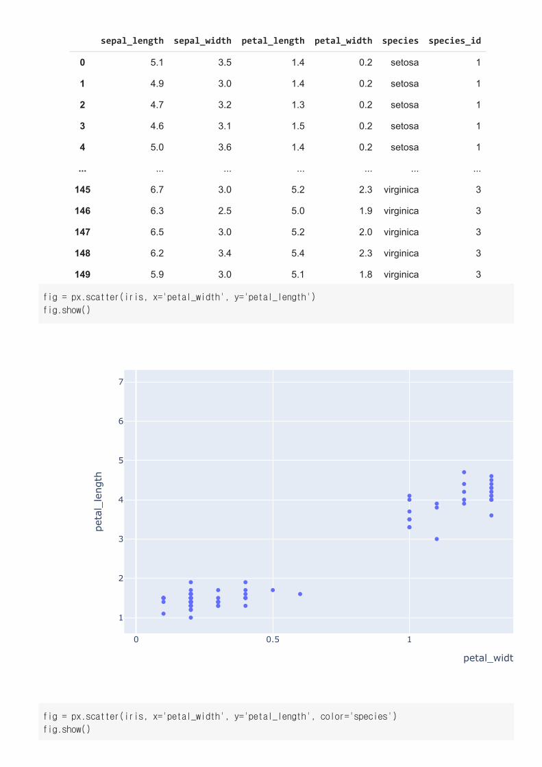
iris = px.data.iris()
iris
sepal_length sepal_width petal_length petal_width species species_id
0 5.1 3.5 1.4 0.2 setosa 1
1 4.9 3.0 1.4 0.2 setosa 1
2 4.7 3.2 1.3 0.2 setosa 1
3 4.6 3.1 1.5 0.2 setosa 1
4 5.0 3.6 1.4 0.2 setosa 1
... ... ... ... ... ... ...
145 6.7 3.0 5.2 2.3 virginica 3
146 6.3 2.5 5.0 1.9 virginica 3
147 6.5 3.0 5.2 2.0 virginica 3
148 6.2 3.4 5.4 2.3 virginica 3
149 5.9 3.0 5.1 1.8 virginica 3
150 rows × 6 columns
0 0.5 1
1
2
3
4
5
6
7
petal_widt
petal_leng
th
fig = px.scatter(iris, x='petal_width', y='petal_length')
fig.show()
fig = px.scatter(iris, x='petal_width', y='petal_length', color='species')
fig.show()
0 0.5 1 1.5
1
2
3
4
5
6
7
petal_width
petal_leng
th
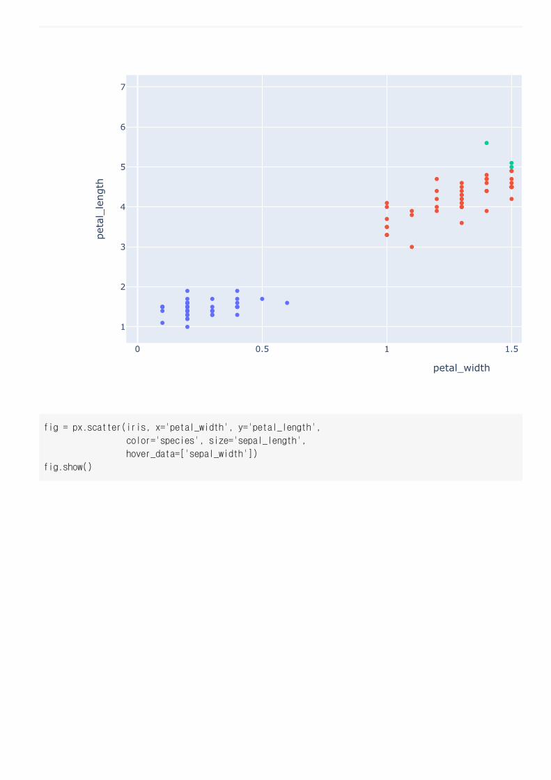
fig = px.scatter(iris, x='petal_width', y='petal_length',
color='species', size='sepal_length',
hover_data=['sepal_width'])
fig.show()
0 0.5 1 1.5
1
2
3
4
5
6
7
petal_width
petal_leng
th
total_bill tip sex smoker day time size
0 16.99 1.01 Female No Sun Dinner 2
1 10.34 1.66 Male No Sun Dinner 3
2 21.01 3.50 Male No Sun Dinner 3
3 23.68 3.31 Male No Sun Dinner 2
4 24.59 3.61 Female No Sun Dinner 4
... ... ... ... ... ... ... ...
239 29.03 5.92 Male No Sat Dinner 3
240 27.18 2.00 Female Yes Sat Dinner 2
241 22.67 2.00 Male Yes Sat Dinner 2
242 17.82 1.75 Male No Sat Dinner 2
243 18.78 3.00 Female No Thur Dinner 2
244 rows × 7 columns
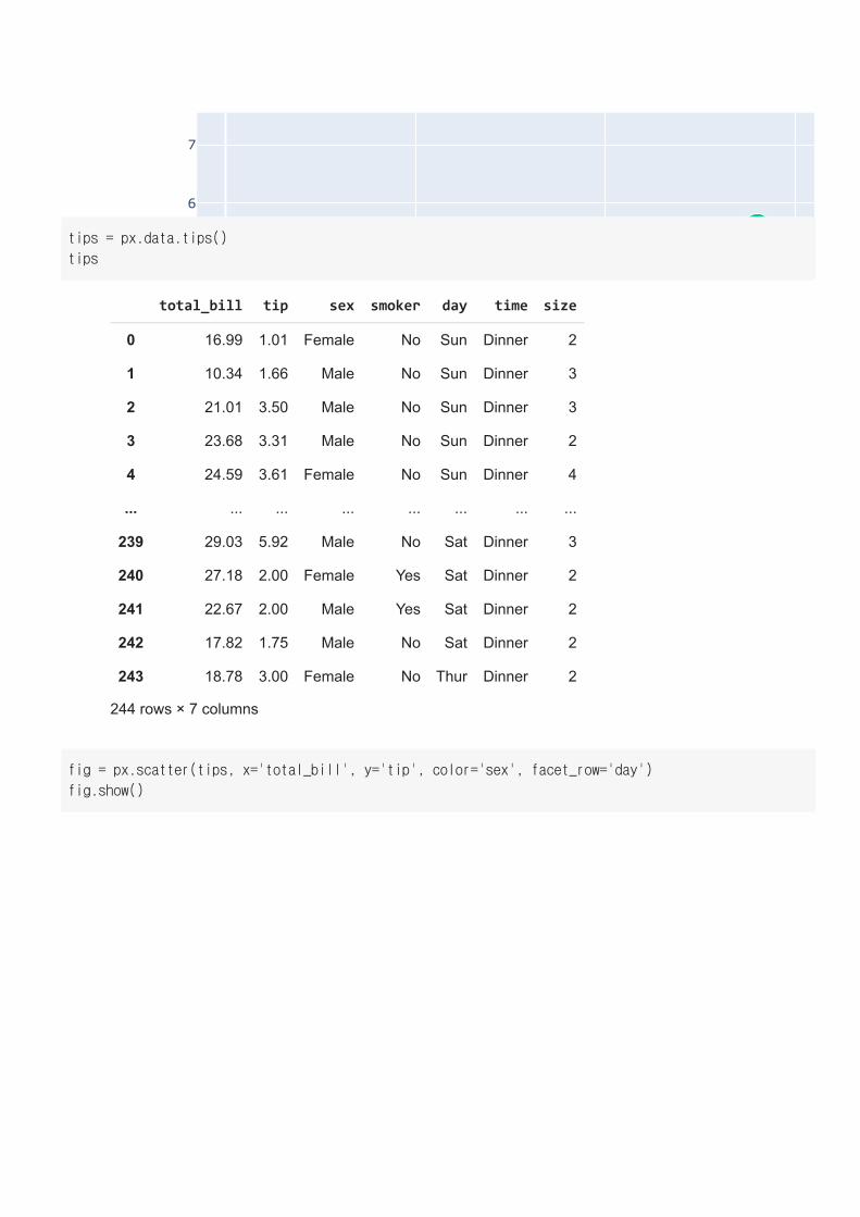
tips = px.data.tips()
tips
fig = px.scatter(tips, x='total_bill', y='tip', color='sex', facet_row='day')
fig.show()
10 20 300
5
100
5
100
5
100
5
10
total_bill
tiptip
tiptip
0 20 40
2
4
6
8
10
0 20 40 0
total_bill total_bill
tip
day=Sun day=Sat
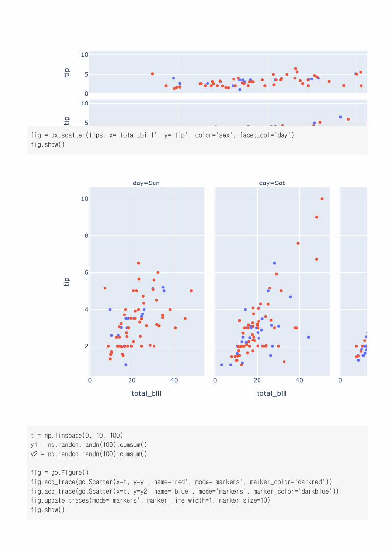
fig = px.scatter(tips, x='total_bill', y='tip', color='sex', facet_col='day')
fig.show()
t = np.linspace(0, 10, 100)
y1 = np.random.randn(100).cumsum()
y2 = np.random.randn(100).cumsum()
fig = go.Figure()
fig.add_trace(go.Scatter(x=t, y=y1, name='red', mode='markers', marker_color='darkred'))
fig.add_trace(go.Scatter(x=t, y=y2, name='blue', mode='markers', marker_color='darkblue'))
fig.update_traces(mode='markers', marker_line_width=1, marker_size=10)
fig.show()
0 2 4
−15
−10
−5
0
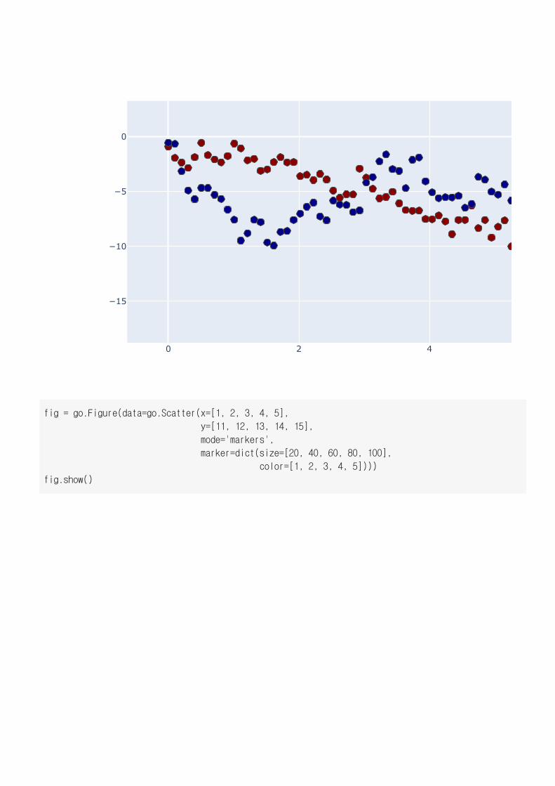
fig = go.Figure(data=go.Scatter(x=[1, 2, 3, 4, 5],
y=[11, 12, 13, 14, 15],
mode='markers',
marker=dict(size=[20, 40, 60, 80, 100],
color=[1, 2, 3, 4, 5])))
fig.show()
1 1.5 2 2.5 3
11
12
13
14
15
16
country continent year lifeExp pop gdpPercap iso_alpha iso_num
0 Afghanistan Asia 1952 28.801 8425333 779.445314 AFG 4
1 Afghanistan Asia 1957 30.332 9240934 820.853030 AFG 4
2 Afghanistan Asia 1962 31.997 10267083 853.100710 AFG 4
3 Afghanistan Asia 1967 34.020 11537966 836.197138 AFG 4
4 Afghanistan Asia 1972 36.088 13079460 739.981106 AFG 4
... ... ... ... ... ... ... ... ...
1699 Zimbabwe Africa 1987 62.351 9216418 706.157306 ZWE 716
1700 Zimbabwe Africa 1992 60.377 10704340 693.420786 ZWE 716
1701 Zimbabwe Africa 1997 46.809 11404948 792.449960 ZWE 716
1702 Zimbabwe Africa 2002 39.989 11926563 672.038623 ZWE 716
1703 Zimbabwe Africa 2007 43.487 12311143 469.709298 ZWE 716
1704 rows × 8 columns
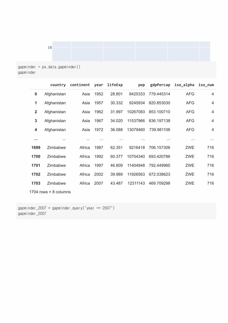
gapminder = px.data.gapminder()
gapminder
gapminder_2007 = gapminder.query("year == 2007")
gapminder_2007
country continent year lifeExp pop gdpPercap iso_alpha iso_nu
11 Afghanistan Asia 2007 43.828 31889923 974.580338 AFG
23 Albania Europe 2007 76.423 3600523 5937.029526 ALB
35 Algeria Africa 2007 72.301 33333216 6223.367465 DZA 1
47 Angola Africa 2007 42.731 12420476 4797.231267 AGO 2
59 Argentina Americas 2007 75.320 40301927 12779.379640 ARG 3
... ... ... ... ... ... ... ... .
1655 Vietnam Asia 2007 74.249 85262356 2441.576404 VNM 70
1667 West Bankand Gaza Asia 2007 73.422 4018332 3025.349798 PSE 27
1679 Yemen,Rep. Asia 2007 62.698 22211743 2280.769906 YEM 88
1691 Zambia Africa 2007 42.384 11746035 1271.211593 ZMB 89
1703 Zimbabwe Africa 2007 43.487 12311143 469.709298 ZWE 71
2 3 4 5 6 7 8 91000
2 3 4 5
40
50
60
70
80
gdpPercap
lifeE
xp
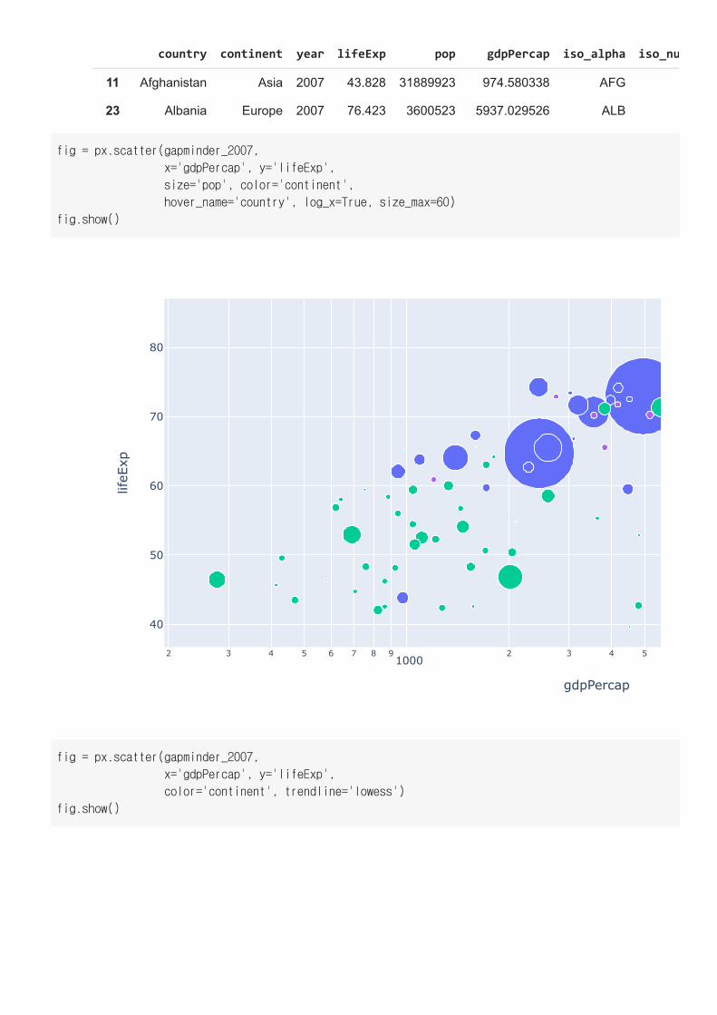
fig = px.scatter(gapminder_2007,
x='gdpPercap', y='lifeExp',
size='pop', color='continent',
hover_name='country', log_x=True, size_max=60)
fig.show()
fig = px.scatter(gapminder_2007,
x='gdpPercap', y='lifeExp',
color='continent', trendline='lowess')
fig.show()
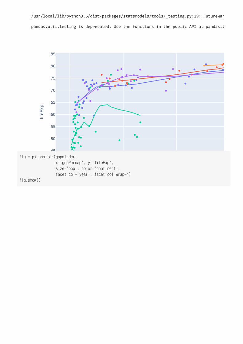
/usr/local/lib/python3.6/dist-packages/statsmodels/tools/_testing.py:19: FutureWar
pandas.util.testing is deprecated. Use the functions in the public API at pandas.t
0 10k 20k
40
45
50
55
60
65
70
75
80
85
gdpPercap
lifeE
xp
fig = px.scatter(gapminder,
x='gdpPercap', y='lifeExp',
size='pop', color='continent',
facet_col='year', facet_col_wrap=4)
fig.show()
0 50k 100k20
40
60
80
0 50k 100k 0
20
40
60
80
20
40
60
80
gdpPercap gdpPercap
lifeExp
lifeExp
lifeExp
year=1992 year=1997
year=1972 year=1977
year=1952 year=1957
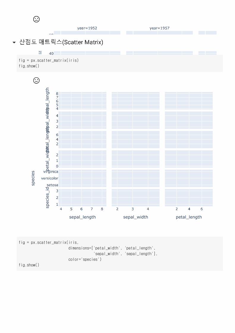
산점도 매트릭스(Scatter Matrix)
45678
234
246
012
setosa
versicolor
virginica
4 5 6 7 81
2
3
2 3 4 2 4 6
sepal_length sepal_width petal_length
sepal_leng
thsepal_width
petal_leng
thpetal_width
species
species_id
fig = px.scatter_matrix(iris)
fig.show()
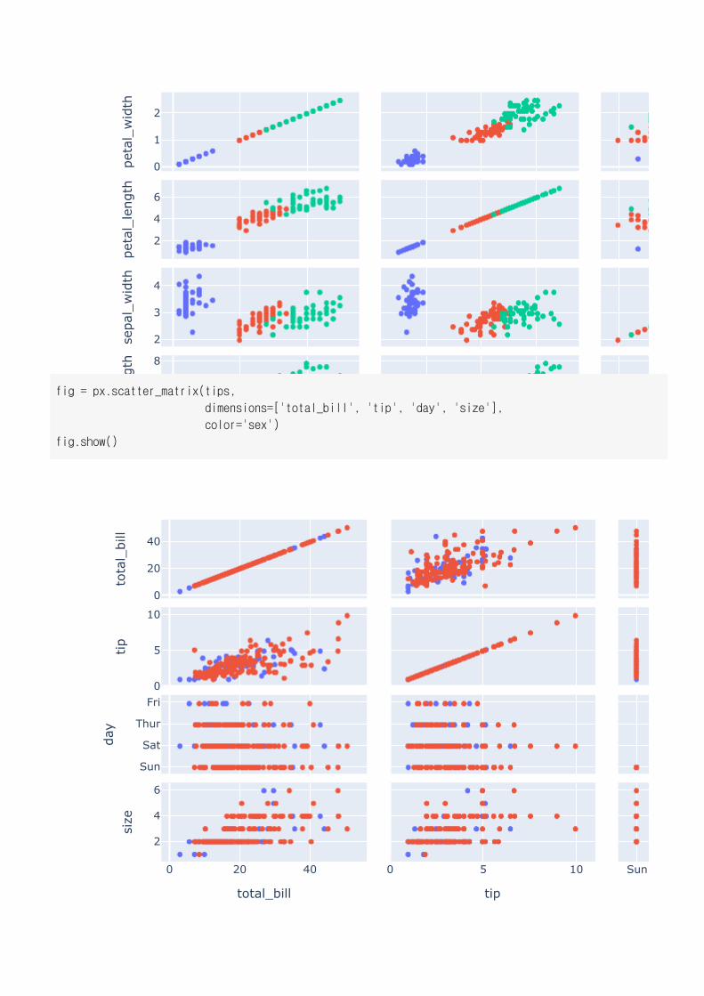
fig = px.scatter_matrix(iris,
dimensions=['petal_width', 'petal_length',
'sepal_width', 'sepal_length'],
color='species')
fig.show()
0
1
2
2
4
6
2
3
4
0 1 245678
2 4 6 2
petal_width petal_length
petal_width
petal_leng
thsepal_width
sepal_leng
th
0
20
40
0
5
10
Sun
Sat
Thur
Fri
0 20 40
2
4
6
0 5 10 Sun
total_bill tip
total_bill
tipda
ysize
fig = px.scatter_matrix(tips,
dimensions=['total_bill', 'tip', 'day', 'size'],
color='sex')
fig.show()
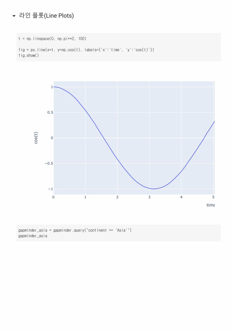
라인 플롯(Line Plots)
0 1 2 3 4 5
−1
−0.5
0
0.5
1
time
cos(t)
t = np.linspace(0, np.pi**2, 100)
fig = px.line(x=t, y=np.cos(t), labels={'x':'time', 'y':'cos(t)'})
fig.show()
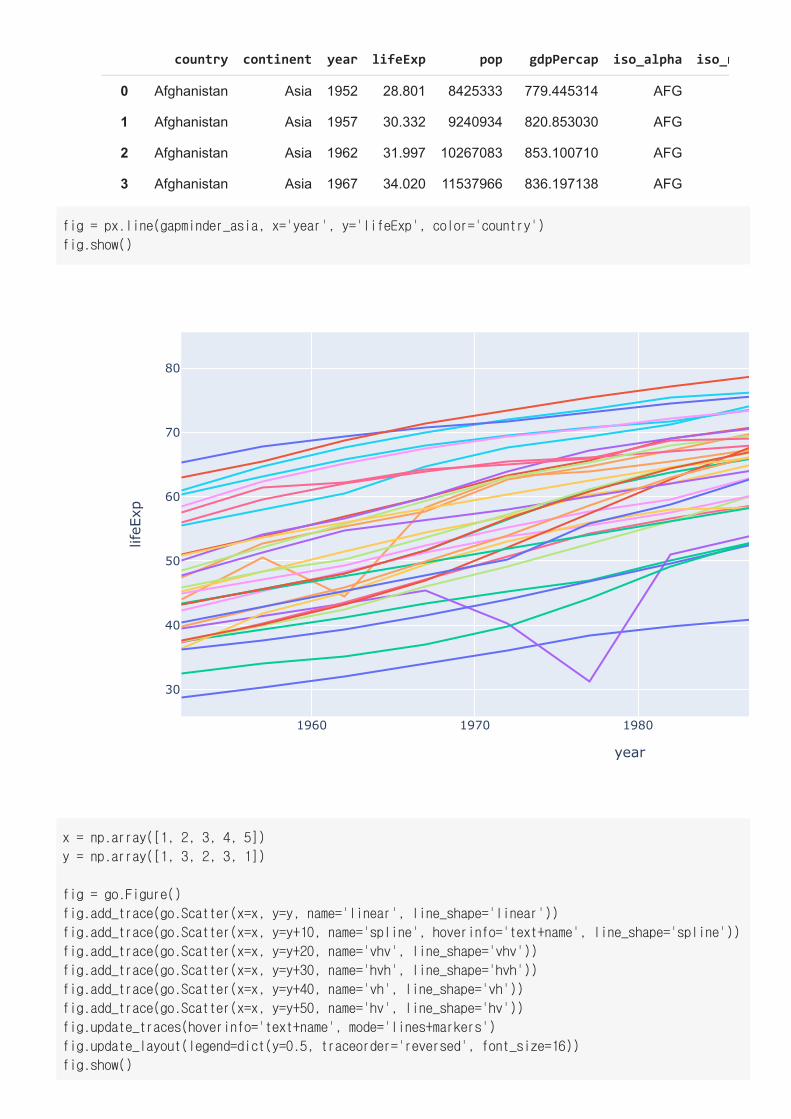
gapminder_asia = gapminder.query("continent == 'Asia'")
gapminder_asia
country continent year lifeExp pop gdpPercap iso_alpha iso_n
0 Afghanistan Asia 1952 28.801 8425333 779.445314 AFG
1 Afghanistan Asia 1957 30.332 9240934 820.853030 AFG
2 Afghanistan Asia 1962 31.997 10267083 853.100710 AFG
3 Afghanistan Asia 1967 34.020 11537966 836.197138 AFG
4 Afghanistan Asia 1972 36.088 13079460 739.981106 AFG
... ... ... ... ... ... ... ...
1675 Yemen,Rep. Asia 1987 52.922 11219340 1971.741538 YEM 8
1676 Yemen,Rep. Asia 1992 55.599 13367997 1879.496673 YEM 8
1677 Yemen,Rep. Asia 1997 58.020 15826497 2117.484526 YEM 8
1678 Yemen,Rep. Asia 2002 60.308 18701257 2234.820827 YEM 8
1960 1970 1980
30
40
50
60
70
80
year
lifeE
xp
fig = px.line(gapminder_asia, x='year', y='lifeExp', color='country')
fig.show()
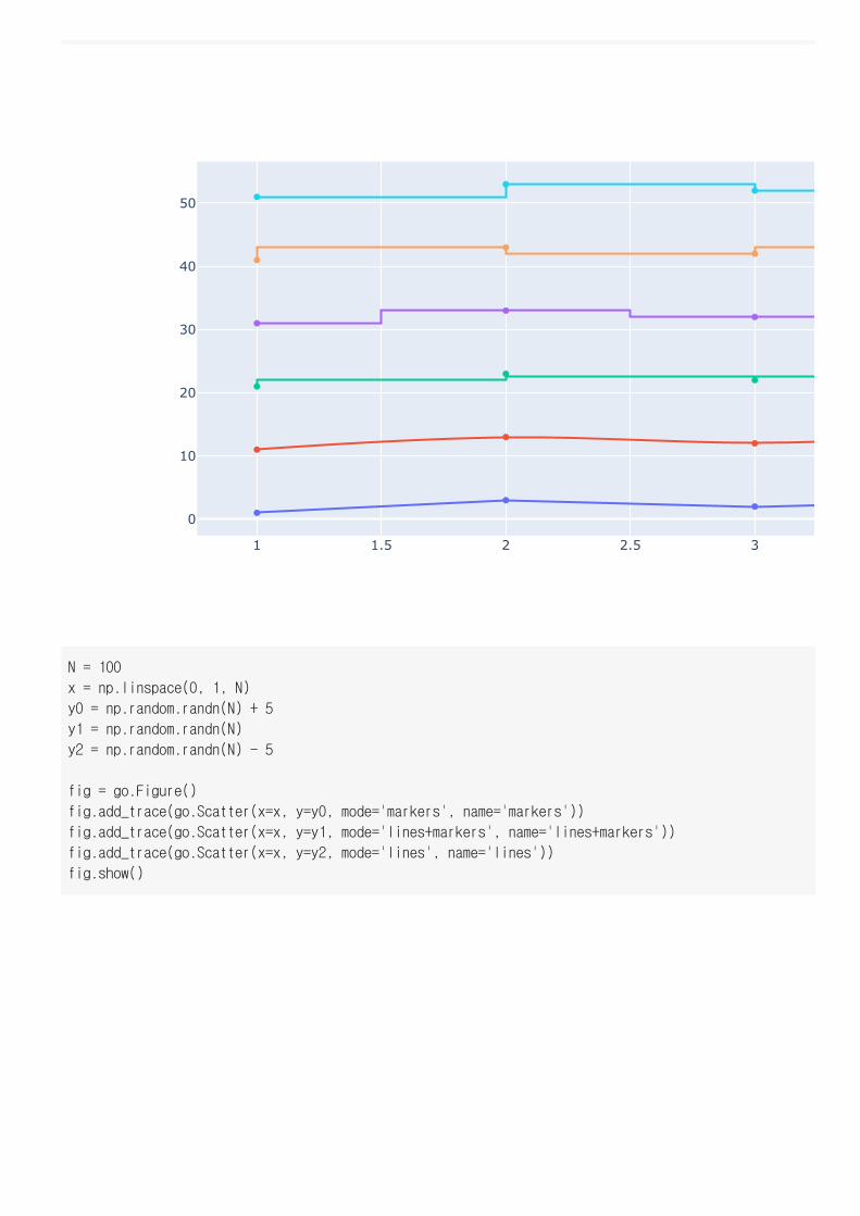
x = np.array([1, 2, 3, 4, 5])
y = np.array([1, 3, 2, 3, 1])
fig = go.Figure()
fig.add_trace(go.Scatter(x=x, y=y, name='linear', line_shape='linear'))
fig.add_trace(go.Scatter(x=x, y=y+10, name='spline', hoverinfo='text+name', line_shape='spline'))
fig.add_trace(go.Scatter(x=x, y=y+20, name='vhv', line_shape='vhv'))
fig.add_trace(go.Scatter(x=x, y=y+30, name='hvh', line_shape='hvh'))
fig.add_trace(go.Scatter(x=x, y=y+40, name='vh', line_shape='vh'))
fig.add_trace(go.Scatter(x=x, y=y+50, name='hv', line_shape='hv'))
fig.update_traces(hoverinfo='text+name', mode='lines+markers')
fig.update_layout(legend=dict(y=0.5, traceorder='reversed', font_size=16))
fig.show()
1 1.5 2 2.5 3
0
10
20
30
40
50
N = 100
x = np.linspace(0, 1, N)
y0 = np.random.randn(N) + 5
y1 = np.random.randn(N)
y2 = np.random.randn(N) - 5
fig = go.Figure()
fig.add_trace(go.Scatter(x=x, y=y0, mode='markers', name='markers'))
fig.add_trace(go.Scatter(x=x, y=y1, mode='lines+markers', name='lines+markers'))
fig.add_trace(go.Scatter(x=x, y=y2, mode='lines', name='lines'))
fig.show()
0 0.2 0.4
−8
−6
−4
−2
0
2
4
6
8
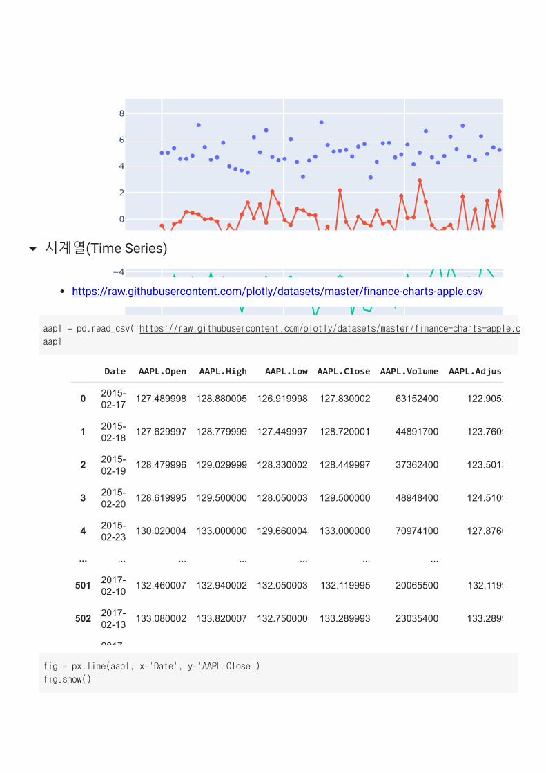
시계열(Time Series)
https://raw.githubusercontent.com/plotly/datasets/master/�nance-charts-apple.csv
Date AAPL.Open AAPL.High AAPL.Low AAPL.Close AAPL.Volume AAPL.Adjust
0 2015-02-17 127.489998 128.880005 126.919998 127.830002 63152400 122.9052
1 2015-02-18 127.629997 128.779999 127.449997 128.720001 44891700 123.7609
2 2015-02-19 128.479996 129.029999 128.330002 128.449997 37362400 123.5013
3 2015-02-20 128.619995 129.500000 128.050003 129.500000 48948400 124.5109
4 2015-02-23 130.020004 133.000000 129.660004 133.000000 70974100 127.8760
... ... ... ... ... ... ...
501 2017-02-10 132.460007 132.940002 132.050003 132.119995 20065500 132.1199
502 2017-02-13 133.080002 133.820007 132.750000 133.289993 23035400 133.2899
2017
aapl = pd.read_csv('https://raw.githubusercontent.com/plotly/datasets/master/finance-charts-apple.c
aapl
fig = px.line(aapl, x='Date', y='AAPL.Close')
fig.show()
Apr 2015 Jul 2015 Oct 2015 Jan 2016
90
100
110
120
130
Date
AAPL
.Clo
se
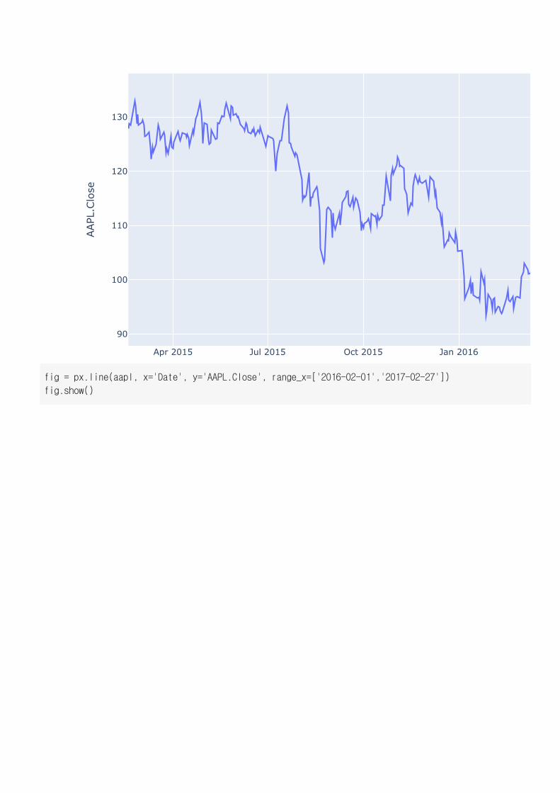
fig = px.line(aapl, x='Date', y='AAPL.Close', range_x=['2016-02-01','2017-02-27'])
fig.show()
Mar 2016 May 2016 Jul 2016
90
100
110
120
130
Date
AAPL
.Clo
se
Apr 2015 Jul 2015 Oct 2015 Jan 2016
90
100
110
120
130
AAPL
.Clo
se
Date
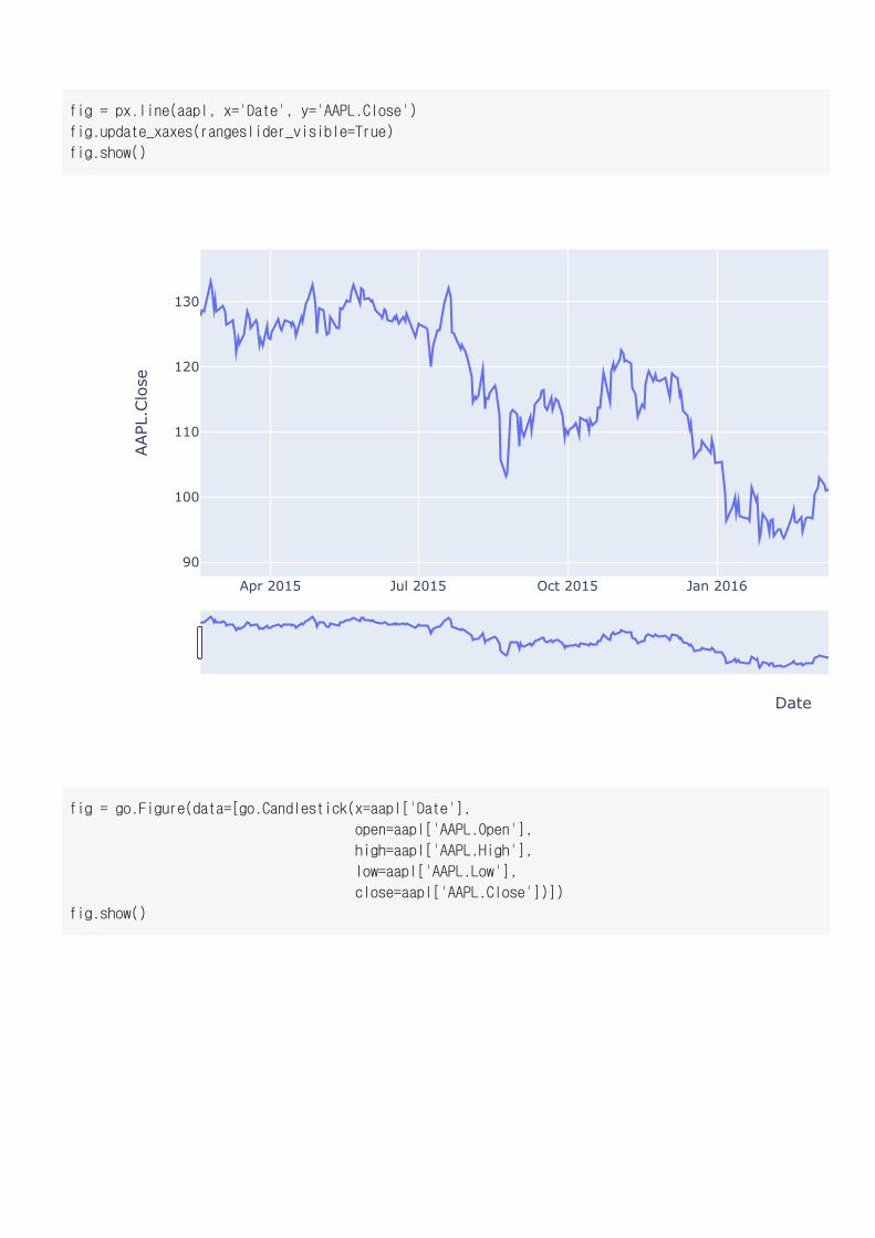
fig = px.line(aapl, x='Date', y='AAPL.Close')
fig.update_xaxes(rangeslider_visible=True)
fig.show()
fig = go.Figure(data=[go.Candlestick(x=aapl['Date'],
open=aapl['AAPL.Open'],
high=aapl['AAPL.High'],
low=aapl['AAPL.Low'],
close=aapl['AAPL.Close'])])
fig.show()
Apr 2015 Jul 2015 Oct 2015 Jan 2016
90
100
110
120
130
Apr 2015 Jul 2015 Oct 2015 Jan 2016
90
100
110
120
130
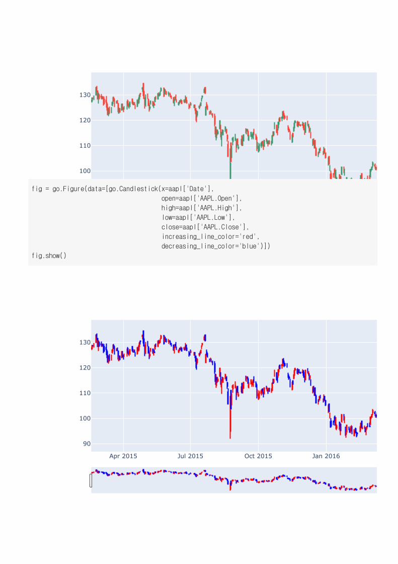
fig = go.Figure(data=[go.Candlestick(x=aapl['Date'],
open=aapl['AAPL.Open'],
high=aapl['AAPL.High'],
low=aapl['AAPL.Low'],
close=aapl['AAPL.Close'],
increasing_line_color='red',
decreasing_line_color='blue')])
fig.show()
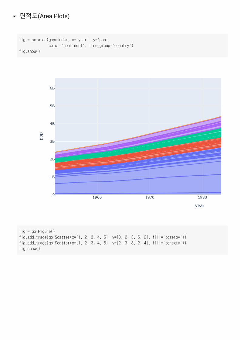
면적도(Area Plots)
1960 1970 19800
1B
2B
3B
4B
5B
6B
year
pop
fig = px.area(gapminder, x='year', y='pop',
color='continent', line_group='country')
fig.show()
fig = go.Figure()
fig.add_trace(go.Scatter(x=[1, 2, 3, 4, 5], y=[0, 2, 3, 5, 2], fill='tozeroy'))
fig.add_trace(go.Scatter(x=[1, 2, 3, 4, 5], y=[2, 3, 3, 2, 4], fill='tonexty'))
fig.show()
1 1.5 2 2.5 30
1
2
3
4
5
1 1.5 2 2.5 30
1
2
3
4
5
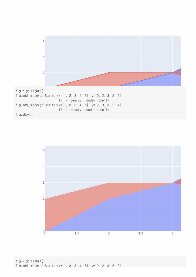
fig = go.Figure()
fig.add_trace(go.Scatter(x=[1, 2, 3, 4, 5], y=[0, 2, 3, 5, 2],
fill='tozeroy', mode='none'))
fig.add_trace(go.Scatter(x=[1, 2, 3, 4, 5], y=[2, 3, 3, 2, 4],
fill='tonexty', mode='none'))
fig.show()
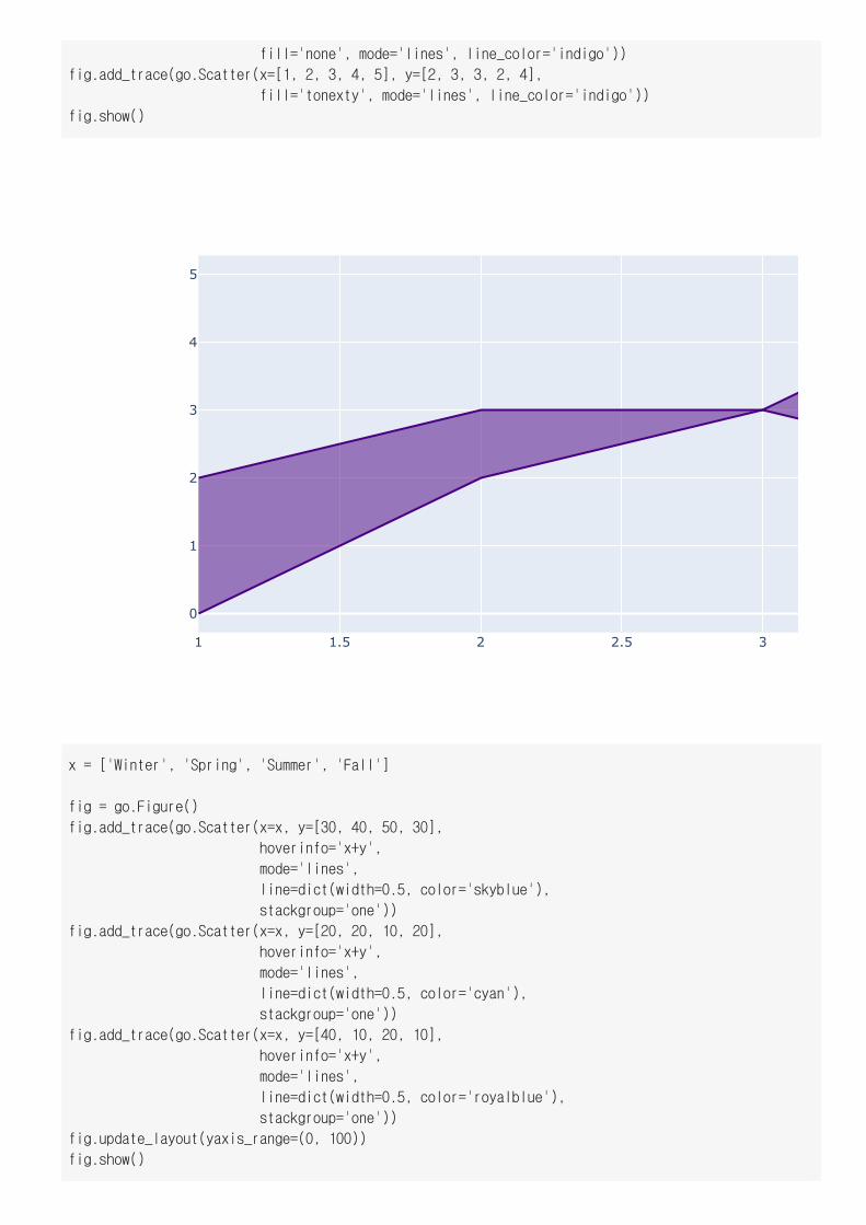
fig = go.Figure()
fig.add_trace(go.Scatter(x=[1, 2, 3, 4, 5], y=[0, 2, 3, 5, 2],
1 1.5 2 2.5 3
0
1
2
3
4
5
fill='none', mode='lines', line_color='indigo'))
fig.add_trace(go.Scatter(x=[1, 2, 3, 4, 5], y=[2, 3, 3, 2, 4],
fill='tonexty', mode='lines', line_color='indigo'))
fig.show()
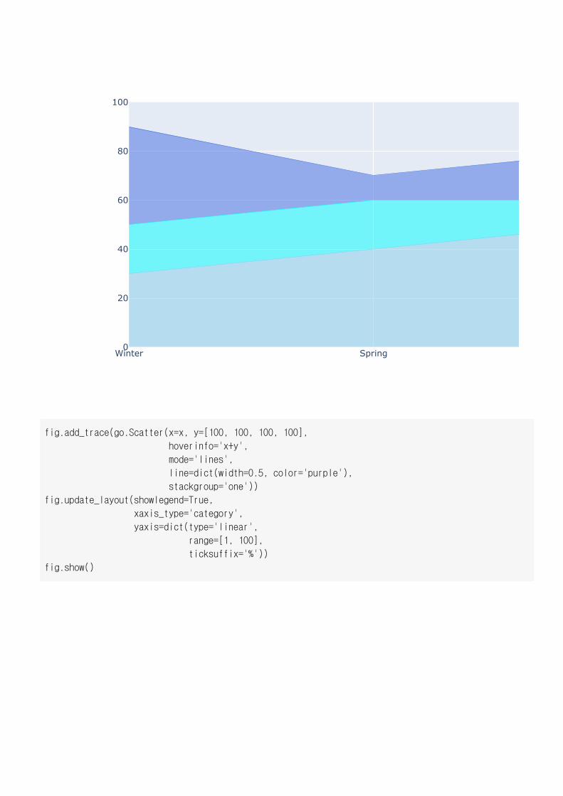
x = ['Winter', 'Spring', 'Summer', 'Fall']
fig = go.Figure()
fig.add_trace(go.Scatter(x=x, y=[30, 40, 50, 30],
hoverinfo='x+y',
mode='lines',
line=dict(width=0.5, color='skyblue'),
stackgroup='one'))
fig.add_trace(go.Scatter(x=x, y=[20, 20, 10, 20],
hoverinfo='x+y',
mode='lines',
line=dict(width=0.5, color='cyan'),
stackgroup='one'))
fig.add_trace(go.Scatter(x=x, y=[40, 10, 20, 10],
hoverinfo='x+y',
mode='lines',
line=dict(width=0.5, color='royalblue'),
stackgroup='one'))
fig.update_layout(yaxis_range=(0, 100))
fig.show()
Winter Spring0
20
40
60
80
100
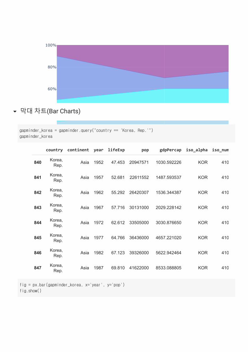
fig.add_trace(go.Scatter(x=x, y=[100, 100, 100, 100],
hoverinfo='x+y',
mode='lines',
line=dict(width=0.5, color='purple'),
stackgroup='one'))
fig.update_layout(showlegend=True,
xaxis_type='category',
yaxis=dict(type='linear',
range=[1, 100],
ticksuffix='%'))
fig.show()
Winter Spring
20%
40%
60%
80%
100%
막대 차트(Bar Charts)
country continent year lifeExp pop gdpPercap iso_alpha iso_num
840 Korea,Rep. Asia 1952 47.453 20947571 1030.592226 KOR 410
841 Korea,Rep. Asia 1957 52.681 22611552 1487.593537 KOR 410
842 Korea,Rep. Asia 1962 55.292 26420307 1536.344387 KOR 410
843 Korea,Rep. Asia 1967 57.716 30131000 2029.228142 KOR 410
844 Korea,Rep. Asia 1972 62.612 33505000 3030.876650 KOR 410
845 Korea,Rep. Asia 1977 64.766 36436000 4657.221020 KOR 410
846 Korea,Rep. Asia 1982 67.123 39326000 5622.942464 KOR 410
847 Korea,Rep. Asia 1987 69.810 41622000 8533.088805 KOR 410
gapminder_korea = gapminder.query("country == 'Korea, Rep.'")
gapminder_korea
fig = px.bar(gapminder_korea, x='year', y='pop')
fig.show()
1950 1960 1970 19800
10M
20M
30M
40M
50M
year
pop
1950 1960 1970 19800
10M
20M
30M
40M
50M
year
pop
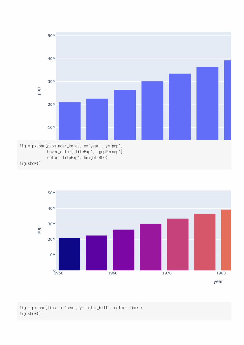
fig = px.bar(gapminder_korea, x='year', y='pop',
hover_data=['lifeExp', 'gdpPercap'],
color='lifeExp', height=400)
fig.show()
fig = px.bar(tips, x='sex', y='total_bill', color='time')
fig.show()
Female0
500
1000
1500
2000
2500
3000
sex
total_bill
Female0
500
1000
1500
2000
sex
total_bill
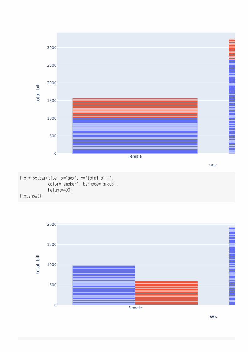
fig = px.bar(tips, x='sex', y='total_bill',
color='smoker', barmode='group',
height=400)
fig.show()
Male Female0
200
400
600
800
Male Female Male
0
200
400
600
800
sex sex
total_bill
total_bill
day=Thur day=Fri
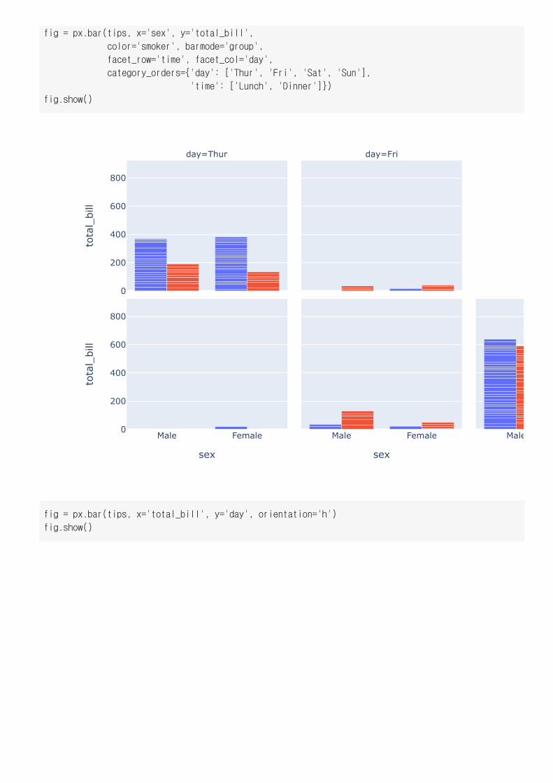
fig = px.bar(tips, x='sex', y='total_bill',
color='smoker', barmode='group',
facet_row='time', facet_col='day',
category_orders={'day': ['Thur', 'Fri', 'Sat', 'Sun'],
'time': ['Lunch', 'Dinner']})
fig.show()
fig = px.bar(tips, x='total_bill', y='day', orientation='h')
fig.show()
0 200 400 600 800
Sun
Sat
Thur
Fri
total_b
day
0 500 1000 1500
Female
Male
total_bill
sex
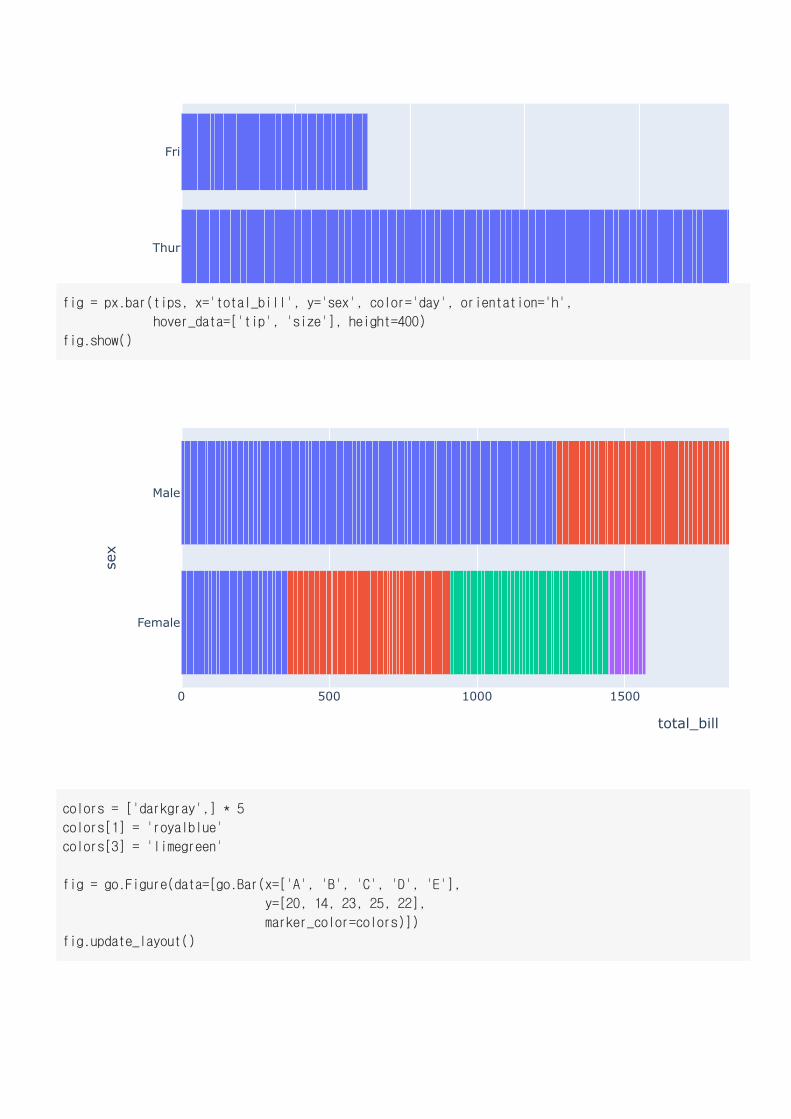
fig = px.bar(tips, x='total_bill', y='sex', color='day', orientation='h',
hover_data=['tip', 'size'], height=400)
fig.show()
colors = ['darkgray',] * 5
colors[1] = 'royalblue'
colors[3] = 'limegreen'
fig = go.Figure(data=[go.Bar(x=['A', 'B', 'C', 'D', 'E'],
y=[20, 14, 23, 25, 22],
marker_color=colors)])
fig.update_layout()
A B C0
5
10
15
20
25
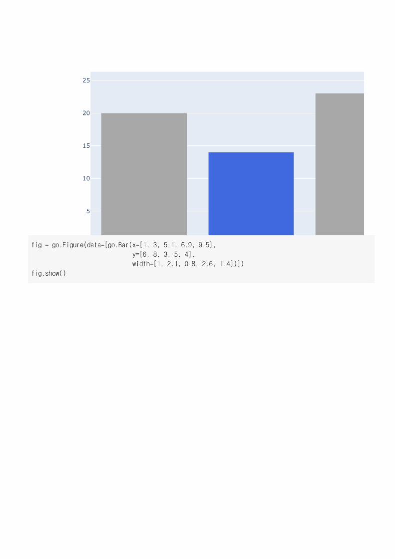
fig = go.Figure(data=[go.Bar(x=[1, 3, 5.1, 6.9, 9.5],
y=[6, 8, 3, 5, 4],
width=[1, 2.1, 0.8, 2.6, 1.4])])
fig.show()
2 40
1
2
3
4
5
6
7
8
2018 2019
−30M
−20M
−10M
0
10M
20M
30M
40M
50M
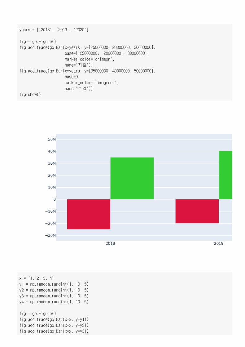
years = ['2018', '2019', '2020']
fig = go.Figure()
fig.add_trace(go.Bar(x=years, y=[25000000, 20000000, 30000000],
base=[-25000000, -20000000, -30000000],
marker_color='crimson',
name='지출'))
fig.add_trace(go.Bar(x=years, y=[35000000, 40000000, 50000000],
base=0,
marker_color='limegreen',
name='수입'))
fig.show()
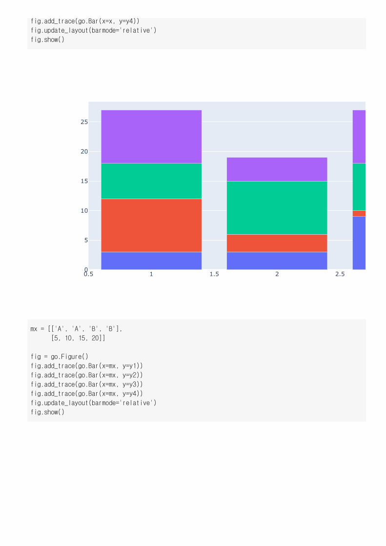
x = [1, 2, 3, 4]
y1 = np.random.randint(1, 10, 5)
y2 = np.random.randint(1, 10, 5)
y3 = np.random.randint(1, 10, 5)
y4 = np.random.randint(1, 10, 5)
fig = go.Figure()
fig.add_trace(go.Bar(x=x, y=y1))
fig.add_trace(go.Bar(x=x, y=y2))
fig.add_trace(go.Bar(x=x, y=y3))
( ( ))
0.5 1 1.5 2 2.50
5
10
15
20
25
fig.add_trace(go.Bar(x=x, y=y4))
fig.update_layout(barmode='relative')
fig.show()
mx = [['A', 'A', 'B', 'B'],
[5, 10, 15, 20]]
fig = go.Figure()
fig.add_trace(go.Bar(x=mx, y=y1))
fig.add_trace(go.Bar(x=mx, y=y2))
fig.add_trace(go.Bar(x=mx, y=y3))
fig.add_trace(go.Bar(x=mx, y=y4))
fig.update_layout(barmode='relative')
fig.show()
5 10A
0
5
10
15
20
25
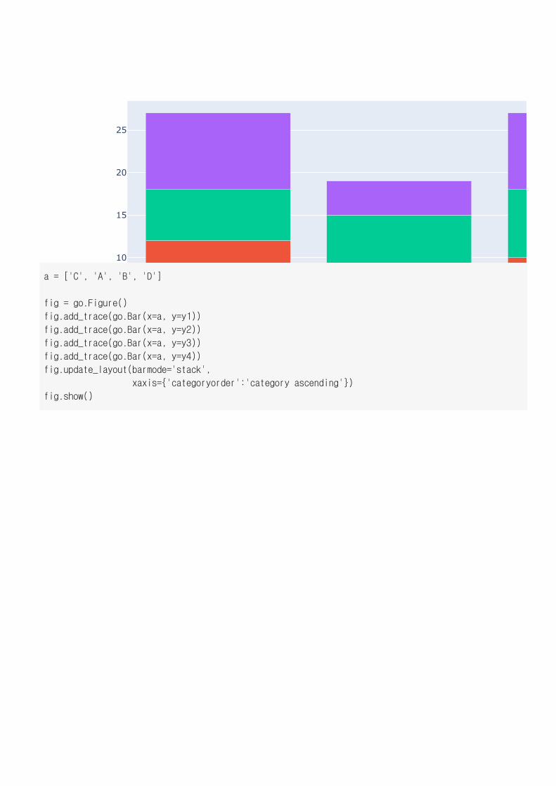
a = ['C', 'A', 'B', 'D']
fig = go.Figure()
fig.add_trace(go.Bar(x=a, y=y1))
fig.add_trace(go.Bar(x=a, y=y2))
fig.add_trace(go.Bar(x=a, y=y3))
fig.add_trace(go.Bar(x=a, y=y4))
fig.update_layout(barmode='stack',
xaxis={'categoryorder':'category ascending'})
fig.show()
A B0
5
10
15
20
25
D A0
5
10
15
20
25
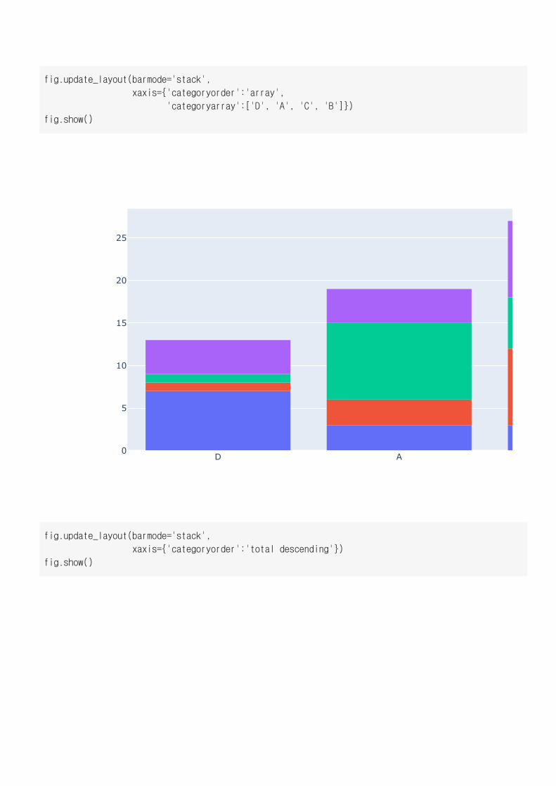
fig.update_layout(barmode='stack',
xaxis={'categoryorder':'array',
'categoryarray':['D', 'A', 'C', 'B']})
fig.show()
fig.update_layout(barmode='stack',
xaxis={'categoryorder':'total descending'})
fig.show()
B C0
5
10
15
20
25
1 1.5 2 2.5 3
1.5
2
2.5
3
3.5
4
4.5
5
5.5
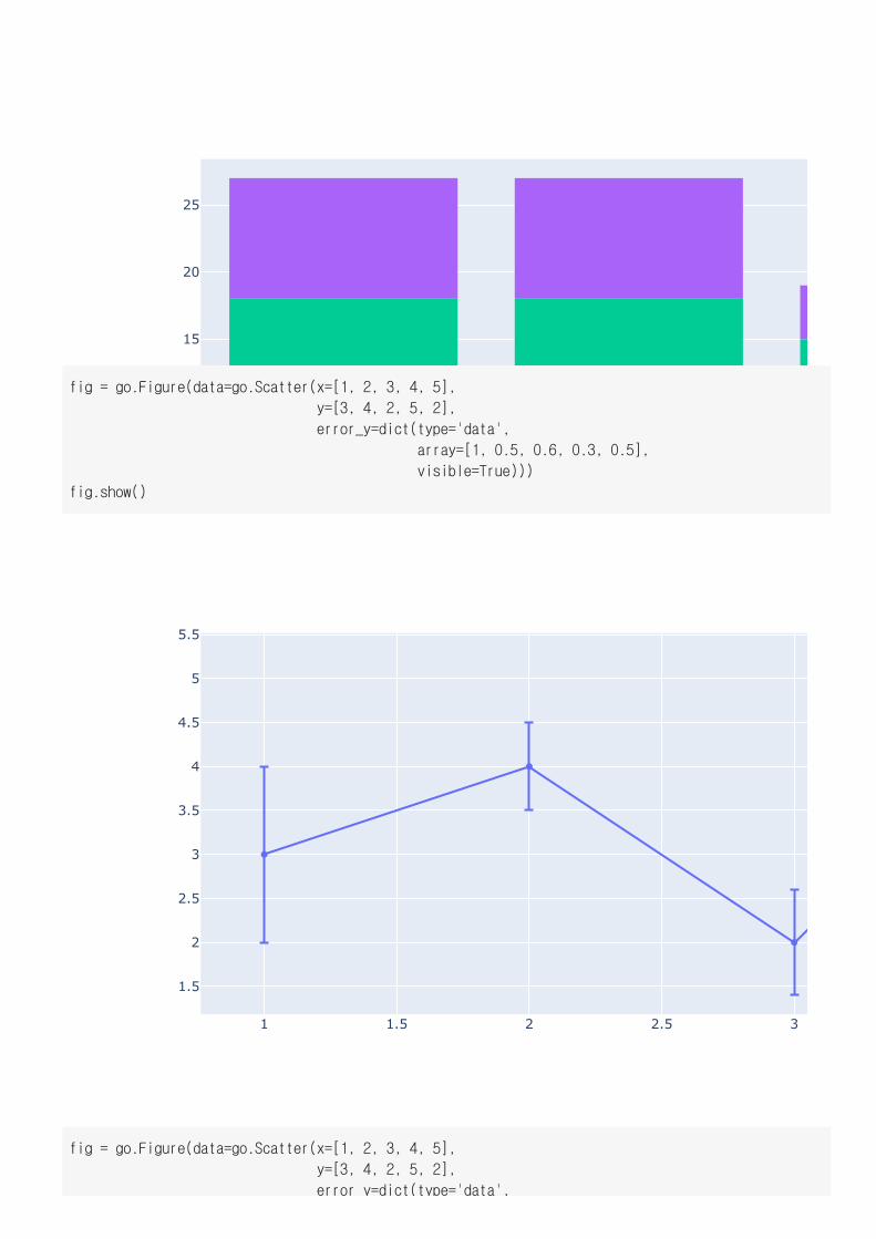
fig = go.Figure(data=go.Scatter(x=[1, 2, 3, 4, 5],
y=[3, 4, 2, 5, 2],
error_y=dict(type='data',
array=[1, 0.5, 0.6, 0.3, 0.5],
visible=True)))
fig.show()
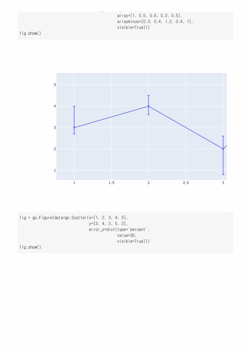
fig = go.Figure(data=go.Scatter(x=[1, 2, 3, 4, 5],
y=[3, 4, 2, 5, 2],
error_y=dict(type='data',
1 1.5 2 2.5 3
1
2
3
4
5
_y ( yp ,
array=[1, 0.5, 0.6, 0.3, 0.5],
arrayminus=[0.3, 0.4, 1.2, 0.4, 1],
visible=True)))
fig.show()
fig = go.Figure(data=go.Scatter(x=[1, 2, 3, 4, 5],
y=[3, 4, 2, 5, 2],
error_y=dict(type='percent',
value=30,
visible=True)))
fig.show()
1 1.5 2 2.5 3
2
3
4
5
6
1 1.5 2 2.5 31.5
2
2.5
3
3.5
4
4.5
5
5.5
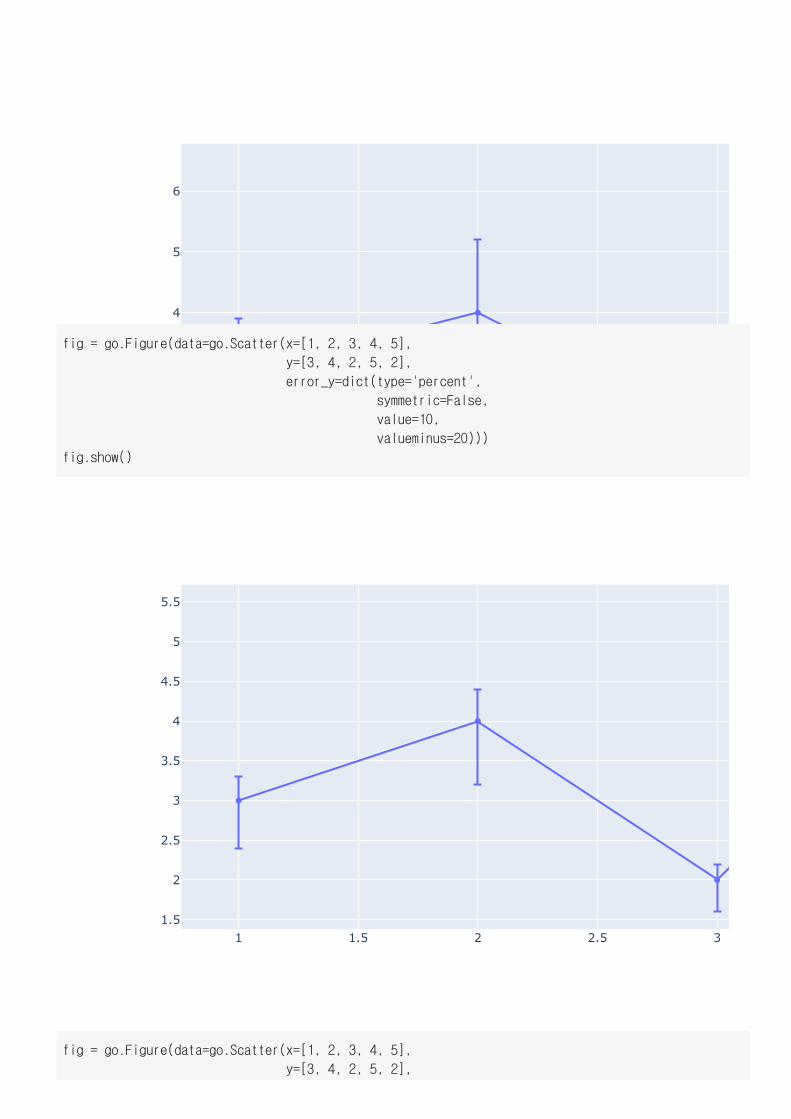
fig = go.Figure(data=go.Scatter(x=[1, 2, 3, 4, 5],
y=[3, 4, 2, 5, 2],
error_y=dict(type='percent',
symmetric=False,
value=10,
valueminus=20)))
fig.show()
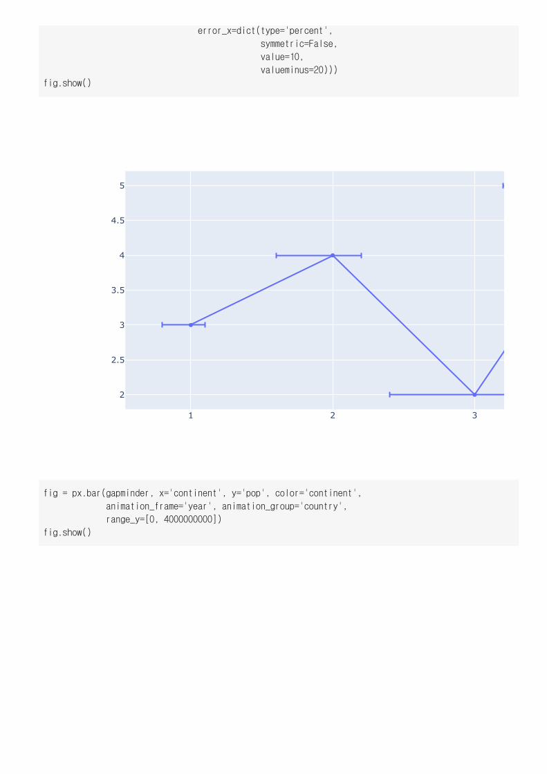
fig = go.Figure(data=go.Scatter(x=[1, 2, 3, 4, 5],
y=[3, 4, 2, 5, 2],
1 2 3
2
2.5
3
3.5
4
4.5
5
error_x=dict(type='percent',
symmetric=False,
value=10,
valueminus=20)))
fig.show()
fig = px.bar(gapminder, x='continent', y='pop', color='continent',
animation_frame='year', animation_group='country',
range_y=[0, 4000000000])
fig.show()
Asia Europe Africa0
0.5B
1B
1.5B
2B
2.5B
3B
3.5B
4B
year=1952
1952 1957 1962 1967 1972 1977
continent
pop
▶ ◼
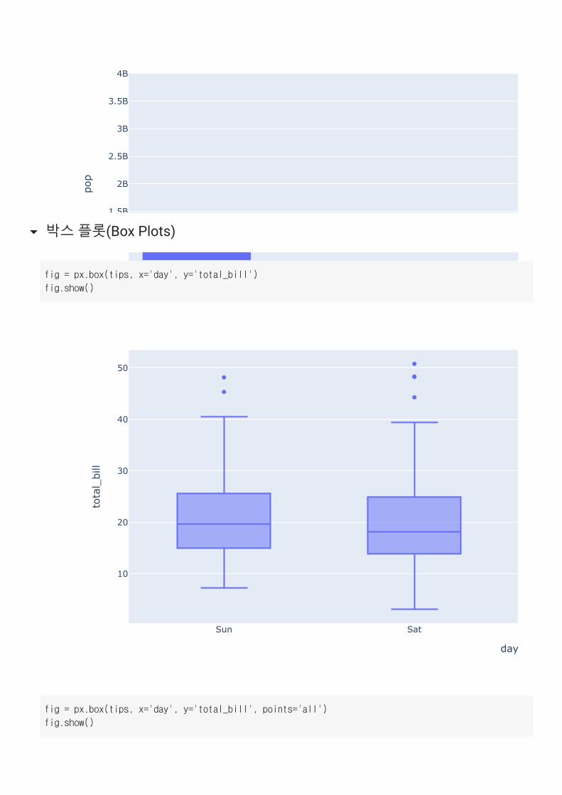
박스 플롯(Box Plots)
Sun Sat
10
20
30
40
50
day
total_bill
fig = px.box(tips, x='day', y='total_bill')
fig.show()
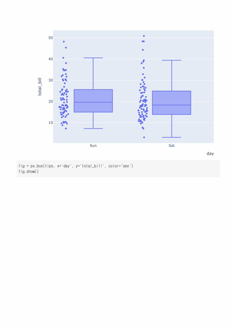
fig = px.box(tips, x='day', y='total_bill', points='all')
fig.show()
Sun Sat
10
20
30
40
50
day
total_bill
fig = px.box(tips, x='day', y='total_bill', color='sex')
fig.show()
Sun Sat
10
20
30
40
50
day
total_bill
Sun Sat
10
20
30
40
50
day
total_bill
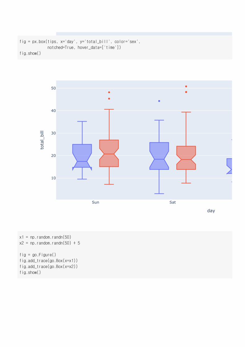
fig = px.box(tips, x='day', y='total_bill', color='sex',
notched=True, hover_data=['time'])
fig.show()
x1 = np.random.randn(50)
x2 = np.random.randn(50) + 5
fig = go.Figure()
fig.add_trace(go.Box(x=x1))
fig.add_trace(go.Box(x=x2))
fig.show()
−2 −1 0 1 2
trace 0
trace 1
−2 −1 0 1 2
trace 0
trace 1
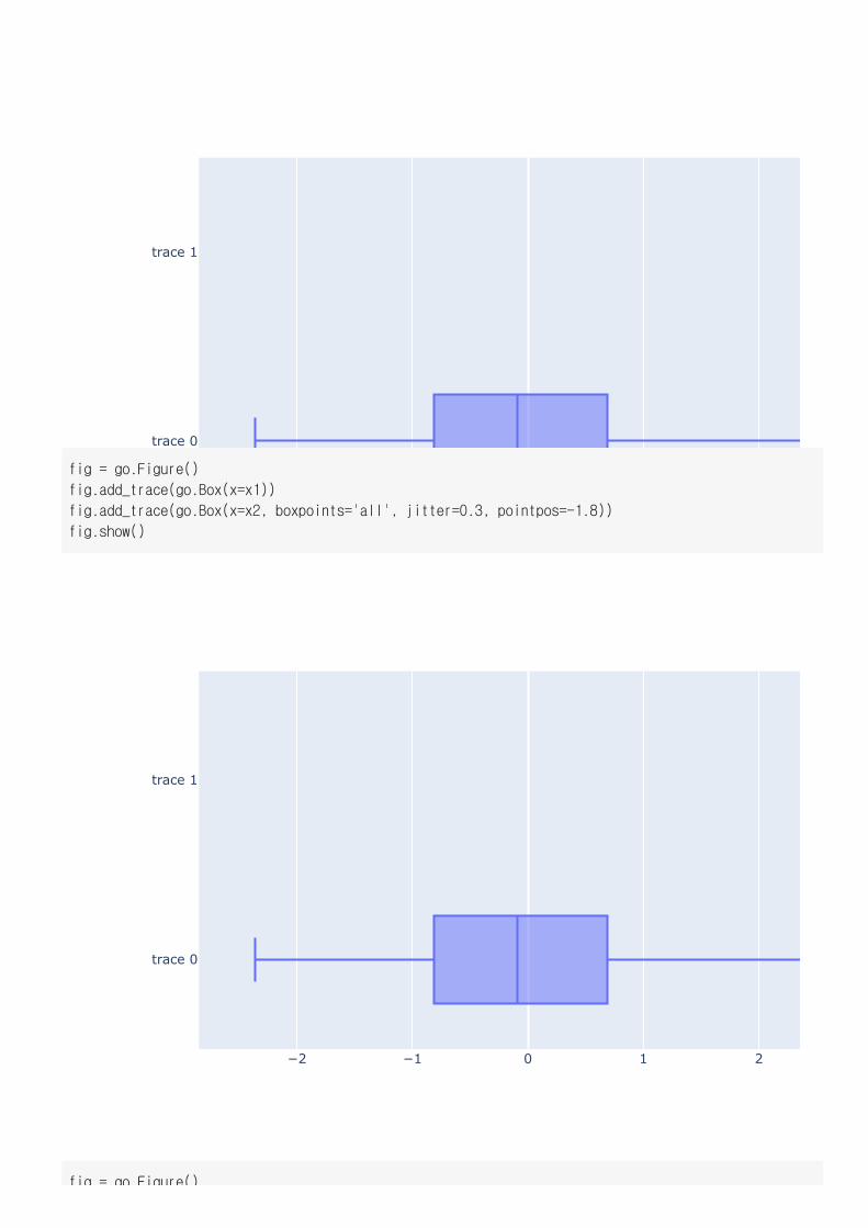
fig = go.Figure()
fig.add_trace(go.Box(x=x1))
fig.add_trace(go.Box(x=x2, boxpoints='all', jitter=0.3, pointpos=-1.8))
fig.show()
fig = go.Figure()
−2 −1 0 1 2
trace 0
trace 1
fig go.Figure()
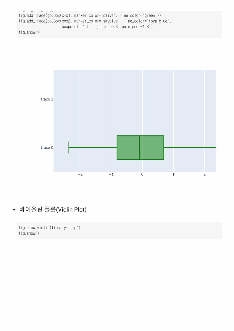
fig.add_trace(go.Box(x=x1, marker_color='olive', line_color='green'))
fig.add_trace(go.Box(x=x2, marker_color='skyblue', line_color='royalblue',
boxpoints='all', jitter=0.3, pointpos=-1.8))
fig.show()
바이올린 플롯(Violin Plot)
fig = px.violin(tips, y='tip')
fig.show()
0
2
4
6
8
10tip
0
2
4
6
8
10
tip
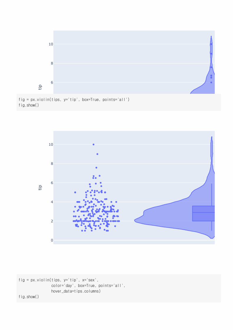
fig = px.violin(tips, y='tip', box=True, points='all')
fig.show()
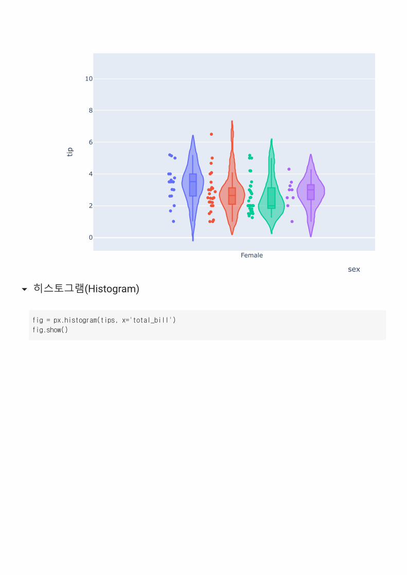
fig = px.violin(tips, y='tip', x='sex',
color='day', box=True, points='all',
hover_data=tips.columns)
fig.show()
Female
0
2
4
6
8
10
sex
tip
히스토그램(Histogram)
fig = px.histogram(tips, x='total_bill')
fig.show()
10 200
5
10
15
20
25
30
total_b
coun
t
0 10 200
10
20
30
40
50
60
70
total_b
coun
t
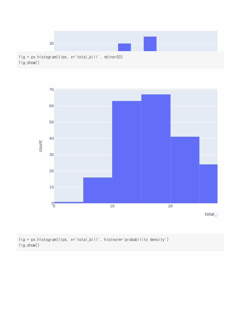
fig = px.histogram(tips, x='total_bill', nbins=20)
fig.show()
fig = px.histogram(tips, x='total_bill', histnorm='probability density')
fig.show()
10 200
0.01
0.02
0.03
0.04
0.05
0.06
total_b
coun
t
10 209
1
2
3
4
5
6
789
10
2
3
Total B
coun
t
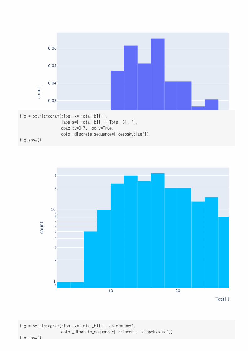
fig = px.histogram(tips, x='total_bill',
labels={'total_bill':'Total Bill'},
opacity=0.7, log_y=True,
color_discrete_sequence=['deepskyblue'])
fig.show()
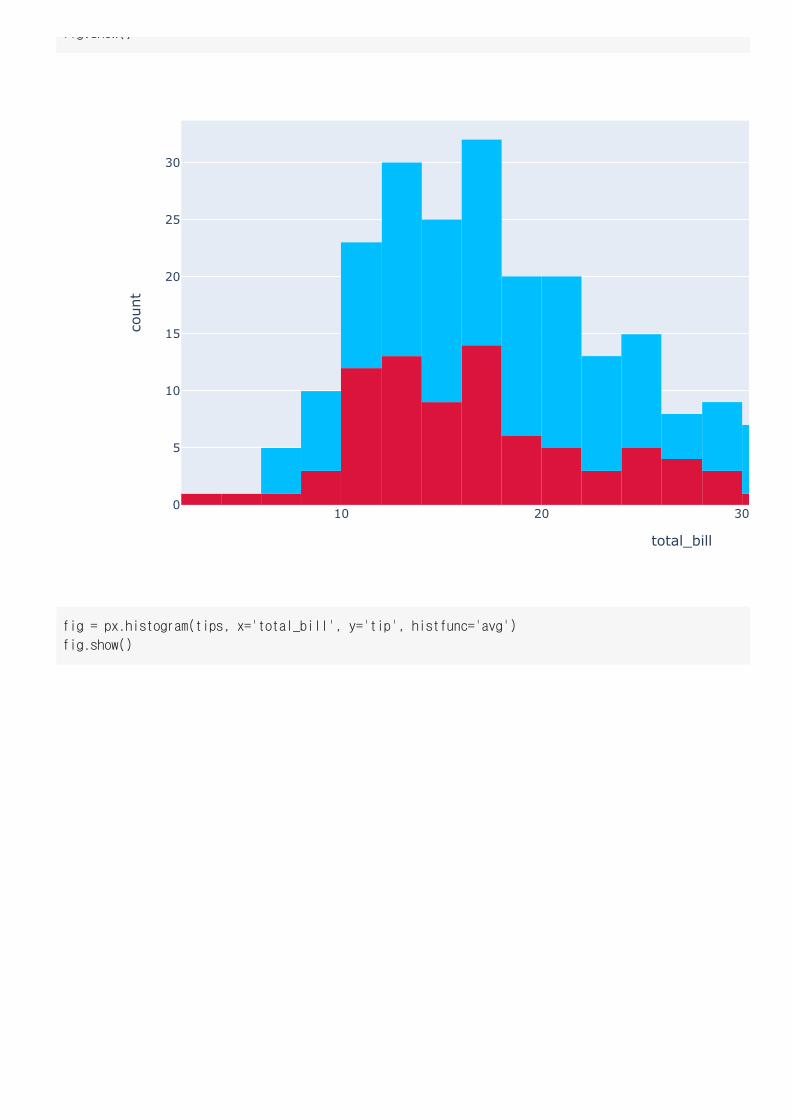
fig = px.histogram(tips, x='total_bill', color='sex',
color_discrete_sequence=['crimson', 'deepskyblue'])
fig.show()
10 20 300
5
10
15
20
25
30
total_bill
coun
t
fig.show()
fig = px.histogram(tips, x='total_bill', y='tip', histfunc='avg')
fig.show()
10 200
2
4
6
8
10
total_b
avg
of t
ip
10 200
5
10
15
20
25
30
total_bill
coun
t
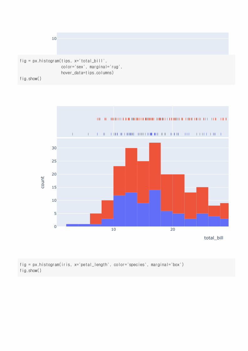
fig = px.histogram(tips, x='total_bill',
color='sex', marginal='rug',
hover_data=tips.columns)
fig.show()
fig = px.histogram(iris, x='petal_length', color='species', marginal='box')
fig.show()
1 2 3 40
10
20
30
40
petal_length
coun
t
40 50 600
10
20
30
40
lifeExp
coun
t
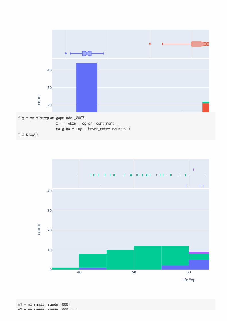
fig = px.histogram(gapminder_2007,
x='lifeExp', color='continent',
marginal='rug', hover_name='country')
fig.show()
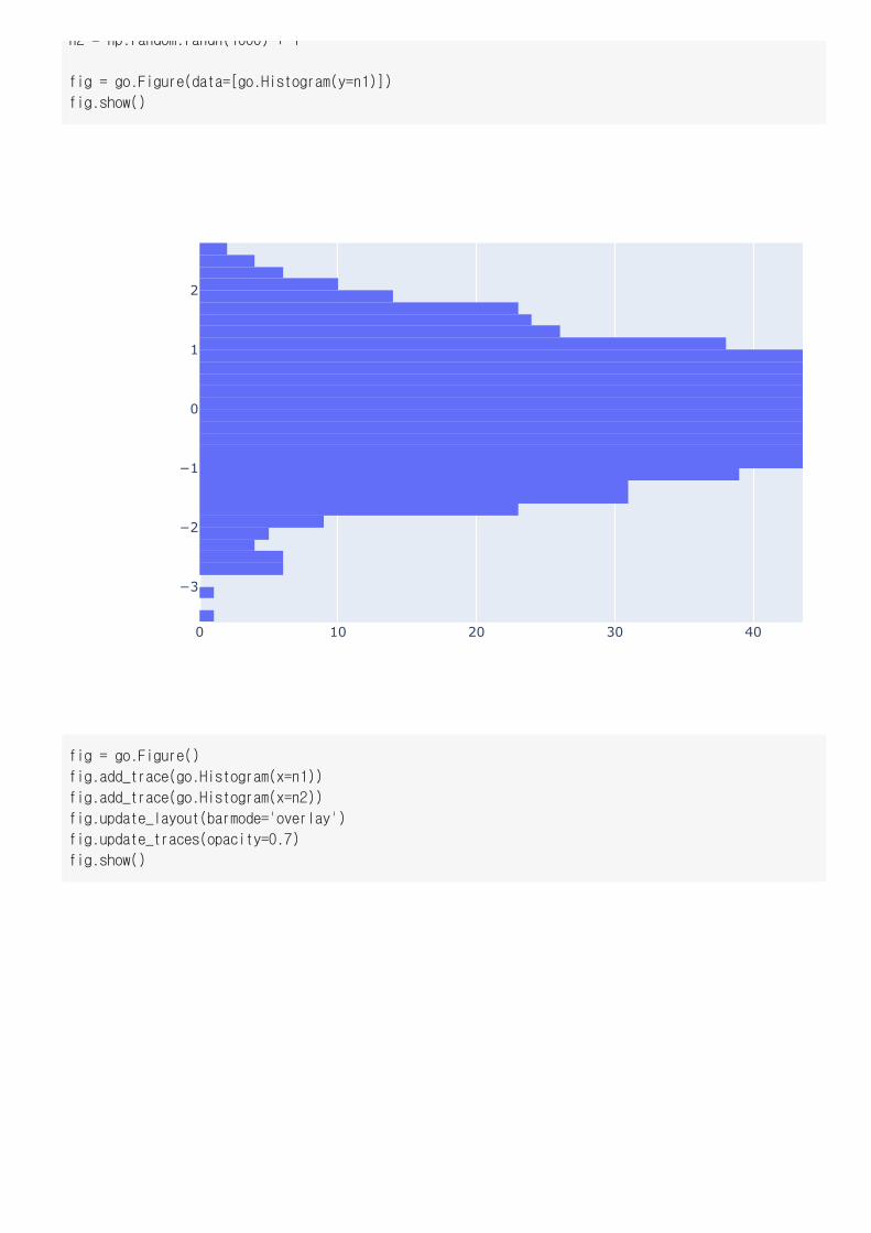
n1 = np.random.randn(1000)
n2 = np random randn(1000) + 1
0 10 20 30 40
−3
−2
−1
0
1
2
n2 = np.random.randn(1000) + 1
fig = go.Figure(data=[go.Histogram(y=n1)])
fig.show()
fig = go.Figure()
fig.add_trace(go.Histogram(x=n1))
fig.add_trace(go.Histogram(x=n2))
fig.update_layout(barmode='overlay')
fig.update_traces(opacity=0.7)
fig.show()
−3 −2 −1 00
10
20
30
40
50
60
70
80
−3 −2 −1 00
20
40
60
80
100
120
140
160
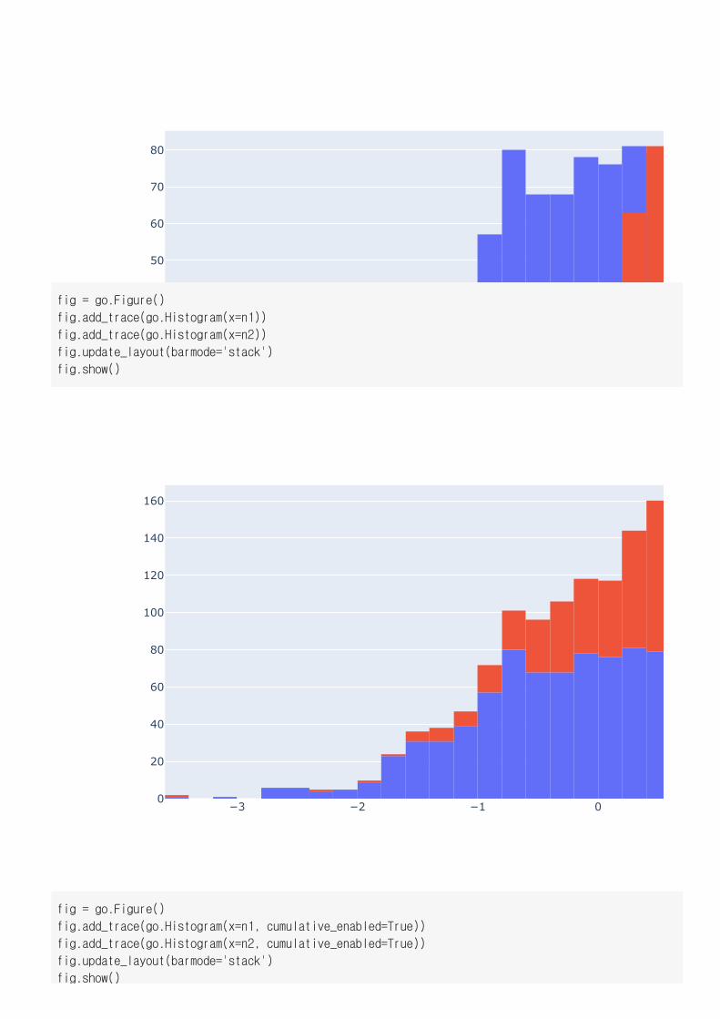
fig = go.Figure()
fig.add_trace(go.Histogram(x=n1))
fig.add_trace(go.Histogram(x=n2))
fig.update_layout(barmode='stack')
fig.show()
fig = go.Figure()
fig.add_trace(go.Histogram(x=n1, cumulative_enabled=True))
fig.add_trace(go.Histogram(x=n2, cumulative_enabled=True))
fig.update_layout(barmode='stack')
fig.show()
−3 −2 −1 00
500
1000
1500
2000
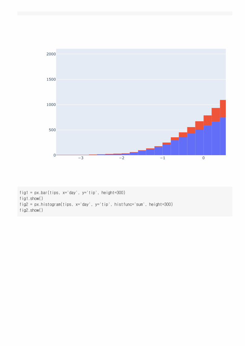
fig1 = px.bar(tips, x='day', y='tip', height=300)
fig1.show()
fig2 = px.histogram(tips, x='day', y='tip', histfunc='sum', height=300)
fig2.show()
Sun Sat0
100
200
day
tip
Sun Sat0
100
200
day
sum
of
tip
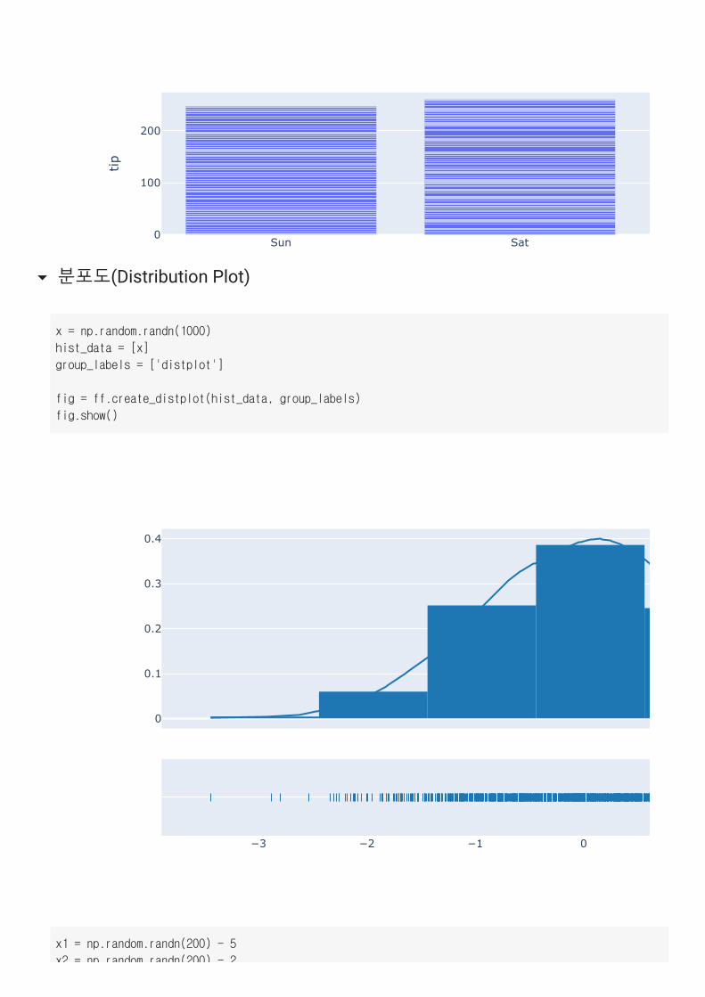
분포도(Distribution Plot)
0
0.1
0.2
0.3
0.4
−3 −2 −1 0
x = np.random.randn(1000)
hist_data = [x]
group_labels = ['distplot']
fig = ff.create_distplot(hist_data, group_labels)
fig.show()
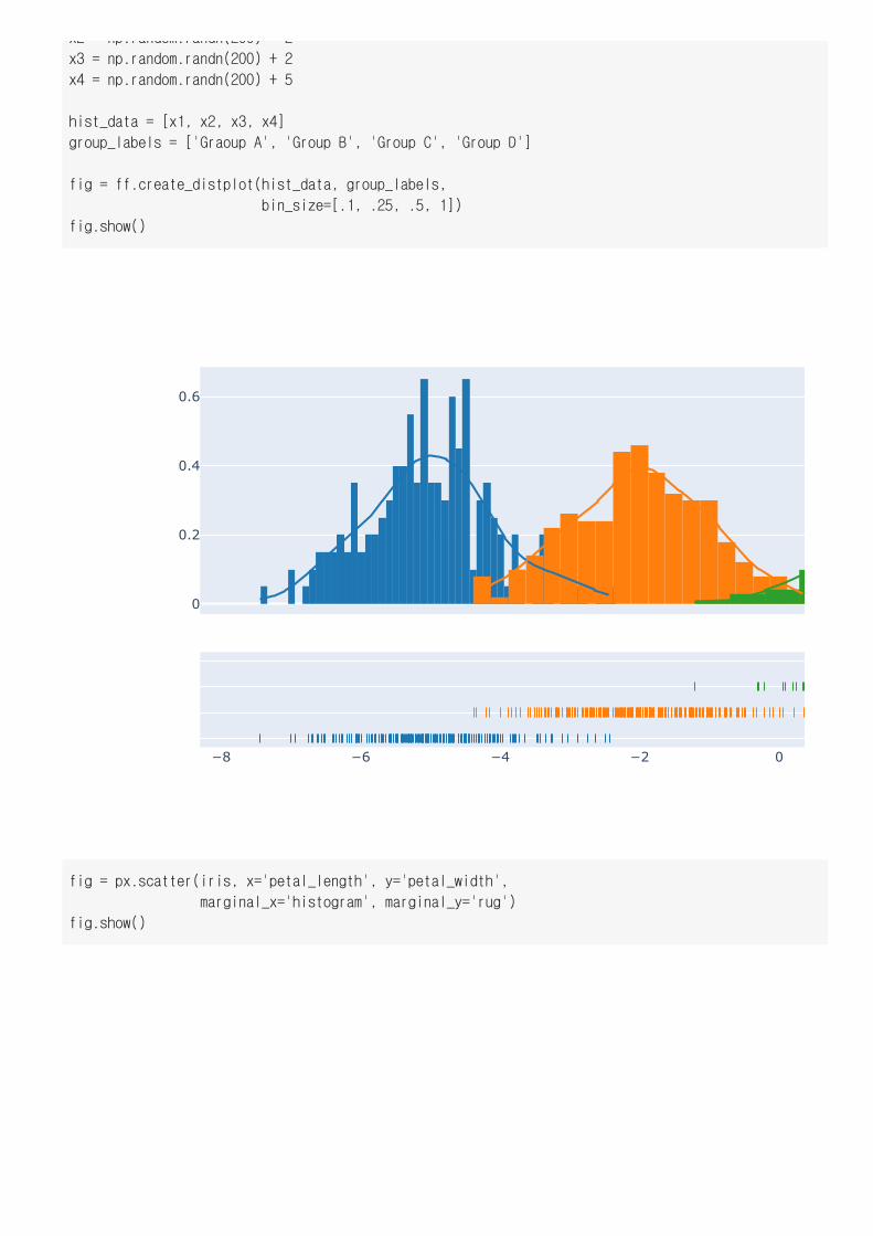
x1 = np.random.randn(200) - 5
x2 = np random randn(200) - 2
0
0.2
0.4
0.6
−8 −6 −4 −2 0
x2 np.random.randn(200) 2
x3 = np.random.randn(200) + 2
x4 = np.random.randn(200) + 5
hist_data = [x1, x2, x3, x4]
group_labels = ['Graoup A', 'Group B', 'Group C', 'Group D']
fig = ff.create_distplot(hist_data, group_labels,
bin_size=[.1, .25, .5, 1])
fig.show()
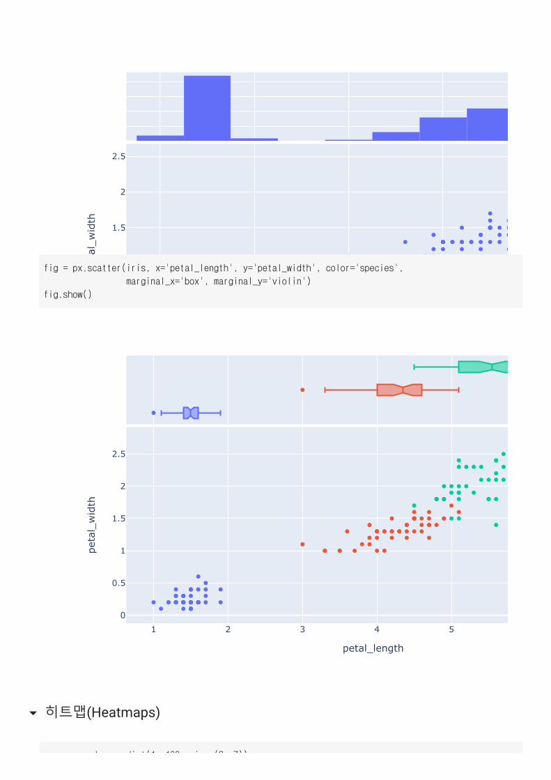
fig = px.scatter(iris, x='petal_length', y='petal_width',
marginal_x='histogram', marginal_y='rug')
fig.show()
1 2 3 40
0.5
1
1.5
2
2.5
petal_length
petal_width
1 2 3 4 50
0.5
1
1.5
2
2.5
petal_length
petal_width
fig = px.scatter(iris, x='petal_length', y='petal_width', color='species',
marginal_x='box', marginal_y='violin')
fig.show()
히트맵(Heatmaps)
n np random randint(1 100 size (3 7))
0 1 2 3−0.5
0
0.5
1
1.5
2
2.5
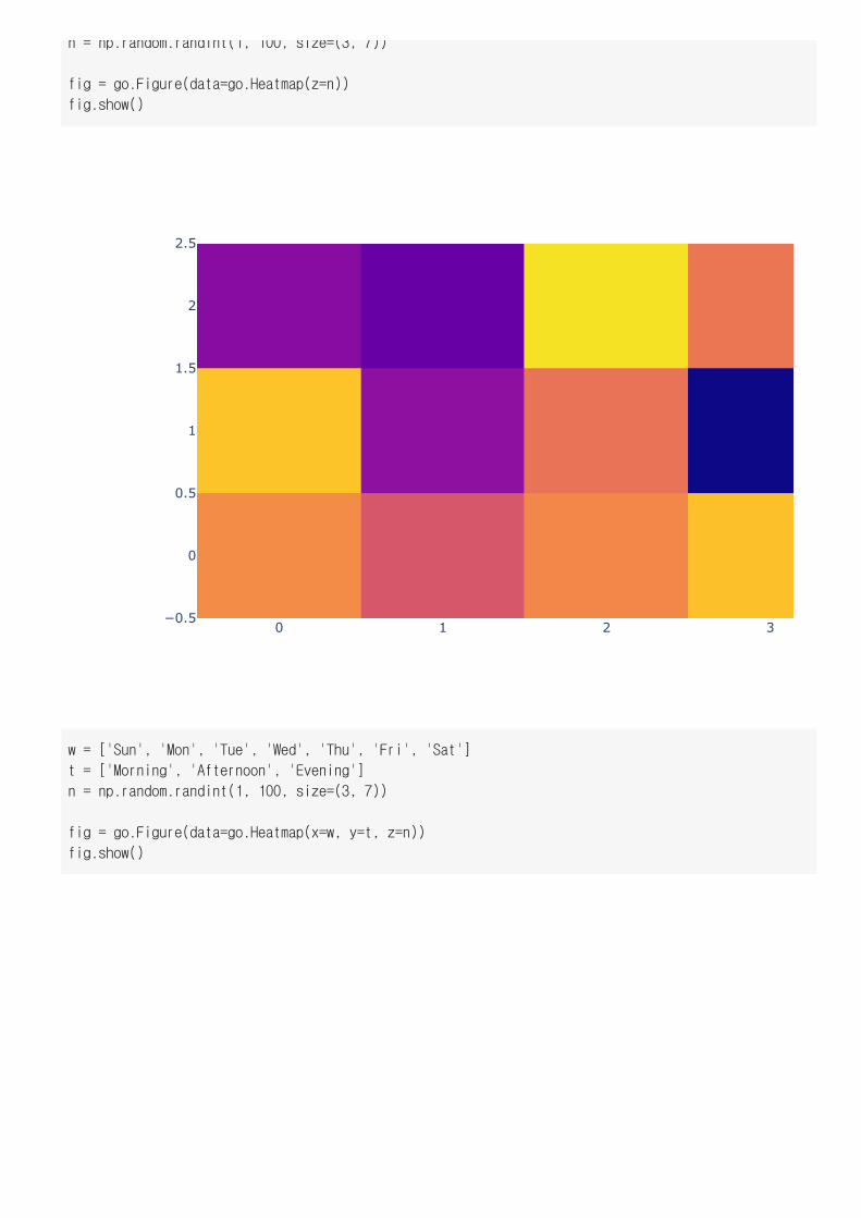
n = np.random.randint(1, 100, size=(3, 7))
fig = go.Figure(data=go.Heatmap(z=n))
fig.show()
w = ['Sun', 'Mon', 'Tue', 'Wed', 'Thu', 'Fri', 'Sat']
t = ['Morning', 'Afternoon', 'Evening']
n = np.random.randint(1, 100, size=(3, 7))
fig = go.Figure(data=go.Heatmap(x=w, y=t, z=n))
fig.show()
Sun Mon Tue Wed
Morning
Afternoon
Evening
Sun Mon Tue Wed
Morning
Afternoon
Evening
78 91 56 49
33 51 77 9
80 85 34 25
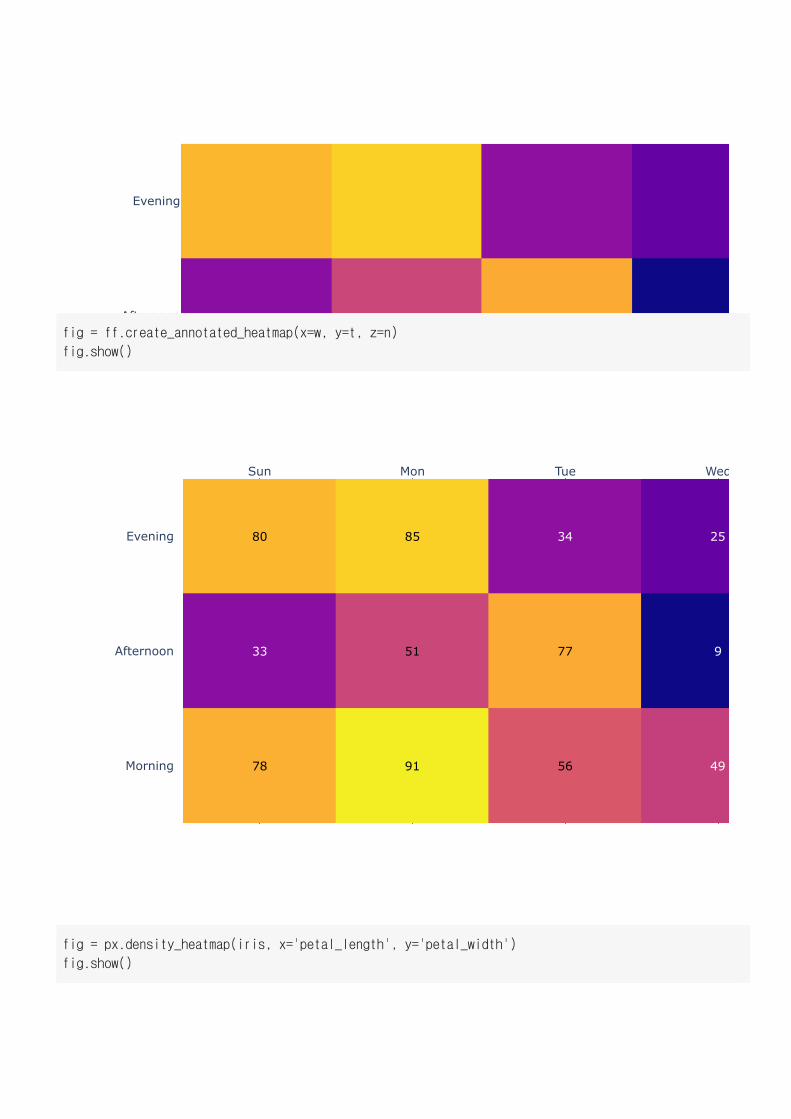
fig = ff.create_annotated_heatmap(x=w, y=t, z=n)
fig.show()
fig = px.density_heatmap(iris, x='petal_length', y='petal_width')
fig.show()
0 1 2 3 4
0
0.5
1
1.5
2
2.5
petal_length
petal_width
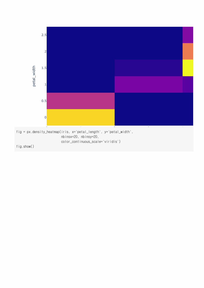
fig = px.density_heatmap(iris, x='petal_length', y='petal_width',
nbinsx=20, nbinsy=20,
color_continuous_scale='viridis')
fig.show()
1 2 3 40
0.5
1
1.5
2
2.5
petal_length
petal_width
1 2 3 4 50
0.5
1
1.5
2
2.5
petal_length
petal_width
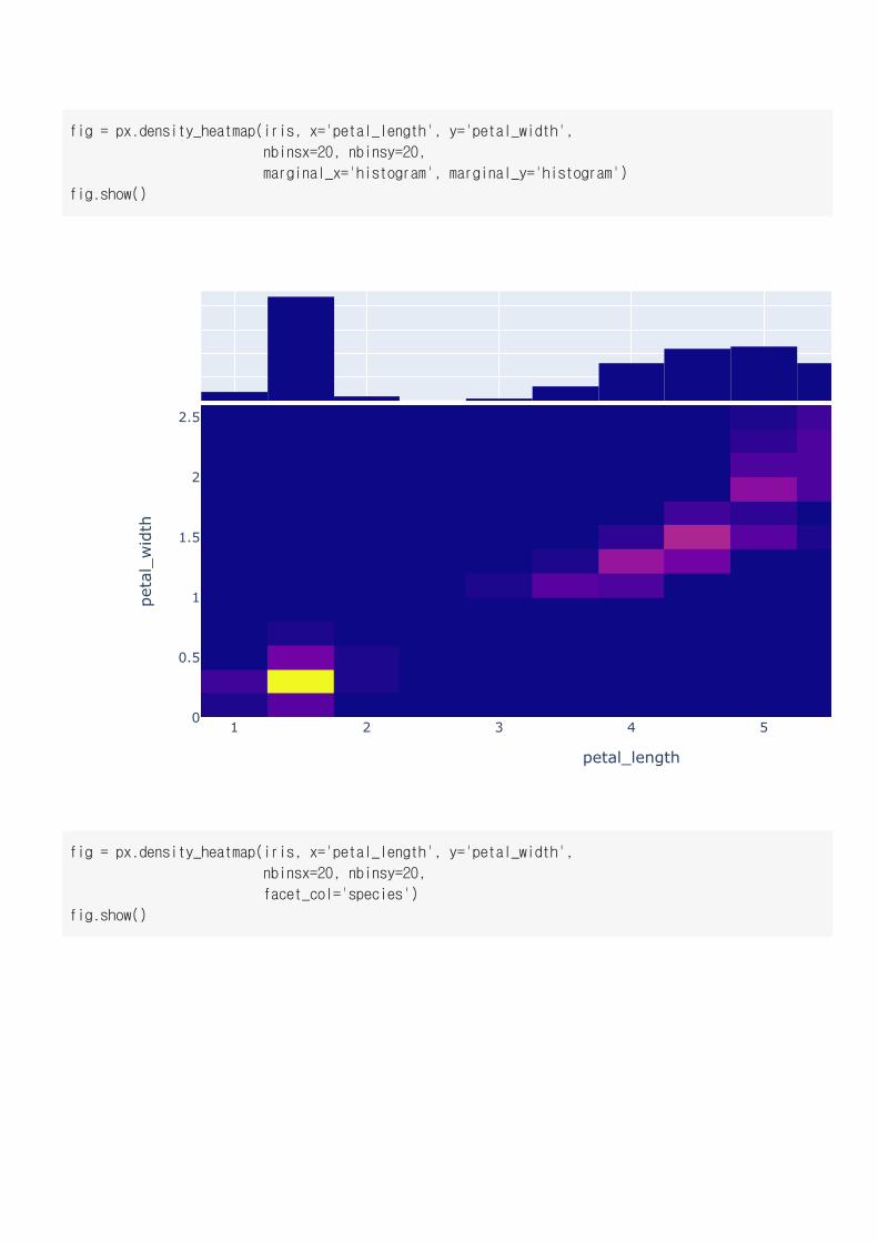
fig = px.density_heatmap(iris, x='petal_length', y='petal_width',
nbinsx=20, nbinsy=20,
marginal_x='histogram', marginal_y='histogram')
fig.show()
fig = px.density_heatmap(iris, x='petal_length', y='petal_width',
nbinsx=20, nbinsy=20,
facet_col='species')
fig.show()
2 4 60
0.5
1
1.5
2
2.5
2 4
petal_length petal_len
petal_width
species=setosa species=vers
0 1 2 3 4
0
0.5
1
1.5
2
2.5
petal_length
petal_width
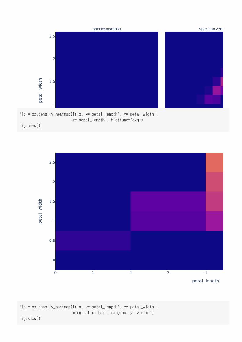
fig = px.density_heatmap(iris, x='petal_length', y='petal_width',
z='sepal_length', histfunc='avg')
fig.show()
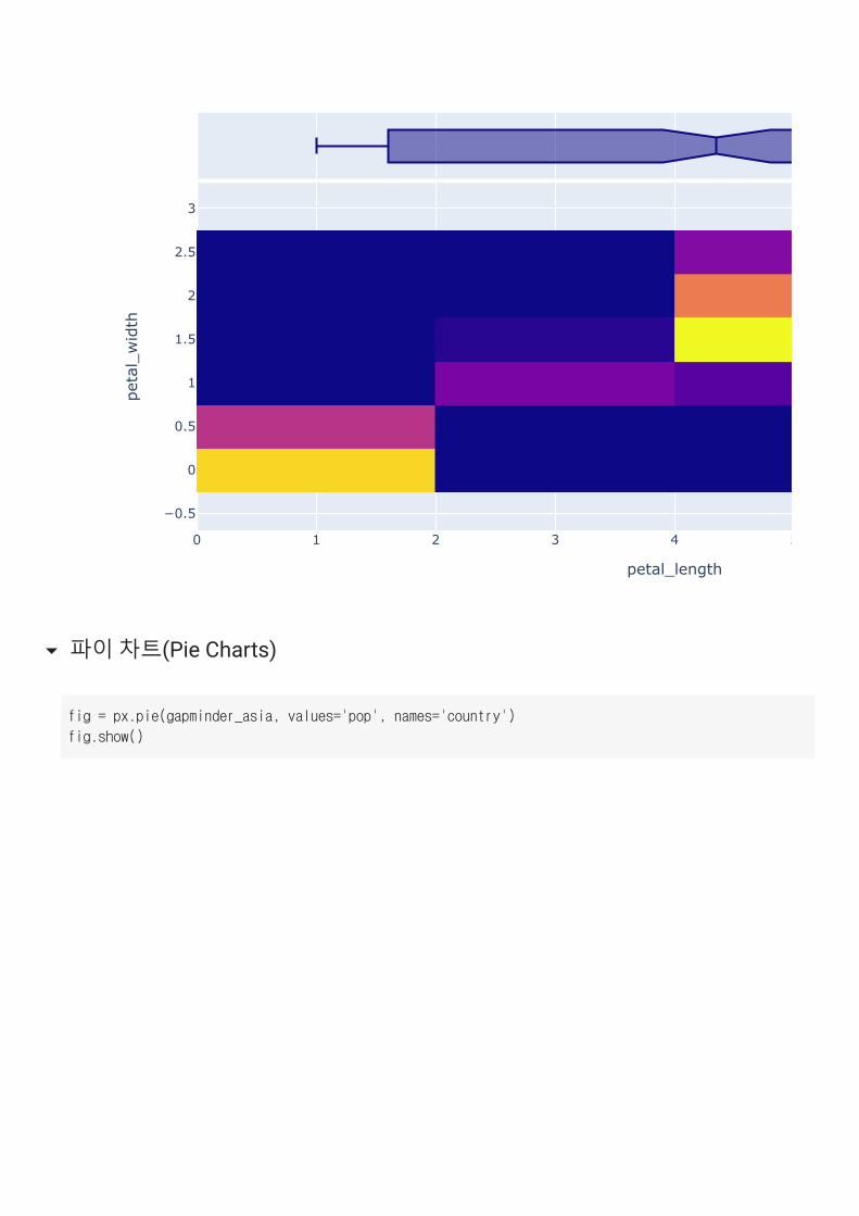
fig = px.density_heatmap(iris, x='petal_length', y='petal_width',
marginal_x='box', marginal_y='violin')
fig.show()
0 1 2 3 4 5
−0.5
0
0.5
1
1.5
2
2.5
3
petal_length
petal_width
파이 차트(Pie Charts)
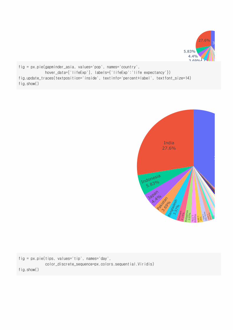
fig = px.pie(gapminder_asia, values='pop', names='country')
fig.show()
327.6%
5.83%4.4%3.69%3.57%2.15%2.07%
113
India27.6%
Indonesia
5.83%
Japan
4.4%
Pakist
an3.
69%
Bang
lade
sh3.
57%
Viet
nam
2.15
%Ph
ilipp
ines
2.07
% Thailand1.77%
Iran1.66%
Korea, Rep.
1.44%
Myanm
ar
1.32%
Taiwan
0.664%0.651%
fig = px.pie(gapminder_asia, values='pop', names='country',
hover_data=['lifeExp'], labels={'lifeExp':'life expectancy'})
fig.update_traces(textposition='inside', textinfo='percent+label', textfont_size=14)
fig.show()
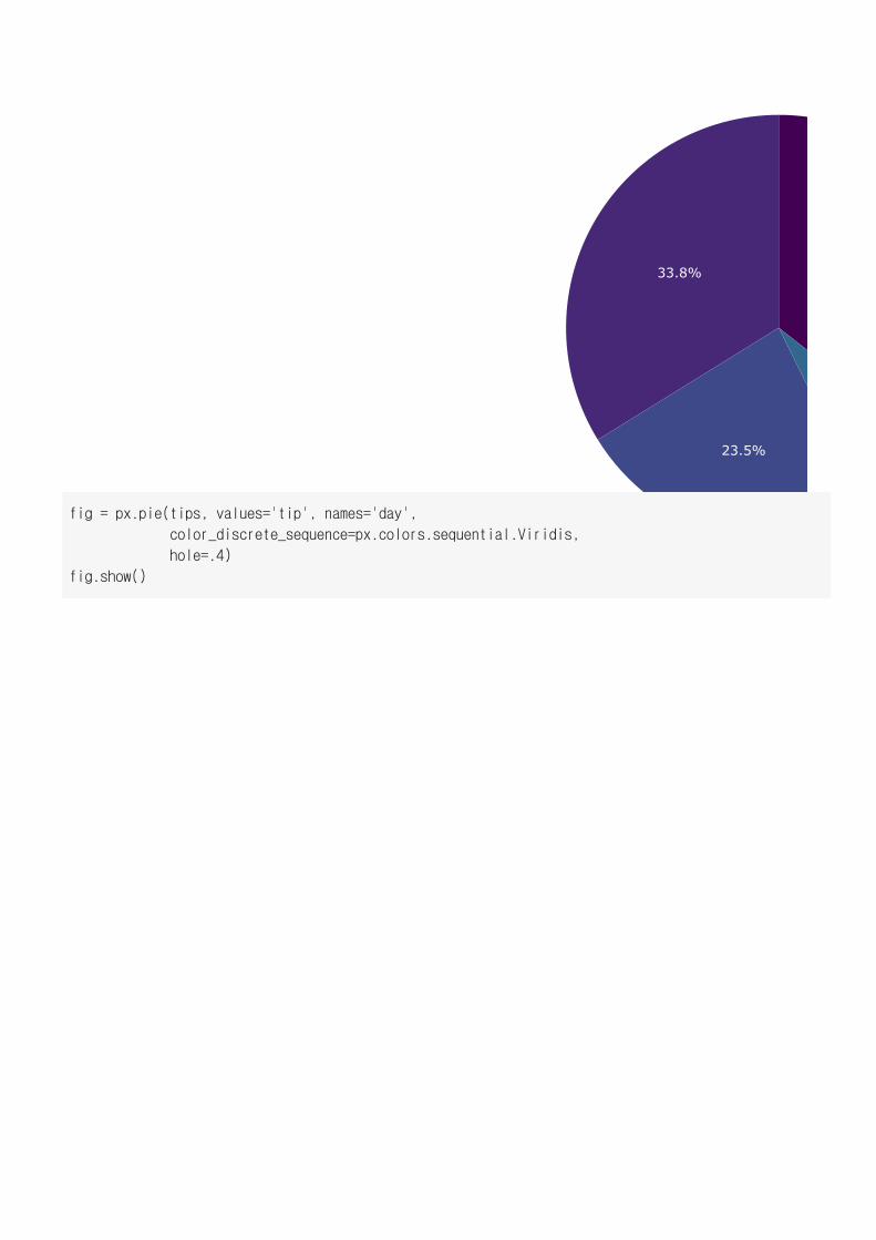
fig = px.pie(tips, values='tip', names='day',
color_discrete_sequence=px.colors.sequential.Viridis)
fig.show()
33.8%
23.5%
fig = px.pie(tips, values='tip', names='day',
color_discrete_sequence=px.colors.sequential.Viridis,
hole=.4)
fig.show()
33.8%
23.5%
247.39
171.83
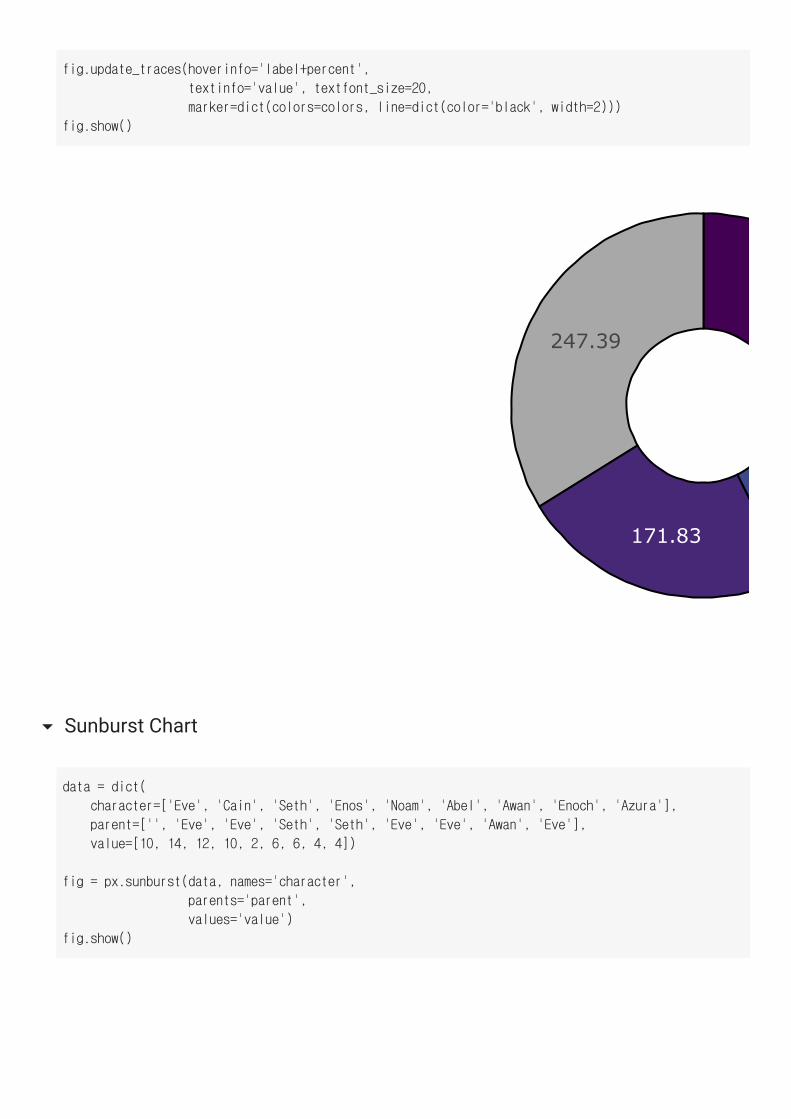
fig.update_traces(hoverinfo='label+percent',
textinfo='value', textfont_size=20,
marker=dict(colors=colors, line=dict(color='black', width=2)))
fig.show()
Sunburst Chart
data = dict(
character=['Eve', 'Cain', 'Seth', 'Enos', 'Noam', 'Abel', 'Awan', 'Enoch', 'Azura'],
parent=['', 'Eve', 'Eve', 'Seth', 'Seth', 'Eve', 'Eve', 'Awan', 'Eve'],
value=[10, 14, 12, 10, 2, 6, 6, 4, 4])
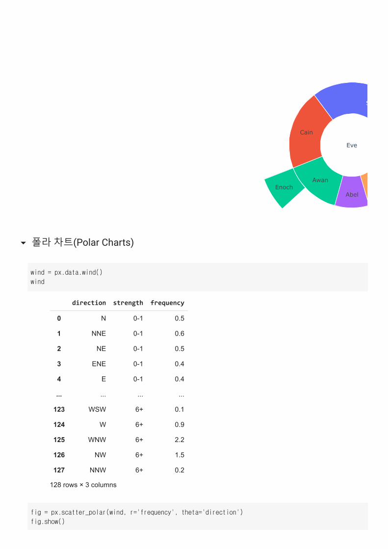
fig = px.sunburst(data, names='character',
parents='parent',
values='value')
fig.show()
Eve
S
Cain
Awan
Abel AEnoch
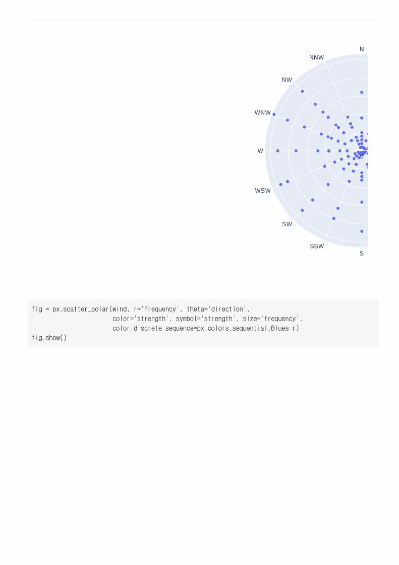
폴라 차트(Polar Charts)
direction strength frequency
0 N 0-1 0.5
1 NNE 0-1 0.6
2 NE 0-1 0.5
3 ENE 0-1 0.4
4 E 0-1 0.4
... ... ... ...
123 WSW 6+ 0.1
124 W 6+ 0.9
125 WNW 6+ 2.2
126 NW 6+ 1.5
127 NNW 6+ 0.2
128 rows × 3 columns
wind = px.data.wind()
wind
fig = px.scatter_polar(wind, r='frequency', theta='direction')
fig.show()
N
SSSW
SW
WSW
W
WNW
NW
NNW
0
fig = px.scatter_polar(wind, r='frequency', theta='direction',
color='strength', symbol='strength', size='frequency',
color_discrete_sequence=px.colors.sequential.Blues_r)
fig.show()
N
SSSW
SW
WSW
W
WNW
NW
NNW
0 0.5
N
SSSW
SW
WSW
W
WNW
NW
NNW
0 0.5
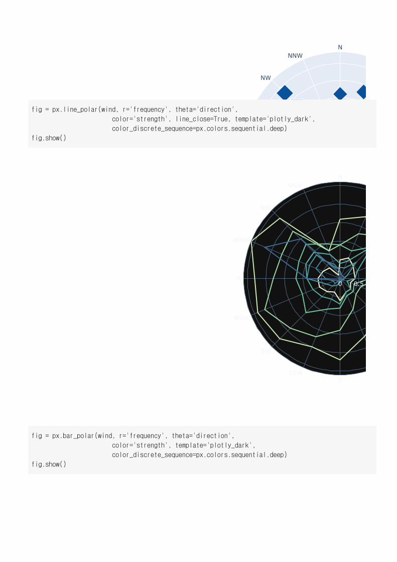
fig = px.line_polar(wind, r='frequency', theta='direction',
color='strength', line_close=True, template='plotly_dark',
color_discrete_sequence=px.colors.sequential.deep)
fig.show()
fig = px.bar_polar(wind, r='frequency', theta='direction',
color='strength', template='plotly_dark',
color_discrete_sequence=px.colors.sequential.deep)
fig.show()

N
SSSW
SW
WSW
W
WNW
NW
NNW
0 2 4
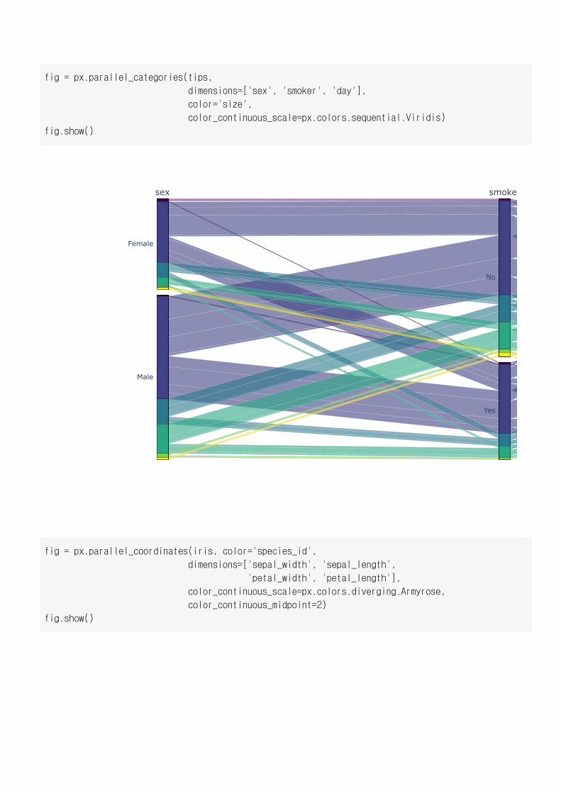
병렬 다이어그램(Parallel Diagram)
fig = px.parallel_categories(tips)
fig.show()
Female
sex
Male
No
smoker
Yes
Sun
day
Sat
Thur
Fri
Female
sex
Male
No
smoke
Yes
fig = px.parallel_categories(tips,
dimensions=['sex', 'smoker', 'day'],
color='size',
color_continuous_scale=px.colors.sequential.Viridis)
fig.show()
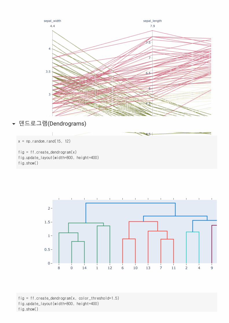
fig = px.parallel_coordinates(iris, color='species_id',
dimensions=['sepal_width', 'sepal_length',
'petal_width', 'petal_length'],
color_continuous_scale=px.colors.diverging.Armyrose,
color_continuous_midpoint=2)
fig.show()
2
2.5
3
3.5
4
sepal_width
4.4
2
4.5
5
5.5
6
6.5
7
7.5
sepal_length
7.9
4.3
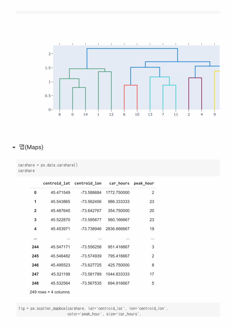
덴드로그램(Dendrograms)
8 0 14 1 12 6 10 13 7 11 2 4 90
0.5
1
1.5
2
x = np.random.rand(15, 12)
fig = ff.create_dendrogram(x)
fig.update_layout(width=800, height=400)
fig.show()
fig = ff.create_dendrogram(x, color_threshold=1.5)
fig.update_layout(width=800, height=400)
fig.show()
8 0 14 1 12 6 10 13 7 11 2 4 90
0.5
1
1.5
2
맵(Maps)
centroid_lat centroid_lon car_hours peak_hour
0 45.471549 -73.588684 1772.750000 2
1 45.543865 -73.562456 986.333333 23
2 45.487640 -73.642767 354.750000 20
3 45.522870 -73.595677 560.166667 23
4 45.453971 -73.738946 2836.666667 19
... ... ... ... ...
244 45.547171 -73.556258 951.416667 3
245 45.546482 -73.574939 795.416667 2
246 45.495523 -73.627725 425.750000 8
247 45.521199 -73.581789 1044.833333 17
248 45.532564 -73.567535 694.916667 5
249 rows × 4 columns
carshare = px.data.carshare()
carshare
fig = px.scatter_mapbox(carshare, lat='centroid_lat', lon='centroid_lon',
color='peak_hour', size='car_hours',
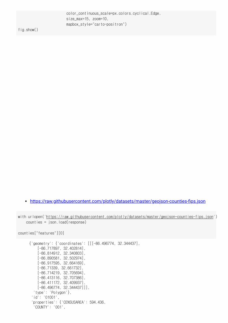
color_continuous_scale=px.colors.cyclical.Edge,
size_max=15, zoom=10,
mapbox_style="carto-positron")
fig.show()
https://raw.githubusercontent.com/plotly/datasets/master/geojson-counties-�ps.json
{'geometry': {'coordinates': [[[-86.496774, 32.344437], [-86.717897, 32.402814], [-86.814912, 32.340803], [-86.890581, 32.502974], [-86.917595, 32.664169], [-86.71339, 32.661732], [-86.714219, 32.705694], [-86.413116, 32.707386], [-86.411172, 32.409937], [-86.496774, 32.344437]]], 'type': 'Polygon'}, 'id': '01001', 'properties': {'CENSUSAREA': 594.436, 'COUNTY': '001',
with urlopen('https://raw.githubusercontent.com/plotly/datasets/master/geojson-counties-fips.json')
counties = json.load(response)
counties["features"][0]
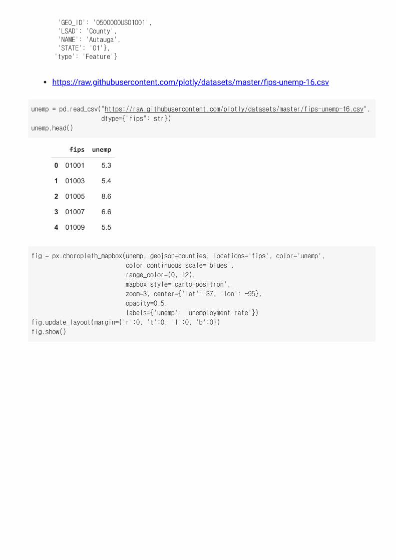
'GEO_ID': '0500000US01001', 'LSAD': 'County', 'NAME': 'Autauga', 'STATE': '01'}, 'type': 'Feature'}
https://raw.githubusercontent.com/plotly/datasets/master/�ps-unemp-16.csv
fips unemp
0 01001 5.3
1 01003 5.4
2 01005 8.6
3 01007 6.6
4 01009 5.5
unemp = pd.read_csv("https://raw.githubusercontent.com/plotly/datasets/master/fips-unemp-16.csv",
dtype={"fips": str})
unemp.head()
fig = px.choropleth_mapbox(unemp, geojson=counties, locations='fips', color='unemp',
color_continuous_scale='blues',
range_color=(0, 12),
mapbox_style='carto-positron',
zoom=3, center={'lat': 37, 'lon': -95},
opacity=0.5,
labels={'unemp': 'unemployment rate'})
fig.update_layout(margin={'r':0, 't':0, 'l':0, 'b':0})
fig.show()
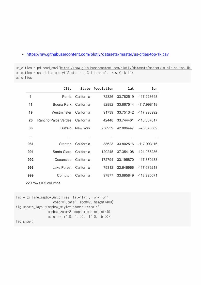
https://raw.githubusercontent.com/plotly/datasets/master/us-cities-top-1k.csv
City State Population lat lon
1 Perris California 72326 33.782519 -117.228648
11 Buena Park California 82882 33.867514 -117.998118
19 Westminster California 91739 33.751342 -117.993992
26 Rancho Palos Verdes California 42448 33.744461 -118.387017
36 Buffalo New York 258959 42.886447 -78.878369
... ... ... ... ... ...
981 Stanton California 38623 33.802516 -117.993116
991 Santa Clara California 120245 37.354108 -121.955236
992 Oceanside California 172794 33.195870 -117.379483
993 Lake Forest California 79312 33.646966 -117.689218
999 Compton California 97877 33.895849 -118.220071
229 rows × 5 columns
us_cities = pd.read_csv("https://raw.githubusercontent.com/plotly/datasets/master/us-cities-top-1k.
us_cities = us_cities.query("State in ['California', 'New York']")
us_cities
fig = px.line_mapbox(us_cities, lat='lat', lon='lon',
color='State', zoom=2, height=400)
fig.update_layout(mapbox_style='stamen-terrain',
mapbox_zoom=2, mapbox_center_lat=40,
margin={'r':0, 't':0, 'l':0, 'b':0})
fig.show()
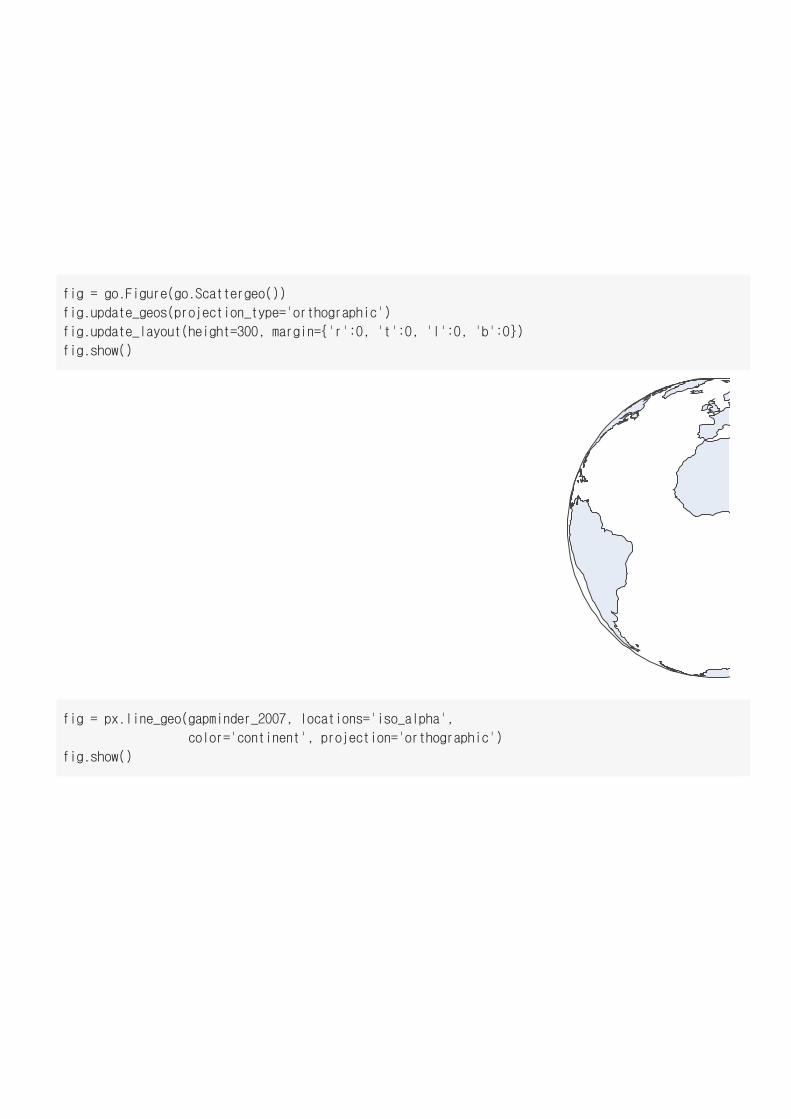
fig = go.Figure(go.Scattergeo())
fig.update_geos(projection_type='orthographic')
fig.update_layout(height=300, margin={'r':0, 't':0, 'l':0, 'b':0})
fig.show()
fig = px.line_geo(gapminder_2007, locations='iso_alpha',
color='continent', projection='orthographic')
fig.show()
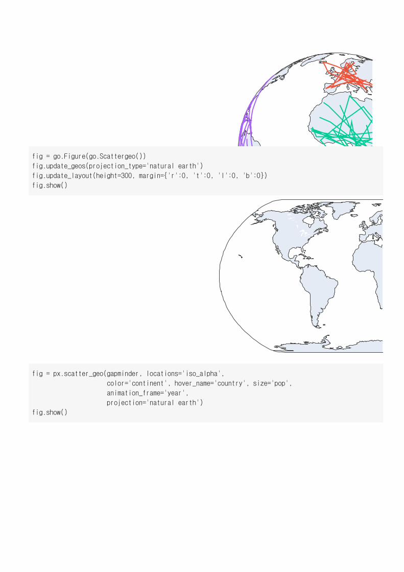
fig = go.Figure(go.Scattergeo())
fig.update_geos(projection_type='natural earth')
fig.update_layout(height=300, margin={'r':0, 't':0, 'l':0, 'b':0})
fig.show()
fig = px.scatter_geo(gapminder, locations='iso_alpha',
color='continent', hover_name='country', size='pop',
animation_frame='year',
projection='natural earth')
fig.show()
year=1952
1952 1957 1962 1967 1972 1977 198
▶ ◼
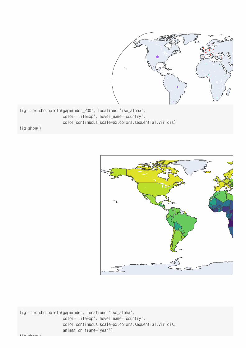
fig = px.choropleth(gapminder_2007, locations='iso_alpha',
color='lifeExp', hover_name='country',
color_continuous_scale=px.colors.sequential.Viridis)
fig.show()
fig = px.choropleth(gapminder, locations='iso_alpha',
color='lifeExp', hover_name='country',
color_continuous_scale=px.colors.sequential.Viridis,
animation_frame='year')
fig show()
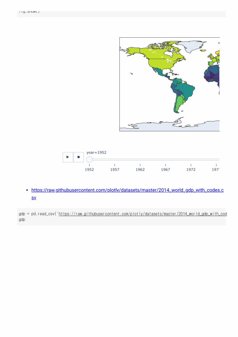
year=1952
1952 1957 1962 1967 1972 1977
▶ ◼
fig.show()
https://raw.githubusercontent.com/plotly/datasets/master/2014_world_gdp_with_codes.csv
gdp = pd.read_csv('https://raw.githubusercontent.com/plotly/datasets/master/2014_world_gdp_with_cod
gdp
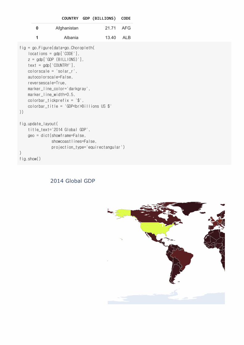
COUNTRY GDP (BILLIONS) CODE
0 Afghanistan 21.71 AFG
1 Albania 13.40 ALB
2 Algeria 227.80 DZA
3 American Samoa 0.75 ASM
4 Andorra 4.80 AND
... ... ... ...
217 Virgin Islands 5.08 VGB
218 West Bank 6.64 WBG
219 Yemen 45.45 YEM
220 Zambia 25.61 ZMB
221 Zimbabwe 13.74 ZWE
222 rows × 3 columns
2014 Global GDP
fig = go.Figure(data=go.Choropleth(
locations = gdp['CODE'],
z = gdp['GDP (BILLIONS)'],
text = gdp['COUNTRY'],
colorscale = 'solar_r',
autocolorscale=False,
reversescale=True,
marker_line_color='darkgray',
marker_line_width=0.5,
colorbar_tickprefix = '$',
colorbar_title = 'GDP<br>Billions US $'
))
fig.update_layout(
title_text='2014 Global GDP',
geo = dict(showframe=False,
showcoastlines=False,
projection_type='equirectangular')
)
fig.show()
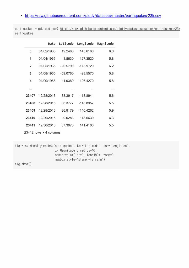
https://raw.githubusercontent.com/plotly/datasets/master/earthquakes-23k.csv
Date Latitude Longitude Magnitude
0 01/02/1965 19.2460 145.6160 6.0
1 01/04/1965 1.8630 127.3520 5.8
2 01/05/1965 -20.5790 -173.9720 6.2
3 01/08/1965 -59.0760 -23.5570 5.8
4 01/09/1965 11.9380 126.4270 5.8
... ... ... ... ...
23407 12/28/2016 38.3917 -118.8941 5.6
23408 12/28/2016 38.3777 -118.8957 5.5
23409 12/28/2016 36.9179 140.4262 5.9
23410 12/29/2016 -9.0283 118.6639 6.3
23411 12/30/2016 37.3973 141.4103 5.5
23412 rows × 4 columns
earthquakes = pd.read_csv('https://raw.githubusercontent.com/plotly/datasets/master/earthquakes-23k
earthquakes
fig = px.density_mapbox(earthquakes, lat='Latitude', lon='Longitude',
z='Magnitude', radius=10,
center=dict(lat=0, lon=180), zoom=0,
mapbox_style='stamen-terrain')
fig.show()
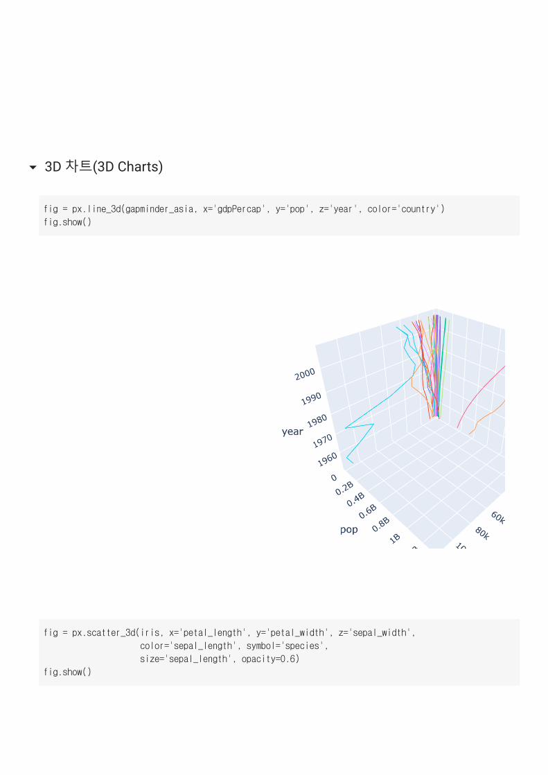
3D 차트(3D Charts)
fig = px.line_3d(gapminder_asia, x='gdpPercap', y='pop', z='year', color='country')
fig.show()
fig = px.scatter_3d(iris, x='petal_length', y='petal_width', z='sepal_width',
color='sepal_length', symbol='species',
size='sepal_length', opacity=0.6)
fig.show()
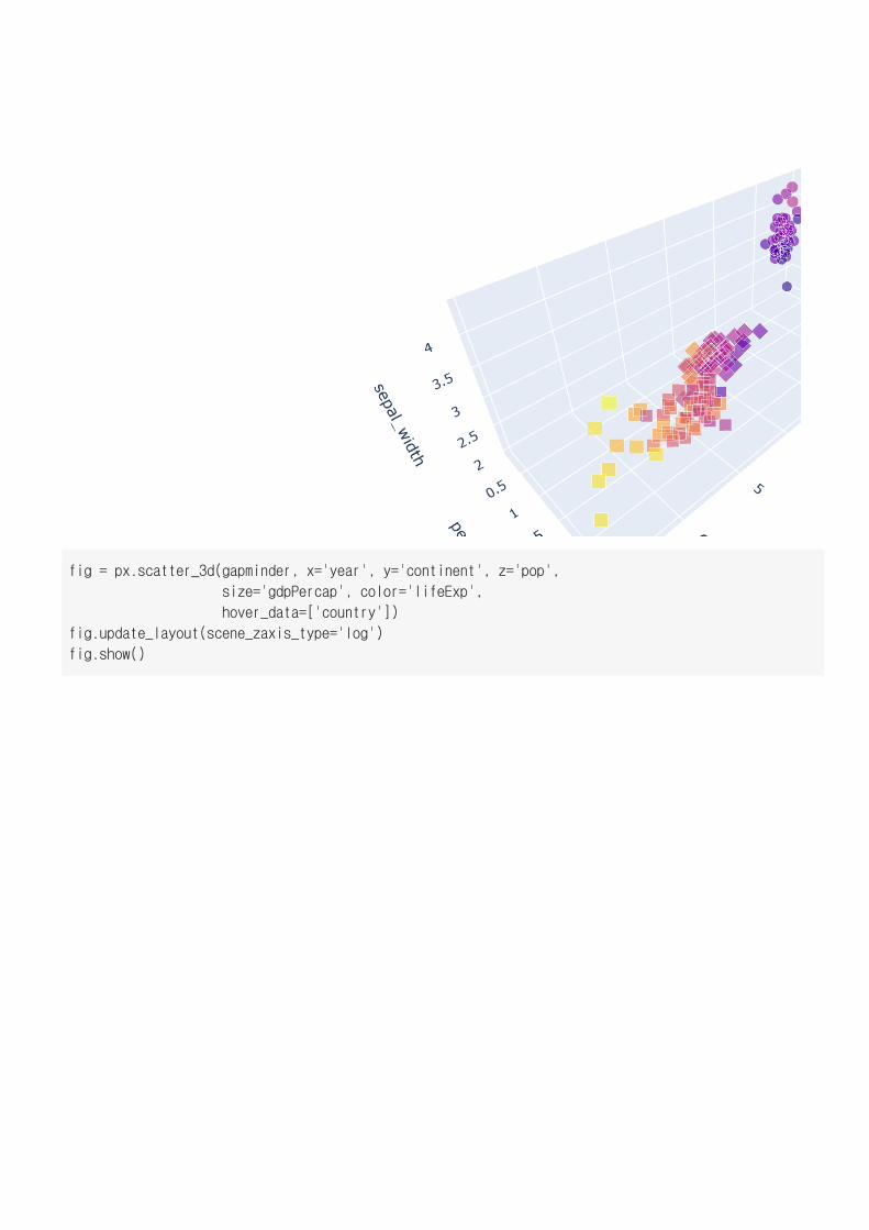
fig = px.scatter_3d(gapminder, x='year', y='continent', z='pop',
size='gdpPercap', color='lifeExp',
hover_data=['country'])
fig.update_layout(scene_zaxis_type='log')
fig.show()

간트 차트(Gantt Charts): https://plotly.com/python/gantt/테이블(Tables): https://plotly.com/python/table/생키 다이어그램(Sankey Diagram): https://plotly.com/python/sankey-diagram/트리맵(Treemap): https://plotly.com/python/treemaps/트리플롯(Tree-plots): https://plotly.com/python/tree-plots/3차 플롯(Ternary Plots): https://plotly.com/python/ternary-plots/3차 오버레이(Ternary Overlay): https://plotly.com/python/ternary-scatter-contour/3차 등고선(Ternary Contours): https://plotly.com/python/ternary-contour/이미지쇼(Image Show): https://plotly.com/python/imshow/Quiver Plots: https://plotly.com/python/quiver-plots/스트림라인 플롯(Streamline Plots): https://plotly.com/python/streamline-plots/카펫 플롯(Carpet Plots): https://plotly.com/python/carpet-plot/카펫 등고선(Carpet Contour Plot): https://plotly.com/python/carpet-contour/카펫 산점도(Carpet Scatter Plot): https://plotly.com/python/carpet-scatter/네트워크 그래프(Network Graphs): https://plotly.com/python/network-graphs/깔대기 차트(Funnel Chart): https://plotly.com/python/funnel-charts/등고선 플롯(Contour Plot): https://plotly.com/python/contour-plots/2D 히스토그램 등고선(2D Histogram Contour): https://plotly.com/python/2d-histogram-contour/Trisurf Plots: https://plotly.com/python/trisurf/3D Mesh Plots: https://plotly.com/python/3d-mesh/3D Isosurface Plots: https://plotly.com/python/3d-isosurface-plots/3D Volume Plots: https://plotly.com/python/3d-volume-plots/3D Cone Plots: https://plotly.com/python/cone-plot/3D Streamtube Plots: https://plotly.com/python/streamtube-plot/3D Camera Controls: https://plotly.com/python/3d-camera-controls/
기타 차트
Plotly 스타일
https://raw.githubusercontent.com/plotly/datasets/master/2014_usa_states.csv
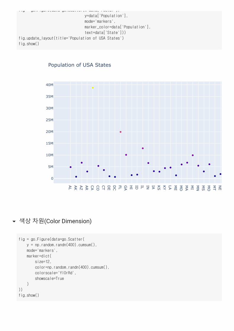
데이터 레이블(Data Label)
data = pd.read_csv('https://raw.githubusercontent.com/plotly/datasets/master/2014_usa_states.csv')
fig = go Figure(data=go Scatter(x=data['Postal']
AL
AK
AZ
AR
CA
CO
CT
DE
DC
FL GA
HI
ID IL IN IA KS
KY
LA ME
MD
MA
MI
MN
MS
MO
MT
NE
0
5M
10M
15M
20M
25M
30M
35M
40M
Population of USA States
fig go.Figure(data go.Scatter(x data[ Postal ],
y=data['Population'],
mode='markers',
marker_color=data['Population'],
text=data['State']))
fig.update_layout(title='Population of USA States')
fig.show()
색상 차원(Color Dimension)
fig = go.Figure(data=go.Scatter(
y = np.random.randn(400).cumsum(),
mode='markers',
marker=dict(
size=12,
color=np.random.randn(400).cumsum(),
colorscale='YlOrRd',
showscale=True
)
))
fig.show()
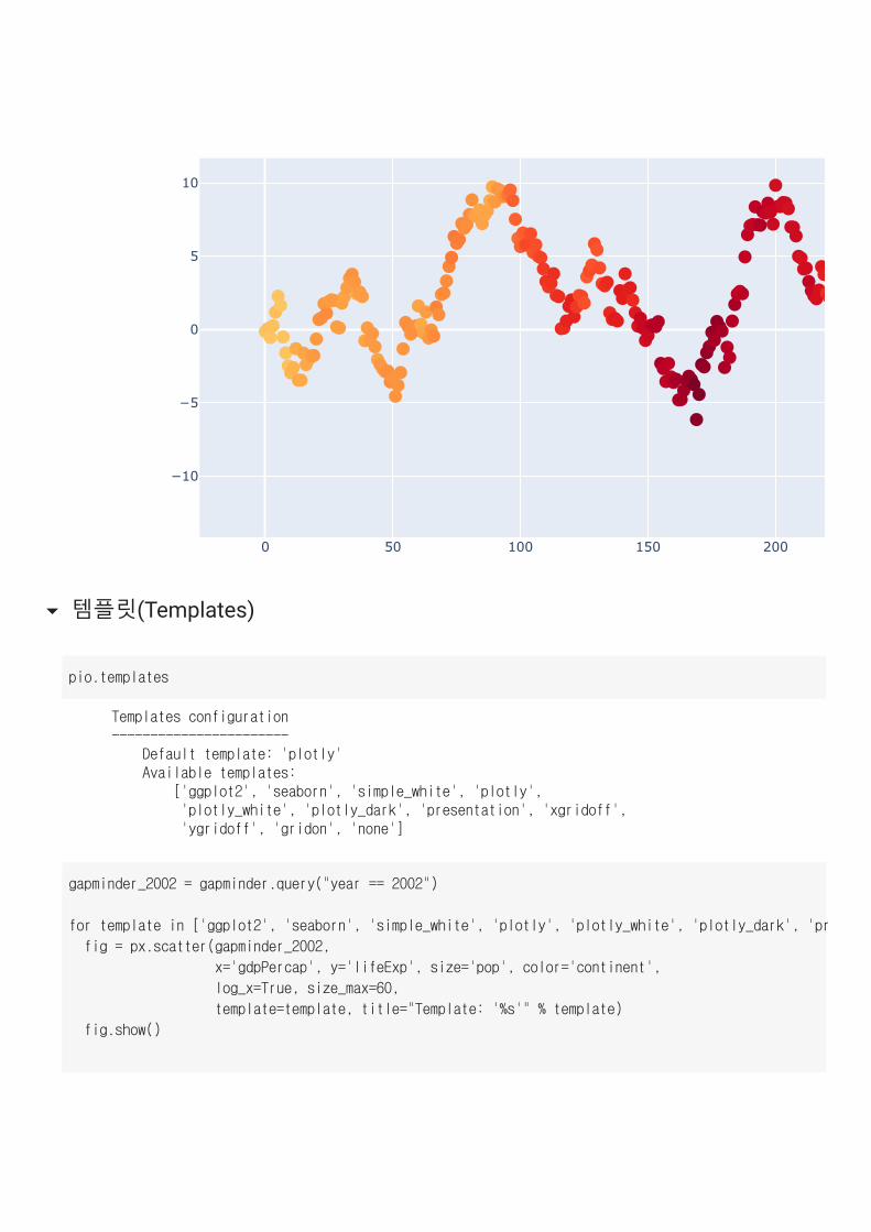
0 50 100 150 200
−10
−5
0
5
10
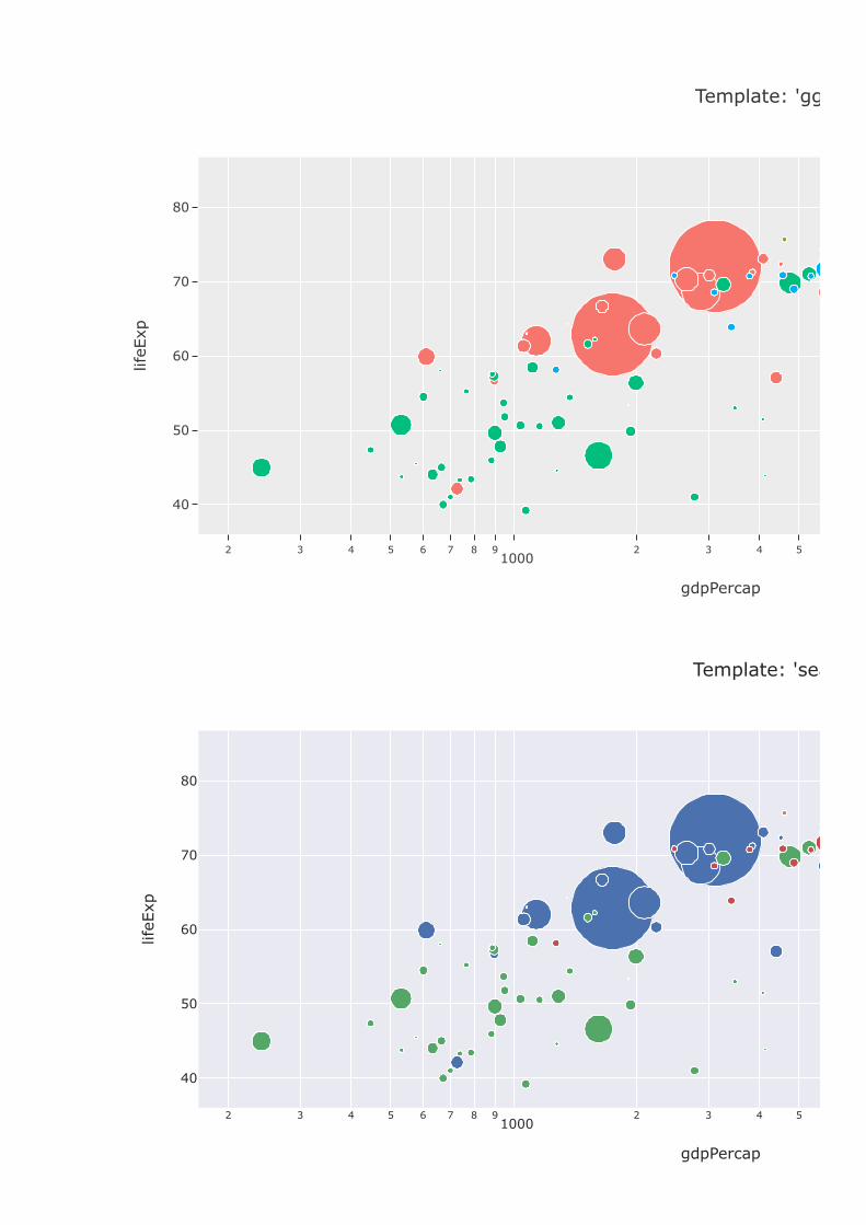
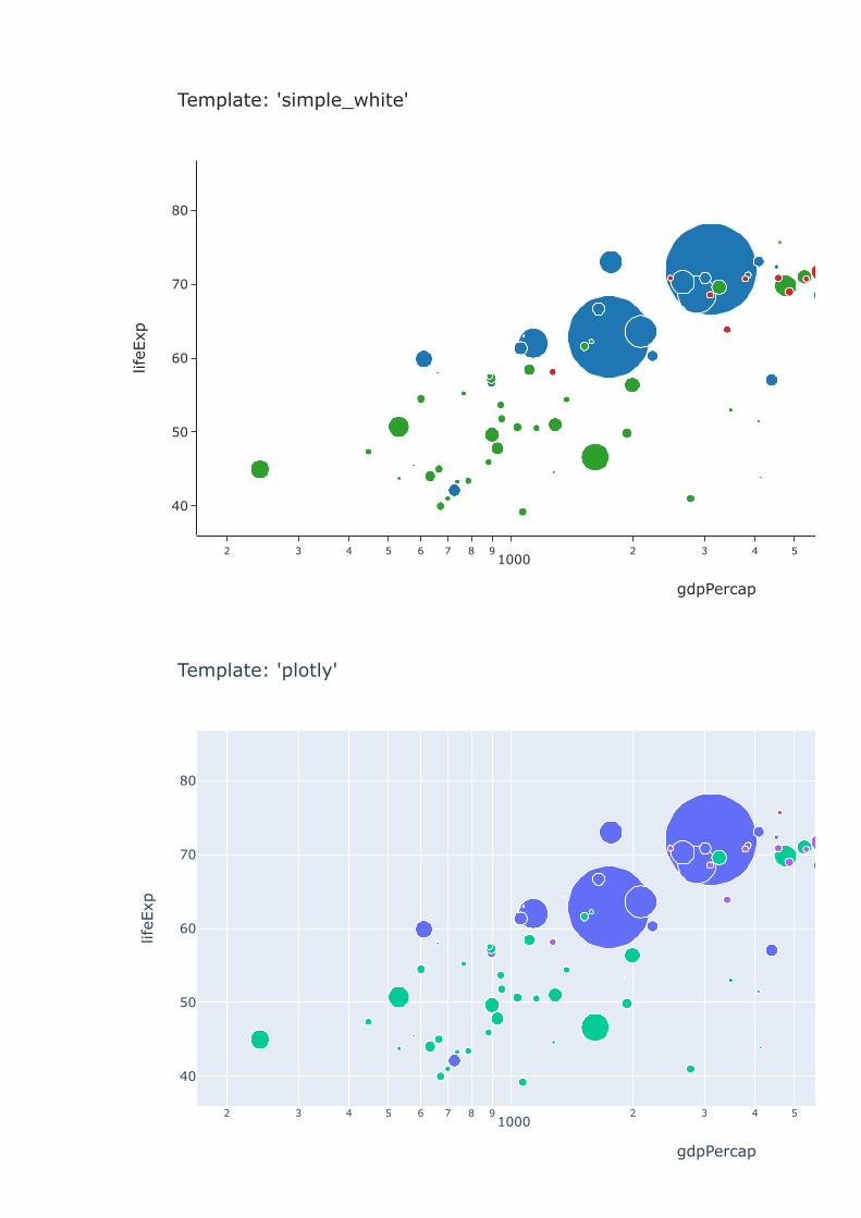
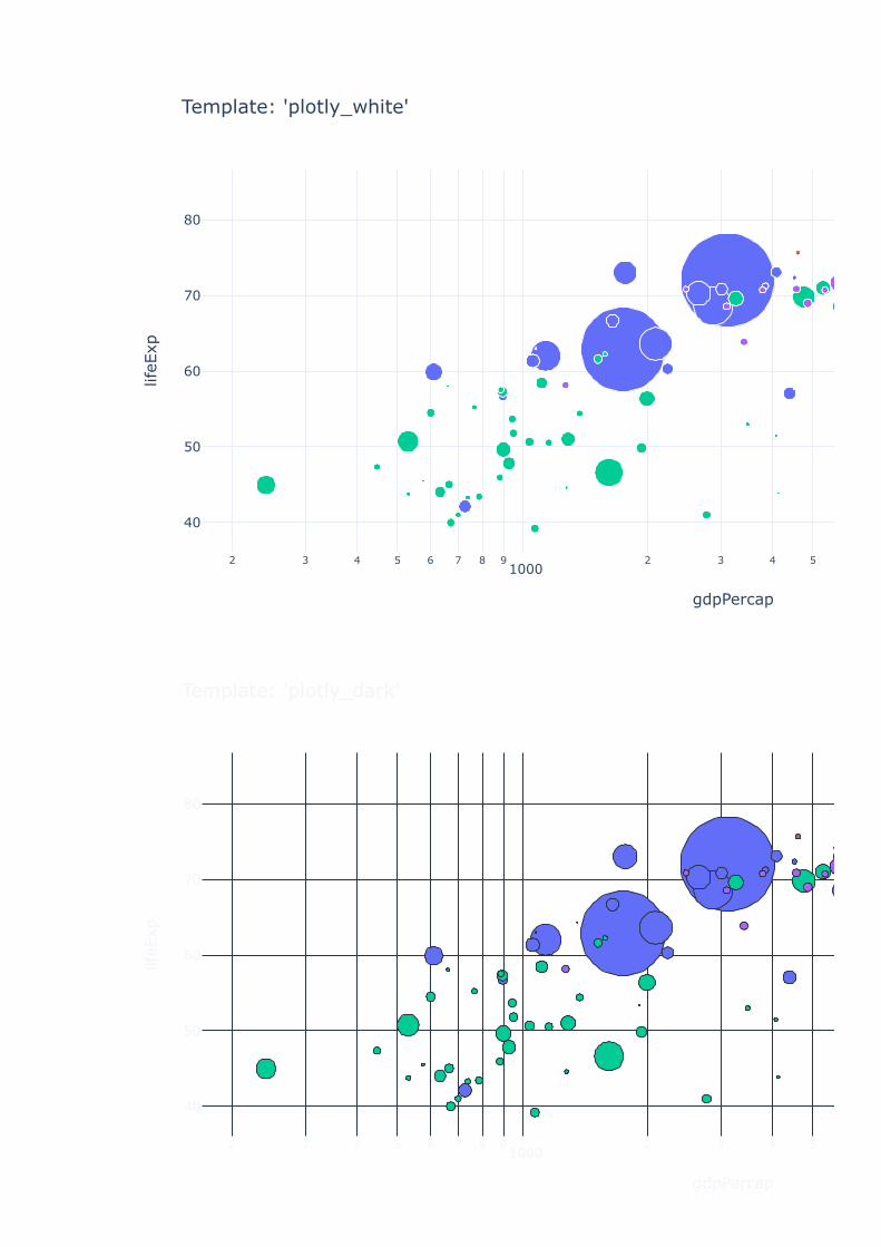
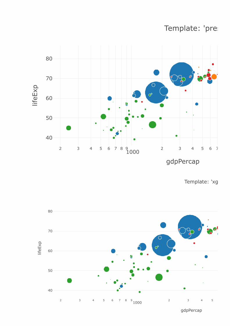
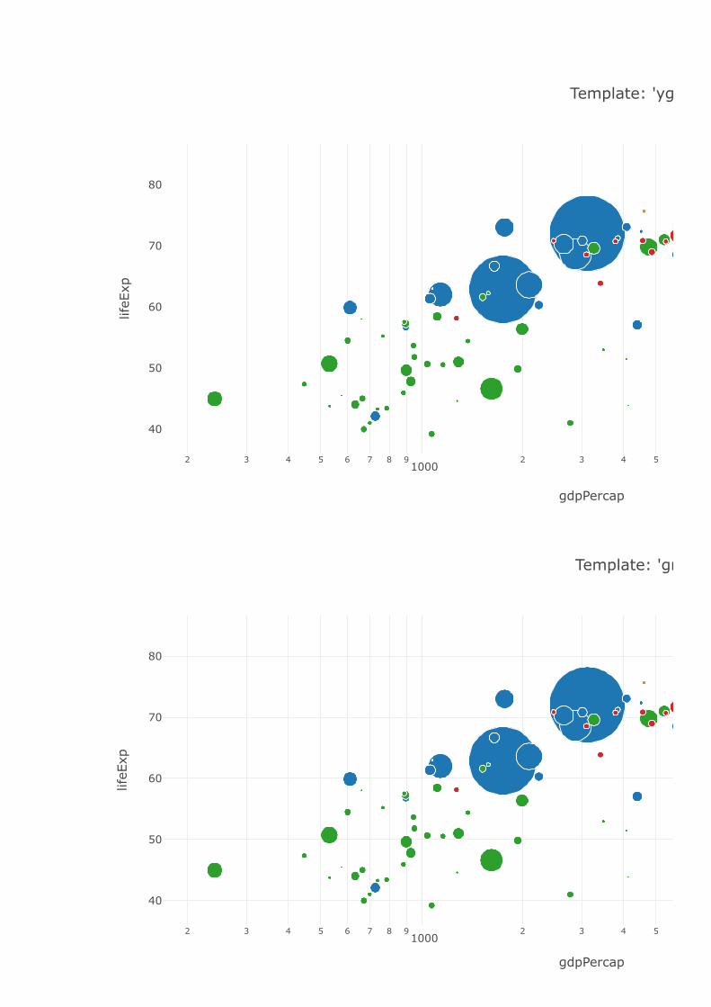
템플릿(Templates)
Templates configuration----------------------- Default template: 'plotly' Available templates: ['ggplot2', 'seaborn', 'simple_white', 'plotly', 'plotly_white', 'plotly_dark', 'presentation', 'xgridoff', 'ygridoff', 'gridon', 'none']
pio.templates
gapminder_2002 = gapminder.query("year == 2002")
for template in ['ggplot2', 'seaborn', 'simple_white', 'plotly', 'plotly_white', 'plotly_dark', 'pr
fig = px.scatter(gapminder_2002,
x='gdpPercap', y='lifeExp', size='pop', color='continent',
log_x=True, size_max=60,
template=template, title="Template: '%s'" % template)
fig.show()
2 3 4 5 6 7 8 91000
2 3 4 5
40
50
60
70
80
Template: 'gg
gdpPercap
lifeE
xp
2 3 4 5 6 7 8 91000
2 3 4 5
40
50
60
70
80
Template: 'sea
gdpPercap
lifeE
xp
2 3 4 5 6 7 8 91000
2 3 4 5
40
50
60
70
80
Template: 'simple_white'
gdpPercap
lifeE
xp
2 3 4 5 6 7 8 91000
2 3 4 5
40
50
60
70
80
Template: 'plotly'
gdpPercap
lifeE
xp
2 3 4 5 6 7 8 91000
2 3 4 5
40
50
60
70
80
Template: 'plotly_white'
gdpPercap
lifeE
xp
2 3 4 5 6 7 8 91000
2 3 4 5
40
50
60
70
80
Template: 'plotly_dark'
gdpPercap
lifeE
xp
2 3 4 5 6 7 8 91000
2 3 4 5 6 7
40
50
60
70
80
Template: 'pres
gdpPercap
lifeE
xp
2 3 4 5 6 7 8 91000
2 3 4 5
40
50
60
70
80
Template: 'xg
gdpPercap
lifeE
xp
2 3 4 5 6 7 8 91000
2 3 4 5
40
50
60
70
80
Template: 'yg
gdpPercap
lifeE
xp
2 3 4 5 6 7 8 91000
2 3 4 5
40
50
60
70
80
Template: 'gr
gdpPercap
lifeE
xp
2 3 4 5 6 7 8 91000
2 3 4 5
40
50
60
70
80
Template: 'n
gdpPercap
lifeE
xp
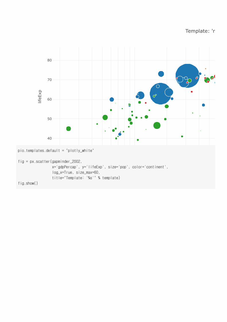
pio.templates.default = "plotly_white"
fig = px.scatter(gapminder_2002,
x='gdpPercap', y='lifeExp', size='pop', color='continent',
log_x=True, size_max=60,
title="Template: '%s'" % template)
fig.show()
2 3 4 5 6 7 8 91000
2 3 4 5
40
50
60
70
80
Template: 'none'
gdpPercap
lifeE
xp
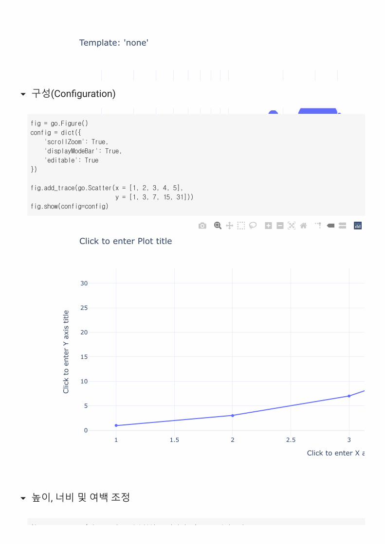
구성(Con�guration)
1 1.5 2 2.5 30
5
10
15
20
25
30
Click to enter Plot title
Click to enter X a
Clic
k to
ent
er Y
axi
s tit
le
fig = go.Figure()
config = dict({
'scrollZoom': True,
'displayModeBar': True,
'editable': True
})
fig.add_trace(go.Scatter(x = [1, 2, 3, 4, 5],
y = [1, 3, 7, 15, 31]))
fig.show(config=config)
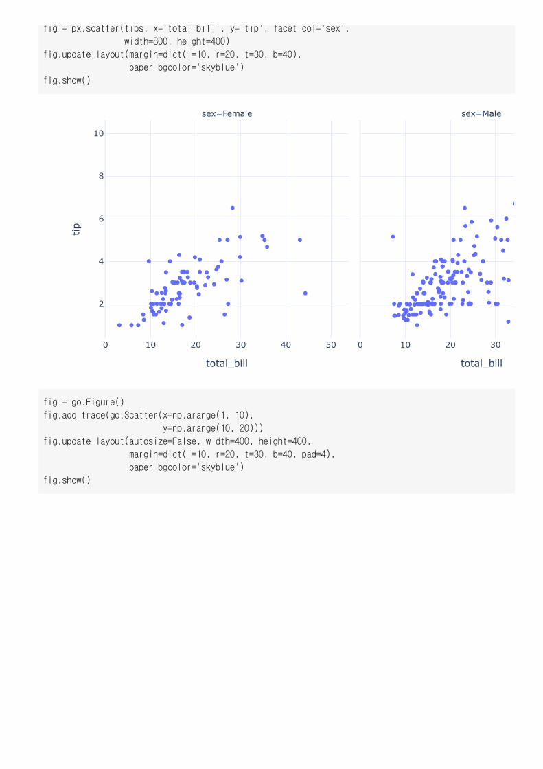
높이, 너비 및 여백 조정
fi tt (ti 't t l bill' 'ti ' f t l ' '
0 10 20 30 40 50
2
4
6
8
10
0 10 20 30
total_bill total_bill
tip
sex=Female sex=Male
fig = px.scatter(tips, x='total_bill', y='tip', facet_col='sex',
width=800, height=400)
fig.update_layout(margin=dict(l=10, r=20, t=30, b=40),
paper_bgcolor='skyblue')
fig.show()
fig = go.Figure()
fig.add_trace(go.Scatter(x=np.arange(1, 10),
y=np.arange(10, 20)))
fig.update_layout(autosize=False, width=400, height=400,
margin=dict(l=10, r=20, t=30, b=40, pad=4),
paper_bgcolor='skyblue')
fig.show()
2 4 6 8
10
11
12
13
14
15
16
17
18
A B C D
long long long long
long long long
short
long long
Y ax
is T
itle
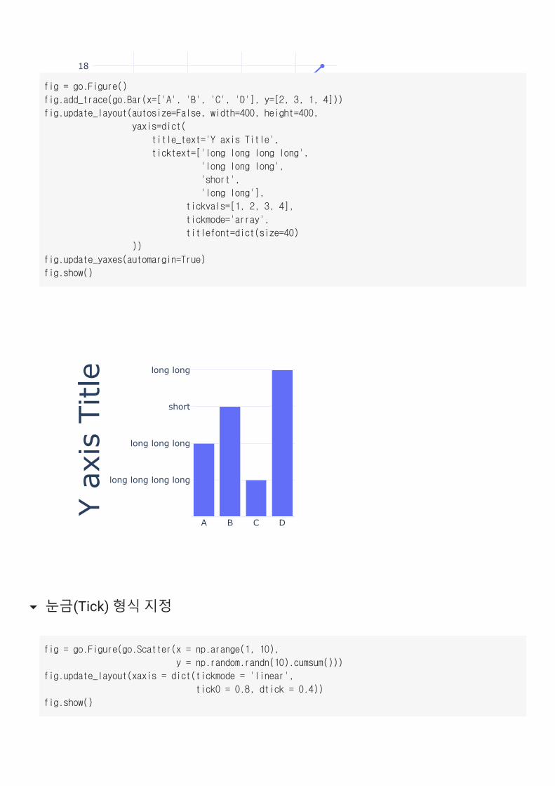
fig = go.Figure()
fig.add_trace(go.Bar(x=['A', 'B', 'C', 'D'], y=[2, 3, 1, 4]))
fig.update_layout(autosize=False, width=400, height=400,
yaxis=dict(
title_text='Y axis Title',
ticktext=['long long long long',
'long long long',
'short',
'long long'],
tickvals=[1, 2, 3, 4],
tickmode='array',
titlefont=dict(size=40)
))
fig.update_yaxes(automargin=True)
fig.show()
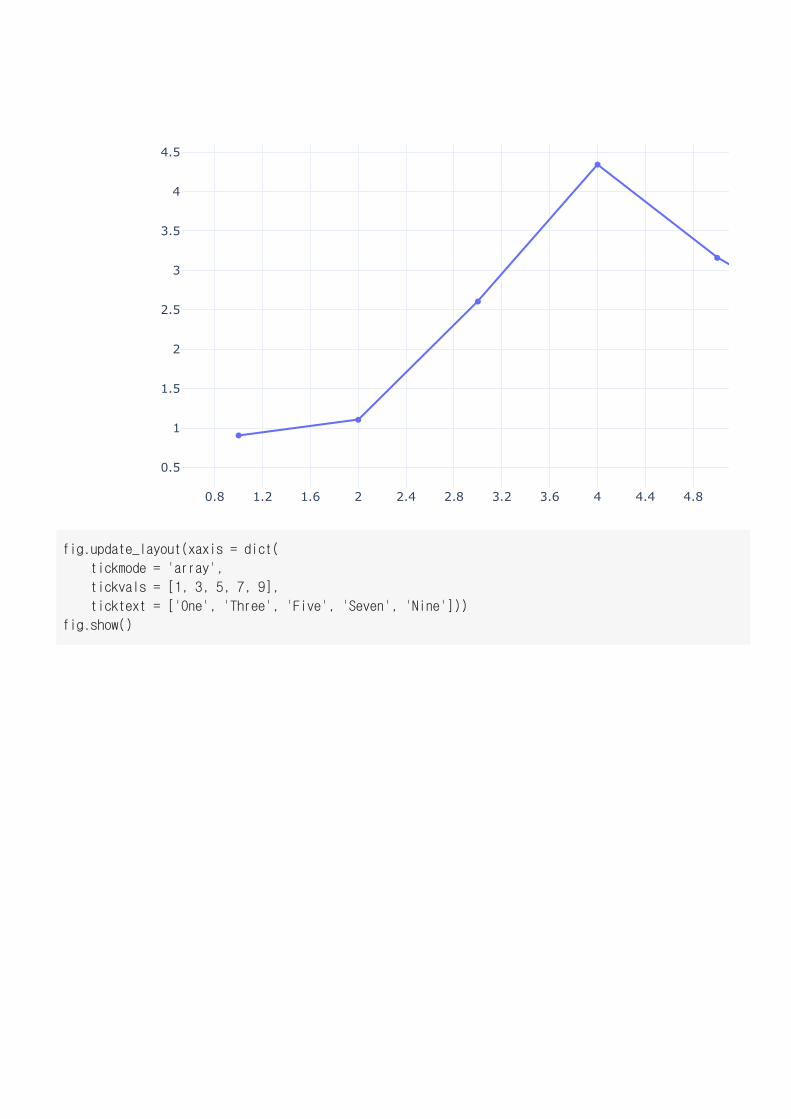
눈금(Tick) 형식 지정
fig = go.Figure(go.Scatter(x = np.arange(1, 10),
y = np.random.randn(10).cumsum()))
fig.update_layout(xaxis = dict(tickmode = 'linear',
tick0 = 0.8, dtick = 0.4))
fig.show()
0.8 1.2 1.6 2 2.4 2.8 3.2 3.6 4 4.4 4.8
0.5
1
1.5
2
2.5
3
3.5
4
4.5
fig.update_layout(xaxis = dict(
tickmode = 'array',
tickvals = [1, 3, 5, 7, 9],
ticktext = ['One', 'Three', 'Five', 'Seven', 'Nine']))
fig.show()
One Three Five
0.5
1
1.5
2
2.5
3
3.5
4
4.5
One Three Five
50%
100%
150%
200%
250%
300%
350%
400%
450%
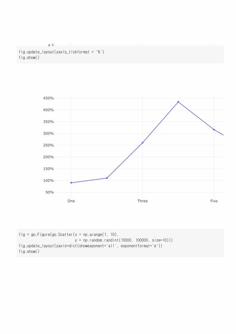
fig.update_layout(yaxis_tickformat = '%')
fig.show()
fig = go.Figure(go.Scatter(x = np.arange(1, 10),
y = np.random.randint(10000, 100000, size=10)))
fig.update_layout(yaxis=dict(showexponent='all', exponentformat='e'))
fig.show()
1 2 3 4 5
2e+4
3e+4
4e+4
5e+4
6e+4
7e+4
8e+4
9e+4
2015-Apr-01(Wed) 2015-Jul-01(Wed) 2015-Oct-01(Thu) 2016-Jan-01(Fri) 201
90
100
110
120
130
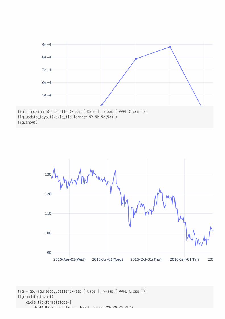
fig = go.Figure(go.Scatter(x=aapl['Date'], y=aapl['AAPL.Close']))
fig.update_layout(xaxis_tickformat='%Y-%b-%d(%a)')
fig.show()
fig = go.Figure(go.Scatter(x=aapl['Date'], y=aapl['AAPL.Close']))
fig.update_layout(
xaxis_tickformatstops=[
dict(dtickrange=[None 1000] value="%H:%M:%S %L")
Apr 2015 Jul 2015 Oct 2015 Jan 2016
90
100
110
120
130
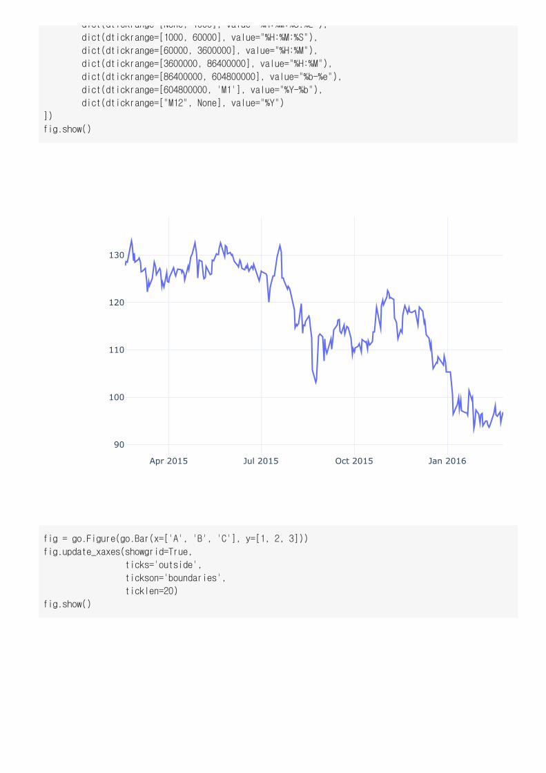
dict(dtickrange [None, 1000], value %H:%M:%S.%L ),
dict(dtickrange=[1000, 60000], value="%H:%M:%S"),
dict(dtickrange=[60000, 3600000], value="%H:%M"),
dict(dtickrange=[3600000, 86400000], value="%H:%M"),
dict(dtickrange=[86400000, 604800000], value="%b-%e"),
dict(dtickrange=[604800000, 'M1'], value="%Y-%b"),
dict(dtickrange=["M12", None], value="%Y")
])
fig.show()
fig = go.Figure(go.Bar(x=['A', 'B', 'C'], y=[1, 2, 3]))
fig.update_xaxes(showgrid=True,
ticks='outside',
tickson='boundaries',
ticklen=20)
fig.show()
A B0
0.5
1
1.5
2
2.5
3
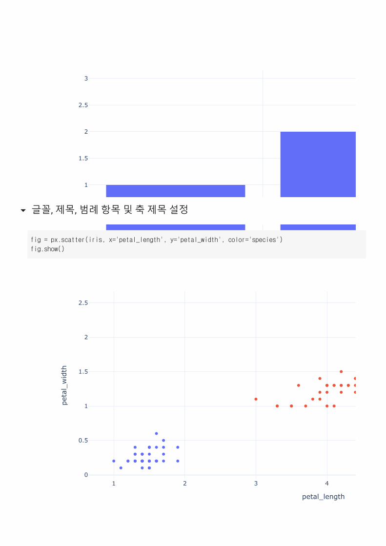
글꼴, 제목, 범례 항목 및 축 제목 설정
1 2 3 40
0.5
1
1.5
2
2.5
petal_length
petal_width
fig = px.scatter(iris, x='petal_length', y='petal_width', color='species')
fig.show()
1 2 3 40
0.5
1
1.5
2
2.5
Petal Length (cm)
Peta
l Wid
th (
cm)
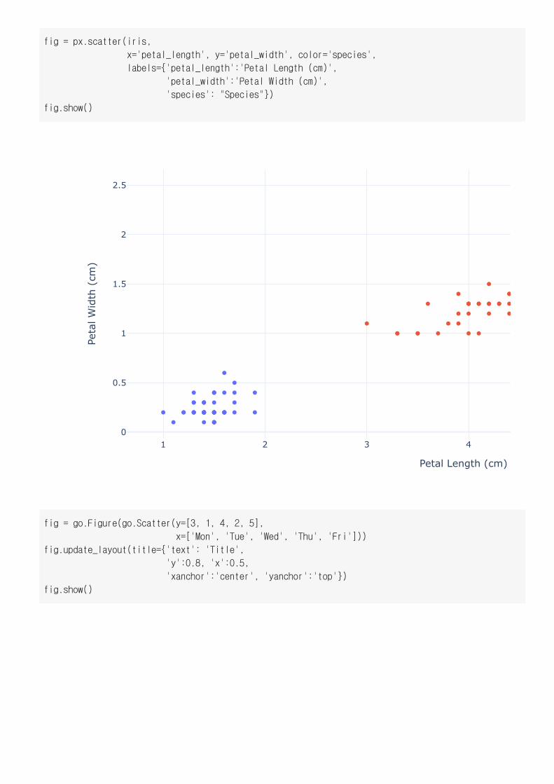
fig = px.scatter(iris,
x='petal_length', y='petal_width', color='species',
labels={'petal_length':'Petal Length (cm)',
'petal_width':'Petal Width (cm)',
'species': "Species"})
fig.show()
fig = go.Figure(go.Scatter(y=[3, 1, 4, 2, 5],
x=['Mon', 'Tue', 'Wed', 'Thu', 'Fri']))
fig.update_layout(title={'text': 'Title',
'y':0.8, 'x':0.5,
'xanchor':'center', 'yanchor':'top'})
fig.show()
Mon Tue Wed
1
1.5
2
2.5
3
3.5
4
4.5
5Title
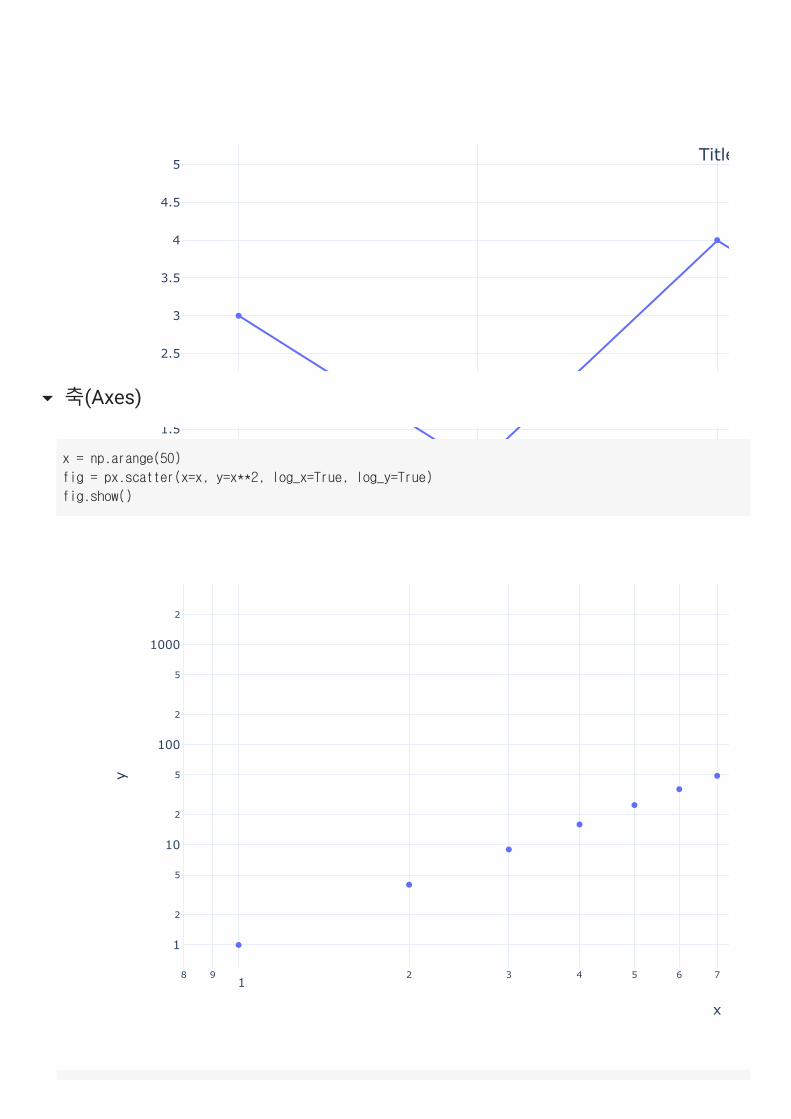
축(Axes)
8 91
2 3 4 5 6 7
1
2
5
10
2
5
100
2
5
1000
2
x
y
x = np.arange(50)
fig = px.scatter(x=x, y=x**2, log_x=True, log_y=True)
fig.show()
1 2 30
10
20
30
40
50
x
y
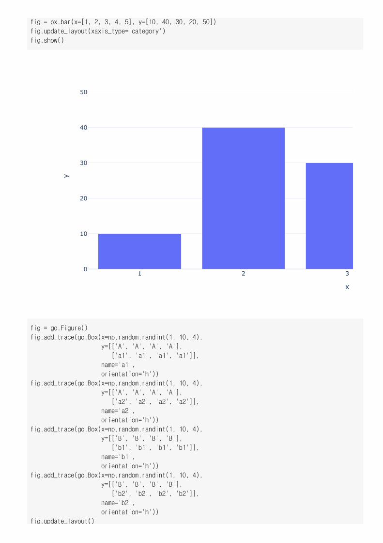
fig = px.bar(x=[1, 2, 3, 4, 5], y=[10, 40, 30, 20, 50])
fig.update_layout(xaxis_type='category')
fig.show()
fig = go.Figure()
fig.add_trace(go.Box(x=np.random.randint(1, 10, 4),
y=[['A', 'A', 'A', 'A'],
['a1', 'a1', 'a1', 'a1']],
name='a1',
orientation='h'))
fig.add_trace(go.Box(x=np.random.randint(1, 10, 4),
y=[['A', 'A', 'A', 'A'],
['a2', 'a2', 'a2', 'a2']],
name='a2',
orientation='h'))
fig.add_trace(go.Box(x=np.random.randint(1, 10, 4),
y=[['B', 'B', 'B', 'B'],
['b1', 'b1', 'b1', 'b1']],
name='b1',
orientation='h'))
fig.add_trace(go.Box(x=np.random.randint(1, 10, 4),
y=[['B', 'B', 'B', 'B'],
['b2', 'b2', 'b2', 'b2']],
name='b2',
orientation='h'))
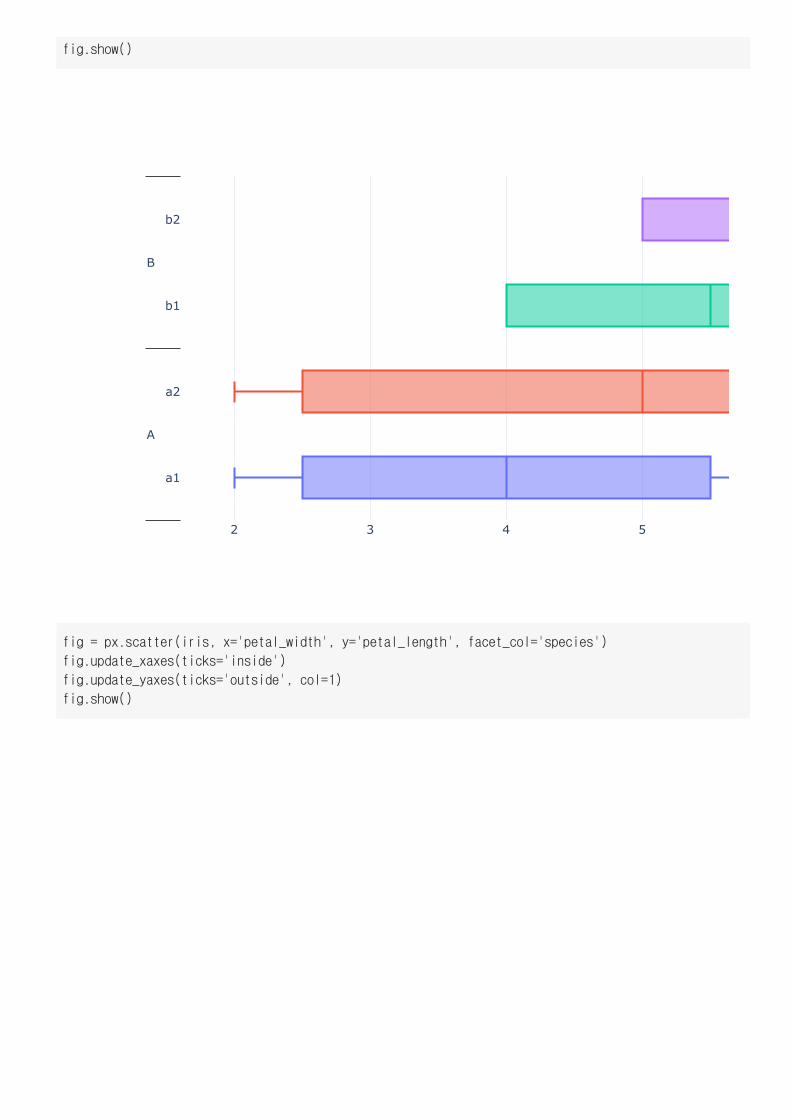
fig.update_layout()
2 3 4 5
a1
a2
b1
b2
A
B
fig.show()
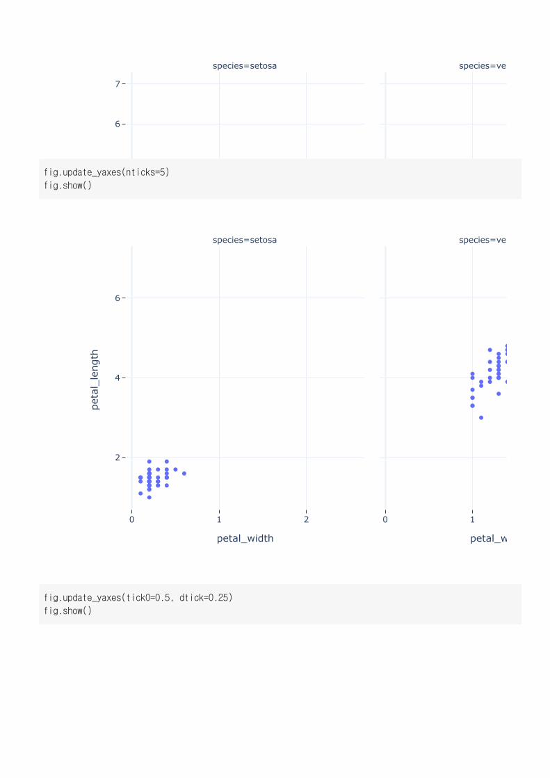
fig = px.scatter(iris, x='petal_width', y='petal_length', facet_col='species')
fig.update_xaxes(ticks='inside')
fig.update_yaxes(ticks='outside', col=1)
fig.show()
0 1 2
1
2
3
4
5
6
7
0 1
petal_width petal_w
petal_length
species=setosa species=ver
0 1 2
2
4
6
0 1
petal_width petal_w
petal_length
species=setosa species=ver
fig.update_yaxes(nticks=5)
fig.show()
fig.update_yaxes(tick0=0.5, dtick=0.25)
fig.show()
0 1 20.751
1.251.51.752
2.252.52.753
3.253.53.754
4.254.54.755
5.255.55.756
6.256.56.757
7.25
0 1
petal_width petal_w
petal_length
species=setosa species=ver
0 1 2
1.2
3.5
4.3
0 1
petal_width petal_w
petal_length
species=setosa species=ver
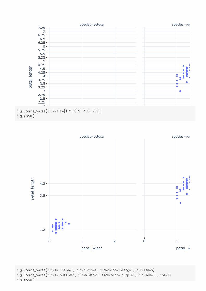
fig.update_yaxes(tickvals=[1.2, 3.5, 4.3, 7.5])
fig.show()
fig.update_xaxes(ticks='inside', tickwidth=4, tickcolor='orange', ticklen=5)
fig.update_yaxes(ticks='outside', tickwidth=2, tickcolor='purple', ticklen=10, col=1)
fig.show()
0 1 2
1.2
3.5
4.3
0 1
petal_width petal_w
petal_length
species=setosa species=ver
fig.show()
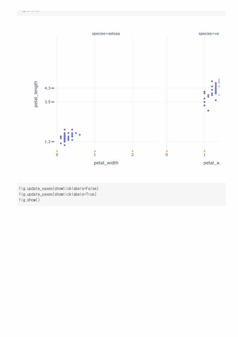
fig.update_xaxes(showticklabels=False)
fig.update_yaxes(showticklabels=True)
fig.show()
1.2
3.5
4.3
1.2
3.5
4.3
petal_width petal_w
petal_length
species=setosa species=ver
Female
Male
0
50
100
150
200
250
300
sex
sum
of
tip
smoker=No
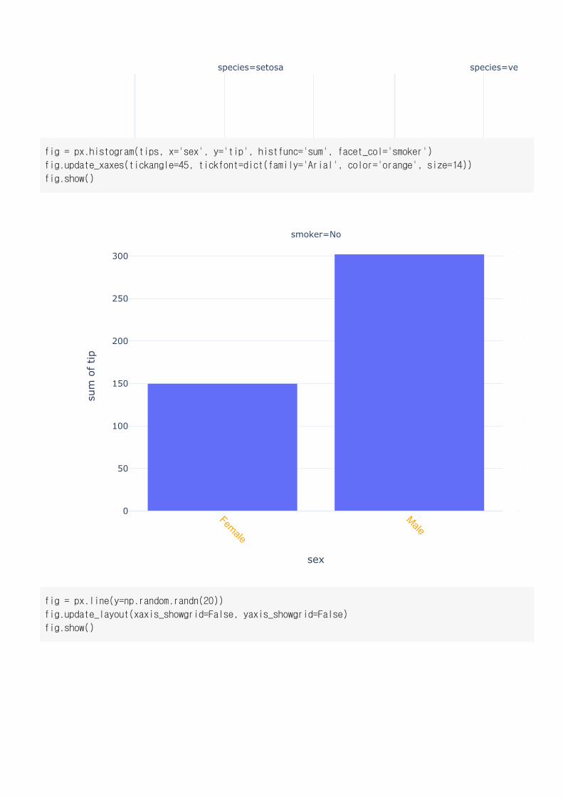
fig = px.histogram(tips, x='sex', y='tip', histfunc='sum', facet_col='smoker')
fig.update_xaxes(tickangle=45, tickfont=dict(family='Arial', color='orange', size=14))
fig.show()
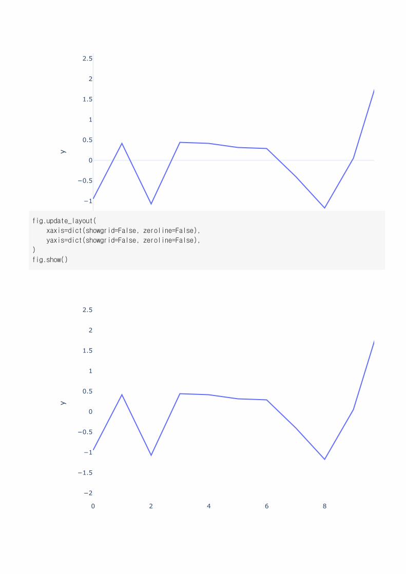
fig = px.line(y=np.random.randn(20))
fig.update_layout(xaxis_showgrid=False, yaxis_showgrid=False)
fig.show()
0 2 4 6 8
−2
−1.5
−1
−0.5
0
0.5
1
1.5
2
2.5y
0 2 4 6 8
−2
−1.5
−1
−0.5
0
0.5
1
1.5
2
2.5
y
fig.update_layout(
xaxis=dict(showgrid=False, zeroline=False),
yaxis=dict(showgrid=False, zeroline=False),
)
fig.show()
0 1 2
1
2
3
4
5
6
7
0 1
petal_width petal_w
petal_length
species=setosa species=ver
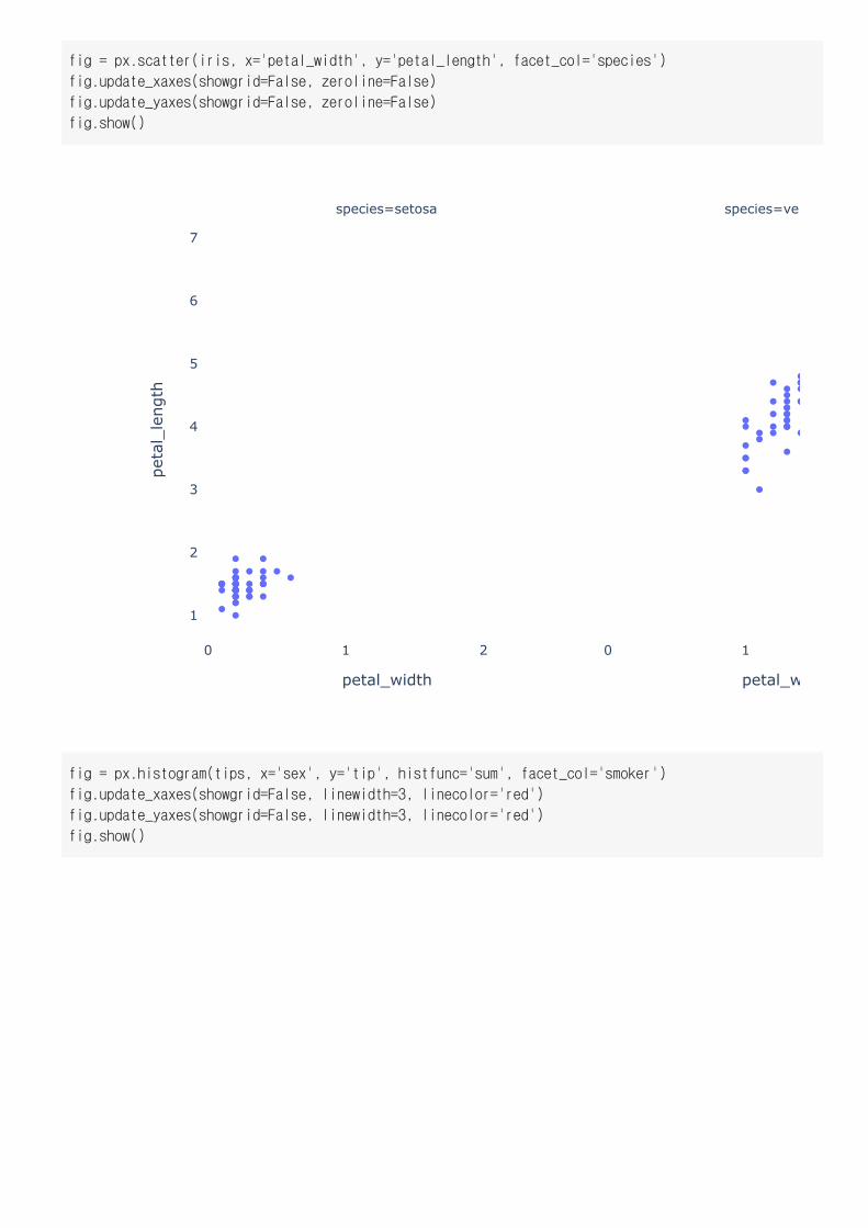
fig = px.scatter(iris, x='petal_width', y='petal_length', facet_col='species')
fig.update_xaxes(showgrid=False, zeroline=False)
fig.update_yaxes(showgrid=False, zeroline=False)
fig.show()
fig = px.histogram(tips, x='sex', y='tip', histfunc='sum', facet_col='smoker')
fig.update_xaxes(showgrid=False, linewidth=3, linecolor='red')
fig.update_yaxes(showgrid=False, linewidth=3, linecolor='red')
fig.show()
Female Male0
50
100
150
200
250
300
sex
sum
of
tip
smoker=No
Female Male0
50
100
150
200
250
300
sex
sum
of
tip
smoker=No
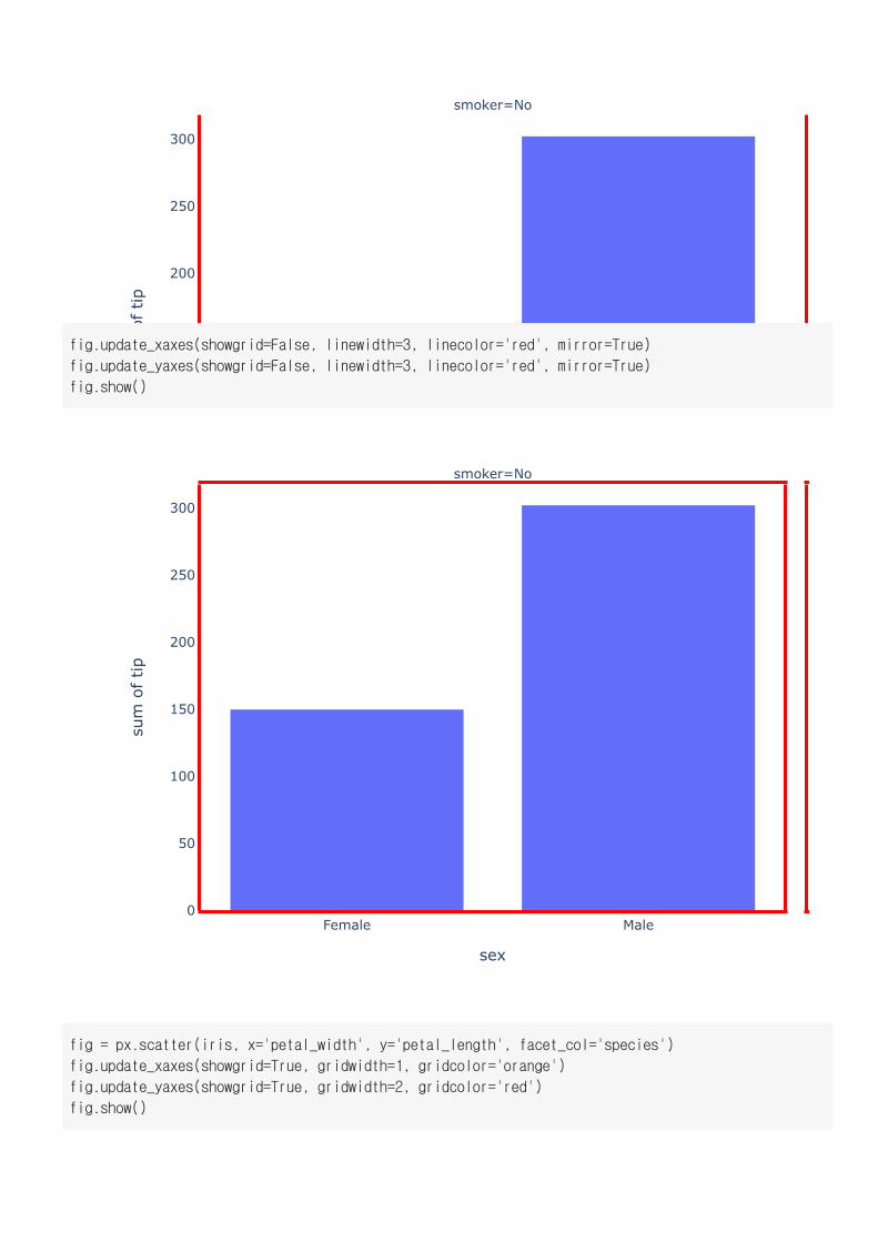
fig.update_xaxes(showgrid=False, linewidth=3, linecolor='red', mirror=True)
fig.update_yaxes(showgrid=False, linewidth=3, linecolor='red', mirror=True)
fig.show()
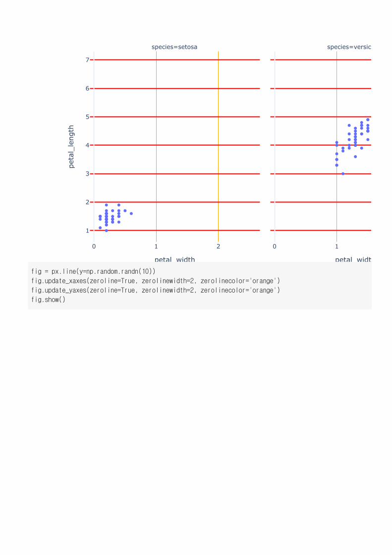
fig = px.scatter(iris, x='petal_width', y='petal_length', facet_col='species')
fig.update_xaxes(showgrid=True, gridwidth=1, gridcolor='orange')
fig.update_yaxes(showgrid=True, gridwidth=2, gridcolor='red')
fig.show()
0 1 2
1
2
3
4
5
6
7
0 1
petal_width petal_widt
petal_length
species=setosa species=versic
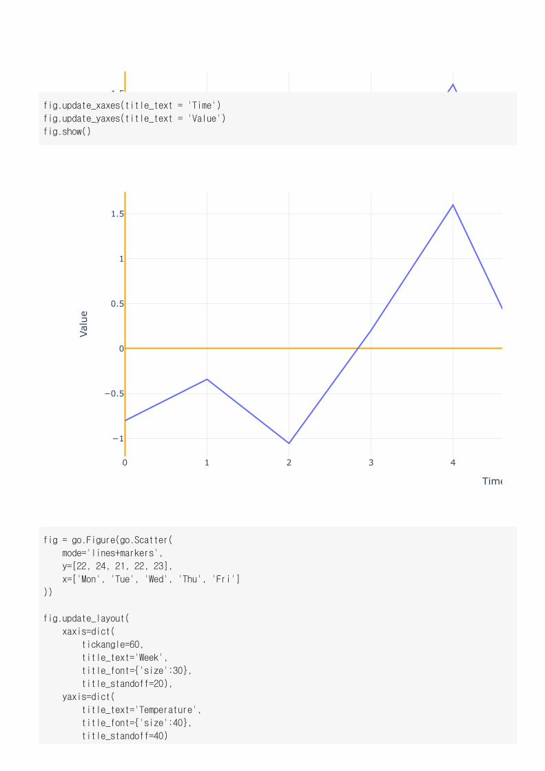
fig = px.line(y=np.random.randn(10))
fig.update_xaxes(zeroline=True, zerolinewidth=2, zerolinecolor='orange')
fig.update_yaxes(zeroline=True, zerolinewidth=2, zerolinecolor='orange')
fig.show()
0 1 2 3 4
−1
−0.5
0
0.5
1
1.5y
0 1 2 3 4
−1
−0.5
0
0.5
1
1.5
Time
Value
fig.update_xaxes(title_text = 'Time')
fig.update_yaxes(title_text = 'Value')
fig.show()
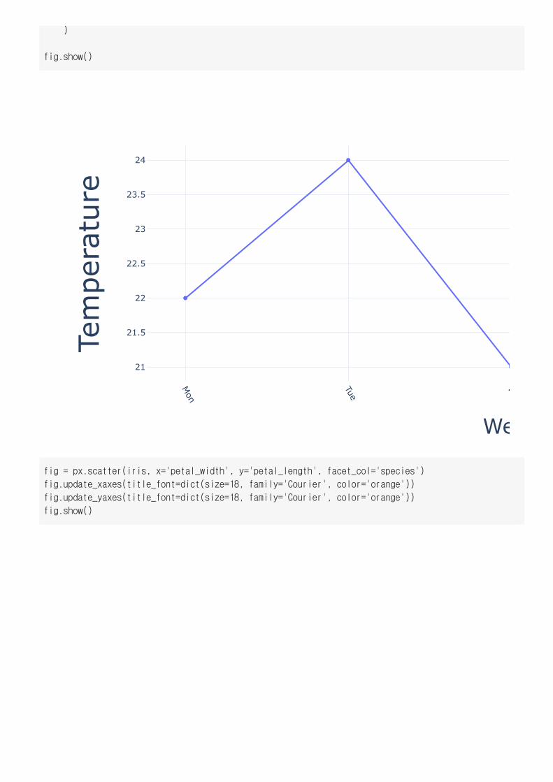
fig = go.Figure(go.Scatter(
mode='lines+markers',
y=[22, 24, 21, 22, 23],
x=['Mon', 'Tue', 'Wed', 'Thu', 'Fri']
))
fig.update_layout(
xaxis=dict(
tickangle=60,
title_text='Week',
title_font={'size':30},
title_standoff=20),
yaxis=dict(
title_text='Temperature',
title_font={'size':40},
title_standoff=40)
)
Mon
Tue
W
21
21.5
22
22.5
23
23.5
24
We
Temperature
)
fig.show()
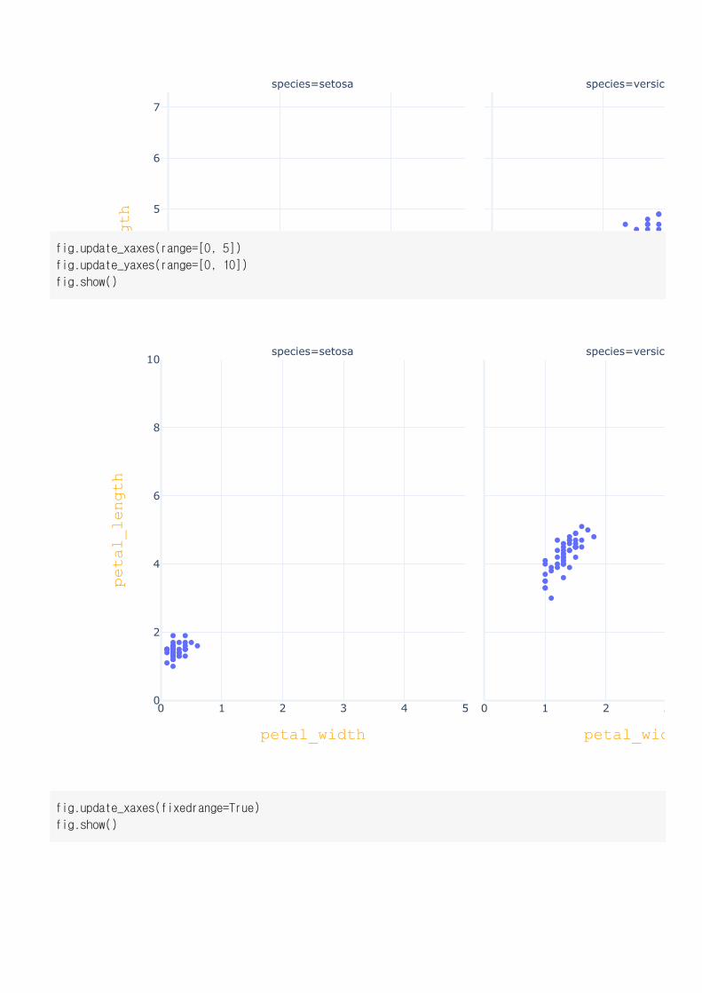
fig = px.scatter(iris, x='petal_width', y='petal_length', facet_col='species')
fig.update_xaxes(title_font=dict(size=18, family='Courier', color='orange'))
fig.update_yaxes(title_font=dict(size=18, family='Courier', color='orange'))
fig.show()
0 1 2
1
2
3
4
5
6
7
0 1
petal_width petal_wid
petal_length
species=setosa species=versic
0 1 2 3 4 50
2
4
6
8
10
0 1 2 3
petal_width petal_wid
petal_length
species=setosa species=versic
fig.update_xaxes(range=[0, 5])
fig.update_yaxes(range=[0, 10])
fig.show()
fig.update_xaxes(fixedrange=True)
fig.show()
0 1 2 3 4 50
2
4
6
8
10
0 1 2
petal_width petal_w
petal_length
species=setosa species=ver
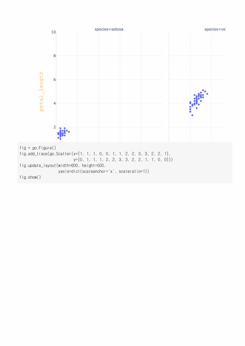
fig = go.Figure()
fig.add_trace(go.Scatter(x=[1, 1, 1, 0, 0, 1, 1, 2, 2, 3, 3, 2, 2, 1],
y=[0, 1, 1, 1, 2, 2, 3, 3, 2, 2, 1, 1, 0, 0]))
fig.update_layout(width=600, height=500,
yaxis=dict(scaleanchor='x', scaleratio=1))
fig.show()
0 1 2 3
0
0.5
1
1.5
2
2.5
3
−1 0 1 2 3 4
0
0.5
1
1.5
2
2.5
3
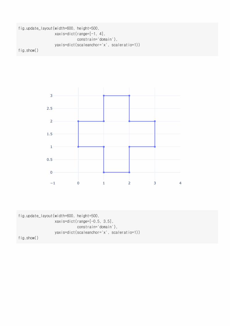
fig.update_layout(width=600, height=500,
xaxis=dict(range=[-1, 4],
constrain='domain'),
yaxis=dict(scaleanchor='x', scaleratio=1))
fig.show()
fig.update_layout(width=600, height=500,
xaxis=dict(range=[-0.5, 3.5],
constrain='domain'),
yaxis=dict(scaleanchor='x', scaleratio=1))
fig.show()
0 1 2 3
0
0.5
1
1.5
2
2.5
3
0 1 2
7
6
5
4
3
2
1
0 1
petal_width petal_w
petal_length
species=setosa species=ver
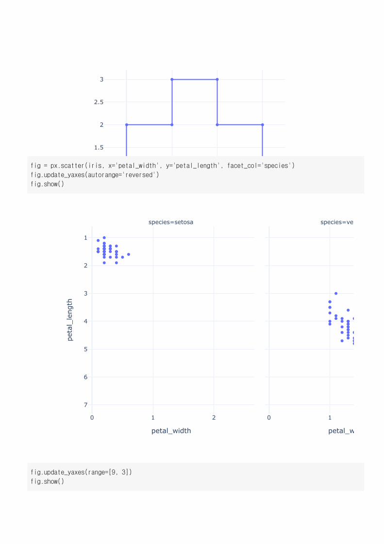
fig = px.scatter(iris, x='petal_width', y='petal_length', facet_col='species')
fig.update_yaxes(autorange='reversed')
fig.show()
fig.update_yaxes(range=[9, 3])
fig.show()
0 1 2
7
6
5
4
3
2
1
0 1
petal_width petal_w
petal_length
species=setosa species=ver
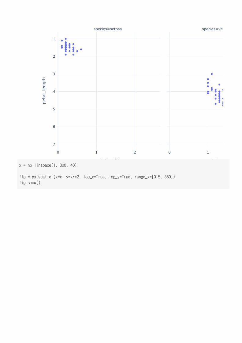
x = np.linspace(1, 300, 40)
fig = px.scatter(x=x, y=x**2, log_x=True, log_y=True, range_x=[0.5, 350])
fig.show()
5 6 7 8 91
2 3 4 5 6 7 8 910
5
1
2
5
10
2
5
100
2
5
1000
2
5
10k
2
5
100k
x
y
5 6 7 8 91
2 3 4 5 6 7 8 910
5
1
2
5
10
2
5
100
2
5
1000
2
5
10k
2
5
100k
x
y
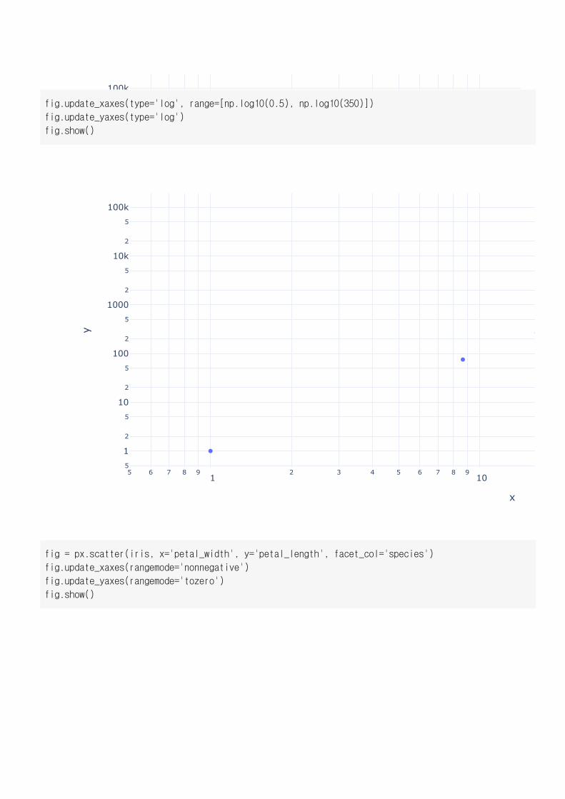
fig.update_xaxes(type='log', range=[np.log10(0.5), np.log10(350)])
fig.update_yaxes(type='log')
fig.show()
fig = px.scatter(iris, x='petal_width', y='petal_length', facet_col='species')
fig.update_xaxes(rangemode='nonnegative')
fig.update_yaxes(rangemode='tozero')
fig.show()
0 1 20
1
2
3
4
5
6
7
0 1
petal_width petal_widt
petal_length
species=setosa species=versic
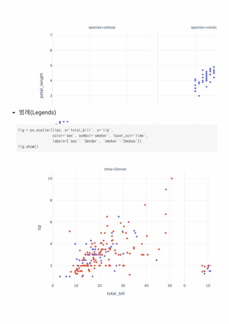
범례(Legends)
0 10 20 30 40 50
2
4
6
8
10
0 10
total_bill
tip
time=Dinner
fig = px.scatter(tips, x='total_bill', y='tip',
color='sex', symbol='smoker', facet_col='time',
labels={'sex': 'Gender', 'smoker':'Smokes'})
fig.show()
Female0
20
40
60
80
100
120
140
160
sex
coun
t of
tot
al_b
ill
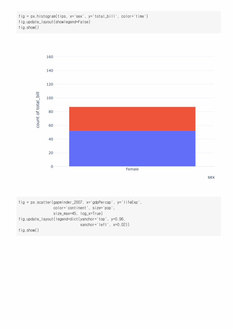
fig = px.histogram(tips, x='sex', y='total_bill', color='time')
fig.update_layout(showlegend=False)
fig.show()
fig = px.scatter(gapminder_2007, x='gdpPercap', y='lifeExp',
color='continent', size='pop',
size_max=45, log_x=True)
fig.update_layout(legend=dict(yanchor='top', y=0.96,
xanchor='left', x=0.02))
fig.show()
2 3 4 5 6 7 8 91000
2 3
40
45
50
55
60
65
70
75
80
85continent=Asiacontinent=Europecontinent=Africacontinent=Americascontinent=Oceania
gdpPer
lifeExp
2 3 4 5 6 7 8 91000
2 3
40
45
50
55
60
65
70
75
80
85
continent=Asia continent=
gdpPer
lifeExp
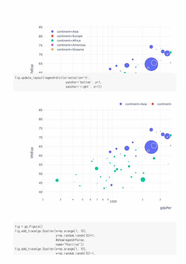
fig.update_layout(legend=dict(orientation='h',
yanchor='bottom', y=1,
xanchor='right', x=1))
fig = go.Figure()
fig.add_trace(go.Scatter(x=np.arange(1, 10),
y=np.random.randn(10)+1,
#showlegend=False,
name="Positive"))
fig.add_trace(go.Scatter(x=np.arange(1, 10),
y=np.random.randn(10)-1,
1 2 3 4 5
−2
−1
0
1
2
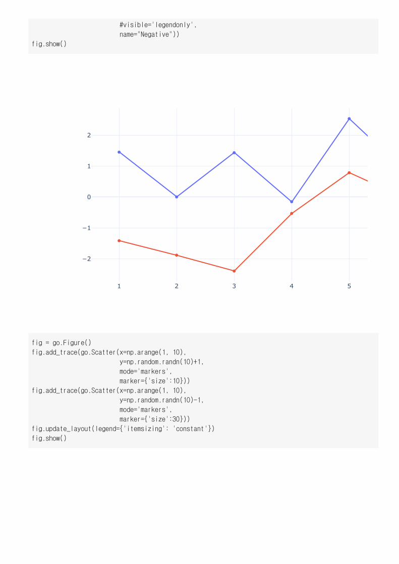
#visible='legendonly',
name="Negative"))
fig.show()
fig = go.Figure()
fig.add_trace(go.Scatter(x=np.arange(1, 10),
y=np.random.randn(10)+1,
mode='markers',
marker={'size':10}))
fig.add_trace(go.Scatter(x=np.arange(1, 10),
y=np.random.randn(10)-1,
mode='markers',
marker={'size':30}))
fig.update_layout(legend={'itemsizing': 'constant'})
fig.show()
1 2 3 4 5
−2
−1
0
1
2
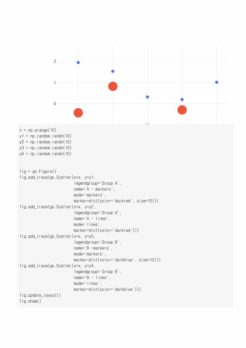
x = np.arange(10)
y1 = np.random.randn(10)
y2 = np.random.randn(10)
y3 = np.random.randn(10)
y4 = np.random.randn(10)
fig = go.Figure()
fig.add_trace(go.Scatter(x=x, y=y1,
legendgroup='Group A',
name='A - markers',
mode='markers',
marker=dict(color='darkred', size=10)))
fig.add_trace(go.Scatter(x=x, y=y2,
legendgroup='Group A',
name='A - lines',
mode='lines',
marker=dict(color='darkred')))
fig.add_trace(go.Scatter(x=x, y=y3,
legendgroup='Group B',
name='B -markers',
mode='markers',
marker=dict(color='darkblue', size=10)))
fig.add_trace(go.Scatter(x=x, y=y4,
legendgroup='Group B',
name='B - lines',
mode='lines',
marker=dict(color='darkblue')))
fig.update_layout()
fig.show()
0 2 4−3
−2
−1
0
1
2
3
4
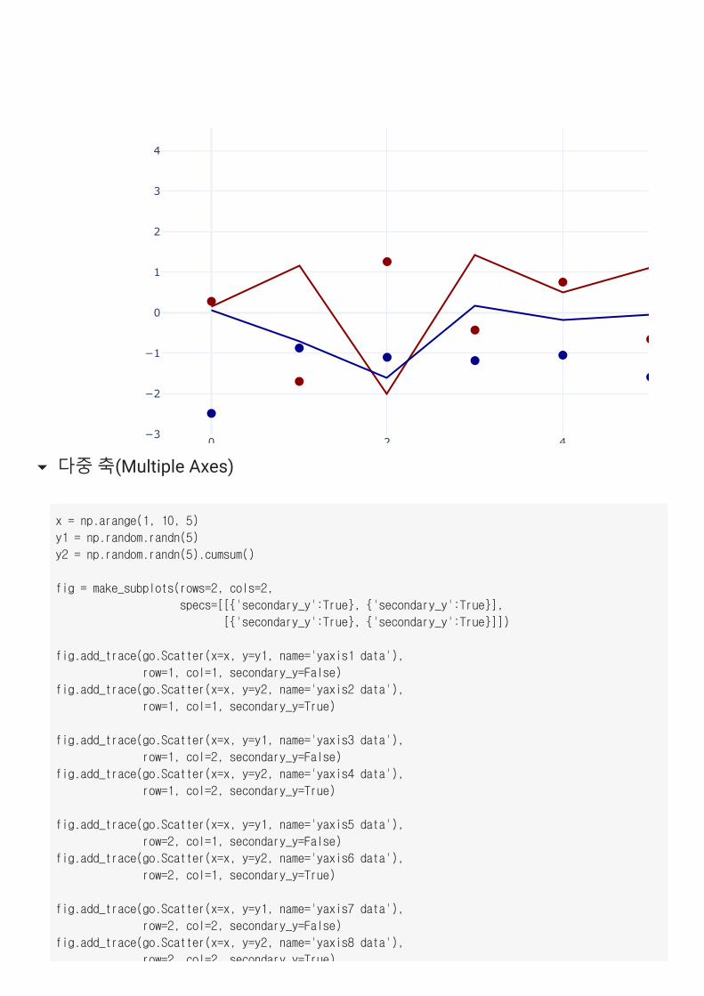
다중 축(Multiple Axes)
x = np.arange(1, 10, 5)
y1 = np.random.randn(5)
y2 = np.random.randn(5).cumsum()
fig = make_subplots(rows=2, cols=2,
specs=[[{'secondary_y':True}, {'secondary_y':True}],
[{'secondary_y':True}, {'secondary_y':True}]])
fig.add_trace(go.Scatter(x=x, y=y1, name='yaxis1 data'),
row=1, col=1, secondary_y=False)
fig.add_trace(go.Scatter(x=x, y=y2, name='yaxis2 data'),
row=1, col=1, secondary_y=True)
fig.add_trace(go.Scatter(x=x, y=y1, name='yaxis3 data'),
row=1, col=2, secondary_y=False)
fig.add_trace(go.Scatter(x=x, y=y2, name='yaxis4 data'),
row=1, col=2, secondary_y=True)
fig.add_trace(go.Scatter(x=x, y=y1, name='yaxis5 data'),
row=2, col=1, secondary_y=False)
fig.add_trace(go.Scatter(x=x, y=y2, name='yaxis6 data'),
row=2, col=1, secondary_y=True)
fig.add_trace(go.Scatter(x=x, y=y1, name='yaxis7 data'),
row=2, col=2, secondary_y=False)
fig.add_trace(go.Scatter(x=x, y=y2, name='yaxis8 data'),
row=2 col=2 secondary y=True)
2 4 6
0.8
1
1.2
−3.5
−3
−2.5
2 4 6
0.8
1
1.2
−3.5
−3
−2.5
row 2, col 2, secondary_y True)
fig.show()
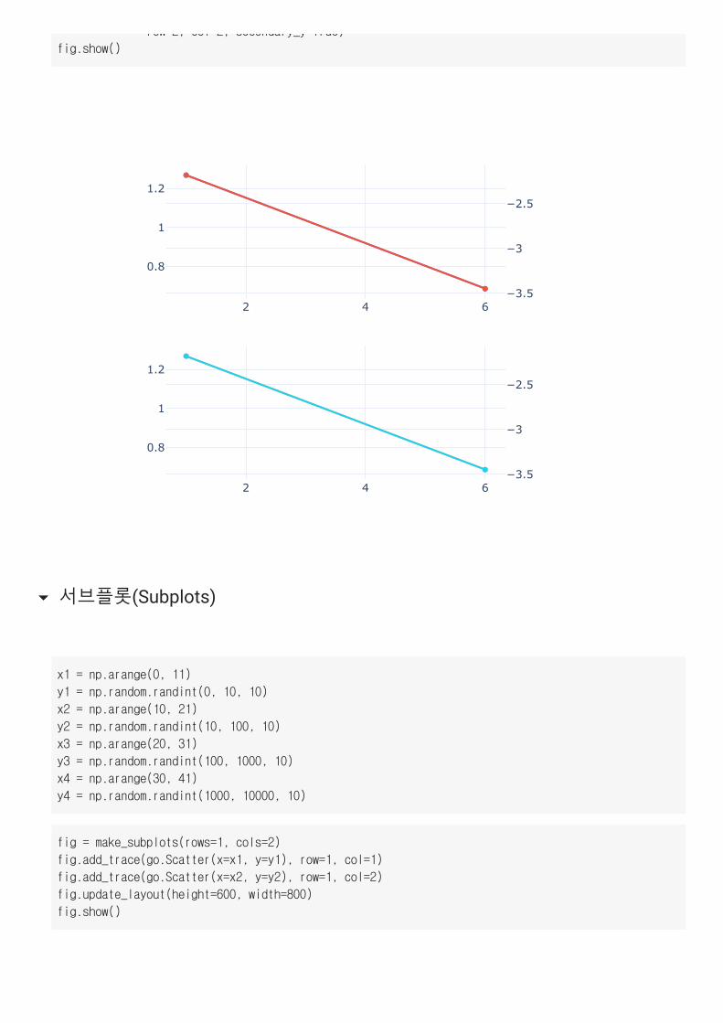
서브플롯(Subplots)
x1 = np.arange(0, 11)
y1 = np.random.randint(0, 10, 10)
x2 = np.arange(10, 21)
y2 = np.random.randint(10, 100, 10)
x3 = np.arange(20, 31)
y3 = np.random.randint(100, 1000, 10)
x4 = np.arange(30, 41)
y4 = np.random.randint(1000, 10000, 10)
fig = make_subplots(rows=1, cols=2)
fig.add_trace(go.Scatter(x=x1, y=y1), row=1, col=1)
fig.add_trace(go.Scatter(x=x2, y=y2), row=1, col=2)
fig.update_layout(height=600, width=800)
fig.show()
0 5
0
2
4
6
8
10 15
10
20
30
40
50
60
70
80
90
100
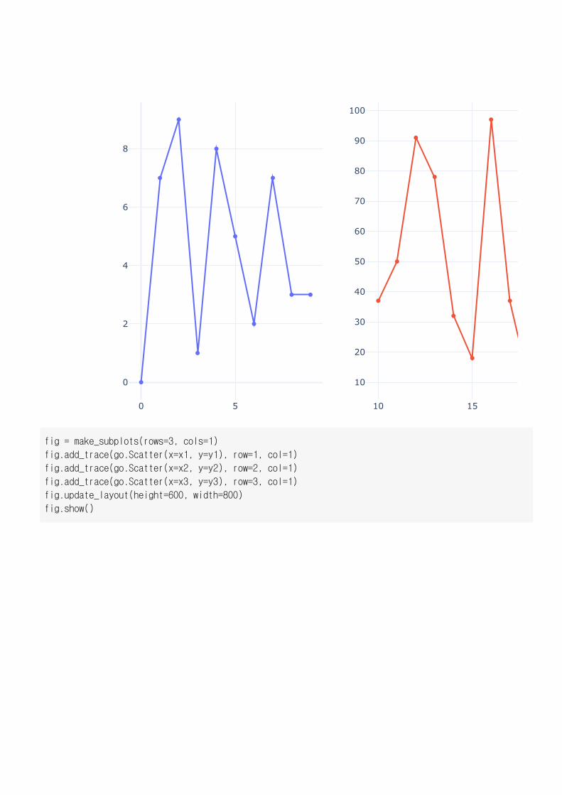
fig = make_subplots(rows=3, cols=1)
fig.add_trace(go.Scatter(x=x1, y=y1), row=1, col=1)
fig.add_trace(go.Scatter(x=x2, y=y2), row=2, col=1)
fig.add_trace(go.Scatter(x=x3, y=y3), row=3, col=1)
fig.update_layout(height=600, width=800)
fig.show()
0 2 4 6 80
5
10 12 14 16 18
50
100
20 22 24 26 28200
400
600
800
0 2 4 6 80
550
100
20 22 24 26 28200
400
600
800
2000
4000
6000
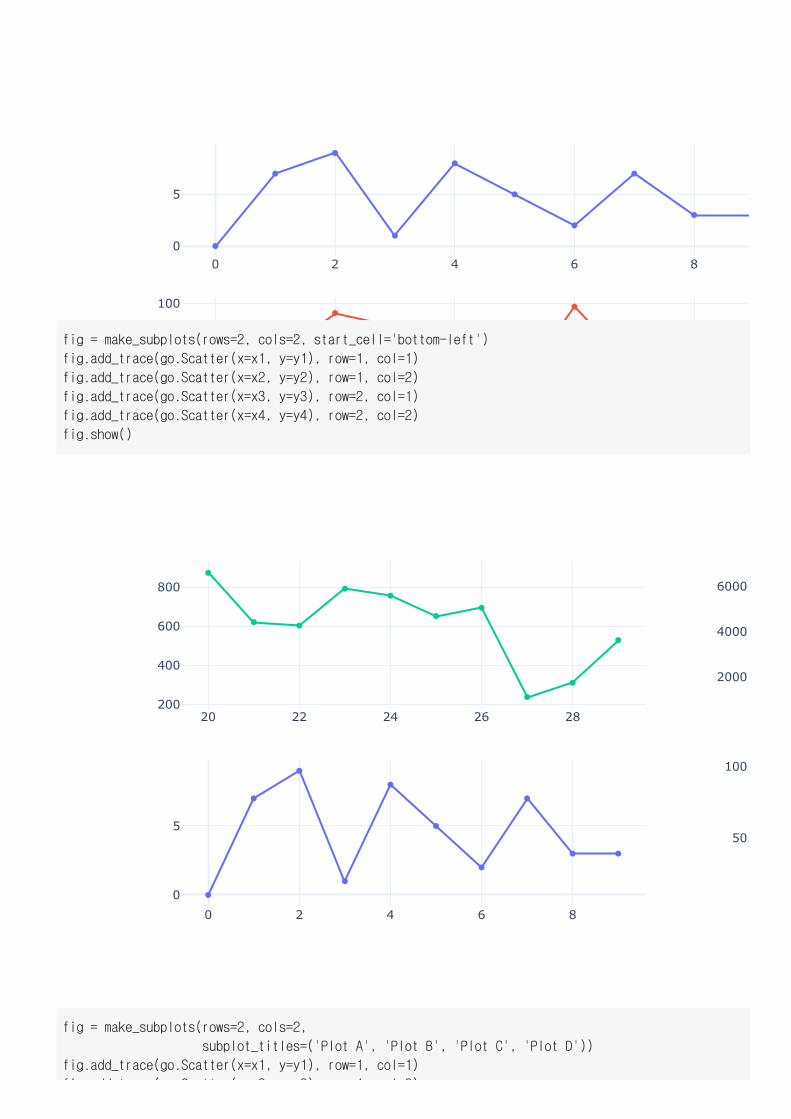
fig = make_subplots(rows=2, cols=2, start_cell='bottom-left')
fig.add_trace(go.Scatter(x=x1, y=y1), row=1, col=1)
fig.add_trace(go.Scatter(x=x2, y=y2), row=1, col=2)
fig.add_trace(go.Scatter(x=x3, y=y3), row=2, col=1)
fig.add_trace(go.Scatter(x=x4, y=y4), row=2, col=2)
fig.show()
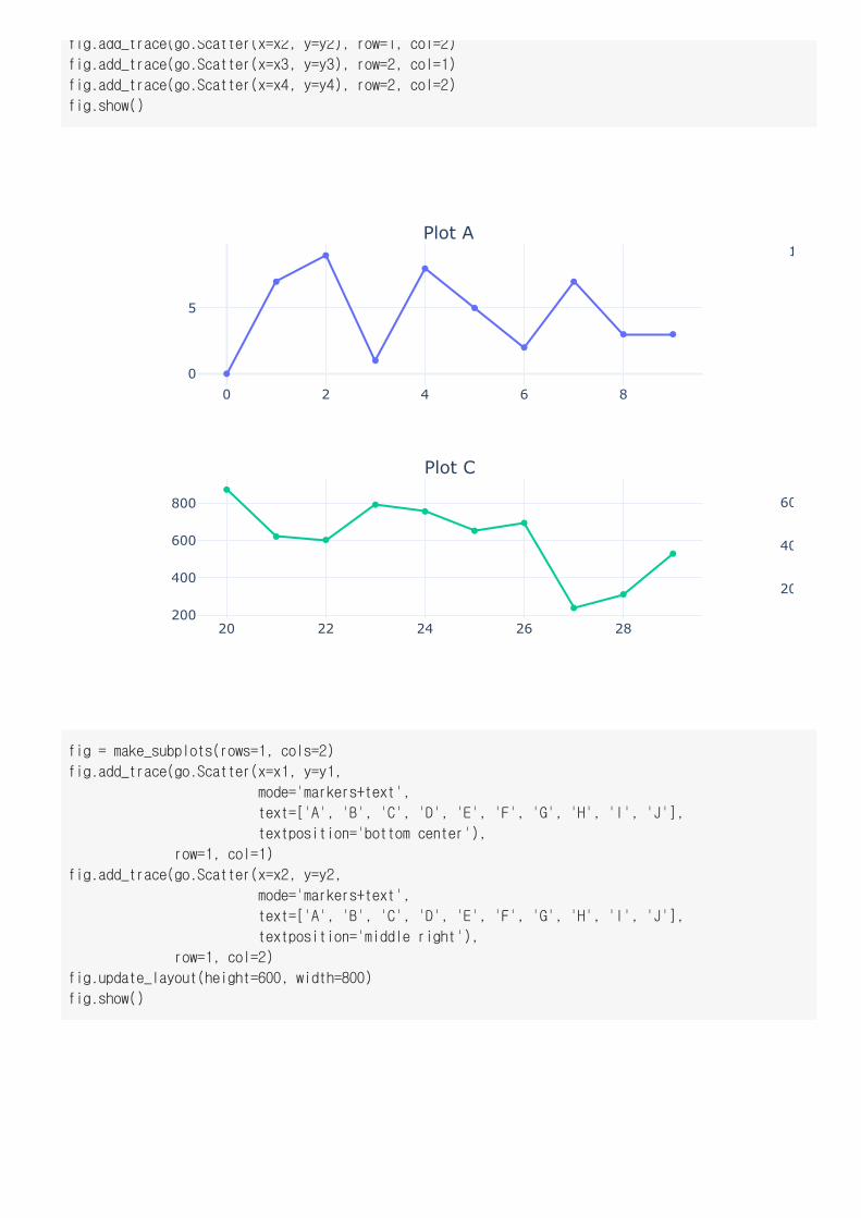
fig = make_subplots(rows=2, cols=2,
subplot_titles=('Plot A', 'Plot B', 'Plot C', 'Plot D'))
fig.add_trace(go.Scatter(x=x1, y=y1), row=1, col=1)
fi dd t ( S tt ( 2 2) 1 l 2)
0 2 4 6 80
5
1
20 22 24 26 28200
400
600
800
20
40
60
Plot A
Plot C
fig.add_trace(go.Scatter(x=x2, y=y2), row=1, col=2)
fig.add_trace(go.Scatter(x=x3, y=y3), row=2, col=1)
fig.add_trace(go.Scatter(x=x4, y=y4), row=2, col=2)
fig.show()
fig = make_subplots(rows=1, cols=2)
fig.add_trace(go.Scatter(x=x1, y=y1,
mode='markers+text',
text=['A', 'B', 'C', 'D', 'E', 'F', 'G', 'H', 'I', 'J'],
textposition='bottom center'),
row=1, col=1)
fig.add_trace(go.Scatter(x=x2, y=y2,
mode='markers+text',
text=['A', 'B', 'C', 'D', 'E', 'F', 'G', 'H', 'I', 'J'],
textposition='middle right'),
row=1, col=2)
fig.update_layout(height=600, width=800)
fig.show()
A
B
C
D
E
F
G
H
I J
0 5
0
2
4
6
8
A
B
C
D
E
F
G
H
10 15
10
20
30
40
50
60
70
80
90
100
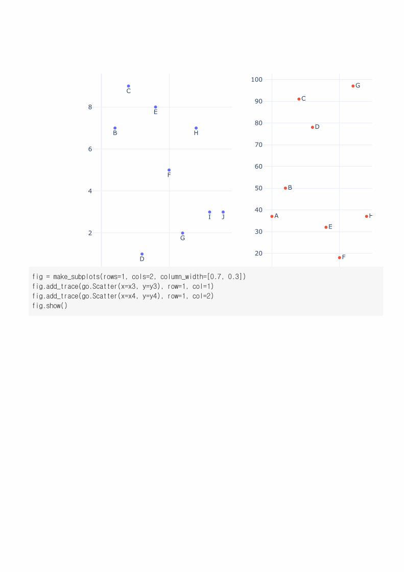
fig = make_subplots(rows=1, cols=2, column_width=[0.7, 0.3])
fig.add_trace(go.Scatter(x=x3, y=y3), row=1, col=1)
fig.add_trace(go.Scatter(x=x4, y=y4), row=1, col=2)
fig.show()
20 22 24 26 2200
300
400
500
600
700
800
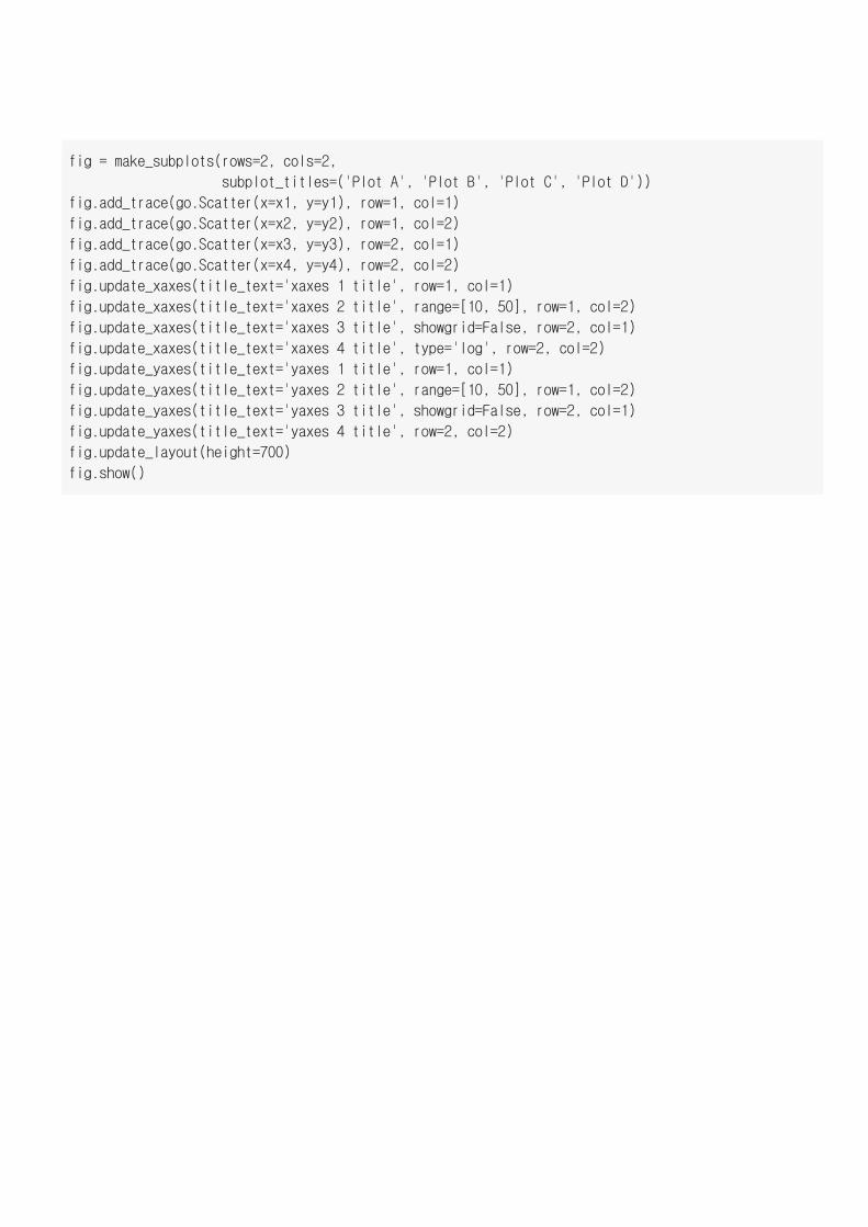
900fig = make_subplots(rows=2, cols=2,
subplot_titles=('Plot A', 'Plot B', 'Plot C', 'Plot D'))
fig.add_trace(go.Scatter(x=x1, y=y1), row=1, col=1)
fig.add_trace(go.Scatter(x=x2, y=y2), row=1, col=2)
fig.add_trace(go.Scatter(x=x3, y=y3), row=2, col=1)
fig.add_trace(go.Scatter(x=x4, y=y4), row=2, col=2)
fig.update_xaxes(title_text='xaxes 1 title', row=1, col=1)
fig.update_xaxes(title_text='xaxes 2 title', range=[10, 50], row=1, col=2)
fig.update_xaxes(title_text='xaxes 3 title', showgrid=False, row=2, col=1)
fig.update_xaxes(title_text='xaxes 4 title', type='log', row=2, col=2)
fig.update_yaxes(title_text='yaxes 1 title', row=1, col=1)
fig.update_yaxes(title_text='yaxes 2 title', range=[10, 50], row=1, col=2)
fig.update_yaxes(title_text='yaxes 3 title', showgrid=False, row=2, col=1)
fig.update_yaxes(title_text='yaxes 4 title', row=2, col=2)
fig.update_layout(height=700)
fig.show()
0 2 4 6 8
0
2
4
6
8
1010
20
30
40
50
20 22 24 26 28200
400
600
800
2000
4000
6000
xaxes 1 title
xaxes 3 title
yaxe
s 1
title
yaxe
s 2
title
yaxe
s 3
title
yaxe
s 4
title
Plot A
Plot C
0
5
50
100
200
400
600
800
0 10 20 30 40
2000
4000
6000
trace 0trace 1trace 2trace 3
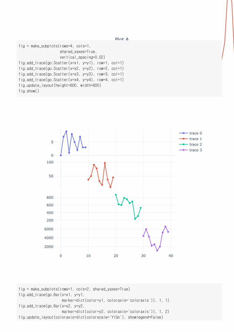
fig = make_subplots(rows=4, cols=1,
shared_xaxes=True,
vertical_spacing=0.02)
fig.add_trace(go.Scatter(x=x1, y=y1), row=1, col=1)
fig.add_trace(go.Scatter(x=x2, y=y2), row=2, col=1)
fig.add_trace(go.Scatter(x=x3, y=y3), row=3, col=1)
fig.add_trace(go.Scatter(x=x4, y=y4), row=4, col=1)
fig.update_layout(height=600, width=600)
fig.show()
fig = make_subplots(rows=1, cols=2, shared_yaxes=True)
fig.add_trace(go.Bar(x=x1, y=y1,
marker=dict(color=y1, coloraxis='coloraxis')), 1, 1)
fig.add_trace(go.Bar(x=x2, y=y2,
marker=dict(color=y2, coloraxis='coloraxis')), 1, 2)
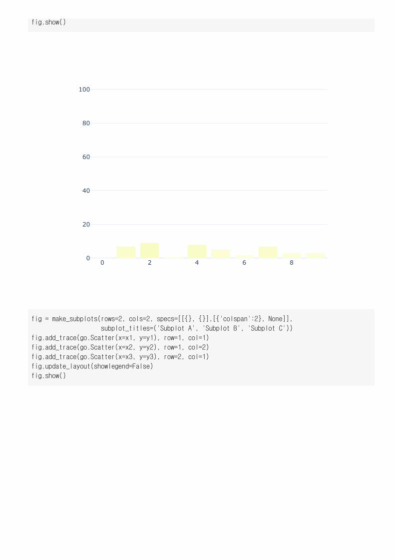
fig.update_layout(coloraxis=dict(colorscale='YlGn'), showlegend=False)
0 2 4 6 80
20
40
60
80
100
fig.show()
fig = make_subplots(rows=2, cols=2, specs=[[{}, {}],[{'colspan':2}, None]],
subplot_titles=('Subplot A', 'Subplot B', 'Subplot C'))
fig.add_trace(go.Scatter(x=x1, y=y1), row=1, col=1)
fig.add_trace(go.Scatter(x=x2, y=y2), row=1, col=2)
fig.add_trace(go.Scatter(x=x3, y=y3), row=2, col=1)
fig.update_layout(showlegend=False)
fig.show()
0 2 4 6 80
5
20 22 24200
400
600
800
Subplot A
Subplo
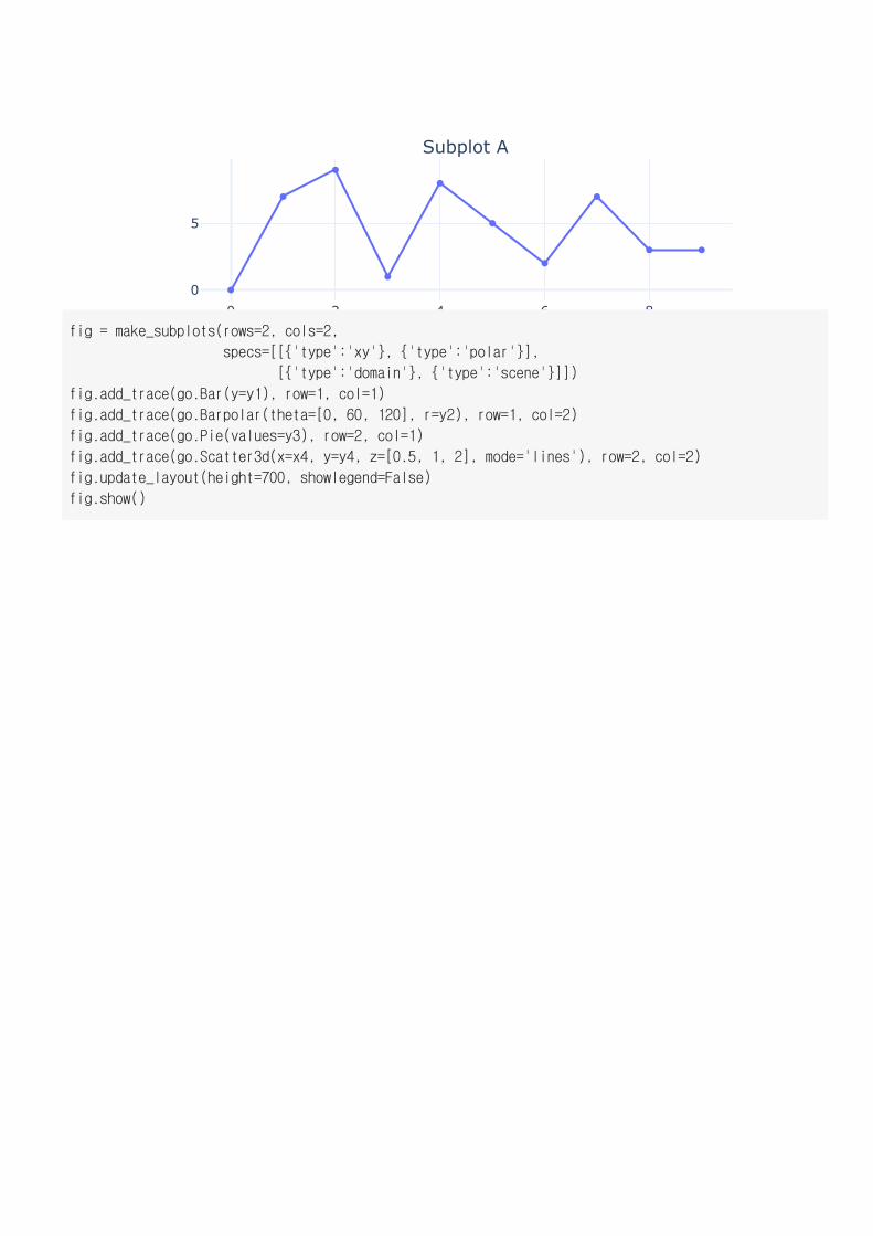
fig = make_subplots(rows=2, cols=2,
specs=[[{'type':'xy'}, {'type':'polar'}],
[{'type':'domain'}, {'type':'scene'}]])
fig.add_trace(go.Bar(y=y1), row=1, col=1)
fig.add_trace(go.Barpolar(theta=[0, 60, 120], r=y2), row=1, col=2)
fig.add_trace(go.Pie(values=y3), row=2, col=1)
fig.add_trace(go.Scatter3d(x=x4, y=y4, z=[0.5, 1, 2], mode='lines'), row=2, col=2)
fig.update_layout(height=700, showlegend=False)
fig.show()
0 2 4 6 80
2
4
6
8
14.4%13%
12.5%
11.4%
10.7%10.2%
9.94%
8.72%
5.12%3.92%
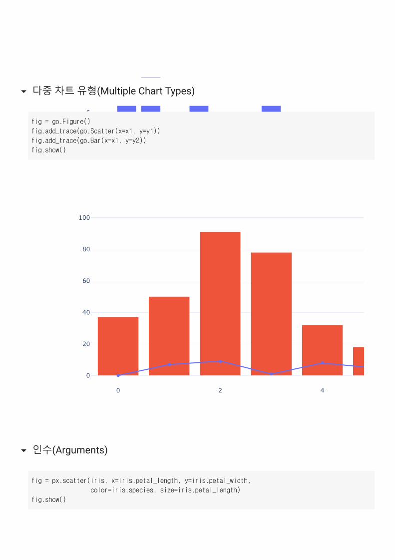
다중 차트 유형(Multiple Chart Types)
0 2 4
0
20
40
60
80
100
fig = go.Figure()
fig.add_trace(go.Scatter(x=x1, y=y1))
fig.add_trace(go.Bar(x=x1, y=y2))
fig.show()
인수(Arguments)
fig = px.scatter(iris, x=iris.petal_length, y=iris.petal_width,
color=iris.species, size=iris.petal_length)
fig.show()
1 2 3 4
0
0.5
1
1.5
2
2.5
petal_length
petal_width
fig = px.scatter(iris, x='petal_length', y='petal_width',
color='species', size='petal_length')
fig.show()

1 2 3 4
0
0.5
1
1.5
2
2.5
petal_length
petal_width
1 2 3 4
0
0.5
1
1.5
2
2.5
petal_length
petal_width
fig = px.scatter(iris, x=iris.petal_length, y=iris.petal_width,
color=iris.species, size=iris.petal_length,
hover_data=[iris.index])
fig.show()
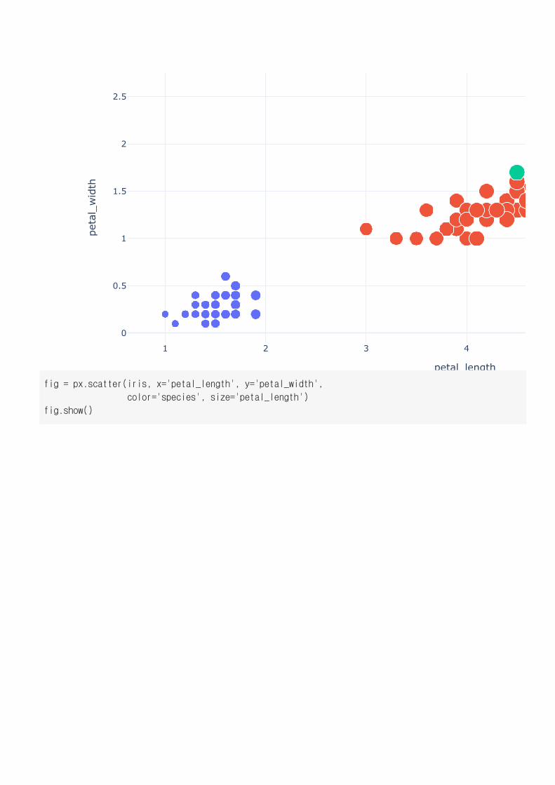
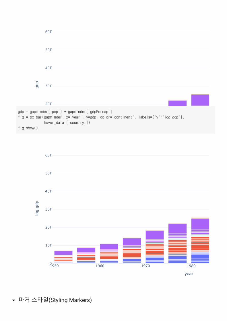
gdp = gapminder['pop'] * gapminder['gdpPercap']
fig = px.bar(gapminder, x='year', y=gdp, color='continent', labels={'y':'gdp'},
hover_data=['country'])
fig.show()
1950 1960 1970 19800
10T
20T
30T
40T
50T
60T
year
gdp
1950 1960 1970 19800
10T
20T
30T
40T
50T
60T
year
log
gdp
gdp = gapminder['pop'] * gapminder['gdpPercap']
fig = px.bar(gapminder, x='year', y=gdp, color='continent', labels={'y':'log gdp'},
hover_data=['country'])
fig.show()
마커 스타일(Styling Markers)
0 0.5 1 1
1
2
3
4
5
6
7
petal_width
petal_leng
th
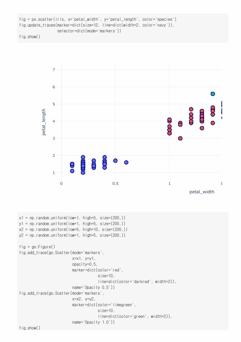
fig = px.scatter(iris, x='petal_width', y='petal_length', color='species')
fig.update_traces(marker=dict(size=12, line=dict(width=2, color='navy')),
selector=dict(mode='markers'))
fig.show()
x1 = np.random.uniform(low=1, high=5, size=(200,))
y1 = np.random.uniform(low=1, high=5, size=(200,))
x2 = np.random.uniform(low=5, high=10, size=(200,))
y2 = np.random.uniform(low=1, high=5, size=(200,))
fig = go.Figure()
fig.add_trace(go.Scatter(mode='markers',
x=x1, y=y1,
opacity=0.5,
marker=dict(color='red',
size=10,
line=dict(color='darkred', width=2)),
name='Opacity 0.5'))
fig.add_trace(go.Scatter(mode='markers',
x=x2, y=y2,
marker=dict(color='limegreen',
size=10,
line=dict(color='green', width=2)),
name='Opacity 1.0'))
fig.show()
2 4 6
1
1.5
2
2.5
3
3.5
4
4.5
5
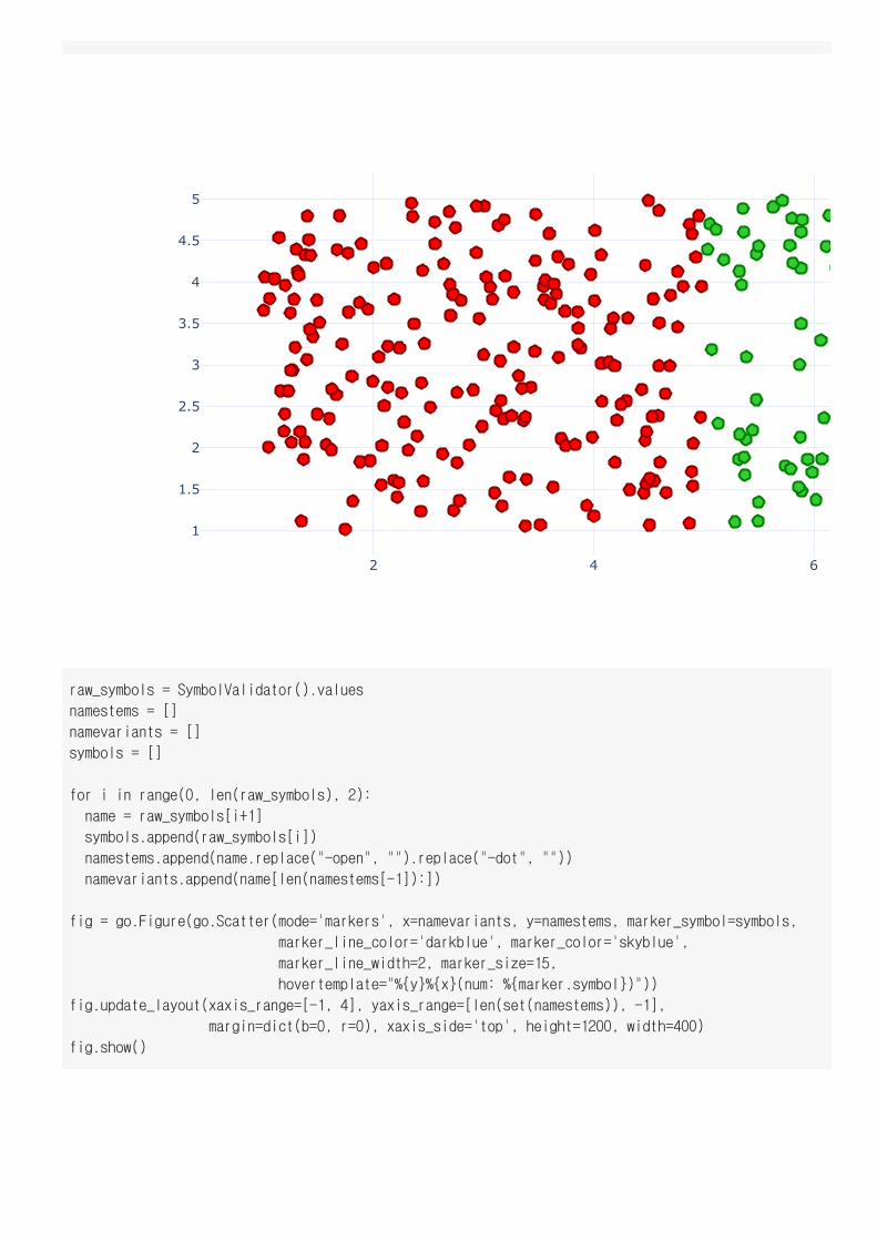
raw_symbols = SymbolValidator().values
namestems = []
namevariants = []
symbols = []
for i in range(0, len(raw_symbols), 2):
name = raw_symbols[i+1]
symbols.append(raw_symbols[i])
namestems.append(name.replace("-open", "").replace("-dot", ""))
namevariants.append(name[len(namestems[-1]):])
fig = go.Figure(go.Scatter(mode='markers', x=namevariants, y=namestems, marker_symbol=symbols,
marker_line_color='darkblue', marker_color='skyblue',
marker_line_width=2, marker_size=15,
hovertemplate="%{y}%{x}(num: %{marker.symbol})"))
fig.update_layout(xaxis_range=[-1, 4], yaxis_range=[len(set(namestems)), -1],
margin=dict(b=0, r=0), xaxis_side='top', height=1200, width=400)
fig.show()
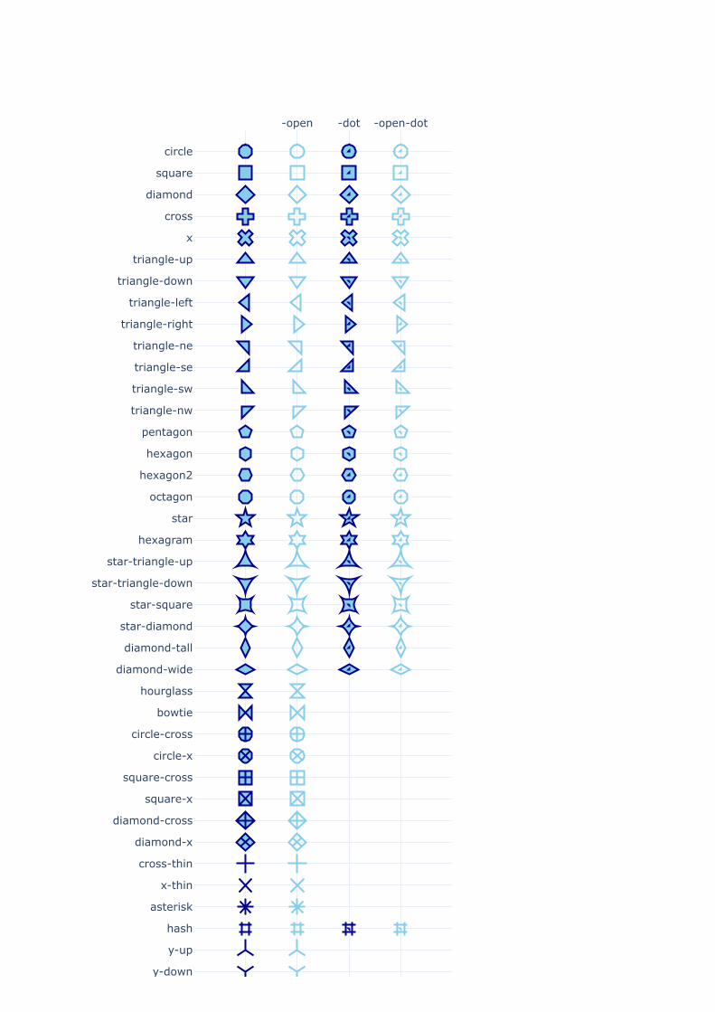
-open -dot -open-dot
y-down
y-up
hash
asterisk
x-thin
cross-thin
diamond-x
diamond-cross
square-x
square-cross
circle-x
circle-cross
bowtie
hourglass
diamond-wide
diamond-tall
star-diamond
star-square
star-triangle-down
star-triangle-up
hexagram
star
octagon
hexagon2
hexagon
pentagon
triangle-nw
triangle-sw
triangle-se
triangle-ne
triangle-right
triangle-left
triangle-down
triangle-up
x
cross
diamond
square
circle
line-nw
line-ne
line-ns
line-ew
y-right
y-left
y
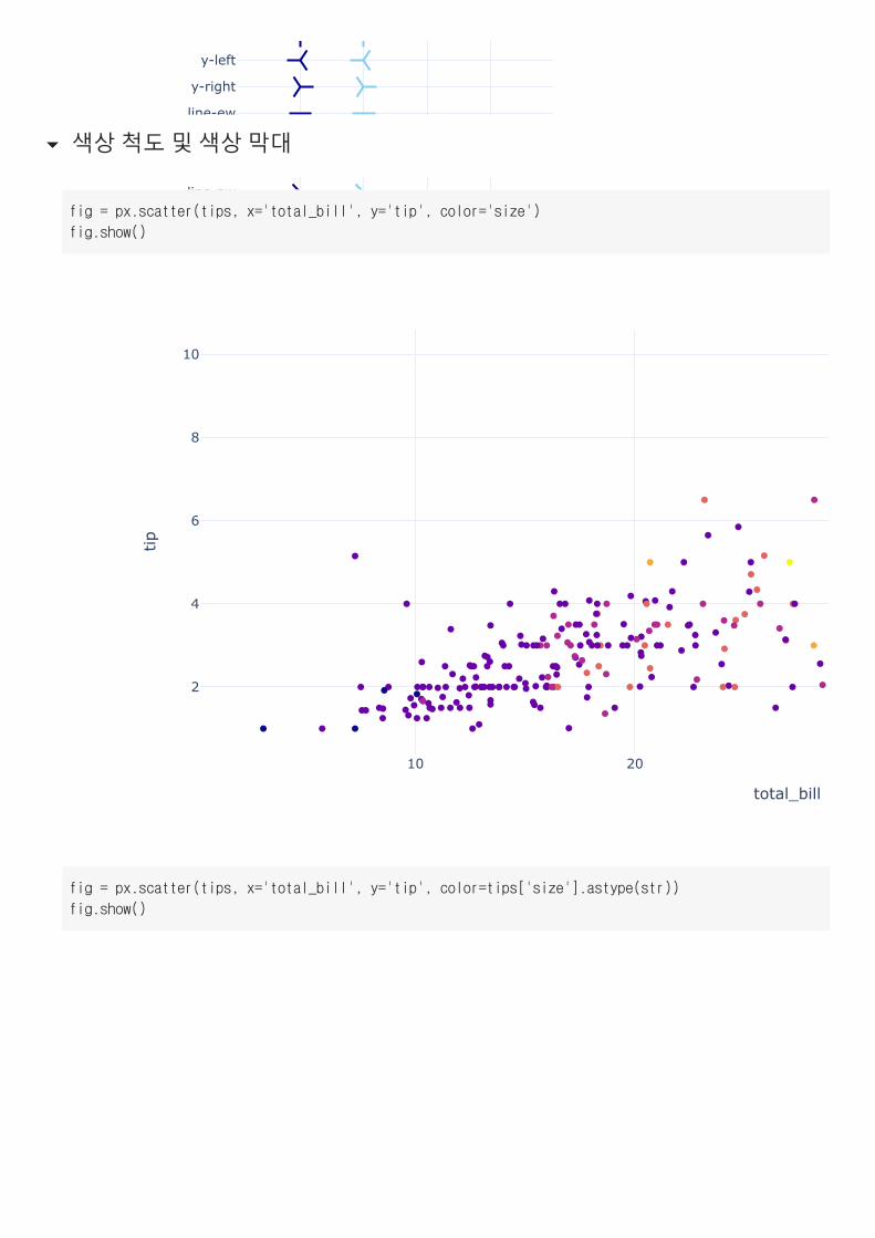
색상 척도 및 색상 막대
10 20
2
4
6
8
10
total_bill
tip
fig = px.scatter(tips, x='total_bill', y='tip', color='size')
fig.show()
fig = px.scatter(tips, x='total_bill', y='tip', color=tips['size'].astype(str))
fig.show()
10 20
2
4
6
8
10
total_bill
tip
10 20
2
4
6
8
10
total_b
tip
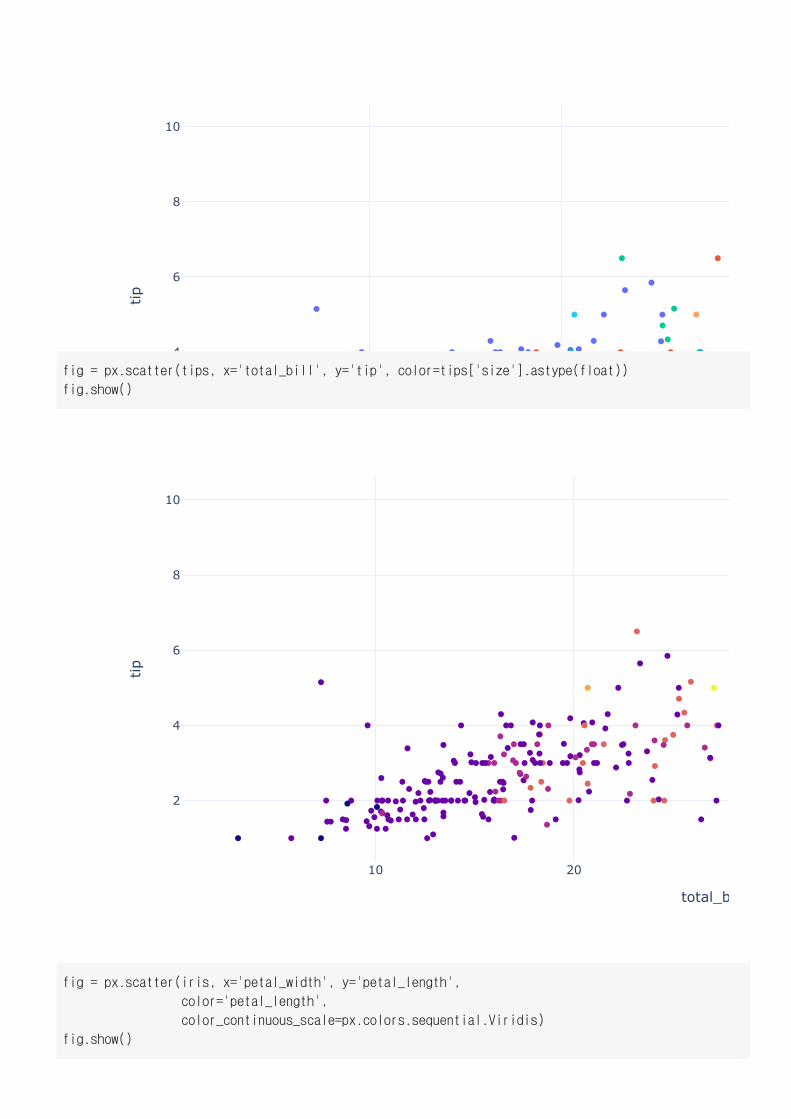
fig = px.scatter(tips, x='total_bill', y='tip', color=tips['size'].astype(float))
fig.show()
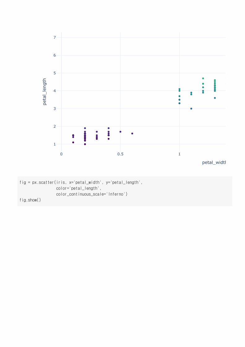
fig = px.scatter(iris, x='petal_width', y='petal_length',
color='petal_length',
color_continuous_scale=px.colors.sequential.Viridis)
fig.show()
0 0.5 1
1
2
3
4
5
6
7
petal_width
petal_leng
th
fig = px.scatter(iris, x='petal_width', y='petal_length',
color='petal_length',
color_continuous_scale='Inferno')
fig.show()
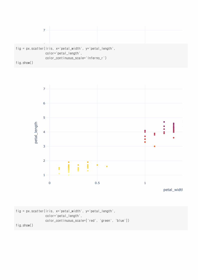
0 0.5 1
1
2
3
4
5
6
7
petal_width
petal_leng
th
0 0.5 1
1
2
3
4
5
6
7
petal_width
petal_leng
th
fig = px.scatter(iris, x='petal_width', y='petal_length',
color='petal_length',
color_continuous_scale='Inferno_r')
fig.show()
fig = px.scatter(iris, x='petal_width', y='petal_length',
color='petal_length',
color_continuous_scale=['red', 'green', 'blue'])
fig.show()
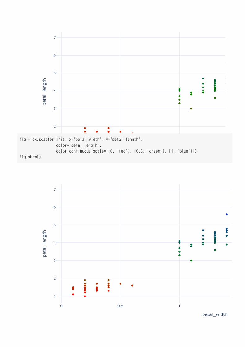
0 0.5 1
1
2
3
4
5
6
7
petal_width
petal_leng
th
0 0.5 1
1
2
3
4
5
6
7
petal_width
petal_leng
th
fig = px.scatter(iris, x='petal_width', y='petal_length',
color='petal_length',
color_continuous_scale=[(0, 'red'), (0.3, 'green'), (1, 'blue')])
fig.show()
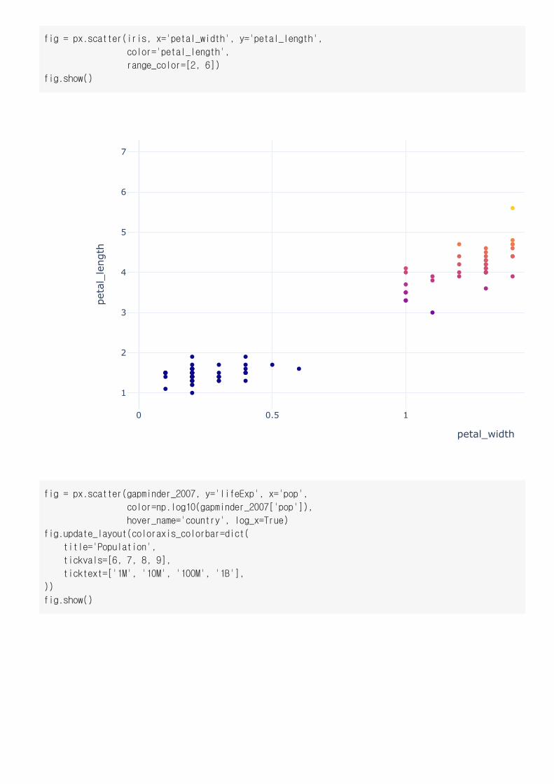
0 0.5 1
1
2
3
4
5
6
7
petal_width
petal_leng
th
fig = px.scatter(iris, x='petal_width', y='petal_length',
color='petal_length',
range_color=[2, 6])
fig.show()
fig = px.scatter(gapminder_2007, y='lifeExp', x='pop',
color=np.log10(gapminder_2007['pop']),
hover_name='country', log_x=True)
fig.update_layout(coloraxis_colorbar=dict(
title='Population',
tickvals=[6, 7, 8, 9],
ticktext=['1M', '10M', '100M', '1B'],
))
fig.show()
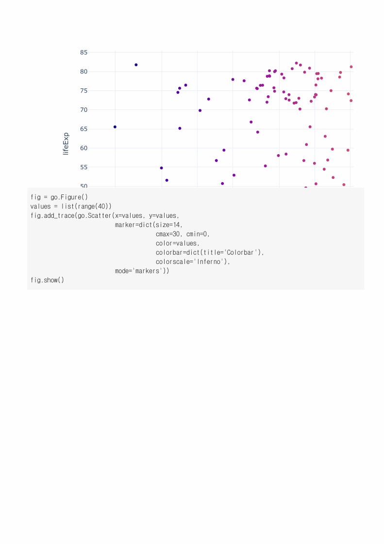
2 5 1M 2 5 10M 2
40
45
50
55
60
65
70
75
80
85
pop
lifeE
xp
fig = go.Figure()
values = list(range(40))
fig.add_trace(go.Scatter(x=values, y=values,
marker=dict(size=14,
cmax=30, cmin=0,
color=values,
colorbar=dict(title='Colorbar'),
colorscale='Inferno'),
mode='markers'))
fig.show()

0 5 10 15 20
0
5
10
15
20
25
30
35
40
텍스트 및 주석(Text and Annotation)
gapminder_asia_2007 = gapminder.query("year == 2007 and continent == 'Asia'")
gapminder_asia_2007

country continent year lifeExp pop gdpPercap iso_alpha is
11 Afghanistan Asia 2007 43.828 31889923 974.580338 AFG
95 Bahrain Asia 2007 75.635 708573 29796.048340 BHR
107 Bangladesh Asia 2007 64.062 150448339 1391.253792 BGD
227 Cambodia Asia 2007 59.723 14131858 1713.778686 KHM
299 China Asia 2007 72.961 1318683096 4959.114854 CHN
671 Hong Kong,China Asia 2007 82.208 6980412 39724.978670 HKG
707 India Asia 2007 64.698 1110396331 2452.210407 IND
719 Indonesia Asia 2007 70.650 223547000 3540.651564 IDN
731 Iran Asia 2007 70.964 69453570 11605.714490 IRN
743 Iraq Asia 2007 59.545 27499638 4471.061906 IRQ
767 Israel Asia 2007 80.745 6426679 25523.277100 ISR
803 Japan Asia 2007 82.603 127467972 31656.068060 JPN
815 Jordan Asia 2007 72.535 6053193 4519.461171 JOR
839 Korea,Dem. Rep. Asia 2007 67.297 23301725 1593.065480 KOR
851 Korea,Rep. Asia 2007 78.623 49044790 23348.139730 KOR
863 Kuwait Asia 2007 77.588 2505559 47306.989780 KWT
875 Lebanon Asia 2007 71.993 3921278 10461.058680 LBN
947 Malaysia Asia 2007 74.241 24821286 12451.655800 MYS
1007 Mongolia Asia 2007 66.803 2874127 3095.772271 MNG
1055 Myanmar Asia 2007 62.069 47761980 944.000000 MMR
1079 Nepal Asia 2007 63.785 28901790 1091.359778 NPL
1163 Oman Asia 2007 75.640 3204897 22316.192870 OMN
1175 Pakistan Asia 2007 65.483 169270617 2605.947580 PAK
1223 Philippines Asia 2007 71.688 91077287 3190.481016 PHL
1319 SaudiArabia Asia 2007 72.777 27601038 21654.831940 SAU
1367 Singapore Asia 2007 79.972 4553009 47143.179640 SGP
1439 Sri Lanka Asia 2007 72.396 20378239 3970.095407 LKA
1499 Syria Asia 2007 74.143 19314747 4184.548089 SYR
1511 Taiwan Asia 2007 78.400 23174294 28718.276840 TWN
fig = px.scatter(gapminder_asia_2007, x='gdpPercap', y='lifeExp',
text='country', log_x=True, size_max=60)
fig.update_traces(textposition='top center')
fig.update_layout(height=800)
fig.show()
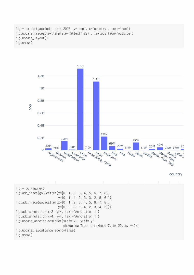
Afghanistan
Bangladesh
Cambodia
China
India
Indonesia
Iraq
Jordan
Korea, Dem. Rep. Mongolia
Myanmar
Nepal
Pakistan
PhilippinesSri Lanka
Syria
Thaila
VietnamWest Bank and Gaza
Yemen, Rep.
8 91000
2 3 4 5 6 7
45
50
55
60
65
70
75
80
85
gdpPercap
lifeE
xp
32M710k
150M
14M
1.3G
7.0M
1.1G
220M
69M27M 6.4M
130M
6.1M 23M 49M2.5M 3.9M 25
Afghanistan
BahrainBangladesh
Cambodia
ChinaHong Kong, China
IndiaIndonesia
IranIraq
IsraelJapan
JordanKorea, Dem. Rep.
Korea, Rep.
KuwaitLebano
M0
0.2B
0.4B
0.6B
0.8B
1B
1.2B
country
pop
fig = px.bar(gapminder_asia_2007, y='pop', x='country', text='pop')
fig.update_traces(texttemplate='%{text:.2s}', textposition='outside')
fig.update_layout()
fig.show()
fig = go.Figure()
fig.add_trace(go.Scatter(x=[0, 1, 2, 3, 4, 5, 6, 7, 8],
y=[0, 1, 4, 2, 3, 3, 2, 5, 6]))
fig.add_trace(go.Scatter(x=[0, 1, 2, 3, 4, 5, 6, 7, 8],
y=[0, 2, 3, 1, 4, 2, 3, 4, 5]))
fig.add_annotation(x=2, y=4, text='Annotation 1')
fig.add_annotation(x=4, y=4, text='Annotation 1')
fig.update_annotations(dict(xref='x', yref='y',
showarrow=True, arrowhead=7, ax=20, ay=-40))
fig.update_layout(showlegend=False)
fig.show()
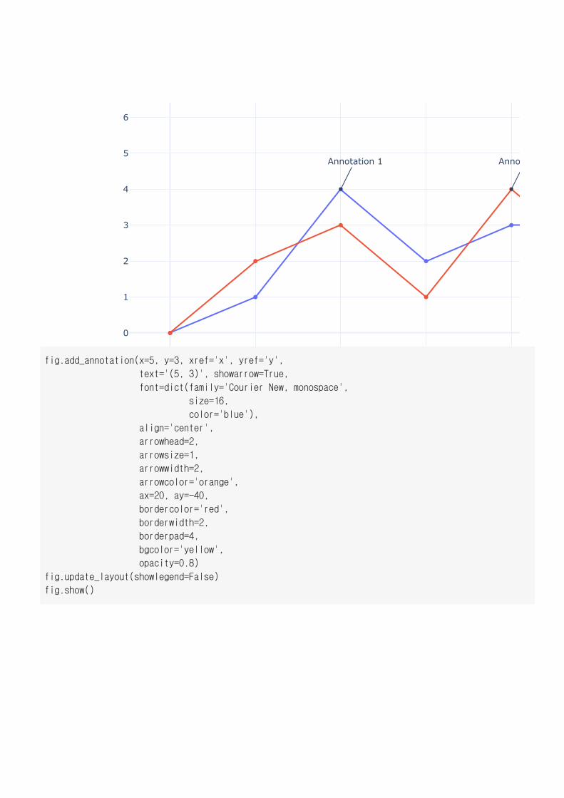
0 1 2 3 4
0
1
2
3
4
5
6
Annotation 1 Anno
fig.add_annotation(x=5, y=3, xref='x', yref='y',
text='(5, 3)', showarrow=True,
font=dict(family='Courier New, monospace',
size=16,
color='blue'),
align='center',
arrowhead=2,
arrowsize=1,
arrowwidth=2,
arrowcolor='orange',
ax=20, ay=-40,
bordercolor='red',
borderwidth=2,
borderpad=4,
bgcolor='yellow',
opacity=0.8)
fig.update_layout(showlegend=False)
fig.show()
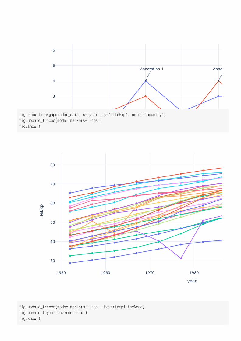
0 1 2 3 4
0
1
2
3
4
5
6
Annotation 1 Anno
1950 1960 1970 1980
30
40
50
60
70
80
year
lifeE
xp
fig = px.line(gapminder_asia, x='year', y='lifeExp', color='country')
fig.update_traces(mode='markers+lines')
fig.show()
fig.update_traces(mode='markers+lines', hovertemplate=None)
fig.update_layout(hovermode='x')
fig.show()
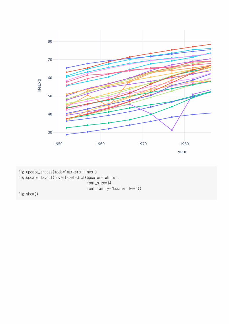
1950 1960 1970 1980
30
40
50
60
70
80
year
lifeE
xp
fig.update_traces(mode='markers+lines')
fig.update_layout(hoverlabel=dict(bgcolor='white',
font_size=14,
font_family="Courier New"))
fig.show()
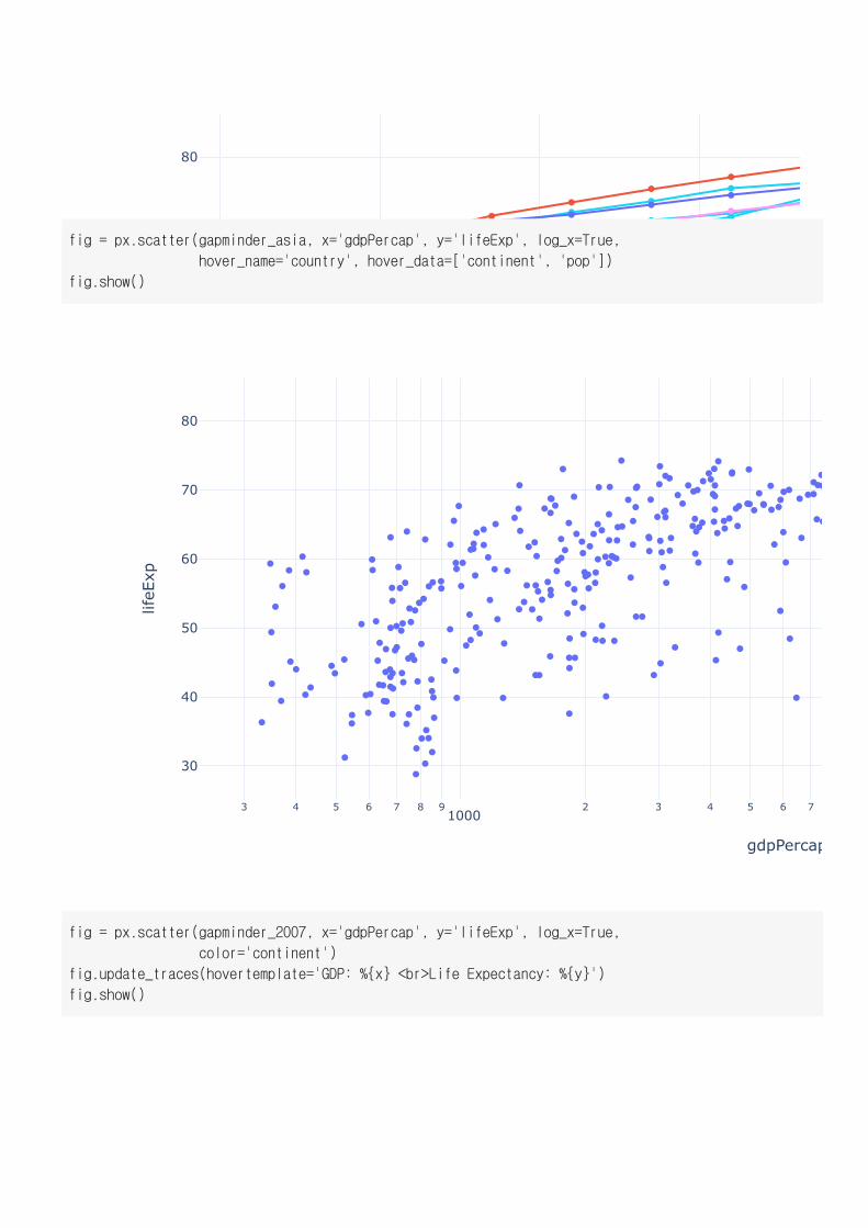
1950 1960 1970 1980
30
40
50
60
70
80
year
lifeE
xp
3 4 5 6 7 8 91000
2 3 4 5 6 7
30
40
50
60
70
80
gdpPercap
lifeE
xp
fig = px.scatter(gapminder_asia, x='gdpPercap', y='lifeExp', log_x=True,
hover_name='country', hover_data=['continent', 'pop'])
fig.show()
fig = px.scatter(gapminder_2007, x='gdpPercap', y='lifeExp', log_x=True,
color='continent')
fig.update_traces(hovertemplate='GDP: %{x} <br>Life Expectancy: %{y}')
fig.show()
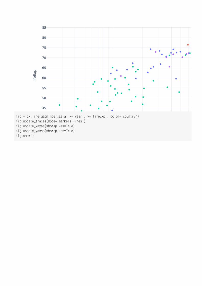
3 4 5 6 7 8 91000
2 3 4 5 6
40
45
50
55
60
65
70
75
80
85
gdpPercap
lifeE
xp
fig = px.line(gapminder_asia, x='year', y='lifeExp', color='country')
fig.update_traces(mode='markers+lines')
fig.update_xaxes(showspikes=True)
fig.update_yaxes(showspikes=True)
fig.show()
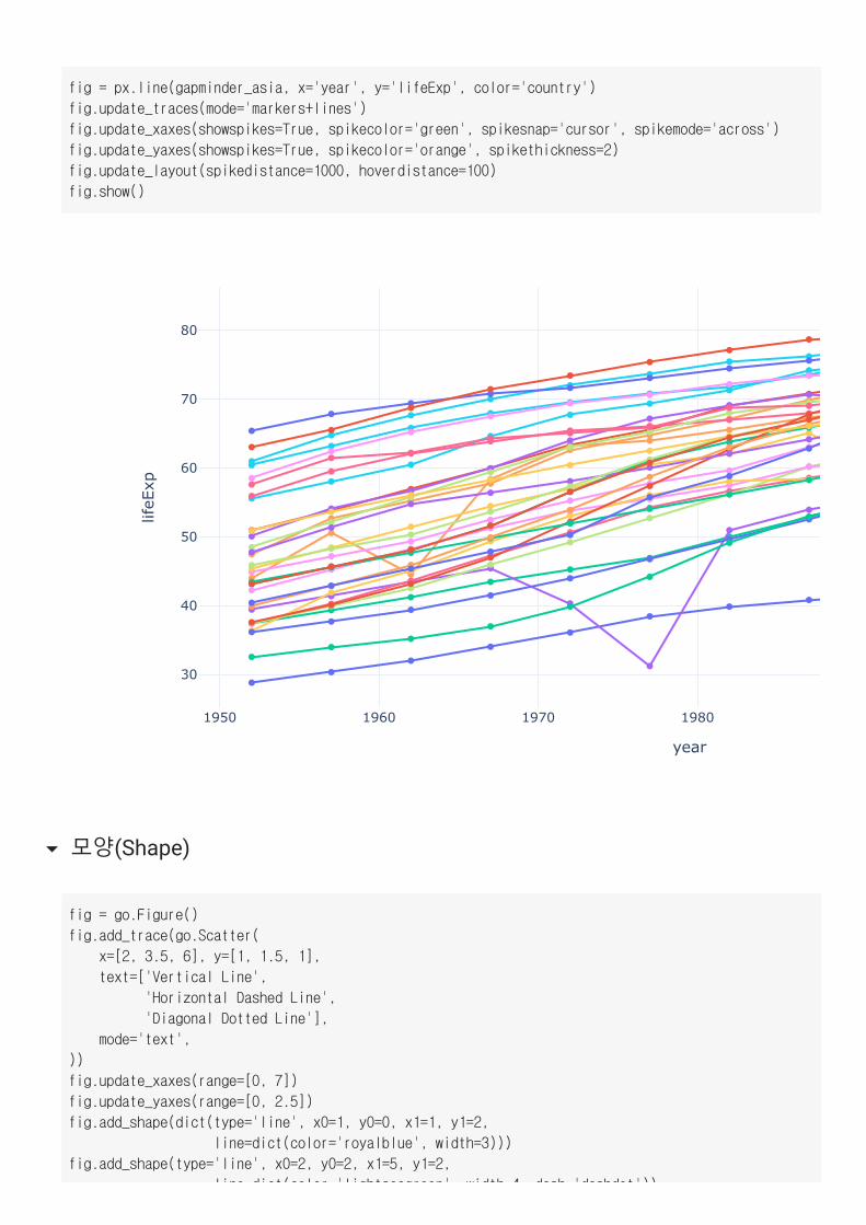
1950 1960 1970 1980
30
40
50
60
70
80
year
lifeE
xp
1950 1960 1970 1980
30
40
50
60
70
80
year
lifeE
xp
fig = px.line(gapminder_asia, x='year', y='lifeExp', color='country')
fig.update_traces(mode='markers+lines')
fig.update_xaxes(showspikes=True, spikecolor='green', spikesnap='cursor', spikemode='across')
fig.update_yaxes(showspikes=True, spikecolor='orange', spikethickness=2)
fig.update_layout(spikedistance=1000, hoverdistance=100)
fig.show()
모양(Shape)
fig = go.Figure()
fig.add_trace(go.Scatter(
x=[2, 3.5, 6], y=[1, 1.5, 1],
text=['Vertical Line',
'Horizontal Dashed Line',
'Diagonal Dotted Line'],
mode='text',
))
fig.update_xaxes(range=[0, 7])
fig.update_yaxes(range=[0, 2.5])
fig.add_shape(dict(type='line', x0=1, y0=0, x1=1, y1=2,
line=dict(color='royalblue', width=3)))
fig.add_shape(type='line', x0=2, y0=2, x1=5, y1=2,
line=dict(color='lightseagreen' width=4 dash='dashdot'))
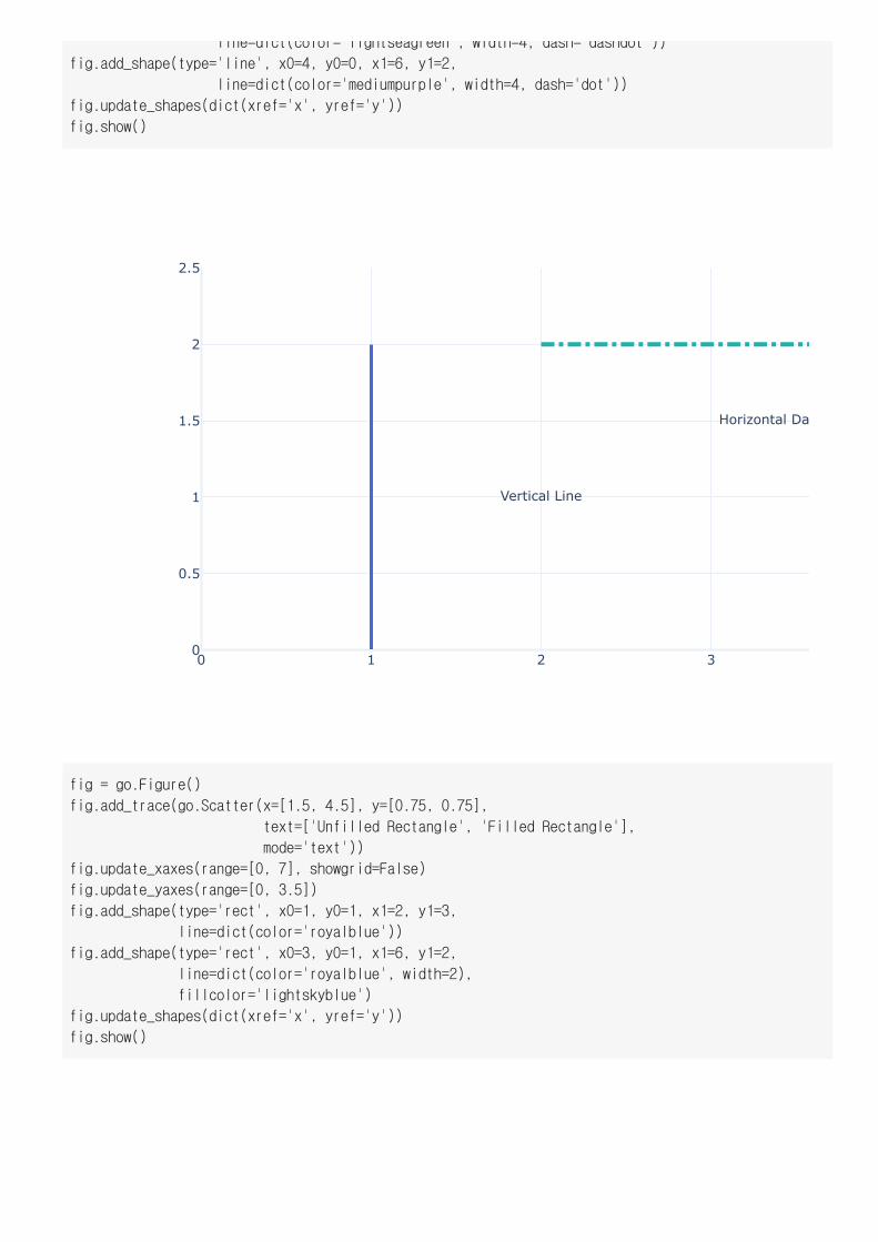
Vertical Line
Horizontal Da
0 1 2 30
0.5
1
1.5
2
2.5
line=dict(color= lightseagreen , width=4, dash= dashdot ))
fig.add_shape(type='line', x0=4, y0=0, x1=6, y1=2,
line=dict(color='mediumpurple', width=4, dash='dot'))
fig.update_shapes(dict(xref='x', yref='y'))
fig.show()
fig = go.Figure()
fig.add_trace(go.Scatter(x=[1.5, 4.5], y=[0.75, 0.75],
text=['Unfilled Rectangle', 'Filled Rectangle'],
mode='text'))
fig.update_xaxes(range=[0, 7], showgrid=False)
fig.update_yaxes(range=[0, 3.5])
fig.add_shape(type='rect', x0=1, y0=1, x1=2, y1=3,
line=dict(color='royalblue'))
fig.add_shape(type='rect', x0=3, y0=1, x1=6, y1=2,
line=dict(color='royalblue', width=2),
fillcolor='lightskyblue')
fig.update_shapes(dict(xref='x', yref='y'))
fig.show()
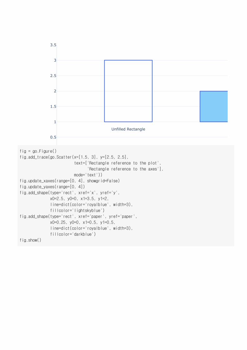
Unfilled Rectangle
0 1 2 30
0.5
1
1.5
2
2.5
3
3.5
fig = go.Figure()
fig.add_trace(go.Scatter(x=[1.5, 3], y=[2.5, 2.5],
text=['Rectangle reference to the plot',
'Rectangle reference to the axes'],
mode='text'))
fig.update_xaxes(range=[0, 4], showgrid=False)
fig.update_yaxes(range=[0, 4])
fig.add_shape(type='rect', xref='x', yref='y',
x0=2.5, y0=0, x1=3.5, y1=2,
line=dict(color='royalblue', width=3),
fillcolor='lightskyblue')
fig.add_shape(type='rect', xref='paper', yref='paper',
x0=0.25, y0=0, x1=0.5, y1=0.5,
line=dict(color='royalblue', width=3),
fillcolor='darkblue')
fig.show()
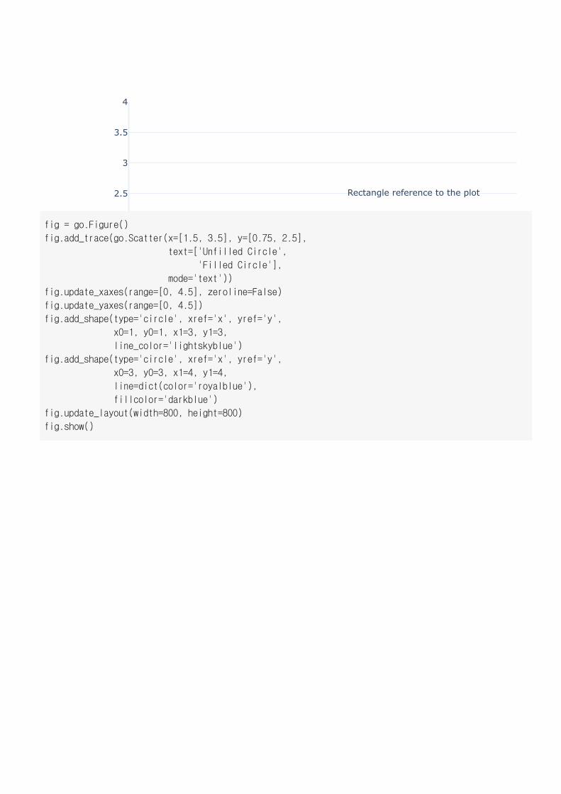
Rectangle reference to the plot
0 0.5 1 1.5 20
0.5
1
1.5
2
2.5
3
3.5
4
fig = go.Figure()
fig.add_trace(go.Scatter(x=[1.5, 3.5], y=[0.75, 2.5],
text=['Unfilled Circle',
'Filled Circle'],
mode='text'))
fig.update_xaxes(range=[0, 4.5], zeroline=False)
fig.update_yaxes(range=[0, 4.5])
fig.add_shape(type='circle', xref='x', yref='y',
x0=1, y0=1, x1=3, y1=3,
line_color='lightskyblue')
fig.add_shape(type='circle', xref='x', yref='y',
x0=3, y0=3, x1=4, y1=4,
line=dict(color='royalblue'),
fillcolor='darkblue')
fig.update_layout(width=800, height=800)
fig.show()


![[중앙도서관] 트위터 페이스북 제대로 알고 쓰기 강의안(2) 111207](https://img.pdfslide.tips/doc/110x75/558b3855d8b42adf378b4698/-2-111207.jpg)

![[중앙도서관] 트위터 페이스북 제대로 알고 쓰기 강의안(3) 111214](https://img.pdfslide.tips/doc/110x75/558b3879d8b42ad9378b467a/-3-111214.jpg)


![[2011 체인지온]사람을 깊게 알아야 사람을 위한 디자인을 제대로 할 수 있다_최병호](https://img.pdfslide.tips/doc/110x75/557a902fd8b42ab7638b5061/2011--558492841b4fb.jpg)


![[중앙도서관] 트위터 페이스북 제대로 알고 쓰기 강의안(4) 111221](https://img.pdfslide.tips/doc/110x75/558b3a5bd8b42ac66a8b4598/-4-111221.jpg)