Embed Size (px)
Citation preview
1
psyc3010 lecture 5
consolidation of between-subjects anova
power
last week: complex anova
next week: Blocking and ANCOVA
2
last week this week last week we looked at how a 2-way anova can be
extended to a 3-way anova, where three factors (IVs) are
included in the model
this week we discuss the assignment
briefly recap on 3-way anova
– Including simple interactions, simple simple effects, and simple
simple comparisons
– A quick note on unequal n
Then on to power
– What it is, graphically & statistically
– effect size measures, d and Φ‟(phi prime)
– non-centrality parameters δ (delta) and Φ (phi)
– What influences power
3
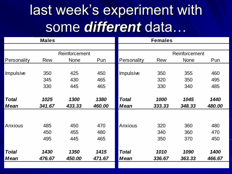
last week‟s experiment with
some different data…Males
Personality Rew None Pun
Impulsive 350 425 450
345 430 465
330 445 465
Total 1025 1300 1380
Mean 341.67 433.33 460.00
Anxious 485 450 470
450 455 480
495 445 465
Total 1430 1350 1415
Mean 476.67 450.00 471.67
Reinforcement
Females
Personality Rew None Pun
Impulsive 350 355 460
320 350 495
330 340 485
Total 1000 1045 1440
Mean 333.33 348.33 480.00
Anxious 320 360 480
340 360 470
350 370 450
Total 1010 1090 1400
Mean 336.67 363.33 466.67
Reinforcement
4
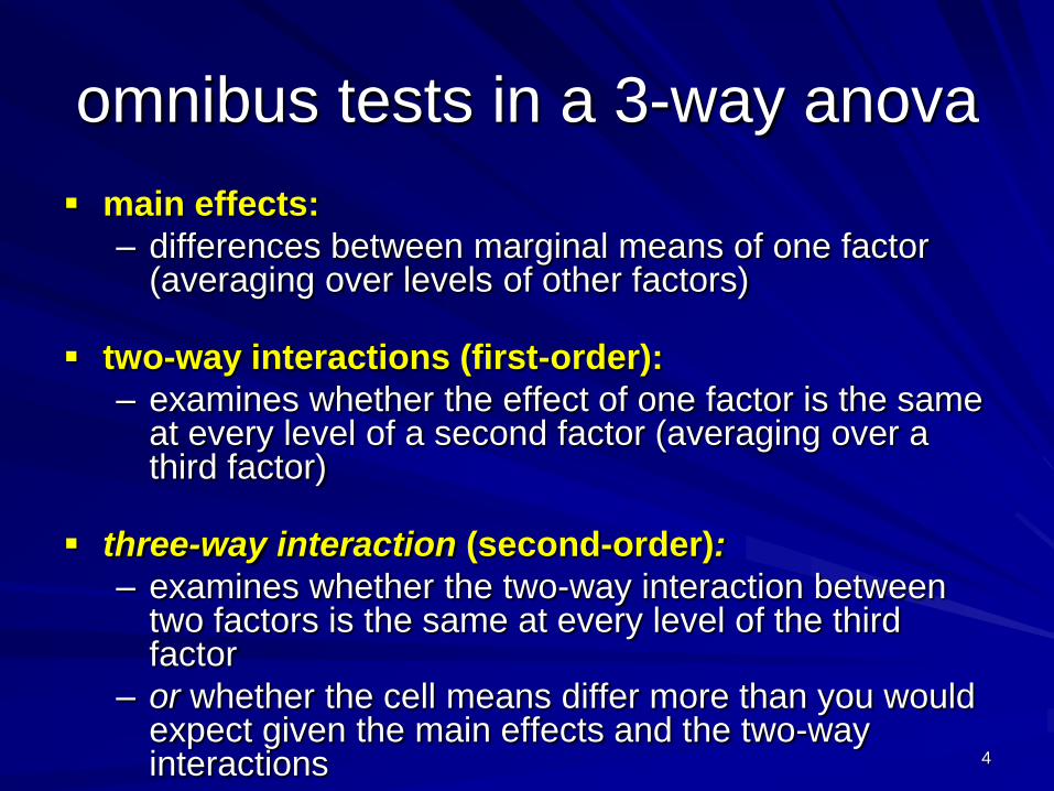
omnibus tests in a 3-way anova
main effects:
– differences between marginal means of one factor (averaging over levels of other factors)
two-way interactions (first-order):
– examines whether the effect of one factor is the same at every level of a second factor (averaging over a third factor)
three-way interaction (second-order):
– examines whether the two-way interaction between two factors is the same at every level of the third factor
– or whether the cell means differ more than you would expect given the main effects and the two-way interactions
5
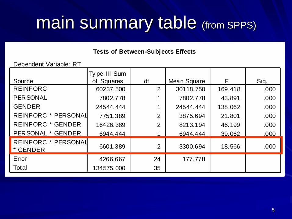
main summary table (from SPPS)
Tests of Between-Subjects Effects
Dependent Variable: RT
60237.500 2 30118.750 169.418 .000
7802.778 1 7802.778 43.891 .000
24544.444 1 24544.444 138.062 .000
7751.389 2 3875.694 21.801 .000
16426.389 2 8213.194 46.199 .000
6944.444 1 6944.444 39.062 .000
6601.389 2 3300.694 18.566 .000
4266.667 24 177.778
134575.000 35
Source
REINFORC
PERSONAL
GENDER
REINFORC * PERSONAL
REINFORC * GENDER
PERSONAL * GENDER
REINFORC * PERSONAL
* GENDER
Error
Total
Ty pe III Sum
of Squares df Mean Square F Sig.
6
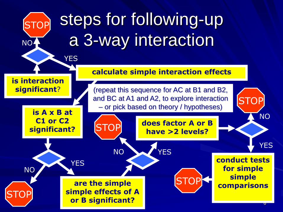
steps for following-up
a 3-way interaction
is interaction significant?
NO
calculate simple interaction effects
YES
NOYES
does factor A or B have >2 levels?
NO YESconduct tests
for simple simple
comparisons
STOP
STOP
STOP
STOP
is A x B at C1 or C2
significant?
are the simple simple effects of A or B significant?
NO
STOP
(repeat this sequence for AC at B1 and B2,
and BC at A1 and A2, to explore interaction
– or pick based on theory / hypotheses)
YES
7
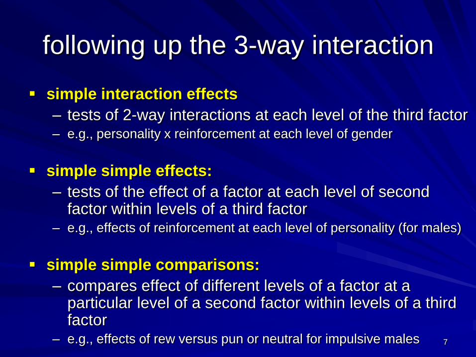
following up the 3-way interaction
simple interaction effects
– tests of 2-way interactions at each level of the third factor– e.g., personality x reinforcement at each level of gender
simple simple effects:
– tests of the effect of a factor at each level of second factor within levels of a third factor
– e.g., effects of reinforcement at each level of personality (for males)
simple simple comparisons:
– compares effect of different levels of a factor at a particular level of a second factor within levels of a third factor
– e.g., effects of rew versus pun or neutral for impulsive males

8
summary table for follow-up testsSource SS df MS F p
Simple Interaction Effects
PR at G1 13744.44 2 6872.22 38.656 0.000
PR at G2 608.33 2 304.17 1.711 0.202
Error 4266.67 24 177.78
Simple Simple effects in the interaction of PR at G1
R at P1 at G1 23116.67 2 11558.33 65.016 0.000
R at P2 at G1 538.89 2 269.44 1.516 0.240
Error 4266.67 24 177.78
Simple Simple comparisons in simple effect of R at P1 at G1
R vs N and P at P1 at G1 22047.90 1 22047.90 124.019 0.000
N vs P at P1 at G1 355.64 1 355.64 2.000 0.170
Error 4266.67 24 177.78

9
summary table for follow-up testsSource SS df MS F p
Simple Interaction Effects
PR at G1 13744.44 2 6872.22 38.656 0.000
PR at G2 608.33 2 304.17 1.711 0.202
Error 4266.67 24 177.78
Simple Simple effects in the interaction of PR at G1
R at P1 at G1 23116.67 2 11558.33 65.016 0.000
R at P2 at G1 538.89 2 269.44 1.516 0.240
Error 4266.67 24 177.78
Simple Simple comparisons in simple effect of R at P1 at G1
R vs N and P at P1 at G1 22047.90 1 22047.9 124.019 0.000
N vs P at P1 at G1 355.64 1 355.64 2.000 0.170
Error 4266.67 24 177.78
the personality x reinforcement interaction is…
- significant for males
- non-significant for females
we can follow up this significant simple interaction
effect of Personality x Reinforcement for males using
simple simple effects
10
summary table for follow-up testsSource SS df MS F p
Simple Interaction Effects
PR at G1 13744.44 2 6872.22 38.656 0.000
PR at G2 608.33 2 304.17 1.711 0.202
Error 4266.67 24 177.78
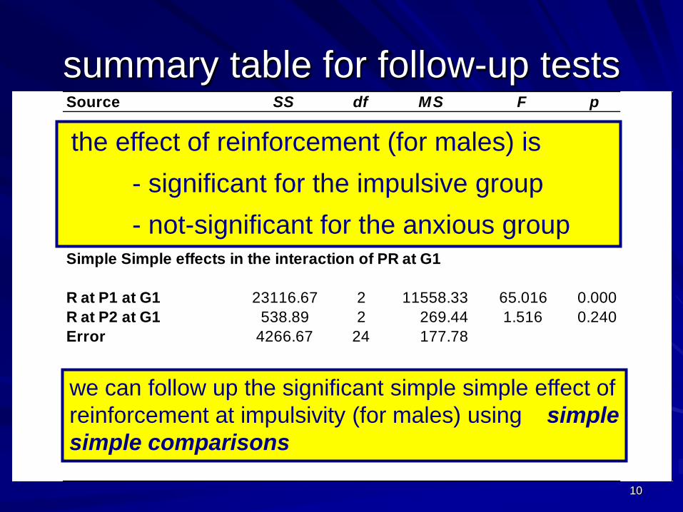
Simple Simple effects in the interaction of PR at G1
R at P1 at G1 23116.67 2 11558.33 65.016 0.000
R at P2 at G1 538.89 2 269.44 1.516 0.240
Error 4266.67 24 177.78
Simple Simple comparisons in simple effect of R at P1 at G1
R vs N and P at P1 at G1 22047.90 1 22047.9 124.019 0.000
N vs P at P1 at G1 355.64 1 355.64 2.000 0.170
Error 4266.67 24 177.78
the effect of reinforcement (for males) is
- significant for the impulsive group
- not-significant for the anxious group
we can follow up the significant simple simple effect of
reinforcement at impulsivity (for males) using simple
simple comparisons
11
summary table for follow-up testsSource SS df MS F p
Simple Interaction Effects
PR at G1 13744.44 2 6872.22 38.656 0.000
PR at G2 608.33 2 304.17 1.711 0.202
Error 4266.67 24 177.78
Simple Simple effects in the interaction of PR at G1
R at P1 at G1 23116.67 2 11558.33 65.016 0.000
R at P2 at G1 538.89 2 269.44 1.516 0.240
Error 4266.67 24 177.78
Simple Simple comparisons in simple effect of R at P1 at G1
R vs N and P at P1 at G1 22047.90 1 22047.90 124.019 0.000
N vs P at P1 at G1 355.64 1 355.64 2.000 0.170
Error 4266.67 24 177.78
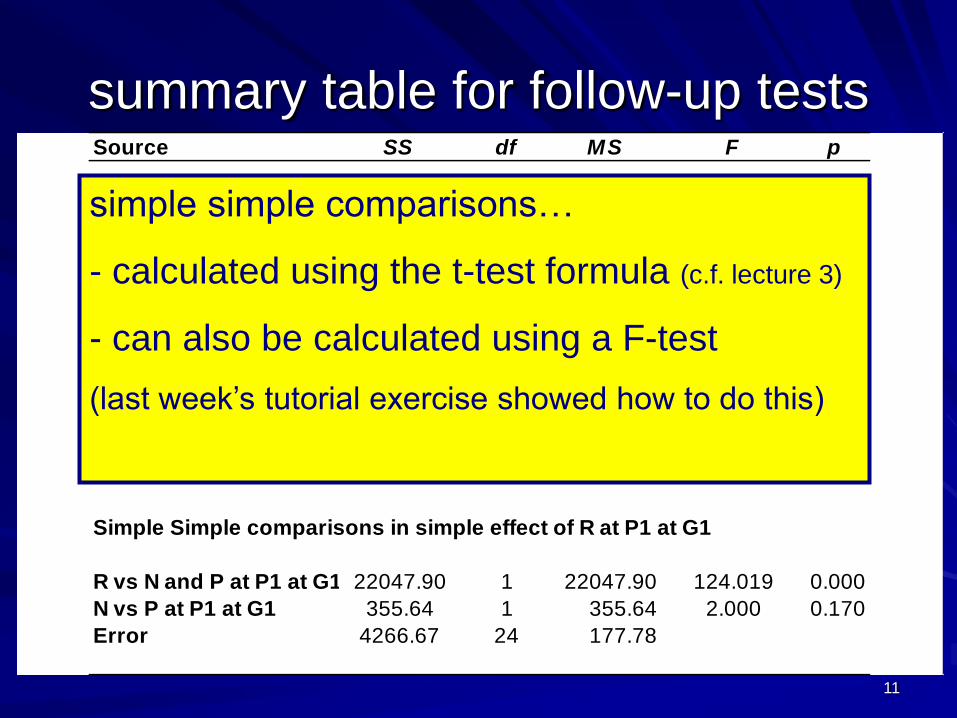
simple simple comparisons…
- calculated using the t-test formula (c.f. lecture 3)
- can also be calculated using a F-test
(last week‟s tutorial exercise showed how to do this)

12
summary table for follow-up testsSource SS df MS F p
Simple Interaction Effects
PR at G1 13744.44 2 6872.22 38.656 0.000
PR at G2 608.33 2 304.17 1.711 0.202
Error 4266.67 24 177.78
Simple Simple effects in the interaction of PR at G1
R at P1 at G1 23116.67 2 11558.33 65.016 0.000
R at P2 at G1 538.89 2 269.44 1.516 0.240
Error 4266.67 24 177.78
Simple Simple comparisons in simple effect of R at P1 at G1
R vs N and P at P1 at G1 22047.90 1 22047.9 124.019 0.000
N vs P at P1 at G1 355.64 1 355.644 2.000 0.170
Error 4266.67 24 177.78
for impulsive males,
1) performance under rewarding feedback was
significantly different from that under neutral or
punishing feedback
2) performance under punishing feedback was not
significantly different to performance under neutral
feedback
13
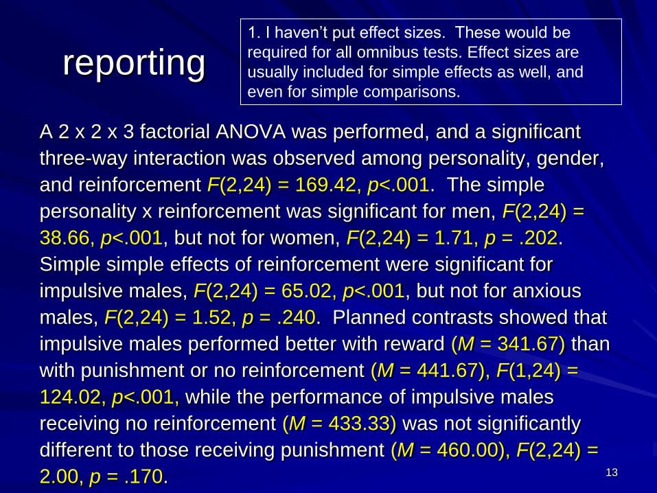
reporting
A 2 x 2 x 3 factorial ANOVA was performed, and a significant
three-way interaction was observed among personality, gender,
and reinforcement F(2,24) = 169.42, p<.001. The simple
personality x reinforcement was significant for men, F(2,24) =
38.66, p<.001, but not for women, F(2,24) = 1.71, p = .202.
Simple simple effects of reinforcement were significant for
impulsive males, F(2,24) = 65.02, p<.001, but not for anxious
males, F(2,24) = 1.52, p = .240. Planned contrasts showed that
impulsive males performed better with reward (M = 341.67) than
with punishment or no reinforcement (M = 441.67), F(1,24) =
124.02, p<.001, while the performance of impulsive males
receiving no reinforcement (M = 433.33) was not significantly
different to those receiving punishment (M = 460.00), F(2,24) =
2.00, p = .170.
1. I haven‟t put effect sizes. These would be
required for all omnibus tests. Effect sizes are
usually included for simple effects as well, and
even for simple comparisons.
14
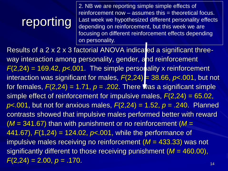
reporting
Results of a 2 x 2 x 3 factorial ANOVA indicated a significant three-
way interaction among personality, gender, and reinforcement
F(2,24) = 169.42, p<.001. The simple personality x reinforcement
interaction was significant for males, F(2,24) = 38.66, p<.001, but not
for females, F(2,24) = 1.71, p = .202. There was a significant simple
simple effect of reinforcement for impulsive males, F(2,24) = 65.02,
p<.001, but not for anxious males, F(2,24) = 1.52, p = .240. Planned
contrasts showed that impulsive males performed better with reward
(M = 341.67) than with punishment or no reinforcement (M =
441.67), F(1,24) = 124.02, p<.001, while the performance of
impulsive males receiving no reinforcement (M = 433.33) was not
significantly different to those receiving punishment (M = 460.00),
F(2,24) = 2.00, p = .170.
2. NB we are reporting simple simple effects of
reinforcement now – assumes this = theoretical focus.
Last week we hypothesized different personality effects
depending on reinforcement, but this week we are
focusing on different reinforcement effects depending
on personality.

15
reporting
Results of a 2 x 2 x 3 factorial ANOVA indicated a significant three-way
interaction among personality, gender, and reinforcement F(2,24) =
169.42, p<.001. The simple personality x reinforcement interaction was
significant for males, F(2,24) = 38.66, p<.001, but not for females,
F(2,24) = 1.71, p = .202. [Insert before simple simple effects of R for
men:] For women, across personality type the simple effect of
reinforcement was / was not significant, F(2,24)=X, p=, eta2=…. [If yes,
would also follow-up with contrasts.] In addition, there was a significant
simple simple effect of reinforcement for impulsive males, F(2,24) =
65.02, p<.001, but not for anxious males, F(2,24) = 1.52, p = .240. etc”
3. NB for simplicity we reported for women that the
simple interaction of P x R was ns, but unless interested
ONLY in interaction we would also „followup‟ ns simple
interaction by looking at simple effect of Reinforcement
for women (collapsing across Personality), if
hypotheses suggest R = the theoretically key IV. We
want to know if there are effects of reinforcement for
women that don‟t change depending on personality.
16
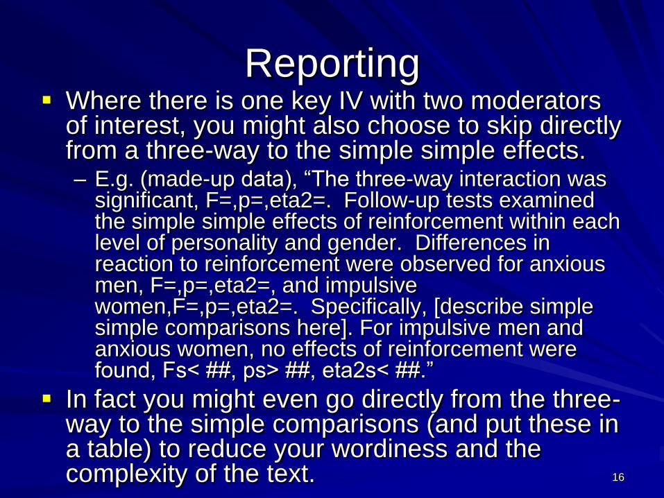
Reporting Where there is one key IV with two moderators
of interest, you might also choose to skip directly from a three-way to the simple simple effects.– E.g. (made-up data), “The three-way interaction was
significant, F=,p=,eta2=. Follow-up tests examined the simple simple effects of reinforcement within each level of personality and gender. Differences in reaction to reinforcement were observed for anxious men, F=,p=,eta2=, and impulsive women,F=,p=,eta2=. Specifically, [describe simple simple comparisons here]. For impulsive men and anxious women, no effects of reinforcement were found, Fs< ##, ps> ##, eta2s< ##.”
In fact you might even go directly from the three-way to the simple comparisons (and put these in a table) to reduce your wordiness and the complexity of the text.
17
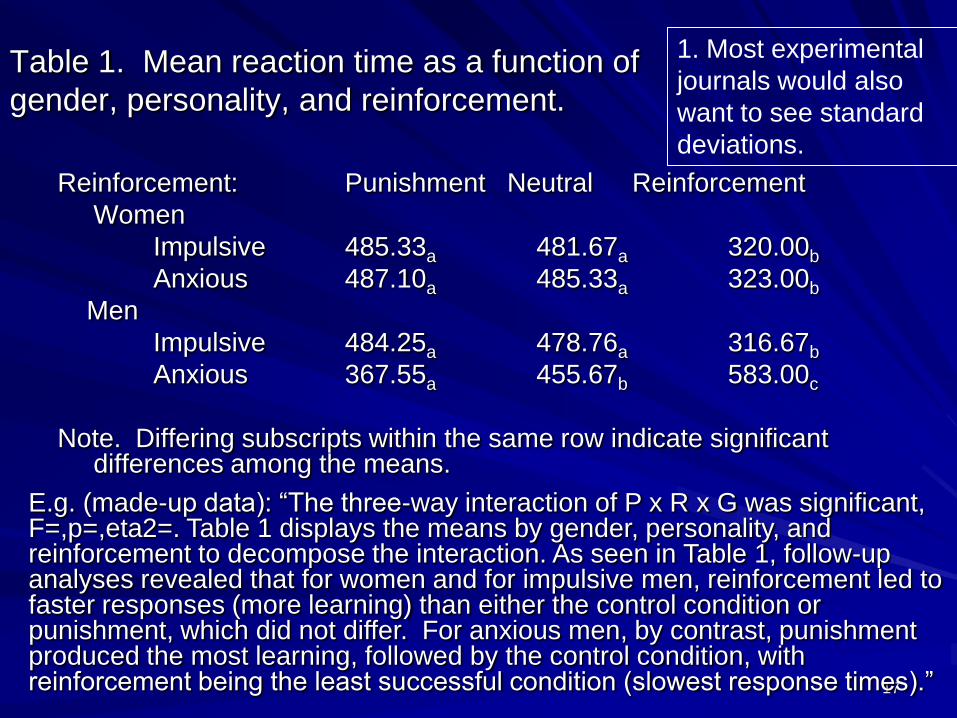
Table 1. Mean reaction time as a function of
gender, personality, and reinforcement.
Reinforcement: Punishment Neutral Reinforcement
Women
Impulsive 485.33a 481.67a 320.00b
Anxious 487.10a 485.33a 323.00b
Men
Impulsive 484.25a 478.76a 316.67b
Anxious 367.55a 455.67b 583.00c
Note. Differing subscripts within the same row indicate significant differences among the means.
1. Most experimental
journals would also
want to see standard
deviations.
E.g. (made-up data): “The three-way interaction of P x R x G was significant, F=,p=,eta2=. Table 1 displays the means by gender, personality, and reinforcement to decompose the interaction. As seen in Table 1, follow-up analyses revealed that for women and for impulsive men, reinforcement led to faster responses (more learning) than either the control condition or punishment, which did not differ. For anxious men, by contrast, punishment produced the most learning, followed by the control condition, with reinforcement being the least successful condition (slowest response times).”
18
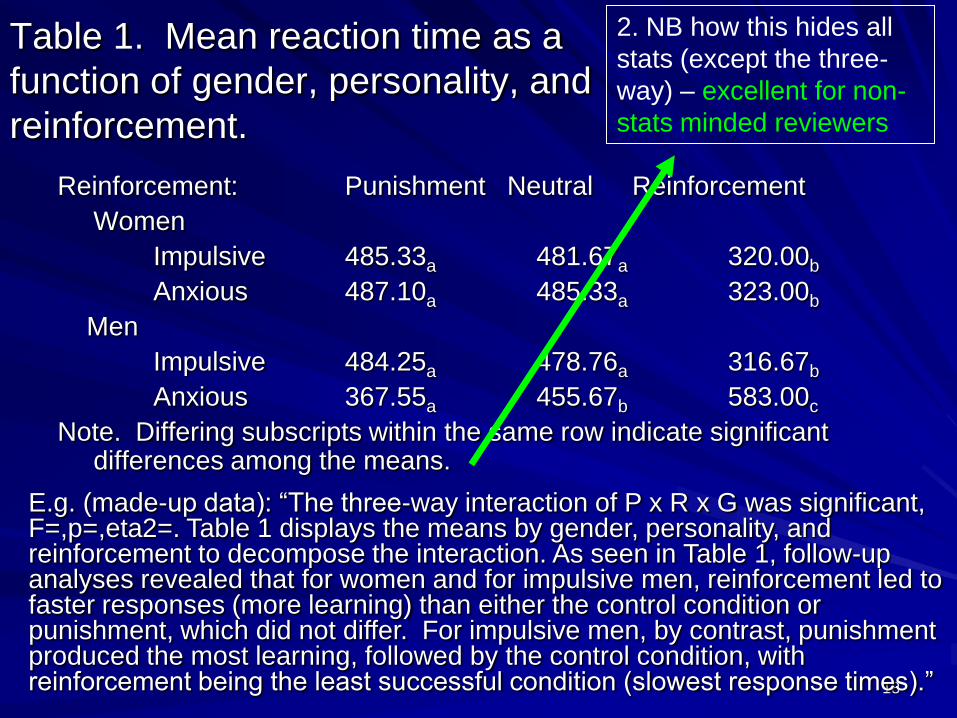
Table 1. Mean reaction time as a
function of gender, personality, and
reinforcement.
Reinforcement: Punishment Neutral Reinforcement
Women
Impulsive 485.33a 481.67a 320.00b
Anxious 487.10a 485.33a 323.00b
Men
Impulsive 484.25a 478.76a 316.67b
Anxious 367.55a 455.67b 583.00c
Note. Differing subscripts within the same row indicate significant differences among the means.
2. NB how this hides all
stats (except the three-
way) – excellent for non-
stats minded reviewers
E.g. (made-up data): “The three-way interaction of P x R x G was significant, F=,p=,eta2=. Table 1 displays the means by gender, personality, and reinforcement to decompose the interaction. As seen in Table 1, follow-up analyses revealed that for women and for impulsive men, reinforcement led to faster responses (more learning) than either the control condition or punishment, which did not differ. For impulsive men, by contrast, punishment produced the most learning, followed by the control condition, with reinforcement being the least successful condition (slowest response times).”
19
Reporting: The bottom line
With higher-order designs, there‟s a lot more flexibility about how you structure the analyses / write-up
It‟s best to be guided by your theory.
This may require you to fully explore the simple interactions, simple simple effects, simple simple comparisons, etc. within the text…
Or allow for some skipping.
The more complex the design, the more likely that you need a Table (or Tables, and/or figures) to report the results.

20
What happens with Unequal n?
Something really complex mathematically – so you‟re not required to learn this material (it will not be assessed on the exam)
We provide a quick overview of the issues for the interested among you on the Blackboard web site in the practice materials section
Take home message: If unequal n are too extreme (ratio of largest to smallest cell size > 3:1), results of analyses are unstable (less likely to replicate – can have more Type 1 and more Type 2 errors). – Always try for equal n in study designs where anticipate using
ANOVA.
– Avoid using natural group variables like gender or ethnicity in ANOVA if ratio of people in groups exceeds 3:1 for largest: smallest.

21
22
power - introduction
See Howell sec. 11.13, 13.7
significant differences are defined with reference to a criterion, or threshold (controlled/acceptable rate) for committing type-1 errors, typically .05 or .01
• the type-1 error finding a significant difference in the sample when it actually doesn‟t exist in the population
• type-1 error rate denoted
in the development of hypothesis testing procedures, little attention has been paid to the type-2 error
• the type-2 error finding no significant difference in the sample when there is a difference in the population
• type-2 error rate denoted
23
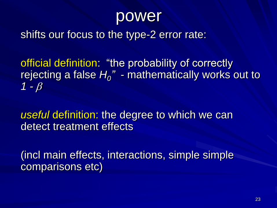
powershifts our focus to the type-2 error rate:
official definition: “the probability of correctly rejecting a false H0” - mathematically works out to 1 -
useful definition: the degree to which we can detect treatment effects
(incl main effects, interactions, simple simple comparisons etc)
24
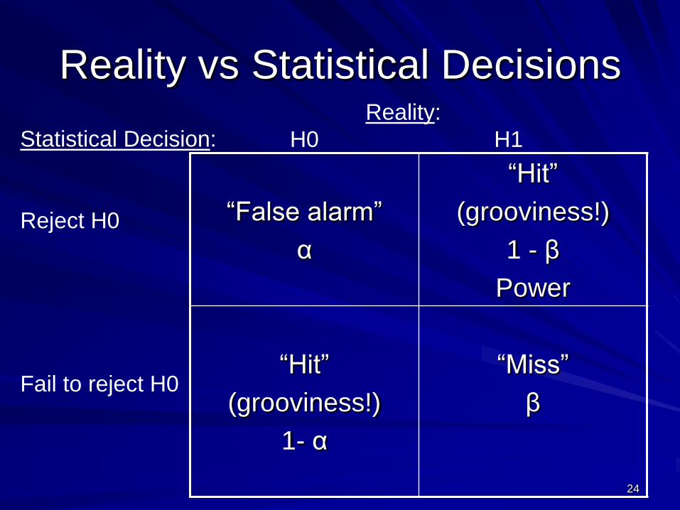
Reality vs Statistical Decisions
“False alarm”
α
“Hit”
(grooviness!)
1 - β
Power
“Hit”
(grooviness!)
1- α
“Miss”
β
Reality:
H0 H1Statistical Decision:
Reject H0
Fail to reject H0
25
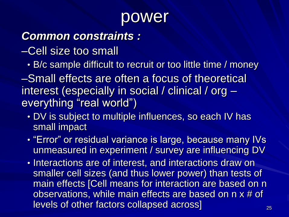
powerCommon constraints :
–Cell size too small• B/c sample difficult to recruit or too little time / money
–Small effects are often a focus of theoretical interest (especially in social / clinical / org –everything “real world”)
• DV is subject to multiple influences, so each IV has small impact
• “Error” or residual variance is large, because many IVs unmeasured in experiment / survey are influencing DV
• Interactions are of interest, and interactions draw on smaller cell sizes (and thus lower power) than tests of main effects [Cell means for interaction are based on n observations, while main effects are based on n x # of levels of other factors collapsed across]
26
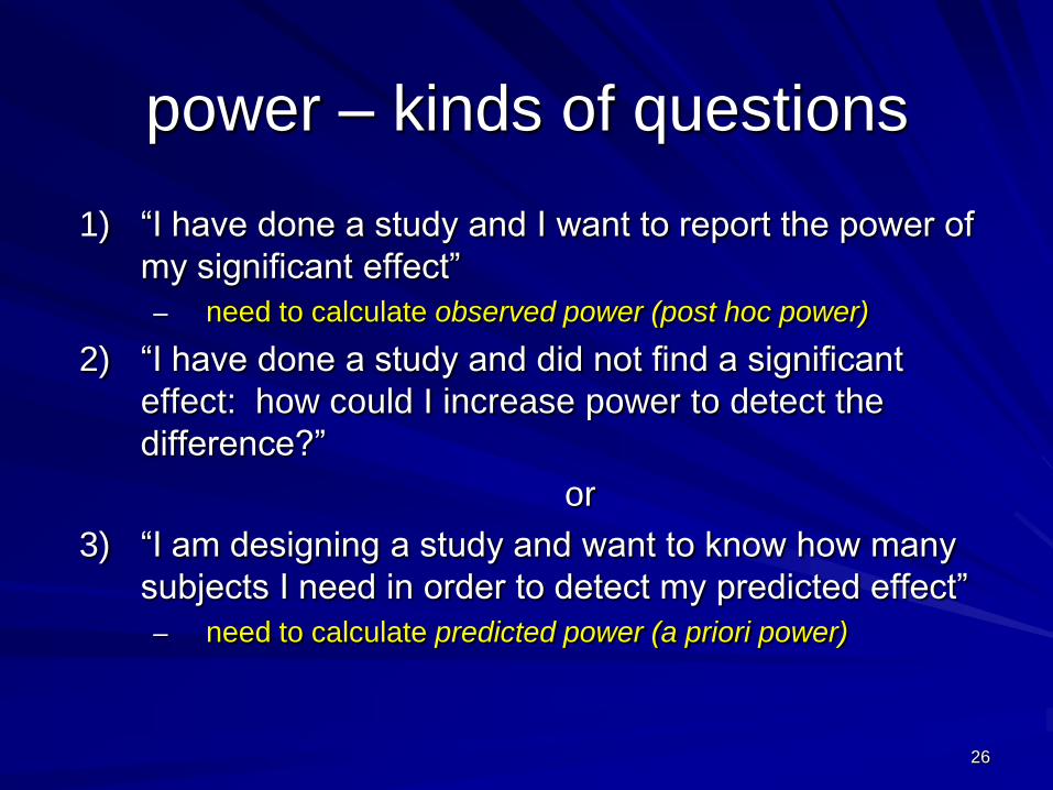
power – kinds of questions
1) “I have done a study and I want to report the power of
my significant effect”
– need to calculate observed power (post hoc power)
2) “I have done a study and did not find a significant
effect: how could I increase power to detect the
difference?”
or
3) “I am designing a study and want to know how many
subjects I need in order to detect my predicted effect”
– need to calculate predicted power (a priori power)
27
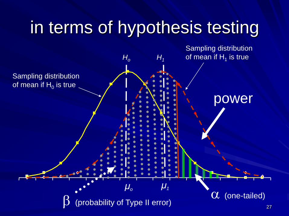
in terms of hypothesis testing
Ho
μo
(one-tailed)
Sampling distribution
of mean if H0 is true
H1
μ1
power
(probability of Type II error)
Sampling distribution
of mean if H1 is true
28
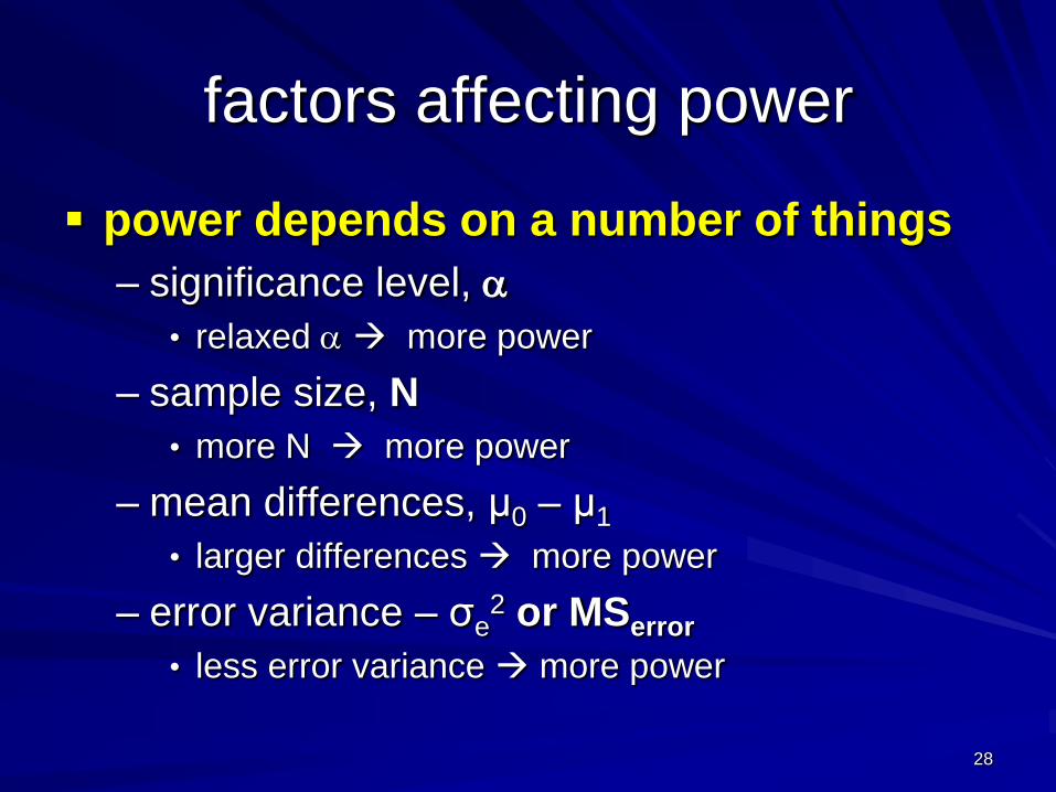
factors affecting power
power depends on a number of things
– significance level,
• relaxed more power
– sample size, N
• more N more power
– mean differences, μ0 – μ1
• larger differences more power
– error variance – σe2 or MSerror
• less error variance more power
29
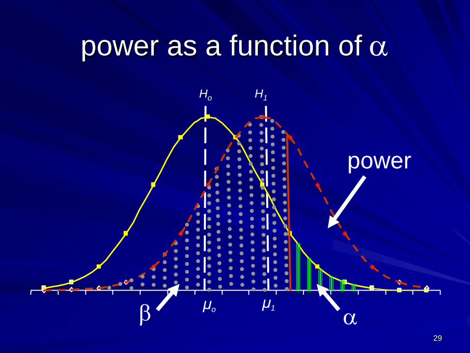
power as a function of
Ho H1
μoμ1
power
30
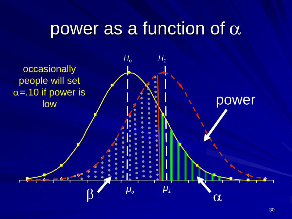
power as a function of
Ho H1
μoμ1
power
occasionally
people will set
=.10 if power is
low
31
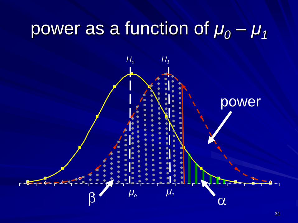
power as a function of μ0 – μ1
Ho H1
μoμ1
power
32
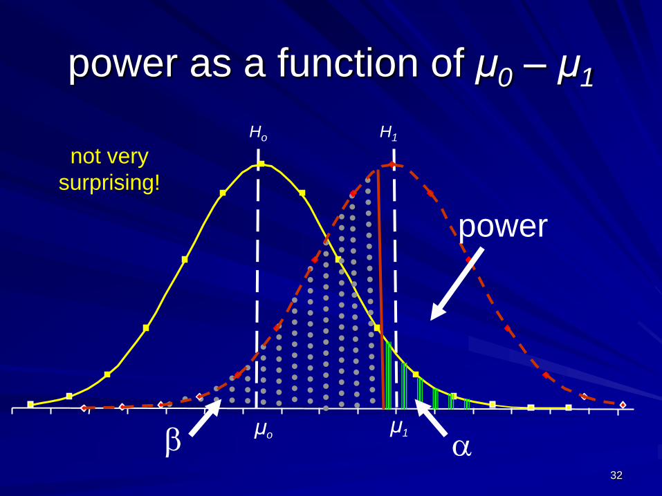
power as a function of μ0 – μ1
Ho H1
μoμ1
power
not very
surprising!

33
Ho H1
μoμ1
power
as a function of n and σ2

34
as a function of n and σ2
Ho H1
μoμ1
power
an increase in
sample size or
decrease
variance will
decrease error
variance
Recall: σ2means = σ2/n
or σmeans = σ2/n
35
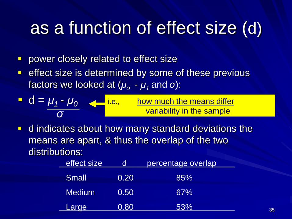
as a function of effect size (d)
power closely related to effect size
effect size is determined by some of these previous
factors we looked at (μo - μ1 and σ):
d = μ1 - μ0
σ
d indicates about how many standard deviations the
means are apart, & thus the overlap of the two
distributions:
i.e., how much the means differ
variability in the sample
effect size d percentage overlap
Small 0.20 85%
Medium 0.50 67%
Large 0.80 53%
36
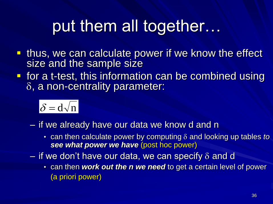
put them all together…
thus, we can calculate power if we know the effect size and the sample size
for a t-test, this information can be combined using , a non-centrality parameter:
– if we already have our data we know d and n
• can then calculate power by computing and looking up tables to see what power we have (post hoc power)
– if we don‟t have our data, we can specify and d • can then work out the n we need to get a certain level of power
(a priori power)
nd
37
Power & Effect
Smaller effect sizes harder to find significant
difference – need more powerful test
“Magnifying glass”
Big effect needs a less powerful
test (magnifying glass)
Small effect needs a more
powerful test

38
39
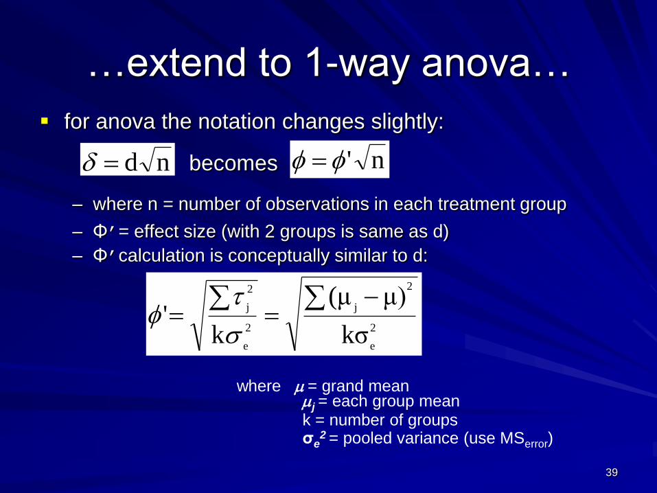
…extend to 1-way anova…
for anova the notation changes slightly:
becomes
– where n = number of observations in each treatment group
– Φ’= effect size (with 2 groups is same as d)
– Φ’calculation is conceptually similar to d:
where = grand meanj = each group meank = number of groupsσe
2 = pooled variance (use MSerror)
2
e
2
j
2
e
2
j
kσ
μ)(μ
k'
nd n'
40
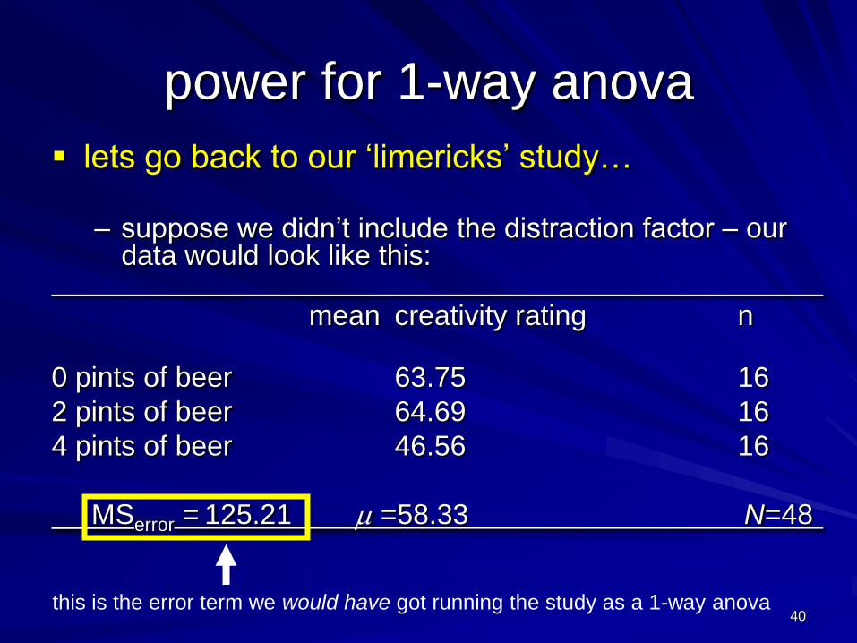
power for 1-way anova
lets go back to our „limericks‟ study…
– suppose we didn‟t include the distraction factor – our data would look like this:
mean creativity rating n
0 pints of beer 63.75 16
2 pints of beer 64.69 16
4 pints of beer 46.56 16
MSerror = 125.21 =58.33 N=48
this is the error term we would have got running the study as a 1-way anova
41
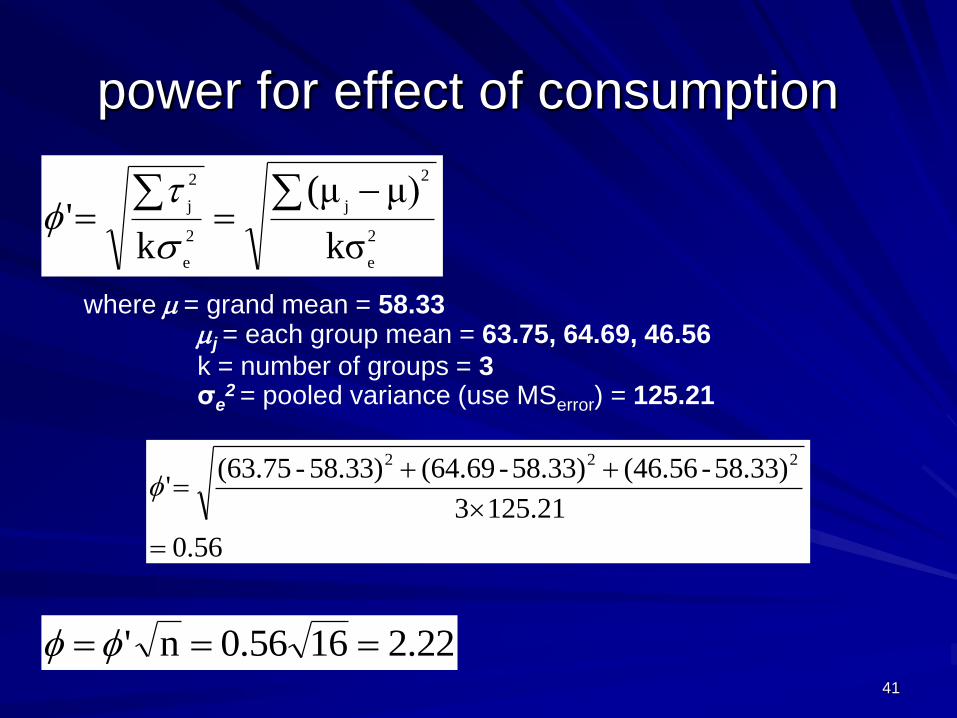
where = grand mean = 58.33j = each group mean = 63.75, 64.69, 46.56
k = number of groups = 3σe
2 = pooled variance (use MSerror) = 125.21
power for effect of consumption
56.0
21.1253
58.33)-(46.5658.33)-(64.6958.33) - (63.75'
222
2
e
2
j
2
e
2
j
kσ
μ)(μ
k'
22.21656.0n'
42
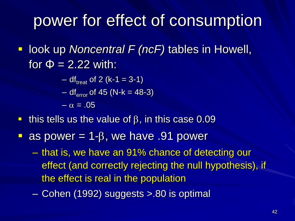
look up Noncentral F (ncF) tables in Howell,
for Φ = 2.22 with:
– dftreat of 2 (k-1 = 3-1)
– dferror of 45 (N-k = 48-3)
– = .05
this tells us the value of , in this case 0.09
as power = 1-, we have .91 power
– that is, we have an 91% chance of detecting our
effect (and correctly rejecting the null hypothesis), if
the effect is real in the population
– Cohen (1992) suggests >.80 is optimal
power for effect of consumption

43
44
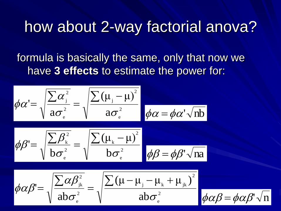
how about 2-way factorial anova?
formula is basically the same, only that now we
have 3 effects to estimate the power for:
2
e
2
j
2
e
2
j
a
μ)(μ
a'
2
e
2
k
2
e
2
k
b
μ)(μ
b'
2
e
2
jkkj
2
e
2
jk
ab
)μμμ(μ
ab'
nb'
na'
n'
45
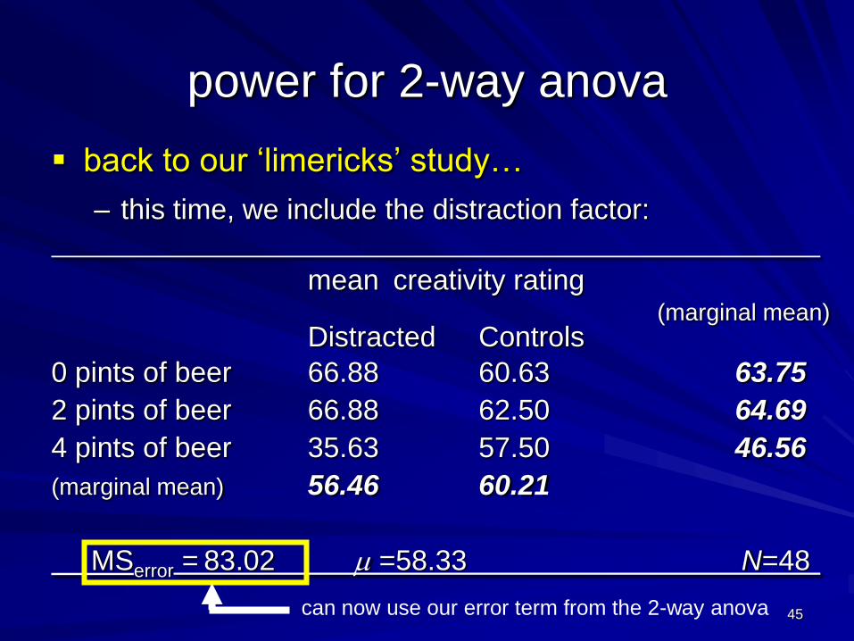
power for 2-way anova
back to our „limericks‟ study…
– this time, we include the distraction factor:
mean creativity rating(marginal mean)
Distracted Controls
0 pints of beer 66.88 60.63 63.75
2 pints of beer 66.88 62.50 64.69
4 pints of beer 35.63 57.50 46.56
(marginal mean) 56.46 60.21
MSerror = 83.02 =58.33 N=48
can now use our error term from the 2-way anova
46
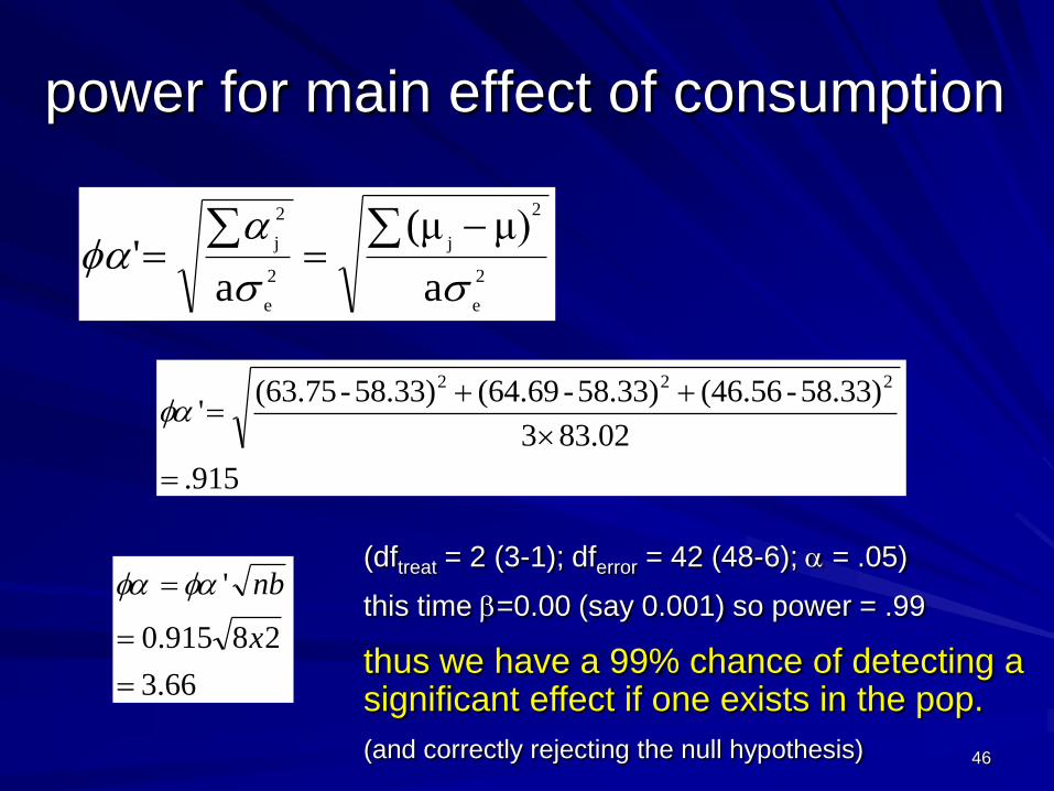
power for main effect of consumption
2
e
2
j
2
e
2
j
a
μ)(μ
a'
(dftreat = 2 (3-1); dferror = 42 (48-6); = .05)
this time =0.00 (say 0.001) so power = .99
thus we have a 99% chance of detecting a significant effect if one exists in the pop.
(and correctly rejecting the null hypothesis)
66.3
28915.0
'
x
nb
915.
02.833
58.33)-(46.5658.33)-(64.6958.33)-(63.75'
222
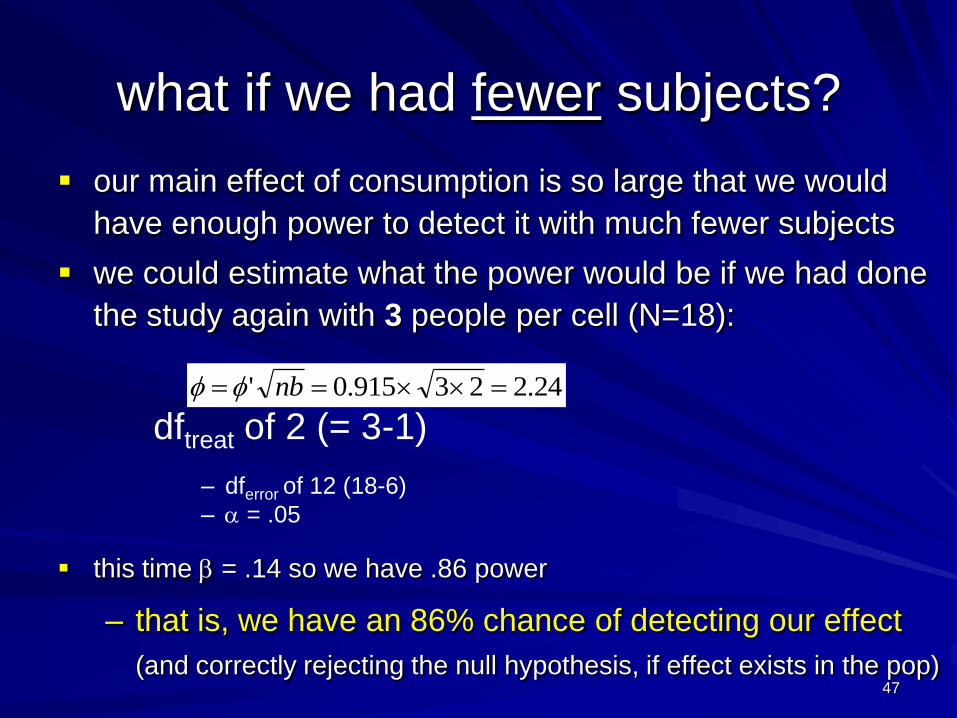
47
our main effect of consumption is so large that we would
have enough power to detect it with much fewer subjects
we could estimate what the power would be if we had done
the study again with 3 people per cell (N=18):
dftreat of 2 (= 3-1)
– dferror of 12 (18-6)
– = .05
this time = .14 so we have .86 power
– that is, we have an 86% chance of detecting our effect
(and correctly rejecting the null hypothesis, if effect exists in the pop)
what if we had fewer subjects?
24.223915.0' nb
48
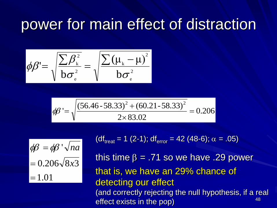
power for main effect of distraction
(dftreat = 1 (2-1); dferror = 42 (48-6); = .05)
this time = .71 so we have .29 power
that is, we have an 29% chance of
detecting our effect (and correctly rejecting the null hypothesis, if a real
effect exists in the pop)
206.0.02832
58.33)-(60.2158.33)-(56.46'
22
01.1
38206.0
'
x
na
2
e
2
k
2
e
2
k
b
μ)(μ
b'
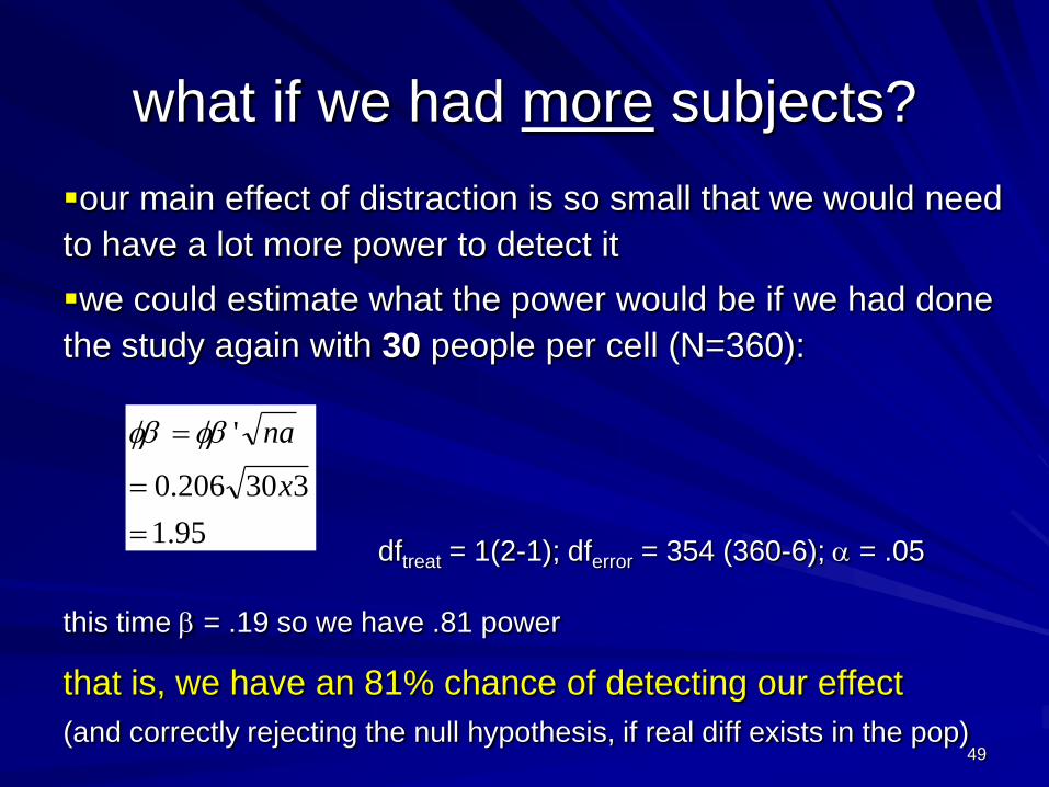
49
our main effect of distraction is so small that we would need
to have a lot more power to detect it
we could estimate what the power would be if we had done
the study again with 30 people per cell (N=360):
dftreat = 1(2-1); dferror = 354 (360-6); = .05
this time = .19 so we have .81 power
that is, we have an 81% chance of detecting our effect
(and correctly rejecting the null hypothesis, if real diff exists in the pop)
what if we had more subjects?
95.1
330206.0
'
x
na

50
What about higher-order ANOVA?
Can generalize from
this formula for each
effect
E.g. in 3-way ANOVA,
look at power for each
of the 7 effects (main
effects of A, B, and C;
AB, BC, and AC
interactions; and ABC
interaction)
2
2
'e
j
k
51
determining sample size
if we can estimate our effect size and error
we can plan studies in terms of how many
participants we need to get .80 power
often use previous studies to derive your
estimates for MSE and effect size
substituting different values of n into the
formula and looking up the ncF tables is one
(tedious) way of doing things…
52
G*POWER
G*POWER is a FREE program that can make the
calculations a lot easier
http://www.psycho.uni-duesseldorf.de/abteilungen/aap/gpower3/
G*Power computes:
power values for given sample sizes, effect sizes,
and alpha levels (post hoc power analyses),
sample sizes for given effect sizes, alpha levels, and
power values (a priori power analyses)
suitable for most major statistical methods
V useful for hons thesis writing or report writing.

53
54
side issues…
recall the logic of calculating estimates of effect
size (i.e., criticisms of significance testing)
– the tradition of significance testing is based upon an
arbitrary rule leading to a yes/no decision
power illustrates further some of the caveats
with significance testing
– with a high N you will have enough power to detect a
very small effect
– if you cannot keep error variance low a large effect
may still be non-significant
55
side issues…
on the other hand…
– sometimes very small effects are important
– by employing strategies to increase power
you have a better chance at detecting these
small effects
56
how can we maximize power? power can be increased a number of different
ways (some of these we have seen already…)
– increase sample size
– increase level (usually not wise!)
– decrease error variance
• improving data collection methods:– procedural
– psychometric
• improving methods of analysis – i.e., use more powerful statistics
57
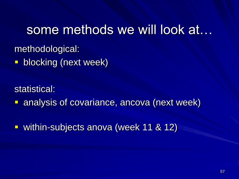
some methods we will look at…
methodological:
blocking (next week)
statistical:
analysis of covariance, ancova (next week)
within-subjects anova (week 11 & 12)

58
Next week in class:
Blocking and ANCOVA
Readings for this week:
Howell
– Chapter 16 (section 16.7)
– Review chapter 9
Field – Chapter 9
In the tutes:
This week: SPSS tute
Next week: Assignment 1 consult.


![0 · )#"uq$'5)#"uq$'v o] o yyyyyyyxxxxxxxxxxxxxxxxxxxxxxxxxxxxxxxxxxxxxxxxxxxxxxxxxxxxxxxxxxxxxxxxxxxxxxxxyíï ' ^ µ v ] ] íx k …](https://img.pdfslide.tips/doc/110x75/5e26df3ff940cb4f5d6bf327/0-uq5uqv-o-o-yyyyyyyxxxxxxxxxxxxxxxxxxxxxxxxxxxxxxxxxxxxxxxxxxxxxxxxxxxxxxxxxxxxxxxxxxxxxxxxy.jpg)