1

DRAG REDUCTION BY FLOW SEPARATION CONTROL ON A CAR AFTER BODY

Mathieu Rouméas*, Patrick Gilliéron* & Azeddine Kou rta**

* Groupe "Mécanique des Fluides et Aérodynamique", Direction de la recherche Renault, 1, avenue du Golf (TCR AVA 058), 78288 GUYANCOURT, FRANCE

** Institut de Mécanique des Fluides de Toulouse, Groupe EMT2 Avenue du professeur Camille Soula, 31000 TOULOUSE, FRANCE

mathieu.roumeas@yahoo.fr Patrick.gillieron@renault.com kourta@imft.fr

Abstract: New development constraints prompted by new pollutant emissions and fuel consumption standards

(Corporate Average Economy Fuel) require that automobile manufacturers develop new flow control

devices capable of reducing the aerodynamic drag of motor vehicles. The solutions envisaged must have a

negligible impact on the vehicle geometry. In this context, flow control by continuous suction is seen as a

promising alternative. The control configurations identified during a previous 2D numerical analysis are

adapted for this purpose and are tested on a 3D geometry. A local suction system located on the upper part

of the rear window is capable of eliminating the rear window separation on simplified fastback car

geometry. Aerodynamic drag reductions close to 17% have been obtained.

Keywords: Lattice Boltzmann Method / Separation / Longitudinal vortices / Drag reduction / Active control / Suction

I NTRODUCTION

New constraints in terms of pollutant emissions and fuel consumption (Corporate Average Economy Fuel) are

warranting the development of new flow control devices capable of reducing the aerodynamic drag of motor vehicles. In

this context, the objective is to modify the near wall flow and thereby limit the development and dissipation of the separated

vortices that contribute towards the development of aerodynamic drag.

The optimization of vehicle shapes and the incorporation of commonly used passive control devices have already

brought about a significant aerodynamic drag reduction (from Cx=0.45 in 1975 to Cx=0.35 in 1985 [1,2], Cx being the

average drag coefficient). The need to further reduce fuel consumption and/or provide automobile designers with more

creative liberty is prompting the automobile industry to develop innovative active flow control solutions. Such solutions [2]

use an external energy source to modify the flow topology without necessarily modifying the shape of the vehicle. Flow

2

control was extensively studied and applied [3, 4] and control theory was developed [5, 6]. Different control techniques

have been analyzed in university and industrial laboratories and significant results have been obtained on academic

geometries [2]. Continuous suction and/or blowing solutions offer a promising alternative [7, 8] and seem well-adapted to

the automobile context [9]. For example, the efficiency of a suction system in controlling the separation of the boundary

layer has been highlighted experimentally on a cylinder by Bourgois et al. [10] and Fournier et al. [11]. The results indicate

that significant drag reductions, close to 30%, are obtained by moving the flow separation downstream; similar results are

obtained by Rouméas et al. [12] on simplified two-dimensional fastback car geometry. In this case, the drag reduction is

associated with the elimination of the separated layer on the rear window when suction is applied.

Such control solutions however cannot be installed on a real vehicle until further investigations have been carried out. In

particular, the results obtained in a 2D configuration [12] must be tested on a 3D numerical model in order to represent the

longitudinal vortices that appear on the lateral edges of the rear window and contribute significantly to the development of

aerodynamic drag [13-17].

A 3D numerical simulation is therefore implemented to analyze the influence of suction on the flow topology

developing around simplified fastback car geometry [17]. The flow topology obtained without control and the numerical

method, based on the Lattice Boltzmann Method, is detailed in a previous publication [17, 18]

In the first part a numerical method and parameters are detailed. A simplified integral formulation of the aerodynamic

drag [13] is presented in the second part to specify the control objectives. The flow topology obtained with suction is

analyzed in the third part to identify the influence of suction mainly to prevent separation and secondary on the longitudinal

vortices development. Finally, the aerodynamic drag values obtained with and without control are compared at different

suction velocities to determine the efficiency of the flow control devices.

NUMERICAL METHOD

The numerical method used in a previous paper [17] is applied here. It consists on a 3D numerical simulation based on

Powerflow code with a Lattice Boltzmann Method (LBM). This method is based on microscopic models and mesoscopic

kinetic equations. The fundamental principle of the LBM is to construct simplified kinetic models that incorporate the

essential physics of microscopic or mesoscopic processes such that the macroscopic-averaged properties conform to the

desired macroscopic equations. The basic premise for using these simplified kinetic-type methods for macroscopic fluid

flows is that the macroscopic fluid dynamics are the result of the collective behavior of many microscopic particles in the

3

system and that the macroscopic dynamics are not sensitive to the underlying details as is the case in microscopic physics.

[17,18].

The fluid particles are distributed on a Cartesian lattice of computation nodes [13]. For each lattice node, a distribution

function [ ] N...1iif = is associated with a discrete velocity distribution [ ] N...1iiV =

r representing N possible velocities of motion.

The kinetic energy is given by ∑=

=N

1i

2iV

2

1e . One particle placed on one node may stay at this node (energy level 0: 0=e ),

move toward an adjacent node in horizontal or vertical plane ( energy level 1: 1=e ) or move to a farthest node ( energy

level 2: 2=e ). The model gives 34 possible combinations and is called 34 velocities model (2 possibilities for level 0, 18

for level 1 and 14 for level 2). More details concerning the algorithm can be found in [17-21].

The general algorithm for the LBM is thus defined in 4 stages. The first consists in propagating the distribution function

in time t+1 [22, 23]. In the second stage, the collisions between the particles are modelled. The collision operator is then

applied to time t-1. The third stage consists in determining the associated values of density and momentum. Finally, the

fourth stage consists in initiating iteration on the basis of the macroscopic values determined in the third stage.

As in the case of all numerical space-time discretization methods, the LBM is not capable of resolving all turbulence

scales. The computation code therefore uses a turbulence model which introduces a turbulent viscosity into the initial

model. The turbulence model is the RNG k-ε model originally developed by Yakhot et al. [24]. The equations describing

the transport of kinetic energy and dissipation applied by the model are resolved on the same lattice as the Boltzmann

equations. The discretization diagram used is a second order in space (Lax-Wendroff finite difference model), associated

with a time-explicit integration diagram [25]. Close to the wall, a specific velocity law is applied to limit the computational

workload [25]. The velocity is then described by a logarithmic law.

The numerical simulations presented in this paper were conducted on a simplified vehicle geometry initially proposed by

Ahmed et al. [14]. The computation is exclusively focused on the rear part. The geometry is the same as the one previously

computed without control [17].

The geometry is defined by its length (L=1.044 m), its width (l=0.389 m) and its height (H=0.288 m). In this

configuration, the rear window with a length of 0.222 m, is inclined at an angle of 25° with respect to the horizontal.

Finally, the lower part is positioned at h=0.17 H from the floor of the numerical wind tunnel. The geometry is located in a

rectangular numerical section of length, width and height equal to 31L, 20L and 10H respectively. These dimensions ensure

there is no interaction between the boundary conditions imposed at the limit of the computational domain, and the

development of the near-wake flow as has been demonstrated in [17]. The outlet condition, downstream from the geometry

4

and on the upper part, is a free flow condition [17] on pressure and velocity. The flow is advected from left to right and a

uniform velocity V0=40m.s-1 is applied to the left-hand surface of the simulation domain (Dirichlet velocity condition). The

Reynolds number associated with length L of the geometry is Re=2.8.106. Finally, symmetry conditions are applied on the

side surfaces of the simulation domain [17].

SUMMARY OF THE PERVIOUS RESULTS OBTAINED WITHOUT CON TROL

In previous paper [17], results obtained without control in this geometry have been compared to previous computational

and experimental results. The longitudinal velocity profiles in the vertical direction (fig. 6 of this reference), measured on

the median longitudinal plane, were compared to the experimental data at six positions: the end of the roof, the top of the

rear window, the first part of the rear window, the middle of the rear window, the last part of the rear window and at the

bottom of the rear window. It has been concluded that the computation code is able to predict both the separation and

attachment of the fluid respectively on the top and bottom of the rear window. This aspect, a common problem in the

numerical representation of the flow around fastback geometry, is correctly processed by the code. However, the

computation code over-estimates the velocity defect in the boundary layer, close to the reattachment. The results obtained in

the separated boundary layer are associated with the logarithmic law used to define the velocity evolution close to the wall.

As known, this law is not adapted to the separated region. The accuracy of these results has been evaluated by

determining the differences with experimental results considered as a basis of comparison. In the external region the error

is less than 1% but it can reach 11% to 13% in the separation zone where the computation is less accurate. Also in the same

paper [17], the friction line traces on the rear window, (fig. 7 of this reference), indicate that the computation code correctly

represents the physical phenomena highlighted in the experiments. Finally, drag coefficient has been compared to previous

experimental and numerical (RANS [26], LES [27, 28]) studies. Good agreement has been obtained both with experiment

and LES computation.

In the present paper, for the same geometry and with the same numerical conditions, the control is applied and obtained

results will be compared to the previous case without control.

THEORETICAL BASES

Aerodynamic drag is defined as an integral over the surface vehicle of the static pressure, friction and turbulence

stresses. The obtained equation constitutes an overall expression of the aerodynamic drag without highlighting the

contribution of the various separated vortices. To obtain a better understanding of various physical phenomena (and their

mutual interaction), it is necessary to develop simplified approaches conducive to identifying which parameters play a

5

significant role in achieving a reduction in aerodynamic drag. Onorato et al. [13] propose a simplified analytical model

based on the momentum equation applied to the air inside a stream tube enclosing the vehicle (see fig. 1). The flow is

assumed to be steady, incompressible, and gravity and turbulence effects are considered negligible compared to the pressure

effect [7]. These simplifications lead to the Onorato expression of the aerodynamic drag, given in (1):

( )∫∫∫ σ−+σ

+

ρ+σ

−

ρ−=

S

i0i

S20

2z

20

2y

20

S

2

0

x20

x dPPdV

V

V

V

2

Vd

V

V1

2

VF (1)

where Pi0 is the reference total pressure, V0 the external flow velocity, ρ the density, Pi the total pressure and

Vx, Vy, Vz the

components of the velocity vector. The Onorato expression (1) is then used to define the aerodynamic drag of a motor

vehicle according to velocity and total pressure fields measured in the wake cross section S, downstream from the base.

Fig. 1- Schematic of the stream tube used for the Onorato expression, Gilliéron [9]

The first term of the expression (1) represents the drag associated with the longitudinal velocity deficit measured inside

the near-wake zone. It is associated with the development of transversal vortices at the base [14]. The second term

corresponds to the vortex drag, associated with the development of longitudinal vortices on the geometry. Finally, the third

term expresses the drag induced by the total pressure loss between the upstream and the downstream of the motor vehicle,

associated with the formation and maintenance of separated swirling structures in the wake.

According to the Onorato expression (1), the aerodynamic drag of a motor vehicle is mainly due to the formation of

separated flow on the geometry, and the formation of transversal and longitudinal swirling structures in the wake.

Therefore, the drag reduction can be obtained by reducing, or even eliminating, the longitudinal vortices (second term), by

reducing the wake cross section S or by limiting the total pressure loss in the wake (third term).

In this study, the objective is to move downstream, or even to eliminate, the flow separation on the rear window in such

a way as to reduce the wake cross section and the associated volume energy loss. According to a previous 2D numerical

study [12], the control consists of a continuous suction located on the rear window. The computation code used is based on

6

la

y

z

H

the Lattice Boltzmann Method and an RNG k-ε schema provides a model of the turbulence effects. The numerical protocol

used, in particular with respect to the mesh, is detailed by Rouméas et al. [17].

The suction system consists of a slot of width e=10-3 m (e=0.5.10-2 l) and length λ=0.379 m (λ=0.97 la), applied close to

the separation line, at the top of the rear window [12], by a Dirichlet condition on suction velocity Vasp (fig. 2.a). The

direction of the suction velocity is perpendicular to the rear window (fig. 2.b) at a suction velocity equal to 0.6 times the

external flow velocity V0 [12]. The inlet velocity is maintained at the same intensity as without control to clearly show the

control effect. It is known that the suction will affect the pressure field around the body and modify the inlet velocity. Also,

the actuator produces the noise, but it was demonstrated that its level is relatively low [8]

In the following developments, the flow topology is analyzed and compared to the topology obtained without control

[11] to define the influence of the suction control on the separated flow.

(a) (b)

Fig. 2- Schematic of the used geometry and implementation of the control system

INFLUENCE OF CONTINUOUS SUCTION – FLOW TOPOLOGY

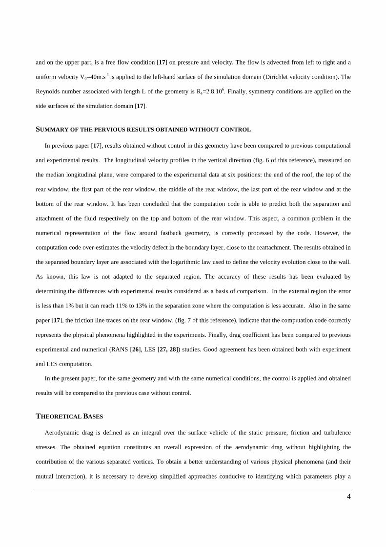
The flow topology analysis is conducted on an iso-surface of total pressure loss (Cpi=1) and friction line traces without

control (fig. 3.a) and with control (fig. 3.b). The rear window separated zone and longitudinal vortices are then analyzed

according to velocity, static pressure and vorticity fields.

The results in Fig. 3.a and 3.b indicate that suction is conducive to eliminating the development of the separated layer D,

and to significantly reducing the associated and energy loss. A residual layer, associated with the total pressure loss induced

by the suction, remains apparent on the upper part of the rear window (annotated F on fig. 3.b). However the separated zone

then disappears downstream in the rear window. It is possible to confirm this result by observing the friction lines: when

suction is applied (Fig. 3.b), the friction lines remain aligned and in parallel to the direction of the main flow, which

L

x

y l

Vasp

V0

Vasp

V0

Roof

Rear window

e

7

indicates that the flow is still attached to the wall on the rear window. The vorticity near the wall, identified under the

separated layer without control [17], disappears totally when the suction system is activated (fig. 3.b).

(a)

(b)

Fig. 3- Total pressure loss iso-surfaces (Cpi=1,22) and friction line traces on rear window: (a) without control, (b) with suction

The results in Fig. 3.a and 3.b reveal that suction has the effect of eliminating the rear window separation. Considering

the interaction between the longitudinal vortices and the separated zone [17], the structure of the vortices should however be

analyzed more accurately when the suction is applied. Each of the constituent longitudinal and transversal vortices of the

wake is then characterized in the following developments, according to static pressure, velocity and vorticity fields to

analyze the mechanisms of the suction control.

1- Suction influence on the rear window separated zone

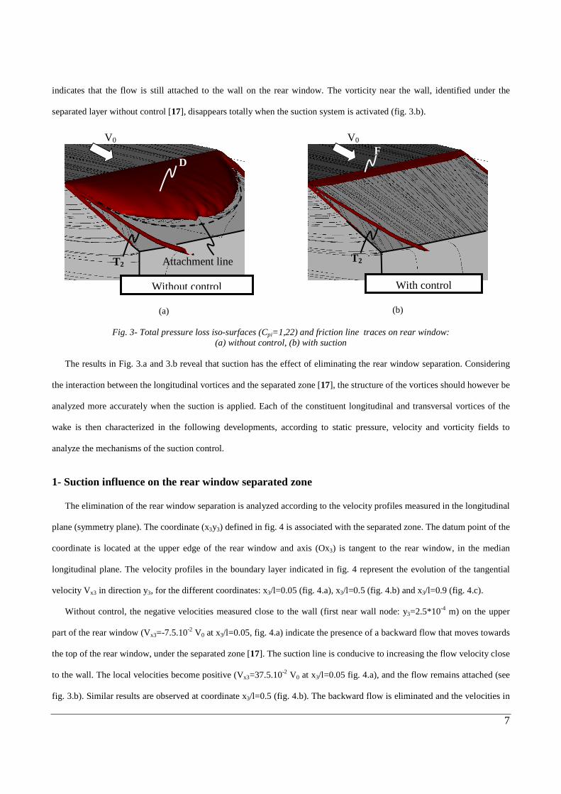
The elimination of the rear window separation is analyzed according to the velocity profiles measured in the longitudinal

plane (symmetry plane). The coordinate (x3y3) defined in fig. 4 is associated with the separated zone. The datum point of the

coordinate is located at the upper edge of the rear window and axis (Ox3) is tangent to the rear window, in the median

longitudinal plane. The velocity profiles in the boundary layer indicated in fig. 4 represent the evolution of the tangential

velocity Vx3 in direction y3, for the different coordinates: x3/l=0.05 (fig. 4.a), x3/l=0.5 (fig. 4.b) and x3/l=0.9 (fig. 4.c).

Without control, the negative velocities measured close to the wall (first near wall node: y3=2.5*10-4 m) on the upper

part of the rear window (Vx3=-7.5.10-2 V0 at x3/l=0.05, fig. 4.a) indicate the presence of a backward flow that moves towards

the top of the rear window, under the separated zone [17]. The suction line is conducive to increasing the flow velocity close

to the wall. The local velocities become positive (Vx3=37.5.10-2 V0 at x3/l=0.05 fig. 4.a), and the flow remains attached (see

fig. 3.b). Similar results are observed at coordinate x3/l=0.5 (fig. 4.b). The backward flow is eliminated and the velocities in

V0

D

T2

Without control

Attachment line

V0 F

With control

T2

8

the vicinity of the wall evolve from Vx3=-32.5.10-2 V0 without suction to Vx3=25.10-2 V0 (x3/l=0.5, fig. 4.b) when suction is

applied.

Finally, the velocity measurements reveal that the velocity increase at the near wall, when suction is applied, remains

significant down to the bottom of the rear window (x3/l=0.9 on fig. 4.c).

0

0.002

0.004

0.006

0.008

0.01

0.012

0.014

-0.5 0 0.5 1 1.5

w ithout control

Vasp=0,6Vo

Vx3/V0

y 3 (m

)

x3/l=0,05

x3

y3

l

(a)

0

0.01

0.02

0.03

0.04

0.05

0.06

0.07

-0.5 0 0.5 1 1.5

Without control

Vasp=0,6Vo

Vx3/V0

y 3 (m

)

x3/l=0,5

x3

y3

l

(b)

0

0.02

0.04

0.06

0.08

-0.5 0 0.5 1 1.5

Without control

Vasp=0,6Vo

Vx3 /V0

y 3 (m

)

x 3/l=0,9

x3

y3

l

(c)

Fig. 4- Tangential velocity profiles measured in longitudinal median plane of the rear window, with and without control:

(a) at coordinate x3/l=0.05, (b) coordinate x3/l=0.5 and (c) coordinate x3/l=0.9.

Wall static pressure loss fields are plotted on the rear window (without control fig. 5.a and with control fig. 5.b) to

complete the analysis. The static pressure distributions measured under the longitudinal vortices, in the vicinity of the lateral

edges, are discussed in § 2, and the analysis is conducted on 2 areas (zone 1 and zone 2 fig. 5) delimited by an iso static

pressure line corresponding to Cpc=-0.6.

9

Without control (fig. 5.a), the total pressure loss in the separation zone leads to a depression on the wall, with Cp<-0.6

(zone 1 on fig. 5.a), associated with the near wall circulation of the fluid under the separated layer [17] (see fig. 3.a). The

suction first induces a significant local depression on the suction slot (zone 1 fig. 5.b) This depression is conducive to

increase locally the velocity on the top of the rear window, see fig. 5.a, and to remain the streamlines attached on the rear

window (fig. 3.b). The surface of the zone 1 is thereby reduced significantly (fig. 5.b) and the static pressure then increases

regularly in zone 2, along the rear window, whereas the flow slows down (Cp=-0,1 at the end of the rear window, with and

without control). Overall, the application of suction results in a mean increase to the static pressure on the rear window

(zone 2 fig. 5.b). The depression created on the top of the rear window is compensated by the recompression on the bottom

of the rear window. This pressure increase is associated with a reduction in the contribution of the rear window to the

pressure drag, which can be estimated as follows:

∫ρ

=cS

p

20

xp dSx.nC2

VF

rr (2)

where Fxp is the pressure drag applied on the surface Sc, nr

the normal exiting surface Sc and xr

the longitudinal direction of

the flow.

(a) (b)

Fig. 5- Static pressure loss fields on rear window: (a) without control (b) with control (Vasp=0,6V0)

On the side parts of the rear window, the static pressure fields in fig. 5.a and fig. 5.b indicate that the static wall pressure

increases locally under the longitudinal vortices, a result indicative of a modification occurring on the vortex topology. The

influence of suction on the longitudinal vortices is then analyzed in the following part.

-0,84

-0,63

-0,42

-0,21

0 Cp

Zone 1

Trace du tourbillon longitudinal

Cp=-0,6 Zone 1

Zone 2 Longitudinal vortex

Cpc=-0,6

Zone 1

Zone 2

Cpc=-0,6

10

2- Suction influence on the longitudinal vortices

Suction has the effect of eliminating the separation zone on the rear window, as shown in § 1. This structure, however,

reacts significantly with the longitudinal vortices [17] and suction may interfere with their development. The structure of

vortex T2 is then analyzed with and without suction according to the profiles of velocity, vorticity and static pressure loss

coefficient, measured in a vortex cross section located at coordinate x2/l=0.5, i.e. downstream from the vortex formation

area identified without control [17]. Coordinate (Ox2y2z2) is associated with the vortex axis (see Fig. 6) which defines

angles β with respect to longitudinal direction x, and θ with respect to the surface of the rear window (see Fig. 6).

Computation of angles θ and β with and without suction indicates that this has no significant impact on the position of the

vortex axis.

Fig. 6- Definition of coordinate system associated with longitudinal left-hand vortex T2 (Vorticity iso-contour surface

(ω=10.4 s-1))

(i)- Azimuthal velocity profiles

The azimuthal velocity profiles Vz2(y2, z2=0) in fig. 7.a indicate that suction does not have a significant influence on the

topology of the longitudinal structures; the velocity profiles obtained with and without control are similar. The results

however highlight an increase in distance L measured between the azimuthal velocity extreme, once suction is applied

(LAC>LSC in fig. 7.a). Hence, the suction line applied on the top of the rear window induces a spreading of the longitudinal

vortex structure in the transverse direction. This spreading is associated with an increase of vorticity at the vortex centre,

ωx=14.103 s-1 without control as opposed to ωx=17.5.103 s-1 with control, which promotes the dissipation of the jet [23]. At

the vortex core defined by the linear evolution of the azimuthal velocity (fig. 7.b), the increase in vorticity is highlighted by

means of the azimuthal velocity gradient (gradient Ω defined in fig. 7.b) which characterizes a local rotation of the fluid.

θθθθ

ββββ

Base

Rear window

Rear window Base

x2

x2

T2

T2

Top view

Side view

Roof

Rear window

x2

y2

z2 T2

11

Gradient Ω increases when suction is applied: Ω=9125 s-1 with control vs. Ω=7120 s-1 without control. If suction promotes

the dissipation of the jet (fig. 7.a), the vortex core on the other hand is inclined to become narrower: the viscous radius R,

defined as the distance at which the evolution of the azimuthal velocity is linear, decreases when the suction system is

activated (RAC<RSC, fig. 7.b).

-0.015

-0.01

-0.005

0

0.005

0.01

0.015

-1-0.500.51

Without control

Vasp=0,6Vo

y 2 (m

)

Vz2 /V0

y2

z2

LSC

LAC

(a)

-0.004

-0.003

-0.002

-0.001

0

0.001

0.002

0.003

0.004

-0.6-0.4-0.200.20.40.6

Without control

Vasp=0,6V0

Vz2 /V0

y 2 (

m)

RSCRAC

Arctan( ΩΩΩΩ )

(b)

Fig. 7- Azimuthal velocity profiles in the vertical direction, measured in transverse plane located coordinate x2/l=0,5 (a) In the longitudinal structure T2 (b) In the vortex core

It is therefore difficult to draw a conclusion at this point with respect to the influence of suction on the contribution of

the longitudinal structures to aerodynamic drag. Whereas suction causes an increase to the transverse section of the

structures (Fig. 7.a) and an increase of vorticity in the vortex core (Fig. 7.b), the viscous radius at which vorticity is

maximum is reduced. The results presented in this paragraph must therefore be completed by axial velocity and static

pressure profiles measured in the vortex.

(ii)- Axial velocity and static pressure loss profiles

The axial velocity is measured in the vortex core at coordinate x2/l=0,5, with and without control, and the results are

indicated in Fig. 8.a. The axial velocity profiles (fig. 8.a) are not modified significantly when suction is applied. The profiles

obtained without control and with control exhibit a jet type structure, with a velocity Vx greater than reference velocity V0 at

the centre of the vortex. The results indicate however a shift on the axial velocity troughs on either side of the vortex core,

which move away from the vortex axis when suction is applied (fig. 8.a). This phase shift is associated with an increase of

distance L between the azimuthal velocity extremes highlighted in Fig. 7.a. Finally, the static pressure loss coefficient

profiles (fig. 8.b) indicate that the static pressure losses are more significant in the vortex core when suction is applied: Cp=-

12

2 at centre (y2=0) without control vs. Cp=-2.2 with suction. Conventionally, this result is associated with an increase of the

vorticity at the vortex core, highlighted in fig. 7.b. On the other hand, as the distance from the core of the vortex increases at

y2>0.005 or y2<-0.005, the effect is reversed and the static pressure measured without control is less than the static pressure

measured with suction (fig. 8.b). Hence, close to the wall (y2<-0.013), the static pressure loss coefficient switches from

Cp=-0.98 without control to Cp=-0.72 with suction ((i) fig. 8.b). This result highlights an increase in static pressure under

the vortex, at the location of the wall, already observed on Fig.5.b, associated with the reduction of the viscous radius R

(Fig. 7.b).

(a)

(b)

Fig. 8- Velocity and static pressure profiles in the vertical direction, measured in vortex T2, cross section plane at coordinate x2/l=0.5: (a) axial velocity, (b) static pressure loss coefficient.

The influence of the vortex on the rear window, with and without suction, is analyzed according to the static pressure

loss measured along the projection of the vortex axis on the wall (axis x4 defined in fig. 9). Rotation of the fluid in the

longitudinal vortex induces a depression on the wall as highlighted in fig. 5.a and fig. 5.b. Without control, the static

pressure is decreasing for x4/l<0.25 (Cp=-0.85 for x4/l=0.05 and Cp=-1.1 for x4/l=0.25, fig. 9). This decrease is associated

with an increase in vorticity in the shear layer [17]. At x4/l>0.3, the structure of he vortex is well-established [11] and the

vortex axis moves away from the wall, its influence on the wall diminishes and the wall pressure increases (Cp=-0.35 for

x4/l=0.95).

-0,015

-0,01

-0,005

0

0,005

0,01

0,015

-2,5 -2 -1,5 -1 -0,5 0

sans contrôle

Vasp=0,6V0

y 2 (m

)

Cp

y2

z2LSC

LAC

(i)

-0,015

-0,01

-0,005

0

0,005

0,01

0,015

0,75 0,85 0,95 1,05 1,15 1,25

sans contrôle

Vasp=0,6Vo

Vx2 / V0

y 2 (m

)

y2

z2

LSC LAC

No control

No control

13

The presence of suction leads to an additional depression on the top of the rear window (Cp=-1.5). This depression is

associated with an increase of vorticity in the vortex when suction is applied, already mentioned in the previous paragraph.

The evolution of the static pressure loss coefficient then increases in direction x4, over the whole length of the rear window,

which suggests that the structure of the vortex becomes established higher up on the rear window when suction is applied.

The static pressure measured with suction is therefore more significant with suction, for x4/l>0.3. This recompression

observed under the vortex (Fig. 5.b, Fig. 8.b and Fig. 9) is associated with the reduction of the transverse development at the

vortex core, as mentioned in the previous paragraph (Fig. 7.b) and is conducive to reducing the contribution of the

longitudinal structures towards the drag pressure, according to equation (4).

Fig. 9- Static pressure loss coefficient measured along the projection of the vortex axis on the wall

To sum up, suction has the effect of increasing the fluid rotation in the vortex core (fig. 7.a) and the associated volume

energy loss as a result. According to the Onorato equation (second and third term of the equation (2)), suction is inclined to

increase the contribution of the longitudinal vortices into aerodynamic drag. However, the analysis also highlights an

increase in the static wall pressure under the vortex axis (fig. 5.b, fig. 8.b and fig. 9), associated with the reduction in the

viscous radius of the vortex (fig. 7.b), which prompts a reduction of the pressure drag and may compensate for the volume

pressure losses.

3- Suction influence on the near-wake flow

The near-wake flow topology is analyzed on total pressure loss and streamlines fields measured in the longitudinal

median plane, without control (Fig. 10.a) and with control (Fig. 10.b).

-1,5

-1,2

-0,9

-0,6

-0,3

0

0 0,2 0,4 0,6 0,8 1

Sans contrôle

Vasp=0,6.V0

x 4/l

Cp

x2

x4

Lunette arrièrePavillon

Rear window Roof

Without control

Vasp=0.6V0

14

The streamlines emanating from the roof roll up in the separation zone around a vortex centre C3 (fig. 10.a and 10.b) and

a singular source point (F fig. 10.b), highlighted at the lower part of the rear window, reveals a saddle point S2 (Fig. 10.a

and 10.b). The streamlines emanating from the rear window and underbody then roll around at the base into 2 counter-

rotating transverse vortices of centre C1 and C2 (Fig. 10.a). The rotation of these 2 swirling structures reveals a saddle point

S1, located at x/hc=0.88 downstream from the base (with hc the base height, Fig. 10.a), which indicates the end of the

recirculation zone. Finally, the attachment point N is located at the bottom of the base, at coordinate yN/hc=-0.37. The lower

vortex (with centre C2 at bottom of base, Fig. 10.a) is less developed, as a result of the velocity deficit in the underbody, as

indicated by Chometon et al. [30].

(a)

(b)

(c)

Fig. 10- Total pressure loss coefficient fields, measured in the longitudinal median plane (a)without control (b) without control on rear window (c) with control

When suction is applied (Fig. 10.c), the separated zone of the rear window disappears and the streamlines remain in

parallel to the rear window. These results have already been mentioned in the previous paragraphs. The velocity increase on

the rear window, highlighted in Fig. 4, is reflected by an increase of vorticity in the structure of vortex centre C1. The

interaction between these 2 vortices and the wall then causes a displacement of the vortex centres and of the attachment

point (Fig. 10.c). The position of vortex centres C1 and C2, and of attachment point N, with and without control, is given in

Table 1.

1.2

0.9

0.6

0.3

0

Cpi

SC2

C1

Elimination of separated area

N

F

S2

C3

S1 C2

C1

C3 S2

N

x

y

hc

15

XC1/hc XC2/hc YC1/hc YC2/hc YN/hc

Without control 0,17 0,32 0 -0,38 -0,34

With control 0,47 0,49 0,17 -0,34 -0,23

Table 1: Positions of points C1, C2 and N, with and without control

The results indicate that vortex centres C1 and C2 move downstream when the suction system is activated, and that they

become aligned on the same abscissa x/hc=0.48. The structure of vortex centre C1 remains however more significant and the

attachment point N is situated on the bottom of the base. The relative position of vortex centres in the vertical direction is

inclined however to become more consistent around the median position y/hc=0, whereas attachment point N rises on the

base. The results in table 1 and fig. 10 suggest therefore that suction is conducive to balancing the symmetry of the near-

wake flow.

The previous results are complemented in Fig. 11 by a total pressure loss profile measured in the longitudinal plane at

coordinate x/hc=0.25 downstream from the base. The datum point of the vertical axis is fixed at the centre of the base, in

accordance with Fig. 10. The results reveal a reduction of the wake cross section, already identified on a two-dimensional

configuration [12]. The transverse development of the wake is therefore arbitrarily characterized by length S at which the

total pressure loss coefficient is greater than 0.1 (see Fig. 12). This criterion is used to determine the transverse wake

sections without control (SSC=1.41hc) and with control (SAC=1.22hc).

At -0.4<y/hc<0.3, the elimination of the rear window separated zone does not significantly modify the total pressure loss

and the total pressure loss coefficient (Cpi=1,1) remains quasi-uniform, with or without control. The quasi-uniformity of the

total pressure (for -0.4<y/hc<0.3) therefore leads to the Eq. (3):

ste2AC

AC

2SC

SC C2

VP

2

VP =ρ+=ρ+ (3)

in which PSC and PAC are the static pressure measured without control and with control respectively, and VSC and VAC the

respective velocities.

The velocity and static pressure profiles, obtained in the longitudinal median plane on the base surface (at coordinate

x/hc=0.005) are given Fig. 12.a and Fig. 12.b, respectively.

The results reveal a velocity maximum, observed close to the base centre without control (V=0.29V0 at y/hc=-0.05, Fig.

12.a) or with control (V=0.15V0 at y/hc=0.03, Fig. 12.a), which corresponds to the presence of the upper swirling structure

(of centre C1, see Fig. 10.a and Fig. 10.b). The velocity then decreases closer to the upper or lower edges of the base (at

y/hc=0.5 and y/hc=-0.5, respectively), due to the presence of a separation point on the top of the base, and of the attachment

16

point N on the bottom of the base (NSC without control, NAC with control, see Fig. 12.a). As the suction is applied, a velocity

plateau ((ii) in Fig. 12.a, with V=0.05V0) appears close to the attachment point NAC, which corresponds to the structure of

centre C2, having a lower energy level. This plateau does not appear without control since attachment point NSC is located at

the bottom of the base.

Overall, suction is reflected by a velocity reduction in the near wake, which leads to an increase of the static pressure on

the base wall, according to Eq. (5) (Fig. 12.b). At y/hc>-0.3, the static pressure distribution obtained with control is

homogenous over the whole height of the base, with Cpmoy=-0.11 vs. Cpmoy=-0.15 without control (Fig. 12.b).

-0.8

-0.6

-0.4

-0.2

0

0.2

0.4

0.6

0.8

1

0 0.25 0.5 0.75 1 1.25

Without control

Vasp=0.6Vo

Cpi

y/h

c

hc x

ySAC

SSC

Fig. 11- Transverse distribution of total pressure loss coefficient measured in longitudinal median plane at x/hc=0,25

The overall effect of suction on aerodynamic drag is analyzed in the following development to quantify the performance

of the control. Several suction velocities are tested in order to optimize the ratio between the energy saved by reducing the

aerodynamic drag and the energy consumed to generate the suction flux.

17

-0.5

-0.25

0

0.25

0.5

0 0.1 0.2 0.3

Without control

Vasp=0.6Vo

V/V0

y/h

c

NSC

NAC (ii)

hc

y

x

(a)

-0.5

-0.25

0

0.25

0.5

-0.25 -0.2 -0.15 -0.1 -0.05 0

Without control

Vasp=0.6Vo

Cp

y/h

c

hc

y

x

(b)

Fig. 12- Transverse velocity and static pressure distributions measured on base (x/hc=0,005) without control and with control (a) Velocity distribution, (b) Static pressure loss coefficient distribution

INFLUENCE OF CONTINUOUS SUCTION - AERODYNAMIC PERFORMANCES

The suction influence is analyzed according to the aerodynamic forces applied to the geometry, with and without

control, and the results are presented through aerodynamic drag reduction with respect to the reference configuration

(without control).

The mean drag coefficients, obtained at different suction velocities are indicated in Fig. 13, and the drag reductions

obtained with respect to the reference configuration (without control) are also indicated. The results reveal 2 variation

phases of the aerodynamic drag as a function of the suction velocity, which highlight a singular suction velocity,

Vasp=0.6V0, already identified in the 2D configuration [12].

In the first phase (phase 1 in Fig. 13), the control performance increases very rapidly with the suction velocity. The

reductions obtained are 12.7 % for Vasp=0.375 V0 and 17.2% for Vasp=0.6V0. These results suggest significant modifications

in the flow topology for Vasp<0.6V0. Fig. 14 therefore represents a total pressure loss iso-surface (Cpi=1.22) obtained at

Vasp=0.375 V0, completed by the friction lines field. The results suggest that the control mechanisms applied in this case are

different from those found in the literature on the suctioned wake control of a cylinder [10, 11]. Whereas the suction moves

the fluid separation line downstream, in the case of the cylinders, it is inclined to limit the development of the separated area

by raising the attachment line of the fluid on the rear window in the direction of the suction line (fig. 14). The separation

line is indeed fixed by the gradient declivity between the roof and the rear window and cannot be pushed downstream in the

18

present configuration. The results indicated in fig. 14 reveal that the application of suction, at Vasp=0.375V0, prompts the re-

attachment of the flow to the middle of the rear window; the volume of the separated area is therefore reduced with respect

to the reference configuration indicated in fig. 3.a, which explains the drag reduction observed in fig. 13 (-12.7%). The

topology of the airflow then varies rapidly with the suction velocity, as long as the separated area of the rear window is not

totally eliminated, at Vasp=0.6V0.

Conversely, during the second phase (phase 2 fig. 13), the drag is inclined to increase; the reductions obtained are 17.2%

for Vasp=0.6V0 and 13.6% for Vasp=1.5V0. The flow is totally attached to the rear window at Vasp=0.6V0 (Fig. 3.b). An

increase in suction velocity therefore only prompts an increase of static wall pressure loss on and close to the slot, which

leads to an increase of the pressure drag (Eq. (4)). Likewise, the total pressure loss associated with the vorticity created

locally at the slot, increase with the suction velocity and contribute towards energy losses which increase the aerodynamic

drag value.

0.23

0.24

0.25

0.26

0.27

0.28

0.29

0.3

0.31

0.32

0.33

0 0.3 0.6 0.9 1.2 1.5Vasp /V0

Cx

mo

yen

Phase 2

0.6

-12.7%

-17.2% -16.9%

-13.6%

Phase 1

Reference configuration

Fig. 13 – Evolution of the time-averaged drag coefficient as a function of suction velocity.

Fig. 14- Total pressure loss iso-surface (Cpi=1.22) and friction lines fields on rear window, with Vasp=0.375V0

The drag reductions presented Fig. 13 indicate that there is an optimum velocity in terms of drag reduction (Vasp=0,6V0),

and the results are similar to those observed in 2D [12]. When developing active flow control solutions that use an external

energy source, it is however necessary to ensure that the system runs efficiently, i.e. that the energy used to generate the

control is less than the energy saved through aerodynamic drag reduction. Efficiency η of the solution is thus evaluated

according to equation (4):

D

T2 Attachment line

19

ρ=

∆=

=η

2

SVKP

VFP

P

P

asp3asp

c

0xec

c

ec

(4)

where Pec and Pc represent the energy saved through aerodynamic drag reduction and the energy used to generate the

control, respectively, K represents a generic total pressure loss [31]. Sasp is the suction surface and ∆Fx is the drag reduction

induced by the suction. The control is considered efficient when the value η is equal to or greater than ηc=1. Here, the

consumed energy is due to the total pressure loss generated through the suction slot (Kslot) and to the losses occurring in the

upstream circuit (Ksys). Usually during continuous flow through a given orifice, Kslot is set to 1.5 to take into account the

inlet and outlet effects of the slot (Id El-Cik [32]). Inside the pumping system, the pressure loss Ksys is arbitrarily set to 3.5.

The total pressure loss coefficient K of the total system is thus equal to 5.

The results given Fig. 15 reveal that the control efficiency is maximum at Vasp=0,375V0. The power saved is therefore

41 times greater than the power consumed. The efficiency then decreases rapidly at higher suction velocities, however they

remain greater than ηc=1. The control therefore remains efficient in this velocity range. It is of interest to note that the

efficiency is maximum at a velocity corresponding to the phase 1 identified in Fig. 13, i.e. a suction velocity at which the

separated zone on the rear window is not totally eliminated.

The critical efficiency ηc=1 is used to determine a critical coefficient Kc beyond which control is no longer economically

viable.

asp3aspc

0xc SV

VF2K

ρη∆= (5)

This critical coefficient characterizes the maximum total pressure losses acceptable at which the suction system remains

efficient. At a suction velocity Vasp=0,375V0, the critical total pressure loss coefficient is Kc=205. This result therefore

highlights the potential of a suction system operating at a very low flowrate, and the possibility of envisaging a high total

pressure loss, while remaining efficient.

20

0

9

18

27

36

45

0 0.3 0.6 0.9 1.2 1.5

Vasp /V0

ηη ηη

Fig. 15- Control efficiency η as a function of suction velocity

CONCLUSION AND PERSPECTIVE

An active flow control solution by continuous suction is tested to reduce the aerodynamic drag on a simplified fastback

geometry. The continuous suction is set up according to a preliminary 2D numerical study, and the analysis of the flow

topology with and without control is carried out according to the 3D numerical Lattice Boltzmann method. The suction

influence on each of the vortices interacting in the near-wake flow is studied and the drag reductions obtained are discussed.

Suction is conducive to creating significant local depression on the separation line identified without control, which has

the effect of re-attaching the flow on the wall. A parametric analysis indicates that the re-attachment occurs at a suction

velocity of 24 m.s-1 (corresponding to 0.6V0). The elimination of the rear windows separated zone therefore prompts a

reduction of the total pressure loss in the wake, a reduction in the wake cross section and an increase of the wall static

pressure on the rear part of the geometry (rear window and base). The drag reductions associated with these modifications

are close to 17% and the suction velocity increase, at Vasp>0.6V0, does not improve such a reduction significantly. Likewise,

the drag reductions rapidly decrease when the suction velocity diminishes below 0,6V0. Considering the power consumed to

generate suction, the suction velocity which maximizes the efficiency of control is however 0.375V0. At this velocity, the

suction remains efficient with significant total pressure loss on the slot.

21

This study also analyzes the influence of suction on the longitudinal vortices which significantly interact with the rear

window separated zone. The vorticity and total pressure loss associated with the longitudinal vortex core increases as the

suction is applied. This increase is reflected by a reduction of the viscous radius in the vortex core which prompts a wall

static pressure increase under the vortex axis, on the rear window. Suction however does not significantly modify the

structure of the vortices.

The importance of the energy losses in the longitudinal swirling structures indicates the necessity of specific control

systems, conducive to limiting their contribution towards the development of aerodynamic drag. The use of 2 suction slots

located on the side edge of the rear window constitutes an interesting perspective capable of reducing, even eliminating the

development of these structures. The combined use of these 2 configurations could prompt significant aerodynamic drag

reductions. Another solution would consist in placing blowing sections on the side edges in order to increase the vorticity of

the vortices and provoke their breakdown [31]. Finally, blowing solutions may be envisaged in order to move the transverse

vortices highlighted on the periphery of the base downwards. The objective is therefore to limit the static pressure losses by

reducing the velocity distribution on the base.

These solutions are currently being analysed and offer a notable potential for reducing aerodynamic drag and automobile

fuel consumption. The results presented in this paper confirm the potential of active suction control in the automobile

industry. The results should however be corroborated by experimental results and tested on real car flow configuration.

REFERENCES

[1] Hucho W.H., 1998, Aerodynamics of road vehicle- Ann. Rev. Fluid Mech. 25, pp. 485-537

[2] Gad-El-Hak M., 1996, Modern developments in flow control, Applied Mechanics reviews, 9, pp. 365-379.

[3] Gad-El-Hak M, Pollard A, Bonnet J, editors. 1998, Flow control: fundamentals and practices, Berlin: Springer.

[4] Collis, S.S., Joslin R.D., Seifert A., Theofilis V., 2004, Issues in active flow control: theory, control,

simulation, and experiment, Progress in Aerospace Sciences, 40, 237-289.

[5] Bewley T., Liu S., 1998, Optimal and robust control and estimation of linear paths to transition. J Fluid Mech , 365:305–49.

[6] Cathalifaud P, Luchini, P., 2002, Optimal control by blowing and suction at the wall of algebraically growing

boundary layer disturbances. In: Saric W, Fasel H, editors. Proceedings of the IUTAM laminar-turbulent

symposium V. Sedona, AZ, USA, p. 307–12.

[7] Glezer A. and Amitay M., 2002, Synthetic jets, Annu. Rev. Fluid Mech. 34, 503.

[8] Kourta A. and Vitale E., 2008 , Analysis and control of cavity flow, Phys. Fluids 20, 077104.

22

[9] Gilliéron P., 2002, Contrôle des écoulements appliqués à l’automobile. Etat de l’art, Mécanique & Industries

3, pp 515-524

[10] Bourgois S & Tensi J., 2003, Contrôle de l’écoulement par autour d’un cylindre par techniques fluidiques et

acoustiques, 16eme Congrès Français de Mécanique, Nice.

[11] Fournier G., Bourgois S., Pellerin S, Ta Phuoc L, Tensi J. & El Jabi,R., 2004, Wall suction influence on the

flow around a cylinder in laminar wake configuration by Large Eddy Simulation and experimental approaches,

39e Colloque d'Aérodynamique Appliquée, Contrôle des écoulements, 22-24 Mars, Paris.

[12] Rouméas M., Gilliéron P. & Kourta A., 2005, Réduction de traînée par contrôle des décollements autour d’une

géométrie simplifiée: Etude paramétrique 2D, 17ème Congrès Français de Mécanique, 29 Août au 02

Septembre 2005, Troyes

[13] Onorato M., Costelli A.F. & Garonne A., 1984, Drag measurement through wake analysis, SAE, SP-569,

International congress and Exposition, Detroit 1984

[14] Ahmed S.R., Ramm R.& Falting G., 1984, Some salient features of the time averaged ground vehicle wake,

SAE technical paper series 840300, Detroit 1984

[15] Spohn A. & Gilliéron P., 2002 Flow Separations Generated by a Simplified Geometry of an Automotive

Vehicle, Congrès IUTAM Symposium on Unsteady Separated Flows, April 8-12, 2002, Toulouse, France

[16] Beaudoin J.F, Cadot O., Aider J.L., Gosse K., Paranthoën P., Hamelin B., 2004, Cavitation as a

complementary tool for automotive aerodynamics, Experiments in Fluids, 37 pp. 763-768

[17] Rouméas M., Gilliéron P. & Kourta A., 2008, Separated flows around the rear window of a simplified car

geometry, Journal of Fluid Engineering, vol. 130 /021101-1

[18] Rouméas, M., 2006, Contribution à l’analyse et au contrôle du sillage épais par aspiration ou soufflage

continu, PHD Thesis, Thèse de Doctorat, INP Toulouse.

[19] Rouméas M., Gilliéron P. & Kourta A., 2008, Analysis and control of the near–wake flow over a square-back

geometry, Computers and Fluids, in press.

[20] Chen S., Chen H. , Martinez D. & Matthaeus W., 1991, Lattice Boltzmann Model for simulation of

magnetohydrodynamics, Phys. Rev. Lett., 67, pp 3776-3779.

[21] Chen S., Chen H. & Matthaeus W., 1992, Recovery of the Navier-Stokes equations using a lattice-gas Boltzmann

method, Phys. Rev. Ann., 45, R5339-42

[22] Bhatnagar P.L., Gross E.P. & Krook M., 1954, A model for collision processes in gases. Small amplitude

processes in charged and neutral one-component systems. Phys. Rev., 94(3), pp 511-525.

23

[23] Chen H., Teixeira C. & Molvig K., 1997, Digital Physics approach to computational fluid dynamics: some

basic theoretical features, Int. J. Modern Phys. C, 8(4), pp. 675-684.

[24] Yakhot V. & Orszag S.A., 1986, Renormalization group analysis of turbulence. Basic theory. Int J. Sci.

Comput, 1, pp. 1-51

[25] Pervaiz M. & Teixeira M., 1999, Two equation turbulence modeling with the lattice-Boltzmann method,

proceedings of ASME PVP Division conference, 2nd International Symposium on Computational Technologies

for Fluid/Thermal& Chemical systems with industrial applications, Boston.

[26] Gilliéron P. and Chometon F.; Modelling of stationary three-dimensional detached airflows around an Ahmed

Reference Body, Third International Workshop on Vortex, ESAIM, Proceedings, Vol 7, 1999, pp 173-182,

http://www.emath.fr/proc/Vol7/.

[27] Krajnovic S. and Davidson L., 2005, Flow around a simplified car, part 1: Large Eddy Simulation, Journal of

Fluid Engineering, 2005, 127, pp. 907-918.

[28] Krajnovic S. and Davidson L., 2005, Flow around a simplified car, part 2: Understanding the flow, Journal of

Fluid Engineering, 2005, 127, pp. 919-928.

[29] Ivanic T., Foucault E. & Pécheux J., 2003, Dynamic of swirling jets flows”, Experiments in Fluids, 35, pp.

317-324.

[30] Chometon L. & Gilliéron P., 1996, Modélisation des écoulements tridimensionnels décollés autour des

véhicules automobiles à l’aide d’un modèle à zéro-dimension, Journée d’étude SIA « Aérodynamique –

Aéroacoustique – Aérothermique automobile et ferroviaire » Courbevoie-Paris, novembre 1996, n°96-09-11.

[31] Lehugeur B., Gilliéron P. & Ivanic T., 2006, Contribution de l’éclatement tourbillonnaire à la réduction de la

traînée des véhicules automobiles: approche numérique, C.R. Mécanique 334 pp. 368-372.

[32] Idel’Cik I. E., 1986, Memento des pertes de charges, Ed. Eyrolles, Paris, 1986.