How do regulated and unregulated labor markets respond to shocks?

Evidence from immigrants during the Great Recession∗

Sergei Guriev, Biagio Speciale and Michele Tuccio

November 2015

Abstract

This paper studies wage adjustment during the recent crisis in regulated and unregulated labor

markets in Italy. Using a unique dataset on immigrant workers, we show that before the crisis wages

in the formal/regulated and informal/unregulated sectors moved in parallel (with a 15 percent premium

in the formal labor market). During the crisis, however, formal wages did not adjust down while wages

in the unregulated informal labor market fell so that by 2013 the gap had grown to 32 percent. The

difference is especially salient for workers in “simple” occupations where there is high substitutability

between immigrant and native workers. Our results are consistent with the view that labor market

regulation prevents downward wage adjustment during recessions.

∗Guriev: Department of Economics, Sciences Po, Paris, and CEPR. Speciale: Paris School of Economics - Universite Paris1 Pantheon-Sorbonne. Tuccio: University of Southampton. The authors are grateful to seminar participants in Fudan andSciences Po.

1 Introduction

The Great Recession has brought a substantial increase in unemployment in Europe. The unemployment

rate in the euro area has grown from 8 percent in 2008 to 12 percent in 2014. The change in unemployment

has been very heterogenous. In northern Europe, unemployment did not grow substantially or even fell: in

Germany, for example, unemployment rate has actually declined from 7 to 5 percent. At the same time, in

Greece unemployment has grown from 8 to 26 percent, in Spain from 8 to 24 percent, and in Italy from 6 to

13 percent.

Why has unemployment dynamics been so different in European countries? The most common explana-

tion is the difference in labor market institutions that prevents wages from adjusting downward. If wages

cannot decline, negative aggregate demand shocks (such as the Great Recession) result in growth of unem-

ployment. On the other hand, if wages can fall, labor markets reach a new equilibrium with unemployment

rates returning to normal levels. Adjustment of nominal wages in response to macroeconomic shocks is es-

pecially important in the euro area where the labor markets cannot accommodate shocks through exchange

rate depreciation or through internal labor mobility (migration among EU countries is much more limited

than, for example, the labor mobility across US states).

While this argument is straightforward, it is not easy to test empirically. Indeed, cross-country studies of

labor markets are subject to comparability concerns. The same problems arise in comparing labor markets

in different industries within the same country. In order to construct a convincing counterfactual for a

regulated labor market, one needs to study a non-regulated labor market in the same sector within the same

country. This is precisely what we do in this paper through comparing formal and informal markets in Italy

over the course of 2001-13. We consider informal employment as a proxy for unregulated counterfactual to

the regulated formal labor market.

We use a unique dataset, a large annual survey of immigrants working in Lombardy carried out by the

Foundation for Initiatives and Studies on Multi-Ethnicity (ISMU). Lombardy is the largest region of Italy

in terms of population (10 million people, or one sixth of Italy’s total) and GDP (one fifth of Italy’s total

GDP). It is also the region with the largest migrant population: in 2005, 23 percent of the entire migrant

population legally residing in Italy were registered in Lombardy. It is also likely to be the largest host of

undocumented migrants: in the last immigrants’ regularization program in 2002, Lombardy accounted for

22 percent of amnesty applications.

While Lombardy has higher GDP per capita and lower unemployment than Italy on average, it has also

suffered from the recent crisis. Unemployment increased from 4 percent in 2008 to almost 9 percent in 2013.

Recession started in 2009, was followed by a weak recovery in 2010-11 and resumed in 2012; in 2012 real

GDP was 5 per cent below its 2008 level.

Our data cover around 4000 full-time workers every year; one fifth of them works in the informal sector.

1

The dataset is therefore sufficiently large to allow us comparing the evolution of wages in the formal and in-

formal sector controlling for household characteristics, occupation, skills and other individual characteristics

(age, gender, year of arrival to Italy and country of origin). We use the difference-in-differences methodology.

Our main hypothesis is that a large recession in Italy (and Lombardy) should have resulted in a larger decline

of wages in the unregulated labor market (i.e. in the informal sector) relative to the regulated labor market

(i.e. the formal sector).

Our main result is presented in Figure 1 that shows logarithms of wages in formal and informal sector

controlling for occupation, gender, age, education, country of origin, family characteristics. We do find that

the wage differential between formal and informal sector has increased after 2008. Moreover, while wages

in the informal sector decreased by about 20 percent in 2008-13, wages in the formal sector virtually did

not fall at all. This is consistent with the view that there is substantial downward stickiness of wages in

the regulated labor markets. Interestingly, before the recession, wages moved in parallel in the formal and

the informal sectors — confirming the validity of the parallel trends assumption required for difference-in-

differences estimation and showing that both regulated and unregulated labor markets have a similar degree

of upward flexibility of wages.

The conventional wisdom relates the downward stickiness of wages to the minimum wage regulation.

Unfortunately, it is impossible to carry out randomized control trials to test this relationship directly; nor

we are aware of natural experiments that exogenously change minimum wages in differential ways within

the same industry and the same country. We construct sector-specific minimum wages using information

from collective bargaining at the industry level. We find that the effect in Figure 1 is similar in occupations

where the average wage is close to the minimum wage and in those where the average wage is far above the

minimum wage. Therefore minimum wages do not seem to explain the downward stickiness of wages in the

formal labor market.

We also check whether the effect is stronger in “simple” rather than “complex” occupations. The former

require generic skills and allow for greater substitutability between workers (in particular, between natives

and immigrants) within occupations and across occupations. In such occupations we should expect a greater

downward adjustment in the absence of regulation. On the contrary, in complex occupations, workers have

specific skills and are harder to replace; therefore even in unregulated labor markets wages may not decline

during the recession. This is exactly what we find: the increase in the wage differential between the formal

and informal sector during the recession is stronger in simple rather than complex occupations.

Our paper contributes to several strands of literature. First, there is the literature on the labor markets’

reaction to recessions and the respective channels of adjustment. The seminal contribution by Blanchard

and Katz (1992) studies the response of the US economy to regional shocks and shows that inter-state labor

mobility is the major channel of adjustment in the long run. After seven years local economies adjust to

2

aggregate demand shocks in terms of labor force participation and unemployment rates; the workers who

cannot find jobs in the depressed states move out to other states. Decressin and Fatas (1995) carry out

a similar analysis for European regions and find that the adjustment mechanisms in Europe are different.

European workers are less mobile than their American counterparts; in Europe, adjustment mainly occurs

through reduced labor force participation. Mauro and Spilimbergo (1999) consider the case of a single

European country, Spain, focusing on the heterogeneity of the adjustment mechanisms across skilled groups.

They show that high-skilled Spanish workers respond with migrating from the depressed provinces while the

low-skilled drop out of the labor force or remain unemployed. Beyer and Smets (2015) show that a decrease

in interstate migration in the US since the 1980s and an increase in migration in Europe over the last 25

years implies a convergence of the adjustment processes in the US and Europe.

The analysis of the heterogeneity of the workforce and therefore of the labor market adjustments has

greatly benefited from the development of measures of skill content of occupations by Autor et al. (2003),

Peri and Sparber (2009), Goos et al. (2009), Goos et al. (2014). We use these measures to disaggregate the

channels of adjustment in our data.

There is also a large literature using the difference-in-differences approach to analyze the impact of labor

market institutions on employment. In particular, the seminal paper by Card and Krueger (1994) compares

the employment evolution in New Jersey after a 20 percent increase in the minimum wage with neighboring

Pennsylvania (where the minimum wage did not change). The recent surveys of this literature by Neumark

et al. (2013) and Neumark (2014) conclude that minimum wages do have a negative impact on employment.

There is also a literature on dual labor markets in Europe. Bentolila et al. (2012) compare labor market

institutions in France and Spain and try to explain the strikingly different evolution of unemployment during

the Great Recession in the two countries. The unemployment rates were around 8 percent in both France

and Spain just before the Great Recession; by 2011, the unemployment rate has increased to 10 percent in

France and to 23 percent in Spain. The authors explain the differential by the larger gap between the firing

costs in the permanent and temporary contracts, and the laxer rules on the use of the latter in Spain. The

issue of the dual labor market in Europe is discussed in detail by Boeri (2011), who provides a comprehensive

survey of the literature on the impact of recent labor market reforms in Europe. Our paper also considers

dual labor markets, although we study the duality of formal/regulated vs. informal/unregulated markets

rather than that of permanent vs. temporary contracts. Another study of the labor market adjustment

during the Great Recession is Elsby et al. (2015), who analyze the experience of the US and the UK. They

find that nominal wage rigidity did play a role in the US during the Great Recession but not in the UK.

Meghir et al. (2015) develop a model with endogenous selection of firms and workers into the formal and

informal sectors and calibrate it using Brazilian data. They show that on average firms in the formal sector

are more productive and pay higher wages (which is consistent with our findings). Since we do not have data

3

on informality at the firm level, we assume that the recession has a similar effect on the labor productivity

in the formal and in the informal sector (controlling for industry and worker characteristics).

Since our data include only immigrants, a direct comparison of the effects of the recession on immi-

grant and native workers is not possible. However, we use the insights from the literature on the impact

of immigration on wages and employment of natives and on the evolution of labor market outcomes of im-

migrants versus natives through the business cycle. Orrenius and Zavodny (2010) compare the impact of

the Great Recession on Mexican-born immigrants and native US workers with similar characteristics. They

find that immigrants’ employment and unemployment rates are particularly affected by the recession; the

impact is especially strong for low-skilled and illegal immigrants. The authors also argue that one of the

major channels of adjustment is a great reduction of the inflow of Mexican immigrants during the recession.

Cadena and Kovak (2015) show that Mexican-born immigrants help to equalize spatial differences across

local US labor markets. Interestingly, this takes place in both high-skilled and low-skilled segments of the

labor market. Low-skilled immigrants turn out to be very responsive to labor market shocks which helps to

equilibrate local labor markets even though low-skilled natives are not mobile. Cortes (2008), Manacorda

et al. (2012) and Ottaviano and Peri (2012) study the impact of immigration on the wages of natives and

find that immigrant and native workers are imperfect substitutes. Using data on fifteen Western European

countries during the 1996-2010 period, D’Amuri and Peri (2014) find that an inflow of immigrants generates

a reallocation of natives to occupations with a stronger content of complex abilities. This reallocation is more

salient in countries with low employment protection and for workers with low education levels. D’Amuri and

Peri (2014) also show that this process remained significant—even if it slowed down—during the first years

of the Great Recession.

The rest of the paper is structured as follows. Section 2 presents background information on the Italian

labor market. Section 3 discusses our empirical methodology. Section 4 introduces the data. Section 5

presents the results. Section 6 concludes.

2 Background information on the Italian labor market

The Italian formal labor market has centralized collective bargaining institutions. After the abolishment of

the automatic indexation of wages to past inflation (the so-called scala mobile) in 1992, Italy created of a two-

tier bargaining structure where the wage was determined in both plant-level and industry-level/centralized

negotiations. However, as Boeri (2014) documents, the percentage of firms relying on the two-tier bargaining

decreased over time, down to less than 10 percent in 2006: employers in Italy prefer following the wages set

by industry agreements, rather than through further negotiations at the plant level.

The Italian formal labor market is also characterized by relatively high levels of employment protection,

and relatively low levels of both unemployment benefits and active labor market policies (such as training

4

programs, job search assistance, counseling, etc.). According to the 2013 OECD indicators of employment

protection, Italy ranks 30 out of the 34 OECD members in terms of protection of permanent workers

against individual and collective dismissals, and 27 out of 34 in terms of regulation on temporary forms

of employment.1 These features make the Italian context different for instance from the flexicurity of

Scandinavian countries. However, over the last decades, and similarly to other European countries, several

reforms aimed at introducing various types of temporary contracts and increasing labor market flexibility.2

Importantly, Italy has a large informal labor market. According to recent estimates (Orsi, Raggi and

Turino, 2014) the Italian underground economy accounts for about 25 percent of the GDP. As Capasso and

Jappelli (2013) describe, industries differ in terms of level of informality: measures of job informality are as

high as 31 percent in the construction sector and 25 percent in the retail and tourism sectors and as low

as 12 and 15 percent in financial and manufacturing ones, respectively. Capasso and Jappelli (2013) also

document that informal labor markets are particularly well-developed in sectors with relatively low levels of

competition and small firm sizes.

The large size of the informal labor market implies that immigrants who reside in Italy without a regular

residence permit (we will refer to these as “undocumented” immigrants) have a relatively high probability

to find a job. Given that they are not entitled to work in the formal sector, illegal immigrants might

prefer to locate in countries like Italy with a large shadow economy. In terms of labor market outcomes,

both documented and undocumented immigrants lag behind natives with similar levels of education. For

instance, Accetturo and Infante (2010) show that returns to schooling for immigrants are much lower than

the ones for native Italians. Moreover, immigrants residing in Italy are likely to work in occupations that

are not appropriate to their level of education. As the OECD (2008) report suggests, one of the reasons why

immigrants’ over-qualification occurs is that Italy is a relatively new immigration country. Given that an

appropriate match between jobs and immigrants’ qualifications takes time—because for instance immigrants

do not have well-developed professional networks in the host country or they lack complementary skills such

as the knowledge of the host country language—upon arrival immigrant workers are likely to accept unskilled

jobs with the hope of upward professional mobility as their stay in Italy continues.

1These indicators rank OECD members from countries with least restrictions to those with most restrictions.2Examples of these reforms are the law no. 196/1997 (“Treu law”), decree law no. 368/2001, law no. 30/2003 (“Biagi

law”) and law 78/2014 (“Poletti decree”). See Ichino and Riphahn (2005), Kugler and Pica (2008), Cappellari, Dell’Aringaand Leonardi (2012), Leonardi and Pica (2013), and Cingano, Leonardi, Messina and Pica (2015) for works on the effects ofchanges in employment protection legislation. For empirical evidence on the consequences of temporary work employment onsubsequent labor market outcomes, see Booth, Francesconi and Frank (2002); Ichino, Mealli and Nannicini (2008); Autor andHouseman (2010).

5

3 Methodology

We use a difference-in-differences methodology. We evaluate the differences in behavior of wages in the

formal and informal sectors before and after the crisis by estimating the following equation:

Wiocpt = αInformali + βCrisist Informali + γXi + δo + δc + δp + δt + εiocpt (1)

Here W is the logarithm of after-tax wage of a full-time employed worker i from country of origin c working

in occupation o and residing in province p at the time of the interview t (t = 2001, ..., 2013).3 We include

dummy variables δo, δc, δp, and δt for occupations, countries of origin, provinces of residence and year

fixed effects, respectively. Furthermore, control variables Xi include gender, age, age squared, years in Italy,

education, married dummy, children abroad and children in Italy. We cluster the standard errors by province

of residence, by low-skilled vs high-skilled occupation dummy and by before vs. after crisis dummy; we end

up with 44 clusters (11 provinces times 2 types of occupations times 2 time periods).

Our main variables of interest are Informali (dummy for the employment in the informal sector) and

Crisist Informali — the interaction term of Informali and Crisist. The latter is the dummy for years

after 2009: Crisist = 1(t > 2009).4 As the informal labor market is unregulated, we should expect β < 0

— during the crisis the wages in the informal sector should adjust downward to a greater extent than wages

in the regulated formal sector.

We also carry out a two-stage procedure similar to one suggested by Donald and Lang (2007). In the first

stage, we regress the wage on individual characteristics (gender, age, age squared, education, family status,

children in Italy, children in the home country, years in Italy, dummies for country of origin and province

of residence) controlling for pre-crisis occupation-specific linear trends, . In the second stage, we regress

the residuals on informal sector dummy and Crisis*Informal interaction term (controlling for year dummies,

occupation dummies, province dummies).

In order to understand what drives the wage adjustment or the lack thereof, we also investigate the

heterogeneity of treatment effects. First, we distinguish between occupations where the minimum wage

is likely to be binding and those where wages are safely above the minimum wage. For each profes-

sion we calculate the average pre-crisis wage in 2007 and divide it by the occupation-specific minimum

wage. We then rank occupations by the ratio of average wage to minimum wage and check whether

results differ for professions above and below the median of this ratio. More precisely, we estimate a

difference-in-difference-in-differences specification similar to equation (1), including three additional in-

3Conditioning on full-time employment, the estimated coefficient of the interaction term does not include the differentialeffect of informality during the crisis through changes in labor supply. In Table 6 we show regressions where we use informationon individuals who are employed on part-time basis.

4In section 5.1, we show that the crisis significantly affected labor market outcomes from 2009 onwards. However, we findqualitatively similar results, but smaller magnitudes, when we consider an alternative proxy for Crisis using Crisist = 1(t >2008) (i.e., assuming that the crisis started a year before).

6

teraction terms: the interaction of high average wage to minimum occupation dummy with crisis time

dummy CrisistHigh avg. wage/min.wageo, the interaction of high average wage to minimum occupation

dummy with informal employment dummy InformaliHigh avg. wage/min.wageo, and the triple interac-

tion Crisist InformaliHigh avg. wage/min.wageo. The coefficient of interest in these specifications is the

one associated with the former interaction term. If the minimum wage prevents downward adjustment of

wages in the formal sector, we should find a positive sign for Crisist InformaliHigh avg. wage/min.wageo,

i.e. a stronger effect of the crisis on the wage differential between formal and informal employment for those

occupations where wages before the crisis were not too far from the minimum wages.

We also distinguish between simple versus complex occupations. Since simple occupations involve generic

skills, there is a greater extent of substitutability between workers (including immigrant and native workers)

within such occupations — as well as across such occupations. Therefore in the absence of regulation, such

occupations should undergo a more substantial downward wage adjustment during recession. On the other

hand, in complex occupations, skills are more specific and workers are less substitutable. In the complex

occupations even unregulated labor markets may not see large drops in wages in times of recession and high

unemployment. To check this, in a specification similar to (1), we include three additional interaction terms:

Crisist Informali Simple occupationso, Crisist Simple occupationso and Informali Simple occupationso.

In this difference-in-difference-in-differences specification, the coefficient of Crisist Informali allows to quan-

tify the effect of the recession on the wage differential between formal (regulated) and informal (unregulated)

employment for complex professions. We expect to find a stronger effect for simple rather than complex

occupations, i.e. a negative sign of the coefficient of the variable Crisist Informali Simple occupationso.

4 Data

Our main database comes from the annual survey of immigrants undertaken by an independent Italian non-

profit organization called Foundation for Initiatives and Studies on Multi-Ethnicity (ISMU). This survey

provides a large and representative sample of both documented and undocumented immigrants residing

in Lombardy and working in both formal and informal sectors. The ISMU survey adopts an intercept

point sampling methodology, where the first step involves listing a series of locations typically frequented

by immigrants (such as religious sites, ethnic shops, or healthcare facilities), while in a second step both

meeting points and migrants to interview are randomly selected. At each interview, migrants are asked how

often they visit the other meeting points, which permits to compute ex-post selection probabilities into the

sample. This approach allows the ISMU survey to produce a representative sample of the total immigrant

population residing in Lombardy.5

Table A1 in the Appendix presents descriptive statistics on immigrants working in the formal sector

5See Dustmann et al. (2015) and Fasani (2015) for more detailed description of these data.

7

(regular workers) and the informal sector (irregular workers) as well as on legal (documented) and illegal

(undocumented) immigrants.6 Approximately 10 percent of legal immigrants work in the informal sector.

The informal sector accounts for around 19 percent of the overall (documented and undocumented) foreign-

born workforce.

In our main regressions we focus on full-time workers to abstract from changes in labor supply (we

show robustness of our findings to including part-time employment as well). Specifically, we consider full-

time employment the following categories of workers: full-time permanent and fixed-term regular workers,

irregular workers in stable employment, regular self-employment, and irregular self-employment. Conversely,

part-time employment includes the following three categories: regular part-time workers, irregular workers

in unstable employment, and subaltern employment (e.g. collaborations). Using this classification, there

are about 4,000 full-time-employed respondents in each year. Respondents also provide information about

their occupation, country of origin, year of arrival to Italy, monthly earnings, family status etc. Summary

statistics are in Table A2 in the Appendix. Table A3 in the Appendix presents the breakdown of the sample

by occupations, as well as formal and informal employment for each occupation. The Table also includes

average wages in the formal and informal sector and the minimum wage for each occupation.

In order to time the beginning of the recession, we use official macroeconomic data on Lombardy and

its eleven provinces.7 Figure 2 plots quarterly data on unemployment rate in Lombardy at the regional

level for the period considered in the regression analysis (2001-2013). The graph shows how the increase in

unemployment during the Great Recession started in 2009. Figure 3 presents the evolution of unemployment

rates in Lombardy’s provinces. This information disaggregated by province is available since 2004. While

there is substantial heterogeneity in levels and dynamics of unemployment, most provinces have experienced

sharp increase in unemployment since 2009.

There is no national minimum wage in Italy, despite Article 36 of the Constitution states that salaries

must be high enough to provide a decent subsistence for the worker and his family. Instead in the highly

centralized Italian system, minimum wages are set upon collective bargaining agreements between employers

associations and trade unions. In particular, national collective contracts impose minimum salaries for

employees at different skill levels in numerous economic activities, covering both unionized and non-unionized

workers (Manacorda, 2004). We collect and reconstruct minimum wages from over 140 nationwide collective

contracts in effect in 2007, just before the start of the crisis. We then aggregate minimum wages in order to

match the professions included in the ISMU dataset (see Table A3 in Appendix). To our knowledge, there

has been no previous study attempting to collect so many collective bargaining agreements and compute

6Throughout the paper we refer to those employed in the formal sector as “regular workers” and those employed in theinformal sector as “irregular workers”. Similarly, we use “illegal” and “undocumented” interchangeably to denote immigrantsresiding in Italy without a regular residence permit.

7The province of Monza e della Brianza was officially created by splitting the north-eastern part from the province of Milanon May 12, 2004, and became fully functional after the provincial elections of June 7, 2009. For consistency with pre-2009 data,we consider the newly-created province of Monza e della Brianza as part of Milan province.

8

occupation-wide minimum wages for Italy.

We adopt several definitions of simple versus complex occupations. Following Peri and Sparber (2009)

and D’Amuri and Peri (2014), we exploit the US Department of Labor’s O*NET abilities survey to gain

information on the abilities required by each occupation. This database estimates the importance of 52

employee’s skills required in each profession. We merge information from the ISMU survey with the O*NET

values and select 23 O*NET variables which are believed to give a correct picture of simple/complex jobs (Peri

and Sparber (2009) carry out a similar procedure). In particular, we distinguish between two types of skills:

manual (or physical) skills represent limb, hand and finger dexterity, as well as body coordination, flexibility

and strength; conversely, communication (or language) skills include oral and written comprehension and

expression.

Once the 23 variables have been selected (see the Table A4 in the Appendix), we normalize them to

[0,1] scale. Importantly, we invert the scale for the four communication skills (oral comprehension, written

comprehension, oral expression, written expression) and then calculate the average of the 23 variables. The

resulting index ranks the professions in the order of complexity where a profession with a high communication

skill intensity is considered as “complex”, whilst high levels of manual skill intensity refer to “simple” jobs.

Finally, we compute the median value for the index and distinguish between simple and complex occupations

(i.e. jobs whose values are above the median are considered simple, and vice versa).

5 Results

5.1 Placebo tests

The identifying assumption of our difference-in-differences specification is that wages of workers in the formal

and informal sectors would have to follow the same time trend in the absence of the Great Recession. If

this parallel trends assumption holds, our empirical strategy allows to control for all unobserved differences

between formal and informal workers that remain constant over time.

Figure 1 has already provided visual support to the main identifying hypothesis, showing that wages

moved in parallel in formal and informal sectors before the recession. For further verification of the common

trends assumption, we have run several placebo tests. The results are presented in Table 1. The main idea

of these checks is to use only data before the recession and create a placebo treatment that precedes the

crisis. This exercise also allows to provide additional confirmation on the timing of the beginning of the

crisis in Lombardy—2009 rather than 2008—a finding that is consisten with the evolution of unemployment

over time in Figure 2.

In the first two columns of Table 1 we use data from 2001 to 2007. The placebo treatment variable

Placebo is equal to 1 for the year 2007 in column 1 and for the years 2006 and 2007 in column 2. In the

9

last three columns of Table 1 we use data from 2001 to 2008. The Placebo variable is equal to 1 for the year

2008 in column 3, for the years 2007 and 2008 in column 4, and for the years 2006, 2007 and 2008 in column

5.

The estimation results in Table 1 also show the absence of an “Ashenfelter’s dip” (see Ashenfelter, 1978),

i.e. the wage differential does not change just prior to the crisis, which would invalidate our measurement

of the treatment effect. No estimated coefficient at the interaction term Placebot Informali is statistically

significant, providing additional confirmation to the validity of our identification strategy.

5.2 Main results

Our main results are presented in Table 2. The first column reports the estimation of specification (1),

considering 2009 as the beginning of the crisis. This choice for the starting year of the recession is supported

by the empirical evidence in Table 1, Figure 2 and Figure 3. Results are in line with our hypotheses: the wage

differential between formal and informal sector is 15 percent before 2009, while it raises by 12 percentage

points to 27 percent during the crisis (the difference is statistically significant).

In order to measure the wage differential between formal and informal sector in every year, in the

second column we include interaction terms of the dummy for the informal sector with year dummies. The

coefficients at these interaction terms are not significant before the crisis but become significant after the

crisis. The wage differential increases by 6 percentage points in 2009 relative to 2008 (also not significant);

the wage differential grows to 11 percentage points in 2010, 14 percentage points in 2011, 15 percentage

points in 2012, and 17 percentage points in 2013 (all statistically significant).

In the third column, we approximate the wage differential with piecewise-linear function of time allowing

for a discontinuous shift at 2009 and a change in the slope afterwards. Once again, we find that in 2009 the

wage differential between formal and informal sector increases by 6 percentage points and then increases by

2.5 percentage points every year.

In the last column of Table 2 we assume that the crisis started in 2008 rather than in 2009. Results are

qualitatively similar, but the magnitude of the coefficient of interest is smaller: a 9-percentage point increase

in the wage differential between formal and informal workers during the crisis, which is smaller than the

12-percentage point increase in the main specification.

The other coefficients are intuitive. Holding other things equal, women earn 17 percent less than men.

The effect of age is positive and non-linear. The coefficient at age squared is negative and statistically

significant. An additional year increases earnings by 1 percent at the age of 18 but has negative effect after

the age of 43; at the age of 55, an additional year of age decreases earnings by about 0.5 percent. Each year

spent in Italy raises wages by 1.1 percent. Completion of compulsory school increases wages by 2.2 percent

(relative to no schooling), higher education by another 5 percent. Such low returns to education are not

10

surprising given that most immigrants are employed in low-skilled and middle-skilled jobs. Married workers

earn wages that are 2 percent higher than those of other workers.

Table 3 reports the results of our two-stage procedure. We run regressions separately with and without

sample weights. We also check whether the results are similar if we group the data into occupation-province

cells (for each year and for formal and informal sector separately) or whether we use individual data (in the

latter case we cluster standard errors by province, occupation, year and informal sector dummy). The results

are similar. Before the crisis, the wage differential between formal and informal sector is 14-21 percent; after

the crisis it increases by additional 12-15 percentage points.

As discussed in Section 3, in order to analyze the role of the minimum wage regulations, we estimate a

difference-in-difference-in-differences specification similar to (1), but where we allow for a differential effect

between occupations where average wage in the formal sector is close to the occupation-specific minimum

wage and occupations where average wage is substantially higher than the minimum wage. For each of

the 18 occupations we calculate the average pre-crisis wage in 2007 (in the formal sector only) and di-

vide it by minimum wage. Estimates are in column 3 of Table 4 and show that our findings do not dif-

fer according to whether this ratio is below or above the median (the coefficient at the interaction term

Crisist InformaliHigh avg. wage/min.wageo is not statistically different from zero). Therefore the mini-

mum wage is not an important driver of our results. This finding is confirmed by the first two columns of

Table 4 where we estimate our baseline specification for the subsample with high average-to-minimum wage

ratios and for the subsamble with low average-to-minimum wage ratios; the coefficient at the Crisis*Informal

interaction term is the same in the two regressions.

We also rank occupations according to complexity. As discussed in the Section 4 above, we refer to

occupations with high intensity of communications skills and low intensity of manual skills as “complex”

and the others as “simple”.8

We also run two checks: the regressions for subsamples of simple and complex occupations (columns 4

and 5 of Table 4) and difference-in-difference-in-differences specification (column 6). We find that our main

result is driven by the simple occupations (where the effect is both large and statistically significant). In the

subsample of complex occupations (column 5) the coefficient at the Crisis*Informal interaction term is not

statistically significant. The results from the difference-in-difference-in-differences specification are similar.

A possible reason for the larger downward wage adjustment during the recession in simple occupations is that

they involve generic skills, which may imply a larger degree of substitutability between workers (including

immigrant and native workers).

8The “simple” occupations include Unskilled workers, Building workers, Farm workers, Cleaners, Craftsmen, and Truckworkers.

11

5.3 Selection

Our results are not biased as long as unobserved omitted differences between formal and informal workers

remain constant over time. If this assumption holds, then—conditional on all control variables in our

difference-in-differences specifications—immigrants do not self-select into informal work status depending on

their unobserved characteristics, and therefore immigrants can be considered exogenously assigned to the

treatment group. We illustrate this identifying assumption with an example. Suppose that workers choose

between formal and informal jobs depending on some unobserved factors, such as their level of risk aversion.

For instance, more risk-averse workers might be more likely to prefer employment in the formal sector. Our

difference-in-differences estimates remain unbiased if differences in risk aversion between formal and informal

workers remain similar before and after the crisis. To check whether our findings are due to changes that

occurred after the crisis in the composition of the immigrant population with respect to their risk aversion,

in Table 5 we show that results remain similar when control variables are added sequentially. We include

observables such as gender, age and education, which are important correlates of the level of risk aversion,

as previous literature shows (see for instance Barsky et al. 1997, Guiso and Paiella 2008, and Borghans et

al. 2009). Estimates of the interaction term of Informali and Crisist in Table 5 are remarkably similar

across all specifications.

The table also reports a test in the spirit of Altonji, Elder, and Taber (2005).9 After estimating the

equation using a restricted set of control variables—as in columns 1-5, where we choose to exclude observed

variables that are good predictors of the unobserved risk aversion—denote the estimated coefficient of interest

(i.e. the coefficient of the interaction term) as βr. The value of the test is then calculated as the absolute

value of βf/(βr − βf ), where βf is the coefficient of the interaction term in column 6 of Table 5, i.e. from

the estimation that includes the full set of covariates. The median value of the test is 12: considering that

age, gender and education are variables that are highly correlated with risk aversion—as previous literature

shows—selection on unobserved risk aversion would have to be at least 12 times greater than selection on

observables to attribute the entire difference-in-differences estimate to selection effects. This check provides

some indirect confirmation that the Crisis dummy is orthogonal to the individuals’ risk aversion, i.e. that

the composition of formal and informal workers with respect to risk aversion remained very similar before

and after the crisis, which is an important identifying assumption in our regressions.

Another potential source of selection is the effect of the Great Recession on return migration. However,

this effect would only strengthen our results. By definition, immigrants are the most mobile category of

workers. If during the crisis the least successful informal workers are more likely to go back to their home

country, then the coefficient of the interaction term in equation (1) would underestimate the true magnitude

of the wage reduction for informal workers. To check whether this may represent an issue in our context,

9See Bellows and Miguel (2009) and Nunn and Wantchekon (2011) for examples of works that use a similar test to assessthe bias from unobservables using selection on observables.

12

in Table A5 in the Appendix we run regressions similar to our main specification, except that we use the

information we have on the immigrants’ intentions to return to their origin country. More precisely, the

dependent variable in these regressions is a dummy equal to 1 if the immigrant intends to return to her home

country. This question is only available in the 2010, 2011, 2012 and 2013 waves of our survey. Therefore we

focus on the coefficient of the Informali variable, while we cannot add the interaction term between the

Informali dummy and the Crisist variable. Given that the long stay in the host country is likely to highly

affect intentions to return (Yang, 2006), we investigate whether results from this check differ according to

the length of stay in Italy: in column 1 of Table A5 there is no restriction on residence in the host country,

column 2 includes individuals whose permanence in Italy is equal to or less than 30 years (as our benchmark

regressions), 25 years in column 3, 20 years in column 4 and 15 years in column 5. In all specifications the

coefficient of interest is not statistically significant. This finding suggests that selection into return migration

does not represent an issue in our context.

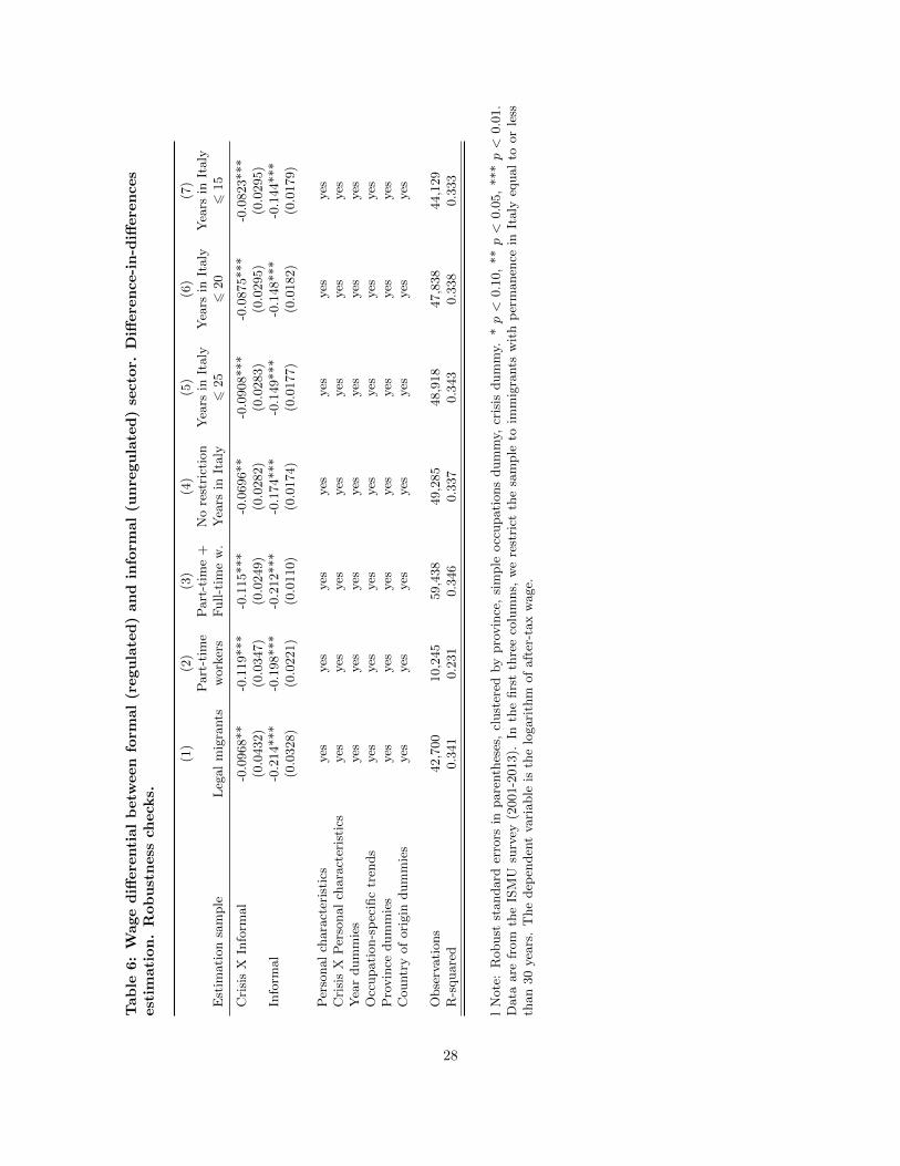
5.4 Robustness checks

Our main results are obtained for the sample of documented and undocumented immigrants in full-time

employment. Table 6 presents the first set of robustness checks. Column (1) excludes illegal immigrants. In

column 2 we focus only on part-time workers, and in column 3 on both full-time and part-time employment

simultaneously. Results are similar to our benchmark specification. Before 2009 documented immigrants

in the informal sector appear to receive 23 percent lower wages than documented immigrants in the formal

sector. The crisis, however, increases this gap up to 36 percent. The wage differential after the recession

remains similar to the benchmark results when we consider part-time workers (-0.136, see column 2) or both

part-time and full-time workers (-0.152, see column 3).

In our benchmark specifications we restrict the estimation sample to immigrants whose length of stay in

Italy does not exceed 30 years. This choice is motivated by Figure A1, which shows that the distribution of

permanence in Italy is much more skewed toward the left for informal workers. This restriction has aimed

to ensure common support for the distributions of formal and informal workers. In columns 4-7 of Table 6

we show that our results remain very similar when we do not consider any restriction on length of stay in

Italy (column 4) or when we consider different maximum permanence durations: 25 years (column 5), 20

years (column 6) and 15 years (column 7). The results are similar across all specifications.

In Table 7 we present additional checks. In column (1) we estimate a specification similar to column (1)

of Table 2, except that we exclude the year 2002. This check is also meaningful because in 2002 there was a

large immigrant regularization program that legalized about 700000 immigrants residing in Italy without a

regular residence permit. In column (2) of Table 7 we exclude the year 2005, while in column (3) we consider

an estimation sample from 2006 to 2013 (rather than from 2001 to 2013 as in the benchmark regressions).

13

In all these specifications, the results are very similar.

In all specifications in Tables 6 and 7 we control for personal characteristics; we also add interaction

terms of personal characteristics with the Crisis dummy thus allowing the returns to personal characteristics

to vary before and after 2009. Coefficients at most of these interaction terms are not significant; the returns

to personal characteristics — including age and education — do not change after 2009.10 The only exception

is gender. The gender gap actually decreases by 3-4 percentage points after 2009.

5.5 Employment in the formal and informal sectors

Our results above describe only one channel of the labor market adjustment to the aggregate demand shocks,

namely the decline in wages. A relevant question is whether this decrease in wages in the informal sector

affects employment rates in both formal (regulated) and informal (unregulated) sector.

In Table 8 we present regressions where the dependent variables are employment in the formal sector

(first two columns) or employment in the informal sector (last three columns). In the second and fourth

columns we condition on labor force participation, while in the fifth column we condition on employment.

We report and discuss the coefficients at the year dummies (where 2008 is the omitted category). We

find that for all specifications the coefficients at the year dummies are never significantly different from

zero before the beginning of the recession. The first column of Table 8 shows that during the crisis the

employment rate in the formal sector decreases by 2 percent in 2009, 4 percent in 2010, 12 percent in 2011,

15 percent in 2012 and 16 percent 2013 (relative to 2008). Results conditional on labor force participation

(column 2) are similar except that the significant decrease in the employment rate in the formal sector starts

in 2011.

Conversely, columns 3 and 4—the latter presenting estimates conditional on labor force participation—

show that the employment rate in the informal sector does not fall (it actually increases by about 2 percent

in 2012 and 2013, relative to 2008). With regard to the estimates that condition on employment, the last

column of the table shows an increase in the informal employment rate by 3 percentage points in 2012 and

2013.

These results suggest that the immigrant labor market undergoes a multi-faceted adjustment. Notwith-

standing the increase in unemployment rate documented by Figure 2, the large fall in informal wages during

the crisis creates a reallocation from the formal (regulated) to the informal (unregulated) sector, and also

generates an increase in the employment rate in the latter sector.

10We have also checked whether the coefficient at the Crisis*Informal interaction term depends on age. We have found nosignificant difference.

14

6 Conclusions

In this paper we study the process of wage adjustment in formal and informal labor markets in Italy. We show

that despite substantial growth of unemployment in 2009-13, the wages in the regulated formal labor market

have not adjusted. In the meanwhile, the wages in the unregulated informal labor market have declined

dramatically. The wage differential between formal and informal market that has been relatively constant

at 15 percent in 2001-08 has grown rapidly after 2009 and reached 32 percent in 2013. We show that the

wage adjustment in the informal sector takes place along with a shift from formal to informal employment.

These results are consistent with the view that regulation is responsible for the lack of wage adjustment

and increase in unemployment during the recessions. Our findings are based on data on immigrants rather

than the general labor force. However, we also find that our results are more pronounced for the individuals

in simple occupations. These are the occupations with relatively easy substitutability between immigrants

and natives. This allows us to speculate that our findings can be generalized for low-skilled natives as well.

While we do find that in unregulated labor markets wages adjust down during the recession, the 2009-13

period does not provide an exhaustive answer with regard to the speed and nature of this adjustment. Figure

1 and Table 2 show that wages in the informal sector continue to fall throughout the period. We cannot yet

judge whether this continuing decrease in wages is the delayed response to the initial one-off shock or every

subsequent decrease is a reaction to the next round of aggregate demand decline. In order to address this

important question, we need to collect data on both formal and informal labor market for several years after

the economy starts to recover.

15

References

Accetturo, Antonio, and Luigi Infante (2010). “Immigrant Earnings in the Italian Labour Market” Giornale

degli Economisti e Annali di Economia 69(1): 1-27.

Altonji, Joseph G., Todd Elder and Christopher Taber (2005). “Selection on Observed and Unobserved

Variables: Assessing the Effectiveness of Catholic Schools.” Journal of Political Economy 113(1): 151-

184.

Angrist, J. and Alan Krueger (1999). “Empirical Strategies in Labor Economics.” In O. Ashenfelter and

D. Card, eds., The Handbook of Labor Economics, Volume 3.

Autor, D. H. and S. N. Houseman “Do Temporary Help Jobs Improve Labor Market Outcomes for Low-

Skilled Workers? Evidence from ’Work First.”’ David H. Autor and Susan N. Houseman American

Economic Journal: Applied Economics, 2(3), July 2010, 96-128

Ashenfelter, Orley (1978). “Estimating the Effect of Training Programs on Earnings” Review of Economics

and Statistics 60(1): 47-57.

Autor, David H., Frank Levy, and Richard Murnane (2003). “The Skill Content of Recent Technological

Change: An Empirical Exploration.” Quarterly Journal of Economics 118 (4): 1279-1333.

Barsky, Robert B., F. Thomas Juster, Miles S. Kimball, and Matthew D. Shapiro (1997). “Preference

Parameters and Behavioral Heterogeneity: an Experimental Approach in the Health and Retirement

Study.” Quarterly Journal of Economics 112(2): 537-579.

Beyer, R. C. M. and Smets, F. (2015). “Reassessing Labour Market Adjustments and Migration in Europe

and the United States: How Different?” Economic Policy, 30(84): 643-682.

Bellows, John, and Edward Miguel (2009). “War and Local Collective Action in Sierra Leone.” Journal of

Public Economics 93 (11-12): 1144-1157.

Bentolila, Samuel, Pierre Cahuc, Juan J. Dolado and Thomas Le Barbanchon (2012). “Two-Tier Labour

Markets in the Great Recession: France versus Spain.” Economic Journal 122: 155-87.

Bertrand, Marianne, Duflo, Esther, and Sendhil Mullainathan (2004). “How Much Should We Trust

Differences-In-Differences Estimates?” Quarterly Journal of Economics, 119(1): 249-275.

Blanchard, Olivier Jean, and Lawrence F. Katz (1992). “Regional Evolutions.” Brookings Papers on

Economic Activity (1): 1-75.

16

Boeri, Tito (2011). “Institutional Reforms and Dualism in European Labor Markets.” in Orley Ashenfelter

and David Card, eds. Handbook of Labor Economics, Volume 4b: 1173-1236.

Boeri, Tito (2014). “Two-Tier Bargaining.” IZA Discussion Paper N. 8358.

Booth, Alison, Marco Francesconi and Jeff Frank (2002). “Temporary jobs: stepping stones or dead ends.”

The Economic Journal 112 (480): 189-213.

Borghans, Lex, James J. Heckman, Bart H. H. Golsteyn, and Huub Meijers (2009). “Gender Differences

in Risk Aversion and Ambiguity Aversion.” Journal of the European Economic Association 7(2-3):

649-658.

Cadena, Brian, and Brian Kovak (2015). “Immigrants Equilibrate Local Labor Markets: Evidence from

the Great Recession.” American Economic Journal: Applied Economics. Forthcoming.

Cameron, Colin, and Douglas Miller (2015) “A Practitioners Guide to Cluster-Robust Inference.” Journal

of Human Resources, 50(2): 317-372.

Capasso, Salvatore and Tullio Jappelli (2013). “Financial development and the underground economy.”

Journal of Development Economics 101(C): 167-178.

Cappellari, Lorenzo, and Marco Leonardi (2013). “Who pays for it? The heterogeneous wage effects of

Employment Protection Legislation.” The Economic Journal 123 (573): 1236-1278.

Card, David, and Alan Krueger (1994). “Minimum Wages and Employment: A Case Study of the Fast-Food

Industry in New Jersey and Pennsylvania.” American Economic Review 84(4): 772-93.

Cingano, Federico, Marco Leonardi, Julian Messina, and Giovanni Pica (2015). “Employment Protec-

tion Legislation, Capital Investment and Access to Credit: Evidence from Italy.” Economic Journal,

forthcoming.

Cortes, Patricia (2008). “The Effect of Low-Skilled Immigration on U.S. Prices: Evidence from CPI Data.”

Journal of Political Economy 116(3): 381-422.

D’Amuri, Francesco, and Giovanni Peri (2014). “Immigration, jobs and employment protection: evidence

from Europe before and during the Great Recession.” Journal of the European Economic Association

12(2): 432-464.

Decressin, Jorg, and Antonio Fatas (1995) “Regional labor market dynamics in Europe.” European Eco-

nomic Review 39 (9): 1627-1655.

17

Donald, Stephen, and Kevin Lang, K. (2007) “Inference with Difference-In-Difference and Other Panel

Data.” Review of Economics and Statistics, 89(2): 221-233.

Dustmann, Christian, Francesco Fasani, and Biagio Speciale (2015) “Illegal migration and consumption

behavior of immigrant households.” CReAM Discussion Paper Series N. 1512.

Elsby, Michael, Donggyun Shin, and Gary Solon (2015) “Wage Adjustment in the Great Recession and

Other Downturns: Evidence from the United States and Great Britain.” Journal of Labor Economics.

Forthcoming.

Fasani, Francesco (2015) “Understanding the Role of Immigrants’ Legal Status: Evidence from Policy

Experiments” CESifo Economic Studies 61(3-4): 722-763.

Goos, Maarten, Alan Manning, and Anna Salomons (2009) “Job Polarization in Europe.” American Eco-

nomic Review 99(2): 58-63.

Goos, Maarten, Alan Manning, and Anna Salomons (2014) “Explaining Job Polarization: Routine-Biased

Technological Change and Offshoring.” American Economic Review 104(8): 2509-26.

Guiso, Luigi and Monica Paiella (2008) “Risk Aversion, Wealth and Background Risk.” Journal of the

European Economic Association 6(6): 1109-1150.

Ichino, Andrea, Fabrizia Mealli and Tommaso Nannicini (2008) “From temporary help jobs to permanent

employment: What can we learn from matching estimators and their sensitivity?” Journal of Applied

Econometrics 23: 305-327.

Ichino, Andrea and Regina T. Riphahn (2005). “The effect of employment protection on worker effort:

absenteeism during and after probation.” Journal of the European Economic Association 3(1): 120-

143.

Kugler, Adriana D. and Giovanni Pica (2008). “Effects of Employment Protection on Job and Worker

Flows: Evidence from the 1990 Italian Reform” Labour Economics 15(1): 78-95.

Manacorda, Marco (2004) “Can the Scala Mobile explain the fall and rise of earnings inequality in Italy?

A semiparametric analysis, 1977–1993” Journal of Labor Economics, 22(3): 585–613.

Manacorda, Marco, Alan Manning, and Jonathan Wadsworth (2012) “The Impact of Immigration on the

Structure of Male Wages: Theory and Evidence from Britain.” Journal of the European Economic

Association 10(1): 120-151.

Mauro, Paolo, and Antonio Spilimbergo (1999) “How Do the Skilled and the Unskilled Respond to Regional

Shocks?: The Case of Spain.” IMF Staff Paper 46(1): 1-17.

18

Meghir, Costas, Renata Narita, and Jean-Marc Robin (2015) “Wages and Informality in Developing Coun-

tries.” American Economic Review 105(4): 1509–1546.

Neumark, David (2014) “Employment effects of minimum wages.” IZA World of Labor 2014: 6.

Neumark, David, Ian Salas, and William Wascher (2013) “Revisiting the Minimum Wage-Employment

Debate: Throwing Out the Baby with the Bathwater?” NBER Working Paper No. 18681.

Nunn, Nathan, and Leonard Wantchekon (2011) “The Slave Trade and the Origins of Mistrust in Africa.”

American Economic Review 101 (7) (December): 3221-3252.

OECD (2008) “A profile of immigrant populations in the 21st century: data from OECD countries.” Paris.

Orrenius, Pia, and Madeline Zavodny (2010) “Mexican Immigrant Employment Outcomes over the Business

Cycle.” American Economic Review: Papers & Proceedings 100(3): 316-320.

Orsi, Renzo, Davide Raggi and Francesco Turino (2014) “Size, Trend, and Policy Implications of the

Underground Economy.” Review of Economic Dynamics 17(3): 417-436.

Ottaviano, Gianmarco I. P. and Giovanni Peri (2012) “Rethinking the gains of immigration on wages.”

Journal of the European Economic Association 10: 152-197.

Peri, Giovanni, and Chad Sparber (2009). “Task Specialization, Immigration, and Wages.” American

Economic Journal. Applied Economics 1(3): 135-169.

Yang, Dean (2006) “Why Do Migrants Return to Poor Countries? Evidence from Philippine Migrants’

Responses to Exchange Rate Shocks.” Review of Economics and Statistics 88(4): 715-735.

19

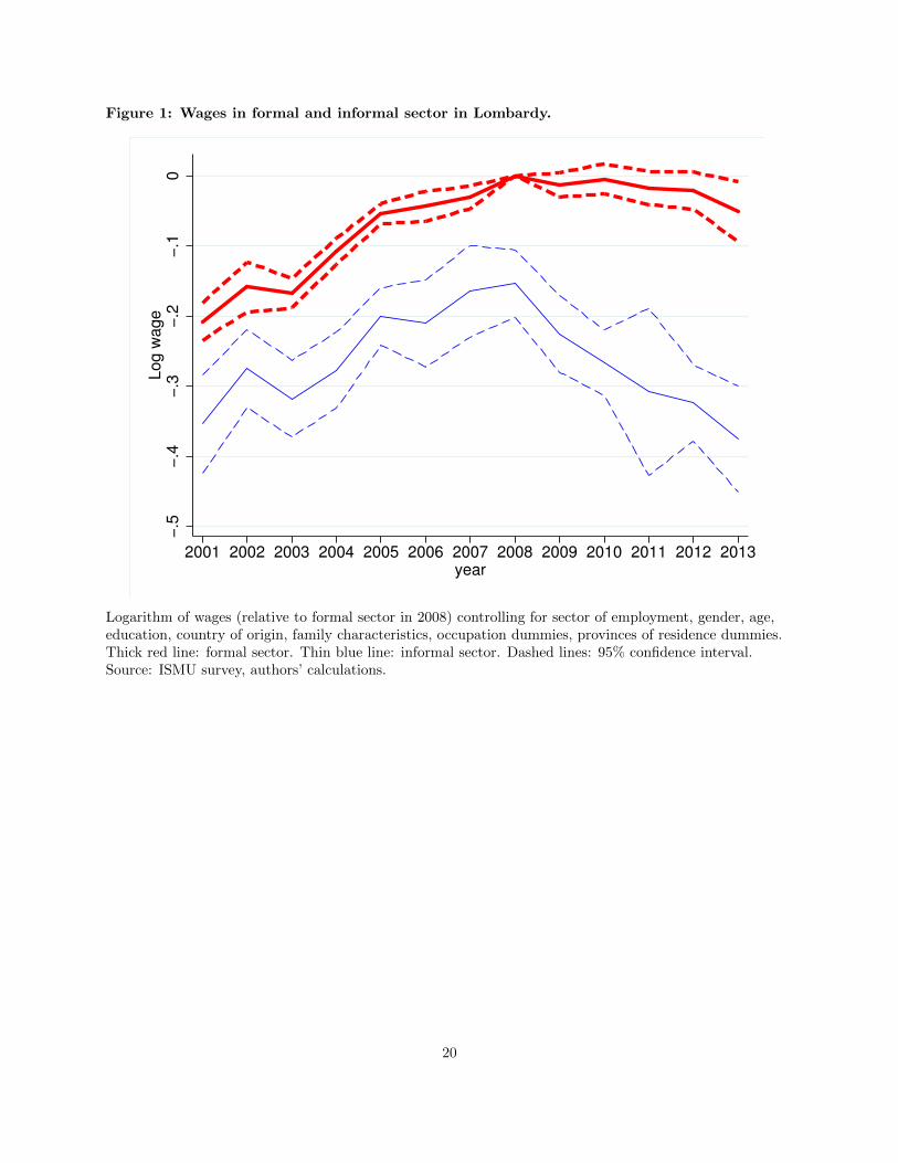
Figure 1: Wages in formal and informal sector in Lombardy.

−.5

−.4

−.3

−.2

−.1

0L

og

wa

ge

2001 2002 2003 2004 2005 2006 2007 2008 2009 2010 2011 2012 2013year

Logarithm of wages (relative to formal sector in 2008) controlling for sector of employment, gender, age,education, country of origin, family characteristics, occupation dummies, provinces of residence dummies.Thick red line: formal sector. Thin blue line: informal sector. Dashed lines: 95% confidence interval.Source: ISMU survey, authors’ calculations.

20

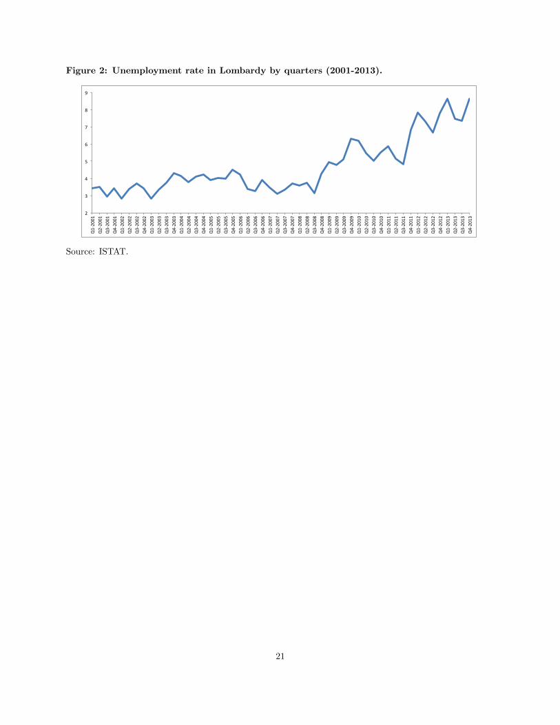
Figure 2: Unemployment rate in Lombardy by quarters (2001-2013).

2  

3  

4  

5  

6  

7  

8  

9  Q1-­‐20

01  

Q2-­‐20

01  

Q3-­‐20

01  

Q4-­‐20

01  

Q1-­‐20

02  

Q2-­‐20

02  

Q3-­‐20

02  

Q4-­‐20

02  

Q1-­‐20

03  

Q2-­‐20

03  

Q3-­‐20

03  

Q4-­‐20

03  

Q1-­‐20

04  

Q2-­‐20

04  

Q3-­‐20

04  

Q4-­‐20

04  

Q1-­‐20

05  

Q2-­‐20

05  

Q3-­‐20

05  

Q4-­‐20

05  

Q1-­‐20

06  

Q2-­‐20

06  

Q3-­‐20

06  

Q4-­‐20

06  

Q1-­‐20

07  

Q2-­‐20

07  

Q3-­‐20

07  

Q4-­‐20

07  

Q1-­‐20

08  

Q2-­‐20

08  

Q3-­‐20

08  

Q4-­‐20

08  

Q1-­‐20

09  

Q2-­‐20

09  

Q3-­‐20

09  

Q4-­‐20

09  

Q1-­‐20

10  

Q2-­‐20

10  

Q3-­‐20

10  

Q4-­‐20

10  

Q1-­‐20

11  

Q2-­‐20

11  

Q3-­‐20

11  

Q4-­‐20

11  

Q1-­‐20

12  

Q2-­‐20

12  

Q3-­‐20

12  

Q4-­‐20

12  

Q1-­‐20

13  

Q2-­‐20

13  

Q3-­‐20

13  

Q4-­‐20

13  

Source: ISTAT.

21

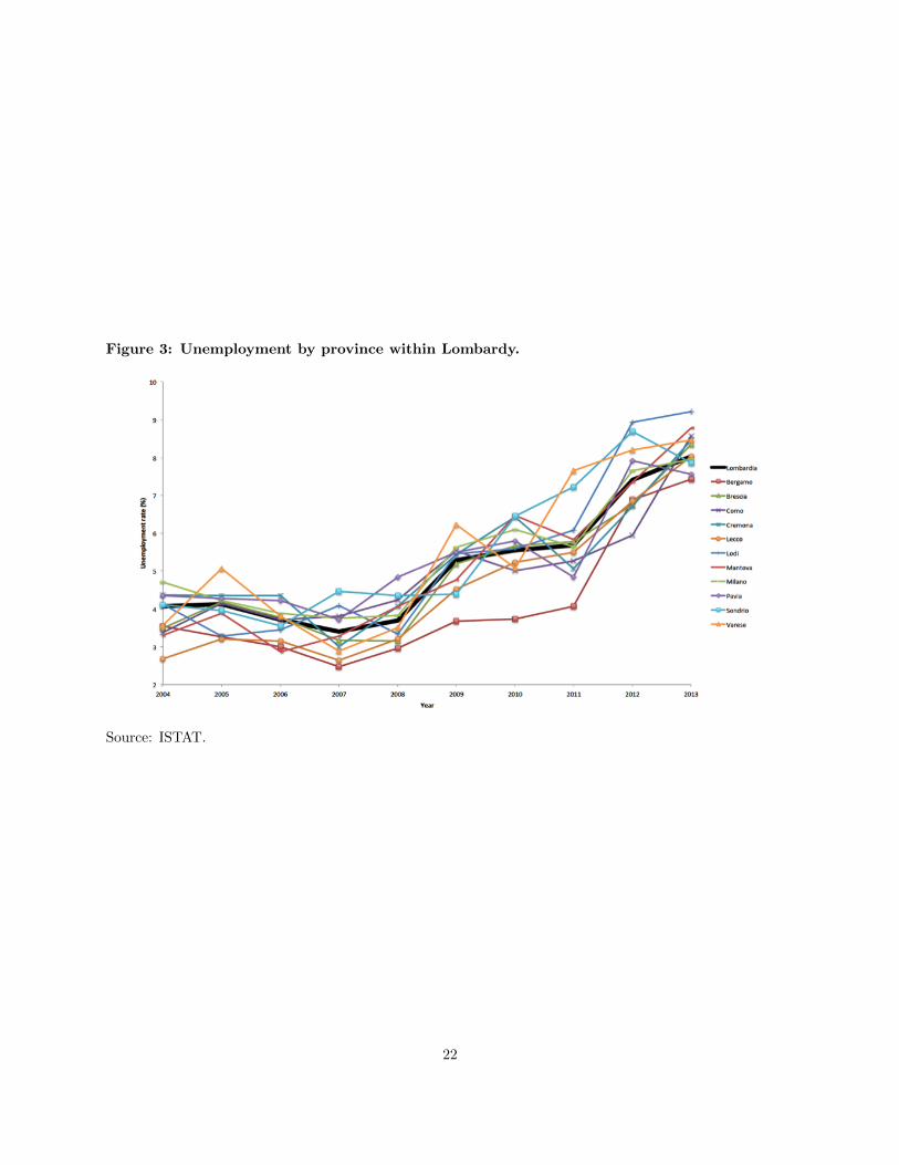
Figure 3: Unemployment by province within Lombardy.

Source: ISTAT.

22

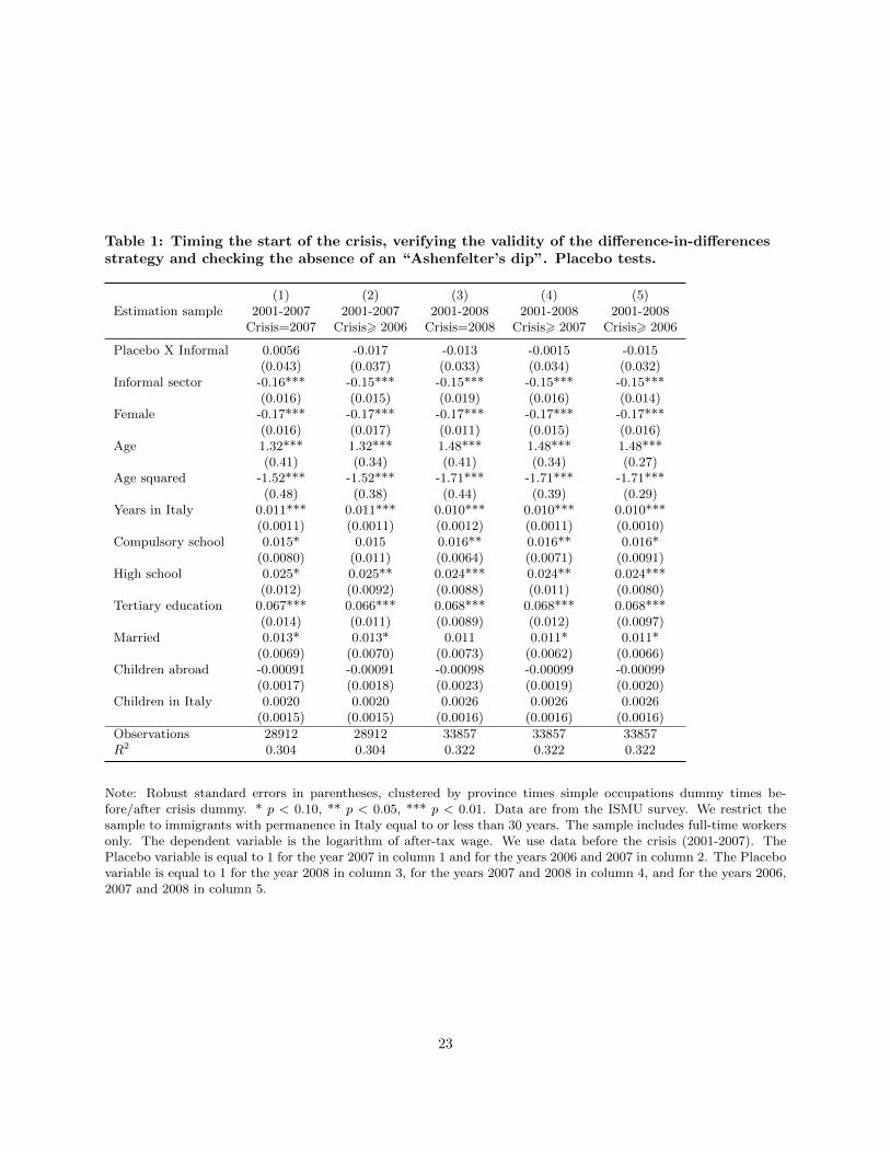
Table 1: Timing the start of the crisis, verifying the validity of the difference-in-differencesstrategy and checking the absence of an “Ashenfelter’s dip”. Placebo tests.

(1) (2) (3) (4) (5)Estimation sample 2001-2007 2001-2007 2001-2008 2001-2008 2001-2008

Crisis=2007 Crisis> 2006 Crisis=2008 Crisis> 2007 Crisis> 2006

Placebo X Informal 0.0056 -0.017 -0.013 -0.0015 -0.015(0.043) (0.037) (0.033) (0.034) (0.032)

Informal sector -0.16*** -0.15*** -0.15*** -0.15*** -0.15***(0.016) (0.015) (0.019) (0.016) (0.014)

Female -0.17*** -0.17*** -0.17*** -0.17*** -0.17***(0.016) (0.017) (0.011) (0.015) (0.016)

Age 1.32*** 1.32*** 1.48*** 1.48*** 1.48***(0.41) (0.34) (0.41) (0.34) (0.27)

Age squared -1.52*** -1.52*** -1.71*** -1.71*** -1.71***(0.48) (0.38) (0.44) (0.39) (0.29)

Years in Italy 0.011*** 0.011*** 0.010*** 0.010*** 0.010***(0.0011) (0.0011) (0.0012) (0.0011) (0.0010)

Compulsory school 0.015* 0.015 0.016** 0.016** 0.016*(0.0080) (0.011) (0.0064) (0.0071) (0.0091)

High school 0.025* 0.025** 0.024*** 0.024** 0.024***(0.012) (0.0092) (0.0088) (0.011) (0.0080)

Tertiary education 0.067*** 0.066*** 0.068*** 0.068*** 0.068***(0.014) (0.011) (0.0089) (0.012) (0.0097)

Married 0.013* 0.013* 0.011 0.011* 0.011*(0.0069) (0.0070) (0.0073) (0.0062) (0.0066)

Children abroad -0.00091 -0.00091 -0.00098 -0.00099 -0.00099(0.0017) (0.0018) (0.0023) (0.0019) (0.0020)

Children in Italy 0.0020 0.0020 0.0026 0.0026 0.0026(0.0015) (0.0015) (0.0016) (0.0016) (0.0016)

Observations 28912 28912 33857 33857 33857R2 0.304 0.304 0.322 0.322 0.322

Note: Robust standard errors in parentheses, clustered by province times simple occupations dummy times be-fore/after crisis dummy. * p < 0.10, ** p < 0.05, *** p < 0.01. Data are from the ISMU survey. We restrict thesample to immigrants with permanence in Italy equal to or less than 30 years. The sample includes full-time workersonly. The dependent variable is the logarithm of after-tax wage. We use data before the crisis (2001-2007). ThePlacebo variable is equal to 1 for the year 2007 in column 1 and for the years 2006 and 2007 in column 2. The Placebovariable is equal to 1 for the year 2008 in column 3, for the years 2007 and 2008 in column 4, and for the years 2006,2007 and 2008 in column 5.

23

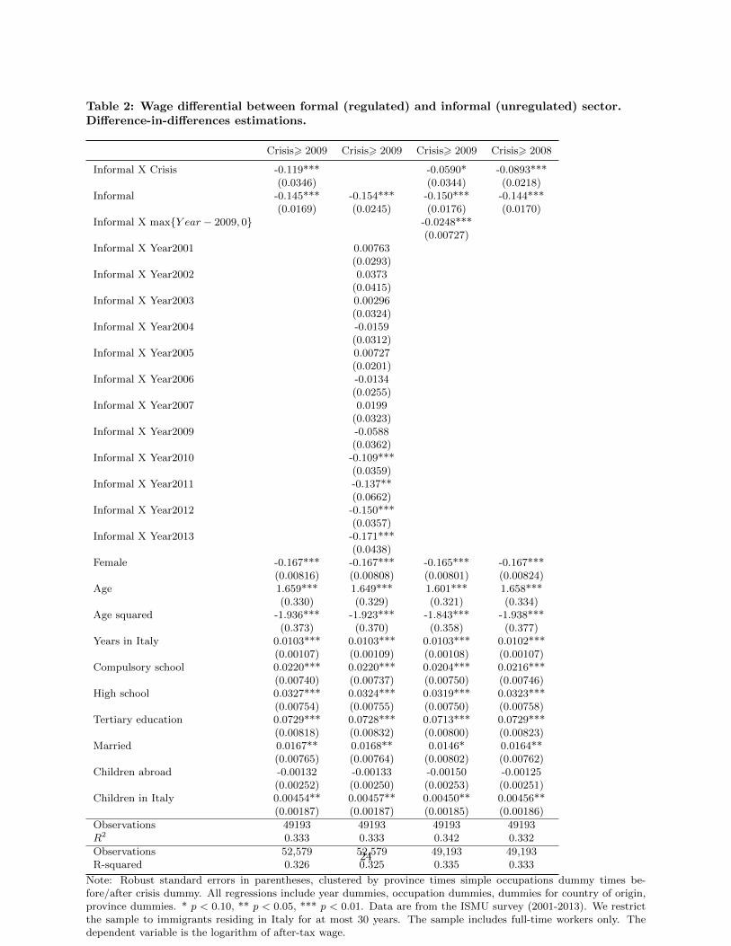
Table 2: Wage differential between formal (regulated) and informal (unregulated) sector.Difference-in-differences estimations.

Crisis> 2009 Crisis> 2009 Crisis> 2009 Crisis> 2008

Informal X Crisis -0.119*** -0.0590* -0.0893***(0.0346) (0.0344) (0.0218)

Informal -0.145*** -0.154*** -0.150*** -0.144***(0.0169) (0.0245) (0.0176) (0.0170)

Informal X max{Y ear − 2009, 0} -0.0248***(0.00727)

Informal X Year2001 0.00763(0.0293)

Informal X Year2002 0.0373(0.0415)

Informal X Year2003 0.00296(0.0324)

Informal X Year2004 -0.0159(0.0312)

Informal X Year2005 0.00727(0.0201)

Informal X Year2006 -0.0134(0.0255)

Informal X Year2007 0.0199(0.0323)

Informal X Year2009 -0.0588(0.0362)

Informal X Year2010 -0.109***(0.0359)

Informal X Year2011 -0.137**(0.0662)

Informal X Year2012 -0.150***(0.0357)

Informal X Year2013 -0.171***(0.0438)

Female -0.167*** -0.167*** -0.165*** -0.167***(0.00816) (0.00808) (0.00801) (0.00824)

Age 1.659*** 1.649*** 1.601*** 1.658***(0.330) (0.329) (0.321) (0.334)

Age squared -1.936*** -1.923*** -1.843*** -1.938***(0.373) (0.370) (0.358) (0.377)

Years in Italy 0.0103*** 0.0103*** 0.0103*** 0.0102***(0.00107) (0.00109) (0.00108) (0.00107)

Compulsory school 0.0220*** 0.0220*** 0.0204*** 0.0216***(0.00740) (0.00737) (0.00750) (0.00746)

High school 0.0327*** 0.0324*** 0.0319*** 0.0323***(0.00754) (0.00755) (0.00750) (0.00758)

Tertiary education 0.0729*** 0.0728*** 0.0713*** 0.0729***(0.00818) (0.00832) (0.00800) (0.00823)

Married 0.0167** 0.0168** 0.0146* 0.0164**(0.00765) (0.00764) (0.00802) (0.00762)

Children abroad -0.00132 -0.00133 -0.00150 -0.00125(0.00252) (0.00250) (0.00253) (0.00251)

Children in Italy 0.00454** 0.00457** 0.00450** 0.00456**(0.00187) (0.00187) (0.00185) (0.00186)

Observations 49193 49193 49193 49193R2 0.333 0.333 0.342 0.332

Observations 52,579 52,579 49,193 49,193R-squared 0.326 0.325 0.335 0.333

Note: Robust standard errors in parentheses, clustered by province times simple occupations dummy times be-fore/after crisis dummy. All regressions include year dummies, occupation dummies, dummies for country of origin,province dummies. * p < 0.10, ** p < 0.05, *** p < 0.01. Data are from the ISMU survey (2001-2013). We restrictthe sample to immigrants residing in Italy for at most 30 years. The sample includes full-time workers only. Thedependent variable is the logarithm of after-tax wage.

24

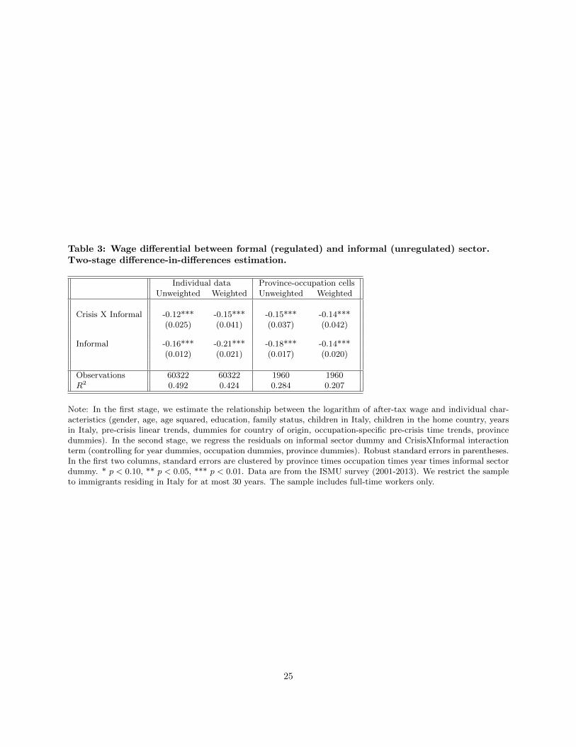
Table 3: Wage differential between formal (regulated) and informal (unregulated) sector.Two-stage difference-in-differences estimation.

Individual data Province-occupation cellsUnweighted Weighted Unweighted Weighted

Crisis X Informal -0.12*** -0.15*** -0.15*** -0.14***(0.025) (0.041) (0.037) (0.042)

Informal -0.16*** -0.21*** -0.18*** -0.14***(0.012) (0.021) (0.017) (0.020)

Observations 60322 60322 1960 1960R2 0.492 0.424 0.284 0.207

Note: In the first stage, we estimate the relationship between the logarithm of after-tax wage and individual char-acteristics (gender, age, age squared, education, family status, children in Italy, children in the home country, yearsin Italy, pre-crisis linear trends, dummies for country of origin, occupation-specific pre-crisis time trends, provincedummies). In the second stage, we regress the residuals on informal sector dummy and CrisisXInformal interactionterm (controlling for year dummies, occupation dummies, province dummies). Robust standard errors in parentheses.In the first two columns, standard errors are clustered by province times occupation times year times informal sectordummy. * p < 0.10, ** p < 0.05, *** p < 0.01. Data are from the ISMU survey (2001-2013). We restrict the sampleto immigrants residing in Italy for at most 30 years. The sample includes full-time workers only.

25

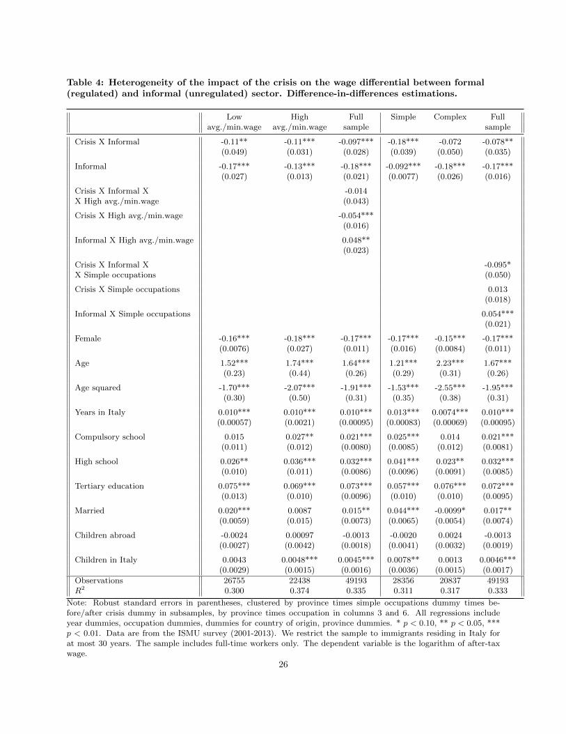
Table 4: Heterogeneity of the impact of the crisis on the wage differential between formal(regulated) and informal (unregulated) sector. Difference-in-differences estimations.

Low High Full Simple Complex Fullavg./min.wage avg./min.wage sample sample

Crisis X Informal -0.11** -0.11*** -0.097*** -0.18*** -0.072 -0.078**(0.049) (0.031) (0.028) (0.039) (0.050) (0.035)

Informal -0.17*** -0.13*** -0.18*** -0.092*** -0.18*** -0.17***(0.027) (0.013) (0.021) (0.0077) (0.026) (0.016)

Crisis X Informal X -0.014X High avg./min.wage (0.043)

Crisis X High avg./min.wage -0.054***(0.016)

Informal X High avg./min.wage 0.048**(0.023)

Crisis X Informal X -0.095*X Simple occupations (0.050)

Crisis X Simple occupations 0.013(0.018)

Informal X Simple occupations 0.054***(0.021)

Female -0.16*** -0.18*** -0.17*** -0.17*** -0.15*** -0.17***(0.0076) (0.027) (0.011) (0.016) (0.0084) (0.011)

Age 1.52*** 1.74*** 1.64*** 1.21*** 2.23*** 1.67***(0.23) (0.44) (0.26) (0.29) (0.31) (0.26)

Age squared -1.70*** -2.07*** -1.91*** -1.53*** -2.55*** -1.95***(0.30) (0.50) (0.31) (0.35) (0.38) (0.31)

Years in Italy 0.010*** 0.010*** 0.010*** 0.013*** 0.0074*** 0.010***(0.00057) (0.0021) (0.00095) (0.00083) (0.00069) (0.00095)

Compulsory school 0.015 0.027** 0.021*** 0.025*** 0.014 0.021***(0.011) (0.012) (0.0080) (0.0085) (0.012) (0.0081)

High school 0.026** 0.036*** 0.032*** 0.041*** 0.023** 0.032***(0.010) (0.011) (0.0086) (0.0096) (0.0091) (0.0085)

Tertiary education 0.075*** 0.069*** 0.073*** 0.057*** 0.076*** 0.072***(0.013) (0.010) (0.0096) (0.010) (0.010) (0.0095)

Married 0.020*** 0.0087 0.015** 0.044*** -0.0099* 0.017**(0.0059) (0.015) (0.0073) (0.0065) (0.0054) (0.0074)

Children abroad -0.0024 0.00097 -0.0013 -0.0020 0.0024 -0.0013(0.0027) (0.0042) (0.0018) (0.0041) (0.0032) (0.0019)

Children in Italy 0.0043 0.0048*** 0.0045*** 0.0078** 0.0013 0.0046***(0.0029) (0.0015) (0.0016) (0.0036) (0.0015) (0.0017)

Observations 26755 22438 49193 28356 20837 49193R2 0.300 0.374 0.335 0.311 0.317 0.333

Note: Robust standard errors in parentheses, clustered by province times simple occupations dummy times be-fore/after crisis dummy in subsamples, by province times occupation in columns 3 and 6. All regressions includeyear dummies, occupation dummies, dummies for country of origin, province dummies. * p < 0.10, ** p < 0.05, ***p < 0.01. Data are from the ISMU survey (2001-2013). We restrict the sample to immigrants residing in Italy forat most 30 years. The sample includes full-time workers only. The dependent variable is the logarithm of after-taxwage.

26

Table 5: Wage differential between formal (regulated) and informal (unregulated) sector.Difference-in-differences estimation. Regressions with gradual inclusion of control variables.Altonji et al.’s (2005) test.

Crisis X Informal -0.081** -0.085*** -0.088*** -0.077** -0.088*** -0.093***(0.033) (0.030) (0.033) (0.033) (0.030) (0.028)

Informal -0.21*** -0.20*** -0.18*** -0.20*** -0.18*** -0.15***(0.016) (0.016) (0.016) (0.016) (0.015) (0.018)

Female yes yes yes

Age yes yes yes

Age squared yes yes yes

Years in Italy yes

Compulsory school yes yes yes

High school yes yes yes

Tertiary education yes yes yes

Married yes

Children abroad yes

Children in Italy yes

Altonji test 7.75 11.63 18.60 5.81 18.60

Observations 49193 49193 49193 49193 49193 49193R2 0.282 0.306 0.302 0.285 0.327 0.344

Note: Robust standard errors in parentheses, clustered by province times simple occupations dummy times be-fore/after crisis dummy in subsamples, by province times occupation in columns 3 and 6. All regressions includeyear dummies, occupation dummies, dummies for country of origin, province dummies.* p < 0.10, ** p < 0.05, ***p < 0.01. Data are from the ISMU survey (2001-2013). We restrict the sample to immigrants with permanencein Italy equal to or less than 30 years. The sample includes full-time workers only. The dependent variable is thelogarithm of after-tax wage. In columns 1-5, we exclude observed variables that are good predictors of the unob-served risk aversion. We denote the estimated coefficient of interest (i.e. the coefficient of the interaction term) inthese specifications as βr. The value of the Altonji et al.’s (2005) test is then calculated as the absolute value ofβf/(βr − βf ), where βf is the coefficient of the interaction term in column 6, i.e. from the estimation that includesthe full set of covariates. Whenever covariates are included, we also include their interaction with the “after crisis”dummy.

27

Tab

le6:

Wage

diff

ere

nti

al

betw

een

form

al

(regu

late

d)

an

din

form

al

(un

regu

late

d)

secto

r.D

iffere

nce-i

n-d

iffere

nces

est

imati

on

.R

ob

ust

ness

check

s.

(1)

(2)

(3)

(4)

(5)

(6)

(7)

Part

-tim

eP

art

-tim

e+

No

rest

rict

ion

Yea

rsin

Italy

Yea

rsin

Italy

Yea

rsin

Italy

Est

imati

on

sam

ple

Leg

al

mig

rants

work

ers

Full-t

ime

w.

Yea

rsin

Italy

625

620

615

Cri

sis

XIn

form

al

-0.0

968**

-0.1

19***

-0.1

15***

-0.0

696**

-0.0

908***

-0.0

875***

-0.0

823***

(0.0

432)

(0.0

347)

(0.0

249)

(0.0

282)

(0.0

283)

(0.0

295)

(0.0

295)

Info

rmal

-0.2

14***

-0.1

98***

-0.2

12***

-0.1

74***

-0.1

49***

-0.1

48***

-0.1

44***

(0.0

328)

(0.0

221)

(0.0

110)

(0.0

174)

(0.0

177)

(0.0

182)

(0.0

179)

Per

sonal

chara

cter

isti

csyes

yes

yes

yes

yes

yes

yes

Cri

sis

XP

erso

nal

chara

cter

isti

csyes

yes

yes

yes

yes

yes

yes

Yea

rdum

mie

syes

yes

yes

yes

yes

yes

yes

Occ

upati

on-s

pec

ific

tren

ds

yes

yes

yes

yes

yes

yes

yes

Pro

vin

cedum

mie

syes

yes

yes

yes

yes

yes

yes

Countr

yof

ori

gin

dum

mie

syes

yes

yes

yes

yes

yes

yes

Obse

rvati

ons

42,7

00

10,2

45

59,4

38

49,2

85

48,9

18

47,8

38

44,1

29

R-s

quare

d0.3

41

0.2

31

0.3

46

0.3

37

0.3

43

0.3

38

0.3

33

lN

ote

:R

obust

standard

erro

rsin

pare

nth

eses

,cl

ust

ered

by

pro

vin

ce,

sim

ple

occ

upati

ons

dum

my,

cris

isdum

my.

*p<

0.1

0,

**p<

0.0

5,

***p<

0.0

1.

Data

are

from

the

ISM

Usu

rvey

(2001-2

013).

Inth

efirs

tth

ree

colu

mns,

we

rest

rict

the

sam

ple

toim

mig

rants

wit

hp

erm

anen

cein

Italy

equal

toor

less

than

30

yea

rs.

The

dep

enden

tva

riable

isth

elo

gari

thm

of

aft

er-t

ax

wage.

28

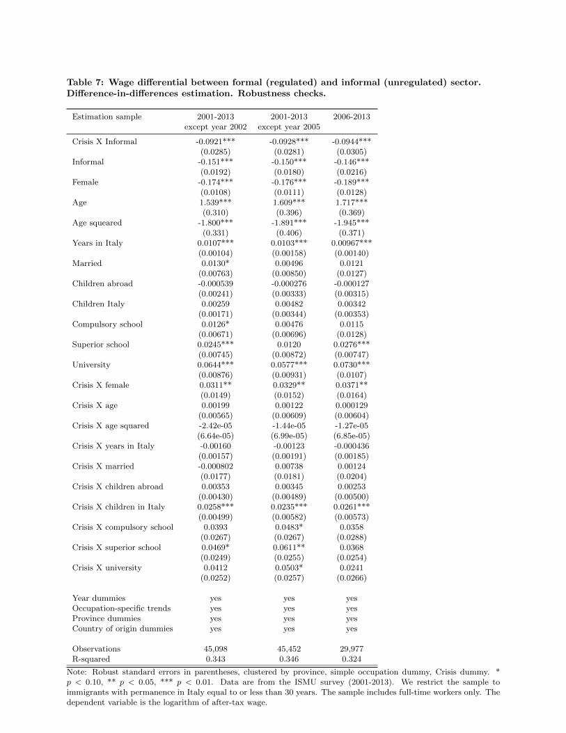
Table 7: Wage differential between formal (regulated) and informal (unregulated) sector.Difference-in-differences estimation. Robustness checks.

Estimation sample 2001-2013 2001-2013 2006-2013except year 2002 except year 2005

Crisis X Informal -0.0921*** -0.0928*** -0.0944***(0.0285) (0.0281) (0.0305)

Informal -0.151*** -0.150*** -0.146***(0.0192) (0.0180) (0.0216)

Female -0.174*** -0.176*** -0.189***(0.0108) (0.0111) (0.0128)

Age 1.539*** 1.609*** 1.717***(0.310) (0.396) (0.369)

Age squeared -1.800*** -1.891*** -1.945***(0.331) (0.406) (0.371)

Years in Italy 0.0107*** 0.0103*** 0.00967***(0.00104) (0.00158) (0.00140)

Married 0.0130* 0.00496 0.0121(0.00763) (0.00850) (0.0127)

Children abroad -0.000539 -0.000276 -0.000127(0.00241) (0.00333) (0.00315)

Children Italy 0.00259 0.00482 0.00342(0.00171) (0.00344) (0.00353)

Compulsory school 0.0126* 0.00476 0.0115(0.00671) (0.00696) (0.0128)

Superior school 0.0245*** 0.0120 0.0276***(0.00745) (0.00872) (0.00747)

University 0.0644*** 0.0577*** 0.0730***(0.00876) (0.00931) (0.0107)

Crisis X female 0.0311** 0.0329** 0.0371**(0.0149) (0.0152) (0.0164)

Crisis X age 0.00199 0.00122 0.000129(0.00565) (0.00609) (0.00604)

Crisis X age squared -2.42e-05 -1.44e-05 -1.27e-05(6.64e-05) (6.99e-05) (6.85e-05)

Crisis X years in Italy -0.00160 -0.00123 -0.000436(0.00157) (0.00191) (0.00185)

Crisis X married -0.000802 0.00738 0.00124(0.0177) (0.0181) (0.0204)

Crisis X children abroad 0.00353 0.00345 0.00253(0.00430) (0.00489) (0.00500)

Crisis X children in Italy 0.0258*** 0.0235*** 0.0261***(0.00499) (0.00582) (0.00573)

Crisis X compulsory school 0.0393 0.0483* 0.0358(0.0267) (0.0267) (0.0288)

Crisis X superior school 0.0469* 0.0611** 0.0368(0.0249) (0.0255) (0.0254)

Crisis X university 0.0412 0.0503* 0.0241(0.0252) (0.0257) (0.0266)

Year dummies yes yes yesOccupation-specific trends yes yes yesProvince dummies yes yes yesCountry of origin dummies yes yes yes

Observations 45,098 45,452 29,977R-squared 0.343 0.346 0.324

Note: Robust standard errors in parentheses, clustered by province, simple occupation dummy, Crisis dummy. *p < 0.10, ** p < 0.05, *** p < 0.01. Data are from the ISMU survey (2001-2013). We restrict the sample toimmigrants with permanence in Italy equal to or less than 30 years. The sample includes full-time workers only. Thedependent variable is the logarithm of after-tax wage.

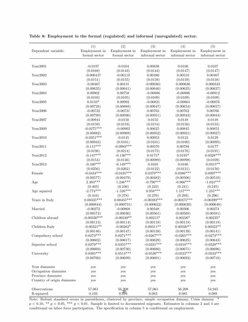
Table 8: Employment in the formal (regulated) and informal (unregulated) sector.

(1) (2) (3) (4) (5)Dependent variable: Employment in Employment in Employment in Employment in Employment in

formal sector formal sector informal sector informal sector informal sector

Year2001 -0.0197 -0.0104 0.00838 0.0108 0.0107(0.0168) (0.0143) (0.0144) (0.0147) (0.0147)

Year2002 -0.000447 -0.00118 0.00480 0.00510 0.00467(0.0151) (0.0155) (0.0158) (0.0159) (0.0158)

Year2003 -0.00467 0.00131 -0.000361 0.000636 0.000343(0.00635) (0.00641) (0.00646) (0.00635) (0.00637)

Year2004 0.00902 0.00758 -0.00886 -0.00906 -0.00912(0.0103) (0.0105) (0.0109) (0.0109) (0.0109)

Year2005 0.0133* 0.00992 -0.00821 -0.00864 -0.00876(0.00728) (0.00688) (0.00647) (0.00654) (0.00657)

Year2006 -0.00722 -0.00731 0.00762 0.00762 0.00766(0.00799) (0.00936) (0.00951) (0.00943) (0.00944)

Year2007 -0.00944 -0.0150 0.0155 0.0148 0.0148(0.0159) (0.0153) (0.0154) (0.0156) (0.0155)

Year2009 -0.0275*** -0.00902 0.00625 0.00845 0.00852(0.00882) (0.00969) (0.00952) (0.00921) (0.00927)

Year2010 -0.0351*** -0.0145 0.00953 0.0124 0.0129(0.00943) (0.0101) (0.0101) (0.0100) (0.00995)

Year2011 -0.115*** -0.0983*** 0.00570 0.00789 0.0177(0.0198) (0.0214) (0.0175) (0.0176) (0.0191)

Year2012 -0.147*** -0.136*** 0.0175* 0.0195* 0.0328***(0.0154) (0.0146) (0.00989) (0.00998) (0.0109)

Year2013 -0.160*** -0.149*** 0.0165 0.0186 0.0315**(0.0256) (0.0262) (0.0122) (0.0121) (0.0150)

Female -0.0434*** -0.0435*** 0.0379*** 0.0386*** 0.0397***(0.00577) (0.00479) (0.00482) (0.00506) (0.00510)

Age 2.383*** 1.246*** -0.790*** -0.966*** -1.024***(0.403) (0.236) (0.223) (0.241) (0.245)

Age squared -2.774*** -1.526*** 0.958*** 1.157*** 1.235***(0.444) (0.278) (0.276) (0.293) (0.296)

Years in Italy 0.00335*** 0.00455*** -0.00383*** -0.00375*** -0.00399***(0.000844) (0.000731) (0.000622) (0.000630) (0.000648)

Married -0.00272 -0.00868 0.00348 0.00306 0.00374(0.00574) (0.00630) (0.00561) (0.00568) (0.00581)

Children abroad -0.00330*** -0.00249** 0.00215* 0.00226* 0.00235*(0.00113) (0.00114) (0.00118) (0.00118) (0.00118)

Children Italy -0.00321** -0.00282* 0.00311** 0.00320** 0.00322**(0.00146) (0.00147) (0.00139) (0.00139) (0.00141)

Compulsory school 0.0273*** 0.0271*** -0.0267*** -0.0265*** -0.0273***(0.00602) (0.00617) (0.00629) (0.00625) (0.00643)

Superior school 0.0279*** 0.0355*** -0.0331*** -0.0318*** -0.0329***(0.00669) (0.00730) (0.00680) (0.00671) (0.00696)

University 0.0385*** 0.0514*** -0.0536*** -0.0522*** -0.0533***(0.00760) (0.00699) (0.00691) (0.00692) (0.00718)

Year dummies yes yes yes yes yesOccupation dummies yes yes yes yes yesProvince dummies yes yes yes yes yesCountry of origin dummies yes yes yes yes yes

Observations 57,061 56,208 57,061 56,208 54,945R-squared 0.103 0.094 0.083 0.085 0.088

Note: Robust standard errors in parentheses, clustered by province, simple occupation dummy, Crisis dummy. *p < 0.10, ** p < 0.05, *** p < 0.01. Sample is limited to documented migrants. Estimates in columns 2 and 4 areconditional on labor force participation. The specification in column 5 is conditional on employment.

30

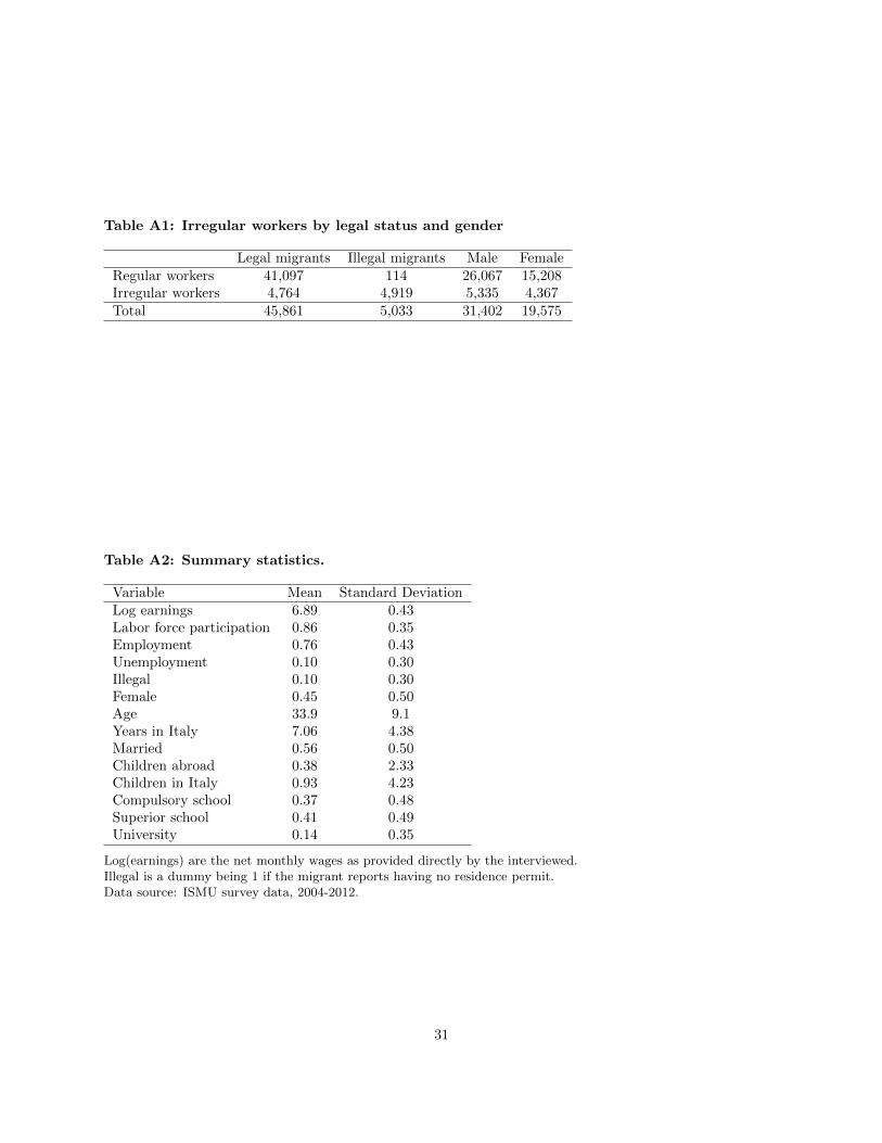
Table A1: Irregular workers by legal status and gender

Legal migrants Illegal migrants Male FemaleRegular workers 41,097 114 26,067 15,208Irregular workers 4,764 4,919 5,335 4,367Total 45,861 5,033 31,402 19,575

Table A2: Summary statistics.

Variable Mean Standard DeviationLog earnings 6.89 0.43Labor force participation 0.86 0.35Employment 0.76 0.43Unemployment 0.10 0.30Illegal 0.10 0.30Female 0.45 0.50Age 33.9 9.1Years in Italy 7.06 4.38Married 0.56 0.50Children abroad 0.38 2.33Children in Italy 0.93 4.23Compulsory school 0.37 0.48Superior school 0.41 0.49University 0.14 0.35

Log(earnings) are the net monthly wages as provided directly by the interviewed.Illegal is a dummy being 1 if the migrant reports having no residence permit.Data source: ISMU survey data, 2004-2012.

31

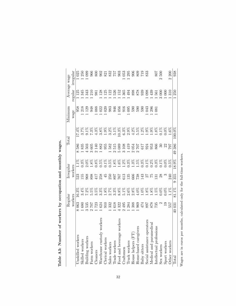
Tab

leA

3:

Nu

mb

er

of

work

ers

by

occu

pati

on

an

dm

onth

lyw

ages.

Reg

ula

rIr

regu

lar

Tota

lM

inim

um

Ave

rage

wag

ew

orke

rsw

ork

ers

wage

regu

lar

irre

gu

lar

Un

skil

led

wor

ker

s8

063

16.3

%523

1.1

%8

586

17.4

%958

1125

1025

Skil

led

wor

ker

s1

680

3.4

%155

0.3

%1

835

3.7

%1

218

1345

1250

Bu

ild

ing

wor

ker

s3

535

7.2

%968

2.0

%4

503

9.1

%1

129

1343

1099

Far

mw

orke

rs2

707

5.5

%898

1.8

%3

605

7.3

%948

1210

966

Cle

aner

s1

723

3.5

%417

0.8

%2

140

4.3

%1

088

981

800

War

ehou

secu

stod

yw

orke

rs1

624

3.3

%258

0.5

%1

882

3.8

%1

022

1128

902

Cle

rica

lw

orke

rs91

01.8

%45

0.1

%955

1.9

%1

020

1125

821

Sal

esw

orke

rs1

332

2.7

%250

0.5

%1

582

3.2

%983

1122

832

Tra

de

wor

kers

161

83.3

%897

1.8

%2

515

5.1

%946

1526

757

Food

and

bev

erag

ew

orker

s4

322

8.8

%767

1.6

%5

089

10.3

%1

056

1152

903

Cra

ftsm

en2

495

5.1

%613

1.2

%3

108

6.3

%916

1365

1053

Tru

ckw

orker

s1

284

2.6

%135

0.3

%1

419

2.9

%1

095

1494

1295

Hou

seh

elp

ers

(FT

)1

388

2.8

%666

1.3

%2

054

4.2

%590

898

906

Hom

e-b

ased

care

giver

s1

969

4.0

%738

1.5

%2

707

5.5

%590

878

809

Bab

ysi

tter

s474

1.0

%143

0.3

%617

1.2

%590

939

719

Soci

alas

sist

ance

oper

ator

s89

71.8

%27

0.1

%924

1.9

%1

043

1098

833

Med

ical

and

para

med

ical

878

1.8

%75

0.2

%953

1.9

%1

296

1439

Inte

llec

tual

pro

fess

ions

735

1.5

%131

0.3

%866

1.8

%1

081

1561

807

Sex

wor

kers

20.0

%28

0.1

%30

0.1

%3

000

2500

Sp

ort

wor

kers

190.0

%3

0.0

%22

0.0

%1

000

Oth

erw

orker

s55

71.1

%240

0.5

%797

1.6

%1

310

2200

Tot

al40

031

81.1

%9

355

18.9

%49

386

100.0

%1

250

938

Wages

are

ineu

ros

per

month

s,ca

lcula

ted

only

for

the

full-t

ime

work

ers.

32

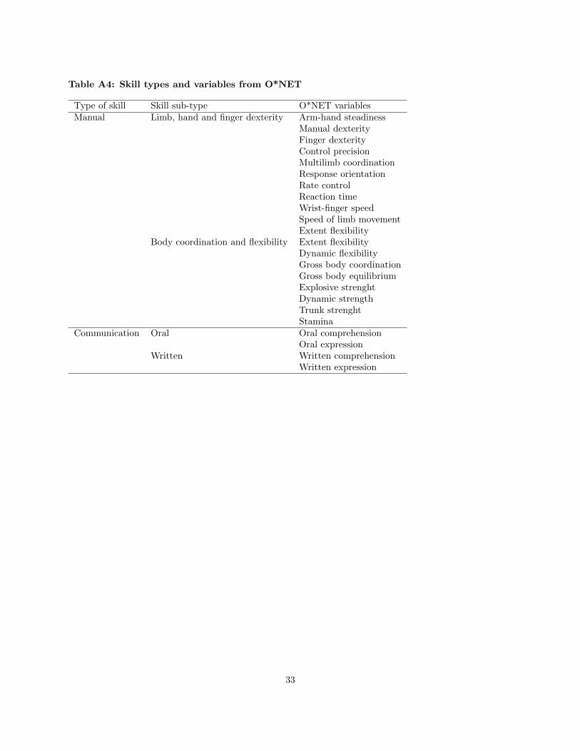
Table A4: Skill types and variables from O*NET

Type of skill Skill sub-type O*NET variablesManual Limb, hand and finger dexterity Arm-hand steadiness

Manual dexterityFinger dexterityControl precisionMultilimb coordinationResponse orientationRate controlReaction timeWrist-finger speedSpeed of limb movementExtent flexibility

Body coordination and flexibility Extent flexibilityDynamic flexibilityGross body coordinationGross body equilibriumExplosive strenghtDynamic strengthTrunk strenghtStamina

Communication Oral Oral comprehensionOral expression

Written Written comprehensionWritten expression

33

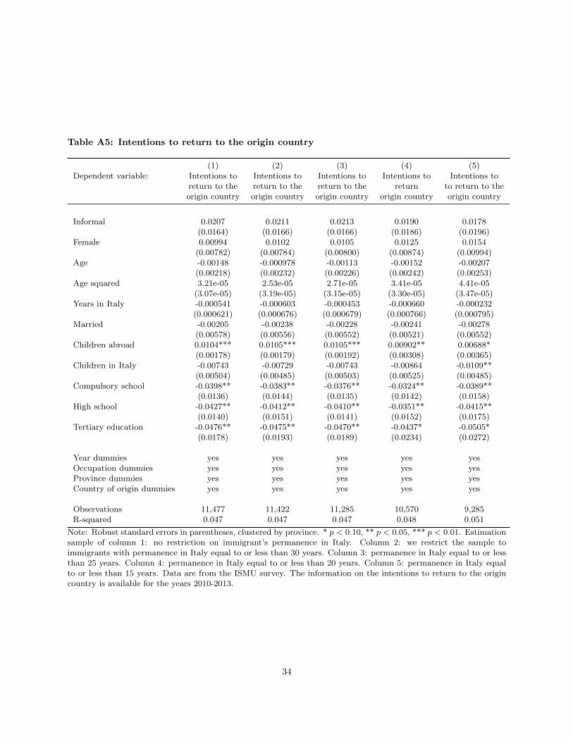
Table A5: Intentions to return to the origin country

(1) (2) (3) (4) (5)Dependent variable: Intentions to Intentions to Intentions to Intentions to Intentions to

return to the return to the return to the return to return to theorigin country origin country origin country origin country origin country

Informal 0.0207 0.0211 0.0213 0.0190 0.0178(0.0164) (0.0166) (0.0166) (0.0186) (0.0196)

Female 0.00994 0.0102 0.0105 0.0125 0.0154(0.00782) (0.00784) (0.00800) (0.00874) (0.00994)

Age -0.00148 -0.000978 -0.00113 -0.00152 -0.00207(0.00218) (0.00232) (0.00226) (0.00242) (0.00253)

Age squared 3.21e-05 2.53e-05 2.71e-05 3.41e-05 4.41e-05(3.07e-05) (3.19e-05) (3.15e-05) (3.30e-05) (3.47e-05)

Years in Italy -0.000541 -0.000603 -0.000453 -0.000660 -0.000232(0.000621) (0.000676) (0.000679) (0.000766) (0.000795)

Married -0.00205 -0.00238 -0.00228 -0.00241 -0.00278(0.00578) (0.00556) (0.00552) (0.00521) (0.00552)

Children abroad 0.0104*** 0.0105*** 0.0105*** 0.00902** 0.00688*(0.00178) (0.00179) (0.00192) (0.00308) (0.00365)

Children in Italy -0.00743 -0.00729 -0.00743 -0.00864 -0.0109**(0.00504) (0.00485) (0.00503) (0.00525) (0.00485)

Compulsory school -0.0398** -0.0383** -0.0376** -0.0324** -0.0389**(0.0136) (0.0144) (0.0135) (0.0142) (0.0158)

High school -0.0427** -0.0412** -0.0410** -0.0351** -0.0415**(0.0140) (0.0151) (0.0141) (0.0152) (0.0175)

Tertiary education -0.0476** -0.0475** -0.0470** -0.0437* -0.0505*(0.0178) (0.0193) (0.0189) (0.0234) (0.0272)

Year dummies yes yes yes yes yesOccupation dummies yes yes yes yes yesProvince dummies yes yes yes yes yesCountry of origin dummies yes yes yes yes yes

Observations 11,477 11,422 11,285 10,570 9,285R-squared 0.047 0.047 0.047 0.048 0.051

Note: Robust standard errors in parentheses, clustered by province. * p < 0.10, ** p < 0.05, *** p < 0.01. Estimationsample of column 1: no restriction on immigrant’s permanence in Italy. Column 2: we restrict the sample toimmigrants with permanence in Italy equal to or less than 30 years. Column 3: permanence in Italy equal to or lessthan 25 years. Column 4: permanence in Italy equal to or less than 20 years. Column 5: permanence in Italy equalto or less than 15 years. Data are from the ISMU survey. The information on the intentions to return to the origincountry is available for the years 2010-2013.

34

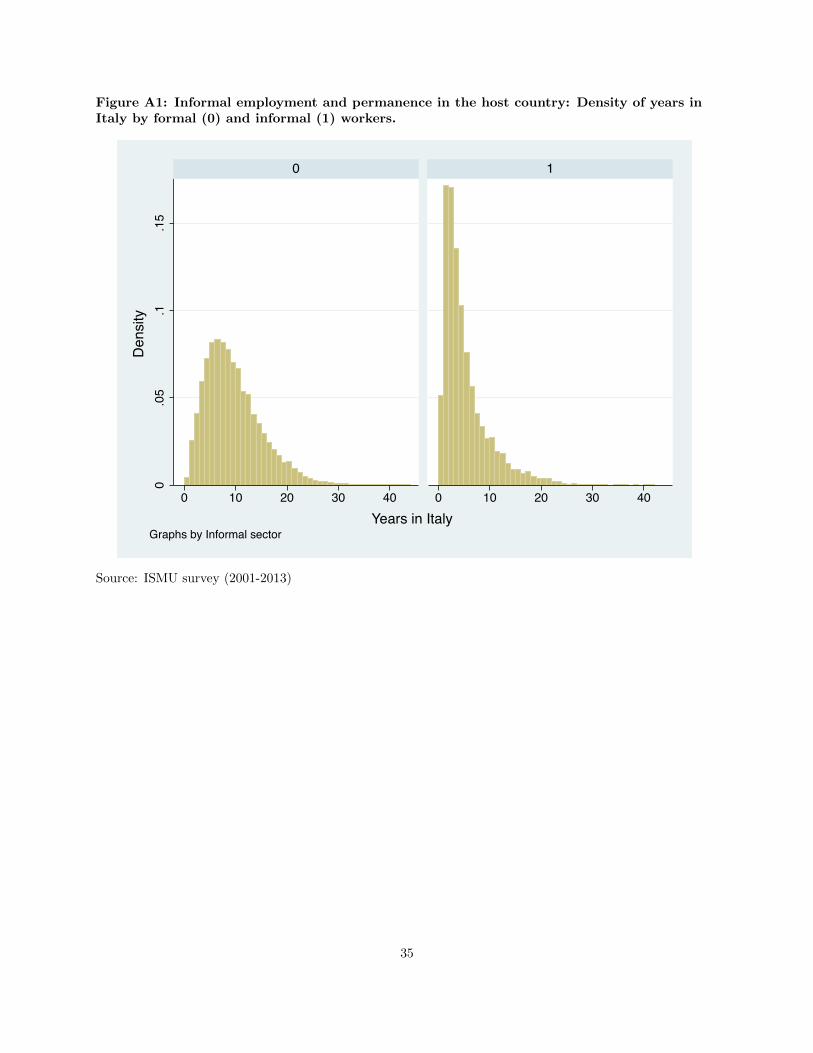
Figure A1: Informal employment and permanence in the host country: Density of years inItaly by formal (0) and informal (1) workers.

0.0

5.1

.15

0 10 20 30 40 0 10 20 30 40

0 1

Den

sity

Years in ItalyGraphs by Informal sector

Source: ISMU survey (2001-2013)

35