Page 1 of 365

TRANSIENT MODELLING OF INDUCTION MOTORS IN A PETROCHEMICAL PLANT USING MATLAB

ANDRIES JOHANNES CLAASSENS

Thesis presented in partial fulfillment of the degree of Master of Science in Engineering at the University of Stellenbosch

Supervisor: Prof. H.J. Vermeulen

March 2008

DECLARATION

I, the undersigned, hereby declare that the work contained in this thesis is my own originalwork and that I have not previously in its entirety or in part submitted it at any university for adesree.

I0 Feruary 2008

Copyight O 2008 Stellenbosch University

All rights resgrved

P^ge 2 of 2

Page 3 of 365

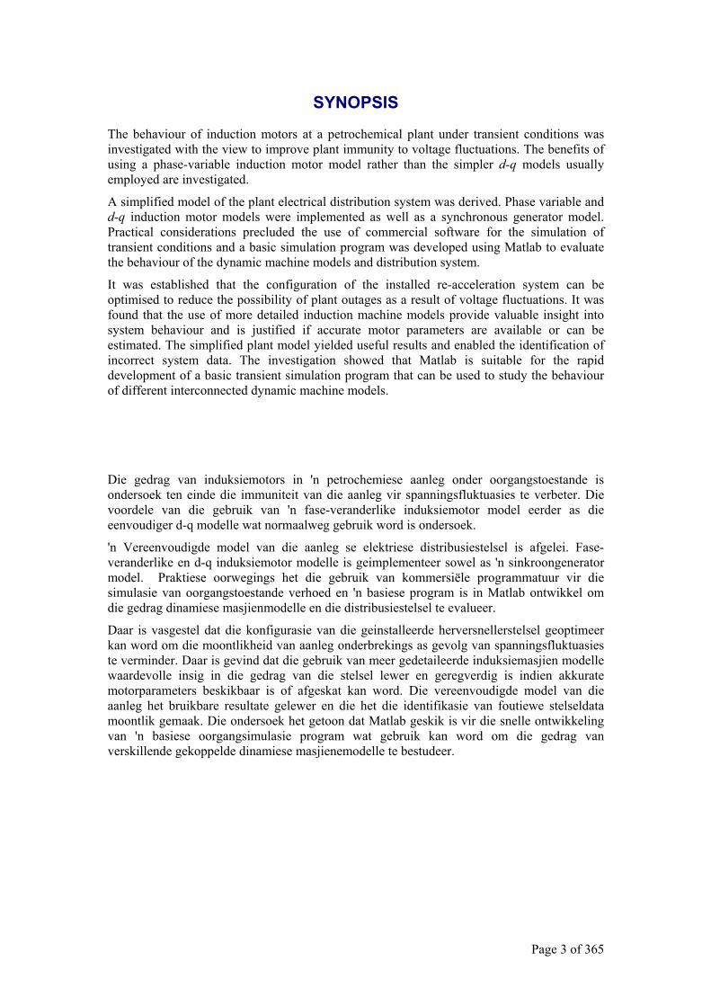
SYNOPSIS

The behaviour of induction motors at a petrochemical plant under transient conditions was investigated with the view to improve plant immunity to voltage fluctuations. The benefits of using a phase-variable induction motor model rather than the simpler d-q models usually employed are investigated.

A simplified model of the plant electrical distribution system was derived. Phase variable and d-q induction motor models were implemented as well as a synchronous generator model. Practical considerations precluded the use of commercial software for the simulation of transient conditions and a basic simulation program was developed using Matlab to evaluate the behaviour of the dynamic machine models and distribution system.

It was established that the configuration of the installed re-acceleration system can be optimised to reduce the possibility of plant outages as a result of voltage fluctuations. It was found that the use of more detailed induction machine models provide valuable insight into system behaviour and is justified if accurate motor parameters are available or can be estimated. The simplified plant model yielded useful results and enabled the identification of incorrect system data. The investigation showed that Matlab is suitable for the rapid development of a basic transient simulation program that can be used to study the behaviour of different interconnected dynamic machine models.

Die gedrag van induksiemotors in 'n petrochemiese aanleg onder oorgangstoestande is ondersoek ten einde die immuniteit van die aanleg vir spanningsfluktuasies te verbeter. Die voordele van die gebruik van 'n fase-veranderlike induksiemotor model eerder as die eenvoudiger d-q modelle wat normaalweg gebruik word is ondersoek.

'n Vereenvoudigde model van die aanleg se elektriese distribusiestelsel is afgelei. Fase-veranderlike en d-q induksiemotor modelle is geimplementeer sowel as 'n sinkroongenerator model. Praktiese oorwegings het die gebruik van kommersiële programmatuur vir die simulasie van oorgangstoestande verhoed en 'n basiese program is in Matlab ontwikkel om die gedrag dinamiese masjienmodelle en die distribusiestelsel te evalueer.

Daar is vasgestel dat die konfigurasie van die geinstalleerde herversnellerstelsel geoptimeer kan word om die moontlikheid van aanleg onderbrekings as gevolg van spanningsfluktuasies te verminder. Daar is gevind dat die gebruik van meer gedetaileerde induksiemasjien modelle waardevolle insig in die gedrag van die stelsel lewer en geregverdig is indien akkurate motorparameters beskikbaar is of afgeskat kan word. Die vereenvoudigde model van die aanleg het bruikbare resultate gelewer en die het die identifikasie van foutiewe stelseldata moontlik gemaak. Die ondersoek het getoon dat Matlab geskik is vir die snelle ontwikkeling van 'n basiese oorgangsimulasie program wat gebruik kan word om die gedrag van verskillende gekoppelde dinamiese masjienemodelle te bestudeer.

Page 4 of 365

CONTENTS

AN INVESTIGATION INTO INDUCTION MOTOR BEHAVIOUR AT A PETROCHEMICAL PLANT UNDER TRANSIENT CONDITIONS USING A PHASE VARIABLE INDUCTION MOTOR MODEL ......................................................................... 1 DECLARATION....................................................................................................................... 2 SYNOPSIS ................................................................................................................................ 3 CONTENTS .............................................................................................................................. 4 LIST OF SYMBOLS............................................................................................................... 12 GLOSSARY............................................................................................................................ 13 LIST OF FIGURES................................................................................................................. 14 LIST OF TABLES .................................................................................................................. 19 1 INTRODUCTION........................................................................................................... 20

1.1 Research Objective.................................................................................................. 20 1.2 Overview Of The Re-Acceleration System ............................................................. 21 1.3 Key Aspects Addressed In This Investigation......................................................... 22

1.3.1 Re-acceleration system optimisation ............................................................... 22 1.3.2 Faults due to veldt fires. .................................................................................. 22 1.3.3 Software development...................................................................................... 22

2 LITERATURE STUDY .................................................................................................. 23 2.1 Review Of Existing Transient Stability Studies ...................................................... 23 2.2 Powerplan Study [28] .............................................................................................. 23

2.2.1 Summary of main conclusions and recommendations..................................... 25 2.3 Merz and McLellan Study [27] ............................................................................... 25

2.3.1 PetroSA plant data .......................................................................................... 25 2.3.2 Summary of main conclusions and recommendations..................................... 26

2.4 Comments On Study Results................................................................................... 26 2.5 Transient Stability Analysis .................................................................................... 26

2.5.1 System representation...................................................................................... 28 2.6 Modelling Of Loads ................................................................................................ 29

2.6.1 Constant impedance load model...................................................................... 30 2.6.2 Constant current load model ........................................................................... 30 2.6.3 Constant power load model............................................................................. 30 2.6.4 Polynomial load model (ZIP model) ............................................................... 30 2.6.5 Exponential load model................................................................................... 31 2.6.6 Static load model for dynamic simulation ....................................................... 31

2.7 System Equations .................................................................................................... 32

Page 5 of 365

2.8 Solution Of System Equations................................................................................. 34 2.8.1 The alternating solution approach .................................................................. 34

2.9 Induction Motor Models.......................................................................................... 35 2.9.1 Equivalent circuit models ................................................................................ 35 2.9.2 The d-q induction motor model ....................................................................... 36 2.9.3 Mechanical equations...................................................................................... 37 2.9.4 The abc – induction motor model .................................................................... 38 2.9.5 Voltage equations ............................................................................................ 39 2.9.6 Stator inductances ........................................................................................... 39 2.9.7 Rotor inductances............................................................................................ 39 2.9.8 Mutual inductances between stator and rotor windings.................................. 40 2.9.9 Torque and power............................................................................................ 41 2.9.10 Inertia constant and mechanical equations..................................................... 42

2.10 Parameter Estimation............................................................................................... 42 2.10.1 Field measurements......................................................................................... 42 2.10.2 Equivalent circuit and torque/slip relation ..................................................... 44 2.10.3 Torque/slip relation ......................................................................................... 45 2.10.4 Approximate parameter estimation. ................................................................ 46 2.10.5 Relationship between equivalent circuit and model parameters ..................... 48

2.11 Synchronous Generator Models .............................................................................. 49 2.11.1 Inductances in the abc-frame [23] .................................................................. 49 2.11.2 Rotor and stator voltage equations in abc frame ............................................ 53 2.11.3 Rotor and stator voltage equations in the dqo frame [23] .............................. 54 2.11.4 Flux linkage equations in terms of reactances ................................................ 57

2.12 Electrical Air-Gap Power And Torque.................................................................... 58 2.12.1 Torque and power expressions in p.u. ............................................................. 58

2.13 Machine Power System Interface ............................................................................ 59 2.13.1 Locating machine q-axis with respect to system reference ............................. 60

2.14 Excitation System Modelling .................................................................................. 61 2.14.1 Automatic voltage regulators .......................................................................... 61 2.14.2 Machine excitation simulation interface ......................................................... 62

2.15 Rotor Dynamics....................................................................................................... 63 2.15.1 The swing equation.......................................................................................... 63 2.15.2 Swing equation in the p.u. system.................................................................... 66 2.15.3 The inertia constant H ..................................................................................... 67

2.16 Speed Governor Models .......................................................................................... 67 2.16.1 Modelling generator without a governor ........................................................ 67

Page 6 of 365

2.16.2 Approximate governor model .......................................................................... 68 2.17 Machine Modelling For Stability Studies................................................................ 72

2.17.1 Rate of change of field flux linkages................................................................ 72 2.17.2 Rate of change of q-axis rotor flux linkages.................................................... 73 2.17.3 Summary of generator models......................................................................... 74 2.17.4 Power equations for two-axis model ............................................................... 75 2.17.5 Modelling of saturation ................................................................................... 75

2.18 Review Of Numerical Methods For Solving Differential Equations ...................... 75 2.18.1 Accuracy and stability ..................................................................................... 76 2.18.2 Existence of unique solution ............................................................................ 77 2.18.3 Explicit (open) Runge-Kutta single-step formulas .......................................... 78 2.18.4 Implicit (closed) Runge-Kutta single-step formulas ........................................ 78 2.18.5 Two-step Runge-Kutta open formulas ............................................................. 79 2.18.6 Multi-step predictor corrector formulas.......................................................... 79 2.18.7 Matlab ODE solvers ........................................................................................ 80 2.18.8 Selection of differential equation solver.......................................................... 81

2.19 Load Flow................................................................................................................ 81 2.19.1 Nodal analysis ................................................................................................. 82 2.19.2 Load flow variables ......................................................................................... 84 2.19.3 Voltage-controlled bus .................................................................................... 84 2.19.4 Nonvoltage-controlled bus .............................................................................. 84 2.19.5 Slack or swing bus. .......................................................................................... 84 2.19.6 Newton-Raphson method of solving load flows............................................... 84 2.19.7 Power system load flow equations................................................................... 85 2.19.8 Improvements to basic Newton-Raphson algorithm........................................ 87

3 OVERVIEW OF SYSTEM COMPONENTS................................................................. 89 3.1 PetroSA Electrical Distribution System Description............................................... 89

3.1.1 Eskom network................................................................................................. 89 3.1.2 PetroSA system overview................................................................................. 90 3.1.3 Critical power system ...................................................................................... 90

3.2 Modelling Of PetroSA Distribution Network ......................................................... 92 3.2.1 Selection of substation for modelling .............................................................. 92 3.2.2 Transformer tap-changers............................................................................... 92 3.2.3 Distributed control system and power disturbances ....................................... 92 3.2.4 Compressors and compressor controls ........................................................... 92 3.2.5 Pumps .............................................................................................................. 93 3.2.6 Motor operated valves ..................................................................................... 93

Page 7 of 365

3.3 Distribution System Model...................................................................................... 93 3.3.1 Substation 01 ................................................................................................... 94 3.3.2 Substation 02 ................................................................................................... 95 3.3.3 Substation 05 ................................................................................................... 95 3.3.4 Substation 06 ................................................................................................... 96 3.3.5 Substation 24 ................................................................................................... 98

3.4 System Data........................................................................................................... 101 3.4.1 Bus data......................................................................................................... 101

3.4.2 Branch data ................................................................................................ 102

4 DETAILED SIMULATION STRATEGY.................................................................... 103 4.1 Software Selection................................................................................................. 103 4.2 Simulation Of Faults.............................................................................................. 104

4.2.1 Switching of motors ....................................................................................... 105 4.3 Model Selection..................................................................................................... 105

4.3.1 System component models ............................................................................. 106 4.3.2 Induction machine models ............................................................................. 110 4.3.3 Synchronous machine model selection .......................................................... 111 4.3.4 Generator model initialisation ...................................................................... 113

4.4 Program Structure.................................................................................................. 115 4.4.1 Summary of subroutines ................................................................................ 119

4.5 Simulation Strategy ............................................................................................... 121 4.5.1 Motor parameter estimation.......................................................................... 122 4.5.2 Alternating solution errors ............................................................................ 122 4.5.3 Voltage dips and switching effects on motor operation................................. 122 4.5.4 Effect of plant generator................................................................................ 122 4.5.5 Examine effects of voltage dips and re-acceleration system ......................... 122

5 PRESENTATION OF RESULTS................................................................................. 123 5.1 Matlab ODE Solver Performance.......................................................................... 123

5.1.1 Stepped vs. Continuous use of ODE solvers.................................................. 123 5.1.2 Comparison of ODE solver performance...................................................... 125 5.1.3 Summary of ODE Solver Test Results ........................................................... 125

5.2 Review Of Motor Parameter Estimation Accuracy ............................................... 126 5.3 Motor Starting Tests .............................................................................................. 130

5.3.1 Comparison Of Test Results With Simulated Results .................................... 131 5.3.2 System bus voltage......................................................................................... 135 5.3.3 Summary of Findings..................................................................................... 139

5.4 Voltage Dips And Switching Effects On Motor Operation................................... 139

Page 8 of 365

5.4.1 Effect of voltage dip duration ........................................................................ 140 5.4.2 abc vs. d-q induction motor model ................................................................ 145

5.5 Generator And Distribution System Behaviour..................................................... 147 5.5.1 Study 1 and 2: abc and d-q models............................................................... 148 5.5.2 Study 1 and 3: effect of generator model when abc motor model is used ..... 150 5.5.3 Study 2 and 4: effect of generator model when d-q motor model is used...... 153 5.5.4 Study 1, 5 and 7: effect of generator model with AVR and governor when abc motor model is used....................................................................................................... 156 5.5.5 Study 2 and 6: effect of generator model with AVR and governor when d-q motor model is used....................................................................................................... 158 5.5.6 Comments on generator model performance. ............................................... 159 5.5.7 Study 8 and 9: comparison of d-q and abc motor model performance following a 20% voltage dip.......................................................................................................... 161 5.5.8 Study 8 and 10: effect of main plant air compressor trip following voltage dip. 167 5.5.9 Study 11: motor re-acceleration following a voltage dip.............................. 169 5.5.10 Study 12: effect of all motors re starting after a voltage dip......................... 172

6 CONCLUSIONS AND RECOMMENDATIONS....................................................... 174 6.1 Re-acceleration System Optimization ................................................................... 174

6.1.1 Induction motor models ................................................................................. 174 6.1.2 Synchronous generator model ....................................................................... 175 6.1.3 PetroSA distribution system model................................................................ 176 6.1.4 Optimization of re-acceleration system......................................................... 176 6.1.5 Recommendations for future work................................................................ 177

6.2 Faults Due To Veldt Fires ..................................................................................... 178 6.3 Software Development .......................................................................................... 178

6.3.1 Matlab ........................................................................................................... 178 6.3.2 Simulink ......................................................................................................... 178 6.3.3 Execution times.............................................................................................. 179

6.4 Topics For Further Investigation ........................................................................... 179 ACKNOWLEDGEMENTS .................................................................................................. 181 REFERENCES...................................................................................................................... 182 7 Appendix A: MOTOR RE-ACCELERATION GROUPS ............................................ 185

7.1 Substation 02 ......................................................................................................... 185 7.2 Substation 03 ......................................................................................................... 185 7.3 Substation 04 ......................................................................................................... 186 7.4 Substation 05 ......................................................................................................... 187 7.5 Substation 06 ......................................................................................................... 189 7.6 Substation 10 ......................................................................................................... 189

Page 9 of 365

7.7 Substation 11 ......................................................................................................... 190 7.8 Substation 13 ......................................................................................................... 190 7.9 Substation 14 ......................................................................................................... 191 7.10 Substation 15 ......................................................................................................... 191 7.11 Substation 17 ......................................................................................................... 192 7.12 Substation 18 ......................................................................................................... 192 7.13 Substation 19 ......................................................................................................... 192 7.14 Substation 20 ......................................................................................................... 193 7.15 Substation 24 ......................................................................................................... 193 7.16 Substation 25 ......................................................................................................... 194 7.17 Substation 26 ......................................................................................................... 194 7.18 Substation 48 ......................................................................................................... 194

8 Appendix B: SOFTWARE LISTINGS ......................................................................... 196 8.1 Flowcharts ............................................................................................................. 198 8.2 Program Listings ................................................................................................... 201

8.2.1 simtrans.m ..................................................................................................... 201 8.2.2 Event simulation – code section .................................................................... 215 8.2.3 read_bus_data.m ........................................................................................... 216 8.2.4 build_Ybus.m ................................................................................................. 218 8.2.5 initialise_NR.m .............................................................................................. 222 8.2.6 set_motor_parameters.m ............................................................................... 223 8.2.7 set_generator_parameters.m......................................................................... 228 8.2.8 set_motor_state_vector.m.............................................................................. 229 8.2.9 locate_gen_axis.m ......................................................................................... 229 8.2.10 init_gen_state.m............................................................................................. 230 8.2.11 pu_bus_voltage.m.......................................................................................... 231 8.2.12 convert_to_gen_ref.m.................................................................................... 231 8.2.13 calc_gen_power.m......................................................................................... 231 8.2.14 calculate_bus_voltage.m ............................................................................... 232 8.2.15 update_loadflow_data.m ............................................................................... 232 8.2.16 calc_abc_tmnl_voltage.m.............................................................................. 233 8.2.17 update_loadflow_data_dq_model.m.............................................................. 233 8.2.18 calc_branch_currents.m................................................................................ 234 8.2.19 loadflow.m ..................................................................................................... 238 8.2.20 calculate_jacobian.m..................................................................................... 243 8.2.21 test_motor_model.m ...................................................................................... 246 8.2.22 induction_motor_01.m................................................................................... 250

Page 10 of 365

8.2.23 induction_motor_03.m................................................................................... 256 8.2.24 sync_gen_model_01.m................................................................................... 258

9 Appendix C: MACHINE DATA AND PARAMETER ESTIMATES ......................... 263 9.1 Induction Motor Data ............................................................................................ 263 9.2 Main Plant Generator Data .................................................................................... 269

9.2.1 Scaling factor between generator and AVR pu systems ................................ 271 10 Appendix D: INDUCTION MOTOR MODELS – ADDITIONAL DATA.............. 272

10.1 Derivation Of Equation (2-27) .............................................................................. 272 10.2 Derivation Of Equation (2-46) .............................................................................. 272 10.3 Derivation Of Equation (2-49) .............................................................................. 273

11 Appendix E: REVIEW OF EXISTING TRANSIENT STABILITY STUDIES....... 275 11.1 Merz & McLellan Study: 23 December 1988 ....................................................... 275 11.2 Powerplan Study: 22 December 1988 28 .............................................................. 275

11.2.1 Summary of main conclusions and study recommendations ........................ 275 11.2.2 Basic system details. ...................................................................................... 275 11.2.3 Study cases..................................................................................................... 277 11.2.4 Summary of Data Used.................................................................................. 277

11.3 Merz and McLellan Study: 3 Feb 1989 [27] ......................................................... 281 11.3.1 Eskom equivalent source representation....................................................... 281 11.3.2 Proteus 400kV fault levels ............................................................................. 282 11.3.3 Fault clearance times .................................................................................... 282 11.3.4 Eskom ‘infinite’ generator representation .................................................... 282 11.3.5 PetroSA plant data ........................................................................................ 282 11.3.6 Synchronous machines .................................................................................. 283 11.3.7 Induction machines........................................................................................ 283

11.4 Study Results ......................................................................................................... 283 12 Appendix F: SYNCHRONOUS MACHINE MODELS – ADDITIONAL INFORMATION ................................................................................................................... 285

12.1 Derivation Of Equation (2-71) .............................................................................. 285 12.2 Derivation Of Rotational Inductance Matrix G..................................................... 285 12.3 Derivation Of Equation (2-81) .............................................................................. 285 12.4 Derivation Of Equation (2-85) .............................................................................. 286 12.5 Derivation Of Equation (2-104) ............................................................................ 287 12.6 Derivation Of Equation (2-130) ........................................................................... 287 12.7 Derivation Of Equation (2-146) ............................................................................ 288 12.8 Derivation Of Equation (2-166) ............................................................................ 289

13 Appendix G: LOAD FLOW RESULTS.................................................................... 290 13.1 Initial Loadflow Solution ...................................................................................... 290

Page 11 of 365

13.2 Study Case 1 – Final State..................................................................................... 292 13.3 Study Case 2 – Final State..................................................................................... 294 13.4 Study Case 3 – Final State..................................................................................... 297 13.5 Study Case 4 – Final State..................................................................................... 299 13.6 Study Case 5 – Final State..................................................................................... 301 13.7 Study Case 6 – Final State..................................................................................... 304 13.8 Study Case 7 – Final State..................................................................................... 306

14 Appendix H: TRANSIENT SIMULATION RESULTS ........................................... 309 14.1 Study 1................................................................................................................... 310 14.2 Study 2................................................................................................................... 311 14.3 Study 3................................................................................................................... 312 14.4 Study 4................................................................................................................... 313 14.5 Study 5................................................................................................................... 315 14.6 Study 6................................................................................................................... 317 14.7 Study 7................................................................................................................... 319 14.8 Study 8................................................................................................................... 321 14.9 Study 9................................................................................................................... 322 14.10 Study 10............................................................................................................. 324 14.11 Study 11............................................................................................................. 325 14.12 Study 12............................................................................................................. 326

15 Appendix I: INDUCTION MOTOR MODEL SIMULATIONS .............................. 328 15.1 Simulation 1 .......................................................................................................... 329 15.2 Simulation 2 .......................................................................................................... 330 15.3 Simulation 3 .......................................................................................................... 332 15.4 Simulation 4 .......................................................................................................... 333 15.5 Simulation 5 .......................................................................................................... 335 15.6 Simulation 6 .......................................................................................................... 336

16 Appendix J: MATLAB ODE SOLVER PERFORMANCE...................................... 338 16.1 Stepped vs. Continuous use of ODE solvers ......................................................... 338 16.2 Comparison of ODE solver performance .............................................................. 343 16.3 ODE Solver performance when using stepped solution ........................................ 348 16.4 Summary of ODE Solver test results..................................................................... 350 16.5 Matlab Software Listings for additional ODE solver tests. ................................... 351

16.5.1 Induction motor model (abc) ......................................................................... 351 16.5.2 Induction motor model (d-q).......................................................................... 356 16.5.3 Motor model parameters ............................................................................... 357 16.5.4 Motor model Test Subroutine ........................................................................ 361

Page 12 of 365

LIST OF SYMBOLS

BA ⇒ A is defined as B

f Frequency in Hertz (Hz)

H Inertia constant, defined as the stored energy per VA rating (J/VA) [16]

J Moment of inertia of a rotating mass( kg m2)

P Power (W)

p.u. Per unit

Q Reactive power (VA)

V Voltage [V]

yx, Vector quantities

Page 13 of 365

GLOSSARY

AVR: Automatic Voltage Regulator. Distribution System: Refer to “Power System”. Disturbance: A ‘disturbance’ in a power system is a sudden change or sequence of changes in one or more of the parameters of the system, or in one or more of the physical quantities. Two types of disturbances are defined, small and large [23]. CT: Current Transformer. HV: High Voltage (132kV). Large Disturbance: A “large disturbance” is a disturbance for which the set of equations which describe the power system cannot be linearised for the purposes of analysis [23]. LV: Low voltage (550V and below). MV: Medium Voltage (11kV and 6.6kV).

MCC: Motor Control Centre

ODE: Ordinary Differential Equation. Operating Condition: An “operating condition” or “operating point” of a power system is a set of physical quantities or physical variables that can be measured or calculated and which can meaningfully describe the state of the system completely [23]. Pre-Fault System: A power system immediately preceding the initiation of a large disturbance is termed a “pre-fault (pre-disturbance) system” . The system is considered to be in the steady-state in this phase [23]. Power dip: A power dip is defined as a momentary reduction in line voltage, typically of the order of 100-200ms duration with a voltage reduction of > 20% of the nominal line voltage. Power System: A “power system” is a collection of generating units, transformers, transmission lines, loads, capacitors1, reactors, associated auxiliaries and switchgear to connect the various components [23]. Note the terms “Distribution System” and “Power System” are used interchangeably in this report. Small Disturbance: A “small disturbance’ is a disturbance for which the set of equations which describe the power system can be linearised for the purposes of analysis [23]. Steady-state operating Condition: “Steady State operating condition” of a power system is an operating condition in which all the physical quantities that characterize the system can be considered to be constant for the purposes of analysis [23]. Transient Period: The “Transient period” is the time duration between the initiation of a large disturbance (or sequence of disturbances) and restoration of operation to an acceptable steady state after the fast electrical transients have died out [23]. Voltage Instability: Apart from insufficient synchronizing and damping torques causing instability, insufficient reactive power to support the system can result in voltage collapse which can also lead to instability. The term “voltage instability” is used to describe this phenomenon [23].

1 Capacitors and reactors may be shunt or series connected

Page 14 of 365

LIST OF FIGURES

FIGURE 2-1 APPROXIMATE PETROSA SYSTEM REPRESENTATION. ......................................... 24 FIGURE 2-2 BLOCK DIAGRAM SHOWING INTERACTION OF MODELS FOR TRANSIENT STABILITY

STUDIES [23]. ................................................................................................................... 33 FIGURE 2-3 SINGLE CAGE INDUCTION MOTOR EQUIVALENT CIRCUIT [21]. ............................ 35 FIGURE 2-4 DOUBLE CAGE INDUCTION MOTOR STEADY-STATE EQUIVALENT CIRCUIT [21]... 35 FIGURE 2-5 STEADY-STATE EQUIVALENT CIRCUIT OF AN INDUCTION MOTOR [23]................ 36 FIGURE 2-6 SIMPLIFIED REPRESENTATION OF INDUCTION MOTOR FOR TRANSIENT ANALYSIS

[23,15] ............................................................................................................................. 36 FIGURE 2-7 INDUCTION MOTOR EQUIVALENT CIRCUIT [16].................................................... 44 FIGURE 2-8 SIMPLIFIED INDUCTION MOTOR EQUIVALENT CIRCUIT [16]................................. 44 FIGURE 2-9 TORQUE/SLIP RELATION [16]............................................................................... 46 FIGURE 2-10 EQUIVALENT CIRCUIT FOR NO-LOAD. ................................................................ 48 FIGURE 2-11 SYNCHRONOUS MACHINE REPRESENTATION FOR MODEL DEVELOPMENT [23].. 52 FIGURE 2-12 MACHINE-SYSTEM INTERFACE RELATIONS [23]. ............................................... 60 FIGURE 2-13 LOCATING MACHINE AXIS WITH RESPECT TO SYSTEM AXIS [23]. ...................... 60 FIGURE 2-14 IEEE TYPE 1 AVR MODEL [23, 22].................................................................... 61 FIGURE 2-15 IEEE STEAM TURBINE MODEL [21, 33, 22]. ....................................................... 68 FIGURE 2-16 BLOCK DIAGRAM REPRESENTATION OF STEAM TURBINE GOVERNOR SYSTEM [23,

33].................................................................................................................................... 69 FIGURE 2-17 SIMULINK GOVERNOR-TURBINE MODEL. ........................................................... 70 FIGURE 2-18 TURBINE-GOVERNOR RESPONSE TO 0.1% SPEED ERROR.................................... 71 FIGURE 2-19 TURBINE-GOVERNOR RESPONSE TO 1% SPEED ERROR....................................... 71 FIGURE 2-20 APPROXIMATE GOVERNOR MODEL..................................................................... 71 FIGURE 2-21 APPROXIMATE GOVERNOR MODEL RESPONSE TO 1% SPEED ERROR. ................ 72 FIGURE 2-22 SIMPLE NETWORK ILLUSTRATING NODAL QUANTITIES [21]. ............................. 82 FIGURE 2-23 BASIC LOAD FLOW ALGORITHM [21].................................................................. 88 FIGURE 3-1 ESKOM NETWORK SUPPLYING PETROSA. ............................................................ 89 FIGURE 3-2 TYPICAL SUBSTATION CRITICAL SUPPLY ARRANGEMENT.................................... 91 FIGURE 3-3 CRITICAL POWER SYSTEM .................................................................................... 91 FIGURE 3-4. SUBSTATION 01 132KV (MAIN SUBSTATION). .................................................... 94 FIGURE 3-5 SUBSTATION 02 11KV DISTRIBUTION. ................................................................. 95 FIGURE 3-6 SUBSTATION 05 MV DISTRIBUTION..................................................................... 96 FIGURE 3-7 SUBSTATION 06 MV DISTRIBUTION..................................................................... 97 FIGURE 3-8 SUBSTATION 24 – 6.6KV...................................................................................... 99 FIGURE 3-9 SUBSTATION 24 - 550V. ..................................................................................... 100 FIGURE 4-1 VOLTAGE DIP MAGNITUDE VS. DURATION. ........................................................ 104 FIGURE 4-2 RECORDING OF VOLTAGE DIP ON ESKOM SUPPLY.............................................. 105 FIGURE 4-3 FEEDER DATA ENTRY. ........................................................................................ 106 FIGURE 4-4 LOAD DATA ENTRY............................................................................................. 107 FIGURE 4-5 TWO WINDING TRANSFORMER DATA ENTRY...................................................... 108 FIGURE 4-6 THREE WINDING TRANSFORMER DATA ENTRY................................................... 109 FIGURE 4-7 SIMULATION SOFTWARE OVERVIEW. ................................................................. 115 FIGURE 4-8 SIMULATION PROGRAM DETAIL FLOWCHART A................................................. 116 FIGURE 4-9 SIMULATION PROGRAM DETAIL FLOWCHART B................................................. 117 FIGURE 4-10 LOADFLOW DETAILED FLOWCHART................................................................. 118 FIGURE 5-1 ODE SOLVER TEST: ABC MODEL, STEPPED VS. CONTINUOUS SOLUTION, 1MS STEP

INTERVAL....................................................................................................................... 124 FIGURE 5-2 ODE SOLVER TEST: ABC MODEL, CONTINUOUS MODE WITH RELTOL CHANGED.

....................................................................................................................................... 124 FIGURE 5-3 ODE SOLVER TEST: ABC MODEL, STEPPED VS. CONTINUOUS SOLUTION .......... 125 FIGURE 5-4 300KW MOTOR STATOR CURRENT – ABC MODEL............................................... 127 FIGURE 5-5 300KW MOTOR STATOR CURRENT – D-Q MODEL .............................................. 127

Page 15 of 365

FIGURE 5-6 300KW MOTOR DOL START: ELECTROMAGNETIC TORQUE (ABC MODEL) ........ 128 FIGURE 5-7 DETAIL OF FIGURE 5-6 ....................................................................................... 128 FIGURE 5-8 300KW MOTOR DOL START: ELECTROMAGNETIC TORQUE (D-Q MODEL) ........ 128 FIGURE 5-9 INDUCTION MOTOR STATOR CURRENT [22]........................................................ 129 FIGURE 5-10 ELECTRO-MAGNETIC TORQUE [22] .................................................................. 130 FIGURE 5-11 300 KW PUMP MOTOR (24PC101A) STATOR CURRENT – MEASURED. ............ 131 FIGURE 5-12 300KW PUMP MOTOR (24PC101A) STATOR CURRENT – ABC MODEL.............. 131 FIGURE 5-13 300KW PUMP MOTOR (24PC101A) STATOR CURRENT – D-Q MODEL.............. 132 FIGURE 5-14 800 KW PUMP MOTOR (24PC102A) STATOR CURRENT – MEASURED. ............ 132 FIGURE 5-15 800 KW PUMP MOTOR (24PC102A) STATOR CURRENT – ABC MODEL............. 133 FIGURE 5-16 800 KW PUMP MOTOR (24PC102A) STATOR CURRENT – D-Q MODEL. ............ 133 FIGURE 5-17 550 KW PUMP MOTOR (24PC104A) STATOR CURRENT – MEASURED. ............ 134 FIGURE 5-18 550 KW PUMP MOTOR (24PC104A) STATOR CURRENT – ABC MODEL............. 134 FIGURE 5-19 550 KW PUMP MOTOR (24PC104A) STATOR CURRENT – D-Q MODEL. ............ 134 FIGURE 5-20 300 KW PUMP MOTOR (24PC101A) BUS VOLTAGE – MEASURED.................... 135 FIGURE 5-21 300 KW PUMP MOTOR (24PC101A) BUS VOLTAGE – DETAIL. ........................ 136 FIGURE 5-22 800 KW PUMP MOTOR (24PC102A) BUS VOLTAGE – MEASURED. .................. 136 FIGURE 5-23 800KW PUMP MOTOR (24PC102A) STATOR CURRENT – SIMULATED ............. 137 FIGURE 5-24 800KW PUMP MOTOR (24PC102A) STATOR CURRENT – MEASURED .............. 137 FIGURE 5-25 800KW PUMP MOTOR (24PC102A) BUS VOLTAGE - SIMULATED.................... 137 FIGURE 5-26 550KW MOTOR ROTOR TORQUE (SIMULATION 2). ........................................... 140 FIGURE 5-27 550KW MOTOR ROTOR TORQUE(SIMULATION 3). ............................................ 141 FIGURE 5-28 550KW MOTOR ROTOR TORQUE (SIMULATION 4). ........................................... 141 FIGURE 5-29 550KW MOTOR ROTOR SPEED (SIMULATION 4)................................................ 141 FIGURE 5-30 550KW MOTOR RMS STATOR CURRENT (SIMULATION 2). ................................ 142 FIGURE 5-31 550KW MOTOR RMS STATOR CURRENT (SIMULATION 3). ................................ 142 FIGURE 5-32 550KW MOTOR RMS STATOR CURRENT (SIMULATION 4). ................................ 143 FIGURE 5-33 550KW MOTOR RMS STATOR CURRENT (SIMULATION 1). ................................ 143 FIGURE 5-34 550KW MOTOR ROTOR TORQUE (SIMULATION 1). ........................................... 144 FIGURE 5-35 550KW MOTOR ROTOR TORQUE (SIMULATION 2). ........................................... 144 FIGURE 5-36 550KW MOTOR RMS STATOR CURRENT (SIMULATION 6). ............................... 145 FIGURE 5-37 550KW MOTOR RMS STATOR CURRENT (SIMULATION 1). ................................ 145 FIGURE 5-38 550KW MOTOR ROTOR TORQUE (SIMULATION 2). ........................................... 146 FIGURE 5-39 550KW MOTOR ROTOR TORQUE (SIMULATION 7). ........................................... 146 FIGURE 5-40 DISTRIBUTION SYSTEM BUS VOLTAGES ( STUDY 1 ). ...................................... 148 FIGURE 5-41 DISTRIBUTION SYSTEM BUS VOLTAGES ( STUDY 2). ........................................ 149 FIGURE 5-42 MOTOR AND SUBSTATION FEEDER CURRENTS ( STUDY1). ............................... 149 FIGURE 5-43 MOTOR AND SUBSTATION FEEDER CURRENTS ( STUDY 2). .............................. 150 FIGURE 5-44 DISTRIBUTION SYSTEM BUS VOLTAGES ( STUDY 1 ). ....................................... 150 FIGURE 5-45 DISTRIBUTION SYSTEM BUS VOLTAGES ( STUDY 3 ). ....................................... 151 FIGURE 5-46 MOTOR AND SUBSTATION FEEDER CURRENTS ( STUDY 1 ). ............................. 151 FIGURE 5-47 MOTOR AND SUBSTATION FEEDER CURRENTS ( STUDY 3 ). ............................. 151 FIGURE 5-48 GENERATOR ROTOR ANGLE ( STUDY 3 ). ......................................................... 152 FIGURE 5-49 DISTRIBUTION SYSTEM BUS VOLTAGES ( STUDY 2). ........................................ 153 FIGURE 5-50 DISTRIBUTION SYSTEM BUS VOLTAGES ( STUDY 4). ........................................ 153 FIGURE 5-51 MOTOR AND SUBSTATION FEEDER CURRENTS ( STUDY 2 ). ............................. 154 FIGURE 5-52 MOTOR AND SUBSTATION FEEDER CURRENTS ( STUDY 4 ). ............................. 154 FIGURE 5-53 GENERATOR ROTOR ANGLE ( STUDY 4 ). ......................................................... 155 FIGURE 5-54 DISTRIBUTION SYSTEM BUS VOLTAGES (STUDY 1). ........................................ 156 FIGURE 5-55 DISTRIBUTION SYSTEM BUS VOLTAGES ( STUDY 5 ). ....................................... 157 FIGURE 5-56 DISTRIBUTION SYSTEM BUS VOLTAGES ( STUDY 7 ). ....................................... 157 FIGURE 5-57 DISTRIBUTION SYSTEM BUS VOLTAGES ( STUDY 2). ........................................ 158 FIGURE 5-58 DISTRIBUTION SYSTEM BUS VOLTAGES ( STUDY 6 ). ....................................... 158 FIGURE 5-59 GENERATOR FIELD VOLTAGE – EXTENDED TIME ( STUDY 6 ). ......................... 159 FIGURE 5-60 GENERATOR FIELD VOLTAGE - DETAIL ( STUDY 6 ). ........................................ 159

Page 16 of 365

FIGURE 5-61 GENERATOR POWER AND REACTIVE POWER (STUDY 6) ................................... 160 FIGURE 5-62 GENERATOR ROTOR ANGLE ( STUDY 6 ). ......................................................... 160 FIGURE 5-63 MOTOR TERMINAL AND BUS VOLTAGES ( STUDY 8 ). ...................................... 161 FIGURE 5-64 MOTOR TERMINAL AND BUS VOLTAGES ( STUDY 9 ). ...................................... 162 FIGURE 5-65 GENERATOR ROTOR ANGLE ( STUDY 8 ). ......................................................... 162 FIGURE 5-66 GENERATOR ROTOR ANGLE ( STUDY 9 ). ......................................................... 163 FIGURE 5-67 DISTRIBUTION SYSTEM BUS VOLTAGES ( STUDY 8 ). ....................................... 163 FIGURE 5-68 DISTRIBUTION SYSTEM BUS VOLTAGES ( STUDY 9 ). ....................................... 164 FIGURE 5-69 GENERATOR POWER AND REACTIVE POWER OUTPUT ( STUDY8 ). ................... 164 FIGURE 5-70 GENERATOR POWER AND REACTIVE POWER OUTPUT ( STUDY 9 ). .................. 164 FIGURE 5-71 MOTOR AND SUBSTATION FEEDER CURRENTS ( STUDY 8 ). ............................. 165 FIGURE 5-72 MOTOR AND SUBSTATION FEEDER CURRENTS ( STUDY 9 ). ............................. 165 FIGURE 5-73 DISTRIBUTION SYSTEM BUS VOLTAGES ( STUDY 8 ). ....................................... 167 FIGURE 5-74 DISTRIBUTION SYSTEM BUS VOLTAGES ( STUDY 10 ). ..................................... 167 FIGURE 5-75 MOTOR AND SUBSTATION FEEDER CURRENTS ( STUDY 8 ). ............................. 168 FIGURE 5-76 MOTOR AND SUBSTATION FEEDER CURRENTS ( STUDY 10 ). ........................... 168 FIGURE 5-77 MOTOR AND SUBSTATION FEEDER CURRENTS ( STUDY 1 ).............................. 169 FIGURE 5-78 MOTOR AND SUBSTATION FEEDER CURRENTS ( STUDY 11 )............................ 170 FIGURE 5-79 MOTOR SHAFT SPEEDS ( STUDY 11 ). ............................................................... 170 FIGURE 5-80 DISTRIBUTION SYSTEM BUS VOLTAGES ( STUDY 11 ). ..................................... 171 FIGURE 5-81 MOTOR AND SUBSTATION FEEDER CURRENTS ( STUDY 12 ). ........................... 172 FIGURE 5-82 MOTOR AND SUBSTATION FEEDER CURRENTS ( STUDY 11). ............................ 172 FIGURE 5-83 DISTRIBUTION SYSTEM BUS VOLTAGES ( STUDY 12 ). ..................................... 173 FIGURE 5-84 DISTRIBUTION SYSTEM BUS VOLTAGES ( STUDY 11). ...................................... 173 FIGURE 8-1 SIMULATION PROGRAM DETAIL FLOWCHART A................................................. 198 FIGURE 8-2 SIMULATION PROGRAM DETAIL FLOWCHART B................................................. 199 FIGURE 8-3 LOADFLOW DETAILED FLOWCHART................................................................... 200 FIGURE 10-1 DERIVATION OF THEVENIN EQUIVALENT CIRCUIT........................................... 272 FIGURE 10-2 THEVENIN EQUIVALENT CIRCUIT [16].............................................................. 273 FIGURE 11-1: ESKOM REPRESENTATION ............................................................................... 276 FIGURE 11-2 EQUIVALENT CIRCUIT FOR INDUCTION MOTORS .............................................. 276 FIGURE 11-3 PETROSA SYSTEM REPRESENTATION............................................................... 280 FIGURE 12-1 LOCATING MACHINE AXIS WITH RESPECT TO SYSTEM AXIS [23]. .................... 287 FIGURE 14-1 MOTOR TERMINAL AND BUS VOLTAGES (1). .................................................... 310 FIGURE 14-2 DISTRIBUTION SYSTEM BUS VOLTAGES (1). .................................................... 310 FIGURE 14-3 MOTOR AND SUBSTATION FEEDER CURRENTS (1)............................................ 310 FIGURE 14-4 MAIN GENERATOR AND ESKOM FEEDER CURRENTS (1)................................... 310 FIGURE 14-5 MOTOR TERMINAL AND BUS VOLTAGES (2). .................................................... 311 FIGURE 14-6 DISTRIBUTION SYSTEM BUS VOLTAGES (2). ..................................................... 311 FIGURE 14-7 MOTOR AND SUBSTATION FEEDER CURRENTS (2)............................................ 311 FIGURE 14-8 MAIN GENERATOR AND ESKOM FEEDER CURRENTS (2)................................... 311 FIGURE 14-9 MOTOR TERMINAL AND BUS VOLTAGES (3). .................................................... 312 FIGURE 14-10 DISTRIBUTION SYSTEM BUS VOLTAGES (3). ................................................... 312 FIGURE 14-11 MOTOR AND SUBSTATION FEEDER CURRENTS (3).......................................... 312 FIGURE 14-12 MAIN GENERATOR AND ESKOM FEEDER CURRENTS (3)................................. 312 FIGURE 14-13 GENERATOR ROTOR ANGLE (3). ..................................................................... 313 FIGURE 14-14 MOTOR TERMINAL AND BUS VOLTAGES (4). .................................................. 313 FIGURE 14-15 DISTRIBUTION SYSTEM BUS VOLTAGES (4). ................................................... 313 FIGURE 14-16 MOTOR AND SUBSTATION FEEDER CURRENTS (4).......................................... 314 FIGURE 14-17 MAIN GENERATOR AND ESKOM FEEDER CURRENTS (4)................................. 314 FIGURE 14-18 GENERATOR ROTOR ANGLE (4). ..................................................................... 314 FIGURE 14-19 MOTOR TERMINAL AND BUS VOLTAGES (5). .................................................. 315 FIGURE 14-20 DISTRIBUTION SYSTEM BUS VOLTAGES (5). ................................................... 315 FIGURE 14-21 MOTOR AND SUBSTATION FEEDER CURRENTS (5).......................................... 315 FIGURE 14-22 MAIN GENERATOR AND ESKOM FEEDER CURRENTS (5)................................. 315

Page 17 of 365

FIGURE 14-23 GENERATOR ROTOR ANGLE (5). ..................................................................... 316 FIGURE 14-24 GENERATOR POWER AND REACTIVE POWER OUTPUT (5). .............................. 316 FIGURE 14-25 MOTOR TERMINAL AND BUS VOLTAGES (6). .................................................. 317 FIGURE 14-26 DISTRIBUTION SYSTEM BUS VOLTAGES (6). ................................................... 317 FIGURE 14-27 MOTOR AND SUBSTATION FEEDER CURRENTS (6).......................................... 317 FIGURE 14-28 MAIN GENERATOR AND ESKOM FEEDER CURRENTS (6)................................. 317 FIGURE 14-29 GENERATOR ROTOR ANGLE (6). ..................................................................... 318 FIGURE 14-30 GENERATOR POWER AND REACTIVE POWER OUTPUT (6). .............................. 318 FIGURE 14-31 GENERATOR ROTOR ANGLE –EXTENDED TIME (6). ........................................ 318 FIGURE 14-32 GENERATOR FIELD VOLTAGE – EXTENDED TIME (6)...................................... 318 FIGURE 14-33 GENERATOR POWER AND REACTIVE POWER OUTPUT – EXTENDED TIME (6). 319 FIGURE 14-34 MOTOR TERMINAL AND BUS VOLTAGES (7). .................................................. 319 FIGURE 14-35 DISTRIBUTION SYSTEM BUS VOLTAGES (7). ................................................... 319 FIGURE 14-36 MOTOR AND SUBSTATION FEEDER CURRENTS (7).......................................... 320 FIGURE 14-37 MAIN GENERATOR AND ESKOM FEEDER CURRENTS (7)................................. 320 FIGURE 14-38 GENERATOR ROTOR ANGLE (7). ..................................................................... 320 FIGURE 14-39 GENERATOR POWER AND REACTIVE POWER OUTPUT (7). .............................. 320 FIGURE 14-40 MOTOR TERMINAL AND BUS VOLTAGES (8). .................................................. 321 FIGURE 14-41 DISTRIBUTION SYSTEM BUS VOLTAGES (8). ................................................... 321 FIGURE 14-42 MOTOR AND SUBSTATION FEEDER CURRENTS (8).......................................... 321 FIGURE 14-43 MAIN GENERATOR AND ESKOM FEEDER CURRENTS (8)................................. 321 FIGURE 14-44 GENERATOR ROTOR ANGLE (8). ..................................................................... 322 FIGURE 14-45 GENERATOR POWER AND REACTIVE POWER OUTPUT (8). .............................. 322 FIGURE 14-46 MOTOR TERMINAL AND BUS VOLTAGES (9). .................................................. 322 FIGURE 14-47 DISTRIBUTION SYSTEM BUS VOLTAGES (9). ................................................... 322 FIGURE 14-48 MOTOR AND SUBSTATION FEEDER CURRENTS (9).......................................... 323 FIGURE 14-49 MAIN GENERATOR AND ESKOM FEEDER CURRENTS (9)................................. 323 FIGURE 14-50 GENERATOR ROTOR ANGLE (9). ..................................................................... 323 FIGURE 14-51 GENERATOR POWER AND REACTIVE POWER OUTPUT (9). .............................. 323 FIGURE 14-52 MOTOR TERMINAL AND BUS VOLTAGES (10). ................................................ 324 FIGURE 14-53 DISTRIBUTION SYSTEM BUS VOLTAGES (10). ................................................. 324 FIGURE 14-54 MOTOR AND SUBSTATION FEEDER CURRENTS (10)........................................ 324 FIGURE 14-55 MAIN GENERATOR AND ESKOM FEEDER CURRENTS (10)............................... 324 FIGURE 14-56 GENERATOR ROTOR ANGLE (10). ................................................................... 325 FIGURE 14-57 GENERATOR POWER AND REACTIVE POWER OUTPUT (10). ............................ 325 FIGURE 14-58 MOTOR TERMINAL AND BUS VOLTAGES (11). ................................................ 325 FIGURE 14-59 DISTRIBUTION SYSTEM BUS VOLTAGES (11). ................................................. 325 FIGURE 14-60 MOTOR AND SUBSTATION FEEDER CURRENTS (11)........................................ 326 FIGURE 14-61 MOTOR SHAFT SPEEDS (11). ........................................................................... 326 FIGURE 14-62 MOTOR AND TERMINAL BUS VOLTAGES (12). ................................................ 326 FIGURE 14-63 DISTRIBUTION SYSTEM BUS VOLTAGES (12). ................................................. 326 FIGURE 14-64 MOTOR AND SUBSTATION FEEDER CURRENTS (12)........................................ 327 FIGURE 15-1 STATOR CURRENTS........................................................................................... 329 FIGURE 15-2 RMS STATOR CURRENT. .................................................................................. 329 FIGURE 15-3 ROTOR TORQUE. ............................................................................................... 329 FIGURE 15-4 ROTOR SPEED................................................................................................... 329 FIGURE 15-5 ACTIVE AND REACTIVE POWER. ....................................................................... 330 FIGURE 15-6 STATOR CURRENTS........................................................................................... 330 FIGURE 15-7 RMS STATOR CURRENT. .................................................................................. 330 FIGURE 15-8 ROTOR TORQUE. ............................................................................................... 331 FIGURE 15-9 ROTOR SPEED. .................................................................................................. 331 FIGURE 15-10 ACTIVE AND REACTIVE POWER. ..................................................................... 331 FIGURE 15-11 STATOR CURRENTS......................................................................................... 332 FIGURE 15-12 RMS STATOR CURRENT. ................................................................................ 332 FIGURE 15-13 ROTOR TORQUE. ............................................................................................. 332

Page 18 of 365

FIGURE 15-14 ROTOR SPEED. ................................................................................................ 332 FIGURE 15-15 POWER AND REACTIVE POWER....................................................................... 333 FIGURE 15-16 STATOR CURRENTS......................................................................................... 333 FIGURE 15-17 RMS STATOR CURRENT. ................................................................................ 333 FIGURE 15-18 ROTOR TORQUE. ............................................................................................. 334 FIGURE 15-19 ROTOR SPEED. ................................................................................................ 334 FIGURE 15-20 ACTIVE AND REACTIVE POWER. ..................................................................... 334 FIGURE 15-21 STATOR CURRENTS......................................................................................... 335 FIGURE 15-22 RMS STATOR CURRENT. ................................................................................ 335 FIGURE 15-23 ROTOR TORQUE. ............................................................................................. 335 FIGURE 15-24 ROTOR SPEED................................................................................................. 335 FIGURE 15-25 ACTIVE AND REACTIVE POWER. ..................................................................... 336 FIGURE 15-26 RMS STATOR CURRENT. ................................................................................ 336 FIGURE 15-27 ROTOR TORQUE. ............................................................................................. 336 FIGURE 15-28 ROTOR SPEED................................................................................................. 337 FIGURE 16-1 ODE SOLVER TEST: D-Q MODEL USING CONTINUOUS INTEGRATION WITH

DIFFERENT STEP LENGTHS. ............................................................................................ 338 FIGURE 16-2 ODE SOLVER TEST: DETAIL VIEW OF FIGURE 16-1. ........................................ 339 FIGURE 16-3 ODE SOLVER TEST: DETAIL VIEW OF FIGURE 16-1. ........................................ 339 FIGURE 16-4 ODE SOLVER TEST: ABC MODEL USING CONTINUOUS INTEGRATION WITH

DIFFERENT STEP LENGTHS. ............................................................................................ 340 FIGURE 16-5 ODE SOLVER TEST: DETAIL VIEW OF FIGURE 16-4. ........................................ 340 FIGURE 16-6 ODE SOLVER TEST: DETAIL VIEW OF FIGURE 16-4. ........................................ 340 FIGURE 16-7 ODE SOLVER TEST: ABC MODEL, STEPPED VS. CONTINUOUS SOLUTION, 1MS

STEP INTERVAL. ............................................................................................................. 341 FIGURE 16-8 ODE SOLVER TEST: ABC MODEL, STEPPED SOLUTION WITH RELTOL PARAMETER

VARIED........................................................................................................................... 341 FIGURE 16-9 ODE SOLVER TEST: DETAIL VIEW OF FIGURE 16-8. ........................................ 342 FIGURE 16-10 ODE SOLVER TEST: ABC MODEL, CONTINUOUS MODE WITH RELTOL CHANGED.

....................................................................................................................................... 342 FIGURE 16-11 ODE SOLVER TEST: ABC MODEL, STEPPED VS. CONTINUOUS SOLUTION....... 343 FIGURE 16-12 ODE SOLVER TEST: DETAIL VIEW OF FIGURE 16-11. .................................... 343 FIGURE 16-13 ODE SOLVER TEST: COMPARE ODE45 AND ODE23. ...................................... 344 FIGURE 16-14 ODE SOLVER TEST: COMPARE ODE45 AND ODE113. .................................... 345 FIGURE 16-15 DETAIL VIEW OF FIGURE 16-14. ..................................................................... 345 FIGURE 16-16 ODE SOLVER TEST: COMPARE ODE45 AND ODE15S. ..................................... 346 FIGURE 16-17 DETAIL VIEW OF FIGURE 16-16. ..................................................................... 346 FIGURE 16-18 ODE SOLVER TEST: COMPARE ODE45 AND ODE23S...................................... 346 FIGURE 16-19 ODE SOLVER TEST: COMPARE ODE45 AND ODE23T. .................................... 347 FIGURE 16-20 ODE SOLVER TEST: COMPARE ODE45 TO ODE23TB...................................... 347 FIGURE 16-21 ODE SOLVER TEST: ODE113 STEPPED VS. CONTINUOUS SOLUTION. ............. 348 FIGURE 16-22 DETAIL VIEW OF FIGURE 16-21. ..................................................................... 349 FIGURE 16-23 ODE SOLVER TEST: ODE113 COMPARISON OF SOLUTIONS WITH DIFFERENT

STEP LENGTHS................................................................................................................ 349 FIGURE 16-24 ODE SOLVER TEST: ODE113 COMPARISON OF SOLUTIONS WITH RELTOL

CHANGE. ........................................................................................................................ 349 FIGURE 16-25 DETAIL VIEW OF FIGURE 16-24. ..................................................................... 350 FIGURE 16-26 ODE SOLVER TEST: COMPARISON OF STEP VS. CONTINUOUS SOLUTION WITH D-

Q MODEL. ....................................................................................................................... 350

Page 19 of 365

LIST OF TABLES

TABLE 2-1 ROTOR/STATOR REACTANCES FOR NEMA MOTORS [24]. ....................................... 47 TABLE 2-2 TYPICAL PARAMETERS USED IN DETAILED TURBINE MODEL ©IEEE [21]. ........... 69 TABLE 2-5 COMPARISON OF METHODS FOR SOLVING DIFFERENTIAL EQUATIONS [20]. ......... 81 TABLE 6-1 OVERALL RE-ACCELERATION LOADS .................................................................. 177 TABLE 9-1 300KW 6.6KV INDUCTION MOTOR DATA............................................................ 263 TABLE 9-2 300KW MOTOR PARAMETERS BASED ON NAMEPLATE DATA .............................. 264 TABLE 9-3 850KW 6.6KV INDUCTION MOTOR DATA............................................................ 265 TABLE 9-4 550KW MOTOR PARAMETERS BASED ON NAMEPLATE DATA ............................. 266 TABLE 9-5 550KW 6.6KV INDUCTION MOTOR DATA ........................................................... 267 TABLE 9-6 850KW MOTOR PARAMETERS BASED ON NAMEPLATE DATA ............................. 268 TABLE 9-7 MAIN PLANT GENERATOR DATA ........................................................................ 269 TABLE 9-8 EXCITER AND AVR PARAMETERS....................................................................... 270 TABLE 9-9 GENERATOR OPEN CIRCUIT TEST ....................................................................... 270 TABLE 11-1 400KV FAULT LEVELS ON ESKOM SYSTEM (1988) ........................................... 277 TABLE 11-2 DERIVED INDUCTION MOTOR PARAMETERS...................................................... 278 TABLE 11-3 SYNCHRONOUS MACHINE PARAMETERS............................................................ 279 TABLE 11-4 PROTEUS 400KV FAULT LEVELS (1988) ............................................................ 282 TABLE 14-1 SUMMARY OF SYSTEM STUDIES........................................................................ 309

Page 20 of 365

1 INTRODUCTION

1.1 Research Objective The transient behaviour of the electrical distribution system at PetroSA1 is to be investigated.

Due to the nature of operations at PetroSA, it is imperative that the manufacturing plant operates in a stable manner, without any unnecessary interruptions or disturbances at all times. In common with any large electrical consumer, the electrical supply to PetroSA is subject to regular disturbances of varying magnitudes. In an attempt to minimise the effect of such disturbances on the steady operation of the plant, many induction motors are equipped with re-acceleration circuits. The purpose of these re-acceleration circuits are to de-energise and re-start motors in a controlled sequence after voltage dips have occurred on the electrical supply. This system is thus intended to allow the plant to continue operating without interruption after a brief disturbance on the electrical supply. A review of the stability studies carried out during the design of the PetroSA plant confirmed that the behaviour of the re-acceleration system has never been investigated. The re-acceleration system clearly plays a major role in determining the behaviour of the PetroSA distribution system following a disturbance. It is therefore reasonable to expect that an investigation into the transient behaviour of the PetroSA distribution system will reveal if the performance of the re-acceleration system, and hence, possibly the stability of the PetroSA distribution system can be improved.

The obvious course of action would be to carry out these simulations on commercial transient stability analysis software. There are several considerations, which preclude this initial approach:

• PetroSA does not currently possess a suitable commercial software package. With prices for this type of software being in the R300 000 – R500 000 range, a sound business case for the purchase of such software is required. In addition, the execution of this work will not be a trivial task and will require a significant allocation of resources. Diverting already limited resources from existing plant performance and cost improvement initiatives requires justification.

• A second alternative would be to make use of external consultants to carry out the necessary studies. Again, a sound business case is required to justify the expenses which are anticipated to easily exceed the software purchase costs mentioned above.

• PetroSA is not currently experiencing any major system stability problems directly attributable to the re-acceleration systems. This makes it difficult to justify a financial commitment to investigating system performance.

Based on the foregoing discussion, it could be argued that further investigation is not really justified. There has however been a considerable, ongoing expansion in the Mossel Bay area which is placing increasing demands on the electrical distribution system supplying PetroSA and the surrounding towns. This has already resulted in Eskom having to increase the bus voltage at the substation feeding PetroSA during high demand periods. As the number of consumers on the system increases, it is likely that quality of supply will deteriorate resulting in more frequent and possibly more severe voltage dips. It is also possible that the current sequence in which motors are re-started can be optimised to reduce the impact on the distribution system and avoid excessively low voltages and in severe cases, motors stalling.

It is important to gain insight into the behaviour of the re-acceleration system to determine what potential scope for improvement exists. Optimising the operation of the re-acceleration

1 PetroSA was formerly known as Mossgas

Page 21 of 365

system is financially attractive since it will only entail re-adjustment of undervoltage relay and delay timer settings and does not require the installation of additional equipment or physical modifications.

It will be necessary to carry out an initial investigation into the transient behaviour of the PetroSA distribution system on a limited scale. A representative portion of the entire system will have to be selected and modelled. This investigation should provide insight into the behaviour of the PetroSA distribution system during motor re-acceleration. In addition, the behaviour of motors during the re-acceleration phase needs to be investigated to determine if the assumptions upon which the design of the system is based are valid. The initial investigation should provide an indication of the steps to be taken to optimise the performance of the re-acceleration system as well as the justification (or otherwise) for carrying out more extensive studies as mentioned above.

The PetroSA manufacturing facility is capacity constrained and not market constrained, therefore any process interruption will result in a financial loss, which cannot be recovered.2 It is therefore important to identify potential problem areas and implement corrective actions before actual production losses occur.

Consideration of the above clearly indicates the need for examining the transient behaviour of the PetroSA distribution system, taking the effect of the re-acceleration system into account.

1.2 Overview Of The Re-Acceleration System The re-acceleration systems described above are designed to prevent unnecessary plant outages due to minor disturbances on the electrical power supply. Short duration (100-300ms) voltage dips are typically caused by line flashovers due to veldt fires and system faults on the Eskom Transmission network. Faults closer to the PetroSA plant will usually result in more severe voltages dips or even supply interruptions.

A large number of the induction motors on site are equipped with undervoltage relays, which detect power dips and de-energise the motor for power dips longer than approximately 100ms exceeding a 20% volt drop. The time constants relating to the petrochemical processes are generally long when compared to the duration of such electrical disturbances. It is thus possible to re-start all motors that were running before the disturbance occurred without unduly affecting the production process. Simply permitting all motors to re-start in an uncontrolled fashion following a disturbance may result in excessive voltage drops on the PetroSA electrical distribution system. Since most of the motors drive fans and pumps, these motors would not stall, but simply continue running at reduced speed with high slip [29]. This could result in a total plant outage since motors will then trip on over-current and/or locked rotor protection.

The re-acceleration systems prevent all motors being re-started simultaneously following a disturbance on the Eskom supply. This is accomplished by equipping motor control circuits with delay timers. All critical motors that need to re-start following an electrical disturbance are divided into groups which are re-started at preset time intervals. These intervals are typically 3, 6, 9 and 12 seconds. The timers in the various motor starters are set to the appropriate time delay. When the power supply returns to normal following a power dip, the re-acceleration timer will prevent the motor contactor from closing until the preset time has elapsed. This ensures that all the motors that were running before the electrical disturbance occurred are started in a controlled sequence

2 A market-constrained facility can manufacture final product at a rate exceeding market demand. This implies that a certain degree of process interruption can be tolerated, since production throughput can be increased to compensate for process downtime.

Page 22 of 365

1.3 Key Aspects Addressed In This Investigation

1.3.1 Re-acceleration system optimisation The existing re-acceleration system is intended to re-start motors in a controlled manner following a power disturbance. The intent is to minimise the impact upon the electrical distribution system of a large number of induction motors starting simultaneously. The assumption is that the motor (and load) will still be running at reduced speed when re-energised and the starting currents will be lower than normally required to start from standstill. The effect of the re-acceleration system upon the electrical distribution system was never simulated or investigated. It is likely that the overall performance of this system can be improved simply by adjusting the re-acceleration time delays, the undervoltage relay settings and possibly the sequence of starting up motors.

1.3.2 Faults due to veldt fires. The re-acceleration system has been designed to respond to a single voltage dip. At times PetroSA experiences voltage dips caused by veldt fires near power lines. A number of short duration dips separated by a couple of seconds are usually observed, due to the operation of auto-reclosers on the Eskom supply lines. The original transient stability studies used for designing the plant were reviewed and it was found that this type of situation was never modelled or analysed.

After a voltage dip, motors will be decelerating, and then re-started by the re-acceleration system. When voltage dips take place due to veldt fires, several dips are usually observed, with subsequent dips occurring while motors are being re-started by the re-acceleration systems. Provided that dips subsequent to the initial power dip are short, the re-acceleration timer circuits will be reset. This re-starts the re-acceleration sequence after each dip. System response under these conditions should also be examined.

1.3.3 Software development It will be necessary to develop software to carry out the proposed analysis of the transient behaviour of the re-acceleration system. A software development platform will have to be selected and the suitability of that platform when applied to the transient stability problem assessed. As discussed in paragraph 1.1, the use of specialised commercially available software packages are not justified under present circumstances. One alternative is to conduct preliminary investigations using more commonly available general purpose software tools. The advantages and disadvantages of using this approach as well as an evaluation of the applicability of the selected software to the problem at hand will provide guidelines for carrying out similar types of investigations in future.

Page 23 of 365

2 LITERATURE STUDY

2.1 Review Of Existing Transient Stability Studies Transient stability studies were carried out during the design of the PetroSA (then Mossgas) onshore facility. These studies are discussed in detail in Appendix E.

The scope of the study by Powerplan Systems Analysis [28] was to undertake a series of supplementary power system analyses in conjunction with Merz & McLellan [27] in order to validate key results of the Merz & McLellan studies and identify any potential problem areas in the proposed design of the PetroSA electrical power system. It was necessary to assume typical data for most equipment parameters [28] since vendor data was not yet available. The performance of the re-acceleration system was not evaluated.

2.2 Powerplan Study [28] A greatly simplified representation of the PetroSA system as shown in Figure 2-1 was utilised. The majority of the system was modelled using lumped equivalent models or omitted entirely.

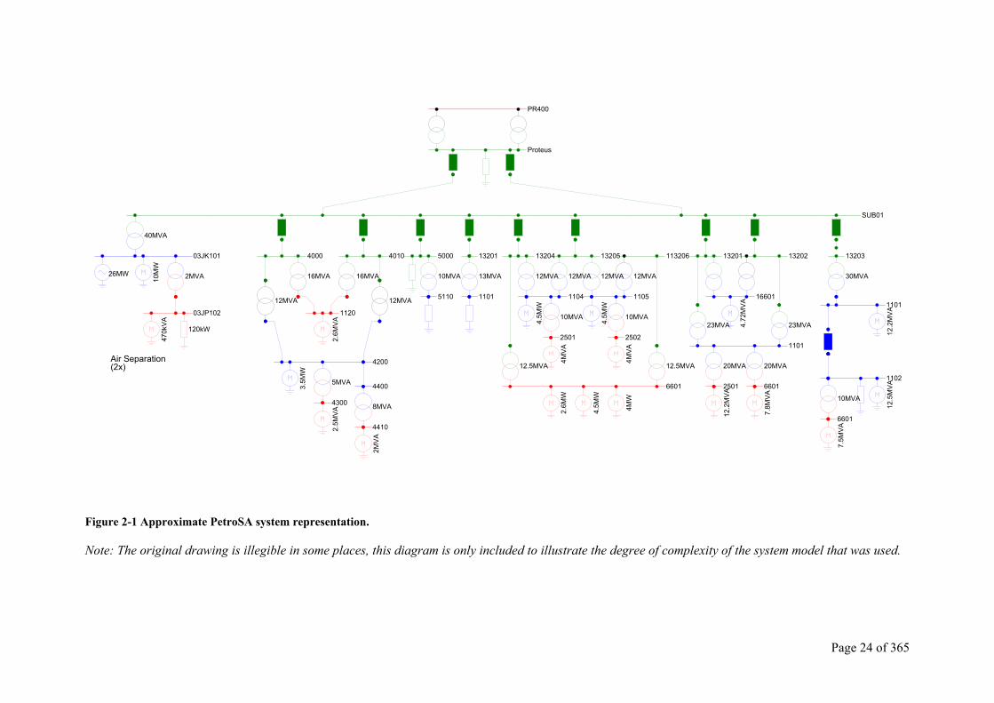
Page 24 of 365

Figure 2-1 Approximate PetroSA system representation.

Note: The original drawing is illegible in some places, this diagram is only included to illustrate the degree of complexity of the system model that was used.

40MVA

26MW

10M

W

03JK101

2MVA

03JP102

470k

VA

120kW

Air Separation(2x)

4000

16MVA

12MVA

4010

16MVA

12MVA

1120

2.6M

VA

4200

3.5M

W

5MVA

4300

2.5M

VA

4400

8MVA

4410

2MVA

5000

10MVA

5110

13201

13MVA

1101

13204

12MVA 12MVA

1104

13205

12MVA

4.5M

W

10MVA

2501

4MVA

12.5MVA

1105

12MVA

113206

4.5M

W

10MVA

2502

4MVA

12.5MVA

6601

2.6M

W

4.5M

W

4MW

13201

16601

23MVA 4.72

MVA

23MVA

13202

1101

20MVA 20MVA

2501 6601

12.2

MVA

7.8M

VA

SUB01

13203

1101

30MVA

12.2

MVA

1102

12.5

MVA

10MVA

6601

7.5M

VA

Proteus

PR400

Page 25 of 365

Lumped LV and HV motors were assumed to run at 85% of full load torque, based on the rating of the motor. Typical HV1 and LV motor characteristics were used to represent numerous equivalent or lumped motors. Due to the approximate nature of the modelling data, a simple equivalent circuit model was used for modelling of induction machines. Synchronous machines were also modelled using typical data. These models were detailed and included a full d-q axis representation taking transient, sub-transient and saturation effects into account. Variable speed drives were modelled simply as constant power loads.

It was incorrectly assumed that three 10MVAr filters installed at each of the three Synthol variable speed drives will provide reactive power compensation2.

Stability studies were carried out assuming a solid 3-phase fault of 100ms duration at different locations on the PetroSA distribution system. It was assumed that all load contactors, i.e. for motors, static loads and drives, remain held in during low control voltage conditions and ride through the fault even if the busbar voltage falls to zero. This represents the most severe recovery condition, which is prevented in practice by the re-acceleration system. It was also assumed that no busbars are isolated by disconnecting network branches after the fault.

2.2.1 Summary of main conclusions and recommendations The Powerplan study gave rise to the following conclusions and recommendations:

• For all 100ms fault and system conditions specified, recovery of all induction motors is possible.

• The local generators are stable for the specified fault conditions. • The 26MW synchronous motors are stable for the specified fault conditions, but

become unstable when subjected to a 400kV fault longer than 200ms. • Stability for all machines for the 100ms fault condition is achieved by a wide margin.

2.3 Merz and McLellan Study [27] The purpose of the Merz and McLellan studies were to determine whether the plant with the then proposed distribution system would recover satisfactorily after a 100ms supply interruption, or any short circuit in the distribution system that is cleared within 100ms.

2.3.1 PetroSA plant data When these studies were carried out, vendor data on drives was minimal. Typical data was therefore assumed throughout with regard to motor load characteristics and drive inertias. The Total Feed Compressor variable speed drives were represented as a constant power (PQ) type load which was correctly assumed to be switched out during the period the fault persisted and switched in after fault clearance. In general, summated equivalent loads based on available load lists were used. The rotating machine models differ from those used by Powerplan Systems [27]. Induction machine modelling was based on a simple equivalent linear impedance model. Saturation was not taken into account and only rotor resistance was changed as a function of slip.

1 Note that the definition of HV (high voltage) used in [27] and [28] differs from that used in this document and refers to 11kV and 6.6kV motors. In this section the terms HV and MV will be used interchangeably and both refer to 11kV - 6.6kV motors. 2 It is not clear from Figure 2-1 how these drives and filters were represented. These drives are supplied from busses 3, 4 and 10 as shown in Figure 3-4

Page 26 of 365

2.3.2 Summary of main conclusions and recommendations The studies showed [27]:

• The PetroSA system would recover satisfactorily after a 100ms supply interruption, or any short circuit in the distribution system that is cleared within 100ms.

• Sufficient reactive power was available to limit the demand from Eskom.

2.4 Comments On Study Results In practice, the 26MW air-compressors, 03KC101 & 03KC201 (Figure 3-5) usually trip during electrical disturbances, and the critical power generator, 48GT102 (Figure 3-4,) is automatically disconnected from the Eskom system when any disturbance is detected. The available reactive power is therefore approximately 27MVAr less than assumed. The two 10MW oxygen compressor motors, 03KC102 and 03KC202 (Figure 3-5), will also trip 10 to 15 seconds after the main air compressors trip due to process reasons. This large load reduction on the system will reduce the demand for reactive power to some extent. It will be necessary to determine the response of the system without the 26MW air compressors (03KC101/201) and the critical generator 48GT102 (Figure 3-4). The main generator has also been found to trip under certain conditions3 during power dips. In these cases, all reactive power has to be supplied by Eskom during system recovery and therefore a study with 48GT101 offline will also be required when a transient stability study encompassing the entire PetroSA system is carried out. Past experience has shown that the PetroSA system is able to recover following a voltage dip without the main generator being online, but it is important to investigate the system behaviour under these conditions.

None of these studies evaluated the impact of the re-acceleration system at PetroSA. A pessimistic approach was taken where it was assumed that all induction motors remain online irrespective of bus voltage levels. Motors were represented by lumped equivalents and generic data used since vendor data was unavailable. Motors were assumed to be operating at 85% full load torque. Surveys have shown that motors purchased individually (not part of an appliance) are usually oversized [10]. Since this practice improves system dynamic performance, it is important to determine the actual motor loadings when carrying out system analysis.

It has also been shown that the practice of assuming what is believed to be a pessimistic system representation can be a dangerous approach [11]. It is not always possible to select representations that would be pessimistic for all parts of the system or all test conditions. Static load models such as the linear impedance model used in the Merz & McLellan studies have also proven to be inaccurate in cases involving large voltage and/or frequency deviations. In such cases, dynamic load models should be used [30, 11].

2.5 Transient Stability Analysis Transient analysis of electrical distribution systems is mainly carried out by electricity suppliers and distributors such as Eskom. There is also a need to limit the complexity of the mathematical models used due to time, cost, manpower and computer hardware constraints when carrying out system studies [23]. It appears as if the majority of large power consumers would typically restrict electrical distribution system analysis to short circuit and load flow studies. Stability studies may only be carried out during the initial design of large industrial

3 These trips are due to limitations in the design of the protection system, which will result in erroneous tripping of the main generator breaker under certain conditions. Detailed studies were carried out to investigate this problem and the protection settings optimised to some extent. Further improvement will require significant capital investment and is not justifiable at this stage.

Page 27 of 365

plants. This is evidenced by the fact that most research effort remains directed at solving the problems encountered by electricity suppliers and distributors. In the case of PetroSA, such studies were carried out, but were limited in scope and accuracy due to the use of generic data parameters, load models used and the limitations of computer hardware available at the time. These studies did not evaluate the behaviour of the re-acceleration system. There have been significant changes to the loading of the Eskom network supplying the PetroSA plant and the PetroSA distribution system transient response could well be significantly different from that originally calculated. The ever-increasing capabilities of personal computers have also provided the means to carry out analysis with model complexity that was not practical several years ago [21, 23].

In order to analyse the dynamic performance of an electrical system, suitable mathematical models have to be developed which represent the system components to the desired degree of accuracy. Solutions to these models that lead to an understanding of the system behaviour during various types of disturbances have to be obtained. Two types of stability studies are carried out. The analysis of system behaviour following a large disturbance is generally referred to as a transient stability study. The time frame for this type of simulation is between a fraction of a second to tens of seconds. The term dynamic stability is used to describe the long-time response of a system to small disturbances or badly set controls and solutions can be obtained in the time or frequency domain. This type of problem will not be considered here.

Most of the available literature dealing with transient analysis of electrical distribution systems consider the problem from the perspective of the electricity supplier and not the electricity consumer [21, 23]. Emphasis is placed on detailed modelling of generators, prime-movers and transmission systems. Various approximations are used to model loads, since it is assumed that the exact composition and behaviour of the loads on the system is unknown [10, 11, 29, 30]. Lesieutre et al [34] comment that although detailed induction motor models are included in some transient stability programs, they capture induction motor dynamic characteristics which lack meaning at the power systems level. Emphasis is therefore placed on developing dynamic models in terms of meaningful bus variables, P, Q, V, θ and ω.4 The purpose of this research is to investigate the behaviour of the system loads (induction motors) under transient conditions as well as the response of the associated distribution system. Load composition is known and can be modelled in greater detail. It is therefore obvious that the general assumptions used to model loads will not apply and a more detailed load representation can be applied.

The multi-machine analysis techniques developed by Smith and Chen [22] are primarily directed at the modelling of small capacity, geographically limited systems. Detailed models are used for all system components. Whilst these techniques could theoretically be extended to the PetroSA distribution system, the additional computational effort involved would be prohibitive.

In transient stability studies, generators with their controls and dynamic loads are usually described by a set of differential equations, whilst the transmission system with static loads is represented by a set of algebraic equations [21, 23]. Two general approaches, namely numerical methods and non-conventional methods are currently used to analyse the transient performance of electrical systems [23]. Numerical methods are able to handle mathematical models of various components of a power system to any desired degree of sophistication. One disadvantage is that, depending on the size, complexity and modelling refinement, a huge computational effort may be required. In addition, the time domain solutions obtained do not provide insight into the response of the system to parameter changes. Such investigations can only be carried out by means of repetitive numerical analysis. 4 Where: P = Bus Power, Q = bus reactive power, V = bus voltage, θ = Bus voltage angle and ω = bus frequency

Page 28 of 365

Non-conventional methods of analysis such as Lyapunov-like direct methods, and extended equal area criterion have been developed to address these shortcomings. Pavella and Murthy [23] comment that although a great deal of research effort has been devoted to developing Lyapunov-like direct methods, the expectations initially put on direct methods have not been fully realized. They are of the opinion that continuing development of these methods should preserve the features for which they have initially been designed, namely features complementary to, rather than competitive with time-domain methods. Various other methods such as Extended Equal-Area Criterion, Decision Tree Transient Stability Method and the Composite Electromechanical Distance Method can be used to investigate system transient stability. These methods were excluded based on the following considerations:

• A time domain solution as provided by conventional numerical analysis will provide a clear insight into the behaviour of the PetroSA system after the occurrence of single and multiple voltage dips. The impact of the re-acceleration system on induction motor behaviour can also be easily assessed.

• Conventional numerical analysis is able to handle system component models of any degree of complexity. It will thus be easy to use load models of differing complexity to determine the degree of modelling sophistication required to adequately determine the behaviour of the PetroSA distribution system.

• A brief review of non-conventional methods indicates that the electrical system representation generally has to be simplified. One of the aims of the current work is to determine the merits of a more detailed representation of induction motor loads when compared to the simplified models generally used.

• It is necessary to restrict the scope of work for the current research to manageable limits.

2.5.1 System representation The mathematical model of an electrical power system usually consists of a set of differential and a set of algebraic equations. These equations need to be solved in transient stability calculations. A step by step procedure normally followed is that during each time interval the differential equations are solved by numerical integration. The values of the variables obtained are then used at the end of the time step in the solution of the algebraic equations. [21, 23] This is usually referred to as the alternating solution method. An alternative approach entails the application of implicit integration techniques which allow the differential equations to be converted to algebraic equations. These equations can then be incorporated with the network’s algebraic equations and solved simultaneously. The use of implicit trapezoidal integration has proved very stable, permitting step lengths greater than the smallest time constant of the system [21]. This is termed the combined solution method.

It was necessary to decide upon a solution method, and the alternating solution method was chosen based on the following considerations:

• Existing Matlab routines and functions could be readily applied – for example, Ordinary Differential Equation (ODE) solvers and matrix calculation routines.

• The resulting software is modular and separate modules can be independently tested, e.g. loadflow (algebraic) and motor dynamic models (differential equations)

• The literature survey carried out yielded more information on the alternating-solution approach. The combined-solution approach appears to be less well documented.

The emphasis is generally on achieving as much reduction in computer time as possible, whilst keeping storage requirements to a minimum. The number of variables that the program has to handle increases dramatically with increasing system size and computer programs must be able to handle large dimensions. Due to the vastly differing time constants associated with different system components, the associated differential equations are usually stiff. Sparsity

Page 29 of 365

programming, optimal ordering, triangular factorization and other techniques have been developed by various researchers to address these problems.

Computer programs for transient stability generally employ some form of step-by-step calculation procedure where the values of the system variables are calculated at regular time intervals, providing a time-domain solution.

The requirements for the present work are as follows:

• Load behaviour following transients needs to be carefully assessed. Exact load composition and behaviour is known. Accurate induction motor models can be employed to simulate the dynamic behaviour of the PetroSA system during the re-acceleration phase following single or multiple voltage dips.

• It would be advantageous if the software developed for transient analysis is modular. This will simplify testing and verification of results with other available software packages. This will also allow evaluation of different induction motor models.

• The Eskom supply network and generators can be represented as a swing bus connected to the PetroSA system via a suitable impedance. The type of disturbance to be considered typically arises due to a line to ground fault on the transmission lines relatively close to PetroSA resulting in voltage dips. Only the stability of the local PetroSA system is to be investigated.

• The single generator embedded in the PetroSA network must be modelled. For the purposes of this work, only a relatively small portion of the PetroSA electrical system will be represented in detail. Clearly, if the entire system is modelled, the behaviour of this generator can be expected to have a significant influence on system behaviour. The importance of modelling the generator, and its potential impact, when a small portion of the system is modelled needs to be determined.

• The size of system to be simulated is reduced quite significantly, thus the system dimensions are kept relatively small5. The specialized techniques developed for handling systems with large dimensions are unlikely to be required.

• Reduction in computer time, although desirable, is not an essential requirement, since determining the behaviour of the distribution system and performance of the induction motor models are of primary concern. The merits of using more complex models will be assessed taking computing time into consideration.

It is thus obvious that the requirements for the present work differs from that of typical transient stability analysis. Detailed models of the induction motors selected for study will be required. The disturbances to be investigated do not affect the stability of the Eskom system, but only have a localized effect on the PetroSA distribution system. It is necessary to model the system loads to a greater level of detail than is normally required and the generation to a lesser degree.

2.6 Modelling Of Loads The following brief review of load modelling was carried out in order to obtain an overview of the typical load models used in power system analysis. In contrast with the present work, load composition and behaviour is generally assumed to be unknown [10, 11, 12, 26]. Various models have been proposed to provide an approximate load representation. In this context, a load model can be defined as a mathematical relationship between a bus voltage (magnitude and frequency) and the power (active and reactive) or current flowing into the bus load [11]. A significant research effort has been directed at improving load modelling with most researchers being of the opinion that more accurate load models are required. The load

5 The system is small when compared to systems with hundreds, if not thousands of busses and thousands of branches.

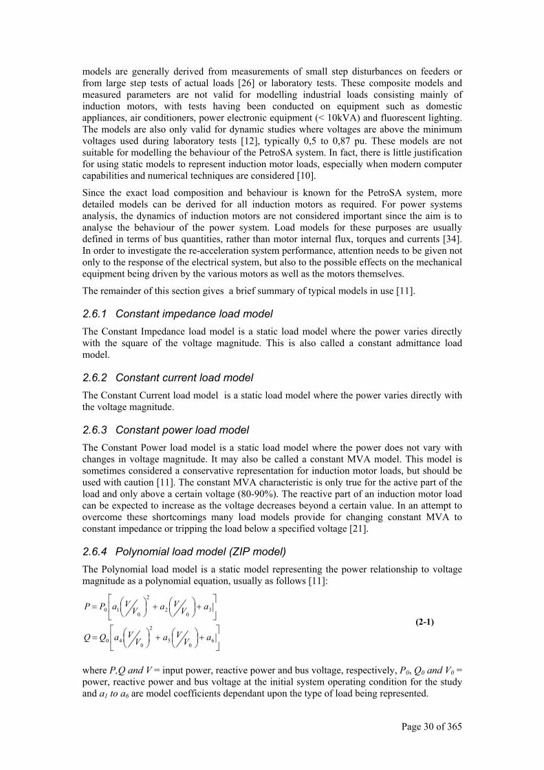
Page 30 of 365

models are generally derived from measurements of small step disturbances on feeders or from large step tests of actual loads [26] or laboratory tests. These composite models and measured parameters are not valid for modelling industrial loads consisting mainly of induction motors, with tests having been conducted on equipment such as domestic appliances, air conditioners, power electronic equipment (< 10kVA) and fluorescent lighting. The models are also only valid for dynamic studies where voltages are above the minimum voltages used during laboratory tests [12], typically 0,5 to 0,87 pu. These models are not suitable for modelling the behaviour of the PetroSA system. In fact, there is little justification for using static models to represent induction motor loads, especially when modern computer capabilities and numerical techniques are considered [10].

Since the exact load composition and behaviour is known for the PetroSA system, more detailed models can be derived for all induction motors as required. For power systems analysis, the dynamics of induction motors are not considered important since the aim is to analyse the behaviour of the power system. Load models for these purposes are usually defined in terms of bus quantities, rather than motor internal flux, torques and currents [34]. In order to investigate the re-acceleration system performance, attention needs to be given not only to the response of the electrical system, but also to the possible effects on the mechanical equipment being driven by the various motors as well as the motors themselves.

The remainder of this section gives a brief summary of typical models in use [11].

2.6.1 Constant impedance load model The Constant Impedance load model is a static load model where the power varies directly with the square of the voltage magnitude. This is also called a constant admittance load model.

2.6.2 Constant current load model The Constant Current load model is a static load model where the power varies directly with the voltage magnitude.

2.6.3 Constant power load model The Constant Power load model is a static load model where the power does not vary with changes in voltage magnitude. It may also be called a constant MVA model. This model is sometimes considered a conservative representation for induction motor loads, but should be used with caution [11]. The constant MVA characteristic is only true for the active part of the load and only above a certain voltage (80-90%). The reactive part of an induction motor load can be expected to increase as the voltage decreases beyond a certain value. In an attempt to overcome these shortcomings many load models provide for changing constant MVA to constant impedance or tripping the load below a specified voltage [21].

2.6.4 Polynomial load model (ZIP model) The Polynomial load model is a static model representing the power relationship to voltage magnitude as a polynomial equation, usually as follows [11]:

+

+

=

+

+

=

60

5

2

040

30

2

2

010

aVVaV

VaQQ

aVVaV

VaPP

(2-1)

where P,Q and V = input power, reactive power and bus voltage, respectively, P0, Q0 and V0 = power, reactive power and bus voltage at the initial system operating condition for the study and a1 to a6 are model coefficients dependant upon the type of load being represented.

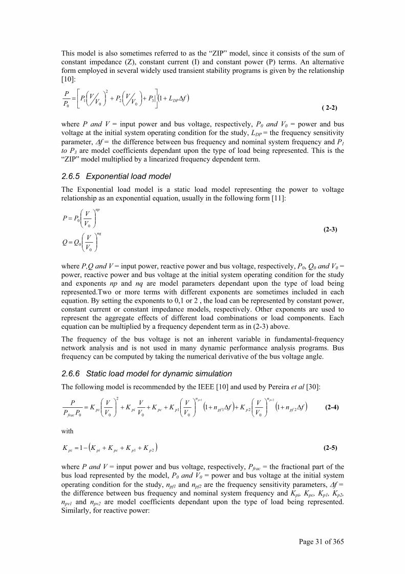
Page 31 of 365

This model is also sometimes referred to as the “ZIP” model, since it consists of the sum of constant impedance (Z), constant current (I) and constant power (P) terms. An alternative form employed in several widely used transient stability programs is given by the relationship [10]:

( )fLPVVPV

VPPP

DP ∆+

+

+

= 13

02

2

01

0 ( 2-2)

where P and V = input power and bus voltage, respectively, P0 and V0 = power and bus voltage at the initial system operating condition for the study, LDP = the frequency sensitivity parameter, ∆f = the difference between bus frequency and nominal system frequency and P1 to P3 are model coefficients dependant upon the type of load being represented. This is the “ZIP” model multiplied by a linearized frequency dependent term.

2.6.5 Exponential load model The Exponential load model is a static load model representing the power to voltage relationship as an exponential equation, usually in the following form [11]:

nq

np

VVQQ

VVPP

=

=

00

00

(2-3)

where P,Q and V = input power, reactive power and bus voltage, respectively, P0, Q0 and V0 = power, reactive power and bus voltage at the initial system operating condition for the study and exponents np and nq are model parameters dependant upon the type of load being represented.Two or more terms with different exponents are sometimes included in each equation. By setting the exponents to 0,1 or 2 , the load can be represented by constant power, constant current or constant impedance models, respectively. Other exponents are used to represent the aggregate effects of different load combinations or load components. Each equation can be multiplied by a frequency dependent term as in (2-3) above.

The frequency of the bus voltage is not an inherent variable in fundamental-frequency network analysis and is not used in many dynamic performance analysis programs. Bus frequency can be computed by taking the numerical derivative of the bus voltage angle.

2.6.6 Static load model for dynamic simulation The following model is recommended by the IEEE [10] and used by Pereira et al [30]:

( ) ( )fnVVKfn

VVKK

VVK

VVK

PPP

pf

n

ppf

n

ppcpipzfrac

pvpv

∆+

+∆+

+++

= 2

021

01

0

2

00

1121

(2-4)

with

( )211 pppcpipz KKKKK +++−= (2-5)

where P and V = input power and bus voltage, respectively, Pfrac = the fractional part of the bus load represented by the model, P0 and V0 = power and bus voltage at the initial system operating condition for the study, npf1 and npf2 are the frequency sensitivity parameters, ∆f = the difference between bus frequency and nominal system frequency and Kpi, Kpc, Kp1, Kp2, npv1 and npv2 are model coefficients dependant upon the type of load being represented. Similarly, for reactive power:

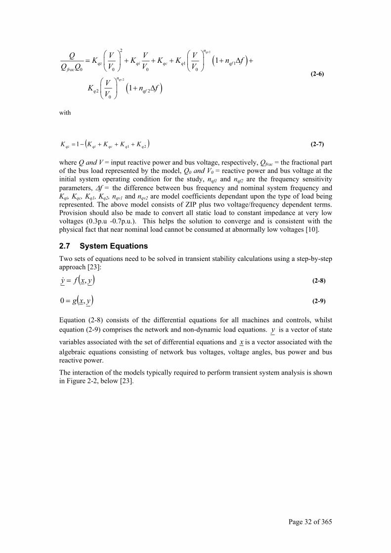
Page 32 of 365

( )

( )

1

2

2

1 10 0 0 0

2 20

1

1

qv

qv

n

qz qi qc q qffrac

n

q qf

Q V V VK K K K n fQ Q V V V

VK n fV

= + + + + ∆ +

+ ∆

(2-6)

with

( )211 qqqcqiqz KKKKK +++−= (2-7)

where Q and V = input reactive power and bus voltage, respectively, Qfrac = the fractional part of the bus load represented by the model, Q0 and V0 = reactive power and bus voltage at the initial system operating condition for the study, nqf1 and nqf2 are the frequency sensitivity parameters, ∆f = the difference between bus frequency and nominal system frequency and Kqi, Kqc, Kq1, Kq2, nqv1 and nqv2 are model coefficients dependant upon the type of load being represented. The above model consists of ZIP plus two voltage/frequency dependent terms. Provision should also be made to convert all static load to constant impedance at very low voltages (0.3p.u -0.7p.u.). This helps the solution to converge and is consistent with the physical fact that near nominal load cannot be consumed at abnormally low voltages [10].

2.7 System Equations Two sets of equations need to be solved in transient stability calculations using a step-by-step approach [23]:

( )yxfy ,= (2-8)

( )yxg ,0 = (2-9)

Equation (2-8) consists of the differential equations for all machines and controls, whilst equation (2-9) comprises the network and non-dynamic load equations. y is a vector of state

variables associated with the set of differential equations and x is a vector associated with the algebraic equations consisting of network bus voltages, voltage angles, bus power and bus reactive power.

The interaction of the models typically required to perform transient system analysis is shown in Figure 2-2, below [23].

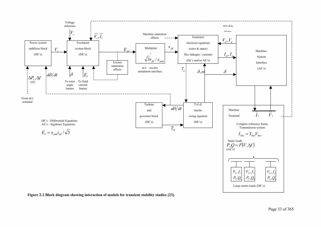
Page 33 of 365

Figure 2-2 Block diagram showing interaction of models for transient stability studies [23].

Machine-

System

Interface

(AE’s)

Generator

electrical equations

(rotor & stator)

flux linkages / currents

(De’s and/or AE’s)

m/c d-q

frame

qd VV ,

qd II ,

ωδ , δgT

Machine saturation effects

Multiplier

x

adufd xr /3

fdv

m/c – exciter simulation interface

Excitation

system block

(DE’s)

Exciter saturation

effects

To field current limiter

To rotor angle limiter

Voltage reference

fdE

1Eδ

rVtt IV ,

Machine

Terminal tI tV

Complex reference frame Transmission system

busbusbus VYI =Static loads

( )fVFQP ∆= ,,(AE’s)

11

11

,,QPfV

22

22

,,QPfV

nn

nn

QPfV

,,

Large motor loads (DE’s)

Power system

stabilizer block

(DE’s) sV

T-G-E

inertia

swing equation

(DE’s)

Turbine

and

governor block

(DE’s)

dtdδ

mT

dtdδfPe ∆∆ ,(or)

From m/c terminal

DE’s : Differential Equations AE’s : Algebraic Equations

3/fdaduI ixE =

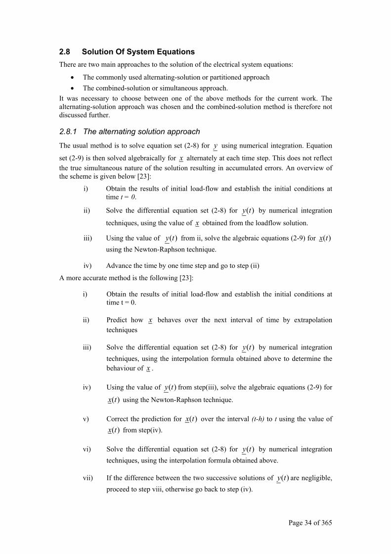
Page 34 of 365

2.8 Solution Of System Equations There are two main approaches to the solution of the electrical system equations:

• The commonly used alternating-solution or partitioned approach • The combined-solution or simultaneous approach.

It was necessary to choose between one of the above methods for the current work. The alternating-solution approach was chosen and the combined-solution method is therefore not discussed further.

2.8.1 The alternating solution approach

The usual method is to solve equation set (2-8) for y using numerical integration. Equation

set (2-9) is then solved algebraically for x alternately at each time step. This does not reflect the true simultaneous nature of the solution resulting in accumulated errors. An overview of the scheme is given below [23]:

i) Obtain the results of initial load-flow and establish the initial conditions at time t = 0.

ii) Solve the differential equation set (2-8) for )(ty by numerical integration

techniques, using the value of x obtained from the loadflow solution.

iii) Using the value of )(ty from ii, solve the algebraic equations (2-9) for )(tx using the Newton-Raphson technique.

iv) Advance the time by one time step and go to step (ii)

A more accurate method is the following [23]:

i) Obtain the results of initial load-flow and establish the initial conditions at time t = 0.

ii) Predict how x behaves over the next interval of time by extrapolation techniques

iii) Solve the differential equation set (2-8) for )(ty by numerical integration techniques, using the interpolation formula obtained above to determine the behaviour of x .

iv) Using the value of )(ty from step(iii), solve the algebraic equations (2-9) for

)(tx using the Newton-Raphson technique.

v) Correct the prediction for )(tx over the interval (t-h) to t using the value of )(tx from step(iv).

vi) Solve the differential equation set (2-8) for )(ty by numerical integration techniques, using the interpolation formula obtained above.

vii) If the difference between the two successive solutions of )(ty are negligible, proceed to step viii, otherwise go back to step (iv).

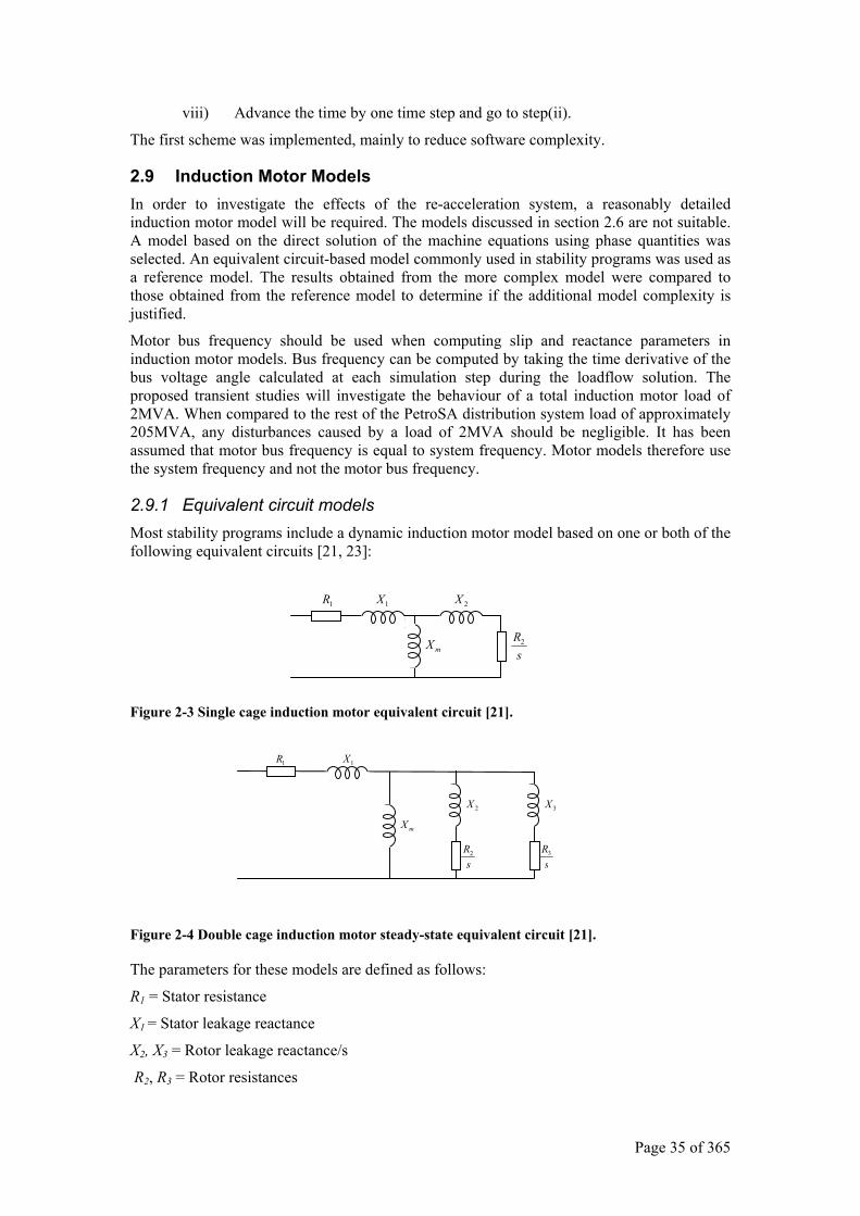
Page 35 of 365

viii) Advance the time by one time step and go to step(ii).

The first scheme was implemented, mainly to reduce software complexity.

2.9 Induction Motor Models In order to investigate the effects of the re-acceleration system, a reasonably detailed induction motor model will be required. The models discussed in section 2.6 are not suitable. A model based on the direct solution of the machine equations using phase quantities was selected. An equivalent circuit-based model commonly used in stability programs was used as a reference model. The results obtained from the more complex model were compared to those obtained from the reference model to determine if the additional model complexity is justified.

Motor bus frequency should be used when computing slip and reactance parameters in induction motor models. Bus frequency can be computed by taking the time derivative of the bus voltage angle calculated at each simulation step during the loadflow solution. The proposed transient studies will investigate the behaviour of a total induction motor load of 2MVA. When compared to the rest of the PetroSA distribution system load of approximately 205MVA, any disturbances caused by a load of 2MVA should be negligible. It has been assumed that motor bus frequency is equal to system frequency. Motor models therefore use the system frequency and not the motor bus frequency.

2.9.1 Equivalent circuit models Most stability programs include a dynamic induction motor model based on one or both of the following equivalent circuits [21, 23]:

Figure 2-3 Single cage induction motor equivalent circuit [21].

Figure 2-4 Double cage induction motor steady-state equivalent circuit [21].

The parameters for these models are defined as follows:

R1 = Stator resistance

X1 = Stator leakage reactance

X2, X3 = Rotor leakage reactance/s

R2, R3 = Rotor resistances

1R

sR2

1X

mX

2X

1X1R

mX2X

sR2

sR3

3X

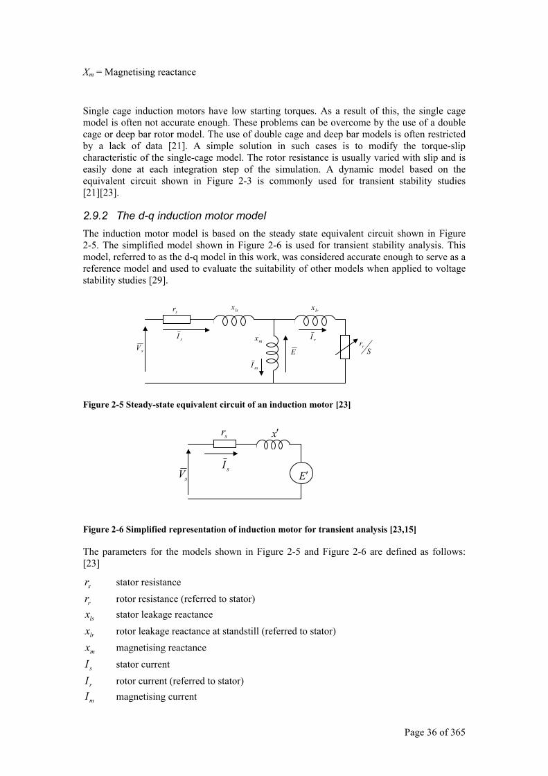
Page 36 of 365

Xm = Magnetising reactance

Single cage induction motors have low starting torques. As a result of this, the single cage model is often not accurate enough. These problems can be overcome by the use of a double cage or deep bar rotor model. The use of double cage and deep bar models is often restricted by a lack of data [21]. A simple solution in such cases is to modify the torque-slip characteristic of the single-cage model. The rotor resistance is usually varied with slip and is easily done at each integration step of the simulation. A dynamic model based on the equivalent circuit shown in Figure 2-3 is commonly used for transient stability studies [21][23].

2.9.2 The d-q induction motor model The induction motor model is based on the steady state equivalent circuit shown in Figure 2-5. The simplified model shown in Figure 2-6 is used for transient stability analysis. This model, referred to as the d-q model in this work, was considered accurate enough to serve as a reference model and used to evaluate the suitability of other models when applied to voltage stability studies [29].

Figure 2-5 Steady-state equivalent circuit of an induction motor [23]

Figure 2-6 Simplified representation of induction motor for transient analysis [23,15]

The parameters for the models shown in Figure 2-5 and Figure 2-6 are defined as follows: [23]

sr stator resistance

rr rotor resistance (referred to stator)

lsx stator leakage reactance

lrx rotor leakage reactance at standstill (referred to stator)

mx magnetising reactance

sI stator current

rI rotor current (referred to stator)

mI magnetising current

sVsI

sr lsx

mI

mx

E

rI

lrx

Srr

sV sI

x′sr

E′

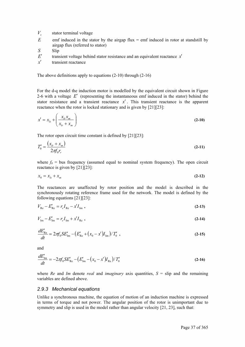
Page 37 of 365

sV stator terminal voltage E emf induced in the stator by the airgap flux = emf induced in rotor at standstill by

airgap flux (referred to stator) S Slip E′ transient voltage behind stator resistance and an equivalent reactance x′ x′ transient reactance

The above definitions apply to equations (2-10) through (2-16)

For the d-q model the induction motor is modelled by the equivalent circuit shown in Figure 2-6 with a voltage E′ (representing the instantaneous emf induced in the stator) behind the stator resistance and a transient reactance x′ . This transient reactance is the apparent reactance when the rotor is locked stationary and is given by [21][23]:

+

+=′mlr

mlrls xx

xxxx (2-10)

The rotor open circuit time constant is defined by [21][23]:

( )r

mlr

rfxxT

00 2π

+=′ (2-11)

where f0 = bus frequency (assumed equal to nominal system frequency). The open circuit reactance is given by [21][23]:

mls xxx +=0 (2-12)

The reactances are unaffected by rotor position and the model is described in the synchronously rotating reference frame used for the network. The model is defined by the following equations [21][23]:

ImReReRe IxIrEV s ′−=′− , (2-13)

ReImImIm IxIrEV s ′+=′− , (2-14)

( )( ) 0Im0ReIm0Re /2 TIxxEESf

dtEd ′′−+′−′=

′π , (2-15)

and

( )( ) 0Re0ImRe0Im /2 TIxxEESf

dtEd ′′−−′−′−=

′π (2-16)

where Re and Im denote real and imaginary axis quantities, S = slip and the remaining variables are defined above.

2.9.3 Mechanical equations Unlike a synchronous machine, the equation of motion of an induction machine is expressed in terms of torque and not power. The angular position of the rotor is unimportant due to symmetry and slip is used in the model rather than angular velocity [21, 23], such that:

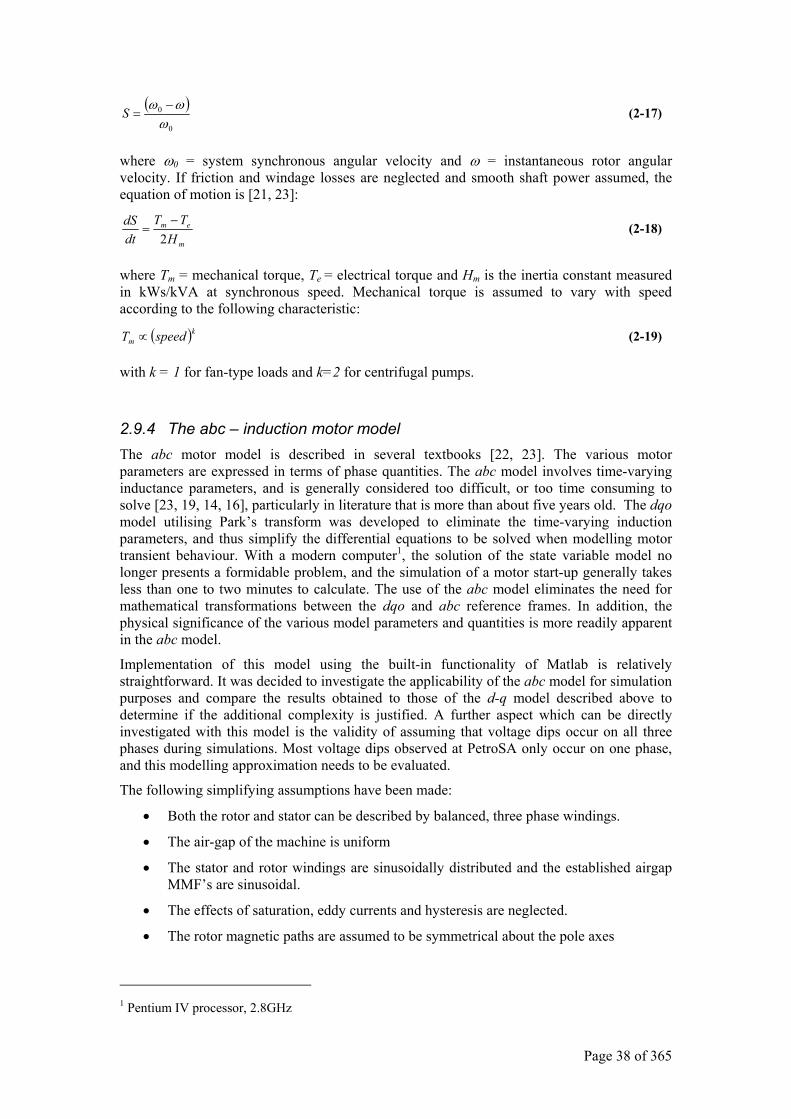
Page 38 of 365

( )0

0

ωωω −

=S (2-17)

where ω0 = system synchronous angular velocity and ω = instantaneous rotor angular velocity. If friction and windage losses are neglected and smooth shaft power assumed, the equation of motion is [21, 23]:

m

em

HTT

dtdS

2−

= (2-18)

where Tm = mechanical torque, Te = electrical torque and Hm is the inertia constant measured in kWs/kVA at synchronous speed. Mechanical torque is assumed to vary with speed according to the following characteristic:

( )km speedT ∝ (2-19)

with k = 1 for fan-type loads and k=2 for centrifugal pumps.

2.9.4 The abc – induction motor model The abc motor model is described in several textbooks [22, 23]. The various motor parameters are expressed in terms of phase quantities. The abc model involves time-varying inductance parameters, and is generally considered too difficult, or too time consuming to solve [23, 19, 14, 16], particularly in literature that is more than about five years old. The dqo model utilising Park’s transform was developed to eliminate the time-varying induction parameters, and thus simplify the differential equations to be solved when modelling motor transient behaviour. With a modern computer1, the solution of the state variable model no longer presents a formidable problem, and the simulation of a motor start-up generally takes less than one to two minutes to calculate. The use of the abc model eliminates the need for mathematical transformations between the dqo and abc reference frames. In addition, the physical significance of the various model parameters and quantities is more readily apparent in the abc model.

Implementation of this model using the built-in functionality of Matlab is relatively straightforward. It was decided to investigate the applicability of the abc model for simulation purposes and compare the results obtained to those of the d-q model described above to determine if the additional complexity is justified. A further aspect which can be directly investigated with this model is the validity of assuming that voltage dips occur on all three phases during simulations. Most voltage dips observed at PetroSA only occur on one phase, and this modelling approximation needs to be evaluated.

The following simplifying assumptions have been made:

• Both the rotor and stator can be described by balanced, three phase windings.

• The air-gap of the machine is uniform

• The stator and rotor windings are sinusoidally distributed and the established airgap MMF’s are sinusoidal.

• The effects of saturation, eddy currents and hysteresis are neglected.

• The rotor magnetic paths are assumed to be symmetrical about the pole axes

1 Pentium IV processor, 2.8GHz

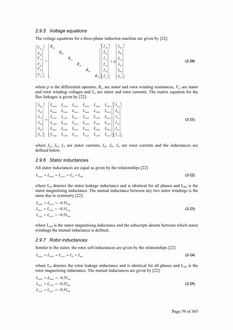
Page 39 of 365

2.9.5 Voltage equations The voltage equations for a three-phase induction machine are given by [22]:

+

=

cr

br

ar

cs

bs

as

cr

br

ar

cs

bs

as

cr

br

ar

cs

bs

as

cr

br

ar

cs

bs

as

p

IIIIII

RR

RR

RR

VVVVVV

λλλλλλ

(2-20)

where p is the differential operator, Rxx are stator and rotor winding resistances, Vxx are stator and rotor winding voltages and Ixx are stator and rotor currents. The matrix equation for the flux linkages is given by [22]:

=

cr

br

ar

cs

bs

as

crcrcrbrcrarcrcscrbscras

brcrbrbrbrarbrcsbrbsbras

arcrarbrarararcsarbsaras

rcsbrcsarscsbscsas

bscrbsbrbsarbscsbsbsbsas

ascrasbrasarascsasbsasas

cr

br

ar

cs

bs

as

IIIIII

LLLLLLLLLLLLLLLLLLLLLLLLLLLLLLLLLLLL

csccsc

λλλλλλ

(2-21)

where Ias, Ibs, Ics are stator currents, Iar, Ibr, Icr are rotor currents and the inductances are defined below.

2.9.6 Stator inductances All stator inductances are equal as given by the relationships [22]

mslssbsbsasas LLLLL +=== csc (2-22)

where Lls denotes the stator leakage inductance and is identical for all phases and Lms is the stator magnetising inductance. The mutual inductance between any two stator windings is the same due to symmetry [22]:

msascscsas

mscsbsbscs

msbsasasbs

LLLLLLLLL

5.05.05.0

−==−==−==

(2-23)

where Lms is the stator magnetising inductance and the subscripts denote between which stator windings the mutual inductance is defined..

2.9.7 Rotor inductances Similar to the stator, the rotor self-inductances are given by the relationships [22]

mrlrcrcrbrbrarar LLLLL +=== (2-24)

where Llr denotes the rotor leakage inductance and is identical for all phases and Lmr is the rotor magnetising inductance. The mutual inductances are given by [22]:

mrarcrcrar

mrcrbrbrcr

mrbrararbr

LLLLLLLLL

5.05.05.0

−==−==−==

(2-25)

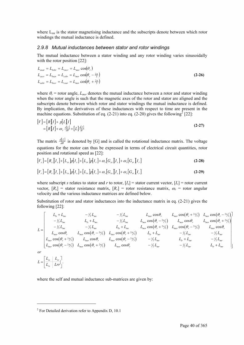
Page 40 of 365

where Lmr is the stator magnetising inductance and the subscripts denote between which rotor windings the mutual inductance is defined.

2.9.8 Mutual inductances between stator and rotor windings The mutual inductance between a stator winding and any rotor winding varies sinusoidally with the rotor position [22]:

( )( )( )3

23

2csc

coscoscos

π

π

θ

θθ

+===

−===

===

rmsrcsarbscrasbr

rmsrcsbrbsarascr

rmsrrbsbrasar

LLLLLLLLLLLL

(2-26)

where θr = rotor angle, Lmsr denotes the mutual inductance between a rotor and stator winding when the rotor angle is such that the magnetic axes of the rotor and stator are aligned and the subscripts denote between which rotor and stator windings the mutual inductance is defined. By implication, the derivatives of these inductances with respect to time are present in the machine equations. Substitution of eq. (2-21) into eq. (2-20) gives the following2 [22]:

[ ] [ ][ ] [ ][ ][ ][ ] [ ] [ ] [ ]

dtId

dLd

r LIR

ILpIRV

++=

+=

θω (2-27)

The matrix [ ]θdLd is denoted by [G] and is called the rotational inductance matrix. The voltage

equations for the motor can thus be expressed in terms of electrical circuit quantities, rotor position and rotational speed as [22]:

[ ] [ ][ ] [ ] [ ] [ ] [ ] [ ][ ] [ ][ ]rsrrsssrrsrssssss IGIGIpLIpLIRV ωω ++++= (2-28)

[ ] [ ][ ] [ ] [ ] [ ] [ ] [ ][ ] [ ][ ]rrrrsrsrrrrsrsrrr IGIGIpLIpLIRV ωω ++++= (2-29)

where subscript s relates to stator and r to rotor, [Is] = stator current vector, [Ir] = rotor current vector, [Rs] = stator resistance matrix, [Rr] = rotor resistance matrix, ωr = rotor angular velocity and the various inductance matrices are defined below.

Substitution of rotor and stator inductances into the inductance matrix in eq. (2-21) gives the following [22]:

( ) ( )( ) ( )( ) ( )

( ) ( )

2 21 12 2 3 3

2 21 12 2 3 3

2 21 12 2 3 3

2 23 3

cos cos coscos cos coscos cos cos

cos cos cos

ls ms ms ms msr r msr r msr r

ms ls ms ms msr r msr r msr r

ms ms ls ms msr r msr r msr r

msr r msr r msr r

L L L L L L LL L L L L L LL L L L L L L

LL L L L

π π

π π

π π

π π

θ θ θθ θ θθ θ θ

θ θ θ

+ − − + −− + − − +− − + + −

=− +

( ) ( )( ) ( )

1 12 2

2 2 1 13 3 2 2

2 2 1 13 3 2 2

cos cos coscos cos cos

.

lr mr mr mr

msr r msr r msr r mr lr mr mr

msr r msr r msr r mr mr lr mr

ss sr

rs

L L LL L L L L L LL L L L L L L

orL L

L L Lrr

π π

π π

θ θ θθ θ θ

+ − − + − − + −

− + − − +

=

where the self and mutual inductance sub-matrices are given by:

2 For Detailed derivation refer to Appendix D, 10.1

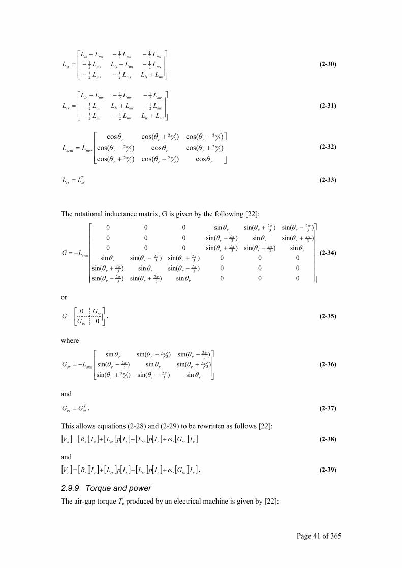
Page 41 of 365

+−−−+−−−+

=

mslsmsms

msmslsms

msmsmsls

ss

LLLLLLLLLLLL

L

21

21

21

21

21

21

(2-30)

+−−−+−−−+

=

mrlrmrmr

mrmrlrmr

mrmrmrlr

rr

LLLLLLLLLLLL

L

21

21

21

21

21

21

(2-31)

−++−−+

=

rrr

rrr

rrr

msrsrm LLθθθ

θθθθθθ

ππ

ππ

ππ

cos)cos()cos()cos(cos)cos()cos()cos(cos

32

32

32

32

32

32

(2-32)

Tsrrs LL = (2-33)

The rotational inductance matrix, G is given by the following [22]:

+−−++−

−++−−+

−=

000sin)sin()sin(000)sin(sin)sin(000)sin()sin(sin

sin)sin()sin(000)sin(sin)sin(000)sin()sin(sin000

32

32

32

32

32

32

32

32

32

32

32

32

rrr

rrr

rrr

rrr

rrr

rrr

srmLG

θθθθθθθθθ

θθθθθθθθθ

ππ

ππ

ππ

ππ

ππ

ππ

(2-34)

or

=

00

rs

sr

GG

G . (2-35)

where

−++−−+

−=

rrr

rrr

rrr

srmsr LGθθθ

θθθθθθ

ππ

ππ

ππ

sin)sin()sin()sin(sin)sin()sin()sin(sin

32

32

32

32

32

32

(2-36)

and Tstrs GG = . (2-37)

This allows equations (2-28) and (2-29) to be rewritten as follows [22]:

[ ] [ ][ ] [ ] [ ] [ ] [ ] [ ][ ]rsrrrsrssssss IGIpLIpLIRV ω+++= (2-38)

and

[ ] [ ][ ] [ ] [ ] [ ] [ ] [ ][ ]srsrrrrsrsrrr IGIpLIpLIRV ω+++= . (2-39)

2.9.9 Torque and power The air-gap torque Te produced by an electrical machine is given by [22]:

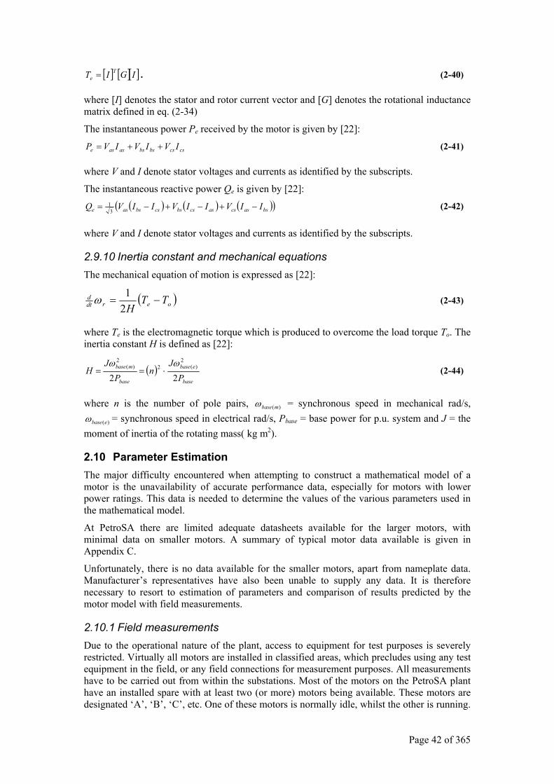
Page 42 of 365

[ ] [ ][ ]IGIT Te = . (2-40)

where [I] denotes the stator and rotor current vector and [G] denotes the rotational inductance matrix defined in eq. (2-34)

The instantaneous power Pe received by the motor is given by [22]:

cscsbsbsasase IVIVIVP ++= (2-41)

where V and I denote stator voltages and currents as identified by the subscripts.

The instantaneous reactive power Qe is given by [22]:

( ) ( ) ( )( )bsascsascsbscsbsase IIVIIVIIVQ −+−+−=3

1 (2-42)

where V and I denote stator voltages and currents as identified by the subscripts.

2.9.10 Inertia constant and mechanical equations The mechanical equation of motion is expressed as [22]:

( )oerdtd TT

H−=

21ω (2-43)

where Te is the electromagnetic torque which is produced to overcome the load torque To. The inertia constant H is defined as [22]:

( )base

ebase

base

mbase

PJ

nP

JH

22

2)(2

2)( ωω

⋅== (2-44)

where n is the number of pole pairs, )(mbaseω = synchronous speed in mechanical rad/s,

)(ebaseω = synchronous speed in electrical rad/s, Pbase = base power for p.u. system and J = the moment of inertia of the rotating mass( kg m2).

2.10 Parameter Estimation The major difficulty encountered when attempting to construct a mathematical model of a motor is the unavailability of accurate performance data, especially for motors with lower power ratings. This data is needed to determine the values of the various parameters used in the mathematical model.

At PetroSA there are limited adequate datasheets available for the larger motors, with minimal data on smaller motors. A summary of typical motor data available is given in Appendix C.

Unfortunately, there is no data available for the smaller motors, apart from nameplate data. Manufacturer’s representatives have also been unable to supply any data. It is therefore necessary to resort to estimation of parameters and comparison of results predicted by the motor model with field measurements.

2.10.1 Field measurements Due to the operational nature of the plant, access to equipment for test purposes is severely restricted. Virtually all motors are installed in classified areas, which precludes using any test equipment in the field, or any field connections for measurement purposes. All measurements have to be carried out from within the substations. Most of the motors on the PetroSA plant have an installed spare with at least two (or more) motors being available. These motors are designated ‘A’, ‘B’, ‘C’, etc. One of these motors is normally idle, whilst the other is running.

Page 43 of 365

The only test which can be carried out while the plant is operational, is to start a motor and measure motor currents and busbar voltages. This test can easily be carried out when routine changeovers between ‘A’ and ‘B’ motors are made3. The loading on the motor will also differ from that encountered following a voltage dip in most cases, but actual loading cannot be simulated. Simulation of a power dip is also clearly out of the question (even on 1 motor), due to the possibility of causing a process upset, and incurring the associated financial losses.

For safety reasons, it is not possible to carry out measurements on the 525V motors. Such measurements require opening the MCC door to install current probes. The drive then has to be started with the MCC door open, and the current probes removed while the circuit is energised. In the majority of cases, production personnel are not able to start and then immediately stop a motor without risking a process upset. The safety risks associated with taking this type of measurement are unacceptable and it will be necessary to estimate parameters for these motors.

Tests can be carried out on medium voltage motors, because the CT secondary circuits are accessible in the protection panels.

3 Changeovers are required between running motors and idle motors to prevent damage to the idle motor and associated equipment. Typical problems encountered if this is not done are brinelling of bearings, failure of pump seals and corrosion.

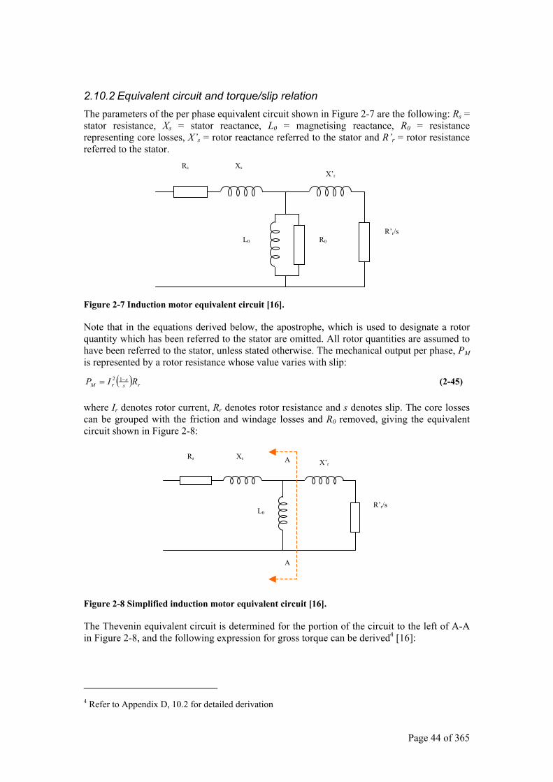
Page 44 of 365

2.10.2 Equivalent circuit and torque/slip relation The parameters of the per phase equivalent circuit shown in Figure 2-7 are the following: Rs = stator resistance, Xs = stator reactance, L0 = magnetising reactance, R0 = resistance representing core losses, X’s = rotor reactance referred to the stator and R’r = rotor resistance referred to the stator.

Figure 2-7 Induction motor equivalent circuit [16].

Note that in the equations derived below, the apostrophe, which is used to designate a rotor quantity which has been referred to the stator are omitted. All rotor quantities are assumed to have been referred to the stator, unless stated otherwise. The mechanical output per phase, PM is represented by a rotor resistance whose value varies with slip:

( ) rss

rM RIP −= 12 (2-45)

where Ir denotes rotor current, Rr denotes rotor resistance and s denotes slip. The core losses can be grouped with the friction and windage losses and R0 removed, giving the equivalent circuit shown in Figure 2-8:

Figure 2-8 Simplified induction motor equivalent circuit [16].

The Thevenin equivalent circuit is determined for the portion of the circuit to the left of A-A in Figure 2-8, and the following expression for gross torque can be derived4 [16]:

4 Refer to Appendix D, 10.2 for detailed derivation

Rs Xs

R’r/s

X’r

L0 R0

Rs Xs

R’r/s

X’r

L0

A

A

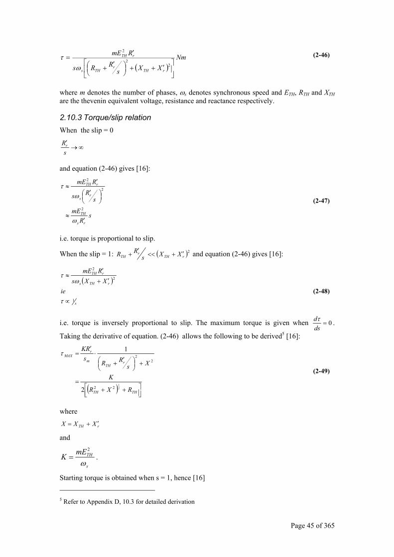
Page 45 of 365

( )Nm

XXsRRs

RmE

rTHr

THs

rTH

′++

′+

′=

22

2

ωτ (2-46)

where m denotes the number of phases, ωs denotes synchronous speed and ETH, RTH and XTH are the thevenin equivalent voltage, resistance and reactance respectively.

2.10.3 Torque/slip relation When the slip = 0

∞→′

sRr

and equation (2-46) gives [16]:

sR

mE

sRs

RmE

rs

TH

rs

rTH

′≈

′

′≈

ω

ωτ

2

2

2

(2-47)

i.e. torque is proportional to slip.

When the slip = 1: ( )2rTH

rTH XXs

RR ′+<<′+ and equation (2-46) gives [16]:

( )

s

rTHs

rTH

ieXXs

RmE

1

2

2

∝

′+

′≈

τ

ωτ

(2-48)

i.e. torque is inversely proportional to slip. The maximum torque is given when 0=dsdτ .

Taking the derivative of equation. (2-46) allows the following to be derived5 [16]:

( )

++

=

+

′+

⋅′

=

THTH

rTH

m

rMAX

RXR

K

XsRR

sRK

21

22

22

2

1τ

(2-49)

where

rTH XXX ′+=

and

s

THmEKω

2

= .

Starting torque is obtained when s = 1, hence [16]

5 Refer to Appendix D, 10.3 for detailed derivation

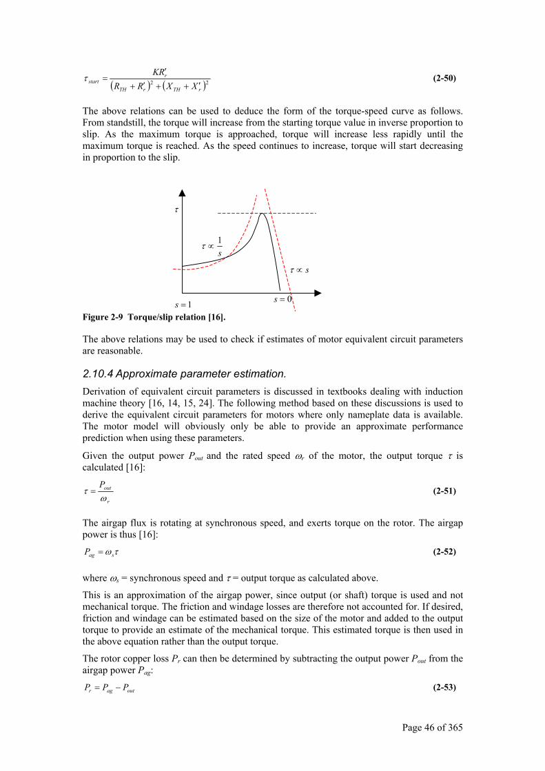
Page 46 of 365

( ) ( )22rTHrTH

rstart XXRR

RK′++′+

′=τ (2-50)

The above relations can be used to deduce the form of the torque-speed curve as follows. From standstill, the torque will increase from the starting torque value in inverse proportion to slip. As the maximum torque is approached, torque will increase less rapidly until the maximum torque is reached. As the speed continues to increase, torque will start decreasing in proportion to the slip.

Figure 2-9 Torque/slip relation [16].

The above relations may be used to check if estimates of motor equivalent circuit parameters are reasonable.

2.10.4 Approximate parameter estimation. Derivation of equivalent circuit parameters is discussed in textbooks dealing with induction machine theory [16, 14, 15, 24]. The following method based on these discussions is used to derive the equivalent circuit parameters for motors where only nameplate data is available. The motor model will obviously only be able to provide an approximate performance prediction when using these parameters.

Given the output power Pout and the rated speed ωr of the motor, the output torque τ is calculated [16]:

r

outPω

τ = (2-51)

The airgap flux is rotating at synchronous speed, and exerts torque on the rotor. The airgap power is thus [16]:

τωsagP = (2-52)

where ωs = synchronous speed and τ = output torque as calculated above.

This is an approximation of the airgap power, since output (or shaft) torque is used and not mechanical torque. The friction and windage losses are therefore not accounted for. If desired, friction and windage can be estimated based on the size of the motor and added to the output torque to provide an estimate of the mechanical torque. This estimated torque is then used in the above equation rather than the output torque.

The rotor copper loss Pr can then be determined by subtracting the output power Pout from the airgap power Pag:

outagr PPP −= (2-53)

s1

∝τ

s∝τ

τ

1=s 0=s

Page 47 of 365

The approximate stator power loss (copper and iron losses) is estimated by subtracting the airgap power from the input power Pin:

agss

aginstator

PIV

PPP

−=

−=

3 (2-54)

It is further assumed that all stator losses are due to the stator winding resistance. Iron losses are thus included with the stator copper losses. The stator resistance can be calculated as follows:

23 fl

stators I

PR = (2-55)

where Ifl denotes motor full load current. At full load, the equivalent circuit input impedance is given by [16]:

jXR

IV

Zfl

phasein

+=

=)cos(2 ϕ (2-56)

where, from Figure 2-8. the following equations are derived if it is assumed that the impedance of L0 is high enough to be considered an open circuit.

sRRR r

s′

+= (2-57)

and

rs XXX ′+= . (2-58)

The slip can be calculated at rated speed allowing the rotor resistance to be calculated. For Nema type motors, the relationship between stator and rotor reactances can be estimated from the following table: Table 2-1 Rotor/stator reactances for nema motors [24].

The no-load current is usually specified, or can be easily determined allowing L0 and R0 to be estimated. The rotor current is assumed to be negligible allowing the following simplified equivalent circuit to be derived from Figure 2-86 where Vl = nominal line voltage and Rs, Xs are stator parameters as derived above:

6 Note, that the core losses were grouped with the stator copper losses and R0 omitted in Figure 2-8. Here core losses are represented by R0 in parallel with L0 giving the impedance

00

000 jXR

jXRZ += .

Nema Type Stator Reactance Rotor Reactance Class A, D & wound rotor 0.5X 0.5X Class B 0.4X 0.6X Class C 0.3X 0.7X

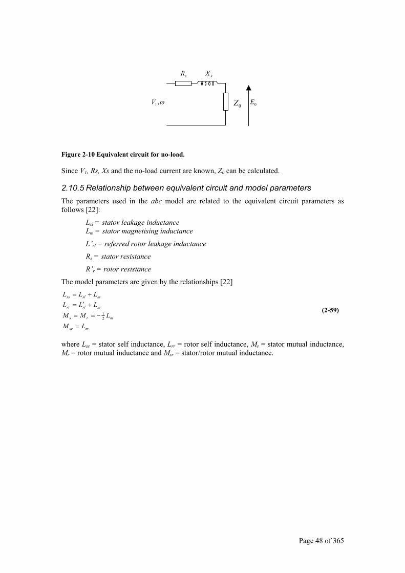
Page 48 of 365

Figure 2-10 Equivalent circuit for no-load.

Since V1, Rs, Xs and the no-load current are known, Z0 can be calculated.

2.10.5 Relationship between equivalent circuit and model parameters The parameters used in the abc model are related to the equivalent circuit parameters as follows [22]:

Lsl = stator leakage inductance Lm = stator magnetising inductance

L’rl = referred rotor leakage inductance

Rs = stator resistance

R’r = rotor resistance

The model parameters are given by the relationships [22]

msr

mrs

mrlrr

mslss

LMLMM

LLLLLL

=

−==

+′=+=

21

(2-59)

where Lss = stator self inductance, Lrr = rotor self inductance, Ms = stator mutual inductance, Mr = rotor mutual inductance and Msr = stator/rotor mutual inductance.

ω,1V

sR sX

0Z 0E

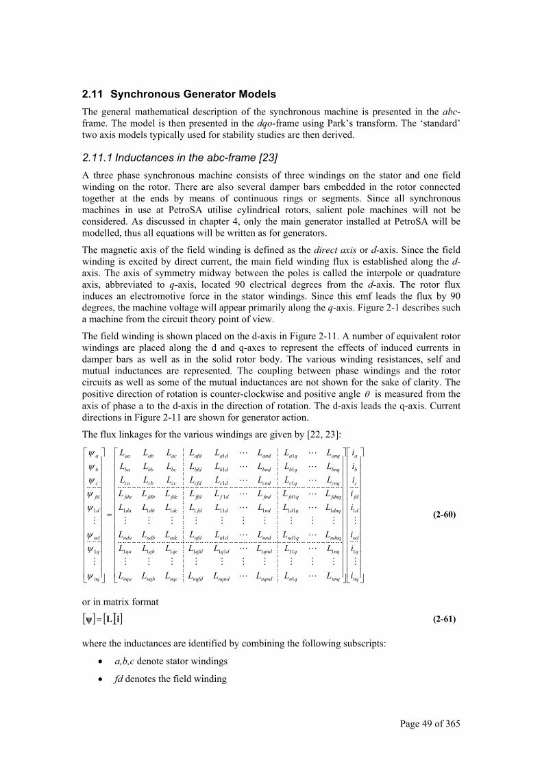
Page 49 of 365

2.11 Synchronous Generator Models The general mathematical description of the synchronous machine is presented in the abc-frame. The model is then presented in the dqo-frame using Park’s transform. The ‘standard’ two axis models typically used for stability studies are then derived.

2.11.1 Inductances in the abc-frame [23] A three phase synchronous machine consists of three windings on the stator and one field winding on the rotor. There are also several damper bars embedded in the rotor connected together at the ends by means of continuous rings or segments. Since all synchronous machines in use at PetroSA utilise cylindrical rotors, salient pole machines will not be considered. As discussed in chapter 4, only the main generator installed at PetroSA will be modelled, thus all equations will be written as for generators.

The magnetic axis of the field winding is defined as the direct axis or d-axis. Since the field winding is excited by direct current, the main field winding flux is established along the d-axis. The axis of symmetry midway between the poles is called the interpole or quadrature axis, abbreviated to q-axis, located 90 electrical degrees from the d-axis. The rotor flux induces an electromotive force in the stator windings. Since this emf leads the flux by 90 degrees, the machine voltage will appear primarily along the q-axis. Figure 2-1 describes such a machine from the circuit theory point of view.

The field winding is shown placed on the d-axis in Figure 2-11. A number of equivalent rotor windings are placed along the d and q-axes to represent the effects of induced currents in damper bars as well as in the solid rotor body. The various winding resistances, self and mutual inductances are represented. The coupling between phase windings and the rotor circuits as well as some of the mutual inductances are not shown for the sake of clarity. The positive direction of rotation is counter-clockwise and positive angle θ is measured from the axis of phase a to the d-axis in the direction of rotation. The d-axis leads the q-axis. Current directions in Figure 2-11 are shown for generator action.

The flux linkages for the various windings are given by [22, 23]:

=

nq

q

nd

d

fd

c

b

a

nnqqnnqndnqndnqfdnqcnqbnqa

nqqqnddqqfdqcqbqa

ndnqqndnnddnnfdndcndbnda

dnqqdnddfddcdbda

fdnqqfdfnddfffdfdcfdbfda

cnqqccnddccfdcccbca

bnqqbbnddbbfdbcbbba

anqqaanddaafdacabaa

nq

q

nd

d

fd

c

b

a

i

ii

iiiii

LLLLLLLL

LLLLLLLLLLLLLLLL

LLLLLLLLLLLLLLLLLLLLLLLLLLLLLLLLLLLLLLLL

1

1

1

1111111111

11

1111111111

11

11

11

11

1

1

ψ

ψψ

ψψψψψ

(2-60)

or in matrix format

[ ] [ ][ ]iLψ = (2-61)

where the inductances are identified by combining the following subscripts:

• a,b,c denote stator windings

• fd denotes the field winding

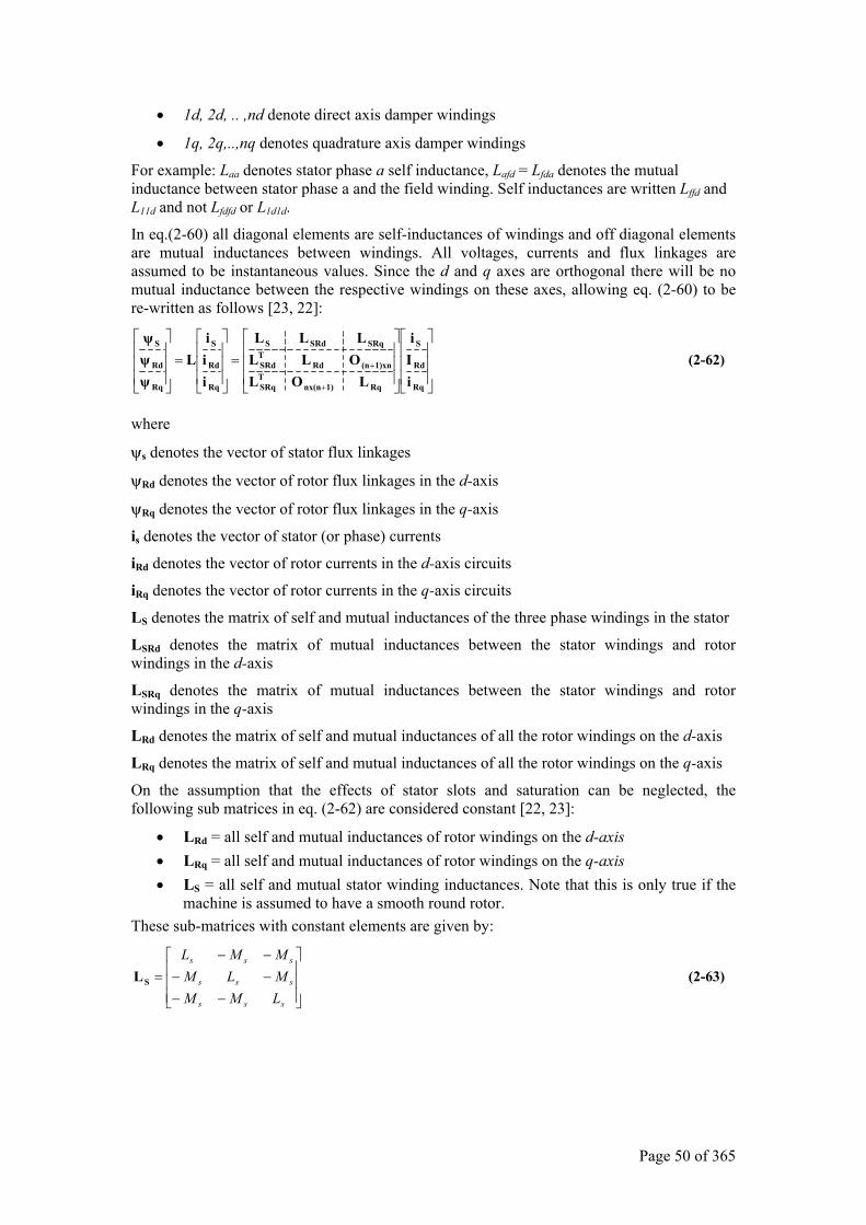
Page 50 of 365

• 1d, 2d, .. ,nd denote direct axis damper windings

• 1q, 2q,..,nq denotes quadrature axis damper windings

For example: Laa denotes stator phase a self inductance, Lafd = Lfda denotes the mutual inductance between stator phase a and the field winding. Self inductances are written Lffd and L11d and not Lfdfd or L1d1d.

In eq.(2-60) all diagonal elements are self-inductances of windings and off diagonal elements are mutual inductances between windings. All voltages, currents and flux linkages are assumed to be instantaneous values. Since the d and q axes are orthogonal there will be no mutual inductance between the respective windings on these axes, allowing eq. (2-60) to be re-written as follows [23, 22]:

=

=

+

+

Rq

Rd

S

Rq1)nx(nTSRq

1)xn(nRdTSRd

SRqSRdS

Rq

Rd

S

Rq

Rd

S

iIi

LOLOLL

LLL

iii

Lψψψ

(2-62)

where

ψs denotes the vector of stator flux linkages

ψRd denotes the vector of rotor flux linkages in the d-axis

ψRq denotes the vector of rotor flux linkages in the q-axis

is denotes the vector of stator (or phase) currents

iRd denotes the vector of rotor currents in the d-axis circuits

iRq denotes the vector of rotor currents in the q-axis circuits

LS denotes the matrix of self and mutual inductances of the three phase windings in the stator

LSRd denotes the matrix of mutual inductances between the stator windings and rotor windings in the d-axis

LSRq denotes the matrix of mutual inductances between the stator windings and rotor windings in the q-axis

LRd denotes the matrix of self and mutual inductances of all the rotor windings on the d-axis

LRq denotes the matrix of self and mutual inductances of all the rotor windings on the q-axis

On the assumption that the effects of stator slots and saturation can be neglected, the following sub matrices in eq. (2-62) are considered constant [22, 23]:

• LRd = all self and mutual inductances of rotor windings on the d-axis • LRq = all self and mutual inductances of rotor windings on the q-axis • LS = all self and mutual stator winding inductances. Note that this is only true if the

machine is assumed to have a smooth round rotor. These sub-matrices with constant elements are given by:

−−−−−−

=

sss

sss

sss

LMMMLMMML

SL (2-63)

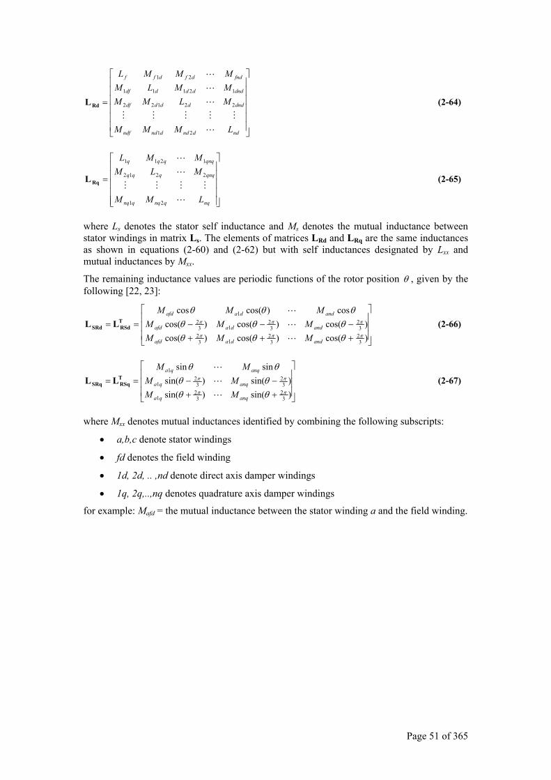
Page 51 of 365

=

nddnddndndf

dndddddf

dndddddf

fnddfdff

LMMM

MLMMMMLMMMML

21

22122

12111

21

RdL (2-64)

=

nqqnqqnq

qnqqqq

qnqqqq

LMM

MLMMML

21

2212

1211

RqL (2-65)

where Ls denotes the stator self inductance and Ms denotes the mutual inductance between stator windings in matrix Ls. The elements of matrices LRd and LRq are the same inductances as shown in equations (2-60) and (2-62) but with self inductances designated by Lxx and mutual inductances by Mxx.

The remaining inductance values are periodic functions of the rotor position θ , given by the following [22, 23]:

+++−−−==

)cos()cos()cos()cos()cos()cos(

cos)cos(cos

32

32

132

32

32

132

1

πππ

πππ

θθθθθθ

θθθ

anddaafd

anddaafd

anddaafd

MMMMMM

MMMTRSdSRd LL (2-66)

++−−==

)sin()sin()sin()sin(

sinsin

32

32

1

32

32

1

1

ππ

ππ

θθθθ

θθ

anqqa

anqqa

anqqa

MMMM

MMTRSqSRq LL (2-67)

where Mxx denotes mutual inductances identified by combining the following subscripts:

• a,b,c denote stator windings

• fd denotes the field winding

• 1d, 2d, .. ,nd denote direct axis damper windings

• 1q, 2q,..,nq denotes quadrature axis damper windings

for example: Mafd = the mutual inductance between the stator winding a and the field winding.

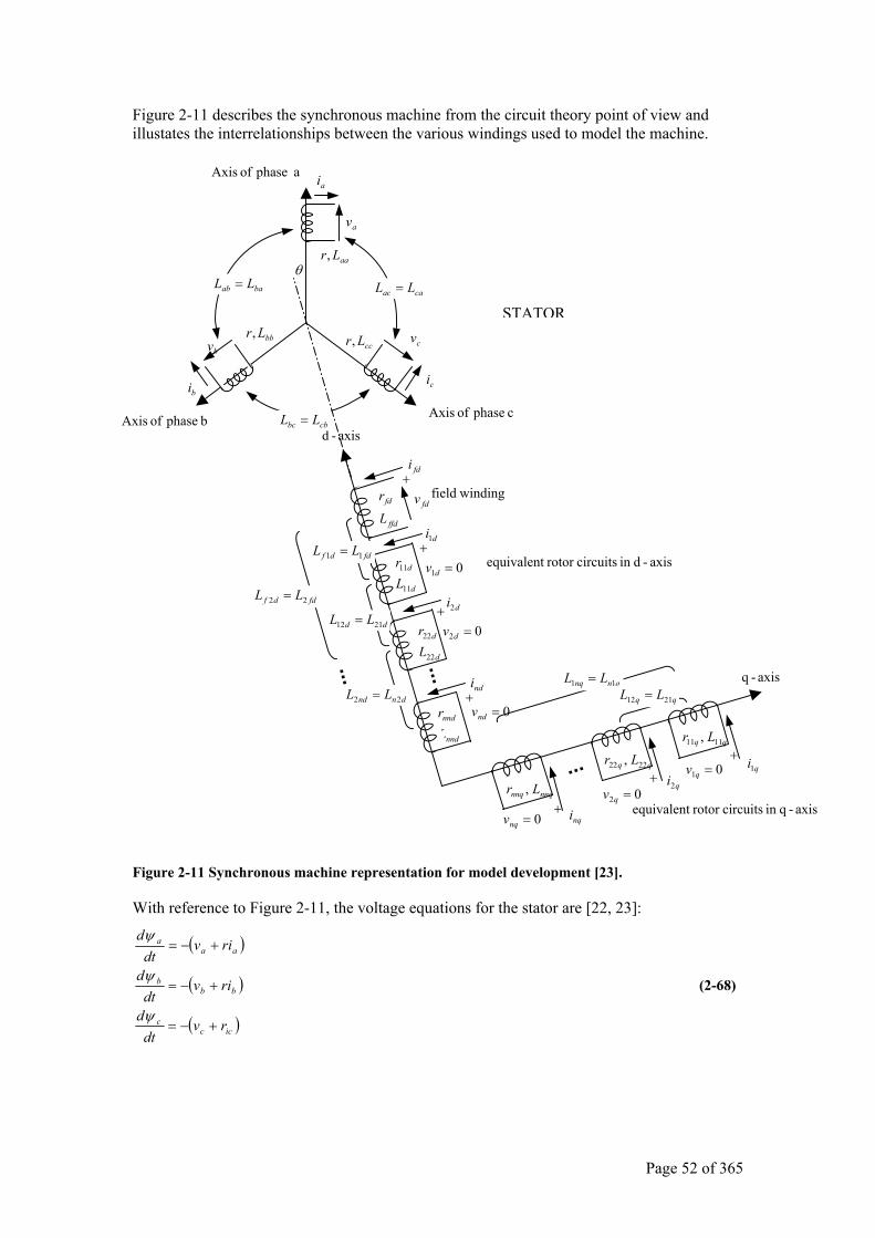
Page 52 of 365

Figure 2-11 describes the synchronous machine from the circuit theory point of view and illustates the interrelationships between the various windings used to model the machine.

Figure 2-11 Synchronous machine representation for model development [23].

With reference to Figure 2-11, the voltage equations for the stator are [22, 23]:

( )

( )

( )iccc

bbb

aaa

rvdt

d

rivdt

d

rivdt

d

+−=

+−=

+−=

ψ

ψ

ψ

(2-68)

ffd

fd

L

r

d

d

Lr

22

22

nnd

nnd

Lr

fdi

di1

di2

ndi

nqi

qi2

qi1

fdv

01 =dv

02 =dv

0=ndv

0=nqv

02 =qv

01 =qv

qnnq LL 11 =

axis-d

axis-q

windingfield

axis-qin circuitsrotor equivalent

axis -din circuitsrotor equivalent

+

+

+

+

+

+

+

d

d

Lr

11

11fddf LL 11 =

dd LL 2112 =fddf LL 22 =

dnnd LL 22 =

qq Lr 1111 ,

qq Lr 2222 ,

qq LL 2112 =

nnqnnq Lr ,

aaLr,

ccLr,bbLr,

baab LL =

cbbc LL =

caac LL =

av

bv cv

ai

bi ci

STATOR

θ

a phase of Axis

b phase of Axis c phase of Axis

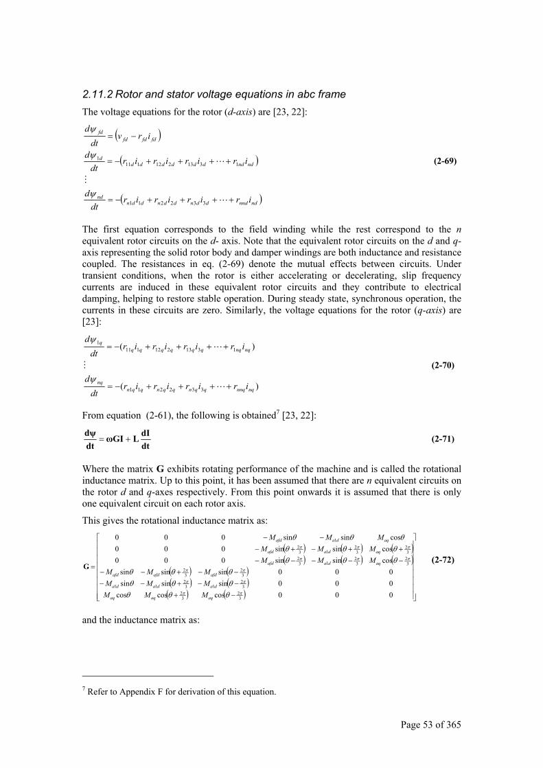
Page 53 of 365

2.11.2 Rotor and stator voltage equations in abc frame The voltage equations for the rotor (d-axis) are [23, 22]:

( )

( )

( )ndnndddnddnddnnd

ndndddddddd

fdfdfdfd

iriririrdt

d

iriririrdt

d

irvdt

d

++++−=

++++−=

−=

332211

13132121111

ψ

ψ

ψ

(2-69)

The first equation corresponds to the field winding while the rest correspond to the n equivalent rotor circuits on the d- axis. Note that the equivalent rotor circuits on the d and q-axis representing the solid rotor body and damper windings are both inductance and resistance coupled. The resistances in eq. (2-69) denote the mutual effects between circuits. Under transient conditions, when the rotor is either accelerating or decelerating, slip frequency currents are induced in these equivalent rotor circuits and they contribute to electrical damping, helping to restore stable operation. During steady state, synchronous operation, the currents in these circuits are zero. Similarly, the voltage equations for the rotor (q-axis) are [23]:

)(

)(

332211

13132121111

nqnnqqqnqqnqqnnq

nqnqqqqqqqq

iriririrdt

d

iriririrdt

d

++++−=

++++−=

ψ

ψ

(2-70)

From equation (2-61), the following is obtained7 [23, 22]:

dtdILωGI

dtdψ

+= (2-71)

Where the matrix G exhibits rotating performance of the machine and is called the rotational inductance matrix. Up to this point, it has been assumed that there are n equivalent circuits on the rotor d and q-axes respectively. From this point onwards it is assumed that there is only one equivalent circuit on each rotor axis.

This gives the rotational inductance matrix as:

( ) ( ) ( )( ) ( ) ( )

( ) ( )( ) ( )

( ) ( )

−+−−+−−−−+−−

−−−−−++−+−

−−

=

000coscoscos000sinsinsin000sinsinsin

cossinsin000cossinsin000

cossinsin000

32

32

32

132

11

32

32

32

32

132

32

32

132

1

ππ

ππ

ππ

πππ

πππ

θθθθθθθθθ

θθθθθθ

θθθ

aqaqaq

dadada

afdafdafd

aqdaafd

aqdaafd

aqdaafd

MMMMMMMMM

MMMMMM

MMM

G (2-72)

and the inductance matrix as:

7 Refer to Appendix F for derivation of this equation.

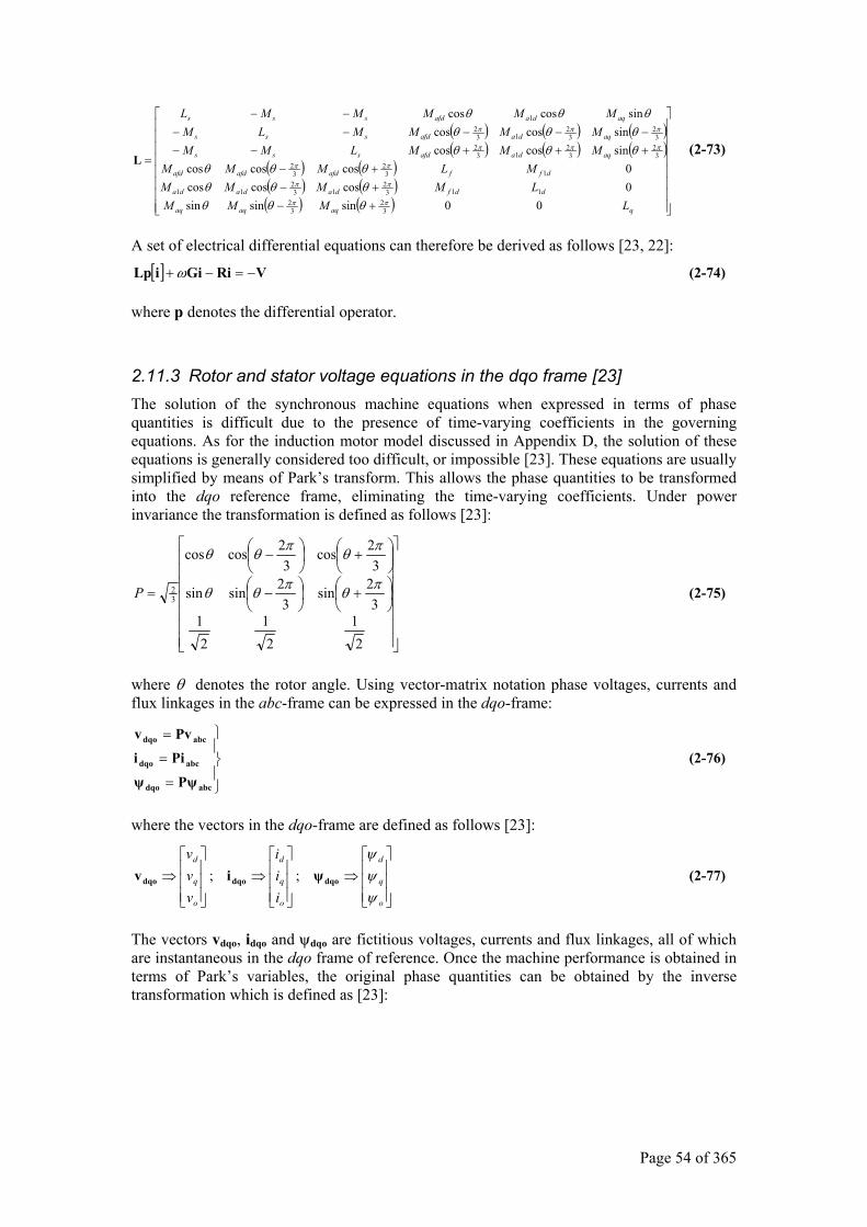
Page 54 of 365

( ) ( ) ( )( ) ( ) ( )

( ) ( )( ) ( )( ) ( )

+−+−+−

+++−−−−−−−

−−

=

qaqaqaq

ddfdadada

dffafdafdafd

aqdaafdsss

aqdaafdsss

aqdaafdsss

LMMMLMMMM

MLMMMMMMLMMMMMMLM

MMMMML

00sinsinsin0coscoscos0coscoscos

sincoscossincoscos

sincoscos

32

32

1132

132

11

132

32

32

32

132

32

32

132

1

ππ

ππ

ππ

πππ

πππ

θθθθθθθθθ

θθθθθθ

θθθ

L (2-73)

A set of electrical differential equations can therefore be derived as follows [23, 22]:

[ ] VRiGiiLp −=−+ ω (2-74)

where p denotes the differential operator.

2.11.3 Rotor and stator voltage equations in the dqo frame [23] The solution of the synchronous machine equations when expressed in terms of phase quantities is difficult due to the presence of time-varying coefficients in the governing equations. As for the induction motor model discussed in Appendix D, the solution of these equations is generally considered too difficult, or impossible [23]. These equations are usually simplified by means of Park’s transform. This allows the phase quantities to be transformed into the dqo reference frame, eliminating the time-varying coefficients. Under power invariance the transformation is defined as follows [23]:

+

−

+

−

=

21

21

21

32sin

32sinsin

32cos

32coscos

32 πθπθθ

πθπθθ

P (2-75)

where θ denotes the rotor angle. Using vector-matrix notation phase voltages, currents and flux linkages in the abc-frame can be expressed in the dqo-frame:

=

=

=

abcdqo

abcdqo

abcdqo

Pψψ

Pii

Pvv

(2-76)

where the vectors in the dqo-frame are defined as follows [23]:

⇒

⇒

⇒

o

q

d

o

q

d

o

q

d

iii

vvv

ψψψ

dqodqodqo ψiv ;; (2-77)

The vectors vdqo, idqo and ψdqo are fictitious voltages, currents and flux linkages, all of which are instantaneous in the dqo frame of reference. Once the machine performance is obtained in terms of Park’s variables, the original phase quantities can be obtained by the inverse transformation which is defined as [23]:

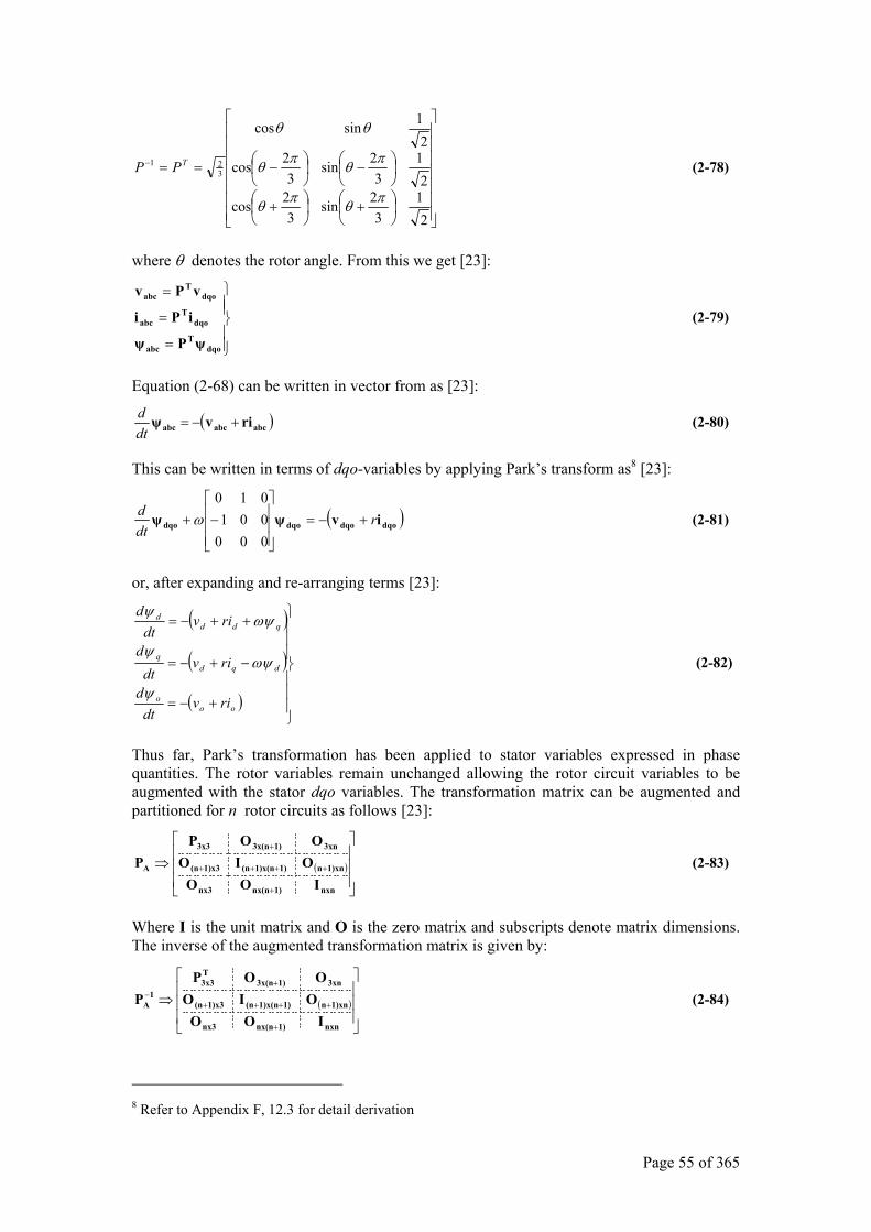
Page 55 of 365

+

+

−

−==−

21

32sin

32cos

21

32sin

32cos

21sincos

321

πθπθ

πθπθ

θθ

TPP (2-78)

where θ denotes the rotor angle. From this we get [23]:

=

=

=

dqoT

abc

dqoT

abc

dqoT

abc

ψPψ

iPi

vPv

(2-79)

Equation (2-68) can be written in vector from as [23]:

( )abcabcabc rivψ +−=dtd (2-80)

This can be written in terms of dqo-variables by applying Park’s transform as8 [23]:

( )dqodqodqodqo ivψψ rdtd

+−=

−+

000001010

ω (2-81)

or, after expanding and re-arranging terms [23]:

( )

( )

( )

+−=

−+−=

++−=

ooo

dqdq

qddd

rivdt

d

rivdt

d

rivdt

d

ψ

ωψψ

ωψψ

(2-82)

Thus far, Park’s transformation has been applied to stator variables expressed in phase quantities. The rotor variables remain unchanged allowing the rotor circuit variables to be augmented with the stator dqo variables. The transformation matrix can be augmented and partitioned for n rotor circuits as follows [23]:

( )

⇒

+

++++

+

nxn1)nx(nnx3

1)xnn1)1)x(n(n1)x3(n

3xn1)3x(n3x3

A

IOOOIO

OOPP (2-83)

Where I is the unit matrix and O is the zero matrix and subscripts denote matrix dimensions. The inverse of the augmented transformation matrix is given by:

( )

⇒

+

++++

+−

nxn1)nx(nnx3

1)xnn1)1)x(n(n1)x3(n

3xn1)3x(nT3x3

1A

IOOOIO

OOPP (2-84)

8 Refer to Appendix F, 12.3 for detail derivation

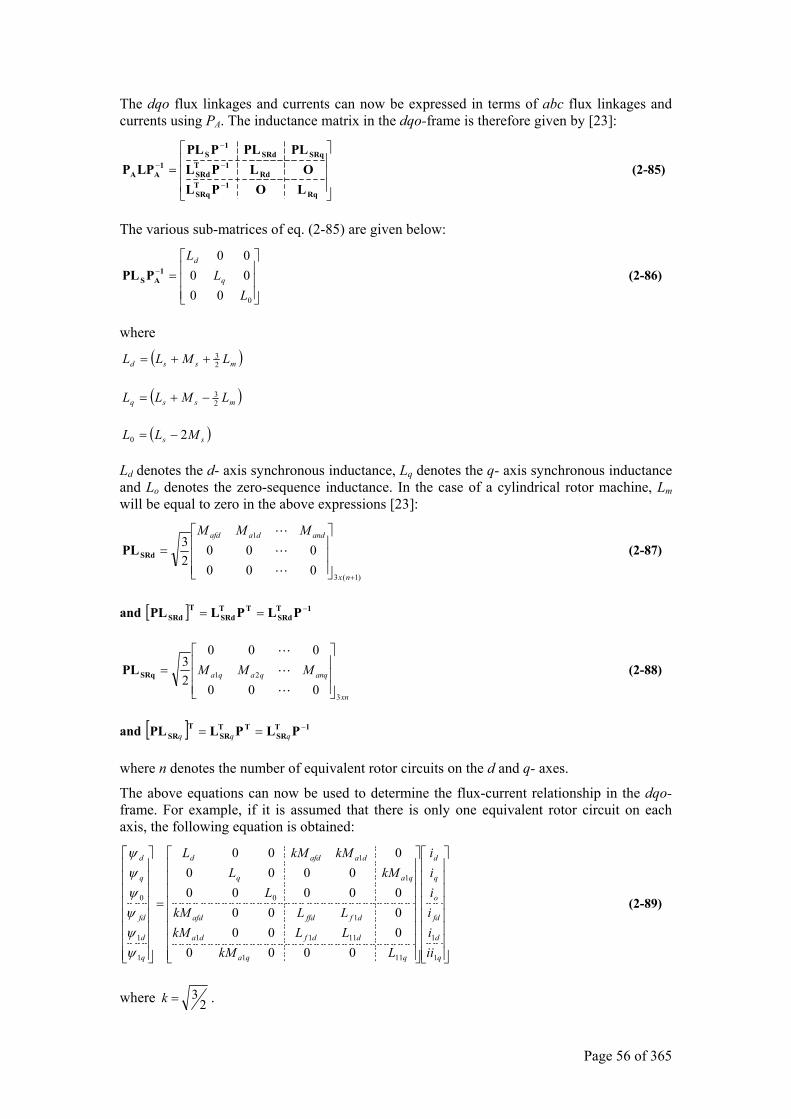
Page 56 of 365

The dqo flux linkages and currents can now be expressed in terms of abc flux linkages and currents using PA. The inductance matrix in the dqo-frame is therefore given by [23]:

=−

−

−

−

Rq1T

SRq

Rd1T

SRd

SRqSRd1

S1

AA

LOPLOLPL

PLPLPPLLPP (2-85)

The various sub-matrices of eq. (2-85) are given below:

=−

0000000

LL

L

q

d1

ASPPL (2-86)

where

( )mssd LMLL 23++=

( )mssq LMLL 23−+=

( )ss MLL 20 −=

Ld denotes the d- axis synchronous inductance, Lq denotes the q- axis synchronous inductance and Lo denotes the zero-sequence inductance. In the case of a cylindrical rotor machine, Lm will be equal to zero in the above expressions [23]:

)1(3

1

000000

23

+

=

nx

anddaafd MMM

SRdPL (2-87)

and [ ] 1TSRd

TTSRd

TSRd PLPLPL −==

xn

anqqaqa MMM

3

21

000

000

23

=SRqPL (2-88)

and [ ] 1TSR

TTSR

TSR PLPLPL −== qqq

where n denotes the number of equivalent rotor circuits on the d and q- axes.

The above equations can now be used to determine the flux-current relationship in the dqo-frame. For example, if it is assumed that there is only one equivalent rotor circuit on each axis, the following equation is obtained:

=

q

d

fd

o

q

d

qqa

ddfda

dfffdafd

qaq

daafdd

q

d

fd

q

d

iiiiiii

LkMLLkMLLkM

LkML

kMkML

1

1

111

1111

1

0

1

1

1

1

0

000000000000000

0000000

ψψψψψψ

(2-89)

where 23=k .

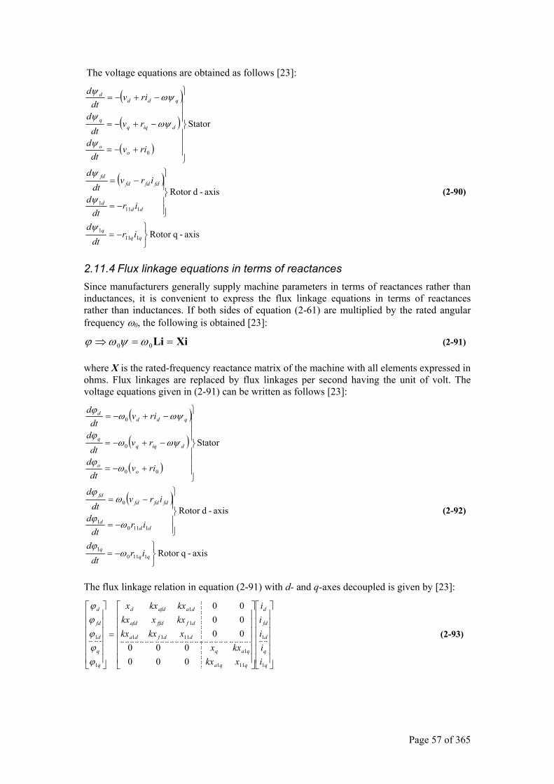
Page 57 of 365

The voltage equations are obtained as follows [23]:

( )

( )

( )

( )

axis-qRotor

axis-dRotor

Stator

1111

1111

0

−=

−=

−=

+−=

−+−=

−+−=

qqq

ddd

fdfdfdfd

oo

diqqq

qddd

irdt

d

irdt

d

irvdt

d

rivdt

d

rvdt

d

rivdt

d

ψ

ψ

ψ

ψ

ωψψ

ωψψ

(2-90)

2.11.4 Flux linkage equations in terms of reactances Since manufacturers generally supply machine parameters in terms of reactances rather than inductances, it is convenient to express the flux linkage equations in terms of reactances rather than inductances. If both sides of equation (2-61) are multiplied by the rated angular frequency ω0, the following is obtained [23]:

XiLi ==⇒ 00 ωψωϕ (2-91)

where X is the rated-frequency reactance matrix of the machine with all elements expressed in ohms. Flux linkages are replaced by flux linkages per second having the unit of volt. The voltage equations given in (2-91) can be written as follows [23]:

( )

( )

( )

( )

axis-qRotor

axis-dRotor

Stator

11101

11101

0

00

0

0

−=

−=

−=

+−=

−+−=

−+−=

qqq

ddd

fdfdfdfd

oo

diqqq

qddd

irdt

d

irdt

d

irvdt

d

rivdt

d

rvdt

d

rivdt

d

ωϕ

ωϕ

ωϕ

ωϕ

ωψωϕ

ωψωϕ

(2-92)

The flux linkage relation in equation (2-91) with d- and q-axes decoupled is given by [23]:

=

q

q

d

fd

d

qqa

qaq

ddfda

dfffdafd

daafdd

q

q

d

fd

d

iiiii

xkxkxx

xkxkxkxxkxkxkxx

1

1

111

1

1111

1

1

1

1

000000

000000

ϕϕϕϕϕ

(2-93)

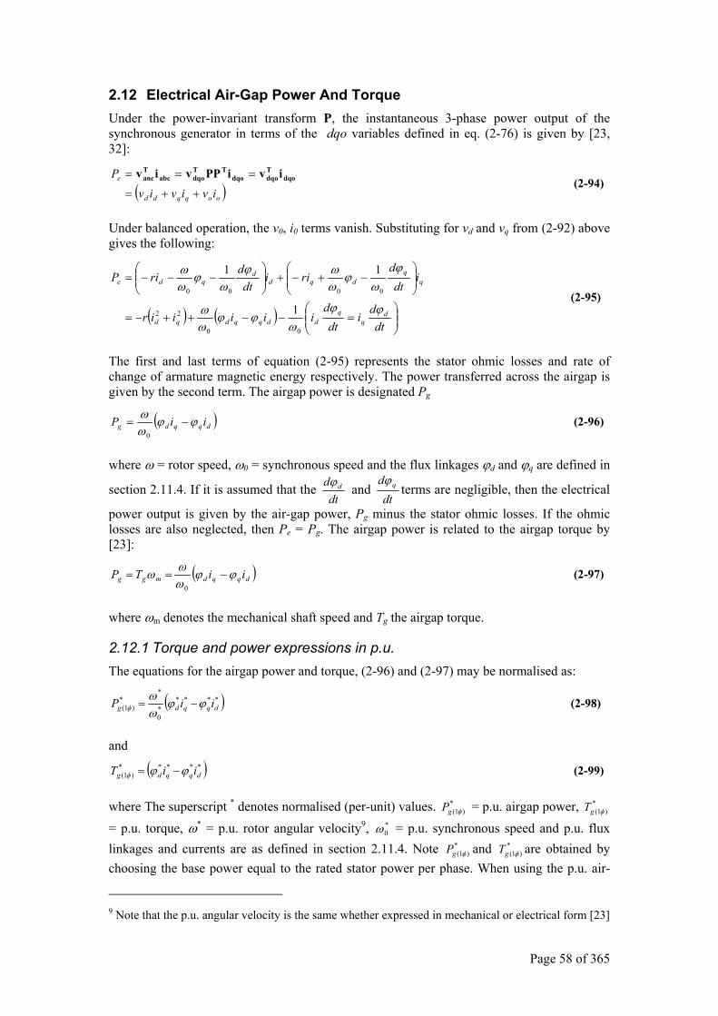
Page 58 of 365

2.12 Electrical Air-Gap Power And Torque Under the power-invariant transform P, the instantaneous 3-phase power output of the synchronous generator in terms of the dqo variables defined in eq. (2-76) is given by [23, 32]:

( )ooqqdd

e

iviviv

P

++=

=== dqoTdqodqo

TTdqoabc

Tanc iviPPviv

(2-94)

Under balanced operation, the v0, i0 terms vanish. Substituting for vd and vq from (2-92) above gives the following:

( ) ( )

=−−++−=

−+−+

−−−=

dtd

idt

diiiiir

idt

drii

dtd

riP

dq

qddqqdqd

qq

dqdd

qde

ϕϕω

ϕϕωω

ϕω

ϕωωϕ

ωϕ

ωω

00

22

0000

1

11

(2-95)

The first and last terms of equation (2-95) represents the stator ohmic losses and rate of change of armature magnetic energy respectively. The power transferred across the airgap is given by the second term. The airgap power is designated Pg

( )dqqdg iiP ϕϕωω

−=0

(2-96)

where ω = rotor speed, ω0 = synchronous speed and the flux linkages ϕd and ϕq are defined in

section 2.11.4. If it is assumed that the dt

d dϕ and dt

d qϕterms are negligible, then the electrical

power output is given by the air-gap power, Pg minus the stator ohmic losses. If the ohmic losses are also neglected, then Pe = Pg. The airgap power is related to the airgap torque by [23]:

( )dqqdmgg iiTP ϕϕωωω −==

0

(2-97)

where ωm denotes the mechanical shaft speed and Tg the airgap torque.

2.12.1 Torque and power expressions in p.u. The equations for the airgap power and torque, (2-96) and (2-97) may be normalised as:

( )*****0

**

)1( dqqdg iiP ϕϕωω

φ −= (2-98)

and

( )*****)1( dqqdg iiT ϕϕφ −= (2-99)

where The superscript * denotes normalised (per-unit) values. *)1( φgP = p.u. airgap power, *

)1( φgT = p.u. torque, ω* = p.u. rotor angular velocity9, *

0ω = p.u. synchronous speed and p.u. flux linkages and currents are as defined in section 2.11.4. Note *

)1( φgP and *)1( φgT are obtained by

choosing the base power equal to the rated stator power per phase. When using the p.u. air-

9 Note that the p.u. angular velocity is the same whether expressed in mechanical or electrical form [23]

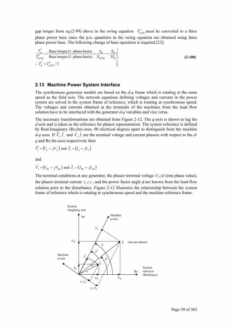
Page 59 of 365

gap torque from eq.(2-99) above in the swing equation *)1( φgT must be converted to a three

phase power base since the p.u. quantities in the swing equation are obtained using three phase power base. The following change of base operation is required [23]:

=∴

===

3/

3basis) phase-(3 torqueBasebasis) phase-(1 torqueBase

*)1(

*

)3(*

)1(

*

φ

φφ

gg

B

B

B

B

g

g

TT

SS

SS

TT

(2-100)

2.13 Machine Power System Interface The synchronous generator models are based on the d-q frame which is rotating at the same speed as the field axis. The network equations defining voltages and currents in the power system are solved in the system frame of reference, which is rotating at synchronous speed. The voltages and currents obtained at the terminals of the machines from the load flow solution have to be interfaced with the generator d-q variables and vice versa.

The necessary transformations are obtained from Figure 2-12. The q-axis is shown to lag the d-axis and is taken as the reference for phasor representation. The system reference is defined by Real-Imaginary (Re,Im) axes, 90 electrical degrees apart to distinguish from the machine d-q axes. If tt IV , and tt IV ˆ,ˆ are the terminal voltage and current phasors with respect to the d-q and Re-Im axes respectively then

( ) ( )dqtdqt jIIIjVVV +=+= and

and

( ) ( )ImReImReˆ and ˆ jIIIjVVV tt +=+=

The terminal conditions at any generator, the phasor terminal voltage β∠tV (rms phase value), the phasor terminal current γ∠tI , and the power factor angle φ are known from the load-flow solution prior to the disturbance. Figure 2-12 illustrates the relationship between the system frame of reference which is rotating at synchronous speed and the machine reference frame.

γ

Machine d-axis

IRe VRe

Re

System real-axis (Reference)

Machine q-axis

VIM

IIm

Vq

Im

φ tI

(-) Id

(-) Vd

tV

δ’

δ

β

(rms per phase)

System imaginary axis

Iq

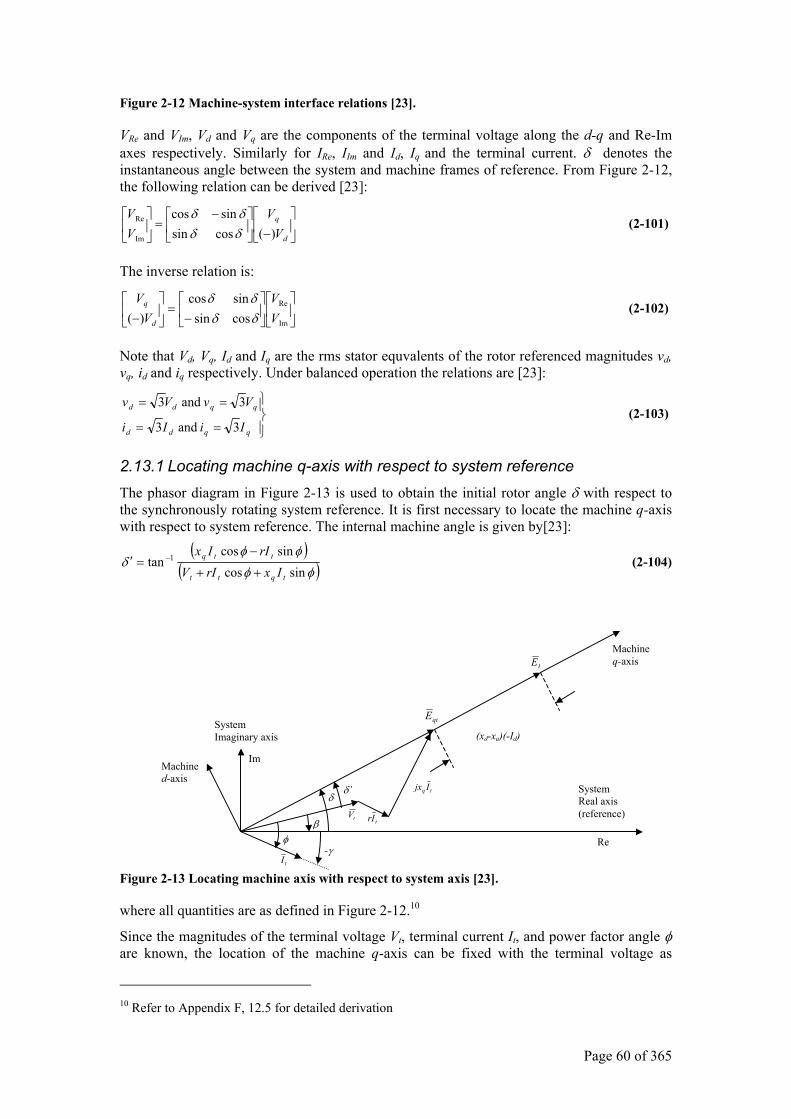
Page 60 of 365

Figure 2-12 Machine-system interface relations [23].

VRe and VIm, Vd and Vq are the components of the terminal voltage along the d-q and Re-Im axes respectively. Similarly for IRe, IIm and Id, Iq and the terminal current. δ denotes the instantaneous angle between the system and machine frames of reference. From Figure 2-12, the following relation can be derived [23]:

−

−=

d

q

VV

VV

)(cossinsincos

Im

Re

δδδδ

(2-101)

The inverse relation is:

−

=

− Im

Re

cossinsincos

)( VV

VV

d

q

δδδδ

(2-102)

Note that Vd, Vq, Id and Iq are the rms stator equvalents of the rotor referenced magnitudes vd, vq, id and iq respectively. Under balanced operation the relations are [23]:

==

==

qqdd

qqdd

IiIi

VvVv

3 and 3

3 and 3 (2-103)

2.13.1 Locating machine q-axis with respect to system reference The phasor diagram in Figure 2-13 is used to obtain the initial rotor angle δ with respect to the synchronously rotating system reference. It is first necessary to locate the machine q-axis with respect to system reference. The internal machine angle is given by[23]:

( )( )φφ

φφδ

sincossincos

tan 1

tqtt

ttq

IxrIVrIIx

++

−=′ − (2-104)

Figure 2-13 Locating machine axis with respect to system axis [23].

where all quantities are as defined in Figure 2-12.10

Since the magnitudes of the terminal voltage Vt, terminal current It, and power factor angle φ are known, the location of the machine q-axis can be fixed with the terminal voltage as

10 Refer to Appendix F, 12.5 for detailed derivation

System Imaginary axis

Machine d-axis

System Real axis (reference)

Im

Re

Machine q-axis

qtE

IE

tq Ijx

tIr

tI φ

-γ

β

δδ’

tV

(xd-xq)(-Id)

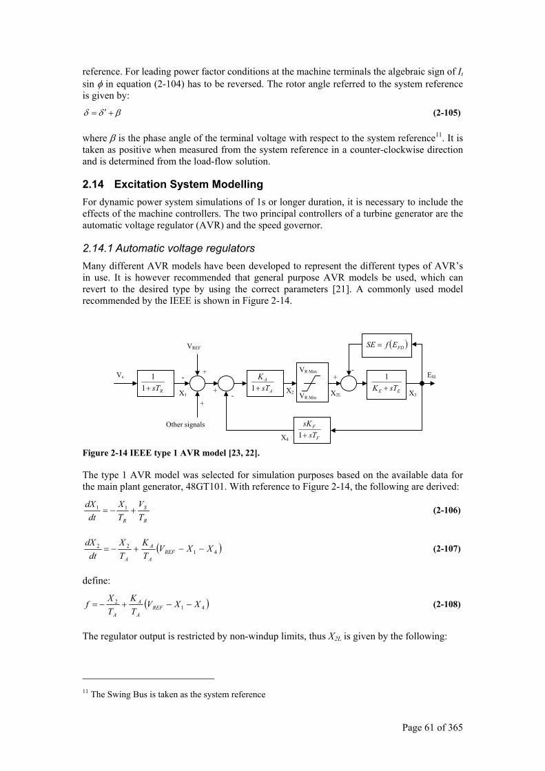
Page 61 of 365

reference. For leading power factor conditions at the machine terminals the algebraic sign of It sin φ in equation (2-104) has to be reversed. The rotor angle referred to the system reference is given by:

βδδ +′= (2-105)

where β is the phase angle of the terminal voltage with respect to the system reference11. It is taken as positive when measured from the system reference in a counter-clockwise direction and is determined from the load-flow solution.

2.14 Excitation System Modelling For dynamic power system simulations of 1s or longer duration, it is necessary to include the effects of the machine controllers. The two principal controllers of a turbine generator are the automatic voltage regulator (AVR) and the speed governor.

2.14.1 Automatic voltage regulators Many different AVR models have been developed to represent the different types of AVR’s in use. It is however recommended that general purpose AVR models be used, which can revert to the desired type by using the correct parameters [21]. A commonly used model recommended by the IEEE is shown in Figure 2-14.

Figure 2-14 IEEE type 1 AVR model [23, 22].

The type 1 AVR model was selected for simulation purposes based on the available data for the main plant generator, 48GT101. With reference to Figure 2-14, the following are derived:

R

S

R TV

TX

dtdX

+−= 11 (2-106)

( )4122 XXV

TK

TX

dtdX

REFA

A

A

−−+−= (2-107)

define:

( )412 XXV

TK

TX

f REFA

A

A

−−+−= (2-108)

The regulator output is restricted by non-windup limits, thus X2L is given by the following:

11 The Swing Bus is taken as the system reference

Vs RsT+1

1 X1

-

VREF

Other signals

+

+

+

A

A

sTK+1

X2

VR Max

VR Min

EE sTK +

1

( )FDEfSE =

-

F

F

sTsK+1

-

+

X3

Efd

X2L

X4

Page 62 of 365

• If MaxRVX ≥2 and f > 0, then dt

dX L2 is set to zero

• If MINRVX ≤2 and f < 0, then dt

dX L2 is set to zero

otherwise, fdt

dX L =2 for VR MIN < X2 < VR MAX

( )SEXT

ETK

dtdE

LE

fdE

Efd −+−= 21 (2-109)

The exciter saturation is specified at maximum field voltage Efdmax and at 0.75 of maximum field voltage Efd0.75 as per IEEE recommendations [21]. The exciter saturation function is then determined using linear interpolation for any value of field voltage as follows:

( ) fdfd EkEkSE 21 −= (2-110)

where

fdMaxfdfdMax EEk

ESEk

75.0 if 0

34

2

75.01

≤

=

=

or

( )fdMaxfd

Max

fdMax

Max

EESESEk

ESESEk

75.0 if 34

4

75.02

75.01

>

−=

−=

For the feedback loop the following is obtained:

dtdE

KTX

dtdX fd

FF

+−= 44 (2-111)

Substitution of equation (2-109) into the above gives:

( )

−+

−+

−= SEX

TE

TK

TK

TX

dtdX

LE

fdE

E

F

F

F2

44 1 (2-112)

The equations derived in this section are added to the synchronous machine electrical equations in order to model the AVR.

2.14.2 Machine excitation simulation interface In order to include the effect of the AVR on machine performance the excitation system equations derived in section 2.14.1 have to be appended to the machine equations and solved simultaneously. The mathematical interface between these two is the field equation of the rotor which relates the time rate of change of field flux linkages to field voltage and current. For consistency between the excitation system and machine equations, it is necessary to convert the rotor quantities (field voltage, current or flux linkage) into an equivalent stator electromotive force (emf)[23].

The open-circuit instantaneous voltage of phase a according to eq. (2-68) is:

dtd

v aa

ψ−= (2-113)

Page 63 of 365

The inductance-rotor position relation for afda L,ψ is defined by[23, 21, 22]:

( ) fdafdfdafda iMiL θψ cos== (2-114)

In steady state,

( ) θω sin0 fdafda iMv = (2-115)

The peak phase a voltage Va is given by

( ) fdafdfdafda ixiMV == 0ω (2-116)

If the rms value of this voltage is denoted by E1 known as field excitation then

Ifdafda EixV 2== (2-117)

Since EI is the rms per-phase value, it has to be multiplied by a factor k to express the above relationship in the dqo frame:

23 where3 == kEikx Ifdafd (2-118)

kxafd is the mutual reactance between stator and field in the dqo frame and IE3 corresponds to the d-axis stator voltage. The correspondence between field voltage and stator emf is determined as follows: In steady state [23]:

fd

fdfd r

vi = (2-119)

This field current corresponds to a peak stator emf of afdiv x

fd

fd volts (per phase) If the rms value of this voltage is denoted by Efd, known as the Exciter voltage referred to the stator, then the d-axis stator emf ( fdE3 ) corresponds to a field voltage vfd, related by [23]:

fdfd

afdfd E

rkx

v 3=

(2-120)

Under steady state Efd = EI.

2.15 Rotor Dynamics One of the most important aspects of transient stability studies is to analyse the behaviour of the synchronous machine rotor during the transient period. The differential equation describing this motion is called the swing equation because of the swinging nature, under disturbed conditions of the rotor angle with respect to an arbitrary synchronously rotating reference frame [23]. These equations are very well established and discussed in most references dealing with synchronous machines and/or electrical power systems [14, 22, 21, 23].

2.15.1 The swing equation The motion of the machine is given by [23]:

αJTnet = (2-121)

where

α is the net acceleration or deceleration of the machine rotor

Page 64 of 365

J is the machine rotor’s moment of inertia.

Tnet is the net torque responsible for α

For a synchronous generator, the generator rotor, exciter and prime mover turbine rotor normally form the rotating body and J is thus the combined moment of inertia of the prime mover-generator-exciter system.

The kinetic energy stored in this rotating body is given by: 2

21

mKE JE ω= (2-122)

where (In MKSA units):

T is expressed in Newton-metre or Joule/radian

J is expressed in kgm2 or joule-sec2/radian2

mω is expressed in radians/sec

α is expressed in radians/sec2

EKE is expressed in joules

The net torque acting on the rotor of the machine is the algebraic sum of the following [23]:

• “The electromagnetic torque. This can be subdivided into two components. (i) The synchronising torque which is in phase with the rotor angle (also known as the air-gap torque) is equal to the electrical output torque plus the torque corresponding to electrical losses in the machine. This is equal to the rate of change, with respect to rotor angle, of the total stored electromagnetic energy. The time rate of change of this energy is the synchronising power. Let gT denote this torque. (ii) The damping torque which is in phase with the rotor speed is produced by the equivalent rotor electrical circuits (i.e. dampers and solid cylindrical rotor body) due to asynchronous action. Let us denote it by DDT ”

• The damping torques contributed by the prime mover and its controls, generator controls, power system and load. This can be combined with TDD to give one single damping torque, TD. This torque is assumed to be proportional to rotor speed deviations.

• The mechanical input torque from the prime mover, corrected for rotational losses and denoted by Tm

The net torque responsible for acceleration or deceleration of the machine rotor under disturbance conditions is:

( )Dgmnet TTTT −−= (2-123)

If the generator and turbine with controls are represented in detail, then TD will not have any significance and can be omitted from equation (2-123) [23]. If the generator model includes the sub-transient effect of damper windings this coefficient is generally omitted [21]. This parameter can also be omitted when the generator model only includes transient effects of damper windings, at the expense of accuracy, particularly during the first 30-50msec following the disturbance being simulated [32]. Assuming that the rotor rotates with uniform angular velocity 0mω , the rotor angle will go on increasing uniformly with time. The mechanical rotor angle is therefore measured with respect to a synchronously rotating reference frame. Thus:

( )00 θωθδ +−= tmmm (2-124)

Page 65 of 365

where

δm = mechanical rotor angle measured with respect to a synchronously rotating reference frame, ωm0 = rated mechanical angular speed of the rotor, θm = rotor mechanical angle with respect to a stationary reference frame and θ0 = constant angle equal to π/2 if the q-axis lags the d-axis.

The swing equation can be written in terms of torque as follows [23]:

( )Dgmnetm TTTT

dtdJ −−==2

2δ (2-125)

The swing equation can be written in terms of power by multiplying both sides of equation (2-125) by the instantaneous mechanical speed [23]:

( ) mDgmm

m TTTdt

dJ ωδω −−=2

2 (2-126)

or

Dgmm PPP

dtd

M −−=2

2δ ( 2-127)

where

Pm denotes the mechanical input power corrected for rotational losses and Pg denotes the electrical output power Pe + electrical losses. The mechanical input power from the turbine is converted into electromagnetic air-gap power. The electrical power output of the machine is determined from the air-gap power by subtracting electrical losses. If losses are neglected, Pg may be replaced by Pe. PD denotes equivalent damping power proportional to slip velocity.

From the above equations:

mJM ω=

Since the deviations from the rated speed following a disturbance can be considered negligible [21, 23] the following approximation can be made [23]:

0mJM ω= (2-128)

When formulating the swing equation, it is more convenient to use the rotor electrical angle, related to the mechanical angle by [23]:

mep δδ2

= (2-129)

where p/2 is the number of pole pairs in the machine.

The swing equation in terms of the electrical angle is given by [23]:

( )Dgme TTT

dtd

fNJ −−=

2

2

0

0 160

δ (2-130)

where

N0 denotes the rated shaft speed of the machine in revolutions per minute and f0 denotes the rated electrical frequency of the machine in Hz.

The inertia constant H, expressed in seconds, of the machine is defined as [23]:

Page 66 of 365

amperes-(Mega)voltin machine of ratingspeed ratedat es(Mega)Joulin energy stored∆

=H (2-131)

The three phase MVA of the machine, denoted by )3( φBS gives

)3(

202

1

φ

ω

B

m

SJH = (2-132)

which allows the following form of the swing equation to be derived [23]:

( )Dgme

m

b TTTdt

df

HS−−=

⋅ 2

2

00

)3(

212 δπω

φ (2-133)

Assuming that under transient conditions, the shaft speed will not vary significantly from the rated speed, i.e. 10 ≅mm ωω , and also that the electrical losses are negligible gives the following:

Deme PPP

dtd

M −−=2

2δ (2-134)

where M is given by an expression equivalent to equation (2-128) as:

0

)3(

fHS

M B

πφ= (2-135)

A damping coefficient D is defined as being related to the damping power by:

dtdDP e

Dδ

⇒ (2-136)

The swing equation can then be written [23]:

( )emee PP

dtd

Ddt

dM −=+

δδ2

2

(2-137)

The swing equation above, employing powers is only an approximation due to the assumption that the rotor speed remains unchanged during the transient period. This form of the swing equation is widely used however, in particular in direct methods [23].

2.15.2 Swing equation in the p.u. system The base torque (TB), defined as the ratio of the 3-phase MVA rating of the machine to the rated angular speed ωm0, can be used to normalise equation (2-133):

0

)3(

m

BB

ST

ωφ⇒ (2-138)

Dividing equation (2-133) by TB and replacing 02 fπ by 0ω gives the following:

( )***2

2

0

2Dgm

e TTTdt

dH−−=

δω

(2-139)

The superscript * denotes normalised (per-unit) values. The base angle is defined as 1 electrical radian, base speed as 1 electrical rad/sec and base time as 1 second. Equation (2-139) is frequently used in time domain simulation studies [23]. The swing equation involving powers can also be normalised. as follows [23]:

Page 67 of 365

( )***2

2*

emee PP

dtd

Ddt

dM −=+

δδ (2-140)

M* is the per-unit value of M normalised to machine rated power and can be expressed as

0

*

fHM

π= .

The damping coefficient D is not used when the machine model includes the subtransient and/or transient effects of the damper windings in the electrical equations [23]. When required, damping coefficient values of 1-2 p.u. may be used to account for the effects of the damper windings [32].

2.15.3 The inertia constant H The constant H which appears in various forms of the swing equation is the combined inertia constant of the prime mover – generator – exciter system expressed in seconds. The value of H is generally in the range of 1-10 seconds for all types of machines and is based on the three-phase MVA rating of the particular machine. It may be necessary to normalise the machine H to the common MVA base chosen for the system in transient stability studies as follows [23]:

( ) ( ).secsysmmmsys MVAMVAHH = (2-141)

2.16 Speed Governor Models There is no data available for modelling the governor of the main plant generator. The generator is driven by a three stage steam turbine. Since the generator was originally commissioned, there have been continual adjustments to the governor control systems by operating personnel. In addition, the entire governor control system was refurbished during the last (2002) shutdown. The hydraulic servo valves were replaced and the operating sequence of the four main governor valves changed12. This will affect the overall dynamic response of the turbine, since the set of governor valves opening first in the current sequence admit steam to the nozzles designed for medium to full load operation, while the second set of valves which open admit steam to the nozzles for light running. It is therefore likely that even if the governor design data had been available, it would not accurately represent the operation of the machine. In view of this, the machine can either be modelled without a governor or an attempt can be made to implement a simple approximate governor model based on generic data.

Since the generator model being used for this work is fairly basic, implementing an elaborate governor-prime mover model, especially in view of the lack of data is not justified. The two possible approaches followed are discussed below.

2.16.1 Modelling generator without a governor When the generator model state variables are initialised, the generator is assumed to be operating under steady-state conditions. The generator output power is assumed to be the same as that calculated during the initial loadflow solution. For steady-state operation, this implies that the mechanical input power to the generator is equal to the electrical output power13. If there are no further disturbances, the generator model state variables will remain

12 These changes were necessitated by difficulties experienced in controlling the speed of the turbine during startup. It is suspected that one of the governor valves is not seating properly causing overspeeding whilst attempting to synchronise the generator. The intention is to correct this during the next major plant shutdown in 2006 13 Friction and windage losses are ignored.

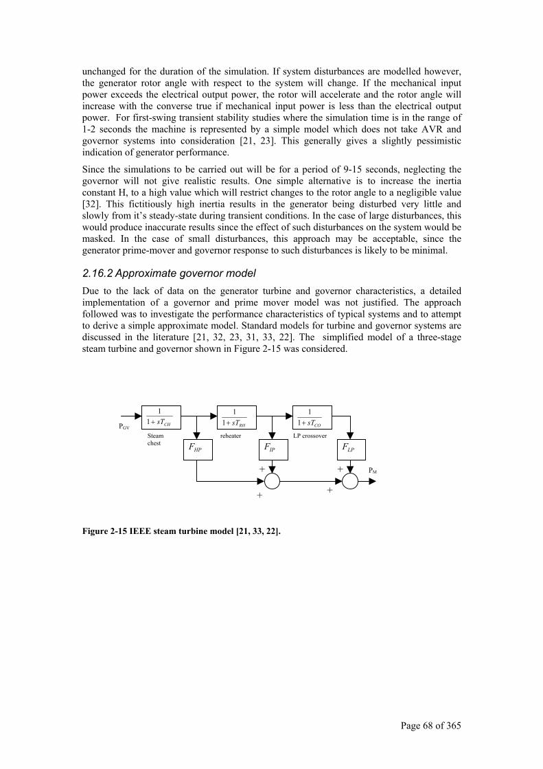
Page 68 of 365

unchanged for the duration of the simulation. If system disturbances are modelled however, the generator rotor angle with respect to the system will change. If the mechanical input power exceeds the electrical output power, the rotor will accelerate and the rotor angle will increase with the converse true if mechanical input power is less than the electrical output power. For first-swing transient stability studies where the simulation time is in the range of 1-2 seconds the machine is represented by a simple model which does not take AVR and governor systems into consideration [21, 23]. This generally gives a slightly pessimistic indication of generator performance.

Since the simulations to be carried out will be for a period of 9-15 seconds, neglecting the governor will not give realistic results. One simple alternative is to increase the inertia constant H, to a high value which will restrict changes to the rotor angle to a negligible value [32]. This fictitiously high inertia results in the generator being disturbed very little and slowly from it’s steady-state during transient conditions. In the case of large disturbances, this would produce inaccurate results since the effect of such disturbances on the system would be masked. In the case of small disturbances, this approach may be acceptable, since the generator prime-mover and governor response to such disturbances is likely to be minimal.

2.16.2 Approximate governor model Due to the lack of data on the generator turbine and governor characteristics, a detailed implementation of a governor and prime mover model was not justified. The approach followed was to investigate the performance characteristics of typical systems and to attempt to derive a simple approximate model. Standard models for turbine and governor systems are discussed in the literature [21, 32, 23, 31, 33, 22]. The simplified model of a three-stage steam turbine and governor shown in Figure 2-15 was considered.

Figure 2-15 IEEE steam turbine model [21, 33, 22].

CHsT+1

1 RHsT+1

1 COsT+1

1

HPF IPF LPF Steam chest

reheater LP crossoverPGV

PM+

+ +

+

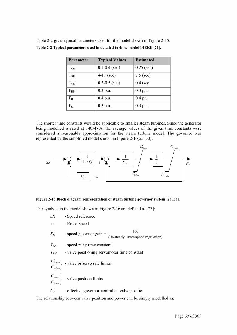
Page 69 of 365

Table 2-2 gives typical parameters used for the model shown in Figure 2-15. Table 2-2 Typical parameters used in detailed turbine model ©IEEE [21].

The shorter time constants would be applicable to smaller steam turbines. Since the generator being modelled is rated at 140MVA, the average values of the given time constants were considered a reasonable approximation for the steam turbine model. The governor was represented by the simplified model shown in Figure 2-16[23, 33]:

Figure 2-16 Block diagram representation of steam turbine governor system [23, 33].

The symbols in the model shown in Figure 2-16 are defined as [23]:

SR - Speed reference

ω - Rotor Speed

KG - speed governor gain = )regulation speed state-steady % (

100

TSR - speed relay time constant

TSM - valve positioning servomotor time constant

′′

Vclose

Vopen

CC

- valve or servo rate limits

min

max

V

V

CC

- valve position limits

CV - effective governor-controlled valve position

The relationship between valve position and power can be simply modelled as:

Parameter Typical Values Estimated

TCH 0.1-0.4 (sec) 0.25 (sec)

TRH 4-11 (sec) 7.5 (sec)

TCO 0.3-0.5 (sec) 0.4 (sec)

FHP 0.3 p.u. 0.3 p.u.

FIP 0.4 p.u. 0.4 p.u.

FLP 0.3 p.u. 0.3 p.u.

RsT+11

SMT1

s1

GK

+ -

+-

VopenC′

VcloseC′

maxVC

minVC

CV SR

ω

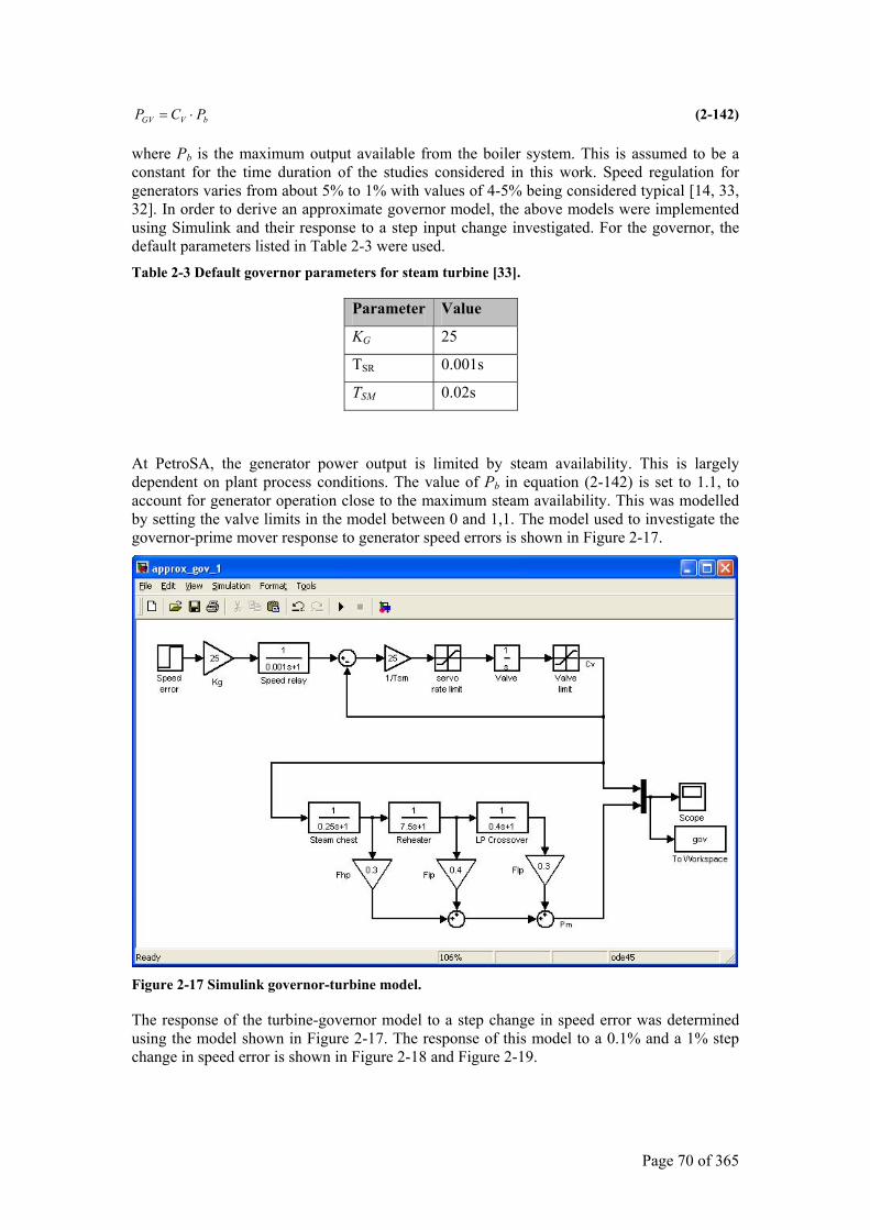
Page 70 of 365

bVGV PCP ⋅= (2-142)

where Pb is the maximum output available from the boiler system. This is assumed to be a constant for the time duration of the studies considered in this work. Speed regulation for generators varies from about 5% to 1% with values of 4-5% being considered typical [14, 33, 32]. In order to derive an approximate governor model, the above models were implemented using Simulink and their response to a step input change investigated. For the governor, the default parameters listed in Table 2-3 were used. Table 2-3 Default governor parameters for steam turbine [33].

Parameter Value

KG 25

TSR 0.001s

TSM 0.02s

At PetroSA, the generator power output is limited by steam availability. This is largely dependent on plant process conditions. The value of Pb in equation (2-142) is set to 1.1, to account for generator operation close to the maximum steam availability. This was modelled by setting the valve limits in the model between 0 and 1,1. The model used to investigate the governor-prime mover response to generator speed errors is shown in Figure 2-17.

Figure 2-17 Simulink governor-turbine model.

The response of the turbine-governor model to a step change in speed error was determined using the model shown in Figure 2-17. The response of this model to a 0.1% and a 1% step change in speed error is shown in Figure 2-18 and Figure 2-19.

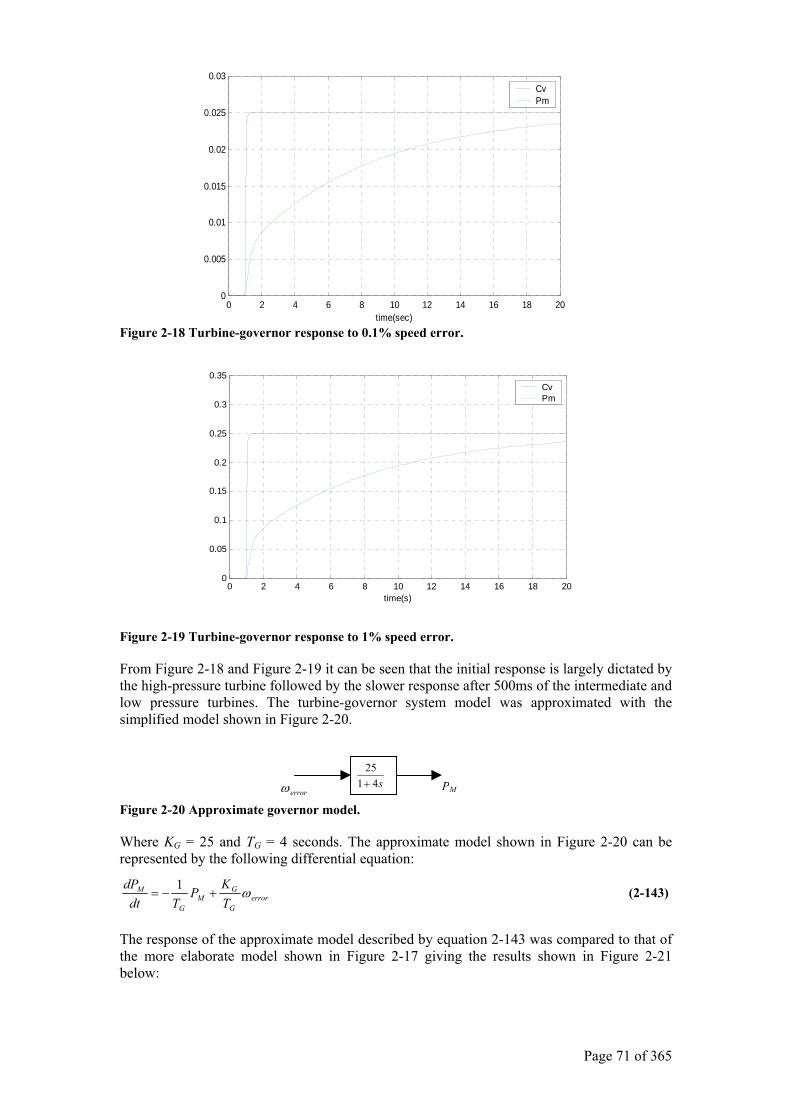
Page 71 of 365

Figure 2-18 Turbine-governor response to 0.1% speed error.

Figure 2-19 Turbine-governor response to 1% speed error.

From Figure 2-18 and Figure 2-19 it can be seen that the initial response is largely dictated by the high-pressure turbine followed by the slower response after 500ms of the intermediate and low pressure turbines. The turbine-governor system model was approximated with the simplified model shown in Figure 2-20.

Figure 2-20 Approximate governor model.

Where KG = 25 and TG = 4 seconds. The approximate model shown in Figure 2-20 can be represented by the following differential equation:

errorG

GM

G

M

TK

PTdt

dPω+−=

1 (2-143)

The response of the approximate model described by equation 2-143 was compared to that of the more elaborate model shown in Figure 2-17 giving the results shown in Figure 2-21 below:

0 2 4 6 8 10 12 14 16 18 200

0.05

0.1

0.15

0.2

0.25

0.3

0.35

time(s)

CvPm

s4125+ PM errorω

0 2 4 6 8 10 12 14 16 18 200

0.005

0.01

0.015

0.02

0.025

0.03

time(sec)

CvPm

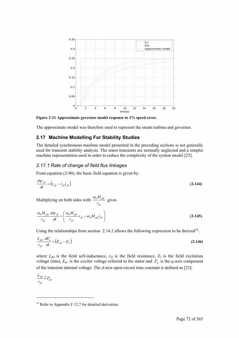
Page 72 of 365

Figure 2-21 Approximate governor model response to 1% speed error.

The approximate model was therefore used to represent the steam turbine and governor.

2.17 Machine Modelling For Stability Studies The detailed synchronous machine model presented in the preceding sections is not generally used for transient stability analysis. The stator transients are normally neglected and a simpler machine representation used in order to reduce the complexity of the system model [23].

2.17.1 Rate of change of field flux linkages From equation (2-90), the basic field equation is given by:

( )fdfdfdfd irv

dtd

−=ψ

(2-144)

Multiplying on both sides with fd

afd

rM0ω

gives

−= fdafdfd

fd

afdfd

fd

afd iMvrM

dtd

rM

000 ω

ωψω (2-145)

Using the relationships from section 2.14.2 allows the following expression to be derived14:

( )Ifdq

fd

ffd EEdtEd

rL

−=′

(2-146)

where Lffd is the field self-inductance, rfd is the field resistance, EI is the field excitation voltage (rms), Efd is the exciter voltage referred to the stator and qE ′ is the q-axis component of the transient internal voltage. The d-axis open-circuit time constant is defined as [23]:

0dfd

ffd TrL

′=∆

14 Refer to Appendix F 12.7 for detailed derivation.

0 2 4 6 8 10 12 14 16 18 200

0.05

0.1

0.15

0.2

0.25

0.3

0.35

time(s)

Cv Pm Approximate model

Page 73 of 365

With this eq. (2-146) becomes:

( )Ifdq

d EEdtEd

T −=′

′0 (2-147)

In the above equation Efd can be constant (manual regulation) or can vary due to automatic voltage regulator action independently of the other variables in the equation. Excitation system dynamics are therefore taken into consideration through Efd. In order to solve the above equation, EI has to be expressed in terms of qE′ . It can be shown that [23]:

( )3

dddqI

ixxEE ′−−′= (2-148)

where dx′ is the d-axis transient reactance. Substituting the above into eq.(2-147) gives:

( )30

dddqfd

qd

ixxEEdtEd

T ′−+′−=′

′

Since dd Ii

=3

, the d-axis component of terminal current (rms stator equivalent) we have the

following equation for taking into account the field flux linkages [23]:

( ) dddqfdq

d IxxEEdtEd

T ′−+′−=′

′0 (2-149)

and eq.(2-148) becomes:

( ) dddqI IxxEE ′−−′= (2-150)

2.17.2 Rate of change of q-axis rotor flux linkages For solid round body rotor machines it is preferable to treat the changes in rotor flux linkages separately in each axis. This will give an additional differential equation for the q-axis to account for the damper and round body currents similar to eq. (2-149). For the q-axis, Ed and

dE′ are related by [23]:

( ) qqqdd IxxEE ′−−′= (2-151)

where Since there is no excitation in the q-axis, by analogy with eq. (2-149) the following is obtained:

( ) qqqdd

q IxxEdtEdT ′−−′−=

′′0 (2-152)

The voltage dE′ (like qE′ ) is defined to be proportional to the q-axis equivalent rotor circuit flux linkages, q1ψ . If only one equivalent circuit is considered in the q-axis the transient open circuit time constant 0qT ′ is equal to 0qT ′′ and is given by qq rL 1111 [23].

Since stator transients have been neglected, the differential equations given in (2-149) and (2-152) for the rotor will have to be augmented with two algebraic equations for the stator. If there are no stator transients, equation. (2-82) can be written:

( ) 0=−−− qdd riv ωψ (2-153)

( ) 0=−−− dqq riv ωψ (2-154)

Page 74 of 365

The stator transient flux linkages are defined as [23]:

( )dddd iL′−⇒′ ψψ and ( )qqqq iL′−⇒′ ψψ

and the corresponding speed voltages defined as:

qde ψω ′−⇒′ and dqe ψω ′−⇒′

If it is assumed that the rotor speed does not change appreciably during the transient, equations (2-153) and (2-154) can be written:

( ) ( ) 0 and 0 00 =′+′−−−=′+′−−− dddqqqqqdd iLriviLriv ψωψω

or

ddqqqqqddd ixrivixrive ′++=′′++=′ e and

The above equations are based on rotor-referenced quantities and can be expressed in rms stator equivalent quantities by dividing by 3 giving:

qqddd IxrIVE ′++=′ (2-155)

ddqqq IxrIVE ′−+=′ (2-156)

dE′ and qE ′ are the components of the transient internal voltage E ′ along the d- and q-axes.

In order to account for the damper windings and other stray circuits in the rotor, the subtransient equations can be developed along similar lines as the above equations and are [21]:

( ) dddqqq

d IxxEEdtEd

T ′′−′+′′−′=′′

′′0 (2-157)

( ) qqqddd

qo IxxEEdtEdT ′′−′−′′−′=

′′′′ (2-158)

qqddd IxrIVE ′′++=′′ (2-159)

ddqqq IxrIVE ′′−+=′′ (2-160)

where superscript “ denotes subtransient voltages, reactances and time constants. These equations are based on the assumption that the subtransient time constants are small compared to the transient time constants.

2.17.3 Summary of generator models Based on the above, models of varying complexity may be defined [21]:

Model 1: d-axis transient effects only. Equations (2-149), (2-155) and (2-156) are used15.

Model 2: d and q-axis transient effects are considered. Equations (2-149),(2-152), (2-155) and (2-156) are used. Equations (2-155) and (2-156) can be written in terms of d and q-axis currents as follows:

15 Note that when this model is used, it will be necessary to account for the effects of the damper bars by including the damping coefficient, D in the swing equation.

Page 75 of 365

( ) ( )[ ]qqqddqd

d EVxVErxxr

I ′−′+−′′′+

= 2

1 (2-161)

( ) ( )[ ]qqdqqqd

q EVxVErxxr

I ′−′+−′′′+

= 2

1 (2-162)

Model 3: d and q-axis sub-transient effects are considered. Equations (2-149), (2-152), and (2-157) through (2-160) are used. Equations (2-159) and (2-160) can be written in terms of d and q-axis currents as follows:

( ) ( )ddqd

qqqd

qd VE

rxxrEV

rxxx

I −′′+′′′′

+′′−+′′′′

′′= 22 (2-163)

( ) ( )qqqd

ddqd

dq EV

rxxrVE

rxxxI ′′−

+′′′′−−′′

+′′′′′′

= 22 (2-164)

2.17.4 Power equations for two-axis model The three phase electrical power output can be derived as follows for the two-axis model from equation (2-94) [23]:

( )( ) [ ]ddqdqdq

qddqqqdqdde

IEIIxxE

IIxIEIIxIEP′+′−′+′=

′+′+′−′=

3

3 (2-165)

The above equation remains unchanged when expressed in p.u. on a single-phase power base. For use in the swing equation the p.u. electrical power output on a 3-phase power base has to be obtained which is given by [23]

( ) p.u. ddqdqdqe IEIIxxEP ′+′−′+′= (2-166)

2.17.5 Modelling of saturation Modelling of saturation was considered. Saturation modelling generally requires more detailed knowledge of machine parameter data than was available for the PetroSA machines. Due to a lack of sufficiently accurate parametric data and the need to limit the scope of work, it was decided not to model saturation.

2.18 Review Of Numerical Methods For Solving Differential Equations A major problem is the stiffness of the system of differential equations. This is due to the large variations in time constants associated with the system variables [21]. When synchronous machines are considered, rotor swing stability is the principal concern. The main time constants associated with the rotor are of the order of 1 to 10s. The electrical transmission network responds rapidly to changes and the time constants associated with the network variables are small enough to be taken as zero without significant loss of accuracy. The relevant differential equations for these rapidly changing variables are transformed into algebraic equations. When a time constant is large, or the disturbance is such that the variable will not change appreciably during the time frame being considered, the time constant may be assumed infinite and the variable becomes a constant. In the following section, the numerical methods usually employed for transient stability studies are discussed along with their properties. Matlab is equipped with built-in subroutines for solving ordinary differential equations (ODE’s). Since the transient stability analysis software was developed using Matlab, these built in routines were used, rather than writing new routines. The review of numerical methods below was mainly carried out to gain an understanding of the application

Page 76 of 365

of numerical methods to transient stability analysis and to aid in selecting the appropriate Matlab routines. Also note that although the various solution methods are discussed below in terms of single variables, all can readily be extended to a system of n first-order differential equations.

2.18.1 Accuracy and stability Accuracy of the solution is affected by round-off and truncation errors. Round-off errors are caused by the computer’s inability to represent numbers exactly. In lengthy calculations this type of error is extremely difficult to analyse and control. Carrying more decimal places in the intermediate calculations, than are required in the final answer is the usual practice to minimize round-off errors [20]. A word length of 48bits is normally considered acceptable for transient stability analysis. The difference between the true and calculated results is primarily determined by the truncation error. In order to compare the performance of various algorithms, Big O notation is used. This is defined as follows [20]:

A function, f(n)=O(h(n)), if and only if there exists an n0 such that, for all n>n0, we have )()( 1 nhKnf ≤ for some K1>0.

The truncation error is mainly a property of the numerical method chosen. In general terms, the truncation error of a method using a step length h is given by [21].

( ) ( )1+= phOhT (2-167)

where p represents the order of accuracy of the method. The true solution y(tn) at tn is therefore:

( ) ( ) np

nn hOyty ε++= +1 (2-168)

where yn is the value of y calculated by the method after n steps, and εn represents other possible errors.

Two types of instability occur in the solution of ordinary differential equations: inherent and induced instability. Inherent instability arises when the initial conditions are not known exactly. The solution will be affected to some extent, depending on the sensitivity of the differential equation. Inherent instability is not a problem with transient stability studies due to the form of the differential equations used [21]. Induced instability is related to the method used for the numerical solution of the differential equations. It is basically a measure of the difference between the true and approximate solutions as the number of steps becomes large.

Partial stability occurs when the step length (h) is critical to the solution and is particularly relevant when considering Runge-Kutta methods. A method with an infinite stability boundary is known as A-stable (unconditionally stable). Backward Euler and the trapezoidal method are A-stable, single-step methods. For a multi-step method to be A-stable, the order of accuracy cannot exceed p = 2. Implicit Runge-Kutta methods in which p<2r may also be A-stable. ( r = number of stages in the method )

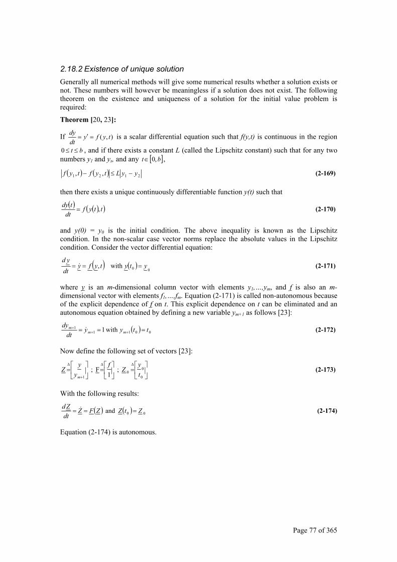
Page 77 of 365

2.18.2 Existence of unique solution Generally all numerical methods will give some numerical results whether a solution exists or not. These numbers will however be meaningless if a solution does not exist. The following theorem on the existence and uniqueness of a solution for the initial value problem is required:

Theorem [20, 23]:

If ),( tyfydtdy

=′= is a scalar differential equation such that f(y,t) is continuous in the region

bt ≤≤0 , and if there exists a constant L (called the Lipschitz constant) such that for any two numbers y1 and ys, and any [ ]bt ,0∈ ,

( ) ( ) 2121 ,, yyLtyftyf −≤− (2-169)

then there exists a unique continuously differentiable function y(t) such that

( ) ( )( )ttyfdt

tdy ,= (2-170)

and y(0) = y0 is the initial condition. The above inequality is known as the Lipschitz condition. In the non-scalar case vector norms replace the absolute values in the Lipschitz condition. Consider the vector differential equation:

( ) ( )00with , ytytyfy

dt

yd=== (2-171)

where y is an m-dimensional column vector with elements y1,…,ym, and f is also an m-dimensional vector with elements f1,…,fm. Equation (2-171) is called non-autonomous because of the explicit dependence of f on t. This explicit dependence on t can be eliminated and an autonomous equation obtained by defining a new variable ym+1 as follows [23]:

( ) 00111 with 1 ttyy

dtdy

mmm === ++

+ (2-172)

Now define the following set of vectors [23]:

=

=

=

∆∆

+

∆

0

00

1

; 1

F ; ty

Zf

yy

Zm

(2-173)

With the following results:

( ) ( ) 00 and ZtZZFZdtZd

=== (2-174)

Equation (2-174) is autonomous.

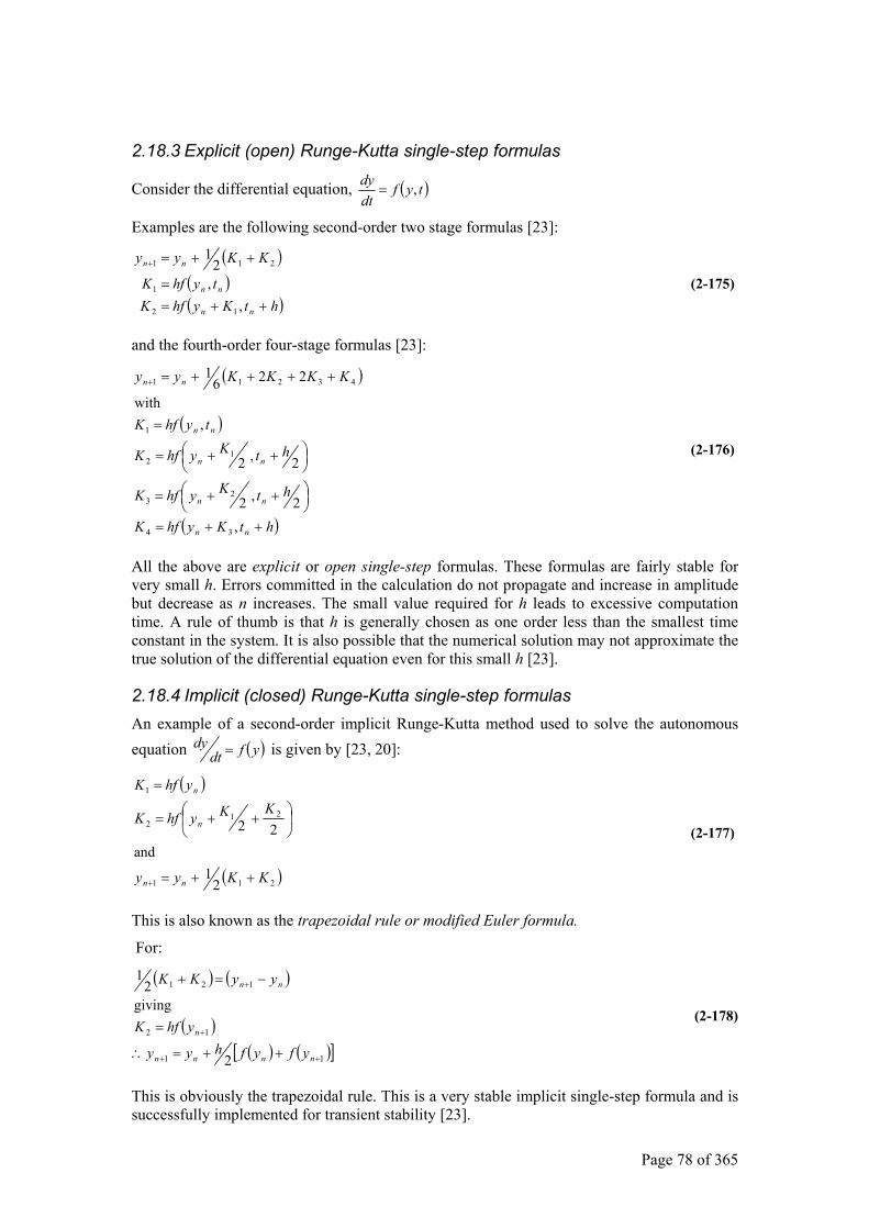
Page 78 of 365

2.18.3 Explicit (open) Runge-Kutta single-step formulas

Consider the differential equation, ( )tyfdtdy ,=

Examples are the following second-order two stage formulas [23]:

( )( )( )htKyhfK

tyhfK

KKyy

nn

nn

nn

++==

++=+

,,2

1

12

1

211

(2-175)

and the fourth-order four-stage formulas [23]:

( )

( )

( )htKyhfK

htKyhfK

htKyhfK

tyhfK

KKKKyy

nn

nn

nn

nn

nn

++=

++=

++=

=

++++=+

,2,2

2,2

,with

2261

34

23

12

1

43211

(2-176)

All the above are explicit or open single-step formulas. These formulas are fairly stable for very small h. Errors committed in the calculation do not propagate and increase in amplitude but decrease as n increases. The small value required for h leads to excessive computation time. A rule of thumb is that h is generally chosen as one order less than the smallest time constant in the system. It is also possible that the numerical solution may not approximate the true solution of the differential equation even for this small h [23].

2.18.4 Implicit (closed) Runge-Kutta single-step formulas An example of a second-order implicit Runge-Kutta method used to solve the autonomous equation ( )yfdt

dy = is given by [23, 20]:

( )

( )211

212

1

21

and22

KKyy

KKyhfK

yhfK

nn

n

n

++=

++=

=

+

(2-177)

This is also known as the trapezoidal rule or modified Euler formula.

For:

( ) ( )

( )( ) ( )[ ]11

12

121

2

giving2

1

++

+

+

++=∴

=

−=+

nnnn

n

nn

yfyfhyy

yhfK

yyKK

(2-178)

This is obviously the trapezoidal rule. This is a very stable implicit single-step formula and is successfully implemented for transient stability [23].

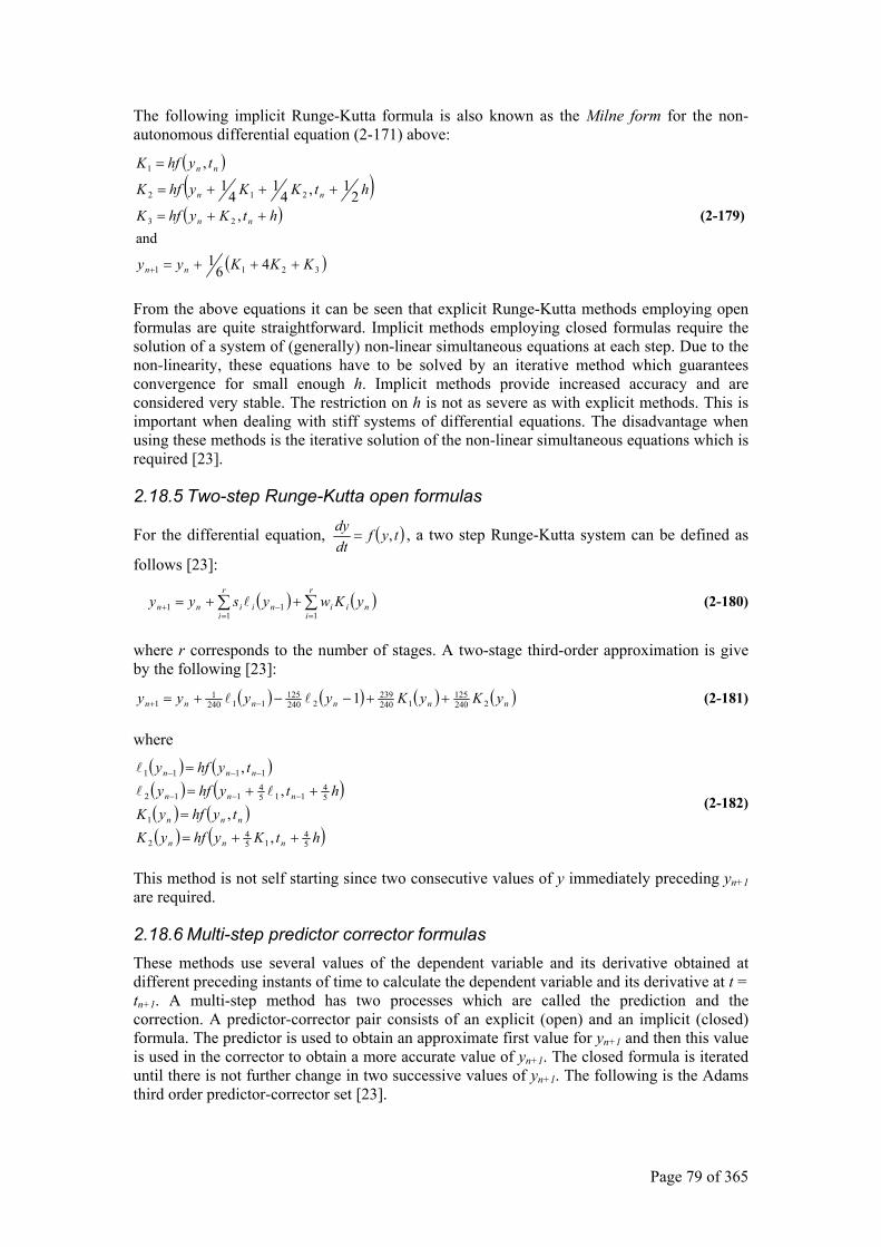
Page 79 of 365

The following implicit Runge-Kutta formula is also known as the Milne form for the non-autonomous differential equation (2-171) above:

( )( )( )

( )3211

23

212

1

461

and,

21,4

14

1,

KKKyy

htKyhfK

htKKyhfK

tyhfK

nn

nn

nn

nn

+++=

++=

+++=

=

+

(2-179)

From the above equations it can be seen that explicit Runge-Kutta methods employing open formulas are quite straightforward. Implicit methods employing closed formulas require the solution of a system of (generally) non-linear simultaneous equations at each step. Due to the non-linearity, these equations have to be solved by an iterative method which guarantees convergence for small enough h. Implicit methods provide increased accuracy and are considered very stable. The restriction on h is not as severe as with explicit methods. This is important when dealing with stiff systems of differential equations. The disadvantage when using these methods is the iterative solution of the non-linear simultaneous equations which is required [23].

2.18.5 Two-step Runge-Kutta open formulas

For the differential equation, ( )tyfdtdy ,= , a two step Runge-Kutta system can be defined as

follows [23]:

( ) ( )∑ ∑= =

−+ ++=r

i

r

iniiniinn yKwysyy

1 111 (2-180)

where r corresponds to the number of stages. A two-stage third-order approximation is give by the following [23]:

( ) ( ) ( ) ( )nnnnnn yKyKyyyy 2240125

1240239

2240125

112401

1 1 ++−−+= −+ (2-181)

where

( ) ( )( ) ( )( ) ( )( ) ( )htKyhfyK

tyhfyKhtyhfy

tyhfy

nnn

nnn

nnn

nnn

54

154

2

1

54

1154

112

1111

,,

,,

++=

=

++=

=

−−−

−−−

(2-182)

This method is not self starting since two consecutive values of y immediately preceding yn+1 are required.

2.18.6 Multi-step predictor corrector formulas These methods use several values of the dependent variable and its derivative obtained at different preceding instants of time to calculate the dependent variable and its derivative at t = tn+1. A multi-step method has two processes which are called the prediction and the correction. A predictor-corrector pair consists of an explicit (open) and an implicit (closed) formula. The predictor is used to obtain an approximate first value for yn+1 and then this value is used in the corrector to obtain a more accurate value of yn+1. The closed formula is iterated until there is not further change in two successive values of yn+1. The following is the Adams third order predictor-corrector set [23].

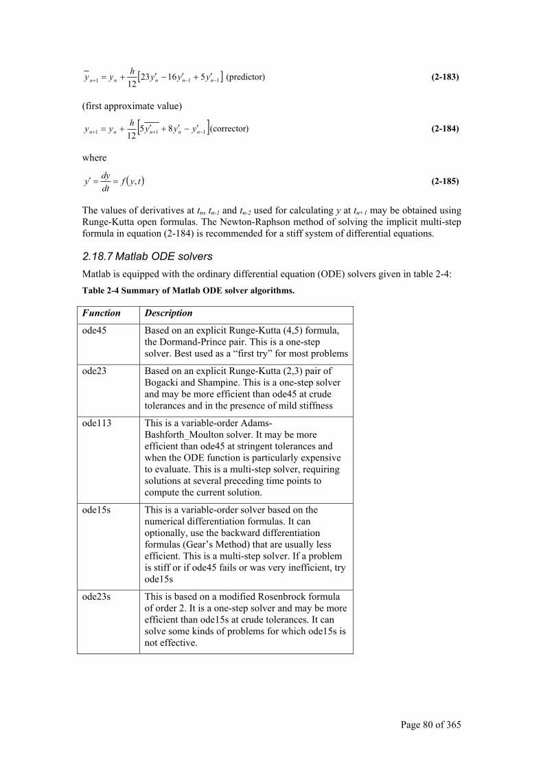
Page 80 of 365

[ ] )(predictor 5162312 111 −−+ ′+′−′+= nnnnn yyyhyy (2-183)

(first approximate value)

[ ] )(corrector 8512 111 −++ ′−′+′+= nnnnn yyyhyy (2-184)

where

( )tyfdtdyy ,==′ (2-185)

The values of derivatives at tn, tn-1 and tn-2 used for calculating y at tn+1 may be obtained using Runge-Kutta open formulas. The Newton-Raphson method of solving the implicit multi-step formula in equation (2-184) is recommended for a stiff system of differential equations.

2.18.7 Matlab ODE solvers Matlab is equipped with the ordinary differential equation (ODE) solvers given in table 2-4: Table 2-4 Summary of Matlab ODE solver algorithms.

Function Description

ode45 Based on an explicit Runge-Kutta (4,5) formula, the Dormand-Prince pair. This is a one-step solver. Best used as a “first try” for most problems

ode23 Based on an explicit Runge-Kutta (2,3) pair of Bogacki and Shampine. This is a one-step solver and may be more efficient than ode45 at crude tolerances and in the presence of mild stiffness

ode113 This is a variable-order Adams-Bashforth_Moulton solver. It may be more efficient than ode45 at stringent tolerances and when the ODE function is particularly expensive to evaluate. This is a multi-step solver, requiring solutions at several preceding time points to compute the current solution.

ode15s This is a variable-order solver based on the numerical differentiation formulas. It can optionally, use the backward differentiation formulas (Gear’s Method) that are usually less efficient. This is a multi-step solver. If a problem is stiff or if ode45 fails or was very inefficient, try ode15s

ode23s This is based on a modified Rosenbrock formula of order 2. It is a one-step solver and may be more efficient than ode15s at crude tolerances. It can solve some kinds of problems for which ode15s is not effective.

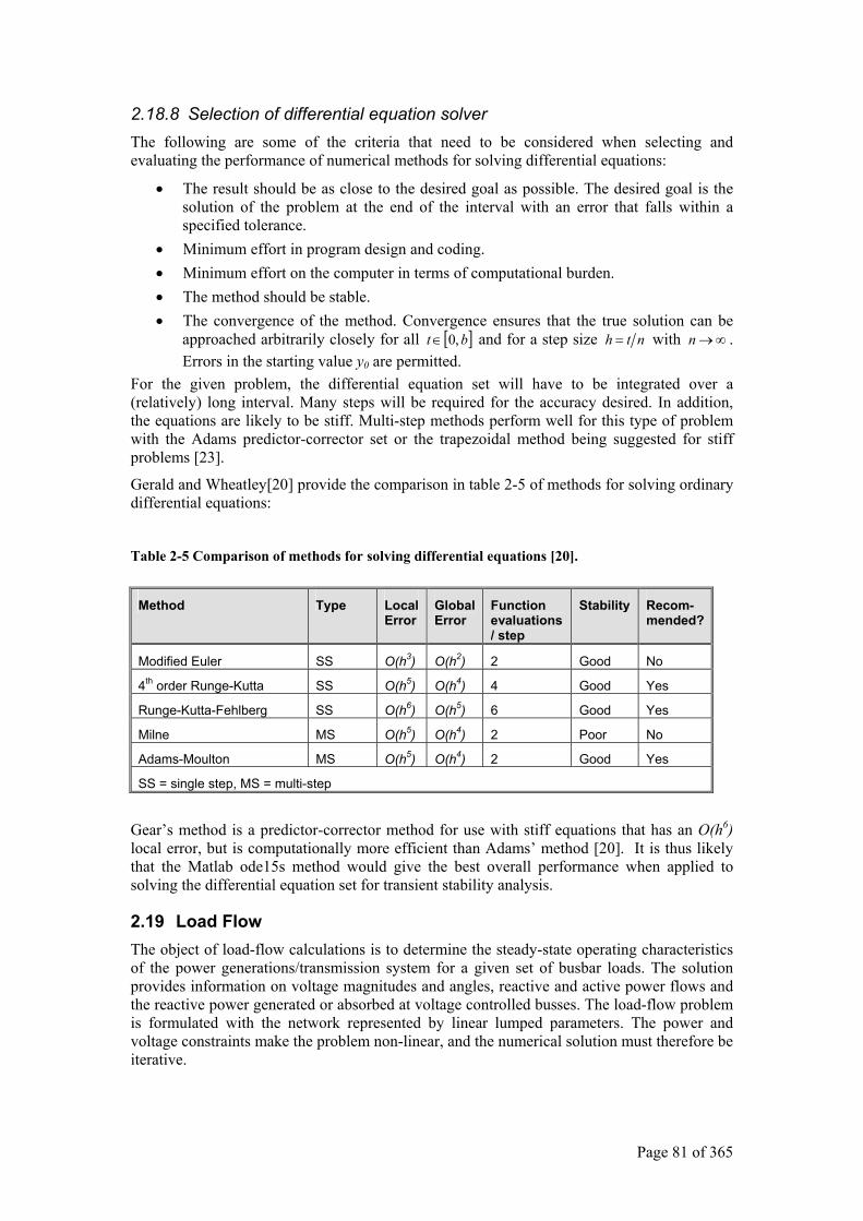
Page 81 of 365

2.18.8 Selection of differential equation solver The following are some of the criteria that need to be considered when selecting and evaluating the performance of numerical methods for solving differential equations:

• The result should be as close to the desired goal as possible. The desired goal is the solution of the problem at the end of the interval with an error that falls within a specified tolerance.

• Minimum effort in program design and coding. • Minimum effort on the computer in terms of computational burden. • The method should be stable. • The convergence of the method. Convergence ensures that the true solution can be

approached arbitrarily closely for all [ ]bt ,0∈ and for a step size nth = with ∞→n . Errors in the starting value y0 are permitted.

For the given problem, the differential equation set will have to be integrated over a (relatively) long interval. Many steps will be required for the accuracy desired. In addition, the equations are likely to be stiff. Multi-step methods perform well for this type of problem with the Adams predictor-corrector set or the trapezoidal method being suggested for stiff problems [23].

Gerald and Wheatley[20] provide the comparison in table 2-5 of methods for solving ordinary differential equations:

Table 2-5 Comparison of methods for solving differential equations [20].

Gear’s method is a predictor-corrector method for use with stiff equations that has an O(h6) local error, but is computationally more efficient than Adams’ method [20]. It is thus likely that the Matlab ode15s method would give the best overall performance when applied to solving the differential equation set for transient stability analysis.

2.19 Load Flow The object of load-flow calculations is to determine the steady-state operating characteristics of the power generations/transmission system for a given set of busbar loads. The solution provides information on voltage magnitudes and angles, reactive and active power flows and the reactive power generated or absorbed at voltage controlled busses. The load-flow problem is formulated with the network represented by linear lumped parameters. The power and voltage constraints make the problem non-linear, and the numerical solution must therefore be iterative.

Method Type Local Error

Global Error

Function evaluations / step

Stability Recom-mended?

Modified Euler SS O(h3) O(h2) 2 Good No

4th order Runge-Kutta SS O(h5) O(h4) 4 Good Yes

Runge-Kutta-Fehlberg SS O(h6) O(h5) 6 Good Yes

Milne MS O(h5) O(h4) 2 Poor No

Adams-Moulton MS O(h5) O(h4) 2 Good Yes

SS = single step, MS = multi-step

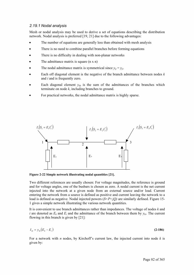
Page 82 of 365

2.19.1 Nodal analysis Mesh or nodal analysis may be used to derive a set of equations describing the distribution network. Nodal analysis is preferred [19, 21] due to the following advantages:

• The number of equations are generally less than obtained with mesh analysis

• There is no need to combine parallel branches before forming equations

• There is no difficulty in dealing with non-planar networks

• The admittance matrix is square (n x n)

• The nodal admittance matrix is symmetrical since yij = yji.

• Each off diagonal element is the negative of the branch admittance between nodes k and i and is frequently zero.

• Each diagonal element ykk is the sum of the admittances of the branches which terminate on node k, including branches to ground.

• For practical networks, the nodal admittance matrix is highly sparse.

Figure 2-22 Simple network illustrating nodal quantities [21].

Two different references are usually chosen: For voltage magnitudes, the reference is ground and for voltage angles, one of the busbars is chosen as zero. A nodal current is the net current injected into the network at a given node from an external source and/or load. Current entering the network from a source is defined as positive and current leaving the network to a load is defined as negative. Nodal injected powers (S=P+jQ) are similarly defined. Figure 15-1 gives a simple network illustrating the various network quantities.

It is convenient to use branch admittances rather than impedances. The voltage of nodes k and i are denoted as Ek and Ei and the admittance of the branch between them by yki. The current flowing in this branch is given by [21]:

( )ikkiki EEyI −= (2-186)

For a network with n nodes, by Kirchoff’s current law, the injected current into node k is given by:

( )*1111 IESI = ( )*

2222 IESI = ( )*3333 IESI =

E1 E2 E3

1 2 3

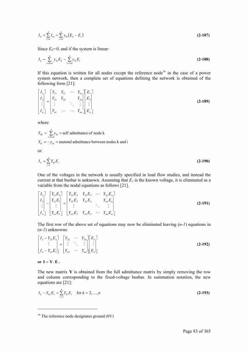
Page 83 of 365

( )∑ ∑= =

−==n

i

n

iikkikik EEyII

0 0 (2-187)

Since E0=0, and if the system is linear:

∑ ∑≠= ≠=

−=n

ki

n

kiikikkik EyEyI

0 1 (2-188)

If this equation is written for all nodes except the reference node16 in the case of a power system network, then a complete set of equations defining the network is obtained of the following form [21]:

=

nnnn

n

n

n E

EE

YY

YYYYYY

I

II

2

1

1

22221

11211

2

1

(2-189)

where

i andk nodesbetween admittance mututal

k node of admittance self 0

=−=

== ∑≠=

kiki

n

kikikk

yY

yY

or:

∑=

=n

iikik EYI

1 (2-190)

One of the voltages in the network is usually specified in load flow studies, and instead the current at that busbar is unknown. Assuming that E1 is the known voltage, it is eliminated as a variable from the nodal equations as follows [21].

=

−

nnnnn

nn

nn

nn EYEYEY

EYEYEYEYEYEY

EY

EYEY

I

II

3322

3332222

2331221

11

112

111

2

1

(2-191)

The first row of the above set of equations may now be eliminated leaving (n-1) equations in (n-1) unknowns:

=

−

−

nnnn

n

nn E

E

YY

YY

EYI

EYI 2

2

222

11

1212

(2-192)

or EYI ⋅= .

The new matrix Y is obtained from the full admittance matrix by simply removing the row and column corresponding to the fixed-voltage busbar. In summation notation, the new equations are [21]:

∑=

==−n

iikikk nkEYEYI

211 ,,2for … (2-193)

16 The reference node designates ground (0V)

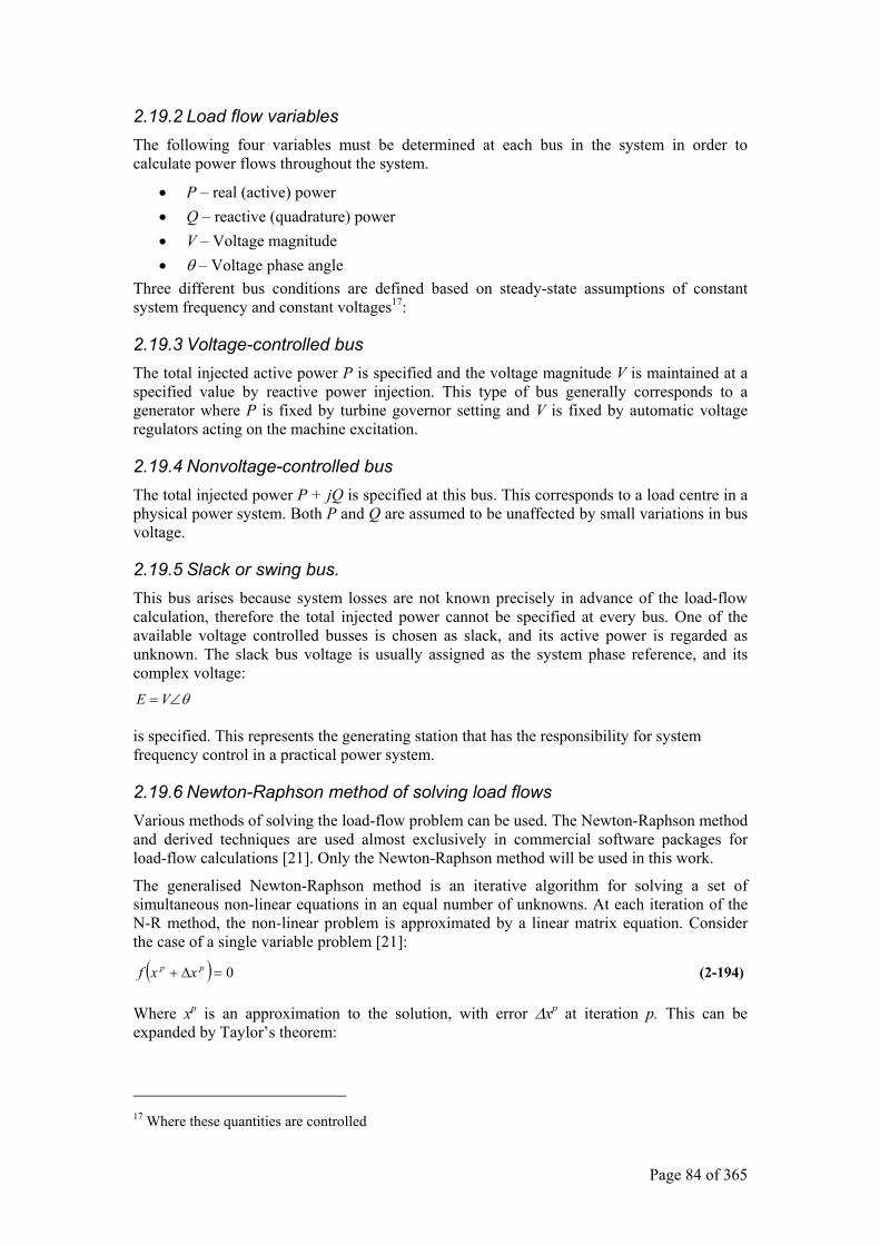
Page 84 of 365

2.19.2 Load flow variables The following four variables must be determined at each bus in the system in order to calculate power flows throughout the system.

• P – real (active) power • Q – reactive (quadrature) power • V – Voltage magnitude • θ – Voltage phase angle

Three different bus conditions are defined based on steady-state assumptions of constant system frequency and constant voltages17:

2.19.3 Voltage-controlled bus The total injected active power P is specified and the voltage magnitude V is maintained at a specified value by reactive power injection. This type of bus generally corresponds to a generator where P is fixed by turbine governor setting and V is fixed by automatic voltage regulators acting on the machine excitation.

2.19.4 Nonvoltage-controlled bus The total injected power P + jQ is specified at this bus. This corresponds to a load centre in a physical power system. Both P and Q are assumed to be unaffected by small variations in bus voltage.

2.19.5 Slack or swing bus. This bus arises because system losses are not known precisely in advance of the load-flow calculation, therefore the total injected power cannot be specified at every bus. One of the available voltage controlled busses is chosen as slack, and its active power is regarded as unknown. The slack bus voltage is usually assigned as the system phase reference, and its complex voltage:

θ∠= VE

is specified. This represents the generating station that has the responsibility for system frequency control in a practical power system.

2.19.6 Newton-Raphson method of solving load flows Various methods of solving the load-flow problem can be used. The Newton-Raphson method and derived techniques are used almost exclusively in commercial software packages for load-flow calculations [21]. Only the Newton-Raphson method will be used in this work.

The generalised Newton-Raphson method is an iterative algorithm for solving a set of simultaneous non-linear equations in an equal number of unknowns. At each iteration of the N-R method, the non-linear problem is approximated by a linear matrix equation. Consider the case of a single variable problem [21]:

( ) 0=∆+ pp xxf (2-194)

Where xp is an approximation to the solution, with error ∆xp at iteration p. This can be expanded by Taylor’s theorem:

17 Where these quantities are controlled

Page 85 of 365

( ) ( ) ( ) ( )+′′∆+′∆+==∆+ p

pppppp xfxxfxxfxxf

!20)(

2

(2-195)

Assuming that the error is small and neglecting all terms of higher powers gives [21]

( ) 0)( =′∆+ ppp xfxxf (2-196)

or

( )( )p

pp

xfxfx

′−

=∆ (2-197)

The new value of the variable is then obtained from: ppp xxx ∆+=+1 (2-198)

Equation (2-197) can be re-written as:

( ) pp xJxf ∆−= (2-199)

This is readily extended to a set of N equations in N unknowns. J becomes the square Jacobian matrix of the first-order partial differentials of the functions fk(xm) [21]:

m

kkm x

fJ

∂∂

= (2-200)

2.19.7 Power system load flow equations The power distribution network is described by the following equations [21]:

∑=

=n

mmkmk kEyI

0 allfor (2-201)

Where Ik denotes the current injected into a bus k and Em denotes the complex voltage at bus m. The power at a bus is then given by [21]

∑=

=

=+=n

mmkmk

kkkkk

EyE

IEjQPS

0

**

*

(2-202)

where I*k denotes the complex conjugate of the current injected into bus k, Pk denotes real

power and Qk denotes reactive power. The complex loadflow equations are nonanalytic and cannot be differentiated in complex form. The problem has to be separated into real equations and variables using polar or rectangular co-ordinates for the bus voltages. this gives the following two equations [21]:

( ) ( )θθ , and , VQQVPP kk == (2-203)

The bus voltages and admittances are defined as [21]:

( )

( )mmmm

kmkmkm

kkkk

jVE

jBGy

jVE

θθ

θθ

sincos

sincos

*

*

−=

−=

+=

(2-204)

Substitution of the above into equation 2-202 and separating the real and imaginary parts gives the following expressions for real and imaginary power in polar co-ordinates [21]:

Page 86 of 365

( )∑∈

+=km

kmkmkmkmmkk BGVVP θθ sincos (2-205)

( )∑∈

−=km

kmkmkmkmmkk BGVVQ θθ cossin (2-206)

where

mkkm θθθ −= (2-207)

For small variations in the voltage and angle variables, the resulting equations are obtained by forming the total differentials [21]:

∑ ∑ ∆∂∂

+∆∂∂

=∆m m

mm

km

m

kk V

VPP

P θθ

(2-208)

and

∑ ∑ ∆∂∂

+∆∂∂

=∆m m

mm

km

m

kk V

VQQ

Q θθ

(2-209)

• For a PQ busbar both equations are used • For a PV busbar, only equation 2-208 is used since Qk is not specified. • For a slack busbar, no equations are required.

The complete set of defining equations is made up of two equations for each PQ busbar and one for each PV busbar. The voltage magnitudes for PV and slack busbars are not variables, since they are specified. Similarly, θ is fixed at the slack busbar. The number of variables is therefore equal to the number of equations giving [21]:

∆∆

=

∆∆

−−−

−−

−

−

111

11

1

1

p

p

p

pp

pp

p

p

VV

LJNH

QP θ

(2-210)

where

∆Pp-1 = P mismatches for all PQ and PV busbars

∆Qp-1 = Q mismatches for all PQ busbars

∆θp = θ corrections for all PQ and PV busbars

∆Vp/Vp-1 = V corrections for all PQ busbars

The differences in bus powers are obtained from [21]

kSPkk

kSP

kk

QQQ

PPP

−=∆

−=∆ (2-211)

The division of each ∆Vp by Vp-1 does not affect the algorithm numerically, but simplifies some of the Jacobian matrix terms. The performance of the Newton-Raphson algorithm is closely related to problem non-linearity, with the best defining equations being the most linear. For busbars k and m the terms of the Jacobian matrix are given by [21]:

Page 87 of 365

( )

( )

( )

( )kmkmkmkmmkm

kkm

kmkmkmkmmkm

kkm

kmkmkmkmmkm

kkm

kmkmkmkmmkm

kkm

BGVVVQ

L

BGVVQ

J

BGVVVP

N

BGVVP

H

θθ

θθθ

θθ

θθθ

cossin

sincos

sincos

cossin

−=∂∂

=

+−=∂∂

=

+=∂∂

=

−=∂∂

=

(2-212)

and for m=k [21]

2

2

2

2

kkkkk

kkk

kkkkk

kkk

kkkkk

kkk

kkkkk

kkk

VBQVQ

L

VGPQ

J

VGPVP

N

VBQP

H

−=∂∂

=

−=∂∂

=

+=∂∂

=

−−=∂∂

=

θ

θ

(2-213)

These equations can also be expressed using voltages in rectangular form, but the polar co-ordinate representation is recommended since it has computational advantages over rectangular co-ordinates [21]. The polar co-ordinate representation was used for this work and rectangular co-ordinates are therefore not discussed further.

A further improvement is to replace the reactive power residual ∆Q in the Jacobian matrix equations by ∆Q/V . If the system power equation is divided throughout by Vk, only one term on the right-hand side of the equation is non-linear in Vk.

The success of the Newton-Raphson method is highly dependent upon the formulation of the problem defining equations. Power mismatch representation is better than current mismatch representations [21].

2.19.8 Improvements to basic Newton-Raphson algorithm The techniques that have been used to improve the efficiency of the Newton-Raphson method are centered around the efficient solution of the Jacobian matrix equation and reducing storage requirements by taking advantage of the sparsity of the system admittance and Jacobian matrices [21]. These techniques become very important when large systems18 need to be analysed. For the present work, the system size will be approximately 100 – 200 busses. Since the main aim of the work is to investigate load behaviour, and not load- flow algorithms, the simplest solution providing accurate reliable results was used. Refinements are only implemented when absolutely necessary. In general, the following principles were adopted [21]:

• Use the basic Newton-Raphson algorithm as far as possible • System size will be kept relatively small • Computational efficiency is not considered a high priority • Utilise the built-in Matlab functions wherever possible • Decoupled load flow algorithms were not considered.

18 A system with approximately 500 or more busses would be considered large

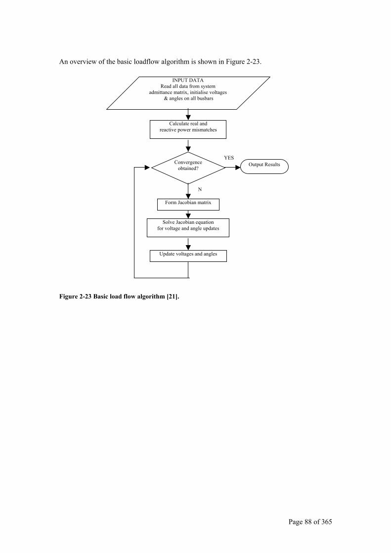
Page 88 of 365

An overview of the basic loadflow algorithm is shown in Figure 2-23.

Figure 2-23 Basic load flow algorithm [21].

INPUT DATA Read all data from system

admittance matrix, initialise voltages & angles on all busbars

Calculate real and reactive power mismatches

Convergence obtained?

Form Jacobian matrix

Solve Jacobian equation for voltage and angle updates

Update voltages and angles

Output Results

N

YES

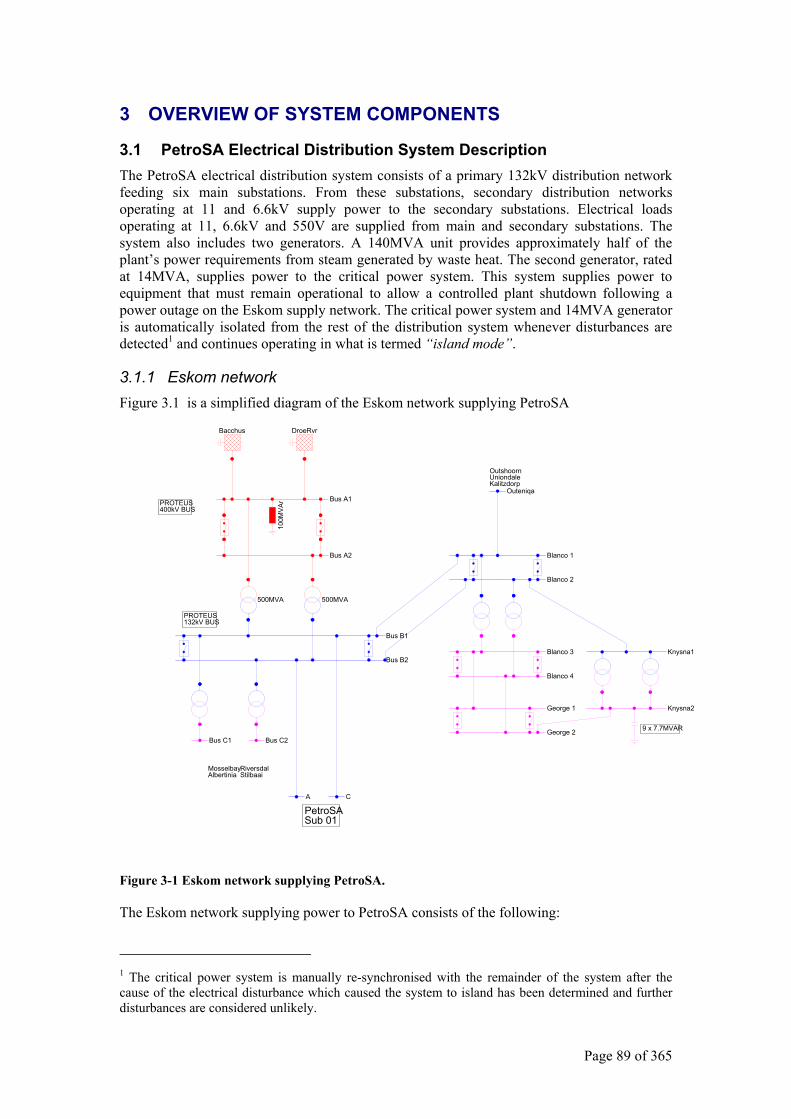
Page 89 of 365

3 OVERVIEW OF SYSTEM COMPONENTS

3.1 PetroSA Electrical Distribution System Description The PetroSA electrical distribution system consists of a primary 132kV distribution network feeding six main substations. From these substations, secondary distribution networks operating at 11 and 6.6kV supply power to the secondary substations. Electrical loads operating at 11, 6.6kV and 550V are supplied from main and secondary substations. The system also includes two generators. A 140MVA unit provides approximately half of the plant’s power requirements from steam generated by waste heat. The second generator, rated at 14MVA, supplies power to the critical power system. This system supplies power to equipment that must remain operational to allow a controlled plant shutdown following a power outage on the Eskom supply network. The critical power system and 14MVA generator is automatically isolated from the rest of the distribution system whenever disturbances are detected1 and continues operating in what is termed “island mode”.

3.1.1 Eskom network Figure 3.1 is a simplified diagram of the Eskom network supplying PetroSA

Bus A1

Bus A2

500MVA 500MVA

Bacchus DroeRvr

Bus B1

Bus B2

Bus C1 Bus C2

MosselbayAlbertinia

RiversdalStilbaai

A C

PetroSASub 01

Blanco 1

Blanco 2

Blanco 3

Blanco 4

George 1

George 2

Knysna1

Knysna2

9 x 7.7MVAR

Outeniqa

OutshoornUniondaleKalitzdorp

PROTEUS400kV BUS

PROTEUS132kV BUS

100M

VAr

Figure 3-1 Eskom network supplying PetroSA.

The Eskom network supplying power to PetroSA consists of the following:

1 The critical power system is manually re-synchronised with the remainder of the system after the cause of the electrical disturbance which caused the system to island has been determined and further disturbances are considered unlikely.

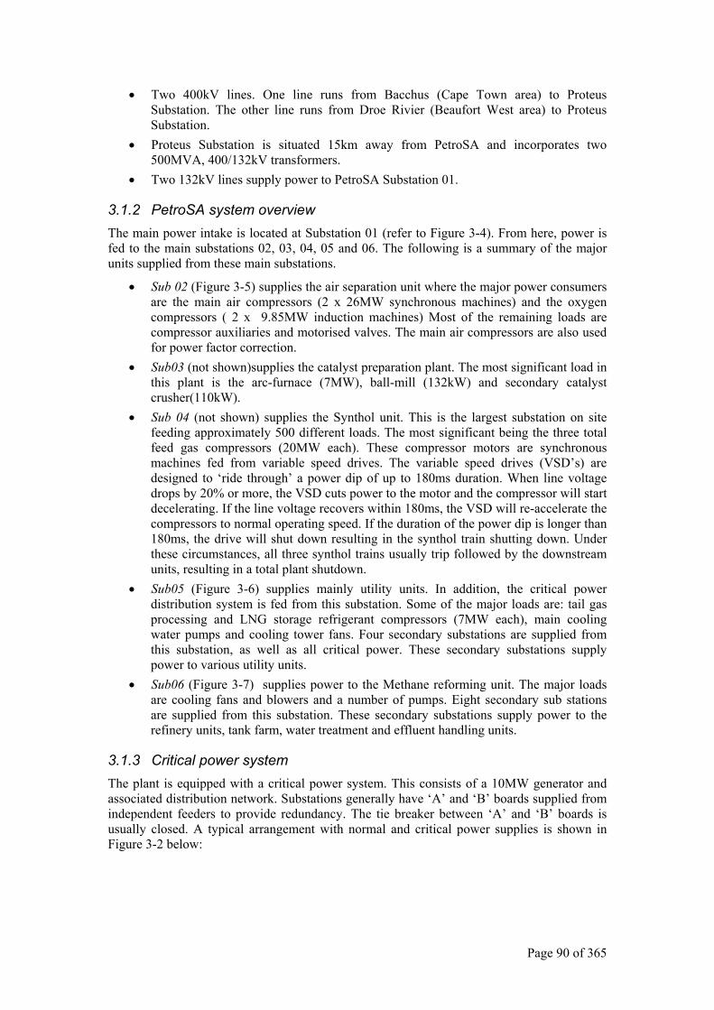
Page 90 of 365

• Two 400kV lines. One line runs from Bacchus (Cape Town area) to Proteus Substation. The other line runs from Droe Rivier (Beaufort West area) to Proteus Substation.

• Proteus Substation is situated 15km away from PetroSA and incorporates two 500MVA, 400/132kV transformers.

• Two 132kV lines supply power to PetroSA Substation 01.

3.1.2 PetroSA system overview The main power intake is located at Substation 01 (refer to Figure 3-4). From here, power is fed to the main substations 02, 03, 04, 05 and 06. The following is a summary of the major units supplied from these main substations.

• Sub 02 (Figure 3-5) supplies the air separation unit where the major power consumers are the main air compressors (2 x 26MW synchronous machines) and the oxygen compressors ( 2 x 9.85MW induction machines) Most of the remaining loads are compressor auxiliaries and motorised valves. The main air compressors are also used for power factor correction.

• Sub03 (not shown)supplies the catalyst preparation plant. The most significant load in this plant is the arc-furnace (7MW), ball-mill (132kW) and secondary catalyst crusher(110kW).

• Sub 04 (not shown) supplies the Synthol unit. This is the largest substation on site feeding approximately 500 different loads. The most significant being the three total feed gas compressors (20MW each). These compressor motors are synchronous machines fed from variable speed drives. The variable speed drives (VSD’s) are designed to ‘ride through’ a power dip of up to 180ms duration. When line voltage drops by 20% or more, the VSD cuts power to the motor and the compressor will start decelerating. If the line voltage recovers within 180ms, the VSD will re-accelerate the compressors to normal operating speed. If the duration of the power dip is longer than 180ms, the drive will shut down resulting in the synthol train shutting down. Under these circumstances, all three synthol trains usually trip followed by the downstream units, resulting in a total plant shutdown.

• Sub05 (Figure 3-6) supplies mainly utility units. In addition, the critical power distribution system is fed from this substation. Some of the major loads are: tail gas processing and LNG storage refrigerant compressors (7MW each), main cooling water pumps and cooling tower fans. Four secondary substations are supplied from this substation, as well as all critical power. These secondary substations supply power to various utility units.

• Sub06 (Figure 3-7) supplies power to the Methane reforming unit. The major loads are cooling fans and blowers and a number of pumps. Eight secondary sub stations are supplied from this substation. These secondary substations supply power to the refinery units, tank farm, water treatment and effluent handling units.

3.1.3 Critical power system The plant is equipped with a critical power system. This consists of a 10MW generator and associated distribution network. Substations generally have ‘A’ and ‘B’ boards supplied from independent feeders to provide redundancy. The tie breaker between ‘A’ and ‘B’ boards is usually closed. A typical arrangement with normal and critical power supplies is shown in Figure 3-2 below:

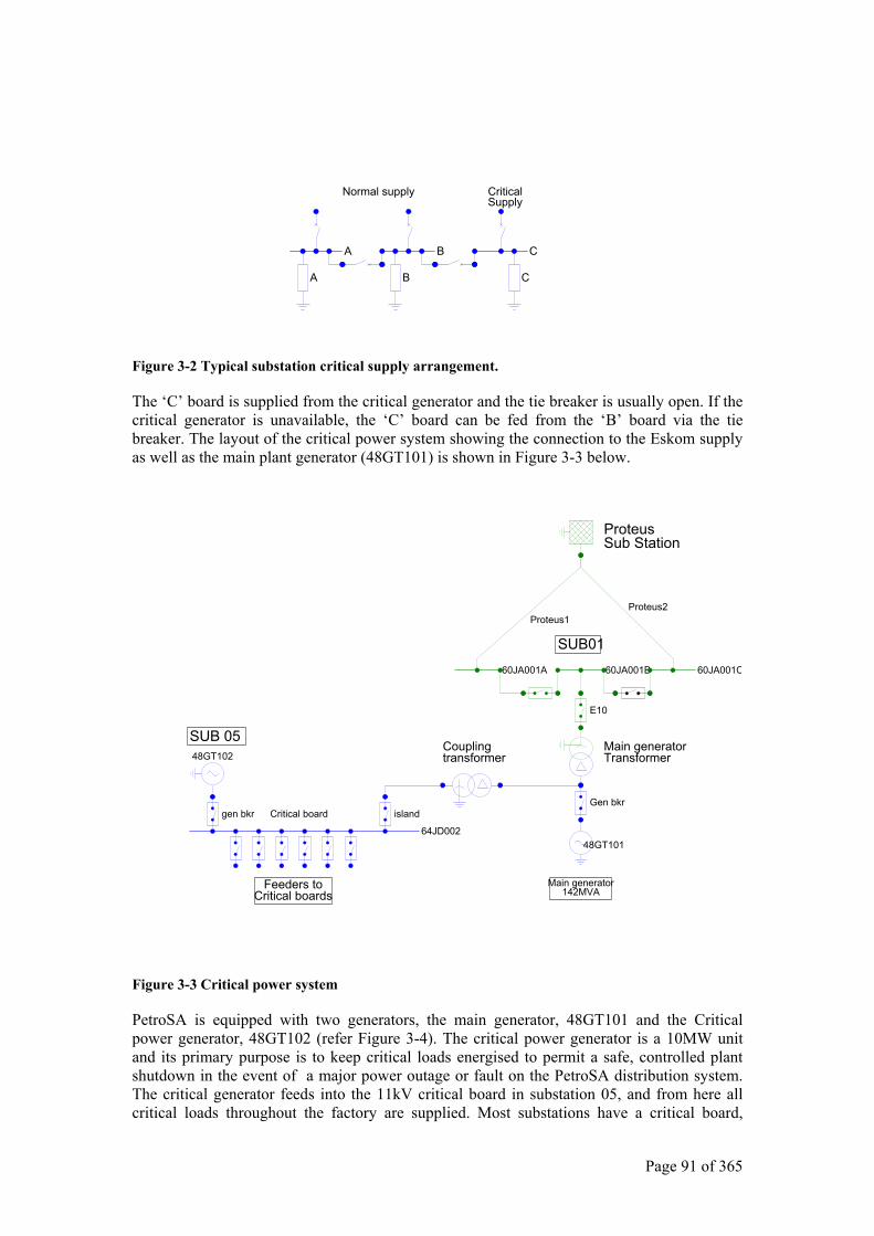
Page 91 of 365

Figure 3-2 Typical substation critical supply arrangement.

The ‘C’ board is supplied from the critical generator and the tie breaker is usually open. If the critical generator is unavailable, the ‘C’ board can be fed from the ‘B’ board via the tie breaker. The layout of the critical power system showing the connection to the Eskom supply as well as the main plant generator (48GT101) is shown in Figure 3-3 below.

60JA001A 60JA001B 60JA001C

Proteus1Proteus2

Gen bkr

48GT101

island

64JD002

48GT102

gen bkr

E10

SUB01

Main generator142MVA

SUB 05

Critical board

Feeders toCritical boards

Couplingtransformer

Main generatorTransformer

ProteusSub Station

Figure 3-3 Critical power system

PetroSA is equipped with two generators, the main generator, 48GT101 and the Critical power generator, 48GT102 (refer Figure 3-4). The critical power generator is a 10MW unit and its primary purpose is to keep critical loads energised to permit a safe, controlled plant shutdown in the event of a major power outage or fault on the PetroSA distribution system. The critical generator feeds into the 11kV critical board in substation 05, and from here all critical loads throughout the factory are supplied. Most substations have a critical board,

A B C

A B C

CriticalSupply

Normal supply

Page 92 of 365

supplied from substation 05 critical board. This board can be connected to the ‘normal’ boards in the substation via a tie breaker. This arrangement allows power to be supplied to the critical network in the event of a failure, or maintenance activities on the critical distribution system, During normal operation, all critical boards are supplied via the 11kV critical board in substation 05, and isolated from the rest of the electrical system. The only point of common coupling with the rest of the system is via the ‘island’ circuit breaker. The island circuit breaker is set up to trip instantaneously if any electrical disturbance is detected on the system. This isolates the critical power system from the rest of the PetroSA (and Eskom) system.

3.2 Modelling Of PetroSA Distribution Network Modelling of the entire PetroSA distribution system is not practical. A portion of the system was modelled in detail, with the remainder of the system being represented by static loads. Where possible, equipment that could be omitted from the model was identified.

3.2.1 Selection of substation for modelling For this initial analysis, selection of a secondary substation is preferable to one of the six main substations. System impedance will be higher at the secondary substations. Busbar voltage drops during starting of motors is likely to be more severe for these substations. The refinery units, which incorporate a large number of pumps normally remain on-line following a power dip. Optimal operation of the re-acceleration systems are essential to ensure that these units remain on-line. One of the refinery substations, substation 24, was selected for detailed modelling since the greatest potential for improvement exists within this area.

3.2.2 Transformer tap-changers All distribution transformers are equipped with tap changers. These are not online tap-changers and thus play no role during system transients. There is rarely, if ever, a need to adjust tap-changer settings on transformers.

3.2.3 Distributed control system and power disturbances The entire production process is controlled by a Distributed Control System (DCS). The DCS2 equipment is located in the Central Control Room and in a number of Satellite buildings distributed around the site. Electrical drives are controlled by the DCS when in auto mode, or from manual stop/start stations in the field.

All DCS equipment is fed from 24VDC uninterruptible power supplies located in the Central Control Room and in each satellite building. The DCS and all field equipment will remain operational for at least one hour following a total power outage. Due to this arrangement, the DCS is not affected by, nor does it directly detect short duration power dips and or disturbances. The DCS will indirectly detect power dips due to flow and pressure changes that occur shortly after pump motors have tripped, and the possible shutdown of equipment such as compressors.

3.2.4 Compressors and compressor controls Compressors are generally equipped with their own local control systems which interface to the DCS. Compressor response to power dip and duration will depend on the individual compressor control systems and varies. The four largest compressors on the plant usually trip following a power disturbance. The two main plant air compressors3 (26MW synchronous

2 Note that throughout this document, this control system will be referred to as the DCS 3 The main plant air compressors, 03KC101 and 03KC201 and oxygen compressors 03KC102 amd 03KC202 are shown on Figure 3-5

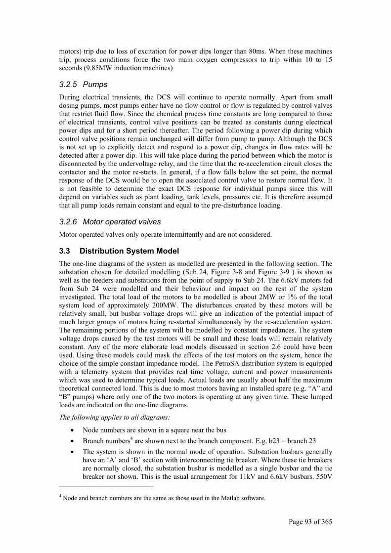
Page 93 of 365

motors) trip due to loss of excitation for power dips longer than 80ms. When these machines trip, process conditions force the two main oxygen compressors to trip within 10 to 15 seconds (9.85MW induction machines)

3.2.5 Pumps During electrical transients, the DCS will continue to operate normally. Apart from small dosing pumps, most pumps either have no flow control or flow is regulated by control valves that restrict fluid flow. Since the chemical process time constants are long compared to those of electrical transients, control valve positions can be treated as constants during electrical power dips and for a short period thereafter. The period following a power dip during which control valve positions remain unchanged will differ from pump to pump. Although the DCS is not set up to explicitly detect and respond to a power dip, changes in flow rates will be detected after a power dip. This will take place during the period between which the motor is disconnected by the undervoltage relay, and the time that the re-acceleration circuit closes the contactor and the motor re-starts. In general, if a flow falls below the set point, the normal response of the DCS would be to open the associated control valve to restore normal flow. It is not feasible to determine the exact DCS response for individual pumps since this will depend on variables such as plant loading, tank levels, pressures etc. It is therefore assumed that all pump loads remain constant and equal to the pre-disturbance loading.

3.2.6 Motor operated valves Motor operated valves only operate intermittently and are not considered.

3.3 Distribution System Model The one-line diagrams of the system as modelled are presented in the following section. The substation chosen for detailed modelling (Sub 24, Figure 3-8 and Figure 3-9 ) is shown as well as the feeders and substations from the point of supply to Sub 24. The 6.6kV motors fed from Sub 24 were modelled and their behaviour and impact on the rest of the system investigated. The total load of the motors to be modelled is about 2MW or 1% of the total system load of approximately 200MW. The disturbances created by these motors will be relatively small, but busbar voltage drops will give an indication of the potential impact of much larger groups of motors being re-started simultaneously by the re-acceleration system. The remaining portions of the system will be modelled by constant impedances. The system voltage drops caused by the test motors will be small and these loads will remain relatively constant. Any of the more elaborate load models discussed in section 2.6 could have been used. Using these models could mask the effects of the test motors on the system, hence the choice of the simple constant impedance model. The PetroSA distribution system is equipped with a telemetry system that provides real time voltage, current and power measurements which was used to determine typical loads. Actual loads are usually about half the maximum theoretical connected load. This is due to most motors having an installed spare (e.g. “A” and “B” pumps) where only one of the two motors is operating at any given time. These lumped loads are indicated on the one-line diagrams.

The following applies to all diagrams:

• Node numbers are shown in a square near the bus • Branch numbers4 are shown next to the branch component. E.g. b23 = branch 23 • The system is shown in the normal mode of operation. Substation busbars generally

have an ‘A’ and ‘B’ section with interconnecting tie breaker. Where these tie breakers are normally closed, the substation busbar is modelled as a single busbar and the tie breaker not shown. This is the usual arrangement for 11kV and 6.6kV busbars. 550V

4 Node and branch numbers are the same as those used in the Matlab software.

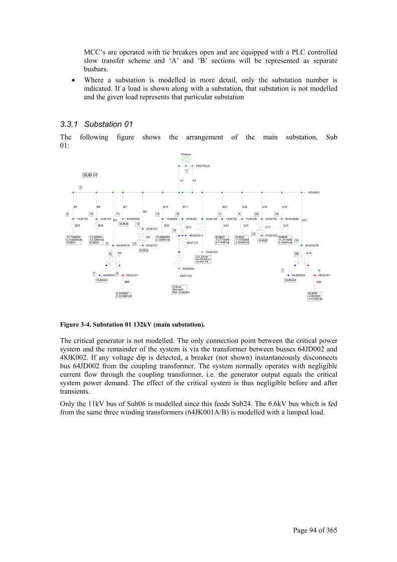
Page 94 of 365

MCC’s are operated with tie breakers open and are equipped with a PLC controlled slow transfer scheme and ‘A’ and ‘B’ sections will be represented as separate busbars.

• Where a substation is modelled in more detail, only the substation number is indicated. If a load is shown along with a substation, that substation is not modelled and the given load represents that particular substation

3.3.1 Substation 01 The following figure shows the arrangement of the main substation, Sub 01:

14JK103

B5

B20

9

12.705MW0.4165MVArSUB04

14JK101

B6

10

B28

13.92MW10.02MVArSUB04

64JK001A

B3

5

B4

64JD003 06JG1017 8

6

SUB06/1 B65

4.043MW3.3038MVAr

64JK002A

B7

SUB05

03JK101

B811

12

B9

03JD10113

SUB02

14JK204

B10

14

B30

12.688MW4.169MVAr

48JK001

B11

B12

48JK002

64JD002

48GT101

48GT102

15

16

03JK103

03JD103Soft StarterNot ModelledUsually Idle

14JK102

B21

b31

SUB0413.771MW9.774MVar

3

14JK305

b22

b32

4

SUB0411.876MW2.828MVAr

03JK102

b16

b17

03JD102

22

23

SUB02

64JK002B

b18

b33

SUB0511.311MW9.354MVAr

24

60JA001

64JK001B

b23

b19

64JD003A 06JG101

25

26

7 8

SUB06/1

SUB064.094MW3.073MVAr

b66

Proteus

PROTEUS

b1 b2

SUB 011

2

CriticalGenratorNot modelled

Figure 3-4. Substation 01 132kV (main substation).

The critical generator is not modelled. The only connection point between the critical power system and the remainder of the system is via the transformer between busses 64JD002 and 48JK002. If any voltage dip is detected, a breaker (not shown) instantaneously disconnects bus 64JD002 from the coupling transformer. The system normally operates with negligible current flow through the coupling transformer, i.e. the generator output equals the critical system power demand. The effect of the critical system is thus negligible before and after transients.

Only the 11kV bus of Sub06 is modelled since this feeds Sub24. The 6.6kV bus which is fed from the same three winding transformers (64JK001A/B) is modelled with a lumped load.

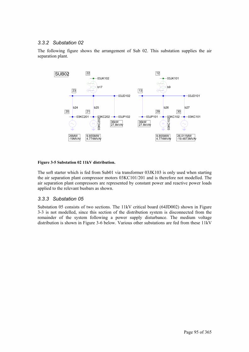
Page 95 of 365

3.3.2 Substation 02 The following figure shows the arrangement of Sub 02. This substation supplies the air separation plant.

03JD102

03JP102

36kW27,8kVAr

03KC202

b25

9.855MW4.774MVAr

03KC201

b24

26MW-19MVAr

03JP101 03KC102

b26

03K

C10

2 03KC101

03JD101

b27

03K

C20

2

36kW27.8kVAr

9.855MW4.774MVAr

26.011MW-19.4873MVAr

20 21

23

29 30

13b9

03JK101

b17

03JK102

1222SUB02

Figure 3-5 Substation 02 11kV distribution.

The soft starter which is fed from Sub01 via transformer 03JK103 is only used when starting the air separation plant compressor motors 03KC101/201 and is therefore not modelled. The air separation plant compressors are represented by constant power and reactive power loads applied to the relevant busbars as shown.

3.3.3 Substation 05 Substation 05 consists of two sections. The 11kV critical board (64JD002) shown in Figure 3-3 is not modelled, since this section of the distribution system is disconnected from the remainder of the system following a power supply disturbance. The medium voltage distribution is shown in Figure 3-6 below. Various other substations are fed from these 11kV

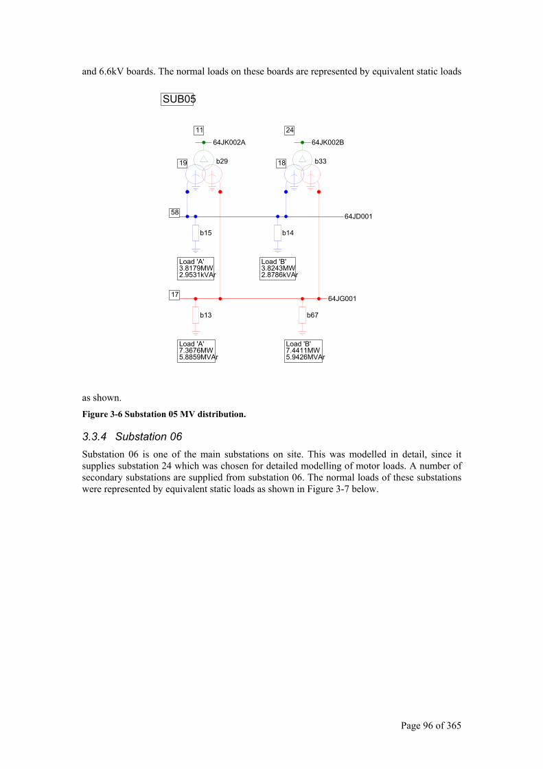
Page 96 of 365

and 6.6kV boards. The normal loads on these boards are represented by equivalent static loads

as shown.

64JK002A 64JK002B

b29

b15

Load 'A'7.3676MW5.8859MVAr

b14

Load 'B'7.4411MW5.9426MVAr

b33

64JG001

b13 b67

64JD001

11 24

19 18

58

17

Load 'A'3.8179MW2.9531kVAr

Load 'B'3.8243MW2.8786kVAr

SUB05

Figure 3-6 Substation 05 MV distribution.

3.3.4 Substation 06 Substation 06 is one of the main substations on site. This was modelled in detail, since it supplies substation 24 which was chosen for detailed modelling of motor loads. A number of secondary substations are supplied from substation 06. The normal loads of these substations were represented by equivalent static loads as shown in Figure 3-7 below.

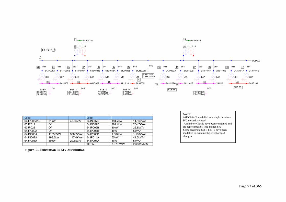
Page 97 of 365

64JP006A

b34

b36

64JP006B

b35

64JJ006

b37

b38

7

32

33

34

64JN001A

b39

64JN001B

b40

64JG002

b41 b42

35 37

36

b43

64JP043A

b44

64JP043B

b45

b47

64JJ010

b48

38

b50

41

39

220.2kW16.46kVAr

3.6611MW2.9145MVAr

2.7021MW2.0266kVAr

64JN003B

b46

64JG005

b49

b51

40

42

1.75MW1.40MVar

b52

3.3737MW2.6881MVAr

64JD003

24JN101B

b64

24JG101

24JN101A

b63

b62b61

46 47

SUB 23_1

48

24JP101B24JP101A

b60b59

24JJ101

b58b57

b76

2.7235MW2.0426MVAr

27 28

31

24JP102B24JP102A

b54b53

24JJ102B

b56b55

24JJ102A

43 44

45 57

SUB23_2

SUB06_1

64JK001A

b4

5

6

64JK001B

b19

25

26

SUB14SUB14 SUB19 SUB19

Load Load 64JP005A/B 61kW 45.6kVAr 64JN007B 194.7kW 147.6kVAr 63JP011 Off 64JN009B 299.4kW 234.7kVAr 63JP023 Off 64JP005B 30kW 22.8kVAr 64JP009A Off 64JP007B 4kW 5kVAr 64JN008A 1135.2kW 908.2kVAr 64JP008B 1.367kW 1.108kVAr 64JN007A 193.6kW 147.0kVAr 64JP014A 55kW 41.5kVAr 64JP005A 30kW 22.5kVAr 64JP007A 4kW 5kVAr TOTAL 3.3737MW 2.6881MVAr

Figure 3-7 Substation 06 MV distribution.

Notes: 64JD003A/B modelled as a single bus since B/C normally closed A number of loads have been combined and are represented by load branch b52 Some feeders to Sub 14 & 19 have been modelled to examine the effect of load changes

Page 98 of 365

3.3.5 Substation 24 This substation was chosen for detailed modelling of the 6.6kV induction motors. The 6.6kV layout is shown in Figure 3-8 and the 525V layout in Figure 3-9 on the following pages.

The motors modelled for simulation purposes are shown with their ratings and re-acceleration timer settings. Note that at any given time, only the ‘A’ or ‘B’ motor would be in operation. It is therefore only necessary to model the following four motors 24PC101A (300kW), 24PC102A(800kW), 24PC104A(300kW) and 24KC101A (550kW – no spare). Motor 24KC101 is a compressor motor with its own independent controls and is not part of the re-acceleration system.

The 525V motor loads are shown as lumped static loads grouped according to re-acceleration time setting.

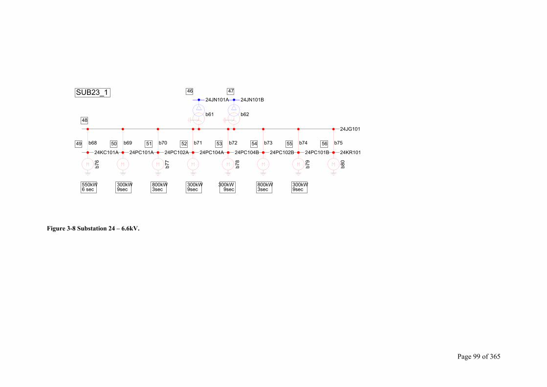
Page 99 of 365

24KC101A

b68

b76

550kW6 sec

24PC101A

b6949 50

300kW9sec

24PC102A

b70

b77

51

800kW3sec

24PC104A

b7152

300kW9sec

24PC104B

b72

b78

300kW9sec

24PC102B

b73

800kW3sec

24PC101B

b74

b79

300kW9sec

24JG101

24KR101

b75

b80

53 54 55 56

48

24JN101A

b61

24JN101B

b62

46 47SUB23_1

Figure 3-8 Substation 24 – 6.6kV.

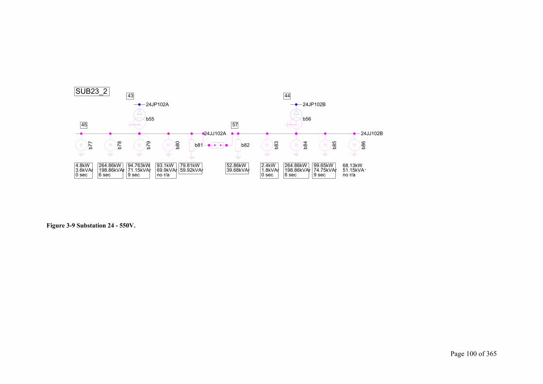
Page 100 of 365

b77

4.8kW3.6kVAr0 sec

b78

264.86kW198.86kVAr6 sec

b79

94.763kW71.15kVAr9 sec

b80

93.1kW69.9kVArno r/a

24JJ102A

b81

79.81kW59.92kVAr

b82

52.86kW39.68kVAr

b83

2.4kW1.8kVAr0 sec

b84

264.86kW198.86kVAr6 sec

b85

99.65kW74.75kVAr9 sec

24JJ102B

b86

68.13kW51.15kVArno r/a

45 57

24JP102A

b55

24JP102B

b56

SUB23_2 43 44

Figure 3-9 Substation 24 - 550V.

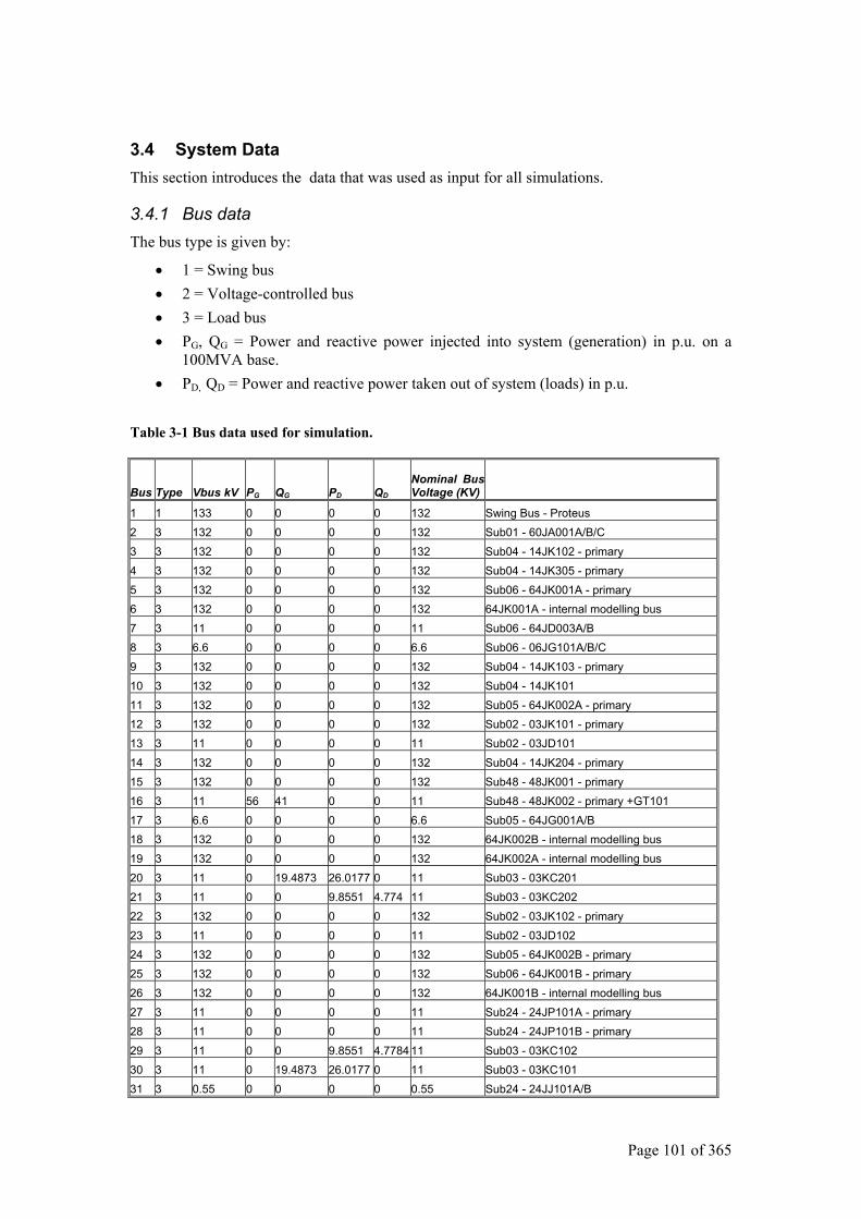
Page 101 of 365

3.4 System Data This section introduces the data that was used as input for all simulations.

3.4.1 Bus data The bus type is given by:

• 1 = Swing bus • 2 = Voltage-controlled bus • 3 = Load bus • PG, QG = Power and reactive power injected into system (generation) in p.u. on a

100MVA base. • PD, QD = Power and reactive power taken out of system (loads) in p.u.

Table 3-1 Bus data used for simulation.

Bus Type Vbus kV PG QG PD QD Nominal Bus Voltage (KV)

1 1 133 0 0 0 0 132 Swing Bus - Proteus 2 3 132 0 0 0 0 132 Sub01 - 60JA001A/B/C 3 3 132 0 0 0 0 132 Sub04 - 14JK102 - primary 4 3 132 0 0 0 0 132 Sub04 - 14JK305 - primary 5 3 132 0 0 0 0 132 Sub06 - 64JK001A - primary 6 3 132 0 0 0 0 132 64JK001A - internal modelling bus 7 3 11 0 0 0 0 11 Sub06 - 64JD003A/B 8 3 6.6 0 0 0 0 6.6 Sub06 - 06JG101A/B/C 9 3 132 0 0 0 0 132 Sub04 - 14JK103 - primary 10 3 132 0 0 0 0 132 Sub04 - 14JK101 11 3 132 0 0 0 0 132 Sub05 - 64JK002A - primary 12 3 132 0 0 0 0 132 Sub02 - 03JK101 - primary 13 3 11 0 0 0 0 11 Sub02 - 03JD101 14 3 132 0 0 0 0 132 Sub04 - 14JK204 - primary 15 3 132 0 0 0 0 132 Sub48 - 48JK001 - primary 16 3 11 56 41 0 0 11 Sub48 - 48JK002 - primary +GT101 17 3 6.6 0 0 0 0 6.6 Sub05 - 64JG001A/B 18 3 132 0 0 0 0 132 64JK002B - internal modelling bus 19 3 132 0 0 0 0 132 64JK002A - internal modelling bus 20 3 11 0 19.4873 26.0177 0 11 Sub03 - 03KC201 21 3 11 0 0 9.8551 4.774 11 Sub03 - 03KC202 22 3 132 0 0 0 0 132 Sub02 - 03JK102 - primary 23 3 11 0 0 0 0 11 Sub02 - 03JD102 24 3 132 0 0 0 0 132 Sub05 - 64JK002B - primary 25 3 132 0 0 0 0 132 Sub06 - 64JK001B - primary 26 3 132 0 0 0 0 132 64JK001B - internal modelling bus 27 3 11 0 0 0 0 11 Sub24 - 24JP101A - primary 28 3 11 0 0 0 0 11 Sub24 - 24JP101B - primary 29 3 11 0 0 9.8551 4.7784 11 Sub03 - 03KC102 30 3 11 0 19.4873 26.0177 0 11 Sub03 - 03KC101 31 3 0.55 0 0 0 0 0.55 Sub24 - 24JJ101A/B

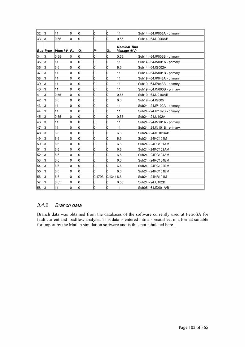
Page 102 of 365

32 3 11 0 0 0 0 11 Sub14 - 64JP006A - primary

33 3 0.55 0 0 0 0 0.55 Sub14 - 64JJ006A/B

Bus Type Vbus kV PG QG PD QD Nominal Bus Voltage (KV)

34 3 0.55 0 0 0 0 0.55 Sub14 - 64JP006B - primary

35 3 11 0 0 0 0 11 Sub14 - 64JN001A - primary 36 3 6.6 0 0 0 0 6.6 Sub14 - 64JG002A 37 3 11 0 0 0 0 11 Sub14 - 64JN001B - primary 38 3 11 0 0 0 0 11 Sub19 - 64JP043A - primary 39 3 11 0 0 0 0 11 Sub19 - 64JP043B - primary 40 3 11 0 0 0 0 11 Sub19 - 64JN003B - primary 41 3 0.55 0 0 0 0 0.55 Sub19 - 64JJ010A/B 42 3 6.6 0 0 0 0 6.6 Sub19 - 64JG005 43 3 11 0 0 0 0 11 Sub24 - 24JP102A - primary 44 3 11 0 0 0 0 11 Sub24 - 24JP102B - primary 45 3 0.55 0 0 0 0 0.55 Sub24 - 24JJ102A 46 3 11 0 0 0 0 11 Sub24 - 24JN101A - primary 47 3 11 0 0 0 0 11 Sub24 - 24JN101B - primary 48 3 6.6 0 0 0 0 6.6 Sub24 - 24JG101A/B 49 3 6.6 0 0 0 0 6.6 Sub24 - 24KC101M 50 3 6.6 0 0 0 0 6.6 Sub24 - 24PC101AM 51 3 6.6 0 0 0 0 6.6 Sub24 - 24PC102AM 52 3 6.6 0 0 0 0 6.6 Sub24 - 24PC104AM 53 3 6.6 0 0 0 0 6.6 Sub24 - 24PC104BM 54 3 6.6 0 0 0 0 6.6 Sub24 - 24PC102BM 55 3 6.6 0 0 0 0 6.6 Sub24 - 24PC101BM 56 3 6.6 0 0 0.1793 0.1344 6.6 Sub24 - 24KR101M 57 3 0.55 0 0 0 0 0.55 Sub24 - 24JJ102B 58 3 11 0 0 0 0 11 Sub05 - 64JD001A/B

3.4.2 Branch data

Branch data was obtained from the databases of the software currently used at PetroSA for fault current and loadflow analysis. This data is entered into a spreadsheet in a format suitable for import by the Matlab simulation software and is thus not tabulated here.

Page 103 of 365

4 DETAILED SIMULATION STRATEGY

4.1 Software Selection In order to investigate the transient behaviour of the PetroSA distribution system, various system models had to be developed. These models then had to be implemented on a suitable software platform. One of the objectives of this work is to investigate the application of ‘general-purpose’ software tools to the transient stability problem. The following were considered:

a) Spreadsheet application – MS-Excel

MS-Excel is equipped with an embedded Visual Basic programming capability. The combination of the programming facility with the spreadsheet user interface allows for very rapid software development, since the spreadsheet can be used to enter and pre-process data as well as present results in tabular or graph format. The Visual Basic application can focus on processing the data. The advantage is that very little time needs to be spent on developing a user interface and associated software allowing most of the time to be spent solving the problem at hand. The major disadvantage is that the Visual Basic application runs through an interpreter resulting in slow execution.

b) Develop a stand-alone application

All the required software could be developed using a standard programming language such as C++. This option will require a significant amount of time and effort to be spent on developing the user interface and support functions allowing less time to focus on the core problem. The time and effort required to develop an de-bug a stand-alone software application is not justified for this type of analysis and this option was not considered.

c) Engineering/scientific analysis software, Matlab.

The Matlab/Simulink environment incorporates an extensive mathematical and numerical analysis function set. The nature of the transient stability problem requires extensive use of matrix manipulation and calculation as well as numerical integration. It would thus be possible to develop the required transient stability analysis software and machine models by building on existing Matlab functionality.

Matlab was selected as the development platform based on the following considerations:

i) Matrix manipulation functions and ODE solvers for stiff and non-stiff problems are built in. There would be no need to devote a significant programming effort to implementing these functions.

ii) Matlab programming code executes somewhat faster than Visual Basic code embedded in Excel1

iii) Matlab has the ability to import and export data in spreadsheet format. Excel can therefore still be used for preparing system data and, if necessary presentation of results.

1 Based on a crude test executing an arbitrary section of code a set number of times.

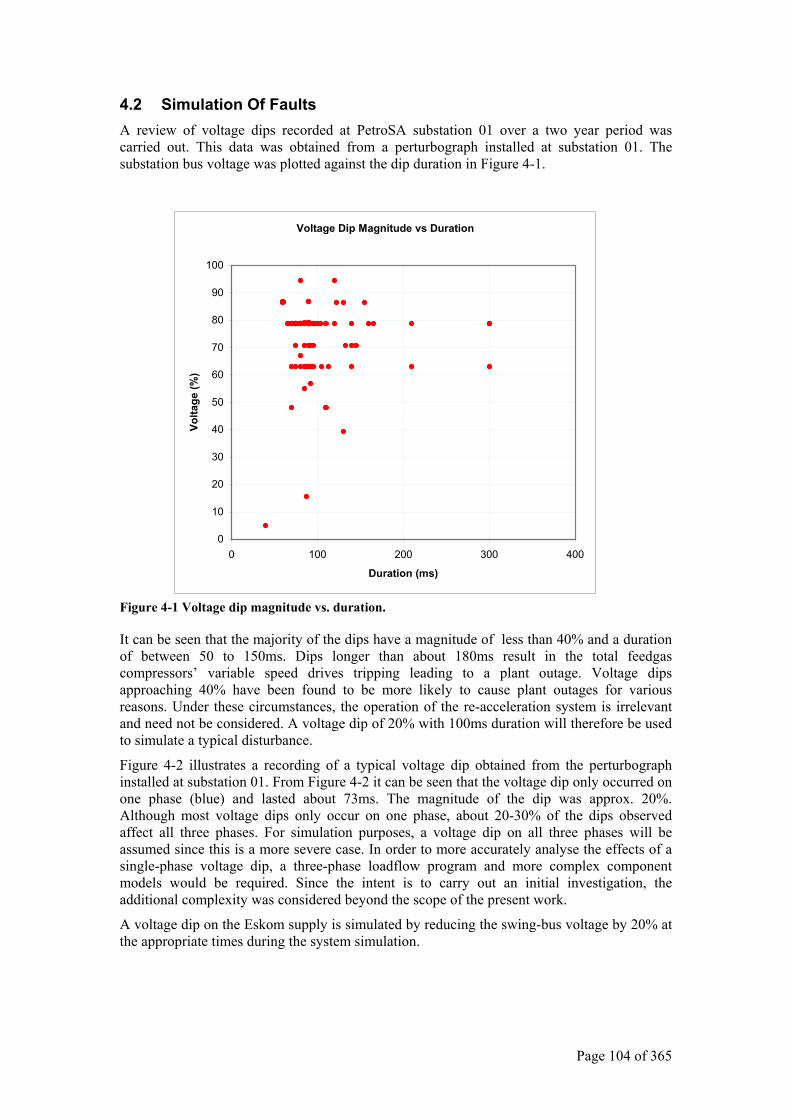
Page 104 of 365

4.2 Simulation Of Faults A review of voltage dips recorded at PetroSA substation 01 over a two year period was carried out. This data was obtained from a perturbograph installed at substation 01. The substation bus voltage was plotted against the dip duration in Figure 4-1.

Figure 4-1 Voltage dip magnitude vs. duration.

It can be seen that the majority of the dips have a magnitude of less than 40% and a duration of between 50 to 150ms. Dips longer than about 180ms result in the total feedgas compressors’ variable speed drives tripping leading to a plant outage. Voltage dips approaching 40% have been found to be more likely to cause plant outages for various reasons. Under these circumstances, the operation of the re-acceleration system is irrelevant and need not be considered. A voltage dip of 20% with 100ms duration will therefore be used to simulate a typical disturbance.

Figure 4-2 illustrates a recording of a typical voltage dip obtained from the perturbograph installed at substation 01. From Figure 4-2 it can be seen that the voltage dip only occurred on one phase (blue) and lasted about 73ms. The magnitude of the dip was approx. 20%. Although most voltage dips only occur on one phase, about 20-30% of the dips observed affect all three phases. For simulation purposes, a voltage dip on all three phases will be assumed since this is a more severe case. In order to more accurately analyse the effects of a single-phase voltage dip, a three-phase loadflow program and more complex component models would be required. Since the intent is to carry out an initial investigation, the additional complexity was considered beyond the scope of the present work.

A voltage dip on the Eskom supply is simulated by reducing the swing-bus voltage by 20% at the appropriate times during the system simulation.

Voltage Dip Magnitude vs Duration

0

10

20

30

40

50

60

70

80

90

100

0 100 200 300 400

Duration (ms)

Volta

ge (%

)

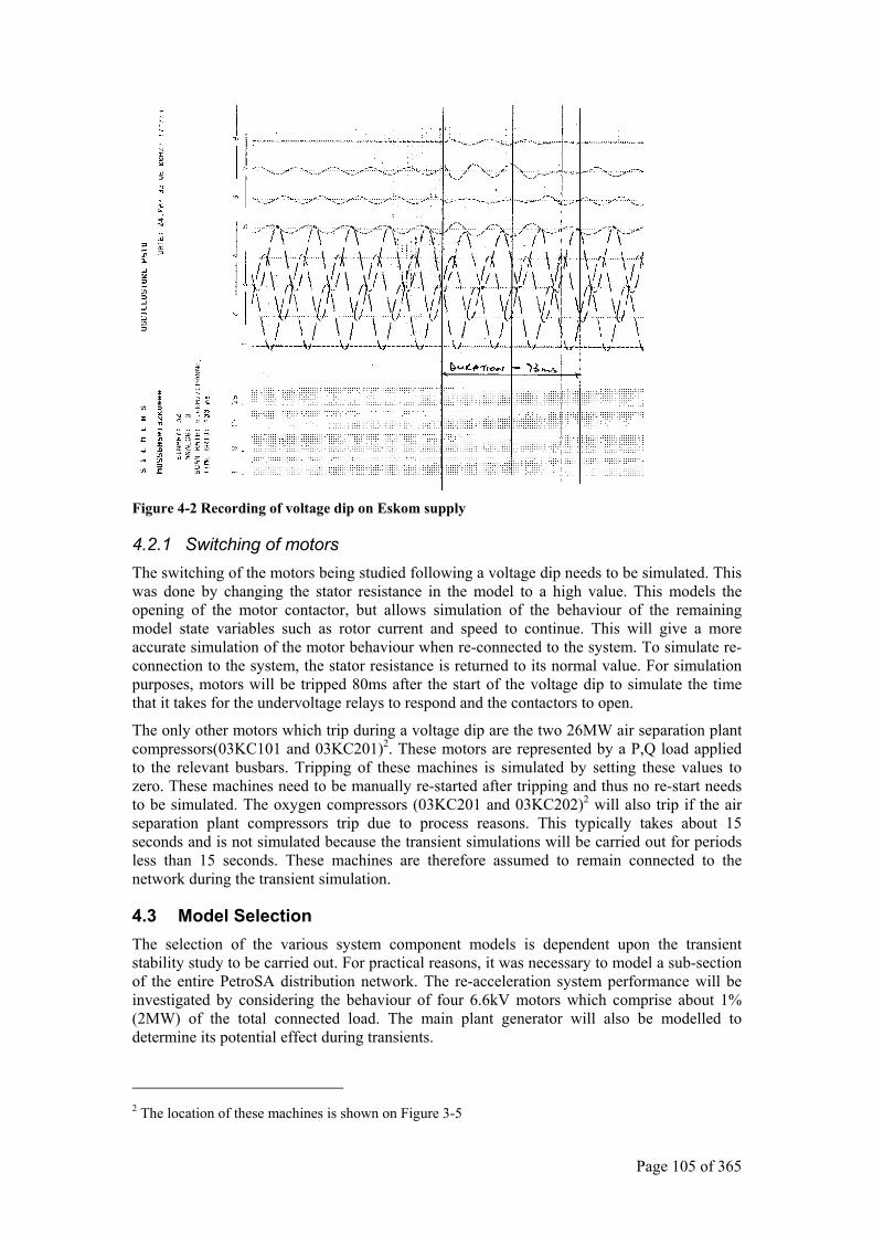
Page 105 of 365

Figure 4-2 Recording of voltage dip on Eskom supply

4.2.1 Switching of motors The switching of the motors being studied following a voltage dip needs to be simulated. This was done by changing the stator resistance in the model to a high value. This models the opening of the motor contactor, but allows simulation of the behaviour of the remaining model state variables such as rotor current and speed to continue. This will give a more accurate simulation of the motor behaviour when re-connected to the system. To simulate re-connection to the system, the stator resistance is returned to its normal value. For simulation purposes, motors will be tripped 80ms after the start of the voltage dip to simulate the time that it takes for the undervoltage relays to respond and the contactors to open.

The only other motors which trip during a voltage dip are the two 26MW air separation plant compressors(03KC101 and 03KC201)2. These motors are represented by a P,Q load applied to the relevant busbars. Tripping of these machines is simulated by setting these values to zero. These machines need to be manually re-started after tripping and thus no re-start needs to be simulated. The oxygen compressors (03KC201 and 03KC202)2 will also trip if the air separation plant compressors trip due to process reasons. This typically takes about 15 seconds and is not simulated because the transient simulations will be carried out for periods less than 15 seconds. These machines are therefore assumed to remain connected to the network during the transient simulation.

4.3 Model Selection The selection of the various system component models is dependent upon the transient stability study to be carried out. For practical reasons, it was necessary to model a sub-section of the entire PetroSA distribution network. The re-acceleration system performance will be investigated by considering the behaviour of four 6.6kV motors which comprise about 1% (2MW) of the total connected load. The main plant generator will also be modelled to determine its potential effect during transients.

2 The location of these machines is shown on Figure 3-5

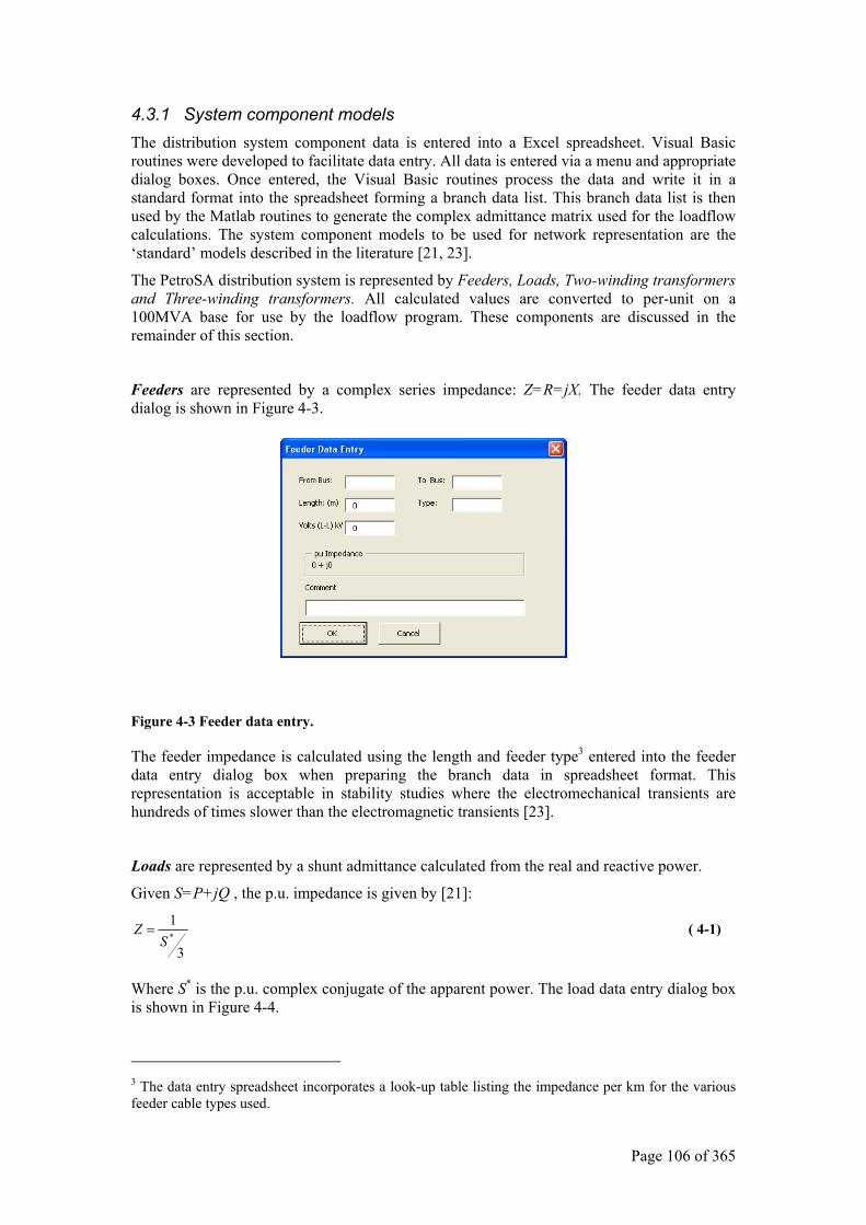
Page 106 of 365

4.3.1 System component models The distribution system component data is entered into a Excel spreadsheet. Visual Basic routines were developed to facilitate data entry. All data is entered via a menu and appropriate dialog boxes. Once entered, the Visual Basic routines process the data and write it in a standard format into the spreadsheet forming a branch data list. This branch data list is then used by the Matlab routines to generate the complex admittance matrix used for the loadflow calculations. The system component models to be used for network representation are the ‘standard’ models described in the literature [21, 23].

The PetroSA distribution system is represented by Feeders, Loads, Two-winding transformers and Three-winding transformers. All calculated values are converted to per-unit on a 100MVA base for use by the loadflow program. These components are discussed in the remainder of this section.

Feeders are represented by a complex series impedance: Z=R=jX. The feeder data entry dialog is shown in Figure 4-3.

Figure 4-3 Feeder data entry.

The feeder impedance is calculated using the length and feeder type3 entered into the feeder data entry dialog box when preparing the branch data in spreadsheet format. This representation is acceptable in stability studies where the electromechanical transients are hundreds of times slower than the electromagnetic transients [23].

Loads are represented by a shunt admittance calculated from the real and reactive power.

Given S=P+jQ , the p.u. impedance is given by [21]:

3

1*S

Z = ( 4-1)

Where S* is the p.u. complex conjugate of the apparent power. The load data entry dialog box is shown in Figure 4-4.

3 The data entry spreadsheet incorporates a look-up table listing the impedance per km for the various feeder cable types used.

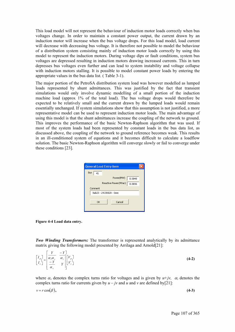
Page 107 of 365

This load model will not represent the behaviour of induction motor loads correctly when bus voltages change. In order to maintain a constant power output, the current drawn by an induction motor will increase when the bus voltage drops. For this load model, load current will decrease with decreasing bus voltage. It is therefore not possible to model the behaviour of a distribution system consisting mainly of induction motor loads correctly by using this model to represent the induction motors. During voltage dips or fault conditions, system bus voltages are depressed resulting in induction motors drawing increased currents. This in turn depresses bus voltages even further and can lead to system instability and voltage collapse with induction motors stalling. It is possible to model constant power loads by entering the appropriate values in the bus data list. ( Table 3-1).

The major portion of the PetroSA distribution system load was however modelled as lumped loads represented by shunt admittances. This was justified by the fact that transient simulations would only involve dynamic modelling of a small portion of the induction machine load (approx 1% of the total load). The bus voltage drops would therefore be expected to be relatively small and the current drawn by the lumped loads would remain essentially unchanged. If system simulations show that this assumption is not justified, a more representative model can be used to represent induction motor loads. The main advantage of using this model is that the shunt admittances increase the coupling of the network to ground. This improves the performance of the basic Newton-Raphson algorithm that was used. If most of the system loads had been represented by constant loads in the bus data list, as discussed above, the coupling of the network to ground reference becomes weak. This results in an ill-conditioned system of equations and it becomes difficult to calculate a loadflow solution. The basic Newton-Raphson algorithm will converge slowly or fail to converge under these conditions [23].

Figure 4-4 Load data entry.

Two Winding Transformers: The transformer is represented analytically by its admittance matrix giving the following model presented by Arrilaga and Arnold[21]:

−

−

=

s

p

v

ivi

s

p

VV

YY

YY

II

α

ααα (4-2)

where αv denotes the complex turns ratio for voltages and is given by u+jv, αi denotes the complex turns ratio for currents given by u – jv and u and v are defined by[21]:

( )βcosrv = , (4-3)

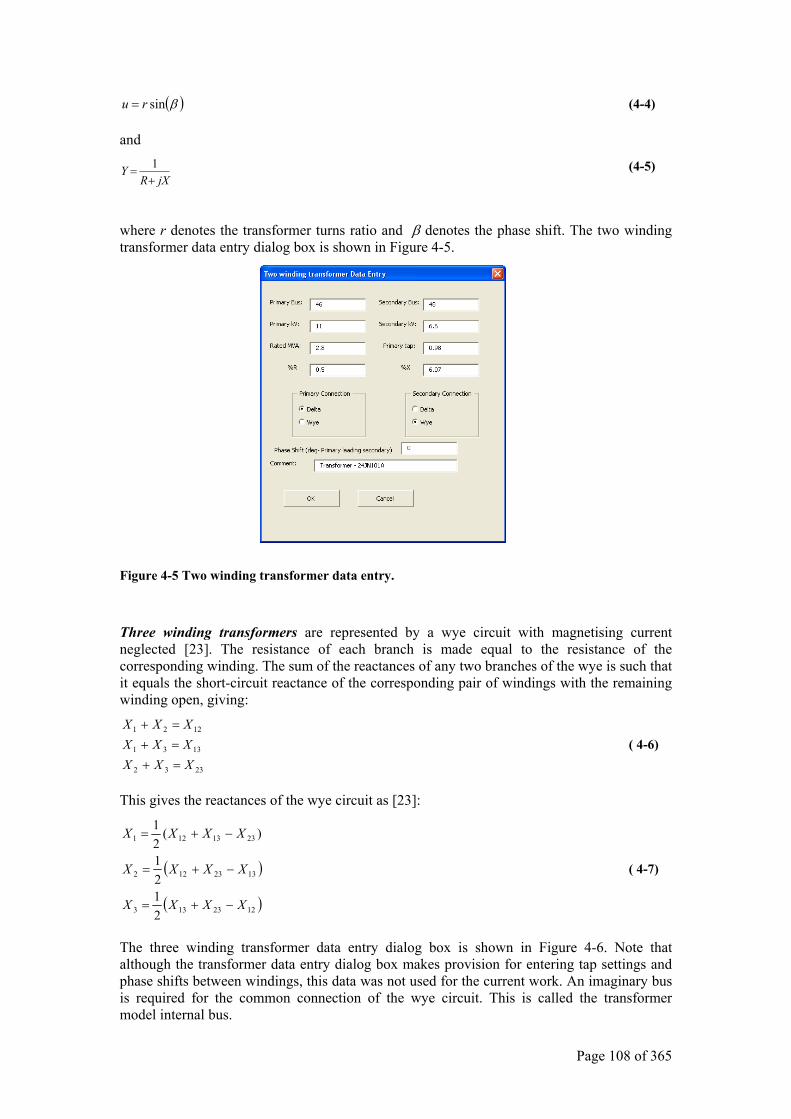
Page 108 of 365

( )βsinru = (4-4)

and

jXRY

+=

1 (4-5)

where r denotes the transformer turns ratio and β denotes the phase shift. The two winding transformer data entry dialog box is shown in Figure 4-5.

Figure 4-5 Two winding transformer data entry.

Three winding transformers are represented by a wye circuit with magnetising current neglected [23]. The resistance of each branch is made equal to the resistance of the corresponding winding. The sum of the reactances of any two branches of the wye is such that it equals the short-circuit reactance of the corresponding pair of windings with the remaining winding open, giving:

2332

1331

1221

XXXXXXXXX

=+=+=+

( 4-6)

This gives the reactances of the wye circuit as [23]:

( )

( )1223133

1323122

2313121

2121

)(21

XXXX

XXXX

XXXX

−+=

−+=

−+=

( 4-7)

The three winding transformer data entry dialog box is shown in Figure 4-6. Note that although the transformer data entry dialog box makes provision for entering tap settings and phase shifts between windings, this data was not used for the current work. An imaginary bus is required for the common connection of the wye circuit. This is called the transformer model internal bus.

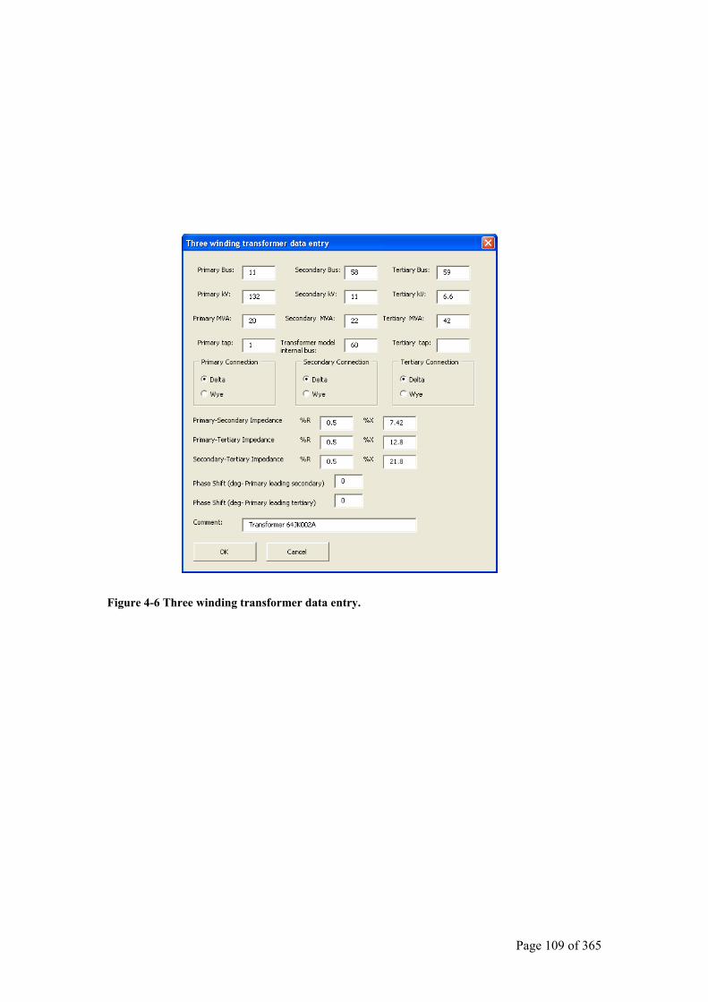
Page 109 of 365

Figure 4-6 Three winding transformer data entry.

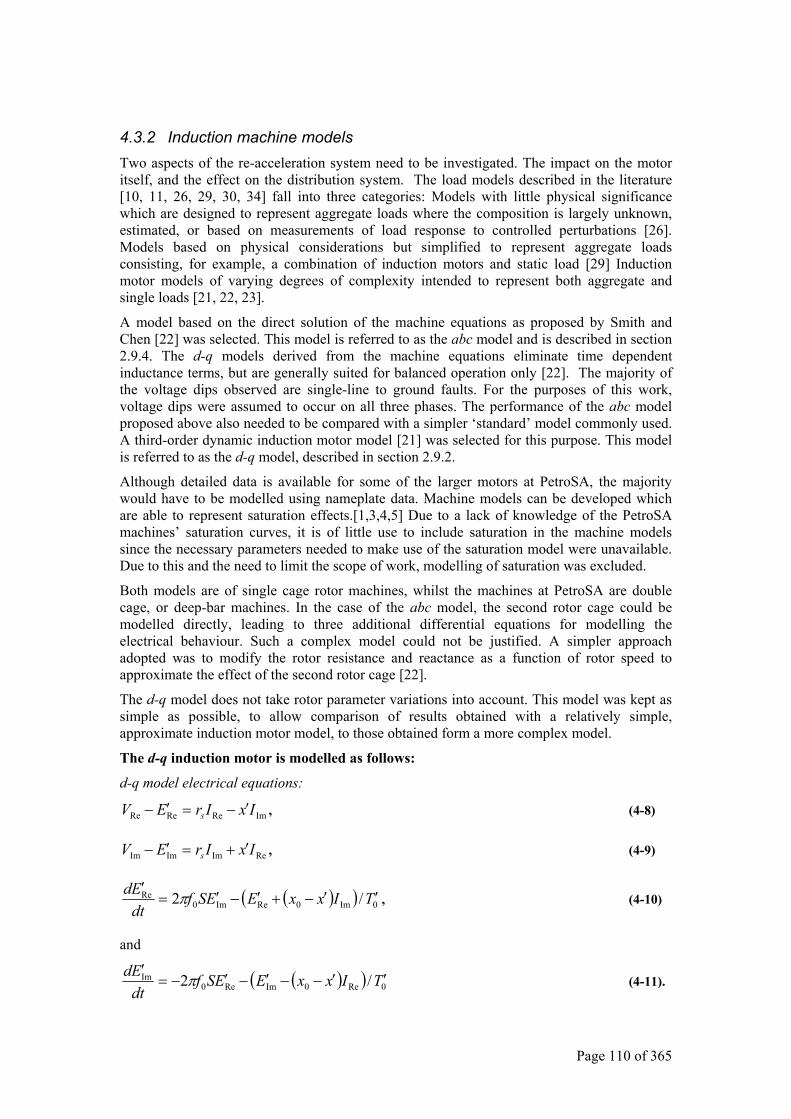
Page 110 of 365

4.3.2 Induction machine models Two aspects of the re-acceleration system need to be investigated. The impact on the motor itself, and the effect on the distribution system. The load models described in the literature [10, 11, 26, 29, 30, 34] fall into three categories: Models with little physical significance which are designed to represent aggregate loads where the composition is largely unknown, estimated, or based on measurements of load response to controlled perturbations [26]. Models based on physical considerations but simplified to represent aggregate loads consisting, for example, a combination of induction motors and static load [29] Induction motor models of varying degrees of complexity intended to represent both aggregate and single loads [21, 22, 23].

A model based on the direct solution of the machine equations as proposed by Smith and Chen [22] was selected. This model is referred to as the abc model and is described in section 2.9.4. The d-q models derived from the machine equations eliminate time dependent inductance terms, but are generally suited for balanced operation only [22]. The majority of the voltage dips observed are single-line to ground faults. For the purposes of this work, voltage dips were assumed to occur on all three phases. The performance of the abc model proposed above also needed to be compared with a simpler ‘standard’ model commonly used. A third-order dynamic induction motor model [21] was selected for this purpose. This model is referred to as the d-q model, described in section 2.9.2.

Although detailed data is available for some of the larger motors at PetroSA, the majority would have to be modelled using nameplate data. Machine models can be developed which are able to represent saturation effects.[1,3,4,5] Due to a lack of knowledge of the PetroSA machines’ saturation curves, it is of little use to include saturation in the machine models since the necessary parameters needed to make use of the saturation model were unavailable. Due to this and the need to limit the scope of work, modelling of saturation was excluded.

Both models are of single cage rotor machines, whilst the machines at PetroSA are double cage, or deep-bar machines. In the case of the abc model, the second rotor cage could be modelled directly, leading to three additional differential equations for modelling the electrical behaviour. Such a complex model could not be justified. A simpler approach adopted was to modify the rotor resistance and reactance as a function of rotor speed to approximate the effect of the second rotor cage [22].

The d-q model does not take rotor parameter variations into account. This model was kept as simple as possible, to allow comparison of results obtained with a relatively simple, approximate induction motor model, to those obtained form a more complex model.

The d-q induction motor is modelled as follows:

d-q model electrical equations:

ImReReRe IxIrEV s ′−=′− , (4-8)

ReImImIm IxIrEV s ′+=′− , (4-9)

( )( ) 0Im0ReIm0Re /2 TIxxEESf

dtEd ′′−+′−′=

′π , (4-10)

and

( )( ) 0Re0ImRe0Im /2 TIxxEESf

dtEd ′′−−′−′−=

′π (4-11).

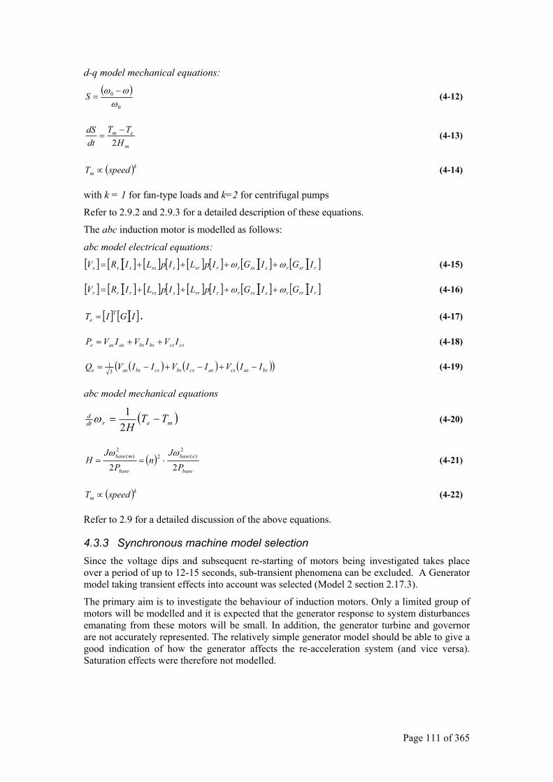
Page 111 of 365

d-q model mechanical equations:

( )0

0

ωωω −

=S (4-12)

m

em

HTT

dtdS

2−

= (4-13)

( )km speedT ∝ (4-14)

with k = 1 for fan-type loads and k=2 for centrifugal pumps

Refer to 2.9.2 and 2.9.3 for a detailed description of these equations.

The abc induction motor is modelled as follows:

abc model electrical equations:

[ ] [ ][ ] [ ] [ ] [ ] [ ] [ ][ ] [ ][ ]rsrrsssrrsrssssss IGIGIpLIpLIRV ωω ++++= (4-15)

[ ] [ ][ ] [ ] [ ] [ ] [ ] [ ][ ] [ ][ ]rrrrsrsrrrrsrsrrr IGIGIpLIpLIRV ωω ++++= (4-16)

[ ] [ ][ ]IGIT Te = . (4-17)

cscsbsbsasase IVIVIVP ++= (4-18)

( ) ( ) ( )( )bsascsascsbscsbsase IIVIIVIIVQ −+−+−=3

1 (4-19)

abc model mechanical equations

( )merdtd TT

H−=

21ω (4-20)

( )base

ebase

base

mbase

PJ

nP

JH

22

2)(2

2)( ωω

⋅== (4-21)

( )km speedT ∝ (4-22)

Refer to 2.9 for a detailed discussion of the above equations.

4.3.3 Synchronous machine model selection Since the voltage dips and subsequent re-starting of motors being investigated takes place over a period of up to 12-15 seconds, sub-transient phenomena can be excluded. A Generator model taking transient effects into account was selected (Model 2 section 2.17.3).

The primary aim is to investigate the behaviour of induction motors. Only a limited group of motors will be modelled and it is expected that the generator response to system disturbances emanating from these motors will be small. In addition, the generator turbine and governor are not accurately represented. The relatively simple generator model should be able to give a good indication of how the generator affects the re-acceleration system (and vice versa). Saturation effects were therefore not modelled.

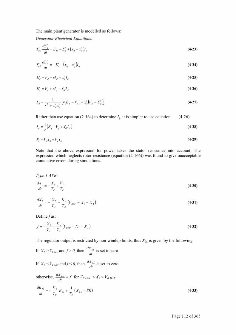
Page 112 of 365

The main plant generator is modelled as follows:

Generator Electrical Equations:

( ) dddqfdq

d IxxEEdtEd

T ′−+′−=′

′0 (4-23)

( ) qqqdd

q IxxEdtEdT ′−−′−=

′′0 (4-24)

qqddd IxrIVE ′++=′ (4-25)

ddqqq IxrIVE ′−+=′ (4-26)

( ) ( )[ ]qqqddqd

d EVxVErxxr

I ′−′+−′′′+

= 2

1 (4-27)

Rather than use equation (2-164) to determine Iq, it is simpler to use equation (4-26):

( )ddqqq IxVEr

I ′+−′=1 (4-28)

qqdde IVIVP += (4-29)

Note that the above expression for power takes the stator resistance into account. The expression which neglects rotor resistance (equation (2-166)) was found to give unacceptable cumulative errors during simulations.

Type 1 AVR:

R

S

R TV

TX

dtdX

+−= 11 (4-30)

( )4122 XXV

TK

TX

dtdX

REFA

A

A

−−+−= (4-31)

Define f as:

( )412 XXV

TK

TX

f REFA

A

A

−−+−= (4-32)

The regulator output is restricted by non-windup limits, thus X2L is given by the following:

If MaxRVX ≥2 and f > 0, then dt

dX L2 is set to zero

If MINRVX ≤2 and f < 0, then dt

dX L2 is set to zero

otherwise, fdt

dX L =2 for VR MIN < X2 < VR MAX

( )SEXT

ETK

dtdE

LE

fdE

Efd −+−= 21 (4-33)

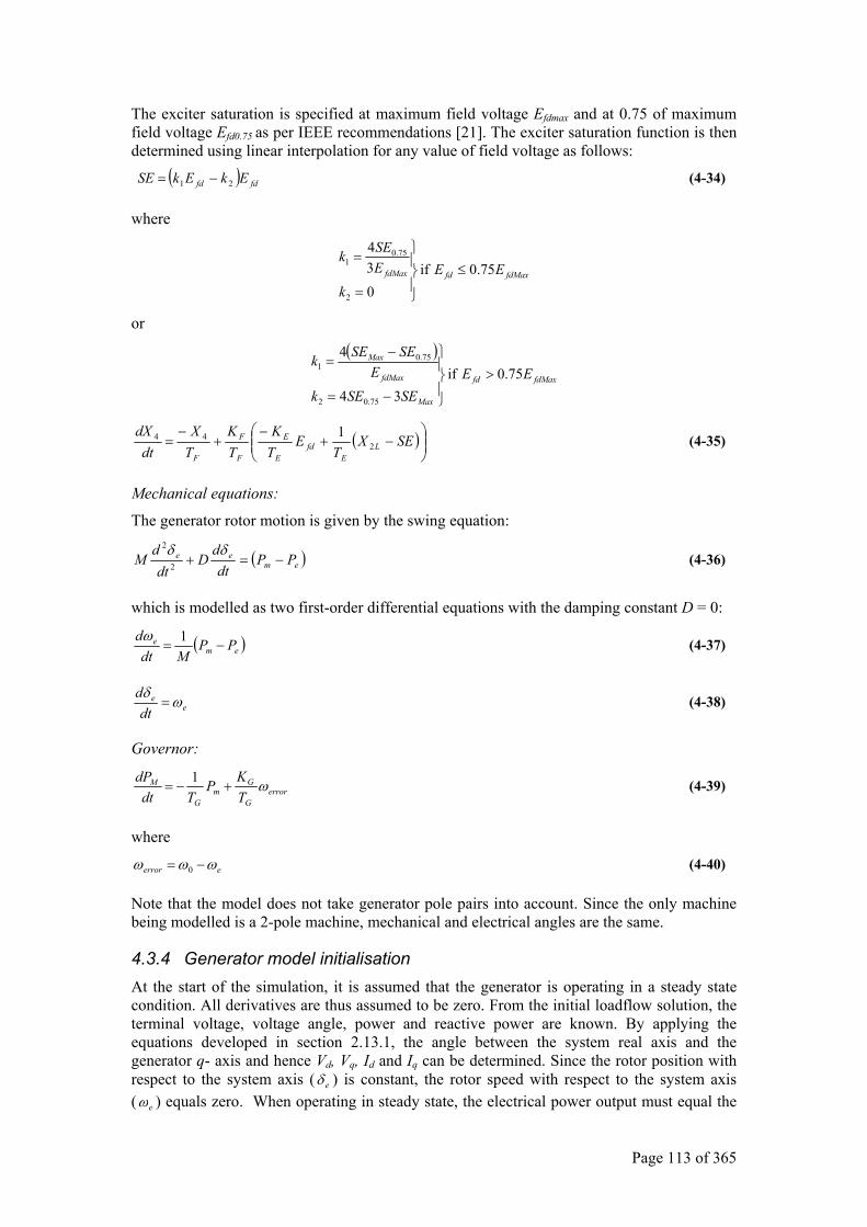
Page 113 of 365

The exciter saturation is specified at maximum field voltage Efdmax and at 0.75 of maximum field voltage Efd0.75 as per IEEE recommendations [21]. The exciter saturation function is then determined using linear interpolation for any value of field voltage as follows:

( ) fdfd EkEkSE 21 −= (4-34)

where

fdMaxfdfdMax EEk

ESEk

75.0 if 0

34

2

75.01

≤

=

=

or

( )fdMaxfd

Max

fdMax

Max

EESESEk

ESESEk

75.0 if 34

4

75.02

75.01

>

−=

−=

( )

−+

−+

−= SEX

TE

TK

TK

TX

dtdX

LE

fdE

E

F

F

F2

44 1 (4-35)

Mechanical equations:

The generator rotor motion is given by the swing equation:

( )emee PP

dtd

Ddt

dM −=+

δδ2

2

(4-36)

which is modelled as two first-order differential equations with the damping constant D = 0:

( )eme PP

Mdtd

−=1ω (4-37)

ee

dtd

ωδ

= (4-38)

Governor:

errorG

Gm

G

M

TKP

TdtdP ω+−=

1 (4-39)

where

eerror ωωω −= 0 (4-40)

Note that the model does not take generator pole pairs into account. Since the only machine being modelled is a 2-pole machine, mechanical and electrical angles are the same.

4.3.4 Generator model initialisation At the start of the simulation, it is assumed that the generator is operating in a steady state condition. All derivatives are thus assumed to be zero. From the initial loadflow solution, the terminal voltage, voltage angle, power and reactive power are known. By applying the equations developed in section 2.13.1, the angle between the system real axis and the generator q- axis and hence Vd, Vq, Id and Iq can be determined. Since the rotor position with respect to the system axis ( eδ ) is constant, the rotor speed with respect to the system axis ( eω ) equals zero. When operating in steady state, the electrical power output must equal the

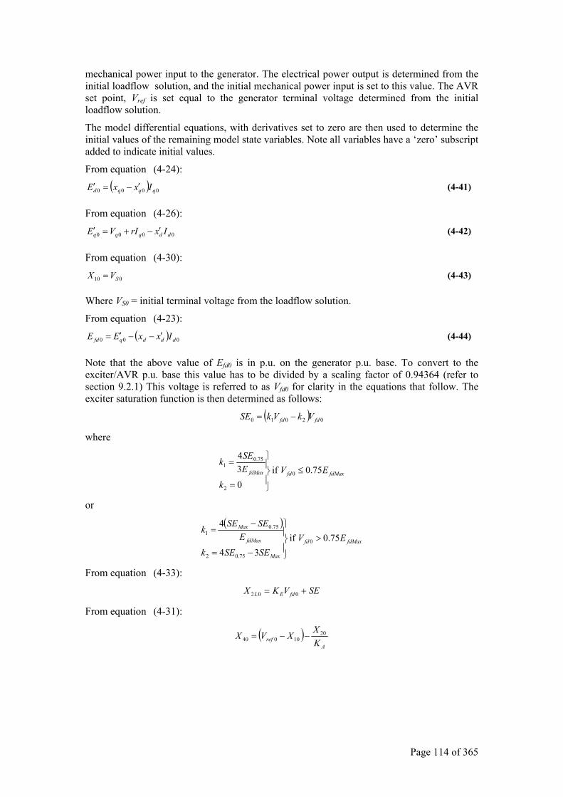
Page 114 of 365

mechanical power input to the generator. The electrical power output is determined from the initial loadflow solution, and the initial mechanical power input is set to this value. The AVR set point, Vref is set equal to the generator terminal voltage determined from the initial loadflow solution.

The model differential equations, with derivatives set to zero are then used to determine the initial values of the remaining model state variables. Note all variables have a ‘zero’ subscript added to indicate initial values.

From equation (4-24):

( ) 0000 qqqd IxxE ′−=′ (4-41)

From equation (4-26):

0000 ddqqq IxrIVE ′−+=′ (4-42)

From equation (4-30):

010 SVX = (4-43)

Where VS0 = initial terminal voltage from the loadflow solution.

From equation (4-23):

( ) 000 dddqfd IxxEE ′−−′= (4-44)

Note that the above value of Efd0 is in p.u. on the generator p.u. base. To convert to the exciter/AVR p.u. base this value has to be divided by a scaling factor of 0.94364 (refer to section 9.2.1) This voltage is referred to as Vfd0 for clarity in the equations that follow. The exciter saturation function is then determined as follows:

( ) 02010 fdfd VkVkSE −=

where

fdMaxfdfdMax EVk

ESEk

75.0 if 0

34

0

2

75.01

≤

=

=

or

( )fdMaxfd

Max

fdMax

Max

EVSESEk

ESESEk

75.0 if 34

4

0

75.02

75.01

>

−=

−=

From equation (4-33):

SEVKX fdEL += 002

From equation (4-31):

( )A

ref KXXVX 20

10040 −−=

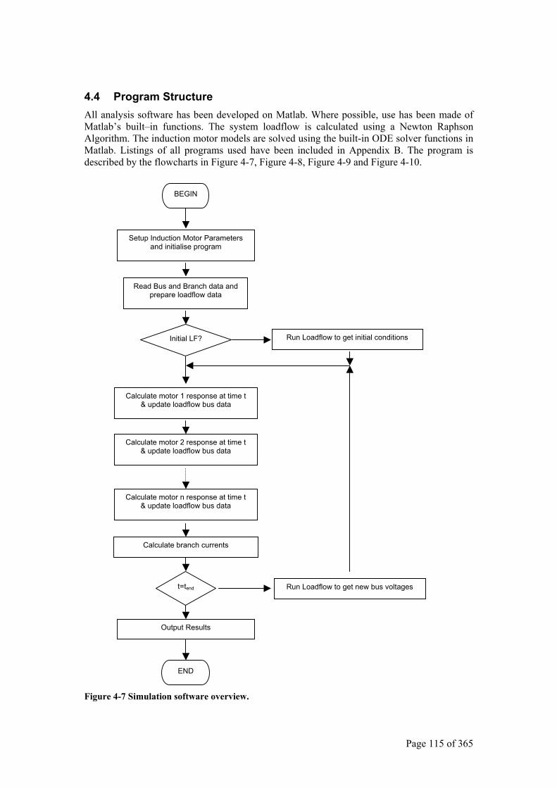
Page 115 of 365

4.4 Program Structure All analysis software has been developed on Matlab. Where possible, use has been made of Matlab’s built–in functions. The system loadflow is calculated using a Newton Raphson Algorithm. The induction motor models are solved using the built-in ODE solver functions in Matlab. Listings of all programs used have been included in Appendix B. The program is described by the flowcharts in Figure 4-7, Figure 4-8, Figure 4-9 and Figure 4-10.

Figure 4-7 Simulation software overview.

Setup Induction Motor Parameters and initialise program

Read Bus and Branch data andprepare loadflow data

Initial LF? Run Loadflow to get initial conditions

Calculate motor 1 response at time t & update loadflow bus data

Calculate motor 2 response at time t & update loadflow bus data

Calculate motor n response at time t & update loadflow bus data

t=tend

Output Results

Calculate branch currents

END

BEGIN

Run Loadflow to get new bus voltages

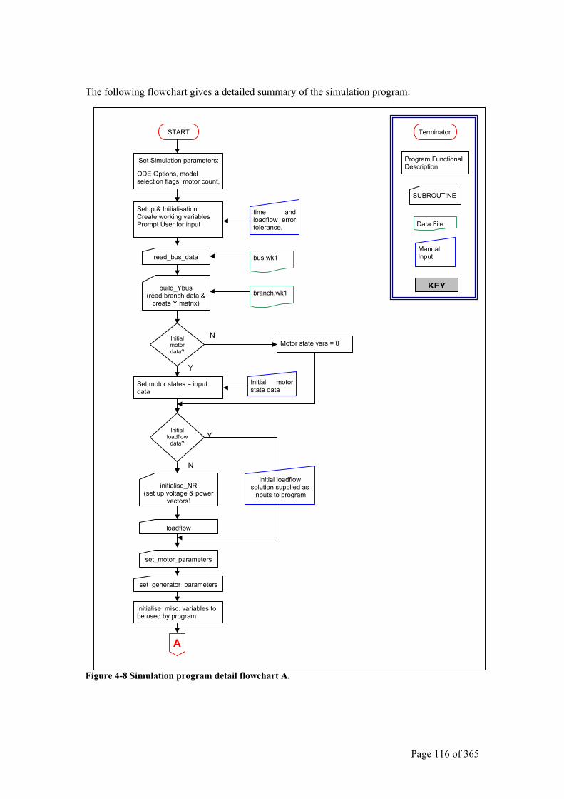
Page 116 of 365

The following flowchart gives a detailed summary of the simulation program:

Figure 4-8 Simulation program detail flowchart A.

Terminator

Program Functional Description

SUBROUTINE

Data File

Manual Input

KEY

Motor state vars = 0

START

Set Simulation parameters:

ODE Options, model selection flags, motor count,

Setup & Initialisation: Create working variables Prompt User for input

time andloadflow errortolerance.

read_bus_data bus.wk1

build_Ybus (read branch data &

create Y matrix) branch.wk1

Initial motor data?

N

Set motor states = input data

Initial motorstate data

Initial loadflow

data?

Y

N

initialise_NR (set up voltage & power

vectors)

loadflow

Y

Initial loadflow solution supplied as inputs to program

set_motor_parameters

set_generator_parameters

Initialise misc. variables to be used by program

A

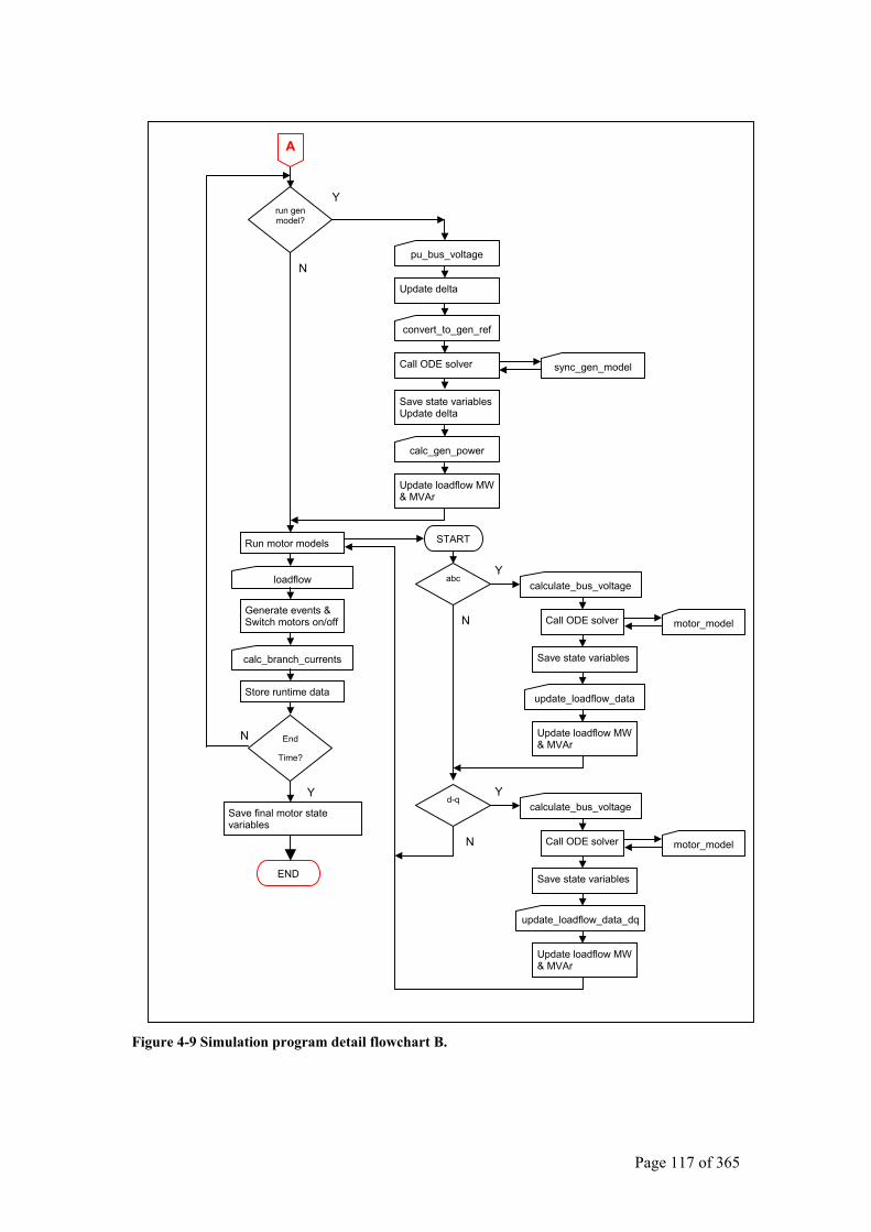
Page 117 of 365

Figure 4-9 Simulation program detail flowchart B.

Save state variablesUpdate delta

Update delta

pu_bus_voltage

convert_to_gen_ref

run gen model?

N

Call ODE solver

End

Time?

Y

N

Y

calc_branch_currents

Save final motor state variables

A

sync_gen_model

calc_gen_power

Update loadflow MW & MVAr

Run motor models

loadflow

Generate events & Switch motors on/off

Store runtime data

END

START

abc calculate_bus_voltage

Y

Call ODE solver motor_model

Save state variables

update_loadflow_data

Update loadflow MW & MVAr

d-q calculate_bus_voltage

Call ODE solver motor_model

Save state variables

update_loadflow_data_dq

Update loadflow MW & MVAr

N

N

Y

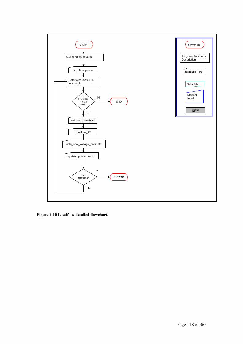
Page 118 of 365

Figure 4-10 Loadflow detailed flowchart.

Terminator

Program FunctionalDescription

SUBROUTINE

Data File

Manual Input

KEY

Determine max. P,Q mismatch

START

Set Iteration counter

calculate_jacobian

P,Q error > max error?

N

max iterations?

Y

N

calc_new_voltage_estimate

update power vector

Y

calc_bus_power

END

calculate_dV

ERROR

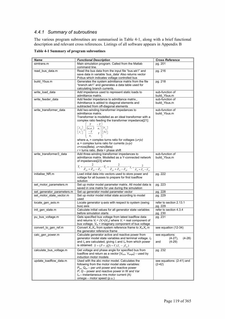
Page 119 of 365

4.4.1 Summary of subroutines The various program subroutines are summarised in Table 4-1, along with a brief functional description and relevant cross references. Listings of all software appears in Appendix B Table 4-1 Summary of program subroutines

Name Functional Description Cross Reference simtrans.m Main simulation program. Called from the Matlab

command line. pg. 201

read_bus_data.m Read the bus data from the input file “bus.wk1” and save data in variable ‘bus_data’ Also returns vector Pvbus which indicates voltage controlled bus

pg. 216

build_Ybus.m Generates the system admittance matrix from the file “branch.wk1” and generates a data table used for calculating branch currents.

pg. 218

write_load_data Add impedance used to represent static loads to admittance matrix.

sub-function of build_Ybus.m

write_feeder_data Add feeder impedance to admittance matrix., Admittance is added to diagonal elements and subtracted from off-diagonal elements

sub-function of build_Ybus.m

write_transformer_data Add two-winding transformer impedances to admittance matrix. Transformer is modelled as an ideal transformer with a complex ratio feeding the transformer impedance[21]:

( )

−

−

=

VsV

Ya

YaY

aaY

II p

v

ivi

s

p

where av = complex turns ratio for voltages (u+jv) ai = complex turns ratio for currents (u-jv) v=rcos(Beta), u=rsin(Beta) r = turns ratio, Beta = phase shift

sub-function of build_Ybus.m

write_transformer3_data Add three-winding transformer impedances to admittance matrix. Modelled as a Y-connected network of impedances[23] where

stptps ZZZY

−+=

21

,ptstps ZZZ

Y−+

=2

2,

psstpt ZZZY

−+=

23

sub-function of build_Ybus.m

initialise_NR.m Load initial data into vectors used to store power and voltage for all busses to prepare for first loadflow solution

pg. 222

set_motor_parameters.m Set up motor model parameter matrix. All model data is saved in one matrix for use during the simulation

pg. 223

set_generator_parameters.m Set up generator model parameter vector pg. 228 set_motor_state_vector.m Set up motor model initial state according to model

used pg. 229

locate_gen_axis.m Locate generator q-axis with respect to system (swing bus) axis

refer to section 2.13.1 pg. 229

init_gen_state.m Calculate initial values for all generator state variables before simulation starts

refer to section 4.3.4 pg. 230

pu_bus_voltage.m Gets specified bus voltage from latest loadflow data and returns Vt = (Vr+jVm) where Vr = real component of bus voltage, Vm = imaginary component of bus voltage

pg. 231

convert_to_gen_ref.m Convert Xr,Xm from system reference frame to Xd,Xq in the generator reference frame

see equation (12-34)

calc_gen_power.m Calculate generator active and reactive power from generator model state variables and terminal voltage. Id and Iq are calculated, giving Ir and Im from which power is obtained: )()( mrt jIIVjQPS −=+=

see equations: (4-27), (4-28) and (4-29)

calculate_bus_voltage.m Get voltage and phase angle for specified bus from loadflow and return as a vector [Vbus, Vangle] – used by induction motor models

pg. 232

update_loadflow_data.m Used with the abc motor model. Calculates the following from the motor model state variables: Ppu, Qpu – per unit power and reactive power P, Q – power and reactive power in W and Var Im – instantaneous rms motor current (A) omega – motor speed (p.u.)

see equations: (2-41) and (2-42)

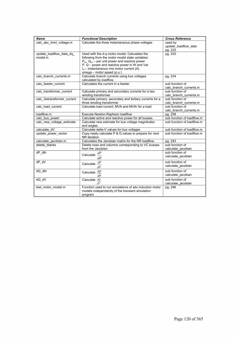
Page 120 of 365

Name Functional Description Cross Reference calc_abc_tmnl_voltage.m Calculate the three instantaneous phase voltages used by

update_loadflow_data pg. 233

update_loadflow_data_dq_ model.m

Used with the d-q motor model. Calculates the following from the motor model state variables: Ppu, Qpu – per unit power and reactive power P, Q – power and reactive power in W and Var Im – instantaneous rms motor current (A) omega – motor speed (p.u.)

pg. 233

calc_branch_currents.m Calculate branch currents using bus voltages calculated by loadflow

pg. 234

calc_feeder_current Calculates the current in a feeder sub function of calc_branch_currents.m

calc_transformer_current Calculate primary and secondary currents for a two winding transformer

sub function of calc_branch_currents.m

calc_3wtransformer_current Calculate primary, secondary and tertiary currents for a three winding transformer

sub function of calc_branch_currents.m

calc_load_current Calculate load current, MVA and MVAr for a load sub function of calc_branch_currents.m

loadflow.m Execute Newton-Raphson loadflow pg. 238 calc_bus_power Calculate active and reactive power for all busses sub function of loadflow.m calc_new_voltage_estimate Calculate new estimate for bus voltage magnitudes

and angles sub function of loadflow.m

calculate_dV Calculate delta-V values for bus voltages sub function of loadflow.m update_power_vector Copy newly calculate P & Q values to prepare for next

NR iteration sub function of loadflow.m

calculate_jacobian.m Calculates the Jacobian matrix for the NR loadflow. pg. 243 delete_blanks Delete rows and columns corresponding to VC busses

from the Jacobian sub function of calculate_jacobian

dP_dth Calculate

θddP

sub function of calculate_jacobian

dP_dV Calculate dVdP sub function of

calculate_jacobian dQ_dth Calculate

θddQ sub function of

calculate_jacobian dQ_dV Calculate

dVdQ sub function of

calculate_jacobian test_motor_model.m Function used to run simulations of abc induction motor

models independently of the transient simulation program

pg. 246

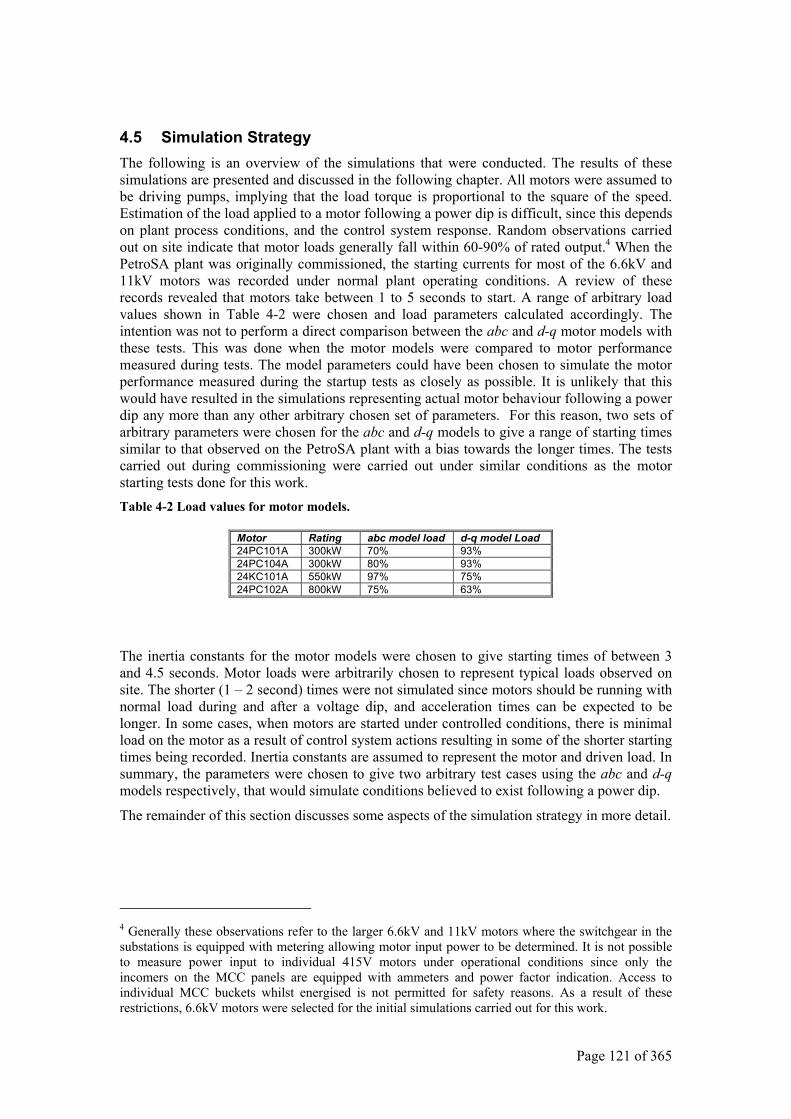
Page 121 of 365

4.5 Simulation Strategy The following is an overview of the simulations that were conducted. The results of these simulations are presented and discussed in the following chapter. All motors were assumed to be driving pumps, implying that the load torque is proportional to the square of the speed. Estimation of the load applied to a motor following a power dip is difficult, since this depends on plant process conditions, and the control system response. Random observations carried out on site indicate that motor loads generally fall within 60-90% of rated output.4 When the PetroSA plant was originally commissioned, the starting currents for most of the 6.6kV and 11kV motors was recorded under normal plant operating conditions. A review of these records revealed that motors take between 1 to 5 seconds to start. A range of arbitrary load values shown in Table 4-2 were chosen and load parameters calculated accordingly. The intention was not to perform a direct comparison between the abc and d-q motor models with these tests. This was done when the motor models were compared to motor performance measured during tests. The model parameters could have been chosen to simulate the motor performance measured during the startup tests as closely as possible. It is unlikely that this would have resulted in the simulations representing actual motor behaviour following a power dip any more than any other arbitrary chosen set of parameters. For this reason, two sets of arbitrary parameters were chosen for the abc and d-q models to give a range of starting times similar to that observed on the PetroSA plant with a bias towards the longer times. The tests carried out during commissioning were carried out under similar conditions as the motor starting tests done for this work. Table 4-2 Load values for motor models.

Motor Rating abc model load d-q model Load 24PC101A 300kW 70% 93% 24PC104A 300kW 80% 93% 24KC101A 550kW 97% 75% 24PC102A 800kW 75% 63%

The inertia constants for the motor models were chosen to give starting times of between 3 and 4.5 seconds. Motor loads were arbitrarily chosen to represent typical loads observed on site. The shorter (1 – 2 second) times were not simulated since motors should be running with normal load during and after a voltage dip, and acceleration times can be expected to be longer. In some cases, when motors are started under controlled conditions, there is minimal load on the motor as a result of control system actions resulting in some of the shorter starting times being recorded. Inertia constants are assumed to represent the motor and driven load. In summary, the parameters were chosen to give two arbitrary test cases using the abc and d-q models respectively, that would simulate conditions believed to exist following a power dip.

The remainder of this section discusses some aspects of the simulation strategy in more detail.

4 Generally these observations refer to the larger 6.6kV and 11kV motors where the switchgear in the substations is equipped with metering allowing motor input power to be determined. It is not possible to measure power input to individual 415V motors under operational conditions since only the incomers on the MCC panels are equipped with ammeters and power factor indication. Access to individual MCC buckets whilst energised is not permitted for safety reasons. As a result of these restrictions, 6.6kV motors were selected for the initial simulations carried out for this work.

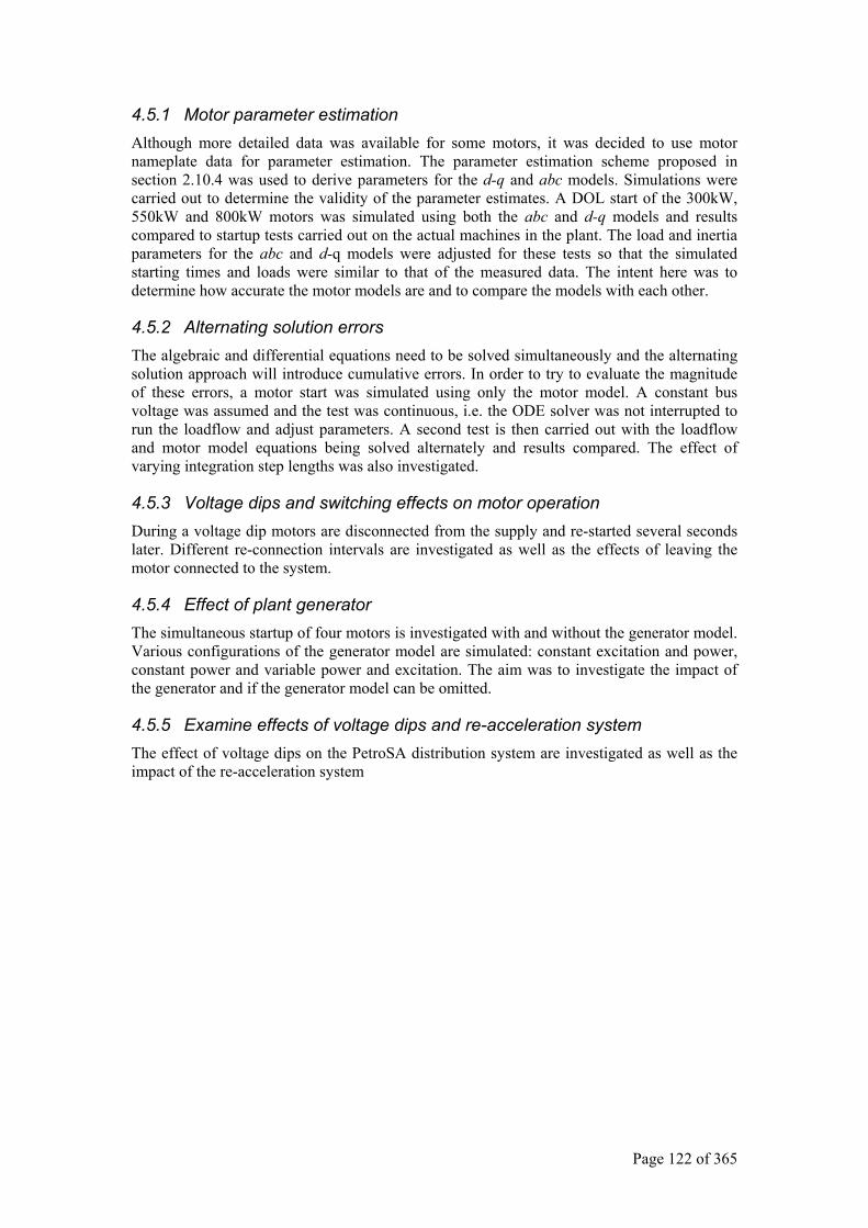
Page 122 of 365

4.5.1 Motor parameter estimation Although more detailed data was available for some motors, it was decided to use motor nameplate data for parameter estimation. The parameter estimation scheme proposed in section 2.10.4 was used to derive parameters for the d-q and abc models. Simulations were carried out to determine the validity of the parameter estimates. A DOL start of the 300kW, 550kW and 800kW motors was simulated using both the abc and d-q models and results compared to startup tests carried out on the actual machines in the plant. The load and inertia parameters for the abc and d-q models were adjusted for these tests so that the simulated starting times and loads were similar to that of the measured data. The intent here was to determine how accurate the motor models are and to compare the models with each other.

4.5.2 Alternating solution errors The algebraic and differential equations need to be solved simultaneously and the alternating solution approach will introduce cumulative errors. In order to try to evaluate the magnitude of these errors, a motor start was simulated using only the motor model. A constant bus voltage was assumed and the test was continuous, i.e. the ODE solver was not interrupted to run the loadflow and adjust parameters. A second test is then carried out with the loadflow and motor model equations being solved alternately and results compared. The effect of varying integration step lengths was also investigated.

4.5.3 Voltage dips and switching effects on motor operation During a voltage dip motors are disconnected from the supply and re-started several seconds later. Different re-connection intervals are investigated as well as the effects of leaving the motor connected to the system.

4.5.4 Effect of plant generator The simultaneous startup of four motors is investigated with and without the generator model. Various configurations of the generator model are simulated: constant excitation and power, constant power and variable power and excitation. The aim was to investigate the impact of the generator and if the generator model can be omitted.

4.5.5 Examine effects of voltage dips and re-acceleration system The effect of voltage dips on the PetroSA distribution system are investigated as well as the impact of the re-acceleration system

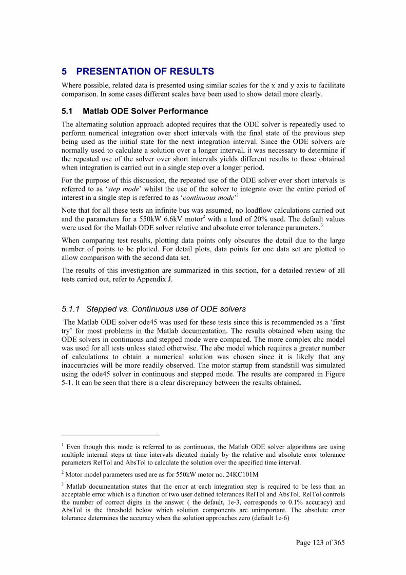
Page 123 of 365

5 PRESENTATION OF RESULTS Where possible, related data is presented using similar scales for the x and y axis to facilitate comparison. In some cases different scales have been used to show detail more clearly.

5.1 Matlab ODE Solver Performance The alternating solution approach adopted requires that the ODE solver is repeatedly used to perform numerical integration over short intervals with the final state of the previous step being used as the initial state for the next integration interval. Since the ODE solvers are normally used to calculate a solution over a longer interval, it was necessary to determine if the repeated use of the solver over short intervals yields different results to those obtained when integration is carried out in a single step over a longer period.

For the purpose of this discussion, the repeated use of the ODE solver over short intervals is referred to as ‘step mode’ whilst the use of the solver to integrate over the entire period of interest in a single step is referred to as ‘continuous mode’1

Note that for all these tests an infinite bus was assumed, no loadflow calculations carried out and the parameters for a 550kW 6.6kV motor2 with a load of 20% used. The default values were used for the Matlab ODE solver relative and absolute error tolerance parameters.3

When comparing test results, plotting data points only obscures the detail due to the large number of points to be plotted. For detail plots, data points for one data set are plotted to allow comparison with the second data set.

The results of this investigation are summarized in this section, for a detailed review of all tests carried out, refer to Appendix J.

5.1.1 Stepped vs. Continuous use of ODE solvers The Matlab ODE solver ode45 was used for these tests since this is recommended as a ‘first try’ for most problems in the Matlab documentation. The results obtained when using the ODE solvers in continuous and stepped mode were compared. The more complex abc model was used for all tests unless stated otherwise. The abc model which requires a greater number of calculations to obtain a numerical solution was chosen since it is likely that any inaccuracies will be more readily observed. The motor startup from standstill was simulated using the ode45 solver in continuous and stepped mode. The results are compared in Figure 5-1. It can be seen that there is a clear discrepancy between the results obtained.

1 Even though this mode is referred to as continuous, the Matlab ODE solver algorithms are using multiple internal steps at time intervals dictated mainly by the relative and absolute error tolerance parameters RelTol and AbsTol to calculate the solution over the specified time interval. 2 Motor model parameters used are as for 550kW motor no. 24KC101M 3 Matlab documentation states that the error at each integration step is required to be less than an acceptable error which is a function of two user defined tolerances RelTol and AbsTol. RelTol controls the number of correct digits in the answer ( the default, 1e-3, corresponds to 0.1% accuracy) and AbsTol is the threshold below which solution components are unimportant. The absolute error tolerance determines the accuracy when the solution approaches zero (default 1e-6)

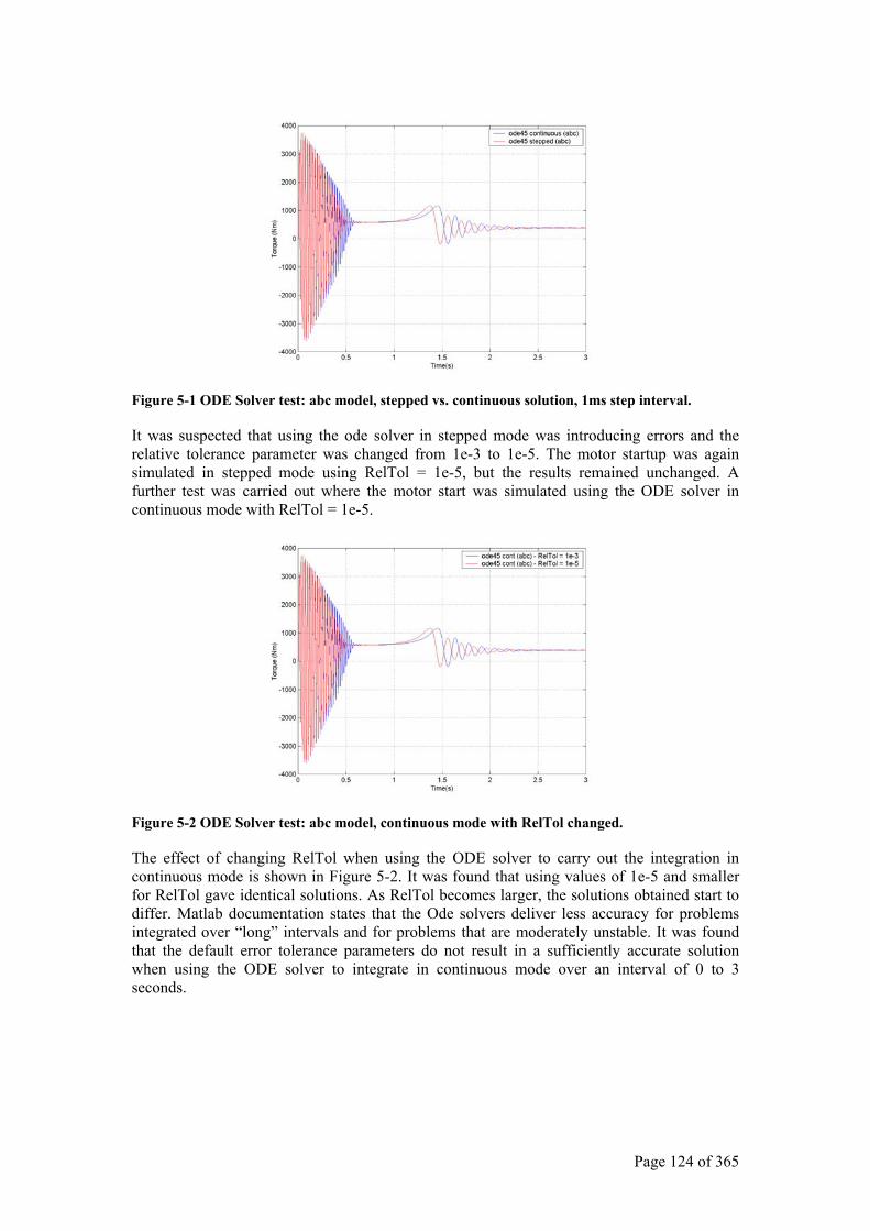
Page 124 of 365

Figure 5-1 ODE Solver test: abc model, stepped vs. continuous solution, 1ms step interval.

It was suspected that using the ode solver in stepped mode was introducing errors and the relative tolerance parameter was changed from 1e-3 to 1e-5. The motor startup was again simulated in stepped mode using RelTol = 1e-5, but the results remained unchanged. A further test was carried out where the motor start was simulated using the ODE solver in continuous mode with RelTol = 1e-5.

Figure 5-2 ODE Solver test: abc model, continuous mode with RelTol changed.

The effect of changing RelTol when using the ODE solver to carry out the integration in continuous mode is shown in Figure 5-2. It was found that using values of 1e-5 and smaller for RelTol gave identical solutions. As RelTol becomes larger, the solutions obtained start to differ. Matlab documentation states that the Ode solvers deliver less accuracy for problems integrated over “long” intervals and for problems that are moderately unstable. It was found that the default error tolerance parameters do not result in a sufficiently accurate solution when using the ODE solver to integrate in continuous mode over an interval of 0 to 3 seconds.

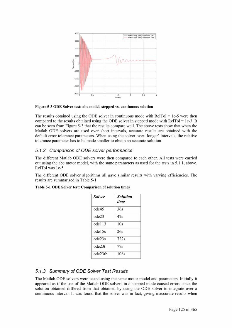
Page 125 of 365

Figure 5-3 ODE Solver test: abc model, stepped vs. continuous solution

The results obtained using the ODE solver in continuous mode with RelTol = 1e-5 were then compared to the results obtained using the ODE solver in stepped mode with RelTol = 1e-3. It can be seen from Figure 5-3 that the results compare well. The above tests show that when the Matlab ODE solvers are used over short intervals, accurate results are obtained with the default error tolerance parameters. When using the solver over ‘longer’ intervals, the relative tolerance parameter has to be made smaller to obtain an accurate solution

5.1.2 Comparison of ODE solver performance The different Matlab ODE solvers were then compared to each other. All tests were carried out using the abc motor model, with the same parameters as used for the tests in 5.1.1, above. RelTol was 1e-5.

The different ODE solver algorithms all gave similar results with varying efficiencies. The results are summarised in Table 5-1 Table 5-1 ODE Solver test: Comparison of solution times

Solver Solution time

ode45 36s

ode23 47s

ode113 10s

ode15s 26s

ode23s 722s

ode23t 77s

ode23tb 108s

5.1.3 Summary of ODE Solver Test Results The Matlab ODE solvers were tested using the same motor model and parameters. Initially it appeared as if the use of the Matlab ODE solvers in a stepped mode caused errors since the solution obtained differed from that obtained by using the ODE solver to integrate over a continuous interval. It was found that the solver was in fact, giving inaccurate results when

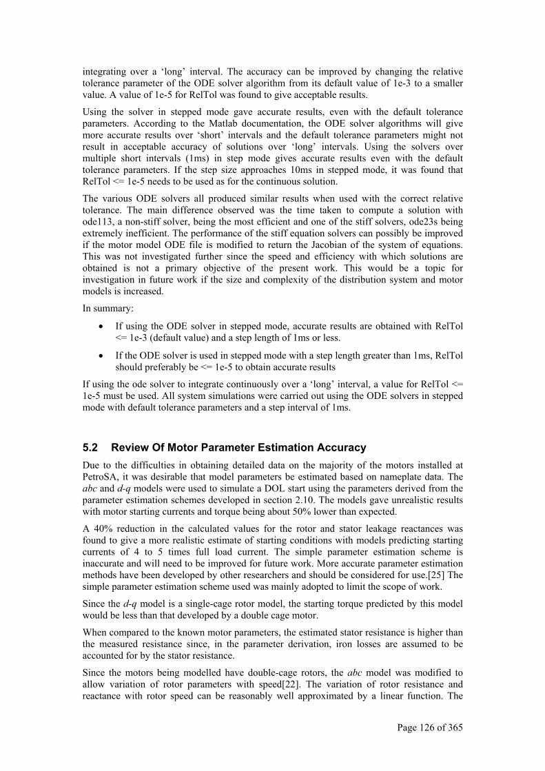
Page 126 of 365

integrating over a ‘long’ interval. The accuracy can be improved by changing the relative tolerance parameter of the ODE solver algorithm from its default value of 1e-3 to a smaller value. A value of 1e-5 for RelTol was found to give acceptable results.

Using the solver in stepped mode gave accurate results, even with the default tolerance parameters. According to the Matlab documentation, the ODE solver algorithms will give more accurate results over ‘short’ intervals and the default tolerance parameters might not result in acceptable accuracy of solutions over ‘long’ intervals. Using the solvers over multiple short intervals (1ms) in step mode gives accurate results even with the default tolerance parameters. If the step size approaches 10ms in stepped mode, it was found that RelTol <= 1e-5 needs to be used as for the continuous solution.

The various ODE solvers all produced similar results when used with the correct relative tolerance. The main difference observed was the time taken to compute a solution with ode113, a non-stiff solver, being the most efficient and one of the stiff solvers, ode23s being extremely inefficient. The performance of the stiff equation solvers can possibly be improved if the motor model ODE file is modified to return the Jacobian of the system of equations. This was not investigated further since the speed and efficiency with which solutions are obtained is not a primary objective of the present work. This would be a topic for investigation in future work if the size and complexity of the distribution system and motor models is increased.

In summary:

• If using the ODE solver in stepped mode, accurate results are obtained with RelTol <= 1e-3 (default value) and a step length of 1ms or less.

• If the ODE solver is used in stepped mode with a step length greater than 1ms, RelTol should preferably be <= 1e-5 to obtain accurate results

If using the ode solver to integrate continuously over a ‘long’ interval, a value for RelTol <= 1e-5 must be used. All system simulations were carried out using the ODE solvers in stepped mode with default tolerance parameters and a step interval of 1ms.

5.2 Review Of Motor Parameter Estimation Accuracy Due to the difficulties in obtaining detailed data on the majority of the motors installed at PetroSA, it was desirable that model parameters be estimated based on nameplate data. The abc and d-q models were used to simulate a DOL start using the parameters derived from the parameter estimation schemes developed in section 2.10. The models gave unrealistic results with motor starting currents and torque being about 50% lower than expected.

A 40% reduction in the calculated values for the rotor and stator leakage reactances was found to give a more realistic estimate of starting conditions with models predicting starting currents of 4 to 5 times full load current. The simple parameter estimation scheme is inaccurate and will need to be improved for future work. More accurate parameter estimation methods have been developed by other researchers and should be considered for use.[25] The simple parameter estimation scheme used was mainly adopted to limit the scope of work.

Since the d-q model is a single-cage rotor model, the starting torque predicted by this model would be less than that developed by a double cage motor.

When compared to the known motor parameters, the estimated stator resistance is higher than the measured resistance since, in the parameter derivation, iron losses are assumed to be accounted for by the stator resistance.

Since the motors being modelled have double-cage rotors, the abc model was modified to allow variation of rotor parameters with speed[22]. The variation of rotor resistance and reactance with rotor speed can be reasonably well approximated by a linear function. The

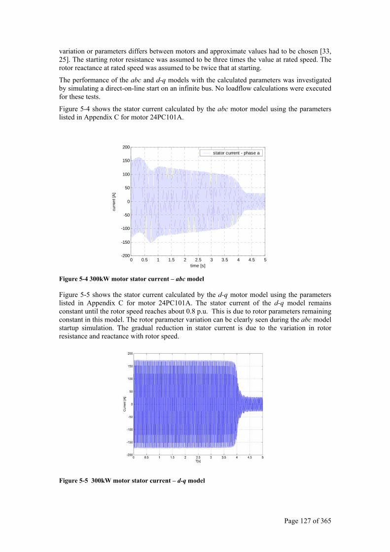
Page 127 of 365

variation or parameters differs between motors and approximate values had to be chosen [33, 25]. The starting rotor resistance was assumed to be three times the value at rated speed. The rotor reactance at rated speed was assumed to be twice that at starting.

The performance of the abc and d-q models with the calculated parameters was investigated by simulating a direct-on-line start on an infinite bus. No loadflow calculations were executed for these tests.

Figure 5-4 shows the stator current calculated by the abc motor model using the parameters listed in Appendix C for motor 24PC101A.

0 0.5 1 1.5 2 2.5 3 3.5 4 4.5 5-200

-150

-100

-50

0

50

100

150

200

time [s]

stator current - phase a

Figure 5-4 300kW motor stator current – abc model

Figure 5-5 shows the stator current calculated by the d-q motor model using the parameters listed in Appendix C for motor 24PC101A. The stator current of the d-q model remains constant until the rotor speed reaches about 0.8 p.u. This is due to rotor parameters remaining constant in this model. The rotor parameter variation can be clearly seen during the abc model startup simulation. The gradual reduction in stator current is due to the variation in rotor resistance and reactance with rotor speed.

Figure 5-5 300kW motor stator current – d-q model

curre

nt [A

]

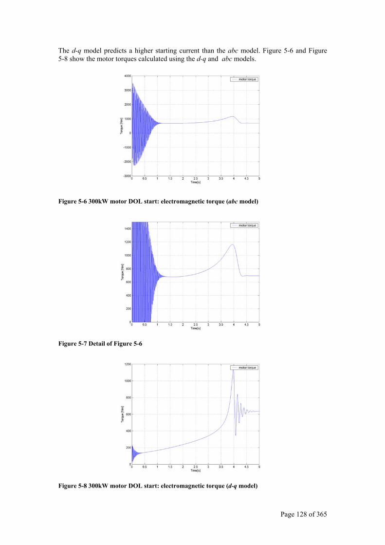
Page 128 of 365

The d-q model predicts a higher starting current than the abc model. Figure 5-6 and Figure 5-8 show the motor torques calculated using the d-q and abc models.

Figure 5-6 300kW motor DOL start: electromagnetic torque (abc model)

Figure 5-7 Detail of Figure 5-6

Figure 5-8 300kW motor DOL start: electromagnetic torque (d-q model)

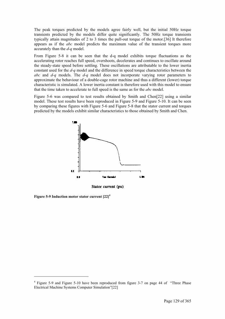
Page 129 of 365

The peak torques predicted by the models agree fairly well, but the initial 50Hz torque transients predicted by the models differ quite significantly. The 50Hz torque transients typically attain magnitudes of 2 to 3 times the pull-out torque of the motor.[36] It therefore appears as if the abc model predicts the maximum value of the transient torques more accurately than the d-q model.

From Figure 5-8 it can be seen that the d-q model exhibits torque fluctuations as the accelerating rotor reaches full speed, overshoots, decelerates and continues to oscillate around the steady-state speed before settling. These oscillations are attributable to the lower inertia constant used for the d-q model and the difference in speed torque characteristics between the abc and d-q models. The d-q model does not incorporate varying rotor parameters to approximate the behaviour of a double-cage rotor machine and thus a different (lower) torque characteristic is simulated. A lower inertia constant is therefore used with this model to ensure that the time taken to accelerate to full speed is the same as for the abc model.

Figure 5-6 was compared to test results obtained by Smith and Chen[22] using a similar model. These test results have been reproduced in Figure 5-9 and Figure 5-10. It can be seen by comparing these figures with Figure 5-6 and Figure 5-8 that the stator current and torques predicted by the models exhibit similar characteristics to those obtained by Smith and Chen.

Figure 5-9 Induction motor stator current [22]4

4 Figure 5-9 and Figure 5-10 have been reproduced from figure 3-7 on page 44 of “Three Phase Electrical Machine Systems Computer Simulation”[22]

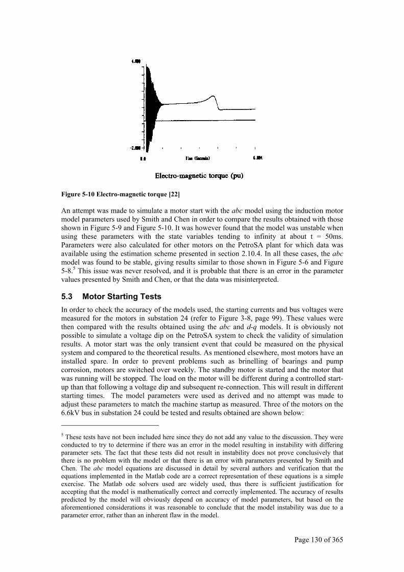
Page 130 of 365

Figure 5-10 Electro-magnetic torque [22]

An attempt was made to simulate a motor start with the abc model using the induction motor model parameters used by Smith and Chen in order to compare the results obtained with those shown in Figure 5-9 and Figure 5-10. It was however found that the model was unstable when using these parameters with the state variables tending to infinity at about t = 50ms. Parameters were also calculated for other motors on the PetroSA plant for which data was available using the estimation scheme presented in section 2.10.4. In all these cases, the abc model was found to be stable, giving results similar to those shown in Figure 5-6 and Figure 5-8.5 This issue was never resolved, and it is probable that there is an error in the parameter values presented by Smith and Chen, or that the data was misinterpreted.

5.3 Motor Starting Tests In order to check the accuracy of the models used, the starting currents and bus voltages were measured for the motors in substation 24 (refer to Figure 3-8, page 99). These values were then compared with the results obtained using the abc and d-q models. It is obviously not possible to simulate a voltage dip on the PetroSA system to check the validity of simulation results. A motor start was the only transient event that could be measured on the physical system and compared to the theoretical results. As mentioned elsewhere, most motors have an installed spare. In order to prevent problems such as brinelling of bearings and pump corrosion, motors are switched over weekly. The standby motor is started and the motor that was running will be stopped. The load on the motor will be different during a controlled start-up than that following a voltage dip and subsequent re-connection. This will result in different starting times. The model parameters were used as derived and no attempt was made to adjust these parameters to match the machine startup as measured. Three of the motors on the 6.6kV bus in substation 24 could be tested and results obtained are shown below: 5 These tests have not been included here since they do not add any value to the discussion. They were conducted to try to determine if there was an error in the model resulting in instability with differing parameter sets. The fact that these tests did not result in instability does not prove conclusively that there is no problem with the model or that there is an error with parameters presented by Smith and Chen. The abc model equations are discussed in detail by several authors and verification that the equations implemented in the Matlab code are a correct representation of these equations is a simple exercise. The Matlab ode solvers used are widely used, thus there is sufficient justification for accepting that the model is mathematically correct and correctly implemented. The accuracy of results predicted by the model will obviously depend on accuracy of model parameters, but based on the aforementioned considerations it was reasonable to conclude that the model instability was due to a parameter error, rather than an inherent flaw in the model.

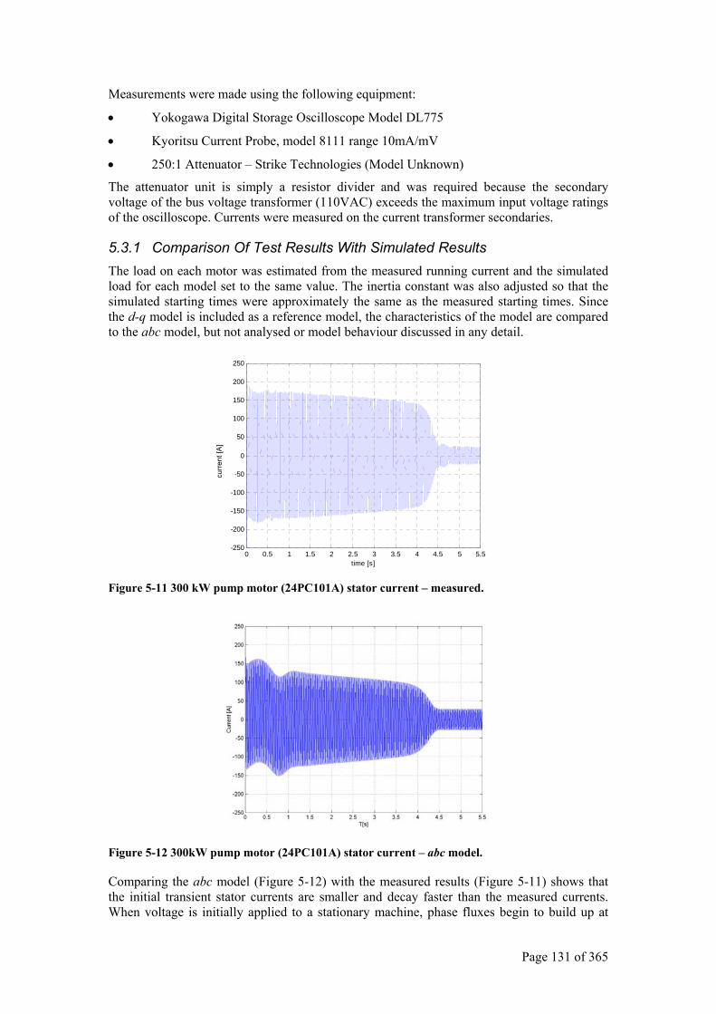
Page 131 of 365

Measurements were made using the following equipment:

• Yokogawa Digital Storage Oscilloscope Model DL775

• Kyoritsu Current Probe, model 8111 range 10mA/mV

• 250:1 Attenuator – Strike Technologies (Model Unknown)

The attenuator unit is simply a resistor divider and was required because the secondary voltage of the bus voltage transformer (110VAC) exceeds the maximum input voltage ratings of the oscilloscope. Currents were measured on the current transformer secondaries.

5.3.1 Comparison Of Test Results With Simulated Results The load on each motor was estimated from the measured running current and the simulated load for each model set to the same value. The inertia constant was also adjusted so that the simulated starting times were approximately the same as the measured starting times. Since the d-q model is included as a reference model, the characteristics of the model are compared to the abc model, but not analysed or model behaviour discussed in any detail.

0 0.5 1 1.5 2 2.5 3 3.5 4 4.5 5 5.5-250

-200

-150

-100

-50

0

50

100

150

200

250

time [s] Figure 5-11 300 kW pump motor (24PC101A) stator current – measured.

Figure 5-12 300kW pump motor (24PC101A) stator current – abc model.

Comparing the abc model (Figure 5-12) with the measured results (Figure 5-11) shows that the initial transient stator currents are smaller and decay faster than the measured currents. When voltage is initially applied to a stationary machine, phase fluxes begin to build up at

curre

nt [A

]

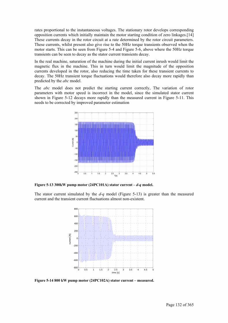
Page 132 of 365

rates proportional to the instantaneous voltages. The stationary rotor develops corresponding opposition currents which initially maintain the motor starting condition of zero linkages.[14] These currents decay in the rotor circuit at a rate determined by the rotor circuit parameters. These currents, whilst present also give rise to the 50Hz torque transients observed when the motor starts. This can be seen from Figure 5-4 and Figure 5-6, above where the 50Hz torque transients can be seen to decay as the stator current transients decay.

In the real machine, saturation of the machine during the initial current inrush would limit the magnetic flux in the machine. This in turn would limit the magnitude of the opposition currents developed in the rotor, also reducing the time taken for these transient currents to decay. The 50Hz transient torque fluctuations would therefore also decay more rapidly than predicted by the abc model.

The abc model does not predict the starting current correctly, The variation of rotor parameters with motor speed is incorrect in the model, since the simulated stator current shown in Figure 5-12 decays more rapidly than the measured current in Figure 5-11. This needs to be corrected by improved parameter estimation

Figure 5-13 300kW pump motor (24PC101A) stator current – d-q model.

The stator current simulated by the d-q model (Figure 5-13) is greater than the measured current and the transient current fluctuations almost non-existent.

0 0.5 1 1.5 2 2.5 3 3.5 4 4.5 5-800

-600

-400

-200

0

200

400

600

800

time [s] Figure 5-14 800 kW pump motor (24PC102A) stator current – measured.

curre

nt [A

]

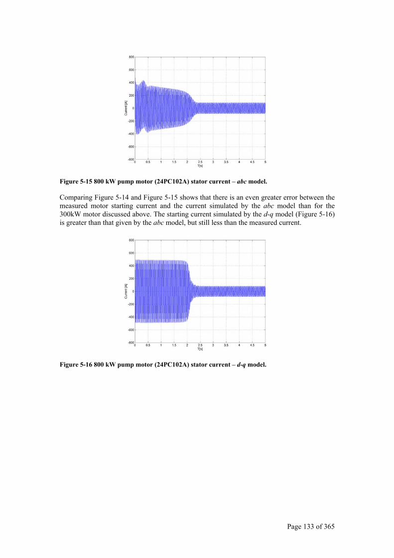
Page 133 of 365

Figure 5-15 800 kW pump motor (24PC102A) stator current – abc model.

Comparing Figure 5-14 and Figure 5-15 shows that there is an even greater error between the measured motor starting current and the current simulated by the abc model than for the 300kW motor discussed above. The starting current simulated by the d-q model (Figure 5-16) is greater than that given by the abc model, but still less than the measured current.

Figure 5-16 800 kW pump motor (24PC102A) stator current – d-q model.

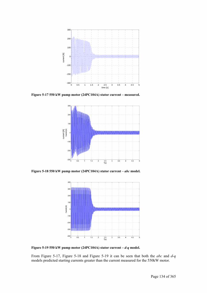
Page 134 of 365

0 0.5 1 1.5 2 2.5 3 3.5 4 4.5 5-300

-200

-100

0

100

200

300

time [s] Figure 5-17 550 kW pump motor (24PC104A) stator current – measured.

Figure 5-18 550 kW pump motor (24PC104A) stator current – abc model.

Figure 5-19 550 kW pump motor (24PC104A) stator current – d-q model.

From Figure 5-17, Figure 5-18 and Figure 5-19 it can be seen that both the abc and d-q models predicted starting currents greater than the current measured for the 550kW motor.

curre

nt [A

] cu

rrent

[A]

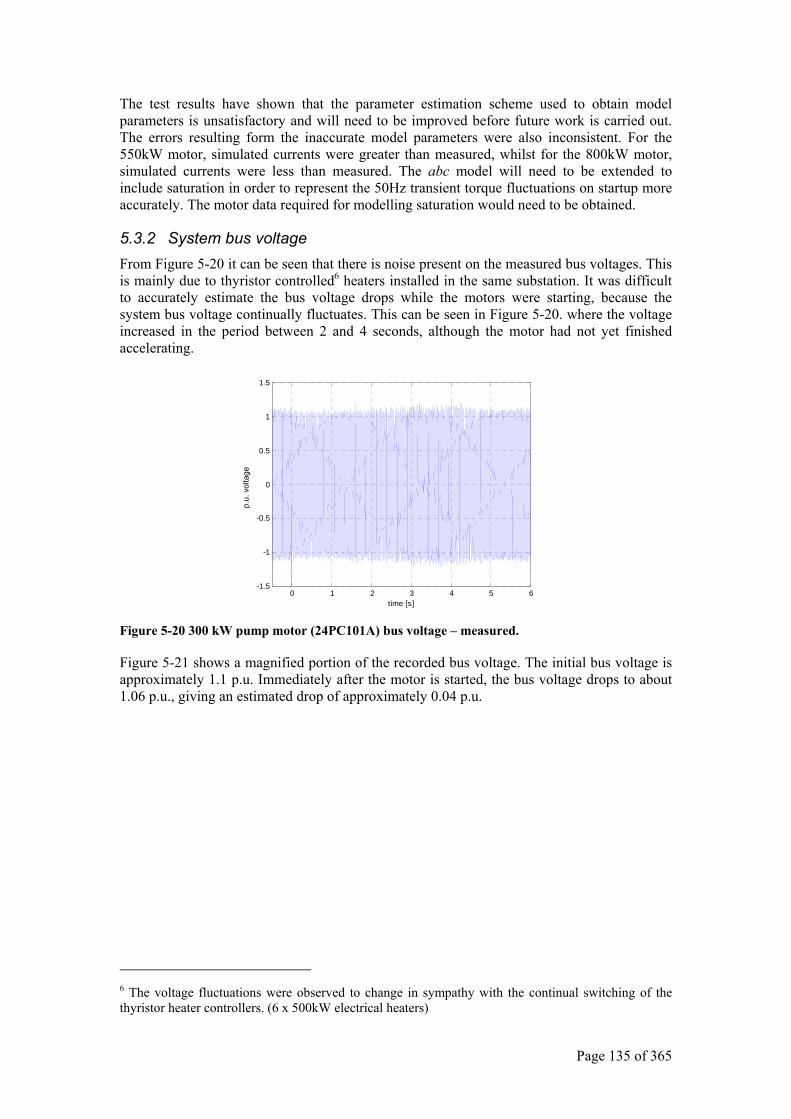
Page 135 of 365

The test results have shown that the parameter estimation scheme used to obtain model parameters is unsatisfactory and will need to be improved before future work is carried out. The errors resulting form the inaccurate model parameters were also inconsistent. For the 550kW motor, simulated currents were greater than measured, whilst for the 800kW motor, simulated currents were less than measured. The abc model will need to be extended to include saturation in order to represent the 50Hz transient torque fluctuations on startup more accurately. The motor data required for modelling saturation would need to be obtained.

5.3.2 System bus voltage From Figure 5-20 it can be seen that there is noise present on the measured bus voltages. This is mainly due to thyristor controlled6 heaters installed in the same substation. It was difficult to accurately estimate the bus voltage drops while the motors were starting, because the system bus voltage continually fluctuates. This can be seen in Figure 5-20. where the voltage increased in the period between 2 and 4 seconds, although the motor had not yet finished accelerating.

0 1 2 3 4 5 6-1.5

-1

-0.5

0

0.5

1

1.5

time [s] Figure 5-20 300 kW pump motor (24PC101A) bus voltage – measured.

Figure 5-21 shows a magnified portion of the recorded bus voltage. The initial bus voltage is approximately 1.1 p.u. Immediately after the motor is started, the bus voltage drops to about 1.06 p.u., giving an estimated drop of approximately 0.04 p.u.

6 The voltage fluctuations were observed to change in sympathy with the continual switching of the thyristor heater controllers. (6 x 500kW electrical heaters)

p.u.

vol

tage

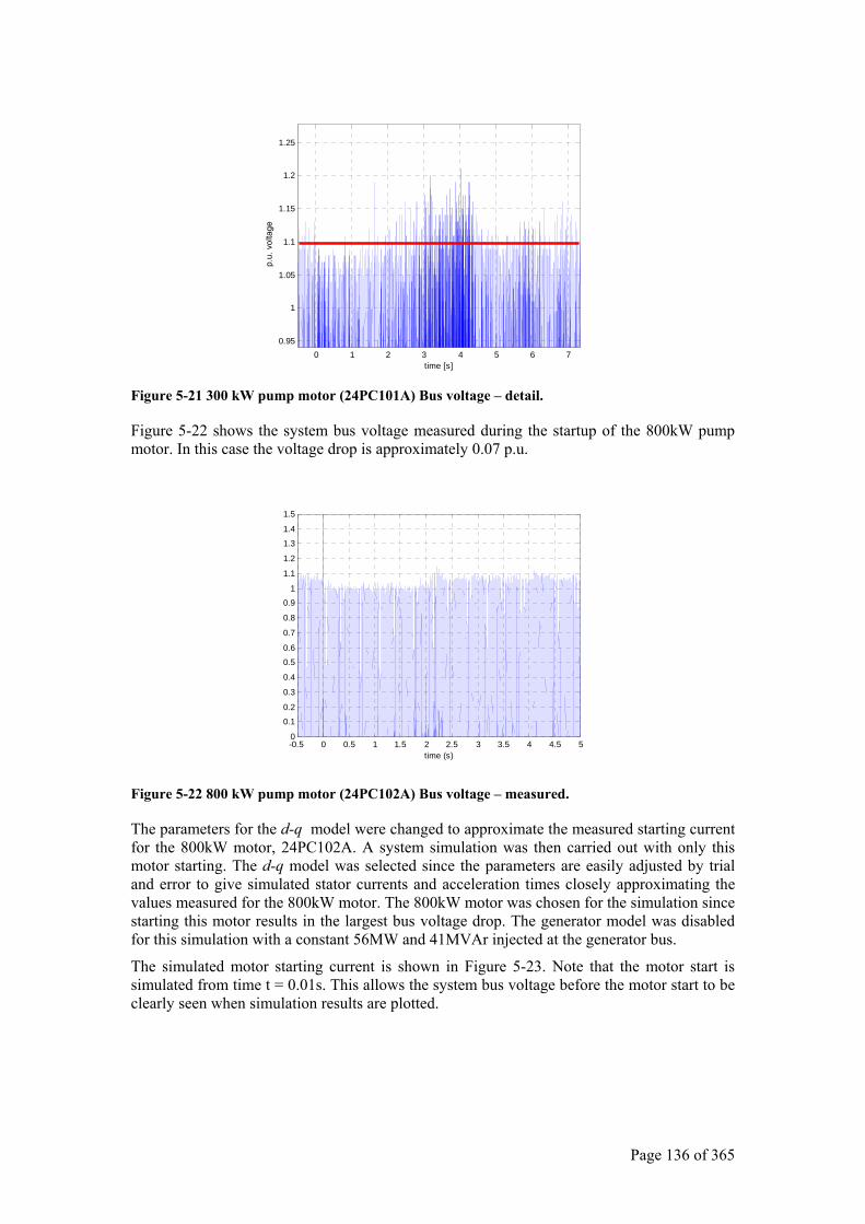
Page 136 of 365

0 1 2 3 4 5 6 7

0.95

1

1.05

1.1

1.15

1.2

1.25

time [s] Figure 5-21 300 kW pump motor (24PC101A) Bus voltage – detail.

Figure 5-22 shows the system bus voltage measured during the startup of the 800kW pump motor. In this case the voltage drop is approximately 0.07 p.u.

-0.5 0 0.5 1 1.5 2 2.5 3 3.5 4 4.5 50

0.1

0.2

0.3

0.4

0.5

0.6

0.7

0.8

0.9

1

1.1

1.2

1.3

1.4

1.5

time (s)

Figure 5-22 800 kW pump motor (24PC102A) Bus voltage – measured.

The parameters for the d-q model were changed to approximate the measured starting current for the 800kW motor, 24PC102A. A system simulation was then carried out with only this motor starting. The d-q model was selected since the parameters are easily adjusted by trial and error to give simulated stator currents and acceleration times closely approximating the values measured for the 800kW motor. The 800kW motor was chosen for the simulation since starting this motor results in the largest bus voltage drop. The generator model was disabled for this simulation with a constant 56MW and 41MVAr injected at the generator bus.

The simulated motor starting current is shown in Figure 5-23. Note that the motor start is simulated from time t = 0.01s. This allows the system bus voltage before the motor start to be clearly seen when simulation results are plotted.

p.u.

vol

tage

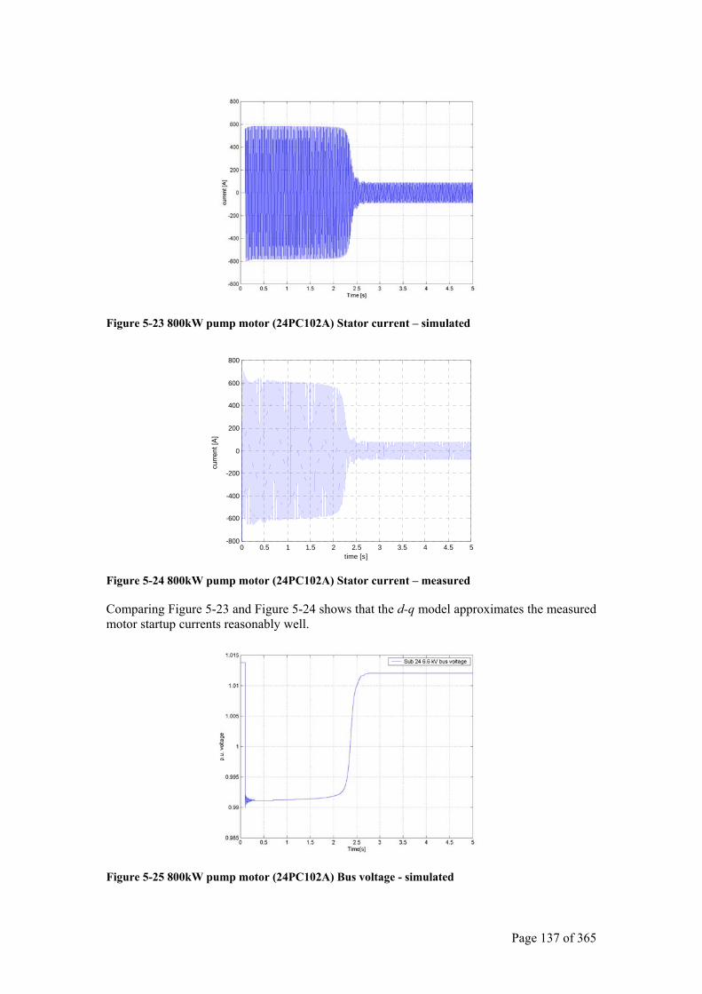
Page 137 of 365

Figure 5-23 800kW pump motor (24PC102A) Stator current – simulated

0 0.5 1 1.5 2 2.5 3 3.5 4 4.5 5-800

-600

-400

-200

0

200

400

600

800

time [s] Figure 5-24 800kW pump motor (24PC102A) Stator current – measured

Comparing Figure 5-23 and Figure 5-24 shows that the d-q model approximates the measured motor startup currents reasonably well.

Figure 5-25 800kW pump motor (24PC102A) Bus voltage - simulated

curre

nt [A

]

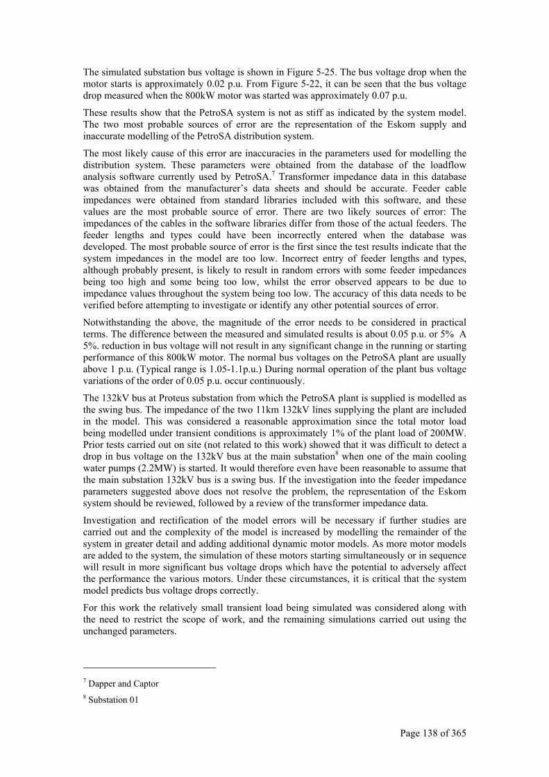
Page 138 of 365

The simulated substation bus voltage is shown in Figure 5-25. The bus voltage drop when the motor starts is approximately 0.02 p.u. From Figure 5-22, it can be seen that the bus voltage drop measured when the 800kW motor was started was approximately 0.07 p.u.

These results show that the PetroSA system is not as stiff as indicated by the system model. The two most probable sources of error are the representation of the Eskom supply and inaccurate modelling of the PetroSA distribution system.

The most likely cause of this error are inaccuracies in the parameters used for modelling the distribution system. These parameters were obtained from the database of the loadflow analysis software currently used by PetroSA.7 Transformer impedance data in this database was obtained from the manufacturer’s data sheets and should be accurate. Feeder cable impedances were obtained from standard libraries included with this software, and these values are the most probable source of error. There are two likely sources of error: The impedances of the cables in the software libraries differ from those of the actual feeders. The feeder lengths and types could have been incorrectly entered when the database was developed. The most probable source of error is the first since the test results indicate that the system impedances in the model are too low. Incorrect entry of feeder lengths and types, although probably present, is likely to result in random errors with some feeder impedances being too high and some being too low, whilst the error observed appears to be due to impedance values throughout the system being too low. The accuracy of this data needs to be verified before attempting to investigate or identify any other potential sources of error.

Notwithstanding the above, the magnitude of the error needs to be considered in practical terms. The difference between the measured and simulated results is about 0.05 p.u. or 5% A 5%. reduction in bus voltage will not result in any significant change in the running or starting performance of this 800kW motor. The normal bus voltages on the PetroSA plant are usually above 1 p.u. (Typical range is 1.05-1.1p.u.) During normal operation of the plant bus voltage variations of the order of 0.05 p.u. occur continuously.

The 132kV bus at Proteus substation from which the PetroSA plant is supplied is modelled as the swing bus. The impedance of the two 11km 132kV lines supplying the plant are included in the model. This was considered a reasonable approximation since the total motor load being modelled under transient conditions is approximately 1% of the plant load of 200MW. Prior tests carried out on site (not related to this work) showed that it was difficult to detect a drop in bus voltage on the 132kV bus at the main substation8 when one of the main cooling water pumps (2.2MW) is started. It would therefore even have been reasonable to assume that the main substation 132kV bus is a swing bus. If the investigation into the feeder impedance parameters suggested above does not resolve the problem, the representation of the Eskom system should be reviewed, followed by a review of the transformer impedance data.

Investigation and rectification of the model errors will be necessary if further studies are carried out and the complexity of the model is increased by modelling the remainder of the system in greater detail and adding additional dynamic motor models. As more motor models are added to the system, the simulation of these motors starting simultaneously or in sequence will result in more significant bus voltage drops which have the potential to adversely affect the performance the various motors. Under these circumstances, it is critical that the system model predicts bus voltage drops correctly.

For this work the relatively small transient load being simulated was considered along with the need to restrict the scope of work, and the remaining simulations carried out using the unchanged parameters.

7 Dapper and Captor 8 Substation 01

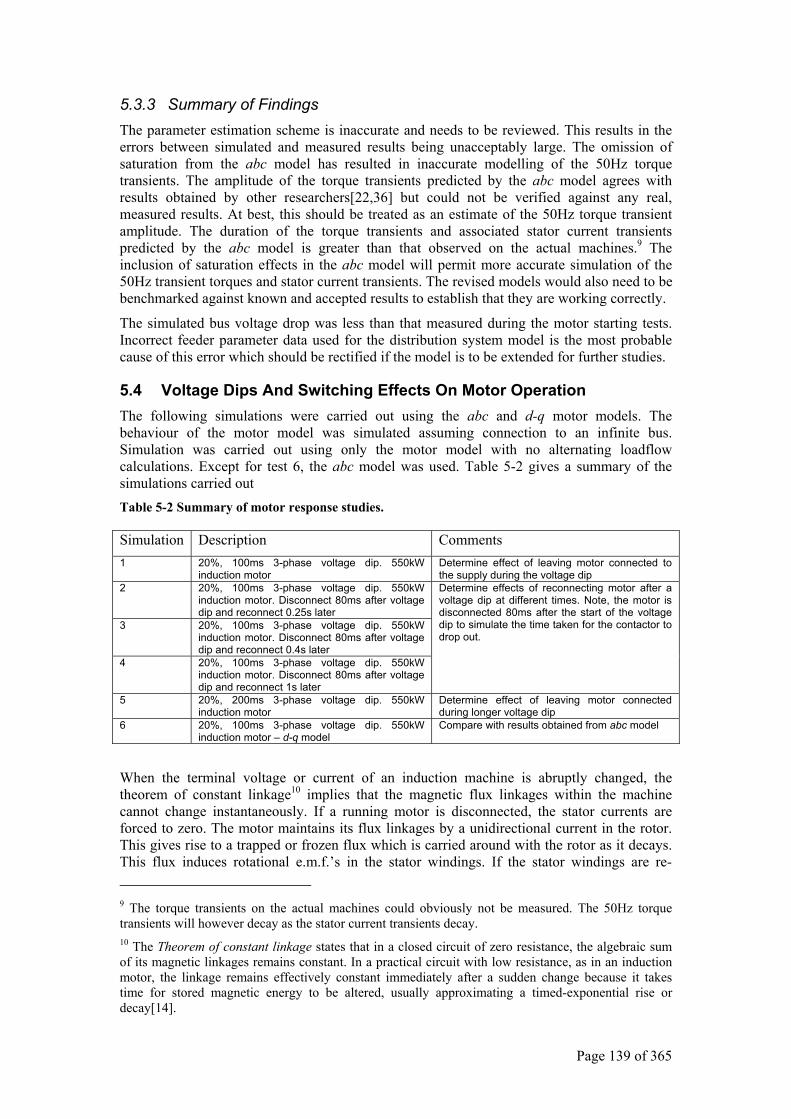
Page 139 of 365

5.3.3 Summary of Findings The parameter estimation scheme is inaccurate and needs to be reviewed. This results in the errors between simulated and measured results being unacceptably large. The omission of saturation from the abc model has resulted in inaccurate modelling of the 50Hz torque transients. The amplitude of the torque transients predicted by the abc model agrees with results obtained by other researchers[22,36] but could not be verified against any real, measured results. At best, this should be treated as an estimate of the 50Hz torque transient amplitude. The duration of the torque transients and associated stator current transients predicted by the abc model is greater than that observed on the actual machines.9 The inclusion of saturation effects in the abc model will permit more accurate simulation of the 50Hz transient torques and stator current transients. The revised models would also need to be benchmarked against known and accepted results to establish that they are working correctly.

The simulated bus voltage drop was less than that measured during the motor starting tests. Incorrect feeder parameter data used for the distribution system model is the most probable cause of this error which should be rectified if the model is to be extended for further studies.

5.4 Voltage Dips And Switching Effects On Motor Operation The following simulations were carried out using the abc and d-q motor models. The behaviour of the motor model was simulated assuming connection to an infinite bus. Simulation was carried out using only the motor model with no alternating loadflow calculations. Except for test 6, the abc model was used. Table 5-2 gives a summary of the simulations carried out Table 5-2 Summary of motor response studies.

Simulation Description Comments 1 20%, 100ms 3-phase voltage dip. 550kW

induction motor Determine effect of leaving motor connected to the supply during the voltage dip

2 20%, 100ms 3-phase voltage dip. 550kW induction motor. Disconnect 80ms after voltage dip and reconnect 0.25s later

3 20%, 100ms 3-phase voltage dip. 550kW induction motor. Disconnect 80ms after voltage dip and reconnect 0.4s later

4 20%, 100ms 3-phase voltage dip. 550kW induction motor. Disconnect 80ms after voltage dip and reconnect 1s later

Determine effects of reconnecting motor after a voltage dip at different times. Note, the motor is disconnected 80ms after the start of the voltage dip to simulate the time taken for the contactor to drop out.

5 20%, 200ms 3-phase voltage dip. 550kW induction motor

Determine effect of leaving motor connected during longer voltage dip

6 20%, 100ms 3-phase voltage dip. 550kW induction motor – d-q model

Compare with results obtained from abc model

When the terminal voltage or current of an induction machine is abruptly changed, the theorem of constant linkage10 implies that the magnetic flux linkages within the machine cannot change instantaneously. If a running motor is disconnected, the stator currents are forced to zero. The motor maintains its flux linkages by a unidirectional current in the rotor. This gives rise to a trapped or frozen flux which is carried around with the rotor as it decays. This flux induces rotational e.m.f.’s in the stator windings. If the stator windings are re- 9 The torque transients on the actual machines could obviously not be measured. The 50Hz torque transients will however decay as the stator current transients decay. 10 The Theorem of constant linkage states that in a closed circuit of zero resistance, the algebraic sum of its magnetic linkages remains constant. In a practical circuit with low resistance, as in an induction motor, the linkage remains effectively constant immediately after a sudden change because it takes time for stored magnetic energy to be altered, usually approximating a timed-exponential rise or decay[14].

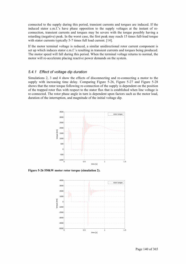
Page 140 of 365

connected to the supply during this period, transient currents and torques are induced. If the induced stator e.m.f.’s have phase opposition to the supply voltages at the instant of re-connection, transient currents and torques may be severe with the torque possibly having a retarding (negative) peak. In the worst case, the first peak may reach 15 times full-load torque with stator currents typically 5-7 times full load current. [14].

If the motor terminal voltage is reduced, a similar unidirectional rotor current component is set up which induces stator e.m.f.’s resulting in transient currents and torques being produced. The motor speed will fall during this period. When the terminal voltage returns to normal, the motor will re-accelerate placing reactive power demands on the system.

5.4.1 Effect of voltage dip duration Simulations 2, 3 and 4 show the effects of disconnecting and re-connecting a motor to the supply with increasing time delay. Comparing Figure 5-26, Figure 5-27 and Figure 5-28 shows that the rotor torque following re-connection of the supply is dependent on the position of the trapped rotor flux with respect to the stator flux that is established when line voltage is re-connected. The rotor phase angle in turn is dependent upon factors such as the motor load, duration of the interruption, and magnitude of the initial voltage dip.

0 0.5 1 1.5-1000

-500

0

500

1000

1500

2000

2500

3000

3500

time [s]

rotor torque

Figure 5-26 550kW motor rotor torque (simulation 2).

0 0.5 1 1.5-5000

-4000

-3000

-2000

-1000

0

1000

2000

3000

4000

time [s]

rotor torque

torq

ue [n

m]

torq

ue [n

m]

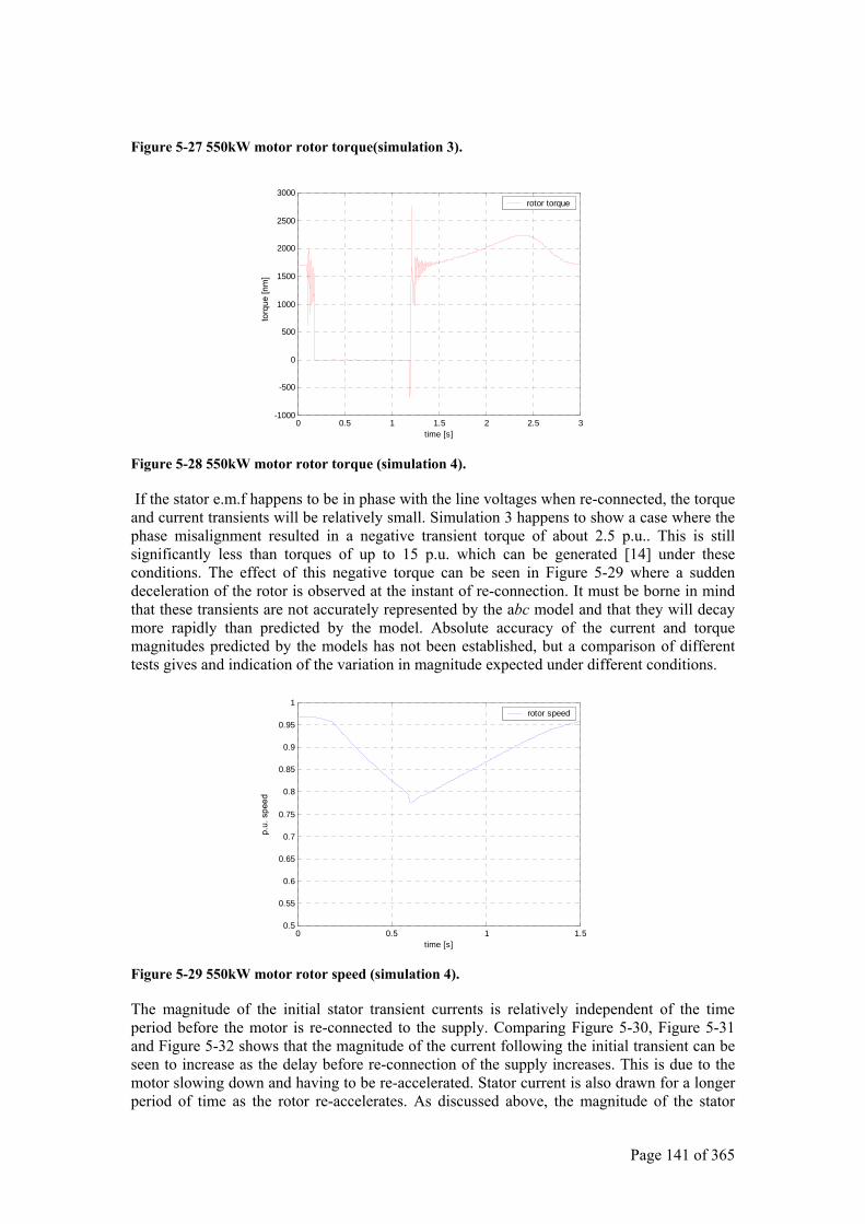
Page 141 of 365

Figure 5-27 550kW motor rotor torque(simulation 3).

0 0.5 1 1.5 2 2.5 3-1000

-500

0

500

1000

1500

2000

2500

3000

time [s]

rotor torque

Figure 5-28 550kW motor rotor torque (simulation 4).

If the stator e.m.f happens to be in phase with the line voltages when re-connected, the torque and current transients will be relatively small. Simulation 3 happens to show a case where the phase misalignment resulted in a negative transient torque of about 2.5 p.u.. This is still significantly less than torques of up to 15 p.u. which can be generated [14] under these conditions. The effect of this negative torque can be seen in Figure 5-29 where a sudden deceleration of the rotor is observed at the instant of re-connection. It must be borne in mind that these transients are not accurately represented by the abc model and that they will decay more rapidly than predicted by the model. Absolute accuracy of the current and torque magnitudes predicted by the models has not been established, but a comparison of different tests gives and indication of the variation in magnitude expected under different conditions.

0 0.5 1 1.50.5

0.55

0.6

0.65

0.7

0.75

0.8

0.85

0.9

0.95

1

time [s]

rotor speed

Figure 5-29 550kW motor rotor speed (simulation 4).

The magnitude of the initial stator transient currents is relatively independent of the time period before the motor is re-connected to the supply. Comparing Figure 5-30, Figure 5-31 and Figure 5-32 shows that the magnitude of the current following the initial transient can be seen to increase as the delay before re-connection of the supply increases. This is due to the motor slowing down and having to be re-accelerated. Stator current is also drawn for a longer period of time as the rotor re-accelerates. As discussed above, the magnitude of the stator

torq

ue [n

m]

p.u.

spe

ed

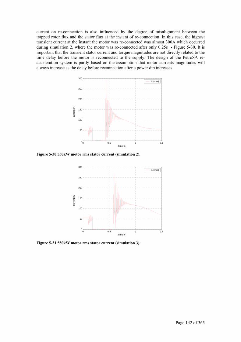
Page 142 of 365

current on re-connection is also influenced by the degree of misalignment between the trapped rotor flux and the stator flux at the instant of re-connection. In this case, the highest transient current at the instant the motor was re-connected was almost 300A which occurred during simulation 2, where the motor was re-connected after only 0.25s - Figure 5-30. It is important that the transient stator current and torque magnitudes are not directly related to the time delay before the motor is reconnected to the supply. The design of the PetroSA re-acceleration system is partly based on the assumption that motor currents magnitudes will always increase as the delay before reconnection after a power dip increases.

0 0.5 1 1.50

50

100

150

200

250

300

time [s]

Is (rms)

Figure 5-30 550kW motor rms stator current (simulation 2).

0 0.5 1 1.50

50

100

150

200

250

300

time [s]

Is (rms)

Figure 5-31 550kW motor rms stator current (simulation 3).

curre

nt [A

] cu

rrent

[A]

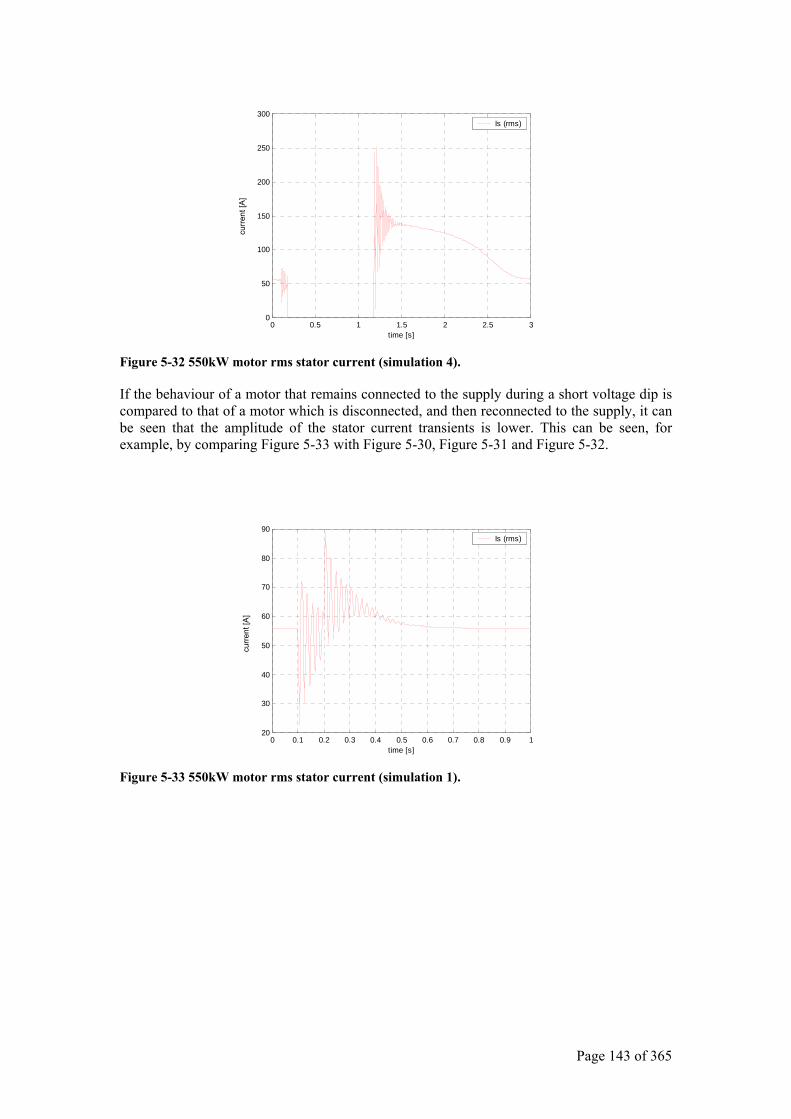
Page 143 of 365

0 0.5 1 1.5 2 2.5 30

50

100

150

200

250

300

time [s]

Is (rms)

Figure 5-32 550kW motor rms stator current (simulation 4).

If the behaviour of a motor that remains connected to the supply during a short voltage dip is compared to that of a motor which is disconnected, and then reconnected to the supply, it can be seen that the amplitude of the stator current transients is lower. This can be seen, for example, by comparing Figure 5-33 with Figure 5-30, Figure 5-31 and Figure 5-32.

0 0.1 0.2 0.3 0.4 0.5 0.6 0.7 0.8 0.9 120

30

40

50

60

70

80

90

time [s]

Is (rms)

Figure 5-33 550kW motor rms stator current (simulation 1).

curre

nt [A

] cu

rrent

[A]

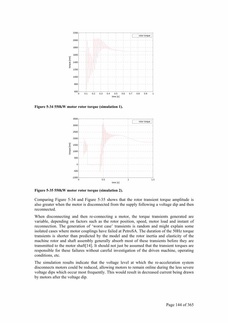
Page 144 of 365

0 0.1 0.2 0.3 0.4 0.5 0.6 0.7 0.8 0.9 1600

800

1000

1200

1400

1600

1800

2000

2200

time [s]

rotor torque

Figure 5-34 550kW motor rotor torque (simulation 1).

0 0.5 1 1.5-1000

-500

0

500

1000

1500

2000

2500

3000

3500

time [s]

rotor torque

Figure 5-35 550kW motor rotor torque (simulation 2).

Comparing Figure 5-34 and Figure 5-35 shows that the rotor transient torque amplitude is also greater when the motor is disconnected from the supply following a voltage dip and then reconnected.

When disconnecting and then re-connecting a motor, the torque transients generated are variable, depending on factors such as the rotor position, speed, motor load and instant of reconnection. The generation of ‘worst case’ transients is random and might explain some isolated cases where motor couplings have failed at PetroSA. The duration of the 50Hz torque transients is shorter than predicted by the model and the rotor inertia and elasticity of the machine rotor and shaft assembly generally absorb most of these transients before they are transmitted to the motor shaft[14]. It should not just be assumed that the transient torques are responsible for these failures without careful investigation of the driven machine, operating conditions, etc.

The simulation results indicate that the voltage level at which the re-acceleration system disconnects motors could be reduced, allowing motors to remain online during the less severe voltage dips which occur most frequently. This would result in decreased current being drawn by motors after the voltage dip.

torq

ue [n

m]

torq

ue [n

m]

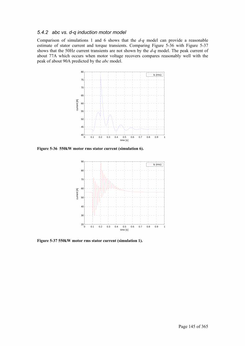
Page 145 of 365

5.4.2 abc vs. d-q induction motor model Comparison of simulations 1 and 6 shows that the d-q model can provide a reasonable estimate of stator current and torque transients. Comparing Figure 5-36 with Figure 5-37 shows that the 50Hz current transients are not shown by the d-q model. The peak current of about 77A which occurs when motor voltage recovers compares reasonably well with the peak of about 90A predicted by the abc model.

0 0.1 0.2 0.3 0.4 0.5 0.6 0.7 0.8 0.9 140

45

50

55

60

65

70

75

80

time [s]

Is (rms)

Figure 5-36 550kW motor rms stator current (simulation 6).

0 0.1 0.2 0.3 0.4 0.5 0.6 0.7 0.8 0.9 120

30

40

50

60

70

80

90

time [s]

Is (rms)

Figure 5-37 550kW motor rms stator current (simulation 1).

curre

nt [A

] cu

rrent

[A]

Page 146 of 365

0 0.1 0.2 0.3 0.4 0.5 0.6 0.7 0.8 0.9 1600

800

1000

1200

1400

1600

1800

2000

2200

time [s]

rotor torque

Figure 5-38 550kW motor rotor torque (simulation 2).

0 0.1 0.2 0.3 0.4 0.5 0.6 0.7 0.8 0.9 1300

350

400

450

500

550

600

650

time [s]

rotor torque

Figure 5-39 550kW motor rotor torque (simulation 7).

Comparing Figure 5-38 and Figure 5-39 shows that 50Hz torque transients during the voltage dip are not well represented. The peak torque of about 1875Nm on voltage recovery predicted by the d-q model appears to give some indication of the magnitudes of the torque peaks that could be expected when compared to the 2050Nm predicted by the abc model. This needs to be carefully investigated if the d-q model is to be used to investigate transient stator currents and rotor torques during system disturbances. The torque oscillations following voltage recovery that are shown in Figure 5-39 are suspected to be caused by mechanical oscillations of the rotor following the voltage dip. These oscillations are due to the lower inertia values that had to be used for the d-q model which were discussed in paragraph 5.2

Comparison of the two models shows that the abc model should be used when the 50Hz torque transients and stator transient currents need to be examined. The d-q model is not recommended for investigation of the 50Hz transient torques or currents.

torq

ue [n

m]

torq

ue [n

m]

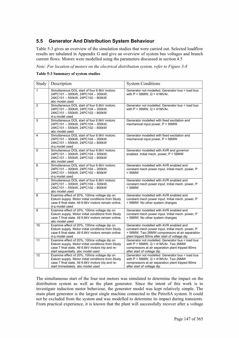
Page 147 of 365

5.5 Generator And Distribution System Behaviour Table 5-3 gives an overview of the simulation studies that were carried out. Selected loadflow results are tabulated in Appendix G and give an overview of system bus voltages and branch current flows. Motors were modelled using the parameters discussed in section 4.5

Note: For location of motors on the electrical distribution system, refer to Figure 3-8 Table 5-3 Summary of system studies

Study Description System Conditions 1 Simultaneous DOL start of four 6.6kV motors:

24PC101 – 300kW, 24PC104 – 300kW, 24KC101 – 550kW, 24PC102 – 800kW abc model used

Generator not modelled. Generator bus = load bus with P = 56MW, Q = 41MVAr.

2 Simultaneous DOL start of four 6.6kV motors: 24PC101 – 300kW, 24PC104 – 300kW, 24KC101 – 550kW, 24PC102 – 800kW d-q model used

Generator not modelled. Generator bus = load bus with P = 56MW, Q = 41MVAr.

3 Simultaneous DOL start of four 6.6kV motors: 24PC101 – 300kW, 24PC104 – 300kW, 24KC101 – 550kW, 24PC102 – 800kW abc model used

Generator modelled with fixed excitation and mechanical input power, P = 56MW

4 Simultaneous DOL start of four 6.6kV motors: 24PC101 – 300kW, 24PC104 – 300kW, 24KC101 – 550kW, 24PC102 – 800kW d-q model used

Generator modelled with fixed excitation and mechanical input power, P = 56MW

5 Simultaneous DOL start of four 6.6kV motors: 24PC101 – 300kW, 24PC104 – 300kW, 24KC101 – 550kW, 24PC102 – 800kW abc model used

Generator modelled with AVR and governor enabled. Initial mech. power, P = 56MW

6 Simultaneous DOL start of four 6.6kV motors: 24PC101 – 300kW, 24PC104 – 300kW, 24KC101 – 550kW, 24PC102 – 800kW d-q model used

Generator modelled with AVR enabled and constant mech power input. Initial mech. power, P = 56MW

7 Simultaneous DOL start of four 6.6kV motors: 24PC101 – 300kW, 24PC104 – 300kW, 24KC101 – 550kW, 24PC102 – 800kW abc model used

Generator modelled with AVR enabled and constant mech power input. Initial mech. power, P = 56MW

8 Examine effect of 20%, 100ms voltage dip on Eskom supply. Motor initial conditions from Study case 6 final state. All 6.6kV motors remain online. d-q model used

Generator modelled with AVR enabled and constant mech power input. Initial mech. power, P = 56MW. No other system changes

9 Examine effect of 20%, 100ms voltage dip on Eskom supply. Motor initial conditions from Study case 7 final state. All 6.6kV motors remain online. abc model used

Generator modelled with AVR enabled and constant mech power input. Initial mech. power, P = 56MW. No other system changes

10 Examine effect of 20%, 100ms voltage dip on Eskom supply. Motor initial conditions from Study case 6 final state. All 6.6kV motors remain online. d-q model used

Generator modelled with AVR enabled and constant mech power input. Initial mech. power, P = 56MW. Two 26MW compressors at air separation plant tripped 80ms after start of voltage dip

11 Examine effect of 20%, 100ms voltage dip on Eskom supply. Motor initial conditions from Study case 7 final state. All 6.6kV motors trip and re-start sequentially. abc model used

Generator not modelled. Generator bus = load bus with P = 56MW, Q = 41MVAr. Two 26MW compressors at air separation plant tripped 80ms after start of voltage dip

12 Examine effect of 20%, 100ms voltage dip on Eskom supply. Motor initial conditions from Study case 7 final state. All 6.6kV motors trip and re-start immediately. abc model used

Generator not modelled. Generator bus = load bus with P = 56MW, Q = 41MVAr. Two 26MW compressors at air separation plant tripped 80ms after start of voltage dip

The simultaneous start of the four test motors was simulated to determine the impact on the distribution system as well as the plant generator. Since the intent of this work is to investigate induction motor behaviour, the generator model was kept relatively simple. The main plant generator is the largest single machine connected to the PetroSA system. It could not be excluded from the system and was modelled to determine its impact during transients. From practical experience, it is known that the plant will successfully recover after a voltage

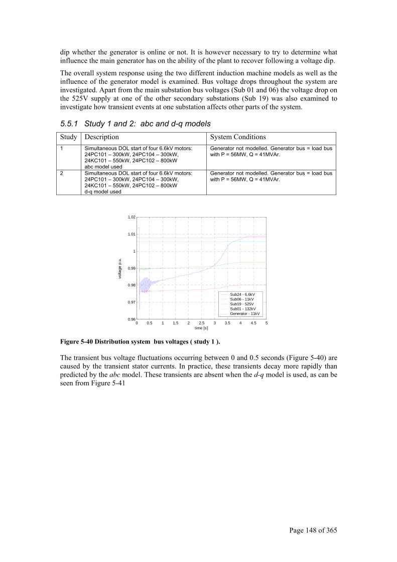
Page 148 of 365

dip whether the generator is online or not. It is however necessary to try to determine what influence the main generator has on the ability of the plant to recover following a voltage dip.

The overall system response using the two different induction machine models as well as the influence of the generator model is examined. Bus voltage drops throughout the system are investigated. Apart from the main substation bus voltages (Sub 01 and 06) the voltage drop on the 525V supply at one of the other secondary substations (Sub 19) was also examined to investigate how transient events at one substation affects other parts of the system.

5.5.1 Study 1 and 2: abc and d-q models Study Description System Conditions 1 Simultaneous DOL start of four 6.6kV motors:

24PC101 – 300kW, 24PC104 – 300kW, 24KC101 – 550kW, 24PC102 – 800kW abc model used

Generator not modelled. Generator bus = load bus with P = 56MW, Q = 41MVAr.

2 Simultaneous DOL start of four 6.6kV motors: 24PC101 – 300kW, 24PC104 – 300kW, 24KC101 – 550kW, 24PC102 – 800kW d-q model used

Generator not modelled. Generator bus = load bus with P = 56MW, Q = 41MVAr.

0 0.5 1 1.5 2 2.5 3 3.5 4 4.5 50.96

0.97

0.98

0.99

1

1.01

1.02

time [s]

Sub24 - 6.6kV Sub06 - 11kV Sub19 - 525V Sub01 - 132kV Generator - 11kV

Figure 5-40 Distribution system bus voltages ( study 1 ).

The transient bus voltage fluctuations occurring between 0 and 0.5 seconds (Figure 5-40) are caused by the transient stator currents. In practice, these transients decay more rapidly than predicted by the abc model. These transients are absent when the d-q model is used, as can be seen from Figure 5-41

volta

ge p

.u.

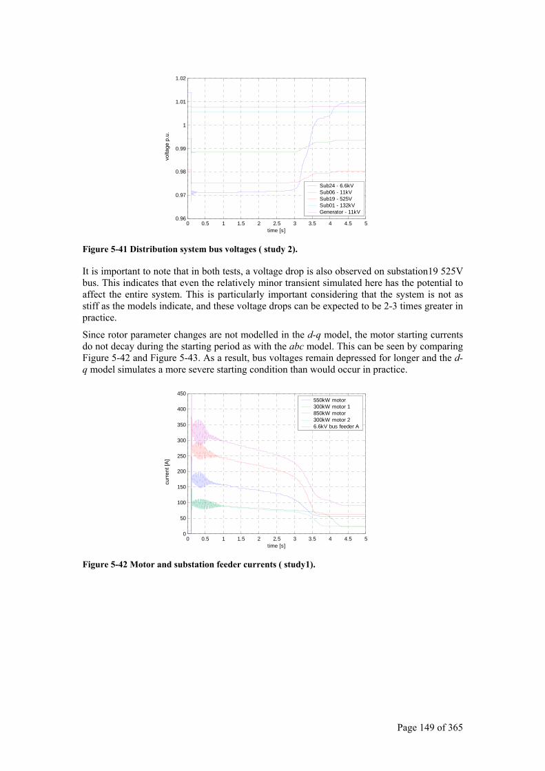
Page 149 of 365

0 0.5 1 1.5 2 2.5 3 3.5 4 4.5 50.96

0.97

0.98

0.99

1

1.01

1.02

time [s]

Sub24 - 6.6kV Sub06 - 11kV Sub19 - 525V Sub01 - 132kV Generator - 11kV

Figure 5-41 Distribution system bus voltages ( study 2).

It is important to note that in both tests, a voltage drop is also observed on substation19 525V bus. This indicates that even the relatively minor transient simulated here has the potential to affect the entire system. This is particularly important considering that the system is not as stiff as the models indicate, and these voltage drops can be expected to be 2-3 times greater in practice.

Since rotor parameter changes are not modelled in the d-q model, the motor starting currents do not decay during the starting period as with the abc model. This can be seen by comparing Figure 5-42 and Figure 5-43. As a result, bus voltages remain depressed for longer and the d-q model simulates a more severe starting condition than would occur in practice.

0 0.5 1 1.5 2 2.5 3 3.5 4 4.5 50

50

100

150

200

250

300

350

400

450

time [s]

550kW motor 300kW motor 1 850kW motor 300kW motor 2 6.6kV bus feeder A

Figure 5-42 Motor and substation feeder currents ( study1).

curre

nt [A

] vo

ltage

p.u

.

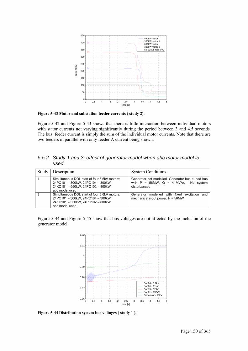
Page 150 of 365

0 0.5 1 1.5 2 2.5 3 3.5 4 4.5 50

50

100

150

200

250

300

350

400

450

time [s]

550kW motor 300kW motor 1 850kW motor 300kW motor 2 6.6kV bus feeder A

Figure 5-43 Motor and substation feeder currents ( study 2).

Figure 5-42 and Figure 5-43 shows that there is little interaction between individual motors with stator currents not varying significantly during the period between 3 and 4.5 seconds. The bus feeder current is simply the sum of the individual motor currents. Note that there are two feeders in parallel with only feeder A current being shown.

5.5.2 Study 1 and 3: effect of generator model when abc motor model is used

Study Description System Conditions 1 Simultaneous DOL start of four 6.6kV motors:

24PC101 – 300kW, 24PC104 – 300kW, 24KC101 – 550kW, 24PC102 – 800kW abc model used

Generator not modelled. Generator bus = load bus with P = 56MW, Q = 41MVAr. No system disturbances

3 Simultaneous DOL start of four 6.6kV motors: 24PC101 – 300kW, 24PC104 – 300kW, 24KC101 – 550kW, 24PC102 – 800kW abc model used

Generator modelled with fixed excitation and mechanical input power, P = 56MW

Figure 5-44 and Figure 5-45 show that bus voltages are not affected by the inclusion of the generator model.

0 0.5 1 1.5 2 2.5 3 3.5 4 4.5 50.96

0.97

0.98

0.99

1

1.01

1.02

time [s]

Sub24 - 6.6kV Sub06 - 11kV Sub19 - 525V Sub01 - 132kV Generator - 11kV

Figure 5-44 Distribution system bus voltages ( study 1 ).

curre

nt [A

]

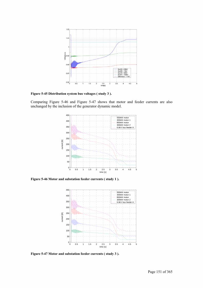
Page 151 of 365

Figure 5-45 Distribution system bus voltages ( study 3 ).

Comparing Figure 5-46 and Figure 5-47 shows that motor and feeder currents are also unchanged by the inclusion of the generator dynamic model.

0 0.5 1 1.5 2 2.5 3 3.5 4 4.5 50

50

100

150

200

250

300

350

400

450

time [s]

550kW motor 300kW motor 1 850kW motor 300kW motor 2 6.6kV bus feeder A

Figure 5-46 Motor and substation feeder currents ( study 1 ).

0 0.5 1 1.5 2 2.5 3 3.5 4 4.5 50

50

100

150

200

250

300

350

400

450

time [s]

550kW motor 300kW motor 1 850kW motor 300kW motor 2 6.6kV bus feeder A

Figure 5-47 Motor and substation feeder currents ( study 3 ).

curre

nt [A

] cu

rrent

[A]

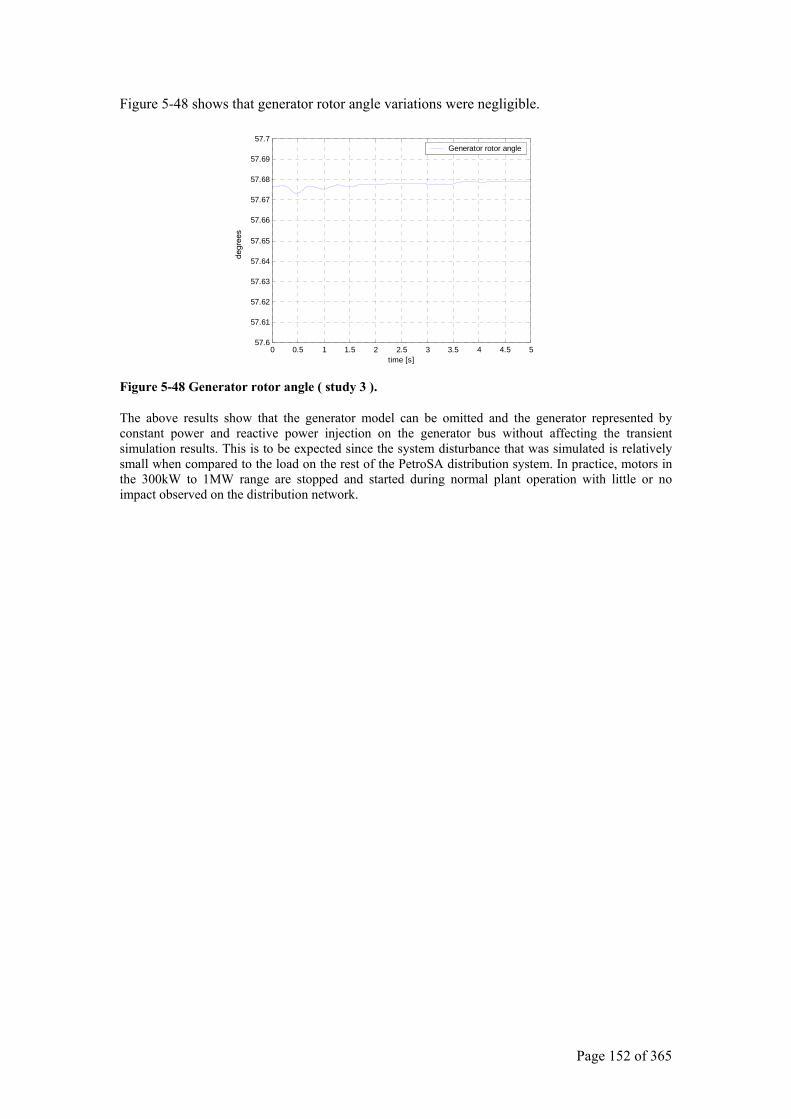
Page 152 of 365

Figure 5-48 shows that generator rotor angle variations were negligible.

0 0.5 1 1.5 2 2.5 3 3.5 4 4.5 557.6

57.61

57.62

57.63

57.64

57.65

57.66

57.67

57.68

57.69

57.7

time [s]

Generator rotor angle

Figure 5-48 Generator rotor angle ( study 3 ).

The above results show that the generator model can be omitted and the generator represented by constant power and reactive power injection on the generator bus without affecting the transient simulation results. This is to be expected since the system disturbance that was simulated is relatively small when compared to the load on the rest of the PetroSA distribution system. In practice, motors in the 300kW to 1MW range are stopped and started during normal plant operation with little or no impact observed on the distribution network.

degr

ees

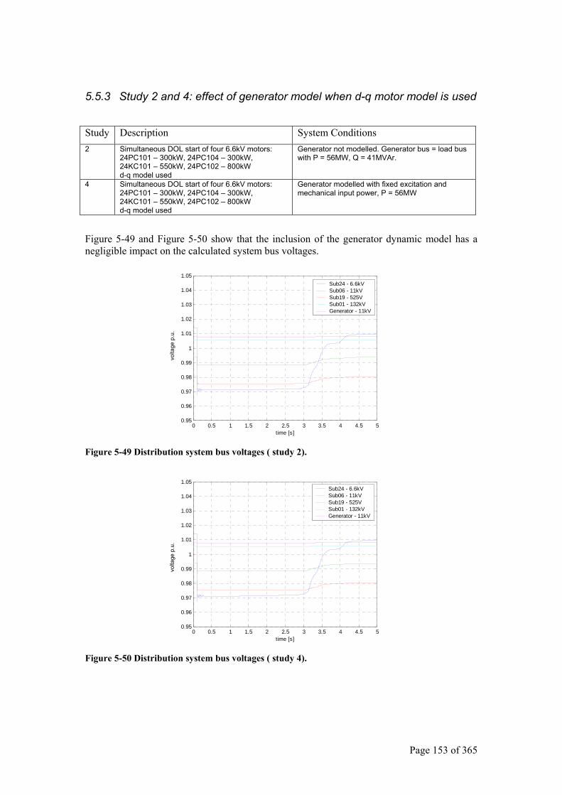
Page 153 of 365

5.5.3 Study 2 and 4: effect of generator model when d-q motor model is used

Study Description System Conditions 2 Simultaneous DOL start of four 6.6kV motors:

24PC101 – 300kW, 24PC104 – 300kW, 24KC101 – 550kW, 24PC102 – 800kW d-q model used

Generator not modelled. Generator bus = load bus with P = 56MW, Q = 41MVAr.

4 Simultaneous DOL start of four 6.6kV motors: 24PC101 – 300kW, 24PC104 – 300kW, 24KC101 – 550kW, 24PC102 – 800kW d-q model used

Generator modelled with fixed excitation and mechanical input power, P = 56MW

Figure 5-49 and Figure 5-50 show that the inclusion of the generator dynamic model has a negligible impact on the calculated system bus voltages.

0 0.5 1 1.5 2 2.5 3 3.5 4 4.5 50.95

0.96

0.97

0.98

0.99

1

1.01

1.02

1.03

1.04

1.05

time [s]

Sub24 - 6.6kV Sub06 - 11kV Sub19 - 525V Sub01 - 132kV Generator - 11kV

Figure 5-49 Distribution system bus voltages ( study 2).

0 0.5 1 1.5 2 2.5 3 3.5 4 4.5 50.95

0.96

0.97

0.98

0.99

1

1.01

1.02

1.03

1.04

1.05

time [s]

Sub24 - 6.6kV Sub06 - 11kV Sub19 - 525V Sub01 - 132kV Generator - 11kV

Figure 5-50 Distribution system bus voltages ( study 4).

volta

ge p

.u.

volta

ge p

.u.

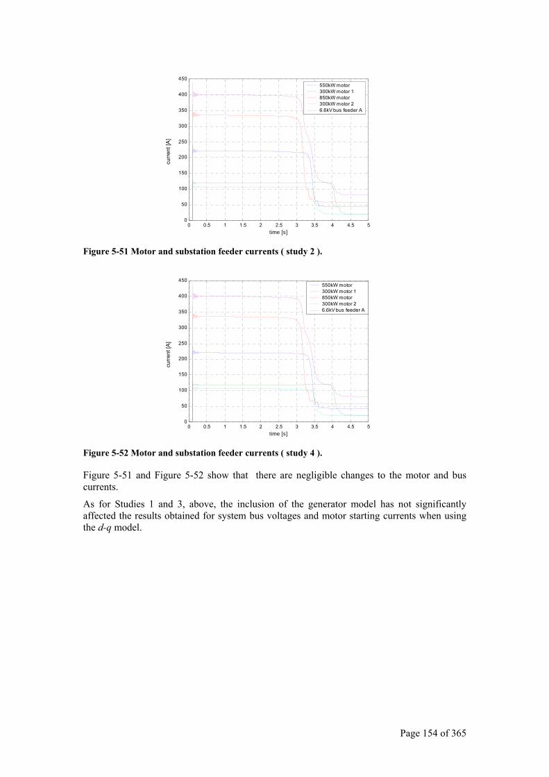
Page 154 of 365

0 0.5 1 1.5 2 2.5 3 3.5 4 4.5 50

50

100

150

200

250

300

350

400

450

time [s]

550kW motor 300kW motor 1 850kW motor 300kW motor 2 6.6kV bus feeder A

Figure 5-51 Motor and substation feeder currents ( study 2 ).

0 0.5 1 1.5 2 2.5 3 3.5 4 4.5 50

50

100

150

200

250

300

350

400

450

time [s]

550kW motor 300kW motor 1 850kW motor 300kW motor 2 6.6kV bus feeder A

Figure 5-52 Motor and substation feeder currents ( study 4 ).

Figure 5-51 and Figure 5-52 show that there are negligible changes to the motor and bus currents.

As for Studies 1 and 3, above, the inclusion of the generator model has not significantly affected the results obtained for system bus voltages and motor starting currents when using the d-q model.

curre

nt [A

] cu

rrent

[A]

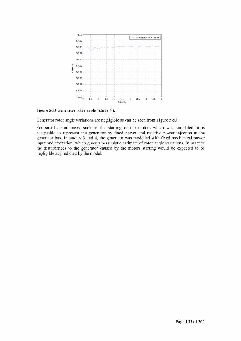
Page 155 of 365

0 0.5 1 1.5 2 2.5 3 3.5 4 4.5 557.6

57.61

57.62

57.63

57.64

57.65

57.66

57.67

57.68

57.69

57.7

time [s]

Generator rotor angle

Figure 5-53 Generator rotor angle ( study 4 ).

Generator rotor angle variations are negligible as can be seen from Figure 5-53.

For small disturbances, such as the starting of the motors which was simulated, it is acceptable to represent the generator by fixed power and reactive power injection at the generator bus. In studies 3 and 4, the generator was modelled with fixed mechanical power input and excitation, which gives a pessimistic estimate of rotor angle variations. In practice the disturbances to the generator caused by the motors starting would be expected to be negligible as predicted by the model.

degr

ees

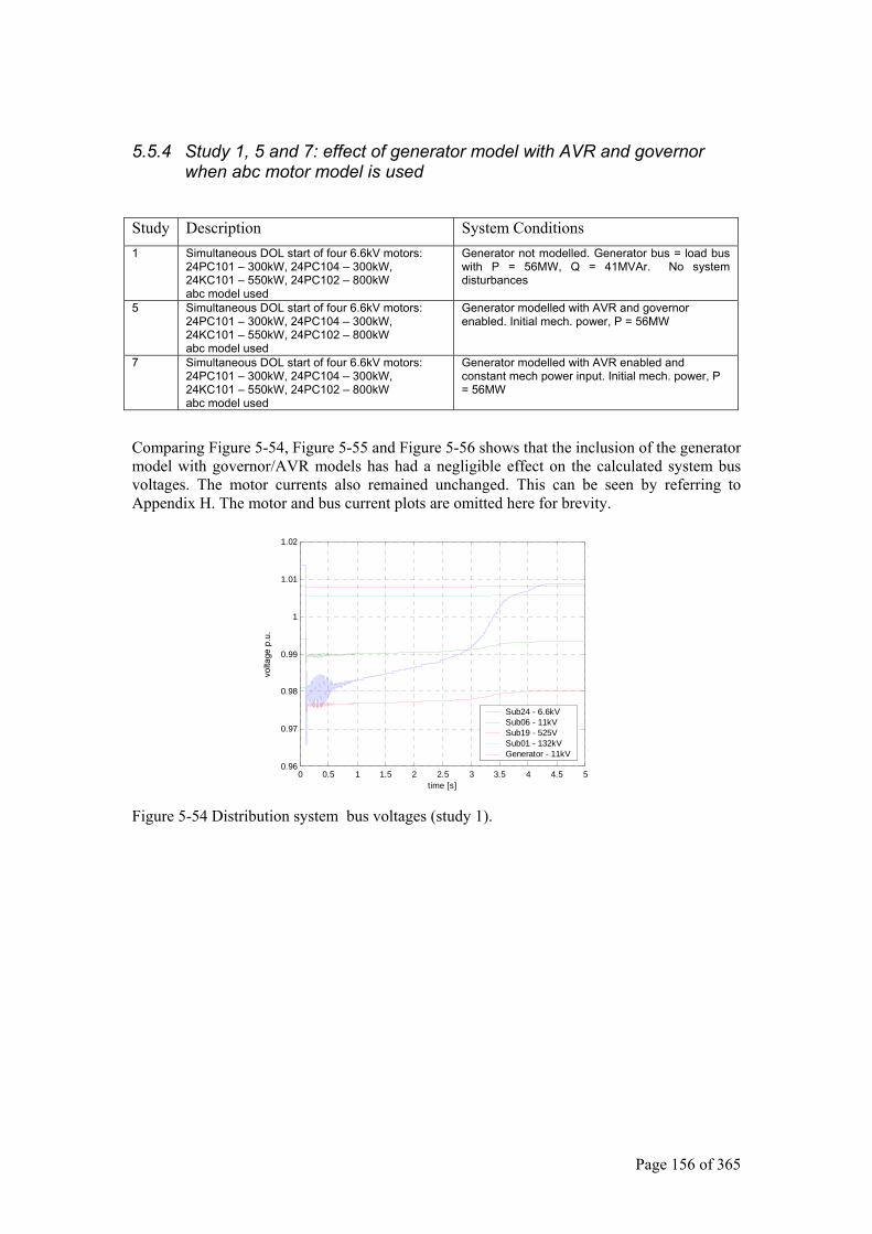
Page 156 of 365

5.5.4 Study 1, 5 and 7: effect of generator model with AVR and governor when abc motor model is used

Study Description System Conditions 1 Simultaneous DOL start of four 6.6kV motors:

24PC101 – 300kW, 24PC104 – 300kW, 24KC101 – 550kW, 24PC102 – 800kW abc model used

Generator not modelled. Generator bus = load bus with P = 56MW, Q = 41MVAr. No system disturbances

5 Simultaneous DOL start of four 6.6kV motors: 24PC101 – 300kW, 24PC104 – 300kW, 24KC101 – 550kW, 24PC102 – 800kW abc model used

Generator modelled with AVR and governor enabled. Initial mech. power, P = 56MW

7 Simultaneous DOL start of four 6.6kV motors: 24PC101 – 300kW, 24PC104 – 300kW, 24KC101 – 550kW, 24PC102 – 800kW abc model used

Generator modelled with AVR enabled and constant mech power input. Initial mech. power, P = 56MW

Comparing Figure 5-54, Figure 5-55 and Figure 5-56 shows that the inclusion of the generator model with governor/AVR models has had a negligible effect on the calculated system bus voltages. The motor currents also remained unchanged. This can be seen by referring to Appendix H. The motor and bus current plots are omitted here for brevity.

0 0.5 1 1.5 2 2.5 3 3.5 4 4.5 50.96

0.97

0.98

0.99

1

1.01

1.02

time [s]

Sub24 - 6.6kV Sub06 - 11kV Sub19 - 525V Sub01 - 132kV Generator - 11kV

Figure 5-54 Distribution system bus voltages (study 1).

volta

ge p

.u.

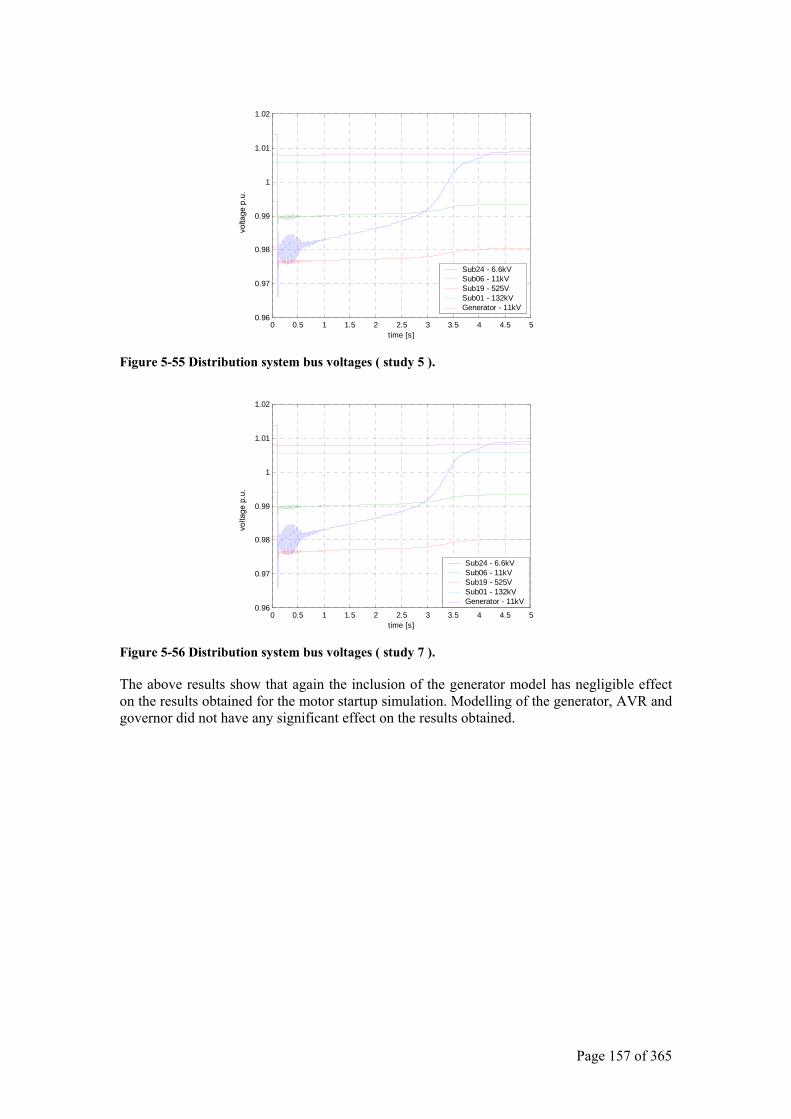
Page 157 of 365

0 0.5 1 1.5 2 2.5 3 3.5 4 4.5 50.96

0.97

0.98

0.99

1

1.01

1.02

time [s]

Sub24 - 6.6kV Sub06 - 11kV Sub19 - 525V Sub01 - 132kV Generator - 11kV

Figure 5-55 Distribution system bus voltages ( study 5 ).

0 0.5 1 1.5 2 2.5 3 3.5 4 4.5 50.96

0.97

0.98

0.99

1

1.01

1.02

time [s]

Sub24 - 6.6kV Sub06 - 11kV Sub19 - 525V Sub01 - 132kV Generator - 11kV

Figure 5-56 Distribution system bus voltages ( study 7 ).

The above results show that again the inclusion of the generator model has negligible effect on the results obtained for the motor startup simulation. Modelling of the generator, AVR and governor did not have any significant effect on the results obtained.

volta

ge p

.u.

volta

ge p

.u.

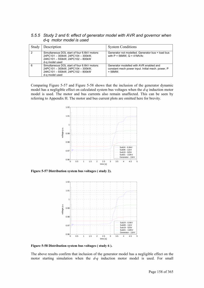
Page 158 of 365

5.5.5 Study 2 and 6: effect of generator model with AVR and governor when d-q motor model is used

Study Description System Conditions 2 Simultaneous DOL start of four 6.6kV motors:

24PC101 – 300kW, 24PC104 – 300kW, 24KC101 – 550kW, 24PC102 – 800kW d-q model used

Generator not modelled. Generator bus = load bus with P = 56MW, Q = 41MVAr.

6 Simultaneous DOL start of four 6.6kV motors: 24PC101 – 300kW, 24PC104 – 300kW, 24KC101 – 550kW, 24PC102 – 800kW d-q model used

Generator modelled with AVR enabled and constant mech power input. Initial mech. power, P = 56MW.

Comparing Figure 5-57 and Figure 5-58 shows that the inclusion of the generator dynamic model has a negligible effect on calculated system bus voltages when the d-q induction motor model is used. The motor and bus currents also remain unaffected. This can be seen by referring to Appendix H. The motor and bus current plots are omitted here for brevity.

0 0.5 1 1.5 2 2.5 3 3.5 4 4.5 50.96

0.97

0.98

0.99

1

1.01

1.02

time [s]

Sub24 - 6.6kV Sub06 - 11kV Sub19 - 525V Sub01 - 132kV Generator - 11kV

Figure 5-57 Distribution system bus voltages ( study 2).

0 0.5 1 1.5 2 2.5 3 3.5 4 4.5 50.96

0.97

0.98

0.99

1

1.01

1.02

time [s]

Sub24 - 6.6kV Sub06 - 11kV Sub19 - 525V Sub01 - 132kV Generator - 11kV

Figure 5-58 Distribution system bus voltages ( study 6 ).

The above results confirm that inclusion of the generator model has a negligible effect on the motor starting simulation when the d-q induction motor model is used. For small

volta

ge p

.u.

volta

ge p

.u.

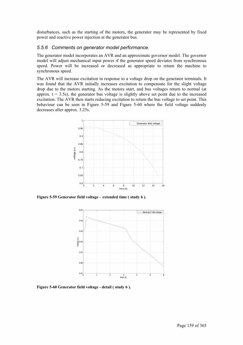
Page 159 of 365

disturbances, such as the starting of the motors, the generator may be represented by fixed power and reactive power injection at the generator bus.

5.5.6 Comments on generator model performance. The generator model incorporates an AVR and an approximate governor model. The governor model will adjust mechanical input power if the generator speed deviates from synchronous speed. Power will be increased or decreased as appropriate to return the machine to synchronous speed.

The AVR will increase excitation in response to a voltage drop on the generator terminals. It was found that the AVR initially increases excitation to compensate for the slight voltage drop due to the motors starting. As the motors start, and bus voltages return to normal (at approx. t = 3.5s), the generator bus voltage is slightly above set point due to the increased excitation. The AVR then starts reducing excitation to return the bus voltage to set point. This behaviour can be seen in Figure 5-59 and Figure 5-60 where the field voltage suddenly decreases after approx. 3.25s.

0 2 4 6 8 10 12 14 160.6

0.65

0.7

0.75

0.8

0.85

0.9

0.95

1

time [s]

Generator field voltage

Figure 5-59 Generator field voltage – extended time ( study 6 ).

Figure 5-60 Generator field voltage - detail ( study 6 ).

volta

ge p

.u.

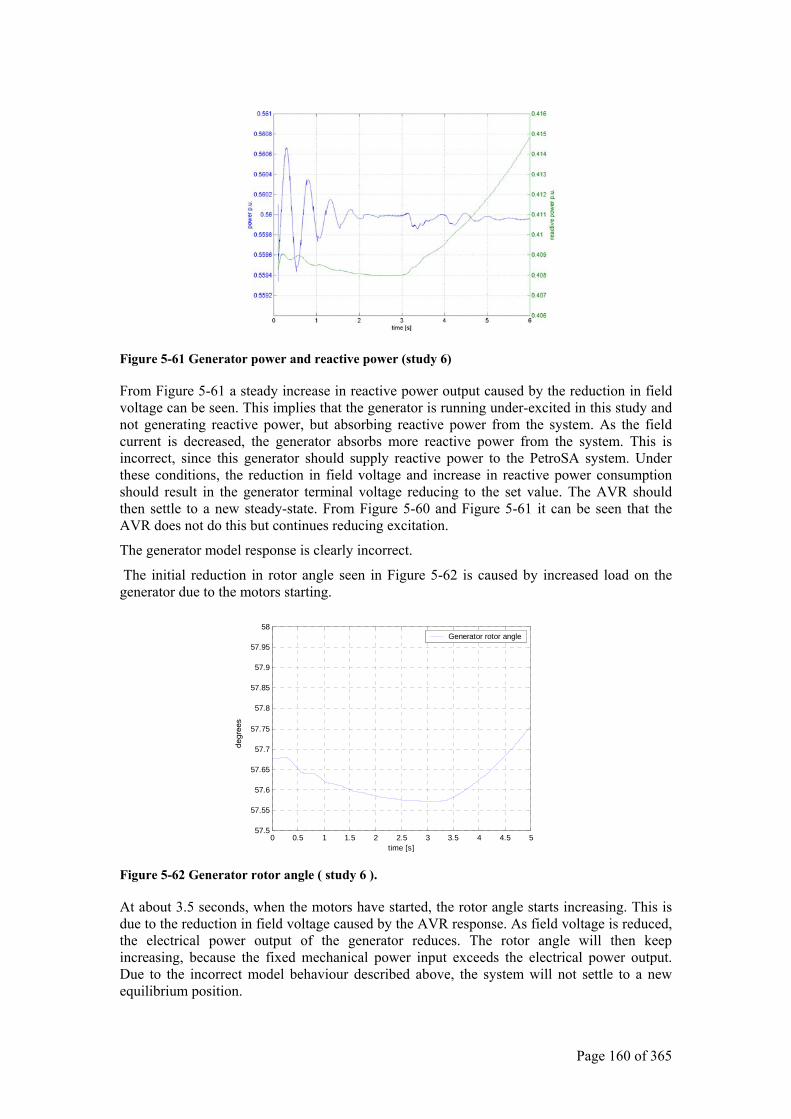
Page 160 of 365

Figure 5-61 Generator power and reactive power (study 6)

From Figure 5-61 a steady increase in reactive power output caused by the reduction in field voltage can be seen. This implies that the generator is running under-excited in this study and not generating reactive power, but absorbing reactive power from the system. As the field current is decreased, the generator absorbs more reactive power from the system. This is incorrect, since this generator should supply reactive power to the PetroSA system. Under these conditions, the reduction in field voltage and increase in reactive power consumption should result in the generator terminal voltage reducing to the set value. The AVR should then settle to a new steady-state. From Figure 5-60 and Figure 5-61 it can be seen that the AVR does not do this but continues reducing excitation.

The generator model response is clearly incorrect.

The initial reduction in rotor angle seen in Figure 5-62 is caused by increased load on the generator due to the motors starting.

0 0.5 1 1.5 2 2.5 3 3.5 4 4.5 557.5

57.55

57.6

57.65

57.7

57.75

57.8

57.85

57.9

57.95

58

time [s]

Generator rotor angle

Figure 5-62 Generator rotor angle ( study 6 ).

At about 3.5 seconds, when the motors have started, the rotor angle starts increasing. This is due to the reduction in field voltage caused by the AVR response. As field voltage is reduced, the electrical power output of the generator reduces. The rotor angle will then keep increasing, because the fixed mechanical power input exceeds the electrical power output. Due to the incorrect model behaviour described above, the system will not settle to a new equilibrium position.

degr

ees

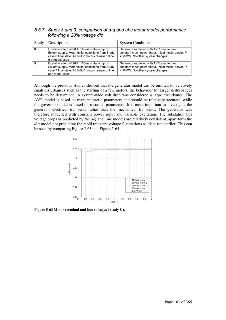
Page 161 of 365

5.5.7 Study 8 and 9: comparison of d-q and abc motor model performance following a 20% voltage dip

Study Description System Conditions 8 Examine effect of 20%, 100ms voltage dip on

Eskom supply. Motor initial conditions from Study case 6 final state. All 6.6kV motors remain online. d-q model used

Generator modelled with AVR enabled and constant mech power input. Initial mech. power, P = 56MW. No other system changes

9 Examine effect of 20%, 100ms voltage dip on Eskom supply. Motor initial conditions from Study case 7 final state. All 6.6kV motors remain online. abc model used

Generator modelled with AVR enabled and constant mech power input. Initial mech. power, P = 56MW. No other system changes

Although the previous studies showed that the generator model can be omitted for relatively small disturbances such as the starting of a few motors, the behaviour for larger disturbances needs to be determined. A system-wide volt drop was considered a large disturbance. The AVR model is based on manufacturer’s parameters and should be relatively accurate, while the governor model is based on assumed parameters. It is more important to investigate the generator electrical transients rather than the mechanical transients. The generator was therefore modelled with constant power input and variable excitation. The substation bus voltage drops as predicted by the d-q and abc models are relatively consistent, apart form the d-q model not predicting the rapid transient voltage fluctuations as discussed earlier. This can be seen by comparing Figure 5-63 and Figure 5-64

0 0.2 0.4 0.6 0.8 1 1.2 1.4 1.6 1.8 20.96

0.97

0.98

0.99

1

1.01

1.02

time [s]

550kW motor 300kW motor 1300kW motor 2850kW motor 6.6kV bus

Figure 5-63 Motor terminal and bus voltages ( study 8 ).

volta

ge p

.u.

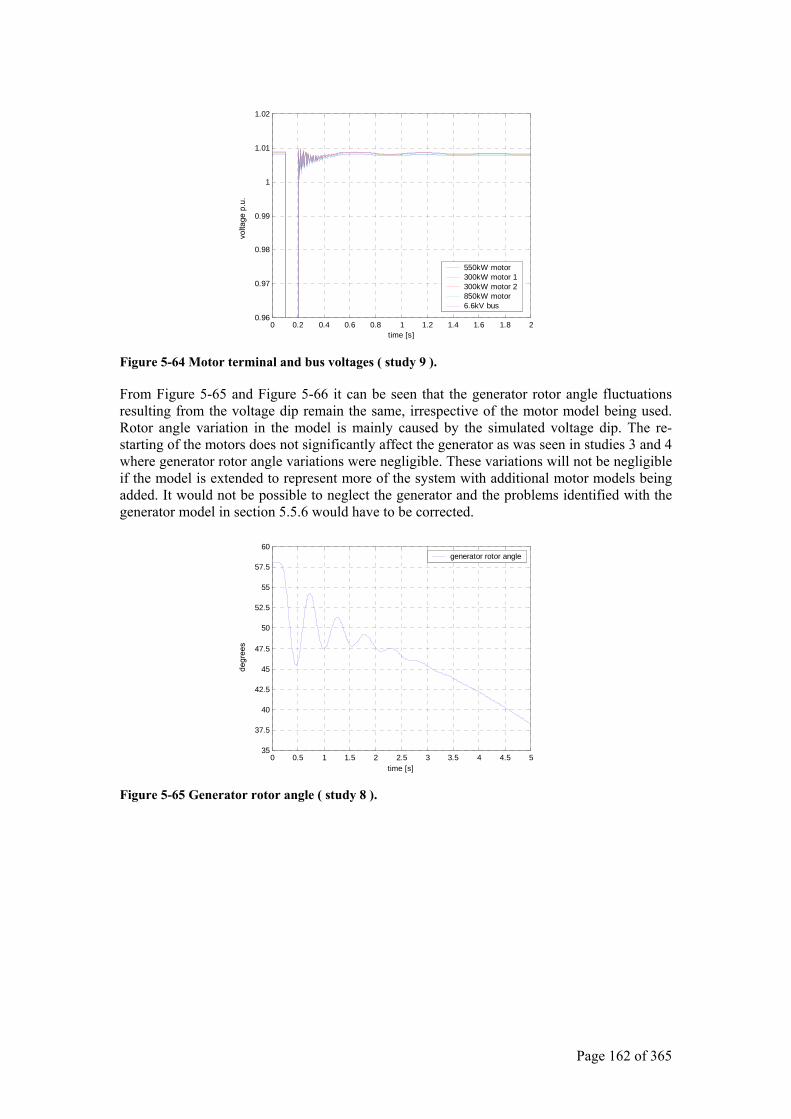
Page 162 of 365

0 0.2 0.4 0.6 0.8 1 1.2 1.4 1.6 1.8 20.96

0.97

0.98

0.99

1

1.01

1.02

time [s]

550kW motor 300kW motor 1300kW motor 2850kW motor 6.6kV bus

Figure 5-64 Motor terminal and bus voltages ( study 9 ).

From Figure 5-65 and Figure 5-66 it can be seen that the generator rotor angle fluctuations resulting from the voltage dip remain the same, irrespective of the motor model being used. Rotor angle variation in the model is mainly caused by the simulated voltage dip. The re-starting of the motors does not significantly affect the generator as was seen in studies 3 and 4 where generator rotor angle variations were negligible. These variations will not be negligible if the model is extended to represent more of the system with additional motor models being added. It would not be possible to neglect the generator and the problems identified with the generator model in section 5.5.6 would have to be corrected.

0 0.5 1 1.5 2 2.5 3 3.5 4 4.5 535

37.5

40

42.5

45

47.5

50

52.5

55

57.5

60

time [s]

generator rotor angle

Figure 5-65 Generator rotor angle ( study 8 ).

volta

ge p

.u.

degr

ees

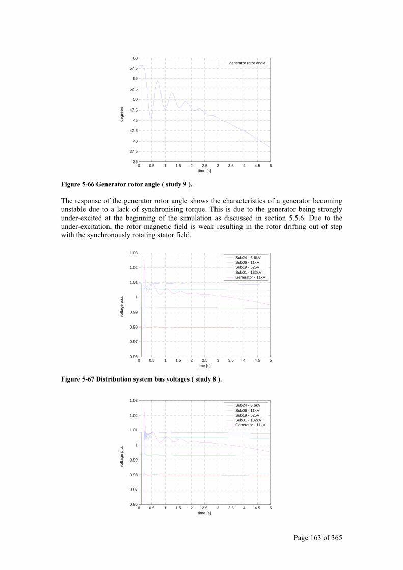
Page 163 of 365

0 0.5 1 1.5 2 2.5 3 3.5 4 4.5 535

37.5

40

42.5

45

47.5

50

52.5

55

57.5

60

time [s]

generator rotor angle

Figure 5-66 Generator rotor angle ( study 9 ).

The response of the generator rotor angle shows the characteristics of a generator becoming unstable due to a lack of synchronising torque. This is due to the generator being strongly under-excited at the beginning of the simulation as discussed in section 5.5.6. Due to the under-excitation, the rotor magnetic field is weak resulting in the rotor drifting out of step with the synchronously rotating stator field.

0 0.5 1 1.5 2 2.5 3 3.5 4 4.5 50.96

0.97

0.98

0.99

1

1.01

1.02

1.03

time [s]

Sub24 - 6.6kV Sub06 - 11kV Sub19 - 525V Sub01 - 132kV Generator - 11kV

Figure 5-67 Distribution system bus voltages ( study 8 ).

0 0.5 1 1.5 2 2.5 3 3.5 4 4.5 50.96

0.97

0.98

0.99

1

1.01

1.02

1.03

time [s]

Sub24 - 6.6kV Sub06 - 11kV Sub19 - 525V Sub01 - 132kV Generator - 11kV

degr

ees

volta

ge p

.u.

volta

ge p

.u.

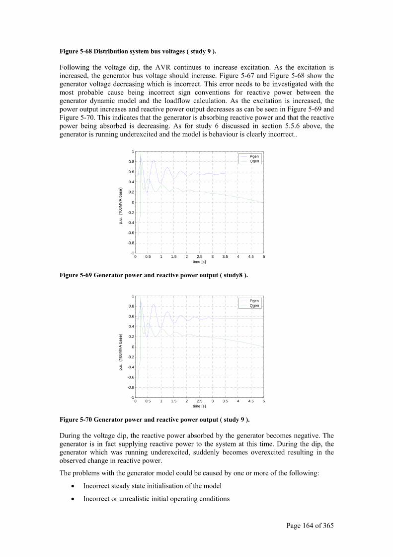
Page 164 of 365

Figure 5-68 Distribution system bus voltages ( study 9 ).

Following the voltage dip, the AVR continues to increase excitation. As the excitation is increased, the generator bus voltage should increase. Figure 5-67 and Figure 5-68 show the generator voltage decreasing which is incorrect. This error needs to be investigated with the most probable cause being incorrect sign conventions for reactive power between the generator dynamic model and the loadflow calculation. As the excitation is increased, the power output increases and reactive power output decreases as can be seen in Figure 5-69 and Figure 5-70. This indicates that the generator is absorbing reactive power and that the reactive power being absorbed is decreasing. As for study 6 discussed in section 5.5.6 above, the generator is running underexcited and the model is behaviour is clearly incorrect..

0 0.5 1 1.5 2 2.5 3 3.5 4 4.5 5-1

-0.8

-0.6

-0.4

-0.2

0

0.2

0.4

0.6

0.8

1

time [s]

PgenQgen

Figure 5-69 Generator power and reactive power output ( study8 ).

0 0.5 1 1.5 2 2.5 3 3.5 4 4.5 5-1

-0.8

-0.6

-0.4

-0.2

0

0.2

0.4

0.6

0.8

1

time [s]

PgenQgen

Figure 5-70 Generator power and reactive power output ( study 9 ).

During the voltage dip, the reactive power absorbed by the generator becomes negative. The generator is in fact supplying reactive power to the system at this time. During the dip, the generator which was running underexcited, suddenly becomes overexcited resulting in the observed change in reactive power.

The problems with the generator model could be caused by one or more of the following:

• Incorrect steady state initialisation of the model

• Incorrect or unrealistic initial operating conditions

p.u.

(10

0MV

A b

ase)

p.

u. (

100M

VA

bas

e)

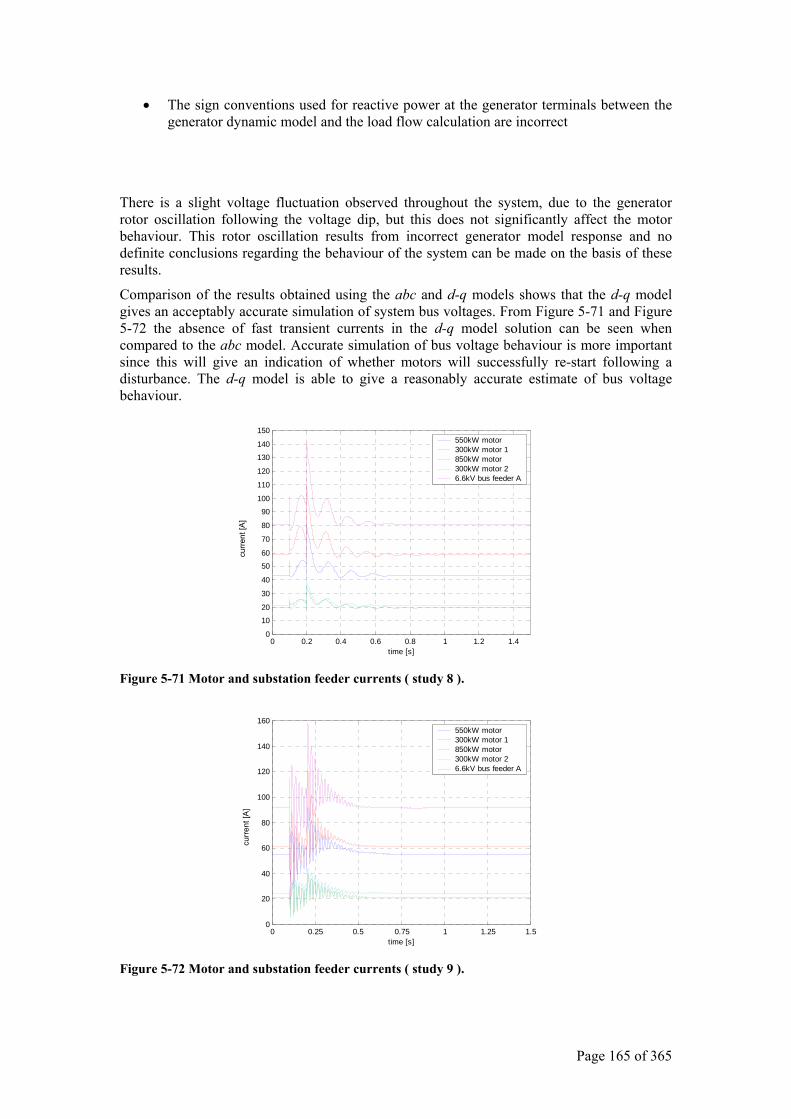
Page 165 of 365

• The sign conventions used for reactive power at the generator terminals between the generator dynamic model and the load flow calculation are incorrect

There is a slight voltage fluctuation observed throughout the system, due to the generator rotor oscillation following the voltage dip, but this does not significantly affect the motor behaviour. This rotor oscillation results from incorrect generator model response and no definite conclusions regarding the behaviour of the system can be made on the basis of these results.

Comparison of the results obtained using the abc and d-q models shows that the d-q model gives an acceptably accurate simulation of system bus voltages. From Figure 5-71 and Figure 5-72 the absence of fast transient currents in the d-q model solution can be seen when compared to the abc model. Accurate simulation of bus voltage behaviour is more important since this will give an indication of whether motors will successfully re-start following a disturbance. The d-q model is able to give a reasonably accurate estimate of bus voltage behaviour.

0 0.2 0.4 0.6 0.8 1 1.2 1.40

10

20

30

40

50

60

70

80

90

100

110

120

130

140

150

time [s]

550kW motor 300kW motor 1 850kW motor 300kW motor 2 6.6kV bus feeder A

Figure 5-71 Motor and substation feeder currents ( study 8 ).

0 0.25 0.5 0.75 1 1.25 1.50

20

40

60

80

100

120

140

160

time [s]

550kW motor 300kW motor 1 850kW motor 300kW motor 2 6.6kV bus feeder A

Figure 5-72 Motor and substation feeder currents ( study 9 ).

curre

nt [A

] cu

rrent

[A]

Page 166 of 365

As discussed previously, both models have problems which need to be resolved before further more detailed work is attempted. The d-q model produces low frequency stator current oscillations caused by mechanical oscillations of the rotor following a disturbance. This is due to the difference in torque speed characteristics between the models and the lower inertia constants used with the d-q model. The abc model appears to give an reasonable indication peak stator current and torque amplitudes which could be expected in practice. These transients take too long to decay though. These problems need to be resolved by extending this model to include saturation, correct parameter estimation and benchmarking of the model against known accurate results.

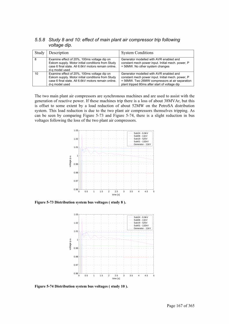
Page 167 of 365

5.5.8 Study 8 and 10: effect of main plant air compressor trip following voltage dip.

Study Description System Conditions 8 Examine effect of 20%, 100ms voltage dip on

Eskom supply. Motor initial conditions from Study case 6 final state. All 6.6kV motors remain online. d-q model used

Generator modelled with AVR enabled and constant mech power input. Initial mech. power, P = 56MW. No other system changes

10 Examine effect of 20%, 100ms voltage dip on Eskom supply. Motor initial conditions from Study case 6 final state. All 6.6kV motors remain online. d-q model used

Generator modelled with AVR enabled and constant mech power input. Initial mech. power, P = 56MW. Two 26MW compressors at air separation plant tripped 80ms after start of voltage dip

The two main plant air compressors are synchronous machines and are used to assist with the generation of reactive power. If these machines trip there is a loss of about 38MVAr, but this is offset to some extent by a load reduction of about 52MW on the PetroSA distribution system. This load reduction is due to the two plant air compressors themselves tripping. As can be seen by comparing Figure 5-73 and Figure 5-74, there is a slight reduction in bus voltages following the loss of the two plant air compressors.

0 0.5 1 1.5 2 2.5 3 3.5 4 4.5 50.96

0.97

0.98

0.99

1

1.01

1.02

1.03

time [s]

Sub24 - 6.6kV Sub06 - 11kV Sub19 - 525V Sub01 - 132kV Generator - 11kV

Figure 5-73 Distribution system bus voltages ( study 8 ).

0 0.5 1 1.5 2 2.5 3 3.5 4 4.5 50.96

0.97

0.98

0.99

1

1.01

1.02

1.03

time [s]

Sub24 - 6.6kV Sub06 - 11kV Sub19 - 525V Sub01 - 132kV Generator - 11kV

Figure 5-74 Distribution system bus voltages ( study 10 ).

volta

ge p

.u.

volta

ge p

.u.

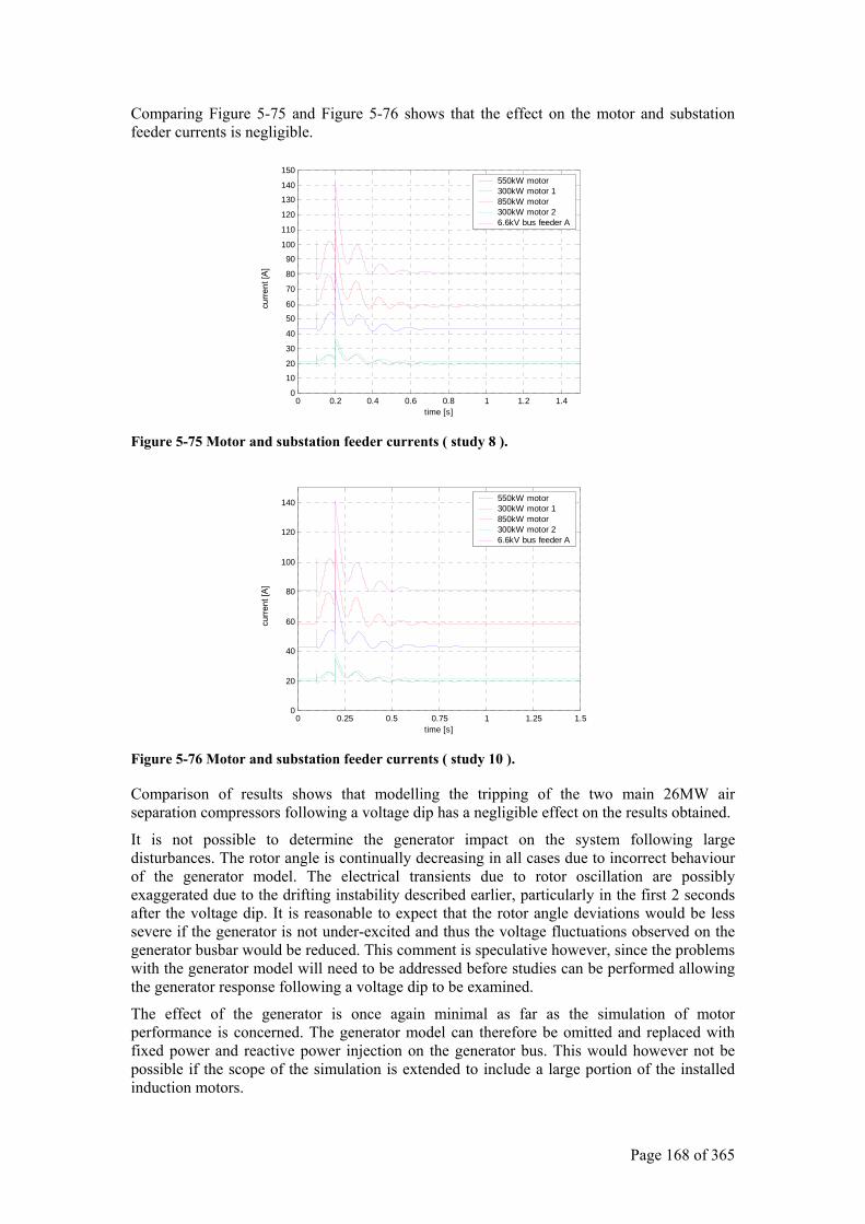
Page 168 of 365

Comparing Figure 5-75 and Figure 5-76 shows that the effect on the motor and substation feeder currents is negligible.

0 0.2 0.4 0.6 0.8 1 1.2 1.40

10

20

30

40

50

60

70

80

90

100

110

120

130

140

150

time [s]

550kW motor 300kW motor 1 850kW motor 300kW motor 2 6.6kV bus feeder A

Figure 5-75 Motor and substation feeder currents ( study 8 ).

0 0.25 0.5 0.75 1 1.25 1.50

20

40

60

80

100

120

140

time [s]

550kW motor 300kW motor 1 850kW motor 300kW motor 2 6.6kV bus feeder A

Figure 5-76 Motor and substation feeder currents ( study 10 ).

Comparison of results shows that modelling the tripping of the two main 26MW air separation compressors following a voltage dip has a negligible effect on the results obtained.

It is not possible to determine the generator impact on the system following large disturbances. The rotor angle is continually decreasing in all cases due to incorrect behaviour of the generator model. The electrical transients due to rotor oscillation are possibly exaggerated due to the drifting instability described earlier, particularly in the first 2 seconds after the voltage dip. It is reasonable to expect that the rotor angle deviations would be less severe if the generator is not under-excited and thus the voltage fluctuations observed on the generator busbar would be reduced. This comment is speculative however, since the problems with the generator model will need to be addressed before studies can be performed allowing the generator response following a voltage dip to be examined.

The effect of the generator is once again minimal as far as the simulation of motor performance is concerned. The generator model can therefore be omitted and replaced with fixed power and reactive power injection on the generator bus. This would however not be possible if the scope of the simulation is extended to include a large portion of the installed induction motors.

curre

nt [A

] cu

rrent

[A]

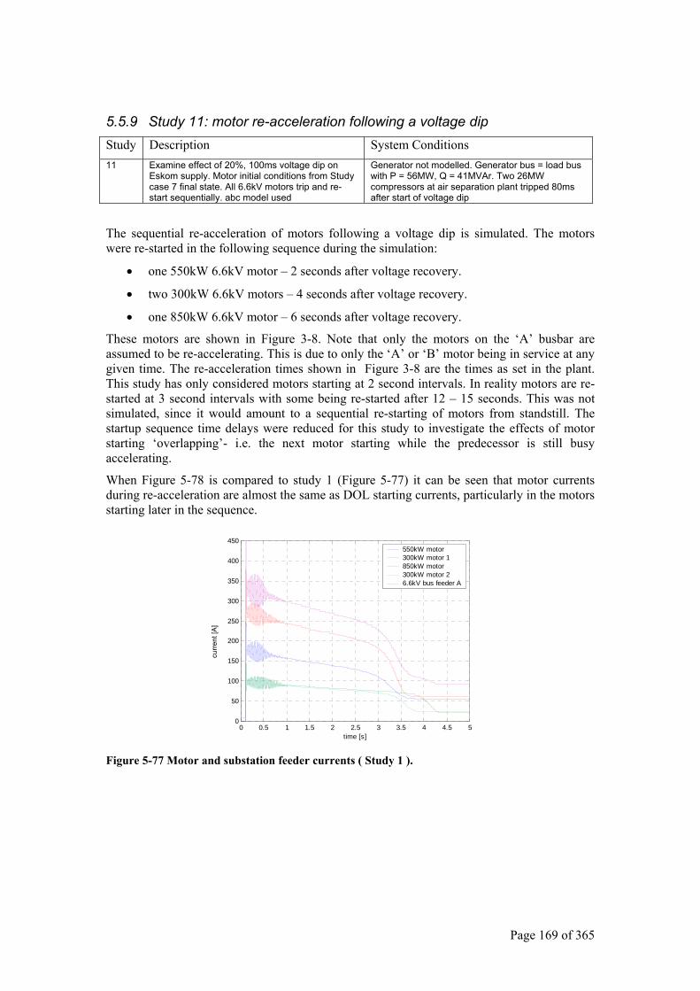
Page 169 of 365

5.5.9 Study 11: motor re-acceleration following a voltage dip Study Description System Conditions 11 Examine effect of 20%, 100ms voltage dip on

Eskom supply. Motor initial conditions from Study case 7 final state. All 6.6kV motors trip and re-start sequentially. abc model used

Generator not modelled. Generator bus = load bus with P = 56MW, Q = 41MVAr. Two 26MW compressors at air separation plant tripped 80ms after start of voltage dip

The sequential re-acceleration of motors following a voltage dip is simulated. The motors were re-started in the following sequence during the simulation:

• one 550kW 6.6kV motor – 2 seconds after voltage recovery.

• two 300kW 6.6kV motors – 4 seconds after voltage recovery.

• one 850kW 6.6kV motor – 6 seconds after voltage recovery.

These motors are shown in Figure 3-8. Note that only the motors on the ‘A’ busbar are assumed to be re-accelerating. This is due to only the ‘A’ or ‘B’ motor being in service at any given time. The re-acceleration times shown in Figure 3-8 are the times as set in the plant. This study has only considered motors starting at 2 second intervals. In reality motors are re-started at 3 second intervals with some being re-started after 12 – 15 seconds. This was not simulated, since it would amount to a sequential re-starting of motors from standstill. The startup sequence time delays were reduced for this study to investigate the effects of motor starting ‘overlapping’- i.e. the next motor starting while the predecessor is still busy accelerating.

When Figure 5-78 is compared to study 1 (Figure 5-77) it can be seen that motor currents during re-acceleration are almost the same as DOL starting currents, particularly in the motors starting later in the sequence.

0 0.5 1 1.5 2 2.5 3 3.5 4 4.5 50

50

100

150

200

250

300

350

400

450

time [s]

550kW motor 300kW motor 1 850kW motor 300kW motor 2 6.6kV bus feeder A

Figure 5-77 Motor and substation feeder currents ( Study 1 ).

curre

nt [A

]

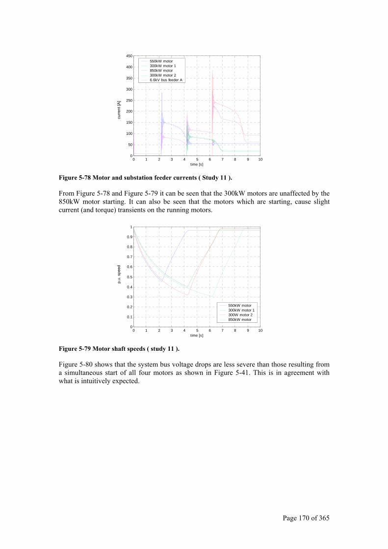
Page 170 of 365

0 1 2 3 4 5 6 7 8 9 100

50

100

150

200

250

300

350

400

450

time [s]

550kW motor 300kW motor 1 850kW motor 300kW motor 2 6.6kV bus feeder A

Figure 5-78 Motor and substation feeder currents ( Study 11 ).

From Figure 5-78 and Figure 5-79 it can be seen that the 300kW motors are unaffected by the 850kW motor starting. It can also be seen that the motors which are starting, cause slight current (and torque) transients on the running motors.

0 1 2 3 4 5 6 7 8 9 100

0.1

0.2

0.3

0.4

0.5

0.6

0.7

0.8

0.9

1

time [s]

550kW motor 300kW motor 1300W motor 2 850kW motor

Figure 5-79 Motor shaft speeds ( study 11 ).

Figure 5-80 shows that the system bus voltage drops are less severe than those resulting from a simultaneous start of all four motors as shown in Figure 5-41. This is in agreement with what is intuitively expected.

curre

nt [A

] p.

u. s

peed

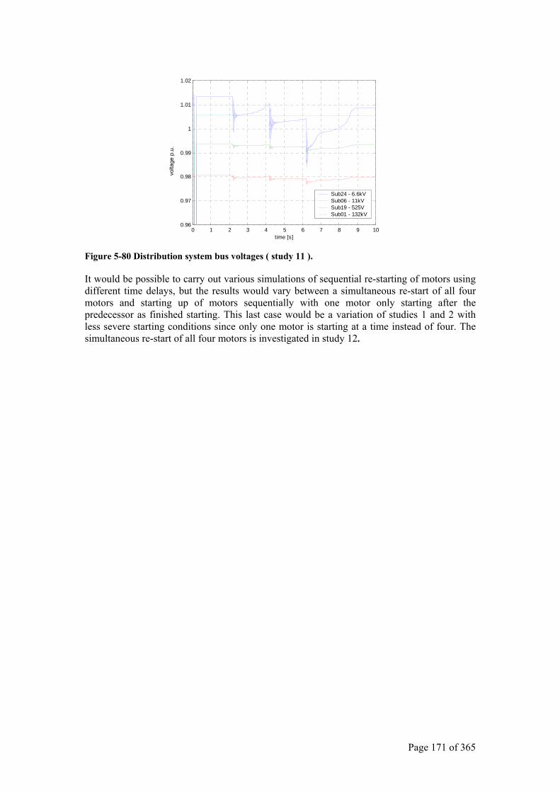
Page 171 of 365

0 1 2 3 4 5 6 7 8 9 100.96

0.97

0.98

0.99

1

1.01

1.02

time [s]

Sub24 - 6.6kVSub06 - 11kV Sub19 - 525V Sub01 - 132kV

Figure 5-80 Distribution system bus voltages ( study 11 ).

It would be possible to carry out various simulations of sequential re-starting of motors using different time delays, but the results would vary between a simultaneous re-start of all four motors and starting up of motors sequentially with one motor only starting after the predecessor as finished starting. This last case would be a variation of studies 1 and 2 with less severe starting conditions since only one motor is starting at a time instead of four. The simultaneous re-start of all four motors is investigated in study 12.

volta

ge p

.u.

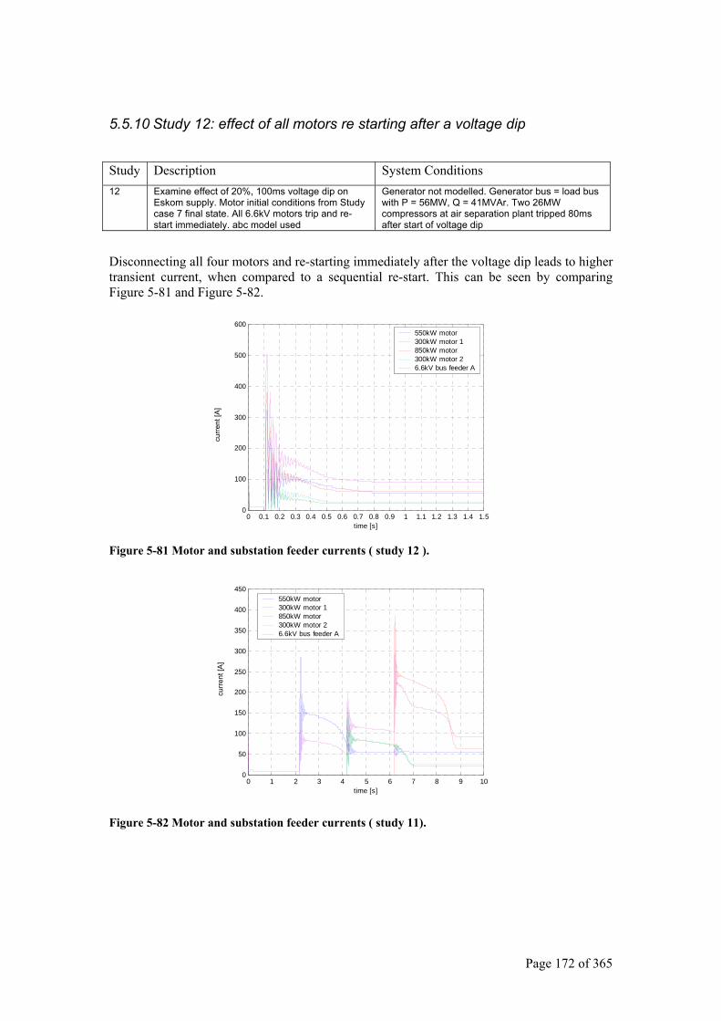
Page 172 of 365

5.5.10 Study 12: effect of all motors re starting after a voltage dip

Study Description System Conditions 12 Examine effect of 20%, 100ms voltage dip on

Eskom supply. Motor initial conditions from Study case 7 final state. All 6.6kV motors trip and re-start immediately. abc model used

Generator not modelled. Generator bus = load bus with P = 56MW, Q = 41MVAr. Two 26MW compressors at air separation plant tripped 80ms after start of voltage dip

Disconnecting all four motors and re-starting immediately after the voltage dip leads to higher transient current, when compared to a sequential re-start. This can be seen by comparing Figure 5-81 and Figure 5-82.

0 0.1 0.2 0.3 0.4 0.5 0.6 0.7 0.8 0.9 1 1.1 1.2 1.3 1.4 1.50

100

200

300

400

500

600

time [s]

550kW motor 300kW motor 1 850kW motor 300kW motor 2 6.6kV bus feeder A

Figure 5-81 Motor and substation feeder currents ( study 12 ).

0 1 2 3 4 5 6 7 8 9 100

50

100

150

200

250

300

350

400

450

time [s]

550kW motor 300kW motor 1 850kW motor 300kW motor 2 6.6kV bus feeder A

Figure 5-82 Motor and substation feeder currents ( study 11).

curre

nt [A

] cu

rrent

[A]

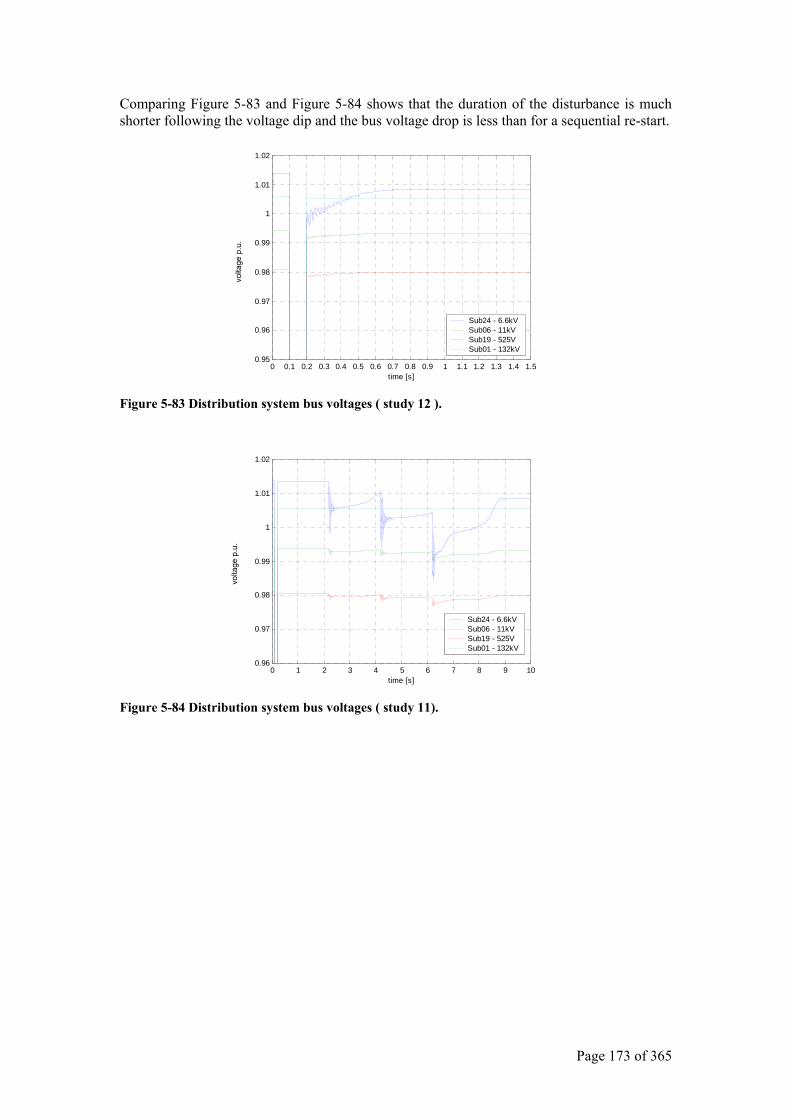
Page 173 of 365

Comparing Figure 5-83 and Figure 5-84 shows that the duration of the disturbance is much shorter following the voltage dip and the bus voltage drop is less than for a sequential re-start.

0 0.1 0.2 0.3 0.4 0.5 0.6 0.7 0.8 0.9 1 1.1 1.2 1.3 1.4 1.50.95

0.96

0.97

0.98

0.99

1

1.01

1.02

time [s]

Sub24 - 6.6kVSub06 - 11kV Sub19 - 525V Sub01 - 132kV

Figure 5-83 Distribution system bus voltages ( study 12 ).

0 1 2 3 4 5 6 7 8 9 100.96

0.97

0.98

0.99

1

1.01

1.02

time [s]

Sub24 - 6.6kVSub06 - 11kV Sub19 - 525V Sub01 - 132kV

Figure 5-84 Distribution system bus voltages ( study 11).

volta

ge p

.u.

volta

ge p

.u.

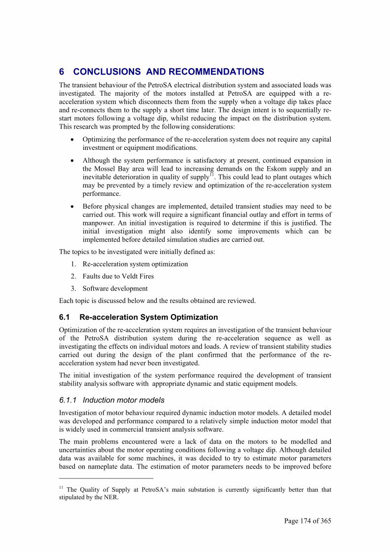
Page 174 of 365

6 CONCLUSIONS AND RECOMMENDATIONS The transient behaviour of the PetroSA electrical distribution system and associated loads was investigated. The majority of the motors installed at PetroSA are equipped with a re-acceleration system which disconnects them from the supply when a voltage dip takes place and re-connects them to the supply a short time later. The design intent is to sequentially re-start motors following a voltage dip, whilst reducing the impact on the distribution system. This research was prompted by the following considerations:

• Optimizing the performance of the re-acceleration system does not require any capital investment or equipment modifications.

• Although the system performance is satisfactory at present, continued expansion in the Mossel Bay area will lead to increasing demands on the Eskom supply and an inevitable deterioration in quality of supply11. This could lead to plant outages which may be prevented by a timely review and optimization of the re-acceleration system performance.

• Before physical changes are implemented, detailed transient studies may need to be carried out. This work will require a significant financial outlay and effort in terms of manpower. An initial investigation is required to determine if this is justified. The initial investigation might also identify some improvements which can be implemented before detailed simulation studies are carried out.

The topics to be investigated were initially defined as:

1. Re-acceleration system optimization

2. Faults due to Veldt Fires

3. Software development

Each topic is discussed below and the results obtained are reviewed.

6.1 Re-acceleration System Optimization Optimization of the re-acceleration system requires an investigation of the transient behaviour of the PetroSA distribution system during the re-acceleration sequence as well as investigating the effects on individual motors and loads. A review of transient stability studies carried out during the design of the plant confirmed that the performance of the re-acceleration system had never been investigated.

The initial investigation of the system performance required the development of transient stability analysis software with appropriate dynamic and static equipment models.

6.1.1 Induction motor models Investigation of motor behaviour required dynamic induction motor models. A detailed model was developed and performance compared to a relatively simple induction motor model that is widely used in commercial transient analysis software.

The main problems encountered were a lack of data on the motors to be modelled and uncertainties about the motor operating conditions following a voltage dip. Although detailed data was available for some machines, it was decided to try to estimate motor parameters based on nameplate data. The estimation of motor parameters needs to be improved before 11 The Quality of Supply at PetroSA’s main substation is currently significantly better than that stipulated by the NER.

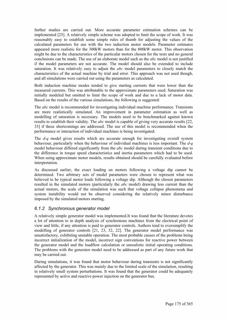
Page 175 of 365

further studies are carried out. More accurate parameter estimation schemes can be implemented [25]. A relatively simple scheme was adopted to limit the scope of work. It was reasonably easy to establish some simple rules of thumb for adjusting the values of the calculated parameters for use with the two induction motor models. Parameter estimates appeared more realistic for the 300kW motors than for the 800kW motor. This observation might be due to the characteristics of the particular motors chosen for the tests and no general conclusions can be made. The use of an elaborate model such as the abc model is not justified if the model parameters are not accurate. The model should also be extended to include saturation. It was relatively easy to adjust the abc model parameters to closely match the characteristics of the actual machine by trial and error. This approach was not used though, and all simulations were carried out using the parameters as calculated.

Both induction machine modes tended to give starting currents that were lower than the measured currents. This was attributable to the approximate parameters used. Saturation was initially modeled but omitted to limit the scope of work and due to a lack of motor data. Based on the results of the various simulations, the following is suggested:

The abc model is recommended for investigating individual machine performance. Transients are more realistically simulated. An improvement in parameter estimation as well as modelling of saturation is necessary. The models need to be benchmarked against known results to establish their validity. The abc model is capable of giving very accurate results [22, 33] if these shortcomings are addressed. The use of this model is recommended when the performance or interaction of individual machines is being investigated.

The d-q model gives results which are accurate enough for investigating overall system behaviour, particularly when the behaviour of individual machines is less important. The d-q model behaviour differed significantly from the abc model during transient conditions due to the difference in torque speed characteristics and inertia parameters which had to be used. When using approximate motor models, results obtained should be carefully evaluated before interpretation.

As discussed earlier, the exact loading on motors following a voltage dip cannot be determined. Two arbitrary sets of model parameters were chosen to represent what was believed to be typical motor loads following a voltage dip. Although the chosen parameters resulted in the simulated motors (particularly the abc model) drawing less current than the actual motors, the scale of the simulation was such that voltage collapse phenomena and system instability would not be observed considering the relatively minor disturbance imposed by the simulated motors starting.

6.1.2 Synchronous generator model A relatively simple generator model was implemented.It was found that the literature devotes a lot of attention to in depth analysis of synchronous machines from the electrical point of view and little, if any attention is paid to generator controls. Authors tend to oversimplify the modelling of generator controls [21, 23, 32, 22]. The generator model performance was unsatisfactory, exhibiting unstable operation. The most probable causes of the problems being incorrect initialization of the model, incorrect sign conventions for reactive power between the generator model and the loadflow calculation or unrealistic initial operating conditions. The problems with the generator model need to be addressed as part of any future work that may be carried out.

During simulations, it was found that motor behaviour during transients is not significantly affected by the generator. This was mainly due to the limited scale of the simulation, resulting in relatively small system perturbations. It was found that the generator could be adequately represented by active and reactive power injection on the generator bus.

Page 176 of 365

6.1.3 PetroSA distribution system model In deriving a suitable model of the electrical distribution system, it was possible to immediately exclude a significant amount of equipment from the model based on an evaluation of the system operation and response to transient conditions. The critical power system and generator could easily be eliminated, as well as the seven largest motors on site. A secondary substation and associated motors were chosen for detailed modelling with the remainder of the system represented by lumped equivalent loads. A constant impedance load model was chosen rather than a constant power load model based on the considerations discussed in sections 2.6.3 and 3.3. The major error attributable to the distribution system modelling identified by comparing simulated results with test results was the underestimation of bus voltage drops.

Measured bus voltage drops were greater than simulated. This can be attributed to one, or both of the following: Feeder cable impedances were underestimated and secondly the representation of the Eskom supply can be improved. Feeder data was obtained from the loadflow and fault calculation software database in use at PetroSA. Transformer impedances should be accurate, having been obtained from vendor specifications.

The system model is far too simple and limited in scope to provide anything more than an indication of voltage drops and current distributions during the transient conditions that were simulated. A far more extensive and accurate model will be required to properly investigate the behaviour of the entire system under transient conditions.

6.1.4 Optimization of re-acceleration system Based on simulation results, it was established that the re-acceleration system introduces unnecessary transients. Most power dips are of approximately 100ms duration with about a 20% volt drop. Simply leaving induction motors connected to the supply during such a dip results in lower system disturbances, than disconnecting motors from the supply and re-starting in sequence. The undervoltage relays can be set to 30% instead of the current 20%. No further studies are required to ensure that this is feasible. The current and voltage transients will be less than with the existing settings. In addition, motor speed fluctuations, and hence the risk of process upsets are reduced.

As a further action, the load distribution due to the re-acceleration system was examined. The total load being re-connected to the distribution system by the re-acceleration system was calculated by adding up the re-acceleration loads for each substation as given in Appendix A. These results are shown in Table 6-1 with all values in kW.

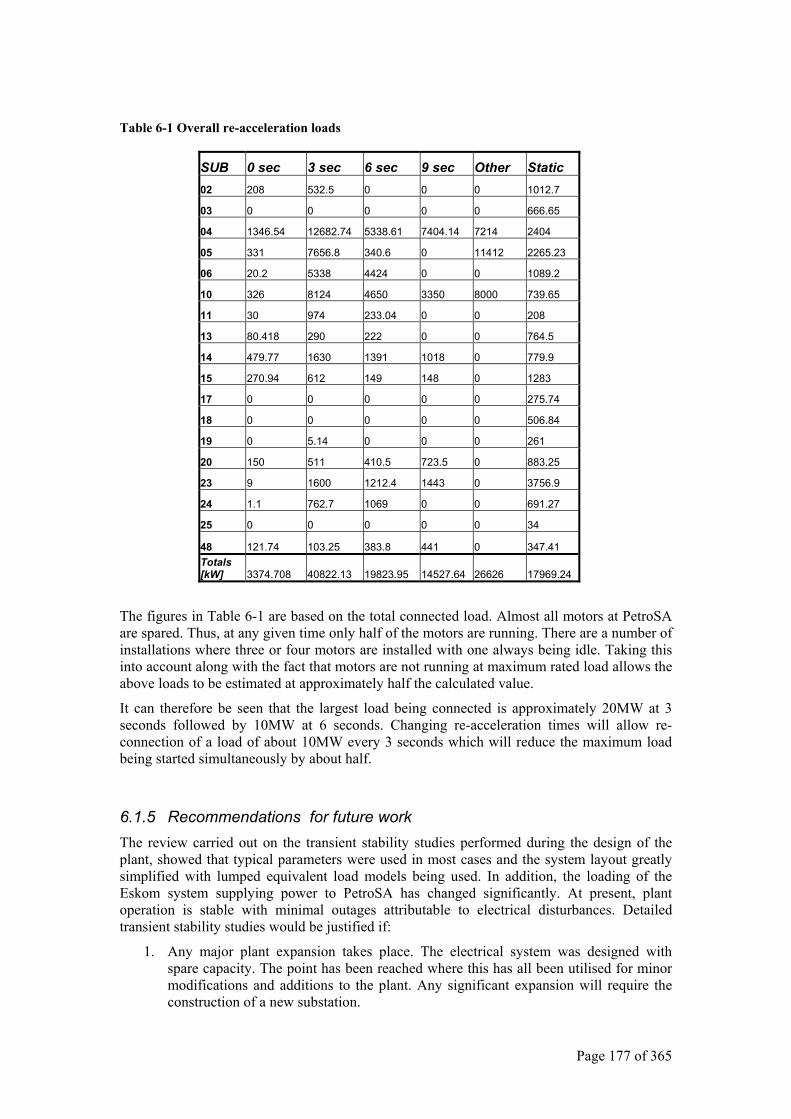
Page 177 of 365

Table 6-1 Overall re-acceleration loads

SUB 0 sec 3 sec 6 sec 9 sec Other Static 02 208 532.5 0 0 0 1012.7 03 0 0 0 0 0 666.65 04 1346.54 12682.74 5338.61 7404.14 7214 2404 05 331 7656.8 340.6 0 11412 2265.23 06 20.2 5338 4424 0 0 1089.2 10 326 8124 4650 3350 8000 739.65 11 30 974 233.04 0 0 208 13 80.418 290 222 0 0 764.5 14 479.77 1630 1391 1018 0 779.9 15 270.94 612 149 148 0 1283 17 0 0 0 0 0 275.74 18 0 0 0 0 0 506.84 19 0 5.14 0 0 0 261 20 150 511 410.5 723.5 0 883.25 23 9 1600 1212.4 1443 0 3756.9 24 1.1 762.7 1069 0 0 691.27 25 0 0 0 0 0 34 48 121.74 103.25 383.8 441 0 347.41 Totals [kW] 3374.708 40822.13 19823.95 14527.64 26626 17969.24

The figures in Table 6-1 are based on the total connected load. Almost all motors at PetroSA are spared. Thus, at any given time only half of the motors are running. There are a number of installations where three or four motors are installed with one always being idle. Taking this into account along with the fact that motors are not running at maximum rated load allows the above loads to be estimated at approximately half the calculated value.

It can therefore be seen that the largest load being connected is approximately 20MW at 3 seconds followed by 10MW at 6 seconds. Changing re-acceleration times will allow re-connection of a load of about 10MW every 3 seconds which will reduce the maximum load being started simultaneously by about half.

6.1.5 Recommendations for future work The review carried out on the transient stability studies performed during the design of the plant, showed that typical parameters were used in most cases and the system layout greatly simplified with lumped equivalent load models being used. In addition, the loading of the Eskom system supplying power to PetroSA has changed significantly. At present, plant operation is stable with minimal outages attributable to electrical disturbances. Detailed transient stability studies would be justified if:

1. Any major plant expansion takes place. The electrical system was designed with spare capacity. The point has been reached where this has all been utilised for minor modifications and additions to the plant. Any significant expansion will require the construction of a new substation.

Page 178 of 365

2. The proposed Peak power Generation Station is constructed adjacent to PetroSA.

3. The quality of supply deteriorates significantly from what is currently being received.

6.2 Faults Due To Veldt Fires This topic was prompted by the assumption that the re-acceleration system significantly reduces the impact of re-starting motors following a voltage dip, as opposed to re-starting from standstill. The concern was that repeated voltage dips, due to veldt fires would re-start the re-acceleration sequence and that motor speeds would reduce, resulting in essentially re-starting motors from standstill. An induction motor will draw a high starting current until the rotor speed is above about 80-90% of rated speed. Initial investigations into the operation of the system showed that due to motor loads remaining unchanged following a voltage dip, the motors would decelerate fairly rapidly. The first motors are only re-started after three seconds. At that stage the rotor speed has reduced significantly resulting in the motor drawing currents close to that required for a startup from standstill. The motors being re-started after 6s, 9s and longer delays can be considered as starting from standstill and drawing full starting current. Re-starting the re-acceleration sequence does not therefore result in a significantly greater demands on the system. This topic did not merit further investigation.

6.3 Software Development

6.3.1 Matlab The use of Matlab greatly accelerated the software development process. The use of the built-in matrix arithmetic functions and ODE solvers permitted rapid software development, allowing time to be spent on developing the transient simulation program and the various models rather than matrix arithmetic functions and ODE solvers. If one of the other software options had been used, a great deal of additional time and effort would have been spent on writing these functions.

Since Matlab is equipped with a number of different ODE solver routines, it was easy to experiment with and investigate the performance of the different solvers. This made it relatively easy to select the ODE solver which performed the best in terms of accuracy and solution speed. It was established that the correct error tolerance parameters need to be set when using the ode solvers since the default parameters did not give accurate results in all cases. A step length of 1ms was chosen for simulations since this allowed system response to be accurately represented. When using the ode solvers alternately with the loadflow calculations, default error tolerance parameters gave correct results.

The Matlab matrix functions proved very useful for implementing both the abc motor model as well as the Newton-Raphson loadflow routines. Due to the relatively small size of the system, the basic Newton-Raphson method was found to be capable of giving accurate results without convergence problems. Step voltage changes of up to 40% could be simulated on the swing bus without the loadflow algorithm failing to converge. For larger voltage changes, or simulation of short circuits, it would be necessary to provide appropriate initial estimates of bus voltages and angles to ensure convergence.

6.3.2 Simulink The Simulink environment within Matlab was found to be extremely useful for development and testing of the d-q motor and generator model. The AVR and governor responses could also be easily evaluated. The major advantage is the speed with which a model can be implemented and tested. The power systems block set was excluded on the basis of tests which showed that the component models were unwieldy to use. Another restriction on the

Page 179 of 365

use of the power systems block set is that the model of the PetroSA distribution system, as used for simulations would be cumbersome and difficult to implement.

6.3.3 Execution times Although the speed of software execution was not considered very important for this work, it will become a factor if the transient simulation program is extended to include more dynamic motor models. The execution times of simulations with similar time steps and time durations were compared. When using the ODE solvers to evaluate the motor models independently, simulation of a motor starting from t = 0 to 5s took about 4 seconds for the d-q model, compared to the abc model which took about 40s on average. The generator model simulation time was comparable to the d-q motor model

The transient simulation program was tested with four motor models and the generator model enabled. Simulation of the four motors starting at t=0 to 5s, takes about 30 minutes when using the abc motor model and 15 minutes when using the d-q model. The loadflow calculations take a major portion of this time. The use of the more complex motor model does result in increased program execution times, but additional execution times are not prohibitive.

6.4 Topics For Further Investigation This initial investigation into the re-acceleration system has yielded useful results and immediate changes can be implemented with will significantly reduce system transients due to the action of the re-acceleration system. Although system bus voltage drops were underestimated by the simulations, the motor startup tests allowed this error to be determined. It will be necessary to review feeder data and include more detailed modelling of the Eskom system before further simulations are conducted. Underestimation of bus voltage drops could lead to overly optimistic results when motor startup simulations are carried out, particularly where system performance is marginal.

The generator model problems need to be addressed. Saturation effects, excluded to limit the scope of work, should be included. If more detailed studies are carried out, investigating the behaviour of a larger number of induction motors, the generator model will definitely need to be included.

The use of a more elaborate induction machine model is only really justified when parameters can be accurately estimated or the behaviour of individual machines needs to be determined. For investigation of distribution system transient response, the simpler d-q models have proven adequate, provided their inherent limitations are appreciated. The more detailed model is useful for investigating motor behaviour and the effects on the driven load under transient conditions. This model needs to be extended to include saturation effects. This would be useful for evaluating peak torques under transient conditions, particularly where mechanical failures have taken place on couplings and driven machinery. If further more detailed studies are to be attempted, models need to be benchmarked and the errors in parameter estimation addressed.

Further work on the PetroSA system will require a detailed representation of the entire system with the majority of the motors represented by dynamic models or lumped equivalent motors. The generator will have to be accurately modelled. It will only be possible to fully investigate the behaviour of the system under transient conditions if the entire system is correctly represented. The bus voltage drops under these conditions will no longer be relatively insignificant and phenomena such as motors stalling and voltage collapse can be properly investigated. In order to proceed further the use of commercially available software such as DigSilent is essential. This will also permit the behaviour of the protection systems to be modelled and incorporates sophisticated routines to estimate parameters of equipment based on ‘nameplate’ data.. The time and effort required to extend the system models developed for this work is not justified if the capabilities of commercial software which is the result of

Page 180 of 365

considerable research and development effort12 is considered. The models developed for this work are considered as a ‘first try’ at investigating system behaviour. Continuing development of these models to further investigate the PetroSA system in detail will require an investment in time and effort that is not justified.

If the problems identified with the models are corrected and saturation effects included, it will be possible to carry out further investigations using the existing models. The behaviour of the generator can be properly investigated and unresolved problems addressed. Additional dynamic motor models can be added to extend the scope of the simulation, but at some stage, the time taken to run the computer simulation will become prohibitive and further work will have to be carried out using commercially available software as suggested above.

12 Commercial software packages are typically the result of tens, if not hundreds of man-years of research and development effort.

Page 181 of 365

ACKNOWLEDGEMENTS

I would like to thank my wife, Lindi, for her patience and support during this project. I realise that at times it seemed as if the work would never end, and that my overly optimistic estimates of the completion date were a source of great frustration. Without her understanding, encouragement and support this project would never have been completed and is as much her achievement as mine.

I would also like to thank Prof. Ron Herman for his assistance and guidance during the initial stages of this project, but a special word of thanks goes to Dr. Johan Vermeulen for all the assistance, guidance and valuable advice he has given me during the finalisation of this work.

Andre Claassens,

February 2008.

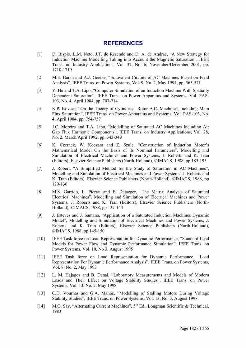
Page 182 of 365

REFERENCES

[1] D. Bispio, L.M. Neto, J.T. de Resende and D. A. de Andrae, “A New Strategy for Induction Machine Modelling Taking into Account the Magnetic Saturation”, IEEE Trans. on Industry Applications, Vol. 37, No. 6, November/December 2001, pp. 1710-1719

[2] M.E. Baran and A.J. Goetze, “Equivalent Circuits of AC Machines Based on Field Analysis”, IEEE Trans. on Power Systems, Vol. 9, No. 2, May 1994, pp. 565-571

[3] Y. He and T.A. Lipo, “Computer Simulation of an Induction Machine With Spatially Dependent Saturation”, IEEE Trans. on Power Apparatus and Systems, Vol. PAS-103, No. 4, April 1984, pp. 707-714

[4] K.P. Kovacs, “On the Theory of Cylindrical Rotor A.C. Machines, Including Main Flux Saturation”, IEEE Trans. on Power Apparatus and Systems, Vol. PAS-103, No. 4, April 1984, pp. 754-757

[5] J.C. Moreira and T.A. Lipo, “Modelling of Saturated AC Machines Including Air Gap Flux Harmonic Components”, IEEE Trans. on Industry Applications, Vol. 28, No. 2, March/April 1992, pp. 343-349

[6] K. Czernek, W. Koczara and Z. Szulc, “Construction of Induction Motor’s Mathematical Model On the Basis of its Nominal Parameters”, Modelling and Simulation of Electrical Machines and Power Systems, J. Roberts and K. Tran (Editors), Elsevier Science Publishers (North-Holland), ©IMACS, 1988, pp 185-195

[7] J. Robert, “A Simplified Method for the Study of Saturation in AC Machines”, Modelling and Simulation of Electrical Machines and Power Systems, J. Roberts and K. Tran (Editors), Elsevier Science Publishers (North-Holland), ©IMACS, 1988, pp 129-136

[8] M.S. Garrido, L. Pierrat and E. Dejaeger, “The Matrix Analysis of Saturated Electrical Machines”, Modelling and Simulation of Electrical Machines and Power Systems, J. Roberts and K. Tran (Editors), Elsevier Science Publishers (North-Holland), ©IMACS, 1988, pp 137-144

[9] J. Esteves and J. Santana, “Application of a Saturated Induction Machines Dynamic Model”, Modelling and Simulation of Electrical Machines and Power Systems, J. Roberts and K. Tran (Editors), Elsevier Science Publishers (North-Holland), ©IMACS, 1988, pp 145-150

[10] IEEE Task force on Load Representation for Dynamic Performance, “Standard Load Models for Power Flow and Dynamic Performance Simulation”, IEEE Trans. on Power Systems, Vol. 10, No 3, August 1995

[11] IEEE Task force on Load Representation for Dynamic Performance, “Load Representation For Dynamic Performance Analysis”, IEEE Trans. on Power Systems, Vol. 8, No. 2, May 1993

[12] L. M. Hajagos and B. Danai, “Laboratory Measurements and Models of Modern Loads and Their Effect on Voltage Stability Studies”, IEEE Trans. on Power Systems, Vol. 13, No. 2, May 1998

[13] C.D. Vournas and G.A. Manos, “Modelling of Stalling Motors During Voltage Stability Studies”, IEEE Trans. on Power Systems, Vol. 13, No. 3, August 1998

[14] M.G. Say, “Alternating Current Machines”, 5th Ed., Longman Scientific & Technical, 1983

Page 183 of 365

[15] A.E. Fitzgerald, C. Kingsley and A. Kusko, “Electric Machinery”. 3rd Ed., McGraw-Hill, 1971

[16] R.E. Steven, “Electrical Machines and Power Electronics”, 1st Ed., Van Nostrand Reinhold (UK) Co. Ltd, 1983

[17] L. S. Bobrow, “Elementary Linear Circuit Analysis”, 1st Ed., Holt-Saunders Japan, Ltd, 1981

[18] J.D. Kraus, “Electromagnetics”, 3rd Ed., McGraw-Hill, 1985

[19] A.E. Guile and W. Paterson, “Electrical Power Systems, Vol. 1 and 2”, 2nd Ed., Pergamon Press, 1986

[20] C.F. Gerald and P.O. Wheatley, “Applied Numerical Analysis”, 6th Ed., Addison-Wesley, 1999

[21] J. Arrilaga and C.P. Arnold, “Computer Analysis of Power Systems”, 1st Ed., John Wiley and Sons Ltd. England., 1990

[22] J.R. Smith and M. Chen, “Three Phase Electrical Machine Systems Computer Simulation”, 1st Ed., Research Studies Press Ltd. John Wiley and Sons Ltd., 1990

[23] M. Pavella and P.G. Murthy, “Transient Stability of Power Systems: Theory and Practice”, 1st Ed., John Wiley & Sons Ltd. England, 1994

[24] P. Vas, “Vector Control of AC Machines”, Oxford University Press, Oxford, 1990

[25] R. Babau and I. Boldea, “Parameter Identification For Large Induction Machines Using Direct On Line Startup Test”, Workshop on Electrical Machines Parameters, Technical University of Cluj-Napoca, Romania, 26th May 2001

[26] K.P. Wong, W.D. Humpage, T.T. Nguyen and K.K.K. Ho, “Dynamic Load Model Synthesis”, IEE Proceedings, Vol.132, Pt.C, No. 4, July 1985

[27] Merz and McLellan (SA) Consulting Engineers, “Mossel Bay Onshore Project Final Report: Initial Transient Stability Studies - Proposed Factory Distribution Scheme”, Feb 1989

[28] Powerplan Systems Analysis (PTY) Ltd, “Mossel Bay Onshore Project: Supplementary Power System Studies For Refinery Electrical System”, Dec. 1988

[29] A. Borghetti, R. Caldon, A. Mari and C.A. Nucci, “On Dynamic Load Models for Voltage Stability Studies”, IEEE Trans. on Power Systems, Vol. 12, No. 1, February 1997

[30] L. Pereira, D. Kosterev, P. Mackin, D. Davies, J. Undrill and W. Zhu, “An Interim Dynamic Induction Motor Model for Stability Studies in the WSCC”, IEEE Trans. on Power Systems, Vol. 17, No. 4, Nov. 2002

[31] A.W. Ordys, A.W. Pike, M.A. Johnson, R.M. Katebi and M.J. Grimble, “Modelling and Simulation of Power Generation Plants”, 1st Ed., Springer-Verlag London Ltd., 1994

[32] P.W. Sauer and M.A. Pai, “Power System Dynamics and Stability”, 1st Ed., Prentice-Hall Inc., 1998

[33] M. Buamud, M.J. Chen, J.R. Smith and D.M. Grant, “Industrial Electrical Power Systems Software”, 1st Ed., Chapman & Hall, London, 1997

[34] B.C. Lesieutre, P.W. Sauer and M.A. Pai, “Development and Comparative Study Of Induction Machine Based Dynamic P, Q Load Models”, IEEE Trans. on Power Systems, Vol. 10, No. 1, February 1995

Page 184 of 365

[35] R. Babau, I. Boldea, “Parameter Identification for Large Induction Machines Using Direct On Line Startup Test”, Workshop on Electrical Machines’ Parameters, Technical University of Cluj-Napoca, 26th May 2001

[36] R.C.H. Richardson, “The Commissioning Of Electrical Plant”, 4th Ed., Chapman & Hall Ltd, 1962

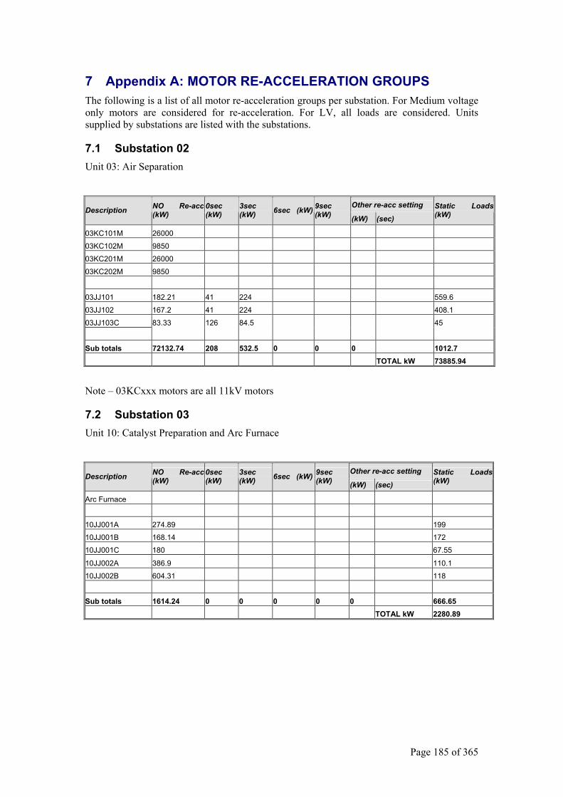
Page 185 of 365

7 Appendix A: MOTOR RE-ACCELERATION GROUPS The following is a list of all motor re-acceleration groups per substation. For Medium voltage only motors are considered for re-acceleration. For LV, all loads are considered. Units supplied by substations are listed with the substations.

7.1 Substation 02 Unit 03: Air Separation

Other re-acc setting Description NO Re-acc

(kW) 0sec (kW)

3sec (kW) 6sec (kW) 9sec

(kW) (kW) (sec) Static Loads (kW)

03KC101M 26000

03KC102M 9850

03KC201M 26000

03KC202M 9850

03JJ101 182.21 41 224 559.6

03JJ102 167.2 41 224 408.1

03JJ103C 83.33 126 84.5 45

Sub totals 72132.74 208 532.5 0 0 0 1012.7 TOTAL kW 73885.94

Note – 03KCxxx motors are all 11kV motors

7.2 Substation 03 Unit 10: Catalyst Preparation and Arc Furnace

Other re-acc setting Description NO Re-acc

(kW) 0sec (kW)

3sec (kW) 6sec (kW) 9sec

(kW) (kW) (sec) Static Loads(kW)

Arc Furnace

10JJ001A 274.89 199

10JJ001B 168.14 172

10JJ001C 180 67.55

10JJ002A 386.9 110.1

10JJ002B 604.31 118

Sub totals 1614.24 0 0 0 0 0 666.65 TOTAL kW 2280.89

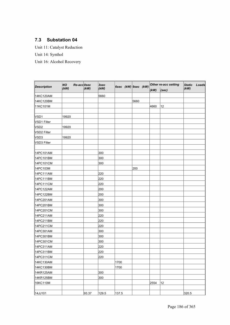
Page 186 of 365

7.3 Substation 04 Unit 11: Catalyst Reduction

Unit 14: Synthol

Unit 16: Alcohol Recovery

Other re-acc setting Description NO Re-acc

(kW) 0sec (kW)

3sec (kW) 6sec (kW) 9sec (kW)

(kW) (sec) Static Loads(kW)

14KC120AM 5660

14KC120BM 5660

11KC101M 4660 12

VSD1 19920

VSD1 Filter

VSD2 19920

VSD2 Filter

VSD3 19920

VSD3 Filter

14PC101AM 300

14PC101BM 300

14PC101CM 300

14PC103M 200

14PC111AM 220

14PC111BM 220

14PC111CM 220

14PC122AM 200

14PC122BM 200

14PC201AM 300

14PC201BM 300

14PC201CM 300

14PC211AM 220

14PC211BM 220

14PC211CM 220

14PC301AM 300

14PC301BM 300

14PC301CM 300

14PC311AM 220

14PC311BM 220

14PC311CM 220

14KC130AM 1700

14KC130BM 1700

14KR125AM 300

14KR125BM 300

16KC110M 2554 12

14JJ101 93.37 129.5 137.5 320.5

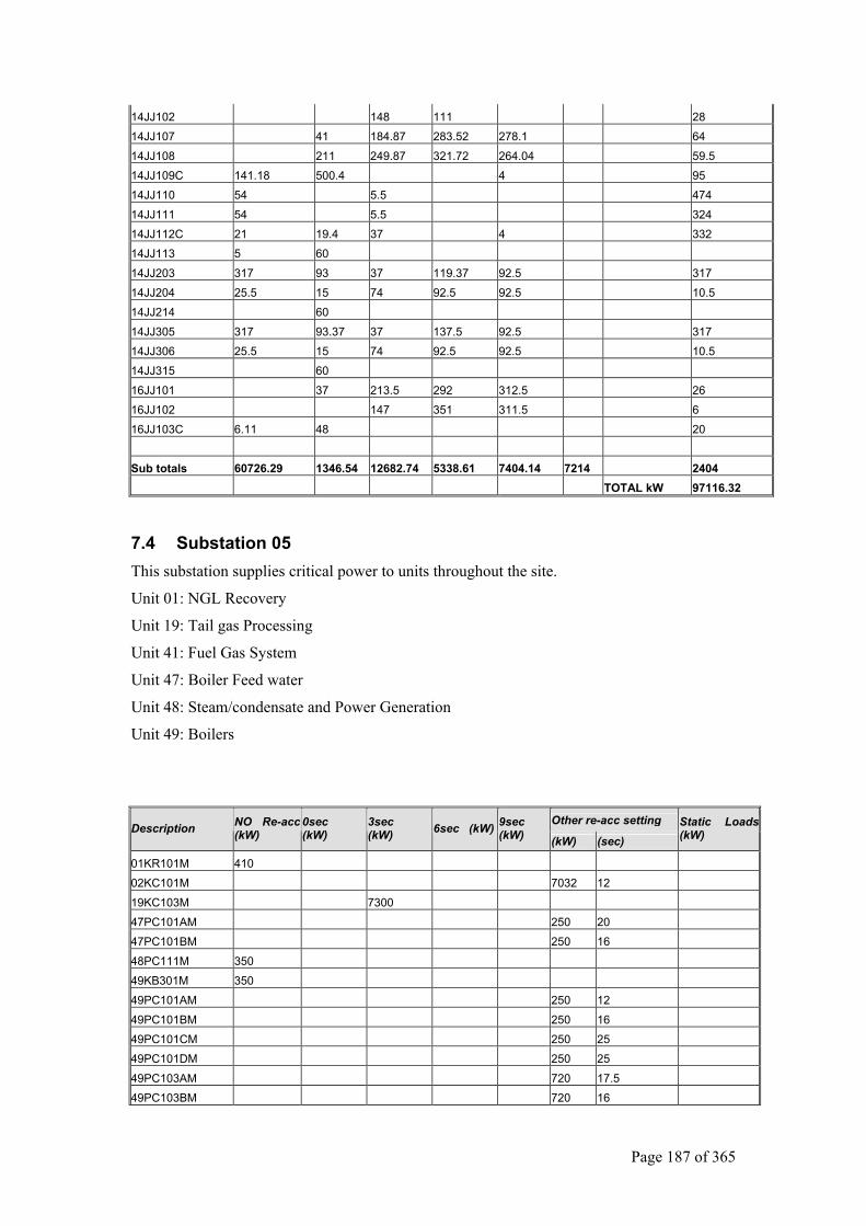
Page 187 of 365

14JJ102 148 111 28

14JJ107 41 184.87 283.52 278.1 64

14JJ108 211 249.87 321.72 264.04 59.5

14JJ109C 141.18 500.4 4 95

14JJ110 54 5.5 474

14JJ111 54 5.5 324

14JJ112C 21 19.4 37 4 332

14JJ113 5 60

14JJ203 317 93 37 119.37 92.5 317

14JJ204 25.5 15 74 92.5 92.5 10.5

14JJ214 60

14JJ305 317 93.37 37 137.5 92.5 317

14JJ306 25.5 15 74 92.5 92.5 10.5

14JJ315 60

16JJ101 37 213.5 292 312.5 26

16JJ102 147 351 311.5 6

16JJ103C 6.11 48 20

Sub totals 60726.29 1346.54 12682.74 5338.61 7404.14 7214 2404 TOTAL kW 97116.32

7.4 Substation 05 This substation supplies critical power to units throughout the site.

Unit 01: NGL Recovery

Unit 19: Tail gas Processing

Unit 41: Fuel Gas System

Unit 47: Boiler Feed water

Unit 48: Steam/condensate and Power Generation

Unit 49: Boilers

Other re-acc setting Description NO Re-acc

(kW) 0sec (kW)

3sec (kW) 6sec (kW) 9sec

(kW) (kW) (sec) Static Loads(kW)

01KR101M 410

02KC101M 7032 12

19KC103M 7300

47PC101AM 250 20

47PC101BM 250 16

48PC111M 350

49KB301M 350

49PC101AM 250 12

49PC101BM 250 16

49PC101CM 250 25

49PC101DM 250 25

49PC103AM 720 17.5

49PC103BM 720 16

Page 188 of 365

49PC103CM 720 15

49PC103DM 720 16

64JJ002A 332.6 15 225.3 514.15

64JJ002B 188.75 352 115.3 1111.2

64JJ015C 232.9 316 4.8 639.88

Sub totals 1864.25 331 7656.8 340.6 0 11412 2265.23 TOTAL kW 23869.88

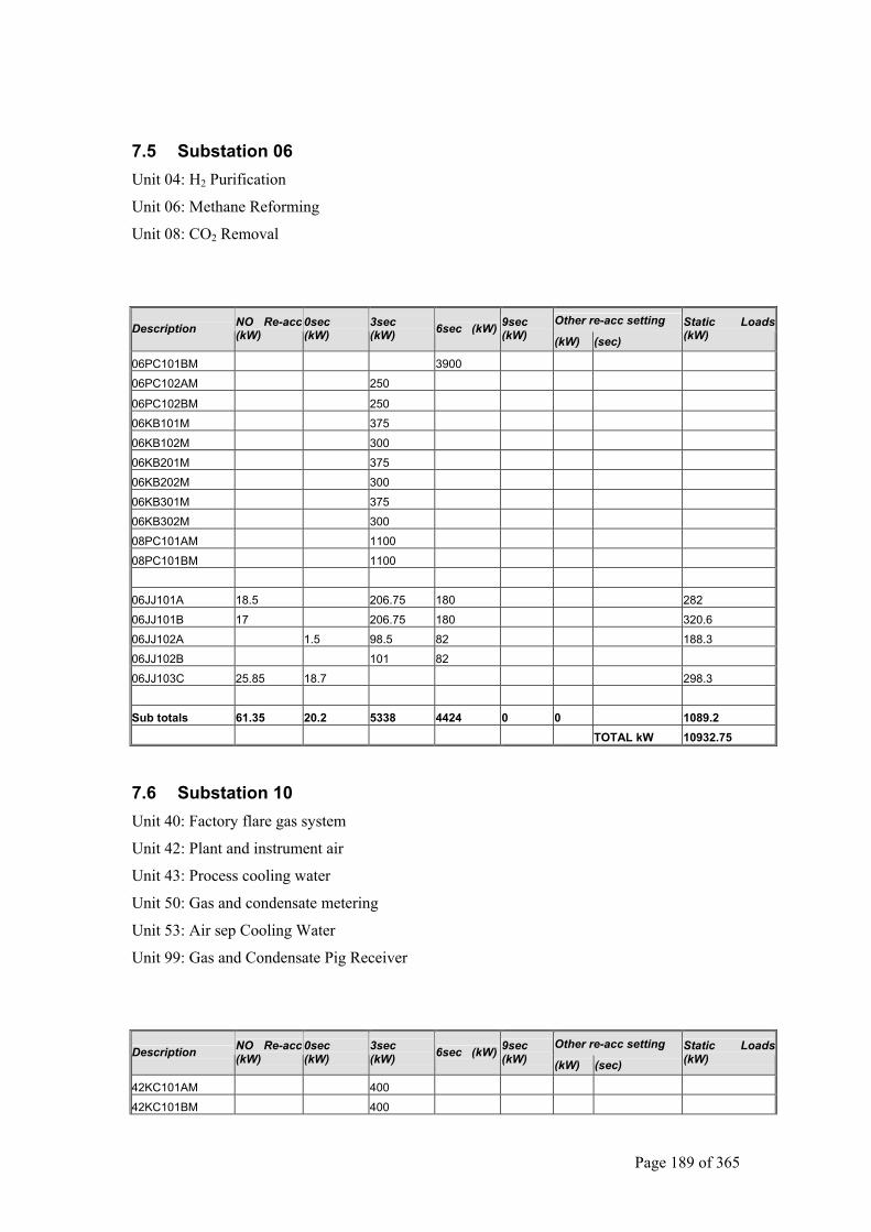
Page 189 of 365

7.5 Substation 06 Unit 04: H2 Purification

Unit 06: Methane Reforming

Unit 08: CO2 Removal

Other re-acc setting Description NO Re-acc

(kW) 0sec (kW)

3sec (kW) 6sec (kW) 9sec

(kW) (kW) (sec) Static Loads(kW)

06PC101BM 3900

06PC102AM 250

06PC102BM 250

06KB101M 375

06KB102M 300

06KB201M 375

06KB202M 300

06KB301M 375

06KB302M 300

08PC101AM 1100

08PC101BM 1100

06JJ101A 18.5 206.75 180 282

06JJ101B 17 206.75 180 320.6

06JJ102A 1.5 98.5 82 188.3

06JJ102B 101 82

06JJ103C 25.85 18.7 298.3

Sub totals 61.35 20.2 5338 4424 0 0 1089.2 TOTAL kW 10932.75

7.6 Substation 10 Unit 40: Factory flare gas system

Unit 42: Plant and instrument air

Unit 43: Process cooling water

Unit 50: Gas and condensate metering

Unit 53: Air sep Cooling Water

Unit 99: Gas and Condensate Pig Receiver

Other re-acc setting Description NO Re-acc

(kW) 0sec (kW)

3sec (kW) 6sec (kW) 9sec

(kW) (kW) (sec) Static Loads(kW)

42KC101AM 400

42KC101BM 400

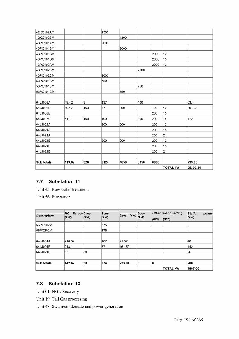
Page 190 of 365

42KC102AM 1300

42KC102BM 1300

43PC101AM 2000

43PC101BM 2000

43PC101CM 2000 12

43PC101DM 2000 15

43PC102AM 2000 12

43PC102BM 2000

43PC102CM 2000

53PC101AM 750

53PC101BM 750

53PC101CM 750

64JJ003A 49.42 3 437 400 63.4

64JJ003B 19.17 163 37 200 400 12 504.25

64JJ003B 200 15

64JJ017C 51.1 160 400 200 200 15 172

64JJ024A 200 200 200 12

64JJ024A 200 15

64JJ024A 200 21

64JJ024B 200 200 200 12

64JJ024B 200 15

64JJ024B 200 21

Sub totals 119.69 326 8124 4650 3350 8000 739.65 TOTAL kW 25309.34

7.7 Substation 11 Unit 45: Raw water treatment

Unit 56: Fire water

Other re-acc setting Description NO Re-acc

(kW) 0sec (kW)

3sec (kW) 6sec (kW) 9sec

(kW) (kW) (sec) Static Loads(kW)

56PC102M 375

56PC202M 375

64JJ004A 218.32 187 71.52 40

64JJ004B 218.1 37 161.52 142

64JJ021C 6.2 30 26

Sub totals 442.62 30 974 233.04 0 0 208 TOTAL kW 1887.66

7.8 Substation 13 Unit 01: NGL Recovery

Unit 19: Tail Gas processing

Unit 48: Steam/condensate and power generation

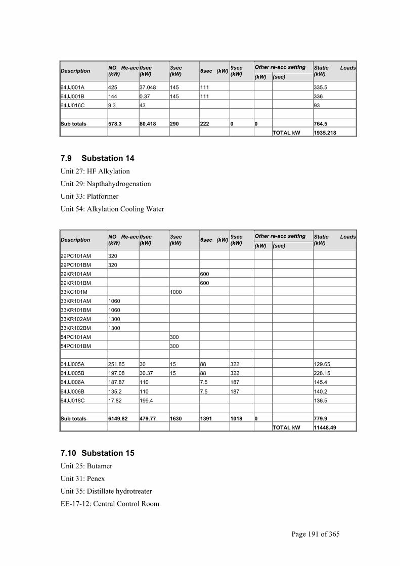
Page 191 of 365

Other re-acc setting Description NO Re-acc

(kW) 0sec (kW)

3sec (kW) 6sec (kW) 9sec

(kW) (kW) (sec) Static Loads(kW)

64JJ001A 425 37.048 145 111 335.5

64JJ001B 144 0.37 145 111 336

64JJ016C 9.3 43 93

Sub totals 578.3 80.418 290 222 0 0 764.5 TOTAL kW 1935.218

7.9 Substation 14 Unit 27: HF Alkylation

Unit 29: Napthahydrogenation

Unit 33: Platformer

Unit 54: Alkylation Cooling Water

Other re-acc setting Description NO Re-acc

(kW) 0sec (kW)

3sec (kW) 6sec (kW) 9sec

(kW) (kW) (sec) Static Loads(kW)

29PC101AM 320

29PC101BM 320

29KR101AM 600

29KR101BM 600

33KC101M 1000

33KR101AM 1060

33KR101BM 1060

33KR102AM 1300

33KR102BM 1300

54PC101AM 300

54PC101BM 300

64JJ005A 251.85 30 15 88 322 129.65

64JJ005B 197.08 30.37 15 88 322 228.15

64JJ006A 187.87 110 7.5 187 145.4

64JJ006B 135.2 110 7.5 187 140.2

64JJ018C 17.82 199.4 136.5

Sub totals 6149.82 479.77 1630 1391 1018 0 779.9 TOTAL kW 11448.49

7.10 Substation 15 Unit 25: Butamer

Unit 31: Penex

Unit 35: Distillate hydrotreater

EE-17-12: Central Control Room

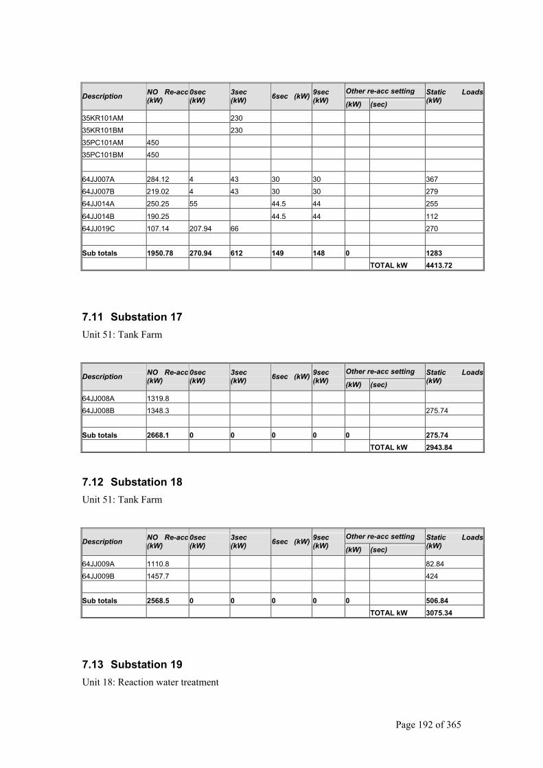
Page 192 of 365

Other re-acc setting Description NO Re-acc

(kW) 0sec (kW)

3sec (kW) 6sec (kW) 9sec

(kW) (kW) (sec) Static Loads(kW)

35KR101AM 230

35KR101BM 230

35PC101AM 450

35PC101BM 450

64JJ007A 284.12 4 43 30 30 367

64JJ007B 219.02 4 43 30 30 279

64JJ014A 250.25 55 44.5 44 255

64JJ014B 190.25 44.5 44 112

64JJ019C 107.14 207.94 66 270

Sub totals 1950.78 270.94 612 149 148 0 1283 TOTAL kW 4413.72

7.11 Substation 17 Unit 51: Tank Farm

Other re-acc setting Description NO Re-acc

(kW) 0sec (kW)

3sec (kW) 6sec (kW) 9sec

(kW) (kW) (sec) Static Loads(kW)

64JJ008A 1319.8

64JJ008B 1348.3 275.74

Sub totals 2668.1 0 0 0 0 0 275.74 TOTAL kW 2943.84

7.12 Substation 18 Unit 51: Tank Farm

Other re-acc setting Description NO Re-acc

(kW) 0sec (kW)

3sec (kW) 6sec (kW) 9sec

(kW) (kW) (sec) Static Loads(kW)

64JJ009A 1110.8 82.84

64JJ009B 1457.7 424

Sub totals 2568.5 0 0 0 0 0 506.84 TOTAL kW 3075.34

7.13 Substation 19 Unit 18: Reaction water treatment

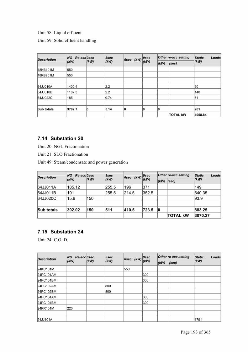
Page 193 of 365

Unit 58: Liquid effluent

Unit 59: Solid effluent handling

Other re-acc setting Description NO Re-acc

(kW) 0sec (kW)

3sec (kW) 6sec (kW) 9sec

(kW) (kW) (sec) Static Loads(kW)

18KB101M 550

18KB201M 550

64JJ010A 1400.4 2.2 50

64JJ010B 1107.3 2.2 140

64JJ022C 185 0.74 71

Sub totals 3792.7 0 5.14 0 0 0 261 TOTAL kW 4058.84

7.14 Substation 20 Unit 20: NGL Fractionation

Unit 21: SLO Fractionation

Unit 49: Steam/condensate and power generation

Other re-acc setting Description NO Re-acc

(kW) 0sec (kW)

3sec (kW) 6sec (kW) 9sec

(kW) (kW) (sec) Static Loads(kW)

64JJ011A 185.12 255.5 196 371 149 64JJ011B 191 255.5 214.5 352.5 640.35 64JJ020C 15.9 150 93.9 Sub totals 392.02 150 511 410.5 723.5 0 883.25 TOTAL kW 3070.27

7.15 Substation 24 Unit 24: C.O. D.

Other re-acc setting Description NO Re-acc

(kW) 0sec (kW)

3sec (kW) 6sec (kW) 9sec

(kW) (kW) (sec) Static Loads(kW)

24KC101M 550

24PC101AM 300

24PC101BM 300

24PC102AM 800

24PC102BM 800

24PC104AM 300

24PC104BM 300

24KR101M 220

24JJ101A 1791

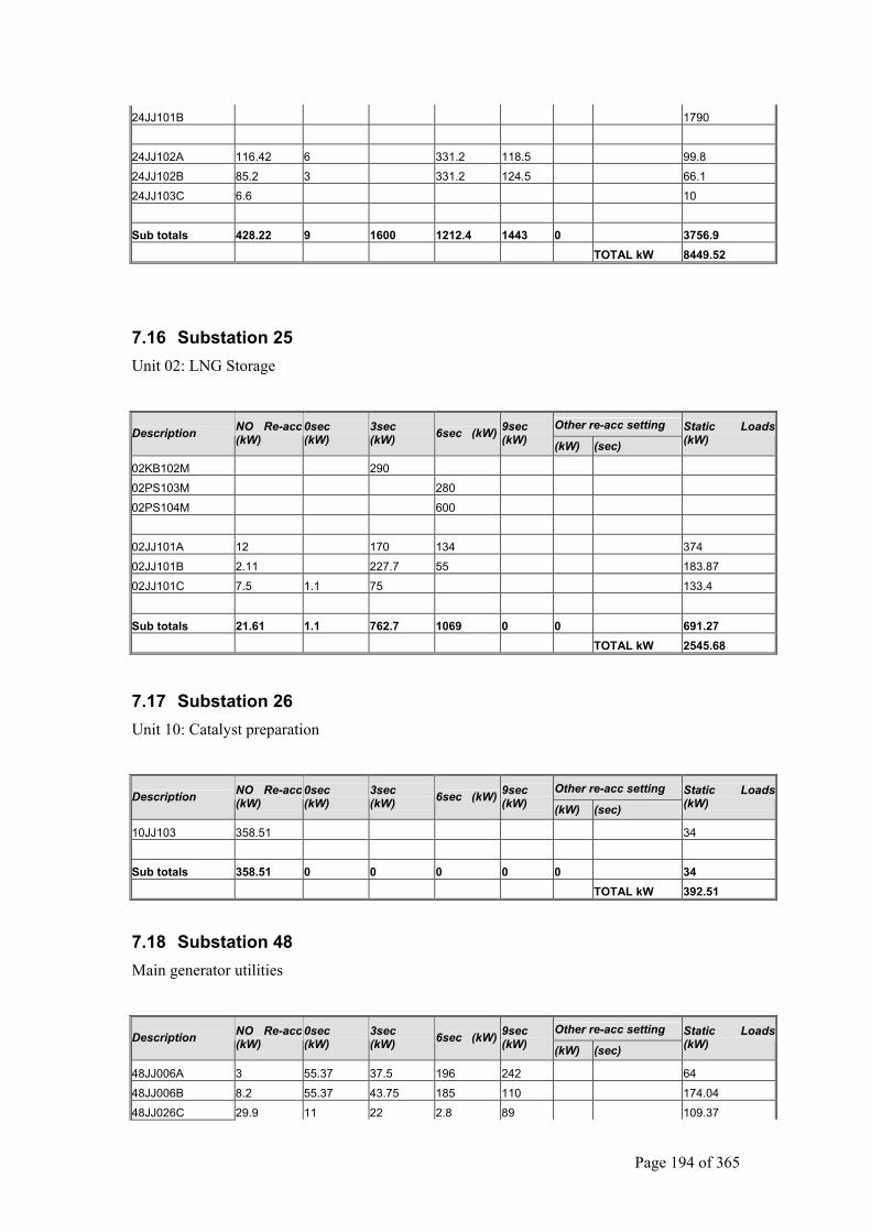
Page 194 of 365

24JJ101B 1790

24JJ102A 116.42 6 331.2 118.5 99.8

24JJ102B 85.2 3 331.2 124.5 66.1

24JJ103C 6.6 10

Sub totals 428.22 9 1600 1212.4 1443 0 3756.9 TOTAL kW 8449.52

7.16 Substation 25 Unit 02: LNG Storage

Other re-acc setting Description NO Re-acc

(kW) 0sec (kW)

3sec (kW) 6sec (kW) 9sec

(kW) (kW) (sec) Static Loads(kW)

02KB102M 290

02PS103M 280

02PS104M 600

02JJ101A 12 170 134 374

02JJ101B 2.11 227.7 55 183.87

02JJ101C 7.5 1.1 75 133.4

Sub totals 21.61 1.1 762.7 1069 0 0 691.27 TOTAL kW 2545.68

7.17 Substation 26 Unit 10: Catalyst preparation

Other re-acc setting Description NO Re-acc

(kW) 0sec (kW)

3sec (kW) 6sec (kW) 9sec

(kW) (kW) (sec) Static Loads(kW)

10JJ103 358.51 34

Sub totals 358.51 0 0 0 0 0 34 TOTAL kW 392.51

7.18 Substation 48 Main generator utilities

Other re-acc setting Description NO Re-acc

(kW) 0sec (kW)

3sec (kW) 6sec (kW) 9sec

(kW) (kW) (sec) Static Loads(kW)

48JJ006A 3 55.37 37.5 196 242 64

48JJ006B 8.2 55.37 43.75 185 110 174.04

48JJ026C 29.9 11 22 2.8 89 109.37

Page 195 of 365

48JJ110C 38.75

Sub totals 79.85 121.74 103.25 383.8 441 0 347.41 TOTAL kW 1477.05

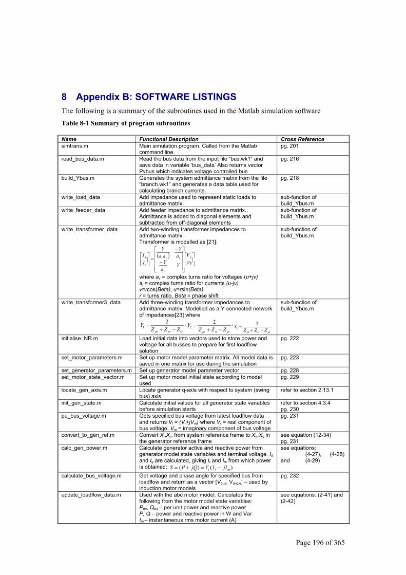
Page 196 of 365

8 Appendix B: SOFTWARE LISTINGS The following is a summary of the subroutines used in the Matlab simulation software Table 8-1 Summary of program subroutines

Name Functional Description Cross Reference simtrans.m Main simulation program. Called from the Matlab

command line. pg. 201

read_bus_data.m Read the bus data from the input file “bus.wk1” and save data in variable ‘bus_data’ Also returns vector Pvbus which indicates voltage controlled bus

pg. 216

build_Ybus.m Generates the system admittance matrix from the file “branch.wk1” and generates a data table used for calculating branch currents.

pg. 218

write_load_data Add impedance used to represent static loads to admittance matrix.

sub-function of build_Ybus.m

write_feeder_data Add feeder impedance to admittance matrix., Admittance is added to diagonal elements and subtracted from off-diagonal elements

sub-function of build_Ybus.m

write_transformer_data Add two-winding transformer impedances to admittance matrix. Transformer is modelled as [21]:

( )

−

−

=

VsV

Ya

YaY

aaY

II p

v

ivi

s

p

where av = complex turns ratio for voltages (u+jv) ai = complex turns ratio for currents (u-jv) v=rcos(Beta), u=rsin(Beta) r = turns ratio, Beta = phase shift

sub-function of build_Ybus.m

write_transformer3_data Add three-winding transformer impedances to admittance matrix. Modelled as a Y-connected network of impedances[23] where

stptps ZZZY

−+=

21

,ptstps ZZZ

Y−+

=2

2,

psstpt ZZZY

−+=

23

sub-function of build_Ybus.m

initialise_NR.m Load initial data into vectors used to store power and voltage for all busses to prepare for first loadflow solution

pg. 222

set_motor_parameters.m Set up motor model parameter matrix. All model data is saved in one matrix for use during the simulation

pg. 223

set_generator_parameters.m Set up generator model parameter vector pg. 228 set_motor_state_vector.m Set up motor model initial state according to model

used pg. 229

locate_gen_axis.m Locate generator q-axis with respect to system (swing bus) axis

refer to section 2.13.1

init_gen_state.m Calculate initial values for all generator state variables before simulation starts

refer to section 4.3.4 pg. 230

pu_bus_voltage.m Gets specified bus voltage from latest loadflow data and returns Vt = (Vr+jVm) where Vr = real component of bus voltage, Vm = imaginary component of bus voltage

pg. 231

convert_to_gen_ref.m Convert Xr,Xm from system reference frame to Xd,Xq in the generator reference frame

see equation (12-34) pg. 231

calc_gen_power.m Calculate generator active and reactive power from generator model state variables and terminal voltage. Id and Iq are calculated, giving Ir and Im from which power is obtained: )()( mrt jIIVjQPS −=+=

see equations: (4-27), (4-28) and (4-29)

calculate_bus_voltage.m Get voltage and phase angle for specified bus from loadflow and return as a vector [Vbus, Vangle] – used by induction motor models

pg. 232

update_loadflow_data.m Used with the abc motor model. Calculates the following from the motor model state variables: Ppu, Qpu – per unit power and reactive power P, Q – power and reactive power in W and Var Im – instantaneous rms motor current (A)

see equations: (2-41) and (2-42)

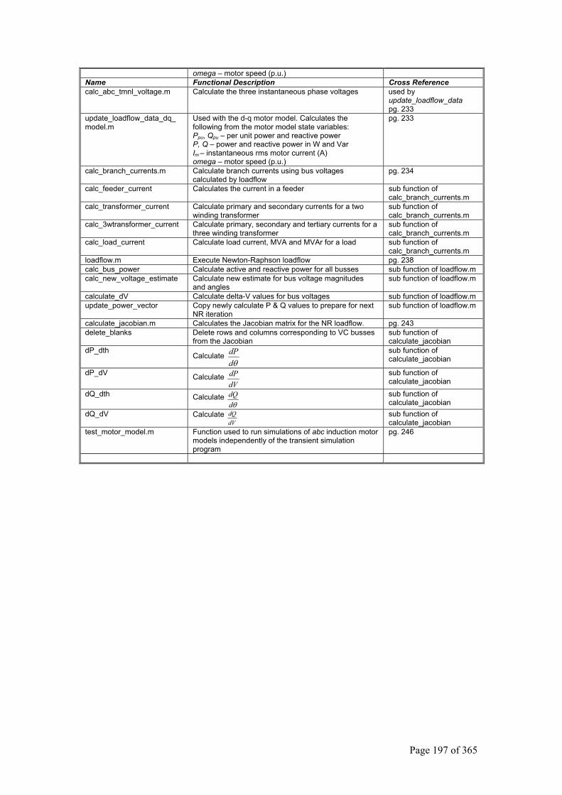
Page 197 of 365

omega – motor speed (p.u.) Name Functional Description Cross Reference calc_abc_tmnl_voltage.m Calculate the three instantaneous phase voltages used by

update_loadflow_data pg. 233

update_loadflow_data_dq_ model.m

Used with the d-q motor model. Calculates the following from the motor model state variables: Ppu, Qpu – per unit power and reactive power P, Q – power and reactive power in W and Var Im – instantaneous rms motor current (A) omega – motor speed (p.u.)

pg. 233

calc_branch_currents.m Calculate branch currents using bus voltages calculated by loadflow

pg. 234

calc_feeder_current Calculates the current in a feeder sub function of calc_branch_currents.m

calc_transformer_current Calculate primary and secondary currents for a two winding transformer

sub function of calc_branch_currents.m

calc_3wtransformer_current Calculate primary, secondary and tertiary currents for a three winding transformer

sub function of calc_branch_currents.m

calc_load_current Calculate load current, MVA and MVAr for a load sub function of calc_branch_currents.m

loadflow.m Execute Newton-Raphson loadflow pg. 238 calc_bus_power Calculate active and reactive power for all busses sub function of loadflow.m calc_new_voltage_estimate Calculate new estimate for bus voltage magnitudes

and angles sub function of loadflow.m

calculate_dV Calculate delta-V values for bus voltages sub function of loadflow.m update_power_vector Copy newly calculate P & Q values to prepare for next

NR iteration sub function of loadflow.m

calculate_jacobian.m Calculates the Jacobian matrix for the NR loadflow. pg. 243 delete_blanks Delete rows and columns corresponding to VC busses

from the Jacobian sub function of calculate_jacobian

dP_dth Calculate

θddP

sub function of calculate_jacobian

dP_dV Calculate dVdP sub function of

calculate_jacobian dQ_dth Calculate

θddQ sub function of

calculate_jacobian dQ_dV Calculate

dVdQ sub function of

calculate_jacobian test_motor_model.m Function used to run simulations of abc induction motor

models independently of the transient simulation program

pg. 246

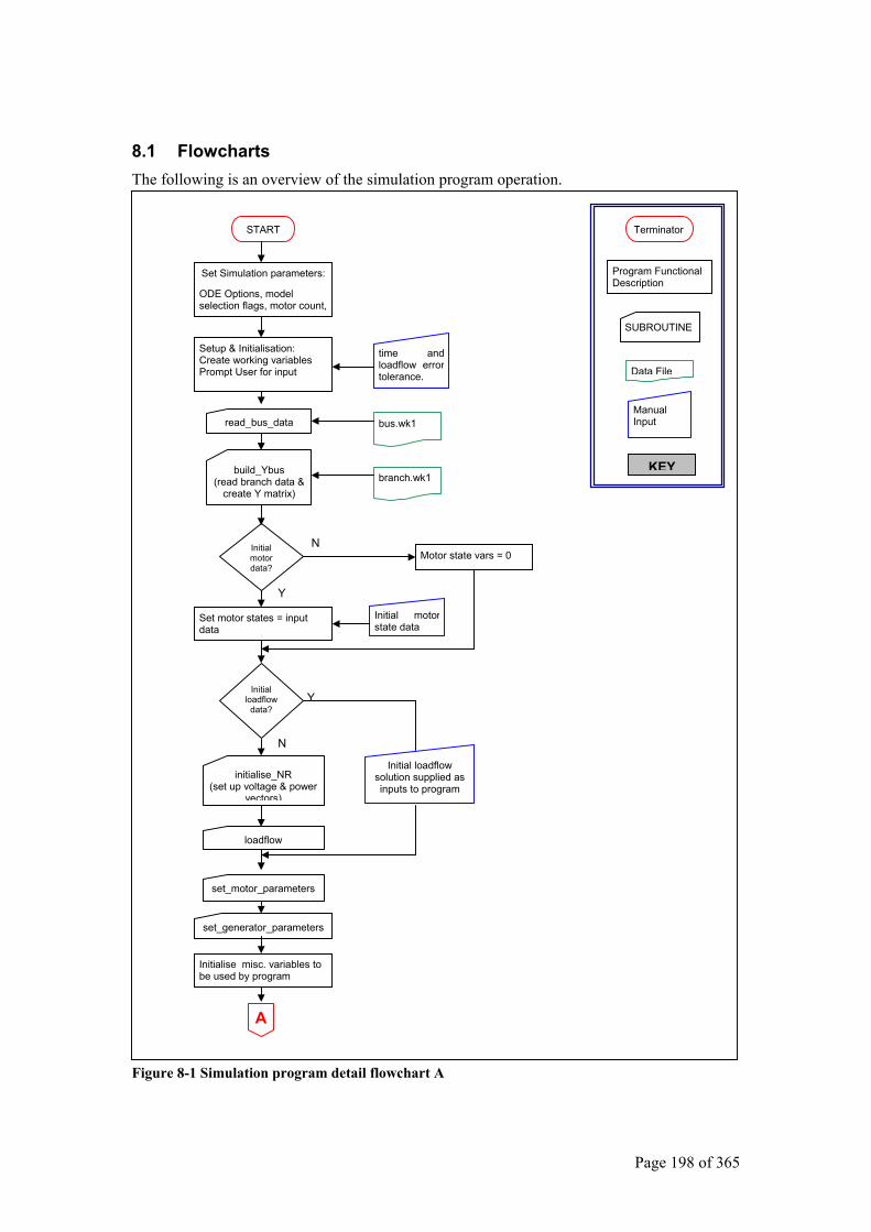
Page 198 of 365

8.1 Flowcharts The following is an overview of the simulation program operation.

Figure 8-1 Simulation program detail flowchart A

Terminator

Program Functional Description

SUBROUTINE

Data File

Manual Input

KEY

Motor state vars = 0

START

Set Simulation parameters:

ODE Options, model selection flags, motor count,

Setup & Initialisation: Create working variables Prompt User for input

time andloadflow errortolerance.

read_bus_data bus.wk1

build_Ybus (read branch data &

create Y matrix) branch.wk1

Initial motor data?

N

Set motor states = input data

Initial motorstate data

Initial loadflow

data?

Y

N

initialise_NR (set up voltage & power

vectors)

loadflow

Y

Initial loadflow solution supplied as inputs to program

set_motor_parameters

set_generator_parameters

Initialise misc. variables to be used by program

A

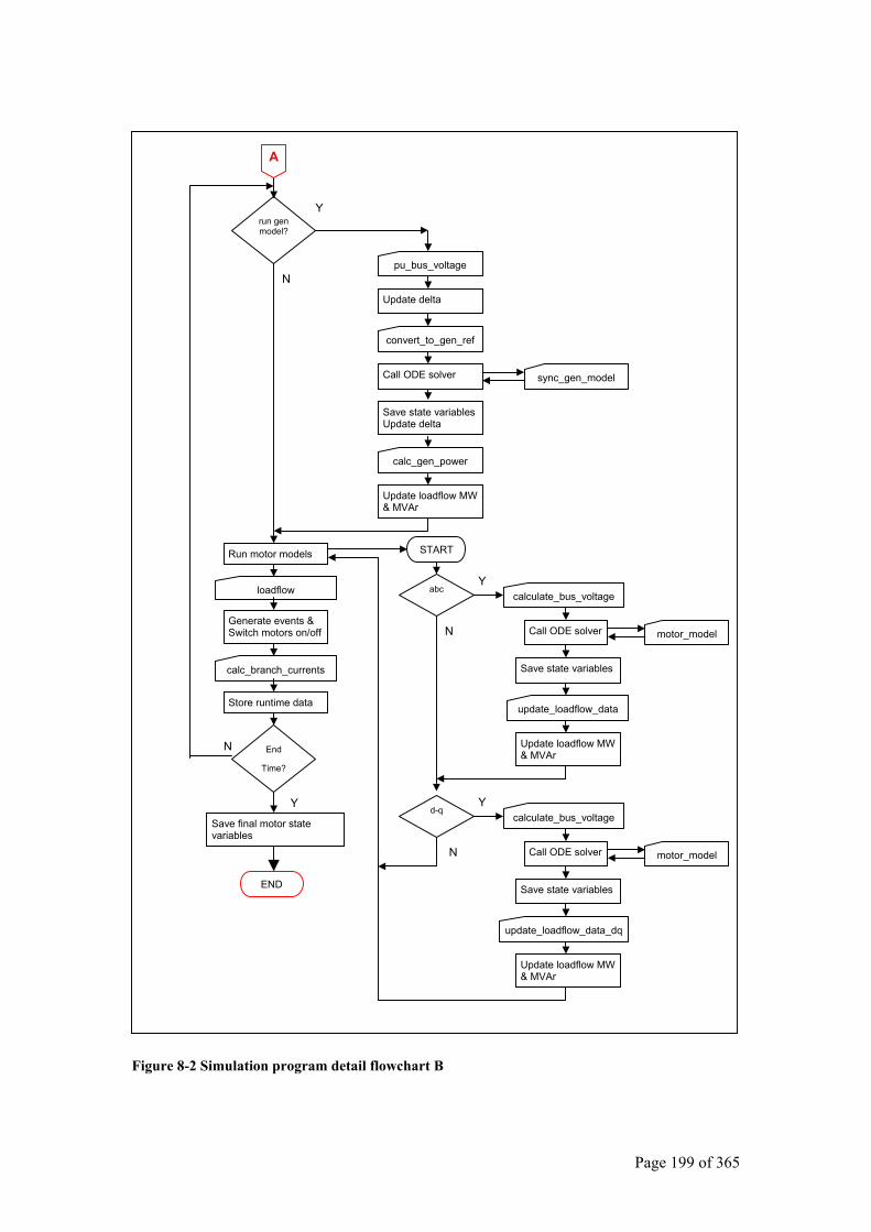
Page 199 of 365

Figure 8-2 Simulation program detail flowchart B

Save state variablesUpdate delta

Update delta

pu_bus_voltage

convert_to_gen_ref

run gen model?

N

Call ODE solver

End

Time?

Y

N

Y

calc_branch_currents

Save final motor state variables

A

sync_gen_model

calc_gen_power

Update loadflow MW & MVAr

Run motor models

loadflow

Generate events & Switch motors on/off

Store runtime data

END

START

abc calculate_bus_voltage

Y

Call ODE solver motor_model

Save state variables

update_loadflow_data

Update loadflow MW & MVAr

d-q calculate_bus_voltage

Call ODE solver motor_model

Save state variables

update_loadflow_data_dq

Update loadflow MW & MVAr

N

N

Y

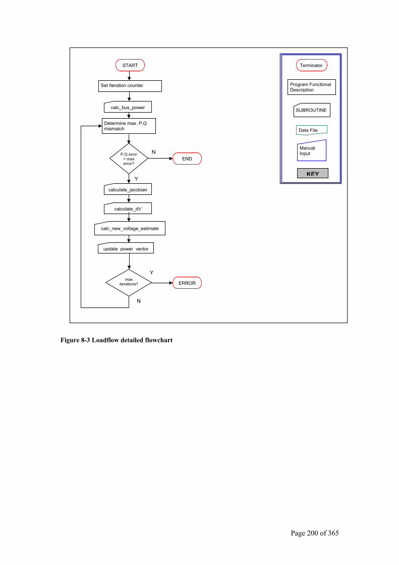
Page 200 of 365

Figure 8-3 Loadflow detailed flowchart

Terminator

Program FunctionalDescription

SUBROUTINE

Data File

Manual Input

KEY

Determine max. P,Q mismatch

START

Set Iteration counter

calculate_jacobian

P,Q error > max error?

N

max iterations?

Y

N

calc_new_voltage_estimate

update power vector

Y

calc_bus_power

END

calculate_dV

ERROR

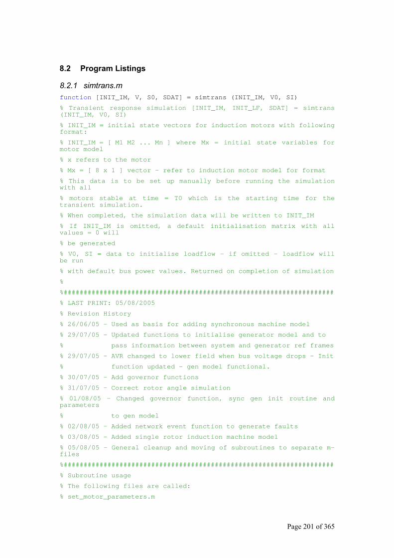
Page 201 of 365

8.2 Program Listings

8.2.1 simtrans.m function [INIT_IM, V, S0, SDAT] = simtrans (INIT_IM, V0, SI)

% Transient response simulation [INIT_IM, INIT_LF, SDAT] = simtrans (INIT_IM, V0, SI)

% INIT_IM = initial state vectors for induction motors with following format:

% INIT_IM = [ M1 M2 ... Mn ] where Mx = initial state variables for motor model

% x refers to the motor

% Mx = [ 8 x 1 ] vector - refer to induction motor model for format

% This data is to be set up manually before running the simulation with all

% motors stable at time = T0 which is the starting time for the transient simulation.

% When completed, the simulation data will be written to INIT_IM

% If INIT_IM is omitted, a default initialisation matrix with all values = 0 will

% be generated

% V0, SI = data to initialise loadflow - if omitted - loadflow will be run

% with default bus power values. Returned on completion of simulation

%

%####################################################################

% LAST PRINT: 05/08/2005

% Revision History

% 26/06/05 - Used as basis for adding synchronous machine model

% 29/07/05 - Updated functions to initialise generator model and to

% pass information between system and generator ref frames

% 29/07/05 - AVR changed to lower field when bus voltage drops - Init

% function updated - gen model functional.

% 30/07/05 - Add governor functions

% 31/07/05 - Correct rotor angle simulation

% 01/08/05 - Changed governor function, sync gen init routine and parameters

% to gen model

% 02/08/05 - Added network event function to generate faults

% 03/08/05 - Added single rotor induction machine model

% 05/08/05 - General cleanup and moving of subroutines to separate m-files

%####################################################################

% Subroutine usage

% The following files are called:

% set_motor_parameters.m

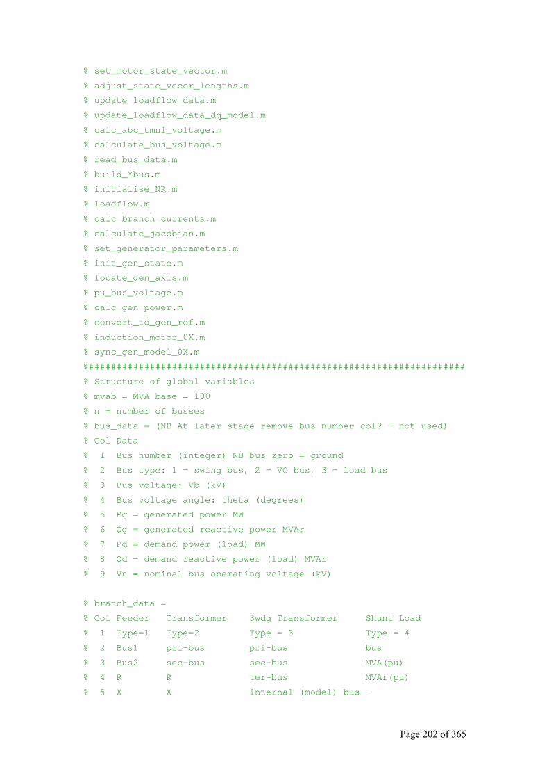
Page 202 of 365

% set_motor_state_vector.m

% adjust_state_vecor_lengths.m

% update_loadflow_data.m

% update_loadflow_data_dq_model.m

% calc_abc_tmnl_voltage.m

% calculate_bus_voltage.m

% read_bus_data.m

% build_Ybus.m

% initialise_NR.m

% loadflow.m

% calc_branch_currents.m

% calculate_jacobian.m

% set_generator_parameters.m

% init_gen_state.m

% locate_gen_axis.m

% pu_bus_voltage.m

% calc_gen_power.m

% convert_to_gen_ref.m

% induction_motor_0X.m

% sync_gen_model_0X.m

%####################################################################

% Structure of global variables

% mvab = MVA base = 100

% n = number of busses

% bus_data = (NB At later stage remove bus number col? - not used)

% Col Data

% 1 Bus number (integer) NB bus zero = ground

% 2 Bus type: 1 = swing bus, 2 = VC bus, 3 = load bus

% 3 Bus voltage: Vb (kV)

% 4 Bus voltage angle: theta (degrees)

% 5 Pg = generated power MW

% 6 Qg = generated reactive power MVAr

% 7 Pd = demand power (load) MW

% 8 Qd = demand reactive power (load) MVAr

% 9 Vn = nominal bus operating voltage (kV)

% branch_data =

% Col Feeder Transformer 3wdg Transformer Shunt Load

% 1 Type=1 Type=2 Type = 3 Type = 4

% 2 Bus1 pri-bus pri-bus bus

% 3 Bus2 sec-bus sec-bus MVA(pu)

% 4 R R ter-bus MVAr(pu)

% 5 X X internal (model) bus -

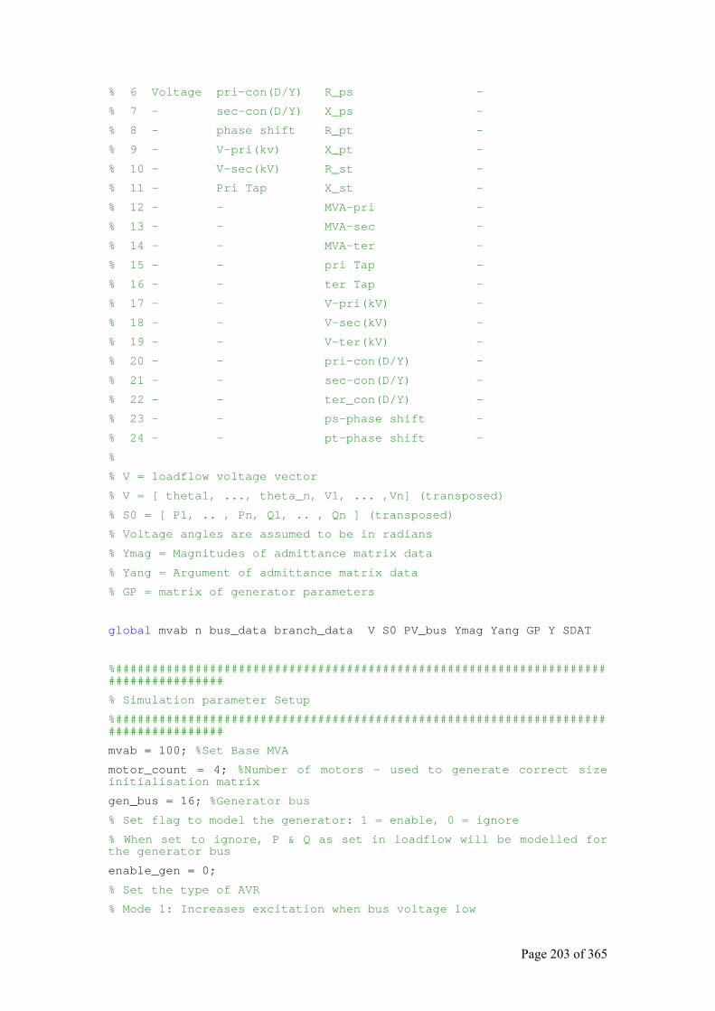
Page 203 of 365

% 6 Voltage pri-con(D/Y) R_ps -

% 7 - sec-con(D/Y) X_ps -

% 8 - phase shift R_pt -

% 9 - V-pri(kv) X_pt -

% 10 - V-sec(kV) R_st -

% 11 - Pri Tap X_st -

% 12 - - MVA-pri -

% 13 - - MVA-sec -

% 14 - - MVA-ter -

% 15 - - pri Tap -

% 16 - - ter Tap -

% 17 - - V-pri(kV) -

% 18 - - V-sec(kV) -

% 19 - - V-ter(kV) -

% 20 - - pri-con(D/Y) -

% 21 - - sec-con(D/Y) -

% 22 - - ter_con(D/Y) -

% 23 - - ps-phase shift -

% 24 - - pt-phase shift -

%

% V = loadflow voltage vector

% V = [ theta1, ..., theta_n, V1, ... ,Vn] (transposed)

% S0 = [ P1, .. , Pn, Q1, .. , Qn ] (transposed)

% Voltage angles are assumed to be in radians

% Ymag = Magnitudes of admittance matrix data

% Yang = Argument of admittance matrix data

% GP = matrix of generator parameters

global mvab n bus_data branch_data V S0 PV_bus Ymag Yang GP Y SDAT

%####################################################################################

% Simulation parameter Setup

%####################################################################################

mvab = 100; %Set Base MVA

motor_count = 4; %Number of motors - used to generate correct size initialisation matrix

gen_bus = 16; %Generator bus

% Set flag to model the generator: 1 = enable, 0 = ignore

% When set to ignore, P & Q as set in loadflow will be modelled for the generator bus

enable_gen = 0;

% Set the type of AVR

% Mode 1: Increases excitation when bus voltage low

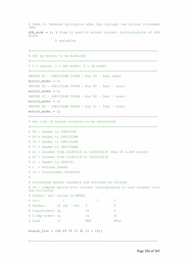
Page 204 of 365

% Mode 2: Reduces excitation when bus voltage low giving increased VARs

AVR_mode = 1; % Flag is used to select correct initialisation of AVR state

% variables

%===================================================================

% Set up motors to be modelled

%===================================================================

% 0 = ignore, 1 = abc model, 2 = dq model

%===================================================================

%MOTOR 01 - 24KC101AM 550kW - bus 49 - 6sec reacc

motor1_model = 1;

%MOTOR 02 - 24PC101AM 300kW - bus 50 - 9sec - reacc

motor2_model = 1;

%MOTOR 03 - 24PC104AM 300kW - bus 52 - 9sec - reacc

motor3_model = 1;

%MOTOR 04 - 24PC102AM 800kW - bus 51 - 3sec - reacc

motor4_model = 1;

%===================================================================

% Set list of branch currents to be calculated

%===================================================================

% 68 = feeder to 24KC101M

% 69 = feeder to 24PC101AM

% 70 = feeder to 24PC102AM

% 71 = feeder to 24PC104AM

% 61 = incomer from 24JN101A to 24JG101A/B (Sub 24 6.6kV board)

% 62 = incomer from 24JN101B to 24JG101A/B

% 11 = feeder to 48GT101

% 1 = Proteus feeder

% 19 = Transformer 64JK001B

%

% Calculated branch currents are returned as follows

% Ib = complex matrix with current corresponding to each element with the following

% format: (All values in MKSA)

% col: 1 2 3

% feeder: If (b1 - b2) 0 0

% transformer: Ip Is 0

% 3 wdg trfmr: Ip Is It

% Load Il MVA MVAr

branch_list = [68 69 70 71 61 11 1 19];

%===================================================================

Page 205 of 365

%Set ODE options

% AbsTol determines the accuracy of the ODE when the solution approaches zero

% the default is 1e-6

% RelTol determines (approximately) the number of correct digits in the

% answer. The default 1e-3 corresponds to 0.1% accuracy

options = odeset('AbsTol', 1e-6, 'RelTol', 1e-3);

%####################################################################################

% End of parameter setup

%####################################################################################

%===================================================================

% Setup and initialisation

%===================================================================

w0 = 100*pi;

a = (2*pi)/3;

root3 = sqrt(3);

motor1 = zeros(1,7);

motor2 = zeros(1,7);

motor3 = zeros(1,7);

motor4 = zeros(1,7);

Pgen = 0;

Qgen = 0;

tinit = input('Start time? '); %All motor init state vars to correspond to this time

time_step = input('Time step? ');

end_time = input('End time? ');

half_step = time_step/2; %Used to set ODE solver to return only three data values

%Create output data matrix

data_points = ceil((end_time - tinit)/time_step);

SDAT = zeros(data_points,48);

% The following functions run once to prepare for the loadflow solution

max_error = input('Maximum Power error tolerance for loadflow? (kVA) ')/(mvab*1e3);

PV_bus = read_bus_data; %read bus data, create bus_data and mark VC busses for loadlfow

% Also sets value of global n = number of busses (Definition below)

Y = build_Ybus; %Calculate admittance matrix for loadlfow - reads branch.wk1

Ymag = abs(Y); %Create matrix containing absolute values of admittances

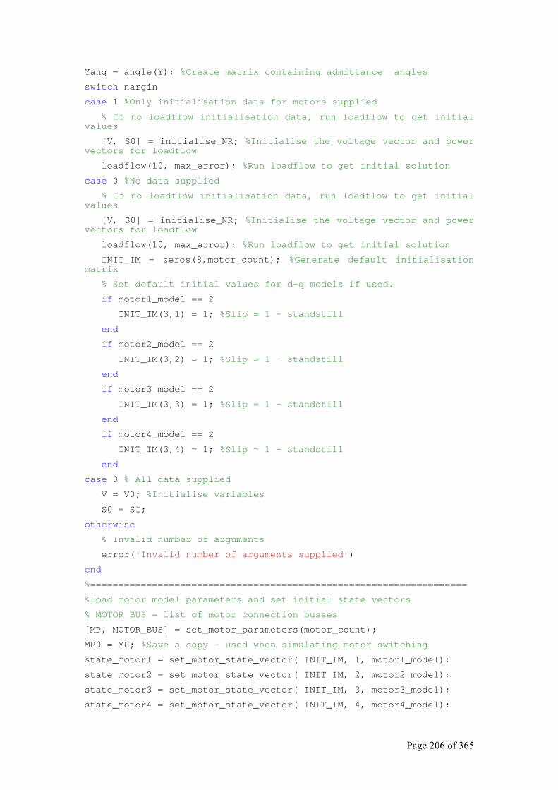
Page 206 of 365

Yang = angle(Y); %Create matrix containing admittance angles

switch nargin

case 1 %Only initialisation data for motors supplied

% If no loadflow initialisation data, run loadflow to get initial values

[V, S0] = initialise_NR; %Initialise the voltage vector and power vectors for loadflow

loadflow(10, max_error); %Run loadflow to get initial solution

case 0 %No data supplied

% If no loadflow initialisation data, run loadflow to get initial values

[V, S0] = initialise_NR; %Initialise the voltage vector and power vectors for loadflow

loadflow(10, max_error); %Run loadflow to get initial solution

INIT_IM = zeros(8,motor_count); %Generate default initialisation matrix

% Set default initial values for d-q models if used.

if motor1_model == 2

INIT_IM(3,1) = 1; %Slip = 1 - standstill

end

if motor2_model == 2

INIT_IM(3,2) = 1; %Slip = 1 - standstill

end

if motor3_model == 2

INIT_IM(3,3) = 1; %Slip = 1 - standstill

end

if motor4_model == 2

INIT_IM(3,4) = 1; %Slip = 1 - standstill

end

case 3 % All data supplied

V = V0; %Initialise variables

S0 = SI;

otherwise

% Invalid number of arguments

error('Invalid number of arguments supplied')

end

%===================================================================

%Load motor model parameters and set initial state vectors

% MOTOR_BUS = list of motor connection busses

[MP, MOTOR_BUS] = set_motor_parameters(motor_count);

MP0 = MP; %Save a copy - used when simulating motor switching

state_motor1 = set_motor_state_vector( INIT_IM, 1, motor1_model);

state_motor2 = set_motor_state_vector( INIT_IM, 2, motor2_model);

state_motor3 = set_motor_state_vector( INIT_IM, 3, motor3_model);

state_motor4 = set_motor_state_vector( INIT_IM, 4, motor4_model);

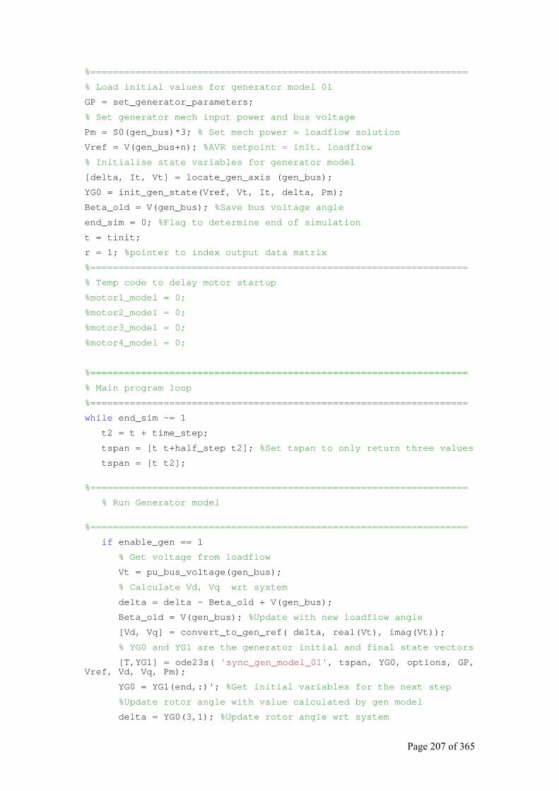
Page 207 of 365

%===================================================================

% Load initial values for generator model 01

GP = set_generator_parameters;

% Set generator mech input power and bus voltage

Pm = S0(gen_bus)*3; % Set mech power = loadflow solution

Vref = V(gen_bus+n); %AVR setpoint = init. loadflow

% Initialise state variables for generator model

[delta, It, Vt] = locate_gen_axis (gen_bus);

YG0 = init_gen_state(Vref, Vt, It, delta, Pm);

Beta_old = V(gen_bus); %Save bus voltage angle

end_sim = 0; %Flag to determine end of simulation

t = tinit;

r = 1; %pointer to index output data matrix

%===================================================================

% Temp code to delay motor startup

%motor1_model = 0;

%motor2_model = 0;

%motor3_model = 0;

%motor4_model = 0;

%===================================================================

% Main program loop

%===================================================================

while end_sim ~= 1

t2 = t + time_step;

tspan = [t t+half_step t2]; %Set tspan to only return three values

tspan = [t t2];

%===================================================================

% Run Generator model

%===================================================================

if enable_gen == 1

% Get voltage from loadflow

Vt = pu_bus_voltage(gen_bus);

% Calculate Vd, Vq wrt system

delta = delta - Beta_old + V(gen_bus);

Beta_old = V(gen_bus); %Update with new loadflow angle

[Vd, Vq] = convert_to_gen_ref( delta, real(Vt), imag(Vt));

% YG0 and YG1 are the generator initial and final state vectors

[T,YG1] = ode23s( 'sync_gen_model_01', tspan, YG0, options, GP, Vref, Vd, Vq, Pm);

YG0 = YG1(end,:)'; %Get initial variables for the next step

%Update rotor angle with value calculated by gen model

delta = YG0(3,1); %Update rotor angle wrt system

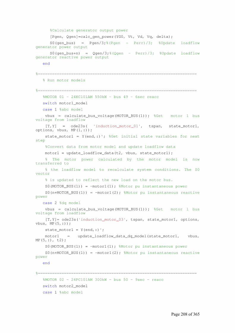
Page 208 of 365

%Calculate generator output power

[Pgen, Qgen]=calc_gen_power(YG0, Vt, Vd, Vq, delta);

S0(gen_bus) = Pgen/3;%(Pgen - Perr)/3; %Update loadflow generator power output

S0(gen_bus+n) = Qgen/3;%(Qgen - Perr)/3; %Update loadflow generator reactive power output

end

%===================================================================

% Run motor models

%===================================================================

%MOTOR 01 - 24KC101AM 550kW - bus 49 - 6sec reacc

switch motor1_model

case 1 %abc model

vbus = calculate_bus_voltage(MOTOR_BUS(1)); %Get motor 1 bus voltage from loadflow

[T,Y] = ode23s( 'induction_motor_01', tspan, state_motor1, options, vbus, MP(1,:));

state_motor1 = Y(end,:)'; %Get initial state variables for next step

%Convert data from motor model and update loadflow data

motor1 = update_loadflow_data(t2, vbus, state_motor1);

% The motor power calculated by the motor model is now transferred to

% the loadflow model to recalculate system conditions. The S0 vector

% is updated to reflect the new load on the motor bus.

S0(MOTOR_BUS(1)) = -motor1(1); %Motor pu instantaneous power

S0(n+MOTOR_BUS(1)) = -motor1(2); %Motor pu instantaneous reactive power

case 2 %dq model

vbus = calculate_bus_voltage(MOTOR_BUS(1)); %Get motor 1 bus voltage from loadflow

[T,Y]= ode23s('induction_motor_03', tspan, state_motor1, options, vbus, MP(5,:));

state_motor1 = Y(end,:)';

motor1 = update_loadflow_data_dq_model(state_motor1, vbus, MP(5,:), t2);

S0(MOTOR_BUS(1)) = -motor1(1); %Motor pu instantaneous power

S0(n+MOTOR_BUS(1)) = -motor1(2); %Motor pu instantaneous reactive power

end

%===================================================================

%MOTOR 02 - 24PC101AM 300kW - bus 50 - 9sec - reacc

switch motor2_model

case 1 %abc model

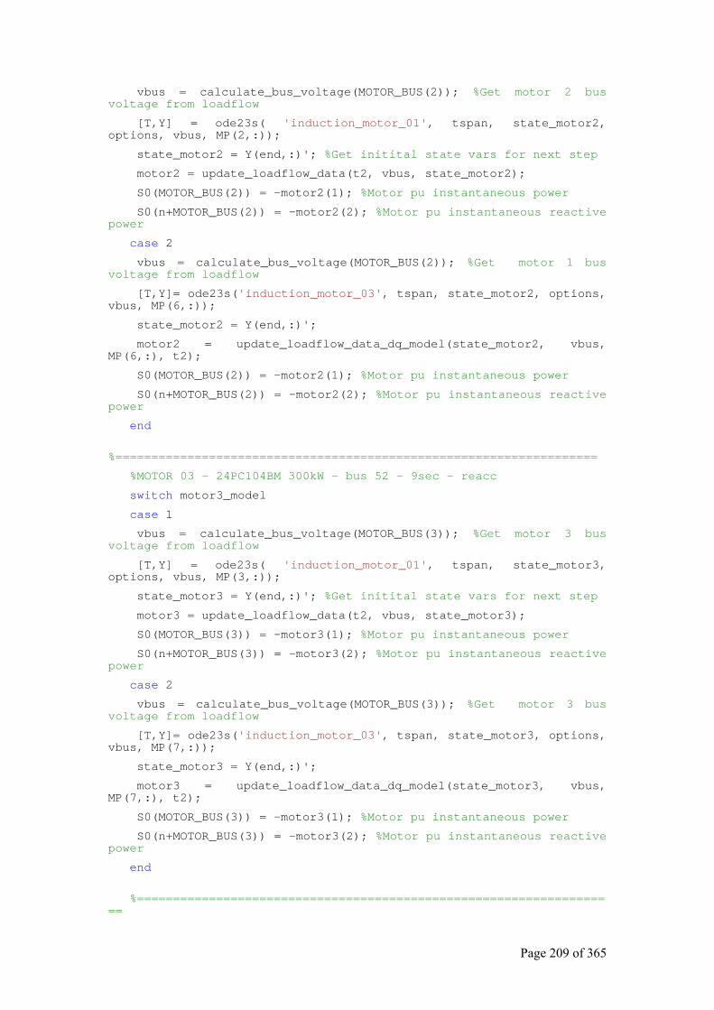
Page 209 of 365

vbus = calculate_bus_voltage(MOTOR_BUS(2)); %Get motor 2 bus voltage from loadflow

[T,Y] = ode23s( 'induction_motor_01', tspan, state_motor2, options, vbus, MP(2,:));

state_motor2 = Y(end,:)'; %Get initital state vars for next step

motor2 = update_loadflow_data(t2, vbus, state_motor2);

S0(MOTOR_BUS(2)) = -motor2(1); %Motor pu instantaneous power

S0(n+MOTOR_BUS(2)) = -motor2(2); %Motor pu instantaneous reactive power

case 2

vbus = calculate_bus_voltage(MOTOR_BUS(2)); %Get motor 1 bus voltage from loadflow

[T,Y]= ode23s('induction_motor_03', tspan, state_motor2, options, vbus, MP(6,:));

state_motor2 = Y(end,:)';

motor2 = update_loadflow_data_dq_model(state_motor2, vbus, MP(6,:), t2);

S0(MOTOR_BUS(2)) = -motor2(1); %Motor pu instantaneous power

S0(n+MOTOR_BUS(2)) = -motor2(2); %Motor pu instantaneous reactive power

end

%===================================================================

%MOTOR 03 - 24PC104BM 300kW - bus 52 - 9sec - reacc

switch motor3_model

case 1

vbus = calculate_bus_voltage(MOTOR_BUS(3)); %Get motor 3 bus voltage from loadflow

[T,Y] = ode23s( 'induction_motor_01', tspan, state_motor3, options, vbus, MP(3,:));

state_motor3 = Y(end,:)'; %Get initital state vars for next step

motor3 = update_loadflow_data(t2, vbus, state_motor3);

S0(MOTOR_BUS(3)) = -motor3(1); %Motor pu instantaneous power

S0(n+MOTOR_BUS(3)) = -motor3(2); %Motor pu instantaneous reactive power

case 2

vbus = calculate_bus_voltage(MOTOR_BUS(3)); %Get motor 3 bus voltage from loadflow

[T,Y]= ode23s('induction_motor_03', tspan, state_motor3, options, vbus, MP(7,:));

state_motor3 = Y(end,:)';

motor3 = update_loadflow_data_dq_model(state_motor3, vbus, MP(7,:), t2);

S0(MOTOR_BUS(3)) = -motor3(1); %Motor pu instantaneous power

S0(n+MOTOR_BUS(3)) = -motor3(2); %Motor pu instantaneous reactive power

end

%===================================================================

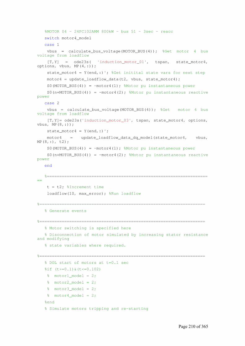
Page 210 of 365

%MOTOR 04 - 24PC102AMM 800kW - bus 51 - 3sec - reacc

switch motor4_model

case 1

vbus = calculate_bus_voltage(MOTOR_BUS(4)); %Get motor 4 bus voltage from loadflow

[T,Y] = ode23s( 'induction_motor_01', tspan, state_motor4, options, vbus, MP(4,:));

state_motor4 = Y(end,:)'; %Get initital state vars for next step

motor4 = update_loadflow_data(t2, vbus, state_motor4);

S0(MOTOR_BUS(4)) = -motor4(1); %Motor pu instantaneous power

S0(n+MOTOR_BUS(4)) = -motor4(2); %Motor pu instantaneous reactive power

case 2

vbus = calculate_bus_voltage(MOTOR_BUS(4)); %Get motor 4 bus voltage from loadflow

[T,Y]= ode23s('induction_motor_03', tspan, state_motor4, options, vbus, MP(8,:));

state_motor4 = Y(end,:)';

motor4 = update_loadflow_data_dq_model(state_motor4, vbus, MP(8,:), t2);

S0(MOTOR_BUS(4)) = -motor4(1); %Motor pu instantaneous power

S0(n+MOTOR_BUS(4)) = -motor4(2); %Motor pu instantaneous reactive power

end

%===================================================================

t = t2; %Increment time

loadflow(10, max_error); %Run loadflow

%===================================================================

% Generate events

%===================================================================

% Motor switching is specified here

% Disconnection of motor simulated by increasing stator resistance and modifying

% state variables where required.

%===================================================================

% DOL start of motors at t=0.1 sec

%if (t>=0.1)&(t<=0.102)

% motor1_model = 2;

% motor2_model = 2;

% motor3_model = 2;

% motor4_model = 2;

%end

% Simulate motors tripping and re-starting

Page 211 of 365

if (t>=0.01)&(t<=0.012)

%NB - this will not work if all motors are not modelled using the same model

% For all simulatione either abc or d-q model used so OK

switch motor1_model

case 1 %abc model - all motors off line

MP(1,6) = 1e6; %set high stator resistance

MP(2,6) = 1e6;

MP(3,6) = 1e6;

MP(4,6) = 1e6;

case 2 %d-q model - all motors offline

MP(5,4) = 1e6; %set stator resistance high

MP(6,4) = 1e6;

MP(7,4) = 1e6;

MP(8,4) = 1e6;

end

end

if (t>=0.11)&(t<0.112) %Restart after dip

switch motor1_model

case 1 %abc model

MP(1,6) = MP0(1,6);

MP(2,6) = MP0(2,6);

MP(3,6) = MP0(3,6);

MP(4,6) = MP0(4,6);

case 2 %d-q model

MP(5,4) = MP0(5,4); %restore original value

MP(6,4) = MP0(6,4);

MP(7,4) = MP0(7,4);

MP(8,4) = MP0(8,4);

end

end

%===================================================================

% Changes to network specified here

%===================================================================

% Simulate 20% voltage dip at Proteus for 100ms

if (t>= 0.1)&(t<=0.2)

V(n+1) = 0.8;

else

V(n+1) = bus_data(1,3); %restore original value

end

Page 212 of 365

% Simulate trip on main 26MW air compressors - assume about 80ms for breakers to open

if (t>=0.18)&(t<=0.182)

S0(20) = 0; %set 03KC201 power = 0

S0(20+n) = 0; %set 03KC201 vars = 0

S0(30) = 0; %set 03KC201 power = 0

S0(30+n) = 0; %set 03KC201 vars = 0

end

%===================================================================

% Store runtime data

%===================================================================

I_branch = calc_branch_currents(branch_list);

%save each step data here

SDAT(r,1) = t;

SDAT(r,2) = V(n+MOTOR_BUS(1));%24KC101AM voltage

SDAT(r,3) = V(n+MOTOR_BUS(2));%24PC104AM voltage

SDAT(r,4) = V(n+MOTOR_BUS(3));%24PC104AM voltage

SDAT(r,5) = V(n+MOTOR_BUS(4));%24PC102AM voltage

SDAT(r,6) = motor1(5); %24KC101AM instantaneous current

SDAT(r,7) = motor2(5); %24PC101AM instantaneous current

SDAT(r,8) = motor3(5); %24PC104AM instantaneous current

SDAT(r,9) = motor4(5); %24PC102AM instantaneous current

SDAT(r,10) = motor1(3)/1000; %24KC101AM power (kW)

SDAT(r,11) = motor2(3)/1000; %24PC101AM power (kW)

SDAT(r,12) = motor3(3)/1000; %24PC104AM power (kW)

SDAT(r,13) = motor4(3)/1000; %24PC102AM power (kW)

SDAT(r,14) = motor1(4)/1000; %24KC101AM Reactive power (kVa)

SDAT(r,15) = motor2(4)/1000; %24PC101AM Reactive power (kVa)

SDAT(r,16) = motor3(4)/1000; %24PC104AM Reactive power (kVa)

SDAT(r,17) = motor4(4)/1000; %24PC102AM Reactive power (kVa)

SDAT(r,18) = motor1(6); %24PC101AM speed pu

SDAT(r,19) = motor2(6); %24KC101AM speed pu

SDAT(r,20) = motor3(6); %24PC104AM speed pu

SDAT(r,21) = motor4(6); %24PC102AM speed pu

SDAT(r,22) = V(n+2); %Sub01

SDAT(r,23) = V(n+48); %Sub24 24JG101A

SDAT(r,24) = abs(I_branch(1,1)); %Proteus incomer A current

SDAT(r,25) = abs(I_branch(11,1)); %48GT101 feeder current

SDAT(r,26) = delta*57.2957; %48GT101 rotor angle

SDAT(r,27) = Pgen; %48GT101 power output

SDAT(r,28) = Qgen; %48GT101 reactive power output

SDAT(r,29) = V(n+gen_bus); %48GT101 bus voltage

Page 213 of 365

SDAT(r,30) = YG0(7); %Field voltage

SDAT(r,31) = V(n+7); %Sub 06 11kV busbar

SDAT(r,32) = V(41+n); %Sub 19 525V bus

SDAT(r,33) = abs(I_branch(19,1)); %64JK001B primary

SDAT(r,34) = abs(I_branch(19,2)); %64JK001B secondary

SDAT(r,35) = abs(I_branch(19,3)); %64JK001B tertiary

SDAT(r,36) = abs(I_branch(68,1)); %24KC101 current

SDAT(r,37) = abs(I_branch(69,1)); %24PC101 current

SDAT(r,38) = abs(I_branch(70,1)); %24PC104 current

SDAT(r,39) = abs(I_branch(71,1)); %24PC102 current

SDAT(r,40) = abs(I_branch(61,2)); %24JK101A secondary current

SDAT(r,41) = motor1(7); %Save phase a current

SDAT(r,42) = motor2(7);

SDAT(r,43) = motor3(7);

SDAT(r,44) = motor4(7);

SDAT(r,45) = YG0(4)*57.2957; %Gen rotor angular speed

SDAT(r,46) = YG0(9); %Pm

SDAT(r,47) = S0(gen_bus)*3; %Loadflow power

SDAT(r,48) = S0(gen_bus+n)*3; %LF Q

%===================================================================

print_runtime_data(SDAT,r);

r = r+1; %increment pointer

if t >= end_time

end_sim = 1; %Check for end of simulation

end

end % End of main simulation loop

%===================================================================

figure(1);

plotsim(SDAT);

figure(2);

plotgen(SDAT, end_time);

%Before saving to workspace, all induction motor state variables are set to the same length

state_motor1 = adjust_state_vecor_lengths(state_motor1);

state_motor2 = adjust_state_vecor_lengths(state_motor2);

state_motor3 = adjust_state_vecor_lengths(state_motor3);

state_motor4 = adjust_state_vecor_lengths(state_motor4);

INIT_IM = [state_motor1 state_motor2 state_motor3 state_motor4];

DATESTR(NOW) %End time to console

%####################################################################################

% END OF MAIN PROGRAM

Page 214 of 365

%####################################################################################

function print_runtime_data(SDAT,r)

%fprintf('t=%6.4f s',SDAT(r,1)); %time

%fprintf('%6.4f Vgen',SDAT(r,29)); %Gen voltage

%fprintf('%6.3f Pgout',SDAT(r,27));

%fprintf('%6.3f Qgout',SDAT(r,28));

%fprintf('%7.2f delta ',SDAT(r,26));

%fprintf('%7.3f omega ', SDAT(r,45));%rotor speed

%fprintf('%5.3f Pm ', SDAT(r,46)); %Mechanical power

%fprintf('%5.3f Plf ', SDAT(r,47));

%fprintf('%5.3f Qlf ', SDAT(r,48));

%fprintf('\n');

fprintf('t=%6.4f s ',SDAT(r,1)); %time

fprintf('%6.4f Vgen ',SDAT(r,29)); %Gen voltage

fprintf('%6.2f Im1 ',SDAT(r,6));

fprintf('%6.2f Im2 ',SDAT(r,7));

fprintf('%6.2f Im3 ',SDAT(r,8));

fprintf('%7.2f Im4 ', SDAT(r,9));

fprintf('%4.3f Pg ', SDAT(r,27));

fprintf('%4.3f Qg ', SDAT(r,28));

fprintf('%7.3f delta', SDAT(r,26));

fprintf('\n');

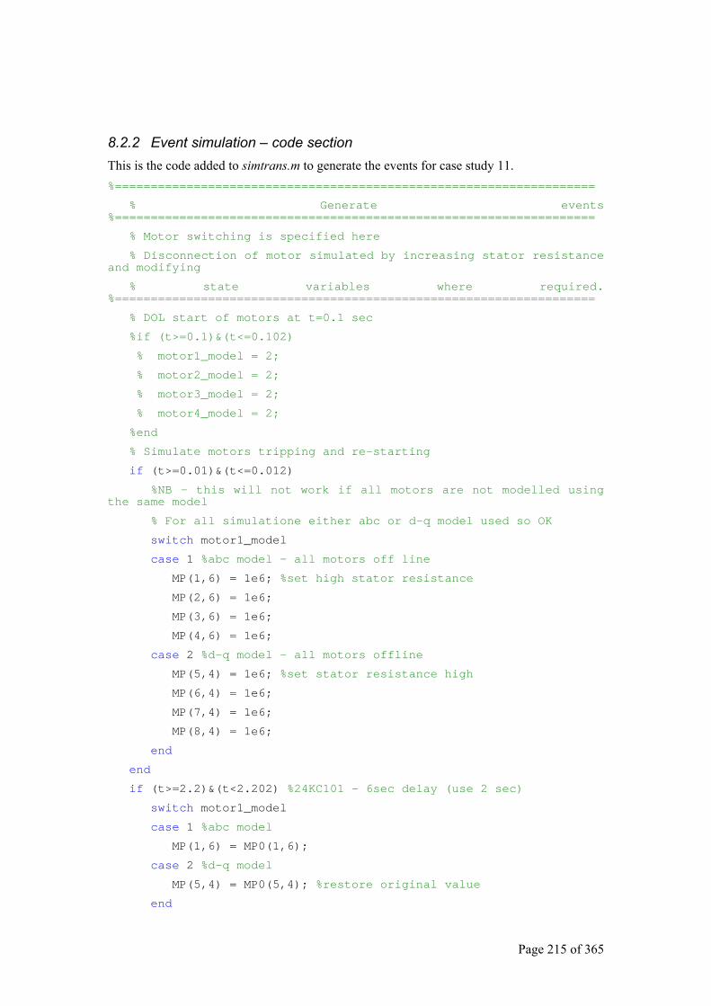
Page 215 of 365

8.2.2 Event simulation – code section This is the code added to simtrans.m to generate the events for case study 11. %===================================================================

% Generate events %===================================================================

% Motor switching is specified here

% Disconnection of motor simulated by increasing stator resistance and modifying

% state variables where required. %===================================================================

% DOL start of motors at t=0.1 sec

%if (t>=0.1)&(t<=0.102)

% motor1_model = 2;

% motor2_model = 2;

% motor3_model = 2;

% motor4_model = 2;

%end

% Simulate motors tripping and re-starting

if (t>=0.01)&(t<=0.012)

%NB - this will not work if all motors are not modelled using the same model

% For all simulatione either abc or d-q model used so OK

switch motor1_model

case 1 %abc model - all motors off line

MP(1,6) = 1e6; %set high stator resistance

MP(2,6) = 1e6;

MP(3,6) = 1e6;

MP(4,6) = 1e6;

case 2 %d-q model - all motors offline

MP(5,4) = 1e6; %set stator resistance high

MP(6,4) = 1e6;

MP(7,4) = 1e6;

MP(8,4) = 1e6;

end

end

if (t>=2.2)&(t<2.202) %24KC101 - 6sec delay (use 2 sec)

switch motor1_model

case 1 %abc model

MP(1,6) = MP0(1,6);

case 2 %d-q model

MP(5,4) = MP0(5,4); %restore original value

end

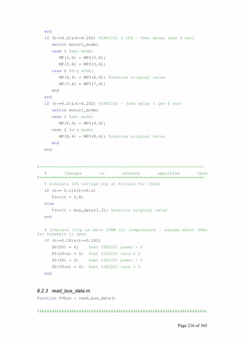
Page 216 of 365

end

if (t>=4.2)&(t<4.202) %24PC101 & 104 - 9sec delay (use 4 sec)

switch motor1_model

case 1 %abc model

MP(2,6) = MP0(2,6);

MP(3,6) = MP0(3,6);

case 2 %d-q model

MP(6,4) = MP0(6,4); %restore original value

MP(7,4) = MP0(7,4);

end

end

if (t>=6.2)&(t<6.202) %24PC102 - 3sec delay ( use 6 sec)

switch motor1_model

case 1 %abc model

MP(4,6) = MP0(4,6);

case 2 %d-q model

MP(8,4) = MP0(8,4); %restore original value

end

end

%===================================================================

% Changes to network specified here %===================================================================

% Simulate 20% voltage dip at Proteus for 100ms

if (t>= 0.1)&(t<=0.2)

V(n+1) = 0.8;

else

V(n+1) = bus_data(1,3); %restore original value

end

% Simulate trip on main 26MW air compressors - assume about 80ms for breakers to open

if (t>=0.18)&(t<=0.182)

S0(20) = 0; %set 03KC201 power = 0

S0(20+n) = 0; %set 03KC201 vars = 0

S0(30) = 0; %set 03KC201 power = 0

S0(30+n) = 0; %set 03KC201 vars = 0

end

8.2.3 read_bus_data.m function PVbus = read_bus_data()

%####################################################################

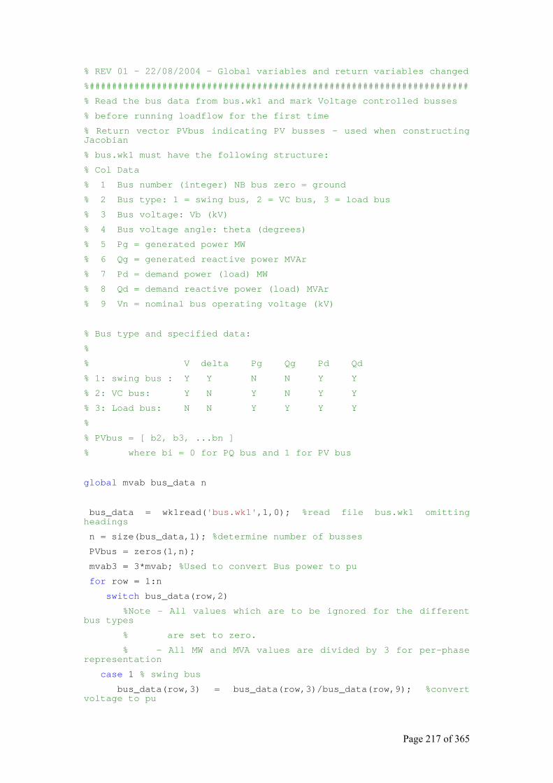
Page 217 of 365

% REV 01 - 22/08/2004 - Global variables and return variables changed

%####################################################################

% Read the bus data from bus.wk1 and mark Voltage controlled busses

% before running loadflow for the first time

% Return vector PVbus indicating PV busses - used when constructing Jacobian

% bus.wk1 must have the following structure:

% Col Data

% 1 Bus number (integer) NB bus zero = ground

% 2 Bus type: 1 = swing bus, 2 = VC bus, 3 = load bus

% 3 Bus voltage: Vb (kV)

% 4 Bus voltage angle: theta (degrees)

% 5 Pg = generated power MW

% 6 Qg = generated reactive power MVAr

% 7 Pd = demand power (load) MW

% 8 Qd = demand reactive power (load) MVAr

% 9 Vn = nominal bus operating voltage (kV)

% Bus type and specified data:

%

% V delta Pg Qg Pd Qd

% 1: swing bus : Y Y N N Y Y

% 2: VC bus: Y N Y N Y Y

% 3: Load bus: N N Y Y Y Y

%

% PVbus = [ b2, b3, ...bn ]

% where bi = 0 for PQ bus and 1 for PV bus

global mvab bus_data n

bus_data = wk1read('bus.wk1',1,0); %read file bus.wk1 omitting headings

n = size(bus_data,1); %determine number of busses

PVbus = zeros(1,n);

mvab3 = 3*mvab; %Used to convert Bus power to pu

for row = 1:n

switch bus_data(row,2)

%Note - All values which are to be ignored for the different bus types

% are set to zero.

% - All MW and MVA values are divided by 3 for per-phase representation

case 1 % swing bus

bus_data(row,3) = bus_data(row,3)/bus_data(row,9); %convert voltage to pu

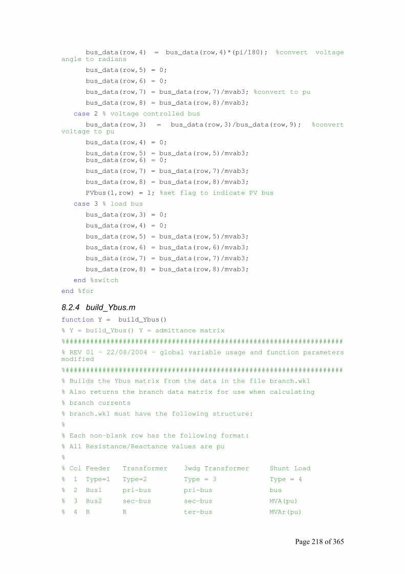
Page 218 of 365

bus_data(row,4) = bus_data(row,4)*(pi/180); %convert voltage angle to radians

bus_data(row,5) = 0;

bus_data(row,6) = 0;

bus_data(row,7) = bus_data(row,7)/mvab3; %convert to pu

bus_data(row,8) = bus_data(row,8)/mvab3;

case 2 % voltage controlled bus

bus_data(row,3) = bus_data(row,3)/bus_data(row,9); %convert voltage to pu

bus_data(row,4) = 0;

bus_data(row,5) = bus_data(row,5)/mvab3; bus_data(row,6) = 0;

bus_data(row,7) = bus_data(row,7)/mvab3;

bus_data(row,8) = bus_data(row,8)/mvab3;

PVbus(1,row) = 1; %set flag to indicate PV bus

case 3 % load bus

bus_data(row,3) = 0;

bus_data(row,4) = 0;

bus_data(row,5) = bus_data(row,5)/mvab3;

bus_data(row,6) = bus_data(row,6)/mvab3;

bus_data(row,7) = bus_data(row,7)/mvab3;

bus_data(row,8) = bus_data(row,8)/mvab3;

end %switch

end %for

8.2.4 build_Ybus.m function Y = build_Ybus()

% Y = build_Ybus() Y = admittance matrix

%####################################################################

% REV 01 - 22/08/2004 - global variable usage and function parameters modified

%####################################################################

% Builds the Ybus matrix from the data in the file branch.wk1

% Also returns the branch data matrix for use when calculating

% branch currents

% branch.wk1 must have the following structure:

%

% Each non-blank row has the following format:

% All Resistance/Reactance values are pu

%

% Col Feeder Transformer 3wdg Transformer Shunt Load

% 1 Type=1 Type=2 Type = 3 Type = 4

% 2 Bus1 pri-bus pri-bus bus

% 3 Bus2 sec-bus sec-bus MVA(pu)

% 4 R R ter-bus MVAr(pu)

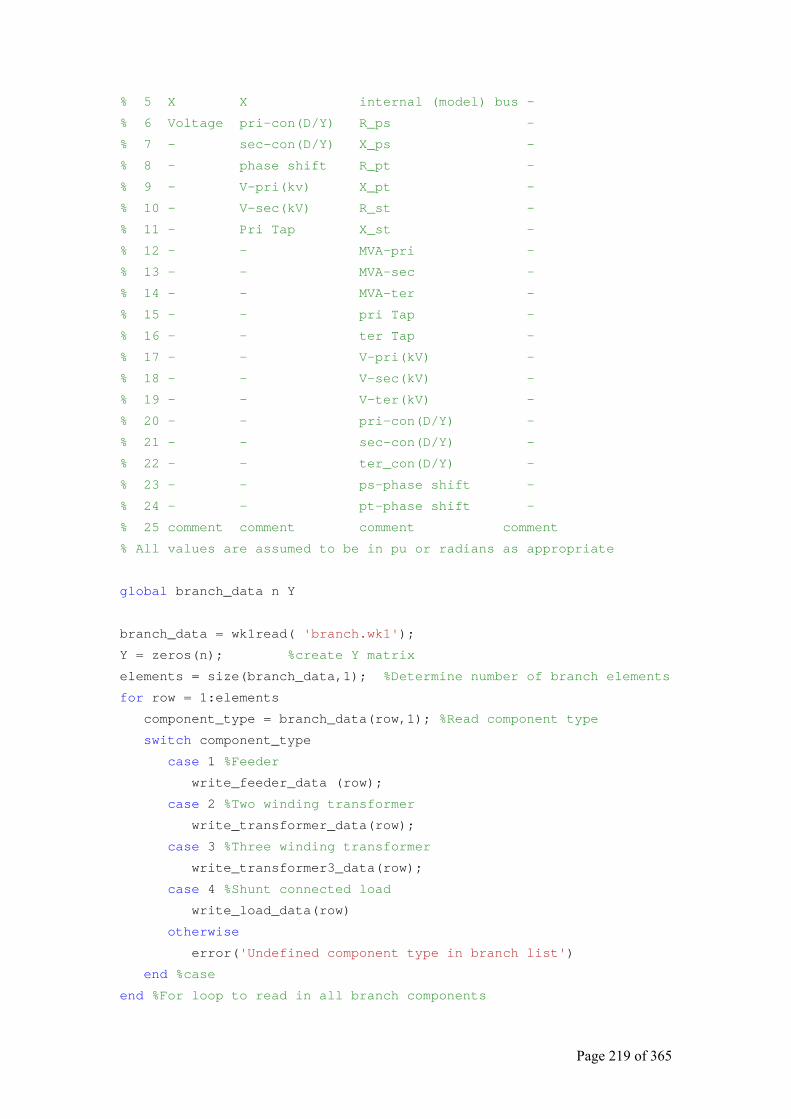
Page 219 of 365

% 5 X X internal (model) bus -

% 6 Voltage pri-con(D/Y) R_ps -

% 7 - sec-con(D/Y) X_ps -

% 8 - phase shift R_pt -

% 9 - V-pri(kv) X_pt -

% 10 - V-sec(kV) R_st -

% 11 - Pri Tap X_st -

% 12 - - MVA-pri -

% 13 - - MVA-sec -

% 14 - - MVA-ter -

% 15 - - pri Tap -

% 16 - - ter Tap -

% 17 - - V-pri(kV) -

% 18 - - V-sec(kV) -

% 19 - - V-ter(kV) -

% 20 - - pri-con(D/Y) -

% 21 - - sec-con(D/Y) -

% 22 - - ter_con(D/Y) -

% 23 - - ps-phase shift -

% 24 - - pt-phase shift -

% 25 comment comment comment comment

% All values are assumed to be in pu or radians as appropriate

global branch_data n Y

branch_data = wk1read( 'branch.wk1');

Y = zeros(n); %create Y matrix

elements = size(branch_data,1); %Determine number of branch elements

for row = 1:elements

component_type = branch_data(row,1); %Read component type

switch component_type

case 1 %Feeder

write_feeder_data (row);

case 2 %Two winding transformer

write_transformer_data(row);

case 3 %Three winding transformer

write_transformer3_data(row);

case 4 %Shunt connected load

write_load_data(row)

otherwise

error('Undefined component type in branch list')

end %case

end %For loop to read in all branch components

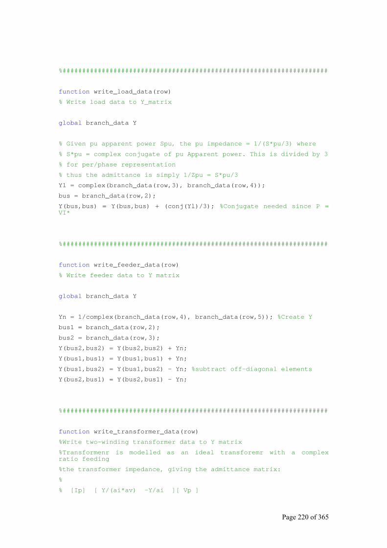
Page 220 of 365

%####################################################################

function write_load_data(row)

% Write load data to Y_matrix

global branch_data Y

% Given pu apparent power Spu, the pu impedance = 1/(S*pu/3) where

% S*pu = complex conjugate of pu Apparent power. This is divided by 3

% for per/phase representation

% thus the admittance is simply 1/Zpu = S*pu/3

Yl = complex(branch_data(row,3), branch_data(row,4));

bus = branch_data(row,2);

Y(bus,bus) = Y(bus,bus) + (conj(Yl)/3); %Conjugate needed since P = VI*

%####################################################################

function write_feeder_data(row)

% Write feeder data to Y matrix

global branch_data Y

Yn = 1/complex(branch_data(row,4), branch_data(row,5)); %Create Y

bus1 = branch_data(row,2);

bus2 = branch_data(row,3);

Y(bus2,bus2) = Y(bus2,bus2) + Yn;

Y(bus1,bus1) = Y(bus1,bus1) + Yn;

Y(bus1,bus2) = Y(bus1,bus2) - Yn; %subtract off-diagonal elements

Y(bus2,bus1) = Y(bus2,bus1) - Yn;

%####################################################################

function write_transformer_data(row)

%Write two-winding transformer data to Y matrix

%Transformenr is modelled as an ideal transforemr with a complex ratio feeding

%the transformer impedance, giving the admittance matrix:

%

% [Ip] [ Y/(ai*av) -Y/ai ][ Vp ]

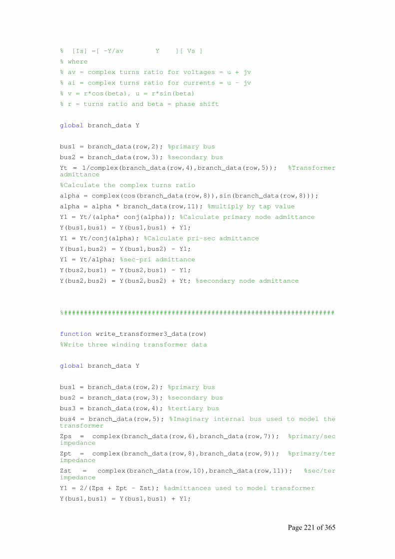
Page 221 of 365

% [Is] =[ -Y/av Y ][ Vs ]

% where

% av = complex turns ratio for voltages = u + jv

% ai = complex turns ratio for currents = u - jv

% v = r*cos(beta), u = r*sin(beta)

% r = turns ratio and beta = phase shift

global branch_data Y

bus1 = branch_data(row,2); %primary bus

bus2 = branch_data(row,3); %secondary bus

Yt = 1/complex(branch_data(row,4),branch_data(row,5)); %Transformer admittance

%Calculate the complex turns ratio

alpha = complex(cos(branch_data(row,8)),sin(branch_data(row,8)));

alpha = alpha * branch_data(row,11); %multiply by tap value

Y1 = Yt/(alpha* conj(alpha)); %Calculate primary node admittance

Y(bus1,bus1) = Y(bus1,bus1) + Y1;

Y1 = Yt/conj(alpha); %Calculate pri-sec admittance

Y(bus1,bus2) = Y(bus1,bus2) - Y1;

Y1 = Yt/alpha; %sec-pri admittance

Y(bus2,bus1) = Y(bus2,bus1) - Y1;

Y(bus2,bus2) = Y(bus2,bus2) + Yt; %secondary node admittance

%####################################################################

function write_transformer3_data(row)

%Write three winding transformer data

global branch_data Y

bus1 = branch_data(row,2); %primary bus

bus2 = branch_data(row,3); %secondary bus

bus3 = branch_data(row,4); %tertiary bus

bus4 = branch_data(row,5); %Imaginary internal bus used to model the transformer

Zps = complex(branch_data(row,6),branch_data(row,7)); %primary/sec impedance

Zpt = complex(branch_data(row,8),branch_data(row,9)); %primary/ter impedance

Zst = complex(branch_data(row,10),branch_data(row,11)); %sec/ter impedance

Y1 = 2/(Zps + Zpt - Zst); %admittances used to model transformer

Y(bus1,bus1) = Y(bus1,bus1) + Y1;

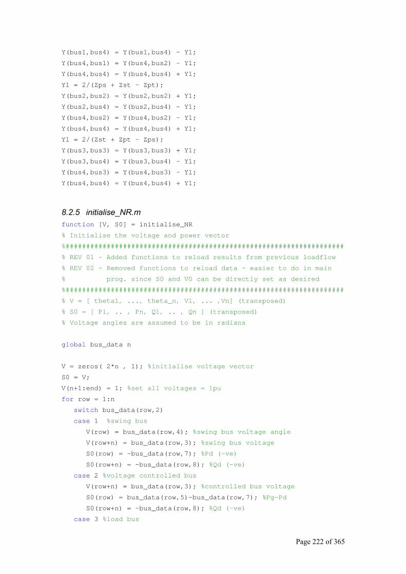
Page 222 of 365

Y(bus1,bus4) = Y(bus1,bus4) - Y1;

Y(bus4,bus1) = Y(bus4,bus2) - Y1;

Y(bus4,bus4) = Y(bus4,bus4) + Y1;

Y1 = 2/(Zps + Zst - Zpt);

Y(bus2,bus2) = Y(bus2,bus2) + Y1;

Y(bus2,bus4) = Y(bus2,bus4) - Y1;

Y(bus4,bus2) = Y(bus4,bus2) - Y1;

Y(bus4,bus4) = Y(bus4,bus4) + Y1;

Y1 = 2/(Zst + Zpt - Zps);

Y(bus3,bus3) = Y(bus3,bus3) + Y1;

Y(bus3,bus4) = Y(bus3,bus4) - Y1;

Y(bus4,bus3) = Y(bus4,bus3) - Y1;

Y(bus4,bus4) = Y(bus4,bus4) + Y1;

8.2.5 initialise_NR.m function [V, S0] = initialise_NR

% Initialise the voltage and power vector

%####################################################################

% REV 01 - Added functions to reload results from previous loadflow

% REV 02 - Removed functions to reload data - easier to do in main

% prog. since S0 and V0 can be directly set as desired

%####################################################################

% V = [ theta1, ..., theta_n, V1, ... ,Vn] (transposed)

% S0 = [ P1, .. , Pn, Q1, .. , Qn ] (transposed)

% Voltage angles are assumed to be in radians

global bus_data n

V = zeros( 2*n , 1); %initialise voltage vector

S0 = V;

V(n+1:end) = 1; %set all voltages = 1pu

for row = 1:n

switch bus_data(row,2)

case 1 %swing bus

V(row) = bus_data(row,4); %swing bus voltage angle

V(row+n) = bus_data(row,3); %swing bus voltage

S0(row) = -bus_data(row,7); %Pd (-ve)

S0(row+n) = -bus_data(row,8); %Qd (-ve)

case 2 %voltage controlled bus

V(row+n) = bus_data(row,3); %controlled bus voltage

S0(row) = bus_data(row,5)-bus_data(row,7); %Pg-Pd

S0(row+n) = -bus_data(row,8); %Qd (-ve)

case 3 %load bus

Page 223 of 365

S0(row) = bus_data(row,5)-bus_data(row,7); %Pg-Pd

S0(row+n) = bus_data(row,6)-bus_data(row,8); %Pg-Pd

end %switch

end %for

8.2.6 set_motor_parameters.m function [MP, MOTOR_BUS] = set_motor_parameters(motor_count)

%[MP, MOTOR_BUS] = set_motor_parameters()

%Set up induction motor model parameters

% MP = motor model parameters

% All inductance and resistance values are in MKSA units

% MP = [Lsl, Lsm, Lsrm, Lrm, Lrl, Rs, Rr H, LC, LT, P, Tf, tds, tde, dt, dp1, dp2]

% MP(1) = Lsl = Stator leakage inductance

% MP(2) = Lsm = Stator mutual induxctance

% MP(3) = Lsrm = Stator/rotor mutual inductance - set according to model

% Vas gives Lsrm = 2/3Lsm = 2/3Lrm

% MP(4) = Lrm = rotor mutual inductance

% MP(5) = Lrl = rotor leakage inductance

% MP(6) = Rs = stator resistance

% MP(7) = Rr = rotor resistance

% MP(8) = H = inertia constant

% MP(9) = L = load constant

% MP(10) = LT = load type: 1=load proportional to speed

% 2=load proportional to speed^2

% MP(11) = number of pole pairs

% MP(12) = Torque due to friction and windage at rated speed.

% MP(13) = Rotor resistance variation factor Rr at standstill = Rr*(1+(factor*slip))

% MP(14) = Rotor reactance variation factor Xr at standstill = Xr*(1-(factor*slip))

% MP(15) to MP(21) - not used

% MOTOR_BUS = loadflow motor bus

%===================================================================

% Revision History

% 2005/08/02 - Added parameters for simple single-cage induction motor model

%===================================================================

MP = zeros(motor_count*2, 21);

MOTOR_BUS = zeros(motor_count,1);

Page 224 of 365

%===================================================================

% Parameters for abc model

%

% Note: MOTOR_BUS is an array storing the connection bus numbers of the

% motors to be simulated. There is no value stored for the d-q model

% since this simply uses the abc model data

%===================================================================

% MOTOR 01 - 24KC101AM 550kW - bus 49

%===================================================================

MOTOR_BUS(1) = 49; %Motor 1 bus number

MP(1,1) = 0.03592; %Lsl = Stator leakage inductance (=equiv. ckt param)

MP(1,2) = 0.8726; %Lsm = Stator magnetising inductance

MP(1,3) = MP(1,2); %Lsrm = Stator/rotor mutual inductance

MP(1,4) = MP(1,2); %Lrm = rotor mutual inductance

MP(1,5) = 0.05389; %Lrl = rotor leakage inductance

MP(1,6) = 1.1895; %Rs = stator resistance

MP(1,7) = 1.941; %Rr = rotor resistance

MP(1,8) = 5.5; %H = inertia constant

MP(1,9) = 0.018; %L = load constant approx 95% of 550kW load

MP(1,10) = 2;%LT = load type: 1= proportional to speed 2= proportional to speed^2

MP(1,11) = 1; %pole pairs

MP(1,12) = 37.93; %Torque due to friction and Windage at rated speed (Nm)

MP(1,13) = 2; %Rr standstill = 3Rr

MP(1,14) = 0.5; %Xr standstill = 0.5*Xr

%===================================================================

% MOTOR 02 - 24PC101AM 300kW - bus 50

%===================================================================

MOTOR_BUS(2) = 50; %Motor 2 bus number

MP(2,1) = 0.0671; %Lsl = Stator leakage inductance (=equiv. ckt param)

MP(2,2) = 1.844; %Lsm = Stator magnetising inductance

MP(2,3) = MP(2,2); %Lsrm = Stator/rotor mutual inductance

MP(2,4) = MP(2,2); %Lrm = rotor mutual inductance

MP(2,5) = 0.1005; %Lrl = rotor leakage inductance

MP(2,6) = 1.456; %Rs = stator resistance

MP(2,7) = 2.739; %Rr = rotor resistance

MP(2,8) = 3.3; %H = inertia constant

Page 225 of 365

MP(2,9) = 7e-3; %L = load constant 70% of load

MP(2,10) = 2;%LT = load type: 1= proportional to speed 2= proportional to speed^2

MP(2,11) = 1; %pole pairs

MP(2,12) = 27; %Torque due to friction and Windage at rated speed

MP(2,13) = 2; %Rr standstill = 2.5Rr

MP(2,14) = 0.5; %Xr standstill = 0.5*Xr

%===================================================================

% MOTOR 03 - 24PC104AM 300kW - bus 52

%===================================================================

MOTOR_BUS(3) = 52; %Motor 3 bus number

MP(3,1) = 0.0671; %Lsl = Stator leakage inductance (=equiv. ckt param)

MP(3,2) = 1.844; %Lsm = Stator magnetising inductance

MP(3,3) = MP(2,2); %Lsrm = Stator/rotor mutual inductance

MP(3,4) = MP(2,2); %Lrm = rotor mutual inductance

MP(3,5) = 0.1005; %Lrl = rotor leakage inductance

MP(3,6) = 1.456; %Rs = stator resistance

MP(3,7) = 2.739; %Rr = rotor resistance

MP(3,8) = 2.6; %6.3 H = inertia constant

MP(3,9) = 8e-3; %L = load constant 80% of load

MP(3,10) = 2;%LT = load type: 1= proportional to speed 2= proportional to speed^2

MP(3,11) = 1; %pole pairs

MP(3,12) = 27; %Torque due to friction and Windage at rated speed

MP(3,13) = 2; %Rr standstill = 4Rr

MP(3,14) = 0.5; %Xr standstill = 0.5*Xr

%===================================================================

% MOTOR 04 - 24PC102AM 850kW - bus 51

%===================================================================

MOTOR_BUS(4) = 51; %Motor 4 bus number

MP(4,1) = 0.023393; %Lsl = Stator leakage inductance (=equiv. ckt param)

MP(4,2) = 0.7080; %Lsm = Stator magnetising inductance

MP(4,3) = MP(4,2); %Lsrm = Stator/rotor mutual inductance

MP(4,4) = MP(4,2); %Lrm = rotor mutual inductance

MP(4,5) = 0.03509; %Lrl = rotor leakage inductance

MP(4,6) = 1.2555; %Rs = stator resistance

MP(4,7) = 1.133; %Rr = rotor resistance

MP(4,8) = 9; %H = inertia constant

Page 226 of 365

MP(4,9) = 0.02064; %L = load constant 80% of load

MP(4,10) = 2;%LT = load type: 1= proportional to speed 2= proportional to speed^2

MP(4,11) = 1; %pole pairs

MP(4,12) = 24; %Torque due to friction and Windage at rated speed (Nm)

MP(4,13) = 2; %Rr standstill = 3Rr

MP(4,14) = 0.5; %Xr standstill = 0.5*Xr

%###################################################################

% Parameters for simplified motor models

%###################################################################

% MP = motor model parameters in MKSA

%

% MP = [X', T'o, Xo, R1, Hm, L, LT, tds, tde, dt, dp1, dp2]

% MP(1) = X': Transient reactance

% MP(2) = T'o: open circuit time constant

% MP(3) = Xo: open circuit reactance

% MP(4) = R1: Stator resistance

% MP(5) = Hm = inertia constant

% MP(6) = L = load constant

% MP(7) = LT = load type: 1=load proportional to speed

% 2=load proportional to speed^2

% MP(8) = bus voltage (kV)

% MP(9) = not used

% MP(10) = not used

% MP(11) = not used

% MP(12) = not used

% MP(13) = Motor base MVA

% MP(14) - MP(21) are not used for this model

%===================================================================

% MOTOR 01 - 24KC101AM 550kW - bus 49

%===================================================================

R1 = 1.189;

X1 = 6.771;

Xm = 274;

X2 = 10.16;

R2 = 0.647;

MP(5,1) = X1 + ((X2*Xm)/(X2+Xm)); %Transient reactance

MP(5,2) = (X2+Xm)/(100*pi*R2); %open circuit time constant

MP(5,3) = X1+Xm; %open circuit reactance

MP(5,4) = R1; %Stator resistance

Page 227 of 365

MP(5,5) = 160; %H, inertia constant

MP(5,6) = 4.73e-3; %load constant 80% load

MP(5,7) = 2; %Load type

MP(5,8) = 6.6; %bus voltage (kv)

MP(5,13) = 0.55; %Sb(MVA) for motor

%===================================================================

% MOTOR 02 - 24PC101AM 300kW - bus 50

%===================================================================

R1 = 1.456;

X1 = 12.64;

Xm = 579;

X2 = 18.96;

R2 = 0.913;

MP(6,1) = X1 + ((X2*Xm)/(X2+Xm)); %Transient reactance

MP(6,2) = (X2+Xm)/(100*pi*R2); %open circuit time constant

MP(6,3) = X1+Xm; %open circuit reactance

MP(6,4) = R1; %Stator resistance

MP(6,5) = 70; %H, inertia constant

MP(6,6) = 2.162e-3; %load constant 80% load

MP(6,7) = 2; %Load type

MP(6,8) = 6.6; %bus voltage (kv)

MP(6,13) = 0.3; %Sb(MVA) for motor

%===================================================================

% MOTOR 03 - 24PC104AM 300kW - bus 52

%===================================================================

R1 = 3.464;

X1 = 14.09;

Xm = 420.6;

X2 = 21.14;

R2 = 1.259;

MP(7,1) = X1 + ((X2*Xm)/(X2+Xm)); %Transient reactance

MP(7,2) = (X2+Xm)/(100*pi*R2); %open circuit time constant

MP(7,3) = X1+Xm; %open circuit reactance

MP(7,4) = R1; %Stator resistance

MP(7,5) = 70; %H, inertia constant

MP(7,6) = 2.162e-3; %load constant 80% load

MP(7,7) = 2; %Load type

MP(7,8) = 6.6; %bus voltage (kv)

Page 228 of 365

MP(7,13) = 0.3; %Sb(MVA) for motor

%===================================================================

% MOTOR 04 - 24PC102AM 800kW - bus 51

%===================================================================

R1 = 1.255;

X1 = 4.409;

Xm = 222.4;

X2 = 6.614;

R2 = 0.377;

MP(8,1) = X1 + ((X2*Xm)/(X2+Xm)); %Transient reactance

MP(8,2) = (X2+Xm)/(100*pi*R2); %open circuit time constant

MP(8,3) = X1+Xm; %open circuit reactance

MP(8,4) = R1; %Stator resistance

MP(8,5) = 200; %H, inertia constant

MP(8,6) = 6.485e-3; %load constant 80% load

MP(8,7) = 2; %Load type

MP(8,8) = 6.6; %bus voltage (kv)

MP(8,13) = 0.8; %Sb(MVA) for motor

8.2.7 set_generator_parameters.m function GEN_PAR = set_generator_parameters

% [GEN_PAR] = set_generator_parameters creates matrix with generator parameters

%

% GP = [Rs Xd X'd T'do Xq X'd T'qo AVR_mode]

% 48GT101 prameters - use with model sync_gen_01,02

% Note all pu values have been referred to 100MVA base

% AVR parameters are not listed here but are coded into AVR DE's.

GEN_PAR = zeros(1,7);

GEN_PAR(1) = 0.003; % Stator winding resistance - ASSUMED VALUE

% d - axis parameters

GEN_PAR(2) = 1.421; % Synchronous reactance Xd

GEN_PAR(3) = 0.1571;% Transient reactance X'd

GEN_PAR(4) = 9.5; % Open circuit transient time constant T'do

% q - axis parameters

GEN_PAR(5) = 1.3143;% Synchronous reactance Xq

GEN_PAR(6) = 0.2; % Transient reactance X'q - ASSUMED VALUE

Page 229 of 365

GEN_PAR(7) = 0.5; % Open circuit transient time constant T'qo - ASSUMED VALUE

% Inertia constant is set in the model - no need to change this value thus

% not included here

8.2.8 set_motor_state_vector.m function SM = set_motor_state_vector( INIT_IM, motor_no, model )

% Sets up the initial motor model state vectors from the imput state vector matrix

% based on the model selected

SM = INIT_IM(:,motor_no); %Default abc model uses full state vector

if model == 2 %d-q model only uses first three variables

SM = SM(1:3,1);

end

8.2.9 locate_gen_axis.m function [delta, It, Vt] = locate_gen_axis (gen_bus)

% Locate generator axis wrt system axis.

global n V GP S0

% Determine generator complex power - Loadflow power is on per phase

% basis and must be multiplied by three

Sgen = complex(S0(gen_bus), S0(gen_bus+n))*3;

% Calculate phase angle

phi = angle(Sgen);

% Take complex conjugate of Sgen to ensure that Q is negative for

% leading power factor and positive for lagging so that the phase

% angle of the current is correct

Sgen = conj(Sgen);

% Get terminal voltage

V_magnitude = V(gen_bus+n);

V_angle = V(gen_bus); %Angle wrt swing bus

Vre = V_magnitude*cos(V_angle); % Real part of voltage

Vim = V_magnitude*sin(V_angle); % Imaginary part of voltage

Vt = complex(Vre, Vim); % Complex voltage

It = conj(Sgen/Vt); %Terminal current

% Calculate internal voltage angle

% temp1 = (xq*cos(phi)+r*sin(phi))*|It|

temp1 = (GP(5)*cos(phi)+GP(1)*sin(phi))*abs(It);

% temp2 = |Vt|+|It|(r*cos(phi)-xq*sin(phi))

temp2 = V_magnitude + ( abs(It)*(GP(1)*cos(phi)-GP(5)*sin(phi)));

Page 230 of 365

d_int = atan(temp1/temp2); %Internal voltage angle

delta = d_int + V_angle;

8.2.10 init_gen_state.m function YG0 = init_gen_state(Vref, Vt, It, delta, Pref)

% This is called after the first loadflow solution to determine

% generator initial state variables

% Vt = complex terminal voltage

% It = complex terminal current

% delta = machine ref frame angle wrt system reference frame

% Pm0 = initial steady-state mechanical input power

global GP

% Calculate voltage and current dq components

[Vd, Vq] = convert_to_gen_ref(delta, real(Vt), imag(Vt));

[Id, Iq] = convert_to_gen_ref(delta, real(It), imag(It));

% Calculate initial values of state variables

% E'do = (x'q-xq)Iq

Ed_t0 = (GP(6)-GP(5))*Iq;

% E'qo = Vq + rIq - x'd*Id

Eq_t0 = Vq + GP(1)*Iq - GP(3)*Id;

delta_e0 = delta;

omega_e0 = 0;

% Efdo = (E'qo - (xd - x'd)*Id)/0.9436

Efd0 = (Eq_t0 - (GP(2)-GP(3))*Id)/0.9436;

X10 = abs(Vt);

% Calculate the exciter saturation function

if Efd0 > 4.06

%Use SE2

SE = ((0.2292*Efd0)-1)*Efd0;

else

%Use SE1

SE = Efd0^2*0.4757;

end

% X20 = SE + KE*Vfd, but KE = 1

X20 = SE + Efd0;

% X40 = Vref-X1-(X2/KA), KA = 1762

X40 = Vref - X10 - (X20 / 1762);

Pm0 = Pref; % omega_e0 = 0

YG0 = [Ed_t0; Eq_t0; delta_e0; omega_e0; X10; X20; Efd0; X40; Pm0];

Page 231 of 365

8.2.11 pu_bus_voltage.m function Vt = pu_bus_voltage(gen_bus)

% Reads generator bus voltage from loadflow and returns as a complex

% variable Vt = (Vr+JVm) where Vr = real bus voltage, Vm = imaginary

% bus voltage. This routine is used for the generator model and the

% single-cage induction machine model

global n V

V_magnitude = V(gen_bus+n);

V_angle = V(gen_bus); %Angle wrt swing bus

Vre = V_magnitude*cos(V_angle); % Real part of voltage

Vim = V_magnitude*sin(V_angle); % Imaginary part of voltage

Vt = complex(Vre, Vim); % Complex voltage

8.2.12 convert_to_gen_ref.m function [Xd, Xq] = convert_to_gen_ref( delta, Xre, Xim )

% Convert voltage or current from system reference frame to

% the generator reference frame

Xd = -sin(delta)*Xre + cos(delta)*Xim;

Xq = cos(delta)*Xre + sin(delta)*Xim;

8.2.13 calc_gen_power.m function [Pg, Qg]=calc_gen_power(YG1, Vt, Vd, Vq, delta )

% Calculate generator output power and vars to update loadflow.

% YG1 = state variable from solution of generator model

% Vt = complex bus voltage (system reference)

% Vd, Vq = bus voltage (generator model reference)

global GP

% Calculate Id, Iq

% temp = (r^2+xd'*xq')

temp = GP(3)*GP(6)+GP(1)^2;

% Id = (r(E'd-Vd)+x'q(Vq-E'q))/temp

Id = ((GP(1)*(YG1(1,1)-Vd))+(GP(6)*(Vq-YG1(2,1))))/temp;

% Iq = (E'd-Vd-r*Id)/x'q

Iq = (YG1(1,1)-Vd-GP(1)*Id)/GP(6);

% Convert current to system reference

Ire = cos(delta)*Iq - sin(delta)*Id;

Iim = sin(delta)*Iq + cos(delta)*Id;

It = complex(Ire, Iim);

S = Vt*conj(It); %Complex power

Page 232 of 365

Pg = real(S);

Qg = -imag(S);

8.2.14 calculate_bus_voltage.m function vbus = calculate_bus_voltage(bus)

% Get phase rms bus voltage from loadflow

% vbus = calculate_bus_voltage(bus)

% bus = bus number

% vbus = [vbus, angle]

% vb = bus voltage

% va = voltage angle (rad) calculated during loadflow solution

% Multiply bus voltage by 1000 since branch data values in kV

global n bus_data V

vb = (V(n+bus)*bus_data(bus,9))*1000; %l-l rms bus voltage

angle = V(bus); % bus voltage angle

vbus = [ vb angle ];

8.2.15 update_loadflow_data.m function S_motor = update_loadflow_data(t, vmot, MSV)

% S_motor = update_loadflow_data(t, vmot, MSV)

% t = time

% vmot = motor terminal voltage

% MSV = motor state variables

%

% This function is used with the abc Induction motor model

% Smot = [Ppu Qpu P Q Im omega, Ia]

% Ppu = inst. motor power (pu) (per-phase)

% Qpu = inst. motor reactive power (pu) (per-phase)

% P = inst motor power (W) (3-phase)

% Q = inst motor reactive power (3-phase)

% Im = inst. rms motor current (A)

% omega = motor_speed (pu)

% Ia = phase A instantaneous motor current

global mvab

S_motor = zeros(1,7);

S_motor(6) = MSV(8)/(100*pi); %Since all motors are single pole this

% calculation ignores the number of motor poles

% Calculate instantaneous motor voltages in abc reference frame

Vm = calc_abc_tmnl_voltage(vmot,t);

%Calculate instantaneous bus power

Page 233 of 365

S_motor(3) = Vm(1)*MSV(1)+Vm(2)*MSV(2)+Vm(3)*MSV(3);

S_motor(1) = S_motor(3)/(3e6*mvab); %convert to pu and divide by 3

%Instantaneous reactive power

%The calculated value will be -ve for lagging power factor, invert

%to get positive value since +ve values are assumed to be power input

%into the machine.

temp1 = MSV(2)-MSV(3); %Ibs - Ics

temp2 = MSV(3)-MSV(1); %Ics - Ias

temp3 = MSV(1)-MSV(2); %Ias - Ibs

S_motor(4) = -(Vm(1)*temp1+Vm(2)*temp2+Vm(3)*temp3)/sqrt(3);

S_motor(2) = S_motor(4)/(3e6*mvab); %convert to pu and divide by 3

%Calculate the instantaneous rms motor current.

S_motor(5) = sqrt((1/3)*(MSV(1)^2+MSV(2)^2+MSV(3)^2));

S_motor(7) = MSV(1); %Phase a inst. stator current

8.2.16 calc_abc_tmnl_voltage.m function Vinst = calc_abc_tmnl_voltage(v,t)

% % Calculate the three instantaneous phase voltages to allow motor power

% to be determined. The voltages are in the abc reference frame

% v = [Vt Va] = motor terminal rms line voltage and angle

% The phase p-p voltage is calculated and the 30degree phase shift between

% phase and line voltage taken into account

Vinst = zeros(3,1);

TWOpi3 = 2*pi/3;

v_angle = v(2)-(pi/6); %Voltage angle from loadflow - 30degrees

% a = instantaneus bus voltage angle

a = (100 * pi * t) + v_angle;

vpeak = v(1)*sqrt(2/3);

Vinst(1,1) = vpeak*cos( a );

Vinst(2,1) = vpeak*cos( a - TWOpi3);

Vinst(3,1) = vpeak*cos( a + TWOpi3);

8.2.17 update_loadflow_data_dq_model.m function Smot = update_loadflow_data_dq_model(SV, vbus, MP, t)

% Calculate the real and reactive power for the single cage induction

% motor model

% SV = model state variables SV = [E'r, E'm, S]

% vbus = [|vbus| angle_vbus ]

% MP = motor model parameters

% Smot = [Ppu Qpu P Q Im omega, Ia]

Page 234 of 365

% Ppu = inst. motor power (pu) (per-phase)

% Qpu = inst. motor reactive power (pu) (per-phase)

% P = inst motor power (W) (3-phase)

% Q = inst motor reactive power (3-phase)

% Im = rms motor current (A)

% omega = motor_speed (pu)

% Ia = phase A instantaneous motor current

global mvab

Smot = zeros(1,7);

temp = vbus(1)/sqrt(3);

Vr = temp*cos(vbus(2));

Vm = temp*sin(vbus(2));

% Ir = (R1(Vr-E'r)+X'(Vm-E'm))/(R1^2+X'^2)

Ir = ((MP(4)*(Vr-SV(1,1)))+(MP(1)*(Vm-SV(2,1))))/(MP(4)^2+MP(1)^2);

% Im = (Vm-E'm-X'Ir)/R1

Im = (Vm-SV(2,1)-(MP(1)*Ir))/MP(4);

It = complex(Ir,Im);

Vt = complex(Vr, Vm);

Sm = Vt*conj(It);

Smot(3) = real(Sm)*3; %Save Power

Smot(4) = imag(Sm)*3; %Save reactive power

% Change to system base

Smot(1) = Smot(3)/(mvab*3e6);

Smot(2) = Smot(4)/(mvab*3e6);

%Convert to pu (motor base)

Smot(5) = abs(It); %rms current (A)

Smot(6) = (1-SV(3,1)); %Calculate speed pu

Smot(7) = abs(It)*1.414*cos((100*pi*t)+angle(It)); %Calculate instantaneous phase a current

8.2.18 calc_branch_currents.m function Ib = calc_branch_currents( branch_list )

% Ib = calc_branch_currents( branch_list ) Calculates the branch currents

%####################################################################

%REV 01 - Added load power calculations - 13/08/2004

%REV 02 - Added functions to calculate only selected branch currents - 28/08/2004

%####################################################################

% If the vector branch_list is omitted, values are calculated for all branches

% If the vector branch_list is present, values are only calculated for the branches

Page 235 of 365

% listed in the branch_list vector

% branch_list = [b1 b2 .... bn]

% V = bus voltage matrix

% Data is returned in Ib with row n = branch n

% When branch_list is specified, currents are only calculated for the specific branches

% the rest are left = 0

% Ib = complex matrix with current corresponding to each element with the following

% format: (All values in MKSA)

% col: 1 2 3

% feeder: If (b1 - b2) 0 0

% transformer: Ip Is 0

% 3 wdg trfmr: Ip Is It

% Load Il MVA MVAr

% n = number of busses

% mvab = base mva

global Ib mvab n bus_data branch_data V

elements = size(branch_data,1); %Determine the number of branch elements

Ib = zeros(elements,3); %Create branch current matrix

if nargin == 0

%Calculate all branch currents

for row = 1:elements

component_type = branch_data(row,1); %Read component type

switch component_type

case 1 %Feeder

calc_feeder_current(row, n, V, branch_data, mvab);

case 2 %Two winding transformer

calc_transformer_current(row, n, V, branch_data, mvab);

case 3 %Three winding transformer

calc_3wtransformer_current(row, n, V, branch_data, mvab);

case 4 %Shunt connected load

calc_load_current(row, n, V, branch_data, bus_data, mvab);

otherwise

error('Undefined component type in branch list')

end %case

end %for loop to read all elements

else

%Calculate only selected branch currents

for row = branch_list

component_type = branch_data(row,1); %Read component type

switch component_type

case 1 %Feeder

Page 236 of 365

calc_feeder_current(row, n, V, branch_data, mvab);

case 2 %Two winding transformer

calc_transformer_current(row, n, V, branch_data, mvab);

case 3 %Three winding transformer

calc_3wtransformer_current(row, n, V, branch_data, mvab);

case 4 %Shunt connected load

calc_load_current(row, n, V, branch_data, bus_data, mvab);

otherwise

error('Undefined component type in branch list')

end %cas

end %for loop to read selected elements

end %If nargin

%####################################################################

function calc_feeder_current(row, n, V, branch_data, mvab)

%Calculate feeder current from bus 1 to bus 2

global Ib

Z = complex(branch_data(row,4), branch_data(row,5)); %Feeder impedance

bus1 = branch_data(row,2);

bus2 = branch_data(row,3);

% Calculate complex bus voltages

V1 = V(bus1+n)*complex(cos(V(bus1)),sin(V(bus1)));

V2 = V(bus2+n)*complex(cos(V(bus2)),sin(V(bus2)));

%Calculate base current

Ibase = (mvab*1000)/branch_data(row,6)* sqrt(3);

Ib(row,1) = ((V1-V2)/Z)*Ibase; %Save branch current

%####################################################################

function calc_transformer_current(row, n, V, branch_data, mvab)

%Calculate transformer primary and secondary currents

global Ib

bus1 = branch_data(row,2); %primary bus

bus2 = branch_data(row,3); %secondary bus

Yt = 1/complex(branch_data(row,4),branch_data(row,5)); %Transformer impedance

%Calculate the complex turns ratio

alpha = complex(cos(branch_data(row,8)),sin(branch_data(row,8)));

Page 237 of 365

alpha = alpha * branch_data(row,11); %multiply by tap value

Y11 = Yt/(alpha* conj(alpha)); %Calculate primary node admittance

Y12 = -Yt/conj(alpha); %Calculate pri-sec admittance

Y21 = -Yt/alpha; %sec-pri admittance

Vp = V(bus1+n)*complex(cos(V(bus1)),sin(V(bus1)));

Vs = V(bus2+n)*complex(cos(V(bus2)),sin(V(bus2)));

Ibase = (mvab*1000)/branch_data(row,9)* sqrt(3);

Ib(row,1) = (Y11*Vp + Y12*Vs)*Ibase; %Primary current

Ibase = (mvab*1000)/branch_data(row,10)* sqrt(3);

Ib(row,2) = -(Y21*Vp + Yt*Vs)*Ibase; %Secondary current

%Note the negative of the secondary current is taken since the model assumes

%current flow into the transformer

%####################################################################

function calc_3wtransformer_current(row, n, V, branch_data, mvab)

%Calculate transformer primary secondary and tertiary currents

global Ib

bus1 = branch_data(row,2); %primary bus

bus2 = branch_data(row,3); %secondary bus

bus3 = branch_data(row,4); %tertiary bus

bus4 = branch_data(row,5); %Imaginary internal bus used to model the transformer

Zps = complex(branch_data(row,6),branch_data(row,7)); %primary/sec impedance

Zpt = complex(branch_data(row,8),branch_data(row,9)); %primary/ter impedance

Zst = complex(branch_data(row,10),branch_data(row,11)); %sec/ter impedance

Zp = (Zps + Zpt - Zst)/2; %impedances used to model transformer

Zs = (Zps + Zst - Zpt)/2;

Zt = (Zst + Zpt - Zps)/2;

Vp = V(bus1+n)*complex(cos(V(bus1)),sin(V(bus1))); %Bus voltages

Vs = V(bus2+n)*complex(cos(V(bus2)),sin(V(bus2)));

Vt = V(bus3+n)*complex(cos(V(bus3)),sin(V(bus3)));

Vm = V(bus4+n)*complex(cos(V(bus4)),sin(V(bus4))); %Internal bus used to model transformer

Ibase = (mvab*1000)/branch_data(row,17)* sqrt(3); %Calc base current

Ib(row,1) = ((Vp - Vm)/Zp)*Ibase; %Calculate primary,secondary and tertiary currents

Ibase = (mvab*1000)/branch_data(row,18)* sqrt(3);

Page 238 of 365

%The secondary and tertiary currents are calculated assuming flow out of the transformer

Ib(row,2) = ((Vm - Vs)/Zs)*Ibase;

Ibase = (mvab*1000)/branch_data(row,19)* sqrt(3);

Ib(row,3) = ((Vm - Vt)/Zt)*Ibase;

%####################################################################

function calc_load_current(row, n, V, branch_data, bus_data, mvab)

%Calculate bus load current

global Ib

% Given pu apparent power Spu, the pu impedance = 1/(S*pu/3)

% * denotes complex conjugate, and S*pu is divided by three for per/phase representation

Zl = 3/conj(complex(branch_data(row,3), branch_data(row,4)));

bus = branch_data(row,2);

Vb = V(bus+n)*complex(cos(V(bus)),sin(V(bus))); %Calculated Bus voltage in pu

Ibase = (mvab*1000)/bus_data(bus,9)* sqrt(3); %Base current

Ib(row,1) = (Vb*Ibase) / Zl; %Load current in amps

Vb = Vb * bus_data(bus,9); %Bus voltage in kV

VA = sqrt(3)*Vb*conj(Ib(row,1))/1000; %Apparenr power in MVA

Ib(row,2) = real(VA); %MW

Ib(row,3) = imag(VA); %MVAr

8.2.19 loadflow.m function loadflow(maxloops, max_error)

% [V, S0] = loadflow(maxloops, max_error, PV_bus, Y, S0)

%####################################################################

% REV 01 - 22/08/2004 - smaller functions added to end of this file

% REV 02 - 22/08/2004 - modified to be called from simtrans

% REV 03 - 02/08/2005 - removed mvab, bus_data & branch_data from

% global variables - not used

%####################################################################

% Data is read from the following files:

% branch.wk1: Branch data for constructing [Y]

% bus.wk1: Bus data defining swing bus (bus 1), load and constant voltage busses

% Variables used

Page 239 of 365

% mvab = constant - base MVA

% Y = bus admittance matrix - all values in pu

% Ymag - magnitutes of bus admittances

% Yang - bus admittance angles

% bus_data = System bus data - read in from file "bus.wk1' - refer to read_bus_data.m for format

% branch_data = system branch data - read in from file "branch.wk1" - refer to build_Ybus.m for format

% PVbus = Vector used to keep track of voltage-controlled busses - used when calculating the

% Jacobian matrix

% n = number of system busses

% V = bus voltage vector - refer to initialise_NR.m for format

% S0 = Current estimate of bus power - refer to initialise_NR.m for format

% S1 = bus power estimate based on current voltage values

% J = Jacobian matrix

global n V Ymag Yang S0 PV_bus

% Loop starts here

q = 0; %quit flag

loopcount = 0; %Used to count iterations

while q == 0

S1 = calc_bus_power(Ymag,Yang); %Calculate Active & reactive powers at all busses

deltaS = S0 - S1;

%Determine power mismatch

mismatch = max(abs(deltaS)); %Get value of the largest mismatch element.

if mismatch < max_error

q = 1; %stop interation

else

q = 0; %Continue iteration

end

if q == 0

J = calculate_jacobian(S1,PV_bus); %Calculate the Jacobian matrix

deltaV = calculate_dV(deltaS,J,PV_bus); %Calculate the new delta-V values

%Calculate new voltage estimate. The last two parameters allow limiting of the deltaV and

%delta@ values - can improve convergence where phase shifting transformers present

%lv = 0.05 and lt = 0.5 (30degrees) reduces iterations by 1

calc_new_voltage_estimate(deltaV,PV_bus,0,0);

S0 = update_power_vector(S1,S0,PV_bus);

loopcount = loopcount + 1;

Page 240 of 365

if loopcount > maxloops

error('Load flow did not converge');

q = 1; %Stop program

end

end

end %while loop

%####################################################################

% End of main function

%####################################################################

function S1 = calc_bus_power(Ymag, Yang )

%S1 = calc_bus_power(Ymag, Yang, V)

%Calculate Pi and Qi based on the current value of V

% V = [@1, @2,...,@n,V1,V2,...,Vn] (@ = theta)

% S1 = [P1, ..Pn, Q1, ..Qn](transpose)

%

% Si = Pi + JQi

% Pi = sum: j = 1 to n : |Vi||Vj||Yij|cos(@j-@i+&ij) & = delta = complex admittance angle

% Qi = sum: j = 1 to n :-|Vi||Vj||Yij|sin(@j-@i+&ij)

global n V

S1 = zeros(2*n,1);

for i = 1:n

%Loop to calculate the i'th P and Q value

sigmaQ = 0; %Variables to store the summation terms

sigmaP = 0;

for j = 1:n

theta = V(j) - V(i) + Yang(i,j); %Calculate angle

sigmaQ = sigmaQ + (V(j+n)*Ymag(i,j)*sin(theta));%Vj*sin(@j-Qi+&ij)

sigmaP = sigmaP + V(j+n)*Ymag(i,j)*cos(theta);%Vj*cos(@j-Qi+&ij)

end %for 'j' loop

S1(i+n) = sigmaQ * (-V(i + n)); %multiply by -|vi|

S1(i) = sigmaP * V(i + n); %multiply by |vi|

end %end 'i' loop

%####################################################################

function calc_new_voltage_estimate(deltaV,PVbus,lv,lt)

Page 241 of 365

% calc_new_voltage_estimate(deltaV,PVbus,lv,lt)

% lv = deltaV limit - ignored if zero - in pu

% lt = delta@ limit - ignored if zero - in radians

% If necessary the voltage magnitudes of deltaV and delta@ can be limited if the

% N-R solution does not converge

%

% Calculates V1 = V0 + deltaV.

% deltaV does not contain V and @ values for bus 1 or V values for voltage controlled

% busses since V is already known(specified)

%

% Update voltage angles - all angles from @2 to @n are present as elements 1 to n-1

% in deltaV, this index i ranges from 2 to n

% There are no voltage magnitude entries for VC busses. Thus j is used to keep track of the

% index position for updating Voltage magnitudes

%

% V = [ @1, @2,...,@n,V2,...Vn ]

% dV= [ @2, @3,...,@n,V?,V?] V?

global n V

j = n; %init j to n since @1 does not exist in deltaV

for i = 2:n %i is used to index V

if lt ~= 0

%Execute if phase angles are to be limited

if abs(deltaV(i-1))>lt

V(i) = V(i) + lt * sign(deltaV(i-1)); %Limit voltage phase angle

else

V(i) = V(i) + deltaV(i-1); %Calculate new voltage phase angle

end

else

%Execute if no limiting of phase angles

V(i) = V(i) + deltaV(i-1); %Calculate new voltage phase angle

end

if PVbus(i) == 0 %only add deltaV for Load busses

if lv ~= 0

%Execute if voltage magnitude changes are to be limited

if abs(deltaV(j))>lv

V(i+n)= V(i+n) + sign(deltaV(j))*lv; %Limit voltage magnitude change

else

Page 242 of 365

V(i+n) = V(i+n) + deltaV(j); %Calculate next voltage estimate

end

else

%Execute if no limiting of Voltage magnitude changes

V(i+n) = V(i+n) + deltaV(j);

end

j = j+1; %If deltaV value copied, set to next index position

end

end

%####################################################################

function deltaV = calculate_dV(deltaS, J, PVbus )

% deltaV = calculate_dV(deltaS, J, PVbus )

% Calculate new delta values for voltage vector.

% deltaS = power mismatch vector

% J = jacobian

% n = number of busses

% PVbus = vector indicating voltage controlled busses,used to determine which

% of the deltaS values are to be deleted.

global n

for i = n:-1:1 %start from end of matrix to ensure index remains correct

if PVbus(i) == 1

%If bus i = Voltage controlled bus, delete row containing Qi

deltaS(i+n,:)=[]; %delete row containing Qi

end

end

deltaS(1+n,:)=[]; %delete Q1

deltaS(1,:) = []; %delete P1

deltaV = J\deltaS;

%####################################################################

function S0 = update_power_vector(S1,S0,PVbus)

%Transfer newly calculated P & Q values to prepare for next iteration

%For swing bus, transfer both values

%For voltage controlled bus, only transfer Q, since P is specified

%For load busses, no transfer, since P and Q specified

global n

Page 243 of 365

S0(1) = S1(1); %Copy P1 (swing bus power)

S0(1+n) = S1(1+n); %copy Q1 (swing bus reactive power)

for i = 2:n

if PVbus(i) == 1 %VC bus

S0(i+n) = S1(i+n); %copy new Qi,Pi remains unchanged at the specified value

end

end

%####################################################################

8.2.20 calculate_jacobian.m function J = calculate_jacobian(S1, PVbus)

% J = calculate_jacobian(S1, PVbus) Calculate the Jacobian matrix for loadflow

%####################################################################

% REV 01 - global variable usage changed

%####################################################################

% Assume that bus 1 = swing bus

% The Jacobian is initialised to full size and row and columns corresponding

% to Voltage controlled busses deleted before returning to calling program

% Elements are not calculated for the rows/columns to be deleted

%

% let @= voltage angle and & = admittance angle

% i and m index step from 2 to n, to access V, Ymag and Yang

% row and col step from 1 to n-1 to access the four suu matrices making up the jacobian

% matrix as follows:

% J = [J1 J2]

% [J3 J4]

% i = 2, m = 2 -> set row = i-1, col = m-1

% eg. 1 = 2, j = 2, row = 1, col = 1

% dp2/d@2 -> J1(1,1) dp2/dV2** -> J2(1,1)

% dq2/d@2* -> J3(1,1) dq2/dv2* -> J4(1,1)

% row = 2, col = 3, row = 1 col = 2

% dp2/d@3 -> J(1,2) dp2/dV3** -> J2(1,2)

% dq2/d@3* -> J3(1,2) dq2/dV3* -> J4(1,2) ... etc.

% * -> do not calculate if i = vc bus

% ** -> do not calculate if j = vc bus

%

% sub-functions are used to calculate the derivatives with all parameters being passed as

Page 244 of 365

% follows:

% P = [ Vi, Vm, Yim, @i, @m, &im, Pi, Qi]

global V P i m n Ymag Yang

J1 = zeros(n-1); %initialise Jacobian sub-matrices leaving out row and column for bus 1

J2 = J1;

J3 = J1;

J4 = J1;

P = zeros(1,8); %initialise parameter matrix

for i = 2:n %loop to step through rows of Y and V

row = i-1; %set correct index for J - (rows 1 to n-1)

for m = 2:n %loop to step through columns of Y and V

col = m-1; %set correct index for J

P(1) = V(i+n); %Vi

P(2) = V(m+n); %Vm

P(3) = Ymag(i,m); %Yim

P(4) = V(i); %@i

P(5) = V(m); %@m

P(6) = Yang(i,m); %&im

P(7) = S1(i); %Pi

P(8) = S1(i+n); %Qi

J1(row,col) = dP_dth; %dp wrt theta - always calculated

if PVbus(m) == 0 %If VC bus, then delta-V = 0 - do not calculate the column in J

J2(row,col) = dP_dV;

end

if PVbus(i) == 0 %For VC bus i, Qi is not known, do not calculate this row in the jacobian

J3(row,col) = dQ_dth;

if PVbus(m) == 0 %Fro VC bus i, delta-V = 0, thus do not calculate the corresponding column

J4(row,col) = dQ_dV;

end

end

end %i loop

end %m loop

J = [J1 J2; J3 J4]; %Combine submatrices to form jacobian

J = delete_blanks(J, n, PVbus); %delete unwanted rows and columns

%####################################################################

% END OF MAIN FUNCTION

%####################################################################

Page 245 of 365

% Delete rows/columns corresponding to VC busses from J

function J = delete_blanks(J,n,PVbus)

for i = n:-1:2

if PVbus(i)== 1

% delete row

J(i+n-2,:) = [];

%delete column

J(:,i+n-2) = [];

end

end

%####################################################################

function dp = dP_dth()

%Calculate dP wrt theta

global P i m

if i == m

dp = P(1)^2*P(3)*sin(P(6)); %vi^2*yim*sin&ii

dp = -P(8) - dp; %-Qi - vi^2*yim*sin&ii

else

dp = sin(P(5)-P(4)+P(6)); %sin(@m-@i+&im)

dp = (-P(1))*P(2)*P(3)*dp; %-Vi*Vm*yim*sin(@m-@i+&im)

end

%####################################################################

function dp = dP_dV()

%Calculate dP wrt V

global P i m

if i == m

dp = P(1)*P(3)*cos(P(6)); %Vi*Yii*cos(&ii)

dp = P(7)/P(1) + dp; %Pi/Vi + %Vi*Yii*cos(&ii)

else

dp = cos(P(5)-P(4)+P(6)); %cos(Vm -Vi + &im)

dp = P(1)*P(3)*dp;%Vi*Yim*cos(Vm -Vi + &im)

end

Page 246 of 365

%####################################################################

function dq = dQ_dth()

%Calculate dQ wrt theta

global P i m

if i == m

dq = P(1)^2*P(3)*cos(P(6)); %Vi^2*Yii*cos(&ii)

dq = P(7) - dq; %Pi - Vi^2*Yii*cos(&ii)

else

dq = cos(P(5)-P(4)+P(6)); %cos(Vm-Vi+&im)

dq = (-P(1))*P(2)*P(3)*dq; %-Vi*Vm*yim*cos(Vm-Vi+&im

end

%####################################################################

function dq = dQ_dV()

%Calculate dQ wrt V

global P i m

if i == m

dq = P(1)*P(3)*sin(P(6)); %Vi*Yii*sin(&ii)

dq = P(8)/P(1) - dq; %Qi/Vi-Vi*Yii*sin(&ii)

else

dq = sin(P(5)-P(4)+P(6)); %sin(Vm-Vi+&im)

dq = (-P(1))*P(3)*dq; %-Vi*Yim*sin(Vm-Vi+&im)

end

8.2.21 test_motor_model.m function [t_final,s_final,T,Y] = test_motor_model(tstart, tstep, tstop, motor_num, odeslv, s_init)

%[t_final,s_final] = test_motor_model(tstart, tstep, tstop, motor_num, odeslv, s_init)

%Test motor model independently of loadflow

%s_init = optional initial state vector

global IM1 T Y

motor_count = 4;

v1 = [6600 0]; %Motor rms line voltage

%Initial state vector

if nargin == 5

S0 = zeros(8,1);

else

Page 247 of 365

S0 = s_init; %Load initial values

end

[MP, MB] = set_motor_parameters(motor_count); %Set up simtrans parametere

tspan = [tstart:tstep:tstop];

switch motor_num

case 1

IM1 = MP(1,:);

ode_model = 'induction_motor_01';

case 2

IM1 = MP(2,:);

ode_model = 'induction_motor_01';

case 3

IM1 = MP(3,:);

ode_model = 'induction_motor_01';

case 4

IM1 = MP(4,:);

ode_model = 'induction_motor_01';

end

%Set ODE options

options = odeset('AbsTol', 1e-6, 'RelTol', 1e-5);

fprintf(1,DATESTR(NOW)); %Print start of ODE solution

switch odeslv

case 1

[T,Y] = ode23( ode_model, tspan, S0, options, v1, IM1);

case 2

%More efficient for transients

[T,Y] = ode15s( ode_model, tspan, S0, options, v1, IM1);

end

fprintf(1,'\n');

fprintf(1,DATESTR(NOW)); %End of ODE solution

fprintf(1,'\n');

TRQ = calc_torque;

t_final = T(end); %Get end time

s_final = Y(end,:)'; %Get final state variables

tp3 = (2*pi)/3;

A = (T*100*pi) - (pi/6) + v1(2);

%Calculate motor stator voltages

vpk = v1(1)*sqrt(2/3);

VA = vpk*cos(A);

VB = vpk*cos(A-tp3);

VC = vpk*cos(A+tp3);

Page 248 of 365

%Input Power

PWR = ((VA.*Y(:,1))+(VB.*Y(:,2))+(VC.*Y(:,3)))/1e3; %kW

VAR = -(VA.*(Y(:,2)-Y(:,3))+VB.*(Y(:,3)-Y(:,1))+VC.*(Y(:,1)-Y(:,2)))/(1e3*sqrt(3));

ISTAT = sqrt((1/3)*(Y(:,1).^2+Y(:,2).^2+Y(:,3).^2)); %Stator rms current

%Calculate torque

%Plot Data

yy = 350;

xx = tstop;

figure(1);

subplot(3,1,1);

h = plot(T,Y(:,1));

legend('stator current - phase a');

xlabel('time (s)');

grid on;

axis([0 xx -yy yy]);

set(h,'Color','r');

subplot(3,1,2);

h=plot(T,Y(:,2));

legend('stator current - phase b');

xlabel('time (s)');

grid on;

axis([0 xx -yy yy]);

set(h,'Color','b');

subplot(3,1,3);

h=plot(T,Y(:,3));

legend('stator current - phase c');

xlabel('time (s)');

set(h,'Color','g');

grid on;

axis([0 xx -yy yy]);

figure(2);

% Plot Stator and rotor current

plot(T,ISTAT,'r');

legend('Is (rms)');

xlabel('time (s)');

grid on;

figure(3);

% Plot Active and Reactive Power

plot(T,PWR, '-r',T,VAR);

legend('kW', 'kVAr');

Page 249 of 365

xlabel('time (s)');

grid on;

% Plot motor torque and speed

figure(4)

plot(T,Y(:,8)/(IM1(11)*314.1592));

xlabel('time (s)');

legend('rotor speed');

grid on;

figure(5);

plot(T,TRQ,'-r');

xlabel('time (s)');

legend('rotor torque');

grid on;

%######################################################################################

function TRQ = calc_torque()

%Calculate motor inst. torque

global IM1 T Y

points = size(T,1);

TRQ = zeros(points,1);

for index = 1:points

MC = Y(index,1:6); %get currents

r_angle = Y(index,7);

G = calculate_G(r_angle, IM1);

TRQ(index) = (IM1(11)/2)*MC*G*MC';

end

%######################################################################################

% This function is only needed in the induction motor ODE solver program when calculating

% system transient response - only used in the test program to calculate instantaneous motor

% torque for plotting

function G = calculate_G(rotor_angle, MP)

% G = calculate_rotational_inductance_matrix(rotor_angle, MP)

% rotor_angle = rotor electrical angle

% MP(1) = Lsl = Stator leakage inductance - not used here

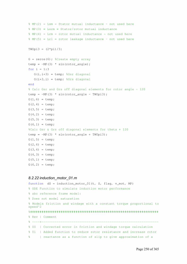
Page 250 of 365

% MP(2) = Lsm = Stator mutual inductance - not used here

% MP(3) = Lsrm = Stator/rotor mutual inductance

% MP(4) = Lrm = rotor mutual inductance - not used here

% MP(5) = Lrl = rotor leakage inductance - not used here

TWOpi3 = (2*pi)/3;

G = zeros(6); %Create empty array

temp = -MP(3) * sin(rotor_angle);

for i = 1:3

G(i,i+3) = temp; %Gsr diagonal

G(i+3,i) = temp; %Grs diagonal

end

% Calc Gsr and Grs off diagonal elements for rotor angle - 120

temp = -MP(3) * sin(rotor_angle - TWOpi3);

G(1,6) = temp;

G(2,4) = temp;

G(3,5) = temp;

G(4,2) = temp;

G(5,3) = temp;

G(6,1) = temp;

%Calc Gsr & Grs off diagonal elements for theta + 120

temp = -MP(3) * sin(rotor_angle + TWOpi3);

G(1,5) = temp;

G(2,6) = temp;

G(3,4) = temp;

G(4,3) = temp;

G(5,1) = temp;

G(6,2) = temp;

8.2.22 induction_motor_01.m function dS = induction_motor_01(t, S, flag, v_mot, MP)

% ODE Function to simulate induction motor performance

% abc reference frame model:

% Does not model saturation

% Models friction and windage with a constant torque proportional to speed^2

%####################################################################

% Rev | Comment

% ----+--------------------------------------------------------------

% 00 | Corrected error in friction and windage torque calculation

% 01 | Added function to reduce rotor resistance and increase rotor

% | reactance as a function of slip to give approximation of a

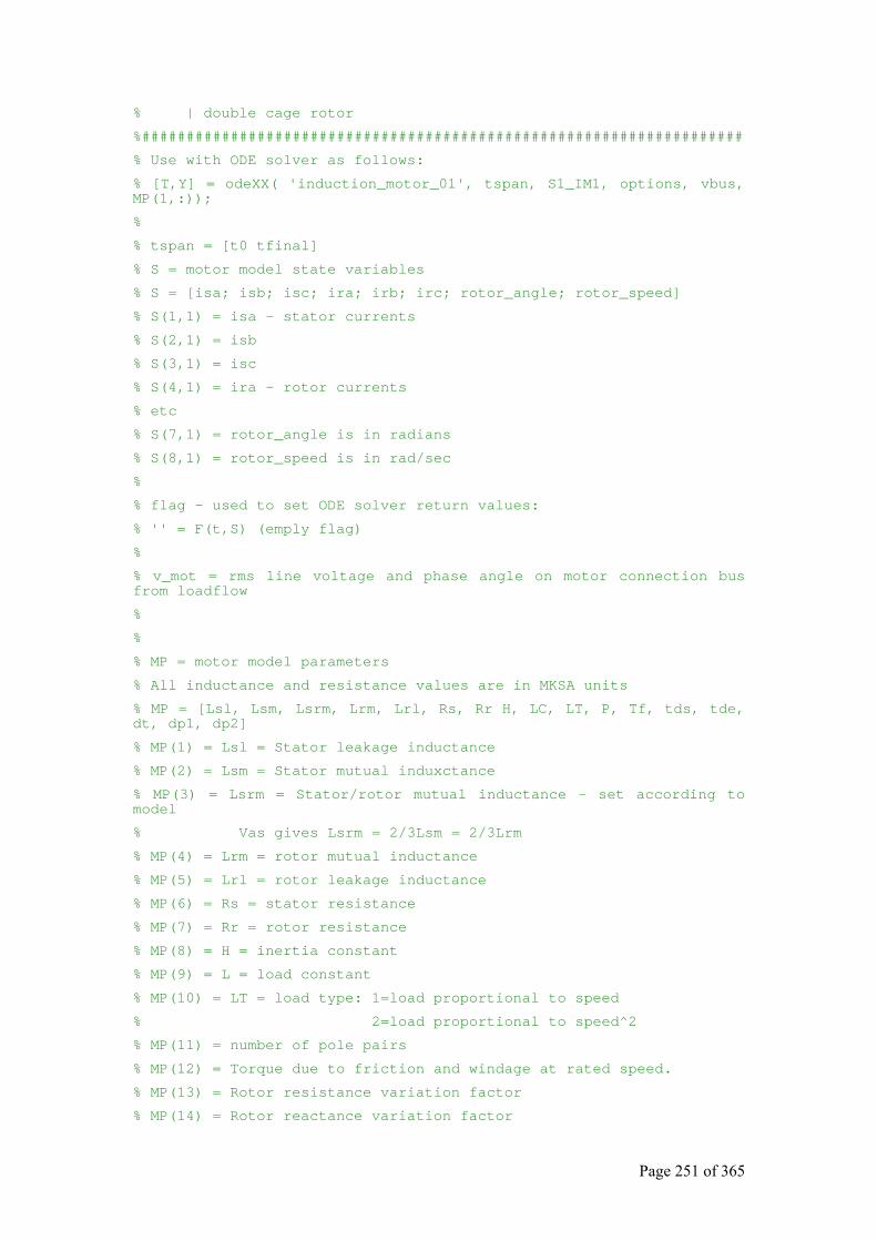
Page 251 of 365

% | double cage rotor

%####################################################################

% Use with ODE solver as follows:

% [T,Y] = odeXX( 'induction_motor_01', tspan, S1_IM1, options, vbus, MP(1,:));

%

% tspan = [t0 tfinal]

% S = motor model state variables

% S = [isa; isb; isc; ira; irb; irc; rotor_angle; rotor_speed]

% S(1,1) = isa - stator currents

% S(2,1) = isb

% S(3,1) = isc

% S(4,1) = ira - rotor currents

% etc

% S(7,1) = rotor_angle is in radians

% S(8,1) = rotor_speed is in rad/sec

%

% flag - used to set ODE solver return values:

% '' = F(t,S) (emply flag)

%

% v_mot = rms line voltage and phase angle on motor connection bus from loadflow

%

%

% MP = motor model parameters

% All inductance and resistance values are in MKSA units

% MP = [Lsl, Lsm, Lsrm, Lrm, Lrl, Rs, Rr H, LC, LT, P, Tf, tds, tde, dt, dp1, dp2]

% MP(1) = Lsl = Stator leakage inductance

% MP(2) = Lsm = Stator mutual induxctance

% MP(3) = Lsrm = Stator/rotor mutual inductance - set according to model

% Vas gives Lsrm = 2/3Lsm = 2/3Lrm

% MP(4) = Lrm = rotor mutual inductance

% MP(5) = Lrl = rotor leakage inductance

% MP(6) = Rs = stator resistance

% MP(7) = Rr = rotor resistance

% MP(8) = H = inertia constant

% MP(9) = L = load constant

% MP(10) = LT = load type: 1=load proportional to speed

% 2=load proportional to speed^2

% MP(11) = number of pole pairs

% MP(12) = Torque due to friction and windage at rated speed.

% MP(13) = Rotor resistance variation factor

% MP(14) = Rotor reactance variation factor

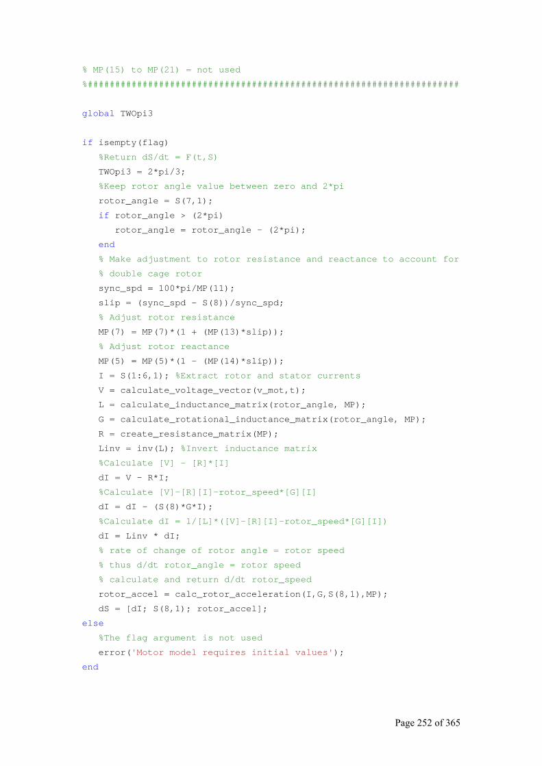
Page 252 of 365

% MP(15) to MP(21) = not used

%####################################################################

global TWOpi3

if isempty(flag)

%Return dS/dt = F(t,S)

TWOpi3 = 2*pi/3;

%Keep rotor angle value between zero and 2*pi

rotor_angle = S(7,1);

if rotor_angle > (2*pi)

rotor_angle = rotor_angle - (2*pi);

end

% Make adjustment to rotor resistance and reactance to account for

% double cage rotor

sync_spd = 100*pi/MP(11);

slip = (sync_spd - S(8))/sync_spd;

% Adjust rotor resistance

MP(7) = MP(7)*(1 + (MP(13)*slip));

% Adjust rotor reactance

MP(5) = MP(5)*(1 - (MP(14)*slip));

I = S(1:6,1); %Extract rotor and stator currents

V = calculate_voltage_vector(v_mot,t);

L = calculate_inductance_matrix(rotor_angle, MP);

G = calculate_rotational_inductance_matrix(rotor_angle, MP);

R = create_resistance_matrix(MP);

Linv = inv(L); %Invert inductance matrix

%Calculate [V] - [R]*[I]

dI = V - R*I;

%Calculate [V]-[R][I]-rotor_speed*[G][I]

dI = dI - (S(8)*G*I);

%Calculate dI = 1/[L]*([V]-[R][I]-rotor_speed*[G][I])

dI = Linv * dI;

% rate of change of rotor angle = rotor speed

% thus d/dt rotor_angle = rotor speed

% calculate and return d/dt rotor_speed

rotor_accel = calc_rotor_acceleration(I,G,S(8,1),MP);

dS = [dI; S(8,1); rotor_accel];

else

%The flag argument is not used

error('Motor model requires initial values');

end

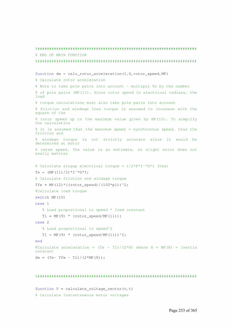
Page 253 of 365

%####################################################################

% END OF MAIN FUNCTION

%####################################################################

function dw = calc_rotor_acceleration(I,G,rotor_speed,MP)

% Calculate rotor acceleration

% Note to take pole pairs into account - multiply Te by the number

% of pole pairs (MP(11). Since rotor speed in electrical radians, the load

% torque calculations must also take pole pairs into account

% Friction and windage loss torque is assumed to increase with the square of the

% rotor speed up to the maximum value given by MP(12). To simplify the calculation

% it is assumed that the maximum speed = synchronous speed, thus the friction and

% windage torque is not strictly accurate since it would be determined at motor

% rated speed. The value is an estimate, so slight error does not really mattter

% Calculate airgap electrical torque = 1/2*P*I'*G*I (Vas)

Te = (MP(11)/2)*I'*G*I;

% Calculate friction and windage torque

Tfw = MP(12)*((rotor_speed)/(100*pi))^2;

%Calculate load torque

switch MP(10)

case 1

% Load proportional to speed * load constant

Tl = MP(9) * (rotor_speed/MP(11));

case 2

% Load proportional to speed^2

Tl = MP(9) * (rotor_speed/MP(11))^2;

end

%Calculate acceleration = (Te - Tl)/(2*H) where H = MP(8) = inertia constant

dw = (Te- Tfw - Tl)/(2*MP(8));

%####################################################################

function V = calculate_voltage_vector(v,t)

% Calculate instantaneous motor voltages

Page 254 of 365

% It is assumed that the motor is connected in star. v = the rms line voltage at the

% motor connection bus. The 30degree phase shift between Vline and Vphase is taken

% into account here and the phase (l-g) p-p voltage used in the model is calculated

% The phase voltage lags the line voltage by 30deg(pi/6) This is subtracted from the

% loadflow voltage angle to get the actual phase voltage angle.

% Vphase = Vline/sqrt(3) and Vpp = Vphase*sqrt(2)

global TWOpi3

V = zeros(6,1);

v_angle = v(2)-(pi/6); %Voltage angle from loadflow - 30degrees

% a = instantaneous bus voltage angle

a = (100 * pi * t)+ v_angle;

vpeak = v(1)*sqrt(2/3);

V(1,1) = vpeak*cos( a );

V(2,1) = vpeak*cos( a - TWOpi3);

V(3,1) = vpeak*cos( a + TWOpi3);

%####################################################################

function L = calculate_inductance_matrix(rotor_angle, MP)

% L = calculate_inductance_matrix(S(3), MP) - calculate motor inductance matrix

% MP(1) = Lsl = Stator leakage inductance

% MP(2) = Lsm = Stator mutual inductance

% MP(3) = Lsrm = Stator/rotor mutual inductance - this is set accoring to model

% MP(4) = Lrm = rotor mutual inductance

% MP(5) = Lrl = rotor leakage inductance

global TWOpi3

L = zeros(6); %Create empty array

temp = MP(1) + MP(2); % Lsm + Lsl - Smith/chen

for i = 1:3

L(i,i)=temp; %Lss diagonal elements

end

temp = MP(4) + MP(5); %Lrm + Lrl - Smith/Chen

for i = 4:6

L(i,i) = temp; %Lrr diagonal

end

Page 255 of 365

temp = -MP(2)/2; %Lss off diagonal elements = -Lsm/2

for i = 1:3

for j = 1:3

if i ~= j

L(i,j) = temp;

end

end

end

temp = -MP(4)/2; %Lrr off diagonal elements = -Lrm/2

for i = 4:6

for j = 4:6

if i ~= j

L(i,j) = temp;

end

end

end

temp = cos(rotor_angle)* MP(3); %cos(@)*Lsrm

for i = 1:3

L(i,i+3) = temp; %Lsr diagonal

L(i+3,i) = temp; %Lrs diagonal

end

% Calc Lsr off diagonal elements

temp = cos(rotor_angle - TWOpi3)*MP(3);

L(2,4) = temp;

L(3,5) = temp;

L(1,6) = temp;

L(4,2) = temp;

L(5,3) = temp;

L(6,1) = temp;

temp = cos(rotor_angle + TWOpi3)*MP(3);

L(1,5) = temp;

L(2,6) = temp;

L(3,4) = temp;

L(4,3) = temp;

L(5,1) = temp;

L(6,2) = temp;

%####################################################################

function G = calculate_rotational_inductance_matrix(rotor_angle, MP)

% G = calculate_rotational_inductance_matrix(rotor_angle, MP)

% rotor_angle = rotor electrical angle

% MP(1) = Lsl = Stator leakage inductance - not used here

Page 256 of 365

% MP(2) = Lsm = Stator mutual inductance - not used here

% MP(3) = Lsrm = Stator/rotor mutual inductance

% MP(4) = Lrm = rotor mutual inductance - not used here

% MP(5) = Lrl = rotor leakage inductance - not used here

global TWOpi3

G = zeros(6); %Create empty array

temp = -MP(3) * sin(rotor_angle);

for i = 1:3

G(i,i+3) = temp; %Gsr diagonal

G(i+3,i) = temp; %Grs diagonal

end

% Calc Gsr and Grs off diagonal elements for rotor angle - 120

temp = -MP(3) * sin(rotor_angle - TWOpi3);

G(1,6) = temp;

G(2,4) = temp;

G(3,5) = temp;

G(4,2) = temp;

G(5,3) = temp;

G(6,1) = temp;

%Calc Gsr & Grs off diagonal elements for theta + 120

temp = -MP(3) * sin(rotor_angle + TWOpi3);

G(1,5) = temp;

G(2,6) = temp;

G(3,4) = temp;

G(4,3) = temp;

G(5,1) = temp;

G(6,2) = temp;

%####################################################################

function R = create_resistance_matrix(MP)

% Create resistance matrix using Rs and Rr

R = eye(6);

Rs = R(1:3,:)*MP(6); %Enter Rs values into array

Rr = R(4:6,:)*MP(7); %Enter Rr values into array

R = [Rs;Rr]; %Form complete matrix

8.2.23 induction_motor_03.m function dS = induction_motor_03(t, S, flag, v_mot, MP)

% ODE Function to simulate induction motor performance

Page 257 of 365

% Simplified Equivalent Circuit d-q model cf Arrilaga pg. 212

% Does not model saturation

% #####################################################################

% Rev | Comment

% ----+--------------------------------------------------------------

% 00 | Initial version

% #####################################################################

% Use with ODE solver as follows:

% [T,Y] = solver('induction_motor_01', tspan , Y0,'',busdata, MP)

%

% tspan = [t0 tfinal]

% S = motor model state variables

% S = [ E'r; E'm; S; ]

% S(1,1) = E'r - Thevinin equivalent circuit voltage (real axis component)

% S(2,1) = E'm - Thevinin equivalent circuit voltage (imaginary axis component)

% S(3,1) = Slip

%

% flag - used to set ODE solver return values:

% '' = F(t,S) (emply flag)

%

% v_mot = [Vbus V_angle] where Vbus = rms l-l Bus voltage(kV)

%

% MP = motor model parameters in MKSA

%

% MP = [X', T'o, Xo, R1, Hm, L, LT, tds, tde, dt, dp1, dp2]

% MP(1) = X': Transient reactance

% MP(2) = T'o: open circuit time constant

% MP(3) = Xo: open circuit reactance

% MP(4) = R1: Stator resistance

% MP(5) = Hm = inertia constant

% MP(6) = L = load constant

% MP(7) = LT = load type: 1=load proportional to speed

% 2=load proportional to speed^2

% MP(8) = Disturbance start time - not used

% MP(9) = Disturbance end time - not used

% MP(10) = Disturbance type - not used

% MP(11) = Distrubance parameter 1 - not used

% MP(12) = Disturbance parameter 2 - not used

% MP(13) = Motor base MVA

% MP(14) - MP(21) are not used for this model

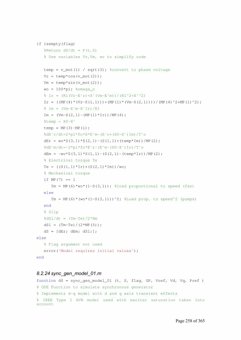
Page 258 of 365

if isempty(flag)

%Return dS/dt = F(t,S)

% Use variables Vr,Vm, wo to simplify code

temp = v_mot(1) / sqrt(3); %convert to phase voltage

Vr = temp*cos(v_mot(2));

Vm = temp*sin(v_mot(2));

wo = 100*pi; %omega_o

% Ir = (R1(Vr-E'r)+X'(Vm-E'm))/(R1^2+X'^2)

Ir = ((MP(4)*(Vr-S(1,1)))+(MP(1)*(Vm-S(2,1))))/(MP(4)^2+MP(1)^2);

% Im = (Vm-E'm-X'Ir)/R1

Im = (Vm-S(2,1)-(MP(1)*Ir))/MP(4);

%temp = X0-X'

temp = MP(3)-MP(1);

%dE'r/dt=2*pi*fo*S*E'm-(E'r+(X0-X')Im)/T'o

dEr = wo*S(3,1)*S(2,1)-(S(1,1)+(temp*Im))/MP(2);

%dE'm/dt=-2*pi*fo*E'r-(E'm-(X0-X')Ir)/T'o

dEm = -wo*S(3,1)*S(1,1)-(S(2,1)-(temp*Ir))/MP(2);

% Electrical torque Te

Te = ((S(1,1)*Ir)+(S(2,1)*Im))/wo;

% Mechanical torque

if MP(7) == 1

Tm = MP(6)*wo*(1-S(3,1)); %load proportional to speed (fan)

else

Tm = MP(6)*(wo*(1-S(3,1)))^2; %Load prop. to speed^2 (pumps)

end

% Slip

%dSl/dt = (Tm-Te)/2*Hm

dSl = (Tm-Te)/(2*MP(5));

dS = [dEr; dEm; dSl;];

else

% Flag argument not used

error('Model requires initial values');

end

8.2.24 sync_gen_model_01.m function dS = sync_gen_model_01 (t, S, flag, GP, Vref, Vd, Vq, Pref )

% ODE Function to simulate synchronous generator

% Implements d-q model with d and q axis transient effects

% IEEE Type I AVR model used with exciter saturation taken into account

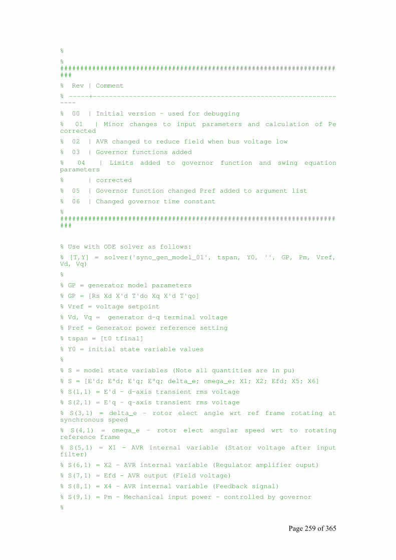
Page 259 of 365

%

% ########################################################################

% Rev | Comment

% -----+-----------------------------------------------------------------

% 00 | Initial version - used for debugging

% 01 | Minor changes to input parameters and calculation of Pe corrected

% 02 | AVR changed to reduce field when bus voltage low

% 03 | Governor functions added

% 04 | Limits added to governor function and swing equation parameters

% | corrected

% 05 | Governor function changed Pref added to argument list

% 06 | Changed governor time constant

% ########################################################################

% Use with ODE solver as follows:

% [T,Y] = solver('sync_gen_model_01', tspan, Y0, '', GP, Pm, Vref, Vd, Vq)

%

% GP = generator model parameters

% GP = [Rs Xd X'd T'do Xq X'd T'qo]

% Vref = voltage setpoint

% Vd, Vq = generator d-q terminal voltage

% Pref = Generator power reference setting

% tspan = [t0 tfinal]

% Y0 = initial state variable values

%

% S = model state variables (Note all quantities are in pu)

% S = [E'd; E"d; E'q; E"q; delta_e; omega_e; X1; X2; Efd; X5; X6]

% S(1,1) = E'd - d-axis transient rms voltage

% S(2,1) = E'q - q-axis transient rms voltage

% S(3,1) = delta_e - rotor elect angle wrt ref frame rotating at synchronous speed

% S(4,1) = omega_e - rotor elect angular speed wrt to rotating reference frame

% S(5,1) = X1 - AVR internal variable (Stator voltage after input filter)

% S(6,1) = X2 - AVR internal variable (Regulator amplifier ouput)

% S(7,1) = Efd - AVR output (Field voltage)

% S(8,1) = X4 - AVR internal variable (Feedback signal)

% S(9,1) = Pm - Mechanical input power - controlled by governor

%

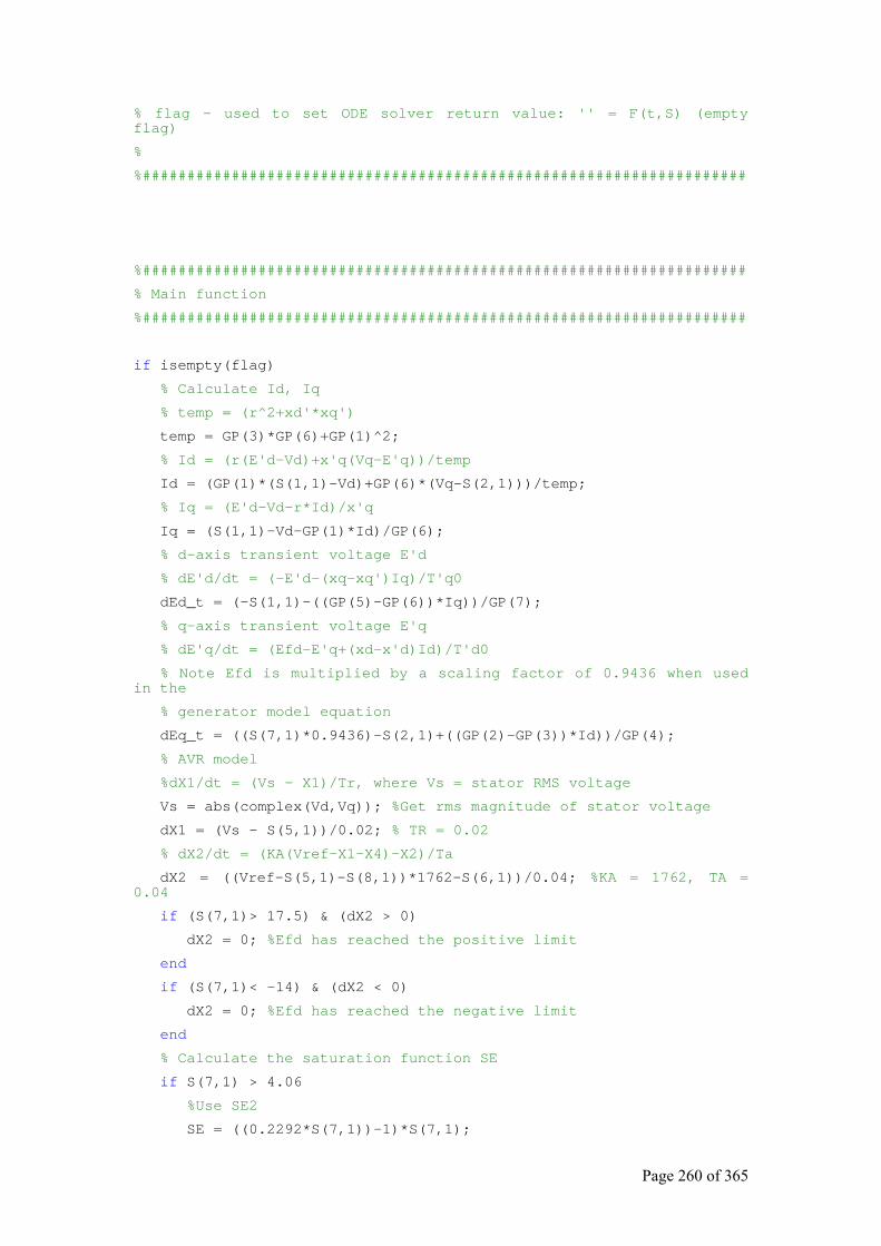
Page 260 of 365

% flag - used to set ODE solver return value: '' = F(t,S) (empty flag)

%

%####################################################################

%####################################################################

% Main function

%####################################################################

if isempty(flag)

% Calculate Id, Iq

% temp = (r^2+xd'*xq')

temp = GP(3)*GP(6)+GP(1)^2;

% Id = (r(E'd-Vd)+x'q(Vq-E'q))/temp

Id = (GP(1)*(S(1,1)-Vd)+GP(6)*(Vq-S(2,1)))/temp;

% Iq = (E'd-Vd-r*Id)/x'q

Iq = (S(1,1)-Vd-GP(1)*Id)/GP(6);

% d-axis transient voltage E'd

% dE'd/dt = (-E'd-(xq-xq')Iq)/T'q0

dEd_t = (-S(1,1)-((GP(5)-GP(6))*Iq))/GP(7);

% q-axis transient voltage E'q

% dE'q/dt = (Efd-E'q+(xd-x'd)Id)/T'd0

% Note Efd is multiplied by a scaling factor of 0.9436 when used in the

% generator model equation

dEq_t = ((S(7,1)*0.9436)-S(2,1)+((GP(2)-GP(3))*Id))/GP(4);

% AVR model

%dX1/dt = (Vs - X1)/Tr, where Vs = stator RMS voltage

Vs = abs(complex(Vd,Vq)); %Get rms magnitude of stator voltage

dX1 = (Vs - S(5,1))/0.02; % TR = 0.02

% dX2/dt = (KA(Vref-X1-X4)-X2)/Ta

dX2 = ((Vref-S(5,1)-S(8,1))*1762-S(6,1))/0.04; %KA = 1762, TA = 0.04

if (S(7,1)> 17.5) & (dX2 > 0)

dX2 = 0; %Efd has reached the positive limit

end

if (S(7,1)< -14) & (dX2 < 0)

dX2 = 0; %Efd has reached the negative limit

end

% Calculate the saturation function SE

if S(7,1) > 4.06

%Use SE2

SE = ((0.2292*S(7,1))-1)*S(7,1);

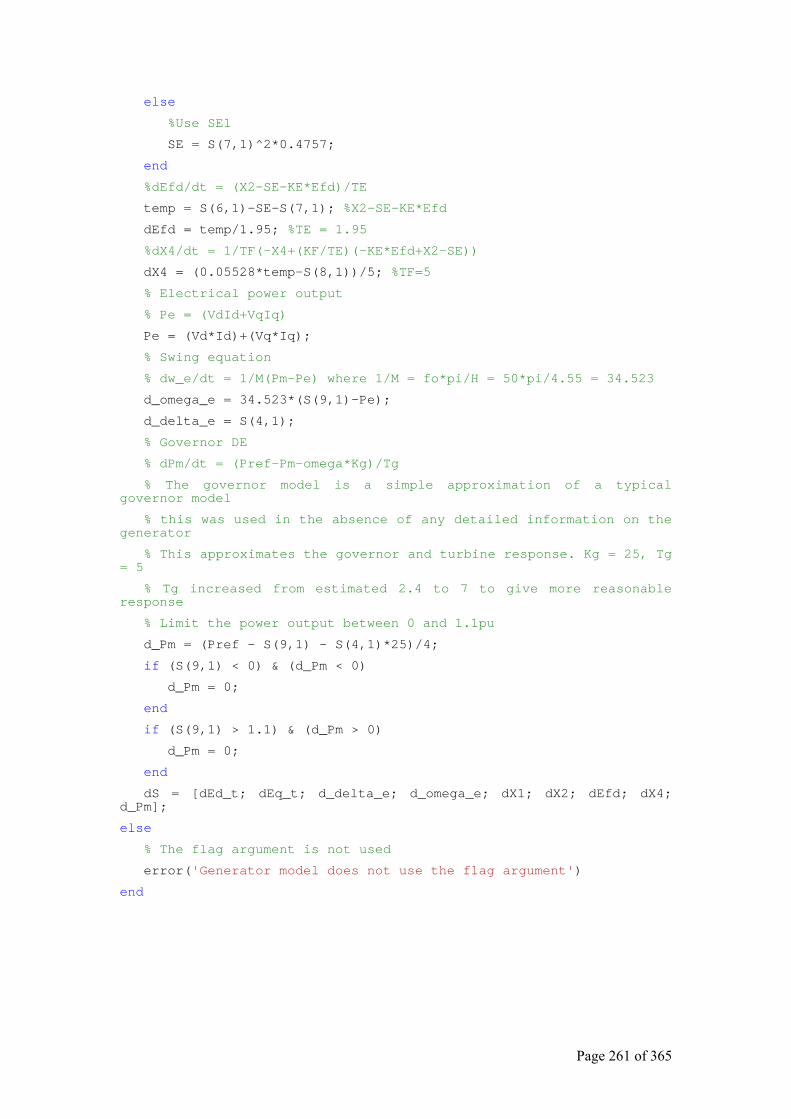
Page 261 of 365

else

%Use SE1

SE = S(7,1)^2*0.4757;

end

%dEfd/dt = (X2-SE-KE*Efd)/TE

temp = S(6,1)-SE-S(7,1); %X2-SE-KE*Efd

dEfd = temp/1.95; %TE = 1.95

%dX4/dt = 1/TF(-X4+(KF/TE)(-KE*Efd+X2-SE))

dX4 = (0.05528*temp-S(8,1))/5; %TF=5

% Electrical power output

% Pe = (VdId+VqIq)

Pe = (Vd*Id)+(Vq*Iq);

% Swing equation

% dw_e/dt = 1/M(Pm-Pe) where 1/M = fo*pi/H = 50*pi/4.55 = 34.523

d_omega_e = 34.523*(S(9,1)-Pe);

d_delta_e = S(4,1);

% Governor DE

% dPm/dt = (Pref-Pm-omega*Kg)/Tg

% The governor model is a simple approximation of a typical governor model

% this was used in the absence of any detailed information on the generator

% This approximates the governor and turbine response. Kg = 25, Tg = 5

% Tg increased from estimated 2.4 to 7 to give more reasonable response

% Limit the power output between 0 and 1.1pu

d_Pm = (Pref - S(9,1) - S(4,1)*25)/4;

if (S(9,1) < 0) & (d_Pm < 0)

d_Pm = 0;

end

if (S(9,1) > 1.1) & (d_Pm > 0)

d_Pm = 0;

end

dS = [dEd_t; dEq_t; d_delta_e; d_omega_e; dX1; dX2; dEfd; dX4; d_Pm];

else

% The flag argument is not used

error('Generator model does not use the flag argument')

end

Page 262 of 365

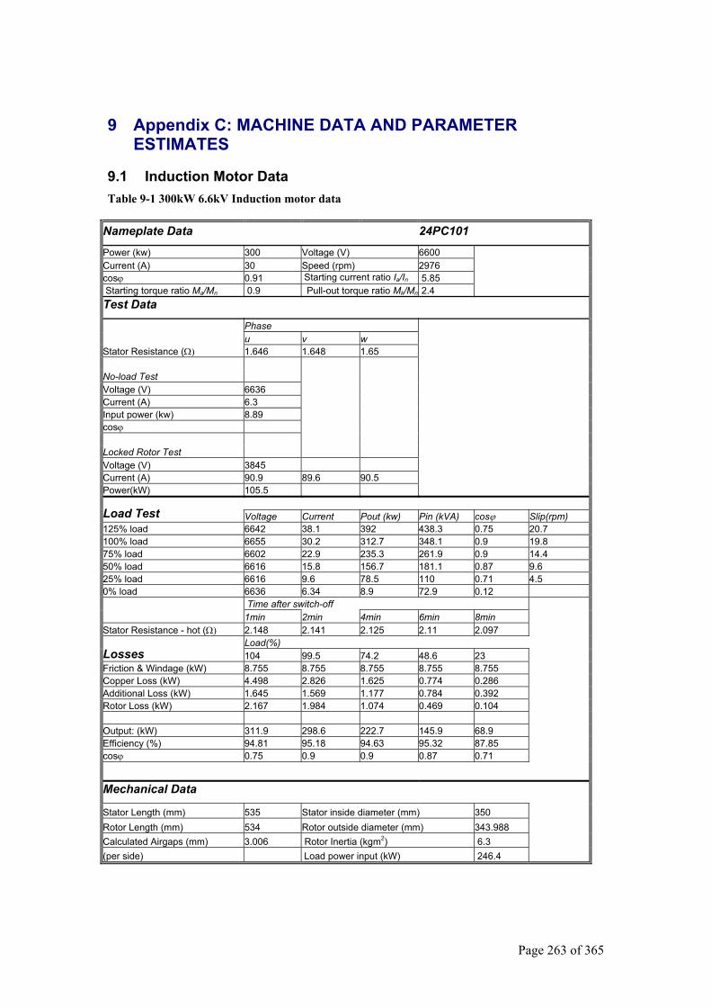
Page 263 of 365

9 Appendix C: MACHINE DATA AND PARAMETER ESTIMATES

9.1 Induction Motor Data Table 9-1 300kW 6.6kV Induction motor data

Nameplate Data 24PC101

Power (kw) 300 Voltage (V) 6600 Current (A) 30 Speed (rpm) 2976 cosϕ 0.91 Starting current ratio Ia/In 5.85 Starting torque ratio Ma/Mn 0.9 Pull-out torque ratio Mk/Mn 2.4 Test Data

Phase u v w Stator Resistance (Ω) 1.646 1.648 1.65 No-load Test Voltage (V) 6636 Current (A) 6.3 Input power (kw) 8.89 cosϕ Locked Rotor Test Voltage (V) 3845 Current (A) 90.9 89.6 90.5 Power(kW) 105.5

Load Test Voltage Current Pout (kw) Pin (kVA) cosϕ Slip(rpm) 125% load 6642 38.1 392 438.3 0.75 20.7 100% load 6655 30.2 312.7 348.1 0.9 19.8 75% load 6602 22.9 235.3 261.9 0.9 14.4 50% load 6616 15.8 156.7 181.1 0.87 9.6 25% load 6616 9.6 78.5 110 0.71 4.5 0% load 6636 6.34 8.9 72.9 0.12 Time after switch-off 1min 2min 4min 6min 8min Stator Resistance - hot (Ω) 2.148 2.141 2.125 2.11 2.097

Load(%) Losses 104 99.5 74.2 48.6 23 Friction & Windage (kW) 8.755 8.755 8.755 8.755 8.755 Copper Loss (kW) 4.498 2.826 1.625 0.774 0.286 Additional Loss (kW) 1.645 1.569 1.177 0.784 0.392 Rotor Loss (kW) 2.167 1.984 1.074 0.469 0.104 Output: (kW) 311.9 298.6 222.7 145.9 68.9 Efficiency (%) 94.81 95.18 94.63 95.32 87.85 cosϕ 0.75 0.9 0.9 0.87 0.71

Mechanical Data

Stator Length (mm) 535 Stator inside diameter (mm) 350 Rotor Length (mm) 534 Rotor outside diameter (mm) 343.988 Calculated Airgaps (mm) 3.006 Rotor Inertia (kgm2) 6.3 (per side) Load power input (kW) 246.4

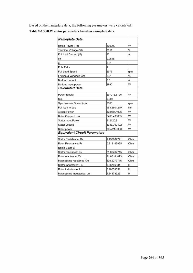
Page 264 of 365

Based on the nameplate data, the following parameters were calculated: Table 9-2 300kW motor parameters based on nameplate data

Nameplate Data

Rated Power (Pn) 300000 W Terminal Voltage (Vt) 3811 V Full load Current (Ifl) 30 A eff 0.9518 pf 0.91 Pole Pairs 1 Full Load Speed 2976 rpm Friction & Windage loss 2.91 % No-load current 6.3 A No-load input power 8890 W Calculated Data

Power (shaft) 297076.6726 W Slip 0.008 Synchronous Speed (rpm) 3000 rpm Full load torque 953.2504219 Nm Airgap Power 308187.1006 W Rotor Copper Loss 2465.496805 W Stator Input Power 312120.9 W Stator Losses 3933.799402 W Rotor power 305721.6038 W Equivalent Circuit Parameters

Stator Resistance: Rs 1.456962741 Ohm Rotor Resistance: Rr 0.913146965 Ohm Nema Class B Stator reactance: Xs 21.06762715 Ohm Rotor reactance: X'r 31.60144073 Ohm Magnetising reactance Xm 579.2277716 Ohm Stator inductance: Ls 0.06706034 H Rotor inductance: Lr 0.10059051 H Magnetising inductance: Lm 1.84373926 H

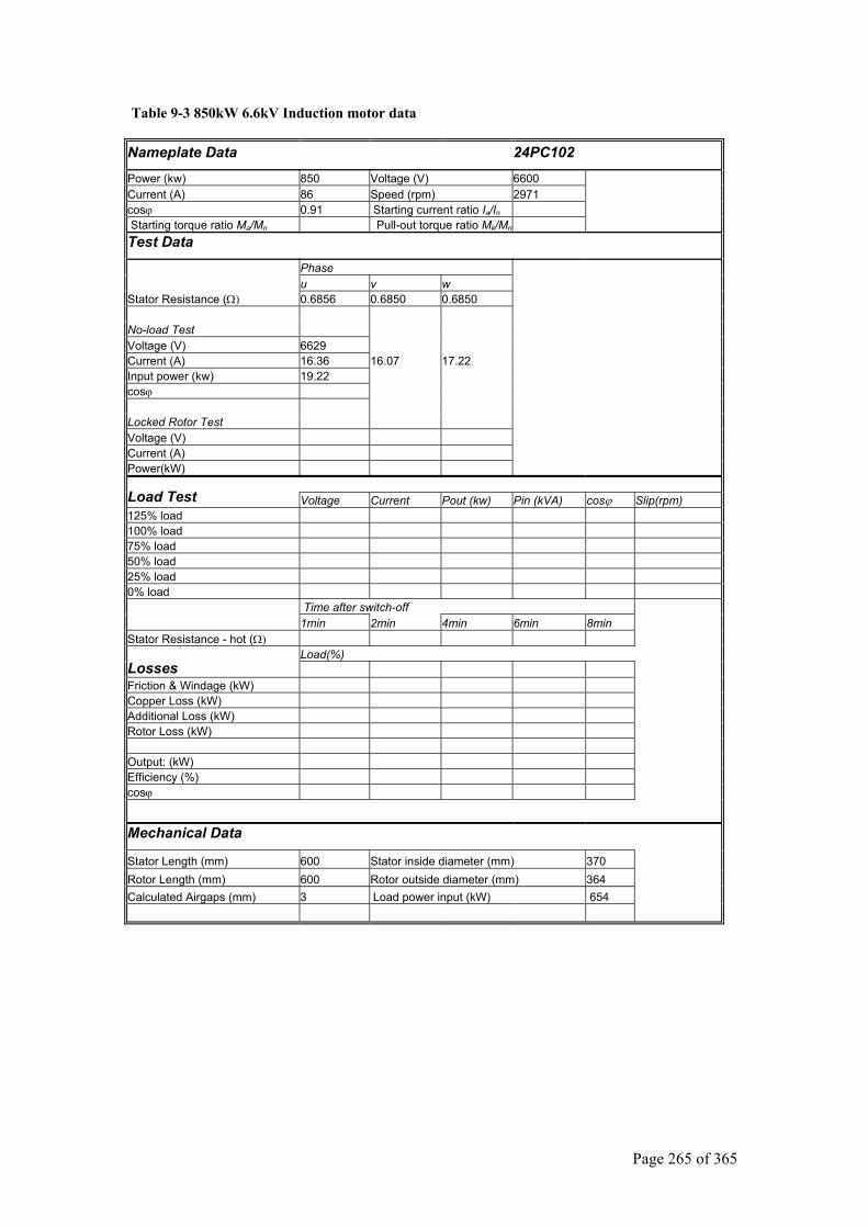
Page 265 of 365

Table 9-3 850kW 6.6kV Induction motor data

Nameplate Data 24PC102

Power (kw) 850 Voltage (V) 6600 Current (A) 86 Speed (rpm) 2971 cosϕ 0.91 Starting current ratio Ia/In Starting torque ratio Ma/Mn Pull-out torque ratio Mk/Mn Test Data

Phase u v w Stator Resistance (Ω) 0.6856 0.6850 0.6850 No-load Test Voltage (V) 6629 Current (A) 16.36 16.07 17.22 Input power (kw) 19.22 cosϕ Locked Rotor Test Voltage (V) Current (A) Power(kW)

Load Test Voltage Current Pout (kw) Pin (kVA) cosϕ Slip(rpm) 125% load 100% load 75% load 50% load 25% load 0% load Time after switch-off 1min 2min 4min 6min 8min Stator Resistance - hot (Ω)

Load(%) Losses Friction & Windage (kW) Copper Loss (kW) Additional Loss (kW) Rotor Loss (kW) Output: (kW) Efficiency (%) cosϕ

Mechanical Data

Stator Length (mm) 600 Stator inside diameter (mm) 370 Rotor Length (mm) 600 Rotor outside diameter (mm) 364 Calculated Airgaps (mm) 3 Load power input (kW) 654

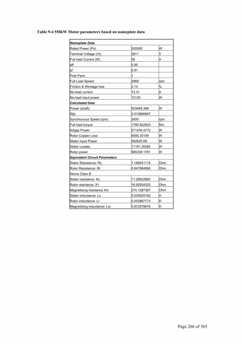
Page 266 of 365

Table 9-4 550kW Motor parameters based on nameplate data

Nameplate Data Rated Power (Pn) 550000 W Terminal Voltage (Vt) 3811 V Full load Current (Ifl) 56 A eff 0.95 pf 0.91 Pole Pairs 1 Full Load Speed 2968 rpm Friction & Windage loss 2.14 % No-load current 13.31 A No-load input power 12130 W Calculated Data Power (shaft) 553494.396 W Slip 0.010666667 Synchronous Speed (rpm) 3000 rpm Full load torque 1780.822825 Nm Airgap Power 571434.4772 W Rotor Copper Loss 6095.30109 W Stator Input Power 582625.68 W Stator Losses 11191.20284 W Rotor power 565339.1761 W Equivalent Circuit Parameters Stator Resistance: Rs 1.189541118 Ohm Rotor Resistance: Rr 0.647884895 Ohm

Nema Class B Stator reactance: Xs 11.28622883 Ohm Rotor reactance: X'r 16.92934325 Ohm Magnetising reactance Xm 274.1287387 Ohm Stator inductance: Ls 0.035925182 H Rotor inductance: Lr 0.053887773 H Magnetising inductance: Lm 0.872578876 H

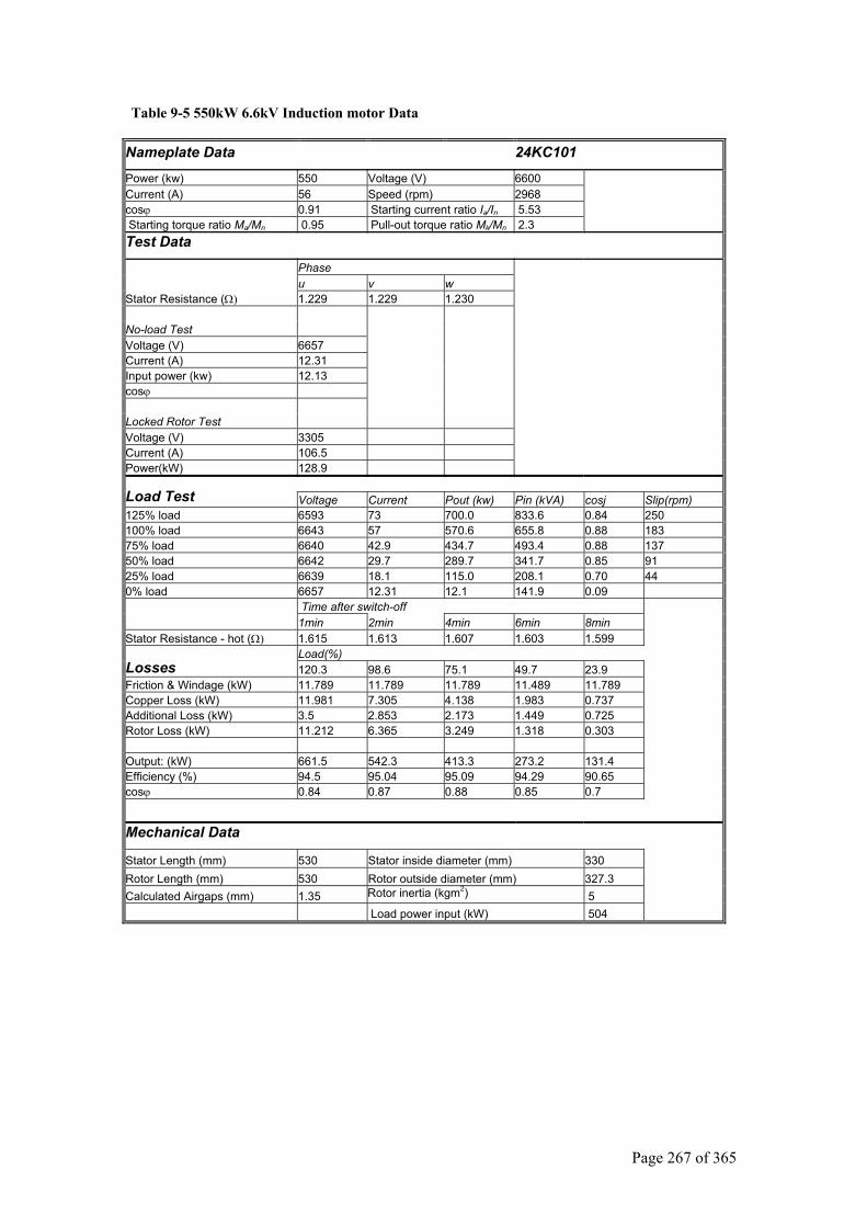
Page 267 of 365

Table 9-5 550kW 6.6kV Induction motor Data

Nameplate Data 24KC101

Power (kw) 550 Voltage (V) 6600 Current (A) 56 Speed (rpm) 2968 cosϕ 0.91 Starting current ratio Ia/In 5.53 Starting torque ratio Ma/Mn 0.95 Pull-out torque ratio Mk/Mn 2.3 Test Data

Phase u v w Stator Resistance (Ω) 1.229 1.229 1.230 No-load Test Voltage (V) 6657 Current (A) 12.31 Input power (kw) 12.13 cosϕ Locked Rotor Test Voltage (V) 3305 Current (A) 106.5 Power(kW) 128.9

Load Test Voltage Current Pout (kw) Pin (kVA) cosj Slip(rpm) 125% load 6593 73 700.0 833.6 0.84 250 100% load 6643 57 570.6 655.8 0.88 183 75% load 6640 42.9 434.7 493.4 0.88 137 50% load 6642 29.7 289.7 341.7 0.85 91 25% load 6639 18.1 115.0 208.1 0.70 44 0% load 6657 12.31 12.1 141.9 0.09 Time after switch-off 1min 2min 4min 6min 8min Stator Resistance - hot (Ω) 1.615 1.613 1.607 1.603 1.599

Load(%) Losses 120.3 98.6 75.1 49.7 23.9 Friction & Windage (kW) 11.789 11.789 11.789 11.489 11.789 Copper Loss (kW) 11.981 7.305 4.138 1.983 0.737 Additional Loss (kW) 3.5 2.853 2.173 1.449 0.725 Rotor Loss (kW) 11.212 6.365 3.249 1.318 0.303 Output: (kW) 661.5 542.3 413.3 273.2 131.4 Efficiency (%) 94.5 95.04 95.09 94.29 90.65 cosϕ 0.84 0.87 0.88 0.85 0.7

Mechanical Data

Stator Length (mm) 530 Stator inside diameter (mm) 330 Rotor Length (mm) 530 Rotor outside diameter (mm) 327.3 Calculated Airgaps (mm) 1.35 Rotor inertia (kgm2) 5 Load power input (kW) 504

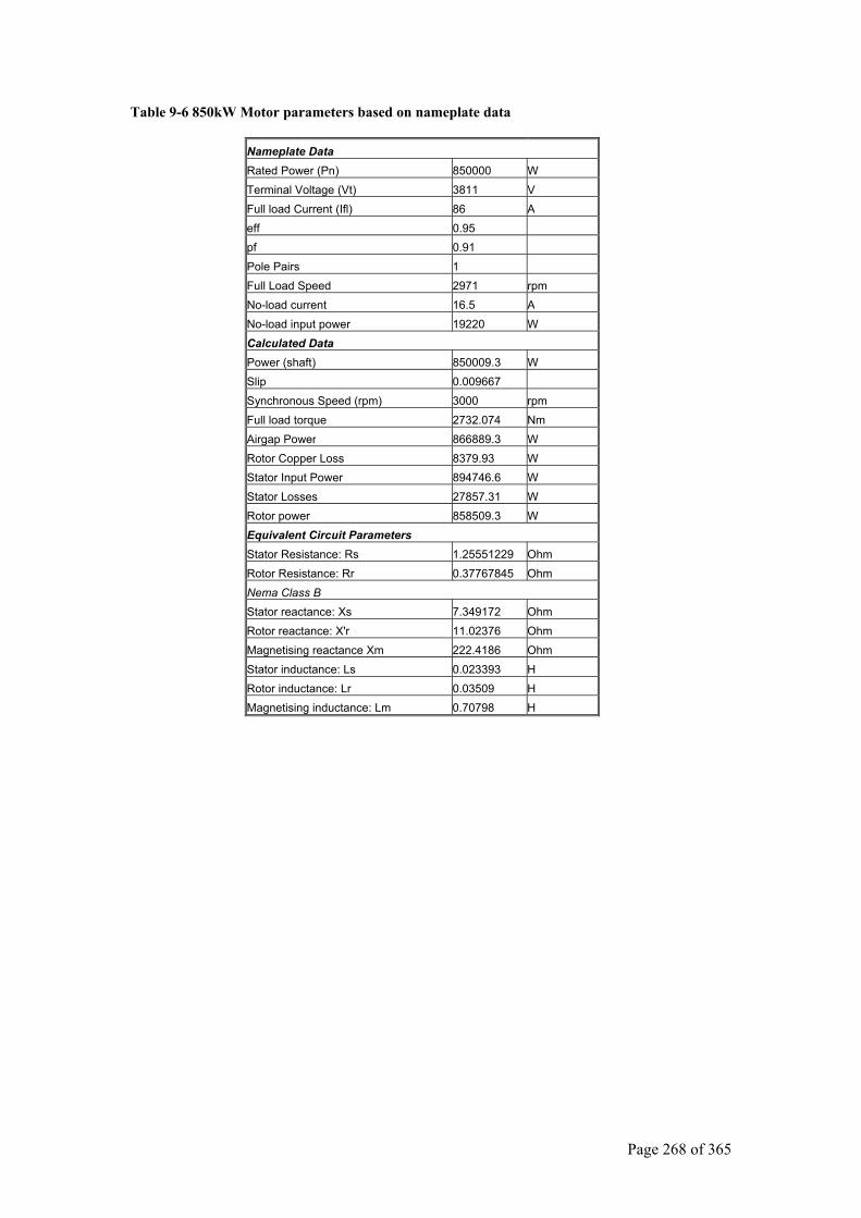
Page 268 of 365

Table 9-6 850kW Motor parameters based on nameplate data

Nameplate Data Rated Power (Pn) 850000 W Terminal Voltage (Vt) 3811 V Full load Current (Ifl) 86 A eff 0.95 pf 0.91 Pole Pairs 1 Full Load Speed 2971 rpm No-load current 16.5 A No-load input power 19220 W Calculated Data Power (shaft) 850009.3 W Slip 0.009667 Synchronous Speed (rpm) 3000 rpm Full load torque 2732.074 Nm Airgap Power 866889.3 W Rotor Copper Loss 8379.93 W Stator Input Power 894746.6 W Stator Losses 27857.31 W Rotor power 858509.3 W Equivalent Circuit Parameters Stator Resistance: Rs 1.25551229 Ohm Rotor Resistance: Rr 0.37767845 Ohm Nema Class B Stator reactance: Xs 7.349172 Ohm Rotor reactance: X'r 11.02376 Ohm Magnetising reactance Xm 222.4186 Ohm Stator inductance: Ls 0.023393 H Rotor inductance: Lr 0.03509 H Magnetising inductance: Lm 0.70798 H

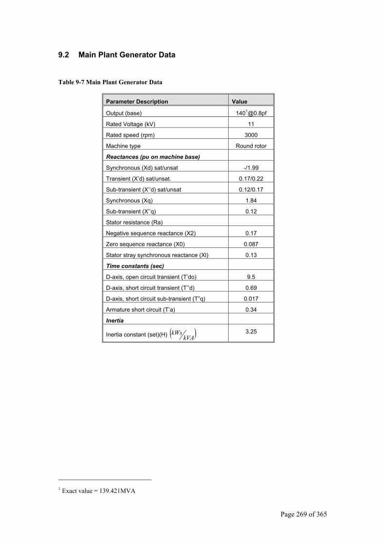
Page 269 of 365

9.2 Main Plant Generator Data

Table 9-7 Main Plant Generator Data

Parameter Description Value

Output (base) 1401@0.8pf

Rated Voltage (kV) 11

Rated speed (rpm) 3000

Machine type Round rotor

Reactances (pu on machine base)

Synchronous (Xd) sat/unsat -/1.99

Transient (X’d) sat/unsat. 0.17/0.22

Sub-transient (X’’d) sat/unsat 0.12/0.17

Synchronous (Xq) 1.84

Sub-transient (X’’q) 0.12

Stator resistance (Ra)

Negative sequence reactance (X2) 0.17

Zero sequence reactance (X0) 0.087

Stator stray synchronous reactance (Xl) 0.13

Time constants (sec)

D-axis, open circuit transient (T’do) 9.5

D-axis, short circuit transient (T’’d) 0.69

D-axis, short circuit sub-transient (T”q) 0.017

Armature short circuit (T’a) 0.34

Inertia

Inertia constant (set)(H) ( )kVAkWs 3.25

1 Exact value = 139.421MVA

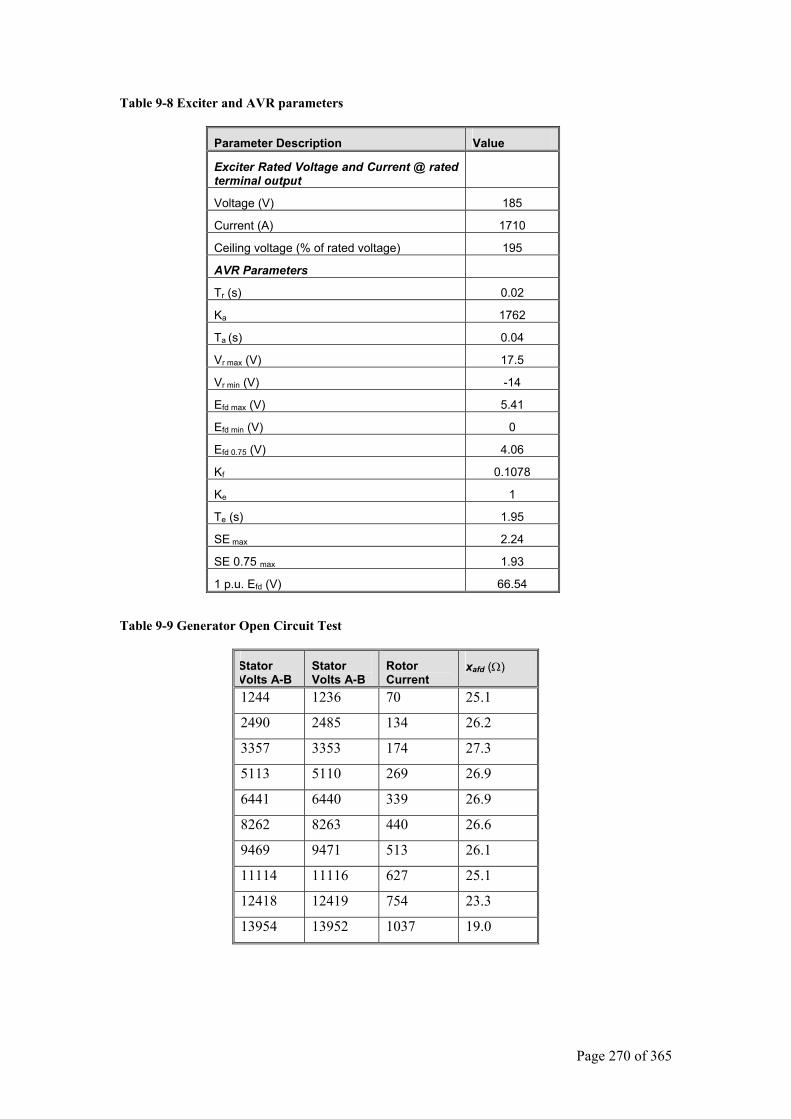
Page 270 of 365

Table 9-8 Exciter and AVR parameters

Parameter Description Value

Exciter Rated Voltage and Current @ rated terminal output

Voltage (V) 185

Current (A) 1710

Ceiling voltage (% of rated voltage) 195

AVR Parameters

Tr (s) 0.02

Ka 1762

Ta (s) 0.04

Vr max (V) 17.5

Vr min (V) -14

Efd max (V) 5.41

Efd min (V) 0

Efd 0.75 (V) 4.06

Kf 0.1078

Ke 1

Te (s) 1.95

SE max 2.24

SE 0.75 max 1.93

1 p.u. Efd (V) 66.54 Table 9-9 Generator Open Circuit Test

Stator Volts A-B

Stator Volts A-B

Rotor Current

xafd (Ω)

1244 1236 70 25.1

2490 2485 134 26.2

3357 3353 174 27.3

5113 5110 269 26.9

6441 6440 339 26.9

8262 8263 440 26.6

9469 9471 513 26.1

11114 11116 627 25.1

12418 12419 754 23.3

13954 13952 1037 19.0

Page 271 of 365

9.2.1 Scaling factor between generator and AVR pu systems In the generator model, it is assumed that 1p.u. field voltage will result in 1p.u. generator terminal voltage. Since the AVR and generator p.u systems differ, a scaling factor is required to convert from the one to the other.

The rotor field resistance is calculated from the exciter rated voltage and current as:

Ω== 10817.01710185

AVrfd

The stator open circuit rms voltage Efd is related to the exciter voltage vfd by equation (2-120) as:

fdfd

afdfd E

rx

v 323

=

From Table 9-9 data, the mutual rotor-stator reactance is estimated xafd = 26.8 Ω giving the following:

fdfd vE ⋅= 91.175

Thus for rated stator voltage of 11kV, a field voltage of

VkVEv fd

fd 79.6291.175

1191.175

===

is required. Now 1p.u. field voltage is 66.54V, thus 1p.u. field voltage needs to be multiplied by a factor of:

9436.054.6679.62

=

Thus the AVR model field voltage must be multiplied by 0.9346 before being used in the generator model equations.

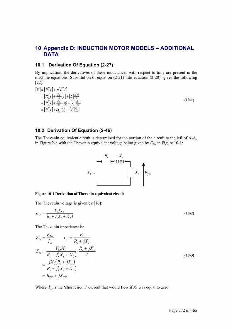
Page 272 of 365

10 Appendix D: INDUCTION MOTOR MODELS – ADDITIONAL DATA

10.1 Derivation Of Equation (2-27) By implication, the derivatives of these inductances with respect to time are present in the machine equations. Substitution of equation (2-21) into equation (2-20) gives the following [22]:

[ ] [ ][ ] [ ][ ][ ][ ] [ ] [ ] [ ] [ ]

[ ][ ] [ ] [ ] [ ]

[ ][ ] [ ] [ ] [ ]dt

Idd

Ldr

dtId

dtd

dLd

dtId

dtLd

LIR

LIR

LIIR

ILpIRV

++=

+⋅+=

++=

+=

θ

θθ

ω

(10-1)

10.2 Derivation Of Equation (2-46) The Thevenin equivalent circuit is determined for the portion of the circuit to the left of A-A, in Figure 2-8 with the Thevenin equivalent voltage being given by ETH in Figure 10-1:

Figure 10-1 Derivation of Thevenin equivalent circuit

The Thevenin voltage is given by [16]:

( )0

01

XXjRjXV

Ess

TH ++= (10-2)

The Thevenin impedance is:

( )( )

( )THTH

ss

ss

ss

ssth

sssc

sc

THth

jXRXXjR

jXRjXV

jXRXXjR

jXVZ

jXRVI

IEZ

+=++

+=

+⋅

++=

+==

0

0

10

01

1

(10-3)

Where scI is the ‘short circuit’ current that would flow if X0 was equal to zero.

ω,1V

sR sX

0XTHE

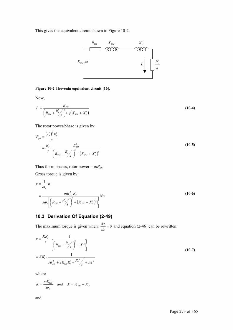
Page 273 of 365

This gives the equivalent circuit shown in Figure 10-2:

Figure 10-2 Thevenin equivalent circuit [16].

Now,

( )rTHr

TH

TH

XXjsRR

EI′++

′+

=1 (10-4)

The rotor power/phase is given by:

( )

( )22

2

2

rTHr

TH

THr

rrph

XXsRR

Es

Rs

RIP

′++

′+

⋅′

=

′′=

(10-5)

Thus for m phases, rotor power = mPph.

Gross torque is given by:

( )Nm

XXsRRs

RmE

p

rTHr

THs

rTH

s

′++

′+

′=

=

22

2

1

ω

ωτ

(10-6)

10.3 Derivation Of Equation (2-49)

The maximum torque is given when: 0=dsdτ and equation (2-46) can be rewritten:

22

2

22

2

1

1

sXsRRRsR

RK

XsRR

sRK

rrTHTH

r

rTH

r

+′+′+⋅′=

+

′+

⋅′

=τ

(10-7)

where

rTHs

TH XXXandmEK ′+==ω

2

and

THR THX rX ′

sRr′

1Iω,THE

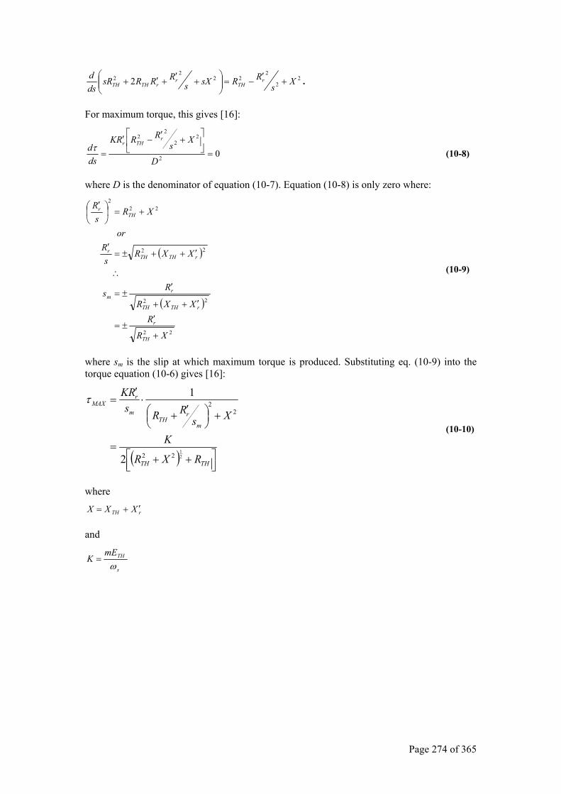
Page 274 of 365

22

222

22 2 X

sRRsXs

RRRsRdsd r

THr

rTHTH +′−=

+′+′+ .

For maximum torque, this gives [16]:

02

22

22

=

+′−′

=D

Xs

RRRK

dsd

rTHrτ (10-8)

where D is the denominator of equation (10-7). Equation (10-8) is only zero where:

( )

( )

22

22

22

222

XR

RXXR

Rs

XXRs

Ror

XRs

R

TH

r

rTHTH

rm

rTHTHr

THr

+

′±=

′++

′±=

∴

′++±=′

+=

′

(10-9)

where sm is the slip at which maximum torque is produced. Substituting eq. (10-9) into the torque equation (10-6) gives [16]:

( )

++

=

+

′+

⋅′

=

THTH

m

rTH

m

rMAX

RXR

K

XsRRs

RK

21

22

22

2

1τ

(10-10)

where

rTH XXX ′+=

and

s

THmEK

ω=

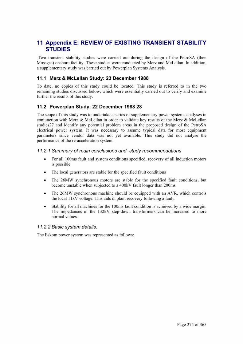
Page 275 of 365

11 Appendix E: REVIEW OF EXISTING TRANSIENT STABILITY STUDIES

Two transient stability studies were carried out during the design of the PetroSA (then Mossgas) onshore facility. These studies were conducted by Merz and McLellan. In addition, a supplementary study was carried out by Powerplan Systems Analysis.

11.1 Merz & McLellan Study: 23 December 1988 To date, no copies of this study could be located. This study is referred to in the two remaining studies discussed below, which were essentially carried out to verify and examine further the results of this study.

11.2 Powerplan Study: 22 December 1988 28 The scope of this study was to undertake a series of supplementary power systems analyses in conjunction with Merz & McLellan in order to validate key results of the Merz & McLellan studies27 and identify any potential problem areas in the proposed design of the PetroSA electrical power system. It was necessary to assume typical data for most equipment parameters since vendor data was not yet available. This study did not analyse the performance of the re-acceleration system.

11.2.1 Summary of main conclusions and study recommendations • For all 100ms fault and system conditions specified, recovery of all induction motors

is possible.

• The local generators are stable for the specified fault conditions

• The 26MW synchronous motors are stable for the specified fault conditions, but become unstable when subjected to a 400kV fault longer than 200ms.

• The 26MW synchronous machine should be equipped with an AVR, which controls the local 11kV voltage. This aids in plant recovery following a fault.

• Stability for all machines for the 100ms fault condition is achieved by a wide margin. The impedances of the 132kV step-down transformers can be increased to more normal values.

11.2.2 Basic system details. The Eskom power system was represented as follows:

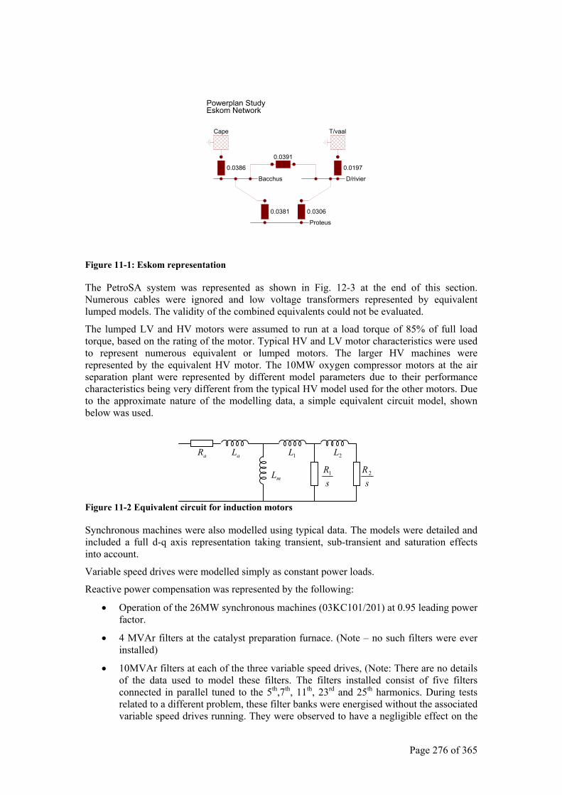
Page 276 of 365

Figure 11-1: Eskom representation

The PetroSA system was represented as shown in Fig. 12-3 at the end of this section. Numerous cables were ignored and low voltage transformers represented by equivalent lumped models. The validity of the combined equivalents could not be evaluated.

The lumped LV and HV motors were assumed to run at a load torque of 85% of full load torque, based on the rating of the motor. Typical HV and LV motor characteristics were used to represent numerous equivalent or lumped motors. The larger HV machines were represented by the equivalent HV motor. The 10MW oxygen compressor motors at the air separation plant were represented by different model parameters due to their performance characteristics being very different from the typical HV model used for the other motors. Due to the approximate nature of the modelling data, a simple equivalent circuit model, shown below was used.

Figure 11-2 Equivalent circuit for induction motors

Synchronous machines were also modelled using typical data. The models were detailed and included a full d-q axis representation taking transient, sub-transient and saturation effects into account.

Variable speed drives were modelled simply as constant power loads.

Reactive power compensation was represented by the following:

• Operation of the 26MW synchronous machines (03KC101/201) at 0.95 leading power factor.

• 4 MVAr filters at the catalyst preparation furnace. (Note – no such filters were ever installed)

• 10MVAr filters at each of the three variable speed drives, (Note: There are no details of the data used to model these filters. The filters installed consist of five filters connected in parallel tuned to the 5th,7th, 11th, 23rd and 25th harmonics. During tests related to a different problem, these filter banks were energised without the associated variable speed drives running. They were observed to have a negligible effect on the

Cape

0.0386

Bacchus

0.0391

D/rivier

0.0197

T/vaal

Proteus

0.0381 0.0306

Powerplan StudyEskom Network

aR aL

mL

1L

sR1

2L

sR2

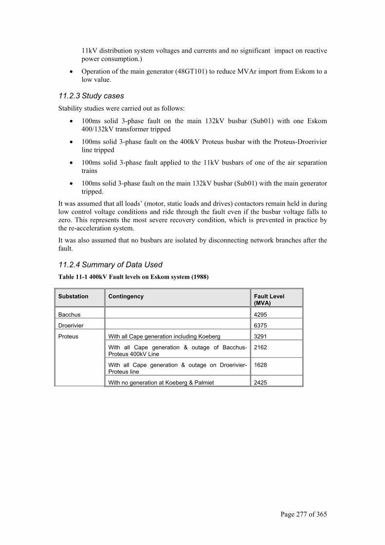
Page 277 of 365

11kV distribution system voltages and currents and no significant impact on reactive power consumption.)

• Operation of the main generator (48GT101) to reduce MVAr import from Eskom to a low value.

11.2.3 Study cases Stability studies were carried out as follows:

• 100ms solid 3-phase fault on the main 132kV busbar (Sub01) with one Eskom 400/132kV transformer tripped

• 100ms solid 3-phase fault on the 400kV Proteus busbar with the Proteus-Droerivier line tripped

• 100ms solid 3-phase fault applied to the 11kV busbars of one of the air separation trains

• 100ms solid 3-phase fault on the main 132kV busbar (Sub01) with the main generator tripped.

It was assumed that all loads’ (motor, static loads and drives) contactors remain held in during low control voltage conditions and ride through the fault even if the busbar voltage falls to zero. This represents the most severe recovery condition, which is prevented in practice by the re-acceleration system.

It was also assumed that no busbars are isolated by disconnecting network branches after the fault.

11.2.4 Summary of Data Used Table 11-1 400kV Fault levels on Eskom system (1988)

Substation Contingency Fault Level (MVA)

Bacchus 4295

Droerivier 6375

With all Cape generation including Koeberg 3291

With all Cape generation & outage of Bacchus-Proteus 400kV Line

2162

With all Cape generation & outage on Droerivier-Proteus line

1628

Proteus

With no generation at Koeberg & Palmiet 2425

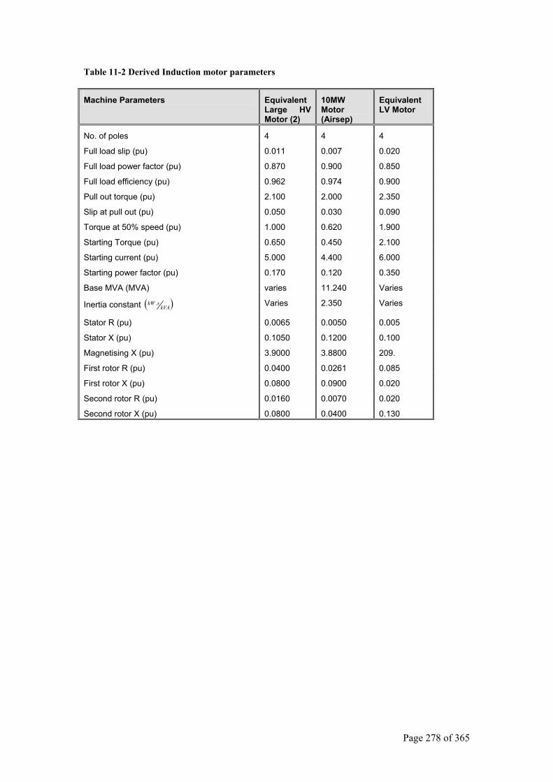
Page 278 of 365

Table 11-2 Derived Induction motor parameters

Machine Parameters Equivalent Large HV Motor (2)

10MW Motor (Airsep)

Equivalent LV Motor

No. of poles 4 4 4

Full load slip (pu) 0.011 0.007 0.020

Full load power factor (pu) 0.870 0.900 0.850

Full load efficiency (pu) 0.962 0.974 0.900

Pull out torque (pu) 2.100 2.000 2.350

Slip at pull out (pu) 0.050 0.030 0.090

Torque at 50% speed (pu) 1.000 0.620 1.900

Starting Torque (pu) 0.650 0.450 2.100

Starting current (pu) 5.000 4.400 6.000

Starting power factor (pu) 0.170 0.120 0.350

Base MVA (MVA) varies 11.240 Varies

Inertia constant ( )kVAskW . Varies 2.350 Varies

Stator R (pu) 0.0065 0.0050 0.005

Stator X (pu) 0.1050 0.1200 0.100

Magnetising X (pu) 3.9000 3.8800 209.

First rotor R (pu) 0.0400 0.0261 0.085

First rotor X (pu) 0.0800 0.0900 0.020

Second rotor R (pu) 0.0160 0.0070 0.020

Second rotor X (pu) 0.0800 0.0400 0.130

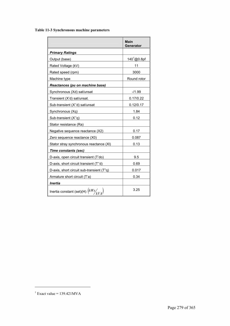
Page 279 of 365

Table 11-3 Synchronous machine parameters

Main Generator

Primary Ratings

Output (base) 1401@0.8pf

Rated Voltage (kV) 11

Rated speed (rpm) 3000

Machine type Round rotor

Reactances (pu on machine base)

Synchronous (Xd) sat/unsat -/1.99

Transient (X’d) sat/unsat. 0.17/0.22

Sub-transient (X’’d) sat/unsat 0.12/0.17

Synchronous (Xq) 1.84

Sub-transient (X’’q) 0.12

Stator resistance (Ra)

Negative sequence reactance (X2) 0.17

Zero sequence reactance (X0) 0.087

Stator stray synchronous reactance (Xl) 0.13

Time constants (sec)

D-axis, open circuit transient (T’do) 9.5

D-axis, short circuit transient (T’’d) 0.69

D-axis, short circuit sub-transient (T”q) 0.017

Armature short circuit (T’a) 0.34

Inertia

Inertia constant (set)(H) ( )kVAkWs 3.25

1 Exact value = 139.421MVA

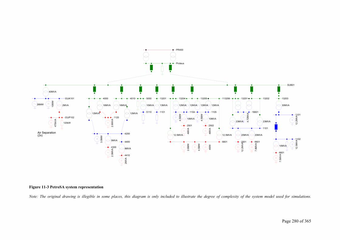
Page 280 of 365

Figure 11-3 PetroSA system representation

Note: The original drawing is illegible in some places, this diagram is only included to illustrate the degree of complexity of the system model used for simulations.

40MVA

26MW

10M

W

03JK101

2MVA

03JP102

470k

VA

120kW

Air Separation(2x)

4000

16MVA

12MVA

4010

16MVA

12MVA

1120

2.6M

VA

4200

3.5M

W

5MVA

4300

2.5M

VA

4400

8MVA

4410

2MV

A

5000

10MVA

5110

13201

13MVA

1101

13204

12MVA 12MVA

1104

13205

12MVA

4.5M

W

10MVA

2501

4MV

A

12.5MVA

1105

12MVA

113206

4.5M

W

10MVA

2502

4MV

A

12.5MVA

6601

2.6M

W

4.5M

W

4MW

13201

16601

23MVA 4.72

MV

A

23MVA

13202

1101

20MVA 20MVA

2501 6601

12.2

MV

A

7.8M

VA

SUB01

13203

1101

30MVA

12.2

MV

A

1102

12.5

MV

A

10MVA

6601

7.5M

VA

Proteus

PR400

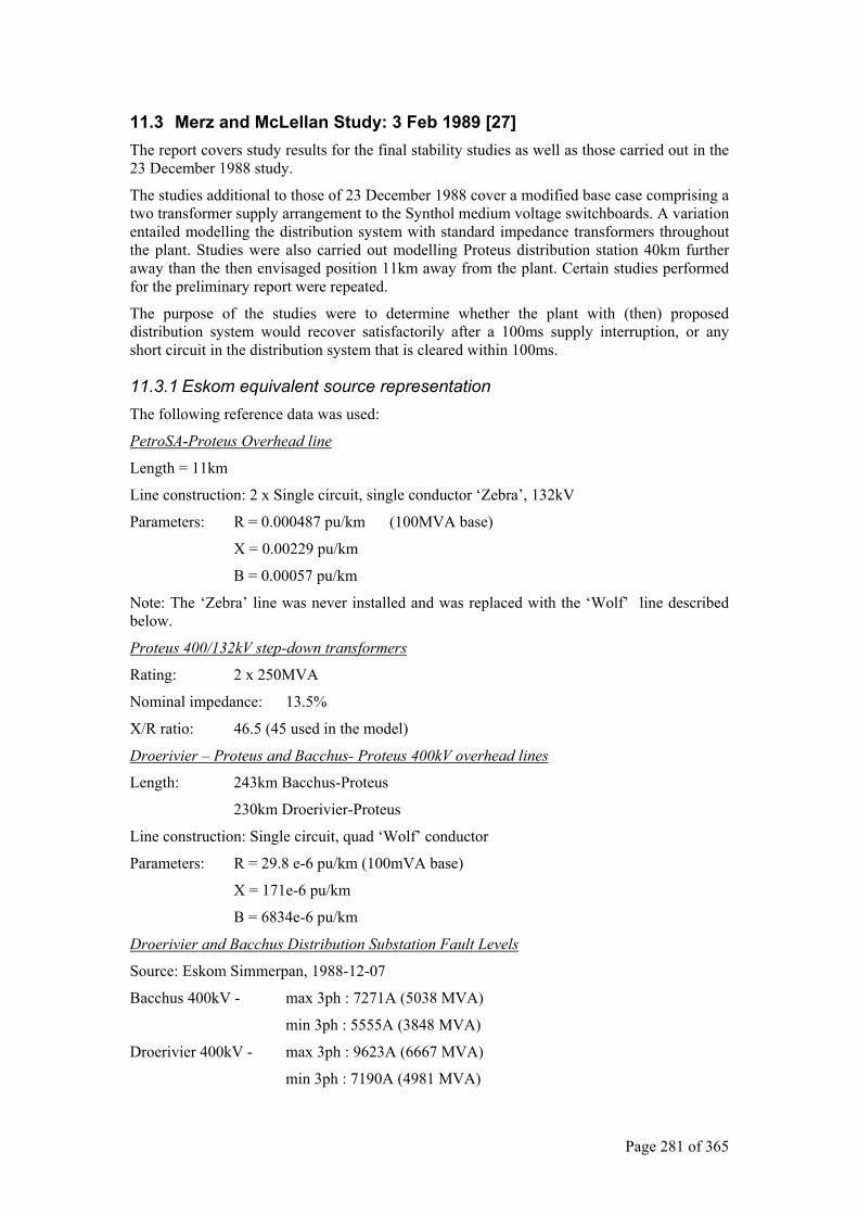
Page 281 of 365

11.3 Merz and McLellan Study: 3 Feb 1989 [27] The report covers study results for the final stability studies as well as those carried out in the 23 December 1988 study.

The studies additional to those of 23 December 1988 cover a modified base case comprising a two transformer supply arrangement to the Synthol medium voltage switchboards. A variation entailed modelling the distribution system with standard impedance transformers throughout the plant. Studies were also carried out modelling Proteus distribution station 40km further away than the then envisaged position 11km away from the plant. Certain studies performed for the preliminary report were repeated.

The purpose of the studies were to determine whether the plant with (then) proposed distribution system would recover satisfactorily after a 100ms supply interruption, or any short circuit in the distribution system that is cleared within 100ms.

11.3.1 Eskom equivalent source representation The following reference data was used:

PetroSA-Proteus Overhead line

Length = 11km

Line construction: 2 x Single circuit, single conductor ‘Zebra’, 132kV

Parameters: R = 0.000487 pu/km (100MVA base)

X = 0.00229 pu/km

B = 0.00057 pu/km

Note: The ‘Zebra’ line was never installed and was replaced with the ‘Wolf’ line described below.

Proteus 400/132kV step-down transformers

Rating: 2 x 250MVA

Nominal impedance: 13.5%

X/R ratio: 46.5 (45 used in the model)

Droerivier – Proteus and Bacchus- Proteus 400kV overhead lines

Length: 243km Bacchus-Proteus

230km Droerivier-Proteus

Line construction: Single circuit, quad ‘Wolf’ conductor

Parameters: R = 29.8 e-6 pu/km (100mVA base)

X = 171e-6 pu/km

B = 6834e-6 pu/km

Droerivier and Bacchus Distribution Substation Fault Levels

Source: Eskom Simmerpan, 1988-12-07

Bacchus 400kV - max 3ph : 7271A (5038 MVA)

min 3ph : 5555A (3848 MVA)

Droerivier 400kV - max 3ph : 9623A (6667 MVA)

min 3ph : 7190A (4981 MVA)

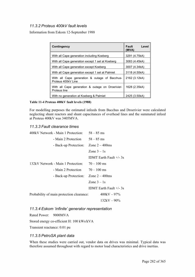
Page 282 of 365

11.3.2 Proteus 400kV fault levels Information from Eskom 12-September 1988

Contingency Fault Level (MVA)

With all Cape generation including Koeberg 3291 (4.75kA)

With all Cape generation except 1 set at Koeberg 3083 (4.45kA)

With all Cape generation except Koeberg 3007 (4.34kA)

With all Cape generation except 1 set at Palmiet 3118 (4.50kA)

With all Cape generation & outage of Bacchus-Proteus 400kV Line

2162 (3.12kA)

With all Cape generation & outage on Droerivier-Proteus line

1628 (2.35kA)

With no generation at Koeberg & Palmiet 2425 (3.50kA)

Table 11-4 Proteus 400kV fault levels (1988)

For modelling purposes the estimated infeeds from Bacchus and Droerivier were calculated neglecting shunt reactors and shunt capacitances of overhead lines and the summated infeed at Proteus 400kV was 3405MVA.

11.3.3 Fault clearance times 400kV Network - Main 1 Protection: 58 – 85 ms

- Main 2 Protection 58 – 85 ms

- Back-up Protection: Zone 2 – 400ms

Zone 3 – 1s

IDMT Earth Fault +/- 3s

132kV Network - Main 1 Protection: 70 – 100 ms

- Main 2 Protection 70 – 100 ms

- Back-up Protection: Zone 2 – 400ms

Zone 3 – 1s

IDMT Earth Fault +/- 3s

Probability of main protection clearance: 400kV – 97%

132kV – 90%

11.3.4 Eskom ‘infinite’ generator representation Rated Power: 9000MVA

Stored energy co-efficient H: 100 kWs/kVA

Transient reactance: 0.01 pu

11.3.5 PetroSA plant data When these studies were carried out, vendor data on drives was minimal. Typical data was therefore assumed throughout with regard to motor load characteristics and drive inertias.

Page 283 of 365

Information on the Total Feed Compressor variable speed drives was not firm and these were represented as a constant power (PQ) type load.. This load was assumed to be switched out during the period the fault persisted and switched in after fault clearance. Note that this assumption was correct, since the variable speed drives will block firing pulses to the inverter thyristors during a voltage dip, effectively disconnecting the drives from the 11kV supply. If the bus voltage returns to normal within 180ms, normal operation is restored. In practice, the impact on the system is relatively minor with the variable speed drive smoothly accelerating the compressor motor to its pre-fault speed and load.

In general, summated equivalent loads based on available load lists were used. An effort was also made to bring the databases used by Merz and McLellan and Powerplan into closer agreement. This was largely done, except in the way rotating machines are modelled, The induction machine parameters, AVR and governor models differ significantly.

11.3.6 Synchronous machines Some parameters for the 33MVA Air separation machines were available from preliminary bid data. Typical data had to be assumed for the plant generators with regard to machine parameters, AVR and governor data.

A dqo axis model is used which includes saturation and transients. A simple first order governor model featuring 4% droop and 5s time delay was used for the generators. The governor representation was not considered important since it only becomes significant when assessing machine performance 5 seconds or more after a disturbance. The influence on transient stability was considered small, since it is readily apparent after 1-2sec duration if the system will recover or not.

Different AVR models for the Air separation machines were used and performance discussed. The machine parameters used were similar to those used by Powerplan.

11.3.7 Induction machines Where possible, preliminary data was used for modelling MV induction machines. This mainly applied to the duty cycle and inertia constant. Real equivalent machine model data was only available for the oxygen compressors (03KC102/202)

LV machines were treated a lumped machines of an equivalent summated loading. Small HV machines where no data was available were similarly modelled as lumped machines.

Induction machine modelling is based on a simple equivalent linear impedance model. Saturation is not taken into account and only rotor resistance is changed as a function of slip.

11.4 Study Results From the load flow study the estimated infeed from Eskom was 102.5MW + 2.7MVAr (lagging) assuming 80MW generation on the main generator and 7.76MW on the critical generator. The reactive power delivered by the synchronous machines was calculated as follows:

120MVA generator 48GT101 - 55MVAr (max. 72)

12.5MVA generator 48GT102 - 5MVAr (max. 8)

33 MVA motors 03KC101/201 - 7.9MVAr (max. 19.5)

From the above figures, it is evident that adequate spare reactive power capacity is available to limit reactive power drawn from Eskom. It was concluded that the PetroSA system would recover satisfactorily after a 100ms supply interruption, or any short circuit in the distribution system that is cleared within 100ms.

Page 284 of 365

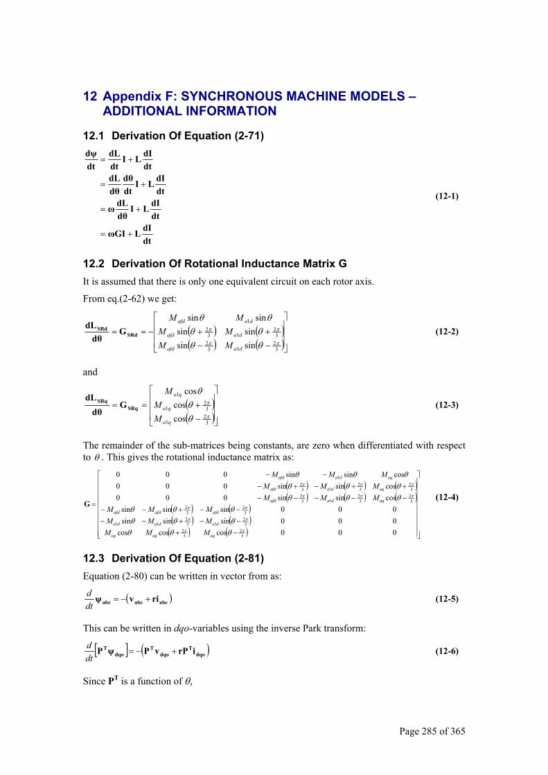
Page 285 of 365

12 Appendix F: SYNCHRONOUS MACHINE MODELS – ADDITIONAL INFORMATION

12.1 Derivation Of Equation (2-71)

dtdILωGI

dtdILI

dθdLω

dtdILI

dtdθ

dθdL

dtdILI

dtdL

dtdψ

+=

+=

+=

+=

(12-1)

12.2 Derivation Of Rotational Inductance Matrix G It is assumed that there is only one equivalent circuit on each rotor axis.

From eq.(2-62) we get:

( ) ( )( ) ( )

−−++−==

32

132

32

132

1

sinsinsinsin

sinsin

ππ

ππ

θθθθ

θθ

daafd

daafd

daafd

MMMM

MM

SRdSRd G

dθdL

(12-2)

and

( )( )

−+==

32

1

32

1

1

coscos

cos

π

π

θθ

θ

qa

qa

qa

MM

M

SRqSRq G

dθdL

(12-3)

The remainder of the sub-matrices being constants, are zero when differentiated with respect to θ . This gives the rotational inductance matrix as:

( ) ( ) ( )( ) ( ) ( )

( ) ( )( ) ( )

( ) ( )

−+−−+−−−−+−−

−−−−−++−+−

−−

=

000coscoscos000sinsinsin000sinsinsin

cossinsin000cossinsin000

cossinsin000

32

32

32

132

11

32

32

32

32

132

32

32

132

1

ππ

ππ

ππ

πππ

πππ

θθθθθθθθθ

θθθθθθ

θθθ

aqaqaq

dadada

afdafdafd

aqdaafd

aqdaafd

aqdaafd

MMMMMMMMM

MMMMMM

MMM

G (12-4)

12.3 Derivation Of Equation (2-81) Equation (2-80) can be written in vector from as:

( )abcabcabc rivψ +−=dtd (12-5)

This can be written in dqo-variables using the inverse Park transform:

[ ] ( )dqoT

dqoT

dqoT irPvPψP +−=

dtd (12-6)

Since PT is a function of θ,

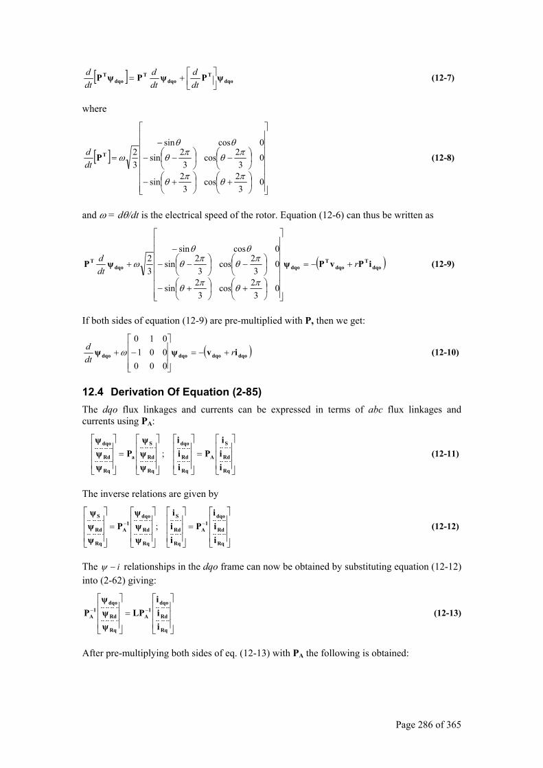
Page 286 of 365

[ ] dqoT

dqoT

dqoT ψPψPψP

+=

dtd

dtd

dtd (12-7)

where

[ ]

+

+−

−

−−

−

=

03

2cos3

2sin

03

2cos3

2sin

0cossin

32

πθπθ

πθπθ

θθ

ωTPdtd (12-8)

and ω = dθ/dt is the electrical speed of the rotor. Equation (12-6) can thus be written as

( )dqoT

dqoT

dqodqoT iPvPψψP r

dtd

+−=

+

+−

−

−−

−

+

03

2cos3

2sin

03

2cos3

2sin

0cossin

32

πθπθ

πθπθ

θθ

ω (12-9)

If both sides of equation (12-9) are pre-multiplied with P, then we get:

( )dqodqodqodqo ivψψ rdtd

+−=

−+

000001010

ω (12-10)

12.4 Derivation Of Equation (2-85) The dqo flux linkages and currents can be expressed in terms of abc flux linkages and currents using PA:

=

=

Rq

Rd

S

A

Rq

Rd

dqo

Rq

Rd

S

a

Rq

Rd

dqo

iii

Piii

ψψψ

Pψψψ

; (12-11)

The inverse relations are given by

=

=

−−

Rq

Rd

dqo1

A

Rq

Rd

S

Rq

Rd

dqo1

A

Rq

Rd

S

iii

Piii

ψψψ

Pψψψ

; (12-12)

The i−ψ relationships in the dqo frame can now be obtained by substituting equation (12-12) into (2-62) giving:

=

−−

Rq

Rd

dqo1

A

Rq

Rd

dqo1

A

iii

LPψψψ

P (12-13)

After pre-multiplying both sides of eq. (12-13) with PA the following is obtained:

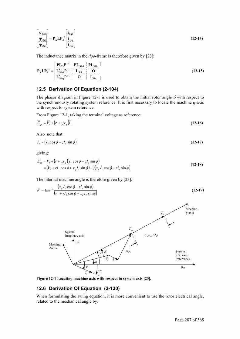
Page 287 of 365

=

−

Rq

Ra

dqo1

AA

Rq

Rd

dqo

iii

LPPψψψ

(12-14)

The inductance matrix in the dqo-frame is therefore given by [23]:

=−

−

−

−

Rq1T

SRq

Rd1T

SRd

SRqSRd1

S1

AA

LOPLOLPL

PLPLPPLLPP (12-15)

12.5 Derivation Of Equation (2-104) The phasor diagram in Figure 12-1 is used to obtain the initial rotor angle δ with respect to the synchronously rotating system reference. It is first necessary to locate the machine q-axis with respect to system reference.

From Figure 12-1, taking the terminal voltage as reference:

( ) tqttqt IjxrVE ++= (12-16)

Also note that:

( )φφ sincos ttt jIII −= (12-17)

giving:

( )( )( ) ( )φφφφ

φφ

sincossincos

sincos

ttqtqtt

ttqtqt

rIIxjIxrIV

jIIjxrVE

−+++=

−++= (12-18)

The internal machine angle is therefore given by [23]:

( )( )φφ

φφδ

sincossincos

tan 1

tqtt

ttq

IxrIVrIIx

++

−=′ − (12-19)

Figure 12-1 Locating machine axis with respect to system axis [23].

12.6 Derivation Of Equation (2-130) When formulating the swing equation, it is more convenient to use the rotor electrical angle, related to the mechanical angle by:

System Imaginary axis

Machine d-axis

System Real axis (reference)

Im

Re

Machine q-axis

qtE

IE

tq Ijx

tIr

tI φ

-γ

β

δδ’

tV

(xd-xq)(-Id)

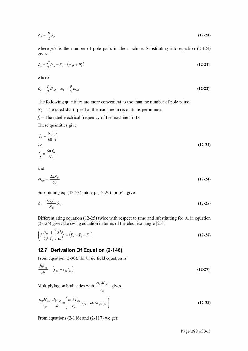
Page 288 of 365

mep δδ2

= (12-20)

where p/2 is the number of pole pairs in the machine. Substituting into equation (2-124) gives:

( )002θωθδδ ′+−== tp

eme (12-21)

where

00 2;

2 mmepp ωωδθ == (12-22)

The following quantities are more convenient to use than the number of pole pairs:

N0 – The rated shaft speed of the machine in revolutions per minute

f0 – The rated electrical frequency of the machine in Hz.

These quantities give:

0

0

00

602

260

Nfp

or

pNf

=

=

(12-23)

and

602 0

0N

mπ

ω = (12-24)

Substituting eq. (12-23) into eq. (12-20) for p/2 gives:

me Nf

δδ0

060= (12-25)

Differentiating equation (12-25) twice with respect to time and substituting for δm in equation (2-125) gives the swing equation in terms of the electrical angle [23]:

( )Dgme TTT

dtd

fNI −−=

2

2

0

0 160

δ (12-26)

12.7 Derivation Of Equation (2-146) From equation (2-90), the basic field equation is:

( )fdfdfdfd irv

dtd

−=ψ

(12-27)

Multiplying on both sides with fd

afd

rM0ω

gives

−= fdafdfd

fd

afdfd

fd

afd iMvrM

dtd

rM

000 ω

ωψω (12-28)

From equations (2-116) and (2-117) we get:

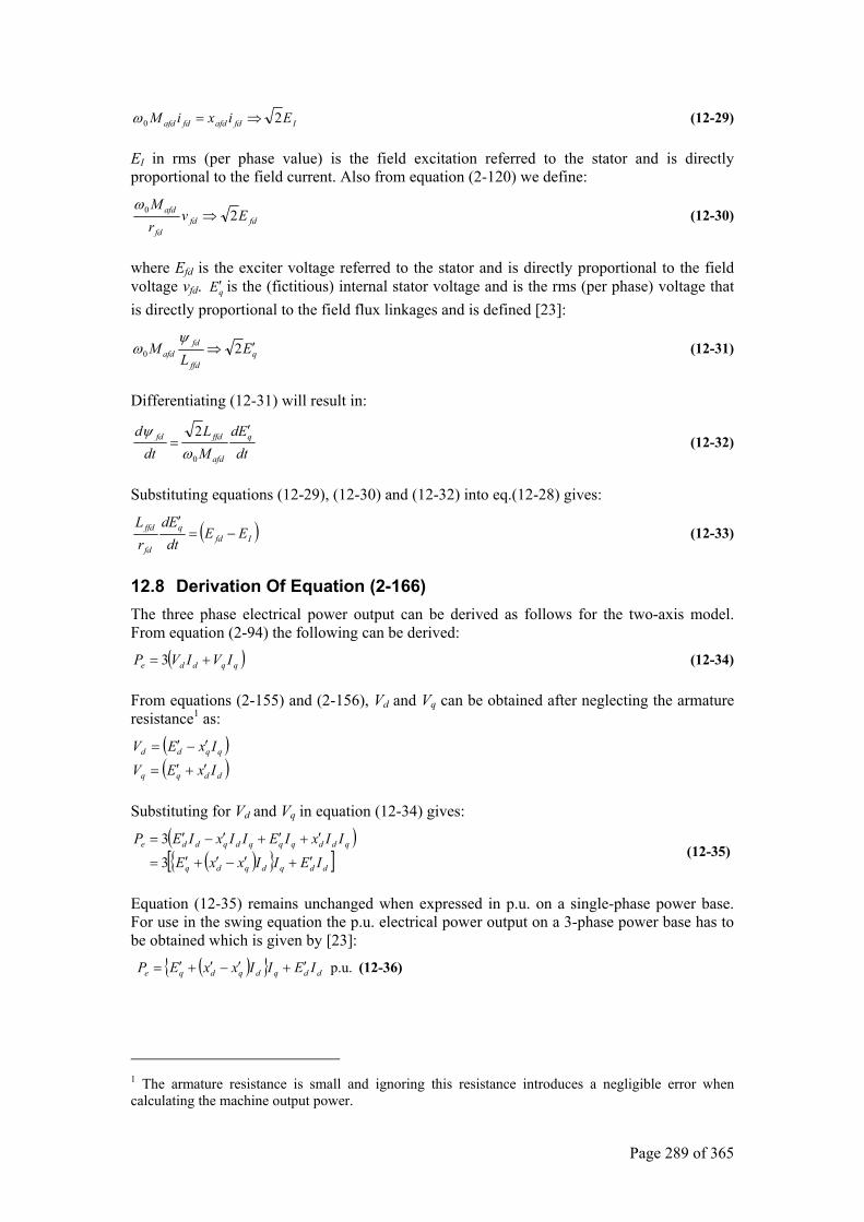
Page 289 of 365

Ifdafdfdafd EixiM 20 ⇒=ω (12-29)

EI in rms (per phase value) is the field excitation referred to the stator and is directly proportional to the field current. Also from equation (2-120) we define:

fdfdfd

afd EvrM

20 ⇒ω

(12-30)

where Efd is the exciter voltage referred to the stator and is directly proportional to the field voltage vfd. qE′ is the (fictitious) internal stator voltage and is the rms (per phase) voltage that is directly proportional to the field flux linkages and is defined [23]:

qffd

fdafd E

LM ′⇒ 20

ψω (12-31)

Differentiating (12-31) will result in:

dtEd

ML

dtd q

afd

ffdfd ′=

0

2ω

ψ (12-32)

Substituting equations (12-29), (12-30) and (12-32) into eq.(12-28) gives:

( )Ifdq

fd

ffd EEdtEd

rL

−=′

(12-33)

12.8 Derivation Of Equation (2-166) The three phase electrical power output can be derived as follows for the two-axis model. From equation (2-94) the following can be derived:

( )qqdde IVIVP += 3 (12-34)

From equations (2-155) and (2-156), Vd and Vq can be obtained after neglecting the armature resistance1 as:

( )( )ddqq

qqdd

IxEV

IxEV′+′=

′−′=

Substituting for Vd and Vq in equation (12-34) gives:

( )( ) [ ]ddqdqdq

qddqqqdqdde

IEIIxxE

IIxIEIIxIEP′+′−′+′=

′+′+′−′=

3

3 (12-35)

Equation (12-35) remains unchanged when expressed in p.u. on a single-phase power base. For use in the swing equation the p.u. electrical power output on a 3-phase power base has to be obtained which is given by [23]:

( ) p.u. ddqdqdqe IEIIxxEP ′+′−′+′= (12-36)

1 The armature resistance is small and ignoring this resistance introduces a negligible error when calculating the machine output power.

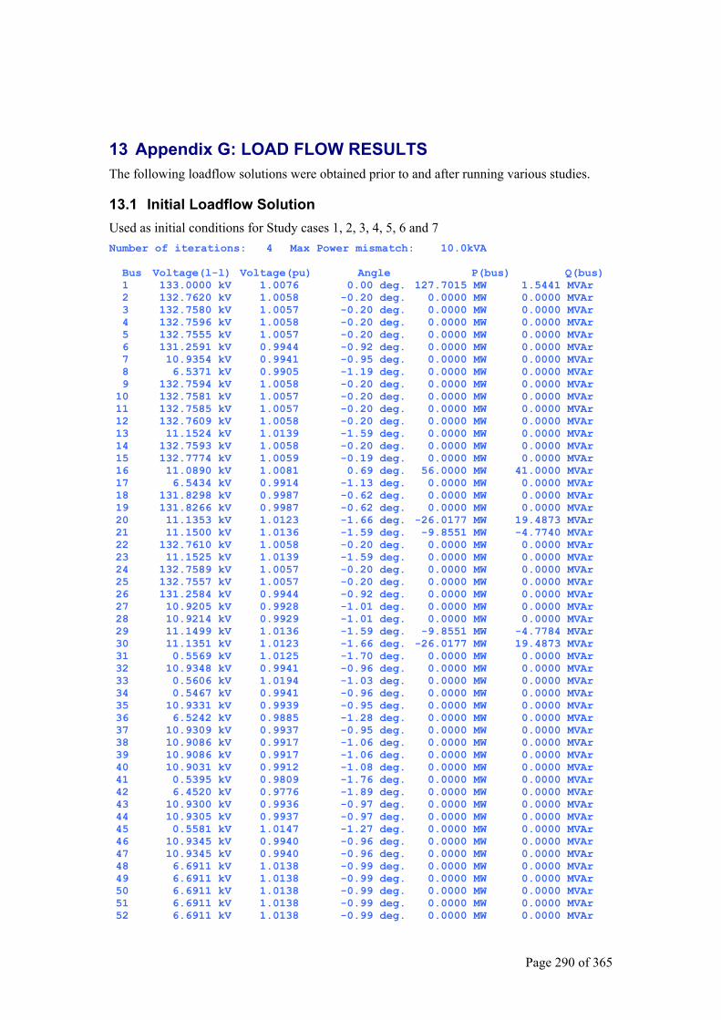
Page 290 of 365

13 Appendix G: LOAD FLOW RESULTS The following loadflow solutions were obtained prior to and after running various studies.

13.1 Initial Loadflow Solution Used as initial conditions for Study cases 1, 2, 3, 4, 5, 6 and 7 Number of iterations: 4 Max Power mismatch: 10.0kVA Bus Voltage(l-l) Voltage(pu) Angle P(bus) Q(bus) 1 133.0000 kV 1.0076 0.00 deg. 127.7015 MW 1.5441 MVAr 2 132.7620 kV 1.0058 -0.20 deg. 0.0000 MW 0.0000 MVAr 3 132.7580 kV 1.0057 -0.20 deg. 0.0000 MW 0.0000 MVAr 4 132.7596 kV 1.0058 -0.20 deg. 0.0000 MW 0.0000 MVAr 5 132.7555 kV 1.0057 -0.20 deg. 0.0000 MW 0.0000 MVAr 6 131.2591 kV 0.9944 -0.92 deg. 0.0000 MW 0.0000 MVAr 7 10.9354 kV 0.9941 -0.95 deg. 0.0000 MW 0.0000 MVAr 8 6.5371 kV 0.9905 -1.19 deg. 0.0000 MW 0.0000 MVAr 9 132.7594 kV 1.0058 -0.20 deg. 0.0000 MW 0.0000 MVAr 10 132.7581 kV 1.0057 -0.20 deg. 0.0000 MW 0.0000 MVAr 11 132.7585 kV 1.0057 -0.20 deg. 0.0000 MW 0.0000 MVAr 12 132.7609 kV 1.0058 -0.20 deg. 0.0000 MW 0.0000 MVAr 13 11.1524 kV 1.0139 -1.59 deg. 0.0000 MW 0.0000 MVAr 14 132.7593 kV 1.0058 -0.20 deg. 0.0000 MW 0.0000 MVAr 15 132.7774 kV 1.0059 -0.19 deg. 0.0000 MW 0.0000 MVAr 16 11.0890 kV 1.0081 0.69 deg. 56.0000 MW 41.0000 MVAr 17 6.5434 kV 0.9914 -1.13 deg. 0.0000 MW 0.0000 MVAr 18 131.8298 kV 0.9987 -0.62 deg. 0.0000 MW 0.0000 MVAr 19 131.8266 kV 0.9987 -0.62 deg. 0.0000 MW 0.0000 MVAr 20 11.1353 kV 1.0123 -1.66 deg. -26.0177 MW 19.4873 MVAr 21 11.1500 kV 1.0136 -1.59 deg. -9.8551 MW -4.7740 MVAr 22 132.7610 kV 1.0058 -0.20 deg. 0.0000 MW 0.0000 MVAr 23 11.1525 kV 1.0139 -1.59 deg. 0.0000 MW 0.0000 MVAr 24 132.7589 kV 1.0057 -0.20 deg. 0.0000 MW 0.0000 MVAr 25 132.7557 kV 1.0057 -0.20 deg. 0.0000 MW 0.0000 MVAr 26 131.2584 kV 0.9944 -0.92 deg. 0.0000 MW 0.0000 MVAr 27 10.9205 kV 0.9928 -1.01 deg. 0.0000 MW 0.0000 MVAr 28 10.9214 kV 0.9929 -1.01 deg. 0.0000 MW 0.0000 MVAr 29 11.1499 kV 1.0136 -1.59 deg. -9.8551 MW -4.7784 MVAr 30 11.1351 kV 1.0123 -1.66 deg. -26.0177 MW 19.4873 MVAr 31 0.5569 kV 1.0125 -1.70 deg. 0.0000 MW 0.0000 MVAr 32 10.9348 kV 0.9941 -0.96 deg. 0.0000 MW 0.0000 MVAr 33 0.5606 kV 1.0194 -1.03 deg. 0.0000 MW 0.0000 MVAr 34 0.5467 kV 0.9941 -0.96 deg. 0.0000 MW 0.0000 MVAr 35 10.9331 kV 0.9939 -0.95 deg. 0.0000 MW 0.0000 MVAr 36 6.5242 kV 0.9885 -1.28 deg. 0.0000 MW 0.0000 MVAr 37 10.9309 kV 0.9937 -0.95 deg. 0.0000 MW 0.0000 MVAr 38 10.9086 kV 0.9917 -1.06 deg. 0.0000 MW 0.0000 MVAr 39 10.9086 kV 0.9917 -1.06 deg. 0.0000 MW 0.0000 MVAr 40 10.9031 kV 0.9912 -1.08 deg. 0.0000 MW 0.0000 MVAr 41 0.5395 kV 0.9809 -1.76 deg. 0.0000 MW 0.0000 MVAr 42 6.4520 kV 0.9776 -1.89 deg. 0.0000 MW 0.0000 MVAr 43 10.9300 kV 0.9936 -0.97 deg. 0.0000 MW 0.0000 MVAr 44 10.9305 kV 0.9937 -0.97 deg. 0.0000 MW 0.0000 MVAr 45 0.5581 kV 1.0147 -1.27 deg. 0.0000 MW 0.0000 MVAr 46 10.9345 kV 0.9940 -0.96 deg. 0.0000 MW 0.0000 MVAr 47 10.9345 kV 0.9940 -0.96 deg. 0.0000 MW 0.0000 MVAr 48 6.6911 kV 1.0138 -0.99 deg. 0.0000 MW 0.0000 MVAr 49 6.6911 kV 1.0138 -0.99 deg. 0.0000 MW 0.0000 MVAr 50 6.6911 kV 1.0138 -0.99 deg. 0.0000 MW 0.0000 MVAr 51 6.6911 kV 1.0138 -0.99 deg. 0.0000 MW 0.0000 MVAr 52 6.6911 kV 1.0138 -0.99 deg. 0.0000 MW 0.0000 MVAr

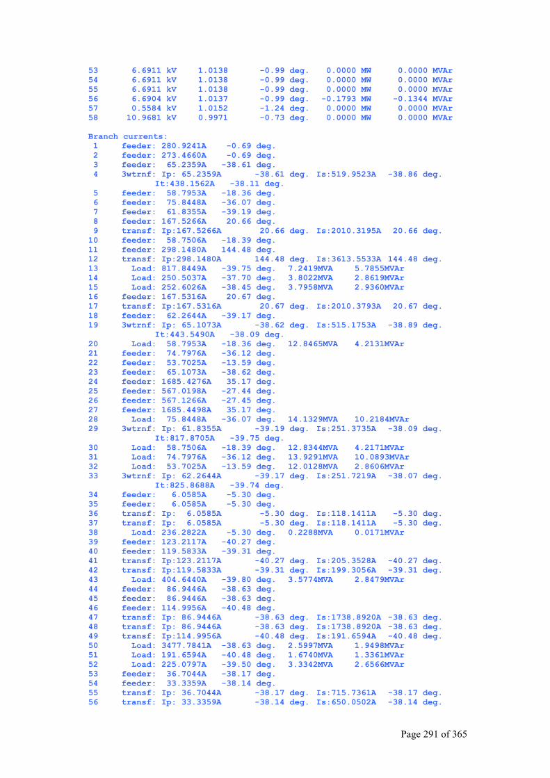
Page 291 of 365

53 6.6911 kV 1.0138 -0.99 deg. 0.0000 MW 0.0000 MVAr 54 6.6911 kV 1.0138 -0.99 deg. 0.0000 MW 0.0000 MVAr 55 6.6911 kV 1.0138 -0.99 deg. 0.0000 MW 0.0000 MVAr 56 6.6904 kV 1.0137 -0.99 deg. -0.1793 MW -0.1344 MVAr 57 0.5584 kV 1.0152 -1.24 deg. 0.0000 MW 0.0000 MVAr 58 10.9681 kV 0.9971 -0.73 deg. 0.0000 MW 0.0000 MVAr Branch currents: 1 feeder: 280.9241A -0.69 deg. 2 feeder: 273.4660A -0.69 deg. 3 feeder: 65.2359A -38.61 deg. 4 3wtrnf: Ip: 65.2359A -38.61 deg. Is:519.9523A -38.86 deg. It:438.1562A -38.11 deg. 5 feeder: 58.7953A -18.36 deg. 6 feeder: 75.8448A -36.07 deg. 7 feeder: 61.8355A -39.19 deg. 8 feeder: 167.5266A 20.66 deg. 9 transf: Ip:167.5266A 20.66 deg. Is:2010.3195A 20.66 deg. 10 feeder: 58.7506A -18.39 deg. 11 feeder: 298.1480A 144.48 deg. 12 transf: Ip:298.1480A 144.48 deg. Is:3613.5533A 144.48 deg. 13 Load: 817.8449A -39.75 deg. 7.2419MVA 5.7855MVAr 14 Load: 250.5037A -37.70 deg. 3.8022MVA 2.8619MVAr 15 Load: 252.6026A -38.45 deg. 3.7958MVA 2.9360MVAr 16 feeder: 167.5316A 20.67 deg. 17 transf: Ip:167.5316A 20.67 deg. Is:2010.3793A 20.67 deg. 18 feeder: 62.2644A -39.17 deg. 19 3wtrnf: Ip: 65.1073A -38.62 deg. Is:515.1753A -38.89 deg. It:443.5490A -38.09 deg. 20 Load: 58.7953A -18.36 deg. 12.8465MVA 4.2131MVAr 21 feeder: 74.7976A -36.12 deg. 22 feeder: 53.7025A -13.59 deg. 23 feeder: 65.1073A -38.62 deg. 24 feeder: 1685.4276A 35.17 deg. 25 feeder: 567.0198A -27.44 deg. 26 feeder: 567.1266A -27.45 deg. 27 feeder: 1685.4498A 35.17 deg. 28 Load: 75.8448A -36.07 deg. 14.1329MVA 10.2184MVAr 29 3wtrnf: Ip: 61.8355A -39.19 deg. Is:251.3735A -38.09 deg. It:817.8705A -39.75 deg. 30 Load: 58.7506A -18.39 deg. 12.8344MVA 4.2171MVAr 31 Load: 74.7976A -36.12 deg. 13.9291MVA 10.0893MVAr 32 Load: 53.7025A -13.59 deg. 12.0128MVA 2.8606MVAr 33 3wtrnf: Ip: 62.2644A -39.17 deg. Is:251.7219A -38.07 deg. It:825.8688A -39.74 deg. 34 feeder: 6.0585A -5.30 deg. 35 feeder: 6.0585A -5.30 deg. 36 transf: Ip: 6.0585A -5.30 deg. Is:118.1411A -5.30 deg. 37 transf: Ip: 6.0585A -5.30 deg. Is:118.1411A -5.30 deg. 38 Load: 236.2822A -5.30 deg. 0.2288MVA 0.0171MVAr 39 feeder: 123.2117A -40.27 deg. 40 feeder: 119.5833A -39.31 deg. 41 transf: Ip:123.2117A -40.27 deg. Is:205.3528A -40.27 deg. 42 transf: Ip:119.5833A -39.31 deg. Is:199.3056A -39.31 deg. 43 Load: 404.6440A -39.80 deg. 3.5774MVA 2.8479MVAr 44 feeder: 86.9446A -38.63 deg. 45 feeder: 86.9446A -38.63 deg. 46 feeder: 114.9956A -40.48 deg. 47 transf: Ip: 86.9446A -38.63 deg. Is:1738.8920A -38.63 deg. 48 transf: Ip: 86.9446A -38.63 deg. Is:1738.8920A -38.63 deg. 49 transf: Ip:114.9956A -40.48 deg. Is:191.6594A -40.48 deg. 50 Load: 3477.7841A -38.63 deg. 2.5997MVA 1.9498MVAr 51 Load: 191.6594A -40.48 deg. 1.6740MVA 1.3361MVAr 52 Load: 225.0797A -39.50 deg. 3.3342MVA 2.6566MVAr 53 feeder: 36.7044A -38.17 deg. 54 feeder: 33.3359A -38.14 deg. 55 transf: Ip: 36.7044A -38.17 deg. Is:715.7361A -38.17 deg. 56 transf: Ip: 33.3359A -38.14 deg. Is:650.0502A -38.14 deg.

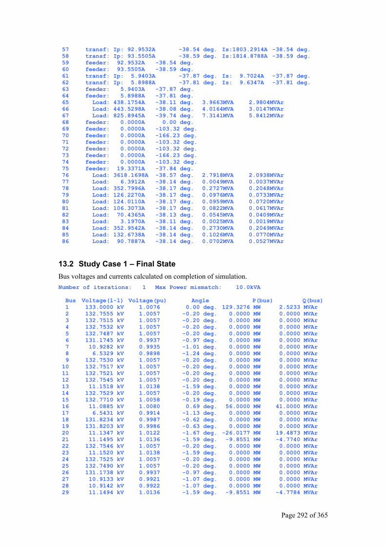
Page 292 of 365

57 transf: Ip: 92.9532A -38.54 deg. Is:1803.2914A -38.54 deg. 58 transf: Ip: 93.5505A -38.59 deg. Is:1814.8788A -38.59 deg. 59 feeder: 92.9532A -38.54 deg. 60 feeder: 93.5505A -38.59 deg. 61 transf: Ip: 5.9403A -37.87 deg. Is: 9.7024A -37.87 deg. 62 transf: Ip: 5.8988A -37.81 deg. Is: 9.6347A -37.81 deg. 63 feeder: 5.9403A -37.87 deg. 64 feeder: 5.8988A -37.81 deg. 65 Load: 438.1754A -38.11 deg. 3.9663MVA 2.9804MVAr 66 Load: 443.5298A -38.08 deg. 4.0164MVA 3.0147MVAr 67 Load: 825.8945A -39.74 deg. 7.3141MVA 5.8412MVAr 68 feeder: 0.0000A 0.00 deg. 69 feeder: 0.0000A -103.32 deg. 70 feeder: 0.0000A -166.23 deg. 71 feeder: 0.0000A -103.32 deg. 72 feeder: 0.0000A -103.32 deg. 73 feeder: 0.0000A -166.23 deg. 74 feeder: 0.0000A -103.32 deg. 75 feeder: 19.3371A -37.84 deg. 76 Load: 3618.1698A -38.57 deg. 2.7918MVA 2.0938MVAr 77 Load: 6.3912A -38.14 deg. 0.0049MVA 0.0037MVAr 78 Load: 352.7996A -38.17 deg. 0.2727MVA 0.2048MVAr 79 Load: 126.2270A -38.17 deg. 0.0976MVA 0.0733MVAr 80 Load: 124.0110A -38.17 deg. 0.0959MVA 0.0720MVAr 81 Load: 106.3073A -38.17 deg. 0.0822MVA 0.0617MVAr 82 Load: 70.4365A -38.13 deg. 0.0545MVA 0.0409MVAr 83 Load: 3.1970A -38.11 deg. 0.0025MVA 0.0019MVAr 84 Load: 352.9542A -38.14 deg. 0.2730MVA 0.2049MVAr 85 Load: 132.6738A -38.14 deg. 0.1026MVA 0.0770MVAr 86 Load: 90.7887A -38.14 deg. 0.0702MVA 0.0527MVAr

13.2 Study Case 1 – Final State Bus voltages and currents calculated on completion of simulation. Number of iterations: 1 Max Power mismatch: 10.0kVA Bus Voltage(l-l) Voltage(pu) Angle P(bus) Q(bus) 1 133.0000 kV 1.0076 0.00 deg. 129.3276 MW 2.5233 MVAr 2 132.7555 kV 1.0057 -0.20 deg. 0.0000 MW 0.0000 MVAr 3 132.7515 kV 1.0057 -0.20 deg. 0.0000 MW 0.0000 MVAr 4 132.7532 kV 1.0057 -0.20 deg. 0.0000 MW 0.0000 MVAr 5 132.7487 kV 1.0057 -0.20 deg. 0.0000 MW 0.0000 MVAr 6 131.1745 kV 0.9937 -0.97 deg. 0.0000 MW 0.0000 MVAr 7 10.9282 kV 0.9935 -1.01 deg. 0.0000 MW 0.0000 MVAr 8 6.5329 kV 0.9898 -1.24 deg. 0.0000 MW 0.0000 MVAr 9 132.7530 kV 1.0057 -0.20 deg. 0.0000 MW 0.0000 MVAr 10 132.7517 kV 1.0057 -0.20 deg. 0.0000 MW 0.0000 MVAr 11 132.7521 kV 1.0057 -0.20 deg. 0.0000 MW 0.0000 MVAr 12 132.7545 kV 1.0057 -0.20 deg. 0.0000 MW 0.0000 MVAr 13 11.1518 kV 1.0138 -1.59 deg. 0.0000 MW 0.0000 MVAr 14 132.7529 kV 1.0057 -0.20 deg. 0.0000 MW 0.0000 MVAr 15 132.7710 kV 1.0058 -0.19 deg. 0.0000 MW 0.0000 MVAr 16 11.0885 kV 1.0080 0.69 deg. 56.0000 MW 41.0000 MVAr 17 6.5431 kV 0.9914 -1.13 deg. 0.0000 MW 0.0000 MVAr 18 131.8234 kV 0.9987 -0.62 deg. 0.0000 MW 0.0000 MVAr 19 131.8203 kV 0.9986 -0.63 deg. 0.0000 MW 0.0000 MVAr 20 11.1347 kV 1.0122 -1.67 deg. -26.0177 MW 19.4873 MVAr 21 11.1495 kV 1.0136 -1.59 deg. -9.8551 MW -4.7740 MVAr 22 132.7546 kV 1.0057 -0.20 deg. 0.0000 MW 0.0000 MVAr 23 11.1520 kV 1.0138 -1.59 deg. 0.0000 MW 0.0000 MVAr 24 132.7525 kV 1.0057 -0.20 deg. 0.0000 MW 0.0000 MVAr 25 132.7490 kV 1.0057 -0.20 deg. 0.0000 MW 0.0000 MVAr 26 131.1738 kV 0.9937 -0.97 deg. 0.0000 MW 0.0000 MVAr 27 10.9133 kV 0.9921 -1.07 deg. 0.0000 MW 0.0000 MVAr 28 10.9142 kV 0.9922 -1.07 deg. 0.0000 MW 0.0000 MVAr 29 11.1494 kV 1.0136 -1.59 deg. -9.8551 MW -4.7784 MVAr

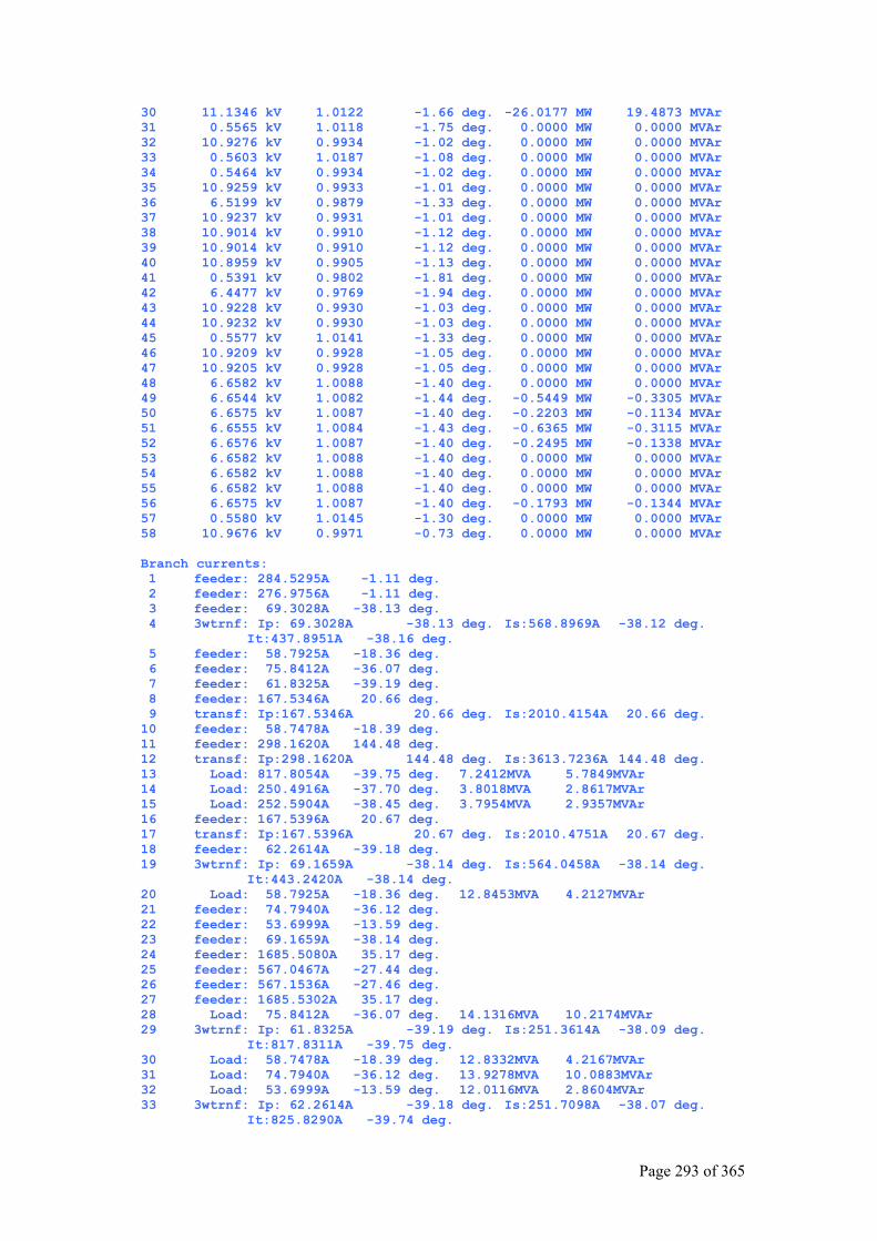
Page 293 of 365

30 11.1346 kV 1.0122 -1.66 deg. -26.0177 MW 19.4873 MVAr 31 0.5565 kV 1.0118 -1.75 deg. 0.0000 MW 0.0000 MVAr 32 10.9276 kV 0.9934 -1.02 deg. 0.0000 MW 0.0000 MVAr 33 0.5603 kV 1.0187 -1.08 deg. 0.0000 MW 0.0000 MVAr 34 0.5464 kV 0.9934 -1.02 deg. 0.0000 MW 0.0000 MVAr 35 10.9259 kV 0.9933 -1.01 deg. 0.0000 MW 0.0000 MVAr 36 6.5199 kV 0.9879 -1.33 deg. 0.0000 MW 0.0000 MVAr 37 10.9237 kV 0.9931 -1.01 deg. 0.0000 MW 0.0000 MVAr 38 10.9014 kV 0.9910 -1.12 deg. 0.0000 MW 0.0000 MVAr 39 10.9014 kV 0.9910 -1.12 deg. 0.0000 MW 0.0000 MVAr 40 10.8959 kV 0.9905 -1.13 deg. 0.0000 MW 0.0000 MVAr 41 0.5391 kV 0.9802 -1.81 deg. 0.0000 MW 0.0000 MVAr 42 6.4477 kV 0.9769 -1.94 deg. 0.0000 MW 0.0000 MVAr 43 10.9228 kV 0.9930 -1.03 deg. 0.0000 MW 0.0000 MVAr 44 10.9232 kV 0.9930 -1.03 deg. 0.0000 MW 0.0000 MVAr 45 0.5577 kV 1.0141 -1.33 deg. 0.0000 MW 0.0000 MVAr 46 10.9209 kV 0.9928 -1.05 deg. 0.0000 MW 0.0000 MVAr 47 10.9205 kV 0.9928 -1.05 deg. 0.0000 MW 0.0000 MVAr 48 6.6582 kV 1.0088 -1.40 deg. 0.0000 MW 0.0000 MVAr 49 6.6544 kV 1.0082 -1.44 deg. -0.5449 MW -0.3305 MVAr 50 6.6575 kV 1.0087 -1.40 deg. -0.2203 MW -0.1134 MVAr 51 6.6555 kV 1.0084 -1.43 deg. -0.6365 MW -0.3115 MVAr 52 6.6576 kV 1.0087 -1.40 deg. -0.2495 MW -0.1338 MVAr 53 6.6582 kV 1.0088 -1.40 deg. 0.0000 MW 0.0000 MVAr 54 6.6582 kV 1.0088 -1.40 deg. 0.0000 MW 0.0000 MVAr 55 6.6582 kV 1.0088 -1.40 deg. 0.0000 MW 0.0000 MVAr 56 6.6575 kV 1.0087 -1.40 deg. -0.1793 MW -0.1344 MVAr 57 0.5580 kV 1.0145 -1.30 deg. 0.0000 MW 0.0000 MVAr 58 10.9676 kV 0.9971 -0.73 deg. 0.0000 MW 0.0000 MVAr Branch currents: 1 feeder: 284.5295A -1.11 deg. 2 feeder: 276.9756A -1.11 deg. 3 feeder: 69.3028A -38.13 deg. 4 3wtrnf: Ip: 69.3028A -38.13 deg. Is:568.8969A -38.12 deg. It:437.8951A -38.16 deg. 5 feeder: 58.7925A -18.36 deg. 6 feeder: 75.8412A -36.07 deg. 7 feeder: 61.8325A -39.19 deg. 8 feeder: 167.5346A 20.66 deg. 9 transf: Ip:167.5346A 20.66 deg. Is:2010.4154A 20.66 deg. 10 feeder: 58.7478A -18.39 deg. 11 feeder: 298.1620A 144.48 deg. 12 transf: Ip:298.1620A 144.48 deg. Is:3613.7236A 144.48 deg. 13 Load: 817.8054A -39.75 deg. 7.2412MVA 5.7849MVAr 14 Load: 250.4916A -37.70 deg. 3.8018MVA 2.8617MVAr 15 Load: 252.5904A -38.45 deg. 3.7954MVA 2.9357MVAr 16 feeder: 167.5396A 20.67 deg. 17 transf: Ip:167.5396A 20.67 deg. Is:2010.4751A 20.67 deg. 18 feeder: 62.2614A -39.18 deg. 19 3wtrnf: Ip: 69.1659A -38.14 deg. Is:564.0458A -38.14 deg. It:443.2420A -38.14 deg. 20 Load: 58.7925A -18.36 deg. 12.8453MVA 4.2127MVAr 21 feeder: 74.7940A -36.12 deg. 22 feeder: 53.6999A -13.59 deg. 23 feeder: 69.1659A -38.14 deg. 24 feeder: 1685.5080A 35.17 deg. 25 feeder: 567.0467A -27.44 deg. 26 feeder: 567.1536A -27.46 deg. 27 feeder: 1685.5302A 35.17 deg. 28 Load: 75.8412A -36.07 deg. 14.1316MVA 10.2174MVAr 29 3wtrnf: Ip: 61.8325A -39.19 deg. Is:251.3614A -38.09 deg. It:817.8311A -39.75 deg. 30 Load: 58.7478A -18.39 deg. 12.8332MVA 4.2167MVAr 31 Load: 74.7940A -36.12 deg. 13.9278MVA 10.0883MVAr 32 Load: 53.6999A -13.59 deg. 12.0116MVA 2.8604MVAr 33 3wtrnf: Ip: 62.2614A -39.18 deg. Is:251.7098A -38.07 deg. It:825.8290A -39.74 deg.

Page 294 of 365

34 feeder: 6.0545A -5.36 deg. 35 feeder: 6.0545A -5.36 deg. 36 transf: Ip: 6.0545A -5.36 deg. Is:118.0631A -5.36 deg. 37 transf: Ip: 6.0545A -5.36 deg. Is:118.0631A -5.36 deg. 38 Load: 236.1263A -5.36 deg. 0.2285MVA 0.0171MVAr 39 feeder: 123.1304A -40.33 deg. 40 feeder: 119.5044A -39.37 deg. 41 transf: Ip:123.1304A -40.33 deg. Is:205.2173A -40.33 deg. 42 transf: Ip:119.5044A -39.37 deg. Is:199.1741A -39.37 deg. 43 Load: 404.3770A -39.86 deg. 3.5727MVA 2.8442MVAr 44 feeder: 86.8872A -38.69 deg. 45 feeder: 86.8872A -38.69 deg. 46 feeder: 114.9198A -40.54 deg. 47 transf: Ip: 86.8872A -38.69 deg. Is:1737.7447A -38.69 deg. 48 transf: Ip: 86.8872A -38.69 deg. Is:1737.7447A -38.69 deg. 49 transf: Ip:114.9198A -40.54 deg. Is:191.5329A -40.54 deg. 50 Load: 3475.4894A -38.69 deg. 2.5963MVA 1.9472MVAr 51 Load: 191.5329A -40.54 deg. 1.6718MVA 1.3343MVAr 52 Load: 224.9312A -39.55 deg. 3.3298MVA 2.6531MVAr 53 feeder: 36.6802A -38.22 deg. 54 feeder: 33.3139A -38.20 deg. 55 transf: Ip: 36.6802A -38.22 deg. Is:715.2638A -38.22 deg. 56 transf: Ip: 33.3139A -38.20 deg. Is:649.6213A -38.20 deg. 57 transf: Ip: 92.8918A -38.60 deg. Is:1802.1015A -38.60 deg. 58 transf: Ip: 93.4887A -38.65 deg. Is:1813.6813A -38.65 deg. 59 feeder: 92.8918A -38.60 deg. 60 feeder: 93.4887A -38.65 deg. 61 transf: Ip: 55.8861A -30.67 deg. Is: 91.2807A -30.67 deg. 62 transf: Ip: 55.4960A -30.61 deg. Is: 90.6435A -30.61 deg. 63 feeder: 55.8861A -30.67 deg. 64 feeder: 55.4960A -30.61 deg. 65 Load: 437.8931A -38.16 deg. 3.9612MVA 2.9765MVAr 66 Load: 443.2441A -38.13 deg. 4.0112MVA 3.0108MVAr 67 Load: 825.8546A -39.74 deg. 7.3134MVA 5.8406MVAr 68 feeder: 55.2912A -32.68 deg. 69 feeder: 21.4862A -28.64 deg. 70 feeder: 61.4772A -27.51 deg. 71 feeder: 24.5522A -29.60 deg. 72 feeder: 0.0000A 76.68 deg. 73 feeder: 0.0000A -166.23 deg. 74 feeder: 0.0000A -103.32 deg. 75 feeder: 19.4326A -38.26 deg. 76 Load: 3615.7825A -38.62 deg. 2.7881MVA 2.0910MVAr 77 Load: 6.3870A -38.20 deg. 0.0049MVA 0.0037MVAr 78 Load: 352.5668A -38.22 deg. 0.2724MVA 0.2045MVAr 79 Load: 126.1437A -38.23 deg. 0.0974MVA 0.0732MVAr 80 Load: 123.9291A -38.22 deg. 0.0957MVA 0.0719MVAr 81 Load: 106.2371A -38.22 deg. 0.0821MVA 0.0616MVAr 82 Load: 70.3901A -38.19 deg. 0.0544MVA 0.0408MVAr 83 Load: 3.1949A -38.17 deg. 0.0025MVA 0.0019MVAr 84 Load: 352.7213A -38.20 deg. 0.2726MVA 0.2047MVAr 85 Load: 132.5863A -38.20 deg. 0.1025MVA 0.0769MVAr 86 Load: 90.7288A -38.19 deg. 0.0701MVA 0.0526MVAr

13.3 Study Case 2 – Final State Bus voltages and currents calculated on completion of simulation. Number of iterations: 1 Max Power mismatch: 10.0kVA Bus Voltage(l-l) Voltage(pu) Angle P(bus) Q(bus) 1 133.0000 kV 1.0076 0.00 deg. 129.1434 MW 2.3913 MVAr 2 132.7564 kV 1.0057 -0.20 deg. 0.0000 MW 0.0000 MVAr 3 132.7524 kV 1.0057 -0.20 deg. 0.0000 MW 0.0000 MVAr 4 132.7541 kV 1.0057 -0.20 deg. 0.0000 MW 0.0000 MVAr 5 132.7496 kV 1.0057 -0.20 deg. 0.0000 MW 0.0000 MVAr 6 131.1868 kV 0.9938 -0.96 deg. 0.0000 MW 0.0000 MVAr 7 10.9293 kV 0.9936 -1.00 deg. 0.0000 MW 0.0000 MVAr

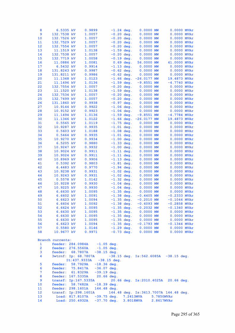
Page 295 of 365

8 6.5335 kV 0.9899 -1.24 deg. 0.0000 MW 0.0000 MVAr 9 132.7538 kV 1.0057 -0.20 deg. 0.0000 MW 0.0000 MVAr 10 132.7526 kV 1.0057 -0.20 deg. 0.0000 MW 0.0000 MVAr 11 132.7529 kV 1.0057 -0.20 deg. 0.0000 MW 0.0000 MVAr 12 132.7554 kV 1.0057 -0.20 deg. 0.0000 MW 0.0000 MVAr 13 11.1519 kV 1.0138 -1.59 deg. 0.0000 MW 0.0000 MVAr 14 132.7538 kV 1.0057 -0.20 deg. 0.0000 MW 0.0000 MVAr 15 132.7719 kV 1.0058 -0.19 deg. 0.0000 MW 0.0000 MVAr 16 11.0886 kV 1.0081 0.69 deg. 56.0000 MW 41.0000 MVAr 17 6.5432 kV 0.9914 -1.13 deg. 0.0000 MW 0.0000 MVAr 18 131.8243 kV 0.9987 -0.62 deg. 0.0000 MW 0.0000 MVAr 19 131.8211 kV 0.9986 -0.62 deg. 0.0000 MW 0.0000 MVAr 20 11.1348 kV 1.0123 -1.66 deg. -26.0177 MW 19.4873 MVAr 21 11.1496 kV 1.0136 -1.59 deg. -9.8551 MW -4.7740 MVAr 22 132.7554 kV 1.0057 -0.20 deg. 0.0000 MW 0.0000 MVAr 23 11.1520 kV 1.0138 -1.59 deg. 0.0000 MW 0.0000 MVAr 24 132.7534 kV 1.0057 -0.20 deg. 0.0000 MW 0.0000 MVAr 25 132.7499 kV 1.0057 -0.20 deg. 0.0000 MW 0.0000 MVAr 26 131.1860 kV 0.9938 -0.97 deg. 0.0000 MW 0.0000 MVAr 27 10.9144 kV 0.9922 -1.06 deg. 0.0000 MW 0.0000 MVAr 28 10.9152 kV 0.9923 -1.06 deg. 0.0000 MW 0.0000 MVAr 29 11.1494 kV 1.0136 -1.59 deg. -9.8551 MW -4.7784 MVAr 30 11.1346 kV 1.0122 -1.66 deg. -26.0177 MW 19.4873 MVAr 31 0.5565 kV 1.0119 -1.75 deg. 0.0000 MW 0.0000 MVAr 32 10.9287 kV 0.9935 -1.01 deg. 0.0000 MW 0.0000 MVAr 33 0.5603 kV 1.0188 -1.08 deg. 0.0000 MW 0.0000 MVAr 34 0.5464 kV 0.9935 -1.01 deg. 0.0000 MW 0.0000 MVAr 35 10.9270 kV 0.9934 -1.00 deg. 0.0000 MW 0.0000 MVAr 36 6.5205 kV 0.9880 -1.33 deg. 0.0000 MW 0.0000 MVAr 37 10.9247 kV 0.9932 -1.00 deg. 0.0000 MW 0.0000 MVAr 38 10.9024 kV 0.9911 -1.11 deg. 0.0000 MW 0.0000 MVAr 39 10.9024 kV 0.9911 -1.11 deg. 0.0000 MW 0.0000 MVAr 40 10.8969 kV 0.9906 -1.13 deg. 0.0000 MW 0.0000 MVAr 41 0.5392 kV 0.9803 -1.81 deg. 0.0000 MW 0.0000 MVAr 42 6.4483 kV 0.9770 -1.94 deg. 0.0000 MW 0.0000 MVAr 43 10.9238 kV 0.9931 -1.02 deg. 0.0000 MW 0.0000 MVAr 44 10.9243 kV 0.9931 -1.02 deg. 0.0000 MW 0.0000 MVAr 45 0.5578 kV 1.0142 -1.32 deg. 0.0000 MW 0.0000 MVAr 46 10.9228 kV 0.9930 -1.04 deg. 0.0000 MW 0.0000 MVAr 47 10.9225 kV 0.9930 -1.04 deg. 0.0000 MW 0.0000 MVAr 48 6.6630 kV 1.0095 -1.35 deg. 0.0000 MW 0.0000 MVAr 49 6.6602 kV 1.0091 -1.38 deg. -0.4405 MW -0.2333 MVAr 50 6.6623 kV 1.0094 -1.35 deg. -0.2010 MW -0.1044 MVAr 51 6.6604 kV 1.0092 -1.38 deg. -0.6093 MW -0.2858 MVAr 52 6.6624 kV 1.0095 -1.35 deg. -0.2032 MW -0.1340 MVAr 53 6.6630 kV 1.0095 -1.35 deg. 0.0000 MW 0.0000 MVAr 54 6.6630 kV 1.0095 -1.35 deg. 0.0000 MW 0.0000 MVAr 55 6.6630 kV 1.0095 -1.35 deg. 0.0000 MW 0.0000 MVAr 56 6.6623 kV 1.0094 -1.35 deg. -0.1793 MW -0.1344 MVAr 57 0.5580 kV 1.0146 -1.29 deg. 0.0000 MW 0.0000 MVAr 58 10.9677 kV 0.9971 -0.73 deg. 0.0000 MW 0.0000 MVAr Branch currents: 1 feeder: 284.0984A -1.05 deg. 2 feeder: 276.5560A -1.05 deg. 3 feeder: 68.7807A -38.15 deg. 4 3wtrnf: Ip: 68.7807A -38.15 deg. Is:562.6085A -38.15 deg. It:437.9333A -38.15 deg. 5 feeder: 58.7929A -18.36 deg. 6 feeder: 75.8417A -36.07 deg. 7 feeder: 61.8329A -39.19 deg. 8 feeder: 167.5335A 20.66 deg. 9 transf: Ip:167.5335A 20.66 deg. Is:2010.4025A 20.66 deg. 10 feeder: 58.7482A -18.39 deg. 11 feeder: 298.1601A 144.48 deg. 12 transf: Ip:298.1601A 144.48 deg. Is:3613.7007A 144.48 deg. 13 Load: 817.8107A -39.75 deg. 7.2413MVA 5.7850MVAr 14 Load: 250.4932A -37.70 deg. 3.8018MVA 2.8617MVAr

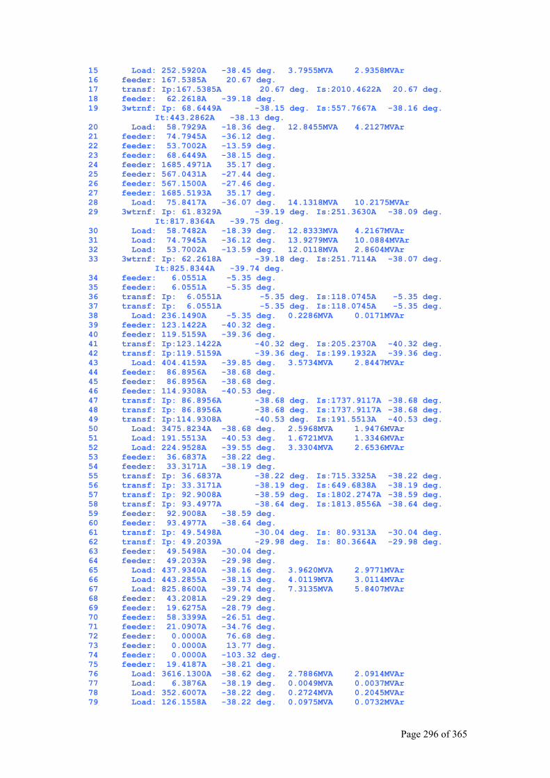
Page 296 of 365

15 Load: 252.5920A -38.45 deg. 3.7955MVA 2.9358MVAr 16 feeder: 167.5385A 20.67 deg. 17 transf: Ip:167.5385A 20.67 deg. Is:2010.4622A 20.67 deg. 18 feeder: 62.2618A -39.18 deg. 19 3wtrnf: Ip: 68.6449A -38.15 deg. Is:557.7667A -38.16 deg. It:443.2862A -38.13 deg. 20 Load: 58.7929A -18.36 deg. 12.8455MVA 4.2127MVAr 21 feeder: 74.7945A -36.12 deg. 22 feeder: 53.7002A -13.59 deg. 23 feeder: 68.6449A -38.15 deg. 24 feeder: 1685.4971A 35.17 deg. 25 feeder: 567.0431A -27.44 deg. 26 feeder: 567.1500A -27.46 deg. 27 feeder: 1685.5193A 35.17 deg. 28 Load: 75.8417A -36.07 deg. 14.1318MVA 10.2175MVAr 29 3wtrnf: Ip: 61.8329A -39.19 deg. Is:251.3630A -38.09 deg. It:817.8364A -39.75 deg. 30 Load: 58.7482A -18.39 deg. 12.8333MVA 4.2167MVAr 31 Load: 74.7945A -36.12 deg. 13.9279MVA 10.0884MVAr 32 Load: 53.7002A -13.59 deg. 12.0118MVA 2.8604MVAr 33 3wtrnf: Ip: 62.2618A -39.18 deg. Is:251.7114A -38.07 deg. It:825.8344A -39.74 deg. 34 feeder: 6.0551A -5.35 deg. 35 feeder: 6.0551A -5.35 deg. 36 transf: Ip: 6.0551A -5.35 deg. Is:118.0745A -5.35 deg. 37 transf: Ip: 6.0551A -5.35 deg. Is:118.0745A -5.35 deg. 38 Load: 236.1490A -5.35 deg. 0.2286MVA 0.0171MVAr 39 feeder: 123.1422A -40.32 deg. 40 feeder: 119.5159A -39.36 deg. 41 transf: Ip:123.1422A -40.32 deg. Is:205.2370A -40.32 deg. 42 transf: Ip:119.5159A -39.36 deg. Is:199.1932A -39.36 deg. 43 Load: 404.4159A -39.85 deg. 3.5734MVA 2.8447MVAr 44 feeder: 86.8956A -38.68 deg. 45 feeder: 86.8956A -38.68 deg. 46 feeder: 114.9308A -40.53 deg. 47 transf: Ip: 86.8956A -38.68 deg. Is:1737.9117A -38.68 deg. 48 transf: Ip: 86.8956A -38.68 deg. Is:1737.9117A -38.68 deg. 49 transf: Ip:114.9308A -40.53 deg. Is:191.5513A -40.53 deg. 50 Load: 3475.8234A -38.68 deg. 2.5968MVA 1.9476MVAr 51 Load: 191.5513A -40.53 deg. 1.6721MVA 1.3346MVAr 52 Load: 224.9528A -39.55 deg. 3.3304MVA 2.6536MVAr 53 feeder: 36.6837A -38.22 deg. 54 feeder: 33.3171A -38.19 deg. 55 transf: Ip: 36.6837A -38.22 deg. Is:715.3325A -38.22 deg. 56 transf: Ip: 33.3171A -38.19 deg. Is:649.6838A -38.19 deg. 57 transf: Ip: 92.9008A -38.59 deg. Is:1802.2747A -38.59 deg. 58 transf: Ip: 93.4977A -38.64 deg. Is:1813.8556A -38.64 deg. 59 feeder: 92.9008A -38.59 deg. 60 feeder: 93.4977A -38.64 deg. 61 transf: Ip: 49.5498A -30.04 deg. Is: 80.9313A -30.04 deg. 62 transf: Ip: 49.2039A -29.98 deg. Is: 80.3664A -29.98 deg. 63 feeder: 49.5498A -30.04 deg. 64 feeder: 49.2039A -29.98 deg. 65 Load: 437.9340A -38.16 deg. 3.9620MVA 2.9771MVAr 66 Load: 443.2855A -38.13 deg. 4.0119MVA 3.0114MVAr 67 Load: 825.8600A -39.74 deg. 7.3135MVA 5.8407MVAr 68 feeder: 43.2081A -29.29 deg. 69 feeder: 19.6275A -28.79 deg. 70 feeder: 58.3399A -26.51 deg. 71 feeder: 21.0907A -34.76 deg. 72 feeder: 0.0000A 76.68 deg. 73 feeder: 0.0000A 13.77 deg. 74 feeder: 0.0000A -103.32 deg. 75 feeder: 19.4187A -38.21 deg. 76 Load: 3616.1300A -38.62 deg. 2.7886MVA 2.0914MVAr 77 Load: 6.3876A -38.19 deg. 0.0049MVA 0.0037MVAr 78 Load: 352.6007A -38.22 deg. 0.2724MVA 0.2045MVAr 79 Load: 126.1558A -38.22 deg. 0.0975MVA 0.0732MVAr

Page 297 of 365

80 Load: 123.9410A -38.22 deg. 0.0958MVA 0.0719MVAr 81 Load: 106.2473A -38.22 deg. 0.0821MVA 0.0616MVAr 82 Load: 70.3968A -38.18 deg. 0.0544MVA 0.0408MVAr 83 Load: 3.1952A -38.16 deg. 0.0025MVA 0.0019MVAr 84 Load: 352.7552A -38.19 deg. 0.2727MVA 0.2047MVAr 85 Load: 132.5990A -38.19 deg. 0.1025MVA 0.0770MVAr 86 Load: 90.7375A -38.19 deg. 0.0701MVA 0.0527MVAr

13.4 Study Case 3 – Final State Bus voltages and currents calculated on completion of simulation. Number of iterations: 1 Max Power mismatch: 10.0kVA Bus Voltage(l-l) Voltage(pu) Angle P(bus) Q(bus) 1 133.0000 kV 1.0076 0.00 deg. 129.3266 MW 2.5245 MVAr 2 132.7555 kV 1.0057 -0.20 deg. 0.0000 MW 0.0000 MVAr 3 132.7515 kV 1.0057 -0.20 deg. 0.0000 MW 0.0000 MVAr 4 132.7532 kV 1.0057 -0.20 deg. 0.0000 MW 0.0000 MVAr 5 132.7487 kV 1.0057 -0.20 deg. 0.0000 MW 0.0000 MVAr 6 131.1745 kV 0.9937 -0.97 deg. 0.0000 MW 0.0000 MVAr 7 10.9282 kV 0.9935 -1.01 deg. 0.0000 MW 0.0000 MVAr 8 6.5329 kV 0.9898 -1.24 deg. 0.0000 MW 0.0000 MVAr 9 132.7530 kV 1.0057 -0.20 deg. 0.0000 MW 0.0000 MVAr 10 132.7517 kV 1.0057 -0.20 deg. 0.0000 MW 0.0000 MVAr 11 132.7521 kV 1.0057 -0.20 deg. 0.0000 MW 0.0000 MVAr 12 132.7545 kV 1.0057 -0.20 deg. 0.0000 MW 0.0000 MVAr 13 11.1518 kV 1.0138 -1.59 deg. 0.0000 MW 0.0000 MVAr 14 132.7529 kV 1.0057 -0.20 deg. 0.0000 MW 0.0000 MVAr 15 132.7710 kV 1.0058 -0.19 deg. 0.0000 MW 0.0000 MVAr 16 11.0885 kV 1.0080 0.69 deg. 55.9999 MW 40.9982 MVAr 17 6.5431 kV 0.9914 -1.13 deg. 0.0000 MW 0.0000 MVAr 18 131.8234 kV 0.9987 -0.62 deg. 0.0000 MW 0.0000 MVAr 19 131.8203 kV 0.9986 -0.63 deg. 0.0000 MW 0.0000 MVAr 20 11.1347 kV 1.0122 -1.67 deg. -26.0177 MW 19.4873 MVAr 21 11.1495 kV 1.0136 -1.59 deg. -9.8551 MW -4.7740 MVAr 22 132.7545 kV 1.0057 -0.20 deg. 0.0000 MW 0.0000 MVAr 23 11.1520 kV 1.0138 -1.59 deg. 0.0000 MW 0.0000 MVAr 24 132.7525 kV 1.0057 -0.20 deg. 0.0000 MW 0.0000 MVAr 25 132.7490 kV 1.0057 -0.20 deg. 0.0000 MW 0.0000 MVAr 26 131.1738 kV 0.9937 -0.97 deg. 0.0000 MW 0.0000 MVAr 27 10.9133 kV 0.9921 -1.07 deg. 0.0000 MW 0.0000 MVAr 28 10.9142 kV 0.9922 -1.07 deg. 0.0000 MW 0.0000 MVAr 29 11.1494 kV 1.0136 -1.59 deg. -9.8551 MW -4.7784 MVAr 30 11.1346 kV 1.0122 -1.66 deg. -26.0177 MW 19.4873 MVAr 31 0.5565 kV 1.0118 -1.75 deg. 0.0000 MW 0.0000 MVAr 32 10.9276 kV 0.9934 -1.02 deg. 0.0000 MW 0.0000 MVAr 33 0.5603 kV 1.0187 -1.08 deg. 0.0000 MW 0.0000 MVAr 34 0.5464 kV 0.9934 -1.02 deg. 0.0000 MW 0.0000 MVAr 35 10.9259 kV 0.9933 -1.01 deg. 0.0000 MW 0.0000 MVAr 36 6.5199 kV 0.9879 -1.33 deg. 0.0000 MW 0.0000 MVAr 37 10.9237 kV 0.9931 -1.01 deg. 0.0000 MW 0.0000 MVAr 38 10.9014 kV 0.9910 -1.12 deg. 0.0000 MW 0.0000 MVAr 39 10.9014 kV 0.9910 -1.12 deg. 0.0000 MW 0.0000 MVAr 40 10.8959 kV 0.9905 -1.13 deg. 0.0000 MW 0.0000 MVAr 41 0.5391 kV 0.9802 -1.81 deg. 0.0000 MW 0.0000 MVAr 42 6.4477 kV 0.9769 -1.94 deg. 0.0000 MW 0.0000 MVAr 43 10.9228 kV 0.9930 -1.03 deg. 0.0000 MW 0.0000 MVAr 44 10.9232 kV 0.9930 -1.03 deg. 0.0000 MW 0.0000 MVAr 45 0.5577 kV 1.0141 -1.33 deg. 0.0000 MW 0.0000 MVAr 46 10.9209 kV 0.9928 -1.05 deg. 0.0000 MW 0.0000 MVAr 47 10.9205 kV 0.9928 -1.05 deg. 0.0000 MW 0.0000 MVAr 48 6.6582 kV 1.0088 -1.40 deg. 0.0000 MW 0.0000 MVAr 49 6.6544 kV 1.0082 -1.44 deg. -0.5449 MW -0.3305 MVAr 50 6.6575 kV 1.0087 -1.40 deg. -0.2203 MW -0.1134 MVAr 51 6.6555 kV 1.0084 -1.43 deg. -0.6365 MW -0.3115 MVAr 52 6.6576 kV 1.0087 -1.40 deg. -0.2495 MW -0.1338 MVAr 53 6.6582 kV 1.0088 -1.40 deg. 0.0000 MW 0.0000 MVAr

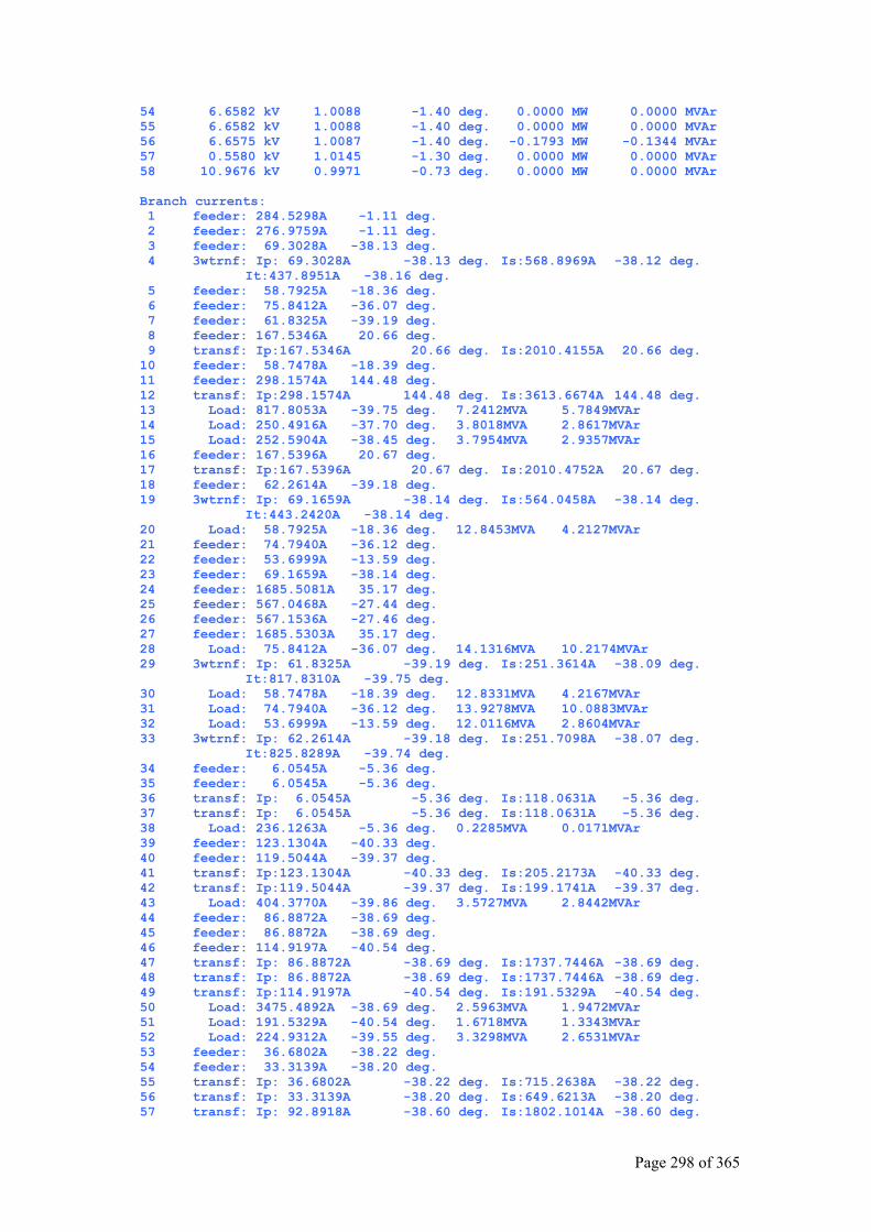
Page 298 of 365

54 6.6582 kV 1.0088 -1.40 deg. 0.0000 MW 0.0000 MVAr 55 6.6582 kV 1.0088 -1.40 deg. 0.0000 MW 0.0000 MVAr 56 6.6575 kV 1.0087 -1.40 deg. -0.1793 MW -0.1344 MVAr 57 0.5580 kV 1.0145 -1.30 deg. 0.0000 MW 0.0000 MVAr 58 10.9676 kV 0.9971 -0.73 deg. 0.0000 MW 0.0000 MVAr Branch currents: 1 feeder: 284.5298A -1.11 deg. 2 feeder: 276.9759A -1.11 deg. 3 feeder: 69.3028A -38.13 deg. 4 3wtrnf: Ip: 69.3028A -38.13 deg. Is:568.8969A -38.12 deg. It:437.8951A -38.16 deg. 5 feeder: 58.7925A -18.36 deg. 6 feeder: 75.8412A -36.07 deg. 7 feeder: 61.8325A -39.19 deg. 8 feeder: 167.5346A 20.66 deg. 9 transf: Ip:167.5346A 20.66 deg. Is:2010.4155A 20.66 deg. 10 feeder: 58.7478A -18.39 deg. 11 feeder: 298.1574A 144.48 deg. 12 transf: Ip:298.1574A 144.48 deg. Is:3613.6674A 144.48 deg. 13 Load: 817.8053A -39.75 deg. 7.2412MVA 5.7849MVAr 14 Load: 250.4916A -37.70 deg. 3.8018MVA 2.8617MVAr 15 Load: 252.5904A -38.45 deg. 3.7954MVA 2.9357MVAr 16 feeder: 167.5396A 20.67 deg. 17 transf: Ip:167.5396A 20.67 deg. Is:2010.4752A 20.67 deg. 18 feeder: 62.2614A -39.18 deg. 19 3wtrnf: Ip: 69.1659A -38.14 deg. Is:564.0458A -38.14 deg. It:443.2420A -38.14 deg. 20 Load: 58.7925A -18.36 deg. 12.8453MVA 4.2127MVAr 21 feeder: 74.7940A -36.12 deg. 22 feeder: 53.6999A -13.59 deg. 23 feeder: 69.1659A -38.14 deg. 24 feeder: 1685.5081A 35.17 deg. 25 feeder: 567.0468A -27.44 deg. 26 feeder: 567.1536A -27.46 deg. 27 feeder: 1685.5303A 35.17 deg. 28 Load: 75.8412A -36.07 deg. 14.1316MVA 10.2174MVAr 29 3wtrnf: Ip: 61.8325A -39.19 deg. Is:251.3614A -38.09 deg. It:817.8310A -39.75 deg. 30 Load: 58.7478A -18.39 deg. 12.8331MVA 4.2167MVAr 31 Load: 74.7940A -36.12 deg. 13.9278MVA 10.0883MVAr 32 Load: 53.6999A -13.59 deg. 12.0116MVA 2.8604MVAr 33 3wtrnf: Ip: 62.2614A -39.18 deg. Is:251.7098A -38.07 deg. It:825.8289A -39.74 deg. 34 feeder: 6.0545A -5.36 deg. 35 feeder: 6.0545A -5.36 deg. 36 transf: Ip: 6.0545A -5.36 deg. Is:118.0631A -5.36 deg. 37 transf: Ip: 6.0545A -5.36 deg. Is:118.0631A -5.36 deg. 38 Load: 236.1263A -5.36 deg. 0.2285MVA 0.0171MVAr 39 feeder: 123.1304A -40.33 deg. 40 feeder: 119.5044A -39.37 deg. 41 transf: Ip:123.1304A -40.33 deg. Is:205.2173A -40.33 deg. 42 transf: Ip:119.5044A -39.37 deg. Is:199.1741A -39.37 deg. 43 Load: 404.3770A -39.86 deg. 3.5727MVA 2.8442MVAr 44 feeder: 86.8872A -38.69 deg. 45 feeder: 86.8872A -38.69 deg. 46 feeder: 114.9197A -40.54 deg. 47 transf: Ip: 86.8872A -38.69 deg. Is:1737.7446A -38.69 deg. 48 transf: Ip: 86.8872A -38.69 deg. Is:1737.7446A -38.69 deg. 49 transf: Ip:114.9197A -40.54 deg. Is:191.5329A -40.54 deg. 50 Load: 3475.4892A -38.69 deg. 2.5963MVA 1.9472MVAr 51 Load: 191.5329A -40.54 deg. 1.6718MVA 1.3343MVAr 52 Load: 224.9312A -39.55 deg. 3.3298MVA 2.6531MVAr 53 feeder: 36.6802A -38.22 deg. 54 feeder: 33.3139A -38.20 deg. 55 transf: Ip: 36.6802A -38.22 deg. Is:715.2638A -38.22 deg. 56 transf: Ip: 33.3139A -38.20 deg. Is:649.6213A -38.20 deg. 57 transf: Ip: 92.8918A -38.60 deg. Is:1802.1014A -38.60 deg.

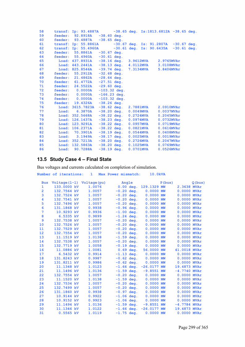
Page 299 of 365

58 transf: Ip: 93.4887A -38.65 deg. Is:1813.6812A -38.65 deg. 59 feeder: 92.8918A -38.60 deg. 60 feeder: 93.4887A -38.65 deg. 61 transf: Ip: 55.8861A -30.67 deg. Is: 91.2807A -30.67 deg. 62 transf: Ip: 55.4960A -30.61 deg. Is: 90.6435A -30.61 deg. 63 feeder: 55.8861A -30.67 deg. 64 feeder: 55.4960A -30.61 deg. 65 Load: 437.8931A -38.16 deg. 3.9612MVA 2.9765MVAr 66 Load: 443.2441A -38.13 deg. 4.0112MVA 3.0108MVAr 67 Load: 825.8546A -39.74 deg. 7.3134MVA 5.8406MVAr 68 feeder: 55.2912A -32.68 deg. 69 feeder: 21.4862A -28.64 deg. 70 feeder: 61.4772A -27.51 deg. 71 feeder: 24.5522A -29.60 deg. 72 feeder: 0.0000A -103.32 deg. 73 feeder: 0.0000A -166.23 deg. 74 feeder: 0.0000A -103.32 deg. 75 feeder: 19.4326A -38.26 deg. 76 Load: 3615.7823A -38.62 deg. 2.7881MVA 2.0910MVAr 77 Load: 6.3870A -38.20 deg. 0.0049MVA 0.0037MVAr 78 Load: 352.5668A -38.22 deg. 0.2724MVA 0.2045MVAr 79 Load: 126.1437A -38.23 deg. 0.0974MVA 0.0732MVAr 80 Load: 123.9291A -38.22 deg. 0.0957MVA 0.0719MVAr 81 Load: 106.2371A -38.22 deg. 0.0821MVA 0.0616MVAr 82 Load: 70.3901A -38.19 deg. 0.0544MVA 0.0408MVAr 83 Load: 3.1949A -38.17 deg. 0.0025MVA 0.0019MVAr 84 Load: 352.7213A -38.20 deg. 0.2726MVA 0.2047MVAr 85 Load: 132.5863A -38.20 deg. 0.1025MVA 0.0769MVAr 86 Load: 90.7288A -38.19 deg. 0.0701MVA 0.0526MVAr

13.5 Study Case 4 – Final State Bus voltages and currents calculated on completion of simulation. Number of iterations: 1 Max Power mismatch: 10.0kVA Bus Voltage(l-l) Voltage(pu) Angle P(bus) Q(bus) 1 133.0000 kV 1.0076 0.00 deg. 129.1329 MW 2.3638 MVAr 2 132.7564 kV 1.0057 -0.20 deg. 0.0000 MW 0.0000 MVAr 3 132.7524 kV 1.0057 -0.20 deg. 0.0000 MW 0.0000 MVAr 4 132.7541 kV 1.0057 -0.20 deg. 0.0000 MW 0.0000 MVAr 5 132.7496 kV 1.0057 -0.20 deg. 0.0000 MW 0.0000 MVAr 6 131.1868 kV 0.9938 -0.96 deg. 0.0000 MW 0.0000 MVAr 7 10.9293 kV 0.9936 -1.00 deg. 0.0000 MW 0.0000 MVAr 8 6.5335 kV 0.9899 -1.24 deg. 0.0000 MW 0.0000 MVAr 9 132.7538 kV 1.0057 -0.20 deg. 0.0000 MW 0.0000 MVAr 10 132.7526 kV 1.0057 -0.20 deg. 0.0000 MW 0.0000 MVAr 11 132.7529 kV 1.0057 -0.20 deg. 0.0000 MW 0.0000 MVAr 12 132.7554 kV 1.0057 -0.20 deg. 0.0000 MW 0.0000 MVAr 13 11.1519 kV 1.0138 -1.59 deg. 0.0000 MW 0.0000 MVAr 14 132.7538 kV 1.0057 -0.20 deg. 0.0000 MW 0.0000 MVAr 15 132.7719 kV 1.0058 -0.19 deg. 0.0000 MW 0.0000 MVAr 16 11.0886 kV 1.0081 0.69 deg. 56.0000 MW 41.0018 MVAr 17 6.5432 kV 0.9914 -1.13 deg. 0.0000 MW 0.0000 MVAr 18 131.8243 kV 0.9987 -0.62 deg. 0.0000 MW 0.0000 MVAr 19 131.8211 kV 0.9986 -0.62 deg. 0.0000 MW 0.0000 MVAr 20 11.1348 kV 1.0123 -1.66 deg. -26.0177 MW 19.4873 MVAr 21 11.1496 kV 1.0136 -1.59 deg. -9.8551 MW -4.7740 MVAr 22 132.7554 kV 1.0057 -0.20 deg. 0.0000 MW 0.0000 MVAr 23 11.1520 kV 1.0138 -1.59 deg. 0.0000 MW 0.0000 MVAr 24 132.7534 kV 1.0057 -0.20 deg. 0.0000 MW 0.0000 MVAr 25 132.7499 kV 1.0057 -0.20 deg. 0.0000 MW 0.0000 MVAr 26 131.1860 kV 0.9938 -0.97 deg. 0.0000 MW 0.0000 MVAr 27 10.9144 kV 0.9922 -1.06 deg. 0.0000 MW 0.0000 MVAr 28 10.9152 kV 0.9923 -1.06 deg. 0.0000 MW 0.0000 MVAr 29 11.1494 kV 1.0136 -1.59 deg. -9.8551 MW -4.7784 MVAr 30 11.1346 kV 1.0122 -1.66 deg. -26.0177 MW 19.4873 MVAr 31 0.5565 kV 1.0119 -1.75 deg. 0.0000 MW 0.0000 MVAr

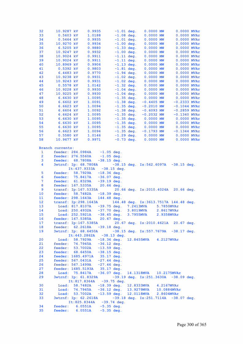
Page 300 of 365

32 10.9287 kV 0.9935 -1.01 deg. 0.0000 MW 0.0000 MVAr 33 0.5603 kV 1.0188 -1.08 deg. 0.0000 MW 0.0000 MVAr 34 0.5464 kV 0.9935 -1.01 deg. 0.0000 MW 0.0000 MVAr 35 10.9270 kV 0.9934 -1.00 deg. 0.0000 MW 0.0000 MVAr 36 6.5205 kV 0.9880 -1.33 deg. 0.0000 MW 0.0000 MVAr 37 10.9247 kV 0.9932 -1.00 deg. 0.0000 MW 0.0000 MVAr 38 10.9024 kV 0.9911 -1.11 deg. 0.0000 MW 0.0000 MVAr 39 10.9024 kV 0.9911 -1.11 deg. 0.0000 MW 0.0000 MVAr 40 10.8969 kV 0.9906 -1.13 deg. 0.0000 MW 0.0000 MVAr 41 0.5392 kV 0.9803 -1.81 deg. 0.0000 MW 0.0000 MVAr 42 6.4483 kV 0.9770 -1.94 deg. 0.0000 MW 0.0000 MVAr 43 10.9238 kV 0.9931 -1.02 deg. 0.0000 MW 0.0000 MVAr 44 10.9243 kV 0.9931 -1.02 deg. 0.0000 MW 0.0000 MVAr 45 0.5578 kV 1.0142 -1.32 deg. 0.0000 MW 0.0000 MVAr 46 10.9228 kV 0.9930 -1.04 deg. 0.0000 MW 0.0000 MVAr 47 10.9225 kV 0.9930 -1.04 deg. 0.0000 MW 0.0000 MVAr 48 6.6630 kV 1.0095 -1.35 deg. 0.0000 MW 0.0000 MVAr 49 6.6602 kV 1.0091 -1.38 deg. -0.4405 MW -0.2333 MVAr 50 6.6623 kV 1.0094 -1.35 deg. -0.2010 MW -0.1044 MVAr 51 6.6604 kV 1.0092 -1.38 deg. -0.6093 MW -0.2859 MVAr 52 6.6624 kV 1.0095 -1.35 deg. -0.2032 MW -0.1340 MVAr 53 6.6630 kV 1.0095 -1.35 deg. 0.0000 MW 0.0000 MVAr 54 6.6630 kV 1.0095 -1.35 deg. 0.0000 MW 0.0000 MVAr 55 6.6630 kV 1.0095 -1.35 deg. 0.0000 MW 0.0000 MVAr 56 6.6623 kV 1.0094 -1.35 deg. -0.1793 MW -0.1344 MVAr 57 0.5580 kV 1.0146 -1.29 deg. 0.0000 MW 0.0000 MVAr 58 10.9677 kV 0.9971 -0.73 deg. 0.0000 MW 0.0000 MVAr Branch currents: 1 feeder: 284.0984A -1.05 deg. 2 feeder: 276.5560A -1.05 deg. 3 feeder: 68.7808A -38.15 deg. 4 3wtrnf: Ip: 68.7808A -38.15 deg. Is:562.6097A -38.15 deg. It:437.9333A -38.15 deg. 5 feeder: 58.7929A -18.36 deg. 6 feeder: 75.8417A -36.07 deg. 7 feeder: 61.8329A -39.19 deg. 8 feeder: 167.5335A 20.66 deg. 9 transf: Ip:167.5335A 20.66 deg. Is:2010.4024A 20.66 deg. 10 feeder: 58.7482A -18.39 deg. 11 feeder: 298.1643A 144.48 deg. 12 transf: Ip:298.1643A 144.48 deg. Is:3613.7517A 144.48 deg. 13 Load: 817.8107A -39.75 deg. 7.2413MVA 5.7850MVAr 14 Load: 250.4932A -37.70 deg. 3.8019MVA 2.8617MVAr 15 Load: 252.5921A -38.45 deg. 3.7955MVA 2.9358MVAr 16 feeder: 167.5385A 20.67 deg. 17 transf: Ip:167.5385A 20.67 deg. Is:2010.4621A 20.67 deg. 18 feeder: 62.2618A -39.18 deg. 19 3wtrnf: Ip: 68.6450A -38.15 deg. Is:557.7679A -38.17 deg. It:443.2862A -38.13 deg. 20 Load: 58.7929A -18.36 deg. 12.8455MVA 4.2127MVAr 21 feeder: 74.7945A -36.12 deg. 22 feeder: 53.7002A -13.59 deg. 23 feeder: 68.6450A -38.15 deg. 24 feeder: 1685.4971A 35.17 deg. 25 feeder: 567.0431A -27.44 deg. 26 feeder: 567.1499A -27.46 deg. 27 feeder: 1685.5193A 35.17 deg. 28 Load: 75.8417A -36.07 deg. 14.1318MVA 10.2175MVAr 29 3wtrnf: Ip: 61.8329A -39.19 deg. Is:251.3630A -38.09 deg. It:817.8364A -39.75 deg. 30 Load: 58.7482A -18.39 deg. 12.8333MVA 4.2167MVAr 31 Load: 74.7945A -36.12 deg. 13.9279MVA 10.0884MVAr 32 Load: 53.7002A -13.59 deg. 12.0118MVA 2.8604MVAr 33 3wtrnf: Ip: 62.2618A -39.18 deg. Is:251.7114A -38.07 deg. It:825.8344A -39.74 deg. 34 feeder: 6.0551A -5.35 deg. 35 feeder: 6.0551A -5.35 deg.

Page 301 of 365

36 transf: Ip: 6.0551A -5.35 deg. Is:118.0745A -5.35 deg. 37 transf: Ip: 6.0551A -5.35 deg. Is:118.0745A -5.35 deg. 38 Load: 236.1490A -5.35 deg. 0.2286MVA 0.0171MVAr 39 feeder: 123.1422A -40.32 deg. 40 feeder: 119.5159A -39.36 deg. 41 transf: Ip:123.1422A -40.32 deg. Is:205.2370A -40.32 deg. 42 transf: Ip:119.5159A -39.36 deg. Is:199.1932A -39.36 deg. 43 Load: 404.4159A -39.85 deg. 3.5734MVA 2.8447MVAr 44 feeder: 86.8956A -38.68 deg. 45 feeder: 86.8956A -38.68 deg. 46 feeder: 114.9308A -40.53 deg. 47 transf: Ip: 86.8956A -38.68 deg. Is:1737.9117A -38.68 deg. 48 transf: Ip: 86.8956A -38.68 deg. Is:1737.9117A -38.68 deg. 49 transf: Ip:114.9308A -40.53 deg. Is:191.5513A -40.53 deg. 50 Load: 3475.8234A -38.68 deg. 2.5968MVA 1.9476MVAr 51 Load: 191.5513A -40.53 deg. 1.6721MVA 1.3346MVAr 52 Load: 224.9528A -39.55 deg. 3.3304MVA 2.6536MVAr 53 feeder: 36.6837A -38.22 deg. 54 feeder: 33.3171A -38.19 deg. 55 transf: Ip: 36.6837A -38.22 deg. Is:715.3325A -38.22 deg. 56 transf: Ip: 33.3171A -38.19 deg. Is:649.6838A -38.19 deg. 57 transf: Ip: 92.9008A -38.59 deg. Is:1802.2747A -38.59 deg. 58 transf: Ip: 93.4977A -38.64 deg. Is:1813.8556A -38.64 deg. 59 feeder: 92.9008A -38.59 deg. 60 feeder: 93.4977A -38.64 deg. 61 transf: Ip: 49.5508A -30.04 deg. Is: 80.9329A -30.04 deg. 62 transf: Ip: 49.2049A -29.98 deg. Is: 80.3680A -29.98 deg. 63 feeder: 49.5508A -30.04 deg. 64 feeder: 49.2049A -29.98 deg. 65 Load: 437.9340A -38.16 deg. 3.9620MVA 2.9771MVAr 66 Load: 443.2855A -38.13 deg. 4.0119MVA 3.0114MVAr 67 Load: 825.8601A -39.74 deg. 7.3135MVA 5.8407MVAr 68 feeder: 43.2089A -29.29 deg. 69 feeder: 19.6284A -28.80 deg. 70 feeder: 58.3407A -26.52 deg. 71 feeder: 21.0914A -34.77 deg. 72 feeder: 0.0000A -103.32 deg. 73 feeder: 0.0000A -166.23 deg. 74 feeder: 0.0000A -103.32 deg. 75 feeder: 19.4187A -38.21 deg. 76 Load: 3616.1300A -38.62 deg. 2.7886MVA 2.0914MVAr 77 Load: 6.3876A -38.19 deg. 0.0049MVA 0.0037MVAr 78 Load: 352.6007A -38.22 deg. 0.2724MVA 0.2045MVAr 79 Load: 126.1558A -38.22 deg. 0.0975MVA 0.0732MVAr 80 Load: 123.9410A -38.22 deg. 0.0958MVA 0.0719MVAr 81 Load: 106.2473A -38.22 deg. 0.0821MVA 0.0616MVAr 82 Load: 70.3968A -38.18 deg. 0.0544MVA 0.0408MVAr 83 Load: 3.1952A -38.16 deg. 0.0025MVA 0.0019MVAr 84 Load: 352.7552A -38.19 deg. 0.2727MVA 0.2047MVAr 85 Load: 132.5990A -38.19 deg. 0.1025MVA 0.0770MVAr 86 Load: 90.7375A -38.19 deg. 0.0701MVA 0.0527MVAr

13.6 Study Case 5 – Final State Bus voltages and currents calculated on completion of simulation. Number of iterations: 1 Max Power mismatch: 10.0kVA Bus Voltage(l-l) Voltage(pu) Angle P(bus) Q(bus) 1 133.0000 kV 1.0076 0.00 deg. 130.3709 MW 1.5078 MVAr 2 132.7573 kV 1.0057 -0.20 deg. 0.0000 MW 0.0000 MVAr 3 132.7533 kV 1.0057 -0.20 deg. 0.0000 MW 0.0000 MVAr 4 132.7549 kV 1.0057 -0.20 deg. 0.0000 MW 0.0000 MVAr 5 132.7504 kV 1.0057 -0.20 deg. 0.0000 MW 0.0000 MVAr 6 131.1762 kV 0.9938 -0.97 deg. 0.0000 MW 0.0000 MVAr 7 10.9283 kV 0.9935 -1.01 deg. 0.0000 MW 0.0000 MVAr 8 6.5330 kV 0.9898 -1.24 deg. 0.0000 MW 0.0000 MVAr

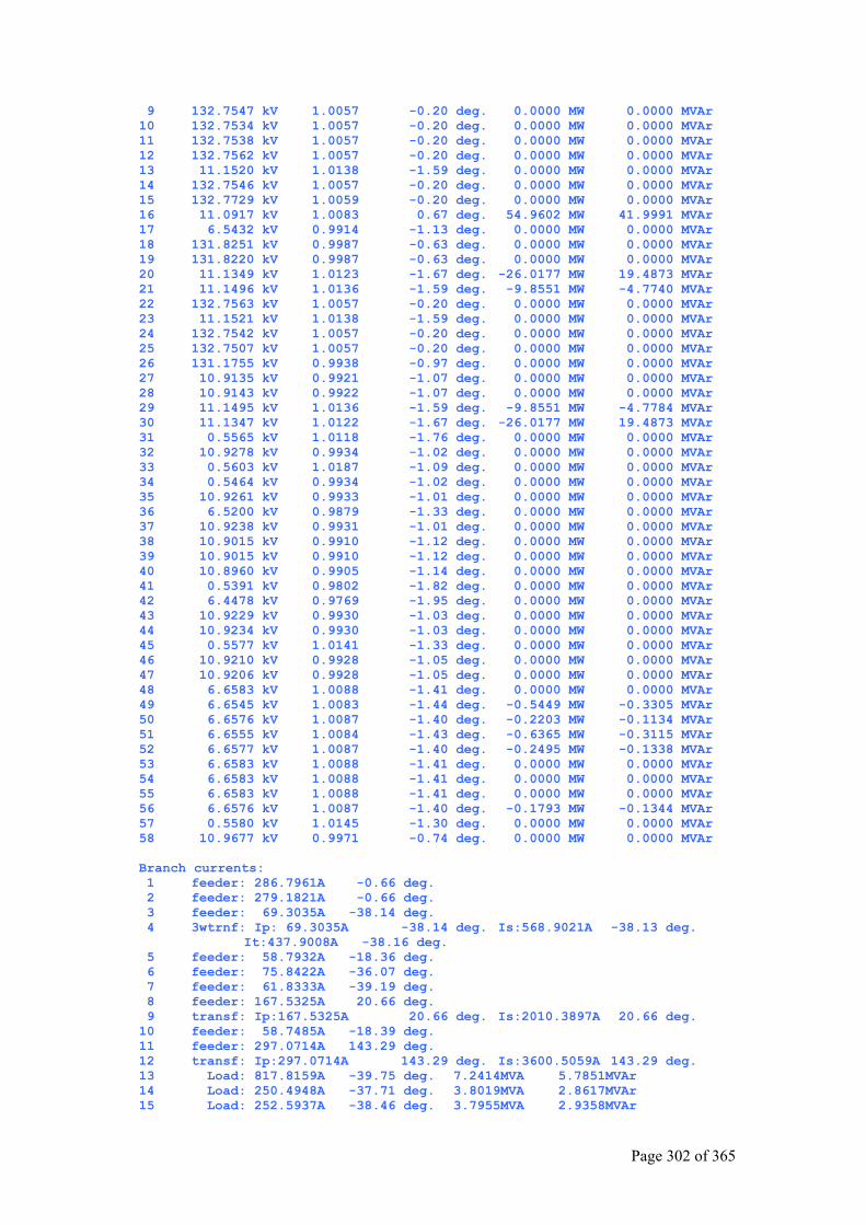
Page 302 of 365

9 132.7547 kV 1.0057 -0.20 deg. 0.0000 MW 0.0000 MVAr 10 132.7534 kV 1.0057 -0.20 deg. 0.0000 MW 0.0000 MVAr 11 132.7538 kV 1.0057 -0.20 deg. 0.0000 MW 0.0000 MVAr 12 132.7562 kV 1.0057 -0.20 deg. 0.0000 MW 0.0000 MVAr 13 11.1520 kV 1.0138 -1.59 deg. 0.0000 MW 0.0000 MVAr 14 132.7546 kV 1.0057 -0.20 deg. 0.0000 MW 0.0000 MVAr 15 132.7729 kV 1.0059 -0.20 deg. 0.0000 MW 0.0000 MVAr 16 11.0917 kV 1.0083 0.67 deg. 54.9602 MW 41.9991 MVAr 17 6.5432 kV 0.9914 -1.13 deg. 0.0000 MW 0.0000 MVAr 18 131.8251 kV 0.9987 -0.63 deg. 0.0000 MW 0.0000 MVAr 19 131.8220 kV 0.9987 -0.63 deg. 0.0000 MW 0.0000 MVAr 20 11.1349 kV 1.0123 -1.67 deg. -26.0177 MW 19.4873 MVAr 21 11.1496 kV 1.0136 -1.59 deg. -9.8551 MW -4.7740 MVAr 22 132.7563 kV 1.0057 -0.20 deg. 0.0000 MW 0.0000 MVAr 23 11.1521 kV 1.0138 -1.59 deg. 0.0000 MW 0.0000 MVAr 24 132.7542 kV 1.0057 -0.20 deg. 0.0000 MW 0.0000 MVAr 25 132.7507 kV 1.0057 -0.20 deg. 0.0000 MW 0.0000 MVAr 26 131.1755 kV 0.9938 -0.97 deg. 0.0000 MW 0.0000 MVAr 27 10.9135 kV 0.9921 -1.07 deg. 0.0000 MW 0.0000 MVAr 28 10.9143 kV 0.9922 -1.07 deg. 0.0000 MW 0.0000 MVAr 29 11.1495 kV 1.0136 -1.59 deg. -9.8551 MW -4.7784 MVAr 30 11.1347 kV 1.0122 -1.67 deg. -26.0177 MW 19.4873 MVAr 31 0.5565 kV 1.0118 -1.76 deg. 0.0000 MW 0.0000 MVAr 32 10.9278 kV 0.9934 -1.02 deg. 0.0000 MW 0.0000 MVAr 33 0.5603 kV 1.0187 -1.09 deg. 0.0000 MW 0.0000 MVAr 34 0.5464 kV 0.9934 -1.02 deg. 0.0000 MW 0.0000 MVAr 35 10.9261 kV 0.9933 -1.01 deg. 0.0000 MW 0.0000 MVAr 36 6.5200 kV 0.9879 -1.33 deg. 0.0000 MW 0.0000 MVAr 37 10.9238 kV 0.9931 -1.01 deg. 0.0000 MW 0.0000 MVAr 38 10.9015 kV 0.9910 -1.12 deg. 0.0000 MW 0.0000 MVAr 39 10.9015 kV 0.9910 -1.12 deg. 0.0000 MW 0.0000 MVAr 40 10.8960 kV 0.9905 -1.14 deg. 0.0000 MW 0.0000 MVAr 41 0.5391 kV 0.9802 -1.82 deg. 0.0000 MW 0.0000 MVAr 42 6.4478 kV 0.9769 -1.95 deg. 0.0000 MW 0.0000 MVAr 43 10.9229 kV 0.9930 -1.03 deg. 0.0000 MW 0.0000 MVAr 44 10.9234 kV 0.9930 -1.03 deg. 0.0000 MW 0.0000 MVAr 45 0.5577 kV 1.0141 -1.33 deg. 0.0000 MW 0.0000 MVAr 46 10.9210 kV 0.9928 -1.05 deg. 0.0000 MW 0.0000 MVAr 47 10.9206 kV 0.9928 -1.05 deg. 0.0000 MW 0.0000 MVAr 48 6.6583 kV 1.0088 -1.41 deg. 0.0000 MW 0.0000 MVAr 49 6.6545 kV 1.0083 -1.44 deg. -0.5449 MW -0.3305 MVAr 50 6.6576 kV 1.0087 -1.40 deg. -0.2203 MW -0.1134 MVAr 51 6.6555 kV 1.0084 -1.43 deg. -0.6365 MW -0.3115 MVAr 52 6.6577 kV 1.0087 -1.40 deg. -0.2495 MW -0.1338 MVAr 53 6.6583 kV 1.0088 -1.41 deg. 0.0000 MW 0.0000 MVAr 54 6.6583 kV 1.0088 -1.41 deg. 0.0000 MW 0.0000 MVAr 55 6.6583 kV 1.0088 -1.41 deg. 0.0000 MW 0.0000 MVAr 56 6.6576 kV 1.0087 -1.40 deg. -0.1793 MW -0.1344 MVAr 57 0.5580 kV 1.0145 -1.30 deg. 0.0000 MW 0.0000 MVAr 58 10.9677 kV 0.9971 -0.74 deg. 0.0000 MW 0.0000 MVAr Branch currents: 1 feeder: 286.7961A -0.66 deg. 2 feeder: 279.1821A -0.66 deg. 3 feeder: 69.3035A -38.14 deg. 4 3wtrnf: Ip: 69.3035A -38.14 deg. Is:568.9021A -38.13 deg. It:437.9008A -38.16 deg. 5 feeder: 58.7932A -18.36 deg. 6 feeder: 75.8422A -36.07 deg. 7 feeder: 61.8333A -39.19 deg. 8 feeder: 167.5325A 20.66 deg. 9 transf: Ip:167.5325A 20.66 deg. Is:2010.3897A 20.66 deg. 10 feeder: 58.7485A -18.39 deg. 11 feeder: 297.0714A 143.29 deg. 12 transf: Ip:297.0714A 143.29 deg. Is:3600.5059A 143.29 deg. 13 Load: 817.8159A -39.75 deg. 7.2414MVA 5.7851MVAr 14 Load: 250.4948A -37.71 deg. 3.8019MVA 2.8617MVAr 15 Load: 252.5937A -38.46 deg. 3.7955MVA 2.9358MVAr

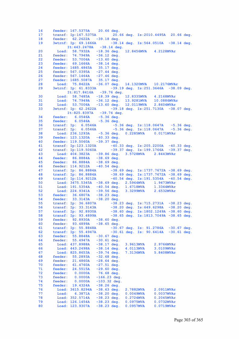
Page 303 of 365

16 feeder: 167.5375A 20.66 deg. 17 transf: Ip:167.5375A 20.66 deg. Is:2010.4495A 20.66 deg. 18 feeder: 62.2622A -39.18 deg. 19 3wtrnf: Ip: 69.1666A -38.14 deg. Is:564.0510A -38.14 deg. It:443.2478A -38.14 deg. 20 Load: 58.7932A -18.36 deg. 12.8456MVA 4.2128MVAr 21 feeder: 74.7949A -36.12 deg. 22 feeder: 53.7006A -13.60 deg. 23 feeder: 69.1666A -38.14 deg. 24 feeder: 1685.4865A 35.17 deg. 25 feeder: 567.0395A -27.44 deg. 26 feeder: 567.1464A -27.46 deg. 27 feeder: 1685.5087A 35.17 deg. 28 Load: 75.8422A -36.07 deg. 14.1320MVA 10.2176MVAr 29 3wtrnf: Ip: 61.8333A -39.19 deg. Is:251.3646A -38.09 deg. It:817.8416A -39.76 deg. 30 Load: 58.7485A -18.39 deg. 12.8335MVA 4.2168MVAr 31 Load: 74.7949A -36.12 deg. 13.9281MVA 10.0886MVAr 32 Load: 53.7006A -13.60 deg. 12.0119MVA 2.8604MVAr 33 3wtrnf: Ip: 62.2622A -39.18 deg. Is:251.7130A -38.07 deg. It:825.8397A -39.74 deg. 34 feeder: 6.0546A -5.36 deg. 35 feeder: 6.0546A -5.36 deg. 36 transf: Ip: 6.0546A -5.36 deg. Is:118.0647A -5.36 deg. 37 transf: Ip: 6.0546A -5.36 deg. Is:118.0647A -5.36 deg. 38 Load: 236.1293A -5.36 deg. 0.2285MVA 0.0171MVAr 39 feeder: 123.1320A -40.33 deg. 40 feeder: 119.5060A -39.37 deg. 41 transf: Ip:123.1320A -40.33 deg. Is:205.2200A -40.33 deg. 42 transf: Ip:119.5060A -39.37 deg. Is:199.1766A -39.37 deg. 43 Load: 404.3823A -39.86 deg. 3.5728MVA 2.8443MVAr 44 feeder: 86.8884A -38.69 deg. 45 feeder: 86.8884A -38.69 deg. 46 feeder: 114.9212A -40.54 deg. 47 transf: Ip: 86.8884A -38.69 deg. Is:1737.7672A -38.69 deg. 48 transf: Ip: 86.8884A -38.69 deg. Is:1737.7672A -38.69 deg. 49 transf: Ip:114.9212A -40.54 deg. Is:191.5354A -40.54 deg. 50 Load: 3475.5345A -38.69 deg. 2.5964MVA 1.9473MVAr 51 Load: 191.5354A -40.54 deg. 1.6718MVA 1.3344MVAr 52 Load: 224.9341A -39.56 deg. 3.3299MVA 2.6532MVAr 53 feeder: 36.6807A -38.23 deg. 54 feeder: 33.3143A -38.20 deg. 55 transf: Ip: 36.6807A -38.23 deg. Is:715.2731A -38.23 deg. 56 transf: Ip: 33.3143A -38.20 deg. Is:649.6298A -38.20 deg. 57 transf: Ip: 92.8930A -38.60 deg. Is:1802.1249A -38.60 deg. 58 transf: Ip: 93.4899A -38.65 deg. Is:1813.7049A -38.65 deg. 59 feeder: 92.8930A -38.60 deg. 60 feeder: 93.4899A -38.65 deg. 61 transf: Ip: 55.8848A -30.67 deg. Is: 91.2786A -30.67 deg. 62 transf: Ip: 55.4947A -30.61 deg. Is: 90.6414A -30.61 deg. 63 feeder: 55.8848A -30.67 deg. 64 feeder: 55.4947A -30.61 deg. 65 Load: 437.8988A -38.17 deg. 3.9613MVA 2.9766MVAr 66 Load: 443.2498A -38.14 deg. 4.0113MVA 3.0109MVAr 67 Load: 825.8653A -39.74 deg. 7.3136MVA 5.8408MVAr 68 feeder: 55.2893A -32.68 deg. 69 feeder: 21.4860A -28.64 deg. 70 feeder: 61.4760A -27.51 deg. 71 feeder: 24.5515A -29.60 deg. 72 feeder: 0.0000A 76.68 deg. 73 feeder: 0.0000A -166.23 deg. 74 feeder: 0.0000A -103.32 deg. 75 feeder: 19.4324A -38.26 deg. 76 Load: 3615.8294A -38.63 deg. 2.7882MVA 2.0911MVAr 77 Load: 6.3871A -38.20 deg. 0.0049MVA 0.0037MVAr 78 Load: 352.5714A -38.23 deg. 0.2724MVA 0.2045MVAr 79 Load: 126.1454A -38.23 deg. 0.0975MVA 0.0732MVAr 80 Load: 123.9307A -38.23 deg. 0.0957MVA 0.0719MVAr

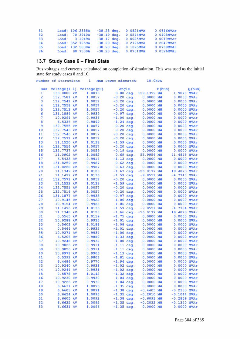
Page 304 of 365

81 Load: 106.2385A -38.23 deg. 0.0821MVA 0.0616MVAr 82 Load: 70.3910A -38.19 deg. 0.0544MVA 0.0408MVAr 83 Load: 3.1949A -38.17 deg. 0.0025MVA 0.0019MVAr 84 Load: 352.7259A -38.20 deg. 0.2726MVA 0.2047MVAr 85 Load: 132.5880A -38.20 deg. 0.1025MVA 0.0769MVAr 86 Load: 90.7300A -38.20 deg. 0.0701MVA 0.0526MVAr

13.7 Study Case 6 – Final State Bus voltages and currents calculated on completion of simulation. This was used as the initial state for study cases 8 and 10. Number of iterations: 1 Max Power mismatch: 10.0kVA Bus Voltage(l-l) Voltage(pu) Angle P(bus) Q(bus) 1 133.0000 kV 1.0076 0.00 deg. 129.1399 MW 1.9070 MVAr 2 132.7581 kV 1.0057 -0.20 deg. 0.0000 MW 0.0000 MVAr 3 132.7541 kV 1.0057 -0.20 deg. 0.0000 MW 0.0000 MVAr 4 132.7558 kV 1.0057 -0.20 deg. 0.0000 MW 0.0000 MVAr 5 132.7513 kV 1.0057 -0.20 deg. 0.0000 MW 0.0000 MVAr 6 131.1884 kV 0.9939 -0.97 deg. 0.0000 MW 0.0000 MVAr 7 10.9294 kV 0.9936 -1.00 deg. 0.0000 MW 0.0000 MVAr 8 6.5336 kV 0.9899 -1.24 deg. 0.0000 MW 0.0000 MVAr 9 132.7555 kV 1.0057 -0.20 deg. 0.0000 MW 0.0000 MVAr 10 132.7543 kV 1.0057 -0.20 deg. 0.0000 MW 0.0000 MVAr 11 132.7546 kV 1.0057 -0.20 deg. 0.0000 MW 0.0000 MVAr 12 132.7571 kV 1.0057 -0.20 deg. 0.0000 MW 0.0000 MVAr 13 11.1520 kV 1.0138 -1.59 deg. 0.0000 MW 0.0000 MVAr 14 132.7554 kV 1.0057 -0.20 deg. 0.0000 MW 0.0000 MVAr 15 132.7737 kV 1.0059 -0.19 deg. 0.0000 MW 0.0000 MVAr 16 11.0902 kV 1.0082 0.69 deg. 55.9956 MW 41.4845 MVAr 17 6.5433 kV 0.9914 -1.13 deg. 0.0000 MW 0.0000 MVAr 18 131.8259 kV 0.9987 -0.62 deg. 0.0000 MW 0.0000 MVAr 19 131.8228 kV 0.9987 -0.63 deg. 0.0000 MW 0.0000 MVAr 20 11.1349 kV 1.0123 -1.67 deg. -26.0177 MW 19.4873 MVAr 21 11.1497 kV 1.0136 -1.59 deg. -9.8551 MW -4.7740 MVAr 22 132.7571 kV 1.0057 -0.20 deg. 0.0000 MW 0.0000 MVAr 23 11.1522 kV 1.0138 -1.59 deg. 0.0000 MW 0.0000 MVAr 24 132.7551 kV 1.0057 -0.20 deg. 0.0000 MW 0.0000 MVAr 25 132.7516 kV 1.0057 -0.20 deg. 0.0000 MW 0.0000 MVAr 26 131.1877 kV 0.9938 -0.97 deg. 0.0000 MW 0.0000 MVAr 27 10.9145 kV 0.9922 -1.06 deg. 0.0000 MW 0.0000 MVAr 28 10.9154 kV 0.9923 -1.06 deg. 0.0000 MW 0.0000 MVAr 29 11.1496 kV 1.0136 -1.59 deg. -9.8551 MW -4.7784 MVAr 30 11.1348 kV 1.0123 -1.66 deg. -26.0177 MW 19.4873 MVAr 31 0.5565 kV 1.0119 -1.75 deg. 0.0000 MW 0.0000 MVAr 32 10.9288 kV 0.9935 -1.01 deg. 0.0000 MW 0.0000 MVAr 33 0.5603 kV 1.0188 -1.08 deg. 0.0000 MW 0.0000 MVAr 34 0.5464 kV 0.9935 -1.01 deg. 0.0000 MW 0.0000 MVAr 35 10.9271 kV 0.9934 -1.00 deg. 0.0000 MW 0.0000 MVAr 36 6.5206 kV 0.9880 -1.33 deg. 0.0000 MW 0.0000 MVAr 37 10.9248 kV 0.9932 -1.00 deg. 0.0000 MW 0.0000 MVAr 38 10.9026 kV 0.9911 -1.11 deg. 0.0000 MW 0.0000 MVAr 39 10.9026 kV 0.9911 -1.11 deg. 0.0000 MW 0.0000 MVAr 40 10.8971 kV 0.9906 -1.13 deg. 0.0000 MW 0.0000 MVAr 41 0.5392 kV 0.9803 -1.81 deg. 0.0000 MW 0.0000 MVAr 42 6.4484 kV 0.9770 -1.94 deg. 0.0000 MW 0.0000 MVAr 43 10.9240 kV 0.9931 -1.02 deg. 0.0000 MW 0.0000 MVAr 44 10.9244 kV 0.9931 -1.02 deg. 0.0000 MW 0.0000 MVAr 45 0.5578 kV 1.0142 -1.32 deg. 0.0000 MW 0.0000 MVAr 46 10.9230 kV 0.9930 -1.04 deg. 0.0000 MW 0.0000 MVAr 47 10.9226 kV 0.9930 -1.04 deg. 0.0000 MW 0.0000 MVAr 48 6.6631 kV 1.0096 -1.35 deg. 0.0000 MW 0.0000 MVAr 49 6.6603 kV 1.0091 -1.38 deg. -0.4405 MW -0.2333 MVAr 50 6.6624 kV 1.0095 -1.35 deg. -0.2010 MW -0.1044 MVAr 51 6.6605 kV 1.0092 -1.38 deg. -0.6093 MW -0.2859 MVAr 52 6.6625 kV 1.0095 -1.35 deg. -0.2032 MW -0.1340 MVAr 53 6.6631 kV 1.0096 -1.35 deg. 0.0000 MW 0.0000 MVAr

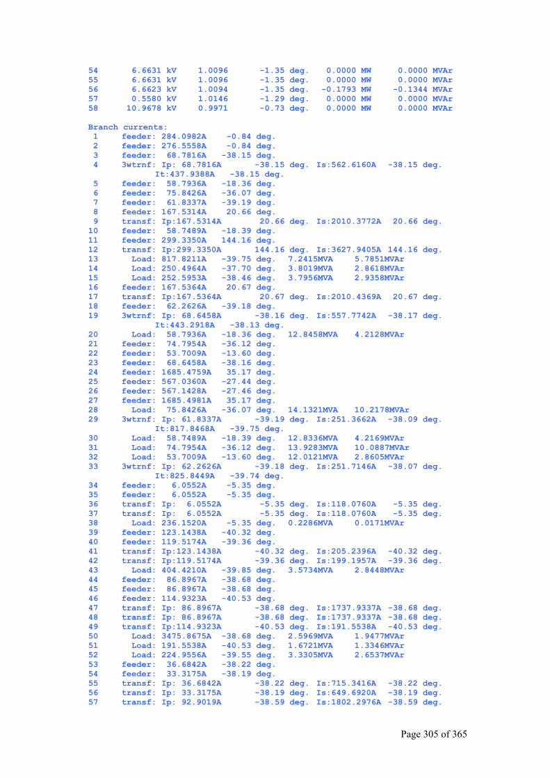
Page 305 of 365

54 6.6631 kV 1.0096 -1.35 deg. 0.0000 MW 0.0000 MVAr 55 6.6631 kV 1.0096 -1.35 deg. 0.0000 MW 0.0000 MVAr 56 6.6623 kV 1.0094 -1.35 deg. -0.1793 MW -0.1344 MVAr 57 0.5580 kV 1.0146 -1.29 deg. 0.0000 MW 0.0000 MVAr 58 10.9678 kV 0.9971 -0.73 deg. 0.0000 MW 0.0000 MVAr Branch currents: 1 feeder: 284.0982A -0.84 deg. 2 feeder: 276.5558A -0.84 deg. 3 feeder: 68.7816A -38.15 deg. 4 3wtrnf: Ip: 68.7816A -38.15 deg. Is:562.6160A -38.15 deg. It:437.9388A -38.15 deg. 5 feeder: 58.7936A -18.36 deg. 6 feeder: 75.8426A -36.07 deg. 7 feeder: 61.8337A -39.19 deg. 8 feeder: 167.5314A 20.66 deg. 9 transf: Ip:167.5314A 20.66 deg. Is:2010.3772A 20.66 deg. 10 feeder: 58.7489A -18.39 deg. 11 feeder: 299.3350A 144.16 deg. 12 transf: Ip:299.3350A 144.16 deg. Is:3627.9405A 144.16 deg. 13 Load: 817.8211A -39.75 deg. 7.2415MVA 5.7851MVAr 14 Load: 250.4964A -37.70 deg. 3.8019MVA 2.8618MVAr 15 Load: 252.5953A -38.46 deg. 3.7956MVA 2.9358MVAr 16 feeder: 167.5364A 20.67 deg. 17 transf: Ip:167.5364A 20.67 deg. Is:2010.4369A 20.67 deg. 18 feeder: 62.2626A -39.18 deg. 19 3wtrnf: Ip: 68.6458A -38.16 deg. Is:557.7742A -38.17 deg. It:443.2918A -38.13 deg. 20 Load: 58.7936A -18.36 deg. 12.8458MVA 4.2128MVAr 21 feeder: 74.7954A -36.12 deg. 22 feeder: 53.7009A -13.60 deg. 23 feeder: 68.6458A -38.16 deg. 24 feeder: 1685.4759A 35.17 deg. 25 feeder: 567.0360A -27.44 deg. 26 feeder: 567.1428A -27.46 deg. 27 feeder: 1685.4981A 35.17 deg. 28 Load: 75.8426A -36.07 deg. 14.1321MVA 10.2178MVAr 29 3wtrnf: Ip: 61.8337A -39.19 deg. Is:251.3662A -38.09 deg. It:817.8468A -39.75 deg. 30 Load: 58.7489A -18.39 deg. 12.8336MVA 4.2169MVAr 31 Load: 74.7954A -36.12 deg. 13.9283MVA 10.0887MVAr 32 Load: 53.7009A -13.60 deg. 12.0121MVA 2.8605MVAr 33 3wtrnf: Ip: 62.2626A -39.18 deg. Is:251.7146A -38.07 deg. It:825.8449A -39.74 deg. 34 feeder: 6.0552A -5.35 deg. 35 feeder: 6.0552A -5.35 deg. 36 transf: Ip: 6.0552A -5.35 deg. Is:118.0760A -5.35 deg. 37 transf: Ip: 6.0552A -5.35 deg. Is:118.0760A -5.35 deg. 38 Load: 236.1520A -5.35 deg. 0.2286MVA 0.0171MVAr 39 feeder: 123.1438A -40.32 deg. 40 feeder: 119.5174A -39.36 deg. 41 transf: Ip:123.1438A -40.32 deg. Is:205.2396A -40.32 deg. 42 transf: Ip:119.5174A -39.36 deg. Is:199.1957A -39.36 deg. 43 Load: 404.4210A -39.85 deg. 3.5734MVA 2.8448MVAr 44 feeder: 86.8967A -38.68 deg. 45 feeder: 86.8967A -38.68 deg. 46 feeder: 114.9323A -40.53 deg. 47 transf: Ip: 86.8967A -38.68 deg. Is:1737.9337A -38.68 deg. 48 transf: Ip: 86.8967A -38.68 deg. Is:1737.9337A -38.68 deg. 49 transf: Ip:114.9323A -40.53 deg. Is:191.5538A -40.53 deg. 50 Load: 3475.8675A -38.68 deg. 2.5969MVA 1.9477MVAr 51 Load: 191.5538A -40.53 deg. 1.6721MVA 1.3346MVAr 52 Load: 224.9556A -39.55 deg. 3.3305MVA 2.6537MVAr 53 feeder: 36.6842A -38.22 deg. 54 feeder: 33.3175A -38.19 deg. 55 transf: Ip: 36.6842A -38.22 deg. Is:715.3416A -38.22 deg. 56 transf: Ip: 33.3175A -38.19 deg. Is:649.6920A -38.19 deg. 57 transf: Ip: 92.9019A -38.59 deg. Is:1802.2976A -38.59 deg.

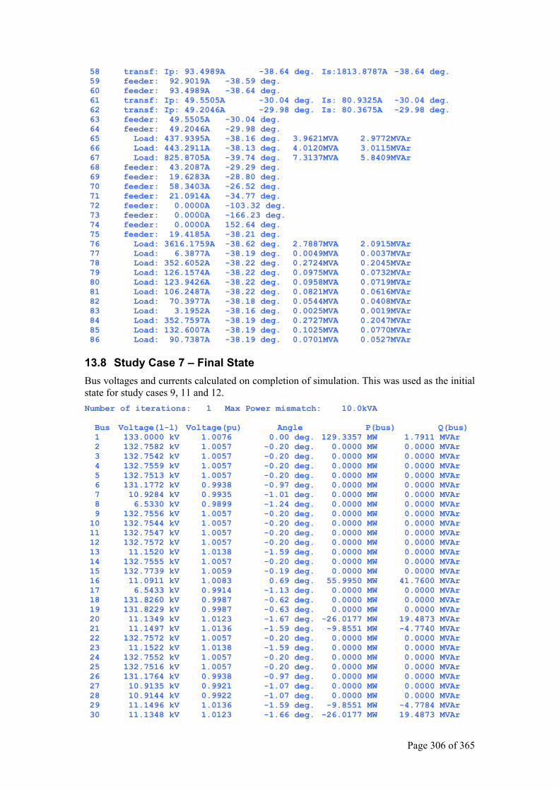
Page 306 of 365

58 transf: Ip: 93.4989A -38.64 deg. Is:1813.8787A -38.64 deg. 59 feeder: 92.9019A -38.59 deg. 60 feeder: 93.4989A -38.64 deg. 61 transf: Ip: 49.5505A -30.04 deg. Is: 80.9325A -30.04 deg. 62 transf: Ip: 49.2046A -29.98 deg. Is: 80.3675A -29.98 deg. 63 feeder: 49.5505A -30.04 deg. 64 feeder: 49.2046A -29.98 deg. 65 Load: 437.9395A -38.16 deg. 3.9621MVA 2.9772MVAr 66 Load: 443.2911A -38.13 deg. 4.0120MVA 3.0115MVAr 67 Load: 825.8705A -39.74 deg. 7.3137MVA 5.8409MVAr 68 feeder: 43.2087A -29.29 deg. 69 feeder: 19.6283A -28.80 deg. 70 feeder: 58.3403A -26.52 deg. 71 feeder: 21.0914A -34.77 deg. 72 feeder: 0.0000A -103.32 deg. 73 feeder: 0.0000A -166.23 deg. 74 feeder: 0.0000A 152.64 deg. 75 feeder: 19.4185A -38.21 deg. 76 Load: 3616.1759A -38.62 deg. 2.7887MVA 2.0915MVAr 77 Load: 6.3877A -38.19 deg. 0.0049MVA 0.0037MVAr 78 Load: 352.6052A -38.22 deg. 0.2724MVA 0.2045MVAr 79 Load: 126.1574A -38.22 deg. 0.0975MVA 0.0732MVAr 80 Load: 123.9426A -38.22 deg. 0.0958MVA 0.0719MVAr 81 Load: 106.2487A -38.22 deg. 0.0821MVA 0.0616MVAr 82 Load: 70.3977A -38.18 deg. 0.0544MVA 0.0408MVAr 83 Load: 3.1952A -38.16 deg. 0.0025MVA 0.0019MVAr 84 Load: 352.7597A -38.19 deg. 0.2727MVA 0.2047MVAr 85 Load: 132.6007A -38.19 deg. 0.1025MVA 0.0770MVAr 86 Load: 90.7387A -38.19 deg. 0.0701MVA 0.0527MVAr

13.8 Study Case 7 – Final State Bus voltages and currents calculated on completion of simulation. This was used as the initial state for study cases 9, 11 and 12. Number of iterations: 1 Max Power mismatch: 10.0kVA Bus Voltage(l-l) Voltage(pu) Angle P(bus) Q(bus) 1 133.0000 kV 1.0076 0.00 deg. 129.3357 MW 1.7911 MVAr 2 132.7582 kV 1.0057 -0.20 deg. 0.0000 MW 0.0000 MVAr 3 132.7542 kV 1.0057 -0.20 deg. 0.0000 MW 0.0000 MVAr 4 132.7559 kV 1.0057 -0.20 deg. 0.0000 MW 0.0000 MVAr 5 132.7513 kV 1.0057 -0.20 deg. 0.0000 MW 0.0000 MVAr 6 131.1772 kV 0.9938 -0.97 deg. 0.0000 MW 0.0000 MVAr 7 10.9284 kV 0.9935 -1.01 deg. 0.0000 MW 0.0000 MVAr 8 6.5330 kV 0.9899 -1.24 deg. 0.0000 MW 0.0000 MVAr 9 132.7556 kV 1.0057 -0.20 deg. 0.0000 MW 0.0000 MVAr 10 132.7544 kV 1.0057 -0.20 deg. 0.0000 MW 0.0000 MVAr 11 132.7547 kV 1.0057 -0.20 deg. 0.0000 MW 0.0000 MVAr 12 132.7572 kV 1.0057 -0.20 deg. 0.0000 MW 0.0000 MVAr 13 11.1520 kV 1.0138 -1.59 deg. 0.0000 MW 0.0000 MVAr 14 132.7555 kV 1.0057 -0.20 deg. 0.0000 MW 0.0000 MVAr 15 132.7739 kV 1.0059 -0.19 deg. 0.0000 MW 0.0000 MVAr 16 11.0911 kV 1.0083 0.69 deg. 55.9950 MW 41.7600 MVAr 17 6.5433 kV 0.9914 -1.13 deg. 0.0000 MW 0.0000 MVAr 18 131.8260 kV 0.9987 -0.62 deg. 0.0000 MW 0.0000 MVAr 19 131.8229 kV 0.9987 -0.63 deg. 0.0000 MW 0.0000 MVAr 20 11.1349 kV 1.0123 -1.67 deg. -26.0177 MW 19.4873 MVAr 21 11.1497 kV 1.0136 -1.59 deg. -9.8551 MW -4.7740 MVAr 22 132.7572 kV 1.0057 -0.20 deg. 0.0000 MW 0.0000 MVAr 23 11.1522 kV 1.0138 -1.59 deg. 0.0000 MW 0.0000 MVAr 24 132.7552 kV 1.0057 -0.20 deg. 0.0000 MW 0.0000 MVAr 25 132.7516 kV 1.0057 -0.20 deg. 0.0000 MW 0.0000 MVAr 26 131.1764 kV 0.9938 -0.97 deg. 0.0000 MW 0.0000 MVAr 27 10.9135 kV 0.9921 -1.07 deg. 0.0000 MW 0.0000 MVAr 28 10.9144 kV 0.9922 -1.07 deg. 0.0000 MW 0.0000 MVAr 29 11.1496 kV 1.0136 -1.59 deg. -9.8551 MW -4.7784 MVAr 30 11.1348 kV 1.0123 -1.66 deg. -26.0177 MW 19.4873 MVAr

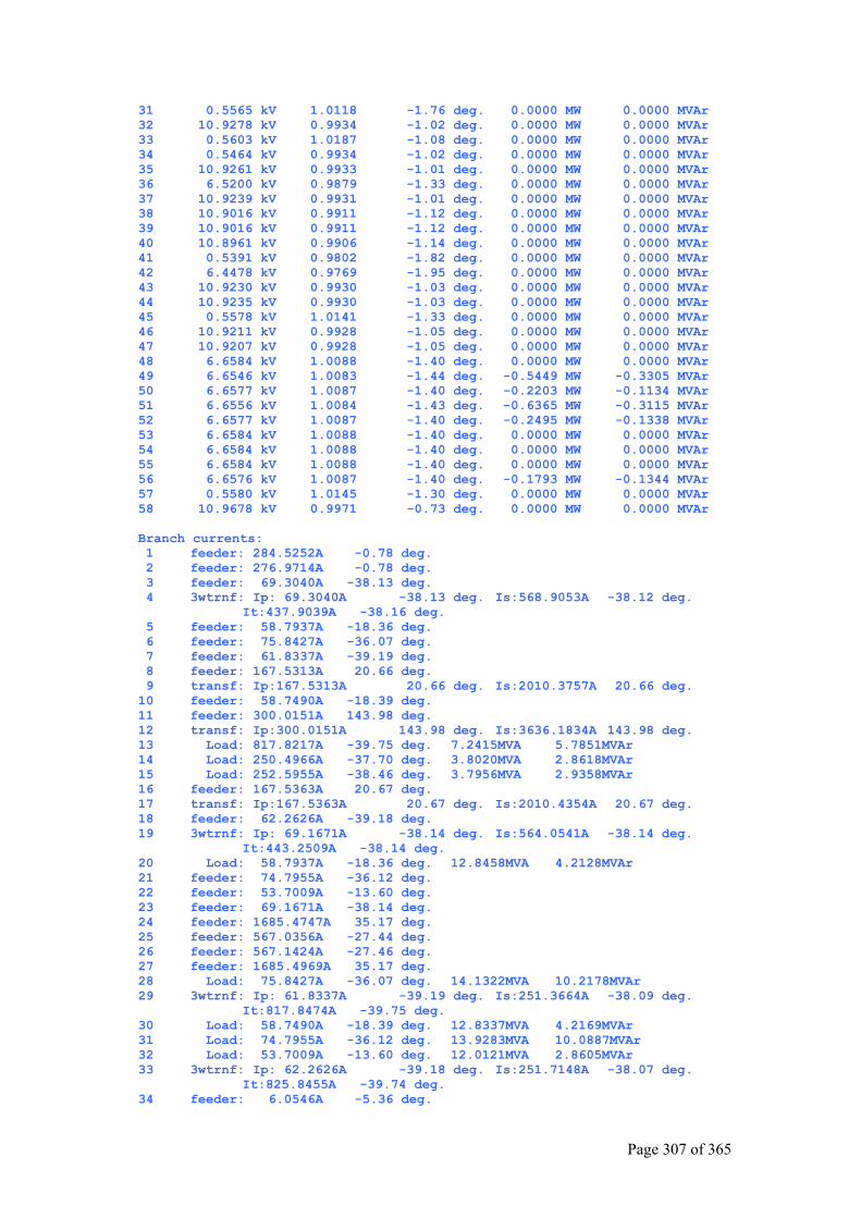
Page 307 of 365

31 0.5565 kV 1.0118 -1.76 deg. 0.0000 MW 0.0000 MVAr 32 10.9278 kV 0.9934 -1.02 deg. 0.0000 MW 0.0000 MVAr 33 0.5603 kV 1.0187 -1.08 deg. 0.0000 MW 0.0000 MVAr 34 0.5464 kV 0.9934 -1.02 deg. 0.0000 MW 0.0000 MVAr 35 10.9261 kV 0.9933 -1.01 deg. 0.0000 MW 0.0000 MVAr 36 6.5200 kV 0.9879 -1.33 deg. 0.0000 MW 0.0000 MVAr 37 10.9239 kV 0.9931 -1.01 deg. 0.0000 MW 0.0000 MVAr 38 10.9016 kV 0.9911 -1.12 deg. 0.0000 MW 0.0000 MVAr 39 10.9016 kV 0.9911 -1.12 deg. 0.0000 MW 0.0000 MVAr 40 10.8961 kV 0.9906 -1.14 deg. 0.0000 MW 0.0000 MVAr 41 0.5391 kV 0.9802 -1.82 deg. 0.0000 MW 0.0000 MVAr 42 6.4478 kV 0.9769 -1.95 deg. 0.0000 MW 0.0000 MVAr 43 10.9230 kV 0.9930 -1.03 deg. 0.0000 MW 0.0000 MVAr 44 10.9235 kV 0.9930 -1.03 deg. 0.0000 MW 0.0000 MVAr 45 0.5578 kV 1.0141 -1.33 deg. 0.0000 MW 0.0000 MVAr 46 10.9211 kV 0.9928 -1.05 deg. 0.0000 MW 0.0000 MVAr 47 10.9207 kV 0.9928 -1.05 deg. 0.0000 MW 0.0000 MVAr 48 6.6584 kV 1.0088 -1.40 deg. 0.0000 MW 0.0000 MVAr 49 6.6546 kV 1.0083 -1.44 deg. -0.5449 MW -0.3305 MVAr 50 6.6577 kV 1.0087 -1.40 deg. -0.2203 MW -0.1134 MVAr 51 6.6556 kV 1.0084 -1.43 deg. -0.6365 MW -0.3115 MVAr 52 6.6577 kV 1.0087 -1.40 deg. -0.2495 MW -0.1338 MVAr 53 6.6584 kV 1.0088 -1.40 deg. 0.0000 MW 0.0000 MVAr 54 6.6584 kV 1.0088 -1.40 deg. 0.0000 MW 0.0000 MVAr 55 6.6584 kV 1.0088 -1.40 deg. 0.0000 MW 0.0000 MVAr 56 6.6576 kV 1.0087 -1.40 deg. -0.1793 MW -0.1344 MVAr 57 0.5580 kV 1.0145 -1.30 deg. 0.0000 MW 0.0000 MVAr 58 10.9678 kV 0.9971 -0.73 deg. 0.0000 MW 0.0000 MVAr Branch currents: 1 feeder: 284.5252A -0.78 deg. 2 feeder: 276.9714A -0.78 deg. 3 feeder: 69.3040A -38.13 deg. 4 3wtrnf: Ip: 69.3040A -38.13 deg. Is:568.9053A -38.12 deg. It:437.9039A -38.16 deg. 5 feeder: 58.7937A -18.36 deg. 6 feeder: 75.8427A -36.07 deg. 7 feeder: 61.8337A -39.19 deg. 8 feeder: 167.5313A 20.66 deg. 9 transf: Ip:167.5313A 20.66 deg. Is:2010.3757A 20.66 deg. 10 feeder: 58.7490A -18.39 deg. 11 feeder: 300.0151A 143.98 deg. 12 transf: Ip:300.0151A 143.98 deg. Is:3636.1834A 143.98 deg. 13 Load: 817.8217A -39.75 deg. 7.2415MVA 5.7851MVAr 14 Load: 250.4966A -37.70 deg. 3.8020MVA 2.8618MVAr 15 Load: 252.5955A -38.46 deg. 3.7956MVA 2.9358MVAr 16 feeder: 167.5363A 20.67 deg. 17 transf: Ip:167.5363A 20.67 deg. Is:2010.4354A 20.67 deg. 18 feeder: 62.2626A -39.18 deg. 19 3wtrnf: Ip: 69.1671A -38.14 deg. Is:564.0541A -38.14 deg. It:443.2509A -38.14 deg. 20 Load: 58.7937A -18.36 deg. 12.8458MVA 4.2128MVAr 21 feeder: 74.7955A -36.12 deg. 22 feeder: 53.7009A -13.60 deg. 23 feeder: 69.1671A -38.14 deg. 24 feeder: 1685.4747A 35.17 deg. 25 feeder: 567.0356A -27.44 deg. 26 feeder: 567.1424A -27.46 deg. 27 feeder: 1685.4969A 35.17 deg. 28 Load: 75.8427A -36.07 deg. 14.1322MVA 10.2178MVAr 29 3wtrnf: Ip: 61.8337A -39.19 deg. Is:251.3664A -38.09 deg. It:817.8474A -39.75 deg. 30 Load: 58.7490A -18.39 deg. 12.8337MVA 4.2169MVAr 31 Load: 74.7955A -36.12 deg. 13.9283MVA 10.0887MVAr 32 Load: 53.7009A -13.60 deg. 12.0121MVA 2.8605MVAr 33 3wtrnf: Ip: 62.2626A -39.18 deg. Is:251.7148A -38.07 deg. It:825.8455A -39.74 deg. 34 feeder: 6.0546A -5.36 deg.

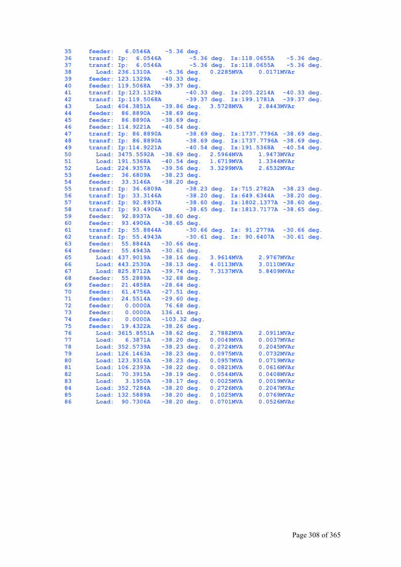
Page 308 of 365

35 feeder: 6.0546A -5.36 deg. 36 transf: Ip: 6.0546A -5.36 deg. Is:118.0655A -5.36 deg. 37 transf: Ip: 6.0546A -5.36 deg. Is:118.0655A -5.36 deg. 38 Load: 236.1310A -5.36 deg. 0.2285MVA 0.0171MVAr 39 feeder: 123.1329A -40.33 deg. 40 feeder: 119.5068A -39.37 deg. 41 transf: Ip:123.1329A -40.33 deg. Is:205.2214A -40.33 deg. 42 transf: Ip:119.5068A -39.37 deg. Is:199.1781A -39.37 deg. 43 Load: 404.3851A -39.86 deg. 3.5728MVA 2.8443MVAr 44 feeder: 86.8890A -38.69 deg. 45 feeder: 86.8890A -38.69 deg. 46 feeder: 114.9221A -40.54 deg. 47 transf: Ip: 86.8890A -38.69 deg. Is:1737.7796A -38.69 deg. 48 transf: Ip: 86.8890A -38.69 deg. Is:1737.7796A -38.69 deg. 49 transf: Ip:114.9221A -40.54 deg. Is:191.5368A -40.54 deg. 50 Load: 3475.5592A -38.69 deg. 2.5964MVA 1.9473MVAr 51 Load: 191.5368A -40.54 deg. 1.6719MVA 1.3344MVAr 52 Load: 224.9357A -39.56 deg. 3.3299MVA 2.6532MVAr 53 feeder: 36.6809A -38.23 deg. 54 feeder: 33.3146A -38.20 deg. 55 transf: Ip: 36.6809A -38.23 deg. Is:715.2782A -38.23 deg. 56 transf: Ip: 33.3146A -38.20 deg. Is:649.6344A -38.20 deg. 57 transf: Ip: 92.8937A -38.60 deg. Is:1802.1377A -38.60 deg. 58 transf: Ip: 93.4906A -38.65 deg. Is:1813.7177A -38.65 deg. 59 feeder: 92.8937A -38.60 deg. 60 feeder: 93.4906A -38.65 deg. 61 transf: Ip: 55.8844A -30.66 deg. Is: 91.2779A -30.66 deg. 62 transf: Ip: 55.4943A -30.61 deg. Is: 90.6407A -30.61 deg. 63 feeder: 55.8844A -30.66 deg. 64 feeder: 55.4943A -30.61 deg. 65 Load: 437.9019A -38.16 deg. 3.9614MVA 2.9767MVAr 66 Load: 443.2530A -38.13 deg. 4.0113MVA 3.0110MVAr 67 Load: 825.8712A -39.74 deg. 7.3137MVA 5.8409MVAr 68 feeder: 55.2889A -32.68 deg. 69 feeder: 21.4858A -28.64 deg. 70 feeder: 61.4756A -27.51 deg. 71 feeder: 24.5514A -29.60 deg. 72 feeder: 0.0000A 76.68 deg. 73 feeder: 0.0000A 136.41 deg. 74 feeder: 0.0000A -103.32 deg. 75 feeder: 19.4322A -38.26 deg. 76 Load: 3615.8551A -38.62 deg. 2.7882MVA 2.0911MVAr 77 Load: 6.3871A -38.20 deg. 0.0049MVA 0.0037MVAr 78 Load: 352.5739A -38.23 deg. 0.2724MVA 0.2045MVAr 79 Load: 126.1463A -38.23 deg. 0.0975MVA 0.0732MVAr 80 Load: 123.9316A -38.23 deg. 0.0957MVA 0.0719MVAr 81 Load: 106.2393A -38.22 deg. 0.0821MVA 0.0616MVAr 82 Load: 70.3915A -38.19 deg. 0.0544MVA 0.0408MVAr 83 Load: 3.1950A -38.17 deg. 0.0025MVA 0.0019MVAr 84 Load: 352.7284A -38.20 deg. 0.2726MVA 0.2047MVAr 85 Load: 132.5889A -38.20 deg. 0.1025MVA 0.0769MVAr 86 Load: 90.7306A -38.20 deg. 0.0701MVA 0.0526MVAr

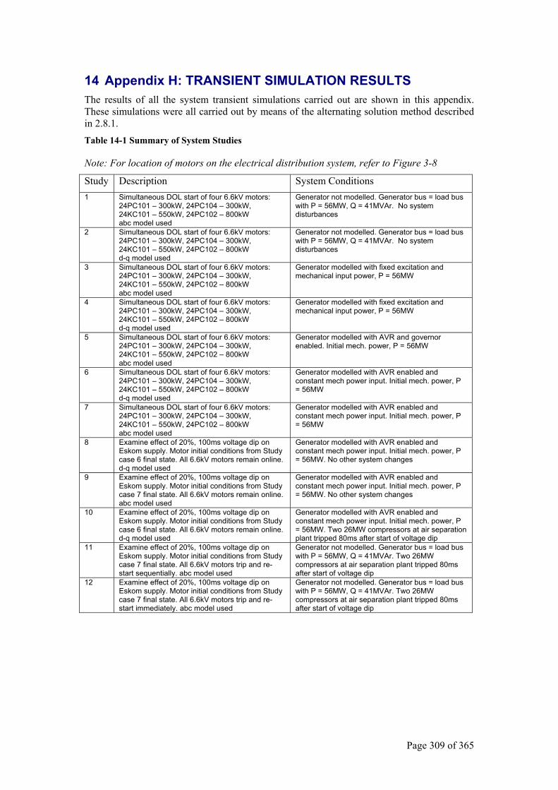
Page 309 of 365

14 Appendix H: TRANSIENT SIMULATION RESULTS The results of all the system transient simulations carried out are shown in this appendix. These simulations were all carried out by means of the alternating solution method described in 2.8.1. Table 14-1 Summary of System Studies

Note: For location of motors on the electrical distribution system, refer to Figure 3-8

Study Description System Conditions 1 Simultaneous DOL start of four 6.6kV motors:

24PC101 – 300kW, 24PC104 – 300kW, 24KC101 – 550kW, 24PC102 – 800kW abc model used

Generator not modelled. Generator bus = load bus with P = 56MW, Q = 41MVAr. No system disturbances

2 Simultaneous DOL start of four 6.6kV motors: 24PC101 – 300kW, 24PC104 – 300kW, 24KC101 – 550kW, 24PC102 – 800kW d-q model used

Generator not modelled. Generator bus = load bus with P = 56MW, Q = 41MVAr. No system disturbances

3 Simultaneous DOL start of four 6.6kV motors: 24PC101 – 300kW, 24PC104 – 300kW, 24KC101 – 550kW, 24PC102 – 800kW abc model used

Generator modelled with fixed excitation and mechanical input power, P = 56MW

4 Simultaneous DOL start of four 6.6kV motors: 24PC101 – 300kW, 24PC104 – 300kW, 24KC101 – 550kW, 24PC102 – 800kW d-q model used

Generator modelled with fixed excitation and mechanical input power, P = 56MW

5 Simultaneous DOL start of four 6.6kV motors: 24PC101 – 300kW, 24PC104 – 300kW, 24KC101 – 550kW, 24PC102 – 800kW abc model used

Generator modelled with AVR and governor enabled. Initial mech. power, P = 56MW

6 Simultaneous DOL start of four 6.6kV motors: 24PC101 – 300kW, 24PC104 – 300kW, 24KC101 – 550kW, 24PC102 – 800kW d-q model used

Generator modelled with AVR enabled and constant mech power input. Initial mech. power, P = 56MW

7 Simultaneous DOL start of four 6.6kV motors: 24PC101 – 300kW, 24PC104 – 300kW, 24KC101 – 550kW, 24PC102 – 800kW abc model used

Generator modelled with AVR enabled and constant mech power input. Initial mech. power, P = 56MW

8 Examine effect of 20%, 100ms voltage dip on Eskom supply. Motor initial conditions from Study case 6 final state. All 6.6kV motors remain online. d-q model used

Generator modelled with AVR enabled and constant mech power input. Initial mech. power, P = 56MW. No other system changes

9 Examine effect of 20%, 100ms voltage dip on Eskom supply. Motor initial conditions from Study case 7 final state. All 6.6kV motors remain online. abc model used

Generator modelled with AVR enabled and constant mech power input. Initial mech. power, P = 56MW. No other system changes

10 Examine effect of 20%, 100ms voltage dip on Eskom supply. Motor initial conditions from Study case 6 final state. All 6.6kV motors remain online. d-q model used

Generator modelled with AVR enabled and constant mech power input. Initial mech. power, P = 56MW. Two 26MW compressors at air separation plant tripped 80ms after start of voltage dip

11 Examine effect of 20%, 100ms voltage dip on Eskom supply. Motor initial conditions from Study case 7 final state. All 6.6kV motors trip and re-start sequentially. abc model used

Generator not modelled. Generator bus = load bus with P = 56MW, Q = 41MVAr. Two 26MW compressors at air separation plant tripped 80ms after start of voltage dip

12 Examine effect of 20%, 100ms voltage dip on Eskom supply. Motor initial conditions from Study case 7 final state. All 6.6kV motors trip and re-start immediately. abc model used

Generator not modelled. Generator bus = load bus with P = 56MW, Q = 41MVAr. Two 26MW compressors at air separation plant tripped 80ms after start of voltage dip

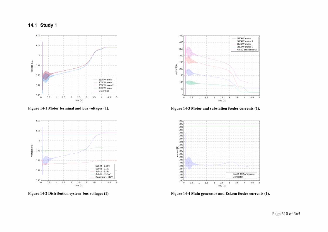
Page 310 of 365

14.1 Study 1

0 0.5 1 1.5 2 2.5 3 3.5 4 4.5 50.96

0.97

0.98

0.99

1

1.01

1.02

time [s]

550kW motor 300kW motor1300kW motor2850kW motor 6.6kV bus

Figure 14-1 Motor terminal and bus voltages (1).

0 0.5 1 1.5 2 2.5 3 3.5 4 4.5 50.96

0.97

0.98

0.99

1

1.01

1.02

time [s]

Sub24 - 6.6kV Sub06 - 11kV Sub19 - 525V Sub01 - 132kV Generator - 11kV

Figure 14-2 Distribution system bus voltages (1).

0 0.5 1 1.5 2 2.5 3 3.5 4 4.5 50

50

100

150

200

250

300

350

400

450

time [s]

550kW motor 300kW motor 1 850kW motor 300kW motor 2 6.6kV bus feeder A

Figure 14-3 Motor and substation feeder currents (1).

0 0.5 1 1.5 2 2.5 3 3.5 4 4.5 5280281282283284285286287288289290291292293294295296297298299300

time [s]

Sub01 132kV incomerGenerator

Figure 14-4 Main generator and Eskom feeder currents (1).

volta

ge p

.u.

volta

ge p

.u.

curre

nt [A

] cu

rrent

[A]

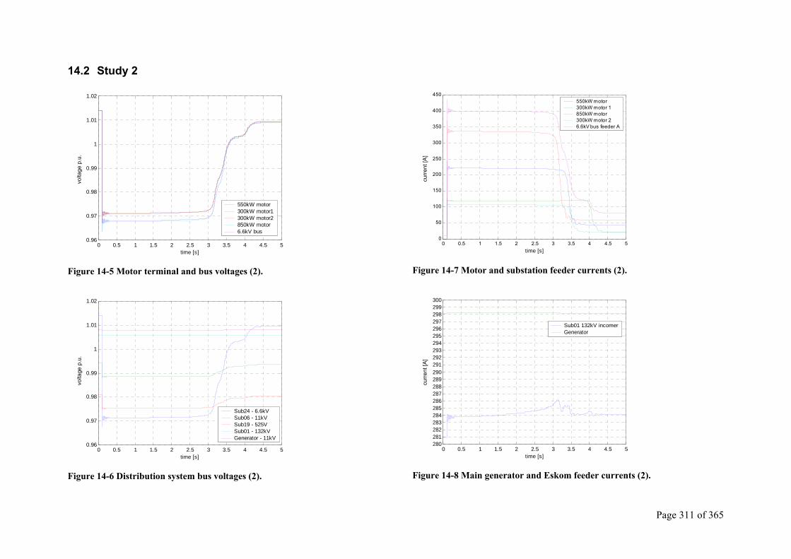
Page 311 of 365

14.2 Study 2

0 0.5 1 1.5 2 2.5 3 3.5 4 4.5 50.96

0.97

0.98

0.99

1

1.01

1.02

time [s]

550kW motor 300kW motor1300kW motor2850kW motor 6.6kV bus

Figure 14-5 Motor terminal and bus voltages (2).

0 0.5 1 1.5 2 2.5 3 3.5 4 4.5 50.96

0.97

0.98

0.99

1

1.01

1.02

time [s]

Sub24 - 6.6kV Sub06 - 11kV Sub19 - 525V Sub01 - 132kV Generator - 11kV

Figure 14-6 Distribution system bus voltages (2).

0 0.5 1 1.5 2 2.5 3 3.5 4 4.5 50

50

100

150

200

250

300

350

400

450

time [s]

550kW motor 300kW motor 1 850kW motor 300kW motor 2 6.6kV bus feeder A

Figure 14-7 Motor and substation feeder currents (2).

0 0.5 1 1.5 2 2.5 3 3.5 4 4.5 5280281282283284285286287288289290291292293294295296297298299300

time [s]

Sub01 132kV incomerGenerator

Figure 14-8 Main generator and Eskom feeder currents (2).

volta

ge p

.u.

volta

ge p

.u.

curre

nt [A

] cu

rrent

[A]

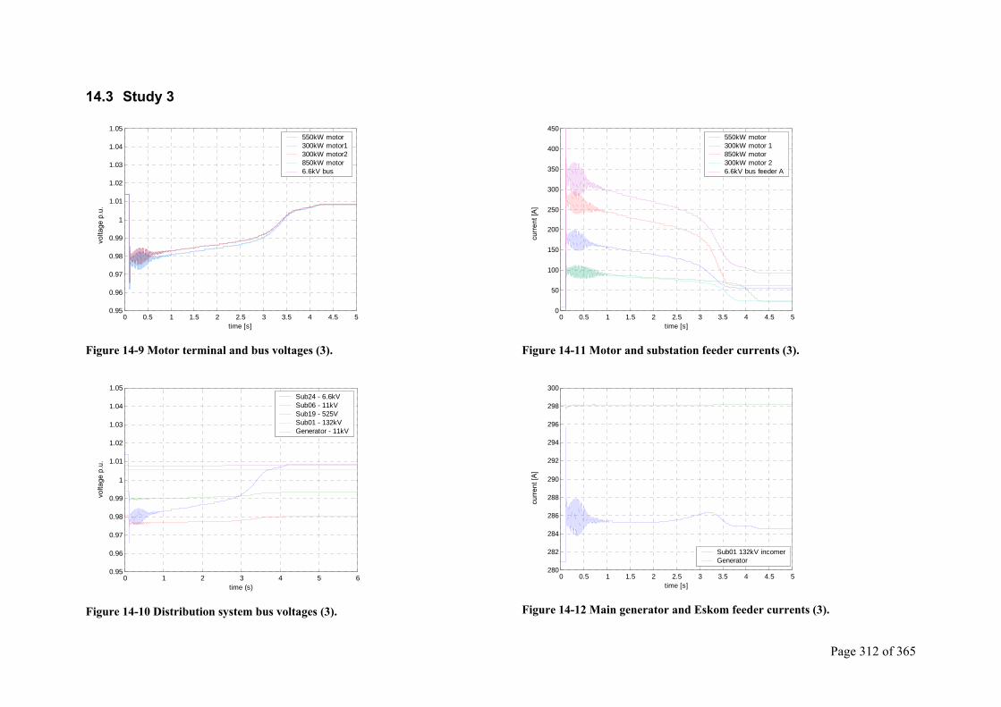
Page 312 of 365

14.3 Study 3

0 0.5 1 1.5 2 2.5 3 3.5 4 4.5 50.95

0.96

0.97

0.98

0.99

1

1.01

1.02

1.03

1.04

1.05

time [s]

550kW motor 300kW motor1300kW motor2850kW motor 6.6kV bus

Figure 14-9 Motor terminal and bus voltages (3).

0 1 2 3 4 5 60.95

0.96

0.97

0.98

0.99

1

1.01

1.02

1.03

1.04

1.05

time (s)

Sub24 - 6.6kV Sub06 - 11kV Sub19 - 525V Sub01 - 132kV Generator - 11kV

Figure 14-10 Distribution system bus voltages (3).

0 0.5 1 1.5 2 2.5 3 3.5 4 4.5 50

50

100

150

200

250

300

350

400

450

time [s]

550kW motor 300kW motor 1 850kW motor 300kW motor 2 6.6kV bus feeder A

Figure 14-11 Motor and substation feeder currents (3).

0 0.5 1 1.5 2 2.5 3 3.5 4 4.5 5280

282

284

286

288

290

292

294

296

298

300

time [s]

Sub01 132kV incomerGenerator

Figure 14-12 Main generator and Eskom feeder currents (3).

volta

ge p

.u.

volta

ge p

.u.

curre

nt [A

] cu

rrent

[A]

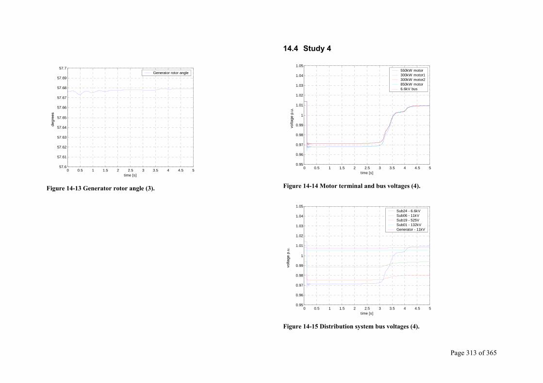
Page 313 of 365

0 0.5 1 1.5 2 2.5 3 3.5 4 4.5 557.6

57.61

57.62

57.63

57.64

57.65

57.66

57.67

57.68

57.69

57.7

time [s]

Generator rotor angle

Figure 14-13 Generator rotor angle (3).

14.4 Study 4

0 0.5 1 1.5 2 2.5 3 3.5 4 4.5 50.95

0.96

0.97

0.98

0.99

1

1.01

1.02

1.03

1.04

1.05

time [s]

550kW motor 300kW motor1300kW motor2850kW motor 6.6kV bus

Figure 14-14 Motor terminal and bus voltages (4).

0 0.5 1 1.5 2 2.5 3 3.5 4 4.5 50.95

0.96

0.97

0.98

0.99

1

1.01

1.02

1.03

1.04

1.05

time [s]

Sub24 - 6.6kV Sub06 - 11kV Sub19 - 525V Sub01 - 132kV Generator - 11kV

Figure 14-15 Distribution system bus voltages (4).

degr

ees

volta

ge p

.u.

volta

ge p

.u.

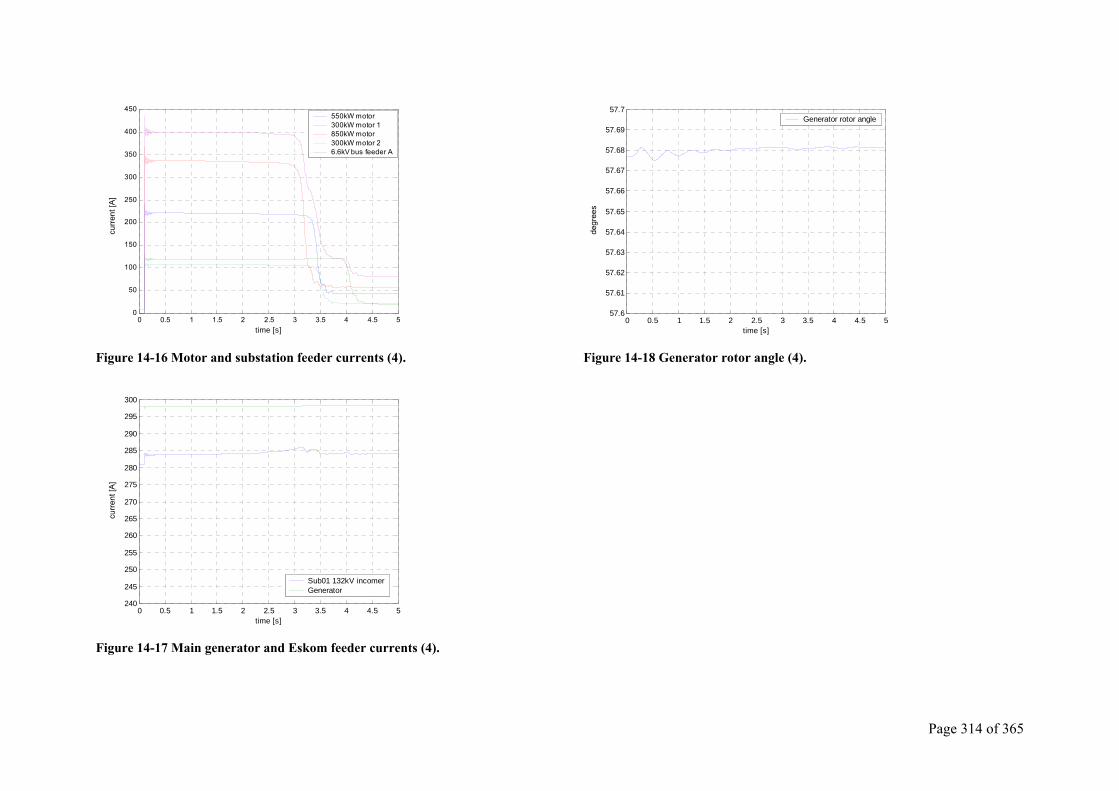
Page 314 of 365

0 0.5 1 1.5 2 2.5 3 3.5 4 4.5 50

50

100

150

200

250

300

350

400

450

time [s]

550kW motor 300kW motor 1 850kW motor 300kW motor 2 6.6kV bus feeder A

Figure 14-16 Motor and substation feeder currents (4).

0 0.5 1 1.5 2 2.5 3 3.5 4 4.5 5240

245

250

255

260

265

270

275

280

285

290

295

300

time [s]

Sub01 132kV incomerGenerator

Figure 14-17 Main generator and Eskom feeder currents (4).

0 0.5 1 1.5 2 2.5 3 3.5 4 4.5 557.6

57.61

57.62

57.63

57.64

57.65

57.66

57.67

57.68

57.69

57.7

time [s]

Generator rotor angle

Figure 14-18 Generator rotor angle (4).

curre

nt [A

] cu

rrent

[A]

degr

ees

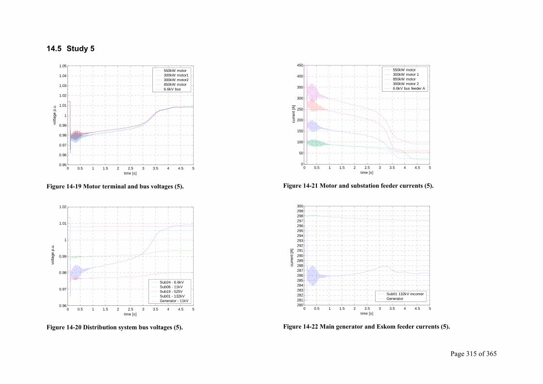
Page 315 of 365

14.5 Study 5

0 0.5 1 1.5 2 2.5 3 3.5 4 4.5 50.95

0.96

0.97

0.98

0.99

1

1.01

1.02

1.03

1.04

1.05

time [s]

550kW motor 300kW motor1300kW motor2850kW motor 6.6kV bus

Figure 14-19 Motor terminal and bus voltages (5).

0 0.5 1 1.5 2 2.5 3 3.5 4 4.5 50.96

0.97

0.98

0.99

1

1.01

1.02

time [s]

Sub24 - 6.6kV Sub06 - 11kV Sub19 - 525V Sub01 - 132kV Generator - 11kV

Figure 14-20 Distribution system bus voltages (5).

0 0.5 1 1.5 2 2.5 3 3.5 4 4.5 50

50

100

150

200

250

300

350

400

450

time [s]

550kW motor 300kW motor 1 850kW motor 300kW motor 2 6.6kV bus feeder A

Figure 14-21 Motor and substation feeder currents (5).

0 0.5 1 1.5 2 2.5 3 3.5 4 4.5 5280281282283284285286287288289290291292293294295296297298299300

time [s]

Sub01 132kV incomerGenerator

Figure 14-22 Main generator and Eskom feeder currents (5).

volta

ge p

.u.

volta

ge p

.u.

curre

nt [A

] cu

rrent

[A]

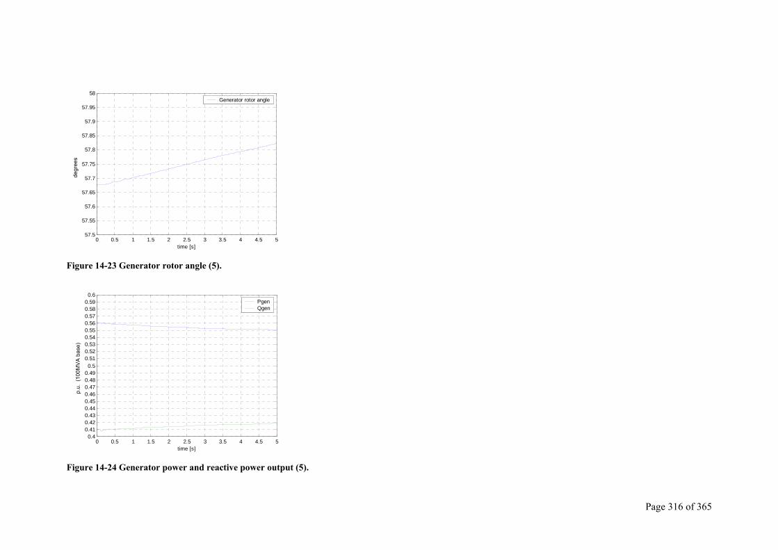
Page 316 of 365

0 0.5 1 1.5 2 2.5 3 3.5 4 4.5 557.5

57.55

57.6

57.65

57.7

57.75

57.8

57.85

57.9

57.95

58

time [s]

Generator rotor angle

Figure 14-23 Generator rotor angle (5).

0 0.5 1 1.5 2 2.5 3 3.5 4 4.5 50.4

0.410.420.430.440.450.460.470.480.490.5

0.510.520.530.540.550.560.570.580.590.6

time [s]

PgenQgen

Figure 14-24 Generator power and reactive power output (5).

degr

ees

p.u.

(10

0MV

A b

ase)

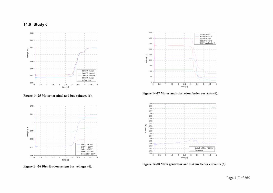
Page 317 of 365

14.6 Study 6

0 0.5 1 1.5 2 2.5 3 3.5 4 4.5 50.96

0.97

0.98

0.99

1

1.01

1.02

1.03

time [s]

550kW motor 300kW motor1300kW motor2850kW motor 6.6kV bus

Figure 14-25 Motor terminal and bus voltages (6).

0 0.5 1 1.5 2 2.5 3 3.5 4 4.5 50.96

0.97

0.98

0.99

1

1.01

1.02

time [s]

Sub24 - 6.6kV Sub06 - 11kV Sub19 - 525V Sub01 - 132kV Generator - 11kV

Figure 14-26 Distribution system bus voltages (6).

0 0.5 1 1.5 2 2.5 3 3.5 4 4.5 50

50

100

150

200

250

300

350

400

450

time [s]

550kW motor 300kW motor 1 850kW motor 300kW motor 2 6.6kV bus feeder A

Figure 14-27 Motor and substation feeder currents (6).

0 0.5 1 1.5 2 2.5 3 3.5 4 4.5 5280281282283284285286287288289290291292293294295296297298299300

time [s]

Sub01 132kV incomerGenerator

Figure 14-28 Main generator and Eskom feeder currents (6).

volta

ge p

.u.

volta

ge p

.u.

curre

nt [A

] cu

rrent

[A]

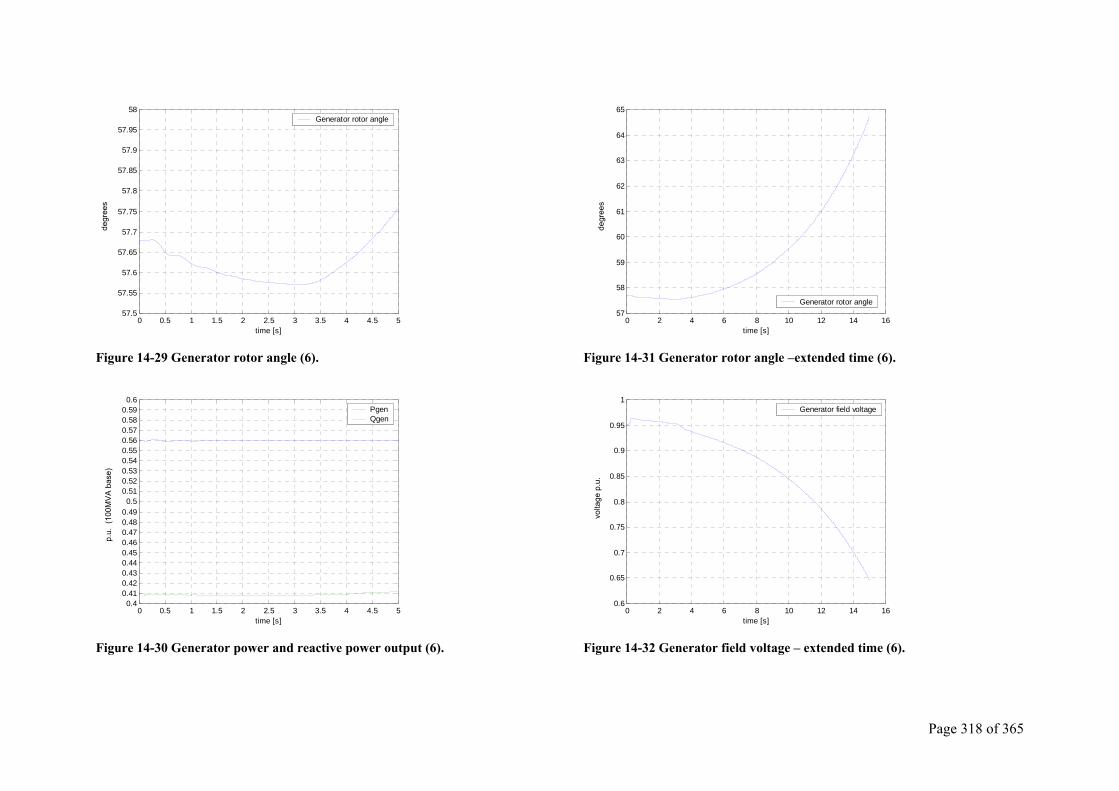
Page 318 of 365

0 0.5 1 1.5 2 2.5 3 3.5 4 4.5 557.5

57.55

57.6

57.65

57.7

57.75

57.8

57.85

57.9

57.95

58

time [s]

Generator rotor angle

Figure 14-29 Generator rotor angle (6).

0 0.5 1 1.5 2 2.5 3 3.5 4 4.5 50.4

0.410.420.430.440.450.460.470.480.490.5

0.510.520.530.540.550.560.570.580.590.6

time [s]

PgenQgen

Figure 14-30 Generator power and reactive power output (6).

0 2 4 6 8 10 12 14 1657

58

59

60

61

62

63

64

65

time [s]

Generator rotor angle

Figure 14-31 Generator rotor angle –extended time (6).

0 2 4 6 8 10 12 14 160.6

0.65

0.7

0.75

0.8

0.85

0.9

0.95

1

time [s]

Generator field voltage

Figure 14-32 Generator field voltage – extended time (6).

degr

ees

p.u.

(10

0MV

A b

ase)

degr

ees

volta

ge p

.u.

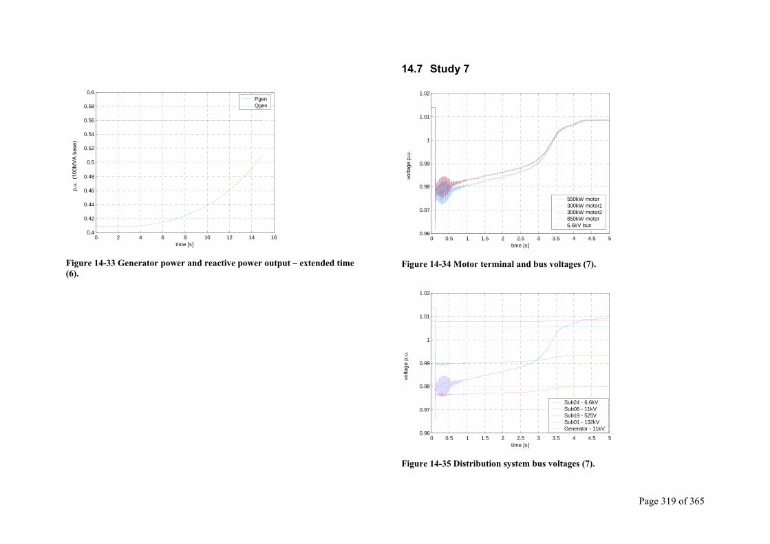
Page 319 of 365

0 2 4 6 8 10 12 14 160.4

0.42

0.44

0.46

0.48

0.5

0.52

0.54

0.56

0.58

0.6

time [s]

PgenQgen

Figure 14-33 Generator power and reactive power output – extended time (6).

14.7 Study 7

0 0.5 1 1.5 2 2.5 3 3.5 4 4.5 50.96

0.97

0.98

0.99

1

1.01

1.02

time [s]

550kW motor 300kW motor1300kW motor2850kW motor 6.6kV bus

Figure 14-34 Motor terminal and bus voltages (7).

0 0.5 1 1.5 2 2.5 3 3.5 4 4.5 50.96

0.97

0.98

0.99

1

1.01

1.02

time [s]

Sub24 - 6.6kV Sub06 - 11kV Sub19 - 525V Sub01 - 132kV Generator - 11kV

Figure 14-35 Distribution system bus voltages (7).

p.u.

(10

0MV

A b

ase)

volta

ge p

.u.

volta

ge p

.u.

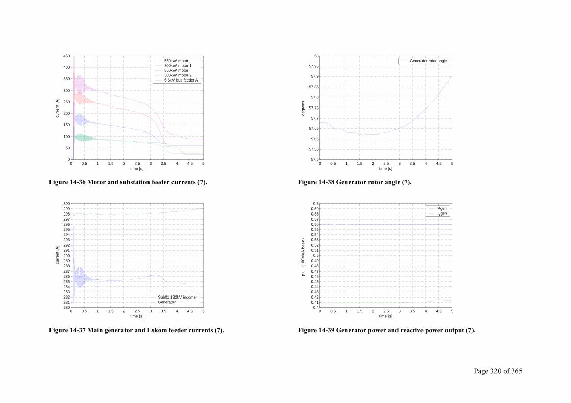
Page 320 of 365

0 0.5 1 1.5 2 2.5 3 3.5 4 4.5 50

50

100

150

200

250

300

350

400

450

time [s]

550kW motor 300kW motor 1 850kW motor 300kW motor 2 6.6kV bus feeder A

Figure 14-36 Motor and substation feeder currents (7).

0 0.5 1 1.5 2 2.5 3 3.5 4 4.5 5280281282283284285286287288289290291292293294295296297298299300

time [s]

Sub01 132kV incomerGenerator

Figure 14-37 Main generator and Eskom feeder currents (7).

0 0.5 1 1.5 2 2.5 3 3.5 4 4.5 557.5

57.55

57.6

57.65

57.7

57.75

57.8

57.85

57.9

57.95

58

time [s]

Generator rotor angle

Figure 14-38 Generator rotor angle (7).

0 0.5 1 1.5 2 2.5 3 3.5 4 4.5 50.4

0.410.420.430.440.450.460.470.480.490.5

0.510.520.530.540.550.560.570.580.590.6

time [s]

PgenQgen

Figure 14-39 Generator power and reactive power output (7).

curre

nt [A

] cu

rrent

[A]

degr

ees

p.u.

(10

0MV

A b

ase)

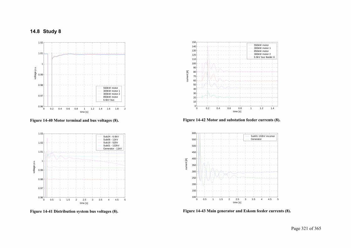
Page 321 of 365

14.8 Study 8

0 0.2 0.4 0.6 0.8 1 1.2 1.4 1.6 1.8 20.96

0.97

0.98

0.99

1

1.01

1.02

time [s]

550kW motor 300kW motor 1300kW motor 2850kW motor 6.6kV bus

Figure 14-40 Motor terminal and bus voltages (8).

0 0.5 1 1.5 2 2.5 3 3.5 4 4.5 50.96

0.97

0.98

0.99

1

1.01

1.02

1.03

time [s]

Sub24 - 6.6kV Sub06 - 11kV Sub19 - 525V Sub01 - 132kV Generator - 11kV

Figure 14-41 Distribution system bus voltages (8).

0 0.2 0.4 0.6 0.8 1 1.2 1.40

10

20

30

40

50

60

70

80

90

100

110

120

130

140

150

time [s]

550kW motor 300kW motor 1 850kW motor 300kW motor 2 6.6kV bus feeder A

Figure 14-42 Motor and substation feeder currents (8).

0 0.5 1 1.5 2 2.5 3 3.5 4 4.5 5100

150

200

250

300

350

400

450

500

550

600

time [s]

Sub01 132kV incomerGenerator

Figure 14-43 Main generator and Eskom feeder currents (8).

volta

ge p

.u.

volta

ge p

.u.

curre

nt [A

] cu

rrent

[A]

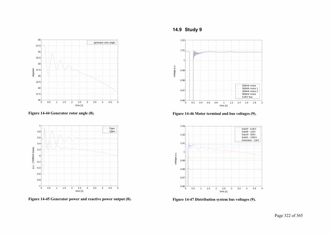
Page 322 of 365

0 0.5 1 1.5 2 2.5 3 3.5 4 4.5 535

37.5

40

42.5

45

47.5

50

52.5

55

57.5

60

time [s]

generator rotor angle

Figure 14-44 Generator rotor angle (8).

0 0.5 1 1.5 2 2.5 3 3.5 4 4.5 5-1

-0.8

-0.6

-0.4

-0.2

0

0.2

0.4

0.6

0.8

1

time [s]

PgenQgen

Figure 14-45 Generator power and reactive power output (8).

14.9 Study 9

0 0.2 0.4 0.6 0.8 1 1.2 1.4 1.6 1.8 20.96

0.97

0.98

0.99

1

1.01

1.02

time [s]

550kW motor 300kW motor 1300kW motor 2850kW motor 6.6kV bus

Figure 14-46 Motor terminal and bus voltages (9).

0 0.5 1 1.5 2 2.5 3 3.5 4 4.5 50.96

0.97

0.98

0.99

1

1.01

1.02

1.03

time [s]

Sub24 - 6.6kV Sub06 - 11kV Sub19 - 525V Sub01 - 132kV Generator - 11kV

Figure 14-47 Distribution system bus voltages (9).

degr

ees

p.u.

(10

0MV

A b

ase)

volta

ge p

.u.

volta

ge p

.u.

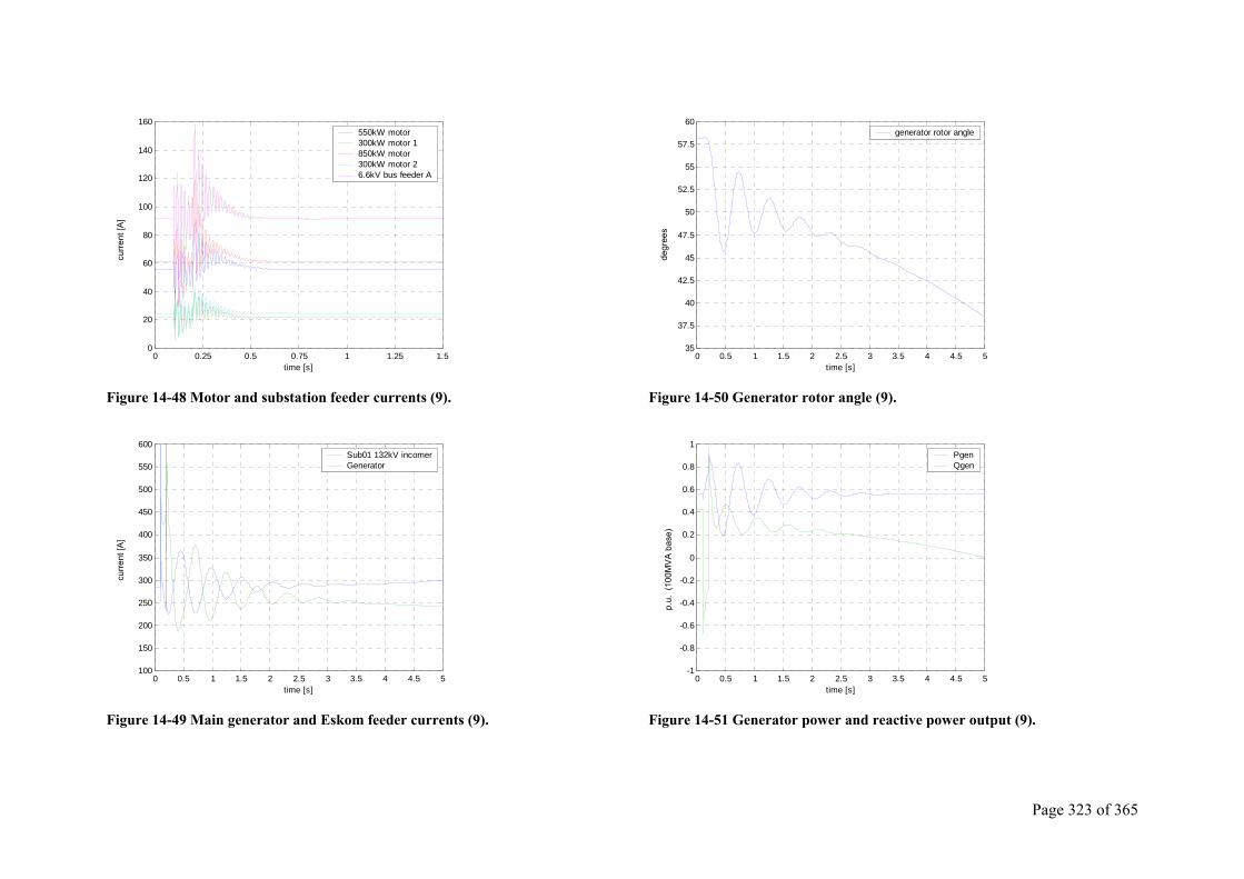
Page 323 of 365

0 0.25 0.5 0.75 1 1.25 1.50

20

40

60

80

100

120

140

160

time [s]

550kW motor 300kW motor 1 850kW motor 300kW motor 2 6.6kV bus feeder A

Figure 14-48 Motor and substation feeder currents (9).

0 0.5 1 1.5 2 2.5 3 3.5 4 4.5 5100

150

200

250

300

350

400

450

500

550

600

time [s]

Sub01 132kV incomerGenerator

Figure 14-49 Main generator and Eskom feeder currents (9).

0 0.5 1 1.5 2 2.5 3 3.5 4 4.5 535

37.5

40

42.5

45

47.5

50

52.5

55

57.5

60

time [s]

generator rotor angle

Figure 14-50 Generator rotor angle (9).

0 0.5 1 1.5 2 2.5 3 3.5 4 4.5 5-1

-0.8

-0.6

-0.4

-0.2

0

0.2

0.4

0.6

0.8

1

time [s]

PgenQgen

Figure 14-51 Generator power and reactive power output (9).

curre

nt [A

] cu

rrent

[A]

degr

ees

p.u.

(10

0MV

A b

ase)

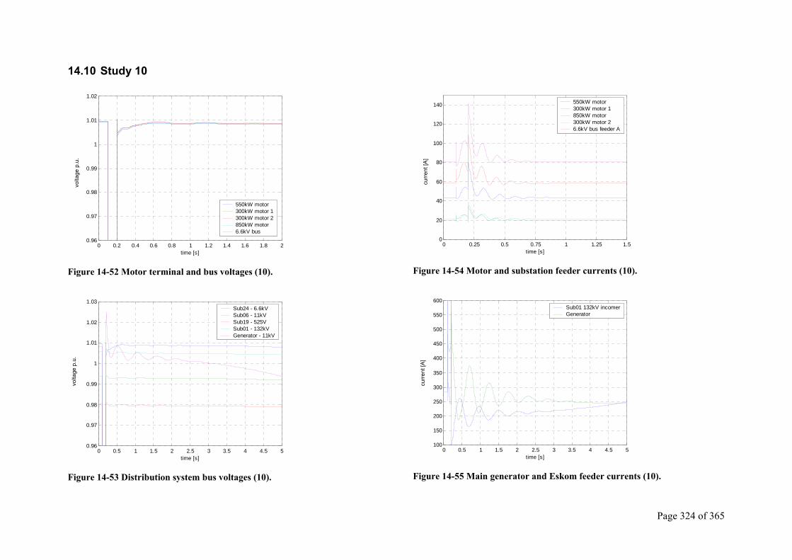
Page 324 of 365

14.10 Study 10

0 0.2 0.4 0.6 0.8 1 1.2 1.4 1.6 1.8 20.96

0.97

0.98

0.99

1

1.01

1.02

time [s]

550kW motor 300kW motor 1300kW motor 2850kW motor 6.6kV bus

Figure 14-52 Motor terminal and bus voltages (10).

0 0.5 1 1.5 2 2.5 3 3.5 4 4.5 50.96

0.97

0.98

0.99

1

1.01

1.02

1.03

time [s]

Sub24 - 6.6kV Sub06 - 11kV Sub19 - 525V Sub01 - 132kV Generator - 11kV

Figure 14-53 Distribution system bus voltages (10).

0 0.25 0.5 0.75 1 1.25 1.50

20

40

60

80

100

120

140

time [s]

550kW motor 300kW motor 1 850kW motor 300kW motor 2 6.6kV bus feeder A

Figure 14-54 Motor and substation feeder currents (10).

0 0.5 1 1.5 2 2.5 3 3.5 4 4.5 5100

150

200

250

300

350

400

450

500

550

600

time [s]

Sub01 132kV incomerGenerator

Figure 14-55 Main generator and Eskom feeder currents (10).

volta

ge p

.u.

volta

ge p

.u.

curre

nt [A

] cu

rrent

[A]

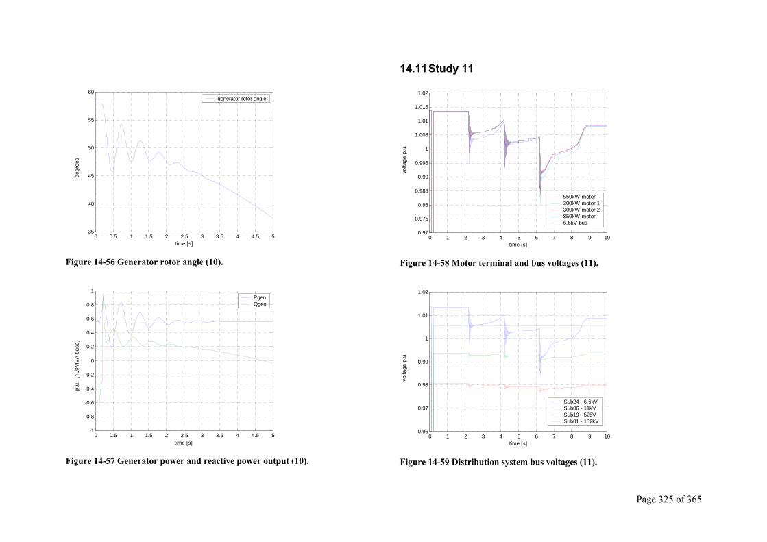
Page 325 of 365

0 0.5 1 1.5 2 2.5 3 3.5 4 4.5 535

40

45

50

55

60

time [s]

generator rotor angle

Figure 14-56 Generator rotor angle (10).

0 0.5 1 1.5 2 2.5 3 3.5 4 4.5 5-1

-0.8

-0.6

-0.4

-0.2

0

0.2

0.4

0.6

0.8

1

time [s]

PgenQgen

Figure 14-57 Generator power and reactive power output (10).

14.11 Study 11

0 1 2 3 4 5 6 7 8 9 100.97

0.975

0.98

0.985

0.99

0.995

1

1.005

1.01

1.015

1.02

time [s]

550kW motor 300kW motor 1300kW motor 2850kW motor 6.6kV bus

Figure 14-58 Motor terminal and bus voltages (11).

0 1 2 3 4 5 6 7 8 9 100.96

0.97

0.98

0.99

1

1.01

1.02

time [s]

Sub24 - 6.6kVSub06 - 11kV Sub19 - 525V Sub01 - 132kV

Figure 14-59 Distribution system bus voltages (11).

degr

ees

p.u.

(10

0MV

A b

ase)

volta

ge p

.u.

volta

ge p

.u.

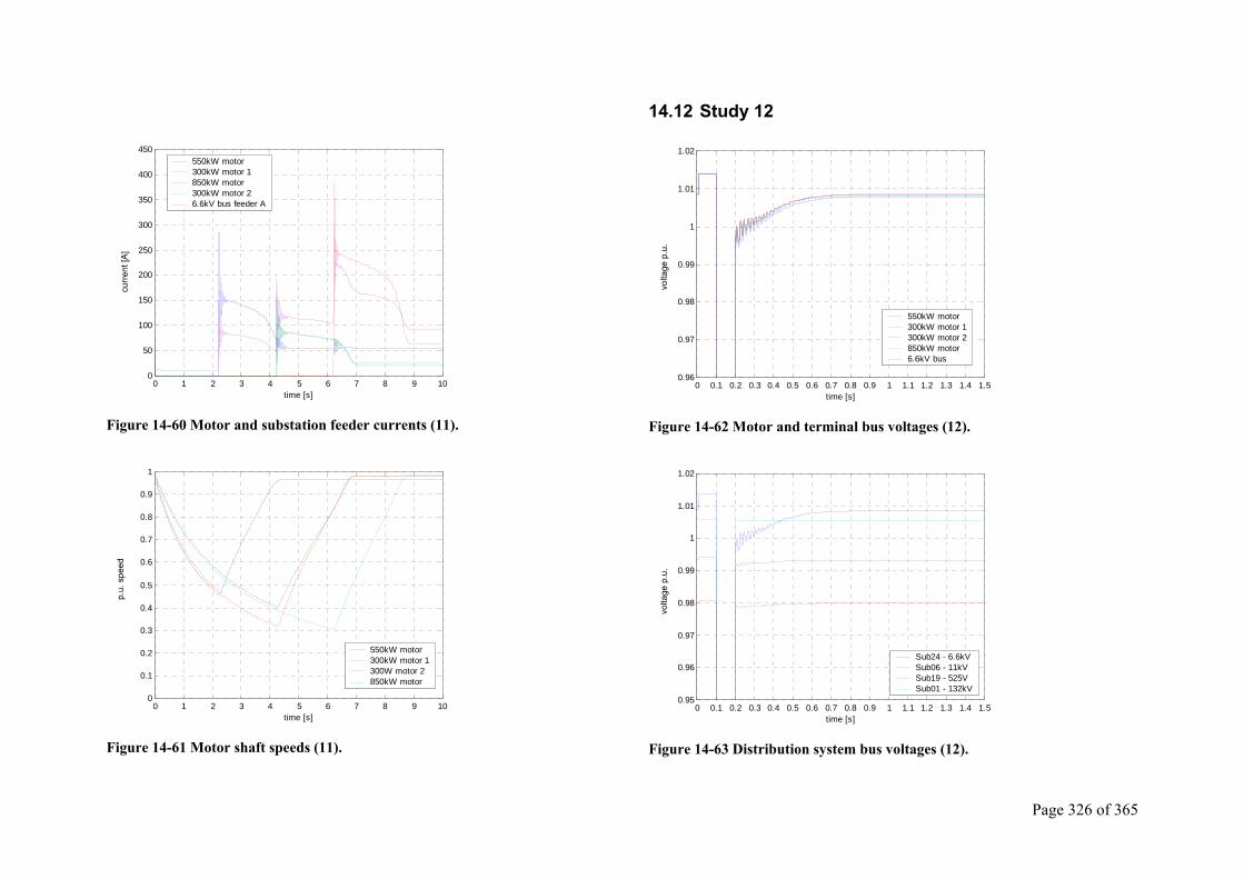
Page 326 of 365

0 1 2 3 4 5 6 7 8 9 100

50

100

150

200

250

300

350

400

450

time [s]

550kW motor 300kW motor 1 850kW motor 300kW motor 2 6.6kV bus feeder A

Figure 14-60 Motor and substation feeder currents (11).

0 1 2 3 4 5 6 7 8 9 100

0.1

0.2

0.3

0.4

0.5

0.6

0.7

0.8

0.9

1

time [s]

550kW motor 300kW motor 1300W motor 2 850kW motor

Figure 14-61 Motor shaft speeds (11).

14.12 Study 12

0 0.1 0.2 0.3 0.4 0.5 0.6 0.7 0.8 0.9 1 1.1 1.2 1.3 1.4 1.50.96

0.97

0.98

0.99

1

1.01

1.02

time [s]

550kW motor 300kW motor 1300kW motor 2850kW motor 6.6kV bus

Figure 14-62 Motor and terminal bus voltages (12).

0 0.1 0.2 0.3 0.4 0.5 0.6 0.7 0.8 0.9 1 1.1 1.2 1.3 1.4 1.50.95

0.96

0.97

0.98

0.99

1

1.01

1.02

time [s]

Sub24 - 6.6kVSub06 - 11kV Sub19 - 525V Sub01 - 132kV

Figure 14-63 Distribution system bus voltages (12).

curre

nt [A

] p.

u. s

peed

volta

ge p

.u.

volta

ge p

.u.

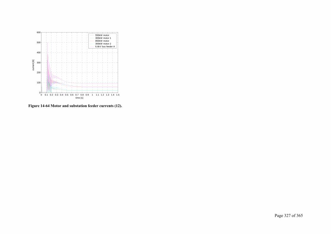
Page 327 of 365

0 0.1 0.2 0.3 0.4 0.5 0.6 0.7 0.8 0.9 1 1.1 1.2 1.3 1.4 1.50

100

200

300

400

500

600

time [s]

550kW motor 300kW motor 1 850kW motor 300kW motor 2 6.6kV bus feeder A

Figure 14-64 Motor and substation feeder currents (12).

curre

nt [A

]

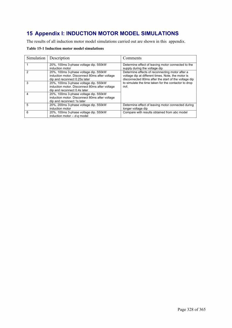
Page 328 of 365

15 Appendix I: INDUCTION MOTOR MODEL SIMULATIONS The results of all induction motor model simulations carried out are shown in this appendix. Table 15-1 Induction motor model simulations

Simulation Description Comments 1 20%, 100ms 3-phase voltage dip. 550kW

induction motor Determine effect of leaving motor connected to the supply during the voltage dip

2 20%, 100ms 3-phase voltage dip. 550kW induction motor. Disconnect 80ms after voltage dip and reconnect 0.25s later

3 20%, 100ms 3-phase voltage dip. 550kW induction motor. Disconnect 80ms after voltage dip and reconnect 0.4s later

4 20%, 100ms 3-phase voltage dip. 550kW induction motor. Disconnect 80ms after voltage dip and reconnect 1s later

Determine effects of reconnecting motor after a voltage dip at different times. Note, the motor is disconnected 80ms after the start of the voltage dip to simulate the time taken for the contactor to drop out.

5 20%, 200ms 3-phase voltage dip. 550kW induction motor

Determine effect of leaving motor connected during longer voltage dip

6 20%, 100ms 3-phase voltage dip. 550kW induction motor – d-q model

Compare with results obtained from abc model

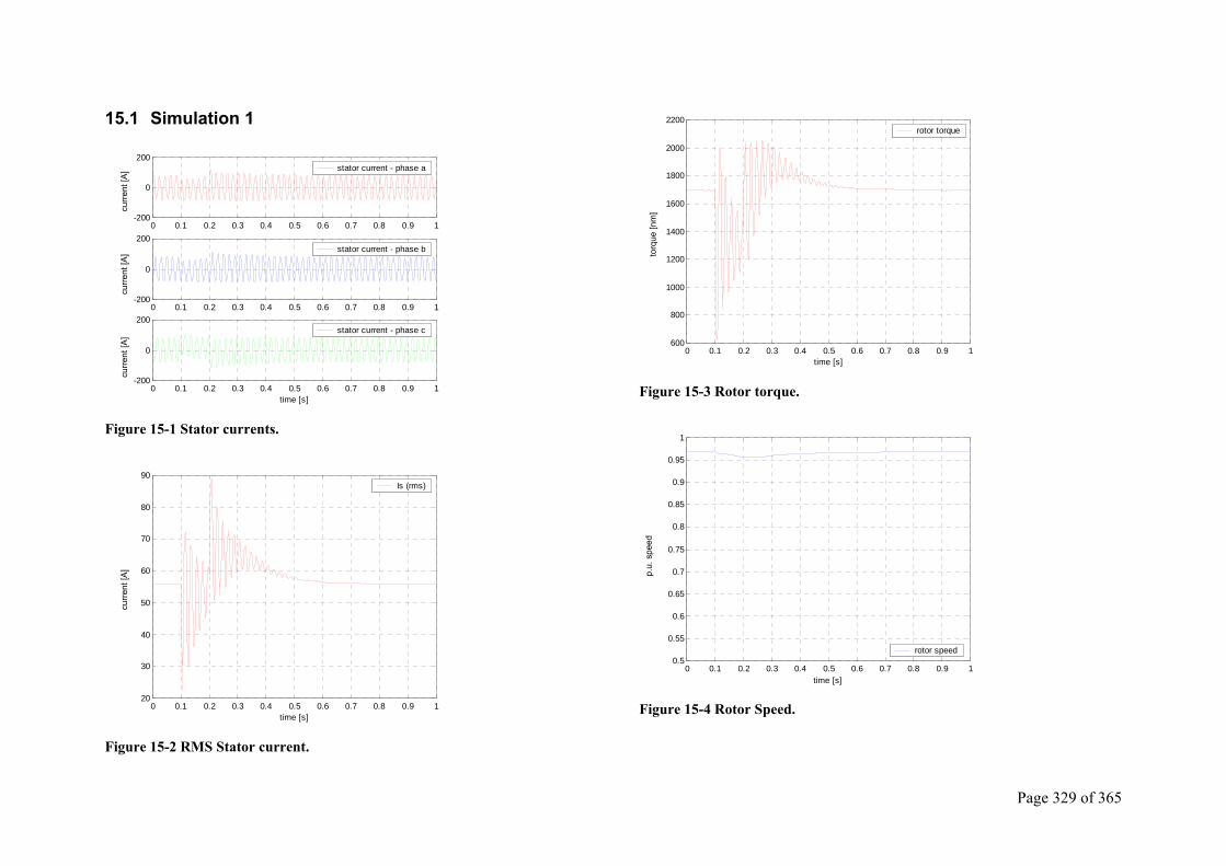
Page 329 of 365

15.1 Simulation 1

0 0.1 0.2 0.3 0.4 0.5 0.6 0.7 0.8 0.9 1-200

0

200stator current - phase a

0 0.1 0.2 0.3 0.4 0.5 0.6 0.7 0.8 0.9 1-200

0

200stator current - phase b

0 0.1 0.2 0.3 0.4 0.5 0.6 0.7 0.8 0.9 1-200

0

200

time [s]

stator current - phase c

Figure 15-1 Stator currents.

0 0.1 0.2 0.3 0.4 0.5 0.6 0.7 0.8 0.9 120

30

40

50

60

70

80

90

time [s]

Is (rms)

Figure 15-2 RMS Stator current.

0 0.1 0.2 0.3 0.4 0.5 0.6 0.7 0.8 0.9 1600

800

1000

1200

1400

1600

1800

2000

2200

time [s]

rotor torque

Figure 15-3 Rotor torque.

0 0.1 0.2 0.3 0.4 0.5 0.6 0.7 0.8 0.9 10.5

0.55

0.6

0.65

0.7

0.75

0.8

0.85

0.9

0.95

1

time [s]

rotor speed

Figure 15-4 Rotor Speed.

curre

nt [A

] cu

rrent

[A]

curre

nt [A

] cu

rrent

[A]

torq

ue [n

m]

p.u.

spe

ed

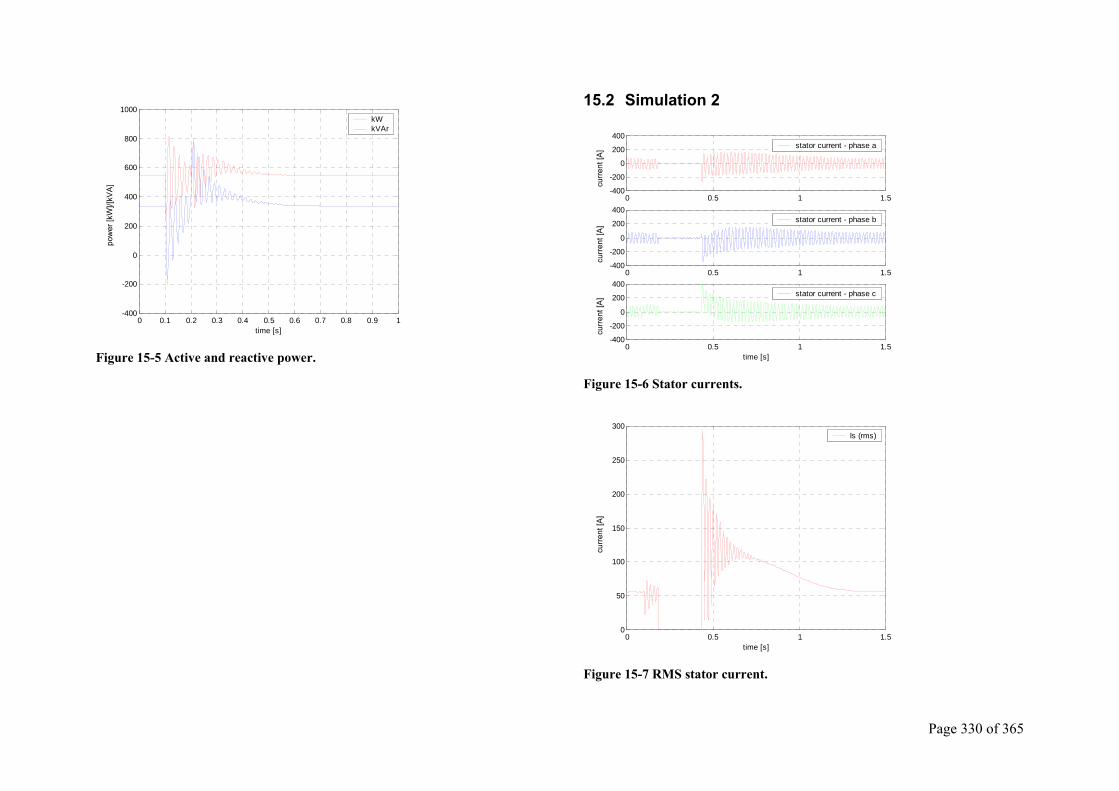
Page 330 of 365

0 0.1 0.2 0.3 0.4 0.5 0.6 0.7 0.8 0.9 1-400

-200

0

200

400

600

800

1000

time [s]

kW kVAr

Figure 15-5 Active and reactive power.

15.2 Simulation 2

0 0.5 1 1.5-400

-200

0

200

400stator current - phase a

0 0.5 1 1.5-400

-200

0

200

400stator current - phase b

0 0.5 1 1.5-400

-200

0

200

400

time [s]

stator current - phase c

Figure 15-6 Stator currents.

0 0.5 1 1.50

50

100

150

200

250

300

time [s]

Is (rms)

Figure 15-7 RMS stator current.

pow

er [k

W]/[

kVA

]

curre

nt [A

] cu

rrent

[A]

curre

nt [A

] cu

rrent

[A]

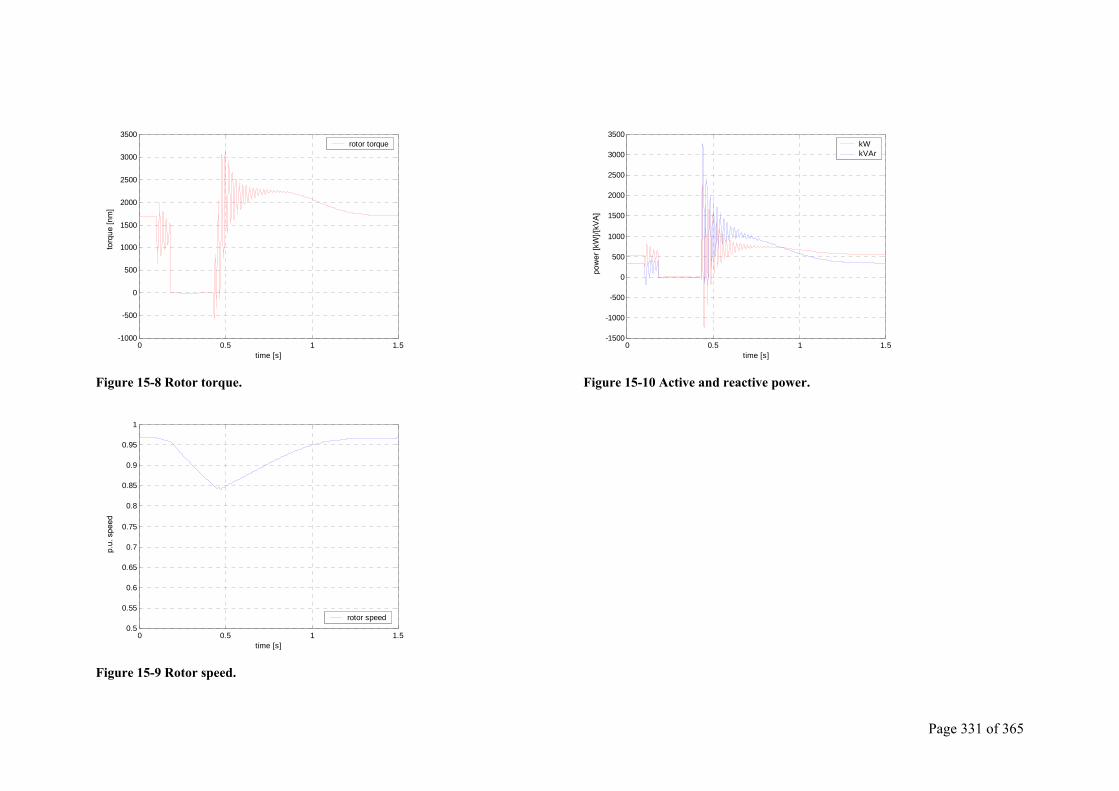
Page 331 of 365

0 0.5 1 1.5-1000

-500

0

500

1000

1500

2000

2500

3000

3500

time [s]

rotor torque

Figure 15-8 Rotor torque.

0 0.5 1 1.50.5

0.55

0.6

0.65

0.7

0.75

0.8

0.85

0.9

0.95

1

time [s]

rotor speed

Figure 15-9 Rotor speed.

0 0.5 1 1.5-1500

-1000

-500

0

500

1000

1500

2000

2500

3000

3500

time [s]

kW kVAr

Figure 15-10 Active and reactive power.

torq

ue [n

m]

p.u.

spe

ed

pow

er [k

W]/[

kVA

]

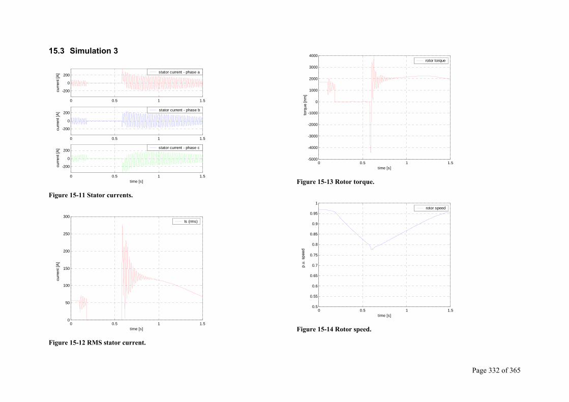
Page 332 of 365

15.3 Simulation 3

0 0.5 1 1.5

-200

0

200stator current - phase a

0 0.5 1 1.5

-200

0

200stator current - phase b

0 0.5 1 1.5

-200

0

200

time [s]

stator current - phase c

Figure 15-11 Stator currents.

0 0.5 1 1.50

50

100

150

200

250

300

time [s]

Is (rms)

Figure 15-12 RMS stator current.

0 0.5 1 1.5-5000

-4000

-3000

-2000

-1000

0

1000

2000

3000

4000

time [s]

rotor torque

Figure 15-13 Rotor torque.

0 0.5 1 1.50.5

0.55

0.6

0.65

0.7

0.75

0.8

0.85

0.9

0.95

1

time [s]

rotor speed

Figure 15-14 Rotor speed.

curre

nt [A

] cu

rrent

[A]

curre

nt [A

] cu

rrent

[A]

torq

ue [n

m]

p.u.

spe

ed

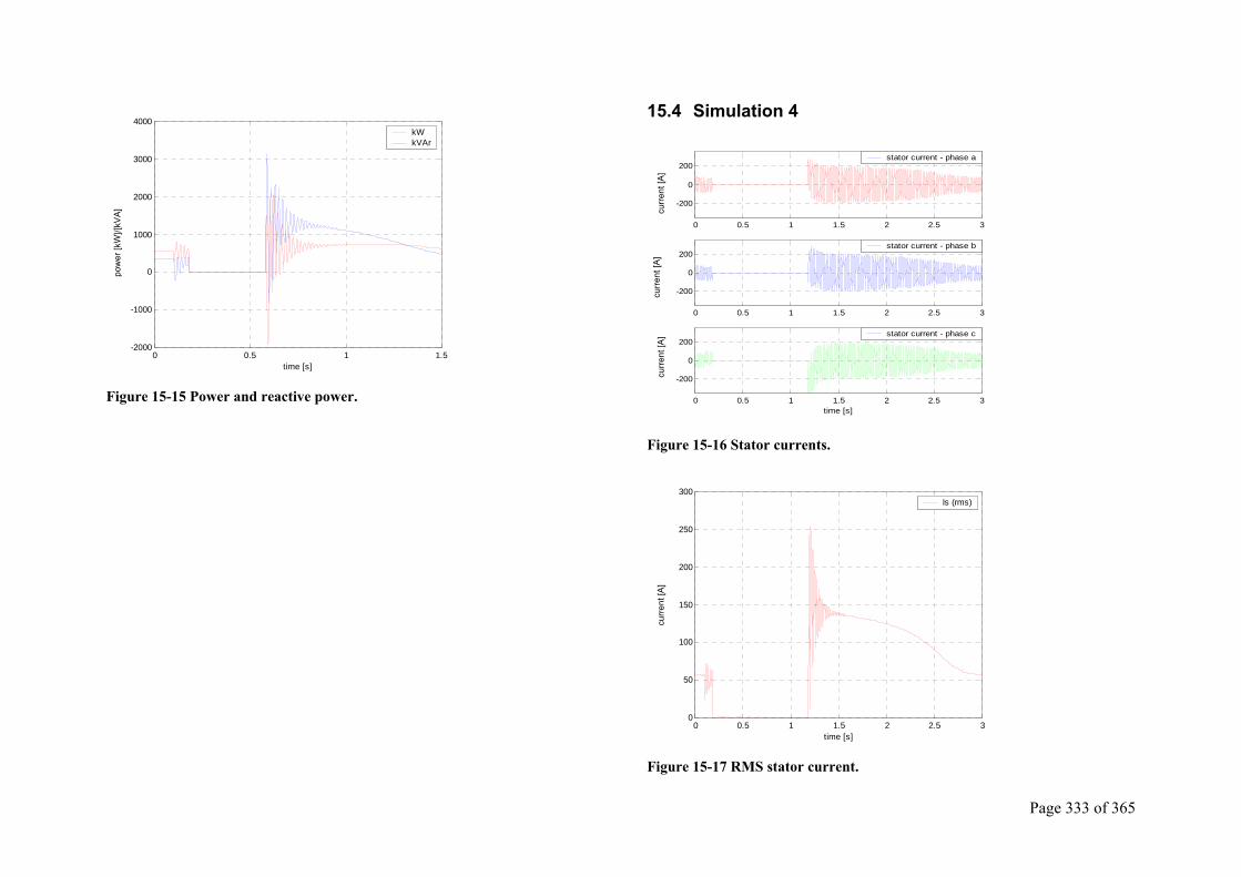
Page 333 of 365

0 0.5 1 1.5-2000

-1000

0

1000

2000

3000

4000

time [s]

kW kVAr

Figure 15-15 Power and reactive power.

15.4 Simulation 4

0 0.5 1 1.5 2 2.5 3

-200

0

200stator current - phase a

0 0.5 1 1.5 2 2.5 3

-200

0

200stator current - phase b

0 0.5 1 1.5 2 2.5 3

-200

0

200

time [s]

stator current - phase c

Figure 15-16 Stator currents.

0 0.5 1 1.5 2 2.5 30

50

100

150

200

250

300

time [s]

Is (rms)

Figure 15-17 RMS stator current.

pow

er [k

W]/[

kVA

]

curre

nt [A

] cu

rrent

[A]

curre

nt [A

] cu

rrent

[A]

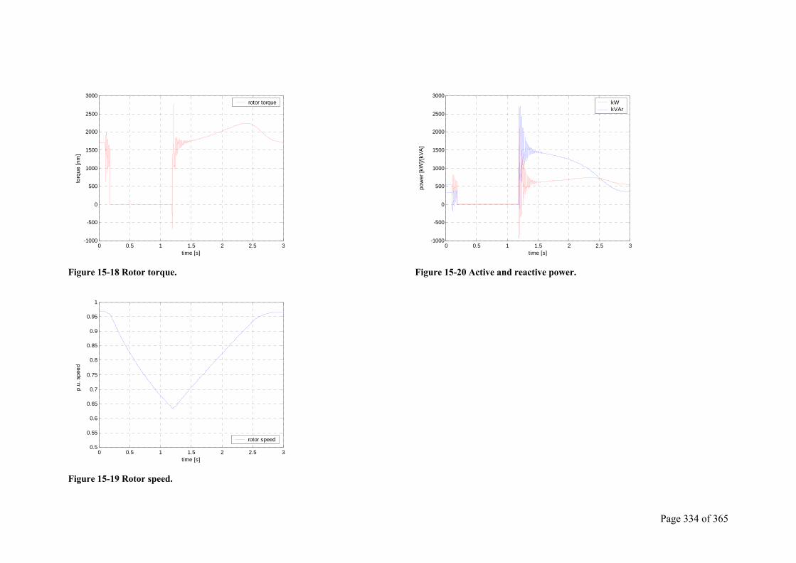
Page 334 of 365

0 0.5 1 1.5 2 2.5 3-1000

-500

0

500

1000

1500

2000

2500

3000

time [s]

rotor torque

Figure 15-18 Rotor torque.

0 0.5 1 1.5 2 2.5 30.5

0.55

0.6

0.65

0.7

0.75

0.8

0.85

0.9

0.95

1

time [s]

rotor speed

Figure 15-19 Rotor speed.

0 0.5 1 1.5 2 2.5 3-1000

-500

0

500

1000

1500

2000

2500

3000

time [s]

kW kVAr

Figure 15-20 Active and reactive power.

torq

ue [n

m]

p.u.

spe

ed

pow

er [k

W]/[

kVA

]

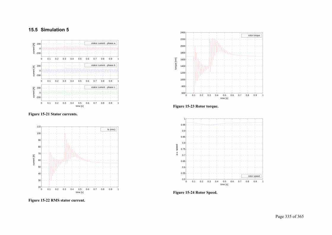
Page 335 of 365

15.5 Simulation 5

0 0.1 0.2 0.3 0.4 0.5 0.6 0.7 0.8 0.9 1

-200

0

200 stator current - phase a

0 0.1 0.2 0.3 0.4 0.5 0.6 0.7 0.8 0.9 1

-200

0

200 stator current - phase b

0 0.1 0.2 0.3 0.4 0.5 0.6 0.7 0.8 0.9 1

-200

0

200

time [s]

stator current - phase c

Figure 15-21 Stator currents.

0 0.1 0.2 0.3 0.4 0.5 0.6 0.7 0.8 0.9 120

30

40

50

60

70

80

90

100

110

time [s]

Is (rms)

Figure 15-22 RMS stator current.

0 0.1 0.2 0.3 0.4 0.5 0.6 0.7 0.8 0.9 1600

800

1000

1200

1400

1600

1800

2000

2200

2400

time [s]

rotor torque

Figure 15-23 Rotor torque.

0 0.1 0.2 0.3 0.4 0.5 0.6 0.7 0.8 0.9 10.5

0.55

0.6

0.65

0.7

0.75

0.8

0.85

0.9

0.95

1

time [s]

rotor speed

Figure 15-24 Rotor Speed.

curre

nt [A

] cu

rrent

[A]

curre

nt [A

] cu

rrent

[A]

torq

ue [n

m]

p.u.

spe

ed

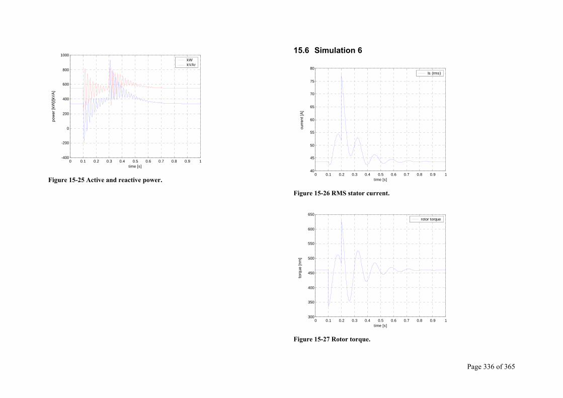
Page 336 of 365

0 0.1 0.2 0.3 0.4 0.5 0.6 0.7 0.8 0.9 1-400

-200

0

200

400

600

800

1000

time [s]

kW kVAr

Figure 15-25 Active and reactive power.

15.6 Simulation 6

0 0.1 0.2 0.3 0.4 0.5 0.6 0.7 0.8 0.9 140

45

50

55

60

65

70

75

80

time [s]

Is (rms)

Figure 15-26 RMS stator current.

0 0.1 0.2 0.3 0.4 0.5 0.6 0.7 0.8 0.9 1300

350

400

450

500

550

600

650

time [s]

rotor torque

Figure 15-27 Rotor torque.

pow

er [k

W]/[

kVA

]

curre

nt [A

] to

rque

[nm

]

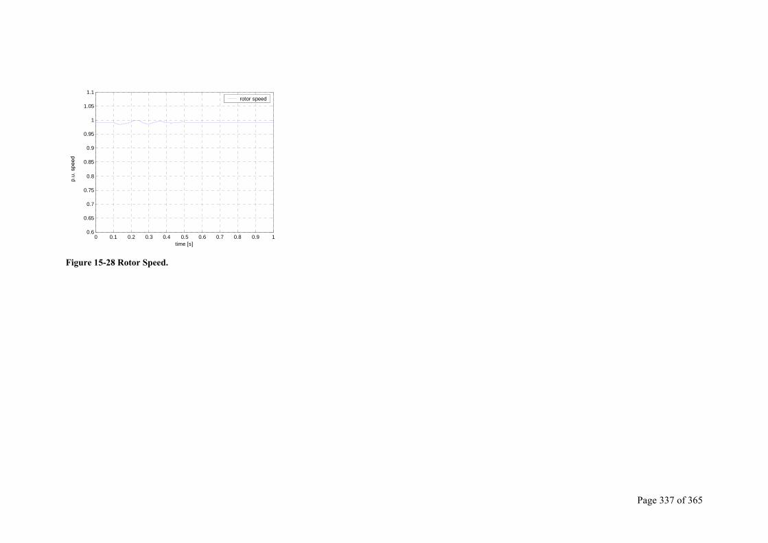
Page 337 of 365

0 0.1 0.2 0.3 0.4 0.5 0.6 0.7 0.8 0.9 10.6

0.65

0.7

0.75

0.8

0.85

0.9

0.95

1

1.05

1.1

time [s]

rotor speed

Figure 15-28 Rotor Speed.

p.u.

spe

ed

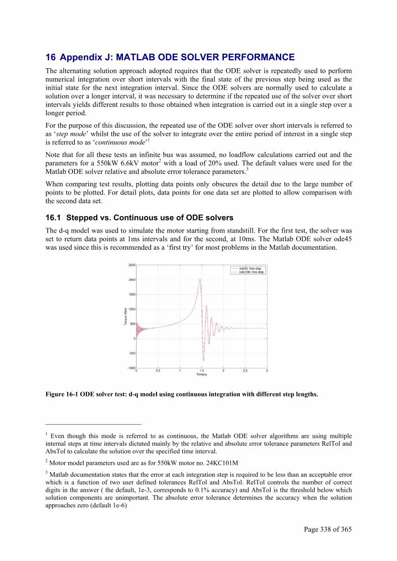
Page 338 of 365

16 Appendix J: MATLAB ODE SOLVER PERFORMANCE The alternating solution approach adopted requires that the ODE solver is repeatedly used to perform numerical integration over short intervals with the final state of the previous step being used as the initial state for the next integration interval. Since the ODE solvers are normally used to calculate a solution over a longer interval, it was necessary to determine if the repeated use of the solver over short intervals yields different results to those obtained when integration is carried out in a single step over a longer period.

For the purpose of this discussion, the repeated use of the ODE solver over short intervals is referred to as ‘step mode’ whilst the use of the solver to integrate over the entire period of interest in a single step is referred to as ‘continuous mode’1

Note that for all these tests an infinite bus was assumed, no loadflow calculations carried out and the parameters for a 550kW 6.6kV motor2 with a load of 20% used. The default values were used for the Matlab ODE solver relative and absolute error tolerance parameters.3

When comparing test results, plotting data points only obscures the detail due to the large number of points to be plotted. For detail plots, data points for one data set are plotted to allow comparison with the second data set.

16.1 Stepped vs. Continuous use of ODE solvers The d-q model was used to simulate the motor starting from standstill. For the first test, the solver was set to return data points at 1ms intervals and for the second, at 10ms. The Matlab ODE solver ode45 was used since this is recommended as a ‘first try’ for most problems in the Matlab documentation.

Figure 16-1 ODE solver test: d-q model using continuous integration with different step lengths.

1 Even though this mode is referred to as continuous, the Matlab ODE solver algorithms are using multiple internal steps at time intervals dictated mainly by the relative and absolute error tolerance parameters RelTol and AbsTol to calculate the solution over the specified time interval. 2 Motor model parameters used are as for 550kW motor no. 24KC101M 3 Matlab documentation states that the error at each integration step is required to be less than an acceptable error which is a function of two user defined tolerances RelTol and AbsTol. RelTol controls the number of correct digits in the answer ( the default, 1e-3, corresponds to 0.1% accuracy) and AbsTol is the threshold below which solution components are unimportant. The absolute error tolerance determines the accuracy when the solution approaches zero (default 1e-6)

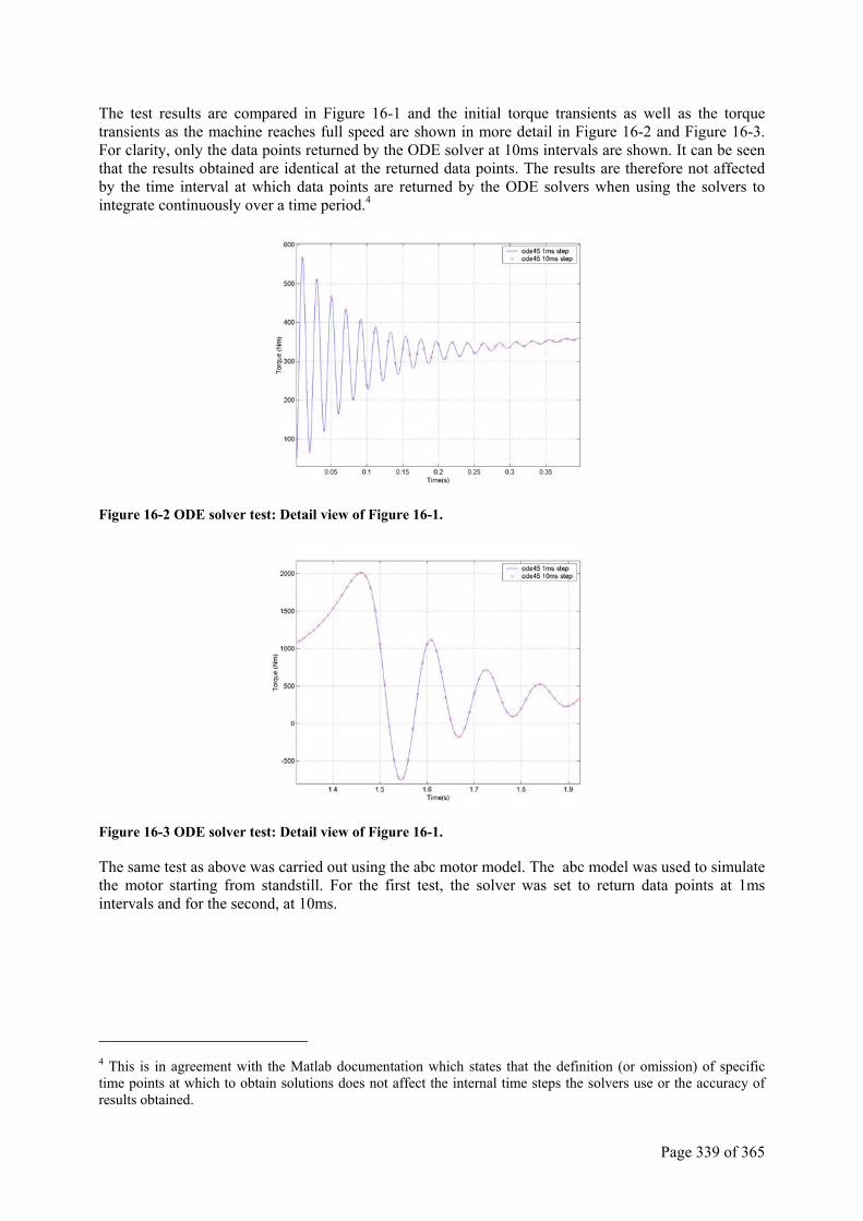
Page 339 of 365

The test results are compared in Figure 16-1 and the initial torque transients as well as the torque transients as the machine reaches full speed are shown in more detail in Figure 16-2 and Figure 16-3. For clarity, only the data points returned by the ODE solver at 10ms intervals are shown. It can be seen that the results obtained are identical at the returned data points. The results are therefore not affected by the time interval at which data points are returned by the ODE solvers when using the solvers to integrate continuously over a time period.4

Figure 16-2 ODE solver test: Detail view of Figure 16-1.

Figure 16-3 ODE solver test: Detail view of Figure 16-1.

The same test as above was carried out using the abc motor model. The abc model was used to simulate the motor starting from standstill. For the first test, the solver was set to return data points at 1ms intervals and for the second, at 10ms.

4 This is in agreement with the Matlab documentation which states that the definition (or omission) of specific time points at which to obtain solutions does not affect the internal time steps the solvers use or the accuracy of results obtained.

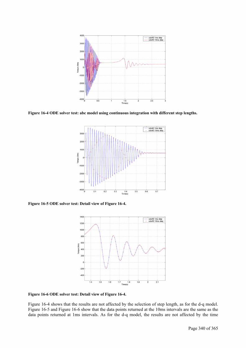
Page 340 of 365

Figure 16-4 ODE solver test: abc model using continuous integration with different step lengths.

Figure 16-5 ODE solver test: Detail view of Figure 16-4.

Figure 16-6 ODE solver test: Detail view of Figure 16-4.

Figure 16-4 shows that the results are not affected by the selection of step length, as for the d-q model. Figure 16-5 and Figure 16-6 show that the data points returned at the 10ms intervals are the same as the data points returned at 1ms intervals. As for the d-q model, the results are not affected by the time

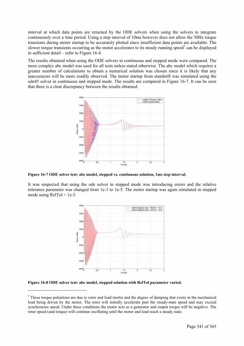
Page 341 of 365

interval at which data points are returned by the ODE solvers when using the solvers to integrate continuously over a time period. Using a step interval of 10ms however does not allow the 50Hz torque transients during motor startup to be accurately plotted since insufficient data points are available. The slower torque transients occurring as the motor accelerates to its steady running speed5 can be displayed in sufficient detail – refer to Figure 16-4.

The results obtained when using the ODE solvers in continuous and stepped mode were compared. The more complex abc model was used for all tests unless stated otherwise. The abc model which requires a greater number of calculations to obtain a numerical solution was chosen since it is likely that any inaccuracies will be more readily observed. The motor startup from standstill was simulated using the ode45 solver in continuous and stepped mode. The results are compared in Figure 16-7. It can be seen that there is a clear discrepancy between the results obtained.

Figure 16-7 ODE solver test: abc model, stepped vs. continuous solution, 1ms step interval.

It was suspected that using the ode solver in stepped mode was introducing errors and the relative tolerance parameter was changed from 1e-3 to 1e-5. The motor startup was again simulated in stepped mode using RelTol = 1e-5.

Figure 16-8 ODE solver test: abc model, stepped solution with RelTol parameter varied.

5 These torque pulsations are due to rotor and load inertia and the degree of damping that exists in the mechanical load being driven by the motor. The rotor will initially accelerate past the steady-state speed and may exceed synchronous speed. Under these conditions the motor acts as a generator and output torque will be negative. The rotor speed (and torque) will continue oscillating until the motor and load reach a steady state.

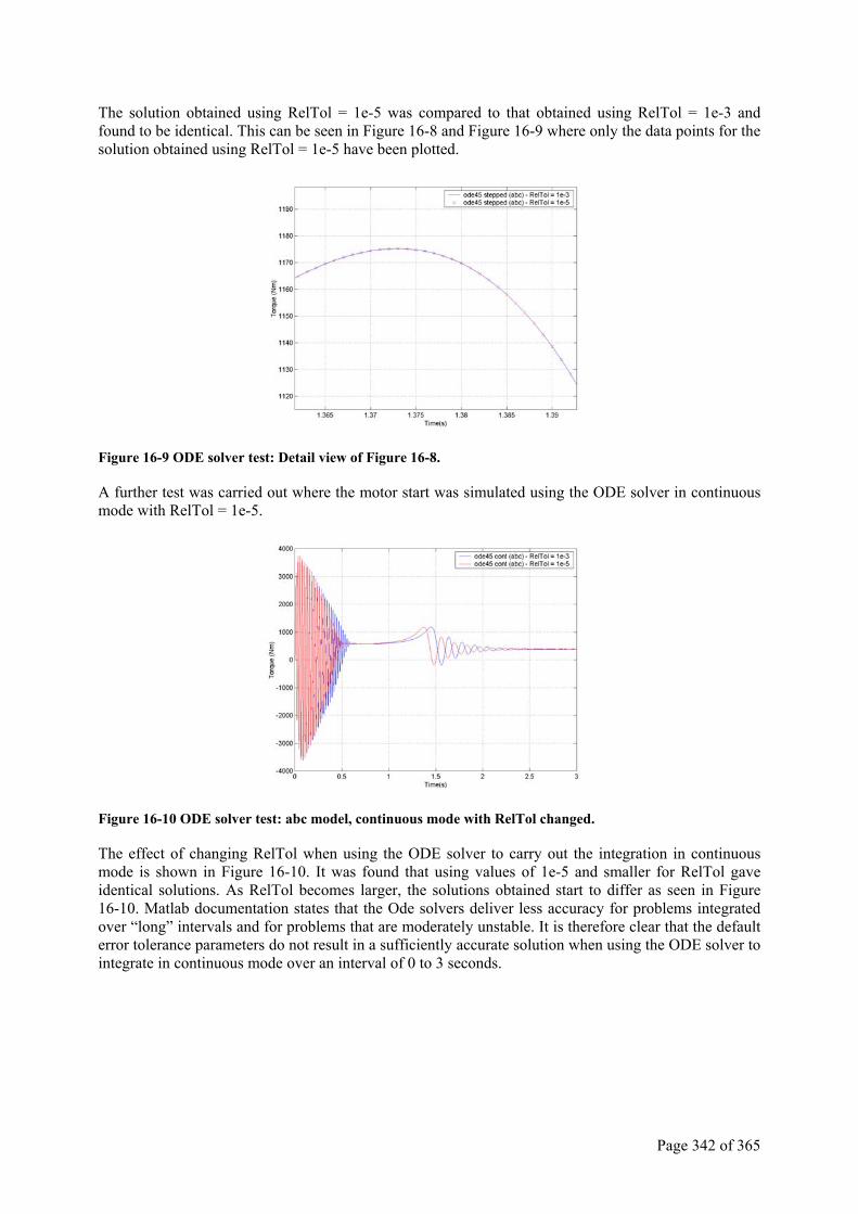
Page 342 of 365

The solution obtained using RelTol = 1e-5 was compared to that obtained using RelTol = 1e-3 and found to be identical. This can be seen in Figure 16-8 and Figure 16-9 where only the data points for the solution obtained using RelTol = 1e-5 have been plotted.

Figure 16-9 ODE solver test: Detail view of Figure 16-8.

A further test was carried out where the motor start was simulated using the ODE solver in continuous mode with RelTol = 1e-5.

Figure 16-10 ODE solver test: abc model, continuous mode with RelTol changed.

The effect of changing RelTol when using the ODE solver to carry out the integration in continuous mode is shown in Figure 16-10. It was found that using values of 1e-5 and smaller for RelTol gave identical solutions. As RelTol becomes larger, the solutions obtained start to differ as seen in Figure 16-10. Matlab documentation states that the Ode solvers deliver less accuracy for problems integrated over “long” intervals and for problems that are moderately unstable. It is therefore clear that the default error tolerance parameters do not result in a sufficiently accurate solution when using the ODE solver to integrate in continuous mode over an interval of 0 to 3 seconds.

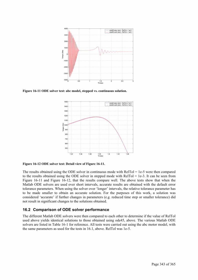
Page 343 of 365

Figure 16-11 ODE solver test: abc model, stepped vs. continuous solution.

Figure 16-12 ODE solver test: Detail view of Figure 16-11.

The results obtained using the ODE solver in continuous mode with RelTol = 1e-5 were then compared to the results obtained using the ODE solver in stepped mode with RelTol = 1e-3. It can be seen from Figure 16-11 and Figure 16-12, that the results compare well. The above tests show that when the Matlab ODE solvers are used over short intervals, accurate results are obtained with the default error tolerance parameters. When using the solver over ‘longer’ intervals, the relative tolerance parameter has to be made smaller to obtain an accurate solution. For the purposes of this work, a solution was considered ‘accurate’ if further changes in parameters (e.g. reduced time step or smaller tolerance) did not result in significant changes to the solutions obtained.

16.2 Comparison of ODE solver performance The different Matlab ODE solvers were then compared to each other to determine if the value of RelTol used above yields identical solutions to those obtained using ode45, above. The various Matlab ODE solvers are listed in Table 16-1 for reference. All tests were carried out using the abc motor model, with the same parameters as used for the tests in 16.1, above. RelTol was 1e-5.

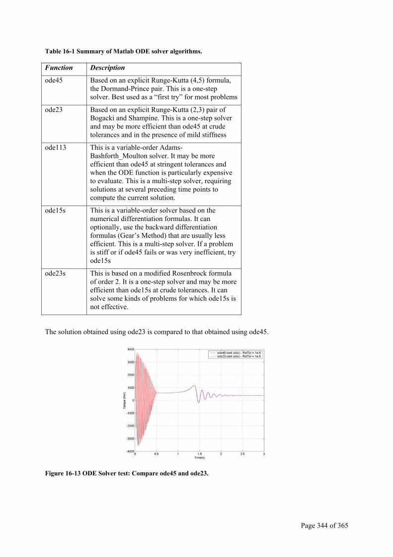
Page 344 of 365

Table 16-1 Summary of Matlab ODE solver algorithms.

Function Description

ode45 Based on an explicit Runge-Kutta (4,5) formula, the Dormand-Prince pair. This is a one-step solver. Best used as a “first try” for most problems

ode23 Based on an explicit Runge-Kutta (2,3) pair of Bogacki and Shampine. This is a one-step solver and may be more efficient than ode45 at crude tolerances and in the presence of mild stiffness

ode113 This is a variable-order Adams-Bashforth_Moulton solver. It may be more efficient than ode45 at stringent tolerances and when the ODE function is particularly expensive to evaluate. This is a multi-step solver, requiring solutions at several preceding time points to compute the current solution.

ode15s This is a variable-order solver based on the numerical differentiation formulas. It can optionally, use the backward differentiation formulas (Gear’s Method) that are usually less efficient. This is a multi-step solver. If a problem is stiff or if ode45 fails or was very inefficient, try ode15s

ode23s This is based on a modified Rosenbrock formula of order 2. It is a one-step solver and may be more efficient than ode15s at crude tolerances. It can solve some kinds of problems for which ode15s is not effective.

The solution obtained using ode23 is compared to that obtained using ode45.

Figure 16-13 ODE Solver test: Compare ode45 and ode23.

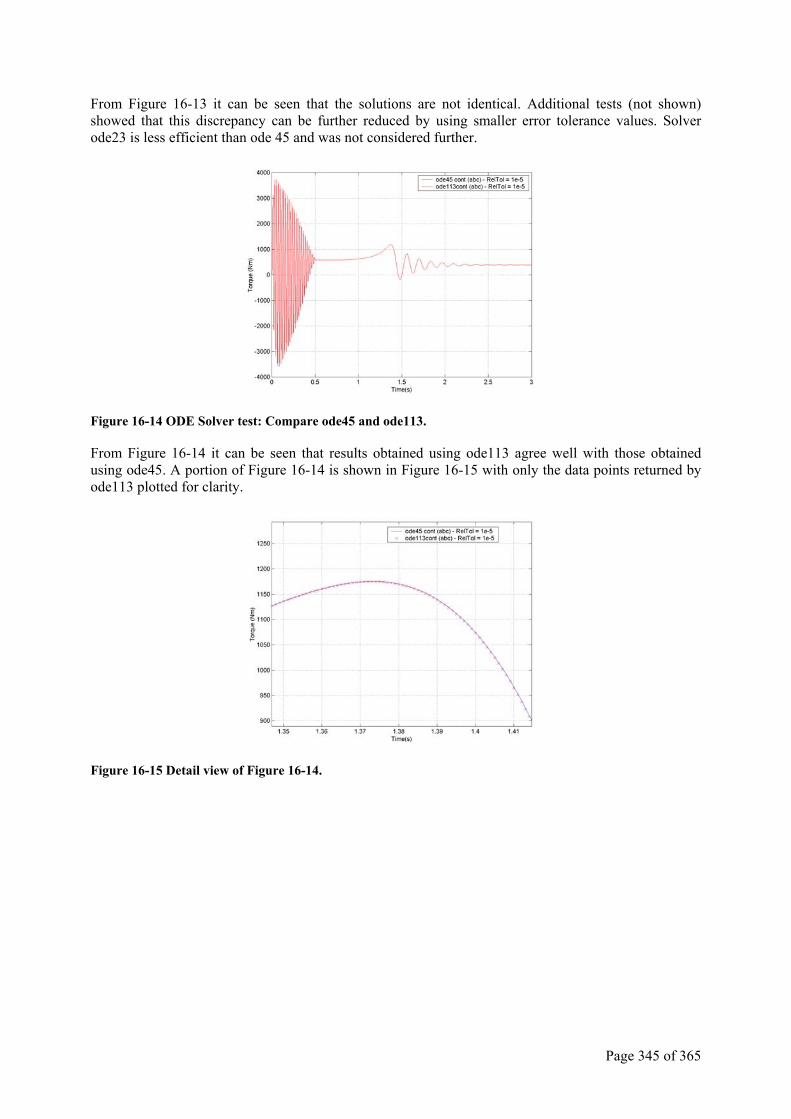
Page 345 of 365

From Figure 16-13 it can be seen that the solutions are not identical. Additional tests (not shown) showed that this discrepancy can be further reduced by using smaller error tolerance values. Solver ode23 is less efficient than ode 45 and was not considered further.

Figure 16-14 ODE Solver test: Compare ode45 and ode113.

From Figure 16-14 it can be seen that results obtained using ode113 agree well with those obtained using ode45. A portion of Figure 16-14 is shown in Figure 16-15 with only the data points returned by ode113 plotted for clarity.

Figure 16-15 Detail view of Figure 16-14.

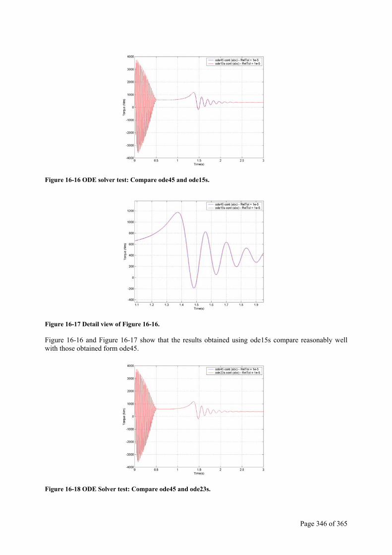
Page 346 of 365

Figure 16-16 ODE solver test: Compare ode45 and ode15s.

Figure 16-17 Detail view of Figure 16-16.

Figure 16-16 and Figure 16-17 show that the results obtained using ode15s compare reasonably well with those obtained form ode45.

Figure 16-18 ODE Solver test: Compare ode45 and ode23s.

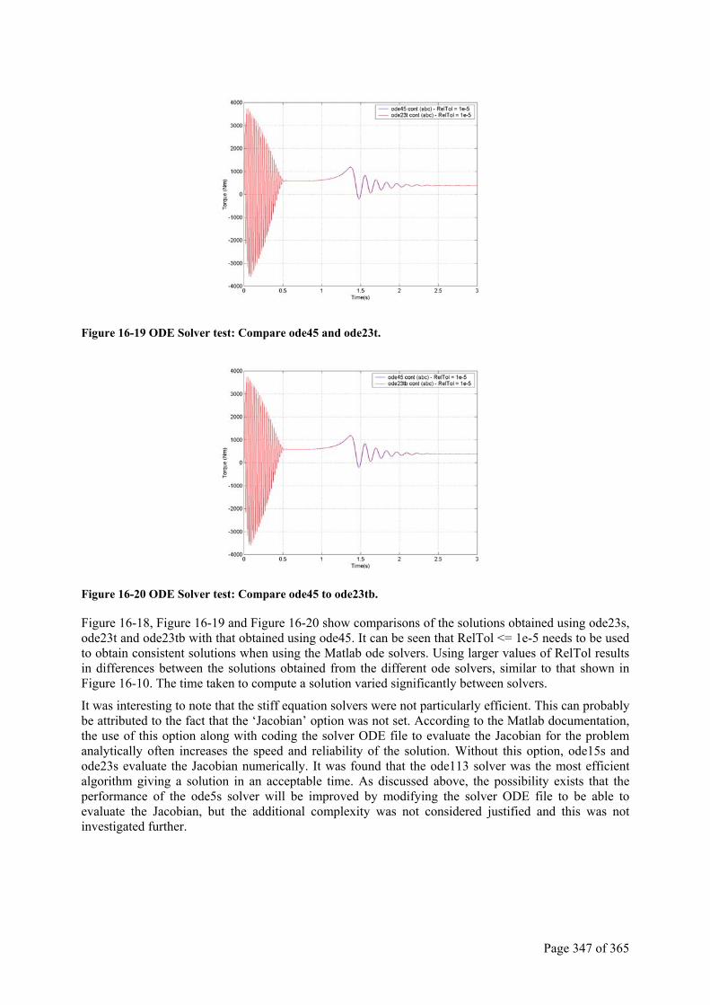
Page 347 of 365

Figure 16-19 ODE Solver test: Compare ode45 and ode23t.

Figure 16-20 ODE Solver test: Compare ode45 to ode23tb.

Figure 16-18, Figure 16-19 and Figure 16-20 show comparisons of the solutions obtained using ode23s, ode23t and ode23tb with that obtained using ode45. It can be seen that RelTol <= 1e-5 needs to be used to obtain consistent solutions when using the Matlab ode solvers. Using larger values of RelTol results in differences between the solutions obtained from the different ode solvers, similar to that shown in Figure 16-10. The time taken to compute a solution varied significantly between solvers.

It was interesting to note that the stiff equation solvers were not particularly efficient. This can probably be attributed to the fact that the ‘Jacobian’ option was not set. According to the Matlab documentation, the use of this option along with coding the solver ODE file to evaluate the Jacobian for the problem analytically often increases the speed and reliability of the solution. Without this option, ode15s and ode23s evaluate the Jacobian numerically. It was found that the ode113 solver was the most efficient algorithm giving a solution in an acceptable time. As discussed above, the possibility exists that the performance of the ode5s solver will be improved by modifying the solver ODE file to be able to evaluate the Jacobian, but the additional complexity was not considered justified and this was not investigated further.

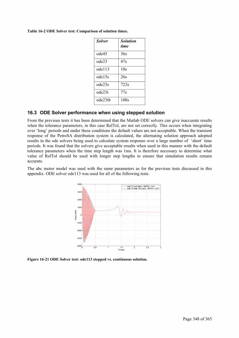
Page 348 of 365

Table 16-2 ODE Solver test: Comparison of solution times.

Solver Solution time

ode45 36s

ode23 47s

ode113 10s

ode15s 26s

ode23s 722s

ode23t 77s

ode23tb 108s

16.3 ODE Solver performance when using stepped solution From the previous tests it has been determined that the Matlab ODE solvers can give inaccurate results when the tolerance parameters, in this case RelTol, are not set correctly. This occurs when integrating over ‘long’ periods and under these conditions the default values are not acceptable. When the transient response of the PetroSA distribution system is calculated, the alternating solution approach adopted results in the ode solvers being used to calculate system response over a large number of ‘short’ time periods. It was found that the solvers give acceptable results when used in this manner with the default tolerance parameters when the time step length was 1ms. It is therefore necessary to determine what value of RelTol should be used with longer step lengths to ensure that simulation results remain accurate.

The abc motor model was used with the same parameters as for the previous tests discussed in this appendix. ODE solver ode113 was used for all of the following tests.

Figure 16-21 ODE Solver test: ode113 stepped vs. continuous solution.

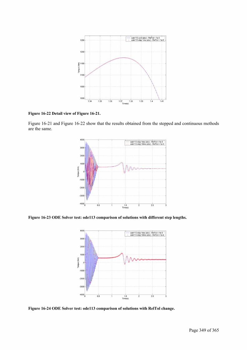
Page 349 of 365

Figure 16-22 Detail view of Figure 16-21.

Figure 16-21 and Figure 16-22 show that the results obtained from the stepped and continuous methods are the same.

Figure 16-23 ODE Solver test: ode113 comparison of solutions with different step lengths.

Figure 16-24 ODE Solver test: ode113 comparison of solutions with RelTol change.

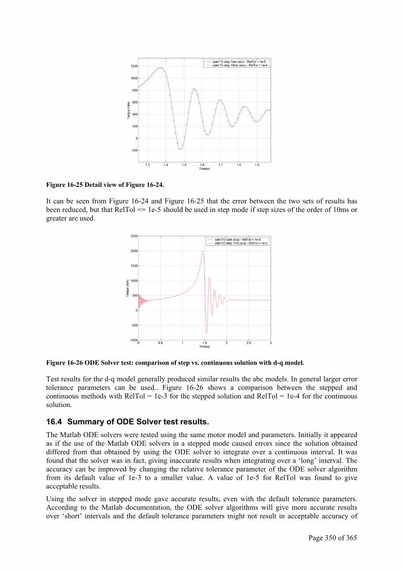
Page 350 of 365

Figure 16-25 Detail view of Figure 16-24.

It can be seen from Figure 16-24 and Figure 16-25 that the error between the two sets of results has been reduced, but that RelTol <= 1e-5 should be used in step mode if step sizes of the order of 10ms or greater are used.

Figure 16-26 ODE Solver test: comparison of step vs. continuous solution with d-q model.

Test results for the d-q model generally produced similar results the abc models. In general larger error tolerance parameters can be used.. Figure 16-26 shows a comparison between the stepped and continuous methods with RelTol = 1e-3 for the stepped solution and RelTol = 1e-4 for the continuous solution.

16.4 Summary of ODE Solver test results. The Matlab ODE solvers were tested using the same motor model and parameters. Initially it appeared as if the use of the Matlab ODE solvers in a stepped mode caused errors since the solution obtained differed from that obtained by using the ODE solver to integrate over a continuous interval. It was found that the solver was in fact, giving inaccurate results when integrating over a ‘long’ interval. The accuracy can be improved by changing the relative tolerance parameter of the ODE solver algorithm from its default value of 1e-3 to a smaller value. A value of 1e-5 for RelTol was found to give acceptable results.

Using the solver in stepped mode gave accurate results, even with the default tolerance parameters. According to the Matlab documentation, the ODE solver algorithms will give more accurate results over ‘short’ intervals and the default tolerance parameters might not result in acceptable accuracy of

Page 351 of 365

solutions over ‘long’ intervals. Using the solvers over multiple short intervals (1ms) in step mode gives accurate results even with the default tolerance parameters. If the step size approaches 10ms in stepped mode, it was found that RelTol <= 1e-5 needs to be used as for the continuous solution.

The various ODE solvers all produced similar results when used with the correct relative tolerance. The main difference observed was the time taken to compute a solution with ode113, a non-stiff solver, being the most efficient and one of the stiff solvers, ode23s being extremely inefficient. The performance of the stiff equation solvers can possibly be improved if the motor model ODE file is modified to return the Jacobian of the system of equations. This was not investigated further since the speed and efficiency with which solutions are obtained is not a primary objective of the present work. This would be a topic for investigation in future work if the size and complexity of the distribution system and motor models is increased.

In summary:

• If using the ode solver in stepped mode, accurate results are obtained with RelTol <= 1e-3 (default value) and a step length of 1ms or less.

• If the ode solver is used in stepped mode with a step length greater than 1ms, RelTol should preferably be <= 1e-5 to obtain accurate results

• If using the ode solver to integrate continuously over a ‘long’ interval, a value for RelTol <= 1e-5 must be used. Intermediate results returned by the ode solvers are unaffected by the intermediate time step. (This is confirmed in the Matlab documentation.)

16.5 Matlab Software Listings for additional ODE solver tests. The source code for the Matlab software used to carry out these additional tests is listed in this section.

16.5.1 Induction motor model (abc) function dS = induction_motor_01(t, S, flag, v_mot, MP) % ODE Function to simulate induction motor performance % abc reference frame model: % Does not model saturation % Models friction and windage with a constant torque proportional to speed^2 % ############################################################################ % Rev | Comment % ----+--------------------------------------------------------------------- % 00 | Corrected error in friction and windage torque calculation % | Printed: 26/06/2005 - before adding synchronous machine model % 01 | Added function to reduce rotor resistance and increase rotor % | reactance % | as a function of slip to give approximation of a double cage rotor % ############################################################################ % Use with ODE solver as follows: % [T,Y] = odeXX( 'induction_motor_01', tspan, S1_IM1, options, vbus, % MP(1,:)); % % tspan = [t0 tfinal] % S = motor model state variables % S = [isa; isb; isc; ira; irb; irc; rotor_angle; rotor_speed] % S(1,1) = isa - stator currents % S(2,1) = isb % S(3,1) = isc % S(4,1) = ira - rotor currents % etc % S(7,1) = rotor_angle is in radians

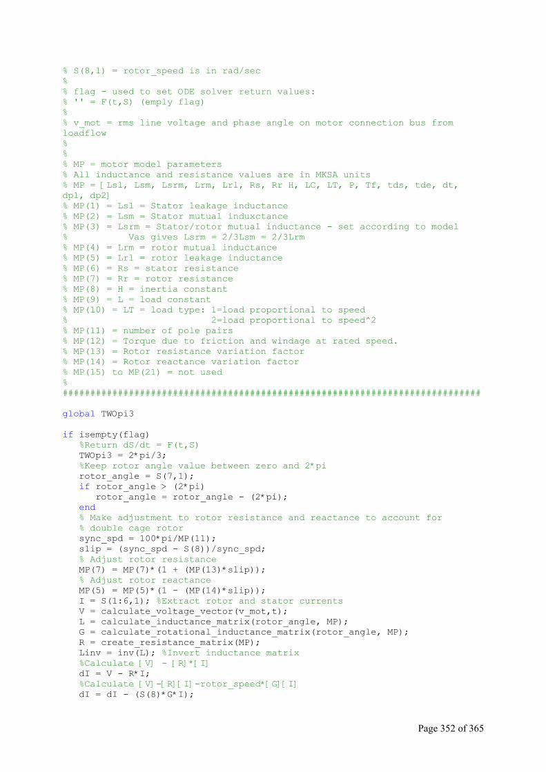
Page 352 of 365

% S(8,1) = rotor_speed is in rad/sec % % flag - used to set ODE solver return values: % '' = F(t,S) (emply flag) % % v_mot = rms line voltage and phase angle on motor connection bus from loadflow % % % MP = motor model parameters % All inductance and resistance values are in MKSA units % MP = [Lsl, Lsm, Lsrm, Lrm, Lrl, Rs, Rr H, LC, LT, P, Tf, tds, tde, dt, dp1, dp2] % MP(1) = Lsl = Stator leakage inductance % MP(2) = Lsm = Stator mutual induxctance % MP(3) = Lsrm = Stator/rotor mutual inductance - set according to model % Vas gives Lsrm = 2/3Lsm = 2/3Lrm % MP(4) = Lrm = rotor mutual inductance % MP(5) = Lrl = rotor leakage inductance % MP(6) = Rs = stator resistance % MP(7) = Rr = rotor resistance % MP(8) = H = inertia constant % MP(9) = L = load constant % MP(10) = LT = load type: 1=load proportional to speed % 2=load proportional to speed^2 % MP(11) = number of pole pairs % MP(12) = Torque due to friction and windage at rated speed. % MP(13) = Rotor resistance variation factor % MP(14) = Rotor reactance variation factor % MP(15) to MP(21) = not used % ############################################################################ global TWOpi3 if isempty(flag) %Return dS/dt = F(t,S) TWOpi3 = 2*pi/3; %Keep rotor angle value between zero and 2*pi rotor_angle = S(7,1); if rotor_angle > (2*pi) rotor_angle = rotor_angle - (2*pi); end % Make adjustment to rotor resistance and reactance to account for % double cage rotor sync_spd = 100*pi/MP(11); slip = (sync_spd - S(8))/sync_spd; % Adjust rotor resistance MP(7) = MP(7)*(1 + (MP(13)*slip)); % Adjust rotor reactance MP(5) = MP(5)*(1 - (MP(14)*slip)); I = S(1:6,1); %Extract rotor and stator currents V = calculate_voltage_vector(v_mot,t); L = calculate_inductance_matrix(rotor_angle, MP); G = calculate_rotational_inductance_matrix(rotor_angle, MP); R = create_resistance_matrix(MP); Linv = inv(L); %Invert inductance matrix %Calculate [V] - [R]*[I] dI = V - R*I; %Calculate [V]-[R][I]-rotor_speed*[G][I] dI = dI - (S(8)*G*I);

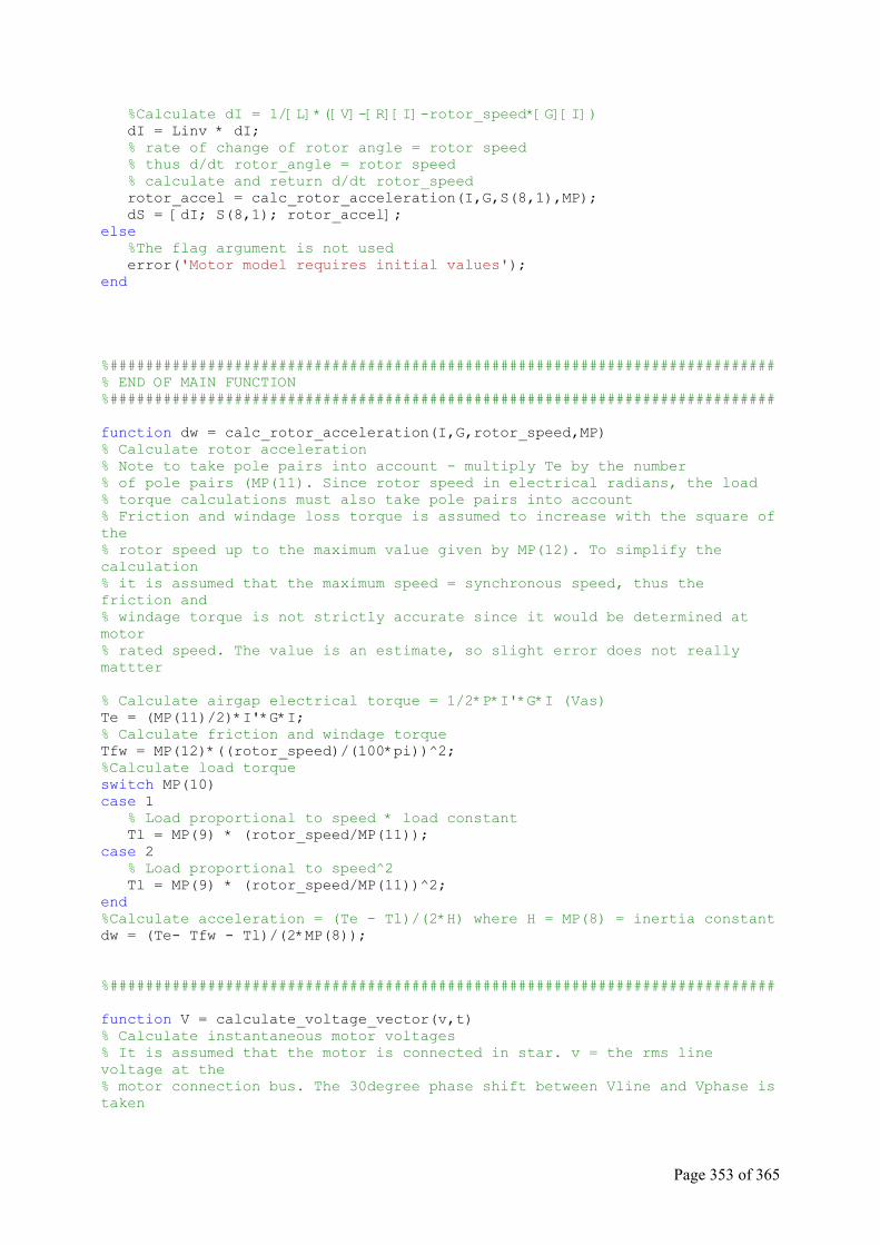
Page 353 of 365

%Calculate dI = 1/[L]*([V]-[R][I]-rotor_speed*[G][I]) dI = Linv * dI; % rate of change of rotor angle = rotor speed % thus d/dt rotor_angle = rotor speed % calculate and return d/dt rotor_speed rotor_accel = calc_rotor_acceleration(I,G,S(8,1),MP); dS = [dI; S(8,1); rotor_accel]; else %The flag argument is not used error('Motor model requires initial values'); end %########################################################################### % END OF MAIN FUNCTION %########################################################################### function dw = calc_rotor_acceleration(I,G,rotor_speed,MP) % Calculate rotor acceleration % Note to take pole pairs into account - multiply Te by the number % of pole pairs (MP(11). Since rotor speed in electrical radians, the load % torque calculations must also take pole pairs into account % Friction and windage loss torque is assumed to increase with the square of the % rotor speed up to the maximum value given by MP(12). To simplify the calculation % it is assumed that the maximum speed = synchronous speed, thus the friction and % windage torque is not strictly accurate since it would be determined at motor % rated speed. The value is an estimate, so slight error does not really mattter % Calculate airgap electrical torque = 1/2*P*I'*G*I (Vas) Te = (MP(11)/2)*I'*G*I; % Calculate friction and windage torque Tfw = MP(12)*((rotor_speed)/(100*pi))^2; %Calculate load torque switch MP(10) case 1 % Load proportional to speed * load constant Tl = MP(9) * (rotor_speed/MP(11)); case 2 % Load proportional to speed^2 Tl = MP(9) * (rotor_speed/MP(11))^2; end %Calculate acceleration = (Te - Tl)/(2*H) where H = MP(8) = inertia constant dw = (Te- Tfw - Tl)/(2*MP(8)); %########################################################################### function V = calculate_voltage_vector(v,t) % Calculate instantaneous motor voltages % It is assumed that the motor is connected in star. v = the rms line voltage at the % motor connection bus. The 30degree phase shift between Vline and Vphase is taken

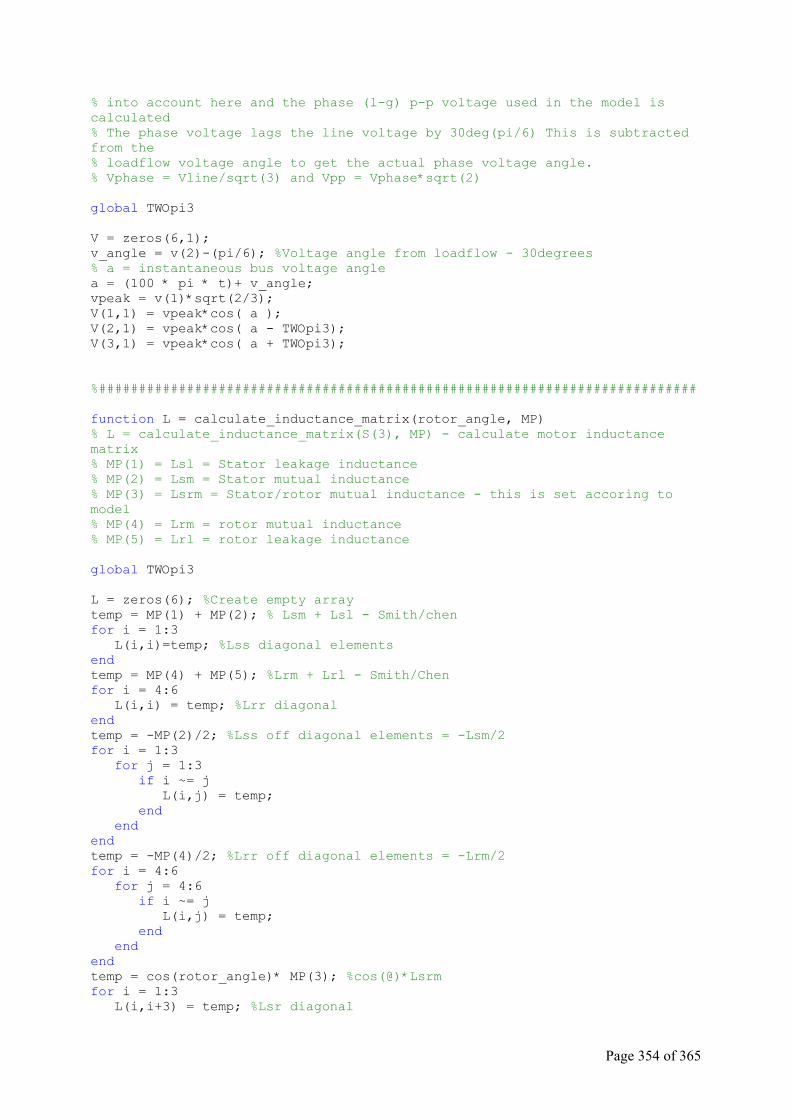
Page 354 of 365

% into account here and the phase (l-g) p-p voltage used in the model is calculated % The phase voltage lags the line voltage by 30deg(pi/6) This is subtracted from the % loadflow voltage angle to get the actual phase voltage angle. % Vphase = Vline/sqrt(3) and Vpp = Vphase*sqrt(2) global TWOpi3 V = zeros(6,1); v_angle = v(2)-(pi/6); %Voltage angle from loadflow - 30degrees % a = instantaneous bus voltage angle a = (100 * pi * t)+ v_angle; vpeak = v(1)*sqrt(2/3); V(1,1) = vpeak*cos( a ); V(2,1) = vpeak*cos( a - TWOpi3); V(3,1) = vpeak*cos( a + TWOpi3); %########################################################################### function L = calculate_inductance_matrix(rotor_angle, MP) % L = calculate_inductance_matrix(S(3), MP) - calculate motor inductance matrix % MP(1) = Lsl = Stator leakage inductance % MP(2) = Lsm = Stator mutual inductance % MP(3) = Lsrm = Stator/rotor mutual inductance - this is set accoring to model % MP(4) = Lrm = rotor mutual inductance % MP(5) = Lrl = rotor leakage inductance global TWOpi3 L = zeros(6); %Create empty array temp = MP(1) + MP(2); % Lsm + Lsl - Smith/chen for i = 1:3 L(i,i)=temp; %Lss diagonal elements end temp = MP(4) + MP(5); %Lrm + Lrl - Smith/Chen for i = 4:6 L(i,i) = temp; %Lrr diagonal end temp = -MP(2)/2; %Lss off diagonal elements = -Lsm/2 for i = 1:3 for j = 1:3 if i ~= j L(i,j) = temp; end end end temp = -MP(4)/2; %Lrr off diagonal elements = -Lrm/2 for i = 4:6 for j = 4:6 if i ~= j L(i,j) = temp; end end end temp = cos(rotor_angle)* MP(3); %cos(@)*Lsrm for i = 1:3 L(i,i+3) = temp; %Lsr diagonal

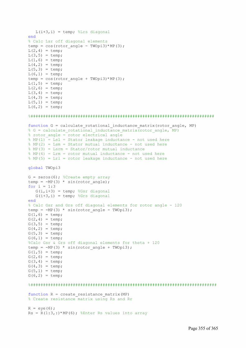
Page 355 of 365

L(i+3,i) = temp; %Lrs diagonal end % Calc Lsr off diagonal elements temp = cos(rotor_angle - TWOpi3)*MP(3); L(2,4) = temp; L(3,5) = temp; L(1,6) = temp; L(4,2) = temp; L(5,3) = temp; L(6,1) = temp; temp = cos(rotor_angle + TWOpi3)*MP(3); L(1,5) = temp; L(2,6) = temp; L(3,4) = temp; L(4,3) = temp; L(5,1) = temp; L(6,2) = temp; %########################################################################## function G = calculate_rotational_inductance_matrix(rotor_angle, MP) % G = calculate_rotational_inductance_matrix(rotor_angle, MP) % rotor_angle = rotor electrical angle % MP(1) = Lsl = Stator leakage inductance - not used here % MP(2) = Lsm = Stator mutual inductance - not used here % MP(3) = Lsrm = Stator/rotor mutual inductance % MP(4) = Lrm = rotor mutual inductance - not used here % MP(5) = Lrl = rotor leakage inductance - not used here global TWOpi3 G = zeros(6); %Create empty array temp = -MP(3) * sin(rotor_angle); for i = 1:3 G(i,i+3) = temp; %Gsr diagonal G(i+3,i) = temp; %Grs diagonal end % Calc Gsr and Grs off diagonal elements for rotor angle - 120 temp = -MP(3) * sin(rotor_angle - TWOpi3); G(1,6) = temp; G(2,4) = temp; G(3,5) = temp; G(4,2) = temp; G(5,3) = temp; G(6,1) = temp; %Calc Gsr & Grs off diagonal elements for theta + 120 temp = -MP(3) * sin(rotor_angle + TWOpi3); G(1,5) = temp; G(2,6) = temp; G(3,4) = temp; G(4,3) = temp; G(5,1) = temp; G(6,2) = temp; %########################################################################### function R = create_resistance_matrix(MP) % Create resistance matrix using Rs and Rr R = eye(6); Rs = R(1:3,:)*MP(6); %Enter Rs values into array

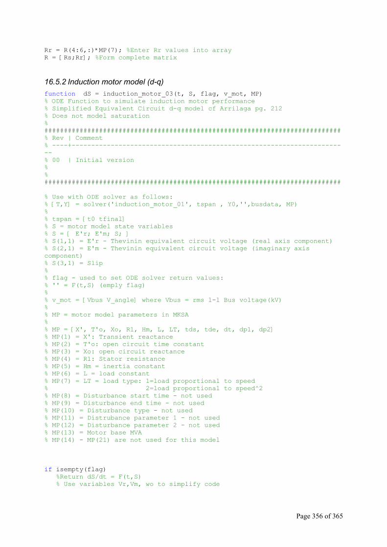
Page 356 of 365

Rr = R(4:6,:)*MP(7); %Enter Rr values into array R = [Rs;Rr]; %Form complete matrix

16.5.2 Induction motor model (d-q) function dS = induction_motor_03(t, S, flag, v_mot, MP) % ODE Function to simulate induction motor performance % Simplified Equivalent Circuit d-q model cf Arrilaga pg. 212 % Does not model saturation % ############################################################################ % Rev | Comment % ----+----------------------------------------------------------------------- % 00 | Initial version % % ############################################################################ % Use with ODE solver as follows: % [T,Y] = solver('induction_motor_01', tspan , Y0,'',busdata, MP) % % tspan = [t0 tfinal] % S = motor model state variables % S = [ E'r; E'm; S; ] % S(1,1) = E'r - Thevinin equivalent circuit voltage (real axis component) % S(2,1) = E'm - Thevinin equivalent circuit voltage (imaginary axis component) % S(3,1) = Slip % % flag - used to set ODE solver return values: % '' = F(t,S) (emply flag) % % v_mot = [Vbus V_angle] where Vbus = rms l-l Bus voltage(kV) % % MP = motor model parameters in MKSA % % MP = [X', T'o, Xo, R1, Hm, L, LT, tds, tde, dt, dp1, dp2] % MP(1) = X': Transient reactance % MP(2) = T'o: open circuit time constant % MP(3) = Xo: open circuit reactance % MP(4) = R1: Stator resistance % MP(5) = Hm = inertia constant % MP(6) = L = load constant % MP(7) = LT = load type: 1=load proportional to speed % 2=load proportional to speed^2 % MP(8) = Disturbance start time - not used % MP(9) = Disturbance end time - not used % MP(10) = Disturbance type - not used % MP(11) = Distrubance parameter 1 - not used % MP(12) = Disturbance parameter 2 - not used % MP(13) = Motor base MVA % MP(14) - MP(21) are not used for this model if isempty(flag) %Return dS/dt = F(t,S) % Use variables Vr,Vm, wo to simplify code

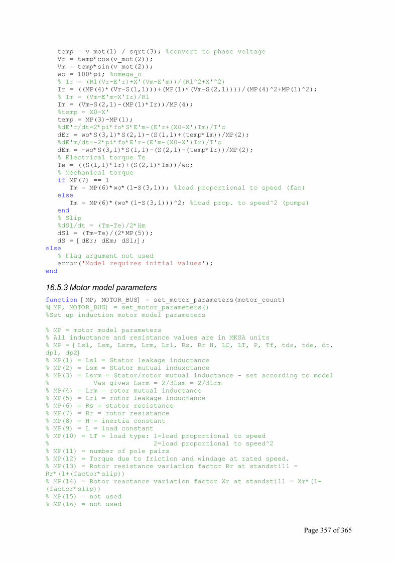
Page 357 of 365

temp = v_mot(1) / sqrt(3); %convert to phase voltage Vr = temp*cos(v_mot(2)); Vm = temp*sin(v_mot(2)); wo = 100*pi; %omega_o % Ir = (R1(Vr-E'r)+X'(Vm-E'm))/(R1^2+X'^2) Ir = ((MP(4)*(Vr-S(1,1)))+(MP(1)*(Vm-S(2,1))))/(MP(4)^2+MP(1)^2); % Im = (Vm-E'm-X'Ir)/R1 Im = (Vm-S(2,1)-(MP(1)*Ir))/MP(4); %temp = X0-X' temp = MP(3)-MP(1); %dE'r/dt=2*pi*fo*S*E'm-(E'r+(X0-X')Im)/T'o dEr = wo*S(3,1)*S(2,1)-(S(1,1)+(temp*Im))/MP(2); %dE'm/dt=-2*pi*fo*E'r-(E'm-(X0-X')Ir)/T'o dEm = -wo*S(3,1)*S(1,1)-(S(2,1)-(temp*Ir))/MP(2); % Electrical torque Te Te = ((S(1,1)*Ir)+(S(2,1)*Im))/wo; % Mechanical torque if MP(7) == 1 Tm = MP(6)*wo*(1-S(3,1)); %load proportional to speed (fan) else Tm = MP(6)*(wo*(1-S(3,1)))^2; %Load prop. to speed^2 (pumps) end % Slip %dSl/dt = (Tm-Te)/2*Hm dSl = (Tm-Te)/(2*MP(5)); dS = [dEr; dEm; dSl;]; else % Flag argument not used error('Model requires initial values'); end

16.5.3 Motor model parameters function [MP, MOTOR_BUS] = set_motor_parameters(motor_count) %[MP, MOTOR_BUS] = set_motor_parameters() %Set up induction motor model parameters % MP = motor model parameters % All inductance and resistance values are in MKSA units % MP = [Lsl, Lsm, Lsrm, Lrm, Lrl, Rs, Rr H, LC, LT, P, Tf, tds, tde, dt, dp1, dp2] % MP(1) = Lsl = Stator leakage inductance % MP(2) = Lsm = Stator mutual induxctance % MP(3) = Lsrm = Stator/rotor mutual inductance - set according to model % Vas gives Lsrm = 2/3Lsm = 2/3Lrm % MP(4) = Lrm = rotor mutual inductance % MP(5) = Lrl = rotor leakage inductance % MP(6) = Rs = stator resistance % MP(7) = Rr = rotor resistance % MP(8) = H = inertia constant % MP(9) = L = load constant % MP(10) = LT = load type: 1=load proportional to speed % 2=load proportional to speed^2 % MP(11) = number of pole pairs % MP(12) = Torque due to friction and windage at rated speed. % MP(13) = Rotor resistance variation factor Rr at standstill = Rr*(1+(factor*slip)) % MP(14) = Rotor reactance variation factor Xr at standstill = Xr*(1-(factor*slip)) % MP(15) = not used % MP(16) = not used

Page 358 of 365

% MP(17) = not used % MP(18) = I0 = base current at which no saturation is assumed % MP(19) = B0 = flux density corresponding to I0 - calculated from saturation curve % MP(20) = Saturation current multiplication factor - scale Im to At/m % MP(21) = Saturation scaling factor % MOTOR_BUS = loadflow motor bus %=================================================================== % Revision History % 2005/06/26 - Used as basis for adding synchronous generator model % 2005/08/02 - Added parameters for single-cage induction motor model %=================================================================== MP = zeros(motor_count*2, 21); MOTOR_BUS = zeros(motor_count,1); %=================================================================== % Parameters for abc model % % Note: MOTOR_BUS is an array storing the connection bus numbers of the % motors to be simulated. There is no value stored for the d-q model % since this simply uses the abc model data %=================================================================== % MOTOR 01 - 24KC101AM 550kW - bus 49 %=================================================================== MOTOR_BUS(1) = 49; %Motor 1 bus number MP(1,1) = 0.03592; %Lsl = Stator leakage inductance (=equiv. ckt param) MP(1,2) = 0.8726; %Lsm = Stator magnetising inductance MP(1,3) = MP(1,2); %Lsrm = Stator/rotor mutual inductance = 2/3Lsm = 2/3Lrm MP(1,4) = MP(1,2); %Lrm = rotor magnetising inductance MP(1,5) = 0.05389; %Lrl = rotor leakage inductance MP(1,6) = 1.1895; %Rs = stator resistance MP(1,7) = 0.6479; %Rr = rotor resistance (running resistance) MP(1,8) = 5.5; %H = inertia constant MP(1,9) = 0.018; %L = load constant approx 50% of 550kW load MP(1,10) = 2;%LT = load type: 1= proportional to speed 2= proportional to speed^2 MP(1,11) = 1; %pole pairs MP(1,12) = 37.93; %Torque due to friction and Windage at rated speed (Nm) MP(1,13) = 2; %Rr standstill = 3Rr MP(1,14) = 0.5; %Xr standstill = 0.5*Xr %Saturation - not used MP(1,18) = 0; %I0 - base current MP(1,19) = 0; %B0 = I0 flux density MP(1,20) = 0; %current scale factor MP(1,21) = 0; %saturation scaling factor ( 0 = no saturation) %=================================================================== % MOTOR 02 - 24PC101AM 300kW - bus 50 %=================================================================== MOTOR_BUS(2) = 50; %Motor 2 bus number MP(2,1) = 0.0671; %Lsl = Stator leakage inductance (=equiv. ckt param) MP(2,2) = 1.844; %Lsm = Stator magnetising inductance MP(2,3) = MP(2,2); %Lsrm = Stator/rotor mutual inductance = 2/3Lsm = 2/3Lrm MP(2,4) = MP(2,2); %Lrm = rotor magnetising inductance

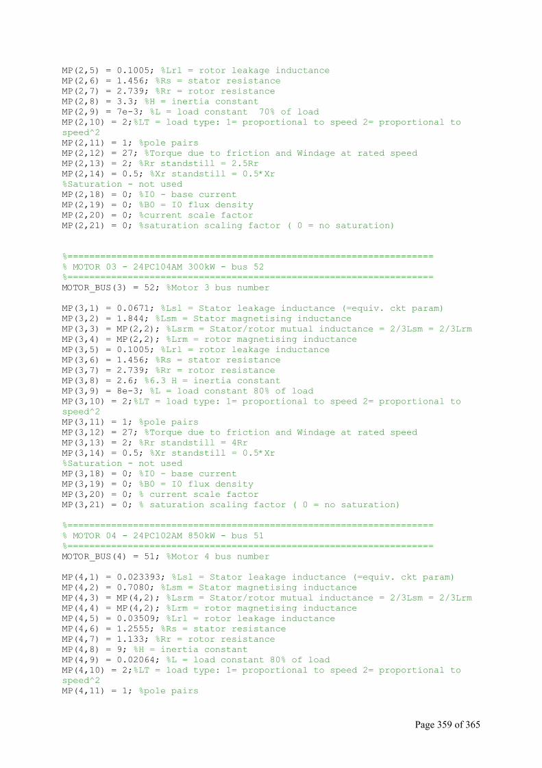
Page 359 of 365

MP(2,5) = 0.1005; %Lrl = rotor leakage inductance MP(2,6) = 1.456; %Rs = stator resistance MP(2,7) = 2.739; %Rr = rotor resistance MP(2,8) = 3.3; %H = inertia constant MP(2,9) = 7e-3; %L = load constant 70% of load MP(2,10) = 2;%LT = load type: 1= proportional to speed 2= proportional to speed^2 MP(2,11) = 1; %pole pairs MP(2,12) = 27; %Torque due to friction and Windage at rated speed MP(2,13) = 2; %Rr standstill = 2.5Rr MP(2,14) = 0.5; %Xr standstill = 0.5*Xr %Saturation - not used MP(2,18) = 0; %I0 - base current MP(2,19) = 0; %B0 = I0 flux density MP(2,20) = 0; %current scale factor MP(2,21) = 0; %saturation scaling factor ( 0 = no saturation) %=================================================================== % MOTOR 03 - 24PC104AM 300kW - bus 52 %=================================================================== MOTOR_BUS(3) = 52; %Motor 3 bus number MP(3,1) = 0.0671; %Lsl = Stator leakage inductance (=equiv. ckt param) MP(3,2) = 1.844; %Lsm = Stator magnetising inductance MP(3,3) = MP(2,2); %Lsrm = Stator/rotor mutual inductance = 2/3Lsm = 2/3Lrm MP(3,4) = MP(2,2); %Lrm = rotor magnetising inductance MP(3,5) = 0.1005; %Lrl = rotor leakage inductance MP(3,6) = 1.456; %Rs = stator resistance MP(3,7) = 2.739; %Rr = rotor resistance MP(3,8) = 2.6; %6.3 H = inertia constant MP(3,9) = 8e-3; %L = load constant 80% of load MP(3,10) = 2;%LT = load type: 1= proportional to speed 2= proportional to speed^2 MP(3,11) = 1; %pole pairs MP(3,12) = 27; %Torque due to friction and Windage at rated speed MP(3,13) = 2; %Rr standstill = 4Rr MP(3,14) = 0.5; %Xr standstill = 0.5*Xr %Saturation - not used MP(3,18) = 0; %I0 - base current MP(3,19) = 0; %B0 = I0 flux density MP(3,20) = 0; % current scale factor MP(3,21) = 0; % saturation scaling factor ( 0 = no saturation) %=================================================================== % MOTOR 04 - 24PC102AM 850kW - bus 51 %=================================================================== MOTOR_BUS(4) = 51; %Motor 4 bus number MP(4,1) = 0.023393; %Lsl = Stator leakage inductance (=equiv. ckt param) MP(4,2) = 0.7080; %Lsm = Stator magnetising inductance MP(4,3) = MP(4,2); %Lsrm = Stator/rotor mutual inductance = 2/3Lsm = 2/3Lrm MP(4,4) = MP(4,2); %Lrm = rotor magnetising inductance MP(4,5) = 0.03509; %Lrl = rotor leakage inductance MP(4,6) = 1.2555; %Rs = stator resistance MP(4,7) = 1.133; %Rr = rotor resistance MP(4,8) = 9; %H = inertia constant MP(4,9) = 0.02064; %L = load constant 80% of load MP(4,10) = 2;%LT = load type: 1= proportional to speed 2= proportional to speed^2 MP(4,11) = 1; %pole pairs

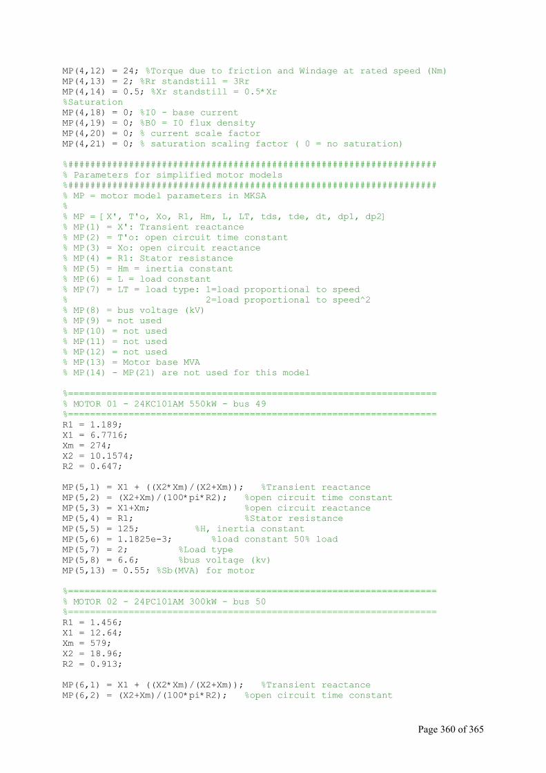
Page 360 of 365

MP(4,12) = 24; %Torque due to friction and Windage at rated speed (Nm) MP(4,13) = 2; %Rr standstill = 3Rr MP(4,14) = 0.5; %Xr standstill = 0.5*Xr %Saturation MP(4,18) = 0; %I0 - base current MP(4,19) = 0; %B0 = I0 flux density MP(4,20) = 0; % current scale factor MP(4,21) = 0; % saturation scaling factor ( 0 = no saturation) %################################################################### % Parameters for simplified motor models %################################################################### % MP = motor model parameters in MKSA % % MP = [X', T'o, Xo, R1, Hm, L, LT, tds, tde, dt, dp1, dp2] % MP(1) = X': Transient reactance % MP(2) = T'o: open circuit time constant % MP(3) = Xo: open circuit reactance % MP(4) = R1: Stator resistance % MP(5) = Hm = inertia constant % MP(6) = L = load constant % MP(7) = LT = load type: 1=load proportional to speed % 2=load proportional to speed^2 % MP(8) = bus voltage (kV) % MP(9) = not used % MP(10) = not used % MP(11) = not used % MP(12) = not used % MP(13) = Motor base MVA % MP(14) - MP(21) are not used for this model %=================================================================== % MOTOR 01 - 24KC101AM 550kW - bus 49 %=================================================================== R1 = 1.189; X1 = 6.7716; Xm = 274; X2 = 10.1574; R2 = 0.647; MP(5,1) = X1 + ((X2*Xm)/(X2+Xm)); %Transient reactance MP(5,2) = (X2+Xm)/(100*pi*R2); %open circuit time constant MP(5,3) = X1+Xm; %open circuit reactance MP(5,4) = R1; %Stator resistance MP(5,5) = 125; %H, inertia constant MP(5,6) = 1.1825e-3; %load constant 50% load MP(5,7) = 2; %Load type MP(5,8) = 6.6; %bus voltage (kv) MP(5,13) = 0.55; %Sb(MVA) for motor %=================================================================== % MOTOR 02 - 24PC101AM 300kW - bus 50 %=================================================================== R1 = 1.456; X1 = 12.64; Xm = 579; X2 = 18.96; R2 = 0.913; MP(6,1) = X1 + ((X2*Xm)/(X2+Xm)); %Transient reactance MP(6,2) = (X2+Xm)/(100*pi*R2); %open circuit time constant

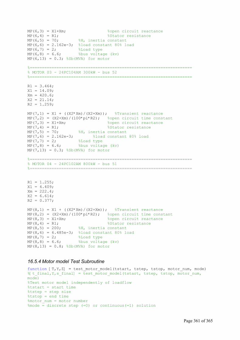
Page 361 of 365

MP(6,3) = X1+Xm; %open circuit reactance MP(6,4) = R1; %Stator resistance MP(6,5) = 70; %H, inertia constant MP(6,6) = 2.162e-3; %load constant 80% load MP(6,7) = 2; %Load type MP(6,8) = 6.6; %bus voltage (kv) MP(6,13) = 0.3; %Sb(MVA) for motor %=================================================================== % MOTOR 03 - 24PC104AM 300kW - bus 52 %=================================================================== R1 = 3.464; X1 = 14.09; Xm = 420.6; X2 = 21.14; R2 = 1.259; MP(7,1) = X1 + ((X2*Xm)/(X2+Xm)); %Transient reactance MP(7,2) = (X2+Xm)/(100*pi*R2); %open circuit time constant MP(7,3) = X1+Xm; %open circuit reactance MP(7,4) = R1; %Stator resistance MP(7,5) = 70; %H, inertia constant MP(7,6) = 2.162e-3; %load constant 80% load MP(7,7) = 2; %Load type MP(7,8) = 6.6; %bus voltage (kv) MP(7,13) = 0.3; %Sb(MVA) for motor %=================================================================== % MOTOR 04 - 24PC102AM 800kW - bus 51 %=================================================================== R1 = 1.255; X1 = 4.409; Xm = 222.4; X2 = 6.614; R2 = 0.377; MP(8,1) = X1 + ((X2*Xm)/(X2+Xm)); %Transient reactance MP(8,2) = (X2+Xm)/(100*pi*R2); %open circuit time constant MP(8,3) = X1+Xm; %open circuit reactance MP(8,4) = R1; %Stator resistance MP(8,5) = 200; %H, inertia constant MP(8,6) = 6.485e-3; %load constant 80% load MP(8,7) = 2; %Load type MP(8,8) = 6.6; %bus voltage (kv) MP(8,13) = 0.8; %Sb(MVA) for motor

16.5.4 Motor model Test Subroutine function [T,Y,Z] = test_motor_model(tstart, tstep, tstop, motor_num, mode) %[t_final,Y,s_final] = test_motor_model(tstart, tstep, tstop, motor_num, mode) %Test motor model independently of loadflow %tstart = start time %tstep = step size %tstop = end time %motor_num = motor number %mode = discrete step (=0) or continuous(=1) solution

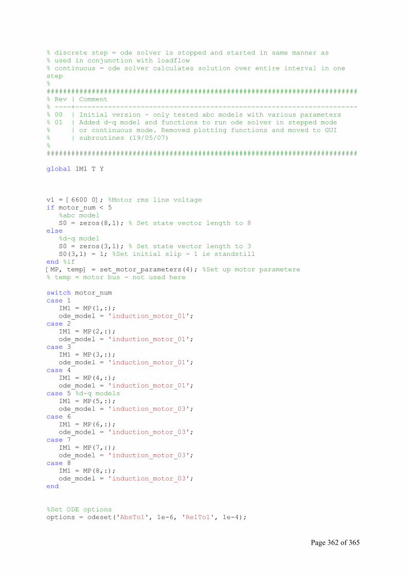
Page 362 of 365

% discrete step = ode solver is stopped and started in same manner as % used in conjunction with loadflow % continuous = ode solver calculates solution over entire interval in one step % ############################################################################ % Rev | Comment % ----+--------------------------------------------------------------------- % 00 | Initial version - only tested abc models with various parameters % 01 | Added d-q model and functions to run ode solver in stepped mode % | or continuous mode. Removed plotting functions and moved to GUI % | subroutines (19/05/07) % ############################################################################ global IM1 T Y v1 = [6600 0]; %Motor rms line voltage if motor_num < 5 %abc model S0 = zeros(8,1); % Set state vector length to 8 else %d-q model S0 = zeros(3,1); % Set state vector length to 3 S0(3,1) = 1; %Set initial slip = 1 ie standstill end %if [MP, temp] = set_motor_parameters(4); %Set up motor parametere % temp = motor bus - not used here switch motor_num case 1 IM1 = MP(1,:); ode_model = 'induction_motor_01'; case 2 IM1 = MP(2,:); ode_model = 'induction_motor_01'; case 3 IM1 = MP(3,:); ode_model = 'induction_motor_01'; case 4 IM1 = MP(4,:); ode_model = 'induction_motor_01'; case 5 %d-q models IM1 = MP(5,:); ode_model = 'induction_motor_03'; case 6 IM1 = MP(6,:); ode_model = 'induction_motor_03'; case 7 IM1 = MP(7,:); ode_model = 'induction_motor_03'; case 8 IM1 = MP(8,:); ode_model = 'induction_motor_03'; end %Set ODE options options = odeset('AbsTol', 1e-6, 'RelTol', 1e-4);

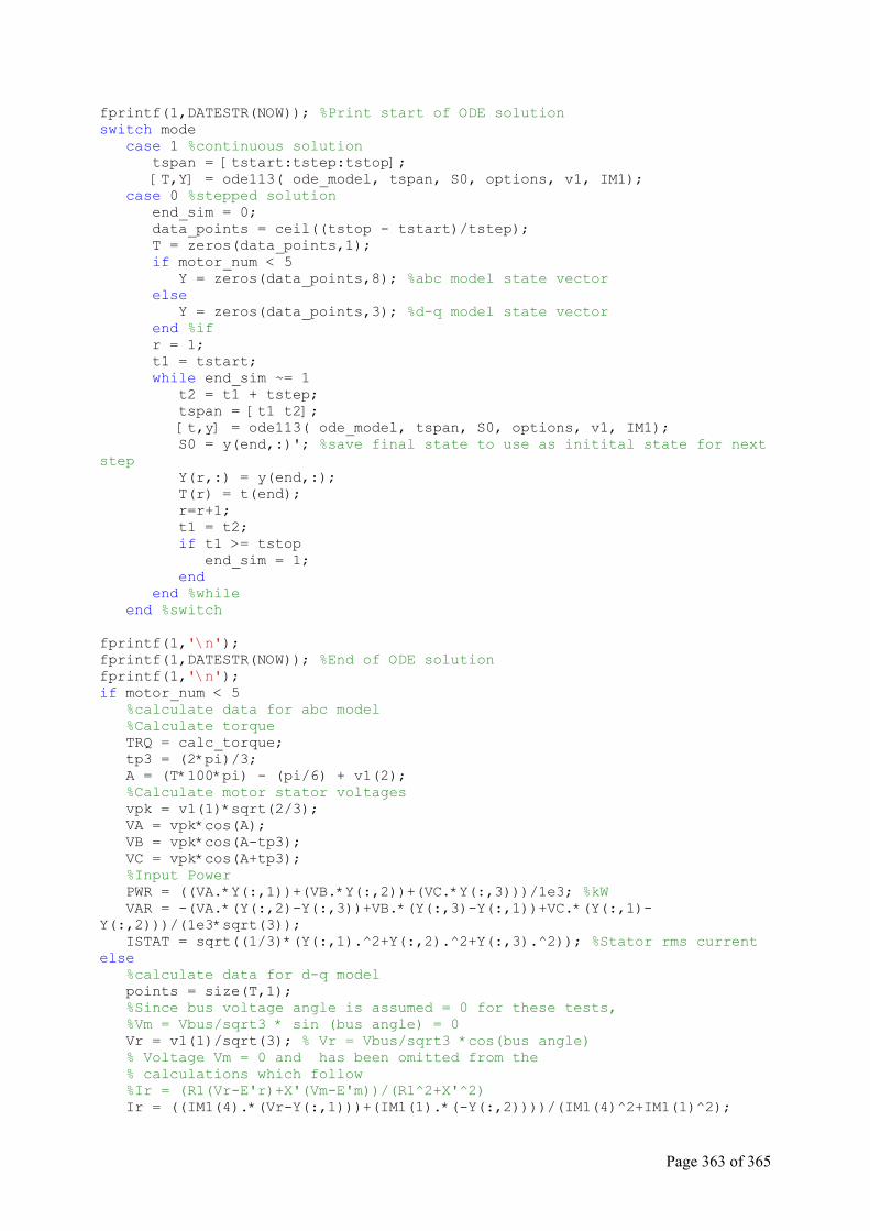
Page 363 of 365

fprintf(1,DATESTR(NOW)); %Print start of ODE solution switch mode case 1 %continuous solution tspan = [tstart:tstep:tstop]; [T,Y] = ode113( ode_model, tspan, S0, options, v1, IM1); case 0 %stepped solution end_sim = 0; data_points = ceil((tstop - tstart)/tstep); T = zeros(data_points,1); if motor_num < 5 Y = zeros(data_points,8); %abc model state vector else Y = zeros(data_points,3); %d-q model state vector end %if r = 1; t1 = tstart; while end_sim ~= 1 t2 = t1 + tstep; tspan = [t1 t2]; [t,y] = ode113( ode_model, tspan, S0, options, v1, IM1); S0 = y(end,:)'; %save final state to use as initital state for next step Y(r,:) = y(end,:); T(r) = t(end); r=r+1; t1 = t2; if t1 >= tstop end_sim = 1; end end %while end %switch fprintf(1,'\n'); fprintf(1,DATESTR(NOW)); %End of ODE solution fprintf(1,'\n'); if motor_num < 5 %calculate data for abc model %Calculate torque TRQ = calc_torque; tp3 = (2*pi)/3; A = (T*100*pi) - (pi/6) + v1(2); %Calculate motor stator voltages vpk = v1(1)*sqrt(2/3); VA = vpk*cos(A); VB = vpk*cos(A-tp3); VC = vpk*cos(A+tp3); %Input Power PWR = ((VA.*Y(:,1))+(VB.*Y(:,2))+(VC.*Y(:,3)))/1e3; %kW VAR = -(VA.*(Y(:,2)-Y(:,3))+VB.*(Y(:,3)-Y(:,1))+VC.*(Y(:,1)-Y(:,2)))/(1e3*sqrt(3)); ISTAT = sqrt((1/3)*(Y(:,1).^2+Y(:,2).^2+Y(:,3).^2)); %Stator rms current else %calculate data for d-q model points = size(T,1); %Since bus voltage angle is assumed = 0 for these tests, %Vm = Vbus/sqrt3 * sin (bus angle) = 0 Vr = v1(1)/sqrt(3); % Vr = Vbus/sqrt3 *cos(bus angle) % Voltage Vm = 0 and has been omitted from the % calculations which follow %Ir = (R1(Vr-E'r)+X'(Vm-E'm))/(R1^2+X'^2) Ir = ((IM1(4).*(Vr-Y(:,1)))+(IM1(1).*(-Y(:,2))))/(IM1(4)^2+IM1(1)^2);

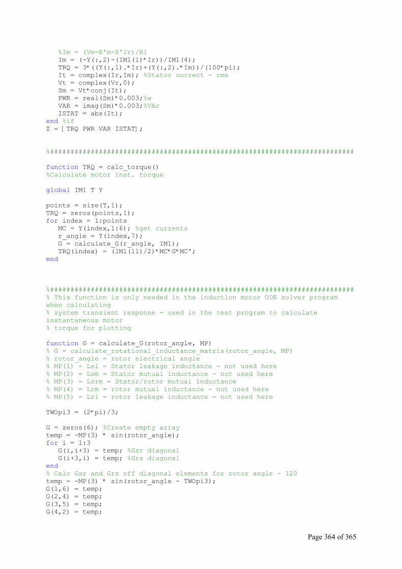
Page 364 of 365

%Im = (Vm-E'm-X'Ir)/R1 Im = (-Y(:,2)-(IM1(1)*Ir))/IM1(4); TRQ = 3*((Y(:,1).*Ir)+(Y(:,2).*Im))/(100*pi); It = complex(Ir,Im); %Stator current - rms Vt = complex(Vr,0); Sm = Vt*conj(It); PWR = real(Sm)*0.003;%w VAR = imag(Sm)*0.003;%VAr ISTAT = abs(It); end %if Z = [TRQ PWR VAR ISTAT]; %########################################################################### function TRQ = calc_torque() %Calculate motor inst. torque global IM1 T Y points = size(T,1); TRQ = zeros(points,1); for index = 1:points MC = Y(index,1:6); %get currents r_angle = Y(index,7); G = calculate_G(r_angle, IM1); TRQ(index) = (IM1(11)/2)*MC*G*MC'; end %########################################################################### % This function is only needed in the induction motor ODE solver program when calculating % system transient response - used in the test program to calculate instantaneous motor % torque for plotting function G = calculate_G(rotor_angle, MP) % G = calculate_rotational_inductance_matrix(rotor_angle, MP) % rotor_angle = rotor electrical angle % MP(1) = Lsl = Stator leakage inductance - not used here % MP(2) = Lsm = Stator mutual inductance - not used here % MP(3) = Lsrm = Stator/rotor mutual inductance % MP(4) = Lrm = rotor mutual inductance - not used here % MP(5) = Lrl = rotor leakage inductance - not used here TWOpi3 = (2*pi)/3; G = zeros(6); %Create empty array temp = -MP(3) * sin(rotor_angle); for i = 1:3 G(i,i+3) = temp; %Gsr diagonal G(i+3,i) = temp; %Grs diagonal end % Calc Gsr and Grs off diagonal elements for rotor angle - 120 temp = -MP(3) * sin(rotor_angle - TWOpi3); G(1,6) = temp; G(2,4) = temp; G(3,5) = temp; G(4,2) = temp;

Page 365 of 365

G(5,3) = temp; G(6,1) = temp; %Calc Gsr & Grs off diagonal elements for theta + 120 temp = -MP(3) * sin(rotor_angle + TWOpi3); G(1,5) = temp; G(2,6) = temp; G(3,4) = temp; G(4,3) = temp; G(5,1) = temp; G(6,2) = temp;