PU/DSS/OTR

Getting Started in Data Analysis using Stata

(ver. 5.0)

Oscar Torres‐ReynaData Consultantotorres@princeton.edu

http://dss.princeton.edu/training/

PU/DSS/OTR

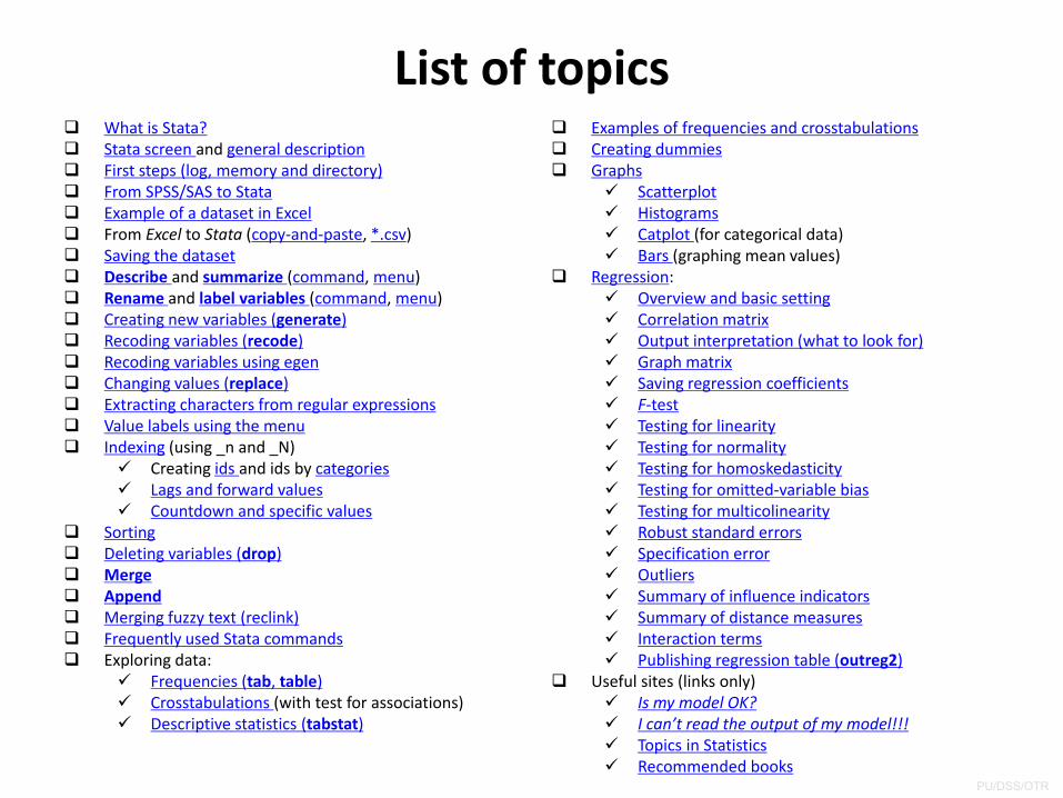
List of topicsWhat is Stata?Stata screen and general descriptionFirst steps (log, memory and directory)From SPSS/SAS to StataExample of a dataset in ExcelFrom Excel to Stata (copy‐and‐paste, *.csv)Saving the datasetDescribe and summarize (command, menu)Rename and label variables (command, menu)Creating new variables (generate)Recoding variables (recode)Recoding variables using egenChanging values (replace)Extracting characters from regular expressionsValue labels using the menuIndexing (using _n and _N)

Creating ids and ids by categoriesLags and forward valuesCountdown and specific values

SortingDeleting variables (drop)MergeAppendMerging fuzzy text (reclink)Frequently used Stata commandsExploring data:

Frequencies (tab, table)Crosstabulations (with test for associations)Descriptive statistics (tabstat)

Examples of frequencies and crosstabulations Creating dummiesGraphs

ScatterplotHistogramsCatplot (for categorical data)Bars (graphing mean values)

Regression: Overview and basic settingCorrelation matrixOutput interpretation (what to look for)Graph matrix Saving regression coefficientsF‐testTesting for linearityTesting for normalityTesting for homoskedasticityTesting for omitted‐variable biasTesting for multicolinearityRobust standard errors Specification errorOutliersSummary of influence indicatorsSummary of distance measuresInteraction termsPublishing regression table (outreg2)

Useful sites (links only)Is my model OK?I can’t read the output of my model!!!Topics in StatisticsRecommended books

PU/DSS/OTR

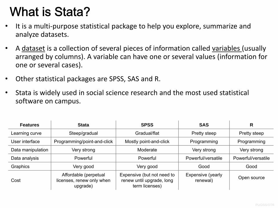
What is Stata?• It is a multi‐purpose statistical package to help you explore, summarize and 

analyze datasets. 

• A dataset is a collection of several pieces of information called variables (usually arranged by columns). A variable can have one or several values (information for one or several cases).

• Other statistical packages are SPSS, SAS and R.

• Stata is widely used in social science research and the most used statistical software on campus.

Features Stata SPSS SAS R

Learning curve Steep/gradual Gradual/flat Pretty steep Pretty steep

User interface Programming/point-and-click Mostly point-and-click Programming Programming

Data manipulation Very strong Moderate Very strong Very strong

Data analysis Powerful Powerful Powerful/versatile Powerful/versatile

Graphics Very good Very good Good Good

CostAffordable (perpetual

licenses, renew only when upgrade)

Expensive (but not need to renew until upgrade, long

term licenses)

Expensive (yearly renewal) Open source

PU/DSS/OTR

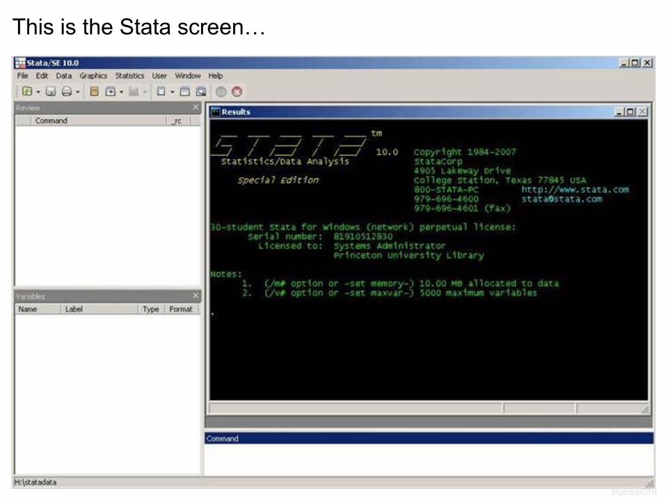
This is the Stata screen…

PU/DSS/OTR

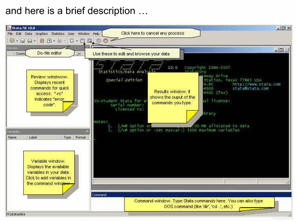
and here is a brief description …

PU/DSS/OTR

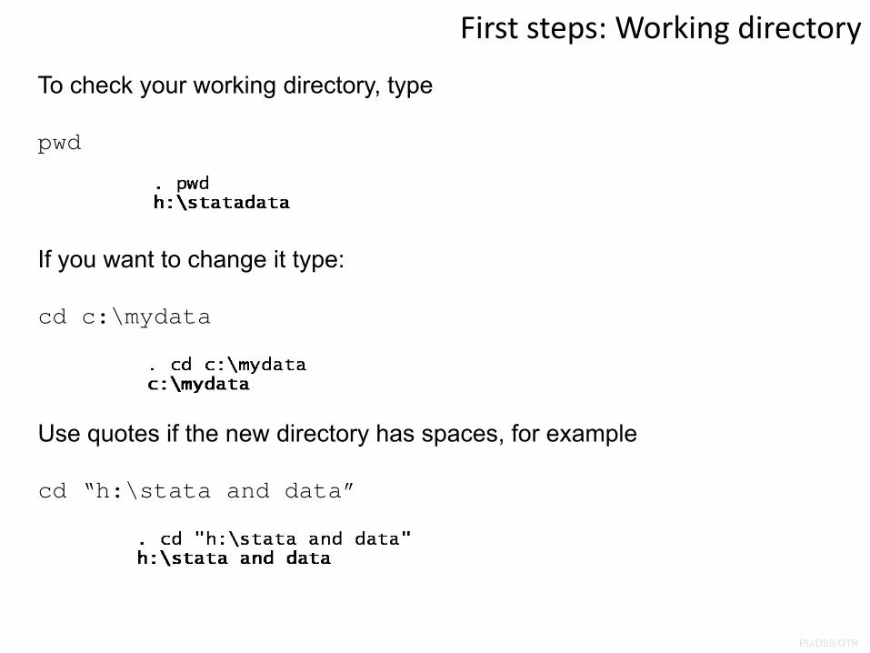
First steps: Working directory

To check your working directory, type

pwd

If you want to change it type:

cd c:\mydata

Use quotes if the new directory has spaces, for example

cd “h:\stata and data”

PU/DSS/OTR

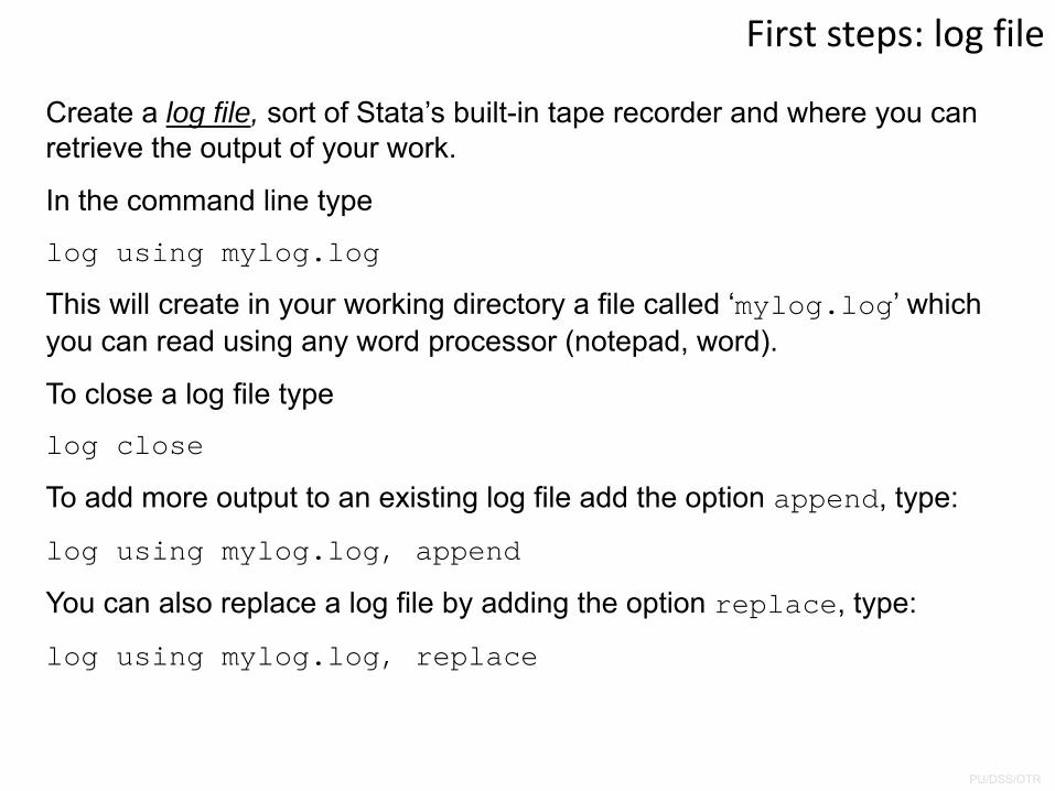
First steps: log file

Create a log file, sort of Stata’s built-in tape recorder and where you can retrieve the output of your work.

In the command line type

log using mylog.log

This will create in your working directory a file called ‘mylog.log’ which you can read using any word processor (notepad, word).

To close a log file type

log close

To add more output to an existing log file add the option append, type:

log using mylog.log, append

You can also replace a log file by adding the option replace, type:

log using mylog.log, replace

PU/DSS/OTR

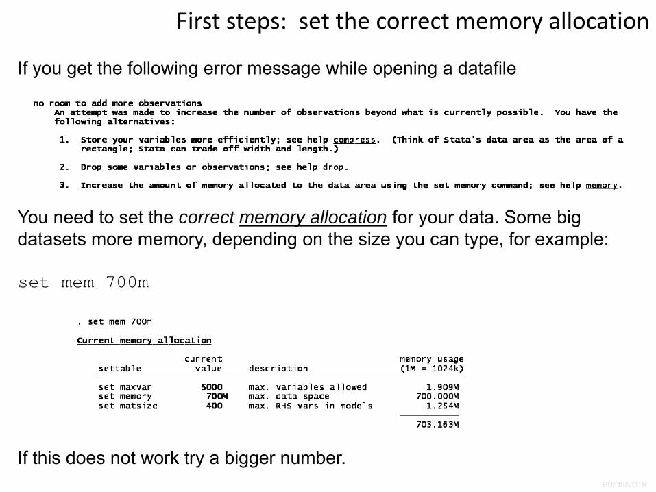
First steps:  set the correct memory allocation

If you get the following error message while opening a datafile

You need to set the correct memory allocation for your data. Some big datasets more memory, depending on the size you can type, for example:

set mem 700m

If this does not work try a bigger number.

PU/DSS/OTR

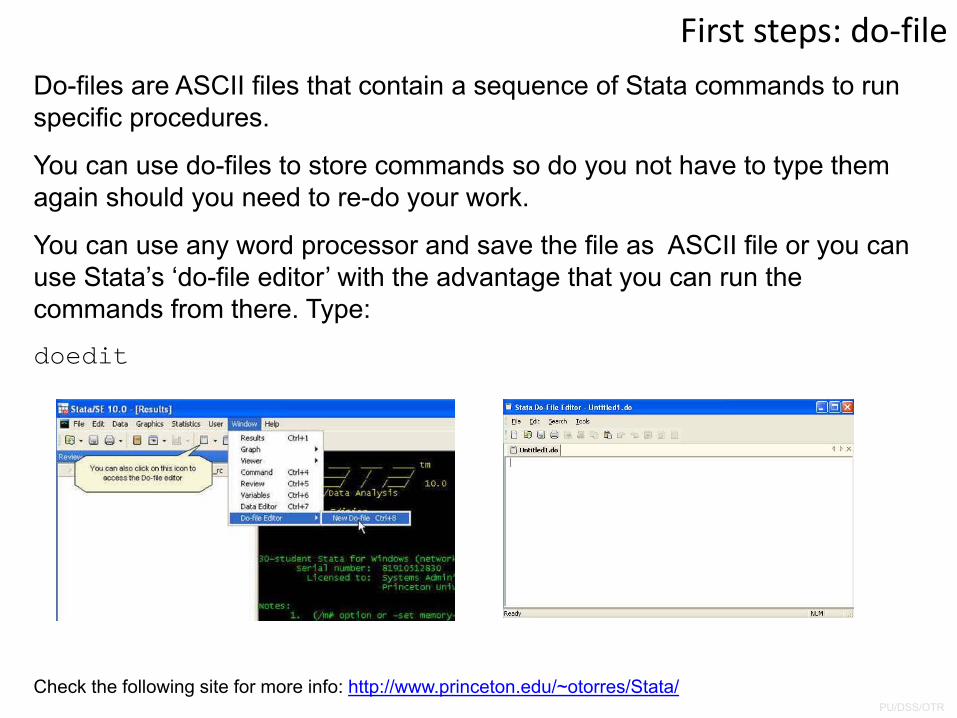
First steps: do‐fileDo-files are ASCII files that contain a sequence of Stata commands to run specific procedures.

You can use do-files to store commands so do you not have to type them again should you need to re-do your work.

You can use any word processor and save the file as ASCII file or you can use Stata’s ‘do-file editor’ with the advantage that you can run the commands from there. Type:

doedit

Check the following site for more info: http://www.princeton.edu/~otorres/Stata/

PU/DSS/OTR

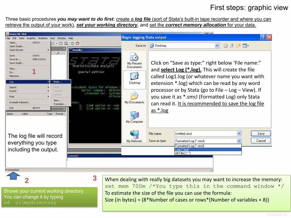
First steps: graphic view

Shows your current working directory.You can change it by typing cd c:\mydirectory

The log file will record everything you type including the output.

1

2 3

Click on “Save as type:” right below ‘File name:” and select Log (*.log). This will create the file called Log1.log (or whatever name you want with extension *.log) which can be read by any word processor or by Stata (go to File – Log – View). If you save it as *.smcl (Formatted Log) only Stata can read it. It is recommended to save the log file as *.log

Three basic procedures you may want to do first: create a log file (sort of Stata’s built-in tape recorder and where you can retrieve the output of your work), set your working directory, and set the correct memory allocation for your data.

When dealing with really big datasets you may want to increase the memory:set mem 700m /*You type this in the command window */To estimate the size of the file you can use the formula:Size (in bytes) = (8*Number of cases or rows*(Number of variables + 8))

PU/DSS/OTR

From SPSS/SAS to Stata

If your data is already in SPSS format (*.sav) or SAS(*.sas7bcat).You can use the command usespss to read SPSS files in Stata or the command usesas to read SAS files. 

If you have a file in SAS XPORT format you can use fduse (or go to file‐import). 

For SPSS and SAS, you may need to install it by typing

ssc install usespssssc install usesas

Once installed just type

usespss using “c:\mydata.sav”usespss using “c:\mydata.sas7bcat”

Type help usespss or help usesas for more details.

For ASCII data please see http://dss.princeton.edu/training/DataPrep101.pdf

PU/DSS/OTR

PU/DSS/OTR

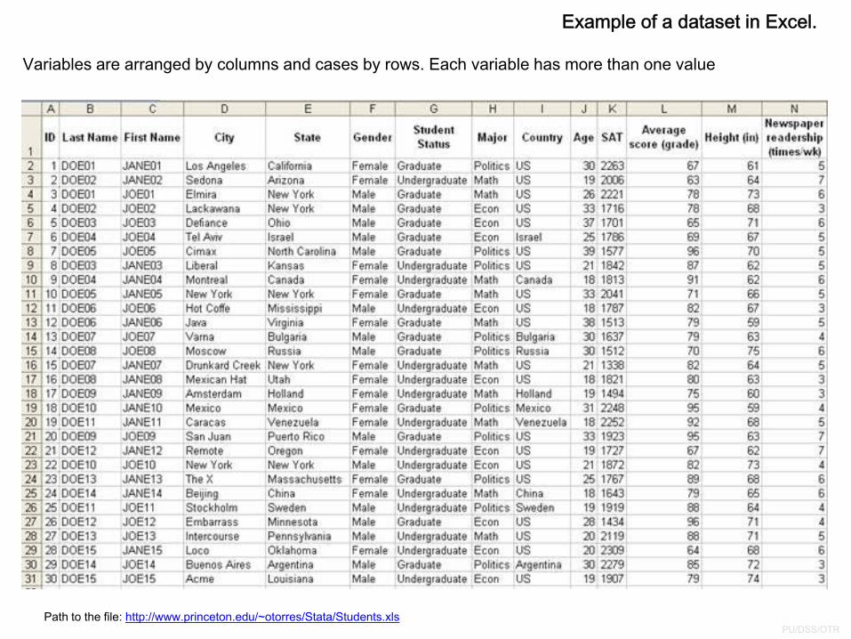
Example of a dataset in Excel.

Path to the file: http://www.princeton.edu/~otorres/Stata/Students.xls

Variables are arranged by columns and cases by rows. Each variable has more than one value

PU/DSS/OTR

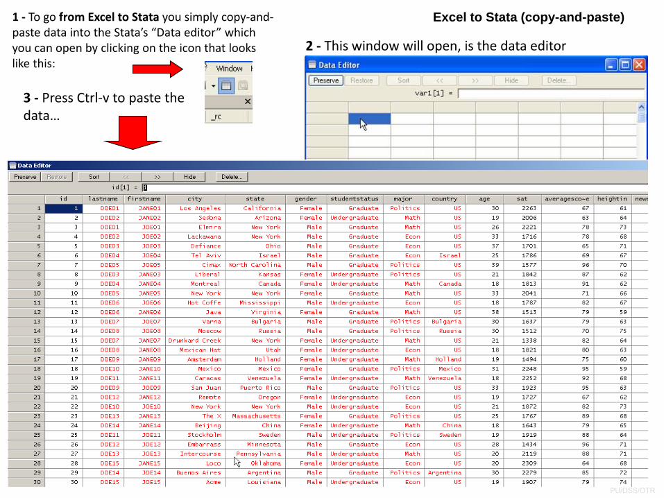
1 ‐ To go from Excel to Stata you simply copy‐and‐paste data into the Stata’s “Data editor” which you can open by clicking on the icon that looks like this:

2 ‐ This window will open, is the data editor

3 ‐ Press Ctrl‐v to paste the data…

Excel to Stata (copy-and-paste)

PU/DSS/OTR

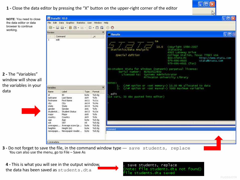
1 ‐ Close the data editor by pressing the “X” button on the upper‐right corner of the editor

2 ‐ The “Variables” window will show all the variables in your data

3 ‐ Do not forget to save the file, in the command window type ‐‐‐ save students, replace

4 ‐ This is what you will see in the output window, the data has been saved as students.dta

You can also use the menu, go to File – Save As

Saving the dataset

NOTE: You need to close the data editor or data browser to continue working.

PU/DSS/OTR

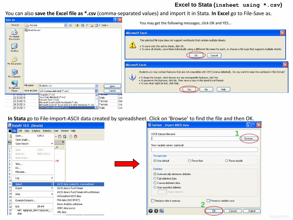
You can also save the Excel file as *.csv (comma‐separated values) and import it in Stata. In Excel go to File‐Save as.

Excel to Stata (insheet using *.csv)

You may get the following messages, click OK and YES…

In Stata go to File‐Import‐ASCII data created by spreadsheet. Click on ‘Browse’ to find the file and then OK.

1

2

PU/DSS/OTR

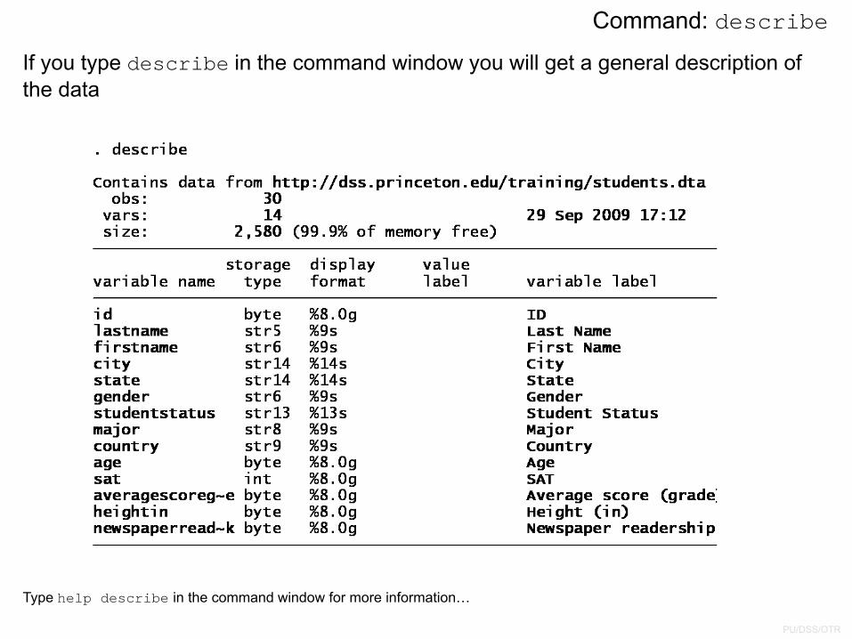
If you type describe in the command window you will get a general description of the data

Type help describe in the command window for more information…

Command: describe

PU/DSS/OTR

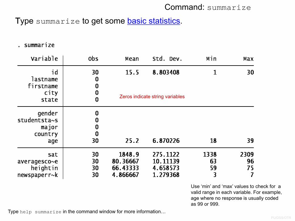
Type summarize to get some basic statistics.

Zeros indicate string variables

Type help summarize in the command window for more information…

Command: summarize

Use ‘min’ and ‘max’ values to check for a valid range in each variable. For example, age where no response is usually coded as 99 or 999.

PU/DSS/OTR

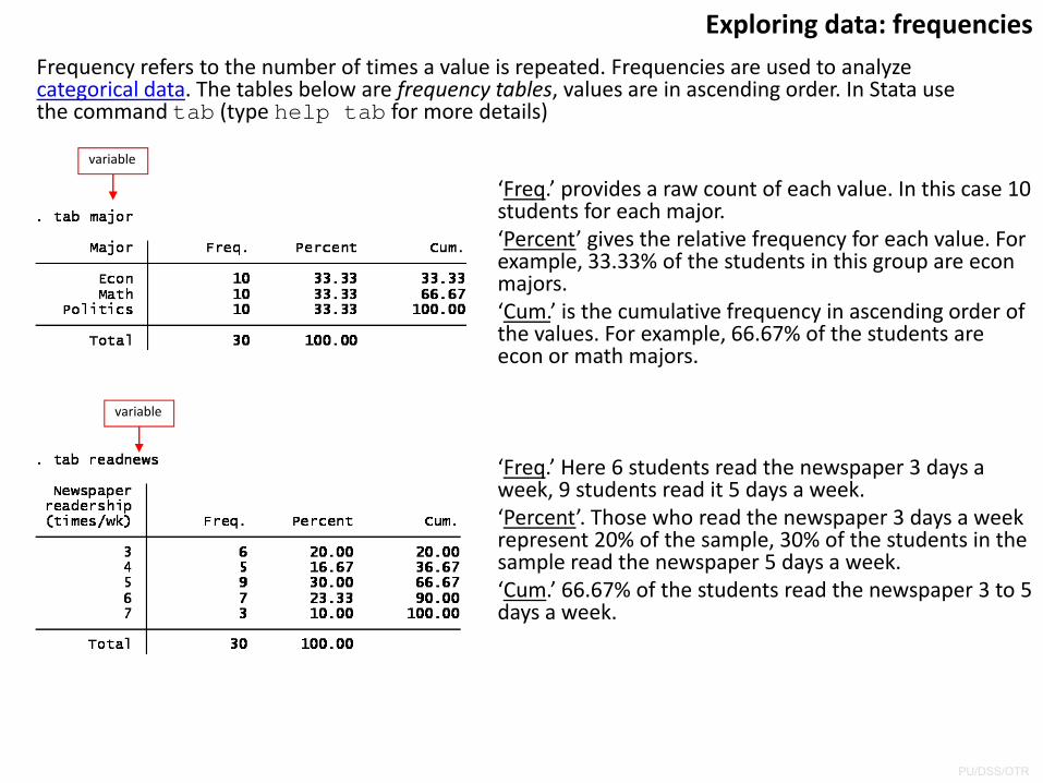
Exploring data: frequenciesFrequency refers to the number of times a value is repeated. Frequencies are used to analyze categorical data. The tables below are frequency tables, values are in ascending order. In Stata use the command tab (type help tab for more details)

‘Freq.’ provides a raw count of each value. In this case 10 students for each major.‘Percent’ gives the relative frequency for each value. For example, 33.33% of the students in this group are econ majors.‘Cum.’ is the cumulative frequency in ascending order of the values. For example, 66.67% of the students are econ or math majors.

‘Freq.’ Here 6 students read the newspaper 3 days a week, 9 students read it 5 days a week.‘Percent’. Those who read the newspaper 3 days a week represent 20% of the sample, 30% of the students in the sample read the newspaper 5 days a week.‘Cum.’ 66.67% of the students read the newspaper 3 to 5 days a week.

variable

variable

PU/DSS/OTR

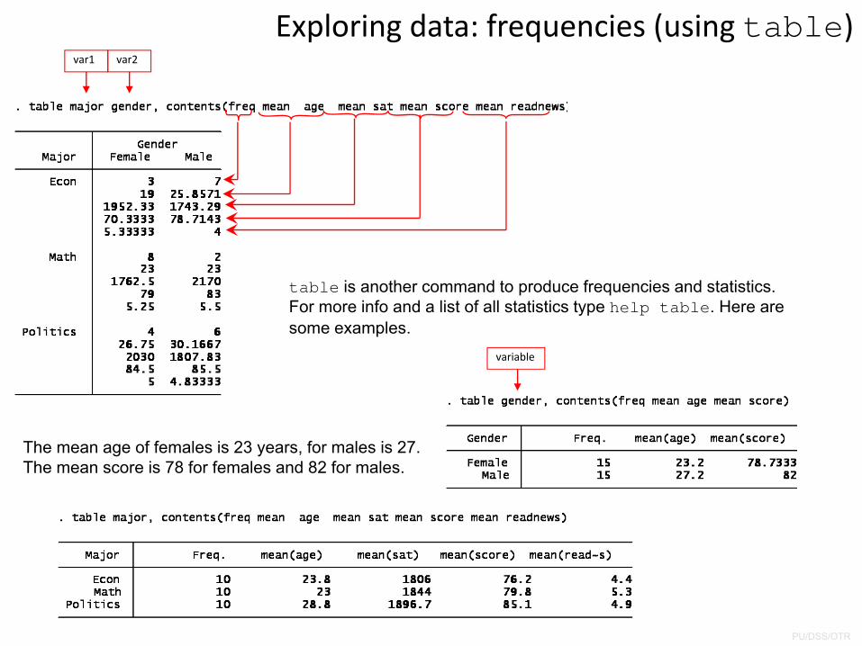
Exploring data: frequencies (using table)

table is another command to produce frequencies and statistics. For more info and a list of all statistics type help table. Here are some examples.

The mean age of females is 23 years, for males is 27. The mean score is 78 for females and 82 for males.

var1 var2

variable

PU/DSS/OTR

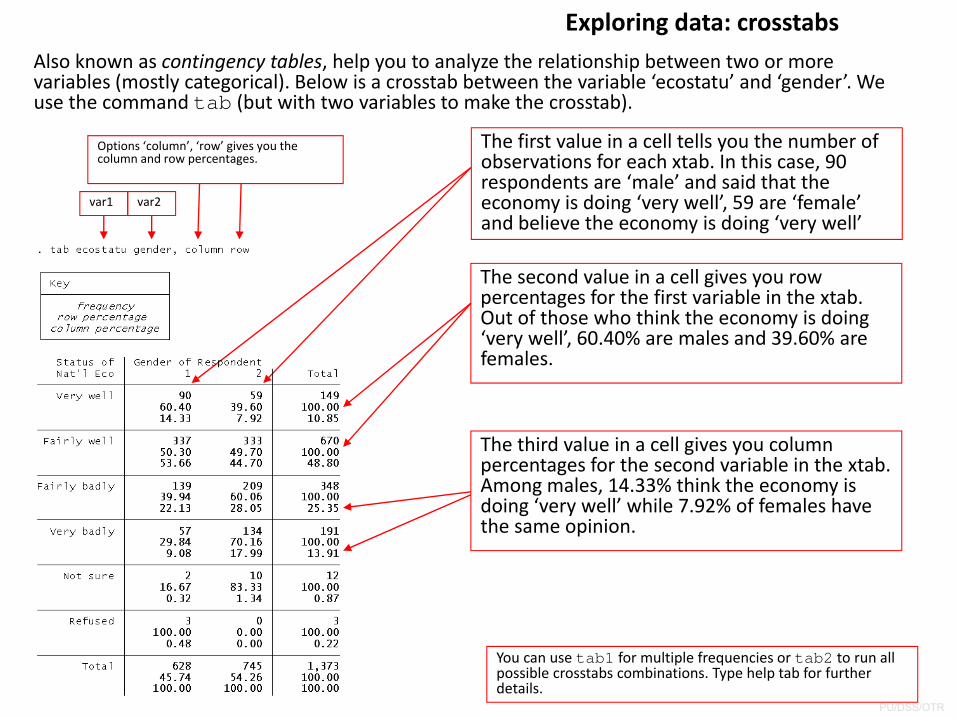
Exploring data: crosstabsAlso known as contingency tables, help you to analyze the relationship between two or more variables (mostly categorical). Below is a crosstab between the variable ‘ecostatu’ and ‘gender’. We use the command tab (but with two variables to make the crosstab).

The first value in a cell tells you the number of observations for each xtab. In this case, 90 respondents are ‘male’ and said that the economy is doing ‘very well’, 59 are ‘female’ and believe the economy is doing ‘very well’

The second value in a cell gives you row percentages for the first variable in the xtab. Out of those who think the economy is doing ‘very well’, 60.40% are males and 39.60% are females.

The third value in a cell gives you column percentages for the second variable in the xtab. Among males, 14.33% think the economy is doing ‘very well’ while 7.92% of females have the same opinion. 

var1 var2

Options ‘column’, ‘row’ gives you the column and row percentages. 

You can use tab1 for multiple frequencies or tab2 to run all possible crosstabs combinations. Type help tab for further details. 

PU/DSS/OTR

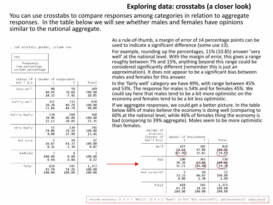
Exploring data: crosstabs (a closer look)You can use crosstabs to compare responses among categories in relation to aggregate responses.  In the table below we will see whether males and females have opinions similar to the national aggregate.

As a rule‐of‐thumb, a margin of error of ±4 percentage points can be used to indicate a significant difference (some use ±3). For example, rounding up the percentages, 11% (10.85) answer ‘very well’ at the national level. With the margin of error, this gives a range roughly between 7% and 15%, anything beyond this range could be considered significantly different (remember this is just an approximation). It does not appear to be a significant bias between males and females for this answer.In the ‘fairly well’ category we have 49%, with range between 45% and 53%. The response for males is 54% and for females 45%. We could say here that males tend to be a bit more optimistic on the economy and females tend to be a bit less optimistic. If we aggregate responses, we could get a better picture. In the table below 68% of males believe the economy is doing well (comparing to 60% at the national level, while 46% of females thing the economy is bad (comparing to 39% aggregate). Males seem to be more optimistic than females.

recode ecostatu (1 2 = 1 "Well") (3 4 = 2 "Bad") (5 6=3 "Not sure/ref"), gen(ecostatu1) label(eco)

PU/DSS/OTR

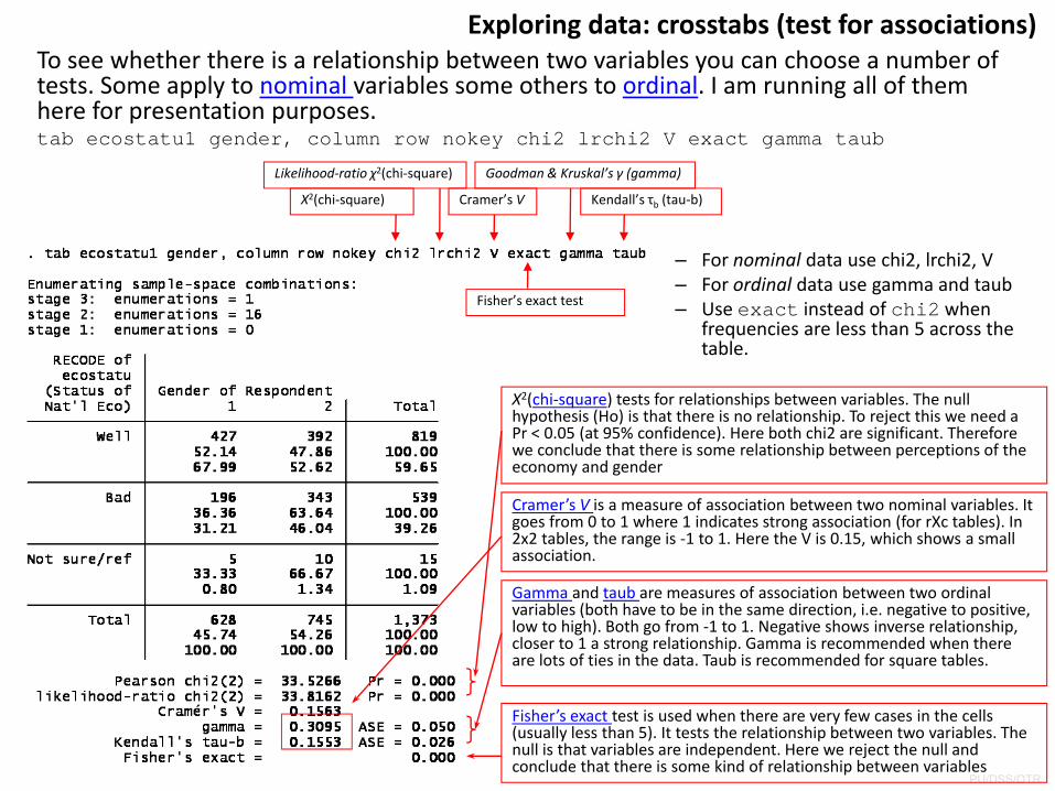
Exploring data: crosstabs (test for associations)To see whether there is a relationship between two variables you can choose a number of tests. Some apply to nominal variables some others to ordinal. I am running all of them here for presentation purposes.tab ecostatu1 gender, column row nokey chi2 lrchi2 V exact gamma taub

– For nominal data use chi2, lrchi2, V– For ordinal data use gamma and taub– Use exact instead of chi2 when 

frequencies are less than 5 across the table.

X2(chi‐square)

Likelihood‐ratio χ2(chi‐square)

Cramer’s V

Fisher’s exact test

Goodman & Kruskal’s γ (gamma)

Kendall’s τb (tau‐b)

X2(chi‐square) tests for relationships between variables. The null hypothesis (Ho) is that there is no relationship. To reject this we need a Pr < 0.05 (at 95% confidence). Here both chi2 are significant. Therefore we conclude that there is some relationship between perceptions of the economy and gender

Cramer’s V is a measure of association between two nominal variables. It goes from 0 to 1 where 1 indicates strong association (for rXc tables). In 2x2 tables, the range is ‐1 to 1. Here the V is 0.15, which shows a small association.

Gamma and taub are measures of association between two ordinal variables (both have to be in the same direction, i.e. negative to positive, low to high). Both go from ‐1 to 1. Negative shows inverse relationship, closer to 1 a strong relationship. Gamma is recommended when there are lots of ties in the data. Taub is recommended for square tables.

Fisher’s exact test is used when there are very few cases in the cells (usually less than 5). It tests the relationship between two variables. The null is that variables are independent. Here we reject the null and conclude that there is some kind of relationship between variables

PU/DSS/OTR

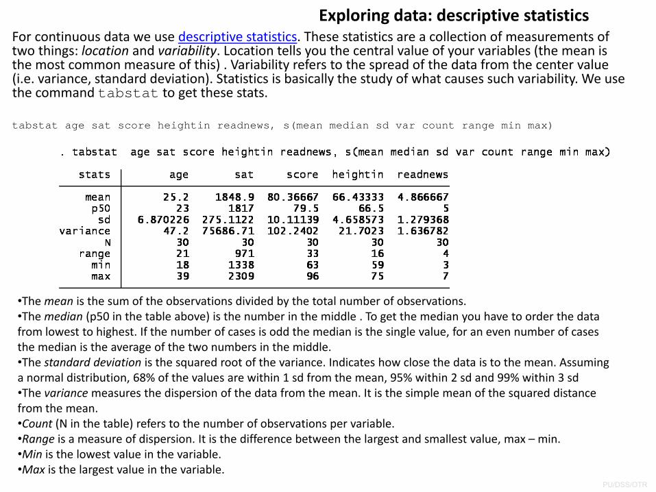
Exploring data: descriptive statisticsFor continuous data we use descriptive statistics. These statistics are a collection of measurements of two things: location and variability. Location tells you the central value of your variables (the mean is the most common measure of this) . Variability refers to the spread of the data from the center value (i.e. variance, standard deviation). Statistics is basically the study of what causes such variability. We use the command tabstat to get these stats.

tabstat age sat score heightin readnews, s(mean median sd var count range min max)

•The mean is the sum of the observations divided by the total number of observations. •The median (p50 in the table above) is the number in the middle . To get the median you have to order the data from lowest to highest. If the number of cases is odd the median is the single value, for an even number of cases the median is the average of the two numbers in the middle.•The standard deviation is the squared root of the variance. Indicates how close the data is to the mean. Assuming a normal distribution, 68% of the values are within 1 sd from the mean, 95% within 2 sd and 99% within 3 sd •The variancemeasures the dispersion of the data from the mean. It is the simple mean of the squared distance from the mean.•Count (N in the table) refers to the number of observations per variable.•Range is a measure of dispersion. It is the difference between the largest and smallest value, max – min.•Min is the lowest value in the variable.•Max is the largest value in the variable.

PU/DSS/OTR

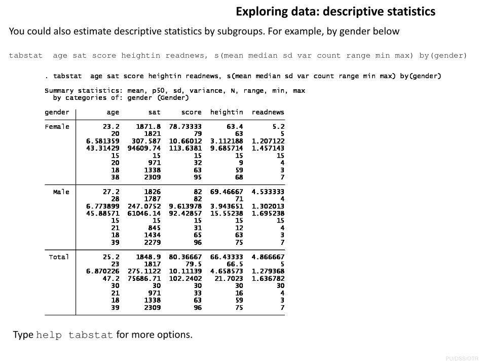
Exploring data: descriptive statisticsYou could also estimate descriptive statistics by subgroups. For example, by gender below

tabstat age sat score heightin readnews, s(mean median sd var count range min max) by(gender)

Type help tabstat for more options.

PU/DSS/OTR

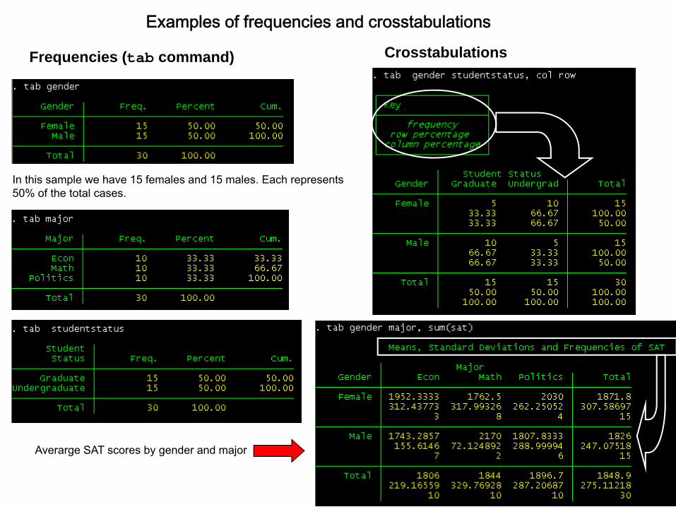
Averarge SAT scores by gender and major

Frequencies (tab command) Crosstabulations

Examples of frequencies and crosstabulations

In this sample we have 15 females and 15 males. Each represents 50% of the total cases.

PU/DSS/OTR

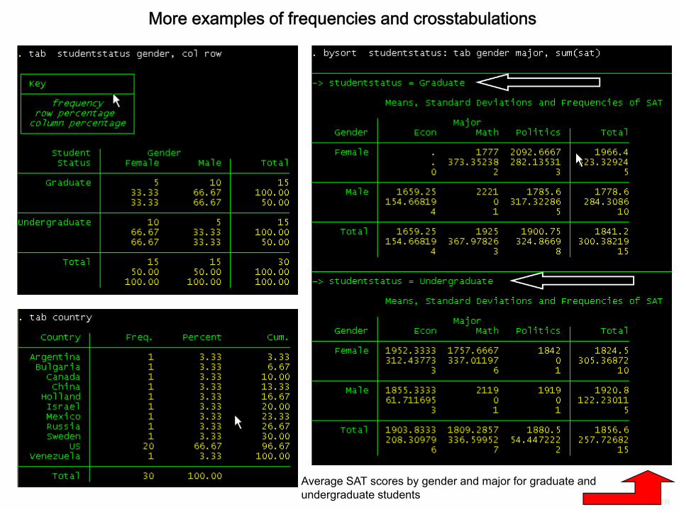
More examples of frequencies and crosstabulations

Average SAT scores by gender and major for graduate and undergraduate students

PU/DSS/OTR

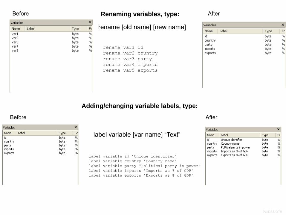
Renaming variables, type:Before After

rename [old name] [new name]

Adding/changing variable labels, type:

Before After

label variable [var name] “Text”

Renaming variables and adding variable labels

rename var1 idrename var2 countryrename var3 partyrename var4 importsrename var5 exports

label variable id "Unique identifier"label variable country "Country name"label variable party "Political party in power"label variable imports "Imports as % of GDP"label variable exports "Exports as % of GDP"

PU/DSS/OTR

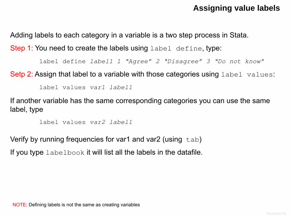
Adding labels to each category in a variable is a two step process in Stata.

Step 1: You need to create the labels using label define, type:

label define label1 1 “Agree” 2 “Disagree” 3 “Do not know”

Setp 2: Assign that label to a variable with those categories using label values:

label values var1 label1

If another variable has the same corresponding categories you can use the same label, type

label values var2 label1

Verify by running frequencies for var1 and var2 (using tab)

If you type labelbook it will list all the labels in the datafile.

NOTE: Defining labels is not the same as creating variables

Assigning value labels

PU/DSS/OTR

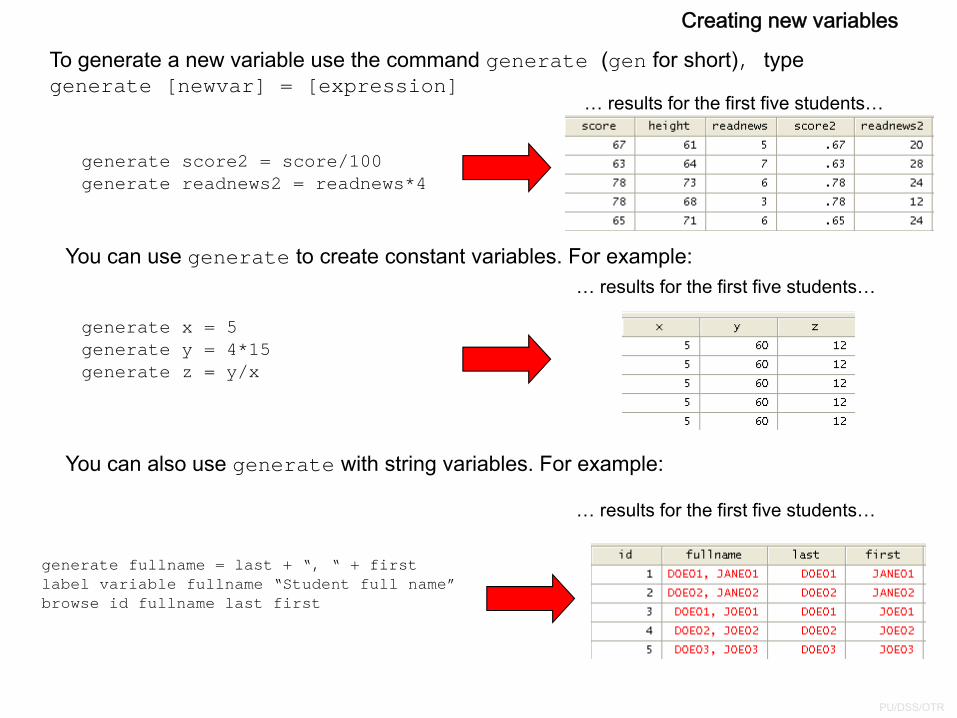
To generate a new variable use the command generate (gen for short), typegenerate [newvar] = [expression]

… results for the first five students…

You can also use generate with string variables. For example:

… results for the first five students…

You can use generate to create constant variables. For example:… results for the first five students…

Creating new variables

generate score2 = score/100generate readnews2 = readnews*4

generate x = 5generate y = 4*15 generate z = y/x

generate fullname = last + “, “ + firstlabel variable fullname “Student full name”browse id fullname last first

PU/DSS/OTR

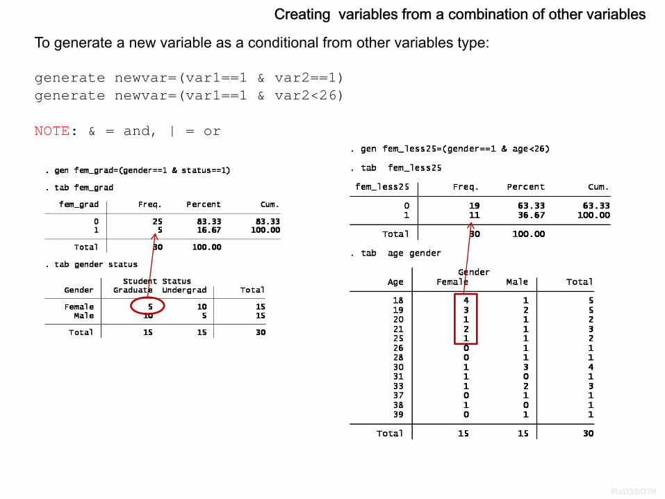
To generate a new variable as a conditional from other variables type:

generate newvar=(var1==1 & var2==1)generate newvar=(var1==1 & var2<26)

NOTE: & = and, | = or

Creating variables from a combination of other variables

PU/DSS/OTR

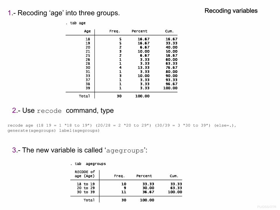
1.- Recoding ‘age’ into three groups.

2.- Use recode command, type

3.- The new variable is called ‘agegroups’:

Recoding variables

recode age (18 19 = 1 “18 to 19”) (20/28 = 2 “20 to 29”) (30/39 = 3 “30 to 39”) (else=.), generate(agegroups) label(agegroups)

PU/DSS/OTR

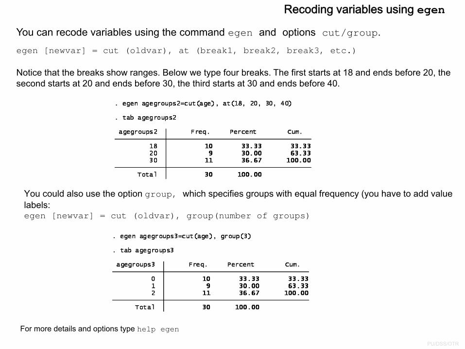
You can recode variables using the command egen and options cut/group.

egen [newvar] = cut (oldvar), at (break1, break2, break3, etc.)

Notice that the breaks show ranges. Below we type four breaks. The first starts at 18 and ends before 20, the second starts at 20 and ends before 30, the third starts at 30 and ends before 40.

You could also use the option group, which specifies groups with equal frequency (you have to add value labels: egen [newvar] = cut (oldvar), group(number of groups)

For more details and options type help egen

Recoding variables using egen

PU/DSS/OTR

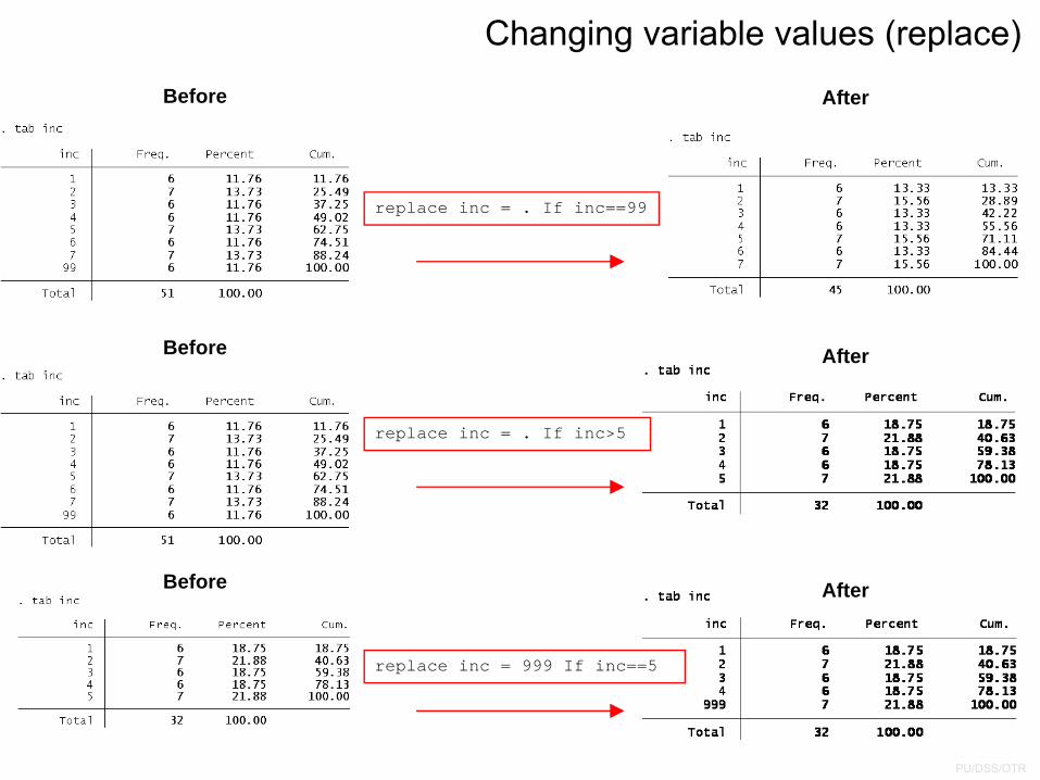
Changing variable values (replace)

replace inc = . If inc==99

Before After

replace inc = . If inc>5

Before After

replace inc = 999 If inc==5

Before After

PU/DSS/OTR

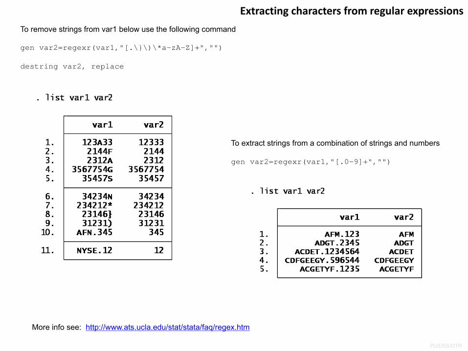
Extracting characters from regular expressions

To remove strings from var1 below use the following command

gen var2=regexr(var1,"[.\}\)\*a-zA-Z]+","")

destring var2, replace

To extract strings from a combination of strings and numbers

gen var2=regexr(var1,"[.0-9]+","")

More info see: http://www.ats.ucla.edu/stat/stata/faq/regex.htm

PU/DSS/OTR

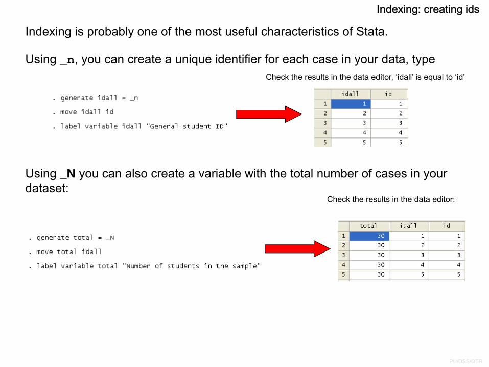
Indexing is probably one of the most useful characteristics of Stata.

Using _n, you can create a unique identifier for each case in your data, typeCheck the results in the data editor, ‘idall’ is equal to ‘id’

Using _N you can also create a variable with the total number of cases in your dataset:

Check the results in the data editor:

Indexing: creating ids

PU/DSS/OTR

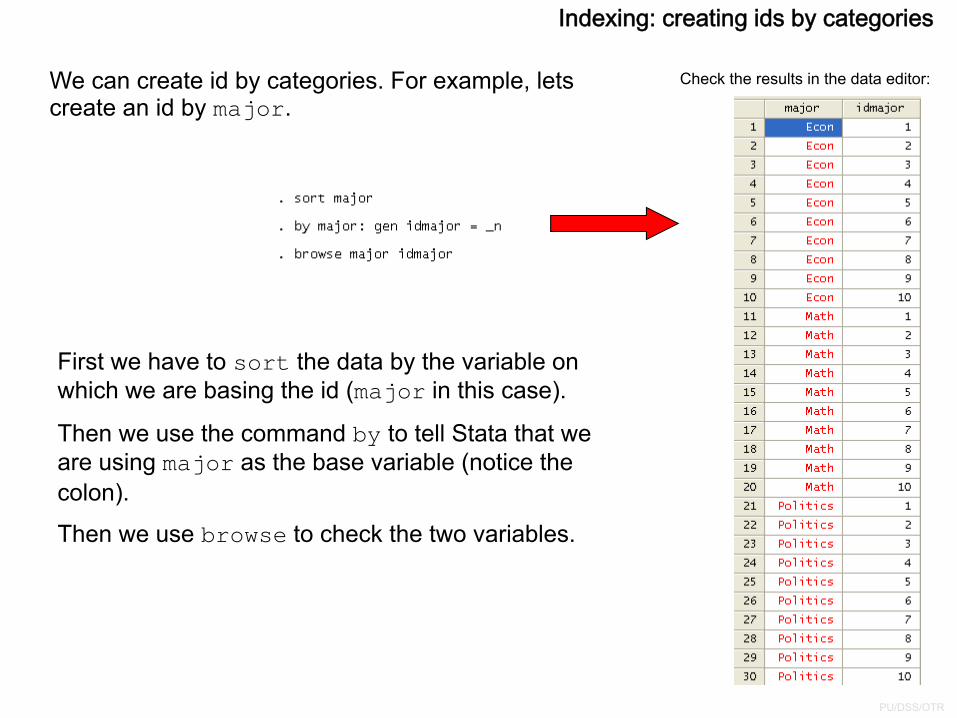
We can create id by categories. For example, lets create an id by major.

Check the results in the data editor:

First we have to sort the data by the variable on which we are basing the id (major in this case).

Then we use the command by to tell Stata that we are using major as the base variable (notice the colon).

Then we use browse to check the two variables.

Indexing: creating ids by categories

PU/DSS/OTR

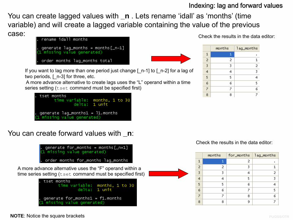
You can create lagged values with _n . Lets rename ‘idall’ as ‘months’ (time variable) and will create a lagged variable containing the value of the previous case: Check the results in the data editor:

Check the results in the data editor:

You can create forward values with _n:

NOTE: Notice the square brackets

If you want to lag more than one period just change [_n-1] to [_n-2] for a lag of two periods, [_n-3] for three, etc. A more advance alternative to create lags uses the “L” operand within a time series setting (tset command must be specified first)

A more advance alternative uses the “F” operand within a time series setting (tset command must be specified first)

Indexing: lag and forward values

PU/DSS/OTR

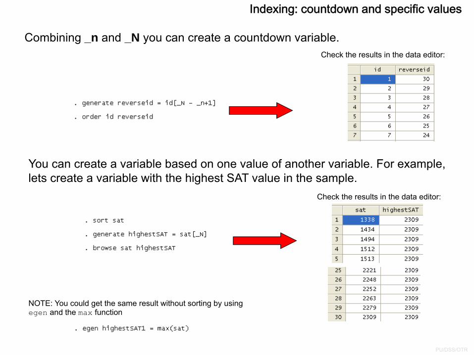
Combining _n and _N you can create a countdown variable.Check the results in the data editor:

Check the results in the data editor:

You can create a variable based on one value of another variable. For example, lets create a variable with the highest SAT value in the sample.

NOTE: You could get the same result without sorting by using egen and the max function

Indexing: countdown and specific values

PU/DSS/OTR

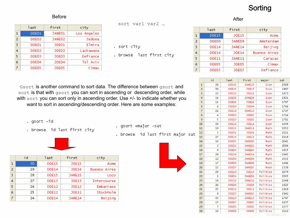
AfterBeforesort var1 var2 …

Gsort is another command to sort data. The difference between gsort and sort is that with gsort you can sort in ascending or descending order, while

with sort you can sort only in ascending order. Use +/- to indicate whether you want to sort in ascending/descending order. Here are some examples:

Sorting

PU/DSS/OTR

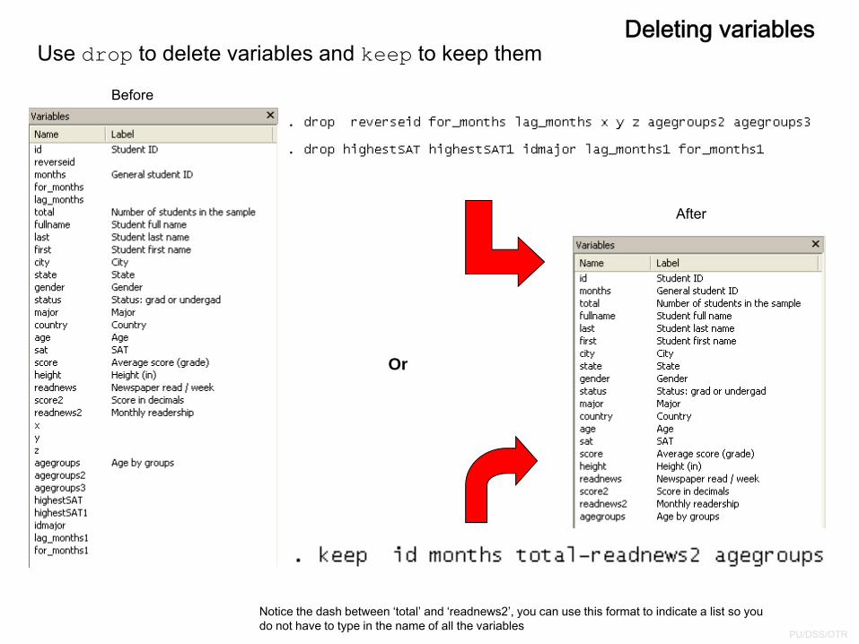
Deleting variablesUse drop to delete variables and keep to keep them

After

Before

Notice the dash between ‘total’ and ‘readnews2’, you can use this format to indicate a list so you do not have to type in the name of all the variables

Or

PU/DSS/OTR

Deleting cases (selectively)

You can drop cases selectively using the conditional “if”, for example

drop if var1==1 /*This will drop observations (rows)

where gender =1*/

drop if age>40 /*This will drop observation where

age>40*/

Alternatively, you can keep options you want

keep if var1==1

keep if age<40

keep if country==7 | country==13

keep if state==“New York” | state==“New Jersey”

| = “or”, & = “and”

For more details type help keep or help drop.

PU/DSS/OTR

Merge/Append

MERGE - You merge when you want to add more variables to an existing dataset.(type help merge in the command window for more details)What you need:

– Both files must be in Stata format– Both files should have at least one variable in common (id)

Step 1. You need to sort the data by the id or ids common to both files you want to merge. For both datasets type:– sort [id1] [id2] …

– save [datafile name], replace

Step 2. Open the master data (main dataset you want to add more variables to, for example data1.dta) and type: – merge [id1] [id2] … using [i.e. data2.dta]

For example, opening a hypothetical data1.dta we type – merge lastname firstname using data2.dta

To verify the merge type– tab _merge

Here are the codes for _merge:_merge==1 obs. from master data

_merge==2 obs. from only one using dataset

_merge==3 obs. from at least two datasets, master or using

If you want to keep the observations common to both datasets you can drop the rest by typing:– drop if _merge!=3 /*This will drop observations where _merge is not equal to 3 */

APPEND - You append when you want to add more cases (more rows to your data, type help append for more details).Open the master file (i.e. data1.dta) and type:

– append using [i.e. data2.dta]

PU/DSS/OTR

Merging fuzzy text (reclink)

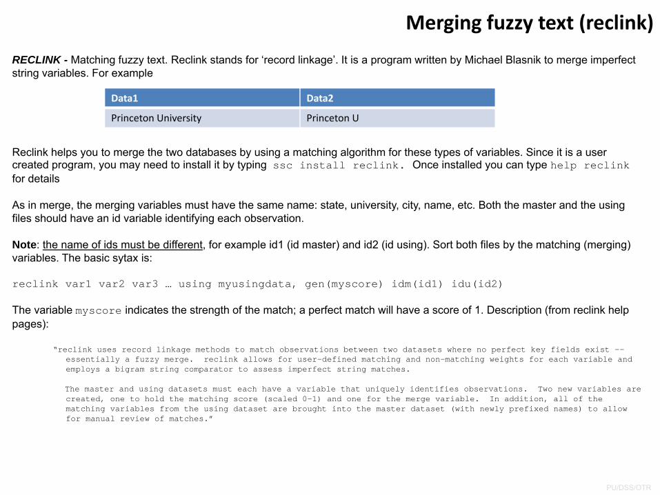
RECLINK - Matching fuzzy text. Reclink stands for ‘record linkage’. It is a program written by Michael Blasnik to merge imperfect string variables. For example

Reclink helps you to merge the two databases by using a matching algorithm for these types of variables. Since it is a user created program, you may need to install it by typing ssc install reclink. Once installed you can type help reclink for details

As in merge, the merging variables must have the same name: state, university, city, name, etc. Both the master and the usingfiles should have an id variable identifying each observation.

Note: the name of ids must be different, for example id1 (id master) and id2 (id using). Sort both files by the matching (merging) variables. The basic sytax is:

reclink var1 var2 var3 … using myusingdata, gen(myscore) idm(id1) idu(id2)

The variable myscore indicates the strength of the match; a perfect match will have a score of 1. Description (from reclink help pages):

“reclink uses record linkage methods to match observations between two datasets where no perfect key fields exist --essentially a fuzzy merge. reclink allows for user-defined matching and non-matching weights for each variable and employs a bigram string comparator to assess imperfect string matches.

The master and using datasets must each have a variable that uniquely identifies observations. Two new variables are created, one to hold the matching score (scaled 0-1) and one for the merge variable. In addition, all of the matching variables from the using dataset are brought into the master dataset (with newly prefixed names) to allow for manual review of matches.”

Data1 Data2

Princeton University Princeton U

PU/DSS/OTR

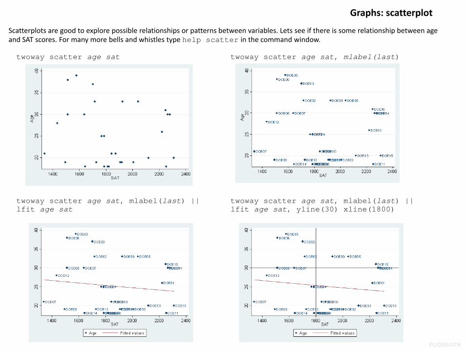
Graphs: scatterplot

Scatterplots are good to explore possible relationships or patterns between variables. Lets see if there is some relationship between age and SAT scores. For many more bells and whistles type help scatter in the command window. 

twoway scatter age sat twoway scatter age sat, mlabel(last)

twoway scatter age sat, mlabel(last) || lfit age sat, yline(30) xline(1800)

twoway scatter age sat, mlabel(last) || lfit age sat

PU/DSS/OTR

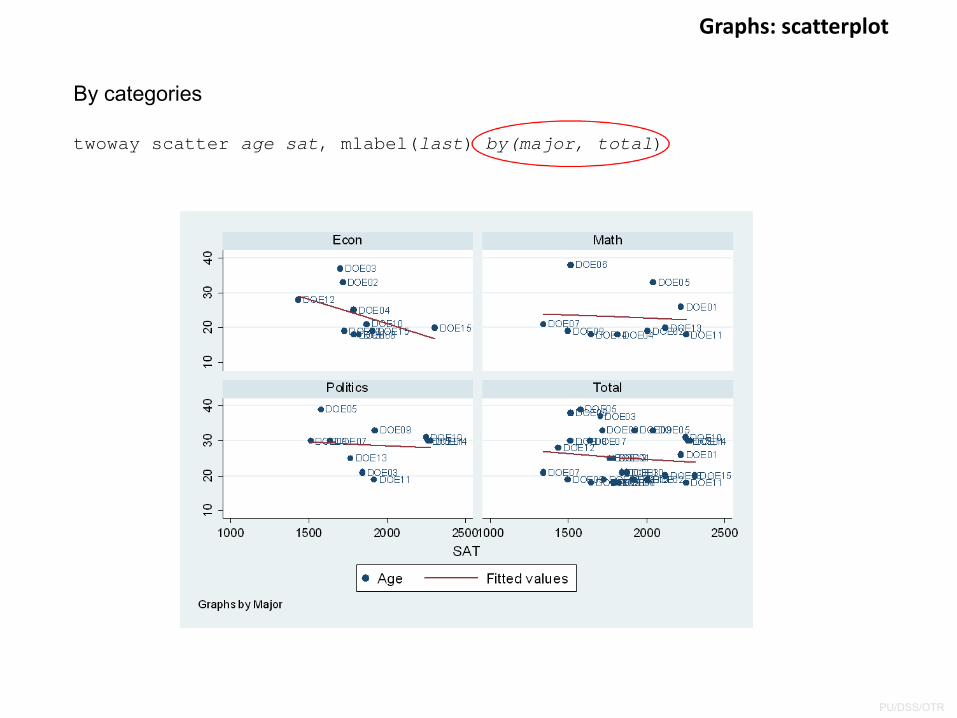
Graphs: scatterplot

twoway scatter age sat, mlabel(last) by(major, total)

By categories

PU/DSS/OTR

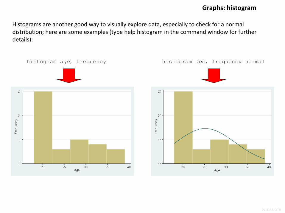
Graphs: histogram

Histograms are another good way to visually explore data, especially to check for a normal distribution; here are some examples (type help histogram in the command window for further details):

histogram age, frequency histogram age, frequency normal

PU/DSS/OTR

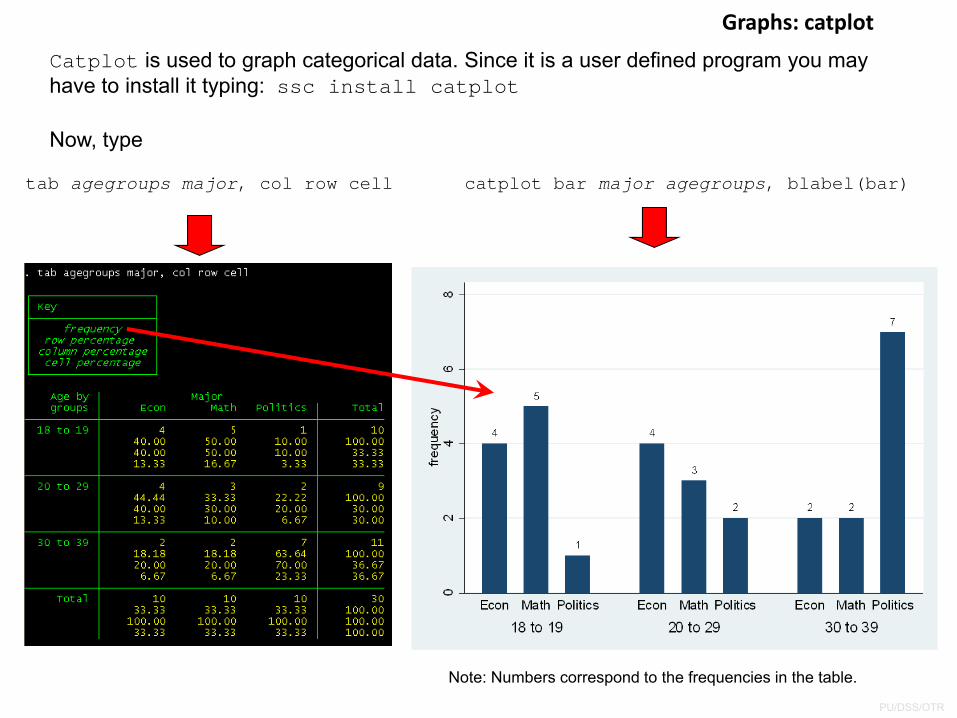
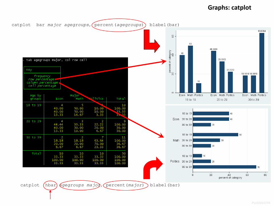
Graphs: catplot

Catplot is used to graph categorical data. Since it is a user defined program you may have to install it typing: ssc install catplot

tab agegroups major, col row cell

Now, type

catplot bar major agegroups, blabel(bar)

Note: Numbers correspond to the frequencies in the table.

PU/DSS/OTR

Graphs: catplot

catplot bar major agegroups, percent(agegroups) blabel(bar)

catplot hbar agegroups major, percent(major) blabel(bar)

PU/DSS/OTR

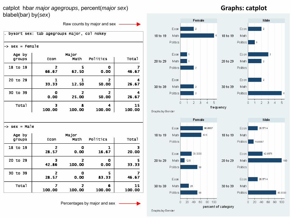
Graphs: catplotcatplot hbar major agegroups, percent(major sex) blabel(bar) by(sex)

Percentages by major and sex

Raw counts by major and sex

PU/DSS/OTR

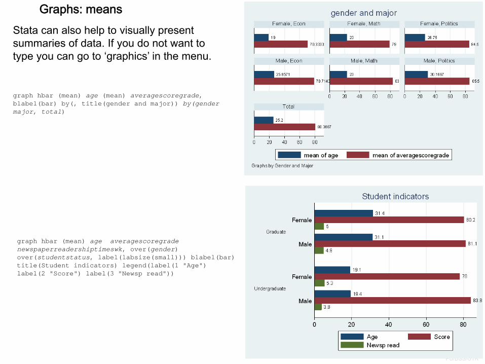
graph hbar (mean) age (mean) averagescoregrade, blabel(bar) by(, title(gender and major)) by(gender major, total)

graph hbar (mean) age averagescoregradenewspaperreadershiptimeswk, over(gender) over(studentstatus, label(labsize(small))) blabel(bar) title(Student indicators) legend(label(1 "Age") label(2 "Score") label(3 "Newsp read"))

Stata can also help to visually present summaries of data. If you do not want to type you can go to ‘graphics’ in the menu.

Graphs: means

PU/DSS/OTR

Regression: a practical approach (intro)

In this section we will explore some basics of regression analysis.We will run a multivariate regression and some diagnostics :

– General setting and output interpretation (what to look for)– Normality– Linearity/functional form– Homoskedasticity/heteroskedasticiy– Robust standard errors– Omitted variable bias/specification error– Outliers– F-test– Interaction terms

The main references/sources for this section are:– Stock, James and Mark Watson, Introduction to Econometrics, 2003– Hamilton, Lawrence, Statistics with Stata (updated for version 9), 2006– The UCLA online tutorial http://www.ats.ucla.edu/stat/stata/

PU/DSS/OTR

Regression: a practical approach (overview)

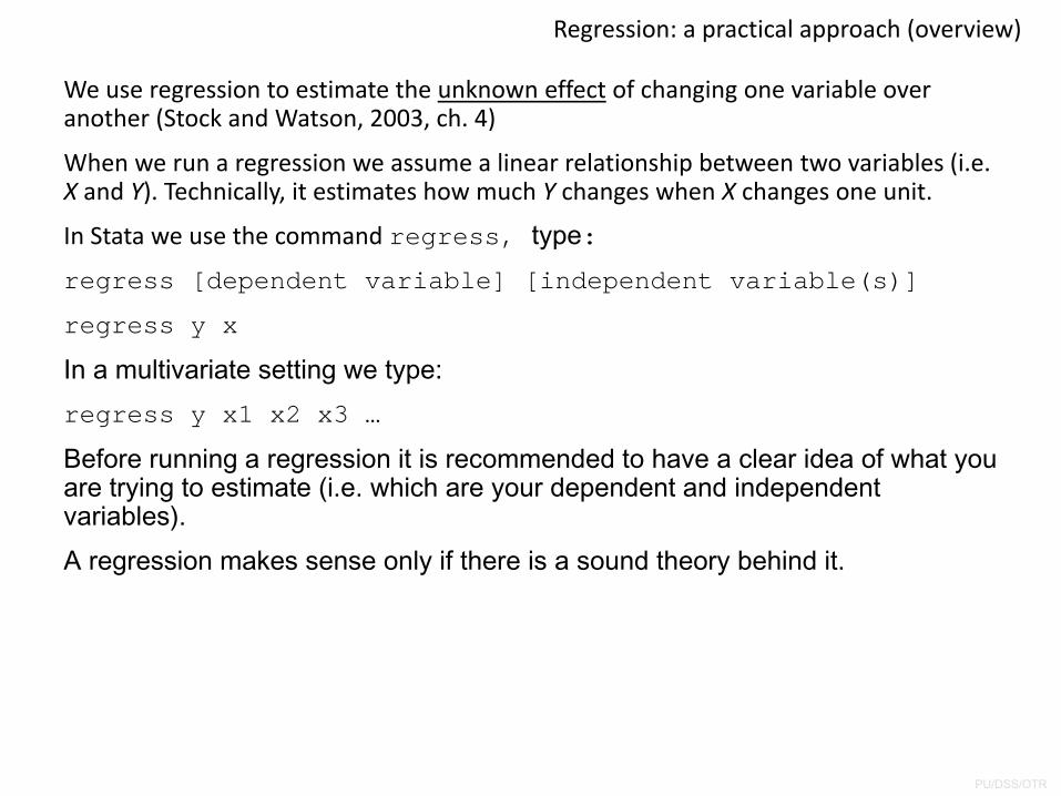
We use regression to estimate the unknown effect of changing one variable over another (Stock and Watson, 2003, ch. 4)

When we run a regression we assume a linear relationship between two variables (i.e. X and Y). Technically, it estimates how much Y changes when X changes one unit. 

In Stata we use the command regress, type:regress [dependent variable] [independent variable(s)]

regress y x

In a multivariate setting we type:regress y x1 x2 x3 …

Before running a regression it is recommended to have a clear idea of what you are trying to estimate (i.e. which are your dependent and independent variables).A regression makes sense only if there is a sound theory behind it.

PU/DSS/OTR

Regression: a practical approach (overview) cont.

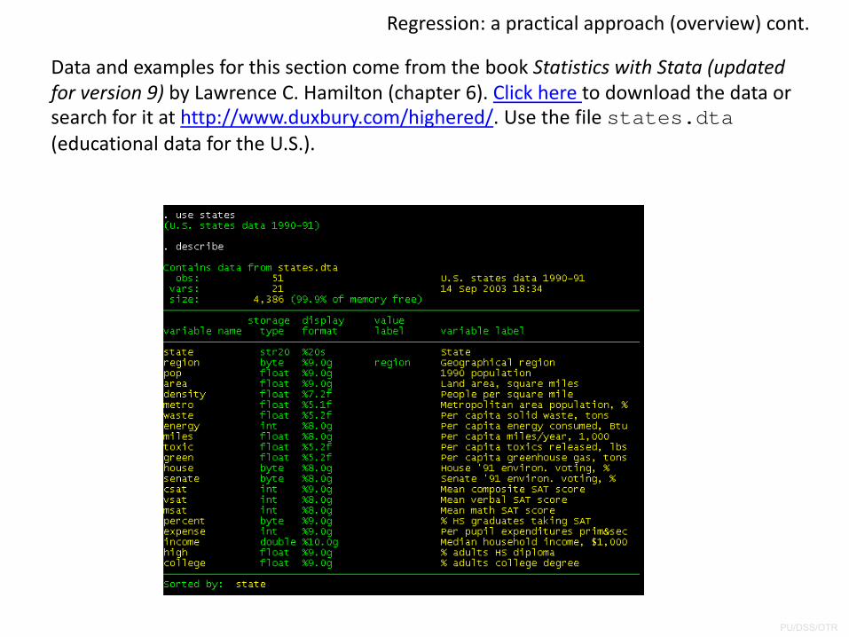
Data and examples for this section come from the book Statistics with Stata (updated for version 9) by Lawrence C. Hamilton (chapter 6). Click here to download the data or search for it at http://www.duxbury.com/highered/. Use the file states.dta(educational data for the U.S.).  

PU/DSS/OTR

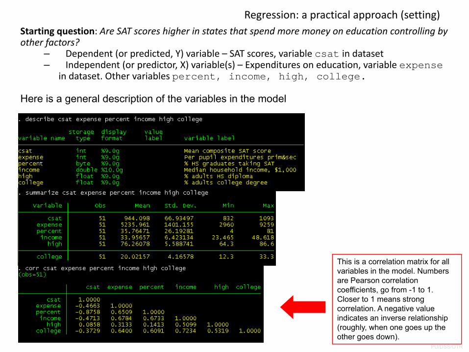
Regression: a practical approach (setting)Starting question: Are SAT scores higher in states that spend more money on education controlling by other factors?

– Dependent (or predicted, Y) variable – SAT scores, variable csat in dataset– Independent (or predictor, X) variable(s) – Expenditures on education, variable expense

in dataset. Other variables percent, income, high, college.

Here is a general description of the variables in the model

This is a correlation matrix for all variables in the model. Numbers are Pearson correlation coefficients, go from -1 to 1. Closer to 1 means strong correlation. A negative value indicates an inverse relationship (roughly, when one goes up the other goes down).

PU/DSS/OTR

Regression: graph matrix

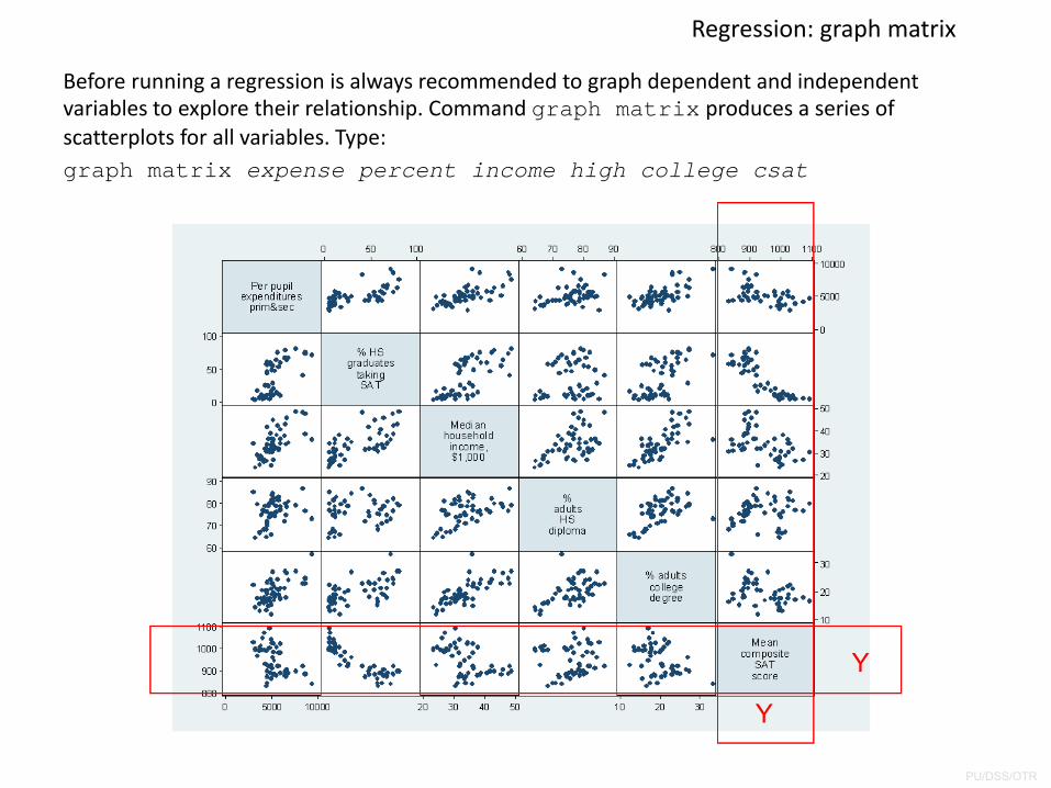
Before running a regression is always recommended to graph dependent and independent variables to explore their relationship. Command graph matrix produces a series of scatterplots for all variables. Type:graph matrix expense percent income high college csat

Y

Y

PU/DSS/OTR

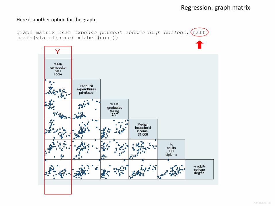
Regression: graph matrix

Here is another option for the graph.

graph matrix csat expense percent income high college, half maxis(ylabel(none) xlabel(none))

Y

PU/DSS/OTR

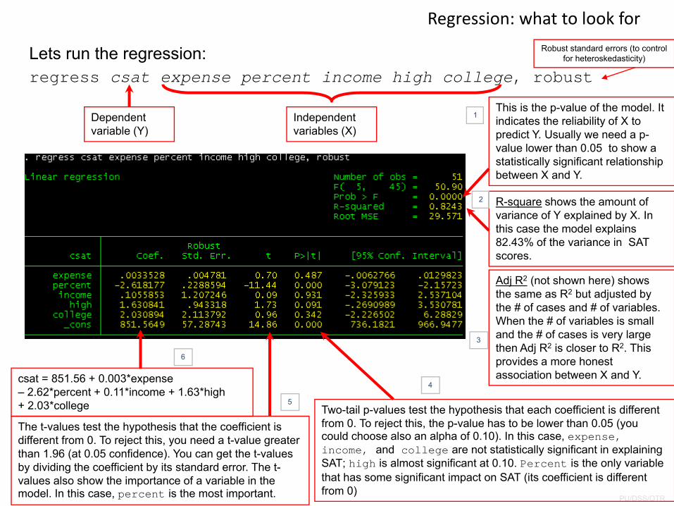
Regression: what to look for

This is the p-value of the model. It indicates the reliability of X to predict Y. Usually we need a p-value lower than 0.05 to show a statistically significant relationship between X and Y.

R-square shows the amount of variance of Y explained by X. In this case the model explains 82.43% of the variance in SAT scores.

Lets run the regression:regress csat expense percent income high college, robust

Adj R2 (not shown here) shows the same as R2 but adjusted by the # of cases and # of variables. When the # of variables is small and the # of cases is very large then Adj R2 is closer to R2. This provides a more honest association between X and Y.

Two-tail p-values test the hypothesis that each coefficient is different from 0. To reject this, the p-value has to be lower than 0.05 (you could choose also an alpha of 0.10). In this case, expense, income, and college are not statistically significant in explaining SAT; high is almost significant at 0.10. Percent is the only variable that has some significant impact on SAT (its coefficient is different from 0)

The t-values test the hypothesis that the coefficient is different from 0. To reject this, you need a t-value greater than 1.96 (at 0.05 confidence). You can get the t-values by dividing the coefficient by its standard error. The t-values also show the importance of a variable in the model. In this case, percent is the most important.

csat = 851.56 + 0.003*expense – 2.62*percent + 0.11*income + 1.63*high + 2.03*college

Dependent variable (Y)

Independent variables (X)

1

2

3

4

5

6

Robust standard errors (to control for heteroskedasticity)

PU/DSS/OTR

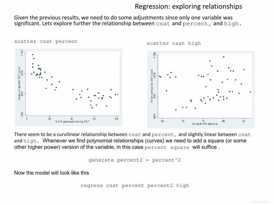
Regression: exploring relationshipsGiven the previous results, we need to do some adjustments since only one variable was significant. Lets explore further the relationship between csat and percent, and high.

scatter csat percent scatter csat high

There seem to be a curvilinear relationship between csat and percent, and slightly linear between csatand high. Whenever we find polynomial relationships (curves) we need to add a square (or some other higher power) version of the variable, in this case percent square will suffice .

generate percent2 = percent^2

Now the model will look like this

regress csat percent percent2 high

PU/DSS/OTR

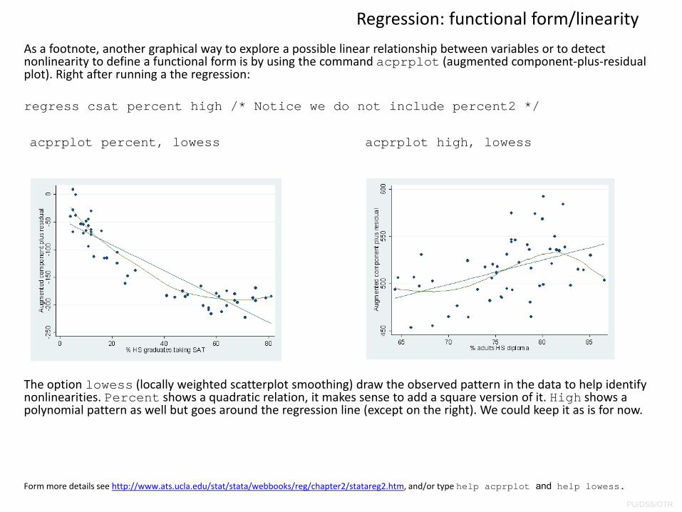
As a footnote, another graphical way to explore a possible linear relationship between variables or to detect nonlinearity to define a functional form is by using the command acprplot (augmented component‐plus‐residual plot). Right after running a the regression:

regress csat percent high /* Notice we do not include percent2 */

Regression: functional form/linearity

Form more details see http://www.ats.ucla.edu/stat/stata/webbooks/reg/chapter2/statareg2.htm, and/or type help acprplot and help lowess.

acprplot percent, lowess acprplot high, lowess

The option lowess (locally weighted scatterplot smoothing) draw the observed pattern in the data to help identify nonlinearities. Percent shows a quadratic relation, it makes sense to add a square version of it. High shows a polynomial pattern as well but goes around the regression line (except on the right). We could keep it as is for now.

PU/DSS/OTR

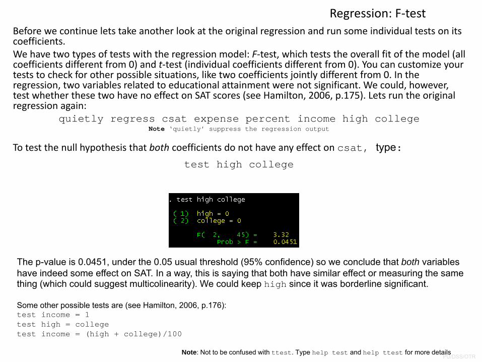
Regression: F‐testBefore we continue lets take another look at the original regression and run some individual tests on its coefficients. We have two types of tests with the regression model: F‐test, which tests the overall fit of the model (all coefficients different from 0) and t‐test (individual coefficients different from 0). You can customize your tests to check for other possible situations, like two coefficients jointly different from 0. In the regression, two variables related to educational attainment were not significant. We could, however, test whether these two have no effect on SAT scores (see Hamilton, 2006, p.175). Lets run the original regression again:

quietly regress csat expense percent income high collegeNote ‘quietly’ suppress the regression output

To test the null hypothesis that both coefficients do not have any effect on csat, type:test high college

The p-value is 0.0451, under the 0.05 usual threshold (95% confidence) so we conclude that both variables have indeed some effect on SAT. In a way, this is saying that both have similar effect or measuring the same thing (which could suggest multicolinearity). We could keep high since it was borderline significant.

Some other possible tests are (see Hamilton, 2006, p.176):test income = 1test high = collegetest income = (high + college)/100

Note: Not to be confused with ttest. Type help test and help ttest for more details

PU/DSS/OTR

Regression: output

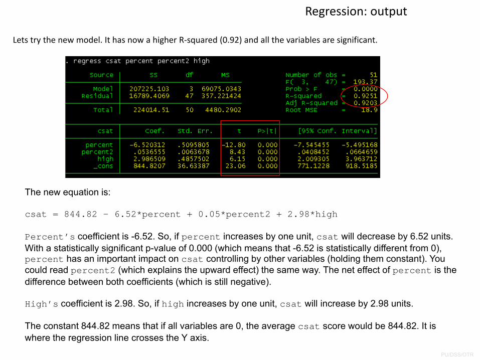
Lets try the new model. It has now a higher R‐squared (0.92) and all the variables are significant.

The new equation is:

csat = 844.82 – 6.52*percent + 0.05*percent2 + 2.98*high

Percent’s coefficient is -6.52. So, if percent increases by one unit, csat will decrease by 6.52 units. With a statistically significant p-value of 0.000 (which means that -6.52 is statistically different from 0), percent has an important impact on csat controlling by other variables (holding them constant). You could read percent2 (which explains the upward effect) the same way. The net effect of percent is the difference between both coefficients (which is still negative).

High’s coefficient is 2.98. So, if high increases by one unit, csat will increase by 2.98 units.

The constant 844.82 means that if all variables are 0, the average csat score would be 844.82. It is where the regression line crosses the Y axis.

PU/DSS/OTR

Regression: saving regression coefficients/getting predicted values

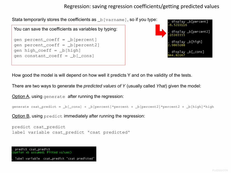
Stata temporarily stores the coefficients as _b[varname], so if you type:

You can save the coefficients as variables by typing:

gen percent_coeff = _b[percent]gen percent_coeff = _b[percent2]gen high_coeff = _b[high]gen constant_coeff = _b[_cons]

How good the model is will depend on how well it predicts Y and on the validity of the tests.

There are two ways to generate the predicted values of Y (usually called Yhat) given the model:

Option A, using generate after running the regression:

generate csat_predict = _b[_cons] + _b[percent]*percent + _b[percent2]*percent2 + _b[high]*high

Option B, using predict immediately after running the regression:

predict csat_predictlabel variable csat_predict "csat predicted"

PU/DSS/OTR

Regression: observed vs. predicted values

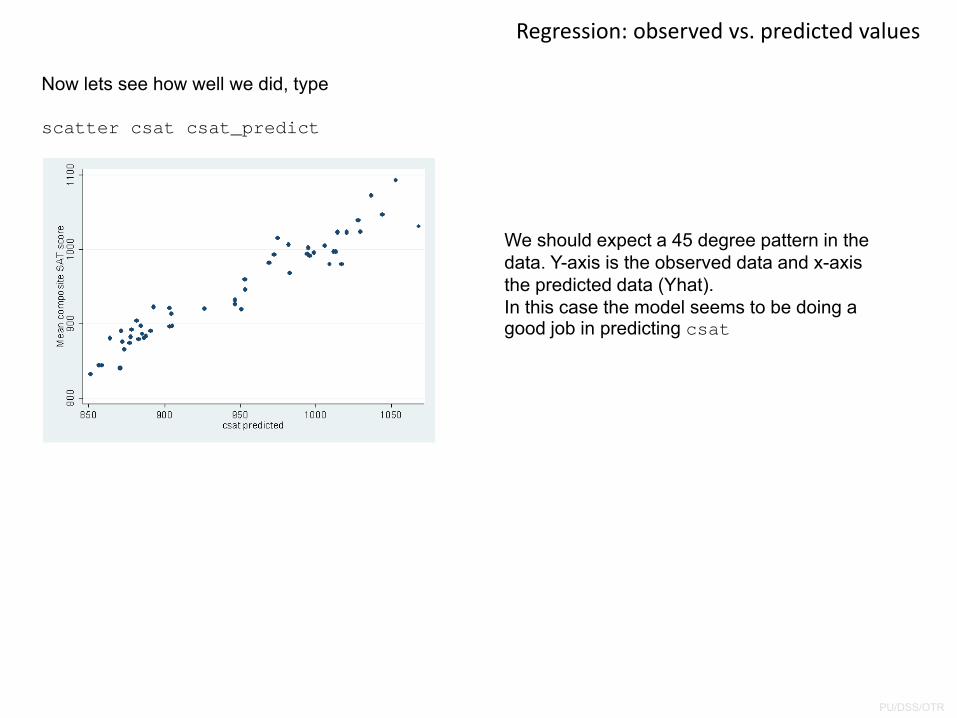
Now lets see how well we did, type

scatter csat csat_predict

We should expect a 45 degree pattern in the data. Y-axis is the observed data and x-axis the predicted data (Yhat). In this case the model seems to be doing a good job in predicting csat

PU/DSS/OTR

Regression: testing for normality

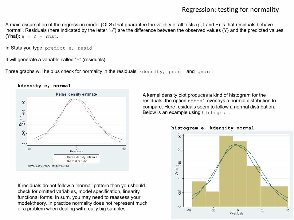
A main assumption of the regression model (OLS) that guarantee the validity of all tests (p, t and F) is that residuals behave ‘normal’. Residuals (here indicated by the letter “e”) are the difference between the observed values (Y) and the predicted values (Yhat): e = Y – Yhat.

In Stata you type: predict e, resid

It will generate a variable called “e” (residuals).

Three graphs will help us check for normality in the residuals: kdensity, pnorm and qnorm.

kdensity e, normal

A kernel density plot produces a kind of histogram for the residuals, the option normal overlays a normal distribution to compare. Here residuals seem to follow a normal distribution. Below is an example using histogram.

histogram e, kdensity normal

If residuals do not follow a ‘normal’ pattern then you should check for omitted variables, model specification, linearity, functional forms. In sum, you may need to reassess your model/theory. In practice normality does not represent much of a problem when dealing with really big samples.

PU/DSS/OTR

Regression: testing for normality

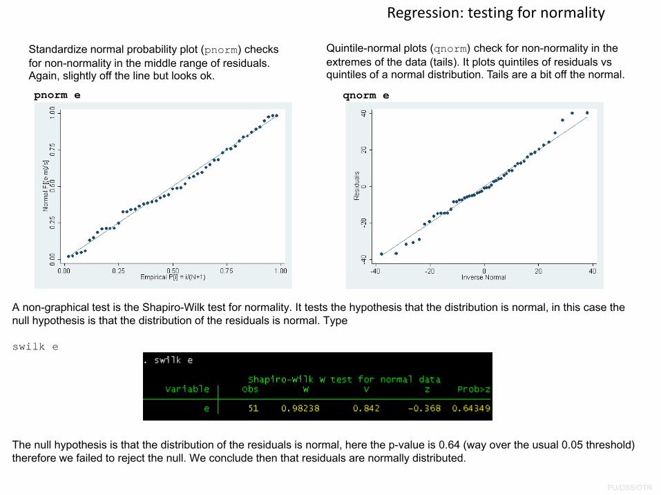
A non-graphical test is the Shapiro-Wilk test for normality. It tests the hypothesis that the distribution is normal, in this case the null hypothesis is that the distribution of the residuals is normal. Type

swilk e

The null hypothesis is that the distribution of the residuals is normal, here the p-value is 0.64 (way over the usual 0.05 threshold) therefore we failed to reject the null. We conclude then that residuals are normally distributed.

Quintile-normal plots (qnorm) check for non-normality in the extremes of the data (tails). It plots quintiles of residuals vs quintiles of a normal distribution. Tails are a bit off the normal.

qnorm epnorm e

Standardize normal probability plot (pnorm) checks for non-normality in the middle range of residuals. Again, slightly off the line but looks ok.

PU/DSS/OTR

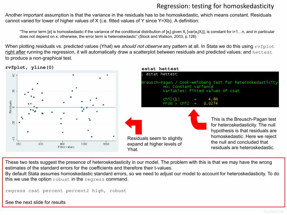
Regression: testing for homoskedasticityAnother important assumption is that the variance in the residuals has to be homoskedastic, which means constant. Residuals cannot varied for lower of higher values of X (i.e. fitted values of Y since Y=Xb). A definition:

“The error term [e] is homoskedastic if the variance of the conditional distribution of [ei] given Xi [var(ei|Xi)], is constant for i=1…n, and in particular does not depend on x; otherwise, the error term is heteroskedastic” (Stock and Watson, 2003, p.126)

When plotting residuals vs. predicted values (Yhat) we should not observe any pattern at all. In Stata we do this using rvfplotright after running the regression, it will automatically draw a scatterplot between residuals and predicted values; and hettest to produce a non-graphical test.

rvfplot, yline(0) estat hettest

Residuals seem to slightly expand at higher levels of Yhat.

This is the Breusch-Pagan test for heteroskedasticity. The null hypothesis is that residuals are homoskedastic. Here we reject the null and concluded that residuals are heteroskedastic.

These two tests suggest the presence of heteroskedasticity in our model. The problem with this is that we may have the wrong estimates of the standard errors for the coefficients and therefore their t-values. By default Stata assumes homoskedastic standard errors, so we need to adjust our model to account for heteroskedasticity. To do this we use the option robust in the regress command.

regress csat percent percent2 high, robust

See the next slide for results

PU/DSS/OTR

Regression: robust standard errors

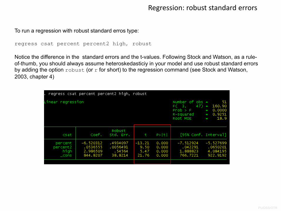
To run a regression with robust standard erros type:

regress csat percent percent2 high, robust

Notice the difference in the standard errors and the t-values. Following Stock and Watson, as a rule-of-thumb, you should always assume heteroskedasticiy in your model and use robust standard errors by adding the option robust (or r for short) to the regression command (see Stock and Watson, 2003, chapter 4)

PU/DSS/OTR

Regression: omitted‐variable test

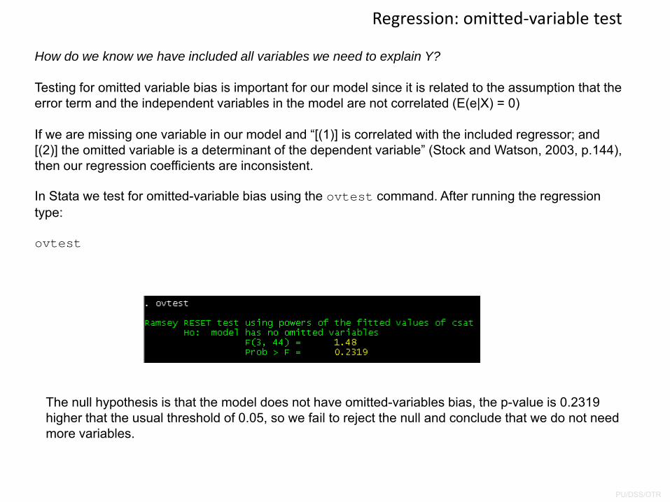
How do we know we have included all variables we need to explain Y?

Testing for omitted variable bias is important for our model since it is related to the assumption that the error term and the independent variables in the model are not correlated (E(e|X) = 0)

If we are missing one variable in our model and “[(1)] is correlated with the included regressor; and [(2)] the omitted variable is a determinant of the dependent variable” (Stock and Watson, 2003, p.144), then our regression coefficients are inconsistent.

In Stata we test for omitted-variable bias using the ovtest command. After running the regression type:

ovtest

The null hypothesis is that the model does not have omitted-variables bias, the p-value is 0.2319 higher that the usual threshold of 0.05, so we fail to reject the null and conclude that we do not need more variables.

PU/DSS/OTR

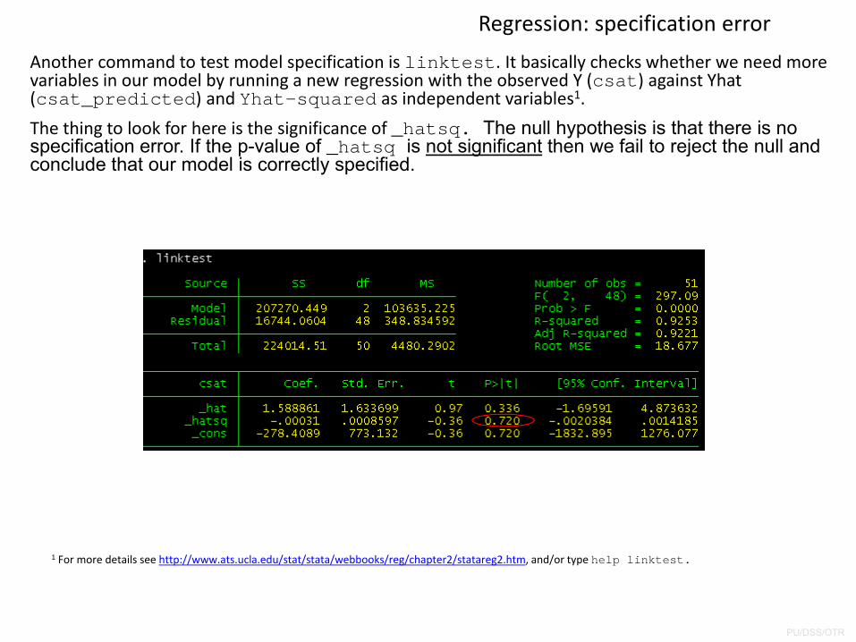
Another command to test model specification is linktest. It basically checks whether we need more variables in our model by running a new regression with the observed Y (csat) against Yhat (csat_predicted) and Yhat-squared as independent variables1. 

The thing to look for here is the significance of _hatsq. The null hypothesis is that there is no specification error. If the p-value of _hatsq is not significant then we fail to reject the null and conclude that our model is correctly specified.

Regression: specification error

1 For more details see http://www.ats.ucla.edu/stat/stata/webbooks/reg/chapter2/statareg2.htm, and/or type help linktest.

PU/DSS/OTR

Regression: outliers

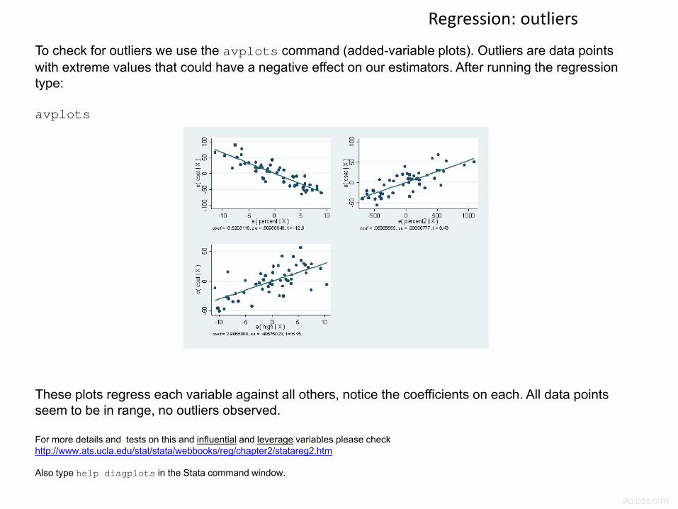
To check for outliers we use the avplots command (added-variable plots). Outliers are data points with extreme values that could have a negative effect on our estimators. After running the regression type:

avplots

These plots regress each variable against all others, notice the coefficients on each. All data points seem to be in range, no outliers observed.

For more details and tests on this and influential and leverage variables please checkhttp://www.ats.ucla.edu/stat/stata/webbooks/reg/chapter2/statareg2.htm

Also type help diagplots in the Stata command window.

PU/DSS/OTR

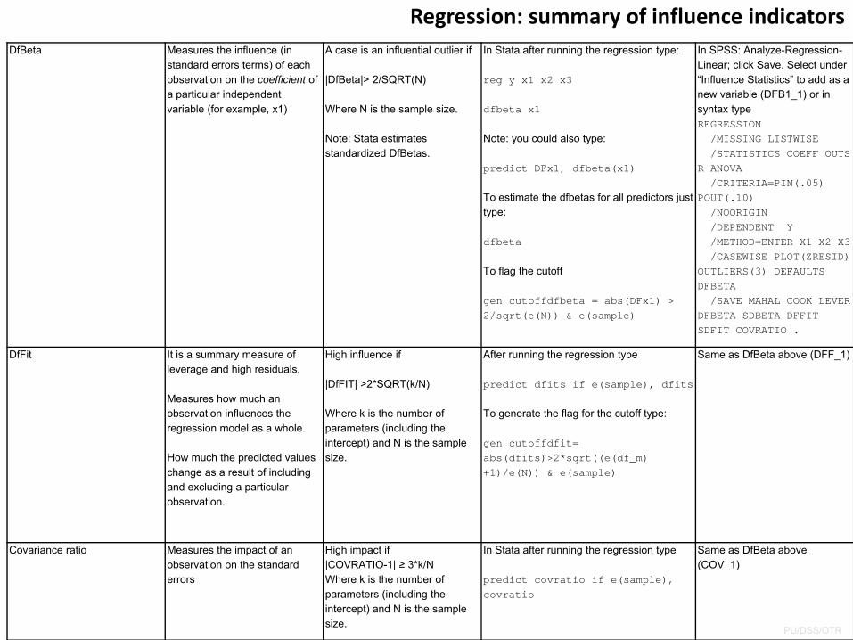
Regression: summary of influence indicatorsDfBeta Measures the influence (in

standard errors terms) of each observation on the coefficient of a particular independent variable (for example, x1)

A case is an influential outlier if

|DfBeta|> 2/SQRT(N)

Where N is the sample size.

Note: Stata estimates standardized DfBetas.

In Stata after running the regression type:

reg y x1 x2 x3

dfbeta x1

Note: you could also type:

predict DFx1, dfbeta(x1)

To estimate the dfbetas for all predictors just type:

dfbeta

To flag the cutoff

gen cutoffdfbeta = abs(DFx1) > 2/sqrt(e(N)) & e(sample)

In SPSS: Analyze-Regression-Linear; click Save. Select under “Influence Statistics” to add as a new variable (DFB1_1) or in syntax type REGRESSION/MISSING LISTWISE/STATISTICS COEFF OUTS

R ANOVA/CRITERIA=PIN(.05)

POUT(.10)/NOORIGIN/DEPENDENT Y/METHOD=ENTER X1 X2 X3/CASEWISE PLOT(ZRESID)

OUTLIERS(3) DEFAULTS DFBETA/SAVE MAHAL COOK LEVER

DFBETA SDBETA DFFIT SDFIT COVRATIO .

DfFit It is a summary measure of leverage and high residuals.

Measures how much an observation influences the regression model as a whole.

How much the predicted values change as a result of including and excluding a particular observation.

High influence if

|DfFIT| >2*SQRT(k/N)

Where k is the number of parameters (including the intercept) and N is the sample size.

After running the regression type

predict dfits if e(sample), dfits

To generate the flag for the cutoff type:

gen cutoffdfit= abs(dfits)>2*sqrt((e(df_m) +1)/e(N)) & e(sample)

Same as DfBeta above (DFF_1)

Covariance ratio Measures the impact of an observation on the standard errors

High impact if |COVRATIO-1| ≥ 3*k/NWhere k is the number of parameters (including the intercept) and N is the sample size.

In Stata after running the regression type

predict covratio if e(sample), covratio

Same as DfBeta above (COV_1)

PU/DSS/OTR

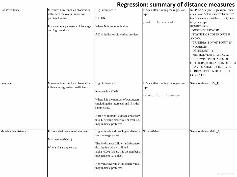
Regression: summary of distance measuresCook’s distance Measures how much an observation

influences the overall model or predicted values.

It is a summary measure of leverage and high residuals..

High influence if

D > 4/N

Where N is the sample size.

A D>1 indicates big outlier problem

In Stata after running the regression type:

predict D, cooksd

In SPSS: Analyze-Regression-Linear; click Save. Select under “Distances” to add as a new variable (COO_1) or in syntax type REGRESSION/MISSING LISTWISE/STATISTICS COEFF OUTS R

ANOVA/CRITERIA=PIN(.05) POUT(.10)/NOORIGIN/DEPENDENT Y/METHOD=ENTER X1 X2 X3/CASEWISE PLOT(ZRESID)

OUTLIERS(3) DEFAULTS DFBETA/SAVE MAHAL COOK LEVER

DFBETA SDBETA DFFIT SDFIT COVRATIO.

Leverage Measures how much an observation influences regression coefficients.

High influence if

leverage h > 2*k/N

Where k is the number of parameters (including the intercept) and N is the sample size.

A rule-of-thumb: Leverage goes from 0 to 1. A value closer to 1 or over 0.5 may indicate problems.

In Stata after running the regression type:

predict lev, leverage

Same as above (LEV_1)

Mahalanobis distance It is rescaled measure of leverage.

M = leverage*(N-1)

Where N is sample size.

Higher levels indicate higher distance from average values.

The M-distance follows a Chi-square distribution with k-1 df and alpha=0.001 (where k is the number of independent variables).

Any value over this Chi-square value may indicate problems.

Not available Same as above (MAH_1)

PU/DSS/OTR

Sources for the summary tables:influence indicators and distance measures

• Statnotes: http://faculty.chass.ncsu.edu/garson/PA765/regress.htm#outlier2

• An Introduction to Econometrics Using Stata/Christopher F. Baum, Stata Press, 2006

• Statistics with Stata (updated for version 9) / Lawrence Hamilton, Thomson Books/Cole,  2006

PU/DSS/OTR

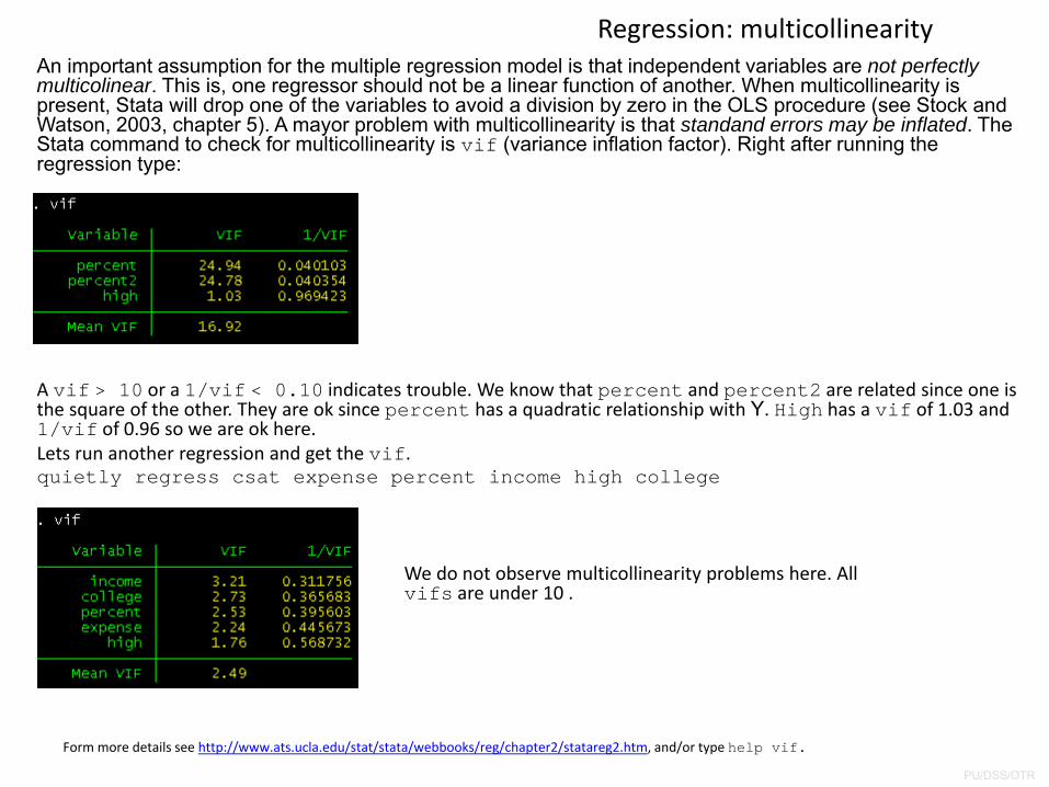
An important assumption for the multiple regression model is that independent variables are not perfectly multicolinear. This is, one regressor should not be a linear function of another. When multicollinearity is present, Stata will drop one of the variables to avoid a division by zero in the OLS procedure (see Stock and Watson, 2003, chapter 5). A mayor problem with multicollinearity is that standand errors may be inflated. The Stata command to check for multicollinearity is vif (variance inflation factor). Right after running the regression type:

Regression: multicollinearity

Form more details see http://www.ats.ucla.edu/stat/stata/webbooks/reg/chapter2/statareg2.htm, and/or type help vif.

A vif > 10 or a 1/vif < 0.10 indicates trouble. We know that percent and percent2 are related since one is the square of the other. They are ok since percent has a quadratic relationship with Y. High has a vif of 1.03 and 1/vif of 0.96 so we are ok here.Lets run another regression and get the vif.quietly regress csat expense percent income high college

We do not observe multicollinearity problems here. All vifs are under 10 .

PU/DSS/OTR

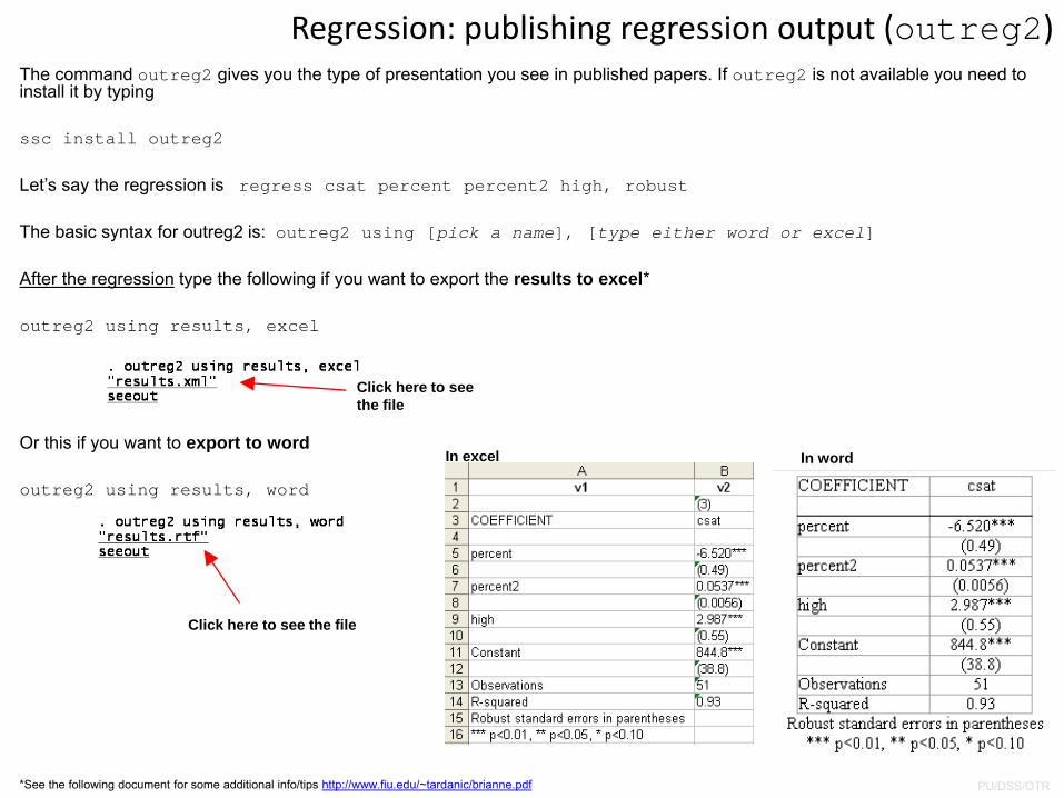
The command outreg2 gives you the type of presentation you see in published papers. If outreg2 is not available you need to install it by typing

ssc install outreg2

Let’s say the regression is regress csat percent percent2 high, robust

The basic syntax for outreg2 is: outreg2 using [pick a name], [type either word or excel]

After the regression type the following if you want to export the results to excel*

outreg2 using results, excel

Or this if you want to export to word

outreg2 using results, word

Regression: publishing regression output (outreg2)

*See the following document for some additional info/tips http://www.fiu.edu/~tardanic/brianne.pdf

In excel In word

Click here to see the file

Click here to see the file

PU/DSS/OTR

Regression: publishing regression output (outreg2)

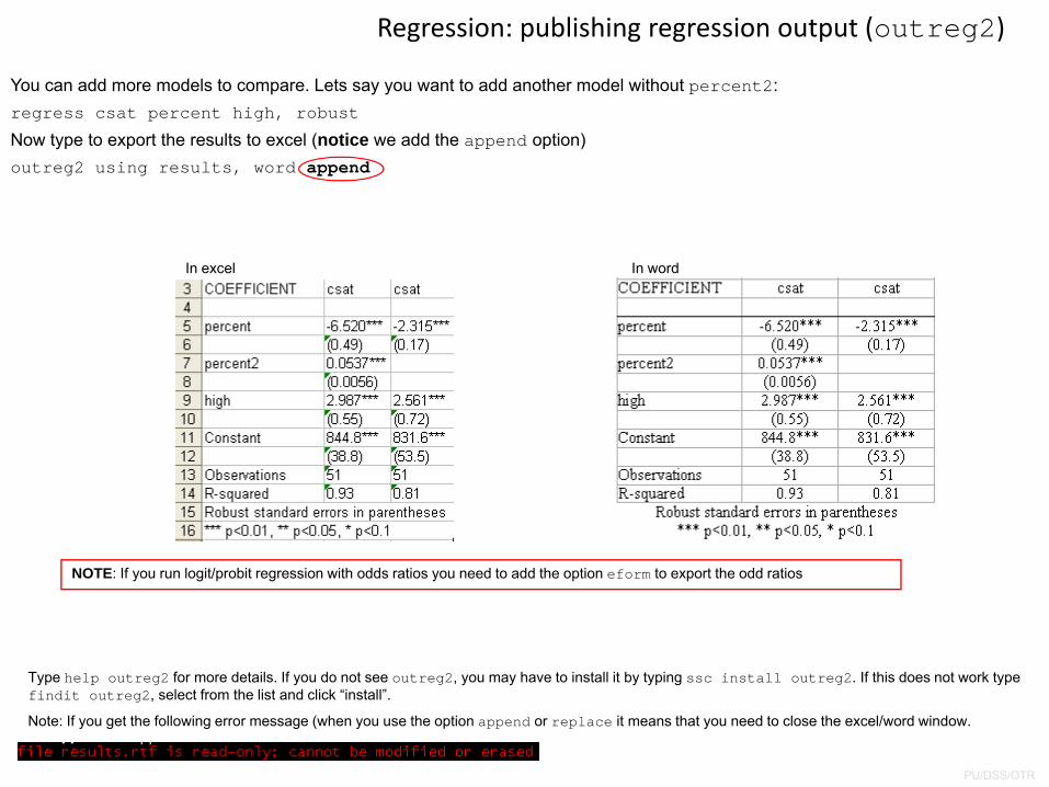
You can add more models to compare. Lets say you want to add another model without percent2:regress csat percent high, robust

Now type to export the results to excel (notice we add the append option)outreg2 using results, word append

In excel In word

NOTE: If you run logit/probit regression with odds ratios you need to add the option eform to export the odd ratios

Type help outreg2 for more details. If you do not see outreg2, you may have to install it by typing ssc install outreg2. If this does not work type findit outreg2, select from the list and click “install”.

Note: If you get the following error message (when you use the option append or replace it means that you need to close the excel/word window.

PU/DSS/OTR

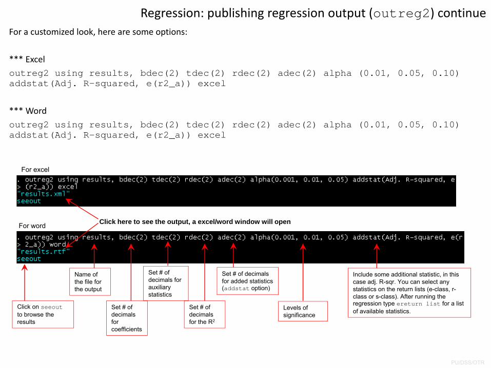
For a customized look, here are some options:

*** Exceloutreg2 using results, bdec(2) tdec(2) rdec(2) adec(2) alpha (0.01, 0.05, 0.10) addstat(Adj. R-squared, e(r2_a)) excel

*** Wordoutreg2 using results, bdec(2) tdec(2) rdec(2) adec(2) alpha (0.01, 0.05, 0.10) addstat(Adj. R-squared, e(r2_a)) excel

Regression: publishing regression output (outreg2) continue

For excel

For word Click here to see the output, a excel/word window will open

Name of the file for the output

Set # of decimals for coefficients

Set # of decimals for auxiliary statistics

Set # of decimals for the R2

Set # of decimals for added statistics (addstat option)

Click on seeoutto browse the results

Levels of significance

Include some additional statistic, in this case adj. R-sqr. You can select any statistics on the return lists (e-class, r-class or s-class). After running the regression type ereturn list for a list of available statistics.

PU/DSS/OTR

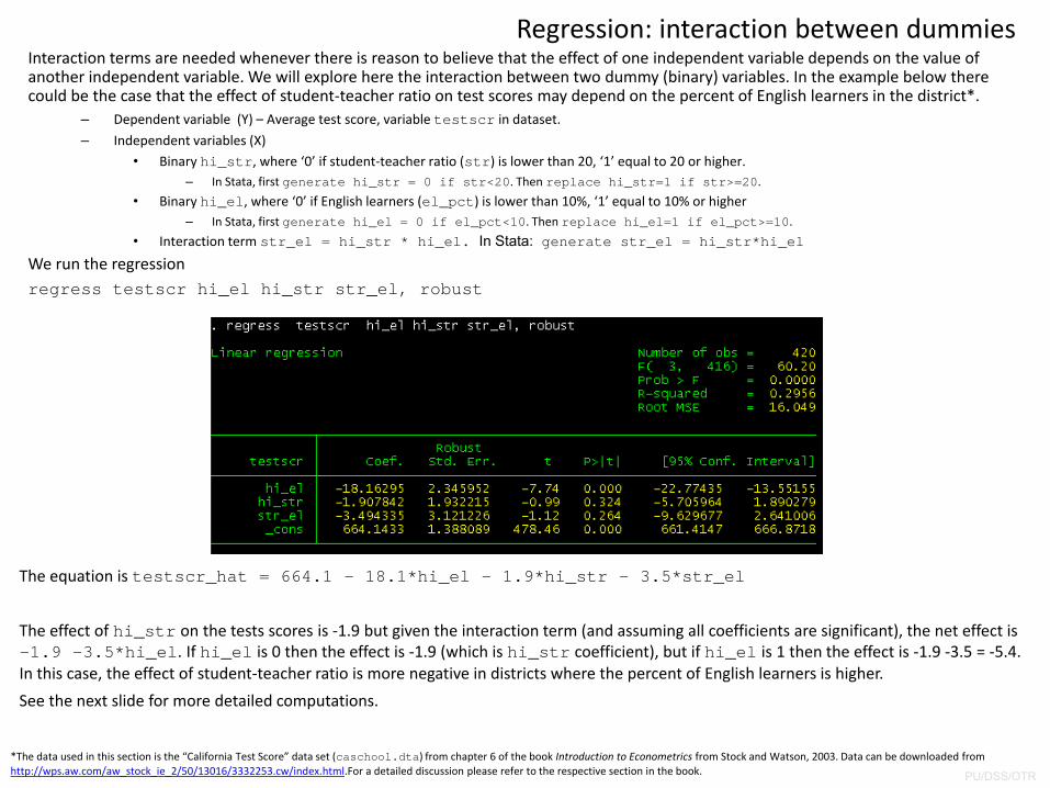
Interaction terms are needed whenever there is reason to believe that the effect of one independent variable depends on the value of another independent variable. We will explore here the interaction between two dummy (binary) variables. In the example below there could be the case that the effect of student‐teacher ratio on test scores may depend on the percent of English learners in the district*.

– Dependent variable  (Y) – Average test score, variable testscr in dataset.

– Independent variables (X) • Binary hi_str, where ‘0’ if student‐teacher ratio (str) is lower than 20, ‘1’ equal to 20 or higher. 

– In Stata, first generate hi_str = 0 if str<20. Then replace hi_str=1 if str>=20.

• Binary hi_el, where ‘0’ if English learners (el_pct) is lower than 10%, ‘1’ equal to 10% or higher– In Stata, first generate hi_el = 0 if el_pct<10. Then replace hi_el=1 if el_pct>=10.

• Interaction term str_el = hi_str * hi_el. In Stata: generate str_el = hi_str*hi_el

We run the regressionregress testscr hi_el hi_str str_el, robust

Regression: interaction between dummies 

*The data used in this section is the “California Test Score” data set (caschool.dta) from chapter 6 of the book Introduction to Econometrics from Stock and Watson, 2003. Data can be downloaded from http://wps.aw.com/aw_stock_ie_2/50/13016/3332253.cw/index.html.For a detailed discussion please refer to the respective section in the book.

The equation is testscr_hat = 664.1 – 18.1*hi_el – 1.9*hi_str – 3.5*str_el

The effect of hi_str on the tests scores is ‐1.9 but given the interaction term (and assuming all coefficients are significant), the net effect is -1.9 -3.5*hi_el. If hi_el is 0 then the effect is ‐1.9 (which is hi_str coefficient), but if hi_el is 1 then the effect is ‐1.9 ‐3.5 = ‐5.4. In this case, the effect of student‐teacher ratio is more negative in districts where the percent of English learners is higher.

See the next slide for more detailed computations.

PU/DSS/OTR

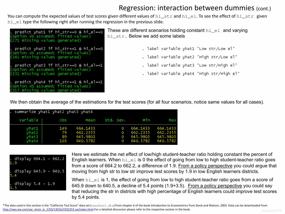
You can compute the expected values of test scores given different values of hi_str and hi_el. To see the effect of hi_str given hi_el type the following right after running the regression in the previous slide.

Regression: interaction between dummies (cont.) 

*The data used in this section is the “California Test Score” data set (caschool.dta) from chapter 6 of the book Introduction to Econometrics from Stock and Watson, 2003. Data can be downloaded from http://wps.aw.com/aw_stock_ie_2/50/13016/3332253.cw/index.html.For a detailed discussion please refer to the respective section in the book.

These are different scenarios holding constant hi_el and varying hi_str. Below we add some labels

We then obtain the average of the estimations for the test scores (for all four scenarios, notice same values for all cases).

Here we estimate the net effect of low/high student-teacher ratio holding constant the percent of English learners. When hi_el is 0 the effect of going from low to high student-teacher ratio goes from a score of 664.2 to 662.2, a difference of 1.9. From a policy perspective you could argue that moving from high str to low str improve test scores by 1.9 in low English learners districts.

When hi_el is 1, the effect of going from low to high student-teacher ratio goes from a score of 645.9 down to 640.5, a decline of 5.4 points (1.9+3.5). From a policy perspective you could say that reducing the str in districts with high percentage of English learners could improve test scores by 5.4 points.

PU/DSS/OTR

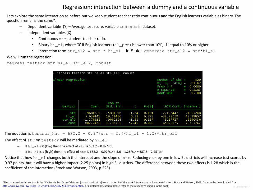
Lets explore the same interaction as before but we keep student‐teacher ratio continuous and the English learners variable as binary. The question remains the same*.

– Dependent variable  (Y) – Average test score, variable testscr in dataset.

– Independent variables (X) • Continuous str, student‐teacher ratio.• Binary hi_el, where ‘0’ if English learners (el_pct) is lower than 10%, ‘1’ equal to 10% or higher• Interaction term str_el2 = str * hi_el. In Stata: generate str_el2 = str*hi_el

We will run the regressionregress testscr str hi_el str_el2, robust

Regression: interaction between a dummy and a continuous variable 

*The data used in this section is the “California Test Score” data set (caschool.dta) from chapter 6 of the book Introduction to Econometrics from Stock and Watson, 2003. Data can be downloaded from http://wps.aw.com/aw_stock_ie_2/50/13016/3332253.cw/index.html.For a detailed discussion please refer to the respective section in the book.

The equation is testscr_hat = 682.2 – 0.97*str + 5.6*hi_el – 1.28*str_el2

The effect of str on testscr will be mediated by hi_el. – If hi_el is 0 (low) then the effect of str is 682.2 – 0.97*str. 

– If hi_el is 1 (high) then the effect of str is 682.2 – 0.97*str + 5.6 – 1.28*str = 687.8 – 2.25*str

Notice that how hi_el changes both the intercept and the slope of str. Reducing str by one in low EL districts will increase test scores by 0.97 points, but it will have a higher impact (2.25 points) in high EL districts. The difference between these two effects is 1.28 which is the coefficient of the interaction (Stock and Watson, 2003, p.223).

PU/DSS/OTR

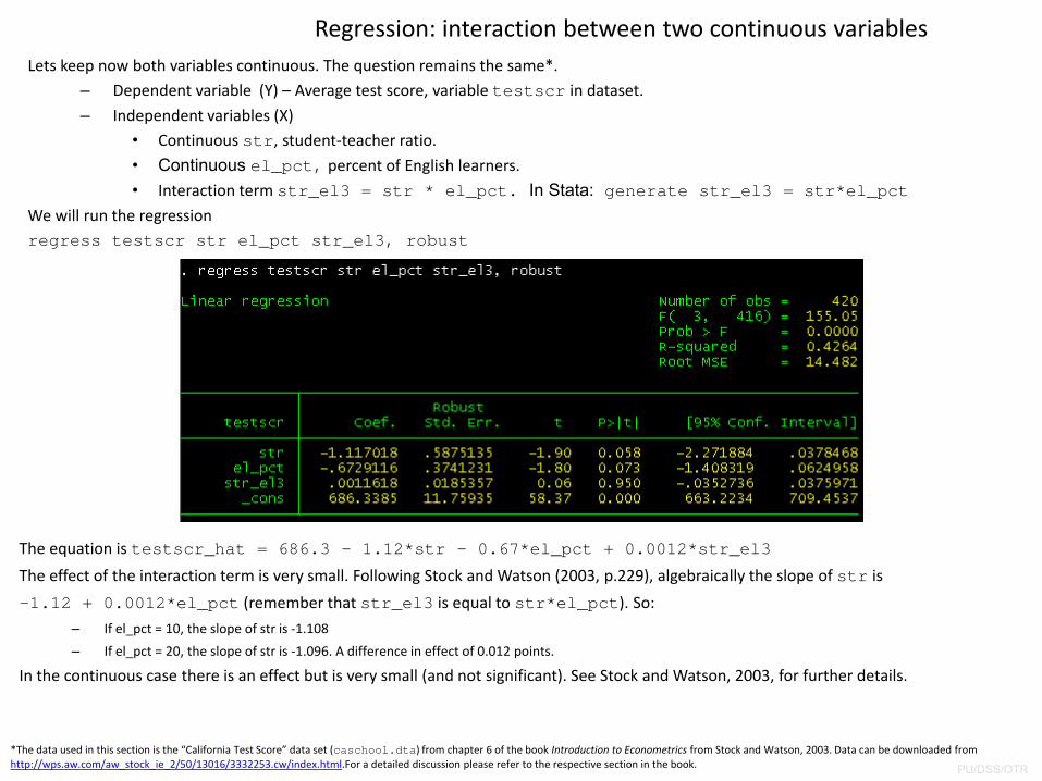
Lets keep now both variables continuous. The question remains the same*.– Dependent variable  (Y) – Average test score, variable testscr in dataset.

– Independent variables (X) • Continuous str, student‐teacher ratio.• Continuous el_pct, percent of English learners.

• Interaction term str_el3 = str * el_pct. In Stata: generate str_el3 = str*el_pctWe will run the regressionregress testscr str el_pct str_el3, robust

Regression: interaction between two continuous variables

*The data used in this section is the “California Test Score” data set (caschool.dta) from chapter 6 of the book Introduction to Econometrics from Stock and Watson, 2003. Data can be downloaded from http://wps.aw.com/aw_stock_ie_2/50/13016/3332253.cw/index.html.For a detailed discussion please refer to the respective section in the book.

The equation is testscr_hat = 686.3 – 1.12*str - 0.67*el_pct + 0.0012*str_el3

The effect of the interaction term is very small. Following Stock and Watson (2003, p.229), algebraically the slope of str is 

–1.12 + 0.0012*el_pct (remember that str_el3 is equal to str*el_pct). So:

– If el_pct = 10, the slope of str is ‐1.108

– If el_pct = 20, the slope of str is ‐1.096. A difference in effect of 0.012 points.

In the continuous case there is an effect but is very small (and not significant). See Stock and Watson, 2003, for further details.

PU/DSS/OTR

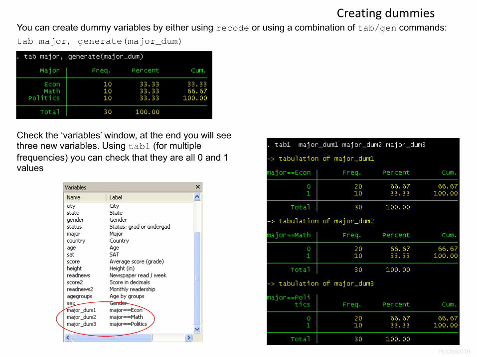
You can create dummy variables by either using recode or using a combination of tab/gen commands:tab major, generate(major_dum)

Creating dummies

Check the ‘variables’ window, at the end you will see three new variables. Using tab1 (for multiple frequencies) you can check that they are all 0 and 1 values

PU/DSS/OTR

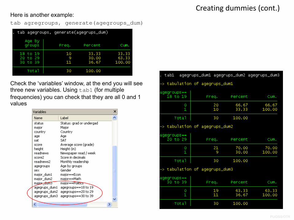
Here is another example:tab agregroups, generate(agegroups_dum)

Creating dummies (cont.)

Check the ‘variables’ window, at the end you will see three new variables. Using tab1 (for multiple frequencies) you can check that they are all 0 and 1 values

PU/DSS/OTR

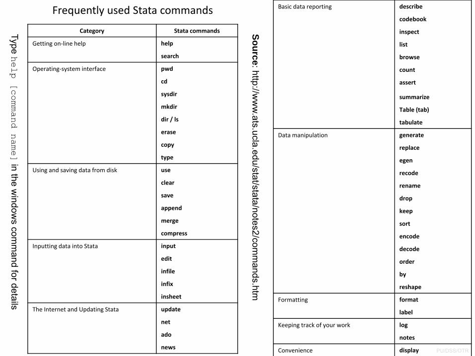
Category Stata commands

Getting on‐line help help

search

Operating‐system interface pwd

cd

sysdir

mkdir

dir / ls

erase

copy

type

Using and saving data from disk use

clear

save

append

merge

compress

Inputting data into Stata input

edit

infile

infix

insheet

The Internet and Updating Stata update

net

ado

news

Basic data reporting describe

codebook

inspect

list

browse

count

assert

summarize

Table (tab)

tabulate

Data manipulation generate

replace

egen

recode

rename

drop

keep

sort

encode

decode

order

by

reshape

Formatting format

label

Keeping track of your work log

notes

Convenience display

Source: http://ww

w.ats.ucla.edu/stat/stata/notes2/comm

ands.htm

Frequently used Stata commands

Type help [command name]

in the window

s comm

and for details

PU/DSS/OTR

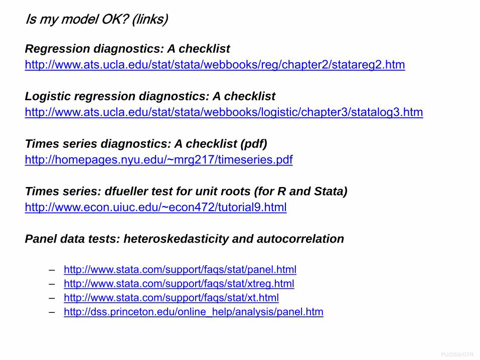
Regression diagnostics: A checklisthttp://www.ats.ucla.edu/stat/stata/webbooks/reg/chapter2/statareg2.htm

Logistic regression diagnostics: A checklisthttp://www.ats.ucla.edu/stat/stata/webbooks/logistic/chapter3/statalog3.htm

Times series diagnostics: A checklist (pdf)http://homepages.nyu.edu/~mrg217/timeseries.pdf

Times series: dfueller test for unit roots (for R and Stata)http://www.econ.uiuc.edu/~econ472/tutorial9.html

Panel data tests: heteroskedasticity and autocorrelation

– http://www.stata.com/support/faqs/stat/panel.html– http://www.stata.com/support/faqs/stat/xtreg.html– http://www.stata.com/support/faqs/stat/xt.html– http://dss.princeton.edu/online_help/analysis/panel.htm

Is my model OK? (links)

PU/DSS/OTR

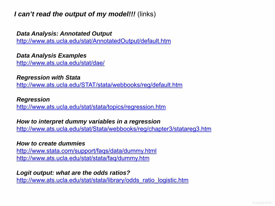
Data Analysis: Annotated Outputhttp://www.ats.ucla.edu/stat/AnnotatedOutput/default.htm

Data Analysis Exampleshttp://www.ats.ucla.edu/stat/dae/

Regression with Statahttp://www.ats.ucla.edu/STAT/stata/webbooks/reg/default.htm

Regressionhttp://www.ats.ucla.edu/stat/stata/topics/regression.htm

How to interpret dummy variables in a regressionhttp://www.ats.ucla.edu/stat/Stata/webbooks/reg/chapter3/statareg3.htm

How to create dummieshttp://www.stata.com/support/faqs/data/dummy.htmlhttp://www.ats.ucla.edu/stat/stata/faq/dummy.htm

Logit output: what are the odds ratios?http://www.ats.ucla.edu/stat/stata/library/odds_ratio_logistic.htm

I can’t read the output of my model!!! (links)

PU/DSS/OTR

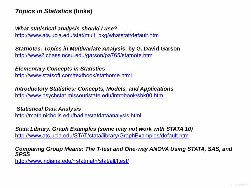
What statistical analysis should I use?http://www.ats.ucla.edu/stat/mult_pkg/whatstat/default.htm

Statnotes: Topics in Multivariate Analysis, by G. David Garsonhttp://www2.chass.ncsu.edu/garson/pa765/statnote.htm

Elementary Concepts in Statisticshttp://www.statsoft.com/textbook/stathome.html

Introductory Statistics: Concepts, Models, and Applicationshttp://www.psychstat.missouristate.edu/introbook/sbk00.htm

Statistical Data Analysishttp://math.nicholls.edu/badie/statdataanalysis.html

Stata Library. Graph Examples (some may not work with STATA 10)http://www.ats.ucla.edu/STAT/stata/library/GraphExamples/default.htm

Comparing Group Means: The T-test and One-way ANOVA Using STATA, SAS, and SPSShttp://www.indiana.edu/~statmath/stat/all/ttest/

Topics in Statistics (links)

PU/DSS/OTR

Useful links / Recommended books

• DSS Online Training Section http://dss.princeton.edu/training/

• UCLA Resources to learn and use STATA http://www.ats.ucla.edu/stat/stata/

• DSS help‐sheets for STATA http://dss/online_help/stats_packages/stata/stata.htm

• Introduction to Stata (PDF), Christopher F. Baum, Boston College, USA. “A 67‐page description of Stata, its key features and benefits, and other useful information.” http://fmwww.bc.edu/GStat/docs/StataIntro.pdf

• STATA FAQ website http://stata.com/support/faqs/

• Princeton DSS Libguides http://libguides.princeton.edu/dss

Books

• Introduction to econometrics / James H. Stock, Mark W. Watson. 2nd ed., Boston: Pearson Addison Wesley, 2007.

• Data analysis using regression and multilevel/hierarchical models / Andrew Gelman, Jennifer Hill. Cambridge ; New York : Cambridge University Press, 2007.

• Econometric analysis / William H. Greene. 6th ed., Upper Saddle River, N.J. : Prentice Hall, 2008.

• Designing Social Inquiry: Scientific Inference in Qualitative Research / Gary King, Robert O. Keohane, Sidney Verba, Princeton University Press, 1994.

• Unifying Political Methodology: The Likelihood Theory of Statistical Inference / Gary King, Cambridge University Press, 1989

• Statistical Analysis: an interdisciplinary introduction to univariate & multivariate methods / Sam Kachigan, New York : Radius Press, c1986

• Statistics with Stata (updated for version 9) / Lawrence Hamilton, Thomson Books/Cole, 2006