TitleMild solutions to the Navier-Stokes equations in unboundeddomains with unbounded boundary (Mathematical Analysis inFluid and Gas Dynamics)

Author(s) Sawada, Okihiro

Citation 数理解析研究所講究録 (2012), 1782: 28-43

Issue Date 2012-03

URL http://hdl.handle.net/2433/171865

Right

Type Departmental Bulletin Paper

Textversion publisher

Kyoto University

Mild solutions to the Navier-Stokes equationsin unbounded domains with unbounded

boundary

Okihiro SawadaDepartment of Mathematical and Design Engineering,Gifu University, Yanagido 1-1, Gifu, 501-1193, Japan

okihiro@gifu-u.ac.jp

Abstract

It is mathematically investigated the incompressible viscous flowsin domains $\Omega\subset \mathbb{R}^{n}$ with nonslip boundary conditions in the frameworkof $L_{\sigma}^{p}(\Omega)$ , where $\Omega$ has a possibly non-compact uniform $C^{3}$-boundaryand boundedness of the Helmholtz projection $\mathbb{P}_{p}$ onto $L_{\sigma}^{p}(\Omega)$ with some$1<p<\infty$ . The key is to show that the Stokes operator generates ananalytic semigroup on $L_{\sigma}^{p}(\Omega)$ admitting the maximal $L^{q}-L^{p}$-regularityestimates. Moreover, the local-in-time existence and the uniqueness ofmild solutions to the Navier-Stokes equation in such $\Omega$ and $p\in(n, \infty)$

are proved, when the initial data belong to $L_{\sigma}^{p}(\Omega)$ .

1 Introduction

This is a brief survey of the results related to [18], mainly.For any open set $\Omega\subset \mathbb{R}^{n}$ , it is well-known that the Stokes operator

$A_{2};=-\mathbb{P}_{2}\triangle$ (with nonslip boundary conditions) is a self adjoint operator in$L_{\sigma}^{2}(\Omega)$ by Masuda [28]. Hence, $-A_{2}$ is the generator of an analytic contractionsemigroup $\{e^{-tA_{2}}\}_{t\geq 0}$ onto $L_{\sigma}^{2}(\Omega)$ . Here, $L_{\sigma}^{2}(\Omega)$ is defined by the solenoidalpart of the Helmholtz decomposition of $L^{2}(\Omega)$ into $L_{\sigma}^{2}(\Omega)\oplus G^{2}(\Omega)$ , where$\oplus$ denotes the direct sum, and $\mathbb{P}_{2}$ denotes the Helmholtz projection from$L^{2}(\Omega)$ to $L_{\sigma}^{2}(\Omega)$ . It seems to be natural to investigate whether this techniquecan be applicable in general If-setting, that is, $\{e^{-tA_{p}}\}_{t\geq 0}$ extends to an

数理解析研究所講究録第 1782巻 2012年 28-43 28

analytic semigroup on an $U_{\sigma}$-space for some 1 $<p<\infty$ , and that thereare the maximal $L^{q}-L^{p}$-regularity estimates for the solution of the associatedStokes equations. Once we obtain the above semigroup theory, we have achance to construct the local-in-time mild solutions to the Navier-Stokesequations in $L_{\sigma}^{p}(\Omega)$ for $n\leq p<\infty$ by the fixed point argument of Kato [26]or Giga-Miyakawa [22]. The notion of a mild solution was first introduced byFujita-Kato [14, 27] when the initial velocity belongs to $H_{\sigma}^{1/2}(\Omega)$ with smoothbounded domains $\Omega\subset \mathbb{R}^{3}$ via Duhamel $s$ principle at the almost same yearsof Browder [6] to study some equations of parabolic type.

It is clear to have the affirmative answer of the above question when $\Omega$

is the whole space or the half space (see Ukai [33] and Desch-Hieber-Pr\"uB[7] $)$ for any $p\in(1, \infty)$ . For bounded or exterior domains with smoothboundaries, the maximal $L^{q}-L^{p}$-regularity estimates were firstly shown bySolonnikov [30]. His proof makes use of potential theoretic arguments. Lateron, Giga [19, 20] also established the Stokes semigroup theory due to thebounded imaginary powers of the Stokes operator, Giga-Sohr [23] appliedthe Dore-Venni theorem in two-dimension case, Grubb-Solonnikov [24] usedthe pseudo-differential techniques, and Fr\"ohlich [13] made use of the conceptof weighted estimates with respect to Muckenhoupt weights. The reader canfind related results in the list of reference in Farwig-Sohr [11]. Furthermore,the ca.se of a perturbed half space is treated by e.g. Noll-Saal [29]. For resultsconcerning infinite layers-like domains, we refer to the works of Abe-Shibata[1], Abels [2] and Abels-Wiegner [3]. Franzke [12] and Hishida [25] consideredthe case of aperture domains. Farwig-Ri [10] derived the maximal $L^{q}-L^{p_{-}}$

regularity estimates in infinite tube-like domains. In the domains listed-upabove the Helmholtz decomposition is valid.

The key of this approach is to show the boundedness of the Helmholtzprojection $\mathbb{P}_{p}$ on $L^{p}(\Omega)$ into its solenoidal subspace. For example, if $\Omega$ isbounded, then the boundedness of $\mathbb{P}_{p}$ ; this fact was first proved by Fujiwara-Morimoto [15].

On the other hand, in the case of general domains $\Omega$ , it is not clearwhether the Helmholtz decomposition makes sense, that is, $U(\Omega)=L_{\sigma}^{p}(\Omega)\oplus$

$G^{p}(\Omega)$ or not, in general, unless $p=2$ . Indeed, $Bogovski_{\dot{1}}[4,5]$ gave examples

29

of unbounded domains $\Omega$ with smooth boundaries in which it is not enableto have the Helmholtz decomposition of If $(\Omega)$ for certain $p$ . For details, seealso [16]. To overcome the difficulties, Farwig-Kozono-Sohr [9] introduced

$\tilde{L}^{p}(\Omega):=\{\begin{array}{ll}L^{2}(\Omega)\cap U(\Omega), 2\leq p<\infty,L^{2}(\Omega)+L^{p}(\Omega), 1<p<2.\end{array}$

for domains $\Omega\subset \mathbb{R}^{3}$ with uniform $C^{2}$-boundaries, proved the existence ofthe Helmholtz projection $\tilde{\mathbb{P}}$ in $\tilde{I}f$ (assisted by $L^{2}$ ), and obtained the usefulproperties as usual in $U(\Omega)$ . Moreover, they proved that the Stokes operator$A_{p}$

$:=-\tilde{\mathbb{P}}\triangle$ with nonslip boundary conditions is well-defined in $\tilde{I}f_{\sigma}$ , and

generates an analytic semigroup onto $\tilde{I}f_{\sigma}(\Omega)$ as well as the maximal $L^{q}-\tilde{I}f-$

regularity estimates in the class $L^{q}$ (Ll’) $:=L^{q}((0, T);\tilde{I}f(\Omega))$ for $T>0$

$\Vert u_{t}\Vert_{L^{q}(\tilde{L}^{p})}+\Vert u\Vert_{L^{q}(\tilde{L}^{p})}+\Vert\nabla^{2}u\Vert_{L^{q}(\tilde{L}^{p})}+\Vert\nabla\tilde{\pi}\Vert_{L^{q}(\tilde{L}^{p})}\leq C\Vert f\Vert_{L^{q}(\tilde{L}^{p})}$

with some constant $C>0$ independent of $f\in L^{q}(\tilde{I}f)$ . Here $(u,\tilde{\pi})$ is asolution to the Stokes equations in domains $\Omega$ with $f\in L^{q}(\tilde{L}^{p})$ :

$u_{t}-\triangle u+\nabla\tilde{\pi}=f$ in $\Omega\cross(0, T)$ ,

$\nabla\cdot u=0$ in $\Omega\cross(0, T)$ ,(1.1)

$u=0$ on $\partial\Omega\cross(0, T)$ ,

$u|_{t=0}=0$ in $\Omega$ .

In the paper [18] they however employed a different approach to [9]. For$\Omega\subset \mathbb{R}^{n}$ having a uniformly $C^{3}$-boundary with $p\in(1, \infty)$ , it is assumed thatthe Helmholtz projection $\mathbb{P}_{p}$ exists bounded in $L^{p}(\Omega)$ . They actually showedthat $-A_{p}$ generates an analytic semigroup onto usual $U_{\sigma}(\Omega)$ , which comesfrom the fact that solutions to the Stokes equation satisfies the maximal $L^{q_{-}}$

If-regularity estimates in $L^{q}((0, T);L^{\rho}(\Omega))$ . They also obtained the local-in-time existence of a unique mild solution to the Navier-Stokes equations in

LP $(\Omega)$ with $p>n$ under the assumption of the existence of the Helmholtzprojection. Although it seems to be an interesting problem in the frameworkof $L_{\sigma}^{n}(\Omega)$ which is excluded by [18], the author has no idea to overcome thedifficulties (for example, it is not clear whether $\mathbb{P}_{p}=\mathbb{P}_{q}$ if $p\neq q$) so far.

This paper is organized as follows. In Sections 2 we will state the mainresults of [18]. In Section 3 the strategy of their approach is explained.

30

2 Main Results

In this section we mention the main results in [18]. Here and hereafter, let$n\geq 2$ . The definition of uniform $C^{k}$-domain for $k\in \mathbb{N}$ will be given in thenext section. For any open set $\Omega\subset \mathbb{R}^{n}$ and for $p\in(1, \infty)$ , we set

$G^{p}(\Omega)$ $:=\{u\in L^{p}(\Omega);u=\nabla\tilde{\pi}$ for some $\tilde{\pi}\in W_{loc}^{1,p}(\Omega)\}$ ,$L_{\sigma}^{p}(\Omega):=\overline{\{u\in C_{c}^{\infty}(\Omega);\nabla\cdot u=0in\Omega\}}^{\Vert\cdot\Vert_{p}}$

We say that the Helmholtz projection $\mathbb{P}$

$:=\mathbb{P}_{p}$ exists for $U(\Omega)$ , whenever$L^{p}(\Omega)$ can be decomposed into

$L^{p}(\Omega)=If_{\sigma}(\Omega)\oplus G^{p}(\Omega)$ .

In this case, there naturally exists a unique projection $\mathbb{P}_{p}:If(\Omega)arrow L_{\sigma}^{p}(\Omega)$

having the properties $\mathbb{P}_{p}^{2}=\mathbb{P}_{p}$ and $G^{p}(\Omega)$ as its null space. A well-known factby e.g. [16] is that the Helmholtz projection exists for $L^{\rho}(\Omega)$ for $p\in(1, \infty)$ ifand only if for every $f\in L^{p}(\Omega)$ , there exists a unique function $u\in\hat{W}^{1,p}(\Omega)$

satisfying

$\langle\nabla u,$ $\nabla\varphi\}=\{f,$ $\nabla\varphi\rangle$ , $\varphi\in\hat{W}^{1,p’}(\Omega)$ .

Thus the Helmholtz projection exists for $\nu(\Omega)$ if and only if for every $f\in$

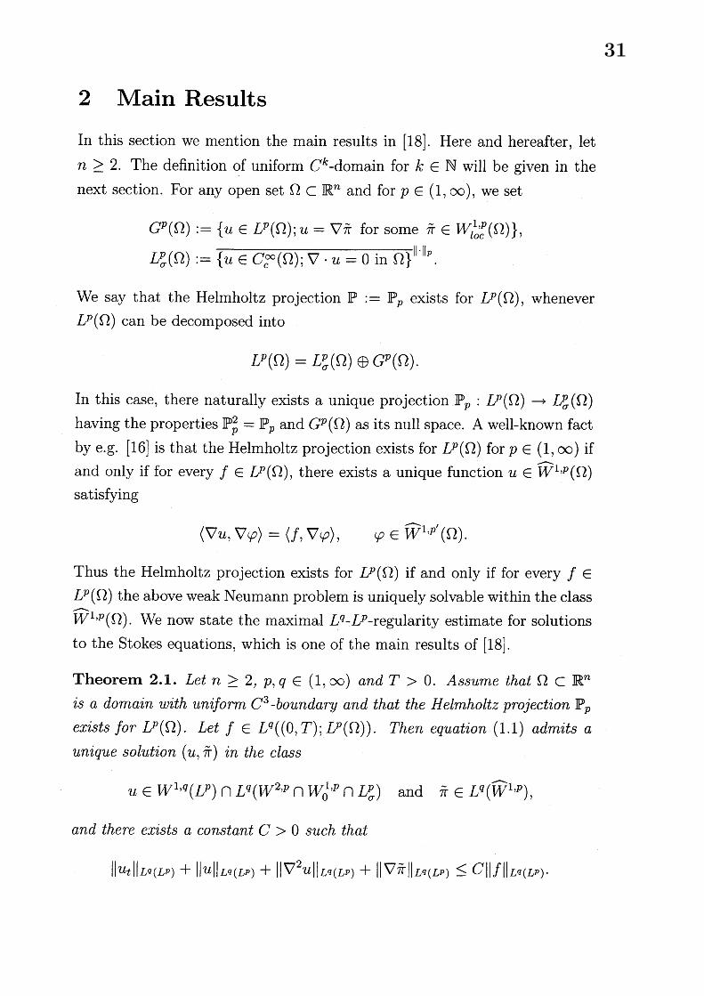
$L^{p}(\Omega)$ the above weak Neumann problem is uniquely solvable within the class$\hat{W}^{1,p}(\Omega)$ . We now state the maximal $L^{q}-L^{p}$-regularity estimate for solutionsto the Stokes equations, which is one of the main results of [18].

Theorem 2.1. Let $n\geq 2_{f}p,$ $q\in(1, \infty)$ and $T>0$ . Assume that $\Omega\subset \mathbb{R}^{n}$

is a domain with uniform $C^{3}$ -boundary and that the Helmholtz projection $\mathbb{P}_{p}$

exists for $L^{p}(\Omega)$ . Let $f\in L^{q}((0, T);U(\Omega))$ . Then equation (1.1) admits aunique solution $(u,\tilde{\pi})$ in the class

$u\in W^{1,q}(L^{p})\cap L^{q}(W^{2,p}\cap W_{0}^{1,p}\cap L_{\sigma}^{p})$ and $\tilde{\pi}\in L^{q}(\hat{W}^{1,p})$ ,

and there exists a constant $C>0$ such that

$\Vert u_{t}\Vert_{Lq(L)}p+\Vert u\Vert_{L(L)}qp+\Vert\nabla^{2}u\Vert_{L^{q}(L)}p+\Vert\nabla\tilde{\pi}\Vert_{Lq(Lp})\leq C\Vert f\Vert_{Lq(Lp})$ .

31

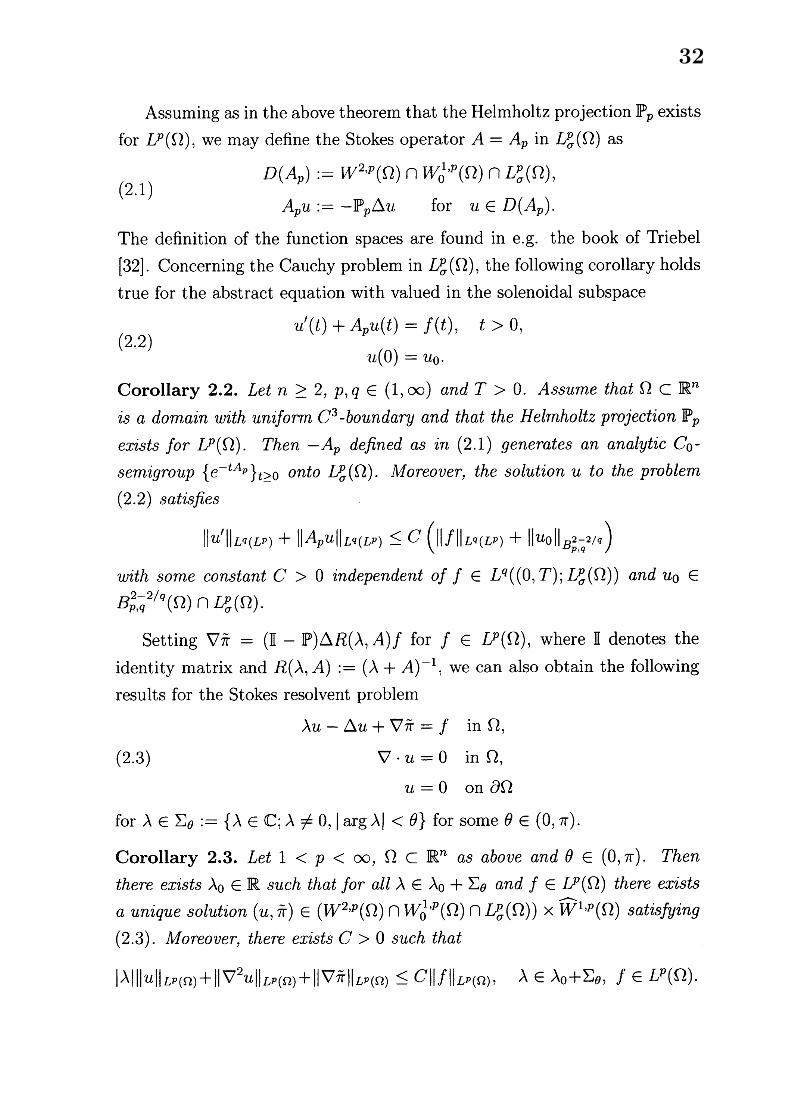
Assuming as in the above theorem that the Helmholtz projection $\mathbb{P}_{p}$ existsfor $U(\Omega)$ , we may define the Stokes operator $A=A_{p}$ in $L_{\sigma}^{p}(\Omega)$ as

$D(A_{p}):=W^{2,p}(\Omega)\cap W_{0}^{1,p}(\Omega)\cap If_{\sigma}(\Omega)$ ,(2.1)

$A_{p}u:=-\mathbb{P}_{p}\triangle u$ for $u\in D(A_{p})$ .

The definition of the function spaces are found in e.g. the book of Triebel[32]. Concerning the Cauchy problem in $U_{\sigma}(\Omega)$ , the following corollary holdstrue for the abstract equation with valued in the solenoidal subspace

$u’(t)+A_{p}u(t)=f(t)$ , $t>0$ ,(2.2)

$u(0)=u_{0}$ .

Corollary 2.2. Let $n\geq 2,$ $p,$ $q\in(1, \infty)$ and $T>0$ . Assume that $\Omega\subset \mathbb{R}^{n}$

is a domain with uniform $C^{3}$ -boundary and that the Helmholtz projection $\mathbb{P}_{p}$

exists for $U(\Omega)$ . Then $-A_{p}$ defined as in (2.1) genemtes an analytic $C_{0^{-}}$

semigroup $\{e^{-tA_{p}}\}_{t\geq 0}$ onto $\nu_{\sigma}(\Omega)$ . Moreover, the solution $u$ to the problem

(2.2) satisfies$\Vert u’\Vert_{L^{q}(L^{p})}+\Vert A_{p}u\Vert_{L^{q}(L^{p})}\leq C(\Vert f\Vert_{L^{q}(L^{p})}+\Vert u_{0}\Vert_{B_{p,q}^{2-2/q}})$

with some constant $C>0$ independent of $f\in L^{q}((0, T);U_{\sigma}(\Omega))$ and $u_{0}\in$

$B_{p,q}^{2-2/q}(\Omega)\cap\nu_{\sigma}(\Omega)$ .

Setting $\nabla\tilde{\pi}=(II-\mathbb{P})\triangle R(\lambda, A)f$ for $f\in If(\Omega)$ , where II denotes theidentity matrix and $R(\lambda, A)$ $:=(\lambda+A)^{-1}$ , we can also obtain the following

results for the Stokes resolvent problem

$\lambda u-\triangle u+\nabla\tilde{\pi}=f$ in $\Omega$ ,

(2.3) $\nabla\cdot u=0$ in $\Omega$ ,

$u=0$ on $\partial\Omega$

for $\lambda\in\Sigma_{\theta}$ $:=\{\lambda\in \mathbb{C};\lambda\neq 0, |\arg\lambda|<\theta\}$ for some $\theta\in(0, \pi)$ .

Corollary 2.3. Let $1<p<\infty,$ $\Omega\subset \mathbb{R}^{n}$ as above and $\theta\in(0, \pi)$ . Thenthere exists $\lambda_{0}\in \mathbb{R}$ such that for all $\lambda\in\lambda_{0}+\Sigma_{\theta}$ and $f\in U(\Omega)$ there existsa unique solution $(u,\tilde{\pi})\in(W^{2,p}(\Omega)\cap W_{0}^{1,p}(\Omega)\cap U_{\sigma}(\Omega))\cross\hat{W}^{1,p}(\Omega)$ satisfying(2.3). Moreover, there exists $C>0$ such that

$|\lambda|\Vert u\Vert_{L^{p}(\Omega)}+\Vert\nabla^{2}u\Vert_{L^{p}(\Omega)}+\Vert\nabla\tilde{\pi}\Vert_{L^{p}(\Omega)}\leq C\Vert f\Vert_{L^{p}(\Omega)}$, $\lambda\in\lambda_{0}+\Sigma_{\theta},$ $f\in L^{p}(\Omega)$ .

32

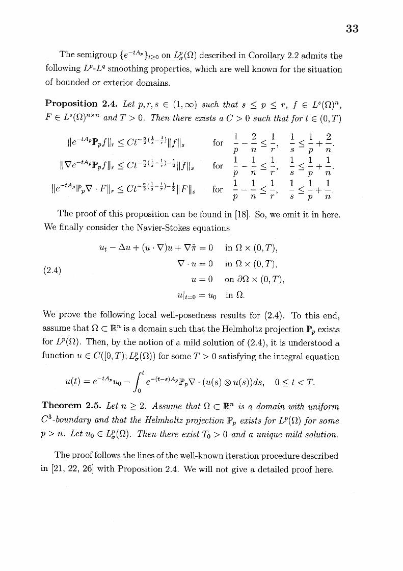
The semigroup $\{e^{-tA_{p}}\}_{t\geq 0}$ on $U_{\sigma}(\Omega)$ described in Corollary 2.2 admits thefollowing U-$L^{}$ smoothing properties, which are well known for the situationof bounded or exterior domains.

Proposition 2.4. Let $p,$ $r,$ $s\in(1, \infty)$ such that $s\leq p\leq r,$ $f\in L^{s}(\Omega)^{n}$ ,$F\in L^{s}(\Omega)^{n\cross n}$ and $T>0$ . Then there exists a $C>0$ such that for $t\in(0, T)$

$\Vert e^{-tA_{p}}\mathbb{P}_{p}f\Vert_{r}\leq Ct^{-\frac{n}{2}(\frac{1}{s}-\frac{1}{r})}\Vert f\Vert_{s}$ for $\underline{1}_{-}\underline{2}\leq\underline{1}$ $\underline{1}\leq\underline{1}+\underline{2}$ .$p$ $n$ $r$

’$s$ $p$ $n$

$\Vert\nabla e^{-tA_{p}}\mathbb{P}_{p}f\Vert_{r}\leq Ct^{-\frac{n}{2}(\frac{1}{s}-\frac{1}{r})-\frac{1}{2}}\Vert f\Vert_{s}$ for $\frac{1}{p}-\frac{1}{n}\leq\frac{1}{r}$ , $\frac{1}{s}\leq\frac{1}{p}+\frac{1}{n}$ .

$\Vert e^{-tA_{p}}\mathbb{P}_{p}\nabla\cdot F\Vert_{r}\leq Ct^{-\frac{n}{2}(\frac{1}{s}-\frac{1}{r})-\frac{1}{2}}\Vert F\Vert_{s}$ for $\frac{1}{p}-\frac{1}{n}\leq\frac{1}{r}$ , $\frac{1}{s}\leq\frac{1}{p}+\frac{1}{n}$ .

The proof of this proposition can be found in [18]. So, we omit it in here.We finally consider the Navier-Stokes equations

$u_{t}-\triangle u+(u\cdot\nabla)u+\nabla\tilde{\pi}=0$ in $\Omega\cross(0, T)$ ,

$\nabla\cdot u=0$ in $\Omega\cross(0, T)$ ,(2.4)

$u=0$ on $\partial\Omega\cross(0, T)$ ,

$u|_{t=0}=u_{0}$ in $\Omega$ .

We prove the following local well-posedness results for (2.4). To this end,assume that $\Omega\subset \mathbb{R}^{n}$ is a domain such that the Helmholtz projection $\mathbb{P}_{p}$ existsfor $L^{p}(\Omega)$ . Then, by the notion of a mild solution of (2.4), it is understood afunction $u\in C([0, T);L_{\sigma}^{p}(\Omega))$ for some $T>0$ satisfying the integral equation

$u(t)=e^{-tA_{p}}u_{0}- \int_{0}^{t}e^{-(t-s)A_{p}}\mathbb{P}_{p}\nabla\cdot(u(s)\otimes u(s))ds$ , $0\leq t<T$ .

Theorem 2.5. Let $n\geq 2$ . Assume that $\Omega\subset \mathbb{R}^{n}$ is a domain with uniform$C^{3}$ -boundary and that the Helmholtz projection $\mathbb{P}_{p}$ exists for $U(\Omega)$ for some$p>n$ . Let $u_{0}\in L_{\sigma}^{p}(\Omega)$ . Then there exist $T_{0}>0$ and a unique mild solution.

The proof follows the lines of the well-known iteration procedure describedin [21, 22, 26] with Proposition 2.4. We will not give a detailed proof here.

33

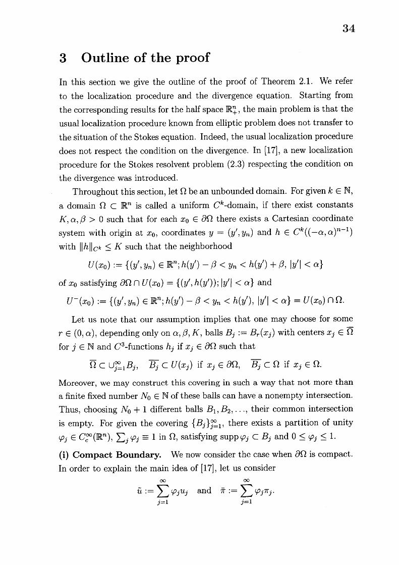
3 Outline of the proof

In this section we give the outline of the proof of Theorem 2.1. We referto the localization procedure and the divergence equation. Starting from

the corresponding results for the half space $\mathbb{R}_{+}^{n}$ , the main problem is that the

usual localization procedure known from elliptic problem does not transfer to

the situation of the Stokes equation. Indeed, the usual localization procedure

does not respect the condition on the divergence. In [17], a new localizationprocedure for the Stokes resolvent problem (2.3) respecting the condition onthe divergence was introduced.

Throughout this section, let $\Omega$ be an unbounded domain. For given $k\in \mathbb{N}$ ,

a domain $\Omega\subset \mathbb{R}^{n}$ is called a uniform $C^{k}$-domain, if there exist constants$K,$ $\alpha,$ $\beta>0$ such that for each $x_{0}\in\partial\Omega$ there exists a Cartesian coordinate

system with origin at $x_{0}$ , coordinates $y=(y’, y_{n})$ and $h\in C^{k}((-\alpha, \alpha)^{n-1})$

with $\Vert h\Vert_{C^{k}}\leq K$ such that the neighborhood

$U(x_{0}):=\{(y^{l}, y_{n})\in \mathbb{R}^{n};h(y’)-\beta<y_{n}<h(y’)+\beta, |y^{l}|<\alpha\}$

of $x_{0}$ satisfying $\partial\Omega\cap U(x_{0})=\{(y’, h(y’));|y’|<\alpha\}$ and

$U^{-}(x_{0}):=\{(y’, y_{n})\in \mathbb{R}^{n};h(y’)-\beta<y_{n}<h(y’), |y’|<\alpha\}=U(x_{0})\cap\Omega$ .

Let us note that our assumption implies that one may choose for some$r\in(O, \alpha)$ , depending only on $\alpha,$

$\beta,$ $K$ , balls $B_{j}$ $:=B_{r}(x_{j})$ with centers $x_{j}\in$ St

for $j\in N$ and $C^{3}$-functions $h_{j}$ if $x_{j}\in\partial\Omega$ such that

$\overline{\Omega}\subset\bigcup_{j=1}^{\infty}B_{j}$ , $\overline{B_{j}}\subset U(x_{j})$ if $x_{j}\in\partial\Omega$ , $\overline{B_{j}}\subset\Omega$ if $x_{j}\in\Omega$ .

Moreover, we may construct this covering in such a way that not more than

a finite fixed number $N_{0}\in \mathbb{N}$ of these balls can have a nonempty intersection.Thus, choosing $N_{0}+1$ different balls $B_{1},$ $B_{2},$

$\ldots$ , their common intersection

is empty. For given the covering $\{B_{j}\}_{j=1}^{\infty}$ , there exists a partition of unity$\varphi_{j}\in C_{c}^{\infty}(\mathbb{R}^{n}),$ $\sum_{j}\varphi_{j}\equiv 1$ in $\Omega$ , satisfying $supp\varphi_{j}\subset B_{j}$ and $0\leq\varphi_{j}\leq 1$ .

(i) Compact Boundary. We now consider the case when $\partial\Omega$ is compact.

In order to explain the main idea of [17], let us consider

$\tilde{u}$

$:= \sum_{j=1}^{\infty}\varphi_{j}u_{j}$ and it: $= \sum_{j=1}^{\infty}\varphi_{j}\pi_{j}$ .

34

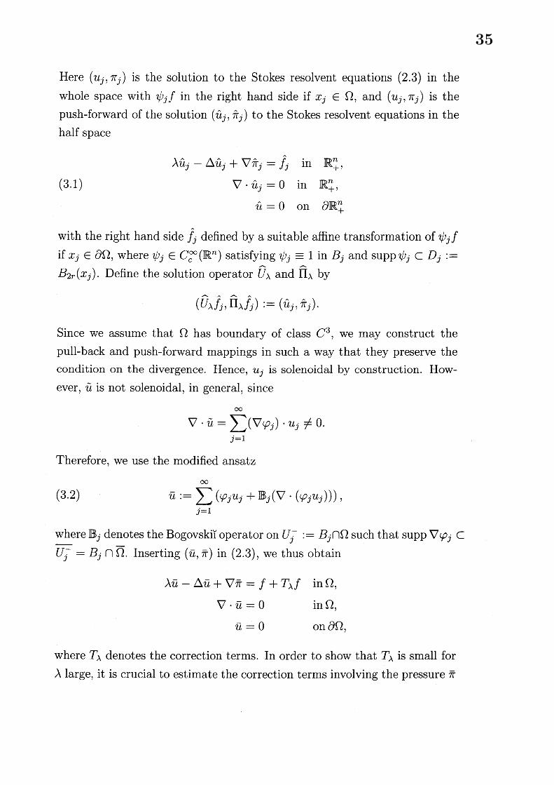
Here $(u_{j}, \pi_{j})$ is the solution to the Stokes resolvent equations (2.3) in thewhole space with $\psi_{j}f$ in the right hand side if $x_{j}\in\Omega$ , and $(u_{j}, \pi_{j})$ is thepush-forward of the solution $(\hat{u}_{j},\hat{\pi}_{j})$ to the Stokes resolvent equations in thehalf space

$\lambda\hat{u}_{j}-\triangle\hat{u}_{j}+\nabla\hat{\pi}_{j}=\hat{f}_{j}$ in $\mathbb{R}_{+}^{n}$ ,

(3.1) $\nabla\cdot\hat{u}_{j}=0$ in $\mathbb{R}_{+}^{n}$ ,

$\hat{u}=0$ on $\partial \mathbb{R}_{+}^{n}$

with the right hand side $\hat{f}_{j}$ defined by a suitable affine transformation of $\psi_{j}f$

if $x_{j}\in\partial\Omega$ , where $\psi_{j}\in C_{c}^{\infty}(\mathbb{R}^{n})$ satisfying $\psi_{j}\equiv 1$ in $B_{j}$ and $supp\psi_{j}\subset D_{j}$ $:=$

$B_{2r}(x_{j})$ . Define the solution operator $\hat{U}_{\lambda}$ and $\hat{\Pi}_{\lambda}$ by

$(U_{\lambda}\hat{f}_{j}, \Pi_{\lambda}^{}\hat{f}_{j}):=(\hat{u}_{j},\hat{\pi}_{j})$へ.

Since we assume that $\Omega$ has boundary of class $C^{3}$ , we may construct thepull-back and push-forward mappings in such a way that they preserve thecondition on the divergence. Hence, $u_{j}$ is solenoidal by construction. How-ever, $\tilde{u}$ is not solenoidal, in general, since

$\nabla\cdot\tilde{u}=\sum_{j=1}^{\infty}(\nabla\varphi_{j})\cdot u_{j}\neq 0$ .

Therefore, we use the modified ansatz

(3.2) $\overline{u}$

$:= \sum_{j=1}^{\infty}(\varphi_{j}u_{j}+B_{j}(\nabla\cdot(\varphi_{j}u_{j})))$ ,

where $B_{j}$ denotes the $Bogovski_{\dot{1}}$ operator on $U_{j}^{-}:=B_{j}\cap\Omega$ such that $supp\nabla\varphi_{j}\subset$

$\overline{U_{j}^{-}}=B_{j}\cap\overline{\Omega}$ . Inserting $(\overline{u},\overline{\pi})$ in (2.3), we thus obtain

$\lambda\overline{u}-\triangle\overline{u}+\nabla\overline{\pi}=f+T_{\lambda}f$ $in\Omega$ ,$\nabla\cdot\overline{u}=0$ $in\Omega$ ,

$\overline{u}=0$ $on\partial\Omega$ ,

where $T_{\lambda}$ denotes the correction terms. In order to show that $T_{\lambda}$ is small for$\lambda$ large, it is crucial to estimate the correction terms involving the pressure it

35

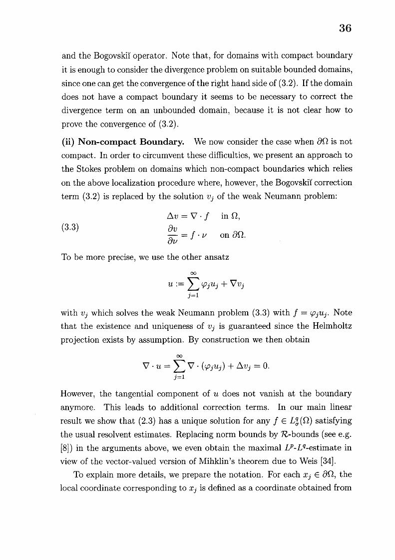
and the $Bogovski_{\dot{1}}$ operator. Note that, for domains with compact boundaryit is enough to consider the divergence problem on suitable bounded domains,

since one can get the convergence of the right hand side of (3.2). If the domaindoes not have a compact boundary it seems to be necessary to correct thedivergence term on an unbounded domain, because it is not clear how toprove the convergence of (3.2).

(ii) Non-compact Boundary. We now consider the case when $\partial\Omega$ is notcompact. In order to circumvent these difficulties, we present an approach to

the Stokes problem on domains which non-compact boundaries which relieson the above localization procedure where, however, the $Bogovski_{\dot{1}}$ correctionterm (3.2) is replaced by the solution $v_{j}$ of the weak Neumann problem:

$\triangle v=\nabla\cdot f$ in $\Omega$ ,(3.3)

$\frac{\partial v}{\partial\nu}=f\cdot\nu$ on $\partial\Omega$ .

To be more precise, we use the other ansatz

$u:= \sum_{j=1}^{\infty}\varphi_{j}u_{j}+\nabla v_{j}$

with $v_{j}$ which solves the weak Neumann problem (3.3) with $f=\varphi_{j}u_{j}$ . Notethat the existence and uniqueness of $v_{j}$ is guaranteed since the Helmholtzprojection exists by assumption. By construction we then obtain

$\nabla\cdot u=\sum_{j=1}^{\infty}\nabla\cdot(\varphi_{j}u_{j})+\triangle v_{j}=0$.

However, the tangential component of $u$ does not vanish at the boundaryanymore. This leads to additional correction terms. In our main linearresult we show that (2.3) has a unique solution for any $f\in L_{\sigma}^{q}(\Omega)$ satisfyingthe usual resolvent estimates. Replacing norm bounds by $\mathcal{R}$-bounds (see e.g.[8] $)$ in the arguments above, we even obtain the maximal $\nu-L^{q}$-estimate in

view of the vector-valued version of Mihklin $s$ theorem due to Weis [34].To explain more details, we prepare the notation. For each $x_{j}\in\partial\Omega$ , the

local coordinate corresponding to $x_{j}$ is defined as a coordinate obtained from

36

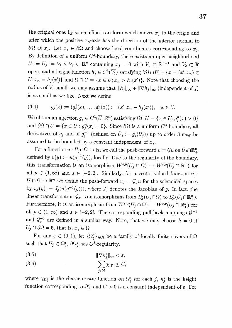
the original ones by some affine transform which moves $x_{j}$ to the origin andafter which the positive $x_{n}$-axis has the direction of the interior normal to$\partial\Omega$ at $x_{j}$ . Let $x_{j}\in\partial\Omega$ and choose local coordinates corresponding to $x_{j}$ .By definition of a uniform $C^{3}$-boundary, there exists an open neighborhood$U$ $:=U_{j}$ $:=V_{1}\cross V_{2}\subset \mathbb{R}^{n}$ containing $x_{j}=0$ with $V_{1}\subset \mathbb{R}^{n-1}$ and $V_{2}\subset \mathbb{R}$

open, and a height function $h_{j}\in C^{3}(\overline{V_{1}})$ satisfying $\partial\Omega\cap U=\{x=(x’, x_{n})\in$

$U;x_{n}=h_{j}(x’)\}$ and $\Omega\cap U=\{x\in U;x_{n}>h_{j}(x’)\}$ . Note that choosing theradius of $V_{1}$ small, we may assume that $\Vert h_{j}\Vert_{\infty}+\Vert\nabla h_{j}\Vert_{\infty}$ (independent of j)is as small as we like. Next we define

(3.4) $g_{j}(x):=(g_{j}^{1}(x), \ldots, g_{j}^{n}(x)):=(x’, x_{n}-h_{j}(x’))$ , $x\in U$.

We obtain an injection $g_{j}\in C^{3}(\overline{U}, \mathbb{R}^{n})$ satisfying $\Omega\cap U=\{x\in U;g_{j}^{n}(x)>0\}$

and $\partial\Omega\cap U=\{x\in U : g_{j}^{n}(x)=0\}$ . Since $\partial\Omega$ is a uniform $C^{3}$-boundary, allderivatives of $g_{j}$ and of $g_{j}^{-1}$ (defined on $\hat{U}_{j}$ $:=g_{j}(U_{j})$ ) up to order 3 may beassumed to be bounded by a constant independent of $x_{j}$ .

For a function $u$ : $U_{j}\cap\Omegaarrow \mathbb{R}$ , we call the push-forward $v=\mathcal{G}u$ on $\hat{U}_{j}\cap \mathbb{R}_{+}^{n}$

defined by $v(y)$ $:=u(g_{j}^{-1}(y))$ , locally. Due to the regularity of the boundary,this transformation is an isomorphism $W^{s,p}(U_{j}\cap\Omega)arrow W^{s,p}(\hat{U}_{j}\cap \mathbb{R}_{+}^{n})$ forall $p\in(1, \infty)$ and $s\in[-2,2]$ . Similarly, for a vector-valued function $u$ :$U\cap\Omegaarrow \mathbb{R}^{n}$ we define the push-forward $v_{\sigma}=\mathcal{G}_{\sigma}u$ for the solenoidal spacesby $v_{\sigma}(y)$ $:=J_{g}(u(g^{-1}(y)))$ , where $J_{g}$ denotes the Jacobian of $g$ . In fact, thelinear transformation $\mathcal{G}_{\sigma}$ is an isomorphisms from $L_{\sigma}^{p}(U_{j}\cap\Omega)$ to $U_{\sigma}(\hat{U}_{j}\cap \mathbb{R}_{+}^{n})$ .Furthermore, it is an isomorphism from $W^{s,p}(U_{j}\cap\Omega)arrow W^{s,p}(\hat{U}_{j}\cap \mathbb{R}_{+}^{n})$ forall $p\in(1, \infty)$ and $s\in[-2,2]$ . The corresponding pull-back mappings $\mathcal{G}^{-1}$

and $\mathcal{G}_{\sigma}^{-1}$ are defined in a similar way. Note, that we may choose $h=0$ if$U_{j}\cap\partial\Omega=\emptyset$ , that is, $x_{j}\in\Omega$ .

For any $\epsilon\in(0,1)$ , let $\{\Omega_{j}^{\epsilon}\}_{j\in \mathbb{N}}$ be a family of locally finite covers of $\Omega$

such that $U_{j}\subset\Omega_{j}^{\epsilon},$ $\partial\Omega_{j}^{\epsilon}$ has $C^{3}$-regularity,

(3.5) $\Vert\nabla h_{j}^{\epsilon}\Vert_{\infty}<\epsilon$ ,

(3.6)$\sum_{j\in \mathbb{N}}\chi_{\Omega_{j}^{\epsilon}}\leq C$

,

where $\chi_{\Omega_{j}^{\epsilon}}$ is the characteristic function on $\Omega_{j}^{\epsilon}$ for each $j,$ $h_{j}^{\epsilon}$ is the heightfunction corresponding to $\Omega_{j}^{\epsilon}$ , and $C>0$ is a constant independent of $\epsilon$ . For

37

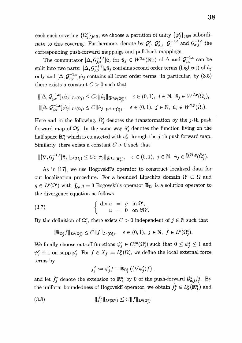
each such covering $\{\Omega_{j}^{\epsilon}\}_{j\in N}$ , we choose a partition of unity $\{\varphi_{j}^{\epsilon}\}_{j\in N}$ subordi-nate to this covering. Furthermore, denote by $\mathcal{G}_{j}^{\epsilon},$ $\mathcal{G}_{\sigma,j}^{\epsilon},$

$\mathcal{G}_{j}^{-1,\epsilon}$ and $\mathcal{G}_{\sigma,j}^{-1,\epsilon}$ the

corresponding push-forward mappings and pull-back mappings.The commutator $[\triangle, \mathcal{G}_{j,\sigma}^{-1,\epsilon}]\hat{u}_{j}$ for $\hat{u}_{j}\in W^{2,p}(\mathbb{R}_{+}^{n})$ of $\triangle$ and $\mathcal{G}_{j,\sigma}^{-1,\epsilon}$ can be

split into two parts: $[\triangle, \mathcal{G}_{j,\sigma}^{-1,\epsilon}]_{h}\hat{u}_{j}$ contains second order terms (highest) of $\hat{u}_{j}$

only and $[\triangle, \mathcal{G}_{j,\sigma}^{-1,\epsilon}]_{l}\hat{u}_{j}$ contains all lower order terms. In particular, by (3.5)

there exists a constant $C>0$ such that

$\Vert[\triangle, \mathcal{G}_{j,\sigma}^{-1,\epsilon}]_{h}\hat{u}_{j}$ Il $Lp(\Omega_{j})\leq C\epsilon\Vert\hat{u}_{j}\Vert_{\overline{W}^{2,p}(\hat{\Omega}_{j}^{\epsilon})}$ , $\epsilon\in(0,1),$ $j\in N,\hat{u}_{j}\in W^{2,p}(\hat{\Omega}_{j})$ ,

$\Vert[\triangle, \mathcal{G}_{j,\sigma}^{-1,\epsilon}]_{l}\hat{u}_{j}\Vert_{L^{p}(\Omega_{j})}\leq C\Vert\hat{u}_{j}\Vert_{W^{1,p}(\hat{\Omega}_{j}^{\epsilon})}$ , $\epsilon\in(0,1),$ $j\in \mathbb{N},\hat{u}_{j}\in W^{2,p}(\hat{\Omega}_{j})$ .

Here and in the following, $\hat{\Omega}_{j}^{\epsilon}$ denotes the transformation by the j-th pushforward map of $\Omega_{j}^{\epsilon}$ . In the same way $\hat{u}_{j}^{\epsilon}$ denotes the function living on the

half space $\mathbb{R}_{+}^{n}$ which is connected with $u_{j}^{\epsilon}$ through the j-th push forward map.

Similarly, there exists a constant $C>0$ such that

$\Vert[\nabla, \mathcal{G}_{j}^{-1,\epsilon}]\hat{\pi}_{j}\Vert_{L^{p}(\Omega_{j})}\leq C\epsilon\Vert\hat{\pi}_{j}\Vert_{\overline{W}^{1,p}(\mathbb{R}_{+}^{n})}$, $\epsilon\in(0,1),$ $j\in \mathbb{N},\hat{\pi}_{j}\in\hat{W}^{1,p}(\hat{\Omega}_{j}^{\epsilon})$ .

As in [17], we use $Bogovski_{\dot{1}}$’s operator to construct localized data forour localization procedure. For a bounded Lipschitz domain $\Omega’\subset\Omega$ and$g\in If(\Omega’)$ with $\int_{\Omega},$ $g=0Bogovski\dot{1}’ S$ operator $B_{\Omega’}$ is a solution operator to

the divergence equation as follows

(3.7) $\{\begin{array}{l}divu = g in \Omega’,u = 0 on\partial\Omega’.\end{array}$

By the definition of $\Omega_{j}^{\epsilon}$ , there exists $C>0$ independent of $j\in \mathbb{N}$ such that

$\Vert B_{\Omega_{j}^{\epsilon}}f\Vert_{Lp(\Omega_{j}^{\epsilon})}\leq C\Vert f\Vert_{L^{p}(\Omega_{j}^{\epsilon})}$, $\epsilon\in(0,1),$ $j\in \mathbb{N},$ $f\in L^{p}(\Omega_{j}^{\epsilon})$ .

We finally choose cut-off functions $\psi_{j}^{\epsilon}\in C_{c}^{\infty}(\Omega_{j}^{\epsilon})$ such that $0\leq\psi_{j}^{\epsilon}\leq 1$ and$\psi_{j}^{\epsilon}\equiv 1$ on $supp\varphi_{j}^{\epsilon}$ . For $f\in X_{f}$ $:=\nu_{\sigma}(\Omega)$ , we define the local external forceterms by

$f_{j}^{\epsilon}:=\psi_{j}^{\epsilon}f-B_{\Omega_{j}^{\epsilon}}((\nabla\psi_{j}^{\epsilon})f)$ ,

and let $\hat{f}_{j}^{\epsilon}$ denote the extension to $\mathbb{R}_{+}^{n}$ by $0$ of the push-forward $\mathcal{G}_{\sigma,j}^{\epsilon}f_{j}^{\epsilon}$ . By

the uniform boundedness of $Bogovski_{\dot{1}}$ operator, we obtain $\hat{f}_{j}^{\epsilon}\in U_{\sigma}(\mathbb{R}_{+}^{n})$ and

(3.8) $\Vert\hat{f}_{j}^{\epsilon}\Vert_{L^{p}(\mathbb{R}_{+}^{n})}\leq C\Vert f\Vert_{Lp(\Omega_{j}^{\epsilon})}$

38

with some $C>0$ independent of $\epsilon,$ $j$ and $f$ . Hence, (3.6) yields that

(3.9) $((S_{j}^{1,\epsilon})_{j\in \mathbb{N}})_{\epsilon\in(0,1)}\subset \mathcal{L}(X_{f}, \ell^{p}(X_{f}))$

へ

is uniformly bounded, where $S_{j}^{1,\epsilon}f$ $:=\hat{f}_{j}^{\epsilon}$ . Similarly, for $(a, b)\in X_{a,b}:=\{a\in$

$W^{1-1/p,p}(\partial\Omega);a\cdot\nu=0\}\cross\{b\in W^{2-1/p,p}(\partial\Omega);b\cdot\nu=0\}$ , we define the localboundary data $a_{j}^{\epsilon}$ $:=\psi_{j}^{\epsilon}a,$ $b_{j}^{\epsilon}$ $:=\psi_{j}^{\epsilon}b,\hat{a}_{j}^{\epsilon}$

$:=\mathcal{G}_{j,\sigma}^{\partial\Omega,\epsilon}\psi_{j}^{\epsilon}a$ and $\hat{b}_{j}^{\epsilon}$ $:=\mathcal{G}_{j,\sigma}^{\partial\Omega,\epsilon}\psi_{j}^{\epsilon}b$ .Here, $\mathcal{G}_{j,\sigma}^{\partial\Omega,\epsilon}$ is the restriction of $\mathcal{G}_{j,\sigma}^{\epsilon}$ to the boundary of $\Omega$ . Again, we see

(3.10) $((S_{j}^{2,\epsilon}(a, b))_{j\in N})_{\epsilon\in(0,1)}\subset \mathcal{L}(X_{a,b}, \ell^{p}(X_{a,b}))$

へ

is uniformly bounded, where $S_{j}^{2,\epsilon}$ $:=S_{j}^{2,\epsilon}(a, b)$ $:=(\hat{a}_{j}^{\epsilon},\hat{b}_{j}^{\epsilon})$ . We now set

$U_{\lambda}^{\epsilon}(f, a, b):= \sum_{j\in N}\varphi_{j}^{\epsilon}\mathcal{G}_{j,\sigma}^{-1,\epsilon}\hat{U}_{\lambda}S_{j}^{\epsilon}(f, a, b)-\nabla \mathcal{N}(\sum_{j\in N}\varphi_{j}^{\epsilon}\mathcal{G}_{j,\sigma}^{-1,\epsilon}\hat{U}_{\lambda}S_{j}^{\epsilon}(f, a, b))$

where $\mathcal{N}$ is the solution operator of the weak Neumann problem and $S_{j}^{\epsilon}$ $:=$

$S_{j}^{\epsilon}(f, a, b)$ $:=(S_{j}^{1,\epsilon}f, S_{j}^{2,\epsilon}(a, b))$ . Here, similarly to (3.2), we add a correctionterm in order to have a solenoidal ansatz $U_{\lambda}^{\epsilon}$ . However, in contrast to thecase (i), the correction term is based on the solution operator of the weakNeumann problem instead of $Bogovski_{\check{1}S}$ operator. Inserting $u$ $:=U_{\lambda}^{\epsilon}(f, a, a)$ ,we calculate

$\lambda u-\mathbb{P}\triangle u=f+\mathcal{T}_{\lambda}^{1,\epsilon}(f, a, a)$ in $\Omega$ ,

(3.11) $\nabla\cdot u=0$ in $\Omega$ ,$u=a+\mathcal{T}_{\lambda}^{2,\epsilon}(f, a, a)$ on $\partial\Omega$ ,

where

$\mathcal{T}_{\lambda}^{\epsilon}(f, a, b):=(\mathcal{T}_{\lambda}^{1,\epsilon}(f, a, b), \mathcal{T}_{\lambda}^{2,\epsilon}(f, a, b)):=T_{1,\lambda}^{\epsilon}(f, a, b)+\cdots+T_{6,\lambda}^{\epsilon}(f, a, b)$

with

$T_{1,\lambda}^{\epsilon}(f, a, b):=( \mathbb{P}\sum_{j\in \mathbb{N}}\varphi_{j}^{\epsilon}[\nabla, \mathcal{G}_{j}^{-1,\epsilon}]\hat{\Pi}_{\lambda}S_{j}^{\epsilon}(f, a, b),$$0,0)$ ,

$T_{2,\lambda}^{\epsilon}(f, a, b);=( \mathbb{P}\sum_{j\in N}(\nabla\varphi_{j}^{\epsilon})\mathcal{G}_{j}^{-1,\epsilon}\Pi_{\lambda}^{へ}S_{j}^{\epsilon}(f, a,b),$$0,0)$ ,

39

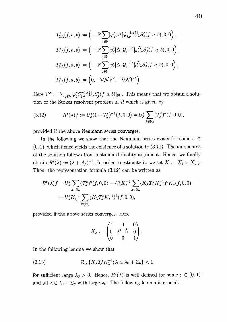
$T_{3,\lambda}^{\epsilon}(f, a, b):=(- \mathbb{P}\sum_{j\in N}[\varphi_{j}^{\epsilon}, \triangle]\mathcal{G}_{j,\sigma}^{-1,\epsilon^{へ}}U_{\lambda}S_{j}^{\epsilon}(f, a, b),$$0,0)$ ,

$T_{4,\lambda}^{\epsilon}(f, a, b):=(- \mathbb{P}\sum_{j\in N}\varphi_{j}^{\epsilon}[\triangle, \mathcal{G}_{j}^{-1,\epsilon^{へ}}]_{h}U_{\lambda}S_{j}^{\epsilon}(f, a, b),$$0,0)$ ,

$T_{5,\lambda}^{\epsilon}(f, a, b):=(- \mathbb{P}\sum_{j\in N}\varphi_{j}^{\epsilon}[\triangle, \mathcal{G}_{j}^{-1,\epsilon}]_{l}\hat{U}_{\lambda}S_{j}^{\epsilon}(f, a, b),$$0,0)$ ,

$T_{6,\lambda}^{\epsilon}(f, a, b)$ $:=(0,$ $-\nabla \mathcal{N}V^{\epsilon},$ $-\nabla \mathcal{N}V^{\epsilon})$ .

Here $V^{\epsilon}$ $:= \sum_{j\in N}\varphi_{j}^{\epsilon}\mathcal{G}_{j,\sigma}^{-1,\epsilon_{U_{\lambda}S_{j}^{\epsilon}(f,a,b)|_{\partial\Omega}}^{へ}}$ . This means that we obtain a solu-tion of the Stokes resolvent problem in $\Omega$ which is given by

(3.12) $R^{\epsilon}(\lambda)f$

$:=U_{\lambda}^{\epsilon}(1+ \mathcal{T}_{\lambda}^{\epsilon})^{-1}(f, 0,0)=U_{\lambda}^{\epsilon}\sum_{k\in N_{0}}(\mathcal{T}_{\lambda}^{\epsilon})^{k}(f,0,0)$,

provided if the above Neumann series converges.In the following we show that the Neumann series exists for some $\epsilon\in$

$(0,1)$ , which hence yields the existence of a solution to (3.11). The uniquenessof the solution follows from a standard duality argument. Hence, we finally

obtain $R^{\epsilon}(\lambda):=(\lambda+A_{p})^{-1}$ In order to estimate it, we set $X$ $:=X_{f}\cross X_{a,b}$ .Then, the representation formula (3.12) can be written as

$R^{\epsilon}( \lambda)f=U_{\lambda}^{\epsilon}\sum_{k\in N_{0}}(\mathcal{T}_{\lambda}^{\epsilon})^{k}(f, 0,0)=U_{\lambda}^{\epsilon}K_{\lambda}^{-1}\sum_{k\in N_{0}}(K_{\lambda}\mathcal{T}_{\lambda}^{\epsilon}K_{\lambda}^{-1})^{k}K_{\lambda}(f, 0,0)$

$=U_{\lambda}^{\epsilon}K_{\lambda}^{-1} \sum_{k\in N_{0}}(K_{\lambda}\mathcal{T}_{\lambda}^{\epsilon}K_{\lambda}^{-1})^{k}(f, 0,0)$,

provided if the above series converges. Here

$K_{\lambda}:=(\begin{array}{lll}1 0 00 \lambda^{l-\frac{1}{3p}} 00 0 1\end{array})$

In the following lemma we show that

(3.13) $\mathcal{R}_{X}\{K_{\lambda}\mathcal{T}_{\lambda}^{\epsilon}K_{\lambda}^{-1};\lambda\in\lambda_{0}+\Sigma_{\theta}\}<1$

for sufficient large $\lambda_{0}>0$ . Hence, $R^{\epsilon}(\lambda)$ is well defined for some $\epsilon\in(0,1)$

and all $\lambda\in\lambda_{0}+\Sigma_{\theta}$ with large $\lambda_{0}$ . The following lemma is crucial.

40

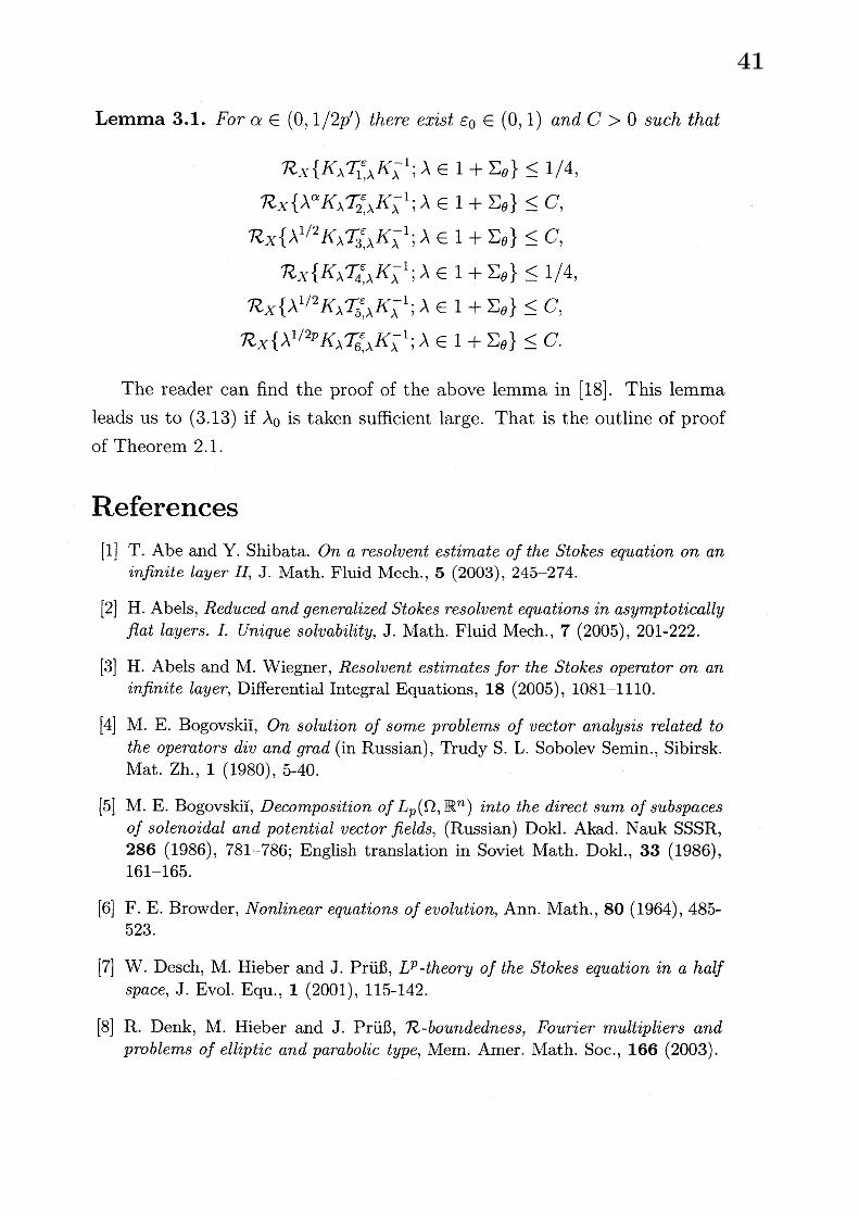
Lemma 3.1. For $\alpha\in(0,1/2p’)$ there exist $\epsilon_{0}\in(0,1)$ and $C>0$ such that

$\mathcal{R}_{X}\{K_{\lambda}\mathcal{T}_{1,\lambda}^{\epsilon}K_{\lambda}^{-1};\lambda\in 1+\Sigma_{\theta}\}\leq 1/4$ ,

$\mathcal{R}_{X}\{\lambda^{\alpha}K_{\lambda}\mathcal{T}_{2,\lambda}^{\epsilon}K_{\lambda}^{-1};\lambda\in 1+\Sigma_{\theta}\}\leq C$,

$\mathcal{R}_{X}\{\lambda^{1/2}K_{\lambda}T_{3,\lambda}^{\epsilon}K_{\lambda}^{-1};\lambda\in 1+\Sigma_{\theta}\}\leq C$ ,

$\mathcal{R}_{X}\{K_{\lambda}\mathcal{T}_{4,\lambda}^{\epsilon}K_{\lambda}^{-1};\lambda\in 1+\Sigma_{\theta}\}\leq 1/4$ ,

$\mathcal{R}_{X}\{\lambda^{1/2}K_{\lambda}\mathcal{T}_{5,\lambda}^{\epsilon}K_{\lambda}^{-1};\lambda\in 1+\Sigma_{\theta}\}\leq C$,

$\mathcal{R}_{X}\{\lambda^{1/2p}K_{\lambda}\mathcal{T}_{6,\lambda}^{\epsilon}K_{\lambda}^{-1};\lambda\in 1+\Sigma_{\theta}\}\leq C$ .

The reader can find the proof of the above lemma in [18]. This lemmaleads us to (3.13) if $\lambda_{0}$ is taken sufficient large. That is the outline of proofof Theorem 2.1.

References[1] T. Abe and Y. Shibata. On a resolvent estimate of the Stokes equation on an

infinite layer $\Pi$, J. Math. Fluid Mech., 5 (2003), 245-274.

[2] H. Abels, Reduced and genemlized Stokes resolvent equations in asymptoticallyflat layers. I. Unique solvability, J. Math. Fluid Mech., 7 (2005), 201-222.

[3] H. Abels and M. Wiegner, Resolvent estimates for the Stokes opemtor on aninfinite layer, Differential Integral Equations, 18 (2005), 1081-1110.

[4] M. E. Bogovskii, On solution of some problems of vector analysis related tothe operators div and gmd (in Russian), Trudy S. L. Sobolev Semin., Sibirsk.Mat. Zh., 1 (1980), 5-40.

[5] M. E. $Bogovski_{\dot{1}}$ , Decomposition of $L_{p}(\Omega, \mathbb{R}^{n})$ into the direct sum of subspacesof solenoidal and potential vector fields, (Russian) Dokl. Akad. Nauk SSSR,286 (1986), 781-786; English translation in Soviet Math. Dokl., 33 (1986),161-165.

[6] F. E. Browder, Nonlinear equations of evolution, Ann. Math., 80 (1964), 485-523.

[7] W. Desch, M. Hieber and J. $Pr\ddot{u}!3,$ $L^{p}$ -theory of the Stokes equation in a halfspace, J. Evol. Equ., 1 (2001), 115-142.

[8] R. Denk, M. Hieber and J. $Pri3,$ $\mathcal{R}$ -boundedness, Fourier multipliers andproblems of elliptic and pambolic type, Mem. Amer. Math. Soc., 166 (2003).

41

[9] R. Farwig, H. Kozono and H. Sohr, An $L^{q}$ -approach to Stokes and Navier-Stokes equations in geneml domains, Acta Math., 195 (2005), 21-53.

[10] R. Farwig and M.-H. Ri, Resolvent estimates and maximal regularity inweighted $L^{q}$ -spaces of the Stokes opemtor in an infinite cylinder, J. Math.Fluid Mech., 10 (2008), 352-387.

[11] R. Farwig and H. Sohr, Genemlized resolvent estimates for the Stokes systemin bounded and unbounded domains, J. Math. Soc. Japan, 46 (1994), 607-643.

[12] M. Ranzke, Strong solution of the Navier-Stokes equations in aperture do-mains, Ann. Univ. Ferrara Sez. VII (N.S.), 46 (2000), 161-173.

[13] A. Fr\"ohlich, The Stokes opemtor in weighted $L^{q}$ -spaces $\Pi$; weighted resloventestimates and maximal IP-regularity, Math. Ann., 339 (2007), 287-316.

[14] H. Fujita and T. Kato, On the Navier-Stokes initial value problem I, Arch.Rat. Mech. Anal., 16 (1964), 269-315.

[15] D. Fujiwara and H. Morimoto, An $L^{r}$ -theorem of the Helmholtz decompositionof vector fields, J. Fac. Sci. Univ. Tokyo Sect. I A Math., 24 (1977), 685-700.

[16] G. P. Galdi, An Introduction to the Mathematical Theory of the Navier-StokesEquations. Vol. I, Springer-Verlag, New York, (1994).

[17] M. Geissert, M. Hess, M. Hieber, C. Schwarz and K. Stavrakidis, MaximalIf $-L^{q}$ -estimates for the Stokes equation: a short proof of Solonnikov’s the-orem, J. Math. Fluid Mech., 12 (2010), 47-60.

[18] M. Geissert, H. Horst, M. Hieber and O. Sawada, Weak Neumann impliesStokes, J. reine Angewand. Math., (to appear).

[19] Y. Giga, Analyticity of the semigroup genemted by the Stokes opemtor in $L_{r}$

spaces, Math. Z., 178 (1981), 297-329.

[20] Y. Giga, Domains of fractional powers of the Stokes opemtor in $L_{r}$ spaces,Arch. Rat. Mech. Anal., 89 (1985), 251-265.

[21] Y. Giga, Solutions for semilinear pambolic equations in If and regularityof weak solutions of the Navier-Stokes system, J. Differential Equations, 61(1986), 186-212.

[22] Y. Giga and T. Miy下上 $\wedge wa$ , Solutions in $L^{r}$ of the Navier-Stokes initial valueproblem, Arch. Rat. Mech. Anal., 89 (1985), 267-281.

[23] Y. Giga and H. Sohr, Abstmct $\nu$ estimates for the Cauchy problem withapplications to the Navier-Stokes equations in exterior domains, J. Funct.Anal., 102 (1991), 72-94.

42

[24] G. Grubb and V. A. Solonnikov, Boundary value problems for the nonsta-tionary Navier-Stokes equations treated by pseudo-differential methods, Math.Scand., 69 (1991), 217-290.

[25] T. Hishida, The nonstationary Stokes and Navier-Stokes flows thmugh anaperture, In: Contributions to current challenges in mathematical fluid me-chanics, Adv. Math. Fluid Mech., $Birkhuser$ , Basel, (2004), 79-123.

[26] T. Kato, Strong $L^{p}$ -solutions of Navier-Stokes equations in $\mathbb{R}^{n}$ with applica-tions to weak solutions, Math. Z., 187 (1984), 471-480.

[27] T. Kato and H. Fujita, On the nonstationary Navier-Stokes system, Rend.Sem. Mat. Univ. Padova, 32 (1962), 243-260.

[28] K. Masuda, Weak solutions of Navier-Stokes equations, Tohoku Math. J., 36(1984), 623-646.

[29] A. Noll and J. Saal, $H^{\infty}$ -calculus for the Stokes opemtor on $L^{q}$ -spaces, Math.Z., 244 (2003), 651-688.

[30] V. A. Solonnikov, Estimates for solutions of nonstationary Navier-Stokesequations, J. Soviet Math., 8 (1977), 213-317.

[31] E. M. Stein, Singular Integmls and Differentiability Properties of Functions,Princeton University Press, New Jersey, (1970).

[32] H. Triebel, Theory of Function Spaces, Birkh\"auser, Basel-Boston-Stuttgart,(1983).

[33] S. Ukai, A solution formula for the Stokes equations in $\mathbb{R}_{+}^{n}$ , Comm. PureAppl. Math., 40 (1987), 611-621.

[34] L. Weis, Operator-valued Fourier multiplier theorems and maximal If-regularity, Math. Ann., 319 (2001), 735-758.

43